High-concentration, spontaneous dispersions and liquid ... · High-concentration, spontaneous dispersions and liquid crystals of ... concentration of the same graphite source in the

1

Supplementary Information

High-concentration, spontaneous dispersions

and liquid crystals of graphene

Natnael Behabtu, Jay R. Lomeda, Micah J. Green, Amanda L. Higginbotham, Alexander

Sinitskii, Dmitry V. Kosynkin, Dmitri Tsentalovich, A. Nicholas G. Parra-Vasquez,

Judith Schmidt, Ellina Kesselman, Yachin Cohen, Yeshayahu Talmon, James M. Tour,

Matteo Pasquali

S-01: Quantitative measurement of isotropic concentration

S-02: Dissolution Efficiency

S-03: Graphene as rigid platelets

S-04: Thin films

S-05: Tyndall effect

S-06: HOPG XPS and Raman

S-07: Angle dependent electron diffraction

S-01: Quantitative measurement of isotropic concentration

The concentration of the isotropic phase was determined as follow. The initial

powder was dried overnight in a vacuum oven (100 °C, -25 mmHg, relative to

atmospheric) to minimize moisture content. The vials were then transferred into a dry

glove box (dew point of -50 °C) and flushed with dry air for 12 h. The acid was then

SUPPLEMENTARY INFORMATIONdoi: 10.1038/nnano.2010.86

nature nanotechnology | www.nature.com/naturenanotechnology 1

© 2010 Macmillan Publishers Limited. All rights reserved.

2

added via glass syringe, and the solution was mixed with a Teflon-coated magnetic stir-

bar for a minimum of 2 days.

The vials containing the initial dispersion were centrifuged on a Fisher Centrific

Model 225 Benchtop centrifuge at 5100 rpm for 12 h, unless otherwise specified. The

vials were then retransferred into the glove box, and the top phase was extracted by glass

pipette. Approximately 50% of the top was extracted. This minimizes undispersed

particles from the bottom to be entrained during the extraction process. The top phase

concentration was determined by quenching in water, filtering, and weighing the

graphene in the top phase. The top phase was then diluted, and the UV-vis-nIR spectra

measured. A Shimadzu UV-3101PC spectrometer in 1 mm path length quartz Starna cells

with Teflon closures was used for UV-vis absorption (Fig. S1a). The extinction

coefficient was determined from the spectra of the various dilutions at a given

wavelength (Fig. S1b), as in Ref. 1. The extinction coefficient was then used to measure

concentration of the same graphite source in the same solvent.

Figure S1. (a) UV-vis absorption spectra from the top phase from the vials after centrifugation. The

dispersions were obtained from the microcrystalline graphite dispersion. The four different spectra

represent different concentration (the top phase and three different dilutions). (b) Optical absorbance

2 nature nanotechnology | www.nature.com/naturenanotechnology

SUPPLEMENTARY INFORMATION doi: 10.1038/nnano.2010.86


3

divided by the cell length as a function of different concentrations. The solution follows the Lambert-Beer

law with an absorption coefficient of 5.6 mL µg-1

m-1

at 660 nm. The error bar is a combination of

instrument resolution for the UV-vis absorption, volume and mass measurement. The main contribution to

the error bar is the determination graphene mass in the isotropic solution.

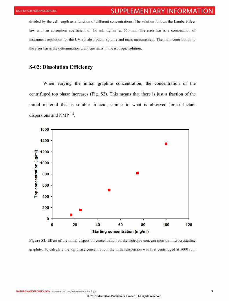
S-02: Dissolution Efficiency

When varying the initial graphite concentration, the concentration of the

centrifuged top phase increases (Fig. S2). This means that there is just a fraction of the

initial material that is soluble in acid, similar to what is observed for surfactant

dispersions and NMP 1,2

.

Figure S2. Effect of the initial dispersion concentration on the isotropic concentration on microcrystalline

graphite. To calculate the top phase concentration, the initial dispersion was first centrifuged at 5000 rpm




4

for 12 h. The UV-vis spectrum of the top phase was then measured and the concentration calculated by

using the extinction coefficient previously calculated.

The most plausible explanation of this difference is graphene flake size. Even

when a molecule is thermodynamically stable in solution, gravitational sedimentation can

cause phase separation between solvent and solute. Sedimentation becomes important as

the size of the molecule becomes larger. The bottom phase is then composed of

sedimenting non Brownian graphene/graphite flakes. Thus, the amount of material that

remains dispersed in the top isotropic phase is governed by the balance between

Brownian diffusive forces and gravitational forces. Interestingly, the intensity of the D

peak increases as a function of centrifugation time (Fig. S3). This can be understood in

terms of flake size. In fact, the amount of graphene edge per flake (which determines the

D peak intensity of pristine graphene3) increases as the flake size decreases, while the D

peak of the bottom phase remains unchanged compared to the initial powder.




5

Figure S3. Solid state Raman spectra with 514 nm excitation and a 50x long working distance lens. The

red curve refers to the initial powder, the black to the quenched bottom phase, the blue to the quenched top

phase after 30 min centrifugation at 5000 rpm and the green after 12 h of centrifugation at 5000 rpm. Each

curve is obtained by averaging the Raman spectra of 5 different spots. Note how the bottom phase Raman

is almost indistinguishable from the original powder. The graphite source was microcrystalline graphite.

An increase in a D peak could also be caused by an increased number of graphite

defects. To independently assess the amount of defect from Raman spectroscopy, we

have also performed XPS on the top phase sample that gave the highest D peak (Fig. S4)

to rule out the possibility of functionalization of the graphene sheets. The C1s spectrum,

centred at 284.8 resembles that of pristine graphite and no other types of carbon, i.e.

oxidized such as peaks observed in GO, is visible. Although elemental analysis shows

increased sulphur and oxygen content after acid dispersion (atomic ratio of C/S=17.6 and

-0.1

0.1

0.3

0.5

0.7

0.9

1100 1200 1300 1400 1500 1600 1700 1800 1900

Raman shift cm-1

inte

ns

ity

(a

.u.)




6

C/O=2.03 for the top phase and C/S=188.3, C/O 35.9 for the bottom phase), we ascribe

the higher oxygen content to aqueous sulphuric acid trapped in the solid material. The

larger sulphur and oxygen content of the top phase is consistent with the large degree of

exfoliation that the top phase experience compared to the bottom phase. In fact, the fully

exfoliated top phase can trap a larger amount of liquid during the re-aggregation process

compared to un-exfoliated bottom phase. Our results are consistent with earlier analysis

of graphene dispersions in NMP. Combustion analysis of graphene recovered from NMP

dispersion shows 11 wt% of trapped NMP in the samples1. Sulphuric acid has a higher

boiling point (~360 °C vs. 200

°C for NMP) than NMP and therefore it is harder to

remove it by vacuum evaporation. Moreover, the high resolution XPS scans (Fig. S4b

and S4c) indicate negligible amount of sulphur on the surface, showing that the surface

graphene is not sulphonated. Because of its shallow penetration depth (few nanometers),

XPS cannot detect any sulphuric acid trapped in the bulk phase (and revealed by

combustion analysis).

Figure S4. XPS data for the graphene obtained from the top phase of the dispersion in ClSO3H. The dry

material was obtained upon quenching the isotropic phase from a centrifuged vial. The solution was




7

centrifuged for 12 h at 5000 rpm. a) The survey scan shows insignificant presence of S (~168 eV) and Cl

(~200 eV). b) and c) High resolution scans of 1s carbon core-level and sulphur respectively.

Also, measurements of the Brunanauer-Emmett-Teller (BET) specific surface area

yields a key difference between the top and bottom phase with a top phase specific area

of 50 m2/g and a bottom phase value of 13 m

2/g for a microcrystalline graphite source

(surface area of the starting powder was 10 m2/g). Although these values are not high

compared to measurements on well-exfoliated graphene oxide4—most likely due to the

presence of residual absorbed acid5 in our samples as well as to the comparative flatness

of graphene vs. graphene oxide—they demonstrate clearly that the top phase is better

exfoliated than the bottom one. Multipoint BET measurements were taken using 11

points on a Quantachrome Autosorb-3b BET surface analyzer using nitrogen at 77 K.

The top phase and bottom phase were obtained by mixing 25 mg/ml of graphite in

chlorosulphonic acid. After 3 days of mixing, the solution was centrifuged for 12 hours at

5000 rpm. The top phase was then extracted and quenched in water. A dry powder was

obtained by filtering the quenched graphite and drying it under vacuum at 100 C over

night. The same quenching and drying procedure was used for the bottom phase.

S-03: Graphene as rigid platelets

The persistence length (Lp = K/kbT) is a measure of the rigidity of a sub-microscopic

object where K is the bending stiffness, kb the Boltzmann factor and T the absolute

temperature. When Lp >> L (where L is the object leading dimension), the object does

not deform appreciably under the action of thermal forces as rigid; when Lp << L, the




8

opposite is true. In graphene nanoribbons, the bending stiffness can be expressed as

K=(!/12)Yh3d, where Y is the Young modulus, h the ribbon thickness, and d the ribbon

width6. Atomistic simulations from Bets and Yakobson showed that narrow nanoribbons

(~1 nm in width) act as flexible at high temperature (~700 K) with persistence length Lp

~100 nm, shorter than their length6. However, when the width is increased to ~100-200

nm (the typical width of the nanoribbons used in our experiments7) Lp increases to ~10

�m; thus, nanoribbons used in our experiments are not expected to deform under thermal

forces.

The previous analysis does not consider intramolecular self attraction or repulsion

that would alter the graphene conformation in solution. Since graphene dissolution

mechanism in chlorosulphonic acid is protonation, this should induce self repulsion and

decrease the likelihood of folding. Indeed, the vast majority of the graphene flakes

examined under cryo-TEM, SEM and STEM (Fig S6) show a fully extended molecular

conformation. In comparison, GO in acetone was visualized using the same sample

preparation technique. Acetone acts as a poor solvent for GO and promotes folding and

compact structure8. Most of the visualized GO sheets had folded configuration (Fig S7).

This suggests that STEM and HR-TEM provide a reasonable representation of graphene

conformation in solution. The images were acquired using Hitachi S-5500 and samples

were prepared as follow. First, 4 ml of ~1 ppm SWNT solution in chlorosulphonic acid

was filtered on alumina (Whatman anodisc, 47 mm, 0.02 µm pore size) filters. Once the

SWNT film is formed, 2 ml of ~1 ppm graphene solution in chlorosulphonic acid is

filtered on top of the SWNT film. After filtration, 20 ml of chloroform is filtered to

neutralize the acid. The thin film thus produced can then easily be detached from the




9

filter in a beaker full of water. The thin film floats at the interface while the filter drops at

the bottom. The thin film is then transferred on a TEM grid (gilder nickel grid, Ernest F.

Fullam, Inc.) The grids were dried under vacuum at 100 °C overnight prior to imaging.

The same grids were also used for HR-TEM.

Figure S6. Representative images of graphene flakes from Chlorosulphonic acid solution. (a) and (b) are

SEM images while (c) and (d) are the same flakes imaged in STEM mode. Note how the nanotube network

beneath the graphene flake is visible also in the SEM mode.




10

Figure S7. Representative images of graphene oxide flakes from acetone solution. (a) and (b) are SEM

images while (c) and (d) are the same flakes imaged in STEM mode.

S-04: Thin films

Thin films were made via vacuum filtration on a Teflon substrate PTFE filters

(Millipore – Omnipore membrane, 13 mm, 0.2 µm), and the deposited mass was

calculated by weighing the mass of the filter before and after filtration. Two types of

graphite sources were used: Graphoil and Sigma graphite. The resistance of the film was

measured using a four-point probe. Sheet resistivity was calculated as != (V/I)"t/ln(2),

where ! is sheet resistivity, V is voltage, I is current, and t is the film thickness. The

thickness was calculated by dividing the known mass by graphite density (assumed to be




11

2.1g/cm3) multiplied by the filter area, assuming uniform coverage. The resistivity

values for the two films are 9.1 µ# m for Graphoil, and 633.6 µ# m for Sigma graphite.

These values differ by two orders of magnitude. SEM images of the films are shown in

Fig. S8.

Figure S8. SEM results showing the typical morphology of films made by vacuum filtration on Teflon

with 100 µm scale bars. Left: Graphoil source. Right: Sigma graphite.

Attempts to produce transparent films from microcrystalline graphite by filtering

on alumina substrate failed because it is not possible to make a free-standing film upon

dissolution of the alumina substrate. These thin films break into small pieces when

detached from the substrate. However, it was possible to make such a film from HOPG

dispersions as well as graphoil dispersions. A measurable difference between these

different graphite sources is their size (Fig. S9).




12

Figure S9. Typical size distribution of the graphene flakes. The distribution was evaluated based on more

than 60 flakes for each graphite source. The size was evaluated by measuring the largest end to end distance

of the irregularly shaped flakes.

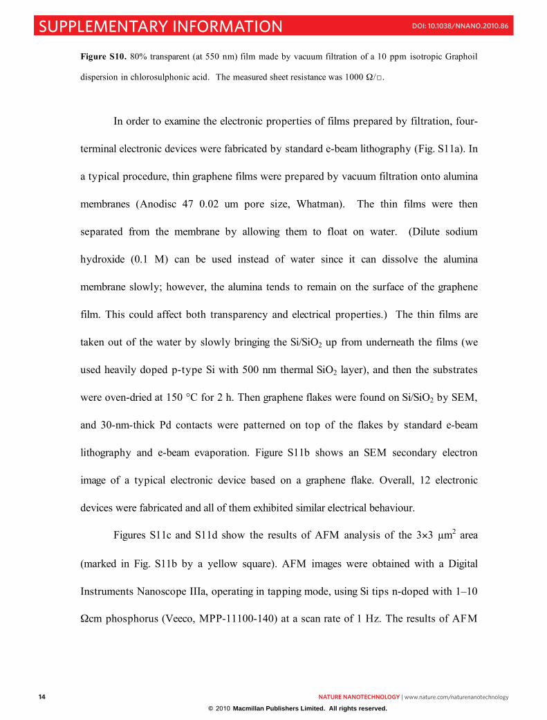
We also measured a sheet resistance of 1000 #/� on an 80% transparent film

(Fig. S10) made from a 10 ppm Graphoil dispersion. Sheet resistance of thin films was

measured using an Alessi four-point probe fitted with custom-made film attachment with




13

Pt leads. Measurements were taken in ambient conditions by securing and pressing the

graphene thin films on glass substrate against the Pt leads.

We compare these values against others in the literature. Lotya et al. report 62%

transmittance and 22,000 #/" for a surfactant-stabilized dispersion of graphene after

annealing 2. Hernandez et al. report a conductivity of 7100 #/" with 42% transmittance

(after annealing) 1. It is noteworthy that these films were not transferred to a clear

substrate; instead, the transparency was measured relative to an alumina substrate. Also,

these values are for films that have been annealed whereas the values obtained here have

not been annealed. Pre-annealing numbers for Hernandez et al. are 7,200,000 #/" and

61% transmittance.

Other, slightly better properties (100-1000 #/" at 80% transmittance) have been

observed for films produced from graphene oxide films, which were then reduced via

hydrazine to graphene and annealed at 1100 °C 9. However, annealing is not compatible

with most practical substrates, and could hinder possible applications.




14

Figure S10. 80% transparent (at 550 nm) film made by vacuum filtration of a 10 ppm isotropic Graphoil

dispersion in chlorosulphonic acid. The measured sheet resistance was 1000 #/".

In order to examine the electronic properties of films prepared by filtration, four-

terminal electronic devices were fabricated by standard e-beam lithography (Fig. S11a). In

a typical procedure, thin graphene films were prepared by vacuum filtration onto alumina

membranes (Anodisc 47 0.02 um pore size, Whatman). The thin films were then

separated from the membrane by allowing them to float on water. (Dilute sodium

hydroxide (0.1 M) can be used instead of water since it can dissolve the alumina

membrane slowly; however, the alumina tends to remain on the surface of the graphene

film. This could affect both transparency and electrical properties.) The thin films are

taken out of the water by slowly bringing the Si/SiO2 up from underneath the films (we

used heavily doped p-type Si with 500 nm thermal SiO2 layer), and then the substrates

were oven-dried at 150 °C for 2 h. Then graphene flakes were found on Si/SiO2 by SEM,

and 30-nm-thick Pd contacts were patterned on top of the flakes by standard e-beam

lithography and e-beam evaporation. Figure S11b shows an SEM secondary electron

image of a typical electronic device based on a graphene flake. Overall, 12 electronic

devices were fabricated and all of them exhibited similar electrical behaviour.

Figures S11c and S11d show the results of AFM analysis of the 3$3 #m2 area

(marked in Fig. S11b by a yellow square). AFM images were obtained with a Digital

Instruments Nanoscope IIIa, operating in tapping mode, using Si tips n-doped with 1–10

#cm phosphorus (Veeco, MPP-11100-140) at a scan rate of 1 Hz. The results of AFM




15

analysis demonstrate that the flake exhibits a significant thickness variation. For different

areas of the flake the measured thickness varied from 2 to 15 nm.

Figure S11e shows the current-voltage (IV) characteristics of the electronic device

shown in Fig. S11b. The electrical transport properties were tested using a probe station

(Desert Cryogenics TT-probe 6 system) under vacuum with chamber base pressure

below 10-5 torr. The IV data were collected by an Agilent 4155C semiconductor

parameter analyzer. Figure S11e shows that the graphene flakes prepared by the reported

method are highly conductive. Assuming the average thickness of the flake to be 10 nm,

the estimated conductivity of the prepared graphene is 9.2·104 S/m. For other electronic

devices the estimated conductivities were in the range from 8·104

to 9.5·104 S/m.




16

Figure S11. Electronic properties of graphene flakes. (a) Schematic of the electrical measurements. (b)

SEM image of a typical four-terminal device based on a graphene flake. The bright horizontal strips are Pd

electrodes. (c) AFM image of the 3$3 #m2 area shown by the yellow square in (b). (d) Height profile along

the white line in (c). (e) The IV characteristics of the device shown in (b), measured by four-probe method.

S-05: Tyndall effect




17

When a chlorosulphonic acid dispersion of graphene is illuminated using a red laser

pointer (~660 nm), a typical scattering effect is observed (Fig. S12). This is known as the

Tyndall effect and is a signature of a colloidal dispersion; this suggests the presence of

exfoliated nano-sheets in solution. This phenomena is also observed in water and organic

dispersions of graphene and chemically converted graphene 10,11

.

Figure S12. Pure chlorosulphonic acid (left) and graphene solution in chlorosulphonic acid (right). The

Tyndall effect is observed on a dilute solution of graphene (graphoil) in ClSO3H (15 µg/ml). There is a

distinct scattering of light in the right vial (containing graphene platelet) in comparison to left side vial

(pure acid).

S-06: HOPG XPS and Raman




18

Figure S13. carbon 1s core-level XPS spectrum from the dry material obtained upon quenching HOPG

from chlorosulphonic acid dispersion. The powder was dried under vacuum over night at 100 C. A fit to

carbon sulphur and carbon oxygen spectra did not yield measurable presence of oxygen and sulphur.

Figure S14. Raman spectra of HOPG before acid dispersion (black line) and after quenching from a

chlorosulphonic acid dispersion (red line). The two spectra are almost identical. Specifically, the disorder

0

0.2

0.4

0.6

0.8

1

278 282 286 290 294 298

Binding Energy (eV)

Inte

nsit

y (

a.u

.)




19

peak is absent on the material quenched from acid. The two spectra are averages over 5 measurements and

they were obtained using 514 nm laser.

S-07: Angle dependent electron diffraction

Monolayer graphene is characterize by a weak dependence of its diffraction intensity as a

function of sample tilting angle with respect the incident beam12. On the contrary, multi-layer

graphene has a diffraction intensity that changes dramatically with tilt angle. Figure S15a and

b show the diffraction intensity of the inner and outer spots versus tilt angle data for a

monolayer flake identified by its diffraction intensity profile. As the sample holder is tilted to

from 0o

-30o

there is just a weak variation of the intensity profile, as expected for monolayer

graphene. We decided to use a range of 30 o

for the tilting angle because for multilayer

graphite, the period of over which there is a full variation of intensity is roughly 30 o

12.This is

further confirmation of the presence of graphene and of our ability to identify it visually.




20

Figure S15. Selected area diffraction of a monolayer graphene flake for a wide range of tilt angles. a)

Intensities of inner spots. b) Intensities of outer spots. The insert image shows the area over which the

diffraction was performed and the size of the aperture.

REFERENCES




21

1 Hernandez, Y. et al. High-yield production of graphene by liquid-phase

exfoliation of graphite. Nature Nanotech. 3, 563-568 (2008). 2 Lotya, M. et al. Liquid Phase Production of Graphene by Exfoliation of Graphite

in Surfactant/Water Solutions. J. Am. Chem. Soc. 131, 3611-3620 (2009). 3 Gupta, A. K., Russin, T. J., Gutierrez, H. R. & Eklund, P. C. Probing Graphene

Edges via Raman Scattering. ACS Nano 3, 45-52 (2009). 4 Stoller, M. D., Park, S., Zhu, Y., An, J. & Ruoff, R. S. Graphene-Based

Ultracapacitors. Nano Lett. 8, 3498-3502 (2008). 5 Leonard, A. D. et al. Nanoengineered carbon scaffolds for hydrogen storage. J. of

Am. Chem. Soc. 131, 723-728 (2009). 6 Bets, K. V. & Yakobson, B. I. Spontaneous Twist and Intrinsic Instabilities of

Pristine Graphene Nanoribbons. Nano Research 2, 161-166 (2009). 7 Kosynkin, D. V. et al. Longitudinal unzipping of carbon nanotubes to form

graphene nanoribbons. Nature 458, 872-875 (2009). 8 Spector, M. S., Naranjo, E., Chiruvolu, S. & Zasadzinski, J. A. Conformation of a

Tethered Membrane: Crumpling in Graphitic Oxide? Phys. Rev. Lett. 73, 2867-

2870 (1994). 9 Becerril, H. A. et al. Evaluation of Solution-Processed Reduced Graphene Oxide

Films as Transparent Conductors. ACS Nano 2, 463-470 (2008). 10

Hamilton, C. E., Lomeda, J. R., Sun, Z. & Tour, J. M. High-yield organic

dispersions of unfunctionalized graphene. Nano Lett., doi:10.1021/nl9016623

(2009). 11

Li, D., Muller, M. B., Gilje, S., Kaner, R. B. & Wallace, G. G. Processable

aqueous dispersions of graphene nanosheets. Nature Nanotech. 3, 101-105 (2008). 12

Meyer, J. C. et al. On the roughness of single- and bi-layer graphene membranes.

Solid State Commun. 143, 101-109 (2007).




Documents

High-concentration, spontaneous dispersions and liquid ... · High-concentration, spontaneous dispersions and liquid crystals of ... concentration of the same graphite source in the