JAVIER CAZORLA AVILÉS

High Altitude Platforms for

UMTS

MASTER OF SCIENCE THESIS

SUBJECT APPROVED BY DEPARTMENT

COUNCIL ON JANUARY 15th, 2007

EXAMINERS: Professor Jukka Lempiäinen

M. Sc. Panu Lähdekorpi

ii

Abstract

TAMPERE UNIVERSITY OF TECHNOLOGY Degree program in Information Technology Institute of Communication Engineering CAZORLA AVILÉS, JAVIER: High Altitude Platforms for UMTS Master of Science Thesis, 92 pages. Examiners: Professor Jukka Lempiäinen, M. Sc. Panu Lähdekorpi Department of Information Technology February 2007 Key words: UMTS, High Altitude Platforms, WCDMA, network optimization.

High Altitude Platforms (HAPs) represent an alternative to wireless communications networks, and pretend to offer a feasible solution for the radio access layer of these kinds of networks. Its importance resides in the fact that HAPs have the most outstanding characteristics of terrestrial and satellite systems, together with the easy deployment and maintenance. HAPs have been proposed for deploying third generation mobile networks as well as other wide kind of telecommunication services. In Europe, the third generation of mobile communication system used is UMTS, which is based in the WCDMA technique. In UMTS, the quality, capacity and coverage are strongly connected to the interference levels, representing the main limitation of this system.

The work shown in this thesis is an analysis of network simulations obtained from the use of High Altitude Platforms in the radio access network of UMTS. The work was aimed to find an optimal configuration for a single HAP scenario, and to apply this optimal configuration to a multi-HAP scenario. The results for the analysis of both cases have been simulated using the NPSW static simulator software tool. For the single HAP scenario, a set of different cell layouts with different antenna beamwidths were simulated. Each one of these configurations was simulated in different load cases, using a wide traffic scale. The results obtained from the analysis of a single HAP scenario lead to a planning rule for the configuration of the antennas on board.

This planning rule is used for the multi-HAP scenario, where three HAPs provide UMTS coverage jointly. The analysis for the multi-HAP architecture was focused on finding the optimal distance between HAPs. The basic parameters for the simulations such as traffic density and configuration of the antennas on board are the same as used for a single HAP scenario. This is due to the fact that the variable under study in this multi-HAP architecture is the distance between HAPs. Consequently the results obtained show the variation of the network performance with the separation between HAPs.

iii

Preface This Master of Science Thesis has been written at the Department of Information Technology at Tampere University of Technology in Finland. The work for this thesis has been done during my Erasmus exchange period in Finland. I would like to express my gratitude to my thesis supervisor and examiner Jukka Lempiäinen for supervising my work. I would also like to thank Jarno Niemelä for being my contact person before starting my exchange period in Finland and helping me to find a topic for the Master Thesis. Special thanks to Panu Lähdekorpi for being my “tutor” in my daily work and giving me all support and guidance I needed during this period. I also thank Jaroslaw Lacki and Tero Isotalo for helping me during this period. My gratitude to my friends in Spain from the ETSIT, to all my Spanish colleagues and all the internationals I met here in Tampere, for giving me such a special moments and with whom I have shared unforgettable experiences. Thank you very much. Finally I would like to express my deepest gratitude to my parents, Javier and Rosa, and my sister Verónica, for their love, their support, their efforts, their understanding and the education they have given me. Special thanks to my girlfriend Maialen, for helping me during this period, for her endless love and for being such a marvellous person. This work is dedicated to them. Tampere, January 19th, 2007. Javier Cazorla Avilés javiercazorla@gmail.com +34 616 75 10 12 , +34 91 812 05 40

iv

Contents

1 INTRODUCTION TO HIGH ALTITUDE PLATFORMS ........................................... 1

1.1 HAPs definition....................................................................................................... 2

1.2 HAPs topologies...................................................................................................... 2

1.2.1 A terrestrial-HAP-satellite system.................................................................... 3

1.2.2 An integrated terrestrial-HAP system .............................................................. 3

1.2.3 A standalone HAP system................................................................................ 4

1.3 HAPs applications ................................................................................................... 5

1.3.1 2G/3G (UMTS) and 4G applications ............................................................... 5

1.3.2 Broadband Fixed Wireless Access Applications.............................................. 6

1.3.3 HAP Networks ................................................................................................. 6

1.3.4 Developing world applications......................................................................... 7

1.3.5 Emergency and disaster scenarios.................................................................... 7

1.3.6 Military Communications................................................................................. 8

1.4 HAPs advantages and challenges ............................................................................ 9

1.4.1 Platform altitude ............................................................................................... 9

1.4.2 Propagation....................................................................................................... 9

1.4.3 Flexibility to respond to traffic demand ......................................................... 10

1.4.4 Low cost ......................................................................................................... 10

1.4.5 Incremental and rapid deployment ................................................................. 10

1.4.6 Cell planning .................................................................................................. 10

1.4.7 Call Admission Control.................................................................................. 11

1.4.8 Handover properties ....................................................................................... 11

2. INTEGRATION OF A HAP WITHIN A TERRESTRIAL UMTS NETWORK..... 12

2.1 General issues........................................................................................................ 12

2.2 UMTS services ...................................................................................................... 13

2.3 UMTS network architecture.................................................................................. 14

2.3.1 Core Network ................................................................................................. 15

2.3.2 UMTS Radio Access Network ....................................................................... 17

2.4 HAP role in UMTS network ................................................................................. 19

2.5 Antenna models..................................................................................................... 21

2.6 Propagation model................................................................................................. 23

v

2.7 Radio planning ...................................................................................................... 25

2.7.1 Cell deployment and hexagonal layout .......................................................... 25

2.7.2 Other cell deployment and antenna pattern issues ......................................... 28

2.7.3 Interference and capacity analysis for HAPs ................................................. 29

3. SIMULATIONS.......................................................................................................... 36

3.1 NPSW static simulator .......................................................................................... 36

3.2 Adapted Simulator for HAPs ................................................................................ 37

3.2.1 Base station antenna modelling for terrestrial networks ................................ 37

3.2.2 Antenna gain estimation for HAPs................................................................. 39

3.3 Single HAP scenario ............................................................................................. 44

3.3.1 Simulation parameters.................................................................................... 45

3.3.2 Variables of study........................................................................................... 47

3.3.4 Simulations structure...................................................................................... 58

3.3.5 Results ............................................................................................................ 59

3.4 Single HAP with modified antenna pattern........................................................... 72

3.5 Multi-HAP............................................................................................................. 75

3.5.1 General parameters and variables of study..................................................... 75

3.5.2 Results ............................................................................................................ 80

4 CONCLUSIONS.......................................................................................................... 81

REFERENCES................................................................................................................ 83

vi

List of abbreviations

2G Second Generation

3G Third Generation

4G Fourth Generation

API Application Program Interface

B-FWA Broadband Fixed Wireless Access

BS Base Station

C/I Carrier to Interference Ratio

CAC Call Admission Control

CN Core Network

CS Circuit Switching

EHF Extremely High Frequency

FDD Frequency Division Duplex

GGSN Gateway GPRS Support Node

GNSS2 Global Navigation Satellite System 2

GPRS General Packet Radio Service

GSM Global System for Mobile Communications

HAP High Altitude Platform

HALO High Altitude Long Operation

IP Internet Protocol

IP-TV Internet Protocol Television

ITU International Telecommunications Union

LEO Low Earth Orbit

MBMS Multimedia Broadcast and Multicast Services

MSC Mobile Switching Centre

NPSW Network Planning Strategies for Wideband CDMA

PS Packet Switching

PSE Personal Service Environment

QoS Quality-of-Service

RF Radio Frequency

RNC Radio Network Controller

SGSN Serving GPRS Support Node

SHO Soft Handover

SIR Signal to Interference Ratio

vii

SMS-GMSC Short Message Service Gateway MSC

SMS-IWMSC Short Message Service InterWorking MSC

TCP Transmission Control Protocol

TDD Time Division Duplex

TDMA Time Division Multiple Access

TETRA Trans European Trunking Radio

UAV Unmanned Aerial Vehicle

UE User Equipment

U-GGSN UMTS-GGSN

U-MSC UMTS-Mobile Switching Centre

UMTS Universal Mobile Telecommunications System

U-SGSN UMTS-SGSN

UTRAN Universal Terrestrial Radio Access Network

VHE Virtual Home Environment

WCDMA Wideband CDMA

WiFi Wireless-Fidelity

1

1 Introduction to High Altitude Platforms

Nowadays the demand for communication services is increasing notoriously all over the world, and it leads to a rapid development and deployment of high capacity services for future generation networks. The most important features for these services are high capacity (high bit rates), mobility on demand (ubiquity), large coverage, and all together represent the concept of “anywhere, anytime” for the final user. This concept has become the flag of future communications services that would solve the need for broadband due to the convergence of high speed Internet access, telephony, TV (also IP-TV) and video-on-demand, sound broadcasting etc. However, this is only the beginning in comparison to the wide range of value-added services that service providers are expected to deploy on behalf of the user necessities. With this horizon, wireless solutions aim to be the best choice to deploy the networks that would supply this kind of broadband and value-add services for small-medium enterprises and small office/home office users, and also for domestic users. Wireless solutions applied to these necessities of broadband services represent a solution to the called “the last mile” problem which deals with the crucial step of delivering connectivity between services providers and customers, and also represent the economical and physical challenge of the high costs of wire and cable based networks. Delivering high capacity services by using wireless solutions becomes a challenge, particularly in the pressure on radio spectrum. As known, the radio spectrum is a limited resource and is becoming saturated due to the increasing demand and development of applications that use radio propagation in the physical layer. Consequently, and for an effective use of spectrum, several strategies have to be adopted, as a suitable frequency reuse and cell sizing and deployment. These topics will be explained in more detail in this thesis. [1][2][3]

The idea of providing present broadband services using static and unmanned aerial platforms is not new, and is becoming one of the most challenging alternatives to terrestrial deployment of broadband networks. In the last few years, there has been significant interest from international community primarily in all related to this kind of unmanned, static airborne platforms.

Nowadays, High Altitude Platforms (HAPs) represent a new alternative to the traditional satellite and terrestrial broadband services and have gained interest thanks to some of their characteristics that make them one of the most potential options in network deployment for future broadband services. High altitude platforms appear as a new emerging technology between the well established and totally dominated terrestrial and satellite systems, gathering major advantageous characteristics from both systems.

Actually, and due to their easy deployment, HAP networks are oriented to provide

2

not only broadband services but also services like remote sensing and Earth monitoring, positioning and navigation, homeland security, meteorological measurements, traffic monitoring and control and emergency application, as well as military applications.

1.1 HAPs definition

HAPs are airships or planes, operating in the stratosphere, at altitudes of typically 17–22 km (around 75,000 ft). At this altitude (which is well above commercial aircraft height), they can maintain a quasi-stationary position, and support payloads to deliver a range of services: principally communications, and remote sensing. Communications services include broadband, 3G, and emergency communications, as well as broadcast services. A HAP can provide the best features of both terrestrial masts (which are then not required) and satellite services (which would be highly expensive). In particular, HAPs permit rapid deployment, and highly efficient use of the radio spectrum (largely through intensive frequency re-use). The relatively wide range of HAPs in terms of service compared to satellites means that imaging and remote sensing is highly effective, offering low cost and high resolution. A variety of hybrid applications may also be planned, such as traffic management, navigation and security management. There are two fundamental types of platform technologies capable of stratospheric flight: unmanned aircraft and unmanned airships. However, manned aircraft (flying in circles) could also represent a HAP. Other platform technologies, such as manned aircraft together with tethered aerostats, and lower altitude UAVs (Unmanned Aerial Vehicles) may also have a developmental role towards HAPs and their applications. [4]

1.2 HAPs topologies

HAPs offer a wide range of network topologies due to their easy and rapid deployment. They can be included in several topologies, depending on the kind of service to provide. Mainly we can find three kinds of topologies where HAPs can be deployed. First, it can be used as an intermediate platform between satellite and terrestrial system, improving the constrictions that satellite radio links, coverage and resource management implies. Second, it can be used as the stratospheric segment of a network architecture used along with a terrestrial network, only with a backhaul link (for more developed areas where exists a connection to terrestrial networks). Finally, it can be also used as a stratospheric segment of a network, as explained above, but also using a satellite as an alternative backhaul link, for areas without connection to terrestrial networks where satellite links are the only one possibility.

3

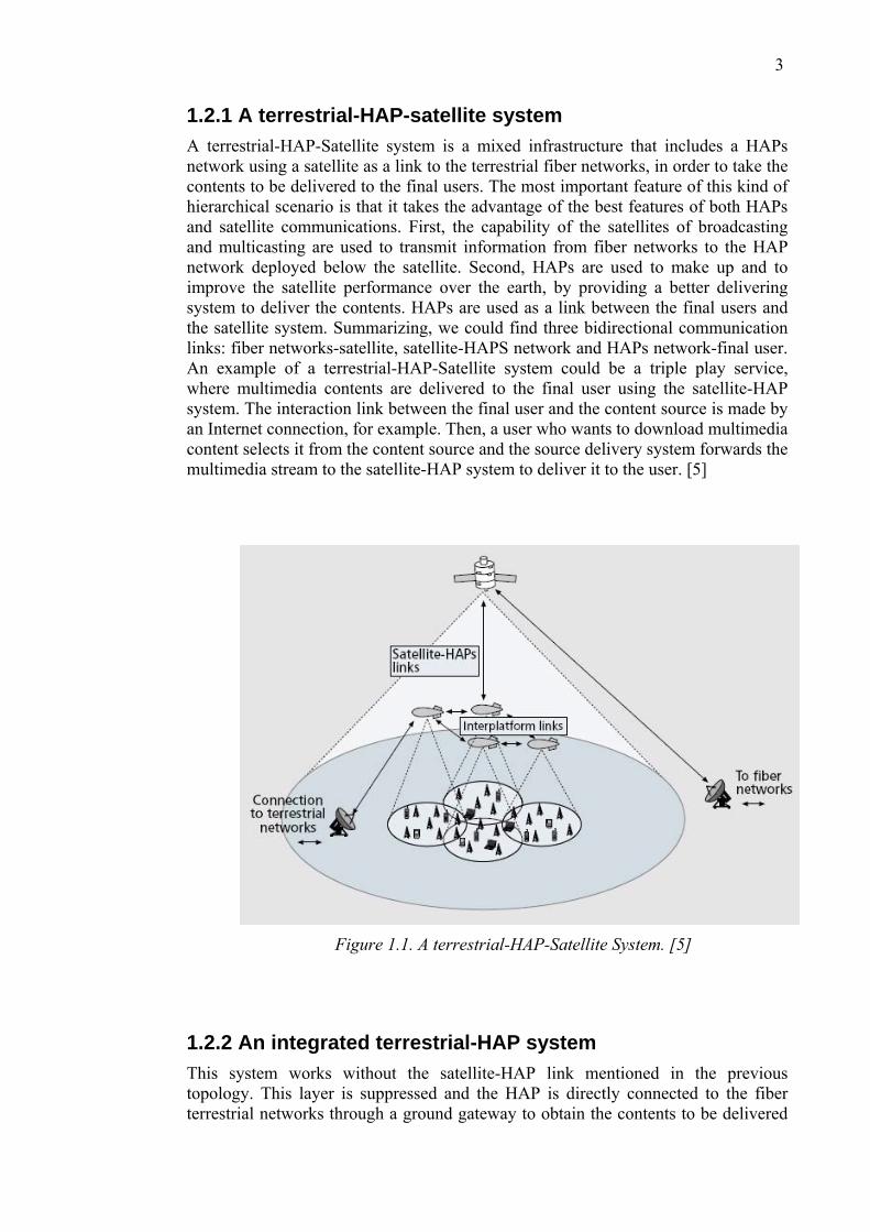
1.2.1 A terrestrial-HAP-satellite system A terrestrial-HAP-Satellite system is a mixed infrastructure that includes a HAPs network using a satellite as a link to the terrestrial fiber networks, in order to take the contents to be delivered to the final users. The most important feature of this kind of hierarchical scenario is that it takes the advantage of the best features of both HAPs and satellite communications. First, the capability of the satellites of broadcasting and multicasting are used to transmit information from fiber networks to the HAP network deployed below the satellite. Second, HAPs are used to make up and to improve the satellite performance over the earth, by providing a better delivering system to deliver the contents. HAPs are used as a link between the final users and the satellite system. Summarizing, we could find three bidirectional communication links: fiber networks-satellite, satellite-HAPS network and HAPs network-final user. An example of a terrestrial-HAP-Satellite system could be a triple play service, where multimedia contents are delivered to the final user using the satellite-HAP system. The interaction link between the final user and the content source is made by an Internet connection, for example. Then, a user who wants to download multimedia content selects it from the content source and the source delivery system forwards the multimedia stream to the satellite-HAP system to deliver it to the user. [5]

Figure 1.1. A terrestrial-HAP-Satellite System. [5]

1.2.2 An integrated terrestrial-HAP system This system works without the satellite-HAP link mentioned in the previous topology. This layer is suppressed and the HAP is directly connected to the fiber terrestrial networks through a ground gateway to obtain the contents to be delivered

4

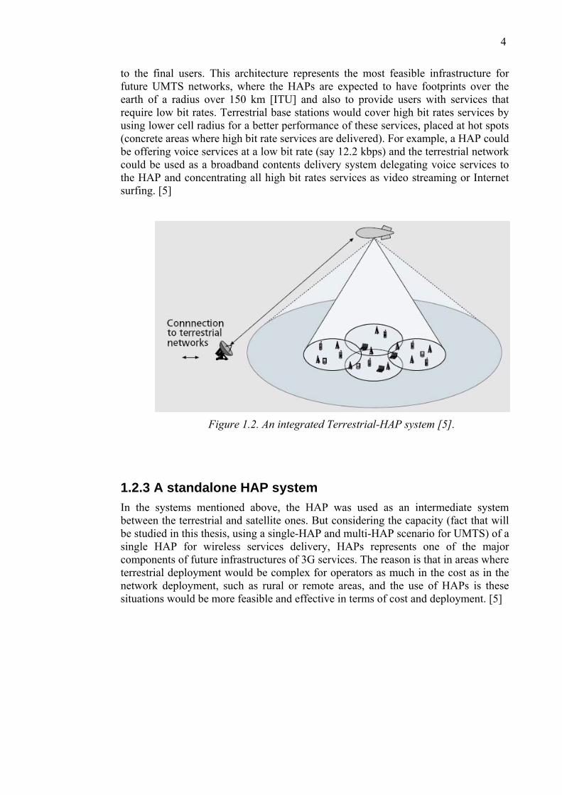
to the final users. This architecture represents the most feasible infrastructure for future UMTS networks, where the HAPs are expected to have footprints over the earth of a radius over 150 km [ITU] and also to provide users with services that require low bit rates. Terrestrial base stations would cover high bit rates services by using lower cell radius for a better performance of these services, placed at hot spots (concrete areas where high bit rate services are delivered). For example, a HAP could be offering voice services at a low bit rate (say 12.2 kbps) and the terrestrial network could be used as a broadband contents delivery system delegating voice services to the HAP and concentrating all high bit rates services as video streaming or Internet surfing. [5]

Figure 1.2. An integrated Terrestrial-HAP system [5].

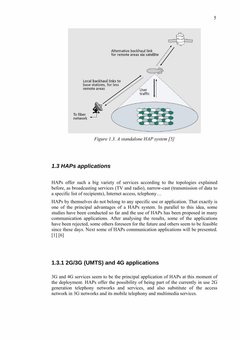
1.2.3 A standalone HAP system In the systems mentioned above, the HAP was used as an intermediate system between the terrestrial and satellite ones. But considering the capacity (fact that will be studied in this thesis, using a single-HAP and multi-HAP scenario for UMTS) of a single HAP for wireless services delivery, HAPs represents one of the major components of future infrastructures of 3G services. The reason is that in areas where terrestrial deployment would be complex for operators as much in the cost as in the network deployment, such as rural or remote areas, and the use of HAPs is these situations would be more feasible and effective in terms of cost and deployment. [5]

5

Figure 1.3. A standalone HAP system [5]

1.3 HAPs applications

HAPs offer such a big variety of services according to the topologies explained before, as broadcasting services (TV and radio), narrow-cast (transmission of data to a specific list of recipients), Internet access, telephony…

HAPs by themselves do not belong to any specific use or application. That exactly is one of the principal advantages of a HAPs system. In parallel to this idea, some studies have been conducted so far and the use of HAPs has been proposed in many communication applications. After analysing the results, some of the applications have been rejected, some others foreseen for the future and others seem to be feasible since these days. Next some of HAPs communication applications will be presented. [1] [6]

1.3.1 2G/3G (UMTS) and 4G applications

3G and 4G services seem to be the principal application of HAPs at this moment of the deployment. HAPs offer the possibility of being part of the currently in use 2G generation telephony networks and services, and also substitute of the access network in 3G networks and its mobile telephony and multimedia services.

6

Multimedia broadcast and multicast services (MBMS) also can be provided by the HAP layer of 3G and beyond 3G in order to achieve higher system capacity and lower cost. To sum up, a longer list of applications are expected to come along with the forth generation (4G) networks. 4G systems will include actually existing and emerging fixed and mobile networks including broadcasting. Continuing with this idea, 3G base stations could be integrated on the HAP aircrafts. A single base station on the platform with a wide beamwidth antenna could provide of service over large sparsely populated areas. In addition to this, in urban areas, where a higher capacity is needed, smaller cells can be deployed with integrated smaller directional antennas (antenna arrays). All this include exceptional benefits such as offering coverage in a large area, quite direct propagation paths without obstacles and elimination of the expensive resources spent in ground station installations, maintenance and wire installations under ground. [6]

1.3.2 Broadband Fixed Wireless Access Applications Another main application for HAPs together with the UMTS generation services is planned to be the Broadband Fixed Wireless Access (B-FWA) services. In other words, this means broadband data provision providing to the user a set of multimedia services, such as high speed Internet, telephony, TV, video-on-demand, etc., at a very high data rate. There are three separate spectrum bands for HAPs systems offering these kinds of services: 2GHz, 28/31 GHz and 47/48 GHz. For instance at the 47/48 GHz bands there are two bands of 300 GHz (47.2-47.5 GHz and 47.9-48.2 GHz) which can be shared between users and backhaul links and also between uplink and downlink. When there is internet traffic, the proportion maintains asymmetric traffic, always the downlink exceeding the uplink traffic. The European HeliNet programme [7] proposal for B-FWA applications is based on a HAP coverage per platform of 60 km of diameter, comprising 121 cells of 5 km diameter on the ground. Each cell provides 1 Watt in the downlink and bit rates up to 60 Mbit/s, if a 25 MHz of bandwidth per cell and 16-QAM or higher order modulation technique are used. The total throughput achieved in this scenario is over 7 Gbit/s, although higher rates around 100 Gbit/s are expected to be achieved by using different HAPs architectures, as High Altitude Long Operation (HALO). Nevertheless there must be a number of distributed backhaul base stations, always fewer than the number of cells served from the HAP. The location of this ground stations is considered to be non-critical and are normally located on the roof of buildings. [6]

1.3.3 HAP Networks

A group of HAPS comprising a HAP network can be deployed in a certain region to offer coverage of it using just a reduced number of platforms that is much smaller

7

than the number of ground base stations that would had been employed. Inter-HAP link could be fulfilled at EHF frequencies (30-300 GHz), as it has been done with satellites, and should not involve any representative trouble. [6]

1.3.4 Developing world applications

By means of HAPs, a wide range of services can be introduced in the developing countries. Some of these services are rural telephony, broadcasting and data services like Internet. Especially, the use of HAPs seems to be the only tool to offer these services when there is a lack of ground structure or the existing one is expensive, deficient, or difficult to use for these purposes. [1][6]

1.3.5 Emergency and disaster scenarios

Due to a natural (flood, earthquake, tsunami…) or a man-provoked disaster (terrorist attack, fire…) the telecommunication core network operating in that area can be damaged in many ways. The infrastructure and the coverage needed for the operation of the emergency services can be partially or fully destroyed, unavailable or overloaded by excessive demand just moments after the disaster has happened. So the use of HAPs is proposed to be an alternative wireless network provider to restore, replace or add capacity to the existing damaged network. This kind of dramatic disaster happenings can cause outages in the service. The mobile network might get saturated and crumble for many hours leaving public and emergency services without operability. In other more catastrophic events, like a tsunami or a nuclear explosion, the network could be seriously damaged, from the loss of base station and repeaters leading to a poor coverage in that area. The principal attraction in the use of HAPs in this situation is that they can be rapidly deployed over the disaster scenario and that by means of a single or a couple of platforms a large area can be served. In addition, another advantage of HAPs deployment is its immunity to most disasters. Different wireless services can be offered depending on the payload on the HAP. Among others reconnaissance, surveillance, telecommunication services as well as meteorological and atmospheric measurements can be provided. [6]

There are some important decisions that must be considered before setting a new HAPs network in a disaster situation:

• The service area needs to be limited. • The cell layout needs to be designed. • The backhaul needs to be set up. • Identification of possible interference operating systems.

According to some research made so far [8], the use of HAPs for deploying of GSM, TETRA and UMTS services over a defined emergency area has been studied and simulated. The area under study that has been considered is an island, 16 km by 18

8

km. In the wake of a natural disaster all communication nodes that the island used for communications failed on the entire island and an emergency mobile network must be deployed using HAPs. TDMA systems, both GSM and TETRA protocols, confront problems with long link lengths due to synchronization problems inherent to their TDMA nature. By use of guard bands, the coverage area can be enlarged up to a maximum of 140 km diameter and consequently it would suppose a loss of capacity. This technique is aimed for sparsely populated areas and nowadays it successfully runs in some rural areas of Australia. Another issue would be whether to use small cells or large cells over such scenario. Small cells provide the same bit rates as a single large cell using a fraction of the power spent with a large cell. On the contrary, a bigger number of handovers is needed to ensure the communication while moving between cells. But maybe the toughest problem especially in GSM would be related to the coexistence between the HAPs based GSM network and the terrestrial GSM network concerning to the spectrum use. It means each network must use different frequencies from each other to avoid interference. To enable this coexistence, the HAPs GSM cells will overlap the terrestrial cells using different frequencies. In order to detect the frequencies not used by the damaged terrestrial system a frequency scanner can be utilized from the air. Supposing now that we are going to restore a damaged UMTS network on the island, and knowing that it employs a WCDMA multiple access technique, we should consider studying the interference, which represents the limiting factor in this type of systems. Two type of interference will be considered: effects on the HAPs network from the interference caused from the terrestrial network and the effects on the terrestrial UMTS network with the introduction of the HAPs network. There have been some studies about this scenario that suggest that the overlap between the HAP and the terrestrial UMTS cells should maintain to the minimum. That means that for causing the right number of handovers the overlap should be no higher than the 20%. [8] [6]

1.3.6 Military Communications

The potential use of HAPs system in the military field is quite clear. The beneficial characteristics of HAPs for rapid deployment in existing military wireless networks as nodes or acting as a part of a surrogate satellite network make them very attractive. Furthermore by means of HAPs it is possible to provide communication and due to their close range operation layout limited by the transmit power from the ground terminal makes its transmissions difficult to be intercepted. These two characteristics are crucial and extremely valued in military activities. [9] It could be thought that HAPS could be vulnerable to enemy attacks as they operate at low altitudes, normally unmanned and in a quite stationary position. However their envelope is pretty transparent to microwaves and they also show a fairly low cross section so that it turns pretty complicated to detect them. [1] [6]

9

1.4 HAPs advantages and challenges

High Altitude Platforms offer a wide range of advantages and potential benefits compared to terrestrial and satellite communications systems deployed nowadays. This advantages are shown in the next subsections.

1.4.1 Platform altitude

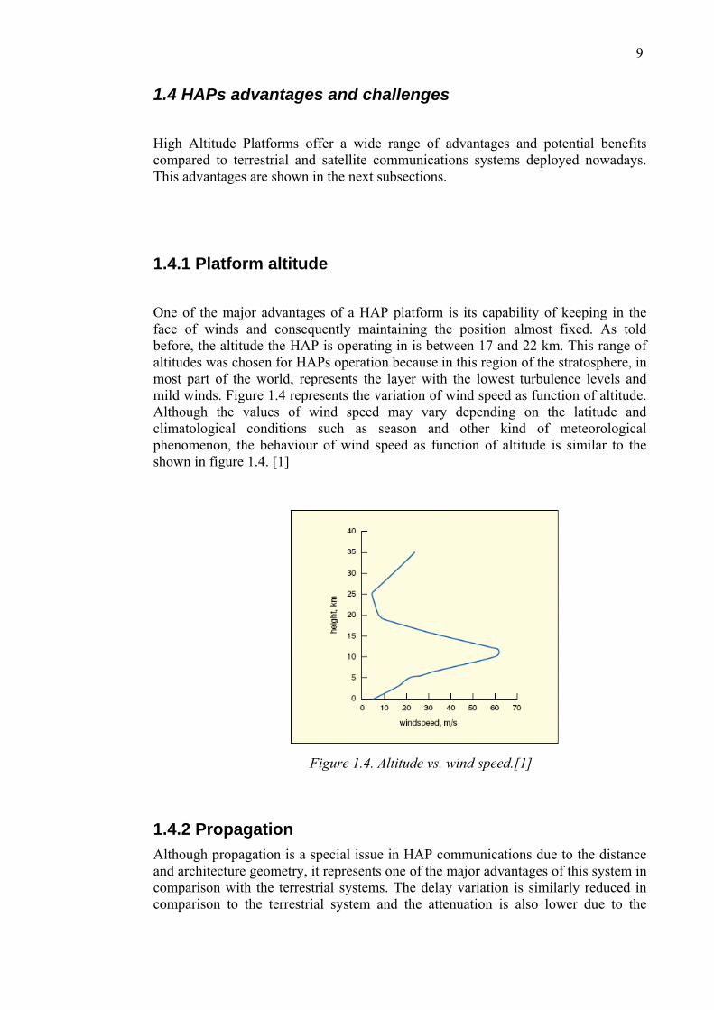
One of the major advantages of a HAP platform is its capability of keeping in the face of winds and consequently maintaining the position almost fixed. As told before, the altitude the HAP is operating in is between 17 and 22 km. This range of altitudes was chosen for HAPs operation because in this region of the stratosphere, in most part of the world, represents the layer with the lowest turbulence levels and mild winds. Figure 1.4 represents the variation of wind speed as function of altitude. Although the values of wind speed may vary depending on the latitude and climatological conditions such as season and other kind of meteorological phenomenon, the behaviour of wind speed as function of altitude is similar to the shown in figure 1.4. [1]

Figure 1.4. Altitude vs. wind speed.[1]

1.4.2 Propagation Although propagation is a special issue in HAP communications due to the distance and architecture geometry, it represents one of the major advantages of this system in comparison with the terrestrial systems. The delay variation is similarly reduced in comparison to the terrestrial system and the attenuation is also lower due to the

10

presence of line-of-sight. Another factor to be considered when modelling the propagation environment in HAP systems is rain attenuation and rain scattering over wide areas. [10]

1.4.3 Flexibility to respond to traffic demand HAPs provide an adaptable system in situations where scenarios and traffic distribution are dynamic, presenting changing characteristics. This feature transforms the resources constraint in terrestrial networks, i.e. frequency reuse patterns and cell sizes, for example. [1]

1.4.4 Low cost Although there is not any experience related to HAP based networks, a simple multi HAP network should be cheaper than launching a set of geostationary or LEO satellites and also cheaper than covering the same area using terrestrial base stations. Compared to Terrestrial systems, HAPs eliminate costs related to site acquisition problems, environmental impact, installation and maintenance costs… Compared to satellite communications systems, there is no need of a launch vehicle to put the platform into orbit. HAPs are solar powered and that reduces also launching and positioning costs [1].

1.4.5 Incremental and rapid deployment It is possible that a service initially provided by a single HAP changes its traffic demands and service characteristics (according to the service and traffic flexibility explained before) and therefore the network need to be expanded in coverage and/or in capacity. In contrast with satellite services and terrestrial networks, whose service capabilities when expanding the network features are constrained by launching/deployment costs, in a HAP network only another antenna configuration (the HAP payload) and other changes (as adding another HAP to the network, for example) are needed. Summed to the low-cost operation and the easy HAP handling of their payload upgrading (they can be brought down to earth relatively readily), HAPs represent an enormous advantage that speeds up network deployment. The same upgrading in terrestrial networks involves a lot of procedures and civil works that usually implies slow procedures. Similarly, in services provided by satellite networks, payloads render obsolete and obviously it is not possible to bring them down [1].

1.4.6 Cell planning Cell planning is one of the greatest matters for a wireless network designer. An efficient cell planning can reduce network costs and increase the network capacity. In HAP deployment the integration of HAP in the terrestrial system should be done in conjunction. HAP cell deployment is not restricted by terrain, obstacles or other

11

parameters like in terrestrial systems, because all base stations are located in the HAP and the antennas are pointing down, providing coverage. Cell planning includes more issues such as bandwidth allocation, QoS requirements, cell sectorization and tessellating, frequency assignments, etc. Furthermore, the study of interference in HAP is should be included in cell planning in order to develop planning rules and obtain optimal coverage and high signal quality. [5]

1.4.7 Call Admission Control

Among the various aspects of resource management, Call Admission Control (CAC) is of a relevant importance since it controls the number of users, and thus is strongly related to the users’ QoS. CAC handles the set processes executed by the network during the phase of connection establishment to decide whether to accept or reject a user’s request for a connection. There are several studies that addressed the issue of CAC for standalone systems. In future integrated telecommunications networks a key objective is to provide a multitude of services using their capabilities in an optimized way. Intelligent CAC schemes should be able to decide on the serving network according to several decision criteria. The most important ones are the QoS requirements of the application, the traffic load of each candidate serving network, the user mobility, the energy available at the user terminal, and pricing. The challenge in this case is to include all these criteria in a CAC algorithm without increasing too much its computational complexity and without further complications in the design of multimode user terminals, by requiring new functionalities to be added to them. [5]

1.4.8 Handover properties In heterogeneous systems two types of handovers can be identified: intrasystem handovers, also referred to as horizontal handovers, and intersystem handover, which are usually referred to as vertical handovers. A handover is usually initiated when the signal-to-interference ratio (SIR) is below a certain and predefined threshold. Several studies have addressed the issue of intrasystem handover, especially for terrestrial code-division multiple access (CDMA) cellular systems. In terrestrial cellular systems user is connected to the base station with the minimum radio path loss, which may not be the closest one. On the contrary, in a HAP system a user is connected to the base station that serves the cell in which the user is located. This fact reduces the need for soft handover in HAP CDMA cellular systems. As known, soft handover is the technique whereby mobile users in transition between one cell and its neighbour transmit to and receive from two or more base stations simultaneously. This technique improves system performance of terrestrial CDMA cellular networks at the expense of increased backhaul connections. Moreover, it ameliorates the undesirable “pingpong” effect where the user is handed back and forth several times from one base station to another as he/she hovers around the cell boundary. Nevertheless, in a practical HAP cellular system this can be avoided by handing over the user only when the base station power is sufficiently below its value at the theoretical cell boundary. [5]

12

2. Integration of a HAP within a terrestrial UMTS network

After introducing the main features of High altitude platforms, the following sections will present the basic concepts needed for the integration of HAPs in UMTS networks.

2.1 General issues

Generally speaking, in a terrestrial cellular network system as for example UMTS, the mobile station (MS) and the base station (BS) use a radio link for communications by using radio resources. Each BS is configured to be accessed by a limited number of users, occupying resources. As known, in UMTS this number depends on the radio planning parameters like cell loading, interference and on the maximum number of users using different kind of services (from low to high bit rates) simultaneously. The problem is the role that HAP plays in UMTS from a network planning point of view, and the architecture used for adapting HAP to UMTS network structure. This question implies in all cases a concrete HAP payload design, a different UMTS Radio Access Network Structure and changes in all issues referred to cell planning, antenna configuration, interference study and propagation.

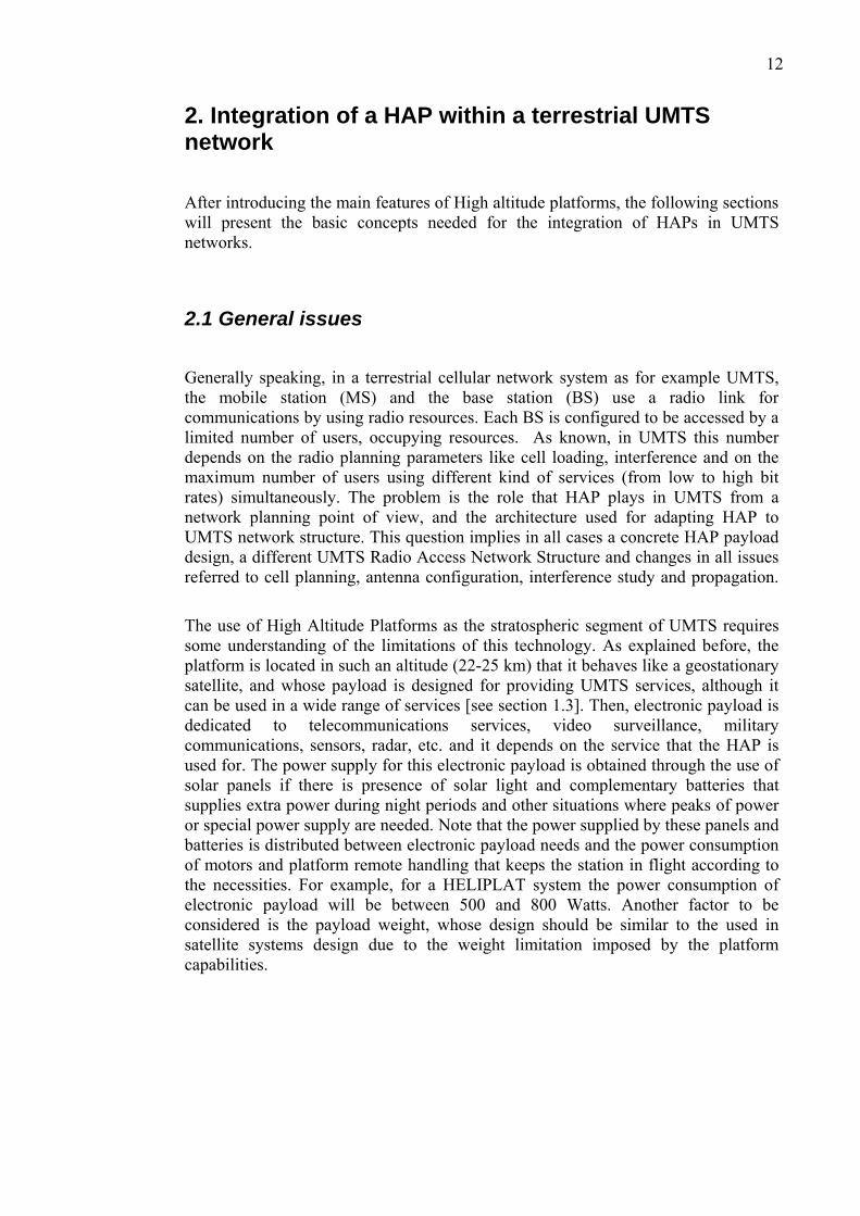
The use of High Altitude Platforms as the stratospheric segment of UMTS requires some understanding of the limitations of this technology. As explained before, the platform is located in such an altitude (22-25 km) that it behaves like a geostationary satellite, and whose payload is designed for providing UMTS services, although it can be used in a wide range of services [see section 1.3]. Then, electronic payload is dedicated to telecommunications services, video surveillance, military communications, sensors, radar, etc. and it depends on the service that the HAP is used for. The power supply for this electronic payload is obtained through the use of solar panels if there is presence of solar light and complementary batteries that supplies extra power during night periods and other situations where peaks of power or special power supply are needed. Note that the power supplied by these panels and batteries is distributed between electronic payload needs and the power consumption of motors and platform remote handling that keeps the station in flight according to the necessities. For example, for a HELIPLAT system the power consumption of electronic payload will be between 500 and 800 Watts. Another factor to be considered is the payload weight, whose design should be similar to the used in satellite systems design due to the weight limitation imposed by the platform capabilities.

13

Figure 2.1. HELIPLAT.

2.2 UMTS services

UMTS specifications do not include excessive information concerning to service specifications in order to favour competitivity between UMTS providers and the introduction of new services providers without the necessity of a network infrastructure. Consequently in the specifications can be found several aspects related to the basic procedures for constituting new services that give the market the chance of being the service “builder” and also the impeller of 3G service horizons.

One of the most important elements defined in the specifications is the Application Program Interfaces, or API. The API defines the path to be followed .An example of this API interfaces is Open Services Access (OSA), conceived to provide a standardized open access to applications developers for UMTS.

Another concept to be considered is Virtual Home Environment (VHE). Virtual Home Environment is a concept for Personal Service Environment (PSE) portability across network boundaries and between terminals. The concept of VHE is such that users are consistently presented with the same personalised features, User Interface customisation and services in whatever network and whatever terminal (within the capabilities of the terminal and the network), wherever the user may be located. [11].

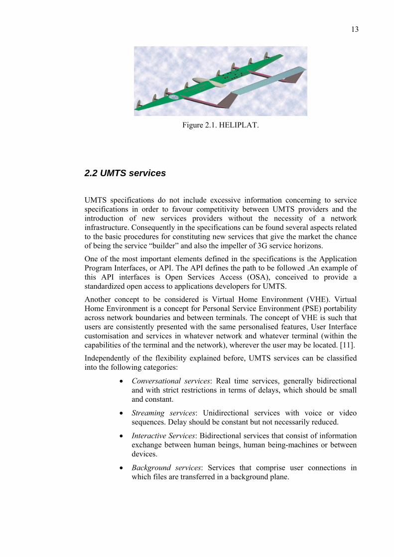
Independently of the flexibility explained before, UMTS services can be classified into the following categories:

• Conversational services: Real time services, generally bidirectional and with strict restrictions in terms of delays, which should be small and constant.

• Streaming services: Unidirectional services with voice or video sequences. Delay should be constant but not necessarily reduced.

• Interactive Services: Bidirectional services that consist of information exchange between human beings, human being-machines or between devices.

• Background services: Services that comprise user connections in which files are transferred in a background plane.

14

2.3 UMTS network architecture

UMTS system is structured in two networks: telecommunications network and management network. The former intends to ensure the information transport between peers in when a connection is established. The latter is designed to provide auxiliary functions of maintenance and operative issues, subscriber’s management and invoicing systems. The telecommunications network can be divided into three parts, Core Network (CN), UMTS Radio Access Network (UTRAN) and User equipments (UE).

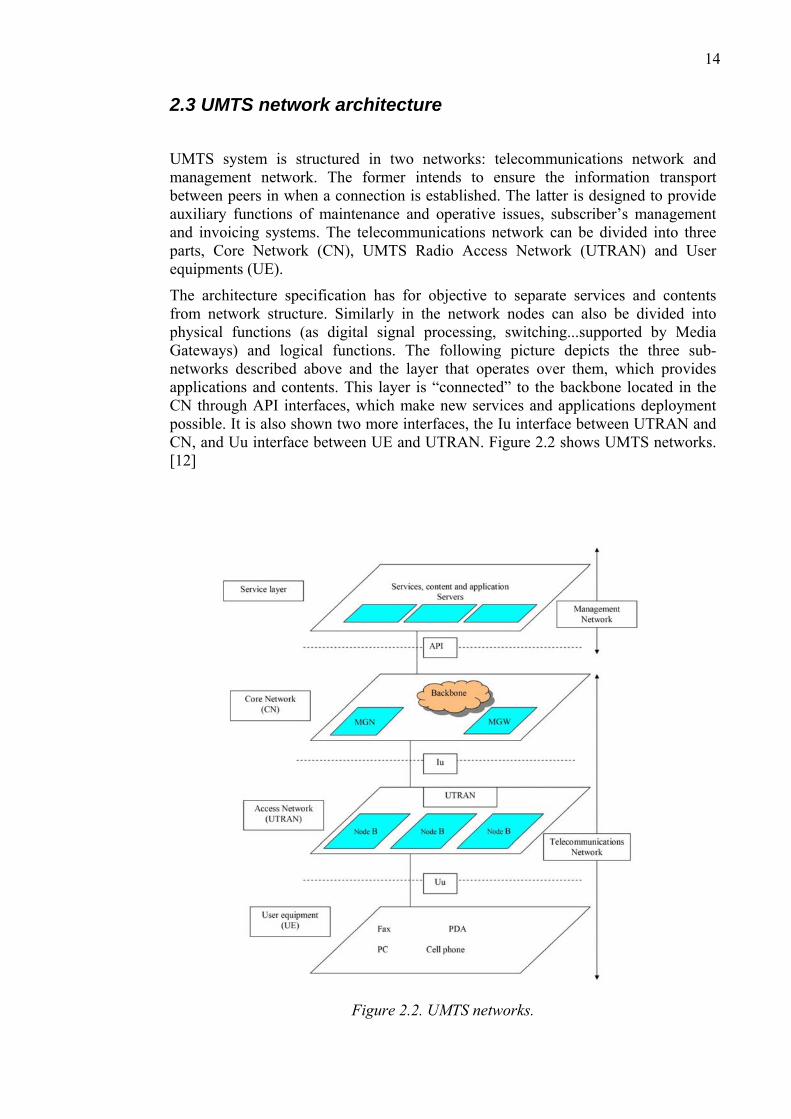
The architecture specification has for objective to separate services and contents from network structure. Similarly in the network nodes can also be divided into physical functions (as digital signal processing, switching...supported by Media Gateways) and logical functions. The following picture depicts the three sub-networks described above and the layer that operates over them, which provides applications and contents. This layer is “connected” to the backbone located in the CN through API interfaces, which make new services and applications deployment possible. It is also shown two more interfaces, the Iu interface between UTRAN and CN, and Uu interface between UE and UTRAN. Figure 2.2 shows UMTS networks. [12]

Figure 2.2. UMTS networks.

15

2.3.1 Core Network

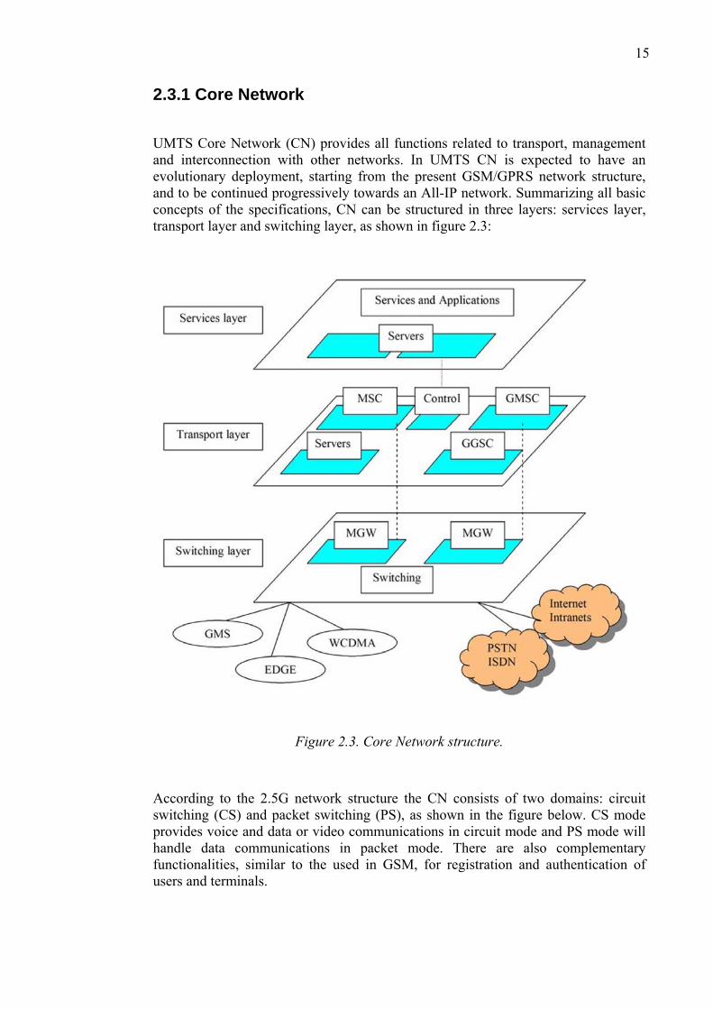
UMTS Core Network (CN) provides all functions related to transport, management and interconnection with other networks. In UMTS CN is expected to have an evolutionary deployment, starting from the present GSM/GPRS network structure, and to be continued progressively towards an All-IP network. Summarizing all basic concepts of the specifications, CN can be structured in three layers: services layer, transport layer and switching layer, as shown in figure 2.3:

Figure 2.3. Core Network structure.

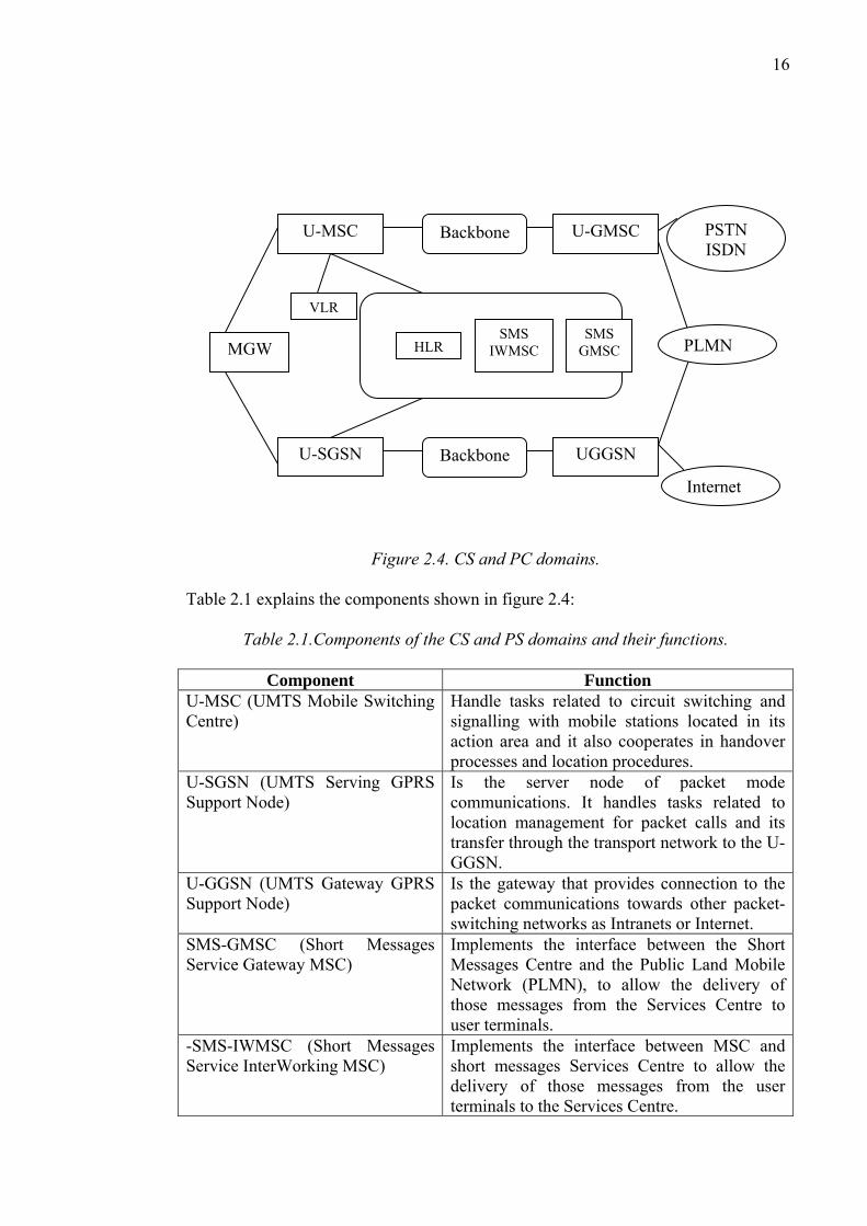
According to the 2.5G network structure the CN consists of two domains: circuit switching (CS) and packet switching (PS), as shown in the figure below. CS mode provides voice and data or video communications in circuit mode and PS mode will handle data communications in packet mode. There are also complementary functionalities, similar to the used in GSM, for registration and authentication of users and terminals.

16

Figure 2.4. CS and PC domains. Table 2.1 explains the components shown in figure 2.4:

Table 2.1.Components of the CS and PS domains and their functions.

Component Function U-MSC (UMTS Mobile Switching Centre)

Handle tasks related to circuit switching and signalling with mobile stations located in its action area and it also cooperates in handover processes and location procedures.

U-SGSN (UMTS Serving GPRS Support Node)

Is the server node of packet mode communications. It handles tasks related to location management for packet calls and its transfer through the transport network to the U-GGSN.

U-GGSN (UMTS Gateway GPRS Support Node)

Is the gateway that provides connection to the packet communications towards other packet-switching networks as Intranets or Internet.

SMS-GMSC (Short Messages Service Gateway MSC)

Implements the interface between the Short Messages Centre and the Public Land Mobile Network (PLMN), to allow the delivery of those messages from the Services Centre to user terminals.

-SMS-IWMSC (Short Messages Service InterWorking MSC)

Implements the interface between MSC and short messages Services Centre to allow the delivery of those messages from the user terminals to the Services Centre.

U-MSC

MGW

Backbone U-GMSC

U-SGSN Backbone UGGSN

VLR

HLRSMS

IWMSC SMS

GMSC PLMN

Internet

PSTN ISDN

17

The evolutive concept adopted for the CN has the advantage to facilitate the migration towards 3G from 2G through the 2.5G networks. Anyhow it could be an inconvenient for the supporting of more advanced services. For that reason the evolution must be trying make the CN perfect gradually. In the future, CN will be based on packet mode using TCP/IP protocol. This concept will be extended to the access network, shaping an “All-IP” network. [12]

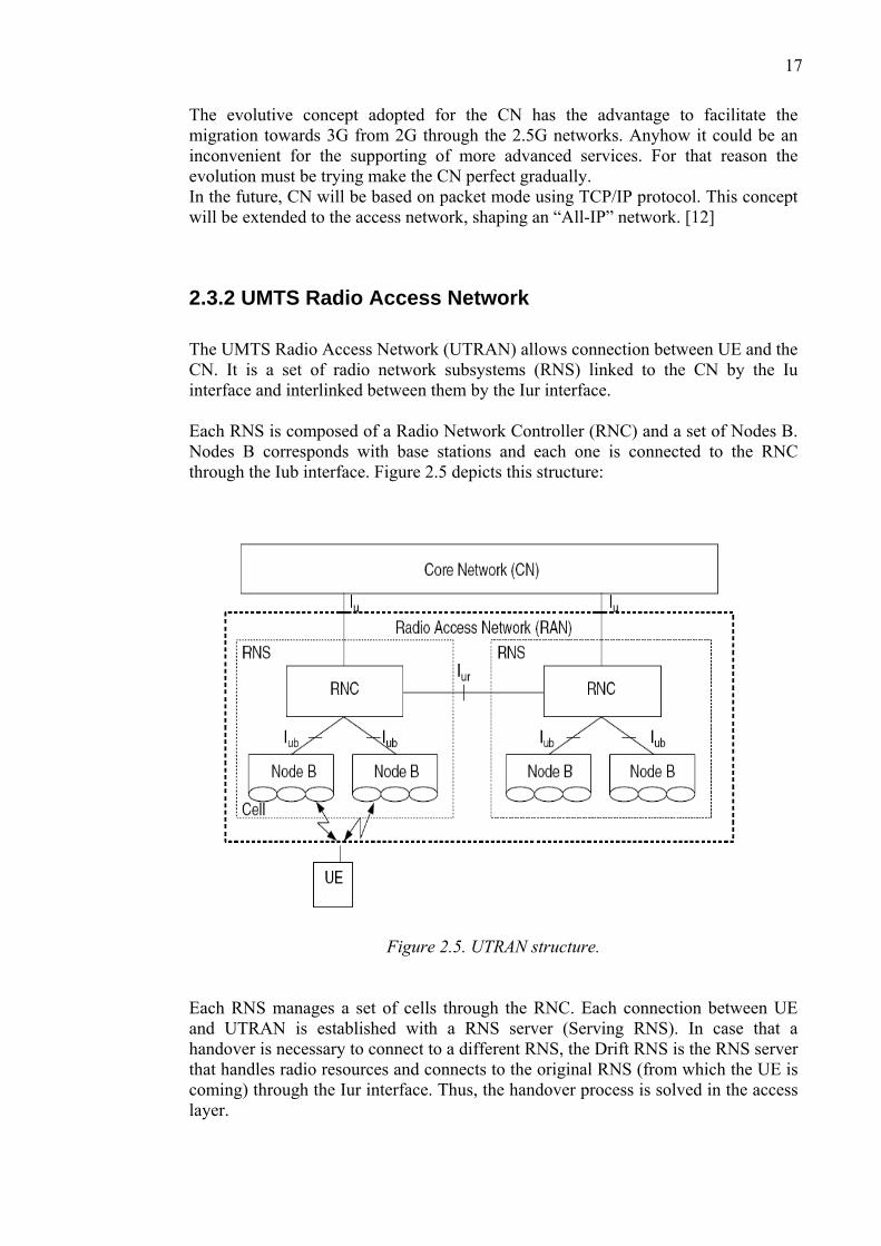
2.3.2 UMTS Radio Access Network The UMTS Radio Access Network (UTRAN) allows connection between UE and the CN. It is a set of radio network subsystems (RNS) linked to the CN by the Iu interface and interlinked between them by the Iur interface. Each RNS is composed of a Radio Network Controller (RNC) and a set of Nodes B. Nodes B corresponds with base stations and each one is connected to the RNC through the Iub interface. Figure 2.5 depicts this structure:

Figure 2.5. UTRAN structure.

Each RNS manages a set of cells through the RNC. Each connection between UE and UTRAN is established with a RNS server (Serving RNS). In case that a handover is necessary to connect to a different RNS, the Drift RNS is the RNS server that handles radio resources and connects to the original RNS (from which the UE is coming) through the Iur interface. Thus, the handover process is solved in the access layer.

18

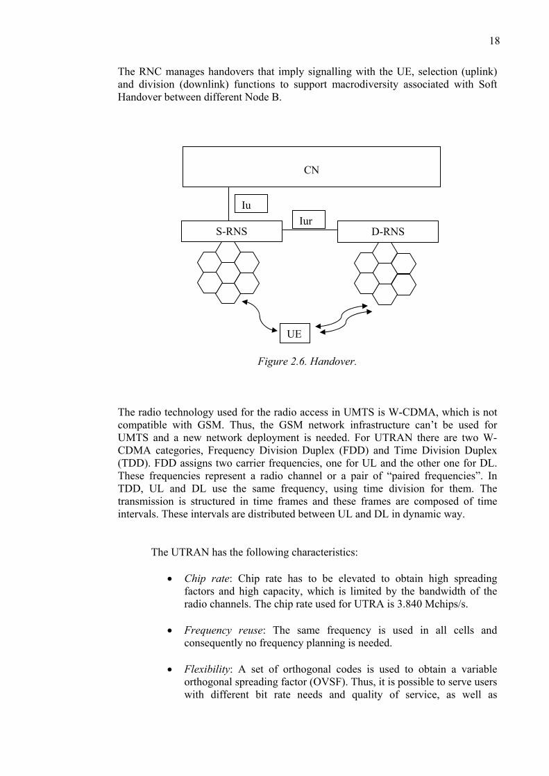
The RNC manages handovers that imply signalling with the UE, selection (uplink) and division (downlink) functions to support macrodiversity associated with Soft Handover between different Node B.

Figure 2.6. Handover. The radio technology used for the radio access in UMTS is W-CDMA, which is not compatible with GSM. Thus, the GSM network infrastructure can’t be used for UMTS and a new network deployment is needed. For UTRAN there are two W-CDMA categories, Frequency Division Duplex (FDD) and Time Division Duplex (TDD). FDD assigns two carrier frequencies, one for UL and the other one for DL. These frequencies represent a radio channel or a pair of “paired frequencies”. In TDD, UL and DL use the same frequency, using time division for them. The transmission is structured in time frames and these frames are composed of time intervals. These intervals are distributed between UL and DL in dynamic way. The UTRAN has the following characteristics:

• Chip rate: Chip rate has to be elevated to obtain high spreading factors and high capacity, which is limited by the bandwidth of the radio channels. The chip rate used for UTRA is 3.840 Mchips/s.

• Frequency reuse: The same frequency is used in all cells and

consequently no frequency planning is needed.

• Flexibility: A set of orthogonal codes is used to obtain a variable orthogonal spreading factor (OVSF). Thus, it is possible to serve users with different bit rate needs and quality of service, as well as

CN

S-RNS D-RNS

IuIur

UE

19

multimedia communications for a certain user.

• Coherent detection: A common pilot channel is used for coherent detection in Node B as well as in mobile terminals.

• Asynchronous operation between Node B: No external synchronous

source is needed for a common synchronization of all nodes in the network.

• Power control is performed 1500 times per second.

• Macrodiversity is processed using Rake receiver structures in base

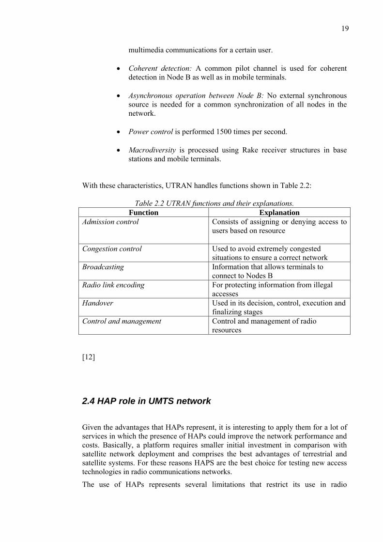
stations and mobile terminals. With these characteristics, UTRAN handles functions shown in Table 2.2:

Table 2.2 UTRAN functions and their explanations. Function Explanation

Admission control Consists of assigning or denying access to users based on resource

Congestion control Used to avoid extremely congested situations to ensure a correct network

Broadcasting Information that allows terminals to connect to Nodes B

Radio link encoding For protecting information from illegal accesses

Handover Used in its decision, control, execution and finalizing stages

Control and management Control and management of radio resources

[12]

2.4 HAP role in UMTS network

Given the advantages that HAPs represent, it is interesting to apply them for a lot of services in which the presence of HAPs could improve the network performance and costs. Basically, a platform requires smaller initial investment in comparison with satellite network deployment and comprises the best advantages of terrestrial and satellite systems. For these reasons HAPS are the best choice for testing new access technologies in radio communications networks.

The use of HAPs represents several limitations that restrict its use in radio

20

communications based networks, and particularly in UMTS, on which this work is focused. Weight and volume of the equipment to be installed onboard is limited, and this should be taken into account when assigning network functions to a platform, because of the payload limit of the platform. Moreover, energy consumption limits are also a restriction as previously commented in section 2.1. Another feature to take into account is the platform positioning planning. There are two possibilities in what is referred to the HAP position: the platform location may vary with time flying along a predefined course or it may try to maintain a quasistatic position above the area to be covered by the platform payload. Another restriction is the availability of the onboard equipment. The availability is limited by the availability of the platform itself, which is affected by weather conditions (e.g. rain attenuation), flight conditions (e.g. position, altitude, winds) and other circumstances (e.g. energy level of the fuel cell providing energy for the platform), as well. [13]

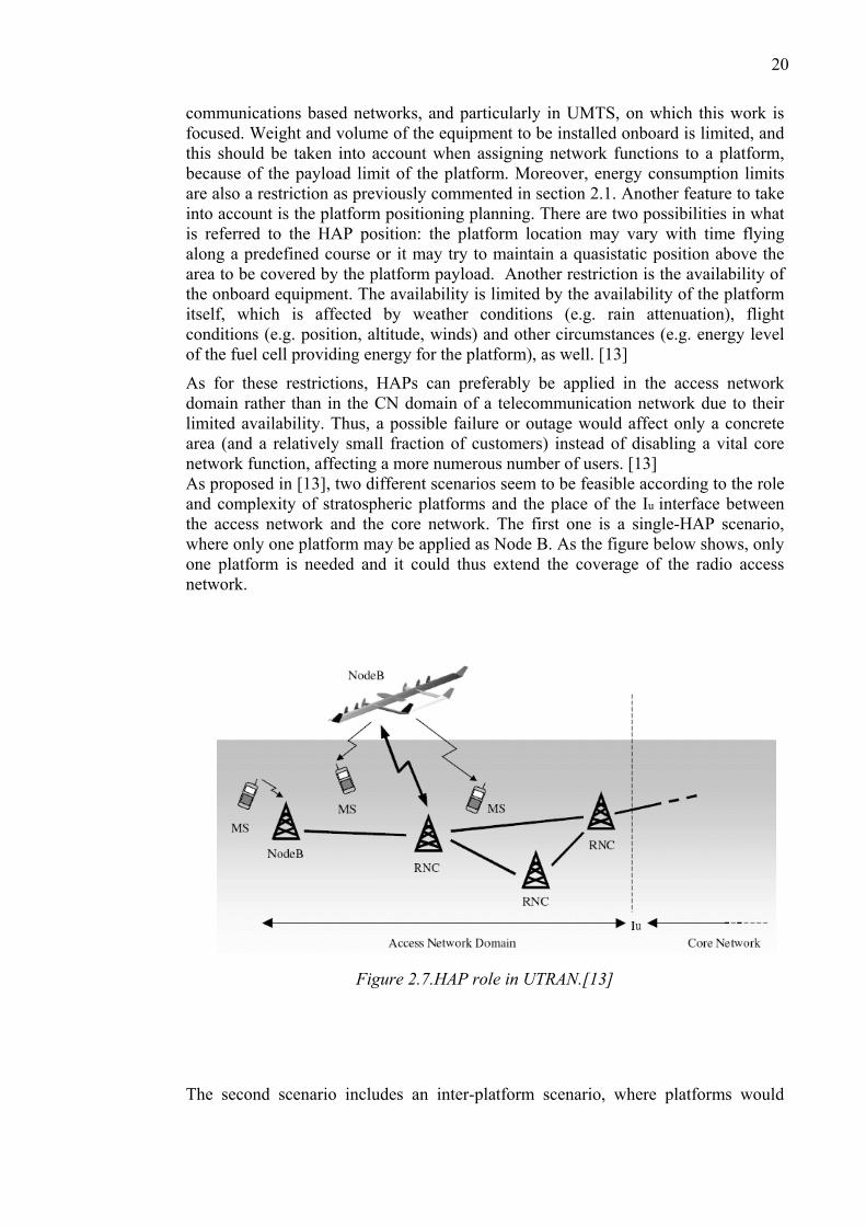
As for these restrictions, HAPs can preferably be applied in the access network domain rather than in the CN domain of a telecommunication network due to their limited availability. Thus, a possible failure or outage would affect only a concrete area (and a relatively small fraction of customers) instead of disabling a vital core network function, affecting a more numerous number of users. [13] As proposed in [13], two different scenarios seem to be feasible according to the role and complexity of stratospheric platforms and the place of the Iu interface between the access network and the core network. The first one is a single-HAP scenario, where only one platform may be applied as Node B. As the figure below shows, only one platform is needed and it could thus extend the coverage of the radio access network.

Figure 2.7.HAP role in UTRAN.[13]

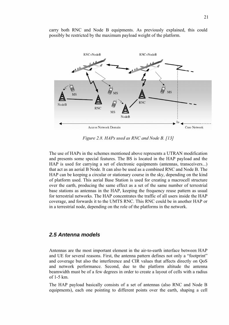
The second scenario includes an inter-platform scenario, where platforms would

21

carry both RNC and Node B equipments. As previously explained, this could possibly be restricted by the maximum payload weight of the platform.

Figure 2.8. HAPs used as RNC and Node B. [13]

The use of HAPs in the schemes mentioned above represents a UTRAN modification and presents some special features. The BS is located in the HAP payload and the HAP is used for carrying a set of electronic equipments (antennas, transceivers...) that act as an aerial B Node. It can also be used as a combined RNC and Node B. The HAP can be keeping a circular or stationary course in the sky, depending on the kind of platform used. This aerial Base Station is used for creating a macrocell structure over the earth, producing the same effect as a set of the same number of terrestrial base stations as antennas in the HAP, keeping the frequency reuse pattern as usual for terrestrial networks. The HAP concentrates the traffic of all users inside the HAP coverage, and forwards it to the UMTS RNC. This RNC could be in another HAP or in a terrestrial node, depending on the role of the platforms in the network.

2.5 Antenna models

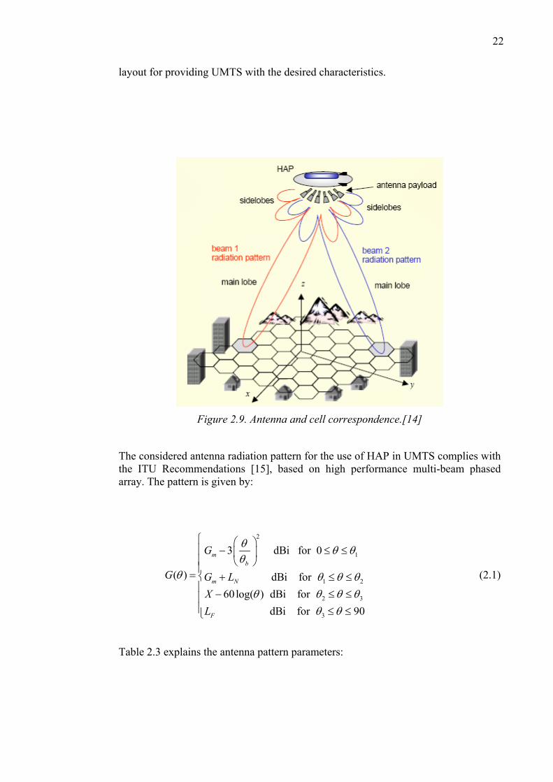
Antennas are the most important element in the air-to-earth interface between HAP and UE for several reasons. First, the antenna pattern defines not only a “footprint” and coverage but also the interference and CIR values that affects directly on QoS and network performance. Second, due to the platform altitude the antenna beamwidth must be of a few degrees in order to create a layout of cells with a radius of 1-5 km.

The HAP payload basically consists of a set of antennas (also RNC and Node B equipments), each one pointing to different points over the earth, shaping a cell

22

layout for providing UMTS with the desired characteristics.

Figure 2.9. Antenna and cell correspondence.[14]

The considered antenna radiation pattern for the use of HAP in UMTS complies with the ITU Recommendations [15], based on high performance multi-beam phased array. The pattern is given by:

2

1

1 2

2 3

3

3 dBi for 0

( ) dBi for 60 log( ) dBi for

dBi for 90

mb

m N

F

G

G G LXL

θ θ θθ

θ θ θ θθ θ θ θ

θ θ

⎧ ⎛ ⎞⎪ − ≤ ≤⎜ ⎟⎪ ⎝ ⎠⎪= ⎨ + ≤ ≤⎪ − ≤ ≤⎪⎪ ≤ ≤⎩

(2.1)

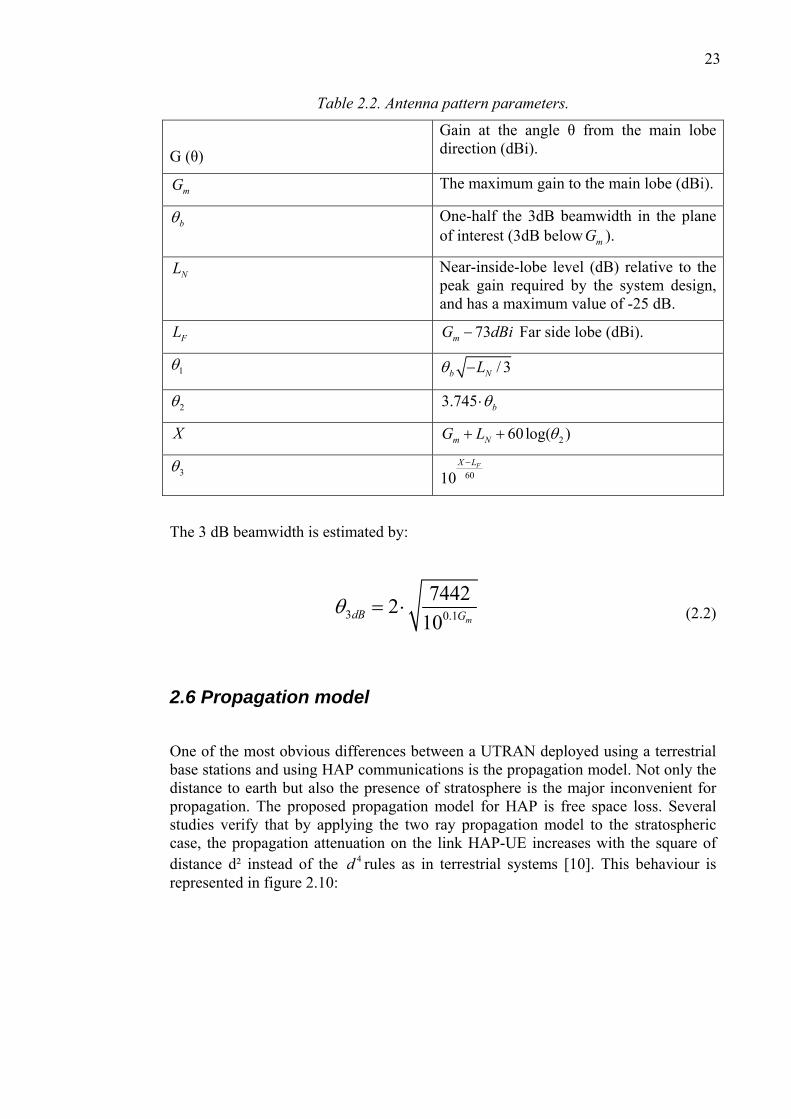
Table 2.3 explains the antenna pattern parameters:

23

Table 2.2. Antenna pattern parameters.

G (θ)

Gain at the angle θ from the main lobe direction (dBi).

mG The maximum gain to the main lobe (dBi).

bθ One-half the 3dB beamwidth in the plane of interest (3dB below mG ).

NL Near-inside-lobe level (dB) relative to the peak gain required by the system design, and has a maximum value of -25 dB.

FL 73mG dBi− Far side lobe (dBi).

1θ / 3b NLθ −

2θ 3.745 bθ⋅

X 260 log( )m NG L θ+ +

3θ 6010

FX L−

The 3 dB beamwidth is estimated by:

3 0.174422

10 mdB Gθ = ⋅ (2.2)

2.6 Propagation model

One of the most obvious differences between a UTRAN deployed using a terrestrial base stations and using HAP communications is the propagation model. Not only the distance to earth but also the presence of stratosphere is the major inconvenient for propagation. The proposed propagation model for HAP is free space loss. Several studies verify that by applying the two ray propagation model to the stratospheric case, the propagation attenuation on the link HAP-UE increases with the square of distance d² instead of the 4d rules as in terrestrial systems [10]. This behaviour is represented in figure 2.10:

24

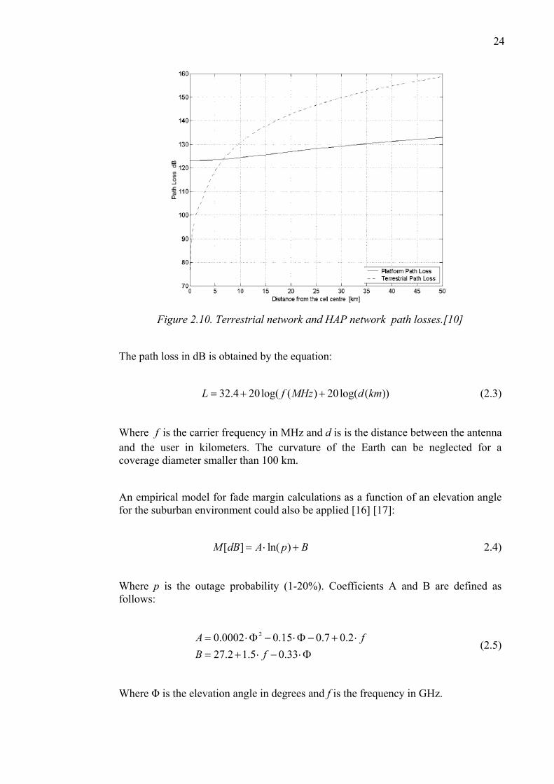
Figure 2.10. Terrestrial network and HAP network path losses.[10]

The path loss in dB is obtained by the equation:

32.4 20log( ( ) 20log( ( ))L f MHz d km= + + (2.3)

Where f is the carrier frequency in MHz and d is is the distance between the antenna and the user in kilometers. The curvature of the Earth can be neglected for a coverage diameter smaller than 100 km.

An empirical model for fade margin calculations as a function of an elevation angle for the suburban environment could also be applied [16] [17]:

[ ] ln( )M dB A p B= ⋅ + 2.4)

Where p is the outage probability (1-20%). Coefficients A and B are defined as follows:

20.0002 0.15 0.7 0.2

27.2 1.5 0.33A fB f= ⋅Φ − ⋅Φ − + ⋅= + ⋅ − ⋅Φ

(2.5)

Where Φ is the elevation angle in degrees and f is the frequency in GHz.

25

Equations 2.3 to 2.5 represent the basic propagation model used for HAPs and are the best approach for estimating path losses. For a more realistic propagation model, rain attenuation, rain scattering (and the interference that it produces) together with indoor propagation models should complement this basic propagation model. This leads to divide the path loss in two parts. The first part, from the HAP to roof, is obtained with the Free Space Loss method. The second part, from roof to street level, propagation is obtained applying indoor propagation, including rain effects.

2.7 Radio planning

2.7.1 Cell deployment and hexagonal layout

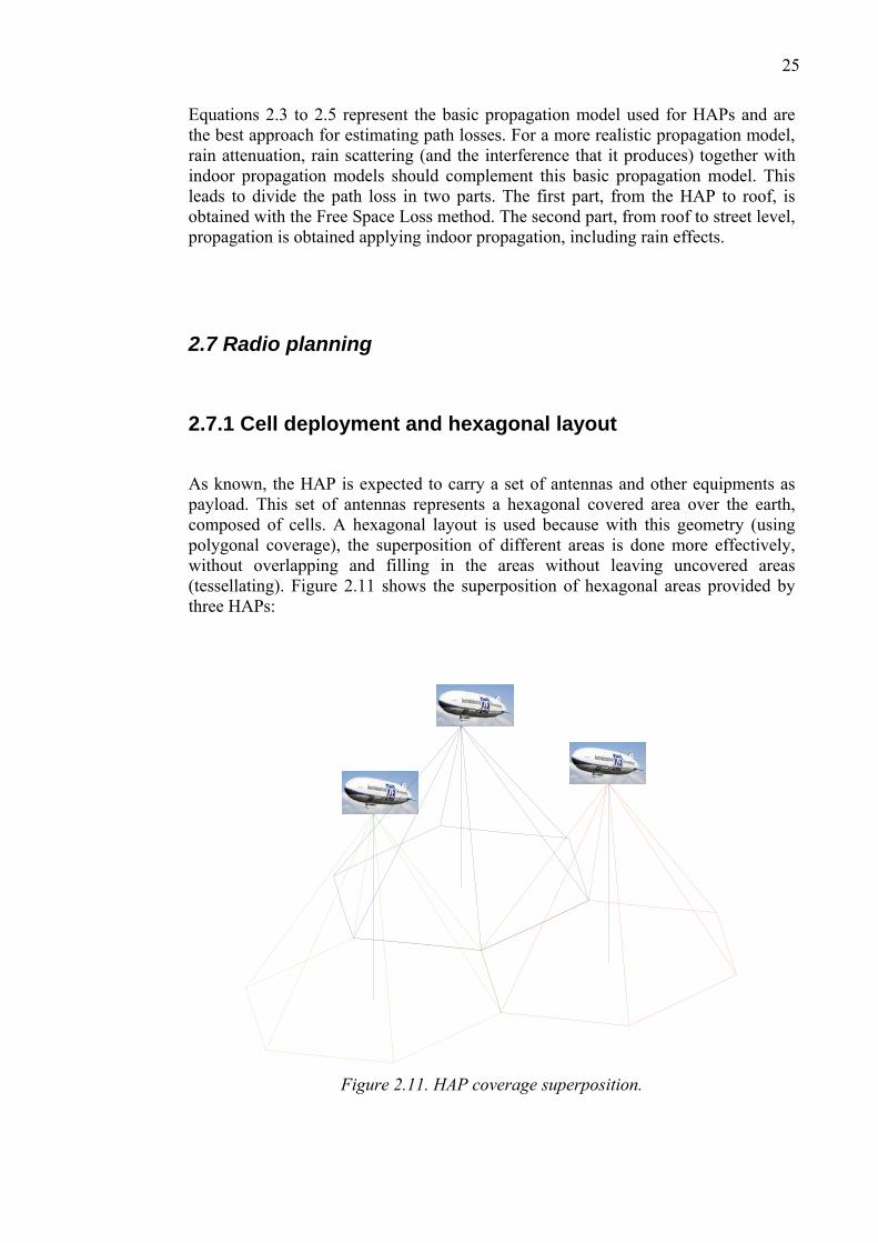
As known, the HAP is expected to carry a set of antennas and other equipments as payload. This set of antennas represents a hexagonal covered area over the earth, composed of cells. A hexagonal layout is used because with this geometry (using polygonal coverage), the superposition of different areas is done more effectively, without overlapping and filling in the areas without leaving uncovered areas (tessellating). Figure 2.11 shows the superposition of hexagonal areas provided by three HAPs:

Figure 2.11. HAP coverage superposition.

26

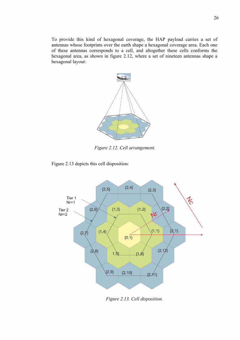
To provide this kind of hexagonal coverage, the HAP payload carries a set of antennas whose footprints over the earth shape a hexagonal coverage area. Each one of these antennas corresponds to a cell, and altogether these cells conforms the hexagonal area, as shown in figure 2.12, where a set of nineteen antennas shape a hexagonal layout:

Figure 2.12. Cell arrangement.

Figure 2.13 depicts this cell disposition:

Figure 2.13. Cell disposition.

27

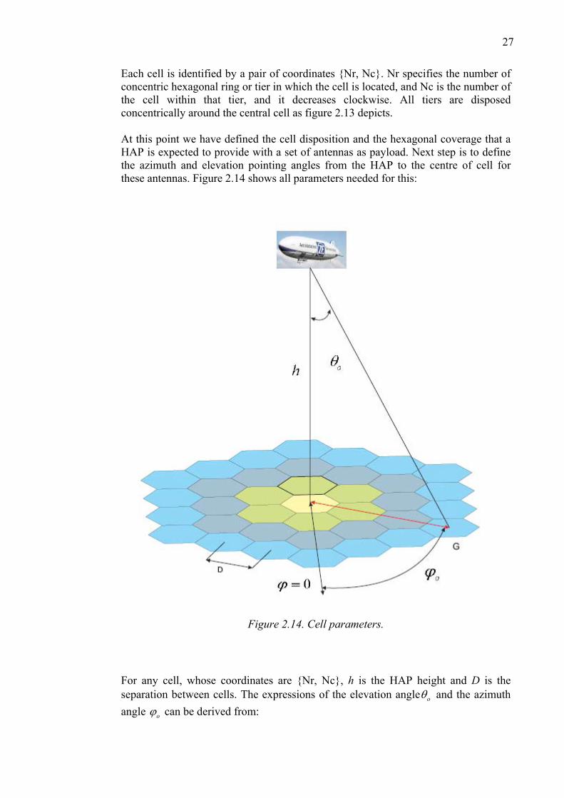
Each cell is identified by a pair of coordinates {Nr, Nc}. Nr specifies the number of concentric hexagonal ring or tier in which the cell is located, and Nc is the number of the cell within that tier, and it decreases clockwise. All tiers are disposed concentrically around the central cell as figure 2.13 depicts. At this point we have defined the cell disposition and the hexagonal coverage that a HAP is expected to provide with a set of antennas as payload. Next step is to define the azimuth and elevation pointing angles from the HAP to the centre of cell for these antennas. Figure 2.14 shows all parameters needed for this:

Figure 2.14. Cell parameters.

For any cell, whose coordinates are {Nr, Nc}, h is the HAP height and D is the separation between cells. The expressions of the elevation angle oθ and the azimuth angle oϕ can be derived from:

28

arctan

( ' 1) sin3arcsin ( 1)

3

o

o

Gh

c DNs

g

θ

ππϕ

⎛ ⎞= ⎜ ⎟⎝ ⎠⎛ ⎞⎛ ⎞− ⎜ ⎟⎜ ⎟⎝ ⎠⎜ ⎟= + −⎜ ⎟⎜ ⎟⎝ ⎠

(2.6)

Where G is the distance from the cell centre to the subplatform point, which can be derived from:

( ) ( )( )22 2' 1 2 ( ' 1) cos3

G Nr d c d Nr d c π⎛ ⎞= ⋅ + − ⋅ − ⋅ ⋅ − ⋅ ⎜ ⎟⎝ ⎠

(2.7)

In this expression c’ is used to identify the cell’s location with respect to the first cell along the side:

' ( 1)c Nc Ns Nr= − − ⋅ (2.8)

Where Ns is an integer between one and six identifying the side of the hexagon:

11 NcNs FloorNr−⎡ ⎤= + ⎢ ⎥⎣ ⎦

(2.9)

With all these parameters it is possible to define the antenna azimuth and elevation angles for all cells that comprise the hexagonal structure. [18]

2.7.2 Other cell deployment and antenna pattern issues

The cell deployment explained in the previous sections presents some limitations that have to be treated. As explained in [19], the cells were deployed based on homogenous hexangular geometry and the cell shape in HAPs is determined by the antenna radiation pattern, and it is not limited by the terrain profile. The distance of the Nc-th cell centre in the Nr-th ring (cell (Nc,Nr)) from the origin is given by:

29

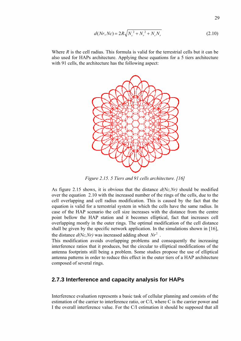
2 2( , ) 2 c r c rd Nr Nc R N N N N= + + (2.10) Where R is the cell radius. This formula is valid for the terrestrial cells but it can be also used for HAPs architecture. Applying these equations for a 5 tiers architecture with 91 cells, the architecture has the following aspect:

Figure 2.15. 5 Tiers and 91 cells architecture. [16]

As figure 2.15 shows, it is obvious that the distance d(Nc,Nr) should be modified over the equation 2.10 with the increased number of the rings of the cells, due to the cell overlapping and cell radius modification. This is caused by the fact that the equation is valid for a terrestrial system in which the cells have the same radius. In case of the HAP scenario the cell size increases with the distance from the centre point bellow the HAP station and it becomes elliptical, fact that increases cell overlapping mostly in the outer rings. The optimal modification of the cell distance shall be given by the specific network application. In the simulations shown in [16], the distance d(Nc,Nr) was increased adding about 2Nr . This modification avoids overlapping problems and consequently the increasing interference ratios that it produces, but the circular to elliptical modifications of the antenna footprints still being a problem. Some studies propose the use of elliptical antenna patterns in order to reduce this effect in the outer tiers of a HAP architecture composed of several rings.

2.7.3 Interference and capacity analysis for HAPs

Interference evaluation represents a basic task of cellular planning and consists of the estimation of the carrier to interference ratio, or C/I, where C is the carrier power and I the overall interference value. For the C/I estimation it should be supposed that all

30

interfering signals are uncorrelated, and the propagation paths are different. Thus, the interfering signals are summed incoherently and the overall interference power is the sum of all the interfering signals.

Generally speaking, two interfering signals have to be considered:

• Downlink interference, caused by signals from base stations in mobile stations.

• Uplink interference, caused by signals from mobile stations in base stations.

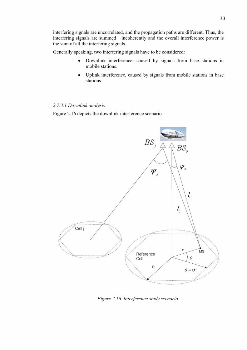
2.7.3.1 Downlink analysis

Figure 2.16 depicts the downlink interference scenario

Figure 2.16. Interference study scenario.

31

A user inside the HAPs service area will experience intracellular and intercellular interference. For a mobile terminal located in ( ,r θ ), the power transmitted to a mobile terminal, using the downlink power control, is given by:

( )t RP P f r= (2.10)

Where RP is the reference power level assigned to the user located at r=R, just at the edge of the cell.

The power control profile can be expressed by:

1

o

2 3

o

for r r( )

for r r

n

n n

ra bR

f rr rc dR R

⎧ ⎛ ⎞+ ≤⎪ ⎜ ⎟⎪ ⎝ ⎠= ⎨⎛ ⎞ ⎛ ⎞⎪ + ≤⎜ ⎟ ⎜ ⎟⎪ ⎝ ⎠ ⎝ ⎠⎩

(2.11)

Where a, b, c, n1, n2, /or R are the power control parameters and or is the distance at which the power control scheme changes its performance.

The user density for N uniformly distributed users inside a cell is:

2

NR

ρπ

= (2.12)

The total power transmitted by a base station is given by:

2

2 20 0 0

2( ) ( ) 2R R

R RT R p

NP NPP f r rdrd f r rdr NP fR R

π πθπ π

= = =∫ ∫ ∫ (2.13)

Where 2 pf is:

2 1 2 2 2 3 22 2 2 2 22

1 2 2 2 2 2 3 2 3 2

n n no o o o

pr r r rb c c d df aR n R n n R n n R

+ + +⎛ ⎞ ⎛ ⎞ ⎛ ⎞ ⎛ ⎞= + + − + −⎜ ⎟ ⎜ ⎟ ⎜ ⎟ ⎜ ⎟+ + + + +⎝ ⎠ ⎝ ⎠ ⎝ ⎠ ⎝ ⎠

(2.14)

With these results, the capacity analysis can be started. Let ( 0,..., )jBS j J=

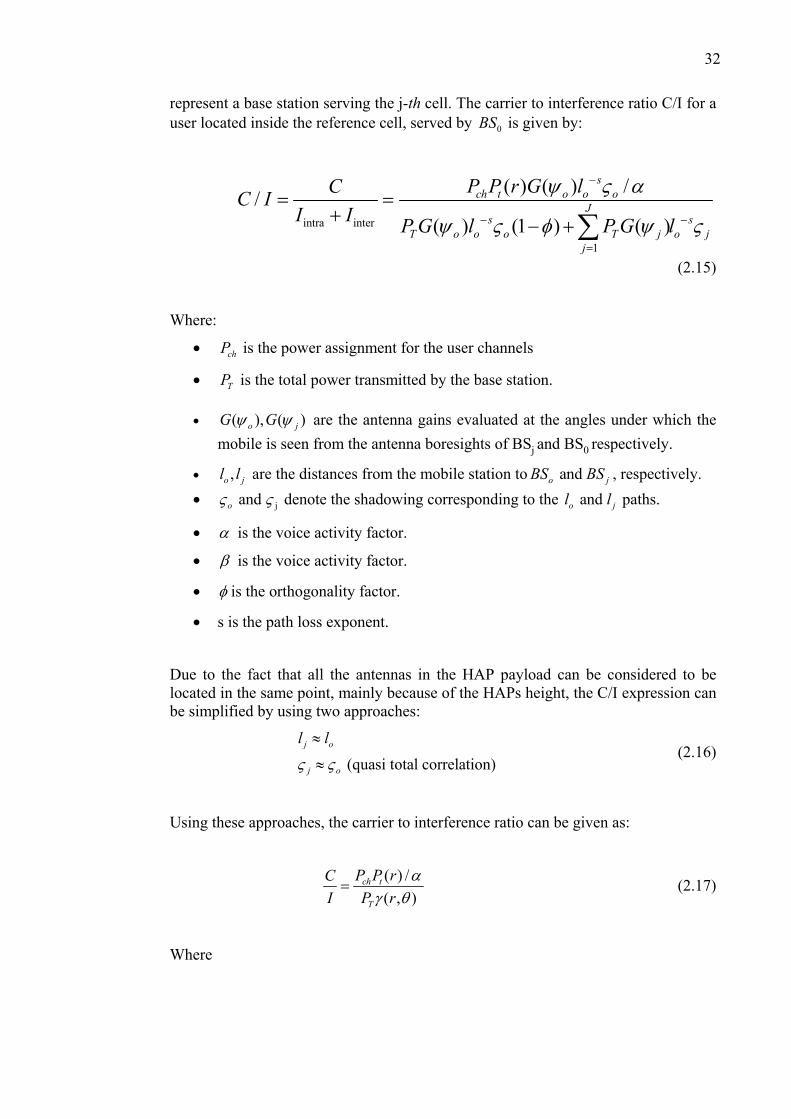
32

represent a base station serving the j-th cell. The carrier to interference ratio C/I for a user located inside the reference cell, served by 0BS is given by:

intra inter

1

( ) ( ) //( ) (1 ) ( )

sch t o o o

Js s

T o o o T j o jj

P P r G lCC II I P G l P G l

ψ ς α

ψ ς φ ψ ς

−

− −

=

= =+ − +∑

(2.15)

Where:

• chP is the power assignment for the user channels

• TP is the total power transmitted by the base station.

• ( ), ( )o jG Gψ ψ are the antenna gains evaluated at the angles under which the mobile is seen from the antenna boresights of BSj and BS0 respectively.

• ,o jl l are the distances from the mobile station to and o jBS BS , respectively. • jand oς ς denote the shadowing corresponding to the and o jl l paths.

• α is the voice activity factor.

• β is the voice activity factor.

• φ is the orthogonality factor.

• s is the path loss exponent.

Due to the fact that all the antennas in the HAP payload can be considered to be located in the same point, mainly because of the HAPs height, the C/I expression can be simplified by using two approaches:

(quasi total correlation)j o

j o

l l

ς ς

≈

≈ (2.16)

Using these approaches, the carrier to interference ratio can be given as:

( ) /( , )

ch t

T

P P rCI P r

αγ θ

= (2.17)

Where

33

1(1 ) ( ) ( )

( , )( )

J

o jj

o

G Gr

G

φ ψ ψγ θ

ψ=

− +=

∑ (2.18)

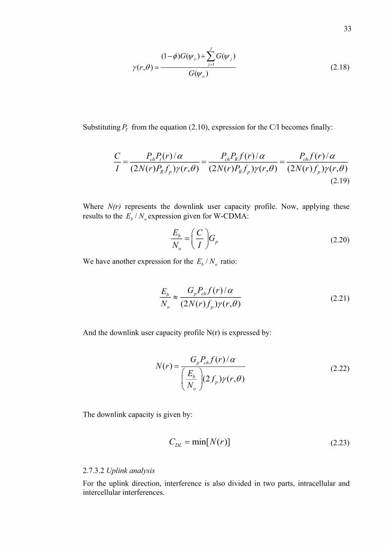
Substituting TP from the equation (2.10), expression for the C/I becomes finally:

( ) / ( ) / ( ) /(2 ( ) ) ( , ) (2 ( ) ) ( , ) (2 ( ) ) ( , )

ch t ch R ch

R p R p p

P P r P P f r P f rCI N r P f r N r P f r N r f r

α α αγ θ γ θ γ θ

= = =

(2.19)

Where N(r) represents the downlink user capacity profile. Now, applying these results to the /b oE N expression given for W-CDMA:

bp

o

E C GN I

⎛ ⎞= ⎜ ⎟⎝ ⎠

(2.20)

We have another expression for the /b oE N ratio:

( ) /(2 ( ) ) ( , )

p chb

o p

G P f rEN N r f r

αγ θ

≈ (2.21)

And the downlink user capacity profile N(r) is expressed by:

( ) /( )

(2 ) ( , )

p ch

bp

o

G P f rN r

E f rN

α

γ θ=⎛ ⎞⎜ ⎟⎝ ⎠

(2.22)

The downlink capacity is given by:

min[ ( )]DLC N r= (2.23)

2.7.3.2 Uplink analysis

For the uplink direction, interference is also divided in two parts, intracellular and intercellular interferences.

34

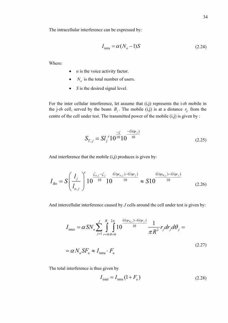
The intracellular interference can be expressed by:

intra ( 1)uI N Sα= − (2.24)

Where:

• α is the voice activity factor.

• uN is the total number of users.

• S is the desired signal level.

For the inter cellular interference, let assume that (i,j) represents the i-th mobile in the j-th cell, served by the beam jB . The mobile (i,j) is at a distance ijr from the centre of the cell under test. The transmitted power of the mobile (i,j) is given by :

( )10 10

, 10 10jG

sT j jS Sl

ψς −−

= (2.25)

And interference that the mobile (i,j) produces is given by:

, , 0,( ) ( ) ( ) ( )10 10 10

,

10 10 10o j j o j j j j

s G G G Gj

Boo j

lI S S

l

ζ ζ ψ ψ ψ ψ− − −⎛ ⎞= ≈⎜ ⎟⎜ ⎟

⎝ ⎠ (2.26)

And intercellular interference caused by J cells around the cell under test is given by:

0,( ) ( )210

inter 21 0 0

intra

110j jG GRJ

u j j jj r

u u u

I SN r dr dR

N SF I F

ψ ψπ

θ

α θπ

α

−

= = =

= =

= ≈ ⋅

∑ ∫ ∫

(2.27)

The total interference is thus given by

total intra (1 )uI I F= + (2.28)

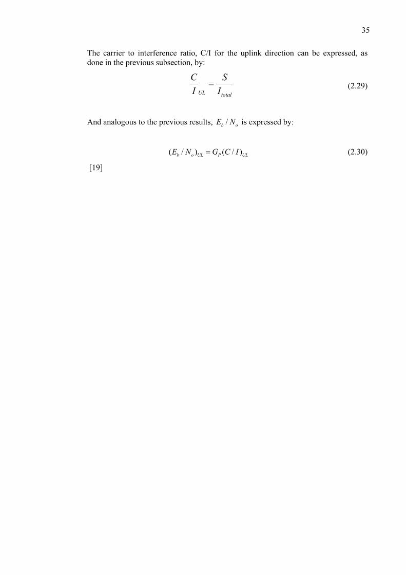
35

The carrier to interference ratio, C/I for the uplink direction can be expressed, as done in the previous subsection, by:

UL total

C SI I

= (2.29)

And analogous to the previous results, /b oE N is expressed by:

( / ) ( / )b o UL P ULE N G C I= (2.30)

[19]

36

3. Simulations

The main goal of this thesis is to find an optimal configuration for HAPs deployment in UMTS services, using iteration based simulator for WCDMA networks. To reach this goal, first a single HAP scenario is analysed in order to find an optimal configuration that maximises the service probability and maximum number of users with and optimal interference ratio. The method of analysis is to run a set of simulations with different cell separations shaping a hexagonal layout. A comparison between results will give an approach of an optimal configuration. After finding the optimal configuration, some simulations are repeated using a different antenna pattern than proposed by the ITU, showing the differences between the results obtained with both antenna patterns. This modification pretends to obtain a better approach using a more realistic antenna mask to be complied by real antenna patterns. The analysis will show the differences, advantages and disadvantages that the use of these patterns causes for the general network performance.

Finally, in the second part, the optimal results obtained from the single HAP scenario are applied to a multi-HAP architecture, where three platforms are used to provide coverage. Results are presented and analysed.

3.1 NPSW static simulator

The previously built NPSW (Network Planning Strategies for Wideband CDMA) upgraded version 5.0.0 [20] [21] simulator software with a modified method for the antenna losses estimation was used to build the scenarios and get simulation results. This simulation tool, NPSW, is a Matlab-based static WCDMA simulator. As no digital map is available, simulations have are done using plain homogenous grid, without a realistic ground and link loss data info. In the simulations, the performance of the network is analyzed in a single static time instance called snapshot. The number of users is defined in a file and mobile stations are randomly distributed all over the considered area. NPSW simulator process consists of three main phases: general initialization phase, combined uplink and downlink iteration phase, and post processing phase. In the initialization phase all needed parameter files are read and calculations to be done just once are done. Since a digital map is not provided link losses are calculated from all Node Bs to all map pixels by using the specified propagation model. The complexity and duration of this phase depends on the set map resolution. The better resolution we select, the longer it takes. In the iteration phase several performance parameters are calculated in an iterative way. UL iterations are needed to allocate the transmit power of UEs in such a way that do not produce excess interference at Node Bs. This iterative process is repeated in the UL until the interference levels at the Node Bs converge. In the post processing phase previously obtained information is post-processed and saved to text and data files. Using these files, results are presented in various colour plots and statistics.

37

3.2 Adapted Simulator for HAPs

The simulator needs a basic modification to adapt it to HAPs architecture, due to the fact that it was designed for terrestrial networks and not for HAPs. The modification concerns to the estimation of the antenna losses given an antenna pattern. In terrestrial networks a linear array of N elements is commonly used to obtain a narrow beamwidth and back lobe levels usually between -15 and -25 dB, and although the radiation diagrams in HAPs are similar, the estimation of antenna loss is different due to the system topology.

First, a short analysis of array antennas is presented and then the new antenna loss estimation method is explained.

3.2.1 Base station antenna modelling for terrestrial networks

Generally, antenna arrays are used to obtain suitable directive characteristics in order to increase the radiation towards the serviced area and suppress it towards other ones. Usually these antenna implementations have a relatively narrow main beam and low back lobe levels (30-45 dB under the main lobe gain). Additionally the antenna is linearly polarised with vertical polarization. In practice, radiation properties of these antenna patterns are characterised by means of two radiation patterns, the horizontal and vertical ones, and the gains. These two patterns are used to estimate the antenna gain in a given direction determined by azimuth and elevation angles. The antenna modelling in wireless systems is used to provide information concerning distribution and strength of signals radiated, and consequently interference and other parameters. Therefore, the antenna radiation capabilities should be known in all directions, to ascribe each point under the antenna covered area the correct signal level and the exact antenna gain in that direction. Most computer based tools use a very simple antenna model for estimating the antenna gain and signal levels in each direction, based on two principal patterns, horizontal and vertical, from the antenna pattern. In order to describe this method, the array of antennas theory is explained first.

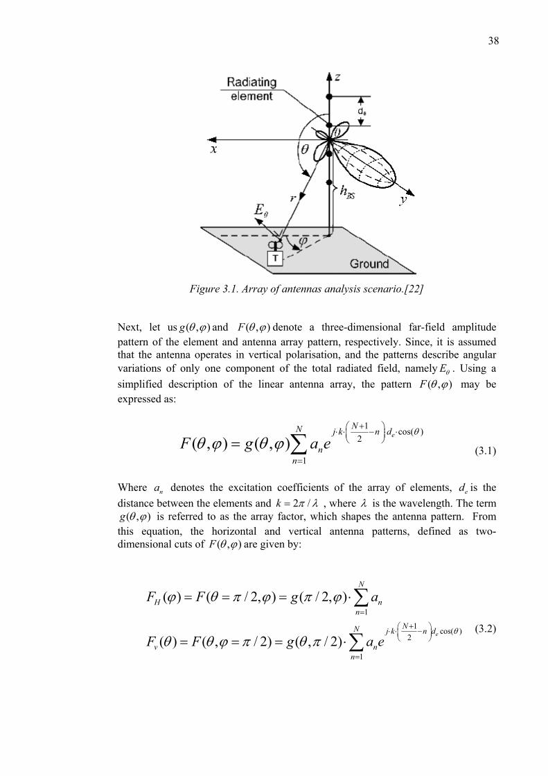
Let assume that the base station antenna is a linear array of N elements, positioned uniformly and symmetrically along the z-axis, with the antenna radiation maximum directed along the y-axis, as shown in figure 3.1:

38

Figure 3.1. Array of antennas analysis scenario.[22]

Next, let us ( , )g θ ϕ and ( , )F θ ϕ denote a three-dimensional far-field amplitude pattern of the element and antenna array pattern, respectively. Since, it is assumed that the antenna operates in vertical polarisation, and the patterns describe angular variations of only one component of the total radiated field, namely Eθ . Using a simplified description of the linear antenna array, the pattern ( , )F θ ϕ may be expressed as:

1 cos( )2

1

( , ) ( , )e

NN j k n d

nn

F g a eθ

θ ϕ θ ϕ+⎛ ⎞⋅ ⋅ − ⋅ ⋅⎜ ⎟

⎝ ⎠

=

= ∑ (3.1)

Where na denotes the excitation coefficients of the array of elements, ed is the distance between the elements and 2 /k π λ= , where λ is the wavelength. The term

( , )g θ ϕ is referred to as the array factor, which shapes the antenna pattern. From this equation, the horizontal and vertical antenna patterns, defined as two-dimensional cuts of ( , )F θ ϕ are given by:

1

1 cos( )2

1

( ) ( / 2, ) ( / 2, )

( ) ( , / 2) ( , / 2)e

N

H nn

NN j k n d

v nn

F F g a

F F g a eθ

ϕ θ π ϕ π ϕ

θ θ ϕ π θ π

=

+⎛ ⎞⋅ ⋅ −⎜ ⎟⎝ ⎠

=

= = = ⋅

= = = ⋅

∑

∑ (3.2)

39

These equations contain only part of the information of the antenna pattern ( , )F θ ϕ and they are insufficient for a rigorous modelling of the three-dimensional radiation capabilities of the antenna, which is, in terms of computing cost, much higher than a two-dimensional modelling. When ( , )F θ ϕ is separable with respect to θ andϕ ,

( , )F θ ϕ can be rewritten as:

( , ) ( , constant) ( constant, ) ( ) ( )V HF F F F Fθ ϕ θ ϕ θ ϕ θ ϕ= = ⋅ = = ⋅ (3.3)

This expression is the one used in most part of computer-based tools to estimate the antenna gain or antenna losses in a given direction. Unfortunately, most of radiating elements applied in practice have a none-separable radiation pattern, and the expression only gives an approximation of the gain value in a given direction with a certain elevation and azimuth angles, θ and φ. [21]

3.2.2 Antenna gain estimation for HAPs

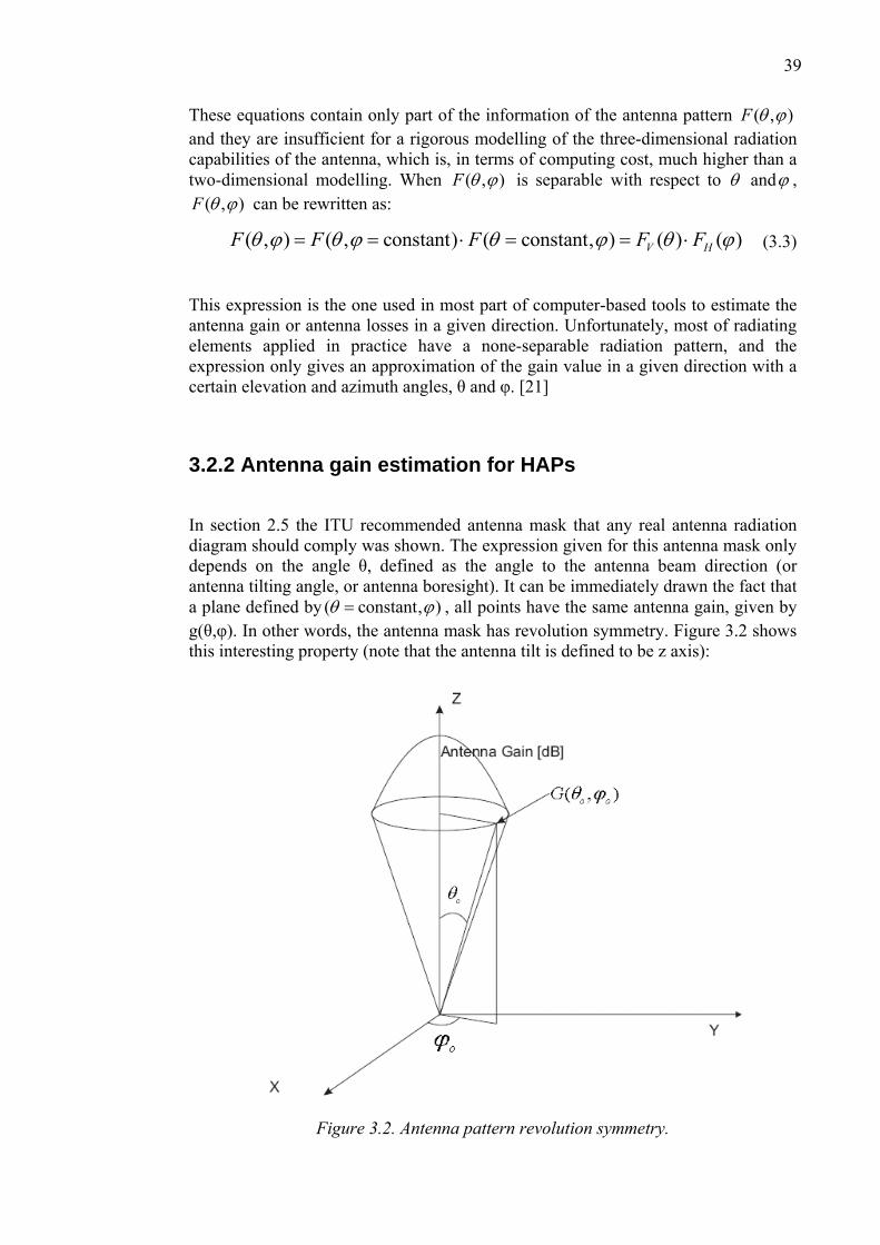
In section 2.5 the ITU recommended antenna mask that any real antenna radiation diagram should comply was shown. The expression given for this antenna mask only depends on the angle θ, defined as the angle to the antenna beam direction (or antenna tilting angle, or antenna boresight). It can be immediately drawn the fact that a plane defined by ( constant, )θ ϕ= , all points have the same antenna gain, given by g(θ,φ). In other words, the antenna mask has revolution symmetry. Figure 3.2 shows this interesting property (note that the antenna tilt is defined to be z axis):

Figure 3.2. Antenna pattern revolution symmetry.

40

It can also be stated that with this antenna pattern, both vertical and horizontal antenna (contained in ( , 0) and ( , / 2)θ ϕ θ ϕ π= = planes, respectively) patterns are exactly the same. Consequently, instead of using two antenna patterns (horizontal and vertical) to estimate the antenna gain in a certain direction, as said in the previous section, it is only needed one of them. Moreover, is it possible to implement a three-dimensional antenna modelling because of this particularity of the antenna mask used for HAPs with a low computing cost.

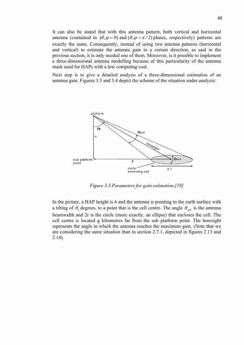
Next step is to give a detailed analysis of a three-dimensional estimation of an antenna gain. Figures 3.3 and 3.4 depict the scheme of the situation under analysis:

Figure 3.3.Parameters for gain estimation.[19]

In the picture, a HAP height is h and the antenna is pointing to the earth surface with a tilting of oθ degrees, to a point that is the cell centre. The angle subθ is the antenna beamwidth and 2r is the circle (more exactly, an ellipse) that encloses the cell. The cell centre is located g kilometres far from the sub platform point. The boresight represents the angle in which the antenna reaches the maximum gain. (Note that we are considering the same situation than in section 2.7.1, depicted in figures 2.13 and 2.14).

41

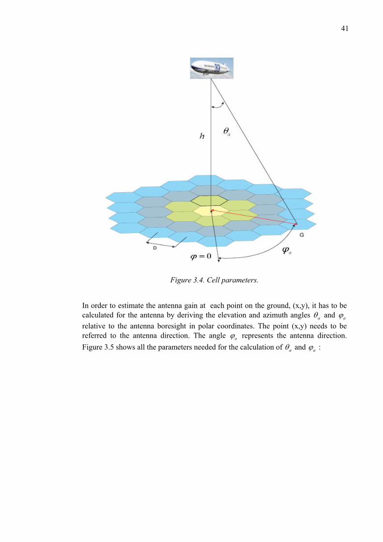
Figure 3.4. Cell parameters.

In order to estimate the antenna gain at each point on the ground, (x,y), it has to be calculated for the antenna by deriving the elevation and azimuth angles aθ and aϕ relative to the antenna boresight in polar coordinates. The point (x,y) needs to be referred to the antenna direction. The angle oϕ represents the antenna direction. Figure 3.5 shows all the parameters needed for the calculation of aθ and aϕ :

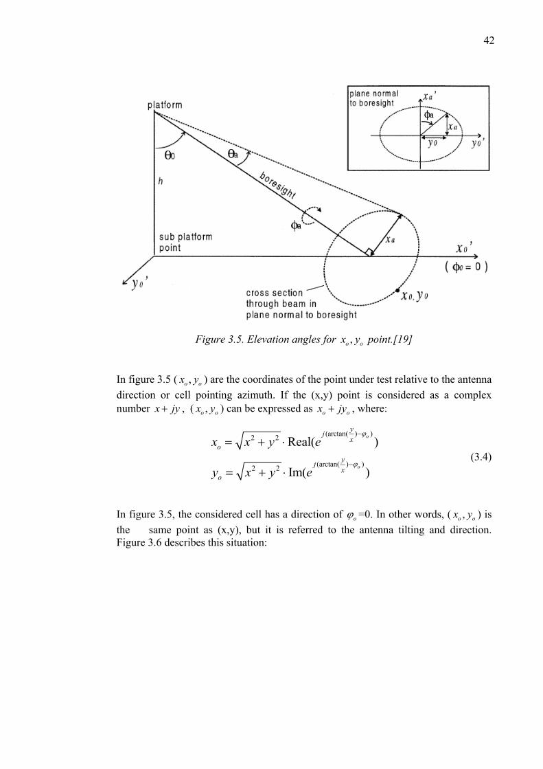
42

Figure 3.5. Elevation angles for ,o ox y point.[19]

In figure 3.5 ( ,o ox y ) are the coordinates of the point under test relative to the antenna direction or cell pointing azimuth. If the (x,y) point is considered as a complex number x jy+ , ( ,o ox y ) can be expressed as o ox jy+ , where:

(arctan( ) )2 2

(arctan( ) )2 2

Real( )

Im( )

o

o

yjx

o

yjx

o

x x y e

y x y e

ϕ

ϕ

−

−

= + ⋅

= + ⋅ (3.4)

In figure 3.5, the considered cell has a direction of oϕ =0. In other words, ( ,o ox y ) is the same point as (x,y), but it is referred to the antenna tilting and direction. Figure 3.6 describes this situation:

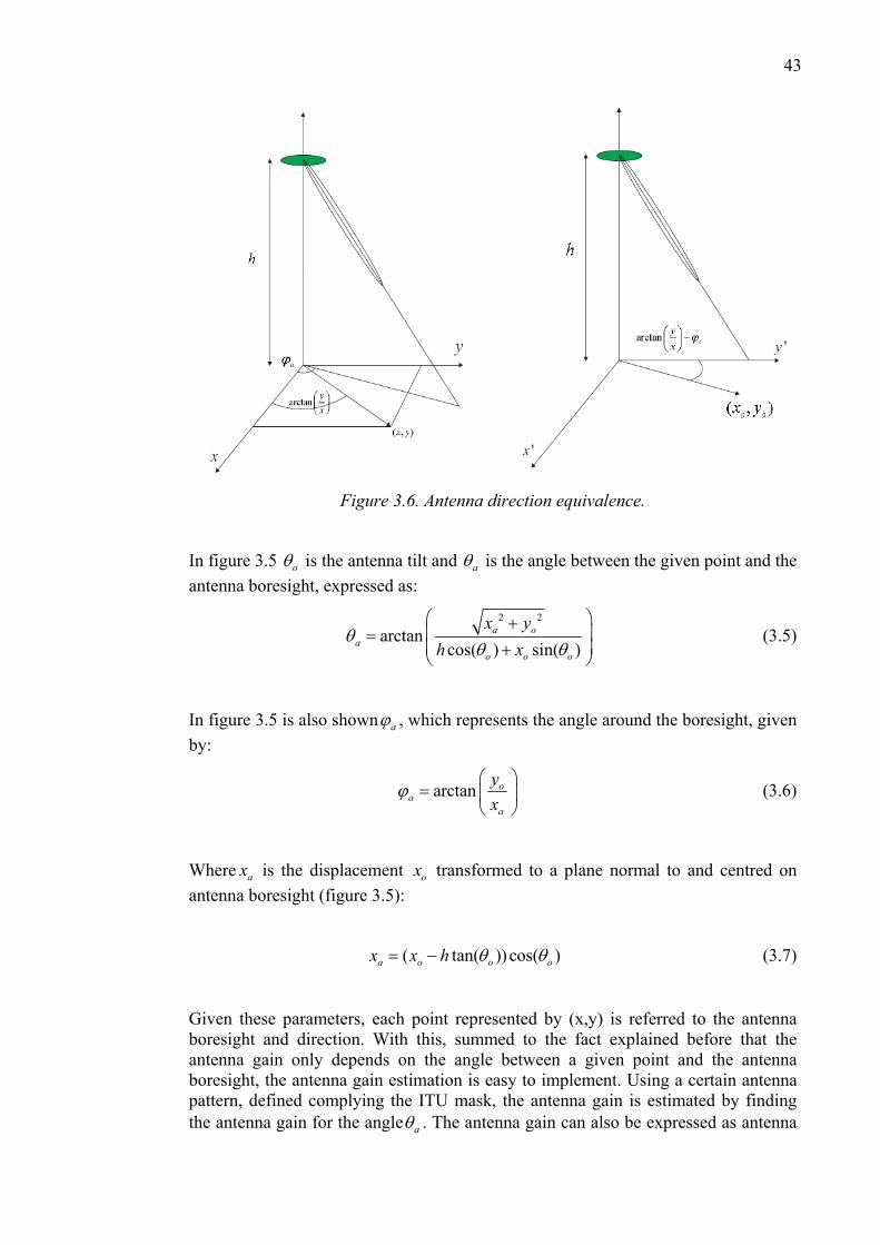
43

Figure 3.6. Antenna direction equivalence.

In figure 3.5 oθ is the antenna tilt and aθ is the angle between the given point and the antenna boresight, expressed as:

2 2

arctancos( ) sin( )

a oa

o o o

x yh x

θθ θ

⎛ ⎞+⎜ ⎟=⎜ ⎟+⎝ ⎠

(3.5)

In figure 3.5 is also shown aϕ , which represents the angle around the boresight, given by:

arctan oa

a

yx

ϕ⎛ ⎞

= ⎜ ⎟⎝ ⎠

(3.6)

Where ax is the displacement ox transformed to a plane normal to and centred on antenna boresight (figure 3.5):

( tan( )) cos( )a o o ox x h θ θ= − (3.7)

Given these parameters, each point represented by (x,y) is referred to the antenna boresight and direction. With this, summed to the fact explained before that the antenna gain only depends on the angle between a given point and the antenna boresight, the antenna gain estimation is easy to implement. Using a certain antenna pattern, defined complying the ITU mask, the antenna gain is estimated by finding the antenna gain for the angle aθ . The antenna gain can also be expressed as antenna

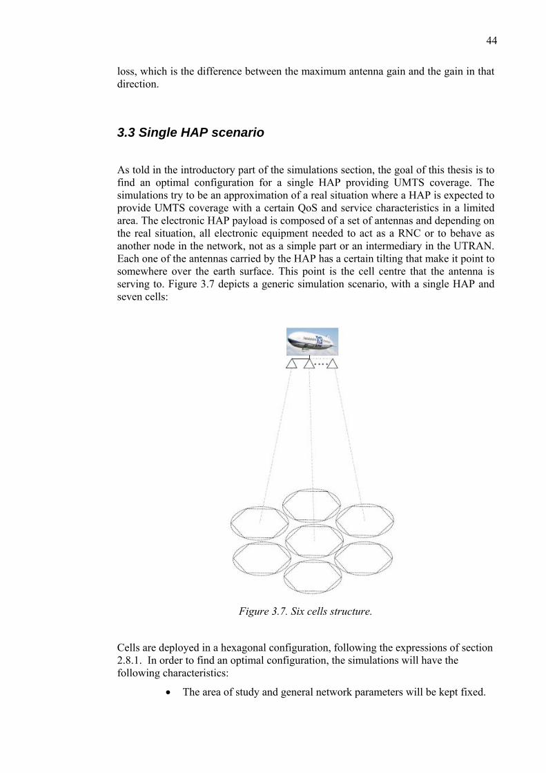
44

loss, which is the difference between the maximum antenna gain and the gain in that direction.

3.3 Single HAP scenario

As told in the introductory part of the simulations section, the goal of this thesis is to find an optimal configuration for a single HAP providing UMTS coverage. The simulations try to be an approximation of a real situation where a HAP is expected to provide UMTS coverage with a certain QoS and service characteristics in a limited area. The electronic HAP payload is composed of a set of antennas and depending on the real situation, all electronic equipment needed to act as a RNC or to behave as another node in the network, not as a simple part or an intermediary in the UTRAN. Each one of the antennas carried by the HAP has a certain tilting that make it point to somewhere over the earth surface. This point is the cell centre that the antenna is serving to. Figure 3.7 depicts a generic simulation scenario, with a single HAP and seven cells:

Figure 3.7. Six cells structure.

Cells are deployed in a hexagonal configuration, following the expressions of section 2.8.1. In order to find an optimal configuration, the simulations will have the following characteristics:

• The area of study and general network parameters will be kept fixed.

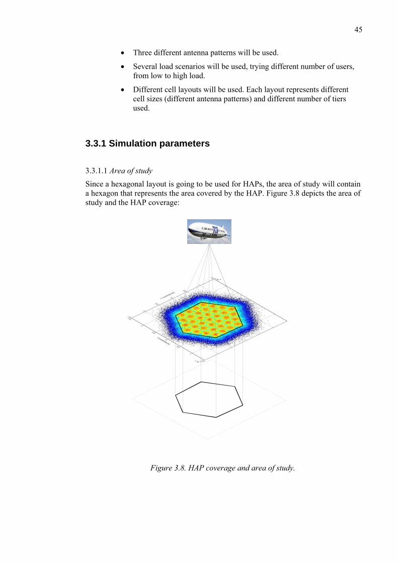
45

• Three different antenna patterns will be used.

• Several load scenarios will be used, trying different number of users, from low to high load.

• Different cell layouts will be used. Each layout represents different cell sizes (different antenna patterns) and different number of tiers used.

3.3.1 Simulation parameters

3.3.1.1 Area of study

Since a hexagonal layout is going to be used for HAPs, the area of study will contain a hexagon that represents the area covered by the HAP. Figure 3.8 depicts the area of study and the HAP coverage:

Figure 3.8. HAP coverage and area of study.

46

The total area is 30x30 km², containing a hexagon that represents the area covered by the HAP. The hexagon side length is 10 km and its area is 260 km², with the area covered by the HAP inside this hexagon. Figure 3.9 depicts the simulation area and the hexagon:

Figure 3.9. Area of study.

3.3.1.2 Network parameters

Table 3.1 contains all simulation parameters regarding HAP, mobile station, propagation model, link performance and other general parameters.

Table 3.1. Simulation parameters.

HAP parameters Description Value Unit

HAP antenna height 22 km Base station total maximum transmission power 37 dBm Base station maximum transmission power per link 30 dBm Pilot power 27 dBm Common channel and other channels power 27 dBm Base station cable losses 1 dB Base station UpLink load limit 0.75 Base station noise figure 5 dB

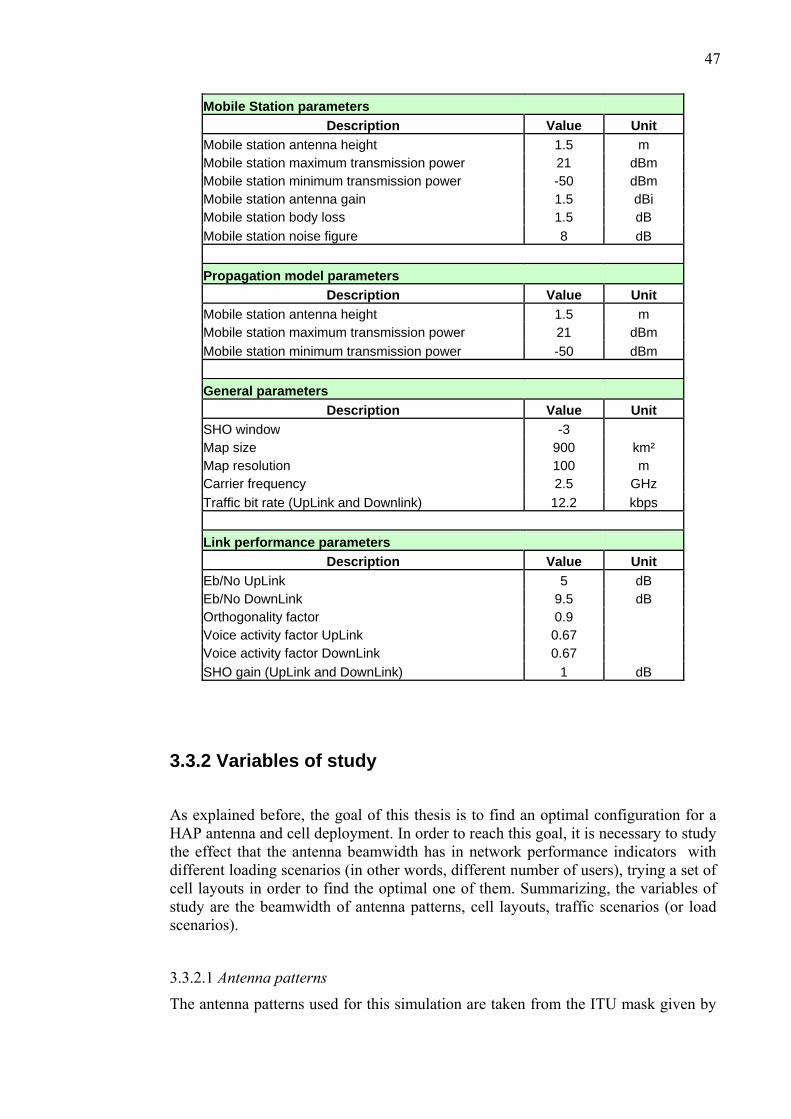
47

Mobile Station parameters Description Value Unit

Mobile station antenna height 1.5 m Mobile station maximum transmission power 21 dBm Mobile station minimum transmission power -50 dBm Mobile station antenna gain 1.5 dBi Mobile station body loss 1.5 dB Mobile station noise figure 8 dB Propagation model parameters

Description Value Unit Mobile station antenna height 1.5 m Mobile station maximum transmission power 21 dBm Mobile station minimum transmission power -50 dBm General parameters

Description Value Unit SHO window -3 Map size 900 km² Map resolution 100 m Carrier frequency 2.5 GHz Traffic bit rate (UpLink and Downlink) 12.2 kbps Link performance parameters

Description Value Unit Eb/No UpLink 5 dB Eb/No DownLink 9.5 dB Orthogonality factor 0.9 Voice activity factor UpLink 0.67 Voice activity factor DownLink 0.67 SHO gain (UpLink and DownLink) 1 dB

3.3.2 Variables of study

As explained before, the goal of this thesis is to find an optimal configuration for a HAP antenna and cell deployment. In order to reach this goal, it is necessary to study the effect that the antenna beamwidth has in network performance indicators with different loading scenarios (in other words, different number of users), trying a set of cell layouts in order to find the optimal one of them. Summarizing, the variables of study are the beamwidth of antenna patterns, cell layouts, traffic scenarios (or load scenarios).

3.3.2.1 Antenna patterns

The antenna patterns used for this simulation are taken from the ITU mask given by

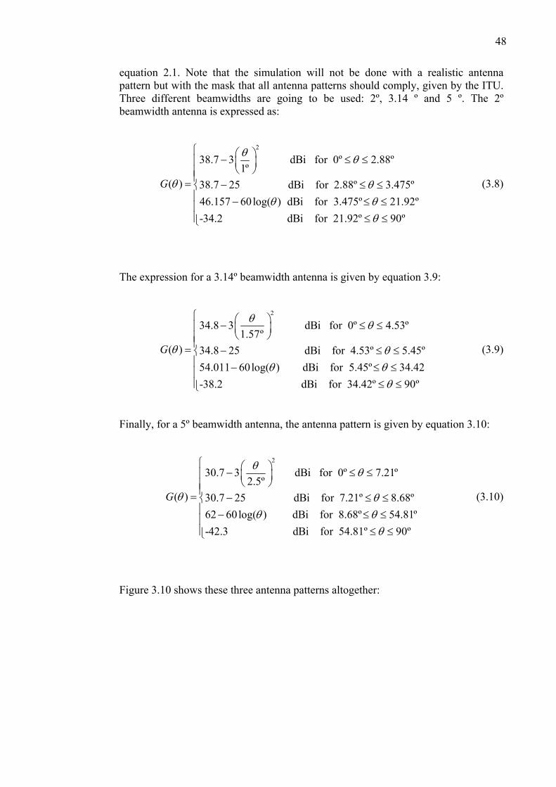
48

equation 2.1. Note that the simulation will not be done with a realistic antenna pattern but with the mask that all antenna patterns should comply, given by the ITU. Three different beamwidths are going to be used: 2º, 3.14 º and 5 º. The 2º beamwidth antenna is expressed as:

2

38.7 3 dBi for 0º 2.88º1º

( ) 38.7 25 dBi for 2.88º 3.475º46.157 60log( ) dBi for 3.475º 21.92º -34.2 dBi for 21.92º 90º

G

θ θ

θ θθ θ

θ

⎛ ⎞− ≤ ≤⎜ ⎟⎝ ⎠

= − ≤ ≤− ≤ ≤

≤ ≤

⎧⎪⎪⎪⎨⎪⎪⎪⎩

(3.8)

The expression for a 3.14º beamwidth antenna is given by equation 3.9:

2

34.8 3 dBi for 0º 4.53º1.57º

( ) 34.8 25 dBi for 4.53º 5.45º54.011 60log( ) dBi for 5.45º 34.42 -38.2 dBi f

G

θ θ

θ θθ θ

⎛ ⎞− ≤ ≤⎜ ⎟⎝ ⎠

= − ≤ ≤− ≤ ≤

or 34.42º 90º θ

⎧⎪⎪⎪⎨⎪⎪⎪ ≤ ≤⎩

(3.9)

Finally, for a 5º beamwidth antenna, the antenna pattern is given by equation 3.10:

2

30.7 3 dBi for 0º 7.21º2.5º

( ) 30.7 25 dBi for 7.21º 8.68º62 60log( ) dBi for 8.68º 54.81º -42.3 dBi for 54.81º 90º

G

θ θ

θ θθ θ

θ

⎛ ⎞− ≤ ≤⎜ ⎟⎝ ⎠

= − ≤ ≤− ≤ ≤

≤ ≤

⎧⎪⎪⎪⎨⎪⎪⎪⎩

(3.10)

Figure 3.10 shows these three antenna patterns altogether:

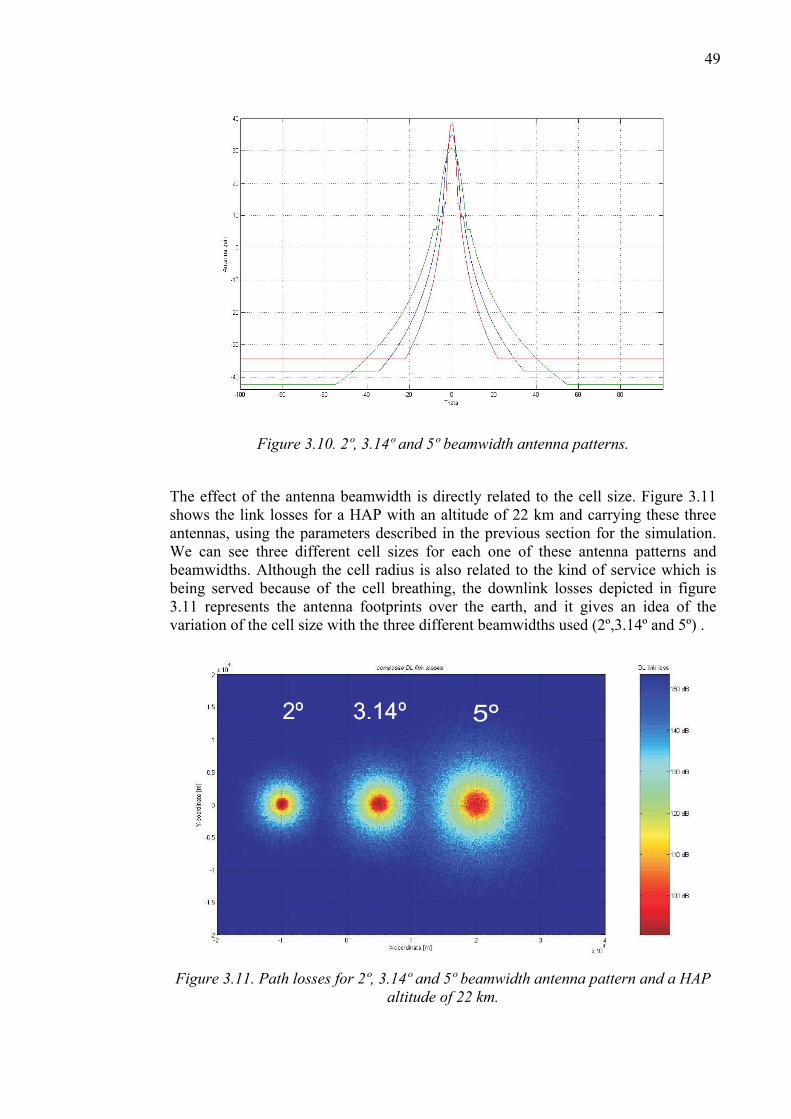
49

Figure 3.10. 2º, 3.14º and 5º beamwidth antenna patterns.

The effect of the antenna beamwidth is directly related to the cell size. Figure 3.11 shows the link losses for a HAP with an altitude of 22 km and carrying these three antennas, using the parameters described in the previous section for the simulation. We can see three different cell sizes for each one of these antenna patterns and beamwidths. Although the cell radius is also related to the kind of service which is being served because of the cell breathing, the downlink losses depicted in figure 3.11 represents the antenna footprints over the earth, and it gives an idea of the variation of the cell size with the three different beamwidths used (2º,3.14º and 5º) .

Figure 3.11. Path losses for 2º, 3.14º and 5º beamwidth antenna pattern and a HAP

altitude of 22 km.

50

3.3.2.2 Traffic scenarios

Traffic scenarios are the second variable under study. It is necessary to see the network performance and the variation of service parameters when the number of users increases inside the hexagon which represents the HAP coverage, depicted in figure 3.9. This variation is made from 2000 users to 8000 users, in steps of 1000. In other words, these seven traffic scenarios represent the evolution from low load (2000 users) to high load (8000 users) service demand.

The initial implementation of the simulator locates users randomly inside the area of study in the stage of assigning positions to mobile stations. Each mobile station is represented by a chart containing data such as transmission power, antenna gain, and also the coordinates (x,y) of the mobile station. The user positioning and distribution consists of two basic steps. First, once the defined area and its limits are defined, two uniform random variables are created: one for the “x” coordinates, and another one for “y” coordinates. If the map limits are defined by ( max min max min, , ,x x y y ), and the number of users is N, each one of these random variables is a set of N numbers that conforms a uniform distribution function:

{ }{ }

1 2

1 2

, ,...,

, ,...,N

N

X x x x

Y y y y

=

= (3.11)

The distribution for the x coordinates, X, contains numbers in the range [ max min,x x ] and the distribution for the y coordinates, Y, contains numbers in the range [ max min,y y ]. Each mobile station position is composed by a pair of coordinates, (x,y), extracted from these set of numbers:

{ }

{ }

1 1 1,.........

,N N N

MS x y

MS y x

=

=

(3.12)

This method of distributing user inside the area of study is not useful for a HAP based service. Basically the problem is that the HAP only provides coverage in a hexagonal area. Using this user distribution means that part of the users in the area is not served because they are not located inside the HAP covered area, and consequently 100% of service probability is never reached. Figure 3.12 depicts this problem, with 3000 voice (12.2 kbps) users located in a 30x30 km² area. The hexagon in black lines represents the area covered by the HAP.

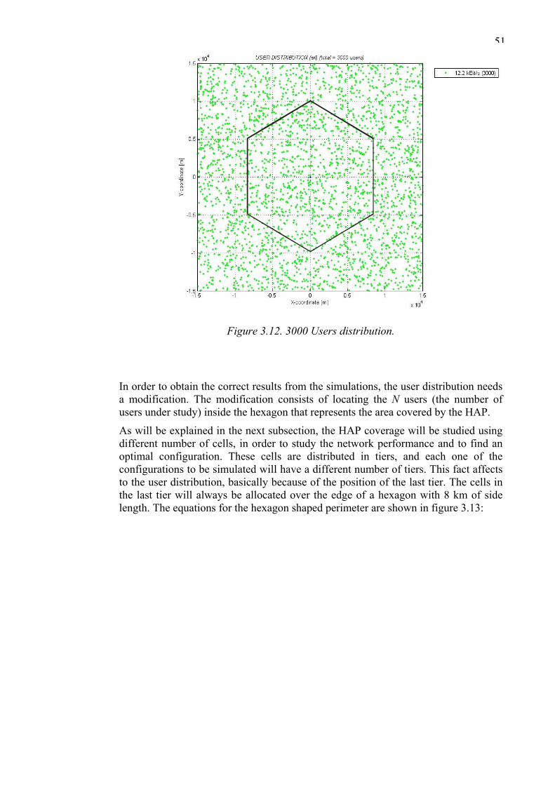
51

Figure 3.12. 3000 Users distribution.

In order to obtain the correct results from the simulations, the user distribution needs a modification. The modification consists of locating the N users (the number of users under study) inside the hexagon that represents the area covered by the HAP.

As will be explained in the next subsection, the HAP coverage will be studied using different number of cells, in order to study the network performance and to find an optimal configuration. These cells are distributed in tiers, and each one of the configurations to be simulated will have a different number of tiers. This fact affects to the user distribution, basically because of the position of the last tier. The cells in the last tier will always be allocated over the edge of a hexagon with 8 km of side length. The equations for the hexagon shaped perimeter are shown in figure 3.13:

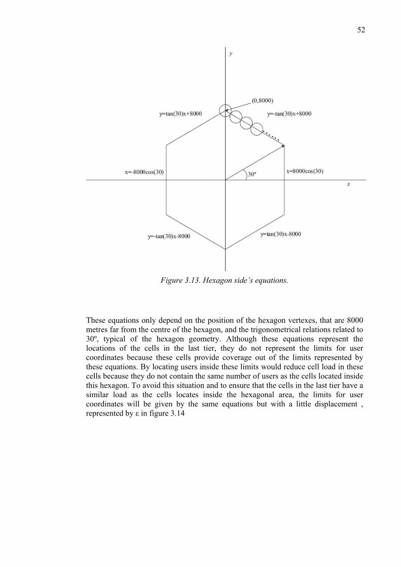
52

Figure 3.13. Hexagon side’s equations.

These equations only depend on the position of the hexagon vertexes, that are 8000 metres far from the centre of the hexagon, and the trigonometrical relations related to 30º, typical of the hexagon geometry. Although these equations represent the locations of the cells in the last tier, they do not represent the limits for user coordinates because these cells provide coverage out of the limits represented by these equations. By locating users inside these limits would reduce cell load in these cells because they do not contain the same number of users as the cells located inside this hexagon. To avoid this situation and to ensure that the cells in the last tier have a similar load as the cells locates inside the hexagonal area, the limits for user coordinates will be given by the same equations but with a little displacement , represented by ε in figure 3.14

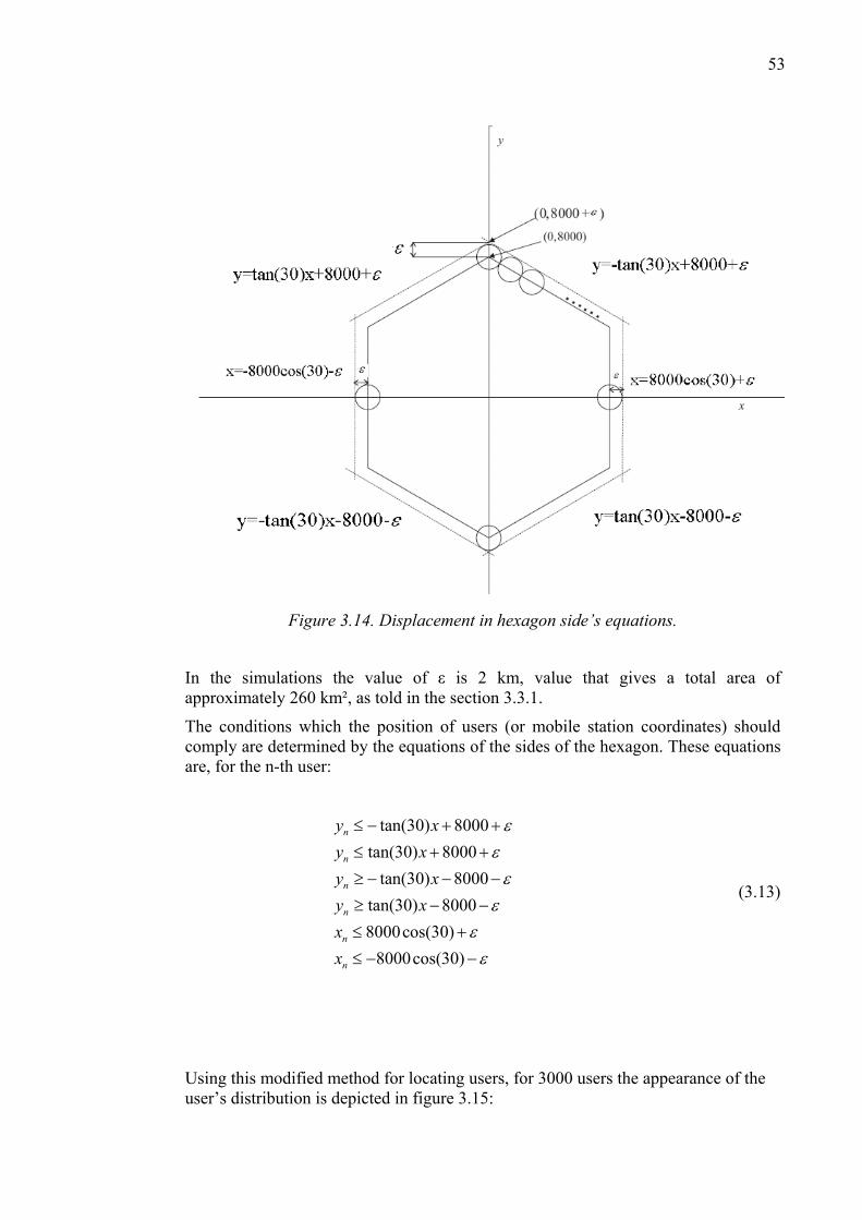
53

Figure 3.14. Displacement in hexagon side’s equations.

In the simulations the value of ε is 2 km, value that gives a total area of approximately 260 km², as told in the section 3.3.1.

The conditions which the position of users (or mobile station coordinates) should comply are determined by the equations of the sides of the hexagon. These equations are, for the n-th user:

tan(30) 8000tan(30) 8000

tan(30) 8000tan(30) 80008000cos(30)

8000cos(30)

n

n

n

n

n

n

y xy xy xy xxx

εεε

εεε

≤ − + +≤ + +≥ − − −≥ − −≤ +≤ − −

(3.13)

Using this modified method for locating users, for 3000 users the appearance of the user’s distribution is depicted in figure 3.15:

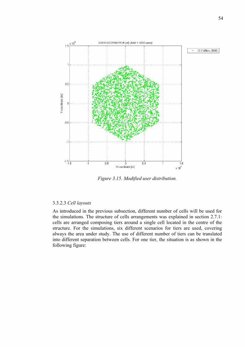
54

Figure 3.15. Modified user distribution.

3.3.2.3 Cell layouts

As introduced in the previous subsection, different number of cells will be used for the simulations. The structure of cells arrangements was explained in section 2.7.1: cells are arranged composing tiers around a single cell located in the centre of the structure. For the simulations, six different scenarios for tiers are used, covering always the area under study. The use of different number of tiers can be translated into different separation between cells. For one tier, the situation is as shown in the following figure:

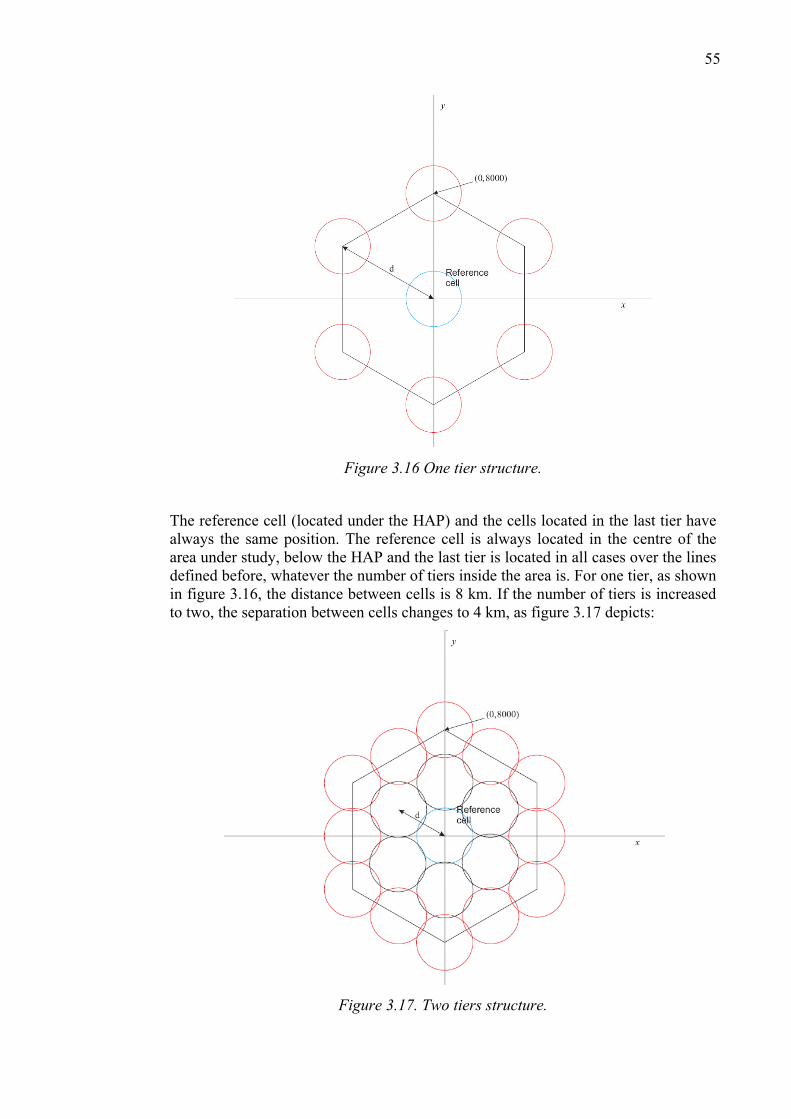
55

Figure 3.16 One tier structure.

The reference cell (located under the HAP) and the cells located in the last tier have always the same position. The reference cell is always located in the centre of the area under study, below the HAP and the last tier is located in all cases over the lines defined before, whatever the number of tiers inside the area is. For one tier, as shown in figure 3.16, the distance between cells is 8 km. If the number of tiers is increased to two, the separation between cells changes to 4 km, as figure 3.17 depicts:

Figure 3.17. Two tiers structure.

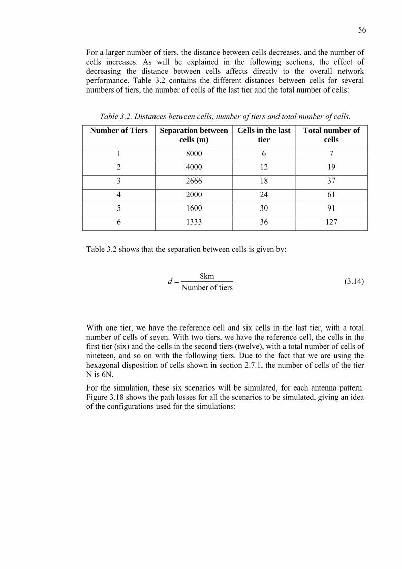
56

For a larger number of tiers, the distance between cells decreases, and the number of cells increases. As will be explained in the following sections, the effect of decreasing the distance between cells affects directly to the overall network performance. Table 3.2 contains the different distances between cells for several numbers of tiers, the number of cells of the last tier and the total number of cells:

Table 3.2. Distances between cells, number of tiers and total number of cells.

Number of Tiers Separation between cells (m)

Cells in the last tier

Total number of cells

1 8000 6 7

2 4000 12 19

3 2666 18 37

4 2000 24 61

5 1600 30 91

6 1333 36 127

Table 3.2 shows that the separation between cells is given by:

8kmNumber of tiers

d = (3.14)

With one tier, we have the reference cell and six cells in the last tier, with a total number of cells of seven. With two tiers, we have the reference cell, the cells in the first tier (six) and the cells in the second tiers (twelve), with a total number of cells of nineteen, and so on with the following tiers. Due to the fact that we are using the hexagonal disposition of cells shown in section 2.7.1, the number of cells of the tier N is 6N.

For the simulation, these six scenarios will be simulated, for each antenna pattern. Figure 3.18 shows the path losses for all the scenarios to be simulated, giving an idea of the configurations used for the simulations:

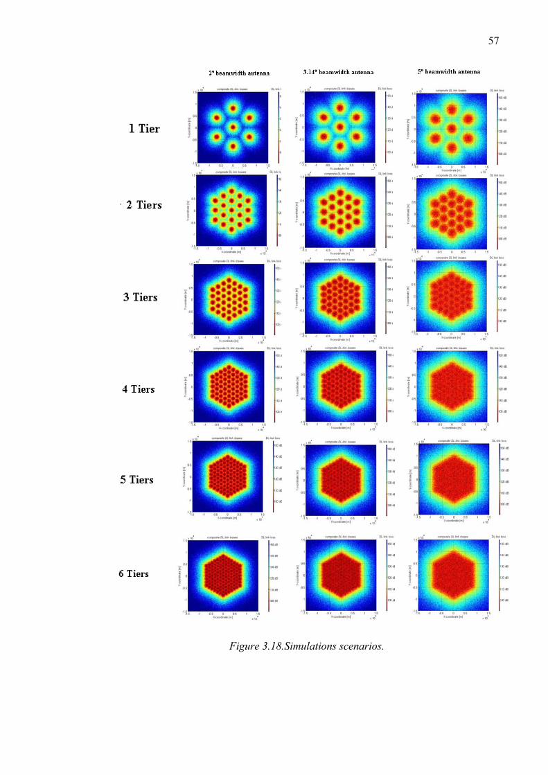
57

Figure 3.18.Simulations scenarios.

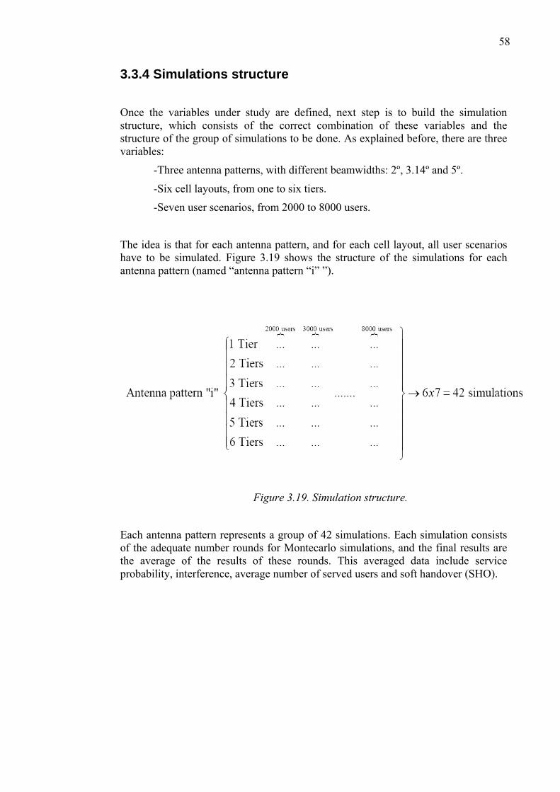
58

3.3.4 Simulations structure

Once the variables under study are defined, next step is to build the simulation structure, which consists of the correct combination of these variables and the structure of the group of simulations to be done. As explained before, there are three variables:

-Three antenna patterns, with different beamwidths: 2º, 3.14º and 5º.

-Six cell layouts, from one to six tiers.

-Seven user scenarios, from 2000 to 8000 users.

The idea is that for each antenna pattern, and for each cell layout, all user scenarios have to be simulated. Figure 3.19 shows the structure of the simulations for each antenna pattern (named “antenna pattern “i” ”).

Figure 3.19. Simulation structure.

Each antenna pattern represents a group of 42 simulations. Each simulation consists of the adequate number rounds for Montecarlo simulations, and the final results are the average of the results of these rounds. This averaged data include service probability, interference, average number of served users and soft handover (SHO).

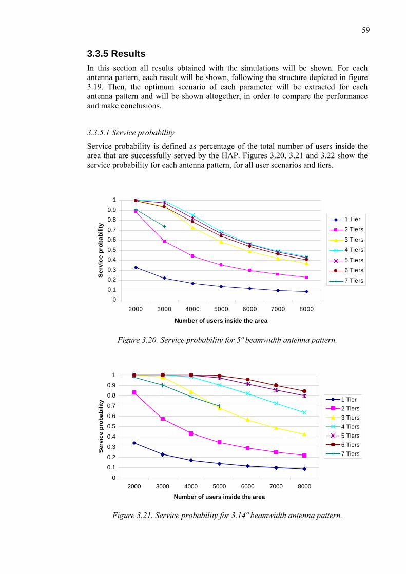
59

3.3.5 Results In this section all results obtained with the simulations will be shown. For each antenna pattern, each result will be shown, following the structure depicted in figure 3.19. Then, the optimum scenario of each parameter will be extracted for each antenna pattern and will be shown altogether, in order to compare the performance and make conclusions.

3.3.5.1 Service probability

Service probability is defined as percentage of the total number of users inside the area that are successfully served by the HAP. Figures 3.20, 3.21 and 3.22 show the service probability for each antenna pattern, for all user scenarios and tiers.

00.1

0.20.3

0.40.50.60.7

0.80.9

1

2000 3000 4000 5000 6000 7000 8000

Number of users inside the area

Serv

ice

prob

abili

ty

1 Tier

2 Tiers

3 Tiers4 Tiers

5 Tiers

6 Tiers

7 Tiers

Figure 3.20. Service probability for 5º beamwidth antenna pattern.

0

0.1

0.2

0.3

0.4

0.5

0.6

0.7

0.8

0.9

1

2000 3000 4000 5000 6000 7000 8000

Number of users inside the area

Serv

ice

prob

abili

ty 1 Tier2 Tiers3 Tiers4 Tiers5 Tiers6 Tiers7 Tiers

Figure 3.21. Service probability for 3.14º beamwidth antenna pattern.

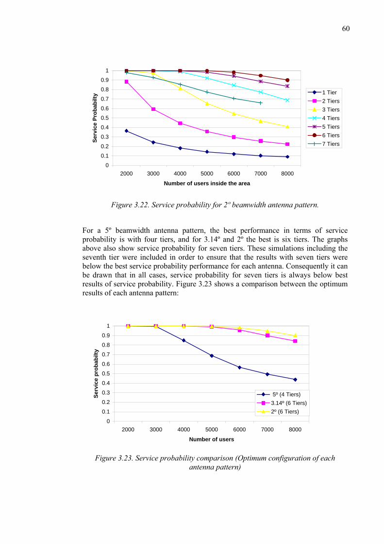
60

0

0.1

0.2

0.3

0.4

0.5

0.6

0.7

0.8

0.9

1

2000 3000 4000 5000 6000 7000 8000

Number of users inside the area

Serv

ice

Prob

abilt

y 1 Tier2 Tiers3 Tiers4 Tiers5 Tiers6 Tiers7 Tiers

Figure 3.22. Service probability for 2º beamwidth antenna pattern.

For a 5º beamwidth antenna pattern, the best performance in terms of service probability is with four tiers, and for 3.14º and 2º the best is six tiers. The graphs above also show service probability for seven tiers. These simulations including the seventh tier were included in order to ensure that the results with seven tiers were below the best service probability performance for each antenna. Consequently it can be drawn that in all cases, service probability for seven tiers is always below best results of service probability. Figure 3.23 shows a comparison between the optimum results of each antenna pattern:

0

0.1

0.2

0.3

0.4

0.5

0.6

0.7

0.8

0.9

1

2000 3000 4000 5000 6000 7000 8000

Number of users

Serv

ice

prob

abilt

y

5º (4 Tiers)3.14º (6 Tiers)2º (6 Tiers)

Figure 3.23. Service probability comparison (Optimum configuration of each antenna pattern)

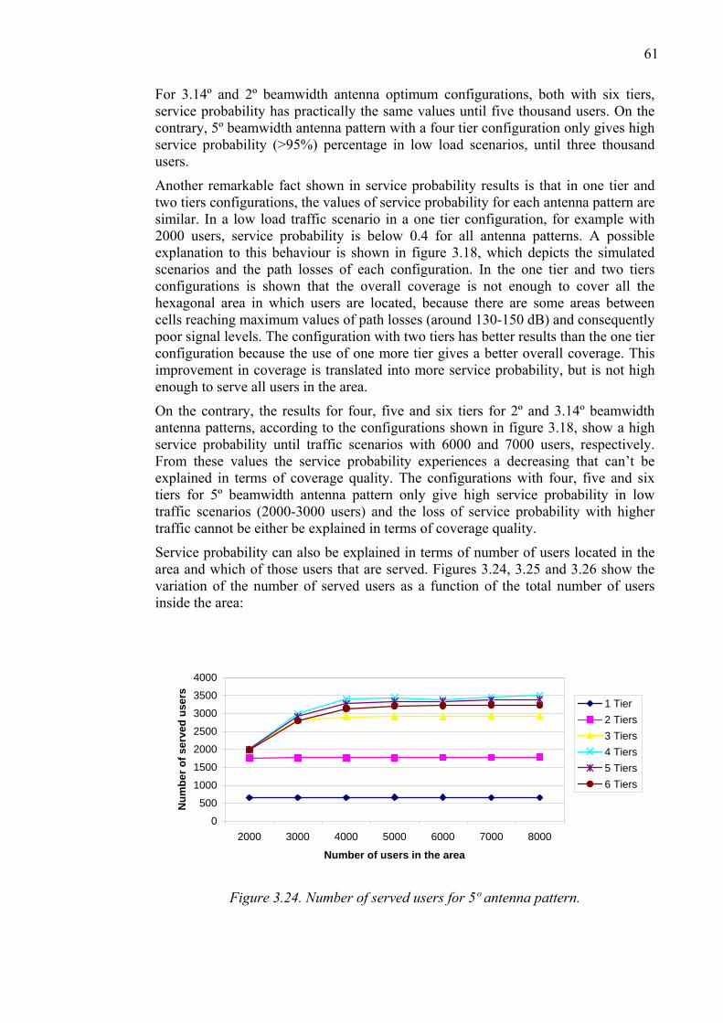
61

For 3.14º and 2º beamwidth antenna optimum configurations, both with six tiers, service probability has practically the same values until five thousand users. On the contrary, 5º beamwidth antenna pattern with a four tier configuration only gives high service probability (>95%) percentage in low load scenarios, until three thousand users.

Another remarkable fact shown in service probability results is that in one tier and two tiers configurations, the values of service probability for each antenna pattern are similar. In a low load traffic scenario in a one tier configuration, for example with 2000 users, service probability is below 0.4 for all antenna patterns. A possible explanation to this behaviour is shown in figure 3.18, which depicts the simulated scenarios and the path losses of each configuration. In the one tier and two tiers configurations is shown that the overall coverage is not enough to cover all the hexagonal area in which users are located, because there are some areas between cells reaching maximum values of path losses (around 130-150 dB) and consequently poor signal levels. The configuration with two tiers has better results than the one tier configuration because the use of one more tier gives a better overall coverage. This improvement in coverage is translated into more service probability, but is not high enough to serve all users in the area.

On the contrary, the results for four, five and six tiers for 2º and 3.14º beamwidth antenna patterns, according to the configurations shown in figure 3.18, show a high service probability until traffic scenarios with 6000 and 7000 users, respectively. From these values the service probability experiences a decreasing that can’t be explained in terms of coverage quality. The configurations with four, five and six tiers for 5º beamwidth antenna pattern only give high service probability in low traffic scenarios (2000-3000 users) and the loss of service probability with higher traffic cannot be either be explained in terms of coverage quality.

Service probability can also be explained in terms of number of users located in the area and which of those users that are served. Figures 3.24, 3.25 and 3.26 show the variation of the number of served users as a function of the total number of users inside the area:

0

500

1000

1500

2000

2500

3000

3500

4000

2000 3000 4000 5000 6000 7000 8000

Number of users in the area

Num

ber o

f ser

ved

user

s

1 Tier2 Tiers3 Tiers4 Tiers5 Tiers6 Tiers

Figure 3.24. Number of served users for 5º antenna pattern.

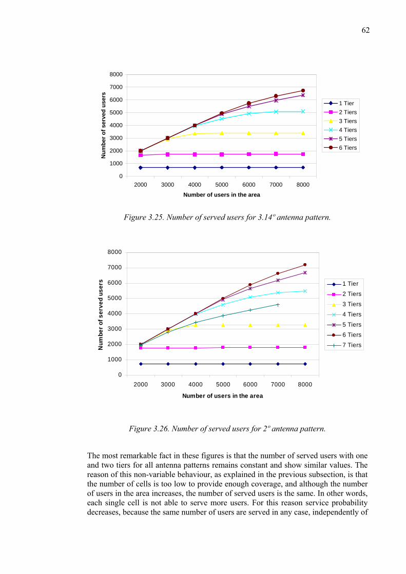
62

0

1000

2000

3000

4000

5000

6000

7000

8000

2000 3000 4000 5000 6000 7000 8000

Number of users in the area

Num

ber o

f ser

ved

user

s1 Tier2 Tiers3 Tiers4 Tiers5 Tiers6 Tiers

Figure 3.25. Number of served users for 3.14º antenna pattern.

0

1000

2000

3000

4000

5000

6000

7000

8000

2000 3000 4000 5000 6000 7000 8000

Number of users in the area

Num

ber o

f ser

ved

user

s 1 Tier

2 Tiers

3 Tiers

4 Tiers

5 Tiers6 Tiers

7 Tiers

Figure 3.26. Number of served users for 2º antenna pattern.

The most remarkable fact in these figures is that the number of served users with one and two tiers for all antenna patterns remains constant and show similar values. The reason of this non-variable behaviour, as explained in the previous subsection, is that the number of cells is too low to provide enough coverage, and although the number of users in the area increases, the number of served users is the same. In other words, each single cell is not able to serve more users. For this reason service probability decreases, because the same number of users are served in any case, independently of

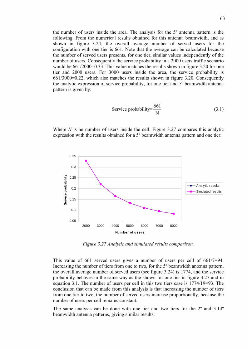
63

the number of users inside the area. The analysis for the 5º antenna pattern is the following. From the numerical results obtained for this antenna beamwidth, and as shown in figure 3.24, the overall average number of served users for the configuration with one tier is 661. Note that the average can be calculated because the number of served users presents, for one tier, similar values independently of the number of users. Consequently the service probability in a 2000 users traffic scenario would be 661/2000=0.33. This value matches the results shown in figure 3.20 for one tier and 2000 users. For 3000 users inside the area, the service probability is 661/3000=0.22, which also matches the results shown in figure 3.20. Consequently the analytic expression of service probability, for one tier and 5º beamwidth antenna pattern is given by:

661Service probability=N

(3.1)

Where N is he number of users inside the cell. Figure 3.27 compares this analytic expression with the results obtained for a 5º beamwidth antenna pattern and one tier:

0.05

0.1

0.15

0.2

0.25

0.3

0.35

2000 3000 4000 5000 6000 7000 8000

Number of users

Serv

ice

prob

abili

ty

Analytic results

Simulated results

Figure 3.27 Analytic and simulated results comparison.

This value of 661 served users gives a number of users per cell of 661/7=94. Increasing the number of tiers from one to two, for the 5º beamwidth antenna pattern, the overall average number of served users (see figure 3.24) is 1774, and the service probability behaves in the same way as the shown for one tier in figure 3.27 and in equation 3.1. The number of users per cell in this two tiers case is 1774/19=93. The conclusion that can be made from this analysis is that increasing the number of tiers from one tier to two, the number of served users increase proportionally, because the number of users per cell remains constant.

The same analysis can be done with one tier and two tiers for the 2º and 3.14º beamwidth antenna patterns, giving similar results.

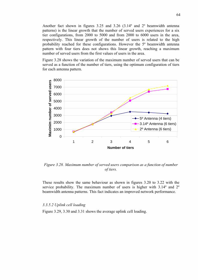
64

Another fact shown in figures 3.25 and 3.26 (3.14º and 2º beamwidth antenna patterns) is the linear growth that the number of served users experiences for a six tier configurations, from 2000 to 5000 and from 2000 to 6000 users in the area, respectively. This linear growth of the number of users is related to the high probability reached for these configurations. However the 5º beamwidth antenna pattern with four tiers does not shows this linear growth, reaching a maximum number of served users from the first values of users in the area.

Figure 3.28 shows the variation of the maximum number of served users that can be served as a function of the number of tiers, using the optimum configuration of tiers for each antenna pattern.

0

1000

2000

3000

4000

5000

6000

7000

8000

1 2 3 4 5 6

Number of tiers

Max

imim

num

ber o

f ser

ved

user

s

5º Antenna (4 tiers)3.14º Antenna (6 tiers)2º Antenna (6 tiers)

Figure 3.28. Maximum number of served users comparison as a function of number of tiers.

These results show the same behaviour as shown in figures 3.20 to 3.22 with the service probability. The maximum number of users is higher with 3.14º and 2º beamwidth antenna patterns. This fact indicates an improved network performance.

3.3.5.2 Uplink cell loading

Figure 3.29, 3.30 and 3.31 shows the average uplink cell loading.

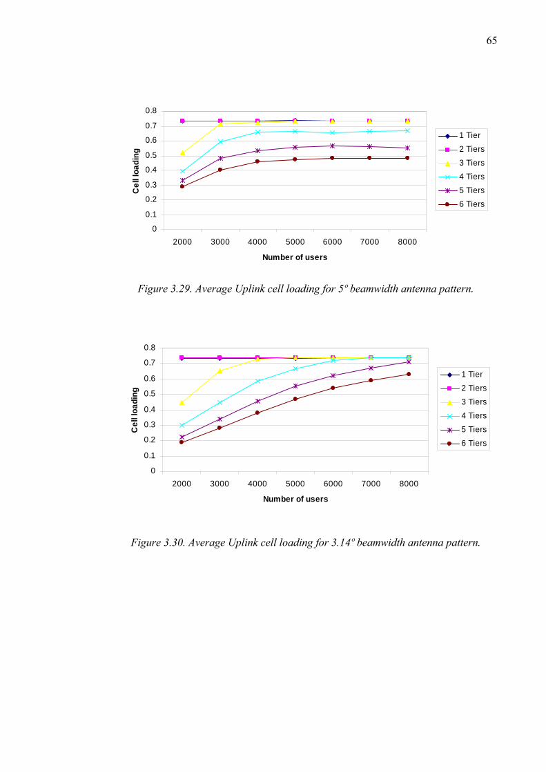
65

0

0.1

0.2

0.3

0.4

0.5

0.6

0.7

0.8

2000 3000 4000 5000 6000 7000 8000

Number of users

Cel

l loa

ding

1 Tier

2 Tiers

3 Tiers

4 Tiers5 Tiers

6 Tiers

Figure 3.29. Average Uplink cell loading for 5º beamwidth antenna pattern.

0

0.1

0.2

0.3

0.4

0.5

0.6

0.7

0.8

2000 3000 4000 5000 6000 7000 8000

Number of users

Cel

l loa

ding

1 Tier

2 Tiers

3 Tiers

4 Tiers

5 Tiers

6 Tiers

Figure 3.30. Average Uplink cell loading for 3.14º beamwidth antenna pattern.

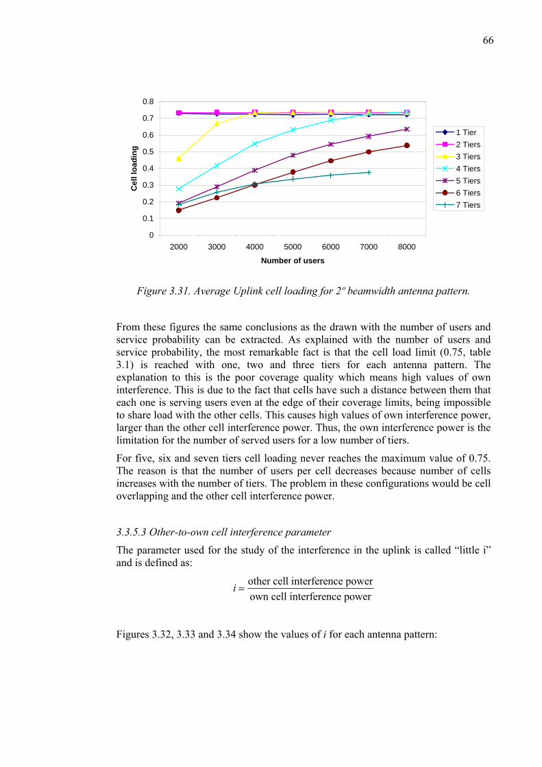
66

0

0.1

0.2

0.3

0.4

0.5

0.6

0.7

0.8

2000 3000 4000 5000 6000 7000 8000

Number of users

Cel

l loa

ding

1 Tier2 Tiers3 Tiers4 Tiers5 Tiers6 Tiers7 Tiers

Figure 3.31. Average Uplink cell loading for 2º beamwidth antenna pattern.

From these figures the same conclusions as the drawn with the number of users and service probability can be extracted. As explained with the number of users and service probability, the most remarkable fact is that the cell load limit (0.75, table 3.1) is reached with one, two and three tiers for each antenna pattern. The explanation to this is the poor coverage quality which means high values of own interference. This is due to the fact that cells have such a distance between them that each one is serving users even at the edge of their coverage limits, being impossible to share load with the other cells. This causes high values of own interference power, larger than the other cell interference power. Thus, the own interference power is the limitation for the number of served users for a low number of tiers.

For five, six and seven tiers cell loading never reaches the maximum value of 0.75. The reason is that the number of users per cell decreases because number of cells increases with the number of tiers. The problem in these configurations would be cell overlapping and the other cell interference power.

3.3.5.3 Other-to-own cell interference parameter

The parameter used for the study of the interference in the uplink is called “little i” and is defined as:

other cell interference powerown cell interference power

i =

Figures 3.32, 3.33 and 3.34 show the values of i for each antenna pattern:

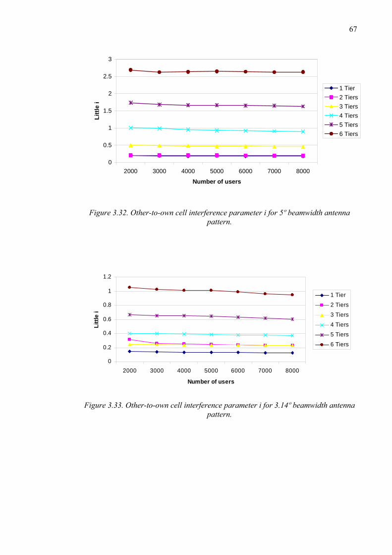
67

0

0.5

1

1.5

2

2.5

3

2000 3000 4000 5000 6000 7000 8000

Number of users

Littl

e i

1 Tier2 Tiers3 Tiers4 Tiers5 Tiers6 Tiers

Figure 3.32. Other-to-own cell interference parameter i for 5º beamwidth antenna pattern.

0

0.2

0.4

0.6

0.8

1

1.2

2000 3000 4000 5000 6000 7000 8000

Number of users

Littl

e i

1 Tier

2 Tiers

3 Tiers

4 Tiers5 Tiers

6 Tiers

Figure 3.33. Other-to-own cell interference parameter i for 3.14º beamwidth antenna

pattern.

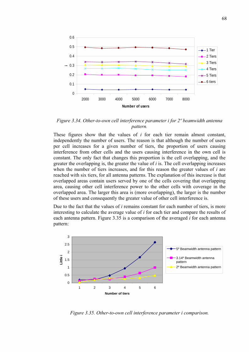
68

0

0.1

0.2

0.3

0.4

0.5

0.6

2000 3000 4000 5000 6000 7000 8000

Number of users

i

1 Tier2 Tiers3 Tiers4 Tiers5 Tiers6 tiers

Figure 3.34. Other-to-own cell interference parameter i for 2º beamwidth antenna

pattern.

These figures show that the values of i for each tier remain almost constant, independently the number of users. The reason is that although the number of users per cell increases for a given number of tiers, the proportion of users causing interference from other cells and the users causing interference in the own cell is constant. The only fact that changes this proportion is the cell overlapping, and the greater the overlapping is, the greater the value of i is. The cell overlapping increases when the number of tiers increases, and for this reason the greater values of i are reached with six tiers, for all antenna patterns. The explanation of this increase is that overlapped areas contain users served by one of the cells covering that overlapping area, causing other cell interference power to the other cells with coverage in the overlapped area. The larger this area is (more overlapping), the larger is the number of these users and consequently the greater value of other cell interference is.

Due to the fact that the values of i remains constant for each number of tiers, is more interesting to calculate the average value of i for each tier and compare the results of each antenna pattern. Figure 3.35 is a comparison of the averaged i for each antenna pattern:

0

0.5

1

1.5

2

2.5

3

1 2 3 4 5 6

Number of tiers

Littl

e i

5º Beamwidth antenna pattern

3.14º Beamwidth antennapattern2º Beamwidth antenna pattern

Figure 3.35. Other-to-own cell interference parameter i comparison.

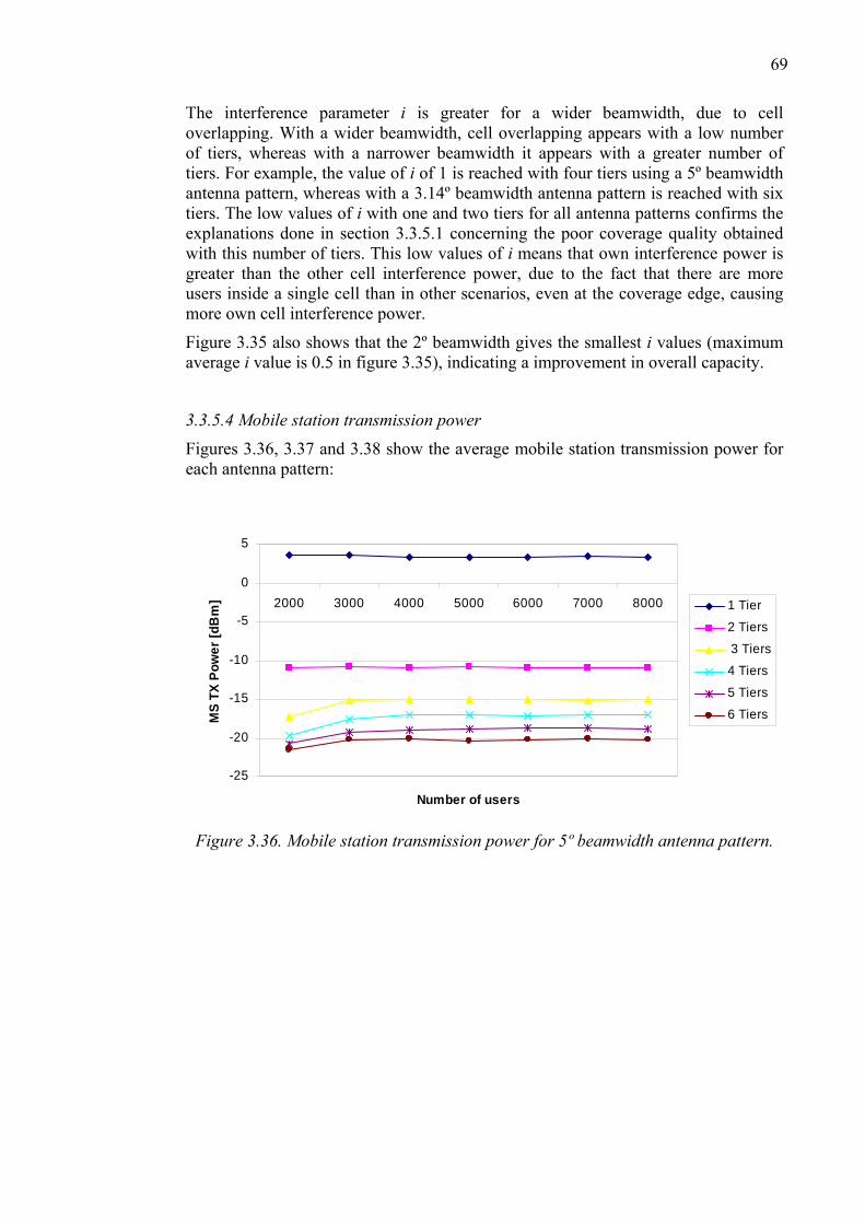
69

The interference parameter i is greater for a wider beamwidth, due to cell overlapping. With a wider beamwidth, cell overlapping appears with a low number of tiers, whereas with a narrower beamwidth it appears with a greater number of tiers. For example, the value of i of 1 is reached with four tiers using a 5º beamwidth antenna pattern, whereas with a 3.14º beamwidth antenna pattern is reached with six tiers. The low values of i with one and two tiers for all antenna patterns confirms the explanations done in section 3.3.5.1 concerning the poor coverage quality obtained with this number of tiers. This low values of i means that own interference power is greater than the other cell interference power, due to the fact that there are more users inside a single cell than in other scenarios, even at the coverage edge, causing more own cell interference power.

Figure 3.35 also shows that the 2º beamwidth gives the smallest i values (maximum average i value is 0.5 in figure 3.35), indicating a improvement in overall capacity.

3.3.5.4 Mobile station transmission power

Figures 3.36, 3.37 and 3.38 show the average mobile station transmission power for each antenna pattern:

-25

-20

-15

-10

-5

0

5

2000 3000 4000 5000 6000 7000 8000

Number of users

MS

TX P

ower

[dB

m] 1 Tier

2 Tiers

3 Tiers

4 Tiers

5 Tiers

6 Tiers

Figure 3.36. Mobile station transmission power for 5º beamwidth antenna pattern.

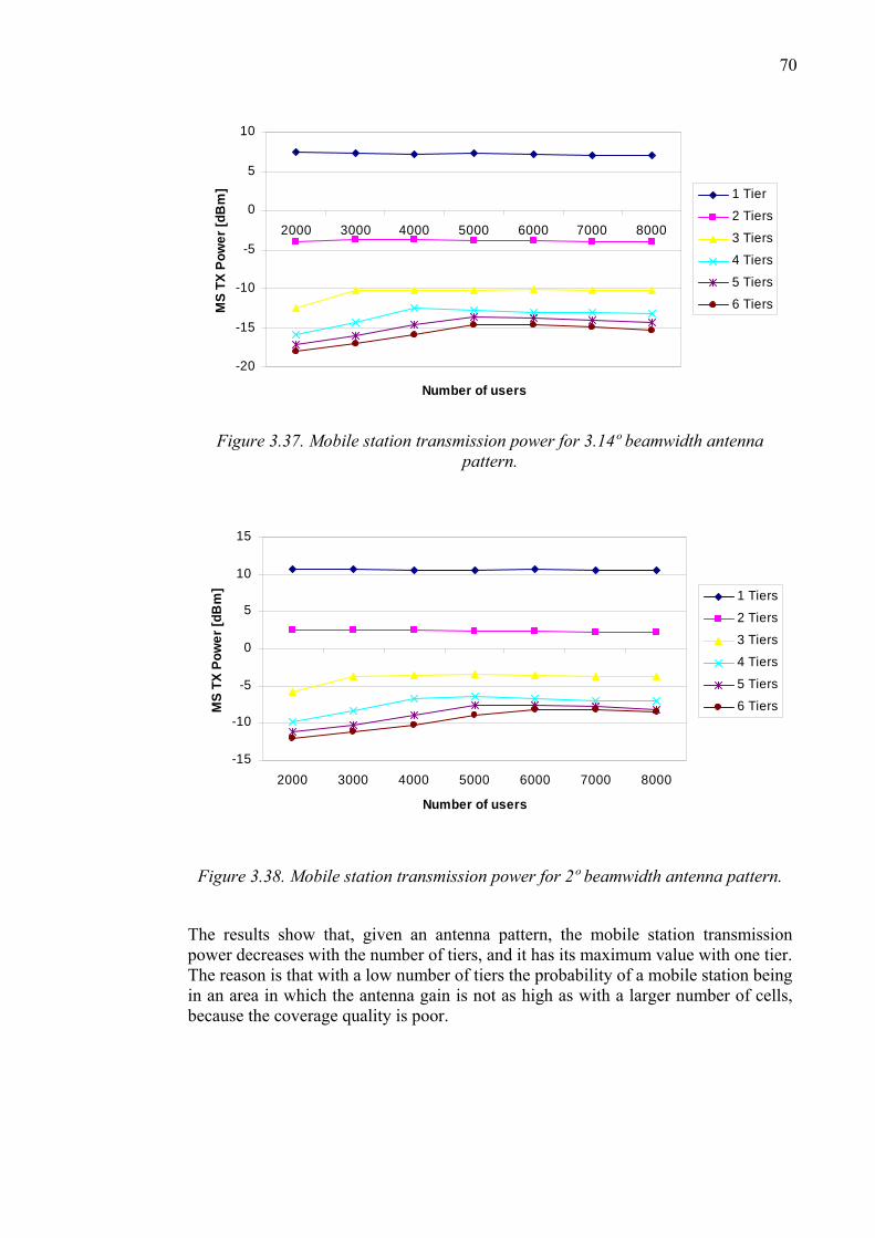
70

-20

-15

-10

-5

0

5

10

2000 3000 4000 5000 6000 7000 8000

Number of users

MS

TX P

ower

[dB

m] 1 Tier

2 Tiers

3 Tiers

4 Tiers

5 Tiers

6 Tiers

Figure 3.37. Mobile station transmission power for 3.14º beamwidth antenna

pattern.

-15

-10

-5

0

5

10

15

2000 3000 4000 5000 6000 7000 8000

Number of users

MS

TX P

ower

[dB

m] 1 Tiers

2 Tiers

3 Tiers

4 Tiers

5 Tiers

6 Tiers

Figure 3.38. Mobile station transmission power for 2º beamwidth antenna pattern.

The results show that, given an antenna pattern, the mobile station transmission power decreases with the number of tiers, and it has its maximum value with one tier. The reason is that with a low number of tiers the probability of a mobile station being in an area in which the antenna gain is not as high as with a larger number of cells, because the coverage quality is poor.

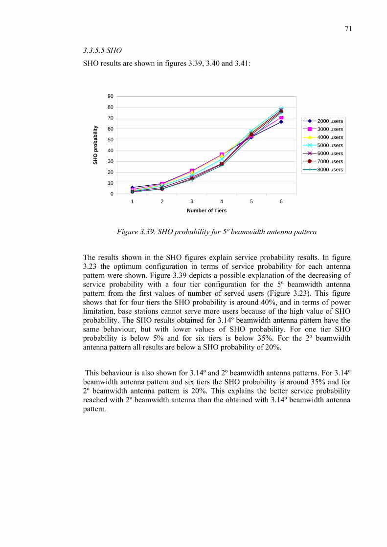
71

3.3.5.5 SHO

SHO results are shown in figures 3.39, 3.40 and 3.41:

0

10

20

30

40

50

60

70

80

90

1 2 3 4 5 6

Number of Tiers

SHO

pro

babi

lity

2000 users3000 users4000 users5000 users6000 users7000 users8000 users

Figure 3.39. SHO probability for 5º beamwidth antenna pattern

The results shown in the SHO figures explain service probability results. In figure 3.23 the optimum configuration in terms of service probability for each antenna pattern were shown. Figure 3.39 depicts a possible explanation of the decreasing of service probability with a four tier configuration for the 5º beamwidth antenna pattern from the first values of number of served users (Figure 3.23). This figure shows that for four tiers the SHO probability is around 40%, and in terms of power limitation, base stations cannot serve more users because of the high value of SHO probability. The SHO results obtained for 3.14º beamwidth antenna pattern have the same behaviour, but with lower values of SHO probability. For one tier SHO probability is below 5% and for six tiers is below 35%. For the 2º beamwidth antenna pattern all results are below a SHO probability of 20%.

This behaviour is also shown for 3.14º and 2º beamwidth antenna patterns. For 3.14º beamwidth antenna pattern and six tiers the SHO probability is around 35% and for 2º beamwidth antenna pattern is 20%. This explains the better service probability reached with 2º beamwidth antenna than the obtained with 3.14º beamwidth antenna pattern.

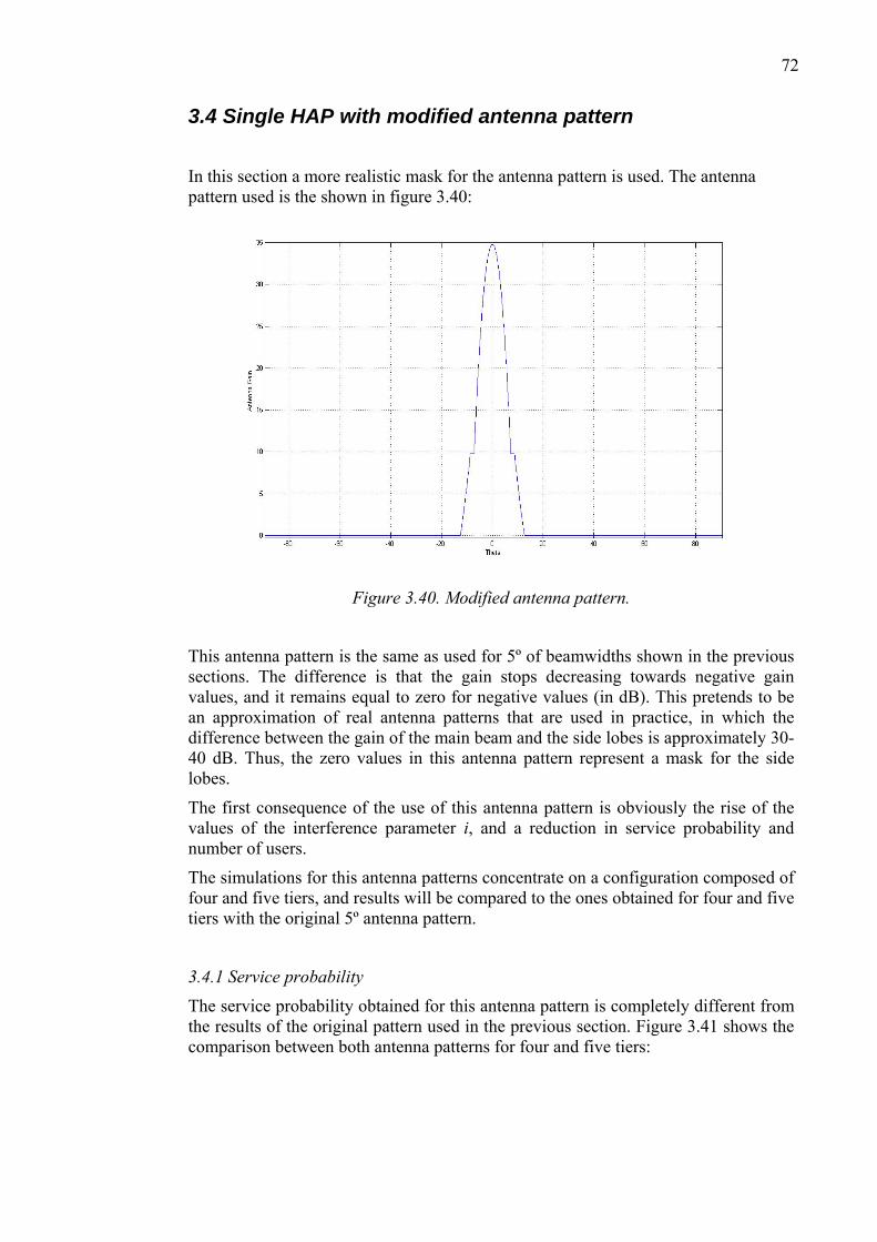
72

3.4 Single HAP with modified antenna pattern

In this section a more realistic mask for the antenna pattern is used. The antenna pattern used is the shown in figure 3.40:

Figure 3.40. Modified antenna pattern.

This antenna pattern is the same as used for 5º of beamwidths shown in the previous sections. The difference is that the gain stops decreasing towards negative gain values, and it remains equal to zero for negative values (in dB). This pretends to be an approximation of real antenna patterns that are used in practice, in which the difference between the gain of the main beam and the side lobes is approximately 30-40 dB. Thus, the zero values in this antenna pattern represent a mask for the side lobes.

The first consequence of the use of this antenna pattern is obviously the rise of the values of the interference parameter i, and a reduction in service probability and number of users.

The simulations for this antenna patterns concentrate on a configuration composed of four and five tiers, and results will be compared to the ones obtained for four and five tiers with the original 5º antenna pattern.

3.4.1 Service probability

The service probability obtained for this antenna pattern is completely different from the results of the original pattern used in the previous section. Figure 3.41 shows the comparison between both antenna patterns for four and five tiers:

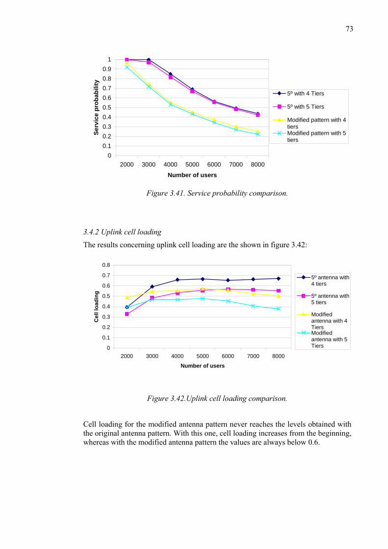
73

00.10.20.30.40.50.60.70.80.9

1

2000 3000 4000 5000 6000 7000 8000

Number of users

Serv

ice

prob

abili

ty5º with 4 Tiers

5º with 5 Tiers

Modified pattern with 4tiersModified pattern with 5tiers

Figure 3.41. Service probability comparison.

3.4.2 Uplink cell loading

The results concerning uplink cell loading are the shown in figure 3.42:

0

0.1

0.2

0.3

0.4

0.5

0.6

0.7

0.8

2000 3000 4000 5000 6000 7000 8000

Number of users

Cel

l loa

ding

5º antenna with4 tiers

5º antenna with5 tiers

Modifiedantenna with 4TiersModifiedantenna with 5Tiers

Figure 3.42.Uplink cell loading comparison.

Cell loading for the modified antenna pattern never reaches the levels obtained with the original antenna pattern. With this one, cell loading increases from the beginning, whereas with the modified antenna pattern the values are always below 0.6.

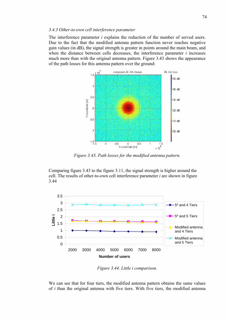
74

3.4.3 Other-to-own cell interference parameter

The interference parameter i explains the reduction of the number of served users. Due to the fact that the modified antenna pattern function never reaches negative gain values (in dB), the signal strength is greater in points around the main beam, and when the distance between cells decreases, the interference parameter i increases much more than with the original antenna pattern. Figure 3.43 shows the appearance of the path losses for this antenna pattern over the ground:

Figure 3.43. Path losses for the modified antenna pattern.

Comparing figure 3.43 to the figure 3.11, the signal strength is higher around the cell. The results of other-to-own cell interference parameter i are shown in figure 3.44

0

0.5

1

1.5

2

2.5

3

3.5

2000 3000 4000 5000 6000 7000 8000

Number of users

Littl

e i

5º and 4 Tiers

5º and 5 Tiers

Modified antennaand 4 Tiers

Modified antennaand 5 Tiers

Figure 3.44. Little i comparison.

We can see that for four tiers, the modified antenna pattern obtains the same values of i than the original antenna with five tiers. With five tiers, the modified antenna

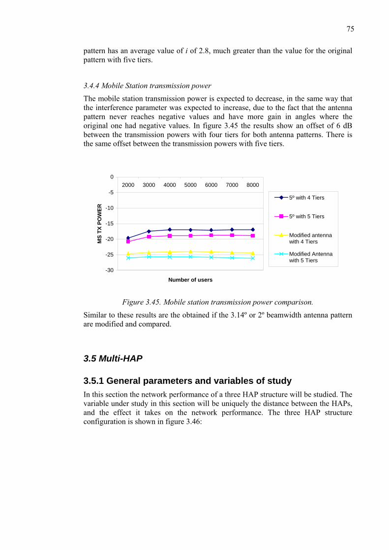
75

pattern has an average value of i of 2.8, much greater than the value for the original pattern with five tiers.

3.4.4 Mobile Station transmission power

The mobile station transmission power is expected to decrease, in the same way that the interference parameter was expected to increase, due to the fact that the antenna pattern never reaches negative values and have more gain in angles where the original one had negative values. In figure 3.45 the results show an offset of 6 dB between the transmission powers with four tiers for both antenna patterns. There is the same offset between the transmission powers with five tiers.

-30

-25

-20

-15

-10

-5

02000 3000 4000 5000 6000 7000 8000

Number of users

MS

TX P

OW

ER

5º with 4 Tiers

5º with 5 Tiers

Modified antennawith 4 Tiers

Modified Antennawith 5 Tiers

Figure 3.45. Mobile station transmission power comparison.

Similar to these results are the obtained if the 3.14º or 2º beamwidth antenna pattern are modified and compared.

3.5 Multi-HAP

3.5.1 General parameters and variables of study In this section the network performance of a three HAP structure will be studied. The variable under study in this section will be uniquely the distance between the HAPs, and the effect it takes on the network performance. The three HAP structure configuration is shown in figure 3.46:

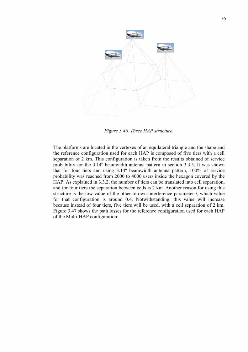
76

Figure 3.46. Three HAP structure.

The platforms are located in the vertexes of an equilateral triangle and the shape and the reference configuration used for each HAP is composed of five tiers with a cell separation of 2 km. This configuration is taken from the results obtained of service probability for the 3.14º beamwidth antenna pattern in section 3.3.5. It was shown that for four tiers and using 3.14º beamwidth antenna pattern, 100% of service probability was reached from 2000 to 4000 users inside the hexagon covered by the HAP. As explained in 3.3.2, the number of tiers can be translated into cell separation, and for four tiers the separation between cells is 2 km. Another reason for using this structure is the low value of the other-to-own interference parameter i, which value for that configuration is around 0.4. Notwithstanding, this value will increase because instead of four tiers, five tiers will be used, with a cell separation of 2 km. Figure 3.47 shows the path losses for the reference configuration used for each HAP of the Multi-HAP configuration:

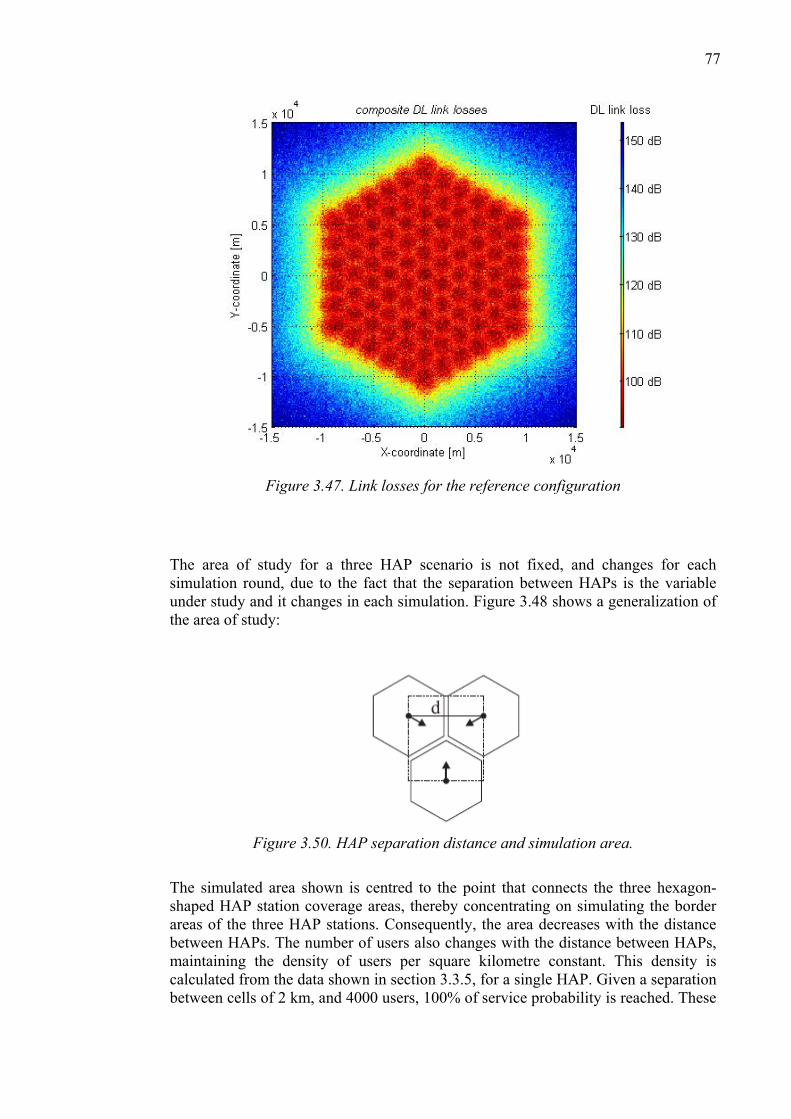
77

Figure 3.47. Link losses for the reference configuration

The area of study for a three HAP scenario is not fixed, and changes for each simulation round, due to the fact that the separation between HAPs is the variable under study and it changes in each simulation. Figure 3.48 shows a generalization of the area of study:

Figure 3.50. HAP separation distance and simulation area.

The simulated area shown is centred to the point that connects the three hexagon-shaped HAP station coverage areas, thereby concentrating on simulating the border areas of the three HAP stations. Consequently, the area decreases with the distance between HAPs. The number of users also changes with the distance between HAPs, maintaining the density of users per square kilometre constant. This density is calculated from the data shown in section 3.3.5, for a single HAP. Given a separation between cells of 2 km, and 4000 users, 100% of service probability is reached. These

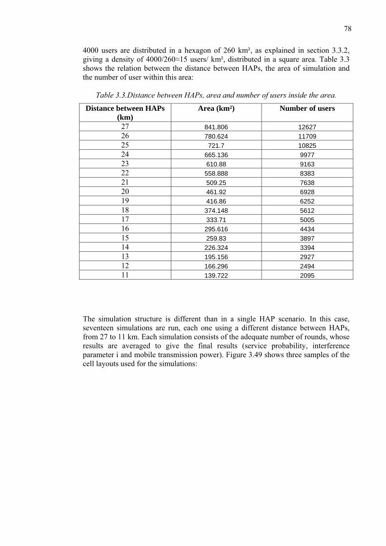
78

4000 users are distributed in a hexagon of 260 km², as explained in section 3.3.2, giving a density of 4000/260≈15 users/ km², distributed in a square area. Table 3.3 shows the relation between the distance between HAPs, the area of simulation and the number of user within this area:

Table 3.3.Distance between HAPs, area and number of users inside the area.

Distance between HAPs (km)

Area (km²) Number of users

27 841.806 12627 26 780.624 11709 25 721.7 10825 24 665.136 9977 23 610.88 9163 22 558.888 8383 21 509.25 7638 20 461.92 6928 19 416.86 6252 18 374.148 5612 17 333.71 5005 16 295.616 4434 15 259.83 3897 14 226.324 3394 13 195.156 2927 12 166.296 2494 11 139.722 2095

The simulation structure is different than in a single HAP scenario. In this case, seventeen simulations are run, each one using a different distance between HAPs, from 27 to 11 km. Each simulation consists of the adequate number of rounds, whose results are averaged to give the final results (service probability, interference parameter i and mobile transmission power). Figure 3.49 shows three samples of the cell layouts used for the simulations:

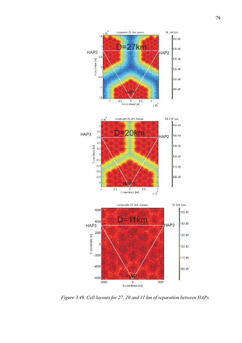
79

Figure 3.49. Cell layouts for 27, 20 and 11 km of separation between HAPs.

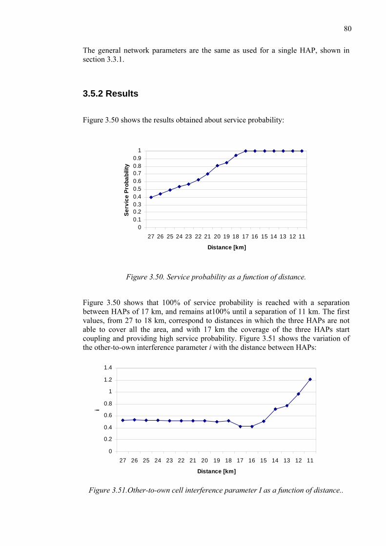
80

The general network parameters are the same as used for a single HAP, shown in section 3.3.1.

3.5.2 Results

Figure 3.50 shows the results obtained about service probability:

00.10.20.30.40.50.60.70.80.9

1

27 26 25 24 23 22 21 20 19 18 17 16 15 14 13 12 11

Distance [km]

Serv

ice

Prob

abili

ty

Figure 3.50. Service probability as a function of distance.

Figure 3.50 shows that 100% of service probability is reached with a separation between HAPs of 17 km, and remains at100% until a separation of 11 km. The first values, from 27 to 18 km, correspond to distances in which the three HAPs are not able to cover all the area, and with 17 km the coverage of the three HAPs start coupling and providing high service probability. Figure 3.51 shows the variation of the other-to-own interference parameter i with the distance between HAPs:

0

0.2

0.4

0.6

0.8

1

1.2

1.4

27 26 25 24 23 22 21 20 19 18 17 16 15 14 13 12 11

Distance [km]

i

Figure 3.51.Other-to-own cell interference parameter I as a function of distance..

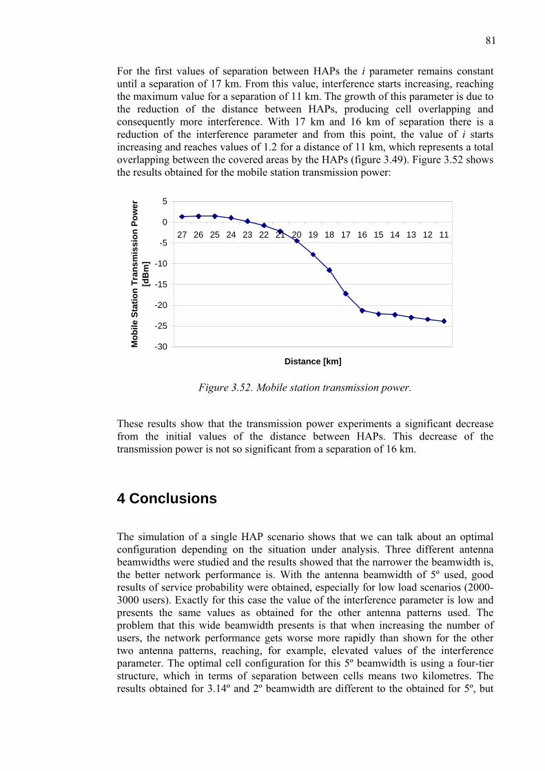
81

For the first values of separation between HAPs the i parameter remains constant until a separation of 17 km. From this value, interference starts increasing, reaching the maximum value for a separation of 11 km. The growth of this parameter is due to the reduction of the distance between HAPs, producing cell overlapping and consequently more interference. With 17 km and 16 km of separation there is a reduction of the interference parameter and from this point, the value of i starts increasing and reaches values of 1.2 for a distance of 11 km, which represents a total overlapping between the covered areas by the HAPs (figure 3.49). Figure 3.52 shows the results obtained for the mobile station transmission power:

-30

-25

-20

-15

-10

-5

0

5

27 26 25 24 23 22 21 20 19 18 17 16 15 14 13 12 11

Distance [km]

Mob

ile S

tatio

n Tr

ansm

issi

on P

ower

[d

Bm

]

Figure 3.52. Mobile station transmission power.

These results show that the transmission power experiments a significant decrease from the initial values of the distance between HAPs. This decrease of the transmission power is not so significant from a separation of 16 km.

4 Conclusions

The simulation of a single HAP scenario shows that we can talk about an optimal configuration depending on the situation under analysis. Three different antenna beamwidths were studied and the results showed that the narrower the beamwidth is, the better network performance is. With the antenna beamwidth of 5º used, good results of service probability were obtained, especially for low load scenarios (2000-3000 users). Exactly for this case the value of the interference parameter is low and presents the same values as obtained for the other antenna patterns used. The problem that this wide beamwidth presents is that when increasing the number of users, the network performance gets worse more rapidly than shown for the other two antenna patterns, reaching, for example, elevated values of the interference parameter. The optimal cell configuration for this 5º beamwidth is using a four-tier structure, which in terms of separation between cells means two kilometres. The results obtained for 3.14º and 2º beamwidth are different to the obtained for 5º, but

82

are quite similar between them. In both cases, the optimal cell configuration is reached using six tiers (or a separation between cells of 1333 meters). The results of service probability are similar, reaching 100% of service probability for low-medium load scenarios, (2000-6000 users), with just half the value of the parameter i reached for 5º beamwidth antenna. This represents an important improvement in terms of network efficiency and performance.

The use of low number of tiers causes a lack in terms of service probability basically produced by a poor coverage quality. The results shown for cell loading in a single HAP configuration confirms this conclusion. For one and two tiers the load limit was always reached, meaning an elevated own interference power. For a higher number of tiers the coverage quality is high but the overlapping between cells seems to be the limitation and the cause of the decreasing of service probability, due to the elevated percentage of SHO and i values, mostly for the 5º beamwidth antenna pattern . The configuration that minimizes SHO probability and i values is the six tiers configuration for 2º beamwidth antenna pattern. In this situation cell overlapping is not as significant as for 3.14º and 5º beamwidth antenna patterns because the cell size is smaller. Summarizing, the optimum configuration for a single HAP scenario is a separation between cells between 1600-2000 m with antenna beamwidths of 2-3º.

Results shown for the modified antenna pattern show that using the modified mask the results for service probability using three and four tiers start decreasing from the first values of service probability, in a similar way to the shown in figure 3.23 for the original 5º beamwidth antenna pattern and four tiers. The high power level of the side lobes gives a better coverage but if i values are compared, the other cell interference power is higher than the obtained for the same configuration with the original pattern and these three and four tiers configurations. Consequently the distance between cells should be lower than in the original antenna pattern. In other words, an increase in the side lobes power represents a increase in the separation between cells. With a two tiers configuration this modified antenna pattern would give better results in terms of service probability.

The configuration used for the multi HAP scenario is taken directly from the results obtained for a single HAP, commented before. In the multi HAP scenario each HAP uses a configuration of five tiers, with a separation between cells of 2 km and a 3.14º beamwidth antenna. This value of 2 km is the one used for four tiers for a single HAP scenario, reaching a high service probability with a low value of the interference parameter i.

The results obtained for a multi HAP architecture showed that for this configuration, the optimal combined service probability is reached with a separation between HAPs of 17-16 km. Note that this value strongly depends on the configuration used for each HAP, because each different configuration represents a certain hexagonal structure whose size is different for each particular case. Consequently the value of 17-16 km is the optimal separation between HAPs for a five tiers configuration with a cell separation of 2 km. A general rule for a multi HAP scenario and the separation between HAPs is that the optimum separation is the diameter of the structure used for each HAP. The reference configuration used for multi HAP simulations presented a diameter of 18 km and the results showed that the distance between HAPs which gives the optimal performance is 16- 17 km. In other words, the optimal situation is when the covered areas of the three HAPs are perfectly coupled.

83

References

[1] T.C. Tozer and D. Grace, High-altitude platforms for wireless communications, Electronics and Communication Engineering Journal, June 2001. [2] D. Grace, Overview of HeliNet: A network of stratospheric platforms for traffic monitoring environmental surveillance and broadband services. April 2000. [3] J. Thornton, D. Grace, C. Spillard, T. Konefal and T. C. Tozer, Broadband communications from a high-altitude platform: the European HeliNet programme, Electronics & Communication Engineering Journal, June 2001. [4] COST 297 website: http://www.hapcos.org. [5] S. Karapantazis, F. Pavlidou, The Role of High Altitude Platforms in beyond 3G networks, IEEE Wireless Communications, Aristotle University of Thessaloniki, December 2005. [6] Borja Artiagoitia González, HAPS Deployment for UMTS Cellular Systems. Master of Science Thesis, Tampere University of Technology. August 2006.

[7] Helinet project website: http://cntic.hit.bme.hu/project_helinet.html. [8] K. Akalestos, T.C. Tozer, David Grace, Emergency Communications from High Altitude Platforms, International Workshop on High Altitude Platform Systems, Athens, 2005. [9] T. Tozer, D. Grace, J. Thompson, P. Baynham, UAVs and HAPs, Potential Convergence for Military Communications, University of York & DERA Defford, 2000.

[10] E. Falletti, Integration of a HAP Within a Terrestrial UMTS Network: Interference Analysis and Cell Dimensioning, Wireless Pers. Commun., Kluwer, vol.24, no. 2, pp. 291–325, January 2003.

84

[11] http://www.umtsworld.com/technology/vhe.htm

[12] José María Hernando Rábanos. Comunicaciones Móviles, 2004. [13] Zs. Pándi, T.V. Do, Cs. Király, Network Planning Aspects of the Helinet Telecommunications Architecture. Proceedings of DASIA 2002, 13 - 16 May 2002, Dublin, Ireland. [14] John Thornton and David Grace, Effect of Antenna Aperture Field on Co- channel Interference,Capacity, and Payload Mass in High Altitude Platform Communications [15] Rec. ITU-R M. 1456, Minimum Performance Characteristics and Operacional Conditions for High Altitude Platform Stations Providing IMT-2000 in the Bands 1885- 1980MHz, 2010-2025MHz and 2110- 2170MHz in Region 1 and 3 and 1885-1980MHz and 2110-2160MHz in Region 2, 1999. [16] Jaroslav Holis and Pavel Pechac, Iteration based simuations of UMTS Capacity and quality of coverage in Hig Altitude Platform Basic Scenarios. [17] M.A.N Parks, B.G. Evans, G. Butt, High elevation angle propagation results applied to a statistical model and an enhanced empirical model, IEEE Electronics letters, Vol.29, No.19, pg.1723-5, September 1993. [18] John Thornton, David Grace, H. Capstick and Tim C. Tozer, Optimizing an Array of Antennas for Cellular Coverage From a High Altitude Platform. IEEE Transactions on Wireless Communications, 2 (3), pp. 484-492. 2003.

[19] Bazil Taa-Ahmed, Miguel Calvo Ramón, and Leandro de Haro-Ariet, High altitude platforms (HAPs) W-CDMA System Over Cities. Departamento de Sistemas, Señales y Radiocomunicaciones, ETSI Telecomunicación, Universidad Politécnica de Madrid. Radioengineering Magazine. (June 2004). Vol. 13. no: 2, pp. 36 – 40. [20] NPSW–Network Planning Strategies for Wideband CDMA, v.5.0.0, application note.

85

[21] Achim Wacker, Jaana Laiho, Kari Sipilä, Kari Heiska, Kai Heikkinen, Matlab Implementation of a Static Radio Network Planning Tool for Wideband CDMA, v.5.0.0, 2001. [22] Understanding UMTS Radio Network Modelling, Planning and Automated Optimisation Edited by Maciej J. Nawrocki, Mischa Dohler and A. Hamid Aghvami © 2006 John Wiley & Sons, Ltd: Chapter 6. Theoretical Models for UMTS Radio Networks. Hans-Florian Geerdes, Andreas Eisenblätter, Piotr M. Słobodzian, Mikio Iwamura, Mischa Dohler, Rafał Zdunek, Peter Gould and Maciej J. Nawrocki