Embed Size (px)
Citation preview
Atmos. Meas. Tech., 6, 837–860, 2013www.atmos-meas-tech.net/6/837/2013/doi:10.5194/amt-6-837-2013© Author(s) 2013. CC Attribution 3.0 License.
EGU Journal Logos (RGB)
Advances in Geosciences
Open A
ccess
Natural Hazards and Earth System
Sciences
Open A
ccess
Annales Geophysicae
Open A
ccess
Nonlinear Processes in Geophysics
Open A
ccess
Atmospheric Chemistry
and Physics
Open A
ccess
Atmospheric Chemistry
and Physics
Open A
ccess
Discussions
Atmospheric Measurement
TechniquesO
pen Access
Atmospheric Measurement
Techniques
Open A
ccess
Discussions
Biogeosciences
Open A
ccess
Open A
ccess
BiogeosciencesDiscussions
Climate of the Past
Open A
ccess
Open A
ccess
Climate of the Past
Discussions
Earth System Dynamics
Open A
ccess
Open A
ccess
Earth System Dynamics
Discussions
GeoscientificInstrumentation
Methods andData Systems
Open A
ccess
GeoscientificInstrumentation
Methods andData Systems
Open A
ccess
Discussions
GeoscientificModel Development
Open A
ccess
Open A
ccess
GeoscientificModel Development
Discussions
Hydrology and Earth System
Sciences
Open A
ccess
Hydrology and Earth System
Sciences
Open A
ccess
Discussions
Ocean Science
Open A
ccess
Open A
ccess
Ocean ScienceDiscussions
Solid Earth
Open A
ccess
Open A
ccess
Solid EarthDiscussions
The Cryosphere
Open A
ccess
Open A
ccess
The CryosphereDiscussions
Natural Hazards and Earth System
Sciences
Open A
ccess
Discussions
High accuracy measurements of dry molefractions of carbon dioxide and methane in humid air
C. W. Rella1, H. Chen2, A. E. Andrews2, A. Filges3, C. Gerbig3, J. Hatakka4, A. Karion 2,7, N. L. Miles5,S. J. Richardson5, M. Steinbacher6, C. Sweeney2,7, B. Wastine8, and C. Zellweger6
1Picarro, Inc., Santa Clara, CA, USA2National Oceanic and Atmospheric Administration, Earth System Research Laboratory,Global Monitoring Division, Boulder, CO, USA3Max Planck Institute for Biogeochemistry, Jena, Germany4FMI, Finnish Meteorological Institute, Helsinki, Finland5The Pennsylvania State University, Department of Meteorology, University Park, PA, USA6Empa, Swiss Federal Laboratories for Materials Testing and Research,Laboratory for Air Pollution/Environmental Technology, Duebendorf, Switzerland7CIRES, University of Colorado, Boulder, CO, USA8Laboratoire des Sciences du Climat et l’Environnement, Gif sur-Yvette, France
Correspondence to:C. W. Rella ([email protected])
Received: 31 July 2012 – Published in Atmos. Meas. Tech. Discuss.: 21 August 2012Revised: 27 February 2013 – Accepted: 27 February 2013 – Published: 27 March 2013
Abstract. Traditional techniques for measuring the molefractions of greenhouse gases in the well-mixed atmospherehave required dry sample gas streams (dew point< −25◦C)to achieve the inter-laboratory compatibility goals set forthby the Global Atmosphere Watch programme of the WorldMeteorological Organisation (WMO/GAW) for carbon diox-ide (±0.1 ppm in the Northern Hemisphere and±0.05 ppmin the Southern Hemisphere) and methane (±2 ppb). Dryingthe sample gas to low levels of water vapour can be expen-sive, time-consuming, and/or problematic, especially at re-mote sites where access is difficult. Recent advances in op-tical measurement techniques, in particular cavity ring downspectroscopy, have led to the development of greenhouse gasanalysers capable of simultaneous measurements of carbondioxide, methane and water vapour. Unlike many older tech-nologies, which can suffer from significant uncorrected in-terference from water vapour, these instruments permit ac-curate and precise greenhouse gas measurements that canmeet the WMO/GAWinter-laboratory compatibility goals(WMO, 2011a) without drying the sample gas. In this paper,we present laboratory methodology for empirically derivingthe water vapour correction factors, and we summarise a se-ries of in-situ validation experiments comparing the measure-
ments in humid gas streams to well-characterised dry-gasmeasurements. By using the manufacturer-supplied correc-tion factors, the dry-mole fraction measurements have beendemonstrated to be well within the GAW compatibility goalsup to a water vapour concentration of at least 1 %. By deter-mining the correction factors for individual instruments onceat the start of life, this water vapour concentration range canbe extended to at least 2 % over the life of the instrument,and if the correction factors are determined periodically overtime, the evidence suggests that this range can be extendedup to and even above 4 % water vapour concentrations.
1 Introduction
In recent decades, there has been growing scientific consen-sus that the increase in the concentrations (i.e., dry mole frac-tions) of several key long-lived species in the atmosphere iscontributing to an overall global warming trend via the ra-diative forcing effect (IPCC, 2007). Carbon dioxide is thelargest contributor to the total increase in radiative forcing(since pre-industrial times), accounting for 62.9 % of the to-tal radiative forcing by all long-lived greenhouse gases in
Published by Copernicus Publications on behalf of the European Geosciences Union.
838 C. W. Rella et al.: Carbon dioxide and methane in humid air
2005 (IPCC, 2007); methane is the second largest single con-tributor at 18.2 % of the 2005 total (IPCC, 2007). Together,these two greenhouse gases accounted for 81 % of the to-tal radiative forcing globally. Between 1990 and 2010, car-bon dioxide accounted for 79.5 % of the increase in radiativeforcing (WMO, 2011b), with methane contributing an addi-tional 5.0 % of the increase. Because these gases are long-lived in the atmosphere (IPCC, 2007), the effects of emis-sions on the energy balance of the atmosphere are cumula-tive over their atmospheric lifetimes. Since 1958, with theinstallation of the first continuous greenhouse gas observ-ing station on Mauna Loa, Hawaii (Keeling, 1960), scien-tific focus on quantifying carbon dioxide and methane molefractions in the well-mixed atmosphere has increased signif-icantly, with the goal of using these data for quantifying themagnitude and rate of the sources and sinks of these gases.Today, there are extensive networks of such background orregional monitoring stations, with many more being broughtonline with each passing year. These measurement networksprovide crucial validation of anthropogenic emissions as wellas constraining the role of the biosphere and the oceans inmodulating the concentrations observed in the atmosphere.The increasing spatial resolution afforded by these networksis already leading to higher resolution emission quantifica-tion, from global/continental scales (Bousquet et al., 2000;Enting et al., 1995; Fan, 1998; Gurney et al., 2002; Peterset al., 2007, 2010; Peylin et al., 2005; Schuh et al., 2010) toregional scales (Corbin et al., 2010; Lauvaux et al., 2009,2012a, b; Matross et al., 2006; Tolk et al., 2009) to evenmunicipal scales (McKain et al., 2012).
The rapid expansion of greenhouse gas monitoring net-works has driven the need for simpler and easier methodsfor making greenhouse gas measurements. Traditional meth-ods of measuring the mole fractions of greenhouse gas inthe well-mixed atmosphere have relied upon non-dispersiveinfrared (NDIR) spectroscopy for carbon dioxide and GasChromatography (GC) for methane. Typically, these mea-surements are performed on dry samples because the molefractions for carbon dioxide and methane are only meaning-ful for understanding global greenhouse gas budgets whenextrapolated back to dry-gas conditions. When water vapouris added to or removed from a sample of ambient air, viaevaporation or condensation processes, the mole fraction ofall the other gases (including carbon dioxide and methane)in the sample are also affected via dilution by water vapour.As a volatile component of the atmosphere, water vapour canvary rapidly geographically and in time, and this variabilitywill mask, via the dilution effect, the less variable concentra-tion of CO2 and CH4. Generally, it has not been possible toachieve the overall inter-laboratory compatibility goal stip-ulated by the WMO/GAW programme for CO2 (±0.1 ppm)and CH4 (±2 ppb) (WMO, 2011a) with these technologieswithout eliminating or rigorously accounting for humiditydifferences between sample and standard air. A water vapourmole-fraction of 500 ppm (dew point−32◦C at 1 bar) causes
a dilution bias of 0.2 ppm toward lower CO2 readings. Thus,in order to compute accurate mole fractions relative to drystandards, it is necessary to dry samples to very low levelsof water vapour. The dilution effect is proportional to thehumidity difference between standards and samples, ratherthan the absolute water amount, and the approach employedby Bakwin et al. (1995) is to dry the sample gas to a moremoderate level (−25◦C dew point) and humidify the stan-dard gases to the same extent by passing both the sample andstandard gases through a common Nafion membrane dryer.
Given the fact that dry-gas measurements are the ultimategoal, it would seem to be appropriate to dry the samples priorto measurement. However, installing drying systems bringsseveral disadvantages:
1. drying systems add both cost and complexity to thesampling system, increasing the number of fittings and,thus, the chances of leaks;
2. these systems often require consumables that requireperiodic replacement;
3. the drying systems often rely on hardware that can fail(e.g., heated rechargeable desiccators) or on materialswhose performance can degrade over time (e.g., Nafionmembranes);
4. many drying systems require at least some human inter-vention periodically to ensure proper operation, whichis a significant drawback at remote sites where access islimited;
5. they often increase the wetted surface area of the inletsystem, increasing the residence time;
6. methods for drying may also induce biases in the drymole fraction, by affecting (positively or negatively) themole fraction of the analyte gas in the sample streamduring the process of drying. For example, the perme-ability of Nafion to carbon dioxide has been shown todepend strongly upon the amount of humidity in the gasstream (Ma and Skou, 2007);
7. some drying methods are also sensitive to changes inambient temperature or pressure;
8. dryers can be impractical to implement robustly on air-craft, which provide critical vertical profiles of green-house gases in the troposphere;
9. finally, and perhaps most importantly, dryers preventmeasurements of ambient water vapour, unless a ded-icated water vapour sensor is installed upstream of thedryer. Water vapour provides a critical tracer for identi-fying atmospheric layers such as the boundary layer topfrom airborne measurements, or changes in air masseson stationary towers (Gupta et al., 2009), and can addi-tionally provide a valuable indicator of water condensa-tion or ingress into the inlet sampling manifold.
Atmos. Meas. Tech., 6, 837–860, 2013 www.atmos-meas-tech.net/6/837/2013/
C. W. Rella et al.: Carbon dioxide and methane in humid air 839
Clearly, it would be a significant practical advantage to beable to measure dry-gas mole fractions for carbon dioxideand methane directly in the humid gas sample, which wouldin turn simplify the rapid, reliable and cost-effective deploy-ment of large measurement networks. However, it has hith-erto been impractical to make measurements in humid gas,not only because many traditional techniques suffer fromsignificant cross-interference between water vapour, carbondioxide and methane (cross-interference is where variationsin the mole fraction of one gas affects the reported reading ofthe other gases), but also because until recently, water vapourmeasurements of sufficient stability and precision have notbeen practical in the field. With an analyser that can directlymeasure the water vapour content of the air at the same timeas carbon dioxide and methane, the dry gas mole fractionsof these two critically important greenhouse gases can be di-rectly quantified with high precision and high accuracy, evenin very humid conditions such as in tropical regions.
In recent years, advances in optical spectroscopy haveled to the development of a new class of greenhouse gasanalysers capable of simultaneous measurements of carbondioxide, methane and water vapour. These instruments havebeen shown to require infrequent calibration (less than onceper day) to meet WMO/GAW (inter-laboratory compatibil-ity) goals (Richardson et al., 2012; Andrews et al., 2013).In this paper, we will focus on analysers based upon cavityring down spectroscopy (CRDS) manufactured by Picarro,Inc. (Santa Clara, CA). In particular, we consider those in-struments which measure CO2, CH4, and H2O: the G1301,G2301, and G2401 models (note: the G2302 model usesa different spectroscopic feature to measure water vapour,and for simplicity and consistency will not be consideredhere). The G1301 model was the first commercial instru-ment of this type (Crosson, 2008). The G2301 model mea-sures the same species as the G1301 model, and the G2401model measures carbon monoxide as well as the other threeconstituents. These later instruments are based on the samecore optical spectrometer as the G1301 with essentially iden-tical performance characteristics. For the purpose of thispaper, they will be assumed to behave identically in re-gard to the dry-mole fraction correction of CO2 and CH4(to date, no operationally significant differences have beennoted). We note that any measurement system that is capa-ble of measurements of carbon dioxide, methane and wa-ter vapour, without substantial systematic bias and inter-species cross-interference, can in principle deliver GAW-quality greenhouse gas measurements in humid gas streams.
These analysers are all based upon CRDS, an optical tech-nology in which direct measurement of infrared absorptionloss in a sample cell is used to quantify the mole-fractionof the gas. Laser light is directed into an optical resonator(called the optical cavity) consisting of three highly reflec-tive mirrors, which serves as a compact flow cell with a vol-ume of less than 10 standard cm3 and an effective opticalpath length of 15–20 km. This long path length allows for
measurements with high precision (with ppb or even parts-per-trillion uncertainty, depending on the analyte gas), us-ing compact and highly reliable near-infrared laser sources.The instrument employs precise monitoring and control ofthe optical wavelength which delivers sub-picometer wave-length targeting on a microsecond timescale. The resultingspectrograms are analysed using nonlinear spectral patternrecognition routines, and the outputs of these routines areconverted into gas concentrations with a typical precision ofabout 0.05 ppm for CO2 and 0.3 ppb for CH4 in a 5 s mea-surement. The gas temperature and pressure are tightly con-trolled in these instruments (Crosson, 2008). This stabilityallows the instrument (when properly calibrated to traceablereference standards) to deliver accurate measurements thatneed very infrequent calibration relative to other CO2 andCH4 instrumentation.
In these instruments, separate and distinct spectral linesare used for each measured species. The lines have been care-fully selected to provide high precision, and little or no inter-ference from other nearby spectral lines of other atmosphericconstituents. At a given temperature and pressure (which arestabilised to within 10 mK and 0.05 Torr of the internal setpoints, respectively), and in a given gas composition, thecharacteristics of these spectral lines do not vary; the linestrength and line shape are intrinsic properties of the targetmolecule. That fact combined with the Beer-Lambert law,which dictates that the absorption per unit length at the peakof a spectral line is proportional to the number of moleculesin the gas sample, means that the response of the instrumentis linear to increases in mole fraction.
A critical requirement for stable instrument performance isthat the background (i.e., non-analyte) gas composition doesnot change. The background gas composition has a signif-icant effect upon the line shape. Different gases have dif-ferent broadening cross-sections and, therefore, broaden thespectral line to varying degrees; for example, 1 ppm of car-bon dioxide in nitrogen has a broader line with lower peakheight than 1 ppm of carbon dioxide in oxygen. For mostvariations in ambient air, these effects are negligible, becausethe mole fractions of most components of the backgroundgas matrix do not vary by a large amount in regular air sam-ples. For example, the oxygen to nitrogen ratio varies lessthan 500 per meg (parts per million of the ratio) in urban air(Keeling, 1988), and less than 250 per meg at remote loca-tions (Keeling et al., 1992). Of more significant concern arevariations in the O2/N2 ratio present in calibration and tar-get tanks. Specifically, in standards generated from syntheticair, the fraction of O2 can vary from 18 to 24 %, depend-ing on the manufacturer. Furthermore, Ar, which is presentin whole air at a level of 0.9 %, is often absent from syn-thetic air. In addition, there are certainly other applicationswhere the O2/N2 ratio can be far from the standard clean airvalues, such as when equilibrating CO2 or CH4 in seawaterwhere O2 mole fraction can vary by 20 %, resulting in signif-icant changes in the CO2 and CH4 peak heights. In Nara et
www.atmos-meas-tech.net/6/837/2013/ Atmos. Meas. Tech., 6, 837–860, 2013
840 C. W. Rella et al.: Carbon dioxide and methane in humid air
al. (2012), the effects of O2, N2, and Ar on the spectral linesused in the Picarro instrumentation have been carefully char-acterised and quantified. Provided the concentrations of thesegases are known, it is possible to correct for their effects.No correction is necessary provided that standards generatedfrom ambient air are used.
Similarly, the range of water vapour content can beextremely large in the troposphere, ranging from 100–500 ppm in arctic regions or dry alpine deserts to more than40 000 ppm (4 %) in rainforests and other warm and hu-mid environments. The variations of water vapour in the at-mosphere modify the mole fractions of CO2 and CH4 viathe dilution effect. In addition, the analyte line will expe-rience a variable amount of broadening due to variabilityof water vapour in the background gas matrix. The watercorrection methodology described below accounts for bothof these biases.
This paper is organised as follows. We begin with a shortdiscussion of the theory behind the effects of water vapouron the measurement of dry mole fractions of carbon dioxideand methane. Next, we present several alternative experimen-tal methods for determining the empirical correction factorsnecessary to calculate dry mole fractions from measurementsof the humid gas mole fractions of CO2, CH4 and H2O. Theresults of instrument-to-instrument variations in the correc-tion factors, and the drift in the correction factors over timeon a single instrument, are also presented, along with an un-certainty analysis. Next, we present the results of several in-situ side-by-side comparisons of measurements in humid gasto well-validated dry-gas measurement systems. Finally, weconclude with a summary.
2 Effects of water vapour on the measurements of car-bon dioxide and methane
For greenhouse gas measurements and inversion analysis,dry-gas mole fractions (moles analyte gas/moles air) for car-bon dioxide and methane are the relevant physical quanti-ties to report; variability in these mole fractions, due to fluc-tuations in water vapour due to evaporation and condensa-tion processes, only masks the underlying atmospheric vari-ations resulting from surface-atmosphere exchange fluxes.The diluted- and dry-gas mole fractions are related by thefollowing expression:
cdilution
cdry= 1− 0.01Hact (1)
wherec is the mole fraction of carbon dioxide or methane(the same equation holds for each), andHact is the actual wa-ter mole fraction (in %). The challenge of implementing eventhis simple equation becomes immediately apparent: the wa-ter mole fractionHact must be known to a high degree ofboth precision and accuracy, to support a high degree of ac-curacy in the measured dry gas concentrations. For example,
to maintain an uncertainty of less than 50 ppb on a 400 ppmcarbon dioxide measurement, the water vapour measurementmust be accurate and precise to within 0.0125 %, or 125 ppm.This requirement exceeds the limit of the reference methodfor hygrometry, the chilled mirror method, which typicallyguarantees an accuracy of 0.1◦C dew point, which is 34 ppmat 10◦C but 260 ppm at 30◦C.
Rather than use Eq. (1) directly, which requires an accu-rate determination ofHact (and cdilution), we instead deriveempirical forms that relate the highly precise but humidity-biased outputs (CO2)wet, (CH4)wet, and (H2O)rep to dry molefractions of CO2 and CH4. Then, by performing the appro-priate experiments (described in Sect. 3), dry-mole fractionsmay then be provided without ever needing to determinethe absolute calibration of the water vapour. This empiricalrelationship is derived below.
The quantitycdilution exhibits systematic bias due to wa-ter vapour via changes in the spectroscopic line shape. Thereare three principal mechanisms that determine the spectralline shape for isolated ro-vibrational lines, such as thoseused in the CRDS instrumentation discussed here: Dopplerbroadening, Lorentzian broadening, and Dicke line narrow-ing (Varghese and Hanson, 1984). The Doppler broadeningcoefficient is an intrinsic property of the analyte molecule,and does not depend on the constituents of the backgroundgas composition. However, the Lorentzian broadening andDicke line narrowing effects do depend both on the analytegas and on the constituents of the background gas composi-tion. Thus, as the concentration of water vapour changes, theshape of the spectral line changes. In spectroscopy, the totalarea of the spectral line is conserved throughout this process.However, the Picarro instrumentation uses peak height ratherthan area as a quantitative measure of the concentration, dueto the fact that the measurement of peak height is more pre-cise and more stable than the area measurement. As a result,the peak height of the absorption features for carbon dioxideand methane have a systematic bias with increasing watervapour due to the effect of the water vapour on both the linebroadening and line narrowing effects. A more detailed treat-ment of these line shape effects is given in Nara et al. (2012)for the broadening effects of oxygen, nitrogen and argon; acompletely analogous treatment applies to water vapour.
As a result, we find that the effect of water vapour on theanalyte peak heights can be expressed by a Taylor series ex-pansion in water vapour concentration (measured as a molefraction in %), and the effect is also proportional to the ana-lyte gas peak height. Thus, the lineshape effect on the peakheight of carbon dioxide or methane due to water vapour isproportional to the peak height itself, but it can be nonlin-ear in water vapour concentration due to higher order termsin the Taylor series. We model this effect with the followingexpression:
cwet
cdilution= 1+ xHact+ yH 2
act (2)
Atmos. Meas. Tech., 6, 837–860, 2013 www.atmos-meas-tech.net/6/837/2013/
C. W. Rella et al.: Carbon dioxide and methane in humid air 841
Here, we have kept terms to second order in the watervapour concentration.x andy are the first two terms of Tay-lor expansion, equal to the partial derivative of the ratio onthe left-hand side with respect to the water concentration.
The final step is to relate the actual water vapour concen-trationHact to the measured water vapour concentrationHrep,which is again derived from the peak height of a water vapourline. This line suffers from a similar lineshape effect that af-fects the carbon dioxide and methane lines with increasingwater vapour concentration (called self-broadening), whichleads to a nonlinearity in the measured water scale. This non-linearity is expressed in the following way (again, keepingterms to second order):
Hact = r1Hrep+ r2H2rep (3)
The valuesr1 and r2 in ambient air were determined byWinderlich et al. (2010) to be 0.772 and 0.019493, respec-tively, comparing against a calibrated hygrometer, with a rel-ative accuracy of±1.5 %. We emphasise that any uncertaintyin these values does not affect the determination of the cor-rection coefficients (as is shown below). Equation (1)–(3) canthen be combined, resulting in the following expression (aftergrouping terms and keeping all terms 2nd order and lower):
cwet
cdry= 1+ aHrep+ bH 2
rep (4)
Note thatcwet, cdry, andHrep are all values that can be deter-mined directly from a properly designed experiment (whichare discussed below), which means that the constantsa andb (which are different for CO2 and CH4) can be determinedentirely empirically, without ever measuring the intermedi-ate constantsx, y, r1, and r2. In other words, no specificknowledge of the lineshape effects on any of the species is re-quired to derive this empirical relationship. In addition, notethat high accuracy water vapour measurements are not re-quired for the correction proposed in this paper; what is re-quired is a high degree of precision and stability. As longasHrep is a well-behaved, monotonically increasing functionof the actual water vapour concentration,Hrep is a function-ally identical equivalent measure of water vapour for the pur-poses of correcting the CO2 and CH4 measurements. Whendiscussing the laboratory experiments, we will useHrep, be-cause this quantity is more physically relevant for the correc-tion, because it is derived directly from the absorbance peakas measured by the optical spectrometer. However, when pre-senting ambient air measurements, we will useHact, becausethis quantity is more physically relevant in the atmosphere.
The correction coefficients determined by Chen etal. (2010) are as follows:
CO2 : a = −1.20× 10⁻²,b = −2.67× 10⁻⁴
CH4 : a = −9.823× 10⁻³,b = −2.39× 10⁻⁴
Obviously, the precision of the dry-mole fractions of CO2and CH4 is degraded somewhat by the finite precision of thewater vapour measurement as modified by the calculationsabove (Eq. 4). The noise in the measurement of water vapouradds additional random noise to the corrected mole fractionrelative to the uncorrected mole fraction. By straightforwardpropagation of errors in Eq. (4), this noise can be shown to be
σcorr ∼
√√√√( −cwet(a + 2bHrep)
(1− aHrep− bH 2rep)
2
)2
σHrep
or about 0.017 ppm for CO2 and∼ 0.081 ppb for CH4, usingthe instrument noise specification of 0.003 % for water on the5 min measurement, and nominal values for CO2 and CH4 of400 ppm and 1800 ppb, respectively, and a water vapour levelof 3 %. This noise, added in quadrature to the instrumentnoise of 0.050 ppm and 0.22 ppb for CO2 and CH4, respec-tively, does not significantly affect the performance of theinstruments relative to the GAW targets or the uncorrectedmeasurements.
We do highlight two important assumptions inherent inthis analysis. First, we have assumed that the correction dueto water isproportional to the concentration of the analytespecies (i.e., CO2 or CH4) – that is, that there is no direct ab-sorption due to water vapour in the spectral regions of CO2and CH4 that causes a systematic bias in the fits for thosetwo gases even at zero CO2 and CH4 concentration. Second,we have assumed that there is no cross-interference from car-bon dioxide and methane to the water vapour measurement,which would cause cross-species contamination and concen-tration dependence in the correction factors. We will exam-ine these assumptions in greater detail in the laboratory re-sults section, below. Next, in the experimental section, wediscuss several experimental techniques for determining theconstantsa andb in Eq. (4).
3 Experimental techniques for determining the watervapour correction factors
Experimentally, to determine the constants in Eq. (4), onemust devise a reliable and simple methodology for generat-ing a gas sample that has constant (or varying but known)and nonzero dry mole fraction of carbon dioxide and/ormethane, but with variable humidity. There are many pos-sible and functionally equivalent solutions to this prob-lem. In this section, we describe two separate methodolo-gies that have been performed independently at MPI (MaxPlanck Institute for Biogeochemistry in Jena, Germany),NOAA/ESRL (NOAA Earth System Research Laboratory,Boulder, Colorado), LSCE (Laboratoire des Sciences du Cli-mat et l’Environnement in Gif sur-Yvette, France), Empa(Swiss Federal Laboratories for Materials Testing and Re-search, Duebendorf, Switzerland) and Picarro, Inc. (SantaClara, CA).
www.atmos-meas-tech.net/6/837/2013/ Atmos. Meas. Tech., 6, 837–860, 2013
842 C. W. Rella et al.: Carbon dioxide and methane in humid air
41
9 Figures 1
2
3
Fig. 1: Schematic for the setup of Method #1, used by MPI-Jena, NOAA, and LSCE. 4
5
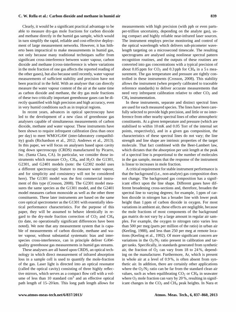
Fig. 1. Schematic for the setup of Method #1, used by MPI-Jena,NOAA, and LSCE.
3.1 Method #1 – switching between wet and dry gasstreams
3.1.1 MPI implementation
The wet and dry mole fractions of CO2 and CH4 of a hu-midified gas stream can be obtained when the gas stream isalternately provided to one or more CRDS analysers throughtwo paths, one with a chemical dryer and the other without.This method relies on the ability to generate a humidified gasstream with rather constant mole fractions of CO2, CH4 andH2O during each of multiple time steps. The wet/dry ratios ofCO2 and CH4 are then calculated for each water vapour level.This method has been described elsewhere (Chen et al., 2010;Nara et al., 2012). A detailed description of this method asimplemented at MPI is given by Chen et al. (2010) and avariant of the setup is shown in Fig. 1. To produce humidifiedgas samples with varying water vapour mole fractions, dryair from a tank (compressed ambient air) was provided to adew point generator (LI-COR model 610, Lincoln, Nebraska,USA) with varying dew point settings. Water concentrationsdelivered by this system were 0.6–6 % (for the instrument re-ported in Chen et al., 2010) and 0.6 to∼ 3 % for the other in-struments described below. A magnesium perchlorate dryerwas used to deliver the dry gas stream. The flow and pres-sure were carefully balanced between the two paths so thatthe pressure at the chemical dryer was not changing whenswitching the flow between the two instruments, which elim-inated the possible modification of CO2 mole fractions. Thewhole experiment can be performed in a temperature con-trolled room to avoid condensation of water vapour on thesurface of the inlet tubes.
The advantage of this method is that wet/dry ratios of CO2and CH4 can be accurately determined for a series of wa-ter vapour levels that may be chosen to be evenly distributedover the experimentally realized range. Cycles of, for exam-ple, 20 min (10 min wet and 10 min dry) can be used, and foreach wet air measurement, the CO2 and CH4 values of dry airmeasurements immediately before and after is interpolated inthe analysis to provide wet/dry ratios. However, only discreteexperimental points can be obtained, and no data are avail-able for water vapour levels below 0◦C dew point, due to thelimitation of the dew point generator used in the experiment.
3.1.2 LSCE implementation
The experimental setup used at LSCE is substantially simi-lar to this setup, with the exception that a single instrumentwas used, and the measurements were performed in a roomwith the standard laboratory air-conditioning set to 30◦C. Acommercial dew point generator (LI-COR 610, Lincoln, Ne-braska, USA) was used to humidify a dry working standardto 25◦C dew point, using deionized water (Milli-Q, Millli-pore, Billerica, Massachusetts, USA) that was not acidified,and a magnesium perchlorate dryer was used to generate thedry gas stream. The inlet to the instrument was alternatedbetween the humid and dry gas streams.
3.1.3 NOAA implementation
The NOAA/ESRL lab has set up a slightly different approachto get a steady-state value of water vapour by using a gas per-meable membrane device (MicroModule Contactor, Liqui-Cel Membrane Contactors, Membrana, Charlotte, NC, USA)in which slightly acidified water (pH∼ 5) resides on the shellside of the micromodule while standard air flows through thelumen side. The micromodule temperature is controlled be-tween 2 and 30◦C (by immersing it in a temperature con-trolled water bath) to obtain water vapour values rangingfrom 0.7 to 4.2 % The flow rate of the standard gas throughthe membrane is regulated by the upstream pressure from thestandard tank regulator. Overflow gas is vented so that ambi-ent pressure is maintained at the analyser inlet and in the mi-cromodule itself. This methodology can be run in the config-uration suggested in Fig. 1, but has the added advantage thatit can be used to slowly vary the water vapour concentrationover the specified range using subtle changes in water bathtemperature and standard gas flow rate. Lower water vapourconcentrations (down to fully dry) are also easily achieved byusing a simple plumbing and valve arrangement to blend drytank air with some of the wetted air from the micromodule.
3.1.4 Method #1 discussion
Because the dry mole fractions of gases are directly checkedon the same analyser, method #1 provides an accurate way ofdetermining wet/dry ratios. One advantage of this method, inaddition to its conceptual simplicity, is that the concentrationof water vapour can be set to specific values in a controlledfashion, at least within the operating range of the dew pointgenerator used for these measurements. Because measure-ments of the wet and dry samples are made simultaneously,this method also provides a robust way of ensuring that theact of humidifying the gas does not also affect the dry-molefraction of the gas. Other methods that dry a filter or mem-brane, such as method #2, below, make this assessment moredifficult. In addition to requiring a dedicated dew point gener-ator, one potential problem with this method is that the waterused to humidify the standard can have a variable amount of
Atmos. Meas. Tech., 6, 837–860, 2013 www.atmos-meas-tech.net/6/837/2013/
C. W. Rella et al.: Carbon dioxide and methane in humid air 843
42
1
Fig. 2: Schematics of the setup for Method #2 (NOAA / MPI implementation). The water 2
droplet is injected through a tee connector before the hydrophobic membrane filter. The 3
components enclosed in a dashed rectangle are optional, and are used to verify the droplet 4
method. 5
6
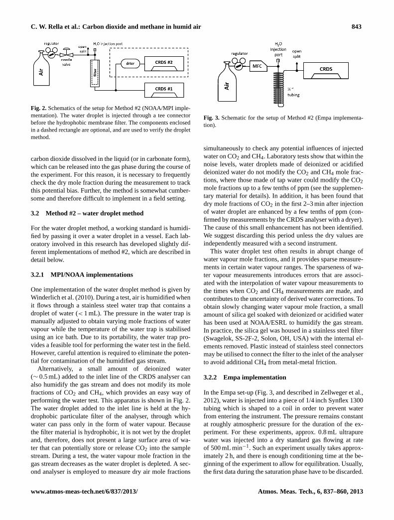
Fig. 2. Schematics of the setup for Method #2 (NOAA/MPI imple-mentation). The water droplet is injected through a tee connectorbefore the hydrophobic membrane filter. The components enclosedin a dashed rectangle are optional, and are used to verify the dropletmethod.
carbon dioxide dissolved in the liquid (or in carbonate form),which can be released into the gas phase during the course ofthe experiment. For this reason, it is necessary to frequentlycheck the dry mole fraction during the measurement to trackthis potential bias. Further, the method is somewhat cumber-some and therefore difficult to implement in a field setting.
3.2 Method #2 – water droplet method
For the water droplet method, a working standard is humidi-fied by passing it over a water droplet in a vessel. Each lab-oratory involved in this research has developed slightly dif-ferent implementations of method #2, which are described indetail below.
3.2.1 MPI/NOAA implementations
One implementation of the water droplet method is given byWinderlich et al. (2010). During a test, air is humidified whenit flows through a stainless steel water trap that contains adroplet of water (< 1 mL). The pressure in the water trap ismanually adjusted to obtain varying mole fractions of watervapour while the temperature of the water trap is stabilisedusing an ice bath. Due to its portability, the water trap pro-vides a feasible tool for performing the water test in the field.However, careful attention is required to eliminate the poten-tial for contamination of the humidified gas stream.
Alternatively, a small amount of deionized water(∼ 0.5 mL) added to the inlet line of the CRDS analyser canalso humidify the gas stream and does not modify its molefractions of CO2 and CH4, which provides an easy way ofperforming the water test. This apparatus is shown in Fig. 2.The water droplet added to the inlet line is held at the hy-drophobic particulate filter of the analyser, through whichwater can pass only in the form of water vapour. Becausethe filter material is hydrophobic, it is not wet by the dropletand, therefore, does not present a large surface area of wa-ter that can potentially store or release CO2 into the samplestream. During a test, the water vapour mole fraction in thegas stream decreases as the water droplet is depleted. A sec-ond analyser is employed to measure dry air mole fractions
43
1
Fig. 3: Schematic for the setup of Method #2 (Empa implementation) 2
3
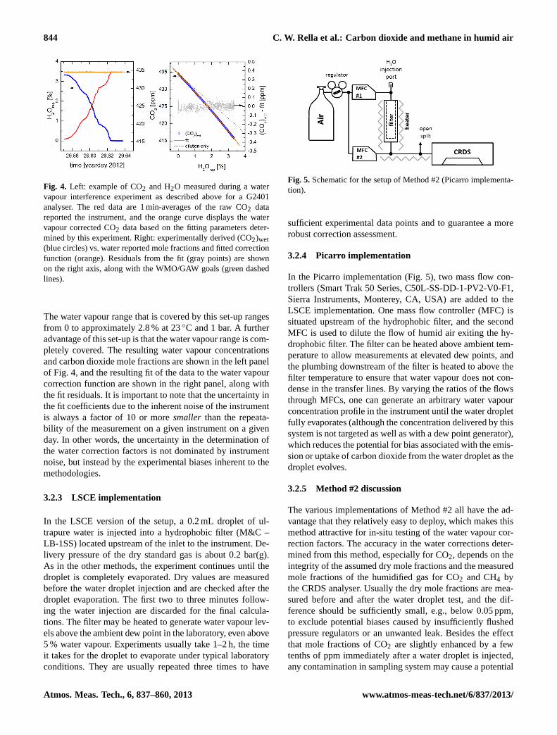
Fig. 3. Schematic for the setup of Method #2 (Empa implementa-tion).
simultaneously to check any potential influences of injectedwater on CO2 and CH4. Laboratory tests show that within thenoise levels, water droplets made of deionized or acidifieddeionized water do not modify the CO2 and CH4 mole frac-tions, where those made of tap water could modify the CO2mole fractions up to a few tenths of ppm (see the supplemen-tary material for details). In addition, it has been found thatdry mole fractions of CO2 in the first 2–3 min after injectionof water droplet are enhanced by a few tenths of ppm (con-firmed by measurements by the CRDS analyser with a dryer).The cause of this small enhancement has not been identified.We suggest discarding this period unless the dry values areindependently measured with a second instrument.
This water droplet test often results in abrupt change ofwater vapour mole fractions, and it provides sparse measure-ments in certain water vapour ranges. The sparseness of wa-ter vapour measurements introduces errors that are associ-ated with the interpolation of water vapour measurements tothe times when CO2 and CH4 measurements are made, andcontributes to the uncertainty of derived water corrections. Toobtain slowly changing water vapour mole fraction, a smallamount of silica gel soaked with deionized or acidified waterhas been used at NOAA/ESRL to humidify the gas stream.In practice, the silica gel was housed in a stainless steel filter(Swagelok, SS-2F-2, Solon, OH, USA) with the internal el-ements removed. Plastic instead of stainless steel connectorsmay be utilised to connect the filter to the inlet of the analyserto avoid additional CH4 from metal-metal friction.
3.2.2 Empa implementation
In the Empa set-up (Fig. 3, and described in Zellweger et al.,2012), water is injected into a piece of 1/4 inch Synflex 1300tubing which is shaped to a coil in order to prevent waterfrom entering the instrument. The pressure remains constantat roughly atmospheric pressure for the duration of the ex-periment. For these experiments, approx. 0.8 mL ultrapurewater was injected into a dry standard gas flowing at rateof 500 mL min−1. Such an experiment usually takes approx-imately 2 h, and there is enough conditioning time at the be-ginning of the experiment to allow for equilibration. Usually,the first data during the saturation phase have to be discarded.
www.atmos-meas-tech.net/6/837/2013/ Atmos. Meas. Tech., 6, 837–860, 2013
844 C. W. Rella et al.: Carbon dioxide and methane in humid air
44
1
Fig. 4: Left: Example of CO2 and H2O measured during a water vapor interference 2
experiment as described above for a G2401 analyzer. The red data are 1min-averages of the 3
raw CO2 data reported the instrument, and the orange curve displays the water vapor 4
corrected CO2 data based on the fitting parameters determined by this experiment. Right: 5
Experimentally derived (CO2)wet (blue circles) vs. water reported mole fractions and fitted 6
correction function (orange). Residuals from the fit (gray points) are shown on the right axis, 7
along with the WMO/GAW goals (green dashed lines). 8
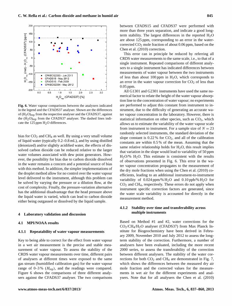
Fig. 4. Left: example of CO2 and H2O measured during a watervapour interference experiment as described above for a G2401analyser. The red data are 1 min-averages of the raw CO2 datareported the instrument, and the orange curve displays the watervapour corrected CO2 data based on the fitting parameters deter-mined by this experiment. Right: experimentally derived (CO2)wet(blue circles) vs. water reported mole fractions and fitted correctionfunction (orange). Residuals from the fit (gray points) are shownon the right axis, along with the WMO/GAW goals (green dashedlines).
The water vapour range that is covered by this set-up rangesfrom 0 to approximately 2.8 % at 23◦C and 1 bar. A furtheradvantage of this set-up is that the water vapour range is com-pletely covered. The resulting water vapour concentrationsand carbon dioxide mole fractions are shown in the left panelof Fig. 4, and the resulting fit of the data to the water vapourcorrection function are shown in the right panel, along withthe fit residuals. It is important to note that the uncertainty inthe fit coefficients due to the inherent noise of the instrumentis always a factor of 10 or moresmaller than the repeata-bility of the measurement on a given instrument on a givenday. In other words, the uncertainty in the determination ofthe water correction factors is not dominated by instrumentnoise, but instead by the experimental biases inherent to themethodologies.
3.2.3 LSCE implementation
In the LSCE version of the setup, a 0.2 mL droplet of ul-trapure water is injected into a hydrophobic filter (M&C –LB-1SS) located upstream of the inlet to the instrument. De-livery pressure of the dry standard gas is about 0.2 bar(g).As in the other methods, the experiment continues until thedroplet is completely evaporated. Dry values are measuredbefore the water droplet injection and are checked after thedroplet evaporation. The first two to three minutes follow-ing the water injection are discarded for the final calcula-tions. The filter may be heated to generate water vapour lev-els above the ambient dew point in the laboratory, even above5 % water vapour. Experiments usually take 1–2 h, the timeit takes for the droplet to evaporate under typical laboratoryconditions. They are usually repeated three times to have
45
1
Fig. 5: Schematic for the setup of Method #2 (Picarro implementation). 2
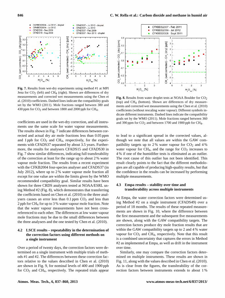
3 Fig. 5. Schematic for the setup of Method #2 (Picarro implementa-tion).
sufficient experimental data points and to guarantee a morerobust correction assessment.
3.2.4 Picarro implementation
In the Picarro implementation (Fig. 5), two mass flow con-trollers (Smart Trak 50 Series, C50L-SS-DD-1-PV2-V0-F1,Sierra Instruments, Monterey, CA, USA) are added to theLSCE implementation. One mass flow controller (MFC) issituated upstream of the hydrophobic filter, and the secondMFC is used to dilute the flow of humid air exiting the hy-drophobic filter. The filter can be heated above ambient tem-perature to allow measurements at elevated dew points, andthe plumbing downstream of the filter is heated to above thefilter temperature to ensure that water vapour does not con-dense in the transfer lines. By varying the ratios of the flowsthrough MFCs, one can generate an arbitrary water vapourconcentration profile in the instrument until the water dropletfully evaporates (although the concentration delivered by thissystem is not targeted as well as with a dew point generator),which reduces the potential for bias associated with the emis-sion or uptake of carbon dioxide from the water droplet as thedroplet evolves.
3.2.5 Method #2 discussion
The various implementations of Method #2 all have the ad-vantage that they relatively easy to deploy, which makes thismethod attractive for in-situ testing of the water vapour cor-rection factors. The accuracy in the water corrections deter-mined from this method, especially for CO2, depends on theintegrity of the assumed dry mole fractions and the measuredmole fractions of the humidified gas for CO2 and CH4 bythe CRDS analyser. Usually the dry mole fractions are mea-sured before and after the water droplet test, and the dif-ference should be sufficiently small, e.g., below 0.05 ppm,to exclude potential biases caused by insufficiently flushedpressure regulators or an unwanted leak. Besides the effectthat mole fractions of CO2 are slightly enhanced by a fewtenths of ppm immediately after a water droplet is injected,any contamination in sampling system may cause a potential
Atmos. Meas. Tech., 6, 837–860, 2013 www.atmos-meas-tech.net/6/837/2013/
C. W. Rella et al.: Carbon dioxide and methane in humid air 845
46
1
Fig. 6: Water vapor comparisons between the analyzers indicated in the legend and the 2
CFADS37 analyzer. Shown are the differences of (H2O)rep from the respective analyzer and 3
the CFADS37, against the (H2O)rep from the CFADS37 analyzer. The dashed lines indicate 4
the 125 ppm H2O differences. 5
6
Fig. 6. Water vapour comparisons between the analysers indicatedin the legend and the CFADS37 analyser. Shown are the differencesof (H2O)rep from the respective analyser and the CFADS37, againstthe (H2O)rep from the CFADS37 analyser. The dashed lines indi-cate the 125 ppm H2O differences.
bias for CO2 and CH4 as well. By using a very small volumeof liquid water (typically 0.2–0.8 mL), and by using distilled(deionized) and/or slightly acidified water, the effects of dis-solved carbon dioxide can be reduced relative to the largerwater volumes associated with dew point generators. How-ever, the possibility for bias due to carbon dioxide dissolvedin the water remains a concern and a potential source of biaswith this method. In addition, the simpler implementations ofthe droplet method allow for no control over the water vapourlevel delivered to the instrument, although this problem canbe solved by varying the pressure or a dilution flow, at thecost of complexity. Finally, the pressure-variation alternativehas the additional disadvantage that the head pressure abovethe liquid water is varied, which can lead to carbon dioxideeither being outgassed or dissolved by the liquid sample.
4 Laboratory validation and discussion
4.1 MPI/NOAA results
4.1.1 Repeatability of water vapour measurements
Key to being able to correct for the effect from water vapourin a wet air measurement is the precise and stable mea-surement of water vapour. To assess the stability of theCRDS water vapour measurements over time, different pairsof analysers at different times were exposed to the samegas stream (humidified calibration gas) for the water vapourrange of 0–3 % (Hrep), and the readings were compared.Figure 6 shows the comparisons of three different analy-sers against the CFADS37 analyser. The two comparisons
between CFADS15 and CFADS37 were performed withmore than three years separation, and indicate a good long-term stability. The largest differences in the reported H2Oare about 125 ppm, corresponding to an error in the water-corrected CO2 mole fraction of about 0.06 ppm, based on theChen et al. (2010) correction.
This error can in principle be reduced by referring allCRDS water measurements to the same scale, i.e., to that of asingle instrument. Repeated comparisons of different analy-sers to a single instrument has indicated differences betweenmeasurements of water vapour between the two instrumentsof less than about 100 ppm in H2O, which corresponds toan error in the water vapour correction for CO2 of less than0.05 ppm.
All G1301 and G2301 instruments have used the same nu-merical factor to relate the height of the water vapour absorp-tion line to the concentration of water vapour; no experimentsare performed to adjust this constant from instrument to in-strument, due to the difficulty of generating an accurate wa-ter vapour concentration in the laboratory. However, there isstatistical information on other species, such as CO2, whichallows us to estimate the variability of the water vapour scalefrom instrument to instrument. For a sample size ofN = 23randomly selected instruments, the standard deviation of theslope constant is 0.22 % for CO2, and all of the calibrationconstants are within 0.5 % of the mean. Assuming that thesame relative relationship holds for H2O, this result impliesthat variation in the slope would lead to variability of 50 ppmH2O/% H2O. This estimate is consistent with the resultsof observations presented in Fig. 6. This error in the wa-ter vapour concentration propagates to the measurement ofthe dry mole fractions when using the Chen et al. (2010) co-efficients, leading to an additional instrument-to-instrumentvariability of 0.024 ppm/% H2O and 0.10 ppb/% H2O forCO2 and CH4, respectively. These errors do not apply wheninstrument specific correction factors are generated, sincethe water scale variability is accounted for directly in themeasurement method.
4.1.2 Stability over time and transferability acrossmultiple instruments
Based on Method #1 and #2, water corrections for theCO2/CH4/H2O analyser (CFADS37) from Max Planck In-stitute for Biogeochemistry have been derived in Febru-ary 2009, November 2010 and July 2012 to assess the long-term stability of the correction. Furthermore, a number ofanalysers have been evaluated, including the more recent2000 series, to assess the transferability of the correctionbetween different analysers. The stability of the water cor-rections for both CO2 and CH4 are demonstrated in Fig. 7,which shows the differences between the measured dry airmole fraction and the corrected values for the measure-ments in wet air for the different experiments and anal-ysers. Note that for all analysers the Chen et al. (2010)
www.atmos-meas-tech.net/6/837/2013/ Atmos. Meas. Tech., 6, 837–860, 2013
846 C. W. Rella et al.: Carbon dioxide and methane in humid air
47
1
Fig. 7: Results from wet-dry experiments using method #1 at MPI Jena for CO2 (left) and CH4 2
(right). Shown are differences of dry measurements and corrected wet measurements using 3
the Chen et al. (2010) coefficients. Dashed lines indicate the compatibility goals set by the 4
WMO (2011). Mole fractions ranged between 380 ppm and 430 ppm for CO2 and between 5
1800 ppb and 2000 ppb for CH4. 6
7
Fig. 7. Results from wet-dry experiments using method #1 at MPIJena for CO2 (left) and CH4 (right). Shown are differences of drymeasurements and corrected wet measurements using the Chen etal. (2010) coefficients. Dashed lines indicate the compatibility goalsset by the WMO (2011). Mole fractions ranged between 380 and430 ppm for CO2 and between 1800 and 2000 ppb for CH4.
coefficients are used in the wet-dry correction, and all instru-ments use the same scale for water vapour measurements.The results shown in Fig. 7 indicate differences between cor-rected and actual dry air mole fractions less than 0.05 ppmand 1 ppb for CO2 and CH4, respectively, for the experi-ments with CFADS37 separated by about 3.5 years. Further-more, the results for analysers CFADS15 and CFADS30 inFig. 7 show similar differences, indicating full transferabilityof the correction at least for the range up to about 2 % watervapour mole fraction. The results from a recent experimentwith the CFKB2004 four-species analyser and CFADS37 (inJuly 2012), where up to 2 % water vapour mole fraction allexcept for one value are within the limits given by the WMOrecommended compatibility goal. Similar results have beenshown for three CRDS analysers tested at NOAA/ESRL us-ing Method #2 (Fig. 8), which demonstrates that transferringthe coefficients based on Chen et al. (2010) to the three anal-ysers causes an error less than 0.1 ppm CO2 and less than2 ppb for CH4 for up to 3 % water vapour mole fraction. Notethat the water vapour measurements have not been cross-referenced to each other. The differences at low water vapourmole fractions may be due to the small differences betweenthe three analysers and the one tested by Chen et al. (2010).
4.2 LSCE results – repeatability in the determination ofthe correction factors using different methods ona single instrument
Over a period of twenty days, the correction factors were de-termined on a single instrument with multiple trials of meth-ods #1 and #2. The differences between these correction fac-tors relative to the values described in Chen et al. (2010)are shown in Fig. 9, for nominal levels of 400 and 1900 ppbfor CO2 and CH4, respectively. The repeated trials appear
48
1
Fig. 8: Results from water droplet tests at NOAA Boulder for CO2 (top) and CH4 (bottom). 2
Shown are differences of dry measurements and corrected wet measurements using the Chen 3
et al. (2010) coefficients (without rescaling water vapor). Different symbols indicate different 4
instruments. Dashed lines indicate the compatibility goals set by the WMO (2011). Mole 5
fractions ranged between 360 ppm and 390 ppm for CO2 and between 1700 ppb and 1900 ppb 6
for CH4. 7
8
Fig. 8. Results from water droplet tests at NOAA Boulder for CO2(top) and CH4 (bottom). Shown are differences of dry measure-ments and corrected wet measurements using the Chen et al. (2010)coefficients (without rescaling water vapour). Different symbols in-dicate different instruments. Dashed lines indicate the compatibilitygoals set by the WMO (2011). Mole fractions ranged between 360and 390 ppm for CO2 and between 1700 and 1900 ppb for CH4.
to lead to a significant spread in the corrected values, al-though we note that all values are within the GAW com-patibility targets up to 2 % water vapour for CO2 and 4 %water vapour for CH4, and the range for CO2 increases to4 % if one of the humidifier tests is eliminated as an outlier.The root cause of this outlier has not been identified. Thisresult clearly points to the fact that the different methodolo-gies are all capable of producing high-quality results, but thatthe confidence in the results can be increased by performingmultiple measurements.
4.3 Empa results – stability over time andtransferability across multiple instruments
At Empa, the water correction factors were determined us-ing Method #2 on a single instrument (CFADS49) over aperiod of 18 months. The results of these repeated measure-ments are shown in Fig. 10, where the difference betweenthe first measurement and the subsequent five measurementsare shown, along with the GAW compatibility targets. Thecorrection factors produce dry mole fraction results that arewithin the GAW compatibility targets up to 2 and 4 % watervapour for CO2 and CH4, respectively. Note that this resultis a combined uncertainty that captures the errors in Method#2 as implemented at Empa, as well as drift in the instrumentover time.
Similarly, one may compare the correction factors deter-mined on multiple instruments. These results are shown inFig. 11, along with the values described in Chen et al. (2010).As is clear from the figures, the transferability of the cor-rection factors between instruments extends to about 1 %
Atmos. Meas. Tech., 6, 837–860, 2013 www.atmos-meas-tech.net/6/837/2013/
C. W. Rella et al.: Carbon dioxide and methane in humid air 847
49
1
Fig. 9: Deviations between the correction factors determined on a single instrument over 20 2
days and 5 replications at LSCE using methods #1 and #2, and the values reported in Chen et 3
al. (2010). Left panel: CO2 measured at 400 ppm. Right panel: CH4 measured at 1900 ppb. 4
The WMO/GAW targets are indicated by the green dashed lines in both panels. 5
6
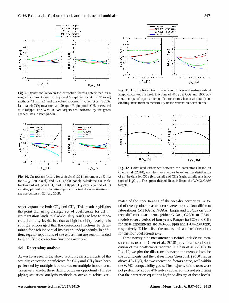
Fig. 9. Deviations between the correction factors determined on asingle instrument over 20 days and 5 replications at LSCE usingmethods #1 and #2, and the values reported in Chen et al. (2010).Left panel: CO2 measured at 400 ppm. Right panel: CH4 measuredat 1900 ppb. The WMO/GAW targets are indicated by the greendashed lines in both panels.
50
1
Fig. 10: Correction factors for a single G1301 instrument at Empa for CO2 (left panel) and 2
CH4 (right panel) calculated for mole fractions of 400 ppm CO2 and 1900 ppb CH4 over a 3
period of 18 months, plotted as a deviation against the initial determination of the correction 4
on 2009/07/22. 5
6
Fig. 10.Correction factors for a single G1301 instrument at Empafor CO2 (left panel) and CH4 (right panel) calculated for molefractions of 400 ppm CO2 and 1900 ppb CH4 over a period of 18months, plotted as a deviation against the initial determination ofthe correction on 22 July 2009.
water vapour for both CO2 and CH4. This result highlightsthe point that using a single set of coefficients for all in-strumentation leads to GAW-quality results at low to mod-erate humidity levels, but that at high humidity levels, it isstrongly encouraged that the correction functions be deter-mined for each individual instrument independently. In addi-tion, regular repetitions of the experiment are recommendedto quantify the correction functions over time.
4.4 Uncertainty analysis
As we have seen in the above sections, measurements of thewet-dry correction coefficients for CO2 and CH4 have beenperformed by multiple laboratories on multiple instruments.Taken as a whole, these data provide an opportunity for ap-plying statistical analysis methods to arrive at robust esti-
51
1
Fig. 11: Dry mole-fraction corrections for several instruments at Empa calculated for mole 2
fractions of 400 ppm CO2 and 1900 ppb CH4, compared against the coefficients from Chen et 3
al. (2010), indicating instrument transferability of the correction coefficients. 4
Fig. 11. Dry mole-fraction corrections for several instruments atEmpa calculated for mole fractions of 400 ppm CO2 and 1900 ppbCH4, compared against the coefficients from Chen et al. (2010), in-dicating instrument transferability of the correction coefficients.
52
1
Fig. 12: calculated difference between the corrections based on Chen et al. (2010), and the 2
mean values based on the distribution of all the data for CO2 (left panel) and CH4 (right 3
panel), as a function of H2Orep. The green dashed lines indicate the WMO/GAW targets. 4
5
Fig. 12. Calculated difference between the corrections based onChen et al. (2010), and the mean values based on the distributionof all the data for CO2 (left panel) and CH4 (right panel), as a func-tion of H2Orep. The green dashed lines indicate the WMO/GAWtargets.
mates of the uncertainties of the wet-dry correction. A to-tal of twenty-nine measurements were made at four differentlaboratories (MPI-Jena, NOAA, Empa and LSCE) on thir-teen different instruments (either G1301, G2301 or G2401models) over a period of four years. Ranges for CO2 and CH4for these experiments are 360–550 ppm and 1700–2300 ppb,respectively. Table 1 lists the means and standard deviationsfor the four coefficientsa–d:
These twenty nine measurements (which include the mea-surements used in Chen et al., 2010) provide a useful vali-dation of the coefficients reported in Chen et al. (2010). InFig. 12, we plot the difference between the mean values forthe coefficients and the values from Chen et al. (2010). Evenabove 4 % H2O, the two correction factors agree, well withinthe WMO compatibility goals. The majority of the tests werenot performed above 4 % water vapour, so it is not surprisingthat the correction equations begin to diverge at these levels.
www.atmos-meas-tech.net/6/837/2013/ Atmos. Meas. Tech., 6, 837–860, 2013
848 C. W. Rella et al.: Carbon dioxide and methane in humid air
53
1
Fig. 13: Distribution of empirically determined correction coefficients (red points) for CO2 2
(left panel) and CH4 (right panel) at LSCE, NOAA, MPI-Jena, and Empa. Also shown in 3
both panels are the values from Chen et al. (2010) (yellow points), and the means of each 4
distribution (blue crosses). The gray points represent the Monte Carlo simulation (N = 2000) 5
of the coefficients as modeled by a bivariate Gaussian distribution (see text for more 6
information). 7
8
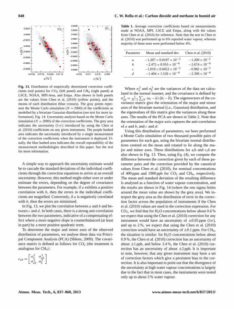
Fig. 13. Distribution of empirically determined correction coeffi-cients (red points) for CO2 (left panel) and CH4 (right panel) atLSCE, NOAA, MPI-Jena, and Empa. Also shown in both panelsare the values from Chen et al. (2010) (yellow points), and themeans of each distribution (blue crosses). The gray points repre-sent the Monte Carlo simulation (N = 2000) of the coefficients asmodelled by a bivariate Gaussian distribution (see text for more in-formation). Fig. 14: Uncertainty analysis based on the Monte Carlosimulation (N = 2000) of the correction coefficients. The grey areaindicates the uncertainty (1-σ ) introduced by using the Chen etal. (2010) coefficients on any given instrument. The purple hashedarea indicates the uncertainty introduced by a single measurementof the correction coefficients when the instrument is deployed. Fi-nally, the blue hashed area indicates the overall repeatability of themeasurement methodologies described in this paper. See the textfor more information.
A simple way to approach the uncertainty estimate wouldbe to cascade the standard deviations of the individual coeffi-cients through the correction equations to arrive at an overalluncertainty. However, this method might either over or underestimate the errors, depending on the degree of covariancebetween the parameters. For example, ifa exhibits a positivecorrelation withb, then the errors in the individual coeffi-cients are magnified. Conversely, ifa is negatively correlatedwith b, then the errors are minimised.
In Fig. 13, we plot the correlation betweena andb and be-tweenc andd. In both cases, there is a strong anti-correlationbetween the two parameters, indicative of a compensating ef-fect where a more negative slope is counterbalanced (at leastin part) by a more positive quadratic term.
To determine the major and minor axes of the observeddistribution of parameters, we analyse these data via Princi-pal Component Analysis (PCA) (Shlens, 2009). The covari-ance matrix is defined as follows for CO2 (the treatment isanalogous for CH4):
cab =
[σ 2
a
σ 2ab
σ 2ab
σ 2b
]
Table 1. Average correction coefficients based on measurementsmade at NOAA, MPI, LSCE and Empa, along with the valuesfrom Chen et al. (2010) for reference. Note that the test in Chen etal. (2010) was performed up to 6% reported water vapour, whereasmajority of these tests were performed below 4%.
Parameter Mean and standard dev. Chen et al. (2010)
a −1.207× 0.0197× 10−2−1.200× 10⁻²
b −2.475× 0.910× 10−4−2.674× 10⁻⁴
c −1.019× 0.0453× 10−2−0.982× 10⁻²
d −1.404× 1.539× 10−4−2.390× 10⁻⁴
Whereσ 2a andσ 2
b are the variances of the data set calcu-lated in the normal manner, and the covariance is defined byσ 2
ab =1
N−1
∑N (ai −a) (bi −b). The eigenvectors of the co-
variance matrix give the orientation of the major and minoraxes of the bivariate normal (i.e., Gaussian) distribution, andthe eigenvalues of this matrix give the variances along theseaxes. The results of the PCA are shown in Table 2. Note thatthe orientation of the major axis captures the anti-correlationof a andb, andc andd:
Using this distribution of parameters, we have performeda Monte Carlo simulation of two thousand possible pairs ofparameters for each gas, using the bivariate normal distribu-tions centred on the mean and rotated to lie along the ma-jor and minor axes. These distributions for a,b and c,d arealso shown in Fig. 13. Then, using Eq. (4), we compute thedifference between the correction given by each of these pa-rameter pairs and the correction provided by the canonicalvalues from Chen et al. (2010), for nominal concentrationsof 400 ppm and 1900 ppb for CO2 and CH4, respectively.The mean and standard deviation of the resulting differenceis analysed as a function of water vapour concentration, andthe results are shown in Fig. 14 (where the one sigma limitsaround the mean value are shown by the grey area). We in-terpret the grey area as the distribution of error in the correc-tion factor across the population of instruments if the Chenet al. (2010) values are used in the correction expression. ForCO2, we find that for H2O concentrations below about 0.6 %we expect that using the Chen et al. (2010) correction for anyinstrument would have an uncertainty of±0.05 ppm (1σ ),and up to 2 %, we expect that using the Chen et al. (2010)correction would have an uncertainty of±0.1 ppm. For CH4,the situation is similar: for H2O concentrations below about0.9 %, the Chen et al. (2010) correction has an uncertainty ofabout±1 ppb, and below 3.4 %, the Chen et al. (2010) cor-rection has an uncertainty of about±2 ppb. It is importantto note, however, that any given instrument may have a setof correction factors which give a persistent bias to the cor-rection. It is also important to point out that the divergence ofthe uncertainty at high water vapour concentrations is largelydue to the fact that in most cases, the instruments were testedonly up to about 3 % water vapour.
Atmos. Meas. Tech., 6, 837–860, 2013 www.atmos-meas-tech.net/6/837/2013/
C. W. Rella et al.: Carbon dioxide and methane in humid air 849
54
1
Fig. 14: Uncertainty analysis based on the Monte Carlo simulation (N = 2000) of the 2
correction coefficients. The gray area indicates the uncertainty (1-sigma) introduced by using 3
the Chen et al. (2010) coefficients on any given instrument. The purple hashed area indicates 4
the uncertainty introduced by a single measurement of the correction coefficients when the 5
instrument is deployed. Finally, the blue hashed area indicates the overall repeatability of the 6
measurement methodologies described in this paper. See the text for more information. 7
8
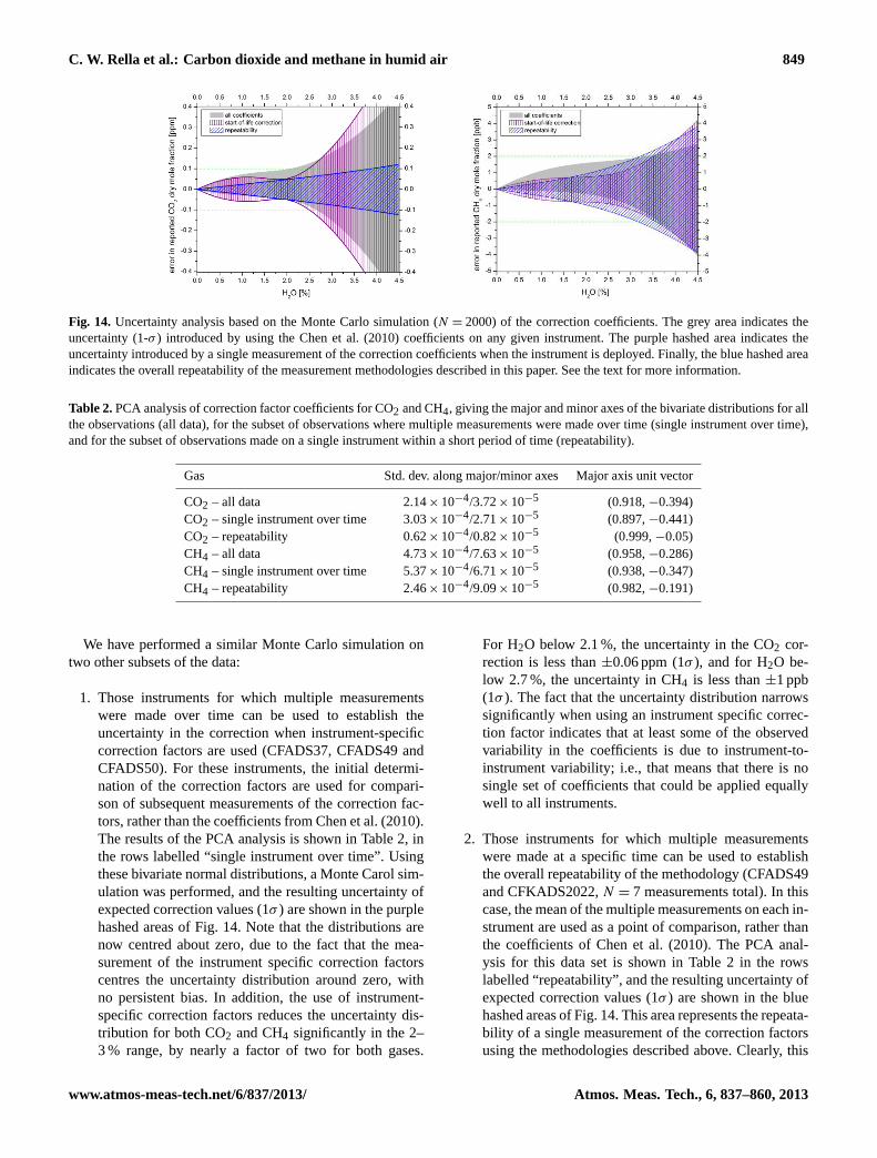
Fig. 14. Uncertainty analysis based on the Monte Carlo simulation (N = 2000) of the correction coefficients. The grey area indicates theuncertainty (1-σ ) introduced by using the Chen et al. (2010) coefficients on any given instrument. The purple hashed area indicates theuncertainty introduced by a single measurement of the correction coefficients when the instrument is deployed. Finally, the blue hashed areaindicates the overall repeatability of the measurement methodologies described in this paper. See the text for more information.
Table 2.PCA analysis of correction factor coefficients for CO2 and CH4, giving the major and minor axes of the bivariate distributions for allthe observations (all data), for the subset of observations where multiple measurements were made over time (single instrument over time),and for the subset of observations made on a single instrument within a short period of time (repeatability).
Gas Std. dev. along major/minor axes Major axis unit vector
CO2 – all data 2.14× 10⁻⁴/3.72× 10−5 (0.918,−0.394)CO2 – single instrument over time 3.03× 10⁻⁴/2.71× 10−5 (0.897,−0.441)CO2 – repeatability 0.62× 10⁻⁴/0.82× 10−5 (0.999,−0.05)CH4 – all data 4.73× 10⁻⁴/7.63× 10−5 (0.958,−0.286)CH4 – single instrument over time 5.37× 10⁻⁴/6.71× 10−5 (0.938,−0.347)CH4 – repeatability 2.46× 10⁻⁴/9.09× 10−5 (0.982,−0.191)
We have performed a similar Monte Carlo simulation ontwo other subsets of the data:
1. Those instruments for which multiple measurementswere made over time can be used to establish theuncertainty in the correction when instrument-specificcorrection factors are used (CFADS37, CFADS49 andCFADS50). For these instruments, the initial determi-nation of the correction factors are used for compari-son of subsequent measurements of the correction fac-tors, rather than the coefficients from Chen et al. (2010).The results of the PCA analysis is shown in Table 2, inthe rows labelled “single instrument over time”. Usingthese bivariate normal distributions, a Monte Carol sim-ulation was performed, and the resulting uncertainty ofexpected correction values (1σ ) are shown in the purplehashed areas of Fig. 14. Note that the distributions arenow centred about zero, due to the fact that the mea-surement of the instrument specific correction factorscentres the uncertainty distribution around zero, withno persistent bias. In addition, the use of instrument-specific correction factors reduces the uncertainty dis-tribution for both CO2 and CH4 significantly in the 2–3 % range, by nearly a factor of two for both gases.
For H2O below 2.1 %, the uncertainty in the CO2 cor-rection is less than±0.06 ppm (1σ ), and for H2O be-low 2.7 %, the uncertainty in CH4 is less than±1 ppb(1σ ). The fact that the uncertainty distribution narrowssignificantly when using an instrument specific correc-tion factor indicates that at least some of the observedvariability in the coefficients is due to instrument-to-instrument variability; i.e., that means that there is nosingle set of coefficients that could be applied equallywell to all instruments.
2. Those instruments for which multiple measurementswere made at a specific time can be used to establishthe overall repeatability of the methodology (CFADS49and CFKADS2022,N = 7 measurements total). In thiscase, the mean of the multiple measurements on each in-strument are used as a point of comparison, rather thanthe coefficients of Chen et al. (2010). The PCA anal-ysis for this data set is shown in Table 2 in the rowslabelled “repeatability”, and the resulting uncertainty ofexpected correction values (1σ ) are shown in the bluehashed areas of Fig. 14. This area represents the repeata-bility of a single measurement of the correction factorsusing the methodologies described above. Clearly, this
www.atmos-meas-tech.net/6/837/2013/ Atmos. Meas. Tech., 6, 837–860, 2013
850 C. W. Rella et al.: Carbon dioxide and methane in humid air
uncertainty represents a significant error, especially athigh water vapour concentrations, although the data setinforming this analysis was limited. This relatively largeuncertainty certainly contributes to the uncertainties ofthe corrections, and points to the need for repeated mea-surement of the correction factors at the start of life toreduce this uncertainty. We note that repeated measure-ments can be used to provide instrument-specific cor-rection factors as a function of time. This uncertaintycan be reduced from what is shown in the figures byrepeated careful measurements of the correction fac-tor over time on each instrument. Note that this uncer-tainty includes the noise and residuals of the measure-ments of the three concentrations, and any variabilityand biases associated with the methodologies used. It isexpected that repeated measurements of the correctionfactor over time will lead to reduced uncertainty in thecorrections to the H2O= 4 % level and beyond for bothanalyte gases, although the validity of this hypothesishas been yet to be demonstrated in practice. It is notclear from this uncertainty analysis whether individualinstruments exhibit significant drift relative to the startof life coefficients. Additional long-term measurementsof the correction coefficients are required to answer thisquestion fully.
4.5 Direct spectroscopic interference analysis
In the previous sections, we have implicitly assumed that thecorrection to water vapour follows the simple dependence de-scribed by Eq. (4). In this section, we discuss and quantifytwo possible effects which could bias the dry mole calcula-tion: direct spectroscopic interference between carbon diox-ide, methane and water vapour, and the effects of stable iso-topes on these measurements.
4.5.1 Direct spectroscopic interference
To derive Eq. (4), it was necessary to explicitly assume thatthe bias in the reported dry mole fractions of CO2 and CH4measurements is zero when the water vapour concentration iszero, or when the CO2 or CH4 concentrations are zero. How-ever, direct spectroscopic interference between the speciescould cause a bias in the measurements that would not fol-low this same functional form. To investigate this effect, thefollowing three sets of measurements were performed:
1. Measurements where the CO2 and CH4 were zero, butthe water vapour was varied over a wide range of values.
2. Measurements where water vapour and CH4 were zero,but CO2 was varied over a wide range of values.
3. Measurements where water vapour and CO2 were zero,but CH4 was varied over a wide range of values.
As a result of these measurements, we obtain the followingresults for the bias between different species:
(CO2)bias= 0.0339ppm/%H2O
(CH4)bias= 1.017ppb/%H2O
(H2O)bias= 9.1× 10⁻⁶%H2O/ppmCO2
−9.4× 10⁻⁶%H2O/ppmCH4
Although these measurements were performed on a singleG2401 instrument, we expect all G1301, G2301 and G2401analyser to exhibit similar behaviour. The first two biases arenot insignificant relative to the GAW targets for CO2 andCH4 dry mole fractions. However, it is important to remem-ber thatall of these biases are included in the measurement ofthe water vapour correction factors at whatever mole fractionof CO2 and CH4 is used for determining the correction fac-tors. These biases only emerge when the ambient air differsfrom the nominal test concentrations for CO2 and CH4. Thebiases are proportional to the difference between ambientand tested values, divided by the tested value, due to the factthat these offset errors are taken up by the linear coefficientsduring fitting of the data. For example, when the ambientdry mole fraction is 400 ppm and the instrument is tested at440 ppm, the CO2 error from water vapour of 0.0339 ppm/%water corresponds to a bias of (440–400)/400× 0.0339=
0.00339 ppm/% H2O. This bias is negligible. Similarly, forambient methane at 2.1 ppm measured on an instrument thatwas tested at 1.9 ppm, the bias in the corrected dry molefraction is (2.1–1.9)/1.9× 1.017= 0.11 ppb/% H2O, whichis similarly negligible. Nevertheless, to avoid any unneces-sary bias in the correction function, experiments deriving thecorrection coefficients should be performed using workingstandards with mole fraction close to ambient values. Finally,the bias term for water, for a 40 ppm change in CO2 and a0.2 ppm change in CH4, leads to a 0.00036 % bias in the wa-ter vapour concentration, which corresponds to a 0.002 ppmbias in the reported dry mole fraction of CO2, and a 0.007 ppbbias in the dry mole fraction of CH4. On the whole, these bi-ases are small and can be ignored for most monitoring situa-tions, but for best results, one may consider removing thesedependencies from the reported humid values prior to testingfor, and applying, the water vapour corrections.
4.5.2 Stable isotope effects
There is no bias in the water vapour correction factor asso-ciated with the stable isotopes of the analyte species CO2 orCH4 (although there are biases associated with the isotopiccomposition of the calibration tanks which must be consid-ered, e.g., Chen et al., 2010; Nara et al., 2012). However,the stable isotope composition of water vapour must also beconsidered. The water vapour concentration is measured us-ing the most abundant isotopologue of water. Variability inthe other, less abundant isotopologues in the ambient air (or
Atmos. Meas. Tech., 6, 837–860, 2013 www.atmos-meas-tech.net/6/837/2013/
C. W. Rella et al.: Carbon dioxide and methane in humid air 851
during testing for the water vapour coefficients) can lead toerrors in the dry-mole fraction corrections.
The four most abundant isotopologues of water are1H2
16O, 1H218O, 1H2
17O and2H1H16O. The nominal abun-dances of these species are 99.7 %, 0.21 %, 0.038 % and0.023 %, respectively, with the next most abundant isotopo-logue having a relative abundance of just 2.4× 10⁻⁷. As longas these ratios remain constant throughout the process of de-termining the correction factors and for all ambient measure-ments, then there is no effect whatsoever upon the dry molecalculation. However, in the real world, the isotope ratios ofwater vapour can vary over a wide range: the abundancesof 1H2
18O, 1H217O, and2H1H16O relative to1H2
16O canvary by up to 3 %, 1.5 % and 25 %, respectively, dependingon the conditions under which the measurements are made(Gupta et al., 2009; Galewsky et al., 2011). Larger variationscan be seen, but only in alpine or arctic environments, wherethe water vapour concentration is extremely low (less than0.2 %). The errors in the three isotopologues are almost al-ways well-correlated for naturally derived waters. We maythen estimate the error in the dry-mole fraction calculationsby taking the maximum value of each of these ranges asthe worst case scenario. The maximal error in the estimationof the total water vapour concentration of all isotopologuesfrom the single measurement of the1H2
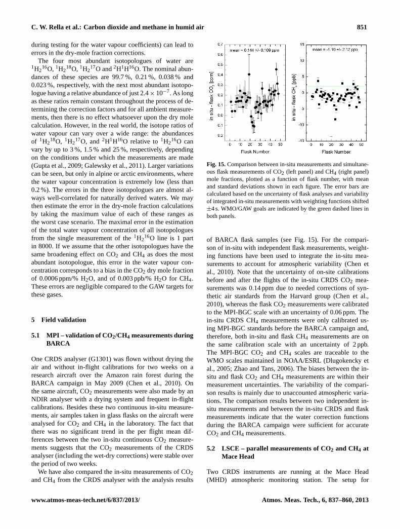
16O line is 1 partin 8000. If we assume that the other isotopologues have thesame broadening effect on CO2 and CH4 as does the mostabundant isotopologue, this error in the water vapour con-centration corresponds to a bias in the CO2 dry mole fractionof 0.0006 ppm/% H2O, and of 0.003 ppb/% H2O for CH4.These errors are negligible compared to the GAW targets forthese gases.
5 Field validation
5.1 MPI – validation of CO2/CH4 measurements duringBARCA
One CRDS analyser (G1301) was flown without drying theair and without in-flight calibrations for two weeks on aresearch aircraft over the Amazon rain forest during theBARCA campaign in May 2009 (Chen et al., 2010). Onthe same aircraft, CO2 measurements were also made by anNDIR analyser with a drying system and frequent in-flightcalibrations. Besides these two continuous in-situ measure-ments, air samples taken in glass flasks on the aircraft wereanalysed for CO2 and CH4 in the laboratory. The fact thatthere was no significant trend in the per flight mean dif-ferences between the two in-situ continuous CO2 measure-ments suggests that the CO2 measurements of the CRDSanalyser (including the wet-dry corrections) were stable overthe period of two weeks.
We have also compared the in-situ measurements of CO2and CH4 from the CRDS analyser with the analysis results
55
1
2
Fig. 15: Comparison between in-situ measurements and simultaneous flask measurements of 3
CO2 (left panel) and CH4 (right panel) mole fractions, plotted as a function of flask number, 4
with mean and standard deviations shown in each figure. The error bars are calculated based 5
on the uncertainty of flask analyses and variability of integrated in situ measurements with 6
weighting functions shifted +/-4 seconds. WMO/GAW goals are indicated by the green 7
dashed lines in both panels. 8
9
Fig. 15.Comparison between in-situ measurements and simultane-ous flask measurements of CO2 (left panel) and CH4 (right panel)mole fractions, plotted as a function of flask number, with meanand standard deviations shown in each figure. The error bars arecalculated based on the uncertainty of flask analyses and variabilityof integrated in-situ measurements with weighting functions shifted±4 s. WMO/GAW goals are indicated by the green dashed lines inboth panels.
of BARCA flask samples (see Fig. 15). For the compari-son of in-situ with independent flask measurements, weight-ing functions have been used to integrate the in-situ mea-surements to account for atmospheric variability (Chen etal., 2010). Note that the uncertainty of on-site calibrationsbefore and after the flights of the in-situ CRDS CO2 mea-surements was 0.14 ppm due to needed corrections of syn-thetic air standards from the Harvard group (Chen et al.,2010), whereas the flask CO2 measurements were calibratedto the MPI-BGC scale with an uncertainty of 0.06 ppm. Thein-situ CRDS CH4 measurements were only calibrated us-ing MPI-BGC standards before the BARCA campaign and,therefore, both in-situ and flask CH4 measurements are onthe same calibration scale with an uncertainty of 2 ppb.The MPI-BGC CO2 and CH4 scales are traceable to theWMO scales maintained in NOAA/ESRL (Dlugokencky etal., 2005; Zhao and Tans, 2006). The biases between the in-situ and flask CO2 and CH4 measurements are within theirmeasurement uncertainties. The variability of the compari-son results is mainly due to unaccounted atmospheric varia-tions. The comparison results between two independent in-situ measurements and between the in-situ CRDS and flaskmeasurements indicate that the water correction functionsduring the BARCA campaign were sufficient for accurateCO2 and CH4 measurements.
5.2 LSCE – parallel measurements of CO2 and CH4 atMace Head
Two CRDS instruments are running at the Mace Head(MHD) atmospheric monitoring station. The setup for
www.atmos-meas-tech.net/6/837/2013/ Atmos. Meas. Tech., 6, 837–860, 2013
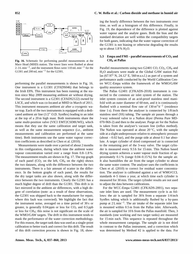
852 C. W. Rella et al.: Carbon dioxide and methane in humid air
56
1
Fig. 16: Schematic for performing parallel measurements at the Mace Head (MHD) station. 2
The tower lines were flushed at about 2-3 L / min, and the instrument flows were 110 mL/min 3
for the G1301 and 200 mL/min for the G2301. 4
5
Fig. 16. Schematic for performing parallel measurements at theMace Head (MHD) station. The tower lines were flushed at about2–3 L min−1, and the instrument flows were 110 mL min−1 for theG1301 and 200 mL min−1 for the G2301.
performing the parallel measurements is shown in Fig. 16.One instrument is a G1301 (CFADS046) that belongs tothe Irish EPA. This instrument has been running at the sta-tion since May 2009 measuring ambient air without drying.The second instrument is a G2301 (CFADS2122) owned byLSCE, and which was co-located at MHD in March of 2011.This instrument measures ambient air after a cryogenic wa-ter trap. Each of the two instruments is equipped with a dedi-cated ambient air line (1/2′′ O.D. Synflex) leading to an inletat the top of a 20 m high mast. Both instruments share thesame multi-position valve (VICI EMT2CSD8UWE), whichmeans that they use the same calibration and target tank,as well as the same measurement sequence (i.e., ambientmeasurements and calibration are performed at the sametime). Both instruments use the same water vapour correc-tion coefficients as described in Chen et al. (2010).
Measurements were made over a period of about 2 monthsin this configuration, during which time the ambient watervapour concentration varied over a range from 0.8–1.8 %.The measurement results are shown in Fig. 17. The top graphof each panel (CO2 on the left, CH4 on the right) showsthe two datasets, along with the difference between the twoinstruments. There is a fair amount of scatter in the differ-ence. In the bottom graphs of each panel, the results forthe dry target tanks are also shown, along with the differ-ence between the two instruments. Clearly the G2301 has amuch higher degree of drift than the G1301. This drift is infact mirrored in the ambient air differences, with a high de-gree of correlation (note: as a result of these observations,the G2301 was shipped back to the manufacturer for repair,where this fault was corrected). We highlight the fact thatthe instrument noise, averaged on a time period of 30 s orgreater, is generally 0.04 ppm or less for CO2 and 0.5 ppbor less for CH4; this noise is not significant on the scale ofthe WMO/GAW targets. The drift in this instrument tends tomask the performance of the water correction methodology.For this reason, the target tank data was used as a single-pointcalibration to better track and correct for this drift. The resultof this drift correction process is shown in Fig. 18, show-
ing the hourly difference between the two instruments overtime, as well as a histogram of this difference. Finally, inFig. 19, the dependence of the difference is plotted againstwater vapour and the analyte gases. Both the bias and thestandard deviation are well within the compatibility targetsfor both gases, indicating that the water vapour correction ofthe G1301 is not biasing or otherwise degrading the resultsup to about 1.8 % H2O.
5.3 Empa and FMI – parallel measurements of CO2 andCH4 at Pallas
Parallel measurements using two G2401 CO, CO2, CH4 andH2O analysers were made at the Global GAW station Pal-las (67.97◦ N, 24.12◦ E, 560 m a.s.l.) as part of a system andperformance audit conducted by the World Calibration Cen-tre WCC-Empa within the framework of the WMO/GAWquality assurance system.
The Pallas G2401 (CFKADS-2018) instrument is con-nected to the common air inlet system of the station. Theinlet system consists of an acid-proof stainless steel mani-fold with an outer diameter of 60 mm, and it is continuouslyflushed with a nominal flow rate of 130 m3 h−1 (residencetime 1 s). From there the analyser is connected by 1/8 inchstainless steel (SS) tubing. The sample air passes through a3-way solenoid valve to a Nafion dryer (Perma Pure MD-070-96S-2) and then to the analyser. Purge air for the Nafionis taken from the analyser’s vacuum line (reflux method).The Nafion was operated at about 20◦C, with the sampleside at a slight underpressure relative to atmospheric pressure(about−0.02 bar), and the purge side at about 0.1 bar abso-lute. A target cylinder of dried compressed air is connectedto the remaining port of the 3-way valve. The target cylin-der is measured every 9.5 h for 15 min. This Nafion baseddrying system achieves a water vapour mole fraction of ap-proximately 0.1 % (range 0.04–0.15 %) for the sample air.It also humidifies the air from the target cylinder to aboutthe same water content. The analyser uses the coefficients inChen et al. (2010) to correct for residual water concentra-tion. The analyser is calibrated against a set of WMO/CCLstandards 4–5 times a year, at which time each cylinder ismeasured for 30 min. The target cylinder results are not usedto adjust the data between calibrations.
For the WCC-Empa G2401 (CFKADS-2001), two sepa-rate inlet lines are used. The measurement cycle is as fol-lows: the air is sampled for 30 h from a separate 1/4 inchSynflex tubing which is additionally flushed by a by-passpump at 2 L min−1. The air intake of the separate inlet lineis mounted within 0.5 m from the Pallas inlet. Afterwards,the air is sampled for 10 h from the Pallas manifold. Then, 3standards (one working and two target tanks) are measuredfor 15 min each. This sequence is repeated throughout thewhole measurement campaign. The sample air is not driedin contrast to the Pallas instrument, and a correction whichwas determined by Method #2 is applied to the data. For
Atmos. Meas. Tech., 6, 837–860, 2013 www.atmos-meas-tech.net/6/837/2013/
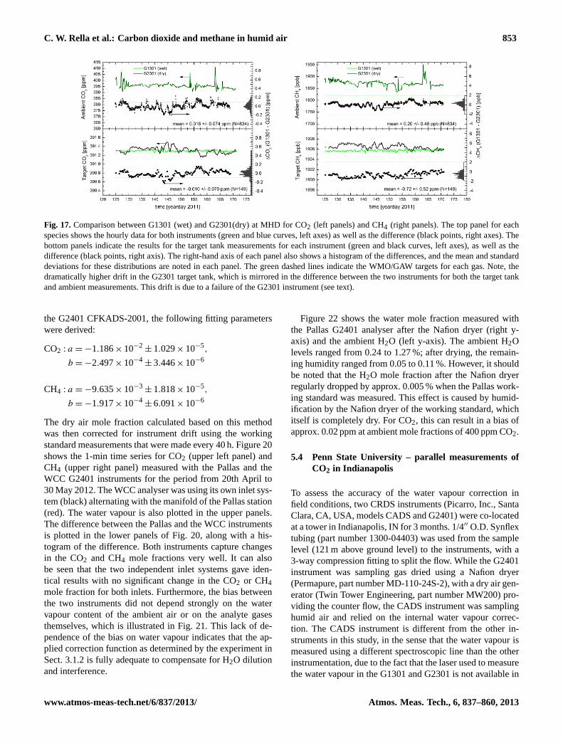
C. W. Rella et al.: Carbon dioxide and methane in humid air 853
57
1
Fig. 17: Comparison between G1301 (wet) and G2301(dry) at MHD for CO2 (left panels) and 2
CH4 (right panels). The top panel for each species shows the hourly data for both instruments 3
(green and blue curves, left axes) as well as the difference (black points, right axes). The 4
bottom panels indicate the results for the target tank measurements for each instrument (green 5
and black curves, left axes), as well as the difference (black points, right axis). The right hand 6
axis of each panel also shows a histogram of the differences, and the mean and standard 7
deviations for these distributions are noted in each panel. The green dashed lines indicate the 8
WMO/GAW targets for each gas. Note the dramatically higher drift in the G2301 target tank, 9
which is mirrored in the difference between the two instruments for both the target tank and 10
ambient measurements. This drift is due to a failure of the G2301 instrument (see text). 11
Fig. 17.Comparison between G1301 (wet) and G2301(dry) at MHD for CO2 (left panels) and CH4 (right panels). The top panel for eachspecies shows the hourly data for both instruments (green and blue curves, left axes) as well as the difference (black points, right axes). Thebottom panels indicate the results for the target tank measurements for each instrument (green and black curves, left axes), as well as thedifference (black points, right axis). The right-hand axis of each panel also shows a histogram of the differences, and the mean and standarddeviations for these distributions are noted in each panel. The green dashed lines indicate the WMO/GAW targets for each gas. Note, thedramatically higher drift in the G2301 target tank, which is mirrored in the difference between the two instruments for both the target tankand ambient measurements. This drift is due to a failure of the G2301 instrument (see text).
the G2401 CFKADS-2001, the following fitting parameterswere derived:
CO2 : a = −1.186× 10⁻²± 1.029× 10⁻⁵,
b = −2.497× 10⁻⁴± 3.446× 10⁻⁶
CH4 : a = −9.635× 10⁻³± 1.818× 10⁻⁵,
b = −1.917× 10⁻⁴± 6.091× 10⁻⁶
The dry air mole fraction calculated based on this methodwas then corrected for instrument drift using the workingstandard measurements that were made every 40 h. Figure 20shows the 1-min time series for CO2 (upper left panel) andCH4 (upper right panel) measured with the Pallas and theWCC G2401 instruments for the period from 20th April to30 May 2012. The WCC analyser was using its own inlet sys-tem (black) alternating with the manifold of the Pallas station(red). The water vapour is also plotted in the upper panels.The difference between the Pallas and the WCC instrumentsis plotted in the lower panels of Fig. 20, along with a his-togram of the difference. Both instruments capture changesin the CO2 and CH4 mole fractions very well. It can alsobe seen that the two independent inlet systems gave iden-tical results with no significant change in the CO2 or CH4mole fraction for both inlets. Furthermore, the bias betweenthe two instruments did not depend strongly on the watervapour content of the ambient air or on the analyte gasesthemselves, which is illustrated in Fig. 21. This lack of de-pendence of the bias on water vapour indicates that the ap-plied correction function as determined by the experiment inSect. 3.1.2 is fully adequate to compensate for H2O dilutionand interference.
Figure 22 shows the water mole fraction measured withthe Pallas G2401 analyser after the Nafion dryer (right y-axis) and the ambient H2O (left y-axis). The ambient H2Olevels ranged from 0.24 to 1.27 %; after drying, the remain-ing humidity ranged from 0.05 to 0.11 %. However, it shouldbe noted that the H2O mole fraction after the Nafion dryerregularly dropped by approx. 0.005 % when the Pallas work-ing standard was measured. This effect is caused by humid-ification by the Nafion dryer of the working standard, whichitself is completely dry. For CO2, this can result in a bias ofapprox. 0.02 ppm at ambient mole fractions of 400 ppm CO2.
5.4 Penn State University – parallel measurements ofCO2 in Indianapolis
To assess the accuracy of the water vapour correction infield conditions, two CRDS instruments (Picarro, Inc., SantaClara, CA, USA, models CADS and G2401) were co-locatedat a tower in Indianapolis, IN for 3 months. 1/4′′ O.D. Synflextubing (part number 1300-04403) was used from the samplelevel (121 m above ground level) to the instruments, with a3-way compression fitting to split the flow. While the G2401instrument was sampling gas dried using a Nafion dryer(Permapure, part number MD-110-24S-2), with a dry air gen-erator (Twin Tower Engineering, part number MW200) pro-viding the counter flow, the CADS instrument was samplinghumid air and relied on the internal water vapour correc-tion. The CADS instrument is different from the other in-struments in this study, in the sense that the water vapour ismeasured using a different spectroscopic line than the otherinstrumentation, due to the fact that the laser used to measurethe water vapour in the G1301 and G2301 is not available in
www.atmos-meas-tech.net/6/837/2013/ Atmos. Meas. Tech., 6, 837–860, 2013
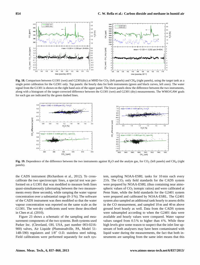
854 C. W. Rella et al.: Carbon dioxide and methane in humid air
58
1
Fig. 18: Comparison between G1301 (wet) and G2301(dry) at MHD for CO2 (left panels) and 2
CH4 (right panels), using the target tank as a single point calibration for the G2301 only. Top 3
panels: the hourly data for both instruments (green and black curves, left axes). The water 4
signal from the G1301 is shown on the right hand axis of the upper panel. The lower panels 5
show the difference between the two instruments, along with a histogram of the target-6
corrected difference between the G1301 (wet) and G2301 (dry) measurements. The 7
WMO/GAW goals for each gas are indicated by the green dashed lines. 8
9
Fig. 18.Comparison between G1301 (wet) and G2301(dry) at MHD for CO2 (left panels) and CH4 (right panels), using the target tank as asingle point calibration for the G2301 only. Top panels: the hourly data for both instruments (green and black curves, left axes). The watersignal from the G1301 is shown on the right hand axis of the upper panel. The lower panels show the difference between the two instruments,along with a histogram of the target-corrected difference between the G1301 (wet) and G2301 (dry) measurements. The WMO/GAW goalsfor each gas are indicated by the green dashed lines.
59
1
Fig. 19: Dependence of the difference between the two instruments against H2O and the 2
analyte gas, for CO2 (left panels) and CH4 (right panels). 3
Fig. 19.Dependence of the difference between the two instruments against H2O and the analyte gas, for CO2 (left panels) and CH4 (rightpanels).
the CADS instrument (Richardson et al., 2012). To cross-calibrate the two spectroscopic lines, a special test was per-formed on a G1301 that was modified to measure both linesquasi-simultaneously (alternating between the two measure-ments every three seconds), while ramping the water vapourconcentration over a substantial range (0–3 %). The softwareof the CADS instrument was then modified so that the watervapour concentration was reported on the same scale as theG1301. The wet-dry coefficients used were those describedin Chen et al. (2010).
Figure 23 shows a schematic of the sampling and mea-surement components of the two systems. Both systems usedParker Inc. (Cleveland, OH, USA, part number 003-0216-900) valves, Air Liquide (Plumsteadville, PA, Model 51-14B-590) regulators and 1/8′′ O.D. stainless steel tubing.Field calibrations were performed separately for each sys-
tem, sampling NOAA-ESRL tanks for 10 min each every23 h. The CO2 only field standards for the CADS systemwere prepared by NOAA-ESRL (thus containing near atmo-spheric values of CO2 isotopic ratios) and were calibrated atPenn State, while the field standards for the G2401 systemwere prepared and calibrated by NOAA-ESRL. The G2401system also sampled an additional tank hourly to assess driftsin the CO measurement, and sampled 10 m and 40 m aboveground level hourly as well. Data from the CADS systemwere subsampled according to when the G2401 data wereavailable and hourly values were compared. Water vapourvalues ranged from 0.5 % to higher than 4 %. While thesehigh levels give some reason to suspect that the inlet line up-stream of both analysers may have been contaminated withliquid water during the measurements, the fact that both in-struments are sampling from the same inlet means that this
Atmos. Meas. Tech., 6, 837–860, 2013 www.atmos-meas-tech.net/6/837/2013/
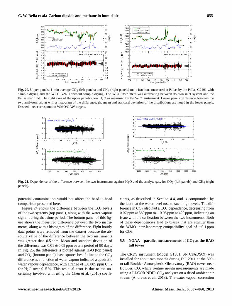
C. W. Rella et al.: Carbon dioxide and methane in humid air 855
60
1
2
Fig. 20: Upper panels: 1-min average CO2 (left panels) and CH4 (right panels) mole fractions 3
measured at Pallas by the Pallas G2401 with sample drying and the WCC G2401 without 4
sample drying. The WCC instrument was alternating between its own inlet system and the 5
Pallas manifold. The right axes of the upper panels show H2O as measured by the WCC 6
instrument. Lower panels: difference between the two analyzers, along with a histogram of 7
the difference; the mean and standard deviation of the distributions are noted in the lower 8
panels. Dashed lines correspond to WMO/GAW targets. 9
10
Fig. 20.Upper panels: 1-min average CO2 (left panels) and CH4 (right panels) mole fractions measured at Pallas by the Pallas G2401 withsample drying and the WCC G2401 without sample drying. The WCC instrument was alternating between its own inlet system and thePallas manifold. The right axes of the upper panels show H2O as measured by the WCC instrument. Lower panels: difference between thetwo analysers, along with a histogram of the difference; the mean and standard deviation of the distributions are noted in the lower panels.Dashed lines correspond to WMO/GAW targets.
61
1
2
Fig. 21: Dependence of the difference between the two instruments against H2O and the 3
analyte gas, for CO2 (left panels) and CH4 (right panels). 4
Fig. 21.Dependence of the difference between the two instruments against H2O and the analyte gas, for CO2 (left panels) and CH4 (rightpanels).
potential contamination would not affect the head-to-headcomparison presented here.
Figure 24 shows the difference between the CO2 levelsof the two systems (top panel), along with the water vapoursignal during that time period. The bottom panel of this fig-ure shows the measured difference between the two instru-ments, along with a histogram of the difference. Eight hourlydata points were removed from the dataset because the ab-solute value of the difference between the two instrumentswas greater than 0.5 ppm. Mean and standard deviation ofthe difference was 0.01± 0.09 ppm over a period of 90 days.In Fig. 25, the difference is plotted against H2O (top panel)and CO2 (bottom panel) least squares best fit line to the CO2difference as a function of water vapour indicated a quadraticwater vapour dependence, with a range of±0.085 ppm CO2for H2O over 0–5 %. This residual error is due to the un-certainty involved with using the Chen et al. (2010) coeffi-
cients, as described in Section 4.4, and is compounded bythe fact that the water level rose to such high levels. The dif-ference in CO2 also had a CO2 dependence, decreasing from0.07 ppm at 360 ppm to−0.05 ppm at 420 ppm, indicating anissue with the calibration between the two instruments. Bothof these dependencies lead to biases that are smaller thanthe WMO inter-laboratory compatibility goal of±0.1 ppmfor CO2.
5.5 NOAA – parallel measurements of CO2 at the BAOtall tower
The CRDS instrument (Model G1301, SN CFADS09) wasinstalled for about two months during Fall 2011 at the 300-m tall Boulder Atmospheric Observatory (BAO) tower nearBoulder, CO, where routine in-situ measurements are madeusing a LI-COR NDIR CO2 analyser on a dried ambient airstream (Andrews et al., 2013). The water vapour correction
www.atmos-meas-tech.net/6/837/2013/ Atmos. Meas. Tech., 6, 837–860, 2013
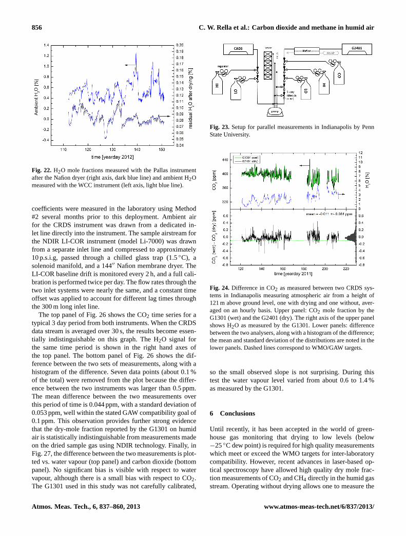
856 C. W. Rella et al.: Carbon dioxide and methane in humid air
62
1
Fig. 22: H2O mole fractions measured with the Pallas instrument after the Nafion dryer (right 2
axis, dark blue line) and ambient H2O measured with the WCC instrument (left axis, light 3
blue line). 4
Fig. 22. H2O mole fractions measured with the Pallas instrumentafter the Nafion dryer (right axis, dark blue line) and ambient H2Omeasured with the WCC instrument (left axis, light blue line).
coefficients were measured in the laboratory using Method#2 several months prior to this deployment. Ambient airfor the CRDS instrument was drawn from a dedicated in-let line directly into the instrument. The sample airstream forthe NDIR LI-COR instrument (model Li-7000) was drawnfrom a separate inlet line and compressed to approximately10 p.s.i.g, passed through a chilled glass trap (1.5◦C), asolenoid manifold, and a 144′′ Nafion membrane dryer. TheLI-COR baseline drift is monitored every 2 h, and a full cali-bration is performed twice per day. The flow rates through thetwo inlet systems were nearly the same, and a constant timeoffset was applied to account for different lag times throughthe 300 m long inlet line.
The top panel of Fig. 26 shows the CO2 time series for atypical 3 day period from both instruments. When the CRDSdata stream is averaged over 30 s, the results become essen-tially indistinguishable on this graph. The H2O signal forthe same time period is shown in the right hand axes ofthe top panel. The bottom panel of Fig. 26 shows the dif-ference between the two sets of measurements, along with ahistogram of the difference. Seven data points (about 0.1 %of the total) were removed from the plot because the differ-ence between the two instruments was larger than 0.5 ppm.The mean difference between the two measurements overthis period of time is 0.044 ppm, with a standard deviation of0.053 ppm, well within the stated GAW compatibility goal of0.1 ppm. This observation provides further strong evidencethat the dry-mole fraction reported by the G1301 on humidair is statistically indistinguishable from measurements madeon the dried sample gas using NDIR technology. Finally, inFig. 27, the difference between the two measurements is plot-ted vs. water vapour (top panel) and carbon dioxide (bottompanel). No significant bias is visible with respect to watervapour, although there is a small bias with respect to CO2.The G1301 used in this study was not carefully calibrated,
63
1
Fig. 23: Setup for parallel measurements in Indianapolis by Penn State University. 2
3 Fig. 23. Setup for parallel measurements in Indianapolis by PennState University.
64
1
Fig. 24: Difference in CO2 as measured between two CRDS systems in Indianapolis 2
measuring atmospheric air from a height of 121 m above ground level, one with drying and 3
one without, averaged on an hourly basis. Upper panel: CO2 mole fraction by the G1301 4
(wet) and the G2401 (dry). The right axis of the upper panel shows H2O as measured by the 5
G1301. Lower panels: difference between the two analyzers, along with a histogram of the 6
difference; the mean and standard deviation of the distributions are noted in the lower panels. 7
Dashed lines correspond to WMO/GAW targets. 8
9
Fig. 24. Difference in CO2 as measured between two CRDS sys-tems in Indianapolis measuring atmospheric air from a height of121 m above ground level, one with drying and one without, aver-aged on an hourly basis. Upper panel: CO2 mole fraction by theG1301 (wet) and the G2401 (dry). The right axis of the upper panelshows H2O as measured by the G1301. Lower panels: differencebetween the two analysers, along with a histogram of the difference;the mean and standard deviation of the distributions are noted in thelower panels. Dashed lines correspond to WMO/GAW targets.
so the small observed slope is not surprising. During thistest the water vapour level varied from about 0.6 to 1.4 %as measured by the G1301.
6 Conclusions
Until recently, it has been accepted in the world of green-house gas monitoring that drying to low levels (below−25◦C dew point) is required for high quality measurementswhich meet or exceed the WMO targets for inter-laboratorycompatibility. However, recent advances in laser-based op-tical spectroscopy have allowed high quality dry mole frac-tion measurements of CO2 and CH4 directly in the humid gasstream. Operating without drying allows one to measure the
Atmos. Meas. Tech., 6, 837–860, 2013 www.atmos-meas-tech.net/6/837/2013/
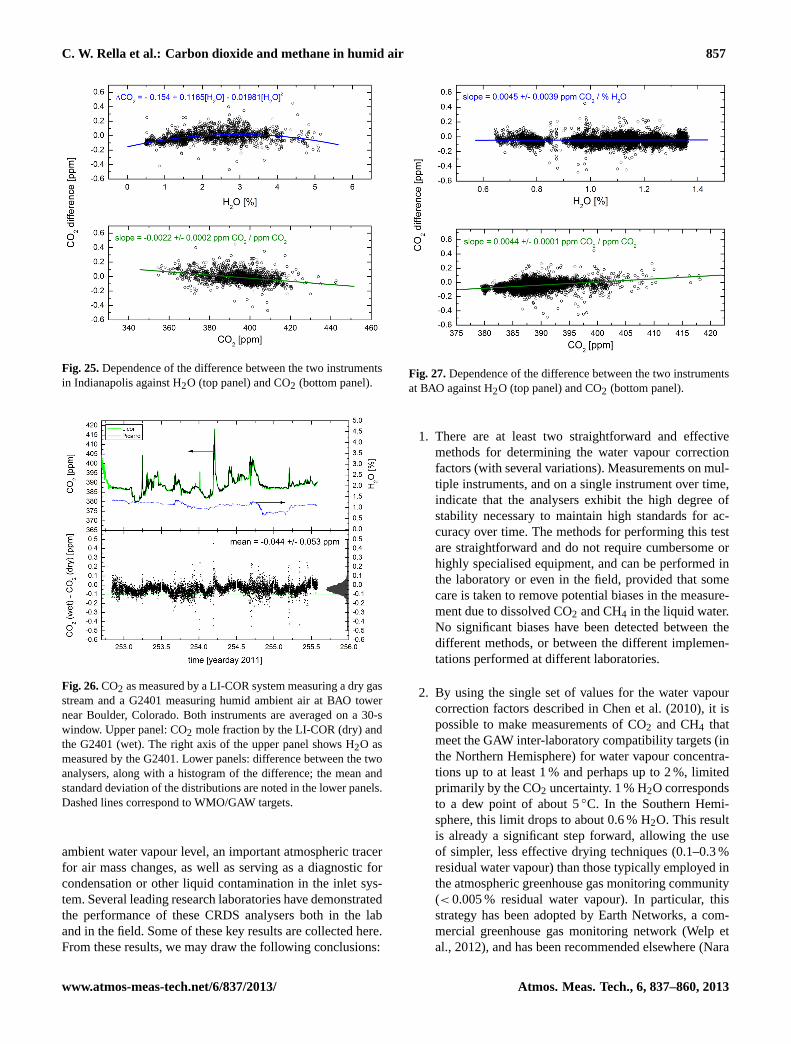
C. W. Rella et al.: Carbon dioxide and methane in humid air 857
65
1
2 Fig. 25: Dependence of the difference between the two instruments in Indianapolis against 3
H2O (top panel) and CO2 (bottom panel). 4
Fig. 25.Dependence of the difference between the two instrumentsin Indianapolis against H2O (top panel) and CO2 (bottom panel).
66
1
Fig. 26: CO2 as measured by a LI-COR system measuring a dry gas stream and a G2401 2
measuring humid ambient air at BAO tower near Boulder, Colorado. Both instruments are 3
averaged on a 30-second window. Upper panel: CO2 mole fraction by the LI-COR (dry) and 4
the G2401 (wet). The right axis of the upper panel shows H2O as measured by the G2401. 5
Lower panels: difference between the two analyzers, along with a histogram of the difference; 6
the mean and standard deviation of the distributions are noted in the lower panels. Dashed 7
lines correspond to WMO/GAW targets. 8
9
Fig. 26.CO2 as measured by a LI-COR system measuring a dry gasstream and a G2401 measuring humid ambient air at BAO towernear Boulder, Colorado. Both instruments are averaged on a 30-swindow. Upper panel: CO2 mole fraction by the LI-COR (dry) andthe G2401 (wet). The right axis of the upper panel shows H2O asmeasured by the G2401. Lower panels: difference between the twoanalysers, along with a histogram of the difference; the mean andstandard deviation of the distributions are noted in the lower panels.Dashed lines correspond to WMO/GAW targets.
ambient water vapour level, an important atmospheric tracerfor air mass changes, as well as serving as a diagnostic forcondensation or other liquid contamination in the inlet sys-tem. Several leading research laboratories have demonstratedthe performance of these CRDS analysers both in the laband in the field. Some of these key results are collected here.From these results, we may draw the following conclusions:
67
1
Fig. 27: Dependence of the difference between the two instruments at BAO against H2O (top 2
panel) and CO2 (bottom panel). 3
Fig. 27.Dependence of the difference between the two instrumentsat BAO against H2O (top panel) and CO2 (bottom panel).
1. There are at least two straightforward and effectivemethods for determining the water vapour correctionfactors (with several variations). Measurements on mul-tiple instruments, and on a single instrument over time,indicate that the analysers exhibit the high degree ofstability necessary to maintain high standards for ac-curacy over time. The methods for performing this testare straightforward and do not require cumbersome orhighly specialised equipment, and can be performed inthe laboratory or even in the field, provided that somecare is taken to remove potential biases in the measure-ment due to dissolved CO2 and CH4 in the liquid water.No significant biases have been detected between thedifferent methods, or between the different implemen-tations performed at different laboratories.
2. By using the single set of values for the water vapourcorrection factors described in Chen et al. (2010), it ispossible to make measurements of CO2 and CH4 thatmeet the GAW inter-laboratory compatibility targets (inthe Northern Hemisphere) for water vapour concentra-tions up to at least 1 % and perhaps up to 2 %, limitedprimarily by the CO2 uncertainty. 1 % H2O correspondsto a dew point of about 5◦C. In the Southern Hemi-sphere, this limit drops to about 0.6 % H2O. This resultis already a significant step forward, allowing the useof simpler, less effective drying techniques (0.1–0.3 %residual water vapour) than those typically employed inthe atmospheric greenhouse gas monitoring community(< 0.005 % residual water vapour). In particular, thisstrategy has been adopted by Earth Networks, a com-mercial greenhouse gas monitoring network (Welp etal., 2012), and has been recommended elsewhere (Nara
www.atmos-meas-tech.net/6/837/2013/ Atmos. Meas. Tech., 6, 837–860, 2013
858 C. W. Rella et al.: Carbon dioxide and methane in humid air
et al., 2012). Also, it is important to note that manyalpine or other cold weather locales never experiencehumidity levels above 1 %.
3. By measuring the water vapour correction factors at thestart of life on a per-instrument basis as described inSect. 3, the range of water vapour mole fraction can beextended up to at least 2 % and perhaps up to 2.5 %,again limited by the CO2 requirement in the NorthernHemisphere. In addition, the uncertainty over most ofthe water vapour range below these limits is reduceddramatically from the situation when using a single setof coefficients. In the Southern Hemisphere, the nar-rower target for CO2 means that the uncertainty of thecorrection is of the order of±0.05 ppm, up to about2.2 % water vapour.
4. By carefully measuring the water vapour correction fac-tors periodically, the evidence suggests that the range ofwater vapour over which GAW quality measurementscan be made extends above 4 %, covering even the mosthumid ambient conditions.
5. Several in-situ comparison studies between measure-ments on humid and dry ambient gas streams have beenperformed to date, using water vapour correction co-efficients determined using the methods described inthis manuscript. In these studies, the mean differencebetween wet and dry measurements is observed to bewithin GAW compatibility targets for the ranges of wa-ter vapour experienced (typically up to about 1–1.5 %),indicating that the laboratory methodologies for deter-mining these coefficients generate unbiased results. Inaddition, the standard deviation of the difference be-tween the dry mole fractions measured in humid anddry measurements is also well within GAW targets. Thisresult is an important validation of the idea that simplyby measuring the water vapour concentration of ambientair in a highly precise and stable (though not necessarilyaccurate) way, the dry-mole fraction can be determinedwith a high degree of precision and accuracy (providedstandards are applied in an appropriate manner).
Given conclusion #4, above, it would be desirable to devisea method for quantifying the water vapour correction fac-tors in situ in an automated fashion. Such a method wouldfurther simplify the field deployment of these analysers andimprove the quality of the data, by increasing the frequencyof the determination of the water correction coefficients. Weemphasise that a field deployable method that would meetthe requirements of periodically testing the water vapourcorrection coefficients need not be a complete measurementmethod, such as those methods described in this paper. It islikely to be sufficient to periodically check the proper opera-tion of the dry-mole fraction reporting, such as by humidify-ing (e.g., with Nafion) a standard or target tank.
Supplementary material related to this article isavailable online at:http://www.atmos-meas-tech.net/6/837/2013/amt-6-837-2013-supplement.pdf.
Acknowledgements.Laboratory experiments at the Max PlanckInstitute for Biogeochemistry were supported through the IAGOSresearch infrastructure, funded in its preparatory phase under theEuropean Community’s Seventh Framework Programme FP7,grant agreement no. 212128. The measurement campaign at Pallaswas supported by MeteoSwiss through engagement in the WMOGlobal Atmosphere Watch Programme. A portion of the datafrom Mace Head observatory was provided thanks to MichaelGeever and Gerard Spain from National University of Ireland,Galway; and thanks to David Dood from Environment ProtectionAgency, Dublin, Ireland. Finally, the authors would also like tothank R. Keeling, R. Weiss, and L. Welp-Smith for thoughtfuldiscussion.
Edited by: O. Tarasova
References
Andrews, A. E., Kofler, J. D., Trudeau, M. E., Williams, J. C.,Neff, D. H., Masarie, K. A., Chao, D. Y., Kitzis, D. R., Novelli,P. C., Zhao, C. L., Dlugokencky, E. J., Lang, P. M., Crotwell,M. J., Fischer, M. L., Parker, M. J., Lee, J. T., Baumann, D.D., Desai, A. R., Stanier, C. O., de Wekker, S. F. J., Wolfe, D.E., Munger, J. W., and Tans, P. P.: CO2, CO and CH4 mea-surements from the NOAA Earth System Research Laboratory’sTall Tower Greenhouse Gas Observing Network: instrumenta-tion, uncertainty analysis and recommendations for future high-accuracy greenhouse gas monitoring efforts, Atmos. Meas. Tech.Discuss., 6, 1461–1553,doi:10.5194/amtd-6-1461-2013, 2013.
Bousquet, P., Peylin, P., Ciais, P., Le Quere, C., Friedlingstein, P.,and Tans, P. P.: Regional Changes in Carbon Dioxide Fluxesof Land and Oceans since 1980, Science, 290, 1342–1346,doi:10.1126/science.290.5495.1342, 2000.
Bakwin, P. S., Tans, P. P., Zhao, C., Ussler, W., and Quesnell, E.:Measurements of carbon dioxide on a very tall tower, Tellus,47B, 535–549, 1995.
Chen, H., Winderlich, J., Gerbig, C., Hoefer, A., Rella, C. W.,Crosson, E. R., Van Pelt, A. D., Steinbach, J., Kolle, O., Beck,V., Daube, B. C., Gottlieb, E. W., Chow, V. Y., Santoni, G. W.,and Wofsy, S. C.: High-accuracy continuous airborne measure-ments of greenhouse gases (CO2 and CH4) using the cavity ring-down spectroscopy (CRDS) technique, Atmos. Meas. Tech., 3,375–386,doi:10.5194/amt-3-375-2010, 2010.
Chen, H., Winderlich, J., Gerbig, C., Katrynski, K., Jordan, A., andHeimann, M.: Validation of routine continuous airborne CO2 ob-servations near the Bialystok Tall Tower, Atmos. Meas. Tech., 5,873–889,doi:10.5194/amt-5-873-2012, 2012.
Corbin, K. D., Denning, A. S., Lokupitiya, E. Y., Schuh, A.E., Miles, N. L., Davis, K. J., and Richardson, S.: Assessingthe impact of crops on regional CO2 fluxes and atmosphericconcentrations, Tellus B, 62, 521–532,doi:10.1111/j.1600-0889.2010.00485.x, 2010.
Crosson, E. R.: A cavity ring-down analyser for measuringatmospheric levels of methane, carbon dioxide, and water
Atmos. Meas. Tech., 6, 837–860, 2013 www.atmos-meas-tech.net/6/837/2013/
C. W. Rella et al.: Carbon dioxide and methane in humid air 859
vapour, Appl. Phys. B, 92, 403–408, Springer Berlin/Heidelberg,doi:10.1007/s00340-008-3135-y, 2008.
Dlugokencky, E. J., Myers, R. C., Lang, P. M., Masarie,K. A., Crotwell, A. M., Thoning, K. W., Hall, B. D.,Elkins, J. W., and Steele, L. P.: Conversion of NOAAatmospheric dry air CH4 mole fractions to a gravimetrically pre-pared standard scale, J. Geophys. Res.-Atmos., 110, D18306,doi:10.1029/2005JD006035, 2005.
Enting, I. G., Trudinger, C. M., and Francey, R. J.: A synthesis inver-sion of the concentration and delta13 C of atmospheric CO2, Tel-lus B, 47, 35–52,doi:10.1034/j.1600-0889.47.issue1.5.x, 1995.
Fan, S.: A Large Terrestrial Carbon Sink in North America Impliedby Atmospheric and Oceanic Carbon Dioxide Data and Mod-els, Science, 282, 442–446,doi:10.1126/science.282.5388.442,1998.
Galewsky, J., Rella, C., Sharp, Z., Samuels, K., and Ward, D.: Sur-face measurements of upper tropospheric water vapour isotopiccomposition on the Chajnantor Plateau, Chile, Geophys. Res.Lett., 38, 1–5,doi:10.1029/2011GL048557, 2011.
Gupta, P., Noone, D., Galewsky, J., Sweeney, C., and Vaughn,B. H.: Demonstration of high-precision continuous measure-ments of water vapour isotopologues in laboratory and remotefield deployments using wavelength-scanned cavity ring-downspectroscopy (WS-CRDS) technology, Rapid communicationsin mass spectrometry?, Rapid Commun. Mass. Spectrom., 23,2534–2542, 2009.
Gurney, K. R., Law, R. M., Denning, A. S., Rayner, P. J., Baker,D., Bousquet, P., Bruhwiler, L., Chen, Y.-H., Ciais, P., Fan, S.,Fung, I. Y., Gloor, M., Heimann, M., Higuchi, K., Jasmin, J.,Maki, T., Maksyutov, S., Masarie, K., Peylin, P., Prather, M., Pak,B., Randerson, J., Sarmiento, J., Taguchi, S., Takahaski, T., andYuen, C.-W.: Towards robust regional estimates of CO2 sourcesand sinks using atmospheric transport models, Nature, 415, 626–630,doi:10.1038/415626a, 2002.
IPCC: Summary for Policymakers, in: Climate Change 2007: ThePhysical Science Basis. Contribution of Working Group I to theFourth Assessment Report of the Intergovernmental Panel onClimate Change, edited by: Solomon, S., Qin, D., Manning, M.,Chen, Z., Marquis, M., Averyt, K. B., Tignor, M., and Miller,H. L., Cambridge University Press, Cambridge, United Kingdomand New York, NY, USA, 2007.
Keeling, C. D.: The Concentration and Isotopic Abundancesof Carbon Dioxide in the Atmosphere, Tellus, 12, 200–203.doi:10.1111/j.2153-3490.1960.tb01300.x, 1960.
Keeling, R. F.: Measuring correlations between atmospheric oxygenand carbon dioxide mole fractions: A preliminary study in urbanair, J. Atmos. Chem., 7, 153–176 ,1988.
Keeling, R. F. and Shertz, S. R.: Seasonal and interannual variationsin atmospheric oxygen and implications for the global carboncycle, Nature, 358, 723–727, 1992.
Lauvaux, T., Gioli, B., Sarrat, C., Rayner, P. J., Ciais, P., Chevallier,F., Noilhan, J., Miglietta, F., Brunet, Y., Ceschia, E., Dolman,H., Elbers, J. A., Gerbig, C., Hutjes, R., Jarosz, N., Legain, D.,and Uliasz, M.: Bridging the gap between atmospheric concen-trations and local ecosystem measurements, Geophys. Res. Lett.,36, L19809,doi:10.1029/2009GL039574, 2009.
Lauvaux, T., Schuh, A. E., Uliasz, M., Richardson, S., Miles, N.,Andrews, A. E., Sweeney, C., Diaz, L. I., Martins, D., Shep-son, P. B., and Davis, K. J.: Constraining the CO2 budget of
the corn belt: exploring uncertainties from the assumptions ina mesoscale inverse system, Atmos. Chem. Phys., 12, 337–354,doi:10.5194/acp-12-337-2012, 2012a.
Lauvaux, T., Schuh, A. E., Bocquet, M., Wu, L., Richardson, S.,Miles, N., and Davis, K. J.: Network design for mesoscaleinversions of CO2 sources and sinks, Tellus B, 64, 17980,doi:10.3402/tellusb.v64i0.17980, 2012b.
Ma, S. and Skou, E.: CO2 permeability in Nafion® EW1100at elevated temperature, Solid State Ionics, 178, 615–619,doi:10.1016/j.ssi.2007.01.030, 2007.
Matross, D. M., Andrews, A., Pathmathevan, M., Gerbig, C., Lin, J.C., Wofsy, S. C., Daube, B. C., Gottlieb, E. W., Chow, V. Y., Lee,J. T., Zhao, C., Bakwin, P. S., Munger, J. W., and Hollinger, D. Y.:Estimating regional carbon exchange in New England and Que-bec by combining atmospheric, ground-based and satellite data,Tellus B, 58, 344–358,doi:10.1111/J.1600-0889.2006.00206.X,2006.
McKain, K., Wofsy, S. C., Nehrkorn, T., Eluszkiewicz, J.,Ehleringer, J. R., and Stephens, B. B.: Assessment of ground-based atmospheric observations for verification of greenhousegas emissions from an urban region, Proc. Natl. Acad. Sci. USA,109, 8423–8428,doi:10.1073/pnas.1116645109, 2012.
Nara, H., Tanimoto, H., Tohjima, Y., Mukai, H., Nojiri, Y.,Katsumata, K., and Rella, C. W.: Effect of air composition(N2, O2, Ar, and H2O) on CO2 and CH4 measurement bywavelength-scanned cavity ring-down spectroscopy: calibrationand measurement strategy, Atmos. Meas. Tech., 5, 2689–2701,doi:10.5194/amt-5-2689-2012, 2012.
Peters, W., Jacobson, A. R., Sweeney, C., Andrews, A. E., Conway,T. J., Masarie, K., Miller, J. B., Bruhwiler, L. M. P., Petron, G.,Hirsch, A. I., Worthy, D. E. J., van der Werf, G. R., Randerson, J.T., Wennberg, P. O., Krol, M. C., and Tans, P. P: An atmosphericperspective on North American carbon dioxide exchange: Car-bonTracker, Proc. Natl. Acad. Sci. USA, 104, 18925–18930,doi:10.1073/pnas.0708986104, 2007.
Peters, W., Krol, M. C., van der Werf, G. R., Houweling, S., Jones,C. D., Hughes, J., Schaefer, K., Masarie, K. A., Jacobson, A. R.,Miller, J. B., Cho, C. H., Ramonet, M., Schmidt, M., Ciattaglia,L., Apadula, F., Heltai, D., Meinhardt, F., di Sarra, A. G., Pi-acentino, S., Sferlazzo, D., Aalto, T., Hatakka, J., Strom, J.,Haszpra, L., Meijer, H. A. J., van der Laan, S., Neubert, R. E. M.,Jordan, A., Rodo, X., Morgui, J.-A., Vermeulen, A. T., Popa, E.,Rozanski, K., Zimnoch, M., Manning, A. C., Uglietti, C., Dol-man, A. J., Ciais, P., Heiman, M., and Tans, P. P.: Seven yearsof recent European net terrestrial carbon dioxide exchange con-strained by atmospheric observations, Global Change Biol., 16,1317–1337,doi:10.1111/j.1365-2486.2009.02078.x, 2010.
Peylin, P., Bousquet, P., Le Quere, C., Sitch, S., Friedling-stein, P., McKinley, G., Gruber, N., Rayner, P., and Ciais,P.: Multiple constraints on regional CO2 flux variations overland and oceans, Global Biogeochem. Cy., 19, GB1011,doi:10.1029/2003GB002214, 2005.
Richardson, S., J., Miles, N. L., Davis, K. J., Crosson, E. R.,Rella, C. W., and Andrews, A. E.: Field Testing of CavityRing-Down Spectroscopy Analyzers Measuring Carbon Diox-ide and Water Vapor, J. Atmos. Ocean. Technol., 29, 397–406,doi:10.1175/JTECH-D-11-00063.1, 2012.
Schuh, A. E., Denning, A. S., Corbin, K. D., Baker, I. T., Uliasz,M., Parazoo, N., Andrews, A. E., and Worthy, D. E. J.: A
www.atmos-meas-tech.net/6/837/2013/ Atmos. Meas. Tech., 6, 837–860, 2013
860 C. W. Rella et al.: Carbon dioxide and methane in humid air
regional high-resolution carbon flux inversion of North Amer-ica for 2004, Biogeosciences, 7, 1625–1644,doi:10.5194/bg-7-1625-2010, 2010.
Shlens, J.: A Tutorial on Principle Component Analysis,available at: http://www.snl.salk.edu/∼shlens/pca.pdf (lastaccess: 24 January 2013), 2009.
Tolk, L. F., Peters, W., Meesters, A. G. C. A., Groenendijk, M., Ver-meulen, A. T., Steeneveld, G. J., and Dolman, A. J.: Modellingregional scale surface fluxes, meteorology and CO2 mixing ra-tios for the Cabauw tower in the Netherlands, Biogeosciences, 6,2265–2280,doi:10.5194/bg-6-2265-2009, 2009.
WMO: Report of the 15th WMO/IAEA Meeting of Ex-perts on Carbon Dioxide, Other Green-house Gases, andRelated Tracers Measurement Techniques, 7–10 September2009, GAW Report No. 194, WMO TD No. 1553, avail-able at: http://www.wmo.int/pages/prog/arep/gaw/documents/GAW194WMOTDNo1553, 2011a.
WMO: WMO Greenhouse Gas Bulletin, ISSN 2078-0796,available at: http://www.wmo.int/pages/prog/arep/gaw/ghg/documents/GHGbulletin7 en.pdf, 2011b.
Varghese, P. L. and Hanson, R. K.: Collisional narrowing effects onspectral line shapes measured at high resolution, Appl. Opt., 23,2376–2385,doi:10.1364/AO.23.002376, 1984.
Welp, L. R., Keeling, R. F., Weiss, R. F., Paplawsky, W., and Heck-man, S.: Design and performance of a Nafion dryer for contin-uous operation at CO2 and CH4 air monitoring sites, Atmos.Meas. Tech. Discuss., 5, 5449–5468,doi:10.5194/amtd-5-5449-2012, 2012.
Winderlich, J., Chen, H., Gerbig, C., Seifert, T., Kolle, O., Lavric,J. V., Kaiser, C., Hofer, A., and Heimann, M.: Continuous low-maintenance CO2/CH4/H2O measurements at the Zotino TallTower Observatory (ZOTTO) in Central Siberia, Atmos. Meas.Tech., 3, 1113–1128,doi:10.5194/amt-3-1113-2010, 2010.
Zellweger, C., Steinbacher, M., and Buchmann, B.: Evalua-tion of new laser spectrometer techniques for in-situ carbonmonoxide measurements, Atmos. Meas. Tech., 5, 2555–2567,doi:10.5194/amt-5-2555-2012, 2012.
Zhao, C. L. and Tans, P. P.: Estimating uncertainty of the WMOmole fraction scale for carbon dioxide in air, J. Geophys. Res.,111, D08S09,doi:10.1029/2005JD006003, 2006.
Atmos. Meas. Tech., 6, 837–860, 2013 www.atmos-meas-tech.net/6/837/2013/


![Thermophysicalpropertiesofdryandhumidair ... · range of temperature and pressure. Data on gW of compressed humid air [7], humid nitrogen, humid argon, and humid carbon dioxide [9]](https://img.pdfslide.us/doc/110x75/5e626081cfea87225a37645c/thermophysicalpropertiesofdryandhumidair-range-of-temperature-and-pressure.jpg)
![Hydrate thermal dissociation behavior and dissociation enthalpies in methane … · mole basis, methane hydrate consists of 85.69(± 0.14)% water and 14.31(± 0.14)% methane [2]](https://img.pdfslide.us/doc/110x75/5fbd4df89eb682309316b186/hydrate-thermal-dissociation-behavior-and-dissociation-enthalpies-in-methane-mole.jpg)