Hierarchically Clustered P2P Video Streaming: Design,

Implementation, and Evaluation

Yang Guoa,∗, Chao Lianga, Yong Liub

aAlcatel-Lucent, Holmdel, NJ 07733bPolytechnic Institute of NYU, Brooklyn, NY 11201

Abstract

P2P based live streaming has been gaining popularity. The new generationP2P live streaming systems not only attract a large number of viewers, butalso support better video quality by streaming the content at higher bit-rate.In this paper, we propose a novel P2P streaming framework, called Hier-archically Clustered P2P Video Streaming, or HCPS, that can support thestreaming rate approaching the optimal upper bound while accommodatinglarge viewer population. The scalability comes with the hierarchical overlayarchitecture by grouping peers into clusters and forming a hierarchy amongthem. Peers are assigned to appropriate cluster so as to balance the band-width resources across clusters and maximize the supportable streaming rate.Furthermore, individual peers perform distributed queue-based scheduling al-gorithms to determine how to retrieve data chunks from source and neigh-boring peers, and how to utilize its uplink bandwidth to serve data chunks toother peers. We show that queue-based scheduling algorithms allow to fullyutilize peers’ uplink bandwidths, and HCPS supports the streaming rate closeto the optimum in practical network environment. The prototype of HCPSis implemented and various design issues/tradeoffs are investigated. Exper-iments over the PlanetLab further demonstrate the effectiveness of HCPSdesign.

Keywords: Peer-to-Peer, streaming, hierarchical clustering, optimalscheduling.

∗Corresponding authorEmail addresses: yang.guo@alcatel-lucent.com (Yang Guo),

chao_c.liang@alcatel-lucent.com (Chao Liang), yongliu@poly.edu (Yong Liu)

Preprint submitted to Elsevier October 31, 2011

1. Introduction

Video over Internet has been gaining popularity due to the fast pene-tration of high-speed Internet access, expanding group of savvy broadbandusers, and rich video contents available over the Internet. ISPs are aggres-sively rolling out new infrastructure enhanced with advanced protocols tooffer customers Internet TV services. Video traffic is expected to domi-nate the Internet in near future. Traditionally, video content is streamed toend users either directly from video source servers, or indirectly from edgeservers belong to Content Distribution Network (CDN). Peer-to-Peer videostreaming has emerged as an alternative with low infrastructure cost. P2Pstreaming systems, such as CoolStreaming [1], PPLive [2], and SopCast [3],attract millions of users to watch live or on-demand video programs. Theexisting P2P based systems show remarkable capability of handling largeviewer population, and being robust against peer churns and dynamic net-work environment.

P2P design philosophy seeks to utilize peers’ upload bandwidth to reduceserver’s workload. The maximum video bit-rate that can be serviced over aP2P system is determined by the server’s upload capacity and peers’ averageupload capacity [4]. The recent study [5] suggests that simple schedulingalgorithm employed by many P2P systems is unable to fully utilize peers’upload capacity. Higher streaming rate equates better video quality. Thecapability to support high bit-rate streaming also provides more cushion toabsorb the bandwidth variations in case the constant-bit-rate (CBR) video isbroadcasted. A new P2P streaming framework that is capable of supportinghigh video bit-rate and accommodating a large number of users is highlydesirable.

Most existing P2P streaming solutions maintain a loosely connected meshto accommodate a large number of users. Individual peers share data witha small set of neighboring peers. While such random mesh is scalable, thestudy in [6] suggests that the supportable video bit-rate in a random meshis throttled by the content bottleneck, i.e., a peer’s upload bandwidth can-not be utilized if it does not have fresh video data for its neighbors. Morerecently, several intelligent scheduling algorithms capable of fully utilizingpeers’ upload capacities have been developed [4, 7, 8]. These scheduling al-gorithms can achieve the maximum streaming rate if peers are connectedin a full mesh. The requirement of fully connected mesh, however, confinesthe system scalability. It is unrealistic to maintain hundreds or thousands of

2

peering connections on a peer.In this paper, we propose Hierarchically Clustered P2P Streaming sys-

tem (HCPS) that supports the streaming rate approaching the optimum yetscales to host a large number of peers. P2P overlay topology and distributedchunk scheduling algorithms running at individual peers collectively deter-mine the performance of a P2P streaming system. Accordingly, we addressthe design challenges following a two-step approach. First, we propose ahierarchically clustered P2P overlay that scales to host a large number ofusers/peers. In addition, the overlay is designed as such that its maximumsupportable streaming rate, defined as the maximum streaming rate allowedby a P2P overlay, approaches the optimum upper bound. Second, we developdistributed queue-based chunk scheduling algorithms that actually achievesthe maximum supportable streaming rate allowed by the HCPS overlay inspite of the large number of users/peers. The main contributions of thispaper can be summarized as follows:

• We propose a novel P2P streaming framework that is scalable and sup-ports the streaming rate approaching the optimum upper bound. Theoptimality is proved analytically and evaluated through experiments.

• The full-fledged prototype is implemented. Various design consider-ations are explored to handle dynamics in realistic network environ-ments, including peer churns, peer bandwidth variations, and insidenetwork congestion.

• The performance of the prototype system is examined through exper-iments over PlanetLab [9]. Both the optimality and the adaptivenessof the proposed chunk scheduling method are demonstrated.

The remaining paper is organized as follows. Related work is presented inSection 2. In Section 3, overlay construction of hierarchically clustered P2Pvideo streaming (HCPS) is presented. In Section 4, distributed queue-basedchunk scheduling algorithms are described. Section 5 discusses the designissues in implementing HCPS prototype. Section 6 presents the experimentresults of HCPS over PlanetLab. Finally, conclusions and discussions areincluded in Section 7.

3

2. Related work

P2P technology has become an effective paradigm for building distributednetworked applications. P2P based file sharing [10], voice-over-IP [11], andvideo streaming services [12, 1, 2, 3] all achieve admirable success, attractinga large number of users and changing the way digital goods are deliveredover the Internet. According to the overlay structure, P2P systems can bebroadly classified into two categories: tree-based systems and mesh-basedsystems. The tree-based systems, such as ESM [12], have well-organizedoverlay structures and typically distribute video by actively pushing datafrom a peer to its children peers. In contrast, a mesh-based system is notconfined to a static topology. A peer dynamically connects to a subset ofrandom peers in the system based on the content and bandwidth availabilityon peers. Video chunk is pulled by a peer from its neighbor who has alreadyobtained the chunk. The study in [13] shows that the mesh-based schemeis superior over the tree-based scheme thanks to the dynamic mapping ofcontent to the delivery paths.

Despite the success of mesh-based P2P streaming systems, the quality ofexperience perceived at end users requires further improvement in terms ofvideo quality, startup delay, and playback smoothness. Measurement studyon PPLive [14, 15] showed that most programs have bit rates around 400 kbpsand the start-up delays for a channel range from a few seconds to a few min-utes. Performance comparison study [5] further sheds lights on the potentialroot cause of limited streaming rate currently supportable over the Internet.It turns out a naieve mesh-based P2P scheme is not able to efficiently utilizethe available bandwidth resources available in the P2P system.

Several efforts have been made to improve the resource utilization. [6]proposes a two phase swarming scheme where the fresh content is diffused tothe entire system in the first phase, and peers exchange available content inthe second phase. Network coding has been applied to P2P streaming anda reality check is done in [16]. [17] further proposes a P2P live streamingprotocol that takes full advantage of random network coding to improve theoverall performance. Neither above approaches, however, can be proved tooptimally utilize the bandwidth resources. [4] develops a centralized solutionthat fully utilizes peer uploading bandwidth and achieves the streaming rateupper bound. [7] designs an optimal randomized distributed algorithm. [8]further expands the result in [7] and designs a set of pushed-based schemes.[18] analyzes pull-based streaming protocol and shows that the streaming

4

rate can be near optimal if the long delay and large signaling overhead aretolerable. A hybrid push-pull based scheme is proposed mitigating someof the issues. The aforementioned studies, nevertheless, always require theassumption of the fully connected mesh in their optimality proofs. HCPSovercomes the challenge by introducing hierarchically clustered P2P over-lay and distributed queue-based scheduling algorithms, which are provablyoptimal with small startup delay. Full-fledge prototype further allows us toaddress realistic implementation issues, and evaluate the system over the realnetwork.

The general idea of clustering has been applied to different networkingproblmes [19, 20, 21]. The clustering in HCPS bears some similarities withthat in NICE [22]. NICE utilizes a hierarchical clustering architecture tobuild a multicast tree over which low bit-rate videos are streamed, whileHCPS employs the mesh-based P2P streaming over the hierarchy to supportthe high bit-rate video streaming. Different design goals lead to differentchallenges and different solutions. NICE attempts to solve the tree buildingcontrol overhead problem, while HCPS intends to build a clustering hierarchythat supports the P2P streaming rate approaching the optimum.

3. Hierarchically Clustered P2P Streaming: Overlay Construction

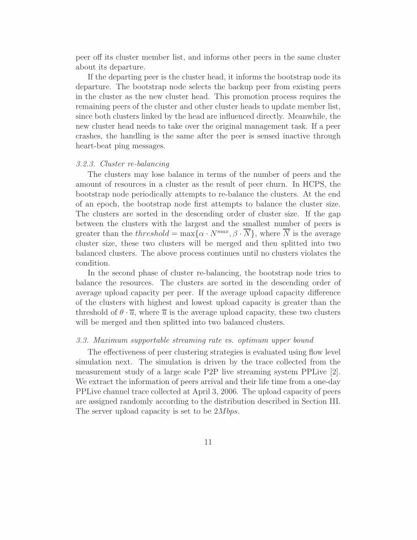
HCPS groups peers into clusters which are then organized into a tree-like hierarchy, with clusters as vertices. Within each cluster, peers are fullyconnected and one peer is elected as the cluster head. The cluster head actsas the video proxy for the cluster and downloads video by joining its parentcluster as a normal/non-head peer. Effectively, the cluster heads serve asthe links that connect clusters to their parent clusters in the hierarchy. Thenumber of connections on each normal peer is bounded by the size of itscluster. Cluster heads additionally maintain connections in the upper levelcluster. The number of connections for cluster heads could be doubled.

Video content is streamed down from the upper-level clusters to the lower-level clusters. Specifically, the source server feeds video to each cluster atthe first level in the hierarchy. Peers in the same cluster efficiently utilizetheir upload capacity and download/upload video from/to one another byemploying a distributed chunk scheduling algorithm to be presented in Sec-tion 4. Since cluster heads at level two join clusters at level one, they relaythe video to clusters at level two. Peers at level two employ the same chunkscheduling algorithm to collaboratively download video from their cluster

5

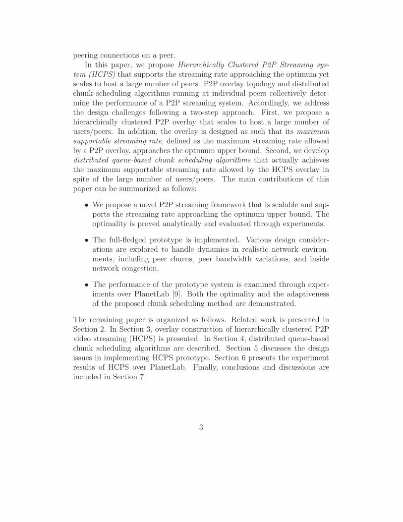
head. The procedure repeats iteratively and video is streamed to all peers atall levels of the hierarchy. Figure 1 illustrates a simple example of two-level

S

r

3

a1

a3

a2

a1 b1

b2

b3

4

5

Cluster Head

Head Mapping

a2

a3

rr

b1

b2

b3

r

r r

6

7

8

1 2

Top Level

Base Level

Figure 1: Hierarchically Clustered P2P Streaming System: two-level hierarchy with 30peers.

HCPS hierarchy. At the base level, peers are grouped into six clusters, eachwith five peers. The peers are fully connected within a cluster. Each clusterhas one cluster head. At the top level, cluster heads form two clusters, eachwith three heads. The video server (source) distributes the content to allcluster heads. At the base level, each cluster head acts as the video proxy inits cluster and distributes the downloaded video to other peers in the samecluster.

While decreasing the number of connections of peers, HCPS has good scal-ability. Suppose that the cluster size is bounded by Nmax, and the source cansupport up to N s top layer clusters. The two-level HCPS system, as shownin Fig. 1, can accommodate up to N s(Nmax)2 peers. Assume N s = 10 andNmax = 20, HCPS supports up to around 4,000 peers. The maximum num-ber of connections a peer needs to maintain is 40 for cluster head and 20 fornormal peer, which is quite manageable. More peers can be accommodatedby adding more levels into the hierarchy. If each of the N sNmax clusters atthe base level has one peer with spare bandwidth higher than or equal to theplayback rate, each such peer can be used as a video proxy to connect morelevels to the two-level hierarchy. By adding one additional level to Figure 1,each peer proxy can support (Nmax)2 additional peers. The system can sus-tain at least N s(Nmax)3 more peers, i.e., 80K peers, only with one more level.

6

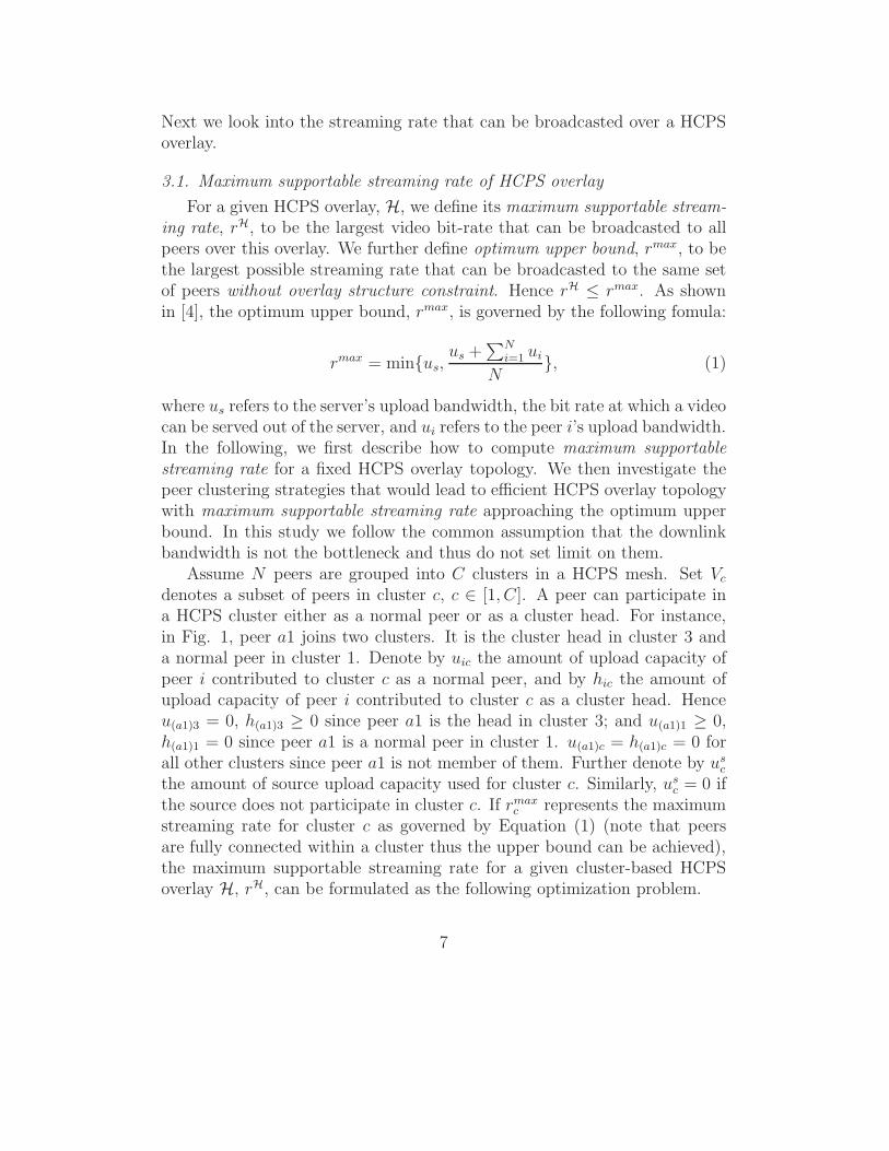
Next we look into the streaming rate that can be broadcasted over a HCPSoverlay.

3.1. Maximum supportable streaming rate of HCPS overlay

For a given HCPS overlay, H, we define its maximum supportable stream-ing rate, rH, to be the largest video bit-rate that can be broadcasted to allpeers over this overlay. We further define optimum upper bound, rmax, to bethe largest possible streaming rate that can be broadcasted to the same setof peers without overlay structure constraint. Hence rH ≤ rmax. As shownin [4], the optimum upper bound, rmax, is governed by the following fomula:

rmax = min{us,us +

∑N

i=1 ui

N}, (1)

where us refers to the server’s upload bandwidth, the bit rate at which a videocan be served out of the server, and ui refers to the peer i’s upload bandwidth.In the following, we first describe how to compute maximum supportablestreaming rate for a fixed HCPS overlay topology. We then investigate thepeer clustering strategies that would lead to efficient HCPS overlay topologywith maximum supportable streaming rate approaching the optimum upperbound. In this study we follow the common assumption that the downlinkbandwidth is not the bottleneck and thus do not set limit on them.

Assume N peers are grouped into C clusters in a HCPS mesh. Set Vc

denotes a subset of peers in cluster c, c ∈ [1, C]. A peer can participate ina HCPS cluster either as a normal peer or as a cluster head. For instance,in Fig. 1, peer a1 joins two clusters. It is the cluster head in cluster 3 anda normal peer in cluster 1. Denote by uic the amount of upload capacity ofpeer i contributed to cluster c as a normal peer, and by hic the amount ofupload capacity of peer i contributed to cluster c as a cluster head. Henceu(a1)3 = 0, h(a1)3 ≥ 0 since peer a1 is the head in cluster 3; and u(a1)1 ≥ 0,h(a1)1 = 0 since peer a1 is a normal peer in cluster 1. u(a1)c = h(a1)c = 0 forall other clusters since peer a1 is not member of them. Further denote by us

c

the amount of source upload capacity used for cluster c. Similarly, usc = 0 if

the source does not participate in cluster c. If rmaxc represents the maximum

streaming rate for cluster c as governed by Equation (1) (note that peersare fully connected within a cluster thus the upper bound can be achieved),the maximum supportable streaming rate for a given cluster-based HCPSoverlay H, rH, can be formulated as the following optimization problem.

7

rH = max{uic,hic,us

c}

{

min [rmaxc |c = 1, 2, . . . , C]

}

(2)

subject to:

rmaxc = min

{

∑N

i=1(uic + hic)

Vc

,

N∑

i=1

hic + usc

}

(3)

C∑

c=1

(uic + hic) ≤ ui (4)

C∑

c=1

usc ≤ us (5)

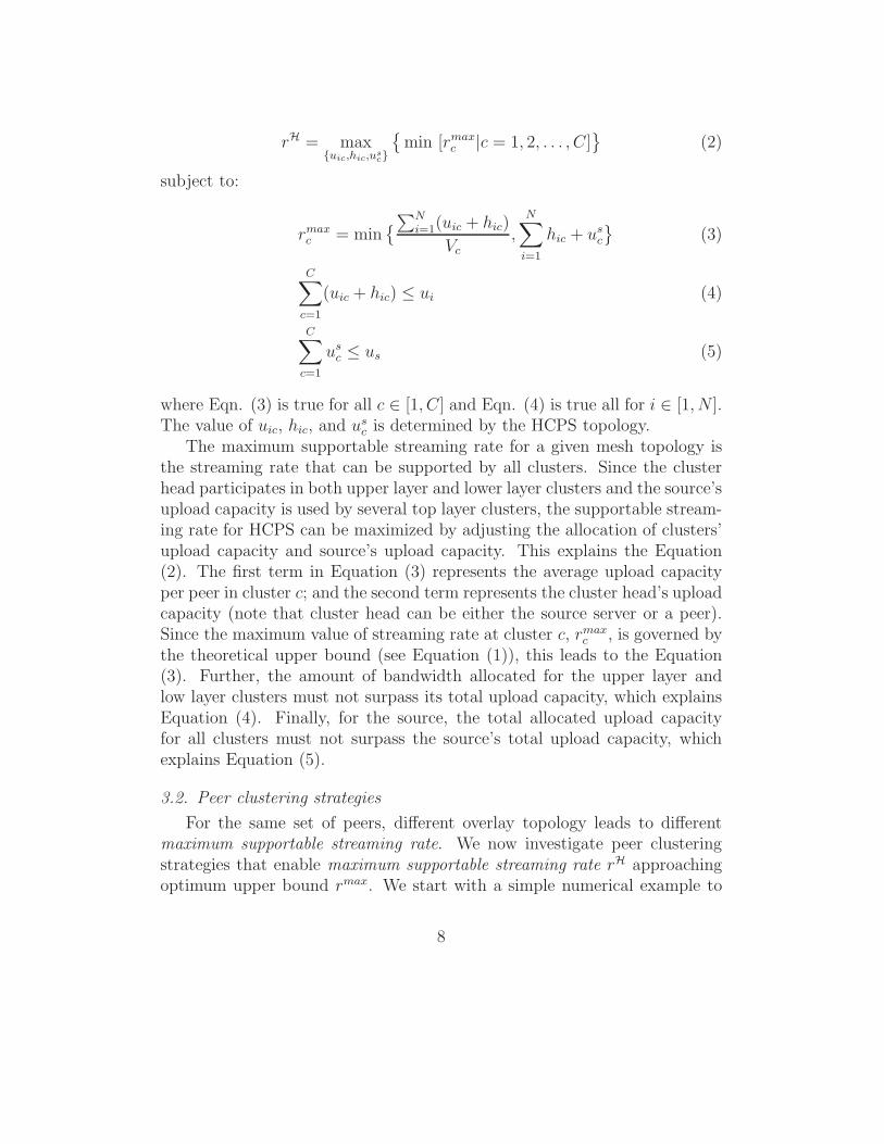
where Eqn. (3) is true for all c ∈ [1, C] and Eqn. (4) is true all for i ∈ [1, N ].The value of uic, hic, and us

c is determined by the HCPS topology.The maximum supportable streaming rate for a given mesh topology is

the streaming rate that can be supported by all clusters. Since the clusterhead participates in both upper layer and lower layer clusters and the source’supload capacity is used by several top layer clusters, the supportable stream-ing rate for HCPS can be maximized by adjusting the allocation of clusters’upload capacity and source’s upload capacity. This explains the Equation(2). The first term in Equation (3) represents the average upload capacityper peer in cluster c; and the second term represents the cluster head’s uploadcapacity (note that cluster head can be either the source server or a peer).Since the maximum value of streaming rate at cluster c, rmax

c , is governed bythe theoretical upper bound (see Equation (1)), this leads to the Equation(3). Further, the amount of bandwidth allocated for the upper layer andlow layer clusters must not surpass its total upload capacity, which explainsEquation (4). Finally, for the source, the total allocated upload capacityfor all clusters must not surpass the source’s total upload capacity, whichexplains Equation (5).

3.2. Peer clustering strategies

For the same set of peers, different overlay topology leads to differentmaximum supportable streaming rate. We now investigate peer clusteringstrategies that enable maximum supportable streaming rate rH approachingoptimum upper bound rmax. We start with a simple numerical example to

8

illustrate the major factors affecting the HCPS’s performance. The clusteringstrategies are laid out thereafter.

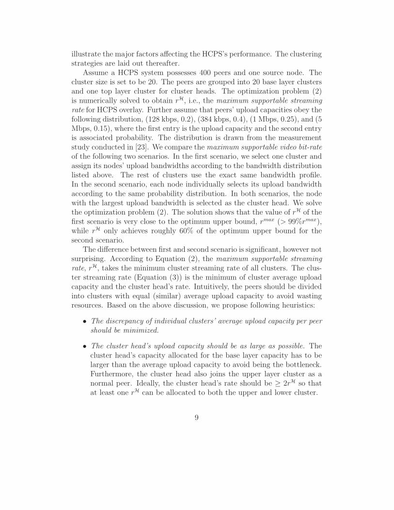
Assume a HCPS system possesses 400 peers and one source node. Thecluster size is set to be 20. The peers are grouped into 20 base layer clustersand one top layer cluster for cluster heads. The optimization problem (2)is numerically solved to obtain rH, i.e., the maximum supportable streamingrate for HCPS overlay. Further assume that peers’ upload capacities obey thefollowing distribution, (128 kbps, 0.2), (384 kbps, 0.4), (1 Mbps, 0.25), and (5Mbps, 0.15), where the first entry is the upload capacity and the second entryis associated probability. The distribution is drawn from the measurementstudy conducted in [23]. We compare the maximum supportable video bit-rateof the following two scenarios. In the first scenario, we select one cluster andassign its nodes’ upload bandwidths according to the bandwidth distributionlisted above. The rest of clusters use the exact same bandwidth profile.In the second scenario, each node individually selects its upload bandwidthaccording to the same probability distribution. In both scenarios, the nodewith the largest upload bandwidth is selected as the cluster head. We solvethe optimization problem (2). The solution shows that the value of rH of thefirst scenario is very close to the optimum upper bound, rmax (> 99%rmax),while rH only achieves roughly 60% of the optimum upper bound for thesecond scenario.

The difference between first and second scenario is significant, however notsurprising. According to Equation (2), the maximum supportable streamingrate, rH, takes the minimum cluster streaming rate of all clusters. The clus-ter streaming rate (Equation (3)) is the minimum of cluster average uploadcapacity and the cluster head’s rate. Intuitively, the peers should be dividedinto clusters with equal (similar) average upload capacity to avoid wastingresources. Based on the above discussion, we propose following heuristics:

• The discrepancy of individual clusters’ average upload capacity per peershould be minimized.

• The cluster head’s upload capacity should be as large as possible. Thecluster head’s capacity allocated for the base layer capacity has to belarger than the average upload capacity to avoid being the bottleneck.Furthermore, the cluster head also joins the upper layer cluster as anormal peer. Ideally, the cluster head’s rate should be ≥ 2rH so thatat least one rH can be allocated to both the upper and lower cluster.

9

• The number of peers in a cluster should be bounded from the above bya relatively small number. The number of peers in a cluster determinesthe out-degree of peers. Large out-degree is prohibitive for peers toperform properly in real networks.

Below we describe the dynamic peer management in HCPS that realizesthe above heuristics. HCPS system has a bootstrapping node whose task is tomanage HCPS topology to balance the resources among clusters. Meanwhile,a cluster head manages the peers in its own cluster. The bootstrap node’stask is to handle the peer arrival and peer departure in such a way that rH isas close to the optimal as possible. Below we describe three key operations inHCPS that handle the peer dynamics: peer join, peer departure, and clusterre-balancing.

3.2.1. Peer join

Depending on the new arrival’s estimated upload capacity compared tothe current rH, the new peer is classified into three categories: HPeer(resourcerich peer) if u ≥ rH + θ, MPeer(resource medium peer) if rH − θ < u <rH+θ, and LPeer(resource poor peer) otherwise, where u is new peer’s uploadcapacity, and θ is a configuration parameter.

Denote by Nmax the maximum number of peers allowed in a cluster. Allclusters with less than Nmax peers are eligible to accept the new peer. Ifthe upload capacity of the new peer, u, is greater than some eligible clusterheads’ upload capacity by a margin, the peer is assigned to the cluster withthe smallest cluster head upload capacity. The new peer is to replace theoriginal cluster head, and the original head becomes the normal peer andstay in the cluster.

If the new peer does not replace any cluster head, it is assigned to a clusteraccording to the peer type. Specifically, the peer is assigned to the clusterwith the minimum average upload capacity if the peer is HPeer; the peer isassigned to the cluster with the smallest number of peers if it is MPeer; andthe peer is assigned to the cluster with the maximum average upload capacityif it is LPeer. The idea behind this is to balance the upload resources amongclusters.The new peer is redirected to the corresponding cluster head, andbootstrap node asks the cluster head to admit the new peer.

3.2.2. Peer departure

The handling of peer departure is straight forward. If the peer is a normalpeer, it informs the cluster head of its departure. The cluster head takes the

10

peer off its cluster member list, and informs other peers in the same clusterabout its departure.

If the departing peer is the cluster head, it informs the bootstrap node itsdeparture. The bootstrap node selects the backup peer from existing peersin the cluster as the new cluster head. This promotion process requires theremaining peers of the cluster and other cluster heads to update member list,since both clusters linked by the head are influenced directly. Meanwhile, thenew cluster head needs to take over the original management task. If a peercrashes, the handling is the same after the peer is sensed inactive throughheart-beat ping messages.

3.2.3. Cluster re-balancing

The clusters may lose balance in terms of the number of peers and theamount of resources in a cluster as the result of peer churn. In HCPS, thebootstrap node periodically attempts to re-balance the clusters. At the endof an epoch, the bootstrap node first attempts to balance the cluster size.The clusters are sorted in the descending order of cluster size. If the gapbetween the clusters with the largest and the smallest number of peers isgreater than the threshold = max{α ·Nmax, β ·N}, where N is the averagecluster size, these two clusters will be merged and then splitted into twobalanced clusters. The above process continues until no clusters violates thecondition.

In the second phase of cluster re-balancing, the bootstrap node tries tobalance the resources. The clusters are sorted in the descending order ofaverage upload capacity per peer. If the average upload capacity differenceof the clusters with highest and lowest upload capacity is greater than thethreshold of θ · u, where u is the average upload capacity, these two clusterswill be merged and then splitted into two balanced clusters.

3.3. Maximum supportable streaming rate vs. optimum upper bound

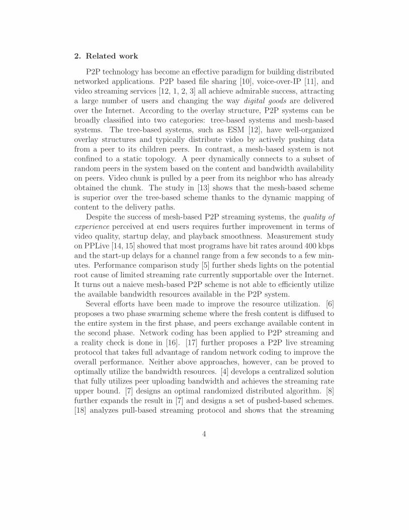
The effectiveness of peer clustering strategies is evaluated using flow levelsimulation next. The simulation is driven by the trace collected from themeasurement study of a large scale P2P live streaming system PPLive [2].We extract the information of peers arrival and their life time from a one-dayPPLive channel trace collected at April 3, 2006. The upload capacity of peersare assigned randomly according to the distribution described in Section III.The server upload capacity is set to be 2Mbps.

11

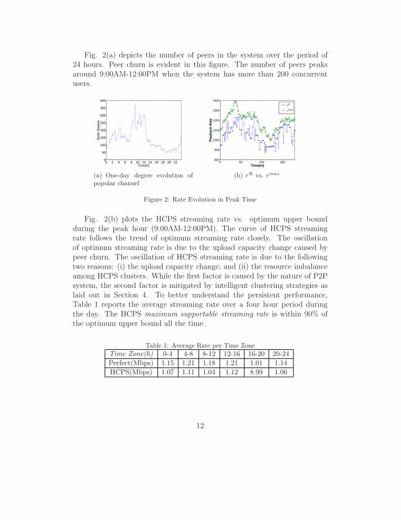
Fig. 2(a) depicts the number of peers in the system over the period of24 hours. Peer churn is evident in this figure. The number of peers peaksaround 9:00AM-12:00PM when the system has more than 200 concurrentusers.

0 2 4 6 8 10 12 14 16 18 20 220

50

100

150

200

250

300

350

400

Time(h)

Nod

e D

egre

e

(a) One-day degree evolution ofpopular channel

0 50 100 150800

900

1000

1100

1200

1300

1400

Time(m)

Pla

ybac

k R

ate

rH

rmax

(b) rH vs. rmax

Figure 2: Rate Evolution in Peak Time

Fig. 2(b) plots the HCPS streaming rate vs. optimum upper boundduring the peak hour (9:00AM-12:00PM). The curve of HCPS streamingrate follows the trend of optimum streaming rate closely. The oscillationof optimum streaming rate is due to the upload capacity change caused bypeer churn. The oscillation of HCPS streaming rate is due to the followingtwo reasons: (i) the upload capacity change; and (ii) the resource imbalanceamong HCPS clusters. While the first factor is caused by the nature of P2Psystem, the second factor is mitigated by intelligent clustering strategies aslaid out in Section 4. To better understand the persistent performance,Table 1 reports the average streaming rate over a four hour period duringthe day. The HCPS maximum supportable streaming rate is within 90% ofthe optimum upper bound all the time.

Table 1: Average Rate per Time Zone

Time Zone(h) 0-4 4-8 8-12 12-16 16-20 20-24

Perfect(Mbps) 1.15 1.21 1.18 1.21 1.01 1.14

HCPS(Mbps) 1.07 1.11 1.04 1.12 8.99 1.06

12

4. Distributed queue-based chunk scheduling algorithms

In Section 3, we studied how to construct HCPS overlay to have largemaximum supportable streaming rate. In this section, we describe distributedqueue-based chunk scheduling algorithms that achieve themaximum support-able streaming rate, rH. Designing a distributed chunk scheduling algorithmthat achieves the maximum supportable streaming rate is not trivial becauseof content bottleneck effect. Peers’ uplink bandwidths are wasted wheneverchunks requested by a peer’s connected neighbors are not available at thispeer. In Eqn. (2), maximum supportable stream rate rH is computed withoutconsidering content bottleneck.

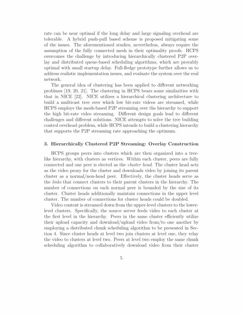
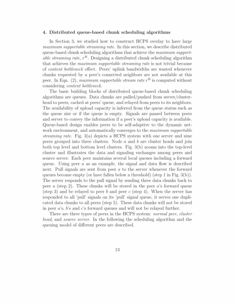
The basic building blocks of distributed queue-based chunk schedulingalgorithms are queues. Data chunks are pulled/pushed from server/cluster-head to peers, cached at peers’ queue, and relayed from peers to its neighbors.The availability of upload capacity is inferred from the queue status such asthe queue size or if the queue is empty. Signals are passed between peersand server to convey the information if a peer’s upload capacity is available.Queue-based design enables peers to be self-adaptive to the dynamic net-work environment, and automatically converges to the maximum supportablestreaming rate. Fig. 3(a) depicts a HCPS system with one server and ninepeers grouped into three clusters. Node a and b are cluster heads and joinboth top level and bottom level clusters. Fig. 3(b) zooms into the top-levelcluster and illustrates the data and signaling exchanges among peers andsource server. Each peer maintains several local queues including a forwardqueue. Using peer a as an example, the signal and data flow is describednext. Pull signals are sent from peer a to the server whenever the forwardqueues become empty (or have fallen below a threshold) (step 1 in Fig. 3(b)).The server responds to the pull signal by sending three data chunks back topeer a (step 2). These chunks will be stored in the peer a’s forward queue(step 3) and be relayed to peer b and peer c (step 4). When the server hasresponded to all ’pull’ signals on its ’pull’ signal queue, it serves one dupli-cated data chunks to all peers (step 5). These data chunks will not be storedin peer a’s, b’s and c’s forward queues and will not be relayed further.

There are three types of peers in the HCPS system: normal peer, clusterhead, and source server. In the following the scheduling algorithm and thequeuing model of different peers are described.

13

S

a b

c

g he j

f i

(a) Queue-based chunk schedulingwith nine peers

ba

S

c

Pull signal from peer to server

Chunks in response to pull signal

Chunks with no pull signal

1

2

34

5 5 5

4

(b) Queue-based chunkscheduling in top cluster

Figure 3: HCPS Overlay using queue-based chunk scheduling: an example with one sourceand nine peers grouped into three clusters

4.1. Scheduling and queuing model of normal peer

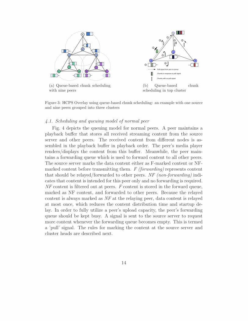
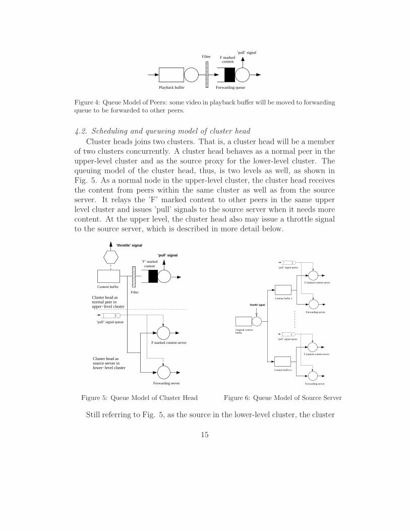
Fig. 4 depicts the queuing model for normal peers. A peer maintains aplayback buffer that stores all received streaming content from the sourceserver and other peers. The received content from different nodes is as-sembled in the playback buffer in playback order. The peer’s media playerrenders/displays the content from this buffer. Meanwhile, the peer main-tains a forwarding queue which is used to forward content to all other peers.The source server marks the data content either as F-marked content or NF-marked content before transmitting them. F (forwarding) represents contentthat should be relayed/forwarded to other peers. NF (non-forwarding) indi-cates that content is intended for this peer only and no forwarding is required.NF content is filtered out at peers. F content is stored in the forward queue,marked as NF content, and forwarded to other peers. Because the relayedcontent is always marked as NF at the relaying peer, data content is relayedat most once, which reduces the content distribution time and startup de-lay. In order to fully utilize a peer’s upload capacity, the peer’s forwardingqueue should be kept busy. A signal is sent to the source server to requestmore content whenever the forwarding queue becomes empty. This is termeda ’pull’ signal. The rules for marking the content at the source server andcluster heads are described next.

14

����������

����������

Playback buffer Forwarding queue

Filter F markedcontent

’pull’ signal

Figure 4: Queue Model of Peers: some video in playback buffer will be moved to forwardingqueue to be forwarded to other peers.

4.2. Scheduling and queueing model of cluster head

Cluster heads joins two clusters. That is, a cluster head will be a memberof two clusters concurrently. A cluster head behaves as a normal peer in theupper-level cluster and as the source proxy for the lower-level cluster. Thequeuing model of the cluster head, thus, is two levels as well, as shown inFig. 5. As a normal node in the upper-level cluster, the cluster head receivesthe content from peers within the same cluster as well as from the sourceserver. It relays the ’F’ marked content to other peers in the same upperlevel cluster and issues ’pull’ signals to the source server when it needs morecontent. At the upper level, the cluster head also may issue a throttle signalto the source server, which is described in more detail below.

’pull’ signal queue

����������

����������

Forwarding server

F marked content server

Content buffer

’throttle’ signal

Filter

’F’ markedcontent

’pull’ signal

Cluster head as

upper−level cluster

Cluster head assource server in

normal peer in

lower−level cluster

Figure 5: Queue Model of Cluster Head

’pull’ signal queue

’pull’ signal queue

Forwarding server

F marked content server

Original contentbuffer

’throttle’ signal

Content buffer 1

Forwarding server

F marked content server

Content buffer n

Figure 6: Queue Model of Source Server

Still referring to Fig. 5, as the source in the lower-level cluster, the cluster

15

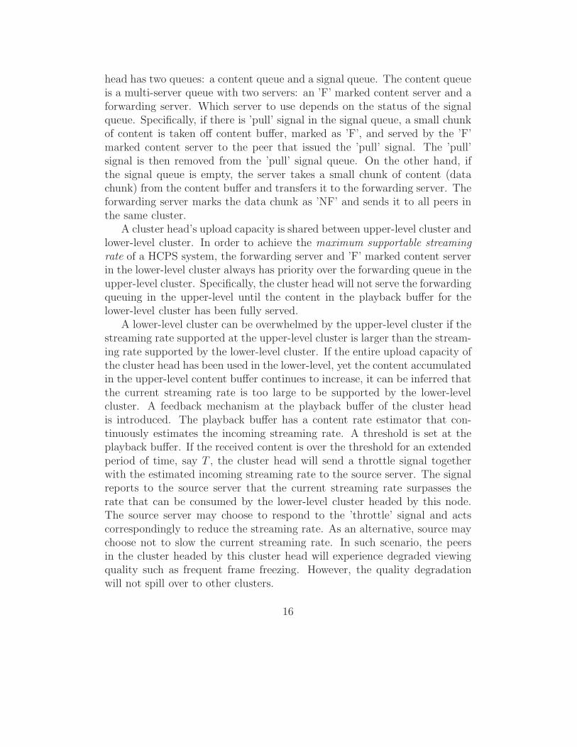
head has two queues: a content queue and a signal queue. The content queueis a multi-server queue with two servers: an ’F’ marked content server and aforwarding server. Which server to use depends on the status of the signalqueue. Specifically, if there is ’pull’ signal in the signal queue, a small chunkof content is taken off content buffer, marked as ’F’, and served by the ’F’marked content server to the peer that issued the ’pull’ signal. The ’pull’signal is then removed from the ’pull’ signal queue. On the other hand, ifthe signal queue is empty, the server takes a small chunk of content (datachunk) from the content buffer and transfers it to the forwarding server. Theforwarding server marks the data chunk as ’NF’ and sends it to all peers inthe same cluster.

A cluster head’s upload capacity is shared between upper-level cluster andlower-level cluster. In order to achieve the maximum supportable streamingrate of a HCPS system, the forwarding server and ’F’ marked content serverin the lower-level cluster always has priority over the forwarding queue in theupper-level cluster. Specifically, the cluster head will not serve the forwardingqueuing in the upper-level until the content in the playback buffer for thelower-level cluster has been fully served.

A lower-level cluster can be overwhelmed by the upper-level cluster if thestreaming rate supported at the upper-level cluster is larger than the stream-ing rate supported by the lower-level cluster. If the entire upload capacity ofthe cluster head has been used in the lower-level, yet the content accumulatedin the upper-level content buffer continues to increase, it can be inferred thatthe current streaming rate is too large to be supported by the lower-levelcluster. A feedback mechanism at the playback buffer of the cluster headis introduced. The playback buffer has a content rate estimator that con-tinuously estimates the incoming streaming rate. A threshold is set at theplayback buffer. If the received content is over the threshold for an extendedperiod of time, say T , the cluster head will send a throttle signal togetherwith the estimated incoming streaming rate to the source server. The signalreports to the source server that the current streaming rate surpasses therate that can be consumed by the lower-level cluster headed by this node.The source server may choose to respond to the ’throttle’ signal and actscorrespondingly to reduce the streaming rate. As an alternative, source maychoose not to slow the current streaming rate. In such scenario, the peersin the cluster headed by this cluster head will experience degraded viewingquality such as frequent frame freezing. However, the quality degradationwill not spill over to other clusters.

16

4.3. Scheduling and queueing model of source

The source server in HCPS system may participate in one or multipletop-level clusters. The source server has one sub-server for each top-levelcluster, as shown in Fig. 6. The source server maintains an original contentqueue that stores the data/streaming content. It also handles the ’throttle’signals from the lower level clusters and from cluster heads the source serverserves at the top-level clusters. The server regulates the streaming rate ac-cording to the ’throttle’ signals from the peers. The server’s upload capacityis shared among all top-level clusters. The bandwidth sharing follows thefollowing rules: (i) the cluster that lags behind other clusters significantly(by a threshold in terms of content queue size) has the highest priority touse the upload capacity; and (ii) if all content queues are of the same/similarsize, then clusters are served in a round robin fashion.

4.4. Optimality of queue-based chunk scheduling algorithms

Theorem 1. Assume that the propagation delay between peers and betweena peer and the server is negligible and the data content can be transmittedat an arbitrary small amount. The distributed queue-based chunk schedulingalgorithm achieves the optimum upper bound, rmax, over a fully connectedmesh, and achieves the maximum supportable streaming rate, rH, over thehierarchically cluster P2P overlay, H.

See Appendix for the proof. Below we discuss the implementation consider-ations in realizing the distributed queue based chunk scheduling algorithmsin practice.

5. Implementation considerations

We implement a full functioning HCPS live streaming system which notonly serves as a proof of concept but also allows us to evaluate the systemperformance over the real network. Below we use the source server as anexample to illustrate the design philosophy. The architecture design aimsat solving practical implementation challenges including the impact of chunksize, network congestion, and peer churn. The same design philosophy can beapplied to the design of other components such as normal peers and clusterheads.

17

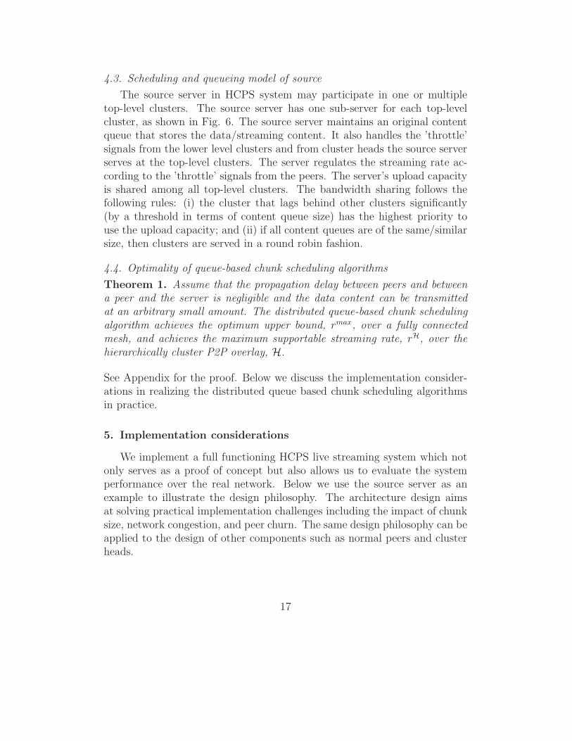
5.1. Source server architecture

The source server maintains one sub-server for each cluster (see Fig. 6).For the ease of illustration, we assume there is one top-level cluster in thesystem. We also assume that the content source server is the bootstrap node.As the bootstrap node, the content source server manages peer information(such as peer id, IP address, port number, etc.) and replies to the requestfor peer list from incoming new peers.

Internet

Select Call

PULL SIG

MSG

Source

Packet Handler

RECOV REQ

Figure 7: Server Architecture

Figure 7 illustrates the architecture of the source server. Using the ’selectcall’ mechanism to monitor the connections with peers, the server maintainsa set of input buffers to store received data. There are three types of incom-ing messages: management message, pull signal, and missing chunk recoveryrequest. Correspondingly three independent queues are formed for these mes-sages. If the output of handling these messages needs to be transmitted toremote peers, the output is put on the per-peer out-unit.

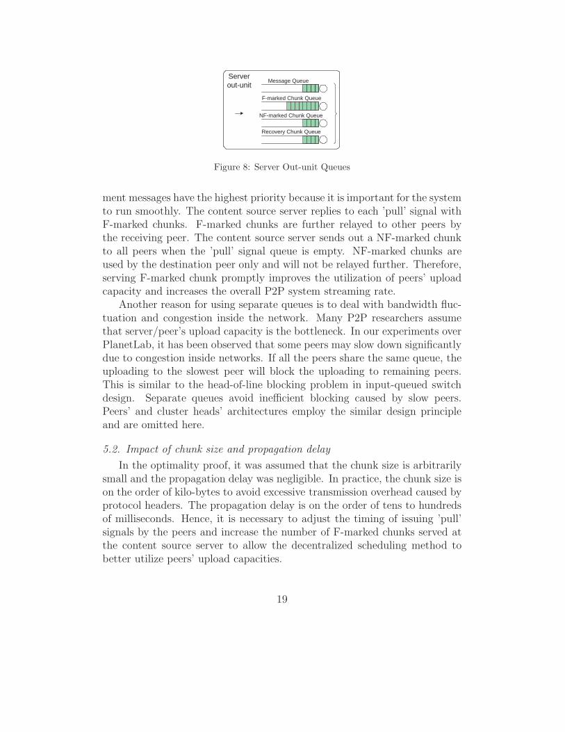
There is one out-unit for each destination peer to handle the data trans-mission process. Figure 8 depicts an example. Each out-unit has four queuesfor a given peer: management message queue, F-marked content queue, NF-marked content queue, and missing chunk recovery queue. The managementmessage queue stores responses to management requests. An example of amanagement request is when a new peer has just joined the P2P system andrequests the peer list. The F/NF marked content queue stores the F/NFmarked content intended for this peer. Finally, chunk recovery queue storesthe missing chunks requested by the peer.

Different queues are used for different types of traffic in order to prioritizethe traffic types. Specifically, management messages have the highest prior-ity, followed by F-marked content, and NF-marked content. The priority ofrecovery chunks can be adjusted based on the design requirement. Manage-

18

Message Queue

F-marked Chunk Queue

NF-marked Chunk Queue

Server out-unit

Recovery Chunk Queue

Figure 8: Server Out-unit Queues

ment messages have the highest priority because it is important for the systemto run smoothly. The content source server replies to each ’pull’ signal withF-marked chunks. F-marked chunks are further relayed to other peers bythe receiving peer. The content source server sends out a NF-marked chunkto all peers when the ’pull’ signal queue is empty. NF-marked chunks areused by the destination peer only and will not be relayed further. Therefore,serving F-marked chunk promptly improves the utilization of peers’ uploadcapacity and increases the overall P2P system streaming rate.

Another reason for using separate queues is to deal with bandwidth fluc-tuation and congestion inside the network. Many P2P researchers assumethat server/peer’s upload capacity is the bottleneck. In our experiments overPlanetLab, it has been observed that some peers may slow down significantlydue to congestion inside networks. If all the peers share the same queue, theuploading to the slowest peer will block the uploading to remaining peers.This is similar to the head-of-line blocking problem in input-queued switchdesign. Separate queues avoid inefficient blocking caused by slow peers.Peers’ and cluster heads’ architectures employ the similar design principleand are omitted here.

5.2. Impact of chunk size and propagation delay

In the optimality proof, it was assumed that the chunk size is arbitrarilysmall and the propagation delay was negligible. In practice, the chunk size ison the order of kilo-bytes to avoid excessive transmission overhead caused byprotocol headers. The propagation delay is on the order of tens to hundredsof milliseconds. Hence, it is necessary to adjust the timing of issuing ’pull’signals by the peers and increase the number of F-marked chunks served atthe content source server to allow the decentralized scheduling method tobetter utilize peers’ upload capacities.

19

At the server/cluster-head side, K F-marked chunks are transmitted asa batch in response to a ’pull’ signal from a requesting peer (via the F-marked content queue). A larger value of K would reduce the ’pull’ signalfrequency and thus reduce the signaling overhead. This, however, increasespeers’ threshold to be shown in Equation (6). Denote by Ti the thresholdfor peer i to issue ’pull’ signal. A ’pull’ signal is sent to server whenever thenumber of chunks in the queue is less than or equal to Ti. The time to emptythe forwarding queue with Ti chunks is t

emptyi = (M−1)Tiδ/ui, whereM is the

number of peers in a cluster. Meanwhile, it takes treceivei = 2tsi +Kδ/us + tqfor peer i to receive K chunks after it issues a pull signal. Here tsi is thepropagation delay between the source server and peer i, Kδ/us is the timerequired for server to transmit K chunks, and tq is queuing delay seen by the’pull’ signal at the server pull signal queue. In order to receive the chunksbefore the forwarding queue becomes fully drained, tempty

i = treceivei . Thisleads to:

Ti =(2tsi +Kδ/us + tq)ui

(M − 1)δ. (6)

All quantities are known except tq, the queuing delay incurred at the serverside signal queue. If the source server is the bottleneck (case 1 in the op-timality proof), the selection of Ti would not affect the streaming rate aslong as the server is always busy. If server resource is rich (case 2 in theoptimality proof), since the service rate of signal queue is faster than thepull signal rate, tq is very small. So we set tq to be zero. Following ’pull’signal threshold formula is used to guide the threshold selection:

Ti =(2tsi +Kδ/us)ui

(M − 1)δ. (7)

5.3. Missing chunk recovery

Peer churn and network congestion may cause chunk losses. Sudden peerdeparture, such as node or connection failure, leaves the system no timeto reschedule the chunks still buffered in the peer’s out-unit. In case thenetwork routes are congested to some destinations, the chunks waiting to betransmitted may overflow the queue in the out-unit, which leads to chunklosses at the receiving end. The missing chunk recovery scheme enables thepeers to recover the missing chunks to avoid viewing quality degradation.

Each peer maintains a playback buffer to store the video chunks receivedfrom the server and other peers. The playback buffer has three windows:

20

Download Window Recovery Window

Neighbor Server

T

Playback Window

d W r W p W r W r W r W

Figure 9: Missing Chunk Recovery

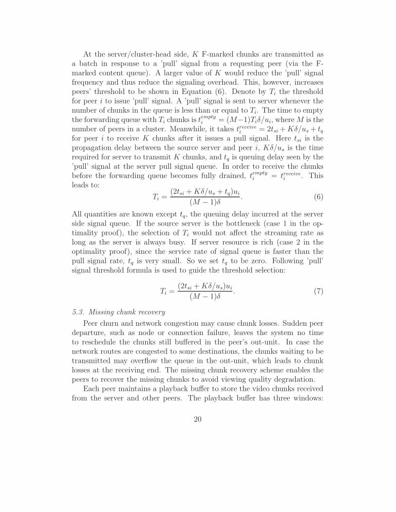
playback window, recovery window, and download window. Wp,Wr andWd denote the size (in terms of number of chunks) of playback window,recovery window, and download window, respectively. The media playerrenders/displays the content from the playback window. Missing chunksin the recovery window are recovered using the method described below.Finally, the chunks in the downloading window are pulled and pushed amongthe server and the other peers.

Heuristics are employed to recover the missing chunks. If peers leavegracefully, the server is notified and the F-marked chunks waiting in the out-unit will be assigned to other peers. The missing chunks falling into therecovery window are recovered as follows. First, the recovery window is fur-ther divided into four sub-windows. Peers send the chunk recovery messagesto the source server directly if the missing chunks are in the window closestin time to the playback window. These chunks are urgently needed other-wise the content quality will be impaired. An attempt is made to recoverthe missing chunks in the other three sub-windows from other peers. A peerrandomly selects three recovery peers from the peer list, and associates onewith each sub-window. The peer needs recovery chunks sends chunk recov-ery messages to the corresponding recovery peers. By randomly selecting arecovery peer, the recovery workload is evenly distributed among all peers.

5.4. Optimality of startup delay

We derive the startup delay here because the queue size has been derivedin 5.2. A peer’s startup delay, τ , is τ = h · τintra−cluster, where h is the heightat which the cluster resides in the HCPS overlay, and τintra−cluster denote thedelay incurred in distributed content within a cluster. Assume there are Npeers in the system and the cluster size is M , the value of h is at the orderof O(logN/M) if the cluster tree is balanced.

The delay incurred inside a cluster comprises of two parts: the timespending waiting in the queue, and the time transmitting a chunk to all otherpeers in the same cluster. Hence τintra−cluster = maxi{Ti ·δ(M−1)/ui+(M−

21

1)δ/ui}. We take the maximum overall all peer in the cluster is because theslowest peer determines the startup delay of this cluster. Plug Ti into theabove equation, we have τintra−cluster = maxi{(2tsi +Kδ)/us + (n− 1)δ/ui}.tsi, K, δ, M , and us (cluster head’s upload bandwidth devoted to the clusterunder consideration) are all constant. Thus the value of τintra−cluster is atthe order of O(M). Therefore, the startup delay is at the order of O(M ·logN/M) = O(logN), which is optimal as proven in [8].

6. Performance Evaluation

Next we examine the performance of HCPS via experiments over Plan-etLab [9]. We started with the single cluster experiments to understand theperformance of queue-based algorithms and the system dynamics in the faceof peer churn and bandwidth variations. We then look into a larger scalesystem with multiple clusters, investigating the cluster head overhead, theeffect of clustering on streaming delay, and the adaptiveness of HCPS.

We select PlanetLab nodes with sufficient bandwidth and use softwarepackage Trickle [24] to set a node’s upload capacity. In our HCPS streamingsystem, all connections between nodes are TCP connections. TCP connec-tions avoid network layer data losses, and facilitate the use of Trickle [24] toset a node’s upload capacity. In our experiments, we observe that Trickle isnot 100% accurate on setting the available bandwidth. The obtained uploadbandwidth is slightly larger (< 8%) than the value we set using Trickle. Toaccount for this error, we measure the actual upload bandwidth, and use themeasured rate for plotting the graphs. The upload capacities of peers areassigned randomly according to the distribution: (128kbps, 0.2), (384kbps,0.4), (1Mbps, 0.25), and (4Mbps, 0.15). The largest uplink speed is adjustedfrom 5 Mbps [23] to 4 Mbps to ensure that PlanetLab nodes have sufficientbandwidth to emulate the targeted rate. We follow the common assumptionthat the downlink bandwidth is not the bottleneck and thus do not set limiton them. The chunk size is chosen to be one KBytes. In the following, we firstevaluate the queue-based chunk scheduling algorithm over a fully connectedmesh. We then investigate its performance over hierarchically clustered P2Poverlay.

22

6.1. Performance of queue-based chunk scheduling over a fully connectedmesh

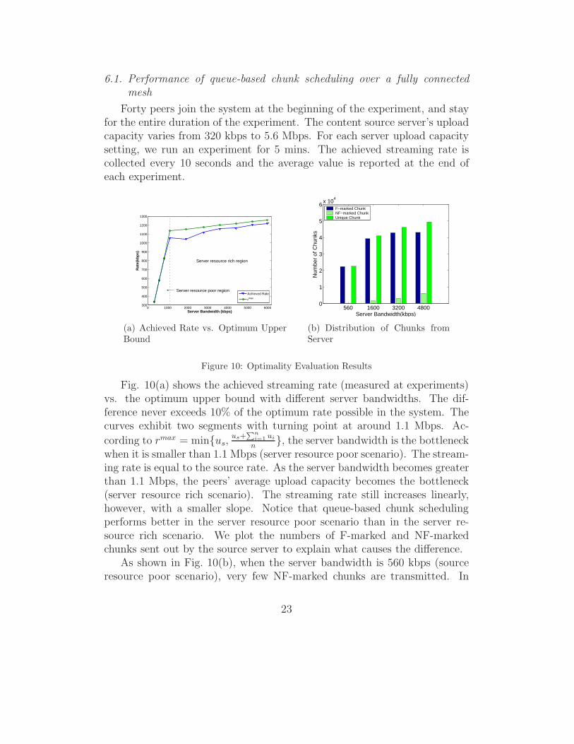
Forty peers join the system at the beginning of the experiment, and stayfor the entire duration of the experiment. The content source server’s uploadcapacity varies from 320 kbps to 5.6 Mbps. For each server upload capacitysetting, we run an experiment for 5 mins. The achieved streaming rate iscollected every 10 seconds and the average value is reported at the end ofeach experiment.

0 1000 2000 3000 4000 5000 6000300

400

500

600

700

800

900

1000

1100

1200

1300

Server Bandwidth (kbps)

Rat

e(kb

ps)

Server resource rich region

Server resource poor region Achieved Rate

rmax

(a) Achieved Rate vs. Optimum UpperBound

560 1600 3200 48000

1

2

3

4

5

6x 10

4

Server Bandwidth(kbps)N

umbe

r of

Chu

nks

F−marked ChunkNF−marked ChunkUnique Chunk

(b) Distribution of Chunks fromServer

Figure 10: Optimality Evaluation Results

Fig. 10(a) shows the achieved streaming rate (measured at experiments)vs. the optimum upper bound with different server bandwidths. The dif-ference never exceeds 10% of the optimum rate possible in the system. Thecurves exhibit two segments with turning point at around 1.1 Mbps. Ac-

cording to rmax = min{us,us+

∑ni=1

ui

n}, the server bandwidth is the bottleneck

when it is smaller than 1.1 Mbps (server resource poor scenario). The stream-ing rate is equal to the source rate. As the server bandwidth becomes greaterthan 1.1 Mbps, the peers’ average upload capacity becomes the bottleneck(server resource rich scenario). The streaming rate still increases linearly,however, with a smaller slope. Notice that queue-based chunk schedulingperforms better in the server resource poor scenario than in the server re-source rich scenario. We plot the numbers of F-marked and NF-markedchunks sent out by the source server to explain what causes the difference.

As shown in Fig. 10(b), when the server bandwidth is 560 kbps (sourceresource poor scenario), very few NF-marked chunks are transmitted. In

23

theory, no NF-marked chunks should be sent in this scenario since signalqueue is always non-empty. We do see several NF-marked chunks, whichis caused by the background noise traffic in the network. The interferenceof the background traffic occasionally causes the server’s pull signal queuebecomes empty. In contrast, more and more NF-marked chunks are sent bythe server as its uplink capacity increases beyond 1.1 Mbps (source resourcerich scenarios). In the server resource poor scenario, the server sends outF-marked chunks exclusively. As long as the pull signal queue is not empty,the optimum streaming rate can be achieved. In the server resource richscenario, the server sends out both F-marked and NF-marked chunks. IfF-marked chunks are delayed at server or along the route from the server topeers due to the bandwidth variations or peer churn, peers can not receiveF-marked chunks promptly. Peers’ forward queues become idle and uploadbandwidth is wasted. Nevertheless, queue-based chunk scheduling alwaysachieve the streaming rate within 10% of the optimum upper bound.

6.2. Adaptiveness to peer churn and bandwidth variations

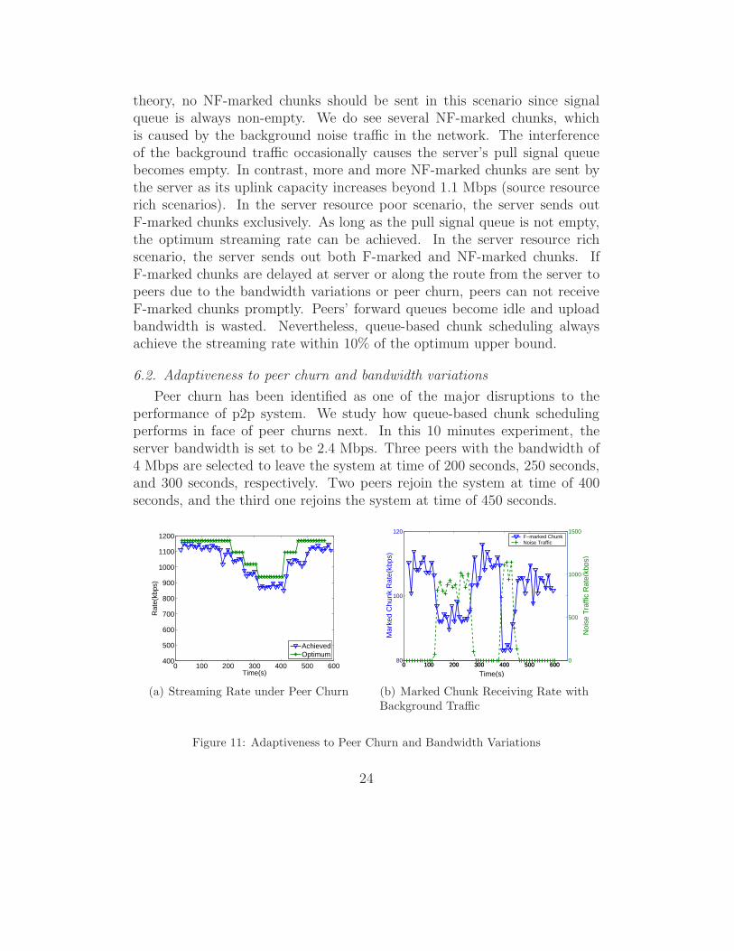
Peer churn has been identified as one of the major disruptions to theperformance of p2p system. We study how queue-based chunk schedulingperforms in face of peer churns next. In this 10 minutes experiment, theserver bandwidth is set to be 2.4 Mbps. Three peers with the bandwidth of4 Mbps are selected to leave the system at time of 200 seconds, 250 seconds,and 300 seconds, respectively. Two peers rejoin the system at time of 400seconds, and the third one rejoins the system at time of 450 seconds.

0 100 200 300 400 500 600400

500

600

700

800

900

1000

1100

1200

Time(s)

Rat

e(kb

ps)

AchievedOptimum

(a) Streaming Rate under Peer Churn

0 100 200 300 400 500 60080

100

120

Time(s)

Mar

ked

Chu

nk R

ate(

kbps

)

F−marked ChunkNoise Traffic

0 100 200 300 400 500 6000

500

1000

1500

Noi

se T

raffi

c R

ate(

kbps

)

(b) Marked Chunk Receiving Rate withBackground Traffic

Figure 11: Adaptiveness to Peer Churn and Bandwidth Variations

24

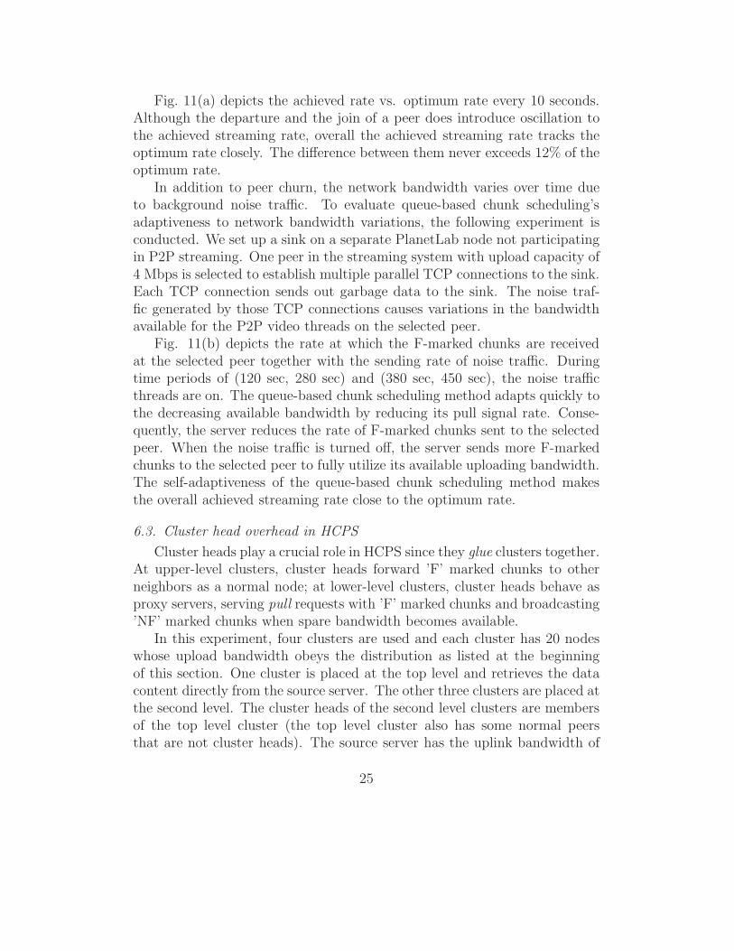
Fig. 11(a) depicts the achieved rate vs. optimum rate every 10 seconds.Although the departure and the join of a peer does introduce oscillation tothe achieved streaming rate, overall the achieved streaming rate tracks theoptimum rate closely. The difference between them never exceeds 12% of theoptimum rate.

In addition to peer churn, the network bandwidth varies over time dueto background noise traffic. To evaluate queue-based chunk scheduling’sadaptiveness to network bandwidth variations, the following experiment isconducted. We set up a sink on a separate PlanetLab node not participatingin P2P streaming. One peer in the streaming system with upload capacity of4 Mbps is selected to establish multiple parallel TCP connections to the sink.Each TCP connection sends out garbage data to the sink. The noise traf-fic generated by those TCP connections causes variations in the bandwidthavailable for the P2P video threads on the selected peer.

Fig. 11(b) depicts the rate at which the F-marked chunks are receivedat the selected peer together with the sending rate of noise traffic. Duringtime periods of (120 sec, 280 sec) and (380 sec, 450 sec), the noise trafficthreads are on. The queue-based chunk scheduling method adapts quickly tothe decreasing available bandwidth by reducing its pull signal rate. Conse-quently, the server reduces the rate of F-marked chunks sent to the selectedpeer. When the noise traffic is turned off, the server sends more F-markedchunks to the selected peer to fully utilize its available uploading bandwidth.The self-adaptiveness of the queue-based chunk scheduling method makesthe overall achieved streaming rate close to the optimum rate.

6.3. Cluster head overhead in HCPS

Cluster heads play a crucial role in HCPS since they glue clusters together.At upper-level clusters, cluster heads forward ’F’ marked chunks to otherneighbors as a normal node; at lower-level clusters, cluster heads behave asproxy servers, serving pull requests with ’F’ marked chunks and broadcasting’NF’ marked chunks when spare bandwidth becomes available.

In this experiment, four clusters are used and each cluster has 20 nodeswhose upload bandwidth obeys the distribution as listed at the beginningof this section. One cluster is placed at the top level and retrieves the datacontent directly from the source server. The other three clusters are placed atthe second level. The cluster heads of the second level clusters are membersof the top level cluster (the top level cluster also has some normal peersthat are not cluster heads). The source server has the uplink bandwidth of

25

4Mbps. The peers in the top level cluster join the system at the beginningof the experiment. The peers in second level clusters join after 20 secondsso that the top-level cluster is at stable state. The experiment lasts for 5minutes. Based on our off-line data analysis, the experiment duration of 300seconds is sufficient since the systems reaches the steady state within tens ofseconds.

320 480 6400

2

4

6

8x 104

Nu

mb

er o

f C

hu

nks

Streaming Video Rate(Kbps)

UPPER F−CHUNKLOWER F−CHUNKLOWER NF−CHUNK

(a) Chunk Distribution of ClusterHead

0 0.5 1 1.5 2 2.50

0.2

0.4

0.6

0.8

1

System Delay(second)

CD

F

1st Level2nd Level3rd Level4th Level

(b) CDF of system delay at differentlevels

300 400 500 600 700 8000

50

100

150

200

250

300

350

400

Streaming rate(kbps)

Ban

dwid

th

C1 Server Resource Poor Region

C1 Server Resource Rich Region

CH1 UpperCH1 LowerCH2 UpperCH2 Lower

(c) Bandwidth usage of cluster headson different levels

Figure 12: Experiment results of HCPS with multiple clusters

Fig. 12(a) shows the total number of chunks transmitted by a clusterhead as the normal peer in upper-level cluster and as the server in lower-levelcluster. Different streaming rates are tested to check their impact. Majorityof cluster head bandwidth has been consumed at the upper level, while thebandwidth allocated to the lower level roughly equals to the streaming rate.The streaming rates of 320 kbps, 480 kbps, and 640 kbps, are smaller thanthe average bandwidth of each cluster. Hence the cluster head only needs

26

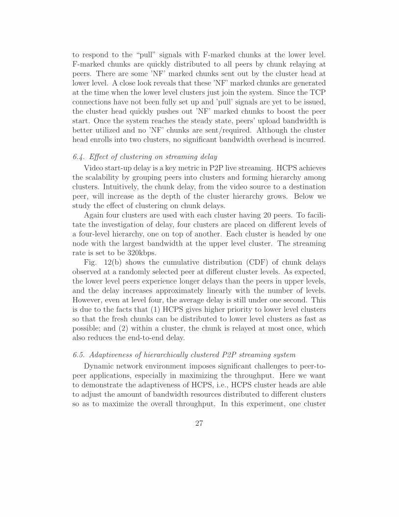
to respond to the “pull” signals with F-marked chunks at the lower level.F-marked chunks are quickly distributed to all peers by chunk relaying atpeers. There are some ’NF’ marked chunks sent out by the cluster head atlower level. A close look reveals that these ’NF’ marked chunks are generatedat the time when the lower level clusters just join the system. Since the TCPconnections have not been fully set up and ’pull’ signals are yet to be issued,the cluster head quickly pushes out ’NF’ marked chunks to boost the peerstart. Once the system reaches the steady state, peers’ upload bandwidth isbetter utilized and no ’NF’ chunks are sent/required. Although the clusterhead enrolls into two clusters, no significant bandwidth overhead is incurred.

6.4. Effect of clustering on streaming delay

Video start-up delay is a key metric in P2P live streaming. HCPS achievesthe scalability by grouping peers into clusters and forming hierarchy amongclusters. Intuitively, the chunk delay, from the video source to a destinationpeer, will increase as the depth of the cluster hierarchy grows. Below westudy the effect of clustering on chunk delays.

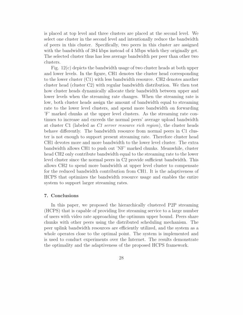
Again four clusters are used with each cluster having 20 peers. To facili-tate the investigation of delay, four clusters are placed on different levels ofa four-level hierarchy, one on top of another. Each cluster is headed by onenode with the largest bandwidth at the upper level cluster. The streamingrate is set to be 320kbps.

Fig. 12(b) shows the cumulative distribution (CDF) of chunk delaysobserved at a randomly selected peer at different cluster levels. As expected,the lower level peers experience longer delays than the peers in upper levels,and the delay increases approximately linearly with the number of levels.However, even at level four, the average delay is still under one second. Thisis due to the facts that (1) HCPS gives higher priority to lower level clustersso that the fresh chunks can be distributed to lower level clusters as fast aspossible; and (2) within a cluster, the chunk is relayed at most once, whichalso reduces the end-to-end delay.

6.5. Adaptiveness of hierarchically clustered P2P streaming system

Dynamic network environment imposes significant challenges to peer-to-peer applications, especially in maximizing the throughput. Here we wantto demonstrate the adaptiveness of HCPS, i.e., HCPS cluster heads are ableto adjust the amount of bandwidth resources distributed to different clustersso as to maximize the overall throughput. In this experiment, one cluster

27

is placed at top level and three clusters are placed at the second level. Weselect one cluster in the second level and intentionally reduce the bandwidthof peers in this cluster. Specifically, two peers in this cluster are assignedwith the bandwidth of 384 kbps instead of 4 Mbps which they originally get.The selected cluster thus has less average bandwidth per peer than other twoclusters.

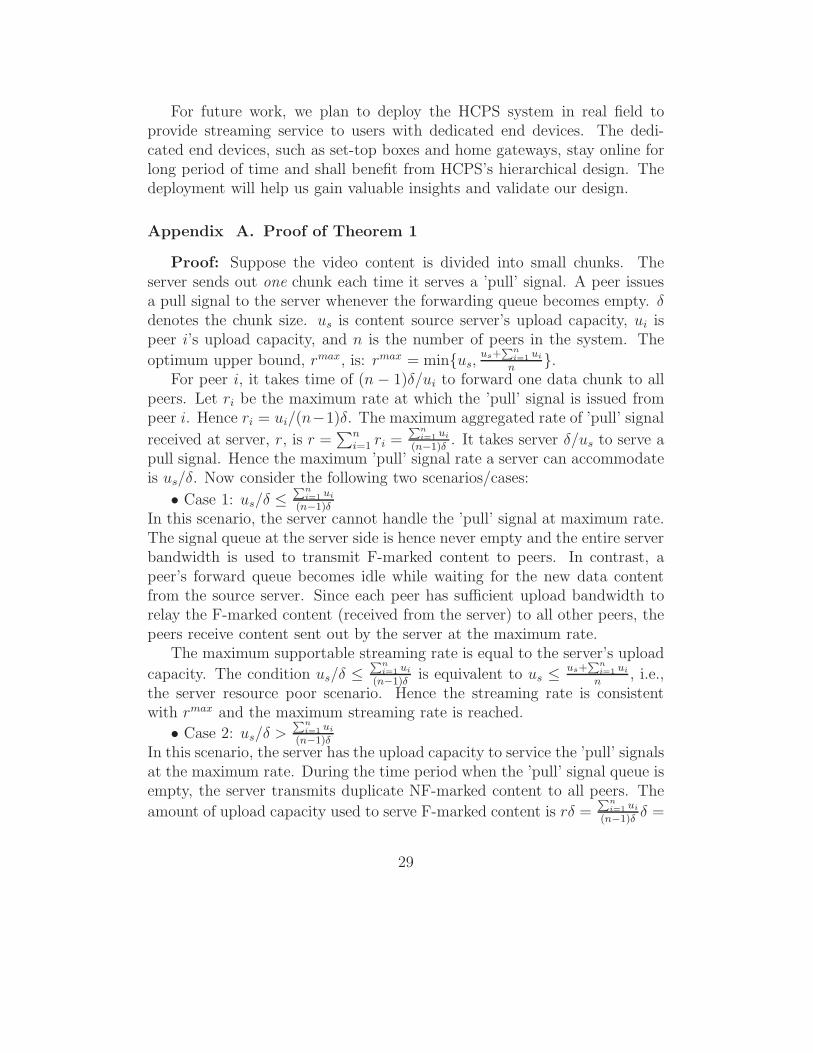
Fig. 12(c) depicts the bandwidth usage of two cluster heads at both upperand lower levels. In the figure, CH1 denotes the cluster head correspondingto the lower cluster (C1) with less bandwidth resource. CH2 denotes anothercluster head (cluster C2) with regular bandwidth distribution. We then testhow cluster heads dynamically allocate their bandwidth between upper andlower levels when the streaming rate changes. When the streaming rate islow, both cluster heads assign the amount of bandwidth equal to streamingrate to the lower level clusters, and spend more bandwidth on forwarding’F’ marked chunks at the upper level clusters. As the streaming rate con-tinues to increase and exceeds the normal peers’ average upload bandwidthat cluster C1 (labeled as C1 server resource rich region), the cluster headsbehave differently. The bandwidth resource from normal peers in C1 clus-ter is not enough to support present streaming rate. Therefore cluster headCH1 devotes more and more bandwidth to the lower level cluster. The extrabandwidth allows CH1 to push out ’NF’ marked chunks. Meanwhile, clusterhead CH2 only contribute bandwidth equal to the streaming rate to the lowerlevel cluster since the normal peers in C2 provide sufficient bandwidth. Thisallows CH2 to spend more bandwidth at upper level cluster to compensatefor the reduced bandwidth contribution from CH1. It is the adaptiveness ofHCPS that optimizes the bandwidth resource usage and enables the entiresystem to support larger streaming rates.

7. Conclusions

In this paper, we proposed the hierarchically clustered P2P streaming(HCPS) that is capable of providing live streaming service to a large numberof users with video rate approaching the optimum upper bound. Peers sharechunks with other peers using the distributed scheduling mechanism. Thepeer uplink bandwidth resources are efficiently utilized, and the system as awhole operates close to the optimal point. The system is implemented andis used to conduct experiments over the Internet. The results demonstratethe optimality and the adaptiveness of the proposed HCPS framework.

28

For future work, we plan to deploy the HCPS system in real field toprovide streaming service to users with dedicated end devices. The dedi-cated end devices, such as set-top boxes and home gateways, stay online forlong period of time and shall benefit from HCPS’s hierarchical design. Thedeployment will help us gain valuable insights and validate our design.

Appendix A. Proof of Theorem 1

Proof: Suppose the video content is divided into small chunks. Theserver sends out one chunk each time it serves a ’pull’ signal. A peer issuesa pull signal to the server whenever the forwarding queue becomes empty. δdenotes the chunk size. us is content source server’s upload capacity, ui ispeer i’s upload capacity, and n is the number of peers in the system. The

optimum upper bound, rmax, is: rmax = min{us,us+

∑ni=1

ui

n}.

For peer i, it takes time of (n − 1)δ/ui to forward one data chunk to allpeers. Let ri be the maximum rate at which the ’pull’ signal is issued frompeer i. Hence ri = ui/(n−1)δ. The maximum aggregated rate of ’pull’ signal

received at server, r, is r =∑n

i=1 ri =∑n

i=1ui

(n−1)δ. It takes server δ/us to serve a

pull signal. Hence the maximum ’pull’ signal rate a server can accommodateis us/δ. Now consider the following two scenarios/cases:

• Case 1: us/δ ≤∑n

i=1ui

(n−1)δ

In this scenario, the server cannot handle the ’pull’ signal at maximum rate.The signal queue at the server side is hence never empty and the entire serverbandwidth is used to transmit F-marked content to peers. In contrast, apeer’s forward queue becomes idle while waiting for the new data contentfrom the source server. Since each peer has sufficient upload bandwidth torelay the F-marked content (received from the server) to all other peers, thepeers receive content sent out by the server at the maximum rate.

The maximum supportable streaming rate is equal to the server’s upload

capacity. The condition us/δ ≤∑n

i=1ui

(n−1)δis equivalent to us ≤

us+∑n

i=1ui

n, i.e.,

the server resource poor scenario. Hence the streaming rate is consistentwith rmax and the maximum streaming rate is reached.

• Case 2: us/δ >∑n

i=1ui

(n−1)δ

In this scenario, the server has the upload capacity to service the ’pull’ signalsat the maximum rate. During the time period when the ’pull’ signal queue isempty, the server transmits duplicate NF-marked content to all peers. The

amount of upload capacity used to serve F-marked content is rδ =∑n

i=1ui

(n−1)δδ =

29

∑ni=1

ui

n−1.

The server’s upload bandwidth used to serve NF-marked content is there-

fore us −∑n

i=1ui

n−1. For each individual peers, the rate of receiving NF-marked

content from server is (us −∑n

i=1ui

n−1)/n since there are n peers in the system.

The streaming rate at peers is:

∑n

i=1 ui

n− 1+ (us −

∑n

i=1 ui

n− 1)/n =

us +∑n

i=1 ui

n. (A.1)

The condition us/δ >∑n

i=1ui

(n−1)δis equivalent to us >

us+∑n

i=1ui

n, i.e., the server

resource rich scenario. Again, the streaming rate reaches rmax. This con-cludes the proof of first claim of theorem.

The proof of second claim is done by contradiction. Denote by by rH

the maximum supportable streaming rate of HCPS, and by rd the maxi-mum steaming rate that can be reached using distributed queue-based chunkscheduling algorithms. Suppose queue-based chunk scheduling algorithmscannot support the maximum supportable streaming rate, rd < rH. Hencethere is at least one cluster in HCPS, say cluster k, whose streaming rate,(rmax

k )d, is less than rH, i.e., (rmaxk )d < rH. Let (rmax

k )∗ be cluster d’s stream-ing rate when achiving maximum supportable streaming rate rH. rH ≤(rmax

k )∗, thus (rmaxk )d < (rmax

k )∗.Denote by (uti

i )∗, (uhi

i )∗, and (usc)

∗ the optimal bandwidth allocation thatachieves maximum supportable streaming rate of rH. According to Eqn. (3),

(rmaxk )∗ = min

{

∑

∀i,ti∈Vk(uti

i )∗ +

∑

∀i,hi∈Vk(uhi

i )∗

|Vk|,

∑

∀i,hi∈Vk

(uhi

i )∗ + (usc)

∗}

(A.2)Further denote by (uti

i )d, (uhi

i )d, and (usc)

d the bandwidth allocation in dis-tributed queue-based chunk scheduling algorithms. According to the firstclaim, queue-based chunk scheduling in one cluster can achieve the optimumupper bound. Thus

(rmaxk )d = min

{

∑

∀i,ti∈Vk(uti

i )d +

∑

∀i,hi∈Vk(uhi

i )d

|Vk|,

∑

∀i,hi∈Vk

(uhi

i )d + (us

c)d}

(A.3)

30

Therefore:

min{

∑∀i,ti∈Vk

(utii )d+

∑∀i,hi∈Vk

(uhii )d

|Vk|,

∑

∀i,hi∈Vk(uhi

i )d + (usc)

d}

< min{

∑∀i,ti∈Vk

(utii )∗+

∑∀i,hi∈Vk

(uhii )∗

|Vk|,

∑

∀i,hi∈Vk(uhi

i )∗ + (usc)

∗}

.(A.4)

Now we argue that Eqn. (A.4) does not hold. Normal peers in cluster k de-vote their entire upload bandwidth solely to cluster k. Hence they are equalat both sides of Eqn. (A.4). For cluster heads that are normal peers in clus-ter k and are cluster heads in other clusters, they will be able to devote equalor more upload bandwidth to cluster k in HCPS. These peers use equal/lessbandwidth in the clusters they head due to the fact rd < rH. Finally, thecluster head of cluster k in HCPS is able to contribute as much bandwidthas in optimal solution. Hence the inequality in Eqn. (A.4) does not hold,which leads to the contradiction and concludes the proof.

Note that in case 2 where the aggregate ’pull’ signal arrival rate is smallerthan the server’s service rate, it is assumed that the peers receive F-markedcontent immediately after issuing the ’pull’ signal. The above assumption istrue only if the ’pull’ signal does not encounter any queuing delay and canbe serviced immediately by the content source server. This means that (i)no two ’pull’ signals arrive at the exact same time and (ii) a ’pull’ signal canbe serviced before the arrival of next incoming ’pull’ signal. Assumption (i)is commonly used in queuing theory and is reasonable since a P2P systemis a distributed system with respect to peers generating ’pull’ signals. Theprobability that two ’pull’ signals arrive at exactly the same time is low.Assumption (ii) means that the data can be transmitted in arbitrary smallamounts, i.e., the size of data chunk, δ, can be arbitrarily small. In practice,the size of data chunks is limited in order to reduce the overhead associatedwith data transfers.

References

[1] X. Zhang, J. Liu, B. Li, and T.-S. P. Yum, “DONet/CoolStreaming: Adata-driven overlay network for live media streaming,” in Proceedings ofIEEE INFOCOM, 2005.

[2] PPLive, “PPLive Homepage,” http://www.pplive.com.

31

[3] SopCast, “SopCast Homepage,” http://www.sopcast.org.

[4] R. Kumar, Y. Liu, and K. Ross, “Stochastic fluid theory for p2p stream-ing systems,” in Proceedings of IEEE INFOCOM, 2007.

[5] C. Liang, Y. Guo, and Y. Liu, “Is random scheduling enough for p2plive streaming?” in IEEE ICDCS, 2008.

[6] N. Magharei and R. Rejaie, “PRIME: Peer-to-Peer Receiver-drIvenMEsh-based Streaming,” in IEEE/ACM Transactions on Networking,vol. 17, no. 4, August 2007.

[7] L. Massoulie, A. Twigg, C. Gkantsidis, and P. Rodriguez, “Randomizeddecentralized broadcasting algorithms,” in Proceedings of IEEE INFO-COM, 2007.

[8] T. Bonald, L. Massouli, F. Mathieu, D. Perino, and A. Twigg, “Epidemiclive streaming: optimal performance trade-offs,” in Proceedings of ACMSIGMETRICS, 2008.

[9] PlanetLab, “PlanetLab Homepage,” http://www.planet-lab.org.

[10] BT, “Bittorent Homepage,” http://www.bittorrent.com.

[11] unkown, “Skype webpage,” http://www.skype.com/.

[12] Y.-H. Chu, S. G.Rao, and H. Zhang, “A case for end system multicast,”in Proceedings of ACM SIGMETRICS, 2000.

[13] N. Magharei, R. Rejaie, and Y. Guo, “Mesh or Multiple-Tree: A Com-parative Study of Live P2P Streaming Approaches,” in Proceedings ofIEEE INFOCOM, 2007.

[14] X. Hei, Y. Liu, and K. Ross, “Inferring Network-Wide Quality in P2PLive Streaming Systems,” IEEE Journal on Selected Areas in Commu-nications, the special issue on advances in P2P streaming, 2008.

[15] X. Hei, C. Liang, J. Liang, Y. Liu, and K. Ross, “A Measurement Studyof a Large-Scale P2P IPTV System,” IEEE Transactions on Multimedia,November 2007.

32

[16] M. Wang and B. Li, “Lava: A reality check of network coding in peer-to-peer live streaming,” in Proceedings of IEEE INFOCOM, 2007.

[17] ——, “R2: Random push with random network coding in live peer-to-peer streaming,” in IEEE Journal on Selected Areas in Communications,Special Issue on Advances in Peer-to-Peer Streaming Systems, vol. 25,no. 9, December 2007.

[18] M. Zhang, Q. Zhang, L. Sun, and S. Yang, “Understanding the Powerof Pull-based Streaming Protocol: Can We Do Better?” IEEE Journalon Selected Areas in Communications, 2007.

[19] A. Amis, R. Prakash, D. Huynh, and T. Vuong, “Max-min d-cluster for-mation in wireless ad hoc networks,” in Proceedings of IEEE INFOCOM,2000.

[20] O. Younis and S. Fahmy, “Distributed clustering in ad-hoc sensor net-works: a hybrid, energy-efficient approach,” in Proceedings of IEEE IN-FOCOM, 2004.

[21] M. Zhao and Y. Yang, “A framework for mobile data gathering withload balanced clustering and MIMO uploading,” in Proceedings of IEEEINFOCOM, 2011.

[22] S. Banerjee, B. Bhattacharjee, and C. Kommareddy, “Scalable Applica-tion Layer Multicast,” in Proceedings of ACM SIGCOMM, 2002.

[23] C. H. Ashwin R. Bharambe and V. N. Padmanabhan, “Analyzing andImproving a BitTorrent Network Performance Mechanisms,” in Proceed-ings of IEEE INFOCOM, 2006.

[24] Trickle, “Trickle Homepage,” http://monkey.org/∼marius/pages/?page=trickle.

33