Hierarchical Simulation of Multiple-Facies Reservoirs

HIERARCHICAL SIMULATION OF

MULTIPLE-FACIES RESERVOIRS USING

MULTIPLE-POINT GEOSTATISTICS

A REPORT

SUBMITTED TO THE DEPARTMENT OF PETROLEUM

ENGINEERING

OF STANFORD UNIVERSITY

IN PARTIAL FULFILLMENT OF THE REQUIREMENTS

FOR THE DEGREE OF

MASTER OF SCIENCE

By

Amisha Maharaja

June 2004

I certify that I have read this report and that in my

opinion it is fully adequate, in scope and in quality, as

partial fulfillment of the degree of Master of Science in

Petroleum Engineering.

Andre Journel(Principal advisor)

ii

Abstract

Joint simulation with presently available multiple-point geostatistical simulation al-

gorithms leads to poor shape reproduction as the number of facies increases. This is

because the training image (Ti) cannot depict with enough replicates all alternative

patterns that can be found. Moreover, the size of the Ti itself and that of the tem-

plate required to capture large-scale structures in the Ti is limited due to memory

restriction, especially in 3D.

Hierarchical simulation of facies with distinct shapes and spatial continuity is

proposed to overcome the disadvantages of joint simulation. The idea is to iden-

tify a hierarchy of deposition within the reservoir using geologic rules of deposition

and simulate the facies accordingly. This amounts to first simulating the large-scale

structures and then simulating smaller structures conditional to the pre-simulated

large-scale structures. The hierarchical approach is demonstrated using synthetic 2D

and 3D meandering fluvial reservoirs and the results are compared with that of joint

simulation. Finally, the hierarchical simulation techinique is applied to a real life

dense data set from the Rhine-Meuse delta.

The advantage of hierarchical approach is better reproduction of large-scale struc-

tures by reducing the size of the Ti and the number of facies being simulated si-

multaneously. Most of the memory demand during mp-simulation comes from the

size of the search-tree, which in turn depends on the size of the Ti, the size of the

data template, and the number of facies in the Ti. Large-scale structures require a

bigger template to capture them, however that increases the size of the search tree.

In hierarchical simulation, the increase in the size of the search tree due to a larger

template is compensated by the reduction in the number of facies being simulated

simultaneously. Once the large-scale structures are simulated the smaller structures

iii

are simulated conditioned to the former. The Ti for simulating the small-scale fea-

tures need not be very large and rich, thereby further reducing the size of search tree.

The hierarchical approach is geologically sound because the sequence of simulations

follows the natural sequence of deposition.

iv

Acknowledgements

v

Contents

Abstract iii

Acknowledgements v

Table of Contents vi

List of Tables viii

List of Figures ix

1 Introduction 1

2 Joint Simulation 5

2.1 Comments . . . . . . . . . . . . . . . . . . . . . . . . . . . . . . . . . 6

3 Hierarchical Simulation 12

3.1 Hierarchical simulation of three facies . . . . . . . . . . . . . . . . . . 12

3.1.1 Comments . . . . . . . . . . . . . . . . . . . . . . . . . . . . . 12

3.2 Hierarchical simulation of four facies . . . . . . . . . . . . . . . . . . 13

3.2.1 Two-step cookie-cut simulation method . . . . . . . . . . . . . 13

3.2.2 Three-step hierarchical simulation method . . . . . . . . . . . 15

3.2.3 Two-step hierarchical simulation method . . . . . . . . . . . 15

3.3 3D Example . . . . . . . . . . . . . . . . . . . . . . . . . . . . . . . . 16

4 Implementation of hierarchical simulation 27

vi

5 Rhine-Meuse Delta Case Study 29

5.1 Introduction to the Data Set . . . . . . . . . . . . . . . . . . . . . . . 29

5.2 Results and Discussion . . . . . . . . . . . . . . . . . . . . . . . . . . 29

6 Conclusions and Future Work 30

6.1 Conclusions . . . . . . . . . . . . . . . . . . . . . . . . . . . . . . . . 30

6.2 Future work . . . . . . . . . . . . . . . . . . . . . . . . . . . . . . . . 31

References 32

vii

List of Tables

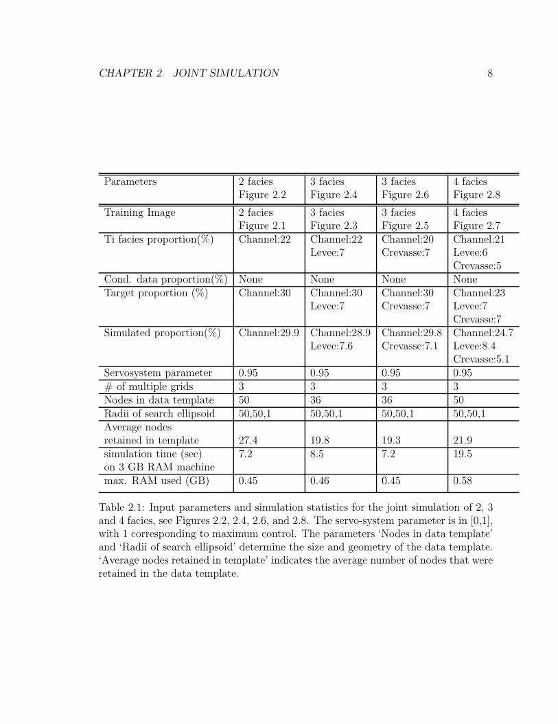
2.1 Input parameters and simulation statistics for the joint simulation of

2, 3 and 4 facies, see Figures 2.2, 2.4, 2.6, and 2.8. The servo-system

parameter is in [0,1], with 1 corresponding to maximum control. The

parameters ‘Nodes in data template’ and ‘Radii of search ellipsoid’

determine the size and geometry of the data template. ‘Average nodes

retained in template’ indicates the average number of nodes that were

retained in the data template. . . . . . . . . . . . . . . . . . . . . . . 8

3.1 Input parameters and simulation statistics for the Two-step cookie-cut

approach . . . . . . . . . . . . . . . . . . . . . . . . . . . . . . . . . . 14

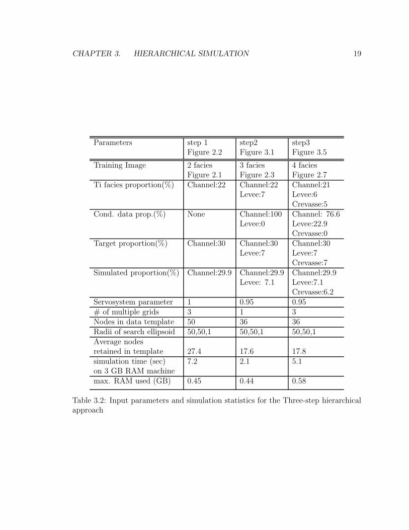
3.2 Input parameters and simulation statistics for the Three-step hierar-

chical approach . . . . . . . . . . . . . . . . . . . . . . . . . . . . . . 19

3.3 Input parameters and simulation statistics for the Two-step hierarchi-

cal approach . . . . . . . . . . . . . . . . . . . . . . . . . . . . . . . . 20

viii

List of Figures

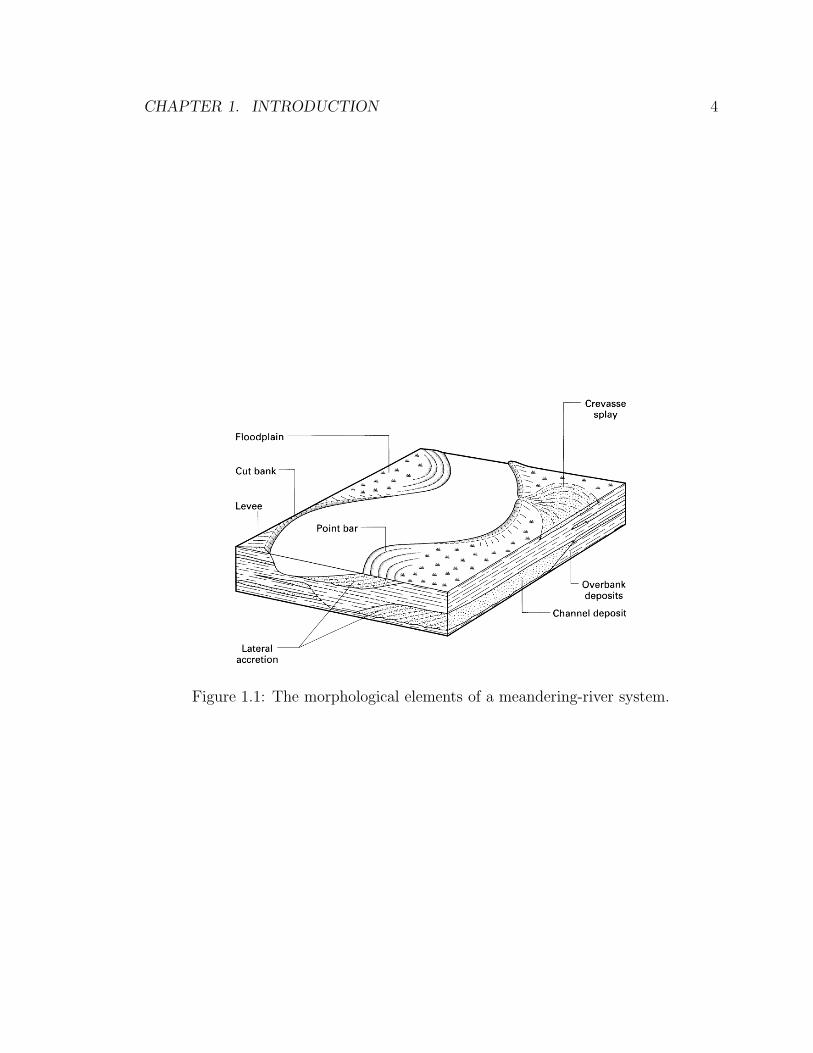
1.1 The morphological elements of a meandering-river system. . . . . . . 4

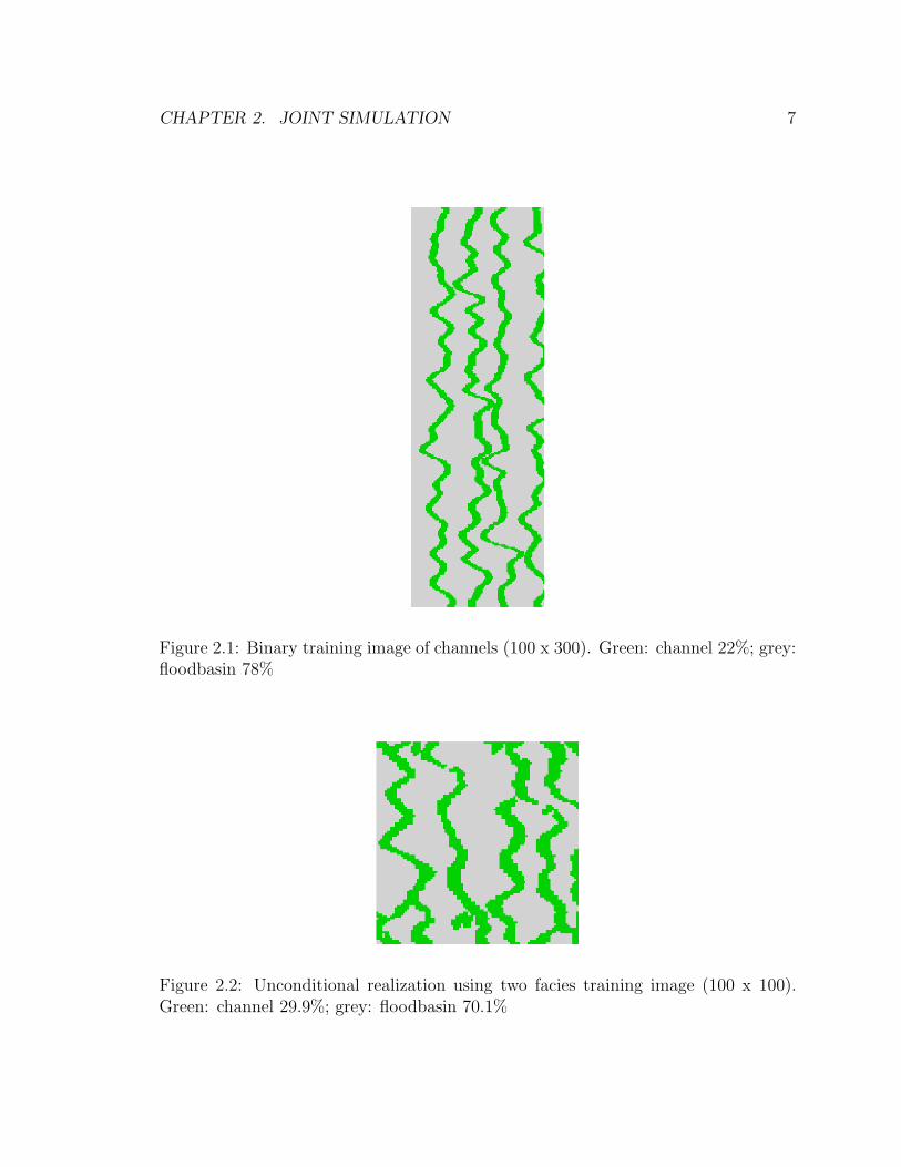
2.1 Binary training image of channels (100 x 300). Green: channel 22%;

grey: floodbasin 78% . . . . . . . . . . . . . . . . . . . . . . . . . . . 7

2.2 Unconditional realization using two facies training image (100 x 100).

Green: channel 29.9%; grey: floodbasin 70.1% . . . . . . . . . . . . . 7

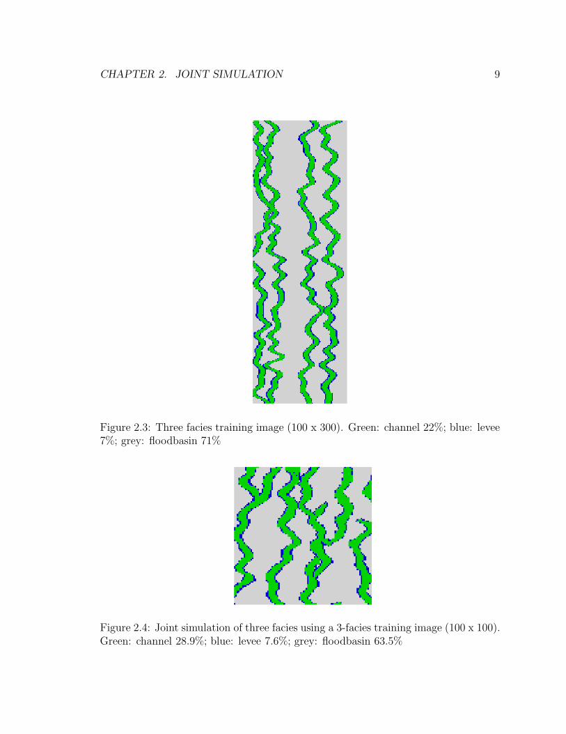
2.3 Three facies training image (100 x 300). Green: channel 22%; blue:

levee 7%; grey: floodbasin 71% . . . . . . . . . . . . . . . . . . . . . 9

2.4 Joint simulation of three facies using a 3-facies training image (100 x

100). Green: channel 28.9%; blue: levee 7.6%; grey: floodbasin 63.5% 9

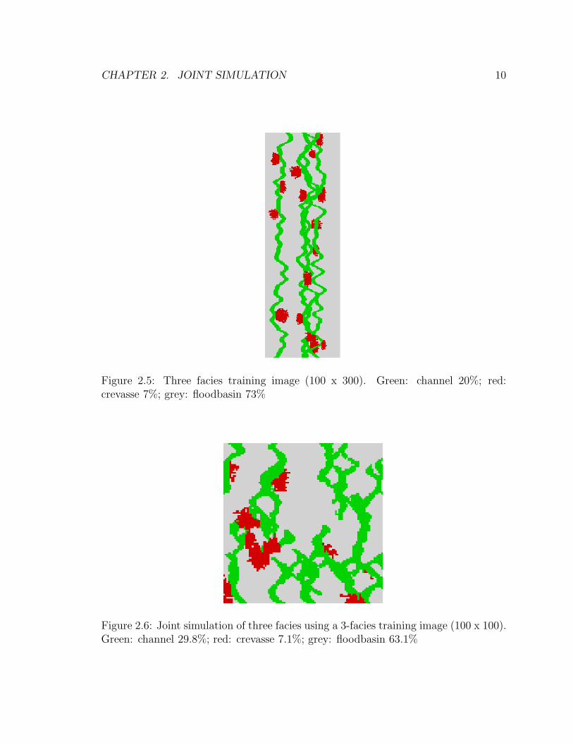
2.5 Three facies training image (100 x 300). Green: channel 20%; red:

crevasse 7%; grey: floodbasin 73% . . . . . . . . . . . . . . . . . . . . 10

2.6 Joint simulation of three facies using a 3-facies training image (100 x

100). Green: channel 29.8%; red: crevasse 7.1%; grey: floodbasin 63.1% 10

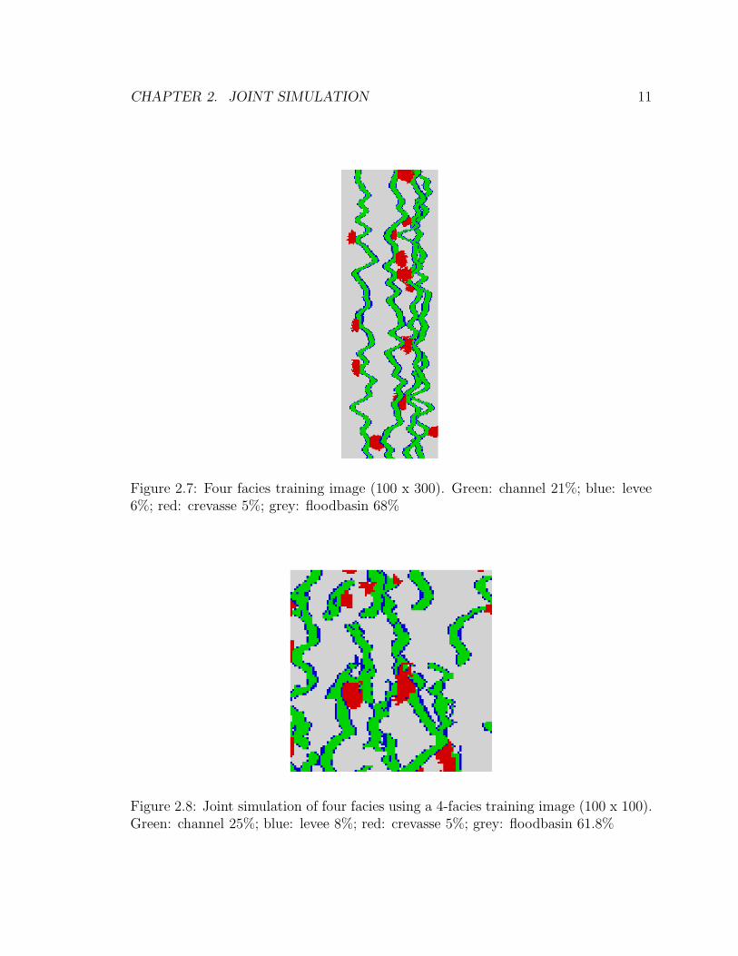
2.7 Four facies training image (100 x 300). Green: channel 21%; blue:

levee 6%; red: crevasse 5%; grey: floodbasin 68% . . . . . . . . . . . 11

2.8 Joint simulation of four facies using a 4-facies training image (100 x

100). Green: channel 25%; blue: levee 8%; red: crevasse 5%; grey:

floodbasin 61.8% . . . . . . . . . . . . . . . . . . . . . . . . . . . . . 11

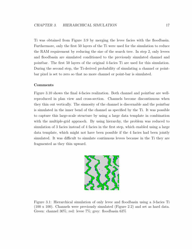
3.1 Hierarchical simulation of only levee and floodbasin using a 3-facies Ti

(100 x 100). Channels were previously simulated (Figure 2.2) and set

as hard data. Green: channel 30%; red: levee 7%; grey: floodbasin 63% 17

ix

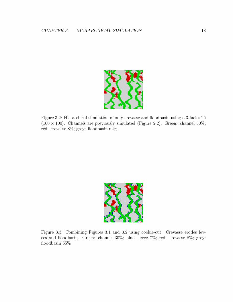
3.2 Hierarchical simulation of only crevasse and floodbasin using a 3-facies

Ti (100 x 100). Channels are previously simulated (Figure 2.2). Green:

channel 30%; red: crevasse 8%; grey: floodbasin 62% . . . . . . . . . 18

3.3 Combining Figures 3.1 and 3.2 using cookie-cut. Crevasse erodes levees

and floodbasin. Green: channel 30%; blue: levee 7%; red: crevasse 8%;

grey: floodbasin 55% . . . . . . . . . . . . . . . . . . . . . . . . . . . 18

3.4 Flowchart for two-step cookie-cut simulation method . . . . . . . . . 21

3.5 Step 3 of three-step method: Simulation of only crevasse and floodbasin

using a 4-facies Ti. The channels were simulated in step 1 (Figure 2.2)

and levees were simulated in step 2 (Figure 3.1) and set as hard data.

Simulated facies proportions:- Green: channel 30%; blue: levee 7%;

red: crevasse 6%; grey: floodbasin 57% . . . . . . . . . . . . . . . . . 22

3.6 Flowchart for three-step hierarchical simulation method . . . . . . . . 22

3.7 Step 2 of two-step hierarchical simulation method. Simulation of crevasse

and floodbasin using 4-facies Ti. The channel and levee have been pre-

viously simulated in step 1 and set as hard data (Figure 2.4). Simu-

lated facies proportions: Green: channel 28.9%; blue: levee 7.6%; red:

crevasse 6.4%; white: floodbasin 57% . . . . . . . . . . . . . . . . . . 23

3.8 Flowchart for two-step hierarchical simulation method . . . . . . . . . 24

3.9 Four facies training image (100 x 100 x 100). Green: channel 25%;

blue: pointbar 4%; red: levee 2%; grey: floodbasin 69% . . . . . . . . 25

3.10 Hierarchical simulation of channel, pointbar, levee and floodbasin (100

x 100 x 100). Green: channel 28%; blue: pointbar 5%; red: levee 4%;

grey: floodbasin 63% . . . . . . . . . . . . . . . . . . . . . . . . . . . 26

x

Chapter 1

Introduction

Stochastic simulation is widely used for generating heterogeneous reservoir models.

Traditional variogram-based simulation methods utilize the correlation between only

two points at a time and therefore cannot simulate curvilinear structures. Exam-

ples are SGS and SIS methods. Multiple-point geostatistical simulation techniques

consider the relation between three or more points taken together and are able to

reproduce curvilinear structures and account for complex patterns between the vari-

ables being simulated.

The pros and cons of various methods that utilize multiple-point geostatistics is

discussed in Strebelle (2000). Boolean object-based methods can reproduce the curvi-

linear geometries but are difficult to condition to dense data. Pixel-based methods are

easier to condition to dense data from different sources. Simulated annealing, MCMC

simulation and similar algorithms are pixel-based but iterative techniques and their

rate of convergence is not known a priori.

The first non-iterative multiple-point algorithm was suggested by Guardiano and

Srivastava (1993) in which mp-statistics were obtained directly by scanning a train-

ing image (Ti). However, the algorithm was extremely CPU demanding because

the entire Ti had to be scanned completely at each unsampled node to obtain con-

ditional probability distribution for that node. Strebelle (2000, 2002) proposed an

1

CHAPTER 1. INTRODUCTION 2

algorithm snesim which was based on the idea of Guardiano and Srivastava of deriv-

ing probabilities directly from a Ti, however, it required scanning the Ti only once

and cataloguing the conditional probabilities using a dynamic data structure called

search-tree. The snesim algorithm is pixel-based, non-iterative, and general so that

any random geometry can be accomodated.

The size of the search-tree depends on three factors

• Size of the training image

• Size of the data template used to scan the training image

• Total number of facies in the training image

Consider a categorical variable Z(u) valued in 1, . . . , K. Let NTI be the total

number of locations in the Ti. Since for a given data event size j, there can not be

more than NTI different data events in the Ti, a (crude) upper-bound of the memory

demand of the search tree is:

Memory Demand ≤J∑

j=1

min(Kj , NTI)

Hydrocarbon reservoirs often consist of multiple facies with different shapes and

sizes. For example, a meandering fluvial system typically contains channels, point-

bars, levees, crevasse splays and floodbasin (Figure 1.1). Note that the geologic

definition of facies is “Accumulation of deposits that exhibits specific characteristics

and grades laterally into other sedimentary accumulations that were formed at the

same time but exhibit different characteristics (Leet, 1982).” In this paper, the term

‘facies’ refers to the morphological elements of a depositional system that have a dis-

tinct shape.

The shapes and proportions of these different facies vary greatly from one fluvial

system to another. Moreover, the facies are related to each other by some definite

geologic rules, for example, crevasse splays must be attached to channel belt. In mp-

simulation, the shapes, relative proportions and the spatial dependence between the


different facies is conveyed through a Ti. Fluvial systems tend to be very complex,

hence a large and rich Ti is required if all the facies are simulated jointly, which can

be very memory demanding. Instead of simulating all the facies jointly, they can

be simulated sequentially. Strebelle (2000) proposed a hierarchical method for sim-

ulating four fluvial facies namely, channels, levees, crevasse splays, and floodbasin.

However, the specific hierarchy used to simulate the facies and the manner in which

the hierarchy was implemented is different from the implementation presented in this

report, see Chapter 4 for details. The hierarchy used here is based on geologic rules

of deposition of the facies, see Chapter 3

Once the shapes of the facies are simulated with the correct proportion and spatial

arrangement, sand and mud with varying net-to-gross can be simulated within each

facies using traditional variogram based algorithms such as SGS. This is similar to

first simulating the different containers and then their specific contents. The net-to-

gross ratio, defined as the percentage of sand, is generally highest in the channels,

followed by the crevasse splays and levees. Floodbasin contains the largest volume of

fine sediments in the fluvial system.

Because this is a pixel-based stochastic simulation, conditioning to dense data of

various support sizes is easier. Moreover, a measure of uncertainty can be attained by

simulating multiple realizations using the same Ti, or by using multiple realizations

of several Tis depicting alternative plausible geological scenarios.

Chapter 2 shows results of joint simulation of two, three and four facies reservoirs.

Hierarchical simulation of three and four facies reservoirs is introduced in Chapter

3. Three alternative approaches are discussed for the 2D reservoir and the results

are compared with that of joint simulation. Finally, a 3D example is presented. The

implementation of hierarchical simulation in the snesim algorithm is discussed in

Chapter 4. The Rhine-Meuse delta case-study is presented in Chapter 5. Conclusions

and recommendations for future work are presented in Chapter 6.


Figure 1.1: The morphological elements of a meandering-river system.

Chapter 2

Joint Simulation

To perform joint simulation of multiple facies, all the facies must be provided in the Ti

exhibiting the proper relationship between these facies. The proportion of the facies

in the Ti need not be equal to the desired simulated proportions as the latter propor-

tions can be controlled by a servo-system. Fluvial systems can be quite complicated

because facies of different shapes and sizes are involved, hence it is desirable to use a

Ti that is larger than the size of the simulation grid to provide enough replicates of any

particular pattern or structure. This comes at a cost of larger RAM memory demand.

A binary training image consisting of channel and floodbasin (Figure 2.1) is used

to simulate the realization shown in Figure 2.2. All the training images in this paper

have been generated using the fluvsim algorithm developed by Deutsch and Tran

(2002). It is important that the Ti provides the correct channel attributes such as,

width, thickness, and sinuosity, to get the desired results. These attributes can be

obtained directly from seismic amplitude maps, outcrop analogues or inferred from

well data (Bridge and Tye, 2000). Moreover, in order to simulate long, thin, contin-

uous channels, it is important to provide a large Ti. In this case, the Ti is 100 x 300

pixels, while the simulation grid is 100 x 100 pixels.

The 3 facies channel, levee, and floodbasin are jointly simulated (Figure 2.4) us-

ing a 3-facies channel-levee-floodbasin Ti (Figure 2.3). Similarly, channel, crevasse,

and floodbasin are jointly simulated (Figure 2.6) using the corresponding 3-facies

5

CHAPTER 2. JOINT SIMULATION 6

channel-crevasse-floodbasin Ti (Figure 2.5). Finally, all four facies are jointly simu-

lated (Figure 2.8) using a 4-facies Ti (Figure 2.7).

2.1 Comments

Table 2.1 summarizes the input parameters and simulation statistics for the joint

simulation approach. The poor quality of results from joint simulation of more than

two facies is evident from the examples in Figures 2.4, 2.6, and 2.8. The complexity

of the Ti in Figure 2.5 is greater than that in Figure 2.3 because the crevasse splays

have a distinctly different shape than the channels. The crevasse splays of Figure 2.5

are discontinuous, fan-like bodies, while the levees of Figure 2.3 are fairly continuous

facies that border the channels with the same elongated rectangular shape. Hence,

the joint simulation of a channel-levee-floodbasin system (Figure 2.4) gives better

results than that of a channel-crevasse-floodbasin system (Figure 2.6).

Since the Ti is three times as long as the simulation grid, the simulated channels

and levees of Figure 2.4 are reasonably continuous. Moreover, the levees and crevasse

splays are simulated close to the channels as specified by the training images. The

servo-system has been enforced, hence the target facies proportions are correctly re-

produced, see Table 2.1. The shape of the crevasse splays is adequately reproduced

in both Figures 2.6 and 2.8.

When the four-facies are simulated jointly (Figure 2.8), the results are much poorer

as the complexity of the Ti has increased considerably. The quality of results can be

improved by using a much larger Ti as the variety of patterns found in the Ti as well

as their number of replicates would increase, however for the same reason the size

of the search tree and hence the RAM demand will increase. Moreover, to ensure a

good reproduction of the large scale features a large data template is required, which

in case of 3 or more facies quickly leads to a large RAM demand, especially in 3D.

Multiple-grid simulation approach (Tran, 1994) has been proposed as a work-around

for simulating large-scale structure, however, a larger template size is still desirable.


Figure 2.1: Binary training image of channels (100 x 300). Green: channel 22%; grey:floodbasin 78%

Figure 2.2: Unconditional realization using two facies training image (100 x 100).Green: channel 29.9%; grey: floodbasin 70.1%


Parameters 2 facies 3 facies 3 facies 4 faciesFigure 2.2 Figure 2.4 Figure 2.6 Figure 2.8

Training Image 2 facies 3 facies 3 facies 4 faciesFigure 2.1 Figure 2.3 Figure 2.5 Figure 2.7

Ti facies proportion(%) Channel:22 Channel:22 Channel:20 Channel:21Levee:7 Crevasse:7 Levee:6

Crevasse:5Cond. data proportion(%) None None None NoneTarget proportion (%) Channel:30 Channel:30 Channel:30 Channel:23

Levee:7 Crevasse:7 Levee:7Crevasse:7

Simulated proportion(%) Channel:29.9 Channel:28.9 Channel:29.8 Channel:24.7Levee:7.6 Crevasse:7.1 Levee:8.4

Crevasse:5.1Servosystem parameter 0.95 0.95 0.95 0.95# of multiple grids 3 3 3 3Nodes in data template 50 36 36 50Radii of search ellipsoid 50,50,1 50,50,1 50,50,1 50,50,1Average nodesretained in template 27.4 19.8 19.3 21.9simulation time (sec) 7.2 8.5 7.2 19.5on 3 GB RAM machinemax. RAM used (GB) 0.45 0.46 0.45 0.58

Table 2.1: Input parameters and simulation statistics for the joint simulation of 2, 3and 4 facies, see Figures 2.2, 2.4, 2.6, and 2.8. The servo-system parameter is in [0,1],with 1 corresponding to maximum control. The parameters ‘Nodes in data template’and ‘Radii of search ellipsoid’ determine the size and geometry of the data template.‘Average nodes retained in template’ indicates the average number of nodes that wereretained in the data template.


Figure 2.3: Three facies training image (100 x 300). Green: channel 22%; blue: levee7%; grey: floodbasin 71%

Figure 2.4: Joint simulation of three facies using a 3-facies training image (100 x 100).Green: channel 28.9%; blue: levee 7.6%; grey: floodbasin 63.5%


Figure 2.5: Three facies training image (100 x 300). Green: channel 20%; red:crevasse 7%; grey: floodbasin 73%

Figure 2.6: Joint simulation of three facies using a 3-facies training image (100 x 100).Green: channel 29.8%; red: crevasse 7.1%; grey: floodbasin 63.1%


Figure 2.7: Four facies training image (100 x 300). Green: channel 21%; blue: levee6%; red: crevasse 5%; grey: floodbasin 68%

Figure 2.8: Joint simulation of four facies using a 4-facies training image (100 x 100).Green: channel 25%; blue: levee 8%; red: crevasse 5%; grey: floodbasin 61.8%

Chapter 3

Hierarchical Simulation

3.1 Hierarchical simulation of three facies

The hierarchical simulation of 3 facies is done in two steps. The first step is joint

simulation of channel and floodbasin facies using the binary Ti shown in Figure 2.1.

The simulated channel pixels (Figure 2.2) are frozen as hard data. In the second

step, the channel-levee-floodbasin Ti (Figure 2.3) and channel-crevasse-floodbasin Ti

(Figure 2.6) are used to generate Figures 3.1 and 3.2 respectively. During the second

step, the Ti-derived probability of simulating a channel pixel is set to zero so that no

more channel is simulated. The servo-system correction is applied at both steps to

ensure reproduction of the target proportions.

3.1.1 Comments

Figure 3.1 indicates a poor reproduction of the elongated shape of the levees, while

Figure 3.2 shows a good reproduction of the crevasse shape. The channels are continu-

ous as they were simulated with a large binary Ti and a large template independently

of the crevasse and levees. Both crevasse and levees are attached to the channels in

spite of having been simulated independently of the channels, however, some isolated

levee pixels are found in Figure 3.1. It is recommended that sequential simulation

proceeds over a single grid for the hierarchical simulation of levee so that isolated

levee pixels are minimized. Indeed, in the multiple-grid approach, the hard data are

12

CHAPTER 3. HIERARCHICAL SIMULATION 13

relocated to the nearest grid node, which combined with the dropping of nodes in the

data template can cause levees to be simulated in the floodbasin detached from the

channels.

3.2 Hierarchical simulation of four facies

In the case of 4 facies, the hierarchical simulation can be done in three ways. In

all three hierarchical approaches the natural sequence of development of the fluvial

facies is adhered to, which is as follows: The main channel belt forms prior to levees

and crevasse splays and all sediments are deposited inside the channel belt, hence in

the first two hierarchical approaches the channels are simulated prior to levees and

crevasse. When excessive sediments are supplied, they cannot be contained within the

channel belt and they spill over to form levees and floodbasin deposits. Consequently,

in the first two approaches levee is simulated after channel, while in the last approach

it is simulated jointly with channel. If the channel has a high sinuosity, the levees can

be breached and crevasse splays are formed adjacent to the channel belt, hence in all

three approaches, crevasse is simulated last.

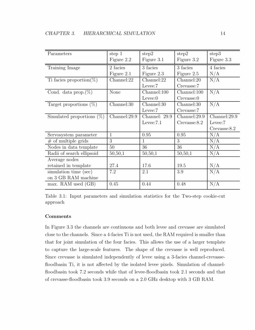
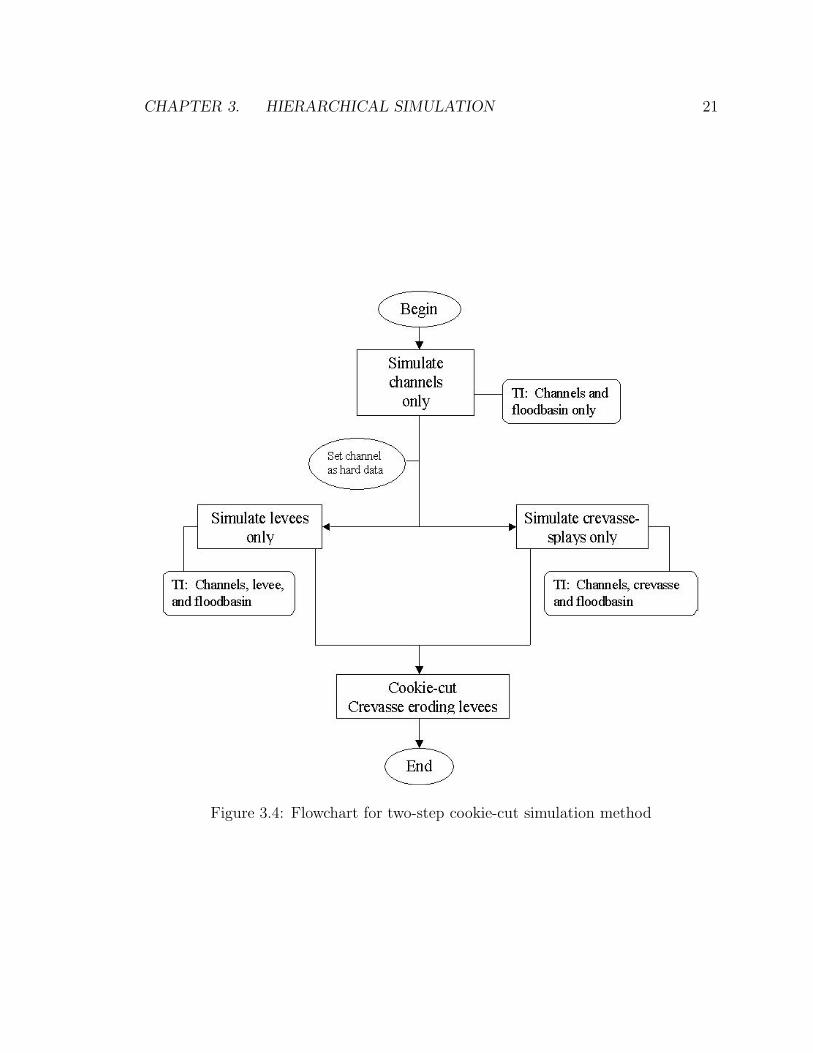
3.2.1 Two-step cookie-cut simulation method

In this method, a 4-facies training image is not needed. The results from hierarchical

simulation of channel-levee-floodbasin (Figure 3.1) and channel-crevasse-floodbasin

(Figure 3.2) are cookie-cut one onto the other such that the crevasse erodes the levee:

this results in a simulated 4-facies image (Figure 3.3). This approach is geologically

correct because the crevasse splays form by breaching the natural levees. After cookie-

cut the proportion of the levee will be lower because some of the levee pixels are

replaced by crevasse pixels. The flowchart in Figure 3.4 summarizes the simulation

procedure and Table 3.1 summarizes the input parameters and simulation statistics

for this method.


Parameters step 1 step2 step2 step3Figure 2.2 Figure 3.1 Figure 3.2 Figure 3.3

Training Image 2 facies 3 facies 3 facies 4 faciesFigure 2.1 Figure 2.3 Figure 2.5 N/A

Ti facies proportion(%) Channel:22 Channel:22 Channel:20 N/ALevee:7 Crevasse:7

Cond. data prop.(%) None Channel:100 Channel:100 N/ALevee:0 Crevasse:0

Target proportions (%) Channel:30 Channel:30 Channel:30 N/ALevee:7 Crevasse:7

Simulated proportions (%) Channel:29.9 Channel: 29.9 Channel:29.9 Channel:29.9Levee:7.1 Crevasse:8.2 Levee:7

Crevasse:8.2Servosystem parameter 1 0.95 0.95 N/A# of multiple grids 3 1 3 N/ANodes in data template 50 36 36 N/ARadii of search ellipsoid 50,50,1 50,50,1 50,50,1 N/AAverage nodesretained in template 27.4 17.6 19.5 N/Asimulation time (sec) 7.2 2.1 3.9 N/Aon 3 GB RAM machinemax. RAM used (GB) 0.45 0.44 0.48 N/A

Table 3.1: Input parameters and simulation statistics for the Two-step cookie-cutapproach

Comments

In Figure 3.3 the channels are continuous and both levee and crevasse are simulated

close to the channels. Since a 4-facies Ti is not used, the RAM required is smaller than

that for joint simulation of the four facies. This allows the use of a larger template

to capture the large-scale features. The shape of the crevasse is well reproduced.

Since crevasse is simulated independently of levee using a 3-facies channel-crevasse-

floodbasin Ti, it is not affected by the isolated levee pixels. Simulation of channel-

floodbasin took 7.2 seconds while that of levee-floodbasin took 2.1 seconds and that

of crevasse-floodbasin took 3.9 seconds on a 2.0 GHz desktop with 3 GB RAM.


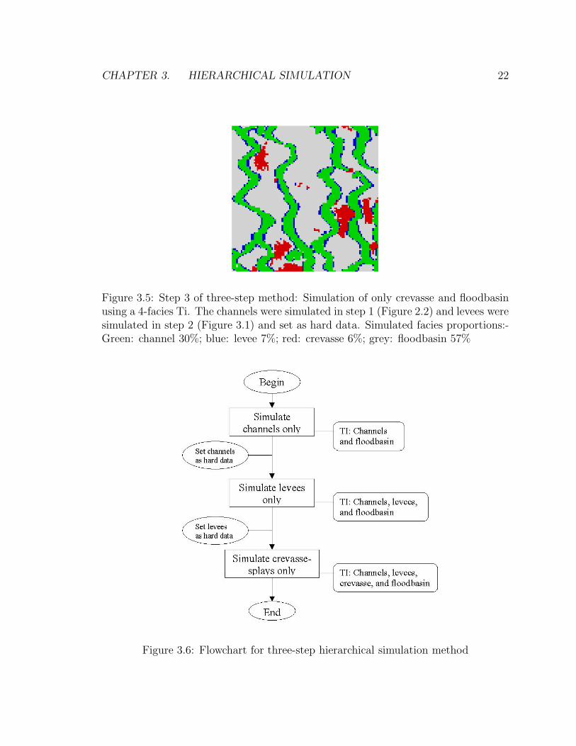
3.2.2 Three-step hierarchical simulation method

The 4 facies can also be simulated in three steps as follows: First only the channel

and floodbasin are simulated using a binary Ti and the simulated channels as set as

hard data (Figure 2.2). In the second step, only levees and floodbasin are simulated

(Figure 3.1) using a 3-facies channel-levee-floodbasin Ti (Figure 2.3). The simulated

levees are set as hard data together with the simulated channels from step 1. Finally,

crevasse and floodbasin are simulated (Figure 3.5) using a 4-facies channel-crevasse-

levee-floodbasin Ti (Figure 2.7).

In the second step, the Ti-derived probability of simulating a channel pixel is

set to zero so that no more channel is simulated. Similarly, in step three, the Ti-

derived probabilities of simulating both channel and levee pixels is set to zero so

that no more channel and levees are simulated. Servo-system correction is applied at

all three steps to ensure reproduction of target proportions. The procedure for this

method is summarized in the flowchart in Figure 3.6. Table 3.2 summarizes the input

parameters and simulation statistics for this method.

Comments

In Figure 3.5 the channels are continuous as they were simulated using a large binary

Ti and a large template. Since the crevasse simulation is conditioned to previously

simulated channel as well as levee values, some crevasse pixels are simulated next to

the isolated levee pixels, which is permitted by the Ti. The target proportions of

the four facies are well reproduced because the servo-system is applied. The total

simulation took 14.4 seconds.

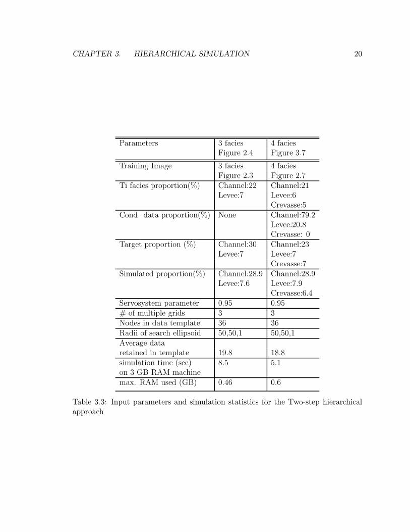
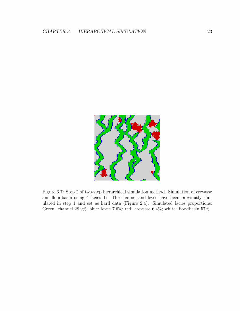
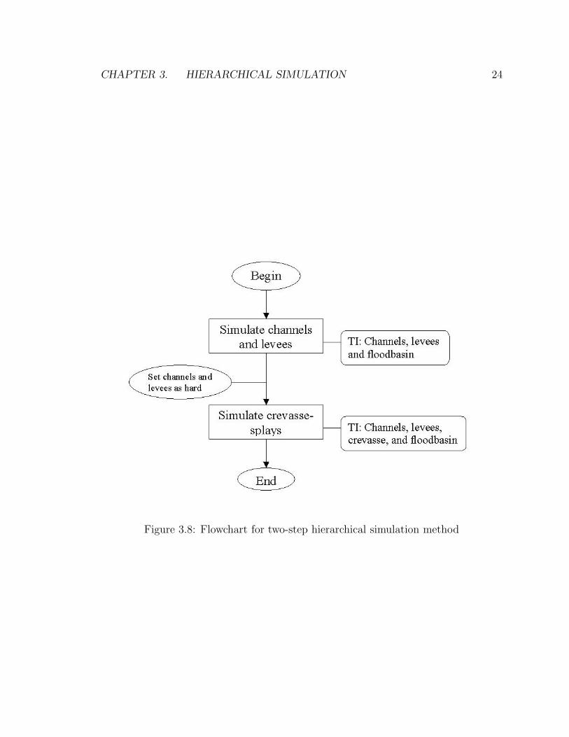
3.2.3 Two-step hierarchical simulation method

Comparing the results of joint versus hierarchical simulation of channel-levee-floodbasin

system, it is observed that the levees are better simulated jointly with channels since

they have the same elongated shape as the channels. Hence, in this last approach,

the levees are simulated jointly with channel and floodbasin in the first step using a

3-facies channel-levee-floodbasin Ti. The simulated channel and levee pixels are then


frozen as hard data (Figure 2.4). Finally, only crevasse and floodbasin are simulated

(Figure 3.7) using a 4-facies channel-levee-crevasse-floodbasin Ti (Figure 2.7) by set-

ting to zero the Ti-derived probability of simulating channel and levee pixels. The

servo-system correction is applied at both steps to ensure reproduction of target pro-

portions of the four facies. The flowchart in Figure 3.8 summarizes the procedure and

Table 3.3 summarizes the input parameters and simulation statistics for this method.

Comments

In Figure 3.7 the continuity of the levees is improved and isolated pixels are minimized

by simulating the levees with the channels. The channels are reasonably continuous

in spite of using a 3-facies Ti, because the levee has the same elongated shape as the

channel. The shape of the crevasse is well reproduced and they are attached to the

channels. The target proportions of the four facies are well reproduced because the

servo-system is applied. The first step took 4.9 seconds, the second step took 5.1

seconds.

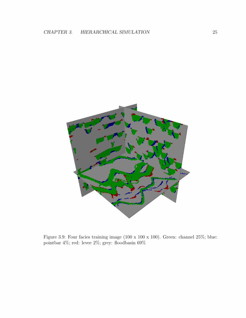
3.3 3D Example

The hierarchical simulation approach is applied to a synthetic 3D meandering chan-

nel reservoir with four facies namely, channel, pointbar, levee, and floodbasin. The

training image is 100 x 100 x 100 grid blocks (Figure 3.9). In Figure 3.9, the channels

are sinuous and have a U-shaped cross-section. The pointbars are deposited in the

inner bends of the channel and in cross-section they occur along one margin of the

channel. The levees have an elongated shape with a triangular cross-section and are

deposited adjacent to the channel. Some of the channels are amalgamated, hence the

pointbar is found between two channels. Thus, the pointbar needs to be simulated

jointly with the channel so that it can be simulated inside channels as depicted by

the Ti.

The simulation grid is 100 x 100 x 100 grid blocks. The two-step hierarchical

approach is used to generate the final 4-facies realization. In step 1, only the channel,

pointbar and floodbasin are simulated using the corresponding 3-facies Ti. That


Ti was obtained from Figure 3.9 by merging the levee facies with the floodbasin.

Furthermore, only the first 50 layers of the Ti were used for the simulation to reduce

the RAM requirement by reducing the size of the search tree. In step 2, only levees

and floodbasin are simulated conditioned to the previously simulated channel and

pointbar. The first 50 layers of the original 4-facies Ti are used for this simulation.

During the second step, the Ti-derived probability of simulating a channel or point-

bar pixel is set to zero so that no more channel or point-bar is simulated.

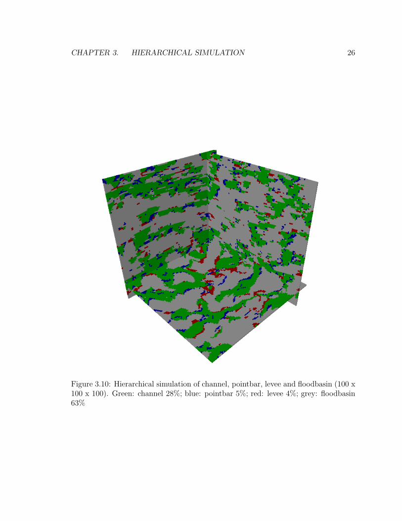
Comments

Figure 3.10 shows the final 4-facies realization. Both channel and pointbar are well-

reproduced in plan view and cross-section. Channels become discontinuous when

they thin out vertically. The sinuosity of the channel is discernable and the pointbar

is simulated in the inner bend of the channel as specified by the Ti. It was possible

to capture this large-scale structure by using a large data template in combination

with the multiple-grid appraoch. By using hierarchy, the problem was reduced to

simulation of 3 facies instead of 4 facies in the first step, which enabled using a large

data template, which might not have been possible if the 4 facies had been jointly

simulated. It was difficult to simulate continuous levees because in the Ti they are

fragmented as they thin upward.

Figure 3.1: Hierarchical simulation of only levee and floodbasin using a 3-facies Ti(100 x 100). Channels were previously simulated (Figure 2.2) and set as hard data.Green: channel 30%; red: levee 7%; grey: floodbasin 63%


Figure 3.2: Hierarchical simulation of only crevasse and floodbasin using a 3-facies Ti(100 x 100). Channels are previously simulated (Figure 2.2). Green: channel 30%;red: crevasse 8%; grey: floodbasin 62%

Figure 3.3: Combining Figures 3.1 and 3.2 using cookie-cut. Crevasse erodes lev-ees and floodbasin. Green: channel 30%; blue: levee 7%; red: crevasse 8%; grey:floodbasin 55%


Parameters step 1 step2 step3Figure 2.2 Figure 3.1 Figure 3.5

Training Image 2 facies 3 facies 4 faciesFigure 2.1 Figure 2.3 Figure 2.7

Ti facies proportion(%) Channel:22 Channel:22 Channel:21Levee:7 Levee:6

Crevasse:5Cond. data prop.(%) None Channel:100 Channel: 76.6

Levee:0 Levee:22.9Crevasse:0

Target proportion(%) Channel:30 Channel:30 Channel:30Levee:7 Levee:7

Crevasse:7Simulated proportion(%) Channel:29.9 Channel:29.9 Channel:29.9

Levee: 7.1 Levee:7.1Crevasse:6.2

Servosystem parameter 1 0.95 0.95# of multiple grids 3 1 3Nodes in data template 50 36 36Radii of search ellipsoid 50,50,1 50,50,1 50,50,1Average nodesretained in template 27.4 17.6 17.8simulation time (sec) 7.2 2.1 5.1on 3 GB RAM machinemax. RAM used (GB) 0.45 0.44 0.58

Table 3.2: Input parameters and simulation statistics for the Three-step hierarchicalapproach


Parameters 3 facies 4 faciesFigure 2.4 Figure 3.7

Training Image 3 facies 4 faciesFigure 2.3 Figure 2.7

Ti facies proportion(%) Channel:22 Channel:21Levee:7 Levee:6

Crevasse:5Cond. data proportion(%) None Channel:79.2

Levee:20.8Crevasse: 0

Target proportion (%) Channel:30 Channel:23Levee:7 Levee:7

Crevasse:7Simulated proportion(%) Channel:28.9 Channel:28.9

Levee:7.6 Levee:7.9Crevasse:6.4

Servosystem parameter 0.95 0.95# of multiple grids 3 3Nodes in data template 36 36Radii of search ellipsoid 50,50,1 50,50,1Average dataretained in template 19.8 18.8simulation time (sec) 8.5 5.1on 3 GB RAM machinemax. RAM used (GB) 0.46 0.6

Table 3.3: Input parameters and simulation statistics for the Two-step hierarchicalapproach


Figure 3.4: Flowchart for two-step cookie-cut simulation method


Figure 3.5: Step 3 of three-step method: Simulation of only crevasse and floodbasinusing a 4-facies Ti. The channels were simulated in step 1 (Figure 2.2) and levees weresimulated in step 2 (Figure 3.1) and set as hard data. Simulated facies proportions:-Green: channel 30%; blue: levee 7%; red: crevasse 6%; grey: floodbasin 57%

Figure 3.6: Flowchart for three-step hierarchical simulation method


Figure 3.7: Step 2 of two-step hierarchical simulation method. Simulation of crevasseand floodbasin using 4-facies Ti. The channel and levee have been previously sim-ulated in step 1 and set as hard data (Figure 2.4). Simulated facies proportions:Green: channel 28.9%; blue: levee 7.6%; red: crevasse 6.4%; white: floodbasin 57%


Figure 3.8: Flowchart for two-step hierarchical simulation method


Figure 3.9: Four facies training image (100 x 100 x 100). Green: channel 25%; blue:pointbar 4%; red: levee 2%; grey: floodbasin 69%


Figure 3.10: Hierarchical simulation of channel, pointbar, levee and floodbasin (100 x100 x 100). Green: channel 28%; blue: pointbar 5%; red: levee 4%; grey: floodbasin63%

Chapter 4

Implementation of hierarchical

simulation

All runs in this paper were done using the snesim algorithm (Strebelle, 2000, 2002).

In order to use hierarchical simulation, modifications to the existing snesim pro-

gram were necessary. To illustrate these changes, consider the two-step hierarchical

approach discussed in the paper.

In the first step, the 3 facies, channel, levee and floodbasin are simulated using the

corresponding 3-facies Ti. The simulated channel and levee pixels should be extracted

from the simulation output file along with their location and saved in a separate file

so that they can be supplied as hard data for the next step. This step requires no

modification in the program. In the second step, a 4-facies channel-levee-crevasse-

floodbasin Ti is used to simulate only two facies, crevasse and floodbasin. In order to

accomplish this, the following must be done at each location to be simulated:

• Get the Ti-derived proportions for a given data event

• Set the local probability of channel and levee to zero

• Re-standardize correspondingly the probabilities of crevasse and floodbasin

• Apply the servo-system correction to crevasse and floodbasin

One last modification is required when obtaining the Ti-derived proportions from

the search tree. When an uninformed node is encountered in the data template, the

27

CHAPTER 4. IMPLEMENTATION OF HIERARCHICAL SIMULATION 28

original snesim program considers the possibility of having any one of the four facies

that exist in the Ti. However, in step 2, since only crevasse and floodbasin can be

simulated, only these two facies should be considered. Indeed channel and levee have

already been simulated in step 1 and set as hard data, hence the uninformed node in

the data template cannot be these two facies.

Chapter 5

Rhine-Meuse Delta Case Study

5.1 Introduction to the Data Set

5.2 Results and Discussion

29

Chapter 6

Conclusions and Future Work

6.1 Conclusions

• Hierarchical simulation gives better results than joint simulation when more

than three facies are involved. This approach is highly recommended for both

algorithmic and geological considerations.

• Three alternative approaches for simulating four facies hierarchically were demon-

strated. As the number of facies increases, the alternatives to simulate them

hierarchically also increases. The actual hierarchy of simulation steps should be

guided by the geological rules of deposition.

• In case of the levees, which have elongation similar to channels, their joint

simulation with channels produces better results than a hierarchical simulation,

in which some isolated pixels can be generated. Thus in similar depositional

contexts, it might be better to simulate similar shaped facies together.

• The shape of crevasse splays is very different from that of the channels and lev-

ees. Hence, simulating crevasse separately from channels and levees gives better

results. Thus, facies with different shapes and continuity should be simulated

separately.

• A 4-facies training image can be used to simulate only two facies as was done in

30

CHAPTER 6. CONCLUSIONS AND FUTURE WORK 31

the two-step hierarchical simulation method, see Figure 3.7. However, the rela-

tionship between the different facies is extracted from the complex four-facies

training image. This concept can be extended to other depositional environ-

ments with multiple facies.

• During hierarchical simulation, facies such as levee and crevasse splays are at-

tached to the channels as specified in the training image, even though the levee

and crevasse are simulated independently of the channels.

• In this particular case-study, the two-step hierarchical simulation method (Fig-

ure 3.7) gives the best results out of the three hierarchical methods, because

channels and levees are simulated jointly, and a 4-facies Ti was used to condition

the relative position of crevasse and floodbasin.

6.2 Future work

Consider the synthetic 2D fluvial reservoir with four facies and assume that condition-

ing data is available for all of them. In the current implementation, during step 1 of

the two-step hierarchical approach the crevasse data are merged with the floodbasin

data, so that only channel, levee and floodbasin data exist. However, crevasse data

are indirect indicator of a channel located nearby. This information is ignored when

the crevasse data are merged with floodbasin data.

To utilize the information carried by the crevasse data, the grid can be pre-

processed to flag the simulation nodes that are within a fixed distance d of the crevasse

data. The distance d depends on the size and shape of the crevasse and should be

provided by the geologist. During simulation if the location to be simulated is flagged,

then the Ti-derived proportion of channel P (A|B) is increased by 10% by multiplying

P (A|B) by a factor 1.1. The 10% percent value increase is an arbitrary choice. The

upper bound is set to 1 so that we do not get proportions greater than 1.

P ∗ = min(1, P (A|B) ∗ 1.1) (6.1)

Step 2 would then proceed as described in section 3.2.3.

Bibliography

[1] Bridge, J.S. and Tye, R.S. Interpreting the dimensions of ancient fluvial channel

bars, channels and channel belts from wireline-logs and cores. AAPG Bulletin,

vol.84, no.8, pp.1205-1228, August 2000.

[2] Deutsch, C.V. and Tran, T.T. Fluvsim: a Program for Object-based Stochastic

modeling of fluvial depositional Systems. Computers and Geosciences, 2002, no.

28, pp. 525-535

[3] Guardino, F. and Srivastava, R.N. Multivariate geostatistics: Beyond bivariate

moments. In A. Soares (ed.), Geostatistics-Troia, vol.1, Kluver Academic Publ.

Dordrecht, pp.133-144, 1993.

[4] Leet, L.D. Physical Geology. Englewood Cliffs, NJ: Prentice-Hall, sixth edition,

1982.

[5] Strebelle, S. Conditional simulation of complex geological structures using

multiple-point statistics. Math. Geology, 2002, vol. 34, no. 7, pp. 1161-68.

[6] Strebelle, S. Sequential Simulation Drawing Structures from Training Images.

PhD thesis, Stanford University, Stanford, CA, 2000.

[7] Tran, T. Improving variogram reproduction on dense simulation grids. Computers

and Geosciences, 20(7), 1161-1168, 1994.

32

Documents

Hierarchical Simulation of Multiple-Facies Reservoirs