Hierarchical Normalized Completely RandomMeasures to Cluster Grouped Data

Raffaele ArgientoESOMAS Department, University of Torino and Collegio Carlo Alberto, Torino, Italy

andAndrea Cremaschi

Department of Cancer Immunology, Institute of Cancer Research, Oslo University Hospital, Oslo, Norway

Oslo Centre for Biostatistics and Epidemiology, University of Oslo, Oslo, Norway

andMarina Vannucci

Department of Statistics, Rice University, Houston, TX, USA

Abstract

In this paper we propose a Bayesian nonparametric model for clustering groupeddata. We adopt a hierarchical approach: at the highest level, each group of datais modeled according to a mixture, where the mixing distributions are conditionallyindependent normalized completely random measures (NormCRMs) centered on thesame base measure, which is itself a NormCRM. The discreteness of the shared basemeasure implies that the processes at the data level share the same atoms. Thisdesired feature allows to cluster together observations of different groups. We obtaina representation of the hierarchical clustering model by marginalizing with respect tothe infinite dimensional NormCRMs. We investigate the properties of the clusteringstructure induced by the proposed model and provide theoretical results concerningthe distribution of the number of clusters, within and between groups. Furthermore,we offer an interpretation in terms of generalized Chinese restaurant franchise process,which allows for posterior inference under both conjugate and non-conjugate models.We develop algorithms for fully Bayesian inference and assess performances by meansof a simulation study and a real-data illustration. Supplementary Materials for thiswork is available online.

Keywords: Bayesian Nonparametrics; Clustering; Mixture Models; Hierarchical Models.

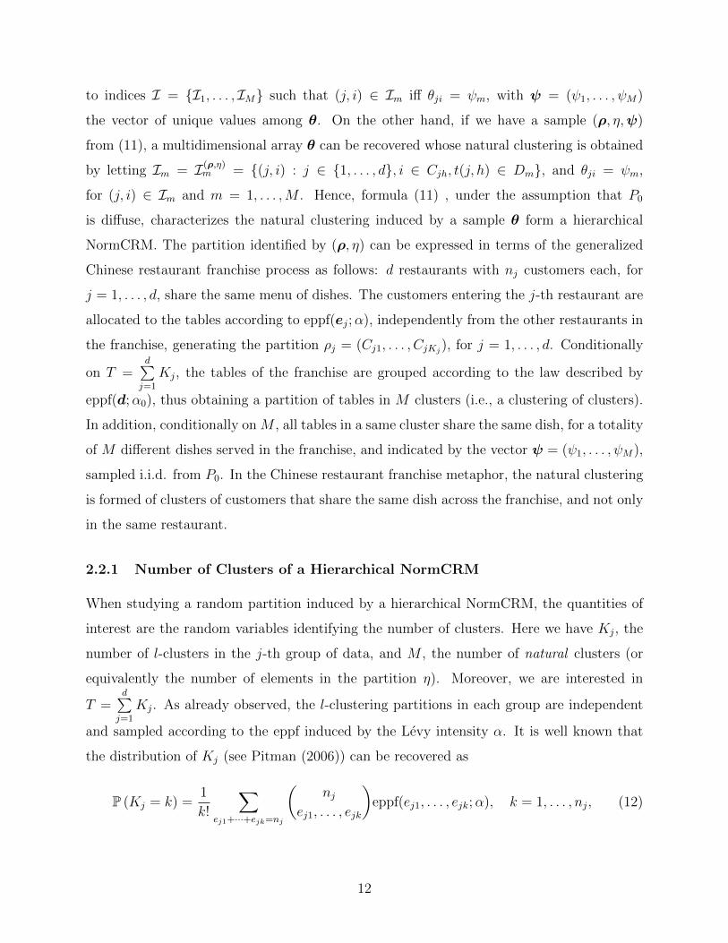
1

1 Introduction

In statistical modeling, dependency among observations can be captured in a number of

different ways, for example through the inclusion of additional components (covariates) that

link data in different groups. A specific type of dependency among observations is the mem-

bership to a specific group or category, where data share similar characteristics. This relates

to the concept of partial exchangeability, where classical exchangeability does not hold for

the whole dataset, but it does within each group. Let θ = (θ1, . . . ,θd) indicate a multidi-

mensional vector of random variables divided into d groups, each of size nj, for j = 1, . . . , d.

Partial exchangeability coincides with assigning a probability distribution Pj to each group,

such that (θj1, . . . , θjnj)|Pjiid∼ Pj, for each j = 1, . . . , d, under a suitable prior (de Finetti mea-

sure) for the vector of random probabilities (P1, . . . , Pd). Readers are referred to Kallenberg

(2005) for an excellent overview on the topic. From an inferential point of view, the specifica-

tion of the joint distribution of (P1, . . . , Pn) is crucial as it defines the dependence structure

among the random probability measures and, consequently, the sharing of information. In

the Bayesian framework, it is common to impose the mild condition of exchangeability, i.e.,

(P1, . . . , Pd)|Piid∼ P , for a suitable probability distribution P . In Bayesian nonparametrics,

such hierarchical structure has been used to introduce the celebrated hierarchical Dirichlet

process (Teh et al. 2005, 2006), with successful applications in genetics, image segmentation

and topic modeling, to mention a few (Blei 2012; Teh and Jordan 2010). More recently,

hierarchical processes have been investigated from an analytical perspective by Camerlenghi

et al. (2017, 2018), while Bassetti et al. (2018) have focused on hierarchical species sam-

pling models. These authors have shown that extensions to normalized completely random

measures encompassing the Dirichlet process allow for richer predictive structures.

Undoubtedly, some of the most popular models in the Bayesian nonparametric framework

are mixture models (see, for example, Ferguson 1983; Lo 1984). In this setting, conditionally

upon a set of latent variables, the observations are assumed independent from a family of

parametric densities, while the latent parameters are distributed according to an almost

surely discrete random probability measure (for further details, see Ishwaran and James

2001; Lijoi et al. 2007). These models owe their popularity to their ease of interpretation,

computational availability, and elegant mathematical properties. Any mixture model with

2

an almost surely discrete mixing measure leads to ties in θ with positive probability. This

induces a random partition of the subject labels via the values of the parameters θ, meaning

that two subjects share the same cluster if and only if the corresponding latent variables

take on the same value. We refer to this as the natural clustering. Pitman (1996, 2003)

showed that assigning the law of the discrete mixing measure is equivalent to assigning the

law of the parameter that identifies the natural clustering. The prior on this partition is

then obtained by marginalizing with respect to the infinite-dimensional parameter, and it is

expressed via the so-called exchangeable partition probability function.

In this paper, we aim at obtaining a similar result in the context of hierarchical normal-

ized completely random measures. We define a hierarchical normalized completely random

measure mixture model by assuming that, conditionally upon θ = (θ1, . . . ,θd), the data

are independent from some parametric family of distributions, and the prior on θ is the

hierarchical process discussed above. Marginalizing with respect to (P1, . . . , Pd) and P , we

write our hierarchical model in terms of the cluster parameters and their prior distributions

(i.e., d + 1 distinct exchangeable partition probability functions). As a result, we obtain a

two-layered hierarchical clustering structure: a clustering within each of the groups (that we

will refer to as the l-clustering), and a natural clustering across the whole multidimensional

array θ. We study such clustering structure by considering a nonparametric mixture model

in which the completely random measure has a discrete centering measure, and provide the-

oretical results concerning the distribution of the number of clusters, within and between

groups. Furthermore, we offer an interpretation in terms of the generalized Chinese restau-

rant franchise process, enabling posterior inference for both conjugate and non-conjugate

models.

With respect to the recent contributions on Bayesian nonparametric hierarchical pro-

cesses of Camerlenghi et al. (2018) and Bassetti et al. (2018), which investigate more the-

oretical aspects, in this paper we provide a detailed study of the two-layered hierarchical

clustering structure induced by these models. Original contributions of our paper include: a

characterization of the mixture model in terms of the clustering structure; interpretation of

the clustering model through the metaphor of the generalized Chinese restaurant franchise;

an MCMC algorithm to compute the posterior of the cluster structure, which makes use of

data augmentation techniques; expressions of moments of the Bayesian nonparametric ingre-

3

dients; applications to simulated and benchmark data sets, to illustrate the effect of critical

hyperparameters on the clustering structure. While in Section 2 below we acknowledge some

overlap between our theoretical results and those of Bassetti et al. (2018), we point out that

our work was developed independently of theirs. In addition, we use original techniques in

the proofs of some of the results (see Proposition 2 in Section 2.2). Finally, we also notice

that the two-layered hierarchical clustering induced by our model can be interpreted as a

“cluster of clusters”, or “mixture of mixtures”, as introduced in Argiento et al. (2014) and

Malsiner-Walli et al. (2017). These authors, however, address a different problem from the

one considered here.

The rest of the paper is organized as follows: completely random measures and nor-

malized completely random measures with discrete centering distribution are introduced in

Section 2. Characteristic properties of the clustering induced by a normalized completely

random measure are also discussed, such as the expression of mixed moments and the law

of the number of clusters. Next, the proposed characterization is extended to hierarchical

normalized completely random measures for grouped data. In Section 3, insights on the pos-

terior sampling process for the proposed mixture models are provided, including prediction.

Simulation results as well as an application to a benchmark dataset are given in Section 4.

Finally, Section 5 concludes the paper. Proofs of the theoretical results, algorithmic details

and additional results are reported in the Supplementary Materials available online.

2 Methodology

2.1 Normalized completely random measures with discrete cen-

tering

Let Θ be a complete and separable metric space, endowed with the corresponding Borel

σ-algebra B. A completely random measure (CRM) on Θ is a random measure µ1 taking

values on the space of boundedly finite measures on (Θ,B) and such that, for any collection

of disjoint sets {B1, . . . , Bn} ∈ B, the random variables µ1(B1), . . . , µ1(Bn) are independent

(see Kingman 1993). In this paper, we focus on the subclass of CRMs that can be written

as µ1(·) =∑l≥1

Jlδτl(·), describing an almost surely discrete random probability measure with

4

random masses J = {Jl} = {Jl, l ≥ 1} independent from the random locations T = {τl}.

The law of this subclass of CRMs, called homogeneous CRMs, is characterized by a Levy

intensity measure ν that factorizes into ν(ds, dτ) = α(s)P (dτ)ds, where α is the density of

a nonnegative measure, absolutely continuous with respect to the Lebesgue measure on R+,

and P is a probability measure over (Θ,B). Hence, the random locations are independent

and identically distributed according to the base distribution P , while the random masses

J are distributed according to a Poisson random measure with intensity α. In what follows,

we will refer to α only as the Levy intensity.

A homogeneous normalized completely random measure (NormCRM) P1 on Θ is a ran-

dom probability measure having the following representation:

P1(·) =µ1(·)µ1(Θ)

=∑l≥1

JlT1

δτl(·) =∑l≥1

wlδτl(·), (1)

where T1 = µ1(Θ) =∑l≥1

Jl, and hence∑l≥1

wl = 1. We point out that the law of the infinite se-

quence {wl} depends only on the Levy intensity α. We indicate with P1 ∼ NormCRM(α, P )

a NormCRM with Levy intensity α and centering measure P . The acronym NRMI is also

used in the literature, in reference to the original definition of NormCRMs on the real line

as normalized random measures with independent increments (Regazzini et al. 2003). To

ensure that the normalization in (1) is well-defined, the random variable T1 has to be positive

and almost surely finite. This is guaranteed by imposing the regularity conditions∫R+

α(s)ds = +∞, and

∫R+

(1− e−s)α(s)ds < +∞. (2)

The class of NormCRMs encompasses the well-known Dirichlet process Dir(κ, P ), obtained

by normalization of a gamma process, with Levy intensity α(s) = κs−1e−sI(0,+∞)(s), for

κ > 0. It also includes the normalized generalized gamma process NGG(κ, σ, P ) of Li-

joi et al. (2007), obtained when α(s) = κΓ(1−σ)

s−1−σe−sI(0,+∞)(s), for 0 ≤ σ < 1, and

the normalized Bessel process NormBessel(κ, ω, P ) of Argiento et al. (2016), when α(s) =

κse−ωsI0(s)I(0,+∞)(s), for ω ≥ 1 and I0(s) the modified Bessel function of the first kind. In

the expressions of the Levy intensities above IA(s) is the indicator function of the set A, i.e.,

IA(s) = 1 if s ∈ A and IA = 0 otherwise.

5

A sample from P1 is an exchangeable sequence such that (θ1, . . . , θn)|P1iid∼ P1. In this

paper we adopt a slightly different representation of a sample from P1, which will be useful

to characterize the clustering induced by P1 when the centering measure P is discrete. Let

P1 be defined as in (1) and let P ?1 be a random probability measure on the positive integers

N = {1, 2, . . . } whose weights coincide with the weight of P1, that is,

P ?1 (·) =

∑l≥1

wlδl(·). (3)

Lemma 1. Let (θ1, . . . , θn) be a sample from P1 defined as in (1) and let (l1, . . . , ln) be a

sample from P ?1 defined as in (3). Define θ1 = τl1 , . . . , θn = τln with {τl}

iid∼ P and P the

centering measure of P1. Then

(θ1, . . . , θn)L= (θ1, . . . , θn).

Proof: See Section 1.1 of the Supplementary Materials. A similar result is shown in Propo-

sition 1 of Bassetti et al. (2018).

Here we refer to a sample from P1 as a sequence (θ1, . . . , θn) obtained under (3) following

the construction in Lemma 1. Since P1 is discrete, a sample (θ1, . . . , θn) from (1) induces a

random partition ρ = {C1, . . . , CKn} on the set of indices {1, . . . , n}. We refer to this as the

natural clustering, with Cj = {i : θi = θ∗j}, for j = 1, . . . , Kn, and (θ∗1, . . . , θ∗Kn

) the set of

unique values derived from the sequence (θ1, . . . , θn). When the centering distribution P is

diffuse, it is well known (see Pitman 1996; Ishwaran and James 2003) that the joint marginal

distribution of a sample (θ1, . . . , θn) can be uniquely characterized by the law of the natural

clustering (ρ, θ∗1, . . . , θ∗Kn

) as

L(ρ, dθ∗1, . . . , dθ∗Kn

) = L(ρ)L(dθ∗1, . . . , dθ∗Kn|Kn) = π(ρ)

Kn∏l=1

P (dθ∗l ), (4)

with π(ρ) the probability law on the set of the partitions of {1, . . . , n}, which is called the

exchangeable partition probability function, or eppf. Since the eppf depends only on the

Levy intensity α of the NormCRM, we write π(ρ) = eppf(e1, ..., eKn ;α), where eppf is a

6

unique symmetric function depending only on ej = Card(Cj), the cardinalities of the sets

Cj, for j = 1, . . . , Kn. A formula for the eppf of a generic NormCRM can be obtained as

(see formulas (36)-(37) in Pitman (2003))

eppf(e1, . . . , eKn ;α) =

∫ +∞

0

un−1

Γ(n)e−φ(u)

Kn∏l=1

cel(u)du, (5)

where φ(u) and the functions cm(u), for m = 1, 2, . . . , are defined as

φ(u) =

∫ +∞

0

(1− e−us)α(s)ds, cm(u) = (−1)m−1φm(u) =

∫ +∞

0

sme−usα(s)ds. (6)

Here, φ(u) is the Laplace exponent of the unnormalized CRM µ1(·), and φm(u) = dm

dumφ(u).

Decomposition (4) sheds light on the law of the clustering structure induced by a NormCRM

when the centering measure is diffuse. It can be decomposed into two factors: the law of

the partition ρ, that depends only on the intensity parameter α, and the law of the cluster-

specific parameters (θ∗1, . . . , θ∗Kn

), that conditionally upon the number of unique values Kn

is the Kn-product of the centering measure P .

We want to show that equation (4) can still be valid in the case of a discrete centering

measure P , even though with a slight different interpretation. With this aim, consider a

sample (l1, . . . , ln) from P ?1 as in (3), and the vector (θ1, . . . , θn) as in Lemma 1. Also, let l∗ =

(l∗1, . . . , l∗Kn

) be the vector of unique values among (l1, . . . , ln) and ρ the induced clustering,

i.e., ρ = {C1, . . . , CKn}, where i ∈ Ch iff li = l∗h, with i = 1, . . . , n and h = 1, . . . , Kn.

The law of ρ can be characterized in terms of generalized Chinese restaurant process (see

Pitman 2006) as the eppf induced by the Levy intensity α. To prove this we first observe

that, if (l1, . . . , ln)|P ?1

iid∼ P ?1 , then L(l1, . . . , ln) = E(wl1 . . . wln). Then, using the equivalent

representation of (l1, . . . , ln) in terms of (l∗1, . . . , l∗Kn

) and ρ = {C1, . . . , CKn}, with ej =

Card(Cj), for j = 1, . . . , Kn, a change of variable leads to L(l∗1, . . . , l∗Kn, ρ) = E(we1l∗1 . . . w

eKnl∗Kn

).

Hence, by formula (4) in Pitman (2003), the law of ρ is L(ρ) =∑

l∗1 ,...,l∗Kn

E(we1l∗1 . . . weKnl∗Kn

) =

eppf(e1, . . . , eKn ;α), where l∗1, . . . , l∗Kn

ranges over all permutations of Kn positive integers.

We are now ready to show that, even if we do not assume P to be diffuse, the law of the

sample (θ1, . . . , θn) has a unique representation as in (4), provided that ρ is the partition

induced by (l1, . . . , ln) and that (θ∗1, . . . , θ∗Kn

) is an i.i.d. sample from P . To this end we first

7

give the following:

Definition 1. An l-clustering representation of (θ1, . . . , θn) is a vector (ρ, θ∗1, . . . , θ∗Kn

) s.t.:

1. ρ = {C1, . . . , CKn} is the clustering induced by the l∗ on the data indices (i.e., i ∈ Chiff li = l∗h for i = 1, . . . , n and h = 1, . . . , Kn),

2. θ∗h is the value shared by all the θ’s in group Ch, for h = 1, . . . , Kn.

We point out that, in an l-clustering representation, (θ∗1, . . . , θ∗Kn

) is not the vector of

unique values among the θ’s, and so Kn is not the random variable representing the number

of different values among the θ’s, as it is usually denoted in the Bayesian nonparametric

literature. Due to the discreteness of the centering measure P , we could have coincidence

also among the θ∗’s. Moreover, from (ρ, θ∗1, . . . , θ∗Kn

), we can recover (θ1, . . . , θn). While from

(θ1, . . . , θn) we cannot recover the l-clustering unless the knowledge of (l1, . . . , ln) is provided.

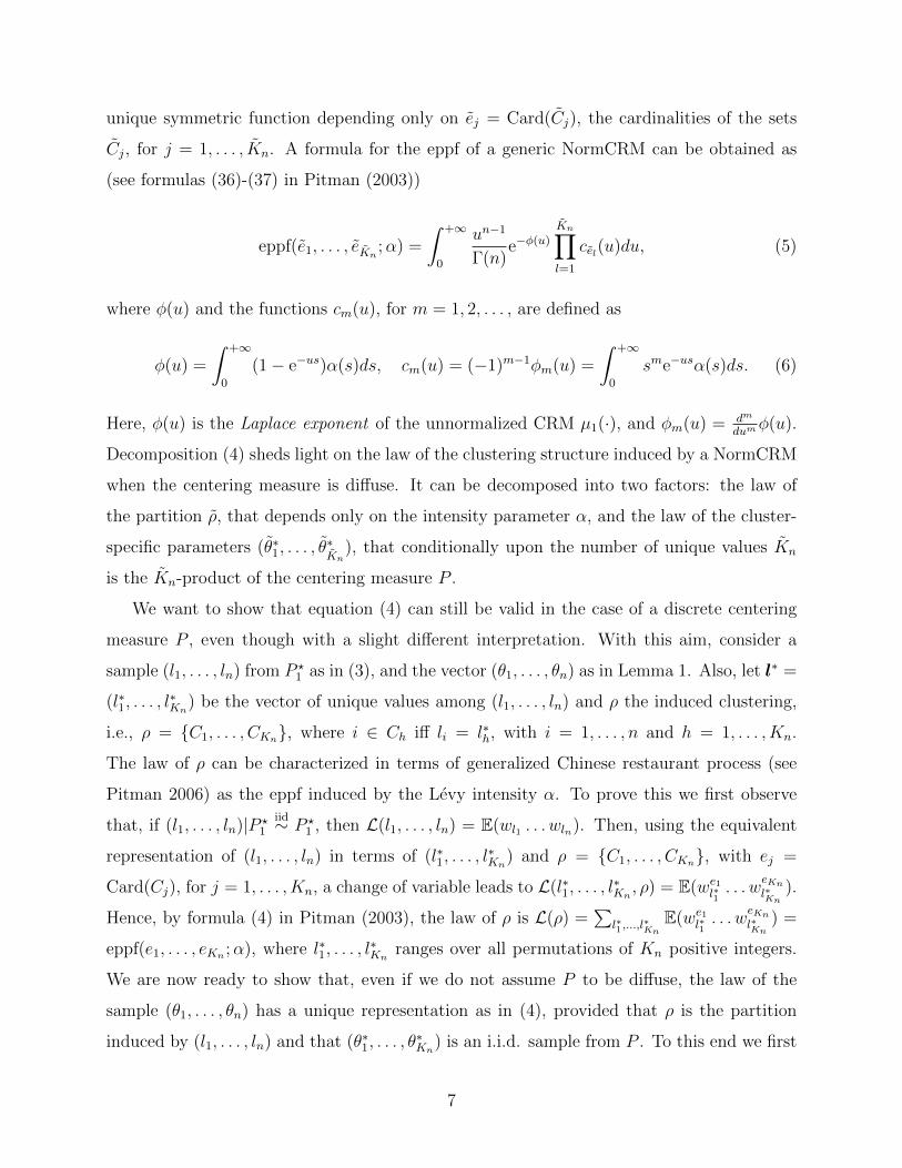
As a simple example to better understand this point, consider a sample of dimension n = 8

C11

3 5

C2

2 7

C3

4

C4

6 8

aFigure 1: Illustration of an l-clustering based on a sample of dimension n = 8 from aNormCRM whose centering measure is a discrete distribution on the colored lines.

from a NormCRM whose centering measure is a discrete distribution on the colored lines.

In this sample we have θ =(continuous green, dashed orange, continuous green, dotted blue,

continuous green, dashed orange, dashed orange, dashed orange), obtained under the hy-

pothesis of Lemma 1, with (l1, . . . , ln) = (1, 2, 1, 3, 1, 4, 2, 4), τ1=continuous green, τ2=dashed

orange, τ3 =dotted blue, τ4=dashed orange. The corresponding l-clustering is represented in

Figure 1, and it is formed by ρ = {C1 = {1, 3, 5}, C2 = {2, 7}, C3 = {4}, C4 = {6, 8}} and

(θ∗1, . . . , θ∗Kn

) =(continuous green, dashed orange, dotted blue,dashed orange). It is clear that

we can recover the sample from the l-clustering partition by letting θi = θ∗li , i = 1, . . . , n.

The opposite, however, is not possible: without the knowledge of (l1, . . . , ln) the l-clustering

cannot be recovered just by looking at (θ1, . . . , θn). We also notice that the partition ρ

8

of the l-clustering is not the one induced by the unique values among the θ’s. In fact,

θ∗2 = θ∗4=dashed orange with both clusters C2 and C4 containing orange dashed lines, while

the natural clustering is ρ = {C1 = {1, 3, 5}, C2 = {2, 7, 6, 8}, C3 = {4}}.

These considerations yield to the following:

Proposition 1. The marginal law of a sample (θ1, . . . , θn) from a NormCRM P1 defined as

in (1), with a general centering measure P , has a unique characterization in terms of ρ and

(θ∗1, . . . , θ∗Kn

) of an l-clustering representation. In particular,

L(ρ, dθ∗1, . . . , dθ∗Kn) = π(ρ)

Kn∏h=1

P (dθ∗h) = eppf(e1, . . . , eKn ;α)Kn∏h=1

P (dθ∗h). (7)

Proof: See Section 1.2 of the Supplementary Materials. A different presentation of this

result is given in Proposition 1 of Bassetti et al. (2018). The result implies that ρ is chosen

according to the eppf induced by α and that (θ∗1, . . . , θ∗Kn

) is an i.i.d. sample from P .

2.2 Hierarchical NormCRMs

In many applications, multiple sources of information can be observed, hence generating

sequences of data points that are related. In particular, data sampled under the same

experimental condition can be considered exchangeable, introducing group-specific param-

eters. In our setting, this translates into including an additional hierarchical level in the

model, yielding (θj1, . . . , θjnj)|Pjiid∼ Pj, for group j = 1, . . . , d. Here, we assume that

(P1, . . . , Pd) are also exchangeable, that infinite experimental conditions are possible, and

that (P1, . . . , Pd)|Piid∼ NormCRM(α, P ), where P ∼ NormCRM(α0, P0), with P0 a diffuse

measure on Θ and α0 and α Levy intensities satisfying the regularity conditions reported in

(2). We define a hierarchical NormCRM as the joint law of (P1, . . . , Pd). A sample from a hi-

erarchical NormCRM is a multidimensional array θ = (θ1, . . . ,θd), with θj = (θj1, . . . , θjnj),

j = 1 . . . , d, with elements in Θ, such that

(θj1, . . . , θjnj)|Pjiid∼ Pj, j = 1, . . . , d,

(P1, . . . , Pd)|Piid∼ NormCRM(α;P ), (8)

P ∼ NormCRM(α0;P0).

9

The class of hierarchical NormCRMs reduces to the celebrated hierarchical Dirichlet process

of Teh et al. (2006) when α0 and α are the Levy intensities of a gamma process. Theoretical

aspects of hierarchical NormCRMs have been thoroughly investigated by Camerlenghi et al.

(2018) and further extended to the class of species sampling models by Bassetti et al. (2018).

Below we derive a central limit theorem for the number of clusters induced by P1, . . . , Pd

at the second level of hierarchy in formula (8) where, unlike other asymptotic results on

NormCRMs, we let the number of observations nj in each group be bounded and the number

of groups d go to infinity. Furthermore, we provide expressions for the mixed moments of a

hierarchical NormCRM.

Using Proposition 1, we integrate out the infinite-dimensional parameters (P1, . . . , Pd)

and P . Firstly, given P , we observe that for each j = 1, . . . , d, θj = (θj1, . . . , θjnj) is a

sample from Pj, that is a NormCRM with the discrete distribution P as centering measure.

Consequently, θj can be obtained from its l-clustering representation ρj = (Cj1, . . . , CjKj),

θ∗j = (θ∗j1, . . . , θ∗jKj

). We refer to Cjh, for h = 1, . . . , Kj as l-clusters hereafter. Hence, we

can marginalize model (8) with respect to Pj as:

ρj|αind∼ eppf(ej;α),

(θ∗j1, . . . , θ∗jKj

)|Kj, Piid∼ P, (9)

P ∼ NormCRM(α0;P0),

where ej = (ej1, . . . , ejKj) is the vector of l-cluster sizes in the j-th group, for j = 1, . . . , d.

Let (K1, . . . , Kd) = (k1, . . . , kd) be the number of l-clusters in each group of data, and

let T =d∑j=1

Kj be the total number of l-clusters across all groups. We define the index

transformation t : {(j, h) : j = 1, . . . , d;h = 1, . . . kj} → {1, . . . , T} as follows:

t(j, h) =

j−1∑s=0

ks + h, h = 1, . . . , kj, j = 1, . . . , d, (10)

where k0 = 0. Consider now the multidimensional array θ = (θ1, . . . ,θd), where each element

θj = (θj1, . . . , θjnj) is a sample of size nj from Pj, for j = 1, . . . , d. Furthermore, consider

θ∗ = (θ∗1, . . . ,θ∗d), the multidimensional array where each element θ∗j is the vector of shared

value of the l-clustering representation of θj for each group of data, as described in definition

10

(1). The action of the function t in (10) on the indices of θ∗ results in a transformation of the

multidimensional array into a vector of length T , where the rows of the array are sequentially

aligned. Since the information carried by this vector remains unchanged, we will refer to it

by using the same notation, θ∗. Conditionally on T , the vector θ∗ is a sample of size T from

P , that is (θ∗1, . . . , θ∗T )|T, P iid∼ P . Since P is a NormCRM with diffuse centering measure

P0, the l-clustering representation of θ∗ coincides with the natural clustering induced by

the NormCRM. In particular, ψ = (ψ1, . . . , ψM) will denote the vector of unique values in

θ∗, and η = (D1, . . . , DM) the clustering induced by ψ on the index set {1, . . . , T}, that is

t ∈ Dm iff θ∗t = ψm, for t = 1, . . . , T and m = 1, . . . ,M . We denote by d = (d1, . . . , dM) the

size of the clusters in η. Interestingly, the vector ψ is also the vector of unique values among

the multidimensional array θ.

Proposition 2. The marginal law of the multidimensional array θ = (θ1, . . . ,θd) from a

hierarchical NormCRM defined as in (8), can be characterized in terms of (ρ, η,ψ), with

ρ = (ρ1, . . . , ρd), as:

L(ρ, η, dψ) = L(η|ρ)d∏j=1

L(ρj)M∏m=1

P0(dψm) = eppf(d;α0)d∏j=1

eppf(ej ;α)M∏m=1

P0(dψm). (11)

We note that Proposition 2 can be derived from Proposition 4 of Bassetti et al. (2018),

as a special case of the larger class of species sampling models, and also that the so called

pEPPF, introduced by Camerlenghi et al. (2018), can be obtained by (11) marginalizing

with respect to η and ψ. Moreover, according to (11), the multidimensional array θ can be

drawn as follows: first, choose the partitions ρj of the indices {1, . . . , nj}, for j = 1, . . . , d,

independently and according to the Chinese restaurant process governed by α. After iden-

tifying the number of elements Kj = kj of ρj in each group, compute T =d∑j=1

kj and draw a

partition η of the indices {1, . . . , T} according to a Chinese restaurant process governed by

α0. Sample ψ = (ψ1, . . . , ψM), with M = #η, i.i.d. from P0, and build θ∗ = (θ∗1, . . . , θ∗T ),

where θ∗t = ψm iff t ∈ Dm, for t = 1, . . . , T and m = 1, . . . ,M . Invert the transformation in

(10) by finding (j, h) such that θ∗jh = θ∗t=t(j,h). Finally, for each i = 1, . . . , nj and j = 1, . . . , d,

set θji = θ∗jh iff i ∈ Cjh, for h = 1, . . . , kj.

Let θ be a multidimensional array sampled according to a hierarchical NormCRM as in

formula (8). The natural clustering is represented by the partition of the data corresponding

11

to indices I = {I1, . . . , IM} such that (j, i) ∈ Im iff θji = ψm, with ψ = (ψ1, . . . , ψM)

the vector of unique values among θ. On the other hand, if we have a sample (ρ, η,ψ)

from (11), a multidimensional array θ can be recovered whose natural clustering is obtained

by letting Im = I(ρ,η)m = {(j, i) : j ∈ {1, . . . , d}, i ∈ Cjh, t(j, h) ∈ Dm}, and θji = ψm,

for (j, i) ∈ Im and m = 1, . . . ,M . Hence, formula (11) , under the assumption that P0

is diffuse, characterizes the natural clustering induced by a sample θ form a hierarchical

NormCRM. The partition identified by (ρ, η) can be expressed in terms of the generalized

Chinese restaurant franchise process as follows: d restaurants with nj customers each, for

j = 1, . . . , d, share the same menu of dishes. The customers entering the j-th restaurant are

allocated to the tables according to eppf(ej;α), independently from the other restaurants in

the franchise, generating the partition ρj = (Cj1, . . . , CjKj), for j = 1, . . . , d. Conditionally

on T =d∑j=1

Kj, the tables of the franchise are grouped according to the law described by

eppf(d;α0), thus obtaining a partition of tables in M clusters (i.e., a clustering of clusters).

In addition, conditionally on M , all tables in a same cluster share the same dish, for a totality

of M different dishes served in the franchise, and indicated by the vector ψ = (ψ1, . . . , ψM),

sampled i.i.d. from P0. In the Chinese restaurant franchise metaphor, the natural clustering

is formed of clusters of customers that share the same dish across the franchise, and not only

in the same restaurant.

2.2.1 Number of Clusters of a Hierarchical NormCRM

When studying a random partition induced by a hierarchical NormCRM, the quantities of

interest are the random variables identifying the number of clusters. Here we have Kj, the

number of l-clusters in the j-th group of data, and M , the number of natural clusters (or

equivalently the number of elements in the partition η). Moreover, we are interested in

T =d∑j=1

Kj. As already observed, the l-clustering partitions in each group are independent

and sampled according to the eppf induced by the Levy intensity α. It is well known that

the distribution of Kj (see Pitman (2006)) can be recovered as

P (Kj = k) =1

k!

∑ej1+···+ejk=nj

(nj

ej1, . . . , ejk

)eppf(ej1, . . . , ejk;α), k = 1, . . . , nj, (12)

12

where the last sum is over all the compositions of nj into k parts, i.e., all positive integers

such that ej1 + · · ·+ ejk = nj. In the same way, given K1, . . . , Kd, the distribution of M , the

number of clusters of a partition sampled according to the eppf induced by α0 on a sample

of size T , can be written as

P(M = m) =n∑t=d

P(M = m|T = t)P(T = t), m = 1, . . . , n, n =d∑j=1

nj, (13)

P (M = m|T = t) =1

m!

∑d1+···+dm=t

(t

d1, . . . , dm

)eppf(d1, . . . , dm;α0), m = 1, . . . , t.

A derivation of this formulas can also be found in Camerlenghi et al. (2018). In the sensitivity

analysis, contained in Section 3.1 of the Supplementary Materials, we present a description

of the a priori behavior of M . A numerical evaluation of expression (13) can be quite

burdensome, since it involves the computation of the distribution of T =∑d

j=1 Kj, that is

a convolution of d random variables with probability mass functions defined in (12). To

simplify the computation, we observe that T is a sum of d independent random variables,

so that the Central Limit Theorem can be used to approximate the distribution of T when

d is large. In particular, we adopt the Berry-Esseen Theorem (see, for instance, Durrett

1991) to quantify the error of the approximation. Let µj = E(Kj), σj = Var(Kj), and

γj = E|Kj − µj|3. Let µ =d∑j=1

µj, σ2 =

d∑j=1

σ2j , γ =

d∑j=1

γj, and let Φ(x;µ, σ2) be the cdf of a

Normal distribution with mean µ and variance σ2. Then:

supx∈R|FT/d(x)− Φ(x;µ, σ2)| ≤ c

γ

σ3√d, (14)

where FT/d is the cdf of the random variable T/d, and c is an absolute constant. The upper

bound on the smallest possible value of c has decreased from Esseen’s original estimate of 7.59

to its current value of 0.4785 provided by Tyurin (2010). We observe that, since Kj < nj

for each j, then γj ≤ (nj − 1)3. Furthermore, under the assumption that the number of

observations in each group is bounded, i.e. 2 ≤ nj ≤ H < ∞ for each j and for a positive

constant H, we have that σ2j > 0. Under the latter two hypotheses: c γ

σ3√d≤ c dH

d3/2σ3min

=

c√d

Hσ3min

. Therefore, from (14), we obtain both the Central Limit Theorem for d → ∞ with

the usual rate of convergence, and an easy bound for the approximation error. We observe

13

also that if the number of observations in each group is constant, i.e. nj = n, and both

previous hypotheses hold true, then the bound is equal to cγ1/(√dσ3

1).

2.2.2 Moments of a Hierarchical NormCRM

Other quantities of interest are the moments of a hierarchical NormCRM. Here, we firstly

derive two formulas for a NormCRM with generic centering measure, clarifying how the

moments of a NormCRM are related to the distribution of the number of clusters studied in

the previous section. We also generalize these formulas to the hierarchical NormCRM case.

Let P1 be a NormCRM(α, P ), and let A be a measurable subset of Θ. We can characterize

the moments of the random variable P1(A) in terms of the distribution of the number of

clusters Kn, for each n > 1, as

E(P1(A)n) = E(P (A)Kn). (15)

This formula can be easily extended to compute the mixed moments. In particular, if A and

B are two disjoint measurable subsets of Θ, and n1, n2 are positive integers, then

E(P1(A)n1P1(B)n2) =

n1∑k1=1

n2∑k2=1

P (A)k1P (B)k2g(k1, k2), (16)

where (k1, k2) is a composition of Kn = k, and n = n1 + n2. Moreover, g is defined as

g(k1, k2) =1

k1!k2!

∑e1,1+···+e1,k1=n1

∑e2,1+···+e2,k2=n2

(n1

e1,1, . . . , e1,k1

)×

(n2

e2,1, . . . , e2,k2

)eppf(e1,1, . . . , e1,k1 , e2,1, . . . , e2,k2).

(17)

We refer to Section 1.4 of the Supplementary Materials for the proofs of (15) and (16). Using

(17), we can recover some well-known results for the moments of a NormCRM.

Consider now P1, P2|Piid∼NormCRM(α, P ), and P ∼NormCRM(α0, P0), and let A,B ⊂ Θ

14

measurable, we have the following:

E(P1(A)n1) = E(P0(A)M)

Cov(P1(A), P2(B)) = η0 (P0(A ∩B)− P0(A)P0(B))

Cov(P1(A), P1(B)) = (η0 + η1 − η0η1) (P0(A ∩B)− P0(A)P0(B)) ,

where M is the number of natural clusters of a sample of size n1 from a NormCRM(α, P )

with just one group, η0 = eppf(2;α0), and η1 = eppf(2;α). Therefore, the expression of the

covariance of the measure across groups of observations is governed only by η0, which is the

probability of ties in a sample from P , i.e. the probability that two tables share the same

dish in the Chinese franchise metaphor. The covariance takes into account only the linear

dependence of two random variables, and thus indices involving higher moments are needed

in order to consider different forms of dependences. In Section 1.5 of the Supplementary

Materials, we extend formula (16) to the hierarchical case, and use it to derive an expression

for the coskewness, CoSk(P1(A), P2(A)), as a measure of departure from linearity.

2.3 A Nonparametric Mixture Model

A NormCRM is almost surely discrete. Thus, it can be conveniently used as a mixing

distribution in a mixture model to induce a clustering of the observations (Argiento et al.

2014; Favaro and Teh 2013). Similarly, a hierarchical NormCRM can be used as a mixing

distribution in a hierarchical mixture model. Let (Y11, . . . , Y1n1 , . . . , Yd1, . . . , Ydnd) be a set

of observations split into d groups, each containing nj observations, for j = 1, . . . , d, with

Yj = (Yj1, . . . , Yjnj) the vector of observations in the j-th group. We write a hierarchical

NormCRM mixture model as follows:

Yj|θjind∼

nj∏i=1

f(yji|θji), for j = 1, . . . , d, (18)

θj = (θj1, . . . , θjnj)|Pjiid∼ Pj, for j = 1, . . . , d,

P1, . . . , Pd|Piid∼ NormCRM(α, P ),

P ∼ NormCRM(α0, P0).

15

The law of the multidimensional array θ = (θ1, . . . ,θd) is assigned using the l-clustering

representation, as discussed in Section 2.1. Using Proposition 2, the infinite-dimensional

parameters (P1, . . . , Pd) and P can be marginalized from (18), yielding

(Y1, . . . ,Yd)|ρ, η,ψ ∼M∏m=1

∏(j,i)∈I(ρ,η)m

f(yji|ψm)

ρj|αind∼ eppf(ej1, . . . , ejKj ;α), (19)

η|T, α0 ∼ eppf(d1, . . . , dM ;α0),

(ψ1, . . . , ψM)|M iid∼ P0,

where the link between η and ρ is described by the transformation t defined in (10). Here,

I(ρ,η)m = {(j, i) : j ∈ {1, . . . , d}, i ∈ Cjh, t(j, h) ∈ Dm} coincides with the natural clustering

induced by θ, i.e., the set of customers in the whole franchise eating the same dish m ∈

{1, . . . ,M}, according to the Chinese restaurant franchise metaphor. Model (19) is fully

specified by choosing α, α0 and P0. The choice of P0 can be any convenient diffuse prior that

would be used in a parametric setting where the sampling model is f(·|ψ) (e.g., a conjugate

prior). As for the choice of the Levy intensities α and α0, satisfying (2), we suggest to depart

from the Dirichlet process in cases where the aim of the statistical analysis is clustering, see

Section 4 for more details. Model (19) induces a standard framework for clustering: data

are considered i.i.d. within cluster Im, for m = 1, . . . ,M , while there is independence

between clusters. Moreover, the prior on the random partition I := {I1, . . . , IM} (i.e. the

natural clustering) is made explicit by introducing ρ and η, and letting Im = I(ρ,η)m , for

m = 1, . . . ,M .

3 Posterior Inference

In this section, we illustrate the sampling procedure for posterior inference from model

(19). With this aim, we introduce a set of auxiliary variables that greatly simplifies the

calculation of the predictive probabilities for the hierarchical NormCRM. We then use the

Chinese restaurant franchise metaphor to describe the sampling process.

16

3.1 Data Augmentation

Proposition 2 is the main ingredient to fully characterize the predictive structure of a hi-

erarchical NormCRM, which is obtained by first marginalizing (11) with respect to ψ, and

then computing the ratio of the marginals evaluated at different clustering configurations.

However, the eppf’s in formula (11) involve the computation of integrals that depend on the

two Levy intensities α and α0, see (5). In order to avoid the computation of such integrals,

we resort to a standard approach for NormCRMs (see Lijoi and Prunster 2010). Specifically,

we introduce a vector of auxiliary variables U = (U1, . . . , Ud, U0), and consider only the

integrand terms in formula (5), re-writing (11) as

L(ρ, η, du) =

(d∏j=1

eppf(ej;α, uj)duj

)eppf(d;α0, u0)du0 (20)

=

d∏j=1

unj−1j

Γ(nj)e−φ(uj)

Kj∏h=1

cejh(uj)duj

uT−10

Γ(T )e−φ(u0)

M∏m=1

cdm(u0)du0,

where eppf(·;α, uj), for j = 1, . . . , d, and eppf(·;α0, u0) are the integrands in (5) after disin-

tegration. We mention here that, conditionally upon the total mass Tj = µj(Θ) of the j-th

unnormalized CRM, Uj is gamma-distributed with shape nj and scale Tj, while, condition-

ally upon the total number of groups of the l-clustering across sources T and the total mass

T0 = µ0(Θ), the variable U0 is gamma-distributed with shape T and scale T0.

We now describe the predictive distribution of a sample from a hierarchical NormCRM,

conditionally to the auxiliary variablesU , when a new observation from one of the d groups of

data is added to the dataset. For sake of clarity, we will use the Chinese restaurant franchise

metaphor introduced in Section 2.2, shedding light on how a new observation modifies the

clustering induced by a hierarchical NormCRM. After all the customers have taken their seats

in the d restaurants, thus generating the table allocations ρ, the new (nj + 1)-th customer

in the j-th restaurant will choose the h-th existing table with probability P(to)jh , or a new one

17

with probability P(tn)j , given by:

P(to)jh := P((nj + 1) ∈ Cjh|Uj = uj) ∝

eppf(ej1, . . . , ejh + 1, . . . , ejKj ;α, uj)

eppf(ej1, . . . , ejKj ;α, uj)=

1

Aj

cejh+1(uj)

cejh(uj),

(21)

P(tn)j := P((nj + 1) ∈ Cj(kj+1)|Uj = uj) ∝

eppf(ej1, . . . , ejKj , 1;α, uj)

eppf(ej1, . . . , ejKj ;α, uj)=c1(uj)

Aj,

where Aj =Kj∑h=1

cejh+1(uj)

cejh (uj)+ c1(uj), for h = 1, . . . , Kj and j = 1, . . . , d. If an existing table

is chosen, the partition η is not modified. However, if the customer chooses to sit at a new

(T+1)-th table, the allocation structure η is also modified, according to the dish served in the

newly-created table. This will be assigned a dish already served elsewhere with probability

P(do)m , for m = 1, . . . ,M , or a new one with probability P (dn), given by:

P (do)m := P((T + 1) ∈ Dm|U0 = u0) ∝ eppf(d1, . . . , dm + 1, . . . , dM ;α0, u0)

eppf(d1, . . . , dM ;α0, u0)=

1

A0

cdm+1(u0)

cdm(u0),

(22)

P (dn) := P((T + 1) ∈ DM+1|U0 = u0) ∝ eppf(d1, . . . , dm, 1;α0, u0)

eppf(d1, . . . , dM ;α0u0)=c1(u0)

A0

,

where A0 =M∑m=1

cdm+1(u0)

cdm (u0)+ c1(u0), for m = 1, . . . ,M . If a new dish is selected to be served at

the (T +1)-th table, its label ψM+1 will be drawn from P0. The Chinese restaurant franchise,

jointly with the dish choices, is outlined in Figure 2, while the derivations of formulas (21)

and (22) are given in the Supplementary Materials.

3.2 MCMC Algorithm

In this section, we concisely illustrate the steps of the MCMC algorithm required for pos-

terior sampling under model (19). The core idea of this algorithm is to extend the one

of Teh et al. (2005) for the hierarchical Dirichlet process to the more general class of hi-

erarchical NormCRMs, hence reproducing an extended version of the generalized Chinese

restaurant franchise inspired by the work of James et al. (2009) and Favaro and Teh (2013).

18

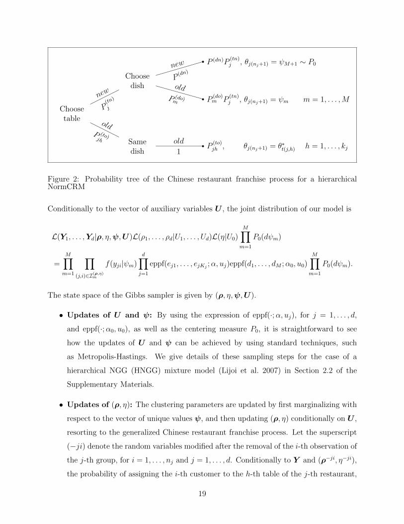
Choosetable

Samedish

P(to)jh , θj(nj+1) = θ∗t(j,h) h = 1, . . . , kj

old

1

oldP (to)jh

Choosedish

P(do)m P

(tn)j , θj(nj+1) = ψm m = 1, . . . ,M

old

P (do)m

P (dn)P(tn)j , θj(nj+1) = ψM+1 ∼ P0new

P(dn)

new

P(tn

)

j

Figure 2: Probability tree of the Chinese restaurant franchise process for a hierarchicalNormCRM

Conditionally to the vector of auxiliary variables U , the joint distribution of our model is

L(Y1, . . . ,Yd|ρ, η,ψ,U)L(ρ1, . . . , ρd|U1, . . . , Ud)L(η|U0)M∏m=1

P0(dψm)

=M∏m=1

∏(j,i)∈I(ρ,η)m

f(yji|ψm)d∏j=1

eppf(ej1, . . . , ejKj ;α, uj)eppf(d1, . . . , dM ;α0, u0)M∏m=1

P0(dψm).

The state space of the Gibbs sampler is given by (ρ, η,ψ,U).

• Updates of U and ψ: By using the expression of eppf(·;α, uj), for j = 1, . . . , d,

and eppf(·;α0, u0), as well as the centering measure P0, it is straightforward to see

how the updates of U and ψ can be achieved by using standard techniques, such

as Metropolis-Hastings. We give details of these sampling steps for the case of a

hierarchical NGG (HNGG) mixture model (Lijoi et al. 2007) in Section 2.2 of the

Supplementary Materials.

• Updates of (ρ, η): The clustering parameters are updated by first marginalizing with

respect to the vector of unique values ψ, and then updating (ρ, η) conditionally on U ,

resorting to the generalized Chinese restaurant franchise process. Let the superscript

(−ji) denote the random variables modified after the removal of the i-th observation of

the j-th group, for i = 1, . . . , nj and j = 1, . . . , d. Conditionally to Y and (ρ−ji, η−ji),

the probability of assigning the i-th customer to the h-th table of the j-th restaurant,

19

where the m-th dish is served (i.e., t(j, h) ∈ D−jim ), is

P(i ∈ C−jijh , t(j, h) ∈ D−jim |Y ,ρ−ji, η−ji, Uj = uj)

∝M(yji

∣∣∣yI(ρ−ji,η−ji)m

)P(i ∈ C−jijh , t(j, h) ∈ D−jim |ρ−ji, η−ji, Uj = uj). (23)

In the latter, when h = 1, . . . , K−jij , then m is the value such that t(j, h) ∈ D−jim ,

i.e. C−jijh is an already occupied table where the m-th dish is served. Moreover, when

h = (K−jij + 1), then m = 1, . . . ,M−ji + 1, i.e. when a new table is allocated the

chosen dish can be either one of those already served or a new one. Here, M(yji|yIm)

is the predictive density of a parametric Bayesian model where the sampling model

is f(y|θ), the prior is P0, and the observations are all the data with index in Im,

with IM−ji+1 the empty set. Probability P(i ∈ C−jijh , t(j, h) ∈ D−jim |ρ−ji, η−ji, Uj = uj)

is depicted in Figure 2 (see also formula (25) below). Thus, (23) is proportional to

the prior probability that the i-th customer of the j-th restaurant will sit at the h-th

table, updated by considering the information yielded by the customers of the franchise

eating the same dish. This dish is served at table h and at all the other tables such that

t(j, h) ∈ D−jim , for j = 1, . . . , d. This step of the algorithm clarifies how the sharing of

information between individuals and across groups takes place in model (19).

The updating process continues by re-allocating Cjh to a cluster of tables. To this end,

we have to assign t = t(j, h) to a new/old cluster of tables Dm. More formally, let the

superscript (−t) indicate the variables after the removal of all the observations in Cjh

such that t = t(j, h). Conditionally on Y and (ρ−t, η−t), the probability of assigning

the t-th table to the m-th cluster is

P(t ∈ D−tm |Y ,ρ−t, η−t, U0 = u0) ∝M(yt

∣∣∣YI(ρ−t,η−t)m

)P(t ∈ D−tm |ρ−t, η−t, U0 = u0),

(24)

for m = 1, . . . ,M−t + 1, where (M−t + 1) indicates the new cluster of tables. Here,

Yt := {Yij : i ∈ Cjh, t = t(j, h)} is the set of all the observations (customers) in the

l-cluster Cjh (i.e., the t-th table), and M(yt|yIm) is the joint predictive density of ejh

observations from a parametric Bayesian model where the sampling model is f(y|θ), the

20

prior is P0, and the observations are all the data with index in Im. Probability P(t ∈

D−tm |ρ−t, η−t, U0 = u0) has been introduced in (22), and it is the predictive probability

prescribed by the generalized Chinese restaurant process of the table indices. Formula

(24) is proportional to the prior probability that the t-th table of the j-th restaurant will

share the m-th dish, updated by considering the information yielded by the customers

of the franchise eating the same dish. This step of the algorithm clarifies how the

sharing of information within and between groups takes place in model (19).

The computation of the conditional probabilitiesM in (23) and (24) is available in closed

analytical form only when P0 and f(·|θ) in (19) are conjugate. For the non-conjugate case, an

extension of the proposed algorithm, that uses Algorithm 8 of Neal (2000) and the algorithm

of Favaro and Teh (2013), is described in the Section 2.4 of the Supplementary Materials.

3.3 Prediction

Consider a configuration (ρ, η,ψ), and hence θ, of n observations in d groups, as well as

a new dish label indicated as ψM+1. We want to make a prediction within the j-th group

of data, according to the law of θj(nj+1). Combining equations (21) and (22) as outlined in

Figure 2, we express this law, jointly with the j-th l-clustering configuration, as follows:

P(θj(nj+1) = ψm, (nj + 1) ∈ Cjh|ρ, η,ψ) =

P

(to)jh h = 1, . . . ,Kj , m = t(j, h)

P(tn)j P

(do)m h = Kj + 1, m = 1, . . . ,M

P(tn)j P (dn) h = Kj + 1, m = M + 1

(25)

where ψM+1 ∼ P0. Interestingly, since we have assumed that the groups are exchangeable

and infinitely many are allowed, as it is usual in hierarchical models, we can make a prediction

on the arrival of a new observation in a new group as:

P(θ(d+1)1 = ψm|ρ, η,ψ) =

P(do)m h = 1 and m = 1, . . . ,M,

P (dn) h = 1 and m = M + 1.(26)

We now derive the law of a new observation given the multidimensional array of data Y =

(Y1, . . . ,Yd) for the mixture in model (19). It is easy to see that, conditionally on (ρ, η,ψ),

this quantity changes depending on the group. In particular, the predictive densities in an

21

existing or in a new group are:

p(yj(nj+1)|Y ,ρ, η,ψ)

=

Kj∑h=1

P(to)jh f(yj(nj+1)|θjh) + P

(tn)j

M∑m=1

P (do)m f(yj(nj+1)|ψm) + P

(tn)j P (dn)

∫Θ

f(yj(nj+1)|ψ)P0(dψ),

p(y(d+1)1|Y ,ρ, η,ψ)) =M∑m=1

P (do)m f(y(d+1)1|ψm) + P (dn)

∫Θ

f(y(d+1)1|ψ)P0(dψ), (27)

where the marginal distribution M(y) =∫Θ

f(y|ψ)P0(dψ) is often not available in practice,

and can be approximated via Monte Carlo integration. Finally, the unconditional predictive

distribution is computed by averaging (27) with respect to the posterior sample of (ρ, η,ψ),

drawn using the Gibbs sampler described in Section 3.2.

As a final remark, in the non-hierarchical case, where the d processes in model (18) are

independent (i.e., P degenerates to the diffuse centering measure P0), P(do)m = 0, for each

m = 1, . . . ,M , and P (dn) = 1. Hence, within each group, the predictive structure of a

standard Chinese Restaurant process is recovered, and the predictive distribution in a new

group coincides with M(y).

4 Applications

In this section, we assess the performance of the proposed mixture model on both simulated

and benchmark datasets. We focus on the hierarchical NGG (HNGG) mixture model, ob-

tained from model (19) when the Levy intensities are α(s) = κΓ(1−σ)

s−1−σe−sI(0,+∞)(s), and

α0(s) = κ0Γ(1−σ0)

s−1−σ0e−sI(0,+∞)(s), so that the hyperparameters of the HNGG process are

(κ, κ0, σ, σ0), with κ, κ0 > 0 and σ, σ0 ∈ (0, 1). We choose f(·|θ) as a Gaussian kernel with

θ = (µ, τ 2) representing the mean and variance parameters, and a centering measure P0 as

a conjugate normal-inverse-gamma with parameters (m0, k0, aτ2 , bτ2). Under this model, the

marginal distributions are known, allowing us to adopt the marginal algorithm introduced in

Section 3.2. Non-conjugate independent normal and inverse-gamma priors on the mean and

variance parameters can also be used (see application in Section 4.2). The NGG adds flexi-

bility to random partition models, mitigating the “rich-gets-richer” effect of the commonly

22

used Dirichlet process via the introduction of an additional parameter. We refer readers to

Section 3 of the Supplementary Materials for the expressions of equations (21) and (22) in

this setting.

4.1 Simulation Study (d = 2)

Our goal is to assess the performance of the nonparametric HNGG process in recovering the

original clustering of the observations, as well as to evaluate its goodness of fit. Here, we first

study performances for different values of the hyperparameters κ, κ0, σ, σ0 of the HNGG. This

allows us to obtain different models, including the Dirichlet counterpart, i.e., the Hierarchical

Dirichlet Process (HDP) model obtained for σ = σ0 = 0, and an independent model where

(P1, . . . , Pd)iid∼ NGG(κ0, σ0, P0). We also consider the case of random hyperparameters.

We simulated the data from two distinct groups of 100 observations, each sampled from

a two-component Gaussian mixture, with one component shared between the two groups.

Membership to the Gaussian components identifies a clustering structure across groups into

three clusters, which we will refer to as the true partition of the data. For i = 1, . . . , 100:

y1iiid∼ 0.2N (y1i|−3, 0.1) + 0.8N (y1i|0, 0.5) ; y2i

iid∼ 0.1N (y2i|0, 0.5) + 0.9N (y2i|1, 1.5) .

We observe how the component shared by the two groups has a higher weight in the first

mixture and we argue that, unlike our hierarchical model that shares information across

groups, the independent model will not be able to adequately recover this component.

We fitted a HNGG model with two groups, i.e. j = 1, 2, and assessed the performance of

the proposed model using the log-pseudo marginal likelihood (LPML) and the Rand index

(RI). The first measures the goodness-of-fit of the model, while the second measures the

goodness-of-clustering. For the RI, we first estimated the natural clustering as the partition

minimizing the Binder’s loss function (Lau and Green 2007), and then computed the Rand

index against the true partition of the data in the second group, since this presents the most

interesting features from a clustering perspective. Throughout the simulation study, we fixed

the hyperparameters of P0 equal to (m0, k0, aτ2 , bτ2) = (0.25, 0.62, 2.07, 0.66), a specification

that corresponds to E[µ] = yn, E[τ 2] = s2n/3, Var(µ) = 1, Var(τ 2) = 5, where yn and s2

n

represent the sample mean and variance of the whole dataset, respectively. The choice of the

23

hyperparameters of the centering measure P0 is crucial, as it influences both the fitting and

the clustering estimation. Results obtained from a sensitivity analysis, reported in Section

3.4 of the Supplementary Materials, show that there is a trade-off between goodness-of-

clustering and goodness-of-fit, when varying the values of the variances of the parameters

a priori. In particular, while large variances yield poor clustering performance in terms of

RI, they can help improve the model fitting in terms of LPML. This behaviour is observed

also in the sensitivity analysis concerning the hyperparameters (κ, κ0, σ, σ0) of the HNGG

process.

We first show results obtained with several combinations of values for the parameters

(κ, κ0, σ, σ0). This strategy, in particular, allows comparison with various HDP and inde-

pendent models. Values of LPML and RI are reported in Tables 1 and 2, respectively, for

some of the parameter settings. The estimated number of natural clusters in the second

group (i.e., the number of different dishes served in the second restaurant) is reported in

brackets in Table 2. Results on additional settings are reported in Section 3.3 of the Sup-

plementary Materials. In general, the best LPML values are observed when σ or σ0 are

different from zero, meaning that the HNGG outperforms the HDP in terms of goodness-of-

fit. On the other hand, higher values of LPML, obtained for large values of the parameters

σ or σ0, correspond also to higher numbers of clusters in each group, as it can be observed

in Table 2. Furthermore, we observe that the RI alone is not indicative of good recovery

of the true partition, since its maximum value is reached when all the observations in the

second group are clustered together. A better clustering of the data in the second group is

instead provided by two estimated clusters and a relatively high RI, as we can observe in

some of the cases where σ and σ0 differ from 0. Results on additional quantities of interest

a priori, such as the expectation and variance of M , and the covariance and coskewness of

P1(A) and P2(A), with A a neighbourhood of zero, are reported in Sections 3.1 and 3.2 of

the Supplementary Materials. These results show how larger values of the hyperparameters

(κ, κ0, σ, σ0) influence the distribution of the number of clusters, as they induce an increase

in the expectation and variance of M . On the other hand, increasing the values of (κ0, σ0)

also increases the dependency between measures, while an opposite trend is observed when

increasing (κ, σ). As expected, the highest values of RI are obtained when the prior expected

value of M is close to the truth. On the other hand, optimal LPML values are obtained for

24

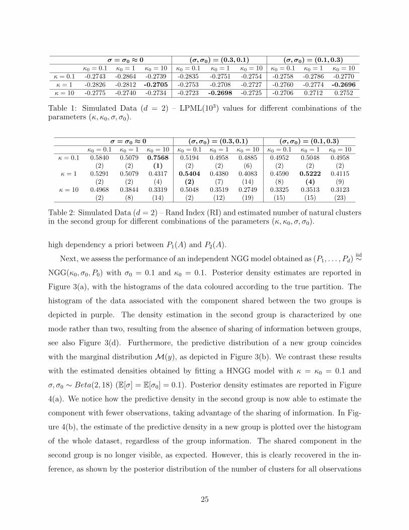
σ = σ0 ≈ 0 (σ,σ0) = (0.3,0.1) (σ,σ0) = (0.1,0.3)κ0 = 0.1 κ0 = 1 κ0 = 10 κ0 = 0.1 κ0 = 1 κ0 = 10 κ0 = 0.1 κ0 = 1 κ0 = 10

κ = 0.1 -0.2743 -0.2864 -0.2739 -0.2835 -0.2751 -0.2754 -0.2758 -0.2786 -0.2770κ = 1 -0.2826 -0.2812 -0.2705 -0.2753 -0.2708 -0.2727 -0.2760 -0.2774 -0.2696κ = 10 -0.2775 -0.2740 -0.2734 -0.2723 -0.2698 -0.2725 -0.2706 0.2712 0.2752

Table 1: Simulated Data (d = 2) – LPML(103) values for different combinations of theparameters (κ, κ0, σ, σ0).

σ = σ0 ≈ 0 (σ,σ0) = (0.3,0.1) (σ,σ0) = (0.1,0.3)κ0 = 0.1 κ0 = 1 κ0 = 10 κ0 = 0.1 κ0 = 1 κ0 = 10 κ0 = 0.1 κ0 = 1 κ0 = 10

κ = 0.1 0.5840 0.5079 0.7568 0.5194 0.4958 0.4885 0.4952 0.5048 0.4958(2) (2) (1) (2) (2) (6) (2) (2) (2)

κ = 1 0.5291 0.5079 0.4317 0.5404 0.4380 0.4083 0.4590 0.5222 0.4115(2) (2) (4) (2) (7) (14) (8) (4) (9)

κ = 10 0.4968 0.3844 0.3319 0.5048 0.3519 0.2749 0.3325 0.3513 0.3123(2) (8) (14) (2) (12) (19) (15) (15) (23)

Table 2: Simulated Data (d = 2) – Rand Index (RI) and estimated number of natural clustersin the second group for different combinations of the parameters (κ, κ0, σ, σ0).

high dependency a priori between P1(A) and P2(A).

Next, we assess the performance of an independent NGG model obtained as (P1, . . . , Pd)iid∼

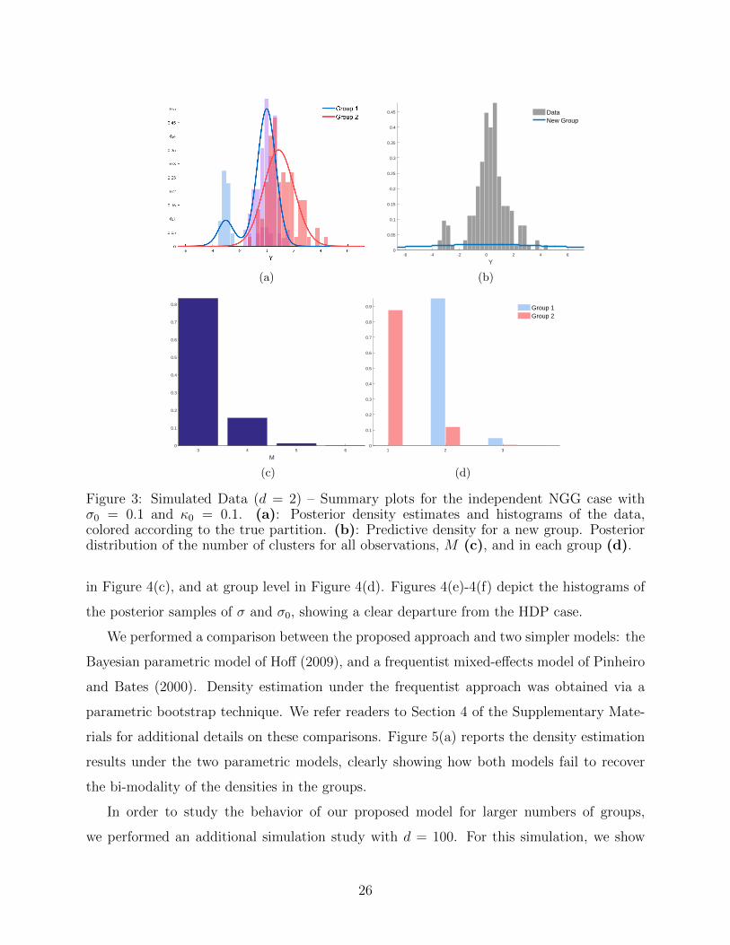
NGG(κ0, σ0, P0) with σ0 = 0.1 and κ0 = 0.1. Posterior density estimates are reported in

Figure 3(a), with the histograms of the data coloured according to the true partition. The

histogram of the data associated with the component shared between the two groups is

depicted in purple. The density estimation in the second group is characterized by one

mode rather than two, resulting from the absence of sharing of information between groups,

see also Figure 3(d). Furthermore, the predictive distribution of a new group coincides

with the marginal distribution M(y), as depicted in Figure 3(b). We contrast these results

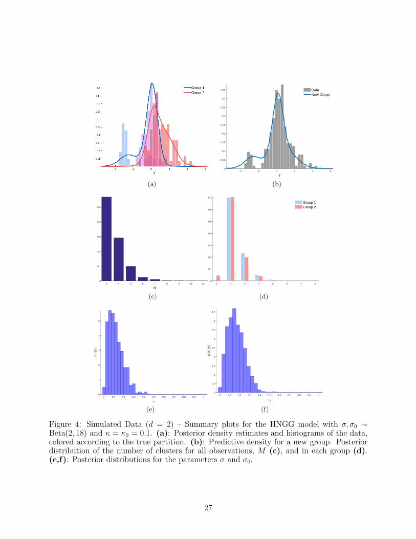
with the estimated densities obtained by fitting a HNGG model with κ = κ0 = 0.1 and

σ, σ0 ∼ Beta(2, 18) (E[σ] = E[σ0] = 0.1). Posterior density estimates are reported in Figure

4(a). We notice how the predictive density in the second group is now able to estimate the

component with fewer observations, taking advantage of the sharing of information. In Fig-

ure 4(b), the estimate of the predictive density in a new group is plotted over the histogram

of the whole dataset, regardless of the group information. The shared component in the

second group is no longer visible, as expected. However, this is clearly recovered in the in-

ference, as shown by the posterior distribution of the number of clusters for all observations

25

(a)

-6 -4 -2 0 2 4 6

Y

0

0.05

0.1

0.15

0.2

0.25

0.3

0.35

0.4

0.45 DataNew Group

(b)

3 4 5 6

M

0

0.1

0.2

0.3

0.4

0.5

0.6

0.7

0.8

(c)

1 2 3

0

0.1

0.2

0.3

0.4

0.5

0.6

0.7

0.8

0.9 Group 1Group 2

(d)

Figure 3: Simulated Data (d = 2) – Summary plots for the independent NGG case withσ0 = 0.1 and κ0 = 0.1. (a): Posterior density estimates and histograms of the data,colored according to the true partition. (b): Predictive density for a new group. Posteriordistribution of the number of clusters for all observations, M (c), and in each group (d).

in Figure 4(c), and at group level in Figure 4(d). Figures 4(e)-4(f) depict the histograms of

the posterior samples of σ and σ0, showing a clear departure from the HDP case.

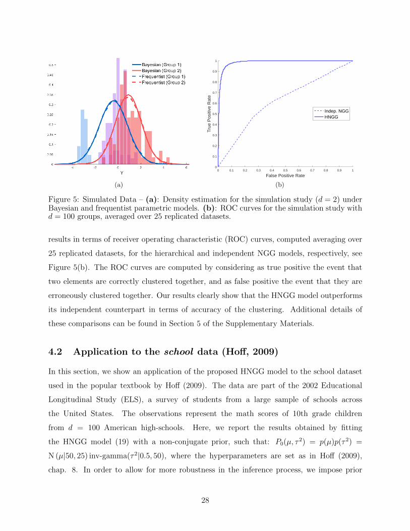
We performed a comparison between the proposed approach and two simpler models: the

Bayesian parametric model of Hoff (2009), and a frequentist mixed-effects model of Pinheiro

and Bates (2000). Density estimation under the frequentist approach was obtained via a

parametric bootstrap technique. We refer readers to Section 4 of the Supplementary Mate-

rials for additional details on these comparisons. Figure 5(a) reports the density estimation

results under the two parametric models, clearly showing how both models fail to recover

the bi-modality of the densities in the groups.

In order to study the behavior of our proposed model for larger numbers of groups,

we performed an additional simulation study with d = 100. For this simulation, we show

26

(a)

-4 -2 0 2 4 6

Y

0

0.05

0.1

0.15

0.2

0.25

0.3

0.35

0.4

0.45 DataNew Group

(b)

3 4 5 6 7 8 9 10 11

M

0

0.1

0.2

0.3

0.4

0.5

(c)

1 2 3 4 5 6 7 8

0

0.1

0.2

0.3

0.4

0.5

0.6

0.7

Group 1Group 2

(d)

0 0.1 0.2 0.3 0.4 0.5 0.6 0.7 0.8 0.9 1

σ

0

1

2

3

4

5

p(σ|y)

(e)

0 0.1 0.2 0.3 0.4 0.5 0.6 0.7 0.8 0.9 1

σ0

0

0.5

1

1.5

2

2.5

3

3.5

4

4.5

p(σ

0|y)

(f)

Figure 4: Simulated Data (d = 2) – Summary plots for the HNGG model with σ, σ0 ∼Beta(2, 18) and κ = κ0 = 0.1. (a): Posterior density estimates and histograms of the data,colored according to the true partition. (b): Predictive density for a new group. Posteriordistribution of the number of clusters for all observations, M (c), and in each group (d).(e,f): Posterior distributions for the parameters σ and σ0.

27

(a)

0 0.1 0.2 0.3 0.4 0.5 0.6 0.7 0.8 0.9 1

False Positive Rate

0

0.1

0.2

0.3

0.4

0.5

0.6

0.7

0.8

0.9

1

Tru

e P

ositi

ve R

ate

Indep. NGGHNGG

(b)

Figure 5: Simulated Data – (a): Density estimation for the simulation study (d = 2) underBayesian and frequentist parametric models. (b): ROC curves for the simulation study withd = 100 groups, averaged over 25 replicated datasets.

results in terms of receiver operating characteristic (ROC) curves, computed averaging over

25 replicated datasets, for the hierarchical and independent NGG models, respectively, see

Figure 5(b). The ROC curves are computed by considering as true positive the event that

two elements are correctly clustered together, and as false positive the event that they are

erroneously clustered together. Our results clearly show that the HNGG model outperforms

its independent counterpart in terms of accuracy of the clustering. Additional details of

these comparisons can be found in Section 5 of the Supplementary Materials.

4.2 Application to the school data (Hoff, 2009)

In this section, we show an application of the proposed HNGG model to the school dataset

used in the popular textbook by Hoff (2009). The data are part of the 2002 Educational

Longitudinal Study (ELS), a survey of students from a large sample of schools across

the United States. The observations represent the math scores of 10th grade children

from d = 100 American high-schools. Here, we report the results obtained by fitting

the HNGG model (19) with a non-conjugate prior, such that: P0(µ, τ 2) = p(µ)p(τ 2) =

N (µ|50, 25) inv-gamma(τ 2|0.5, 50), where the hyperparameters are set as in Hoff (2009),

chap. 8. In order to allow for more robustness in the inference process, we impose prior

28

distributions κ, κ0 ∼ gamma(1, 1) and σ, σ0 ∼ Beta(2, 18).

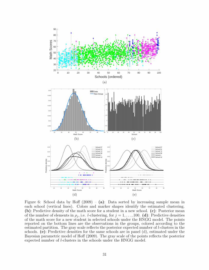
Figure 6(a) shows the data organized by school. The order of the schools is given by

increasing sample mean in each group, and the color of each data point refers to its natural

cluster assignment, obtained by minimizing the Binder’s loss function, which identified 5

clusters. Three major clusters can be observed, corresponding to students with low (squares),

medium (dots), or high (diamonds and triangles) math scores, respectively. However, these

clusters also characterize different school compositions: on one hand, low-sized schools are

composed of only one type of students, while on the other hand, when the number of students

increases, we observe more heterogeneity in the school composition. We argue that this could

be explained by additional latent variables representing socio-economical information. To

explore the clustering structure at group level, in Figure 6(c) we plot the posterior mean of the

number of elements in ρj, i.e. l-clusters, for j = 1, . . . , 100. We observe some heterogeneity,

with some schools having just one l-cluster of students, and others with up to three different

l-clusters. We then selected the 3 schools with the highest posterior expected numbers

of l-clusters (schools 98, 1, 12) and the 3 with the lowest ones (schools 67, 51, 72), and

estimated the corresponding predictive densities, see Figure 6(d). The composition of the

selected schools is shown by plotting the observations underneath the predictive densities,

specifically according to the natural clustering estimated via the Binder’s loss. The intensity

of the grey scale for the predictive densities increases with the posterior expected number

of l-clusters. Schools 67 and 51 have students with higher math scores, while school 72

is characterized by lower math scores. The other three selected schools present a more

heterogeneous composition. This confirms our interpretation of the results in Figure 6(d).

In Figure 6(b), the predictive density in a new group is depicted, with the histogram of the

whole dataset obtained without considering the group information. The predictive density

does not appear to be multimodal, showing how the proposed mixture model preserves the

shrinkage effect typical of the Bayesian hierarchical models while the underlying clustering

allows for a more detailed interpretation of the information in the data.

Finally, following the suggestion of one of the reviewers, we performed a comparison of

our results with a simple parametric hierarchical model fitted as in Hoff (2009) (Chapter

8). In Figure 6(e) the predictive densities under the parametric model are reported for a

selection of the schools. Comparing these densities with the corresponding ones in panel (d),

29

it is clear how the parametric model does not capture the skewness and the heavy tails of

the data, as it does not allow for heterogeneity within groups. Additional details on this

comparison can be found in Section 4 of the Supplementary Materials.

30

0 10 20 30 40 50 60 70 80 90 100

Schools (ordered)

20

30

40

50

60

70

80

90

Mat

h S

core

s

(a)

20 30 40 50 60 70 80 90

Math Score

0

0.005

0.01

0.015

0.02

0.025

0.03

0.035

0.04DataNew Group

(b)

0 10 20 30 40 50 60 70 80 90 100

School

0

0.5

1

1.5

2

2.5

3

3.5

4

(c)

20 30 40 50 60 70 80 90

Math Score

0

0.01

0.02

0.03

0.04

0.05

Pre

dict

ive

dens

ity

School 67School 51School 72School 98School 1School 12

(d)

20 30 40 50 60 70 80 90

Math Score

0

0.01

0.02

0.03

0.04

0.05

Pre

dict

ive

dens

ity

School 67School 51School 72School 98School 1School 12

(e)

Figure 6: School data by Hoff (2009) – (a): Data sorted by increasing sample mean ineach school (vertical lines). Colors and marker shapes identify the estimated clustering.(b): Predictive density of the math score for a student in a new school. (c): Posterior meanof the number of elements in ρj, i.e. l-clustering, for j = 1, . . . , 100. (d): Predictive densitiesof the math score for a new student in selected schools under the HNGG model. The pointsreported on the bottom lines are the observations in the groups, colored according to theestimated partition. The gray scale reflects the posterior expected number of l-clusters in theschools. (e): Predictive densities for the same schools are in panel (d), estimated under theBayesian parametric model of Hoff (2009). The gray scale of the points reflects the posteriorexpected number of l-clusters in the schools under the HNGG model.

31

5 Conclusion

In this paper, we have conducted a thorough investigation of the clustering induced by a

NormCRM mixture model. This model is suitable for data belonging to groups or categories

that share similar characteristics. At group level, each NormCRM is centered on the same

base measure, which is a NormCRM itself. The discreteness of the shared base measure

implies that the processes at data level share the same atoms. This desirable feature allows

to cluster together observations of different groups. By integrating out the nonparametric

components of our prior (i.e. P1, · · · , Pd, P ), we have obtained a representation of our model

through formula (19) that sheds light on the hierarchical clustering induced by the mixture.

At the first level of the hierarchy, data are clustered within each of the groups (l-clustering).

These partitions are i.i.d. with law identified by the eppf induced by the NormCRM(α, P ),

that is the law of the mixing measure at the same level of the hierarchy. These l-clusters can

in turn be aggregated into M clusters according to the partition induced by the eppf at the

lowest level of the hierarchy, corresponding to NormCRM(α0, P0). This clustering structure

reveals the sharing of information among the groups of observations in the mixture model.

Furthermore, we have offered an interpretation of this hierarchical clustering in terms of the

generalized Chinese restaurant franchise process, which has allowed us to perform posterior

inference in the presence of both conjugate and non-conjugate models. We have provided

theoretical results concerning the a priori distribution of the number of clusters, within or

between groups, and a general formula to compute moments and mixed moments of general

order. To evaluate the model performance and the elicitation of the hyperparameters, we

have conducted a simulation study and an analysis on a benchmark dataset. Results have

shed insights on the sharing of information among clusters and groups of data, showing how

our model is able to identify components of the mixture that are less represented in a group

of data. The proposed characterization has the potential to be generalized. For example,

an interesting future direction is to investigate extensions to situations where covariates are

available, following either the approach of MacEachern (1999), via dependent nonparametric

processes, or the product partition model approach of Muller and Quintana (2010).

32

6 Acknowledgements

Raffaele Argiento gratefully acknowledges Collegio Carlo Alberto for partially funding this work.

Andrea Cremaschi thanks the Norway Centre for Molecular Medicine (NCMM) IT facility for the

computational support.

SUPPLEMENTARY MATERIAL

Title: Supplementary Materials The file:

HNCRM Supplementary Materials.pdf

reports additional details on the material presented in the main paper. This includes

proofs of the theoretical results presented in the paper and details on how to com-

pute covariance and coskewness of a hierarchical NormCRM, details on the MCMC

algorithm and additional results from the simulation studies.

Title: Code The Matlab code implementing the algorithm described in the paper (both

conjugate and non), is publicly available on GitHub:

https://github.com/AndCre87/HNCRM

References

Argiento, R., Bianchini, I., Guglielmi, A., et al. (2016). Posterior sampling from ε-

approximation of normalized completely random measure mixtures. Electronic Journal

of Statistics, 10(2):3516–3547.

Argiento, R., Cremaschi, A., and Guglielmi, A. (2014). A “density-based” algorithm for clus-

ter analysis using species sampling Gaussian mixture models. Journal of Computational

and Graphical Statistics, 23(4):1126–1142.

Bassetti, F., Casarin, R., and Rossini, L. (2018). Hierarchical species sampling models. arXiv

preprint arXiv:1803.05793.

Blei, D. M. (2012). Probabilistic topic models. Communications of the ACM, 55(4):77–84.

Camerlenghi, F., Lijoi, A., Orbanz, P., and Prunster, I. (2018). Distribution theory for

hierarchical processes. The Annals of Statistics, to appear.

33

Camerlenghi, F., Lijoi, A., and Prunster, I. (2017). Bayesian prediction with multiple-

samples information. Journal of Multivariate Analysis, 156:18–28.

Durrett, R. (1991). Probability: Theory and Examples. Pacific Grove, CA: Wadsworth &

Brooks/Cole.

Favaro, S. and Teh, Y. (2013). MCMC for normalized random measure mixture models.

Statistical Science, 28(3):335–359.

Ferguson, T. S. (1983). Bayesian density estimation by mixtures of normal distributions. In

Recent Advances in Statistics, pages 287–302. Elsevier.

Hoff, P. D. (2009). A first course in Bayesian statistical methods. Springer Verlag.

Ishwaran, H. and James, L. F. (2001). Gibbs sampling methods for stick-breaking priors.

Journal of the American Statistical Association, 96(453):161–173.

Ishwaran, H. and James, L. F. (2003). Generalized weighted chinese restaurant processes for

species sampling mixture models. Statistica Sinica, 13(4):1211–1235.

James, L. F., Lijoi, A., and Prunster, I. (2009). Posterior analysis for normalized random

measures with independent increments. Scandinavian Journal of Statistics, 36(1):76–97.

Kallenberg, O. (2005). Probabilistic Symmetries and Invariance Principles. Springer Science

& Business Media.

Kingman, J. F. C. (1993). Poisson Processes, volume 3. Oxford university press.

Lau, J. W. and Green, P. J. (2007). Bayesian model-based clustering procedures. Journal

of Computational and Graphical Statistics, 16(3):526–558.

Lijoi, A., Mena, R. H., and Prunster, I. (2007). Controlling the reinforcement in bayesian non-

parametric mixture models. Journal of the Royal Statistical Society: Series B (Statistical

Methodology), 69(4):715–740.

Lijoi, A. and Prunster, I. (2010). Models beyond the Dirichlet process. In Hjort, N., Holmes,

C., Muller, P., and Walker, editors, In Bayesian Nonparametrics, pages 80–136. Cambridge

University Press.

34

Lo, A. Y. (1984). On a class of bayesian nonparametric estimates: I. density estimates. The

annals of statistics, 12(1):351–357.

MacEachern, S. N. (1999). Dependent nonparametric processes. In ASA Proceedings of the

Section on Bayesian Statistical Science, pages 50–55.

Malsiner-Walli, G., Fruhwirth-Schnatter, S., and Grun, B. (2017). Identifying mixtures of

mixtures using bayesian estimation. Journal of Computational and Graphical Statistics,

26(2):285–295.

Muller, P. and Quintana, F. (2010). Random partition models with regression on covariates.

Journal of Statistical Planning and Inference, 140(10):2801–2808.

Neal, R. M. (2000). Markov chain sampling methods for dirichlet process mixture models.

Journal of computational and graphical statistics, 9(2):249–265.

Pinheiro, J. and Bates, D. (2000). Mixed-Effects Models in S and S-PLUS. Springer.

Pitman, J. (1996). Some developments of the Blackwell-MacQueen urn scheme. Lecture

Notes-Monograph Series, pages 245–267.

Pitman, J. (2003). Poisson-Kingman partitions. In Science and Statistics: a Festschrift for

Terry Speed, volume 40 of IMS Lecture Notes-Monograph Series, pages 1–34. Institute of

Mathematical Statistics, Hayward (USA).

Pitman, J. (2006). Combinatorial Stochastic Processes. LNM n. 1875. Springer, New York.

Regazzini, E., Lijoi, A., Prunster, I., et al. (2003). Distributional results for means of

normalized random measures with independent increments. The Annals of Statistics,

31(2):560–585.

Teh, Y. W. and Jordan, M. I. (2010). Hierarchical bayesian nonparametric models with

applications. volume 1, pages 158–207. Camb. Ser. Stat. Probab. Math.

Teh, Y. W., Jordan, M. I., Beal, M. J., and Blei, D. M. (2005). Sharing clusters among related

groups: Hierarchical dirichlet processes. In Advances in neural information processing

systems, pages 1385–1392.

35

Teh, Y. W., Jordan, M. I., Beal, M. J., and Blei, D. M. (2006). Hierarchical Dirichlet

processes. Journal of the American Statistical Association, 101(476):1566–1581.

Tyurin, I. S. (2010). An improvement of upper estimates of the constants in the lyapunov

theorem. Russian Mathematical Surveys, 65(3):201–202.

36