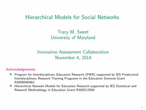
Hierarchical Models for Social Networks

Tracy M. Sweet University of Maryland

Innovative Assessment Collaboration November 4, 2014

Acknowledgements � Program for Interdisciplinary Education Research (PIER) supported by IES Predoctoral

Interdisciplinary Research Training Programs in the Education Sciences Grant R305B040063

� Hierarchical Network Models for Education Research supported by IES Statistical and Research Methodology in Education Grant R305D12004

1

Outline

1

2

3

Motivation

Estimation of Node/Dyad Attributes Effect of Teaching the Same Grade with HLSM

Estimation of Network Attributes Effect of Network Covariate with HMMSBM

2

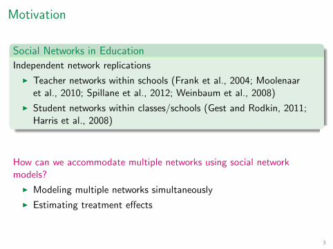
Motivation Social Networks in Education Independent network replications

�I

�I

Teacher networks within schools (Frank et al., 2004; Moolenaar et al., 2010; Spillane et al., 2012; Weinbaum et al., 2008)

Student networks within classes/schools (Gest and Rodkin, 2011; Harris et al., 2008)

3

�

�

�

�

Motivation

Social Networks in Education Independent network replications

Teacher networks within schools (Frank et al., 2004; Moolenaar et al., 2010; Spillane et al., 2012; Weinbaum et al., 2008)

Student networks within classes/schools (Gest and Rodkin, 2011; Harris et al., 2008)

How can we accommodate multiple networks using social network models?

Modeling multiple networks simultaneously

Estimating treatment effects

3

I

I

I

I

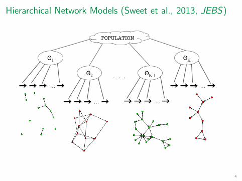
Hierarchical Network Models (Sweet et al., 2013, JEBS)

POPULATION

Θ1

Θ2 ΘK-1

ΘK

…

…

…

…

. . .

4

�

�

�

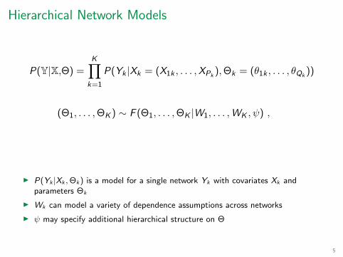
Hierarchical Network Models

KK P(Y|X,Θ) = P(Yk |Xk = (X1k , . . . , XPk ), Θk = (θ1k , . . . , θQk ))

k=1

(Θ1, . . . , ΘK ) ∼ F (Θ1, . . . , ΘK |W1, . . . , WK , ψ) ,

P(Yk |Xk , Θk ) is a model for a single network Yk with covariates Xk and parameters Θk

Wk can model a variety of dependence assumptions across networks

ψ may specify additional hierarchical structure on Θ

5

I

I

I

�

�

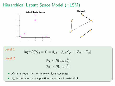
Hierarchical Latent Space Model (HLSM)

1 2 3 4 5

12

34

5

Latent Social Space

Z1

Z2

Z3

Z4

Z5 Z6

Network1

2

3

4

5

6

Level 1 logit P[Yijk = 1] = β0k + β1k Xijk − |Zik − Zjk |

Level 2 β0k ∼ N(µ0, σ0

2)

β1k ∼ N(µ1, σ12)

Xijk is a node-, tie-, or network- level covariate

Zik is the latent space position for actor i in network k

6

I

I

�

�

�

�

�

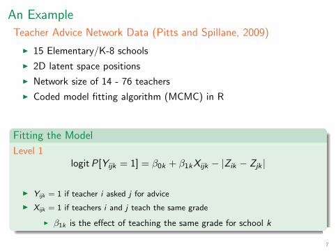
An Example Teacher Advice Network Data (Pitts and Spillane, 2009)

15 Elementary/K-8 schools

2D latent space positions

Network size of 14 - 76 teachers

Coded model fitting algorithm (MCMC) in R

Fitting the Model Level 1

logit P[Yijk = 1] = β0k + β1k Xijk − |Zik − Zjk |

Yijk = 1 if teacher i asked j for advice

Xijk = 1 if teachers i and j teach the same grade

� β1k is the effect of teaching the same grade for school k

7

I

I

I

�I

I

I

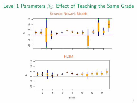
Level 1 Parameters β1: Effect of Teaching the Same Grade Separate Network Models

-10

-50

510

15

β 1

-10

-50

510

15 * * *

**2 4 6 8 10 12 14

HLSM

2 4 6 8 10 12 14

-10

-50

510

15

School

β 1

8

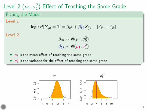
Figure : Effect of Teaching the Same Grade

Level 2 (µ1, σ12) Effect of Teaching the Same Grade

Fitting the Model Level 1

logit P[Yijk = 1] = β0k + β1k Xijk − |Zik − Zjk |

Level 2 β0k ∼ N(µ0, σ

2 0)

β1k ∼ N(µ1, σ2 1)

µ1 is the mean effect of teaching the same grade

σ2 1 is the variance for the effect of teaching the same grade

-1 0 1 2 3 4

0.0

0.3

0.6

µ1

0 2 4 6 8 10

0.00

0.15

0.30

σ12

9

I�

I�

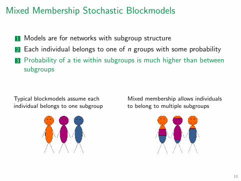
Mixed Membership Stochastic Blockmodels

1

2

3

Models are for networks with subgroup structure

Each individual belongs to one of n groups with some probability

Probability of a tie within subgroups is much higher than between subgroups

Typical blockmodels assume each individual belongs to one subgroup

Mixed membership allows individuals to belong to multiple subgroups

10

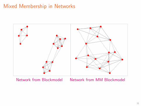
Mixed Membership in Networks

Network from Blockmodel Network from MM Blockmodel

11

�

�

�

�

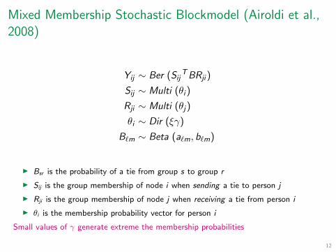
Mixed Membership Stochastic Blockmodel (Airoldi et al., 2008)

Yij Ber (Sij T BRji ) ∼

Sij ∼ Multi (θi )

Rji ∼ Multi (θj )

θi ∼ Dir (ξγ)

Bem ∼ Beta (aem, bem)

Bsr is the probability of a tie from group s to group r

Sij is the group membership of node i when sending a tie to person j

Rji is the group membership of node j when receiving a tie from person i

θi is the membership probability vector for person i

Small values of γ generate extreme the membership probabilities

12

I

I

I

I

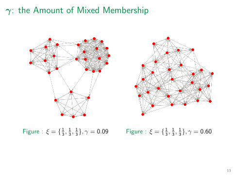
111 ξ = { }, γ = 0.09 , , 3 3 3111ξ = { }, γ = 0.60, , 333

γ: the Amount of Mixed Membership

Figure : Figure :

13

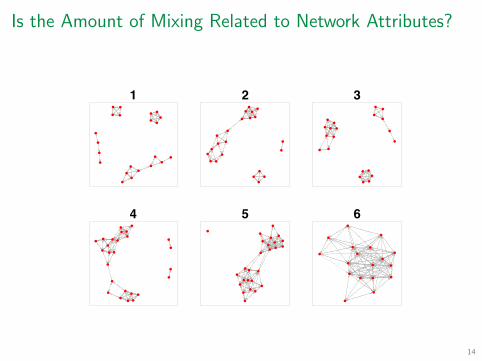
Is the Amount of Mixing Related to Network Attributes?

8/15

Model Multiple Networks SimultaneouslyI Higher e�ciency in educational researchI Make multiple networks comparable

Figure: Selected 5th Grade Cognitive Friendship Networks

1 2 3

4 5 6

14

Is the Amount of Mixing Related to Network Attributes?

�

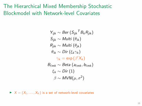
The Hierarchical Mixed Membership Stochastic Blockmodel with Network-level Covariates

Yijk ∼ Ber (Sijk T Bk Rjik )

Sijk ∼ Multi (θik )

Rjik ∼ Multi (θjk )

θik ∼ Dir (ξk γk )

γk = exp (β'Xk )

Bemk ∼ Beta (aemk , bemk )

ξk ∼ Dir (1)

β ∼ MVN(µ, σ2)

X = (X1, . . . , XK ) is a set of network-level covariates

15

I

�

�

�

�

�

�

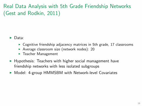
Real Data Analysis with 5th Grade Friendship Networks (Gest and Rodkin, 2011)

Data:

Cognitive friendship adjacency matrices in 5th grade, 17 classrooms Average classroom size (network nodes): 20 Teacher Management

Hypothesis: Teachers with higher social management have friendship networks with less isolated subgroups

Model: 4-group HMMSBM with Network-level Covariates

16

I

I

I

I

I

I

�

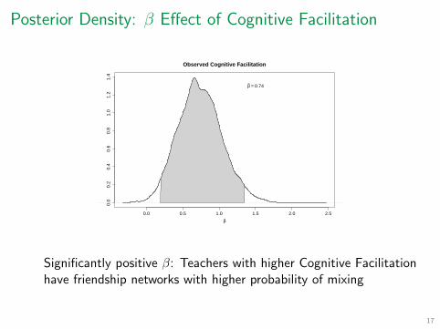
Posterior Density: β Effect of Cognitive Facilitation

0.0 0.5 1.0 1.5 2.0 2.5

0.0

0.2

0.4

0.6

0.8

1.0

1.2

1.4

β

β = 0.74

Observed Cognitive Facilitation

Significantly positive β: Teachers with higher Cognitive Facilitation have friendship networks with higher probability of mixing

17

Positive Relationship between Teacher Management and Mixed Membership

CF = −0.56 CF = 0.03

CF = 0.75

18

Airoldi, E., Blei, D., Fienberg, S., and Xing, E. (2008), “Mixed membership stochastic blockmodels,” The Journal of Machine Learning Research, 9, 1981–2014.

Bradley, R. and Gart, J. (1962), “The asymptotic properties of ML estimators when sampling from associated populations,” Biometrika, 49, 205–214.

Cramer, H. (1946), Mathematical methods of statistics, Princeton, NJ: Princeton University Press.

Daly, A., Moolenaar, N., Bolivar, J., and Burke, P. (2010), “Relationships in reform: The role of teachers’ social networks,” Journal of educational administration, 48, 359–391.

Ennett, S. and Bauman, K. (1993), “Peer group structure and adolescent cigarette smoking: a social network analysis,” Journal of Health and Social Behavior, 226–236.

Espelage, D. and Low, S. (2009), “Multi-site Evaluation of Second Step: Student Success Through Prevention (Second Step ­SSTP) in Preventing Bullying and Sexual Violence,” CDC Grant.

Frank, K. A., Zhao, Y., and Borman, K. (2004), “Social Capital and the Diffusion of Innovations Within Organizations: The Case of Computer Technology in Schools,” Sociology of Education, 77, 148–171.

Gest, S. D. and Rodkin, P. C. (2011), “Teaching practices and elementary classroom peer ecologies,” Journal of Applied Developmental Psychology, 32, 288–296.

Harris, K. M., Florey, F., Tabor, J., Bearman, P. S., Jones, J., Udry, J. R., of Adolescent Health, N. L. S., et al. (2008), “Research design,” Carolina Population Center, University of North Carolina at Chapel Hill.

Hoff, P. D., Raftery, A. E., and Handcock, M. S. (2002), “Latent Space Approaches to Social Network Analysis,” Journal of the American Statistical Association, 97, 1090–1098.

Krackhardt, D. and Porter, L. (1986), “The snowball effect: Turnover embedded in communication networks.” Journal of Applied Psychology; Journal of Applied Psychology, 71, 50.

Lawrence, J., Sweet, T., and Junker, B. (2014), “Professional learning communities and the adoption of novel instructional practices: An evaluation of the School Reform Initiative,” IES Grant Proposal.

Lewis, K., Kaufman, J., Gonzalez, M., Wimmer, A., and Christakis, N. (2008), “Tastes, ties, and time: A new social network dataset using Facebook. com,” Social Networks, 30, 330–342.

Moolenaar, N., Daly, A., and Sleegers, P. (2010), “Occupying the principal position: Examining relationships between transformational leadership, social network position, and schools’ innovative climate,” Educational Administration Quarterly, 46, 623.

19

Pitts, V. and Spillane, J. (2009), “Using social network methods to study school leadership,” International Journal of Research & Method in Education, 32, 185–207.

Smith, D. and White, D. (1992), “Structure and dynamics of the global economy: Network analysis of international trade 1965–1980,” Social Forces, 70, 857–893.

Snijders, T. and Nowicki, K. (1997), “Estimation and prediction for stochastic blockmodels for graphs with latent block structure,” Journal of Classification, 14, 75–100.

Spillane, J., Kim, C., and Frank, K. (2011), “Instructional Advice and Information Providing and Receiving Behavior in Elementary Schools: Exploring Tie Formation as a Building Block in Social Capital Development,” Institute for Policy Research Northwester University Working Paper Series.

Spillane, J. P. and Hopkins, M. (2013), “Organizing for instruction in education systems and school organizations: how the subject matters,” Journal of Curriculum Studies, 45, 721–747.

Spillane, J. P., Kim, C. M., and Frank, K. A. (2012), “Instructional Advice and Information Providing and Receiving Behavior in Elementary Schools Exploring Tie Formation as a Building Block in Social Capital Development,” American Educational Research Journal.

Sweet, T. M., Thomas, A. C., and Junker, B. W. (2013), “Hierarchical Network Models for Education Research: Hierarchical Latent Space Models,” Journal of Educational and Behavioral Statistics, 38, 295–318.

Wasserman, S. and Pattison, P. (1996), “Logit models and logistic regressions for social networks: I. An introduction to Markov graphs and p*,” Psychometrika, 61, 401–425, 10.1007/BF02294547.

Weinbaum, E., Cole, R., Weiss, M., and Supovitz, J. (2008), “Going with the flow: Communication and reform in high schools,” in The implementation gap: understanding reform in high schools, eds. Supovitz, J. and Weinbaum, E., Teachers College Press, pp. 68–102.

20

�

�

�

�

�

�

�

�

�

�

For More Information:

http://hnm.stat.cmu.edu or tsweet@umd.edu

Current Work HLSMs for covariate effects and interventions

Power Analysis for HLSMs

Blockmodels and Mixed Membership

Other ways to incorporate covariates into blockmodels

HNMs for Mediation and Influence

Future Work Develop new models and extensions (longitudinal models)

Operating characteristics

Identifiability and estimation issues

Applications with educational data

Valued ties 21

I

I

I

I

I

I

I

I

I

I

�

�

�

�

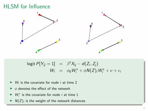
HLSM for Influence 1

2

3

4

5

6

1

2

3

4

5

6

logit P[Yij = 1] = βt Xij − d(Zi , Zj )

Wi = φ0Wit + φN(Z )i Wi

t + ν + Ei

Wi is the covariate for node i at time 2

φ denotes the effect of the network

Wi; is the covariate for node i at time 1

N(Z )i is the weight of the network distances

1

I

I

I

I

Extra Slides

2

�

�

�

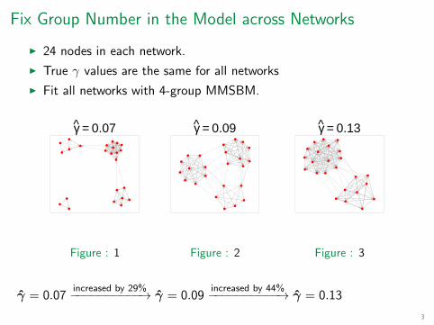
Fix Group Number in the Model across Networks

24 nodes in each network.

True γ values are the same for all networks

Fit all networks with 4-group MMSBM.

γ = 0.07 γ = 0.09 γ = 0.13

Figure : 1 Figure : 2 Figure : 3

increased by 29% increased by 44%γ = 0.07 −−−−−−−−−−→ γ = 0.09 −−−−−−−−−−→ γ = 0.13

3

I

I

I

�

Fitting the HLSM for Interventions

Fitted Model

logit P[Yijk = 1] = β0 + β1k Xijk − |Zik − Zjk | + αTk

Zik ∼ MVN

0 0

,

10 0 0 10

β0 ∼ N(0, 100)

β1k ∼ N(0, 100)

α ∼ N(0, 100)

Xijk is the indicator that teacher i and j in network k teach the same grade

Coded model fitting algorithm (MCMC) in R

4

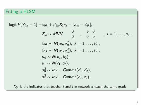
Fitting a HLSM

logit P[Yijk = 1] =β0k + β1k X1ijk − |Zik − Zjk |, 0 a 0

Zik ∼ MVN , , i = 1, . . . , nk ,0 0 a

β0k ∼ N(µ0, σ02), k = 1, . . . , K ,

β1k ∼ N(µ1, σ12), k = 1, . . . , K ,

µ0 ∼ N(b1, b2),

µ1 ∼ N(c1, c2),

σ02 ∼ Inv − Gamma(d1, d2),

σ12 ∼ Inv − Gamma(e1, e2),

Xijk is the indicator that teacher i and j in network k teach the same grade

5

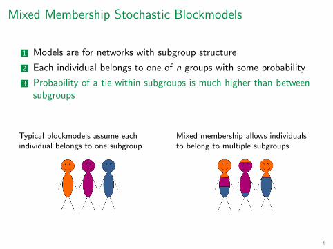
Mixed Membership Stochastic Blockmodels

1

2

3

Models are for networks with subgroup structure

Each individual belongs to one of n groups with some probability

Probability of a tie within subgroups is much higher than between subgroups

Typical blockmodels assume each individual belongs to one subgroup

Mixed membership allows individuals to belong to multiple subgroups

6

�

�

�

�

The Hierarchical Mixed Membership Stochastic Blockmodel (HMMSBM)

Yijk ∼ Bernoulli(Sijk T Bk Rjik )

Sijk ∼ Multinomial(θik , 1)

Rjik ∼ Multinomial(θjk , 1)

θik ∼ Dirichlet(λk )

Bemk ∼ Beta(aemk , bemk )

Bk [S , R] is the probability of a tie from group S to group R in network k

Sijk is the group membership of person i when sending a tie to person j

Rjik is the group membership of person j when receiving a tie from person i

θisk is the probability that person i in network k belongs to group s

Small values of λk generate extreme the membership probabilities

7

I

I

I

I

�

�

�

�

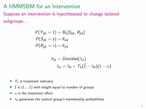
A HMMSBM for an Intervention Suppose an intervention is hypothesized to change isolated

subgroups...

P(Yijk = 1) = Bk [Sijk , Rjik ]

P(Sijk = s) = θisk

P(Rjik = r) = θjrk

θik ∼ Dirichlet(λk )

λk = λ0 + Tk (l1 − λ0)(1 − α)

Tk is treatment indicator

l1 is (1, ...1) with length equal to number of groups

α is the treatment effect

λ0 generates the control group’s membership probabilities

8

I

I

I

I

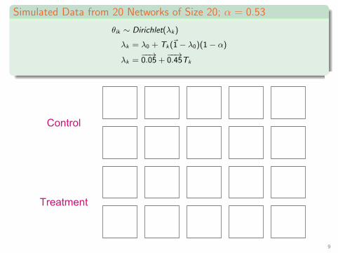
θik ∼ Dirichlet(λk )

λk = λ0 + Tk (l1 − λ0)(1 − α) −−→ −−→

λk = 0.05 + 0.45Tk

Simulated Data from 20 Networks of Size 20; α = 0.53

Control

Treatment

9

�

�

�

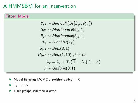
A HMMSBM for an Intervention

Fitted Model

Yijk ∼ Bernoulli(Bk [Sijk , Rjik ])

Sijk ∼ Multinomial(θik , 1)

Rjik ∼ Multinomial(θjk , 1)

θik ∼ Dirichlet(λk )

Beek ∼ Beta(3, 1)

Bemk ∼ Beta(1, 10) , £ = m −→

λk = λ0 + Tk ( 1 − λ0)(1 − α)

α ∼ Uniform(0, 1)

Model fit using MCMC algorithm coded in R

λ0 = 0.05

4 subgroups assumed a priori

10

I

I

I

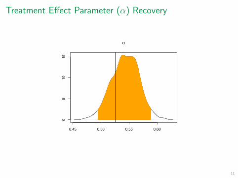
Treatment Effect Parameter (α) Recovery

0.45 0.50 0.55 0.60

05

1015

α

11

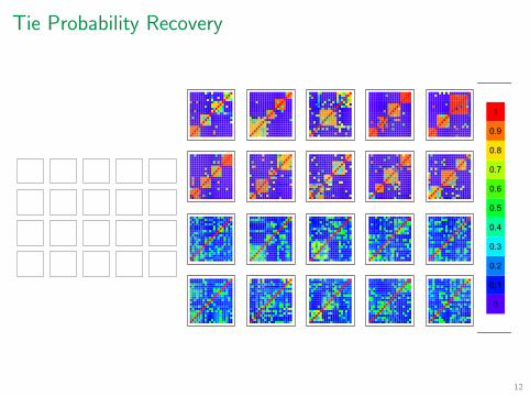
Tie Probability Recovery

0

0.1

0.2

0.3

0.4

0.5

0.6

0.7

0.8

0.9

1

12