Embed Size (px)
Citation preview
Hierarchical Bayesian Analysis of the Spiny
Lobster Fishery in California
Brian Kinlan, Steve Gaines, Deborah McArdle, Katherine Emery
UCSB
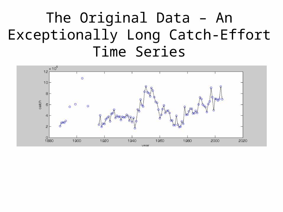
The Original Data – An Exceptionally Long Catch-Effort Time Series

Goals
• Estimate dynamics of lobster population (including recruits and sublegals) over history of fishery
• Evaluate alternative models for population replenishment
• Examine interactive effects of variation in effort, climate, and population dynamics over long time series
• NEED: Model linking catch-effort time series to population dynamics
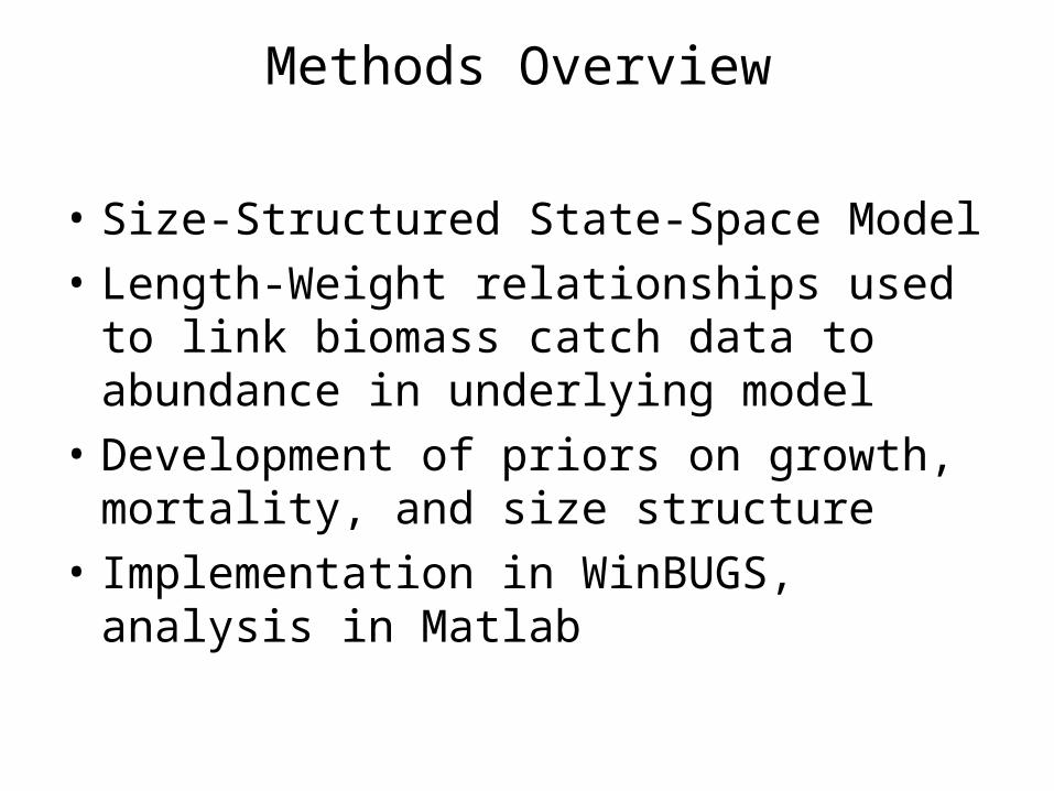
Methods Overview
• Size-Structured State-Space Model
• Length-Weight relationships used to link biomass catch data to abundance in underlying model
• Development of priors on growth, mortality, and size structure
• Implementation in WinBUGS, analysis in Matlab
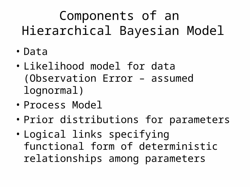
Components of an Hierarchical Bayesian Model
• Data
• Likelihood model for data (Observation Error – assumed lognormal)
• Process Model
• Prior distributions for parameters
• Logical links specifying functional form of deterministic relationships among parameters
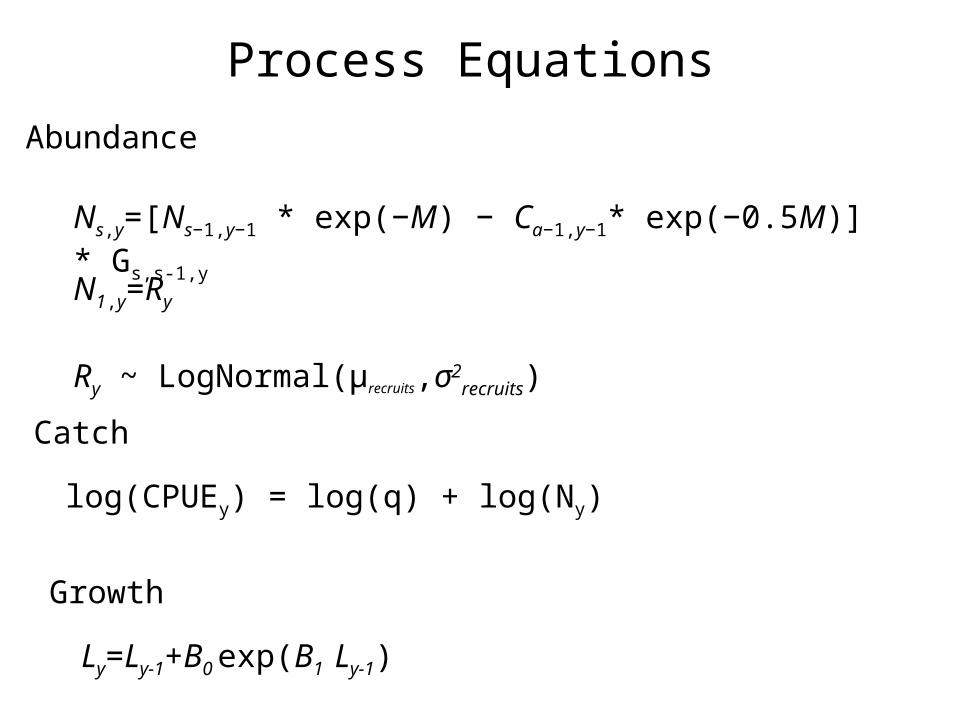
Ns,y=[Ns−1,y−1 * exp(−M) − Ca−1,y−1* exp(−0.5M)] * Gs,s-1,y
Process Equations
log(CPUEy) = log(q) + log(Ny)
Abundance
Catch
N1,y=Ry
Ry ~ LogNormal(μrecruits,σ2recruits)
Ly=Ly-1+B0 exp(B1 Ly-1)
Growth

Results
• Posterior distributions of parameters summarized by their mean
• Evaluation of Model Fit
• Patterns emerging from model – stock-recruitment relationships, climate correlations

1900 1920 1940 1960 1980 2000
0
0.5
1
1.5
2
2.5
3
x 106 legal stock
Year
No.
of
Lob
ste
rs
total including catch
escapement

1900 1910 1920 1930 1940 1950 1960 1970 1980 1990 2000
0.2
0.4
0.6
0.8
1
1.2
1.4
1.6
1.8
2x 10⁷
Year
No
. o
f L
ob
ste
rstotal stock(1-8)sublegal stock(1-3)legal stock(4-8)reproductive stock(3-8)

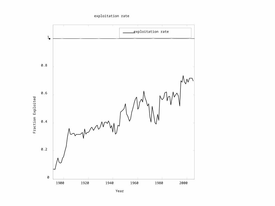
1900 1920 1940 1960 1980 2000
0
0.2
0.4
0.6
0.8
1
exploitation rate
Year
Fra
ctio
n E
xplo
ited
exploitation rate
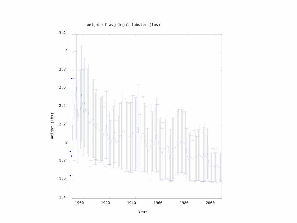
1900 1920 1940 1960 1980 2000
1.4
1.6
1.8
2
2.2
2.4
2.6
2.8
3
3.2
weight of avg legal lobster (lbs)
Year
Wei
gh
t (L
bs)
1900 1920 1940 1960 1980 2000
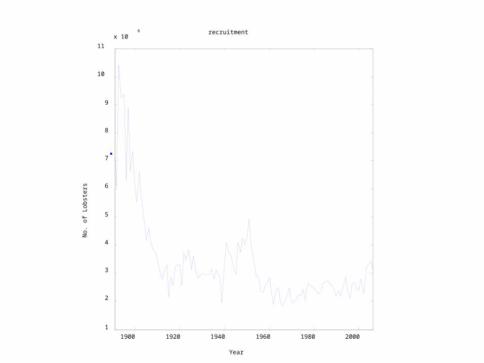
1
2
3
4
5
6
7
8
9
10
11
x 106 recruitment
Year
No.
of
Lob
ste
rs
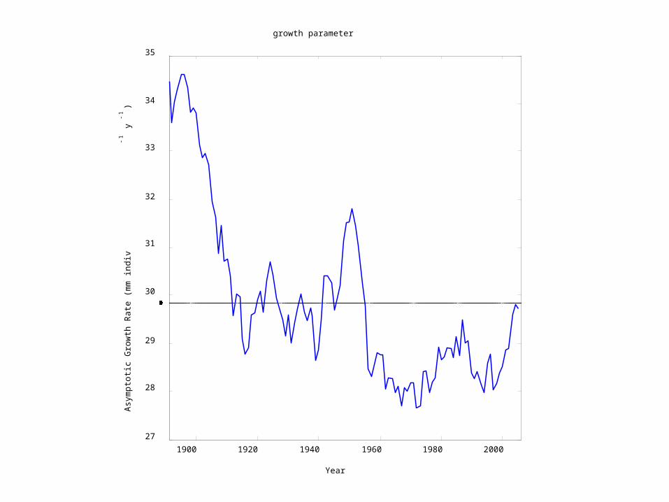
1900 1920 1940 1960 1980 2000
27
28
29
30
31
32
33
34
35
growth parameter
Year
Asy
mp
totic
Gro
wth
Ra
te (
mm
ind
iv-
1 y
-1
)

Comparison with simpler standard fisheries models
• DeLury depletion model (abundance)
• Shaeffer surplus production model (biomass)
• Both assume constant r, K, q and fit unknown No; model estimated by least-squares or MLE
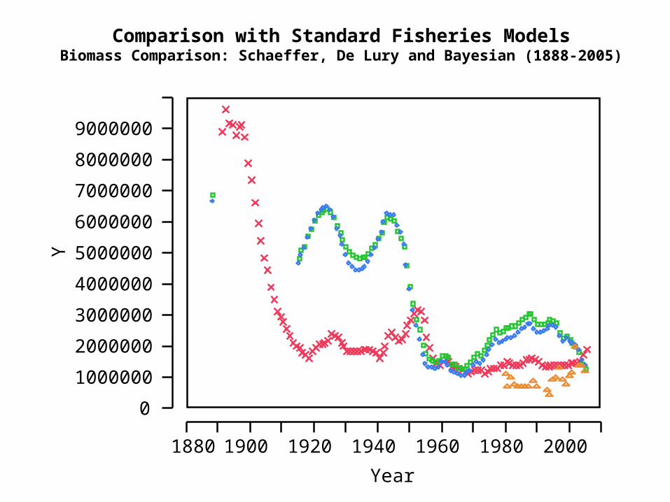
Comparison with Standard Fisheries ModelsBiomass Comparison: Schaeffer, De Lury and Bayesian (1888-2005)
YBayesian total biomassSchaeffer biomass (7 outliers)Schaefer biomass (12 outliers)DeLury biomass
0
1000000
2000000
3000000
4000000
5000000
6000000
7000000
8000000
9000000
Y
1880 1900 1920 1940 1960 1980 2000
Year
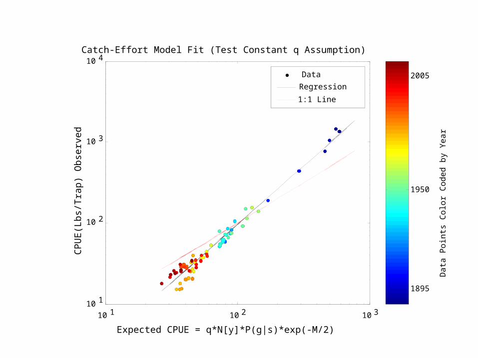
Model Fit and Residuals
• Model vs. Predicted Total Catch
• Model vs. Predicted CPUE
• Residuals – Effect of Constant Catchability Assumptions
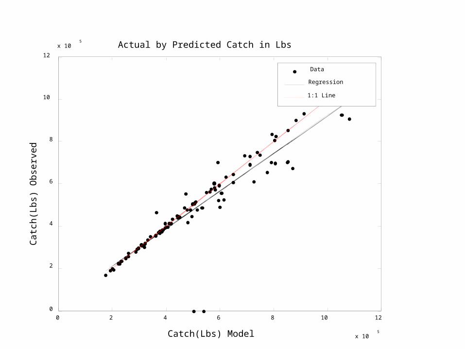
0 2 4 6 8 10 12
x 105
0
2
4
6
8
10
12
x 105
Cat
ch(L
bs)
Obs
erve
d
Catch(Lbs) Model
Actual by Predicted Catch in Lbs
Data
Regression
1:1 Line
10 1 10 2 10 310 1
10 2
10 3
10 4
CP
UE
(Lbs
/Tra
p)
Obs
erv
ed
Expected CPUE = q*N[y]*P(g|s)*exp(-M/2)
Catch-Effort Model Fit (Test Constant q Assumption)
Data
Regression
1:1 Line
Da
ta P
oin
ts C
olo
r C
od
ed
by
Ye
ar
1895
1950
2005
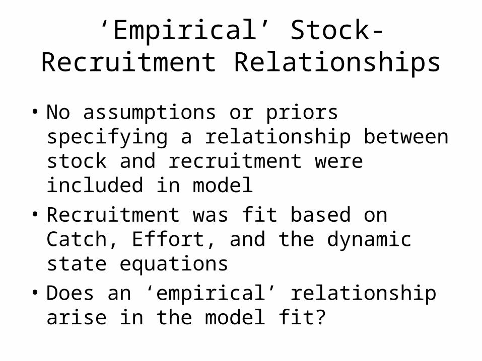
‘Empirical’ Stock-Recruitment Relationships
• No assumptions or priors specifying a relationship between stock and recruitment were included in model
• Recruitment was fit based on Catch, Effort, and the dynamic state equations
• Does an ‘empirical’ relationship arise in the model fit?
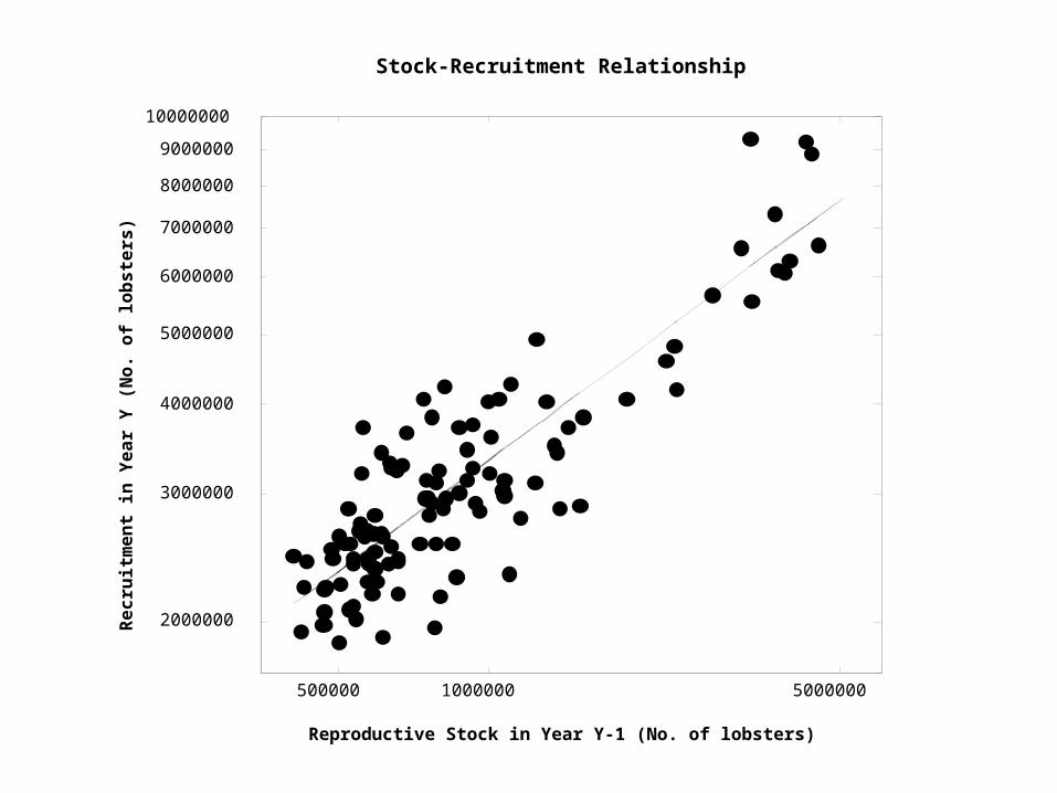
500000 1000000 5000000
2000000
3000000
4000000
5000000
6000000
7000000
8000000
9000000
10000000
Stock-Recruitment Relationship
Reproductive Stock in Year Y-1 (No. of lobsters)
Re
cru
itm
en
t in
Ye
ar
Y (
No
. o
f lo
bs
ters
)
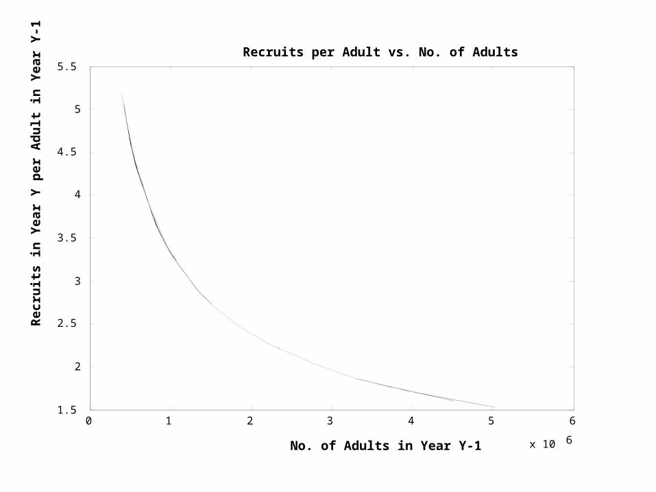
0 1 2 3 4 5 6
x 10 6
1.5
2
2.5
3
3.5
4
4.5
5
5.5Recruits per Adult vs. No. of Adults
No. of Adults in Year Y-1
Rec
ruit
s in
Yea
r Y
per
Ad
ult
in
Yea
r Y
-1

Future Model Directions
• allow time-dependency of catchability, time+size dependent mortality
• additional growth, mortality, size info via priors
• age-structured version with explicit modeling of cohort growth-in-length
• ocean climate covariates
• Spatial Model

Future Model Directions
• Spatial Model – use regional (port-based) catch-effort data– compare alternative models of connectivity via
larval movement and/or juvenile migration– will help clarify the population dynamic
mechanism underlying the compensatory recruits-per-spawner relationship (pre- or post-dispersal density dependence)

Applications in Context of the Sustainable Fisheries Group
• Evaluate forecast and hindcast scenarios of changing temporal (and spatial) patterns of effort
• Incorporate process and observation uncertainty explicitly using bayesian posteriors
• Assess value of information in this fishery