Embed Size (px)
Citation preview

Hierarchical Bayesian analysisof high complexity data
for the inversion of metric InSARin urban environments
Vom Fachbereich Elektrotechnik und Informatik der
Universitat Siegen
zur Erklarung des akademischen Grades
Doktor der Ingenieurwissenschaften(Dr.-Ing.)
genehmigte Dissertation
von
Dipl.-Phys. Marco Francesco Quartulli
1. Gutachter: Prof. Dr.-Ing. habil. O. Loffeld
2. Gutachter: Prof. Dr.-Ing. habil. M. Datcu
Vorsitzender: Prof. Dr.-Rer.Nat. W. Wiechert
Tag der mundlichen Prufung:
18 Marz 2005
urn:nbn:de:hbz:467-1084

Abstract
In this thesis, structured hierarchical Bayesian models and estimators are considered forthe analysis of multidimensional datasets representing high complexity phenomena.
The analysis is motivated by the problem of urban scene reconstruction and understand-ing from meter resolution InSAR data, observations of highly diverse, structured settlementsthrough sophisticated, coherent radar based instruments from airborne or spaceborne plat-forms at distances of up to hundreds of kilometers from the scene.
Based on a Bayesian analysis framework, stochastic models are developed for both theoriginal signals to be recovered (in this case, the original scene characteristics that are objectof the analysis— 3D geometry, radiometry in terms of cover type) and the noisy acquisitioninstrument (a meter resolution SAR interferometer). The models are then combined toprovide a consistent description of the acquisition process that can be inverted by theapplication of the so called Bayes’ equation.
The developed models for both the scene and the acquisition system are splitted into aseries of separated layers with likelihoods providing a probabilistic link between the differentlevels and with Maximum A Posteriori Bayesian inference as a basis for the estimationalgorithms.
To discriminate between different Prior scene models and to provide the necessary abilityto choose in a given set the most probable model for the data, a Bayesian model selectionframework is considered.
In particular, a set of existing Gauss–Markov randon field model–based algorithms forSAR and InSAR information extraction and denoising are extended by automated space–variant model–order selection capabilities whose performance is demonstrated by generatingand validating model–complexity based classification maps of a set of test images as well asof real SAR data.
Based on that, a method for building recognition and reconstruction from InSAR datacentered on Bayesian information extraction and data classification and fusion is developed.The system integrates signal based classes and user conjectures, and is demonstrated oninput data ranging from on board Shuttle based observations of large urban centers toairborne data acquired at sub–metric resolutions on small rural ones.
To overcome the limitations of pixel based models and inference methods, a system basedon stochastic geometry, decomposable object Gibbs fields and Monte Carlo Markov Chains

ii
is developed and evaluated on sub–metric data acquired on both urban and industrial sites.
The developed algorithms are then extensively validated by integrating them in an imageinformation mining system that enables the navigation and exploitation of large imagearchives based on a generic characterization of the data that is automatically generated.

Zusammenfassung
In dieser Dissertation werden strukturierte, hierarchische Bayes’sche Modelle undSchatzverfahren zur Analyse von komplexen mehrdimensionalen Fernerkundungsdatenvorgestellt.
Die entwickelten Methoden befassen sich mit der Problematik der Rekonstruktion und In-terpretation von interferometrischen Radardaten mit einer Auflosung in der Großenordnungvon einem Meter. Die betrachteten Daten beschreiben Stadtgebiete, wie sie von koharentenluft– oder raumbasierten Sensoren aus großer Entfernung aufgenommen werden.
Basierend auf einem Bayes’schen Ansatz werden stochastische Modelle entwickelt sowohlfur die Rekonstruktion der Szeneneigenschaften als auch fur den verwendeten Sensor. An-schließend werden die Modelle kombiniert, um eine konsistente Beschreibung des Aufnah-mevorgangs zu erreichen. Die enwickelten Modelle fur die Szene und das Beobachtungssys-tem werden in mehrere getrennte Ebenen aufgeteilt. Dabei verbinden Wahrscheinlichkeitendie unterschiedlichen Ebenen. Die Basis fur die Schatzverfahren liefert die Maximum APosteriori Statistik.
Um zwischen unterschiedlichen A Priori Modellen der Szene zu unterscheiden und dasModell mit der hochsten Wahrscheinlichkeit auszuwahlen, wird eine sog. Modellauswahlnach Bayes benutzt. Diese Methodik fuhrt zur Entwicklung von einigen Algorithmen, die dieInterpretation von Radar- und interferometrischen Radardaten von Stadtszenen erlauben.Im Besonderen werden einige bereits existierende Algorithmen zur Informationsgewinnungund Filterung von Radardaten, basierend auf Gauß–Markov–Zufallsfeldern, erweitert zurraumvarianten automatischen Bestimmung der Modellordnung. Die Leistungsstarke dieserMethoden wird durch modellordnungsbasierte Klassfikationen dargestellt.
Basierend auf diesem Wissen wird eine Methode zur Rekonstruktion von Gebauden mit-tels interferometrischer Radardaten entwickelt. Die Methode integriert signal–basierte undnutzerrelevante Klassen durch Bayes’sche Informationsgewinnung, Fusion und Klassifika-tion. Die Leistung des Systems wird an Hand von raumbezogenen Fernerkundungsdatengezeigt.
Um die Beschrankungen von pixelbasierten Modellen und statistischen Verfahren zuuberwinden, wurde ein System auf der Grundlage von stochastischer Geometrie, aufteil-baren Gibbs-Objektfeldern und Monte Carlo Methoden entwickelt. Zur Evaluiering werdenFernerkundungsbilder verwendet, die große Stadte und Industrieanlagen bedecken.
Die entwickelten Algorithmen werden anschliessend ausfuhrlich evaluiert, indem sie in

iv
ein Image Information Mining System integriert werden. Das System ermoglicht es, in demDatenarchiv zu navigieren und es zu analysieren.

Acknowledgments
I am indebted to my supervisor at DLR Prof. Dr. Mihai Datcu for his scientific guidanceand his encouragement throughout these years of work. I am also grateful to Prof. Dr.Otmar Loffeld of ZESS at the University of Siegen for giving me the opportunity to carryout this thesis. Further thanks go to Prof. Dr. Wolfgang Wiechert from the University ofSiegen for being the chairman of the thesis committee.
An essential part in the development of the ideas presented in this thesis is due tothe stimulating working environment I have encountered in DLR at the Institute for Re-mote Sensing Technology of Prof. Dr. Richard Bamler. In particular, the daily work andexchange of ideas and encouragement in the Image Science group were fundamental in pro-viding focus and breadth to the everyday work: I would like to thank Herbert Daschiel,Andrea Pelizzari, Mariana Ciucu, Inez Gomez, Cyrille Maire and Patrick Heas. Thanks goto Vito Alberga, Miguel Lopez-Martinez and Jose-Luis Alvarez-Perez of the High-Frequencyand Microwaves Institute at DLR.
Without the collaboration of colleagues and friends at Advanced Computer Systemsin Rome this work would have had significantly less broad scope. Thanks go to GastoneTrevisiol, Roberto Medri, and the many others who supported my work and myself. Inparticular, people in the Image Mining group at ACS were fundamental in helping to aimat operational quality in the developed systems. Thanks go to Marco Pastori, AndreaColapicchioni, Achille Valente, Annalisa Galoppo, Achille Natale and Massimo Manfredinofor the encouragement, the advice, and the collaboration in the development, managementand operation of the image archives used in the framework of the KIM project. Also, thecollaboration of ETHZ was a key one in establishing a fruitful cooperation environmentin which ideas could be developed and brought to an operational status. Thanks go inparticular to Prof. Dr. Klaus Seidel.
For their friendly cooperations not only in professional matters I would also like to thankthe many friends in Munchen who divided with me the years of discovery and excitement:Sonia, Anna, Antonio, Silvia, Luis, Millah, Sandro, Daniela, Annette, Francesco, Leonardoand the so many others.
Finally, I want to thank Valeria Radicci and my family for their support during theseyears of studying.

Contents
Abstract i
Zusammenfassung iii
Acknowledgements v
Contents vi
List of Figures x
List of Tables xiv
1 Introduction 2
1.1 Advances in Bayesian inferencefor signal processing and analysis . . . . . . . . . . . . . . . . . . . . . . . . 2
1.2 On the information contentof InSAR data at metric resolutions . . . . . . . . . . . . . . . . . . . . . . 4
1.3 Outline: the contribution of this thesis . . . . . . . . . . . . . . . . . . . . . 7
I Preliminaries 10
2 Synthetic Aperture Radar Interferometry at meter resolution 12
2.1 Synthetic Aperture Radar . . . . . . . . . . . . . . . . . . . . . . . . . . . . 12
2.1.1 SAR radiometry and geometry . . . . . . . . . . . . . . . . . . . . . 14
2.1.2 SAR processing and PSF . . . . . . . . . . . . . . . . . . . . . . . . 17
2.1.3 SAR statistics . . . . . . . . . . . . . . . . . . . . . . . . . . . . . . 23
2.2 SAR interferometry . . . . . . . . . . . . . . . . . . . . . . . . . . . . . . . . 25

CONTENTS vii
2.2.1 InSAR principle and processing . . . . . . . . . . . . . . . . . . . . . 26
2.2.2 InSAR statistics . . . . . . . . . . . . . . . . . . . . . . . . . . . . . 29
2.3 The metric InSAR domain . . . . . . . . . . . . . . . . . . . . . . . . . . . . 30
2.3.1 Meter resolution SAR and InSAR for single isolated buildings . . . . 37
2.3.2 Metric SAR statistics in urban environments . . . . . . . . . . . . . 38
2.3.3 High resolution urban SAR and InSAR inversion: state of the art . . 39
2.4 Summary . . . . . . . . . . . . . . . . . . . . . . . . . . . . . . . . . . . . . 41
3 Bayesian modeling, estimation and decision theory for multidimensional
signal analysis 42
3.1 Bayesian modeling and analysis . . . . . . . . . . . . . . . . . . . . . . . . . 42
3.1.1 A principled approach to the composition of stochastic descriptions . 43
3.1.2 Modeling interdependence in random variable sets: chain Rule andMarkov property . . . . . . . . . . . . . . . . . . . . . . . . . . . . . 44
3.2 Gibbs random fields . . . . . . . . . . . . . . . . . . . . . . . . . . . . . . . 45
3.2.1 Lattices, sets, neighborhoods, cliques, sites, pixel values . . . . . . . 45
3.2.2 Random fields in terms of potentials and energies . . . . . . . . . . . 46
3.2.3 Markov random fields in terms of belief networks . . . . . . . . . . . 46
3.2.4 Hierarchical models . . . . . . . . . . . . . . . . . . . . . . . . . . . 47
3.2.5 Principle of inference for 2–level hierarchical models . . . . . . . . . 48
3.2.6 Occam razor and Occam factor . . . . . . . . . . . . . . . . . . . . . 49
3.2.7 From posterior distributions to estimates and decisions . . . . . . . . 51
3.3 Estimation and decision theory . . . . . . . . . . . . . . . . . . . . . . . . . 51
3.3.1 Decisions as posterior ratios . . . . . . . . . . . . . . . . . . . . . . . 52
3.3.2 Estimation and decision algorithms . . . . . . . . . . . . . . . . . . . 52
3.3.2.1 Analytic derivation of MAP estimate . . . . . . . . . . . . 53
3.3.2.2 Exact inference by complete enumeration . . . . . . . . . . 53
3.3.2.3 The Iterated Conditional Modes algorithm . . . . . . . . . 53
3.3.2.4 The Gibbs sampler and Monte Carlo Markov chains . . . . 53
3.4 Summary . . . . . . . . . . . . . . . . . . . . . . . . . . . . . . . . . . . . . 54

CONTENTS viii
II Hierarchical Bayesian modelling 56
4 Space–variant model selection in model–based information extraction 58
4.1 Model based image denoising and information extraction . . . . . . . . . . . 59
4.2 Image models . . . . . . . . . . . . . . . . . . . . . . . . . . . . . . . . . . . 60
4.2.1 Gauss–Markov random fields . . . . . . . . . . . . . . . . . . . . . . 60
4.2.2 Gaussian likelihoods for additive Gaussian noise . . . . . . . . . . . 60
4.2.3 Gamma likelihoods for multiplicative fully developed speckle noise . 61
4.3 Locally–adaptive parameter estimation by evidence maximization . . . . . . 61
4.3.1 Fixed model order computational overview . . . . . . . . . . . . . . 62
4.3.2 Fixed model order processing examples and global model evidencecomputation . . . . . . . . . . . . . . . . . . . . . . . . . . . . . . . 64
4.4 Model order selection . . . . . . . . . . . . . . . . . . . . . . . . . . . . . . . 64
4.4.1 Variable order Gauss–Markov random field hierarchical modeling . . 68
4.4.2 Local evidence maximization in Gauss–Markov random field imagemodels . . . . . . . . . . . . . . . . . . . . . . . . . . . . . . . . . . . 69
4.4.3 Model order selection examples and comments . . . . . . . . . . . . 70
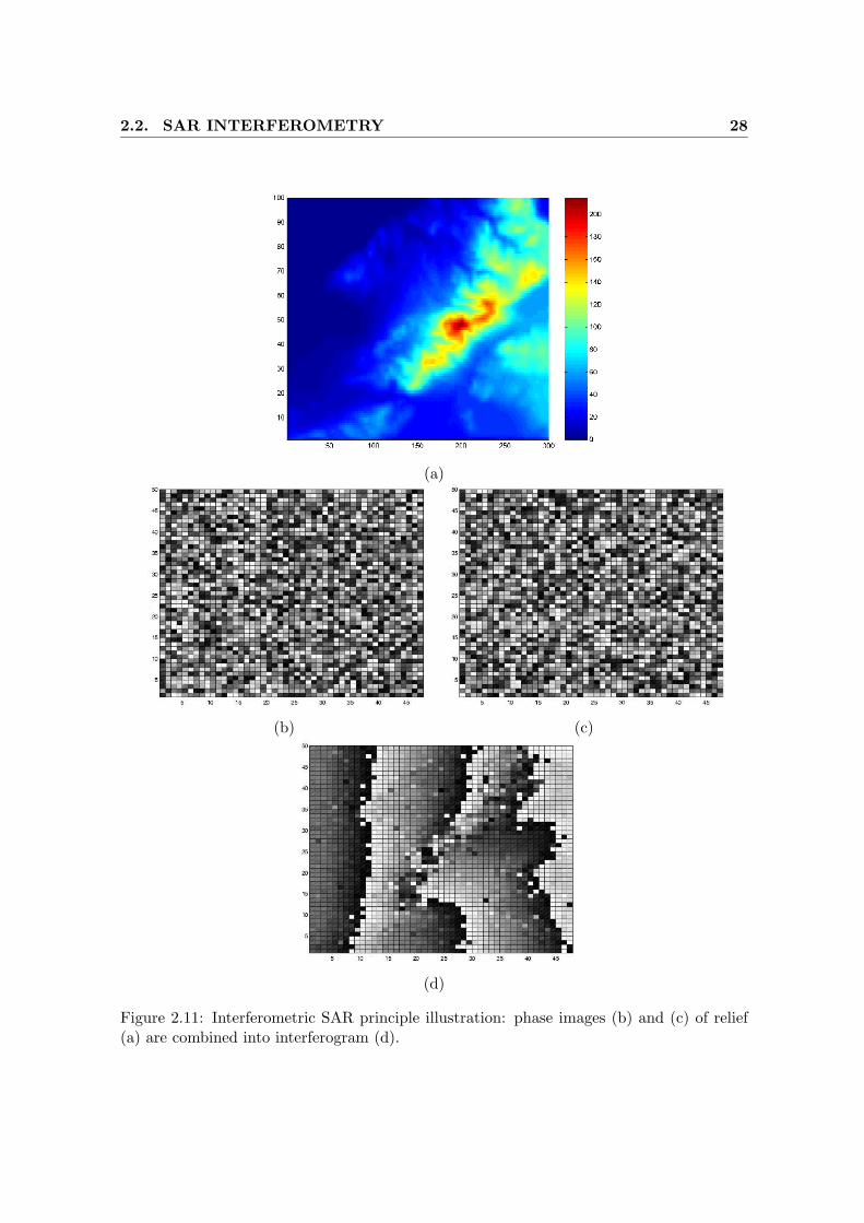
4.4.4 Spatially–variant model order selection for SAR data analysis . . . . 74
4.5 Summary . . . . . . . . . . . . . . . . . . . . . . . . . . . . . . . . . . . . . 74
5 Information Fusion for scene reconstruction
from Interferometric SAR Data
in Urban Environments 76
5.1 The need for probabilistic modeling in scene reconstruction . . . . . . . . . 77
5.2 Scene–to–data hierarchical models . . . . . . . . . . . . . . . . . . . . . . . 78
5.2.1 Scene reconstruction Bayesian belief networks . . . . . . . . . . . . . 78
5.2.2 User feedback and machine learning . . . . . . . . . . . . . . . . . . 80
5.2.3 Information extraction from backscatter and height image data . . . 81
5.3 Learning procedure . . . . . . . . . . . . . . . . . . . . . . . . . . . . . . . . 81
5.4 Urban scene reconstruction from InSAR data . . . . . . . . . . . . . . . . . 83
5.4.1 E-SAR Dresden data analysis for settlement understanding . . . . . 83
5.5 Summary . . . . . . . . . . . . . . . . . . . . . . . . . . . . . . . . . . . . . 87
6 Stochastic geometrical modeling
for urban scene understanding

CONTENTS ix
from a single SAR intensity image
with meter resolution 88
6.1 Scene understanding from SAR: objects and their relations . . . . . . . . . 89
6.2 Marked spatial point processes as prior scene models . . . . . . . . . . . . . 91
6.2.1 Point and mark distributions . . . . . . . . . . . . . . . . . . . . . . 92
6.2.2 Modelling hierarchy . . . . . . . . . . . . . . . . . . . . . . . . . . . 92
6.3 Scene posterior structure decompositionin Gibbs potential terms . . . . . . . . . . . . . . . . . . . . . . . . . . . . . 94
6.4 The scene prior potential term . . . . . . . . . . . . . . . . . . . . . . . . . 95
6.5 The data likelihood potential term . . . . . . . . . . . . . . . . . . . . . . . 95
6.5.1 Extraction of strong targets from clutter in urban environments byinverse Gaussian statistics, decision theory–based classification . . . 95
6.5.1.1 Radiometric likelihood potential term . . . . . . . . . . . . 96
6.5.2 Geometric likelihood potential terms . . . . . . . . . . . . . . . . . . 97
6.6 Inference in Bayesian scene understanding with non–analytic posteriors . . 97
6.6.1 Monte Carlo Markov Chain Gibbs sampling of the scene posterior . 97
6.6.2 Scene configuration initialization . . . . . . . . . . . . . . . . . . . . 98
6.6.3 Scene configuration sampling and Gibbs dynamics . . . . . . . . . . 98
6.7 Overview of estimation method . . . . . . . . . . . . . . . . . . . . . . . . . 100
6.8 Marked Point Process based scene understanding example . . . . . . . . . . 102
6.9 Summary . . . . . . . . . . . . . . . . . . . . . . . . . . . . . . . . . . . . . 102
III Evaluation and validation of results 104
6.10 Content–based retrieval, information mining, scene understanding . . . . . . 106
6.10.1 Information extraction for application–independent data characteri-zation . . . . . . . . . . . . . . . . . . . . . . . . . . . . . . . . . . . 106
6.10.2 The knowledge-based information mining system . . . . . . . . . . . 107
6.10.3 Knowledge-based information mining evaluation results . . . . . . . 109
6.11 Case studies with local model order selection in model based informationextraction . . . . . . . . . . . . . . . . . . . . . . . . . . . . . . . . . . . . . 112
6.12 Urban scene reconstruction from InSAR data . . . . . . . . . . . . . . . . . 112
6.12.1 Urban land-use mapping from SRTM data . . . . . . . . . . . . . . . 116
6.12.2 Large building recognition from SRTM data . . . . . . . . . . . . . . 120

CONTENTS x
6.12.3 Building recognition from Intermap data . . . . . . . . . . . . . . . . 120
6.13 Marked point process model–based building reconstruction from metric air-borne SAR . . . . . . . . . . . . . . . . . . . . . . . . . . . . . . . . . . . . 124
6.13.1 Industrial scene understanding from metric SAR backscatter . . . . 124
6.13.2 Composed building understanding from sub–metric SAR backscatter 127
6.14 Summary . . . . . . . . . . . . . . . . . . . . . . . . . . . . . . . . . . . . . 130
C onc lus ions 131
Summar y of the obtai ne d r e sul ts . . . . . . . . . . . . . . . . . . . . . . . . 132
Eval uati on of the obtai ne d r e sul ts and outl o ok . . . . . . . . . . . . . . . . . 133
A The K-means clustering algorithm 134
B Non–analytical optimization and MAP estimation by simulated annealing135
Bibliography 137

List of Figures
1.1 Growing spaceborne SAR sensor resolution with time, together with mostrelevant features for image understanding. . . . . . . . . . . . . . . . . . . . 4
1.2 Scene geometry and SAR backscatter intensity for different sensor resolutions. 5
1.3 Scene understanding, resolution and reconstruction levels . . . . . . . . . . 9
2.1 SAR image coordinate system with sub-metric resolution SAR intensity im-age example. . . . . . . . . . . . . . . . . . . . . . . . . . . . . . . . . . . . 13
2.2 SAR acquisition geometry for side looking configurations. . . . . . . . . . . 15
2.3 Slant and ground range. . . . . . . . . . . . . . . . . . . . . . . . . . . . . . 16
2.4 Chirp signal characteristics. . . . . . . . . . . . . . . . . . . . . . . . . . . . 20
2.5 Spectral characteristics of SAR data. . . . . . . . . . . . . . . . . . . . . . . 21
2.6 Theoretical SAR Point Spread Function amplitude. . . . . . . . . . . . . . . 22
2.7 Measured sub-metric SAR Point Spread Function amplitude. . . . . . . . . 23
2.8 SAR backscatter intensity autocorrelation. . . . . . . . . . . . . . . . . . . . 24
2.9 Measured SAR image distribution examples. . . . . . . . . . . . . . . . . . . 24
2.10 Interferometric SAR geometry. . . . . . . . . . . . . . . . . . . . . . . . . . 26
2.11 Interferometric SAR data processing principle illustration. . . . . . . . . . . 28
2.12 Absolute and wrapped phase surfaces. . . . . . . . . . . . . . . . . . . . . . 29
2.13 Analytical InSAR data distributions. . . . . . . . . . . . . . . . . . . . . . . 29
2.14 Resolution–dependent interferometric SAR phenomenology. . . . . . . . . . 32
2.15 Specular and diffuse scattering. . . . . . . . . . . . . . . . . . . . . . . . . . 34
2.16 Electromagnetic wave paths for direct reflections, double bouncings and triplebouncings on a dihedral. . . . . . . . . . . . . . . . . . . . . . . . . . . . . . 36
2.17 Projection of a building into slant and ground. . . . . . . . . . . . . . . . . 38
3.1 Bayes’ law illustration. . . . . . . . . . . . . . . . . . . . . . . . . . . . . . . 43

LIST OF FIGURES xii
3.2 Markov property for random variables: random variables are depicted ascircles. Two neighborhoods are represented. First–order cliques for neigh-borhood N1 are depicted by closed shapes enclosing the variables. The threecliques C1, C2 and C3 form the first–order neighborhood N1. The diagramdescribes a belief network encoding statistical independence relations: vari-able A is independent of D (no path exists between the two), while A isindependent of B if C is known. Independence and conditional independenceare respectively denoted by · ⊥ · and · ⊥ ·|·. The exploitation of conditionalindependence relations allows the simplification of high complexity proba-bilistic descriptions. . . . . . . . . . . . . . . . . . . . . . . . . . . . . . . . 45
3.3 Hierarchical model illustration. . . . . . . . . . . . . . . . . . . . . . . . . . 47
4.1 Clique structures for different Gauss–Markov random field model orders. . . 59
4.2 Flowchart of the evidence maximization algorithm used for texture parameterestimation in the model based denoising and information extraction systemseen as an Expectation–Maximization algorithm. . . . . . . . . . . . . . . . 61
4.3 Flowchart of the evidence maximization algorithm used for contextual textureparameter and model order estimation in the extended model based denois-ing and information extraction system seen as an Expectation–Maximizationalgorithm. . . . . . . . . . . . . . . . . . . . . . . . . . . . . . . . . . . . . . 62
4.4 Synthetic and natural realizations of random fields. . . . . . . . . . . . . . . 63
4.5 Speckled versions of synthetic and natural instances of random fields. . . . . 65
4.6 Denoising and information extraction with fixed model order on synthetic data. 66
4.7 Denoising and information extraction with fixed model order on natural im-age data. . . . . . . . . . . . . . . . . . . . . . . . . . . . . . . . . . . . . . 67
4.8 Clean and speckled multiple model (autobinomial and GMRF with order 2)test image. . . . . . . . . . . . . . . . . . . . . . . . . . . . . . . . . . . . . 70
4.9 Clean and speckled multiple model (GMRF with orders 2 and 5) test image. 71
4.10 Clean and speckled multiple model (Brodatz “cloud” and “straw”) test image. 72
4.11 Model order estimation for synthetic and natural mixed images. . . . . . . . 73
4.12 E-SAR X band SAR backscatter amplitude image over Oberpfaffenhofen,Germany. . . . . . . . . . . . . . . . . . . . . . . . . . . . . . . . . . . . . . 74
4.13 Despeckled image and estimated model order for SAR intensity image overOberpfaffenhofen, Germany. . . . . . . . . . . . . . . . . . . . . . . . . . . . 75
5.1 Learning scene semantics through hierarchical Bayesian Networks. . . . . . 79
5.2 Scene reconstruction processing chain. . . . . . . . . . . . . . . . . . . . . . 81

LIST OF FIGURES xiii
5.3 Model based SAR backscatter–InSAR derived height information extractionsystem. . . . . . . . . . . . . . . . . . . . . . . . . . . . . . . . . . . . . . . 82
5.4 E-SAR Dresden - Ground truth optical image, interferometric land use, SARbackscatter intensity and SAR texture norm. . . . . . . . . . . . . . . . . . 84
5.5 E-SAR Dresden - Ground truth optical image and generated land use map. 85
5.6 E-SAR Dresden Semper Oper- Ground truth optical image and interferomet-ric land use. . . . . . . . . . . . . . . . . . . . . . . . . . . . . . . . . . . . . 85
5.7 E-SAR Dresden Semper Oper- interferometric SAR backscatter coherenceand interferometric phase. . . . . . . . . . . . . . . . . . . . . . . . . . . . . 86
5.8 E-SAR Dresden Semper Oper- land use map obtained by unsupervised clas-sification and Bayesian classification/fusion. . . . . . . . . . . . . . . . . . . 86
6.1 Meter resolution interferometric SAR phenomenology. . . . . . . . . . . . . 90
6.2 Levels in the hierarchical scene model. . . . . . . . . . . . . . . . . . . . . . 93
6.3 SAR phenomenology considered in the scene understanding process. . . . . 94
6.4 Gibbs sampler dynamics. . . . . . . . . . . . . . . . . . . . . . . . . . . . . 100
6.5 The complete marked point process MAP estimation system. . . . . . . . . 101
6.6 Intermap AeS-2 data on Trudering test area. . . . . . . . . . . . . . . . . . 103
6.7 Image information mining data analysis hierarchy. . . . . . . . . . . . . . . 106
6.8 Scheme of principle of ingestion chain operations. . . . . . . . . . . . . . . . 107
6.9 Hierarchical modeling of image content and user semantic. . . . . . . . . . . 108
6.10 KIM coverage of Mozambique. . . . . . . . . . . . . . . . . . . . . . . . . . 109
6.11 X-SAR scene reconstruction by data classification and fusion results. . . . . 110
6.12 ERS data scene reconstruction by classification and fusion results. . . . . . 111
6.13 Meter resolution information mining example ground truth and intensity data.112
6.14 Meter resolution information mining example results. . . . . . . . . . . . . . 113
6.15 Uncalibrated optical and RADARSAT-1 fine mode data over Las Vegas, USA.114
6.16 Filtered RADARSAT-1 data with locally estimated number of looks. . . . . 115
6.17 Automatically estimated despeckled amplitude and local estimated modelorder for the Las Vegas RADARSAT-1 scene. . . . . . . . . . . . . . . . . . 116
6.18 Scene reconstruction SRTM backscatter intensity image and DEM. . . . . . 117
6.19 Scene reconstruction procedure for SRTM data. . . . . . . . . . . . . . . . . 118
6.20 Bayesian classification/fusion results and ground truth for SRTM data. . . . 119
6.21 Full resolution intensity and DEM SRTM data. . . . . . . . . . . . . . . . . 121

LIST OF FIGURES xiv
6.22 Full resolution SRTM Bayesian classification/fusion results and ground truthmap. . . . . . . . . . . . . . . . . . . . . . . . . . . . . . . . . . . . . . . . . 122
6.23 Full resolution scene reconstruction results and ground truth map. . . . . . 123
6.24 Views of the rural scene reconstruction test area. . . . . . . . . . . . . . . . 124
6.25 Rural scene reconstruction test data. . . . . . . . . . . . . . . . . . . . . . . 125
6.26 Rural test scene reconstruction results. . . . . . . . . . . . . . . . . . . . . . 126
6.27 Industrial scene understanding data and results. . . . . . . . . . . . . . . . 128
6.28 Building understanding data and results. . . . . . . . . . . . . . . . . . . . . 129
B.1 Simulated annealing scheme of principle. . . . . . . . . . . . . . . . . . . . . 136

List of Tables
2.1 Resolution and information content in SAR data. . . . . . . . . . . . . . . . 30
2.2 Recognizable object structures with varying resolutions in SAR data. . . . . 31
3.1 The Gibbs Sampling algorithm. . . . . . . . . . . . . . . . . . . . . . . . . . 54
6.1 Summary of SAR data ingested in the KIM system and the level of dataanalysis considered. . . . . . . . . . . . . . . . . . . . . . . . . . . . . . . . . 109
A.1 A simple version of the K–means clustering algorithm. . . . . . . . . . . . . 134
B.1 Simulated annealing algorithm description. . . . . . . . . . . . . . . . . . . 136

Chapter 1
Introduction
One of the goals of signal processing is the extraction of information from data that arenoisy, vague or otherwise affected by incertitude. In many situations additional complexityis introduced by the non-stationariety of the data both in the useful information and in itsdistortions. From information theory we know that the most compact encoding of data isgiven by the probabilistic model that describes it best. However, to find tractable modelsfor high complexity data is not an easy task.
This thesis explains and proposes new methods to model high complexity data and todevelop algorithms for parameter estimation for hierarchical Bayesian models, in the frame-work of image information mining and three dimensional structure analysis and reconstruc-tion. Its goal is the derivation and real-world validation of a paradigm for the extraction,characterization and construction of features tied to a three dimensional spatial domainstarting from incomplete, multiple-source data with high complexity. Emphasis is placedon the study of Bayesian hierarchical modeling methods and on the problematic of modelselection in the framework of machine learning with models having hidden parameters.
The analysis is motivated by the problem of urban scene understanding from meterresolution InSAR data, in which data cubes are acquired by the observation of highlydiverse, structured settlements through sophisticated, coherent radar based instrumentsfrom airborne or spaceborne platforms at distances of up to hundreds of kilometers from thescene. The thesis therefore includes an application of the obtained theoretical results to theaccurate recovery of geometrical information describing built-up, urbanized areas observedthrough a very high resolution interferometric synthetic aperture radar apparatus.
1.1 Advances in Bayesian inferencefor signal processing and analysis
The techniques of hierarchical Bayesian modeling for feature extraction and model basedmeasure from incomplete, noisy data have been established since a number of years in thesignal processing literature. Applications have ranged from frequency analysis (Jaynes,
1.1. ADVANCES IN BAYESIAN INFERENCE
FOR SIGNAL PROCESSING AND ANALYSIS 3
1987) to modelling feedback in human–computer interaction studies (Pavlovic et al., 1997).The seminal works by Besag (Besag, 1974; Besag et al., 1995) were instrumental in intro-ducing the ideas of stochastic Markov modelling to the field of image processing (Winkler,1995; Chellappa, 1985; Chellappa and Jain, 1993). Geman and Geman (1984) introducedthe techniques of Gibbs modelling and sampling to the field. Their ideas were applied inproviding solutions to a number of problems from noisy image data filtering (Besag, 1986)to content–based image retrieval (Flickner et al., 1995; Schroder et al., 2000b).
Bayesian analysis is often characterized by the fundamental role played in it by priordistributions. The usage of subjective ones has often been the ground for objections andcontroversies. Jeffreys (1939) and Jaynes (1986) layed the ground for the developmentof techniques that can be applied to generate objective prior descriptions starting from aset of objective constraints to the problem and from the principle of Maximum Entropy.Furthermore, Bayesian analysis can be used to perform a principled choice of a prior modelin a class of available ones by employing a two–level description of the problem underanalysis in which inference is performed both on the model parameters and on the modelsthemselves. MacKay (1992) and O’Hagan (1994) showed how model selection naturallymaps into the maximization of the Bayesian evidence across a model class.
A number of the principles and techniques of hierarchical Bayesian modelling and two–level Bayesian inference for the modelling and estimation of noisy, nonstationary 2D signalsare summarized by Datcu et al. (1998) and Schroder et al. (1998a). Their works introducethe general problem of estimation theory in a Bayesian framework centering on the prop-erties of 2D Gibbs random fields and on their role in estimation. The focus of Walessaand Datcu (2000) centers instead on the extraction of reliable estimates of the parametersof these models from noisy, nonstationary observations in a two–levels Bayesian approach.Gauss–Markov random fields are used to describe textured radar backscatter images cor-rupted by speckle noise. The described system performs an estimation of the texture pa-rameters of the clean image. The order of the model that is used as a prior description of thedata is not an object of the estimation, though, and is considered a fixed input parameterinstead.
Further works concentrate on object–based stochastic geometry models for the analysisof the structure of image data. In particular, based on Ripley and Kelly (1977), Stoica et al.(2000), Imberty and Descombes (2002) and Ortner et al. (2002) focus on marked point pro-cesses whose attached label processes describe the characteristics of the elements in a scene.Gibbs fields can then be used to describe the interactions between the objects (Cressie,1991).
The problem of conducting estimation from the often non–analytic posterior distribu-tions is approached by considering Monte Carlo Markov Chain methods (Winkler, 1995).Estimation is conducted by Expectation Maximization methods (Dempster et al., 1977) ina number of image denoising and information extraction problems.

1.2. ON THE INFORMATION CONTENT
OF INSAR DATA AT METRIC RESOLUTIONS 4
Figure 1.1: Growing spaceborne SAR sensor resolution with time, together with most rel-evant features for image understanding. This thesis addresses the area marked with aquestion mark on the upper right part of the plot, where relevant features are not yet esta-bilished and therefore new methods are needed to fully exploit the information content inthe data.
1.2 On the information contentof InSAR data at metric resolutions
The reconstruction of buildings and of other typical settlement structures is a goal ofgreat interest in an increasing number of applications related to the understanding andmanagement of urbanized areas. At present, due to the broad availability of high resolutionoptical and of metric interferometric Synthetic Aperture Radar (SAR) data originatingfrom both airborne and spaceborne sensors, new and more efficient methods of analysis areneeded to address the challenges that are specific of the inherent complexity of the imagedscenes and of the acquisition systems themselves.
From the point of view of the traditional deterministic, pixel–based SAR and inter-ferometric SAR data processing techniques, urban scenes are often regarded as problem-atic (D. L. Bickel, 1997):
• the scene: height discontinuities originated by vertical surfaces such as building wallsare the norm in such data, while a wider dynamic range of the image shows upfrequently, often saturating the receiver. Strong layover and shadowing effects implyan accentuated sparseness of the data with respect to the classical case. Multipathreflections and multiplicative noise from the sidelobes of the radar beam, as well as thepresence of areas of low coherence are no more isolated deficiencies of generally simplerand more consistent data, but embody instead its most peculiar traits. Complex man-made objects and structures, moving elements such as cars or even varying housingdetails such as open and closed doors or windows show up at the imaging scales;

1.2. ON THE INFORMATION CONTENT
OF INSAR DATA AT METRIC RESOLUTIONS 5
X-SAR 20 m resolution Intermap AeS-2 0.5 m resolution
scen
est
ruct
ure
(a) (b)
SA
Rback
scatt
erin
tensi
ty
→ range direction(c) (d)
smooth backscatter variations high dynamics, multiple reflectionsdescribe local geometry/reflectivity complicate scene reconstruction
Figure 1.2: Scene geometry and SAR backscatter intensity for X-SAR view of Mount Aetna(a,c) at X band, 25 meters resolution, with the main vulcanic cone visible (Schwabisch, 1994)and Intermap AeS-2 view of Maastricht, the Netherlands, X band, 0.5 meters resolution,showing a single building composed by a number of square elements and by a round metallictower generating multiple reflections clearly visible. With growing resolution, more complexmodels are needed to account for the mutated characteristics of observable scene elementclasses as well as for the peculiar effects introduced by sensors.

1.2. ON THE INFORMATION CONTENT
OF INSAR DATA AT METRIC RESOLUTIONS 6
• the acquisition geometry: new corrections need to be taken into account for theattitude variations of the platform that carries the acquisition system and for thevariations in the acquisition geometry from near to far range, that are much morepronounced than in the spaceborne case;
• the sensor: the high resolution of the acquisition system itself leads to image process-ing and SNR issues — speckle noise tends to change in nature, appearing in largecorrelated blobs, the sensitiveness to target texture changes completely and the wholestatistics of the data must be re-evaluated. Strong isolated scatterers are mode com-mon.
The acquired result changes so much in nature with respect to its traditional low-resolution counterpart on natural surfaces that the whole reconstruction approach needsto be shifted from the usual image processing based, two dimensional view to a full 3Ddomain in order to be able to explain and in the very end to exploit the effects and featuresthat characterize this kind of data (Figure 1.2).
Significantly, up to now the problem of the reconstruction in the three dimensions of urbanscenes from interferometric radar data has never been addressed in a unified, consistentframework by well-integrated algorithms and approaches: usually solutions originating fromthe well assessed problem of reconstructing low resolution imagery of natural surfaces areported to the new operating environment and supplemented by manual intervention by theuser (Heuel and Nevatia, 1995; Li et al., 1999) or are used as preliminary steps with moderateimportance for some further processing carried out on higher resolution optical data thatuses the obtained results as preliminary cues (Huertas et al., 1998). Strong assumptionsare often made in the processing that tend to be appropriate for narrow application casesonly (Gamba and Houshmand, 1999; Burkhart et al., 1996).
Unwrapped interferometric SAR phase surfaces are employed directly or after simple (e.g.morphologic) processing to obtain simple segmentation and classification maps that are usedto initialize some shape from shade algorithm applied on coregistered optical imagery, oralternatively user assisted segmentation is followed by some back-projection operation in ashape from shade fashion (Bolter and Leberl, 2000).
While applications of stochastic modelling and analysis techniques have recently startedto appear in the remote sensing field with particular reference to SAR with model baseddespeckling filters, knowledge based mining of large image databases and automatic targetrecognition and classification, the hierarchical modeling of data acquired on complex, de-tailed three dimensional structures in complicated environments has never been addressed:most of the studies up to now published limit themselves to the two dimensional case (Tupinet al., 1998; Schroder, 1999a) as a natural consequence of the simpler situation of naturalenvironments imaged by lower resolution sensors. Traditional radargrammetric and inter-ferometric techniques are used in the new environment along with ad-hoc methods that tendto provide very preliminary and partial results essentially by treating the peculiarities ofthe problem simply as shortcomings of the data that must be regularized in the processinginstead of being used as additional sources of information.

1.3. OUTLINE: THE CONTRIBUTION OF THIS THESIS 7
1.3 Outline: the contribution of this thesis
The concept developed in this thesis is centered on the synergetic analysis of intensityand interferometric SAR data: a hierarchical model of the acquisition process and of itsresult is defined starting from a set of three–dimensional features that describe the sceneand the sensor. The set is both deterministic and stochastic: while the deterministic sec-tion describes the SAR imaging geometry and its peculiar effects on the imaged scene andexpresses a spatial description of the different scene structures, the stochastic part encap-sulates instead prior knowledge about the SAR signal and details specific signal attributes.
The analysis is carried out as follows:
• a set of existing Gauss–Markov random field model–based algorithms for SAR andInSAR information extraction and denoising are extended by space–variant automatedmodel–order selection capabilities (chapter 4) whose performance is demonstrated bygenerating and validating model complexity–based classification maps (figures 1.3a,b)of a set of test images as well as of real SAR data (Datcu and Quartulli, 2003);
• based on that, a method for building recognition and reconstruction from InSARdata centered on Bayesian information extraction and data classification and fusionis developed (chapter 5). Bayesian inference and networks are used to couple thedifferent models specifying dependencies and to define further parameter estimationalgorithms. The system integrates signal based classes and user conjectures, andis demonstrated on input data ranging from on–board Shuttle–based observations oflarge urban centers (figures 1.3c,d) to airborne data acquired at sub–metric resolutionson small rural center (Quartulli and Datcu, 2003b);
• to overcome the limitations of pixel–based models and inference methods, a systembased on stochastic geometry, decomposable object Gibbs fields and Monte CarloMarkov Chains (Quartulli and Datcu, 2004) is developed. A semantic model is usedas an important factor in the derivation of the results along with computer visionalgorithms in order to provide a strong and robust discrimination criterion for thedifferent elements showing up in the image as well as to simplify the separation of thedifferent structures.
Such an approach (figures 1.3e,f) strongly reduces the need for the most problematicsteps in the traditional interferometric SAR data processing chains (e.g. the phaseunwrapping of the interferogram describing the city elevations model) and in the veryend turn the sources of processing problems in standard interferometric methods intostrengths in the form of additional sources of information providing added performanceand robustness in a unified, coherent fashion (chapter 6);
• the developed approaches are validated on sub–metric data acquired on both urbanand industrial sites (chapter III).
Such a conceptual shift, modeling the peculiarities of high resolution SAR acquisitions in-stead of considering them as artifacts to be treated by ad-hoc techniques generally separated

1.3. OUTLINE: THE CONTRIBUTION OF THIS THESIS 8
from the main corpus of the processing, produces as a final effect a significant simplificationof the whole processing chain.
The methods here proposed are new with regards to both the estimation theory, withparticular reference to the usage of a hierarchical mixed model for the evaluation andmeasurement of spatial features tied to a three dimensional domain, and to practice: to thebest of our knowledge, none of the paradigms up to date employed for city reconstructionfrom SAR data shares the 3D hierarchical Bayesian modeling scheme that we propose, andnone of them exploits in a unified fashion the multiple sources of information in SAR datato derive results in an attempt to overcome the limitations induced by the peculiar effectsof the acquisition systems and of the complexity of the imaged scene.
The developed algorithms tend to construct a hierarchy of data models that leads froma set of data features to model–based descriptors and finally to features of the scene thathas generated the data. While the first of the developed algorithms only considers thestarting step of the modelling (from the data to the model–based features), all the otherslead to the definition of scene characteristics in terms of scene elements or directly in termsof parametric, interacting scene objects.
This scheme provides results that, with respect to the reconstruction of geometricalfeatures at least, outperforms the existing algorithms for urban area reconstruction fromSAR data by overcoming their limitations related to the ad–hoc methods and conceptuallyseparated processing steps and by turning into strengths the weaknesses of the existingapproaches in the urban environment.
This work proceeds as follows: Chapters 2 and 3 introduce respectively Synthetic Aper-ture Radar systems with a resolution of the order of magnitude of one meter and theprinciples and techniques of Hierarchical Bayesian Modelling used in the remainder of thethesis. In part II, a set of techniques for feature extraction and scene understanding fromhigh resolution SAR and interferometric SAR are introduced and explained in Chapters 4to 6 and evaluated in Chapter III. Finally, conclusions are drawn.

1.3. OUTLINE: THE CONTRIBUTION OF THIS THESIS 9
30 m resolution 15 m resolution 1 m resolutionmlooked RADARSAT-1 SRTM Intermap-AeS1
SA
Rback
scatt
erin
tensi
tyopti
cal/
map
gro
und
truth
reco
nst
ruct
edsc
ene
relevant reconstructed scene description level:
pixel-based pixel-based 3D aspect object-basedestimated Gauss-Markov by Bayesian classification/ parametric scene element listclean data model order fusion from interferometry
chapter 4 chapter 5 chapter 6
Figure 1.3: Scene understanding, sensor resolutions and obtained reconstruction levels. Inthe first row, SAR backscatter intensity of data acquired over urban areas by sensors atdifferent resolutions (respectively RADARSAT-1, SRTM at X band, Intermap AeS-1). Inthe second row, either optical- or map-based ground truth for the datasets considered. Inthe third row, reconstructed scenes and obtained reconstruction levels. While for lowerresolution data an essentially two–dimensional scene reconstruction in terms of land coveris usually sufficient (chapter 4) and can be extended to the third dimension by takinginto account interferometric datasets and classifications in terms of typical scene elements(chapter 5), the information contained in high-resolution data is most naturally describedin terms of scene objects in a three-dimensional domain (chapter 6).

Part I
Preliminaries

11
Abstract
In chapter 2, the characteristics of SAR and InSAR systems with metric resolu-tions are analyzed with reference to their performance in urban environments.Their geometric and radiometric properties are introduced together with thefundamental processing techniques used in their exploitation. The statisticalproperties of SAR and InSAR data are then detailed.
After introducing the peculiar phenomenology of SAR and InSAR with metricresolution in urban environments, traditional and model–based inversion algo-rithms in the literature are evaluated and compared.
Motivated by the challenges implicit in the exploitation of such high—complexitydata in chapter 3, Bayesian modelling and estimation techniques for the analysisof multidimensional fields are introduced. After presenting the properties ofGibbs–Markov fields, hierarchical Bayesian models are introduced.
The second level of Bayesian analysis for model selection is presented. Bayesianestimation and decision theories are introduced together with modern posterioroptimization techniques based on expectation maximization and on the Gibbssampler and Monte Carlo Markov chains.

Chapter 2
Synthetic Aperture RadarInterferometry at meter resolution
Abstract
The geometric and radiometric characteristics of SAR and InSAR systems andthe relevant processing techniques are introduced.
They are analyzed with reference to their performance at metric resolutions inurban environments: geometric effects such as layover, shadowing and occlu-sion are investigated together with the radiometric effect of smooth surfaces onspeckle noise, backscatter texture and signal–to–noise ratio and on the appear-ance of multiple reflections of the incident radar beam. Strong isolated scattererclasses and behaviors are subsequently analyzed and related to the statistics ofmeter resolution data.
Traditional, simulation– and model–based inversion algorithms in the literatureare evaluated and compared.
2.1 Synthetic Aperture Radar
The weather–resistent, all–time characteristics of the Synthetic Aperture Radar (SAR),as well as its peculiar sensitivity to scene characteristics such as dielectric properties andboth large and small scale geometry (Curlander and McDonough, 1992), have made it theinstrument of choice in a number of remote–sensing applications.
The instrument works by moving along its trajectory while recording echoes of a coherentmodulated transmitted signal and by correlating them with a reference function that takesinto account both the characteristics of the original signal as well as the expected rates ofvariation of these characteristics with both the along and across range sensor-target distanceby considering the sensor platform motion characteristics.

2.1. SYNTHETIC APERTURE RADAR 13
↑ azimuth → range
Figure 2.1: SAR image coordinate system: unless otherwise stated, SAR images are pre-sented with the range direction in the left–right direction, while the azimuth direction isrepresented as growing bottom to top. In the figure, view of a car parking at X band,resolution 0.5 meters: a number of isolated scatterers as well as large areas of very low SNR— very low energy return — are clearly visible.
The SAR principle The system can be described as a way of incrementing the resolutionin the along track direction (the azimuth) by generating a synthetic virtual aperture thatis orders of magnitude more extended than the physical one by coherently summing theechoes from a target in response to a coherent signal generated on board by a closelycontrolled oscillator. The usage of a longer antenna allows a corresponding increase in theazimuth resolution ∆x. If, furthermore, the simplified expression the diffraction limit withλ denoting the carrier wavelength, W the antenna size, ηa the angular aperture of the beamand R the sensor to target distance is considered
∆xeff ' λ
2W· R
Weff ' ηa · R =λ
W· R
a figure can be obtained for the system resolution
∆xeff ' λR
2λ/WR=
W
2
that is independent of the range distance R.
A second approach describes the system as increasing the azimuth resolution by esti-mating Doppler shifts generated in the recorded signal by the angular difference between

2.1. SYNTHETIC APERTURE RADAR 14
the instantaneous position of the scatterer and a reference “zero Doppler” plane. Fromthis point of view, the resolution of the SAR system depends directly on the quality of thefrequency analysis performed: the instantaneous Doppler shift fD of the target, generatedby the relative speed v between sensor and ground, can be written as
fD ' − 2
λ
dR
dt= − 2
λ
v2
Rt = − 2
λ
v
R· x
and thefore
∆x =
(
2λ
2v
)
∆fD
and considering that the Doppler resolution is related to the duration of the illuminationof a single target on the ground
∆fD ' 1
T=
ηa
vR =
Rλ
Wv
an expression for the azimuth resolution can again be written as
∆x ' λR
2v
Lv
λR=
W
2
according to Curlander and McDonough (1992).
The key point that makes the SAR principle possible is the presence of a stable oscillatorfrom which all the signals are synthesized: the SAR is similar to a holographic devicein which the recorded signal needs to be compared to a reference signal, a copy of thetransmitted signal, to be visualized.
2.1.1 SAR radiometry and geometry
The radar equation The “radar equation” characterizes the energy of a backscatteredwave given the properties of the target object. In the case in which the emitting and thereceiving antenna coincide, if Pt and Pr are the emitted and the received power, then foran unfocussed SAR
Pr = Ptλ2
4πσ
Gt(θi)
4πR2
Gr(θi)
4πR2(2.1)
being Gt and Gr the emission and the reception gains at incidence angle θi, λ the carrierwavelength, R the antenna to target distance, and σ the radar backscatter equivalent surfaceof the target
σ = 4π limR→+∞
R2 Ar
At
with Ar and At the received and transmitted signal amplitudes. The radar backscatterexpresses the ratio between the energy received and that backscattered by the target. Itdepends on the incidence angle, on the dielectric characteristics of the target and on therugosity of its surface with respect to the incident wavelength. The backscatter coefficientσ0 is defined as the radar backscatter per unit surface. The intensity observed in the radarimage is proportional to σ0 (Curlander and McDonough, 1992).

2.1. SYNTHETIC APERTURE RADAR 15
beta
0
t
tau
theta
v
L
y
r0
R
Figure 2.2: Acquisition geometry for side looking configurations: the asymmetry of thesystem with respect to the azimuth directions allows it to avoid the ambiguity right-left bythe illumination of one side only of the trajectory.
SAR geometry To simplify the description of SAR systems and that of the data theyproduce, a coordinate system tied to the platform is employed. It has origin in the instan-taneous position of the sensor, one axis x pointing in the instantaneous direction of motionof the sensor, the “azimuth”, and a second axis in the “slant range” direction, the vectorlinking the position of the antenna with the point nearest to it on the plane in which theillumination vector lies in the illuminated area on the ground.
Every point of a SAR image is then identified as belonging to a given point on theground, to a specific equi–range surface (a sphere centered in the position of the sensor)and to an equi–Doppler surface (a double cone with vertex in the sensor position and axiscoincident with the azimuth): each ground element can be identified from its range delayand its Doppler displacement in azimuth, and therefore the terrain can be described bya system made of concentric circles and coaxial hyperbole. The only potential ambiguitycomes from the complete symmetry of the system with respect to the azimuth direction. Toavoid this ambiguity, the antenna is not directly pointed to nadir but rather tilted laterallywith respect to the the platform trajectory at a “look angle” θi in a so–called Side Lookinggeometry (see Figure 2.2) (Curlander and McDonough, 1992; Elachi, 1988).
Geometric effects The use of SAR images computed in the natural coordinates (slantrange and azimuth) is complicated by the presence of geometric distortions intrinsic to therange imaging mode.

2.1. SYNTHETIC APERTURE RADAR 16
theta_i
alpha
Figure 2.3: Slant and ground range (Walessa, 2000): the uniform sampling along the slantdirection implies a dependence of the sampling step in ground on the local height of theilluminated terrain. The SAR system suffers from a series of prospectic deformations thatneed to be compensated in the data processing step.
It is clear that if the system samples uniformly the terrain reflectivity in the slant andazimuth directions, it must sample the ground range direction with a density that dependsson the terrain topography. The fact that the SAR system is set in a side looking geometryand the fact that is operates in cylindrical rather than in angular coordinates generates anumber of geometrical effects.
Even if the illuminated area is planar, a constant resolution ∆r in the slant range direc-tion does not correspond to a similarly constant resolution, say ∆y, on the ground range. Inparticular, the decrease of the incidence angle θi from near to far range leads to a decreaseof the ground resolution
∆y =∆r
sin θi
and these results also apply to the ground range pixel dimension. For a surface slope of α,the resolution on the ground depends on the local incidence angle θi − α. Three cases areof interest (Franceschetti and Lanari, 1999):
• Foreshortening: −θi < α < θi. It corresponds to a dilation or compression of the reso-lution cell on the ground with respect to the planar case, depending on the conditions0 < α < θi or −θi < α < 0.
• Layover: α ≥ θi. It causes an inversion of the image geometry. Ground elementswith a steep slope commute with their bases in slant range, thus causing an extremelysevere image distortion. A particular case is represented by the situation α = θi
corresponding to the compression of the area with this slope into a single pixel.

2.1. SYNTHETIC APERTURE RADAR 17
• Shadow: α ≤ θi − π/2. In this case the region does not produce any backscatteredsignal.
Geocoding To generate SAR images with uniform and earth–fixed grids, a post-processing step is necessary; this is usually referred to as geocoding (Schreier, 1993). Toperform it, knowledge of the location of each pixel of the SAR image with respect to areference system is required. Processing of a single SAR data set generates a 2D SAR im-age related only to the two variables x, r of the cylindrical coordinate system (x, r, θi). Asolution to this problem is the use of SAR interferometry, that allows the determination ofthe further coordinate θi through the use of a second sensor. In cases in which InSAR dataare severely distorted by foreshortening, layover and shadowing, and hence the traditionalapproach based on phase unwrapping tends to fail, the θi coordinate needs to be introducedinto the system as external information in order to provide the full information needed forgeolocalization.
2.1.2 SAR processing and PSF
The stop and go approximation Although in a somewhat physically inaccurate fash-ion, a fairly good description of the behavior of a SAR system in the along–track (orazimuth) direction can be derived in terms of a stop–and–go approximation as in Bamlerand Schattler (1993). The antenna is supposed to be moving along a trajectory at constantaltitude h with constant speed v. At well specified equally spaced positions along the tra-jectory, it stops, emits an electromagnetic wave, receives its echo and moves further alongthe trajectory.
The range chirp Focusing in the range direction is simply achieved by computing thecorrelation between transmitted wave and received signal. To obtain good resolution prop-erties, signals with narrow autocorrelation and tendentially white spectrum have to bechosen. A “chirp” signal
g(τ) = exp(2πjkτ2
2) rect(τ
k
Bν) (2.2)
can be used to obtain a complete analogy between the range and the azimuth directions.Since both the received signal and the transmitted chirp are long, the correlation is usuallycomputed in the Fourier domain. Furthermore, modern SAR systems do not generate achirp signal at each transmission act, but rather keep on board a digitized copy of thesignal in order to better preserve its characteristics (see Figure 2.4).
The azimuth chirp An object placed on a flat ground surface below the system at rangeand azimuth coordinates r0 and x = v(t − t0) has an overall instantaneous distance fromthe antenna of
R(r0, t − t0) =√
r20 + v2 · (t − t0)2 ' r0 +
v2(t − t0)2
2r0

2.1. SYNTHETIC APERTURE RADAR 18
and a “range migration” of
∆R(r0, t − t0) = R(r0, t − t0) − r0 ' v2(t − t0)2
2r0
where the last equalities hold if a parabolic approximation is considered. This range varia-tion appears as a phase modulation ϕ(r0, t − t0)
exp[−jϕ(r0, t − t0)] = exp
[
−j4π
λR(r0, t − t0)
]
= exp
[
−j4π
λ
(
r0 −v2(t − t0)
2
2r0
)
]
in the backscattered received signal. The term
limt→t0
ϕ(r0, t − t0) =[
−4π
λR(r0, t, t0)
]
= −4π
λr0
is called “zero Doppler phase”.
This modulation results in an instantaneous “Doppler” frequency
fD(r0, t − t0) =1
2π
∂
∂tϕ(r0, t − t0) = − 2
λ
v2
r0(t − t0)
and in a “Doppler” rate
FM(r0) ≡∂
∂tfD(t − t0) = − 2
λ
∂2
∂t2R(r0, t − t0) = − 2
λ
v2r20
R(t − t0, r0)3= − 2
λ
v2
r0< 0 .
The instantaneous frequency at beam center t0 + tC
fDC = fD(r0, t − t0)|t=t0+tC = − 2
λ
v2
R(r0, tC)= FM(r0) · tC
is called the “Doppler centroid” of the data. The energy of the data is distributed in azimutharound this center.
A signal characterized by a frequency increase like the one generated by the quadraticterm in the last relations is again a chirp like the one considered in range.
SAR raw point scatterer response If a raw SAR point scatterer response (normalizedto unity radar cross section) is considered
ha(τ, t − t0, r0) = C(r0)aβ(v(t − t0 − tC)/r0)g(τ − 2R(r0, t − t0)/c) exp[−jϕ(r0, t − t0)]
in which the delayed range signal g(·) is multiplied by the instantaneous range–dependentmodulation term exp[−jϕ(·)] and by C(·), containing an R−2 amplitude range dependenceterm as well as an elevation antenna pattern, and an amplitude gain aβ(·) term function ofazimuth time reflecting the shape of the two–way azimuth antenna pattern of the sensor,then if a unit δ-point is considered as a ground target having complex reflectivity
γ0(r, t) = δ(t − t0, r − r0) exp[j4πr0/λ]

2.1. SYNTHETIC APERTURE RADAR 19
being δ(·) a two–dimensional Dirac function and a response of
ha(τ, t − t0, r0) exp[j4πr0/λ] = ha(τ − 2r0/c, t − t0, r0)
then the “SAR data acquisition model” can be described in terms of a linear relationshipbetween raw data d(τ, t) and object γ0(r, t)
d(τ, t) =
∫ ∫ +infty
−∞γ0(r, t′)ha(τ − 2r/c, t − t′, r)dr dt′
=
∫ +infty
−∞γ0(r, t) ?t ha(τ − 2r/c, t, r)dr
wich is evidently a convolution in the azimuth dimension (denoted by ?t) but is space variantin range.
If the range dependence of ha is neglected (which is appropriate within a narrow swath),the last expression can be written as a two–dimensional convolution
d(τ, r) ' c
2γ0(τc/2, t) ?r ?tha(τ, t, r0) .
Focussed SAR point scatterer response The focussing in the azimuth direction isperformed according to the theory of matched filtering by computing the correlation betweenthe recorded radar echoes and the expected space–variant azimuth chirp.
The complex image u(r, t) is then related to the raw data d(τ, t) via
u(r, t) =
∫ ∫ +∞
−∞d(τ, t′)h?
a(2r/c − τ, t − t′, r)dτdt′ (2.3)
which in the narrow swath approximation can be written as
u(τc/2, t) ' d(τ, t) ?r ?th?a(τ, t, r0) ∝ d(τ, t) ⊗τ ⊗tha(τ, t, r0)
with ⊗ denoting convolution.
The shape of the point scatterer response therefore obtained can be shown to be a cubicspline in azimuth and a sinc function in range:
s(r, t) ∝ spline(2v/L · t) sinc(2/c Bνr) exp(j2πfDCt)
being Bν the available range bandwidth, with
spline(x) =
2/3 − x2 + |x|3/2 for |x| <= 1
4/3 − 2|x| + x2 − |x|3/6 for 1 < |x| <= 2
0 else .
The range and azimuth resolutions, defined as the half–power widths of s(·), are foundas
res(r) = 0.885 · c/(2Bν) ⇒ res(y) = 0.885c/(2Bν sin θi)
res(t) = 1.024 · L/(2ν) ⇒ res(x) = 1.024L/2 .

2.1. SYNTHETIC APERTURE RADAR 20
(a) (b)
(c) (d)
Figure 2.4: Real part (a) and amplitude (b), Fourier transform amplitude (c) and autocor-relation (d) of the 768 samples long ERS “chirp” signal. The characteristic linear frequency,constant amplitude, frequency modulation of the signal are visible in (a), (b) and (c). (d)shows the narrow autocorrelation of the signal.
The latter equation again states the fact that the azimuth resolution of a SAR system isin the order of half the physical antenna size L, irrespective of wavelength or sensor–targetdistance.
SAR processing strategies Altough last equations look quite simple, the followingpeculiarities of the correlation kernel make SAR image formation a challenge for signalprocessing:
• the support of ha(·) can be as large as a hundred range samples (due to range mi-gration) and several thousand azimuth samples, which forbids the direct time domainimplementation of equation 2.3 in most case;
• equation 2.3 is range-variant, i.e. an implementation via a two–dimensional FFT and

2.1. SYNTHETIC APERTURE RADAR 21
(a) (b)
Figure 2.5: Azimuth (a) and range (b) spectra of sample ERS data. While the azimuthspectrum is Hamming weighted and shifted of a Doppler centroid frequency, the observedrange spectrum is centered.
a single spectral filter multiply is only possible within a narrow range segment;
• due to range migration, the response function is inherently two–dimensional and nonseparable. Hence, the range–variance cannot be accounted for by simply using rangedependent one–dimensional azimuth correlation kernels.
A direct implementation of the azimuth compression using a two–dimensional time do-main correlation would be extremely computation time intensive. Therefore, frequencydomain correlation methods are preferred. Common approaches to data focussing include:
• the range–Doppler approach (Cumming and Bennett, 1979; Wu et al., 1982; Jin andWu, 1984), which operates in the range signal/azimuth frequency domain on thealready range–compressed signal. Its main disadvantage is that the interpolation toconvert the target trajectory along azimuth to a straight line given only by r0 has to becarried out with a truncated kernel for efficiency purposes, which might cause imagedegradation. Furthermore, usually a single central frequency (usually the Dopplercentroid, or a common mean one for the two antennas for physical interferometerconfigurations) is used for the entire processed block;
• wave–number techniques (Cafforio et al., 1991; Rocca et al., 1989; Bamler, 1992) makeuse of concepts from the field of wave propagation. The (already range compressed)signal is again treated in the two–dimensional frequency domain. The problem ofthe range variance of the two–dimensional compression filter can be overcome by anonlinear mapping of the range frequency. This technique is sometimes referred to as‘Stolt interpolation’ or ‘grid deformation’. The mapping can be split into a shift, ascale factor and a negligible higher order terms. It poses a trade–off between efficiencyand image quality if phase preservation is a key issue;

2.1. SYNTHETIC APERTURE RADAR 22
Figure 2.6: Theoretical SAR Point Spread Function amplitude.
• chirp–scaling algorithms (Runge and Bamler, 1992; Cumming et al., 1992; Raneyet al., 1994) are based on the scaling properties of chirp signals. They avoid the use ofinterpolations (common to range–Doppler and wave–number techniques) during theprocessing. The range migration correction is performed by means of a scaling of thetarget trajectory in the range–Doppler domain: all the targets along the swath areshifted to have the same curvature as the one located at a reference range, usually atmid–swath;
• in an alternative approach, the need for range–dependent scaling of the along trackpixel dimension is met by replacing the standard Fourier transform with a chirp ztransform, the kernel of which includes a range-dependent correction (scaling) factor.The chirp z-transform can be computed by use of fast-Fourier-transform software,without need for zero-padding, instead of a post-processing interpolation step thatcan degrade either computational efficiency or accuracy (Lanari, 1995). Lanari andFornaro (1997) subsequently showed that the chirp-z transform was actually a partic-ular implementation of the chirp scaling algorithm. Both are equivalent to a scaledinverse Fourier transform (Loffeld et al., 1998).
It is important to notice the presence of sidelobes that may hinder the detection of weakmain peaks in the vicinity of much stronger targets.
Resolution and multilooking The SNR of SAR data is often not sufficiently large formost remote sensing applications. The problem is usually handled by multilooking. It

2.1. SYNTHETIC APERTURE RADAR 23
Figure 2.7: Measured SAR Point Spread Function amplitude at X band, 0.5 meters resolu-tion.
consists of first dividing and then separately processing N non-overlapped portions of theSAR bandwidth. The incoherent average of the so obtained N SAR images improves theSNR by a factor N. However, antenna pattern spectral modulation, aliasing etc. renderthis improvement only an upper bound. Its effective value can be quantified in terms of anequivalent number N ′ < N of uncorrelated samples; this number is usually referred to asequivalent number of looks (ENL).
Figure 2.8 represents the correlation coefficients computed in range and azimuth for atypical meter resolution SAR image at X band.
2.1.3 SAR statistics
Since the scattering properties of the illuminated scene can only be described in termsof statistical parameters, thus rendering the scattered field (and the SAR raw signal) arandom process, SAR raw signals cannot be considered to be deterministic variables.
At resolutions of tens of meters, a SAR resolution cell is very large when compared tothe centimeter wavelength of the illuminating electromagnetic wave. In addition, a largenumber of scatterers are generally present within each cell due to the roughness of thesurface and/or the inhomogeneities of the scattering volume. The returned echo is theresult of the coherent summation of all the returns due to the single scatterers: the phaseof each single return is related to the distance between the sensor and the scatterer itself,their mutual orientation, and to the electromagnetic properties of the scattering material.
By describing the summation of the single vector responses as a random walk in thecomplex Gauss plane, it can be shown that magnitude and phase of the scatterers are

2.1. SYNTHETIC APERTURE RADAR 24
(a) (b)
Figure 2.8: Measured SAR backscatter intensity autocorrelation values for high resolutionSAR in range (a) and azimuth (b). Image was oversampled 2 times in azimuth.
(a) (b)
(c) (d)
Figure 2.9: Measured SAR image distributions: (a) Gaussian distribution for real andimaginary part of complex SAR image, (b) uniform distribution SAR phase distribution (c)square–root Gamma distribution SAR amplitude distribution, (d) negative exponential forSAR backscatter intensity.

2.2. SAR INTERFEROMETRY 25
statistically independent. Furthermore, by simple derivations it is possible to show that ifthe number of individual wavelength–sized scatterers per resolution cell is high, real andimaginary parts of the received signal are Gaussian distributed with zero mean (accordingto the central limit theorem) and are statistically independent. The phase of the scatterersis uniformly distributed between 0 and 2π. Speckle is in this case assumed to be fullydeveloped (Tur et al., 1982). This assumption does not apply for reflections from specularscatterers.
Speckle properties The characteristics of detected SAR images are quite different fromthose of both optical data and complex SAR data: in contrast to data acquired by incoherentsystems, SAR backscatter intensity images appear to be affected by a granular and ratherstrong “speckle” noise (Goodman, 1975), an effect caused by random interferences betweenthe electromagnetic waves reflected from the different scatterers present in the single reso-lution cell. Speckle becomes visible only in the detected amplitude or intensity signal: thecomplex signal by itself is distorted by thermal noise and signal processing induced effectsonly. Multilook intensity speckle adheres to a Gamma distribution characterized by thedensity
p(I = i0, Mi = µi) =LLiL−1
0
µLi Γ(L)
exp
(
−Li0µi
)
where L is the estimated number of looks of the data and µi its expected value.
Multi–look amplitude images are instead square–root Gamma distributed
p(A = a|Ma = µa) = 2a2L−1 LL
µ2La Γ(L)
exp
(
−La2
µ2a
)
if µa is the square root of the expectation value of the amplitude.
2.2 SAR interferometry
varSynthetic Aperture Radar Interferometry (InSAR) is an extension of the radar con-cept that is made possible by the coherent nature of the signal (Prati et al., 1994; Massonnet,1993). The contextual exploitation of data acquired on the same area from a number ofslightly different positions allows the measurement of the local distance between the sceneelements and the interferometer.
An indication of the geometric and radiometric stability of the scene is obtained byconsidering the interferometric coherence, an estimate of the amplitude of the normalizedcross-correlation between the observations (Touzi, 1999).
The processing of SAR and InSAR data for the generation of backscatter intensity,Digital Elevation Model (DEM) and interferometric coherence measurements is a well-established field that has attained the operational stage since a number of years.

2.2. SAR INTERFEROMETRY 26
S1
B
Bperp
h
H
S2
Figure 2.10: Interferometric SAR geometry.
2.2.1 InSAR principle and processing
If two antennas are involved, with ’baseline’ spacing l across the range direction r, andif a point target is located in the plane orthogonal to the azimuth direction, at (r = r′, θ),the signals collected by the antennas are
I1 = |I1| exp[−j4π
λr + jϕscatter]
and
I2 = |I2| exp[−j4π
λ(r + δr) + jϕscatter]
if the effect of the random reflectivity term is neglected (Franceschetti and Lanari, 1999;Massonnet, 1993). From the two signals an interferometric pattern can be generated
6 I1I?2 = |I1 I2| exp[j
4π
λδr′] = exp[jψ]
with 6 denoting the complex versor angle and
r + δr = r − l sin(θ − β)
and therefore
ψ = −4π
λl sin(θ − β) .
which relates the interferometric phase ψ to the cylindrical coordinate θ of the imaged point.
The transformation of slant range altitudes to ground range ones implies the possibilityof obtaining height maps of the imaged areas solving the 3D location of the point because

2.2. SAR INTERFEROMETRY 27
all its three coordinates are determined. The third coordinate can be specified in terms ofa length rather than an angle: if s is a slant range altitude,
ψ = 22π
λ
l⊥s
r0
and
s = −ελr
2πlψ ∼ −ε
λr
2πl⊥ψ
where ε = 1/2 for dual pass and ε = 1 for single pass interferometry, respectively.
InSAR processing The first step in InSAR processing is the formation of the interfer-ogram: complex images are coregistered (Carrasco et al., 1998; Scheiber et al., 1999) tosub–pixel precision by an interpolation whose factors are evaluated by local measures ofsignal correlation in the Fourier domain.
After the interferogram is computed by data common–band pre–filtering for the can-cellation of non–common spectral contributions leading to decreased SNR in the interfero-gram (Gatelli et al., 1994), complex conjugate product of corresponding pixel values, phaseextraction and phase pre–filtering techniques (Goldstein and Werner, 1997; Lee et al., 1998),multilooking and flat–earth phase removal algorithms (Carrasco et al., 1998) are applied toobtain a phase surface representing only the local surface heights.
Similar to intensity images, also in the interferometric case an average operation canapplied to reduce speckle effects and to improve the estimate of the interferometric phase.In this case the average step is carried out in the complex quantity I1I
?2 and therefore is
referred to as complex multilooking. This operation asymptotically (N → +∞) providesa maximum likelihood estimate of the phase interferogram (Curlander and McDonough,1992; Franceschetti and Lanari, 1999).
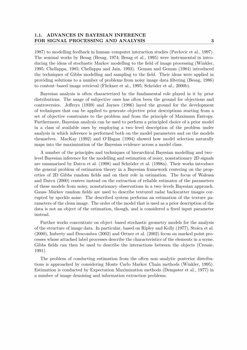
Since the slant altitude is linearly proportional to the interferometric phase pattern,but the latter can only be measured in the [−π, π[ interval, appropriate phase unwrappingtechniques must be implemented (Ghiglia and Romero, 1998; Costantini, 1998) to recoverthe full phase value ϕ (see figure 2.11).
Subsequent processing is necessary to convert the obtained absolute phase surface to aheight map by multiplication with the local phase–cycle–height and to re-sample the result-ing topographic map of the terrain in a map projection such as the Universal TransverseMercator by geocoding techniques (Schreier, 1993) that allow the generation of ground rangealtitude maps.
InSAR coherence It is convenient for the statistical description of the interferogram todefine the correlation coefficient
χ = | E[I1I?2 ]
√
E[I1I?1 ]E[I2I?
2 ]|
2.2. SAR INTERFEROMETRY 28
(a)
(b) (c)
(d)
Figure 2.11: Interferometric SAR principle illustration: phase images (b) and (c) of relief(a) are combined into interferogram (d).

2.2. SAR INTERFEROMETRY 29
(a) (b)
Figure 2.12: Absolute (a) and wrapped (b) Gaussian phase surfaces.
(a) (b)
Figure 2.13: Analytical InSAR data distributions (Touzi and Lopes, 1996): (a) the Wishartdistribution of interferometric phase noise for different looks: L=3(-), L=6(–), L=10(.-.) and(b) interferometric coherence distribution for different looks: L=3(-), L=10(–), L=20(.-.).
that has to be compensated for the topograhic mean effective phase difference ϕ withϕ ∈ [−π, π[ as in
χ0 = |E[I1I?2 ] · exp(−iϕ)
√
E[I1I?1 ]E[I2I?
2 ]| .
The term χ0 is usually referred to as interferometric coherence and provides an estimate ofthe local phase image SNR and of the small–scale geometric stability of the scene, amongothers.
2.2.2 InSAR statistics
The probability distribution function of the degree of coherence χ is derived by Touziand Lopes (1996) to be
p(X = χ) = 2(L − 1)(1 − χ20)
Lχ(1 − χ2)L−2F (L; L; 1;χ2χ20)
for L > 2 and χ0 6= 1, and being F the hypergeometric function.

2.3. THE METRIC INSAR DOMAIN 30
Sensor Information Applications Methodologiesresolution sources for interpretation for data analysis
10-30 m InSAR DEM, natural scenes Parametercoherence, retrieval,backscatter, classification,some texture DEM generation
2-10 m Structure: natural scenes- texture- linesedges-backscatterInSAR
0.5-2 m Strong targets man–made scenes analysis onsparse scattering
Table 2.1: Resolution and information content in SAR data.
The interferometric phase noise can instead be shown (Sarabandi, 1992; Lee et al., 1994;Touzi and Lopes, 1996) to be Wishart distributed: if ϕ is the true phase value and ϕn theassociated noise, then
p(Ψ = ψ) =(1 − χ2)L
2π· F (L, 1; 1/2; κ2)
+ κΓ(L + 1/2)
Γ(L)
(1 − χ2)L
√4π (1 − κ2)L+1/2
beingκ = χ cos(ϕ − ϕn) .
The Wishart distribution can be shown to correspond here to that expected for that ofthe phase of a sinusoid summed to complex, white Gaussian noise with SNR=χ2/(1 − χ2).A series of plots of different Wishart distribution functions with different values of theinterferometric coherence are reported in Figure 2.13.
2.3 The metric InSAR domain
The phenomenology of urban high resolution SAR is peculiar and has to be studied specif-ically. With higher resolution, while natural targets show a typical fractal self–similarityproperty, man made scene elements, well confined in their scale of relevance, tend to changetheir appearance noticeably. A new level of complexity appears, determined by the pres-ence in the scene of a number of objects whose influence on the data has to be understood.Historical buildings, moving vehicles, metallic structures need to be modeled and recon-structed.
Data geometric phenomenology at metric resolutions In the traditional approachto SAR data processing, a number of effects like layover or shadowing are regarded as data

2.3. THE METRIC INSAR DOMAIN 31
Resolution Object / Structure Notes
2 m - 4 m buildings, settlementsforest, strong textureother vegetation
10 m - 30 m agriculture, low textureindustrial areas,vegetation
60 m - 100 m drainage, strong texturegeomorphology,agriculture
Table 2.2: Recognizable object structures with varying resolutions in SAR data.
shortcomings that have to be regularized or filtered out in pre-processing steps. While thisapproach is justified in the case of natural surfaces imaged by lower resolution sensors, inthe case of meter resolution SAR, and especially in urban environments, these hindrancesbecome the norm rather than the exception and must be dealt with appropriately (Adragnaet al., 2002):
• shadowing is a lack of signal caused by very steep surfaces in a way similar to that ofgeometrical optics: no energy is returned to the sensor in a given frame. The intensityimages appear correspondingly dark, whereas interferometric coherence and phaseturn to pure noise. Shadowing from buildings is ubiquitous in city scenes. It mustbe noted, though, that any triple scattering mechanism (figure 2.16c) corresponds toscattering from a virtual point whose position depends on the elevation of the building.This virtual point can easily be located inside the shadow area of a building. Therefore,in the case of meter resolution SAR data the presence of shadows from buildings isnot guaranteed. Shadows, therefore, have only limited relevance when used as hintsfor the presence of buildings in an automatic scene understanding system;
• foreshortening and specular reflections represent an opposite lack respectively of rangeand of radiometric resolution to account for particular target geometries or radiome-tries (generally a combination of the two). The structure of the target becomes par-tially unobservable, and side–lobe effects might become important, especially in veryhigh resolution data, thus further hindering information in other areas of the image.Specular reflections from house roofs and metallic structures appear frequently incities;
• layover — an inversion of the range–to–height relation also caused by very steepsurfaces — is the norm in scenes with buildings. Layover areas are generally simplymasked out and ignored in the traditional processing approach;
• occlusion is a phenomenon also occurring in optical imaging. Although it is relativelyinfrequent in low resolution space-borne radar imaging, it becomes a key factor in thephenomenology of urban HR SAR imaging. Again, some information about the sceneis missing from the data.

2.3. THE METRIC INSAR DOMAIN 32
(a) (b)
layover shadowing extended saturation correlated speckle
(c) (d)
Figure 2.14: Resolution-dependent interferometric SAR phenomenology: scene (a,b) andbasic signal features (c,d) for X-SAR image of Mount Etna (Schwabisch, 1994) and for Xband sub-metric resolution Intermap data over Maastricht, the Netherlands.

2.3. THE METRIC INSAR DOMAIN 33
While all of these effects do appear in low–resolution images acquired on natural surfaces,their effect is usually limited to a small minority of the imaged areas (an important exceptionbeing alpine regions characterized by extremely steep slopes and very dense mountainouspeaks). The affected image areas can, therefore, be left out of the processing results andintegrated with data resulting from different sources. In high–resolution SAR data onurban environments, though, this exceptional cases become the norm, and the effects needto be dealt with appropriately. Furthermore, the fact that they are originated by thecharacteristics of the scene geometry means that they contain information on it: theyshould be consequently considered as information sources rather than hindrances. Furthereffects that become fundamental in metric urban SAR include:
• along–range variations of the acquisition geometry and therefore of the SAR PSF arean important factor in airborne acquisitions of SAR data: the incidence angle is verydifferent at near and at far range, and therefore the sensitivity of the system to scenegeometry can change noticeably. Reconstruction algorithms that operate on largedatasets must be aware of the effect;
• speckle appears as a strong multiplicative noise that makes the radar cross section notdirectly observable. While in lower resolution SAR it is spatially uncorrelated, in HRdata the fully developed assumption does not hold: noise appears in large correlatedblobs in strict dependence with the scene geometry;
• backscatter texture is different than expected: much more textural information ap-pears in the images, especially on non saturated, natural surfaces, but the statistics ofnoise (which now appears as correlated speckle) change in a significant way, imposinga redesign of analysis techniques; in urban environments, instead, the prevalence ofspecular reflections on smooth extended surfaces renders most of the scene as nontextured;
• low-return areas are not limited to shadows: electromagnetic waves are returned witha definite strength from clear edges, while they tend to be scattered away from smoothsurfaces, except in conditions of perpendicular incidence, when they saturate the re-ceiver. In these conditions, returns from strong — e.g. dihedral — scatterers dominatethe image extending well beyond the resolution cell;
• isolated scatterers are more frequent with increased resolution/wavelength ratio andwith the presence of wavelength-sized man made metallic objects in the scene.
Scattering phenomenology Two main forms of scattering are possible for radar waveswhen they interact with a target surface:
• smooth surfaces tend to scatter the incoming way in a privileged direction: the scat-tering is specular;
• surfaces with high rugosities tend to re–radiate the received energy uniformly in alldirections: the backscattering is diffuse.

2.3. THE METRIC INSAR DOMAIN 34
(a) (b)Im
Re Re
Im
(c) (d)
(e) (f)
Figure 2.15: Scheme of principle: diffuse (a,c,e) and specular (b,d,f) scattering with resultingrandom walks in the complex Gauss plane.

2.3. THE METRIC INSAR DOMAIN 35
According to the Rayleigh criterion, a surface tends to be smoother as the incidence angleincreases and as the wavelength becomes larger, since any irregularities on the target becomenegligeable. It must be noted that the Rayleigh criterion does not take into account theactual density of scatterers on the scattering surface. In the extreme case in which a singlescatterer appears in a resolution cell (the probability increases as the wavelength and theresolution increase), the backscattered energy is dominated by the scatterer. Since the singlescatterer tends to appear similar to itself when observed from different incidence angles inthe azimuth direction (as well as in the range one), if its backscatter equivalent surface σ issufficiently large it is possible to discriminate it by means of a correlation between differentlooks generated by considering different sub–apertures along the azimuth direction (Elachi,1988).
Man–made targets, particularly such complex targets as those found in urban centers,contain scatterers with a variety of scattering behaviors (Rihaczeck and Hershkowitz, 1996):
• discontinuities: discontinuities are made of scatterers whose effective extents are rel-atively small in terms of the wavelength. Such discontinuities essentially act as fixedpoint scatterers, and their returns are usually relatively weak compared with thosefrom other features on the target scene object. Discontinuities will become conspic-uous on a target if the gain is set to high values or if the corner-like and cavity-likefeatures on it are ineffective or inexistent;
• smooth extended surfaces: if a flat surface is illuminated at its broadside aspect, it willgenerate a huge return, commonly referred to as a specular return. Since the angularwidth ηa of the specular return is about equal to the ratio of the wavelength to twicethe width of the antenna plate, this specular reflection is generated only within anextremely small angular section and is therefore rarely observed in practice. When itis, though, the return can be so strong that the other responses in the vicinity, muchbeyond the resolution cell in which the specular flash occurs, are more or less masked.In addition, for a practical radar the flash will generate inordinately high range andDoppler sidelobes, which tend to mask other responses.
When, on the other hand, smooth surfaces are observed out of the small broadsideaspect, they tend to scatter most of the energy away from the incidence direction ina specular fashion. This makes them appear as areas of very low SNR in the datacontaining no usable information, often indistinguishable from shadows.
Since smooth extended surfaces are the norm in man–made objects such as vehicles,streets and many important classes of buildings, they determine a large part of thephenomenology of SAR data in urban environments;
• corners: an ideal trihedral, whose three sides are perpendicular to one another, acts asa triple bounce reflector and has the unique property that its effective phase center isat the corner point, independently of the aspect angle and of the frequency within verybroad limits. The corner thus acts as a fixed, strong point reflector. A sizeable cornerreflector that closely approaches the ideal trihedral generates returns that compete instrength with those from flat plates at perpendicular incidence.

2.3. THE METRIC INSAR DOMAIN 36
(a) (b) (c)
Figure 2.16: Electromagnetic wave paths (Simonetto et al., 1999) for direct reflections (a),double bouncings (b) and triple bouncings (c) on a dihedral.
Real corners only poorly approximate the ideal trihedral, but anyway tend to trap theincoming wave in a complicated fashion that usually cannot be explained by multiple-bounce reflections.
The general corner–type reflector typically gives much stronger returns than discon-tinuities: it will appear with a very bright phase center (the point from which thereturn appears to emanate, giving the effective position of the reflector as measuredby radar).
• multiple reflections: with fixed azimuth and fixed target altitude, a number of targetechoes will appear on a typical scene building image ordered by increasing distanceor by decreasing altitude:
– direct reflections on the borders of the structure edge;
– direct reflections on the ground/structure edge;
– double bouncings on the border, accumulating on the pixel corresponding tothe edge: double-bounce propagation at the extended dihedral corner reflectorbetween the ground and the building wall is mapped to the location at thebuilding footprint. This leads to a line of bright intensity in azimuth directionat the edge of the building wall and ground;
– higher–order bouncings.
Multiple bouncings generate an ambiguity in the interpretation of structure imagesand in the evaluation of its altitude, since every phenomenon corresponds to a differ-ent altitude. Their energy is normally much lower than that of direct bouncings onstructure edges and of scattering on the structure base edge. They might be thereforedifficult to observe.
Interferometric data phenomenology The processing of distance information ac-quired by interferometric techniques also becomes more complicated.
• interferometric phase, describing the distance between sensor and scene targets andhence the geometry of the scene, is often regarded as the key content in interferometricSAR observations. In metric resolution data over urban areas it cannot be directly

2.3. THE METRIC INSAR DOMAIN 37
used as in traditional systems, though, unless many other information sources arerecognized as such — instead of being considered as shortcomings in the data — to gainin robustness and discrimination power. Correct phase unwrapping is a complicatedproblem, and noise has to be accounted for without lowering the resolution if thecharacteristics of many of the scene elements have to be extracted;
• interferometric coherence images have different appearance: both geometry and ra-diometry tend to segment the scene into isolated patches of very coherent and verynoisy responses. Simply increasing the size of the estimation windows loses geometri-cal information and raises further estimation problems.
The scene understanding problem is made more difficult by the compromises that are nec-essarily made in the design of very high resolution radar systems:
• spatial (and temporal) baselines might often be sub-optimal;
• signal–to–noise ratio issues might make the interpretation more difficult;
• motion–compensation effects, again for airborne acquisitions, can complicate the phe-nomenology: once the data is transformed to ground coordinates, strong deformationsand even rotations of the PSF can be visible and need to be accounted for in inversionalgorithms.
The increased resolution, on the other hand, means that contextual geometric informa-tion content is acquired at finer scales, and thus describes in greater detail every structurein the scene: backscatter, texture, edges and strong targets are evidently still valuabledescriptors even in the new scenario. What is needed, though, is to relate them to a three–dimensional domain providing a natural context for their understanding.
2.3.1 Meter resolution SAR and InSAR for single isolated buildings
The reconstruction of man-made objects in dense urban areas from SAR imagery iscomplicated by inherent geometric constraints.
The incidence of phenomena like layover, shadow and multi-path signals (Schreier, 1993;Simonetto et al., 1999; Stilla et al., 2002) has to be considered with care in urban areas (seeFigure 2.17).
If the building in Figure 2.17a is illuminated by a sensor located in F , in the slant rangeimage the points A, B and C will appear ordered according to their range distance. Hence,the point A of the building footprint will appear as A′, behind point B′ and in-between B′
and C ′.
The area B′A′ will therefore be layovered, as always happens at vertical building wallsfacing towards the sensor. This will lead to a mixture of signal contributions from thebuilding and the ground in the SAR image, because the elevated objects will be closer tothe sensor than the ground.

2.3. THE METRIC INSAR DOMAIN 38
(a) (b)
Figure 2.17: Projection of a building into a a) slant and b) ground range image (Stilla et al.,2002).
Since the slant image shows a geometric distortion in the ground range direction whichmakes an object recognition and interpretation more difficult, for image interpretation thedata will be sampled to a rectangular grid on the ground (Fig. 2.17b). However, the orderof the points B′′, A′′, C ′′ in the ground image will still be the same as in the slant image:no complete geocoding procedure can take place, since the true heights in the scene areunknown and cannot be derived by simple unwrapping–based processes.
On its far range side, the building will cast a shadow which might occlude smaller objectsbehind it and that will appear as an energy–less, very low SNR, dark area in the image. Intheory, the height of a detached building might be derived from the shadow length and theviewing angle. In real cases, the fact that triple reflections extend often to shadow areasposes serious limits on this kind of approach.
2.3.2 Metric SAR statistics in urban environments
When resolution cells are not anymore populated by a large number of scatterers butinstead only a small number of scatterers determines their behavior, the fully developedspeckle assumption (Tur et al., 1982) does not hold any more. New distributions have tobe taken into account if a proper description of the statistics of the data is sought.
Usually, a K law is used to describe high resolution SAR data. The K law is derivedunder the hypotheses of Gamma reflectivity and Gamma speckle:
pK(A = a) =2λL
Γ(α)Γ(L)(λLa)(α+L)/2−1Kα−L(2
√λLa)
where Kn denotes the modified Bessel function of the third kind and order n and x is theamplitude. The difficulty in using K-law distributed random variables lies in the complica-tions related to the evaluation of the Bessel function.
Inverse Gaussian distributed backscatter values corrupted by square–root Gammaspeckle model well the amplitude return from the slowly varying small number of scatterersthat compose these elements. They have been shown to approximate well a K–distribution

2.3. THE METRIC INSAR DOMAIN 39
while keeping a better tractability, and have been used to model backscatter in urban en-vironments (Frery et al., 1997; Mejail et al., 2001):
p(A = a) = exp
[
− LL Γ(L − α) aL−1
γαΓ(−α)(γ + L a)L−α
]
(2.4)
with L > 0 the number of looks of the data, a > 0 the amplitude pixel value, and −αs, γs > 0and −α0, γ0 > 0 respectively the parameters for the distribution that models the amplitudevalues of the strong scattering elements, and those for remaining clutter obtained by solvingthe system
γ = L
[
m1 Γ(−α)Γ(L)
Γ(−α − 1/2)Γ(L + 1/2)
]2
m21/2
m1=
Γ2(−α − 1/4)Γ2(L + 1/4)
Γ(−α − 1/2)Γ(L + 1/2)Γ(−α)Γ(L)
where mn is the n−th order moment estimated on a training area and Γ(·) is the Gammafunction.
2.3.3 High resolution urban SAR and InSAR inversion: state of the art
The problem of scene understanding from meter resolution SAR data is increasinglypresent in the remote sensing literature. Most studies limit themselves to the two–dimensional intensity case. Up to now the problem of the reconstruction in the threedimensions of urban scenes from interferometric radar data has never been addressed in aunified, consistent framework by well–integrated and clearly justified algorithms and ap-proaches. Actually, if the peculiarities of urban HR SAR are analyzed, it is clear that theusual approach of identifying and excluding from further processing problematic shadowingor layover areas proves problematic, since they are almost ubiquitous.
Simulation based scene understanding A number of simulation–based approacheshave been considered. In them, a model of the scene is progressively updated looking forthe configuration that best explains the data.
The comparison between the scene and the data is actually carried out in the data space:the candidate scene is mapped into the data by using a simulator, that is able to mimicthe acquisition system. The distance between data and simulated scene is computed as across–correlation.
In (Bolter, 2000) and (Bolter and Leberl, 2000) interferometric coherence, absolute phaseand shadowing are identified as powerful image features for the reconstruction of buildings.A deterministic correlation measure between real and simulated data is used as a qualitycriterion for the reconstruction.
In (Gamba and Houshmand, 1999) segmentation and plane–fitting techniques are appliedto interferometry-derived local elevation data to identify buildings. In one case only (Huer-tas et al., 1998), a segmentation of local heights from interferometric radar is used as a cuein a pre–processing step of the building reconstruction system chain.

2.3. THE METRIC INSAR DOMAIN 40
Ad hoc data regularization techniques A number of studies were carried out onthe peculiar effects encountered in very high resolution SAR images in urban environments.They have the great merit of having brought to a better understanding of the characteristicsof HR SAR phenomenology.
In (Burkhart et al., 1996) layover in the height profiles of buildings reconstructed by SARinterferometry is investigated. Some ad–hoc algorithms for the correction of this effect arealso proposed. The peculiarities of HR urban SAR tend to be treated as shortcomings ofthe data that must be regularized instead of being used as additional sources of information.
Stochastic approaches The main limit of deterministic simulation based approaches isthat
• only the scene that best explains a given dataset is extracted from the data: no fullposterior probabilistic distribution for it is generated;
• they are strongly dependent on the quality of the simulator: if good results are to beobtained, a good simulator is needed, hence
• they are computationally expensive.
As an alternative, a probabilistic approach can be considered, where full probabilisticdescriptions are given for the phenomena and terms involved.
To deal with the high complexity of the problem, stochastic algorithms have been pro-posed in recent years from a number of authors. Although exploiting interferometric radardata in a limited way, (Heuel and Nevatia, 1995) makes use in an explicit way of models forthe scene objects of interest. Parallelepipedal buildings are extracted from high resolutionoptical images supplementing in some cases automatic processing with user intervention (Liet al., 1999; Chellappa et al., 1993; Heuel and Nevatia, 1995).
If a Bayesian system is considered, then A–Priori descriptions of the scene can be incor-porated into the description.
In (Simonetto, 2002) the phenomenology of HR SAR is investigated. A stochastic algo-rithm for the exploitation of stereo intensity observations for industrial building extractionis proposed. In (Tupin and Roux, 2003), the extraction of building outlines using a pairof optical and SAR images is considered. In (Stoica et al., 2000), a model for a set ofsegments is employed in a stochastic geometry framework to overcome the difficulties witha part of the linear feature extraction process. In a related paper (Ortner et al., 2002) asimilar approach is used for the reconstruction of building areas from Laser digital elevationdata. In (Stilla et al., 2003), techniques for the extraction of building models from inter-ferometric SAR data are considered and the results are compared with those obtained byLIDAR data. The full hierarchical modeling of both the geometry and the radiometry ofHR SAR data acquired on complex structures in urban environments has — to the best ofour knowledge — never been addressed as a tool for scene understanding, though.

2.4. SUMMARY 41
2.4 Summary
In this Chapter, the following points have been discussed:
• SAR and InSAR systems have very peculiar geometric and radiometric properties thatcan be treated by appropriate, well established processing techniques;
• their performance at metric resolutions in urban environments is determined by
– geometric effects such as layover, shadowing and occlusion;
– the radiometric effect of smooth surfaces on speckle noise, backscatter textureand signal–to–noise ratio;
– the appearance of multiple reflections of the incident radar beam;
– the various classes of strong isolated scatterers;
– the peculiar statistics of meter resolution data;
• the limiting effects on the traditional interferometry–based scene reconstruction ap-proaches of the presence of very strong reflectors and of phenomena like layover andmultiple reflections depend on the scene geometry. Therefore, they contain informa-tion about it;
• traditional, simulation– and model–based inversion algorithms in the literature havebeen evaluated and compared.
The phenomenology and effects described in this chapter form the basis for the hierarchicalprobabilistic modelling and inversion algorithms presented in chapters from 4 to 6 andvalidated in chapter III.

Chapter 3
Bayesian modeling, estimation anddecision theory formultidimensional signal analysis
Abstract
Bayesian modeling and estimation techniques for the analysis of multidimen-sional fields are introduced. After presenting the properties of Gibbs–Markovfields on random variable networks and the results of the Hammersley–Cliffordtheorem, hierarchical Bayesian models are introduced.
The second level of Bayesian analysis for model selection is presented togetherwith the role of the Occam factor in model choice and analysis.
Bayesian estimation and decision theories are then introduced: the analysisfocuses on Maximum A Posteriori estimates and on decisions as posterior ratios.
Posterior optimization techniques based on complete enumeration, on IteratedConditional Modes and on the Gibbs Sampler and Monte Carlo Markov chainsare then introduced and detailed.
3.1 Bayesian modeling and analysis
The high complexity of models made up by large numbers of possibly interdependentvariables can be tackled by considering and exploiting conditional independence assump-tions. The use of independence assumptions allows efficient inference to be carried out evenfor problems involving a large number of variables.

3.1. BAYESIAN MODELING AND ANALYSIS 43
X1 X2
p(X2=x2|X1=x1)
p(X2=x2)
p(X2=x2|X1=x1)p(X1=x1)p(X1=x1|X2=x2)=
Figure 3.1: The Bayes’ law enables the reversal of probabilistic links and therefore allowsinference to take place based on the existence of direct models. Following the usual notationfor Bayesian networks, random variables are represented by circles at the nodes of a graphwhile probabilistic relations are represented by (oriented) edges.
3.1.1 A principled approach to the composition of stochastic descriptions
The Bayes’ equation In Bayesian probability theory, logical links are expressed bymeans of conditional probabilities
p(X1 = x1|X2 = x2) ≡p(X1 = x1, X2 = x2)
p(X2 = x2)
that express the degree of belief that event x1 takes place given that event x2 happens withcertainty.
An immediate consequence of the definition of conditional probability is the so–calledBayes’ law
p(X1 = x1|X2 = x2) =p(X2 = x2|X1 = x1) p(X1 = x1)
p(X2 = x2)(3.1)
that enables the reversal of probabilistic links and therefore allows inference to take placebased on the existence of direct models. The law can be seen as a rule for updating anexisting description of a phenomenon X1, the prior p(X1 = x1), based on new information— new data or a new description — x2. The direct link from the old to the new descriptionneeds to be modeled in the likelihood p(X2|X1). Furthermore, an evidence normalizationterm is introduced in p(X2 = x2) that expresses the probability of the data and that canbe computed as a Marginalization on the prior model used
p(X2 = x2) =∑
x1,i
p(X2 = x2|X1 = x1,i) p(X1 = x1,i) . (3.2)
Bayesian inversion results in a powerful method in the understanding of complex phe-nomena for which precise mathematical modeling is available starting from incomplete in-formation available in datasets of different nature.
This measure and the dependence description itself is updated from a starting prior beliefto a posterior one by considering the data available.

3.2. GIBBS RANDOM FIELDS 44
On the logical nature of conditional probability connections It is important tonotice that conditional probabilities are used to express logical links, not causal ones. If, forinstance, event X1 generates by some physical process event X2, a link that is both causaland logical exists between events X1 and X2, but a link that is only logical exists betweenevents X2 and X1 in the sense that an occurrence of event X2 gives us a hint about theoccurrence of event X1.
3.1.2 Modeling interdependence in random variable sets: chain Rule andMarkov property
The chain rule We consider a set of N stochastic variables
X = (X1, X2, · · ·XN )
with valuesx = (x1, x2, · · ·xN ) .
Independently of the type of stochastic process considered, the joint probability of Xcan be written as
p(X = x) = p(X1 = x1, · · ·XN = xN )
and can be decomposed based only on the definition of conditional probability as in
p(X = x) =p(X1 = x1) p(X2 = x2|X1 = x1) p(X3 = x3|X2 = x2, X1 = x1)
· · · p(XN = xn|XN−1 = xn−1, · · ·X2 = x2, X1 = x1)
which is called the “chain rule” decomposition theorem of probability. The last terms inthe decomposition are based on a very large number of variables, and are therefore likelyto render an inference process based on them hard to treat.
The Markov property A k–order Markov source is a symbol–emitting device with mem-ory for which if X denotes the ordered set of symbols emitted by the source, the Markovproperty
p(X = x) =p(X1 = x1) · · · p(Xk−1 = xk−1|Xk−2 = xk−2 · · ·X1 = x1)
N∏
i=k+1
p(Xi = xi|Xi−1 = xi−1 · · ·Xi−k = xi−k)
holds. Even if the number of elements in the set X grows, only a maximum number of ksymbols has to be taken into account in modeling the source.

3.2. GIBBS RANDOM FIELDS 45
A C
B
N_2D
C2C1
C3
N_1
A ⊥ D, A ⊥ B|C
Figure 3.2: Markov property for random variables: random variables are depicted as cir-cles. Two neighborhoods are represented. First–order cliques for neighborhood N1 aredepicted by closed shapes enclosing the variables. The three cliques C1, C2 and C3 formthe first–order neighborhood N1. The diagram describes a belief network encoding statisti-cal independence relations: variable A is independent of D (no path exists between the two),while A is independent of B if C is known. Independence and conditional independence arerespectively denoted by · ⊥ · and · ⊥ ·|·. The exploitation of conditional independencerelations allows the simplification of high complexity probabilistic descriptions.
3.2 Gibbs random fields
3.2.1 Lattices, sets, neighborhoods, cliques, sites, pixel values
For any variable Xi in X a neighborhood Ni is defined by
Ni = j such that
i 6∈ Ni
j ∈ Ni ⇔ i ∈ Nj
.
A neighborhood is assigned a relative set C of cliques Ck
C = Ck
each made of k random variables and each characterized by a vector parameter
~θ = θ11, θ12, θ21, θ22, · · ·
that expresses the local interactions in the clique Ck.
While in the case of image processing and analysis neighborhoods are limited to thegeometric vicinity of the central pixel under analysis Xi, it must be noticed that onceagain the important point is the logical link between the variables in the same clique whichmight or might not be associated to a location and even belong to spaces with differentdimensionality.

3.2. GIBBS RANDOM FIELDS 46
3.2.2 Random fields in terms of potentials and energies
Local interactions, that is interactions that take place between elements of the sameclique, can be now expressed in terms of energies and potentials
U(X = x) =∑
c∈C
Vc(x)
where the energy of the full variable set is expressed by a sum of the potentials of all thesingle cliques in the model and the energy of a single variable
Ui(Xi = xi) =∑
c∈C,i∈c
Vc(xi)
is expressed as a sum of all the energies of the cliques that include that variable.
Markov on a lattice: restating the Markov property at higher dimensionality
The Markov property can then be restated as specifying the interdependence between vari-ables to actually occur only among variables belonging to the same clique. In a Markovrandom field a random variable can be expressed in terms of a limited number of its neigh-bors:
if xi = (xj)j 6=i then p(Xi = xi|Xi = xi) = p(Xi = xi|xj ∈ Ni) .
The specification of statistical independence relations between random variables allows thedesign of faster inference algorithms taking into account only meaningful logical links.
Gibbs random fields In a Gibbs random field probability distribution functions can beexpressed in terms of potentials, as in
p(X = x) =1
∑
xiexp(−U(xi))
exp(−∑
c∈C
Vc(x)) .
The denominator partition function integral over the configuration space is often hard toevaluate due to the large number of elements in the domain of X.
The Hammersley–Clifford theorem The Hammersley–Clifford theorem states thatthe probability of one random variable instead of the whole set can be derived from itsneighbors only, and hence states the equivalence between Markov and Gibbs fields:
p(Xi = xi|Xj = xj) =1
∑
xi,xjexp(−Ui(xi|xj ∈ Ni))
exp(−Ui(xi|xj ∈ Ni)) .
3.2.3 Markov random fields in terms of belief networks
A Bayesian network (Hackerman et al., 1995) is a graphical model for probabilistic rela-tionships among variables in a set. It consists of an annotated directed graph that encodes

3.2. GIBBS RANDOM FIELDS 47
p(Xk−1=xk−1|Xk=xk)
X1 Xk XNXk−1
p(Xk=xk|Xk−1=xk−1)
Figure 3.3: Hierarchical model illustration: the distribution of parameters at any levelof the hierarchy depends on parameters at the next lower level and, conditional on thoseparameters, is independent of parameters at all levels below that.
probabilistic relationships among variables of interest in uncertain–reasoning problems. Therepresentation formally encodes the joint probability distribution for its domain, yet includesa human–oriented qualitative structure that facilitates communication between a user anda system incorporating the probabilistic model.
Bayesian networks allow us to overcome the curse of dimensionality by encoding proba-bilistic independence between the elements of the inference problem. They can be mappedto graphs whose nodes represent the random variables under study, while dependenciesare encoded in their structure. The learning procedure progressively updates the networkthereby obtaining a description of the statistical link between the variables based on all theinformation available. Once the graph structure is set up, it can be used to perform effi-cient inference by taking into account only significant dependencies in between the randomvariables.
The nodes in the graph correspond to the variables in the problem, while the directededges encode the significant probabilistic dependencies. The fundamental property of thenet is that a node is conditionally independent of its ancestors given its parents. Hence,inference on the graph can be reduced to a message passing algorithm in which startingfrom a set of root nodes, probability is propagated down the graph to the node of interest.
3.2.4 Hierarchical models
As noted by O’Hagan (1994), the p(X1 = x1|X2 = x2) posterior statistical model andp(X2 = x2) prior model together form an ordered structure in which the distribution ofthe data x1 is written conditionally on parameters X2 = x2 as p(X1 = x1|X2 = x2).Analogously, the prior distribution of X2 can be written conditionally on hyperparametersX3 as p(X2 = x2|X3 = x3), and be completed by the distribution of X3 = x3, p(X3 = x3).We could go further and write the distribution of X3 conditionally on some more (’hyper-hyper’) parameters X4 = x4 as p(X3 = x3|X4 = x4), and this process could continue as faras is needed. Such models are called hierarchical models, because of the way in which thedistribution of parameters in each level of the hierarchy depends on the parameters in theprevious level.
In fact it is usual to say that the distribution of parameters at any level of the hierarchydepends on parameters at the next lower level and, conditional on those parameters, isindependent of parameters at all levels below that. For instance, if we model the distribution

3.2. GIBBS RANDOM FIELDS 48
of X2 in terms of p(X2 = x2|X3 = x3) and p(X3 = x3), then the likelihood p(X1 =x1|X2 = x2) is formally the distribution of X1 given X2 = x2 and X3 = x3. Writing itas p(X1 = x1|X2 = x2) incorporates a judgment that if we know X2 = x2 then knowingX3 = x3 would not add any information about X1. This is reasonable because X3 has beenintroduced only as a way of formulating p(X3 = x3) as in the (discrete) evidence integral
p(X2 = x2) =∑
x3
p(X2 = x2|X3 = x3)p(X3 = x3) . (3.3)
The reason for making this interpretation of p(X1 = x1|X2 = x2) is that otherwise thedistributions of p(X1 = x1|X2 = x2), p(X2 = x2|X3 = x3) and p(X3 = x3) together do notcompletely specify the joint distribution of X1, X2 and X3. The extra assumption allowsus to write
p(X1 = x1, X2 = x2, X3 = x3) = p(X1 = x1|X2 = x2) p(X2 = x2|X3 = x3) p(X3 = x3) .(3.4)
A hierarchical model does always specify the full joint distribution of all quantities thisway 1.
3.2.5 Principle of inference for 2–level hierarchical models
If a set (M1, · · ·MN ) of models is available, and we consider that each model M = m hasa vector of parameters Θ = θ, then a full three–levels hierarchical model can be describedas in
M → Θ → D .
A model is defined by its functional form and two probability distributions: a prior distri-bution p(Θ = θ|M = m) which states what values the model’s parameters might plausiblytake; and the predictions p(D = d|Θ = θ;M = m) that the model makes about the dataD = d when its parameters have a particular value θ. Note that models with the same pa-rameterization but different priors over the parameters are therefore defined to be differentmodels.
At the first level of inference, we assume that one model M = m is true, and we inferwhat the model’s parameters Θ = θ might be given the data d. Using Bayes’ rule in eq. 3.1,the posterior probability of the parameters θ is:
p(Θ = θ|D = d;M = m) =p(D = d|Θ = θ;M = m) p(Θ = θ|M = m)
p(D = d|M = m). (3.5)
1The equivalence of this formulation with that of Bayesian networks and graphical models is indicatedby the correspondence of the description above with the textbook definition (as in Heckerman (1995) orin Myllymaki and Tirri (1993)) of a Bayesian belief network representation for a probability distributionp(·) on a domain (X1, · · ·XN ) as a pair (G, P ) where G is a directed acyclic graph whose nodes correspondto the variables X1, · · ·XN and whose topology satisfies the following: each variable Xi is conditionallyindependent of all of its non–descendants in G, given its set of parents paXi
and no proper subset of paXi
satisfies this condition. The second component P is a set consisting of all the conditional probabilities ofthe form p(Xi|paXi
).

3.2. GIBBS RANDOM FIELDS 49
The normalizing constant p(D = d|M = m) is commonly ignored, since it is irrelevant tothe first level of inference, i.e., the choice of Θ = θ; but it is important in the second levelof inference, and is called the evidence. It is common to use gradient-based methods tofind the maximum of the posterior, which defines the most probable value for the vectorparameter, θMAP, that is subsequently used to summarize the posterior distribution by itsvalue 2 (section 3.3).
3.2.6 Occam razor and Occam factor
As noted by MacKay (1992), model comparison is a difficult task because it is not possiblesimply to choose the model that fits the data best: more complex models can always fit thedata better, so the maximum likelihood model choice would lead us inevitably to implausiblyover-parameterized models which generalize poorly.
‘Occam’s razor’ is the principle that states that unnecessarily complex models should notbe preferred to simpler ones. Bayesian methods automatically and quantitatively embodyOccam’s razor (Jeffreys, 1939; Gull, 1988), without the introduction of ad hoc penalty terms:complex models are automatically self-penalizing under Bayes’ rule.
At the second level of inference, we wish to infer which model is most plausible giventhe data. The posterior probability of each model is:
p(M = m|D = d) ∝ p(D = d|M = m) p(M = m) . (3.7)
Notice that the data-dependent likelihood term p(D = d|M = m) is the first-level Bayesianinference evidence for M = m of equation 3.5. The second term, p(M = m), is a ‘subjective’prior over the hypothesis space, kept constant when there is no reason to assign stronglydiffering priors p(M = m) to the alternative models.
The evidence then naturally embodies Occam’s razor: in order to assign a preference toalternative models M = m, the evidence p(D = d|M = m) has to be evaluated.
It should be pointed out that the emphasis of this modern Bayesian approach is not onthe inclusion of priors into inference. Historically, Bayesian analysis has been accompaniedby methods to work out the ‘right’ prior p(Θ = θ|M = m) for a problem, for example, theprinciples of insufficient reason and maximum entropy. Modern Bayesian theory, however,does not take a fundamentalist attitude to assigning the ‘right’ priors – many different priorscan be tried, allowing the data to inform us which is most appropriate. Each particularprior corresponds to a different hypothesis about the way the world is. These alternativehypotheses can be compared in the light of the data by evaluating the evidence.
2The width of the posterior distribution is approximately characterized by the curvature of the posterior;writing the Hessian H = ∇∇ log p(Θ = θ|D = d;M = m) and Taylor-expanding the log posterior with∆θ = θ − θMAP, with T denoting the transpose operator,
p(Θ = θ|D = d;M = m) ' p(θMAP|D = d;M = m) expˆ
−1
2∆θ
TH ∆θ
˜
(3.6)
we see that the posterior can be locally approximated as a Gaussian with covariance matrix H−1.

3.2. GIBBS RANDOM FIELDS 50
In practice, the evaluation of the Marginalization integral of eq. 3.3
p(D = d|M = m) =∑
θ
p(D = d|Θ = θ,M = m) p(Θ = θ|M = m) (3.8)
can be conducted by approximating the posterior as a Gaussian around its MAP peak,using Laplace’s method:
p(D = d|M = m) ' p(D = d|θMAP,M = m) · p(θMAP|M = m)det−1
2 (H/2π) (3.9)
in which the Hessian H = −∇∇ log p(Θ = θ|D = d;M = m) appears in the last two termsthat account for the so called ‘Occam factor’
Ω ≡ p(θMAP|M = m)det−1
2 (H/2π) < 1 (3.10)
which penalizes M = m for having the parameter θ. The first–level evidence p(D = d|M =m) can then be obtained simply by multiplying the best fit likelihood by the Occam factor,favoring less complicated models whenever a choice is made for instance by making use ofthe Bayes’ factor
Bij =p(D = d|M = m)
p(D = d|M = m′)' Ωm
Ωm′
(3.11)
in a set of given models.
The maximization of the evidence is therefore regarded as a criterion for the choice of asuitable model to explain a given dataset.
Jeffrey’s priors Frequently partial prior information is available, outside of which it isdesired to use a prior that is as non-informative as possible.
The maximum entropy distribution “is uniquely determined as the one which is max-imally noncommittal with regard to missing information” (Jaynes, 1957): it “agrees withwhat is known, but expresses ‘maximum uncertainty’ with regard to all other matters,and thus leaves a maximum possible freedom for our final decision to be influenced by thesubsequent sample data” (Jaynes, 1968). It has been further shown by Jaynes that themaximum entropy distribution is equal to the frequency distribution that can be realizedin the greatest number of ways.
In order to define the requested maximum entropy prior, constraints can be composedby using Lagrange multipliers with a Shannon entropy measure
−∑
x
p(X = x) log p(X = x) (3.12)
and the resulting composite equation can therefore be maximized providing the requestedresulting prior.

3.3. ESTIMATION AND DECISION THEORY 51
3.2.7 From posterior distributions to estimates and decisions
Full probabilistic inference produces as output full posterior distributions rather thansimple scalar values. On the other hand, in a number of situations, scalar values are requiredin order to be able to compare a theoretical result with actual measured quantities.
Estimation and decision theory considers the problem of choosing a representative valuefor a given probabilistic distribution in a principled way.
3.3 Estimation and decision theory
The problem of estimation and decision theory is the derivation in a principled wayof criteria for the choice of single scalar values from a full probabilistic description of aproblem.
It is clear that moving from a full probabilistic description of a phenomenon to a singlevalue must involve some kind of loss in the quality of the descriptor. This loss must beexpressed by some kind of cost function leading to a definition of an optimal estimator: theclassical parameter estimation is formulated as the minimization of the Bayes risk R definedover the signal space. The risk R is the expectation value of a cost function defined overthe joint space of observations (Y ) and model parameters X
R = E[c(X = x, x)] =∑
y
∑
y
c(X = x, x) p(X = x, Y = y) . (3.13)
The cost function c(X = x, x) is a measure of goodness of the estimated parameter x, beingdefined as a distance between the actual and the desired but unknown value of x. Minimizingthe risk and using a uniform cost function, at the limit ε → 0, we obtain the Maximum APosteriori (MAP) estimator that summarizes the posterior description of phenomenon y interms of the position of its maximum
yMAP = arg maxy
p(X = x|Y = y) p(Y = y)/p(X = x) . (3.14)
We observe that, in classical estimation theory, using a cost function is nothing else butdescribing a type of prior information. The expression for the posterior encapsulates thedeterministic prior knowledge represented by the forward model. In addition, the knowledgeabout the observation noise and the a priori information about the desired parameter arealso included. We conclude that MAP is a complete frame for model–based approaches ininformation extraction.
This can be demonstrated (Rissanen, 1985) to be equivalent to a shortest descriptionlength estimate obtained by considering that the best model of a phenomenon is the one thatproduces the most compact encoding of it. A very similar approach, also considering twoterms, a data one requiring the maximization of a likelihood and a penalty term consideringthe complexity of the model, is the Akaike information criterion (Akaike, 1974).

3.3. ESTIMATION AND DECISION THEORY 52
3.3.1 Decisions as posterior ratios
Decision theory focuses on the problem of choosing the most probable hypothesis in aset of given ones. It is clearly strongly related to the problem of model selection as wellas to estimation: even in this case, the fundamental problem is the reduction of a fullprobabilistic description to a single value. We consider the problem of binary hypothesistesting under data D. If the two competing hypotheses we are considering are called H0
and H1, it can be seen that the decision reduces itself to the evaluation of the ratio
p(H = h0)p(D = d|H = h0)
p(H = h1)p(D = d|H = h1)
that, introducing the evidence p(D) and using the Bayes’ theorem, equals
p(H = h0|D = d)
p(H = h1|D = d)
a comparison of the posterior probabilities that becomes, when identical priors are consid-ered, to the usual likelihood ratio estimator of decision theory
L(D = d) ≡ p(H = h0|D = d)
p(H = h1|D = d).
3.3.2 Estimation and decision algorithms
The optimization of probability distributions of large sets of random variables is compli-cated by the large dimensionality of the spaces where these sets are located. Examples ofsuch sets include
• gray-scale image processing: X is a set of mono-dimensional stochastic pixels Xi withvalues xi in some set L. The number of configurations N is usually very large (iteasily takes up values in the order of a million), and the size of L can be considerablylarge as well, especially if instead of limiting the problem to a quantized space of 256values larger pixel ranges are considered
• color image processing: the size of L increases considerably with respect to the gray-scale image processing example. Quite often, different mechanisms have to be ac-counted for in describing the way different physical phenomena are responsible for thegeneration of the different bands
• hierarchical geometrical modeling: X is decomposed into a series of subsets X =(X1D, X2D, X3D) each of which models a set of interdependent objects with differentdimensionality. For instance, the full problem space might be composed of a set ofpoints that probabilistically generate a set of segments that are composed into bi–and three–dimensional graphs.
The characterization of the behavior of the set X is in cases like these made complex by thevery size of the state space one has to consider. Even in the simple case of a 1000 × 1000pixels 256–levels image processing, with N fixed and Xi mono-dimensional, the possiblenumber of states of X is 1000 × 1000 × 256.

3.3. ESTIMATION AND DECISION THEORY 53
3.3.2.1 Analytic derivation of MAP estimate
In the cases when the posterior is analytic, the MAP estimate
x = arg maxx
p(X = x|Y = y)
can be computed directly from
dp(X = x|Y = y)
dx|X=xMAP
= 0,d2p(X = x|Y = y)
dx2|X=xMAP
< 0 .
When this is not possible, the optimization is instead carried out by numerical methods (Co-hen and Cooper, 1987).
3.3.2.2 Exact inference by complete enumeration
A possible method for statistical inference is a brute–force one: complete enumeration ofall the hypotheses, and evaluation of their probabilities. This approach is an exact method,and the difficulty of carrying it out motivates the approximate methods introduced in laterParagraphs.
It has to be noted that, even though the hypothesis spaces of many problems can bethought of as continuous, such continuous spaces can be discretized and so can, in principle,be enumerated –at a grid of parameter values, for example.
3.3.2.3 The Iterated Conditional Modes algorithm
The Iterated Conditional Modes (Besag, 1986; Winkler, 1995) algorithm is an iterativeoptimization technique specifically designed for probabilistic models. It is a local technique,and so is susceptible to local minima. The algorithm works by iteratively computing theMAP estimate of the data using the available observations and the current estimates of themodel parameters until convergence is reached. The IEM algorithm is closely related to theExpectation–Maximization algorithm of Dempster et al. (1977), that operates instead byoptimizing on a simpler, convex approximation (a form of the Jensen’s inequality, the factthat an arithmetic mean is never smaller than a geometric mean, is used as a bound) of theposterior.
3.3.2.4 The Gibbs sampler and Monte Carlo Markov chains
A Metropolis algorithm based on a Simulated Annealing procedure (see Appendix B)can be adopted for the estimation of the MAP: the multivariate posterior is maximized byiteratively evaluating many possible solutions in a multidimensional parameter space.
The Metropolis algorithm can therefore be understood as a special case of a thresholdrandom search, a relaxation of the greedy maximal ascent algorithm.

3.4. SUMMARY 54
• Step 0: Choose arbitrary starting point
θ0 = (θ01, θ
02, ..., θ
0p)
′
and set i = 0;
• Step 1: Generate θ1 = (θ11, θ
12, ..., θ
1p)
′ as follows:
– Generate θi+11 ∼ p(Θ1 = θ1|Θ2 = θi
2, Θ3 = θi3, ...,Θp = θi
p, D);
– Generate θi+12 ∼ p(Θ2 = θ2|Θ1 = θi
1, Θ2 = θi2, ...,Θp = θi
p, D);
– ...
– Generate θi+1p ∼ p(Θp = θp|Θ1 = θi
1, Θ2 = θi2, ...,Θp−1 = θi
p−1, D);
• Step 2: Set i = i + 1, go to Step 1.
Table 3.1: The Gibbs Sampling algorithm. Starting from a purely random initial configu-ration θ0, the algorithm sequentially updates all parameters at each iteration by samplingthe new value from the local probability distribution conditioned on those that influencethe one under analysis.
This approach allows the system to explore solutions that a direct maximum-gradientmaximization would not consider, permitting it to identify the global maximum of a mul-tivariate distribution avoiding the burden of constructing the full posterior distribution.
A Gibbs sampler can be set up to sample the posterior distribution keeping all the dimen-sions of the Scene process fixed but one: this modified distribution can be shown (Winkler,1995; Stoica et al., 2000) to converge to the full posterior.
For generating the new candidate solutions to the optimization problem from the previousones, update rules have to be defined. Special care must be used in ensuring that themutation dynamics of the Gibbs sampler are completely reversible, to avoid getting stuckon some local maxima or on the borders of the domain. Each of the defined mutation stepmust have an equiprobable opposite move.
3.4 Summary
In this chapter, the following points have been discussed:
• Bayesian modeling and estimation techniques for the analysis of multidimensionalfields have been introduced;
• the properties of Gibbs–Markov fields and hierarchical Bayesian models were detailed;
• Bayesian model selection was presented together with the role of evidence maximiza-tion and of the Occam factor in model choice and analysis;

3.4. SUMMARY 55
• Bayesian estimation and decision theories were introduced focusing on Maximum APosteriori estimates and on decisions as posterior ratios;
• Posterior optimization techniques based on complete enumeration, on Iterated Con-ditional Modes and on the Gibbs Sampler and Monte Carlo Markov chains were thenintroduced and detailed.
The techniques presented in this chapter are applied to the construction of hierarchicalmodels of complex acquisition procedures and of their results and to the derivation ofestimation algorithms for the inversion of these procedures in the next chapters of thisthesis.

Part II
Hierarchical Bayesian modelling

57
Abstract
A set of novel algorithms for urban scene understanding from high resolutionSAR imagery are introduced that are based on hierarchial stochastic models ofthe scene and the data and on Bayesian estimation and decision.
A new algorithm for space–variant model order selection in Bayesian model–based image denoising and information extraction is developed based on evidencemaximization in the framework of second–level Bayesian inference for modelselection. The algorithm is demonstrated on real and simulated data generatedfrom different models and corrupted by multiplicative speckle noise.
Based on the information extracted and in order to complement different typesof information derived from various data sources, a novel approach to scenereconstruction based on Bayesian data classification and fusion is introduced:generic features extracted from the data are combined with user conjecturesto generate land use maps. The system is demonstrated on real InSAR dataacquired by spaceborne sensors.
To overcome the limitations of pixel–based analysis applied to sub–metric reso-lution data, an new object–based algorithm is presented that models the sceneas an instance of a decomposable–object hierarchic marked–point prior process.The geometric and radiometric phenomenologies of sub–metric SAR in urbanenvironments are taken into account in the likelihood term. The optimizationof the obtained posterior is based on Gibbs sampling and Monte Carlo Markovchains. The developed algorithm is demonstrated on real data acquired by air-borne X band sensors on built–up areas in high complexity settings characterizedby tall vegetation and strong metallic scatterers.

Chapter 4
Space–variant model selection inmodel–based informationextraction
Abstract
While the problematic of model selection in the Bayesian framework is wellknown, most applications in the image processing literature deal with cleandata that are assumed completely known.
Here instead, an extension of the image denoising and information extractionmethod of Walessa and Datcu (2000) is introduced that incorporates a furtherestimation level to allow the space–variant selection of the model order by meansof the maximization of the Bayesian model evidence.
This allows the system to properly model and reconstruct images that are com-posed of instances of different stochastic image models with varying degrees ofcomplexity.
The extended algorithm is demonstrated on simulated data generated with well–known model orders as well as on Brodatz textures corrupted by multiplicativespeckle noise. Classification maps based on model order are generated that forairborne X band SAR data at metric resolution demonstrate the discriminationpotential of the Bayesian evidence maximization with respect to model choice.
The first approach to data analysis we consider fills the gap from data to applicationgeneric signal features. In particular, we consider the problem of image denoising and in-formation extraction. A model–based approach (Walessa, 2000) can be applied that modelsthe image data as a sample of a Markov random field whose parameters express the localtexture (Cross and Jain, 1983).

4.1. MODEL BASED IMAGE DENOISING AND INFORMATION
EXTRACTION 59
Figure 4.1: Clique structures for different Gauss–Markov random field model orders (respec-tively one, two, three and four): the number of model parameters in the vector θ increaseswith model order, allowing the expression of more complex structures.
4.1 Model based image denoising and information extraction
Bayesian model based image denoising makes use of the Bayes’ equation
p(X = x|Y = y) = p(Y = y|X = x) p(X = x) / p(Y = y)
applying it to the case where X is a stochastic process generating images x, Y describes“dirty” images y and the likelihood p(Y = y|X = x) describes the noise in the image. Ifa further modeling level Θ generating X is included in the analysis and its most probableparameter θMAP is estimated, the denoising system is able to perform an information extrac-tion task: the clean image is not only extracted from the noisy one, but it is also explainedin terms of a lower–level model. In this chapter, we will introduce a further extensionto the speckle filtering and image information extraction approach described by Walessaand Datcu (2000), introducing a third modeling level that, in addition to the denoising andmodel parameter estimation, allows the local space–variant estimation of the most probablemodel to have generated the data.

4.2. IMAGE MODELS 60
4.2 Image models
The probabilistic models used play a central role in Bayesian analysis. We introduce herethe image models and the noise models used in the denoising and information extractionsystem of Walessa and Datcu (2000) and Datcu et al. (1998) that is object of the extensionto space–variant model order selection in the following section of this chapter.
Since the system is developed in a Bayesian framework, the choice of appropriate priormodels for the clean data plays an important role, and affects in a direct way the obtainedresults.
A prior scene model used for scene reconstruction should ideally be completely inde-pendent of the data available and its characteristics. On the other hand, the developmentof tractable scale-independent probabilistic scene models is a complicated task, both forthe practical need of constraining the model complexity and because the properties of thesensor (and in particular its incidence angle and spatial resolution)we influence in a verydirect way the classes of objects that are actually observable and their perceived level ofdetail.
4.2.1 Gauss–Markov random fields
The prior model considered for image data is the Gauss-Markov random field(GMRF) (Datcu et al., 1998; Schroder et al., 1998a)
p(Xs = xs|Xr = xr, r ∈ GMs , σs, θs,Ms) =1
√
2πσ2s
exp
[
−( xs −∑
r∈G θs,rr xs+r )2
2σ2s
]
.
(4.1)It expresses the generic pixel value xs as normally distributed with width σs around themean of its neighboring pixels xs+r symmetrically weighted by the texture parameter vectorθ = (θ0, ...θm) defined on a neighborhood of cliques G centered on the pixel xs, and such thatthe scalar parameters are symmetric around the central element (see figure 4.1) accordingto Chellappa (1985); Chellappa et al. (1985).
The main strength of the Gauss-Markov model lies in its ability to model local de-pendencies between pixels in a wide set of textured images, while still allowing analyticaltractability.
While the prior model employed in both information extraction modules is the GMRF,the likelihoods considered have to be adapted to the characteristics of the data under anal-ysis.
4.2.2 Gaussian likelihoods for additive Gaussian noise
If an additive Gaussian noise model is assumed for the data (as is the case, for example,for SAR interferometry–derived Digital Elevation models), a Gaussian likelihood can be used

4.3. LOCALLY–ADAPTIVE PARAMETER ESTIMATION BY EVIDENCE
MAXIMIZATION 61
M
x_i
theta_iMAP Evidencemax?
theta_i −> theta_i’
M_theta step
y_i x_i_MAP
E step
p(theta_i|y_i)
...
Figure 4.2: Flowchart of the evidence maximization algorithm used for texture parameterestimation in the model based denoising and information extraction system seen as anExpectation–Maximization algorithm.
to describe the relation between noise–less pixel values and their noise corrupted instances:
ph(Yi = yi|Xi = xi) =1
√
2πσ2n
exp
[
−(yi − xi)2
2σ2n
]
where σn is the width of the distribution.
4.2.3 Gamma likelihoods for multiplicative fully developed speckle noise
The data model can be also adapted to model uncorrelated multiplicative noise, as forthe (fully developed) speckle corrupting coherent SAR backscatter intensity data.
The likelihood therefore employed in the Bayes equation is a space-variant square rootGamma distribution
p(Yi = yi|Xi = xi) = 2( yi
xi
)2L−1 LL
xiΓ(L)exp
[
−L( yi
xi
)2]
(4.2)
where yi and xi are the corrupted and the original backscatter square-root intensity values,L is the number of looks of the data, and Γ(·) is the Gamma function.
4.3 Locally–adaptive parameter estimation by evidence max-imization
The denoising system of Walessa and Datcu (2000) uses the GMRF and the square–rootGamma models to describe and filter out additive Gaussian and speckle noise from imageswhile preserving basic textures performing an inversion of the hierarchical model
Θ → X → Y

4.3. LOCALLY–ADAPTIVE PARAMETER ESTIMATION BY EVIDENCE
MAXIMIZATION 62
...
MAP Evidencemax?
theta_i −> theta_i’
max?
M −> M’
M_theta step
p(theta_i,M_i|y_i)y_i x_i_MAP
M_M step
E step
x_i
theta_i
M_i
Figure 4.3: Flowchart of the evidence maximization algorithm used for contextual textureparameter and model order estimation in the extended model based denoising and infor-mation extraction system seen as an Expectation–Maximization algorithm.
being Θ, X and Y stochastic processes describing respectively clean image parameters,clean images and noise–degraded images.
Analytically computed MAP estimates of the noise-less data are generated from thefilter. These estimates are then employed (as in figure 4.2) to produce parameters forthe Gauss–Markov texture random field by maximization of the analytical evidence termp(Yi = yi|Θi = θi, M = m) ∝ p(Θi = θi|Yi = yi, M = m). The model order M = m isconsidered fixed. The estimated model parameters express the characteristics of the textureand the strength of geometrical structures in the data and can therefore be used as an inputto further image interpretation methods.
Non–linear features such as sharp edges and targets are also extracted from the data andseparately handled in order to restore them in the filtered images.
4.3.1 Fixed model order computational overview
Usually, stochastic relaxation methods are required for MAP optimization tasks. Inthe system, however, a deterministic Iterated Conditional Modes algorithm (Besag, 1986;Winkler, 1995) is employed, since convergence to the final solution is much faster. Thealgorithm is applied to the estimation by
• computing the MAP estimate of the despeckled backscatter using the available obser-vations and the current estimates of the model parameters;
• keeping the MAP estimate fixed and determining the model parameters that maximizethe expression for the evidence.
To be able to perform the integration over the posterior product p(Y = y|X = x)p(X =x|Θ = θ) and to keep the problem tractable several approximations must be made (Walessaand Datcu, 2000):

4.3. LOCALLY–ADAPTIVE PARAMETER ESTIMATION BY EVIDENCE
MAXIMIZATION 63
(a) (b) (c)
(d) (e)
Figure 4.4: Synthetic and natural realizations of random fields. Figures (a) and (b) are in-stances of Gauss–Markov random fields obtained by Fourier techniques (Fenton, 1990) withmodel orders respectively 2 and 5. Figure (c) is an instance of a synthesized autobinomialmodel. Figures (d) and (e) are examples of natural textures from the Brodatz (1966) albumrespectively with low and high textural complexity, and therefore presumably descriptiblerespectively through low and high model order fields.
• the multi-dimensional posterior product is approximated by a multivariate Gaussiandistribution, which is centered around the MAP estimate xMAP, i.e. around the max-imum of the posterior (MacKay, 1992)
• the integrand of equation 3.2 is considered to consist of mutually independent randomvariables, allowing us to break the conditional probability density functions into theproducts of their components. Of course, this statistical independence is not givenbut has been shown to be a good approximation for large numbers of pixels, beingequivalent to the maximum pseudo-likelihood approach (Besag, 1986).
By approximating the square–root Gamma likelihood with a Gaussian around its maximum,an analytic expression for the Occam factor can be computed.

4.4. MODEL ORDER SELECTION 64
4.3.2 Fixed model order processing examples and global model evidencecomputation
A set of test images is reported in figure 4.4. It contains synthetic and natural realiza-tions of random fields. In particular, figures 4.4a and 4.4b are instances of Gauss–Markovrandom fields obtained by Fourier techniques (Fenton, 1990) with model orders respectively2 and 5. Figure 4.4c is an instance of a synthesized autobinomial model (Cross and Jain,1983). Figures 4.4d and 4.4e are examples of natural textures from the Brodatz album (Bro-datz, 1966) respectively with low and high textural complexity, and therefore presumablydescriptible respectively through low and high model order fields.
All the images are corrupted with a three–looks speckle noise generated accordingto Rainey and Wessels (1988): if L denotes the number of looks of the output image, L in-dependent instances of Rayleigh distributed noise are generated, band–passed and averagedbefore being multiplied with the original noise–less image.
The generated images are fed to the filtering system imposing both low and high modelorders: the results show too that low model orders generate an over-smoothing of the results,while too high model orders might generate spurious results by letting noise leak into thetexture parameters of highest order.
Examples of denoising and information extraction with fixed model order are given infigure 4.6: results are shown on the model order 2 synthetic noisy texture in 4.5a: foreach model M = m used for processing, the model order, the obtained local backscatterσ0 and texture ||θ|| intensities are reported together with the local evidence of the modelp(M = m) and its histogram with “+” marking model order 2 and “×” marking modelorder 5. The simpler model order 2 is most evident in the data, consistently with theconsidered simulation parameters. Similar results, reported in figures 4.7, hold for naturalBrodatz textures.
4.4 Model order selection
It is clear that the order influences the degree of structural complexity that a model isable to express: lower order models properly describe simple, uniform scenes, but mightresult in an over-smoothing of very structured data; on the other hand, higher order modelsare able to describe more complicated dependencies at the cost of growing complexity andat the risk of introducing noise–induced artifacts when dealing with simple, unstructureddata.
Since both natural and remote sensing images are in general only approximated byinstances of Gauss–Markov random fields, imposing a uniform model order to a wholeimage can severely limit the quality of the obtained results. Conversely, a system forthe automatic analysis of local image model order can be used to discriminate betweenphenomena of different complexity in the data.
To be able to distinguish between different model orders in the data, a new modelinglevel needs to be added to the hierarchy leading from the GMRF parameter Θ = θ to the

4.4. MODEL ORDER SELECTION 65
(a) (b) (c)
(d) (e)
Figure 4.5: Speckled versions of the images in figure 4.4. The speckle noise has beengenerated with number of looks L = 3 according to (Rainey and Wessels, 1988): if Ldenotes the number of looks of the output image, L independent instances of Rayleighdistributed noise are generated, band–passed and averaged before being multiplied with theoriginal noise–less image.

4.4. MODEL ORDER SELECTION 66
m σ0 ||θ|| p(M = m)
2
5
0
20
40
60
80
100
120
140
160
180
200
0 100 200 300 400 500 600 700 800
p(p(M2))p(p(M5))
Figure 4.6: Denoising and information extraction with fixed model order — results on thesynthetic, model order 2 noisy texture in 4.5a: for each model M = m used for processing,the model order, the obtained local backscatter σ0 and texture ||θ|| intensities are reportedtogether with the local evidence of the model p(M = m) and its histogram with “+” mark-ing model order 2 and “×” marking model order 5. Although the two models consideredare very similar to each other, model order 2 is most evident in the data, consistently withthe simulation parameters.

4.4. MODEL ORDER SELECTION 67
m σ0 ||θ|| p(M = m)
2
7
0
100
200
300
400
500
600
700
800
900
0 50 100 150 200 250
p(p(M2))p(p(M7))
Figure 4.7: Denoising and information extraction with fixed model order — results on thenatural Brodatz “cloud” image, with low geometrical complexity speckled texture in 4.5a:for each model m used for processing, the model order, the obtained local backscatter σ0 andtexture ||θ|| intensities are reported together with the local evidence of the model p(M = m)and its histogram with “+” marking model order 2 and “×” marking model order 7. Again,model order 2 is most evident in the data, consistently with the simplicity of the data.

4.4. MODEL ORDER SELECTION 68
noisy backscatter image Y = yΘ → X → Y
making explicit the model order m.
M → Θ → X → Y.
The new hierarchical model is able to generate more diverse classes of realizations than theprevious one: realizations with locally variable model complexity are now included in themodel. This comes at the cost of a growing estimation complexity: the new causal relationmust be inverted in addition to the ones related to the fixed order hierarchical model.
4.4.1 Variable order Gauss–Markov random field hierarchical modeling
As noted in section 3.2.6, Bayesian methods automatically and quantitatively includemodel order selection (Gull, 1988; Jeffreys, 1939). Complex models are automatically self-penalizing under Bayes’ rule.
The joint probability of a given model M = m and a given parameter Θ = θ at a givenlocation i in the image lattice with data pixel value Yi = yi can be written explicitly as
p(Θi = θi,Mi = mi|Yi = yi) =p(Yi = yi|Θi = θi,Mi = mi)p(Θi = θi,Mi = mi)
p(Yi = yi)
∝ p(Yi = yi|Θi = θi,Mi = mi)
by using the Bayes’ equation: the probability of the model is proportional to the evidenceif a uniform non–informative prior for the location parameters M = m and Θ = θ isassumed and if the data Y = y is fixed. The evidence then naturally embodies Occam’srazor: in order to assign a preference to alternative models Mi, the first–level evidencep(D = d|M = m, Θ = θ) has to be evaluated.
If the despeckled backscattered pixel value Xi = xi is introduced as a nuisance parameter,the expression for the evidence of the model (Θi = θi,Mi = mi) in the data pixel becomes
p(Θi = θi,Mi = mi|Yi = yi) ∝∫
Xi
p(Yi = yi|Xi = xi) p(Xi = xi|Θi = θi,Mi = mi) dxi
where Xi = [0, +∞[ is the space of the allowed values for the despeckled pixel values xi.
If the integrand posterior distribution can be approximated by a Gaussian around itsMAP maximum value — or, equivalently, if the monotonous logarithm of the posteriorcan be approximated by its second order Taylor expansion around the MAP (as shown forinstance by Stan et al. (2001)), then
p(Θi = θi,Mi = mi|Yi = yi) '∫
Xp(Yi = yi|Xi = xiMAP) p(Xi = xiMAP|Θi = θi,Mi = mi)
· exp(
−1
2∆xT
i Hi∆xi
)
dxi
' 2π p(Yi = yi|Xi = xiMAP) p(Xi = xiMAP|Θi = θi,Mi = mi) h−1/2ii

4.4. MODEL ORDER SELECTION 69
with
hii ≡ − d2
dx2i
[
p(Yi = yi|Xi = xi) p(Xi = xi|Θi = θi,Mi = mi)
]
|xi=xiMAP
.
The log probability of the model given the data therefore becomes
log p(Θi = θi,Mi = mi|Yi = yi) ' log p(Yi = yi|Xi = xiMAP)
+ log p(Xi = xiMAP|Θi = θi,Mi = mi)
− 1
2log
(
− d2
dx2i
p(Yi = yi|Xi = xi) p(Xi = xi|Θi = θi,Mi = mi))
and by substituting Gauss–Markov prior (equation 4.1) and square–root Gamma likelihood(equation 4.2) in the expression:
'[
(2L − 1)(log yi − log xiMAP) − log xiMAP − L
(
yi
xiMAP
)2]
+1
2
[
log σ2 − (xiMAP − µi)2
2σ2
]
− 1
2
[
− 2L
xi2MAP
+6Ly2
i
xi4MAP
+1
σ2+
1
σ2
Nmi∑
k,l
θ2k,l
]
where according to Walessa and Datcu (2000):
xi3MAP
− µixi2MAP
+ Lσ2xiMAP = Lσ2yi
µi ≡Nmi∑
k,l
θk,lxk .
A contextual local model parameter and local model order estimation can be carried outby maximizing this obtained approximated expression for the probability p(Θ = θ,M =m|Y = y).
4.4.2 Local evidence maximization in Gauss–Markov random field imagemodels
The selection of the most probable model order is performed by extending the IterativeEvidence Maximization loop to consider a spatially variant model order. The probabilityp(Y = y|Θ = θ,M = m) is maximized as a function of Θ and of M.
The computational complexity grows with respect to the fixed model order case, since anew parameter has to be inverted by probability maximization.

4.4. MODEL ORDER SELECTION 70
σ0 speckled σ0 p(M = m2)
0
50
100
150
200
250
300
350
400
450
0 10 20 30 40 50 60
p(p(M2))
Figure 4.8: Clean and speckled multiple model (autobinomial and GMRF with order 2)test image, evidence of GMRF model with order 2 and histogram of this evidence. Themulti-modality of the histogram – in abscissa, binned values of the model M = m2 evidencep(M = m2) – is an indication that the models can be clearly separated by the evidence.
4.4.3 Model order selection examples and comments
Further “mixed” test images are produced by combining different samples of the consid-ered models and processed, as in figures 4.8, 4.9 and 4.10, the multi-modality of the evidencehistogram is an indication of the contextual presence of different models in the data. Thisindication is of course more pronounced in the cases in which the difference between modelsis more significant, but it is observable even in the case of GMRF models with differentmodel orders.
The results in the estimated evidence and model order maps (in figure 4.11) tend todiscriminate the different phenomena.

4.4. MODEL ORDER SELECTION 71
σ0 speckled σ0 p(M2)
0
20
40
60
80
100
120
140
160
180
200
0 100 200 300 400 500 600 700 800
p(p(M2))p(p(H5))
Figure 4.9: Clean and speckled multiple model (GMRF with orders 2 and 5) test image,evidence of GMRF model with order 2 and histogram of this evidence. In abscissa, againbinned values for the model M = m2 evidence p(M = m2). Two curves are clearly vis-ible, but the discrimination between the two models in the evidence histogram is moreproblematic than in the case with different models.

4.4. MODEL ORDER SELECTION 72
σ0 speckled σ0 p(M = m2)
0
50
100
150
200
250
300
350
400
0 50 100 150 200 250 300 350
p(p(M2))
Figure 4.10: Clean and speckled multiple model (Brodatz “cloud” and “straw”) test image,evidence of GMRF model with order 2 and histogram of this evidence. In abscissa, binnedvalues for the model M = m2 evidence p(M = m2). Again, the clear bimodality suggeststhe contextual presence of multiple models in the data.

4.4. MODEL ORDER SELECTION 73
σ0 p(M = mMAP) mMAP
Figure 4.11: By using the second level of Bayesian inference based on the maximizationof the local evidence across models, a local MAP estimate of the local model order can beperformed from noisy data. The noisy intensity data, the evidence of the MAP model andthe order of the MAP model itself are reported. In the right hand column, the discriminationof the order of the model from noisy data is performed even though the estimate itself isvery noisy.
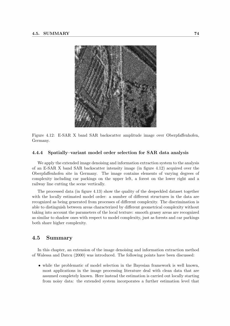
4.5. SUMMARY 74
Figure 4.12: E-SAR X band SAR backscatter amplitude image over Oberpfaffenhofen,Germany.
4.4.4 Spatially–variant model order selection for SAR data analysis
We apply the extended image denoising and information extraction system to the analysisof an E-SAR X band SAR backscatter intensity image (in figure 4.12) acquired over theOberpfaffenhofen site in Germany. The image contains elements of varying degrees ofcomplexity including car parkings on the upper left, a forest on the lower right and arailway line cutting the scene vertically.
The processed data (in figure 4.13) show the quality of the despeckled dataset togetherwith the locally estimated model order: a number of different structures in the data arerecognized as being generated from processes of different complexity. The discrimination isable to distinguish between areas characterized by different geometrical complexity withouttaking into account the parameters of the local texture: smooth grassy areas are recognizedas similar to shadow ones with respect to model complexity, just as forests and car parkingsboth share higher complexity.
4.5 Summary
In this chapter, an extension of the image denoising and information extraction methodof Walessa and Datcu (2000) was introduced. The following points have been discussed:
• while the problematic of model selection in the Bayesian framework is well known,most applications in the image processing literature deal with clean data that areassumed completely known. Here instead the estimation is carried out locally startingfrom noisy data: the extended system incorporates a further estimation level that

4.5. SUMMARY 75
(a) (b)
Figure 4.13: Despeckled image (a) and estimated model order (b) for the SAR intensityimage in 4.12
allows the space–variant selection of the model–order by means of the maximizationof the Bayesian model evidence;
• this extension allows the system to properly model and reconstruct images that arecomposed of instances of different stochastic image models with varying degrees ofcomplexity;
• the extended algorithm was demonstrated on simulated data generated with well–known model orders as well as on Brodatz textures corrupted by multiplicative specklenoise;
• we gave examples of classification by model order in the context of Gauss–Markovrandom field model based image denoising and information extraction starting fromspeckled Synthetic Aperture Radar data. Model complexity maps were generated thatdemonstrate the discrimination potential of the Bayesian evidence maximization withrespect to model choice.
The extended system is able to extract descriptors from the data in terms of a model–basedvocabulary, to choose models for the data in a space–variant way in a given reference classand to discriminate different image elements by their complexity, again in terms of themodel.
An application of the derived algorithm to the analysis of SAR data is presented inchapter III.

Chapter 5
Information Fusion for scenereconstructionfrom Interferometric SAR Datain Urban Environments
Abstract
A novel framework for scene understanding from InSAR data is presented thatis based on Bayesian machine learning and information extraction and fusion.
The system is based on a hierarchical model of the acquisition process that leadsfrom the scene to the data: this model is introduced and its different levels andcomponents are detailed.
A generic description of the data in terms of multiple models is automaticallygenerated from the original signals based on the denoising and information ex-traction algorithms presented in chapter 4.
The obtained feature space is then mapped by the application of simple Bayesiannetworks to user semantics representing urban scene elements in a supervisedstep.
The developed system is demonstrated by generating high–resolution land-usemaps on urban environments from real InSAR data acquired from spacebornesensors.
Interferometric SAR systems are able to contextually acquire multidimensional datasetswhose channels, in particular the SAR backscatter intensity, the interferometric coherenceand the interferometric phase, carry different kinds of information about the acquired scene:
• the phase is a very direct descriptor of the geometry of the scene in terms of thedistances between the sensor and the scene elements (Massonnet, 1993);

5.1. THE NEED FOR PROBABILISTIC MODELING IN SCENE
RECONSTRUCTION 77
• the interferometric coherence contains a description of the geometric and radiometricstability of the scene elements, and therefore allows a discrimination between differentkinds of scene features;
• in the backscatter intensity, radiometric and geometric factors are again intermixed:many classes of scene elements are directly recognizable from their backscatter signa-ture as well as from their spatial aspect.
To exploit the complementarity of the features derived from the different data sources, aBayesian classification and information fusion framework can be employed that composesthe different semantic–less descriptions of the data originated by the denoising and infor-mation extraction systems described in chapter 4 to associate them with user semanticsmapping the acquisition into a well defined set of scene elements and features.
5.1 The need for probabilistic modeling in scene reconstruc-tion
Scene reconstruction can be thought of as the procedure of finding the scene that bestexplains a given dataset:
SCENE → DATA direct model of acquisition
SCENE ← DATA scene reconstruction .
Examples of scene reconstruction include building recognition and the generation of landuse maps from remote sensing data.
When the reconstruction is carried out from measurements derived from multiple sensorsof dissimilar nature, or from sources that are fundamentally different — such as radar imagesand records of knowledge gathered from humans —, the techniques of information fusionare used to derive conclusions and decisions based on a synergy of all the data available.
A limitation of deterministic scene reconstruction algorithms is that the presence ofincertitudes and noise in the available measurements — as well as the imperfect knowledgeof the parameters of the acquisition — generates an inherent incompleteness of the data.
We therefore approach the problem of scene understanding and information fusion in aprobabilistic framework.
In particular, we consider the nature of the scene reconstruction problem by adoptingregularization strategies that incorporate external sources of information into the availabledata set.
Posterior probability as a measure of reconstruction quality In this context, thedata d and the scene s are considered to be samples drawn from the multidimensionalrandom processes D and S (Geman and Geman, 1984; Cressie, 1991).

5.2. SCENE–TO–DATA HIERARCHICAL MODELS 78
A treatment of the scene reconstruction inversion problem that incorporates and com-poses models for these processes is obtained by rewriting the Bayes’ equation as
p(S = s|D = d) p(D = d) = p(D = d|S = s) p(S = s) . (5.1)
The main characteristic of the Bayesian approach is the explicitation of the modelingassumptions made for both the data formation mechanism S → D in the likelihood termp(D = d|S = s) and for the phenomenon under analysis S in the prior p(S = s). Furtherimportant features in this context include the capacity to deal with incomplete data, tolearn causal relationships — thus learning the problem domain, and the power to combineknowledge and signal information.
The inversion can again be carried out by maximization of the posterior probability,resulting in the so called Maximum A Posteriori (MAP) estimate of the phenomenon S
sMAP = arg maxs
p(D = d|S = s) p(S = s) . (5.2)
Bayesian modeling and inversion as machine learning The MAP equation in (5.2)can be considered as a model for a learning device (Hackerman et al., 1995): a descriptionfor s is obtained from D by learning about their relation with the model S. Probability isused as a measure for the uncertainty in the knowledge of this relation.
5.2 Scene–to–data hierarchical models
When models for the scene S and the data D become so complicated that the inversionin terms of (5.2) becomes intractable, a common solution is a divide-and-conquer approachin which simpler intermediate description levels are introduced in the modeling.
Curse of dimensionality in stochastic data inversion The large amount of datarequired to perform a full inference while keeping high resolution detail observable wouldprohibit the treatment of high-order probability distribution functions. This explosion ofcomputational complexity, known as the“curse of dimensionality”, has to be treated byrecurring to models described by only local statistics, as is the case in Markov models andof hierarchical Bayesian networks.
5.2.1 Scene reconstruction Bayesian belief networks
A Bayesian network is set up for the task of scene reconstruction as in figure 5.1a. Atree edge structure encodes statistical independence between the random variables in thenodes. The last level of inference is performed by learning the problem semantics throughuser interaction.
Since the problem of inferring a general network structure from the data is in prov-ably NP-hard, simplifying assumptions are often made about the nature of the existingdependencies between the variables.

5.2. SCENE–TO–DATA HIERARCHICAL MODELS 79
links
AGRICULTURAL
(...)
GRASS
BUILT−UP
original signals secondary signals basic features user semantics
D_i T_j F_k S_l
p(T_j=t_j|D_i=d_i) p(F_k=f_k=T_j=t_j) p(S_l=s_l|F_k=f_k)
SLC 1
SLC 2
I
DEM
I0
TEX_I
DEM0
TEX_DEM
Bayesian
Classifier
Naive
description
levels
probabilisticuser
probabilistic
likelihood
BARE
(a)
WATER
TextureSAR
IntensityIntensityTexture
Interf.Coherence
link notconsidered by Naive Bayes
probabilistic
DEM
(b)
Figure 5.1: Learning scene semantics through hierarchical Bayesian Networks: (a) the treeedge structure encodes statistical independence between the random variables in the nodes.The last level of inference is performed by learning the problem semantics through userinteraction. As in naive Bayesian classification variables on the same level of the treestructure are assumed mutually independent. This might not be strictly the case, as in theexample in (b): the label WATER might be characterized by very low backscatter intensityand interferometric coherence. Although in general very low backscatter areas also showlow coherence values, the relation between the two variables is not taken into account bythe classifier.

5.2. SCENE–TO–DATA HIERARCHICAL MODELS 80
As in naive Bayesian classifiers, the considered simplified network consist only of a seriesof levels of parents and of several mutually independent children nodes. Classification isobtained by considering the parent node to be a hidden variable stating which class eachdata element should belong to. The classification is termed “naive” since the hypothesisof statistical independence between variables belonging to the same level is not necessarilyjustified (see for instance figure 5.1b).
5.2.2 User feedback and machine learning
When the naive Bayesian approximation is considered valid, the scene S can be relatedto the data D through more levels of intermediate simpler models Fi which are causallylinked
S → F1 → ... → Fn → D direct modeling
S ← F1 ← ... ← Fn ← D scene reconstruction .
The learning is in this case performed across levels, again by making use of the Bayes’equation in a version that considers the various levels of inference involved
p(S = s|F1 = f1) ... p(Fn = fn|D = d) p(D = d) = p(D = d|Fn = fn) ... p(F1 = f1|S = s) p(S = s)(5.3)
to derive a conclusion about the underlying scene S.
In this framework, a model for the image formation mechanism can be described in thisway:
S → Ω → R → D direct model
S ← Ω ← R ← D scene reconstruction (5.4)
a scene S is illuminated and generates a reflected field carrying information in the parameterω, a realization of the scene feature process Ω. The scene features are translated to signalfeatures R by the instrument and finally to data D by the image formation systems.
The scene reconstruction procedure must invert this causal chain, recovering the originalscene features from the data. The layers of inference needed are implemented in the stagesof a processing chain that is described in figure 5.2: the original signals acquired are used togenerate image data products (backscatter intensity, coherence and height map) by usingstandard operational processors. These products are analyzed by a feature extraction sys-tem (described in chapter 4 and section 5.2.3) and translated into a set of image features.The features are grouped by similarity using a simple unsupervised classification system, andthe generic multidimensional description obtained is fed into a Bayesian classification andinformation fusion system (section 5.3). This new level of description in the data-to-scenechain can incorporate user-provided semantic information into the available representation,finally connecting the generic, multiple–model based obtained description to the domain ofthe unknowns in the particular scene reconstruction problem under investigation.

5.3. LEARNING PROCEDURE 81
UNSUPERVISED
CLUSTERINGPREPARATION
DATA FEATURE
EXTRACTION INFO FUSION
BAYESIANORIGINALDATA
SCENEDESCRIPTION
Figure 5.2: The scene reconstruction processing chain: data preparation is followed byinformation extraction. An unsupervised clustering module performs a grouping of theimage features by similarity. Its output is subject to information fusion incorporatingsemantics by user feedback, thereby producing the final scene description.
5.2.3 Information extraction from backscatter and height image data
Since the height noise in interferometric SAR DEMs is additive Gaussian while thenoise affecting SAR backscatter intensity is a form of strong multiplicative speckle noise,the feature extraction from SAR intensity and topographic height data can be performedrespectively by the backscatter despeckling/Gaussian noise filtering and feature extractionsystems introduced in chapter 4.
We postulate in this context that a quasi–complete description of a typical remote sensingimage requires a separation of the sources of interesting information and of hindrances inthe data — SAR backscatter despeckling, DEM noise filtering — and the estimation of thestructural texture properties of the images thereby obtained.
The combined feature extraction system models and reconstructs a dataset that is freeof noise, while still preserving its most important attributes: it estimates the parametersthat describe the data in terms of the employed models. In this sense, it is not only a setof filters, but also a model–based feature extraction system that generates a representationof its input. The model fitting is performed in a space-variant manner that accommodatesfor local nonstationarities in the data.
5.3 Learning procedure
After the basic features have been extracted by the combined image information ex-traction system, they are grouped by similarity, by using a simple unsupervised K-Meansclassification system (appendix A). The multiple layers of information thereby obtainedhave then to be fused with each other: the clusters —here indicated as ωi — play therole of an abstract image vocabulary that is able to explain, by different combinations, theimage semantics S.
Instead of imposing an explicit definition of the phenomenon under study as in a rule-based expert system, descriptions are learnt from the human user by example. This impliesa much more direct and powerful way of providing information to the system and enablingit to consider the interpreter conjectures.

5.3. LEARNING PROCEDURE 82
full texture vector, local model order
Bayesian model based
image additive noise
filtering and information
extraction
Bayesian model based
image despeckling
and information
extraction
speckle degraded
image
(e.g. SAR backscatter)
additive noise
degraded image
(e.g. InSAR DEM)
despeckled image intensity
despeckled image texture norm
filtered image intensity (e.g. clean DEM)
filtered image texture norm (e.g. DEM texture)
edges, non−linear features (e.g. strong scatterers),
Figure 5.3: The model based SAR backscatter–InSAR derived height information extractionsystem: input square root intensity and interferometric height data are used to generatenoise-clean estimates for the backscatter and for the height as well as local texture estimates.
Again, to be able to capture the subjective, interpreter-dependent aspects of information,a Bayesian formalization is needed: probability is interpreted as a degree of belief ratherthan as a frequency of realization. This contextual fusion and interactive classification isperformed via a Bayesian classification and fusion system.
The process of interactive learning consists in progressively computing the probability ofa specific cover-type in the image, on the basis of positive and negative pixel–level examplesprovided by the user. The inference process for the label S = sν given the image data dand the features in the clusters ωi is realized through the probability
p(Sν = sν |D = d) = p(Sν = sν)∑
i
p(Ωi = ωi|Sν = sν) p(Ωi = ωi|D = d)
p(Ωi = ωi)
where p(Sν = sν) and p(Ωi = ωi) are (usually non-informative) prior probabilities, whilep(Ωi = ωi|Sν = sν) has to be learnt from user examples. An independence condition isassumed, i.e., the probability is assumed equal to the product of the separate likelihoodsfor the cover type dν given each single model
p(Ωi = ωi|Sν = sν) = p(Ωi,M1= ωi,M1
, Ωi,M2= ωi,M2
, ...,Ωi,Mm = ωi,Mm |sν)
= p(Ωi,M1= ωi,M1
|Sν = sν) p(Ωi,M2= ωi,M2
|Sν = sν)...
p(Ωi,Mm = ωi,Mm |Sν = sν)
since each cover type is considered a combination of different models
ωi = ωM1⊗ ωM2
⊗ ... ⊗ ωMm
where ⊗ denotes scalar product between sets.
If we denote with φ the vector parameter which satisfies the identities
p(Ωi = ωi|Sν = sν , Φ = φ) = φi, p(Φ = φ) = Γ(r)
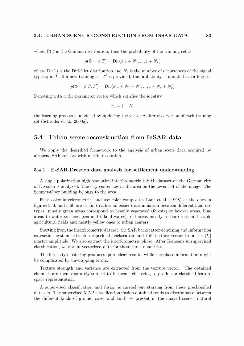
5.4. URBAN SCENE RECONSTRUCTION FROM INSAR DATA 83
where Γ(·) is the Gamma distribution, then the probability of the training set is
p(Φ = φ|T ) = Dir(φ|1 + N1, ..., 1 + Nr)
where Dir(·) is the Dirichlet distribution and Ni is the number of occurrences of the signaltype ωi in T . If a new training set T ′ is provided, the probability is updated according to
p(Φ = φ|T, T ′) = Dir(φ|1 + N1 + N ′1, ..., 1 + Nr + N ′
r)
Denoting with a the parameter vector which satisfies the identity
ai = 1 + Ni
the learning process is modeled by updating the vector a after observation of each trainingset (Schroder et al., 2000a).
5.4 Urban scene reconstruction from InSAR data
We apply the described framework to the analysis of urban scene data acquired byairborne SAR sensors with metric resolution.
5.4.1 E-SAR Dresden data analysis for settlement understanding
A single polarization high resolution interferometric E-SAR dataset on the German cityof Dresden is analyzed. The city center lies in the area on the lower left of the image. TheSemper-Oper building belongs to the area.
False color interferometric land use color composites Laur et al. (1998) as the ones infigures 5.4b and 5.6b are useful to allow an easier discrimination between different land usetypes: mostly green areas correspond to heavily vegetated (forests) or layover areas, blueareas to water surfaces (sea and inland water), red areas mostly to bare rock and stableagricultural fields and mostly yellow ones to urban centers.
Starting from the interferometric dataset, the SAR backscatter denoising and informationextraction system extracts despeckled backscatter and full texture vector from the |I1|master amplitude. We also extract the interferometric phase. After K-means unsupervisedclassification, we obtain vectorized data for these three quantities.
The intensity clustering produces quite clear results, while the phase information mightbe complicated by unwrapping errors.
Texture strength and variance are extracted from the texture vector. The obtainedchannels are then separately subject to K–means clustering to produce a classified featurespace representation.
A supervised classification and fusion is carried out starting from these preclassifieddatasets. The supervised MAP classification/fusion obtained tends to discriminate betweenthe different kinds of ground cover and land use present in the imaged scene: natural

5.4. URBAN SCENE RECONSTRUCTION FROM INSAR DATA 84
(a) (b)
(c) (d)
Figure 5.4: E-SAR Dresden - Ground truth optical image (a), interferometric land use (Lauret al., 1998) false color image (R=coherence, G=average intensity, B=intensity difference)(b), SAR backscatter intensity (c), SAR texture norm (d).

5.4. URBAN SCENE RECONSTRUCTION FROM INSAR DATA 85
(a) (b)
Figure 5.5: E-SAR Dresden - Ground truth optical image (a) and generated land use map (b)with classes vegetation (GREEN), vertical flat surface (WHITE), strong scatterer (RED),water/shadow (BLACK).
(a) (b)
Figure 5.6: E-SAR Dresden Semper Oper- Ground truth optical image (a), interfero-metric land use (Laur et al., 1998) false color image (R=coherence, G=average intensity,B=intensity difference) (b).

5.4. URBAN SCENE RECONSTRUCTION FROM INSAR DATA 86
(a) (b)
Figure 5.7: E-SAR Dresden Semper Oper- interferometric SAR backscatter coherence (a),interferometric SAR phase (b).
(a) (b)
Figure 5.8: E-SAR Dresden Semper Oper- land use map obtained by unsupervised classifica-tion (a) and Bayesian classification/fusion (b) by considering intensity, coherence, absolutephase: vertical surfaces in layover (YELLOW), strong scattering areas (RED), flat terrain(LIGHT GRAY), layover areas (ORANGE), water/shadow (BLACK).

5.5. SUMMARY 87
(grass, water, trees) as well as man–made scene elements (walls, roofs) are extracted andseparated from each other yielding results that outperform those obtained by simple K–means clustering conducted across all available channels.
5.5 Summary
In this chapter, a novel framework for scene understanding from InSAR data was pre-sented that is based on Bayesian machine learning and information extraction and fusion.The following points were detailed:
• the system is based on a hierarchical model of the acquisition process that leads fromthe scene to the data: a generic description of the data in terms of multiple modelsis automatically generated from the original signals, based on modifications of thedenoising and information extraction algorithms presented in chapter 4;
• unsupervised K–means clustering is used to group by similarity the elements popu-lating the feature space;
• the obtained feature space is then mapped by the application of simple Bayesiannetworks to user semantics representing urban scene elements in a supervised step.
The developed system was demonstrated by generating high–resolution land-use maps onurban environments from real InSAR data acquired from spaceborne sensors. Further ap-plications of the method to the reconstruction of urban scenes from high–resolution InSARdata are reported in chapter III.

Chapter 6
Stochastic geometrical modelingfor urban scene understandingfrom a single SAR intensity imagewith meter resolution
Abstract
To overcome the limitations of pixel–based analysis applied to sub–metric res-olution data, a novel model based algorithm for the automatic reconstructionof building areas from single observation meter-resolution Synthetic ApertureRadar intensity data is introduced.
The reconstruction is based on the Maximum A Posteriori estimation by MonteCarlo methods of an optimal scene that is modeled as a set of pairwise-interacting Poisson-distributed marked points describing parametric buildings.
Each of the objects can be hierarchically decomposed into a collection of ra-diometrically and geometrically specified object facets that in turn get mappedinto data features.
The geometric and radiometric phenomenologies of sub–metric SAR in urbanenvironments are taken into account in the likelihood term.
The detection of the buildings is based on a decision likelihood ratio.
The optimization of the obtained posterior is based on Gibbs sampling andMonte Carlo Markov chains.
The developed algorithm is demonstrated on real data acquired by airborne Xband sensors on built–up areas in high complexity settings characterized by tallvegetation and strong metallic scatterers.
The Bayesian classification and information fusion approach to scene reconstruction pre-sented in the last chapter is applicable in the range of resolutions from tens of meters down

6.1. SCENE UNDERSTANDING FROM SAR: OBJECTS AND THEIR
RELATIONS 89
to about one meter. At lower scales, two phenomena take place in urban environments:
• information in SAR data becomes inherently sparse, in the sense that the areas of theimage containing some energy (mostly corresponding to cavities and sharp edges) areintermixed by much larger areas of very low SNR caused by the specular reflectionof the incident signal on smooth surfaces: a traditional lattice–based model shouldconsider an inordinately large amount of (mostly totally noisy) pixels in order to gainsome discrimination and modeling capability;
• a pixel–based description of the scene would anyway be of limited interest, since atsub–metric resolutions single objects are recognizable as separate entities associatedwith specific semantics and generating peculiar effects in the data.
The usual interferometric approach based on unwrapping tends to be difficult in high res-olution SAR data, since very steep surfaces and areas of very low coherence are the norm.Unwrapping needs to be regularized by means of external information. If, for instance, thetower in Figure 6.1 is considered, it is evident that extreme layover, multiple reflectionsand the presence of very strong, high coherence echoes in combination with very low en-ergy, low coherence returns from non-dihedral scattering will render the usual lattice–basedinterferometric reconstruction approach quite limited.
The artifacts complicating the analysis are actually due to the geometry of the scene: thisis why they carry information about it. We therefore concentrate our analysis on the caseof single pass, single model high resolution SAR data on urban environments. Phenomenausually considered as limitations of the dataset and excluded from further processing areinstead recognized and exploited as information sources to provide added robustness to theestimation algorithm.
Normal lattice-based image data models and inversion algorithms can then be effectivelycomplemented by descriptions in terms of scene objects. Evident features in the data haveto be exploited in the scene reconstruction problem. Hindrances (e.g. a dihedral scatteringfrom a building base partially hidden by the surrounding vegetation) can be overcome byusing a prior description for the scene. A hierarchical modeling of remote sensing data canbe constructed that considers the whole structure from data to reconstructed scene objects.
6.1 Scene understanding from SAR: objects and their rela-tions
Scene understanding (SU) is in Computer Vision the recognition and reconstruction ofthe objects in the scene and of the spatial relations between them (Edelman and Weinshall,1989). The problem is related to that of understanding visual perception in informationprocessing terms: assuming that the purpose of vision is to reconstruct the spatial layoutof the outside world, one is confronted with the problem of ambiguity in inferring the thirddimension from retinal projection. This ambiguity is a necessary consequence of the imagingprocess, during which the depth information is lost. Marr (1982) proposed to compensate
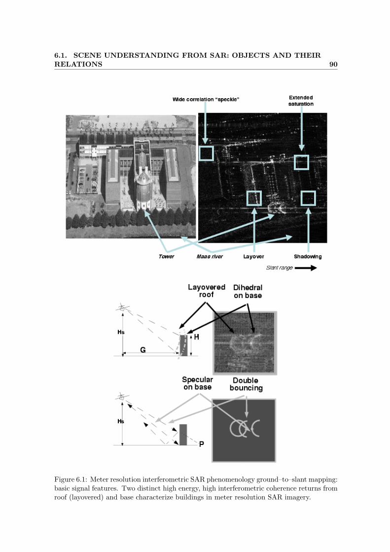
6.1. SCENE UNDERSTANDING FROM SAR: OBJECTS AND THEIR
RELATIONS 90
Figure 6.1: Meter resolution interferometric SAR phenomenology ground–to–slant mapping:basic signal features. Two distinct high energy, high interferometric coherence returns fromroof (layovered) and base characterize buildings in meter resolution SAR imagery.

6.2. MARKED SPATIAL POINT PROCESSES AS PRIOR SCENE
MODELS 91
for this loss by constraining the solution to the reconstruction problem to conform to apriori assumptions, dictated by our knowledge of the physical world.
As the resolution of SAR systems approaches the level where the scene can be representedas a set of separated interacting objects, the methods and techniques of computer vision,traditionally centered on optical data taken on man–made settings, can be can be employedin radar remote sensing inversion problems, provided proper modeling of the specificities ofthe sensor and of the scene is assured.
6.2 Marked spatial point processes as prior scene models
A marked spatial point process (Upton and Fingleton, 1985; Diggle, 1983; Cressie, 1991)on the space X with marks in F can be represented mathematically as a point process onthe product space X × F . It can be defined in terms of random locations of events in aset X and corresponding random marks Z(·) in a set F and used to model random eventsoccurring at sparse, random locations according to its marginal spatial bidimensional pointpattern. For example, events might represent the unknown positions of buildings in a sceneand the corresponding marks may be describing them parametrically.
Gibbs point processes In particular, Gibbs marked point processes of order m are aclass of inhomogeneous point processes for which the intensity function is written in terms ofexponentials of functions of up to m distinct point process events. If m = 2, the probabilitydistribution can be written as
p(S = (s1, · · · sn), N = n) =exp(−ν(A))
αn!exp
[
−n
∑
i=1
g1(si) −n
∑
i=1,j=1,j 6=i
g1,2(si, sj)]
with g1(·) and g1,2(·, ·) two positive first- and second-order potential terms, ν and α two freeparameters. We approach the scene understanding problem by considering a marked pointprocess to model built-up areas: a random parametric description O(·) of the geometry ofa building object marks a random site Ci representing its geometric position (Ortner et al.,2002) in a study area D imaged in the data:
S ≡ (Ci, O(Ci)), Ci ∈ D .
The expression for the posterior corresponds to that for a generic Markov point process,in which the joint density function p(S) can be factored uniquely into a series of terms ifonly the first two are considered.
p(S, n) =1
Z(n)exp−Un(s1, · · · , sn)
Un(s1, · · · , sn) =n
∑
i=1
g1(si) +∑ ∑
1≤i<j≤n
g1,2(si, sj) + · · ·
with Un the total potential energy of the Markov point process.

6.2. MARKED SPATIAL POINT PROCESSES AS PRIOR SCENE
MODELS 92
A Gibbs marked point process can be demonstrated to be equivalent to a Markov pointprocess. The spatial point process that we consider is Markov with range ρ,
p(O(C0)|S \ O(C0)) ≡ p(O(C0)|O(C), C ∈ b(C0, ρ) \ C0) (6.1)
with \ indicating the set subtraction operation, where b(C0, ρ) is a ball of center C0 andray ρ in the domain D: scene objects tend to interact with each other to produce moreplausible ordered configurations. The properties of the marginal spatial point process (andin particular its density) are conserved in the marked point process, except for a finitenumber of sites in some vicinity of each of the given points in which local (repulsive)interactions are modeled that tend to decrease the density of the original marginal pointprocess.
6.2.1 Point and mark distributions
The building centers are Poisson–distributed in the domain D. The marks describingthe building geometry are instead defined as in
O(C) ≡ (W, α, Q)
with uniformly distributed random parameters
Q one of
cylinder
block
v–shaped roof
building shape element
W ∈ R3 width, length, height of building element
α ∈ [−π/2, +π/2] base angle to ref. direction.
6.2.2 Modelling hierarchy
We further assume that each of the separate building objects Oi in which we can de-compose the scene S in turn can be described as composed by different facets Fij . Each ofthose can be mapped to a set of SAR amplitude pixels with values Ak in the SAR amplitudedata image space (Figure 6.2): the parameters of each building define together with theacquisition geometry its observable facets and the pixels that belong to them
S ≡ Oii ≡ Fijji → Akk ≡ D .
The hierarchical structure models a container/contained relation whose top level representsthe full scene while the bottom one is a set of data pixels.

6.2. MARKED SPATIAL POINT PROCESSES AS PRIOR SCENE
MODELS 93
(a) (b)
(c) (d)
Figure 6.2: Levels in the hierarchical scene model: (a) the scene S is a collection of buildingsOi that are pairwise interacting within a given range; (b) objects are described parametri-cally as marked Poisson–distributed points; (c) objects can be decomposed into a collectionof facets Fij that have both a geometric and a radiometric parametric probabilistic descrip-tion; (d) the facet Fij is probabilistically mapped into a set of pixels Dkk in the amplitudeimage data space.

6.3. SCENE POSTERIOR STRUCTURE DECOMPOSITION
IN GIBBS POTENTIAL TERMS 94
→ range direction
(a) (b) (c)
Figure 6.3: SAR phenomenology considered in the scene understanding process: (a) forevery scene object (in this case a v–shaped roof house) (b) dihedral scattering region and(c) layovered roof are considered in the computation of the likelihood potential as clues forthe reconstruction.
6.3 Scene posterior structure decompositionin Gibbs potential terms
Given a single meter resolution SAR intensity image, we want to infer by Maximum APosteriori (MAP) estimation a description of the scene that is most likely to have generatedit: if S and D denote respectively the scene and the data stochastic processes, then p(S =s|D = d), the posterior probability we maximize, can be understood as a measure of qualityfor the reconstructed scene given the data.
Scene posterior description in terms of Gibbs formalism The posterior probabilitycan be written under a Gibbs field formalism (Winkler, 1995) as in
sMAP = arg maxS
p(S = s|D = d) = arg maxS
1
Z· exp
[
−U(s|d)]
where Z is a normalizing constant (the partition function) and U(s|d) is a local potentialfunction. U(S = s|D = d) can be decomposed into a regularization prior potential UP (S =s) while a likelihood potential UL(D = s|S = s) describes a distance between scene anddata that takes into account a model of the acquisition system:
U(S = s|D = d) ∼ UP (S = s) + UL(D = d|S = s) .
Scene posterior decomposition The potential terms can therefore be decomposed asin
UP (S = s) =∑
oi,oj∈s,j 6=i
Up(Oi = oi|Oj = oj)
UL(D = d|S = s) =∑
oi∈s
∑
Fij=fij∈oi
∑
ak∈d
Ul(Ak = ak|Fij = fij)

6.4. THE SCENE PRIOR POTENTIAL TERM 95
where Up(·) and Ul(·) are the object–level prior and the pixel–level likelihood potentialsand where some of the possible dependencies have been neglected to simplify the modelingin the spirit of naive Bayesian classification: when the descriptions for both the sceneand the data formation mechanism become too complex, both theoretical considerationsconnected to the “curse of dimensionality” (Jaynes, 1987) and practical concerns about thetractability of the model suggest the adoption of a divide-and-conquer approach in whichsimpler intermediate representation levels are introduced in the modeling. In our case,for simplicity, elements at the same level of the description are considered independent ofeach other, as in the case of Naive Bayesian Classification. This assumption allows a muchsimpler handling of the estimation process.
6.4 The scene prior potential term
To keep the modeling as simple and general as possible, the potential term
UP (S = s) =∑
i,j
Up(Oi = oi, Oj = oj)
is kept totally independent of the data and the sensor characteristics, and therefore describesan a priori plausibility of the scene only.
Keeping the prior term as general as possible, and therefore avoiding introducing localmaxima in the posterior distribution through it, is desirable both to keep the reconstruc-tion algorithm general and to ease the subsequent search for the global MAP. The priorinteraction potential Up(·) is used to avoid overlapping conditions between scene objectsand corresponds to a geometric intersection measure between different scene objects:
Up(Oi = oi|Oj = oj) ∼ area of intersection(oi, oj) .
6.5 The data likelihood potential term
While the prior potential is independent of the data, the likelihood potential must insteadexpress a definition of the relevant acquisition phenomenology. Both the geometric andradiometric causal relations that compose the direct model of the acquisition are expressedthrough the likelihood.
6.5.1 Extraction of strong targets from clutter in urban environments byinverse Gaussian statistics, decision theory–based classification
Strong signals generated by dihedral scattering on the building basement and by directlayovered returns from clean edges on the building roofs need to be modeled and extractedto be exploited in Ul(·).
Inverse Gaussian distributed backscatter values (Section 2.3.2) are assumed to model theamplitude return from the slowly varying small number of scatterers that compose these

6.5. THE DATA LIKELIHOOD POTENTIAL TERM 96
elements: they have been shown to approximate well a K–distribution while keeping a bettertractability, and have been used to model backscatter in urban environments (Frery et al.,1997; Mejail et al., 2001).
An expression for the discriminating likelihood ratio
p(Ak = ak|αs, γs, L)
p(Ak = ak|α0, γ0, L)(6.2)
with
p(Ak = ak|α, γ, L) = exp
[
− LL Γ(L − α) aL−1k
γαΓ(−α)(γ + L ak)L−α
]
is obtained with L > 0 the number of looks of the data, ak > 0 the amplitude pixel value, and−αs, γs > 0 and −α0, γ0 > 0 respectively the parameters for the distribution that modelsthe amplitude values of the strong scattering facet elements, and those for remaining clutterobtained by solving the system
γ = L
[
m1 Γ(−α)Γ(L)
Γ(−α − 1/2)Γ(L + 1/2)
]2
m21/2
m1=
Γ2(−α − 1/4)Γ2(L + 1/4)
Γ(−α − 1/2)Γ(L + 1/2)Γ(−α)Γ(L)
where mn is the n−th order moment estimated on a training area and Γ(·) is the Gammafunction.
6.5.1.1 Radiometric likelihood potential term
Based on the discriminating likelihood in Equation 6.2, the likelihood potential can bewritten as
Ul(Ak = ak|Fij = fij) =
p(Ak=ak|αs,γs,L)p(Ak=ak|α0,γ0,L) if ak taken in fij
0 otherwise
p(Ak = ak|α, γ, L) = exp
[
− LL Γ(L − α) aL−1k
γαΓ(−α)(γ + L ak)L−α
]
.
Given a hypothesis on the 3D disposition of strong scatterers in the scene, the loci ofthe strong scattering phenomena can be defined in deterministic terms, as in Figure 6.1.Since the likelihood ratio potential Ul(Ak = ak|Fij = fij) is non–zero for the candidate facetpixel values only, its computation requires the determination of the geometry of the strongresponses from the visible facets in the data: the candidate scene object edges are iteratedupon, they are projected in slant range coordinates and the loci in the image of the relevantdihedral scattering and roof layover phenomena to be analyzed are therefore determined.
The expression for the decision ratio in the last paragraph provides by itself a discrimi-nation between strong clutter and backscatter that are typical of very high resolution SARdata.

6.6. INFERENCE IN BAYESIAN SCENE UNDERSTANDING WITH
NON–ANALYTIC POSTERIORS 97
It can therefore be directly used to assess the probability that a candidate strong scat-tering area in the scene space (linked to some phenomenology in the image space by aground–to–slant transformation) appears as such in the data.
6.5.2 Geometric likelihood potential terms
The analysis of the data must take into account the peculiar aspects of the phenomenol-ogy of high resolution radar. Strong responses often appear translated in range due tolayover (and to multiple signal reflections), but no full geocoding is possible, since localheights at metric resolutions are unknown.
In particular, if Hs is the altitude of flight of the sensor with respect to the ground,H = h is the building height and G its position in ground range, then the layovered signalgenerated from building roof edges is located at a slant–range distance ∆rg of
∆rg = (H2s + G2)1/2 + ((Hs − h)2 + G2)1/2
from the first one produced by dihedral scattering at the border between the vertical struc-ture and the terrain.
The loci of the hypothesized top and bottom of the scene building facets are thereforeused as the loci on which the estimation of the likelihood potential is performed.
6.6 Inference in Bayesian scene understanding with non–analytic posteriors
MAP inference is performed globally on the whole scene parameter space. The practicalcomputation of the posterior probability p(S = s|D = d) of a given candidate scene S isperformed by decomposing it in terms of the hierarchically dependent elements Oi and Fij
that constitute it. The α0, γ0 and αs, γs factors are estimated starting from clutter andstrong scattering training areas. A decision likelihood ratio image can then be generatedfrom the data and used directly in the computation of the Ul likelihood potential.
The obtained posterior expression is not analytic: as a consequence, the MAP estimateof the optimal scene given the data
sMAP = arg maxs
p(S = s|D = d)
cannot be computed directly. The optimization is instead carried out by Monte Carlomethods.
6.6.1 Monte Carlo Markov Chain Gibbs sampling of the scene posterior
We adopt a simulated annealing procedure (Metropolis et al., 1953) for the estimationof the MAP (see Appendix B) : the multivariate posterior is maximized by iteratively

6.6. INFERENCE IN BAYESIAN SCENE UNDERSTANDING WITH
NON–ANALYTIC POSTERIORS 98
evaluating many possible solutions in a multidimensional parameter space. In stages, theoptimization algorithm restricts the search paths to only the most promising solutions.While at the beginning of the iterative optimization procedure the sampled posterior func-tion is essentially flat, at the end of the annealing the algorithm is forced to follow a steepestascent trajectory. The net effect is that of maximizing the f(.)1/T for T that slowly changesfrom high values to zero to be able to find the maximum of the function.
Scene configuration acceptance ratio and cooling schedule An acceptance ratiothat is dependent on the rate of improvement in the solution is used together with thedecreasing “temperature” T acceptance factor to probabilistically accept or reject new so-lutions. The Metropolis algorithm can therefore be understood as a relaxation of thegreedy maximal ascent algorithm.
This approach allows the system to explore solutions that a direct maximum-gradientmaximization would not consider, permitting it to identify the global maximum of a mul-tivariate distribution.
The acceptance ”temperature” factor is decreased from starting temperature T0 withiteration step iter according to a logarithmic cooling schedule as in Stoica et al. (2000)
τ(i) = T0/ log(1 + 2√
iter)
in order to allow for a sufficiently slow confinement of the optimization algorithm to steepestascent paths.
6.6.2 Scene configuration initialization
For simplicity, the initialization starting solution that is input into the system at temper-ature T0 consists of a set of identical objects, all located at the same location in the centerof the image and in the minimum allowed number of objects. More sophisticated startingconfiguration schemes (such as the initialization of the system by some simpler sub–optimalscene understanding algorithm) might improve the convergence speed.
6.6.3 Scene configuration sampling and Gibbs dynamics
A Gibbs sampler is set up to sample the posterior distribution keeping all the dimensionsof the scene process fixed but one: this modified distribution can be shown (Winkler, 1995;Stoica et al., 2000) to converge to the full posterior.
For generating the new candidate solutions to the optimization problem from the previousones, update rules are defined as in (Ortner et al., 2002) with the addition of the mutationof the building type parameter Q.
The scene marked point process with varying number of objects is simulated under thespatial birth–and–death process framework, as shown by Imberty and Descombes (2002).Special care must be used in ensuring that the mutation dynamics of the Gibbs sampler

6.6. INFERENCE IN BAYESIAN SCENE UNDERSTANDING WITH
NON–ANALYTIC POSTERIORS 99
are completely reversible, to avoid getting stuck on some local maxima or on the borders ofthe domain. Each of the defined mutation step must have an equiprobable opposite move.The moves considered are object creation and destruction, and displacements and mutationmoves for the building parameters.
All the transformations are symmetric: first a building object
U ≡ (Ci, O(Ci)) = u ≡ ((x, y), (α, w, q))
centered at location Ci ≡ (x, y) in a lattice and having parameters α (the orientation angle),w (a three–terms width, length and height size term) and q (the building element type) isuniformly chosen in the image spatial domain, and then the mutation is applied to it:
• Translations are generated by
– uniformly sampling δ = (δx, δy) from [−dx, +dx] × [−dy, +dy] and
– settingu = ((x, y), (α, w, q)) → v = ((x + δx, y + δy), (α, w, q))
considering for this transformation that the image space is a torus, in order toobtain the symmetry of the transformation.
• Rotations are generated by
– sampling δα uniformly in [−dα, +dα], and
– settingu = ((x, y), (α, w, q)) → v = ((x, y), (α + δα, w, q)) .
In particular, we consider [−dα, +dα] = [−π/2, +π/2].
• Dilations are generated according to the same principle: the length, width or hight ofthe object are modified. This modification is applied contextually to the dimensionof the object and to its center coordinate, in order to let one side of it constant underthe transformation, as shown in Figure 6.4, by
– uniformly sampling (δDX , δDY , δDZ) from [−dDX , +dDX ] × [−dDY , +dDY ] ×[−dDZ , +dDZ ] and
– setting u = ((x, y), α, w, q) to
∗ v = ((x + δDX/2 · cos α, y + δDY /2 · sinα), (α, w + (δDX/2, δDY /2, δDZ), q))for rectangle-shaped objects and
∗ v = ((x+δDX/2, y+δDY /2), (α, w+(δDX/2, δDY /2, δDZ), q) for round shapedones for which the components of W = w are by definition coincident.
We notice that this kind of dilation transformation is the one that is naturallyapplied to height mutations of buildings on a plane: the roof of the building ismoved, while the its base remains fixed.

6.7. OVERVIEW OF ESTIMATION METHOD 100
Figure 6.4: Gibbs sampler dynamics. Dilation moves are preferred to width and lengthmodification with fixed center, since they leave one of the borders of the object totallyuntouched.
• Mutations are generated by sampling a q′ uniformly in the spacecylinder, box, v–shaped roof building \ q (with \ again the set exclusion oper-ator) and consequently setting
u = ((x, y), (α, w, h, q)) → v = ((x, y), (α, w, h, q′))
with the convention that for transitions to a cylinder from square–based objects onlythe first element of w is kept as a radius of the new base, whereas for transitions fromround objects to square ones the new horizontal components of w are again decoupledbut keep at the next step after the mutation their common value equal to the cylinderradius.
For simplicity, the initialization starting solution that is input into the system at temper-ature T0 consists of a set of identical objects, all located at the same location in the centerof the image and in the minimum allowed number of objects. More sophisticated startingconfiguration schemes (such as the initialization of the system by some simpler sub–optimalscene understanding algorithm) might improve the convergence speed.
6.7 Overview of estimation method
The full estimation system is described in Figure 6.5.
Simulated annealing is often considered too computationally expensive to be used inimage processing. Since the scene understanding system considers only a limited number ofobjects in the scene compared to the huge number of image lattice sites, the dimensionalityof the problem is reduced, speeding up convergence. The only operations performed atevery iteration are the mutation of one of the parameters of the model and then, given theupdated scene model, the recomputation of the mutated potential terms in the posterior.

6.7. OVERVIEW OF ESTIMATION METHOD 101
Figure 6.5: The complete MAP estimation system: simulated annealing is used for themaximization of the posterior via Gibbs sampling. The posterior depends on an a prioridefined measure of plausibility of the hypothesis scene and on a likelihood ratio for theactual building detection.

6.8. MARKED POINT PROCESS BASED SCENE UNDERSTANDING
EXAMPLE 102
In the implementation, all objects provide iterators to their component sub–objects. Inparticular, Facet objects provide iterator access to facet edges, corners and, by using asimple acquisition geometry model, to data pixels.
While the prior is computed at the object level by evaluating a geometrical intersectionmeasure between different scene objects (O’Rourke, 1998), the computation of the likelihoodpotential needs to take into account the data pixel–level description of the buildings in thecandidate scene (Simonetto, 2002; Haines, 1994) and the likelihood Ratio image.
When the MAP optimization is carried out iteratively, only the terms related to mutatedobjects need to be recalculated at each iteration.
The quantities related to the non–mutated scene elements (the intersection potentialvalues and the data related ones that are generated by taking into account pixel–leveldescriptions of the buildings that are dynamically generated from the object parameters)are constant and are therefore not object of re–computation, yielding better performance.
The optimization procedure on images containing about a million of pixels takes about30 minutes on a common PC workstation.
6.8 Marked Point Process based scene understanding exam-ple
In Figure 6.6, Intermap AeS-2 data on Trudering test area, east of Munich. Some housesare visible (a), together with the generated shadows and a part of the road network. In(b), the main identified buildings are shown with their location, size and orientation. Thelimitation of the obtain results is explained by the complexity of the scene: the structuresto be reconstructed are small houses partially hidden at X band by surrounding tallervegetation Typically for very high–resolution SAR data in built–up environments, multiplescattering and other disturbing effects tend to dominate the data, saturating the receiverand propagating to different areas in the image.
6.9 Summary
In this chapter, a novel algorithm based on stochastic geometry, decomposable objectmodels and Gibbs sampling was introduced. The following points were detailed:
• an algorithm for the reconstruction of building areas from a single high resolution SARintensity image was introduced, described and demonstrated on data with resolutionsranging from 0.5 to 2 meters;
• the algorithm is based on the Maximum A Posteriori estimation via Monte Carlomethods of an optimal scene described in a hierarchical Bayesian framework as a set ofpairwise interacting Poisson distributed marked points that represent parametricallydescribed scene buildings;

6.9. SUMMARY 103
(a) (b)
Figure 6.6: Intermap AeS-2 data on Trudering test area, east of Munich. Some houses arevisible (a), together with the generated shadows and a part of the road network. In (b),the locations of the identified buildings are shown with their location, size and orientation.Although the phenomenology of the data is very different from the one of industrial buildingsfor which the algorithm has been developed, the three most evident targets are identified.
• each of the scene objects can be decomposed into a set of elements that get proba-bilistically mapped into the image data space via a likelihood term that takes intoaccount the geometric and radiometric phenomenologies of sub–metric SAR in urbanenvironments;
• the detection of the buildings is based on a decision likelihood ratio;
• the optimization of the obtained posterior is based on Gibbs sampling and MonteCarlo Markov chains.
The developed algorithm was demonstrated on real data acquired by airborne X bandsensors on built–up areas in high complexity settings characterized by tall vegetation andstrong metallic scatterers. Further results are presented in chapter III using airborne datawith resolutions in the range of 0.5 to 2 meters on a variety of scenes.

Part III
Evaluation and validation of results

105
Abstract
The novel methods and techniques developed are evaluated, validated and ap-plied to large amounts of data.
The information extraction systems are combined into a complete, automaticdata processing chain that serves a knowledge–based information mining andcontent–based image retrieval system used in the analysis of a nation–wide ERSdataset.
The automatic, space–variant model–order selection capabilities of the extendeddenoising and information extraction system are demonstrated by generating alocal model complexity based classification map from fine–mode RADARSATdata.
The developed system for scene reconstruction based on Bayesian classificationand fusion of the extracted features is applied to the analysis of images ac-quired by the SRTM mission and by the DLR E-SAR system. The scenes arereconstructed by combining the obtained classification and land–use maps withinterferometric height data.
Finally, the scene understanding algorithm based on the Gibbs sampling of hi-erarchical marked point processes is evaluated by applying it to sub–metricIntermap data acquired on an industrial site as well as on high-complexity com-posed buildings in urban environments.

6.10. CONTENT–BASED RETRIEVAL, INFORMATION MINING,
SCENE UNDERSTANDING 106
Query byImage content
Datamining
Sceneunderstanding
DataVolume
ExtractedInformation
Figure 6.7: The data analysis hierarchy, from content-based query to scene understanding.Due to the problem complexity, the system scales down the amount of data to be analyzedsuch that the detail of extracted information can be increased.
chapterLarge scale evaluation and validation of developed methods and algorithms Ab-
stract
The algorithms and techniques introduced in the last chapter are evaluatedand validated on a variety of data including real meter resolution SAR datafrom airborne sensors serving as a testbed for next generation spaceborne radarsystems.
6.10 Content–based retrieval, information mining, scene un-derstanding
Modern remote sensing systems are capable of acquiring and processing very largeamounts of data: the SRTM mission collected about 11 TBytes of interferometric SARdata per day. Content–based image retrieval, image information mining and scene under-standing all relate to the need of analyzing large amounts of data to produce descriptionsof their content in terms of models.
6.10.1 Information extraction for application–independent data charac-terization
Content based image retrieval, image data mining and scene understanding share com-mon methods (data analysis and probabilistic modeling techniques) and goals (the extrac-tion of meaningful information from data affected by incertitude), but they operate atdifferent scales of data amount. Content based image retrieval focuses on extracting com-pact representations for the retrieval of interesting elements in very large amounts of data;image data mining works at an intermediate level, trying to find interesting configurations

6.10. CONTENT–BASED RETRIEVAL, INFORMATION MINING,
SCENE UNDERSTANDING 107
Figure 6.8: Scheme of principle of ingestion chain operations.
in moderately populated feature spaces; scene understanding tries to extract the maxi-mum possible amount of information from a given dataset applying to it models of highcomplexity.
All three approaches to the analysis of the data, although they operate on differentscales of detail and of data amount, share the same need for an application–independentdescription of the contents of the data. Such description needs to be generated in anautomatic way, must be application independent and needs to be as general and completeas possible.
As in the case of the hierarchical model inversion algorithms developed in previous chap-ters, the analysis is based on a series of description levels linked by conditional probabilitylinks. The image data (level 0) is processed to extract primitive features and meta features(levels 1 and 2). Information at level 1 is in form of a parameter vector of a signal model.The specific signal model is the level 2 of information representation. A further descriptionlevel, a characteristic vocabulary of signal classes (level 3), is generated by unsupervisedinformation clustering for each signal model. User specific interests, that is, cover typelabels, are linked to combinations of terms in these vocabularies using simple Bayesian net-works. Levels 1 to 3 are obtained in a completely unsupervised and application free wayduring data ingestion in the system. The information at level 4 can be interactively definedby users employing a learning paradigm. In an additional step of stochastic modeling, thestochastic link between signal classes and user (subjective) labels is described using a vectorof hyper-parameters.
6.10.2 The knowledge-based information mining system
The knowledge-based information mining (KIM) system is designed as a system to oper-ate on large archives of remote sensing data in a way that is free from application specificity.After extraction of primitive features takes place as described in previous chapters, the fea-tures are grouped by similarity by using a K-means clustering algorithm. The clusters haveno direct meaning, since they group points in an n-dimensional space of non-commensurablevariables. Still, they represent characteristics of the image seen as a multi-dimensional sig-nal. It is possible to associate meaning with these clusters through training. A user cantell the system that a specific, weighted combination of clusters represents a derived featureof the data. By making this association, it is possible to select all images in the databasethat have that specific combination and may therefore contain the feature that the user issearching for.

6.10. CONTENT–BASED RETRIEVAL, INFORMATION MINING,
SCENE UNDERSTANDING 108
Figure 6.9: Hierarchical modeling of image content and user semantic (Schroder et al.,2000a): description levels are linked by conditional probability links.

6.10. CONTENT–BASED RETRIEVAL, INFORMATION MINING,
SCENE UNDERSTANDING 109
Figure 6.10: KIM coverage of Mozambique.
Kossovo Mozambique
Sensor E-SAR ERS-1Scenes 1 30Archive 800 MB 3.5 GBMining 24 MB 800 MB
Compression 33 4Application scene understanding information mining
Table 6.1: Summary of SAR data ingested in the KIM system and the level of data analysisconsidered.
6.10.3 Knowledge-based information mining evaluation results
Table 6.1 presents the summary of all SAR data sets ingested in the KIM system, or-ganized by site. The table outlines the nature of the function implemented in KIM. In theContent Based Image Retrieval mode the compression factor is very high (∼ 100), thusenabling the search of very large volumes of data: the accuracy of the search is limited,proportional to the available information for on–line search. The information mining modeis using a moderate compression factor, thus enabling the access to more detailed informa-tion for on–line mining. In the scene understanding mode, all image content informationis used, thus enabling accurate exploration and interpretation of the images and observedscenes.
The described image information mining based approach to SAR model based despeck-ling and information extraction evaluation has been applied to large ERS and SIRC/X-SARcoverages of Mozambique and Switzerland. The results obtained allow the navigation of im-age archives containing 15 GBytes of data imaging surfaces that span about 800 x 600 km2
and demonstrate the value of the obtained image features.

6.10. CONTENT–BASED RETRIEVAL, INFORMATION MINING,
SCENE UNDERSTANDING 110
(a)
(b)
Figure 6.11: (a) Classification based only on backscatter cannot separate lake and moun-tain shadow in a scene from 75 m resolution X-SAR data. (b) If the fusion of estimatedbackscatter and texture norm is used, the lake is correctly identified.
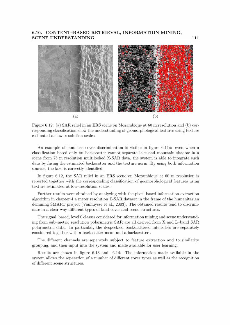
6.10. CONTENT–BASED RETRIEVAL, INFORMATION MINING,
SCENE UNDERSTANDING 111
(a) (b)
Figure 6.12: (a) SAR relief in an ERS scene on Mozambique at 60 m resolution and (b) cor-responding classification show the understanding of geomorphological features using textureestimated at low–resolution scales.
An example of land use cover discrimination is visible in figure 6.11a: even when aclassification based only on backscatter cannot separate lake and mountain shadow in ascene from 75 m resolution multilooked X-SAR data, the system is able to integrate suchdata by fusing the estimated backscatter and the texture norm. By using both informationsources, the lake is correctly identified.
In figure 6.12, the SAR relief in an ERS scene on Mozambique at 60 m resolution isreported together with the corresponding classification of geomorphological features usingtexture estimated at low–resolution scales.
Further results were obtained by analyzing with the pixel–based information extractionalgorithm in chapter 4 a meter resolution E-SAR dataset in the frame of the humanitariandemining SMART project (Vanhuysse et al., 2003). The obtained results tend to discrimi-nate in a clear way different types of land cover and scene structures.
The signal–based, level 0 classes considered for information mining and scene understand-ing from sub–metric resolution polarimetric SAR are all derived from X and L–band SARpolarimetric data. In particular, the despeckled backscattered intensities are separatelyconsidered together with a backscatter mean and a backscatter .
The different channels are separately subject to feature extraction and to similaritygrouping, and then input into the system and made available for user learning.
Results are shown in figure 6.13 and 6.14. The information made available in thesystem allows the separation of a number of different cover types as well as the recognitionof different scene structures.

6.11. CASE STUDIES WITH LOCAL MODEL ORDER SELECTION IN
MODEL BASED INFORMATION EXTRACTION 112
(a) (b)
Figure 6.13: Meter resolution information mining example: ground truth Daedalus ATMimage (bands 2,3,4) in (a) with Gaussian–normalized RGB quicklook in (b).
6.11 Case studies with local model order selection in modelbased information extraction
We consider a RADARSAT-1 fine mode four–looks image (in figure 6.15a) of Las Vegas,USA. At least two different kinds of structures with very different target complexities arepresent in the data. Smooth desert areas lay close to a very complex urbanized environment.
The RADARSAT-1 image in figure 6.15, is filtered by using the model order fixed acrossthe whole image. figure 6.16a is processed assuming a low order GMRF model. Thisaccounts well for the smoothness of the desert area, but tends to smear the borders of thecity scene. Figure 6.16b, processed instead with higher model order, tends to provide abetter reconstruction of the complex city structures, but produces a sub–optimal filteringof the smooth desert area.
Figure 6.17 shows the automatically estimated local SAR intensity backscatter and thecorresponding space variant model order for the Las Vegas RADARSAT-1 scene: the sys-tem tends to discriminate the complex urban area from the smoother natural surroundings.Roads and natural relief structures are separated as being more complex than the surround-ing desert area. Furthermore, the city area is clearly discriminated from the smoother,simpler surroundings.
6.12 Urban scene reconstruction from InSAR data
A different application of the algorithms presented in previous chapter for the extractionof geometrical information from high resolution SAR and InSAR data is related to the

6.12. URBAN SCENE RECONSTRUCTION FROM INSAR DATA 113
(a) (b)
(c) (d)
Figure 6.14: Meter resolution information mining example: the original data hh polarizedintensity and texture from 6.13b express features that are linked to the user domain bymachine learning. In the example, borders (a), fields (b), urban (c), and isolated trees (d).

6.12. URBAN SCENE RECONSTRUCTION FROM INSAR DATA 114
(a) (b)
Figure 6.15: Uncalibrated optical (from Microsoft Terraserver Imagery, Images courtesyof the U.S. Geological Survey (LasVegas aerial photographies, 10 jun 1994)) (a) andRADARSAT-1 fine mode four–looks image (b) of Las Vegas, USA. At least two differentkinds of structures with very different target complexities are present in the data. Smoothdesert areas lay close to a very complex urbanized environment.
specific scene understanding task of recovering the aspect of an urban scene starting fromremote sensing data.
InSAR as a multiple model, high dimensionality data source The scene recon-struction procedure described in chapter 5 is applied to the understanding of urban scenesstarting from an interferometric dataset acquired in the context of the Shuttle RadarTopography Mission (SRTM) on the city of Baltimore, USA. The mission, occurred Feb.11-22, 2000, was based on the single-pass acquisition of multiple streams of data from twosets of antennas on board of the Space Shuttle. The 12 Terabytes of raw data acquired arecurrently being processed into digital elevation maps, providing the first-ever global coher-ent DEM of the Earth between latitudes −60, +54 together with radar backscatter andinterferometric coherence information. The dataset under study, with a spatial resolutionof about 25 m, was acquired at X band.
A very different dataset, acquired on the outskirts of Munich, Germany, from an Intermapairborne sensor with a spatial resolution of about 0.5 m again at X band, is used as a secondexample.
We consider the results obtained with this second dataset indicative of the quality ofthe developed algorithms for their application to the large amounts of data that will beacquired at comparable resolutions by the next generation of satellite–borne SAR systemsin the next few years.

6.12. URBAN SCENE RECONSTRUCTION FROM INSAR DATA 115
(a) (b)
(c)
Figure 6.16: The RADARSAT-1 image in figure 6.15, filtered by using the model orderfixed across the whole image. The left part of the picture, (a), is processed assuming a loworder GMRF model. This accounts well for the smoothness of the desert area, but tendsto smear the borders of the city scene. The right part, (b), processed instead with highermodel order, tends to provide a better reconstruction of the complex city structures, butproduces a sub–optimal filtering of the smooth desert area. In (c), local SNR as estimatednumber of looks.

6.12. URBAN SCENE RECONSTRUCTION FROM INSAR DATA 116
xMAP ||HMAP||0
Figure 6.17: Automatically estimated despeckled amplitude and locally estimated maxi-mum evidence model order for the Las Vegas RADARSAT-1 scene: the system tends todiscriminate the complex urban area from the smoother natural surroundings. Roads andnatural relief structures are separated as being more complex than the surrounding desertarea.
6.12.1 Urban land-use mapping from SRTM data
We apply the whole procedure described in chapter 5 — and summarized in figure 5.2 —to urban land use mapping on the city of Baltimore, USA, from an SRTM dataset. A USGSmap of the scene is reported in figure 6.20b, while the original backscatter and the DEMdata are shown in figure 6.18. No interferometric coherence information is used.
Before being fed into the Bayesian classification and information fusion system, theoriginal dataset layers are subject to separate information extraction and unsupervisedclassification. A description of the procedure and the intermediate results are shown infigure 6.19.
The information fusion step takes user input in the form of the definition of trainingregions. The ones defined for the scene under study are reported in figure 6.18a togetherwith their class definitions. The obtained classified results are reported in figure 6.20atogether with USGS ground truth: the main directions of development of the city are visibleas radial areas of higher building density, while the city center and the areas with highesturbanization around it are well separated from the rest of the urbanized regions. Limitedmisclassifications are visible in the lower–right part of the dataset where the original heightinformation is corrupted by strong artifacts generated by unmasked water areas. The LochRaven Reservoir on the upper right part of the image is also recognizable.

6.12. URBAN SCENE RECONSTRUCTION FROM INSAR DATA 117
(a)
(b)
Figure 6.18: (a) SRTM backscatter intensity image (resolution 25 m, number of looks4) on the city of Baltimore, USA. A strong multiplicative noise called speckle gen-erated from the coherent nature of the SAR system is visible. Supervised classifica-tion/feature fusion training is superimposed on the data: FOREST (green), WATER(light blue), SPARSE URBANIZED (middle grey), MIDDLE URBANIZED (light gray),DENSE URBANIZED (dark grey), AGRICULTURAL (yellow). (b) corresponding SRTMheight image on the city of Baltimore. Artifacts on unmasked water areas are visible.

6.12. URBAN SCENE RECONSTRUCTION FROM INSAR DATA 118
Figure 6.19: The scene reconstruction procedure for urban land use mapping on the Balti-more scene with intermediate and final processing results: the original backscatter intensityand elevation data are processed into their clean estimates and textural descriptions throughthe information extraction system. The features obtained are grouped by similarity and fedinto the Bayesian classification/fusion system together with the training in figure 6.18a toobtain the final land use map.

6.12. URBAN SCENE RECONSTRUCTION FROM INSAR DATA 119
(a)
(b)
Figure 6.20: (a) Bayesian classification/fusion results: FOREST (green), WATER(light blue), SPARSE URBANIZED (middle grey), MIDDLE URBANIZED (light gray),DENSE URBANIZED (very light grey), AGRICULTURAL (yellow). (b) USGS 01 Jul1984 ground truth (from Microsoft Terraserver Imagery, Images courtesy of the U.S. Ge-ological Survey (Baltimore map 01 jul 1982)). The main directions of development of thecity are visible as radial areas of higher building density, while the city center and the areaswith highest urbanization around it are separated from the rest of the urbanized regions.Misclassifications appear on areas where the DEM information is corrupted by artifacts.

6.12. URBAN SCENE RECONSTRUCTION FROM INSAR DATA 120
6.12.2 Large building recognition from SRTM data
Although the limited spatial resolution (25 m) of the SRTM dataset limits its applica-bility to the understanding of very complex urban environments, we evaluate the resultsof the application of the described scene reconstruction framework to the identification oflarge buildings.
The area of the city that we concentrate our analysis on (about 10x10 km wide) isreported in figure 6.22b: it includes a city park as well as highly developed urban elements.Original backscatter intensity and heights are reported in figure 6.21.
The input training regions provided to the interactive Bayesian information fusion systemare described in figure 6.21a. The results of the procedure are reported in figure 6.22: thedifferent elements in the scene are discriminated from each other, and many individualbuildings are separated.
A perspective view of center portion (about 2.5 km of side) of the local DEM wherethe heights of class BUILDING have been exaggerated by 10% (in figure 6.23c) shows thedistribution and the 3D aspect of some of the streets in the scene.
A comparison with the ground truth in figure 6.23b shows that all but one of the buildingsreported in the 1986 USGS ground truth map are recognized as such. The remainingdetected buildings, many of which are aligned to the existing road network, are eitheractual buildings erected after the ground truth map was produced or false alarms.
6.12.3 Building recognition from Intermap data
While the resolution of the SRTM system makes it more appropriate for the study oflarge scale natural structures than for the understanding of complex urban environments,the next generation of meter–resolution spaceborne SAR sensors will be producing on aregular basis vast amounts of detailed data on urban environments.
Despite differences in some aspects of the sensor characteristics, current airborne systemsprovide a test bed for the evaluation of scene reconstruction algorithms to next–generationspaceborne data.
An Intermap X band interferometric dataset with resolution of about 0.5 m taken duringa flight on a rural area east of the city of Munich, Germany, is used in a further buildingrecognition experiment.
The test scene has very high complexity. The structures to be reconstructed are smallhouses partially hidden at X band by surrounding taller vegetation (see figure 6.24). Typi-cally for very high–resolution SAR data in built–up environments, multiple scattering andother disturbing effects tend to dominate the data, saturating the receiver and propagatingto different areas in the image (figure 6.25).
The signal features used include the interferometric coherence, interferometric phasegradients obtained via Gabor filters and single image intensities and intensity texturesas well as interferometry–derived measures of the local elevations. The signal features are

6.12. URBAN SCENE RECONSTRUCTION FROM INSAR DATA 121
(a)
(b)
Figure 6.21: (a) SRTM backscatter intensity image on the area object of building recogni-tion with superimposed Bayesian classification/fusion training: BARE-AGRICULTURAL(yellow), BUILDING (dark grey in red circles), WATER/SHADOW (dark green), GEN-ERAL URBANIZED (light grey), FOREST (light green). (b) SRTM height image on thesame area. Artifacts are visible on unmasked shadow/water areas.

6.12. URBAN SCENE RECONSTRUCTION FROM INSAR DATA 122
(a)
(b)
Figure 6.22: (a) Bayesian classification/fusion results: BARE-AGRICULTURAL (lightgreen), BUILDING (grey), WATER/SHADOW (light blue), SHADOW (black), GEN-ERAL URBANIZED (white), FOREST (green) and (b) USGS 01 Jul 1984 ground truth(from Microsoft Terraserver Imagery, Images courtesy of the U.S. Geological Survey (Bal-timore map 01 jul 1982)).

6.12. URBAN SCENE RECONSTRUCTION FROM INSAR DATA 123
(a) (b)
(c)
Figure 6.23: (a) Bayesian classification/fusion results with in transparency (b) USGS 01Jul 1986 ground truth (from Microsoft Terraserver Imagery, Images courtesy of the U.S.Geological Survey (Baltimore map 01 jul 1982)). All but one of the buildings reportedon the 1986 map are recognized as such. The remaining detected buildings are eitheractual buildings erected after the ground truth map was produced or false alarms. (c)3D view of center portion (about 2.5km of side) of the local DEM where the heights ofclass BUILDING have been exaggerated by 10% with superimposed annotation data. Thedistribution of some of the streets in the scene is visible.

6.13. MARKED POINT PROCESS MODEL–BASED BUILDING
RECONSTRUCTION FROM METRIC AIRBORNE SAR 124
(a) (b)
Figure 6.24: Views of the rural test area: buildings are partially hidden by trees at X band.Viewpoints are indicated in figure 6.25b.
separately subject to feature extraction and unsupervised classification and are subsequentlyfused in a supervised way after specifying the training mask in figure 6.25a.
Although the scene is very complex and the user provided training is intentionally limitedto two very simple areas describing respectively built–up and natural scene elements, theresults tend to separate built–up elements from different image objects such as trees orvegetation. Buildings in the scene are marked as such, while some spurious classification inthe middle of the scene is determined by responses by greenhouses and other non–permanentstructures. The results obtained are shown together with ground truth in figure 6.26.
6.13 Marked point process model–based building reconstruc-tion from metric airborne SAR
The results obtained with pixel–based methodologies in figure 6.26 are of limited interestbecause they fail to decompose the scene into a set of different, separated scene objects.We apply therefore the object–based methodology introduced in chapter 6 to the analysisof very high resolution SAR data.
6.13.1 Industrial scene understanding from metric SAR backscatter
A single intensity image with a spatial resolution of 2 meters acquired on the GermanOberpfaffenhofen site by the Intermap airborne X band SAR system is used for the valida-tion of the proposed SU strategy.
The scene contains a number of large parallelepipedal industrial buildings surroundedby elements of the transport infrastructure.

6.13. MARKED POINT PROCESS MODEL–BASED BUILDING
RECONSTRUCTION FROM METRIC AIRBORNE SAR 125
(a) (b)
(c) (d)
← range direction
Figure 6.25: Rural test scene data: (a) intensity image of the site presented in figure 6.24.The intentionally very limited training areas are chosen to allow the detection of buildings byseparating them from other scene structures. The information on buildings is extracted fromintensity image, coherence (b), interferometric-derived elevations (c) and interferometricphase gradients (d), and further fused according to the “example” given by the trainingarea. The cross–track direction is indicated as an aid in the interpretation of the data,given the strong dependence of meter–resolution SAR phenomenology on the acquisitiongeometry.

6.13. MARKED POINT PROCESS MODEL–BASED BUILDING
RECONSTRUCTION FROM METRIC AIRBORNE SAR 126
(a)
(b)
Figure 6.26: Rural test scene results: (a) extracted building map with ground truth providedfor comparison. The arrows mark the view points for the photographs in figure 6.24 whilethe red box marks invalid results on image borders.

6.13. MARKED POINT PROCESS MODEL–BASED BUILDING
RECONSTRUCTION FROM METRIC AIRBORNE SAR 127
The data show well visible artifacts related to the high resolution of the sensor used andto the smooth, reflective nature of the buildings in the scene. In particular, radiometricsaturation extending on many image areas by very strong dihedral scatterers affects mostpart of the data.
The object model considered constrains it to be a parallelepipedal building that getsmapped in the data into a direct edge and a dihedral scattering facet only.
The original image and the obtained results are reported in figure 6.27.
The main buildings in the data are identified. While their geometry is generally con-sistent with the scene, the dimensions in the range direction are exaggerated due to theinfluence of SAR phenomenology: strong scatterer responses tend to appear elongated inthe range direction, acting as features that suggest an effective building shape that is widerin that direction. There are clear errors in the upper building on the left, where thereconstruction does not seem well related to the original image.
6.13.2 Composed building understanding from sub–metric SARbackscatter
A similar dataset with a resolution of 0.5 meters acquired on the Dutch city of Maastrichtby the Intermap airborne sensor is used as a second example.
The scene is much more complex than in the case of the first dataset. It contains amuseum building situated near to the river Maas crossing the city, visible in the lower rightcorner of the image. The areas surrounding the building are coverd by low vegetation. Thebuilding is composed of a strongly reflective, round metallic tower with uneven surfaces.The main body of the building consists of a closely spaced array of tall, thin block buildingsthat tend to occlude each other when observed through the sensor. Even with ground-truthoptical data available, the analysis of the amplitude SAR data is complicated by a number ofartifacts that are typical of sub-metric resolution SAR. In particular, radiometric saturationeffects, layover from the main building body and multiple reflections are clearly visible. Aseparated set of multiple returns originates from clear edges, early direct echo returns anddihedral scattering on the base of the building are observed as well. The models used forthe scene have to account for the complexity of the building. In particular, parallelepipedaland round tower objects are considered together with models for houses with a V-shapedroof.
The results are reported in figure 6.28.
The limitations of the method are both evident: although the principal elements in thescene are correctly identified, the reconstructed main building body is insufficient becausethe of the fact that the actual structure of the building is not observable in the radar return.Furthermore, local along-range radiometric saturation completely hinders the backscatter-ing from one of the edges of the object. In other areas, the return from the far–range edgeof the building roofs might be invisible: the lack of an indication of the extent of the objecthas a direct effect on the validity of the results just as it would constitute a limit to humaninterpretation of the data. It is clear that since the presented algorithm is designed as a tool

6.13. MARKED POINT PROCESS MODEL–BASED BUILDING
RECONSTRUCTION FROM METRIC AIRBORNE SAR 128
← range direction
(a) (b)
(c) (d)
Figure 6.27: (a) Input 8 looks intensity SAR data on the Oberpfaffenhofen, Germany sitewith spatial resolution of 2 meters. Growing range in right–to–left direction. Trainingareas for clutter, building response are marked by short oblique white lines. (b) likelihoodratio classification for the data (c) results on the Oberpfaffenhofen area: most buildings areidentified, while radiometric distortion in the range direction explains the missed elements.The image represents the reconstructed scene model with each of the objects representedby a set of facets plus a front and a shadow region in an optical-like view; (d) aerial imageof the relevant area, in ground range.

6.13. MARKED POINT PROCESS MODEL–BASED BUILDING
RECONSTRUCTION FROM METRIC AIRBORNE SAR 129
→ range direction
(a) (b)
(c)
Figure 6.28: (a) Input intensity SAR data on the Maastricht site with spatial resolution0.5 meters Growing range in left–to–right direction. Training areas for clutter, buildingresponse are marked by short oblique white lines. (b) results on the Maastricht area. Theimage represents the reconstructed scene model with each of the objects represented by a setof facets plus a front and a shadow region in an optical-like view. Along–range radiometricdistortion due to saturation completely hinders the backscattering from one of the edgesof the main building object, producing an incorrect reconstruction of the close array ofbox–shaped buildings that tend to occlude each other when observed through the sensor;(d) ground truth.

6.14. SUMMARY 130
for the investigation of the limits and merits of information extraction from a single highresolution intensity image rather than for building reconstruction, application scenarios willneed the integration of its output with data derived from different sources.
6.14 Summary
In this chapter, the following points have been considered:
• the algorithms and techniques introduced in the last chapters were evaluated andvalidated on real high resolution SAR data from airborne sensors as a testbed fornext generation spaceborne radar;
• a number of approaches were taken in the validation, making use of large quantitiesof data. In particular, an approach based on the evaluation of the quality of thedifferent extracted image descriptors was introduced that makes use of image infor-mation mining techniques: applications related to the handling of large archives inContent–based image queries as well as to the detailed analysis of single scenes wereconsidered;
• furthermore, the geometrical features extracted by the data were considered as a basisfor the further reconstruction of a number of urban scenes starting from InSAR andSAR data at resolutions ranging from 25 meters to 0.5 meters.

Conclusions
In this thesis, structured hierarchical Bayesian models and estimators were consideredfor the analysis of multidimensional datasets representing high complexity phenomena.
The analysis was motivated by the problem of urban scene reconstruction and under-standing from meter resolution InSAR data, focussing on the inversion of data acquiredby the observation of highly diverse, structured settlements through sophisticated, coher-ent radar based instruments from airborne or spaceborne platforms at distances of up tohundreds of kilometers from the scene.
Based on a Bayesian analysis framework, stochastic models were developed for boththe original signals to be recovered (the original scene characteristics that are object ofthe analysis— 3D geometry, radiometry in terms of cover type) and the noisy acquisitioninstrument (a meter resolution SAR interferometer). The models were then combined toprovide a consistent description of the acquisition process. to be inverted by the applicationof the so called Bayes’ equation.
The developed models for both the scene and the acquisition system were splitted into aseries of separated layers with likelihoods providing a probabilistic link between the layersand with Maximum A Posteriori Bayesian inference as a basis for the estimation algorithms.To discriminate between different prior scene models and provide the necessary ability tochoose the most probable model for the data in a given set, a Bayesian model selectionframework was considered. This approach resulted in a set of algorithms for the analysis ofmeter resolution SAR and InSAR data acquired on urban environments.
In particular, a set of existing Gauss–Markov random field model–based algorithms forSAR and InSAR information extraction and denoising were extended by space–variant au-tomated model–order selection capabilities whose performance was demonstrated by gener-ating and validating model–complexity based classification maps of a set of test images aswell as on real SAR data.
Based on that, a method for building recognition and reconstruction from InSAR datacentered on Bayesian information extraction and data classification and fusion was devel-oped. The system integrates signal based classes and user conjectures, and is demonstratedon input data ranging from on board Shuttle based observations of large urban centers toairborne data acquired at sub–metric resolutions on small rural centers.
To overcome the limitations of pixel based models and inference methods, a system basedon stochastic geometry, decomposable object Gibbs fields and Monte Carlo Markov chains

6.14. SUMMARY 132
was developed and validated on sub–metric data acquired on both urban and industrialsites.
The developed algorithms were then extensively validated by integrating them in animage information mining system that enables the navigation and exploitation of largeimage archives based on a generic probabilistic characterization of the data that is performedautomatically.
Summary of the obtained results
First, the properties of SAR and InSAR systems at metric resolutions in urban environ-ments were introduced as a motivation for the employment of Bayesian analysis for highcomplexity hierarchical models. The processing techniques that are used to treat the verypeculiar geometric and radiometric phenomenology of SAR and InSAR systems were intro-duced. The system properties were analyzed at metric resolutions in urban environments,investigating geometric effects such as layover, shadowing and occlusion, the radiometriceffect of smooth surfaces on speckle noise, backscatter texture and signal–to–noise ratio,the appearance of multiple reflections of the incident radar beam, the various classes ofstrong isolated scatterers and the peculiar statistics of meter resolution data. Traditional,simulation– and model–based inversion algorithms in the literature were finally evaluatedand compared.
Bayesian modelling and estimation techniques for the analysis of multidimensional fieldswere introduced. The properties of Gibbs–Markov fields and hierarchical Bayesian modelswere detailed. Bayesian model selection was presented together with the role of the Occamfactor and of evidence maximization in model choice and analysis. Bayesian estimationand decision theories were introduced focussing on Maximum A Posteriori estimates and ondecisions as posterior ratios. Posterior optimization techniques based on complete enumer-ation, on Iterated Conditional Modes and on the Gibbs Sampler and Monte Carlo Markovchains were then introduced and detailed.
In the second part, dedicated to novel methods developed for the hierarchical modellingand the inversion of SAR and InSAR datasets, an extension of the image denoising andinformation extraction method of Walessa and Datcu (2000) and Datcu et al. (1998) wasintroduced: it incorporates a further estimation level that allows the space–variant selectionof the model–order by means of the maximization of the Bayesian model evidence. Thisallows the system to properly model and reconstruct images that are composed of instancesof different stochastic image models with varying degrees of complexity. The extendedalgorithm was demonstrated on simulated data generated with well–known model orders aswell as on Brodatz textures corrupted by multiplicative speckle noise. We gave examplesof classification by model order in the context of Gauss–Markov random field model basedimage denoising and information extraction starting from specked Synthetic Aperture Radardata: classification maps based on model order were therefore generated that demonstratethe discrimination potential of the Bayesian evidence maximization with respect to modelchoice. The extended system is able to extract descriptors from the data in terms of a

6.14. SUMMARY 133
model–based vocabulary, to choose models for the data in a space–variant way in a givenreference class and to discriminate different image elements by their complexity, again interms of the model.
Based on this, a novel framework for scene understanding from InSAR data was presentedthat is based on Bayesian machine learning and information extraction and fusion in orderto complement the strengths and limitations of different data sources. The system is basedon a hierarchical model of the acquisition process that leads from the scene to the data: ageneric description of the data in terms of multiple models is automatically generated fromthe original signals, based on modifications of the denoising and information extractionalgorithms presented in chapter 4. The obtained feature space is then mapped by theapplication of simple Bayesian networks to user semantics representing urban scene elementsin a supervised step. The developed system was demonstrated by generating high–resolutionland-use maps on urban environments from real InSAR data acquired from spacebornesensors.
Subsequently, to overcome the limitations of lattice–based models, an algorithm for thereconstruction of building structures from a single High Resolution SAR intensity imagewas introduced, described and demonstrated on data with resolutions ranging from 0.5 to2 meters. The algorithm is based on the Maximum A Posteriori estimation via MonteCarlo methods of an optimal scene described in a hierarchical Bayesian framework as aset of pairwise interacting Poisson distributed marked points that represent parametricallydescribed scene buildings. Each of the scene objects can be decomposed into a set ofelements that get probabilistically mapped into the image data space via a likelihood termthat takes into account the geometric and radiometric phenomenologies of sub–metric SARin urban environments. The detection of the buildings is based on a decision likelihoodratio. The optimization of the obtained posterior is based on Gibbs sampling and MonteCarlo Markov chains. The developed algorithm was demonstrated on real data acquired byairborne X band sensors on built–up areas in high complexity settings characterized by tallvegetation and strong metallic scatterers. Further results are presented in chapter III usingairborne data with resolutions in the range of 0.5 to 2 meters on a variety of scenes.
Evaluation of the obtained results and outlook
The alogrithms and techniques introduced were evaluated and validated on real highresolution SAR data from airborne sensors as a testbed for next generation spaceborneradar. Large quantities of data and a number of data analysis approaches were taken inthe validation. In particular, an approach based on the evaluation of the quality of thedifferent extracted image descriptors was introduced that makes use of image informationmining techniques: applications related to the handling of large archives in content–basedimage queries as well as to the detailed analysis of single scenes were considered.

Appendix A
The K-means clustering algorithm
One of the basic problems that arise in a great variety of fields, including pattern recogni-tion, machine learning and statistics, is the so–called clustering problem. The fundamentaldata clustering problem may be defined as discovering groups in adata or grouping similarobjects together. Each of these groups is called a cluster, a region in which he density ofobjects is locally higher than in other regions.
The K-means algorithm (Marroquin and Girosi, 1993; MacKay, 2002) partitions thepoints in the data matrix X into k clusters. This iterative partitioning minimizes thesum, over all clusters, of the within-cluster sums of point-to-cluster-centroid distances. Bydefault, it uses squared Euclidean distances.
Although this algorithm is known for its robustness, it is widely reported in literaturethat its performance depends upon two key points: initial clustering and instance order.
After the k means have been initialized (Pen et al., 1999), the K-means is an iterativetwo–step algorithm. In the assignment step, each data point n is assigned to the nearestmean. In the update step, the means are adjusted to match the sample means of the datapoints that they are responsible for. The algorithm converges when point assignments areunchanged so the means remain unmoved when updated. The K-means algorithm alwaysconverges to a fixed point.
• initialize solution;
• loop until termination condition is met:
– for each pixel in the image, assign that pixel to a classsuch that the distance from this pixel to the center ofthat class is minimized;
– for each class, recalculate the means of the class basedon the pixels that belong to that class.
Table A.1: A simple version of the K–means clustering algorithm.

Appendix B
Non–analytical optimization andMAP estimation by simulatedannealing
The simulated annealing optimization algorithm exploits an analogy between the way inwhich a metal cools and freezes into a minimum energy crystalline structure (the annealingprocess) and the search for a minimum in a more general system.
The algorithm is based upon that of Metropolis et al. (1953), which was originally pro-posed as a means of finding the equilibrium configuration of a collection of atoms at a giventemperature. The connection between this algorithm and mathematical minimization wasfirst noted by Pincus (1970), but it was Kirkpatrick et al. (1983) who proposed that it formthe basis of an optimization technique for combinatorial problems.
A simulated annealing procedure can be adopted for the estimation of the Maximum APosteriori: the multivariate posterior is maximized by iteratively evaluating many possiblesolutions in a multidimensional parameter space. In stages, the optimization algorithmrestricts the search paths to only the most promising solutions. While at the beginning ofthe iterative optimization procedure the sampled posterior function is essentially flat, atthe end of the annealing the algorithm is forced to follow a steepest ascent trajectory. Thenet effect is that of maximizing the f(.)1/T for T that slowly changes from high values tozero to be able to find the maximum of the function.
An acceptance ratio that is dependent on the rate of improvement in the solution isused together with a decreasing “temperature” acceptance factor to probabilistically acceptor reject new solutions.
A simulated annealing program consists of a pair of nested DO-loops. The outer-mostloop sets the temperature and the inner-most loop runs a Metropolis Monte Carlo simulationat that temperature. The way in which the temperature is decreased is known as the coolingschedule. In practice, two different cooling schedules are predominantly used; a linearcooling schedule (Tnew = Told − dT ) and a proportional cooling schedule (Tnew = C × Told)

136
0 2 4 6 8 10 12 14 16 18 201.1
1.2
1.3
1.4
1.5
1.6
1.7
1.8
1.9
2.0
x
f(x)
0 2 4 6 8 10 12 14 16 18 201.0
1.1
1.2
1.3
1.4
1.5
1.6
1.7
1.8
1.9
2.0
0 2 4 6 8 10 12 14 16 18 201.0
1.1
1.2
1.3
1.4
1.5
1.6
1.7
1.8
1.9
2.0
0 2 4 6 8 10 12 14 16 18 201.0
1.1
1.2
1.3
1.4
1.5
1.6
1.7
1.8
1.9
2.0
0 2 4 6 8 10 12 14 16 18 201.0
1.1
1.2
1.3
1.4
1.5
1.6
1.7
1.8
1.9
2.0
0 2 4 6 8 10 12 14 16 18 201.0
1.1
1.2
1.3
1.4
1.5
1.6
1.7
1.8
1.9
2.0
0 2 4 6 8 10 12 14 16 18 201.0
1.1
1.2
1.3
1.4
1.5
1.6
1.7
1.8
1.9
2.0
0 2 4 6 8 10 12 14 16 18 201.0
1.1
1.2
1.3
1.4
1.5
1.6
1.7
1.8
1.9
2.0
T=1,2,3,4,8,10,100
x
f(x,T)
(a) (b)
Figure B.1: Simulated annealing principle: the function f1/T (in this case f(x) = x·sin(x)) issampled for (logarithmically) decreasing temperature in order to locate the global maximumof the function in the early stages of the optimization, concentrating on it in later ones.
where C < 1.0. In our implementation instead, the acceptance ”temperature” factor isdecreased from starting temperature T0 with iteration step i according to a logarithmiccooling schedule in order to allow for a sufficiently slow confinement of the optimizationalgorithm to steepest ascent paths.
According to Aarts and Korst (1989), it can be proven that the algorithm convergestowards the global minimum if T is lowered not faster than T (n) = c/ log(n + 1), where ndenotes the iteration and c is a constant, which usually can be set to one.
Simulated annealing is often considered too computationally expensive to be used inimage processing. Since the scene understanding system presented in chapter 6 considersonly a limited number of objects in the scene compared to the huge number of image latticesites, the dimensionality of the problem is reduced, speeding up convergence.
• generate initial trial solution trial
• best = curr = trial
– generate trial from curr
– if cost(trial) < cost(best): best = curr = trial
– else if cost(trial) < cost(curr): curr = trial
– else:
∗ anneal = exp((cost(curr)-cost(trial))/temp(i))
∗ generate uniform random number in [0,1]
∗ if r < anneal: curr = trial
Table B.1: Simulated annealing algorithm description.

Bibliography
E. H. L. Aarts and J. Korst. Simulated annealing and Boltzmann machines: a stochasticapproach to combinatorial optimization and neural computing. John Wiley and Sons,Tiptree, Essex, 1989.
F. Adragna, M. Datcu, I. Hajnsek, J. Inglada, K. Papathanassiou, D. Petit, M. Quartulli,and J. C. Souyris. Information extraction from high resolution SAR data. Proc. XIEuropean Signal Processing Conference, 3-6 sept 2002, Toulouse France EUSIPCO 2002,Paper Num. 855, Signal and Image Processing for Space Applications (1/2), 2002.
H. Akaike. A new look at the statistical model identification. IEEE Transactions onAutomation and Control, 19(6):716–723, 1974.
C. Andrieu, P. Djuric, and A. Doucet. Model selection by MCMC computation. SignalProcessing, 81:19–37, 2001.
C. Andrieu, A. Doucet, W. Fitzgerald, and J. Per’ez. Bayesian computational approachesto model selection. In in W.J. Fitzgerald, R.L. Smith, P.C. Young and A. Walden(Eds.) Nonlinear and Non Gaussian Signal Processing. Cambridge Newton Institute Se-ries, Cambridge University Press, 2000.
R. Bamler. A comparison of Range–Doppler and Wavenumber domain SAR focussingalgorithms. IEEE Trans. Geosci. and R.S., 34(5), 1992.
R. Bamler and B. Schattler. SAR data acquisition and image formation. In G.Schreier,editor, SAR Geocoding: Data and Systems, pages 103–134. Wichmann, Karlsruhe, 1993.
J. Besag. Spatial interaction and the statistical analysis of lattice systems. J.Royal StatisticalSociety B, 36:192–236, 1974.
J. Besag. On the statistical analysis of dirty pictures. J.Royal Statistical Society B, 48:259–302, 1986.
J. Besag, P. Green, D. Higdon, and K. Mengersen. Bayesian computation and stochasticsystems (with discussion). Statistical Science, 10:3–66, 1995.
R. E. Blahut. Principles and practice of information theory. Addison-Wesley, 1987.
R. Bolter. Reconstruction of man-made objects from high resolution SAR images. Proceed-ings of IEEE Aerospace Conference 2000, Big Sky, Montana, Paper No. 6.0305, 2000.

BIBLIOGRAPHY 138
R. Bolter and F. Leberl. Phenomenology-based and interferometry-guided building re-construction from multiple SAR images. Proceedings of EUSAR 2000, Munich, pages687–690, 2000.
G. L. Bretthorst. An introduction to model selection using probability theory as logic.In Maximum Entropy and Bayesian Methods, G. R. Heidbreder ed. Kluwer AcademicPublishers, Dordrecht, 1996.
P. Brodatz. Textures: a photograhic album for artists and designers. Dover, New York,1966.
S. P. Brooks. MCMC convergence diagnosis via multivariate bounds on log-concave densi-ties. Annals of Statistics, 26(1):398–433, 1998.
G. R. Burkhart, Z. Begen, and R. Carande. Elevation correction and building extractionfrom interferometric SAR imagery. IGARSS 96, pages 659–660, 1996.
C. Cafforio, C. Prati, and F. Rocca. SAR data focussing using seismic migration techniques.IEEE Trans. Geosci. and R.S., 27(199-207):2, 1991.
D. Carrasco, D. Esteban, F. Lopez, J. Tena, O. Rodrıguez, M. Bara, and A. Broquetas. Pre-cise geometry techniques for ERS SAR interferometry. Proc. EUSAR’89, Friedrichshafen,Germany, 1998.
R. Chellappa. Two-dimensional discrete gaussian Markov random field models for imageprocessing. L. Kanal and A. Rosenfeld editors, Progress in Pattern Recognition 2, Ma-chine Intelligence and Pattern Recognition, Elsevier Science Publishers, pages 79–113,1985.
R. Chellappa, S. Chatterjee, and R. Bagdazian. Texture synthesis and compression usingGaussian-Markov random field models. IEEE Trans. Systems Man Cybernet., 15(2):298–303, 1985.
R. Chellappa and A. Jain. Markov Random Fields - Theory and Applications. AcademicPress, 1993.
R. Chellappa, Q. Zheng, L. Davis, C. Liu, X. Zhang, C. Rodriguez, and A. Rosenfeld. Sitemodel based image registration and change detection. Technical report, Contract DACA76-92-C0024, First Annual Report on Radius Project for the period 30 Sept. 92 – 29 Sept.93, 1993, 1993.
F. S. Cohen and D. B. Cooper. Simple parallel hierarchical and relaxation algorithms forsegmenting noncausal Markovian random fields. IEEE Transactions on Pattern Analysisand Machine Intelligence, 2(9):195–219, 1987.
M. Costantini. A novel phase unwrapping method based on network programming. IEEETrans. Geosci. and R.S., 36(3):813–821, 1998.
R. T. Cox. Probability, frequency and reasonable expectation. American Journal of Physics,14(1):1–13, 1946.
BIBLIOGRAPHY 139
R. T. Cox. The algebra of probable inference. Johns Hopkins Univ Pr., re-published February2002.
N. A. C. Cressie. Statistics for Spatial Data. Wiley-Interscience, 1991.
G. R. Cross and A. K. Jain. Markov random field texture models. IEEE Transactions onPattern Analysis and Machine Intelligence, 1(5):25–39, 1983.
I. Cumming, F. Wong, and R.K.Raney. A SAR processing algorithm with no interpolation.Proc. of IGARSS’92, Huston, USA, pages 376–379, 1992.
I. G. Cumming and J. R. Bennett. Digital processing of SEASAT SAR data. In IEEE1979 International Conference on Acoustics, Speech and Signal Processing, (Washington,D.C.), April 2-4, 1979, 1979.
J. C. Curlander and R. N. McDonough. Synthetic Aperture Radar: Systems and SignalProcessing. Wiley, 1992.
D. A. Yocky D. L. Bickel, W. H. Hensley. The effect of scattering from buildings oninterferometric SAR measurements. IGARSS 97, pages 1545–1547, 1997.
M. Datcu, A. Pelizzari, H. Daschiel, K. Seidel, and M. Quartulli. Advanced value addingto metric resolution SAR data: Information mining. Proc. 4th European Conference onSynthetic Aperture Radar EuSAR2002, 4-6 June 2002, Cologne, Germany, 2002a.
M. Datcu and M. Quartulli. Two–level Bayesian inference for modelling and estimationof noisy, nonstationary 2D signals. Submitted for publication on IEEE Trans. on ImageProcessing, 2003.
M. Datcu and G. Schwarz. The application of forward modelling as a data analysis tool.Information Processing for Remote Sensing, Ed. C.H. Chen, World Scientific PublishingCompany Pte Ltd, 1999.
M. Datcu, K. Seidel, S. D Elia, and P.G. Marchetti. Knowledge driven information miningin remote sensing image archives. ESA Bulletin, pages 26–33, May 2002b.
M. Datcu, K. Seidel, and M. Walessa. Spatial information retrieval from remote sensingimages - Part I: Information theoretical perspective. IEEE Trans. Geosci. and R.S., 36(5):1431–1445, 1998.
F. dell’Acqua and P. Gamba. Preparing an urban test site for SRTM data validation. IEEETrans. on Geoscience and Remote Sensing, 40(10):2248–2256, October 2002.
A. P. Dempster, N. M. Laid, and D. B. Rubin. Maximum Likelihood from incomplete datavia the EM algorithm. Journal of the Royal Statistical Society, 39(1):1–38, 1977.
P. J. Diggle. Statistical Analysis of Spatial Point Patterns. Academic Press, New York,1983.
R. Dubes and A. Jain. Clustering methodologies in exploratory data analysis. Yovits, M.,editor, Advances in Computers, Academic Press, 19:113–228, 1980.

BIBLIOGRAPHY 140
Shimon Edelman and Daphna Weinshall. Computational vision: A critical review. TechnicalReport AIM-1158, MIT Artificial Intelligence Laboratory, 1989.
C. Elachi. Spaceborne Radar Remote Sensing: Applications and Techniques. IEEE, 1988.
G. A. Fenton. Simulation and analisis of random fields. PhD thesis, Princeton University,Princeton, New Jersey, 1990.
P. Ferrazzoli. SAR for agriculture: Advances, problems and prospects. Proceedings ofLandSAR 2001, 11-14 Sept. 2001, Sheffield, UK, pages 47–56, 2001.
W. Fitzgerald, S. Godsill, A. Kokaram, and J. Stark. Bayesian methods in signal and imageprocessing. In Bayesian Statistics 6, eds. J.M. Bernardo, et. al., pages 239–254. OxfordUniversity Press, 1999.
M. Flickner, H. Sawhney, W. Niblack, J. Ashley, Q. Huang, B. Dom, M. Gorkani, J. Hafner,D. Lee, D. Petkovic, D. Steele, and P. Yanker. Query by image and video content: theQBIC system. IEEE Computer, 28(9):23–32, 1995.
M. Fowler. UML Distilled: A Brief Guide to the Standard Object Modeling Language.Addison-Wesley Publishing Company, New York, NY, 1999.
G. Franceschetti, A. Iodice, and D. Riccio. A canonical problem in electromagnetic backscat-tering from buildings. IEEE Trans. Geosci. and R.S., 40(8):1787–1801, 2002.
G. Franceschetti and R. Lanari. Synthetic Aperture Radar Processing. CRC Press, 1999.
A. C. Frery, H. J. Muller, C. Yanasse, and S. J. Siqueira. A model for extremely hetero-geneous clutter. IEEE Transactions on Geoscience and Remote Sensing, 35(3):648–659,1997.
V. S. Frost, J. A. Stiles, K. S. Shanmugan, and J. C. Holtzman. A model for radar imagesand its application to adaptive filtering of multiplicative noise. IEEE Trans. on PatternAnalysis and Machine Intelligence, 4:157–166, 1982.
U. M. Fyyad and al. Advances in knowledge discovery and data mining. AAAI Press/ TheMIT Press., 1996.
P. Gamba, F. dell’Acqua, and B. Houshmand. SRTM data characterization in urban ar-eas. Proc. Photogrammetric Computer Vision ISPRS Commission III, Symposium 2002,September 9 - 13, 2002, Graz, Austria, 2002.
P. Gamba and B. Houshmand. Three dimensional urban characterization by IFSAR mea-surements. IGARSS 99, pages 2401–2403, 1999.
P. Gamba and B. Houshmand. Three-dimensional road network by fusion of polarimetricand interferometric SAR data. Proc. of the 1999 IEEE International Geoscience andRemote Sensing Symposium (IGARSS’99), I:302–304, Hamburg, Germany, June 1999.

BIBLIOGRAPHY 141
E. Gamma, R. Helm, R. Johnson, and J. Vlissides. Design Patterns: Elements od ReusableObject-Oriented Software. Addison-Wesley Professional Computing Series. Addison-Wesley Publishing Company, New York, NY, 1995.
F. Gatelli, A. Monti Guarnieri, F. Parizzi, P. Pasquali, C. Prati, and F. Rocca. Thewavenumber shift in SAR interferometry. IEEE Trans. Geosci. and R.S., 32(4), 1994.
D. Geman. Random fields and inverse problems in imaging. Lecture Notes in Mathematics,Springer, pages 117–193, 1998.
S. Geman and D. Geman. Stochastic relaxation, Gibbs distributions and the Bayesianrestoration of images. IEEE Transactions on Pattern Analysis and Machine Intelligence,6(6):721–741, 1984.
C. Geyer. Likelihood inference for spatial point processes. Skandinavian journal of statistics,21:359–373, 1994.
D. C. Ghiglia and L. A. Romero. Robust two–dimensional weighted and unweighted phaseunwrapping that uses fast transforms and iterative methods. Journal of the OpticalSociety of America, 11(1), 1998.
R. M. Goldstein and C. M. Werner. Radar ice motion interferometry. Proc. of the 3rd ERSSymposium, Florence, Italy, 1997.
J. W. Goodman. Statistical properties of laser speckle patterns. In J.C.Dainty, editor, Laserspeckle and related phenomena. Springer–Verlag, Berlin, 1975.
L. Van Gool, P. Dewaele, and A. Oosterlicck. Texture analysis. CVGIP, 29:336–357, 1985.
S. F. Gull. Bayesian inductive inference and maximum entropy. In G.J.Erickson andC.R.Smith, editors, Maximum Entropy and Bayesian methods in science and engeneering,volume 1: Foundations. Kluwier, 1988.
D. Hackerman, D. Geiger, and D. M. Chickering. Learning Bayesian networks: the combi-nation of knowledge and statistical data. Machine Learning, 20(3):197–243, 1995.
E. Haines. Point in polygon strategies. in: Graphics Gems IV, edited by P.S.Heckelbert,Academic Press, pages 24–46, 1994.
R. M. Haralick, K. Shanmugan, and I. Dinstein. Textural features for image classication.IEEE Trans. on Systems, Man, and Cybernetics, 3(6):610–621, Nov. 1973.
D. Heckerman. A tutorial on learning with Bayesian networks. Technical Report MSR-TR-95-06, Microsoft Research, Redmond, Washington, 1995 Revised June 96., 1995.
D. Heckerman, D. Geiger, and D. M. Chickering. Learning Bayesian networks: The combi-nation of knowledge and statistical data. In KDD Workshop, pages 85–96, 1994.
S. Heuel and R. Nevatia. Including interaction in an automated modelling system. IEEESymposium on Computer Vision, pages 383–388, 1995.

BIBLIOGRAPHY 142
R. Huber and L. V. Dutra. Feature selection for ERS1/2 InSAR classification: High dimen-sionality case. IGARSS 98, 1998.
A. Huertas, Z. Kim, and R. Nevatia. Use of IFSAR with intensity images for automaticbuilding modeling. DARPA Project, Annual Report 1998, Los Angeles, California, 1998.
M. Imberty and X. Descombes. Simulation de processus objets: Etude de faisabilite pour uneapplication a la segmentation d’image. INRIA, Rapport De Recherche N.3881, France,February 2000, 2002.
E. T. Jaynes. Information theory and statistical mechanics. Phys. Rev., 106(620), 1957.
E. T. Jaynes. Prior probabilities. IEEE Trans. on Systems Science and Cybernetics, sec-4(3):227–241, 1968.
E. T. Jaynes. On the rationale of maximum entropy methods. Proc. IEEE, 70(9), 1982.
E. T. Jaynes. Bayesian methods: general background. In J.H.Justice, editor, MaximumEntropy and Bayesian methods in applied statistics. CUP, 1986.
E. T. Jaynes. Bayesian spectrum and chirp analysis. Maximum Entropy and BayesianSpectral Analisis and Estimation Problems, C. R. Smith and G. J. Erickson eds., page 1,1987.
E. T. Jaynes. Probability Theory - The Logic of Science - G. L. Bretthorst (Ed.). CambridgeUniversity Press, 2003.
H. Jeffreys. Theory of Probability. Oxford Univ. Press, 1939.
M. Y. Jin and C. Wu. A SAR correlation algorithm which accomodates large range migra-tions. IEEE Trans. Geosci. and R.S., 22:592–597, 1984.
S. Kirkpatrick, C. D. Gerlatt, and M. P. Vecchi. Optimization by Simulated Annealing.Science, 220:671–680, 1983.
R. Kothari and D. Ensley. On the use of model order for detecting potential target locationsin SAR images. Proc. SPIE on Algorithms for Synthetic Aperture Radar Imagery V, 3370:351–357, 1998.
R. Lanari. A new method for the compensation of the SAR range cell migration based onthe Chirp-z transform. Trans. Geosci. and Remote Sensing, 33(5):1229–1299, 1995.
R. Lanari and G. Fornaro. A short discussion on the exact compensation of the SARrange-dependent range cell migration effect. Trans. Geosci. and Remote Sensing, 35(6):1446–1452, 1997.
R. Lanari, S. Hensley, and P. A. Rosen. Chirp-z transform based SPECAN approachfor phase-preserving ScanSAR image generation. Proc. Instr. Electr. Eng. Radar SonarNavig., 145:254–261, 1998.

BIBLIOGRAPHY 143
H. Laur, S. Coulson, M. Doherty, and N. Walker. ERS SAR processing and post–processingat ESA. In Proc. of CEOS SAR Calibration Workshop, 1998.
J Lee, K. P. Papathanassiou, T. L. Ainsworth, M. R. Grunes, and A. Reigber. A newtechnique for noise filtering of SAR interferometric phase images. IEEE Trans. Geosci.and R.S., 36(5), 1998.
J. S. Lee. Speckle analysis and smoothing of synthetic aperture radar images. ComputerGraphics and Image Processing, 17:24–32, 1981.
J. S. Lee. A simple speckle smoothing algorithm for synthetic aperture radar images. IEEETransactions ON Systems, Man and Cybernetics, SMC-13(17):85–89, 1983.
J. S. Lee. Speckle suppression and analysis for synthetic aperture radar images. OpticalEngeneering, 25(5):636–643, 1986.
J. S. Lee, K. W. Hoppel, S. A. Mango, and A. R. Miller. Intensity and phase statistics ofmultilook polarimetric and interferometric SAR imagery. IEEE Trans. Geosci. and R.S.,32(5):1017–1028, 1994.
J. Li, R. Nevatia, and S. Nornoha. User assisted modeling of buildings from aerial images.Proceedings of the IEEE Computer Society Conference on Computer Vision and PatternRecognition, II:274–279, 1999.
S. Z. Li. Markov random field modeling in Computer Vision. T. L. Kunii (Ed.), Springer–Verlag, Tokyo, 1995.
C. Lin and R. Nevatia. Building detection and description from a single intensity image.Computer Vision and Image Understanding, pages 101–121, 1998.
O. Loffeld, A. Hein, and F. Schneider. SAR focusing: scaled inverse Fourier transformationand chirp scaling. In Proc. Int. Geosci. and Remote Sensing Symp., June 1998, pages630–632, 1998.
A. Lopes, E. Nezry, R. Touzi, and H. Laur. Structure detection and statistical adaptivespeckle filtering in SAR images. International Journal of Remote Sensing, 9(14):1735–1758, 1993.
D. J. C. MacKay. Maximum entropy and Bayesian methods in inverse problems. in BayesianInterpolation, Kluwer Academic Publisher, pages 39–66, 1991.
D. J. C. MacKay. Bayesian interpolation. Neural Computation, 4(3):415–447, 1992.
D. J. C. MacKay. Information theory, inference and learning algorithms. Cambridge Uni-versity Press, 2002.
D. Marr. Vision. W. H. Freeman, San Francisco, CA, 1982.
J. L. Marroquin and F. Girosi. Some extensions of the K-means algorithm for image seg-mentation and pattern classification. AIM, 1390:21, 1993.

BIBLIOGRAPHY 144
D. Massonnet. Geoscientific applications at cnes. In G.Schreier, editor, SAR Geocoding:Data and Systems, pages 103–134. Wichmann, Karlsruhe, 1993.
H. Mayer. Automatic object extraction from aerial imagery - a survey focusing on buildings.Computer Vision and Image Understanding, 74(2):138–149, 1999.
I. McConnell and C. Oliver. Comparison of annealing and iterated filters for speckle reduc-tion in SAR. Microwave Sensing and Synthetic Aperture Radar, edited by G. Franceschettiet al, Proc. SPIE, 2958:74–85, 1996.
M. E. Mejail, A. C. Frery, J. Jacobo-Berlles, and O. H. Bustos. Approximation of distribu-tions for SAR images: proposal, evaluation and practical consequences. Latin AmericanApplied Research, 31:83–92, 2001.
N. Metropolis, A. W. Rosenbluth, M. N. Rosenbluth, A. H. Teller, and E. Teller. Equationof state calculations by fast computing machines. J.of Chem. Phys., 21(6):1087–1092,1953.
Microsoft Terraserver Imagery, Images courtesy of the U.S. Geological Survey.http://terraserver-usa.com/, Baltimore map 01 jul 1982.
Microsoft Terraserver Imagery, Images courtesy of the U.S. Geological Survey.http://terraserver-usa.com/, LasVegas aerial photographies, 10 jun 1994.
T. P. Minka and R. W. Picard. Interactive learning with a ’society of models’. PatternRecognition, 30(4):565–581, 1997.
T. K. Moon. The Expectation-Maximization algorithm. IEEE Signal Processing Magazine,11:47–60, 1996.
P. Myllymaki and H. Tirri. Bayesian case-based reasoning with neural networks. In Proc.of the IEEE International Conf. on Neural Networks, San Francisco, March 1993, pages422–427. IEEE Press, 1993.
G. Nico, M. Walessa, and M. Datcu. Topographic mapping: a new approach. Proc.IGARSS’98, Seattle, Washington, Jul. 1998, 1:91–93, 1998.
A. O’Hagan. Kendall’s Advanced Theory of Statistics, volume 2B Bayesian Inference.Arnold, London, 1994.
C. J. Oliver. Information from SAR images. J. Phys. D: Appl. Phys., 24:1493–1514, 1991.
C. J. Oliver and S. Quegan. Understanding Synthetic Aperture Radar images. Artech House,Boston and London, 1998.
J. O’Rourke. Computational Geometry in C. Cambridge University Press, 1998.
M. Ortner, X. Descombes, and J. Zerubia. Building extraction from digital elevation model.INRIA, Rapport De Recherche N.4517, France, July 2002, 2002.
A. Papoulis. Signal analysis. MacGraw–Hill, New York, 1977.

BIBLIOGRAPHY 145
A. Papoulis. Probability, random variables and stochastic processes. MacGraw–Hill, Singa-pore, 1984.
V. Pavlovic, R. Sharma, and T. S. Huang. Visual interpretation of hand gestures for human-computer interaction: A review. IEEE Transactions on Pattern Analysis and MachineIntelligence, 19(7):677–695, 1997.
A. Pen, J. Lozano, and J. Larran. An empirical comparison of four initialization methodsfor the k-means algorithm. Pattern Recognition Letters, 20(50):1027–1040, 1999.
A. Piardi, H. Daschiel, M. Quartulli, S. Serpico, F. Tupin, and M. Datcu. Scene understand-ing for settlements from metric resolution imagery. Proc. IEEE/ISPRS Joint Workshopon Remote Sensing and Data Fusion over Urban Areas URBAN2001, Rome, Italy, 8-9nov 2001, 2001.
M. Pincus. A Monte Carlo method for the approximate solution of certain types of con-strained optimization problems. Operative Research, 18:1225–1228, 1970.
C. Prati, F. Rocca, A. Monti Guarnieri, and P. Pasquali. Report on ERS-1 SAR interfero-metric techniques and applications. Technical report, ESA Study Contract Report , ESAContract N.:3-7439/92/HGE-I, 1994.
RADARSAT-2 presentation web site. http://www.radarsat2.info/, 1995-2003.
M. Quartulli and M. Datcu. A Bayesian inversion method for the 3D reconstructionof settlements from metric SAR observations. Proceedings of SPIE 2001, 17-18 sept.2001, Toulouse, France, 4543 SAR Image Analysis, Modeling and Techniques IV:161–168, 2001a.
M. Quartulli and M. Datcu. Bayesian model based city reconstruction from high resolutionInSAR data. Proc. IEEE/ISPRS Joint Workshop on Remote Sensing and Data Fusionover Urban Areas URBAN2001, Rome, Italy, 8-9 nov 2001, 2001b.
M. Quartulli and M. Datcu. Quality of model-based information extraction from SARimages. Proceedings of SPIE 2001, 17-18 sept. 2001, Toulouse, France, 4543 SAR ImageAnalysis, Modeling and Techniques IV, 2001c.
M. Quartulli and M. Datcu. Scene understanding for settlements from metric resolutionimagery. Proc. 3rd Int. Symposium on Retrieval of Bio- and Geophysical Parameters fromSAR Data for Land Applications LandSAR2001, 11-14 Sept.2001, Sheffield, UK, 2001d.
M. Quartulli and M. Datcu. 3-d scene reconstruction and structure recognition from metricresolution InSAR. Proc. 4th European Conference on Synthetic Aperture Radar Eu-SAR2002, 4-6 June 2002, Cologne, Germany, 2002.
M. Quartulli and M. Datcu. Information extraction from high resolution SAR data for urbanscene understanding. In Proc. 2nd GRSS/ISPRS Joint Workshop on Remote Sensing andData Fusion over Urban Areas Urban2003,Berlin, Germay, 22-23 may 2003, 2003a.

BIBLIOGRAPHY 146
M. Quartulli and M. Datcu. Information fusion for scene understanding from interferometricSAR data in urban environments. IEEE Transactions on Geoscience and Remote Sensing,41(9):1976–1985, 2003b.
M. Quartulli and M. Datcu. Structural information extraction from high resolution SARdata. In Proceedings of Interational Geoscience And Remote Sensing Symposium IGARSS2003, Toulouse France 20-26 july 2003, 2003c.
M. Quartulli and M. Datcu. Structural object modeling for high resolution SAR urbanscene understanding. In Proc. 2nd GRSS/ISPRS Joint Workshop on Remote Sensingand Data Fusion over Urban Areas Urban2003,Berlin, Germay, 22-23 may 2003, 2003d.
M. Quartulli and M. Datcu. Stochastic geometrical modeling for urban scene understandingfrom a single SAR intensity image with meter resolution. IEEE Trans. Geosci. andRemote Sensing, 42(9), 2004.
R. K. Rainey and G. J. Wessels. Spatial considerations in SAR speckle simulation. IEEETransactions on Geoscience and Remote Sensing, 26(5):666–671, 1988.
T. Randen and J. Husoy. Filtering for texture classification: A comparative study. IEEETransactions on Pattern Analysis and Machine Intelligence, 4(21):291–309, 1999.
R. K. Raney, H. Runge, R. Bamler, I. G. Cumming, and F. H. Wong. Precision SARprocessing using chirp scaling. IEEE Trans. Geosci. and R.S., 32(4), 1994.
A. W. Rihaczeck and S. J. Hershkowitz. Radar resolution and complex-image analysis.Artech House, 1996.
B. D. Ripley. Modelling spatial patterns. Journal of the Royal Statistical Society B, 39:172–192, 1977.
B. D. Ripley and F. P. Kelly. Markov point processes. J. London Math. Soc., 15:188–192,1977.
J. Rissanen. Modeling by shortest data description. Automatica, 1978.
J. Rissanen. Minimum-description-length principle. In Encyclopedia of Statistical Sciences,volume 5, pages 523–527. Wiley, New York, 1985.
F. Rocca, C. Prati, and A. Monti Guarnieri. New algorithms for processing of SAR data.Technical report, ESA-ESRIN contract, 1989.
D. Ruelle. Statistical mechanics: rigorous results. Benjamin, New York, 1969.
H. Runge and R. Bamler. A novel high precision SAR focussing algorithm based on chirpscaling. Proc. of IGARSS’92, Huston, USA, pages 372–375, 1992.
K. Sarabandi. Derivation of phase statistics from the Mueller matrix. Radio Science, 27(5):553–560, 1992.

BIBLIOGRAPHY 147
R. Scheiber, A. Reigber, A. Ulbricht, K. P. Papathanassiou, R. Horn, S. Buckreuß, andA. Moreira. Overview of interferometric data acquisition and processing modes of theexperimental airborne SAR system of DLR. Proc. IGARSS’99, Hamburg, Germany, 1999.
G. Schreier. Geometrical properties of SAR images. In G.Schreier, editor, SAR Geocoding:Data and Systems, pages 103–134. Wichmann, Karlsruhe, 1993.
M. Schroder. Interactive learning in remote sensing image databases. IEEE Intern. Geo-science and Remote Sensing Symposium IGARSS 99, 1999a.
M. Schroder. Stochastic Modeling of Image Content in Remote Sensing Image Archives.PhD thesis, ETH Zurich Switzerland, 1999b.
M. Schroder and H. Rehrauer. MMDEMO documentation. Image Science Group, ETHZurich, 1999.
M. Schroder, H. Rehrauer, K. Seidel, and M. Datcu. Spatial information retrieval fromremote sensing images - Part II: Gibbs Markov fields. IEEE Trans. Geosci. and R.S., 36(5):1446–1455, 1998a.
M. Schroder, H. Rehrauer, K. Seidel, and M. Datcu. Interactive learning and probabilisticretrieval in remote sensing image archives. IEEE Transactions on Geoscience and RemoteSensing, 38:2288–2298, 2000a.
M. Schroder, K. Seidel, and M. Datcu. Gibbs random field models for image contentcharacterization. Stein, T. I., editor, IEEE International Geoscience and Remote SensingSymposium (IGARSS97), 1:258–260, 1998b.
M. Schroder, M. Walessa, H. Rehrauer, K. Seidel, and M. Datcu. Gibbs random fieldmodels: A toolbox for spatial information extraction. Computers and Geosciences, 26(4):423–432, 2000b.
M. Schwabisch. DFD-DLR X-SAR unwrapped Mount Etna, 8 and 9 October 1994 Shuttledata, http://ceos.cnes.fr:8100/cdrom-00b2/ceos1/casestud/fdb/aetna2.htm, 1994.
K. Seidel, M. Schroder, H. Rehrauer, and M. Datcu. Query by image content from remotesensing archives. IEEE Intern. Geoscience and Remote Sensing Symposium IGARSS98,1:393–396, 1998.
C. E. Shannon. A mathematical theory of communication. Bell System Technical Journal,27:379–423, 1948.
E. Simonetto. Extraction 3-D de Structures Industrielles sur des Images RAMSES HauteResolution par Radargrammetrie. PhD Thesis, Universite de Rennes 1, 2002.
E. Simonetto and H. Oriot. Analyse du contenu topographique d’images radar haute rso-lution dans un contexte radargrammtrique. Presentation au GDR-ISIS, runion PR2,ENST Paris, 2000.
E. Simonetto, H. Oriot, and R. Garello. 3d extraction from airborne SAR imagery. Proc.EUROPTO’99, Florence, 1999.

BIBLIOGRAPHY 148
E. Simonetto, H. Oriot, and R. Garello. Extraction of industrial structures and DEM fromairborne SAR images. Proceedings of the Second International Symposium, PSIP’2001,Marseille, 23-24 January 2001, France, pages 412–417, 2001.
D. S. Sivia. Data analysis: a Bayesian tutorial. Clarendon Press, Oxford, 1996.
A. W. M. Smeulders, M. Worring, S. Santini, A. Gupta, and R. Jain. Content–based imageretrieval at the end of the early years. IEEE Trans. Pattern Anal. Mach. Intell., 22(12):1349–1380, 2000.
S. Stan, G. Palubinskas, and M. Datcu. Bayesian selection of the neighborhood order forGauss-Markov texture models. Elsevier Pattern Recognition Letters, 23:1229–1238, 2001.
U. Stilla, U. Sorgel, and U. Thonnessen. Geometric constraints for building reconstructionfrom InSAR data of urban areas. Proc. Symposium on geospatial theory,processing andapplications. International Archives of Photogrammetry and Remote Sensing, 34(4), 2002.
U. Stilla, U. Sorgel, and U. Thonnessen. Potential and limits of InSAR data for buildingreconstruction in built-up areas. ISPRS Journal of Photogrammetry & Remote Sensing,58:113–123, 2003.
R. Stoica, X. Descombes, and J. Zerubia. Road extraction in remote sensed images using astochastic geometry framework. In Bayesian Inference and Maximum Entropy Methodsin Science and Engineering: 20th International Workshop Gif-Sur-Yvette, France 8-13July 2000, 2000.
D. Stoyan and H. Stoyan. On one of Mathern’s hard–core point process models. Matema-tische Nachrichten, 122:205–214, 1985.
R. Touzi. A protocol for speckle filtering of SAR images. Proc. CEOS’99, Toulouse, France,26 - 29 October, 1999.
R. Touzi and A. Lopes. Statistics of the Stokes parameters and of the complex coherenceparameters in one–look and multilook speckle fields. IEEE Trans. Geosci. and R.S., 34(2):519–531, 1996.
R. Touzi, A. Lopes, J. Bruniquel, and P. W. Vachon. Coherence estimation for SAR imagery.IEEE Trans. Geosci. and R.S., 37(1):135–149, 1999.
H. L. Van Trees. Detection, Estimation, and Modulation Theory. Wiley, 1968.
M. Tuceryan and A. Jain. Texture segmentation using Voronoi polygons. IEEE PAMI, 12:211–216, 1990.
F. Tupin, H. Maitre, J.-F. Mangin, J.-M. Nicolas, and E. Pechersky. Detection of linearfeatures in SAR images: Application to road network extraction. IEEE Trans. Geosci.and RS., 36(2):434–453, 1998.
F. Tupin and M. Roux. Detection of building outlines based on the fusion of SAR andoptical features. ISPRS Journal of Photogrammetry & Remote Sensing, 58:71–82, 2003.

BIBLIOGRAPHY 149
M. Tur, K. C. Chin, and J. W. Goodman. When is speckle noise multiplicative? AppliedOptics, 21(7):1157–1159, 1982.
G. J. G. Upton and B. Fingleton. Spatial Data Analysis by Example, Volume 1, in PointPattern and Quantitative Data. Wiley, Chirchester, 1985.
S. Vanhuysse, E. Wolff, M. Acheroy, Y. Yvinec, D. Borghys, H. Suss, M. Keller, M. Bajuic,I. Bloch, Y. Yu, and O. Damanet. Space and airborne mined area reduction tools - poster.In Space and Disasters Management forum, 26 March 2003, 2003.
M. Walessa. Bayesian Information Extraction from SAR Images. PhD Thesis, UniversitaetSiegen, 2000.
M. Walessa and M. Datcu. Model-based despeckling and information extraction from SARimages. IEEE Trans. Geosci. and R.S., 38(5):2258–2269, 2000.
SRTM web site. http://www.dfd.dlr.de/srtm/index.html. DLR DFD web site, 2000.
G. Winkler. Image Analysis, Random Fields and Dynamic MonteCarlo Methods. Springer-Verlag, 1995.
I. H. Woodhouse. Stop, look and listen: auditory perception analogies for radar remotesensing. International Journal of Remote Sensing, 21(15):2901–2913, 2000.
C. Wu, K. Y. Liu, and M. Jin. Modelling and a correlation algorithm for spaceborne SARsignals. IEEE Trans. Geosci. and R.S., 18(5):563–574, 1982.
J. S. Yedidia, W. T. Freeman, and Y. Weiss. Understanding belief propagation and its gener-alizations. in Exploring Artificial Intelligence in the New Millennium, eds. G. Lakemeyerand B. Nebel, Morgan Kaufmann, pages 239–269, 2003.

Curriculum vitae
Professional Carrer:
november 2000 till date:
DLR IMF, Oberpfaffenhofen GermanyWorking on model-based high resolution SAR and InSAR information extraction and data miningsystems with the Image Analysis group of Prof.Dr.Mihai Datcu at the German Aerospace CenterDLR in the Institute for Remote Sensing Technology, IMF directed by Prof.Dr.Richard Bamler
october 1998 till date:
ACS, Rome ItalyWorking in Rome on SAR and InSAR data processing systems research and development in theEarth Observation division of Advanced Computer Systems, an Italian company producing satellitedata acquisition and processing chains at receiving ground stations, digital image analysis systems,remote sensing applications and multimedia digital archives
Education:
till october 1998:
University of Bari, Italy‘Laurea’ degree in Physics with 107/110 marks on the 20th of october with a thesis on “SARDifferential Interferometry: Theory and Applications” (“Teoria e applicazioni dell’interferometriaSAR differenziale”) under the supervision of Prof.Dr. Luciano Guerriero
till 1992:
Classical studies Lyceum in Bari, 60/60 exit mark