Embed Size (px)
Citation preview

Hidden Markov Models
1
10-601 Introduction to Machine Learning
Matt GormleyLecture 22
April 2, 2018
Machine Learning DepartmentSchool of Computer ScienceCarnegie Mellon University
Reminders
• Homework 6: PAC Learning / GenerativeModels– Out: Wed, Mar 28– Due: Wed, Apr 04 at 11:59pm
• Homework 7: HMMs– Out: Wed, Apr 04– Due: Mon, Apr 16 at 11:59pm
2

DISCRIMINATIVE AND GENERATIVE CLASSIFIERS
3
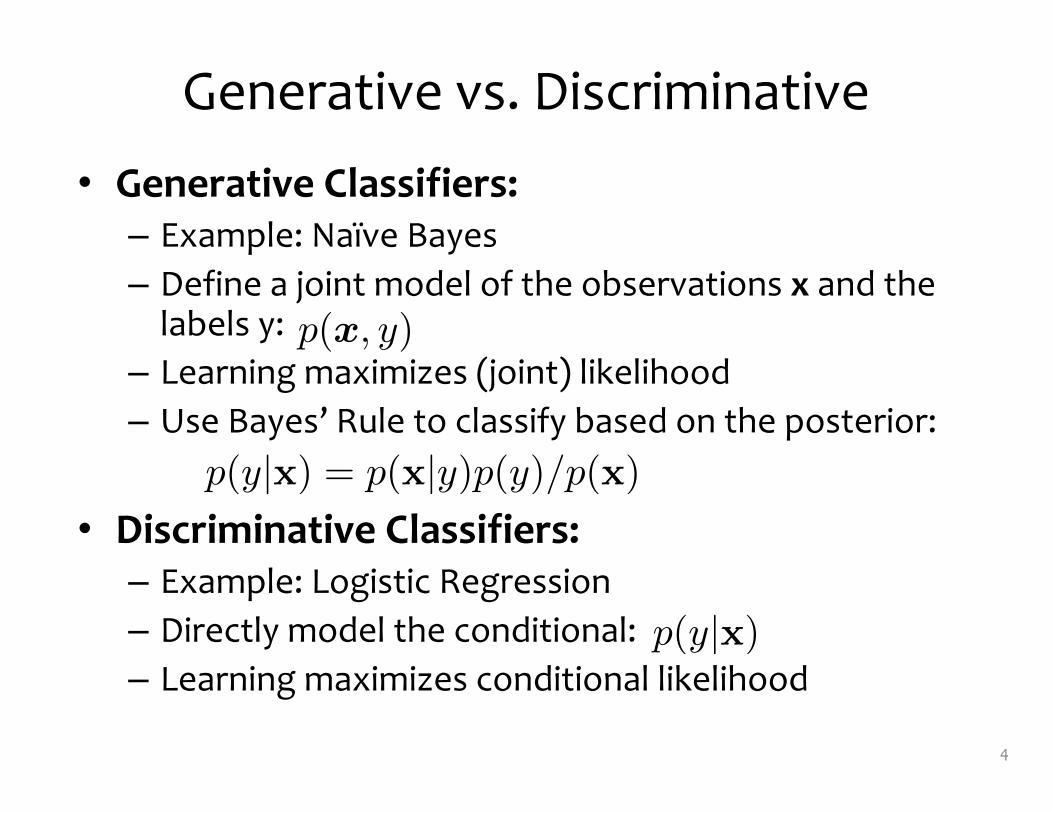
Generative vs. Discriminative• Generative Classifiers:– Example: Naïve Bayes– Define a joint model of the observations x and the
labels y:– Learning maximizes (joint) likelihood– Use Bayes’ Rule to classify based on the posterior:
• Discriminative Classifiers:– Example: Logistic Regression– Directly model the conditional: – Learning maximizes conditional likelihood
4
p(x, y)
p(y|x)
p(y|x) = p(x|y)p(y)/p(x)
Generative vs. Discriminative
Whiteboard– Contrast: To model p(x) or not to model p(x)?
5
Generative vs. Discriminative
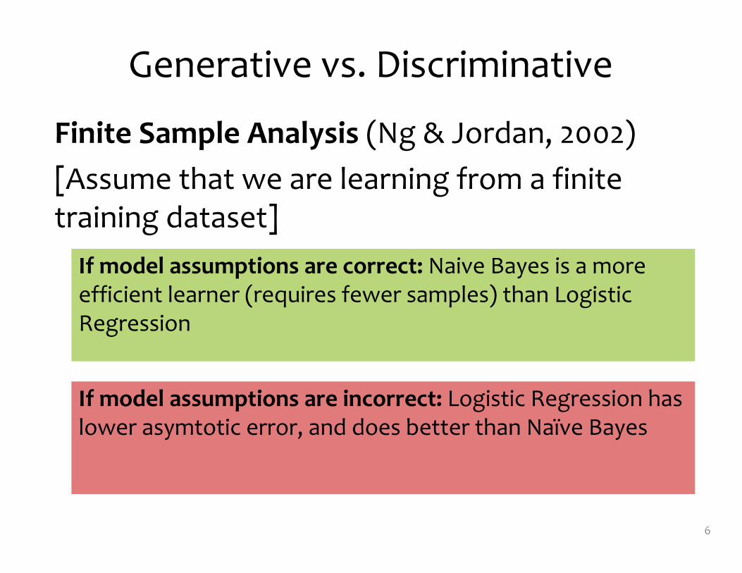
Finite Sample Analysis (Ng & Jordan, 2002)[Assume that we are learning from a finite training dataset]
6
If model assumptions are correct: Naive Bayes is a more efficient learner (requires fewer samples) than Logistic Regression
If model assumptions are incorrect: Logistic Regression has lower asymtotic error, and does better than Naïve Bayes
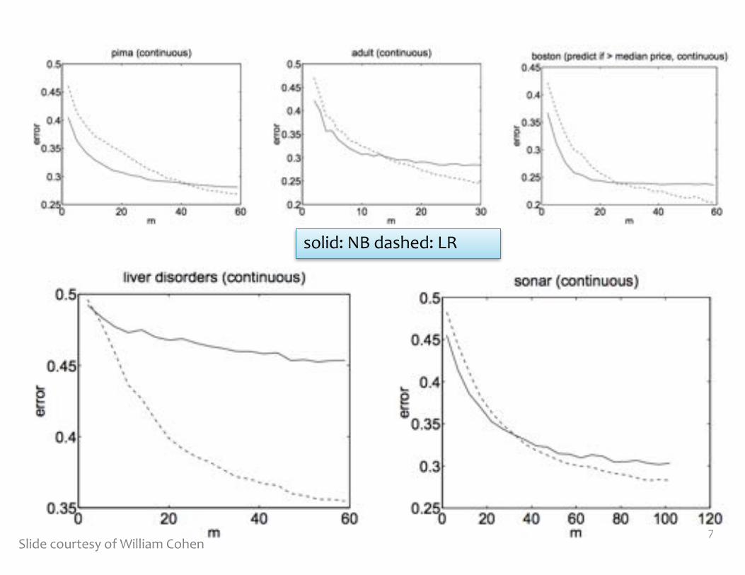
solid: NB dashed: LR
7Slide courtesy of William Cohen
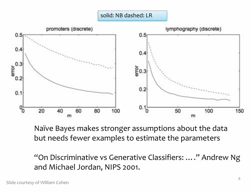
Naïve Bayes makes stronger assumptions about the databut needs fewer examples to estimate the parameters
“On Discriminative vs Generative Classifiers: ….” Andrew Ng and Michael Jordan, NIPS 2001.
8
solid: NB dashed: LR
Slide courtesy of William Cohen
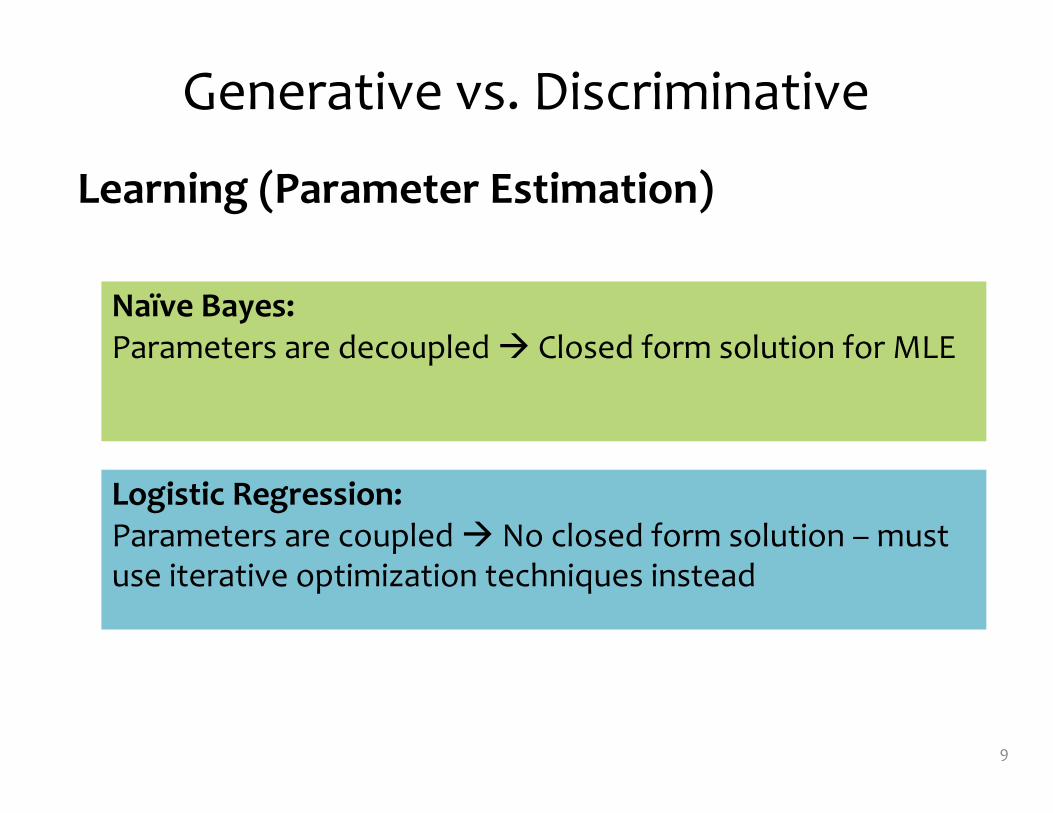
Generative vs. Discriminative
Learning (Parameter Estimation)
9
Naïve Bayes: Parameters are decoupled à Closed form solution for MLE
Logistic Regression: Parameters are coupled à No closed form solution – must use iterative optimization techniques instead
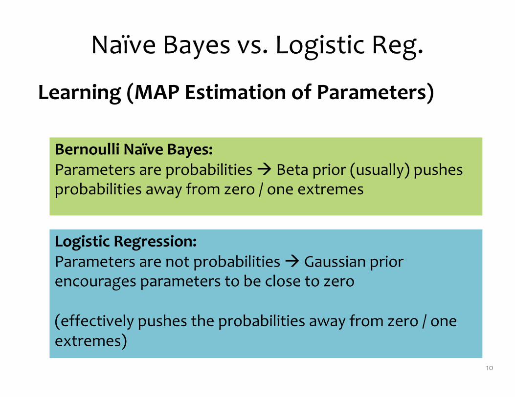
Naïve Bayes vs. Logistic Reg.
Learning (MAP Estimation of Parameters)
10
Bernoulli Naïve Bayes: Parameters are probabilities à Beta prior (usually) pushes probabilities away from zero / one extremes
Logistic Regression: Parameters are not probabilities à Gaussian prior encourages parameters to be close to zero
(effectively pushes the probabilities away from zero / one extremes)

Naïve Bayes vs. Logistic Reg.
Features
11
Naïve Bayes: Features x are assumed to be conditionally independent given y. (i.e. Naïve Bayes Assumption)
Logistic Regression: No assumptions are made about the form of the features x. They can be dependent and correlated in any fashion.

MOTIVATION: STRUCTURED PREDICTION
12
Structured Prediction
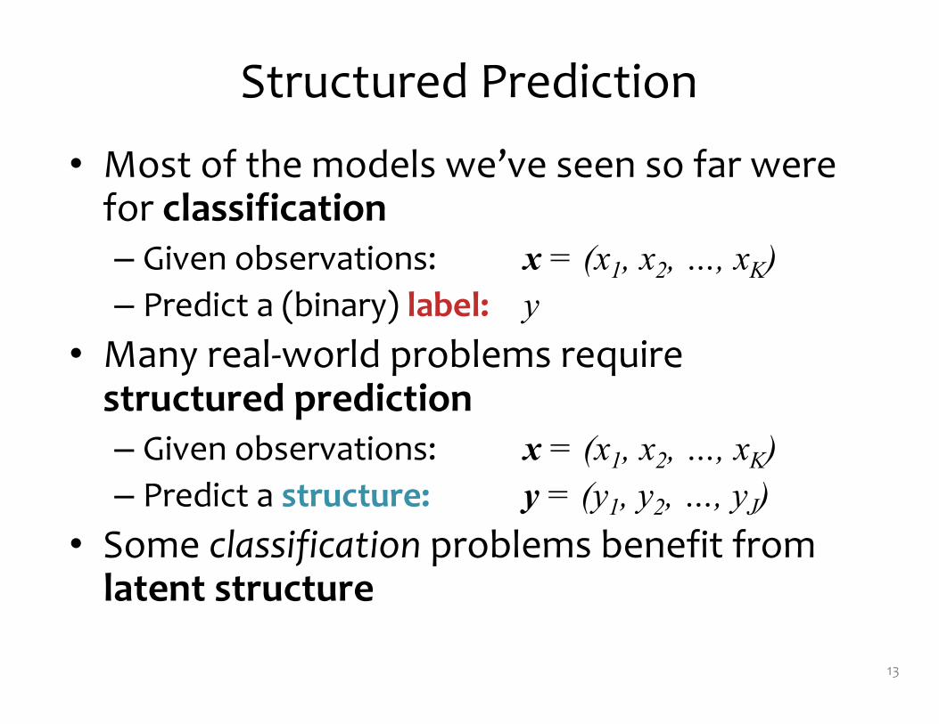
• Most of the models we’ve seen so far were for classification– Given observations: x = (x1, x2, …, xK) – Predict a (binary) label: y
• Many real-world problems require structured prediction– Given observations: x = (x1, x2, …, xK) – Predict a structure: y = (y1, y2, …, yJ)
• Some classification problems benefit from latent structure
13
Structured Prediction Examples
• Examples of structured prediction– Part-of-speech (POS) tagging– Handwriting recognition– Speech recognition– Word alignment– Congressional voting
• Examples of latent structure– Object recognition
14
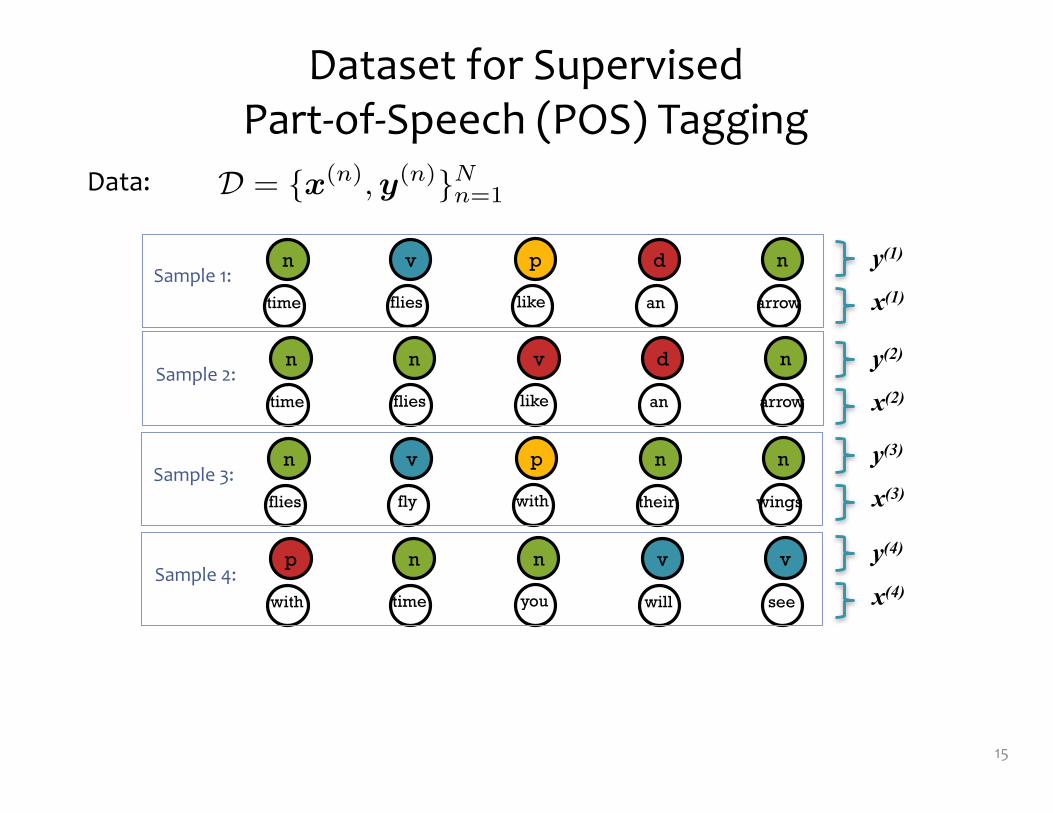
n n v d nSample 2:
time likeflies an arrow
Dataset for Supervised Part-of-Speech (POS) Tagging
15
n v p d nSample 1:
time likeflies an arrow
p n n v vSample 4:
with youtime will see
n v p n nSample 3:
flies withfly their wings
D = {x(n),y(n)}Nn=1Data:
y(1)
x(1)
y(2)
x(2)
y(3)
x(3)
y(4)
x(4)
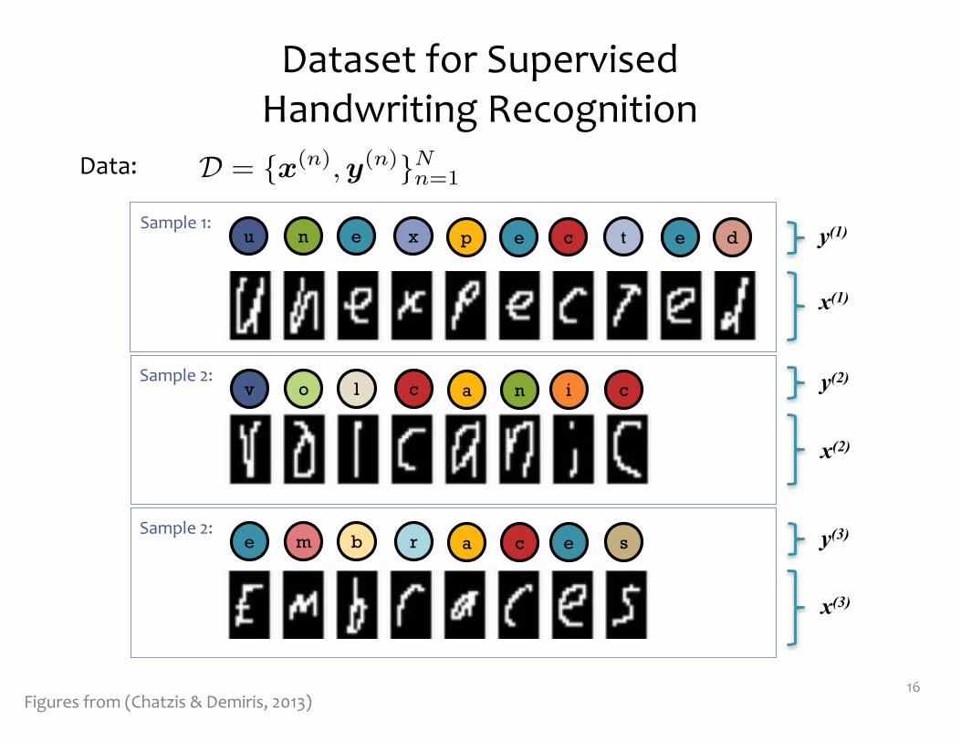
Dataset for Supervised Handwriting Recognition
16
D = {x(n),y(n)}Nn=1Data:
values. The obtained results are depicted in Table 4; weprovide means, standard deviations, and the p-metric valueof the Student’s-t test run on the pairs of performances ofthe models (CRF, CRF1), (moderate order CRF, CRF1),and (HMM, CRF1).
As we observe, the proposed approach offers a sig-nificant improvement over first-order linear-chain CRFs, aswell as the rest of the considered alternatives. Therefore, weonce again notice the practical significance of coming up
with computationally efficient ways of relaxing the Marko-vian assumption in linear-chain CRF models applied tosequential data modeling. Note also that, in this experi-ment, the moderate order CRF models of [41] seem to yielda rather competitive result. This was expectable since theaverage modeled sequence in this experiment is less than10 time points long. Finally, regarding the HMM method,with the number of mixture components M selected so as tooptimize model performance, we observe that the CRF1
model yields a clear improvement, irrespective of theemployed likelihood optimization approach.
4.3 Part-of-Speech Tagging
Finally, here we consider an experiment with the PennTreebank corpus [25], containing 74,029 sentences with atotal of 1,637,267 words. It is comprised of 49,115 uniquewords, and each word in the corpus is labeled according toits part of speech; there are a total of 43 different part-of-speech labels. We use four types of features:
1. First-order word-presence features.2. Four-character prefix presence features.
10 IEEE TRANSACTIONS ON PATTERN ANALYSIS AND MACHINE INTELLIGENCE, VOL. 35, NO. 12, XXXXXXX 2013
TABLE 3Activity-Based Segmentation of Skateboard: Push and Turn
Videos: Error Rates Obtained by the Evaluated Methods
Fig. 4. Skateboard: push and turn: A few example frames from a sequence considered in our experiments.
Fig. 5. Handwriting recognition: Example words from the dataset used.
TABLE 4Handwriting Recognition: Error Rates Obtained
by the Evaluated Methods
Figures from (Chatzis & Demiris, 2013)
u e p c tSample 1:
y(1)
x(1)
n x e de
v l a i cSample 2:
o c n
e b a e sSample 2:
m r c
y(2)
x(2)
y(3)
x(3)
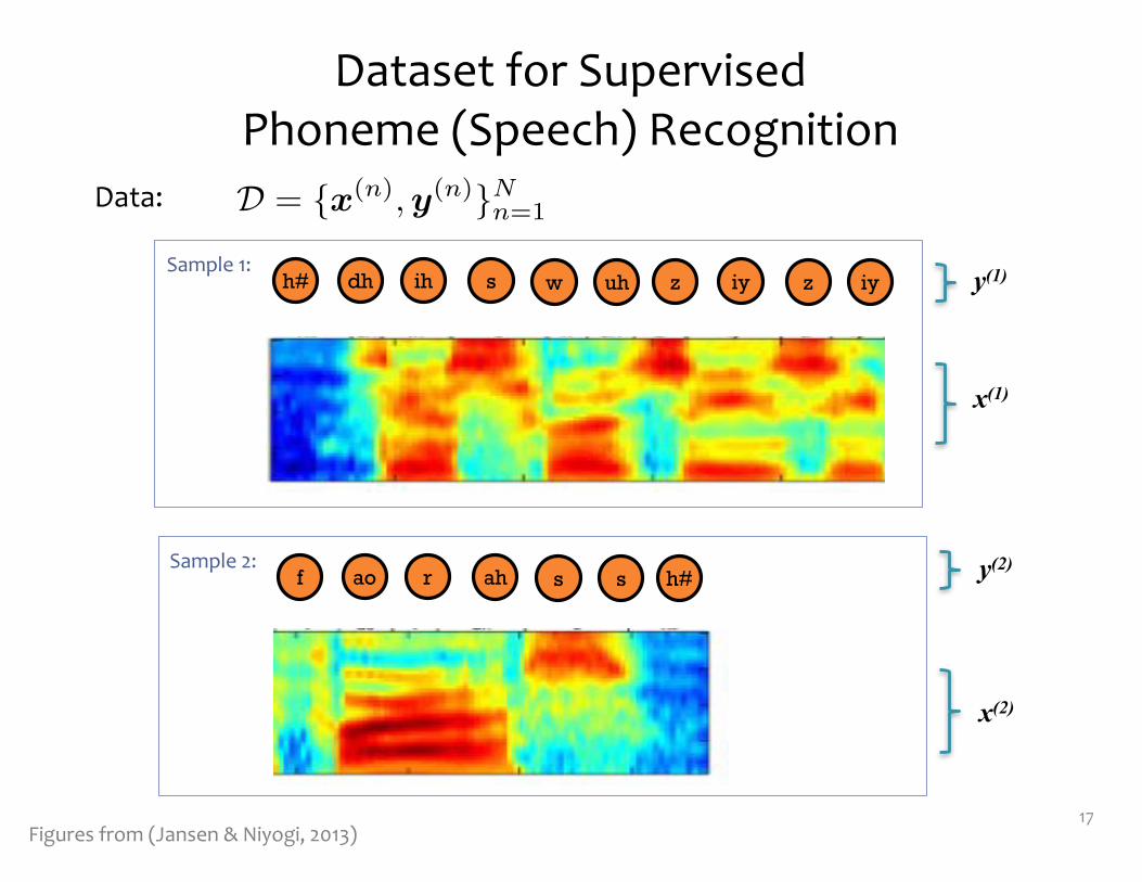
Dataset for Supervised Phoneme (Speech) Recognition
17
D = {x(n),y(n)}Nn=1Data:
Figures from (Jansen & Niyogi, 2013)
h# ih w z iySample 1:
y(1)
x(1)
dh s uh iyz1704 IEEE TRANSACTIONS ON SIGNAL PROCESSING, VOL. 61, NO. 7, APRIL 1, 2013
Fig. 5. Extrinsic (top) and intrinsic (bottom) spectral representations for the utterance “This was easy for us.” Note that a nonlinear mel-scale frequency warpingwas used.
where are the input unlabeled data and is the
new parametrization of the function we need to estimate. To
proceed, we plug the functional form of (9) into the optimization
problem of (8). Taking the gradient with respect to the parameter
vector and setting it to zero sets up the following generalized
eigenvalue problem:
(10)
Here, is the Grammatrix defined on the input unlabeleddata by . This eigenvalue decomposition will
produce a full spectrum of eigenvectors, each defining its ownintrinsic projection map defined by the th eigenvector .
Unlike the unsupervised learning algorithm of [5], we are now
interested in several of the , not just one for binary clas-
sification or clustering. Recall that the intrinsic basis functionsproduced by the Laplacian eigenmaps algorithm were definedonly on the points used to construct the graph Laplacian. Our
new set of projection maps is now defined out-of-sample, i.e.,may be computed for arbitrary points on the manifold and
may also be used more generally for any point in .
B. Intrinsic Spectrogram Algorithm
Given the nomenclature define above, the algorithm for com-puting the intrinsic spectrogram is comprised of three steps:
1) Given a set of unlabeled data sampled from
the manifold, construct a nearest neighbor graph and
compute the graph Laplacian (either normalized or un-
normalized).
2) Given a kernel , solve the generalized eigenvalue
problem of (10) for the weights .
3) Project amplitude spectrum at each time point of the ex-
trinsic spectrogram onto the first intrinsic basis functions
(sorted by increasing eigenvalue) according to (9).
Note that steps 1 and 2 are computed offline using the standardtraining set . Thus, converting the extrinsic spectrogram of a
novel utterance into this intrinsic representation requires only
the computation of Equation (9) across the utterance.
Fig. 5 shows an example extrinsic and intrinsic
spectrograms for the TIMIT utterance “This was easy
for us” (TIMIT sentence sx3). Here, we constructed the dataset
with 200 examples of each of the 48 phonetic categories spec-
ified in [26].2 Each example was extrinsically represented bya 40-dimensional, homomorphically smoothed, auditory (log)
spectrum (40 mel scale bands, from 0–8 kHz) computed from
a 25 ms signal window centered in each phonetic segment. The
adjacency graph was constructed using nearest Euclidean
neighbors and binary-valued edge weights. For the optimiza-
tion problem of (8), we take as the intrinsic smoothness param-
eter . Finally, to accommodate nonlinear intrinsic projec-
tions maps, we employ the radial basis function (RBF) kernel,
, where is taken to be 1/3 of the mean
Euclidean distance between the graph vertices. Note that op-
timal settings of , and depend on the intended application
and manifold sampling density; we investigate the role this pa-
rameter in the experiments described below. Given the low-di-
mensional curved manifold structure motivated in previous sec-
tions, one might expect phonetic content to be more transpar-
ently differentiated in the intrinsic basis than in a traditional
spectrogram. It is clear from Fig. 5 that the intrinsic represen-
tation redistributes much of the spectral variation to the lower
eigenvalued components. It is also clear that these initial com-
ponents do not each covary with the presence of a single speech
sound. In the next section, we examine whether this alternative
organization may have a natural linguistic interpretation.
V. INTRINSIC SPECTRAL ANALYSIS INTERPRETATION
The intrinsic representation is a projection of spectral infor-
mation onto a set of basis functions ordered by their smooth-
2Note that while we use a class balanced sample here, balancing was notrequired to obtain good performance in the experiments in Section VII in whichwe randomly selected examples from the entire corpus (ignoring class).
1704 IEEE TRANSACTIONS ON SIGNAL PROCESSING, VOL. 61, NO. 7, APRIL 1, 2013
Fig. 5. Extrinsic (top) and intrinsic (bottom) spectral representations for the utterance “This was easy for us.” Note that a nonlinear mel-scale frequency warpingwas used.
where are the input unlabeled data and is the
new parametrization of the function we need to estimate. To
proceed, we plug the functional form of (9) into the optimization
problem of (8). Taking the gradient with respect to the parameter
vector and setting it to zero sets up the following generalized
eigenvalue problem:
(10)
Here, is the Grammatrix defined on the input unlabeleddata by . This eigenvalue decomposition will
produce a full spectrum of eigenvectors, each defining its ownintrinsic projection map defined by the th eigenvector .
Unlike the unsupervised learning algorithm of [5], we are now
interested in several of the , not just one for binary clas-
sification or clustering. Recall that the intrinsic basis functionsproduced by the Laplacian eigenmaps algorithm were definedonly on the points used to construct the graph Laplacian. Our
new set of projection maps is now defined out-of-sample, i.e.,may be computed for arbitrary points on the manifold and
may also be used more generally for any point in .
B. Intrinsic Spectrogram Algorithm
Given the nomenclature define above, the algorithm for com-puting the intrinsic spectrogram is comprised of three steps:
1) Given a set of unlabeled data sampled from
the manifold, construct a nearest neighbor graph and
compute the graph Laplacian (either normalized or un-
normalized).
2) Given a kernel , solve the generalized eigenvalue
problem of (10) for the weights .
3) Project amplitude spectrum at each time point of the ex-
trinsic spectrogram onto the first intrinsic basis functions
(sorted by increasing eigenvalue) according to (9).
Note that steps 1 and 2 are computed offline using the standardtraining set . Thus, converting the extrinsic spectrogram of a
novel utterance into this intrinsic representation requires only
the computation of Equation (9) across the utterance.
Fig. 5 shows an example extrinsic and intrinsic
spectrograms for the TIMIT utterance “This was easy
for us” (TIMIT sentence sx3). Here, we constructed the dataset
with 200 examples of each of the 48 phonetic categories spec-
ified in [26].2 Each example was extrinsically represented bya 40-dimensional, homomorphically smoothed, auditory (log)
spectrum (40 mel scale bands, from 0–8 kHz) computed from
a 25 ms signal window centered in each phonetic segment. The
adjacency graph was constructed using nearest Euclidean
neighbors and binary-valued edge weights. For the optimiza-
tion problem of (8), we take as the intrinsic smoothness param-
eter . Finally, to accommodate nonlinear intrinsic projec-
tions maps, we employ the radial basis function (RBF) kernel,
, where is taken to be 1/3 of the mean
Euclidean distance between the graph vertices. Note that op-
timal settings of , and depend on the intended application
and manifold sampling density; we investigate the role this pa-
rameter in the experiments described below. Given the low-di-
mensional curved manifold structure motivated in previous sec-
tions, one might expect phonetic content to be more transpar-
ently differentiated in the intrinsic basis than in a traditional
spectrogram. It is clear from Fig. 5 that the intrinsic represen-
tation redistributes much of the spectral variation to the lower
eigenvalued components. It is also clear that these initial com-
ponents do not each covary with the presence of a single speech
sound. In the next section, we examine whether this alternative
organization may have a natural linguistic interpretation.
V. INTRINSIC SPECTRAL ANALYSIS INTERPRETATION
The intrinsic representation is a projection of spectral infor-
mation onto a set of basis functions ordered by their smooth-
2Note that while we use a class balanced sample here, balancing was notrequired to obtain good performance in the experiments in Section VII in whichwe randomly selected examples from the entire corpus (ignoring class).
f r s h#Sample 2:
ao ah s y(2)
x(2)
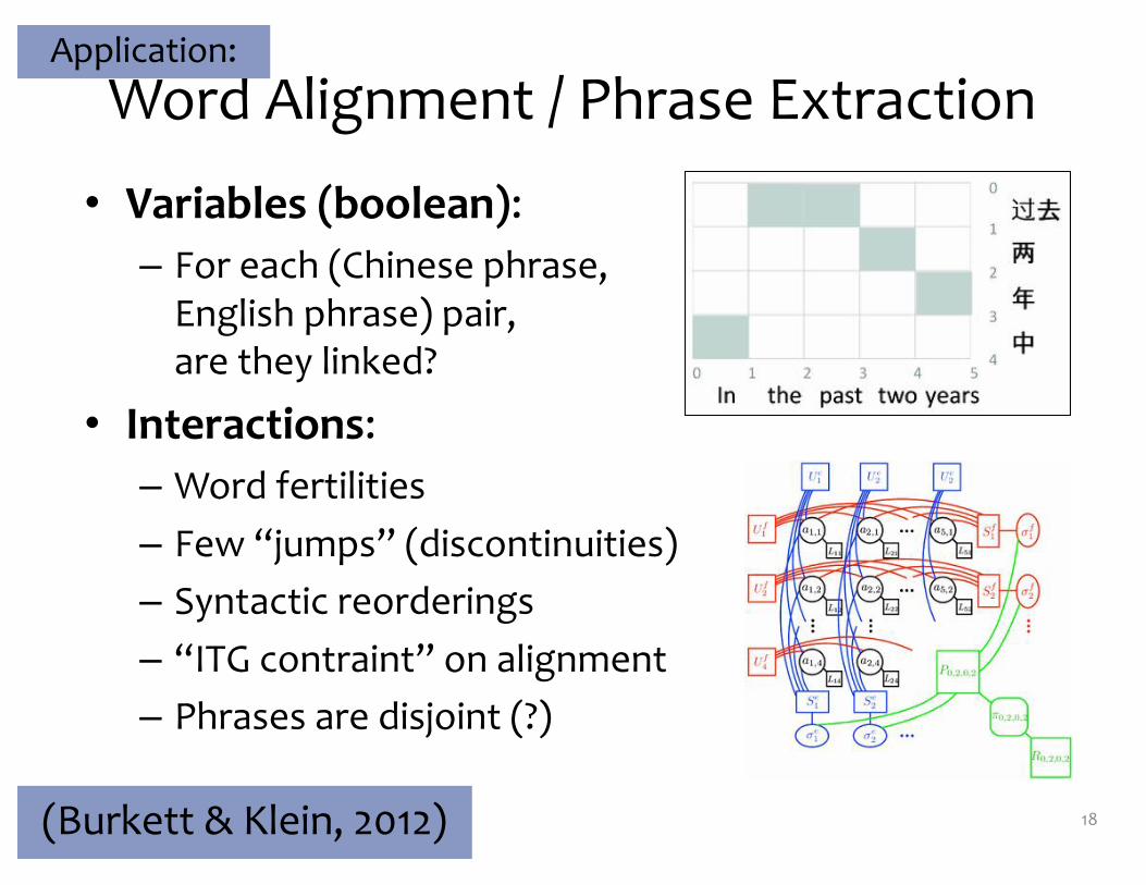
Word Alignment / Phrase Extraction
• Variables (boolean):– For each (Chinese phrase,
English phrase) pair, are they linked?
• Interactions:– Word fertilities– Few “jumps” (discontinuities)– Syntactic reorderings– “ITG contraint” on alignment– Phrases are disjoint (?)
18(Burkett & Klein, 2012)
Application:
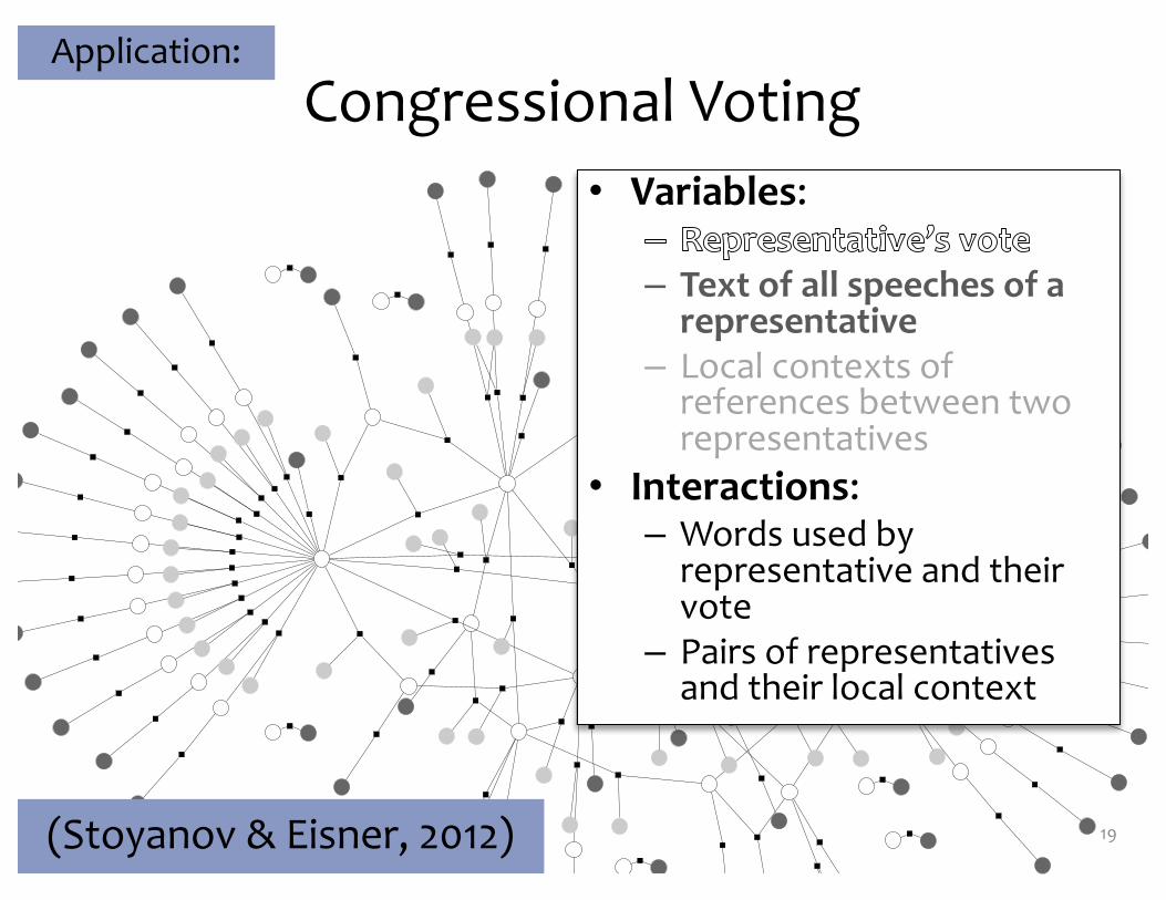
Figure 1: An example of a debate structure from the Con-Vote corpus. Each black square node represents a factorand is connected to the variables in that factor, shownas round nodes. Unshaded variables correspond to therepresentatives’ votes and depict the output variables thatwe learn to jointly predict. Shaded variables correspondto the observed input data— the text of all speeches of arepresentative (in dark gray) or all local contexts of refer-ences between two representatives (in light gray).
and that ERMA further significantly improves per-formance, particularly when it properly trains withthe same inference algorithm (max-product vs. sum-product) to be used at test time.
Baseline. As an exact baseline, we compareagainst the results of Thomas et al. (2006). Theirtest-time Min-Cut algorithm is exact in this case: bi-nary variables and a two-way classification.
4.2 Information Extraction fromSemi-Structured Text
We utilize the CMU seminar announcement corpusof Freitag (2000) consisting of emails with seminarannouncements. The task is to extract four fields thatdescribe each seminar: speaker, location, start timeand end time. The corpus annotates the documentwith all mentions of these four fields.
Sequential CRFs have been used successfully forsemi-structured information extraction (Sutton andMcCallum, 2005; Finkel et al., 2005). However,they cannot model non-local dependencies in thedata. For example, in the seminar announcementscorpus, if “Sutner” is mentioned once in an emailin a context that identifies him as a speaker, it is
Figure 2: Skip-chain CRF for semi-structured informa-tion extraction.
likely that other occurrences of “Sutner” in the sameemail should be marked as speaker. Hence Finkel etal. (2005) and Sutton and McCallum (2005) proposeadding non-local edges to a sequential CRF to repre-sent soft consistency constraints. The model, calleda “skip-chain CRF” and shown in Figure 2, containsa factor linking each pair of capitalized words withthe same lexical form. The skip-chain CRF modelexhibits better empirical performance than its se-quential counterpart (Sutton and McCallum, 2005;Finkel et al., 2005).
The non-local skip links make exact inferenceintractable. To train the full model, Finkel et al.(2005) estimate the parameters of a sequential CRFand then manually select values for the weights ofthe non-local edges. At test time, they use Gibbssampling to perform inference. Sutton and McCal-lum (2005) use max-product loopy belief propaga-tion for test-time inference, and compare a train-ing procedure that uses a piecewise approximationof the partition function against using sum-productloopy belief propagation to compute output variablemarginals. They find that the two training regimensperform similarly on the overall task. All of thesetraining procedures try to approximately maximizeconditional likelihood, whereas we will aim to mini-mize the empirical loss of the approximate inferenceand decoding procedures.
Baseline. As an exact (non-loopy) baseline, wetrain a model without the skip chains. We give twobaseline numbers in Table 1—for training the exactCRF with MLE and with ERM. The ERM setting re-sulted in a statistically significant improvement evenin the exact case, thanks to the use of the loss func-tion at training time.
4.3 Multi-Label Classification
Multi-label classification is the problem of assign-ing multiple labels to a document. For example, anews article can be about both “Libya” and “civil
125
Congressional Voting
19(Stoyanov & Eisner, 2012)
Application:
• Variables:
– Text of all speeches of a representative
– Local contexts of references between two representatives
• Interactions:– Words used by
representative and their vote
– Pairs of representatives and their local context

Structured Prediction Examples
• Examples of structured prediction– Part-of-speech (POS) tagging– Handwriting recognition– Speech recognition– Word alignment– Congressional voting
• Examples of latent structure– Object recognition
20
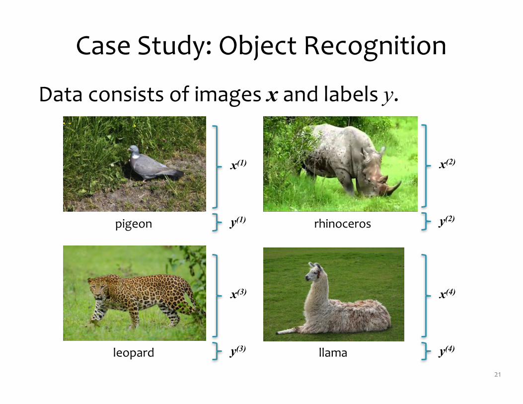
Case Study: Object Recognition
Data consists of images x and labels y.
21
pigeon
leopard llama
rhinocerosy(1)
x(1)
y(2)
x(2)
y(4)
x(4)
y(3)
x(3)
Case Study: Object Recognition
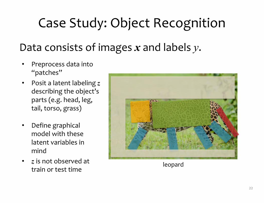
Data consists of images x and labels y.
22
• Preprocess data into “patches”
• Posit a latent labeling zdescribing the object’s parts (e.g. head, leg, tail, torso, grass)
leopard
• Define graphical model with these latent variables in mind
• z is not observed at train or test time
Case Study: Object Recognition
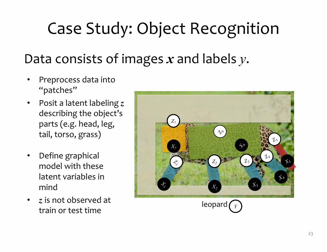
Data consists of images x and labels y.
23
• Preprocess data into “patches”
• Posit a latent labeling zdescribing the object’s parts (e.g. head, leg, tail, torso, grass)
leopard
• Define graphical model with these latent variables in mind
• z is not observed at train or test time
X2
Z2
X7
Z7
Y
Case Study: Object Recognition
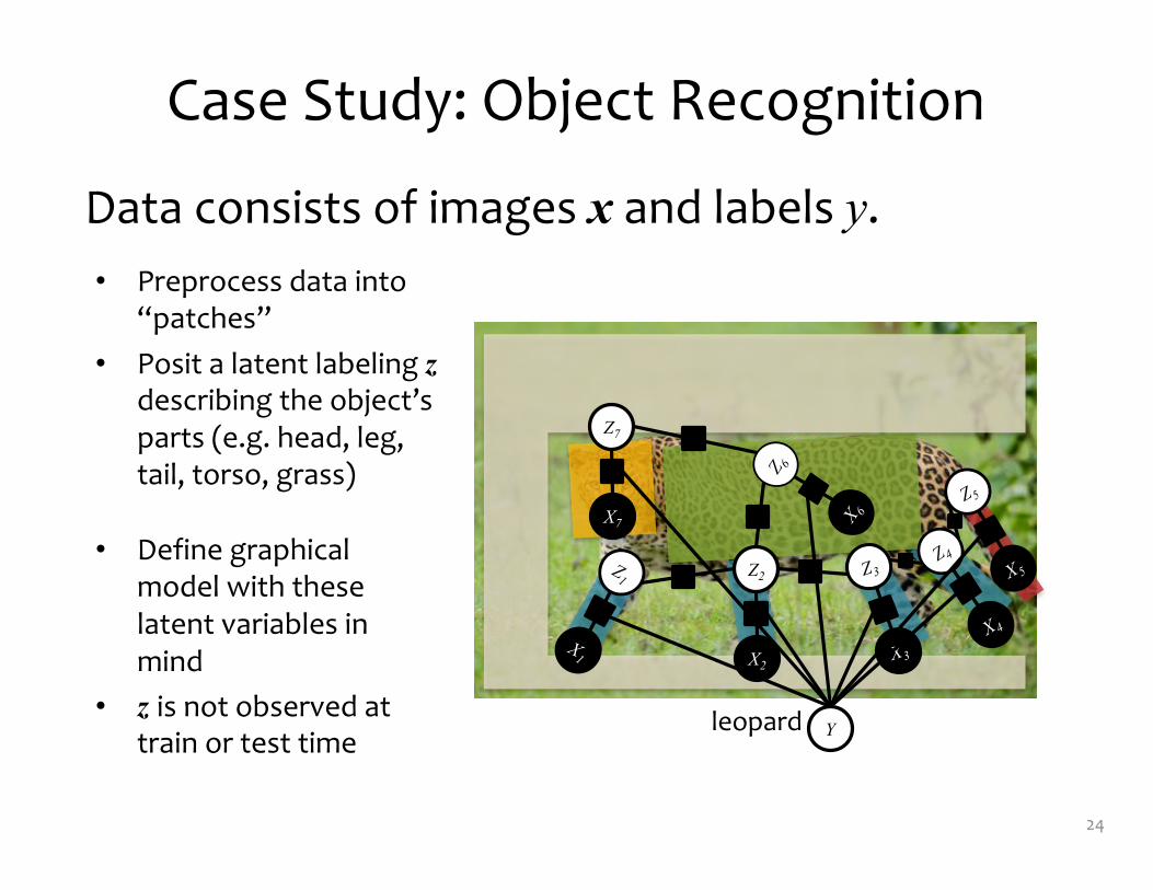
Data consists of images x and labels y.
24
• Preprocess data into “patches”
• Posit a latent labeling zdescribing the object’s parts (e.g. head, leg, tail, torso, grass)
leopard
• Define graphical model with these latent variables in mind
• z is not observed at train or test time
ψ2ψ4
X2
Z2
ψ3
X7
Z7
ψ1
ψ4
ψ4
Y
Structured Prediction
25
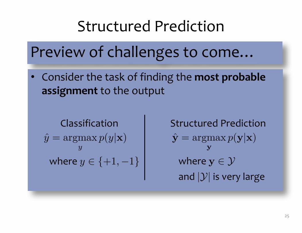
Preview of challenges to come…• Consider the task of finding the most probable
assignment to the output
Classification Structured Predictiony =
yp(y| )
where y � {+1, �1}
ˆ = p( | )
where � Yand |Y| is very large
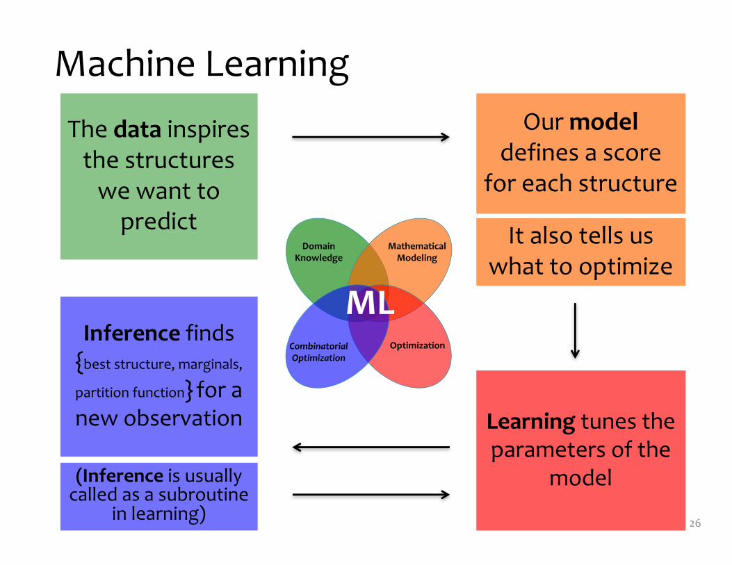
Machine Learning
26
The data inspires the structures
we want to predict It also tells us
what to optimize
Our modeldefines a score
for each structure
Learning tunes the parameters of the
model
Inference finds {best structure, marginals,
partition function} for a new observation
Domain Knowledge
Mathematical Modeling
OptimizationCombinatorial Optimization
ML
(Inference is usually called as a subroutine
in learning)
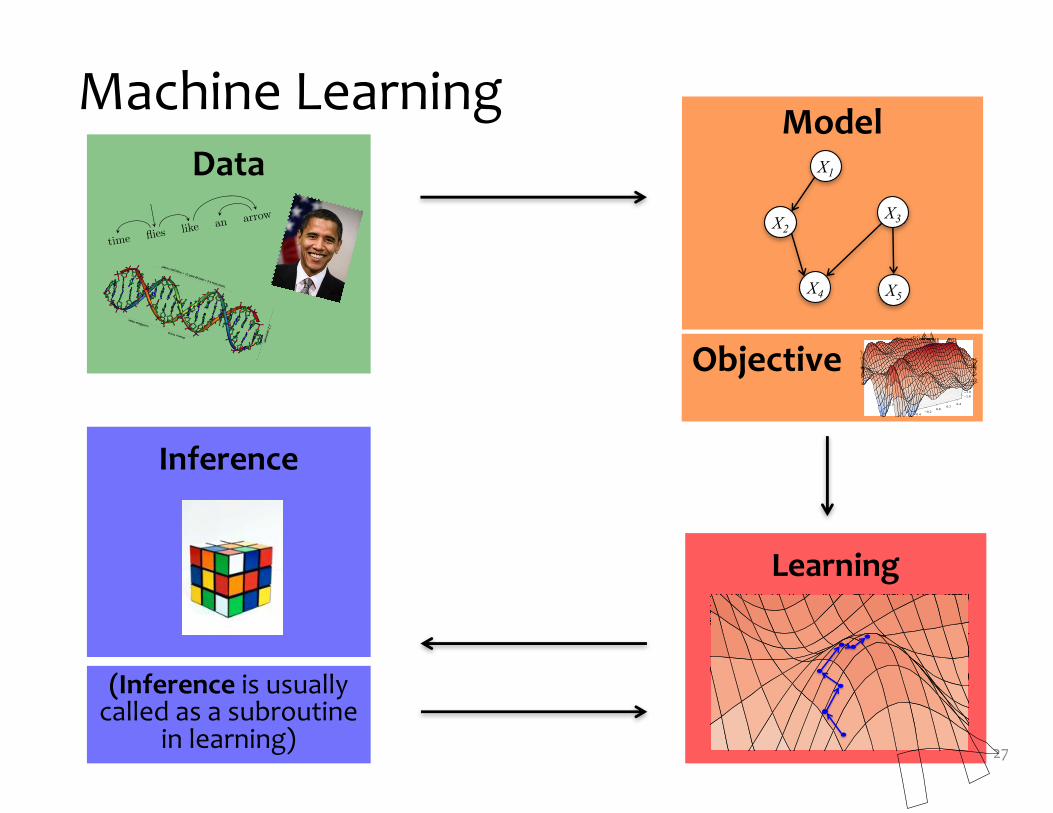
Machine Learning
27
DataModel
Learning
Inference
(Inference is usually called as a subroutine
in learning)
3
A
l
i
c
e
s
a
w
B
o
b
o
n
a
h
i
l
l
w
i
t
h
a
t
e
l
e
s
c
o
p
e
A
l
i
c
e
s
a
w
B
o
b
o
n
a
h
i
l
l
w
i
t
h
a
t
e
l
e
s
c
o
p
e
4
t
i
m
e
fl
i
e
s
l
i
k
e
a
n
a
r
r
o
w
t
i
m
e
fl
i
e
s
l
i
k
e
a
n
a
r
r
o
w
t
i
m
e
fl
i
e
s
l
i
k
e
a
n
a
r
r
o
w
t
i
m
e
fl
i
e
s
l
i
k
e
a
n
a
r
r
o
w
t
i
m
e
fl
i
e
s
l
i
k
e
a
n
a
r
r
o
w
2
Objective
X1
X3X2
X4 X5

BACKGROUND
28

Background
Whiteboard– Chain Rule of Probability– Conditional Independence
29
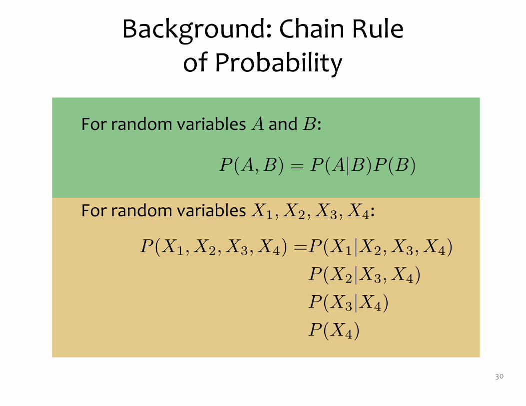
Background: Chain Ruleof Probability
30
For random variables A and B:
P (A, B) = P (A|B)P (B)
P (X1, X2, X3, X4) =P (X1|X2, X3, X4)
P (X2|X3, X4)
P (X3|X4)
P (X4)
For random variables X1, X2, X3, X4:
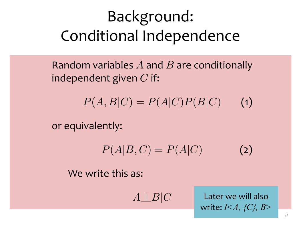
Background:Conditional Independence
31
Random variables A and B are conditionallyindependent given C if:
P (A, B|C) = P (A|C)P (B|C) (1)
or equivalently:
P (A|B, C) = P (A|C) (2)
We write this as:
A | B|C (3)Later we will also write: I<A, {C}, B>

HIDDEN MARKOV MODEL (HMM)
32
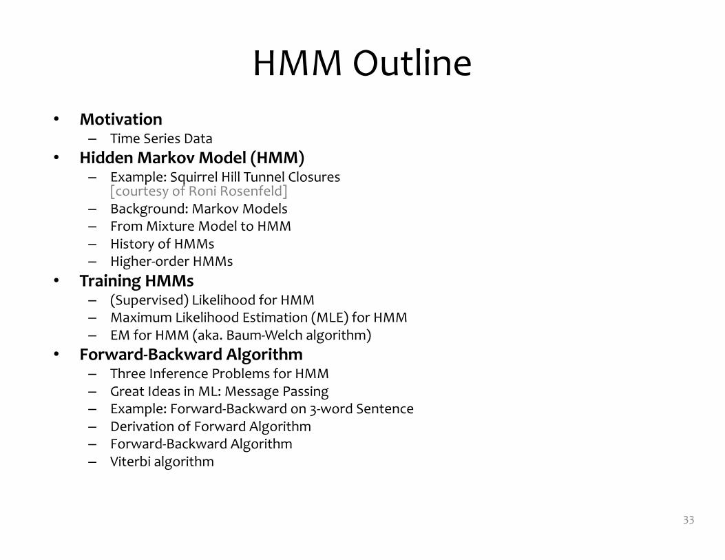
HMM Outline• Motivation
– Time Series Data• Hidden Markov Model (HMM)
– Example: Squirrel Hill Tunnel Closures [courtesy of Roni Rosenfeld]
– Background: Markov Models– From Mixture Model to HMM– History of HMMs– Higher-order HMMs
• Training HMMs– (Supervised) Likelihood for HMM– Maximum Likelihood Estimation (MLE) for HMM– EM for HMM (aka. Baum-Welch algorithm)
• Forward-Backward Algorithm– Three Inference Problems for HMM– Great Ideas in ML: Message Passing– Example: Forward-Backward on 3-word Sentence– Derivation of Forward Algorithm– Forward-Backward Algorithm– Viterbi algorithm
33
Markov Models
Whiteboard– Example: Squirrel Hill Tunnel Closures
[courtesy of Roni Rosenfeld]– First-order Markov assumption– Conditional independence assumptions
34
2m 3m 18m 9m 27m
O S S O C
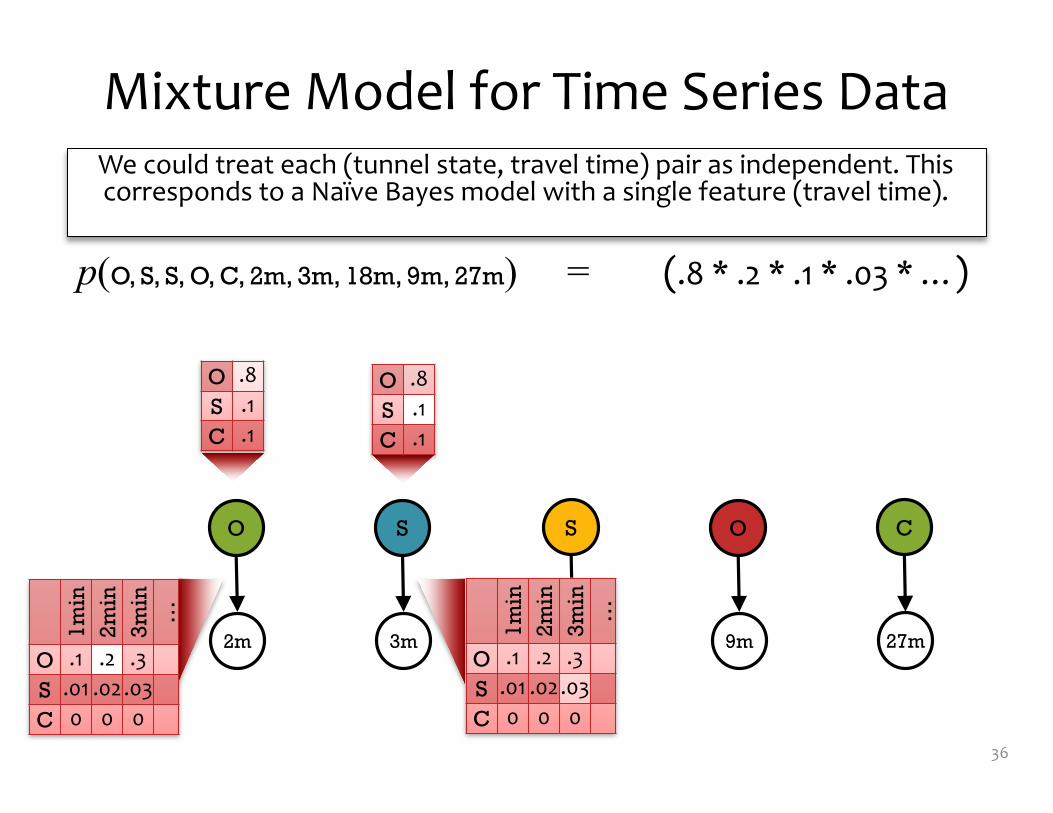
Mixture Model for Time Series Data
36
We could treat each (tunnel state, travel time) pair as independent. This corresponds to a Naïve Bayes model with a single feature (travel time).
O .8S .1C .1
p(O, S, S, O, C, 2m, 3m, 18m, 9m, 27m) = (.8 * .2 * .1 * .03 * …)
O .8S .1C .1
1min
2min
3min
…
O .1 .2 .3S .01 .02.03C 0 0 0
1min
2min
3min
…
O .1 .2 .3S .01 .02.03C 0 0 0
2m 3m 18m 9m 27m
O S S O C1m
in2m
in3m
in…
O .1 .2 .3S .01 .02.03C 0 0 0
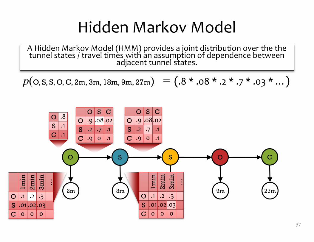
Hidden Markov Model
37
A Hidden Markov Model (HMM) provides a joint distribution over the the tunnel states / travel times with an assumption of dependence between
adjacent tunnel states.
p(O, S, S, O, C, 2m, 3m, 18m, 9m, 27m) = (.8 * .08 * .2 * .7 * .03 * …)
O S CO .9 .08.02S .2 .7 .1C .9 0 .1
1min
2min
3min
…
O .1 .2 .3S .01 .02.03C 0 0 0
O S CO .9 .08.02S .2 .7 .1C .9 0 .1
O .8S .1C .1
HMM:
“Naïve Bayes”:
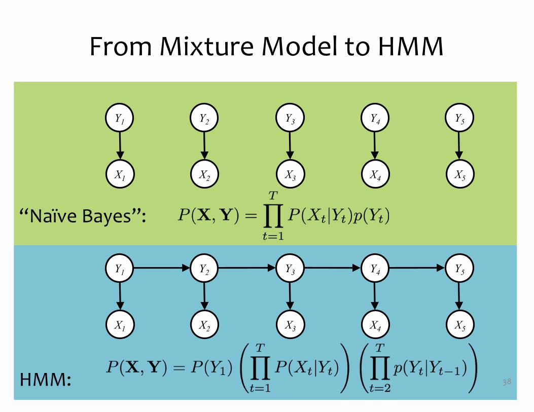
From Mixture Model to HMM
38
X1 X2 X3 X4 X5
Y1 Y2 Y3 Y4 Y5
X1 X2 X3 X4 X5
Y1 Y2 Y3 Y4 Y5
HMM:
“Naïve Bayes”:
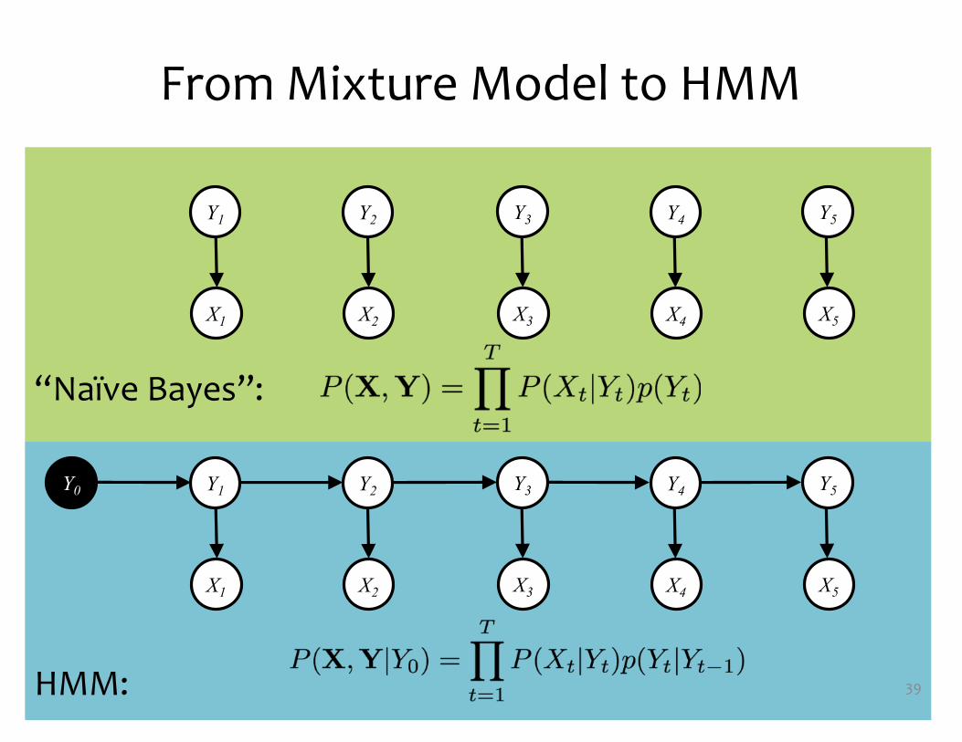
From Mixture Model to HMM
39
X1 X2 X3 X4 X5
Y1 Y2 Y3 Y4 Y5Y0
X1 X2 X3 X4 X5
Y1 Y2 Y3 Y4 Y5

SUPERVISED LEARNING FOR HMMS
44
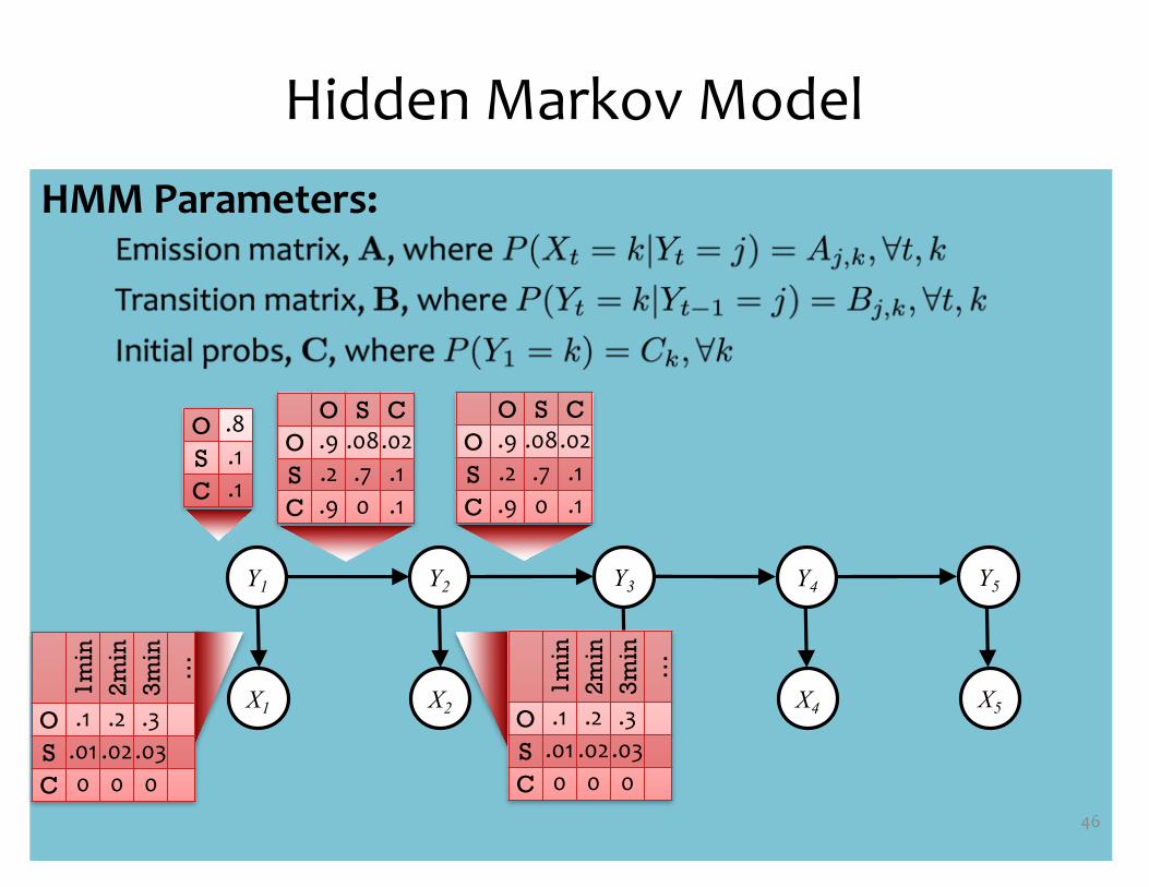
HMM Parameters:
Hidden Markov Model
46
X1 X2 X3 X4 X5
Y1 Y2 Y3 Y4 Y5
O S CO .9 .08.02S .2 .7 .1C .9 0 .1
1min
2min
3min
…
O .1 .2 .3S .01 .02.03C 0 0 0
O S CO .9 .08.02S .2 .7 .1C .9 0 .1
1min
2min
3min
…
O .1 .2 .3S .01 .02.03C 0 0 0
O .8S .1C .1
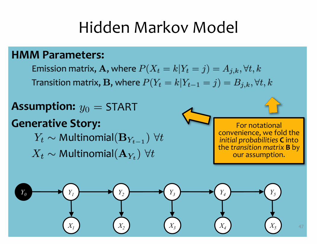
HMM Parameters:
Assumption:Generative Story:
Hidden Markov Model
47X1 X2 X3 X4 X5
Y1 Y2 Y3 Y4 Y5Y0
y0 = STARTFor notational
convenience, we fold the initial probabilities C into the transition matrix B by
our assumption.
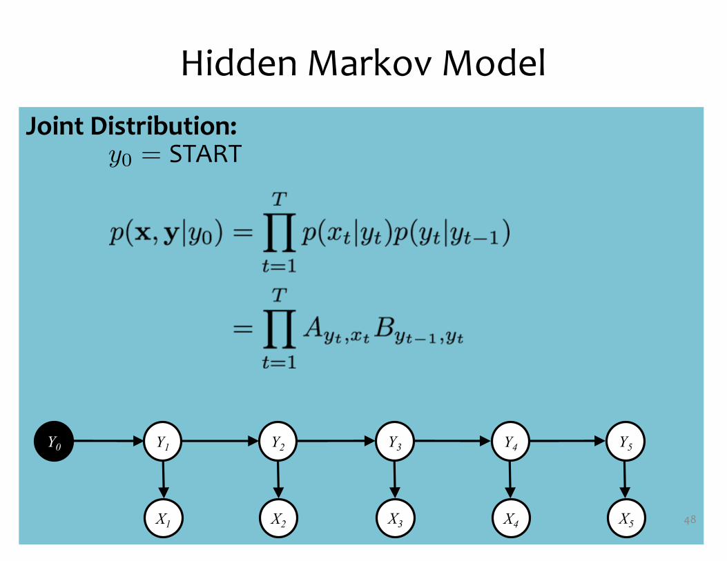
Joint Distribution:
Hidden Markov Model
48X1 X2 X3 X4 X5
Y1 Y2 Y3 Y4 Y5Y0
y0 = START
Training HMMs
Whiteboard– (Supervised) Likelihood for an HMM– Maximum Likelihood Estimation (MLE) for HMM
49