Hidden Markov Models

Slides mostly from Mitch Marcus and Eric Fosler (with lots of modifications).

Have you seen HMMs? Have you seen Kalman filters? Have you seen dynamic programming?

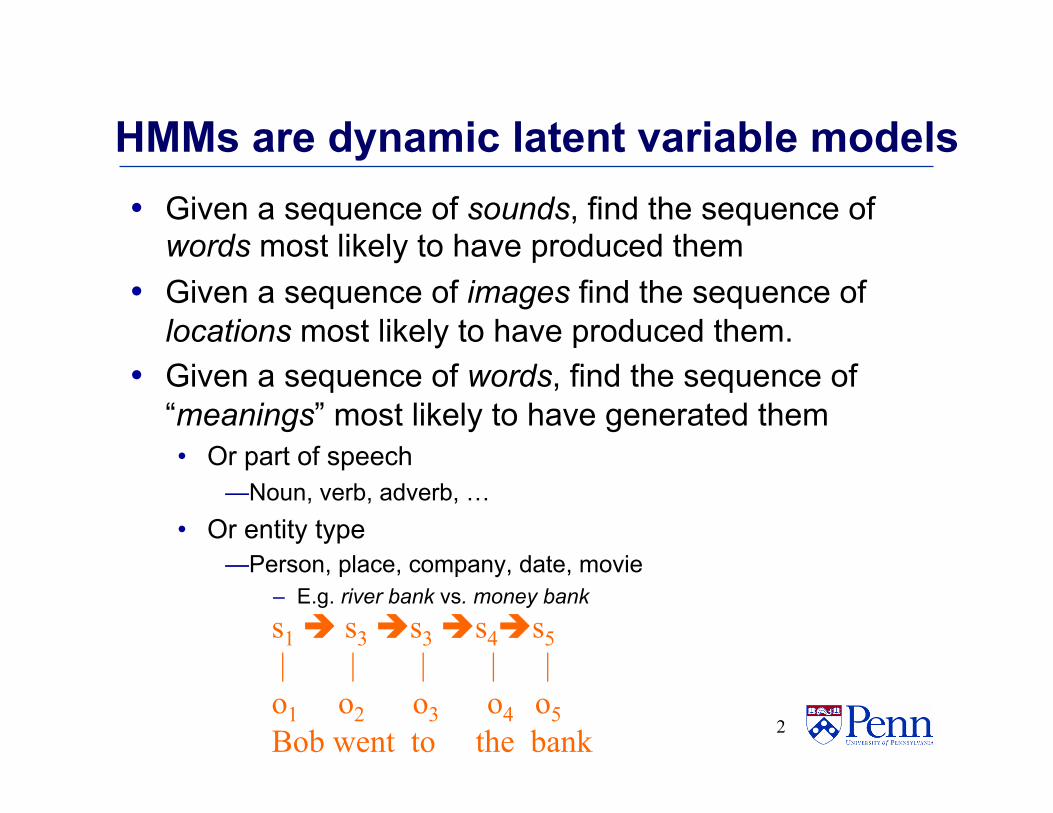
HMMs are dynamic latent variable models •  Given a sequence of sounds, find the sequence of

words most likely to have produced them •  Given a sequence of images find the sequence of

locations most likely to have produced them. •  Given a sequence of words, find the sequence of

“meanings” most likely to have generated them •  Or part of speech

— Noun, verb, adverb, … •  Or entity type

— Person, place, company, date, movie –  E.g. river bank vs. money bank

2

s1 è s3 ès3 ès4ès5 | | | | | o1 o2 o3 o4 o5 Bob went to the bank

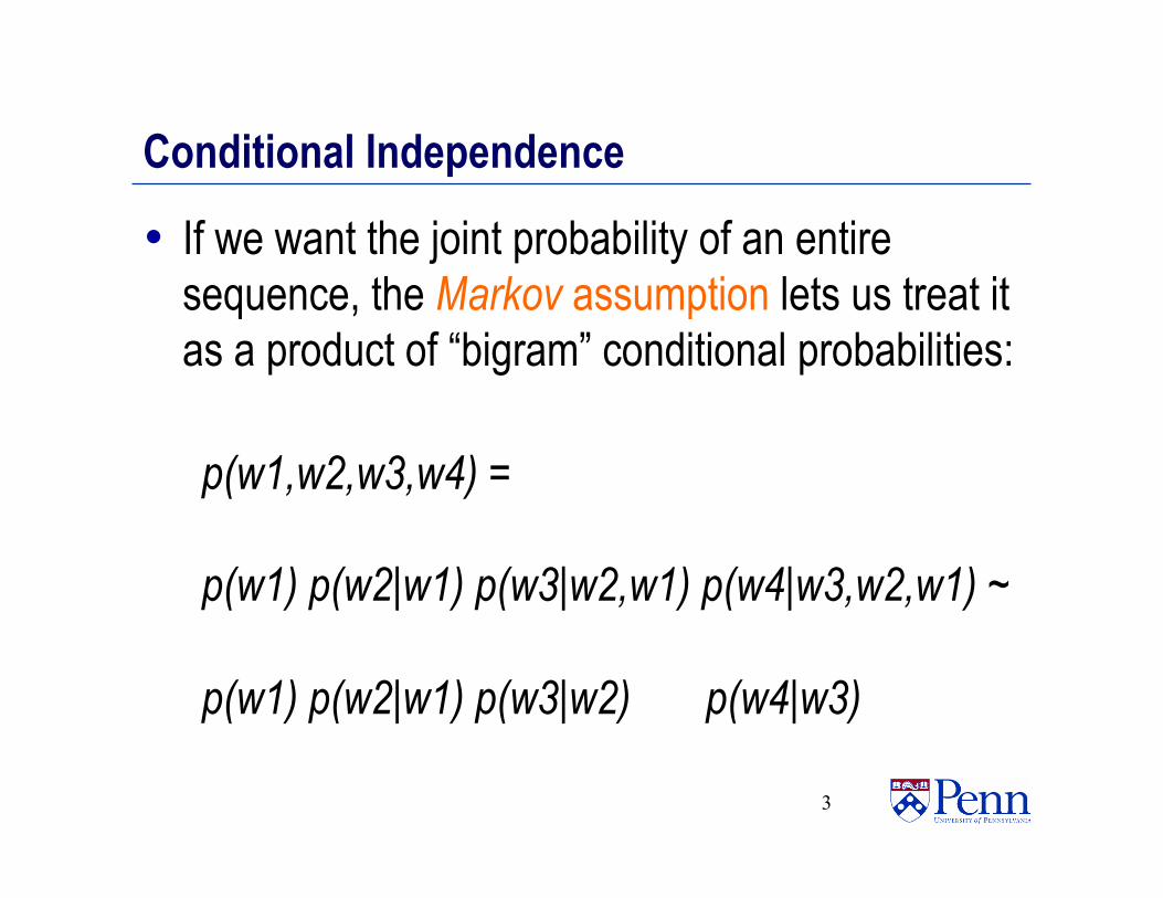
Conditional Independence

•  If we want the joint probability of an entire sequence, the Markov assumption lets us treat it as a product of “bigram” conditional probabilities:

3

p(w1,w2,w3,w4) = p(w1) p(w2|w1) p(w3|w2,w1) p(w4|w3,w2,w1) ~ p(w1) p(w2|w1) p(w3|w2) p(w4|w3)

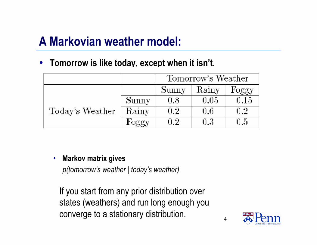
A Markovian weather model: •  Tomorrow is like today, except when it isn’t.

•  Markov matrix gives p(tomorrow’s weather | today’s weather)

4

If you start from any prior distribution over states (weathers) and run long enough you converge to a stationary distribution.

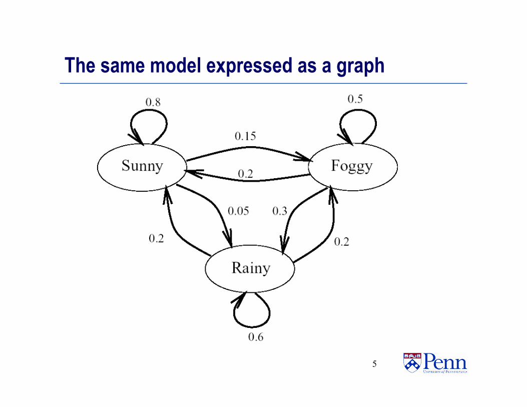
The same model expressed as a graph

5

6

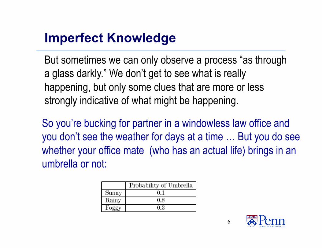
Imperfect Knowledge But sometimes we can only observe a process “as through a glass darkly.” We don’t get to see what is really happening, but only some clues that are more or less strongly indicative of what might be happening.

So you’re bucking for partner in a windowless law office and you don’t see the weather for days at a time … But you do see whether your office mate (who has an actual life) brings in an umbrella or not:

7

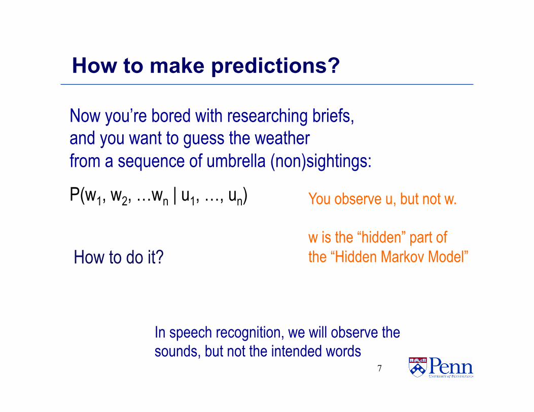
How to make predictions?

Now you’re bored with researching briefs, and you want to guess the weather from a sequence of umbrella (non)sightings:

P(w1, w2, …wn | u1, …, un)

How to do it?

You observe u, but not w. w is the “hidden” part of the “Hidden Markov Model”

In speech recognition, we will observe the sounds, but not the intended words

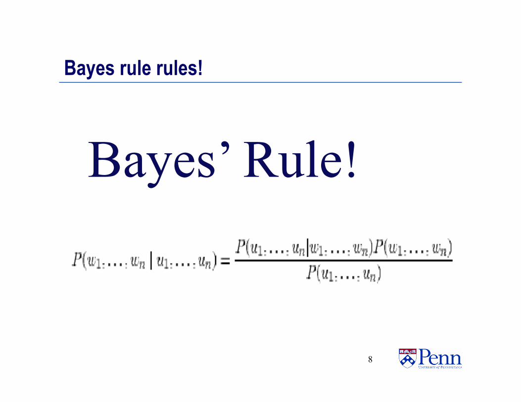
Bayes rule rules!

8

Bayes’ Rule!

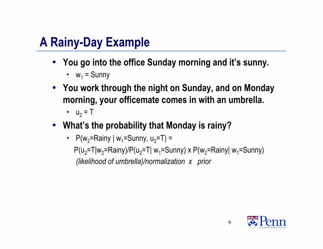
A Rainy-Day Example •  You go into the office Sunday morning and it’s sunny.

•  w1 = Sunny •  You work through the night on Sunday, and on Monday

morning, your officemate comes in with an umbrella. •  u2 = T

•  What’s the probability that Monday is rainy? •  P(w2=Rainy | w1=Sunny, u2=T) = P(u2=T|w2=Rainy)/P(u2=T| w1=Sunny) x P(w2=Rainy| w1=Sunny) (likelihood of umbrella)/normalization x prior

9

10

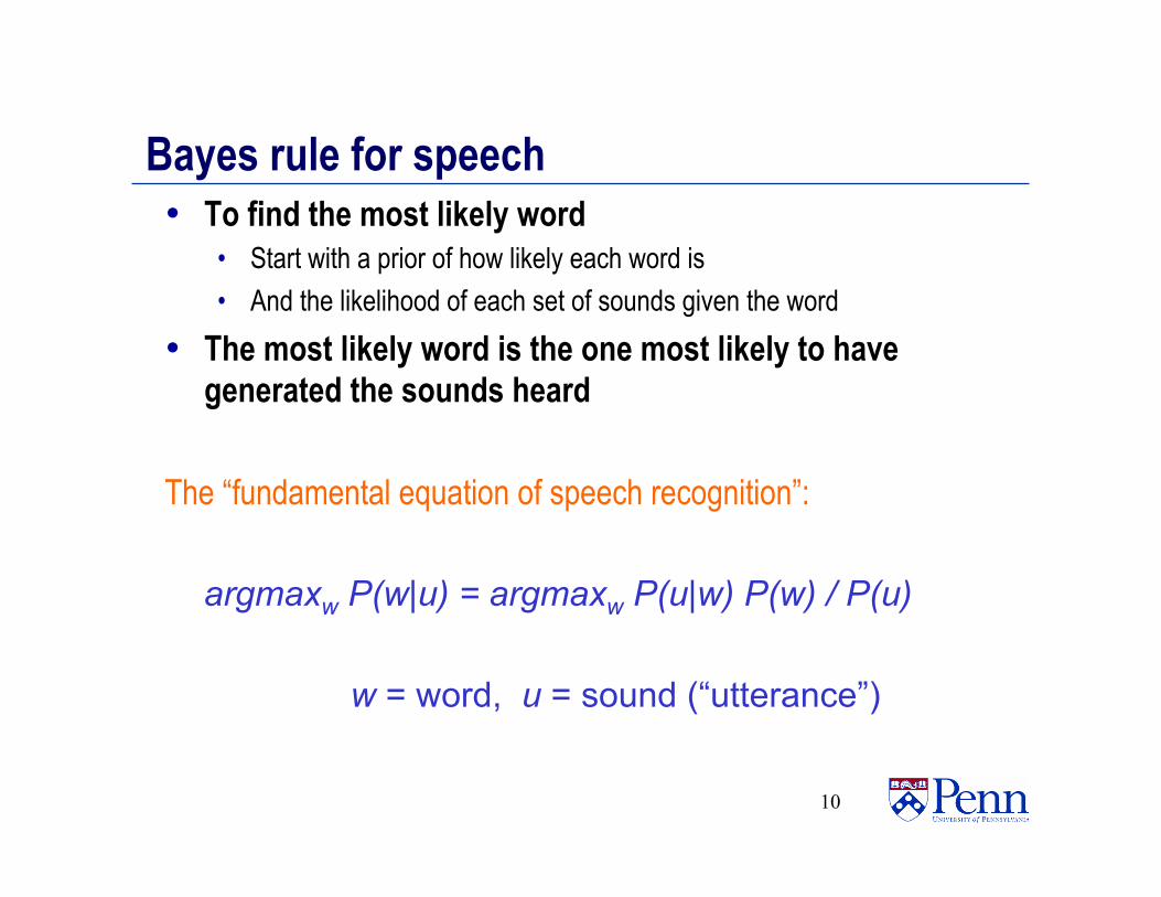
Bayes rule for speech •  To find the most likely word

•  Start with a prior of how likely each word is •  And the likelihood of each set of sounds given the word

•  The most likely word is the one most likely to have generated the sounds heard

The “fundamental equation of speech recognition”: argmaxw P(w|u) = argmaxw P(u|w) P(w) / P(u) w = word, u = sound (“utterance”)

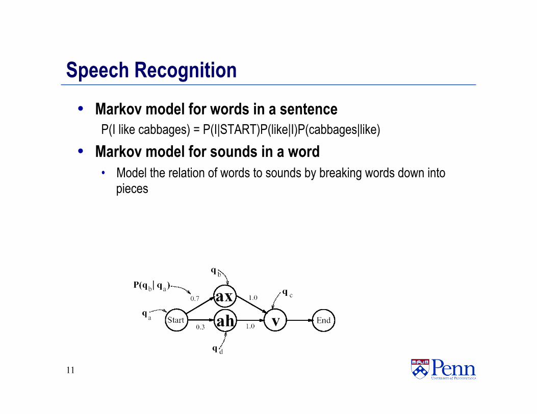
Speech Recognition •  Markov model for words in a sentence

P(I like cabbages) = P(I|START)P(like|I)P(cabbages|like) •  Markov model for sounds in a word

•  Model the relation of words to sounds by breaking words down into pieces

11

HMMs can also extract meaning •  Natural language is ambiguous

— “Banks banks in banks on banks.”

•  Sequence of hidden states are the “meanings” (what the word refers to) and words are the percepts

•  The (Markov) Language Model says how likely each meaning is to follow other meanings •  All meanings of “banks” may produce the same percept

12

HMMs: Midpoint Summary •  Language can be modeled by HMMs

•  Predict words from sounds •  Captures priors on words •  Hierarchical

— Phonemes to morphemes to words to phrases to sentences •  Was used in all commercial speech recognition software until recently

— Rapidly being replaced by deep networks

•  Markov assumption, HMM definition •  “Fundamental equation of speech recognition”

13

Hidden Markov Models (HMMs)

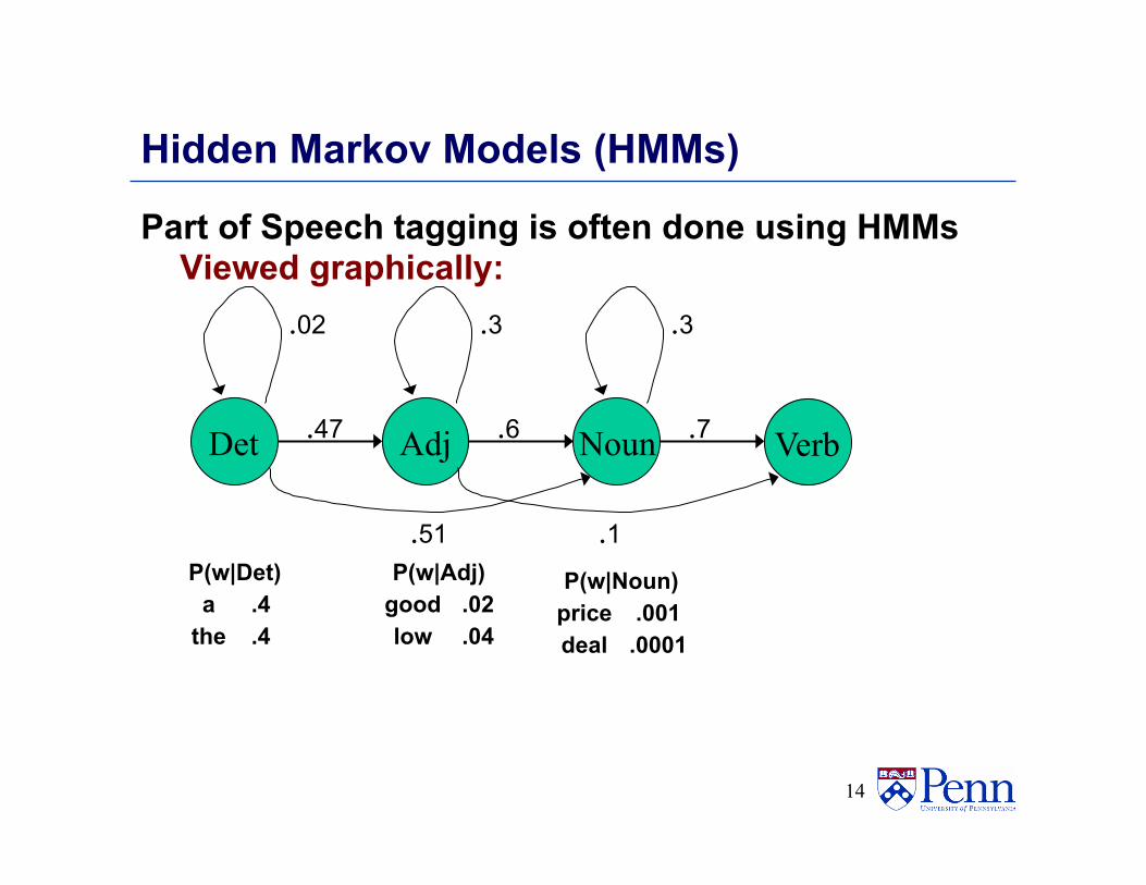
Part of Speech tagging is often done using HMMs Viewed graphically:

14

Adj

.3

.6 Det

.02

.47 Noun

.3

.7 Verb

.51 .1 P(w|Det)

a .4 the .4

P(w|Adj) good .02 low .04

P(w|Noun) price .001 deal .0001

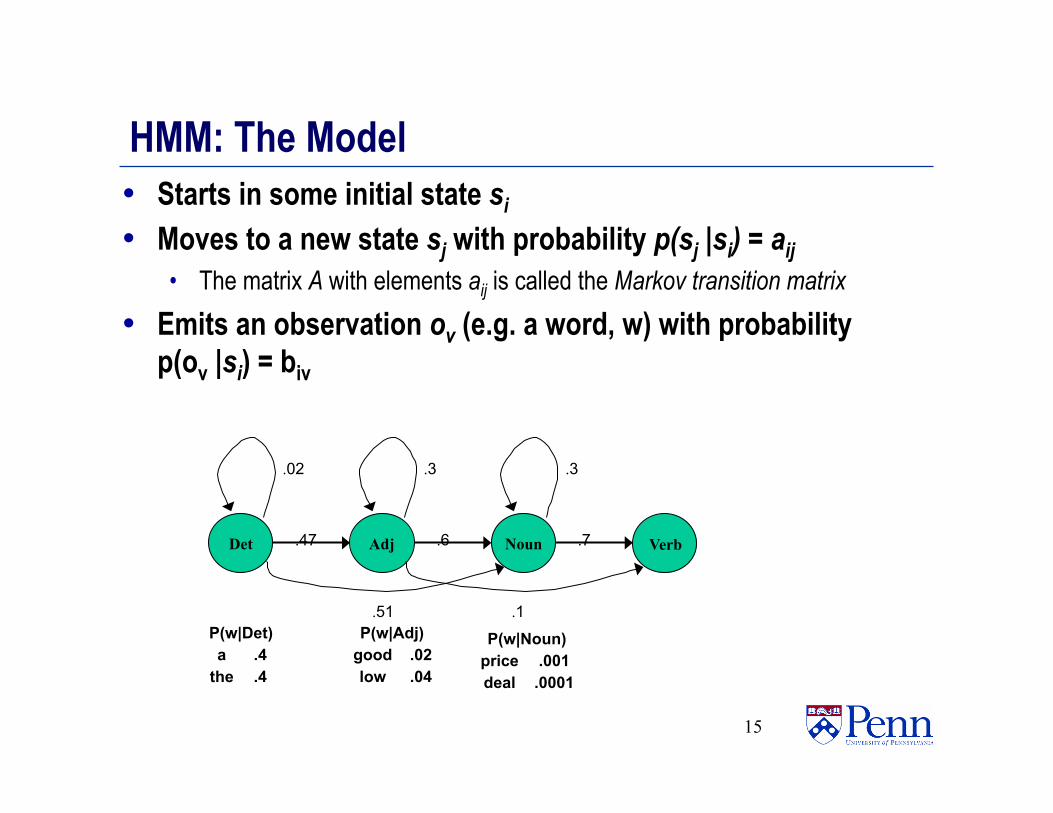
HMM: The Model •  Starts in some initial state si •  Moves to a new state sj with probability p(sj |si) = aij

•  The matrix A with elements aij is called the Markov transition matrix

•  Emits an observation ov (e.g. a word, w) with probability p(ov |si) = biv

15

Adj

.3

.6 Det

.02

.47 Noun

.3

.7 Verb

.51 .1

.4 the

.4 a P(w|Det)

.04 low

.02 good P(w|Adj)

.0001 deal .001 price

P(w|Noun)

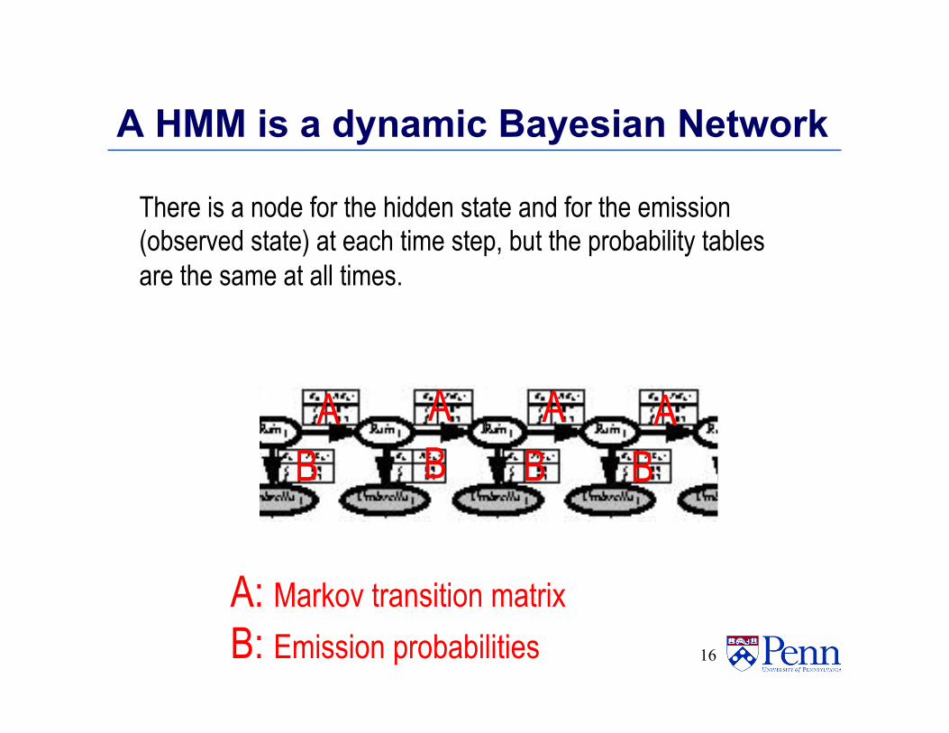
A HMM is a dynamic Bayesian Network

16

There is a node for the hidden state and for the emission (observed state) at each time step, but the probability tables are the same at all times.

A B

A: Markov transition matrix B: Emission probabilities

A A A B B B

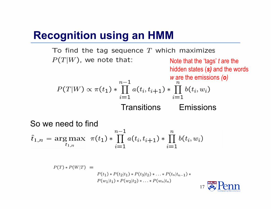
Recognition using an HMM

17

So we need to find

Transitions Emissions

Note that the ‘tags’ t are the hidden states (s) and the words w are the emissions (o)

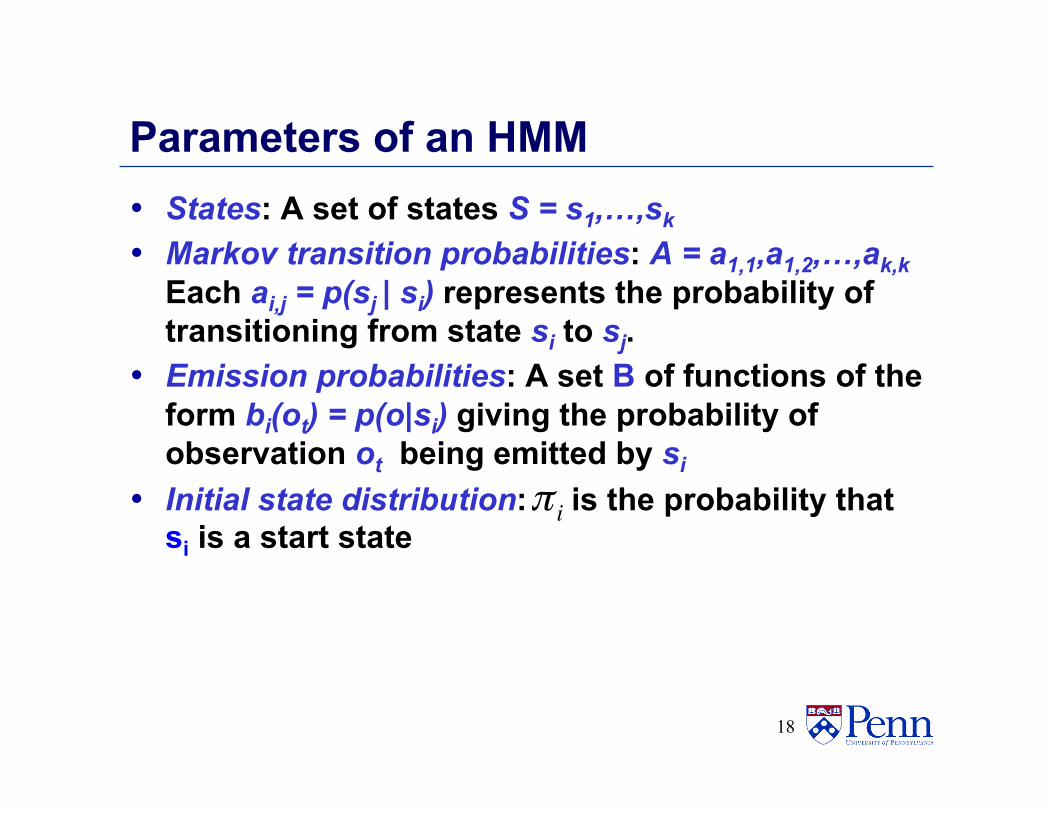
Parameters of an HMM •  States: A set of states S = s1,…,sk •  Markov transition probabilities: A = a1,1,a1,2,…,ak,k

Each ai,j = p(sj | si) represents the probability of transitioning from state si to sj.

•  Emission probabilities: A set B of functions of the form bi(ot) = p(o|si) giving the probability of observation ot being emitted by si

•  Initial state distribution: is the probability that si is a start state

18

π i

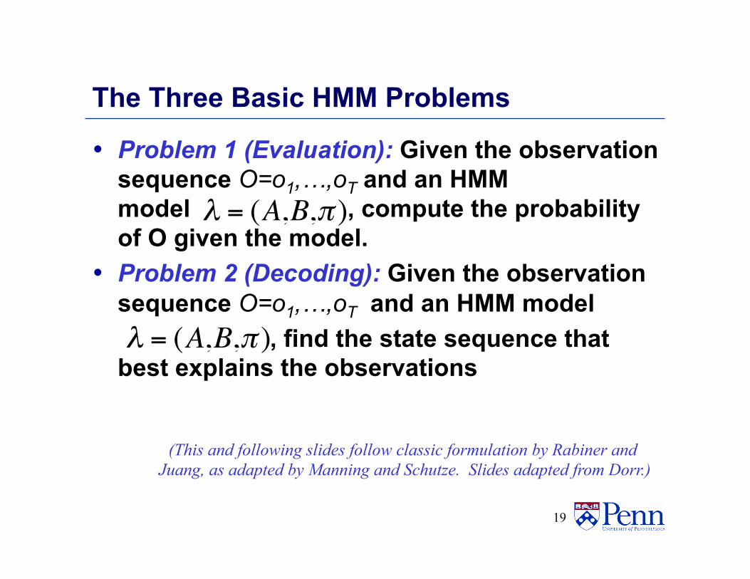
The Three Basic HMM Problems •  Problem 1 (Evaluation): Given the observation

sequence O=o1,…,oT and an HMM model , compute the probability of O given the model.

•  Problem 2 (Decoding): Given the observation sequence O=o1,…,oT and an HMM model

, find the state sequence that best explains the observations

19

€

λ = (A,B,π )

€

λ = (A,B,π )

(This and following slides follow classic formulation by Rabiner and Juang, as adapted by Manning and Schutze. Slides adapted from Dorr.)

The Three Basic HMM Problems

•  Problem 3 (Learning): Pick the model parameters to maximize

20

€

λ = (A,B,π )

€

P(O | λ)

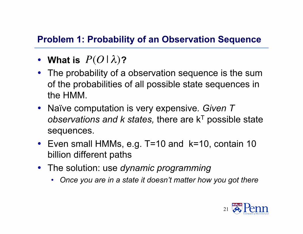
Problem 1: Probability of an Observation Sequence

•  What is ? •  The probability of a observation sequence is the sum

of the probabilities of all possible state sequences in the HMM.

•  Naïve computation is very expensive. Given T observations and k states, there are kT possible state sequences.

•  Even small HMMs, e.g. T=10 and k=10, contain 10 billion different paths

•  The solution: use dynamic programming •  Once you are in a state it doesn’t matter how you got there

21

€

P(O | λ)

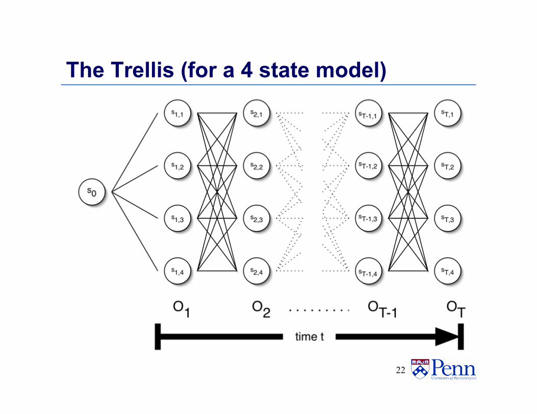
The Trellis (for a 4 state model)

22

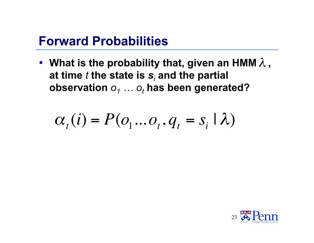
Forward Probabilities •  What is the probability that, given an HMM ,

at time t the state is si and the partial observation o1 … ot has been generated?

23

€

α t (i) = P(o1...ot , qt = si | λ)€

λ

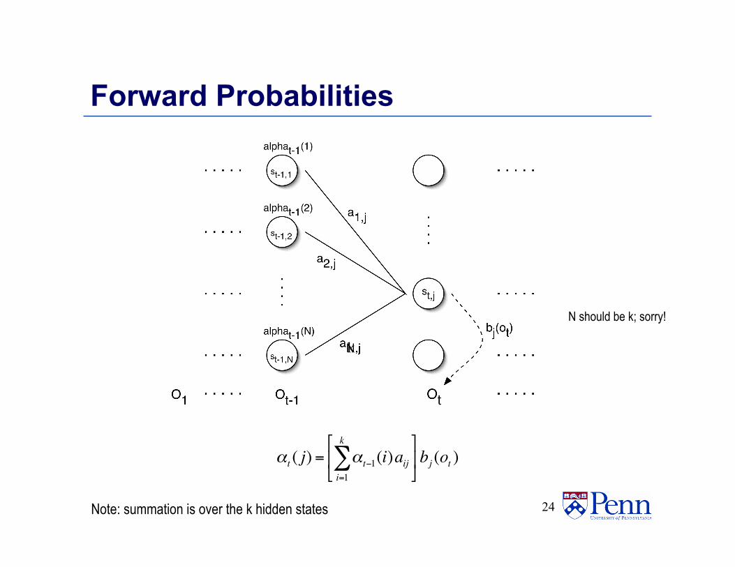
Forward Probabilities

24

αt ( j) = αt−1(i)aiji=1

k

∑#

$%

&

'( bj (ot )

€

α t (i) = P(o1...ot , qt = si | λ)

Note: summation is over the k hidden states

N should be k; sorry!

k

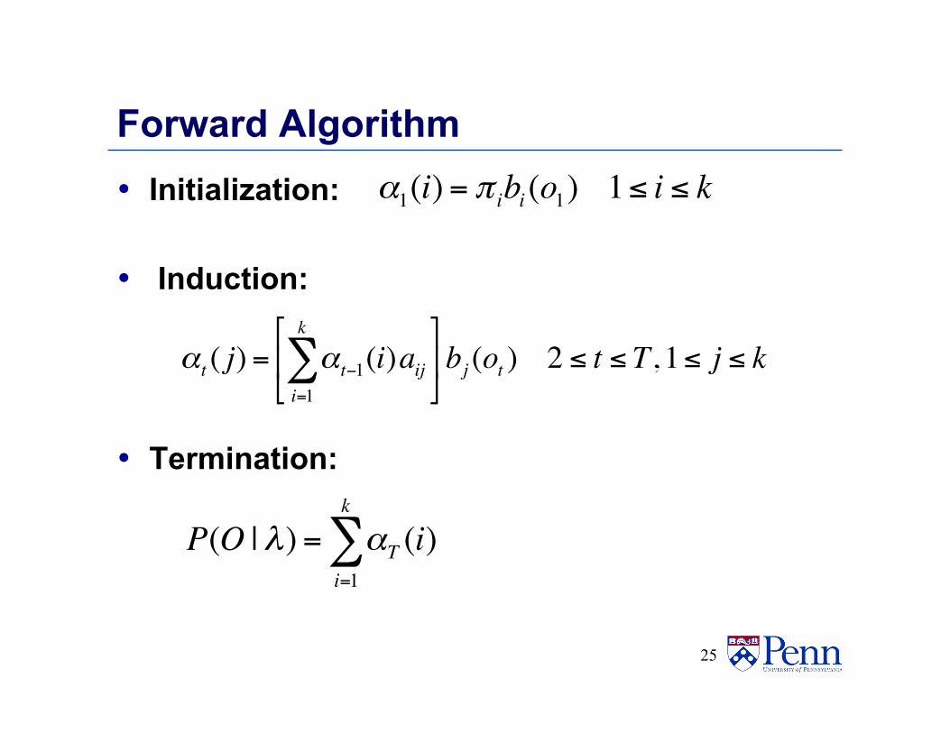
Forward Algorithm •  Initialization:

•  Induction:

•  Termination:

25

αt ( j) = αt−1(i)aiji=1

k

∑#

$%

&

'( bj (ot ) 2 ≤ t ≤ T, 1≤ j ≤ k

α1(i) = π ibi (o1) 1≤ i ≤ k

P(O | λ) = αT (i)i=1

k

∑

Forward Algorithm Complexity •  Naïve approach takes O(2T*kT) computation •  Forward algorithm using dynamic programming

takes O(k2T) computations

26

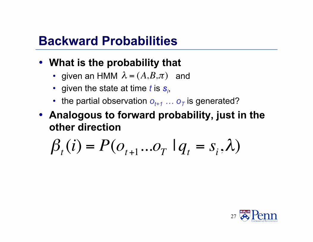
Backward Probabilities •  What is the probability that

•  given an HMM and •  given the state at time t is si, •  the partial observation ot+1 … oT is generated?

•  Analogous to forward probability, just in the other direction

27 €

βt (i) = P(ot+1...oT |qt = si,λ)

€

λ = (A,B,π )

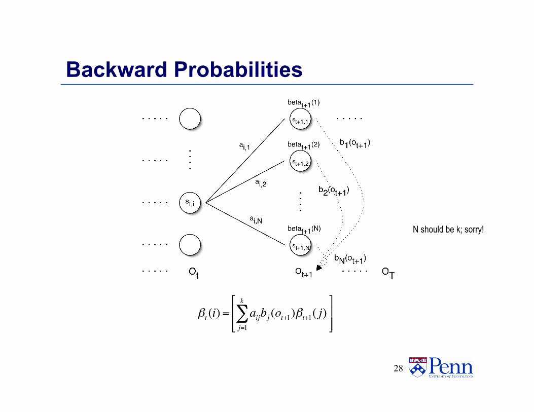
Backward Probabilities

28

βt (i) = aijbj (ot+1)βt+1( j)j=1

k

∑"

#$$

%

&''

€

βt (i) = P(ot+1...oT |qt = si,λ)

N should be k; sorry!

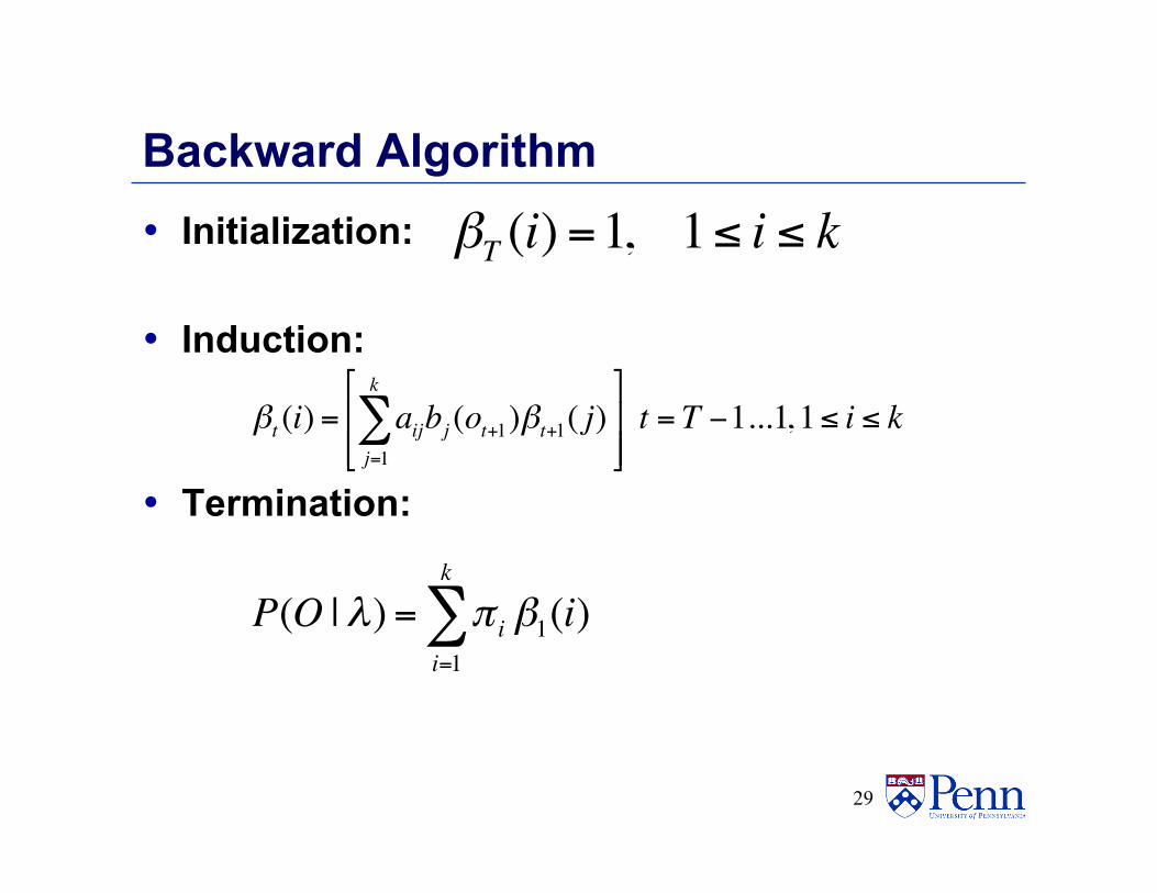
Backward Algorithm •  Initialization:

•  Induction:

•  Termination:

29

βT (i) =1, 1≤ i ≤ k

βt (i) = aijbj (ot+1)βt+1( j)j=1

k

∑"

#$$

%

&''t = T −1...1, 1≤ i ≤ k

P(O | λ) = π i β1(i)i=1

k

∑

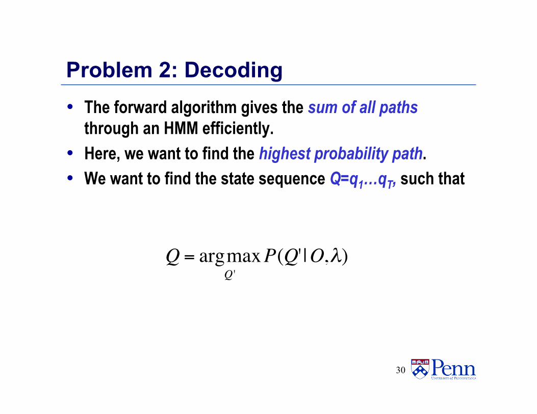
Problem 2: Decoding •  The forward algorithm gives the sum of all paths

through an HMM efficiently. •  Here, we want to find the highest probability path. •  We want to find the state sequence Q=q1…qT, such that

30 €

Q = argmaxQ '

P(Q' |O,λ)

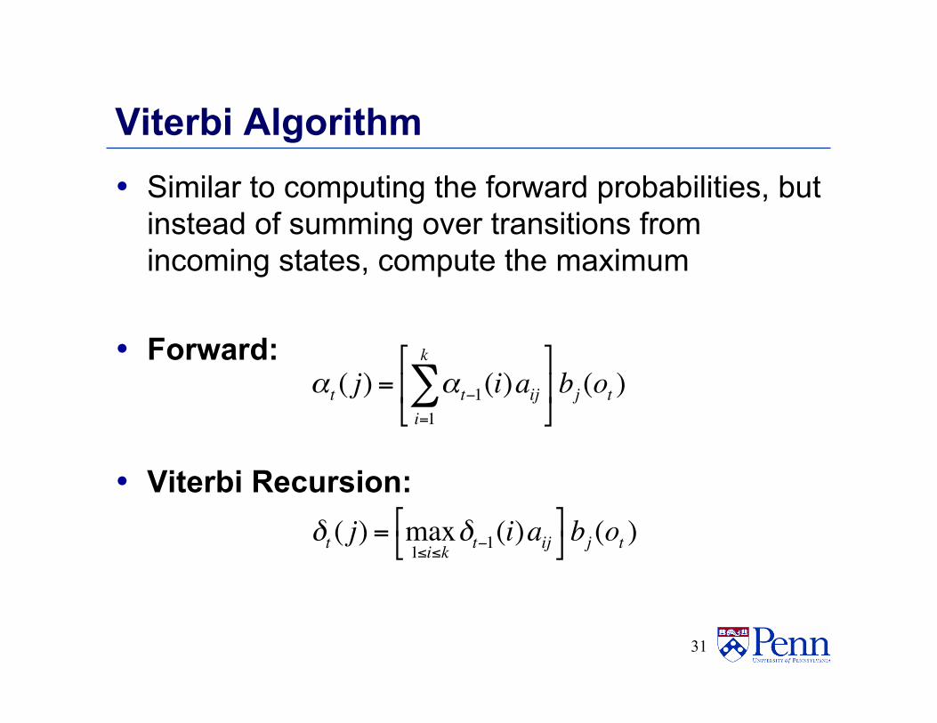
Viterbi Algorithm •  Similar to computing the forward probabilities, but

instead of summing over transitions from incoming states, compute the maximum

•  Forward:

•  Viterbi Recursion:

31

αt ( j) = αt−1(i)aiji=1

k

∑#

$%

&

'( bj (ot )

δt ( j) = max1≤i≤k

δt−1(i)aij#$

%& bj (ot )

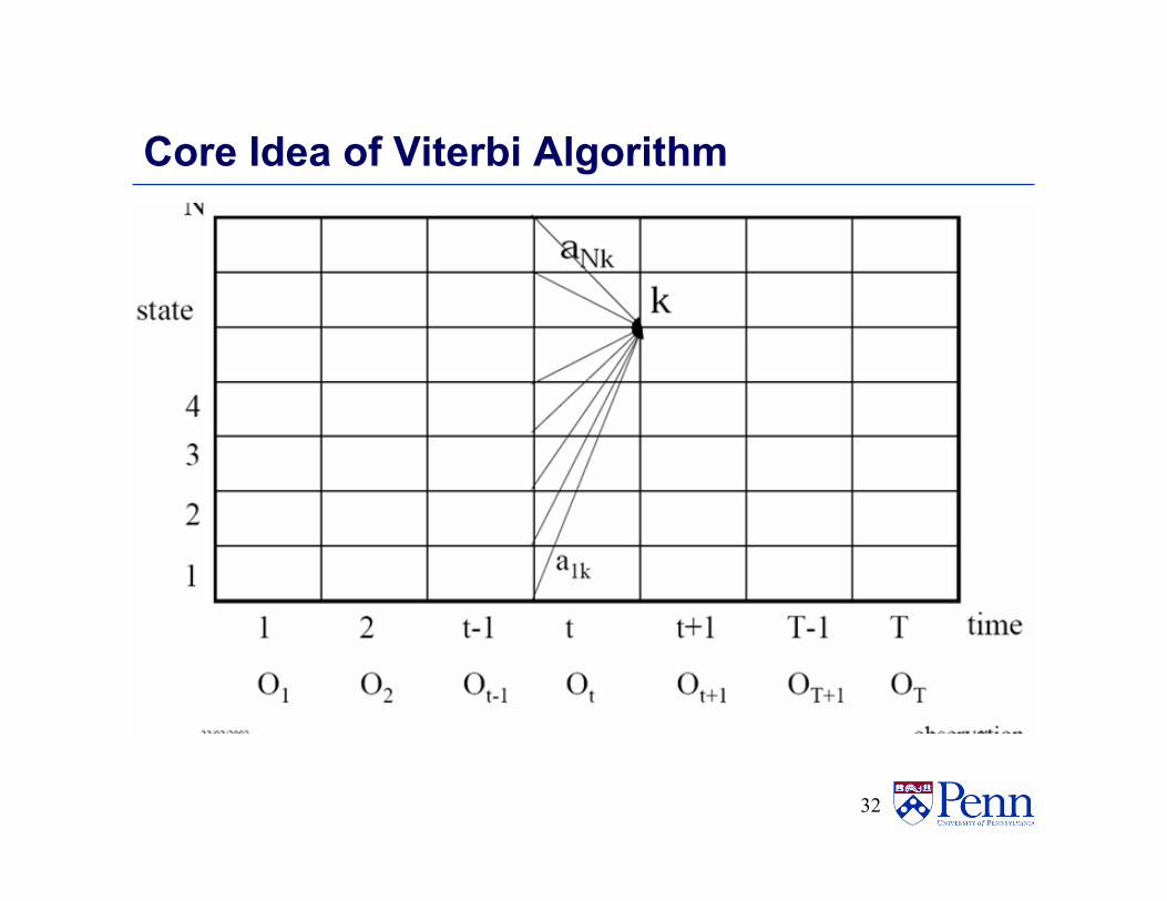
Core Idea of Viterbi Algorithm

32

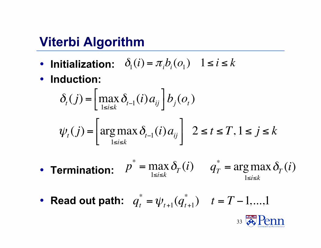
Viterbi Algorithm •  Initialization: •  Induction:

•  Termination:

•  Read out path:

33

δ1(i) = π ibi (o1) 1≤ i ≤ k

δt ( j) = max1≤i≤k

δt−1(i)aij#$

%& bj (ot )

ψt ( j) = argmax1≤i≤k

δt−1(i)aij#$%

&'(2 ≤ t ≤ T, 1≤ j ≤ k

p* =max1≤i≤k

δT (i) qT* = argmax

1≤i≤kδT (i)

€

qt* =ψt+1(qt+1

* ) t = T −1,...,1

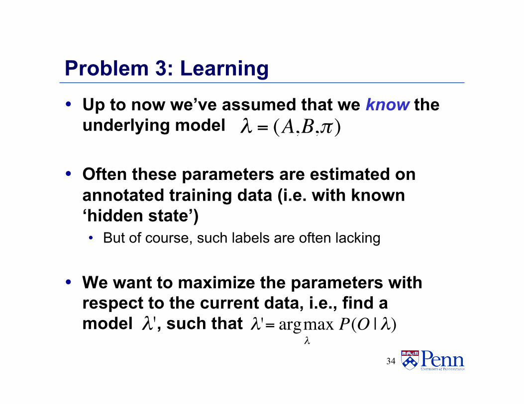
Problem 3: Learning •  Up to now we’ve assumed that we know the

underlying model

•  Often these parameters are estimated on annotated training data (i.e. with known ‘hidden state’) •  But of course, such labels are often lacking

•  We want to maximize the parameters with respect to the current data, i.e., find a model , such that

34

€

λ = (A,B,π )

€

λ'

€

λ'= argmaxλ

P(O | λ)

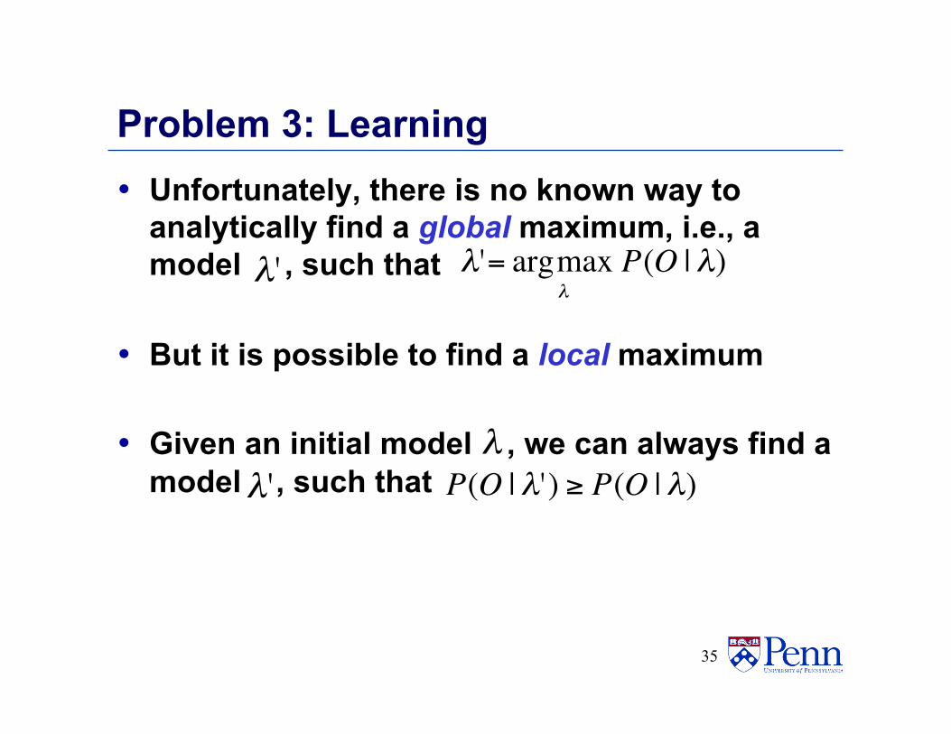
Problem 3: Learning •  Unfortunately, there is no known way to

analytically find a global maximum, i.e., a model , such that

•  But it is possible to find a local maximum

•  Given an initial model , we can always find a model , such that

35

€

λ'

€

λ'= argmaxλ

P(O | λ)

€

λ

€

λ'

€

P(O | λ') ≥ P(O | λ)

Forward-Backward (Baum-Welch) algorithm •  EM algorithm

•  Find the forward and backward probabilities for the current parameters

•  Re-estimate the model parameters given the estimated probabilities

•  Repeat

36

Parameter Re-estimation •  Three parameters need to be re-estimated:

•  Initial state distribution: •  Transition probabilities: ai,j •  Emission probabilities: bi(ot)

37

€

π i

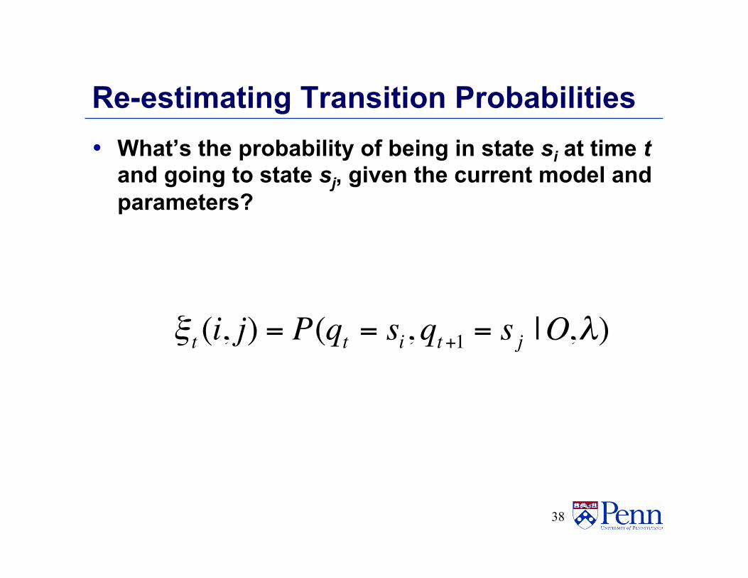
Re-estimating Transition Probabilities •  What’s the probability of being in state si at time t

and going to state sj, given the current model and parameters?

38

€

ξ t (i, j) = P(qt = si, qt+1 = s j |O,λ)

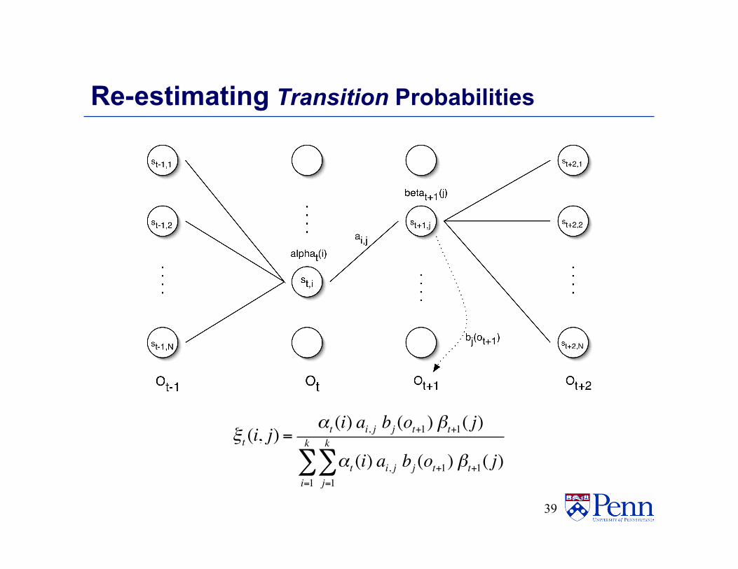
Re-estimating Transition Probabilities

39

ξt (i, j) =αt (i) ai, j bj (ot+1) βt+1( j)

αt (i) ai, j bj (ot+1) βt+1( j)j=1

k

∑i=1

k

∑

€

ξ t (i, j) = P(qt = si, qt+1 = s j |O,λ)

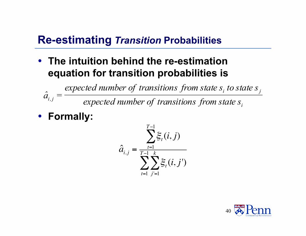
Re-estimating Transition Probabilities

•  The intuition behind the re-estimation equation for transition probabilities is

•  Formally:

40

i

jij,i s statefrom stransition of number expected

s stateto s statefrom stransition of number expecteda =

ai, j =ξt (i, j)

t=1

T−1

∑

ξt (i, j ')j '=1

k

∑t=1

T−1

∑

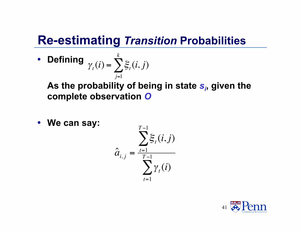
Re-estimating Transition Probabilities •  Defining

As the probability of being in state si, given the complete observation O

•  We can say:

41

€

ˆ a i, j =

ξ t (i, j)t=1

T−1

∑

γ t (i)t=1

T−1

∑

γ t (i) = ξt (i, j)j=1

k

∑

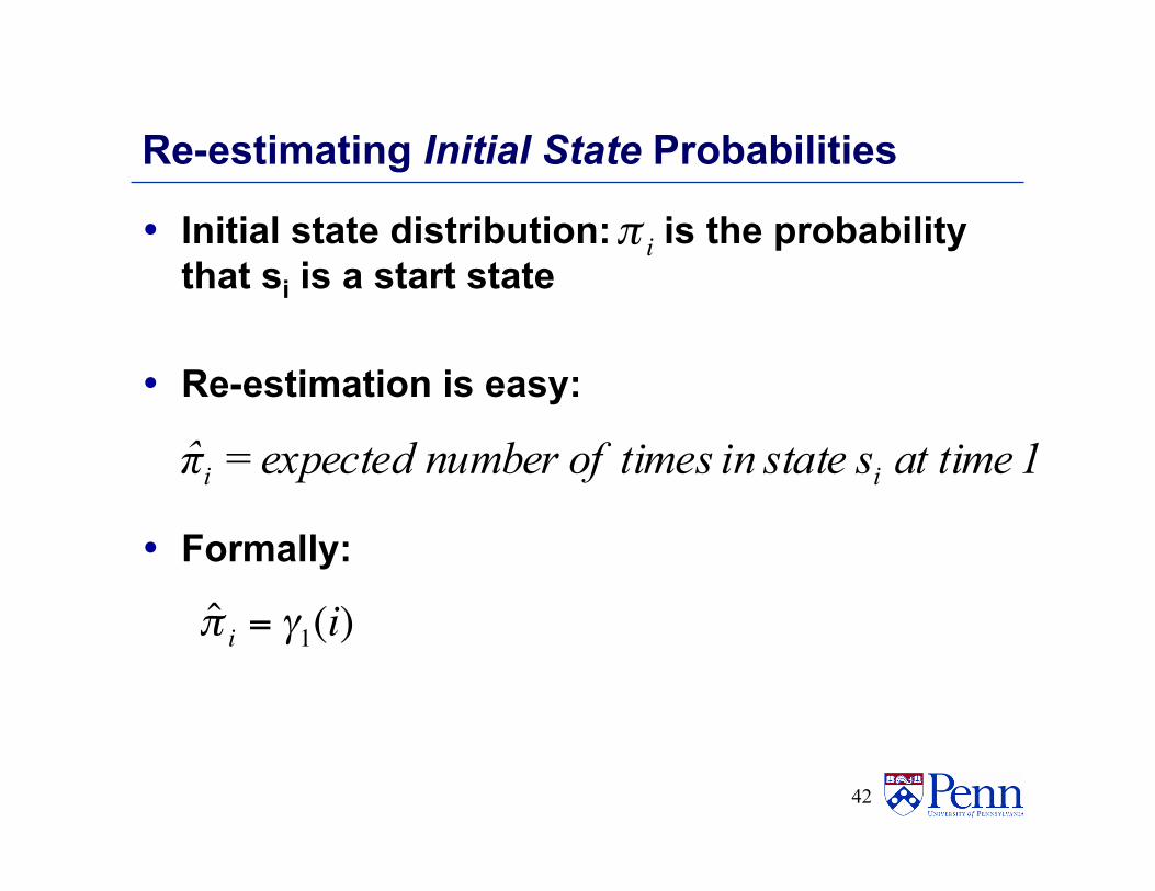
Re-estimating Initial State Probabilities •  Initial state distribution: is the probability

that si is a start state

•  Re-estimation is easy:

•  Formally:

42

€

π i

1 time at s statein times of number expectedπ ii =

€

ˆ π i = γ1(i)

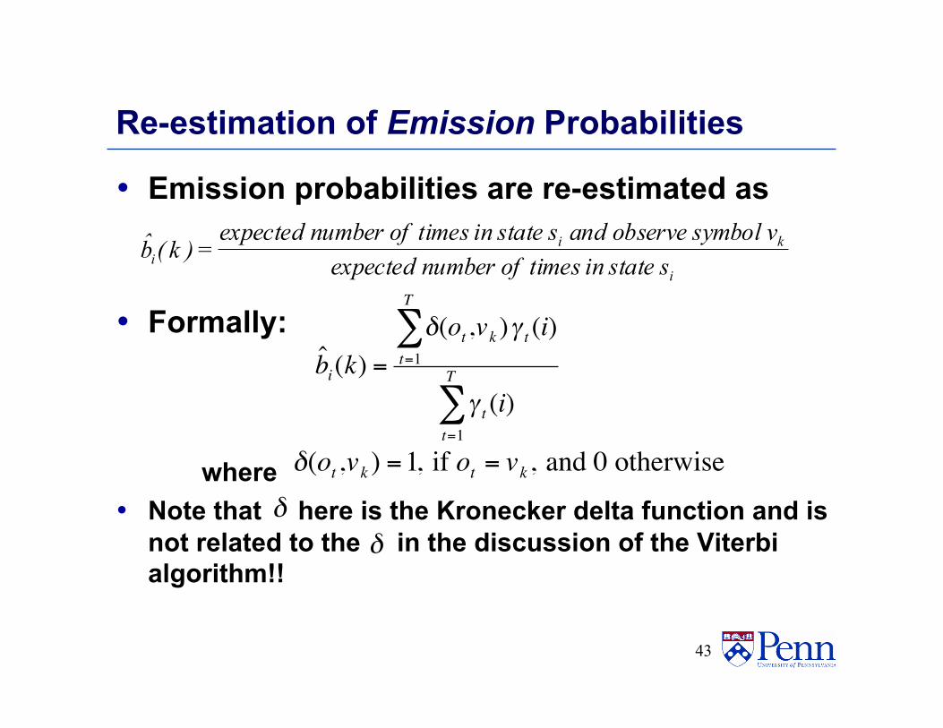
Re-estimation of Emission Probabilities •  Emission probabilities are re-estimated as

•  Formally:

where •  Note that here is the Kronecker delta function and is

not related to the in the discussion of the Viterbi algorithm!!

43

i

kii s statein times of number expected

v symbolobserve and s statein times of number expected)k(b =

€

ˆ b i(k) =

δ(ot ,vk )γ t (i)t=1

T

∑

γ t (i)t=1

T

∑

€

δ(ot ,vk ) =1, if ot = vk, and 0 otherwise

€

δ

€

δ

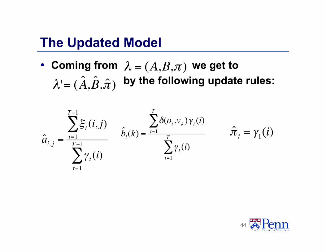
The Updated Model •  Coming from we get to by the following update rules:

44

€

λ = (A,B,π )

€

λ'= ( ˆ A , ˆ B , ˆ π )

€

ˆ b i(k) =

δ(ot ,vk )γ t (i)t=1

T

∑

γ t (i)t=1

T

∑

€

ˆ a i, j =

ξ t (i, j)t=1

T−1

∑

γ t (i)t=1

T−1

∑

€

ˆ π i = γ1(i)

HMM vs CRF •  HMMs are generative models

•  They model the full probability distribution

•  Conditional Random Fields are discriminative •  Similar to HMMs, but only model the probability of labels

given the data •  Generally give more accurate predictions •  A bit harder to code

— But good open source versions are available •  Very popular in the research world (until deep nets arrived)

45

What you should know •  HMMs

•  Markov assumption •  Markov transition matrix, Emission probabilities •  Viterbi decoding (just well enough to do the homework)

46