Embed Size (px)
Citation preview

Hidden Markov Models (HMMs)
Steven SalzbergCMSC 828H, Univ. of Maryland Fall 2010
S. Salzberg CMSC 828H
2
What are HMMs used for? Real time continuous speech recognition
(HMMs are the basis for all the leading products)
Eukaryotic and prokaryotic gene finding (HMMs are the basis of GENSCAN, Genie, VEIL, GlimmerHMM, TwinScan, etc.)
Multiple sequence alignment Identification of sequence motifs Prediction of protein structure
S. Salzberg CMSC 828H
3
What is an HMM? Essentially, an HMM is just
A set of states A set of transitions between states
Transitions have A probability of taking a transition (moving from
one state to another) A set of possible outputs Probabilities for each of the outputs
Equivalently, the output distributions can be attached to the states rather than the transitions
S. Salzberg CMSC 828H
4
HMM notation The set of all states: {s} Initial states: SI
Final states: SF
Probability of making the transition from state i to j: aij
A set of output symbols Probability of emitting the symbol k
while making the transition from state i to j: bij(k)
S. Salzberg CMSC 828H
5
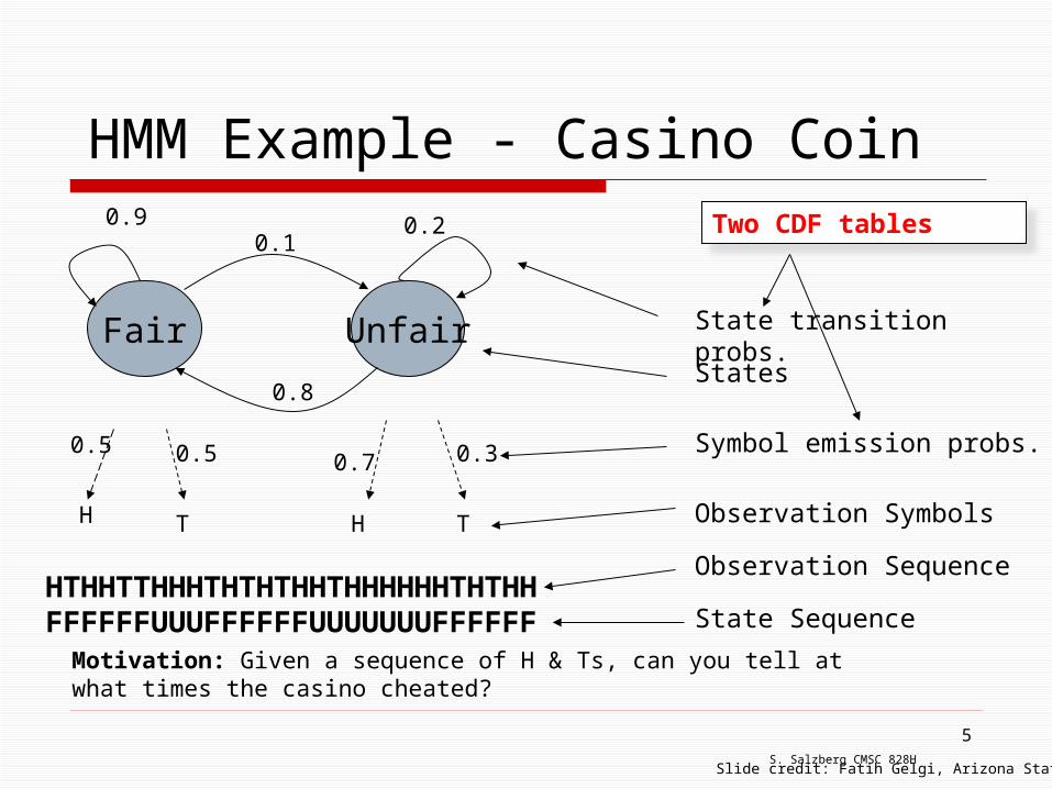
HMM Example - Casino Coin
Fair Unfair
0.9 0.2
0.8
0.1
0.30.5 0.5 0.7
H HT T
State transition probs.
Symbol emission probs.
HTHHTTHHHTHTHTHHTHHHHHHTHTHHObservation Sequence
FFFFFFUUUFFFFFFUUUUUUUFFFFFF State Sequence
Motivation: Given a sequence of H & Ts, can you tell at what times the casino cheated?
Observation Symbols
States
Two CDF tables
Slide credit: Fatih Gelgi, Arizona State U.
S. Salzberg CMSC 828H
6
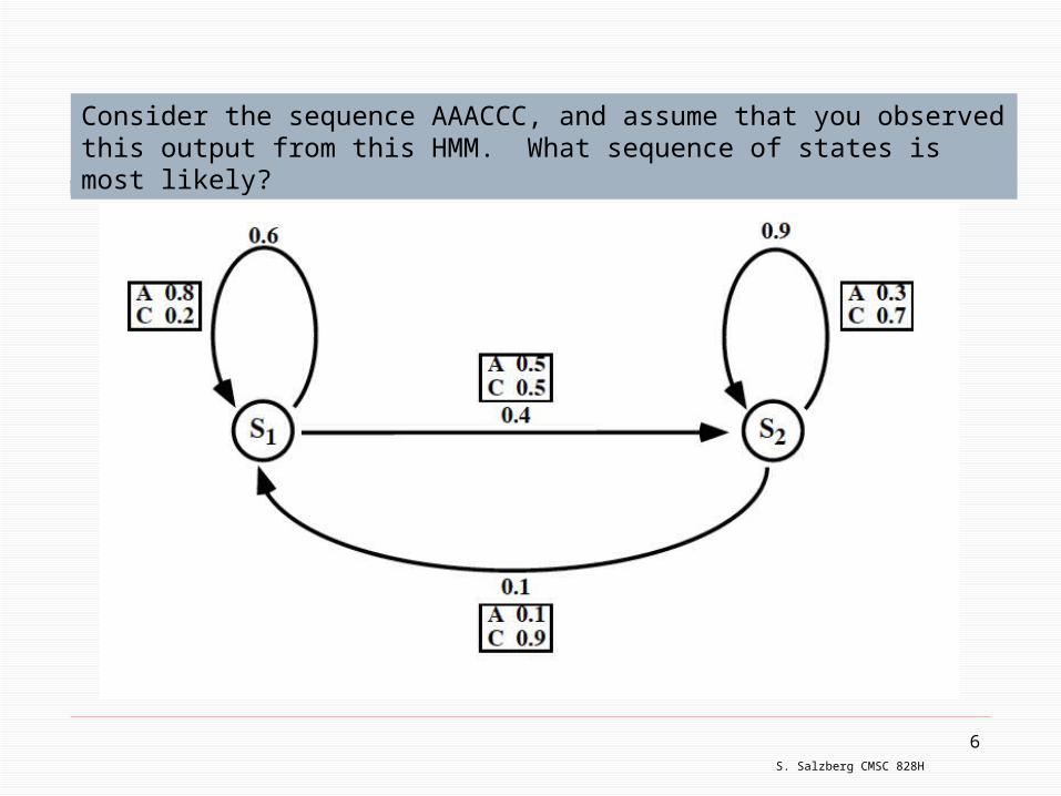
HMM example: DNAConsider the sequence AAACCC, and assume that you observed this output from this HMM. What sequence of states is most likely?
S. Salzberg CMSC 828H
7
Properties of an HMM
First-order Markov process st only depends on st-1
However, note that probability distributions may contain conditional probabilities
Time is discrete
Slide credit: Fatih Gelgi, Arizona State U.
S. Salzberg CMSC 828H
8
Three classic HMM problems1. Evaluation: given a model and an output
sequence, what is the probability that the model generated that output?
To answer this, we consider all possible paths through the model
A solution to this problem gives us a way of scoring the match between an HMM and an observed sequence
Example: we might have a set of HMMs representing protein families
S. Salzberg CMSC 828H
9
Three classic HMM problems2. Decoding: given a model and an output
sequence, what is the most likely state sequence through the model that generated the output?
A solution to this problem gives us a way to match up an observed sequence and the states in the model.
In gene finding, the states correspond to sequence features such as start codons, stop codons, and splice sites
S. Salzberg CMSC 828H
10
Three classic HMM problems3. Learning: given a model and a set of
observed sequences, how do we set the model’s parameters so that it has a high probability of generating those sequences?
This is perhaps the most important, and most difficult problem.
A solution to this problem allows us to determine all the probabilities in an HMMs by using an ensemble of training data
S. Salzberg CMSC 828H
11
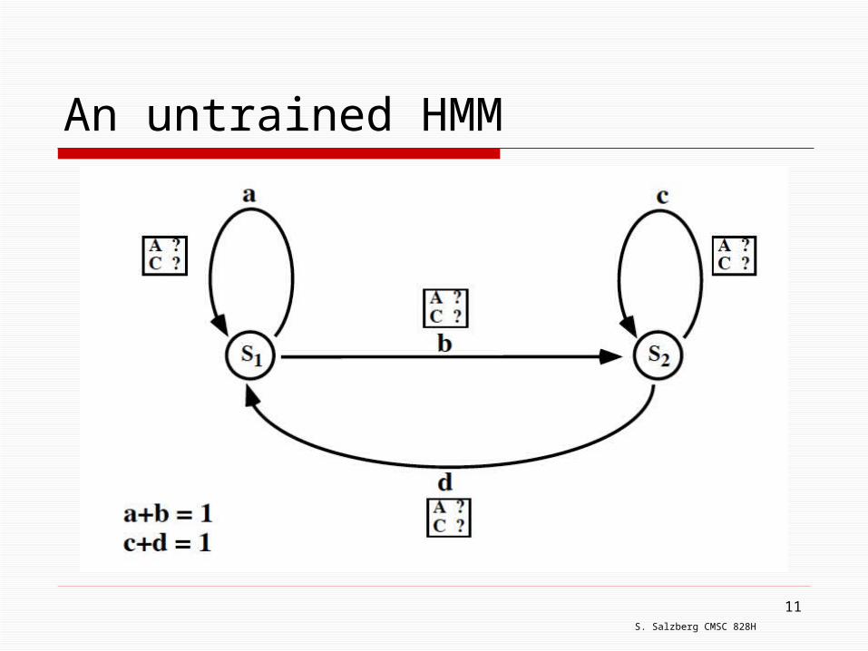
An untrained HMM

S. Salzberg CMSC 828H
12
Basic facts about HMMs (1)
The sum of the probabilities on all the edges leaving a state is 1
€
aij =1j
∑… for any given state j
S. Salzberg CMSC 828H
13
Basic facts about HMMs (2)
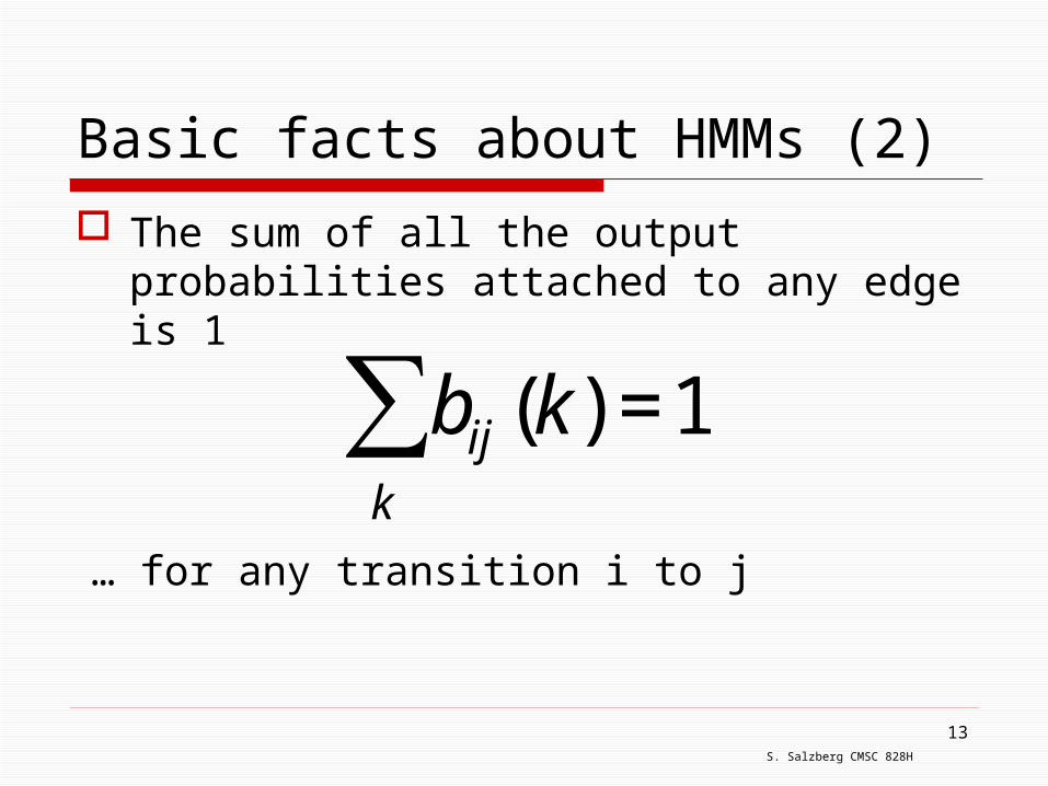
The sum of all the output probabilities attached to any edge is 1
€
bij (k) =1k
∑… for any transition i to j
S. Salzberg CMSC 828H
14
Basic facts about HMMs (3)
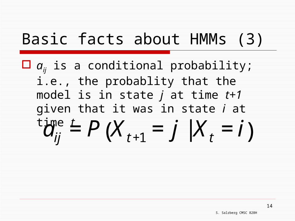
aij is a conditional probability; i.e., the probablity that the model is in state j at time t+1 given that it was in state i at time t
€
aij = P X t+1 = j | X t = i( )
S. Salzberg CMSC 828H
15
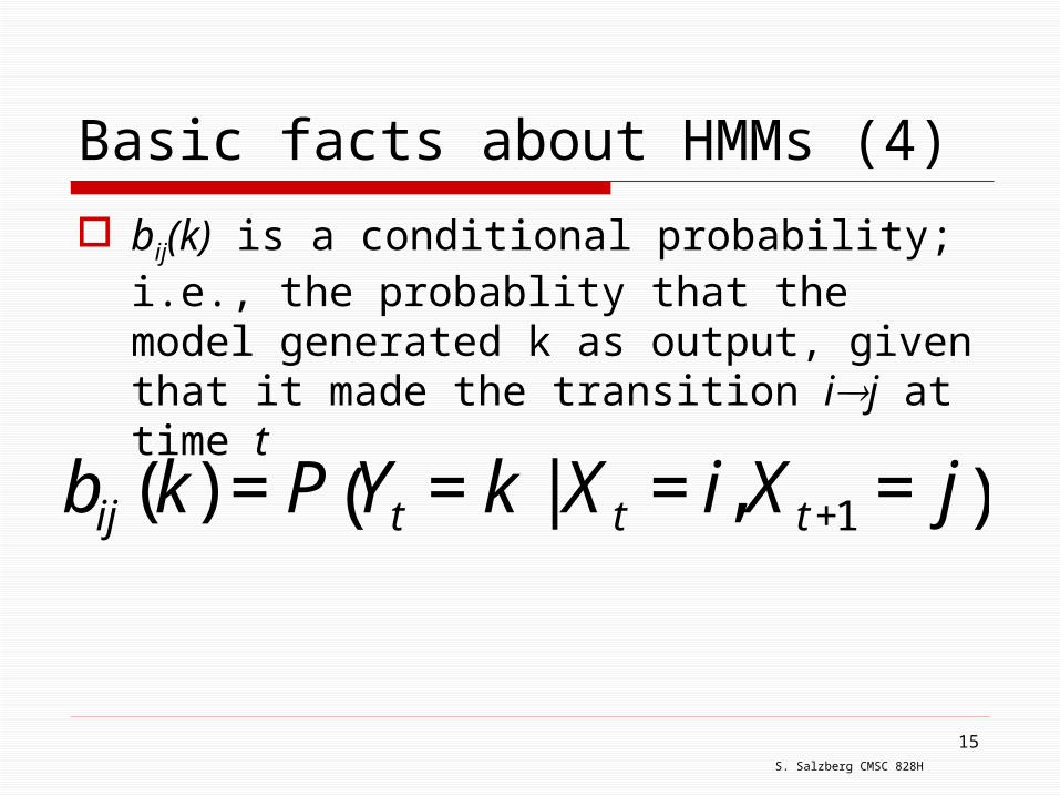
Basic facts about HMMs (4)
bij(k) is a conditional probability; i.e., the probablity that the model generated k as output, given that it made the transition ij at time t
€
bij (k) = P Yt = k | X t = i,X t+1 = j( )
S. Salzberg CMSC 828H
16
Why are these Markovian? Probability of taking a transition depends only
on the current state This is sometimes called the Markov assumption
Probability of generating Y as output depends only on the transition ij, not on previous outputs This is sometimes called the output independence
assumption Computationally it is possible to simulate an
nth order HMM using a 0th order HMM This is how some actual gene finders (e.g., VEIL)
work
S. Salzberg CMSC 828H
17
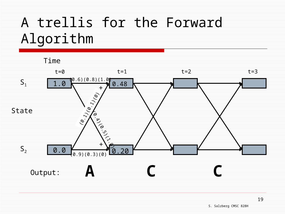
Solving the Evaluation problem: the Forward algorithm To solve the Evaluation problem, we use the
HMM and the data to build a trellis Filling in the trellis will give tell us the
probability that the HMM generated the data by finding all possible paths that could do it
S. Salzberg CMSC 828H
18
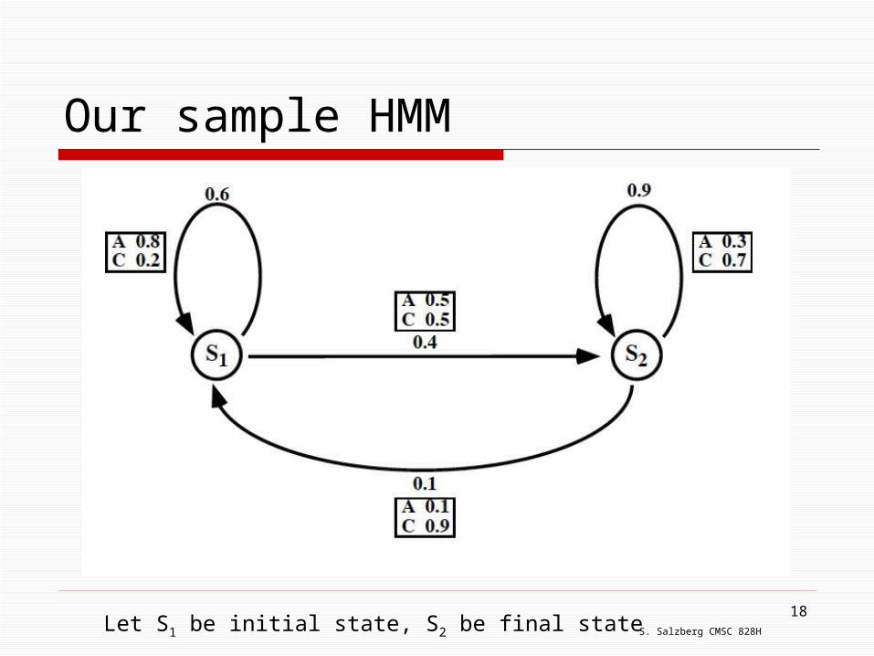
Our sample HMM
Let S1 be initial state, S2 be final state
S. Salzberg CMSC 828H
19
A trellis for the Forward Algorithm
State
1.0
0.0
S1
S2
Time
t=0 t=2 t=3t=1
Output: A CC
(0.6)(0.8)(1.0)
(0.4)(0.5)(1.0)
(0.1
)(0.
1)(0
)
(0.9)(0.3)(0)
+
+
0.48
0.20
S. Salzberg CMSC 828H
20
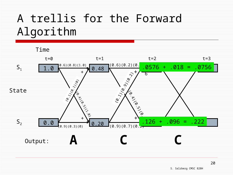
A trellis for the Forward Algorithm
State
1.0
0.0
S1
S2
Time
t=0 t=2 t=3t=1
Output: A CC
(0.6)(0.8)(1.0)
(0.4)(0.5)(1.0)
(0.1
)(0.
1)(0
)
(0.9)(0.3)(0)
+
+
0.48
0.20
(0.6)(0.2)(0.48)
(0.4)(0.5)(0.48)
(0.1
)(0.
9)(0
.2)
(0.9)(0.7)(0.2)
+
+
.0756
.222
.0576 + .018 = .0756
.126 + .096 = .222
S. Salzberg CMSC 828H
21
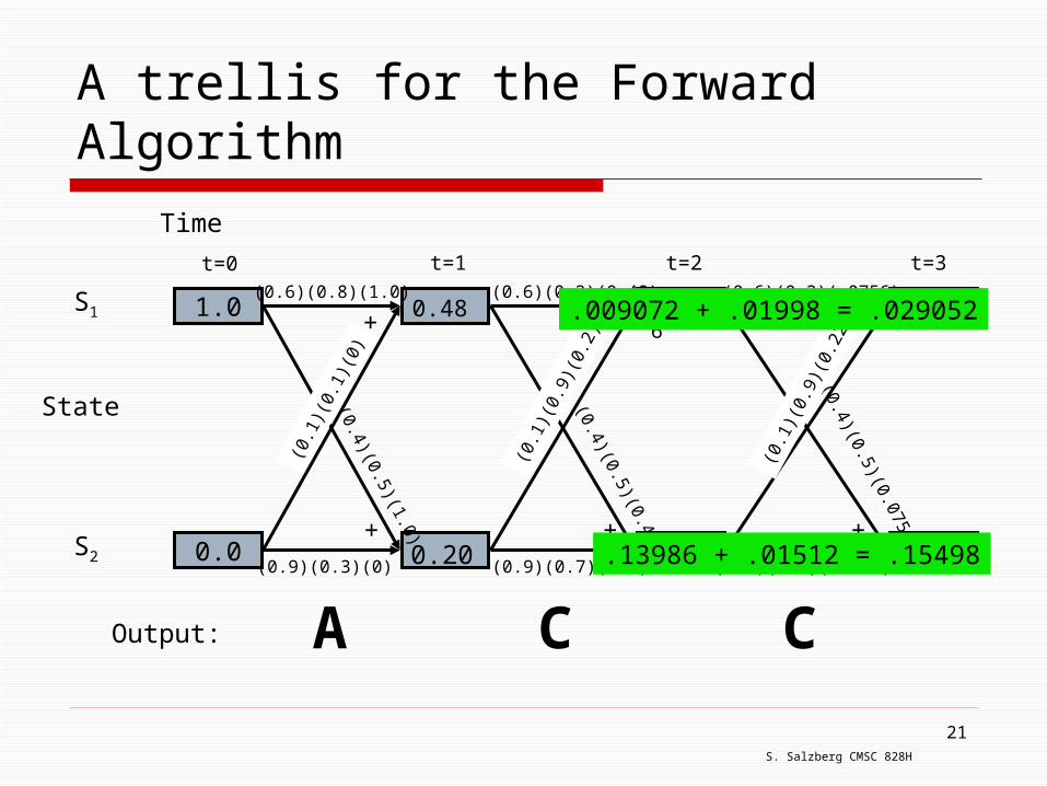
A trellis for the Forward Algorithm
State
1.0
0.0
S1
S2
Time
t=0 t=2 t=3t=1
Output: A CC
(0.6)(0.8)(1.0)
(0.4)(0.5)(1.0)
(0.1
)(0.
1)(0
)
(0.9)(0.3)(0)
+
+
0.48
0.20
(0.6)(0.2)(0.48)
(0.4)(0.5)(0.48)
(0.1
)(0.
9)(0
.2)
(0.9)(0.7)(0.2)
+
+
.0756
.222
(0.6)(0.2)(.0756)
(0.4)(0.5)(0.0756)
(0.1
)(0.
9)(0
.222
)
(0.9)(0.7)(0.222)
+
+
.029
.155
.009072 + .01998 = .029052
.13986 + .01512 = .15498
S. Salzberg CMSC 828H
22
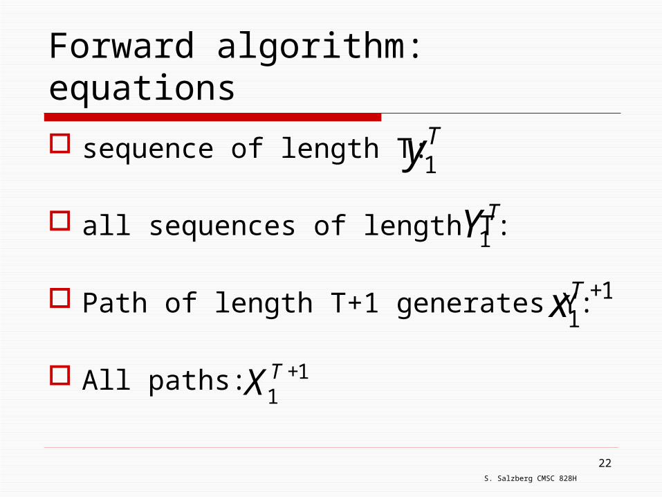
Forward algorithm: equations
sequence of length T:
all sequences of length T:
Path of length T+1 generates Y:
All paths:
€
y1T
€
Y1T
€
x1T +1
€
X1T +1
S. Salzberg CMSC 828H
23
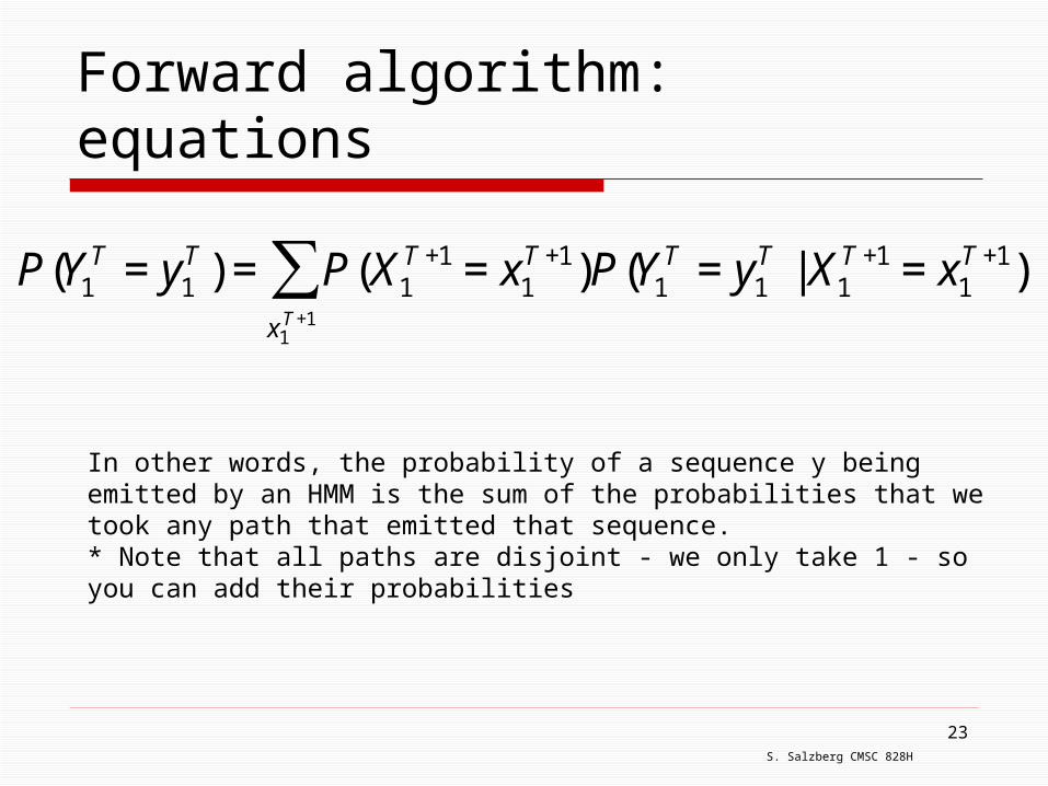
Forward algorithm: equations
€
P(Y1T = y1
T ) = P(X1T +1 = x1
T +1)P(Y1T = y1
T | X1T +1 = x1
T +1)x1T+1
∑
In other words, the probability of a sequence y being emitted by an HMM is the sum of the probabilities that we took any path that emitted that sequence. * Note that all paths are disjoint - we only take 1 - so you can add their probabilities
S. Salzberg CMSC 828H
24
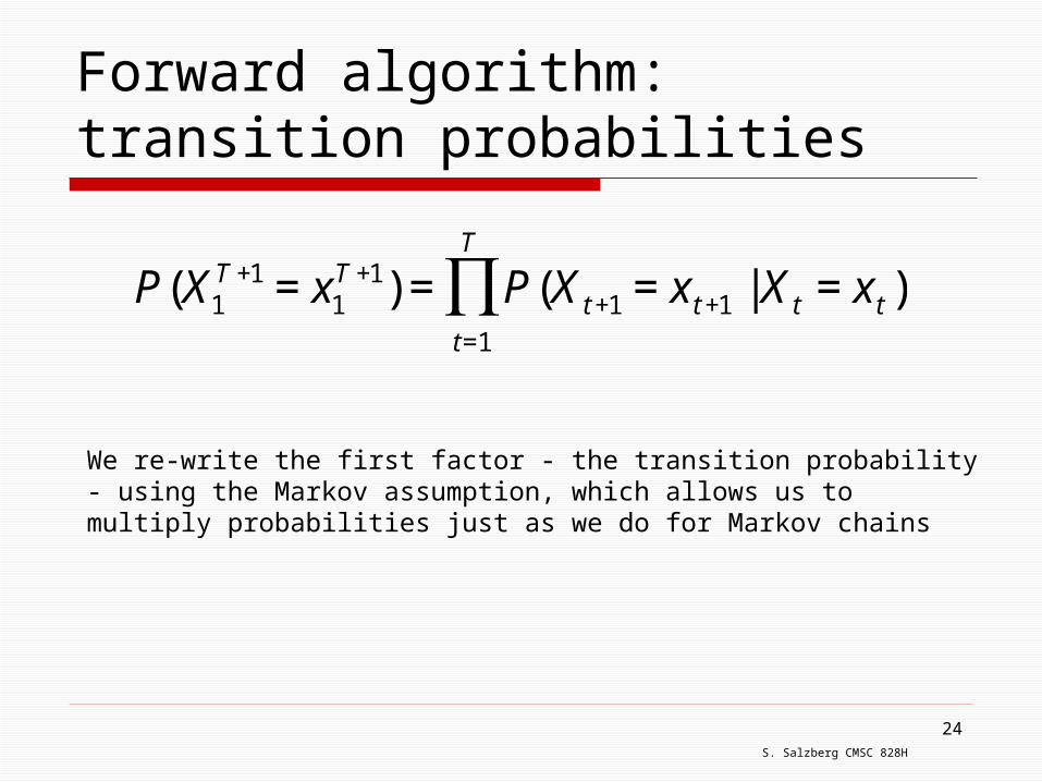
Forward algorithm: transition probabilities
€
P(X1T +1 = x1
T +1) = P(X t+1 = x t+1 | X t = x t )t=1
T
∏
We re-write the first factor - the transition probability - using the Markov assumption, which allows us to multiply probabilities just as we do for Markov chains
S. Salzberg CMSC 828H
25
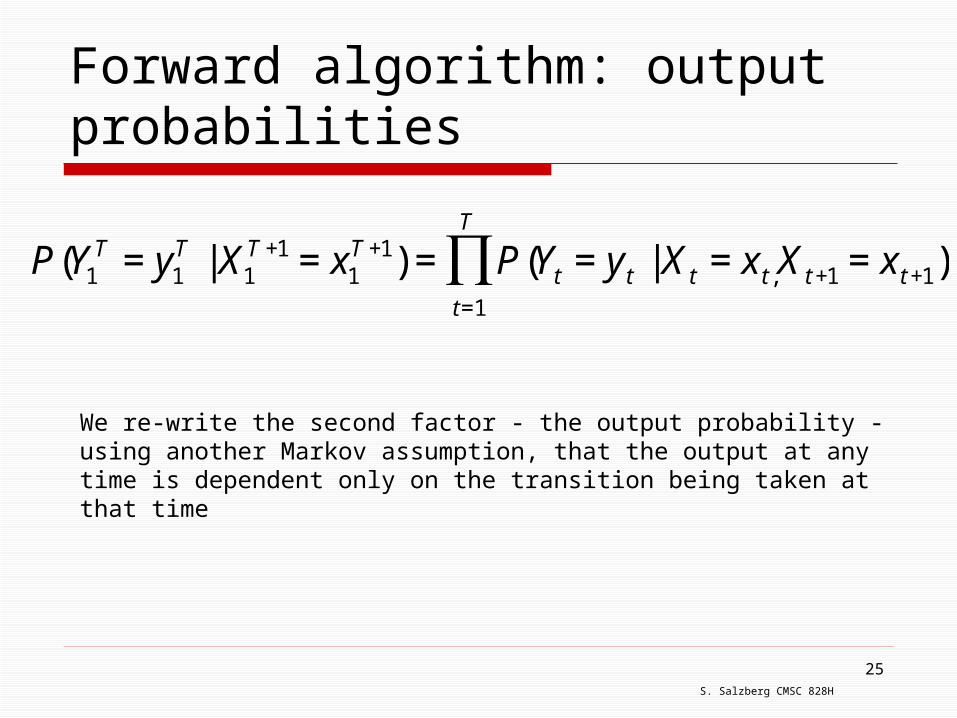
Forward algorithm: output probabilities
We re-write the second factor - the output probability - using another Markov assumption, that the output at any time is dependent only on the transition being taken at that time €
P(Y1T = y1
T | X1T +1 = x1
T +1) = P(Yt = y t | X t = x t ,X t+1 = x t+1)t=1
T
∏
S. Salzberg CMSC 828H
26
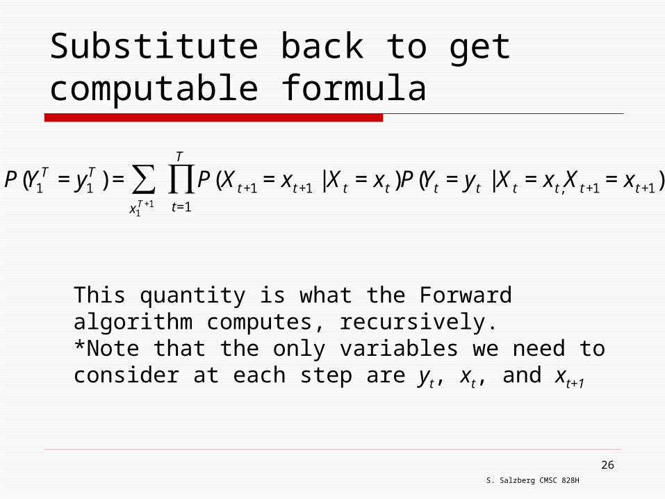
Substitute back to get computable formula
This quantity is what the Forward algorithm computes, recursively.*Note that the only variables we need to consider at each step are yt, xt, and xt+1
€
P(Y1T = y1
T ) =x1T+1
∑ P(X t+1 = x t+1 | X t = x t )P(Yt = y t | X t = x t,X t+1 = x t+1)t=1
T
∏
S. Salzberg CMSC 828H
27
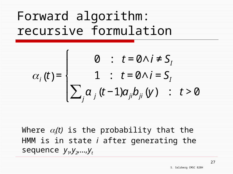
Forward algorithm: recursive formulation
Where i(t) is the probability that the HMM is in state i after generating the sequence y1,y2,…,yt€
α i t( ) =
0 : t = 0∧i ≠ SI1 : t = 0∧i = SI
α j (t −1)a jib ji(y) : t > 0j
∑
⎧
⎨ ⎪
⎩ ⎪
S. Salzberg CMSC 828H
28
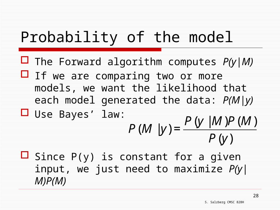
Probability of the model The Forward algorithm computes P(y|M) If we are comparing two or more models,
we want the likelihood that each model generated the data: P(M|y)
Use Bayes’ law:
Since P(y) is constant for a given input, we just need to maximize P(y|M)P(M)
€
P(M | y) =P(y |M)P(M)
P(y)