Heuristic and simulated annealing algorithms forwireless ATM backbone network design problem

Der-Rong Din†

Department of Computer Science and Information Engineering,

National Changhua University of Education,

Changhua City, Taiwan R.O.C.

Abstract

Personal Communication Network (PCN) is an emerging wireless network that promises

many new services for the telecommunication industry. The high speed backbone network

(ATM or WDM) is one possible approach to provide broadband wireless transmission with

PCN’s using the ATM switches for interconnection of PCN cells. The wireless ATM backbone

network design (WABND) problem is to allocate backbone links among ATM switches such

that the effects of terminal mobility on the performance of ATM-based PCN’s can be reduced.

In this paper, the WABND problem is formulated and studied. The goal of the WABND

is to minimize the location update cost under constraints. Since WABND is an NP-hard

problem, two heuristic algorithms and a simulated annealing algorithm were proposed and

used to find the close-to-optimal solutions. The simulated annealing algorithm was able to

achieve good performance as indicated from the simulated results.

Keywords: wireless ATM, heuristic algorithm, simulated annealing, NP-hard, backbone net-

work design.

†To whom all correspondences should be addressed,E MAIL: deron@ms45.hinet.net,Address: No. 1, Jin De Road, Changhua 500, Taiwan R.O.C.Tel: 886-4-7232105-7047FAX: 886–4–7211081

1

1 Introduction

Personal Communication Network (PCN )[1, 2, 3] is an emerging wireless network that promises

many new services. Users may move from one place to another and can maintain transparent net-

work access through wireless links. Information exchanging between users, may be bidirectional,

which includes voice, data, and image.

In a PCN, the covered geographical area is typically partitioned into a set of cells . Each cell

has a base station(BS ) used for exchanging radio signals with mobile terminals. Due to the limited

power of wireless transceivers, mobile users can communicate only with base stations that reside

within the same cell. Moreover, several coverage areas of cells are grouped and formed a location

area(LA). That is, an LA consists of an aggregation of coverage areas of cells forming a contiguous

geographical region.

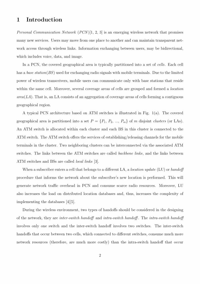
A typical PCN architecture based on ATM switches is illustrated in Fig. 1(a). The covered

geographical area is partitioned into a set P = {P1, P2, ..., Pm} of m disjoint clusters (or LAs).

An ATM switch is allocated within each cluster and each BS in this cluster is connected to the

ATM switch. The ATM switch offers the services of establishing/releasing channels for the mobile

terminals in the cluster. Two neighboring clusters can be interconnected via the associated ATM

switches. The links between the ATM switches are called backbone links , and the links between

ATM switches and BSs are called local links [3].

When a subscriber enters a cell that belongs to a different LA, a location update (LU) or handoff

procedure that informs the network about the subscriber’s new location is performed. This will

generate network traffic overhead in PCN and consume scarce radio resources. Moreover, LU

also increases the load on distributed location databases and, thus, increases the complexity of

implementing the databases [4][5].

During the wireless environment, two types of handoffs should be considered in the designing

of the network, they are inter-switch handoff and intra-switch handoff . The intra-switch handoff

involves only one switch and the inter-switch handoff involves two switches. The inter-switch

handoffs that occur between two cells, which connected to different switches, consume much more

network resources (therefore, are much more costly) than the intra-switch handoff that occur

2

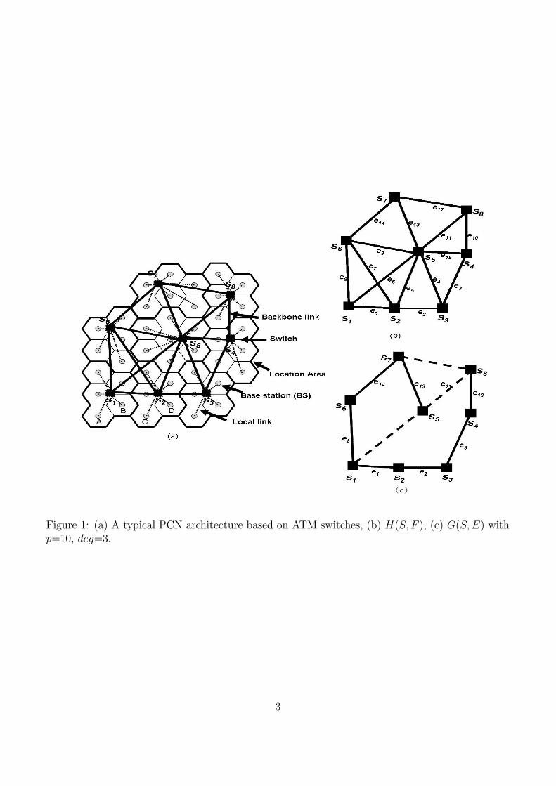
Figure 1: (a) A typical PCN architecture based on ATM switches, (b) H(S, F ), (c) G(S,E) withp=10, deg=3.

3

between cells, which connected to the same switch[6, 7, 8, 9]. Thus, the cost of intra-switch

handoffs involving only one switch is negligible in designing the two-level wireless ATM network.

Consider the example shown in Fig. 1, where cells A and B are connected to switch s1, and

cells C and D are connected to switch s2. If the subscriber moves from cell B to cell A, switch

s1 will perform a handoff for this call. This intra-switch handoff is relatively simple and does

not involve any location update in the databases that record the position of the subscriber. The

handoff also does not involve any network entity other than switch s1. Now imagine that the

subscriber moves from cell B to cell C. Then the inter-switch handoff involves the execution of a

fairly complicated protocol between switches s1 and s2[6, 7, 8, 9].

In this paper, the wireless ATM network design (WABND) problem is studied. Given the

PCN network, the handoff frequencies between cells, the local links between cells and switches,

the degree constraint, and the number of backbone links, the WABND problem is to find a set of

backbone links which forms a connected network such that the total cost is minimized under the

degree constraint. In [10], the WABND problem is studied and formulated, a heuristic algorithm

and a genetic algorithm have proposed to find the sub-optimal solution. Due to the complexity of

the WABND problem in a wireless ATM network, the provision of an optimal solution in reasonable

time is not guaranteed. In this respect, the usual step is to devise an approximate algorithm for

solving this problem. Simulated annealing (SA) is a stochastic computational technique derived

from statistical mechanics for finding near globally-minimum-cost solutions to large optimization

problems. Kirkpatrick et al [11] were the first to propose and demonstrate the application of

simulation techniques from statistical physics to problem of combinatorial optimization. In this

paper, two heuristic algorithms and a simulated annealing algorithm are proposed to solve it.

The organization of this paper is as follows. Section 2 gives a formal description of the WABND

problem. Section 3 describes the proposed heuristic algorithms. In Section 4, the details of the

proposed simulated annealing algorithm are presented. Simulation results are presented in Section

5, and some concluding remarks are given in Section 6.

4

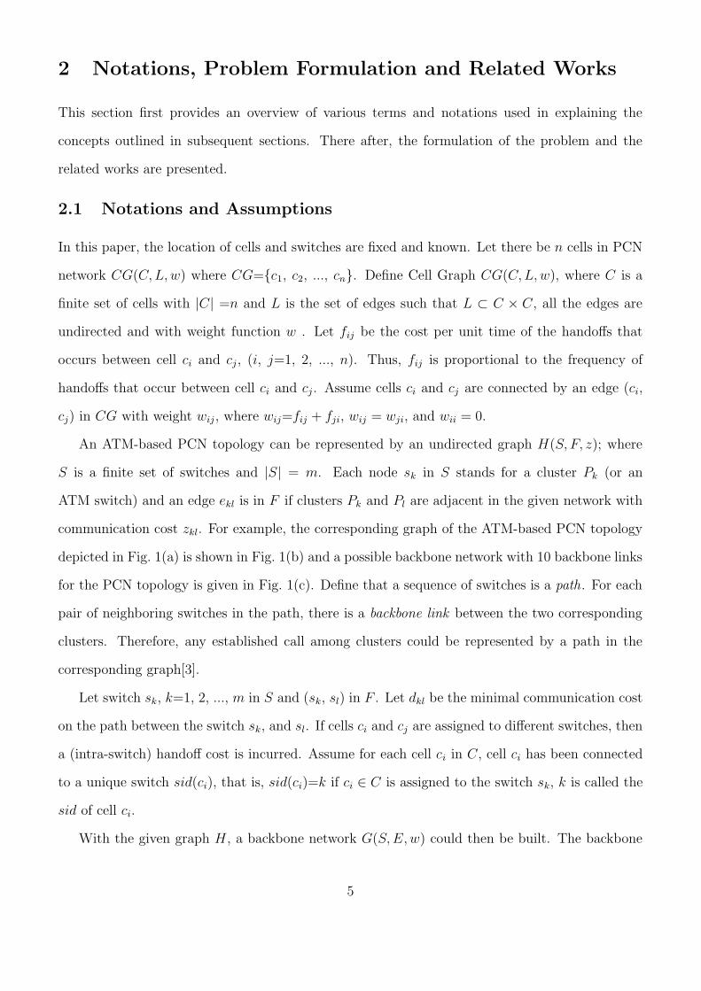
2 Notations, Problem Formulation and Related Works

This section first provides an overview of various terms and notations used in explaining the

concepts outlined in subsequent sections. There after, the formulation of the problem and the

related works are presented.

2.1 Notations and Assumptions

In this paper, the location of cells and switches are fixed and known. Let there be n cells in PCN

network CG(C,L,w) where CG={c1, c2, ..., cn}. Define Cell Graph CG(C,L,w), where C is a

finite set of cells with |C| =n and L is the set of edges such that L ⊂ C × C, all the edges are

undirected and with weight function w . Let fij be the cost per unit time of the handoffs that

occurs between cell ci and cj, (i, j=1, 2, ..., n). Thus, fij is proportional to the frequency of

handoffs that occur between cell ci and cj. Assume cells ci and cj are connected by an edge (ci,

cj) in CG with weight wij, where wij=fij + fji, wij = wji, and wii = 0.

An ATM-based PCN topology can be represented by an undirected graph H(S, F, z); where

S is a finite set of switches and |S| = m. Each node sk in S stands for a cluster Pk (or an

ATM switch) and an edge ekl is in F if clusters Pk and Pl are adjacent in the given network with

communication cost zkl. For example, the corresponding graph of the ATM-based PCN topology

depicted in Fig. 1(a) is shown in Fig. 1(b) and a possible backbone network with 10 backbone links

for the PCN topology is given in Fig. 1(c). Define that a sequence of switches is a path. For each

pair of neighboring switches in the path, there is a backbone link between the two corresponding

clusters. Therefore, any established call among clusters could be represented by a path in the

corresponding graph[3].

Let switch sk, k=1, 2, ..., m in S and (sk, sl) in F . Let dkl be the minimal communication cost

on the path between the switch sk, and sl. If cells ci and cj are assigned to different switches, then

a (intra-switch) handoff cost is incurred. Assume for each cell ci in C, cell ci has been connected

to a unique switch sid(ci), that is, sid(ci)=k if ci ∈ C is assigned to the switch sk, k is called the

sid of cell ci.

With the given graph H, a backbone network G(S,E,w) could then be built. The backbone

5

network is built by utilizing the available edges in graph H. Typically, some limitation is placed

on the number of links that could to be laid in the backbone network as the cost of the network

is proportional to the number of links that are to be set up in the network. The objective is to

determine the link between switches so as to minimize the handoff costs per unit time under the

degree constraint. Let deg(s) denote the degree of switch s and deg(G) denote the degree of graph

G which is the maximum degree of the switches in G. Thus deg(G) = max {deg(s)|s ∈ S }.

For example, given the graph shown in Fig. 1(b), the corresponding graph of a possible backbone

network with 10 links and deg(G) = 3 is shown in Fig. 1(c).

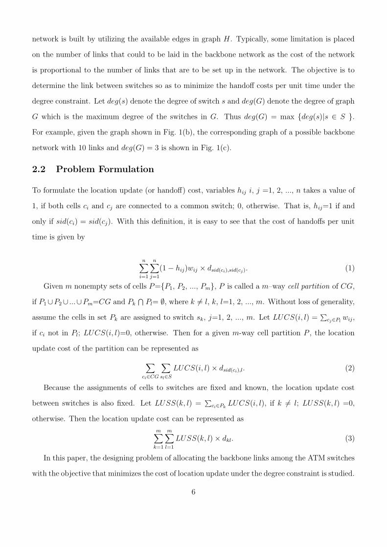
2.2 Problem Formulation

To formulate the location update (or handoff) cost, variables hij i, j =1, 2, ..., n takes a value of

1, if both cells ci and cj are connected to a common switch; 0, otherwise. That is, hij=1 if and

only if sid(ci) = sid(cj). With this definition, it is easy to see that the cost of handoffs per unit

time is given by

n∑

i=1

n∑

j=1

(1 − hij)wij × dsid(ci),sid(cj). (1)

Given m nonempty sets of cells P={P1, P2, ..., Pm}, P is called a m–way cell partition of CG,

if P1∪P2∪ ...∪Pm=CG and Pk⋂

Pl= ∅, where k 6= l, k, l=1, 2, ..., m. Without loss of generality,

assume the cells in set Pk are assigned to switch sk, j=1, 2, ..., m. Let LUCS(i, l) =∑

cj∈Plwij,

if ci not in Pl; LUCS(i, l)=0, otherwise. Then for a given m-way cell partition P , the location

update cost of the partition can be represented as

∑

ci∈CG

∑

sl∈S

LUCS(i, l) × dsid(ci),l. (2)

Because the assignments of cells to switches are fixed and known, the location update cost

between switches is also fixed. Let LUSS(k, l) =∑

ci∈PkLUCS(i, l), if k 6= l; LUSS(k, l) =0,

otherwise. Then the location update cost can be represented as

m∑

k=1

m∑

l=1

LUSS(k, l) × dkl. (3)

In this paper, the designing problem of allocating the backbone links among the ATM switches

with the objective that minimizes the cost of location update under the degree constraint is studied.

6

With the above definition, the wireless ATM backbone network design(WABND) problem can be

formally defined as follows:

Wireless ATM backbone network design (WABND) problem[10]: Given a graph H =

(S, F, z) with |S| = m, the m × m matrix LUSS, and positive integers deg and p, deg ≤ |S| and

|S| − 1 ≤ p ≤ |F |, the WABND problem is to find a connected subgraph G(S,E, z) of H with

|E| = p, such that the location update cost∑m

k=1

∑ml=1 LUSS(k, l)× dkl is minimized and satisfies

the constraint deg(G) ≤ deg, where dkl is the minimal communication cost between sk and sl on

G(S,E, z).

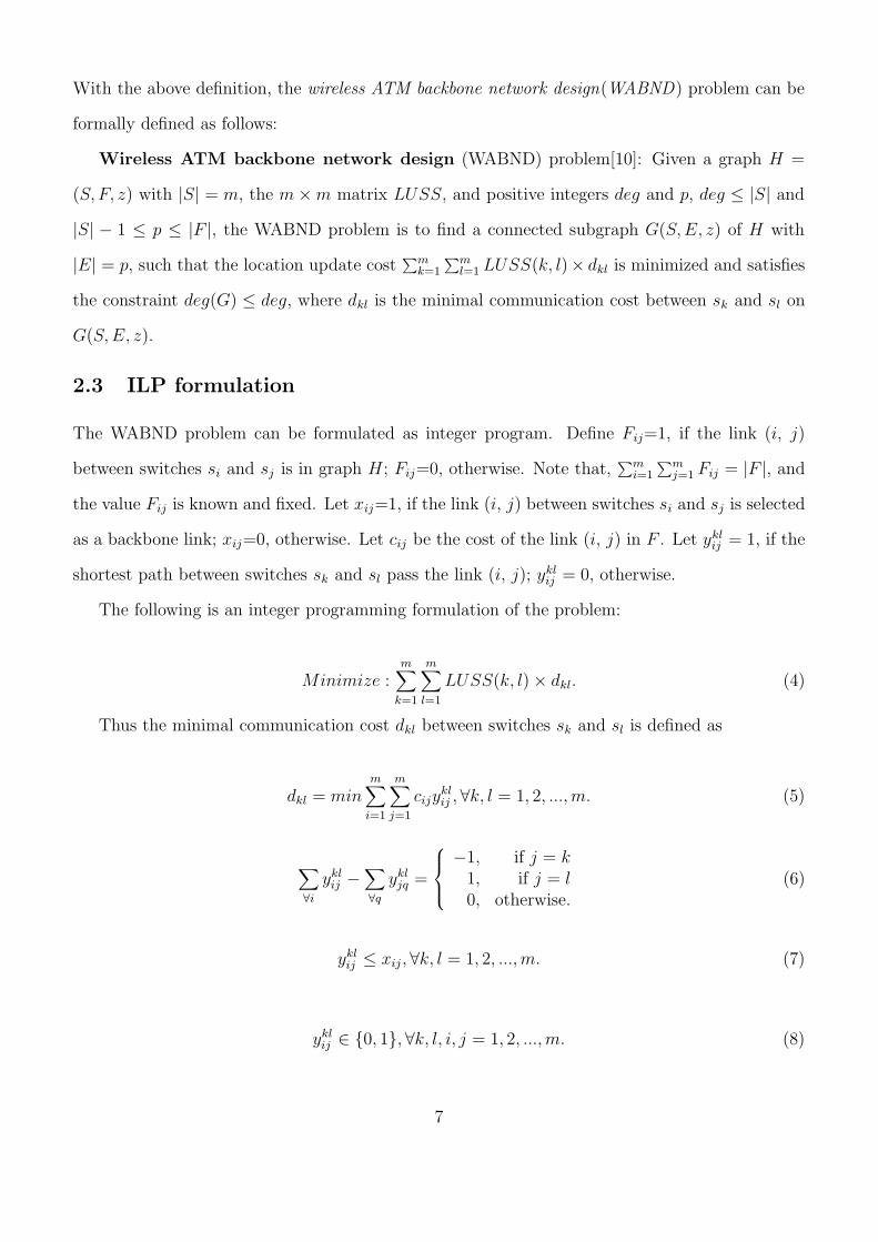
2.3 ILP formulation

The WABND problem can be formulated as integer program. Define Fij=1, if the link (i, j)

between switches si and sj is in graph H; Fij=0, otherwise. Note that,∑m

i=1

∑mj=1 Fij = |F |, and

the value Fij is known and fixed. Let xij=1, if the link (i, j) between switches si and sj is selected

as a backbone link; xij=0, otherwise. Let cij be the cost of the link (i, j) in F . Let yklij = 1, if the

shortest path between switches sk and sl pass the link (i, j); yklij = 0, otherwise.

The following is an integer programming formulation of the problem:

Minimize :m

∑

k=1

m∑

l=1

LUSS(k, l) × dkl. (4)

Thus the minimal communication cost dkl between switches sk and sl is defined as

dkl = minm

∑

i=1

m∑

j=1

cijyklij ,∀k, l = 1, 2, ...,m. (5)

∑

∀i

yklij −

∑

∀q

ykljq =

−1, if j = k1, if j = l0, otherwise.

(6)

yklij ≤ xij,∀k, l = 1, 2, ...,m. (7)

yklij ∈ {0, 1},∀k, l, i, j = 1, 2, ...,m. (8)

7

m∑

i=1

m∑

j=1

xij = p, (9)

m∑

i=1

xij ≤ deg,∀j = 1, 2, ...,m; (10)

xij ≤ Fij,∀i, j = 1, 2, ...,m; (11)

xij ∈ {0, 1},∀i, j = 1, 2, ...,m; (12)

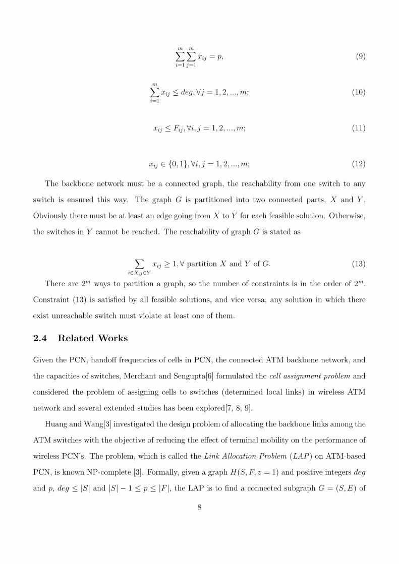
The backbone network must be a connected graph, the reachability from one switch to any

switch is ensured this way. The graph G is partitioned into two connected parts, X and Y .

Obviously there must be at least an edge going from X to Y for each feasible solution. Otherwise,

the switches in Y cannot be reached. The reachability of graph G is stated as

∑

i∈X,j∈Y

xij ≥ 1,∀ partition X and Y of G. (13)

There are 2m ways to partition a graph, so the number of constraints is in the order of 2m.

Constraint (13) is satisfied by all feasible solutions, and vice versa, any solution in which there

exist unreachable switch must violate at least one of them.

2.4 Related Works

Given the PCN, handoff frequencies of cells in PCN, the connected ATM backbone network, and

the capacities of switches, Merchant and Sengupta[6] formulated the cell assignment problem and

considered the problem of assigning cells to switches (determined local links) in wireless ATM

network and several extended studies has been explored[7, 8, 9].

Huang and Wang[3] investigated the design problem of allocating the backbone links among the

ATM switches with the objective of reducing the effect of terminal mobility on the performance of

wireless PCN’s. The problem, which is called the Link Allocation Problem (LAP) on ATM-based

PCN, is known NP-complete [3]. Formally, given a graph H(S, F, z = 1) and positive integers deg

and p, deg ≤ |S| and |S| − 1 ≤ p ≤ |F |, the LAP is to find a connected subgraph G = (S,E) of

8

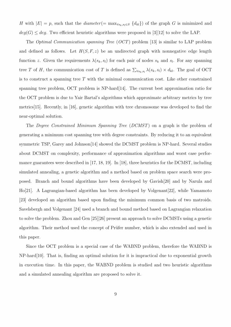
H with |E| = p, such that the diameter(= max∀sk,sl∈S {dkl}) of the graph G is minimized and

deg(G) ≤ deg. Two efficient heuristic algorithms were proposed in [3][12] to solve the LAP.

The Optimal Communication spanning Tree (OCT ) problem [13] is similar to LAP problem

and defined as follows. Let H(S, F, z) be an undirected graph with nonnegative edge length

function z. Given the requirements λ(sk, sl) for each pair of nodes sk and sl. For any spanning

tree T of H, the communication cost of T is defined as∑

∀sk,slλ(sk, sl) × dkl. The goal of OCT

is to construct a spanning tree T with the minimal communication cost. Like other constrained

spanning tree problem, OCT problem is NP-hard[14]. The current best approximation ratio for

the OCT problem is due to Yair Bartal’s algorithms which approximate arbitrary metrics by tree

metrics[15]. Recently, in [16], genetic algorithm with tree chromosome was developed to find the

near-optimal solution.

The Degree Constrained Minimum Spanning Tree (DCMST ) on a graph is the problem of

generating a minimum cost spanning tree with degree constraints. By reducing it to an equivalent

symmetric TSP, Garey and Johnson[14] showed the DCMST problem is NP-hard. Several studies

about DCMST on complexity, performance of approximation algorithms and worst case perfor-

mance guarantees were described in [17, 18, 19]. In [18], three heuristics for the DCMST, including

simulated annealing, a genetic algorithm and a method based on problem space search were pro-

posed. Branch and bound algorithms have been developed by Gavish[20] and by Narula and

Ho[21]. A Lagrangian-based algorithm has been developed by Volgenant[22], while Yamamoto

[23] developed an algorithm based upon finding the minimum common basis of two matroids.

Savelsbergh and Volgenant [24] used a branch and bound method based on Lagrangian relaxation

to solve the problem. Zhou and Gen [25][26] present an approach to solve DCMSTs using a genetic

algorithm. Their method used the concept of Prufer number, which is also extended and used in

this paper.

Since the OCT problem is a special case of the WABND problem, therefore the WABND is

NP-hard[10]. That is, finding an optimal solution for it is impractical due to exponential growth

in execution time. In this paper, the WABND problem is studied and two heuristic algorithms

and a simulated annealing algorithm are proposed to solve it.

9

3 Heuristic Algorithm for WABND

In this section, two heuristic algorithms are proposed to solve the WABND problem, they are

remove-based heuristic (RBH) and weight-median-based heuristic (WMBH) algorithms.

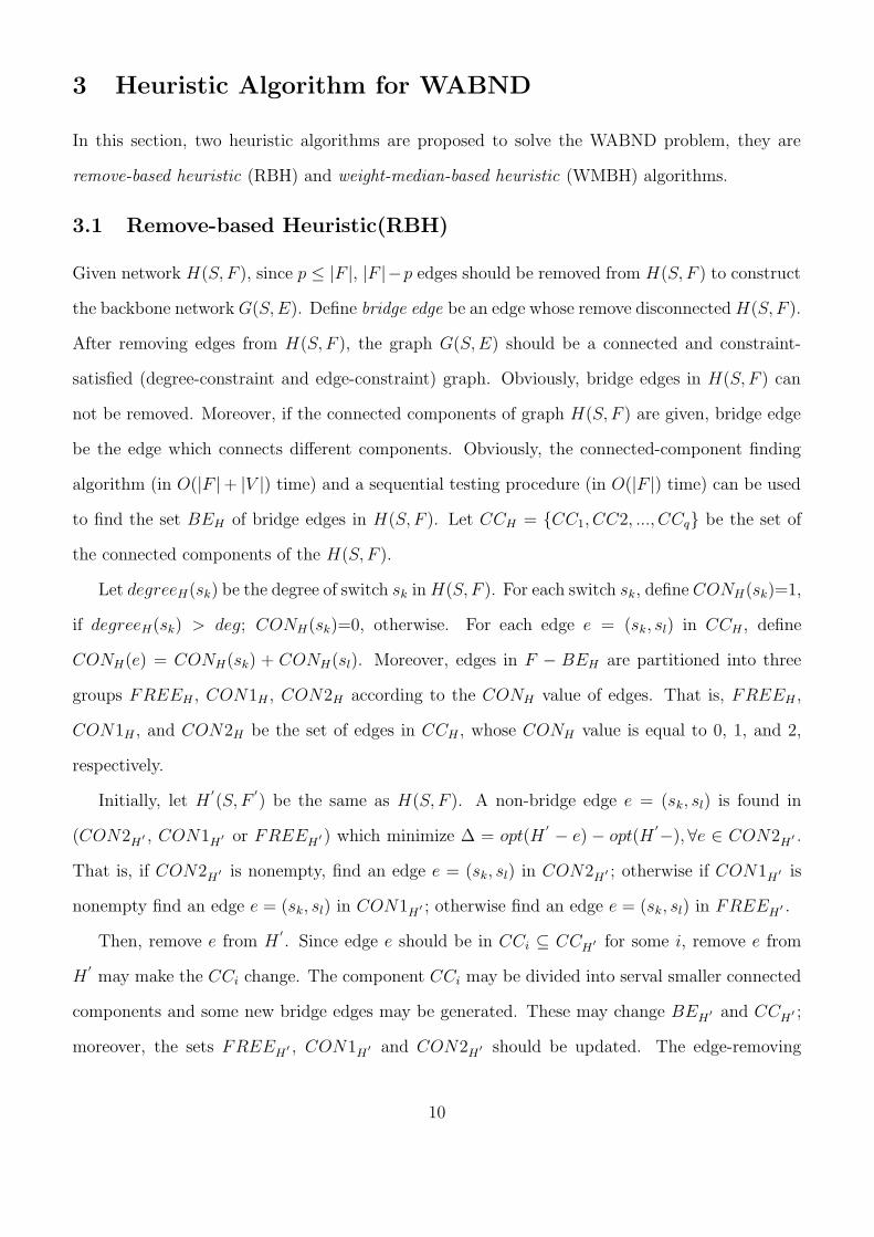
3.1 Remove-based Heuristic(RBH)

Given network H(S, F ), since p ≤ |F |, |F |−p edges should be removed from H(S, F ) to construct

the backbone network G(S,E). Define bridge edge be an edge whose remove disconnected H(S, F ).

After removing edges from H(S, F ), the graph G(S,E) should be a connected and constraint-

satisfied (degree-constraint and edge-constraint) graph. Obviously, bridge edges in H(S, F ) can

not be removed. Moreover, if the connected components of graph H(S, F ) are given, bridge edge

be the edge which connects different components. Obviously, the connected-component finding

algorithm (in O(|F |+ |V |) time) and a sequential testing procedure (in O(|F |) time) can be used

to find the set BEH of bridge edges in H(S, F ). Let CCH = {CC1, CC2, ..., CCq} be the set of

the connected components of the H(S, F ).

Let degreeH(sk) be the degree of switch sk in H(S, F ). For each switch sk, define CONH(sk)=1,

if degreeH(sk) > deg; CONH(sk)=0, otherwise. For each edge e = (sk, sl) in CCH , define

CONH(e) = CONH(sk) + CONH(sl). Moreover, edges in F − BEH are partitioned into three

groups FREEH , CON1H , CON2H according to the CONH value of edges. That is, FREEH ,

CON1H , and CON2H be the set of edges in CCH , whose CONH value is equal to 0, 1, and 2,

respectively.

Initially, let H′

(S, F′

) be the same as H(S, F ). A non-bridge edge e = (sk, sl) is found in

(CON2H′ , CON1H

′ or FREEH′ ) which minimize ∆ = opt(H

′

− e) − opt(H′

−),∀e ∈ CON2H′ .

That is, if CON2H′ is nonempty, find an edge e = (sk, sl) in CON2H

′ ; otherwise if CON1H′ is

nonempty find an edge e = (sk, sl) in CON1H′ ; otherwise find an edge e = (sk, sl) in FREEH

′ .

Then, remove e from H′

. Since edge e should be in CCi ⊆ CCH′ for some i, remove e from

H′

may make the CCi change. The component CCi may be divided into serval smaller connected

components and some new bridge edges may be generated. These may change BEH′ and CCH

′ ;

moreover, the sets FREEH′ , CON1H′ and CON2H′ should be updated. The edge-removing

10

process is performed repeatedly until H′

(S, F′

) contains exact |p| edges. Clearly, if there exists

a feasible solution, then after performing the edge-removing processes, all edges (include bridge

edges) should be in FREEH′ . The details of the RBH algorithm is stated as follows:

Remove–based heuristic (RBH)

Let H′

(S, F′

) = H(S, F ).

Perform Connected-component finding algorithm to find the CCH′ = {CC1, CC2, ..., CCq} of H

′

(S, F′

).

Group those edges which connected two different connected components into BEH′ .

Determine the associated group (FREEH′ , CON1H

′ , or CON2H′ ) of edge e in F −BEH

′ according to

the value of CONH′ (e).

while (|F′

| > p ) do

begin

if (CON2H′ 6= ∅)

then

Select an edge e = (sk, sl) in CON2H′ which minimizes opt(H

′

− e) − opt(H′

), ∀e ∈ CON2H′ ;

else if (CON1 6= ∅)

then

Select an edge e in CON1H′ which minimizes opt(H

′

− e) − opt(H′

), ∀e ∈ CON1H′ ;

else

Select an edge e in FREEH′ which minimizes opt(H′

− e) − opt(H′

), ∀e ∈ FREEH′ ;

Remove e form H′

(S, F′

).

Update degreeH′ (sk), degreeH

′ (sl), CCH′ , BEH

′ , FREEH′ , CON1H

′ , CON2H′ .

end//end of while

if ((CON1H′ 6= ∅) or (CON2H

′ 6= ∅))

then

return notfound.

else

return H′

(S, F′

).

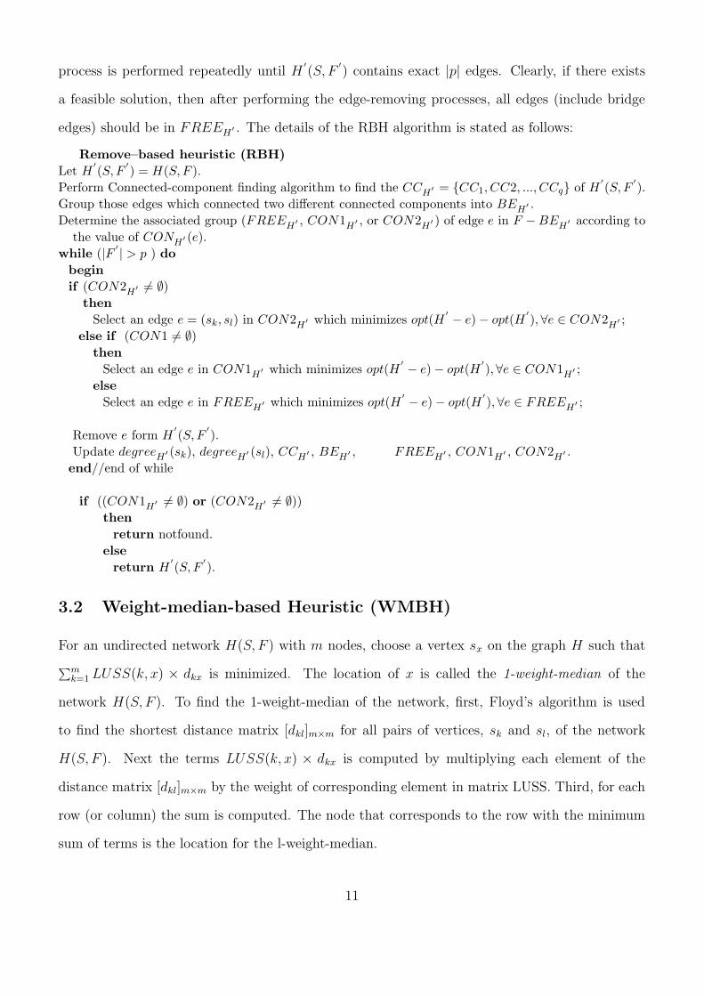
3.2 Weight-median-based Heuristic (WMBH)

For an undirected network H(S, F ) with m nodes, choose a vertex sx on the graph H such that

∑mk=1 LUSS(k, x) × dkx is minimized. The location of x is called the 1-weight-median of the

network H(S, F ). To find the 1-weight-median of the network, first, Floyd’s algorithm is used

to find the shortest distance matrix [dkl]m×m for all pairs of vertices, sk and sl, of the network

H(S, F ). Next the terms LUSS(k, x) × dkx is computed by multiplying each element of the

distance matrix [dkl]m×m by the weight of corresponding element in matrix LUSS. Third, for each

row (or column) the sum is computed. The node that corresponds to the row with the minimum

sum of terms is the location for the l-weight-median.

11

1-Weight-Median Algorithm

Perform Floyd’s algorithm to find the shortest distance matrix [dkl]m×m for the nodes of H.

Let sumk = 0, for k = 1, 2, ...m represents the sum of row k.

for k = 1 to m

for l = 1 to m

sumk = sumk + LUSS(k, l) × d(k, l)

Find the node sx which minimizes sumx.

Then, the famous Dijkstra’s algorithm is modified to find shortest-path based degree-constrained

spanning tree. The details of algorithm is shown as follows:

Degree-constrained-tree (source s)

V ={s}, N = S − V , T = ∅ ;

while (S − V 6= ∅) begin

for all links (u, v), u ∈ V and v ∈ S − V begin

find the link (k, l) such that deg(T ∪ (k, l)) ≤ deg and with smallest cost zkl ≤ min∀u∈V,v∈S−V {zuv}

if (found)

then { T = T ∪ (k, l); V = V ∪ {l}; N = S − V ;}

else return notfound;

end

end

return T ;

Final, The shortest-path based degree-constrained spanning trees Tx of H(S, F, z) with 1-

weight-median sx as root is found by performing the degree-constrained algorithm[10](as shown

above). Define opt(T ) be the object cost of the spanning tree T , that is, opt(T ) =∑m

k=1

∑ml=1 LUSS(k, l)×

dkl, where dkl be the shortest distance between switches sk and sl in T . Let Tx = (S,E1). Finally, a

set of p−|Tx| edges are added in phase two to form the graph G; where |Tx| is the number of edges

in Tx and p is the total number of edges to be included in G. The order of edges to be added to G,

12

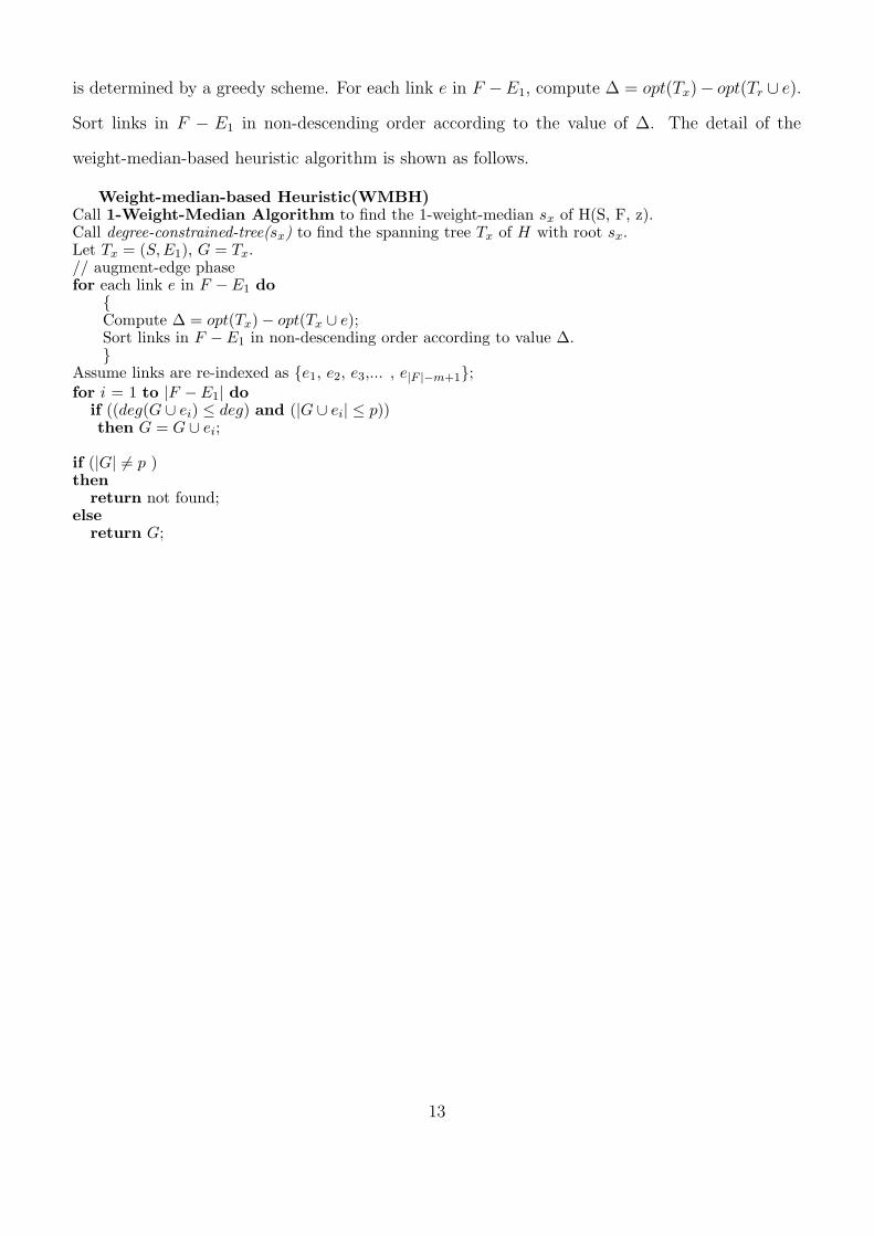
is determined by a greedy scheme. For each link e in F −E1, compute ∆ = opt(Tx)− opt(Tr ∪ e).

Sort links in F − E1 in non-descending order according to the value of ∆. The detail of the

weight-median-based heuristic algorithm is shown as follows.

Weight-median-based Heuristic(WMBH)Call 1-Weight-Median Algorithm to find the 1-weight-median sx of H(S, F, z).Call degree-constrained-tree(sx) to find the spanning tree Tx of H with root sx.Let Tx = (S, E1), G = Tx.// augment-edge phasefor each link e in F − E1 do

{Compute ∆ = opt(Tx) − opt(Tx ∪ e);Sort links in F − E1 in non-descending order according to value ∆.}

Assume links are re-indexed as {e1, e2, e3,... , e|F |−m+1};for i = 1 to |F − E1| do

if ((deg(G ∪ ei) ≤ deg) and (|G ∪ ei| ≤ p))then G = G ∪ ei;

if (|G| 6= p )then

return not found;else

return G;

13

4 Simulated Annealing Algorithm for WABND

Simulated annealing is a stochastic computational technique derived from statistical mechanics

for finding near globally-minimum-cost solutions to large optimization problems. Kirkpatrick et

al [11] were the first to propose and demonstrate the application of simulation techniques from

statistical physics to problem of combinatorial optimization.

Due to the complexity of the WABND problem, the provision of an optimal solution in reason-

able time is not guaranteed. In this respect, the usual step is to devise an approximate algorithm

for solving this problem. The simulated annealing (SA) technique is applied to solve the WABND

problem in this section.

In this section, the details of simulated annealing algorithm developed to solve the WABND

problem is present. The key elements in a simulated annealing algorithm are: (1) a configuration

space, (2) a cost function, (3) a perturbation mechanism, and (4) a cooling schedule. The solution

methods are shown in following subsections.

4.1 Configuration Space

The objective of WABND problem is to find an optimal topology so that the object function value

is minimized under the connected and degree-constraint. To do this, the configuration space is

designed to be the set of possible solutions. Each configuration is defined as a topology network

which is represented by adjacency matrix .

4.2 Initial Configuration Generation

The initial configuration of the simulated annealing algorithm is generated by performing one of

the heuristic algorithms described in Section 3.

4.3 Cost Function

Generally, simulated annealing algorithms use costs function to achieve the goal of finding op-

timally assignments. The goal is to minimize the total cost of the wireless ATM network. For

the given network topology, the all-pair shortest path algorithm is used to find the distance dkl

14

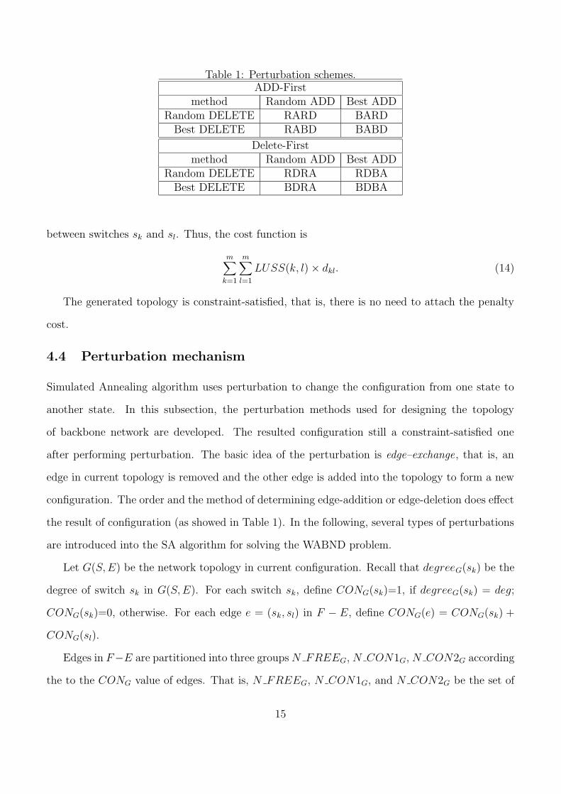
Table 1: Perturbation schemes.ADD-First

method Random ADD Best ADDRandom DELETE RARD BARD

Best DELETE RABD BABD

Delete-Firstmethod Random ADD Best ADD

Random DELETE RDRA RDBABest DELETE BDRA BDBA

between switches sk and sl. Thus, the cost function is

m∑

k=1

m∑

l=1

LUSS(k, l) × dkl. (14)

The generated topology is constraint-satisfied, that is, there is no need to attach the penalty

cost.

4.4 Perturbation mechanism

Simulated Annealing algorithm uses perturbation to change the configuration from one state to

another state. In this subsection, the perturbation methods used for designing the topology

of backbone network are developed. The resulted configuration still a constraint-satisfied one

after performing perturbation. The basic idea of the perturbation is edge–exchange, that is, an

edge in current topology is removed and the other edge is added into the topology to form a new

configuration. The order and the method of determining edge-addition or edge-deletion does effect

the result of configuration (as showed in Table 1). In the following, several types of perturbations

are introduced into the SA algorithm for solving the WABND problem.

Let G(S,E) be the network topology in current configuration. Recall that degreeG(sk) be the

degree of switch sk in G(S,E). For each switch sk, define CONG(sk)=1, if degreeG(sk) = deg;

CONG(sk)=0, otherwise. For each edge e = (sk, sl) in F − E, define CONG(e) = CONG(sk) +

CONG(sl).

Edges in F−E are partitioned into three groups N FREEG, N CON1G, N CON2G according

the to the CONG value of edges. That is, N FREEG, N CON1G, and N CON2G be the set of

15

edges in F − E, whose CONG value is equal to 0, 1, and 2, respectively.

If edge e in N CON2G is selected and added into G(S,E). Then after removing an arbitrary

edge other than e, the resulted configuration will not be a constraint-satisfied one. Thus, only

those edges in N FREEG or N CON1G can be selected and added to G(S,E). Let G′

(S,E′

) =

G(S,E) ∪ e.

To remove an edges from G′

(S,E′

), the resulted graph should be connected and constraint-

satisfied. Thus bridge edges in G′

(S,E′

) can not be removed. Let BEG′ be the set of bridge

edges in G′

(S,E′

). Edges in G′

− BEG′ are partitioned into two groups FREEG

′ and CON1G′

according to the CONG′ value of edges. That is, FREEG

′ and CON1G′ be the set of edges in

G′

(S,E′

), whose CONG′ value is equal to 0 and 1, respectively.

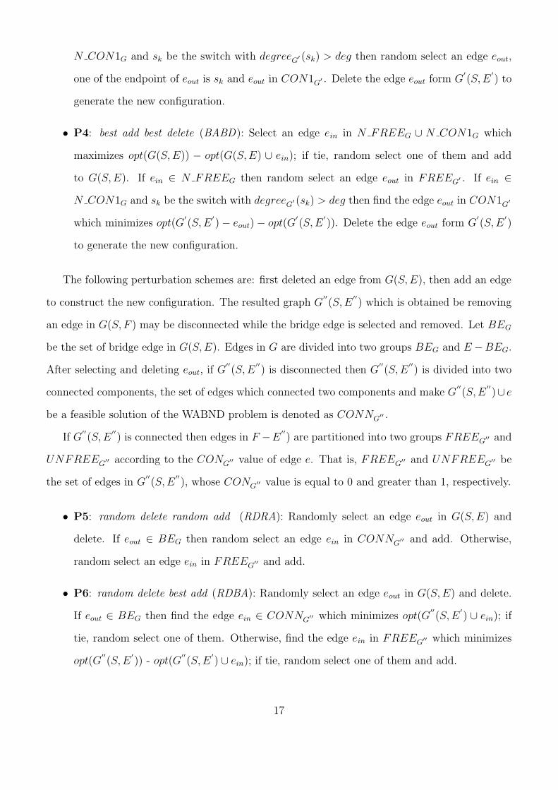
Eight types of perturbations are introduced into the simulated annealing algorithm and shown

as follows. The following perturbation schemes are: first added an edge into G(S,E), then deleted

an edge to construct the new configuration.

• P1: random add random delete (RARD): Randomly select an edge ein in N FREEG ∪

N CON1G and add to G(S,E). If ein ∈ N FREEG then random select an edge eout in

FREEG′ and delete. If ein ∈ N CON1G and sk be the switch with degree(sk)G

′ > deg then

random select an edge eout, one of the endpoint of eout is sk and eout in CON1G′ . Delete the

edge eout form G′

(S,E′

) to generate the new configuration.

• P2: random add best delete (RABD): Randomly select an edge ein in N FREEG∪N CON1G

and add to G(S,E). If ein ∈ N FREEG then find the edge eout which minimizes opt(G′

(S,E′

)−

eout) − opt(G′

(S,E′

)); if tie, random select one of them. If ein ∈ N CON1G and sk be

the switch with degreeG′ (sk) > deg then find the edge eout in CON1G

′ which minimizes

opt(G′

(S,E′

) − eout) − opt(G′

(S,E′

)). Delete the edge eout form G′

(S,E′

) to generate the

new configuration.

• P3: best add random delete (BARD): Select an edge ein in N FREEG ∪ N CON1G which

maximizes opt(G(S,E)) − opt(G(S,E) ∪ ein); if tie, random select one of them and add

to G(S,E). If ein ∈ N FREEG then random select an edge eout in FREEG′ . If ein ∈

16

N CON1G and sk be the switch with degreeG′ (sk) > deg then random select an edge eout,

one of the endpoint of eout is sk and eout in CON1G′ . Delete the edge eout form G

′

(S,E′

) to

generate the new configuration.

• P4: best add best delete (BABD): Select an edge ein in N FREEG ∪ N CON1G which

maximizes opt(G(S,E)) − opt(G(S,E) ∪ ein); if tie, random select one of them and add

to G(S,E). If ein ∈ N FREEG then random select an edge eout in FREEG′ . If ein ∈

N CON1G and sk be the switch with degreeG′ (sk) > deg then find the edge eout in CON1G′

which minimizes opt(G′

(S,E′

) − eout) − opt(G′

(S,E′

)). Delete the edge eout form G′

(S,E′

)

to generate the new configuration.

The following perturbation schemes are: first deleted an edge from G(S,E), then add an edge

to construct the new configuration. The resulted graph G′′

(S,E′′

) which is obtained be removing

an edge in G(S, F ) may be disconnected while the bridge edge is selected and removed. Let BEG

be the set of bridge edge in G(S,E). Edges in G are divided into two groups BEG and E −BEG.

After selecting and deleting eout, if G′′

(S,E′′

) is disconnected then G′′

(S,E′′

) is divided into two

connected components, the set of edges which connected two components and make G′′

(S,E′′

)∪ e

be a feasible solution of the WABND problem is denoted as CONNG′′ .

If G′′

(S,E′′

) is connected then edges in F −E′′

) are partitioned into two groups FREEG′′ and

UNFREEG′′ according to the CONG

′′ value of edge e. That is, FREEG′′ and UNFREEG

′′ be

the set of edges in G′′

(S,E′′

), whose CONG′′ value is equal to 0 and greater than 1, respectively.

• P5: random delete random add (RDRA): Randomly select an edge eout in G(S,E) and

delete. If eout ∈ BEG then random select an edge ein in CONNG′′ and add. Otherwise,

random select an edge ein in FREEG′′ and add.

• P6: random delete best add (RDBA): Randomly select an edge eout in G(S,E) and delete.

If eout ∈ BEG then find the edge ein ∈ CONNG′′ which minimizes opt(G′′

(S,E′

) ∪ ein); if

tie, random select one of them. Otherwise, find the edge ein in FREEG′′ which minimizes

opt(G′′

(S,E′

)) - opt(G′′

(S,E′

) ∪ ein); if tie, random select one of them and add.

17

• P7: best delete random add (BDRA): Select an edge eout in E − BEG which minimizes

opt(G(S,E) − eout) − opt(G(S,E)); if tie, random select one of them and delete. Random

select an edge ein in FREEG′′ and add.

• P8: best delete best add (BDBA): Select an edge eout in E−BEG which minimizes opt(G(S,E)−

eout) − opt(G(S,E)); if tie, random select one of them and delete. Find the edge ein in

FREEG′′ which minimizes opt(G

′′

(S,E′

)) - opt(G′′

(S,E′

)∪ ein); if tie, random select one of

them and add.

Let pi be the probability of transforming current configuration to a new one by applying the

perturbation Pi, i=1,2,...,8, respectively. Assume that Σ8i=1pi = 1. Let AP0 = 0 and APi = Σi

j=1pj

be the accumulated probability of pi, i=1, 2, ..., 8.

4.5 Cooling Schedule

One of the most important problems involved in the simulated annealing algorithm implementa-

tion is the definition of a proper cooling schedule, which is based on the choice of the following

parameters: starting temperature, final temperature, length of Markov chains , the way of decreas-

ing temperature. A correct choice of these parameters is crucial because the performances of the

algorithm strongly depend on it. These parameters are described as follows.

(1) Initial value of the control parameter : The rule used in SA that the starting temperature

c0 is determined by calculating the average increasing in cost, ∆C+, for 50 random transitions

and solve c0 from c0 = ∆C+/ln(χ−1

0 ), where accepted ratio χ0 defined as the number of accepted

transitions divided by the number of proposed transitions. In this paper, the accepted ratio χ0 is

empirically set to 0.55.

(2) Decrement of the control parameter : The decreasing rate of the temperature needs to be

small enough to reach thermal equilibrium for each temperature value. As the temperature is

decreased, the accepted ratio is lowered. When no solution that increases the objective function

can be found, the system is ‘frozen’ and converged to a certain solution. The speed of coverage

of the simulated annealing algorithm depended on the decreasing rate of the temperature and the

length of the Markov chain. As mentioned in [27], the decrement is chosen such that small Markov

18

chain lengths suffice to re-establish quasi-equilibrium after the decrement of the temperature is

applied. The decrement rule in SA is defined as follows: Tk+1 = γTk, where γ is empirically set

to 0.99.

(3) The final value of the control parameter : The iterative procedure is terminated when there

is no significant improvement in the solution after a pre-specified number of iterations. It can also

be terminated when the maximum number of iterations is reached.

(4) The length of Markov Chains : The decrement function of the control parameter requires

only a ’small’ number of trial solutions to rapidly approach the stationary distribution for a given

next value of the control parameter[27]. In general, a chain length of more than 100 transitions is

reasonable. In this paper, the chain length is empirically set to a value of 100 × p.

4.6 Simulated Annealing Algorithm of WABND Problem

The details of the simulated annealing is described as follows:Algorithm: Simulated Annealing

Step 1. For a given initial temperature T , perform RBH or WMBH algorithm to generate initial

configuration IC . The currently best configuration (CBC) is IC, i.e. CBC = IC, and the

current temperature value (CT ) is T , i.e. CT = T . Determine pi, i = 1, 2, ..., 8, AP0 = 0 and

APi = Σij=1pj , i=1,2,...,8.

Step 2. If CT = 0 or the stop criterion is satisfied then go to Step 7.

Step 3. Generate a random number p in [0, 1), if APi−1 ≤ p ≤ APi, (i = 1, 2, ..., 8) then new configuration

(NC) is generated by applying the Pi perturbation schema.

Step 4. The difference of the costs of the two configurations, CBC and NC is computed, i.e. ∆C =

E(CBC) − E(NC).

Step 5. If ∆C ≥ 0 then the new configuration NC becomes the currently best configuration, i.e. CBC =

NC. Otherwise, if e−(∆C/CT ) > random[0, 1), the new configuration NC becomes the currently

best configuration, i.e. CBC = NC. Otherwise, go to Step 2.

Step 6. The cooling schedule is applied, in order to calculate the new current temperature value CT

and go to Step 1.

Step 7. End.

19

5 Experimental Results

In order to evaluate the performance of the proposed algorithms, these algorithms have been

implemented and applied to solve several randomly generated examples. The results of these

experiments are reported below. All the algorithms were implemented by C, and all experiments

conducted on a personal computer (PC) with Pentium IV 2.8 HZ CPU and 512MB RAM. A

hexagonal system in which the cells were configured as an H-mesh was used for simulation. Assume

the antenna for each cell was at the center of the cells, and were also assumed to be at the center

of the cells. Switches are located at the same position of cells which are randomly selected from

the cells. The cabling cost between a switch and a cell was taken to be proportional to the

geometric distance between the two. The communication cost between two switches is assumed

to be proportional to the geometric distance. The handoff frequency fij for each border was

generated from a normal random number with mean 100 and variance 20.

Several examples were used to test the efficiency of the proposed algorithms. The mean result

obtained by running ten times of simulated annealing algorithm(SA), genetic algorithm (GA)[10],

and the result obtained by performing the heuristic algorithms RBH, WMBH, and HA (proposed

in [10]) were examined. The parameters of the GA[10] were: crossover probability is 1.0, mutation

probability is 0.3, the population size is 5 × (m + p), and the number generations of the GA is

500.

For the set of examples: m = 20, deg = 5, p is in {25, 30, 35, 40, 45}, the result is showed

in Fig. 2(a). For the set of examples: m = 20, deg is in {5, 6, 7, 8, 9, 10, 11, 12}, p=25, the

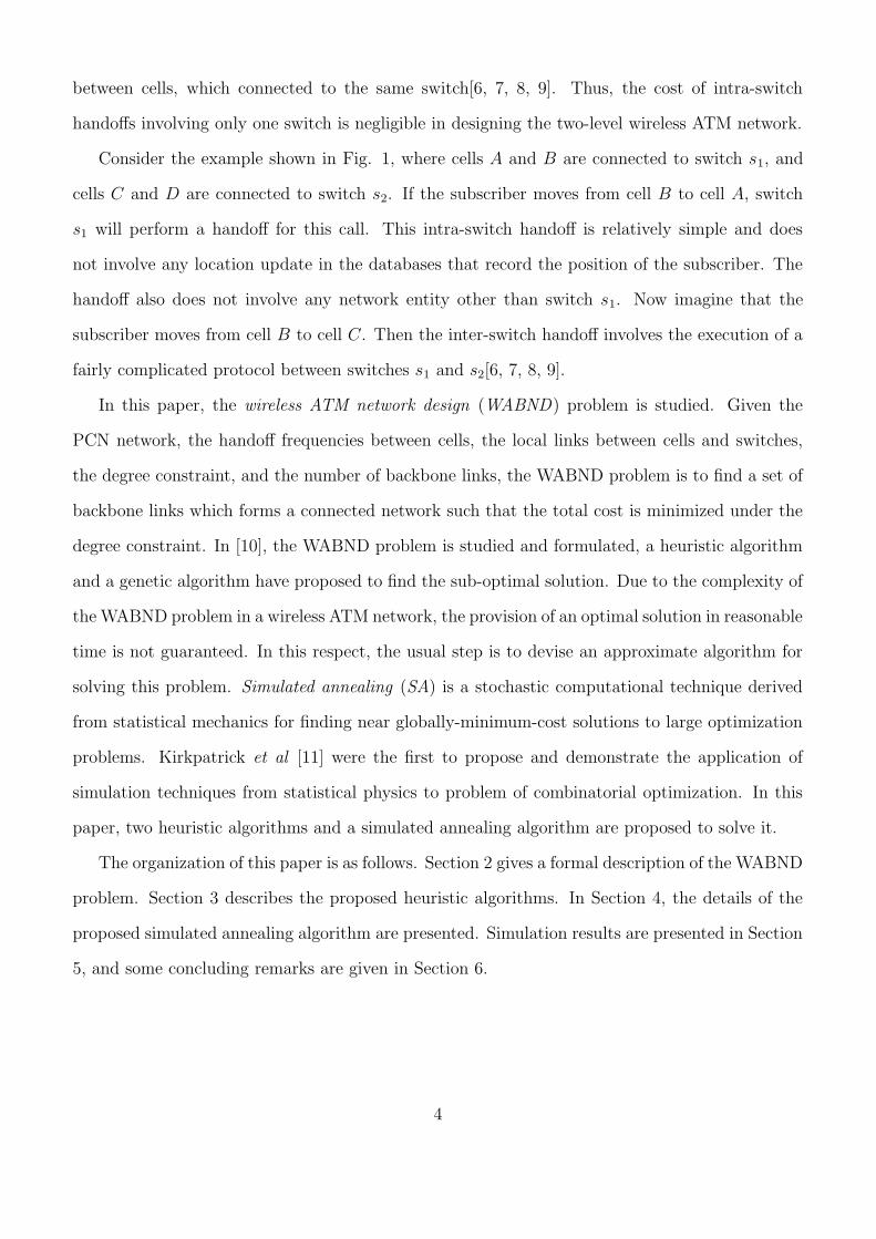
result is showed in Fig. 2(b). For the set of examples: m = 30, deg = 10, p is in {40, 50, 60, 70,

80, 90}, the result is showed in Fig. 3(a). For the set of examples: m = 30, deg is in {5, 10, 15,

20, 25, 30}, p=40, the result is showed in Fig. 3(b). The proposed simulated annealing algorithm

can get the best result as the same obtained by the genetic algorithm (GA) as indicated from the

experimental results. Moreover, the proposed heuristic algorithms RBH and WMBH get better

results than HA.

20

Figure 2: Experiments on set of examples with m =20 , (a) different values of p, (b)different valuesof deg.

21

Figure 3: Experiments on set of examples with m =30, (a) different values of p, (b)different valuesof deg.

22

6 Conclusions

In this paper, the problem of optimum design of the two-level wireless ATM network is investigated.

Given PCN network, handoff frequencies between cells, locations of switches on an ATM network,

the number of backbone links, the communication cost between switches, and the degree constraint

of switch, the problem is to determine the topology of the backbone network in an optimum manner

and named as the wireless ATM backbone network design problem (WABND).

First, the formulation of the WABND problem is given, since the optimal communication

spanning tree (OCT) problem is a special case of WABND which is NP-hard, thus the WABND

is NP-hard. Thus finding an optimal solution of this problem in reasonable time is impractical.

In this paper, two heuristic algorithms (RBH and WMBH) and a simulated annealing algorithm

(SA) are proposed to solve this problem. Simulation results showed that simulated annealing

algorithm are robust for this problem.

In the SA method, adjacency matrix is used to represent the topology of the backbone net-

work. In the design encoding method, the configuration represents a connected graph witch is a

constraint-satisfied one. Thus there is no need for penalty function and thus the performance of

SA can be improved. Experimental results indicate that the proposed SA runs efficiently. The

total cost of SA gets better performance than heuristic algorithms.

7 Acknowledgment

This work was supported in part by National Science Council (NSC) of R. O. C under Grant

NSC-94-2213-E-018-015.

23

References

[1] R. Steele, “Deploying personnal communication networks,” IEEE Commun. Mag., vol. 4, no.6, pp.12-15, Sept. 1990.

[2] D. C. Cox, “Personal communication - a viewpoint,” IEEE Commun. Mag., vol.11, no.8,pp.8–20, Nov. 1990.

[3] N. F. Huang and R. C. Wang, “The link allocation problem on ATM based personal commu-nication networks,” Wireless Personal Commun., vol.4, no.2, pp.257–275, Mar. 1997.

[4] Y. B. Lin and S. Y. Hwang, “Comparing the PCS location tracking strategies,” IEEE Trans.Veh. Tech., vol.45, no.1, pp.114–121, Feb. 1996.

[5] D. Raychaudhuri and N. D. Wilson, “ATM-based transport architecture for multiserviceswireless personal communication networks,” IEEE J. Select. Areas Commun., vol.12, no. 8,pp.1041–1414, Oct. 1994.

[6] A. Merchant and B. Sengupta, “Assignment of cells to switches in PCS networks,”IEEE/ACM Trans. on Netw., vol.3, no.5, pp.521–526, Oct. 1995.

[7] D. R. Din and S. S. Tseng, “Genetic algorithms for optimal design of two-level wirelessATM network,” Proc. of National Science Council, R. O. C. Part A: Physical Science andEngineering vol.25, no.3, pp.151–162, 2001.

[8] D. R. Din and S. S. Tseng, “A solution model for optimal design of two-level wireless ATMnetwork,” IEICE Trans. on Commu., E85-B, no.8, pp.1533–1541, Aug. 2002.

[9] D. R. Din and S. S. Tseng, “Heuristic and simulated annealing algorithms for solving extendedcell assignment problem in wireless ATM network,” Int. J. of Commu. Syst., vol.15, no.1,pp.47–65, Feb. 2002.

[10] D. R. Din, “Wireless ATM backbone network design problem,” IEICE Transactions on Com-munications, vol. e88-b, pp. 1347–1354, April, 2005.

[11] S. Kirkpatrick , C. D. Gelatt, and M. P. Vecchi, “Optimization by simulated annealing,”Science, vol.220, pp.671–680, 1983.

[12] C. P. Low, “An efficient algorithm for the link allocation problem on ATM-based personalcommunication networks,” IEEE J. on Sel. Areas in Commu., vol.18, no.7, pp.1279–1288,July 2000.

[13] T. C. Hu, “Optimum communication spanning tree,” SIAM J. Comput. vol.3, no.3, pp.188–195, 1974.

[14] M. R. Garey and D. S. Johnson, Computers and Intractability–A guild to the theory ofNP-Completeness, 1979.

[15] Y. Bartal, “On approximating arbitrary metrics by tree metrics,” In Proceedings of the 30thAnnual ACM Symposium on Theory of Computing, Dallas, TX, USA, pp.161–168, May 1998.

[16] Y. Li and Y. Bouchebaba, “A new genetic algorithm for the optimal communication spanningtree problem,” Arti. Evolu., 4th European Conference, AE’99, Lecture Notes in ComputerScience 1829, pp.162–173, 2000.

[17] B. Boldon, N. Deo, and N. Kumar, “Minimum-weight degree-constrained spanning tree prob-lem: heuristics and implementation on an SIMD parallel machine,” Paral. Comput., vol.22,no.3, pp.369–382, Mar. 1996.

24

[18] M. Krishnamoorthy, A. T. Ernst and Yazid M. S, “Comparison of algorithms for the degreeconstrained minimum spanning tree,” J. of Heur., vol.7, no.6, pp.587–611, Nov. 2001.

[19] N. Deo and N. Kumar, “Computation of constrained spanning trees: A unified approach,”Network Optimization: Lecture Notes in Economics and Mathematical Systems, no. 450, pp.194–220, Springer-Verlag, 1997.

[20] B. Gavish, “Topological design of centralized computer networks: Formulations and algo-rithms,” Netw., vol. 12, pp. 355–377, Dec. 1982.

[21] S. C. Narula, C. A. Ho, “Degree constrained minimum spanning tree,” Comput. and Oper.Rese., vol.7, no.4, pp. 239–249, 1980.

[22] A. Volgenant, “A Lagrangian approach to the degree-constrained minimum spanning treeproblem,” Euro. J. of Oper. Rese., vol. 39, pp. 325–331, 1989.

[23] Y. Yamamoto, “The Held-Karp algorithm and degree-constrained minimum 1-tree,” Math.Prog., vol. 15, no.2, pp. 228–231, 1978.

[24] M. Savelsbergh, T. Volgenant, “Edge exchanges in the degree constrained minimum spanningtree problem,” Comput. and Oper. Rese., vol. 12, no. 4, pp. 341–348, 1985.

[25] G. Zhou and M. Gen, “Approach to the degree-constrained minimum spanning tree problemusing genetic algorithms,” Engin. Design and Auto. vol.3, no.2, pp. 156–165, 1997.

[26] G. Zhou and M. Gen, “A note on genetic algorithms for degree constrained minimum spanningtree problems,” Netw., vol.30, no.2 pp.91–95, Sept. 1997.

[27] Van Laarhoven and E. Arts, Simulated Annealing: Theory and Application, D. Reidel Pub-lishing Company, Holand, 1987.

25