Embed Size (px)
Citation preview

Theoretical Computer Science 125 (1994) 91-109
Elsevier
91
Heterogeneous multiprocessor systems with breakdowns: performance and optimal repair strategies
Ram Chakka and Isi Mitrani Computing Science Department, University of Newcastle upon Tyne, Newcastle upon Tyne. NE1 7RlJ. UK
Abstract
Chakka, R. and I. Mitrani, Heterogeneous multiprocessor systems with breakdowns: performance
and optimal repair strategies, Theoretical Computer Science 125 (1994) 91-109.
A model of a system with N parallel processors subject to occasional interruptions of service, and a common unbounded queue fed by a Poisson arrival stream, is analyzed in the steady state. The
service, breakdown and repair characteristics may vary from processor to processor. A solution
method called spectral expansion is used to determine the joint distribution of the state of the
processors and the number of jobs in the queue. The problem of optimizing the repair policy is
addressed. The optimal policy is determined in the case when all breakdown rates are equal, and
some heuristics for the general case are investigated.
1. Introduction
We are interested in the behaviour of a system where jobs are served by a collection
of nonidentical parallel processors, each of which breaks down occasionally and takes
some time to be repaired (or replaced). The general topic of modelling systems which
are subject to interruptions of service has of course received considerable attention in
the literature. Some of the work has concentrated on single-processor models
[l, 3,14,15,16], and some on multiprocessor ones, where all the processors are
statistically identical [2,8,9,12]. However, very little progress has been made
in modelling heterogeneous multiprocessor systems with breakdowns. Although
Correspondence to: I. Mitrani, Computing Science Department, University of Newcastle upon Tyne,
Newcastle upon Tyne NE1 7RU, UK. Email: [email protected].
0304-3975/94/$07.00 c 1994-Elsevier Science B.V. All rights reserved
SSDI 0304-3975(93)E0117-M
92 R. Chakka, I. Mitrani
Markov-modulated queueing systems [ 13,171 provide a rather general framework in
which this problem may be placed, there are no existing solutions. Some of the
difficulty of the analysis stems from the fact that, at any moment in time, the total rate
at which service is given depends both on the state of the processors and, to a limited
extent, on the number of jobs present.
The contribution of this paper is twofold. First, we employ a rather novel solution
method that applies to a class of Markov models of heterogeneous multiprocessor
systems. This method, called spectral expansion [lo], yields the joint distribution of
the set of operative processors and the number of jobs in the system in terms of the
eigenvalues and left eigenvectors of a certain matrix polynomial. The approach is
readily implementable and is efficient in computing various performance measures. It
can thus be recommended as an attractive alternative to the matrix-geometric solution
[ll]. The model and the spectral expansion solution method are described in Sections
2 and 3, respectively.
The second contribution concerns optimization. If the number of repairmen is less
than N, thus restricting the number of processors that can be repaired in parallel, then
the repair scheduling strategy (i.e. the order in which broken processors are selected
for repair) has an important effect on performance. We study this effect at some length,
concentrating on the case of a single repairman (Section 4). An interesting problem
which, to our knowledge, has not been addressed before, is to find the repair strategy
that maximizes the average processing capacity of the system. A related problem -
that of optimizing the utilization of the repairman - was considered by Kameda [6],
and was solved in the case when the breakdown rates of all processors are equal. We
establish a correspondence between the two problems and hence find the optimal
capacity strategy for the same special case.
The general optimal capacity problem still lacks an exact solution. We propose
several heuristics and examine their performance empirically (Section 5).
2. The model
Jobs arrive into the system in a Poisson stream at rate 0, and join an unbounded
queue. There are N nonidentical parallel processors numbered 1,2, . . . , N. The service
times of jobs executed on processor i are distributed exponentially with mean l/pi.
However, processor i executes jobs only during its operative periods, which are
distributed exponentially with mean l/ti. At the end of an operative period, processor
i breaks down and requires an exponentially distributed repair time with mean l/vi.
The number of repairs that may proceed in parallel could be restricted: if so, this is
expressed by saying that there are R repairmen (R < N), each of whom can work on at
most one repair at a time. Thus, an inoperative period of a processor may include
waiting for a repairman. No operative processor can be idle if there are jobs awaiting
service, and no repairman can be idle if there are broken down processors. All

Heterogeneous multiprocessor systems with breakdowns 93
interarrival, service, operative and repair random variables are independent of each
other.
If there are more operative processors than jobs in the system, then the busy
processors are selected according to some service priority ordering. This ordering can
be arbitrary, but it is clearly best to execute the jobs on the processors whose service
rates are the highest; this is therefore assumed to be the case (it is further assumed that
jobs can migrate instantaneously from processor to processor in the middle of
a service). Services that are interrupted by breakdowns are eventually resumed
(perhaps on a different processor and hence at a different rate) from the point of
interruption. Similarly, if R <N and the repair strategy allows pre-emptions of repairs,
then these are eventually resumed from the point of interruption and there are no
switching delays.
The model is illustrated in Fig. 1.
The system state at time t can be described by a pair of integers K(t) and J(t)
specifying the processor configuration and the number of jobs present, respectively.
The precise meaning of “processor configuration”, and hence the range of values of
K(t), depends on the assumptions. For example, if the processors are identical, then it
is only necessary to specify how many of them are operative: K(t) = 0, 1, . . . , N. In the
heterogeneous case, if R = N, or if the repair strategy is pre-emptive priority or
processor sharing, the processor configuration should specify, for each processor,
whether it is operative or broken down. This can be done by using a range of values
zc(t)=O, 1, . . . , 2N - 1 (e.g. each bit in the N-bit binary expansion of K(t) can indicate
7<->_ dcparturcs
joh arrivals *
*
Fig. 1. Heterogeneous multiprocessor system with a. common unbounded queue

94 R. Chakka, I. Mitrani
the state of one processor). If, on the other hand, R < N and the repair strategy is
nonpre-emptive, then it is necessary to specify both the processors that are broken
down and those among them that are being repaired. That would require an even
wider range of values for K(t).
In general, suppose that there are M processor configurations represented by the
values K(t) = 0, 1, . , , M - 1. The model assumptions ensure that X = {K(t); t > 0} is an
irreducible Markov process. Let A be the matrix of instantaneous transition rates
from state k to state 1 for this process (k, 1 =O, 1, . . . , M - 1; k#l), with zeros on the
main diagonal. The elements of A depend on the parameters ci and vi (i = 1,2, . . . , N)
and, if R <N, on the repair strategy. For example, consider a system with 3 processors
and 1 repairman under a pre-emptive priority repair strategy with priority ordering
(1,2,3) (i.e. processor 1 has top pre-emptive priority for repair, while processor 3 has
bottom priority). There are now 8 processor configurations, K(t) = 0, 1, . . . ,7, repres-
enting the operative states (O,O, 0), (O,O, l), . . . ,(l, 1, l), respectively (bit i is 0 when
processor i is broken, 1 when operative). In this case, the matrix A is given by
(0, 0, 0) 0 0 0 0 q10 0 0
(O,Q 1) 53 0 0 0 0 yI10 0
(0, 120) (2 0 0 0 0 0 r/l 0
(0, 1, 1) 0 0 0 0 0
A=
52 t3 81
. (LQO) 51 0 0 0 0 0 r/z 0
(1,091) 0 51 0 0 53 0 0 rlz
(1,L 0) 0 0 (1 0 52 0 0 v3
(LLl) 0 0 0 51 0 52 53 o_
(1)
Let also DA be the diagonal matrix whose ith diagonal element is the ith row sum of
A. The matrix A-DA is the generator matrix of the process X.
Denote by pk the steady-state probability that the processor configuration is k. The
row vectorp=(pO,p,, . . . . pM- 1) is determined by solving the linear equations
p(A-DA)=O; pe= 1, (2)
where e is the column vector with M elements, all of which are equal to 1. This
solution is not too expensive, even for large values of M, because the matrix A is very
sparse. Having obtained p, one can find the steady-state probability qi that processor
i is operative. It is given by
qi= c pk; i=O,l, . . . . N, (3) ksai
where Cli is the set of processor configurations in which processor i is operative. The
linear combination
Y= f 4iPi
i=l
(4)

Heterogeneous multiprocessor systems with breakdowns 95
will be referred to as the processing capacity of the system. This is the overall average
rate at which jobs can be executed. The system is stable when CJ < y.
In order to compute performance measures involving jobs, it is necessary to study
the two-dimensional Markov process Y= { [K(t),J(t)]; t 20} with state space
{O,l, ... , M-l} x {O,l, . ..}. A ssuming that the stability condition holds, our next task
is to compute the steady-state probabilities pk,j that the processor configuration is
k and the number of jobs in the system is j.
3. Spectral expansion solution
The process Y evolves according to the following instantaneous transition rates:
(a) from state (k,j) to state (I,j) (k, l= 0, 1, . . , M - 1;j = 0, 1, . . . ; 1# k), with rate A(k, 1) (for an example of the matrix A, see (l)),
(b) from state (k,j) to state (k,j+ 1) (k =O, 1, . . . , M - 1; j=O, 1, . ..). with rate CJ,
(c) from state (k, j) to state (k, j- 1) (k =O, 1, . . . , M - 1; j= 1,2, . . .), with rate Bk,j,
equal to the sum of the service rates of the processors which are operative and busy
when the processor configuration is k and the number of jobs is j.
It is important to note that the transition rates (a) and (b) do not depend on j. The
rates (c) may depend on j when j < N, but cease to do so for j> N. In the three-
processor example mentioned in the previous section, supposing that pi >pLz >,pL3
(which means that the service priority order is (1,2,3)), the values of bk, j are
configuration
(0, 090)
(0, 0, 1)
(0, LO)
(0,191)
(l,O,O)
(LO, 1)
(1, LO)
(1, 1, 1)
P k, 1
0
113
P2
P2
Pl
111
/Jl
/Jl
Pk,j(.i23)
0
P3
P2
P2 +P3
Pl
Pl +p3
Pl +P2
pl+pZ+p3
The probabilities { Pk, j} satisfy an infinite set of balance equations. It is convenient
to write these in matrix form, by introducing the row vectors,
uj’(P0,j9Pl,j3 ... ,PM-1,j); j=O,L..., (5)
whose elements represent the states with j jobs in the system. Also, let Bj be the
diagonal matrix
(6)

96 R. Chakka, I. Mitrani
We have seen that the index j can be omitted when ja N:
B,=B; j=N,N+l,...
The balance equations can now be written as
Uj(DA+,Z+Bj)=vj_laZ+UjA+Uj+lBj+,; j=O, 1, . . . N-l,
where I is the A4 x M identity matrix and u- 1 = 0 by definition, and
A Uj(D +OZ+B)=Uj_lC7Z+UjA+Uj+1 B; j=N,N+l,...
In addition, all probabilities must sum up to 1:
(7)
(8)
jro uje= l. (9)
Equation (8) is a homogeneous vector difference equation of order 2, with constant coefficients. It can be rewritten in the form
ujQo+uj+lQ1+Uj+2Q2=0; j=N-LN,..., (10)
where Q. = ol, Q I = A -DA - CJZ - B and Qz = B. Associated with (10) is the character- istic matrix polynomial Q(A) defined as
Q@,=Qo+Q,~+Qd*. (11)
Denote by A, and $,,, the eigenvalues and corresponding left eigenvectors of Q(L). In other words,
detCQ&)I=O; $,Q(Ad=Q m=l,2 ,..., d, (12)
where d =degree(det [Q(n)]}. We shall focus our attention on the case where all d eigenvalues are single. This is the most interesting case in practice, since the likelihood that a real-life problem of this type will exhibit multiple eigenvalues is negligible (if the coefficients of a random polynomial are sampled from a continuous distribution, then the probability that it will have multiple roots is 0).
The following result was established in [lo]:
Proposition 3.1. Suppose that c of the eigenvalues of Q(A) are strictly inside the unit disk,
while the others are on the circumference or outside. Let the numbering be such that
I&,,I<lfirm=l,2 ,..., cand(il,,~~lfirm=c+l,..., d. Then any solution of equation
(10) which can be normalized to a probability distribution is of the form
Uj= f Xm*mjli; j=N-1,N 3 ..., (13)
m=l
where x, (m = 1,2, . . . , c) are arbitrary complex constants.

Heterogeneous multiprocessor systems with breakdowns 91
Note that, if there are nonreal eigenvalues in the unit disk, then they appear in
complex-conjugate pairs. The corresponding eigenvectors are also complex-conju-
gate. The same must be true for the appropriate pairs of constants x,, in order that the
right-hand side of (13) be real. To ensure that it is also positive, it seems that the real
parts of A,,,, $m and x, should be positive. Indeed, that is invariably observed to be the
case.
So far, we have obtained expressions for the vectors t+ 1, uN, . . . , which contain
c unknown constants. Now it is time to consider equations (7), for j=O, 1, . . . , N- 1.
This is a set of NM linear equations with (N - l)M unknown probabilities (the vectors
Uj for j=O,l,..., N-2), plus the c constants x,. However, only NM- 1 of these
equations are linearly independent, since the generator matrix of the Markov process
is singular. On the other hand, an additional independent equation is provided by (9).
Clearly, this set of NM equations with (N - l)M + c unknowns will have a unique
solution if, and only if, c= M. This observation, together with the fact that an
irreducible Markov process has a steady-state distribution if, and only if, its balance
and normalizing equations have a unique solution, implies the following proposition.
Proposition 3.2. The condition c = M (the number of eigenvalues of Q(A) strictly inside the unit disk is equal to the number of processor configurations) is necessary and su&ient for the stability of the Markov process Y= {[K(t), J(t)]; t 2 O}.
The intuitively appealing stability condition given in the previous section, a<?,
should be equivalent to the one provided by Proposition 3.2. This is confirmed by all
numerical experiments, but we have not been able to prove it formally.
A few additional remarks concerning Proposition 3.2 are, perhaps, in order. It can
be shown that the eigenvalue of Q(n) with the largest modulus in the unit disk is
always real. That is, in fact, the Perron-Frobenius eigenvalue of Neuts’ matrix R, defined in [ 111. When the load on the system increases, i.e. when G approaches y, that
eigenvalue approaches 1, while the other eigenvalues in the unit disk remain strictly in
the interior. Hence, the heavy-traffic behaviour of the system is governed by just one
(real) term in the spectral expansion ~ the term involving the dominant eigenvalue and
its left eigenvector.
In summary, our solution procedure consists of the following steps:
(1) Compute the eigenvalues 1, and the corresponding left eigenvectors I//, of Q(n).
If c # M, stop; a steady-state distribution does not exist.
(2) Solve the finite set of linear equations (7) and (9), with uN- 1 and uN given by (13),
to find the constants x, and the vectors uj for j< N - 1. The entire joint distribution
pk,j is now determined.
(3) Use the obtained solution for the purpose of computing various moments,
marginal probabilities, percentiles and other system performance measures that may
be of interest.
An efficient computational method for step 1, based on reducing the quadratic
eigenvalue-eigenvector problem to a linear one, is described in [2,5].

98 R. Chakka, I. Mitrani
The computational complexity of step 2 is not as great as it appears. The vectors
UN-Z,uN-3, ... , v,, can be expressed in terms of Us _ 1 and Us, by successive application
of (7) for j = N - 1, N - 2, . . , 1. This leaves just equations (7) for j = 0 , plus (9) (a total
of M independent linear equations) for the M unknowns x,.
Some numerical results obtained by the above procedure are presented in the
following section.
It should be pointed out that the spectral expansion method is applicable in
considerably more general situations than the one considered here. For example, the
job arrival rate could depend on the processor configuration. The only effect of this
generalization would be to replace the matrix Q0 = al with a different diagonal matrix
with nonidentical elements. One could also envisage models where the breakdown
rate of a processor depends on whether the latter is busy or not; where breakdowns
can be triggered by arrivals; or where several processors are liable to break down or be
repaired simultaneously. Assumptions of that kind are easily reflected in the form of
the matrices Qo, Q1 and Q2.
A more substantial generalization would be to allow arrivals and departures to
occur in batches of fixed or random sizes. Provided that the batch sizes are bounded,
such models also lead to finite vector difference equations. However, the order of
those equations is higher than 2. More precisely, if the number of jobs in the system
can jump up by at most y1 at a time, and down by at most r2 at a time, with or without
triggered breakdowns or repairs, then the difference equation similar to (10) would be
of order r1 +r,. The degree of the matrix polynomial Q(A) would correspond to that
order. The complexity of the solution procedure would obviously be higher, but its
form, based on Propositions 3.1 and 3.2, is the same.
4. Repair strategy optimization
When the number of repairmen is less than the number of processors, the order in
which processors are selected for repair has an influence on the performance of the
system. Different repair strategies can lead to different values of the processing
capacity y and hence to arbitrarily large differences in performance measures like the
average queue size or the average response time. This situation is illustrated in Fig. 2,
where the average number ofjobs E(J) in a 3-processor system with one repairman, is
plotted against the job arrival rate. Four repair strategies are compared, three of
which are of the pre-emptive-resume type, allowing repairs to be interrupted at an
arbitrary point without any overheads, and one is nonpre-emptive. In all cases, the
values of E ( J) are determined by applying the spectral expansion procedure described
in the previous section.
The parameters in this example have not been chosen to be realistic; nevertheless,
the behaviour that is displayed in the figure is quite typical. The important feature of
all such performance curves is that they have a vertical asymptote at the point where

Heterogeneous multiprocessor systems with breakdowns 99
N=3 ; R=l b] =3.0 ; 5, =0.4 ; Tj] =o.s
pr eniptivc pi iorit) (. 2 1,) y :’ - 1.81
preemptive priority
Fig. 2. Average number of jobs in the system against arrival rate, for different repair strategies.
the arrival rate is equal to the processing capacity. Any difference in y, no matter how
small, caused by a change in the repair strategy, implies different vertical asymptotes.
Hence, given a sufficiently heavy traffic, there will be unbounded differences in
performance. In particular, on the interval between the two processing capacities, the
queue is saturated under one strategy and stable under the other.

100 R. Chnkka, I. Mitrani
Clearly, it can be very important to use a repair strategy that maximizes the
processing capacity. We shall consider the problem of finding such strategies, in the
case where N heterogeneous processors are attended to by a single repairman. This is
obviously the case with the greatest practical relevance, since increasing the number of
repairmen can only reduce the effect of the repair strategy on the processing capacity.
For a given strategy, let Ui be the fraction of time that processor i spends being
repaired (i = 1,2, . . . , N); alternatively, this is the repairman utilization factor due to
processor i. Let also ri be the average period between two consecutive instants when
processor i becomes operative (i.e. the average operative-inoperatioe cycle for proces-
sor i). Then we can write
l/Vi ’ ui=Ti 2
i=l,2 ,..., N. (14)
Similarly, the probability that processor i is operative can be written as
1/5i. i=l 2 N 4i=T 9 2 >..., . (15)
Hence, we have the relation qi = (qi/ti)ui. This allows us to rewrite the expression for
the processing capacity (4) in the form
y= 2 CiUi, i=l
where ci=piqi/ti.
(16)
Thus, the problem of maximizing the processing capacity can be reduced to that of
maximizing a linear combination of repairman utilizations. This latter problem has
been studied by Kameda [6,7] in the context of finite-source queues with different
jobs and a single server. He considered the special case where the job arrival rates
(which correspond to our breakdown rates) are equal: <i = c2 = . . . = tN. Under that
assumption, and using our terminology, Kameda’s main result can be summarized as
follows:
(a) When the exact repair times are not known in advance, the strategy that
maximizes the right-hand side of (16) is one of the N! static pre-emptive priority
strategies.
(b) In the optimal pre-emptive priority strategy, processor i is given higher priority
for repair than processor j if ci > Cj .
Thus, when the breakdown rates are equal, the highest processing capacity is
achieved by a static repair strategy which gives processor i pre-emptive priority over
processor j if ~iri > ~jrlj.
In the general case of unequal breakdown rates, it is not known whether statement
(a) is true or not. It may be that, in order to achieve global optimality, one has to allow
dynamic scheduling decisions which depend in a complex way on the current proces-
sor configuration. Nevertheless, we shall confine our search to the set of N! static
pre-emptive priority policies. Even so, it seems that there is no simple rule for
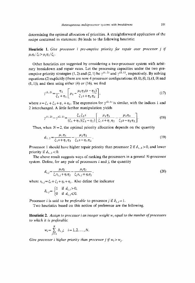
Heterogeneous multiprocessor systems with breakdowns 101
determining the optimal allocation of priorities. A straightforward application of the
recipe contained in statement (b) leads to the following heuristic:
Heuristic 1. Give processor i pre-emptive priority for repair over processor j if
Pir?ilti>PjSj/5j.
Other heuristics are suggested by considering a two-processor system with arbit-
rary breakdown and repair rates. Let the processing capacities under the two pre-
emptive priority strategies (1,2) and (2,l) be yC1’ ‘) and y”’ ‘I, respectively. By solving
equations (2) explicitly (there are now 4 processor configurations: (0, 0), (0, l), (1,0) and
(1, l)), and then using either (4) or (16), we find
Y (l,Z)_.!L
tl+Vl [
pl+P2v2(s-v2) 1 52s+il1v2 ’ (17)
where s = 4 1 + t2 + r] 1 + q2. The expression for y (2,1) is similar, with the indices 1 and
2 interchanged. A little further manipulation yields
(1.2)_.+2,1)= 5152s
[
Pl?l P2V2 Y
(tl+YlH52+r2) 51~+u11~2-42~+9I2~2 . 1 (18) Thus, when N = 2, the optimal priority allocation depends on the quantity
(19)
Processor 1 should have higher repair priority than processor 2 if dl, 2 >O, and lower
priority if dl, 2 <O. The above result suggests ways of ranking the processors in a general N-processor
system. Define, for any pair of processors i and j, the quantity
(20)
where si, j = ti + rj + I?i + ylj. Also define the indicator
6i,j=
1 if di,j>O,
0 if di,j~O.
Processor i is said to be preferable to processor j if 6i,j= 1.
Two heuristics based on this notion of preference are the following.
Heuristic 2. Assign to processor i an integer weight wi equal to the number of processors to which it is preferable:
N
wi= 1 6i,j; i=l,2,...,N. j=l
Give processor i higher priority than processor j if wi > wj.

102 R. Chakka, 1. Mitrani
Heuristic 3. Assign to processor i a real weight wi equal to the accumulated differences (20), for all processors to which it is preferable:
wi= ; 6i,jdi,j; i=1,2 ,..., N. j=l
Give processor i higher priority than processor j if wi > Wj,
Heuristic 2 concentrates on the existence of preference relations, whereas Heuristic
3 attempts to take into account their extent. Of course, both produce the optimal
allocation in the case N = 2.
The relation preferable is not transitive. For example, it may happen that processor
i is preferable to processor j, processor j is preferable to processor k, and processor k is preferable to processor i. Heuristic 2 could then assign equal weights to those three
processors, necessitating some tie-breaking rule. We have simply used the processor
indices to break ties. It should be pointed out that these occurrences are very rare (less
than 1% of all cases examined).
One can put forward other heuristics which, while being intuitively weaker, do not
seem unreasonable. For example:
Heuristic 4. Give processor i priority over processor j ifpiri >pjqj.
Heuristic 5. Give processor i priority over processor j ifpi>pj.
Heuristic 6. Give processor i priority over processor j if 5i< i”j.
Heuristic 7. Give processor i priority over processor j if vi > qj,
In the absence of theoretical results with general validity, the only way of evaluating
all these heuristics is by experimentation. Some empirical results are reported in the
next section.
5. Evaluation of the heuristics
The first set of three experiments involves a lOO-processor system where the
breakdown rates are about an order of magnitude smaller than the repair rates, which
are in turn a couple of orders of magnitude smaller than the service rates. An
experiment consists of generating 100 random models, i.e. random sets of values for
the parameters pi, ti and vi (i= 1,2, . . . , 100). The latter are uniformly distributed
within prescribed ranges. For each model, the processing capacity under the seven
heuristics of the previous section, and under the first-come-first-served (FCFS) repair
strategy, is estimated by simulation (exact solutions are not feasible, due to the large
state spaces of the Markov chains). The three experiments differ in the range of the
parameters v]i.

Heterogeneous multiprocessor systems with breakdowns 103
1o07y
4 N= 100 : K= I ; 1, F ( 1000.0 . 100000.0 ) : E E ( 0.01 . 0.40 )
nunihcr of cabcs in which the 001
heuristic i:, best ;
80; 1, F ( 1 .o 3’1.0 ) 1, E ( 1 .o , 49.0 ) q E ( 1.0 ) so.0 )
7( )-
I
60 1
50 I
I 40
1
30
20 ;
10
0
heuristic number *
Fig. 3. Performance of the heuristics in experiment with large N: number of cases in which each heuristic
performed best.
The bar chart in Fig. 3 shows, for each heuristic, the number of models in which it
produced the highest processing capacity among the eight heuristics (Heuristic 8 is the
FCFS strategy). We observe that Heuristic 1 is most frequently best, while Heuristics
$6 and 8 are never best. However, the dominance of Heuristic 1 diminishes when the
mean and variance of Y/i increase, and hence the average utilization of the repairman
decreases. A somewhat surprising feature of this figure is the poor performance of
Heuristic 3, and the relatively good performance of Heuristic 4.
It is interesting to note the improvement in processing capacity achieved by each
heuristic, compared to FCFS. This is shown in Fig. 4, where each bar measures the

104 R. Chakka, I. Mitrani
4 140.0
perccntagc capacity improvcmcnt
110.0
80.0
6 7 8
heuristic numhcr W
Fig. 4. Performance of the heuristics in experiment with large N: improvements of capacity compared with
FCFS policy.
quantity (Yheuristic - yFCFS)/yFCFS, averaged over the 100 models. It is rather remarkable
that, with the exception of 5 and 6, all heuristics achieve roughly the same average
relative improvement. More predictable is the fact that the heavier the load on the
repairman, the greater the magnitude of that improvement (however, even in the third
experiment, a 25% average improvement is achieved by most heuristics).
Another strategy that can be used as a standard of comparison instead of FCFS is
the random repair strategy, whereby at every scheduling decision instant, every one
of the broken processors is equally likely to be selected for repair. This was tried,
but no appreciable difference between the random and the FCFS strategies was
observed.

Heterogeneous multiprocessor systems with breakdowns 105
The above results do not tell us how close to optimal are the heuristics, since they
are compared only among themselves. On the other hand, in a lOO-processor system,
an exhaustive search of all permutations in order to find the optimal priority
allocation is obviously out of the question. Therefore, we have carried out an
experiment with a 6-processor system.
Again, 100 random models are generated, sampling the parameters pi, <i and
Q(i=1,2,... ,6) uniformly from prescribed ranges. Those ranges are piE(5000,95 000),
{+(O, 30), qi~(5, 145). The breakdown and repair rates are now much closer together,
so that there is still some competition for the repairman.
For each model, the processing capacity y is computed (exactly, by solving the
appropriate Markov chain) under all 6! = 720 possible pre-emptive priority alloca-
tions. The seven heuristics are of course among them, and so is the optimal allocation.
The following performance measures of each heuristic are determined in every model:
b = number of allocations that are better than the heuristic,
h= (Yoptimal-Yheuristic)lYoptimal,
a=lOO(yh,,*i,ti,-YFCFS)IYFCFS.
(The processing capacity of the FCFS strategy is again estimated by simulation.)
A rough comparison between the heuristics is displayed in Table 1, where the
quantities b, h and a are averaged over the 100 models.
The table shows that in this experiment the first three heuristics perform consider-
ably better than the others. Their average relative distances from the optimum h are
very small indeed. However, even the worst two Heuristics 5 and 6 yield processing
capacities within about 12% of the optimum. The average relative improvement in
capacity with respect to the FCFS strategy is considerable: it is on the order of 30%
for all heuristics except 5 and 6.
The frequency histograms for b and h are displayed in Figs. 5 and 6, respectively. It
can be seen that Heuristic 2 finds the best allocation in about 63% of the models,
Heuristic 3 is optimal in about 45% of the models, and Heuristic 1 is optimal in less
than 30% of the models. Figure 6 demonstrates very clearly that, even when the best
allocation is not found, the processing capacity by all three heuristics is very close to
optimal, In almost 90% of the models for Heuristic 2, 75% for Heuristic 3 and 50%
for heuristic 1, the relative error as measured by h is less than 0.001.
Table I
Heuristic Average b Average h Average a
1 13.26 0.0027 33.0 2 1.44 0.0006 33.2 3 3.08 0.0018 33.0 4 22.28 0.0095 32.1 5 155.40 0.0891 19.3 6 241.23 0.1270 13.0 I 94.73 0.0368 28.2

106 R. Chakka. I. Mitrani
100
4 frequency of
occurcncc
heuristic 1
h.i!lll ‘I
nl 3. __~_ 11 L nnnn -lb 2 .?i 4 5 6 8 7 9 20 30 40
heuristic 2
n I
number of better priority orders -+
Fig. 5. Performance of Heuristics l-3 with N = 6: number of better allocations.
A similar experiment with a more heavily loaded repairman produced similar
results, except that there the order of the first three heuristics was reversed: 1 was
slightly better than 3, which was slightly better than 2. Again, the relative errors of all
heuristics apart from 5 and 6 were very small.
6. Conclusions
We have presented an efficient solution method, which can be applied to a class of
heterogeneous multiprocessor models of moderate size. The bounds on the feasibility

Heterogeneous multiprocessor systems with breakdowns 107
100
4 frequency of
occurcncc 9~1
80
7C
h(‘
SC
4(
3(
2(
l( 1
, hliLL& ! LlL,, ’ 0.1 0.5 I .(I
1 0 heuristic 1 [ heuristic 2 1 heuristic 3 11
I 1
I
3.0 4.0
rclativc error (To) -)
Fig. 6. Performance Heuristics l-3 with N = 6: relative errors.
of a solution are dictated by the number of possible processor configurations: when
that number is very large, the eigenvalue-eigenvector problem becomes ill-
conditioned.
As far as the optimal repair strategies are concerned, it is clear that any one among
four or five heuristics would produce acceptable results in practice. In all cases, the
priorities allocated may be pre-emptive or nonpre-emptive. If one accepts the proposi-
tion, intuitively supported by Kameda’s argument in [7], that the globally optimal
policy is one of the N! pre-emptive priority ones, then any nonpre-emptive policy is
bound to be sub-optimal. However, our experiments provide a strong indication that
the processing capacities of several sub-optimal strategies tend to be very close to that

108 R. Chakka, I. Mitrani
of the optimal one. The effort of searching for an optimal allocation would be justified
only if the traffic rate is such that the job queue is close to saturation.
The outstanding theoretical problems in this context are
(i) to prove or disprove the fact that, when the exact repair times are not known in
advance, the globally optimal policy is indeed one of the N! static pre-emptive priority
allocations,
(ii) to find an efficient algorithm for determining the optimal (as opposed to
a nearly optimal) priority allocation.
It would also be interesting to get an estimate of the rate at which the relative error
of the heuristics grows with the number of processors. Further experimentation could
shed some light on this, but it will be expensive (already with 7 processors, there are
5040 possible priority allocations).
Acknowledgment
This work was carried out in connection with the Basic Research projects PDCS II
(Predictably Dependable Computer Systems) and QMIPS (quantitative methods in
parallel systems), funded by the European Community.
References
[l] B. Avi-Itzhak and P. Noar, Some queueing problems with the service station subject to breakdowns, Oper. Res. 11 (1963) 303-320.
[2] R. Chakka and I. Mitrani, A numerical solution method for multiprocessor systems with general breakdowns and repairs, Proc. 6th Internat. Conf: Modelling Techniques and Tools, Edinburgh, 1992.
[3] D.P. Gaver, A waiting line with interrupted service including priorities, J. Roy. Statist. Sot. Ser. B 24 (1962) 73-90.
[4] I. Gohberg, P. Lancaster and L. Rodman, Matrix Polynomials (Academic Press, New York, 1982). [S] A. Jennings, Matrix Computationsfor Engineers and Scientists (Wiley, New York, 1977).
[6] H. Kameda, A finite-source queue with different customers, J. ACM 29 (1982) 478-491.
[7] H. Kameda, Realizable performance vectors of a finite source queue, Oper. Res. 32 (1984) 135881367.
[S] I. Mitrani and B. Avi-Itzhak, A many-server queue with service interruptions, Oper. Res. 16 (1968) 628638.
[9] I. Mitrani and P.J.B. King, Multiserver systems subject to breakdowns: an empirical study, IEEE Trans. Comput. C-32 (1983) 96-99.
[lo] I. Mitrani and D. Mitra, A spectral expansion method for random walks on semi-infinite strips, in: IMACS Symp. Iterative Methods in Linear Algebra, Brussels, 1991.
[l l] M.F. Neuts, Matrix Geometric Solutions in Stochastic Models (John Hopkins Univ. Press, Baltimore, MD, 1981).
[12] M.F. Neuts and D.M. Lucantoni, A Markovian queue with N servers subject to breakdowns and repairs, Management Sci. 25 (1979) 849-861.
[13] N.U. Prabhu and Y. Zhu, Markov-modulated queueing systems, Queueing Systems Theory Appl. 5 (1989) 215-246.
[14] B. Sengupta, A queue with service interruptions in an alternating Markovian environment, Oper. Res. 38 (1990) 308-318.
[15] K. Thiruvengadam, Queueing with breakdowns, Oper. Res. 11 (1963) 62-71.

Heterogeneous multiprocessor systems with breakdowns 109
[16] H.C. White and L.S. Christie, Queueing with preemptive priorities or with breakdown, Oper. Res. 6 (1958) 79-95.
1173 U. Yechiali, A queueing-type birth-and-death process defined on a continuous time Markov chain,
Oper. Res. 21 (1973) 604-609.


![Mapping Stream Programs onto Heterogeneous Multiprocessor Systems [by Barcelona Supercomputing Centre, Spain, Oct 09] S. M. Farhad Programming Language](https://img.pdfslide.us/doc/110x75/56649e115503460f94afcb3e/mapping-stream-programs-onto-heterogeneous-multiprocessor-systems-by-barcelona.jpg)