EE249 Lecture

Taken from

Roberto Passerone PhD Thesis

Heterogeneous Models of Computation: An Heterogeneous Models of Computation: An Abstract Algebra ApproachAbstract Algebra Approach

ObjectivesObjectives

�Provide the foundation to represent different semantic

domains for the Metropolis metamodel

�Study the problem of heterogeneous interactionheterogeneous interactionheterogeneous interactionheterogeneous interaction

�Formalize concepts such as abstraction and refinement

An Example of InteractionAn Example of Interaction

�Combine a synchronous model with a dataflow model

�Synchronous model

� Total order of event

�Data flow model

� Partial order of events

�Discrete Time model

� Metric order of events

An Example of Heterogeneous An Example of Heterogeneous InteractionInteraction

�The interaction is derived from a common refinement

of the heterogeneous models

�The resulting interaction depends on the particular

refinements employed

�Our objective is to derive the consequences of the

interaction at the higher levels of abstraction

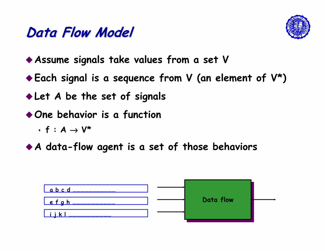
Data Flow ModelData Flow Model

�Assume signals take values from a set V

�Each signal is a sequence from V (an element of V*)

�Let A be the set of signals

�One behavior is a function

� f : A →→→→ V*

�A data-flow agent is a set of those behaviors

a b c d ……………………………

Data flowData flowe f g h ……………………………

i j k l ……………………………

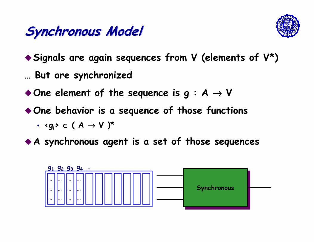
Synchronous ModelSynchronous Model

�Signals are again sequences from V (elements of V*)

… But are synchronized

�One element of the sequence is g : A →→→→ V

�One behavior is a sequence of those functions

� <gi> ∈∈∈∈ ( A →→→→ V )*

�A synchronous agent is a set of those sequences

…

…

…

g1

…

…

…

g2

…

…

…

g3

…

…

…

g4 …

SynchronousSynchronous

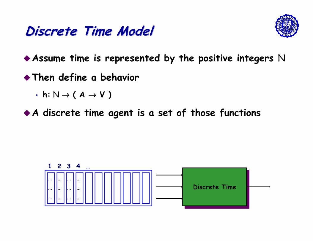
Discrete Time ModelDiscrete Time Model

�Assume time is represented by the positive integers N

�Then define a behavior

� h: N →→→→ ( A →→→→ V )

�A discrete time agent is a set of those functions

…

…

…

1

…

…

…

2

…

…

…

3

…

…

…

4 …

Discrete TimeDiscrete Time

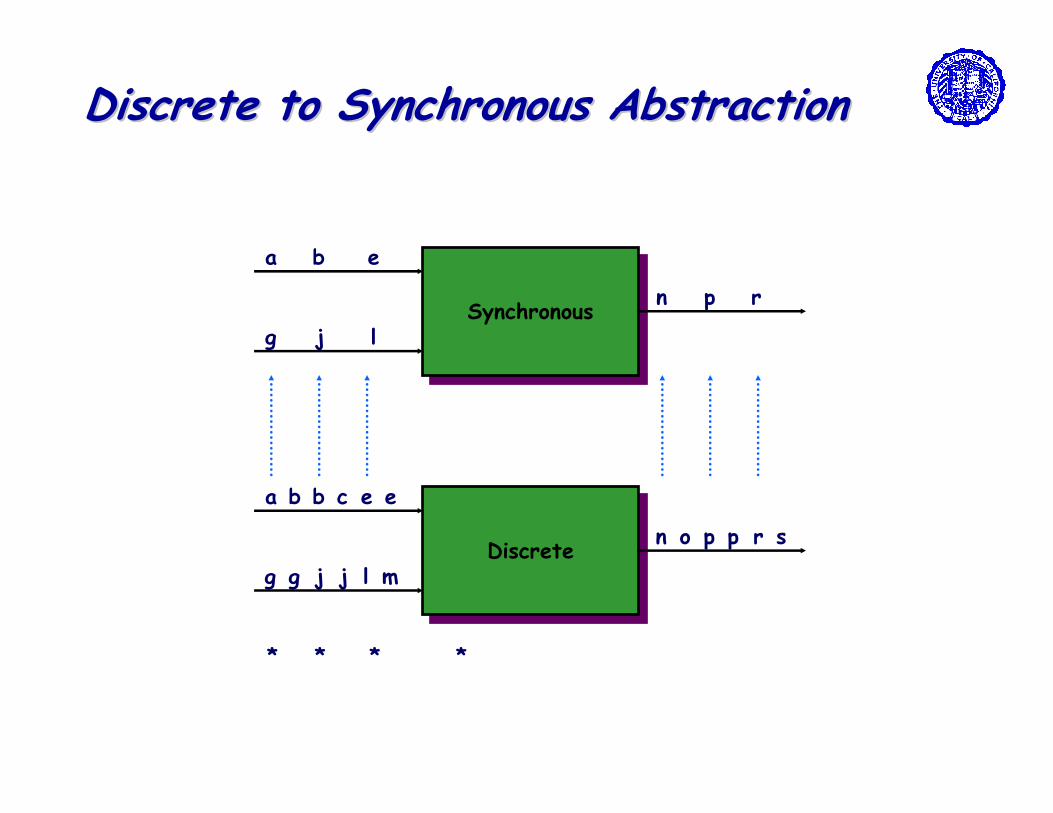
Discrete to Synchronous AbstractionDiscrete to Synchronous Abstraction

SynchronousSynchronous

DiscreteDiscrete

ba b c e e

gg j j l m

on p p r s

* * * *

a b e

g j l

n p r

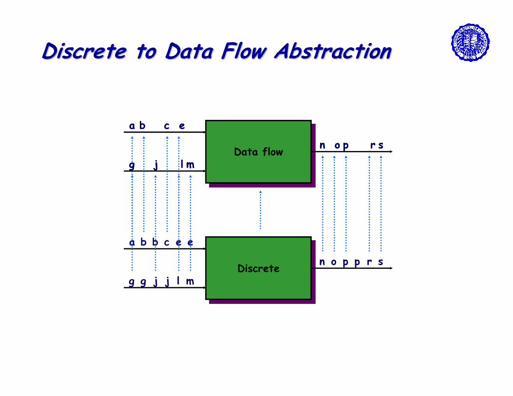
Discrete to Data Flow AbstractionDiscrete to Data Flow Abstraction

Data flowData flow

DiscreteDiscrete

ba b c e e

gg j j l m

on p p r s

b a c e

g j l m

on p r s

b a c e

g j l m

on p r s

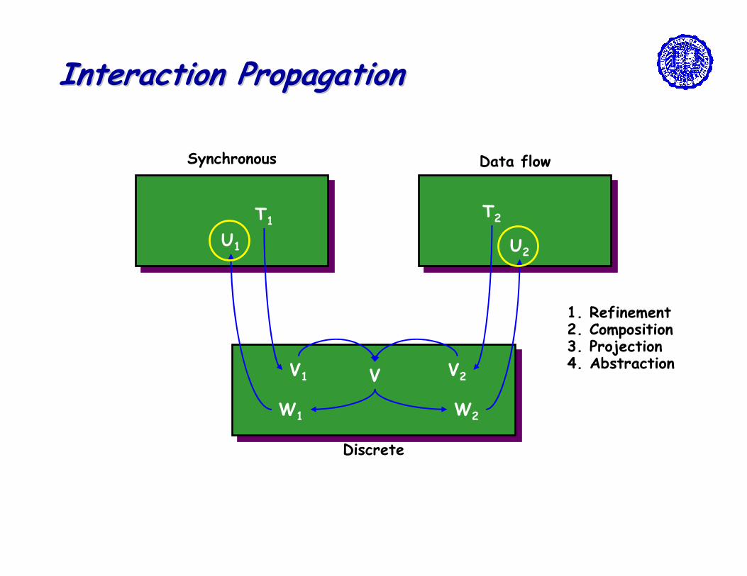
Interaction PropagationInteraction Propagation

Synchronous Data flow

Discrete

T1T2

V1 V2V

W1 W2

U1 U2

1. Refinement2. Composition3. Projection4. Abstraction

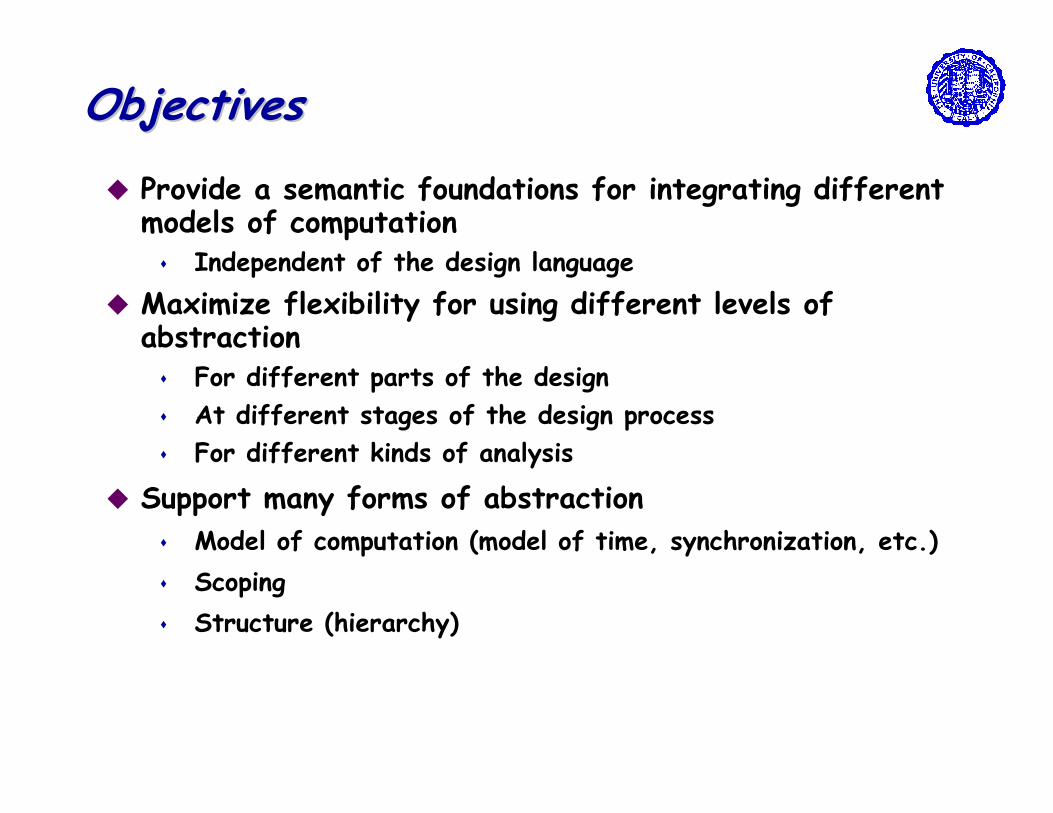
ObjectivesObjectives

� Provide a semantic foundations for integrating different models of computation� Independent of the design language

� Maximize flexibility for using different levels of abstraction� For different parts of the design

� At different stages of the design process

� For different kinds of analysis

� Support many forms of abstraction

� Model of computation (model of time, synchronization, etc.)

� Scoping

� Structure (hierarchy)

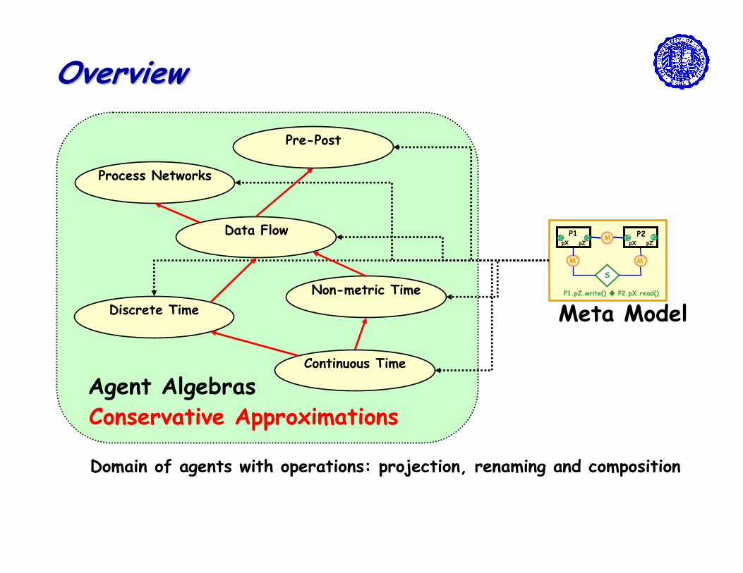
OverviewOverview

P1 P2M

S

P1.pZ.write() ���� P2.pX.read()

pX pZ pX pZ

M’ M’

Meta Model

Pre-Post

Process Networks

Data Flow

Discrete Time

Non-metric Time

Continuous Time

Agent AlgebrasConservative Approximations

Domain of agents with operations: projection, renaming and composition

ScopeScope

�Concentrate on

� Natural semantic domains (sets of agents)

� Relations and functions over semantic domains

� Relationships between semantic domains and their relations and functions

�Defer worrying about specific abstract syntaxes and semantic functions

� Convenient for manual, formal reasoning

� De-emphasizing executable and finitely-representable models (for now)

Agents and BehaviorsAgents and Behaviors

� For each model of computation we always distinguish between

� the domain of individual behaviors

� the domain of agents

� For different models of computation individual behaviors can be

very different mathematical objects

� We always call these objects traces

� The nature of the elements of the carrier is irrelevant!

� An agent is primarily a set P of traces

� We call them trace structures

� Also includes the signature: T = ( γγγγ, P )

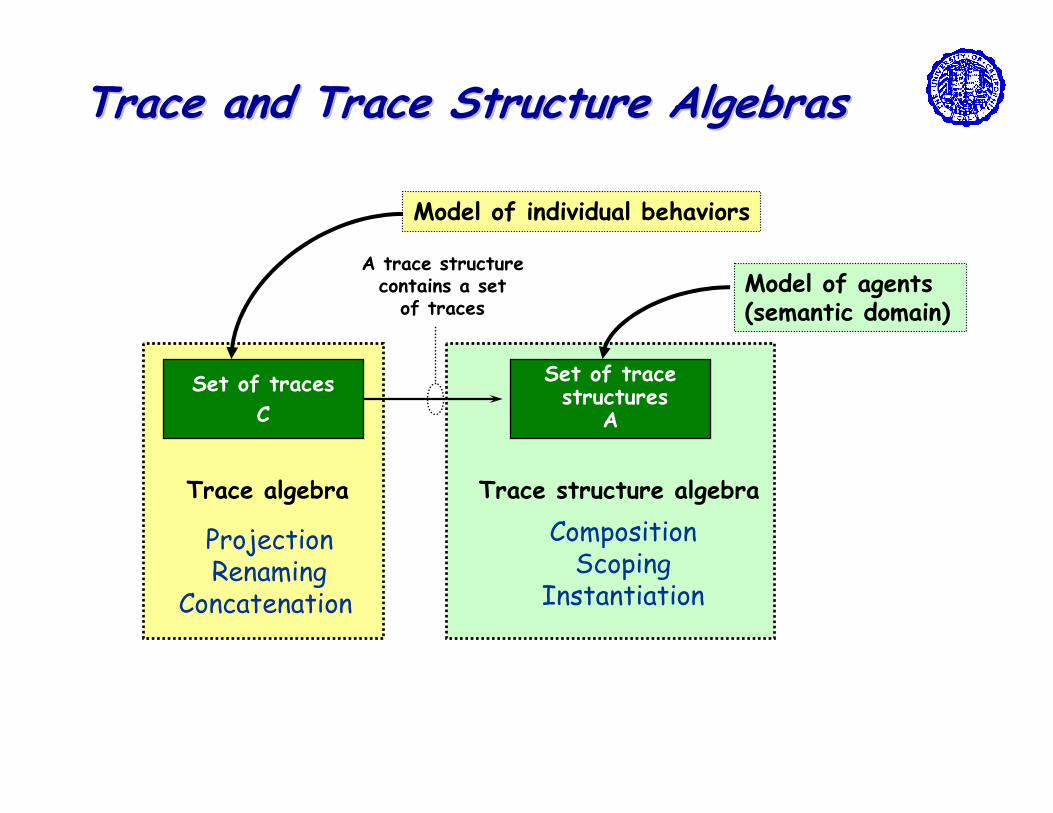
Trace structure algebra

CompositionScoping

Instantiation

Trace algebra

ProjectionRenaming

Concatenation

Trace and Trace Structure AlgebrasTrace and Trace Structure Algebras

Model of individual behaviors

Model of agents(semantic domain)

A trace structurecontains a set

of traces

Set of traces

C

Set of tracestructures

A

Essential ElementsEssential Elements

�Must be able to name elements of the model

� Variables, actions, signals, states

� We do not distinguish among them and refer to them collectively as a set of signals W

� Each agent has an alphabet and a signature

� Alphabet: A ⊆⊆⊆⊆ W

� Signature: γγγγ = A, γγγγ = ( I, O ), etc.

� The operations on traces and trace structures must satisfy certain axioms

� The axioms formalize the intuitive meaning of the operations

� They also provide hypothesis used in proving theorems

� Trade-off between generality and structure

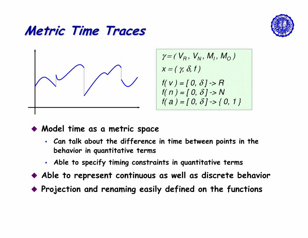
Metric Time TracesMetric Time Traces

γ = ( VR , VN , MI , MO )

x = ( γ, δ, f )

f( v ) = [ 0, δ ] -> R

f( n ) = [ 0, δ ] -> N

f( a ) = [ 0, δ ] -> { 0, 1 }

� Model time as a metric space

� Can talk about the difference in time between points in the behavior in quantitative terms

� Able to specify timing constraints in quantitative terms

� Able to represent continuous as well as discrete behavior

� Projection and renaming easily defined on the functions

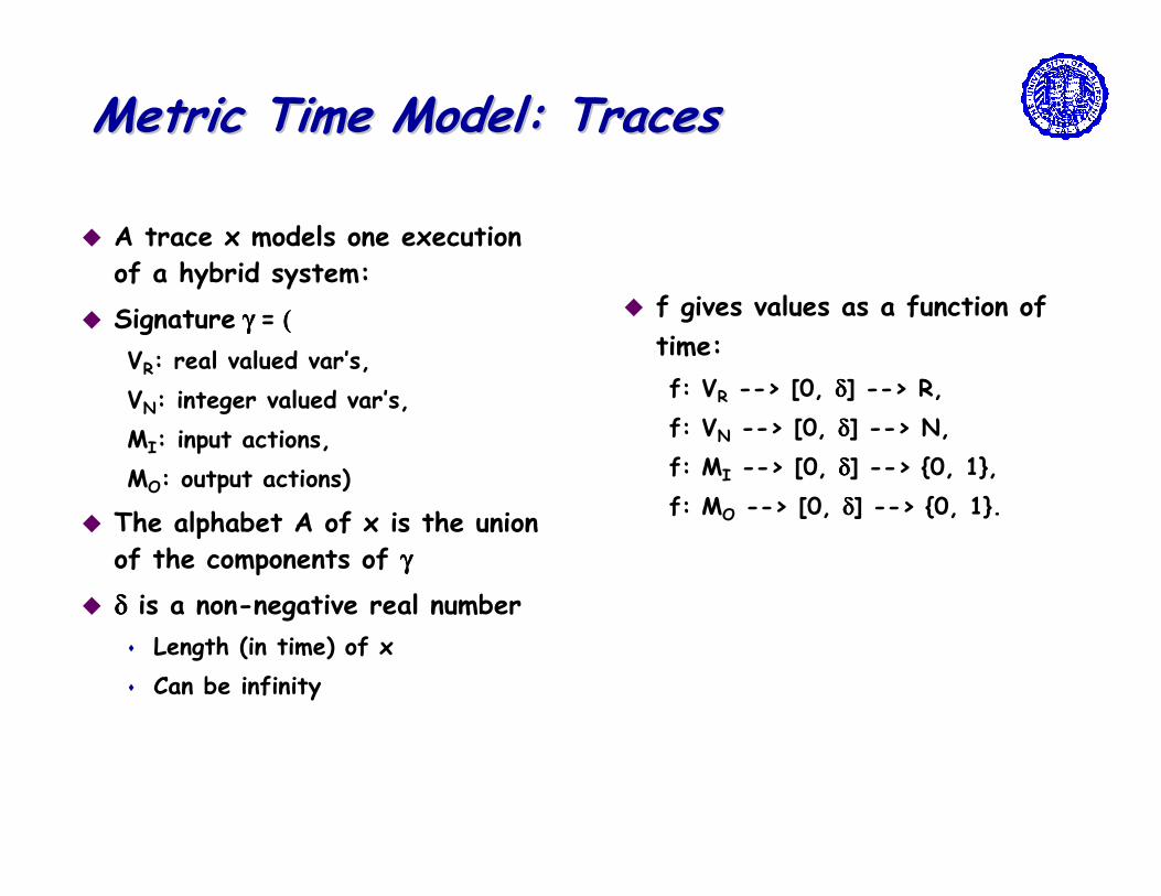
Metric Time Model: TracesMetric Time Model: Traces

� A trace x models one execution of a hybrid system:

� Signature γγγγ = ( ( ( (

VR: real valued var’s,

VN: integer valued var’s,

MI: input actions,

MO: output actions)

� The alphabet A of x is the union of the components of γγγγ

� δδδδ is a non-negative real number

� Length (in time) of x

� Can be infinity

� f gives values as a function of

time:

f: VR --> [0, δδδδ] --> R,

f: VN --> [0, δδδδ] --> N,

f: MI --> [0, δδδδ] --> {0, 1},

f: MO --> [0, δδδδ] --> {0, 1}.

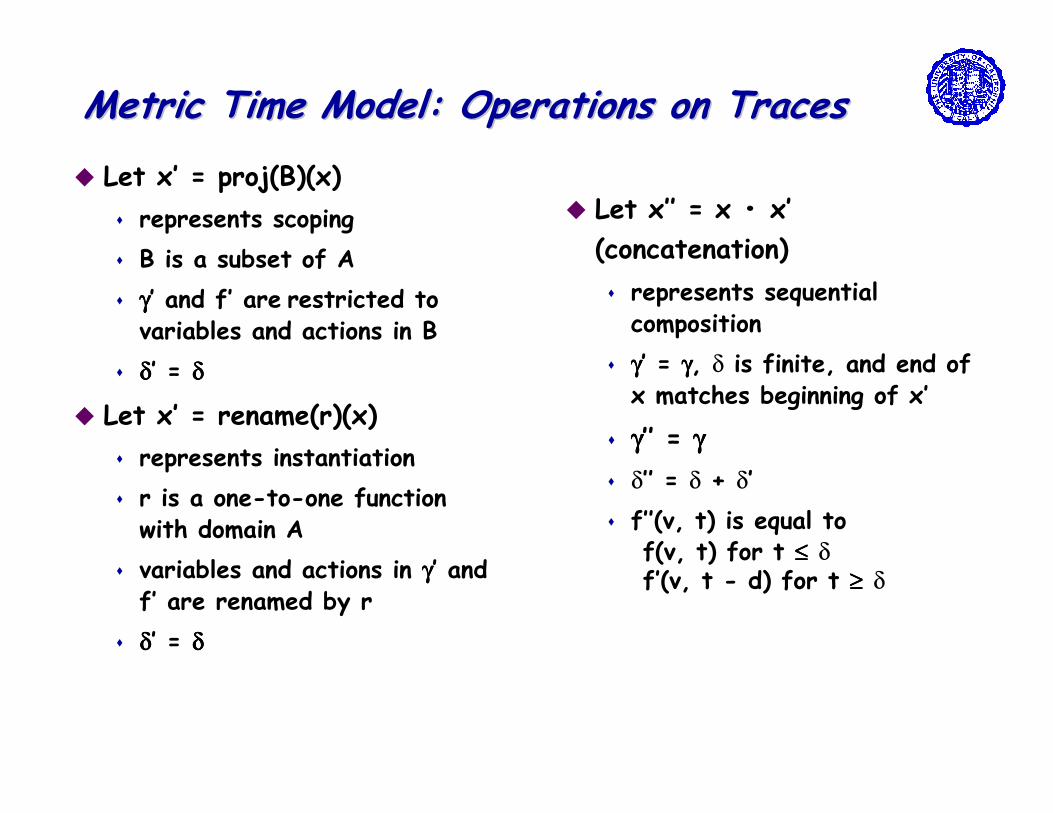
Metric Time Model: Operations on TracesMetric Time Model: Operations on Traces

� Let x’ = proj(B)(x)

� represents scoping

� B is a subset of A

� γγγγ’ and f’ are restricted to variables and actions in B

� δδδδ’ = δδδδ

� Let x’ = rename(r)(x)

� represents instantiation

� r is a one-to-one function with domain A

� variables and actions in γγγγ’ and f’ are renamed by r

� δδδδ’ = δδδδ

� Let x’’ = x • x’

(concatenation)

� represents sequential composition

� γγγγ’ = γγγγ, δ is finite, and end of x matches beginning of x’

� γγγγ’’ = γγγγ

� δ’’ = δ + δ’

� f’’(v, t) is equal tof(v, t) for t ≤≤≤≤ δ

f’(v, t - d) for t ≥≥≥≥ δ

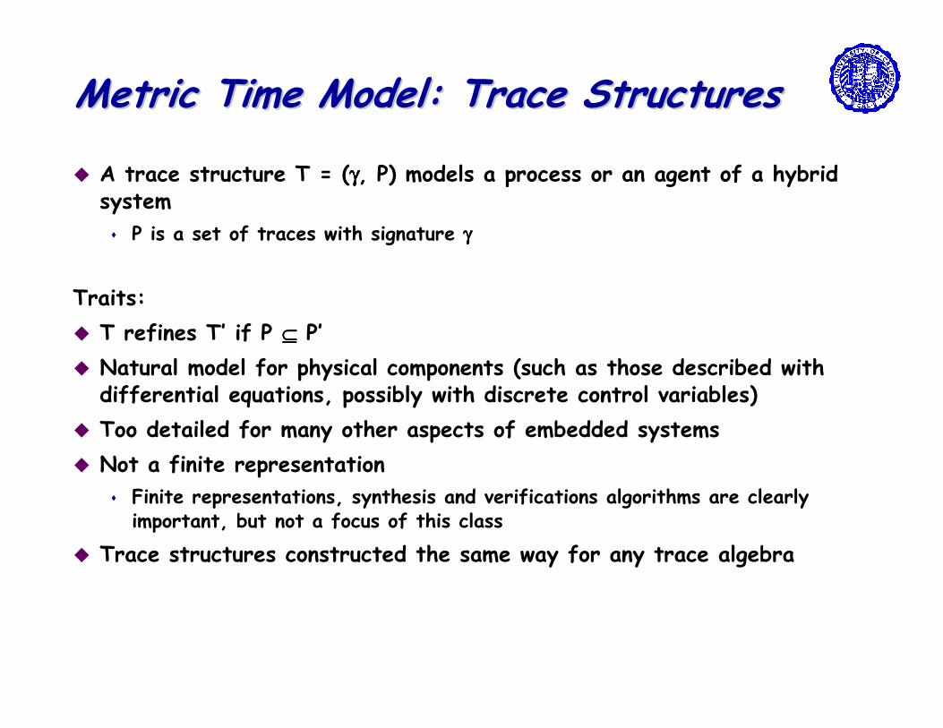
Metric Time Model: Trace StructuresMetric Time Model: Trace Structures

� A trace structure T = (γγγγ, P) models a process or an agent of a hybrid system

� P is a set of traces with signature γγγγ

Traits:

� T refines T’ if P ⊆⊆⊆⊆ P’

� Natural model for physical components (such as those described with differential equations, possibly with discrete control variables)

� Too detailed for many other aspects of embedded systems

� Not a finite representation

� Finite representations, synthesis and verifications algorithms are clearly important, but not a focus of this class

� Trace structures constructed the same way for any trace algebra

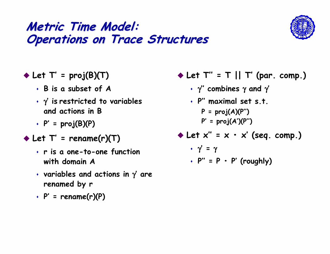
Metric Time Model: Metric Time Model: Operations on Trace StructuresOperations on Trace Structures

� Let T’ = proj(B)(T)

� B is a subset of A

� γγγγ’ is restricted to variables and actions in B

� P’ = proj(B)(P)

� Let T’ = rename(r)(T)

� r is a one-to-one function with domain A

� variables and actions in γγγγ’ are renamed by r

� P’ = rename(r)(P)

� Let T’’ = T || T’ (par. comp.)

� γγγγ’’ combines γγγγ and γγγγ’

� P’’ maximal set s.t.P = proj(A)(P’’)

P’ = proj(A’)(P’’)

� Let x’’ = x • x’ (seq. comp.)

� γγγγ’ = γγγγ

� P’’ = P • P’ (roughly)

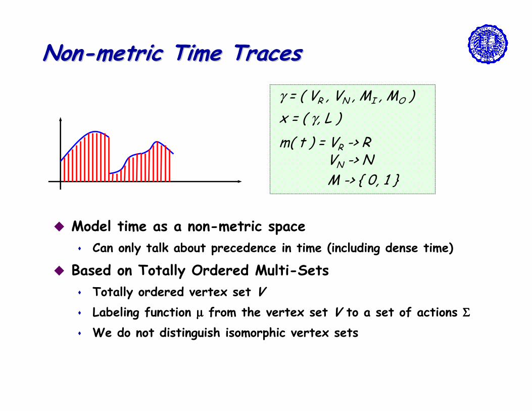
NonNon--metric Time Tracesmetric Time Traces

γ = ( VR , VN , MI , MO )

x = ( γ, L )

m( t ) = VR -> RVN -> N

M -> { 0, 1 }

� Model time as a non-metric space

� Can only talk about precedence in time (including dense time)

� Based on Totally Ordered Multi-Sets

� Totally ordered vertex set V

� Labeling function µµµµ from the vertex set V to a set of actions ΣΣΣΣ

� We do not distinguish isomorphic vertex sets

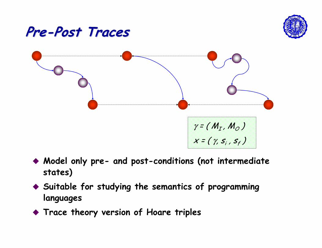
PrePre--Post TracesPost Traces

γ = ( MI , MO )

x = ( γ, si , sf )

� Model only pre- and post-conditions (not intermediate states)

� Suitable for studying the semantics of programming languages

� Trace theory version of Hoare triples

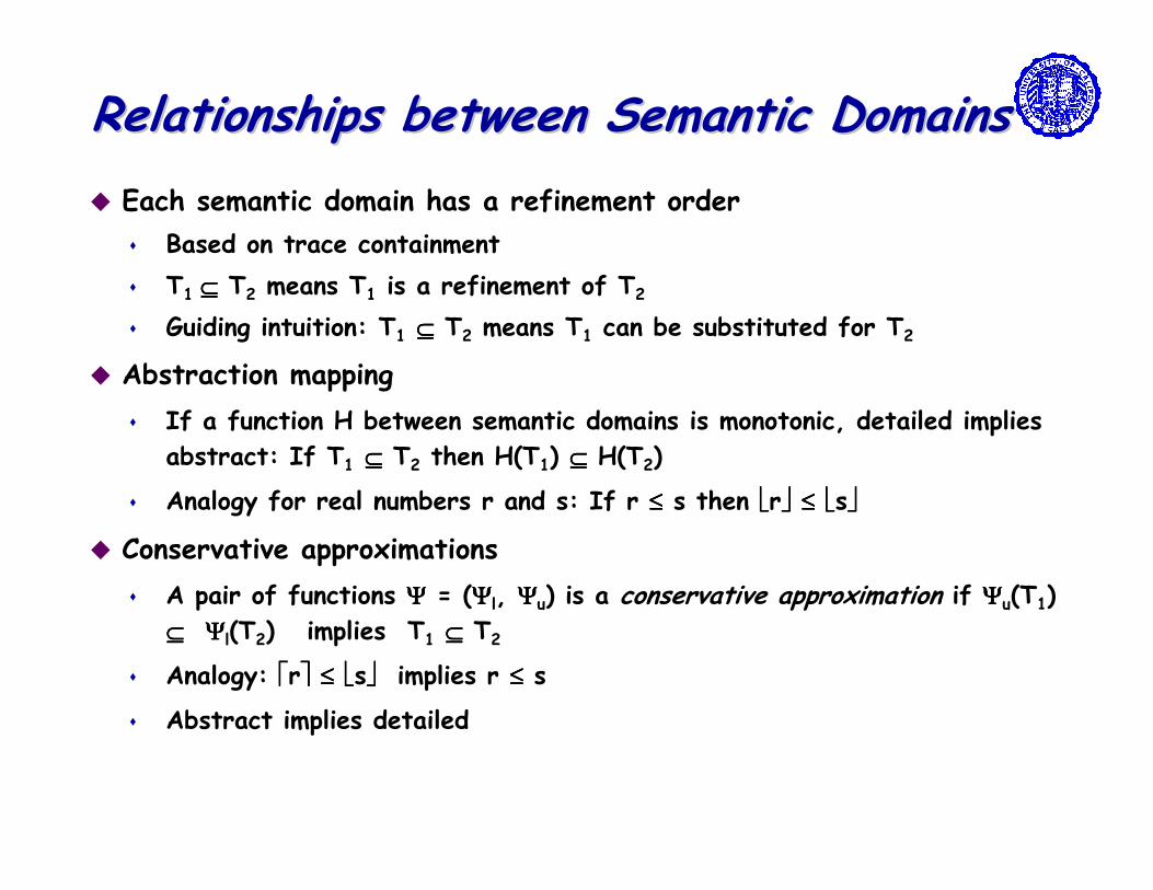
Relationships between Semantic DomainsRelationships between Semantic Domains

� Each semantic domain has a refinement order

� Based on trace containment

� T1 ⊆⊆⊆⊆ T2 means T1 is a refinement of T2

� Guiding intuition: T1 ⊆⊆⊆⊆ T2 means T1 can be substituted for T2

� Abstraction mapping

� If a function H between semantic domains is monotonic, detailed implies

abstract: If T1 ⊆⊆⊆⊆ T2 then H(T1) ⊆⊆⊆⊆ H(T2)

� Analogy for real numbers r and s: If r ≤≤≤≤ s then r ≤≤≤≤ s

� Conservative approximations

� A pair of functions ΨΨΨΨ = (ΨΨΨΨl, ΨΨΨΨu) is a conservative approximation if ΨΨΨΨu(T1)

⊆⊆⊆⊆ ΨΨΨΨl(T2) implies T1 ⊆⊆⊆⊆ T2

� Analogy: r ≤≤≤≤ s implies r ≤≤≤≤ s

� Abstract implies detailed

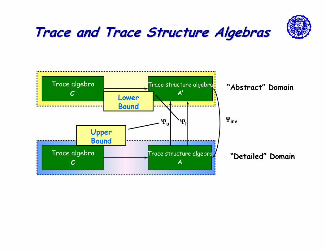
Trace structure algebra

A’

Trace algebra

C’“Abstract” Domain

Trace structure algebra

A

Trace algebra

C“Detailed” Domain

Trace and Trace Structure AlgebrasTrace and Trace Structure Algebras

ΨΨΨΨu ΨΨΨΨlΨΨΨΨinv

LowerBound

UpperBound

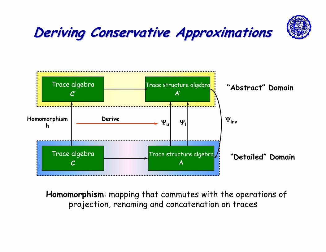
Deriving Conservative ApproximationsDeriving Conservative Approximations

Trace structure algebra

A’

Trace structure algebra

A

Trace algebra

C

Trace algebra

C’

Homomorphismh

ΨΨΨΨu ΨΨΨΨlΨΨΨΨinv

“Abstract” Domain

“Detailed” Domain

Derive

Homomorphism: mapping that commutes with the operations of projection, renaming and concatenation on traces

HomomorphismHomomorphism

�From metric to non-metric

� Must define a notion of event in the metric model

� Must define how to construct the corresponding vertex set

�From non-metric to pre-post

� Simply remove the intermediate steps and keep only the end-points

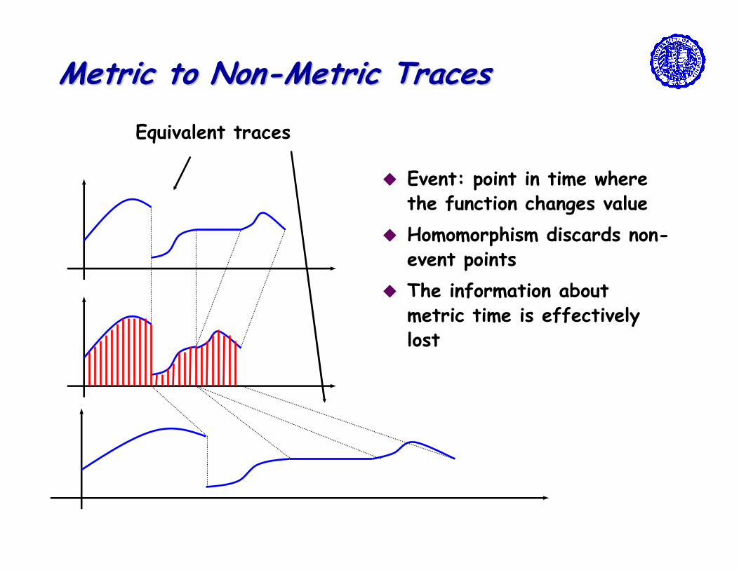
Metric to NonMetric to Non--Metric TracesMetric Traces

Equivalent traces

� Event: point in time where the function changes value

� Homomorphism discards non-event points

� The information about metric time is effectively lost

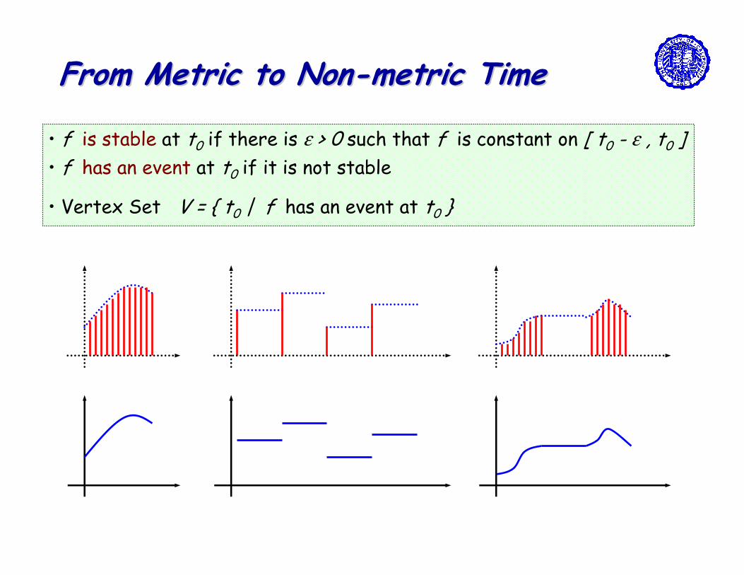
From Metric to NonFrom Metric to Non--metric Timemetric Time

• f is stable at t0 if there is ε > 0 such that f is constant on [ t0 - ε , t0 ]

• f has an event at t0 if it is not stable

• Vertex Set V = { t0 | f has an event at t0 }

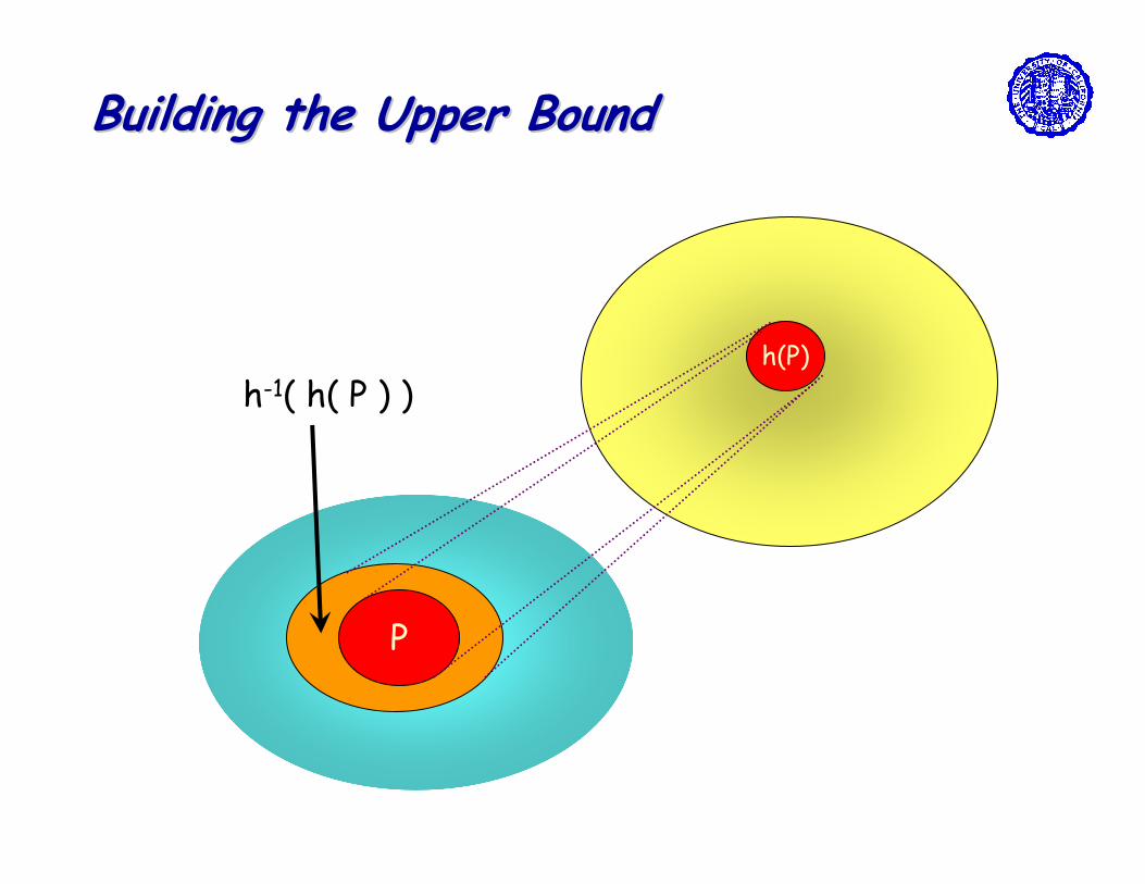
Building the Upper BoundBuilding the Upper Bound

�Let P be a set of traces, and consider the natural extension to sets h( P ) of h

�Clearly P ⊆⊆⊆⊆ h-1( h( P ) )� Because h is many-to-one

� This indeed is an upper bound!

� Equality holds if h is one-to-one

�Hence define� ΨΨΨΨu( T ) = ( γγγγ, h( P ) )

Building the Upper BoundBuilding the Upper Bound

P

h(P)

h-1( h( P ) )

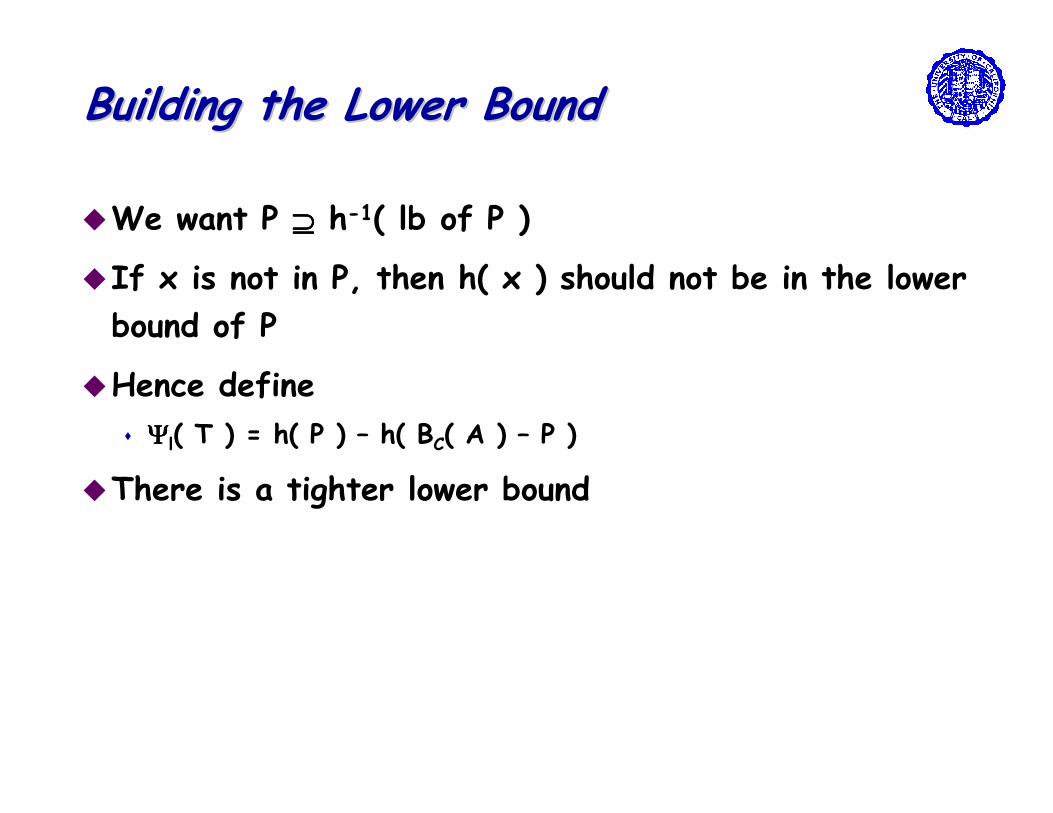
Building the Lower BoundBuilding the Lower Bound

�We want P ⊇⊇⊇⊇ h-1( lb of P )

�If x is not in P, then h( x ) should not be in the lower

bound of P

�Hence define

� ΨΨΨΨl( T ) = h( P ) – h( BC( A ) – P )

�There is a tighter lower bound

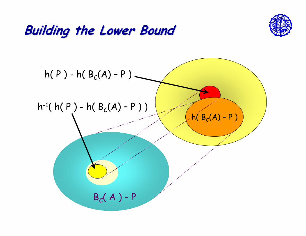
Building the Lower BoundBuilding the Lower Bound

h( BC(A) – P )

BC( A ) - P

h-1( h( P ) - h( BC(A) – P ) )

h( P ) - h( BC(A) – P )

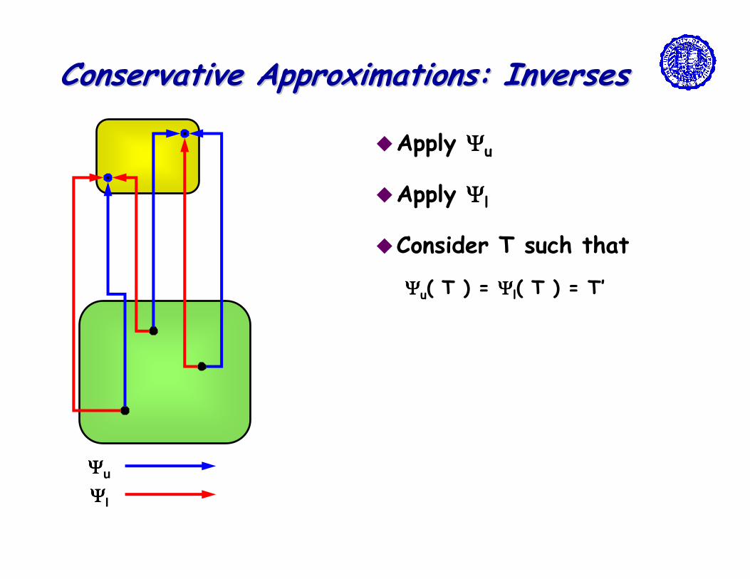
Conservative Approximations: InversesConservative Approximations: Inverses

�Apply ΨΨΨΨu

ΨΨΨΨu

�Consider T such that

ΨΨΨΨu( T ) = ΨΨΨΨl( T ) = T’

ΨΨΨΨl

�Apply ΨΨΨΨl

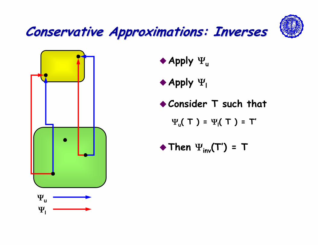
Conservative Approximations: InversesConservative Approximations: Inverses

�Apply ΨΨΨΨu

ΨΨΨΨu

�Then ΨΨΨΨinv(T’) = T

�Consider T such that

ΨΨΨΨu( T ) = ΨΨΨΨl( T ) = T’

ΨΨΨΨl

�Apply ΨΨΨΨl

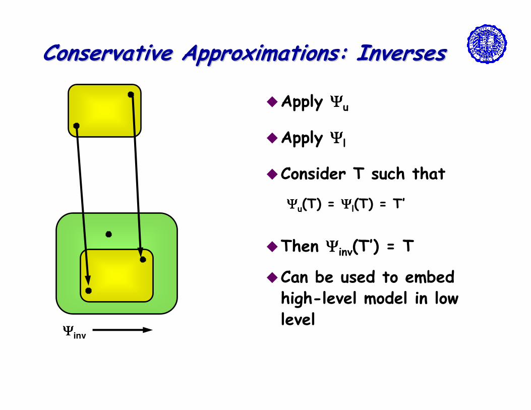
�Can be used to embed high-level model in low level

Conservative Approximations: InversesConservative Approximations: Inverses

�Apply ΨΨΨΨu

ΨΨΨΨinv

�Then ΨΨΨΨinv(T’) = T

�Consider T such that

ΨΨΨΨu(T) = ΨΨΨΨl(T) = T’

�Apply ΨΨΨΨl

Combining MoCsCombining MoCsWant to compose T1 and T2from different trace structure algebras

T1T2 �Construct a third, more

detailed trace algebra, with

homomorphisms to the other

two

�Construct a third trace

structure algebra

�Construct cons.

approximations and their

inverses

�Map T1 and T2 to T1’ and T2’

in the third trace structure

algebra

�Compose T1’ and T2’

ΨΨΨΨinv

T1’

T2’

ConclusionsConclusions

� Semantic foundations for the Metropolis meta-model

� All models of computation of importance “reside” in a unified framework� They may be better understood and optimized

� Trace Algebra used as the underlying mathematical machinery� Showed how to formalize a semantic domain for several models of

computation

� Conservative approximations and their inverses used to relate different models