Embed Size (px)
Citation preview
HETEROGENEITY OF DUTCH RAINFALL
J.V. Witter
CENTRALE LANDBOUWCATALOGUS
0000 0060 0631

Promotoren: dr.ir. L.C.A. Corsten, hoogleraar in de Wiskundige
Statistiek
ir. D.A. Kraijenhoff van de Leur, hoogleraar in de
Hydraulica, de Afvoerhydrologie en de Grondmechanica

J.V. WITTER
HETEROGENEITY OF DUTCH RAINFALL
Proefschrift
ter verkrijging van de graad van
doctor in de landbouwwetenschappen,
op gezag van de rector magnificus,
dr. C.C. Oosterlee,
in het openbaar te verdedigen
op woensdag 12 december 1984
des namiddags te vier uur in de aula
van de Landbouwhogeschool te Wageningen
U^l : %\*\ ^8b-<ok
TABLE OF CONTENTS
ACKNOWLEDGEMENTS
NOTATIONS AND ABBREVIATIONS
INTRODUCTION 1
HOMOGENEITY OF DUTCH RAINFALL RECORDS 4
2.1. Introduction 4
2.2. Rainfall levels 6
2.3. Time-inhomogeneity of rainfall 10
2.4. Local differences in rainfall level and in
rainfall trend 16
2.4.1. Kriging method 16
2.4.2. Local differences in rainfall level 22
2.4.3. Local differences in rainfall trend 26
2.5. Partitions of the Netherlands based on rainfall 29
2.5.1. Possible partitions 31
2.5.2. Testing the statistical significance of
the partitions 33
2.5.3. The hydrological significance of the
partitions 36
2.6. Effect of urbanization and industrialization
on precipitation 45
2.6.1. Urban effects in the Netherlands 49
STATISTICAL AREAL REDUCTION FACTOR ARF 88
3.1. Introduction 88
3.2. Prediction of areal rainfall 92
3.2.1. The order k and the estimation of
the semi-variogram 93
3.2.2. Comparison of the kriging, Thiessen,
and arithmetic mean predictors 102
3.3. ARF for daily rainfall and its dependence
on location, season, and return period 108

3.3.1. Methods to estimate ARF 109
3.3.2. Estimates of ARF,. for three areas
of 1000 km2 in the Netherlands 115
3.3.3. Variance of ARF for daily rainfall 124
3.4. ARF for hourly rainfall 128
3.4.1. The distribution of hourly areal
rainfall 129
3.4.2. Estimates of ARF1 130
3.5. Storm-centred areal reduction factor SRF 133
4. SUMMARY AND CONCLUSIONS 162
SAMENVATTING EN CONCLUSIES 167
APPENDICES A. Data and supplementary results of the
study on homogeneity 173
B. Data and supplementary results of the
study on ARF 192
REFERENCES 195
CURRICULUM VITAE 204

ACKNOWLEDGEMENTS
This study was carried out under the supervision and guidance of
Professor L.C.A. Corsten, and Professor D.A. Kraijenhoff. I would
like to thank them for their advice and stimulating and critical
discussions. I am also grateful to Dr. M.A.J, van Montfort for his
support throughout this study. Dr. T.A. Buishand and Dr. J.N.M.
Strieker made valuable comments on the manuscript.
I would like to thank also: Mrs. H.J. West, for revising the Eng
lish text; Mr. A. van 't Veer for preparing the numerous drawings
in the manuscript; and Mrs. J. Hei j ne kamp -van de Molen and Mrs.
W.B.J. Korte-Bayer for typing the manuscript.

NOTATIONS AND ABBREVIATIONS
An estimate of a particular parameter is denoted by a caret above
the parameter. Thus c^ is an estimate of ax. However, estimates of
correlation coefficients (p) are denoted by r and estimates of the 2 2
variance (a ) are denoted by s . Stochastic variables are under
lined. The expectation operator is denoted by E, and a frequency
of, for instance, two events per year is written as 2 (# year ).
Means of variables with two subscripts x. . are denoted by x. , l, j i •
x ., or x , where a point indicates the suffix with respect to
which the mean has been taken.
Although notations are introduced as they are used, some symbols
appear throughout this study, and are listed here for convenience.
A area
C symmetric N by N covariance matrix
cc coefficient of covariation
cv coefficient of variation
D duration of rainfall
Fö annual frequency of exceedance in summer (beginning of May to
the end of September) of a certain threshold of daily rain
fall depth H (mm), for instance F1 5 w F. annual frequency of exceedance in winter (beginning of October
to the end of April) of a certain threshold of daily rainfall
depth £ (mm)
h distance
I intensity of rainfall
i suffix indicating station number
j suffix indicating year number
K symmetric N by N generalized covariance matrix
N number of sample points
n length of record
N(h) number of paired data in a particular distance class
L dimension of a region V, in particular the maximum distance
occurring between sample points

g exceedance of a threshold or peak
g, peak guantile corresponding to a T-year return period
R total annual rainfall
r(h) estimate of the correlation coefficient p(h)
s estimate of the standard deviation a
s residual standard error r T test statistic
T return period
t time co-ordinate
u spatial co-ordinate vector
V region
x variable, denoting mean areal rainfall
x variable, denoting point rainfall at point S
x guantile (eventually written as x. or x„ ) P "/P -5 / P
Z(u) intrinsic random function located at u z(u) realization at u of an intrinsic random function Z(u)
a significance level
r symmetric N by N matrix of semi-variances y. .
Y(h) semi-variance at distance h
p(h) correlation coefficient at distance h
a standard deviation 2
a_ sguared estimation error ov sguared kriging error
Freguently used abbreviations
ACN Aitken condensation nuclei
ARF statistical areal reduction factor
BLUP best linear unbiased predictor
CCN cloud condensation nuclei
cdf cumulative distribution function
df degrees of freedom
D14 data set consisting of 14 long-term daily rainfall records
for the period 1906-1979

D32 data set consisting of 32 daily rainfall records for the
period 1932-1979
D140 data set consisting of 140 daily rainfall records for the
period 1951-1979
edf empirical distribution function
GMT Greenwich mean time
H12 data set consisting of 12 hourly rainfall records
IRF-k intrinsic random function of order k
KNMI Koninklijk Nederlands Meteorologisch Instituut (Royal
Netherlands Meteorological Institute)
LS least squares
MM method of moments
ML maximum likelihood
ms mean of squares
OLS ordinary least squares
POT peaks-over-threshold
pdf probability density function
SRF storm-centred areal reduction factor
UTC universal time co-ordinated

1. INTRODUCTION
The object of this study is to investigate heterogeneity of rain
fall in time and space in the Netherlands. The length scale consid
ered is several hundreds kilometres in Chapter 2, in which possible
partitions of the Netherlands into regions on the basis of local
differences in rainfall are investigated, and a few tenths of a
kilometre in Chapter 3, in a study of spatial variability of time-
aggregated rainfall (over an hour or a day) at the basin scale.
The time scale considered in Chapter 2 is a year, divided into a
summer period (May to September) and a winter period (October to
April). As alternatives to homogeneity in rainfall series, trends
and jumps are considered in Chapter 2.
The absence of homogeneity of rainfall may have relevance for hy-
drological design. For instance, the possible effects of urbaniza
tion and industrialization on precipitation, may have design impli
cations. Also, the question may be raised as to whether it would
be preferable for a particular design to use rainfall data from
a nearby site instead of rainfall data measured at the Royal
Netherlands Meteorological Institute (KNMI) at De Bilt. In addi
tion, because of rainfall variation in time and space, considera
tion may be given to whether an areal reduction factor is applica
ble in a design. Therefore, rainfalls with rather low return periods
were studied. Because the object was to include as many rainfall
records as possible, which were of good and even quality, the study
was almost completely confined to rainfall data collected and pub
lished by the KNMI. As the network of rainfall recorders in the
Netherlands is very sparse, the study is concerned mainly with
daily records, but some hourly rainfall records have also been
used.
Homogeneity of Dutch rainfall records is investigated in Chapter 2,
and in Chapter 3 the statistical areal reduction factor (ARF) is
estimated for daily and hourly rainfall. In the introduction to
each chapter a number of issues is raised, which are dealt with
in the subsequent sections. Conclusions are presented within each
section and not in a separate section at the end of the chapter.

All equations, tables and figures are numbered consecutively with
in each chapter; equations and tables are to be found in the appro
priate place in the text, and figures at the end of the relevant
chapter.
A survey of the rainfall data used in this study is given in the
Appendices A.l and B.l. The geographical location of the rainfall
stations and regions used throughout this study are given in Fig
ure 1.1; and a list of all provinces and rainfall stations together
with their KNMI code numbers is presented in Table 1.1.

PROPOSITIONS 1. The Netherlands may be assumed to be inhomogeneous with regard
to daily rainfall level. A partition of the Netherlands based
on the combined effects of friction, topography, differential
heating, and urban precipitation enhancement, and a partition
based on mean annual rainfall, show significant inhomogeneities.
[This thesis]
2. The effect of urbanization on heavy daily rainfall in summer
increases with rainfall depth.
[This thesis]
3. Statistical areal reduction factors depend inter alia on climate
and on season.
[This thesis]
4. Present theories about the causes of urban precipitation enhance
ment stress the influence of thermodynamic and mechanical pro
cesses rather than the influence of additional condensation
and freezing nuclei from urban aerosols. This does not support
the assumption of Petit-Renaud (1980) that there was an urban
effect due to coal-based industrialization in northern France
in the second half of the nineteenth century.
[Petit-Renaud, G., 1980. Les principaux aspects de la variabi
lité des précipitations dans le nord de la France. Récherches
Géographiques à Strasbourg no. 13-14: 31-38]
5. The areal reduction factors for discharge presented in the "Cul
tuurtechnisch Vademecum" are unnecessarily high.
6. The choice of a design rainfall intensity of 60-90 1-s -ha
is partly a consequence of uncertainties about the actual per
formance of a sewerage system. Thus firstly, evaluation of ac
tual performance is necessary.
Bi•>;;.!. VH :-.,•:iL
LANDBOUW i KM HOOL "WAGEN INGfcN

7. The method which is currently used for estimating the general
ized covariance is ad hoc, and it is by no means certain that
it provides asymptotically efficient parameter estimates.
[Barendregt, L.G., 1983. Maximum-likelihood schatting van de
gegeneraliseerde covariantie, in: Enkele kanttekeningen bij de
stochastische interpolatiemethode 'kriging'. IWIS-TNO,
's-Gravenhage]
8. The sole criterion of a maximum overflow frequency is inappro
priate for the design of centrally operated, regional sewage
water transport systems. However, in order to include other
criteria, certain technical, legal, and financial obstacles
must be overcome.
9. Strategies for the Third World, such as, 'small farmers approach'
and 'intermediate technology' reflect, inter alia, too academic
an attitude and paternalism.
J.V. Witter. Heterogeneity of Dutch rainfall. Wageningen,
12 December 1984.

2. HOMOGENEITY OF DUTCH RAINFALL RECORDS
2.1. INTRODUCTION
Rainfall series can be seen as realizations of a process {x(u,t)},
where the co-ordinate vector of the sample points is denoted by u
and time is denoted by t. Although such a process can be homogene
ous in several ways, in this chapter, only two types of homogeneity
are investigated:
homogeneity in time: given a location U, the probability distri
bution of the process {x(U,t)} is independent of time;
homogeneity in space : given a time co-ordinate T, the probabil
ity distribution of the process {x(u,T)} is independent of
location.
As rainfall series exhibit periodicities, the homogeneity of the
following seven annual rainfall characteristics are investigated:
total annual rainfall R;
annual frequency of exceedance F of a certain threshold Z of
daily rainfall depth,
. in summer F , the summer being defined as the period from the
beginning of May to the end of September w . in winter F , the winter being defined as the period from the
beginning of October to the end of April
. three thresholds were chosen for the annual frequency of ex
ceedance, 1, 15, 25 mm.
Total annual rainfall R, and annual frequency of exceedance of s w
1 mm in summer (F. ) and in winter (F. ) give a general indication
of rainfall level: its long-term mean value. Annual frequencies of
exceedance of 15 and 25 mm, which are of more relevance to hydro-
logical practice, are also useful in investigating the effect of
industrialization and urbanization on rainfall trend. Convective
rather than frontal rainfall events are more susceptible to modi
fication, and severe weather phenomena (thunderstorms) are likely
to be affected in particular (Oke, 1980).
The existence of regional differences in rainfall depths has been
reported by various investigators, (e.g., Buishand and Velds, 1980),
and also regional differences in rainfall trend have been reported

(e.g., Kraijenhoff and Prak, 1979; Buishand, 1979). These differ
ences in trend have been attributed to the anthropogenic effects
of industrialization and urbanization. Therefore, it has been sug
gested (Werkgroep Afvoerberekeningen, 1979) that more stringent
design criteria should be used for urban than for rural areas.
Earlier investigations of homogeneity in time of Dutch rainfall
records have focused mainly on total monthly and annual rainfall,
except Kraijenhoff and Prak (1979), who established the inhomoge-
neity in time of the annual frequency of daily rainfall exceeding
30 mm in summer. Jumps in the mean seasonal and annual rainfall
of Dutch rainfall series roughly for the period 1925-1970, have
been studied by Buishand (1977a). Departures from homogeneity in
24 Dutch long-term monthly and annual rainfall records were report
ed by Buishand (1981), who also investigated departures from homo
geneity in 264 Dutch records of annual rainfall for the period
1950-1980 (Buishand, 1982a). In all three studies, strong indi
cations of a change in the mean were found for large numbers of
records.
In this chapter the following issues are dealt with:
. In Section 2.2, mean values of the rainfall characteristics
defined above for the Netherlands are determined from daily
rainfall records for the period 1951-1979 for 140 rainfall
stations of the Royal Netherlands Meteorological Institute
(KNMI). This data set is denoted as D140 (Appendix A.l).
These mean values are compared with mean values determined
from the long-term records for the period 1906-1979 for
14 KNMI rainfall stations considered to be of good quality
(Buishand, 1982b). This data set is referred to as D14
(Appendix A.l).
. In Section 2.3, time-inhomogeneity of rainfall in the
Netherlands is considered. Use is made of data set D140
for the period 1951-1979 and of data set D14 for the period
1906-1979.
. In Section 2.4, local differences in rainfall level and rain
fall trend between Dutch rainfall stations are investigated.
Use is made of data set D140.
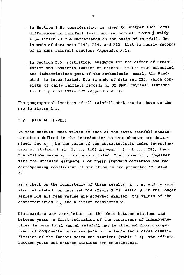
. In Section 2.5, consideration is given to whether such local
differences in rainfall level and in rainfall trend justify
a partition of the Netherlands on the basis of rainfall. Use
is made of data sets D140, D14, and H12, that is hourly records
of 12 KNMI rainfall stations (Appendix A.l).
. In Section 2.6, statistical evidence for the effect of urbani
zation and industrialization on rainfall in the most urbanized
and industrialized part of the Netherlands, namely the Rand
stad, is investigated. Use is made of data set D32, which con
sists of daily rainfall records of 32 KNMI rainfall stations
for the period 1932-1979 (Appendix A.l).
The geographical location of all rainfall stations is shown on the
map in Figure 2.1.
2.2. RAINFALL LEVELS
In this section, mean values of each of the seven rainfall charac
teristics defined in the introduction to this chapter are deter
mined. Let x. .be the value of one characteristic under investiga-
tion at station i (i= 1,..., 140) in year j (j= 1,..., 29), then
the station means x. can be calculated. Their mean x , together
with the unbiased estimate s of their standard deviation and the
corresponding coefficient of variation cv are presented in Table
2.1.
As a check on the consistency of these results, x , s, and cv were
also calculated for data set D14 (Table 2.2). Although in the longer
series D14 all mean values are somewhat smaller, the values of the
characteristics F and R differ considerably.
Disregarding any correlation in the data between stations and
between years, a first indication of the occurrence of inhomogene-
ities in mean total annual rainfall may be obtained from a compa
rison of components in an analysis of variance and a cross classi
fication of the factors years and stations (Table 2.3). The effects
between years and between stations are considerable.

Table 2.1. Mean x , standard deviation s, and coefficient of
variation cv of rainfall characteristics for data set D140
Rainfall
character Mean
istic Summer
Exceedance
frequency
1 mm (F )
15 mm (F1 5)
25 mm (F2 5)
Total annual
rainfall (R)
52.4
4.7
1.15
X
Winter
80.5
3.5
0.48
775.8 (mm)
Standard
Summer
2.6
0.5
0.25
deviation s
Winter
36
2.6
0.6
0.13
.4 (mm)
Coefficient of
variati
Summer
4.9
11.2
21.9
on cv (%)
Winter
3.2
16.4
27.4
4.7
Table 2.2. Mean x , standard deviation s, and coefficient of
variation cv of rainfall characteristics for data set D14
Rainfall
character Mean
istic Summer
Exceedance
frequency
1 mm (F )
15 mm (F1 5)
25 mm (F 2 5 )
Total annual
rainfall (R)
50.6
4.2
1.03
X
Winter
78.1
3.1
0.45
732.0 (mm)
Standard deviation s
Summer Winter
3.2 3.0
0.5 0.3
0.14 0.07
32.8 (mm)
Coefficient of
variât:
Summer
6.3
11.6
13.2
ton cv (%)
Winter
3.9
10.6
16.8
4.5
Table 2.3. ANOVA table for between years and between stations
effects for total annual rainfall
Source of variation df ms(mm )
Between years
Between stations
Residual
28
139
3892
2.21*10
3.83*104
3.47*10]
Total 4059

In order to obtain a general impression of daily rainfall level at
a Dutch rainfall station, peaks-over-threshold series (POT series)
were extracted for each station in the D140 data set for summer,
winter, and the total year, and with a mean annual number of thres
hold exceedances of two. To assure independence of the exceedan-
ces, these had to be separated by at least one day without rain.
Mean order statistics were obtained by taking the mean of peaks
of equal ranking. It was assumed that both the POT series for an
individual station, and the series of mean peaks q were exponen
tially distributed. Thus, a probability density function was fitted
according to
f(q) = |exp[-(q-q0)/ß], (WQ) (2.1)
where
qn : parameter for location
ß : parameter for scale.
The maximum likelihood (ML) estimators of ß and q_, corrected for
bias, are (NERC, 1975; Vol. 1)
i = HTî<â-a,)- (2.2)
and
â0 = %-i/n' (2-3)
n : sample size (58)
3 : lowest peak in the sample
2 : sample mean of peaks.
Estimates of ß and q. are given in Table 2.4.
where

^0
23
20
16
(mm)
1
1
8
Table 2.4. Maximum likelihood estimates of ß and q. in Equation
2.1 for POT series of daily rainfall in the Netherlands (mean an
nual number of threshold exceedances: 2)
Period ß (mm)
Year 8.1
Summer 8.5
Winter 5.8
These mean POT series have been plotted and are presented, together
with the fitted exponential distributions in Figure 2.2. For the
plotting position of the order statistics g. . . , with q,-,»!-•-iq, >,
the following equation was used
1 _i E(Y,H x) = * (n+l-j) x, (2.4) 1 ' j=l
where
y,.. : order statistic of a standard-exponential variate
with density f(y) = e~y (y^.0).
The assumption of an exponential distribution was tested in the
following way. Let the order statistics g.. ...<_.. .<_g. > be samples
of a truncated exponential distribution, then the standardized
increments
±1 = ^ ( n - i + D - ^ n - i ) ) ' i = 1 n"! (2-5)
are independent exponential variâtes. After eliminating the location
parameter, the scale parameter is eliminated. Let
n-1 s = 1 L., (2.6)
i=l x
and
i Z.H = * L./s. i = 1, ..., n-2 (2.7)

10
The series (z,,.., z _) is distributed as an ordered sample of
size n-2 from a uniform distribution on (0,1) (Durbin, 1961). Thus,
a test statistic T can be used, where
n-2 T = -2 I In z.. (2.8)
i=l 1
Under the null hypothesis of exponentially distributed peaks, T has
a -distribution with parameter 2(n-2). As lack of fit with regard
to the exponential distribution can lead to high as well as to low
values of T, a two-sided test is used. Very long tails give low
values of T, and very short tails high values. Realizations of T
for the total year, summer, and winter for the POT series were 95.9,
99.8, and 94.6, respectively. As these values are not significant
(two-sided test, significance level a = 0.10), the exponential dis
tribution fits the POT series reasonably well.
2.3. TIME-INHOMOGENEITY OF RAINFALL
In this section, time-inhomogeneity of mean values of the seven
rainfall characteristics defined in the introduction to this chap
ter is considered. Let x . be the mean value of a rainfall charac
teristic for all rainfall stations considered in year j (j=l,...,
n). For rainfall characteristics F and FW, the x . are means of
transformed variâtes x. ., where the transformation is according to i, J
P = VP+V(P+D, (2.9)
the untransformed p being any positive integer. This transformation
has a variance stabilizing and normalizing effect on Poisson vari
âtes, resulting in that case in a variance of almost 1 (see Appen
dix A.2).
In this section, consideration is given only to a possible change
in the expected mean x ., described by either a linear trend
E(x.j) = Mj = M+Jô, (2.10)

11
j = 1,.. ., m E(x _;) = M.; =<! (2.11)
j = m+1,..., n 3' "j
that is, a jump at j = m+1 with m unknown. Under the null hypothesis
H- of a homogeneous series,
and for data set D14, n=74.
H of a homogeneous series, 6 = 0 . Note that for data set D140, n=29
When anthropogenic effects on rainfall are being studied, it is
logical to look for a trend. However, since there are many factors
affecting rainfall and rainfall measurements, including climatologie
fluctuations or changes in methods of measuring rainfall, it is also
necessary to consider jumps. Test statistics are needed which are
powerful for the alternatives H (Equation 2.10) and H l b (Equation
2.11), both with ô 7* 0 (the power of a test is defined as the prob
ability of rejection of H. in favour of the alternative H 1 ) .
The homogeneity of the series x . was tested by the three test
statistics described below.
Von Neumann ratio Q
n _ 1 a , n , .2 2 = 2 (x -j+1-x .:> / * (x ,-x
j=l ° X ° j=l ° * r . (2.12)
A monotonie trend or slow oscillations in level tend to produce low
values of 2; and rapid oscillations in the mean may yield high
values of Q. For the alternatives H, and H,., a left-sided criti-a la lb cal region of g seems adequate. An advantage of the statistic 2 is
its sensitivity for a great variety of inhomogeneities. A table of
percentage points of 2 f°r normally distributed samples is given by
Abrahamse and Koerts (1969).
Student's statistic T for a linear time trend
r V(n-2) T = , (2.13)
Vd-r2)

12
where
r: the sample correlation coefficient between the variate
x . and time.
The statistic T is an adequate tool for testing homogeneity when
H is the alternative. Under the null hypothesis T is a Student
variate with n-2 degrees of freedom. The test is two-sided, since
an increasing trend gives high positive values of T, and a decreas
ing trend, high negative values.
The maximum or minimum M of weighted rescaled adjusted partial sums
For a series x . (j=l,..., n), the adjusted partial sum is defined
S, = I (x .-x), k = 1,..., n-1 (2.14) k j=l -3
and S. = S = 0 . The adjusted partial sums are rescaled to scale
invariance by dividing S, by the sample standard deviation s
S_k* = Sk/sx, k = 1,..., n-1. (2.15)
The weighted rescaled adjusted partial sums S** are defined as
S** = {k(n-k)}"i5 S*, k=l,..., n-1. (2.16)
-i-
Because of the multiplication factor {k(n-k)} 2
var(S**) = -^zr, , k=l,..., n-1 (2.17) —k ' n-1
independent of k (Appendix A.3). The test statistic is
M = max \it*\' (2.18) k=l, .. ., n-1
A particular advantage of this test procedure is that it gives a
value of k, say k*, which maximizes |S**|. In case of H-,, k* is

13
the maximum likelihood (ML) estimate of m (Buishand, 1981). Because
there is a unique relationship between M and Worsley's W (Worsley,
1979)
W = (n-2)*5 M/U-M2)*5, (2.19)
percentage points of W were used in the test, which is two-sided
(Appendix A.3).
The power of a test can be determined directly by solving the power
function only in a few cases. Here, the power of the test statistics
2/ T, and M for alternatives according to Equations 2.10 and 2.11
was investigated by means of Monte Carlo methods with 2000 samples
of 29 normal variâtes; for each sample the test statistics were
calculated for
a linear trend: 6 = 0 (r^) F5°'
1 9 a jump : ô = 0 (gti) g0, and m = 7, 14.
The simulated power functions of 2» ï< an<i M a r e presented for al
ternative B1 in Figure 2.3A, for alternative H . (m=7) in Figure
2.3B, and for alternative H . (m=14) in Figure 2.3C.
Simulated powers of 2 an<^ H f°r Hiv. have been given by Buishand
(1982a) for n = 30, a = 0.05 and m = 5, and 15; and those given in
Figure 2.3B and 2.3C compare well with his results. It may be con
cluded from Figure 2.3 that the statistic T has favourable charac
teristics when trends or jumps according to Equation 2.10 or 2.11
have to be detected. For other types of inhomogeneities, however,
2 may be superior to both T and M.
For data sets D140 and D14, values of the test statistics 2' Z a n d
M, determined for the rainfall characteristics total annual rainfall
R and annual exceedance frequencies for summer and winter F ' ,
are presented in Table 2.5.

14
Table 2.5. Realizations of the statistics £, T, and M and of the
estimated jump point k*
Rainfall characte ristic
Exceedance frequency Summer
1 mm
15 mm
25 mm
Winter
1 mm
15 mm
25 mm
<F1>
<F*s> <F?s>
(Fj) (FW ) 1 15' (FW ) 1 25'
Total annual
rainfall (R)
Q
2
1
1
2
1
1
1
Data set D140
03
74
85
03
16°°
18°°
92
T
-1.29
-1.93°
-2.03°
0.84
0.68
-0.34
-0.55
M
0
0
0
-0
-0
-0
0
35
48°
50°
24
40
33
30
k*
18
24
25
14
9
9
20
Data set Q
2.19
1.81
1.92
1.90
1.63
1.65
1.78
T
0.39
0.45
0.64
0.87
1.96°
1.15
1.62
D14 M
0.16
0.30
0.30
-0.20
-0.33°
-0.26
-0.26
k*
69
70
67
59
19
23
44
° Indicates values inside the critical region for a = 0.10. 0 0 Indicates values inside the critical region for a = 0.05.
The test statistics T and M lead to very similar conclusions. The
Von Neumann ratio g, however, is very clearly sensitive to other
types of inhomogeneities. The values of k* indicate a jump towards
the end of the summer series during the period 1970-1975, while in
the winter series the jump points are more evenly spread throughout.
The positive trend of the D14 series is very likely to be affected
by improvements in rainfall measurements, notably the introduction
of standardized measurement practice at the beginning of this cen
tury, and the lowering of the rain gauge from 150 to 40 cm above
ground level in the period 1946-1950 (Deij, 1968). Buishand (1977a)
concluded that this last improvement resulted in an increase in
measured rainfall of about 10% for coastal rainfall stations (see
also Braak, 1945), and an increase of about 2% for stations at a
distance from the coast.

15
The hypothesis that improvements in rainfall measurements are the
main reason for the positive trend of the D14 series is supported
by the higher values of T for the winter. The lowering of the gauge
has led to a reduction of the wind-field deformation around the
gauge, which causes a loss of catch. This loss, however, is smallest
in summer because raindrops are relatively large as a consequence
of the rainfall intensity in this season.
The observed inhomogeneities may also be affected by the general
circulation pattern during the period of the records used. The cir
culation pattern is described by distinct circulation types, the
frequency of which is known to fluctuate. Each period is character
ized by the predominance of certain circulation types (Barry and
Perry, 1973), each having its own probability of rainfall.
A record of daily circulation types for the Netherlands in the
period 1881-1976 has been compiled by Hess (1977); data for 1977
and 1978 have been supplied by KNMI. In addition, the rainfall pro
bability, given the occurrence of a certain circulation type, has
been worked out for five KNMI stations (Bijvoet and Schmidt, 1958,
1960). The effect of circulation types on rainfall trend was inves
tigated by calculating the expected annual number of days in a cer
tain rainfall class, according to the above-mentioned rainfall pro
babilities. In this study only the rainfall class in excess of 5 mm
has been considered. The series of expected annual numbers of days
was compared to the series of actual numbers of days in this rain
fall class for the period 1956-1978, because the 1881-1955 data
were used to calculate the rainfall probabilities. Both series are
shown in Figure 2.4A (summer) and Figure 2.4B (winter) for the
rainfall station Den Helder/De Kooy.
From Figure 2.4 it can be concluded that there is some evidence of
the effect of the general circulation on rainfall trend. This effect
is illustrated by the high values of k* in Table 2.5 for most rain
fall characteristics. This seems to be an immediate consequence of
the wet sixties. This may also be concluded from Figure 2.5, where
10-year moving averages and the weighted rescaled adjusted partial
sums are shown for total annual rainfall R for data set D14. The

16
10-year moving average of summer rainfall for the period 1734-1960
is given in Figure 2.5C (Wind, 1963).
2.4. LOCAL DIFFERENCES IN RAINFALL LEVEL AND IN RAINFALL TREND
In this section local differences in rainfall level and in rainfall
trend are investigated as follows. Let x. . be the value in year j
at station i of one of the rainfall characteristics: (i) exceedance s w
frequency (in summer F , with 11=1, 15, or 25 mm; and in winter F ,
also with 11=1, 15, or 25 mm), (ii) total annual rainfall R. Local
differences in rainfall level are studied by comparing the station
means x. for each rainfall characteristic (Section 2.4.2), and
local differences in rainfall trend by analysing the time series
x. . for each particular rainfall station and each rainfall charac-
teristic (Section 2.4.3). Use is made of data set D140. To give an
impression of the local differences, maps of the Netherlands,
showing the geographical distribution of station means and trend
statistics, are presented. These maps were derived by the kriging
method, which is a best linear unbiased predictor (BLUP).
Firstly, the kriging method is discussed in Section 2.4.1.
2. 4. 1. Kriging method
Let Z(u) be an intrinsic random function (IRF) which is defined in
every point with co-ordinate vector u of a region V, and let z(u)
be a realization of 2(u), known at the N sample points u.GV. For
example, the set of station means x. for data set D140 is a real
ization z(u), known at the 140 sample points.
A best linear unbiased predictor (BLUP) z(uQ) of z(u) at some point
u. is defined as
N z(u ) = I \.z(u.), (2.20)
i=l
where :
\. : coefficients to be determined. l
17
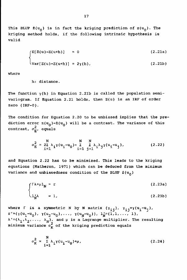
This BLUP z(u ) is in fact the kriging prediction of z(uQ). The
kriging method holds, if the following intrinsic hypothesis is
valid
(E[Z(u)-Z(u+h)] = 0 (2.21a)
Uar[2(u)-Z(u+h)] = 2y(h), (2.21b)
where
h: distance.
The function y(h) in Equation 2.21b is called the population semi-
variogram. If Equation 2.21 holds, then Z(u) is an IRF of order
zero (IRF-O).
The condition for Equation 2.20 to be unbiased implies that the pre
diction error z(u0)-z(u~) will be a contrast. The variance of this
contrast, a , equals
_ N N N at = 21 \.y(u,-un)- I I A,X.Y(U,-u.), (2.22)
E i=l X X ° i=l j=l x 3 1 D
and Equation 2.22 has to be minimized. This leads to the kriging
equations (Matheron, 1971) which can be deduced from the minimum
variance and unbiasedness condition of the BLUP z(uß)
rr\+nl N = r (2.23a)
lljJjA = 1, (2.23b)
where r is a symmetric N by N matrix (y- . ) , v • J=Y (u--u. ),
r^tYt^-UQ), Y ( U 2 - U Q ) , .. ., Y ( U N - U 0 ) ) , 1N=(1,1,..., 1),
\'=(A.1,\_,..., ^N)# and p is a Lagrange multiplier. The resulting
minimum variance av of the kriging prediction equals
2 N
or£ = I \iY(ui-U0)+M, (2.24)

18
which follows from inserting Equation 2.23a into Equation 2.22. As
will become clear in the following chapter, point to area interpo
lation requires some of the semi-variances in Equations 2.22, 2.23
and 2.24 to be replaced by certain types of mean semi-variances.
The weights A., in Equations 2.20 and 2.24 can be determined if the
semi-variances are known. For an IRF-0 these semi-variances can be
estimated by
, N(h) * ( h ) = 2NThT .* [z(ui)-z(ui+h)]z, (2.25)
where N(h) is the number of paired data points at mutual distance
h, particularly suitable if sampling has been done according to a
regular grid. For a random sample, paired data are grouped accor
ding to distance classes and N(h) is the number of paired data in
a particular class. Note that I,N(h)=N(N-l )/2. Because of Equation
2.21a, v(h) is an unbiased estimator.
A population semi-variogram \(h) may be fitted to y(h) according to
a parametric model, for instance a linear model
•y(h) = Cô+oijh, (2.26a)
or an exponential model
Y(h) = CÔ+a1(l-exp(-h/a2)), (2.26b)
where
C : a parameter for the nugget effect
ô : 0 (h=0) or 1 (h^O)
a1,a2: parameters.
The nugget effect represents discontinuity of the semi-variogram at
the origin, due to spatial variability at very small distances in
relation to the working scale, resulting for example from measure
ment errors and/or the physical characteristics of the spatial pro
cess concerned.

19
The linear model described in Equation 2.26a corresponds to intrin
sic random functions Z(u) of order zero, for which an a priori
variance or a covariance need not exist. The exponential model
described in Equation 2.26b exhibits a limit or a sill, equal to
C+di, as h->°°. This sill is almost (for 95%) reached at a distance
or range equal to 3a2• Models exhibiting a sill may correspond to
second-order stationary random functions Z(u) with spatial corre
lation.
The fitted v(h) should not only resemble the sample function y(h), but should also satisfy the condition for the variance of a contrast I.A.Z(u.), with I.A. = 0, to be possible for all A.
l l v î " i l r l
var(I.A.Z(u.)) = -1.1 .A.A.y(u.-u.)>0, (2.27)
v i i v i ' ' l j l j J v l ; j ' — x '
furthermore
y(0) = 0, y(h) = y(-h)>0. (2.28)
As the Equations 2.26 imply independence of y(h) of orientation, it
should be verified that z(u) is isotropic. In case of anisotropy,
additional modifications are possible, see Journel and Huijbregts
(1978).
If the assumption according to Equation 2.21a holds, then the in
crease of a semi-variogram for h>>0 can be shown to be necessarily 2
slower than that of h , that is
lim ( h ) = 0, (2.29) h-»°° h
which can be deduced from Equation 2.27. Consequently, a sample 2
variogram which increases at least as rapidly as h for large distances h is incompatible with the intrinsic hypothesis, as stated in Equation 2.21. Such an increase very often indicates the presence of a drift defined as

20
E[Z(u)] = m(u). (2.30)
Where only one realization z(u) of Z(u) is known, and Z(u) is
only intrinsic, var[y(h)] becomes very large (Appendix A.4) for
h>L/2, where L is the maximum distance between sample points in V.
Therefore, only for distances h<L/2, v(h) is fitted to y(h).
For a second-order stationary Z(u), Equation 2.23 can also be writ
ten in terms of covariances instead of semi-variances. The advantage
of using semi-variances is that assumptions can be weaker, for ex
ample, the a priori variance var[Z(u)] need not exist. A disadvan
tage is that calculation of the A. according to Equation 2.23 in
volves inverting a (N+l) by (N+l) matrix with zeros at the main
diagonal; some common inversion methods can not handle this. Thus
in the actual calculations, the semi-variances v(h) in Equation
2.23 are replaced by pseudo-covariances C(h)=A--y (h), where A is a
constant, exceeding the maximum of semi-variances occurring in
Equation 2.23.
The kriging method developed by Matheron (1971) is very closely re
lated to the method of optimum interpolation developed by Russian
statisticians, such as Gandin (1965). This last method, however, is
based on second-order stationary realizations z(u), and no use is
made of the concept of intrinsic random functions. As a result, all
equations, such as 2.22 and 2.23 are in terms of correlation coef
ficients. For an application of this method, see De Bruin (1975).
The connection between kriging and linear regression has been point
ed out by Corsten (1982). The Equation 2.23 leads to
z(u0) = 2T-1r-(zT-1lN)(l^r-1lN)"1(l^r"1r) +
+ ( 1Nr"l lN)"1 ( z'r"l lN)- ( 2 - 3 1 )
Defining x T ~ y as an inner product of the vectors x and y. Equation
2.31 becomes
z(u0) = (z'r)-(z'lN)(lN'lN)-1(lN'r)+(lN'lN)-1(z'lN).(2.32)

21
The last term in Equation 2.32 can be interpreted as the estimate
p of JJ=E[Z(U)]. The other terms in the right-hand side of Equation
2.32 can then be written as (z-pl 'r)=rT~ (z-plN), where the r T ~
may be termed the best linear approximation coefficients for z(u)
by z(u.)/ i=l,..., N. Working along the same lines, an alternative
expression to Equation 2.24 is obtained for the kriging variance
in Corsten (1982)
a£ = rT"1r-(l-l^r"1r)(l^r"1lN)"1(l-l^r"1r). (2.33)
The last term in Equation 2.33 is closely related to the variance
of the estimate of the stationary expectation E[z(u-)], and the
other term on the right-hand side is an estimate of the residual
variance of z(u.) with regard to the best linear approximation.
The IRF-k theory
In the presence of drift as defined by Equation 2.30, use may be
made of the IRF-k theory, (Delfiner, 1976; Kafritsas and Bras,
1981). Basically, the drift is described as
m(u) = 1 a g (u), (2.34) &=0 * *
where g0(u) are known monomial functions (in the one-dimensional ."• 2
case with k=2: gQ(u)=l, g1(u)=u, g2(u)=u , and the a£(£=0,..., k) are coefficients which need not be estimated).
For an intrinsic random function Z(u) of order k (IRF-k) the fol
lowing now hold:
- Any generalized increment of 2(u), that is l.k.Z(u) with coef
ficient vector A not only perpendicular to 1 but to all columns
of the matrix U=(u. ), where u. =g (u,), will have expectation
zero. In other words, a generalized increment is a new process
for which a drift according to Equation 2.34 is filtered out.
Var(I.\JZ(U)) exists and equals \*K\, where K is a (symmetric)
matrix of generalized covariances. Note that for k=0, K=-r.

22
The condition of unbiasedness of the estimator z(u0) in this case
leads to k+1 constraints
N
.1 X i g £ ( u i ) " g A ( u O ) = °' Z=° ' k
which, in matrix notation, may be represented as
U'A = g.
The modified form of Equation 2.23 is
fKA+Up = k (2.35a)
lu'\ = g, (2.35b)
•v. • .
where k = (K(u , u Q ) , . . . , K(u ,uQ)), and p is a vector of Lagrange
multipliers. Alternative expressions for z(u ) and a , analogous
to Equation 2.32 and Equation 2.33 for an IRF-k Z(u) are given in
Corsten (1982).
2.4.2. Local differences in rainfall level
In order to analyze local differences in rainfall level, at each
station i the station mean x, was calculated for each of the rain
fall characteristics for data set D140. Values for the characteris
tics F , F were not transformed, because the normality assumption
is superfluous. To give a more complete picture of the rainfall
differences between stations, the station means have been interpo
lated to a dense and regular grid (7.5 x 7.5 km) by the kriging
method.
Semi-variances, estimated by Equation 2.25, for distance classes
0-10, 10-20, 20-30,... km, are presented in Figure 2.6 for each
rainfall characteristic. A tendency for anisotropy of the semi-
variograms was investigated by classifying paired data according
to their orientation: in the NW-NE sector or in the NE-SE sector
(see also Figure 2.6). These two particular sectors were chosen
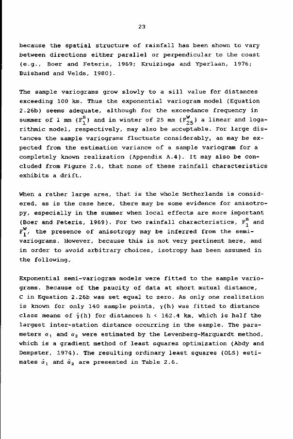
23
because the spatial structure of rainfall has been shown to vary
between directions either parallel or perpendicular to the coast
(e.g., Boer and Feteris, 1969; Kruizinga and Yperlaan, 1976;
Buishand and Velds, 1980).
The sample variograms grow slowly to a sill value for distances
exceeding 100 km. Thus the exponential variogram model (Equation
2.26b) seems adequate, although for the exceedance frequency in
summer of 1 mm (F^) and in winter of 25 mm (F„5) a linear and loga
rithmic model, respectively, may also be acceptable. For large dis
tances the sample variograms fluctuate considerably, as may be ex
pected from the estimation variance of a sample variogram for a
completely known realization (Appendix A.4). It may also be con
cluded from Figure 2.6, that none of these rainfall characteristics
exhibits a drift.
When a rather large area, that is the whole Netherlands is consid
ered, as is the case here, there may be some evidence for anisotro-
py, especially in the summer when local effects are more important
(Boer and Feteris, 1969). For two rainfall characteristics, F and w F.. , the presence of anisotropy may be inferred from the semi-
variograms. However, because this is not very pertinent here, and
in order to avoid arbitrary choices, isotropy has been assumed in
the following.
Exponential semi-variogram models were fitted to the sample vario
grams. Because of the paucity of data at short mutual distance,
C in Equation 2.26b was set equal to zero. As only one realization
is known for only 140 sample points, y(h) was fitted to distance
class means of y(h) f°r distances h < 162.4 km, which is half the
largest inter-station distance occurring in the sample. The para
meters ax and a2 were estimated by the Levenberg-Marquardt method,
which is a gradient method of least squares optimization (Abdy and
Dempster, 1974). The resulting ordinary least squares (OLS) esti
mates âx and â2 are presented in Table 2.6.

24
Table 2.6. Ordinary least squares estimates âj (-) and â2 (km)
in Equation 2.26b
Rainfall characteristic Summer Winter
Exceedance frequency
1 mm (F1) 11.94 139.16 7.25 38.98
15 mm (F15) 0.29 21.07 0.35 21.72
25 mm (F ) 0.065 14.62 0.018 28.01
Total annual rainfall1 (R) 1355.1 (=&1) 23.65 (=â2)
1 For rainfall characteristic R, âx has dimension mm 2
From a comparison of Table 2.6 with Table 2.1, it can be seen that
the sill »! of the exponential semi-variogram model is of the same 2
order as s in Table 2.1. The usual vai
the mean of the estimates v(h), because
2 2 order as s in Table 2.1. The usual variance estimator s equals
N S2 = r^j 1 (Z(U.)-5(u))2
1N"-L i = l x
N 2 I (z<u.)-z(u.)r N(N-l) v~v i' ~v j
N ( N;1 ) 2 Y(h) = HhT- (2.36) N(N-l) 2
As most estimated semi-variances have been calculated for pairs of
sample points at large mutual distances, that is beyond the range, 2 „ -
•y(h) = â , and because of Equation 2.36, s = à .
The matrix Equation 2.23 was solved by using the fitted semi-
variograms. A fixed neighbourhood, the complete set of observations,
has been applied because with a random design and a range of consid
erable magnitude, as is the case here, it is simpler to invert the
left-hand side of Equation 2.23 only once, and to solve the equa
tion by this inverted matrix, each point u leading to a different

25
right-hand side (y (u..-u_), . . . , y(u -u. ),1)'. Application of a fixed
neighbourhood implies assigning values to y(h) for h>L/2, that is
for distances for which the semi-variogram model has not been fit
ted to the data. From Table 2.6 it can be seen that for rainfall
characteristic F. this casts doubts about semi-variances at large
mutual distances.
The resulting maps are shown in Figure 2.7. Figure 2.7G for rain
fall characteristic R is in accordance with the regional differen
ces in total annual rainfall within the Netherlands described by
Buishand and Velds (1980). They also indicated the regions with
most abundant annual rainfall as the Veluwe and the extreme south
ern part of Limburg, followed by central Drenthe, the eastern part
of Friesland, the hilly parts of Overijssel and Utrecht, and regions
leeward of the dunes in Zuid-Holland and Noord-Holland. The driest
parts of the Netherlands are the coast of Groningen, the islands of
Zeeland and Zuid-Holland, narrow strips adjacent to the IJsselmeer,
the eastern part of Noord-Brabant and the northern and central
part of Limburg (for the location of these regions, see Figure 1.1).
This regional distribution of annual rainfall is not only consis
tent with that of Buishand and Velds (1980) based on 1941-1970
data, but it is also, in close agreement with that of KNMI (1972)
based on 1931-1960 rainfall records with some extended series.
Thus, analysis of rainfall records for the three periods, 1931-1960,
1941-1970, and 1951-1979, have yielded much the same regional dis
tribution of total annual rainfall.
The south-west to north-east oriented strip across the Netherlands
with high frequencies of heavy daily rainfall in summer reported by
Kraijenhoff and Prak (1979) for the period 1957-1975 is also visible
in Figure 2.7B and 2.7C.
The regional distribution of relatively heavy daily rainfall in
summer and winter is distinguishable in Figure 2.7B and 2.7E.
Seasonal rainfall differences have been found to occur in the fol
lowing regions:
Rotterdam-Dordrecht region, extending into the western part of
Noord-Brabant;

26
Noord-Oost Polder;
northern part of Noord-Holland;
eastern parts of Overijssel and Groningen;
a small area in the south-eastern part of Noord-Brabant.
From Figure 2.7A and 2.7B, it can be concluded that in summer, the
regional distribution of heavy daily rainfall differs greatly from
that of rainfall in excess of a low threshold value, particularly
in:
- the Randstad and the north-western part of Noord-Brabant;
- eastern parts of Groningen, Drenthe, Overijssel, and Gelder
land.
In the winter, these differences are considerably less (Figure 2.7D
and 2.7E). Differences between Figure 2.7B and 2.7E, 2.7A and 2.7B,
and 2.7D and 2.7E, may be of interest in studying the possible in
fluences on rainfall by the processes of urbanization and industri
alization.
2. 4. 3. Local differences in rainfall trend
As before, let x. .be the value in year j at station i of a cer-1 ' J s w s
tain rainfall characteristic (F , F or R). In the case of F and w F , the x. . were transformed variâtes, according to Equation 2.9. a i,J
Local differences in rainfall trend for data set D140 were investi
gated as follows. The time series {x. ., j=l,..., n} for each sta-i1 3
tion was reduced by the annual mean x . for each year
y. . = x. .-x .. (2.37) • l, 3 -1,3 -.3
This reduction is useful because here the interest is in local
rainfall trends with respect to the general rainfall trend over
the whole of the Netherlands (Kraijenhoff and Prak, 1979). Further
more, because of this reduction, var(y. . )<var(x. . ) , as there is 1,3 1/3
a high positive correlation between x. . and x . (Buishand, 1981).
For each series y_. . (i=l,..., N) the test statistics £, T, M, and 1/3
k* defined in Section 2.3 were calculated and the results are presented in Appendix A.5. For each rainfall characteristic, the number

27
of series for which at least one of these statistics is significant
(a = 0.10) is given in Table 2.7. For all rainfall characteristics,
many series exhibit inhomogeneities. This is in accordance with the
findings of Buishand (1982a) who tested homogeneity of annual rain
fall series at 264 Dutch rainfall stations.
Table 2.7. Number of series with at least one of the statistics
to test homogeneity, 2' Ï' o r M, significant (a = 0.10; for 2 the
test was one-sided, for T and M two-sided)
Rainfall characteristic Number of series
Summer
44
43
35
Winter
50
45
29
Exceedance frequency
1 mm (F1)
15 mm (F15)
25 mm (F2g)
Total annual rainfall (R) 72
For those rainfall series having a significant M, a check was made
whether there was a preferred location for the estimated jump point
k*. For each rainfall characteristic, these values of k* were clas
sified in intervals: 1951-1959; 1960-1969; and 1970-1979. From the
results, which are presented in Table 2.8, there is no evidence of
non-randomness.
Table 2.8. Number of significant (a = 0.10) jump points (data set
D140) in three periods: 1951-1959; 1960-1969; and 1970-1979
Peric
1951-
1960-
1970-
Sum
3d
-1959
-1969
-1979
"!
8
11
5
24
F15
7
7
6
20
Rainfall
Exceedance
FS
25
0
6
2
8
characteristic
frequency
•Ï 8
9
17
34
FW
15
15
1
10
26
FW
*25
6
6
6
18
Total
annual
rainfall
10
21
12
43
Sum
54
61
58
173

28
In order to obtain an overall picture of the distribution of local
rainfall trends, that is, of the reduced series (Equation 2.37),
the calculated T statistics were interpolated by the kriging method
(Figure 2.9). Sample semi-variograms were calculated according to
Equation 2.25, and are depicted in Figure 2.8. Again, checks were
made for indications of anisotropy in the sample semi-variograms,
and again no evidence for anisotropy was found. Therefore, the pa
rameters «j and a2 in Equation 2.26b were estimated by the proce
dure outlined in Section 2.4.2, and the resulting OLS estimates âx
and â2 are presented in Table 2.9.
Table 2.9. Ordinary least squares estimates 51 (-) and â2 (km) in
Equation 2.26b
Rainfall characteristic Summer Winter
Exceedance frequency
1 mm (F )
15 mm (F15)
25 mm (F25)
Total annual rainfall (R)
.62
.73
.41
â, =
17.07
15.11
25.11
= 3.00
2
1
1
43
60
70
« 2
17.21
32.63
75.02
= 31.86
The ranges (= 3<x2 ) of t n e semi-variograms for local rainfall trends
are rather limited and are of the same order as the ranges of semi-
variograms for rainfall levels (Table 2.6).
From Table 2.9 a large variance of the T statistic can be implied.
Under the null hypothesis var(T) = var(t _ ? ) , where t _ is a Stu
dent variate with (n-2) degrees of freedom with var(t _)=(n-2)/
(n-4)=1.08. Thus, it may be concluded that T is a non-central Stu-Ô.
dent variate t , where v=n-2 and with non-centrality parameter ô. ô .
at station i. For t 1, the following holds (Johnson and Kotz, 1970;
p. 203, 204))
Eft/} = 6i(v/2)l5r(^i)/r(v/2), (2.38)
ô . _ ô .
varf^1) = ( l + ô f ) - ^ ^ 1 } ) 2 . (2.39)

29
6. If v=27, then E{t 1} s ô., and when inserted into Equation 2.39 this
yields
ôi 2 var(t ) = 1.08 + 0.0214 6.. (2.40)
From Figure 2.9, for winter rainfall series there seems to be a
general positive trend along the coast and a negative trend along
the eastern border of the Netherlands. For the summer series, the ' s s
picture is rather complicated. For the characteristics F-5 and F_5
there are positive trends in the extreme north of Noord-Holland,
in a north-south strip through the centre of the Netherlands, the
Noord-Oost Polder, and parts of Zeeland. Negative trends occur along
the eastern border, and in some parts of Friesland, Noord-Holland
and Zeeland.
For F^ and FW seasonal differences in rainfall trend occur in Gro
ningen, Noord-Holland, Randstad, Utrecht, Noord-Brabant, and Zee
land. (Figure 2.9A and 2.9D). With higher threshold values, char
acteristics F^5 and F" (Figure 2.9B and 2.9E), these seasonal dif
ferences occur only in Noord-Holland, Randstad, Utrecht, and Noord-
Brabant. Within-season differences are particularly pronounced in
summer.
The regional distribution of trends in total annual rainfall R cor
responds rather well to the regional distributions of trends in the
winter series, that is, a positive trend along the coast and a ne
gative trend along the eastern border of the Netherlands (Figure
2.9G).
2.5. PARTITIONS OF THE NETHERLANDS BASED ON RAINFALL
Figure 2.7 and Figure 2.9 suggest local rainfall differences. How
ever, replacing the real data with correlated random variâtes and
applying the same interpolation and plotting procedures as used for
Figure 2.7 and 2.9 also results in maps suggesting local differen
ces. To be sure that a partitioning of the Netherlands based on
rainfall is realistic, the following two points are important:

30
the variation of a rainfall characteristic between regions
should be significantly different to the variation within re
gions ;
a partition resulting from a statistical procedure should lead
to physically interprétable regions. Such a partition should be
valid for several rainfall characteristics. For design criteria
in particular, the partition should be valid for the frequency
of heavy rainfall of short duration, that is, of five minutes
up to one hour.
Such a partition has been devised for France, in which three re
gions are distinguished (Ministère de l'Intérieur, 1977), and one
is further subdivided into two regions (CTGREF, 1979). The United
Kingdom has been divided into two regions, England and Wales, and
Scotland and Northern Ireland (NERC, 1975, Vol. 2), which are not
homogeneous with respect to rainfall. Thus, the recognition of
local rainfall differences is not sufficient to justify a parti
tion.
The actual procedure for rainfall durations shorter than 48 hours
used by NERC (1975; Vol. 2) is as follows: the threshold value of
rainfall corresponding to a 5-year return period, q-, for the ap
propriate duration and location is related to the two day g and
the 60 minute g_ values; these last two values can be derived from
detailed maps showing their geographical distribution. Then the q,.
value for the appropriate rainfall duration is related to the two
day and the 60 minute values by q,. = a/(l+bD)n, where q5 is in
mm/hour, D is the rainfall duration expressed in hours and the
parameters a, b, and n are related to the ratio of the two day and
the 60 minute values of q^. This relationship coincides with a re
lationship of these parameters to mean annual rainfall (see Section
2.5.3). Once the q5 value is determined, the value of o , for a
T-year return period can also be determined by considering the
growth factor : the ratio «Ip/q • These growth factors which were
found to vary slightly with geographical location, have been tab
ulated for the two regions of the United Kingdom mentioned above.

31
In NERC (1975) it is also pointed out that for rainfall durations
of at least 24 hours, guantile estimates of rainfall for a given
return period and rainfall duration are proportional to mean annual
rainfall. Without partitioning the country into regions, such pro
portionality is mentioned for possible use in Belgium (Nonclerg,
1982) and the Netherlands (Buishand and Velds, 1980). As a conse
quence of the rainfall increase in urban areas, reported by Kraijen-
hoff and Prak (1979), it is suggested in Werkgroep Afvoerberekenin-
gen (1979) to divide the Netherlands into urban and rural regions.
Possible partitions of the Netherlands based on rainfall are sug
gested in Section 2.5.1 and tested statistically in Section 2.5.2.
Finally, the implications of local differences for hydrological
design are discussed in Section 2.5.3.
2.5.1. Possible partitions
When suggesting possible partitions with respect to rainfall of
the Netherlands, it seems natural to start with a summary of the
relevant publications of the Royal Netherlands Meteorological
Institute (KNMI): Hartman (1913), Braak (1933), Timmerman (1963),
Buishand and Velds (1980) and Buishand (1983); also maps showing
the geographical distribution of certain rainfall characteristics
can be found in KNMI (1972).
Maps showing the geographical distribution of mean annual rainfall
from Hartman (1913), Braak (1933), and Buishand and Velds (1980)
are reproduced in Figure 2.10. The absence of a rainfall maximum
in the southern part of Limburg in Figure 2.10A is due to the use
made of the Maastricht and Ubachsberg records, which are of a
rather questionable quality (Braak, 1933). The mean annual rainfall
in Figure 2.10B ranged from 597 mm at Kampen to 862 mm at Vaals; in
the present study (Figure 2.7G) the range is from 706 mm at Stavoren
to 916 mm at Vaals. There is a general trend towards higher mean an
nual rainfalls which can at least partially be ascribed to improved
measurement practices (Buishand, 1977a). The local rainfall differ
ences can be attributed mainly to the following (Timmerman, 1963):

32
Friction. Convergence of air masses reaching the coastline from
south-west to north is induced by the increasing roughness. This
results in an increase in rainfall levels and frequencies with
increasing distance from the coast up to a maximum of about
30-35 km from the coast.
Topography. The forced ascent of the air leads to an increase
in rainfall on the windward side of the hills of Utrecht, Over
ijssel, the southern part of Limburg and the Veluwe.
Differential heating. Temperature differences between sea and
land lead to a relative increase in rainfall levels and frequen
cies along the coast in the autumn, and a decrease in the spring
and the early summer.
The effects of urbanization on rainfall have been mentioned by
Timmerman (1963), but not in relation to the geographical distri
bution of rainfall in the Netherlands. Buishand and Velds (1980)
have concluded that cities, such as Amsterdam and Rotterdam, may
have an effect on rainfall.
Four partitions of the Netherlands, based on rainfall, are proposed:
- partition (i), based on rainfall differences from east to west,
that is from inland to the coast, and from north to south
(Figure 2.IIA);
- partition (ii), based on the effects of friction, topography,
and differential heating (Figure 2.IIB);
- partition (iii), based on the effects of friction, topography,
and differential heating, and on anomalies attributed to urban
effects reported by Kraijenhoff and Prak (1979) (Figure 2.11C);
- partition (iv), based on mean annual rainfall for the period
1951-1979 (Figure 2.11D; the three isolated dry stations have
been included in the group of normal stations).
Each station in data set D140 has been assigned to one of the sub-
regions in each of the proposed partitions (see Appendix A.5).
Each partition is to some extent a posteriori. Particularly par
tition (iv), but the other partitions are also partly based on maps
showing the geographical distribution of rainfall.

33
2.5.2. Testing the statistical significance of the partitions
An indication of the existence of significant local differences in
mean annual rainfall has already been given in Section 2.2. Here,
the effect of spatial correlation is considered. The following
three null hypotheses are considered:
H : all the expectations of a certain rainfall characteristic in
all rainfall stations considered in the Netherlands are equal.
If this were true, then the Netherlands can be considered to
be homogeneous with regard to rainfall;
H_: after assigning the rainfall stations to regions, all result
ing regions are homogeneous ;
H_: differences between internal homogeneous regions vanish.
The following rainfall characteristics are considered
rainfall levels: R, FS , F ™ , ai
relevant for hydrological design;
rainfall trends: F and F?I-, bee
of the importance of urban effects (see Section 2.6)
- rainfall levels: R, Flc, F- _ , and F__ , because these are -Lb -Lb zb cal d€
s s - raxnfall trends: F.. _ and F?_, because these give an indication
The following model is used to test spatial homogeneity (M.A.J.
Van Montfort, pers. connu., 1981). Let z=(z,,..., z„)' be a vector 1 N
of measurements, and let z~N(Ç,C), that is a N-dimensional normal N
distribution with expectation £=(£,..., £ )'eR , and a N by N co-variance matrix C, where C is assumed to be known. Furthermore,
N . R is the direct sum of two orthogonal subspaces
N R = D+R,
where D is the space of vectors £ for a given null hypothesis. Ob
viously, C=£D+tR=4D. i
D and R, respectively.
viously, Ç=Ç_+Ç_=4_^, Ç and Ç are orthogonal projections of £ on D i\ D D ix.
With respect to the subspace D, H is equivalent to D=<s> and N s=l , a vector in R consisting of merely ones. Hypothesis H. will
be tested by the omnibus statistic T , where

34
ïl z'C^z
-1 2 (s'C Z)
s,C~1s
2 H AN-1
(2.41)
H is equivalent to D =<e , , e,>, dim(D„)=d, and d is the number d z
of regions into which the Netherlands is partitioned; the vector e.
(j=l,..., d) indicates by one or zero whether or not a station be
longs to region j. The hypothesis H_ is tested by T„, where
T2 = z'C^z - proj2 & 2 4 _ d , (2.42)
and proj is the square of a special projection of z on D_, to be
obtained by inserting the solution of the normal equations
eiC-1e1 eiC-1ed
edC"l ed
e^C_1z
eJLC_1z d —
(2.43)
into 1 S.e.C~ z. i=l X * -
H_ is equivalent to £GD _, where D_=<s>, and the alternative hypothe
sis is H . The test statistic T is the difference of the squares
of the special projections of z on D under H_ and under H_
2 2 2 T = z. - z ~ v ±3 2 D 2 ZD H3 * d _ r
(2.44)
As the statistics T , T , and T tend to large values under the
alternative, a right-hand sided critical region (a=0.05) is used.
In the present application, standardized variables are used, so
that in Equations 2.41, 2.42, and 2.44, £=0 and a =1. The Student
variâtes used as trend characteristics (Section 2.3) have been

35
standardized by considering their ratio to the standard deviation,
estimated as the square root of the sill value of the serai-variogram,
that is V«i# where â1 is given in Table 2.9. Rainfall levels x. have
been standardized by subtracting x , followed by dividing by -v/â x
(Table 2.6).
For rainfall levels, the normality assumption may be doubted, ex-s w cept for mean annual rainfall. However, the frequencies F.-, F..-,
F2 5 could follow a binomial distribution and it is only by virtue
of the Central Limit Theorem that the standardized values may have
a normal distribution. For the Student variâtes, the normality as
sumption seems more plausible.
The covariance matrix C=(c .) has been estimated as
c, . = exp(-h/a2), (2.45)
where a2 has already been estimated. In Table 2.10 the values of
(*! and â2 are reproduced, together with the results of the tests.
The test statistics are obviously functions of â2, but it has been
verified that the conclusions to be drawn from Table 2.10 do not
change within a reasonable range of â2 values.
Table 2.10. The statistical significance of four partitions of the Netherlands (Figure 2.11);
not significant values of T„, and significant values of T, and T_ support inhomogeneities
PARTITION
Rainfall (i) (ii) (Hi) (iv> characteristic â, â2 T1 T T T , T, T2 T3 T2 T3
Trends F^5 1.73 15.11 128.4 124.1 1.2 124.1 2.4 127.6 0.4 127.9 0.3
Fl* 1.41 25.11 193.1°° 187.2°° 1.1 192.3°° 0.3 192.1°° 0.4 191.8°° 0.5
Levels of F ,.
rainfall F*
0.29
0.35
0.065
355.1
21
21
14
23
07
72
62
65
142.2
145.4
135.3
157.9
138.5
141.9
133.4
154.6
0.9
0.8
0.5
0.7
131.7
131 .0
129.8
143.8
5.5
7.5°°
2.9
6.7°°
127
135
122
141
0
4
1
0
8.2°°
5.1
7.4°°
8.2°°
94
107
115
89
1
1
5
8
35
24
11
52
0
3
7
0
°° Indicates values inside the critical region for a = 0.05.
With respect to the Student variâtes it could be argued that, in
stead of standardizing on division by V«i/ division by the standard
deviation of such Student variâtes under the null hypothesis is
preferable. This, however, would lead to inconsistencies in the
estimation of a2 in Equation 2.45.

36
Wi ith regard to trends, it can be seen from the T.. values in Table
2.10 that only for rainfall characteristic F!L, the hypothesis of
inhomogeneity in space has statistical support. This is not sur
prising, as the alternative for hypothesis H.. is quite general.
With regard to rainfall levels it can be seen from the T„ and T_
values in Table 2.10 that, in spite of an insignificant value of
T , partitions (Hi) and especially (iv) are statistically signifi
cant partitions of the Netherlands. Regional rainfall differences
are to a certain extent the consequence of differences in time,
for example, the distribution of rainfall over the seasons is dif
ferent for inland and for coastal areas. Thus the attractive fea
ture of partition (iv) is that it yields significant results for
the year as a whole and for both winter and summer.
The adequacy of the partitions for rainfall levels but not for
rainfall trends can be explained by the large differences between
Figure 2.7C and 2.9C for levels and trends respectively of rainfall
characteristic F»_. As the partitions have been suggested from maps
of rainfall levels, the adequacy of the partitions for rainfall
trends could be expected to be less.
2. 5. 3. The hydrological significance of the partitions
Of the four partitions of the Netherlands proposed in Section 2.5.2,
only one explains successfully regional differences in rainfall lev
els, but none explains successfully regional differences in trends.
It is difficult to draw conclusions of relevance to hydrological
practice about regional differences in rainfall trend. A signifi
cant trend for a particular series may very well reverse when the
period of analysis is extended (Table 2.5 and Figure 2.5). This is
the result of the pseudo fluctuations which many hydrological time
series exhibit as a result of the infinite memory of hydrological
processes, that is a small but not negligible autocorrelation of
the process at very large time lags (Wallis and O'Connell, 1973).
The physical cause of this infinite memory is the storage effect,
which acts in many hydrological processes (Feller, 1951). Sample
curves from such processes reveal seemingly periodic swings, and

37
as pointed out by Mandelbrot and Wallis (1969): "... such cycles
must be considered spurious. (...) Such cycles are useful in de
scribing the past but have no predictive value for the future"
(p. 231). Note that the moving averages considered in Figure 2.5B
and 2.5C also cause pseudo fluctuations.
On the other hand, the differences in trend are quite notable.
For rainfall characteristic F?I-, the stations with highest and low
est values of T (Section 2.3) are Medemblik and Vroomshoop, respec
tively. If a simple linear regression line is fitted to the un-
transformed frequencies F-^ for these stations, the difference in
slope is 0.06-(-0.07) = 0.13 # year" . For rainfall characteristic
F15, the stations with highest and lowest values of T are Dordrecht
and Leeuwarden, respectively, and the difference in slope of the
regression lines is 0.06-(-0.16) = 0.22 # year
These are extremes, and for a more general picture, a partition
(v) of the Netherlands, suggested by Figures 2.9B and 2.9C, is
presented in Figure 2.12 (see also Appendix A.5). Let x. . be the
annual frequency F ,. at station i in year j, and x . the annual
mean for year j, then for each rainfall station in D140, the esti
mate B. of the slope parameter of the regression line of (x. .-x .)
on j has been calculated. It has been verified by the test proce
dures given in Section 2.5.2 that the partition was statistically
sound. For each of the three subregions of the partition, the aver
age slope parameter (5 has been estimated by Equation 2.43. The
covariance matrix C of the B. in Equation 2.43 has been estimated
from the semi-van ogr am of the B. . Results for F.. _ are
0! = 0.041, ß2 = -0.037, ß3 = -0.002 (# year-1).
s Application of this procedure to rainfall characteristic F?I- yields
ß\ = 0.005, ß2 = -0.016, ß3 = 0.001 (# year-1).
An indication of the homogeneity in time of the partition has been
obtained by calculating the slope B. for the D14 series (1906-1979)
for rainfall characteristics F^5 and F^. For data set D14, only

38
three rainfall stations were assigned to region 1 (Den Helder/De
Kooy, Vlissingen, and Kerkwerve), and only two stations to region
3 (West Terschelling and Heerde). Results for rainfall characteris-g
tic F1_ are
ßx = -0.008, ß2 = 0.003, ß3 = -0.004 (# year"1),
and for F-_
ßt = -0.003, ß2 = 0.002, ß3 = -0.005 (# year"1).
These results were obtained as the mean B. value for a particular
region. Note that this partition has been designed to give a posi
tive ßx, a negative $2< an^ a n approximately vanishing ß3. Further
more, values of ß for data set D14 are considerably smaller than
those for data set D140, which reflects the fact that the trends
studied here are not constant in time. Therefore, it can be con
cluded that the partition with regard to trends is only valid for
data set D140.
Kraijenhoff et al. (1981) present a map of the Netherlands (their
Figure 5), showing the geographical distribution of the change
AF = £-.F-0 - I F ., where the symbol 2. refers to a summation over
the period, 1933-1956 (excluding 1945) for i=l, and 1957-1979 for i=2. These changes AF were calculated as the means of such changes
2 for all stations within a moving, square grid area of 1000 km .
The order of magnitude of the change AF in rainfall characteristic
F_0, as reported in Kraijenhoff et al. (1981), corresponds to that
for rainfall characteristic F|5 (data set D140) in the present
study. However, the pattern of regions with positive and with nega
tive trends is very distinct. In fact, the map in Kraijenhoff et
al. (1981) suggests an effect of urbanization and industrialization
on rainfall.
With regard to regional differences in rainfall levels, the spatial
distribution of annual frequencies of heavy rainfall seems, from
a hydrological point of view, more interesting than that of mean
annual rainfall. As an example, the estimated difference between
rainfall levels for F^5 in the wet and the dry region of partition

39
(iv) (Section 2.5.1) is 1.14 times per year. As before, this dif
ference has been estimated by Equation 2.43.
Such local differences in frequency of heavy daily rainfall have
been pointed out by Braak (1933) with a map of the Netherlands,
showing the geographical distribution of deviations in the annual
frequency of daily rainfall in excess of 20 mm. This map is repro
duced here as Figure 2.13, together with an updated version, based
on data set D140. Braak concluded that "local differences appear
to be rather large" (p. 36), but continued that such maps should
be interpreted with care. Above a certain rainfall level the rela
tive change in the mean number of exceedances in a year is larger
than the relative change in rainfall level itself, see also Figure
2.14. As a consequence, rainfall levels for a given low frequency
of exceedance will show less local differences than the frequencies
of exceedance themselves.
In statistical terms, it can be stated that confidence intervals
for quantiles (x ) are relatively smaller than those for probabil
ities (p). Consider for example, a level with number of exceedances
k during the whole period of observation (29 years for data set
D140). The number of exceedances has a binomial distribution with
parameters n and p, and could be approximated by a Poisson distri
bution with expectation \=np, for which confidence intervals can
easily be constructed. In addition, distribution free confidence
intervals for x given p can be constructed from an ordered sample
of daily rainfalls. From the results given in Table 2.11, it can be
seen that for levels which are exceeded rather frequently, confi
dence intervals for x are narrow. This is not true for low values P
of k . The level of 20 mm is attained or exceeded about 3.55 times e
a year (data set D140).

365*29*p
58
29
6
x (mm) P
( 2 2 . 8 , 2 5 . 4 )
( 2 7 . 1 , 3 0 . 6 )
( 3 6 . 0 , 6 6 . 2 )
40
Table 2.11. Confidence intervals for the expected number of exceed-
ances and for quantiles x at confidence level 0.90
k Expected number of exceedances
58 (45.5, 70.5)1
29 (20.8, 39.6)
6 ( 2.6, 11.9)
1 Estimated by using the normal approximation.
Maps of the Netherlands showing the geographical distribution of
q5, q10/ and q for daily rainfall for the months, February, April,
June, August, October, and December have been presented in KNMI
(1972), where q,- denotes the estimated threshold value of rainfall
of the appropriate duration and for a 5-year return period. Here,
such maps are produced for q. ~ (that is, the event with a 0.5-year
return period) and q for the summer (Figure 2.15), the winter
period (Figure 2.16), and for the whole year (Figure 2.17). These
were obtained by maximum likelihood estimation of q. - and q^ from
data set D140, in particular the POT series of daily rainfall from
Section 2.2 (for a particular series q_ . simply equals the estimate
q0 of the location parameter). A test on the exponentiality of the
individual series has been carried out. The hypothesis of an ex
ponential distribution was rejected by the test outlined in Sec
tion 2.2, at significance level 0.10, for 34 year series, for 27
summer series, and for 39 winter series. For a relatively large
number of series the test statistic is small, indicating too long
a tail of the POT series.
Although local differences in daily rainfall are important for
drainage design for rural areas in the Netherlands, this is not
necessarily so for urban areas: the order of magnitude of the time
lag between the centres of the hyetograph and the hydrograph for
an urban drainage system is about one hour. Thus, it should be ver
ified that a partition also holds for this duration of rainfall.
Buishand (1983) found that there are only small differences between
the quantiles of the distribution of hourly rainfall for the series

41
Den Helder/De Kooy, Eelde, De Bilt, Vlissingen, and Beek. Further
more, somewhat larger differences may very often be the result of
seasonal effects on rainfall distribution.
Consequences of differences in level of hourly rainfall have been
investigated, by using the hourly rainfall data (data set H12) as
input into a simulation model of urban runoff, STORM (HEC, 1977).
This model operates as follows. The basin excess is calculated
for each hourly interval as the sum of the dry weather flow and
the net rainfall (evaporation and depression storage being taken
into account) multiplied by a coefficient. The basin excess is
routed to the outlet of the basin by the Soil Conservation Service
triangular unit hydrograph. Storage, treatment, and overflow quan
tities are calculated by means of a simple bookkeeping system.
The model has been calibrated for a particular urban basin in the
Netherlands (Leenen and Groot, 1980), and the resulting values of
the input parameters of STORM have been used in the present study,
together with the hourly rainfall of the twelve series of data
set H12. The 12 stations have been assigned to each of the three
regions within partition (iv) (Figure 2.11D). The mean annual num
ber (N) and total quantity (Q) of overflows, calculated for the
period 1975-1980, are presented in Table 2.12. This partition is
not particularly convincing. This is partly due to the difficulty
of deciding which of the three regions is most appropriate for a
particular rainfall station, for example, Volkel. The proposition
of a certain partition necessitates not only a dense network of
rainfall stations but also meteorological insight.
Furthermore, a partition based on the level of mean annual rain
fall, and which also appeared to be valid for daily rainfall,
may not be adequate for hourly rainfall. The reason for this is
that the behaviour of quantiles of hourly and of daily rainfall
with respect to mean annual rainfall may be different, as can be
illustrated with results of NERC (1975).

42
Table 2.12. Mean annual number (N) and total quantity (Q) of over
flows over the period 1975-1980, calculated with the STORM model
(the partitioning into regions is in accordance with Figure 2.11D)
Rainfall station N (# year ) Q (mm)
Region 1 2.00 51.53
Schiphol 1.50 11.23
Rotterdam 2.50 91.82
Region 2 2.00 53.16
Vlissingen 1.67 59.32
Volkel 2.33 46.99
Region 3 1.96 39.01
Soesterberg 2.17 43.34
Den Helder/De Kooy 2.17 80.87
Valkenburg 1.33 18.74
Beek 2.00 53.83
De Bilt 2.17 30.17
Eelde 1.67 15.79
Leeuwarden 2.67 37.60
Twente 1.50 31.73
A model for relating rainfall intensities of equal probability of
exceedance to durations from some minutes to some days is
(D+b)n (2.46)
where
I : intensity (mm/hour)
D : duration (hour)
a,b,n: parameters to be estimated.

43
Quantiles q for rainfall durations of one minute to 48 hours have
been described by a somewhat different equation, I = a/(l+bD) in
NERC (1975; Vol. 2). The approximate relation of the parameters a,
b, and n to mean annual rainfall as presented in NERC (1975; Vol. 2,
p. 26) was used to estimate q^ for rainfall durations of one and
24 hours (Table 2.13). For a rainfall duration of one hour, q5 is
rather insensitive to variations of mean annual rainfall, and as
far as there is a relationship to mean annual rainfall, it is op
posite to the relationship of qR for a rainfall duration of 24 hours
to mean annual rainfall.
Table 2.13. Quantiles q5 according to NERC (1975) for rainfall
durations of 1 and 24 hours, as a function of mean annual rainfall
Mean annual
rainfall (mm)
500 - 600
600 - 800
800 - 1000
1000 - 1400
1400 - 2000
Define a depth-duration ratio as the ratio of two quantiles of
rainfall of different duration, but with equal probability of
exceedance. Such a ratio for durations D.. and D_ can be written as
D D +b n
—(—-—) D 2 D l + b "
If local differences in these depth-duration ratios were totally
absent, geographical variation in mean annual rainfall would be a
perfect indicator of geographical variation of rainfall for all
durations. However, Equation 2.46 is only valid for rainfall dura
tions up to a few days, and for these durations, the total absence
of local differences of depth-duration ratios also implies the ab
sence of local differences of the coefficients b and n in Equation
1 h o u r
1 9 . 6
2 0 . 6
1 9 . 0
1 8 . 6
1 8 . 5
% (mm)
24 h o u r s
4 1 . 3
4 7 . 8
5 0 . 9
6 0 . 0
6 7 . 1

44
2.46. But in fact, these have been found to vary locally with mean
annual rainfall, as does the coefficient a in Equation 2.46, giving
rise to the phenomenon illustrated in Table 2.13. Only for dura
tions up to two hours, there is very little geographical variation
in depth-duration ratios (Hershfield, 1961; Bell, 1969).
On the other hand, the impression offered by Table 2.13 does not
seem to be typical. This may be concluded from comparing the maps
showing the geographical distribution of the one-hour and 24-hour
rainfall of a T-year return period for the United States (Hershfield,
1961). The one-hour maps in Hershfield (1961) have been extracted
from the data of 200 US Weather Bureau first-order stations with a
mean length of record of 48 years. Taking into consideration the
reduced number of rainfall stations on which the one-hour rainfall
maps are based in relation to the 24-hour rainfall maps, the pat
terns of isolines in both maps can be considered to agree very well.
For all of the H12 series, POT series have been extracted for du
rations of one hour and 24 hours (daily rainfall for each 24-hour
period ending at 8h UTC), with a mean annual number of threshold
exceedances of two. To assure independence, peaks had to be sepa
rated by a time gap of at least ten hours for rainfall durations
of one hour (Buishand, 1983), and for daily rainfall by a dry
period of 24 hours. Quantiles q_ ^ have been estimated as the lo
cation parameter in Equation 2.3, for the summer, winter, and the
whole year, and are plotted in Figure 2.18 as a function of mean
seasonal or annual rainfall.
Especially when the year is divided into seasons, there is a sig
nificant positive correlation of quantiles of both hourly and daily
rainfall and mean seasonal rainfall (one-sided t-test at signifi
cance level 0.05). There is not a very pronounced difference in the
behaviour of quantiles of hourly and daily rainfall with respect
to mean annual rainfall, and such differences cannot explain com
pletely the unconvincing results presented in Table 2.12 of the
partition of the Netherlands. Further, the total number and quanti
ty of overflows tend to correlate positively with mean annual rain
fall, although not statistically significant (both correlation coef-

45
ficients 0.16). A third explanation for the unconvincing results of
the partition is, that only six of the 12 rainfall stations in the
data set H12 have been used in designing the partition (iv), from
which Twente has an atypically low mean annual rainfall for the
period 1975-1980, as compared to the period 1951-1979 considered
when designing the partition. Finally, the STORM model does not
seem sensitive enough to yield large differences in overflow para
meters, given the spatial differences in rainfall.
Thus it can be concluded that the proposed partition of the
Netherlands based on rainfall trend (Figure 2.12) is only valid
for the most recent period (data set D140), and for the particular
rainfall characteristic considered, that is, the exceedance frequen
cy of heavy daily rainfall in summer. The partition based on rain
fall levels (Figure 2.11D) has considerably more support.
2.6. EFFECT OF URBANIZATION AND INDUSTRIALIZATION ON PRECIPITATION
The effect of urbanization and industrialization on precipitation
is an aspect of urban climatology, which requires an understanding
of the whole urban climate because of the interaction between the
climatic elements. This understanding, however, is far from com
plete. For example, little is known about the physical mechanisms
governing urban enhancement of precipitation. According to Oke
(1980), the impact of cities upon precipitation is still a topic of
some controversy, concerning both the proof that effects exist and
the nature of the processes involved. The present concensus is that
there is reasonable statistical and other support for the hypothe
sis of precipitation enhancement by large cities but that proof
including knowledge of the governing physical mechanisms remains
to be demonstrated. According to this consensus, the maximum effect
is usually about 20-40 kilometres downwind of the city, and con-
vective events are more susceptible to modification than frontal
events. Effects increase with increasing intensity of rainfall,
but this should not be interpreted as being restricted only to a
few large rainstorms. Presumably such effects extend to rainstorms
which, if unaffected, would be of rather modest size (Braham, 1978).
It should be emphasized, however, that not everyone agrees with the
above-mentioned consensus view (Hershfield, 1979).

46
The step from measurements to hypotheses about causal relationships
is extremely complicated in urban climatology, because of the com
plexity of the system. For example, in the spatial definition of
the urban system, not only is the urban surface involved, but also
a certain part of the atmosphere, as evidenced by city-induced
changes in wind, temperature, precipitation, and also pollution.
The vertical extension of this part of the atmosphere, usually di
vided into an urban canopy layer, that is below roof level (UCL),
and an urban boundary layer, that is above roof level (UBL), depends
on meteorological conditions, for example, stability. To complicate
matters further, a part of the soil is also involved, and there is
considerable import to the system, including advected heat, im
ported water, etc.
Possible causes of urban enhancement of precipitation are suggested
in two reports on urban climatology to the World Meteorological
Organization by Oke (1974, 1979), and by Bornstein and Oke (1980)
and Oke (1980); and methodology on statistical research into urban
precipitation enhancement is suggested by Lowry (1977). These ref
erences are used in this introduction.
Thermodynamic and mechanical processes rather than the extra provi
sion of condensation and freezing nuclei by urban aerosols and
the extra supply of water vapour in the city due to combustion
and cooling processes, lead to the urban enhancement of precipita
tion. The uplift associated with the heat island, mass convergence
due to frictional retardation of the airflow and to heat island
induced circulations, the barrier effect of the physical presence
of the city, and increased mechanical and thermal turbulence, could
well be sufficient to permit urban clouds to penetrate stable layers
in the mid-troposphere and to reach glaciation levels, or to produce
greater instability in general, or to produce confluence zones of
preferred activity (Oke, 1980).
Two other processes sometimes mentioned as affecting urban precipi
tation are urban emissions of condensation nuclei and the extra
supply of water vapour in the city, but these are considered to
be less important by Oke. With regard to the former, in the urban
atmosphere, Aitken condensation nuclei (ACN, with radius

47
-3 r: 4*10 < r < 0.1 pm) and the larger cloud condensation nuclei
(CCN) in the background atmosphere are added to greatly by urban
emissions. These emissions are supplemented by gas-to-particle
conversions, especially from pollutant gases, such as, SO- and NO .
These conversions result in particles of ACN size, which can grow
by further absorption to CCN sizes. This leads to urban clouds
having much higher drop concentrations than non-urban clouds, so
that urban clouds are characterized by a very large number of small
droplets.
Thus, if the mechanism responsible for precipitation is coalescence
of cloud droplets rather than the formation and growth of ice par
ticles, then there appears to be a negative urban microphysical
effect on raindrop growth, and therefore on precipitation. The
balance is at least partially redressed, however, with the discov
ery that certain industrial sources produce ultra-giant nuclei
and thus provide an appropriate distribution of droplets for drop
let growth. But, even where the appropriate seeding of nuclei from
urban-industrial sources is present, it is likely that more than
microphysical modification of clouds will be necessary for signi
ficant precipitation enhancement (Oke, 1980).
In this context numerous observations made downwind of isolated
power-generating plants have not revealed significant increases
in convective rainfall (Huff and Vogel, 1979). Although precipita
tion enhancement by cloud seeding has been accepted, seeding should
take place under appropriate conditions, and even then the increase
in rainfall is only modest (Rogers, 1979). In the case of power-
generating plants, continuous cloud seeding may very well lead to
occasional suppression of rainfall. Apart from that, the cloud seed
ing material emitted by these plants may not be very effective.
With the exception of daytime values during summer, absolute humid
ity in a city tends to be higher than in the surrounding rural area.
In cloud physics, however, relative humidity is often a more impor
tant factor than the actual moisture concentration.

48
The difficulty of discriminating between controlling factors and
the natural variability in time and in space of the precipitation,
has allowed widely used estimators of urban effects, such as urban-
rural and upwind-downwind rainfall differences, to become open to
criticism (Lowry, 1977). Let x.. be the mean measured rainfall
at location u on days within a period t given weather type i during
those days, then the expectation of x. may be considered to be
the sum of three components (Lowry, 1977)
E{x.. } = E{c }+E{l. }+E{e.. }, (2.47) l—ltu' '-lu' '-lu' —ltu3
where the component c refers to the background climate, 1 to the
local landscape and e to local urbanization. The variables c and
1 are assumed to be time-independent
c . = c . = c. ; 1.. = 1-4. = 1. . (2.48) —lt.u —it, u — lu — it,u —it, u —1U J K J K
Furthermore, it is assumed that prior to urbanization and industri
alization, at period t=0, there is no urban effect: E{e. } = 0.
As pointed out by Lowry (1977), estimators of the urban effect,
E{e. . }, such as urban-rural and upwind-downwind differences are
subject to doubt. Consider, for example, urban-rural differences,
ô(C,R). The recognition of urban effects beyond the urban boundary
motivates the specification of areas C (city), R (rural), and Z
(zone of influence beyond the urban area) (Figure 2.19). Because
the location of the boundary between R and Z is one of the objects
of study, it is not certain whether or not the urban-rural differ
ences refer in fact to differences between the urban area and
area Z: ô(C,Z). However, even if this were not so, then
<5(C,R) = (E{çic}-E{çir}) + (E{lic}-E{lir}) + E{ei t c}, (2.49)
and it is by no means self-evident that the first two terms within
brackets on the right-hand side of Equation 2.49 vanish.
Instead of the afore-mentioned indicators of the urban effect in
the space domain, Lowry (1977) advocates the use of indicators in
the time domain: estimated differences, for one station or for a

49
network of stations, between observations from urban and pre-urban
periods, stratified by synoptic weather type
6.(t,0) = E{x.. }-E{x.„ }. (2.50) iv ' l—ltu —lOu'
The estimate S.(t,0) = x. . -x._ is unbiased, because of the iv ' ltu lOu assumptions in Equation 2.48.
Although the estimate S.(t,0) is an improvement on, for instance,
urban-rural differences, the assumptions in Equation 2.48 remain
questionable. There may be within-circulation type precipitation
changes (Barry and Perry, 1973) and/or geographical shifts of cli
matic zones. However, as already stated in Section 2.3, rainfall
can be predicted to a certain degree from weather type. In addition,
if the importance of these factors is stressed, then the urban
effect is measured by the local differences in rainfall which have
been considered in Section 2.4.
Urban enhancement of precipitation in the Netherlands has been
investigated by Yperlaan (1977), Buishand (1979), Kraijenhoff and
Prak (1979), and Kraijenhoff et al. (1981). With some caution it
may be concluded from these studies that cities, such as Rotterdam
and Amsterdam, do have an effect. These effects are not only pre
sent in summer but also in winter (Yperlaan, 1977; Buishand, 1979).
In this section the effects of urbanization and industrialization
on precipitation with regard to daily rainfall levels and frequen
cies of heavy rainfall are investigated using the statistical pro
cedure of Lowry (1977).
2.6.1. Urban effects in the Netherlands
As already stated, mechanical and thermal processes are considered
to be the most effective agents in urban precipitation enhancement.
In this context, the Rotterdam area must be considered to be the
urban/industrial area par excellence in the Netherlands. Even though
Amsterdam has a larger population than Rotterdam (CBS, 1980), the 2 gross energy consumption of these cities m 1980 was 30 W/m and

50
2 70 W/m respectively, and incoming solar radiation was estimated to
be 109 W/m2 (Können, 1983). Not all of the gross energy consumption
results in direct heat production, but say about 60%. Neither does
all incoming solar radiation result in heat production. Only 50%-
65% is converted into net radiation, of which only 25% results in 2
direct heat production: about 18 W/m . Furthermore, both gross
energy consumption and incoming solar radiation vary throughout
the day and throughout the year.
The high energy consumption in the Rotterdam area is undoubtedly
the result of the concentration of industry and to a lesser extent
of other activities, such as, commerce and transport. This may be
inferred from Table 2.14, which gives the emissions of sulphur di
oxide, carbon monoxide and hydrocarbons in the Amsterdam and Rot
terdam areas. The emissions of sulphur dioxide give a good indica
tion of the degree of industrialization, and emissions of carbon
monoxide of transport activities. Gross energy consumption in the
Netherlands for the period 1946-1979 is presented in Figure 2.20.
The gross energy consumption is unknown for the period 1932-1946;
available data on the production of electricity and gas suggest
a very slight increase during this period (CBS, 1979).
Table 2.14. Emissions of pollutants in the Rotterdam and in the Am
sterdam area1
Sulphur dioxide Carbon monoxide Hydrocarbons
(103 t/y) (103 t/y) (103 t/y)
Rotterdam (1974) 149 61 50
Amsterdam (1975) 7 38 28
1 Data: Ministerie van Volksgezondheid en Milieuhygiene, 1978,
1980. The Rotterdam area corresponds to blocks F6, G6, H6, 16,
J6, 17, and J7 of the 1978 publication, the Amsterdam area to
blocks F4, G4, H4, F5, G5, H5, E6, and G6 of the 1980 publica
tion.

51
As the urban effects are considered to be greater in summer, it
is important that heat production, for example in industry and
transport, occurs throughout the year in contrast to heat produc
tion for the heating of buildings, which occurs mainly during the
winter. Further, the heat produced by petro-chemical industries
in and around Rotterdam is very often released from chimneys more
than 100 m tall. Indeed, at these petro-chemical complexes, the
combined effects of heat production, of its release at considerable
heights, and of friction, create an important local circulation
pattern over these areas : upward currents above its centres and
downward movements in the immediate surroundings (Schmidt and Boer,
1962).
While the Rotterdam area is the most industrialized part of the
Netherlands, it is by no means the only urban area in the country.
In fact, the presence of several smaller urban industrial centres,
the smallness of the country in relation to the scale of the meteo
rological processes (wind at a velocity of 10 m/s crosses the coun
try in three to eight hours), and the large quantities of pollutants
from neighbouring countries (for instance, the Dutch contribution
to the mean sulphur dioxide level over the Netherlands is only 30%,
see also Figure 2.21, reproduced from KNMI/RIV, 1982), all indicate
that most of the Netherlands belongs in varying degree to area Z
of the classification presented in Figure 2.19.
In order to provide information about the rainfall stations in
data set D32 which has been used in this section, data on local
emissions of pollutants together with the number of inhabitants
in the municipality in which the station is located are given in
Appendix A.6. The pollutant data have been extracted from publica
tions of the Ministry of Public Health and Environmental Hygiene,
which give total emissions over 5 x 5 km grid areas. Here, for each
rainfall series the grid area in which the rainfall station is lo
cated has been considered.
In the application of Lowry's procedure, the weather type occur
ring on a given day has been extracted from Hess (1977), and clas
sified according to one of the ten "Grosswettertypen" (Types of

52
large-scale weather patterns) of Hess and referred to as circula
tion types.
The grouping of rainfall stations into urban affected and urban
unaffected depends upon wind direction. In the classification of
the circulation types, 500 mbar level maps have been used to re
present the steering of tropospheric disturbances. An investigation
into the relationship between prevailing wind direction at De Bilt
at ground level and circulation type (Bijvoet and Schmidt, 1958)
has shown that for a given circulation type, the pattern of flow
remains characteristic at considerable heights. The most frequently
occurring wind direction at ground level for each circulation type
(Bijvoet and Schmidt, 1958) is given in Table 2.15. Wind direction
at ground level for circulation types 4 and 5 is extremely variable.
Circulation types 2, 3, 5, 7, 8 and 9 were not analysed statisti
cally because they occurred rather unfreguently, being virtually
absent in some years, or for short spells only (Table 2.15). The
spell length is important because rainfall is measured in 24-hour
intervals ending at 7.55 h UTC, whereas circulation types hold for
calendar days.
It is difficult to assign rainfall stations to the three areas,
C, Z, and R, in Figure 2.19 mainly because of:
difficulties in determining the predominant wind direction;
uncertainties about the regional effect of various urban indus
trial centres, especially the smaller centres;
uncertainties about the urban industrial rainfall enhancement
in general.
Difficulties in determining the predominant wind direction include
the frictional drag exerted by the earth surface. Wind direction
in, say, the lowest 0.5 km of the atmosphere deviates from the
dominant winds at the 500 mbar level by about 30° in a counter
clockwise direction in the northern hemisphere (Mcintosh and Thorn,
1978). For example, if for a certain circulation type the dominant
wind direction at the 500 mbar level is west, the wind direction
measured at ground level will tend to be west-southwest. Storms
tend to move in correspondence with wind at the 700 mbar level,

53
instead of with that at the 500 mbar level or at ground level. Fur
ther, there may be local circulations, which are quite different to
the large-scale pattern.
Table 2.15. Most frequently occurring wind direction at ground
level at De Bilt measured at 13.40 GMT, period 1881-1955 (Bijvoet
and Schmidt, 1958)
Circulation
type
1. West (Zonal)
2. South West
3. North West
4. High Middle
Europe
5. Low Middle
Europe
6. North "]
7. North East
8. East
9. South East
10. South j
Unknown
~\
ï\(Mixed)
>
>(Meridione
Wind
direction
Ll)
S-SW
S-SW
NW-W l
l
NW-NE
NNE
E-NE
E-SE
SE-SW
Mean
(# ye
frequency
ar
Summer
40.1
6.5
13.3
24.3
3.4
24.4
10.8
12.3
2.4
13.9
1.6
- 1 )
Winter
54.3
13.3
14.1
33.9
5.3
33.9
6.8
18.4
11.3
19.3
1.6
Mean spell
length
Summer
5.6
4.0
4.2
4.1
3.3
4.5
4.0
4.5
3.3
3.8
1.2
(days)
Winte
6.0
4.0
3.7
4.1
3.6
4.2
2.8
4.9
4.2
3.9
1.0
1 Highly variable wind directions.
In full recognition of the difficulties, an attempt has been made
to identify for each circulation type the stations or groups of
stations with and without a potential urban effect. For these sta
tions, differences between mean daily rainfall for the period 1956-
1979 and 1932-1955 for the given circulation type are presented in
Table 2.16. In this table, stations have been classified as urban
affected or urban unaffected, using information about the predom
inant wind direction, once the circulation type is known.

54
Table 2.16. Differences (0.1 mm) in mean daily rainfall, given cir
culation type and season, between the period 1956-1979 and 1932-1955,
according to Equation 2.51
Rainfall station Circulation types
10 4
Summer Winter Winter Summer Winter Summer Winter
Urban affected Urban unaffected
Delft, Bergschenhoek,+2.6 +5.9°° -2.8 -1.4 +0.6 +3.0 +1.9 Boskoop, Leiden
Den Helder, West +0.2 Terschelling, Groningen, Ter Apel, Dwin-gelo, Heerde, Dene-kamp, Winterswijk, Arnhem, Vlissingen
Urban unaffected
+3.6°° -4.2°° -1.3 -0.3 +0.1 +0.8
Sche11ingwoude Amsterdam IJsselmonde
+1.2 +1.8 +5.7
Urban affected
+5.1°° +2.6 -1.7 -0.3 +5.4°° +0.3 -2.7 -0.4 +6.1°° -1.9 -2.4 +0.2
+1.6 +1.8 +3.9
+2.1 + 0.5 +3.3
Indicates values inside the critical region for a = 0.05; there
are no differences significant at the 5-10% level.
The differences 6!(0,t) in Table 2.16 have been calculated as
i!(0,t) = X!;2-X!fl, (2.51)
where
-, _ _i 2 4 _ Xi,l " 24 t^itu
1 4 8 -i,2 24 t t 2 5 itu'
Thus, x! _ is the arithmetic mean of the observations x.. for l,2 itu
period II (1956-1979), while x! .. is the arithmetic mean for i, i

55
period I. Denote the standard deviation of the observations x..
by s., then realizations of a test statistic T can be calculated as
x! _-x! n 1,2 1,1
^<24+24)si
(2.52)
For samples from a normal distribution and for H- : M1-M2 = °
ï a ^48-2- ( 2 - 5 3 )
o
For the normal distribution to be valid, the observations x.
have been transformed according to Equation 2.9.
Table 2.16 should be read in conjunction with Figure 2.22A-J, which
shows differences in mean daily rainfall between the period 1956-
1979 and 1932-1955 for given circulation type and season for all
rainfall stations. At this point a remark on the computations has
to be made. A comparison of Table 2.16 and, for example. Figure
2.22A, shows that there are small divergencies, because the differ
ences S.(t,0) in Figure 2.22A-J are differences of weighted aver
ages
6.(t,0) = xi ( 2-xi j l ( (2.54)
where
1 2 4
Xi,l = N^ t ^ i ^ i t u ( 2 - 5 5 )
24 I
t=l N, = 2! n.. 1 . ., it
n..: frequency of occurrence of circulation type i in
year t,
and the weighted means x. , are defined analogously. The statisti-
cal significance of the differences S.(t,0) cannot be tested.
As an estimate of 6.(t,0) in Equation 2.50, however, the estimate
according to Equation 2.54 is preferable to the estimate according

56
to Equation 2.51. Figure 2.23 presents the differences in seasonal
rainfall for the two periods considered. In accordance with the
conclusions of Section 2.3, total summer and winter rainfall is
higher for the more recent period for most rainfall stations in
data set D32.
Although the differences in Figure 2.22 should be interpreted with
caution, some observations can be made. Firstly, there are large
differences between some stations classified as urban unaffected.
This may indicate either local within-circulation type climatic
changes, or effects other than industrialization and urbanization.
Any conclusions, however, should also be based on the station his
tory of all selected rainfall records.
Furthermore, Table 2.16 and Figure 2.22 suggest that there is an
urban effect for circulation types 1, 6 and 10; but for circulation
type 4, the results are not in accordance with an urban effect
for summer and inconclusive for winter. Figure 2.22 shows that
results for the remaining circulation types are somewhat inconclu
sive. The results for circulation type 5 and 10 are of special
relevance to the present study, because on summer days with these
circulation types, relatively many heavy daily rainfalls occurred.
In summary, for all circulation types, and including days with
the circulation type not specified, it can be seen from Figure
2.23 that for the entire Randstad area, there is an increase in
total summer rainfall, with maximum increases for rainfall sta
tions near Amsterdam and Rotterdam, and in Leiden. It is somewhat
doubtful whether the increase for the Leiden rainfall station can
be attributed to industrialization and urbanization only. There
are also high rainfall increases at the rainfall stations Roermond
and Axel. For winter, the situation is more or less the same, with
increases in total winter rainfall for the Randstad area exceeding
those for other parts of the Netherlands. Again, there are several
maxima within the Randstad, for which it is doubtful whether they
can be attributed to industrialization and urbanization only.

57
Figure 2.23 is useful for assessing the relative contribution of
each circulation type to seasonal rainfall. The differences, A,
presented in this figure, can be calculated as
A = I i { S i ( t , 0 ) m i n ( n i l , n i / 2 ) + (n^-n^ ± )i.f k? , (2.56)
where
n. : mean annual frequency of circulation type i in period I
n. _: mean annual frequency of circulation type i in period II
x. .: the mean of x. (as in Equation 2.55 for period k,
where k refers to the period with maximum N. (j=l,2) in
Equation 2.55).
The first term of the right-hand side of Equation 2.56 vanishes
when either n. „ or n. .. is equal to zero, and the second term 1 , z 1 , x vanishes when n. , is equal to n. .. Equation 2.56 shows that com-
1 , A 1 , -L
paring the differences A for a rural and an urban station is not
particularly suitable for assessing urban effects on rainfall,
because A is dependent on x. . through x. . . Recognition of this
dependence must have been Lowry's starting point.
An indication whether urban effects extend to rainfall which, if
urban unaffected, would be rather moderate, has been obtained by
registering the numbers of rainfalls in excess of 15 mm at each
station for both periods, pre-urban (1932-1955) and urban (1956-
1979). Their differences, which are presented in Table 2.17, indi
cate that for most circulation types, there are no consistent inter-
station differences, except for circulation types 1, 6, 8 (in sum
m e r ) , and 10 where there are indications of an urban effect.
For circulation type 4 (in summer) and 9 the results are not in
accordance with the hypothesis of an urban effect. Furthermore,
it can be seen from the last two columns of this table that during
the period 1956-1979 stations in urbanized regions increased their
effectivity in realizing an already potential heavy daily rainfall,
in relation to stations in other regions. This is also concluded
by Kraijenhoff et al. (1981) for daily summer rainfalls in excess
of 30 mm.

58
CO <tf <T> H m N + + +
ro ro »H H en + + +
l-H 1
en i
N *
+ +
o O)
H 1
H 1
00
CM N H rH H H + + +
.. 0)
G i-i o ai m m s -a g s a § o 3 «3 -H -o g
B T J H H H u u r-t ai a <D ai D p M •P P .G U) M P m u g >r> 0 | « S ~
a« m o ui H i / i * * m r H f O r H H N r H r H r H t M C M + + + + + + + + + +
CM (NI * • * CO CO H H h d r l O M N N r H I I + + + + + + +
O O i T l rH^DCOr^^OHr - t fO I^ + + + + + + + + + +
O H CO M D i O h i O i n c O H H H + + + + + + + + + +
N O O H U l i H C O C O C h C O C n H ^ O + + + + + + + + + +
O * o
+ 1 + I + + + + + +
** co
> I + + + + + + +
fl -r*
IQ & o •O 3 r G M i m U t
H f t O » 4» Î7-P ï O 4) Ï T 3 *
O
a .c -o O U ß H O P m oi v
r H « * H O n i O H CM CO
+ I + I I I I + I + + + + + + + + 1
CM CM i-i co en CM rs CM m o * t ^ H H O ) t S H H ( D H H ( N n H ( n H M n a ) H N + + I I I I + + + I I I + I + I + + +
O ro c o c M i O H r o ' t i n H H O c o m m c o c n c o ^ c M r ^ + I + I + + + + + + + + + + + + i +
O (M ^ r H r - < t f « 3 * r o o i n c o r ^ < J " H r o c M C n r H i - i c o * 0 + + + + + + + + + + + + + + + + + +
CM O M H O r ^ H H i ^ < n c o t ^ c o t ^ c o r - r * - H C f t H H ( ^ c o r -+ + + + + + + + + + + + + + + + + + +
in CM CM
+ I + I I I I + + + + + + I + I + I
o * CM CM co o m CM * *o m H J ) H H H H h H N H N H H N N « O O i O H I 1 I I I I + + + I I I + + + I + +
O U
(0 W H O -n 4) G .G •p *o ai w G -H g -P c a» o) u M C D M O H 0 A Ï 3 U J( M 0»> 1 0 . m <o H ai o» ai .-4 g u u o ai o G w o c " " E - < C Q . 4 > a > * g r < - H O O O - H O ) " " .18 H a> P C C M « J Ï + J ^ T 3 H 2 ^ I D Ü H D G ( Ü Ä C U O M - H D C C Ö f f l Ö O O W - H H D - O O J
5 P < U V M H 3 V t > H - H « i t f 0 0 0 H l l » < ^ 0
O 2
H *
ii> o
ro en
n co H rH
* CM
rH O
<* CO
(M O
rH o
* o H
N
T-i
o
o
<# o
ro CO
ro co
r-
o
en
en
* N H H
N
CO
CM
r>
t ^
ro
co
es
10
N
o
N
* H
co
t ^
lO
ro
i n
r-
<tf r-
Ch *
rH r-
en o rH
o
CO
co
rH
ai &m en ai m t*-M en en ^ H H
i i G N lO nj m in m c* en S rH rH
59
In order to verify whether urban effects increase with increasing
rainfall intensity, the following procedure could be followed. Reg
ister daily rainfall at each station for those days only on which
at least at one station rainfall exceeded 15 mm. Then the mean of
these daily rainfalls should be compared for the two periods con
sidered, the circulation type and the season taken into account,
and the difference between the two means obtained. Especially for
those circulation types not occurring frequently, this method of
sampling leads to results which are very much affected by chance.
This can also be inferred from the last two rows in Table 2.17,
which give the number of occurrences during both periods of days
with a certain circulation type and rainfall in excess of 15 mm,
averaged over all stations in data set D32.
Finally, in order to investigate whether urban effects result in
a shift of the probability mass towards the right tail of the dis
tribution, considered as the interval [15 mm, °°), each rainfall
series of data set D140 has been analysed in the following way.
The interval [15 mm, » ) has been divided into two subintervals,
each with equal probability mass when averaged over the complete
data set. The two subintervals were found to be [15 mm, 19.7 mm)
and [19.7 mm, °° ) for the summer, and [15 mm, 18.4 mm) and [18.4 mm,
°°) for the winter. The period of record of data set D140, 1951-1979,
roughly coincides with the industrialized period 1956-1979, analysed
above for data set D32. A weighted difference of the frequencies
in both subintervals has been calculated according to
-1 i"-2 i = — L L Ä — ^ i — # i = i,..., 140 (2.57)
— l ^ i , i + n
2 / i )
where
n1 . : frequency in subinterval [15 mm, 19.7 mm) or [15 mm,
18.4 mm) for station i
n_ . : frequency in subinterval [19.7 mm, ») or
[18.4 mm, ») for station i.

60
The choice of subintervals gives approximately
z. & N(0,1), (2.58) - 1 H 0
where HQ states that for each rainfall series, the probability
mass is equally distributed over the two subintervals ("expectation
of all z. zero").
The null hypothesis has been tested by the statistic T from Equa
tion 2.41, where the covariance matrix C=(c. .) has been estimated
as c. .=exp(-h/a2), according to Equation 2.45. Also, the statis-
tics T in Equation 2.42, and T in Equation 2.44 have been calcu
lated, after partitioning the country into urban affected and urban
unaffected regions (partition (vi) in Appendix A.5; see also, Figure
2.24). For the summer, the tests indicated that the partition re
flected the regional pattern of the z. (T and T not significant,
T significant at the 5% level). Thus in summer, urban effects in
crease with rainfall depth (see also Kraijenhoff et al. 1981).
For the winter, however, the tests did not yield a positive result,
although the level of z. was slightly lower in the affected regions
than in the other parts of the Netherlands, indicating a shift of
the probability mass towards the right tail of the distribution
also for the winter. Figure 2.25 shows the distribution of the
n1 ., n„ . and z. in Equation 2.57 over the Netherlands, for both
the summer and the winter.
Thus in conclusion, it can be stated that, when assessing the ef
fects of urbanization and industrialization on precipitation, com
parisons have to be made of differences between mean rainfall over
two periods: an urbanized and a pre-urbanized period. To avoid
biased estimates of the differences, caused by changes in frequency
of occurrence of large-scale weather types over the two periods,
the data should be stratified according to weather type (Lowry,
1977). On the other hand, evaluating these time differences in
mean rainfall at one site only could lead to erroneous conclusions,
for example, because of all types of changes in measurement prac
tices, and also because of within-circulation type changes, proces
ses on a local scale other than urbanization and industrialization

61
affecting rainfall, and sample effects due to rainfall variability
in time and space. In view of Equation 2.56, however, spatial analy
sis of these differences should be carried out with caution.
Thus with regard to statistical evidence for the effect of urban
ization and industrialization on rainfall in the Randstad area,
the following can be concluded:
Although the results in the present study are sometimes incon
clusive or even contrary to the hypothesis of an urban effect
on rainfall, for the circulation types 1, 6, 10, and 8 (in sum
mer only) there are indications of an urban effect. This sup
ports the possibility of an urban effect on rainfall, already
put forward by Yperlaan (1977), Buishand (1979), Kraijenhoff
and Prak (1979) and Kraijenhoff et al. (1981).
Urban effects are not only restricted to a few large rainstorms
(Table 2.17). For the summer, urban effects seem to increase
with rainfall depth (Figure 2.25C).
A quantitative estimation of the urban effect on rainfall is
given in Huff and Changnon (1973). In the Netherlands, this
should be undertaken by using the statistical procedure suggested
by Lowry (1977). This would require data over a sufficiently long
period from groups of stations, preferably located in and near
Rotterdam and to the north-east of Rotterdam, complemented with
data on the local wind field. An additional complication to such
an estimation is the effect of changes in measurement practices
(Buishand, 1977a).

62
Legend: • (D140)
O (014 I D (D32
•::• (H12 )
Fig. 2.1. Geographical location of rainfall stations considered in Chapter 2.

6 3
0.0 Q8
60-
52
C Winter
_ U
00 08 24 32 40 48 EU(i>)
Fig. 2.2. Ten highest peaks (out of 58) of average POT series of daily rainfall and fitted exponential pdf s , for the complete year (A), for the summer (B) and the winter (C) with an average of two exceedances each season or year. j
Plotting position E [y ( n) = I (n*1 -j )."' -H%

64
1.00
0.80
060
0.40-
0.20 a=010
A
\/
1/29
/ M / VB
2/29 -6/0
1.00
0.80
0.60
0.40
0.20 CfcO.10
3/29
Fig 2.3. Power curves of the test s t a t i s t i c s for a l te rnat ives H ] a ( A ) and H t b ( m = 7 :B ; m = 14 :C
50
40-
30
20
B. Winter
1956 '58 '60 '62 '64 '66 '68 '70 '72 '74 '76 '78 1956 '58 '60 '62 '64 '66 '68 '70 '72 '74 '76 '78
Fig. 2.4. Expected annual number of days with rainfall in excess of 5 m m ® and the actual number(
Rainfall station : Den Helder (1956 - 1972) / De Kooy (1973-1978).

65
«« k
î
020-
0.10-
o.
-0.10
-0.20.
-0.30
A
• • •
'°.. •. . . 20 30
• . - • • • •
40 50
•
•"."••" .
y 60
,
• . .
70" " 74 -
*
850
N[mm] 800
700
650
1915*-20 40 60 1980 •year
1740 '60 '80 1800 '20 '40 '60 '80 1900 '20 '40 '60 From Wind (1963)
Fig. 2.5. Weighted rescaled adjusted partial sums S|< for annual rainfall ( A ) , and 10-year moving averages of annual rainfall (B ) (data set D U ) ; Figure C shows 10-year moving averages of summer rainfall for 1734-1960 , and is reproduced from Wind (1963).

6 6
200 — » h (km) 300 200 — • h ( k m ) 300
10
•y (h)
I 5-
j\/
II
0. F,w
NW-NE,
A A N /\ 1. v v'
<\ ; V / \ A /
\ V\
\ \\
v A NE-SE\ / X 1 \
200 — - h ( k m ) 300 100 200 — - h ( k m ) 300

6 7
• h(km) 300 200 — h(km) 300
Fig. 2.6. Sample semi - variograms (averaged and for the sectors NW.NE , NE .SE ).
200 — h(km) 300

68
F,ss;49 49<F,s^5l|51<Ff<54|54^Ff < 5 6 | F f ^ 5 6 Fj|«4.0 40<F5äS45k.5<Fi|<5id5D<Fi<55j_fe55 uiiiiiiliiiii — t e s * ; » ' Ï M É »
'<lg<l25|l25<f5<150| FJ ISO F7<77 | 77<F"<79 |79<F7<82 |82<F7<8^ | F > 8 t

69
Fig. 2.7 Regional distribution of the annual f re. quency of exceedance of 1,15 and 25 mm in summer (AjB and C) and in win. ter (D,E and F) and of total annual rainfall (mm) ( G ) .

•y(h)
î
100 200 — M km) 300 100 ~20Ö — h(km) W
4.04
200 - ^ h ( k m ) 300

Fig. 2.8. Sample semi.variograms (averaged and for the sectors NW.NE, N E . S E ) ; trends.

72

73
&"
G. R
Fig. 2.9. Regional distribution of trends in the annual frequency of exceedance of 1,15 and 25 mm in summer (A,B and C ) and in winter (D.E and F ) and of trends in total annual rainfall (G).

74
Vs "/f.!

75
Fig. 2.11. Partitions of the Netherlands. Figure A presents a partition based on distance from the coast and on north south differences. Figure B is based on the influence of frictional effects and topography. Figure C includes the effects of urbanization,as reported in Kraijenhoff and Prak (1979). Figure Dis based on average annual rainfall (in this figure "1"denotes a wet region, and "2"a dry region).

7 6
Fig. 2.12. A partition of the Netherlands with regard to trends in frequency of heavy summer rainfall : (1) positive trends (2) negative trends (3) no trend.
Fig. 2.13. Deviations (%) of annual frequency of daily rainfall in excess of 20 mm according to Braak (19331(A) and according to data set DUO (B).

77 6.0T
5.0-
Ratio
t 4.0-
3.0-
2.0-
0.0-1 , , , , , 0 10 20 30 40 50
» Rainfall level (mm)
Fig. 2.14. Ratio of the relative decrease in no. otexceedances to the relative increase in rainfall level due to an increase of one millimetre in rain, fall level ,as a function of rainfall level (mm).
Fig. 2.15. Geographical distribution of summer daily rainfall (mm) for a 0.5-year return period (A), and for a 5-year return period (B).

78
Fig. 2.16. Geographical distribution of winter daily rainfall (mm) for a 0.5-year return period (A) , and for a 5-year return period (B).
Fig. 2.17. Geographical distribution of daily rainfall (mm) for a 0.5-year return period (A),and for a 5 -year return period (B).

7 9
•ß °4
20- qQ5=U72-f00092 aar (r=0.25)_ __
»2 .10 ol
,a°3— — — —- — «9 »5
20
»11
qnjlmm)
] qrj5= 6.88 «00023 aar (r=0O6) »6
»12 " 3
15-
qQjImm)
-, !
10-
"650 7ÖcT • average annual rainfall (mm)
1*10
«8 ®5
q 0.5=5.84 »0.0253 awr (r=056) 0 .
s12 «7 «2
06
oil ®3
750 350
qQ5=Q22 «0.0111 awr (r=0.80) >ß 2
« - « - — — - " " 89 "5 12 11
<5Ö «ST average winter rainfall ( mm)
20-
•12 qnc=-4.76«0D774asr(r=0.75)
»1 e*L
s3
^©g
o5
o2 --»4 15-
â.g5(mm)
10-
«11
©7 06
q05=-0.73* 0.0312 asr (r=0.45) 8X ,"H ]_*J2 — -
_ ^ - J »4 "' »0
© D e Bilt
© D e n Helder /De Kooy
© B e e k
© Vlissingen
©Eelde © Valkenburg
® Schiphol
® Leeuwarden
® Rotterdam
® Soesterberg
© Twente
® Volkei
5-
>-250 260 270 280 290 300 310 320
— » • average summer rainfall (mm)
Fig. 2.18. qosfor hourly (x) and daily (o) rainfall as
a function of :
A average annual rainfall ( aa r )
B average summer rainfall ( as r )
C average winter rainfall (awr) .

8 0
A. Weather type i B. Weather type j
Fig. 2.19. Hypothetical relationships between area C (City), Z (Zone of influence) and
R (Rural) during weather types i (A) and j (B).
3000
2500-
2000
£ 1500-
S O
»00
500
1946 850 1960 1970 —»years 1979
Fig. 2.20. Gross energy consumption in the Netherlands (CBS ,1979)

8 1
1978-1981 ^ / & ^ T ? N
/ /T T MÄ- ' -C ) 59 ;
LJ5>v\ if ii i&
/ 67
ido J ^ ^
/ l 677) 71 S } 7 t ^
75
Fig. 221 Average S042~ concentration in | imol/ l
of precipitation over the Netherlands for the perbd 1978-1981 (reproduced from KNMI / RIV,1982).

- °? £ >* ft ir f £ ! ä a. at en -o *- E Ifl (Tj t l , : C "Q . . OI = . .£ 5 I ^ o a
< o if) > ö a>

8
•ü 1 1 -S 5 "Pin §*ff!l

C .> o en
o ui
o tz ° o •«- u.
O) ± ï PO
c ^ Q
— o o
3 TD
ra ° 'S ""
.Si
E E — £ <u
- 5 S KJ
*c o *-_>» '5 • o
O)
en o % o c
s
a> o L>
T 3 _C
c <u 0)
J 3
l/l O
.e i n
o o
Ç
3 u o o
>-c <u D CT 0)
«t t/1 O
E
4) cn o
> a
E E
a c a
>» £ - 5 - S

8 5
All circulation types Sumrtier fi^"^
Fig. 2.23. Differences (mm) between average summer /winter rainfall for periods land II (Average seasonal rainfall over both periods and over all stations : 334.5 mm (summer) and 432.7 mm (winter)).
Fig. 2.24. Partition of the Netherlands with regard to the degree of influence of urbanization and industrialization : (1) affected, (2) unaffected.

86
£ = *
A Summer, n
C. Summer, z
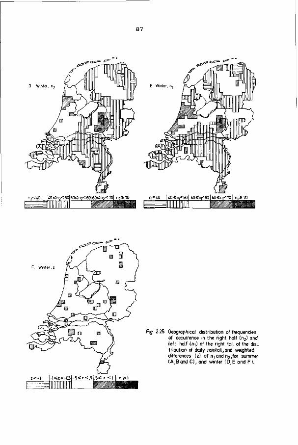
87
£ = "
D Winter, n
*="
F. Winter, z
Fig. 2.25 Geographical distribution of frequencies of occurrence in the right half (n2) and left half (rt)) of the right tail of the dis. tribution of daily rainfall,and weighted differences (2) of nj and n2,for summer (A,Band C), and winter (D,E and F).

3. STATISTICAL AREAL REDUCTION FACTOR ARF
3.1. INTRODUCTION
In this chapter variability in space of hourly and daily rainfall
is considered over a length scale of up to, say, 50 km. This length
scale differs from that considered in Chapter 2, in which the dis
tribution of rainfall over the whole of the Netherlands was con
sidered. In this chapter discussion is confined to space varia
bility in rainfall within periods of one hour and of one day by
studying the quotient of the mean areal rainfall with a given low
exceedance probability and the point rainfall with the same ex-
ceedance probability. This quotient is called the statistical areal
reduction factor (ARF).
The statistical ARF is a function of the size of the area A, the
duration D of the time increment of rainfall recording and the re
currence time T
ARF(A,D,T) = xA(D,T)/xs(D,T), (3.1)
where
x (D,T): the rainfall amount at point S for duration D
and with recurrence time T
x (D,T): the areal rainfall amount, being the mean of
x_(D,T) over all points S of a region V with
area A.
The recurrence time T is defined by a quantile x with F(x )=p as
T = ïTïèry = ïV (3-2)
where F(x) is the cdf of x- Obviously, ARF will decrease as A and
T increase and as D decreases. In this study, A and T in Equation
3.1 are dropped; in some cases D will remain as a suffix to ARF.
Thus, ARF.. and ARF„. are hourly and daily values respectively.

89
Although for very low recurrence times, ARF will exceed one (Nguyen
et al., 1981), ARF is usually less than one. Design dimensions of
drainage networks serving large areas can be reduced, if a critical
point rainfall is used as an input to the design. A critical rain
fall is a rainfall event of a certain duration, exceeded by a given
frequency. In general, a reduction in design because of the size
of the drainage area cannot be made only on the basis of variabili
ty in time and space of rainfall. Certain geomorphological and land
use characteristics of the drainage area and of the orientation of
the catchment with respect to prevailing winds must also be con
sidered. In design of drainage networks, the following procedures
are often used with respect to areal reduction.
Rural drainage in the Netherlands
In the Netherlands with its flat topography, the waterways draining
the polders are dimensioned in such a way that excesses of water
will have a low and predetermined frequency of occurrence. For rural
areas, the first stage in the drainage process is the flow of
groundwater towards the ditches surrounding small parcels of land.
This flow is assumed to be constant, given a minimum allowable depth
of the groundwater table. Under the assumption of stationary flow,
critical flows have been determined for given depths of the ground
water table and for various land uses and soil types, critical flow
meaning such a flow that an excess of it is undesirable. The as
sumption of stationary flow is probably not only adopted because
of its simplicity, but also because winter rainfall is used in the
design of rural drainage. Winter rainfall is to a large extent
caused by the passage of fronts, which leads to rainfall of long
duration. For arable land, an acceptable critical flow is 3 -1 -2 0.08 m .s .km given a minimum depth of groundwater table of
0.50 m; for pasture land, the same flow is considered acceptable
but a minimum depth of groundwater table of 0.30 m is assumed (Werk
groep Afvoerberekeningen, 1979). These are empirical values, how
ever, corresponding to a daily rainfall of about 7 mm. As waterways
should be able to convey the upstream flow, given certain allowable
exceedances of the polder level, the dimensions of the waterways
in all parts of the network can be determined. Thus critical rain
fall is not used directly in the design of rural drainage. As a

90
consequence, reductions because of areal size are empirically veri
fied reductions of the discharge to be conveyed by the drainage
network. For example, an equation for the reduction factor f of
the discharge if areal size exceeds 10 000 ha is (Cultuurtechnische
Vereniging, 1971)
f = 1.60-0.1510log A, (3.3)
where
A: areal size (ha).
This purely empirical approach, which does not take into account
the dynamic character of the runoff process, seems to satisfy re
quirements in the flat parts of the Netherlands where storage in
groundwater and surface water tends to suppress short-period fluc
tuations in discharge. The design of drainage systems in glass-
covered horticultural and in sloping rural areas, however, requires
a non-stationary approach in which the actual input of areal preci
pitation should be considered.
Urban drainage in the Netherlands
In the design of urban drainage, a critical depth of rainfall is
often used, and also a certain storm profile is assumed. Finally,
the capacity of the drainage network to convey flow from the up
stream area must be checked. A reduction in the rainfall input
because of areal size is not applied. However, for larger areas
such a reduction could be applied by multiplying the critical
rainfall depth by ARF.
In this chapter the following issues are dealt with:
In Section 3.2 prediction of areal rainfall by means of kriging
is discussed, in particular whether the IRF-0 theory is adequate
for making kriging predictions of areal rainfall, and whether
different predictors of areal rainfall produce different results.

91
In Section 3.3, ARF_. is estimated by various methods for each 2 of three areas of about 1000 km in the Netherlands (Figure 3.1).
Several estimators of ARF have been proposed, based on annual
maxima series of both point and areal rainfall (e.g., USWB, 1957-
1960; and NERC, 1975, Vol. 2); on POT series of both point and
areal rainfall (e.g.. Bell, 1976); and on the marginal distribu
tion of point rainfall (e.g., Roche, 1963; Rodriquez-Iturbe and
Mejia, 1974; Buishand, 1977b and c). The estimates by these
three methods are compared, and also with earlier estimates of
ARF„4 for the Netherlands (Kraijenhoff, 1963; Buishand, 1977c).
In Section 3.3, attention is also paid to the dependence of ARF
on location, on season, and on exceedance frequency of rainfall,
particularly whether the three areas in the Netherlands vary
with regard to ARF„., and whether these estimates of ARF_ differ Z4 £.**
from those for other countries; whether ARF0„ differs between
seasons, and whether annual maxima of both point and areal rain
fall occur in the same season; and whether ARF depends on fre
quency of exceedance.
Section 3.4 deals with the dependence of ARF on duration of rain
fall and on areal size, and in particular whether estimates of
ARF1 for the Netherlands differ from those for other countries;
and whether ARF calculated from the marginal distributions of
rainfall varies with duration of rainfall at fixed return period
and areal size.
In Section 3.5, a variable related to ARF, the storm-centred
areal reduction factor SRF, is discussed. This reduction factor
SRF is defined as
SRF = x./x , (3.4) A' max v '
where
x : local maximum point rainfall over a certain time max r
period (e.g., one specific day)

92
x : simultaneous areal rainfall over area A bounded by
an isohyet.
The relationship between ARF and SRF is discussed.
The rainfall series used concerning the 29-year period 1951-1979
are given in Appendix B.l and the location of the rainfall stations
is shown in Figure 3.1.
3.2. PREDICTION OF AREAL RAINFALL
Most estimators of ARF require information on mean areal rainfall.
Areal rainfall may be predicted from the arithmetic mean of point
samples provided that these are approximately evenly distributed
throughout the area, and there are no orographic effects (Buishand
and Velds, 1980). Other predictors of areal rainfall include:
the isohyet method;
the Thiessen method;
an extension of the method of optimum interpolation (De Bruin,
1975);
the Kalman filter method (Bras and Colon, 1978);
- the kriging method (e.g., Journel and Huijbregts, 1978).
The kriging method, the optimum interpolation method, and the
Kalman filter method result in best linear unbiased predictors
(BLUP), where 'best' is used in the sense that prediction variances
are minimized (see Section 2.4.1). As the kriging predictor requires
only a minimum set of assumptions (most notably the variance of
the regionalized variable Z(u) need not exist), discussion in this
section is confined to the kriging predictor.
The adequacy of the IRF-0 theory for obtaining a kriging prediction
of areal rainfall, is discussed in Section 3.2.1 and in Section
3.2.2 the kriging predictor is compared with the commonly used
arithmetic mean predictor and the Thiessen predictor.
Throughout this section only daily rainfall series are used, as
there is insufficient hourly rainfall data for the Hupsel catch
ment area to obtain reliable estimates of the semi-variances or

93
generalized covariances. Discussion is restricted to monthly maxima
of daily rainfall, occurring on days with maximum arithmetic mean
of the available point samples.
3.2.1. The order k and the estimation of the semi-variogram
It has been assumed in the present application that the regionalized
variable 2(u) is stationary in the mean. The mean summer and winter
daily rainfall at each rainfall station in the three areas consid
ered (Figure 3.1) on days with a monthly maximum of areal rainfall
are given in Figure 3.2; the respective areas are approximated by
rectangles. As no clearly defined drift is shown, an IRF-0 model
seems to be adequate.
For area 1, for each of the 29 available January and August rain
fall maxima, the order k has been determined with the computer pro
gramme AKRIP (Kafritsas and Bras, 1981) for IRF-k point and block
kriging. As suggested by Delfiner (1976), in AKRIP the order k is
determined by kriging the data points, on the assumption that in
turn k = 0, 1, and using for both values of k the same neighbouring
points for the kriging of a data point and the same generalized co-
variance function: K(h) = -h. In this chapter only intrinsic random
functions of order one or zero are considered, because 12 data
points are insufficient for the identification of higher order
random functions. The order that results in the smallest kriging
error at a data point should be given the grade 1, and the other
the grade 2. The grades of both orders should be averaged over all
points kriged and the order with the smallest average grade should
be chosen.
Quite contrary to what is generally accepted, in a substantial num
ber of cases, the order k was estimated to be one (see Table 3.1).
The estimate of the order k depends to some extent on the number
of neighbouring data points used to krige each data point separately
(see also Table 3.1). The kriging algorithm was applied to each
data point, with all the remaining points as its neighbourhood.

94
Table 3.1. Number of years (29 in total) with order k for rainfall
maxima in January and August (area 1), determined by the computer
programme AKRIP (Kafritsas and Bras, 1981)
Number of neighbouring Order k
January:
August :
11 (all)
6
11 (all)
6
12
19
14
14
points k = 0 k = 1 ex aequo
12 5 7 3
7 8
9 6
When the grades are equal the coefficients C, o1( and a3
of the polynomial generalized covariance functions
K(h ) = Cô+cfjh (C>_0, a i < 0 ) ( 3 . 5 a )
and
K (h ) = Cô+cf jh+aah 3 , (C>0, or i<0, or3>0) ( 3 . 5 b )
for order k = 0 and 1, respectively, have to be determined. Because
it is possible to equate one or more of the coefficients in Equation
3.5a and Equation 3.5b to zero, the resulting number of possible
choices for K(h) is three and seven, respectively. Given the order
k, AKRIP creates generalized increments by kriging a data point T,
using a generalized covariance function that is appropriate to any
order k: K(h) = -h. The resulting kriging error can be directly ob-2 served; denote its square for data point T to be kriged by s,. .
The theoretical prediction variance, av = X.1-k.\.K(u.-u.) is A, T 1 J 1 J 1 J
obtained by using the desired, more specific generalized covariance
function according to Equation 3.5a or Equation 3.5b.
On repeating the procedure for several data points, the sum of
squares Q may be obtained of the differences between the squared 2 2 kriging errors sT;r and the theoretical prediction variances av K , X n., I

95
The coefficients of K(h) can then be obtained by regression. The
results can be used to create new generalized increments and to
find new sets of coefficients (for each permissible model of K(h)),
and so on, until the coefficients stabilize. From the generalized
covariances thus determined, the one is selected that has the ratio
r = T 2*'T (3.7)
V K,t
closest to unity. This provides the ultimate choice of k, in case
of equal grades: for each k the selected generalized covariance
function is used to redetermine the grades. Because of Equation
2.36, the ratio r is always equal to one, if k=0 and K(h)=C6. Thus,
the procedure should be used cautiously, as K(h)=C6 is often se
lected incorrectly, especially for August maxima. Therefore, where
these grades were equal, the structure identification part of the
programme was rerun, using as generalized covariance functions both
K(h)=C6 and K(h)=-h. The final result was that k was equal to zero
in 15 and 18 out of 29 cases for January and for August, respec
tively.
In the following, it is assumed that k is equal to zero. This is
also in accordance with the work of Chua and Bras (1980), who for 2
a plain area of 550 km in the USA, assumed the IRF-0 theory to be
adequate to predict daily areal rainfall from 10 point samples. In
8 out of the 9 cases studied, this was also the case for a moun-2 tainous area of 4400 km , ranging in height from 2350 to 3660 m,
and sampled at 21 to 29 points. Moreover, the structure identifi
cation in the IRF-k theory proceeds iteratively. Therefore, this
theory is not particularly suitable for the routine calculations
of mean areal rainfall, involved in the calculation of ARF.
Further arguments in favour of the IRF-0 theory are provided by
the sample semi-variograms as estimated by the multi-realization
approach; these semi-variograms increase roughly linearly with
the distance h (Figures 3.3, 3.4, and 3.5). It is known that

96
the IRF-0 theory is valid, for a regionalized variable Z(u) having
a linear semi-variogram (Section 2.4.1). To the sample semi-
variograms, linear population semi-variograms y(h) have been fitted
according to Equation 2.26a
Y(h) = CO+öih, (3.8)
where
C, c^: non-negative coefficients
ô : 0 (h=0) or 1 (h*0).
In the single-realization approach, as opposed to the multi-
realization approach, for each event (monthly rainfall maximum in
this case) separately, a sample semi-variogram is estimated ac
cording to Equation 2.25. To this a population semi-variogram y(h)
is fitted, which is used in the prediction of areal rainfall for
that particular event. In the multi-realization approach, as applied
here, monthly maxima for all years of record and one particular
month are grouped together, and a mean sample semi-variogram is
estimated. Subsequently, a function y(h) is fitted, which is used
in the prediction of areal rainfall for all maxima within the group.
An argument in favour of the multi-realization approach is that it
does not seem unreasonable to group monthly maxima for one partic
ular month of the year together for all years of record. In addi
tion, the use of the multi-realization approach is almost unavoid
able, because there are not enough sample points available to esti
mate the semi-variogram for each event separately. Using the well-
known property (Kendall and Stuart, 1977; p. 258) of the variance 2 estimator s
var s2 s 2a4/n, (3.9)
where n is the number of samples, it follows that N(h) in Equation
2.25 should exceed 40, for the squared coefficient of variation of
the estimator y(h) to be less than 5%. However, the use of Equation
3.9 is rather restrictive. The regionalized variable Z(u) is assumed
to be independent and normally distributed, and second order sta-
97
tionary. Furthermore, the one realization z(u) which is sampled is
thought of as to constitute the whole population, if only sampled
exhaustively. This, in fact, is contrary to the concept of a sto
chastic function Z(u).
Similarly, Gandin (1965) presented the required minimum number of
sample points to obtain a given accuracy, by considering the nor
malized semi-variogram g(h)
g(h) - Y(h)/a2, (3.10)
2 where a is the point variance var[z(u)]. With a second order stationary z(u), the variance of the estimator c[(n) equals
vartâ(h)] =var[r(h)], (3.11)
where r(h) is the estimate of the correlation coefficient p(h) at
distance h. With normally distributed variables, this variance is
approximately (Kendall and Stuart, 1977; p. 258)
var[r(h)] = H ^ I M J - . (3.12)
By using Equation 3.11 and Equation 3.12, N(h) can be presented as
a function of var[â(h)] and of g(h), and from Equation 3.12 it can
be seen that N(h) increases with h.
With 12 sample points, there are 66 data pairs. As indicated by
the semi-variograms, the realizations z(u) are not second order
stationary, but intrinsic only. Thus clearly, a single-realization
approach would not permit reliable estimation of the semi-variogram.
This, in fact, is a further argument in favour of using the IRF-0
theory, because the present IRF-k algorithms have been developed
for the single-realization approach. Chua and Bras (1980) also con
cluded that a multi-realization approach was necessary. For the
plain area they analysed, in about half of the 35 events, the
single-realization approach did not permit detection of the semi-
variogram structure. For the remaining events, the single-
realization semi-variograms were either spherical (ten events) or

98
linear (seven events). For one event both a spherical and a linear
semi-variogram seemed to fit, and six events showed a nugget effect.
The sample semi-variograms for monthly rainfall maxima stratified
according to month are presented in Figures 3.3, 3.4, and 3.5.
These have been calculated by using Equation 2.25 but adapted to
the multi-realization approach, which means averaging over the
29 years of record
, 2 9 29 N(h)
V(h) = sl.Z^.Ch) = 2 5 ^ 2 5 1 ^ [z<V-z(ui+h)]2, (3-13)
where
Y-(h): single-realization sample semi-variogram for monthly
maximum in year j.
Distance classes of 5 km up to 35 km have been considered. For area
1 in Figure 3.1, the sample standard deviations of the values of
the single-realization sample semi-variograms which were averaged,
are presented in Figure 3.3. It has been verified whether less va
riation between the single-realization sample semi-variograms for
each particular month may result from further classification of
monthly maxima according to rainfall depth, because it is known
that with increasing areal rainfall the coefficient of variation
decreases. This is confirmed by the results presented in Figure 3.6,
in which the coefficient of variation is the ratio of the sample
estimate of the standard deviation of point rainfall, and the es
timated mean areal rainfall (equal to the arithmetic mean of the
point rainfalls).
Two classifications according to rainfall depth have been attempted:
one on the basis of mean areal rainfall in exceedance of 15 mm or
not; and the other on the basis of maximum point rainfall in ex
ceedance of 20 mm or not (thus placing more emphasis on 'spottiness'
of rainfall). However, these classifications did not result in any
noteworthy reduction in variation between the single-realization
•y.(h) to be averaged, and did not result in different limiting
behaviour of the semi-variograms with regard to distance.
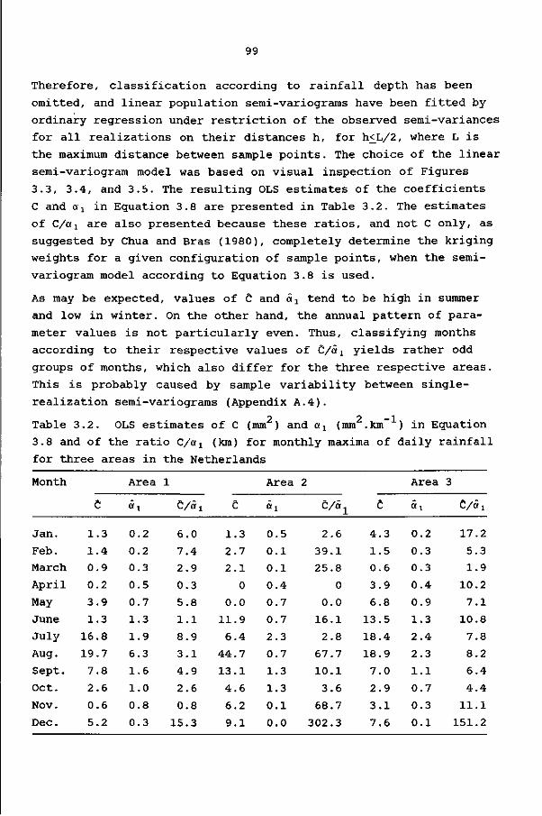
99
Therefore, classification according to rainfall depth has been
omitted, and linear population semi-variograms have been fitted by
ordinary regression under restriction of the observed semi-variances
for all realizations on their distances h, for h<L/2, where L is
the maximum distance between sample points. The choice of the linear
semi-variogram model was based on visual inspection of Figures
3.3, 3.4, and 3.5. The resulting OLS estimates of the coefficients
C and dj in Equation 3.8 are presented in Table 3.2. The estimates
of C/Oi are also presented because these ratios, and not C only, as
suggested by Chua and Bras (1980), completely determine the kriging
weights for a given configuration of sample points, when the semi-
variogram model according to Equation 3.8 is used.
As may be expected, values of C and âj tend to be high in summer
and low in winter. On the other hand, the annual pattern of para
meter values is not particularly even. Thus, classifying months
according to their respective values of C/â1 yields rather odd
groups of months, which also differ for the three respective areas.
This is probably caused by sample variability between single-
realization semi-variograms (Appendix A.4).
2 2 -1 .
Table 3.2. OLS estimates of C (mm ) and «j (mm .km ) in Equation
3.8 and of the ratio C/ofj (km) for monthly maxima of daily rainfall
for three areas in the Netherlands Month
Jan.
Feb.
March
April
May
June
July
Aug.
Sept.
Oct.
Nov.
Dec.
C
1.3
1.4
0.9
0.2
3.9
1.3
16.8
19.7
7.8
2.6
0.6
5.2
Area
« i
0.2
0.2
0.3
0.5
0.7
1.3
1.9
6.3
1.6
1.0
0.8
0.3
1
e / â j
6.0
7.4
2.9
0.3
5.8
1.1
8.9
3.1
4.9
2.6
0.8
15.3
C
1.3
2.7
2.1
0
0.0
11.9
6.4
44.7
13.1
4.6
6.2
9.1
Area
«i
0.5
0.1
0.1
0.4
0.7
0.7
2.3
0.7
1.3
1.3
0.1
0.0
2
c/â1
2.6
39.1
25.8
0
0.0
16.1
2.8
67.7
10.1
3.6
68.7
302.3
C
4.3
1.5
0.6
3.9
6.8
13.5
18.4
18.9
7.0
2.9
3.1
7.6
Area
«i
0.2
0.3
0.3
0.4
0.9
1.3
2.4
2.3
1.1
0.7
0.3
0.1
3
e/«!
17.2
5.3
1.9
10.2
7.1
10.8
7.8
8.2
6.4
4.4
11.1
151.2

100
It is unlikely that these differences have been caused by anisotro-
py. For the Netherlands, anisotropy of the correlation function
p(h) for 10-day and monthly rainfall has been demonstrated by Buis-
hand and Velds (1980). For the relatively small areas considered
here, anisotropy of the semi-variograms for daily rainfall is not
expected. Stol (1972), investigating p(h) for daily rainfall in an 2 area of about 2000 km found no indications for anisotropy.
Further, it is unlikely that differences between areas have been
caused by differences in the quality of the measurements. Well-
scrutinized measurements from the Royal Netherlands Meteorological
Institute (KNMI) obtained by means of one type of daily rainfall
measuring device only have been used. Differences in quality of
measurements will lead to systematic differences in estimated semi-
variograms for each area, as demonstrated by Gandin (1965). Con
sider, for example, a random error e, according to
If = h+^i' (3.14)
where
f* : measured rainfall at station i
f. : actual rainfall at station i
e. : random measurement and observational error with ex-2 pectation zero and variance a at station l.
Assume also that the errors are uncorrelated with actual rainfall,
and uncorrelated with random errors at other stations, then such 2
errors lead to an increase in the nugget effect by a .
If only systematic measurement and observational errors occur, ac
cording to
f* = ß ^ , (3.15)

101
where
ß- : factor, indicating the systematic error at station i,
and if ß± = ß^ = ß, then E[y*(h)] = ßy(h).
Thus errors according to Equation 3.14 and Equation 3.15 would lead
to systematic differences between the estimates of C and «j in Equa
tion 3.8 for different areas. Such systematic differences do not
seem to be apparent in Table 3.2, although C values for area 1 are
rather low, and âx values for area 2 are low. These, however, seem
to be caused by a pattern of sample points in area 1 relatively
well suited to the estimation of C, and by the effect of wide tidal
inlets in area 2.
Another physical cause of differences between the three areas, which
is reflected to some degree in Table 3.2, is the relatively frequent
occurrence of convective rainfall during summer in the east and
south-east of the Netherlands, as a result of high surface tempera
tures. Along the coast, convective rainfall is suppressed during
spring and early summer, because of relatively low sea temperatures.
During autumn, however, the relatively warm sea enhances the devel
opment of showers along the coast (Buishand and Velds, 1980).
Thus, it cannot be conclusively stated that the IRF-0 theory is
adequate to predict areal rainfall. As reported by Delhomme (1978)
and by Chua and Bras (1980), the IRF-0 theory seems to be adequate
to predict areal rainfall over climatologically homogeneous areas.
Yet the results of this study are not in accordance with this.
Apparently, the issue of structure identification requires further
investigation, both statistical and physical. As k was set at zero,
calculations were simple. Contrary to the IRF-k theory, where esti
mation of the generalized covariance is carried out for each reali
zation separately, the semi-variogram to be used in the IRF-0 theory
can be estimated by the multi-realization approach. As only few
data points were available, a more reliable estimation of the semi-
variogram was possible. On the other hand, variation both between
months and between areas in the semi-variograms in the multi-
realization approach is large.

102
3.2.2. Comparison of the kriging, Thiessen, and arithmetic mean predictors
The mean areal rainfall Z over a region V with area A, where
Z = rj Z(u)du, can be predicted by a linear combination of the
point samples
N z = I X.z(u.), (3.16)
i=l
where
À. : weighting factor
N : total number of sample points u.£V.
The unbiasedness and minimum variance conditions of the prediction
obtained with Equation 3.16 lead to the kriging Equations 2.23
rr\+MlN = r (3.17a)
ll£\ = 1, (3.17b)
where in the present application r' = (7(u1;V),..., y(u ;V)).
Such mean semi-variances y(u.;V), where one of a pair of points
remains fixed at location u., and the other point sweeps V, can be
calculated numerically according to the method proposed by Bras
and Rodriguez-Iturbe (1976). In this method, V is approximated by
a rectangle V', which is then split into four subrectangles by axes
passing through u. and parallel to the sides of V'; then
1 4 Li * ( U i ; V ) A [.* o' * ( h ) f i ( h ) d h J ' (3.18)
where
L. : largest distance in subrectangle i
f.(h): pdf of distance h between the fixed point u. and
a random point in subrectangle i.

103
The single integral in Equation 3.18 can be easily calculated numer
ically.
Here auxiliary functions are used (Journel and Huijbregts, 1978).
These are analytical functions which yield y(u;V) for certain sim
ple geometric forms of the regions u and V, and given a certain
semi-variogram model, for example, linear or exponential. Although
there are several auxiliary functions, in this study, following
the notation of Journel and Huijbregts (1978), use is made of
H(a;b) = Y ( U ; V ) , where V is a rectangle with sides a and b and u
is a point, that is one of V's vertices. The function H(a;b) is
defined as (Journel and Huijbregts, 1978; p. 113)
H(a;b) = f ( a2+b2 )H+|!ln{ »+ < ^ >*} + f î l n ( b + < \ ^ >*} . (3.19)
After approximating V by a rectangle V', V' is split into four sub-
rectangles, and for each of these H(a;b) is calculated. Weighted,
by the area of the corresponding subrectangle, means of these yield
y(u.;V), apart from the nugget effect C in Equation 3.8. Then this
nugget effect, which is a constant value for all sample points in
V, is added to the weighted mean H(a;b) to obtain y(u.;V).
Solving Equations 3.17a and b yields the kriging weights, which
are presented in Appendix B.2 for each of the three areas and for
each month separately. All weights are positive. With all sample
points inside V, negative weights are only to be expected in point
interpolation if shadow effects occur. The kriging weights for
January and for August, and the arithmetic mean weights and Thiessen
weights are presented in Table 3.3.
Kriging weights tend to correlate well with the area of the Thiessen
polygons, especially when the nugget effect c of the semi-variogram
is relatively unimportant. The kriging weights are equal to the
arithmetic mean weights, if &t = 0. Differences in kriging weights
for maxima of daily rainfall in different months are rather small.

104
Table 3.3. Kriging weights for predicting mean areal rainfall for
monthly maxima of daily rainfall for three areas in the Netherlands1
KNMI code no.
223
225
226
229
230
233
435
436
437
438
441
454
Area 1
Kriging Jan.
.0904
.0877
.0750
.0547
.0735
.0807
.0751
.0671
.1143
.1106
.1082
.0628
Aug.
.0833
.0913
.0751
.0514
.0719
.0784
.0689
.0665
.1187
.1176
.1114
.0605
Thies-sen
.0345
.1171
.0790
.0458
.0786
.0950
.0616
.0228
.1162
.1406
.1453
.0636
KNMI code no.
733
736
743
746
749
751
752
754
755
756
758
760
Area
Krig Jan.
.0477
.0709
.0623
.1064
.0763
.1515
.1821
.0376
.0979
.0658
.0624
.0391
2
ing Aug.
.0714
.0909
.0820
.0972
.0737
.1054
.1160
.0596
.0838
.0807
.0751
.0642
Thies-sen
.0537
.0471
.0604
.0684
.0834
.1750
.1987
.0386
.1054
.0652
.0578
.0464
KNMI code no.
542
543
558
564
565
567
570
571
573
578
579
580
Area
Krig Jan.
.0826
.0934
.0739
.0904
.0623
.0983
.1051
.0933
.0947
.0955
.0581
.0524
3
ing Aug.
.0842
.0907
.0766
.0897
.0573
.1011
.1119
.0988
.0936
.1000
.0522
.0438
Thies-sen
.1036
.0804
.0959
.0634
.0480
.0937
.1478
.1065
.0840
.1166
.0361
.0241
1 Arithmetic mean weights would be 0.0833 regardless of month or
area.
Mean areal rainfall predicted by each of the three methods can be
compared by evaluating their prediction variances. When predicting
mean values over an area, the prediction variance equals
N N N a; = 2 I Y ( U . ; V ) - Y ( V ; V ) - 2 1 A,À,Y(u.-u.
E i=l X i=l j=l 1 J X : (3.20)
In comparing Equation 3.20 with Equation 2.22, it should be noted
that for a point V, Y(V;V) vanishes. The resulting minimum variance 2 a of the kriging prediction equals (see Equation 2.24)
at = 1 AHY(u.;V)+M-Y(V;V), K i=l 1 1
(3.21)

105
or in matrix notation, following Corsten (1982)
a£ = -ï(V;V)+rT"1r-(l-l^r"1r)(l^r"1lN)"1(l-l^r"1r), (3.22)
where (as in Equation 2.33) the last term is closely related to
the variance of the estimate of the stationary expectation E[Z ],
and the sum of the remaining terms on the right-hand side is an
estimate of the residual variance of Z with regard to the best
linear approximation. Note that r in Equation 3.22 is r from Equa
tion 3.17: r=v(ui;V).
2 2 To calculate a and a , use has been made of Equations 3.20 and 3.22, hi K
respectively. The Y(U.;V) in Equation 3.20, denoted as r in Equation
3.22, have been obtained previously. To calculate Y ( V ; V ) , the auxi
liary function F(a;b) has been used (Journel and Huijbregts, 1978;
p. 113)
w = K! - /=2J.,2,V 1 1 a2 1 b 2 l.a3 b 3 , . F(a;b) - (a +b ) (rîf -j-j^ ^ ^ - J * ^ ) +
b a b a
2 2 + | |-ln{(b+(a2+b2)1'5)/a}+| |-ln{ (a+(a2+b2)**)/b} . (3.23)
The results are presented in Table 3.4. In most cases the Thiessen 2 2 . mean prediction variance a_ _ is less than a_ ., the arithmetic hj, x hi, A
mean prediction variance. The arithmetic mean can be a very ineffi
cient predictor, if a region is characterized by a few very large
Thiessen polygons. If, however, there is virtually no spatial coher
ence (high values of C/ä1 in Table 3.2), then areal rainfall is
more efficiently predicted by the arithmetic mean than by the Thies
sen method.

106
2 2 Table 3.4. Prediction variances o_ (mm ) and efficiencies (%) with respect to the minimum 2 variance oK for three predictors of areal mean values for monthly maxima of daily rainfall
for three areas in the Netherlands
Month
Jan.
Feb.
March
April
May
June
July
Aug.
Sept.
Oct.
Nov.
Dec.
Arithmetic
mean
2 °E,A
0.27
0.25
0.29
0.40
0.81
1.02
2.7S
6.21
1.79
0.92
0.65
0.68
eff.
87
89
82
75
87
77
90
83
86
82
76
94
Area 1
Thiessen
2 °E,T
0.27
0.25
0.27
0.34
0.81
0.90
2.84
5.85
1.76
0.85
0.57
0.73
eff
87
87
88
87
87
87
87
88
88
88
87
87
Kriging
4 0.23
0.22
0.23
0.30
0.71
0.79
2.48
5.13
1.54
0.75
0.50
0.63
Arithmetic
mean
2 °E,A
0.83
0.33
0.30
0.65
1.00
2.08
3.85
4.69
2.99
2.26
0.65
0.79
eff.
49
90
83
37
37
76
49
95
68
52
95
100
Area 2
Thiessen
2 °E,T
0.43
0.35
0.28
0.26
0.39
1.77
2.03
5.42
2.23
1.26
0.75
1.04
eff
94
85
88
93
93
90
94
82
92
94
82
76
Kriging
2 °K
0.40
0.30
0.25
0.24
0.37
1.59
1.90
4.45
2.04
1.18
0.62
0.79
Arithmetic
mean
2 °E,A
0.53
0.31
0.27
0.58
1.20
1.98
3.14
3.15
1.32
0.69
0.45
0.66
eff.
89
75
64
83
79
84
80
80
77
72
84
99
Area 3
Thiessen
2 aE,T
0.51
0.25
0.18
0.51
1.00
1.77
2.65
2.69
1.07
0.52
0.40
0.75
eff
92
95
97
94
95
94
94
94
95
96
94
88
Kriging
2 °K
0.47
0.23
0.17
0.48
0.95
1.66
2.51
2.53
1.02
0.50
0.38
0.66
Denote the kriging prediction of mean areal rainfall for a maximum
in month i and year j by x ~K 1,3
T A and let x. . and x. .be the Thiessen
1,3 i,3 and arithmetic mean predictions, respectively. The latter two pre
dictions have been compared with the kriging predictions by calcu
lating differences V. . according to
V. . i,3
-K -T x. .-x. . ,
i,3 1,3 (3.24a)
1,3 „K -A x . .-x .
1,3 1,3 (3.24b)
respectively. The mean V. = I.V. ./n, where n is the number of years
of record gives an indication of possible systematic differences
between kriging predictions and the Thiessen and arithmetic mean
predictions. The relative magnitude of such differences may be ob
tained from, for example
= M.' K. .-X. . /X. . } , 1,3 1,3 1,3
(3.25)

107
where
n: number of years of record (n=29).
The results are presented in Table 3.5.
Table 3.5. Absolute differences V. (mm) and relative differences
V! (%) between kriging predictions of mean monthly maximum rain
fall, and Thiessen and arithmetic mean predictions for three areas
in the Netherlands
Month
Jan.
Feb.
March
April
May
June
July
Aug.
Sept.
Oct.
Nov.
Dec.
Area 1
Thiessen Arithmetic
V i .
-0.34
-0.58
-1.13
-0.24
-0.45
0.66
-1.90
-3.10
-0.34
-0.57
-1.59
-0.60
V!
1.21
1.38
1.28
1.28
1.89
1.57
2.39
2.54
1.89
2.19
1.32
1.14
mean
V. l .
0.70
0.74
0.67
0.74
0.88
2.46
1.21
3.95
1.00
0.49
-0.59
1.10
V! l.
1.14
1.10
1.81
1.67
1.58
2.33
2.94
3.99
2.18
1.85
1.22
1.06
Area 2
Thiessen Arithmetic
V. l .
0.21
-0.54
-0.68
-0.15
-0.17
-0.58
-0.29
-0.46
0.98
-0.42
-1.32
-0.46
V! l.
0.97
1.53
1.54
0.76
1.51
2.15
1.56
3.53
1.66
1.27
2.20
2.93
mean
V i .
0.68
-0.31
-0.02
1.93
1.78
-2.04
-3.21
-1.25
-1.20
-2.06
0.35
-0.04
V! l.
3.03
1.98
1.90
5.29
7.41
4.54
7.80
3.03
4.00
4.82
1.20
0.45
Area 3
Thiessen Arithmetic
V i .
-0.26
-0.52
-0.32
-0.95
-2.10
-0.08
-1.12
0.10
-0.02
-0.32
-0.76
-1.52
V! l.
0.85
0.85
0.68
1.66
1.76
1.78
2.10
1.58
0.78
1.26
0.92
1.59
mean
V. l.
0.88
0.83
1.61
1.17
2.86
-1.48
-1.21
2.58
1.10
1.39
0.96
0.61
V! 1 .
1.09
1.49
1.91
2.39
2.89
2.08
2.26
2.89
1.95
2.02
1.13
0.51
Thus, as reported earlier by Delhomme (1978), the differences
between kriging and Thiessen predictions of areal rainfall are
rather small. Results of the arithmetic mean predictor are less
satisfactory. In the present application, the Thiessen predictions
tend to be higher than the respective kriging predictions, and the
arithmetic mean predictions tend to be lower.
Although in general the kriging predictions do not differ greatly
from the Thiessen and arithmetic mean predictions (Table 3.5),
the efficiency of the other two predictors can be quite low. In

108
August, when prediction variances are highest, the efficiency of
the Thiessen predictor is 0.88, 0.82, and 0.94 for areas 1, 2, and
3, respectively; and for the arithmetic mean predictor 0.83, 0.95,
and 0.80 for areas 1, 2, and 3, respectively. The efficiency of the
Thiessen predictor does not vary very much for the three areas, but
that of the arithmetic mean predictor does.
3.3. ARF FOR DAILY RAINFALL AND ITS DEPENDENCE ON LOCATION,
SEASON, AND RETURN PERIOD
In Section 3.3.1, methods to estimate ARF are presented and esti
mates of ARF for three areas in the Netherlands are presented in
Section 3.3.2. Finally, in Section 3.3.3 the variance of ARF24 is
estimated, in order to determine whether the various methods for
estimating ARF produce different estimates of ARF-.. This variance
is also used in the discussion on the dependence of ARF on certain
factors.
As defined by Equation 3.1, ARF is
ARF(A,D,T) = XA(D,T)/XS(D,T),
implying that ARF is at least a function of duration of rainfall
D, of return period T, and of areal size A. Other factors likely
to effect ARF are location, season, and storm type. In this discus
sion D is fixed at 24-hour intervals where observations were taken
only at specified times, at 7.55 h UTC daily. Thus, attention is
restricted to location, season, and return period, although the
results also indicate that there is a decrease in ARF with areal
size.
The degree to which ARF depends on location is not certain. On the
one hand, ARF values as determined for the United Kingdom (NERC,
1975; Vol. 2) have been recommended for use in countries as far
apart as the Netherlands (Buishand and Velds, 1980) and New Zealand
(Tomlinson, 1980); and values determined for the USA (USWB, 1957-
1960) have been recommended for use in Australia (Pattison (ed.),
1977). On the other hand, Bell (1976) has concluded that for the

109
United Kingdom, there may be a slight tendency for ARF„4 to increase
with latitude. For the USA, Myers and Zehr (1980) suggest that
ARF is dependent on location. Thus it would seem that there are
substantial differences in ARF_. values for very distinct climatol-
ogical regions. This is supported by the comparatively low values
of ARF_4 for several tropical African countries reported by Vuil-
laume (1974). The dependence of ARF24 on location is considered
in Section 3.3.3 particularly with reference to three areas in
the Netherlands of approximately equal areal size. Estimates of
ARF„. are compared with those for other countries.
The dependence of ARF on season has received little attention. From
the effect of climate on ARF already mentioned, it may be inferred
that there is a seasonal effect on ARF_„. In this section considèrent ation is given to whether ARF„. varies with season and whether annu-
al maxima of both point and areal rainfall occur in the same season.
The effect of return period on ARF has been investigated by Bell
(1976), using data for the United Kingdom. In Bell's study, which
was a follow-up to NERC (1975) in which it was assumed that the
dependence of ARF on return period was of no practical value, evi
dence was found for a decrease in ARF with return period. Therefore,
in the present study it was decided to investigate the dependence
of ARF on frequency of exceedance.
3.3.1. Methods to estimate ARF
In this section, methods to estimate ARF are discussed which are
based on annual maxima series of both point and areal rainfall, on
POT series of both point and areal rainfall, and on the marginal
distribution of point rainfall, respectively. Methods used to esti
mate ARF in previous studies in the Netherlands are also discussed.
a. Estimation of ARF from annual maxima series
Two methods to estimate ARF from annual maxima series are described,
the USWB (1957-1960) and the NERC (1975) method. Neither method
uses the complete probability distributions of annual maxima, but

110
only their expectations and, consequently, the exceedance proba
bilities of the expectations. If, for instance the annual maxima
follow a Gumbel distribution, then the ARF values correspond to a
2.33-year return period. In the following discussion on both meth
ods, N is the total number of rainfall stations in a region, and n
is the length of the period of record (year).
In the first of these methods (USWB, 1957-1960), the maximum value
x (j) in year j of mean areal rainfall of a given duration is de
termined. The mean of the annual maxima of areal rainfall is denoted
by x . For all rainfall stations i (i=l,..., N), the maximum value
x j(j) in year j of point rainfall of this duration is determined. b , X
The mean of the annual maxima of point rainfall at location i is
denoted by x .. The areal mean of the annual maxima of point rain-b , X
fall is calculated as
N x = I x ,/N.
b- i=i S'1
Thus, ARF is estimated as
ARF = xA/xs .
In the second method (NERC, 1975), for each year j, the maximum
value x (j) of areal rainfall of a given duration is determined,
and for all rainfall stations the simultaneous point rainfall is
denoted by x' j(j) (i=l,..., N). For all rainfall stations i the b , 1
maximum value x -(j) in year j of point rainfall of this dura-b , X
tion is determined. For each pair (i,j) the following ratio is cal
culated
g(i, j) = xs;i(i)AS)i(i).
Thus, ARF is estimated as
N n ARF = I I q(i,j)/(nN)
i=l j=l

Ill
b. Estimation of ARF from peaks-over-threshold (POT) series
Bell (1976) used the following method to estimate ARF from POT se
ries. The frequency curves (rainfall versus return period) of peaks
of point rainfall of a given duration for each rainfall station
are determined. The point rainfall frequency curve is then derived
by averaging these curves. Also, the areal rainfall frequency curve
for this duration of rainfall is determined. The estimate of ARF
for a given return period is the ratio of the ordinates of the areal
and point rainfall frequency curve, respectively, corresponding to
that return period. This method makes full use of the probability
distribution of peaks.
c. Estimation of ARF from the marginal distribution of point rain
fall
Estimation of ARF from the marginal distribution of point rainfall
was first suggested by Roche (1963). In contrast to the methods
described above, which require data from relatively dense, rainfall
measuring networks in order to predict areal rainfall, this method
and that of Rodriguez-Iturbe and Mejia (1974), only use point rain
fall at paired sample points. However, Roche's method is rather
complicated and in a subsequent publication Brunet-Moret and Roche
(1966) have proposed another method which makes use of the marginal
distribution of both point and areal rainfall. This method which
has been used by Vuillaume (1974) and Le Barbe (1982), counts the
number of occurrences of pairs of (x ,x„) values in certain classes
of rainfall depth. This leads to a description of the empirical
bivariate (x.,x_) frequency distribution. Adding up over x classes
gives the empirical marginal frequency distribution of areal rain
fall, and adding up over x classes gives the empirical marginal
frequency distribution of point rainfall.
As data sets which permit the calculation of areal rainfall are
usually restricted in record length, but rather long records of
point rainfall are likely to be available, Brunet-Moret and Roche
recommend that the empirical marginal frequency distribution of
point rainfall be corrected as follows. The longest rainfall record

112
available within the region should be used to fit a pdf of point
rainfall according to a certain model, thus permitting the estima
tion of guantiles of point rainfall: x . This pdf should then be b , P
used to replace, for each class of point rainfall depth, the observed
number of point rainfalls with the expected number. As a conse
quence, the number of observed areal rainfalls is also corrected.
Then the number of exceedances of a certain threshold value of x.
can easily be determined by integrating the corrected bivariate
frequency distribution. The number of exceedances of this particu
lar threshold value of x is then transformed into a quantile esti
mate: x . Thus ARF, is estimated as A, p
ARF = x. /x_ A,p' S,p
Another method for estimating ARF that uses essentially the margin
al distribution of point rainfall is that used by Rodriguez-Iturbe
and Mejia (1974), and Buishand (1977b,c). Rainfall at a point with
co-ordinate vector u during period t is denoted by x (u,t).
Rodriguez-Iturbe and Mejia assumed that the point rainfall process 2
{x (u,t)} has expectation u and variance a , and is stationary and o S o
isotropic. The volume of rainfall h(t) over the region V with
area A is
h(t) = JyXgC^tJdu.
Furthermore,
E[h(t)] = MAA (with M A = E[xA]).
Time-space covariance is
cov[h(t),h(t+At)] = E[h(t)h(t+At)]-{E[h(t)]}2
= E[ƒvxs(ux,t)du1Syxs(u2,t+At)du2]-MAA2
= Jv/v{E[xs(u1,t)xs(u2,t+At)]-MA}du1du2.
If At=0,
cov[h(t),h(t)] = var[h(t)] = CJ2 = Jv/v{E[xs(u1( t)xs(u2, t)] -uj^du^d^ .

113
Because the rainfall process is stationary, p_ = pft. Consequently,
CTh = /v^V?E[-S(Ul't)-S(u2't)"|JS5dUldU2
2 = asJvJvr(u1;u2)du1du2, (3.26)
where
r(u ;u ): spatial correlation coefficient between rainfall
at points with co-ordinate vector u.. and u_,
respectively.
Consequently,
and
where
a£ = A2agr(V;V), (3.27)
var[xA] = a2h = o*r(V;V), (3.28)
r(V;V): mean of the correlation coefficient between rain
fall at points, each independently sweeping the
area V.
If the point rainfall process is Gaussian, the areal process will
also be Gaussian, and as implied in Equation 3.28, a reduction fac-
tor equal to [r(V;V)]^ will relate identical return periods. This
reduction factor does not vary with return period.
Unlike Rodriguez-Iturbe and Mejia, Buishand (1977c) assumed that
both point and areal rainfall follow a gamma distribution with ex-2 2
pectation and variance (j„ and a„, and p. and a., respectively, and MA = Ms» (3.29a)
o2A = £a2
s. (3.29b)
Furthermore, instead of f=r(V;V), Buishand (1977c) uses the approxi
mation f=r(E[h]).

114
ARF is estimated by Buishand (1977c) by fitting for each month of
the year, a Gumbel distribution to the monthly maxima series, and
by determining the point rainfall x for the relevant rainfall b , P
duration and return period. Then by using the gamma distribution
fitted to the point rainfalls by the method of moments,
Pr{xs<xSp} (3.30)
is determined. The gamma distribution for areal rainfall, with pa
rameters determined by Equation 3.29a and Equation 3.29b, is used
to find x according to A, p
Pr*XA<*A,p} = Pr*Xsi*S,p>-
Thus, ARF is estimated as
ARF = x. /x„ A,p7 S,p
Buishand's method is used in this study with the following minor
modifications :
use is made of POT series which are assumed tó be exponentially
distributed;
use is made of f = r(V;V), although in this case with a linear
correlation-distance function r(h), both f = r(V;V) and f =
r(E[h]) yield the same result;
application of the ML estimation procedure of the parameters of
the gamma distribution of point rainfalls, as given in Buishand
(1977a).
d. Methods used to estimate ARF in earlier studies in the Netherlands
Statistical areal reduction factors for the Netherlands have been
estimated from daily rainfall data over the 1932-1956 period by
Kraijenhoff (1963). For a group of 30 rainfall stations evenly dis
tributed throughout the Netherlands, areal rainfall has been pre
dicted by the isohyet method for circular areas of 10, 50, 100, 2 250, and 500 km around these stations for summer days with ram-

115
fall in excess of 40 mm at least at one of the stations. For each
areal size considered, areal rainfall was plotted as a function of
the point rainfall of equal ranking on double logarithmic paper.
By the method of least squares, straight lines were fitted (Figure
3.7). Along each line in Figure 3.7, ARF decreases with increasing
rainfall depth, and therefore with increasing return period. This
method is somewhat similar to that of Bell (1976), described ear
lier.
3.3.2. Estimates of ARF„. for three areas of 1000 km2 in the 24
Netherlands
a. ARF„. estimated from annual maximum series 24
For the areas 1, 2, and 3 indicated in Figure 3.1, ARF-. has been
estimated by both the USWB (1957-1960) and the NERC (1975) method,
for the summer, winter, and the complete year. The results are
presented in Table 3.12.
b. ARFn. estimated from POT series
For the areas 1, 2 and 3 indicated in Figure 3.1, POT series have
been extracted from the daily point and areal rainfall records, for
summer, winter, and the complete year. Thresholds have been selected
that resulted on average in two peaks per year or season. In order
to assure independence of the peaks, these have to be separated by
at least one day without rain in the area considered. The mean POT
series of point rainfall for a given area were obtained from the
means of peaks of equal ranking of all records of point rainfall
for that area. Exponential probability distribution functions
according to
f(q) = iexp[-(q-q0)/ß], (3.31)
where

116
qn,ß: positive parameters of location and scale, respec
tively,
were fitted to the POT series of areal rainfall and to the mean
POT series of point rainfall. As in Section 2.2, ML estimates of
ß and gQ in Equation 3.31 were calculated according to Equation 2.2
and 2.3 and the fit of the exponential probability distribution
functions was checked by calculating realizations of the test sta
tistic T according to Equation 2.8. The realizations of T and the
ML estimates ß and q„ are presented in Table 3.6. The exponential
distribution seems to fit the POT series sufficiently well. Plots
of the empirical distribution functions and the fitted distribution
functions are presented in Figure 3.8. The plotting positions are
according to Equation 2.4.
Table 3.6. ML estimates ß (mm) and qn (mm) from Equation 3.31 and
realizations of the test statistic T to assess the fit of the ex
ponential distribution function to POT series of areal and point
rainfall in three areas of the Netherlands
Summer
ß
^0 T
Winter
ß
% T
Year
ß
So T
Areal rain
1
5.8
18.4
119.7
6.2
15.6
87.6°°
6.2
21.2
103.9
Area
2
6.2
17.6
136.0
6.3
15.0
135.7
5.6
21.5
133.9
fall
3
7.9
18.0
95.9
5.2
15.8
94.5
7.9
20.6
100.0
Point rain
1
7.7
19.4
100.5
6.5
16.5
89.4
7.9
22.6
100.3
Area
3
7.8
19.6
109.3
6.9
15.8
105.5
7.3
23.2
106.7
fall
3
10.3
19.3
98.1
5.5
16.6
95.0
9.4
22.6
94.6
Indicates values inside the critical region for a = 0.05.
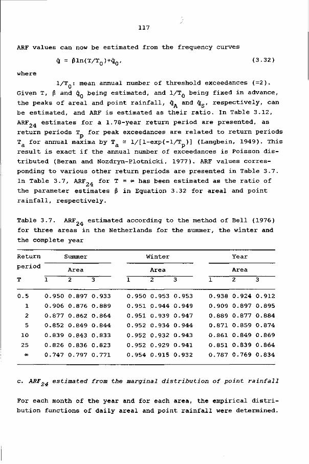
117
ARF values can now be estimated from the frequency curves
q = ßln(T/T0)+q0, (3.32)
where 1/T : mean annual number of threshold exceedances (=2)
Given T, fi and q. being estimated, and 1/T- being fixed in advance,
the peaks of areal and point rainfall, q. and q , respectively, can
be estimated, and ARF is estimated as their ratio. In Table 3.12,
ARF . estimates for a 1.78-year return period are presented, as
return periods T for peak exceedances are related to return periods
T for annual maxima by T s l/[l-exp(-1/T )] (Langbein, 1949). This ci cl p
result is exact if the annual number of exceedances is Poisson dis
tributed (Beran and Nozdryn-Plotnicki, 1977). ARF values corres
ponding to various other return periods are presented in Table 3.7.
In Table 3.7, ARF_ for T = °° has been estimated as the ratio of
the parameter estimates ß in Equation 3.32 for areal and point
rainfall, respectively.
Table 3.7. ARF? estimated according to the method of Bell (1976)
for three areas in the Netherlands for the summer, the winter and
the complete year
Return Summer Winter Year
period » » r Area Area Area
0 .5 0 .950 0.897 0 .933 0 .950 0 .953 0 .953 0 .938 0 .924 0.912
1 0 .906 0 .876 0 .889 0 .951 0 .944 0 .949 0 .909 0.897 0 .895
2 0 .877 0.862 0 .864 0 .951 0.939 0 .947 0 .889 0 .877 0 .884
5 0 .852 0 .849 0 .844 0.952 0 .934 0 .944 0 .871 0 .859 0 .874
10 0 .839 0 .843 0 .833 0.952 0.932 0 .943 0 .861 0 .849 0.869
25 0 .826 0.836 0 .823 0.952 0 .929 0 .941 0 .851 0 .839 0 .864
» 0 .747 0.797 0 .771 0 .954 0 .915 0.932 0 .787 0.769 0 .834
c. ARF' estimated from the marginal distribution of point rainfall
For each month of the year and for each area, the empirical distri
bution functions of daily areal and point rainfall were determined.

118
Those of point rainfall were determined from all rainfall records
within the area considered. Shifted rainfall amounts were not con
sidered, although in many applications it is advisable to do so
(Buishand, 1977a). But then, in view of the assumption made in
Equation 3.29a, areal rainfall should have been calculated as a
linear combination of shifted point rainfalls instead of, more
logically, a shifted linear combination of point rainfalls. Rain
fall is assumed to occur in the centre of the measurement inter
vals.
Areal rainfall was predicted by kriging with the IRF-0 theory.
Sample semi-variances of daily point rainfall were determined for
all days with at least 0.5 mm rainfall at one or more rainfall
stations. The sample semi-variances and the fitted (H<L/2) linear
semi-variance models for January and for August are presented in
Figures 3.9 to 3.11. OLS estimates of C and ax in Equations 3.8
are presented in Table 3.8. The resulting kriging weights are
listed in Appendix B.3 for each of the three areas and for each
month separately.
2 2 - 1
Table 3.8. OLS estimates c (mm ) and ô, (mm .km ) of the linear semi-variogram model,
and ratio C/ô, (km) for all days with at least 0.5 mm of rainfall at one or more rainfall
stations for three areas in the Netherlands; comparison between the mean point rainfall
ps (mm) and the mean kriging predictions of areal rainfall p. (mm) Month
Jan.
Feb.
March
April
May
June
July
Aug.
Sept.
Oct.
Nov.
Dec.
e
0
0
0
0
0
2
3
3
2
1
0
0
55
43
48
56
89
04
01
46
69
29
82
90
«
0
0
0
0
0
0
0
0
0
0
0
0
Area 1
060
070
060
078
162
263
370
736
400
238
137
085
C/Ä,
9.2
6.2
8.1
7.3
5.5
7.7
8.1
4.7
6.7
5.4
6.0
10.6
P S
2.18
1.74
1.53
1.58
1.50
1.78
2.35
2.86
2.67
2.57
2.88
2.55
P A
2.18
1.75
1.53
1.59
1.51
1.81
2.36
2.88
2.67
2.58
2.88
2.56
C
0
0
0
0
0
2
4
7
2
1
0
1
55
71
51
48
77
64
03
11
52
69
82
30
a
0
0
0
0
0
0
0
0
0
0
0
0
Area 2
056
038
046
082
132
184
331
392
378
222
115
035
C/â,
9.8
18.7
11.2
5.8
5.8
14.3
12.2
18.1
6.7
7.6
7.1
36.8
^S
1.96
1.66
1.46
1.45
1.44
1.89
2.20
2.58
2.34
2.41
2.66
2.21
^A
1.97
1.66
1.46
1.45
1.44
1.86
2.16
2.55
2.35
2.41
2.69
2.21
C
0
0
0
0
1
3
5
4
1
1
1
1
71
63
53
79
92
66
40
31
55
49
12
28
ô
0
0
0
0
0
0
0
0
0
0
0
0
Area 3
068
062
066
132
227
328
369
443
289
090
070
058
C/5,
10.5
10.0
8.0
6.0
8.5
11.2
14.7
9.7
5.4
16.5
16.0
22.0
^S
2.31
1.88
1.73
1.90
1.94
2.29
2.74
2.96
2.26
2.11
2.50
2.65
^A
2.33
1.89
1.75
1.91
1.95
2.30
2.77
2.98
2.28
2.12
2.52
2.66

119
A comparison of Tables 3.8 and 3.2 shows that both C and âx tend
to be smaller in Table 3.8. As C/âi varies less between months in
Table 3.8, the kriging weights in Appendix B.3 show less variation
throughout the year than their counterparts in Appendix B.2 for
monthly rainfall maxima. As there are no months with very low C/â1
values, the variation between rainfall stations is also less, as
shown in Appendix B.3. In months with similar C/ât values in
Tables 3.2 and 3.8, the resulting kriging weights are also more
or less the same (area 1: May, July; area 2: June; area 3: June).
Prediction of the areal rainfall by kriging implies that & / p ,
even though the assumption in Equation 3.29a still holds. The dif
ferences are negligible, however, see also Table 3.8.
Gamma probability distribution functions have been fitted to the
empirical distribution functions of point and areal rainfall ac
cording to
f(x) = A(Ax)V-1exp(-Ax)/T(v), (0<x<°°) (3.33)
where
F(.): the gamma function
A,v : positive parameters of scale and shape, respectively.
As a first approximation, the parameters A and v in Equation 3.33
have been estimated according to the method of moments (MM)
A=x/s2 , (3.34a)
v=x2/s2, (3.34b)
- 2 • •
where x and s are the sample mean and variance, respectively. As
MM estimators are very inefficient compared with ML estimators, Â
and v have only been used as starting values in the calculation of
ML estimates.
If rainfall amounts not exceeding a certain threshold value are
counted only, the likelihood L*(A,v) in accordance with Buishand
(1977a) can be expressed as
nv .. xmv m m .. L*(A,v)= — {r.;eexp(-Ax)xV_1dx}n— mexp(-A 1 x . ) H x^"X,(3.35)
(T(v))n ° (T(v))m i=l X i=l X

where
120
x. (i=l,..., m): observations > e (e=0.95 mm)
n : number of observations < e.
The integral in Equation 3.35 can be approximated for small e by
0Je exp(-\x)xV_1dx s 0Je(l-\x)xV_1dx = f - d - ^ f ) - (3.36)
For e equal to 0.95 mm, the resulting relative error in the integral
is about 0.1%. The ML estimates, K* and v*, were calculated by using
the Newton-Raphson procedure, as given in Buishand (1977a). The re
sults are presented in Table 3.10.
Parameters of the pdf of areal rainfall were estimated by
and
*A = X S / f ' (3.37a)
v* = v*/f, (3.37b)
where f = r(V;V), as in Section 3.3.1. In calculating the reduction
factor f, the parameters in the linear correlation-distance function
r(h) = po+0h, (0<p0<l, 0<O) (3.38)
were estimated for areas 1, 2, and 3. As only distances h less than
about 40 km were considered, a linear correlation-distance function
has been fitted (Van Montfort, 1968; De Bruin, 1975; Buishand,
1977b). Table 3.9 gives the OLS estimates p and 0, r(V;V) (calcu
lated with the auxiliary function F(a;b) according to Equation 3.23),
and the residual standard deviation s . An exponential correlation-
distance function r(h) = p.exp(-eh) did not give a better fit.
Plots of the estimated correlation coefficients and the fitted
linear models for January and for August are shown in Figures 3.12,
3.13, and 3.14.
With the number of samples in this study, according to Equation 3.12
the following should hold approximately: s = 0.006 (winter) and
s = 0.015 (summer). The rather large values of s in Table 3.9 are
probably caused by autocorrelation and non-normality of the obser
vations. A cube root transformation of the observations resulted in

121
substantially lower values of s : s S 0.012 (winter) and sr s 0.014
(summer). Probably because of autocorrelation, winter values of s
remain high.
Table 3.9. OLS estimates Pn(-) and 0 (km" ), mean correlation coefficients r(V;V) {-) ac
cording to the linear correlation-distance function (Equation 3.38), and residual standard
deviation s (-) for daily rainfall for three areas in the Netherlands
Month
Jan.
Feb.
March
April
May
June
July
Aug.
Sept.
Oct.
Nov.
Dec.
P0
.965
.962
.963
.957
.920
.922
.907
.868
.916
.960
.957
.956
S
------------
Area
.0026
.0024
.0030
.0028
.0045
.0053
0057
0068
0044
0036
0030
0017
1
r(V;V)
.922
.922
.913
.911
.846
.835
.813
.756
.843
.900
.907
.928
Sr
.013
.016
.012
.013
.037
.031
.022
.058
.045
.018
.018
.013
P0
.954
.962
.964
.942
.908
.917
.878
.853
.921
.955
.963
.961
0
------------
Area
.0025
.0028
.0029
.0029
0057
0031
0046
0067
0056
0036
0033
0028
2
r(V;V)
.907
.910
.910
.887
.800
.859
.791
.727
.815
.888
.901
.908
Sr
.014
.015
.013
.027
.045
.024
.046
.039
.028
.017
.013
.019
Po
.967
.962
.959
.957
.875
.916
.910
.876
.933
.966
.958
.970
ê
------------
Area
.0025
.0023
.0030
.0053
0037
0057
0064
0067
0053
0031
0027
0020
3
r(V;V)
.925
.923
.909
.868
.813
.820
.802
.763
.843
.914
.913
.936
Sr
.015
.013
.015
.019
.039
.037
.048
.027
.027
.025
.022
.014
With f = r(V;V) from Table 3.9, the parameters of the pdfs of areal
rainfall have been estimated by Equations 3.37a and 3.37b and the
results are presented in Table 3.10. The adequacy of the estimates
was checked by calculating realizations D of the Kolmogorov
Smirnov test statistic for single observations > e
D max{|F0(xA)-FN(xA) (3.39)
where
F0(XA):
FN(XA>;
the fitted gamma cdf
the edf according to F (x )=k/N, where k is the
number of observations < x (multiples of .1 mm),
N=n+m, and n, m as defined in Equation 3.35.
Realizations D of the test statistic are also presented in max r
Table 3.10. Critical values of the test statistic for the exponen
tial distribution were obtained from Pearson and Hartley (1972).
This is not quite correct as critical values of the test statistic
depend on v. In addition, the term 'test' is somewhat misleading
here, as the fit was only assessed for x_>e. Nevertheless, Figures
3.15 to 3.17 show, together with Table 3.10, that the fit of the
gamma distribution function is satisfactory.

122
Table 3.10. ML parameter estimates v* (-) and X* (mm" ), and v* (-) and X* (mm" ), for the
gamma distribution functions of daily point and daily areal rainfall respectively, and
realizations D of the Kolmogorov Smirnov statis max areal rainfall for three areas in the Netherlands
Month
Jan.
Feb.
March
April
May
June
July
Aug.
Sept.
Oct.
Nov.
Dec.
*s .330
.245
.247
.229
.189
.158
.192
.220
.189
.208
.336
.319
Area 1
*S
.148
.137
.156
.140
.122
.086
.080
.076
.070
.080
.115
.123
*A
.358
.265
.271
.252
.223
.189
.237
.291
.224
.231
.370
.344
*A
.160
.149
.171
.154
.144
.103
.098
.100
.083
.089
.127
.133
max
.017
.023
.027
.018
.017
.031
.037°°
.029
.030
.030
.032
.026
*S .330
.265
.254
.229
.229
.147
.179
.196
.185
.191
.312
.301
Area 2
H .164
.156
.167
.152
.152
.076
.079
.075
.077
.078
.115
.133
*;
.364
.292
.280
.258
.286
.171
.226
.270
.227
.215
.347
.332
*Â
.181
.171
.184
.171
.190
.088
.100
.103
.094
.088
.128
.146
D max
.017
.015
.016
.009
.021
.023
.014
.027
.026
.020
.031
.030
*S
.327
.252
.268
.257
.230
.185
.220
.242
.201
.201
.315
.286
Area 3
*S .138
.131
.149
.131
.116
.079
.079
.080
.087
.094
.123
.107
*Â
.354
.273
.295
.296
.283
.226
.274
.318
.239
.220
.345
.305
max
.149
.142
.164
.151
.143
.096
.099
.105
.103
.103
.135
.114
D
.033°
.024
.030
.028
.021
.031
.022
.027
.030
.020
.018
.022
° Indicates values inside the critical region for a = 0.10.
°° Indicates values inside the critical region for a = 0.05.
The adequacy of the method for obtaining the pdf of areal rainfall
having been assessed, ARF values representative for the whole of
the Netherlands were determined by combining the point rainfall
records from the three areas. Then, M L estimates v* and X* of the
p d f according to Equation 3.33 of point rainfall were determined.
Estimates p . and 5 of a mean correlation-distance function accordir
to Equation 3.38 were determined as the arithmetic mean o f the p .
and ê values in Table 3.9. As pointed out in Section 3.3.1, POT
series of p o i n t rainfall are required for the determination of
Pr{x <x } (Equation 3 . 3 0 ) . The POT series were assumed to have b b , P
an exponential distribution. The m e a n number of peaks per month
was chosen to be one. The parameters q~ and ß of the exponential
distribution functions, and also their fit were assessed in the
usual way. The results are presented in Table 3.11; for January
and for August the POT series and the fitted exponential distribu
tions are shown in Figure 3.18.

123
Table 3.11. Parameter values for estimating ARF.., realizations of
the lack of fit statistic T with respect to the exponential distri
bution
Period
Jan.
Feb.
March
April
May
June
July
Aug.
Sept.
Oct.
Nov.
Dec.
Summer
Winter
Year
<-)
0.328
0.253
0.256
0.237
0.214
0.163
0.197
0.219
0.191
0.199
0.321
0.300
0.194
0.265
0.232
(mm )
0.149
0.140
0.157
0.139
0.128
0.080
0.079
0.077
0.077
0.083
0.117
0.120
0.084
0.123
0.105
P 0
(-)
0.962
0.962
0.962
0.952
0.901
0.918
0.898
0.866
0.923
0.960
0.959
0.962
0.897
0.960
0.927
ê
(km"1)
-0.0025
-0.0025
-0.0030
-0.0037
-0.0046
-0.0047
-0.0056
-0.0067
-0.0051
-0.0034
-0.0030
-0.0022
-0.0055
-0.0029
-0.0043
^0 (mm)
10.3
8.4
8.4
9.2
9.2
12.1
13.8
15.5
13.1
12.1
11.3
10.6
20.11
16. 81
23.11
ß (mm)
4.3
4.9
4.2
4.6
5.4
7.7
9.1
8.5
7.9
8.6
6.5
7.2
8.51
5.81
8.11
T
49.8
53.3
59.5
56.0
51.3
47.1
47.3
51.5
51.8
52.8
62.6
42.9
99.8
94.6
95.9
1 Corresponding to two threshold exceedances per period, on the
average.
The reduction factor was obtained as r(V;V) with the parameter es
timates from Table 3.11, and estimates v* and X* were obtained by
using Equations 3.37a and 3.37b. For each month separately, ARF_„ 2
was calculated for areas of 25, 100, 250, and 1000 km , and return
periods of 1, 1.78, 5, 10, and 50 years. Figure 3.19 shows the re
sulting eye-fitted curves for January and for August. Curves for
the winter and summer are shown in Figure 3.20, and curves for the
complete year including the 0.5-year return period ARF_. in Figure
3.21. In Table 3.12, estimates of ARF from Figure 3.20 and
Figure 3.21 are compared with ARF.. estimates according to other
methods described previously.

124
Table 3.12. Four estimates of ARF~ corresponding to a 2.33-year 2 return period for annual maxima, and to an area of about 1000 km
Season Bell1
(1976)
NERC1
(1975)
USWB1
(1957-1960)
Marginal
distribution
Summer
Winter
Year
0.871
0.946
0.886
0.853
0.943
0.866
0.860
0.951
0.871
0.878
0.946
0.902
1 Averaged over the three areas.
3.3.3. Variance of ARF for daily rainfall
Table 3.12 can only be interpreted if the variance of ARF_4 is
known. Var(ARF_ ) was determined according to the method proposed
by Bell (1976). If a peak quantile q is estimated by using Equation
3.32, with parameter estimates by Equations 2.2 and 2.3, then the
estimation variance can be shown (NERC, 1975; Vol. 1, p. 195) to
be
var(â) = i H 1 ^ ^ 2 } , (3.40)
where
G: ln(T/TQ),
Equation 3.40 was used to estimate the variance of estimates of
quantiles of point and areal rainfall, g and q , respectively,
and
var(ARF) = var(âA/âs) (3.41)
The variance of this ratio is approximately equal to (Kendall and
Stuart, 1977; Vol. 1, p. 247)
where
{E(gA)/E(3s)}2{cv2(3A)+cv2(âs)-2cc2(âA,2s)}, (3.42)
E(g ), E(g ): expectation of g and g , respectively, for
a given return period

125
cv: coefficient of variation
cc: coefficient of covariation.
A reasonable estimate of cov(gAȉc) in the coefficient of co
variation appearing in Equation 3.42 is not available, because
there are only three areas. Bell (1976), who estimated ARF 4 with
data for nine areas, determined a correlation coefficient r
r = cov(gA,§s)/(var(äA)var(as))*5, (3.43)
where g stands for a 'standardized' peak according to
ä = (â-âe)/âe'
where 3 is the estimate of the 'true' or population value q for
the given return period, as obtained from the frequency analysis
carried out in NERC (1975). The correlation coefficient varied with
return period, the minimum value being 0.76. Thus r=0.70 and r=0.80
were inserted in Equation 3.42 and the standard deviation estimates
obtained are given in Table 3.13.
Table 3.13. Standard deviation of ARF.. according to Equation 3.42
for different values of the return period T and of the correlation
coefficient r in Equation 3.43
r
0.7
0.8
T
1
2
5
10
25
1
2
5
10
25
Year
0.017
0.028
0.038
0.043
0.049
0.014
0.023
0.031
0.035
0.040
Area 1
Summer
0.019
0.030
0.040
0.045
0.049
0.016
0.025
0.033
0.037
0.040
Winter
0.021
0.034
0.046
0.053
0.059
0.017
0.028
0.038
0.043
0.048
Year
0.015
0.026
0.035
0.040
0.046
0.013
0.021
0.029
0.033
0.037
Area 2
Summer
0.018
0.030
0.040
0.046
0.051
0.015
0.025
0.033
0.037
0.042
Winter
0.022
0.036
0.047
0.054
0.060
0.018
0.029
0.039
0.044
0.049
Year
0.020
0.032
0.043
0.048
0.054
0.016
0.026
0.035
0.040
0.044
Area 3
Summer
0.023
0.036
0.046
0.050
0.055
0.019
0.029
0.037
0.041
0.045
Winter
0.018
0.030
0.042
0.048
0.054
0.015
0.025
0.034
0.039
0.044

126
Table 3.13 suggests that the standard deviation of ARF24 is inde
pendent of season, but varies with return period. For a return pe
riod of 2 years, it may be safely assumed that the standard devia
tion of ARF-. is 0.03, or about 3 to 3.5%. Thus from Table 3.12 it
can be concluded that the various methods for estimating ARF„4 do
not produce practically different results and that the three areas
of about the same size do not vary with respect to ARF 24" Figure
3.22 shows the estimates of ARF_4 in this study according to NERC
(1975), and the USWB (1957-1960) and NERC (1975) estimates of ARF24
as a function of areal size. The difference between the estimates
in this study and those of NERC (1975), which stem from a similar
climatic region and which were derived by the same method, are about
one standard deviation. As can be seen from Table 3.14, differences
with earlier estimates of ARF_. from Dutch rainfall records are
moderately small for large areal sizes.
Table 3.14.
records
Comparison of estimates of ARF_ from Dutch rainfall
Investigator
Rainfall
Depth
(mm)
40
40
40
19
19
32
32
Period
Summer
Summer
Summer
July
July
July
July
Area
(km2)
50
250
500
100
1000
100
1000
A R F 2 4
0.968
0.928
0.918
0.926
0.895
0.900
0.866
ARF
to
and
24 Fi<
3
according
jures 3.19
20
0.915
0.898
0.883
0.942
0.911
0.919
0.879
Kraijenhoff (1963)
Buishand (1977a)
For small areas the estimates from Figure 3.20 differ considerably
from those of Kraijenhoff (1963), see Figure 3.23. When the yearly
values of ARF- from Figure 3.21 are compared with those of NERC
(1975), differences are also found: for a 1.78-year return period 2
and an area of 25 km , according to NERC (1975), ARF,. = 0.966, but 2 according to Figure 3.21, ARF,,. = 0.946; for areas of about 150 km
Z4
both estimates are the same, and for larger areas the estimates
from Figure 3.21 exceed those of NERC (1975).

127
The low values of ARF?. in this study for small areas are probably
due to the large discontinuity of the fitted correlation-distance
functions at the origin. In a late stage in this study it was real
ized that such a large discontinuity is not physically plausible.
The correlation coefficients for daily rainfall for the three
rainfall stations in the Hupsel catchment area, all about 1.5 km
apart, are between 0.97 and 0.98. For the rainfall data used in the
study of short distance variability of rainfall by Denkema (1970),
correlation coefficients for distances of 4 m are about 0.999 (sum
mer), 0.997 (winter), and 0.998 (year).
Thus, it appears that the correlation-distance function should model
a smoother decrease of the correlation coefficients at small dis
tances . A possible correlation-distance function could be the mix
ture of two exponential functions, r(h)=pQexp(-0 h)+(l-p.)exp(-92h)
(see Rhenals-Figueredo et al., 1974; p. 133), to be referred to in
the text as double exponential correlation-distance function.
This double exponential correlation-distance function does ne c
provide a much better fit (residual standard deviation for the
summer season is 0.025, as against 0.027 for the linear model),
but does result in higher ARF_. estimates for smaller areas. The
resulting ARF_. values corresponding to a 1.78-year return period
have been plotted in Figure 3.19, 3.20, and 3.21.
These ARF_. values have also been plotted for a return period cor
responding to a daily rainfall depth of 40 mm in summer in Figure
3.23. For small areas they differ less from those of Kraijenhoff
(1963) than the estimates derived under the assumption of a linear
correlation-distance function. The higher values of ARF for all
areal sizes in Kraijenhoff (19.63) may be due to the fact that areal
rainfall was determined by the isohyet method, which implies an
other way of smoothing. Moreover, his data covered the period 1932-
1956 whereas the present study is based on 1951-1979 data. Also,
areal rainfall was considered for circular areas of 10, 50, 100, 2
250, and 500 km , centred around 30 rainfall stations evenly
distributed throughout the Netherlands. In the present study, three 2
rectangular areas of 1000 km have been considered.

128
When comparing estimates of ARF_4 for different seasons and return
periods, Table 3.7 and Figure 3.20 show, in conjuncton with Table
3.13, that ARF„. does depend on season and return period. Winter
values of ARF„4, however, appear to be independent of return period.
Table 3.15 shows that annual maxima of both point and areal rain
fall tend to occur in summer, and, averaged over the three areas,
the maximum areal rainfall occurs in winter in only 33% of all
years, and maxima of point and areal rainfall occur on the same
day in 49% of all years. Although winter maxima are generally
smaller than summer maxima. Figure 3.24 shows that if the annual
maximum occurs in the winter, such maxima are not necessarily small.
The differences shown in Figure 3.24 between the three areas may be
explained by the fact that areas 1 and 2 are near the coast and
area 3 is further inland and somewhat hilly.
Table 3.15. Seasonal distribution (%) of annual maxima of daily
point rainfall, given the season of occurrence of the areal maximum
for the three areas
Maximum of
areal rainfall
Maximum of
point rainfall
Area
Summer Summer
Winter
89
11
89
11
90
10
Winter Winter
Summer
64
36
67
33
53
47
3.4. ARF FOR HOURLY RAINFALL
Estimates of ARF ^ are only available for the USA (USWB, 1957-1960)
and the United Kingdom (NERC, 1975). It is not surprising that few
studies have been carried out on ARF.. because in comparison with
ARF_4, methods to estimate ARF1 require data from dense rainfall
measuring networks. Few such networks exist. In the Netherlands
during the period October 1969 to October 1974, three rainfall
recorders were in operation in the Hupselse Beek experimental

129
2 catchment area (5 km ). In the present study only the first
four years of record have been used. With so few data, ARF. can
only be estimated from the marginal distribution of hourly point
rainfall, together with additional data from sources outside the
network. The De Bilt series, 1906-1982, were used to obtain both
the marginal distribution of hourly point rainfall and the distri
bution of threshold exceedances, and the Soesterberg series, 1974-
1982, for additional data on the correlation-distance function.
In this section, consideration is given to whether the pdf of areal
rainfall can be obtained from the pdf of point rainfall by using
Equations 3.29a and 3.29b which relate the first two moments of
areal and point rainfall (Section 3.4.1). In Section 3.4.2, ARF.
is estimated and consideration is given to whether estimates of
ARF1 for the Netherlands differ from those for other countries,
and whether ARF calculated from the marginal distributions of
rainfall varies with duration of rainfall at fixed return period
and areal size.
3.4.1. The distribution of hourly areal rainfall
In order to investigate whether the pdf of hourly areal rainfall
can be obtained from the pdf of hourly point rainfall, firstly the
edf of hourly point rainfall was obtained by combining the records
of the three rainfall stations in the Hupselse Beek catchment area.
To the edf, a gamma distribution function according to Equation
3.33 was fitted, using the procedure set out in Section 3.3.2. As
the recorders in the Hupselse Beek catchment area measure rainfall
in 0.12 mm units, e in Equation 3.35 was taken to be 0.18 mm. Then,
the relative error because of the approximation in Equation 3.36
is about 0.01%. The ML estimates v* and K* of the parameters in
Equation 3.33 are given in Table 3.16.
The edf of areal rainfall, and also the edf of point rainfall were
determined from only those hourly periods for which no data were
missing. Areal rainfall was estimated by averaging point rainfalls.
As the three rainfall stations are evenly distributed throughout
the area so that the distance between stations is about the same

130
(1100 to 1700 m), all stations will receive about the same kriging
weights, irrespective of the semi-variogram (but with equal weights
in case of a pure nugget effect). Furthermore, a reliable estimate
of the semi-variogram seems impossible with only three pairs of
sample points, all about the same distance apart. The factor f in
Equation 3.29b, relating the variance of areal and point rainfall,
was estimated as the mean of the correlation coefficients between
hourly rainfalls at the three stations. Table 3.16 gives f in
Equation 3.29b and the resulting ML estimates v* and k* of the pa
rameters in the pdf of hourly rainfall. Realizations D „ o f the c J max
Kolmogorov Smirnov test statistic are also shown in Table 3.16.
Figure 3.25 shows, together with Table 3.16, that the fit of the
gamma distribution is satisfactory.
Table 3.16. Estimates v*(-) and X*(mm~ ) of the parameters in A A
the pdf of hourly areal rainfall, obtained from the ML point rain
fall parameter estimates v*(-) and Ä*(mm~ ), and from the variance
reduction factor f; Kolmogorov Smirnov test statistic D to
assess the fit of the pdf of areal rainfall
Month
Jan.
Feb.
March
April
May
June
July
Aug.
Sept.
Oct.
Nov.
Dec.
*%
0.0694
0.0574
0.0671
0.0480
0.0329
0.0262
0.0304
0.0162
0.0284
0.0173
0.0660
0.0529
*S 1.240
1.132
0.983
0.486
0.400
0.315
0.293
0.293
0.389
0.776
0.719
1.223
f
0.841
0.898
0.924
0.922
0.905
0.889
0.879
0.823
0.859
0.904
0.945
0.927
*i 0.0825
0.0639
0.0727
0.0521
0.0363
0.0295
0.0346
0.0197
0.0331
0.0191
0.0699
0.0571
*Ä 1.474
1.261
1.064
0.527
0.442
0.355
0.333
0.356
0.453
0.859
0.761
1.319
D max
0.006
0.004
0.006
0.010
0.005
0.007
0.003
0.006
0.008
0.002
0.012
0.006
3.4.2. Estimates of ARF^
The parameters v and A. of the pdf of hourly point rainfall were
estimated from the hourly rainfall records for De Bilt. In the ML
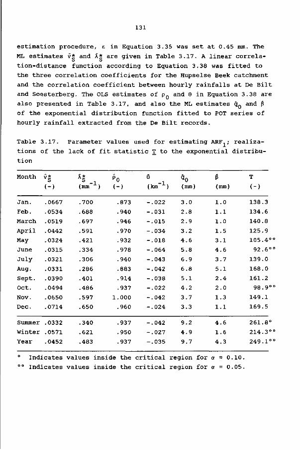
131
estimation procedure, e in Equation 3.35 was set at 0.45 mm. The
ML estimates v* and K* are given in Table 3.17. A linear correla
tion-distance function according to Equation 3.38 was fitted to
the three correlation coefficients for the Hupselse Beek catchment
and the correlation coefficient between hourly rainfalls at De Bilt
and Soesterberg. The OLS estimates of p. and 0 in Equation 3.38 are
also presented in Table 3.17, and also the ML estimates qn and ß
of the exponential distribution function fitted to POT series of
hourly rainfall extracted from the De Bilt records.
Table 3.17. Parameter values used for estimating ARF.. ; realiza
tions of the lack of fit statistic T to the exponential distribu
tion
Month
Jan.
Feb.
March
April
May
June
July
Aug.
Sept.
Oct.
Nov.
Dec.
Summer
Winter
Year
(-)
.0667
.0534
.0519
.0442
.0324
.0315
.0321
.0331
.0390
.0494
.0650
.0714
.0332
.0571
.0452
(mm )
.700
.688
.697
.591
.421
.334
.306
.286
.401
.486
.597
.650
.340
.621
.483
Po (-)
.873
.940
.946
.970
.932
.978
.940
.883
.914
.937
1.000
.960
.937
.950
.937
0
(km-1)
-.022
-.031
-.015
-.034
-.018
-.064
-.043
-.042
-.038
-.022
-.042
-.024
-.042
-.027
-.035
(mm)
3.0
2.8
2.9
3.2
4.6
5.8
6.9
6.8
5.1
4.2
3.7
3.3
9.2
4.9
9.7
ß (mm)
1.0
1.1
1.0
1.5
3.1
4.6
3.7
5.1
2.4
2.0
1.3
1.1
4.6
1.6
4.3
T
(-)
138.3
134.6
140.8
125.9
105.4°°
92.6°°
139.0
168.0
161.2
98.9°°
149.1
169.5
261.8°
214.3°°
249.1"
Indicates values inside the critical region for a = 0.10.
Indicates values inside the critical region for a = 0.05.

132
The mean number of threshold exceedances is one for each month,
and two for each year or season, and peaks are separated by an
interval of at least ten hours, as indicated in Section 2.5.3. The
validity of the assumption of exponentially distributed peaks has
been assessed by the test statistic T according to Equation 2.8.
Table 3.17 also gives the realizations T. The winter, summer, and
year series show poor fit. This could have been improved, had only
one exceedance for each year been allowed which would have yielded
for the winter series only a T critical at the 10% level. However,
as interest is in low return period events, these results are ac
cepted. Figure 3.26 shows the POT series of hourly point rainfall
and also the fitted exponential distributions for January, August,
summer, winter, and the complete year.
2 ARF1 has been estimated for areas of 10, 50, 100, and 250 km , and
return periods of 1, 1.78, 5, and 10 years. Figure 3.27 shows ARFX
for January and August as a function of area and return period, and
Figure 3.28 shows ARFn for winter and summer. ARF.. and ARF». for
the complete year are shown in Figure 3.21. ARFs corresponding to a
0.5-year return period are shown in this figure, but ARF.. values
corresponding to a 5- and 10-year return period are not shown,
because these require the extreme right tail of the fitted distri
butions, which is not accurately known.
Figure 3.21 shows that ARF increases with rainfall duration. The
ARF.. estimates in the present study for the Netherlands are some
what lower than those reported in USWB (1957-1960) and NERC (1975)
(see Table 3.18). Apart from different estimation methods, both
the USWB (1957-1960) and NERC (1975) studies were based on more
data obtained from dense rainfall measuring networks. Both USWB
(1957-1960) and Bell (1976) show that there is a large variation
in ARFj values derived from different areas. Lack of data rather
than climatological differences could be the reason of the differ
ences in ARF values shown in Table 3.18.

133
Table 3.18. Comparison of ARF. estimates in the present study for
the Netherlands with those from USWB (1957-1960) for the USA and
NERC (1975) for the United Kingdom
Area ARF1
(km2) Present study USWB (1957-1960) NERC (1975)
100 0.76 0.83 0.79
250 0.66 0.73 0.72
3.5. STORM-CENTRED AREAL REDUCTION FACTOR SRF
The storm-centred areal reduction factor SRF which is similar to
the statistical areal reduction factor ARF is defined as (Equation
3.4)
where
SRF = xA/x , A' max
x : local maximum point rainfall over a certain time max ^ period (e.g., one specific day)
x : simultaneous areal rainfall over area A bounded by
an isohyet.
SRF is used in the derivation of statistical estimates of probable
maximum precipitation: theoretically, the greatest depth of pre
cipitation that can occur in a particular drainage basin for a par
ticular duration in a particular season. It may also be of use in
simulation studies. But, as pointed out by Holland (1967), the re
quirement to develop a relationship between point and areal rain
fall is "... in the engineering context the need to match frequen
cies or periods of return (p. 194)."
While ARF relates point and areal rainfall of equal exceedance
probability and without any assumption of simultaneousness, SRF
relates point and areal rainfall over the same time span and con
sequently with almost certainly different exceedance probabilities.
ARF intrinsically refers to fixed areas, whereas SRF is quite often
determined from isohyet patterns occurring within a larger area
(referred to as moving target area SRF).

134
When a fixed area is considered, a densely-gauged experimental
catchment may be selected. This may lead to accurate estimates of
SRF, but also has the disadvantage that very often the point rain
fall maximum occurs near the edge of the catchment, or even outside
it, so that the presumed maximum is not the maximum at all. As SRF
is often derived under the assumption of circular isohyets, it may
be cumbersome both to verify this assumption, and to estimate x ,
when a fixed area is used. In principle, however, whether a moving
target area or a fixed area is used is immaterial, but the possi
bility with a fixed area that the true maximum is not recognized
may have the consequence that different estimates of SRF are ob
tained.
In general, SRF is equal to or less than ARF, see also Figure 3.29
(from Bell, 1976). The smaller the area and the shorter the period
during which rainfall totals are considered (for example, SRF and
ARF values for a particular month instead of the complete year),
the closer the values of SRF and ARF will be. By extending both the
period and the area, the probability of non-simultaneousness of
point and areal maxima will increase. This will generally lead to
ARF values which are high compared to SRF values, but this depends
also on the criteria according to which the days are selected for
estimating SRF.
According to Eagleson (1970), the difference x -x in general III ci X A
(i) increases with area;
(ii) decreases with total rainfall depth (which causes an increase
of the coefficient of variation with decrease of total rain
fall depth (Figure 3.6);
(iii) decreases with duration;
(iv) is greater for convective and orographic precipitation than for
cyclonic precipitation.
Therefore, the ratio SRF of x and x will generally show oppo-A max
site behaviour.
An insight into the dependence of SRF on A can be obtained from
depth-area curves, "Curves showing, for a given duration, the rela
tion of maximum average depth to size of area within a storm or
storms" (USWB, 1947; p. 252), or from minimum-rainfall curves,
which are similar to the depth-area curves, "... except that ordi-

135
nates represent minimum instead of average depths within the areas"
(USWB, 1947; p. 297). The equation representing a minimum-rainfall
curve can be written so as to represent a depth-area curve. Such an
equation gives x. as a function of A. When the equation is divided
by x , the result is SRF as a function of A max Table 3.19 contains
expressions for SRF derived from published equations representing
depth-area and minimum-rainfall curves.
Table 3.19. Expressions for the storm-centred areal reduction factor SRF, deduced from
equations representing depth-area and minimum-rainfall curves
Investigator SRF Duration General remarks
Horton (1924) 1-OA'4+0.5C(2A-
Huff and Stout 1-oA^
(1952)
Chow (1953, 1954) l-aA^+ßA-...
Boyer (1957) l -aA l 5+0.41a 2A-
Kra i j enho f f (1958) 1-oA+ßA - . . .
3 /5 Woolh i se r and 1-aA
Schwalen (1959)
Court (1961) l-aA+2/3a2A2-
Smith (1974) 1-aA
2 Nicks and Igo 1-oA+oßA
(1980)
1 one day
30 min-18
hours
not specified
.2 6-48 hours
3 one day
one day
4 not specified
one day
s up to 24
hours
heavy rainfall in the eastern USA;
moving target area
small, densely-gauged networks in
Illinois (USA); thunderstorm rainfall
applied to data from one of Huff and
Stout's networks
great storms over the central plains
of the USA; moving target area
heavy summer rainfall in the
Netherlands; moving target area
thunderstorm rainfall over a small,
densely-gauged network in Arizona (USA)
applied to convective rainfall of less
than two hours duration over a small,
densely-gauged network in southern
Arizona (USA), by Fogel and Duckstein
(1969)
thunderstorm rainfall in southern
Arizona (USA) 2
large (3885 km ), densely-gauged
network in Oklahoma (USA); verified
with other USA rainfall data
Taylor expansion of SRF = exp(-aAp), with ß s 0.50.
This expression follows from Boyer's SRF =
j^|f{l-exp(-1.09(A/a1)^)(1.09(A/a')^+l)}, after a Taylor expan
sion, followed by some simplifications, as noted by Chow (1958).
Taylor expansion of SRF = X^-{l-exp(-A/a')? + (1~^')P'{l-exp(-A/ß')} • Taylor expansion of SRF = -{l-exp(-A/a')}.
Their original expression is approximated as follows
SRF = l-( ,Y'
a'+ß'A a '
1-a 1+ßA
= l-aA(l-ßA)
1-aA+aßA ; D denotes the duration of rainfall.
136
None of the expressions in Table 3.19, except for that of Nicks and
Igo (1980) which has duration as an independent variable, contains
explicitly the following above-mentioned factors: total rainfall
depth (ii); duration (Hi); and the nature of the precipitation
(iv). Thus, they should be used only for those circumstances under
which they have been derived.
Many approximations have been used in Table 3.19, notably the
Taylor expansions mentioned in the footnotes, and the replacement
by x of all such quantities as the measured x , the 'true', max max that is interpolated, x , and the maximum areal rainfall at the ^ max eye of the storm over ten square miles. Close examination of these
studies, and similar approximations used by Court (1961) indicate
that the approximations in Table 3.19 are acceptable. Table 3.19
shows that, basically, there are two expressions for SRF
SRF = l-aA4^..., (3.44a)
and
SRF = l-aA+... . (3.44b)
A general relationship between ARF and SRF can only be derived on
the basis of many assumptions. Firstly, an equation for the depth-
area curve needs to be postulated, for example, one of the equa
tions referred to in Table 3.19. As the coefficient a in Table 3.19
may depend on x , this dependence also needs to be postulated.
SRF can then be estimated, and for certain depth-area relationships,
the correlation-distance function can be obtained from the work of
Stol (1981a,b,c), on the assumptions that this relationship is the
same for all storms and that storms occur randomly and are uniform
ly distributed in space, with at most one storm occurring during
one interval of precipitation measurement (for example, one day).
Stol (1981a,b,c) has obtained the correlation-distance function
as a space average over straight lines passing through the loca
tion of maximum rainfall. By spatially averaging the correlation-
distance function, one finds f=r(V;V). Then, from the pdf of point
rainfall, the pdf of areal rainfall can be obtained, and ARF esti
mated. In such a comparison, SRF is compared with ARF corresponding
to a certain return period.

137
A more general approach uses only the pdf of point rainfall, the
pdf of maximum rainfall x , and the correlation-distance function c max as estimated, without assumptions on the depth-area relationship.
Then, as seen before, ARF is determined completely, and SRF can
be found as follows (Smith, 1974). A minimum-rainfall relationship
gives the minimum rainfall x ( h ) along an isohyet at distance h
from the rainfall maximum as a function of A. Its inverse gives
A as a function of x (h). A dimensionless inverse may be written
as AA(x*), which gives the dimensionless area AÄ=A/A. . (see
Figure 3.30) as a function of the dimensionless rainfall depth
x*=x (h)/x . Note that A.(0)=1, and A.(1)=0. As 0<x„.<l, l-A^x*)
can be seen as the cdf of x^.
Let the random variable x represent point rainfall depth at point
S within an area, then the probability of the event {x<d} can be
expressed as (see Figure 3.30)
P{xs<d} = P{xmaxid} + P[{xmax>d}n{S:Xs<d}]. (3.45)
The last event in Equation 3.45 indicates the possibility that,
although x >d, S is so remote from the rainfall maximum as to 3 max
cause x <d. Because l-AÄ(xÄ) is a cdf
P{S:Xs<d} = 1-A*(d/Xmax). (3.46)
Combining Equations 3.45 and 3.46 yields
P{xs<d} = P{xmax£d} + ;;=d[l-A*(d/y)]dP{xmax<d},
P{x <d} = l-r,AÄ(d/y)p (y)dy, (3.47) s y a xmax
where
Px(-) : Pdf of x.
According to Equation 3.47, the dimensionless depth-area relation
ship A^(xA) can be determined from the pdfs of centre depth and
point rainfall, and SRF can be determined from A„.(xÄ).

138
Also similar to ARF is the epicentre coefficient (Kraijenhoff,
1963; Galea et al., 1983), the ratio of the maximum point rainfall
over an area for a given return period and duration, and the quan-
tile estimate of point rainfall for that return period and duration.
The epicentre coefficient is always at least one, and increases
with area and return period, and decreases with duration. Estimates
of epicentre coefficients also depend heavily on network density.
Kraijenhoff (1963) related the minimum and maximum point rainfall
depth to return period and to the point rainfall depth with the
same return period for summer days with measured rainfall at a
particular rainfall station in excess of 40 mm (see Figure 3.31).
From this figure, epicentre coefficients and a related quantity
with regard to minimum rainfall can easily be estimated. Because
of the low density of the rainfall measuring network, estimates of
the epicentre coefficients from Figure 3.31 will be rather lower
than those from Galea et al. (1983) for France. For daily summer 2
rainfall, an area of 50 km , and a 10-year return period, according
to Figure 3.31 the epicentre coefficient is 1.14, but according to
Galea et al. (their Figure 3), it is 1.56.

139
Fig. 3.1. Location of rainfall stations and areas considered in Chapter 3.

140
AREA 3
AREA
454 10.0636)
w:13i s:155
w : t27 s:150 _436 ,10022«
w:14,1 s:l72 578 (011661
Fig. 3.2. Thiessen polygons for the areas 1,2 and 3 in Figure 3.1. Sample points are numbered according to their KNMI code 743
(006041
w:i23 number, and the Thiessen s : 15.0 weights are given in brackets.
w: mean winter monthly maximum (mm)
s : mean summer monthly maxium (mm).

1«h
Y (h) (mm2)
t 100
50-
1261.5)/
A. Summer
123.31
IK»
141 28n
25-
Ylh) (mm2)
15-
^ G T 1 5 " 1135)
_ -,
5
_43 81_
à) (!)
15 20
173 22.2-12.3
(15) (17) (9)-*N(h)(l5)
X ,. 30 km. -> distance
-*U(h)295km - I -
B. Winter
„April (KUÎ^Jan.
-M.2) „--March
1191 r-tó.5) Febr.
20
43
-+-ai -+-
12.3 - r -
173
25 30km — » • distance
22.2-*U(h) 295km H H
(3) (7) (15) (17) (9)-»N(h)(15)
Fig. 3.3. Multi - realization sample semi-variograms. Monthly maxima of daily rainfall. Area 1.
Sample standard deviations of the results are given in brackets.
U (h) ; location of centres of distance classes / l 3 7 3 ) w o o ) 0 c t
N(h) : number of pairs of sample points within a distance class.
Yfh)
(mm2)
100-1 '20-
Y(h) (mm2)
50
A. Summer
10-
10 15 20
12.5 176
25 30 km -» distance
16 11
22.7-* U(h)
11-»N(h) 21
31.7km - I -
B. Winter,
20
70 -r 12.5
16
176 - H —
25 30 km —»distance
22.7-»U(h) 31.7 km
11-»N(h) 21
Fig. Z.U. Multi-realization sample semi-variograms. Monthly maxima of daily rainfall. Area 2. U(h) location of centres of distance classes N(h) .number of pairs of sample points within a distance class.

142
100
Y(h)
(mm2)
50-
A. Summer
25-
20
Yfh) (mm 2)
Î .5-
5-
20
4.3 82 T2A —I
171 - t -
25 30 km -»distance
225-»U(h)294km
-+-
B. Winter
4.3 8.2 124 _ l 1 1_
1 8 13
15 20
171
15 13 15 13-*N(h) l6
F ig. 3.5. Multi.realization sample semi.variograms. Monthly maxima of daily rainfall. Area 3
U ( h ) : location of centres of distance classes
N(h) : number of pairs of sample points within a distance class.
25 30km —»distance
225-» U(h) 29.4 km
13-»N(h)l6
1.5
1.4
1.3
1.2
1.1
1.0
0.9
0.8
' 0.7
0.6
0.5
0.4
03
Ü2
0.1
0
A. Area 1 Summer r= -0.10
* **
14 21 28 35 42 49 56 63 70 —»area ! rainfall (mm)
1.5
1.4
1.3
1.2
1.1
1.0
09
0.8
' 0.7
0.6
0.5
0.4
0.3
0.2
0.1
0
B. Area 1 Winter r=-0.20
.&*:
21 28 35 42 49 56 63 70 — * areal rainfall (mm)

143
1.5
1.4
1.3
12
1.1
1.0
0.9
0.8
Q7
0.6
0.5
0.4
0.3
02
0.1
0
4 ^ " J
x » x x j
«xx X*K , x
C. Area 2 Summer r=-Q25
14 21 28 35 42 49 56 63 70 — » areal rainfall I mm )
1.5
1.4
1.3
1.2
1.1
1.0
0.9
0.8
0.7
0.6
0.5
0.4
0.3
0.2
0.1
0
-
-
» -
* X
_ " " x \
* * * X * x x *
D. Area 2 Winter
r = -0.23
14 21 35 42 49 56 63 70 — » areal rainfall (mm)
1.5
1.4
1.3
1.2
1.1
10
0.9
08
>
• 0.7
0.6
0.5
0.4
0.3
0.2
01
0
Fig. 3.6.
-
-
" x x
x
" X
* X x x
"x "
x * * x X X "
x «x x * x - x ^ x
" * x x «
x . * * X* " X " - x „ >(, „ ^
x x x * * " x*x
x" x * >?** " .x
** *Xxy " - J V -X X X y
E. Area 3 Summer r = -Q21
x X '
y
14 21 28 35 42 49 56 63 70 —»• areal rainfall (mm I
1.5
1.4
1.3
1.2
1.1
1.0
0.9
0.8
0.7
0.6
0.5
0.4
0.3
0.2
0.1
0
x Ä x * x
x x ^ * X " "x *
i-$S*x V
X » f t x1fc * * * x * " # xxx
- .x">x:sä «
E Area 3 Winter r = -0.33
14 21 28 35 42 49 56 63 70 — • areal rainfall (mm)
Coefficient of variation cv for monthly maxima of daily rainfall, plotted against mean areal rainfall, r is the correlation coefficient between cv and mean areal rainfall.

144
50 km2
100 km2
250 km i
500 km2
3 9 . 3 - ^ j ^ 50 55 60 65 70 75 80 85 90 95 100 381 371^5^ — * point rainfall (mm)
36.7-
Fig. 3.7. Regression tines relating areal daily summer rainfalls to point rainfalls of equal return period , according to Krai jenhoff (1963).
Q0 08 16 2A 32 40 48 00 08 1.6 24 32 40 48
^ E N —EU(i!) Q0 08 t6 24 32 40 48

145
0.0 Q8 16 2.4 3.2 40 4.8
- * E ( y ( i ) )
Q0 08 16 2Â 32 40 4.8 00 0.8 1.6 2A 32 40 4.8
42
£ £ 36
"5
2 30
Î 24
18
/r // Y Area 3
•// Winter
00 Q8 16 24 32 4.0 48 - * E ( y ( i ) j
0.0 Q8 1.6 2Â 3.2 4.0 4.8 0.0 Q8 1.6 2Â 32 40 48
Fig. 3.8. Ten highest peaks (out of 58) from POT series of daily areal rainfall (•) and
daily point rainfall (x), and fitted exponential distribution functions for the three
areas considered in the derivation of ARF24.
Plotti ng position E ( V ( j ) \ = £ ( n * 1 - j ) -1

146
20 40 20 40 —»hlkml —»h(km)
Fig. 3.9. Sample semi, variances and fitted linear y (h) model ; area 1.
24
16' Y(W|
(mm2)
x x i
x B. August
^_ 20 40
»h(km) Fig. 3.101 Sample semi.variances and fitted linear Y (h )mode l ; area 2 .

147
4.0
3 0 -
(mm 2)
20
1.0
x4«*x
/ * - / x A. January
20 40 — » h ( k m )
20 40 »h(km)
Fig. 3.11. Sample semi, variances and fitted linear Y (h) model ; area 3.
1.00
0.60
r(h)
0.40
0.20 A. January
0.80
0.60
(h)
0.40
0.20
20 40 50 » h ( km)
B. August
20 30 40 50 » h (km)
Fig. 3.12. Calculated correlation coefficients and fitted linear correlation-distance function r(h) for area 1 .

148
080
060
r (h)
0.40 -
0 . 2 0 - A. January
20 30
1 00
0.80
0.60
r(hl
' 0.40
0.20 B. August
40 50 » Il (km)
40 50 » h ( km)
Fig. 3.13. Calculated correlation coefficients and fitted linear correlation-distance function r(h) for area 2.
1.00
0.80
0.60-
r(h)
0 . 4 0 -
0.20
1.00
V**5-
A. January
0.60
r(h)
0.40
0.20
20 40 50 » h (km)
B. August
30 40 50 • • ! > ( k m )
Fig. 3.U. Calculated correlation coefficients and fitted linear correlation-distance function r(h) for area 3.

149
S1
<
... £
O)
CL
<"
. _
i le -t -
S.' la .. ~
m S

150
ë
S Z
< cc
X 0)
"in
I "S
q. <
9--Î-
Î ° 1 £ n ° 3 ts
UJ C
1 '8.
csi
s <
£ "

151
LH ^
S'S
- ö
g ^
a
o
I ju u, a •
J2 S
gl?
0.

152
28.5 i
25.5-
22.5
QO 0.8 1.6 2.4 3.2 4.0 4.E 0.0 0.8 1.6 2.4 3.2 4.0 4.8
— É ( ï ( i | )
Fig. 3.18. Ten highest peaks (out of 29) f rom POT ser ies of da i ly point r a i n f a l l
and f i t ted exponential d istr ibution funct ions. The TOT ser ies have been
derived by averaging over the indiv idual POT series of all rainfall series
in the three areas cons idered.
1.00
090
ARE,,
0.60-
070-
0.60 25 100 250 — » A (km2) 1000
F ig . 3.19. ARF 2 4 for January and August as a func t ion of areal s ize A and
return period T.
( : for a double exponential co r re la t i on -d i s tance func t ion ).
January
August

153
1.00
0.90
ARF24
t
0.80
0.70
0.60 25 100 250 - * A ( k m 2 ) 1000
Fig. 3.20. ARF 2 4 for summer and winter as a function of areal size A and
return period T.
( : for a double exponential correlation-distance function).
Winter
Summer
1.00
ARF,,
0.60-T , , —
25 100 250 — » A (km2) 1000
Fig. 3.21. ARF24 and ARF; for the complete year as a function of areal
size A and return period T. ( : for a double exponential correlation - distance function).

154
2000 5000 —» Areal size (km2)
Fig. 3.22. Estimates of ARF24(x) according to NERC (1975) for areas 1,2 and 3, and the USWB (1957-1960) and NERC (1975) estimates of ARF24. (corresponding to a 1.78-year return period for peak exceedances ).
1.00
0.90
ARF, ,
Î 0.80-
0.70
25 »0 250 — • A lkm 2 ) 500
Fig. 3.23. ARF 2 4 es t imates according to Kraijenhoff (1963) for a daily rainfall depth in summer of 40 m m , compared to estimates from the marginal distribution of point rainfall for a double exponential (1) and a linear correlation -distance function (2).

155
ç

156
25
2.0
1.5
* A ,p(mm)
1.0
0.5
A. January
8.0
6.0
XA plranl
4.0
2.0
B. August
005 0.025 00125 0005 0001 0.0005
* ( 1 - p )
0.075 0.05 0025 0.0125 0005 0.001 0.0005
* ( 1 - p )
Fig. 3.25. Percentage points of areal hourly rainfall XA ,p plotted against exceedance frequency ( 1 -p ) , according
to the edf ( ) and the pdf ( ).

157
- |vü
(UJUJ) ]|D}U|DJ .
(LULU) ||DJU|DJ-
-Ar'°.
(LULU) i p j u p j •

158
wi — W l n *% w
o» £ s o * *-
I— x -
e : g£ p
— 'S £ "2 S1 S
a £ o Ü'
5-8 I g in ^ O
O) -, 'JZ _>. in -c £* 3 ^ ~
^ 5 °-
2 wi
§1 J o £
j» LU
J (2 o .=
(WW) |]DJU|DJ •

159
T(year)
• January
August
lb 50 100 — » A (km2) 250
F ig . 3.27. ARF, for January and August as a function of
a rea l size A and return period T.
1.00
T(year)
Summer
10 50 100 — » A (km2) 250 Fig. 3.28. ARF, for summer and winter as a function of
areal size A and return period T .

160
200 500 1000 2000 5000 Area (km )
Fig. a29. Comparison of A R F 2 4 and SRF values for the USA ( f rom Bett, 1976).
F ig. 3.30. Hypo the t i ca l d e p t h - a r e a re la t ionsh ip .

161
100
90
80
70
60
50
40-
maximum point rainfall
70krr?30 IP 2 15012015,1 / } f K •
//////// / / / /
vow////<'
/point rainfall
minimum point rainfall
2 5 10 20 30 50 70km2
/ / / y /////// //////// /// //
J"//// / /// SS . /////////// // /
y / y y y y
/s s / / / / / / / y ///////
MW/////// jjjy/'// " s ''s s /
//S///// S SS / / / / S//S//// /ss s, / s
///s//// / y / s/ s y s/ss/ss/ss/ s / / /
S///SS// s sy / / / / sss///// / y / s/ / y
//j£</S///S/ / / /y ///ssssY /s y y y y y
y y
1 10 100 1000 return period (years) Fig. 331. Maximum and minimum point rainfall depths as a function of areal size and
return period, according to Kraijenhoff ( 1963 ).

4. SUMMARY AND CONCLUSIONS
Rainfall data for the Netherlands have been used in this study to
investigate aspects of heterogeneity of rainfall, in particular
local differences in rainfall levels, time trends in rainfall, and
local differences in rainfall trend. The possible effect of ur
banization and industrialization on the distribution of rainfall
has also been studied. Consideration has been given to whether lo
cal differences in rainfall justify a partition of the Netherlands
into regions. Finally, the degree of areal reduction which
is possible in hydrological design because of variation of rain
fall in time and space has been investigated.
A statistical analysis of these aspects is useful because they
frequently appear in the hydrological literature. The statistical
analysis presented in this thesis uses hydrological concepts, such
as the statistical areal reduction factor, and attention is focused
on moderately low return period events. Only rainfall levels and
trends in rainfall have been investigated and not more complicated
aspects, such as, trends in the variance of rainfall. Further, rain
fall variations in time and space have been analysed separately.
Estimates of the levels of the rainfall characteristics used in
the investigation of homogeneity in time and space are given in
Section 2.2. These are annual frequencies of exceedance during
the summer or the winter period of a certain threshold value and
the total annual rainfall (Tables 2.1 and 2.2). The expected daily
rainfall has also been estimated for return periods in excess of
half a year (Table 2.4, Figure 2.2). Time trends in rainfall aver
aged over the Netherlands have been estimated. For the period
1951-1979, the time trend is negative for the summer period; and
for the period 1906-1979, the time trend is positive for the win
ter period (Table 2.5). Time trends in rainfall series were found
to be related to the occurrence of circulation types (Figure 2.4).
In Section 2.4 local differences in these rainfall characteristics
have been investigated using the kriging method that gives the

163
best linear unbiased predictor. As may be expected, there are local
differences, both in rainfall level (Figure 2.7), and in time
trends in the rainfall series which were reduced by the annual
mean (Figure 2.9). Many of the rainfall series investigated exhib
it inhomogeneities (Table 2.7). Two possible causes of these inho-
mogeneities, changes in the frequency of occurrence of circulation
types and anthropogenic activities, such as urbanization and in
dustrialization, are discussed in Section 2.6.
A possible partition of the Netherlands into regions is investi
gated by using rainfall data for the period 1951-1979. Earlier
studies on the geographical distribution of certain rainfall char
acteristics in the Netherlands are presented in Section 2.5.1. The
model to test the statistical significance of the partitions used
in this study is presented in Section 2.5.2.
One of the proposed partitions, an a posteriori partition based on
mean annual rainfall (Figure 2.11D), is in agreement with the re
sulting spatial patterns of the levels of the rainfall character
istics considered (Table 2.10). Also, the level of hourly rain
fall was found to be related to mean annual rainfall (Figure 2.18A),
but, with a simple urban runoff model with a time-step of one hour,
no differences were found between the number and quantity of over
flow for 12 rainfall stations, classified according to this parti
tion (Section 2.5.3).
These partitions into regions are not satisfactory for rainfall
trends, except for an a posteriori partition based on time trends
for the period 1951-1979 (Figure 2.12). But both the geographical
distribution of trends and the degree of trend in some long-term
rainfall records are not in agreement with this partition. Appar
ently, the changes in rainfall pattern are recent. Because the
partition is based on trends in reduced rainfall series (reduced
by the annual mean), the changes are also local. Thus on the
basis of data used in this study, it was not possible to devise
a satisfactory partition of the Netherlands for rainfall trends.
With regard to rainfall level it is suffice to assume that the de
sign rainfall at a given location is proportionate to the mean sum-

164
mer or winter rainfall; therefore, a partition of the Netherlands
into regions is not necessary. This has already been suggested in
Buishand and Velds (1980).
The influence of urbanization and industrialization on precipita
tion (urban effects) has been investigated by using the method of
Lowry (1977), which allows for changes in frequency of occurrence
of circulation types. In Section 2.6, this method is discussed and
the findings of other studies on the occurrence, causes, and magni
tude of urban effects are presented. In Section 2.6.1, the occur
rence of urban effects is discussed, for instance, on the basis of
changes in mean daily rainfall for 32 rainfall stations between the
industrialized and urbanized period (1956-1979) and the non-indus-
triai..zed period (1932-1955), with a stratification of days accord
ing to season and circulation type (according to Hess, 1977), see
Figure 2.22. Although the results were sometimes inconclusive and
not always in accordance with the hypothesis of an urban effect,
there are indications of urban effects for the zonal circulation
type and for three of the meridional circulation types (Tables 2.16
and 2.17; Figure 2.22). Moderate rainfalls were also found to be
affected (Table 2.17, where a threshold value for daily rainfall of
15 mm has been considered), and urban effects in the summer period
increase with rainfall depth.
In Chapter 3 consideration is given to the degree of areal reduc
tion which is possible in hydrological design because of varia
tions of rainfall in time and space. Use has been made of the
IRF-0 kriging theory, and semi-variograms were estimated by the
multi-realization approach. The applicability of the IRF-0 theory
to predict the mean areal rainfall is discussed in Section 3.2.1.
Contrary to what had been expected, in a substantial number of
cases the estimated order of the intrinsic random function dif
fers from zero (Tabel 3.1). Further research is needed on the
structure identification, both on the statistical aspects (esti
mation of the order k of the intrinsic random function and of the
coefficients of the generalized covariance model) and on the physi
cal aspects (semi-variogram or generalized covariance model to be

165
expected under certain assumptions regarding rainfall). The varia
tion in semi-variogram estimates for individual rainfall events
was found to be large (Figure 3.3). In Section 3.2.2, the kriging
predictor of areal rainfall is compared with the more commonly
used arithmetic mean and Thiessen predictor. All three predictors
yield similar results (Table 3.5), but the kriging predictor is
more efficient (Table 3.4).
Methods to estimate the statistical areal reduction factor (ARF)
are presented in Section 3.3.1. With the methods proposed in
USWB (1957-1960), NERC (1975), Bell (1976), and Rodriguez-Iturbe
and Mejia (1974) and Buishand (1977c), the areal reduction factor
for daily rainfall (ARF_.) has been estimated for three areas each 2 of about 1000 km in the Netherlands, for the summer period, the
winter period, and the complete year. In Section 3.3.3, the varian
ce of ARF_ is estimated. All four estimators of ARF_4 were found
to produce similar results (Tabel 3.12), and the three areas consid
ered do not clearly differ with respect to ARF-.. These estimates
of ARF_ are somewhat lower than those of USWB (1957-1960) for
the United States and those of NERC (1975) for the United Kingdom
(Figure 3.22), and they are in reasonable agreement with earlier
estimates of ARF_ for the Netherlands (Table 3.14). For small
areas, ARF„„ is underestimated by the method which uses the mar-
ginal distribution of point rainfall and the fitted correlation-
distance function. This is also evidenced by the higher ARF_„ Z4
values in Kraijenhoff (1963). ARF-. depends heavily on season and
return period (Table 3.7). Averaged over the three areas, the maxi
mum areal rainfall occurs in the winter period in 33% of the years
considered.
In Section 3.4 ARF for hourly rainfall (ARF ) is estimated. As a
function of areal size and return period, ARF. has been estimated
for the summer and the winter period (Figure 3.28) and for the
complete year (Figure 3.21). These ARF.. estimates are somewhat
lower than those of USWB (1957-1960) and NERC (1975) (Table 3.18),
probably because few hourly rainfall data were available for this
study. Especially the correlation-distance function for hourly
rainfalls could not be estimated very satisfactorily.

166
The storm-centred areal reduction factor (SRF) is discussed in
Section 3.5. Models for SRF based on a literature survey of
minimum-rainfall curves are presented in Table 3.19. For equal
areal size, SRF values from network data are generally lower than
ARF values (Figure 3.29). The smaller the areal size and the short
er the period for which rainfall totals are considered, the closer
SRF and ARF values.
In this study, rainfall variations in time and space have been
analysed separately. Because of this simplification of the pro
blem, the results presented in Chapter 3 may be of less relevance
to practical design issues related to areal rainfall. Areal re
duction is partly caused by spatial differences in rainfall pat
terns in time. This aspect of areal reduction is not taken into
account, when time aggregates of rainfall over a measurement in
terval are considered, and rainfall depths over consecutive inter
vals are assumed to be independent. For this reason, the degree of
areal reduction applicable to regional transport systems of sewer
age water cannot be determined by using the statistical areal re
duction factor.
When rainfall variations in time and space are analysed as being
interdependent, the need for knowledge and understanding of mete
orology increases because the rainfall events described have first
to be classified. Further, instead of the univariate statistical
methods as used almost exclusively in this study, multivariate
methods are required. However, at present, data from a dense net
work of rainfall recorders, necessary for such an investigation,
are not available for the Netherlands.
Further research on the causes of homogeneities in rainfall series
is necessary. Although this study of homogeneity has been restricted
to rainfall records of good and even quality, many rainfall series
are statistically inhomogeneous, and local differences in trend
often seem inexplicable. To explain this, meteorological knowledge
and knowledge of the station history of rainfall series used is
essential.

SAMENVATTING EN CONCLUSIES
In deze studie zijn met behulp van Nederlandse neerslaggegevens
aspecten van de heterogeniteit van de neerslag onderzocht, met
name plaatselijke verschillen in het niveau van de neerslag,
trends in het neerslagverloop en plaatselijke verschillen in
trend. De mogelijke invloed van verstedelijking en industriali
satie op de neerslagverdeling is eveneens bestudeerd. Aandacht is
besteed aan de vraag of plaatselijke verschillen in neerslag een
opsplitsing van Nederland in deelgebieden rechtvaardigen. Tenslot
te is onderzocht de mate waarin gebiedsreductie mogelijk is in
sommige ontwerpen als gevolg van de variatie van de neerslag naar
tijd en plaats.
De bovenvermelde aspecten komen geregeld ter sprake in de hydrolo
gische literatuur, hetgeen een statistische behandeling ervan zin
vol maakt. Deze statistische behandeling maakt gebruik van hydro
logische begrippen zoals de statistische gebiedsreductiefactor,
en vooral gebeurtenissen met een betrekkelijk korte herhalings
tijd zijn beschouwd. Alleen het niveau van de neerslag en trends
daarin zijn onderzocht, en niet gecompliceerdere aspecten, zoals
trends in de variantie van de neerslag. Ook zijn de variaties naar
tijd en plaats steeds afzonderlijk behandeld.
In Paragraaf 2.2 is het niveau geschat van de neerslagkenmerken
waarvan de homogeniteit naar tijd en plaats is onderzocht: jaar
lijkse aantallen dagneerslagen groter dan een zekere drempelwaar
de in de zomer- of winterperiode, en de jaarneerslag (Tabellen 2.1
en 2.2). Ook is voor herhalingstijden langer dan een half jaar de
verwachte dagneerslagsom geschat (Tabel 2.4, Figuur 2.2). Trends
in het over Nederland gemiddelde neerslagverloop zijn bepaald.
Voor de periode 1951-1979 is de trend voor de zomerperiode nega
tief; voor de periode 1906-1979 is de trend voor de winterperiode
positief (Tabel 2.5). Trends in het verloop van neerslagkenmerken
blijken gerelateerd aan het optreden van circulatietypen (Figuur
2.4).

168
In Paragraaf 2.4 zijn plaatselijke verschillen in deze neerslag-
kenmerken onderzocht, waarbij gebruik is gemaakt van de kriging
methode, ter verkrijging van de beste lineaire zuivere voorspeller.
Zoals te verwachten is, zijn er plaatselijke verschillen, zowel in
het niveau van de neerslag (Figuur 2.7), als in trends in ver-
schilreeksen (Figuur 2.9); deze verschilreeksen ontstaan door af
trekken van het jaargemiddelde. Veel van de onderzochte neerslag
reeksen blijken statistisch niet homogeen te zijn (Tabel 2.7).
Twee mogelijke verklaringen van de geconstateerde afwijkingen van
homogeniteit, veranderingen in de frequentie van voorkomen van
circulatietypen en antropogene activiteiten zoals verstedelijking
en industrialisatie, zijn onderzocht in Paragraaf 2.6.
Een mogelijke opdeling van Nederland in deelgebieden is onderzocht
met behulp van neerslaggegevens voor de periode 1951-1979. Eerder
onderzoek naar de geografische verdeling van bepaalde neerslagken-
merken in Nederland is vermeld in Paragraaf 2.5.1. Het hier ge
bruikte toetsingsmodel is vermeld in Paragraaf 2.5.2.
Een van de voorgestelde gebiedsindelingen, een a posteriori inde
ling gebaseerd op gemiddelde jaarneerslag (Figuur 2.11D), is in
overeenstemming met de ruimtelijke patronen van de niveaus van de
beschouwde neerslagkenmerken (Tabel 2.10). Ook het niveau van uur-
neerslagsommen blijkt samen te hangen met de gemiddelde jaarneer
slag (Figuur 2.18A), maar met behulp van een eenvoudig stedelijk
afvoermodel met een tijdstap van een uur konden geen verschillen
in aantallen en hoeveelheden van overstorten worden aangetoond
tussen 12 volgens deze gebiedsindeling geklassificeerde neerslag
stations (Paragraaf 2.5.3).
Voor trends in het neerslagverloop voldoen deze gebiedsindelin
gen niet, behalve een a posteriori indeling gebaseerd op trends
voor de periode 1951-1979 (Figuur 2.12). Voor enkele langjarige
reeksen blijken de geografische verdeling van trends en de mate
van trend echter niet overeen te stemmen met deze gebiedsindeling.
Blijkbaar gaat het om recente veranderingen in het neerslagpatroon.
Aangezien de gebiedsindeling gebaseerd is op trends in verschil
reeksen, gaat het hier om lokale veranderingen. Met behulp van de

169
in deze studie gebruikte gegevens kon de vraag naar een opdeling
van Nederland in gebieden voor trends in het neerslagverloop dan
ook niet worden beantwoord. Met betrekking tot het niveau van de
neerslag is het voldoende om de ontwerpneerslag voor een bepaalde
plaats evenredig te veronderstellen met de normaalwaarde van de
seizoensneerslag en hoeft Nederland niet in gebieden te worden op
gedeeld. Deze suggestie is al gedaan in Buishand en Velds (1980).
De invloed van verstedelijking en industrialisatie op de neerslag
(stedelijke effecten) is bestudeerd volgens de in Lowry (1977) ge
presenteerde methode, waarbij wordt gecorrigeerd voor veranderin
gen in frequentie van voorkomen van circulatietypen. In Paragraaf
2.6 is Lowry's methode gepresenteerd, en is verslag gedaan van re
sultaten van elders verricht onderzoek naar het voorkomen, de oor
zaken en de omvang van stedelijke effecten. In Paragraaf 2.6.1 is
het voorkomen van stedelijke effecten nagegaan, onder andere aan
de hand van de verandering van de gemiddelde dagneerslag voor de
geïndustrialiseerde en verstedelijkte periode (1956-1979) ten op
zichte van de niet-geïndustrialiseerde periode (1932-1955) voor
32 neerslagstations, waarbij onderscheid is gemaakt naar seizoen
en circulatietype (volgens Hess, 1977), zie Figuur 2.22. Alhoewel
de resultaten soms onduidelijk zijn en niet altijd in overeenstem
ming met de hypothese van stedelijke effecten, zijn er voor het
zonale hoofdcirculatietype en voor drie meridionale circulatie-
typen aanwijzingen voor het bestaan van stedelijke effecten (Ta
bellen 2.16 en 2.17; Figuur 2.22). Alhoewel de effecten zich ook
uitstrekken tot matige neerslagen (zie Tabel 2.17, waar is uitge
gaan van een drempelwaarde voor de dagneerslag van 15 mm), nemen
gedurende de zomerperiode de stedelijke effecten toe met de neer-
slaghoeveelheid.
In Hoofdstuk 3 is aandacht geschonken aan de mate waarin gebieds
reductie mogelijk is in sommige ontwerpen als gevolg van de vari
atie van de neerslag naar tijd en plaats. Er is gebruik gemaakt
van de IRF-0 kriging theorie, en semi-variogrammen zijn geschat
met behulp van de meervoudige-realisatiebenadering. De toepas
baarheid van de IRF-0 theorie voor het bepalen van gebiedsgemid-

170
delden van de neerslag is nagegaan in Paragraaf 3.2.1. In tegen
stelling tot wat verwacht werd, is in vrij veel van de onderzoch
te gevallen de geschatte orde van de intrinsieke toevalsfunctie
ongelijk nul (Tabel 3.1). Het verdient aanbeveling toekomstig on
derzoek onder andere te richten op deze zogenaamde structuurver
kenning, zowel op de statistische aspecten (het schatten van de
orde k van de intrinsieke toevalsfunctie en van de coëfficiënten
van het gegeneraliseerde covariantiemodel) als op de fysische as
pecten (het te verwachten semi-variogram of gegeneraliseerd co
variantiemodel onder zekere veronderstellingen met betrekking tot
de neerslag). De variatie tussen semi-variogram schattingen voor
afzonderlijke neerslaggebeurtenisen is groot (zie Figuur 3.3). In
Paragraaf 3.2.2 is de voorspeller van het gebiedsgemiddelde door
kriging vergeleken met twee gebruikelijke voorspellers van het
gebiedsgemiddelde, het rekenkundig gemiddelde en het Thiessen
gemiddelde. Toepassing van kriging leidt hier niet zozeer tot re
sultaten die gemiddeld sterk verschillen ten opzichte van de re
sultaten van andere methoden (Tabel 3.5), maar tot efficiëntere
voorspellingen (Tabel 3.4).
Enige schatters van de statistische gebiedsreductiefactor ARF zijn
gepresenteerd in Paragraaf 3.3.1. Met behulp van de schatters vol
gens USWB (1957-1960), NERC (1975), Bell (1976) en volgens Rodri-
guez-Iturbe en Mejia (1974) en Buishand (1977c) is in Paragraaf 2
3.3.2 voor een drietal gebieden in Nederland van ongeveer 1000 km
ARF_-, de gebiedsreductiefactor voor dagsommen van de neerslag,
geschat, zowel voor het gehele jaar, als voor de zomer- en winter
periode afzonderlijk. In Paragraaf 3.3.3 is de variantie van
ARF„. geschat. Alle vier genoemde schatters van ARF-. blijken
praktisch dezelfde resultaten op te leveren (Tabel 3.12), en de
drie beschouwde gebieden verschillen niet duidelijk met betrek
king tot ARF . Deze schattingen van ARF zijn iets lager dan de
schattingen in USWB (1957-1960) voor de Verenigde Staten en in
NERC (1975) voor het Verenigd Koninkrijk (Figuur 3.22), en stem
men redelijk overeen met eerdere schattingen van ARF_. voor Neder
land (Tabel 3.14). Voor kleine gebiedsgrootten onderschat de me
thode die gebruik maakt van de marginale kansverdeling van punt-
neerslagen en het aangepaste correlatieverloop ARF... Dit blijkt

171
ook uit de hogere ARF waarden in Kraijenhoff (1963). ARF is
sterk afhankelijk van seizoen en herhalingstijd (Tabel 3.7). Ge
middeld over de drie gebieden valt in 33% van de jaren het jaar-
maximum van de gebiedsneerslag gedurende de winterperiode.
In Paragraaf 3.4 is ARF voor uurneerslagen (ARFX) geschat. Als
functie van de gebiedsgrootte en de herhalingstijd is ARF1 weer
gegeven in Figuur 3.21 voor het gehele jaar, en in Figuur 3.28
voor de zomer- en winterperiode. De in deze studie geschatte ARF.
waarden zijn lager dan die in NERC (1975) en USWB (1957-1960)
(zie Tabel 3.18), waarschijnlijk als gevolg van de geringe hoeveel
heid beschikbare uurneerslaggegevens voor deze studie. Vooral het
ruimtelijk correlatieverloop van uurneerslagen kon niet erg bevre
digend worden geschat.
In Paragraaf 3.5 is aandacht besteed aan de bui-gecentreerde ge
biedsreductiefactor (SRF). Enige modellen voor SRF, gebaseerd op
in de literatuur vermelde modellen voor het neerslagverloop langs
een isohyeet, als functie van de afstand van die isohyeet tot het
neerslagcentrum, zijn vermeld in Tabel 3.19. Op metingen gebaseer
de SRF waarden blijken in het algemeen lager te zijn dan ARF waar
den (Figuur 3.29). SRF en ARF liggen dichter bij elkaar naarmate de
gebiedsgrootte kleiner is en de periode waarbinnen neerslagsommen
beschouwd worden, korter is.
In deze studie zijn de variatie naar tijd en de variatie naar
plaats steeds afzonderlijk behandeld. Vanwege deze vereenvoudiging
kunnen de resultaten in Hoofdstuk 3 van minder belang zijn voor
sommige met de gebiedsneerslag samenhangende ontwerpproblemen.
Gebiedsreductie wordt gedeeltelijk veroorzaakt doordat het neer
slagverloop in de tijd binnen een neerslaggebeurtenis van plaats
tot plaats verschilt. Doordat de neerslag wordt gesommeerd over
een waarnemingsinterval, en doordat er geen samenhang tussen in
opeenvolgende waarnemingsintervallen gevallen neerslaghoeveelheden
wordt verondersteld, blijft dit aspect van de gebiedsreductie bui
ten beschouwing. Hierdoor kan de mogelijke gebiedsreductie voor
regionale afvalwatertransportsystemen niet met de gebiedsreductie
factor worden beantwoord.

172
Wanneer de variaties van de neerslag naar tijd en plaats in hun
onderlinge samenhang worden behandeld, zal de noodzaak om meteoro
logische kennis toe te passen toenemen, omdat dan neerslaggebeur
tenissen worden beschreven, die eerst in klassen moeten worden in
gedeeld. In plaats van de in deze studie bijna uitsluitend toege
paste statistische methoden voor enkelvoudige kenmerken, zijn dan
statistische methoden voor meervoudige kenmerken nodig. Op dit
moment zijn in Nederland de voor een dergelijk onderzoek benodig
de neerslaggegevens van een dicht netwerk van regenschrijvers
overigens nog niet beschikbaar.
Ook nader onderzoek naar de oorzaken van inhomogeniteiten in neer
slagreeksen is noodzakelijk. Hoewel het hier verrichte homogeni-
teitsonderzoek zich beperkte tot een selectie van neerslagreeksen
van goede en van gelijkmatige kwaliteit, zijn statistisch gezien
veel neerslagreeksen inhomogeen, en lijken plaatselijke verschil
len in trend vaak onverklaarbaar. Meteorologisch inzicht en kennis
van de stationsgeschiedenis van de beschouwde neerslagstations zijn
ook daarom eerste vereisten.

APPENDIX A. DATA AND SUPPLEMENTARY RESULTS OF THE STUDY ON HOMO
GENEITY
A.l. DUTCH RAINFALL STATIONS USED IN THE STUDY OF HOMOGENEITY OF
RAINFALL RECORDS
In this appendix, the names are given of the rainfall stations in
the data sets used in the study of homogeneity of rainfall records.
The KNMI code number is given in brackets after the name of the
station, and comments on missing data are presented as footnotes
to the end of the appendix.
A. 1.1. Data set 140: daily rainfall records (1951-1979) of 140
KNMI rainfall stations distributed evenly throughout the Netherlands
(data from KNMI magnetic tape REGEN).
Hollum (10)
Schiermonnikoog (12)
Petten (16)
Den Burg (17)
Cocksdorp (19)
Dokkum (67)
Lemmer (Tacozijl) (74)
Oldeholtpade (75)
Kornwerderzand (76)
Stavoren (80)
Gorredijk (82)
Ezumazijl (84)
Leeuwarden (85)
Groningen (139)
Assen (140)
Ter Apel1 (144)
Zoutkamp (145)
Sappemeer (148)
Roodeschool (151)
Winschoten (153)
Eenrum2 (154)
Vlagtwedde (156)
Onnen (158)
Eelde (161)
Niekerk (162)
Marum (166)
Enkhuizen3 (221)
Hoorn (222)
Overveen (225)
Schagen (228)
Zaandijk (230)
Bergen (234)
Castricum (235)
Medemblik (236)
De Haukes (238)
Den Oever (239)
Kreileroord (240)
Marken (246)
Kolhorn (252)
Wapenveld (329)
Zwolle (330)
Emmen (333)
Rheezerveen (339)
Zweelo (341)
Vroomshoop (345)
Kraggenburg (346)
Urk (347)
Emmeloord (348)
Nagele (352)
Blokzijl (353)
Dedemsvaart (354)
Kuinre (356)
Lemmer (Buma)4 (359)
Groot Ammers5 (434)
Sassenheim (436)
Lijnsden (437)
Hoofddorp (438)
Oude Wetering (439)
Scheveningen (440)
Amsterdam (441)
Boskoop (442)
Gouda (443)
Katwijk aan de Rijn (444)
Rotterdam (445)
Delft6 (449)
Numansdorp (450)

174
Bergschenhoek (453)
Mookhoek7 (455)
Oostvoorne (456)
Aalsmeer (458)
Dordrecht (459)
Dirksland (462)
Wassenaar (466)
Poortugaal8 (467)
Leiden (469)
Ouddorp9 (471)
Nijmegen (539)
Arnhem10 (541)
Apeldoorn (543)
Nijkerk11 (547)
De Bilt (550)
Bussum (556)
Lunteren (558)
Tiel (562)
Hulshorst (564)
Harskamp12 (571)
Beekbergen (573)
Oosterbeek (578)
Veenendaal (579)
Geldermalsen (584)
Hilversum (586)
Almelo (664)
Enschede (665)
Winterswijk (666)
Doetinchem (667)
Hengelo (668)
Borculo13 (669)
Twente (670)
Gendringen (673)
Rekken (674)
Oldenzaal (676)
Deventer14 (677)
Almen (678)
Lettele15 (681)
Vlissingen (733)
Sint Kruis (740)
Terneuzen (742)
Axel (745)
Krabbendijke16 (747)
Vrouwenpolder (751)
Haamstede17 (752)
Middelburg (756)
Sint Annaland (759)
's-Heerenhoek (760)
Cadzand (763)
Tilburg (827)
Oudenbosch (828)
Herwijnen (830)
Bergen op Zoom (832)
Oosterhout (833)
Chaam (834)
Andel (835)
Ginneken (838)
Hoogerheide (839)
Nieuwendijk (840)
Gilze Rijen (843)
Capelle18 (844)
Helmond19 (896)
Gemert (899)
Nuland (901)
Eindhoven (902)
Megen20 (903)
Deurne21 (908)
Dinther (911)
Leende (912)
Eersel22 (915)
Vaals (968)
Stramproij (970)
Beek (973)
Buchten (974)
A.1.2. Data set D14: long-term daily rainfall records (1906-1979) of
14 KNMI rainfall stations distributed evenly throughout the Nether
lands .
Den Helder/De Kooy (9/25) Heerde (328) Kerkwerve24 (737/743/46
West Terschelling (11) Denekamp23 (331) Axel (745)
Groningen (139) Hoofddorp (438) Oudenbosch (828)
Ter Apel (144) Winterswijk (666) Roermond25 (961)
Hoorn (222) Vlissingen (733)
Before 1951, data are from the KNMI magnetic tape CODE2X. For the
period 1951-1979, data are from the KNMI magnetic tape REGEN.
Records of the stations West Terschelling, Heerde and Kerkwerve

175
showed some gaps for the period 1951-1953. In these cases use was
made of the C0DE2X tape for supplementary data.
A.1.3. Data set D32: daily rainfall records (1932-1979) of 32 KNMI
rainfall stations; 17 in the Rijnmond area, and 15 evenly distri
buted throughout the rest of the Netherlands (data from magnetic
tapes C0DE2X and REGEN, and from punch card lists).
The data set includes all stations listed in Section A.1.2 plus
the following stations:
Schellingwoude26 (223)
Zandvoort27 (229)
Castricum (235)
Dwingelo (327)
Cruquius/Heemstede28 (435)
Sassenheim (436)
Oude Wetering (439) Lisse30 (454)
Amsterdam (441) Mookhoek31 (455)
Boskoop (442) Oostvoorne (456)
Delft29 (449) Leiden (469)
IJsselmonde (451) Zegveld32 (470)
Bergschenhoek (453) Arnhem33 (541)
A. 1.4. Data set H12: hourly rainfall records and the period of
observation for 12 KNMI rainfall stations.
De Bilt34 (260), 1906-1982
Den Helder/De Kooy (235),
1957-1980
Beek (380), 1957-1980
Vlissingen (310), 1 May 1958-1980
Eelde (280), 1957-1980
Valkenburg (210), 1 May 1972-1980
Schiphol (240), 1971-1980
Leeuwarden (270), 1 June 1974-1980
Rotterdam (344), 1974-1980
Soesterberg 3 5 (265), 1 June
1974-1982
Twente36 (290) 1 June 1974-1980
Volkel (375), 1 June 1974-1980
1 Missing: 2 Missing: 3 Missing: 4 Missing: 5 Missing: 6 Missing: 7 Missing: 8 Missing: 9 Missing:
Aug. 1955, supplemented by Vlagtwedde.
March 1964, supplemented by Ulrum.
Feb. 1951, supplemented by Hoorn.
Dec. 1958, supplemented by Lemmer (Tacozijl).
Jan. 1953, supplemented by Oud Alblas.
Feb. 1951, supplemented by Naaldwijk.
Feb. 1953, supplemented by Numansdorp.
June, July 1951, supplemented by IJsselmonde.
Feb. 1953, supplemented by Brielle.

176
1 0 Missing: Sept. 1955, supplemented by Arnhem (data from yearbook). 11 Missing: 11-28 Feb. 1955, supplemented by Lunteren. 12 Missing: 21-28 Feb. 1955 and Dec. 1955 supplemented by Beekbergen. 13 Missing: 14 May 1978, supplemented by Borculo (data from year
book) . 14 Missing: Dec. 1952, supplemented by Deventer (data from year
book) . 15 Missing: Oct. 1952, supplemented by Lettele (data from yearbook). 16 Missing: 6-28 Feb. 1953, supplemented by Kapelle. 17 Missing: Feb. 1953, supplemented by Vrouwenpolder. 18 Missing: Jan., Feb. 1951, supplemented by Oosterhout. 19 Missing: Aug. 1951, supplemented by Gemert. 2 0 Missing: Feb. 1960, supplemented by Oss. 2 1 Missing: July 1969, supplemented by Helmond. 2 2 Missing: July 1952, supplemented by Eersel (data from yearbook). 2 3 Missing: 211 days in 1956-1959, supplemented by Weerselo. 2 4 Missing: Jan., Feb. 1954, supplemented by Noordgouwe. 2 5 Missing: March, Nov. 1971, supplemented by Beesel. 2 6 Missing: Jan. 1945, 1-10 March 1947 and Feb. 1957, supplemented
by Marken. 2 7 Missing: Aug. 1944, supplemented by Overveen. 2 8 Missing: Nov., Dec. 1948, Dec. 1973 and Jan. 1974, supplemented
by Lisse. 2 9 Missing: Feb. 1951, supplemented by Naaldwijk. 3 0 Missing: Dec. 1945, supplemented by Sassenheim. 3 1 Missing: June 1945, supplemented by Oud Beijerland and Feb.
1953, supplemented by Numansdorp. 3 2 Missing: April 1945, Feb. 1956, supplemented by Gouda. 3 3 Missing: Sept. 1955, supplemented by Arnhem (data from yearbook). 3 4 Missing: Apr. 1945, not supplemented. 3 5 Missing: 25 April-18 June 1981, not supplemented. 3 6 Missing: 3-7 Jan. 1976, not supplemented.

177
A.2. PROPERTIES OF THE TRANSFORMATION ACCORDING TO EQUATION 2.9
APPLIED TO POISSON VARIATES
Consider a transformation
x = VX+V(x+l). (A.2.1)
Its variance stabilizing effect on Poisson variâtes can be easily
verified by calculating the first and second moment of x by
E(xK) = f - — — (Vx+V(x+1)), (A.2.2)
where
x=0 x!
2 2 A = Ex; note varx = Ex -(Ex)
The summation in Equation A.2.2 converges rapidly enough to make
calculation by computer feasible. For values of A. ranging from 1
to 50, the variance calculated with Equation A.2.2 ranges from
0.940 to 1.001.
As a secondary effect x tends to be normally distributed; this is
particularly useful because the distribution of the statistics to
test homogeneity of a series is usually derived for independent
normally distributed variâtes. In Chapter 2, the independence of
the variâtes is quite well satisfied. This tendency to a normal
distribution of x has been verified by comparing the distribution
functions of
29 X2=*s I ( x 2 k _ 1 - x 2 k ) 2 , (A.2.3)
2 and X.OQ' by calculating the Kolmogorov Smirnov statistic D, that is
the maximum absolute value of the difference between the edf (Equa-2 tion A.2.3) and the cdf of &oq' where the edf has been simulated
by 1000 samples of 58 independent Poisson variâtes x. each. The
results for different values of \ are given in Table A.2.1. The 2
expectation and variance of x.2g a r e 2 9 a n d 58< respectively.

178
Table A.2.1. The Kolmogorov Smirnov statistic D and the first two 2
moments of X for different values of A
A.
1
5
15
50
mean
27.3
29.1
28.9
29.1
x2
variance
38.9
68.1
61.4
61.5
D
0.10800
0.045
0.027
0.024
°° Inside the critical region for a = 0.05.
Although for A = 1, D is rather large, for all values of A the edf 2
of X produces a virtually straight line when plotted on Gauss
paper (see Figure A.2.1). Thus, for a Poisson variate x, it can be
assumed that x is normally distributed.
50
40-
30
20-
0* .01 .02 .05 .20 .30 .40 .50 .60 .70 .80 .90 .95
—«-P 98 99
Fig.A.2.1 The edf of X2 for different values of X. The lines were fitted by eye.

179
A.3. PROPERTIES OF WEIGHTED RESCALED ADJUSTED PARTIAL SUMS
In the notation in Section 2.3, it can be shown that under the null
hypothesis ô = 0 in Equations 2.10 and 2.11 (Anis and Lloyd, 1976)
(S**)2 -v £(4s,4sn-l), (A.3.1)
from which it follows that var(S**) = ——r- (k=l,..., n-1), that is
independent of k.
It follows from Equation A.3.1 that under the null hypothesis
(S**)2 (n-2)^(h,hn-l) (n-2) 5 ,, ,, t; . (A.3.2)
l-(S**r l-i(*s,%n-l)
Since Worsley's test statistic W is defined as maxIZ.I, with Z. -t _
(Worsley, 1979), it may be concluded that under the null hypothesis
W = (n-2)X'5M/(l-M2)15. (A.3.3)

180
A.4. VARIANCE OF THE SEMI-VARIANCE ESTIMATOR
Let X = (X, ,X_,X_,X.) be simultaneously normally distributed
with expectation vector 0 and covariance matrix Z = (a. . ) , then
E(X1X2^3^4) = CT12°34+al3a24+al4CT23- (A.4.1)
This may be proved by using characteristic functions (Anderson,
1958; p. 38, 39), and as a consequence
E[{Z(u1+h)-2(u1)}2{Z(u2+h)-Z(u2)}2] =
= E[{Z(u1+h)-Z(u1)}{Z(u1+h)-Z(u1)}{Z(u2+h)-Z(u2)}{Z(u2+h)-Z(u2)}] =
= Var[Z(u1+h)-Z(u1)]Var[Z(u2+h)-Z(u2)]+
+2Cov2[{Z(u1+h)-Z(u1)},{Z(u2+h)-Z(u2)}], (A.4.2)
where Z(u) is an intrinsic random function, defined on a transect
V of length L, and veR , and the increments {Z(u+h)-Z(u)} are
normally distributed.
General results are
Cov[{Z(u1+h)-Z(u1)},{Z(u2+h)-Z(u2)}]=Cov[Z(u1+h),Z(u2+h)]-
-Cov[Z(u1+h),Z(u2)]-Cov[Z(u1),Z(u2+h)]+Cov[Z(u1),Z(u2)] =
= -2v(u1-u2)+v(u1-u2+h)+-y(u1-u2-h), (A.4.3)
and
Var[{Z(u1+h)-Z(u1)}]=Var[{Z(u2+h)-Z(u2)}]=2v(h). (A.4.4)
Inserting Equations A.4.3 and A.4.4 into Equation A.4.2 leads to
E[{Z(u1+h)-Z(u1)}2{Z(u2+h)-Z(u2)}2]=
= 4Y2(h)+2[v(u1-u2+h)+v(u1-u2-h)-2y(u1-u2)]2, (A.4.5)

where
Thus
181
4y2(h) = {E{2(u1+h)-Z(u1)}2}2.
Cov[{Z(u1+h)-Z(u1)}2,{2(u2+h)-Z(u2)}2] =
= 2[v(u1-u2+h)+Y(u1-u2-h)-2y(u1-u2)]2. (A.4.6)
Let Vv(h) be the sample semi-variogram in case of complete infor
mation on V of the realization z(u) of Z(u). Then, because of
Equation A.4.6
L-h L-h 4E{Var[y (h)]} = -=- ƒ ƒ 2[y(u-u+h)+ V (L-hr °
+\(u1-u2-h)-2y(u1-u2)]2du1du2.
If one assumes a linear population semi-variogram y(h)=ah, then
1 L _ h u l 2
Var[yv(h)] = i - j J ff [Y(u1-u2+h)+Y(u1-u2-h)-2Y(u1-u2)] zdu1du2
(L-h) 2 L-h u . An2 1 2 o ƒ ƒ [ h - u + u ] V d u
(L-h) z o s up(0 , (u 1 -h ) )
Thus for h<L/2
Var[y (h)] = (i(j* )-!( h ))a2, (A.4.7) V 3 L-h 3 ( L_h)2
and for h>L/2
Var[Yv(h)] = (2h2+|(L-h)2-|h(L-h))a2. (A.4.8)
? 4h Specifically, for h^O, Var[y (h)]/[y(h)] =§£, while for h=L/2
Var[yv(h)]/[y(h)]2 = 1.

182
As a numerical illustration, a random walk 2(u) was considered, sim
ulated on an interval [o,L), and starting at the origin
Z ( u i ) = Y o + - - - + Y i ' i=0,l,..., N-l, (A.4.9)
where the Y. are standard normal variâtes and the N points u. are
equidistant at distance 1, thus
r"E[2(u)-Z(U+h)] = 0
lï(h) = |h, h=0,l N-l.
For each of 500 realizations of random walks Z(u) on [0,140)
the quantity Vv(h) as well as the ratio of the experimental vari
ance of -yv(h) to [v(h)]2 for the first 2, the first 50, and all
500 realizations have been calculated for h=l,10,70 and 139. These
ratios are presented in Figure A.4.1. It may be concluded that for 2 n=500 realizations, the ratios Var[y (h)]/[y(h)] are very close
to the expected values, which are 0.0952 (h=10), 1 (h=70) and about
2 (h=139). For a small number of realizations (n=2) the results are
rather unpredictable.
Thus, if only one realization out of the infinitely many possible
is considered the possibility of statistical inference rapidly de
creases with increasing h. When more realizations on V of the same
process Z(u) are known, the situation is more favourable. Using the
above simulation results, the ratio was calculated
|vv(h)-Y(h)|/v(h), (A.4.10)
where Vv(h) was calculated for the first realization or averaged
over the first 2, the first 50, or all 500 realizations. From Fig
ure A.4.2, it can be seen that for these mean 9 ( h ) , the ratio ac
cording to Equation A.4.10 rapidly decreases with increasing n.

1 8 3
Var [Yv(h)]/[v(hl]
Fig.A.4.1. Var[Yv(h)]/[Y(h)] as function of hand n.
Ivylh)- ylh) 7(h)
n=2
n = 50
n = 500 1 10 70 —»h 139
Fig.A.4.2. I Y v < n ' - Y ( n ) l / Y ( n ) as function of h and n

184
A.5. RESULTS OF HOMOGENEITY TESTS AND CLASSIFICATION OF RAINFALL
STATIONS IN DATA SET D140
Table A.5.1 gives the results of homogeneity tests for rainfall
characteristics for rainfall stations in data set D140. The Table
should be read as follows:
0: only R critical
1: only T critical
2: only M critical
3 : both R and T, but not M critical
4: both R and M, but not T critical
5: both T and M, but not R critical
6: all three statistics critical.
The sign of these numbers in Table A.5.1 indicates the direction
of the trend or jump.
In addition, the classification of each station according to the
six proposed partitions of the Netherlands on the basis of rainfall
level and rainfall trend is also given in Table A.5.1. The six parti
tions are as follows:
- partitions (i), (ii), (iii), and (iv) on the basis of rainfall
level, discussed in Section 2.5.1 and shown in Figure 2.11;
- partition (v) on the basis of rainfall trend, discussed in
Section 2.5.3 and shown in Figure 2.12;
- partition (vi) on the basis of urbanization and industrializa
tion, discussed in Section 6.1 and shown in Figure 2.24.
Table A.5.1. Results of homogeneity tests on rainfall characteristics
and classification of rainfall stations in data set D140
Rainfall Results of homogeneity tests
station on rainfall characteristic Partition
code
number F^ F ^ 5 F | 5 F W F W5 F W
5 R (i) (ii) (Hi) (iv) (v) ( v i )
10 1 2 2 3 3 2
12 - 1 - 2 1 2 2 3 3 2
16 3 0 1 2 2 3 3 2
17 0 1 2 2 3 1 2

185
Rainfall
station
code
number
19
67
74
75
76
80
82
84
85
139
140
144
145
148
151
153
154
156
158
161
162
166
221
222
225
228
230
234
235
236
238
239
Results of
on rainfall
F l F15
-6 0
0
-4
-1 -6
-1
0
5 0
5
5
0
5
-6
-5
0
-1
-1
4s
0
-1
-6
0
0
6
lomogeneity tests
characteristic
•Ï
-6
0
-6
0
-6
-6
-5
-6
-5
-5
0
0
5
0
0
4
-5
F W r15
-1
-1
6
2
-6
2
-6
0
F W
25
-5
-5
-1
-5
-4
1
1
R
0
-3
4
-6
-4
6
0
6
-6
0
2
5
2
4
2
6
5
(i)
1
2
2
3
2
2
3
2
2
3
3
5
2
3
2
3
2
5
3
3
3
3
1
1
1
1
1
1
1
1
1
1
(H)
2
2
3
3
2
3
3
2
3
3
3
3
2
3
2
3
2
3
3
3
3
3
3
3
2
2
1
2
2
3
2
2
Partition
(Hi)
2
2
3
3
2
3
3
2
3
3
2
2
2
3
2
3
2
2
2
2
3
3
3
3
2
2
1
2
2
3
2
2
(iv)
3
1
3
1
2
2
1
3
3
3
3
2
3
2
2
2
3
2
2
3
3
1
3
3
3
3
3
3
3
3
3
3
(v)
3
3
2
1
2
2
3
3
2
2
2
2
3
3
3
3
3
3
2
2
3
3
3
2
2
3
2
2
2
1
1
1
(vi)
2
2
2
2
2
2
2
2
2
2
2
2
2
2
2
2
2
2
2
2
2
2
2
2
2
2
1
2
2
2
2
2

186
Rainfall Results of homogeneity tests
station on rainfall characteristic Partition
number
240
246
252
329
330
333
339
341
345
346
347
348
352
353
354
356
359
434
436
437
438
439
440
441
442
443
444
445
449
450
453
455
Fï
2
-5
1
-5
0
-4
-2
*î5
0
-6
0
1
1
5
0
5
FS
25
1
0
0
0
0
-3
-6
1
1
0
F I
-1
5
-2
-5
5
4
-6
6
5
5
F W r 15
1
-6
0
-1
-6
-1
-1
2
2
2
4
-6
6
F W £25
-5
-1
-4
-1
-1
4
5
R
5
-1
-5
0
-6
-6
-6
-5
0
-6
-6
5
-2
5
6
5
(i)
1
1
1
3
3
5
5
5
5
2
2
2
2
2
3
2
2
4
1
1
1
1
1
1
1
1
1
1
1
1
1
1
(ii)
3
3
3
3
3
3
3
3
3
3
3
3
3
3
3
3
3
3
1
1
1
1
2
1
1
1
2
1
1
2
1
3
(Hi)
3
3
3
3
1
3
3
3
3
1
3
1
3
1
3
1
1
1
1
1
1
1
2
1
1
1
2
1
1
2
1
3
(iv)
3
3
3
1
3
3
3
3
3
3
3
3
3
3
3
3
3
3
3
1
1
1
1
1
1
1
3
1
1
3
1
3
(v)
1
3
3
3
3
2
2
2
2
3
1
1
1
1
2
1
1
1
3
2
2
2
3
3
2
1
3
3
3
1
3
1
(vi)
2
2
i 2 2
2
2
2
2
2
2
4 2
2
2 2
2
1
1
1
1
1
2
1
1
1
2
1
1
2
1
1

187
Rainfall
station
code
number
456
458
459
462
466
467
469
471
539
541
543
547
550
556
558
562
564
571
573
578
579
584
586
664
665
666
667
668
669
670
673
674
Results
on
F !
i
5
2
-1
6
-5
0
4
-4
2
-5
-1
rain:
*ls
-6
6
0
0
1
1
4
-4
of ]
fall
F 25
0
0
1
6
5
-6
-6
homogeneity tests
characteristic
FI
6
1
1
6
-2
6
6
-6
5
2
-1
-2
-6
F W
15
1
1
0
0
0
-6
0
2
-6
0
-6
-5
FW
25
-6
0
-5
-5
-5
-1
-1
R
6
1
1
1
5
-5
-6
-4
0
-6
5
0
-1
-5
-6
(i)
1
1
1
1
1
1
1
1
5
5
4
4
4
4
4
4
4
4
4
4
4
4
4
5
5
5
5
5
5
5
5
5
(ii)
2
1
3
2
2
3
1
2
3
1
1
3
3
3
3
3
3
1
1
1
3
3
3
3
1
1
3
3
3
1
3
1
Partition
(Hi)
2
1
1
2
2
1
1
2
3
1
1
3
3
1
3
3
3
1
1
1
3
3
1
3
1
1
3
3
3
1
3
1
(iv)
3
1
3
3
1
1
1
2
3
1
1
3
3
1
1
3
3
1
1
1
3
3
1
3
3
3
3
3
3
3
2
3
(V)
1
2
1
1
3
3
3
1
2
1
3
3
1
3
1
1
3
3
3
1
1
1
3
2
2
2
3
2
2
2
2
2
(vi)
2
1
1
2
2
1
1
2
2
2
2
2
2
2
2
2
2
2
2
2
2
2
2
2
2
2
2
2
2
2
2
2

188
Rainfall
station
code
number
676
677
678
681
733
740
742
745
747
751
752
756
759
760
763
827
828
830
832
833
834
835
838
839
840
843
844
896
899
901
902
903
Results
on
*l -5
5
0
0
0
4
0
0
5
1
of
rainfall
Fs
15
-2
-6
4
0
6
1
5
4
0
2
0
1
4
F2S5
-1
0
-1
-1
0
0
1
0
1
ïomogeneity tests
characteristic
^
-2
3
0
6
0
2
1
2
F W
15
6
1
4
4
2
1
0
0
2
F W
25
-5
2
4
4
5
1
2
2
R
-1
-1
0
3
0
0
3
0
-6
6
-6
4
1
1
6
2
(i)
5
4
5
3
1
1
1
1
1
1
1
1
1
1
1
4
4
4
1
4
4
4
4
1
4
4
4
5
1
4
5
4
(ii)
1
3
3
3
2
2
2
2
2
2
2
2
2
2
2
3
3
3
2
3
3
3
3
2
3
3
3
3
3
3
3
3
Partition
(Hi)
1
3
3
3
2
2
1
1
1
2
2
2
2
2
2
3
3
3
2
3
3
3
3
2
3
3
3
3
3
3
3
3
(IV)
3
3
3
3
2
3
3
3
3
2
2
2
3
2
2
2
3
3
3
3
3
3
3
3
3
3
3
2
2
3
2
3
(v)
2
3
3
3
1
1
2
2
2
1
1
1
1
3
1
1
2
1
2
1
1
1
3
3
1
1
1
1
1
1
1
1
(vi)
2
2
2
2
2
2
1
1
1
2
2
2
2
2
2
2
2
2
2
2
2
2
2
2
2
2
2
2
2
2
2
2

189
Rainfall
station
code
number
908
911
912
915
968
970
973
974
Results
on
•1 0
0
0
-6
of ]
rainfall
FS
15
-4
1
0
-5
"I5
-3
0
-6
homogeneity
characteris
FI FW
15
-2
-5
0
FW
25
tests
tic
R
0
-1
0
-1
-1
-1
-6
(i)
5
4
5
5
5
5
5
5
(ii)
3
3
3
3
1
3
3
3
Partition
(Hi)
3
3
3
3
1
3
1
3
(iv)
2
3
2
3
1
2
3
2
(v)
2
1
3
1
2
2
2
2
(vi)
2
2
2
2
1
1
1
1

190
A.6. DEGREE OF INDUSTRIALIZATION AND URBANIZATION OF THE RAINFALL
STATIONS IN DATA SET D32
Table A.6.1. The degree of urbanization and industrialization of
the rainfall stations in data set D32
Rainfall station
Amsterdam
Arnhem
Axel
Bergschenhoek
Boskoop
Castricum
Cruquius/Heemsted
Delft
Denekamp
Pollution
data avail
able from
year
1975
1977
1978
1974
1974
1975
s. 1975
1974
1977
Den Helder/De Kooy 1975
Dwingelo
Groningen
Heerde
Hoofddorp
Hoorn
Kerkwerve
Leiden
Lisse
Mookhoek
Oostvoorne
Oudenbosch
Oude Wetering
Roermond
Sassenheim
S che11i ngwoude
Ter Apel
n.a.2
n.a.2
1977
1975
1975
1978
1974
1974
1974
1974
1978
1974
n.a.2
1974
1975
n.a.2
Grid
area1
G5
N6
13
18
KIO
D9
C4
G9
U7
E18
015
D3
111
112
112
J14
K3
D7
F10
K13
J14
H5
3 Emissions (10
Sulphur
dioxide
1.6
2.0
0.0
0.1
0.0
0.1
0.1
1.4
0.0
0.1
0.1
0.1
0.1
0.0
0.2
0.0
0.1
5.8
0.0
0.0
0.0
0.1
Carbon
monox
ide
11.1
3.2
0.3
2.9
0.8
1.9
1.2
4.6
0.2
1.0
0.8
2.0
1.4
0.1
5.1
1.7
2.3
8.6
0.9
1.5
1.7
0.5
t/y)
Hydro
car
bons
3.7
1.7
0.2
0.7
0.4
0.7
1.0
1.5
0.3
0.8
0.6
0.5
0.5
0.1
3.9
0.5
0.4
0.7
0.3
0.4
0.5
0.4
Inhab
itants
(xlOOD)
(CBS,
718.6
1980)
127.0
11.9
6.7
13.4
22.8
26.9
83.7
11.8
61.3
3.6
160.6
17.5
76.0
37.3
2.4
102.7
19.2
8.1
7.0
11.9
12.7
37.2
12.5
718.6
16.5

191
Rainfall station Pollution Grid Emissions (10 t/y) Inhab-
data avail- area1 Sulphur Carbon Hydro itants
able from dioxide monox- car- (xlOOO)
year ide bons (CBS,1980)
Vlissingen 1978
West Terschelling n.a.2
Winterswijk 1977
IJsselmonde 1974
Zandvoort 1975
Zegveld 1975
D7
Y6
J 6
B5
B5
0 . 2
0 . 1
0 . 2
0 . 0
0 . 0
1 .0
0 . 7
8 . 1
0 . 7
0 . 0
0 . 6
0 . 5
1 .7
0 . 4
0 . 2
44 .9
4 . 6 27 .4
582.4
16 .4
1.8
Map references: Emission registrations, published by the Ministry
of Public Health and Environmental Hygiene (Ministerie van Volks
gezondheid en Milieuhygiëne). These are issued for each province
of the Netherlands. Those for the provinces Zuid-Holland and
Noord-Holland are included in the references,
n.a.: data not available.

192
APPENDIX B. DATA AND SUPPLEMENTARY RESULTS OF THE STUDY ON ARF
B.l. RAINFALL RECORDS USED IN THE DETERMINATION OF ARF
The following records were used to estimate ARF1:
- data from three recording rainfall stations in the Hupsel catchment area;
- hourly rainfall records from De Bilt (1906-1982) and Soesterberg (1974-1982).
Records used to estimate ARF,. are presented in Table B.l.l.
Table B.l.l. Records used to estimate ARF,. (period of observation: 1951-1979)
Area Areal Name size1 rainfall (km2) station
Code Days number without (KNMI) obser
vations
Periods of gap(s) (code no. of station supplying supplementary data)
990 Schellingwoude 223 28 Overveen 225 0 Wijk aan Zee 226 31 Zandvoort 229 0 Zaandijk 230 0 Zaandam 233 92 Cruquius/Heemstede 435 61 Sassenheim 436 0 Lijnsden 437' 0 Hoofddorp 438 '0 Amsterdam 441 0 Lisse 454 0
Feb. 1957 (441)
Jan. 1953 (225)
June-Aug. 1958 (230) Dec. 1973-Jan. 1974 (438)
1270 Vlissingen Brouwershaven Noordgouwe Westkapelle Wilhelminadorp vrouwenpolder Haamstede Ovezande Kortgene Middelburg wolphaartsdijk 's-Heerenhoek
733 736 743 746 749 751 752 754 755 756 758 760
0 90 59
0 0 0
28 0
90 0
31 0
Oct. 1952; Feb.-March 1953 (751) Feb.-March 1953 (751)
Feb. 1953 (751)
Jan.-March 1953 (751)
Jan. 1951 (749)
1360 Putten Apeldoorn Lunteren Hulshorst Voorthuizen Kootwijk Elspeet Harskamp Beekbergen Oosterbeek Veenendaal Barneveld
542 543 558 564 565 567 570 571 573 578 579 580
0 0 0 0 0
31 0
39 0 0 0
81
Nov. 1953 (543)
21-28 Feb. 1955; Dec. 1955 (573)
Nov.-Dec•1955; 10-30 Sept•1956(565)
Calculated according to USWB (1957-1960) as ber of rainfall records used) circles, each tance between rainfall stations. These mean using the Thiessen polygons from Figure 3.2.
the total areal extent of 12 (num-with radius equal to the mean dis-distances have been established

193
B.2. KRIGING WEIGHTS FOR AREAL MEANS OF MONTHLY MAXIMA
The kriging weights, multiplied by the number of stations (12), are given in
Tables B.2.1 to B.2.3.
Table B.2.1. Kriging weights for area 1
Month
Jan. Feb. March April May June July Aug. Sept. Oct. Nov. Dec.
Table
Month
Jan. Feb. March April May June July Aug. Sept. Oct. Nov. Dec.
Table
Month
Jan. Feb. March April May June July Aug. Sept. Oct. Nov. Dec.
223 1.08 1.09 1.06 1.00 1.08 1.02 1.10 1.06 1.08 1.05 1.02 1.11
B.2.2.
733 0.57 0.80 0.75 0.55 0.55 0.70 0.57 0.86 0.65 0.58 0.86 0.96
B.2.3.
542 0.99 1.02 1.05 1.00 1.01 1.00 1.01 1.01 1.02 1.03 1.00 0.99
225 1.05 1.04 1.10 1.20 1.05 1.16 1.02 1.10 1.06 1.11 1.17 1.00
226 0.90 0.90 0.90 0.90 0.90 0.90 0.90 0.90 0.90 0.90 0.90 0.90
Kriging we
736 0.85 1.09 1.06 0.75 0.75 1.03 0.86 1.09 0.98 0.88 1.09 1.04
743 0.75 0.95 0.91 0.72 0.72 0.87 0.75 0.98 0.83 0.76 0.98 1.01
KNMI
229 0.66 0.68 0.61 0.56 0.66 0.58 0.69 0.62 0.64 0.61 0.57 0.74
ights
KNMI
746 1.28 1.21 1.25 1.25 1.26 1.27 1.28 1.17 1.28 1.28 1.17 1.05
Kriging weights
543 1.12 1.07 1.03 1.10 1.08 1.10 1.09 1.09 1.08 1.06 1.10 1.08
558 0.89 0.95 1.02 0.91 0.93 0.90 0.92 0.92 0.94 0.96 0.90 0.93
KNMI
564 1.08 1.07 1.04 1.08 1.07 1.08 1.08 1.08 1.07 1.06 1.08 1.04
code number
230 0.88 0.89 0.86 0.85 0.88 0.85 0.90 0.86 0.88 0.86 0.85 0.93
233 0.97 0.98 0.94 0.89 0.97 0.90 0.99 0.94 0.96 0.93 0.90 1.01
for area 2
code number
749 0.92 0.86 0.86 0.95 0.95 0.86 0.91 0.88 0.87 0.91 0.88 0.96
751 1.82 1.37 1.46 1.93 1.93 1.55 1.81 1.26 1.64 1.79 1.27 1.07
for area 3
code number
565 0.75 0.66 0.62 0.70 0.68 0.71 0.68 0.69 0.67 0.65 0.71 0.92
567 1.18 1.22 1.23 1.20 1.22 1.20 1.21 1.21 .1.22 1.23 1.20 1.06
of rainfall
435 0.90 0.93 0.82 0.63 0.90 0.71 0.94 0.83 0.88 0.81 0.68 0.97
436 0.81 0.81 0.80 0.80 0.81 0.80 0.81 0.80 0.80 0.80 0.80 0.83
of rainfall
752 2.19 1.54 1.68 2.33 2.33 1.80 2.18 1.39 1.93 2.14 1.40 1.11
754 0.45 0.63 0.57 0.45 0.45 0.52 0.45 0.72 0.49 0.45 0.71 0.91
of rainfall
570 1.26 1.39 1.47 1.32 1.36 1.31 1.35 1.34 1.37 1.41 1.31 1.08
571 1.12 1.22 1.28 1.17 1.20 1.16 1.19 1.19 1.21 1.23 1.16 1.02
station
437 1.37 1.35 1.43 1.50 1.37 1.48 1.33 1.42 1.39 1.44 1.48 1.27
438 1.33 1.29 1.42 1.59 1.33 1.53 1.27 1.41 1.35 1.43 1.55 1.20
station
755 1.17 1.02 1.05 1.22 1.22 1.08 1.17 1.01 1.11 1.16 1.01 1.00
756 0.79 0.95 0.93 0.72 0.72 0.90 0.79 0.97 0.87 0.81 0.97 0.99
station
573 1.14 1.11 1.09 1.13 1.12 1.13 1.12 1.12 1.12 1.11 1.13 1.07
578 1.15 1.23 1.27 1.19 1.21 1.18 1.20 1.20 1.22 1.24 1.18 1.03
441 1.30 1.28 1.34 1.41 1.30 1.38 1.27 1.34 1.31 1.35 1.39 1.23
758 0.75 0.87 0.85 0.69 0.69 0.83 0.75 0.90 0.81 0.76 0.90 0.97
579 0.70 0.59 0.52 0.65 0.61 0.65 0.62 0.63 0.60 0.57 0.66 0.90
454 0.75 0.77 0.72 0.68 0.75 0.69 0.78 0.73 0.75 0.72 0.69 0.81
760 0.47 0.70 0.64 0.43 0.43 0.60 0.47 0.77 0.55 0.48 0.77 0.93
580 0.63 0.47 0.37 0.56 0.51 0.56 0.52 0.53 0.49 0.45 0.57 0.89

194
B.3. KRIGING WEIGHTS FOR AREAL MEANS OF DAILY RAINFALL
The kriging weights, multiplied by the number of stations (12),
Tables B.3.1 to B.3.3.
are gxven in
Table
Month
Jan. Feb. March April May June July Aug. Sept. Oct. Nov. Dec.
Table
Month
Jan. Feb. March April May June July Aug. Sept. Oct. Nov. Dec.
Table
Month
Jan. Feb. March April May June July Aug. Sept. Oct. NOV. Dec.
B.3.1.
223 1.10 1.09 1.10 1.09 1.08 1.10 1.10 1.08 1.09 1.08 1.09 1.11
B.3.2.
733 0.65 0.72 0.66 0.61 0.61 0.69 0.67 0.71 0.62 0.63 0.62 0.79
B.3.3.
542 1.00 1.00 1.01 1.02 1.01 1.00 0.99 1.00 1.02 0.99 0.99 0.99
Kriging weights
225 1.02 1.05 1.03 1.04 1.06 1.03 1.03 1.07 1.04 1.06 1.05 1.02
226 0.90 0.90 0.90 0.90 0.90 0.90 0.90 0.90 0.90 0.90 0.90 0.90
Kriging we
736 0.98 1.04 0.99 0.93 0.93 1.02 1.00 1.04 0.94 0.95 0.95 1.08
743 0.82 0.88 0.84 0.78 0.78 0.86 0.84 0.88 0.79 0.80 0.80 0.95
KNMI
229 0.69 0.66 0.68 0.67 0.65 0.68 0.68 0.64 0.67 0.65 0.66 0.70
ights
KNMI
746 1.28 1.26 1.28 1.28 1.28 1.27 1.27 1.26 1.28 1.28 1.28 1.22
Kriging weights
543 1.10 1.10 1.09 1.07 1.09 1.10 1.11 1.10 1.07 1.12 1.12 1.13
558 0.91 0.91 0.92 0.94 0.92 0.90 0.89 0.91 0.95 0.89 0.89 0.88
KNMI
564 1.08 1.08 1.08 1.07 1.08 1.08 1.08 1.08 1.07 1.08 1.08 1.08
for area 1
code number
230 0.90 0.88 0.90 0.89 0.88 0.89 0.90 0.87 0.89 0.88 0.88 0.91
233 0.99 0.97 0.98 0.98 0.96 0.98 0.98 0.96 0.97 0.96 0.97 0.99
for area 2
code number
749 0.87 0.86 0.87 0.89 0.89 0.86 0.86 0.86 0.88 0.88 0.88 0.86
751 1.64 1.52 1.62 1.72 1.72 1.57 1.60 1.52 1.70 1.68 1.69 1.38
for area 3
code number
565 0.71 0.70 0.69 0.67 0.69 0.71 0.73 0.70 0.66 0.74 0.74 0.77
567 1.20 1.21 1.21 1.22 1.21 1.20 1.19 1.21 1.22 1.18 1.18 1.17
of rainfall
435 0.94 0.91 0.93 0.92 0.89 0.93 0.93 0.88 0.91 0.89 0.90 0.95
436 0.81 0.81 0.81 0.81 0.80 0.81 0.81 0.80 0.81 0.80 0.81 0.82
of rainfall
752 1.93 1.76 1.90 2.05 2.05 1.83 1.88 1.77 2.03 2.00 2.01 1.56
754 0.49 0.54 0.49 0.46 0.46 0.51 0.50 0.54 0.47 0.47 0.47 0.62
of rainfall
570 1.32 1.32 1.35 1.38 1.34 1.31 1.28 1.32 1.39 1.27 1.27 1.23
571 1.16 1.17 1.19 1.21 1.18 1.16 1.13 1.17 1.22 1.12 1.13 1.10
station
437 1.32 1.37 1.34 1.35 1.38 1.34 1.34 1.39 1.36 1.38 1.37 1.31
438 1.27 1.32 1.28 1.30 1.34 1.29 1.28 1.36 1.31 1.34-1.32 1.25
station
755 1.11 1.07 1.10 1.14 1.14 1.08 1.09 1.07 1.13 1.12 1.13 1.03
756 0.87 0.91 0.88 0.84 0.84 0.90 0.89 0.91 0.84 0.85 0.85 0.95
station
573 1.13 1.13 1.12 1.12 1.12 1.13 1.13 1.13 1.11 1.14 1.14 1.14
578 1.18 1.19 1.20 1.22 1.20 1.18 1.16 1.19 1.23 1.15 1.15 1.13
441 1.27 1.29 1.28 1.28 1.30 1.28 1.28 1.31 1.29 1.30 1.30 1.26
758 0.81 0.84 0.82 0.78 0.79 0.83 0.82 0.84 0.79 0.80 0.80 0.87
579 0.65 0.65 0.63 0.60 0.63 0.66 0.68 0.64 0.59 0.69 0.69 0.72
454 0.78 0.76 0.77 0.76 0.75 0.77 0.77 0.74 0.76 0.75 0.75 0.78
760 0.55 0.61 0.56 0.51 0.51 0.58 0.57 0.61 0.52 0.53 0.52 0.69
580 0.56 0.55 0.52 0.49 0.53 0.57 0.61 0.55 0.47 0.62 0.62 0.66

195
REFERENCES
Abdy, P.R., and Dempster, M.A.H., 1974. Introduction to optimiza
tion methods. Chapman and Hall, London.
Abrahamse, A.P.J., and Koerts, J., 1969. A comparison between the
power of the Durbin-Watson test and the power of the BLUS
test. Journal of the American Statistical Association 64:
938-948.
Anderson, T.W., 1958. An introduction to multivariate statistical
analysis. Chapman and Hall, London.
Anis, A.A., and Lloyd, E.H., 1976. The expected value of the ad
justed rescaled Hurst range of independent normal summands.
Biometrika 63: 111-116.
Barry, A.G., and Perry, A.N., 1973. Synoptic climatology. Methods
and applications. Methuen & Co., London.
Bell, F.C., 1969. Generalized rainfall-duration-frequency rela
tionships. Journal of the Hydraulics Division (ASCE) 95: 311-
327.
Bell, F.C., 1976. The areal reduction factor in rainfall frequency
estimation. Report 35, Institute of Hydrology, Wallingford.
Beran, M.A., and Nozdryn-Plotnicki, M.J., 1977. Estimation of low
return period floods. Hydrological Science Bulletin 22: 275-
282.
Boer, J.H., and Feteris, P.J., 1969. The influence of the sea on
the distribution of lightning and rain over a coastal area.
Annalen der Meteorologie (Neue Folge) 4: 109-111.
Boyer, M.C., 1957. A correlation of the characteristics of great
storms. Transactions American Geophysical Union 38: 233-238.
Bornstein, R.D., and Oke, T., 1980. Influence of pollution on ur
ban climatology. Advances in Environmental Sciences and Engi
neering 3: 171-202.
Braak, C , 1933. Het klimaat van Nederland. A (vervolg). Neerslag.
Eerste gedeelte. Neerslag volgens zelfregistreerende en gewone
regenmeters, regenkaarten (The climate of the Netherlands. A
(continued). Precipitation. First part. Precipitation, observed
with selfrecording and ordinary raingauges, rainfall maps).
KNMI Mededelingen en Verhandelingen 34a, Koninklijk Nederlands
Meteorologisch Instituut, De Bilt.
196
Braak, C , 1945. Invloed van den wind op regenwaarnemingen (In
fluence of the wind on rainfall measurements). KNMI Mededelin
gen en Verhandelingen 48, Rijksuitgeverij, 's-Gravenhage.
Braham, R.R., 1979. Comments on 'Urban, topographic and diurnal
effects on rainfall in the St. Louis region'. Journal of Ap
plied Meteorology 18: 371-375.
Bras, R.L., and Rodriguez-Iturbe, I., 1976. Evaluation of the mean
square error involved in approximating the real average of a
rainfall event by a discrete summation. Water Resources Research
12: 181-184.
Bras, R.L., and Colon, R., 1978. Time-averaged areal mean of pre
cipitation estimates and network design. Water Resources Re
search 14: 878-888.
Brunet-Moret, Y., and Roche, M., 1966. Etude théorique et méthodo
logique de l'abattement des pluies. Cahiers ORSTOM. Série Hy
drologie 3(4): 3-13.
Buishand, T.A., 1977a. Stochastic modelling of daily rainfall se
quences . Communications Agricultural University 77-3, Veenman
& Zonen, Wageningen.
Buishand, T.A., 1977b. De variantie van de gebiedsneerslag als
functie van puntneerslagen en hun onderlinge samenhang (The
variance of the amount of rainfall on an area related to point
rainfall amounts). Communications Agricultural University 77-
10, Veenman & Zonen, Wageningen.
Buishand, T.A., 1977c. Het gebiedsgrootte-effect bij dagneerslagen.
Mimeograph, Department of Mathematics of the Agricultural Uni
versity, Wageningen.
Buishand, T.A., 1979. Urbanization and changes in precipitation,
a statistical approach. Journal of Hydrology 40: 365-375.
Buishand, T.A., 1981. The analysis of homogeneity of long-term
rainfall records in the Netherlands. KNMI Scientific Report
81-7, Koninklijk Nederlands Meteorologisch Instituut, De Bilt.
Buishand, T.A., 1982a. Some methods for testing the homogeneity
of rainfall records. Journal of Hydrology 58: 11-27.
Buishand, T.A., 1982b. Maandsommen en jaarsommen van enkele lang
jarige neerslagreeksen in Nederland (Monthly and annual amounts
of long-term rainfall records in the Netherlands). KNMI Tech
nical Report 26, Koninklijk Nederlands Meteorologisch Instituut,
De Bilt.

197
Buishand, T.A., 1983. De kansverdeling van D-uurlijkse neerslag-
sommen (D = 1, 2, 4, 6, 12, 24 of 48) in Nederland (The distri
bution of D-hour precipitation amounts (D = 1, 2, 4, 6, 12, 24
or 48) in the Netherlands). KNMI Scientific Report 83-5,
Koninklijk Nederlands Meteorlogisch Instituut, De Bilt.
Buishand, T.A., and Velds, CA., 1980. Neerslag en verdamping.
Koninklijk Nederlands Meteorlogisch Instituut, De Bilt.
Bijvoet, H.C., and Schmidt, F.H., 1958. Het weer in Nederland in
afhankelijkheid van circulatietypen. Deel 1. KNMI Wetenschap
pelijk Rapport 58-4, Koninklijk Nederlands Meteorologisch
Instituut, De Bilt.
Bijvoet, B.C., and Schmidt, F.H., 1960. Het weer in Nederland in
afhankelijkheid van circulatietypen. Deel 2. KNMI Wetenschap
pelijk Rapport 60-1, Koninklijk Nederlands Meteorlogisch Insti
tuut, De Bilt.
CBS, 1979. 80 jaar statistiek in tijdreeksen. 1899-1979 (Histori
cal series of the Netherlands. 1899-1979). Staatsuitgeverij, 1s-Gravenhage.
CBS, 1980. Regionaal statistisch zakboek 1980. (Regional pocket
yearbook 1980). Staatsuitgeverij, 's-Gravenhage.
Chow, V.T., 1953. Discussion of 'Area-depth studies for thunder
storm rainfall in Illinois' by F.A. Huff and G.E. Stout. Trans
actions American Geophysical Union 34: 628-630.
Chow, V.T., 1954. Discussion on rainfall studies using rain-gage
networks and radar. Transactions American Society of Civil
Engineers 119: 274-275.
Chow, V.T., 1958. Discussion of 'A correlation of the characteris
tics of great storms' by M.C. Boyer. Transactions American Geo
physical Union 39: 124-125.
Chua, S.H., and Bras, R.L., 1980. Estimation of stationary and non-
stationary random fields: kriging in the analysis of orographic
precipitation. Ralph M. Parsons Laboratory Report 255, Massa
chusetts Institute of Technology, Cambridge (Massachusetts).
Corsten, L.C.A., 1982. Geregionaliseerde stochastische functies.
Department of Mathematics of the Agricultural University,
Wageningen.
Court, A., 1961. Area-depth rainfall formulas. Journal of Geo
physical Research 66: 1823-1831.

198
CTGREF, 1979. Analyse des pluies de 1 à 10 jours sur 300 postes
métropolitains. Centre Technique du Génie Rural des Eaux et
des Forêts, Antony.
Cultuurtechnische Vereniging, 1971. Cultuurtechnisch vademecum.
Cultuurtechnische Vereniging, Utrecht.
De Bruin, H.A.R., 1975. Over het interpoleren van de neerslag
hoogte. KNMI Wetenschappelijk Rapport 75-2, Koninklijk Neder
lands Meteorlogisch Instituut, De Bilt.
Delfiner, P., 1976. Linear estimation of non stationary spatial
phenomena. In: Guarascio, M. , David, M., and Huijbregts, C.
(ed.), 1976. Advanced geostatistics in the mining industry.
D. Reidel Publishing Company, Dordrecht.
Delhomme, J.P., 1978. Kriging in the hydrosciences. Advances in
Water Resources 1: 251-266.
Denkema, A., 1970. Representativiteit van een puntmeting. KNMI
Wetenschappelijk Rapport 70-6, Koninklijk Nederlands Meteorolo
gisch Instituut, De Bilt.
Deij, L.J.L., 1968. Enige opmerkingen over de neerslagmeting en de
neerslagverdeling naar tijd en plaats in ons land (Some notes
on the measuring of precipitation and its partition in time and
space in the Netherlands). In: Committee for hydrological re
search T.N.O. Proceedings and Informations 14, T.N.O., 's-Gra-
venhage.
Durbin, J.D., 1961. Some methods of constructing exact tests. Bio-
metrika 48: 41-55.
Eagleson, P.S., 1970. Dynamic hydrology. McGraw-Hill, New York.
Feller, W., 1951. The asymptotic distribution of the range of sums
of independent random variables. Annals of Mathematical Statis
tics 22: 427-432.
Fogel, M.M., and Duckstein, L., 1969. Point rainfall frequencies
in convective storms. Water Resources Research 5: 1229-1237.
Galea, G., Michel, C , and Oberlin, G., 1983. Maximal rainfall on
a surface the epicentre coefficient of 1- to 48-hour rainfall.
Journal of Hydrology 66: 159-167.
Gandin, L.S., 1965. Objective analysis of meteorological fields.
Israel Program for Scientific Translations, Jerusalem.
Hartman, Ch.M.A., 1913. Het klimaat van Nederland. A. Neerslag.
KNMI Mededelingen en Verhandelingen 15, Koninklijk Nederlands
Meteorologisch Instituut, De Bilt.

199
HEC, 1977. Storage, treatment, overflow, runoff model STORM. Hydro-
logic Engineering Center, US Army Corps of Engineers, Davis.
Hershfield, D.M., 1961. Rainfall frequency atlas of the United
States. Weather Bureau Technical Paper 40, US Department of
Commerce, Washington D.C.
Hershfield, D.M., 1979. Secular trends in extreme rainfalls. Jour
nal of Applied Meteorology 18: 1078-1081.
Hess, P., 1977. Katalog der Grosswetterlagen Europas. Deutsche
Wetterdienst, Offenbach am Main.
Holland, D.J., 1967. The Cardington rainfall experiment. Meteoro
logical Magazine 96: 193-202.
Horton, R.E., 1924. Discussion of 'The distribution of intense
rainfall and some other factors in the design of storm-water
drains' by Frank A. Marston. Proceedings American Society of
Civil Engineers 50: 660-667.
Huff, F.A., and Changnon, S.A., 1973. Precipitation modification by
major urban areas. Bulletin American Meteorological Society 54:
1220-1232.
Huff, F.A., and Stout, G.E., 1952. Area-depth studies for thun
derstorm rainfall in Illinois, Transactions American Geophysi
cal Union 33: 495-498.
Huff, F.A., and Vogel, J.L., 1979. Reply to comments on 'Urban,
topographic and diurnal effects on rainfall in the St. Louis
region' by R.R. Braham. Journal of Applied Meteorology 18:
375-378.
Johnson, N.L., and Kotz, S., 1970. Distributions in statistics -
Continuous univariate distributions-2. John Wiley & Sons, New
York.
Journel, A.G., and Huijbregts, Ch.J., 1978. Mining geostatistics.
Academic Press, New York.
Kafritsas, J., and Bras, R.L., 1981. The practice of kriging.
Ralph M. Parsons Laboratory Report 263, Massachusetts Insti
tute of Technology, Cambridge (Massachusetts).
Kendall, M.G., and Stuart, A.D., 1977. The advanced theory of
statistics. Three-volume edition: Volume 1. Distribution theo
ry. Charles Griffin & Company Limited, London.
KNMI, 1972. Klimaatatlas. Staatsuitgeverij, 's-Gravenhage.

200
KNMI/RIV, 1982. Chemical composition of precipitation over the
Netherlands. Annual Report 1981. Koninklijk Nederlands Meteoro
logisch Instituut, De Bilt.
Können, G.P., 1983. Het weer in Nederland. Thieme, Zutphen.
Kraijenhoff, D.A., 1958. Discussion of 'A correlation of the cha
racteristics of great storms' by M.C. Boyer. Transactions Ame
rican Geophysical Union 39: 125-127.
Kraijenhoff, D.A., 1963. Areal distribution of extreme summer rain
fall in the Netherlands. Mimeograph, Department of Hydraulics and
Catchment Hydrology of the Agricultural University, Wageningen.
Kraijenhoff, D.A., and Prak, H., 1979. Verstedelijking, industrie
en zware zomerregens: een verkennende studie. (Urbanization,
industrialization and heavy summer rainfalls: a reconnaissance). H2° 11: 75-81.
Kraijenhoff, D.A., Kroeze, J., and Arnold, G.E., 1981. Heftige re-
gens leiden tot snelle afvoeren. Waterschapsbelangen 6_6: 64-68.
Kruizinga, S., and Yperlaan, G.J., 1976. Ruimtelijke interpolatie
van de dagtotalen van de neerslag. Een experimentele benadering
(Spatial interpolation of daily rainfall totals). KNMI Weten
schappelijk Rapport 76-4, Koninklijk Nederlands Meteorlogisch
Instituut, De Bilt.
Langbein, W.B., 1949. Annual floods and the partial-duration flood
series. Transactions American Geophysical Union 30: 879-881.
Le Barbe, L., 1982. Etude du ruissellement urbain à Ouagadougou.
Essai d'interprétation théorique. Recherche d'une méthode
d'évaluation de la distribution des débits de pointes de crues
à l'exutoire des bassins urbains (Urban runoff survey at Ouaga
dougou (Upper-Volta). Attempt of theoretical interpretation.
Research of an assessment method of the discharge peak flow
distribution at the outlet of urban basins). Cahiers ORSTOM,
Série Hydrologie 19: 135-204.
Leenen, J.D., and Groot, S., 1980. Kwalitatieve en kwantitatieve
aspecten van de afvoer van stedelijke gebieden. Speurwerkver
slag, calibratie STORM-model. Technical Note 45, Department of
Hydraulics and Catchment Hydrology of the Agricultural Univer
sity, Wageningen.

201
Lowry, W.P., 1977. Emperical estimation of urban effects on cli
mate: a problem analysis. Journal of Applied Meteorlogy 16 :
129-135.
Mandelbrot, B.B., and Wallis, J.R., 1969. Computer experiments
with fractional Gaussian noises. Part 1, averages and varian
ces. Water Resources research 5: 228-241.
Matheron, G., 1971. The theory of regionalized variables and its
applications. Ecole Nationale Supérieure des Mines de Paris,
Paris.
Mcintosh, D.H., and Thom, A.S., 1978. Essentials of meteorology.
Wykeham Publications, London.
Ministère de l'Intérieur, 1977. Circulaire no. 77-284/JN5. In:
Instruction technique relative aux réseaux d'assainissement
des agglomérations. Ministère de l'Intérieur, Paris.
Ministerie van Volksgezondheid en Milieuhygiëne, 1978. Emissie
registratie 2. Rapport emissieregistratie Zuid-Holland.
Staatsuitgeverij, 's-Gravenhage.
Ministerie van Volksgezondheid en Milieuhygiëne, 1980. Emissie
registratie 3. Rapport emissieregistratie Noord-Holland.
Staatsuitgeverij, 's-Gravenhage.
Myers, V.A., and Zehr, R.M., 1980. A methodology for point-to-area
rainfall frequency ratios. NOAA Technical Report NWS 24, US De
partment of Commerce, Washington D.C.
NERC, 1975. Flood Studies Report (5 volumes). Natural Environment
Research Council, London.
Nguyen, V.T., Rouselle, J., and McPherson, M.B., 1981. Evaluation
of areal versus point rainfall with sparse data. Canadian Jour
nal of Civil Engineers 8: 173-178.
Nicks, A.D., and Igo, F.A., 1980. A depth-area-duration model of
storm rainfall in the Southern Great Plains. Water Resources
Research 16: 939-945.
Nonclerq, P., 1982. Le dimensionnement hydraulique des collecteurs
d'eaux pluviales. Cebedoc. Liège.
Oke, T.R., 1974. Review of urban climatology 1968-1973. WMO Techni
cal Note 134, World Meteorological Organization, Geneva.
Oke, T.R., 1979. Review of urban climatology 1973-1976. WMO Techni
cal Note 169, World Meteorological Organization, Geneva.

202
Oke, T.R., 1980. Climatic impacts of urbanization. In: Bach, W.,
Pankrap, J., and Williams, J. Interactions of energy and cli
mate. D. Reidel Publishing Company, Dordrecht.
Pattison, A. (ed.), 1977. Australian rainfall and runoff. Flood
analysis and design. Institution of Engineers. Canberra.
Pearson, E.S., and Hartley, H.O., 1972. Biometrika tables for
statisticians. Volume 2. Cambridge University Press, Cambridge.
Rhenals-Figueredo, A.E., Rodriguez-Iturbe, I., and Schaake Jr.,
J.C., 1974. Bidimensional spectral analysis of rainfall events.
Ralph M. Parsons Laboratory Report 193, Massachusetts Institute
of Technology, Cambridge (Massachusetts).
Roche, M., 1963. Hydrologie de surface. Gauthier-Villars, Paris.
Rodriguez-Iturbe, I., and Mejia, J.M., 1974. On the transformation
of point rainfall to areal rainfall. Water Resources Research
10: 729-736.
Rogers, R.R., 1979. A short course in cloud physics. Pergamon
Press, Oxford.
Schmidt, F.H., and Boer, J.H., 1962. Local circulation around an
industrial area. Berichte des Deutschen Wetterdienstes 91:
28-31.
Smith, R.E., 1974. Point processes of seasonal thunderstorm rain
fall. 3. Relation of point rainfall to storm areal properties.
Water Resources Research 10: 424-426.
Stol, Ph.Th., 1972. The relative efficiency of the density of
raingage networks. Journal of Hydrology 15_: 193-208.
Stol, Ph.Th., 1981a. Rainfall interstation correlation functions.
I. An analytic approach. Journal of Hydrology 50: 45-71.
Stol, Ph.Th., 1981b. Rainfall interstation correlation functions.
II. Application to three storm models with the percentage of
dry days as a new parameter. Journal of Hydrology 50: 73-104.
Stol, Ph.Th., 1981c. Rainfall interstation correlation functions.
III. Approximations to the analytically derived equation of the
correlation function for an exponential storm model compared
to those for a rectangular and a triangular storm. Journal of
Hydrology 52: 269-289.
Timmermans, H., 1963. The influence of topography and orography
on the precipitation patterns in the Netherlands. KNMI Medede
lingen en Verhandelingen 80, Staatsdrukkerij- en uitgeverij-
bedrijf, 's-Gravenhage.

203
Tomlinson, A.I., 1980. The frequency of high intensity rainfalls
in New Zealand, Part 1. National Water and Soil Conservation
Organisation, Wellington.
USWB, 1947. Thunderstorm rainfall. US Weather Bureau Hydrometeoro-
logical Report 5, US Department of Commerce, Washington D.C.
USWB, 1957-1960. Rainfall intensity-frequency regime (5 volumes).
US Department of Commerce, Washington D.C.
Van Montfort, M.A.J., 1968. Enige statistische opmerkingen over
neerslag en afvoer (Some statistical remarks on precipitation
and runoff). In: Committee for hydrological research T.N.O.
Proceedings and Informations 14, T.N.O., 's-Gravenhage.
Vuillaume, G., 1974. l'Abattement des précipitations journalières
en Afrique intertropicale. Variabilité et précision de calcul.
Cahiers ORSTOM, Série Hydrologie 11: 205-240.
Wallis, J.R., and O'Connell, P.E., 1973. Firm reservoir yield -
How reliable are historic hydrological records? Hydrological
Science Bulletin 18: 347-365.
Werkgroep Af voerberekeningen, 1979. Richtlijnen voor het bereke
nen van afwateringsstelsels in landelijke gebieden. Studie
kring voor Cultuurtechniek, Drachten.
Wind, G.P., 1963, Gevolgen van wateroverlast in de moderne land
bouw (High soil moisture contents and modern farming). In:
Committee for hydrological research T.N.O. Proceedings and
Informations 9, T.N.O., 's-Gravenhage.
Woolhiser, D.A., and Schwalen, H.C., 1959. Area-depth-frequency
relations for thunderstorm rainfall in Southern Arizona. Tech
nical Paper 527, University of Arizona, Tucson.
Worsley, K.J., 1979. On the likelihood ratio test for a shift in
location of Normal populations. Journal of the American Statis
tical Association 74: 365-367.
Yperlaan, G.J., 1977. Statistical evidence of the influence of
urbanization on precipitation in the Rijnmond area: In: Ef
fects of urbanization and industrialization on the hydrological
regime and on water quality. Proceedings of the Amsterdam Sym
posium, October 1977. IAHS-AISH Publication 123.

204
CURRICULUM VITAE
Jan Victor Witter was b o m on 1 September 1950 in the village of
Poortugaal, near Rotterdam. He attended secondary school in
Rotterdam, which he finished in 1969. He studied rural engineering
at the Agricultural University, Wageningen. During his studies,
in 1977 he carried out field-work in Venezuela on reservoir
management. In 1978, he worked for the Surinam government on
mathematical models of open channel flow and of salt intrusion
in estuaries. In 1979, he graduated from the Agricultural
University and between September 1979 and September 1983 worked
as a research assistant in the Department of Hydraulics and
Catchment Hydrology at the Agricultural University.