Heteroclinic Networks in Coupled Cell Systems

Arch. Rational Mech. Anal. 148 (1999) 107–143. c© Springer-Verlag 1999

Heteroclinic Networksin Coupled Cell Systems

Peter Ashwin & Michael Field

Communicated by P. Holmes

Abstract

We give an intrinsic definition of a heteroclinic network as a flow-invariant setthat is indecomposable but not recurrent. Our definition covers many previouslydiscussed examples of heteroclinic behavior. In addition, it provides a natural frame-work for discussing cycles between invariant sets more complicated than equilibriaor limit cycles. We allow for cycles that connect chaotic sets (cycling chaos) or het-eroclinic cycles (cycling cycles). Both phenomena can occur robustly in systemswith symmetry.

We analyze the structure of a heteroclinic network as well as dynamics on andnear the network. In particular, we introduce a notion of ‘depth’ for a heteroclinicnetwork (simple cycles between equilibria have depth 1), characterize the connec-tions and discuss issues of attraction, robustness and asymptotic behavior near anetwork.

We consider in detail a system of nine coupled cells where one can find avariety of complicated, yet robust, dynamics in simple polynomial vector fieldsthat possess symmetries. For this model system, we find and prove the existence ofdepth-2 networks involving connections between heteroclinic cycles and equilibria,and study bifurcations of such structures.

Contents

1. Introduction . . . . . . . . . . . . . . . . . . . . . . . . . . . . . . . . . . . . . 1082. Heteroclinic Networks . . . . . . . . . . . . . . . . . . . . . . . . . . . . . . . 109

2.1. Preliminaries . . . . . . . . . . . . . . . . . . . . . . . . . . . . . . . . . 1102.2. Heteroclinic Cycles . . . . . . . . . . . . . . . . . . . . . . . . . . . . . . 1112.3. Intrinsic Definition of a Heteroclinic Network . . . . . . . . . . . . . . . . 113

3. Dynamics and Asymptotics Near Embedded Heteroclinic Networks . . . . . . . 1193.1. Recurrence and Attraction Near Embedded Networks . . . . . . . . . . . . 1203.2. Averaged Behavior Near Embedded Networks . . . . . . . . . . . . . . . . 122

4. Regularity and Stability of Embedded Heteroclinic Networks . . . . . . . . . . . 123

108 P. Ashwin & M. Field

4.1. Orbit Strata . . . . . . . . . . . . . . . . . . . . . . . . . . . . . . . . . . 1244.2. Relating the Asymptotic Filtration to the Orbit Stratification . . . . . . . . 1254.3. Robustness of Networks . . . . . . . . . . . . . . . . . . . . . . . . . . . 126

5. A Coupled Cell System . . . . . . . . . . . . . . . . . . . . . . . . . . . . . . . 1265.1. Equilibria . . . . . . . . . . . . . . . . . . . . . . . . . . . . . . . . . . . 1285.2. Stabilities of the Equilibria p100 and p300 . . . . . . . . . . . . . . . . . . 1295.3. The Invariant-Sphere Theorem . . . . . . . . . . . . . . . . . . . . . . . . 1295.4. Connections . . . . . . . . . . . . . . . . . . . . . . . . . . . . . . . . . . 131

6. Heteroclinic Cycles . . . . . . . . . . . . . . . . . . . . . . . . . . . . . . . . . 1326.1. A Depth-1 Heteroclinic Network . . . . . . . . . . . . . . . . . . . . . . . 1326.2. A Depth-2 Heteroclinic Network . . . . . . . . . . . . . . . . . . . . . . . 1336.3. Numerical Simulations . . . . . . . . . . . . . . . . . . . . . . . . . . . . 1356.4. Bifurcation Behavior . . . . . . . . . . . . . . . . . . . . . . . . . . . . . 1386.5. Extensions and Generalizations . . . . . . . . . . . . . . . . . . . . . . . . 139

7. Discussion . . . . . . . . . . . . . . . . . . . . . . . . . . . . . . . . . . . . . . 140Acknowledgements . . . . . . . . . . . . . . . . . . . . . . . . . . . . . . . . . . . 141References . . . . . . . . . . . . . . . . . . . . . . . . . . . . . . . . . . . . . . . . 141

1. Introduction

Dynamical systems that commute with a group of symmetries often displaycomplicated robust dynamics that results from the presence of symmetry. In sym-metric (equivariant) dynamical systems one can find robust attractors that (a) arenot recurrent, and (b) do not display ergodic behavior. The simplest examples of thisphenomenon are heteroclinic cycles of the type made famous by Guckenheimer& Holmes [23]. Slight variations on these examples can lead to rather complicated,but apparently robust, attractors. While the presence of symmetry can lead to com-plexity, the assumption of symmetry yields a range of new tools, algebraic andgeometric, that can often make the complicated dynamics analytically tractable.

Up until now, there has been no general definition that covers all examples of‘heteroclinic’-type attractors. In this paper, we aim to give a usable definition thatincludes all known examples of heteroclinic cycles and networks. Our definition isnonetheless strong enough that we can prove structural results about heteroclinicnetworks. To this end, we concentrate on the problem of describing the dynamicson the network. That is, the dynamics intrinsic to the network, rather than dynam-ics near the network. We then examine the consequences for dynamics near thenetwork.

The paper is organized in the following way. In Sections 2–4, we present defi-nitions and theoretical results. The remaining sections discuss specific models andexamples.

In Section 2, we start by discussing recurrence properties of flows, in particular,topological and chain recurrence. Next we give definitions for homoclinic and het-eroclinic cycles. Roughly speaking, these are cyclic chains of connections betweenrecurrent invariant sets. This leads up to our intrinsic definition of a heteroclinicnetwork in Section 2.3. A heteroclinic network is a continuous flow on a compactmetric space that is indecomposable and such that the set of recurrent points (theset of nodes) satisfies certain regularity conditions.

Heteroclinic Networks in Coupled Cell Systems 109

We refer to the set of non-recurrent points as the set of connections. Associatedto every network we define a positive integer invariant that we call the depth ofthe network. Heteroclinic cycles have depth 1, more complicated networks havedepth greater than 1. A quantity related to depth appears in the construction ofthe ‘Birkhoff center’ of a dynamical system. We prove some basic results on thestructure of heteroclinic networks and discuss a number of examples.

In Section 3, we discuss the dynamics and asymptotics near a heteroclinicnetwork that is embedded as an invariant set of a dynamical system on Rn. Wediscuss various conditions that imply that an embedded heteroclinic network is anattractor for nearby trajectories and we characterize the behavior of observablesfrom trajectories converging to such networks.

In Section 4 we tackle the problem of how to decide whether a given networkis robust in a given equivariant setting. At least for networks of depth greaterthan 1, structural stability does not appear to form the basis of a good definitionof robustness. We formulate a weak, though verifiable, definition of stability thatrelates the asymptotics on the network to the orbit structure of the group action.

In the remaining sections we focus on specific examples of equivariant systemsin Rn. Let ∆n = (Z2)

n be the group generated by the set of reflections in all coor-dinate hyperplanes and Γ be a finite group of linear symmetries of Rn containing∆n. It has been known for some time that the presence of the symmetries ∆n canlead to robust attracting heteroclinic cycles in flows with symmetry Γ .

In Sections 5 and 6, we study a model system of nine coupled identical one-degree-of-freedom cells with Z3×Z3 global permutation symmetry and ‘internal’Z2 symmetry. We do this both from a theoretical point of view and also numerically.We find, among other phenomena,

• Existence of depth-2 heteroclinic networks between equilibria with depth-1 sub-networks that are attracting.

• Bifurcation of such networks to create networks between periodic orbits.• Existence of cycles between ‘synchronized’ states that are ‘essentially asymptot-

ically stable’.

All of this behavior is robust to perturbations preserving the symmetry. We alsobriefly discuss some generic one-parameter bifurcations of these generalized net-works.

Finally, in Section 7, we consider the correspondence between our model equiv-ariant systems and Lotka-Volterra-type equations that arise in game dynamics [33].(This correspondence arises because equations that are symmetric under ∆n re-stricted to an invariant sphere are equivalent to a game system on an (n − 1)-simplex.) We also discuss some other consequences of the observed behavior andimplications for cycles between more complicated invariant sets, for example cy-cling chaos [12, 20].

2. Heteroclinic Networks

In this section our emphasis is on describing the intrinsic properties of a classof compact flow-invariant sets. Although this class naturally arises in the study of


smooth flows on Rn, it is helpful at first to formulate our definitions in an abstractsetting. Consequently, throughout this section, we shall work with continuous flowson a compact metric space. In Sections 3 and 4, this metric space is embedded intoRn and the flow is the restriction of a smooth flow on Rn.

2.1. Preliminaries

Suppose Σ is a compact connected metric space with metric ρ. We considerthe continuous flow

φt : Σ→Σ, t ∈ R.(1)

In the sequel, we sometimes write (Σ, φ) to denote the set Σ together with the flowφ. If the flow is clear from the context, we usually just write Σ .

For x ∈ Σ , let ω(x) and α(x) denote the set of limit points of the trajectorypassing through x as t →∞ and−∞, respectively. Recall that ω(x) and α(x) arecompact, connected flow-invariant subsets of Σ .

Definition 2.1. Given x, y ∈ Σ and ε, T > 0, we say there is an (ε, T )-pseudoorbit joining x to y if we can find a finite subset {x = x0, y0, x1, . . . , xn, yn = y}of Σ and ti = T , 0 5 i < n such that for all 0 5 i < n we have

ρ(xi, yi) < ε,

xi+1 = φti (yi).

Remark 2.2. Our definition of (ε, T )-pseudo orbit follows that given in Shub [41,page 18] and is slightly different from that originally used by Conley [11]. Ithas the advantage that an (ε, T )-pseudo orbit joining x to y is automatically an(ε, T )-pseudo orbit joining y to x for the time reversed flow.

Following [11], we define a relation ∼ on Σ2 by requiring that x ∼ y if andonly if for all ε, T > 0, there exists an (ε, T )-pseudo orbit joining x to y. LetP(Σ) = {(x, y) ∈ Σ2 | x ∼ y}. Just as in [11, Chapter III, §6], it may be shownthat ∼ is transitive and that P(Σ) ⊂ Σ2 is closed and invariant with respect to thediagonal flow on Σ2.

Definition 2.3. The chain recurrent set Rch(Σ) of Σ is defined to be the subsetof Σ consisting of all x such that x ∼ x.

Since we may identify Rch(Σ) with the intersection of P(Σ) and the diagonalof Σ2, it follows that Rch(Σ) is a closed flow-invariant subset of Σ .

We recall that

Rch(Rch(Σ)) =Rch(Σ),(2)

Rch(ω(x)) = ω(x), (x ∈ Σ),(3)

Rch(α(x)) = α(x), (x ∈ Σ).(4)


Definition 2.4 (cf. Guckenheimer & Holmes [22, Defn. 5.2.5]). We say that(Σ, φ) is indecomposable if x ∼ y for all x, y ∈ Σ .

Since we are assuming that Σ is compact and connected, it follows that Rch(Σ)

= Σ if and only if Σ is indecomposable.

Remarks 2.5. (1) The definition of indecomposability given by Guckenheimer &Holmes is weaker than ours in that they require points to be connected by (ε, 1)-pseudo orbits, ε > 0.(2) It follows from (4) that ω(x) and α(x) are always indecomposable.

Definition 2.6. A φ-invariant subset S ⊂ Σ is recurrent if there is an x ∈ S suchthat ω(x) = α(x) = S.

Remarks 2.7. (1) A recurrent subset of Σ is always connected and compact.(2) Obviously, if S is recurrent, then S is topologically transitive. Conversely, ifthere exists an x ∈ S such that ω(x) = S, then there is a residual subset of S

consisting of recurrent points (see, for example, Mane [34]).(3) If there exists x ∈ S such that S = α(x) ∪ ω(x) and x ∈ α(x) ∩ ω(x), then S

is recurrent.

If S is an invariant subset of Σ , we define

R(S) = {x ∈ S | x ∈ ω(x) ∩ α(x)}.We call R(S) the set of recurrent points (of S).

Remarks 2.8. (1) Even if S is closed, R(S) may not be a closed subset of S. Inthe literature, R(S) is often defined to be the closure of the set of recurrent points.In our applications we shall primarily be interested in R(Σ) and as part of ourregularity hypotheses, we shall require that R(Σ) is closed.(2) If S = R(S), then S is a union of recurrent sets – S = ∪x∈Sα(x) ∩ ω(x).

Lemma 2.9. Suppose that X is a closed invariant connected subset of Σ and thatX is a union of recurrent sets. Then X is indecomposable.

Proof. Suppose that X = ∪i∈IXi , where the Xi are recurrent sets. If x, y ∈ X andε, T > 0, we may choose {x = x0, x1, . . . , xn} ⊂ X such that ρ(xi, xi+1) < 1

2ε,0 5 i < n. Since recurrent sets are indecomposable (Remarks 2.5(2)), we havexi ∼ xi . Hence there is an ( 1

2ε, T )-pseudo orbit Oi joining xi to xi , 0 5 i < n.Concatenate the pseudo orbitsO0, . . . , On−1 to obtain a (ε, T )-pseudo orbit joiningx to y. ut

2.2. Heteroclinic Cycles

Before we give our definition of a heteroclinic network, we briefly review thedefinition and basic properties of a heteroclinic cycle. We start by giving an intrinsicdefinition of a heteroclinic cycle (that is, without reference to the phase space inwhich it may be embedded). Suppose that φt has equilibria

A = {p0, . . . , pk−1, pk = p0}.


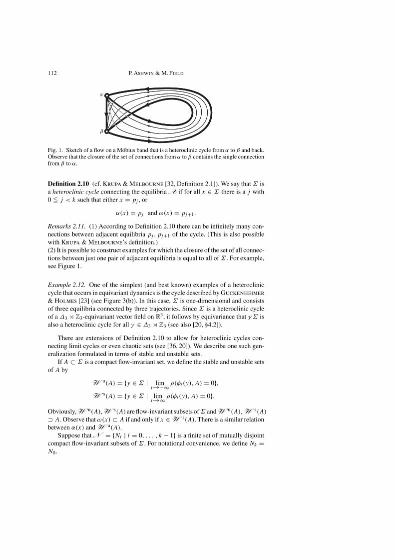
Fig. 1. Sketch of a flow on a Mobius band that is a heteroclinic cycle from α to β and back.Observe that the closure of the set of connections from α to β contains the single connectionfrom β to α.

Definition 2.10 (cf. Krupa & Melbourne [32, Definition 2.1]). We say that Σ isa heteroclinic cycle connecting the equilibria A if for all x ∈ Σ there is a j with0 5 j < k such that either x = pj , or

α(x) = pj and ω(x) = pj+1.

Remarks 2.11. (1) According to Definition 2.10 there can be infinitely many con-nections between adjacent equilibria pj , pj+1 of the cycle. (This is also possiblewith Krupa & Melbourne’s definition.)(2) It is possible to construct examples for which the closure of the set of all connec-tions between just one pair of adjacent equilibria is equal to all of Σ . For example,see Figure 1.

Example 2.12. One of the simplest (and best known) examples of a heterocliniccycle that occurs in equivariant dynamics is the cycle described by Guckenheimer& Holmes [23] (see Figure 3(b)). In this case, Σ is one-dimensional and consistsof three equilibria connected by three trajectories. Since Σ is a heteroclinic cycleof a ∆3 o Z3-equivariant vector field on R3, it follows by equivariance that γΣ isalso a heteroclinic cycle for all γ ∈ ∆3 o Z3 (see also [20, §4.2]).

There are extensions of Definition 2.10 to allow for heteroclinic cycles con-necting limit cycles or even chaotic sets (see [36, 20]). We describe one such gen-eralization formulated in terms of stable and unstable sets.

If A ⊂ Σ is a compact flow-invariant set, we define the stable and unstable setsof A by

W u(A) = {y ∈ Σ | limt→−∞ ρ(φt (y), A) = 0},

W s(A) = {y ∈ Σ | limt→∞ ρ(φt (y), A) = 0}.

Obviously, W u(A), W s(A) are flow-invariant subsets ofΣ and W u(A), W s(A)

⊃ A. Observe that ω(x) ⊂ A if and only if x ∈W s(A). There is a similar relationbetween α(x) and W u(A).

Suppose that N = {Ni | i = 0, . . . , k − 1} is a finite set of mutually disjointcompact flow-invariant subsets of Σ . For notational convenience, we define Nk =N0.


Definition 2.13. We say that Σ is a heteroclinic cycle with node set N if

(a) W u(Ni) ∩W s(Nj ) |= ∅ if and only if j = i + 1 or j = k, i = 0, and(b) ∪iW u(Ni) = ∪iW s(Ni) = Σ .

Remarks 2.14. (1) If N consists of equilibria, then Definition 2.13 is equivalentto Definition 2.10.(2) Although we have connections between nodes of the cycle, there may be few,if any, connections between proper invariant subsets of nodes.

It is worthwhile singling out a class of particularly well behaved heterocliniccycles, also called closed cycles in [4].

Definition 2.15. We say that Σ is a regular heteroclinic cycle if W u(Nj )∪{Nj+1}is closed, j = 0.

Remarks 2.16. (1) If Σ is regular, then the behavior described in Remarks 2.11(2)does not occur. For example, the Guckenheimer-Holmes cycle is regular.(2) An equivalent definition of regularity is to require that {Nj } ∪W s(Nj+1) isclosed, j = 0.(3) If the stable (or unstable) sets of the nodes are all one-dimensional, then Σ isregular.

A characteristic feature of a heteroclinic cycle is that the asymptotic dynamicsof points within the cycle is supported on the nodes of the cycle. That is, for allx ∈ Σ , we have

ω(x) ∪ α(x) ⊂ ∪iNi.

In the literature, there have been several attempts to extend the concept of aheteroclinic cyclic to allow for more complicated connections between equilibriaor other invariant sets (see, for example, [31], [16, §15], [20], [4]). The resultingconstructions are typically referred to as ‘heteroclinic networks’ or ‘heterocliniccomplexes’.

In the next section, we present a definition of a heteroclinic network that gen-eralizes these definitions. Roughly speaking, we require that asymptotic dynamicson the network is supported on the nodes of the network. The nodes may, for exam-ple, consist of equilibria or more generally compact topologically transitive sets.Our definition includes the examples of ‘cycling chaos’ found in [20, 12, 1] butnot the ‘Shilnikov’ network discussed in [20, Appendix]. It also includes the typeof cycling chaos discussed in [5] where there are connections to fixed points con-tained within chaotic attractors. Although the dynamics on the cycle is relativelysimple, we emphasize that the dynamics in a neighborhood of an embedded cycleis typically rich and complex.

2.3. Intrinsic Definition of a Heteroclinic Network

We defineC(Σ) = Σ \ R(Σ).

In the sequel, we refer to C(Σ) as the set of connections of Σ .


Lemma 2.17. If X is a compact invariant subset of Σ , then X ∩ R(Σ) |= ∅.Proof. Since R(X) = ∪x∈Xα(x)∩ω(x) ⊂ ∪x∈Σα(x)∩ω(x) = R(Σ), it followsthat R(X) ⊂ R(Σ) ∩ X. Since X is compact and invariant, R(X) |= ∅ (see [30,Chapter 3]). utDefinition 2.18. We say that (Σ, φ) has a finite nodal set if we can write R(Σ) asa finite union of disjoint, compact, connected flow-invariant subsets. The set N ofsuch subsets is referred to as the nodal set of (Σ, φ). Elements of N are referredto as the nodes.

Remarks 2.19. (1) If (Σ, φ) admits a finite nodal set, then necessarily R(Σ) isclosed and C(Σ) is open. Moreover, if it is finite then the nodal set is unique (upto re-ordering).(2) Since a node is connected and is a union of recurrent sets, it follows fromLemma 2.9 that nodes are indecomposable.

Examples 2.20. (1) Suppose that Σ is a heteroclinic cycle between the equilibriap0, . . . , pk = p0. Then Σ has finite nodal set N = {p0, . . . , pk−1}.(2) Suppose that Γ is a non-finite connected compact Lie group acting continuouslyon Σ and φ is Γ -equivariant. Suppose that (Σ, φ) has nodal set N = {Ni | 0 5i 5 k − 1}. It follows by the Γ -equivariance of φ and the connectedness of Γ thateach Ni is Γ -invariant. Let φt denote the flow induced by φt on the orbit spaceΣ = Σ/Γ . Then ˜N = {Ni/Γ | 0 5 i 5 k − 1} is a finite nodal set for (Σ, φ).In this context, it is natural to assume that each orbit space Ni/Γ is recurrent for φ.This would be the situation, for example, if the sets Ni were relative equilibria. Inparticular, Σ is a heteroclinic cycle between relative equilibria N0, . . . , Nk = N0 ifand only if Σ is a heteroclinic cycle between equilibria N0/Γ, . . . , Nk/Γ = N0/Γ .

Suppose that X is a compact subset of Σ . Define

λ+(X) = ∪x∈Xω(x),

λ−(X) = ∪x∈Xα(x),

λ1(X) = λ(X) = λ−(X) ∪ λ+(X).

Remark 2.21. If X is closed but not finite, neither ∪x∈Xω(x) nor ∪x∈Xα(x) needbe closed.

For n > 1 we define λn(X) = λ(λn−1(X))) inductively. Taking X = Σ , wehave the sequence of inclusions

Σ = λ0(Σ) ⊇ λ1(Σ) ⊇ · · · ⊇ λn(Σ) ⊇ · · · .Set Σn = λn(Σ), n = 0. We call {Σ0, Σ1, . . . } the asymptotic filtration of (Σ, φ).Obviously, Σn ⊃ R(Σ), n = 0. Moreover, since Σn is a compact flow-invariantset, each connected component of Σn has non-empty intersection with R(Σ).


Definition 2.22. We say that (Σ, φ) has depth N if

(a) ΣN = R(Σ).(b) Σn ) R(Σ), n < N .

Remarks 2.23. (1) If depth(Σ) = N , then Σn = R(Σ), n = N . In this case, weregard {Σ0, . . . , ΣN } as the asymptotic filtration.(2) depth(Σ) = 0 if and only if R(Σ) = Σ .

Example 2.24. Let Σ be a heteroclinic cycle connecting equilibria p0, . . . , pk =p0. Then depth(Σ) = 1 and the asymptotic filtration of Σ is given by Σ0 = Σ ,i.e., the whole cycle, and Σ1 = {p0, . . . , pk−1}, the set of equilibria. For example,if Σ is the Guckenheimer-Holmes cycle, then Σ1 consists of three equilibria.

Lemma 2.25. Suppose that depth(Σ) = N and that X is a compact connectedinvariant subset of Σ . There exists a unique n, 0 5 n 5 N , and a connectedcomponent Σ0

n of Σn such that

(a) X ⊂ Σ0n .

(b) X |⊂ Σn \Σn+1.

Proof. Obviously there exists a largest n 5 N such that X ⊂ Σn. Since X isconnected, X is a subset of a unique connected component Σ0

n of Σn. If X ⊂ Σn,then λ(X) ⊂ Σn+1. Since X ⊃ λ(X), it follows that X |⊂ Σn \Σn+1. utDefinition 2.26. We say that (Σ, φ) is a heteroclinic network if

(a) Σ is indecomposable.(b) Σ has a finite nodal set.(c) Σ has finite depth.

Remarks 2.27. (1) If depth(Σ) > 0, or equivalently if the set of connections C(Σ)

is non-empty, we say that the heteroclinic network is non-trivial; otherwise we saythe network is trivial.(2) Since each connected component of Σn contains at least one node, it followsthat Σn has finitely many connected components, n > 0.

Definition 2.28. If Σ is a heteroclinic network and R(Σ) is a finite set of equilibria,then we say Σ is a heteroclinic network between equilibria in R(Σ).

Lemma 2.29. Suppose that Σ is a heteroclinic network between finitely many equi-libria and that depth(Σ) = 1. Then Σ is a (possibly infinite) union of heterocliniccycles.

Proof. We are given that depth(Σ) = 1 and R(Σ) is a finite set of equilibria.Hence, if x ∈ C(Σ), we can find p, q ∈ R(Σ) such that α(x) = p, ω(x) = q.Define X1 to consist of the union of W s(p) and those equilibria which are theα-limit points of trajectories in W s(p). Iterating in the obvious way, we obtainan increasing sequence of subsets (Xn) of Σ . Since there are only finitely manyequilibria, it follows that there exists N = 1 such that Xn = XN , n = N . If


XN = Σ , we are done since then q ∈ XN and so there is a sequence of connectionsof distinct equilibria joining q to p. The required cycle is obtained by adding theconnection from p to q. We assert that XN is a closed connected flow-invariantsubset of Σ . Under this assertion, it follows that XN = Σ , since if XN |= Σ ,then Σ cannot be indecomposable (XN is a repellor). To prove the assertion, letz ∈ XN \R(Σ). Necessarily, the trajectory through z must also lie in the closure ofXN . But this implies that λ(z) ⊂ XN (otherwise depth(Σ) > 1). Hence z ∈ XN .ut

Since a heteroclinic network has an associated asymptotic filtration, it is naturalto ask whether each component of the filtration has the structure of a heteroclinicnetwork.

Theorem 2.30. Let (Σ, φ) be a heteroclinic network of depth N . For N = n > 0,Σn is a finite union of heteroclinic networks each with depth less than or equal toN − n.

Proof. We use induction on N . If N = 1, the result is trivial since λ(Σ) is a finiteunion of trivial heteroclinic networks. Suppose that the result is proved for N−1 andthat depth(Σ) = N . Recall that λ(Σ) ⊇ R(Σ) and that each connected componentof λ(Σ) intersects R(Σ). Since R(Σ) has finitely many connected components,we can conclude that λ(Σ) has finitely many connected components. Thereforewe restrict our attention to one connected component Λ of λ(Σ). Observe that if aconnected component of R(Σ) intersects Λ, then it is contained within Λ and soR(Λ) has a nodal set that is a union of connected components of R(Σ). Moreover,depth(Λ) < N , and so it only remains to prove that Λ is indecomposable.

If x ∈ Λ, there exist sequences {xn} ⊂ Λ and {yn} ⊂ Σ such that xn→x

and xn ∈ λ(yn), n = 0. Without loss of generality we assume that xn ∈ ω(yn),n = 0. Since ω(yn) is connected, it follows that ω(yn) ⊂ Λ, n = 0. But ω(yn) isindecomposable and so xn ∼ xn on ω(yn) for all n = 0. Hence xn ∼ xn on Λ andso, letting n→∞, x ∼ x. utRemark 2.31. Obviously, there are other possible ways of defining the ‘asymptoticfiltration’. For example, we could define the filtration by taking Σi to be the non-wandering set of φ|Σi−1 . This gives a nested sequence Σ0 ⊇ Σ1 ⊇ · · · that in thetransfinite limit defines the Birkhoff center of the system (see [30, pp. 129–130]). Ifwe assume finite depth, the Birkhoff center corresponds to the nodal set. However,it is possible to construct examples for which Σi is not indecomposable and soTheorem 2.30 fails (for example, see [11, §6.4]).

Definition 2.32. We say that a heteroclinic network of depth N is regular if allconnected components in Σn, 0 5 n < N , which are of depth 1 are finite unionsof regular heteroclinic cycles.

Remark 2.33. In the case of a regular heteroclinic cycle, one can represent the dy-namics as a directed graph on vertices that represent the equilibria. For heteroclinicnetworks with depth greater than 1, this is not possible since there is an x ∈ Σ

whose limits are not contained within R(Σ). For networks with depth 1, there is a


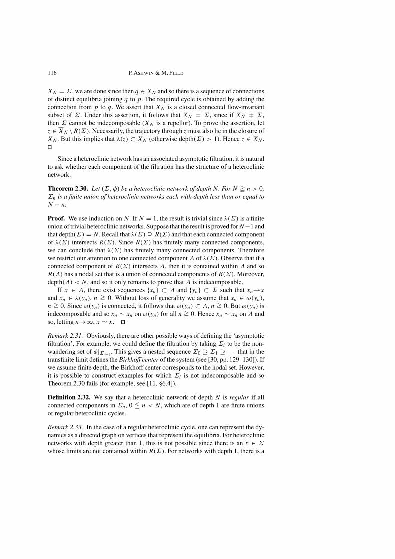
Fig. 2. The Chawanya heteroclinic network; a network with depth equal to 2.

graphical representation of the network, although this can be misleading becausein principle the set of connections between one pair of equilibria may accumulateon connections between totally unrelated equilibria. This problem is related to ourdefinition of regularity for heteroclinic cycles. See also an example of Chossat,Guyard & Lauterbach [9].

Example 2.34. An example due to Chawanya [7, 8] of a regular (and robust) hete-roclinic network of depth 2 is shown in Figure 2. This network contains a connectionbetween an equilibrium and a heteroclinic cycle. More precisely, if we let Σ ′ denotethe heteroclinic cycle a→b→c→d→a, then ω(y) = Σ ′ for all points y |= h withα(y) = {h}. Since the ω-limit set of any point in Σ ′ lies in {a, b, c, d}, it follows thatthe network has depth 2. The associated asymptotic filtration is given by Σ0 = Σ ,Σ1 = Σ ′ ∪ {e, f, g, h}, Σ2 = {a, b, . . . , h}. We remark that in Homburg [29]there is a (non-robust) example of a network where there is a connection from anequilibrium to a heteroclinic cycle.

In the next example we show how to construct a (regular) network of arbitrarydepth.

Example 2.35. Let N = 1. We construct a smooth flow φt on the torus TN =RN/(2πZ)N such that (TN, φ) is a heteroclinic network of depth N . Define φt tobe the flow of the system

θj = (1− cos θj )2 + α(1− cos θj+1), 1 5 j < N,

θN = (1− cos θN)2,

where α > 0 is a constant. Regard Tj as embedded in Tj+1 by the inclusion(θ1, . . . , θj ) 7→ (θ1, . . . , θj , 0), and T0 ⊂ TN as the point θ1 = . . . = θN = 0.

We assert that if x? ∈ TN \TN−1, then the closure of the trajectory through x?

has depth N and λ(x?) ⊂ TN−1 has depth N − 1. Given this assertion, the resultfollows easily.

The fact that for any x? ∈ TN \ TN−1 we have [φt (x?)]N → 0 as t → ∞

and [φt (x?)]N−1 winds arbitrarily many times around [0, 2π ] as long as θN(t) |= 0

proves the assertion for N = 2. Suppose the result is proved for all 2 5 n 5 N − 1


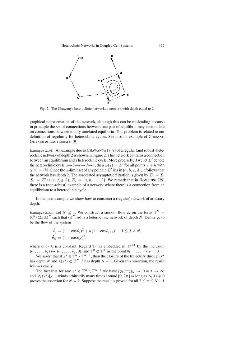
(a) Kirk–Silber network (b) Guckenheimer–Holmes network

Fig. 3. Examples of heteroclinic networks.

and pick any x? ∈ TN \ TN−1. It follows from the equation for θ ′N , that θN(t)→0as t→±∞. Hence λ(x?) ⊂ TN−1. Since θN−1(t) visits all values infinitely often,given any 0 < ξ < 2π there must be (by compactness) an accumulation point of thetrajectory having θN−1 = ξ . Therefore there exists a y? ∈ λ(x?)∩ (TN−1 \TN−2)

and so φy?(R) ⊂ λ(x?). By the inductive hypothesis, depth(φy?(R)) = N − 1.Since φx?(R) is indecomposable, it follows that depth(φx?(R)) = N .

Heteroclinic networks often occur robustly in systems with symmetry and wegive some simple examples below of heteroclinic networks that occur in equivariantdynamics. All of these examples have depth 1.

Examples 2.36. In Figure 3(a), we show the one-dimensional heteroclinic networkstudied by Kirk & Silber [31]. The network contains four equilibria A, B, C, D

and three heteroclinic cycles: A→B→D→A, A→C→D→A and A→B→C→D→A.

In Figure 3(b) we show the ∆3oZ3-orbit of the Guckenheimer & Holmes het-eroclinic cycle. Note that the network contains more cycles than just the translatesof the original cycle by elements of ∆3 oZ3. For example, a→ e→ b→ c→ d→f → a is a heteroclinic cycle.

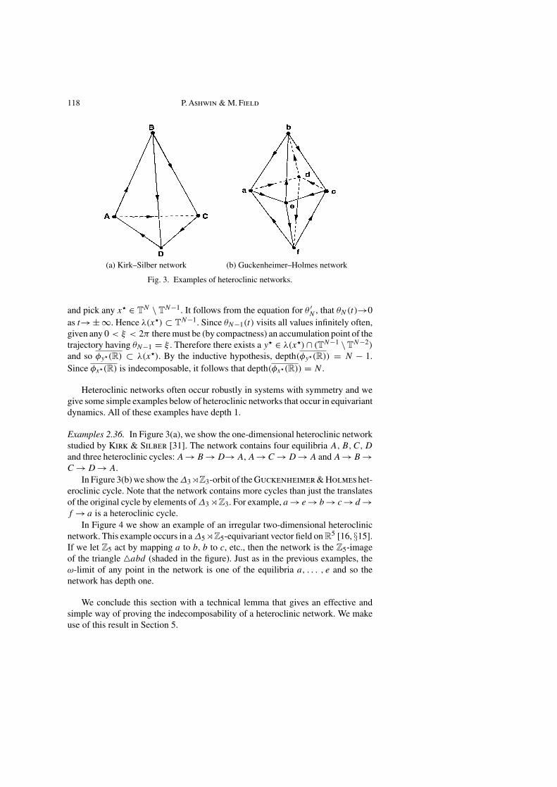
In Figure 4 we show an example of an irregular two-dimensional heteroclinicnetwork. This example occurs in a ∆5 oZ5-equivariant vector field on R5 [16, §15].If we let Z5 act by mapping a to b, b to c, etc., then the network is the Z5-imageof the triangle 4abd (shaded in the figure). Just as in the previous examples, theω-limit of any point in the network is one of the equilibria a, . . . , e and so thenetwork has depth one.

We conclude this section with a technical lemma that gives an effective andsimple way of proving the indecomposability of a heteroclinic network. We makeuse of this result in Section 5.


Fig. 4. A two-dimensional, depth-1 network.

Lemma 2.37. Suppose that Φ is a continuous flow on a compact connected metricspace Σ such that λ(Σ) ⊂ Σ ′, where Σ ′ is compact and indecomposable. ThenΣ is indecomposable.

Proof. Suppose x ∈ Σ . Either x ∈ Σ ′, and so x is chain recurrent, or x |∈ Σ ′. Inthe latter case, since λ(Σ) ⊂ Σ ′ we pick any two points y ∈ ω(x) and z ∈ α(x).Given any ε, T > 0, we can find (ε, T )-pseudo orbits from z to x and from x to y

and so z ∼ x and x ∼ y. Since Σ ′ is indecomposable, we have y ∼ z and so, bytransitivity, x ∼ x. ut

3. Dynamics and Asymptotics Near Embedded Heteroclinic Networks

Although the dynamics on a heteroclinic network are relatively simple to quan-tify, the dynamics that can occur in a neighborhood of an embedded network canbe very subtle and complex. For example, the Chawanya network arose out of astudy of a Lotka-Volterra type cubic five-dimensional system of differential equa-tions restricted to a four-dimensional hyperplane. Careful numerical investigationsby Chawanya indicate that there can be parameter values for which there areinfinitely many attractors in a neighborhood of the cycle [7, 8].

For the remainder of this section, we suppose that F is a smooth vector fieldon Rn with flow Φt . Given x, y ∈ Rn, let d(x, y) = ‖x − y‖ denote Euclideandistance, and let d(x, X) = infy∈Xd(x, y). If X is a compact Φ-invariant subsetof Rn, we define the stable and unstable sets of X by

Wu(X) = {y ∈ Rn | limt→−∞ d(Φt (y), X) = 0},

Ws(X) = {y ∈ Rn | limt→∞ d(Φt (y), X) = 0}.

If X has hyperbolic structure, then W s(X), W u(X) are fibered by smooth man-ifolds (see [30, Chapter 6]). In particular, if X is a hyperbolic equilibrium or limitcycle, then W s(X) and W u(X) are smoothly immersed manifolds. If X is not hy-perbolic, then W s(X), W u(X) typically do not have smooth structure.


On occasions, we refer to W s(X) as the basin of attraction of X. We say thatX is a (Milnor) attractor [38] if

`(W s(X)) > 0,

where `(·) is Lebesgue measure on Rn.Now suppose that Σ is a compact Φ-invariant subset of Rn and set Φt |Σ = φt .

For the remainder of this section, we assume that (Σ, φ) is a heteroclinic networkwith node set N = {N1, . . . , Nk}.

3.1. Recurrence and Attraction Near Embedded Networks

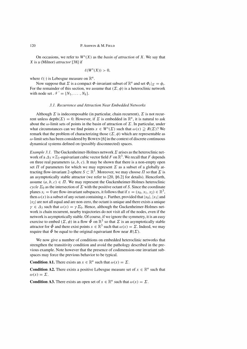
Although Σ is indecomposable (in particular, chain recurrent), Σ is not recur-rent unless depth(Σ) = 0. However, if Σ is embedded in Rn, it is natural to askabout the ω-limit sets of points in the basin of attraction of Σ . In particular, underwhat circumstances can we find points x ∈ W s(Σ) such that ω(x) ⊇ R(Σ)? Weremark that the problem of characterizing those (Σ, φ) which are representable asω-limit sets has been considered by Bowen [6] in the context of discrete continuousdynamical systems defined on (possibly disconnected) spaces.

Example 3.1. The Guckenheimer-Holmes network Σ arises as the heteroclinic net-work of a ∆3 oZ3-equivariant cubic vector field F on R3. We recall that F dependson three real parameters (a, b, c). It may be shown that there is a non-empty openset Π of parameters for which we may represent Σ as a subset of a globally at-tracting flow-invariant 2-sphere S ⊂ R3. Moreover, we may choose Π so that Σ isan asymptotically stable attractor (we refer to [20, §6.2] for details). Henceforth,assume (a, b, c) ∈ Π . We may represent the Guckenheimer-Holmes heterocliniccycle Σ0 as the intersection of Σ with the positive octant of S. Since the coordinateplanes xi = 0 are flow-invariant subspaces, it follows that if x = (x0, x1, x2) ∈ R3,then ω(x) is a subset of any octant containing x. Further, provided that |x0|, |x1| and|x2| are not all equal and are non-zero, the octant is unique and there exists a uniqueγ ∈ ∆3 such that ω(x) = γΣ0. Hence, although the Guckenheimer-Holmes net-work is chain recurrent, nearby trajectories do not visit all of the nodes, even if thenetwork is asymptotically stable. Of course, if we ignore the symmetry, it is an easyexercise to embed (Σ, φ) in a flow Φ on R3 so that Σ is an asymptotically stableattractor for Φ and there exist points x ∈ R3 such that ω(x) = Σ . Indeed, we mayrequire that Φ be equal to the original equivariant flow near R(Σ).

We now give a number of conditions on embedded heteroclinic networks thatstrengthen the transitivity condition and avoid the pathology described in the pre-vious example. Note however that the presence of codimension-one invariant sub-spaces may force the previous behavior to be typical.

Condition A1. There exists an x ∈ Rn such that ω(x) = Σ .

Condition A2. There exists a positive Lebesgue measure set of x ∈ Rn such thatω(x) = Σ .

Condition A3. There exists an open set of x ∈ Rn such that ω(x) = Σ .


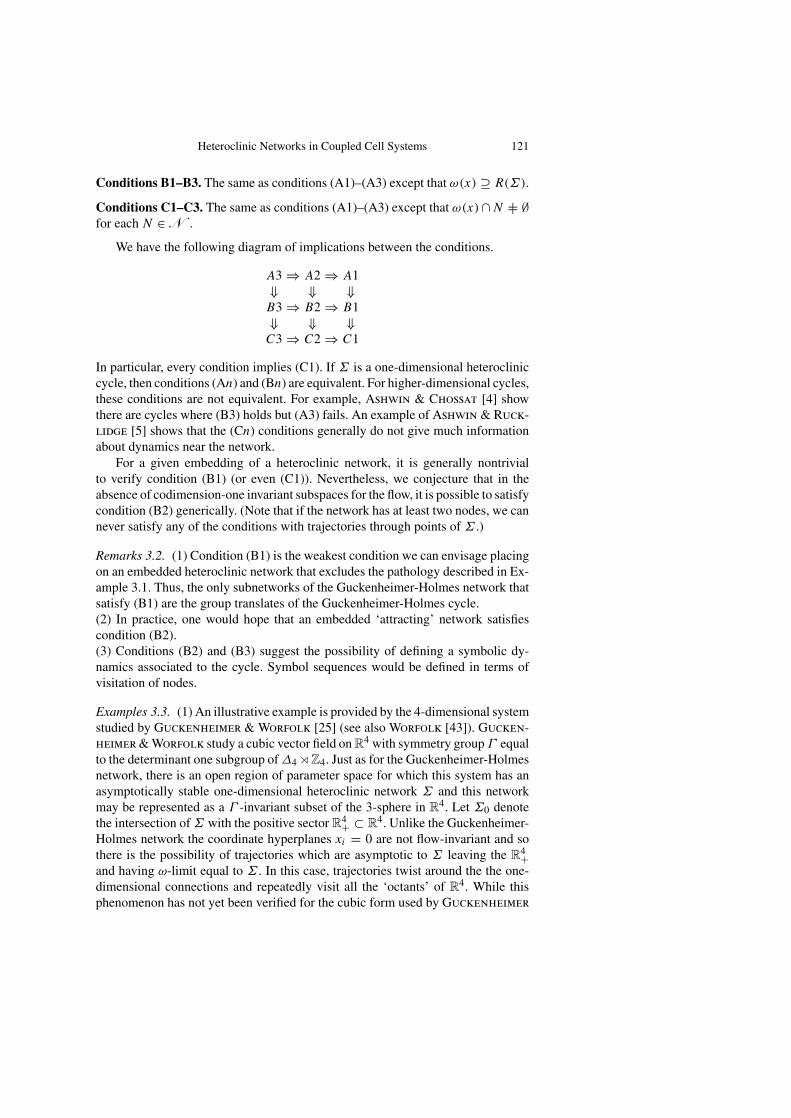
Conditions B1–B3. The same as conditions (A1)–(A3) except that ω(x) ⊇ R(Σ).

Conditions C1–C3. The same as conditions (A1)–(A3) except that ω(x)∩N |= ∅for each N ∈N .

We have the following diagram of implications between the conditions.

A3⇒ A2 ⇒ A1⇓ ⇓ ⇓B3⇒ B2⇒ B1⇓ ⇓ ⇓C3⇒ C2⇒ C1

In particular, every condition implies (C1). If Σ is a one-dimensional heterocliniccycle, then conditions (An) and (Bn) are equivalent. For higher-dimensional cycles,these conditions are not equivalent. For example, Ashwin & Chossat [4] showthere are cycles where (B3) holds but (A3) fails. An example of Ashwin & Ruck-lidge [5] shows that the (Cn) conditions generally do not give much informationabout dynamics near the network.

For a given embedding of a heteroclinic network, it is generally nontrivialto verify condition (B1) (or even (C1)). Nevertheless, we conjecture that in theabsence of codimension-one invariant subspaces for the flow, it is possible to satisfycondition (B2) generically. (Note that if the network has at least two nodes, we cannever satisfy any of the conditions with trajectories through points of Σ .)

Remarks 3.2. (1) Condition (B1) is the weakest condition we can envisage placingon an embedded heteroclinic network that excludes the pathology described in Ex-ample 3.1. Thus, the only subnetworks of the Guckenheimer-Holmes network thatsatisfy (B1) are the group translates of the Guckenheimer-Holmes cycle.(2) In practice, one would hope that an embedded ‘attracting’ network satisfiescondition (B2).(3) Conditions (B2) and (B3) suggest the possibility of defining a symbolic dy-namics associated to the cycle. Symbol sequences would be defined in terms ofvisitation of nodes.

Examples 3.3. (1) An illustrative example is provided by the 4-dimensional systemstudied by Guckenheimer & Worfolk [25] (see also Worfolk [43]). Gucken-heimer & Worfolk study a cubic vector field on R4 with symmetry group Γ equalto the determinant one subgroup of ∆4 oZ4. Just as for the Guckenheimer-Holmesnetwork, there is an open region of parameter space for which this system has anasymptotically stable one-dimensional heteroclinic network Σ and this networkmay be represented as a Γ -invariant subset of the 3-sphere in R4. Let Σ0 denotethe intersection of Σ with the positive sector R4+ ⊂ R4. Unlike the Guckenheimer-Holmes network the coordinate hyperplanes xi = 0 are not flow-invariant and sothere is the possibility of trajectories which are asymptotic to Σ leaving the R4+and having ω-limit equal to Σ . In this case, trajectories twist around the the one-dimensional connections and repeatedly visit all the ‘octants’ of R4. While thisphenomenon has not yet been verified for the cubic form used by Guckenheimer


& Worfolk, it can be shown that condition (A2) is satisfied for generic vectorfields near the cubic normal form.(2) The example of Kirk & Silber [31], shown in Figure 3(a), gives an examplewhere none of the conditions (A1)–(B3) is satisfied. This is because of the pres-ence of codimension-one invariant subspaces. Kirk & Silber show that points areattracted to one of two possible subcycles.

3.2. Averaged Behavior Near Embedded Networks

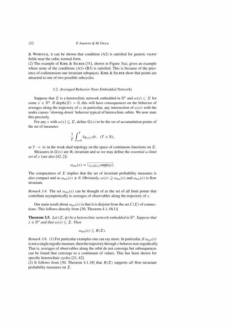
Suppose that Σ is a heteroclinic network embedded in Rn and ω(x) ⊂ Σ forsome x ∈ Rn. If depth(Σ) > 0, this will have consequences on the behavior ofaverages along the trajectory of x; in particular, any intersection of ω(x) with thenodes causes ‘slowing-down’ behavior typical of heteroclinic orbits. We now statethis precisely.

For any x with ω(x) ⊆ Σ , define �(x) to be the set of accumulation points ofthe set of measures

1

T

∫ T

t=0δΦt (x) dt, (T ∈ R),

as T →∞ in the weak dual topology on the space of continuous functions on Σ .Measures in �(x) are Φt -invariant and so we may define the essential ω-limit

set of x (see also [42, 2])

ωess(x) = ∪µ∈�(x)supp(µ).

The compactness of Σ implies that the set of invariant probability measures isalso compact and so ωess(x) |= ∅. Obviously, ω(x) ⊇ ωess(x) and ωess(x) is flowinvariant.

Remark 3.4. The set ωess(x) can be thought of as the set of all limit points thatcontribute asymptotically to averages of observables along the trajectory of x.

Our main result about ωess(x) is that it is disjoint from the set C(Σ) of connec-tions. This follows directly from [30, Theorem 4.1.18(1)]

Theorem 3.5. Let (Σ, φ) be a heteroclinic network embedded in Rn. Suppose thatx ∈ Rn and that ω(x) ⊆ Σ . Then

ωess(x) ⊆ R(Σ).

Remark 3.6. (1) For particular examples one can say more. In particular, if ωess(x)

is not a single ergodic measure, then the trajectory throughx behaves non-ergodically.That is, averages of observables along the orbit do not converge but subsequencescan be found that converge to a continuum of values. This has been shown forspecific heteroclinic cycles [21, 42].(2) It follows from [30, Theorem 4.1.18] that R(Σ) supports all flow-invariantprobability measures on Σ .


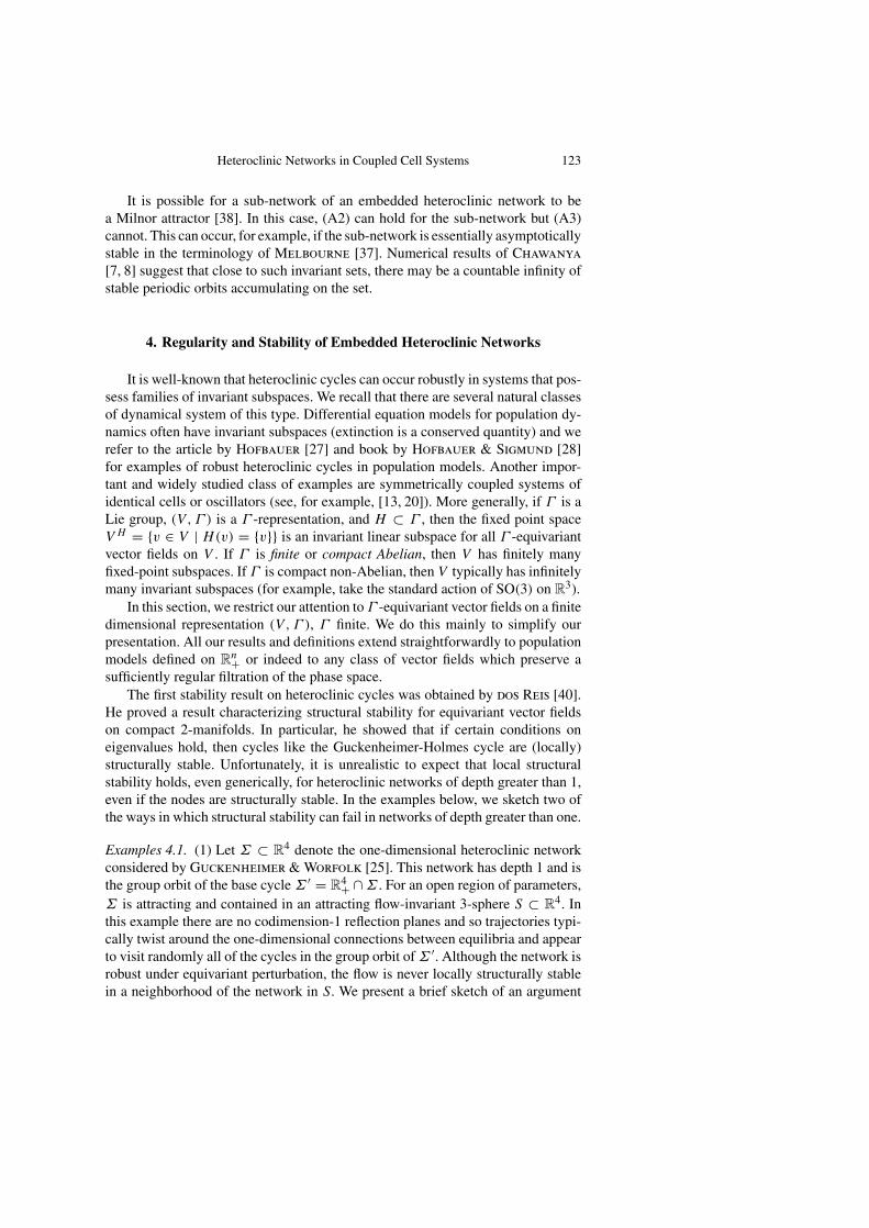
It is possible for a sub-network of an embedded heteroclinic network to bea Milnor attractor [38]. In this case, (A2) can hold for the sub-network but (A3)cannot. This can occur, for example, if the sub-network is essentially asymptoticallystable in the terminology of Melbourne [37]. Numerical results of Chawanya[7, 8] suggest that close to such invariant sets, there may be a countable infinity ofstable periodic orbits accumulating on the set.

4. Regularity and Stability of Embedded Heteroclinic Networks

It is well-known that heteroclinic cycles can occur robustly in systems that pos-sess families of invariant subspaces. We recall that there are several natural classesof dynamical system of this type. Differential equation models for population dy-namics often have invariant subspaces (extinction is a conserved quantity) and werefer to the article by Hofbauer [27] and book by Hofbauer & Sigmund [28]for examples of robust heteroclinic cycles in population models. Another impor-tant and widely studied class of examples are symmetrically coupled systems ofidentical cells or oscillators (see, for example, [13, 20]). More generally, if Γ is aLie group, (V , Γ ) is a Γ -representation, and H ⊂ Γ , then the fixed point spaceV H = {v ∈ V | H(v) = {v}} is an invariant linear subspace for all Γ -equivariantvector fields on V . If Γ is finite or compact Abelian, then V has finitely manyfixed-point subspaces. If Γ is compact non-Abelian, then V typically has infinitelymany invariant subspaces (for example, take the standard action of SO(3) on R3).

In this section, we restrict our attention to Γ -equivariant vector fields on a finitedimensional representation (V , Γ ), Γ finite. We do this mainly to simplify ourpresentation. All our results and definitions extend straightforwardly to populationmodels defined on Rn+ or indeed to any class of vector fields which preserve asufficiently regular filtration of the phase space.

The first stability result on heteroclinic cycles was obtained by dos Reis [40].He proved a result characterizing structural stability for equivariant vector fieldson compact 2-manifolds. In particular, he showed that if certain conditions oneigenvalues hold, then cycles like the Guckenheimer-Holmes cycle are (locally)structurally stable. Unfortunately, it is unrealistic to expect that local structuralstability holds, even generically, for heteroclinic networks of depth greater than 1,even if the nodes are structurally stable. In the examples below, we sketch two ofthe ways in which structural stability can fail in networks of depth greater than one.

Examples 4.1. (1) Let Σ ⊂ R4 denote the one-dimensional heteroclinic networkconsidered by Guckenheimer & Worfolk [25]. This network has depth 1 and isthe group orbit of the base cycle Σ ′ = R4+ ∩Σ . For an open region of parameters,Σ is attracting and contained in an attracting flow-invariant 3-sphere S ⊂ R4. Inthis example there are no codimension-1 reflection planes and so trajectories typi-cally twist around the one-dimensional connections between equilibria and appearto visit randomly all of the cycles in the group orbit of Σ ′. Although the network isrobust under equivariant perturbation, the flow is never locally structurally stablein a neighborhood of the network in S. We present a brief sketch of an argument


showing the failure of local structural stability. We associate to each forward tra-jectory asymptotic to Σ ′ a symbol sequence identifying the ordered sequence ofedges in Σ ′ visited by the trajectory (we ignore the measure-zero set of trajectorieswhich are asymptotic to one of the equilibria in the network). The symbol sequenceof a trajectory is then a conjugacy invariant of the trajectory (we may assume theconjugacy is C0-close to the identity map). By making arbitrarily small perturba-tions supported near a single edge we can change the order of symbol sequencesand hence structural stability fails.(2) It is possible to modify the Guckenheimer-Holmes cycle and obtain a cycleΣ ⊂ R6 between three limit cycles which has two-dimensional connections andeach pair of cycles lying in a four-dimensional fixed point space. We may furtherrequire that Σ be attracting and that Σ be contained in an attracting flow-invariant5-sphere S. In this case, the flow is not structurally stable in a neighborhood ofΣ ⊂ S because of the appearance of moduli of stability [39] such as ratios ofeigenvalues of linearizations near fixed points. In fact the codimension of the C0-equivalence class of the flow is infinite.

In spite of the limited prospects of obtaining satisfactory conjugacy or structuralstability results for networks, or even higher-dimensional cycles, there are still goodstability questions one can ask. In particular, we would like to have some stabilityin the asymptotics and symmetry properties of the network. This stability shouldbe related to the structure of the invariant subspaces of our phase space. Our aimin this section is to formulate a verifiable concept of robustness for heteroclinicnetworks in a symmetric system.

4.1. Orbit Strata

Henceforth, we assume thatΓ is a finite group and (V , Γ ) is a finite-dimensionalreal Γ -representation.

If J ⊂ Γ , we let V J denote the fixed point set of J acting on V . Obviously, V J

is a linear subspace of V and is equal to the fixed-point subspace of the subgroupof Γ generated by J . It is known (see below) that there is an open and dense subsetU of V J such that all points in U have the same isotropy, say H , and

V J = V H .

It follows that the set of invariant linear subspaces of V is parametrized by the setI = I (V , Γ ) of isotropy groups for the action of Γ on V . Let V (H) denote theset of points in V H with isotropy group equal to H . Then

V (H) = V H \⋃

J)H,J∈IV J ,

and so V (H) is open and dense in V H .Let 〈H 〉 denote the conjugacy class of H in Γ and define

V 〈H 〉 =⋃

J∈〈H 〉V (J ).


The collection {V 〈H 〉 | H ∈ I (V, Γ )} defines the stratification of V by iso-tropy type or the orbit stratification of V . We call connected components of V 〈H 〉orbit strata. Note that V 〈H 〉 consists of at least |Γ/H | orbit strata. We let S (V , Γ ),or just S , denote the set of all orbit strata. If X is a smooth Γ -equivariant vectorfield on V , then the orbit strata are all invariant by the flow of X.

Let S be a stratum of the orbit stratification and let ∂S denote the frontier of S.Using the linearity of the Γ -action, we can show that if H ∈ I , then

∂V 〈H 〉 ∩ V 〈J 〉 |= ∅ ⇐⇒ J ) H and ∂V 〈H 〉 ⊃ V 〈J 〉.

Example 4.2. The symmetry group associated to the Guckenheimer-Holmes cycleis the semi-direct product ∆3 o Z3, and ∆3 o Z3 acts linearly on R3. Defineconnected subsets of R3 by V0 = {(0, 0, 0)}, V1 = {(x, 0, 0) | x > 0}, V2 ={(x, x, x) | x > 0}, V3 = {(x, y, 0) | x, y > 0}, V4 = {(x, y, z) | x, y, z > 0} \V2. The orbit stratification of R3 is given as the union of the ∆3 o Z3-orbits ofV0, . . . , V4. Thus, γVj is a connected orbit stratum for all γ ∈ ∆3 oZ3. All pointsin ∆3 o Z3(Vj ) have the same isotropy type, and x, y ∈ R3 have the same isotropytype if and only if x, y ∈ ∆3 o Z3(Vj ) for some (unique) j .

4.2. Relating the Asymptotic Filtration to the Orbit Stratification

Let Σ ⊂ V be a ‘robust’ heteroclinic network for a Γ -equivariant flow Φ onV and suppose that depth(Σ) = N . Let x ∈ Σ and suppose that x lies in the orbitstratum S ∈ S . Provided that x |∈ R(Σ), it is often the case that λ(x) ⊂ ∂S.Indeed, the existence of a robust cycle between equilibria, implies that we have atleast one non-transverse saddle connection between equilibria. The only way thesecan persist under equivariant perturbation is if at least some of the equilibria lie inthe frontier of the orbit strata containing the connections.

We restrict our attention to networks where we have the strongest relationbetween the asymptotic filtration of the network to the orbit stratification of V .It should be possible to weaken our requirements to allow for cycles like thoseconstructed by Matthews et al. [35] (see below).

Suppose that Σ has asymptotic filtration {Σ = Σ0, Σ1, . . . , ΣN }. Given j ∈{0, . . . , N}, we recall that Σj can be written (uniquely) as a finite union Σj =∪p(j)

i=1 Σij of heteroclinic networks, each of depth less than or equal to N − j .Let A(Σ) denote the set of all subnetworks of Σ derived in this way from theasymptotic filtration. Suppose that S ∈ A. Denote the asymptotic filtration of S

by {S0, . . . , SM}, where M = depth(S). For 0 5 k 5 M , let ρk(S) be the minimalunion of orbit strata such that

Sk \ Sk+1 ⊂ ρk(S).

Set F(S) = (ρ0(S), . . . , ρk−1(S)). We call F(S) the orbit flag of S.

Definition 4.3. Let Σ, Σ ′ be heteroclinic networks. We say that Σ, Σ ′ are iso-morphic if there is a bijection ι : A(Σ)→A(Σ ′) such that for all S ∈ A(Σ),F(S) = F(ι(S)).


Definition 4.4. Let S ∈A(Σ). We say that S is symmetry adapted if

Sk+1 ⊂ ∂ρk(S), 0 5 k < depth(S).

If all the heteroclinic subnetworks in A(Σ) are symmetry adapted, we say thatΣ is symmetry adapted.

Example 4.5. The Guckenheimer-Holmes network is symmetry adapted as indeedare all the edge cycles and networks described in [20, Chapter 6]. So also is theKirk-Silber network [31]. However, the robust heteroclinic cycle of Matthewset al. [35] is not symmetry adapted as there are connections between equilibriawithin a fixed orbit stratum. In other words, their cycle includes connections thatlimit to equilibria with the same symmetry as the points on the connecting orbit.

4.3. Robustness of Networks

Definition 4.6. Let Σ be a symmetry adapted heteroclinic network for the Γ -equivariant vector field X. We say that Σ is geometrically robust if for every openΓ -invariant neighborhood U of Σ , we can find an open neighborhood U of X inthe C1-topology such every Y ∈U has a heteroclinic network ΣY ⊂ U such thatΣY is symmetry adapted and A(Σ) is isomorphic to A(ΣY ).

Example 4.7. The Guckenheimer-Holmes network is geometrically robust as in-deed are all the edge cycles and networks described in [20, Chapter 6]. So also isthe Kirk-Silber network [31].

5. A Coupled Cell System

We think of a cell as being a low-dimensional ordinary differential equationthat can be coupled to other cells. In this way we can build up a higher-dimensionaldynamical system with desired symmetries that can have specifiable properties suchas a heteroclinic network.

In particular, we consider a coupled-cell network consisting of nine cells, eachwith one degree of freedom, coupled directionally such that the network has globalZ3 × Z3 symmetry. To simplify notation, we write Z3 × Z3 = Z(3, 3). We shallassume that each of the cells has an independent internal Z2 symmetry. We maythink of this system as a coupling of three Guckenheimer-Holmes models [23] ina ring. The symmetry group Γ of the system is ∆9 o Z(3, 3) or, equivalently, thewreath-product Z2 o Z(3, 3) [13]. Some of the dynamical and bifurcation theoreticconsequences of wreath-product symmetries are discussed in [13] (see also theworks [16, 20] which treat similar groups in semi-direct rather than wreath-productnotation).

The phase space we work with is R9. We regard R9 as (R3)3 and denote pointsin R9 as 3-tuples (x, y, z), where x = (x0, x1, x2), y = (y0, y1, y2) and z =(z0, z1, z2).

Let σ be a generator of Z3 and define an action of Z3 on R3 by σ(x, y, z) =(y, z, x). We let κ : R3→R3 be defined by κ(x, y, z) = (−x, y, z).


The action of Γ on R9 is generated by

ρ1(x, y, z) = (σx, σy, σz),

ρ2(x, y, z) = (y, z, x),

κ0x (x, y, z) = (κx, y, z).

Note that

Z3 × Z3 = 〈ρ1, ρ2〉,and that Z3×Z3 is a transitive subgroup of S9. Consequently, in order to specify aΓ -equivariant differential equation on R9 it suffices to write down one componentof the equation (see [16]).

In the sequel we use the following notational conventions. Let A = (a0, a1, a2),B = (b0, b1, b2), . . . denote general points of R3. We let A0 denote a point(0, a1, a2) of R3 with first coordinate zero. If x ∈ R3, A ∈ R3, we define

A(x2) = a0x20 + a1x

21 + a2x

22 .

If X = (x, y, z) ∈ R9, we define ‖X‖2 = ‖x‖2 + ‖y‖2 + ‖z‖2, where ‖ ‖denotes the Euclidean norm.

We consider two modelΓ -equivariant vector fields whose dynamics are uniquelydetermined by their first component:

x0 = x0(1− ‖X‖2 + A0(x2)+ B(y2)+ C(z2)),(5)

x0 = x0(1− ‖X‖2 + A0(x2)+ B(y2)+ C(z2))+ x0(dx2

1x22 + ey2

0z20).(6)

Both vector fields consist of a general Γ -equivariant cubic polynomial. In (6),fifth-order terms with (small) coefficients d and e have been added to the secondvector field in order to break a degeneracy of the third-order system; see [1]. Thecoefficient of the radial term x0‖X‖2 is chosen to be−1 so that if ‖A0‖, ‖B‖, ‖C‖are sufficiently small, then the conditions of the invariant-sphere theorem hold [15].That is, near the origin of R9, the dynamics of both systems are forward asymptoticto a flow-invariant 8-sphere, S ⊂ R9.

In fact, we will often discuss a system that has more symmetry. Let ρ3 ∈ S9 bedefined by

ρ3(x, y, z) = (σx, y, z),

where σ is a generator of Z3. Let H = 〈ρ1, ρ2, ρ3〉 and set Γ ? = ∆9 oH . In termsof wreath products we have

Γ ? = (Z2 o Z3) o Z3.

The system (5) is Γ ?-equivariant if and only if B = (b, b, b) and C = (c, c, c),for some b, c ∈ R.

We emphasize that all of the phenomena we describe below persist under per-turbations with only ∆9 symmetry.


5.1. Equilibria

In order to describe the equilibria of (6) it is easiest to work with the truncatedcubic system (5). It follows from [16, §§13, 14] that there is an open and densesemialgebraic subset R of R8 such that if (A0, B, C) ∈R, then all equilibria of(5) are hyperbolic. Consequently, for fixed (A0, B, C) ∈R, the equilibria of (6) arehyperbolic for sufficiently small |d|, |e|. Moreover, the isotropy of the equilibria isthe same as in the truncated system. That is, the symmetry of equilibria is unchangedif we perturb (6) by higher-order symmetric terms.

Using the results of [16, §§13, 14] enables us to give a useful ‘parametrization’of the equilibria that occur for (A0, B, C) ∈ R. First, however, we need somepreliminaries. We define a fundamental domain for the action of ∆9:

R9+ = {(x0, . . . , z2) | x0, . . . , z2 = 0}.Since ∆9 ⊂ Γ , it is clear that if X is an equilibrium of (5), then we can find δ ∈ ∆9such that δX ∈ R9+. Consequently, to describe the set of equilibria of (5), it sufficesto find the equilibria lying in R9+. Since R9+ is Z(3, 3)-invariant for the flow of (5),it follows that the action of Z(3, 3) restricts to an action on R9+.

Let E denote the Z(3, 3)-invariant subset of R9+ consisting of all non-zerovectors V such that each component of V lies in {0,+1}. It is shown in [16] thatif X ∈ R9+ is a hyperbolic equilibrium of (5), then there exists a unique pointV ∈ E such that ΓX = ΓV (equivalently, Z(3, 3)X = Z(3, 3)V). If V ∈ E , thenV = (a, b, c), where a, b, c ∈ R3. In future, we just set V = abc. If a = (0, 0, 0),we write a = 0. If a = (1, 0, 0), we set a = 1 and if a = (1, 1, 1), we set a = 3.In the sequel, if X ∈ R9+ is an equilibrium, we usually set X = pa, where a is theunique point in E such that ΓX = Γa.

As an easy application of the methods in [16] (see also [20]), we have

Lemma 5.1. An equilibrium X ∈ R9+ of (6), (5) has maximal isotropy type if andonly if X corresponds to a point on the Z(3, 3)-orbit of 100 or 111 or 300 or 333.All other equilibria have submaximal isotropy type. The same result also holds ifequations are Γ ?-equivariant (with Z(3, 3) replaced by the subgroup of Γ ? leavingR9+ invariant).

If V ∈ E is not maximal, (5) may have no equilibria with isotropy equal toΓV. In fact, corresponding to each submaximal V ∈ E it is possible to computeexplicit equations and inequalities that determine the closed subset of R8 for whichthere are no equilibria with isotropy equal to ΓV. In practice, these computations,although quite tractable, can be complicated (see [16, §14]). The following resultwill suffice for our needs.

Lemma 5.2. There is a nonempty open subset D of R such that if (A0, B, C) ∈D , then (5) has no equilibria with isotropy group equal to Γab0, where a, b rangeover all 3-tuples for which Γab0 is submaximal.

Proof. Let us start by assuming that (5) is Γ ?-equivariant. Let R? ⊂ R4 bethe open and dense semialgebraic subset consisting of all A0, B = (b, b, b) and


C = (c, c, c) for which (5) has only hyperbolic equilibria. Let D ? denote theopen subset of R? corresponding to which (5) has no equilibria with submaximalisotropy equal to Γab0.

Straightforward computations show that a point (a1, a2, b, c) ∈R? lies in D ?

if and only if

a1a2 < 0,

bc < 0,

(3c − a1 − a2)b < 0,

(3c − a1 − a2)(3b − a1 − a2) < 0.

Hence D ? |= ∅. But now every point of D ? determines an interior pointof D . ut

5.2. Stabilities of the Equilibria p100 and p300

It is straightforward to compute the eigenvalues and eigenspaces of the lin-earization of (5) at the equilibria p100 and p300. The eigenvalues at p100 may bewritten as the 3-tuple

([−2, a2, a1], [c0, c1, c2], [b0, b1, b2]),(7)

where the eigenvalue−2 corresponds (as always) to the radial direction. The triples[−2, a2, a1], [c0, c1, c2], and [b0, b1, b2] respectively correspond to eigenvaluesof the linearization in the x-hyperplane, y-hyperplane and z-hyperplane. (Each ofthese subspaces is invariant by the flow of (5).) For every eigenvalue, the eigenvectorcan be taken to be the unit vector along the corresponding coordinate axis.

The eigenvalues at p300 are given by the triple([− 2,

a1 + a2 ± ı√

3(a1 − a2)

a1 + a2 − 3

],

[c0 + c1 + c2

3− (a1 + a2)

],

[b0 + b1 + b2

3− (a1 + a2)

]).(8)

The single eigenvalues associated to the y, and z-spaces occur with multiplicity3. The eigenvalues in the x-space are exactly those that occur in the linearizationanalysis of the Guckenheimer-Holmes cycle (see [16, §15] or [20, Chapter 6]).

5.3. The Invariant-Sphere Theorem

We recall some details on the invariant-sphere theorem. Suppose that X is asmooth vector field on Rn of the form X(x) = x+Q(x), where Q is a homogeneouscubic polynomial. If we define

m(Q) = inf{(Q(u), u) | u ∈ Rn, ‖u‖ = 1},M(Q) = sup{(Q(u), u) | u ∈ Rn, ‖u‖ = 1},

then for all x ∈ Rn

m(Q)‖x‖4 5 (Q(x), x) 5 M(Q)‖x‖4.


If M(Q) < 0, then (Q(x), x) < 0 for all x ∈ Rn, x |= 0. If this condition onQ holds, we say that Q is contracting. It is shown in [20, Chapter 5] that if Q

is contracting, then there exists a topologically embedded flow-invariant (n − 1)-sphere S for the flow of x = X(x) such that ω(x) ⊂ S for all x ∈ Rn, x |= 0.Moreover, the invariant sphere S is contained in the annulus A(r, R) = {x | r 5‖x‖ 5 R}, where

r =√−1

M(Q), R =

√−1

m(Q).

In general, S is not differentiably embedded.For a ∈ R, define Qa(x) = Q(x) + a‖x‖2x, Xa = I + Qa . Obviously,

M(Qa) = M(Q)+ a, m(Qa) = m(Q)+ a. It follows by rescaling and the theoryof normal hyperbolic sets [26] that if we fix Q, N ∈ N, we can find aN ∈ R

such that if a 5 aN , then Qa is contracting and the corresponding invariant sphereS = Sa is embedded as a CN -submanifold of Rn.

Remark 5.3. If a 5 aN , the invariant sphere Sa is contained in the annulus A(r, R),

where r =√

−1M(Q)+a

, R =√

−1m(Q)+a

. In particular, r→0, R/r→1 as a→−∞.

It follows from the previous remark that if we are given Q and N ∈ N, we canrescale so that R < 1, for all a 5 aN .

Suppose that Z is a smooth vector field on Rn. Let ‖Z‖1 denote the uniformC1-norm of Z restricted to the unit ball. As a straightforward consequence of thetheory of normally hyperbolic sets, we have the following differentiable version ofthe invariant-sphere theorem.

Theorem 5.4 (cf. [15, Theorem 5.2]). Let N ∈ N and let Q be a homogeneouscubic polynomial on Rn. We may choose aN ∈ R and δ > 0 such that if Z isa smooth vector field on Rn satisfying Z(0) = 0, DZ(0) = 0, and ‖Z‖1 < δ,then for a 5 aN the vector field Za(x) = x + Qa(x) + Z(x) has a unique CN

flow-invariant (n−1)-sphere S contained in the unit ball of Rn. Further, ω(x) ⊂ S

for all x ∈ Rn, 0 < ‖x‖ 5 1.

Remark 5.5. In practice, we apply Theorem 5.4 whenQ is the third-order truncationof a smooth vector field on Rn and Z is the remainder term. Roughly speaking, thetheorem implies that if X(x) = x +Q(x) +O(‖x‖4) is a smooth vector field onRn, then we can add a cubic term a‖x‖2x, so that if a is sufficiently negative theresulting equation has a differentiably embedded flow-invariant sphere containingthe origin.

We use the invariant-sphere theorem in our study of dynamics of (6) in thefollowing way. First of all, we consider the cubic truncation (5). Provided that thehomogeneous cubic part is contracting, all non-trivial trajectories of (5) are forwardasymptotic to a flow-invariant embedded 8-sphere. Further, for an open dense setof coefficients A0, B, C, all equilibria of (5) are hyperbolic. The hyperbolicity ofequilibria persists if we add on a term a‖X‖2X, a < 0, except at possibly finitely


many values of a. For sufficiently negative values of a, the invariant sphere can bemade to have any prescribed finite order of differentiability. If the invariant sphereis at least of class C1 (in fact, C0 in our case), we can add on small fifth- andhigher-order terms without changing stability or destroying the invariant sphere.(Of course, dynamics on the invariant sphere may and do change.)

5.4. Connections

We recall that there exists a nonempty open subset D of R8 such that if(A0, B, C) ∈ D , then (5) has no equilibria of submaximal isotropy type in (x, y)-space (Lemma 5.2). In particular, all equilibria in (x, y)-space are of maximalisotropy type and lie in {(x, y) | x = 0 or y = 0}. Let D ′ denote the nonemptyopen subset of D consisting of coefficient values for which the conditions ofthe invariant-sphere theorem hold (C0-invariant spheres suffice). We investigateconnections between equilibria in x-space and y-space under the assumption that(A0, B, C) ∈ D ′.

First, we need some notation. Let Z3 = 〈ρ1〉, and recall that ρ1 acts on the R9 bysimultaneous cyclic permutation of coordinates in the x-, y- and z-coordinate sub-spaces. We also set Z3 = 〈ρ2〉, and recall that ρ2 cyclically permutes the coordinatesubspaces.

We write 100−→010, if there exist ρ, δ ∈ Z3 such that there is a connectionfrom ρp100 = pρ100 to δp010. That is, if W u(ρp100)∩W s(δp010) |= ∅. Note that itfollows by Z3-equivariance that if there is a connection from ρp100 to δp010, thenthere are connections from ρ

j

1 ρp100 to ρj

1 δp010, for j = 1, 2.If there are connections from ρp100 to δp010 for all ρ, δ ∈ Z3, we write

100 ⇒ 010.

We generalize this notation to allow for connections between 300 and 030 or 010.Of course, it follows by Z3-equivariance that

100 −→ 030 H⇒ 100 ⇒ 030,

300 −→ 030 H⇒ 300 ⇒ 030,

300 −→ 010 H⇒ 300 ⇒ 010.

Lemma 5.6. There is a nonempty open subset D ? of D ′ such that if (A0, B, C) ∈D ?, then (5) has connections

100 ⇒ 010, 100 ⇒ 030, 300 ⇒ 010, 300 ⇒ 030.

All of these connections persist for small values of e, f .

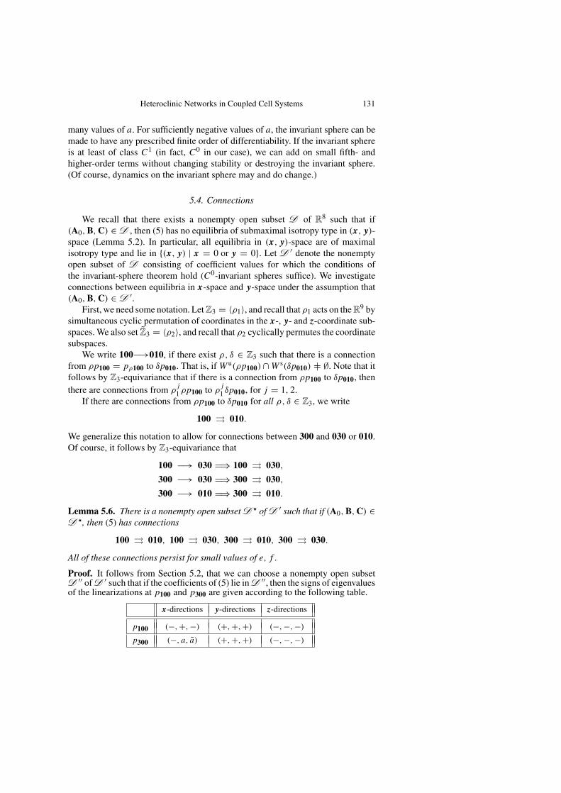
Proof. It follows from Section 5.2, that we can choose a nonempty open subsetD ′′ of D ′ such that if the coefficients of (5) lie in D ′′, then the signs of eigenvaluesof the linearizations at p100 and p300 are given according to the following table.

x-directions y-directions z-directions

p100 (−,+,−) (+,+,+) (−,−,−)

p300 (−, a, a) (+,+,+) (−,−,−)


Note that a, a signify that there is a complex conjugate pair of eigenvalues withnonzero real part.

Let P denote the 2-plane in (xy)-space defined by P = {(x, 0, 0, y, 0, 0) |x, y ∈ R}. Observe that P is a fixed-point subspace of R9-space and hence P isinvariant by the flow of (5). If we set P+ = R6+ ∩ P , then P+ is also invariant bythe flow of (5). The intersection of P+ with the invariant sphere is a flow-invariantarc joining p100 to p010. Since the only equilibria on the arc are p100 and p010, itfollows that there is a connection from p100 to p010. Similarly, we may show thatthere is a connection from ρp100 to τp010 for all ρ, τ ∈ 〈ρ1〉. Hence 100 ⇒ 010. Asimilar argument proves that 300 ⇒ 030

For the remaining cases, we start by working with the group Γ ?. Each pair ofequilibria that we wish to prove connected are then contained in a two-dimensionalfixed point space of Γ ? and intersection with the invariant sphere then gives aconnecting flow-invariant arc. Connections persist when we break symmetry fromΓ ? to Γ and hence we obtain the required open subset D ? of D ′.

Finally, these connections persist if we allow e, d to be nonzero but small. ut

6. Heteroclinic Cycles

In this section, we describe a variety of nontrivial robust heteroclinic networkspresent in the model systems (5) and (6). We present numerical simulations illus-trating the asymptotic behavior of trajectories near these networks. For simplicity,we work entirely within the flow-invariant region R9+.

6.1. A Depth-1 Heteroclinic Network

We assume that the coefficients of (5) lie in the region D ? described byLemma 5.6. In particular,

(a) The system (5) has an attracting invariant sphere S.(b) The signs of the eigenvalues of the linearization of (5) at p100 and p300 are

given by

(−,+,−,+,+,+,−,−,−) and (−, a, a,+,+,+,−,−,−),

respectively.(c) There are no submaximal equilibria in (x, y)-space.

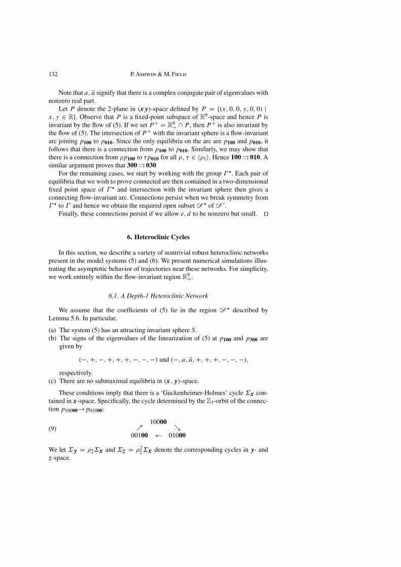
These conditions imply that there is a ‘Guckenheimer-Holmes’ cycle Σx con-tained in x-space. Specifically, the cycle determined by the Z3-orbit of the connec-tion p10000→p01000:

10000↗ ↘00100 ← 01000

(9)

We let Σy = ρ2Σx and Σz = ρ22Σx denote the corresponding cycles in y- and

z-space.


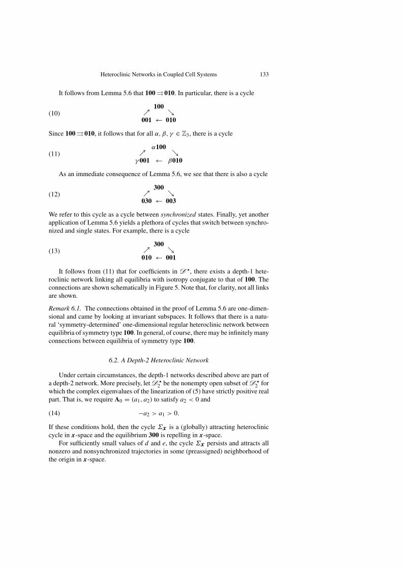
It follows from Lemma 5.6 that 100 ⇒ 010. In particular, there is a cycle

100↗ ↘001 ← 010

(10)

Since 100 ⇒ 010, it follows that for all α, β, γ ∈ Z3, there is a cycle

α100↗ ↘γ 001 ← β010

(11)

As an immediate consequence of Lemma 5.6, we see that there is also a cycle

300↗ ↘030 ← 003

(12)

We refer to this cycle as a cycle between synchronized states. Finally, yet anotherapplication of Lemma 5.6 yields a plethora of cycles that switch between synchro-nized and single states. For example, there is a cycle

300↗ ↘010 ← 001

(13)

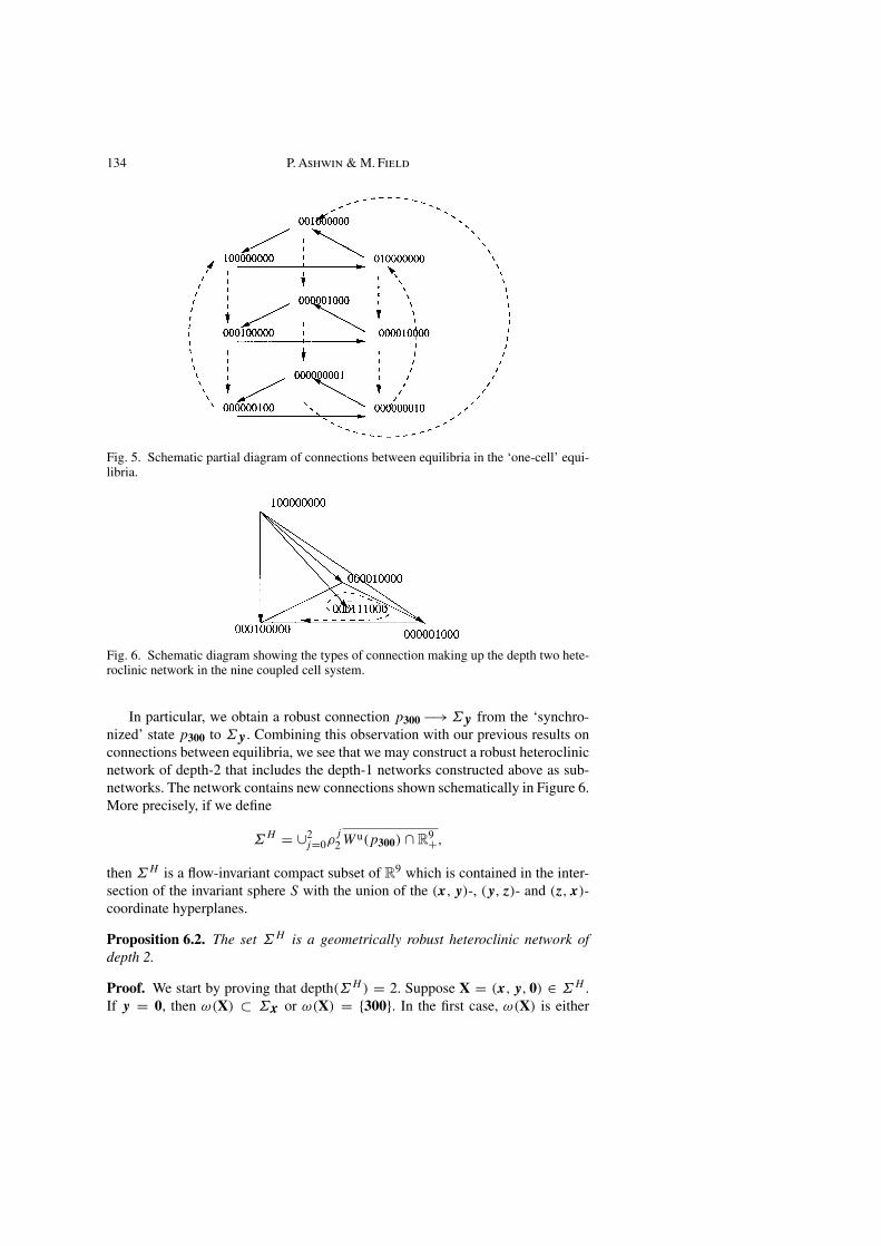
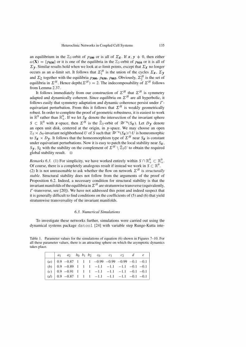
It follows from (11) that for coefficients in D ?, there exists a depth-1 hete-roclinic network linking all equilibria with isotropy conjugate to that of 100. Theconnections are shown schematically in Figure 5. Note that, for clarity, not all linksare shown.

Remark 6.1. The connections obtained in the proof of Lemma 5.6 are one-dimen-sional and came by looking at invariant subspaces. It follows that there is a natu-ral ‘symmetry-determined’ one-dimensional regular heteroclinic network betweenequilibria of symmetry type 100. In general, of course, there may be infinitely manyconnections between equilibria of symmetry type 100.

6.2. A Depth-2 Heteroclinic Network

Under certain circumstances, the depth-1 networks described above are part ofa depth-2 network. More precisely, let D ?

2 be the nonempty open subset of D ?2 for

which the complex eigenvalues of the linearization of (5) have strictly positive realpart. That is, we require A0 = (a1, a2) to satisfy a2 < 0 and

−a2 > a1 > 0.(14)

If these conditions hold, then the cycle Σx is a (globally) attracting heterocliniccycle in x-space and the equilibrium 300 is repelling in x-space.

For sufficiently small values of d and e, the cycle Σx persists and attracts allnonzero and nonsynchronized trajectories in some (preassigned) neighborhood ofthe origin in x-space.


Fig. 5. Schematic partial diagram of connections between equilibria in the ‘one-cell’ equi-libria.

Fig. 6. Schematic diagram showing the types of connection making up the depth two hete-roclinic network in the nine coupled cell system.

In particular, we obtain a robust connection p300−→Σy from the ‘synchro-nized’ state p300 to Σy . Combining this observation with our previous results onconnections between equilibria, we see that we may construct a robust heteroclinicnetwork of depth-2 that includes the depth-1 networks constructed above as sub-networks. The network contains new connections shown schematically in Figure 6.More precisely, if we define

ΣH = ∪2j=0ρ

j

2 W u(p300) ∩ R9+,

then ΣH is a flow-invariant compact subset of R9 which is contained in the inter-section of the invariant sphere S with the union of the (x, y)-, (y, z)- and (z, x)-coordinate hyperplanes.

Proposition 6.2. The set ΣH is a geometrically robust heteroclinic network ofdepth 2.

Proof. We start by proving that depth(ΣH ) = 2. Suppose X = (x, y, 0) ∈ ΣH .If y = 0, then ω(X) ⊂ Σx or ω(X) = {300}. In the first case, ω(X) is either


an equilibrium in the Z3-orbit of p100 or is all of Σx . If x, y |= 0, then eitherω(X) = {p030} or it is one of the equilibria in the Z3-orbit of p010 or it is all ofΣy . Similar results hold when we look at α-limit points, except that Σx no longeroccurs as an α-limit set. It follows that ΣH

1 is the union of the cycles Σx , Σy

and Σz together with the equilibria p300, p030, p003. Obviously, ΣH2 is the set of

equilibria in ΣH . Hence depth(ΣH ) = 2. The indecomposability of ΣH followsfrom Lemma 2.37.

It follows immediately from our construction of ΣH that ΣH is symmetryadapted and dynamically coherent. Since equilibria on ΣH are all hyperbolic, itfollows easily that symmetry adaptation and dynamic coherence persist under Γ -equivariant perturbation. From this it follows that ΣH is weakly geometricallyrobust. In order to complete the proof of geometric robustness, it is easiest to workin R9 rather than R9+. If we let Sx denote the intersection of the invariant sphereS ⊂ R9 with x-space, then ΣH is the Z3-orbit of W u(Sx). Let Dy denotean open unit disk, centered at the origin, in y-space. We may choose an openZ3 o∆9-invariant neighborhood U of S such that W u(Sx)∩U is homeomorphicto Sx × Dy . It follows that the homeomorphism type of ΣH near Sx is constantunder equivariant perturbations. Now it is easy to patch the local stability near Sx ,Sy , Sz with the stability on the complement of ΣH \ Z3U to obtain the requiredglobal stability result. utRemarks 6.3. (1) For simplicity, we have worked entirely within S ∩ R9+ ⊂ R9+.Of course, there is a completely analogous result if instead we work in S ⊂ R9.(2) It is not unreasonable to ask whether the flow on network ΣH is structurallystable. Structural stability does not follow from the arguments of the proof ofProposition 6.2. Indeed, a necessary condition for structural stability is that theinvariant manifolds of the equilibria inΣH are stratumwise transverse (equivalently,Γ -transverse, see [20]). We have not addressed this point and indeed suspect thatit is generally difficult to find conditions on the coefficients of (5) and (6) that yieldstratumwise transversality of the invariant manifolds.

6.3. Numerical Simulations

To investigate these networks further, simulations were carried out using thedynamical systems package dstool [24] with variable step Runge-Kutta inte-

Table 1. Parameter values for the simulations of equation (6) shown in Figures 7–10. Forall these parameter values, there is an attracting sphere on which the asymptotic dynamicstakes place.

a1 a2 b0 b1 b2 c0 c1 c2 d e

(a) 0.9 −0.87 1 1 1 −0.99 −0.99 −0.99 −0.1 −0.1(b) 0.9 −0.89 1 1 1 −1.1 −1.1 −1.1 −0.1 −0.1(c) 0.9 −0.91 1 1 1 −1.1 −1.1 −1.1 −0.1 −0.1(d) 0.9 −0.87 1 1 1 −1.1 −1.1 −1.1 −0.1 −0.1


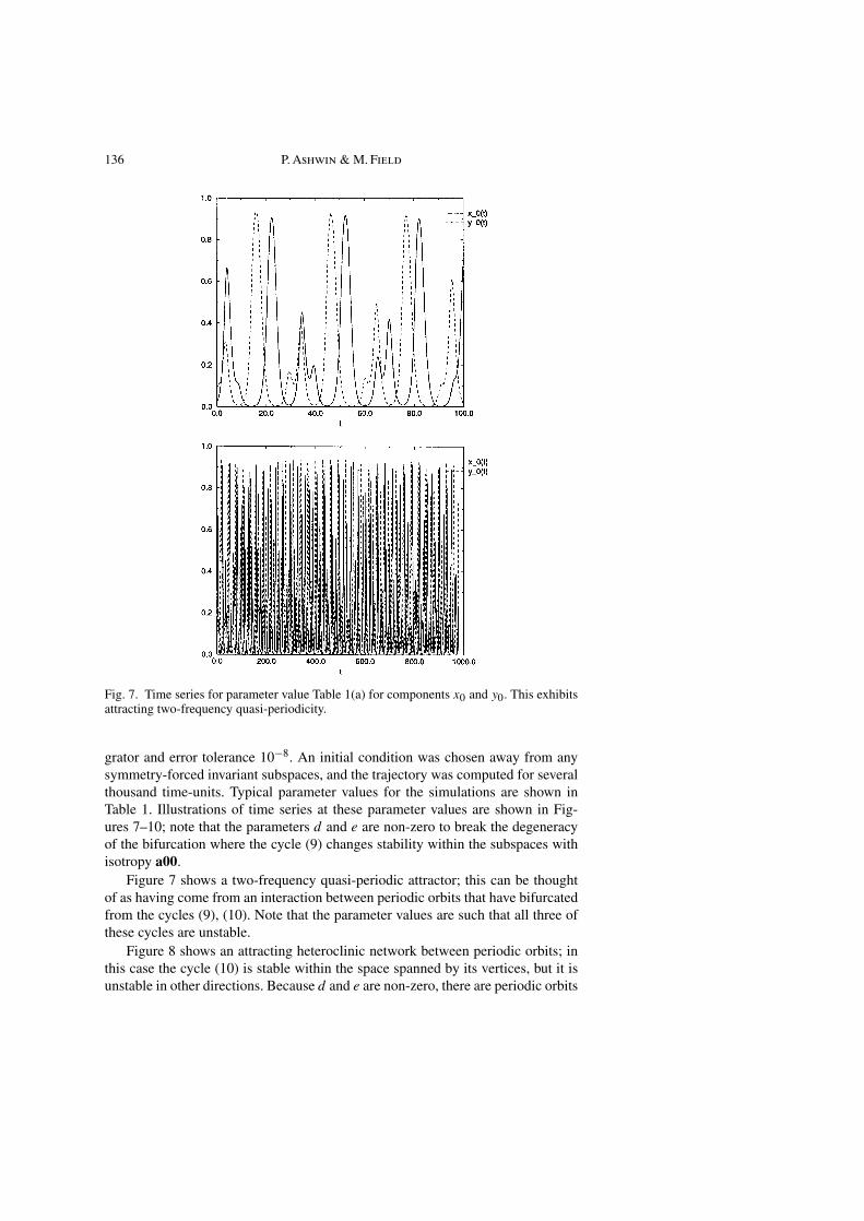
Fig. 7. Time series for parameter value Table 1(a) for components x0 and y0. This exhibitsattracting two-frequency quasi-periodicity.

grator and error tolerance 10−8. An initial condition was chosen away from anysymmetry-forced invariant subspaces, and the trajectory was computed for severalthousand time-units. Typical parameter values for the simulations are shown inTable 1. Illustrations of time series at these parameter values are shown in Fig-ures 7–10; note that the parameters d and e are non-zero to break the degeneracyof the bifurcation where the cycle (9) changes stability within the subspaces withisotropy a00.

Figure 7 shows a two-frequency quasi-periodic attractor; this can be thoughtof as having come from an interaction between periodic orbits that have bifurcatedfrom the cycles (9), (10). Note that the parameter values are such that all three ofthese cycles are unstable.

Figure 8 shows an attracting heteroclinic network between periodic orbits; inthis case the cycle (10) is stable within the space spanned by its vertices, but it isunstable in other directions. Because d and e are non-zero, there are periodic orbits


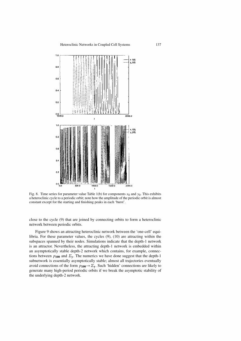
Fig. 8. Time series for parameter value Table 1(b) for components x0 and y0. This exhibitsa heteroclinic cycle to a periodic orbit; note how the amplitude of the periodic orbit is almostconstant except for the starting and finishing peaks in each ‘burst’.

close to the cycle (9) that are joined by connecting orbits to form a heteroclinicnetwork between periodic orbits.

Figure 9 shows an attracting heteroclinic network between the ‘one-cell’ equi-libria. For these parameter values, the cycles (9), (10) are attracting within thesubspaces spanned by their nodes. Simulations indicate that the depth-1 networkis an attractor. Nevertheless, the attracting depth-1 network is embedded withinan asymptotically stable depth-2 network which contains, for example, connec-tions between p100 and Σy. The numerics we have done suggest that the depth-1subnetwork is essentially asymptotically stable; almost all trajectories eventuallyavoid connections of the form p100→Σy. Such ‘hidden’ connections are likely togenerate many high-period periodic orbits if we break the asymptotic stability ofthe underlying depth-2 network.


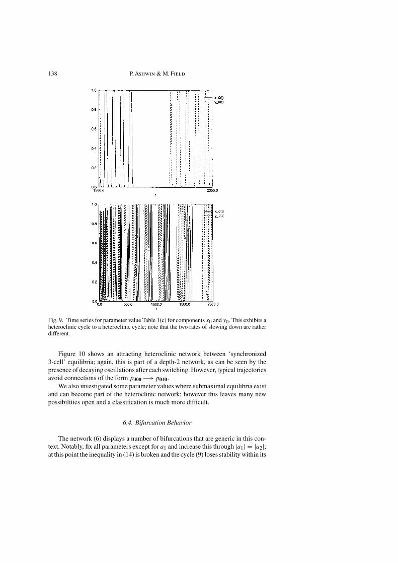
Fig. 9. Time series for parameter value Table 1(c) for components x0 and y0. This exhibits aheteroclinic cycle to a heteroclinic cycle; note that the two rates of slowing down are ratherdifferent.

Figure 10 shows an attracting heteroclinic network between ‘synchronized3-cell’ equilibria; again, this is part of a depth-2 network, as can be seen by thepresence of decaying oscillations after each switching. However, typical trajectoriesavoid connections of the form p300−→p010.

We also investigated some parameter values where submaximal equilibria existand can become part of the heteroclinic network; however this leaves many newpossibilities open and a classification is much more difficult.

6.4. Bifurcation Behavior

The network (6) displays a number of bifurcations that are generic in this con-text. Notably, fix all parameters except for a1 and increase this through |a1| = |a2|;at this point the inequality in (14) is broken and the cycle (9) loses stability within its


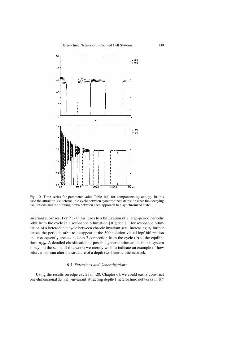
Fig. 10. Time series for parameter value Table 1(d) for components x0 and y0. In thiscase the attractor is a heteroclinic cycle between synchronized states; observe the decayingoscillations and the slowing down between each approach to a synchronized state.

invariant subspace. For d > 0 this leads to a bifurcation of a large-period periodicorbit from the cycle in a resonance bifurcation [10]; see [1] for resonance bifur-cation of a heteroclinic cycle between chaotic invariant sets. Increasing a1 furthercauses the periodic orbit to disappear at the 300 solution via a Hopf bifurcationand consequently creates a depth-2 connection from the cycle (9) to the equilib-rium p300. A detailed classification of possible generic bifurcations in this systemis beyond the scope of this work; we merely wish to indicate an example of howbifurcations can alter the structure of a depth two heteroclinic network.

6.5. Extensions and Generalizations

Using the results on edge cycles in [20, Chapter 6], we could easily constructone-dimensional Z2 o Zp-invariant attracting depth-1 heteroclinic networks in Rp


for all p = 3. Just as we did in our construction of the Z(3, 3)-invariant network,it is then straightforward to show that for all p, q = 3 it is possible to construct adepth-2 geometrically robust attracting heteroclinic network in Rpq with symmetrygroup (Z2 o Zp) o Zq (or Z2 × (Zp o Zq ).

We believe that it is possible to extend our methods so as to construct geometri-cally robust networks of arbitrary depth in systems of symmetrically coupled cells.As details of this work in progress will appear elsewhere, we limit ourselves to afew brief remarks and comments.

One might guess that the construction of our depth-2, Z(3, 3)-invariant networkcould be iterated N−1 times to form a geometrically robust Z(3, 3, ..., 3)-invariantnetwork of depth N . However, this approach turns out to be too simplistic as it ig-nores a crucial feature of the dynamics that leads to the Z(3, 3)-invariant networkhaving depth 2. Specifically, depth 2 follows from the existence of points x ∈ Σ

such that α(x) is a synchronized state 100 and ω(x) is a Guckenheimer-Holmescycle. In order to obtain higher depths, we need cycling between synchronizedstates and ‘Guckenheimer-Holmes’ cycles. One way to achieve this is to alternatethe stabilities of the synchronized states and heteroclinic cycles in a symmetricallycoupled ring consisting an even number of heteroclinic cycles. Just as before, thisleads to a depth-2 heteroclinic network. An appropriate coupling of three suchnetworks should then lead to a depth-3 heteroclinic network. We believe that itera-tion of this procedure would lead to geometrically robust heteroclinic networks ofarbitrary depth.

A particularly interesting feature of networks of this type (including iteratedZ(3, 3)-invariant networks) is that if the network is asymptotically stable and thereis a bifurcation-breaking asymptotic stability or, alternatively, a forced symmetrybreaking, then there are periodic orbits near the cycle that exhibit multiple timescales corresponding to their tracking of cycles in the original network.

7. Discussion

We have proposed a definition of a heteroclinic network that encompasses manyprevious definitions, but also allows such cycles as that discovered by Chawanya[7, 8] where connections may limit on to other connections. In doing so we showthat the concept of ‘depth’ of a flow on an invariant set (previously regarded ashaving little direct application to generic systems) has real relevance to structurallystable attractors in symmetric systems.

We have shown that such networks (which may contain robust continua ofconnections and/or chaotic invariant sets) have a hierarchical structure that can becharacterized by their depth. We have given sufficient conditions for their embed-dings that they can appear as ω-limit sets of nearby points, as well as sufficientconditions that they are robustly embedded in symmetric systems. We emphasizethat these are only sufficient, and in many cases would be hard to verify. It is anopen problem to obtain improved results for stability and robustness. This is likelyto be difficult due to the appearance of essentially asymptotic stable subnetworks,


and possible existence of sets of stable periodic orbits or other invariant sets accu-mulating on the network [8].

To address some of the questions about stability, we have examined a model sys-tem on R9 that has a number of relatively easily analyzable but nontrivial networks;we can show their robust existence and numerically find attracting networks.

As there is an equivalence between differential equations on Rn with 1n sym-metry and game dynamics differential equations on the (n−1)-simplex [33], theseresults apply in both settings.

Trajectories that are asymptotic to ‘cycling chaos’ networks show a slowing-down series of switchings between shadowing of different types of recurrent be-havior characterized by possibly chaotic nodal sets. If the nodes are not uniquelyergodic, then there is also a question of which of these ergodic measures contributesto averages of observables along trajectories that approach C. Chaotic sets raise anumber of further questions that we leave to future research.

Acknowledgements. M. Field thanks the EPSRC for support in the form of a Visiting Fel-lowship GR/L63051 to enable a visit to the University of Surrey during which this researchwas initiated, and for partial support from NSF Grant DMS-1551704 and Texas AdvancedResearch Program Award 1127681. P. Ashwin thanks the Nuffield foundation for supportin the form of a “Newly Appointed Science Lecturer” award. We both thank Martin Golu-bitsky for raising the question of cycling between different heteroclinic cycles in a coupledcell system.

References

1. P. Ashwin: Cycles homoclinic to chaotic sets; robustness and resonance Chaos 7(1997), 207–220.

2. P. Ashwin, P. Aston & M. Nicol: On the unfolding of a blowout bifurcation. PhysicaD 111 (1997), 81–95.

3. P. Ashwin, J. Buescu & I. N. Stewart: From attractor to chaotic saddle: a tale oftransverse instability. Nonlinearity 9 (1996), 703–737.

4. P. Ashwin & P. Chossat: Attractors for robust heteroclinic cycles with continua ofconnections. J. Nonlinear Sci. 8 (1997), 103–129.

5. P. Ashwin & A. M. Rucklidge: Cycling chaos: its creation, persistence and loss ofstability in a model of nonlinear magnetoconvection. To appear in Physica D (1998).

6. R. Bowen: ω-limit Sets for Axiom A Diffeomorphisms. J. Diff. Eqns. 18 (1975),333–339.

7. T. Chawanya: Infinitely many attractors in a game dynamics system. Prog. Theor.Phys. 95 (1996), 679–684.

8. T. Chawanya: Coexistence of infinitely many attractors in a simple flow. Physica D109 (1997), 201–241.

9. P. Chossat, F. Guyard & R. Lauterbach: Generalized heteroclinic cycles in spher-ically invariant systems and their perturbations. Preprint 303, Weierstrass-Institute,Berlin (1996).

10. S.-N. Chow, B. Deng & B. Fiedler: Homoclinic bifurcation at resonant eigenvalues.J. Dyn. Diff. Eqns. 2 (1990) 177–244.

11. C. Conley. Isolated Invariant Set and the Morse Index, CBMS Regional ConferenceSeries in Mathematics, vol. 38. American Mathematical Society, Providence, RI, 1978.

12. M. Dellnitz, M. Field, M. Golubitsky, A. Hohmann & J. Ma: Cycling chaos, IEEETrans. Circuits and Systems-I. 42 (1995), 821–823.


13. B. Dionne, M. Golubitsky & I. Stewart: Coupled cells with internal symmetry: I.Wreath products, Nonlinearity 9 (1996), 559–574.

14. M. J. Field: Equivariant Bifurcation Theory and Symmetry Breaking, J. Dyn. Diff.Eqs., 1 (1989), 369–421.

15. M. J. Field: Equivariant Bifurcation Theory and Symmetry Breaking, J. Dyn. Diff. Eqs.1 (1989), 369–421.

16. M. J. Field & R. W. Richardson: Symmetry breaking and branching patterns in equiv-ariant bifurcation theory II, Arch. Rational Mech. Anal. 120 (1992), 147–190.

17. M. J. Field & J. W. Swift: Static bifurcation to limit cycles and heteroclinic cycles,Nonlinearity 4 (1991), 1001–1043.

18. M. J. Field: Geometric methods in bifurcation theory, in Normal forms and homoclinicchaos, eds. W. F. Langford & W. Nagata, Field’s Institute Communications, Amer.Math. Soc. (1995).

19. M. Field: Symmetry breaking for compact Lie groups, Mem. Amer. Math. Soc. 574(1996).

20. M. Field: Lectures on Dynamics, Bifurcation and Symmetry. Pitman Res. Notes inMath. 356 (1996).

21. A. Gaunersdorfer: Time averages for heteroclinic attractors, SIAM J. Appl. Math.52, (1992) 1476–1489.

22. J. Guckenheimer & P. Holmes: Nonlinear oscillations, dynamical systems and bifur-cations of vector fields, Springer-Verlag (1983).

23. J. Guckenheimer & P. Holmes: Structurally stable heteroclinic cycles, Math. Proc.Camb. Phil. Soc. 103 (1988), 189–192.

24. J. Guckenheimer, M. R. Myers, F. J. Wicklin & P. A. Worfolk: Dstool: a dynamicalsystems toolkit with an interactive graphical interface, user’s manual, Center for Ap-plied Mathematics, Cornell University (1991). (See also: A. Back, J. Guckenheimer,M. Myers, F. Wicklin, & P. Worfolk: dstool: Computer Assisted Exploration of Dy-namical Systems’, Notices Amer. Math. Soc. 39 (1992), 303–309.

25. J. Guckenheimer & P. Worfolk: Instant chaos, Nonlinearity 5 (1992), 1211–1222.26. M. W. Hirsch, C. C. Pugh & M. Shub: Invariant Manifolds, Springer Lect. Notes

Math. 583 (1977).27. J. Hofbauer: Heteroclinic cycles on the simplex, Proc. Int. Conf. Nonlinear Oscilla-

tions, Janos Bolyai Math. Soc. Budapest, (1987).28. J. Hofbauer & K. Sigmund: The Theory of Evolution and Dynamical Systems, Cam-

bridge University Press, Cambridge (1988).29. A. Homburg: Some global aspects of homoclinic bifurcations of vector fields, PhD

Thesis, Dept. of Maths., University of Groningen (1993).30. A. Katok & B. Hasselblatt: Introduction to the Modern Theory of Dynamical Sys-

tems, Cambridge University Press (1995).31. V. Kirk & M. Silber: A competition between heteroclinic cycles, Nonlinearity 7

(1994), 1605–1622.32. M. Krupa & I. Melbourne: Asymptotic stability of heteroclinic cycles in systems

with symmetry, Erg. Th. Dyn. Sys. 15 (1995), 121–147.33. M. Krupa: Robust heteroclinic cycles, J. Nonlinear Sci. 7 (1997), 129–176.34. R. Mane: Ergodic Theory and Differentiable Dynamics, Springer-Verlag (1987).35. P. C. Matthews, A. M. Rucklidge, N. O. Wiess & M. R. E. Proctor: The three-

dimensional development of the shearing instability of convection, Phys. Fluids 8(1996), 1350–1352.

36. I. Melbourne, P. Chossat & M. Golubitsky: Heteroclinic cycles involving periodicsolutions in mode interactions with O(2) symmetry, Proc. Roy. Soc. Edinburgh 113A(1989), 315–345.

37. I. Melbourne: An example of a non-asymptotically stable attractor, Nonlinearity 4(1991), 835–844.

38. J. Milnor: On the concept of attractor, Commun. Math. Phys. 99 (1985), 177–195;Comments, Comm. Math. Phys. 102 (1985), 517–519.


39. J. Palis: A differentiable invariant of topological conjugacies and moduli of stability,Asterisque 51 (1978), 335–346.

40. G. L. dos Reis: Structural stability of equivariant vector Fields on two-manifolds, Trans.Amer. Math. Soc. 283 (1984), 633–642.

41. M. Shub: Global Stability of Dynamical Systems, Springer-Verlag (1987).42. K. Sigmund: Time averages for unpredictable orbits of deterministic systems, Annals

of Operations Research 37 (1992), 217–228.43. P. A. Worfolk: An equivariant, inclination-flip, heteroclinic bifurcation, Nonlinearity

9 (1966), 631–648.

Department of Mathematics and StatisticsUniversity of Surrey

Guildford GU2 5XH, UKe-mail: [email protected]

and

Department of MathematicsUniversity of Houston

Houston, Texas 77204-3476e-mail: [email protected]

(Accepted July 6, 1998)

Documents

Heteroclinic Networks in Coupled Cell Systems