Heteroclinic Chaos in Attitude Dynamics of a Dual-Spin Spacecraft at

Small Oscillations of Its Magnetic Moment

ANTON V. DOROSHIN

Space Engineering Department (Division of Flight Dynamics and Control Systems)

Samara State Aerospace University (SSAU)

SSAU, Moscowskoe shosse 34, Samara, Russia 443086

doran@inbox.ru

Abstract: - The paper contains an investigation results in the heteroclinic dynamics of a magnetic (magnetized)

dual-spin spacecraft (DSSC) in the geomagnetic field at the realization of the orbital motion of its mass centre

along an equatorial circular orbit. Exact heteroclinic analytical solutions are obtained. These analytical exact

solutions are used for the research of the DSSC perturbed motion and its chaotization properties at the presence

of small polyharmonic perturbations of the magnetic moment.

Key-Words: - Magnetic/Magnetized Dual-Spin Spacecraft; Heteroclinic Explicit Solutions; Melnikov Function;

Lagrange Top; Euler Top; Chaos

1. Introduction

Chaotic regimes in the angular/attitude motion of

multibody systems/spacecraft and the corresponding

many-sided research’s aspects are undoubtedly very

important parts of modern non-linear mechanics,

including spaceflight dynamics [1-42].

One of the main multibody spacecraft’s schemes

is the dual-spin spacecraft (DSSC) which represents

the mechanical system of coaxial bodies and the

single-rotor gyrostat. The versatile explorations of

the DSSC/gyrostat’s dynamics were conducted in

many research works devoted in different

formulations to the analytical/numerical modeling

of unperturbed/perturbed modes and to obtaining of

exact/approximate solutions for the motion under

influence of different external/internal disturbances

(gravity, aerodynamic torques, dissipative/excitative

effects from external environments, interactions

between the system bodies, etc.) [e.g. 5-31].

Equally with numerous types of perturbations

acting on the DSSC, the (electro)magnetic torque

from the Earth’s magnetic field is the very important

dynamical factor. It is needed to note that numerous

works and publications were connected with the

investigation of the attitude dynamics/control of the

magnetic (magnetized) spacecraft, for example [32-

42]. Here we can underline the connection of the

task of the attitude motion of the magnetized DSSC

with classical tasks of the rigid body mechanics (the

Euler, the Lagrange tops) [1-4].

The "magnetic" torque arises due to DSSC

usually contains internal electrical equipment with

powerful inductive elements and magnets. Also this

factor can be one of the main reasons of the chaos

initiation in the DSSC dynamics. The consideration

of connected causes and effects of the heteroclinic

chaotization is the primary task of this paper.

So, in this paper the chaotization analysis of the

attitude dynamics of the magnetic/magnetized

DSSC is provided. This analysis is based on the

Melnikov function evaluation along heteroclinic

trajectories in the phase space of the

magnetic/magnetized DSSC, which performs an

orbital motion on a circular equatorial orbit at the

realization of the spin-stabilized attitude motion in

the “cylindrical precession” regime, when the

angular momentum of the DSSC is directed

perpendicularly to the orbit’s plane. This motion

regime is quite important for the practice because it

corresponds (in ideal conditions) to one of the

preferred regimes of the stationary attitude motions

of the DSSC with the conservation of the spatial

orientation of its longitudinal axes (especially it is

important for communication satellites).

The paper material is presented the continuation

and expansion of the previous author’s analytical

research [26] into the applied aria corresponding to

the magnetic DSSC chaotic motion investigation.

The main paper results connected with obtaining of

analytical heteroclinic solutions and with the

illustration of non-regular regimes of the motion

dynamics. Also the paper results can be additionally

investigated in aspects of non-trivial complex

dynamical modes implementation with the help of

modern simulation tools [43-49].

WSEAS TRANSACTIONS on SYSTEMS Anton V. Doroshin

E-ISSN: 2224-2678 158 Volume 14, 2015

2. Equations of the attitude dynamics of the

magnetic/magnetized DSSC

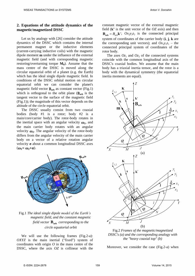
Let us by analogy with [26] consider the attitude

dynamics of the DSSC which contains the internal

permanent magnet or the inductive elements

(current-carrying inductive coils) with the magnetic

dipole moment m under the influence of the external

magnetic field (and with corresponding magnetic

restoring/overturning torque Mθ). Assume that the

mass centre of the DSSC is moved along the

circular equatorial orbit of a planet (e.g. the Earth)

which has the ideal single dipole magnetic field. In

conditions of the DSSC orbital motion on circular

equatorial orbit we can consider the planet's

magnetic field vector Borb as constant vector (Fig.1)

which is orthogonal to the orbit plane (Borb is the

tangent vector to the surface of the magnetic field

(Fig.1)); the magnitude of this vector depends on the

altitude of the circle equatorial orbit.

The DSSC usually consist from two coaxial

bodies (body #1 is a rotor; body #2 is a

main/core/carrier body). The rotor-body rotates in

the inertial space with an angular velocity ω1, and

the main carrier body rotates with an angular velocity ω2. The angular velocity of the rotor-body

differs from the angular velocity of the main carrier

body on a vector of a relative rotation angular

velocity σ about a common longitudinal DSSC axes (ω1= ω2+σ).

Fig.1 The ideal single dipole model of the Earth’s

magnetic field, and the constant magnetic

field vector orbB corresponding to the

circle equatorial orbit

We will use the following frames (Fig.2-a):

OXYZ is the main inertial ("fixed") system of

coordinates with origin O in the mass centre of the

DSSC, where the axis OZ is collinear with the

constant magnetic vector of the external magnetic

field (k’ is the unit vector of the OZ axis) and then

orbBorb

B k' ; Ox2y2z2 is the connected principal

system of coordinates of the carrier body (i, j, k are

the corresponding unit vectors); and Ox1y1z1 – the

connected principal system of coordinates of the

rotor body.

The axes Oz1 and Oz2 of the connected systems

coincide with the common longitudinal axis of the

DSSC's coaxial bodies. We assume that the main

body has a triaxial inertia tensor, and the rotor is a

body with the dynamical symmetry (the equatorial

inertia moments are equal).

(a)

(b)

Fig.2 Frames of the magnetic/magnetized

DSSC's (a) and the corresponding analogy with

the "heavy coaxial top" (b)

Moreover, we consider the case (Fig.2-a) when

WSEAS TRANSACTIONS on SYSTEMS Anton V. Doroshin

E-ISSN: 2224-2678 159 Volume 14, 2015

the DSSC's intrinsic magnetic moment is aligned

with the DSSC’s longitudinal axis mm k .

The Euler general dynamical equations of the

system can be written with the help of the low of the

angular momentum changing in the rotating with the

angular velocity ω2 frame Ox2y2z2 e

2K +ω ×K = M (1)

where K is the system angular momentum, e

M – is

the vector of external torques.

The scalar form of the vector equation (1)

represents the following system:

1

1

1

1

e

x

e

y

e

z

Ap C B qr qC M

Bq A C pr pC M

Cr C B A pq M

C r M

(2)

where , ,p q r are the components of the carrier

body's angular velocity 2ω in projections onto the

axes of the Ox2y2z2 frame; is the rotor angular

velocity relatively the carrier body ;

2 2 2 2, ,diag A B CI is the triaxial inertia tensor

of the carrier body in the connected frame Ox2y2z2;

1 1 1 1, ,diag A A CI is the inertia tensor of the

dynamically symmetrical rotor in the connected

frame Ox1y1z1; 1 2 ,A A A 1 2 ,B A B

1 2C C C are the main inertia moments of the

coaxial bodies system in the frame Ox2y2z2

(including rotor); 1C r the longitudinal

angular moment of the rotor along Oz1; 11 zC h

the rotor relative angular moment in the carrier body

frame Ox2y2z2. M is the internal torque of the

coaxial bodies interaction. Let us consider the

following mass-inertia distribution A B C .

We ought to note that the orbital motion of the

spacecraft can be considered as the motion fulfilled

under the action of such perturbations as the

magnetic torque, the gravity gradient torque, the

small aerodynamics drag from the Earth’s

atmosphere, and other disturbances (the solar

pressure torque, etc.). These perturbations have

magnitudes, which can essentially differ from each

other.

The torque of the magnetic interaction of the

magnetic/magnetized DSSC with the external

magnetic field is

2 2 2

02 1 3

;

, ,

, ,0 ;4

T

x y zOx y z

T morb orb

M M M

B m BR

θ

θ

orbM m B

M (3)

Here µ0 is the magnetic permeability of free space

7

0 4 10 T m A ; µm≈7.8∙1022

[A∙m2]

is the

geomagnetic dipole moment; R is the orbit’s

altitude (relative the mass centre of the Earth); m is

the magnetic moment of the DSSC

(m~100÷1000 [A∙m2] – it corresponds, e.g., to the

magnet of the ordinal system of the SC angular

momentum shedding); parameters γi are the

directional cosines of the axis OZ (the "fixed"

inertial direction of the Borb vector) in the main body

frame Ox2y2z2:

1 2

2 2

3 2

cos , ,

cos , ,

cos ,

OZ Ox

OZ Oy

OZ Oz

i k'

j k'

k k'

(4)

The torque corresponding to the gravity gradient

can be written in the form

2 2 2

2 3 3 1 1 23

, ,

3, , ,

T

G Gx Gy GzOx y z

T

GI

I I I

M M M

C B A C B A

R

M

where µG=Gme=3.986∙1014

N∙m2/kg is the Earth’s

mass-gravity parameter; i are the directional

cosines of the axis of the local normal to the circular

orbit of the DSSC (the local direction to the gravity

centre); and I A C is the difference between

the largest and the smallest inertia moment of the

DSSC.

Let us consider the attitude motion of the

relatively small DSSC with normal distribution of

the mass (without the extremely expressed inertia-

mass configuration like the “gravitational

dumbbell”), when the difference of the inertia

moments does not exceed δI={1÷10} kg∙m2. Then it

is possible to estimate the comparative magnitudes

of the main influences (gravitational and magnetic).

If we take as initial conditions the parameters of the

ordinal orbital motion (including geostationary

orbits) and parameters of the ordinal small magnetic

SC, the estimation follows:

14 15

3 3

4 2

12 10 ; 8 10 ;

10 10 .10

IG

IG

m

R R

m

θ

θ

M M

M M

As we can see, the magnitude of the gravity gradient

WSEAS TRANSACTIONS on SYSTEMS Anton V. Doroshin

E-ISSN: 2224-2678 160 Volume 14, 2015

torque in the considered case is less than the value

of the magnetic torque by three orders (on the

average) - it corresponds to the significant

predominance of the magnetic torque over others

torques; and in this case the results/findings [26] are

applicable, including the unperturbed general

solutions for the magnetic DSSC attitude motion.

So, in this research we will take into account

only general influence, which corresponds to the

magnetic torque. Then equations (2) take the form:

2 2

2 1

2

;

;

0;

Ap C B qr q Q

Bq A C pr p Q

C r B A pq M

(5)

orbQ const B m (6)

We assume the following conditions:

2 2 2 1 1, const 0.A B C A C

Also in our research we will use the Hamiltonian

form of equations in the well-known Andoyer–

Deprit canonical variables. The Andoyer–Deprit

variables [11, 12] (l, L, I2, I3) are expressed through

components of the system's angular momentum

(Fig.2): 2 2 22 2 2

, ,T

x y zOx y zK K K K K

2

2

3 2

3

;

;

;

TL

l

TI K

TI L I

K k

K s K

K k

(7)

2

2

2

2 2

2

2 2

2

2

sin ;

cos ;

x

y

z

K Ap I L l

K Bq I L l

K C r L

(8)

The system Hamiltonian in the Andoyer–Deprit

phase space has the form [e.g. 4-10]:

0 01

22 2 2 2 2

2

1 2 1 2 1 2

;

sin co

;

s 1,

2 2

LI L l lT

A A A B

P

C

T

C

(9)

where T – is the system's kinetic energy; P – is the

potential energy; 1 is the small perturbed part

of the Hamiltonian. In the considered case the

potential energy corresponds to the "magnetic"

torque (or, as it was described in [26], to the

restoring/overturning torque from the system’s

weight in the generalized coaxial Lagrange top) – it

takes the form depending only on the nutation angle:

cos ; sinP

P Q M Q

(10)

Repeating the main findings of the previous

work [26] we underscore the full compliance (in a

dynamic sense) of two mechanical models (Fig.2):

the magnetic/magnetized DSSC (Fig.2-a) and the

coaxial Lagrange top (the heavy coaxial top) motion

(Fig.2-b). Here we have to note that the Lagrange

top in the classical formulation [1-4] describes the

angular motion of the heavy body about fixed point

O when the gravity force W (the system weight) is

applied in the point OW on the general longitudinal

axis Oz2. In our consideration the both models (the

magnetic DSSC and the heavy coaxial top) are

reduced to the interconnected common case at the

corresponding conversion of the torque's magnitude

(depending on proper signs of the values):

;orb WQ B m W OO (11)

Therefore, the paper results and conclusions will be

applicable to the both tasks (the

magnetic/magnetized DSSC, and generalized heavy

coaxial Lagrange top).

3. Heteroclinic analytical solutions for the

angular momentum components

Let us consider the angular motion of the

magnetic/magnetized DSSC in the “cylindrical

precession” regime in the case when the vector of

the angular momentum K is directed strongly along

the inertial ("fixed") axis OZ KK k' coinciding

with the vector of the external magnetic field

orbB . In this case the system angular momentum

K is the constant vector, and then we can rewrite the

expressions (4) for the directional cosines, and the

canonical Andoyer–Deprit momentums (7) as

follows:

2

2

2

1

2

23

,

,

x

y

z

K Ap

K K

K Bq

K K

K C r

K K

(12)

2

2

2

2 3

2

2

;

const;

cos ,

z

z

L K C r

I I K

K C r L

K K I

(13)

Using (12) it is possible to rewrite the

WSEAS TRANSACTIONS on SYSTEMS Anton V. Doroshin

E-ISSN: 2224-2678 161 Volume 14, 2015

components of the magnetic torque:

2 2

2 2 2

, ,0

, ,0

T

y x

Ox y z

T

QK QK

K K

QBq QAp

K K

θM

(14)

Finally the dynamical equations (5) take the form

2

2

2

;

;

0;

Ap C B qr q QBq K

Bq A C pr p QAp K

C r B A pq M

(15)

Also, taking into account (13), we can write the

final shape of the Hamiltonian

2 2 2 2

2

1 2 1 2

22

1 2 2

sin cos

2

1

2

I L l l

A A A B

L LQ

C C I

(16)

The Hamiltonian (16) does not depend on the

canonical coordinates 2 3, , then impulses

2 3,I I are constant; and the dynamical system is

reduced to one degree of freedom ,l L :

0 0

1 1

, ;

, ;

; ;

; ;

L L

l l

L l

L l

L f l L g

l f l L g

f fl L

g gl L

(17)

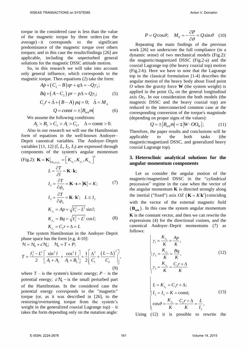
Let us obtain the analytical solution for the

heteroclinic orbits/polhodes 1 2S S in the phase

space of the angular velocity components {p, q, r,

σ} (Fig.3) by full analogy with the previous results

[10].

Theorem. Assume the absence of the coaxial

bodies interaction 0M . Then we have the

following heteroclinic solutions , ,p t q t r t

for the system (15):

2 2

22 2

2

1

;

;

;

;

C B Cp t y t

A A B

q t s k y t E

EBr t y t

B C

t r tC

(18)

where

0

0 0 2

2

0

0 1 2 02

4 exp

,

exp 4

M aa E y t

ky t

Mt aE y a a a

k

with the set of constants:

2

2

2

1

22 2

0

const 0;

;

2 ;

;

a k

a E k

a s k E

0

2 2

2 2

2 22 2

;

;

1 1

; ;

sy E

k

A B

A C B C

B C A C

C A CHs k

B A B B A B

22

2

2

1

2 00

22 2 2

0 0 0 2 0

1

2

1 2 ;

const;

2 ;

CH T A D EA

A C

AEA

C

C rT T Q

K

T Ap Bq C rC

22

2

2

1

2 2 2

1

2

1 2

; .

CD B EB

T B C

BEB

C

A C C B CQE M

K B A A B

The proof.

Let us prove the theorem directly following to

the algorithm which was used in the paper [10].

We will use the polhodes geometry [1-3]. The

polhode is the fourth-order curve in 3D-space

(Fig.3) corresponding to the intersection of a kinetic

energy ellipsoid and an angular momentum

ellipsoid, which are defined with the help of the

expressions for the dynamical theorems/laws of the

changing of the kinetic energy and the angular

momentum:

WSEAS TRANSACTIONS on SYSTEMS Anton V. Doroshin

E-ISSN: 2224-2678 162 Volume 14, 2015

22 2 2

2 0

1

0

2

2 2

Ap Bq C r TC

P P

(19)

22 2 2 2 2

2A p B q C r K (20)

With the help of (10) and (13) we can write the

expressions (19) and (20) in the form

2

2 2 2

2 2

1

2 2Ap Bq C r E C r TC

(21)

22 2 2 2 2

2 2A p B q C r K DT (22)

with the following constants 2

2 2 2

0 0 0 2 0

1

2 00

2

2 ;

const;

;2

T Ap Bq C rC

C rT T Q

K

Q KE D

K T

(23)

Based on a combination of the expressions (21)

and (22) (using the multiplication of (21) by A with

the subsequent subtraction of (22)) we obtain:

2

22

2 2

1

2

2

2

2

B A B q

A C r E C rC

C r T A D

(24)

Analogically, after the multiplication of (21) by

B with the subsequent subtraction of (22) we receive

2

22

2 2

1

2

2

2

2

A B A p

B C r E C rC

C r T B D

(25)

The separation of a perfect square in (25) gives

the equation for hyperbolae (corresponding curves

are depicted at the coordinate plane Opr – Fig.3)

2

2

2 2

2

A A B p

EBC B C r F

B C

(26)

where

22

2

2

1

2

1 2

F T B D

CEB

B C

BEB

C

(27)

Now we can use the shifted coordinate axes

Opr (Fig.3) and the scalable component of the

angular velocity

2

EBr r

B C

(28)

As a result we write in the plane Opr canonical

form of the hyperbolas equation

2 2

2 2A A B p C B C r F (29)

The asymptotes of the hyperbolas correspond to

the value F=0 and, therefore, to the following

straight line equation:

2 2A A B p C B C r (30)

So, the equation

0F (31)

defines the initial conditions of the motion

realization along hyperbolas’ asymptotes. We can

consider the equation (31) as an equation on value D

22

2

2

1

0

1

2

1 2

F D D

CD B EB

T B C

BEB

C

(32)

Thereby, at the value D D the system realizes the

motion along the hyperbolas asymptotes.

Let us choose the trivial initial condition for the

component 0( 0) 0q t q which is equivalent

to taking as a time-datum the time-moment when

the q-component takes on the zero-value. Then the

equation (31) can be rewritten in the form of the

quadratic equation for the initial value 0r (at

arbitrary values 0p and )

22 2 22 00 2 0

1

22

2

2

1

2

1 2 0

C rB Ap C r Q K

C K

CEB

B C

BEB

C

(33)

So, we can find the value 0r as the root of the eq.

(33), which guarantees the equality D D and the

motion along the hyperbolas asymptotes

(1,2)

0 0 0 ,r r f p (34)

From the eq. (24), taking into account a perfect

square, the expression follows

WSEAS TRANSACTIONS on SYSTEMS Anton V. Doroshin

E-ISSN: 2224-2678 163 Volume 14, 2015

2

2

2 2

2

B A B q

EAC A C r H

A C

(35)

22

2

2

1

2

1 2

H T A D

CEA

A C

AEA

C

(36)

From (35) we obtain

2

2 2 2

H B A B qEAr

A C C A C

(37)

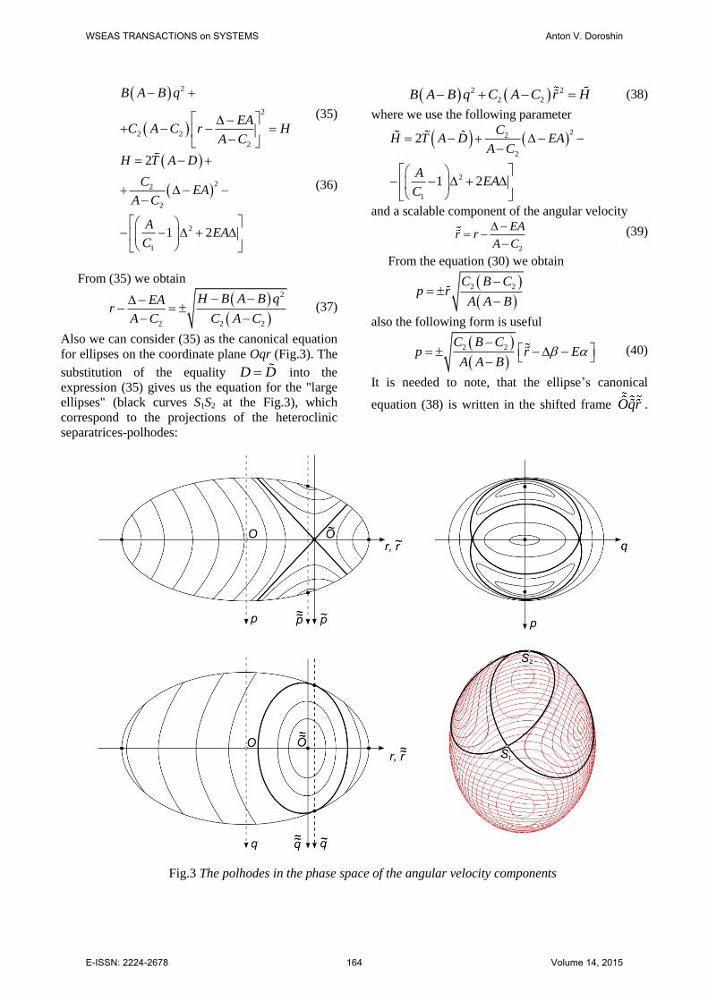
Also we can consider (35) as the canonical equation

for ellipses on the coordinate plane Oqr (Fig.3). The

substitution of the equality D D into the

expression (35) gives us the equation for the "large

ellipses" (black curves S1S2 at the Fig.3), which

correspond to the projections of the heteroclinic

separatrices-polhodes:

2 2

2 2B A B q C A C r H (38)

where we use the following parameter

22

2

2

1

2

1 2

CH T A D EA

A C

AEA

C

and a scalable component of the angular velocity

2

EAr r

A C

(39)

From the equation (30) we obtain

2 2C B C

p rA A B

also the following form is useful

2 2C B C

p r EA A B

(40)

It is needed to note, that the ellipse’s canonical

equation (38) is written in the shifted frame Oqr .

Fig.3 The polhodes in the phase space of the angular velocity components

WSEAS TRANSACTIONS on SYSTEMS Anton V. Doroshin

E-ISSN: 2224-2678 164 Volume 14, 2015

From (38) the expression follow 2 2

2

2

s qr

k

(41)

where

2 22 2const; const

C A CHs k

B A B B A B

The second equation (15) can be written as follows

2

2

0EA

Bq A C r pA C

(42)

With the help of (41) and (40) the last equation is

reduced to the form

2 2

2 2

2 22 2

20

s qBq A C

k

C B C s qE

A A B k

(43)

The differential equation (43) contains a possible

quaternary signs alternation, corresponded to the

four heteroclinic orbits "saddle-to-saddle"

1 2S S . These four orbits form the "large

ellipses".

We can make the change of variables 2 2

2

s qx

k

(44)

From (44) the expressions follow 2

2 2 2

2 2 2;

k xdxq s k x dq

s k x

Then the equation (43) is rewritten in a differential

form

2

2 2 2

2 2 2

k dxMdt

x E s k x

A C C B CM

B A A B

(45)

The equation (45) includes two cases of signs of the

x-variable. In the both cases we make corresponding

substitutions

2

2 2 2

0 0

2

2 2 2

1). ;

k dxMdt

x E s k x

y x E

x y E dx dy

y x E

k dyMdt

y s k x

(46)

2

2 2 2

0 0

2

2 2 2

2). ;

k dxMdt

x E s k x

y x E

x y E dx dy

y x E

k dyMdt

y s k x

As we can see from the expressions (46), the

both cases give the interconnected equation again 2

2 2 2

k dyMdt

y s k x

(47)

Taking into account the twoness of the initial

condition 0 0y x E from (47) the

integral expression follows

0

22 2 2

2

0 0 0 0

2

;

;

y

y

dy

y s k y E y E

Mt

k

sy y x E x

k

(48)

The expression (48) reduces to the standard integral

0

02

2 1 0

2 2

2 1

22 2

0

;

; 2 ;

y

y

dyy y

y a y a y a

a k a E k

a s k E

(49)

where the antiderivative y has the following

standard shape

0

0

2

0 1 0 2 1 0

1ln ; 0;

2 2

z E z aa

a a z a a z a z aE z

z

From (49) we get the solution for the equation (47)

0

0 2exp

M aE y t E y t

k

(50)

After transformations the exact explicit

analytical solution for the time-series y(t) follows

0

0 0 2

2

0

0 1 2 02

4 exp

exp 4

M aa E y t

ky t

Mt aE y a a a

k

(51)

WSEAS TRANSACTIONS on SYSTEMS Anton V. Doroshin

E-ISSN: 2224-2678 165 Volume 14, 2015

It is needed to note, that the quadrature (49) is

quite frequent for heteroclinic solutions in rigid

body dynamics [e.g. 7-10].

Making back substitutions we get the exact

explicit analytical heteroclinic parametrized

solutions for all components of the angular velocity

, ,p t q t r t :

2 2

22 2

2

1

;

;

;

C B Cp t y t

A A B

q t s k y t E

EBr t y t

B C

t r tC

(52)

The theorem is completely proved.

We have to additionally underline, that the

heteroclinic solutions also can be obtained using

functional transformations of the general

solutions [26] at the condition of the hyperbolic

singularity of the elliptic integrals and functions

(the elliptic modulus k=1), when the elliptic

functions express in terms of hyperbolic

functions. However, the considered way (based

on the theorem’s proof) of the heteroclinic

solutions obtaining is the preferable, natural and

geometrically clear technique.

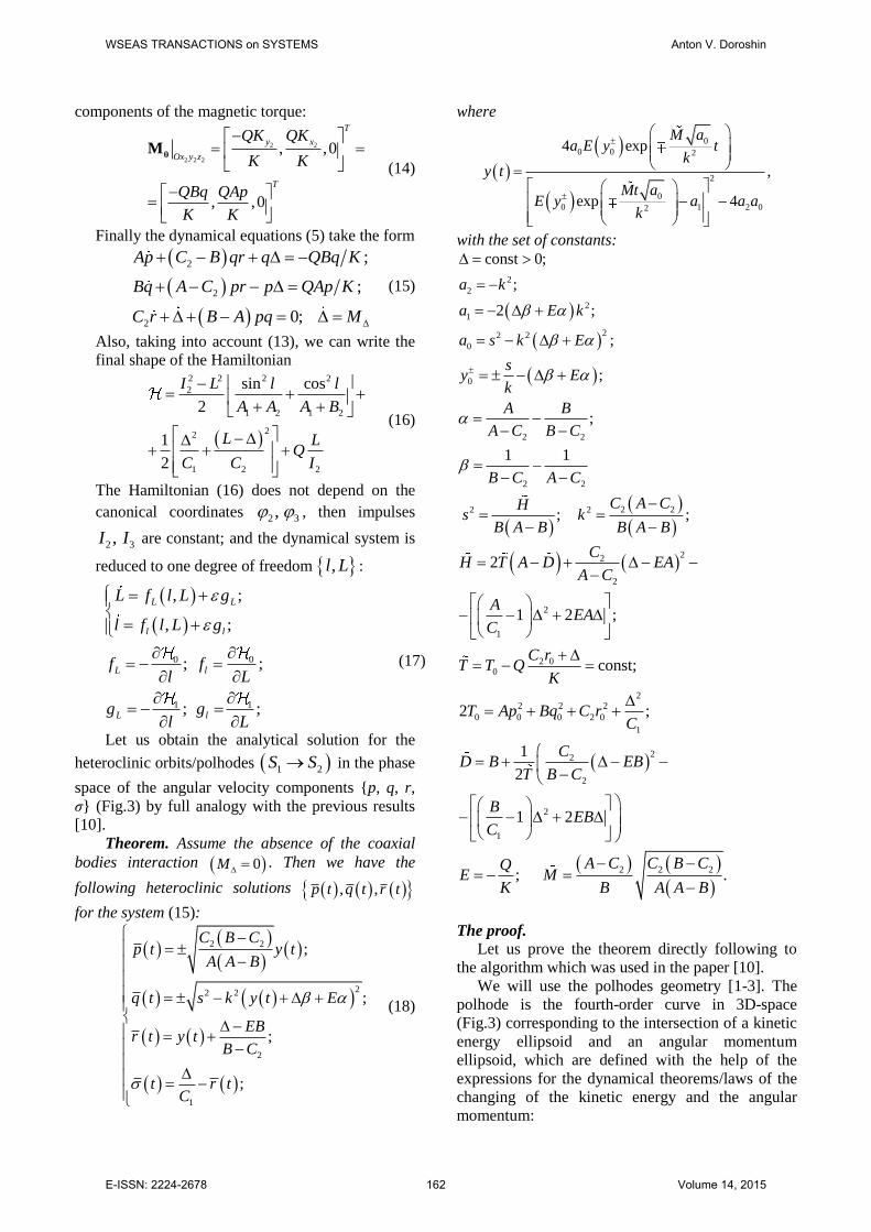
Figure (Fig.4) demonstrates the validity of

the solutions (52) as the comprehensive

coincidence of the calculation results (by the

analytical dependences - points) with the

numerical integration results (lines). The upper

graphs (Fig.4-a) correspond to the first root (1)

0r

of the quadratic equation (31), and the graphs

(fig.4-b) correspond to the second root (2)

0r .

(a)

(b)

Fig.4 The heteroclinic dependences: 2

2 2 2 1 115, 10, 6, 5, 4 [ ];A B C A C kg m 2 2 2

020 [ ]; 3 [ ]; 1.5[1/ ]Q kg m s kg m s p s

a). (1) (1)

0 0 03.262; -2.512r r [1/s]

b). (2) (2)

0 0 0-0.597; 1.347r r [1/s]

WSEAS TRANSACTIONS on SYSTEMS Anton V. Doroshin

E-ISSN: 2224-2678 166 Volume 14, 2015

It is worth to note that the solutions (52) allow the

easy transformation to the Andoyer–Deprit

heteroclinc dependences:

2 2

2 2

2

22

2 2

2 2

2 2

;

arcsin

arcsin ;

arcsin ;

L t C r t C y t W

Ap tl t

I L t

Vy t

I C y t W

VL t Wl L t

C I L t

(53)

where

2 2

2

2

const;

const .

AC B CV

A B

BW C E

B C

The solutions (52) and (53) generalize the well-

known heteroclinic dependencies for the free rigid

body and for free coaxial bodies, which were used

in numerous research works, for example [7-10, 13,

23, 24].

4. The motion chaotization analysis

Let us examine some features of the system

motion chaotization at the presence of the

perturbation corresponding to the action of small

complex variations/oscillations in the magnetic

moment of the DSSC m m m t , or in the

magnet Earth-dipole orb orbB B B t , or in

the case of the variations of the both values

composition. Then this complexified perturbation

can be expressed by the use of the time-series of the

value Q (6) in the form of the sum of the generating

“unperturbed” constant part 0Q and the small

varying part 1Q t :

0 1 0 1Q t Q Q t Q Q t (54)

1

0

0

; ;orb

Q tQ B m Q t

Q

where the dimensionless small parameter ε scales

the smallness of the perturbation – this parameter

can be defined by standard ways, but in this research

we do not focus on this aspect. Indeed, in our

research we will use the shape of the varying part,

which is actual practically in any case of a

periodical perturbation and corresponds to the

general form of the expansion in a Fourier series

(taking into account N harmonic components) [21]:

0

sin cosN

n p n p

n

Q t a n t b n t

(55)

where Tp is the main period of the perturbation;

2p pT - is the main frequency of perturbation,

,n na b are the constant Fourier coefficients. At the

presence of the perturbation (55) the perturbed

Hamiltonian can be rewritten

2 2 2 2

2

1 2 1 2

22

0

1 2

1

2

1

0

2

0

0

sin cos

2

1;

2

I L l l

A A A B

L LQ

C C I

LQ Q t

I

(56)

Then we have the following right parts (17) of the

dynamical equations

2 2

2

2 2

2 1 2 1 2

0

2 2

0

02

1 1, sin cos ;

1 sin cos,

;

0;

sin cos ,

L

l

L

N

l n p n p

n

f l L I L l lB A

l lf l L L

C A A A B

Q

C I

g

Q Q tg a n t b n t

I

where 0

2

Q

I .

Then the Melnikov function in considered case

takes the similar with results [29-31, 10, 23] form:

0 0( ), ( )L lM t f l t L t g t t dt

(57)

where the ( ), ( )Lf l t L t can be directly expressed

through heteroclinic dependences , ,p t q t r t

based on the expressions (8):

2 2

2

1 1, sin cos

1 1

Lf l L I L l lB A

Ap t Bq tB A

Then the Melnikov function is evaluated as follows

WSEAS TRANSACTIONS on SYSTEMS Anton V. Doroshin

E-ISSN: 2224-2678 167 Volume 14, 2015

0

0 0

0

0 0

0

0 0

( ) ( )

sin cos

cos sin

sin cos ,

N

n p n p

n

Nn

s n p n p

n

n

c n p n p

M t Ap t Bq t

a n t t b n t t dt

J a n t b n t

J a n t b n t

sin ;

cos ;

1 1

n

s p

n

c p

J g t n t dt

J g t n t dt

B A

(58)

22 2

2 2

( ) ( )

;

g t ABp t q t

s k y t E y t

C B CAB

A A B

The function g t is the odd-function tended to

zero (at t ). Then the integrals (58) are

convergent to the corresponding constants:

0; constn n

c s nJ J (59)

Finally we obtain the polyharmonic form of the

Melnikov function:

0 0 0

0

cos sinN

n

s n p n p

n

M t J a n t b n t

(60)

Here we ought to note the possibility of the

“quasiperiodic Melnikov function” building based

on the S.Wiggins’ methodology [30, 31] – this

approach gives the same structure of the Melnikov

function (60).

The polyharmonic form (60) defines the

infinitude of simple zero-roots of the Melnikov

function, that eventually confirms the fact of the

local heteroclinic chaos initiation; the perturbed

heteroclinic orbits form complicated heteroclinic

nets with the corresponding production of the

chaotic layer (the area of the phase-space with the

dense cloud of the separate points of the Poincaré’s

intersection) near the heteroclinic separatrix region.

This is one of the main reasons of the DSSC’s

complex tilting motion.

Certainly, there are the separate combinations of

the Fourier coefficients which eliminate the roots of

the Melnikov function – these combinations

correspond to the antichaotization conditions and

can be found in the special research.

5. Numerical modelling results

In the previous section we showed the fact of

the heteroclinic chaotization using the Melnikov’s

method. Now we can give numerical illustrations of

the chaotic properties based on the Poincaré sections

(Fig.5), the time series, polhode 3D-curve plotting

and the heteroclinic nets (Fig.6). The indicated

Poincaré sections were plotted based on the

“stroboscopic” condition of the main phase pt

repetition mod 2 0pt

in the dimensionless

Andoyer's-Deprit's phase space 2,l L I .

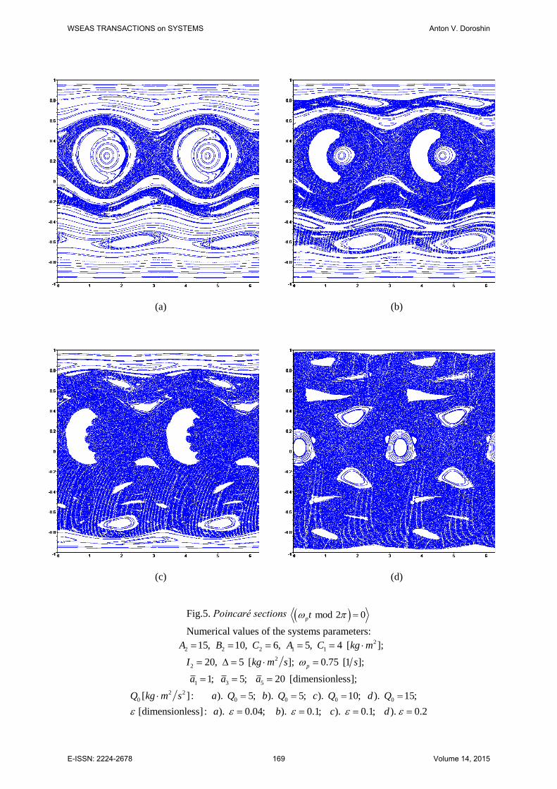
First of all, we have to indicate the production

of the chaotic layer near the heteroclinic separatrix

region – it is showed as a cloud of blue points at the

figures (Fig.5). Also at the figures (Fig.5) we can

see the primary and secondary chaotic layers (in the

regions of the primary and secondary separatrix

bundles with the meander-line tori), and the "islands

of regularity" – this is the phase portrait’s areas

corresponding to local oscillations regimes into the

chaotic layer.

The heteroclinic nets were plotted as a

collection of the Poincaré images and preimages

(corresponding to the separated generations) of the

unperturbed separatrix polhode's points.

So, as we can see, all of the standard features of

the chaotic modes are realized: the Poincaré sections

have the chaotic layers; the time-series of the

angular velocity components are complex and

oscillating with variable (irregular) amplitudes; the

heteroclinic nets are tangled.

Conclusion

Heteroclinic dynamics of the magnitized DSSC

was examined in the case of the “cylindrical

precession”. The heteroclinic analytical solutions for

the polhode-separatrix in the phase space of the

angular velocity components were obtained. These

heteroclinic solutions are the main result of the

paper, which can be applied to the investigation and

modeling of chaotic properties of the

magnetic/magnetized DSSC attitude dynamics in

many cases of perturbations and conditions of the

attitude motion.

As an example of the chaotization analysis, the

case of polyharmonic perturbations was studied

based on the Melnikov’s methodology. Also the

corresponding numerical modeling of the

magnetic/magnetized DSSC attitude motion was

fulfilled.

WSEAS TRANSACTIONS on SYSTEMS Anton V. Doroshin

E-ISSN: 2224-2678 168 Volume 14, 2015

(a)

(b)

(c)

(d)

Fig.5. Poincaré sections mod 2 0pt

Numerical values of the systems parameters: 2

2 2 2 1 1

2

2

1 3 5

2 2

0 0 0 0 0

15, 10, 6, 5, 4 [ ];

20, 5 [ ]; 0.75 [1 ];

1; 5; 20 [dimensionless];

[ ] : ). 5; ). 5; ). 10; ). 15;

[dimensionless] : ). 0.04; ). 0.1; ). 0.1; ). 0.2

p

A B C A C kg m

I kg m s s

a a a

Q kg m s a Q b Q c Q d Q

a b c d

WSEAS TRANSACTIONS on SYSTEMS Anton V. Doroshin

E-ISSN: 2224-2678 169 Volume 14, 2015

(a)

(b)

(c)

(d)

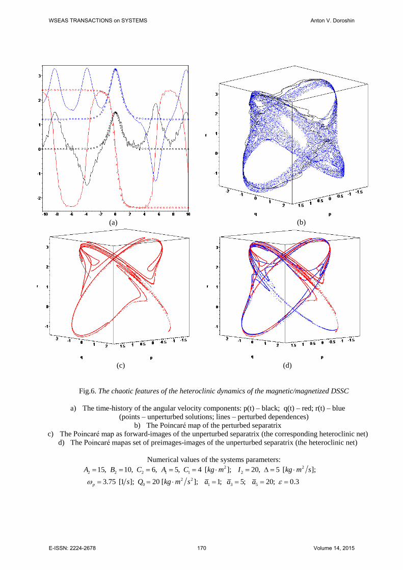
Fig.6. The chaotic features of the heteroclinic dynamics of the magnetic/magnetized DSSC

a) The time-history of the angular velocity components: p(t) – black; q(t) – red; r(t) – blue

(points – unperturbed solutions; lines – perturbed dependences)

b) The Poincaré map of the perturbed separatrix

c) The Poincaré map as forward-images of the unperturbed separatrix (the corresponding heteroclinic net)

d) The Poincaré mapas set of preimages-images of the unperturbed separatrix (the heteroclinic net)

Numerical values of the systems parameters: 2 2

2 2 2 1 1 2

2 2

0 1 3 5

15, 10, 6, 5, 4 [ ]; 20, 5 [ ];

3.75 [1 ]; 20 [ ]; 1; 5; 20; 0.3p

A B C A C kg m I kg m s

s Q kg m s a a a

WSEAS TRANSACTIONS on SYSTEMS Anton V. Doroshin

E-ISSN: 2224-2678 170 Volume 14, 2015

The modeling illustrated all of the standard

features of the chaotic modes: the Poincaré sections

have the chaotic layers; the time-series of the

angular velocity components are complex

oscillating with variable (irregular) amplitudes; the

heteroclinic nets are tangled.

These indicated chaotic dynamical properties

in the practice of the real space-missions result in

the DSSC chaotic attitude motion and in

failures/anomalies of its operation; also the desired

target motion of the DSSC due to this chaos

phenomenon is inevitably involved in the chaotic

regime, and, therefore, the stabilized regime of the

magnetic/magnetized DSSC “cylindrical

precession” can be lost.

The paper results are also applicable to the task

of the generalized heavy coaxial Lagrange top; and,

on the contrary, in the case when the magnetic

moment of the DSSC is equal to zero, the

investigation results are directly reduced to the

Euler coaxial top [5-10].

Acknowledgment

This work was partially supported by the

Ministry education and science of the Russian

Federation

- in the framework of the implementation of

the Program of increasing the

competitiveness of SSAU among the

world’s leading scientific and educational

centers for 2013-2020 years;

- in the framework of the State Assignments

to higher education institutions and

research organizations in the field of

scientific activity.

References

[1] J. Wittenburg, Dynamics of Systems of Rigid

Bodies. Stuttgart: Teubner, 1977.

[2] J. Wittenburg, Beitrage zur dynamik von

gyrostaten, Accademia Nazional dei Lincei,

Quaderno N. 227 (1975) 1–187.

[3] V.V. Golubev, Lectures on Integration of the

Equations of Motion of a Rigid Body about a

Fixed Point, State Publishing House of

Theoretical Literature, Moscow, 1953.

[4] V.V. Kozlov, Methods of qualitative analysis in

the dynamics of a rigid body, Gos. Univ.,

Moscow, 1980.

[5] A. Elipe, V. Lanchares, Exact solution of a

triaxial gyrostat with one rotor, Celestial

Mechanics and Dynamical Astronomy, Issue 1-

2, Volume 101, 2008, pp 49-68.

[6] E.A. Ivin, Decomposition of variables in task

about gyrostat motion. Vestnik MGU

(Transactions of Moscow’s University). Series:

Mathematics and Mechanics. No.3 (1985) Pp.

69-72.

[7] V.S. Aslanov, Integrable cases in the dynamics

of axial gyrostats and adiabatic invariants,

Nonlinear Dynamics, Volume 68, Numbers 1-2

(2012) 259-273.

[8] V.S. Aslanov, A.V. Doroshin, Chaotic

dynamics of an unbalanced gyrostat. Journal of

Applied Mathematics and Mechanics, Volume

74, Issue 5 (2010) 525-535.

[9] A.V. Doroshin, Exact solutions for angular

motion of coaxial bodies and attitude dynamics

of gyrostat-satellites, International Journal of

Non-linear Mechanics 50 (2013) 68-74.

[10] A.V. Doroshin, Heteroclinic dynamics and

attitude motion chaotization of coaxial bodies

and dual-spin spacecraft, Communications in

Nonlinear Science and Numerical Simulation,

Volume 17, Issue 3 (2012) 1460–1474.

[11] H. Andoyer, Cours de Mecanique Celeste,

Paris: Gauthier-Villars, 1924.

[12] A. Deprit, A free rotation of a rigid body

studied in the phase plane, American Journal of

Physics 35 (1967) 425 – 428.

[13] P. J. Holmes, J. E. Marsden, Horseshoes and

Arnold diffusion for Hamiltonian systems on

Lie groups, Indiana Univ. Math. J. 32 (1983)

283-309.

[14] C.D. Hall, R.H. Rand, Spinup Dynamics of

Axial Dual-Spin Spacecraft, Journal of

Guidance, Control, and Dynamics, Vol. 17, No.

1 (1994) 30–37.

[15] C.D. Hall, Momentum Transfer Dynamics of a

Gyrostat with a Discrete Damper, Journal of

Guidance, Control, and Dynamics, Vol. 20, No.

6 (1997) 1072-1075.

[16] A.I. Neishtadt, M.L. Pivovarov, Separatrix

crossing in the dynamics of a dual-spin

satellite. Journal of Applied Mathematics and

Mechanics, Volume 64, Issue 5, 2000, Pages

709-714.

[17] A.V. Doroshin, Evolution of the precessional

motion of unbalanced gyrostats of variable

structure. Journal of Applied Mathematics and

Mechanics, Volume 72, Issue 3, October 2008,

WSEAS TRANSACTIONS on SYSTEMS Anton V. Doroshin

E-ISSN: 2224-2678 171 Volume 14, 2015

Pages 259-269.

[18] A.V. Doroshin, Synthesis of attitude motion of

variable mass coaxial bodies, WSEAS

Transactions on Systems and Control, Issue 1,

Volume 3 (2008) 50-61.

[19] A.V. Doroshin, Analysis of attitude motion

evolutions of variable mass gyrostats and

coaxial rigid bodies system, International

Journal of Non-Linear Mechanics, Volume 45,

Issue 2 (2010) 193–205.

[20] A.V. Doroshin, Modeling of chaotic motion of

gyrostats in resistant environment on the base

of dynamical systems with strange attractors.

Communications in Nonlinear Science and

Numerical Simulation, Volume 16, Issue 8

(2011) 3188–3202.

[21] A.V. Doroshin, Chaos and its avoidance in

spinup dynamics of an axial dual-spin

spacecraft. Acta Astronautica, Volume 94,

Issue 2, February 2014, Pages 563-576.

[22] M. Iñarrea, V. Lanchares, Chaos in the

reorientation process of a dual-spin spacecraft

with time-dependent moments of inertia, Int. J.

Bifurcation and Chaos. 10 (2000) 997-1018.

[23] A.V. Doroshin, M.M. Krikunov, Attitude

dynamics of a spacecraft with variable structure

at presence of harmonic perturbations, Applied

Mathematical Modelling, Volume 38, Issues 7–

8 (2014) 2073-2089

[24] Jinlu Kuang, Soonhie Tan, Kandiah

Arichandran, A.Y.T. Leung, Chaotic dynamics

of an asymmetrical gyrostat, International

Journal of Non-Linear Mechanics, Volume 36,

Issue 8 (2001) 1213-1233.

[25] Awad El-Gohary, Chaos and optimal control of

steady-state rotation of a satellite-gyrostat on a

circular orbit, Chaos, Solitons & Fractals,

Volume 42, Issue (2009) 2842-2851.

[26] A.V. Doroshin, Exact Solutions in Attitude

Dynamics of a Magnetic Dual-Spin Spacecraft

and a Generalization of the Lagrange Top,

WSEAS Transactions on Systems, Issue 10,

Volume 12 (2013) 471-482.

[27] A. Guran, Chaotic motion of a Kelvin type

gyrostat in a circular orbit, Acta Mech. 98

(1993) 51–61.

[28] X. Tong, B. Tabarrok, F. P. J. Rimrott, Chaotic

motion of an asymmetric gyrostat in the

gravitational field, Int. J. Non-Linear Mech. 30

(1995) 191-203.

[29] V.K. Melnikov, On the stability of the centre

for time-periodic perturbations, Trans. Moscow

Math. Soc. No.12 (1963) 1-57.

[30] S. Wiggins, Chaotic Transport in Dynamical

System. Springer-Verlag. 1992.

[31] A.V. Doroshin, Homoclinic solutions and

motion chaotization in attitude dynamics of a

multi-spin spacecraft, Communications in

Nonlinear Science and Numerical

Simulation, Vol. 19, Issue 7 (2014) 2528-2552.

[32] M. Iñarrea, Chaos and its control in the pitch

motion of an asymmetric magnetic spacecraft

in polar elliptic orbit, Chaos, Solitons &

Fractals,Volume 40, Issue 4, 30 May

2009, Pages 1637-1652.

[33] M. Iñarrea, Chaotic pitch motion of a magnetic

sspacecraft with viscous drag in an elliptical

polar orbit, Internatioanl Journal of Bifurcation

and Chaos, Vol.21, No.7 (2011) 1959-1975.

[34] V.A. Bushenkov, M. Yu. Ovchinnikov,

G.V. Smirnov, Attitude stabilization of a

satellite by magnetic coils, Acta

Astronautica, Volume 50, Issue 12 (2002) 721-

728

[35] M.Yu. Ovchinnikov, D.S. Roldugin, V.I.

Penkov, Asymptotic study of a complete

magnetic attitude control cycle providing a

single-axis orientation, Acta Astronautica 77

(2012) 48–60

[36] M.Yu. Ovchinnikov, A.A. Ilyin, N.V.

Kupriynova, V.I. Penkov, A.S. Selivanov,

Attitude dynamics of the first Russian

nanosatellite TNS-0, Acta Astronautica,

Volume 61, Issues 1–6, June–August

2007, Pages 277-285

[37] Yan-Zhu Liua, Hong-Jie Yu, Li-Qun Chen,

Chaotic attitude motion and its control of

spacecraft in elliptic orbit and geomagnetic

field, Acta Astronautica 55 (2004) 487 – 494.

[38] Li-Qun Chen, Yan-Zhu Liu, Chaotic attitude

motion of a magnetic rigid spacecraft and its

control, International Journal of Non-Linear

Mechanics 37 (2002) 493–504.

[39] Li-Qun Chen, Yan-Zhu Liu, Gong Cheng,

Chaotic attitude motion of a magnetic rigid

spacecraft in a circular orbit near the equatorial

plane, Journal of the Franklin Institute 339

(2002) 121–128.

[40] M. Lovera, A. Astolfi, Global Magnetic

Attitude Control of Spacecraft in the Presence

of Gravity Gradient, IEEE Ttansactions On

WSEAS TRANSACTIONS on SYSTEMS Anton V. Doroshin

E-ISSN: 2224-2678 172 Volume 14, 2015

Aerospace And Electronic Systems, Vol. 42,

No. 3 (2006) 796-805.

[41] M. Lovera, A. Astolfi, Spacecraft attitude

control using magnetic actuators, Automatica

40 (2004) 1405 – 1414.

[42] Enrico Silani, Marco Lovera, Magnetic

spacecraft attitude control: a survey and some

new results, Control Engineering Practice 13

(2005) 357–371.

[43] Filippo Neri, Traffic packet based intrusion

detection: decision trees and generic based

learning evaluation. WSEAS Transactions on

Computers, WSEAS Press (Wisconsin, USA),

issue 9, vol. 4, 2005, pp. 1017-1024.

[44] Filippo Neri, Software agents as a versatile

simulation tool to model complex systems.

WSEAS Transactions on Information Science

and Applications, WSEAS Press (Wisconsin,

USA), issue 5, vol. 7, 2010, pp. 609-618.

[45] L. Nechak, S. Berger, E. Aubry, Robust

Analysis of Uncertain Dynamic Systems:

Combination of the Centre Manifold and

Polynomial Chaos theories, WSEAS

Transactions on Systems, Issue 4, Volume 9,

April 2010, pp.386-395.

[46] N. Jabli, H. Khammari, M. F. Mimouni, R.

Dhifaoui, Bifurcation and chaos phenomena

appearing in induction motor under variation of

PI controller parameters, WSEAS Transactions

on Systems, Issue 7, Volume 9, July 2010,

pp.784-793.

[47] S. Staines A., Neri F. (2014). "A Matrix

Transition Oriented Net for Modeling

Distributed Complex Computer and

Communication Systems". WSEAS

Transactions on Systems, 13, WSEAS Press

(Athens, Greece), 12-22.

[48] M. Camilleri, F. Neri, M. Papoutsidakis (2014),

"An Algorithmic Approach to Parameter

Selection in Machine Learning using Meta-

Optimization Techniques". WSEAS

Transactions on Systems,13, WSEAS Press

(Athens, Greece), 202-213.

[49] M. Papoutsidakis, D. Piromalis, F. Neri, M.

Camilleri (2014), "Intelligent Algorithms

Based on Data Processing for Modular Robotic

Vehicles Control". WSEAS Transactions on

Systems, 13, WSEAS Press (Athens,

Greece), 242-251.

WSEAS TRANSACTIONS on SYSTEMS Anton V. Doroshin

E-ISSN: 2224-2678 173 Volume 14, 2015