“hermann50” — 2012/9/11 — 12:52 — page 1 — #1cbraga/hermann50/hermann50.pdf · “hermann50” — 2012/9/11 — 12:52 — page 2 — #2 ... – Luis Fernando Gomes Soares

ii

“hermann50” — 2012/9/11 — 12:52 — page 1 — #1 ii

ii

ii

ii

“hermann50” — 2012/9/11 — 12:52 — page 2 — #2 ii

ii

ii

Christiano Braga (Ed.)

Truth and Meaning

Essays dedicated to Edward Hermann Haeusleron the occasion of his 50th birthday

ii

“hermann50” — 2012/9/11 — 12:52 — page 3 — #3 ii

ii

ii

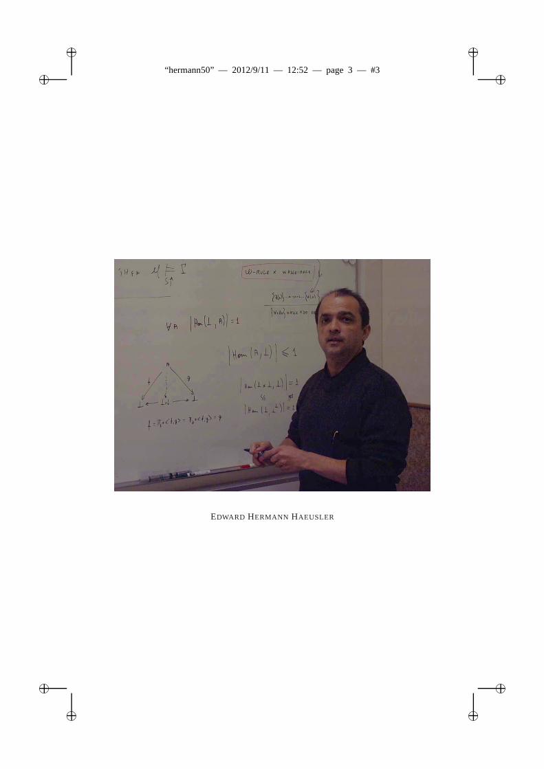
EDWARD HERMANN HAEUSLER

ii

“hermann50” — 2012/9/11 — 12:52 — page 4 — #4 ii

ii

ii

Preface

Former students, collaborators and friends joined together on September 29th, 2012 atPUC-Rio during the 7th Logical and Semantic Frameworks with Applications (LSFA2012) to celebrate Edward Hermann Haeusler’s 50th birthday. Some of them gave talkson subjects that his teachings and ideas had a direct or indirect contribution. Here is theprogramme of the event:

– Opening: Christiano Braga– Paulo Veloso– Andrey Bovykin, (on behalf of Lew Gordeev)– Luiz Carlos Pereira– Mario Benevides– Mauricio Kischinhevsky– Marcelo Corrêa– Isabel Cafezeiro– Leonardo Moura– Alexandre Rademaker– Luis Fernando Gomes Soares– Closing: Hermann

The following collaborators and friends of Hermann’s contributed1 to these essays:Paulo Veloso, Lew Gordeev, Luiz Carlos Pereira, Wagner Sanz, Valeria de Paiva, UweWolter, Mario Benevides, Alfio Martini, Marcelo Corrêa, Isabel Cafezeiro, LeonardoMoura, Vaston Costa, and Alexandre Rademaker. (I have chosen to display only theirnames in the table of contents, even when they have co-authors. Their co-authors, ifany, appear in the contribution inside the book.)

Thanks to Isabel Cafezeiro for suggesting the use of IBM’s Many Eyes with a con-catenation of the preambles of each article in this book for the cover picture. The actualpicture was generated by Wordle. Thanks to Debora MuchaluatSaade for mentioning itto me by. Thanks to Vaston Costa for helping me with LATEX issues and Bruno Lopes foridentifying some formatting inconsistencies in a draft of this book. (Of course, all edit-ing mistakes are my fault!) Aspecialthanks to Renata de Freitas and Isabel Cafezeirofor working hard to make Hermann’s celebration a joint venture with LSFA. Manythanks to the Department of Informatics at PUC-Rio for partially sponsoring the cele-bration, in particular to Ruth Maria de Barros Fagundes de Sousa and Professor MarcusVinicius Soledade Poggi de Aragão.

September 2012 Christiano Braga

1 Some of the papers included here were already published somewhere else. This book wasedited as a gift to E. Hermann Haeusler only. Reproduction ofcopyrighted material requiresauthorization of the copyright owner.

ii

“hermann50” — 2012/9/11 — 12:52 — page 5 — #5 ii

ii

ii

Table of Contents

A celebration of Hermann’s achievements in the year of his half centenary. . . . . 1Christiano Braga

H., we’ve got a problem. . . . . . . . . . . . . . . . . . . . . . . . . . . . . . . . . . . . . . . . . . . . 3Paulo A. S. Veloso

DAG-like term compression. . . . . . . . . . . . . . . . . . . . . . . . . . . . . . . . . . . . . . . . . . 20Lew Gordeev

A short note on discharging functions and unicity of normal form for naturaldeduction. . . . . . . . . . . . . . . . . . . . . . . . . . . . . . . . . . . . . . . . . . . . . . . . . . . . . . . . . 34

Luiz Carlos Pereira and Wagner de Campos Sanz

Indexed logical closure operators. . . . . . . . . . . . . . . . . . . . . . . . . . . . . . . . . . . . . . 36Uwe Wolter and Alfio Martini

Linear logic model of state revisited. . . . . . . . . . . . . . . . . . . . . . . . . . . . . . . . . . . 48Valeria de Paiva

On the computational complexity of the intuitionistic modal logic IK . . . . . . . . . 62Mario R. F. Benevides

Modelling the Lambek calculus via a hierarchical structureof categories. . . . . . . 69Marcelo da Silva Corrêa

Interweavings of Alan Turing’s mathematics and sociology of knowledge. . . . . . 100Isabel Cafezeiro

Satisfiability modulo theories: A calculus of computation. . . . . . . . . . . . . . . . . . . 111Leonardo Moura

A discussion on compressing proofs through proof-theoretical techniques. . . . . . 128Vaston G. Costa

Intuitionistic description logic and legal reasoning. . . . . . . . . . . . . . . . . . . . . . . . 140Alexandre Rademaker

ii

“hermann50” — 2012/9/11 — 12:52 — page 6 — #6 ii

ii

ii

ii

“hermann50” — 2012/9/11 — 12:52 — page 1 — #7 ii

ii

ii

A celebration of Hermann’s achievements in the year ofhis half centenary

Christiano Braga

Instituto de Computação,Universidade Federal Fluminense

[email protected]

In 2012 the world is celebrating the centenary of Alan Turing’s birth. One of thegreatest minds of the 20th century as Hermann himself wrote in a recent paper to honorTuring’s achievements. Hermann is one of the most brilliantminds I had the pleasureto meet.

Edward Hermann Haeusler was born in 1962. He is married to Olivia with whomhe has a son, Rafael. Hermann received his BA in Mathematics from Universidade deBrasília in 1983 and MSc and DSc in Computer Science from PUC-Rio in 1986 and1990, respectively. From 1986 to 1990 he was a faculty memberat Universidade FederalFluminense and then at PUC-Rio, his current position. Hermann was also a postdocvisitor at Aarhus University in 1994 and at Eberhard Karls Universität Tüebingen in2003.

Hermann is interested in many things, technical and otherwise. Paulo Blauth, a col-laborator and friend of his, has a quite interesting way to qualify it: “encyclopedic”. Itis not surprising that his research interests are quite diverse. Essentially, if it is relatedto theoretical computer science, Hermann is interested in.Quoting his webpage:

My research interests are Proof Theory, Automated Theorem Proving, Logical Systems,Category Theory (CT), Toposes and Higher-Order Theories and their Models, Seman-tics, and the application of this knowledge and the techniques emerged from them inSoftware Development and Validation. Structural and Computational Complexity callmy attention too.I have written, together with Paulo Blauth Menezes, a book onCategory Theory forComputer Science, aimed to help teaching CT to undergraduated classes.

A quite unusual property that Hermann has is that it does not exist a person whodislikes him. (Of course, I do not know everyone who knows himbut I know quite afew and I think this is a fair extrapolation.) Moreover, he iscapable of putting togetheraround a restaurant table, for instance, people that otherwise would not stand to be atthe same quadrant of the known universe. Those people got together just to be with him.(I was one of the afore mentioned people so this is a true story!)

It is only natural that people would enjoy working with someone with these threeproperties together, that is, (i) an exquisite mind, (ii) a diverse interest in ComputerScience and (iii) a way with people. By the time I wrote this tribute, Hermann hassupervised 20 DSc theses, with 4 more underway, 13 MSc dissertations and many un-dergraduate students. Here is the list of Hermann’s academic (DSc) offspring, so far:

ii

“hermann50” — 2012/9/11 — 12:52 — page 2 — #8 ii

ii

ii

2 C. Braga

1. Luiz Carlos Castro Guedes,2. Marcelo da Silva Corrêa,3. Lucília Camarão Figueiredo,4. Eliana Silva Almeida,5. Regina Celia Moreth Bragança,6. Ana Isabel de Azevedo Spinola,7. Leonardo Mendonça de Moura (co-

supervision),8. Alex Vasconcelos Garcia,9. Isabel Leite Cafezeiro,

10. Christiano Braga,11. Geiza Maria Hamazaki da Silva,12. Fernando Naufel do Amaral,13. Christian Jacques Renteria,

14. José Antonio F. de Macedo (co-supervision),

15. Carlos Bazílio Martins,16. Juliana Carpes Imperial,17. David Romero de Vasconcelos,18. Vaston Gonçalves da Costa,19. Alexandre Rademaker,20. Ricardo Queiroz de Araujo Fernandes,

with the following people being advised:

– Cecília Englander Lustosa,– Bruno Lopes Vieira,– Marcela Quispe Cruz,– Jefferson Santos.

The following is a non-exhaustive list of collaborators, recovered from DBLP.

– Fernando Naufel do Amaral,– Mauricio Ayala-Rincón,– Carlos Bazílio,– Mario R. F. Benevides,– Christiano Braga,– Karin Koogan Breitman,– Isabel Cafezeiro,– Nuno Caminada,– Luis Fariñas del Cerro,– Marcelo da Silva Corrêa,– Vaston G. Costa,– Alexandre R. Duarte,– Markus Endler,– Cecilia Englander,– Ricardo Queiroz de Araujo Fernandes,– Aluízio Haendchen Filho,– José Viterbo Filho,– Alex de V. Garcia,– Lew Gordeev,

– Luiz Carlos Castro Guedes,– Eduardo Sany Laber,– Alfio Martini,– José Meseguer ,– Peter D. Mosses,– Loana Tito Nogueira,– Valeria de Paiva,– Luiz Carlos Pereira,– Ruy J. G. B. de Queiroz,– Alexandre Rademaker,– José Lucas Rangel,– Christian Jacques Rentería,– Wagner Sanz,– Geiza Maria Hamazaki da Silva,– Arndt von Staa,– Sebastián Urrutia,– Davi R. Vasconcelos,– Paulo A. S. Veloso, and– Uwe Wolter.

It is easy to understand now why it was a very difficult task to decide who to inviteto contribute to these essays and also to give a talk at the event in his honor on Septem-ber 29th at PUC-Rio during LSFA 2012. I wish that those who in one way oranothercontributed to this celebration find these essays a nice memento of it.

Hermann, this is for you, a token of my friendship and gratitude with my wishes ofmany springs to come.

ii

“hermann50” — 2012/9/11 — 12:52 — page 3 — #9 ii

ii

ii

H., we’ve got a problem⋆

Paulo A. S. Veloso

Systems and Computing Engin. Progr., COPPE-UFRJ,Universidade Federal do Rio de Janeiro; RJ, Brazil,

[email protected]

Abstract. We present and discuss some aspects of a mathematical theoryof gen-eral problems and solutions. The aim is providing a framework for the preciseanalysis of these notions as well as reduction and decompositions. Despite itswide diversity, problems present some common features. We try to give preciseformulations for some intuitive notions of Polya’s relatedto Heuristics.

1 Introduction

Here we present and discuss some aspects of a research program aiming at a mathemati-cal theory of general problems and solutions. The overall goal is providing a frameworkfor the precise analysis of these notions as well as related ones, such as reductions anddecompositions.1

Problems have been faced for quite a long time. Some examplesmay be: gatheringfood; balancing checkbooks; preparing/gradingexams; selecting flight/metro itineraries;assembling objects (like cars, aeroplanes, furniture); classifying biological specimens;conducting experiments; proving (mathematical) theorems; constructing geometricalfigures; solving algebraic equations.2

There is a wide diversity of problems, coming from several walks of life and havingdistinct goals. They may, however, present some common features. This is more likelyto become apparent if we emphasize ‘what’ rather than ‘how’,i. e. what is a problem,rather than how to solve it. Thus, some intuitive notions of Polya related to Heuris-tics [Pol ’57] can be given precise formulations and analyses.3 For instance, divide-and-conquer was formulated in terms of abstract data types [Vel ’80].

The structure of this paper is as follows. In Section 2, we introduce some basic ideasand discuss them. In Section 3, we examine the central concepts: problems, conditionsand solutions. In Section 4, we introduce transformations leading to reductions. In Sec-tion 5, we consider decompositions as reductions to structured problems. In Section 6,we briefly examine some other aspects. Section 7 presents some concluding remarks.

⋆ Research partly sponsored by the Brazilian agencies CNPq and FAPERJ.1 This presentation is an extension of some previous ones [Vel’84,Vel ’11].2 Kolmogorov used problems in an interpretation for intuitionistic logic [Kol ’32].3 To clarify this goal, an analogy may be appropriate: logic formalizes notions such as proof and

theorem [Ent ’72], but its aim is not to teach how to prove theorems.

ii

“hermann50” — 2012/9/11 — 12:52 — page 4 — #10 ii

ii

ii

4 Paulo A. S. Veloso

2 Basic Ideas

We now examine some basic ideas and discuss them.We introduce our basic ideas by means of a simple example, namely finding roots

of polynomials. The concept of root of a polynomial is clear enough. Nevertheless, theproblem is not yet clearly specified.

Polya [Pol ’57] suggests asking three questions in approaching a problem.

(D) What are the data? What kind of polynomials are we to handle: linear, quadratic orof arbitrary degree? This affects the nature of the problem:finding roots of polyno-mials is much easier for linear or quadratic ones.

(R) What are the results? What kind of results do we expect: natural, real or complexnumbers? This may affect solvability and the choice of a method.

(q) What is the condition? A polynomial may have several roots; which one do wewish: any one, all of them, the smallest one?

Let us say, for definiteness, that we wish to find any complex root of a real-coefficientpolynomial with non-zero degree. We now have specified our problemQ as having datafrom the set IR[x] of real-coefficient polynomials with non-zero degree, results in theset IC of complex numbers, its condition being the relationq from IR[x] to IC given byp(x)qc iff p(c) = 0.4

Now, a solution for our problemQ should provide at least one root for each poly-nomial in IR[x]. So, one might conceive it as a functionf : IR[x] → IC assigning to eachpolynomial p(x) ∈ IR[x] a complex numberf (p(x)) ∈ IC so as to satisfy the conditionq,i. e. polynomial p(x) evaluated atf (p(x)) gives 0.5

This example suggests that a problem is specified by means of sets D, of data, andR, of results, as well as a binary relationq from D to R. Some remarks may be in order.First, we wish to consider general problems and not only specific instances: finding acomplex root of the polynomial 3x4+5x3+7x2+8x+6 is an instance of our problemQ. Also, this idea encompasses decision problems [Rog ’62], as well as questions ingeneral, as those with Boolean results:⊤ or⊥. Note that sets D and R may have somestructure (e. g. operations). In addition to D and R, one may have other sets; for instance,our problemQ also involves the sets: IN of naturals, ZZ of integers and IR of reals.

As for the notion of solution, shall we accept any function satisfying the condition?The Axiom of Choice may provide functions not fitting our intuitions.6

3 Problems: Solutions and Requirements

We now examine the central concepts: problems, conditions and solutions.

4 If we wished, instead, to find the smallest real root of a real-coefficient polynomial with non-zero degree, the results would be real numbers with condition p(x)q′ r iff p(r) = 0 and, for anyr′ < r, p(r′) 6= 0.

5 For instance, we may havef (2x−8) = 4 and f (x2−5x+6) = 2.6 The sentence(∀u : D)(∃z : R)q(u,z) asserts that the domain of relationq is all of D. The

sentence(∀u : D)q(u, f (u)) asserts that the Skolem functionf satisfies conditionq. Suchideas were used in analyses of decomposition and reduction [V+V ’81].

ii

“hermann50” — 2012/9/11 — 12:52 — page 5 — #11 ii

ii

ii

Problem Theory 5

We consider a problem as a structureQ with distinguished domains D, ofdata, andR, of results, and acondition: a binary relationq from D to R.

Let us now examine the concept of solution. It was long felt that identifying solu-tions with functions meeting the condition was an oversimplification. While these ideaswere used in a programming context, little, if any, harm seems to have been done. Acrucial insight came from the work of E. Hermann Haeusler [Hae ’88,Hae ’96] combin-ing problems and Martin Löf’s Intuitionistic Type Theory [M-L ’84], where he showedthat conditions and solutions may collapse. In the constructive framework of ITT, whenones finishes specifying a problem, one has already described a solution for it!

Now, in geometrical problems, one generally wishes solutions to be constructedby straight edge and compass. This rules out a priori some possible functions: onlyadmissible ones are to be considered. Similarly, in a programming context, one maywish only computable functions.7

Let us examine some geometrical problems.

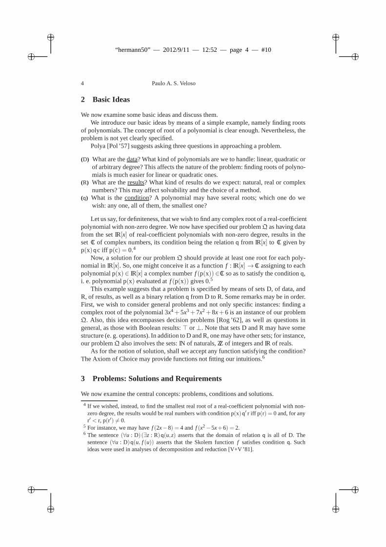
Example 1.Consider the geometrical problemG′ of finding the midpoint of a segment.Its solution involves drawing circles, straight lines and intersecting them. More pre-cisely, we have domains D, consisting of pairs of points, andR, of points, with condition(A,B)qM iff M is equidistant fromA andB. Its solution involves the steps:

1. first, draw circlesC′ andC′′, centred atA andB, with the same radius;2. next, intersect circlesC′ andC′′, to obtain pointsP′ andP′′;3. then, draw straight linesABandP′P′′;4. finally, intersect straight linesABandP′P′′, obtaining pointM.

z|xy~.MC′ C′′

A B

P′

P′′

______

The result of a geometrical construction may fail to be unique.

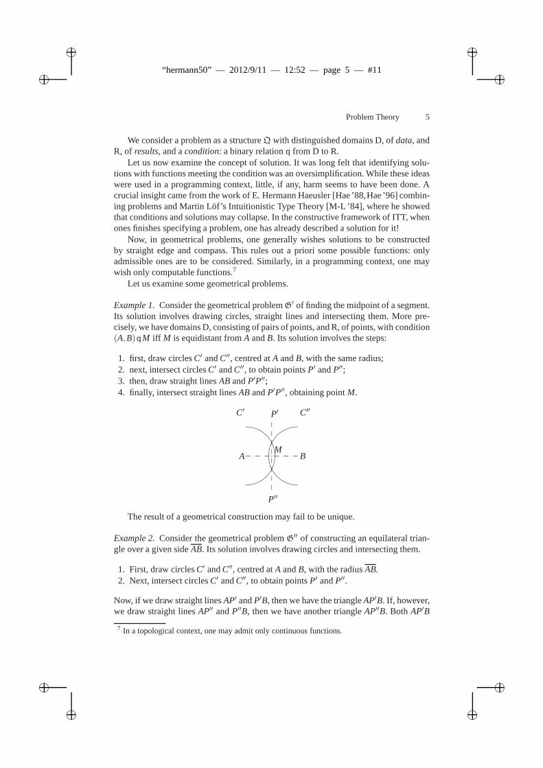
Example 2.Consider the geometrical problemG′′ of constructing an equilateral trian-gle over a given sideAB. Its solution involves drawing circles and intersecting them.

1. First, draw circlesC′ andC′′, centred atA andB, with the radiusAB.2. Next, intersect circlesC′ andC′′, to obtain pointsP′ andP′′.

Now, if we draw straight linesAP′ andP′B, then we have the triangleAP′B. If, however,we draw straight linesAP′′ andP′′B, then we have another triangleAP′′B. Both AP′B

7 In a topological context, one may admit only continuous functions.

ii

“hermann50” — 2012/9/11 — 12:52 — page 6 — #12 ii

ii

ii


andAP′′B are equilateral triangles over sideAB.

A B

P′

P′′

????

Which one of these triangles should one take as result?

We take aconstructionto be a text that can be executed, like a (maybe non-deterministic)program, or a proof.8 As texts, we now have some non-extensional comparisons: bothprecise comparisons (such as a more efficient program as a faster one or one requiringless storage) and intuitive ones (such as a more elegant construction as involving fewerauxiliary lines and a more informative proof as clearer or better structured).

Now, a problem is to be stated. And how is it stated? One describes its condition; sowe also have a text describing the problem condition: itsrequirement.

We define aproblemas a structureQ with distinguished domains D and R, as before,

and arequirementq describing a binary relation from D to R (notedQ= 〈↓

D,↑

R: q〉).Requirements and constructions may very well be described in different languages.

For instance, constructions may described in a programminglanguage and requirementsin predicate logic. The crucial difference between these descriptions is that a require-ment is intended to be declarative, whereas a construction is supposed to be executable.It is often convenient to regard constructions as being a special case of requirements.

A requirementq connects pairs of objects: aq|−−> b. The execution of a construction

σ transforms objects: aσ7→ b. So, requirements and constructions have extensions con-

sisting of their ordered pairs. We will use ‘⊑’ and ‘≡’, respectively, forinclusionandequalityof extensions.

Consider a constructionσ. Given sets D and R, we say thatσ transformsD to R(notedσ : D→R) iff for every d∈D, the execution ofσ on d produces some r∈R. We

say thatσ respectsa requirementq (notedσ ⊑ q) iff dq|−−> r, whenever d

σ7→ r.

Henceforth, we will consider a givencontextA of admissible constructions.

Given a problemQ= 〈↓

D,↑

R: q〉, by anA-solutionfor problemQ (or a solution forA-problemQ) we mean a constructionσ ∈ A, such that:

(→) σ transforms D to R, i. e.σ : D→ R, and(⊑) σ respects requirementq, i. e.σ ⊑ q.

The proviso (→) is analogous to termination for programs [Man’74]. In the geometricalproblemG′ of Example 1, if we select too small a radius in step 1, the circlesC′ andC′′

will not intersect and the construction will fail to produceresults.

8 Such constructions may be those obtained from basic ones by combinations. For the primitiverecursive functions, the basic ones are zero, successor andprojections, the combinations beingcomposition and primitive recursion; for the partial recursive functions, one adds minimiza-tion [Rog ’62].

ii

“hermann50” — 2012/9/11 — 12:52 — page 7 — #13 ii

ii

ii

Problem Theory 7

There are some natural operations on constructions and requirements. Given con-structionsσ′ andσ′′, theirconcatenationσ′;σ′′ is defined by applying firstσ′ and thenσ′′ to the result. So, ifσ′ : S1→ S2 andσ′′ : S2→ S3, thenσ′;σ′′ : S1→ S3. Given re-quirementsq′, from D to S, andq′′, from S to R, their(serial) compositionq′;q′′ is the

requirement from D to R described by dq′;q′′|−−> r iff, for some element s∈S, d

q′

|−−> s and

sq′′

|−−> r. Another familiar operation on requirements interchanges input and outputs: fora requirementq, from S to T, itsconversein the requirementq, from T to S, described

by tq

|−−> s iff sq|−−> t. These operations on requirements correspond to familiarones

on binary relations: composition to relational product andconverse to transposal. Otheroperations are⊔ and⊓ corresponding, respectively, to Boolean∪ and∩.

These operations preserve extension inclusions.

Remark 1.If p ⊑ q, thenp ⊑ q, p;g ⊑ q;g andf;p ⊑ f;q.

4 Problem Transformations

We now examine problem transformations: one often transforms problems to problems.Some transformations break problems by interpolating a domain.

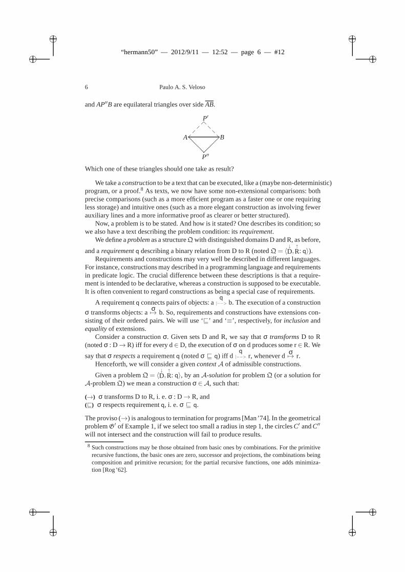
Example 3.Consider the problemP of finding the center of a rectangle. One may inter-polate a domain of (non-parallel) straight lines, thereby breaking it into two consecutiveproblems:P′, of drawing the diagonals, andP′′, of intersecting them, as follows:

A B

CD diagonals

&&MM

MM

MM

MM

MM

A B

CD

intersect

wwo oooooooooo

M

Some transformations traditionally receive particular names.

Example 4.Examples of specializations and generalizations are as follows.

ii

“hermann50” — 2012/9/11 — 12:52 — page 8 — #14 ii

ii

ii


– The problem of determining the parity of a sum of integers canbe specialized bytransforming it to that of adding them modulo 2.

ZZ×ZZ

PrSm

mod2 // // ZZ2×ZZ2

+2

Evn,Odd oo // ZZ2

– Generalization is often convenient for induction. The problem of determining whethera sentence holds in structureM can be generalized by transforming it to that ofwhether a formula holds in structureM under an assignmentα [Ent ’72].

ϕ

|=M

// addα // (ϕ,α)

|=M

⊥,⊤ ⊥,⊤

These ideas can be formulated as follows.

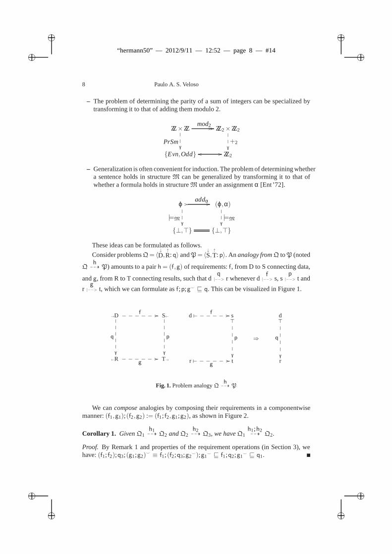
Consider problemsQ= 〈↓

D,↑

R: q〉 andP= 〈↓

S,↑

T: p〉. An analogy fromQ toP (noted

Qh99K P) amounts to a pairh= (f,g) of requirements:f, from D to S connecting data,

andg, from R to T connecting results, such that dq|−−> r whenever d

f|−−> s, s

p|−−> t and

rg|−−> t, which we can formulate asf;p;g ⊑ q. This can be visualized in Figure 1.

→D

q

f //______ S←

p

←Rg

//______ T→

d f //______ s_

p

d_

q

⇒

r g

//______ t r

Fig. 1.Problem analogyQh99K P

We cancomposeanalogies by composing their requirements in a componentwisemanner:(f1,g1);(f2,g2) := (f1; f2,g1;g2), as shown in Figure 2.

Corollary 1. GivenQ1h199K Q2 andQ2

h299K Q3, we haveQ1

h1;h299K Q2.

Proof. By Remark 1 and properties of the requirement operations (inSection 3), wehave:(f1; f2);q3;(g1;g2)

≡ f1;(f2;q3;g2);g1

⊑ f1;q2;g1 ⊑ q1.

ii

“hermann50” — 2012/9/11 — 12:52 — page 9 — #15 ii

ii

ii

Problem Theory 9

Q1h1 //___ Q2

h2 //___ Q3

D1

q1

f1 //___ D2

q2

f2 //___ D3

q3

R1 g1//___ R2 g2

//___ R3

Q1h1;h2 //______ Q3

D1

q1

f1; f2++g d _ Z WD3

q3

R1g1;g2

33W Z _ d gR3

Fig. 2. Analogy composition

Reduction is an idea closer to the spirit of problems. [Vel ’84, Enl ’87]. An exam-ple of reduction is the Cartesian one, reducing geometric problems to algebraic equa-tions. Various special kinds of reduction are used in Recursion Theory [Rog ’62] andpolynomial reductions are crucial in Complexity [T+V ’05].Reduction can be formu-lated as two domain interpolations: one for data and one for results (see also [VMg ’84,VMh ’84]).

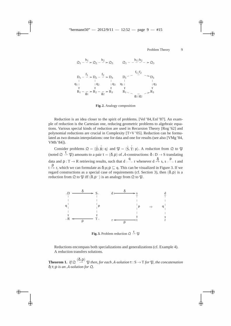
Consider problemsQ = 〈↓

D,↑

R: q〉 andP = 〈↓

S,↑

T: p〉. A reductionfrom Q to P

(notedQτ P) amounts to a pairτ = (δ,ρ) of A-constructions:δ : D→ S translating

data andρ : T→ R retrieving results, such that dq|−−> r whenever d

δ7→ s, s

p|−−> t and

tρ7→ r, which we can formulate asδ;p;ρ ⊑ q. This can be visualized in Figure 3. If we

regard constructions as a special case of requirements (cf.Section 3), then(δ,ρ) is areduction fromQ to P iff (δ,ρ) is an analogy fromQ to P.

→D

q

δ // S←

p

←R T→ρoo

d δ // s_

p

d_

q

⇒

r tρoo r

Fig. 3. Problem reductionQτ P

Reductions encompass both specializations and generalizations (cf. Example 4).A reduction transfers solutions.

Theorem 1. If Q(δ,ρ) P then, for eachA-solutionτ : S→T for P, the concatenation

δ;τ;ρ is anA-solution forQ.

ii

“hermann50” — 2012/9/11 — 12:52 — page 10 — #16 ii

ii

ii


Proof. By Remark 1 (in Section 3): ifτ ⊑ p, thenδ;τ;ρ ⊑ δ;p;ρ ⊑ q.

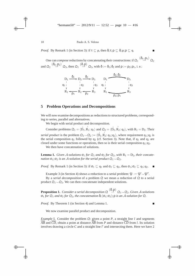
One cancomposereductions by concatenating their constructions: ifQ1(δ1,ρ1)

Q2

andQ2(δ2,ρ2)

Q3, thenQ1(δ,ρ) Q3, with δ := δ1;δ2 andρ := ρ2;ρ1, i. e.:

D1

q1

δ1 // D2

q2

δ2 // D3

q3

R1 R2ρ1oo R3ρ2

oo

D1

q1

δ1;δ2++ D3

q3

R1 R3ρ2;ρ1

kk

5 Problem Operations and Decompositions

We will now examine decompositions as reductions to structured problems, correspond-ing to series, parallel and alternatives.

We begin with serial product and decomposition.

Consider problemsQ1 = 〈↓

D1,↑

R1: q1〉 andQ2 = 〈↓

D2,↑

R2: q2〉, with R1 = D2. Their

serial productis the problemQ1;Q2 := 〈↓

D1,↑

R2: q1;q2〉, where requirementq1;q2 isthe serial compositionq1 followed by q2 (cf. Section 3). Note that, ifq1 andq2 areclosed under some functions or operations, then so is their serial compositionq1;q2.

We then have concatenation of solutions.

Lemma 1. GivenA-solutionsσ1 for Q1 andσ2 for Q2, with R1 = D2, their concate-nationσ1;σ2 is anA-solution for the serial productQ1;Q2.

Proof. By Remark 1 (in Section 3): ifσ1 ⊑ q1 andσ2 ⊑ q2, thenσ1;σ2 ⊑ q1;q2.

Example 3 (in Section 4) shows a reduction to a serial problem: P P′;P′′.By a serial decompositionof a problemQ we mean a reduction ofQ to a serial

productQ1;Q2. We can then concatenate independent solutions.

Proposition 1. Consider a serial decompositionQ(δ,ρ) Q1;Q2. GivenA-solutions

σ1 for Q1 andσ2 for Q2, the concatenationδ;(σ1;σ2);ρ is anA-solution forQ.

Proof. By Theorem 1 (in Section 4) and Lemma 1.

We now examine parallel product and decomposition.

Example 5.Consider the problemQ: given a pointP, a straight linel and segmentsAB andCD, obtain a point at distanceAB from P and distanceCD from l . Its solutioninvolves drawing a circleC and a straight linel ′ and intersecting them. Here we have 2

ii

“hermann50” — 2012/9/11 — 12:52 — page 11 — #17 ii

ii

ii

Problem Theory 11

independent problems:Q1, of drawing a circleC centred atP with radiusAB, andQ2,of drawing a straight linel ′ parallel tol at distanceCD, as follows:

(P , AB)_

q1

(l , CD)

_

q2

C l′

Given requirementsq1, from D1 to R1, andq2, from D2 to R2, the parallel re-quirementis the requirementq1×q2, from D1×D2 to R1×R2, described naturally by

(d1,d2)q1×q2|−−> (r1, r2) iff d1

q1|−−> r1 and d2

q2|−−> r2. Note that, ifp1 ⊑ q1 andp2 ⊑ q2,

thenp1×p2 ⊑ q1×q2. Given constructionsσ1 andσ2, theirparallelizationis the con-

structionσ1×σ2 such that(d1,d2)σ1×σ27→ (r1, r2) iff d1

σ17→ r1 and d2σ27→ r2.

For problemsQ1 = 〈↓

D1,↑

R1: q1〉 andQ2 = 〈↓

D2,↑

R2: q2〉, theirparallel productis the

problemQ1 1Q2 := 〈↓

D1×D2,↑

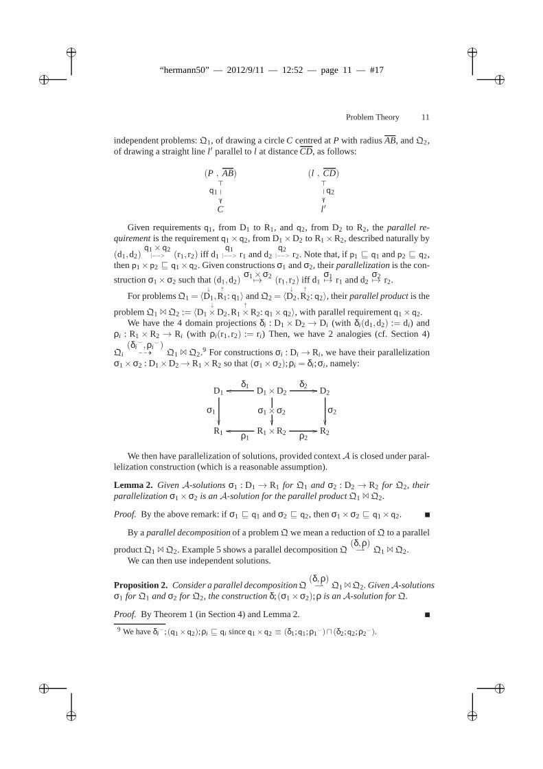
R1×R2: q1×q2〉, with parallel requirementq1×q2.We have the 4 domain projectionsδi : D1×D2→ Di (with δi(d1,d2) := di) and

ρi : R1×R2 → Ri (with ρi(r1, r2) := ri) Then, we have 2 analogies (cf. Section 4)

Qi(δi

,ρi)

99K Q1 1Q2.9 For constructionsσi : Di → Ri , we have their parallelizationσ1×σ2 : D1×D2→ R1×R2 so that(σ1×σ2);ρi = δi ;σi , namely:

D1

σ1

D1×D2δ1oo δ2 //

σ1×σ2

D2

σ2

R1 R1×R2ρ1

ooρ2

// R2

We then have parallelization of solutions, provided contextA is closed under paral-lelization construction (which is a reasonable assumption).

Lemma 2. GivenA-solutionsσ1 : D1→ R1 for Q1 and σ2 : D2→ R2 for Q2, theirparallelizationσ1×σ2 is anA-solution for the parallel productQ1 1Q2.

Proof. By the above remark: ifσ1 ⊑ q1 andσ2 ⊑ q2, thenσ1×σ2 ⊑ q1×q2.

By aparallel decompositionof a problemQ we mean a reduction ofQ to a parallel

productQ1 1Q2. Example 5 shows a parallel decompositionQ(δ,ρ) Q1 1Q2.

We can then use independent solutions.

Proposition 2. Consider a parallel decompositionQ(δ,ρ) Q11Q2. GivenA-solutions

σ1 for Q1 andσ2 for Q2, the constructionδ;(σ1×σ2);ρ is anA-solution forQ.


9 We haveδi;(q1×q2);ρi ⊑ qi sinceq1×q2 ≡ (δ1;q1;ρ1

)⊓ (δ2;q2;ρ2).

ii

“hermann50” — 2012/9/11 — 12:52 — page 12 — #18 ii

ii

ii


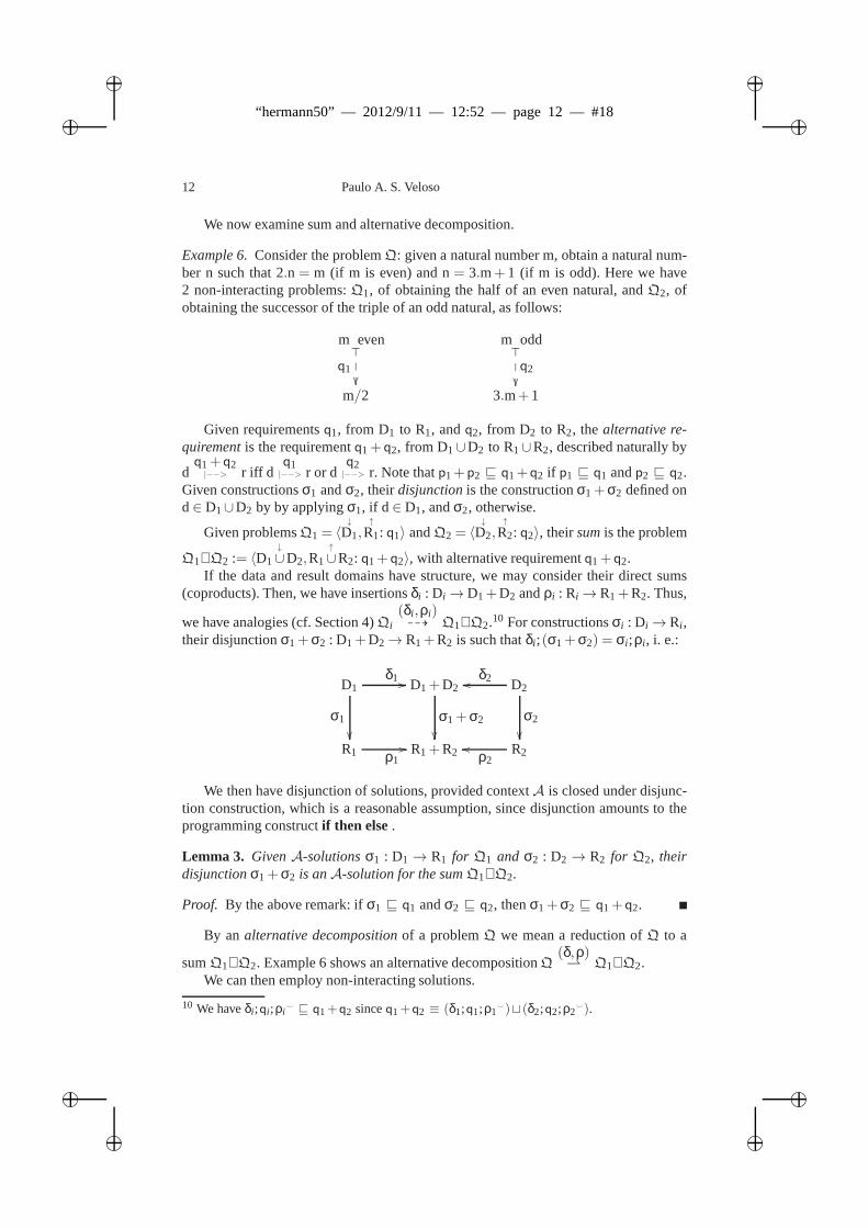
We now examine sum and alternative decomposition.

Example 6.Consider the problemQ: given a natural number m, obtain a natural num-ber n such that 2.n = m (if m is even) and n= 3.m+ 1 (if m is odd). Here we have2 non-interacting problems:Q1, of obtaining the half of an even natural, andQ2, ofobtaining the successor of the triple of an odd natural, as follows:

m even_

q1

m odd_

q2

m/2 3.m+1

Given requirementsq1, from D1 to R1, andq2, from D2 to R2, thealternative re-quirementis the requirementq1+q2, from D1∪D2 to R1∪R2, described naturally by

dq1+q2|−−> r iff d

q1|−−> r or d

q2|−−> r. Note thatp1+p2 ⊑ q1+q2 if p1 ⊑ q1 andp2 ⊑ q2.

Given constructionsσ1 andσ2, theirdisjunctionis the constructionσ1+σ2 defined ond∈ D1∪D2 by by applyingσ1, if d ∈D1, andσ2, otherwise.

Given problemsQ1 = 〈↓

D1,↑

R1: q1〉 andQ2 = 〈↓

D2,↑

R2: q2〉, theirsumis the problem

Q1∇Q2 := 〈↓

D1∪D2,↑

R1∪R2: q1+q2〉, with alternative requirementq1+q2.If the data and result domains have structure, we may consider their direct sums

(coproducts). Then, we have insertionsδi : Di →D1+D2 andρi : Ri →R1+R2. Thus,

we have analogies (cf. Section 4)Qi(δi ,ρi)99K Q1∇Q2.10 For constructionsσi : Di →Ri ,

their disjunctionσ1+σ2 : D1+D2→ R1+R2 is such thatδi ;(σ1+σ2) = σi ;ρi , i. e.:

D1

σ1

δ1 // D1+D2

σ1+σ2

D2δ2oo

σ2

R1 ρ1

// R1+R2 R2ρ2oo

We then have disjunction of solutions, provided contextA is closed under disjunc-tion construction, which is a reasonable assumption, sincedisjunction amounts to theprogramming constructif then else.

Lemma 3. GivenA-solutionsσ1 : D1→ R1 for Q1 and σ2 : D2→ R2 for Q2, theirdisjunctionσ1+σ2 is anA-solution for the sumQ1∇Q2.

Proof. By the above remark: ifσ1 ⊑ q1 andσ2 ⊑ q2, thenσ1+σ2 ⊑ q1+q2.

By an alternative decompositionof a problemQ we mean a reduction ofQ to a

sumQ1∇Q2. Example 6 shows an alternative decompositionQ(δ,ρ) Q1∇Q2.

We can then employ non-interacting solutions.

10 We haveδi ;qi ;ρi ⊑ q1+q2 sinceq1+q2 ≡ (δ1;q1;ρ1

)⊔ (δ2;q2;ρ2).

ii

“hermann50” — 2012/9/11 — 12:52 — page 13 — #19 ii

ii

ii

Problem Theory 13

Proposition 3. Consider an alternative decompositionQ(δ,ρ) Q1∇Q2. GivenA-

solutionsσ1 for Q1 andσ2, for Q2, δ;(σ1+σ2);ρ is anA-solution forQ.


6 Other Aspects

We now briefly examine some other aspects: instances of interest, change of contexts,homogeneous problems and divide-and-conquer.

We first examine instances of interest.Often, one does not wish a solution for all data, but only for some of them. For in-

stance, consider the problem: given a natural m, obtain a natural n,such thatn< m. Thisis not always possible, but we may restrict our attention to the set of positive naturals.We then have a restricted problem with subset IN+ ⊆ IN of instances of interest.

A restricted problemis a structureIQ= 〈I ,↓

D,↑

R: q〉, with D, R andq as in Section 3andI ⊆ D asset of instances of interest.

We can relativize the previous concepts to sets of instancesof interest.The behavior of a solution (cf. Section 3) is considered onlyon instances of interest.

Given a restricted problemIQ = 〈I ,↓

D,↑

R: q〉, by anA-solution for problemIQ (or asolution forA-problemIQ) we mean a constructionσ ∈ A, such that:

(I →) σ transformsI to R: for every d∈ I , the execution ofσ on d produces some r∈R;

(I ⊑) σ respects requirementq overI : whenever d∈ I and dσ7→ r, we have d

q|−−> r.

A reduction is to preserve instances of interest.

Given restricted problemsIQ = 〈I ,↓

D,↑

R: q〉 andJP = 〈J,↓

S,↑

T: p〉, a restricted re-ductionfrom IQ to JP amounts to a pairτ = (δ,ρ) of A-constructions:δ : D→ S andρ : T→ R as in Section 4, with the added proviso thatδ transformsI to J: for everyd∈ I , the execution ofσ on d produces some s∈ J, i. e.δ : I → J (cf. Section 3).

We then have transfer of solutions much as in Theorem 1 (of Section 4): given

IQ(δ,ρ) IQ, for eachA-solutionτ : J→R for JP, δ;τ;ρ is anA-solution forIQ.

We now consider change of contexts. For proper solution transfer, we require con-text closure under the translations.

Given problemsQ = 〈↓

D,↑

R: q〉, in contextA, andP = 〈↓

S,↑

T: p〉, in contextB, acontext reductionfromQ toP amounts to a pairτ = (δ,ρ) of constructions:δ : D→ Sandρ : T→ R in A as in Section 4, with the added proviso thatδ andρ transformBto A, the former by pre concatenation and the latter by post concatenation:δ;B ⊆ A(δ;τ ∈ A, wheneverτ ∈ B) andB;ρ⊆A (τ;ρ ∈ A, wheneverτ ∈ B).

We now examine homogeneous problems.The data and result domains of a problem may be the same, e. g. the sorting problem

has sequences as both domains. By ahomogeneousproblem we mean one with D= R.It turns out that a problem has a homogeneous version connected to it.

ii

“hermann50” — 2012/9/11 — 12:52 — page 14 — #20 ii

ii

ii


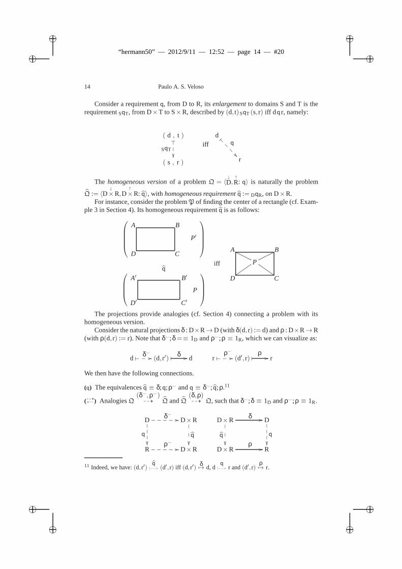
Consider a requirementq, from D to R, itsenlargementto domains S and T is therequirementSqT, from D×T to S×R, described by(d, t)SqT (s, r) iff d q r, namely:

( d , t )_

SqT

( s , r )

iffd~

q

>>

>>

r

The homogeneous versionof a problemQ = 〈↓

D,↑

R: q〉 is naturally the problem

Q := 〈↓

D×R,↑

D×R: q〉, with homogeneous requirementq := DqR, on D×R.For instance, consider the problemP of finding the center of a rectangle (cf. Exam-

ple 3 in Section 4). Its homogeneous requirementq is as follows:

A B

CD

P′

q

A′ B′

C′D′

P

iff

A B

CD

P

The projections provide analogies (cf. Section 4) connecting a problem with itshomogeneous version.

Consider the natural projectionsδ : D×R→D (with δ(d, r) := d) andρ : D×R→R(with ρ(d, r) := r). Note thatδ;δ =≡ 1D andρ;ρ ≡ 1R, which we can visualize as:

d δ//___ (d, r′)

δ // d r ρ

//___ (d′, r) ρ

// r

We then have the following connections.

(q) The equivalencesq ≡ δ;q;ρ andq ≡ δ; q;ρ.11

(99KL99 ) AnalogiesQ(δ,ρ)99K Q andQ

(δ,ρ)99K Q, such thatδ;δ ≡ 1D andρ;ρ ≡ 1R.

D

q

δ//_____ D×R

q

Rρ

//_____ D×R

D×Rδ //

q

D

q

D×Rρ

// R

11 Indeed, we have:(d, r′)q|−−> (d′, r) iff (d, r′)

δ7→ d, d

q|−−> r and(d′, r)

ρ7→ r.

ii

“hermann50” — 2012/9/11 — 12:52 — page 15 — #21 ii

ii

ii

Problem Theory 15

Thus, we can transfer analogies back and forth between problems and their homo-geneous versions:Q 99K P iff Q 99K P.

Given problemsQ = 〈↓

D,↑

R: q〉 andP = 〈↓

S,↑

T: p〉, consider their homogeneous

versionsQ = 〈↓

D×R,↑

D×R: q〉 andP = 〈↓

S×T,↑

S×T: p〉, as well as the projectionsδ : D×R→ D, ρ : D×R→ R, σ : S×T→ S andτ : S×T→ T. So, withµ := (δ,ρ)

andν := (σ,τ), we have analogiesQµ

99K Q andPν99K P, as well asQ

µ

99K Q and

Pν

99K P, with µ := (δ,ρ) andν := (σ,τ).

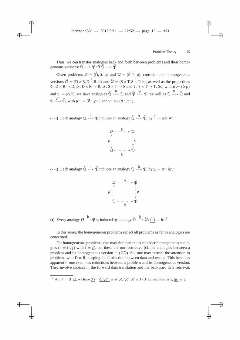
(99K) Each analogyQh99K P induces an analogyQ

h99K P, by h := µ;h;ν:

Qh //____ P

ν

Q

µ

OO

h

//____ P

(L99) Each analogyQh99K P induces an analogyQ

h99K P, by h := µ;h;ν:

Qh //____ P

ν

Q

µ

OO

h//____ P

(•) Every analogyQh99KP is induced by analogyQ

h99K P: (h) ≡ h.12

In this sense, the homogeneous problems reflect all problemsas far as analogies areconcerned.

For homogeneous problems, one may find natural to consider homogeneous analo-gies (h = (f,g) with f = g), but these are too restrictive (cf. the analogies between aproblem and its homogeneous version in (99K

L99 )). So, one may restrict the attention toproblems with D= R, keeping the distinction between data and results. This becomesapparent if one examines reductions between a problem and its homogeneous version.They involve choices in the forward data translation and thebackward data retrieval.

12 With h= (f,g), we have(f) = δ; f;σ ≡ δ;δ; f;σ;σ ≡ 1D; f;1S, and similarly,(g) ≡ g.

ii

“hermann50” — 2012/9/11 — 12:52 — page 16 — #22 ii

ii

ii


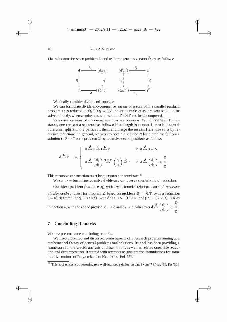
The reductions between problemQ and its homogeneous versionQ are as follows:

d_

q

ιr0 // (d, r0)

_

q

r (d′, r)

ρoo

(d′, r′)_

q

δ // d′_

q

(d0, r′′) r′′

ιdo

oo

We finally consider divide-and-conquer.We can formulate divide-and-conquer by means of a sum with a parallel product:

problemQ is reduced toQ0∇(Q1 1 Q2), so that simple cases are sent toQ0 to besolved directly, whereas other cases are sent toQ1 1Q2 to be decomposed.

Recursive versions of divide-and-conquer are common [Vel ’80, Vel ’85]. For in-stance, one can sort a sequence as follows: if its length is atmost 1, then it is sorted;otherwise, split it into 2 parts, sort them and merge the results. Here, one sorts by re-cursive reductions. In general, we wish to obtain a solutionσ for a problemQ from asolutionτ : S→ T for a problemP by recursive decompositions as follows:

dσ7→ r ⇔

d δ7→ s τ

7→ tρ7→ r if d δ

7→ s ∈ S

dδ7→

(d1

d2

)σ×σ7→

(r1

r2

)ρ7→ r if d

δ7→

(d1

d2

)∈

D×D

This recursive construction must be guaranteed to terminate.13

We can now formulate recursive divide-and-conquer as special kind of reduction.

Consider a problemQ= 〈↓

D,↑

R: q〉, with a well-founded relation≺ on D. A recursive

division-and-conquestfor problemQ based on problemP = 〈↓

S,↑

T: p〉 is a reductionτ = (δ,ρ) fromQ toP∇(Q1Q) with δ : D→ S∪ (D×D) andρ : T∪ (R×R)→R as

in Section 4, with the added proviso: d1 ≺ d and d2 ≺ d, whenever dδ7→

(d1

d2

)∈

D×D

.

7 Concluding Remarks

We now present some concluding remarks.We have presented and discussed some aspects of a research program aiming at a

mathematical theory of general problems and solutions. Itsgoal has been providing aframework for the precise analysis of these notions as well as related ones, like reduc-tion and decomposition. It started with attempts to give precise formulations for someintuitive notions of Polya related to Heuristics [Pol ’57].

13 This is often done by resorting to a well-founded relation ondata [Man ’74,Wag ’83,Tos ’88].

ii

“hermann50” — 2012/9/11 — 12:52 — page 17 — #23 ii

ii

ii

Problem Theory 17

We have begun by introducing and discussing some basic ideasin Section 2. In Sec-tion 3, we have examined the central concepts: problems, requirements and solutions.We have introduced analogies as transformations leading toreductions in Section 4. InSection 5, we have considered decompositions as reductionsto structured problems,corresponding to series, parallel and alternatives. In Section 6, we have briefly exam-ined some other aspects: restriction to instances of interest, change of contexts, homo-geneous problems and (recursive) divide-and-conquer.

In reductions such as the Cartesian one, the same coordinatesystem should be usedfor data and results. This may lead to result retrievals withextra arguments, such asρT : S×T→ R or Dρ : D×S→ R [VMg ’84, VMh ’84]. This can handled as follows:

instead of reducingQ= 〈↓

D,↑

R: q〉 to P = 〈↓

S,↑

T: p〉, reduceQ to P′ = 〈↓

S,↑

S×T: p′〉 or

to P′′ = 〈↓

D×S,↑

D×T: p′′〉, wherep′ andp′′ are appropriate requirements.14

The concepts defined seem to capture (part of) our intuition about these notions,which is corroborated by the (simple) results presented. The approach is based on ex-amining structural properties that ensure appropriate behavior of solutions. Also, thebinary operations introduced in Section 5 can be extended toseveral arguments.

We have seen some categories [Mac ’71]: the categoryCnstr of domains and con-structions (in Section 3) and the categoryRed of problems and reductions (in Sec-tion 4). Similarly, one has some allegories [F+S ’90]: the allegoryRqrmt of domainsand requirements (in Section 3) and the allegoryAnlg of problems and analogies (inSection 4). Examining the operations (introduced in Section 5), we notice that they areoften inherited from corresponding ones on domains. So, onemight envisage formu-lating these ideas in terms of categories and allegories based on domains, namely thecategoryCnstr of domains and constructions and the allegoryRqrmt of domains andrequirements, satisfying properties such as those of Remark 1 (in Section 3).

This theory of problems and solutions has found some applications: formalizationof program development [HVB’89], program construction [LMV’84,Vel ’91] and syn-thesis [Hae ’96, SHV ’02, Sil ’04], problem solving [Wag ’83,Vel ’86, Enl ’87, Vel ’87,Vel ’88], design and (complexity) analysis of algorithms [Tos ’88, T+V ’90, DTV ’02,T+V’05], as well as heuristics [Ama’04].

References

[Ama ’04] Amaral, F. Náufel. Teoria de modelos para heurísticas baseada em topoi. D. Sc. thesis,PUC-Rio: Dept. Informática (2004).

[DTV ’02] Divério, Tiarajú, A., Toscani, Laira V. and Veloso, Paulo A. S. Análise da complex-idade de algoritmos paralelos. InAnais da2a Escola Regional de Alto Desempenho - ERAD2002: 67–106, São Leopoldo: Sociedade Brasileira de Computação(2002).

[Ent ’72] Enderton, Herbert B.A Mathematical Introduction to Logic. New York: AcademicPress (1972).

[Enl ’87] Endler, Markus. O método de redução e a decomposição de problemas: alguns aspec-tos. M. Sc. diss., PUC-Rio: Dept. Informática (1987).

14 For the former case, we can definep′ by sp′|−−> (s′, t) iff s = s′ and s

p|−−> t. For the latter case,

we can usep′′ := 1D×p with data translationδ′′ given by dδ′′7→ (d′,s) iff d = d′ and d

δ7→ s.

ii

“hermann50” — 2012/9/11 — 12:52 — page 18 — #24 ii

ii

ii


[F+S ’90] Freyd, Peter and Scedrov, Andre.Categories, Allegories. Amsterdam: North-Holland(1990).

[HVB ’89] Haeberer, Armando M., Veloso, Paulo A. S. and Baum,Gabriel A.Formalización delProceso de Desarrollo de Software. Buenos Aires: Kapelusz (1989).

[Hae ’88] Haeusler, E. Hermann. Intuitionistic type theoryand general problem theory: a rela-tionship.Monografias em Ciência da ComputçãoMCC 18/88, PUC-Rio: Dept. Informática(1988).

[Hae ’96] Haeusler, E. Hermann. Generating programs from problems: an interaction betweenProblem Theory and Type Theory.Investigación Operativa5(2-3): 153–168 (1996).

[Kol ’32] Kolmogorov, A. N. Zur Deutung der intuitionistischen Logik. MathematischeZeitschrif35 (1932).

[LMV ’84] Lucena, Carlos J. P., Martins, Raul C. B. and Veloso, Paulo A. S. Construção deprogramas por transformadores de dados: introdução e estudo de caso.Revista Brasileira deComputação3: 5–17 (1984).

[Mac ’71] MacLane, Saunders.Categories for the Working Mathematician. Berlin: Springer-Verlag (1971).

[M-L ’84] Martin-Löf, P. Intuitionistic Type Theory. Napoli: Bibliopolis (1984).[Man ’74] Manna, Zohar.The Mathematical Theory of Computation. New York: McGraw-Hill

(1974).[Pol ’57] Polya, George.How to Solve it: a new aspect of the mathematical method. Princeton:

Princeton Univ. Press, Princeton (1957).[Rog ’62] Rogers Jr., Hartley.The Theory of Recursive Functions and Effective Computability.

New York: McGraw-Hill (1962).[Sil ’04] Silva, Geiza M. H. Síntese construtiva de programas em linguagem imperativa usando

lógica intuicionista e dedução natural. D. Sc. thesis, PUC-Rio: Dept. Informática (2004).[SHV ’02] Silva, Geiza M. H., Haeusler, E. Hermann, Veloso, Paulo A. S.: Constructive program

synthesis using Intuitionistic Logic and Natural Deduction. In Abe, J. M. and Silva Filho, J. I.(eds.)Logic, Artificial Intelligence and Robotics - Proc. Laptec 2002: 224–233, Amsterdam:IOS Press (2002).

[Tos ’88] Toscani, Laira V. Métodos de desenvolvimento de algoritmos: especificação, análisecomparativa e de complexidade. D. Sc. thesis, PUC-Rio: Dept. Informática (1988).

[T+V ’90] Toscani, Laira V. and Veloso, Paulo A. S. A programação dinâmica: um caso particu-lar da divisão e conquista.Revista de Informática Teórica e Aplicada1(2): 53–67 (1990).

[T+V ’05] Toscani, Laira V. and Veloso, Paulo A. S.Complexidade de Algoritmos: análise, pro-jeto e métodos. Porto Alegre: Sagra Luzzato (2005).

[Vel ’80] Veloso, Paulo A. S. Divide-and-conquer via abstract data types. InAnales de la VIIConferencia Latinoamericana de Informática: 530–539, Caracas (1980).

[Vel ’84] Veloso, Paulo A. S. Outlines of a mathematical theory of general problems.PhilosophiaNaturalis21(2/4): 354–362 (1984).

[Vel ’85] Veloso, Paulo A. S. How to “divide-and-conquer”: alogical basis. In Brucker, P. andPauly, R. (eds.)Methods of Operations Research49: 431–442, Hain Verlag bei Athenäum(1985).

[Vel ’86] Veloso, Paulo A. S. Problem solving by interpretation of theories.J. Symbolic Logic51(4): 1103 (1986).

[Vel ’87] Veloso, Paulo A. S. On the concepts of problem and problem-solving method.DecisionSupport Systems3(2): 133–139 (1987).

[Vel ’88] Veloso, Paulo A. S. Problem solving by interpretation of theories. In Carnielli, W. A.and Alcântara, L. P. (eds.)Methods and Applications of Mathematical Logic: 241–250, Provi-dence: American Mathematical Society (1988).

ii

“hermann50” — 2012/9/11 — 12:52 — page 19 — #25 ii

ii

ii

Problem Theory 19

[Vel ’91] Veloso, Paulo A. S. Program construction (with data abstractions) as transformations ontheories. In Alcoforado, P. (ed.)Lógica, Computação e Epistemologia - ensaios em homenagemao Prof. Jorge Barbosa: 241–250, Niterói: ILTC (1991).

[Vel ’11] Veloso, Paulo A. S. Problemas: aspectos de uma teoria geral. In Lasalle Casanave, A.and Schultz, S. R. (eds.)Filosofia da Prática Matemática - XV Colóquio Conesul de Filosofiadas Ciências Formais: 60, Salvador: UFBA (2011).

[VMg ’84] Veloso, Paulo A. S. and Martins, Raul C. B. On reducibilities among general prob-lems. In Trappl, R. (ed.)Cybernetics and Systems Research 2 - Proc. 7th European Meeting onCybernetics and Systems Research: 21–25, Amsterdam: North-Holland (1984).

[VMh ’84] Veloso, Paulo A. S. and Martins, Raul C. B.: A logical hierarchy of reductions ofproblems. InProc. 6th International Congress of Cybernetics and Systems, vol. B: 731–736,Paris (1984).

[V+V ’81] Veloso, Paulo A. S. and Veloso, Sheila R. M. Problemdecomposition and reduction:applicability, soundness, completeness. InProgress in Cybernetics and Systems Research: 199–203, Washington, DC: Hemisphere (1981).

[Wag ’83] Waga, Cristina E. M. F. Métodos de resolução de problemas. M. Sc. diss., PUC-Rio:Dept. Informática (1983).

ii

“hermann50” — 2012/9/11 — 12:52 — page 20 — #26 ii

ii

ii

DAG-like term compression⋆

Preliminary version

L. Gordeev

Tübingen University, Germany

Ghent University, Ghent, Belgium

Preamble

This essay is dedicated to Hermann Haeusler’s 50th birthdaycelebration. Dag-like proofcompression along the lines of [4, 5] is our joint research project inspired by com-prehensive discussions in PUC-Rio with Hermann, Vaston da Costa and Luiz-CarlosPereira. In this paper general dag-like compression is adapted to representations of al-gebraic terms. It is shown that any tree-like term representation can be compressedto the uniquely determined and easily computable minimal-size dag. In many cases thesize of the corresponding compressed dag-like representation is essentially smaller thanthe one of the input. In fact there are simple termst whose tree-like representations arecompressible to dags whose size is merely logarithmic in thesize oft.

1 Introduction

Many familiar tree-like structures admit essential size-reduction via dag-like compres-sion. For example consider ordinaryterm algebrain the languageL with constantsand function symbols (abbr.:f (k),g(k),h(k), · · · ; deg( f (k)) := k > 0), individual vari-ables (abbr.:x,y,z, · · · ). Denote byTL (or just T ) the corresponding set of algebraicterms(abbr.:s, t, r, etc.) defined by standard recursive clauses:

1. Individual variables and constants are terms of the depth0, also called atoms.2. If t1, · · · , tk are terms andf (k) a function symbol, thenf (k) (t1, · · · , tk) is a term and

depth( f (k) (t1, · · · , tk)) := 1+maxdepth(ti) : 1≤ i ≤ k; we can spare brackets us-ing prenex Łukasiewicz form and writef (k)t1 · · · tk instead off (k) (t1, · · · , tk).

For anyt ∈ T , denote bySUB(t) the set of subterms oft (includingt) that is definedrecursively as follows:

1. If depth(t) = 0 thenSUB(t) = t.2. If t = f (k) (t1, · · · , tk) thenSUB(t) = t∪SUB(t1)∪·· ·∪SUB(tk).

Denote by|SUB(t)| the cardinality ofSUB(t).By a familiar observation, everyt ∈ T admits plaintree-like representation, t, that

is generated by standard recursive clauses (see also Definition 3):

⋆ Research partially supported by the ANR/DFG project HYPOTHESES (DFG grant Schr275/16).

ii

“hermann50” — 2012/9/11 — 12:52 — page 21 — #27 ii

ii

ii

DAG-like term compression 21

1. t is the root oft.2. Non-atomic nodess= f (k) (s1, · · · ,sk) of t generatek childrens1, · · · ,sk.

Thus everyt is a rooted vertex-labeled tree whose labels are subterms oft. So ina language with binary function symbols∗,, a termt = ∗(x,(∗(x,y) ,x)) is rep-resented by a treet having 7 verticesv1,v2,v3,v4,v5,v6,v7 (v1 being the root) as-signed with subterm labelst,x,(∗(x,y) ,x) ,∗(x,y) ,x,x,y, respectively, and 6 edges(arrows)v1→ v2,v1→ v3,v3→ v4,v3→ v5,v4→ v6,v4→ v7. Since the same atomxoccurs more than once int, we can equalize leavesv2 andv5 and replacet by a “com-pressed” rooteddag-like representationt1 (dag: directed acyclic graph) that has 6 ver-ticesv1,v2,v3,v4,v6,v7 and 6 edgesv1→ v2,v1→ v3,v3→ v4,v3→ v2,v4→ v6,v4→ v7.Note thatt1 is not the optimal compression, since by the same token we canfurtherequalizev2 with v6 and obtain a smaller dagt2 having only 5 verticesv1,v2,v3,v4,v7

and (still) 6 edgesv1→ v2,v1→ v3,v3→ v4,v3→ v2,v4→ v2,v4→ v7. But t2 can’t becompressed anymore. This yields a maximal chain of compressions t 7→ t1 7→ t2 witht2 being corresponding minimal compression oft. Furthermore we observe that otherchains of equalizing compressions yield the same (modulo isomorphism) minimal dagt = t2. It turns out that for any given termt, the corresponding minimal dag-like repre-sentationt, that we in the sequel denote byDmin (t), is uniquely determined (modulodag-isomorphism) and definable bya) a natural bottom-up recursion (see Theorem 19)and/orb) any maximal chain of compressions equalizing arbitrary pairs of vertices withequal subterm labels (see Corollary 22). Moreover, the total number of vertices occur-ring inDmin (t) is just |SUB(t)|.1

Note thatt andt are uniquely determined by the correspondingnormal formswhosevertices are natural numbers labeled by function symbolsf (k), instead of full subtermsf (k) (s1, · · · ,sk) (see Definition 15). The normal form ofDmin (t) we denote byDNF

min (t).

2 Basic notations and definitions

2.1 Term-like labeled dags

Notations 1. We considerlabeled dagsD= 〈D, ℓ〉, where D is the (possibly multiedge)underlying finitedagandℓ : V(D)→ T the labeling function,V(D) being thevertices(or nodes) of D (: a,b,u,v,w,z, etc.).S(D), L(D), E(D) denote respectively thesources(or roots), leaves(or terminals) andedges(‘→’) of D. Thus

(∀u∈ S(D))(∀v∈ V (D))(v9 u) and (∀u∈ L (D))(∀v∈ V (D)) (u9 v) .

Labeled dags are considered equal if underlying dags are isomorphic and preserve thelabels. If S(T) = u then D andD are calledrootedandroot(T) := u. Thesizeof any

1 Similar observations (without rigorous proofs) are folklore in the context of logic program-ming, compiler design and related structures (cf. e.g. [1, 3, 8]). Note that [8] refers to theminimal compacted (the same as compressed) dag representations as being definable via theequivalence classes on the input (planar) trees. However, analogous dag representations of al-gebraic terms should have required more careful clarification to handle branching order and/oridentical children (cf. Definition 2 below).

ii

“hermann50” — 2012/9/11 — 12:52 — page 22 — #28 ii

ii

ii

22 L. Gordeev

givenD= 〈D, ℓ〉 is defined by

|D| := |D| := #(V (D))

Special dags –trees– we’ll denote by T rather than D.

Definition 2. In a term-like labeled dagD= 〈D, ℓ〉we assume that any u∈V(D)\L(D)with ℓ(u) = f (k) (s1, · · · ,sk) ∈ T has k children (not necessarily pairwise different)which are numbered u(1), · · ·u(k) and labeledℓ

(u(i))

:= si . We also assume that theadjacent edges u→ u(i) are pairwise different, which we sometimes emphasize by writ-ing u→i v to mean u→ v∧ v = u(i). Thus(u→i v) 6= (u→ j v′) for any i 6= j, re-gardless if v6= v′ or v = v′. In the sequel we denote byD (DR) the set of all la-beled term-like (rooted) dagsD. Moreover for the sake of brevity we’ll expose termshaving only binary function symbols f(2),g(2),h(2) (abbr.: f,g,h, · · · ). In this case wehave binary-branching vertices u withdeg(ℓ(u)) = 2 and pairs of adjacent edgesu→1 u(1),u→2 u(2) such that u(1) = u(2) = u′ impliesℓ(u) = f (s,s) whereℓ(u′) = s.

Definition 3. For any t∈ T , the tree-like representationt = 〈T, ℓ〉 ∈ DR is a rootedlabeled planar tree defined as follows by recursion ondepth(t).

1. If t = x thenV(T) := u andℓ(u) := x.2. If t = f (k) (t1, · · · , tk) andti = 〈Ti , ℓi〉 (1≤ i ≤ k) then

V (T) : = V (T1)⊎·· ·⊎ V (Tk)⊎u

E(T) : = E(T1)⊎·· ·⊎ E(Tk)⊎u→ ui : 1≤ i ≤ k

ℓ(w) : =

ℓi (w) if w ∈ Ti (1≤ i ≤ k) ,t if w = u.

where ui = root(Ti) (and thereby i6= j ⇒ ui 6= u j and u= root(T)).

Note that if t include only binary function symbols, then thecorresponding tree-likerepresentationst are binary-branching trees.

Now letT + be the set of listst = t1, · · · , tm, where ti ∈ T . ThusT ⊂ T +. For anyt = t1, · · · , tn ∈T + let t := t1⊎·· ·⊎ tn = 〈T, ℓ〉 ∈D be analogous tree-like representationof t. That is

V (T) : = V (T1)⊎·· ·⊎ V (Tn)

E(T) : = E(T1)⊎·· ·⊎ E(Tn)

ℓ(w) : = ℓi (w) if w∈ Ti (i = 1, · · · ,n)

whereti = 〈Ti , ℓi〉 (i = 1, · · · ,n). Note thatt ∈ D has n sources.

Definition 4. For anyD= 〈D, ℓ〉 ∈ D, D1 = 〈D1, ℓ1〉 ∈ D let

DDD1 :⇔(∃ϕ : V (D)

onto→ V (D1)

)(E(D1) = ϕ(E(D))∧ ℓ= ℓ1ϕ) ,

D⊲D1 :⇔DDD1∧|D|> |D1| ,

whereϕ(E(D)) := ϕ(u)→i ϕ(v) : u→i v∈ E(D). We callbasic dag-like (proper)compressionthe reductionDDD1 (D⊲D1) .

ii

“hermann50” — 2012/9/11 — 12:52 — page 23 — #29 ii

ii

ii


Lemma 5. The following conditions hold (ϕ being as above).

1. D (⊲) is reflexive (irreflexive) and transitive.2. V(D1) = ϕ(V (D)), S(D1) = ϕ(S(D)) andL(D1) = ϕ(L (D)).3. (∀u,v∈ V (D)) (ϕ(u) = ϕ(v)⇒ ℓ(u) = ℓ1 (ϕ(u)) = ℓ1(ϕ(v)) = ℓ(v)).

4. (∀u∈ V (D)) (∀i ≤ deg(ℓ(u)))(

ϕ(u(i))= (ϕ(u))(i)

).

5. (∀u,v∈ V (D)) (∀i ≤ deg(ℓ(u)))(ϕ(u) = ϕ(v)⇒ ϕ

(u(i))= ϕ

(v(i)))

.

Proof. Straightforward. Note that 4 implies 5.

Lemma 6. (∀D= 〈D, ℓ〉 ∈ DR)(∃t ∈ T )(t DD

). Moreover t= ℓ(root(D)).

Proof. Straightforward by bottom-up induction.

Lemma 7. For anyD= 〈D, ℓ〉 ∈ D, supposeϕ : V(D)→V(D) satisfies

(∀u,v∈ V (D))

((ϕ(u) = ϕ(v)⇒ ℓ(u) = ℓ(v))∧

(∀i ≤ deg(ℓ(u)))(

ϕ(u(i))= (ϕ(u))(i)

))

Consider a labeled digraphD′ = 〈D′, ℓ′〉 uniquely determined byD andϕ via V(D′) :=Rng(ϕ), E(D′) := ϕ(u)→i ϕ(v) : u→i v∈ E(D), ℓ′ (ϕ(u)) := ℓ(u). ThenD D D′

holds with respect toϕ.

Proof. This is obvious, sinceϕ(u(i))= (ϕ(u))(i) impliesu→i v∈E(D)⇒ ϕ(u)→i

ϕ(v) ∈E(D).

Example 8. For any given t∈ T considert = 〈T, ℓ〉. Let a 6= b ∈V(T) be such thatℓ(a) = ℓ(b) ∈ T (hencedepth(t) > 0). Denote by T≥a (T≥b) the subtree of T with theroot a (b). Since by the assumptionℓ(a) = ℓ(b) = s (a subterm of t) we have T≥a

∼=T≥b∼= T(s),V (T≥a)∩ V (T≥b) = /0, wheres=

⟨T(s), ℓ(s)

⟩∈ D, there is an isomorphism

V(T≥b) ∋ u1−17→ I (u) ∈V(T≥a) with ℓ(u) = ℓ(I (u)) and u→i u′ ∈E(T≥b)⇔ I (u)→i

I (u′) ∈E(T≥a), i.e. I(u(i))= (I (u))(i), where0 < i ≤ deg(ℓ(u)). Defineϕ : V(T)→

V(T) by

ϕ(u) :=

I (u) ∈ V (T≥a) if u ∈ V (T≥b) ,u if u /∈ V (T≥b) .

We observe thatϕ satisfies the conditions of Lemma 7. For clearlyϕ(u) = ϕ(v) ⇒

ℓ(u) = ℓ(v). In order to establish(∀i ≤ deg(ℓ(u)))(

ϕ(u(i))= (ϕ(u))(i)

)it will suf-

fice to showϕ(u) = ϕ(v)⇒ ϕ(u(i))= ϕ

(v(i)), as follows. Supposeϕ(u) = ϕ(v) and

consider the following three cases.

1. u,v /∈V(T≥b).2. u,v∈V(T≥b) .3. u∈V(T≥b) and v/∈V(T≥b).

ii

“hermann50” — 2012/9/11 — 12:52 — page 24 — #30 ii

ii

ii

24 L. Gordeev

Case 1: We have u= ϕ(u) = ϕ(v) = v. This obviously yields u(i) = v(i) and henceϕ(u(i))= ϕ

(v(i)).

Case 2: We have I(u) = ϕ(u) = ϕ(v) = I (v), which yields u= v by the definition ofI. The rest follows as above.

Case 3: We have I(u) = ϕ(u) = ϕ(v) = v∈V(T≥a). This yieldsϕ(u(i))= I(u(i))=

(I (u))(i) = v(i) = ϕ(v(i))

by u(i) ∈V(T≥b) , V(T≥a) ∋ v(i) /∈V(T≥b).

Now considerD′ = 〈D′, ℓ′〉 ∈ D determined byD = t and ϕ as in Lemma 7. ByLemma 7 we havet D D′. Moreover D′ ⊂ T andϕ(b) = a, hence|T| > |D′|. Thust ⊲D′ (with respect toϕ). This yields a simple instance of vertex-equalization.

Definition 9. For any listt = t1, · · · , tn ∈ T + denote byset(t) the minimal sublist (mod-ulo permutation)s= s1, · · · ,sm containing all elements oft. Thus

(∀1≤ i < j ≤m)(si 6= sj )∧s1, · · · ,sm= t1, · · · , tn .

Example 10. For any t = t1, · · · , tn ∈ T + let set(t) = s1, · · · ,sm =: t′. So m≤ n and

∃ψ : 1, · · · ,nonto→ 1, · · · ,m such that(∀1≤ i ≤ n)

(ti = sψ(i)

). LetD := t = 〈T, ℓ〉 ∈

D andD′ := t′ = 〈T ′, ℓ′〉 ∈ D. It is readily seen thatψ yields a surjectionϕ : V(T)onto→

V(T ′) generatingD D D′; moreoverD ⊲ D′ ⇔ m< n. Analogously, for any sublistt′ ⊂ t we havet D t′.

Example 11. We generalize Example 8. Supposet ∈ T + and let t = 〈T, ℓ〉 D D1 =

〈D1, ℓ1〉 ∈ D be generated byϕ1 : V(T)onto→ V(D1). Suppose a6= b ∈V(D1) such that

ℓ1 (a) = ℓ1(b) ∈ T . Choose any u∈ ϕ−11 (a), i.e. u∈V(T) such thatϕ1 (u) = a, and let

ϕ−11 (≥b) :=V

(T−1≥b

)where T−1

≥b :=⋃

T≥v : v∈ ϕ−11 (b)

. For any v∈ ϕ−1

1 (b), ℓ(u) =

ℓ1 (a) = ℓ1(b) = ℓ(v), and hence T≥u∼= T≥v, V (T≥u)∩ V (T≥v) = /0 (cf. Example 8).

Hence there is a homomorphismϕ−11 (≥b) ∋ w 7→ H (w) ∈V(T≥u) such thatℓ(w) =

ℓ1 (H (w)) and H(w(i)

)= (H (w))(i), where0< i ≤ deg(ℓ(w)). Now defineϕ : V(T)→

V(D1) by

ϕ(w) :=

ϕ1 (H (w)) if w ∈ ϕ−1

1 (≥b) ,ϕ1 (w) if w /∈ ϕ−1

1 (≥b) .

By the assumption we haveϕ1 (w) = ϕ1 (w′)⇒ ℓ(w) = ℓ(w′), which easily implies thesame forϕ instead ofϕ1. Arguing as in Example 8 we reduce the remaining condition

of Lemma 7,(∀i ≤ deg(ℓ(w)))(

ϕ(w(i))= (ϕ(w))(i)

), to corresponding implication

ϕ(w) = ϕ(w′)⇒ ϕ(w(i)

)= ϕ

(w′(i)

). So supposeϕ(w) = ϕ(w′) and consider the fol-

lowing three cases.

1. w,w′ /∈ ϕ−11 (≥b).

2. w,w′ ∈ ϕ−11 (≥b) .

3. w∈ ϕ−11 (≥b) and w′ /∈ ϕ−1

1 (≥b).

Case 2:ϕ1 (H (w)) = ϕ(w) = ϕ(w′) = ϕ1 (H (w′)), since w(i),w′(i) ∈ ϕ−1

1 (≥b). So

Lemma 5 (5) yieldsϕ(w(i))= ϕ1

(H(w(i)))

= ϕ1

((H (w))(i)

)= ϕ1

((H (w′))(i)

)=

ϕ1

(H(

w′(i)

))= ϕ

(w′(i)

).

ii

“hermann50” — 2012/9/11 — 12:52 — page 25 — #31 ii

ii

ii


Case 1: We haveϕ1 (w) = ϕ(w) = ϕ(w′) = ϕ1 (w′). If w(i),w′(i) /∈ ϕ−1

1 (≥b) then

ϕ(w(i)

)= ϕ1

(w(i)

)= ϕ1

(w′(i)

)= ϕ

(w′(i)

), as required. Otherwise suppose (with-

out loss of generality) w(i) ∈ ϕ−11 (≥b). Then b= ϕ1

(w(i))= ϕ1

(w′(i)

), and hence

w′(i) ∈ ϕ−11 (≥b) and H

(w(i))= (H (w))(i) ,H

(w′(i)

)= (H (w′))(i), which by Lemma 5

(5) yieldsϕ(w(i)

)= ϕ

(w′(i)

)as in Case 2.

Case 3: We haveϕ1 (H (w)) = ϕ(w) = ϕ(w′) = ϕ1 (w′) and H(w(i))= (H (w))(i).

The rest follows by distinction of cases as in Case 1.ConsiderD′ = 〈D′, ℓ′〉 ∈ D determined byD := t andϕ as in Lemma 7. So Lemma

7 yieldst DD′. Moreover D′ ⊂ D1 andϕ(b) = a, and hence|D1|> |D′|. Hencet ⊲D′

(with respect toϕ). In the sequel we denote suchD′ by D1 [ax b]. Furthermore we

observe thatD1 ⊲D1 [ax b]. A required surjectionϕ′ : V(D1)onto→ V(D′) is well-defined

by the conditions

ϕ′ (z) =

z if(∃w /∈ ϕ−1

1 (≥b))(z= ϕ1 (w)) ,

ϕ1 (H (w)) else if w∈ ϕ−11 (≥b)∧z= ϕ1 (w) .

Namely, for any w,w′ ∈ ϕ−11 (≥b) we have

ϕ1 (w) = ϕ1(w′)

⇒ ℓ(w) = ℓ(w′)⇒w∼= w′

(in T−1

≥b

)

⇒ H (w) = H(w′)⇒ ϕ1 (H (w)) = ϕ1

(H(w′))

.

Now clearlyϕ′ satisfies

ϕ′ (ϕ1 (w)) =

ϕ1 (H (w)) if w ∈ ϕ−1

1 (≥b) ,ϕ1 (w) if w /∈ ϕ−1

1 (≥b) ,

and henceD1 ⊲D′ follows by previous considerations (cf. Cases 1–3).

Definition 12. For anyt = t1, · · · , tn ∈ T + we call a natural number

δ(t) := min|D| : t DD

thedag-complexityof t . A reductiont DD such that|D|= δ(t) is calledoptimal dag-like compression oft. The correspondingoptimaldagsD are calledminimal dag-likerepresentations(abbr.:mdr) of t.

Lemma 13. If D= 〈D, ℓ〉 is a mdr oft, thenℓ is injective,i.e. (∀a,b∈ V (D)) (ℓ(a) = ℓ(b)⇒ a= b).

Proof. This follows from Example 11 by contradiction.

Corollary 14. For any t = t1, · · · , tn ∈ T +, δ(t) =∣∣∣∣

n⋃i=1

SUB(ti)

∣∣∣∣=: |SUB(t)|. In partic-

ular for any t∈ T , δ(t) = |SUB(t)|.

Proof. Note that by Lemma 5 (3),t DD implies |D| ≥ |SUB(t)|. Now by Lemma13, |D| = |ℓ(V (D))| = |SUB(t)|, provided thatD= 〈D, ℓ〉 is a mdr oft. Henceδ(t) =|SUB(t)|.

ii

“hermann50” — 2012/9/11 — 12:52 — page 26 — #32 ii

ii

ii

26 L. Gordeev

2.2 Normal forms

Definition 15. For anyD = 〈D, ℓ〉 ∈ D, V(D) = u1, · · · ,un, denote byDNF be anisomorphic labeled digraph that is obtained fromD by vertex renamingν(ui) := i,while dropping arguments in the proper term labels. To put itmore precisely we letDNF := 〈DNF, ℓNF〉 where:

V (DNF) := 1, · · · ,n ,

E(DNF) :=

p→i q : up→i uq ∈ E(D),

(∀p∈ V (DNF))ℓNF (p) :=

f (k) if ℓ(up) = f (k) (t1, · · · , tk) ,ℓ(up) if depth(ℓ(up)) = 0.

Clearly |D|= |DNF|. If D is rooted we assume that the root is u1 and choose a naturallinear encoding

cod(DNF) := ℓNF (1)α1,1 · · ·α1,deg(ℓ(u1)) · · ·ℓNF (n)αn,1 · · ·αn,deg(ℓ(un))

where

αp,i :=

q if up→i uq ∈ E(D) ,/0 if up ∈ L (D) .

For example (cf. above dag-like compressing of∗(x,(∗(x,y) ,x)) ), if

V (D) = v1,v2,v3,v4,v7E(D) = v1→1 v2,v1→3 v3,v3→1 v4,v3→2 v2,v4→1 v2,v4→2 v7ℓ(v1) = ∗(x,(∗(x,y) ,x)) , ℓ(v2) = x, ℓ(v3) = (∗(x,y) ,x) ,ℓ(v4) = ∗(x,y) , ℓ(v5) = y

thenDNF := 〈DNF, ℓNF〉 where

V (DNF) = 1,2,3,4,5E(DNF) = 1→1 2,1→2 3,3→1 4,3→2 2,4→1 2,4→2 5ℓNF (1) = ∗, ℓNF (2) = x, ℓNF (3) = , ℓNF (4) = ∗, ℓNF (5) = y

This yieldscod(DNF) = ∗23x42∗25y.

Lemma 16. There are 1–1 (modulo dag-isomorphism) algorithms

D 7→DNF 7→D , cod(DNF) 7→DNF

Proof. This is obvious.

3 Basic results

According to Definition 10, for anyt ∈ T + the set of mdr oft is not empty. We’llshow that in fact there is only one (modulo dag-isomorphism)mdrD of t. Moreover,we’ll show that suchD is constructively definable by a natural bottom-up recursion onweight(t), where

ii

“hermann50” — 2012/9/11 — 12:52 — page 27 — #33 ii

ii

ii


1. weight(x) := 0,

2. weight(

f (k) (t1, · · · , tk))

:= 1+k∑i=1

weight(ti),

3. weight(t1, · · · , tn) :=n∑

i=1weight(ti).

Definition 17. For any t= f (k) (r1, · · · , rk)∈ T ,D= 〈D, ℓ〉 ∈D with distinguished (notnecessarily distinct) sources a1, · · · ,ak ∈ S(D) and any v∈S(D), u /∈V(D), let

D∗ [a1, · · · ,ak,u, t] = 〈D∗, ℓ∗〉 ∈ D andD− [v] :=

⟨D−, ℓ−

⟩∈ D

be defined by

V (D∗) := V (D)∪u , V (D−) := V (D)\ v ,

E(D∗) := E(D)∪u→i ai : 1≤ i ≤ k , E(D−) := E(D) V(D−),

ℓ∗ (w) :=

t if w = u,ℓ(w) else.

ℓ− := ℓ V(D−) .

Lemma 18. The following conditions hold for all parameters involved,provided that

depth(

f (k) (r1, · · · , rk))≥maxdepth(ti) : 1≤ i ≤ n.

1. LetD be a mdr ofset(t). ThenD is a mdr oft.2. If maxdepth(ti) : 1≤ i ≤ n= 0, thenset(t1, ..., tn) is a mdr of t1, · · · , tn.3. LetD = 〈D, ℓ〉 be a mdr ofset(r1, · · · , rk, t1, · · · , tn), a1, · · · ,ak ∈S(D), ℓi (ai) =

r i (1≤ i ≤ n), u /∈V(D). ThenD∗[a1, · · · ,ak,u, f (k) (r1, · · · , rk)

]is a mdr of

set(

f (k) (r1, · · · , rk) , t1, · · · , tn).

4. LetD= 〈D, ℓ〉 be a mdr ofset(

f (k) (r1, · · · , rk) , t1, · · · , tn)

, ℓ(v) = f (k) (r1, · · · , rk),

v∈S(D). ThenD− [v] is a mdr ofset(r1, · · · , rk, t1, · · · , tn). Moreover

(D− [v]

)∗ [a1, · · · ,ak,v, f (k) (r1, · · · , rk)

]=D.

Proof. 1 follows from Example 10. 2 is trivial. Consider 3 wherek = 2. Let s0 :=set(r1, r2, t1, · · · , tk), s0 = 〈T0, ℓ0〉 ands1 := set( f (r1, r2) , t1, · · · , tk), s1 = 〈T1, ℓ1〉. Letv1,v2 ∈S(T0) be the sources withℓ1 (v1) = r1, ℓ2 (v2) = r2 andv∈S(T1) the one withℓ1 (v) = f (r1, r2). ThenV(T1) = V (T0)∪v . Supposes0 DD= 〈D, ℓ〉 with respect to

ϕ : V(T0)onto→ V(D), |D|= δ(s0), and considerD∗ [ϕ(v1) ,ϕ(v2) ,u, f (r1, r2)] = 〈D∗, ℓ∗〉

whereu /∈V(D) (cf. Definition 17). Defineϕ∗ : V(T1)onto→ V(D∗) by

ϕ∗ (w) :=

u if w= v,ϕ(w) else.

ii

“hermann50” — 2012/9/11 — 12:52 — page 28 — #34 ii

ii

ii

28 L. Gordeev

It is readily seen thats1 D 〈D∗, ℓ∗〉with respect toϕ∗. Moreover, sincedepth( f (r1, r2))≥maxdepth(ti) : 1≤ i ≤ n, by Corollary 14 we have

|D∗| = 1+ |D|= 1+ δ(s0)

= 1+ |SUB(r1)∪ SUB(r2)∪ SUB(t1)∪·· ·∪ SUB(tn)|

= |SUB( f (r10, r2))∪ SUB(t1)∪·· ·∪ SUB(tn)|

= δ(s1)

Hence〈D∗, ℓ∗〉 is a mdr ofs1, as desired. Assertion 4 is treated analogously. Suppose

s1 DD = 〈D, ℓ〉, |D|= δ(s1), is generated byϕ : V(T1)onto→ V(D) and letv∈S(D) with

ℓ(v) = f (r0, r1). By Lemma 5,u∈S(T1) with ℓ1 (u) = f (r0, r1) is the only solution ofthe equationv= ϕ(u), u∈V(T1). ConsiderD− [v] = 〈D−, ℓ−〉 (cf. Definition 17). It is

readily seen thatt0 D 〈D−, ℓ−〉 is generated byϕ V(T1)\u: V (T0)onto→ V (D−). More-

over, sincedepth( f (r0, r1))≥maxdepth(ti) : 1≤ i ≤ k, by Corollary 14 we have

∣∣D−∣∣ = |D|−1= δ(s1)−1

= |SUB( f (r0, r1))∪ SUB(t1)∪·· ·∪ SUB(t1)|−1

= |SUB(r0)∪ SUB(r1)∪ SUB(t1)∪·· ·∪ SUB(t1)|

= δ(s0)

Hence〈D−, ℓ−〉 is a mdr ofs0. (D− [v])∗ [a,b,v, f (r0, r1)] =D is readily seen.

Below for the sake of brevity we abbreviateD∗[a1, · · · ,ak,u, f (k) (r1, · · · , rk)

]by

D∗[u, f (k) (r1, · · · , rk)

], provided thatai ∈S(D) are uniquely determined inD = 〈D, ℓ〉

by the conditionsℓ(ai) = r i .

Theorem 19. For anyt ∈ T + supposeD1 andD2 are arbitrary mdr’s oft. ThenD1 =D2 (modulo dag-isomorphism). So letDmin (t) :=D1 be the uniquely determined mdrof t. We claim thatDmin (t) is constructively definable by the following recursion 1–2 onweight(x). In particular this recursive definition determinesDmin (t) ∈ DR, and hencealsoDNF

min (t), for any t∈ T . Moreover|Dmin (t)|=∣∣DNF

min (t)∣∣ = |SUB(t)|.

1. Dmin (t1, ..., tn) := set(t1, ..., tn), if maxdepth(ti) : 1≤ i ≤ n= 0.

2. Supposedepth(

f (k) (r1, · · · , rk))≥maxdepth(ti) : 1≤ i ≤ n.

ThenDmin

(f (k) (r1, · · · , rk) , t1, · · · , tk

):=D∗

[u, f (k) (r1, · · · , rk)

]where

D =Dmin (set(r1, · · · , rk, t1, · · · , tk)) and u/∈V(D).

Proof. By induction onweight(x), Lemma 18 (1–3) implies that recursive clauses1, 2 determine a family ofDmin (t)-like mdr’s of t, while Lemma 18 (4) guaranteesthat every mdr oft is defined by clauses 1, 2. Summing up,Dmin (t) that is defined byrecursive clauses 1, 2 is the only (modulo dag-isomorphism)mdr of t. The rest followsfrom Corollary 14.

ii

“hermann50” — 2012/9/11 — 12:52 — page 29 — #35 ii

ii

ii


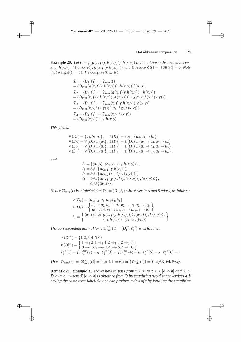
Example 20. Let t := f (g(x, f (y,h(x,y))) ,h(x,y)) that contains6 distinct subterms:x, y, h(x,y), f (y,h(x,y)), g(x, f (y,h(x,y))) and t. Henceδ(t) = |SUB(t)| = 6. Notethatweight(t) = 11. We computeDmin (t).

D1 = 〈D1, ℓ1〉 :=Dmin (t)= (Dmin (g(x, f (y,h(x,y))) ,h(x,y)))∗ [u1, t] ,

D2 = 〈D2, ℓ2〉 :=Dmin (g(x, f (y,h(x,y))) ,h(x,y))= (Dmin (x, f (y,h(x,y)) ,h(x,y)))∗ [u2,g(x, f (y,h(x,y)))] ,

D3 = 〈D3, ℓ3〉 :=Dmin (x, f (y,h(x,y)) ,h(x,y))= (Dmin (x,y,h(x,y)))

∗ [u3, f (y,h(x,y))] ,

D4 = 〈D4, ℓ4〉 :=Dmin (x,y,h(x,y))= (Dmin (x,y))

∗ [u4,h(x,y)] .

This yields:

V (D4) = a4,b4,u4 , E(D4) = u4→ a4,u4→ b4 ,V (D3) = V (D4)∪u3 , E(D3) = E(D4)∪u3→ b4,u3→ u4 ,V (D2) = V (D3)∪u2 , E(D2) = E(D3)∪u2→ a4,u2→ u3 ,V (D1) = V (D2)∪u1 , E(D1) = E(D3)∪u1→ u2,u1→ u4 ,

andℓ4 = 〈a4,x〉 ,〈b4,y〉 ,〈u4,h(x,y)〉 ,ℓ3 = ℓ4∪〈u3, f (y,h(x,y))〉 ,ℓ2 = ℓ3∪〈u2,g(x, f (y,h(x,y)))〉 ,ℓ1 = ℓ2∪〈u1, f (g(x, f (y,h(x,y))) ,h(x,y))〉 ,= ℓ2∪〈u1, t〉 .

HenceDmin (t) is a labeled dagD1 = 〈D1, ℓ1〉 with 6 vertices and8 edges, as follows:

V (D1) = u1,u2,u3,u4,a4,b4

E(D1) =

u1→ u2,u1→ u4,u2→ a4,u2→ u3,u3→ b4,u3→ u4,u4→ a4,u4→ b4

ℓ1 =

〈u1, t〉 ,〈u2,g(x, f (y,h(x,y)))〉 ,〈u3, f (y,h(x,y))〉 ,

〈u4,h(x,y)〉 ,〈a4,x〉 ,〈b4,y〉

The corresponding normal formDNFmin (t) = 〈D

NF1 , ℓNF

1 〉 is as follows:

V (DNF1 ) = 1,2,3,4,5,6

E(DNF1 ) =

1→1 2,1→2 4,2→1 5,2→2 3,3→1 6,3→2 4,4→2 5,4→1 6

ℓNF1 (1) = f , ℓNF

1 (2) = g, ℓNF1 (3) = f , ℓNF

1 (4) = h, ℓNF1 (5) = x, ℓNF

1 (6) = y

Thus|Dmin (t)|=∣∣DNF

min (t)∣∣= |SUB(t)|= 6, cod

(DNF

min (t))= f 24g53f 64h56xy.

Remark 21. Example 12 shows how to pass fromt D D to t D D [ax b] andD ⊲

D [ax b], whereD [ax b] is obtained fromD by equalizing two distinct vertices a,bhaving the same term-label. So one can produce mdr’s oft by iterating the equalizing

ii

“hermann50” — 2012/9/11 — 12:52 — page 30 — #36 ii

ii

ii

30 L. Gordeev

reduction as long as possible. Now the theorem shows that anysufficiently long itera-tion of this kind produces the same mdrDmin (t). Also note that the recursive definitionof Dmin (t) in question corresponds to the most natural “fast” bottom-up iteration pro-cedure. By Lemmata 5, 6 this yields a following result.

Corollary 22. LetD= 〈D, ℓ〉 ∈ DR, t = ℓ(root(D)). Then|D| ≥ |SUB(t)| andt DDD

Dmin (t) ∈ DR. Moreover the following assertions hold.

1. Dmin (t) is the uniqueD′ ∈DR such thatDDD′ and|D′|= |SUB(t)|. Thus∂(t) isthe uniquely determined minimal-size dag-like compression ofD.

2. If |D|> |SUB(t)| then

Dmin (t) =D [a1 x b1] · · · [am x bm]

where m= |D|− |SUB(t)| and a1 6= b1, · · · ,am 6= bm are arbitrary pairs of verticesfrom

D,D [a1 x b1] , · · · ,D [a1 x b1] · · · [am−1 x bm−1] ,

respectively, while

D⊲D [a1 x b1]⊲D [a1 x b1] [a2 x b2]⊲ · · ·⊲D [a1 x b1] · · · [am x bm] .

4 Discussion

4.1 Efficiency of term compression

We regard|D| as basic measure of complexity of any givenD= 〈D, ℓ〉 ∈ DR. Note that#(E(D)) is linear in|D|.2 However, the term labelsℓ(−) are unnecessarily complex.Therefore we switch to the normal formDNF = 〈DNF, ℓNF〉 whose labelsℓNF (−) arejust symbols of the underlying languageL (either function symbols or atoms), whichmakes the size ofDNF linear in |DNF| = |D|. By the same token the weight of thecorresponding normal form encodingcod(DNF) is also (nearly) linear in|D|.3 ThusTheorem 19 says thatDNF

min (t) is the most economic dag-like representation of a givenalgebraic termt, while Corollary 22 strengthens this claim by showing thatDNF

min (t) isthe normal form of the minimal-size compression of anyD such thatt = ℓ(root(D)).Consequently the average ratio betweenweight(t) andδ(t) = |Dmin (t)|=

∣∣DNFmin (t)

∣∣=|SUB(t)| characterizes the efficiency of the underlying dag-like compression. It is nothard to construct a termt such thatweight(t) exponentially exceeds|SUB(t)|, whichimplies that the dag-like compression can exponentially reduce the weight of standardterm presentation. The following examples show it explicitly.

Example 23. Consider binary–tree termsBii≥0 in the language with one functionsymbol∗ :

B0 := x, Bi+1 := Bi ∗Bi

2 More precisely, the total number of edges is bounded byd · |D|, whered is maximal dimension(or arity) of function symbols occurring int.

3 More precisely,weight(cod(DNF))∼ d · |D| · log|D|.

ii

“hermann50” — 2012/9/11 — 12:52 — page 31 — #37 ii

ii

ii


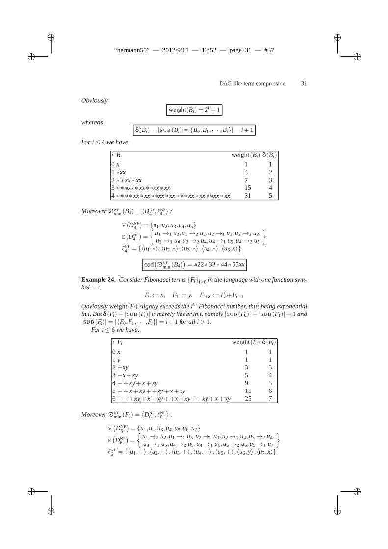
Obviously

weight(Bi) = 2i +1

whereasδ(Bi) = |SUB(Bi)|= |B0,B1, · · · ,Bi|= i +1

For i ≤ 4 we have:

i Bi weight(Bi) δ(Bi)

0 x 1 11 ∗xx 3 22 ∗ ∗ xx∗ xx 7 33 ∗ ∗ ∗xx∗ xx∗ ∗xx∗xx 15 44 ∗ ∗ ∗ ∗ xx∗ xx∗ ∗xx∗xx∗∗∗xx∗xx∗∗xx∗xx 31 5

MoreoverDNFmin (B4) = 〈DNF

4 , ℓNF4 〉 :

V (DNF4 ) = u1,u2,u3,u4,u5

E(DNF4 ) =

u1→1 u2,u1→2 u2,u2→1 u3,u2→2 u3,u3→1 u4,u3→2 u4,u4→1 u5,u4→2 u5

ℓNF4 = 〈u1,∗〉 ,〈u2,∗〉 ,〈u3,∗〉 ,〈u4,∗〉 ,〈u5,x〉

cod(DNF

min (B4))= ∗22∗33∗44∗55xx

Example 24. Consider Fibonacci termsFii≥0 in the language with one function sym-bol+ :

F0 := x, F1 := y, Fi+2 := Fi +Fi+1

Obviouslyweight(Fi) slightly exceeds the ith Fibonacci number, thus being exponentialin i. Butδ(Fi) = |SUB(Fi)| is merely linear in i, namely|SUB(F0)|= |SUB(F1)|= 1 and|SUB(Fi)|= |F0,F1, · · · ,Fi|= i +1 for all i > 1.

For i ≤ 6 we have:

i Fi weight(Fi) δ(Fi)

0 x 1 11 y 1 12 +xy 3 33 +x+ xy 5 44 ++ xy+ x+ xy 9 55 ++ x+ xy++xy+x+xy 15 66 +++xy+ x+ xy++x+xy++xy+x+xy 25 7

MoreoverDNFmin (F6) =

⟨DNF

6 , ℓNF6

⟩:

V(DNF

6

)= u1,u2,u3,u4,u5,u6,u7

E(DNF

6

)=

u1→2 u2,u1→1 u3,u2→2 u3,u2→1 u4,u3→2 u4,u3→1 u5,u4→2 u5,u4→1 u6,u5→2 u6,u5→1 u7

ℓNF6 = 〈u1,+〉 ,〈u2,+〉 ,〈u3,+〉 ,〈u4,+〉 ,〈u5,+〉 ,〈u6,y〉 ,〈u7,x〉

ii

“hermann50” — 2012/9/11 — 12:52 — page 32 — #38 ii

ii

ii

32 L. Gordeev

cod(DNF

min (F6))=+32+43+54+65+76xy

Problem 25. Consider any algebraic languageL. Estimate#t ∈ TL : |SUB(t)| ≤ n,for any n> 0, in comparison to#t ∈ TL : weight(t)≤ n to obtain a more precisecharacterization (previous examples suggest that on average the former should domi-nate). Approximate solutions can be obtained by the methodsof analytic combinatorics([8,9], et al).

Remark 26. Apart from obvious encoding connections this problem has interestingproof theoretic applications. Namely, regard standard systems of ordinal notations asterm algebras. So along with traditional tree-like form thecorresponding terms (i.e. or-dinals)α also admit the (more economical) minimal dag-like representationsDNF

min (α)with

∣∣DNFmin (α)

∣∣= |SUB(α)|. Now appropriate approximations of#α : |SUB(α)| ≤ nmight provide new insights into the theory of analytic phasetransitions of provability([6,7,10,11], et al).

4.2 Proof compression

Tree-like deductions (or proofs) in familiar proof systemsare treated analogously withrespect to proof-like dags whose vertices are labeled with formulas (or sequents). Ascompared to the term-like case (see above), these labels arenot supposed to deter-mine children’s ones and might vary under the correspondingdag-like compressions.Initial research along these lines is presented in [4], [5] and deals with propositionaldeductions (see also [2]). Especially in [5] we specify basic proof compressions withrespect to appropriate proof system for DNF tautologies designated bySEQ∗0. Note thatSEQ∗0 is a cutfree dag-like semi-analytic sequent calculus with substitution that haspolynomial size deductions of basic “hard” tautologies that are known to have only ex-ponential size deductions in familiar cutfree sequent calculi, resolution or cutting planeproof systems. MoreoverSEQ∗0 admits efficient proof search and exponential speed-upof the corresponding minimal dag-like compressions of standard tree-like proofs. Moredetailed elaboration of propositional proof compression is being work in progress. Fur-ther research will concentrate on predicate logic with quantifiers that admits dag-likeproof compressions providing superexponential size reduction.

References

1. A. V. Aho, M. S. Lam, R. Sethi, J. R. Ullmann,Compilers: Principles, Techniques andTools (Second Edition, Ch. 6), Addison-Wesley, 2007

2. S. Buss,Cut Elimination In Situ, manuscript (2011)3. P. J. Downey, R. Sethi, R. E. Tarjan,Variations on the common subexpression problem,

J.A.C.M. 27 (1980) 758-7714. L. Gordeev, E. H. Haeusler, V. G. da Costa,Proof compressions with circuit-structured sub-

stitutions, Journal of Mathematical Sciences, 158(5) (2009) 645–658;Zapiski Nauchn. Sem.POMI, 358 (2008) 77–99

5. L. Gordeev, E. H. Haeusler and L. C. Pereira,Propositional proof compressions and DNFlogic, Logic Journal of IGPL, 19(1) (2011) 62–86 ; doi: 10.1093/jigpal/jzq003

ii

“hermann50” — 2012/9/11 — 12:52 — page 33 — #39 ii

ii

ii


6. L. Gordeev, A. Weiermann,Phase transitions in Proof Theory, DMTCS proc. AM (2010)343-358

7. L. Gordeev, A. Weiermann,Phase transitions of iterated Higman-style well-partial-ordering,Arch. Math. Logic 51(1–2) (2012) 127-161; DOI 10.1007/s00153-011-0258-3

8. Ph. Flajolet, P. Sipala, J.-M. Steyaert,Analytic variations on the common subexpression prob-lem, In: Automata, Languages, and Programming: 17th International Colloquium, SpringerLecture Notes in Comp. Sci. 433 (1990) 220–234

9. Ph. Flajolet, R. Sedgewick,Analytic Combinatorics, Cambridge University Press, 200910. A. Weiermann,Phase transition thresholds for some Friedman-style independence results,

Math. Logic Q. 53(1) (2007) 4–1811. A. Weiermann,Phase transitions for Gödel incompleteness, Ann. Pure Appl. Logic 157(2-3)

(2009) 281–296

ii

“hermann50” — 2012/9/11 — 12:52 — page 34 — #40 ii

ii

ii

A short note on discharging functions and unicity ofnormal form for natural deduction

Luiz Carlos Pereira1⋆ and Wagner de Campos Sanz2⋆⋆

1 Philosophy Dept. [email protected] Philosophy Dept. [email protected]

Abstract. We show that the crude discharging strategy for Natural Deductionimplies a loss of unicity of normal form in the implicative fragment.

1 Unicity of Normal Form

The concept ofdischarging functionwas introduced by Dag Prawitz as a component ofan alternative definition of deduction for Natural Deduction systems (see [Pra65] pp. 29-31). In Prawitz’ first definition of deduction, an application of implication-introductionwith conclusionA→ B eliminates every occurrence (if any) of an assumptionA inthe derivation of the premissB. The discharging strategy present in this formulationof implication-introduction is sometimes calledthe crude discharging strategy. In thealternative definition not every occurrence of the assumption A would have to be dis-charged by the corresponding application of implication-introduction. Adischargingfunctionwould tell us which assumptions are discharged and where they are dischargedin a proof-tree. Instead of assumptions simply, we would nowhaveassumption classesand these would be discharged by applications of implication-introduction. Prawitz’first definition of deduction clearly does not allow us to talkaboutnon-trivial assump-tion classes. Although the alternative definition was already introduced in the first chap-ter of [Pra65], it was not used until chapter VI, a chapter devoted to Modal Logic,where a finer analysis of dependency relations was required so that modal systems withgood proof-theoretical properties could be defined (as for example, the property of be-ing closed under reductions). In [Lei79], Leivant showed that discharging functions (ornon-trivial assumption classes) were required in order to ensure that every reduction se-quence for a given derivationΠ is finite. In [Wid01], Wideback showed that dischargingfunctions are also required if generalizations are to be preserved. The aim of this shortnote is to show thatdischarging functionsare also required if one wants to preserveunicity of normal.

We shall present below a very simple derivation that reduces(in two steps) to twodifferent normal forms, if implication-introduction is taken in its more restricted formaccording to the first definition of deduction,the crude discharging strategy:

⋆ CNPq and PRONEX/FAPERJ⋆⋆ CNPq 401882/2011-0

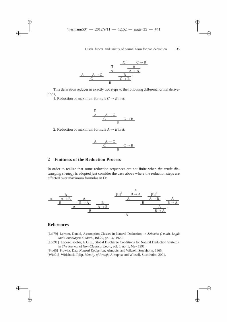
ii

“hermann50” — 2012/9/11 — 12:52 — page 35 — #41 ii

ii

ii

Disch. functs. and unicity of normal form for nat. deduction 35

A A → CC

ΠA

[C]1 C→ BB

A→ BB 1

C→ BB

This derivation reduces in exactly two steps to the following different normal deriva-tions,

1. Reduction of maximum formulaC→ B first:

ΠA A → C

C C→ BB

2. Reduction of maximum formulaA→ B first:

A A → CC C→ B

B

2 Finitness of the Reduction Process

In order to realize that some reduction sequences are not finite whenthe crude dis-charging strategyis adopted just consider the case above where the reduction steps areeffected over maximum formulas inΠ:

AB

A → BB

AB→ A

AB

A→ BB

[B]1A

B→ AA

[B]1

A→ BB

AB→ A

A 1B→ A

A

References

[Lei79] Leivant, Daniel, Assumption Classes in Natural Deduction, inZeitschr. f. math. Logikund Grundlagen d. Math., Bd.25, pp.1-4, 1979.

[Lop91] Lopez-Escobar, E.G.K., Global Discharge Conditions for Natural Deduction Systems,in The Journal of Non-Classical Logic, vol. 8, no. 1, May 1991.

[Pra65] Prawitz, Dag,Natural Deduction, Almqvist and Wiksell, Stockholm, 1965.[Wid01] Wideback, Filip,Identity of Proofs, Almqvist and Wiksell, Stockholm, 2001.

ii

“hermann50” — 2012/9/11 — 12:52 — page 36 — #42 ii

ii

ii

Indexed logical closure operators

Uwe Wolter1, Alfio Martini2, and Edward Hermann Haeusler3

1 University of [email protected]

2 Pontifícia Universidade Católica do Rio Grande do [email protected]

3 Pontifícia Universidade Católica do Rio de [email protected]

Abstract. The fundamental idea of “What a logic is?” is now establishedas avery active field of research within Computer Science. Usingadjunctions as abuilt-in foundation we introduce the notion of anIndexed Partial Order Frameand show that it captures in an uniform way important examples of General Log-ics, like Institutions and Entailment Systems. On the otherhand, the idea of aClosure Operator is a fundamental logical tool used to formalize many aspectsossyntax and entailment in traditional logic. Capitalizing on the strong relationshipbetween Triples (as theories) and Adjunctions, our IndexedPartial Order Framescan be seen in an equivalent way as generalized (indexed by categories) closureoperators. This is shown by theorems 3 and 4, which together,state that eachIndexed Partial Order Frame defines uniquely an Indexed Closure Operator andvice-versa.

Preamble

Alfio and Uwe, worked together on the theory of institutions when Alfio took his PhDat Technical University Berlin from 1995 to 1999. After Alfiowent back to Brazil, heproposed in 2005 to involve Hermann when we decided to relaunch our research onabstract model theory. Fortunately, Hermann agreed and we can today look back to avery nice and fruitful collaboration resulting in many contributions to conferences andjournal papers.

The present paper is based on ideas and proposals of Hermann and was presentedby himself at XV. EBL 2008. When preparing the paper in January 2008 Hermannhad a serious injury while playing volleyball and had to undergo a surgery. ThereforeAlfio and Uwe took over the job to work out Hermann’s ideas. We still remember withgladness how happy Hermann was when we managed to send the paper in time and hisenthusiastic email from the sickbed:

I love you both !!!! That is a quite good thing to know. We haveat least one thing to get happy this starting of 2008 !!!!

Dear Hermann, we wish you all the very best for your birthday and are lookingforward for your nice company and collaboration also in the years that come.

ii

“hermann50” — 2012/9/11 — 12:52 — page 37 — #43 ii

ii

ii

Indexed logical closure operators 37

1 Introduction

The fundamental question of “What is a logic?” is now established as a very activefield of research within Computer Science [6,13]. In [11] we look at this problem fromthe point of view of “What mathematical structures lie underneath logics with indexedsyntax and semantics on the level of abstraction given by specifications and modelclasses?”. This is done by introducing the concept of anIndexed Partial Order Framewhich provides an indexed general definition of Logics that takes natural transforma-tions and adjunctions as built-in tools to formalize the relevant structures of a logicalsystem. This concept appears as an abstraction of the concepts Institution and Entail-ment System and provides, especially, an elegant and natural account of the coherenceaxioms pertaining to these both logical systems.

On the other hand, one can argue in favour of a purely syntactical definition of aparticular logic. This in fact happened with Intuitionistic Type Theory (see [10]) andother constructive approaches to the foundations of mathematics. Such exclusively syn-tactically defined logical systems abound in computer science. We cannot forget thestrong syntactical tradition that Logic has.

Moreover, logical consequence (closure) operators are a well-established abstractconcept to treat (some aspects) of syntax in Logics and it is well-known that they arisenaturally from Galois Correspondences between specifications and model classes. Thecategorical generalization of this connection between closure operators and Galois Con-nections is established by the connection between (co-)triples and adjoint pairs. We usethis connection in order to provide a purely categorical account for logical consequenceoperators in our setting. Further we investigate under whatconditions the co-Eilenbergand co-Kleisli constructions provide a way back from Indexed Logical ConsequenceOperators to Indexed Frames.

Do to the limitations in space the treatment of morphisms between the differentkinds of structures presented in this paper and of the various transitions between themhas to be postponed for a later extended version.

2 Institutions and Indexed Frames

The concept of aninstitutionintroduced by GOGUENand BURSTALL [7] formally cap-tures the notion of logical systems and allowed them to reformulate and to generalizethe work they had done in the 70’s on structuring (equational) specifications (see [3,4])independently of the underlying logic. A similiar proposalof an abstract concept of alogic had been given already by BARWISE [1].

Definition 1 (Institution). An INSTITUTION I = (Sign,Sen,Mod, |=) is given by thefollowing data and operations:

– A CATEGORY OF ABSTRACT SIGNATURESSign;– A SYNTAX FUNCTOR Sen: Sign→ Sets, defining for each signature its set of sen-

tences;– A MODEL FUNCTOR Mod : Signop→ Cat, defining for each signature, its corre-

sponding category of models;

ii

“hermann50” — 2012/9/11 — 12:52 — page 38 — #44 ii

ii

ii

38 U. Wolter and A. Martini

– AN INDEXED FAMILY OF SATISFACTION RELATIONS |=Σ⊆ |Mod(Σ)|×Sen(Σ),Σ ∈ |Sign|; such that the followinginstitution condition

Mod(φ)(M2) |=Σ1 ϕ1⇐⇒M2 |=Σ2 Sen(φ)(ϕ1)

holds for eachφ : Σ1→ Σ1 in Sign, M2 ∈ |Mod(Σ2)|, andϕ1 ∈ Sen(Σ1).

Institutions are based on a pointwise assignment of signatures, sentences, and models.But in design (programming), the relevant objects are not sentences (program lines),but specifications (programs). The following investigations on this level of abstractionprovide new insights into the conceptual nature of logical systems so that we can givea fully categorial account of theinstitution condition.

Assuming an institutionI, and a set ofΣ-sentencesΓ ⊆ Sen(Σ), we define thecategorymod(Σ)(Γ) as the full subcategory induced by those models in|Mod(Σ)| thatsatisfyΓ, i.e.,

|mod(Σ)(Γ)| de f= M ∈ |Mod(Σ)| | ∀ϕ ∈ Γ : M |=Σ ϕ. (1)

Analogously, we define for a given subcategoryM⊆Mod(Σ) of Σ-models, the set oftheoremsth(Σ)(M)⊆ Sen(Σ) given by those sentencesϕ ∈ Sen(Σ) which are satisfiedby all models inM, i.e., we have

th(Σ)(M)de f= ϕ ∈ Sen(Σ) | ∀M ∈ |M| : M |=Σ ϕ. (2)

Obviously,mod(Σ) andth(Σ) induce mappings betweenΣ-specifications and cate-gories ofΣ-models and vice-versa.

Definition 2 (Partial Order Categories). Given a signatureΣ ∈ |Sign|, we define thepartial order categorySpec(Σ) of strict specifications, the category where the objectsare all setsΓ ⊆ Sen(Σ), and the arrows are all the inverse inclusionsΓ1 ⊇ Γ2. Analo-gously, the partial order categorySub(Σ) has as objects all subcategoriesM⊆Mod(Σ)and as arrows all inclusion functorsM1⊆M2.

By definition ofSpec(Σ) andSub(Σ), we can formulate the usual categorical pre-sentation of the Galois correspondence arising from any (satisfaction) relation as anadjunctionth(Σ) ⊣mod(Σ).

Proposition 1 (Galois Correspondence).Given a signatureΣ ∈ |Sign|, the equations(1) and (2) define functors mod(Σ) : Spec(Σ)→ Sub(Σ) and th(Σ) : Sub(Σ)→ Spec(Σ),such that th(Σ) is left-adjoint to mod(Σ), written th(Σ) ⊣mod(Σ), where forΓ,Γ1,Γ2 ∈|Spec(Σ)|, andM,M1,M2 ∈ |Mod(Σ)|, we have:

1. th(Σ) functor:M1 ⊆M2 implies th(Σ)(M1)⊇ th(Σ)(M2);2. mod(Σ) functor:Γ2 ⊇ Γ1 implies mod(Σ)(Γ2)⊆mod(Σ)(Γ1);3. unit:M⊆mod(Σ)(th(Σ)(M));4. counit: th(Σ)(mod(Σ)(Γ))⊇ Γ;5. adjointness:M⊆mod(Σ)(Γ) iff th(Σ)(M)⊇ Γ.

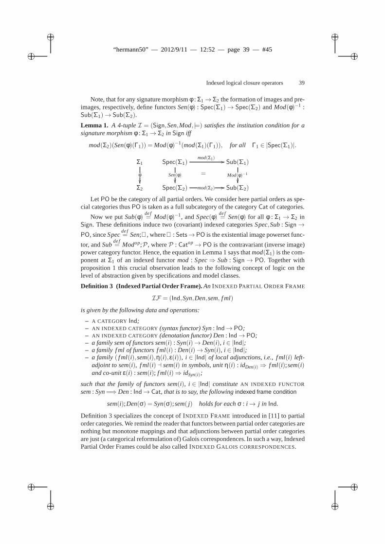
ii

“hermann50” — 2012/9/11 — 12:52 — page 39 — #45 ii

ii

ii


Note, that for any signature morphismφ : Σ1→ Σ2 the formation of images and pre-images, respectively, define functorsSen(φ) : Spec(Σ1)→ Spec(Σ2) andMod(φ)−1 :Sub(Σ1)→ Sub(Σ2).

Lemma 1. A 4-tupleI = (Sign,Sen,Mod, |=) satisfies the institution condition for asignature morphismφ : Σ1→ Σ2 in Sign iff

mod(Σ2)(Sen(φ)(Γ1)) = Mod(φ)−1(mod(Σ1)(Γ1)), for all Γ1 ∈ |Spec(Σ1)|.

Σ1

φ

Spec(Σ1)mod(Σ1) //

Sen(φ)

=

Sub(Σ1)

Mod(φ)−1

Σ2 Spec(Σ2) mod(Σ2) // Sub(Σ2)

Let PO be the category of all partial orders. We consider here partial orders as spe-cial categories thusPO is taken as a full subcategory of the categoryCat of categories.

Now we putSub(φ) de f= Mod(φ)−1, andSpec(φ) de f

= Sen(φ) for all φ : Σ1→ Σ2 inSign. These definitions induce two (covariant) indexed categoriesSpec,Sub: Sign→

PO, sinceSpecde f= Sen;℘, where℘: Sets→ PO is the existential image powerset func-

tor, andSubde f= Modop;P , whereP : Catop→ PO is the contravariant (inverse image)

power category functor. Hence, the equation in Lemma 1 says thatmod(Σ1) is the com-ponent atΣ1 of an indexed functormod : Spec⇒ Sub: Sign→ PO. Together withproposition 1 this crucial observation leads to the following concept of logic on thelevel of abstraction given by specifications and model classes.

Definition 3 (Indexed Partial Order Frame). An INDEXED PARTIAL ORDERFRAME

IF = (Ind,Syn,Den,sem, f ml)

is given by the following data and operations:

– A CATEGORY Ind;– AN INDEXED CATEGORY (syntax functor) Syn: Ind→ PO;– AN INDEXED CATEGORY (denotation functor) Den: Ind→ PO;– a family sem of functors sem(i) : Syn(i)→ Den(i), i ∈ |Ind|;– a family f ml of functors f ml(i) : Den(i)→ Syn(i), i ∈ |Ind|;– a family ( f ml(i),sem(i),η(i),ε(i)), i ∈ |Ind| of local adjunctions, i.e., f ml(i) left-

adjoint to sem(i), f ml(i) ⊣ sem(i) in symbols, unitη(i) : idDen(i)⇒ f ml(i);sem(i)and co-unitε(i) : sem(i); f ml(i)⇒ idSyn(i);

such that the family of functors sem(i), i ∈ |Ind| constituteAN INDEXED FUNCTOR

sem: Syn=⇒ Den: Ind→ Cat, that is to say, the followingindexed frame condition

sem(i);Den(σ) = Syn(σ);sem( j) holds for eachσ : i→ j in Ind.

Definition 3 specializes the concept of INDEXED FRAME introduced in [11] to partialorder categories. We remind the reader that functors between partial order categories arenothing but monotone mappings and that adjunctions betweenpartial order categoriesare just (a categorical reformulation of) Galois correspondences. In such a way, IndexedPartial Order Frames could be also called INDEXED GALOIS CORRESPONDENCES.

ii

“hermann50” — 2012/9/11 — 12:52 — page 40 — #46 ii

ii

ii


Theorem 1 (Institutional Frame). A 4-tupleI = (Sign,Sen,Mod, |=) is an institutioniff the 5-tupleIF = (Sign,Spec,Sub,mod, th) is an indexed partial order frame, calledthe INSTITUTIONAL FRAME for I.

3 Entailment Systems

The concept ofentailment systemintroduced in [12] reflects those properties of the en-tailment relationΓ ⊢ ϕ which are independent from the particular rules used to generatethe relation⊢. This section is devoted to validate the concept of indexed partial orderframe by showing that also entailment systems give rise, quite naturally, to indexedpartial order frames.

Definition 4 (Entailment System).An ENTAILMENT SYSTEM is a triple

E = (Sign,Sen,⊢),

with Sign a category ofsignatures, Sen: Sign→ Set a functor, and⊢ a function as-sociating to each signatureΣ a binary relation⊢Σ⊆℘(Sen(Σ))×Sen(Σ) called en-tailment relationsuch that the following properties are satisfied:reflexivity: for anyϕ ∈ Sen(Σ),ϕ ⊢ ϕ; monotonicity:if Γ1 ⊢Σ ϕ and Γ2 ⊇ Γ1 thenΓ2 ⊢Σ ϕ; transi-tivity: if Γ ⊢Σ ϕ1, for i ∈ I, andΓ∪ϕi | i ∈ I ⊢Σ ψ, thenΓ ⊢Σ ψ; ⊢-translation:ifΓ1 ⊢Σ1 ϕ1, then for anyφ : Σ1→ Σ2 in Sign,Sen(φ)(Γ1) ⊢Σ2 Sen(φ)(ϕ1).

The entailment relation⊢Σ between sets ofΣ-sentences and singleΣ-sentencescan be extended to an equivalent entailment relation between Σ-specifications. Forany signatureΣ in Sign we define a correspondingextended entailment relation⊢℘

Σ=℘(Sen(Σ))×℘(Sen(Σ)) = |Spec(Σ)|× |Spec(Σ)|, where forΣ-specificationsΓ1,Γ2 ∈Spec(Σ) :

Γ1 ⊢℘Σ Γ2 iff ∀ϕ2 ∈ Γ2 : Γ1 ⊢Σ ϕ2 (3)

Lemma 2. Given a signatureΣ ∈ Sign the entailment relation⊢Σ has the properties(1)-(4) of definition 4 if and only if the extended entailmentrelation ⊢℘

Σ satisfies thefollowing properties for anyΓ1,Γ2,Γ3 ∈ |Spec(Σ)|:

1. projection:Γ1∪Γ2 ⊢℘Σ Γ2, i.e., especiallyΓ1 ⊇ Γ2 impliesΓ1 ⊢

℘Σ Γ2;

2. product property:if Γ1 ⊢℘Σ Γ2 andΓ1 ⊢

℘Σ Γ3, thenΓ1 ⊢

℘Σ Γ2∪Γ3;

3. compositionality:if Γ1 ⊢℘Σ Γ2 andΓ2 ⊢

℘Σ Γ3, thenΓ1 ⊢

℘Σ Γ3;

4. functor property:if Γ1 ⊢℘Σ1

Γ2, then for anyφ : Σ1→ Σ2 in Sign,Sen(φ)(Γ1) ⊢℘Σ2

Sen(φ)(Γ2).

Note that forΓ1 = /0 the projection property provides the identity property, i.e.,Γ ⊢℘

Σ Γ for anyΓ∈Spec(Σ). Lemma 2 makes clear that the extended entailment relation⊢

℘Σ determines a preorder categoryEnt(Σ).

Definition 5 (Extended Entailment).Given a signatureΣ ∈ |Sign| we define the par-tial order category Ent(Σ) of all Σ-specifications with entailment as follows:objects:are all specificationsΓ ∈ |Spec(Σ)|; morphisms:are all extended entailment relationsΓ1 ⊢

℘Σ Γ2; identities:are all entailmentsΓ ⊢℘

Σ Γ, Γ ∈ |Spec(Σ)|; composition:is givenby the compositionality property in lemma 2.

ii

“hermann50” — 2012/9/11 — 12:52 — page 41 — #47 ii

ii

ii


Theprojectionproperty in lemma 2 entails thatEnt(Σ) is an extension of the categorySpec(Σ), i.e., for any signatureΣ we obtain an embedding functor

em(Σ) : Spec(Σ)→ Ent(Σ) with em(Σ)(Γ) = Γ. (4)

If we consider the set of sentences provable from a specification Γ, i.e., if we set

cl(Σ)(Γ) = ϕ ∈ Sen(Σ) | Γ ⊢Σ ϕ, (5)

we obtain a so-calledclosurefunctor fromEnt(Σ) to Spec(Σ).

Proposition 2 (Galois Correspondence).Given a signatureΣ ∈ |Sign|, the equations(4) and (5) define functors em(Σ) : Spec(Σ)→ Ent(Σ) and cl(Σ) : Ent(Σ)→ Spec(Σ),such that cl(Σ) is left-adjoint to em(Σ), i.e., for any specificationsΓ,Γ1,Γ2∈ |Spec(Σ)|=|Ent(Σ)| we have:

1. em(Σ) functor:Γ1 ⊇ Γ2 impliesΓ1 ⊢℘Σ Γ2;

2. cl(Σ) functor:Γ1 ⊢℘Σ Γ2 implies cl(Σ)(Γ1)⊇ cl(Σ)(Γ2);

3. unit: Γ ⊢℘Σ cl(Σ)(Γ) in Ent(Σ);

4. counit:cl(Σ)(Γ) ⊇ Γ in Spec(Σ);5. adjointness:Γ1 ⊢

℘Σ Γ2 iff cl(Σ)(Γ1)⊇ Γ2.

In the next steps we exploit the functor property in lemma 2 togain a fully categorialpresentation of the concept “entailment system”.

Proposition 3 (Entailment Functor). The mappings Spec: |Sign| → |PO| and Ent:|Sign| → |PO| given by definition 2 and definition 5 respectively can be extended tofunctors Spec: Sign → PO and Ent: Sign→ PO if we set for anyφ : Σ1 → Σ2 inSign and for anyΓ1 ∈ |Spec(Σ1)|: Spec(φ)(Γ1) = Ent(φ)(Γ1) = Sen(φ)(Γ1). In thisway all the functors em(Σ) : Spec(Σ)→ Ent(Σ), Σ ∈ |Sign| define an indexed functorem: Spec⇒ Ent : Sign→ PO.

Theorem 2 (Entailment Frames).A triple E = (Sign,Sen,⊢) is an entailment systemiff the 5-tupleEF = (Sign,Spec,Ent,em,cl) defines an indexed partial order frame,called theENTAILMENT FRAME for E .

π-institutions as originally introduced by FIADEIRO and SERNADAS are essentiallythe same as entailment systems. Only transitivity is formulated in a different but equiv-alent way (see [5]). An abstract interpretation ofπ-institutions can be given in termsof closure operators, i.e., in terms of the functorsem(Σ);cl(Σ) : Spec(Σ)→ Spec(Σ).The generalization of this abstraction step to arbitrary indexed frames based on the co-triples (co-monads) given by the adjunctionsf ml(i) ⊣ sem(i) is approached in the nextsection.

4 Indexed Logical Closure Operators

In the preceding sections of this article we have seen that adjunctions can be taken as thefundamental concept in defining a Logical Framework.Indexed Partial Order Frames

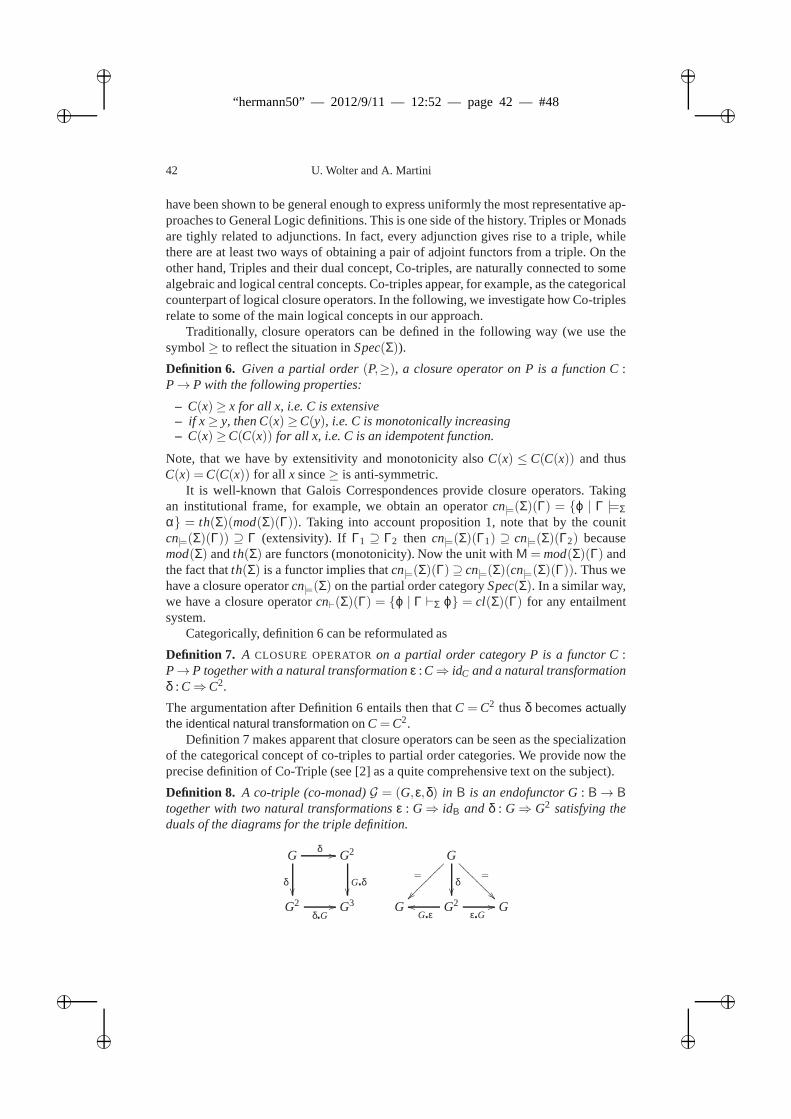
ii

“hermann50” — 2012/9/11 — 12:52 — page 42 — #48 ii

ii

ii


have been shown to be general enough to express uniformly themost representative ap-proaches to General Logic definitions. This is one side of thehistory. Triples or Monadsare tighly related to adjunctions. In fact, every adjunction gives rise to a triple, whilethere are at least two ways of obtaining a pair of adjoint functors from a triple. On theother hand, Triples and their dual concept, Co-triples, arenaturally connected to somealgebraic and logical central concepts. Co-triples appear, for example, as the categoricalcounterpart of logical closure operators. In the following, we investigate how Co-triplesrelate to some of the main logical concepts in our approach.

Traditionally, closure operators can be defined in the following way (we use thesymbol≥ to reflect the situation inSpec(Σ)).Definition 6. Given a partial order(P,≥), a closure operator on P is a function C:P→ P with the following properties:

– C(x)≥ x for all x, i.e. C is extensive– if x≥ y, then C(x)≥C(y), i.e. C is monotonically increasing– C(x)≥C(C(x)) for all x, i.e. C is an idempotent function.

Note, that we have by extensitivity and monotonicity alsoC(x) ≤ C(C(x)) and thusC(x) =C(C(x)) for all x since≥ is anti-symmetric.

It is well-known that Galois Correspondences provide closure operators. Takingan institutional frame, for example, we obtain an operatorcn|=(Σ)(Γ) = ϕ | Γ |=Σα = th(Σ)(mod(Σ)(Γ)). Taking into account proposition 1, note that by the counitcn|=(Σ)(Γ)) ⊇ Γ (extensivity). If Γ1 ⊇ Γ2 then cn|=(Σ)(Γ1) ⊇ cn|=(Σ)(Γ2) becausemod(Σ) andth(Σ) are functors (monotonicity). Now the unit withM= mod(Σ)(Γ) andthe fact thatth(Σ) is a functor implies thatcn|=(Σ)(Γ)⊇ cn|=(Σ)(cn|=(Σ)(Γ)). Thus wehave a closure operatorcn|=(Σ) on the partial order categorySpec(Σ). In a similar way,we have a closure operatorcn⊢(Σ)(Γ) = ϕ | Γ ⊢Σ ϕ = cl(Σ)(Γ) for any entailmentsystem.

Categorically, definition 6 can be reformulated as

Definition 7. A CLOSURE OPERATORon a partial order category P is a functor C:P→P together with a natural transformationε : C⇒ idC and a natural transformationδ : C⇒C2.

The argumentation after Definition 6 entails then thatC = C2 thusδ becomesactuallythe identical natural transformation onC=C2.

Definition 7 makes apparent that closure operators can be seen as the specializationof the categorical concept of co-triples to partial order categories. We provide now theprecise definition of Co-Triple (see [2] as a quite comprehensive text on the subject).

Definition 8. A co-triple (co-monad)G = (G,ε,δ) in B is an endofunctor G: B→ B

together with two natural transformationsε : G⇒ idB and δ : G⇒ G2 satisfying theduals of the diagrams for the triple definition.

Gδ //

δ

G2

Gδ

G

=

=

???

????

?

δ

G2δG

// G3 G G2Gε

ooεG

// G

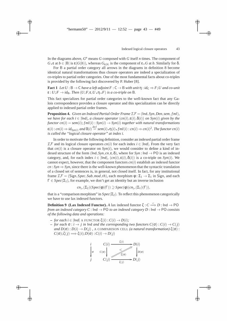
ii

“hermann50” — 2012/9/11 — 12:52 — page 43 — #49 ii

ii

ii


In the diagrams above,Gn meansG composed withG itself n times. The component ofG ε atb∈ |B| is ε(G(b)), whereasGε(b) is the component ofε G atb. Similarly for δ.

For B a partial order category all arrows in the diagrams in definition 8 becomeidentical natural transformations thus closure operatorsare indeed a specialization ofco-triples to partial order categories. One of the most fundamental facts about co-triplesis provided by the following fact discovered by P. Huber [8].

Fact 1 Let U :B→C have a left adjoint F: C→B with unitη : idC⇒F ;U and co-unitε : U ;F → idB. Then(U ;F,ε,U η F) is a co-triple onB.

This fact specializes for partial order categories to the well-known fact that any Ga-lois correspondence provides a closure operator and this specialization can be directlyapplied to indexed partial order frames.

Proposition 4. Given an Indexed Partial Order FrameIF =(Ind,Syn,Den,sem, f ml),we have for each i∈ |Ind|, a closure operator(cn(i),ε(i),δ(i)) on Syn(i) given by thefunctor cn(i) = sem(i); f ml(i) : Syn(i)→ Syn(i) together with natural transformations

ε(i) : cn(i)⇒ idSyn(i) andδ(i) de f= sem(i) η(i) f ml(i) : cn(i)⇒ cn(i)2. The functor cn(i)

is called the “logical closure operator” at index i.

In order to motivate the following definition, consider an indexed partial order frameIF and its logical closure operatorscn(i) for each indexi ∈ |Ind|. From the very factthat cn(i) is a closure operator onSyn(i), we would consider to define a kind of in-dexed structure of the form(Ind,Syn,cn,ε,δ), where forSyn: Ind→ PO is an indexedcategory, and, for each indexi ∈ |Ind|, (cn(i),ε(i),δ(i)) is a co-triple onSyn(i). Wecannot expect, however, that the component functorscn(i) establish an indexed functorcn : Syn⇒Syn, since there is the well-known phenomenon that the syntactic translationof a closed set of sentences is, in general, not closed itself. In fact, for any institutionalframeIF = (Sign,Spec,Sub,mod, th), each morphismφ : Σ1→ Σ1 in Sign, and eachΓ ∈ Spec(Σ1), for example, we don’t get an identity but an inverse inclusion

cn|=(Σ2)(Spec(φ)(Γ))⊇ Spec(φ)(cn|=(Σ1)(Γ)),

that is a “comparison morphism” inSpec(Σ2). To reflect this phenomenon categoricallywe have to use lax indexed functors.

Definition 9 (Lax Indexed Functor). A lax indexed functorζ : C<

=⇒ D : Ind→ PO

from an indexed category C: Ind→ PO to an indexed category D: Ind→ PO consistsof the following data and operations:

– for each i∈ |Ind| A FUNCTOR ζ(i) : C(i)→D(i);– for eachσ : i → j in Ind and the corresponding two functors C(σ) : C(i)→C( j)

and D(σ) : D(i)→ D( j) , A COMPARISON CELL (a natural transformation)ζ(σ) :C(σ);ζ( j) =⇒ ζ(i);D(σ) : C(i)→ D( j)

i

σ

C(i)

<C(σ)

ζ(i) // D(i)

D(σ)

j C( j)

ζ(σ)

3;oooooooooooo

oooooooooooo

ζ( j)// D( j)

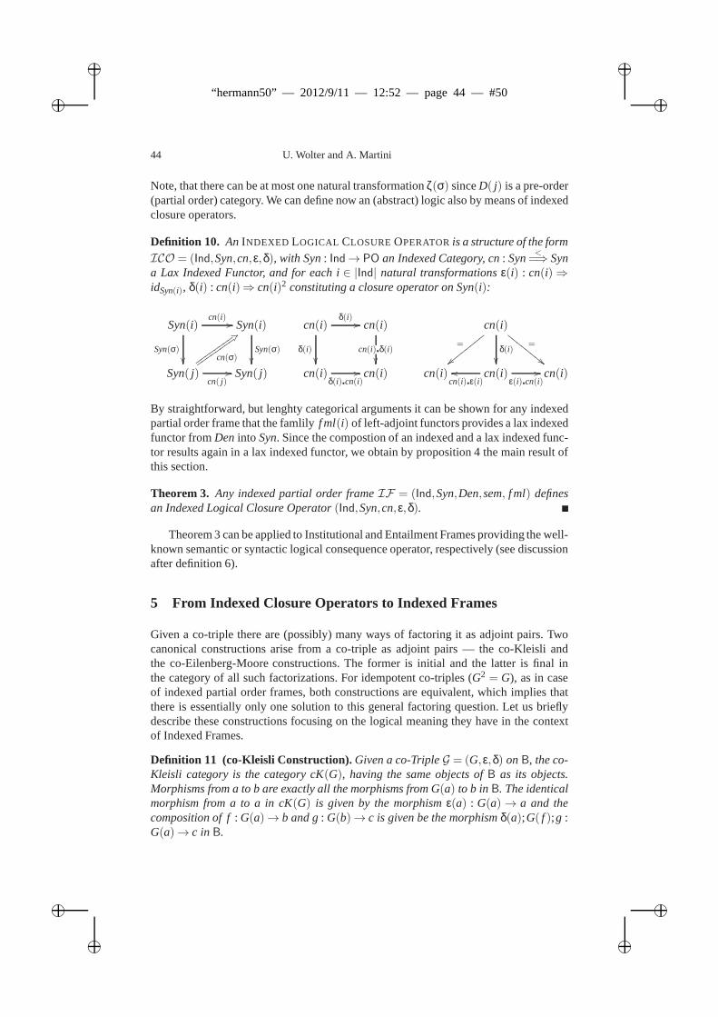
ii

“hermann50” — 2012/9/11 — 12:52 — page 44 — #50 ii

ii

ii


Note, that there can be at most one natural transformationζ(σ) sinceD( j) is a pre-order(partial order) category. We can define now an (abstract) logic also by means of indexedclosure operators.

Definition 10. An INDEXED LOGICAL CLOSUREOPERATORis a structure of the formICO = (Ind,Syn,cn,ε,δ), with Syn: Ind→ PO an Indexed Category, cn: Syn

<=⇒ Syn

a Lax Indexed Functor, and for each i∈ |Ind| natural transformationsε(i) : cn(i)⇒idSyn(i), δ(i) : cn(i)⇒ cn(i)2 constituting a closure operator on Syn(i):

Syn(i)cn(i) //

Syn(σ)

Syn(i)

Syn(σ)

cn(i)δ(i) //

δ(i)

cn(i)

cn(i)δ(i)

cn(i)

=

||yyyyyyyy =

""EEE

EEEE

E

δ(i)

Syn( j)cn( j)

//cn(σ)

6>vvvvvvvv

vvvvvvvv

Syn( j) cn(i)δ(i)cn(i)

// cn(i) cn(i) cn(i)cn(i)ε(i)oo

ε(i)cn(i)// cn(i)

By straightforward, but lenghty categorical arguments it can be shown for any indexedpartial order frame that the famlilyf ml(i) of left-adjoint functors provides a lax indexedfunctor fromDeninto Syn. Since the compostion of an indexed and a lax indexed func-tor results again in a lax indexed functor, we obtain by proposition 4 the main result ofthis section.

Theorem 3. Any indexed partial order frameIF = (Ind,Syn,Den,sem, f ml) definesan Indexed Logical Closure Operator(Ind,Syn,cn,ε,δ).

Theorem 3 can be applied to Institutional and Entailment Frames providing the well-known semantic or syntactic logical consequence operator,respectively (see discussionafter definition 6).

5 From Indexed Closure Operators to Indexed Frames

Given a co-triple there are (possibly) many ways of factoring it as adjoint pairs. Twocanonical constructions arise from a co-triple as adjoint pairs — the co-Kleisli andthe co-Eilenberg-Moore constructions. The former is initial and the latter is final inthe category of all such factorizations. For idempotent co-triples (G2 = G), as in caseof indexed partial order frames, both constructions are equivalent, which implies thatthere is essentially only one solution to this general factoring question. Let us brieflydescribe these constructions focusing on the logical meaning they have in the contextof Indexed Frames.

Definition 11 (co-Kleisli Construction).Given a co-TripleG = (G,ε,δ) onB, the co-Kleisli category is the category cK(G), having the same objects ofB as its objects.Morphisms from a to b are exactly all the morphisms from G(a) to b inB. The identicalmorphism from a to a in cK(G) is given by the morphismε(a) : G(a)→ a and thecomposition of f: G(a)→ b and g: G(b)→ c is given be the morphismδ(a);G( f );g :G(a)→ c inB.

ii

“hermann50” — 2012/9/11 — 12:52 — page 45 — #51 ii

ii

ii


Example 1.In an Institutional FrameIF , the co-Kleisli categorycK(cn|=(Σ)) for eachΣ ∈ |Sign| is the category of Theory PresentationsΓ ∈ |Spec(Σ)|, and there is a mor-phism fromΓ ∈ |Spec(Σ)| into ∆ ∈ |Spec(Σ)| iff cn|=(Σ)(Γ) ⊇ ∆. In other words,Γ |=Σ ∆. This category is well-known for the algebraic logicians. It is worth noticingthat, since there is at most one morphism fromΓ into ∆, they are isomorphic as objectsin cK(cn|=(Σ)), whenever they are logically equivalent, that isΓ |=Σ ∆ and∆ |=Σ Γ.

It is clear from the above example that the co-Kleisli category seems to be morenatural to be regarded as a logical instance of a categoricalconcept. On the other hand,theories are captured by the following construction.

Definition 12 (Co-Eilenberg-Moore Construction). Also known as the category ofco-Algebras for a co-Triple, the co-Eilenberg-Moore construction BG for a co-tripleG = (G,ε,δ) onB onB has pairs(a,α), with α : a→G(a) a morphism inB, as objects.A morphism between(a,α) and (b,β) is any morphism f: a→ b in B for which, thefollowing diagram commutes:

a

f

α // G(a)

T f

b

β // G(b)

The composition inBG is provided by the composition onB itself.

Example 2.The co-Eilenberg-Moore categorySpec(Σ)cn|=(Σ), for eachΣ ∈ |Sign|, inan Institutional FrameIF , is the category of Theories, i.e., of sets of sentences sat-isfying the “closedness condition”∆ ⊇ cn|=(Σ)(∆), i.e., satisfying the condition∆ =cn|=(Σ)(∆), since we havecn|=(Σ)(Γ)⊇ Γ for all sets of sentences. In such a way,∆⊇ Γmeans alsocn(Σ)(∆)⊇ cn(Σ)(Γ) for theories∆ andΓ thusSpec(Σ)cn|=(Σ) is indeed thefull subcategory ofSpec(Σ) given by all theories.

The above pair of examples on co-Kleisli and co-Eilenberg-Moore constructionsshow equivalent categories. For closure operators, in general, both constructions pro-vide equivalent categories thus we can concentrate on one ofthese constructions. Wewill look now at the adjunction provided by the co-Kleisli construction.

Proposition 5. For any co-TripleG =(G,ε,δ) onB the assignments a7→ a and( f : a→b) 7→ (ε(a); f : G(a)→ b) define a functor inG :B→ cK(G). Moreover, the assignmentsa 7→G(a) and( f : G(a)→ b) 7→ (δ(a); f : G(a)→G(b)) define a functor G∗ : cK(G)→B left-adjoint to inG, G∗ ⊣ inG, and such that inG;G∗ = G.

The arrowε : inG;G∗⇒ idB is the co-unit and the unitη : idcK(G)⇒G∗; inG is givenbyη(a) = idG(a) : G(a)→G(a) for each a in cK(G).

It can be shown also, that the co-triple that we construct dueto fact 1 out of the adjunc-tion (G∗, inG,η,ε) is exactly the original co-triple(G,ε,δ).

Example 3.For an Institutional FrameIF , the functorincn|= : Spec(Σ)→ cK(cn|=) isthe identity on objects and assigns to each inverse inclusion Γ ⊇ ∆ the semantical en-tailmentΓ |=Σ ∆. And, the functorcn∗|= : cK(cn|=)→ Spec(Σ) translates a semantical

ii

“hermann50” — 2012/9/11 — 12:52 — page 46 — #52 ii

ii

ii


entailmentΓ |=Σ ∆ into an inverse inclusioncn|=(Γ)⊇ cn|=(∆) between the correspond-ing theories.

For partial order categories proposition 5 allows to construct for any closure opera-tor a Galois correspondence that defines exactly this closure operator. And this special-ization can be directly applied to indexed logical closure operators.

Proposition 6. Given an Indexed Logical Closure OperatorICO = (Ind,Syn,cn,ε,δ)we have for each i∈ |Ind|, a Galois correspondence(cn(i)∗, incn(i),η(i),ε(i)) with func-tors cn(i)∗ : cK(cn(i))→ Syn(i), incn(i) : Syn(i)→ cK(cn(i)) such that incn(i);cn(i)∗ =cn(i) together with natural transformationsε(i) : cn(i)⇒ idSyn(i) andη(i) : idcK(cn(i))⇒cn(i)∗; incn(i).

The result in proposition 6 for local Galois correspondences can be lifted up toIndexed Partial Order Frames providing the inverse to theorem 3.

Theorem 4. Any Indexed Logical Closure OperatorICO = (Ind,Syn,cn,ε,δ) definesan indexed partial order frame(Ind,Syn,cK(cn), incn(i),cn∗).

Example 4.Applying theorem 3 and theorem 4 to an Institutional FrameIF we ob-tain an Entailment Frame that represents exactly semantical entailment in the originalinstitution.

Due to lack of space we have not considered morphisms betweenthe different struc-tures in this paper. Considering them, we should be able, however, to show that the con-structions in theorems 3 and 4, respectively, can be extended to functors between thecorresponding two categories of structures. And these functors may even establish anadjunction between these two categories.

In the discussion above, the co-Eilenberg-Moore construction associated to the pre-sentation of the logicL in terms of its (indexed) logical closure operatorcn resemblesthe syntactical model built up from maximal consistent set of sentences, largely usedin proof of completeness, while the co-Kleisli construction resembles the algebraicallydefined Lindenbaum models for a logicL based on equivalence classes of equiprovablesentences. This connection between proofs of completenessand solutions to factoringof co-triples is, apart from worth of mentioning, out of scope of the present article.

6 Concluding Remarks

In this paper, we have introduced the concept ofIndexed Partial Order Frame and shownthat it expresses in an uniform and elegant way very important notions of General Log-ics, like Institutions andEntailment Systems. In our abstraction, the satisfaction relationis precisely captured by families of local adjunctions between syntax and semantics.Moreover, since we work with partial order categories, we show that such indexedframes are tightly related to special cases of co-triples (co-monads) called closure oper-ators. To cater for the indexed case we introduce the conceptof Indexed Logical ClosureOperators. In fact theorems 3 and 4 show that each Indexed Partial OrderFrame definesuniquely an Indexed Closure Operator and vice-versa. This very important connection

ii

“hermann50” — 2012/9/11 — 12:52 — page 47 — #53 ii

ii

ii


with such varied and traditional logical tools is due to our decision to use adjunctionsas the very foundation to define what a logical systems shouldbe. It is worth to mentionthat our approach, being based on adjunctions, is somehow related to Hyperdoctrines,the structure that captures predicates and all logical operations as adjunctions [9]. Theapproach presented here follows Lawvere’s idea of regarding adjunctions as one of themost fundamental concepts in logic. The main difference between both approaches isthat while Hyperdoctrines work out the adjunctions internally from the language level,our approach uses it to express the (external) relationshipbetween syntax and models.

References

1. K. J. Bairwise. Axioms for Abstract Model Theory.Annals of Mathematical Logic, 7:221–265, 1974.

2. M. Barr and C. Wells.Toposes, Triples and Theories. Springer-Verlag, 1984.3. R. M. Burstall and J. A. Goguen. Putting theories togetherto make specifications. InProc.

Int. Conf. Artificial Intelligence, 1977.4. R. M. Burstall and J. A. Goguen. The semantics of Clear, a specification language. In

D. Bjøner, editor,Abstract Software Specification, Proc. 1979 Copenhagen Winter School,LNCS 86, pages 292–332. Springer, 1980.

5. J. Fiadeiro.Categories for Software Engineering. Springer, Berlin, 2005.6. D. M. Gabbay. What is a logical system. In D. M. Gabbay, editor, What is a Logical System,

pages 179–216. Clarendon Press, Oxford, 1994.7. J. A. Goguen and R. M. Burstall. Institutions: Abstract Model Theory for Specification and

Programming.Journal of the ACM, 39(1):95–146, January 1992.8. P. Huber. Homotopy theory in general categories.Math. Ann., (144):361–385, 1961.9. F.W. Lawvere. Adjointness in foundations.Dialectica, pages 281–296, 1969.

10. Per Martin-Löf.Intuitionistic Type Theory. Bibliopolis, 1984.11. A. Martini, U. Wolter, and E. H. Haeusler. Fibred and Indexed Categories for Abstract Model

Theory.Journal of the IGPL, 15(5-6):707–739, October/December 2007.12. J. Meseguer. General logics. In H. D. et. al. Ebbinghaus,editor,Logic colloquium ’87, pages

275–329. Elsevier Science Publishers B. V., North Holland,1989.13. T. Mossakowski, J. Goguen, R. Diaconescu, and A. Tarlecki. What is a logic? In J.-Y Beziau,

editor,Logica Universalis, pages 113–133. Birkhäuser, 2005.

ii

“hermann50” — 2012/9/11 — 12:52 — page 48 — #54 ii

ii

ii

Linear logic model of state revisited⋆

Valeria de Paiva

Rearden Commerce,Foster City, CA 94405, USA

[email protected]

Abstract. In an unpublished note, Reddy introduced an extended intuitionisticlinear calculus, calledLLMS (for Linear Logic Model of State), to model statemanipulation via the notions of sequential composition and‘regenerative values’.His calculus introduces the connective “before” and an associated modality†, for the storage of objects sequentially reusable. Meanwhile independently dePaiva introduced a (collection of) dialectica categoricalmodels for (classical andintuitionistic) Linear Logic, the categoriesDial2Set. These categories contain,apart from the structure needed to model linear logic, an extra tensor productfunctor⊙ and a comonad structure corresponding to a modality relatedto thistensor.It is surprising that these works arising from completely different motivationscan be related in a meaningful way. But in this paper, following our joint workwith Corrêa and Haeusler, we first adapt Reddy’s systemLLMS providing it with acommutative version of the connective “before”, denoted by⊙, and an associatedmodality and construct a dialectica category onSets, which we show is a soundmodel for the modified systemLLMSc. Moreover, following the work of Tucker,we provide another variant of the Dialectica categories with a non-commutativetensor and associated modality, which models soundlyLLMS itself. We concludewith some speculation on future applications.

Keywords Intuitionistic Linear Logic, Sequentiality, Models of State, Proof Theory,Categorical Models.

Preamble

This paper is heavily based on “A dialectica model of state” by Marcelo da Silva Corrêa,E. Hermann Haeusler and myself, presented by Marcelo (then Hermann’s PhD student)at CATS: Computing, the Australian Theory Symposium, in January 1996 [5]. Thepaper has never been published in a journal, it only exists inthe informal proceedingsof that conference, so it is hard to find and hard to cite. But work on modelling statemanipulation using linear logic ideas is still flourishing.Mostly via the connection togame semantics and the work of G. McCusker, P. O’Hearn and U. Reddy himself, manyideas are still being being debated and improved upon. Thus the work on linear logicmodel of state seems to me an ideal contribution to this tribute to E. Hermann Haeusler.⋆ I would like to thank Marcelo da Silva Corrêa not only for the work we did together many

years ago, but also for keeping the files that allowed me to produce this version to celebrate E.Hermann Haeusler’s birthday.

ii

“hermann50” — 2012/9/11 — 12:52 — page 49 — #55 ii

ii

ii

Linear logic model of state revisited 49

It is a real pleasure for me to acknowledge the extent of my collaboration, over theyears, with Hermann. Through the ups and downs of the fundingsituations in Brazil,England and the United States of America, we have managed to work together in severalprojects, some more official, some more personal, all, always, a lot of fun. Hermannhas always been extremely generous with his time and that of his students and throughhim I have had the privilege of working with many young talented people. CelebratingHermann’s birthday seems to me the best way of bringing the discussion on imperativenotions of state and linear logic back into focus. Happy Birthday Hermann!

1 Introduction

The concept of state-manipulation plays an important role in computation. There aremany attempts to formalise this concept especially using type systems derived fromGirard’s Linear Logic [9,11]. Some aspects of state-manipulation, like sequencing andregenerative values, are captured in an interesting way by Reddy’s work on the typ-ing system described in [11]. Reddy presents an extended intuitionistic linear calculusfor modelling state manipulation; his calculusLLMS (for Linear Logic Model of State)adds two extra connectives to those of Intuitionistic Linear Logic: a sequencing binaryoperator, called “before”, and a “regenerative” storage operator †,a modality asso-ciated with “before”, in a way that parallels the relationship between tensor and theexponential !.

The connective “before” is motivated as the denotation of sequential compositionof components while the “regenerative” storage operator allows us to build sequentiallyreusable storage objects. These two constructors are used to express dynamic values andimperative programs within the framework of linear logic, while Girard’s “of course”modality is used to express static values. The approach is shown to work by embbedinga higher-order Algol-like language in the systemLLMS.

Reddy’s intuitive idea is that the connective “before” captures the computationalfeature of composition with possible one way (left to right)communication. Thus thisconnective must be noncommutative. If one considers a variant of this connective whichis commutative, one obtains an operator denoting non-ordered (or aleatory) combina-tion of elements. Non-ordered combination does not mean here communication bothways, but it can be said to represent concurrent execution without interaction or syn-chronization. In this paper we first introduce a new connective ⊙ which is just thecommutative version of Reddy’s and we modify the systemLLMS accordingly, toprovide a presentation of a systemLLMSc, for commutativeLLMS.

Reddy presents a specific categorical model for his calculususing a variant of co-herent spaces and linear maps. However, considering the commutative version of theconnective “before”, related to interleaving as we suggestin [5], we end up with thecalculusLLMSc for which we had already a dialectica categorical model manyyearsbefore.

Dialectica models were introduced by de Paiva [6] as a model for the intuitionisticfragment of Linear Logic, that arises from Gödel’s Dialectica Interpretation, hence thename. Later, de Paiva introduced the categoriesGC [7, 8], a simplified kind of dialec-tica model, which following a suggestion of Girard, model the whole of Linear Logic.

ii

“hermann50” — 2012/9/11 — 12:52 — page 50 — #56 ii

ii

ii

50 V. de Paiva

The categoriesGC have been re-christenedDial2(Set). The categoriesDial2(Set) haveexactly the extra structure (an extra tensor product and an extra modality, associatedwith this tensor product) to modelLLMSc. The extra tensor product, denoted here by⊙,can be seen as representing an aleatory combination of elements. The extra (monoidal)comonad can be seen as a commutative version of the “regenerative” storage operator.

We first (section 2) describe the proof systemLLMSc, obtained by modifyingLLMSto make the connective “before” commutative. In the section3, we describe the specificdialecticaG category (built over Sets) and show that it is a sound model for LLMSc.Then we recap the work of Tucker [14] where a variation of the construction producesa model ofLLMS itself. Finally, we conclude pointing out some future work.

2 The systemLLMSc

The presentation of the system ofLLMSc follows strictly the presentation ofLLMS [11],which itself follows from Retoré’s work [13] onpomset logic.

The left context of a sequent inLLMSc has the following syntax :

Γ ::= ε|A|Γ0,Γ1|Γ0;Γ1

whereε (empty context) is interpreted as1 and the contextsΓ0,Γ1 andΓ0;Γ1 are inter-preted asΓ0⊗Γ1 andΓ0⊙Γ1, respectively. A contextΓ, which does not contain anyoccurrences of the connective “;”, is called anindependent context.

A contextΓ is characterized as a pomset(partially ordered multiset)(|Γ|,≤Γ), where|Γ| is the set of formula occurrences inΓ, and≤Γ is a partial order on|Γ|. They aredefined inductively as follows:

|ε| = |A| = A ≤A = (A,A)

|Γ1,Γ2| = |Γ1|+ |Γ2| ≤Γ1,Γ2 =≤Γ1 ∪ ≤Γ2

|Γ1;Γ2| = |Γ1|+ |Γ2| ≤Γ1;Γ2 =≤Γ1 ∪ ≤Γ2 ∪ (|Γ1|× |Γ2|)∪ (|Γ2|× |Γ1|)

The rules ofLLMSc, are just those ofLLMS [11], except that we use the symbol⊙ instead of. The fact that⊙ is commutative, whereas is not, is “hidden” in thedefinition of the contexts. The rules ofLLMSc are presented in the Figure 1.

Figure 1 also works as a representation of the rules ofLLMS, if we replace in thedefinition of contexts the last rule by:

|Γ1;Γ2|= |Γ1|+ |Γ2| where≤Γ1;Γ2 =≤Γ1 ∪ ≤Γ2 ∪ (|Γ1|× |Γ2|))

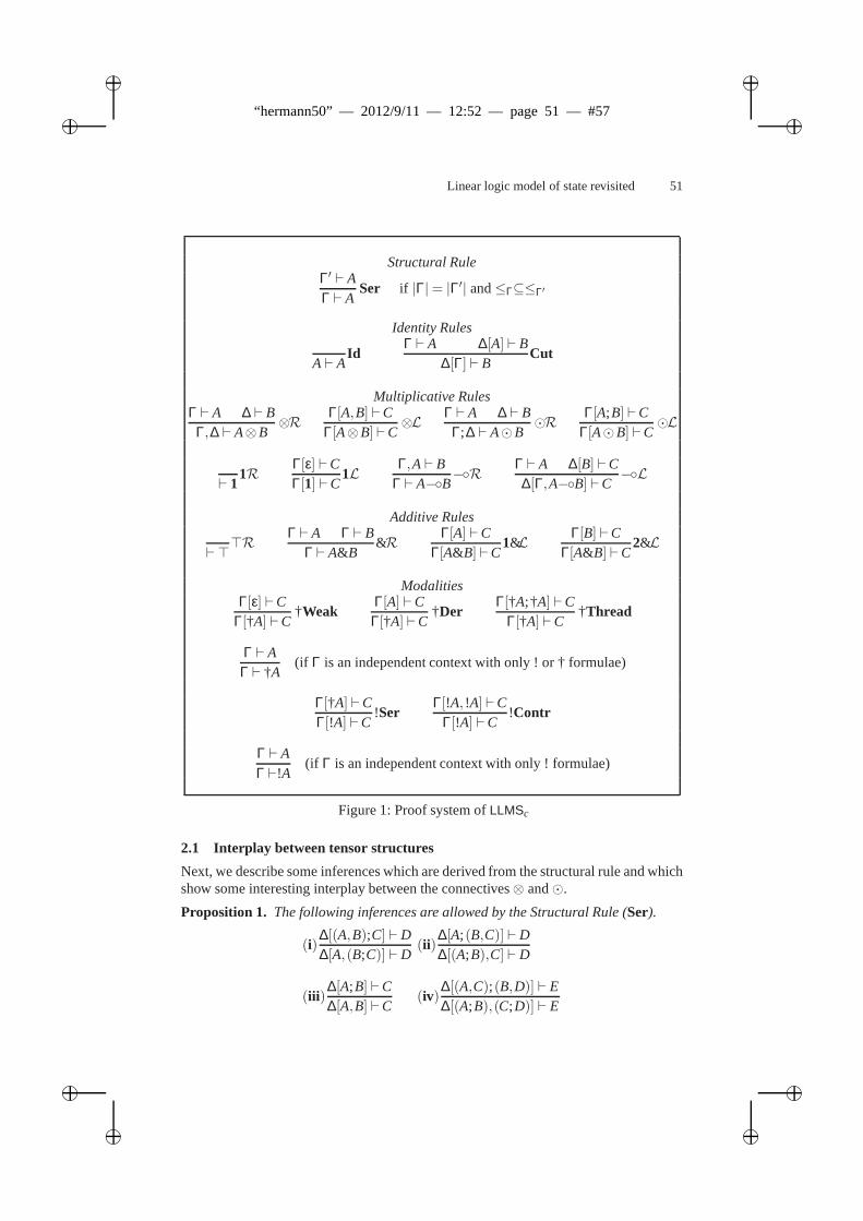
ii

“hermann50” — 2012/9/11 — 12:52 — page 51 — #57 ii

ii

ii


Structural RuleΓ′ ⊢ AΓ ⊢ A

Ser if |Γ|= |Γ′| and≤Γ⊆≤Γ′

Identity Rules

A⊢ AId

Γ ⊢ A ∆[A] ⊢ B∆[Γ] ⊢ B

Cut

Multiplicative RulesΓ ⊢ A ∆ ⊢ B

Γ,∆ ⊢ A⊗B⊗R

Γ[A,B] ⊢CΓ[A⊗B] ⊢C

⊗LΓ ⊢ A ∆ ⊢ B

Γ;∆ ⊢ A⊙B⊙R

Γ[A;B] ⊢CΓ[A⊙B] ⊢C

⊙L

⊢ 11R

Γ[ε] ⊢CΓ[1] ⊢C

1LΓ,A⊢ B

Γ ⊢ A−B−R

Γ ⊢ A ∆[B] ⊢C∆[Γ,A−B] ⊢C

−L

Additive Rules

⊢ ⊤⊤R

Γ ⊢ A Γ ⊢ BΓ ⊢ A&B

&RΓ[A] ⊢C

Γ[A&B] ⊢C1&L

Γ[B] ⊢CΓ[A&B] ⊢C

2&L

ModalitiesΓ[ε] ⊢C

Γ[†A] ⊢C†Weak

Γ[A] ⊢CΓ[†A] ⊢C

†DerΓ[†A;†A] ⊢C

Γ[†A] ⊢C†Thread

Γ ⊢ AΓ ⊢ †A

(if Γ is an independent context with only ! or † formulae)

Γ[†A] ⊢CΓ[!A] ⊢C

!SerΓ[!A, !A] ⊢C

Γ[!A] ⊢C!Contr

Γ ⊢ AΓ ⊢!A

(if Γ is an independent context with only ! formulae)

Figure 1: Proof system ofLLMSc

2.1 Interplay between tensor structures

Next, we describe some inferences which are derived from thestructural rule and whichshow some interesting interplay between the connectives⊗ and⊙.

Proposition 1. The following inferences are allowed by the Structural Rule(Ser).

(i)∆[(A,B);C] ⊢ D∆[A,(B;C)] ⊢ D

(ii)∆[A;(B,C)] ⊢ D∆[(A;B),C] ⊢ D

(iii )∆[A;B] ⊢C∆[A,B] ⊢C

(iv)∆[(A,C);(B,D)] ⊢ E∆[(A;B),(C;D)] ⊢ E

ii

“hermann50” — 2012/9/11 — 12:52 — page 52 — #58 ii

ii

ii

52 V. de Paiva

Commutativity and associativity of the tensor products arealso consequences of thestructural rule. Theweak-distributivityproperties

A⊗ (B⊙C)− (A⊗B)⊙C(A⊙B)⊗C− A⊙ (B⊗C)

follow from the inferences(i) and(ii), respectively. The inferences(iii ) and(iv) allowus to prove that

A⊗B− A⊙B(A⊙B)⊗ (C⊙D)− (A⊗C)⊙ (B⊗D)

Summing up and naming the transformations, the following are direct consequencesof the structural ruleSer:

ser : A⊗B→ A⊙Bwd1 : A⊗ (B⊙C)→ (A⊗B)⊙Cwd2 : (A⊙B)⊗C→ A⊙ (B⊗C)int : (A⊙B)⊗ (C⊙D)→ (A⊙C)⊗ (B⊙D)

They all draw on the fact that we can impose the same order on formulae as wecan on contexts, by turning⊗’s into commas,⊙’s into semicolons and applying≤ tothe resulting context. A formula on the left can then be transformed into the one on theright if the order on the left formula is included in the orderon the right formula.

2.2 Cut Elimination for LLMS

We can obtain a Gentzen’s style proof of the cut-eliminationtheorem forLLMSc.

Theorem 1 (Cut Elimination). If a sequent is provable inLLMSc, then it is provablein LLMSc without an application of the cut rule.

This proof is probably similar to Reddy’s proof [11], but we consider as a measureof the complexity, the rank as well as the degree of the last cut-formula, with the usualdefinitions. Special attention must be payed to the cases involving †, for instance, thecase in which the †Thread is applied in the lower right sequent of a proof ending by acut rule is proved using the inferences(iii ) and(iv). Corrêa’s proof can be found in thetechnical report [4].

3 A Categorical Model for LLMSc

To characterizeLLMSc categorically, we consider an instantiationG of the (symmetricmonoidal closed) categoriesDial2(Set), developed in [8]. As usual, the interpretation ofthe formulae is given by objects of the categoryG and proofs ofLLMSc are interpretedby morphisms ofG.

Recall that the partial-order with two elements2, where one thinks of0 as false and1 as true, is closed as a poset. It has a tensor product (⊗) and an internal-hom (−) suchthata⊗b≤ c iff a≤ b−c, where⊗ is the usual conjunction∧ and the internal-homlinear is the usual Heyting implication→.

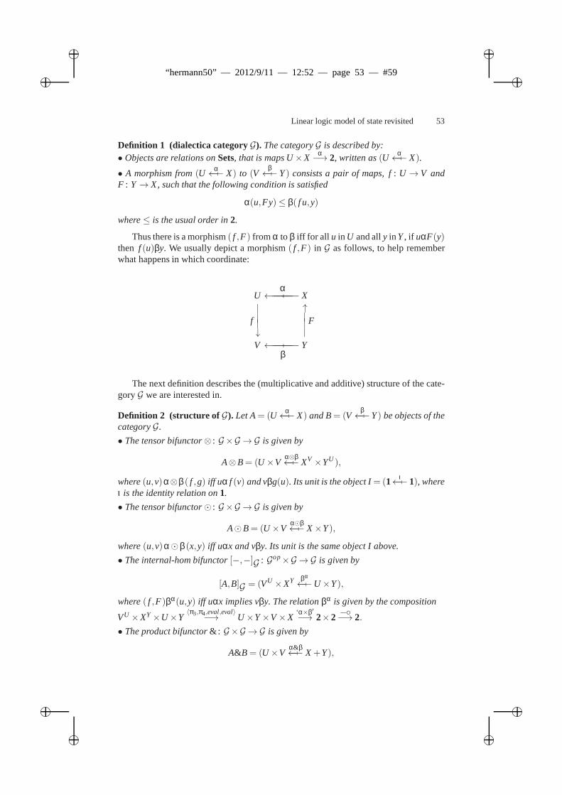
ii

“hermann50” — 2012/9/11 — 12:52 — page 53 — #59 ii

ii

ii


Definition 1 (dialectica categoryG). The categoryG is described by:• Objects are relations onSets, that is maps U×X

α−→ 2, written as(U

α7− X).

• A morphism from(Uα

7− X) to (Vβ

7− Y) consists a pair of maps, f: U → V andF : Y→ X, such that the following condition is satisfied

α(u,Fy)≤ β( f u,y)

where≤ is the usual order in2.

Thus there is a morphism( f ,F) fromα to β iff for all u in U and ally in Y, if uαF(y)then f (u)βy. We usually depict a morphism( f ,F) in G as follows, to help rememberwhat happens in which coordinate:

U ←−−α−−7−−−−− X

f|||↓

↑|||F

V ←−−−−7−−β−−− Y

The next definition describes the (multiplicative and additive) structure of the cate-goryG we are interested in.

Definition 2 (structure of G). Let A= (Uα

7− X) and B= (Vβ

7−Y) be objects of thecategoryG.

• The tensor bifunctor⊗ : G×G → G is given by

A⊗B= (U ×Vα⊗β7− XV ×YU ),

where(u,v)α⊗β( f ,g) iff uα f (v) and vβg(u). Its unit is the object I= (1 ι7− 1), where

ι is the identity relation on1.

• The tensor bifunctor⊙ : G×G → G is given by

A⊙B= (U×Vα⊙β7− X×Y),

where(u,v)α⊙β(x,y) iff uαx and vβy. Its unit is the same object I above.

• The internal-hom bifunctor[−,−]G : Gop×G → G is given by

[A,B]G = (VU ×XY βα7−U×Y),

where( f ,F)βα(u,y) iff uαx implies vβy. The relationβα is given by the composition

VU ×XY×U×Y〈π3,π4,eval,eval〉−→ U×Y×V×X

‘α×β′−→ 2×2 −−→ 2.

• The product bifunctor&: G×G → G is given by

A&B= (U×Vα&β7− X+Y),

ii

“hermann50” — 2012/9/11 — 12:52 — page 54 — #60 ii

ii

ii

54 V. de Paiva

where(u,v)α&β(

x,0y,1

)iff either uαx or vβy. Its unit is the objectT= (1 e

7− 0).

We could also describe coproducts (or additive disjunctions), a par connective andthe linear negation, but these will not play an important role in the following discussion.

Lemma 1 (G is a smcc).With the structure just described the categoryG is a symmetricmonoidal closed category.

The proof is easy, but worth doing on your own, to appreciate the naturalness of thecategorical constructions.

Lemma 2 (G natural transformations). For any A and B objects ofG there are naturalmorphisms:

(i) ser(A,B) : A⊗B→ A⊙B; 1

(ii) wd1(A,B,C) : A⊗ (B⊙C)→ (A⊗B)⊙C (called weak-distributivity 1)(iii) wd2(A,B,C) : (A⊙B)⊗C→ A⊙ (B⊗C) (called weak-distributivity 2)(iv int(A,B,C,D) : (A⊙B)⊗ (C⊙D)→ (A⊗C)⊙ (B⊗D).

Following the pattern of linear logic, modelling the modalities ofLLMSc, is morecomplicated than the tensors. Recall that the categorySetsdoes have free (commutative)monoid structures. There is an adjunction

F ⊣ U: Monc→ Sets

where Monc is the category of commutative monoids U is the forgetful functor andthe free functorF applied to a setX

F(X) = (X∗,eX ,mX)

consists ofX∗ the set of finite sequences (up to permutation) of elements ofX, eX : 1→X∗ is the empty sequence andmX : X∗×X∗→ X∗ means concatenation of sequences.

We need to consider another, different, monad structure inSetstoo. Consider themonad(TU ,ηTU ,µTU ), where for a givenU in Sets, TU : Sets→ Setsis the endofunctorwhich takesX 7→ XU , Y 7→YU and if g: X→Y, f ∈ XU is taken tof ;g∈YU . Its unitis given by the transpose of the projection, that is the constant map (ηTU )X : X →XU and its multiplication(µTU )X : XU×U → XU , is simply precomposition with thediagonal map onU .

We define two endofuctors onG to model the modalities ofLLMSc.

Definition 3 († and G in G). Consider the following endofunctors onG:

1. The functor† onG given on objects by

†(Uα

7− X) = (U†α7− X∗) where the relation†(α) is defined by

u(†α)(x1, · · · ,xk) iff uαx1 and· · ·and uαxk

and† acts on maps as†( f ,F) = ( f ,F∗).

1 There is another natural morphismσA,B : (A⊙B)→ (A2B) where2 is the functor correpond-ing to the par connective, but it shall not concern us here.

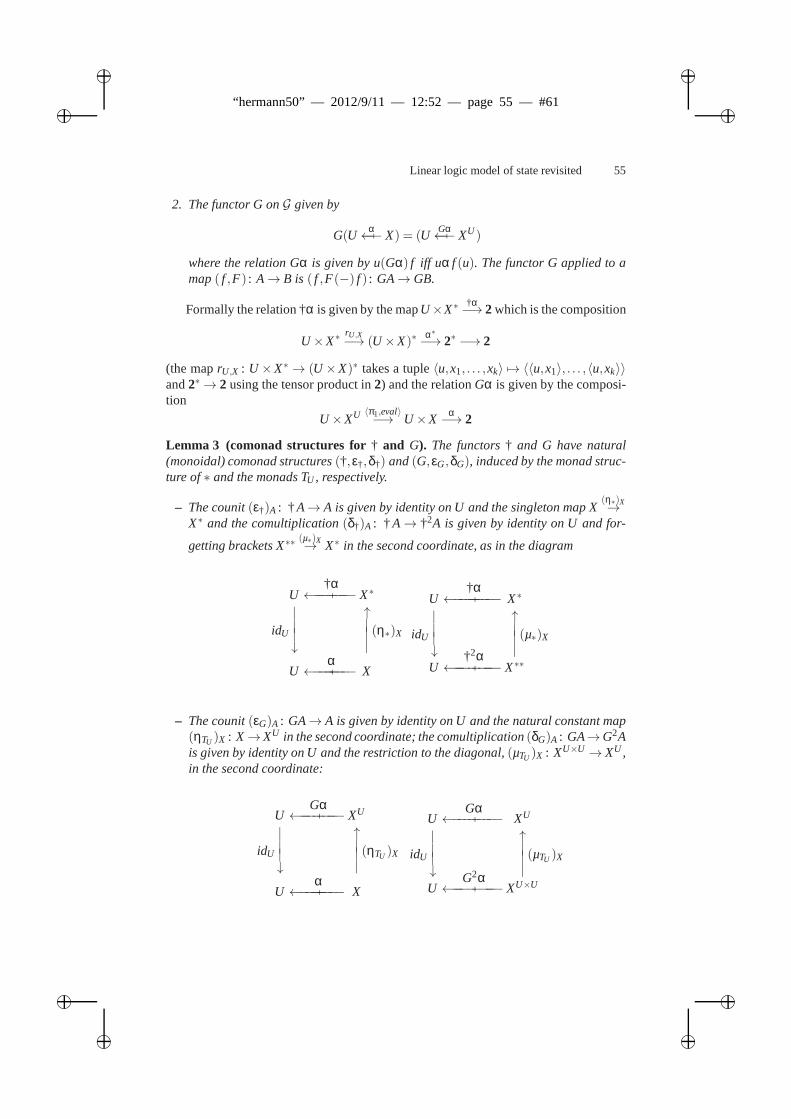
ii

“hermann50” — 2012/9/11 — 12:52 — page 55 — #61 ii

ii

ii


2. The functor G onG given by

G(Uα

7− X) = (UGα7− XU)

where the relation Gα is given by u(Gα) f iff uα f (u). The functor G applied to amap( f ,F) : A→ B is ( f ,F(−) f ) : GA→GB.

Formally the relation †α is given by the mapU×X∗†α−→ 2 which is the composition

U×X∗rU,X−→ (U×X)∗

α∗−→ 2∗ −→ 2

(the maprU,X : U ×X∗→ (U ×X)∗ takes a tuple〈u,x1, . . . ,xk〉 7→ 〈〈u,x1〉, . . . ,〈u,xk〉〉and2∗→ 2 using the tensor product in2) and the relationGα is given by the composi-tion

U×XU 〈π1,eval〉−→ U×X

α−→ 2

Lemma 3 (comonad structures for† and G). The functors† and G have natural(monoidal) comonad structures(†,ε†,δ†) and(G,εG,δG), induced by the monad struc-ture of∗ and the monads TU , respectively.

– The counit(ε†)A : †A→ A is given by identity on U and the singleton map X(η∗)X→

X∗ and the comultiplication(δ†)A : †A→ †2A is given by identity on U and for-

getting brackets X∗∗(µ∗)X→ X∗ in the second coordinate, as in the diagram

U ←−−†α−−7−−−−− X∗

idU

|||↓

↑|||(η∗)X

U ←−−α−−7−−−−− X

U ←−−†α−−7−−−−− X∗

idU

|||↓

↑|||(µ∗)X

U ←−−†2α−−7−−−−− X∗∗

– The counit(εG)A : GA→ A is given by identity on U and the natural constant map(ηTU )X : X→XU in the second coordinate; the comultiplication(δG)A : GA→G2Ais given by identity on U and the restriction to the diagonal,(µTU )X : XU×U → XU ,in the second coordinate:

U ←−−Gα−−7−−−−− XU

idU

|||↓

↑|||(ηTU )X

U ←−−α−−7−−−−− X

U ←−−Gα−−7−−−−− XU

idU

|||↓

↑|||(µTU )X

U ←−−G2α−−7−−−−− XU×U

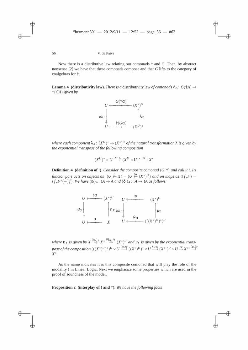
ii

“hermann50” — 2012/9/11 — 12:52 — page 56 — #62 ii

ii

ii

56 V. de Paiva

Now there is a distributive law relating our comonads † andG. Then, by abstractnonsense [2] we have that these comonads compose and thatG lifts to the category ofcoalgebras for †.

Lemma 4 (distributivity law). There is adistributivity lawof comonadsΛA : G(†A)→†(GA) given by

U ←−−G(†α)−−−7−−−−−− (X∗)U

idU

|||↓

↑|||

λX

U ←−−†(Gα)−−−7−−−−−− (XU)∗

where each componentλX : (XU)∗→ (X∗)U of the natural transformationλ is given bythe exponential transpose of the following composition

(XU)∗×UrXU ,U−→ (XU ×U)∗

ev∗−→ X∗

Definition 4 (definition of !). Consider the composite comonad(G;†) and call it !. Its

functor part acts on objects as!(Uα← X) = (U

!α← (X∗)U ) and on maps as!( f ,F) =

( f ,F∗(−) f ). We have(ε!)A : !A→ A and(δ!)A : !A→!!A as follows:

U ←−−!α−−7−−−−− (X∗)U

idU

|||↓

↑|||

ηX

U ←−−α−−7−−−−− X

U ←−−!α−−7−−−−− (X∗)U

idU

|||↓

↑|||µX

U ←−−!2α−−7−−−−− (((X∗)U)∗)U

whereηX is given by X(η∗)X→ X∗

(ηTU )X→ (X∗)U and µX is given by the exponential trans-

pose of the composition(((X∗)U)∗)U×U〈ev,π〉−→ ((X∗)U )∗×U

λ×U−→ (X∗∗)U×U

ev→X∗∗

(µ∗)X→

X∗.

As the name indicates it is this composite comonad that will play the role of themodality ! in Linear Logic. Next we emphasize some properties which are used in theproof of soundness of the model.

Proposition 2 (interplay of ! and †). We have the following facts

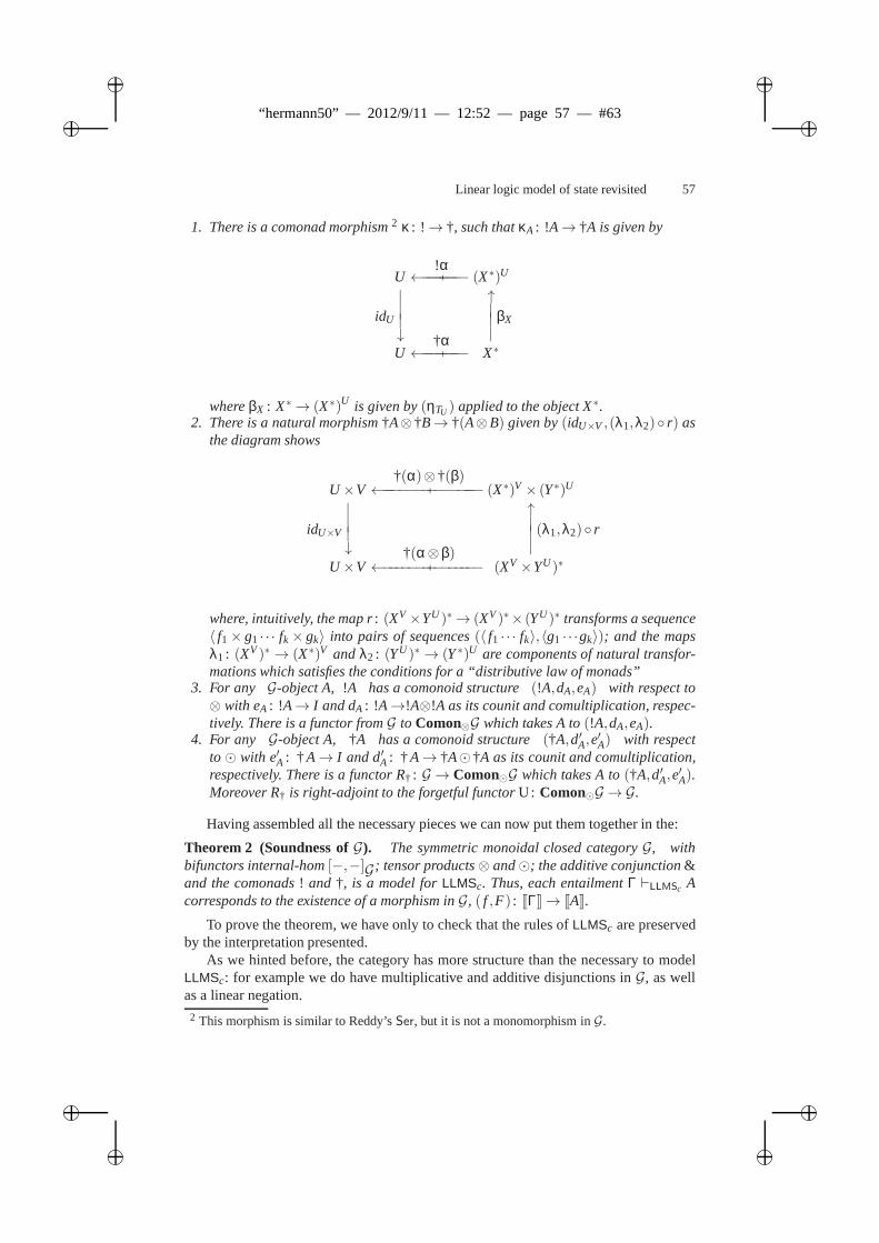
ii

“hermann50” — 2012/9/11 — 12:52 — page 57 — #63 ii

ii

ii


1. There is a comonad morphism2 κ : !→ †, such thatκA : !A→ †A is given by

U ←−−!α−−7−−−−− (X∗)U

idU

|||↓

↑|||

βX

U ←−−†α−−7−−−−− X∗

whereβX : X∗→ (X∗)U is given by(ηTU ) applied to the object X∗.2. There is a natural morphism†A⊗†B→ †(A⊗B) given by(idU×V ,(λ1,λ2) r) as

the diagram shows

U×V ←−−†(α)⊗†(β)−−−−−7−−−−−−−− (X∗)V × (Y∗)U

idU×V

|||↓

↑|||(λ1,λ2) r

U×V ←−−−†(α⊗β)−−−−7−−−−−−−− (XV ×YU)∗

where, intuitively, the map r: (XV×YU )∗→ (XV)∗× (YU)∗ transforms a sequence〈 f1× g1 · · · fk× gk〉 into pairs of sequences(〈 f1 · · · fk〉,〈g1 · · ·gk〉); and the mapsλ1 : (XV)∗ → (X∗)V andλ2 : (YU)∗→ (Y∗)U are components of natural transfor-mations which satisfies the conditions for a “distributive law of monads”

3. For any G-object A, !A has a comonoid structure(!A,dA,eA) with respect to⊗ with eA : !A→ I and dA : !A→!A⊗!A as its counit and comultiplication, respec-tively. There is a functor fromG to Comon⊗G which takes A to(!A,dA,eA).

4. For any G-object A, †A has a comonoid structure(†A,d′A,e′A) with respect

to⊙ with e′A : †A→ I and d′A : †A→ †A⊙†A as its counit and comultiplication,respectively. There is a functor R† : G → Comon⊙G which takes A to(†A,d′A,e

′A).

Moreover R† is right-adjoint to the forgetful functorU: Comon⊙G → G.

Having assembled all the necessary pieces we can now put themtogether in the:

Theorem 2 (Soundness ofG). The symmetric monoidal closed categoryG, withbifunctors internal-hom[−,−]G ; tensor products⊗ and⊙; the additive conjunction&and the comonads! and †, is a model forLLMSc. Thus, each entailmentΓ ⊢LLMSc Acorresponds to the existence of a morphism inG, ( f ,F) : [[Γ]]→ [[A]].

To prove the theorem, we have only to check that the rules ofLLMSc are preservedby the interpretation presented.

As we hinted before, the category has more structure than thenecessary to modelLLMSc: for example we do have multiplicative and additive disjunctions inG, as wellas a linear negation.

2 This morphism is similar to Reddy’sSer, but it is not a monomorphism inG.

ii

“hermann50” — 2012/9/11 — 12:52 — page 58 — #64 ii

ii

ii

58 V. de Paiva

4 Back toLLMS

Two years after the work onLLMSc, I realized that the modelling using dialectica cate-gories could be extended for non-commutative systems likeLLMS. My doctoral studentthen, Alexander Tucker, wrote a short note on his investigations of the non-commutativedialectica model and published it in the ESSLLI Student Session proceedings [14]. ButAlex decide to stop working on his doctorate and hence this work was left untouchedfor several years. We recall some of Tucker’s results.

Reddy first set out the criteria he believed necessary for a categorical model ofLLMS. He starts with a symmetric monoidal closed category(C,⊗, I ,−) together withan additional monoidal structure(, I) such that(⊗, I) is a sub-monoidal structure of(, I). The last condition means that there is a natural monicser : A⊗B→ AB whichpreserves the associated monoidal structure. He then adds two comonads associated tothe tensorial structures given by⊗ and.

Given such a set up, Reddy defined aLLMS-categoryas a symmetric monoidalclosed category, with products and co-products, together with the extra tensor product and two monoidal comonads, ! and † with the former being a sub-comonad of thelatter via a comonad monomorphismSer : !→ †. So the intuitio is that † transformstensors into⊗ tensors and ! (as usual) transforms tensors into cartesian products. Butalso !A must be a comonoid with respect to⊗ and †A a comonoid with respect to.Then since⊗ is a sub-monoidal structure of, !A becomes a comonoid with respectto via the monicser. This comonoid must be a sub-comonoid of †A via the naturalmonicSer which must now be a morphism of comonoids as well.

This definition, generalized from the example of coherence spaces, needs to be takenwith a pinch of salt. Further work by Bechet, de Groote and Retoré [1] showed that thetwo kinds of logical context, represented by the operationsof ⊗ and need a moresophisticated treatment.

The partial order over the contexts of theLLMS calculus are in fact a class of ordercalledseries parallel ordersor SP-orders. These are defined as the least class of partialorders containing the single element order, and closed under disjoint union and ordinalsum.

In Bechet et al [1] a set of rewrite rules is given which is a complete characterizationof the inclusion of one SP-order in another and so by extension corresponds exactly toReddy’sSer rule. In fact, the non-trivial rewrite rules correspond precisely to the fourrules given above. Moreover, if we insist that both⊗ and have identities which areequal, that⊗ is associative and commutative and that is associative and not commu-tative, then the set of rewrite rules are all derivable from just the middle interchangerule.

The natural transformationser can be obtained fromint by instantiatingB andCas I , wd1 can be obtained by instantiatingB as I andwd2 by instantiatingC as I . Wetherefore need to exchangeser for int in the definition of an LLMS-category. With thisbig difference in setting, we can re-state Reddy’s definition of aLLMS-category.

We relax Reddy’s requirements somewhat by neither insisting on monotonicity ofthe natural transformations, nor dealing with the additiveconstructs. We also exchangethe natural transformationser with a natural transformationint corresponding to themiddle interchange rule.

ii

“hermann50” — 2012/9/11 — 12:52 — page 59 — #65 ii

ii

ii


Definition 5 (Tucker). A modality-freeLLMS-category is an smcc(C,⊗,−, I) togetherwith an additional monoidal structure(, I). The two structures are related via amonoidal natural transformation:int : (AB)⊗ (CD)→ (AC)⊗ (BD).

AnLLMS-categoryis then a modality-freeLLMS-category along with two monoidalcomonads! and† related by a comonad morphismSer : ! → †. Also !A must be a co-monoid with respect to(⊗, I), †A a comonoid with respect to(, I) andSer a morphismof comonoids.

With this new definition in tow we can provide a simple dialetica model for thesystemLLMS itself, instead of its commutative versionLLMSc. As before, our categor-ical model ofLLMS is based on a simple dialectica category over the category ofsets,but this time the objects are partial relations over athree valued poset, or maps intofalse,undefined, true.

Definition 6 (dialectica categoryL). The categoryL is described by:• Objects arepartialrelations onSets, that is maps U×X

α−→ 3, written as(U

α7− X).

• A morphism from(Uα

7− X) to (Vβ

7− Y) consists a pair of maps, f: U → V andF : Y→ X, such that the following condition is satisfied

α(u,Fy)≤ β( f u,y)

where≤ is the usual order in3.

With easy, suitable modifications of the work in the previoussection, we can de-scribe the structure ofL.

Definition 7 (structure of L). Let A= (Uα

7− X) and B= (Vβ

7−Y) be objects of thecategoryL.• The tensor bifunctor⊗ : G×G → G given by

A⊗B= (U ×Vα⊗β7− XV ×YU ),

where(u,v)α⊗β( f ,g) iff uα f (v) and vβg(u) still has as its unit the object I= (1 ι7−

1), whereι is the identity relation on1.• The internal-hom bifunctor[−,−]G : Gop×G → G is still given by

[A,B]G = (VU ×XY βα7−U×Y),

where( f ,F)βα(u,y) iff uαx implies vβy. The relationβα is given by the composition

VU ×XY×U×Y〈π3,π4,eval,eval〉−→ U×Y×V×X

‘α×β′−→ 3×3 −−→ 3.

• There is a non-commutative tensor bifunctor : G×G → G given by

AB= (U×Vαβ7− X×Y),

where(u,v)αβ(x,y) iff uαx landvβy, whereland is the computer sciencelazy and.This connective is non-commutative, sincefalselandundefined is false, butundefinedlandfalse is undefined. The unit of this tensor product is the same object I that we hadbefore.

ii

“hermann50” — 2012/9/11 — 12:52 — page 60 — #66 ii

ii

ii

60 V. de Paiva

Using the same definitions we had before for comonads ! and †, except that now,instead ofcommutativefree monoids, we use simply free monoids, we can model thesystemLLMS modalities and obtain.

Theorem 3 (Soundness ofL). The symmetric monoidal closed categoryL, withbifunctors internal-hom[−,−]L; tensor products⊗ and; and the comonads! and†,is a model forLLMS. Thus, each entailmentΓ ⊢LLMS A corresponds to the existence ofa morphism inL, ( f ,F) : [[Γ]]→ [[A]].

5 Conclusions

The motivation for this work came from O’Hearn’s and Reddy’suse of Linear Logic todeal with sequentiality in the semantics of Algol-like programming languages. Earlieron we realised that we could use Reddy’s ideas to give a syntactical characterizationto some of the (somewhat mysterious) constructions of dialectica categorical modelsDial2(Set) for Classical Linear Logic. In particular it was interesting to find an intuitiveexplanation for the comonad † in terms of the extra tensor product⊙.

Summing up the work so far, we adapted Reddy’s system LLMS providing it witha commutative version of the connective “before” and an associated modality. A di-alectica categoryG was constructed onSetsand shown to be a sound model of thenew system LLMSc. Then we went back to the drawing board, in the light of work ofBechet, de Groote and Retoré and uncovered a dialectica model of LLMS itself.

Much work remains to be done. Firstly, going back to the original motivation, morework is needed to relate the system LLMSc to O’Hearn’s and Reddy’s other work onAlgol-like languages [10, 12]. Secondly, from a logical pespective, we might want touse this system with two modalities, as a blueprint for work on relating modalities ingeneral. Thirdly most of the recent work on sequentiality [3] uses games andpolar-ized linear logic. It would would be nice if we could find a mathematically significantrelationship between linear logic polarization and dialectica categories.

References

1. D. Bechet, Ph. de Groote, and C. Retoré. A complete axiomatisation for the inclusion ofseries-parallel partial orders. InInternational Conference on Rewriting Techniques and Ap-plications, Sitges, Spain, October 1997.

2. J. Beck. Distributive laws. InSeminar on Triples and Categorical Homoly Theory, LNM 80,pages 119–140. Springer-Verlag, 1969.

3. M. Churchill and J. Laird. A logic of sequentiality. InComputer Science Logic (LectureNotesin Computer Science). Springer Verlag, pp. 215-229., Brno, Czech Republic, August 2010.

4. M. da S. Corrêa, E. H. Haeusler, and V. C. V. de Paiva. A dialecticamodel of state. Technical Report PUC-Rio.MCC21/95, Dept. de Informática,Pontifícia Univ. Católica PUC-Rio, August 1995. (Electronically available inftp://ftp.inf.puc-rio.br/pub/docs/techreports/95_21_correa.ps.gz).

5. M. da S. Corrêa, E. H. Haeusler, and V. C. V. de Paiva. A dialectica model of state. InCATS’96, Computing: The Australian Theory Symposium Proceedings, Melbourne, Aus-tralia, January 1996.

ii

“hermann50” — 2012/9/11 — 12:52 — page 61 — #67 ii

ii

ii


6. V. C. V de Paiva. Dialectica categories. InCategories in Computer Science and Logic, Boul-der, Colorado, June 1987. American Mathematical Society. (Contemporary Mathematics,Vol. 92).

7. V. C. V de Paiva.Dialectica Categories. PhD thesis, Lucy Cavendish College, Cambridge,November 1988. Printed as Technical Report No. 213, University of Cambridge ComputerLaboratory, January, 1991.

8. V. C. V. de Paiva. A dialectica-like model of linear logic.In Category Theory in ComputerScience, volume 389 ofLNCS, pages 341–356, September 1989.

9. P. W. O’Hearn. Linear logic and interference control. InCategories in Computer Science andLogic, volume 530 ofLNCS, pages 74–93, Paris, France, September 1991. Springer-Verlag,Berlin.

10. P. W. O’Hearn, A. J. Power, M. Takeyama, and R. D. Tennent.Syntactic control of interfer-ence revisited. InMFPS XI, volume 1 ofEletronic Notes in Theoretical Computer Science,New Orleans, March 1995.

11. U. S. Reddy. A linear logic model of state: Preliminar report. Electronic manuscript(ftp),csc.uiuc.edu, directory /pub/reddy/papers, May 1993.

12. U. S. Reddy. Passivity and independence. In9th Annual IEEE Symposium on Logic inComputer Science, pages 342–352, Paris, France, 1994. IEEE Computer SocietyPress, LosAlamitos, California.

13. C. Retoré.Reseaux et Séquents Ordonnés Mathématiques. PhD thesis, Université Paris 7,Février 1993.

14. A. Tucker. Categorical modelling of a state oriented version of linear logic. InProceedingsof the Third ESSLLI Student Session, Saarbruecken, Germany, August 1998.

ii

“hermann50” — 2012/9/11 — 12:52 — page 62 — #68 ii

ii

ii

On the computational complexity of the intuitionisticmodal logic IK

Edward Hermann Haeusler1, Mario R. F. Benevides2, Valeria de Paiva3, andAlexandre Rademaker4 ⋆

1 Department of Informatics, PUC-Rio, [email protected]

2 Systems and Computer Engineering Program and Computer Science Department, FederalUniversity of Rio de Janeiro, Brazil.

[email protected] Computer Science Department, University of Birmingham, UK.

[email protected] School of Applied Mathematics, FGV, Brazil

[email protected]

Abstract. This article shows that some decision problems for the IntuitionisticModal Logic IK are PSPACE-complete.

Keywords Intuitionistic Logic, Modal Logics, PSPACE-Completeness, Complexity

Preamble

Hermann and I have known each other for more than 27 years. We first met in theComputer Science Department at PUC-Rio in 1985. One year later, we started work-ing together at Universidade Federal Fluminense, where we started to build a valuablefriendship.

For more than 20 years, we have participated together in manyacademic and bu-reaucratic activities: organizing workshops, taking partin program committees, exami-nation boards, and so forth. In 2005, we published our first scientific research togetherand, since then, we have done quite a lot of work in partnership, including the one pre-sented in this article. Recently, we have been working on a paper related to Petri Netsand Propositional Dynamic Logic.

Hermann has always been very sincere, reliable and supportive. He is also an ex-tremely committed collaborator, hard worker and always full of good ideas. If I hadto summarize my relationship with Hermann, I would proudly say that it was built onhonesty, cooperation, and friendship.

On your birthday, my very best wishes to you,Mario.

⋆ This work was supported by the Brazilian research agencies CNPq and CAPES.

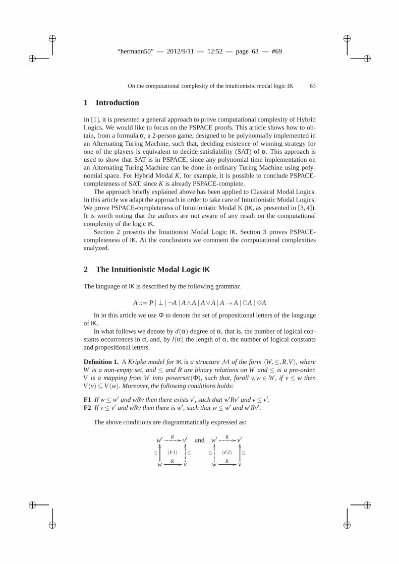
ii

“hermann50” — 2012/9/11 — 12:52 — page 63 — #69 ii

ii

ii

On the computational complexity of the intuitionistic modal logic IK 63

1 Introduction

In [1], it is presented a general approach to prove computational complexity of HybridLogics. We would like to focus on the PSPACE proofs. This article shows how to ob-tain, from a formulaα, a 2-person game, designed to be polynomially implemented inan Alternating Turing Machine, such that, deciding existence of winning strategy forone of the players is equivalent to decide satisfiability (SAT) of α. This approach isused to show that SAT is in PSPACE, since any polynomial time implementation onan Alternating Turing Machine can be done in ordinary TuringMachine using poly-nomial space. For Hybrid ModalK, for example, it is possible to conclude PSPACE-completeness of SAT, sinceK is already PSPACE-complete.

The approach briefly explained above has been applied to Classical Modal Logics.In this article we adapt the approach in order to take care of Intuitionistic Modal Logics.We prove PSPACE-completeness of Intuitionistic Modal K (IK, as presented in [3, 4]).It is worth noting that the authors are not aware of any resulton the computationalcomplexity of the logicIK.

Section 2 presents the Intuitionist Modal LogicIK. Section 3 proves PSPACE-completeness ofIK. At the conclusions we comment the computational complexitiesanalyzed.

2 The Intuitionistic Modal Logic IK

The language ofIK is described by the following grammar.

A ::= P | ⊥ | ¬A | A∧A | A∨A | A→ A | 2A |3A

In in this article we useΦ to denote the set of propositional letters of the languageof IK.

In what follows we denote byd(α) degree ofα, that is, the number of logical con-stants occurrences inα, and, byl(α) the length ofα, the number of logical constantsand propositional letters.

Definition 1. A Kripke model forIK is a structureM of the form〈W,≤,R,V〉, whereW is a non-empty set, and≤ and R are binary relations on W and≤ is a pre-order.V is a mapping from W into powerset(Φ), such that, forall v,w ∈W, if v≤ w thenV(v)⊆V(w). Moreover, the following conditions holds:

F1 If w≤ w′ and wRv then there exists v′, such that w′Rv′ and v≤ v′.F2 If v≤ v′ and wRv then there is w′, such that w≤ w′ and w′Rv′.

The above conditions are diagrammatically expressed as:

w′ R //

(F1)

v′

wR //

≤

OO

v

≤

OO and w′ R //

(F2)

v′

wR //

≤

OO

v

≤

OO

ii

“hermann50” — 2012/9/11 — 12:52 — page 64 — #70 ii

ii

ii

64 E. H. Haeusler, M. Benevides, V. de Paiva, A. Rademaker

It is worthwhile noting that in the above definition, ifR is transitive then we aretalking about the logicIS4. At the conclusion we will discuss the complexity of thislogic.

Definition 2. LetM = 〈W,≤,R,V〉 be a Kripke model forIK, w∈W andα be anIKformula. The satisfaction relation,M,w |= α, is defined inductively as follows:

A M,w |= P, iff, P∈V(w)B M,w 6|=⊥C M,w |= α∧β, iff,M,w |= α andM,w |= βD M,w |= α∨β, iff,M,w |= α orM,w |= βNEG M,w |= ¬α, iff, for all w′, w≤ w′,M,w′ 6|= αIMP M,w |= α→ β, iff, for all w′, w≤ w′, ifM,w′ |= α thenM,w′ |= βIBOX M,w |=2α, iff, for all w′, w≤ w′, for all v′, w′Rv′,M,v′ |= α.IDIA M,w |=3α, iff, there is v, wRv,M,v |= α.

We writeM |= α to mean that, for allw∈W,M,w |= α. We say that a formula issatisfiable, iff, there is a modelM, such that,M |= α. We say that a set of formulasΓis satisfiable, iff, there is a modelM, such that,M |= γ, for eachγ ∈ Γ. We say that aformulaα is IK-valid, iff,M|= α, for each modelM. Given two set of formulasΓ and∆, we say thatΓ ⊢ ∆, iff, there are finite setsΓo and∆o, such thatΓo ⊆ Γ and∆o ⊆ ∆and

∧

γ∈Γo

γ→∨

δ∈∆o

δ is IK-valid. A set of formulasΓ is consistent, iff,Γ 6⊢ ⊥.

3 PSPACE-Completeness ofIK

We prove thatIK SAT5 is PSPACE complete. SinceIPL is properly included inIK, thelower bound is provided by the well-known theorem of Ladner [2] on PSPACE com-pleteness of IPL. The upper bound is shown by adapting the game defined in [1] toIK. It is a 2-person game of polynomial size where one of the players aims to find outsatisfiability of a formula. It is such that one of the playershas a winning strategy ifand only if the proposed formula is satisfiable. We remind that determining existence ofwinning strategies in polynomial sized 2-person games can be implemented by PTIMEAlternating Turing Machines, and the later are implementedby PSPACE ordinary Tur-ing machines. This concludes the upper bound. Finally, as PSPACE=CO-PSPACE, weconclude that provability ofIK formulas is also PSPACE-complete.

Theorem 1. IK is decidable regarding satisfiability. The complexity of satisfiability andprovability problems are both PSPACE-complete.

Before the proof of above theorem, we need some terminology.If ∆ is a set offormulas, a∆-Hintikka set is a consistent set of subformulas from∆.

Proof Consider the formulaα. We argue the we can find a model forα in polyno-mial space. We denote byF(α) the set of subformulas ofα. The game is played bytwo players∀belard and∃loise. ∃loisestarts by presenting a listL0, . . . ,Lk of α-Hintikka sets, and two relationsR and2 on them, where2 is a inclusion relation. The

5 SAT is the decision problem of finding out whether a formula issatisfiable or not.

ii

“hermann50” — 2012/9/11 — 12:52 — page 65 — #71 ii

ii

ii


numberk should be polynomially bounded byα’s length. This is ensured by lemma 1and lemma 2 below. She loses immediately whenever at least one of the following con-ditions does not hold

Conditions onL

CR1 If LvRLw then for some formula3β, 3β ∈ Lv andβ ∈ Lw.CR2 If H p

0 , . . . ,Hpi , . . . ,H

pn be a maximal sub-list of distinct members ofL, such that

for all j = 0,n−1, H pj RH p

j+1, then there is a list of formulas3β0, . . .3βn suchthat3β j ∈ H p

j and the degree of3β j+1 is strictly smaller than the degree of3β j ,for all j = 0,n−1.

CI Lv 2 Lw iff Lv⊆ Lw

CF1 If Lw 2 L′w andLwRLv then there existsL′v, such thatL′wRL′v andLv 2 L′v.CF2 If Lv 2 L′v andLwRLv then there isL′w, such thatLw 2 L′w andL′wRL′v.Here If β ∈ F(α), β ∈ Li andLi 2 L j , thenβ ∈ L j .Form α ∈ L0 and, ifLi = L j theni = jCNEG for all Li , for all ¬β ∈ F(α), if Li 2 L j andβ ∈ L j then¬β 6∈ Li

AND for all Li , for all β1∧β2 ∈ F(α), if β1∧β2 ∈ Li thenβk ∈ Li , k= 1,2OR for all Li , for all β1∨β2 ∈ F(α), if β1∨β2 ∈ Li then eitherβ1 ∈ Li or β2 ∈ L2

CIMP for all Li , for all β1→ β2 ∈ F(α), if Li 2 L j , β1 ∈ L j andβ2 6∈ L j thenβ1→β2 6∈ Li

CIDIA for all 3β ∈ F(α), if LiRL j and3β 6∈ Li thenβ 6∈ L j

CIBOX for all Li andL j , for all2β∈F(α), if Li 2 L j , L jRLh andβ 6∈ Lh, then2β 6∈ Li

In fact, conditions AND and OR, above, are direct consequences of Hintikka setdefinition.

If ∃loisedoes not lose when she presentsL0, . . . ,Lk then the game continues and∀belardmay follow one of the two moves below:

MODAL ∀belard must choose three setsLi , L j , Lh, Li 2 L j , LiRLh and a formulaA∈ L j to attack and∃loisemust provide anα-Hintikka setY, such thatL jRY andLh 2Y and respond according to the following items:DIA If A is 3β, then∃loise must provide anα-Hintikka setY, such that:β ∈ Y

and for all3γ ∈ F(α), if 3γ 6∈ L j thenγ 6∈ Y. For all2γ ∈ F(α), if 2γ ∈ Li

then2γ ∈ L j , γ ∈ Lh andγ ∈Y.BOX If A is2β, then∃loisemust provide anα-Hintikka setY, such that:β∈Y and

for all 2γ∈F(α), if 2γ∈ Li then2γ∈ L j , γ∈ Lh andγ∈Y. For all3γ∈F(α),if 3γ 6∈ L j thenγ 6∈Y.

IntProp For all ¬γ ∈ F(α), if ¬γ ∈ Lh then γ 6∈ Y. For all γ1 → γ2 ∈ F(α), ifγ1→ γ2 ∈ Lh then eitherγ1 6∈Y or γ2 ∈Y.

INTUI ∀belardmust choose three setsLi , L j , Lh, Li 2 L j , L jRLh and a formulaA∈ L j

to attack and∃loisemust provide anα-Hintikka setY, such thatL j 2Y and mustrespond according to the following items:Imp If A is β1→ β2, then∃loise must provide anα-Hintikka setY, such that,

either β1 6∈ Y or β2 ∈ Y. For all ¬γ ∈ F(α), if ¬γ ∈ Li then γ 6∈ Y. For allγ1→ γ2 ∈ F(α), if γ1→ γ2 ∈ Li then eitherγ1 6∈Y or γ2 ∈Y.

ii

“hermann50” — 2012/9/11 — 12:52 — page 66 — #72 ii

ii

ii


Neg If A is¬β, then∃loisemust provide anα-Hintikka setY, such that,β 6∈Y. Forall ¬γ ∈ F(α), if ¬γ ∈ Li thenγ 6∈ Y. For all γ1→ γ2 ∈ F(α), if γ1→ γ2 ∈ Li

then eitherβ1 6∈Y or β2 ∈Y.Modal For all3γ∈F(α), if 3γ 6∈Y thenγ 6∈ Lh. For all2γ ∈F(α), if γ 6∈ Lh, then

2γ 6∈Y.STOP1 In any of the items above, if theY ∃loise provides is among theα-Hintikka

sets already on the match, then the game stops and∃loisewin.STOP2 If ∀belard cannot provide any of the three sets stated in itemsMODAL and

INTUI , under the respective conditions, then∃loise loses.

If she cannot provide such anY as above then she loses. If she is able to provide ananswer then the game continues with the thisY added to the set of Hintikka sets alreadypresented.∀belardhas to choose a newL j and a formula, belonging to it, with smallerdegree than the previous one to attack and twoα-Hintikka setsLi andLh and the gamegoes on this new formula and the three statesL j , Li andLh. ∃loisewins, whenever shecan answer the attacks, otherwise∀belardwins.

The game is finite, since its termination is determined by thedegree ofα. Moreover,since the number of subformulas of a formula is polynomiallybounded by its degree,the game has polynomial size.

We prove the following lemmas, that, together, ensure that∃loisecan always pro-vide a polynomially bounded sets ofα-Hintikka sets whenα is satisfiable.

Lemma 1. Let L= H0,H1, . . . ,Hk be a list ofα-Hintikka sets satisfying the initialconditions on L. LetHp0, . . . ,Hpi , . . . ,Hpn be a maximal sub-list of distinct membersof L, such that for all j= 0,n−1, Hp jRHp j+1 or for all j = 0,n−1, Hp j 2 Hp j+1, andfor all j1, j2 = 0,n, if Hp j1

= Hp j2then j1 = j2. So, k is polynomially bounded by l(α).

Proof. We have two cases:

2: We firstly observe that, by itemHere of the conditions that hold onL, if β ∈ Hpi

andHpi 2Hp j thenβ∈Hp j . From this observation we can conclude that a maximallist of inclusions of distinct Hintikka sets is limited byl(α).

R: This case is straightforward by the condition bf CR, once for every maximal sub-list of distinct members ofL Hp0, . . . ,Hpi , . . . ,Hpn, there is a list of subformulasof α 3β0, . . .3βn such that3β j ∈Hp j and the degree of3β j+1 is strictly smallerthan the degree of3β j , for all j = 0,n−1. Hence, the sub-list of Hintikka sets islimited by l(α).

Given a list ofα-Hintikka sets satisfying the conditions stated in 3, as stated above,we can, without generality loss, consider that the listL = H0,H1, . . . ,Hk is orderedsuch that for alli, j = 0,k, i < j, H jRHi holds only in the caseHiRH j also holds.Besides that, for alli, j = 0,k, if HiRH j then i < j. This ordering corresponds to adisplay the list in a tree form, withH0 as root.

Lemma 2. Let L= H0,H1, . . . ,Hk be a list ofα-Hintikka sets satisfying the initialconditions on L. Let Hi ∈ L and R(Hi) = H1

i , . . . ,Hni be the set of all members of

L that can be reached by aR-transition from Hi , i.e., HiRH ji , for all j = 1..n. Then,

n= c.log(l(α)).

ii

“hermann50” — 2012/9/11 — 12:52 — page 67 — #73 ii

ii

ii


Proof. By conditionCR, each ramification determined by each of theα-Hintikka setsH j

i is only possible by existence ofIK subformulas3β j ∈ Hi andβ j ∈ H ji . In order to

have such a3β j ∈Hi , these subformulas must have occurred inα inside a conjunction,disjunction, implication, negation or a modal operation. So, the possible number of suchformulas is bounded bylog(l(α)), possibly, with a multiplicative factorc, related to theoccurrences of distinctβ j , j = 1,2, . . .c.

The above lemma can be equally proved considering the relation2 ∪R, since con-ditionsCF1 andCF1 implies that there are only transient ramifications. These transientramifications do not change the logarithmic bound, for they only add 2 extraα-Hintikkasets for each ramification originated in eachHpi .

From the two above lemmas and the observation above we can conclude that themaximal number of ramification in the tree-like ordering of the listH0,H1, . . . ,Hk isbounded by alog(l(α)), and, the maximum height of this ordering is polynomial onl(α). Thus, the listH0,H1, . . . ,Hk is polynomially bounded byl(α). Hence, we knowthat the first move of∃loisecan be done with a polynomially bounded list ofα-Hintikkasets.

We now proceed with the proof of the main result. For this we need the followinglemma.

Lemma 3. ∃loise has a winning strategy, if and only ifα is satisfiable.

Proof. If α is satisfiable, then the model that satisfies it allows the definition of a listof α-Hintikka to∃loisepresent at the starting move. Her winning strategy is to providethe Hintikka set associated to the world that validates eachpossibly attacked formulachoosen by∀belard. In other worlds, she presents the whole model that satisfiesα, asa list of Hintikka sets. After she uses the model to answer hisattacks.

For the other direction, let us suppose that∃loisehas a winning strategy. This win-ning strategy will provide us with model forα. Since∃loisehas a winning strategy, shecan answer to each possible attack of∀belard, she also has a winning starting set ofHintikka sets. Thus,∃loisecan produce a Hintikka set for each attack of his opponent.Let M be this collection of all Hintikka sets possible to be generated by the winningstrategy of∃loise. The model< M,R,2,V > is such that:

– R is such that, given Hintikka setsm,w∈M, mRw, if and only if, for every3β ∈F(α), if 3β 6∈m, thenβ 6∈ w.

– 2 is such that, given Hintikka setsm,w ∈ M, m2 w, if and only if, for everyβ1→ β2 ∈ F(α), if β1→ β2 6∈m thenβ1 ∈w andβ2 6∈ w6

– V(A) = m : A∈m.

Fact 1 LetM be the model defined above and m,v∈W. If m2 v, then for every sub-formulaα1→ α2 of α, if α1→ α2 6∈m, thenα1 ∈ v andα2 6∈ v.

Lemma 4. For every subformulaδ of α, < M,R,2,V >|=m α, if and only if,α ∈m.

6 The negation is already taken in this definition, since⊥ 6∈ w

ii

“hermann50” — 2012/9/11 — 12:52 — page 68 — #74 ii

ii

ii


Proof. We proceed by induction on the number of symbols inα. For assertions atomicformulasA it is a straightforward application of the definition of< M,R,2,V >|=m α.Considerα of the formα1∧α2 and< M,R,2,V >|=m α1∧α2. By definition of |=we have< M,R,2,V >|=m αk, k = 1,2. By inductive hypothesis, we haveαk ∈ Mi .As m is maximal and consistent,α1∧α2 ∈ m. For the other direction, if we supposethat α1∧α2 ∈ m, thenalphak ∈ m, k = 1,2, sincem is a maximal consistent set ofsubformulas ofα. By inductive hypothesis and the definition of|= we conclude that< M,R,2,V >|=m α1∧α2. If α is of the formα1∨α2 the reasoning is analogous. Ifα1→α2 6∈m, asm2w and by fact 1 we haveα1∈wandα2 6∈w, and hence by inductivehypothesis< M,R,2,V >|=w α1 and< M,R,2,V > 6|=w α2, hence< M,R,2,V > 6|=m

α1→ α2. On the other hand, consider thatα1→ α2 ∈ m. We know that∃loise has awinning strategy, so, if∀belardattackα1→α2 in m, ∃loiseis able to provide an answerY, such thatm2Y, inM , and eitherα1 ∈Y andα2 ∈Y, or α1 6∈Y. By definitionMcontains every possible answerY of ∃loiseas a world inW, and since for each of themwe havem2 Y, we have< M,R,2,V >|=m α1→ α2. The cases for¬α is analogousto this last case. This finishes the proof of the lemma.

4 Conclusions

As PSPACE=CO-PSPACE, we conclude that provability inIK is also PSPACE-complete.It is worth to note that, since both games are polynomially bounded and hence finite,

we can affirm.

Corollary 1. IK has Finite Model Property.

References

1. Carlos Areces, Patrick Blackburn, and Maarten Marx. A road-map on complexity for hybridlogics. InLNCS, 1683, pages 307–321, 1999.

2. R. Ladner. The Computational Complexity of Provability in Systems of Modal Logics.SIAMJournal on Computing, 6:467–480, 1977.

3. G. Plotkin and C. Stirling. A framework for intuitionistic modal logics. InProceedings ofthe Conference of Theoretical Aspects of Reasoning about Knowledge, Monterrey, CA, USA,1986.

4. A. Simpson. The Proof Theory and Semantics of Intuitionistic Modal Logic. PhD thesis,University of Edinburgh, December 1993. Revised September1994.

ii

“hermann50” — 2012/9/11 — 12:52 — page 69 — #75 ii

ii

ii

Modelling the Lambek calculus via a hierarchicalstructure of categories

Marcelo da Silva Corrêa1 and Edward Hermann Haeusler2

1 Depto. de Análise, Universidade Federal Fluminense, Rua Mario Santos Braga s/n, Niterói,RJ, BRASIL, 24005-140,

[email protected] Depto. de Informática, Pontifícia Universidade Católica do Rio de Janeiro, Rua Marquês de

São Vicente, 225, Rio de Janeiro, RJ, BRASIL, 22453-900,[email protected]

Preamble

I am grateful to Hermann for our research collaboration but mainly for his friendship.The very initial idea of this work is due to him and it was simple, intuitive and techni-cally fruitful, as many others, since it gave rise to a paper published in an internationaljournal. The present work is a second version of that paper.

Marcelo Correa

1 Introduction

The sequencing operation is not only restricted to sentenceformation in natural lan-guages. It is a quite basic concept used in other formal theories, for instance, serialcomposition of programs, processes or even mathematical functions. In most of suchcases, a new object (program, process or function) is obtained by serial compositionif and only if certain lexical conditions hold. This verification could not only be con-cerned with type compatibility, but also with extra information provided by an externalenvironment. The notion of “sequencing arrow”, which was first introduced in [4] torepresent the possibility of combining expressions, can bethought as representing sucha kind of information. In this work, we present a categoricalmodel for the LambekCalculus (L ), formerly the Calculus of Syntactic Categories, based on a hierarchicalstructure of categories that generalizes the approach in [4].

2 Sequencing Arrows and a Non-commutative CategoricalProduct

The usual (commutative) categorical producta×b can be determined by means of thelimit for the diagram containing just the objectsa andb [19]. We recall the basic conceptof limit to determine a categorical construction for a non-commutative product operator,calledSequential Product.

Intuitively, given a pair of objectsa andb of a categoryC, we consider a pair ofspecial arrows

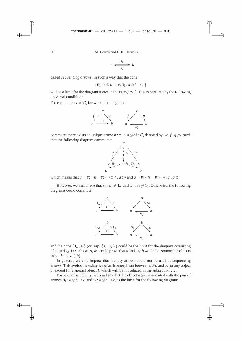
ii

“hermann50” — 2012/9/11 — 12:52 — page 70 — #76 ii

ii

ii

70 M. Corrêa and E. H. Haeusler

a b-s2

s1

calledsequencing arrows, in such a way that the cone

π1 : a⊗b→ a;π2 : a⊗b→ b

will be a limit for the diagram above in the categoryC. This is captured by the followinguniversal condition:

For each objectc of C, for which the diagrams

c

a b

@@R

-s1

f gc

a b

@@R

s2

f g

commute, there exists an unique arrowh : c→ a⊗b in C, denoted by≪ f , g≫, suchthat the following diagram commutes:

a b

a⊗b

c

f gh

π1 π2

JJJJJJ9 XXXz

?

which means thatf = π1h= π1 ≪ f , g≫ andg= π2h= π2 ≪ f , g≫

However, we must have thats2s1 6= 1a and s1s2 6= 1b. Otherwise, the followingdiagrams could commute:

a

a b

@@R

-s1

1a s1

a

a b

@@R

s2

1a s1

b

a b

@@R-s1

s2 1b

b

a b

@@R

s2

s2 1b

and the cone1a , s1 (or resp.s2 , 1b ) could be the limit for the diagram consistingof s1 ands2. In such cases, we could prove thata anda⊗b would be isomorphic objects(resp.b anda⊗b).

In general, we also impose that identity arrows could not be used as sequencingarrows. This avoids the existence of an isomorphism betweena⊗a anda, for any objecta, except for a special objectI , which will be introduced in the subsection 2.2.

For sake of simplicity, we shall say that the objecta⊗b, associated with the pair ofarrowsπ1 : a⊗b→ a andπ2 : a⊗b→ b, is the limit for the following diagram:

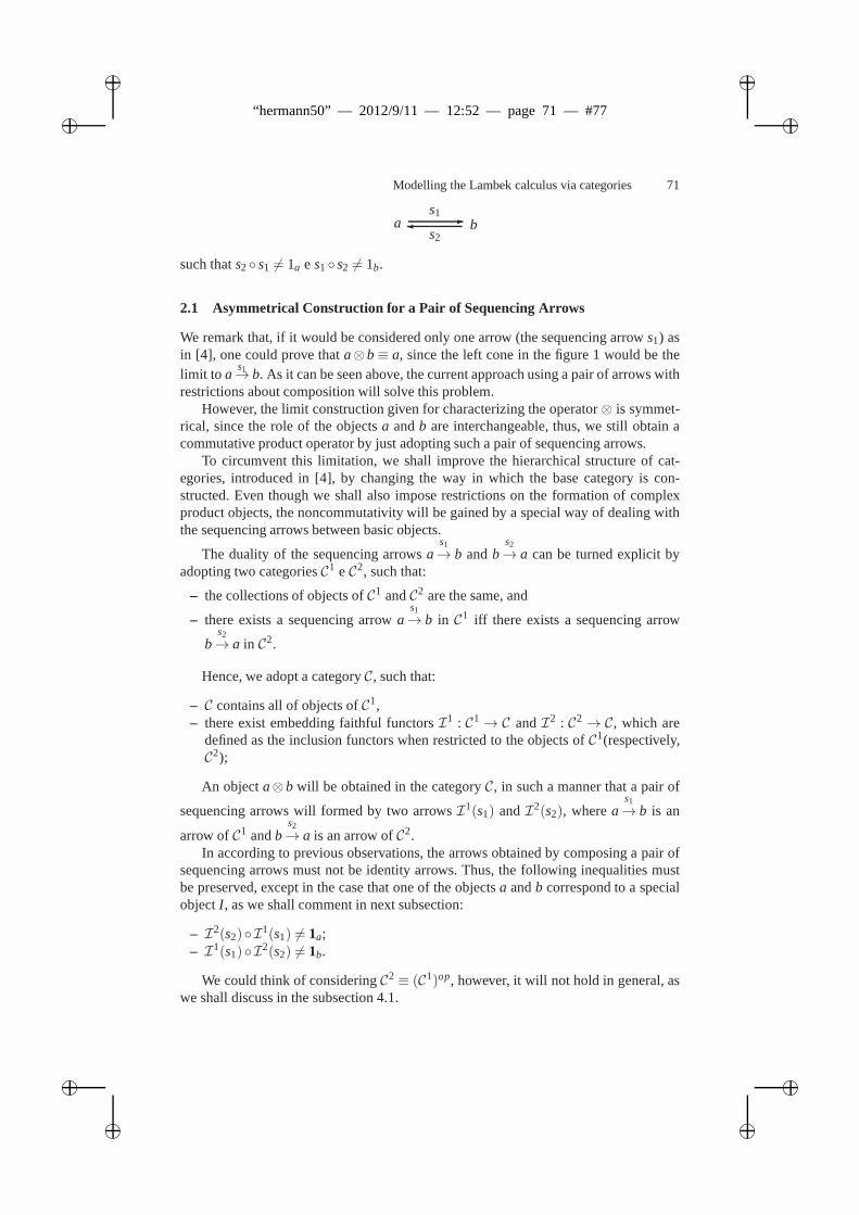
ii

“hermann50” — 2012/9/11 — 12:52 — page 71 — #77 ii

ii

ii

Modelling the Lambek calculus via categories 71

a b-s2

s1

such thats2 s1 6= 1a e s1 s2 6= 1b.

2.1 Asymmetrical Construction for a Pair of Sequencing Arrows

We remark that, if it would be considered only one arrow (the sequencing arrows1) asin [4], one could prove thata⊗b≡ a, since the left cone in the figure 1 would be thelimit to a

s1→ b. As it can be seen above, the current approach using a pair of arrows withrestrictions about composition will solve this problem.

However, the limit construction given for characterizing the operator⊗ is symmet-rical, since the role of the objectsa andb are interchangeable, thus, we still obtain acommutative product operator by just adopting such a pair ofsequencing arrows.

To circumvent this limitation, we shall improve the hierarchical structure of cat-egories, introduced in [4], by changing the way in which the base category is con-structed. Even though we shall also impose restrictions on the formation of complexproduct objects, the noncommutativity will be gained by a special way of dealing withthe sequencing arrows between basic objects.

The duality of the sequencing arrowss1

a→ b ands2

b→ a can be turned explicit byadopting two categoriesC1 eC2, such that:

– the collections of objects ofC1 andC2 are the same, and

– there exists a sequencing arrows1

a→ b in C1 iff there exists a sequencing arrows2

b→ a in C2.

Hence, we adopt a categoryC, such that:

– C contains all of objects ofC1,– there exist embedding faithful functorsI1 : C1→ C andI2 : C2→ C, which are

defined as the inclusion functors when restricted to the objects ofC1(respectively,C2);

An objecta⊗b will be obtained in the categoryC, in such a manner that a pair of

sequencing arrows will formed by two arrowsI1(s1) andI2(s2), wheres1

a→ b is an

arrow ofC1 ands2

b→ a is an arrow ofC2.In according to previous observations, the arrows obtainedby composing a pair of

sequencing arrows must not be identity arrows. Thus, the following inequalities mustbe preserved, except in the case that one of the objectsa andb correspond to a specialobjectI , as we shall comment in next subsection:

– I2(s2)I1(s1) 6= 1a;

– I1(s1)I2(s2) 6= 1b.

We could think of consideringC2 ≡ (C1)op, however, it will not hold in general, aswe shall discuss in the subsection 4.1.

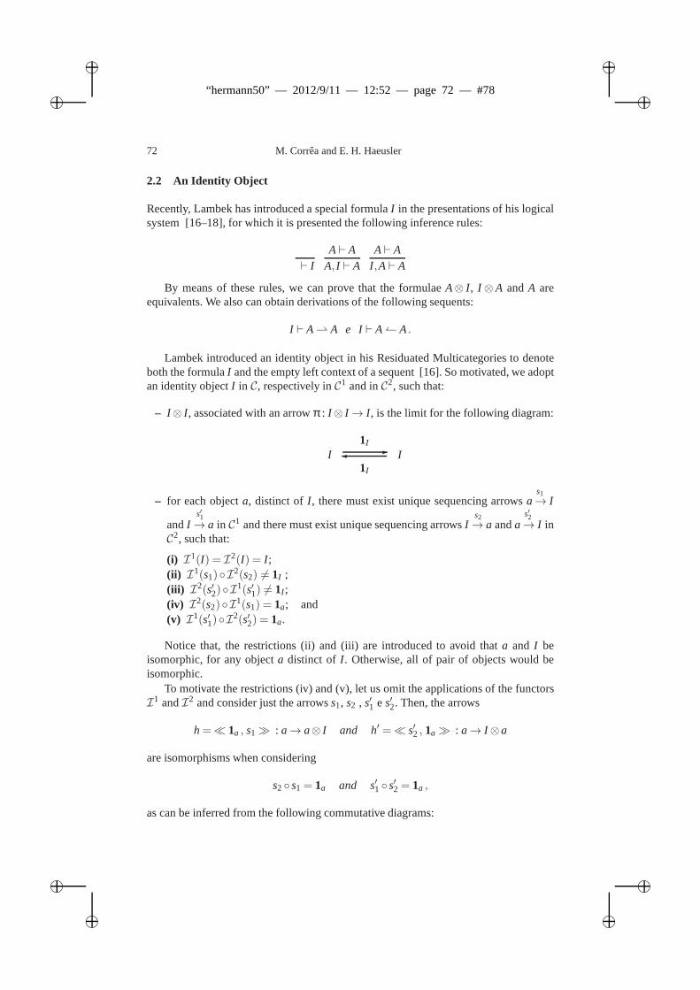
ii

“hermann50” — 2012/9/11 — 12:52 — page 72 — #78 ii

ii

ii


2.2 An Identity Object

Recently, Lambek has introduced a special formulaI in the presentations of his logicalsystem [16–18], for which it is presented the following inference rules:

⊢ IA⊢ A

A, I ⊢ AA⊢ A

I ,A⊢ A

By means of these rules, we can prove that the formulaeA⊗ I , I ⊗A andA areequivalents. We also can obtain derivations of the following sequents:

I ⊢ A A e I⊢ A A.

Lambek introduced an identity object in his Residuated Multicategories to denoteboth the formulaI and the empty left context of a sequent [16]. So motivated, weadoptan identity objectI in C, respectively inC1 and inC2, such that:

– I ⊗ I , associated with an arrowπ : I ⊗ I → I , is the limit for the following diagram:

I I-1I

1I

– for each objecta, distinct of I , there must exist unique sequencing arrowss1

a→ I

ands′1

I → a in C1 and there must exist unique sequencing arrowss2

I → a ands′2

a→ I inC2, such that:

(i) I1(I) = I2(I) = I ;(ii) I1(s1)I

2(s2) 6= 1I ;(iii) I2(s′2)I

1(s′1) 6= 1I ;(iv) I2(s2)I

1(s1) = 1a; and(v) I1(s′1)I

2(s′2) = 1a.

Notice that, the restrictions (ii) and (iii) are introducedto avoid thata and I beisomorphic, for any objecta distinct of I . Otherwise, all of pair of objects would beisomorphic.

To motivate the restrictions (iv) and (v), let us omit the applications of the functorsI1 andI2 and consider just the arrowss1, s2 , s′1 e s′2. Then, the arrows

h=≪ 1a , s1≫ : a→ a⊗ I and h′ =≪ s′2 , 1a≫ : a→ I ⊗a

are isomorphisms when considering

s2 s1 = 1a and s′1 s′2 = 1a ,

as can be inferred from the following commutative diagrams:

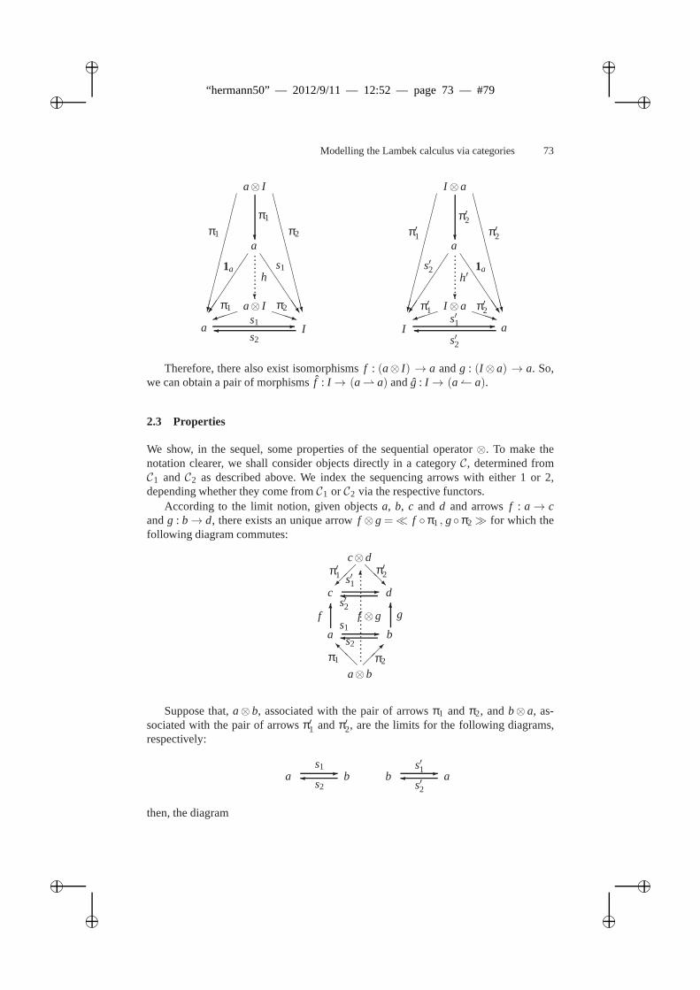
ii

“hermann50” — 2012/9/11 — 12:52 — page 73 — #79 ii

ii

ii


a I

a⊗ I

-s1s2

a

1a s1h

π1 π2

JJJJJJ) PPPq

?

?

π1

a⊗ I

π1 π2

CCCCCCCCCCCW

I a

I ⊗a

-s′1s′2

a

s′2 1ah′

π′1 π′2

JJJJJJ) PPPq

?

?

π′2

I ⊗a

π′1 π′2

CCCCCCCCCCCW

Therefore, there also exist isomorphismsf : (a⊗ I) → a andg : (I ⊗a) → a. So,we can obtain a pair of morphismsf : I → (a a) andg : I → (a a).

2.3 Properties

We show, in the sequel, some properties of the sequential operator⊗. To make thenotation clearer, we shall consider objects directly in a categoryC, determined fromC1 andC2 as described above. We index the sequencing arrows with either 1 or 2,depending whether they come fromC1 or C2 via the respective functors.

According to the limit notion, given objectsa, b, c and d and arrowsf : a→ candg : b→ d, there exists an unique arrowf ⊗g=≪ f π1 , gπ2≫ for which thefollowing diagram commutes:

c⊗d

c d

@@Rs′1

s′2

-

π′1 π′2

a⊗b

π1 π2@@I

a b-s1

s2

6 6f g

6

f ⊗g

Suppose that,a⊗ b, associated with the pair of arrowsπ1 andπ2, andb⊗ a, as-sociated with the pair of arrowsπ′1 andπ′2, are the limits for the following diagrams,respectively:

a b-s1

s2b a-

s′1

s′2

then, the diagram

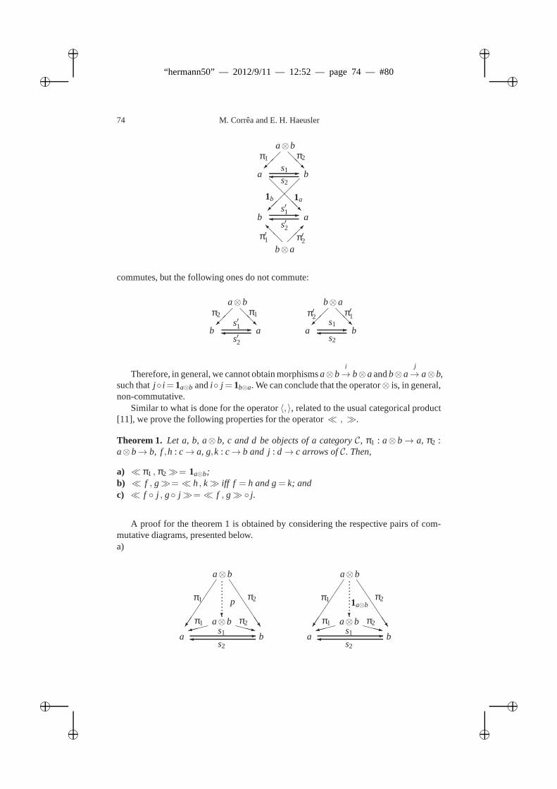
ii

“hermann50” — 2012/9/11 — 12:52 — page 74 — #80 ii

ii

ii


a⊗b

a b

-s1

s2

@@R

π1 π2

@@@@R

1b 1a

b a-s′1

s′2

b⊗aπ′1 π′2@@I

commutes, but the following ones do not commute:

a⊗b

b a

@@R-

s′1

s′2

π2 π1

b⊗a

a b

@@R-

s1

s2

π′2 π′1

Therefore, in general, we cannot obtain morphismsi

a⊗b→ b⊗aandj

b⊗a→ a⊗b,such thatj i = 1a⊗b andi j = 1b⊗a. We can conclude that the operator⊗ is, in general,non-commutative.

Similar to what is done for the operator〈,〉, related to the usual categorical product[11], we prove the following properties for the operator≪ , ≫.

Theorem 1. Let a, b, a⊗ b, c and d be objects of a categoryC, π1 : a⊗ b→ a, π2 :a⊗b→ b, f,h : c→ a, g,k : c→ b and j: d→ c arrows ofC. Then,

a) ≪ π1 , π2≫= 1a⊗b;b) ≪ f , g≫= ≪ h, k≫ iff f = h and g= k; andc) ≪ f j , g j≫= ≪ f , g≫ j.

A proof for the theorem 1 is obtained by considering the respective pairs of com-mutative diagrams, presented below.a)

a b

a⊗b-

s1

s2

a⊗b

π1 π2p

π1 π2

JJJJJJ9 XXXz

?

a b

a⊗b-

s1

s2

a⊗b

π1 π21a⊗b

π1 π2

JJJJJJ9 XXXz

?

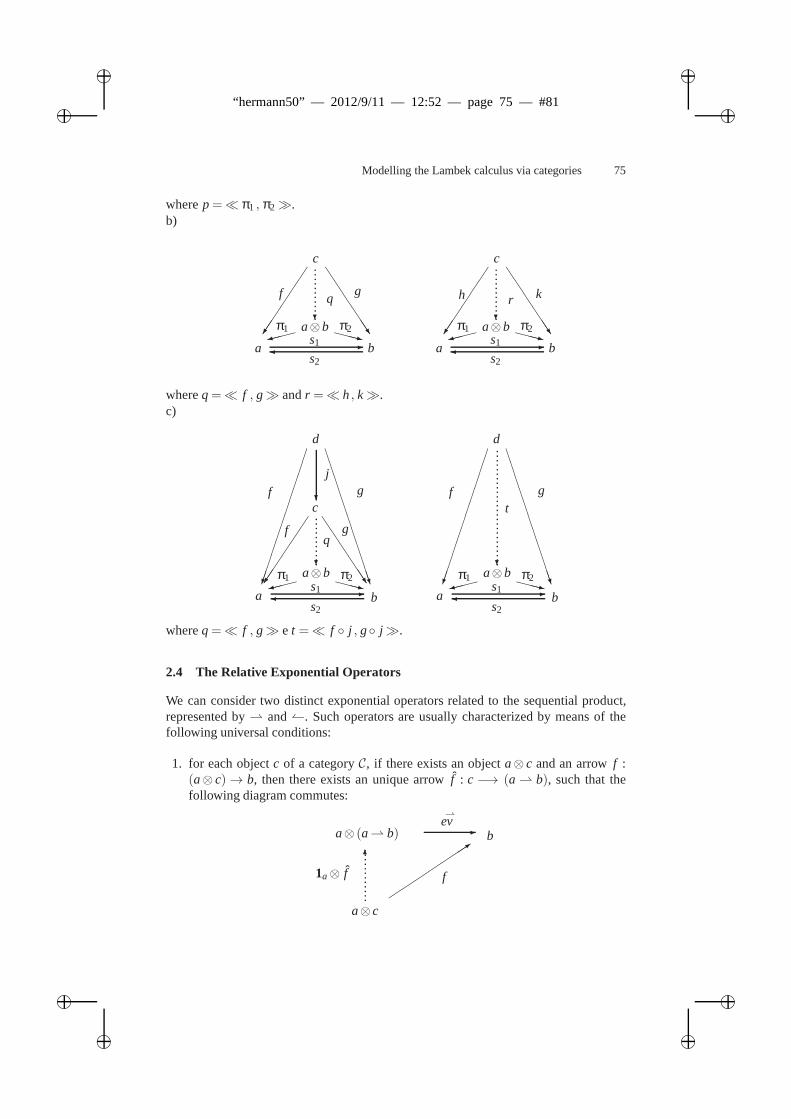
ii

“hermann50” — 2012/9/11 — 12:52 — page 75 — #81 ii

ii

ii


wherep=≪ π1 , π2≫.b)

a b

a⊗b-

s1

s2

c

f gq

π1 π2

JJJJJJ9 XXXz

?

a b

a⊗b-

s1

s2

c

h kr

π1 π2

JJJJJJ9 XXXz

?

whereq=≪ f , g≫ andr =≪ h, k≫.c)

a b

a⊗b-

s1

s2

c

f gq

π1 π2

JJJJJJ9 XXXz

?

?

j

d

f g

BBBBBBBBBBBN

a b

a⊗b-

s1

s2

π1 π29 XXXz

?

t

d

f g

BBBBBBBBBBBN

whereq=≪ f , g≫ e t =≪ f j , g j≫.

2.4 The Relative Exponential Operators

We can consider two distinct exponential operators relatedto the sequential product,represented by and. Such operators are usually characterized by means of thefollowing universal conditions:

1. for each objectc of a categoryC, if there exists an objecta⊗ c and an arrowf :(a⊗ c)→ b, then there exists an unique arrowf : c−→ (a b), such that thefollowing diagram commutes:

a⊗ (a b)

ev

b

1a⊗ f

a⊗ c

6

-

f

3

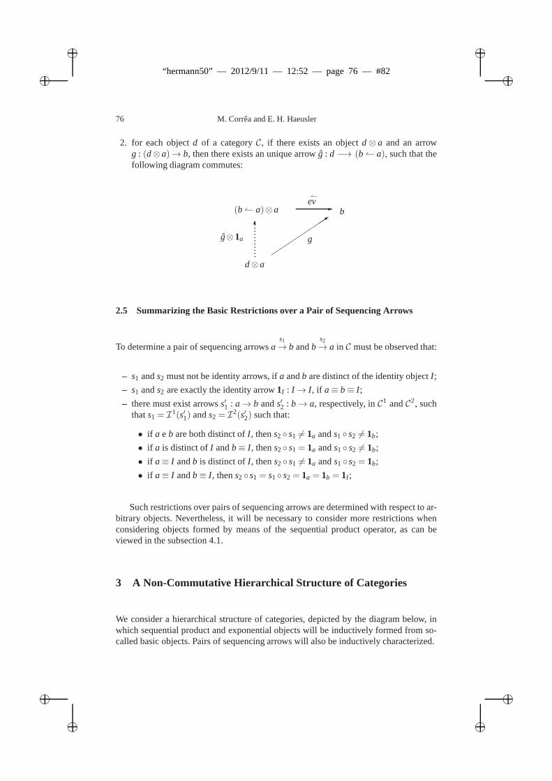
ii

“hermann50” — 2012/9/11 — 12:52 — page 76 — #82 ii

ii

ii


2. for each objectd of a categoryC, if there exists an objectd⊗ a and an arrowg : (d⊗a)→ b, then there exists an unique arrow ˆg : d−→ (b a), such that thefollowing diagram commutes:

(b a)⊗a

ev

b

g⊗1a

d⊗a

6

-

g

3

2.5 Summarizing the Basic Restrictions over a Pair of Sequencing Arrows

To determine a pair of sequencing arrowss1

a→ b ands2

b→ a in C must be observed that:

– s1 ands2 must not be identity arrows, ifa andb are distinct of the identity objectI ;

– s1 ands2 are exactly the identity arrow1I : I → I , if a≡ b≡ I ;

– there must exist arrowss′1 : a→ b ands′2 : b→ a, respectively, inC1 andC2, suchthats1 = I

1(s′1) ands2 = I2(s′2) such that:

• if a e b are both distinct ofI , thens2 s1 6= 1a ands1 s2 6= 1b;

• if a is distinct ofI andb≡ I , thens2 s1 = 1a ands1 s2 6= 1b;

• if a≡ I andb is distinct ofI , thens2 s1 6= 1a ands1 s2 = 1b;

• if a≡ I andb≡ I , thens2 s1 = s1 s2 = 1a = 1b = 1I ;

Such restrictions over pairs of sequencing arrows are determined with respect to ar-bitrary objects. Nevertheless, it will be necessary to consider more restrictions whenconsidering objects formed by means of the sequential product operator, as can beviewed in the subsection 4.1.

3 A Non-Commutative Hierarchical Structure of Categories

We consider a hierarchical structure of categories, depicted by the diagram below, inwhich sequential product and exponential objects will be inductively formed from so-called basic objects. Pairs of sequencing arrows will also be inductively characterized.

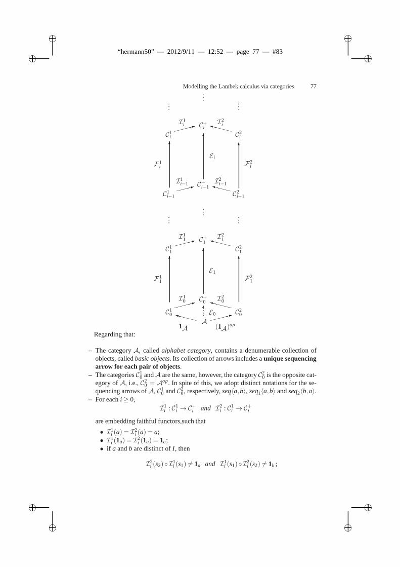
ii

“hermann50” — 2012/9/11 — 12:52 — page 77 — #83 ii

ii

ii


......

...

C1i−1 C2

i−1

C+i−1: XXXyI1

i−1 I2i−1

66

6

C1i C2

i

C+i: XXXXyI1i I2

i

F1i F2

i

E i

......

...

C+0

66

6

C11 C2

1

C+1: XXXXyI1

1 I21

F11 F2

1

E1

C10 C2

0

: XXXXyI1

0 I20

:XXXXyA

1A (1A)op

6E0

Regarding that:

– The categoryA, calledalphabet category, contains a denumerable collection ofobjects, calledbasic objects. Its collection of arrows includes aunique sequencingarrow for each pair of objects.

– The categoriesC10 andA are the same, however, the categoryC2

0 is the opposite cat-egory ofA, i.e.,C2

0 = Aop. In spite of this, we adopt distinct notations for the se-quencing arrows ofA, C1

0 andC20, respectively,seq〈a,b〉, seq1〈a,b〉 andseq2〈b,a〉.

– For eachi ≥ 0,I1

i : C1i →C

+i and I2

i : C1i →C

+i

are embedding faithful functors,such that

• I1i (a) = I

2i (a) = a;

• I1i (1a) = I

2i (1a) = 1a;

• if a andb are distinct ofI , then

I2i (s2)I

1i (s1) 6= 1a and I1

i (s1)I2i (s2) 6= 1b ;

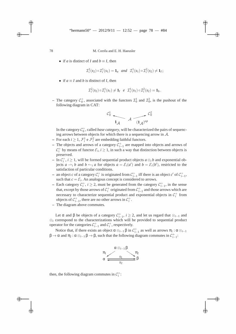
ii

“hermann50” — 2012/9/11 — 12:52 — page 78 — #84 ii

ii

ii


• if a is distinct ofI andb≡ I , then

I2i (s2)I

1i (s1) = 1a and I1

i (s1)I2i (s2) 6= 1I ;

• if a≡ I andb is distinct ofI , then

I2i (s2)I

1i (s1) 6= 1I e I1

i (s1)I2i (s2) = 1b .

– The categoryC+0 , associated with the functorsI10 andI2

0, is the pushout of thefollowing diagram in CAT:

C10 C2

0:XXXXy

A1A (1A)

op

In the categoryC+0 , calledbase category, will be characterized the pairs of sequenc-ing arrows between objects for which there is a sequencing arrow inA.

– For eachi ≥ 1,F1i eF2

i are embedding faithful functors.– The objects and arrows of a categoryC+i−1 are mapped into objects and arrows ofC+i by means of functorE i , i ≥ 1, in such a way that distinction between objects ispreserved.

– In C+i , i ≥ 1, will be formed sequential product objectsa⊗i b and exponential ob-jects a i b and b i a for objectsa = E i(a′) and b = E i(b′), restricted to thesatisfaction of particular conditions.

– an objectc of a categoryC+i is originated fromC+i−1 iff there is an objectc′ of C+i−1,such thatc= E i . An analogous concept is considered to arrows.

– Each categoryC+i , i ≥ 2, must be generated from the categoryC+i−1, in the sensethat, except by those arrows ofC+i originated fromC+i−1 and those arrows which arenecessary to characterize sequential product and exponential objects inC+i fromobjects ofC+i−1, there are no other arrows inC+i .

– The diagram above commutes.

Let α andβ be objects of a categoryC+i−1, i ≥ 2, and let us regard that⊗i−1 and⊗i correspond to the characterizations which will be providedto sequential productoperator for the categoriesC+i−1 andC+i , respectively.

Notice that, if there exists an objectα⊗i−1 β in C+i−1 as well as arrowsπ1 : α⊗i−1

β→ α andπ2 : α⊗i−1 β→ β, such that the following diagram commutes inC+i−1:

α β

α⊗i−1 β

-s1

s2

π1 π2+

QQQs

then, the following diagram commutes inC+i :

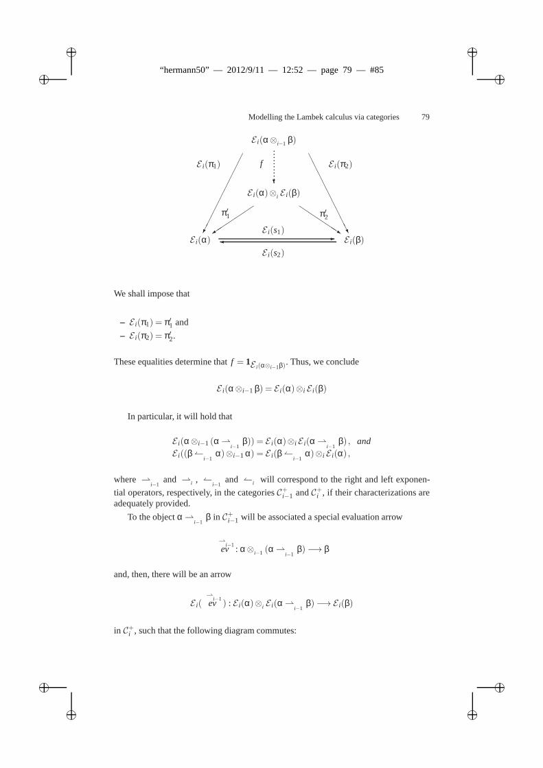
ii

“hermann50” — 2012/9/11 — 12:52 — page 79 — #85 ii

ii

ii


E i(α) E i(β)

E i(α)⊗i E i(β)

-E i(s1)

E i(s2)

+

QQQQQs

?

f

E i(α⊗i−1 β)

AAAAAAAAAU

π′2π′1

E i(π2)E i(π1)

We shall impose that

– E i(π1) = π′1 and

– E i(π2) = π′2.

These equalities determine thatf = 1E i(α⊗i−1β). Thus, we conclude

E i(α⊗i−1 β) = E i(α)⊗i E i(β)

In particular, it will hold that

E i(α⊗i−1 (α i−1

β)) = E i(α)⊗i E i(α i−1

β) , andE i((β

i−1α)⊗i−1 α) = E i(β

i−1α)⊗i E i(α) ,

where i−1

and i , i−1

and i will correspond to the right and left exponen-

tial operators, respectively, in the categoriesC+i−1 andC+i , if their characterizations areadequately provided.

To the objectα i−1

β in C+i−1 will be associated a special evaluation arrow

i−1

ev : α⊗i−1 (α i−1

β)−→ β

and, then, there will be an arrow

E i(

i−1ev ) : E i(α)⊗i E i(α

i−1β)−→ E i(β)

in C+i , such that the following diagram commutes:

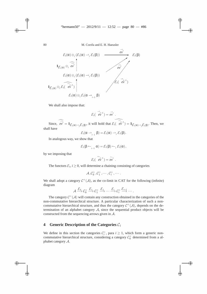
ii

“hermann50” — 2012/9/11 — 12:52 — page 80 — #86 ii

ii

ii


E i(α)⊗i (E i(α)i E i(β))iev

E i(β)

1E i(α)⊗i

iev

E i(α)⊗i (E i(α)i E i(β))

6

-

iev3

E i(α)⊗i E i(α i−1

β)

1E i(α)⊗i

E i(

i−1

ev )

6 E i(

i−1ev )

7

We shall also impose that:

E i(

i−1ev ) =

iev .

Since,iev = 1E i(α)iE i(β), it will hold that

E i(

i−1

ev ) = 1E i(α)iE i(β). Then, we

shall haveE i(α

i−1β) = E i(α)i E i(β).

In analogous way, we show that

E i(β i−1

α) = E i(β)i E i(α) ,

by we imposing that

E i(

i−1ev ) =

iev .

The functorsE i , i ≥ 0, will determine a chaining consisting of categories

A ,C+0 ,C+1 , · · · , C+i , · · · .

We shall adopt a categoryC+(A), as the co-limit in CAT for the following (infinite)diagram

AE0−→ C+0

E1−→ C+1E2−→ ·· ·

E i−→ C+iE i+1−→ ·· · .

The categoryC+(A) will contain any construction obtained in the categories ofthenon-commutative hierarchical structure. A particular characterization of such a non-commutative hierarchical structure, and thus the categoryC+(A), depends on the de-termination of an alphabet categoryA, since the sequential product objects will beconstructed from the sequencing arrows given inA.

4 Generic Description of the CategoriesC i

We define in this section the categoriesC+i , para i ≥ 1, which form a generic non-commutative hierarchical structure, considering a category C+0 determined from a al-phabet categoryA.

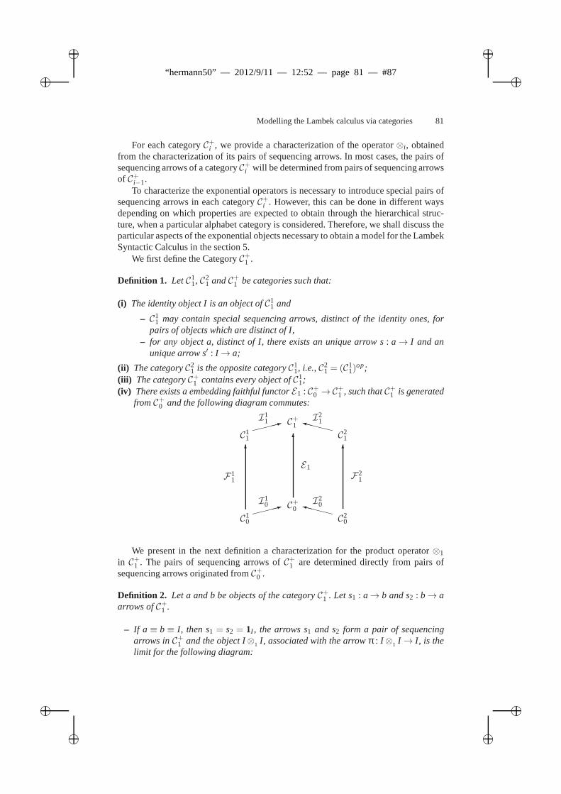
ii

“hermann50” — 2012/9/11 — 12:52 — page 81 — #87 ii

ii

ii


For each categoryC+i , we provide a characterization of the operator⊗i , obtainedfrom the characterization of its pairs of sequencing arrows. In most cases, the pairs ofsequencing arrows of a categoryC+i will be determined from pairs of sequencing arrowsof C+i−1.

To characterize the exponential operators is necessary to introduce special pairs ofsequencing arrows in each categoryC+i . However, this can be done in different waysdepending on which properties are expected to obtain through the hierarchical struc-ture, when a particular alphabet category is considered. Therefore, we shall discuss theparticular aspects of the exponential objects necessary toobtain a model for the LambekSyntactic Calculus in the section 5.

We first define the CategoryC+1 .

Definition 1. LetC11, C2

1 andC+1 be categories such that:

(i) The identity object I is an object ofC11 and

– C11 may contain special sequencing arrows, distinct of the identity ones, for

pairs of objects which are distinct of I,– for any object a, distinct of I, there exists an unique arrow s: a→ I and an

unique arrow s′ : I → a;

(ii) The categoryC21 is the opposite categoryC1

1, i.e.,C21 = (C1

1)op;

(iii) The categoryC+1 contains every object ofC11;

(iv) There exists a embedding faithful functorE1 : C+0 →C+1 , such thatC+1 is generated

fromC+0 and the following diagram commutes:

C10 C2

0

C+0: XXXXyI1

0 I20

66

6

C11 C2

1

C+1: XXXXyI1

1 I21

F11 F2

1

E1

We present in the next definition a characterization for the product operator⊗1

in C+1 . The pairs of sequencing arrows ofC+1 are determined directly from pairs ofsequencing arrows originated fromC+0 .

Definition 2. Let a and b be objects of the categoryC+1 . Let s1 : a→ b and s2 : b→ aarrows ofC+1 .

– If a ≡ b≡ I, then s1 = s2 = 1I , the arrows s1 and s2 form a pair of sequencingarrows inC+1 and the object I⊗1 I, associated with the arrowπ : I ⊗1 I → I, is thelimit for the following diagram:

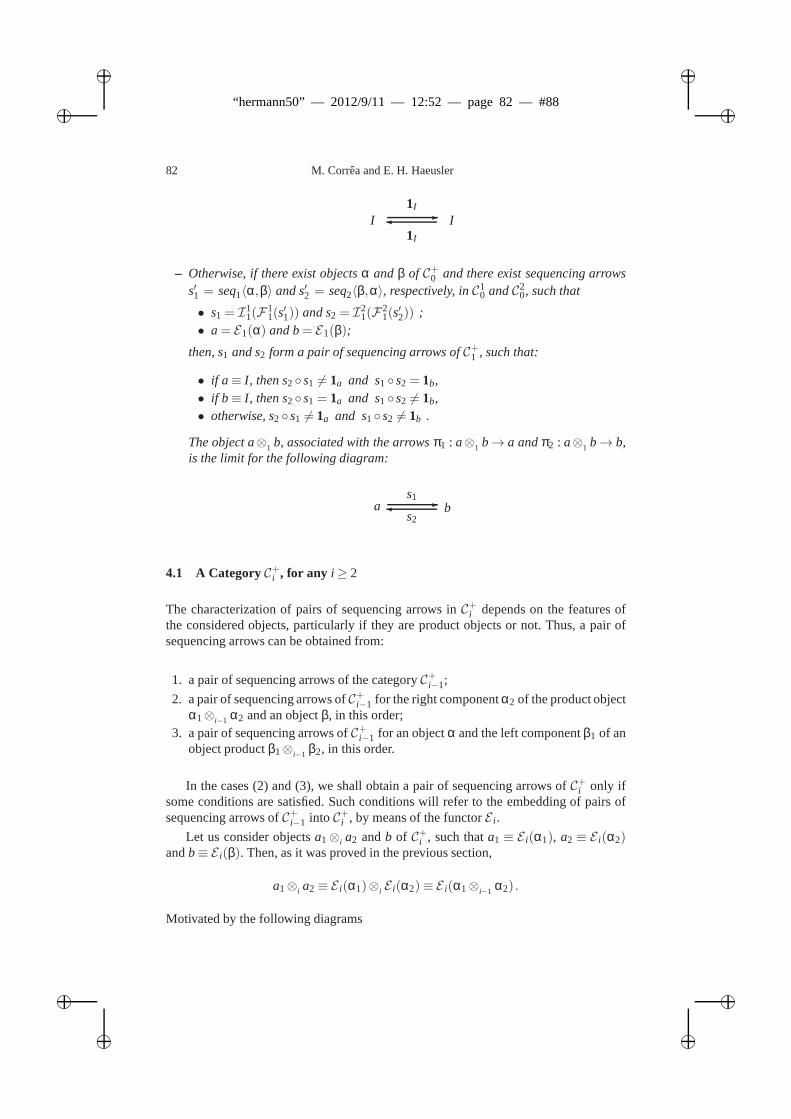
ii

“hermann50” — 2012/9/11 — 12:52 — page 82 — #88 ii

ii

ii


I I-1I

1I

– Otherwise, if there exist objectsα andβ of C+0 and there exist sequencing arrowss′1 = seq1〈α,β〉 and s′2 = seq2〈β,α〉, respectively, inC1

0 andC20, such that

• s1 = I11(F

11(s′1)) and s2 = I2

1(F21(s′2)) ;

• a= E1(α) and b= E1(β);

then, s1 and s2 form a pair of sequencing arrows ofC+1 , such that:

• if a≡ I, then s2 s1 6= 1a and s1 s2 = 1b,• if b≡ I, then s2 s1 = 1a and s1 s2 6= 1b,• otherwise, s2 s1 6= 1a and s1 s2 6= 1b .

The object a⊗1 b, associated with the arrowsπ1 : a⊗1 b→ a andπ2 : a⊗1 b→ b,is the limit for the following diagram:

a b-s2

s1

4.1 A CategoryC+i , for any i ≥ 2

The characterization of pairs of sequencing arrows inC+i depends on the features ofthe considered objects, particularly if they are product objects or not. Thus, a pair ofsequencing arrows can be obtained from:

1. a pair of sequencing arrows of the categoryC+i−1;

2. a pair of sequencing arrows ofC+i−1 for the right componentα2 of the product objectα1⊗i−1 α2 and an objectβ, in this order;

3. a pair of sequencing arrows ofC+i−1 for an objectα and the left componentβ1 of anobject productβ1⊗i−1 β2, in this order.

In the cases (2) and (3), we shall obtain a pair of sequencing arrows ofC+i only ifsome conditions are satisfied. Such conditions will refer tothe embedding of pairs ofsequencing arrows ofC+i−1 into C+i , by means of the functorE i .

Let us consider objectsa1⊗i a2 andb of C+i , such thata1 ≡ E i(α1), a2 ≡ E i(α2)andb≡ E i(β). Then, as it was proved in the previous section,

a1⊗i a2≡ E i(α1)⊗i E i(α2)≡ E i(α1⊗i−1 α2) .

Motivated by the following diagrams

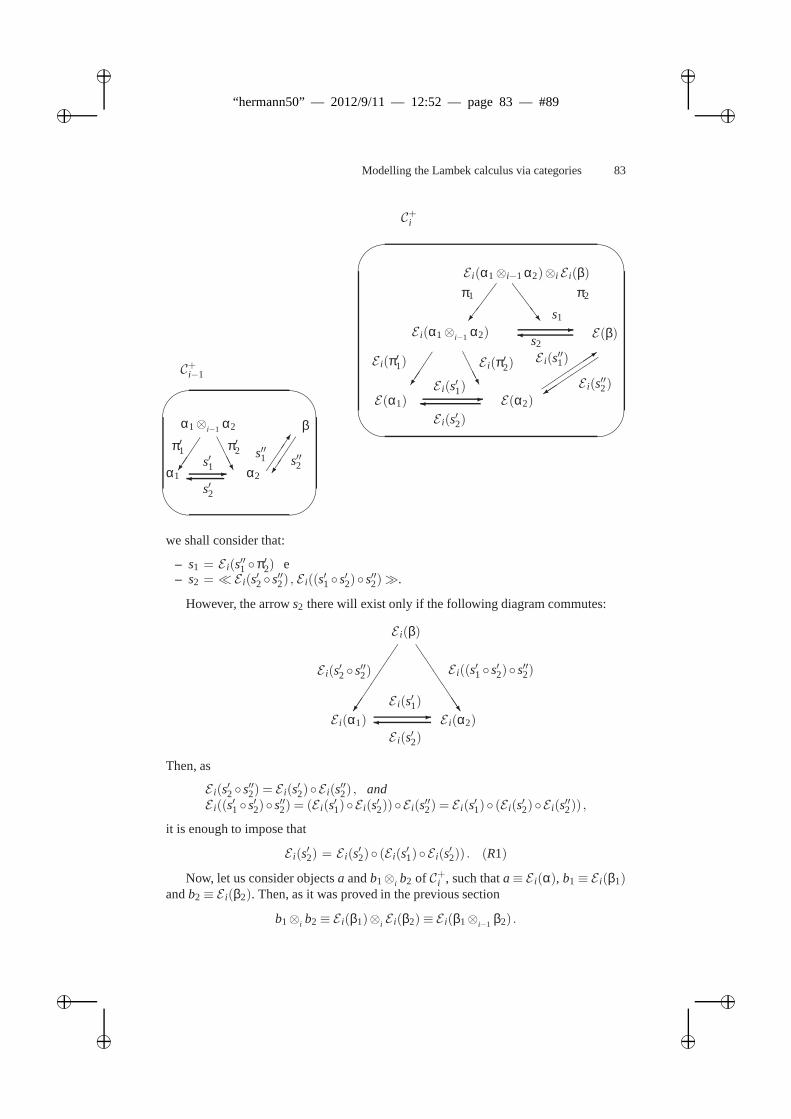
ii

“hermann50” — 2012/9/11 — 12:52 — page 83 — #89 ii

ii

ii


α1⊗i−1 α2

π′1 π′2

β

s′′1 s′′2α1 α2-s′1

s′2

AAAU

E(β) -

3

+

E i(α1⊗i−1 α2)⊗i E i(β)

/

SSSw

π1 π2

s1

s2

E i(s′′1)

E i(s′′2)E(α1) E(α2)

E i(α1⊗i−1 α2)

-E i(s′1)

E i(s′2)

AAAUE i(π′2)E i(π′1)'

&

$

%

'

&

$

%

C+i

C+i−1

we shall consider that:

– s1 = E i(s′′1 π′2) e– s2 = ≪E i(s′2 s′′2) , E i((s′1 s′2) s′′2)≫.

However, the arrows2 there will exist only if the following diagram commutes:

E i(α1) E i(α2)-

E i(s′1)

E i(s′2)

E i(β)

E i(s′2 s′′2) E i((s′1 s′2) s′′2)

JJJJJJ

Then, as

E i(s′2 s′′2) = E i(s′2)E i(s′′2) , andE i((s′1 s′2) s′′2) = (E i(s′1)E i(s′2))E i(s′′2) = E i(s′1) (E i(s′2)E i(s′′2)) ,

it is enough to impose that

E i(s′2) = E i(s

′2) (E i(s

′1)E i(s

′2)) . (R1)

Now, let us consider objectsa andb1⊗i b2 of C+i , such thata≡ E i(α), b1≡ E i(β1)andb2≡ E i(β2). Then, as it was proved in the previous section

b1⊗i b2≡ E i(β1)⊗i E i(β2)≡ E i(β1⊗i−1 β2) .

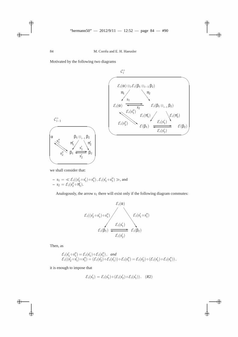
ii

“hermann50” — 2012/9/11 — 12:52 — page 84 — #90 ii

ii

ii


Motivated by the following two diagrams

β1⊗i−1 β2

π′1 π′2

αs′′1

s′′2 β1 β2-

s′1

s′2

AAAU

ZZZZ~Z

ZZZ

C+i−1'

&

$

%

E i(α) -

E i(α)⊗i E i(β1⊗i−1 β2)

/

SSSw

π1 π2

s1

s2E i(s′′1)

E i(s′′2)

ZZZZZ~Z

ZZ

ZZ

E(β1) E(β2)

E i(β1⊗i−1 β2)

-E i(s′1)

E i(s′2)

AAAUE i(π′2)E i(π′1)

'

&

$

%

C+i

we shall consider that:

– s1 = ≪E i((s′2 s′1) s′′1) , E i(s′1 s′′1)≫, and– s2 = E i(s′′2 π′1).

Analogously, the arrows1 there will exist only if the following diagram commutes:

E i(β1) E i(β2)-

E i(s′1)

E i(s′2)

E i(α)

E i((s′2 s′1) s′′1) E i(s′1 s′′1)

JJJJJJ

Then, as

E i(s′1 s′′1) = E i(s′1)E i(s′′1) , andE i((s′2 s′1) s′′1) = (E i(s′2)E i(s′1))E i(s′′1) = E i(s′2) (E i(s′1)E i(s′′1)) ,

it is enough to impose that

E i(s′1) = E i(s

′1) (E i(s

′2)E i(s

′1)) . (R2)

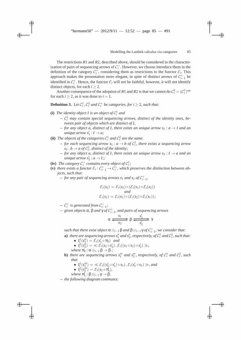
ii

“hermann50” — 2012/9/11 — 12:52 — page 85 — #91 ii

ii

ii


The restrictionsR1 andR2, described above, should be considered in the character-ization of pairs of sequencing arrows ofC+i . However, we choose introduce them in thedefinition of the categoryC+i , considering them as restrictions to the functorE i . Thisapproach makes the presentation more elegant, in spite of distinct arrows ofC+i−1 beidentified inC+i . Hence, the functorE i will not be faithful, however, it will not identifydistinct objects, for eachi ≥ 2.

Another consequence of the adoption ofR1 andR2 is that we cannot doC2i = (C1

i )op

for eachi ≥ 2, as it was done toi = 1.

Definition 3. LetC1i , C2

i andC+i be categories, for i≥ 2, such that:

(i) The identity object I is an object ofC1i and

– C1i may contain special sequencing arrows, distinct of the identity ones, be-

tween pair of objects which are distinct of I,– for any object a, distinct of I, there exists an unique arrow s1 : a→ I and an

unique arrow s′1 : I → a;(ii) The objects of the categoriesC1

i andC2i are the same.

– for each sequencing arrow s1 : a→ b of C1i , there exists a sequencing arrow

s2 : b→ a ofC2i , distinct of the identity;

– for any object a, distinct of I, there exists an unique arrow s2 : I → a and anunique arrow s′2 : a→ I;;

(iv) The categoryC+i contains every object ofC1i ;

(v) there exists a functorE i : C+i−1→ C+i , which preserves the distinction between ob-

jects, such that:– for any pair of sequencing arrows s1 and s2 of C+i−1,

E i(s2) = E i(s2) (E i(s1)E i(s2))and

E i(s1) = E i(s1) (E i(s2)E i(s1)) ;

– C+i is generated fromC+i−1;– given objectsα, β andγ of C+i−1, and pairs of sequencing arrows

α β-s2

s1γ-

s′2

s′1

such that there exist objectα⊗i−1 β andβ⊗i−1 γ of C+i−1, we consider that:

a) there are sequencing arrows s′′1 and s′′2, respectively, ofC1i andC2

i , such that:• I1

i (s′′1) = E i(s′1 π2) and

• I2i (s′′2) = ≪E i(s2 s′2) , E i((s1 s2) s′2)≫,

whereπ2 : α⊗i−1 β→ β ;b) there are sequencing arrows s′′′1 and s′′′2 , respectively, ofC1

i and C2i , such

that• I1

i (s′′′1 ) = ≪E i((s′2 s′1) s1) , E i(s′1 s1)≫, and

• I2i (s′′′2 ) = E i(s2π′1),

whereπ′1 : β⊗i−1 γ→ β.– the following diagram commutes:

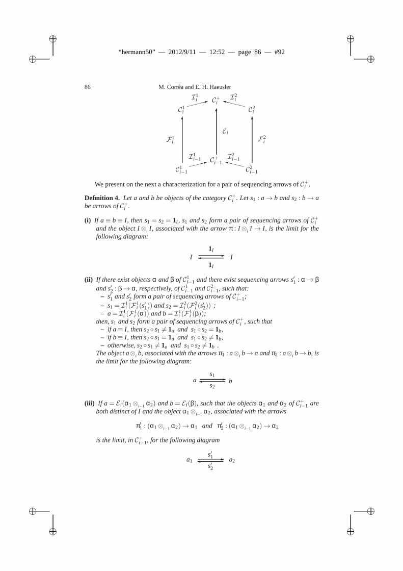
ii

“hermann50” — 2012/9/11 — 12:52 — page 86 — #92 ii

ii

ii


C1i−1 C2

i−1

C+i−1: XXXyI1

i−1 I2i−1

66

6

C1i C2

i

C+i: XXXXyI1i I2

i

F1i F2

i

E i

We present on the next a characterization for a pair of sequencing arrows ofC+i .

Definition 4. Let a and b be objects of the categoryC+i . Let s1 : a→ b and s2 : b→ abe arrows ofC+i .

(i) If a ≡ b≡ I, then s1 = s2 = 1I , s1 and s2 form a pair of sequencing arrows ofC+iand the object I⊗i I, associated with the arrowπ : I ⊗i I → I, is the limit for thefollowing diagram:

I I-1I

1I

(ii) If there exist objectsα andβ of C1i−1 and there exist sequencing arrows s′

1 : α→ βand s′2 : β→ α, respectively, ofC1

i−1 andC2i−1, such that:

– s′1 and s′2 form a pair of sequencing arrows ofC+i−1;– s1 = I

1i (F

1i (s′1)) and s2 = I2

i (F2i (s′2)) ;

– a= I1i (F

1i (α)) and b= I1

i (F1i (β));

then, s1 and s2 form a pair of sequencing arrows ofC+i , such that– if a≡ I, then s2 s1 6= 1a and s1 s2 = 1b,– if b≡ I, then s2 s1 = 1a and s1 s2 6= 1b,– otherwise, s2 s1 6= 1a and s1 s2 6= 1b .

The object a⊗i b, associated with the arrowsπ1 : a⊗i b→ a andπ2 : a⊗i b→ b, isthe limit for the following diagram:

a b-s2

s1

(iii) If a = E i(α1⊗i−1 α2) and b= E i(β), such that the objectsα1 andα2 of C+i−1 areboth distinct of I and the objectα1⊗i−1 α2, associated with the arrows

π′1 : (α1⊗i−1 α2)→ α1 and π′2 : (α1⊗i−1 α2)→ α2

is the limit, inC+i−1, for the following diagram

a1 a2-

s′2

s′1

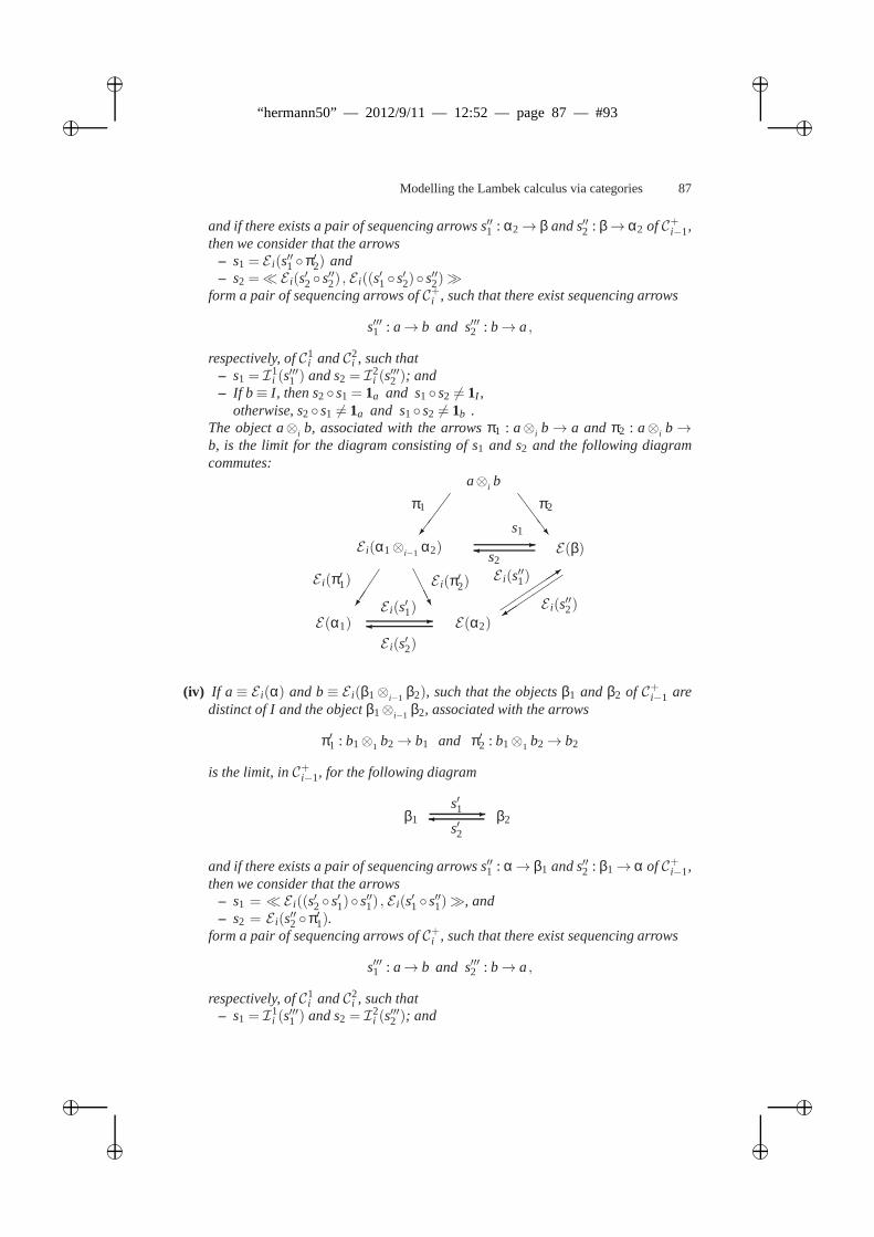
ii

“hermann50” — 2012/9/11 — 12:52 — page 87 — #93 ii

ii

ii


and if there exists a pair of sequencing arrows s′′1 : α2→ β and s′′2 : β→ α2 of C+i−1,

then we consider that the arrows– s1 = E i(s′′1 π′2) and– s2 =≪E i(s′2 s′′2) , E i((s′1 s′2) s′′2)≫

form a pair of sequencing arrows ofC+i , such that there exist sequencing arrows

s′′′1 : a→ b and s′′′2 : b→ a,

respectively, ofC1i andC2

i , such that– s1 = I

1i (s′′′1 ) and s2 = I2

i (s′′′2 ); and

– If b≡ I, then s2 s1 = 1a and s1 s2 6= 1I ,otherwise, s2 s1 6= 1a and s1 s2 6= 1b .

The object a⊗i b, associated with the arrowsπ1 : a⊗i b→ a andπ2 : a⊗i b→b, is the limit for the diagram consisting of s1 and s2 and the following diagramcommutes:

E(β) -

3

+

a⊗i b

/

SSSw

π1 π2

s1

s2

E i(s′′1)

E i(s′′2)E(α1) E(α2)

E i(α1⊗i−1 α2)

-E i(s′1)

E i(s′2)


(iv) If a ≡ E i(α) and b≡ E i(β1⊗i−1 β2), such that the objectsβ1 and β2 of C+i−1 aredistinct of I and the objectβ1⊗i−1 β2, associated with the arrows

π′1 : b1⊗1 b2→ b1 and π′2 : b1⊗1 b2→ b2

is the limit, inC+i−1, for the following diagram

β1 β2-

s′2

s′1

and if there exists a pair of sequencing arrows s′′1 : α→ β1 and s′′2 : β1→ α of C+i−1,

then we consider that the arrows– s1 = ≪E i((s′2 s′1) s′′1) , E i(s′1 s′′1)≫, and– s2 = E i(s′′2 π′1).

form a pair of sequencing arrows ofC+i , such that there exist sequencing arrows

s′′′1 : a→ b and s′′′2 : b→ a,

respectively, ofC1i andC2

i , such that– s1 = I

1i (s′′′1 ) and s2 = I2

i (s′′′2 ); and

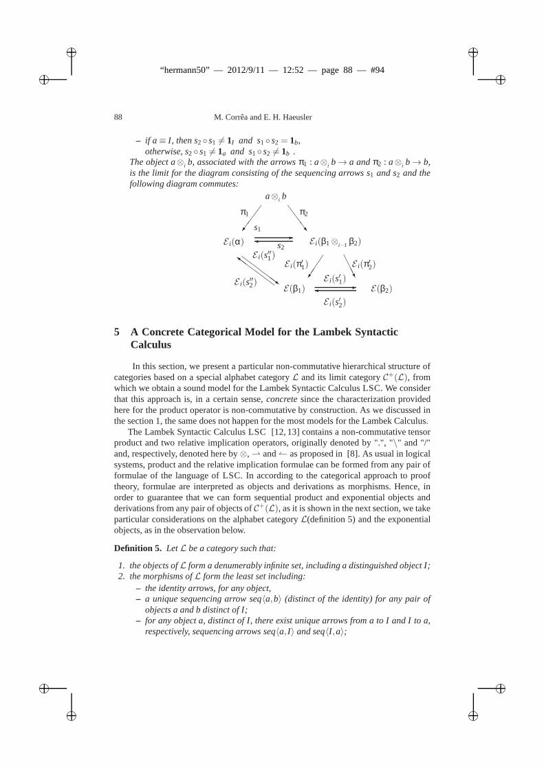
ii

“hermann50” — 2012/9/11 — 12:52 — page 88 — #94 ii

ii

ii


– if a≡ I, then s2 s1 6= 1I and s1 s2 = 1b,otherwise, s2 s1 6= 1a and s1 s2 6= 1b .

The object a⊗i b, associated with the arrowsπ1 : a⊗i b→ a andπ2 : a⊗i b→ b,is the limit for the diagram consisting of the sequencing arrows s1 and s2 and thefollowing diagram commutes:

E i(α) -

a⊗i b

/

SSSw

π1 π2

s1

s2E i(s′′1)

E i(s′′2)

ZZZZZ~Z

ZZ

ZZ

E(β1) E(β2)

E i(β1⊗i−1 β2)

-E i(s′1)

E i(s′2)


5 A Concrete Categorical Model for the Lambek SyntacticCalculus

In this section, we present a particular non-commutative hierarchical structure ofcategories based on a special alphabet categoryL and its limit categoryC+(L), fromwhich we obtain a sound model for the Lambek Syntactic Calculus LSC. We considerthat this approach is, in a certain sense,concretesince the characterization providedhere for the product operator is non-commutative by construction. As we discussed inthe section 1, the same does not happen for the most models forthe Lambek Calculus.

The Lambek Syntactic Calculus LSC [12, 13] contains a non-commutative tensorproduct and two relative implication operators, originally denoted by ".", "\" and "/"and, respectively, denoted here by⊗, and as proposed in [8]. As usual in logicalsystems, product and the relative implication formulae canbe formed from any pair offormulae of the language of LSC. In according to the categorical approach to prooftheory, formulae are interpreted as objects and derivations as morphisms. Hence, inorder to guarantee that we can form sequential product and exponential objects andderivations from any pair of objects ofC+(L), as it is shown in the next section, we takeparticular considerations on the alphabet categoryL(definition 5) and the exponentialobjects, as in the observation below.

Definition 5. LetL be a category such that:

1. the objects ofL form a denumerably infinite set, including a distinguished object I;2. the morphisms ofL form the least set including:

– the identity arrows, for any object,– a unique sequencing arrow seq〈a,b〉 (distinct of the identity) for any pair of

objects a and b distinct of I;– for any object a, distinct of I, there exist unique arrows from a to I and I to a,

respectively, sequencing arrows seq〈a, I〉 and seq〈I ,a〉;

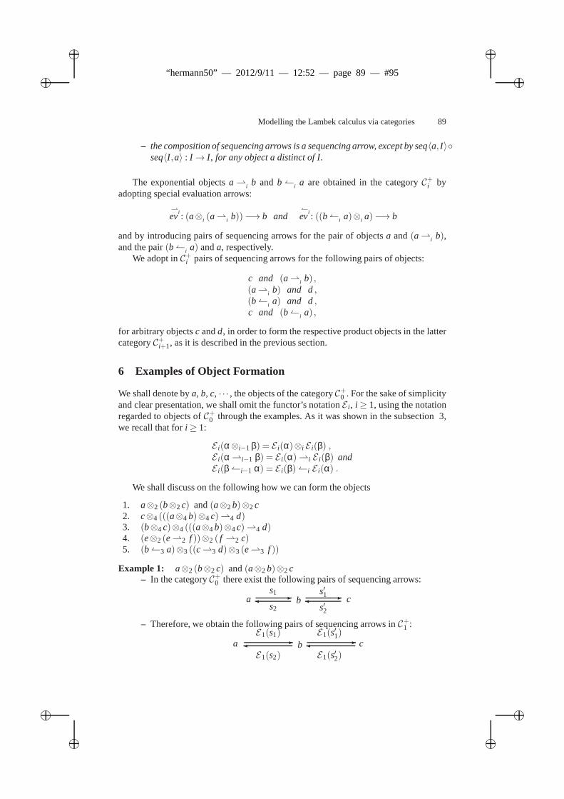
ii

“hermann50” — 2012/9/11 — 12:52 — page 89 — #95 ii

ii

ii


– the composition of sequencing arrows is a sequencing arrow,except by seq〈a, I〉seq〈I ,a〉 : I → I, for any object a distinct of I.

The exponential objectsa i b and b i a are obtained in the categoryC+i byadopting special evaluation arrows:

iev : (a⊗i (ai b))−→ b and

iev : ((bi a)⊗i a)−→ b

and by introducing pairs of sequencing arrows for the pair ofobjectsa and(ai b),and the pair(bi a) anda, respectively.

We adopt inC+i pairs of sequencing arrows for the following pairs of objects:

c and (ai b) ,(ai b) and d,(bi a) and d,c and (bi a) ,

for arbitrary objectsc andd, in order to form the respective product objects in the lattercategoryC+i+1, as it is described in the previous section.

6 Examples of Object Formation

We shall denote bya, b, c, · · · , the objects of the categoryC+0 . For the sake of simplicityand clear presentation, we shall omit the functor’s notation E i , i ≥ 1, using the notationregarded to objects ofC+0 through the examples. As it was shown in the subsection 3,we recall that fori ≥ 1:

E i(α⊗i−1 β) = E i(α)⊗i E i(β) ,E i(α i−1 β) = E i(α)i E i(β) andE i(β i−1 α) = E i(β)i E i(α) .

We shall discuss on the following how we can form the objects

1. a⊗2 (b⊗2 c) and(a⊗2 b)⊗2 c2. c⊗4 (((a⊗4 b)⊗4 c)4 d)3. (b⊗4 c)⊗4 (((a⊗4 b)⊗4 c)4 d)4. (e⊗2 (e2 f ))⊗2 ( f 2 c)5. (b3 a)⊗3 ((c3 d)⊗3 (e3 f ))

Example 1: a⊗2 (b⊗2 c) and(a⊗2 b)⊗2 c– In the categoryC+0 there exist the following pairs of sequencing arrows:

a b-s2

s1c-

s′2

s′1

– Therefore, we obtain the following pairs of sequencing arrows inC+1 :

a b-E1(s2)

E1(s1)c-

E1(s′2)

E1(s′1)

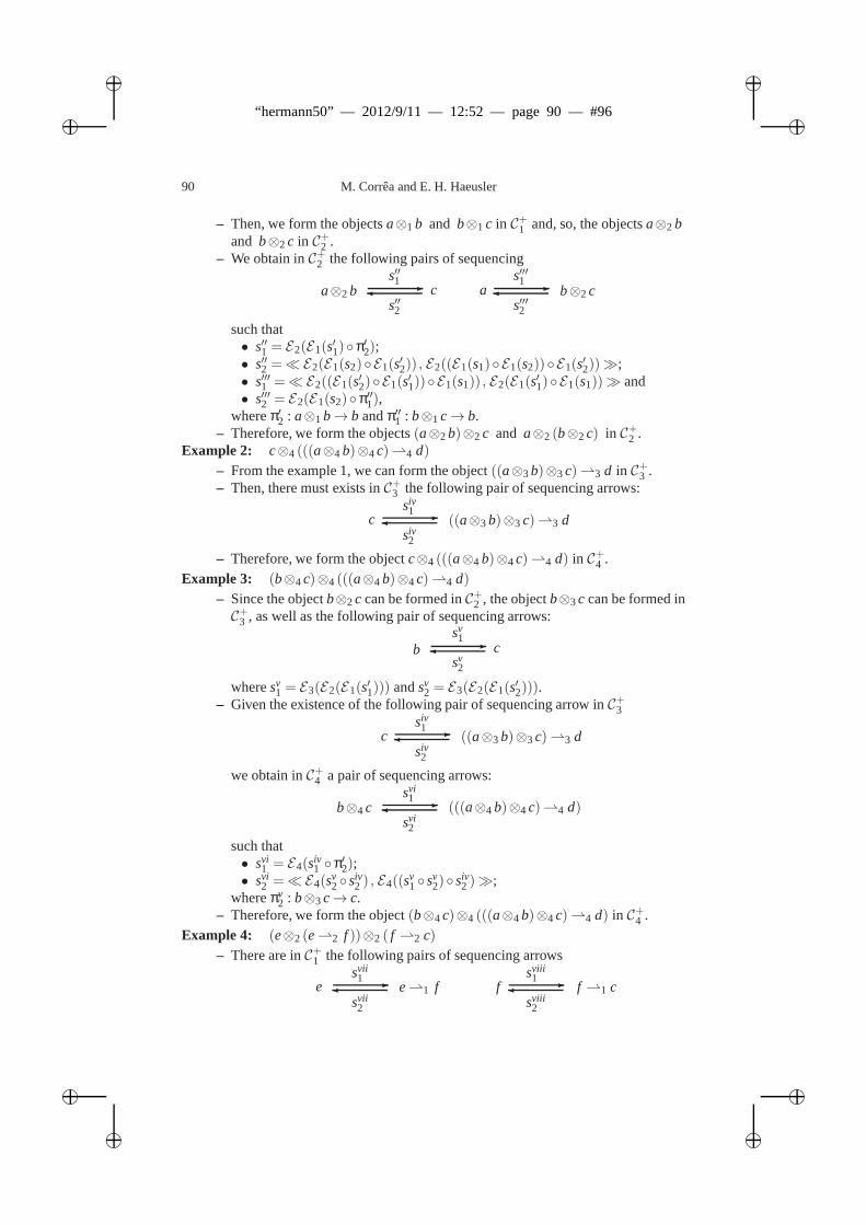
ii

“hermann50” — 2012/9/11 — 12:52 — page 90 — #96 ii

ii

ii


– Then, we form the objectsa⊗1 b and b⊗1 c in C+1 and, so, the objectsa⊗2 band b⊗2 c in C+2 .

– We obtain inC+2 the following pairs of sequencing

a⊗2 b c-s′′2

s′′1a b⊗2 c-

s′′′2

s′′′1

such that• s′′1 = E2(E1(s′1)π′2);• s′′2 =≪E2(E1(s2)E1(s′2)) , E2((E1(s1)E1(s2))E1(s′2))≫;• s′′′1 =≪E2((E1(s′2)E1(s′1))E1(s1)) , E2(E1(s′1)E1(s1))≫ and• s′′′2 = E2(E1(s2)π′′1),

whereπ′2 : a⊗1 b→ b andπ′′1 : b⊗1 c→ b.– Therefore, we form the objects(a⊗2 b)⊗2 c and a⊗2 (b⊗2 c) in C+2 .

Example 2: c⊗4 (((a⊗4 b)⊗4 c)4 d)

– From the example 1, we can form the object((a⊗3 b)⊗3 c)3 d in C+3 .– Then, there must exists inC+3 the following pair of sequencing arrows:

c ((a⊗3 b)⊗3 c)3 d-siv2

siv1

– Therefore, we form the objectc⊗4 (((a⊗4 b)⊗4 c)4 d) in C+4 .Example 3: (b⊗4 c)⊗4 (((a⊗4 b)⊗4 c)4 d)

– Since the objectb⊗2 c can be formed inC+2 , the objectb⊗3c can be formed inC+3 , as well as the following pair of sequencing arrows:

b c-sv2

sv1

wheresv1 = E3(E2(E1(s′1))) andsv

2 = E3(E2(E1(s′2))).– Given the existence of the following pair of sequencing arrow in C+3

c ((a⊗3 b)⊗3 c)3 d-siv2

siv1

we obtain inC+4 a pair of sequencing arrows:

b⊗4 c (((a⊗4 b)⊗4 c)4 d)-svi2

svi1

such that• svi

1 = E4(siv1 π′2);

• svi2 =≪E4(sv

2 siv2 ) , E4((sv

1 sv2) siv

2 )≫;whereπv

2 : b⊗3 c→ c.– Therefore, we form the object(b⊗4 c)⊗4 (((a⊗4 b)⊗4 c)4 d) in C+4 .

Example 4: (e⊗2 (e2 f ))⊗2 ( f 2 c)

– There are inC+1 the following pairs of sequencing arrows

e e1 f-svii2

svii1

f f 1 c-sviii2

sviii1

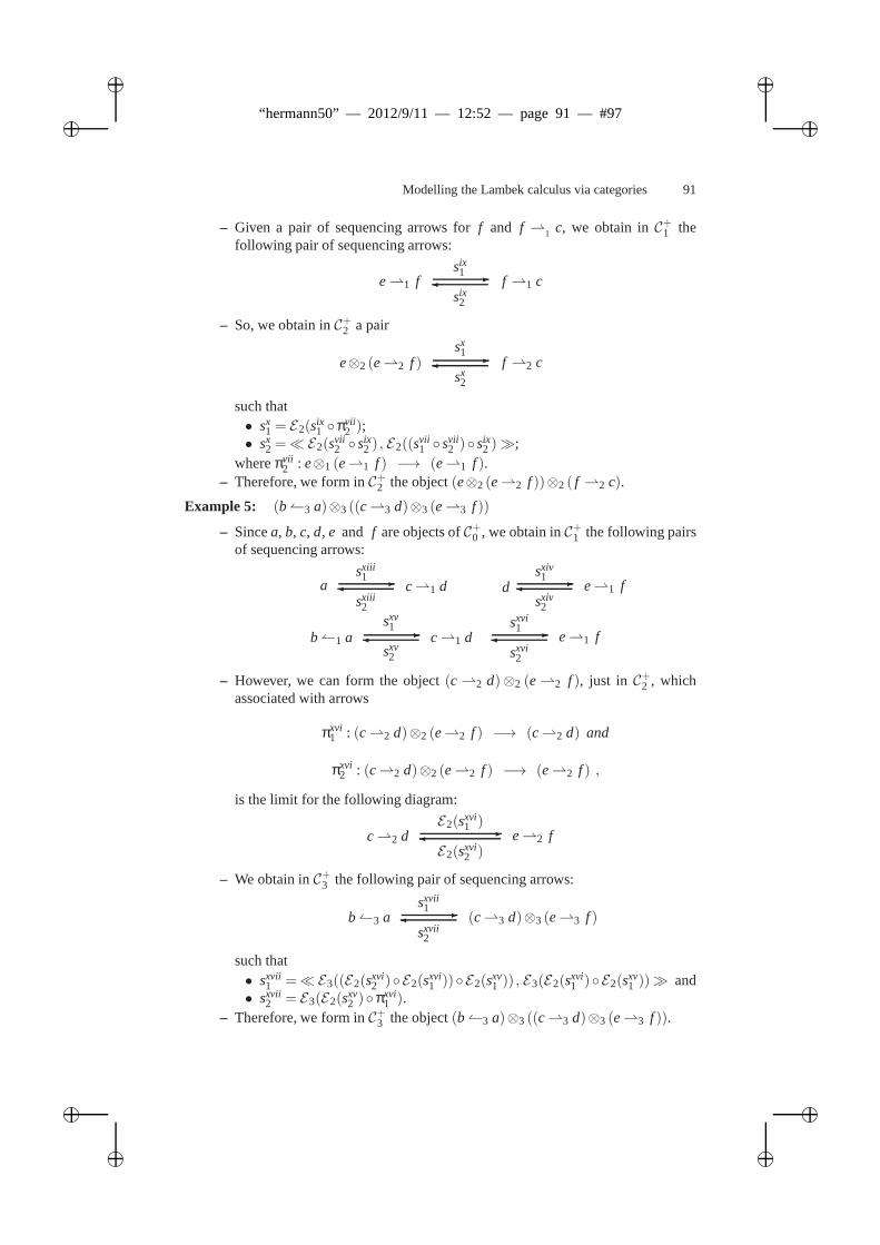
ii

“hermann50” — 2012/9/11 — 12:52 — page 91 — #97 ii

ii

ii


– Given a pair of sequencing arrows forf and f 1 c, we obtain inC+1 thefollowing pair of sequencing arrows:

e1 f f 1 c-six2

six1

– So, we obtain inC+2 a pair

e⊗2 (e2 f ) f 2 c-sx2

sx1

such that• sx

1 = E2(six1 πvii

2 );• sx

2 =≪E2(svii2 six

2 ) , E2((svii1 svii

2 ) six2 )≫;

whereπvii2 : e⊗1 (e1 f ) −→ (e1 f ).

– Therefore, we form inC+2 the object(e⊗2 (e2 f ))⊗2 ( f 2 c).

Example 5: (b3 a)⊗3 ((c3 d)⊗3 (e3 f ))

– Sincea, b, c, d, e and f are objects ofC+0 , we obtain inC+1 the following pairsof sequencing arrows:

a c1 d-sxiii2

sxiii1

d e1 f-sxiv2

sxiv1

b1 a c1 d-sxv2

sxv1

e1 f-sxvi2

sxvi1

– However, we can form the object(c 2 d)⊗2 (e2 f ), just in C+2 , whichassociated with arrows

πxvi1 : (c2 d)⊗2 (e2 f ) −→ (c2 d) and

πxvi2 : (c2 d)⊗2 (e2 f ) −→ (e2 f ) ,

is the limit for the following diagram:

c2 d e2 f-E2(sxvi

2 )

E2(sxvi1 )

– We obtain inC+3 the following pair of sequencing arrows:

b3 a (c3 d)⊗3 (e3 f )-sxvii2

sxvii1

such that• sxvii

1 =≪E3((E2(sxvi2 )E2(sxvi

1 ))E2(sxv1 )) , E3(E2(sxvi

1 )E2(sxv1 ))≫ and

• sxvii2 = E3(E2(sxv

2 )πxvi1 ).

– Therefore, we form inC+3 the object(b3 a)⊗3 ((c3 d)⊗3 (e3 f )).

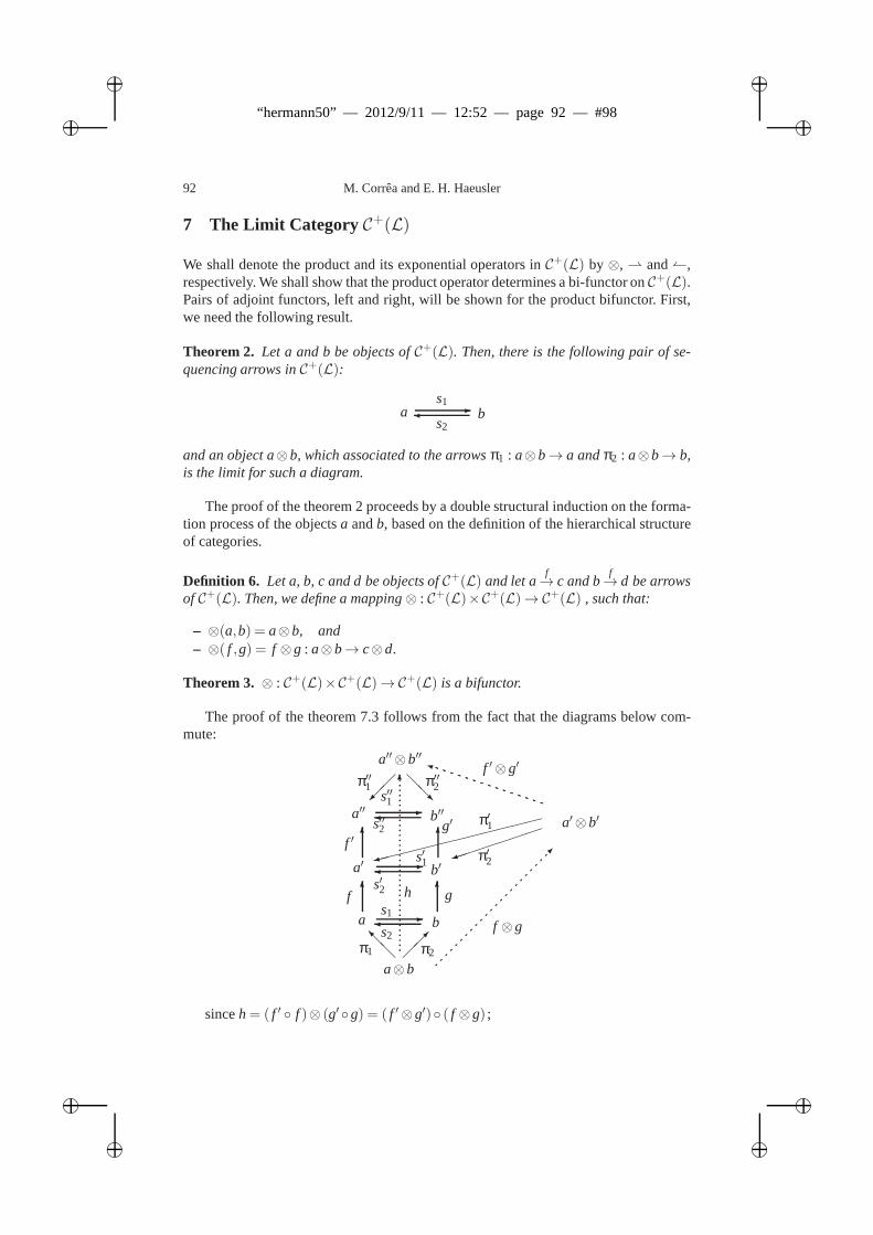
ii

“hermann50” — 2012/9/11 — 12:52 — page 92 — #98 ii

ii

ii


7 The Limit Category C+(L)

We shall denote the product and its exponential operators inC+(L) by ⊗, and,respectively. We shall show that the product operator determines a bi-functor onC+(L).Pairs of adjoint functors, left and right, will be shown for the product bifunctor. First,we need the following result.

Theorem 2. Let a and b be objects ofC+(L). Then, there is the following pair of se-quencing arrows inC+(L):

a b-s2

s1

and an object a⊗b, which associated to the arrowsπ1 : a⊗b→ a andπ2 : a⊗b→ b,is the limit for such a diagram.

The proof of the theorem 2 proceeds by a double structural induction on the forma-tion process of the objectsa andb, based on the definition of the hierarchical structureof categories.

Definition 6. Let a, b, c and d be objects ofC+(L) and let af→ c and b

f→ d be arrows

of C+(L). Then, we define a mapping⊗ : C+(L)×C+(L)→C+(L) , such that:

– ⊗(a,b) = a⊗b, and– ⊗( f ,g) = f ⊗g : a⊗b→ c⊗d.

Theorem 3. ⊗ : C+(L)×C+(L)→C+(L) is a bifunctor.

The proof of the theorem 7.3 follows from the fact that the diagrams below com-mute:

a′′⊗b′′

@@R

a′′ b′′-s′′1

s′′2

π′′1 π′′2

a⊗b

π1 π2@@I

a b-s1

s2

6 6f g

s′1

s′2

a′ b′-

6 6f ′g′ a′⊗b′9

)

6

π′1

π′2

f ⊗g

h

f ′⊗g′i

......................................................................................................................................................

............

............

............

............

............

............

............

............

............

............

............

......

sinceh= ( f ′ f )⊗ (g′ g) = ( f ′⊗g′) ( f ⊗g) ;

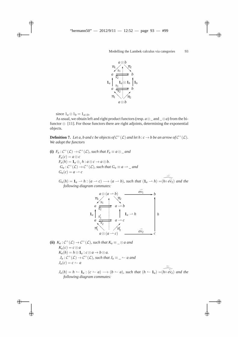
ii

“hermann50” — 2012/9/11 — 12:52 — page 93 — #99 ii

ii

ii


a⊗b

a b

@@Rs1

s2

-

π1 π2

a⊗b

π1 π2@@I

a b-s1

s2

6 61a 1b

6

1a⊗1b

since 1a⊗1b = 1a⊗b.As usual, we obtain left and right product functors (resp.a⊗_ and _⊗a) from the bi-

functor⊗ [11]. For those functors there are right adjoints, determining the exponentialobjects.

Definition 7. Let a, b and c be objects ofC+(L) and let h: c→ b be an arrow ofC+(L).We adopt the functors

(i) Fa : C+(L)→C+(L), such that Fa≡ a⊗_ andFa(c) = a⊗ cFa(h) = 1a⊗1 h : a⊗ c→ a⊗b.Ga : C+(L)→C+(L), such that Ga ≡ a _ and

Ga(c) = a c

Ga(h) = 1a h : (a c) −→ (a b), such that(1a h) =

(h

ev2) and the

following diagram commutes:

a⊗ (a b)

a a b

@@Rs1

s2

-

π1 π2

a⊗ (a c)π′1 π′2@@I

a a c-s′1s′2

6 61a 1a h

6

- bev1

6

ev2 - c

h

(ii) Ka : C+(L)→C+(L), such that Ka≡ _⊗a andKa(c) = c⊗aKa(h) = h⊗1a : c⊗a→ b⊗a.Ja : C+(L)→C+(L), such that Ja≡ _ a and

Ja(c) = c a

Ja(h) = h 1a : (c a) −→ (b a), such that(h 1a) =

(h

ev2) and the

following diagram commutes:

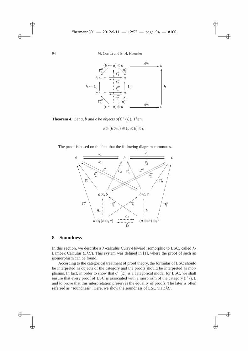
ii

“hermann50” — 2012/9/11 — 12:52 — page 94 — #100 ii

ii

ii


(b a)⊗a

ab a

@@Rs′′1

s′′2

-

π′′1 π′′2

(c a)⊗aπ′′′1 π′′′2@@I

ac a -s′′′1

s′′′2

6 61ah 1a

6

- bev1

6

ev2 - c

h

Theorem 4. Let a, b and c be objects ofC+(L). Then,

a⊗ (b⊗ c)∼= (a⊗b)⊗ c.

The proof is based on the fact that the following diagram commutes.

a⊗i (b⊗i c) (a⊗i b)⊗i c-

a⊗i b b⊗i c

a b cs1 s′1

π1

π2 π′1

π′2

π′′1 π′′2π′′′1 π′′′2g1

g2

f2

f1

s2 s′2HHHHHHHHHHHHHHjHHHHHHHHHHHHHHY

*

SS

SS

SSo

AAA

AA

AAK

- -

6 6

3

QQ

QQ

QQQk

BBBBBBBBBBBBBM

s′′1

s′′2s′′′1

s′′′2

8 Soundness

In this section, we describe aλ-calculus Curry-Howard isomorphic to LSC, calledλ-Lambek Calculus (LλC). This system was defined in [1], where the proof of such anisomorphism can be found.

According to the categorical treatment of proof theory, theformulas of LSC shouldbe interpreted as objects of the category and the proofs should be interpreted as mor-phisms. In fact, in order to show thatC+(L) is a categorical model for LSC, we shallensure that every proof of LSC is associated with a morphism of the categoryC+(L),and to prove that this interpretation preserves the equality of proofs. The later is oftenreferred as “soundness”. Here, we show the soundness of LSC via LλC.

ii

“hermann50” — 2012/9/11 — 12:52 — page 95 — #101 ii

ii

ii


The results and definitions shown in this section are strongly based on the similarones developed in [4].

Next, we present the syntax of the types and terms of theλ-Lambek Calculus.

λ-Lambek Calculus

– Types:• Atomic types:T1, · · · ,Tn, · · · ;• If A andB are types, thenA⊗B, A B andA B are types.

– Terms:

x : A[x : A]

t1 : A[Γ1] t2 : B[Γ2]

〈t1, t2〉 : A⊗B[Γ1,Γ2]

t : C[Γ,x : A,y : B,Γ1] t1 : A⊗B[∆]LET(< x : A,y : B>= t1)t : C[Γ,∆,Γ1]

t : B[x : A,Γ]

λ x.t : A B[Γ]

t : B[Γ,x : A]

λ x.t : B A[Γ]

t1 : A[Γ] t2 : A B[∆]

APP(t2, t1) : B[Γ,∆]

t2 : B A[∆] t1 : A[Γ]

APP(t2, t1) : B[∆,Γ]

This calculus has the followingReduction Rules:

–

APP(

λ x.t, t ′) : B[Γ,∆] t[x← t ′] : B[Γ,∆]

–

APP(

λ x.t, t ′) : B[∆,Γ] t[x← t ′] : B[∆,Γ]– LET(< x : A,y : B>=< t1, t2 >)t : C[Γ,∆1,∆2,Γ′] t[x← t1,y← t2] :

C[Γ,∆1,∆2,Γ′]

Next, we define a denotational semantics for thisλ-calculus in terms of the categor-ical framework presented.

Denotational Semantics

– Types are mapped to objects of the categoryC+(L):

• [[A]] ∈ ob j(C+(L))

• [[A⊗B]] = [[A]]⊗ [[B]]

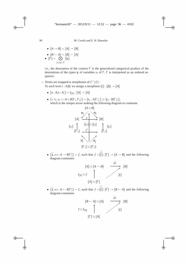
ii

“hermann50” — 2012/9/11 — 12:52 — page 96 — #102 ii

ii

ii


• [[A B]] = [[A]] [[B]]

• [[B A]] = [[B]] [[A]]• [[Γ]] =

⊗

(xi :γi)∈Γ[[γi ]]

i.e., the denotation of the contextΓ is the generalized categorical product of thedenotations of the typesγi of variablesxi of Γ. Γ is interpreted as an ordered se-quence.

– Terms are mapped to morphisms ofC+(L):To each termt : A[∆] we assign a morphism[[t]] : [[∆]]→ [[A]]

• [[x : A[x : A] ]] = I[[A]] : [[A]]→ [[A]]

• [[< t1, t2 >: A⊗B[Γ1,Γ2] ]] = [[t1 : A[Γ1] ]] ⊗ [[t2 : B[Γ2] ]],which is the unique arrow making the following diagram to commute

[[A⊗B]]

[[A]] [[B]]

-

@@@Rs

π1 π2

[[Γ1]]⊗ [[Γ2]]

π′1 π′2@@@I

[[Γ1]] [[Γ2]]-s′6 6[[t1]] [[t2]]

6

[[t1]]⊗ [[t2]]

• [[

λ x.t : A B[Γ] ]] = f , such thatf =

[[t]]: [[Γ]]→ [[A B]] and the followingdiagram commutes

[[A]]⊗ [[A B]]

ev

[[B]]

I[[A]]⊗ f

[[A]]⊗ [[Γ]]

6

-

>

[[t]]

• [[

λ x.t : A B[Γ] ]] = f , such thatf =

[[t]]: [[Γ]]→ [[B A]] and the followingdiagram commutes

[[B A]]⊗ [[A]]

ev

[[B]]

f ⊗ I[[A]]

[[Γ]]⊗ [[A]]

6

-

>

[[t]]

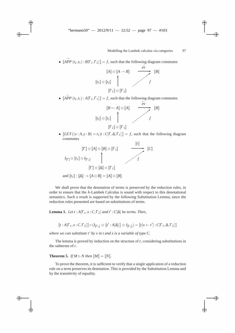
ii

“hermann50” — 2012/9/11 — 12:52 — page 97 — #103 ii

ii

ii


• [[

APP(t2, t1) : B[Γ1,Γ2] ]] = f , such that the following diagram commutes

[[A]]⊗ [[A B]]

ev

[[B]]

[[t1]]⊗ [[t2]]

[[Γ1]]⊗ [[Γ2]]

6

-

>

f

• [[

APP(t2, t1) : A[Γ2,Γ1] ]] = f , such that the following diagram commutes

[[B A]]⊗ [[A]]

ev

[[B]]

[[t2]]⊗ [[t1]]

[[Γ2]]⊗ [[Γ1]]

6

-

>

f

• [[LET((x : A,y : B) = t1)t : C[Γ,∆,Γ1] ]] = f , such that the following diagramcommutes

[[Γ]]⊗ [[A]]⊗ [[B]]⊗ [[Γ1]]

[[t]][[C]]

I[[Γ]]⊗ [[t1]]⊗ I[[Γ1]]

[[Γ]]⊗ [[∆]]⊗ [[Γ1]]

6

-

f3

and[[t1]] : [[∆]]→ [[A⊗B]] = [[A]]⊗ [[B]]

We shall prove that the denotation of terms is preserved by the reduction rules, inorder to ensure that theλ-Lambek Calculus is sound with respect to this denotationalsemantics. Such a result is supported by the following Substitution Lemma, since thereduction rules presented are based on substitutions of terms.

Lemma 1. Let t : A[Γ1,x : C,Γ2] and t′ : C[∆] be terms. Then,

[[t : A[Γ1,x : C,Γ2] ]] (I[[Γ1]] ⊗ [[t ′ : A[∆] ]] ⊗ I[[Γ2]]) = [[t[x← t ′] : C[Γ1,∆,Γ2] ]]

where we can substitute t’ by x in t and x is a variable of type C.

The lemma is proved by induction on the structure oft, considering substitutions inthe subterms oft.

Theorem 5. If M N then[[M]] = [[N]].

To prove the theorem, it is sufficient to verify that a single application of a reductionrule on a term preserves its denotation. This is provided by the Substitution Lemma andby the transitivity of equality.

ii

“hermann50” — 2012/9/11 — 12:52 — page 98 — #104 ii

ii

ii


9 Conclusions and Related Works

We presented a hierarchical structure of categories that can be used to provide a con-crete categorical model for the Lambek Syntactic Calculus.This categorical structurecan provide insights to the development of models for partial sequential operators. Forexample, one can think of other alphabet categories but the one related to the LambekCalculus. The Selective Lambek Syntactic Calculus [6] is a calculus that was definedusing the very idea of the sequencing arrow. This is done in such a way that a productformula of the calculus need a proof in order to be formed, that is, the formulaA⊗Bcan be formed just in the case of a permission to combineA andB can be derived. Inthis way, sequencing arrows go into the syntax of the calculus.

We proved that the categoryC+(L) is a model [5] for LSC providing a denotationsemantics for a typedλ-Lambek Calculus [1], Curry-Howard isomorphic to LSC, withrespect toC+(L), which is preserved through the reduction steps related to the normal-ization procedure.

References

1. E. Da S. Almeida & E. H. Haeusler.A λ-Lambek Calculus for the Lambek Calculus. Techni-cal Report PUC-RioInf.MCC40/96, Depto. de Informática, Pontifícia Univ. Católica PUC-Rio (http//:www.inf.puc-rio.br), 1996.

2. J. Barwise & J. Seligman. Information Flow: the logic of distributed systems. CambridgeTracts in Theoretical Computer Science: 44. 1997.

3. W. Buszkowski.Completeness results for Lambek Syntactic Calculus. Zeitschr. f. Math.Logik und Grundlagen d. Math. 32,1986,13-22.

4. M. Da S. Corrêa & E. H. Haeusler.A concrete categorical model for the Lambek Calculus.Mathematical Logic Quarterly (Formerly Zeitschr. f. Math.Logik und Grundlagen d. Math.)43,1997,49-59.

5. M. Da S. Corrêa.Categories and Sequentiality. Doctoral Thesis, Department of Informat-ics, Catholic University of Rio de Janeiro, 1997 (in portuguese).

6. M. Da S. Corrêa & E. H. Haeusler.Selective Lambek Syntactic Calculus. Prooceedingsof the 5th Workshop on Logic, Language, Information and Computation. São Paulo, July1998, pp 39-46. Abstract appeared in the Conference Report published in Vol 6, N. 6 (Nov.1998) of the Logic Journal of the IGPL.

7. V.C.V. De Paiva.Dialectica Categories. In Categories in Computer Science and Logic,Boulder, Colorado, Junho, 1987. American Mathematical Society. Contemporary Mathe-matics, Vol 92, 1989, 47-62.

8. V.C.V. De Paiva.A Dialectica Model of the Lambek Calculus. University of Cam-bridge.1991. (Manuscrito)

9. K. Došen.A Completeness Theorem for The Lambek Calculus of SyntacticCategories.Zeitschr. f. Math. Logik und Grundlagen d. Math. 31,1985,235-241.

10. K. Došen.Brief Survey of Frames for The Lambek Calculus. Zeitschr. f. Math. Logik undGrundlagen d. Math. 38,1992,179-187.

11. R.Goldblatt. Topoi: The Categorical Analysis of Logic.North-Holland. Amsterdam.1979.12. J. Lambek.The Mathematics of Sentence Structure. American Math. Monthly 65,1958,154-

169.13. J. Lambek.On the calculus of syntactic types. In: Structure of Language and its

Mathematical Aspects. Proceedings of 12th Symp. Appl.Math., American Math. Soc.,Providence,R.I.,1961,166-178.

ii

“hermann50” — 2012/9/11 — 12:52 — page 99 — #105 ii

ii

ii


14. J. Lambek.Deductive Systems and Categories I: Syntactic Calculus andResiduated Cate-gories, Mathematical Systems Theory, 2(4),1968,278-318.

15. J. Lambek.Deductive Systems and Categories II: Standard Constructions and Closed Cat-egories. Lecture Notes in Mathematics 86,1969,76-122.

16. J. Lambek.Multicategories Revisited. Contemporary Mathematics, 92,1989,217-239.17. J. Lambek.From Categorial Grammar to Bilinear Logic. Substructural Logics, eds. P.

Schroeder-Heister & K. Došen, Clarendon, Oxford University Press, 1995, 207-237.18. J. Lambek.Bilinear Logics in Algebra and LinguisticsIn Advances in Linear Logic, eds.

J.-Y. Girard et al., London Mathematics Society Lecture Notes, 222, Cambridge,1995,43-58.

19. S. Maclane. Categories for the Working Mathematician. Graduate Texts in Mathematics 5.Springer-Verlag.1971.

ii

“hermann50” — 2012/9/11 — 12:52 — page 100 — #106 ii

ii

ii

Interweavings of Alan Turing’s mathematics andsociology of knowledge

Isabel Cafezeiro1 and Ivan da Costa Marques2

1 Universidade Federal Fluminense, Rua Passo da Pátria 156, Niterói, [email protected],

2 HCTE / Universidade Federal do Rio de Janeiro,Av Atlântica 822 apt 402, Leme, RJ

[email protected]

Abstract. We start from the analysis of how Alan Turing proceeded to build thenotion of computability in his famous 1936 text ‘On computable numbers, withan application to the Entscheidungsproblem’. Looking in detail at his stepwiseconstruction, which starts from the materialities to achieve a satisfactory levelof abstraction, we will demonstrate how his way of doing mathematics was onethat constructs mathematical knowledge by evading a definite separation betweenmatter and form; in this way, making the world and language come together. Fol-lowing the same line of reasoning, the abstract and the concrete, the deductionand the induction, the technical and the social as well as theobjective and thesubjective are unthinkable as pure entities. By considering the controversies anddiscussions from the mid-nineteenth century until now, we can indicate local (so-cial) elements that necessarily participate in what is usually considered ‘technicalcontent’ or ‘objectivity’. While Alan Turing was a precursor of what today mightbe said to be an ‘anthropological approach to mathematical culture’, unveilingand reviving approaches that enable the axis of authority for mathematics, logicand computing to be shifted, he also opened different paths for the constructionof a variety of mathematical knowledge as well.

Keywords Computability, Alan Turing, Knowledge Construction

Preamble

In 1988 I had the opportunity to study Formal Aspects of Computing, during the un-dergraduate course in Computer Science at Universidade Federal Fluminense. The pro-fessor? Edward Hermann Haeusler! From the issues discussedin the discipline resultedmy final project (part of the requirements to obtain a degree)in denotational semantics(Cafezeiro, [1992]), which then, led to my master dissertation on Formal Specifica-tion of Concurrent Systems (Cafezeiro, [1994]), and then, my doctoral thesis, based onCategory Theory (Cafezeiro, [2000]), and has continued through several paths, suchthat our latest article (Cafezeiro, Rademaker, Viterbo et al, [2013]), in partnership withAlexandre Rademaker, José Viterbo and Markus Endler, expected to be published in2013, is about Formal Specification of Ubiquitous Systems. This means twenty-fouryears of learning, interaction, partnership and friendship with Hermann. It was thenwith great pleasure that I accepted Christiano Braga’s invitation to participate in this

ii

“hermann50” — 2012/9/11 — 12:52 — page 101 — #107 ii

ii

ii

Interweavings of Turing’s mathematics and sociology of knowledge 101

event in celebration of Hermann 50th birthday. I take this preamble to contextualize thepaper presented here considering these 24 years of partnership with Hermann. I imaginethat this paper is able to illuminate a facet of Hermann’s personality that is very evidentin everyday life, in supervisions and in the classroom: his interest in the history ofmathematics, in the history of people that do mathematics, and in the process of ‘doingmathematics’, ie in the construction of mathematical knowledge. With this motivation,we have prepared, in 2007, a mini-course for the Regional School of Minas Gerais(Cafezeiro,Haeusler, [2007]) on the history of computability which was then invited toreplay in Goiás in the following year. Also in this subject, but this time with the part-nership of Henrique Cukierman and Ivan da Costa Marques, we published in 2011 anarticle in the Journal of the Brazilian Society of History ofScience (Cafezeiro,Haeusleret al, [2010]) with purpose of retelling the history of computability in the period from1900 to 1936 in light of the Studies of Science-Technology-Society, an area that pro-vided us with a theoretical instrumentation to highlight the interweavings of issues thatare usually considered ‘technical’ and those which are usually separated from math-ematics or computer science, considered as ‘social’ or ‘non-technical’. The paper wepresent here was developed by me and Ivan da Costa Marques andargues in favor ofthe nebulization of the boundaries between areas of knowledge, considering that fac-tors so-called ‘non-technical’ have effective participation in the configuration of whatis called ‘technical’ and vice versa.

1 Introduction

The practice in the field of mathematics often attributes thesoundness and completenessof results to purely deductive reasoning, and the criterionof truthfulness as well asthe applicability of results are usually dependent upon confidence in proof. Hence, inthe so called ‘objective discourse’, inductive reasoning,tests and empirical approachesare often rejected. Computer science suggests that this should be open to discussionsince abstract (formal) knowledge becomes directly embodied in computer programs,and therefore would seem to make ‘immediate’ (that is, without mediation) contactwith the ‘only real world, the one that is actually given through perception, that isever experienced and experienceable - our every-day life-world’ (Husserl, 1954:48-49).For Alan Turing, the empirical question and inductive thought seemed to have beenclear from the start. Turing’s way of doing mathematics contrasts with that of thosewho, at this time in the 1930s, were engaged in questions regarding computability. Theprevailing view was that mathematical deduction was the guarantee of correct thinking.Hence, a study of Turing’s way of working draws attention to approaches that considerdiverse factors of diverse natures, these being on the same scale or order as what isusually indicated as ‘objective factors’ in the construction of the ‘objective’ facts ofscience. These approaches may shed new light on questions about the neutrality anduniversality of mathematical knowledge.

ii

“hermann50” — 2012/9/11 — 12:52 — page 102 — #108 ii

ii

ii

102 Isabel Cafezeiro et al.

2 Turing: An Ethnographer

In 1936, the mathematician Alan Turing designed a machine, and proposed it as aformal counterpart to the intuitive notion of mechanical procedure (algorithm). Hisproposition was readily accepted by mathematicians. ‘Whatare the possible processeswhich can be carried out in computing a number?’ was the starting question of Turing( [1936]). He made the (imagined) experiment of following a human actor in the processof calculating. In order to provide a convincing argument for what is understood by theterm ‘mechanical’ Turing held closely to the material processes observed in the act ofcalculating and defined an extremely simple device based on the materiality of the as-semblage (human + pencil + paper). This approach reenacts the process that a human ac-tant, equipped with pencil and paper, enacts to perform a calculation. Turing’s approachrelates directly to the ethnographic approaches developedby anthropologists to identifyrelevant information, this commonly being disguised behind everyday practices. Ethno-graphers collect and record information to yield analysis.‘[T]he good ethnographer iscapable not only of good description but of recognizing whatelements most warrant at-tention when ethnography (. . . ) is the intended outcome’ (Wolcott, [1987]:39). To makeexplicit the tacit knowledge ethnographers ‘are rightly accused of making the obviousobvious’ (Wolcott, [1987]: 41-42). In order to achieve this, the observer and observedremain so close that it is sometimes difficult to identify whois who.

As an ethnographer who follows traces and behaviour, Turingtook into account thedetails of the activity of the computer: ‘We may now construct a machine to do the workof this computer’ (Turing, [1936]). The word ‘computer’ wasthe term adopted by himto describe the assemblage (human + pencil + paper) in the actof calculation. The 1936paper shows how Turing held obsessively close to materiality as he observed and tracedeach step in the process of a calculation. He literally stated that the abstract machine hehad conceived possessed all the materiality that corresponded with the materiality of thecalculating activity of a person with a pencil and paper: ‘Wemay compare a man in theprocess of computing a real number to a machine which is only capable of a finite num-ber of conditions’ (Turing, [1936]). This correspondence is accurate enough to considersituations where the man takes a break, so interrupting calculations to resume them lateron: ‘It is always possible for the computer to break off from his work, to go away andforget all about it, and later to come back and go on with it. Ifhe does this, he must leavea note of instructions (written in some standard form) explaining how the work is to becontinued. This note is the counterpart of the “state of mind” ’. (Turing, [1936]). Thisprocess resulted in an ‘abstract’ conception (apparently devoid of materiality) which is,nevertheless, clearly embodied in the computer machines which emerged shortly after-wards. Although Turing never mentioned this anthropological technique, his approachto the issues of mathematics, and particularly the questionof what is ‘calculable’ or‘computable’ is precisely ethnographic.

Twenty years later, Turing reinforced the ethnographic character of his work. In‘Computing Machinery and Intelligence’ (Turing, [1950]),he proposed a game wherea man and a machine have their roles confused as players: ‘What will happen when amachine takes the part of A in this game? Will the interrogator decide wrongly as oftenwhen the game is played like this as he does when the game is played between a manand a woman?’ The ethnographic nature of this approach is explained by (Cohen &

ii

“hermann50” — 2012/9/11 — 12:52 — page 103 — #109 ii

ii

ii


Court, [2003]): ‘[T]he ultimate test of an ethnographer would be for a naive member ofa specific culture to ask both an ethnographer and a member of that culture to respondto specific questions and perform certain actions. If the judge failed to determine who isthe genuine member and who is the “imposter” ethnographer, this would indicate thatthe ethnographer has fully identified the characteristics of the group’. Turing’s commit-ment to the notion of materiality is also visible in the 1950 paper where he takes intoaccount new elements for a new time: ‘He has also an unlimitedsupply of paper onwhich he does his calculations. He may also do his multiplications and additions on a“desk machine” ’ . For Turing, more than just a style of writing, adherence to empiricalfacts, inductive reasoning and local conjunctures were a way of thinking.

3 Turing: An Empiricist

In the mid-nineteenth century, John Stuart Mill argued thatknowledge initiates withexperience. For Mill, an empiricist, the foundations of allof sciences come from ex-perience and observation, and thus, all sciences are inductive, including mathematics(Mill, [1848]: 148). A few years later, the argument of Mill was severely criticized byphilosophers and mathematicians, for example, Gottlob Frege ( [1950]). When lookingfor sound foundations for mathematics in the late nineteenth and early twentieth cen-tury, these critics attributed supreme power to mathematical truth through an attemptat a purification process. This sought to eliminate from deductive sciences any trace ofsubjectivity: ‘mathematics has become a court of arbitration, a supreme tribunal to de-cide fundamental questions on a concrete basis on which everyone can agree and whereevery statement can be controlled’ (Hilbert, [1925]). In this context, philosophers andmathematicians took any evidence of experience and observation as a threat to the au-thority of science or even, as a mere joke: ‘all Münchhausen’s tales are empirical too;for certainly all sorts of observations must have been made before they could be in-vented’(Frege, [1950]:12).

Despite the criticisms, the empirical ideal resisted throughout the twentieth century,with new contributions and questions being posed. About onehundred years after Mill’s‘A System of Logics’, the empiricist Quine rejected dichotomies in the understandingof science, indicating the need to consider science as a single body, where truth valuesdepend on experience only as border conditions, and are therefore constantly subjectto revisions (Quine, [1951]:39-40). He also rejected ‘the belief that each meaningfulstatement is equivalent to some logical construct upon terms which refer to immediateexperience’. As for Quine ( [1951]:20), experiences were peripheral conditions and notattached to statements.

‘This is in accordance with experience’ wrote Turing ( [1936]) when conclud-ing that the machine should take into account one symbol at a time, since a humanwould not be able to decide at a glance if the two sequences 9999999999999999 and999999999999999 are the same. It is clearly evident here that even before Quine, Tur-ing seems to have realized that mathematics and a kind of immediate experience overlaponly in a limited way: the inequality between 99 and 999, for example, would be ‘im-mediately’ (i.e. without mediation) perceived.

ii

“hermann50” — 2012/9/11 — 12:52 — page 104 — #110 ii

ii

ii


The Turing machine is perhaps the most famous characterization of a formal coun-terpart to the informal notion of algorithm. The equivalence between the Turing ma-chine and several other characterizations that have been proposed suggests that math-ematicians were in agreement about what they thought was calculability. However, asRogers ( [1967]:20) observes: ‘The claim that each of the standard formal characteri-zations provides satisfactory counterparts to the informal notions of algorithm and al-gorithmic function cannot be proved. It must be accepted or rejected on grounds thatare, in large part, empirical’. By adopting an empirical attitude, Turing faced the prob-lem of formalizing an intuitive notion: ‘All arguments which can be given are bound tobe, fundamentally, appeals to intuition, and for this reason rather unsatisfactory math-ematically. (. . . ) The arguments which I shall use are of three kinds. a. A direct appealto intuition. b. (. . . ) c. Giving examples of large classes ofnumbers which are com-putable. (Turing, [1936]). What emerged in Turing’s approach was the empiricist natureof knowledge construction, which he reached through ethnographic research.

4 The Mathematics of Turing and Models of KnowledgeConstruction

Occasionally in the process of knowledge construction, theproximity between the ma-terial (matter, thing, object) and the form is no longer so evident. Once the links to thematerialities are lost, there is a sense of the ‘abstract’, of ideas that come out of ‘nothings’. The pragmatist William James explains this process of purification that pro-duces an epistemological gap between matter (thing/object) and form (idea): ‘For wefirst empty idea, object and intermediaries of all their particularities, in order to retainonly a general scheme, and then we consider the latter only inits function of giving aresult, and not in its character of being a process. In this treatment, the intermediariesshrivel into the form of a mere space of separation, while theidea and object retain onlythe logical distinctness of being the end-terms that are separated’ (James, [1907]:VI).

James defines his approach to knowledge construction asambulatory, in the sensethat it considers the intermediate steps that characterizeknowledge in every real case,as opposed to thesaltatoryapproach which describes results that are only abstractlyattained. By highlighting the bridge between object and idea, he undoes the separationbetween the concrete and the abstract, and brings back to thescene all the particularitiesand local contingencies that the process of abstraction eradicates.

According to Latour ( [1999]:69), knowledge is constructedby means of a chain ofshort reversible steps; he named these the ‘circulating reference’. Here, Latour’s con-ception of reference differs from Frege’s ( [1892]), for whom the reference is a pointerto something in the exterior world. For Latour, each intermediate step in the chain ofknowledge construction is only a small gap between matter (thing) and form, and whatserves as matter (thing, world) in one step becomes form in the next step. In this chain,what remains invariant when going forward or backward is thereference. Thus, theworld and the language are not isolated domains that are linked by the reference. In-stead, the chain is a continuum where thing and form are very close: ‘If the chain isinterrupted in any point, it ceases to transport truth –ceases, that is, to produce, to con-struct, to trace, and to conduct it.The word “reference” designates the quality of the

ii

“hermann50” — 2012/9/11 — 12:52 — page 105 — #111 ii

ii

ii


chain in its entirety, and no longeradequatio rei et intellectus. The truth valuescir-culateshere like electricity through a wire, so long as this circuitis not interrupted’(Latour, [1999]:69).

Turing ( [1936]) enables one to circulate the small steps in the chain(human +pencil + paper)↔ state of mind↔ note of instructions↔ instruction tableback andforth. What is originally thing (matter) is also idea (form)when a (small) step is takenin the chain of knowledge construction. Thus, the materiality of the amalgamation (hu-man + pencil + paper) becomes the form of the state of mind, which then becomes asconcrete as a materia to inspire the form of a note of instructions. As Turing explains:‘If he does this [the computer breaks off] he must leave a noteof instructions (writtenin some standard form) explaining how the work is to be continued. This note is thecounterpart of the “state of mind”.’ Ultimately, the note ofinstructions took the form ofa table with a shape closer to a program for the computing machines which came abouta few years later: ‘q1 S0 PS1, R q2 q2 S0 PS0, R q3 q3 S0 PS0, R q4 q4S0 PS0, R q1’.Again, the form serves as thing in the current step. Along this chain from the (human+ pencil + paper) computer to the computing machine, something remains unchanged;this makes a tracing back and forward possible, which occursstep by step, and fromthe most abstract representation of computability to the original materiality. What thenremains unchanged here despite the transformations is the reference.

James’s approach is resumed in Latour’s concept of circulating reference, and canalso be seem in Alan Turing’s work. Here we will not pursue thekinds of models of con-struction put forward by authors such as James and Latour, but these models will leadto an understanding of any knowledge, including mathematical knowledge, as historicaland local constructions, as ‘situated knowledge’.

5 A Sociology of Mathematics

If it is recognized that mathematical knowledge, like any other form of knowledge, islocally produced and kept attachable (by circulating reference) to the conditions of itsconstruction, it begins to make sense to talk about the sociology of mathematics, whichcould ‘explain the logical necessity of a step in reasoning or why a proof is in fact aproof’ (Bloor, [1976]:84). Such an approach helps to bring out asymmetric power re-lations which are manifested and strengthened in mathematics. These asymmetries areperformative, that is to say, theydeterminemathematical configurations which are of-ten presented and justified by mathematicians as purely technical options. Hence, ‘theargument is: although mathematical shapes are historically acquired and learned, theyare subsequently naturalized, apprehended, and widely used in enacting the real world’(Marques, [2004]). Controversies about the use of formal specifications of software forensuring correctness exemplify how the authority of what issaid to be ‘objective’, cou-pled with its naturalized attributes of universality and neutrality, serves as an ultimateguarantee of correctness, so preventing further questions.Computer systems certificationcompanies adopt standards that ensure reliability ina broad spectrum of applications. The vast majority of computer professionals are notable to understand the complicated proofs of correctness ofsystems and there are anec-dotal evidences that it is easier to understand the programsthemselves. However, in

ii

“hermann50” — 2012/9/11 — 12:52 — page 106 — #112 ii

ii

ii


practice, if the software is ‘certified’, it is generally accepted that it is ready to be usedeven in extremely high risk situations.

In 1999, an arrangement of international organizations called Common Criteria(CC) created a basis for evaluating the security of information technology products.The CC defined seven levels of assurance, establishing a degree of trust directly propor-tional to an adherence to formal methods. To earn certification the developerchoosesand formalizes the propertieshe considersindispensable for safety, provides a formalspecification of the parts of the softwarehe considerscritical and proof thatthe cho-senproperties meet the specification. The last step is then to prove that the programis indeed a refinement (an implementation) of the given specification, and thus meetsthe properties proved at the formal level. These documents are then analysed by the‘evaluation authority’ –a team of specialists whose name reveals the sense of authorityprovided by mathematics.

A closer examination of the process3 will reveal, however, that arbitrariness, con-vention, and hence ‘subjectivity’ are inevitabily presentin the initial stages, when sev-eral choices are made by the developer. Being unable to eliminate subjectivity, the for-mal method, stealthily propagates it throughout the entireprocess. Therefore, what pre-vails here is not purely deductive thinking where mathematical entities are said to bebuilt, but the strength of the discourse of true and universal knowledge and a ‘centeredreality’. This authorizes statements such as ‘IT products and protection profiles whichearn a Common Criteria certificate can be procured or used without the need for furtherevaluation’ (http://www.commoncriteriaportal.org/ccra/).

The myth of security arising out of the mathematization of software that remains un-til today had its origins in the discussions sponsored by theNorth American Departmentof Defense in the seventies (Makenzie, [1996]). However, even then the confidence informal methods was not a consensus: ‘[L]et us suppose that the programmer gets themessage ‘VERIFIED.’ (. . . ) What does the programmer know? Heknows that his pro-gram is formally, logically, provably, certifiably correct. He does not know, however, towhat extent it is reliable, dependable, trustworthy, safe;he does not know within whatlimits it will work; he does not know what happens when it exceeds those limits. Andyet he has that mystical stamp of approval: “VERIFIED.” ’ (DeMillo, et al., [1979]).Hence, subjectivity was clearly pointed out, but was insufficient to shake the confidencethat rested solely on formal methods, and even applies today. •

A sociology of mathematics allows for explanations of mathematical facts (such asproved theorems) which distance themselves from explanations of a more absolutist fla-vor prevailing among the majority of mathematicians. For the Social Studies of Scienceand Technology, where the universality of knowledge is understood as a mechanism toensure authority and science is viewed as a local phenomenon, objectivity is addressedin its interweaving with the social; this makes it possible that other elements besidesthose considered as ‘technical’ come into play in the composition of the facts regardedas ‘mathematical’. An intertwined approach could possiblyhave placed more light on

3 For an example, see the approach of Heitmeyer ( [2008]) to support a CC evaluation of the sep-aration kernel of an embedded software system. See also the report CCMB-2009-07-003:229available on the CC web page.

ii

“hermann50” — 2012/9/11 — 12:52 — page 107 — #113 ii

ii

ii


theexposure of software to collective processesas an additional mechanism to ensurecorrectness; this was raised by researchers, but was not considered by their peers.Social processes for software correctness:‘What elements could contribute to mak-ing programming more like engineering and mathematics? Onemechanism that can beexploited is the creation of general structures whose specific instances become morereliable as the reliability of the general structure increases. This notion has appeared inseveral incarnations, of which Knuth’s insistence on creating and understanding gen-erally useful algorithms is one of the most important and encouraging. Baker’s team-programming methodology is an explicit attempt to expose software to social processes.If reusability becomes a criterion for effective design, a wider and wider community willexamine the most common programming tools.’(DeMillo, et al., [1979]). Researcherscitedgenerally useful algorithmsthat took the form of the present design patterns,teamprogramming methodologiesthat nowadays have been improved by the collaborativecapabilities introduced through the internet andreusabily, which is a key issue in theconception of modern program environments. Finally, thereis currently a proliferationof software development methodologies which rely on socialcollaboration for securesoftware development. This starts from the assumption thatthe collective creation, ne-gotiation, discussion and review by multiple agents, amongother mechanisms of par-ticipation, tend to maximize the chances of success in building a product, especiallysoftware.•

6 An Open Path to a New Mathematics

The discussions on the issues of the mathematical foundations at the end of nineteenthand early twentieth centuries provided space for an alternative form of mathematicsthat would be able to survive incompleteness. This trend wasreinforced by the ma-terialization of formal systems on computers that appearedin the second half of thetwentieth century. Now computers are present in almost all of the everyday life. Com-puting machines therefore require constant negotiation with mathematics to meet thenew conformations of material requirements and to highlight the reconfigurations re-sulting from the coming together of what would be taken as theory and things of life.An example of this are the controversies giving rise to the IEEE Standard for Floating-Point Arithmetic:The attempts to define computer arithmeticin the 1970s failed miserably as regardsthe ‘objectivity of arithmetic in solving life-world problems. The core issue was theconfrontation of the infinite expansion of certain real numbers and the finite size ofcomputational representation, which certainly requires some form of truncation. Differ-ent algorithms were used by different companies (IBM, Digital, HP, Intel, Texas) whichgenerated different results for the same purpose. A comparison between them showedthat there weremany decisions to be taken: ‘One specialist cite[d] a compound-interestproblem producing four different answers when done on calculators of four differenttypes: $331,667.00, $293,539.16, $334,858.18 and $331,559.38. He identifie[d] ma-chines on which a/1 is not equal to a (as, in human arithmetic,it always should be) andeπ−πe is not zero.’ (MacKenzie, [1996]:168) Hence, negotiating arithmetic proved tobe a long process. A committee began to work in 1977 but IEEE 754, Numbers Frac-

ii

“hermann50” — 2012/9/11 — 12:52 — page 108 — #114 ii

ii

ii


tional Binary Arithmetic, was not adopted until 1985. The crucial point here, is thatthe stable, consensual human arithmetic against which computer arithmetic could bejudged was insufficient to determine the best form of computer arithmetic. (Macken-zie, [1996]:182) Following this, extra-mathematical factors emerged and the negotia-tion of an agreementoverlapped with the authority of mathematics, resulting inthearithmetic of overwhelmingly prevalent use now.•

These ‘negotiations’ and ‘reconfigurations’ resonate withthe hypotheses of James( [1907]: VI) concerning the ‘vulgar fallacy of opposing abstractions to the concretesfrom which they are abstracted’, causing a nuisance to thosewho seek in mathemat-ics a field free of uncertainties that would be able to providea rigorous foundation forother fields of pure science. Life runs its course and in its flux requires mathematics tobe able to act in uncertainty, to abide creativity, and not tobe paralyzed when facingincompleteness. We therefore claim that in some ways Turingopened a path to this‘new’ mathematics; as early as 1939, he introduced the notion of an oracle attachedto a computation and inaugurated a mathematical intimacy between of what is formaland what cannot be formalized: ‘Let us suppose that we are supplied with some un-specified means of solving number-theoretic problems; a kind of oracle as it were. Weshall not go any further into the nature of this oracle apart from saying that it cannotbe a machine. With the help of the oracle we could form a new kind of machine (...),having as one of its fundamental processes that of solving a given number-theoreticproblem.’(Turing [1939]:172-173). Later, in 1960, Computer Science showed a casewhere the mathematical accuracy and requirements of life were actually mediated byan oracle:

Errors among algorithm certitude: In 1960, the computer scientist Michael Rabin,worked with probabilistic automata, employing coin tossesin order to decide whichstate transition to take. As a result, he achieved an exponential reduction in the numberof states of automata. In 1975, he again used the same idea foradapting a primality testalgorithm which, although deterministic, depended on an unproven assumption: ‘Withthe idea of using probability and allowing the possibility of error, I took [this] test andmade it into what is now called a randomized algorithm’ (Rabin, [2010]) Even replacingan unproved statement, the possibility of error caused discussions among mathemati-cians. Rabin showed that the number 2400−593 passes his test and hence is a prime‘for all practical purposes’ (Kolata,1976). Disputes about algorithmic techniques de-clined in terms of the definition of what constituted ‘practical purposes’. ‘Of Rabin’scontention that probabilistic methods of proof are necessary, Weinberger answers, “I’mwilling to be convinced. Just show me one substantial example.” ’ (Kolata, [1976])Despite criticisms and rejections, Rabin asserted that research in Randomized Algo-rithms was growing as an important branch in Computer Science (Shasha, [2010]). Inthe life-world, the mathematics fitted the new realities andbecame useful for ‘practicalpurposes’.•

Given that it is ‘unspecified, the use of an ‘oracle means recognizing that the ‘objec-tivity of mathematics cannot control everything. Moreover, the harmonic coexistence ofunruliness and formalized mathematics, as it happens in Turing work, indicates a pos-sibility of mathematical action with incomplete knowledge, allowing mathematics toreach out to other domains.

ii

“hermann50” — 2012/9/11 — 12:52 — page 109 — #115 ii

ii

ii


The Metabiology proposed by Chaitin ( [2011]) provides a description of a biologicorganism in its essential features, making DNA into a programming language that com-putes the fitness of an organism. In order to model life, and considering all the possibleconfigurations of biological organisms, metabiology employs the space of all possiblealgorithms, these being written in a fixed programming language. In the analogy of lifeas an evolving software, what accounts for biological creativity is randomness, whichrepresents the generation of organism mutations that, being eventually fitter, replacesthe previous organisms. ‘[A]nd that is sufficiently simple to permit rigorous proofsor at least heuristic arguments as convincing as those that are employed in theoreti-cal physics.’(Chaitin [2011], p.51). Here, metabiology moves away from a ‘realistic’fidelity to biological processes, and thus simultaneously deprives and releases math-ematics of its role as a spokesman of a pregiven world. Employing mathematical ap-paratus over aninspiration in biology, metabiology undermines the dichotomy ‘sub-jective’/‘objective’ and enriches both biology and mathematics in an interweaving ofknowledge.•

The authority of the ‘objectivity’, contrasted with its powerlessness in solving par-ticular problems in everyday life, had to give way to new forms of mathematics whichclosely reflect local requirements. The negotiation between the consensual deductivereasoning and the new conformations imposed by local constraints thereby gave riseto new “objectivities”. Although not always widely recognized this emergent and ne-gotiated mathematics remains in use, as in the world of life,it is what makes thingsworking.

References

[1976] Bloor, D.: Knowledge and social imagery. Chicago: University of Chicago Press. (1991).[2011] Chaitin, G.; da Costa, N.; Doria, F. A.: Gödel’s way: Exploits into an undecidable world,

CRC Press (2011)[2003] Cohen, A., Court, D.: Ethnography and case study: a comparative analysis , BNET Li-

braryhttp://findarticles.com/p/articles/mi_hb3325/is_3_7/ai_n29051787/.[1979] De Millo, R. A, Lipton, R. J. & Perlis,A. J.: Social Processes and proofs of theorems and

programs, Communications of the ACM 22 (1979): 271-280.[1892] Frege, G.: On Sense and Reference. Philosophical Review 57 (3):209-230. (1948).[1950] Frege, G.: The Foundations of Arithmetic. A logico-mathematical enquiry into the con-

cept of number, Harper & Brothers. New York. 2Ed (1953).[2008] Heitmeyer, C.L.; Archer, M.M.; Leonard, E.I.; McLean, J.D.: Applying Formal Methods

to a Certifiably Secure Software System IEEE Trans. Softw. Eng., v.34, n.1 (2008)[1925] Hilbert, D.: On the infinite, In: Bencerraf, P., Putnam, H.(eds.) Philosophy of Mathemat-

ics Cambridge University Press (1984).[1954] Husserl, E.: The crisis of European sciences and transcendental phenomenology; an in-

troduction to phenomenological philosophy. NorthwesternUniversity Press. (1970).[1907] James, W.: The Meaning of Truth Burkhardt, F. H., Bowers. F. & Skrupskelis, I. K. (Eds).

Cambridge: Harvard University Press, (1909).[1976] Kolata, G. B.: Mathematical Proof: The Genesis of Reasonable Doubt. Science 192, no

4243, pp 989-990, (1976)[1999] Latour, B.: Pandora’s hope: essays on the reality of science studies, Harv. U. P., (1999)[1996] Mackenzie, D.: Negotiating Arithmetic, Constructing Proof. In: D. Mackensie (Ed.).

Knowing Machines - Essays on Technical Change. The MIT Press(1996).

ii

“hermann50” — 2012/9/11 — 12:52 — page 110 — #116 ii

ii

ii


[2004] Marques, I. D. C.: Mathematical metaphors and politics of presence / absence. Environ-ment and Planning D: Society and Space, v.22, n.1, p.71-82. (2004).

[1848] Mill, J. S.: A System of Logic, Raciocinative and Inductive. Londres: H& B Pub, (1848).[1951] Quine, W.: Two dogmas of empiricism, Philosophical Review, 60(1): 20-43 (1951).[1967] Rogers, H.: Theory of recursive functions and effective computability. New York:

McGraw-Hill. (1967). xix, 482 p. p.[2010] Shasha, D.:, An Interview with Michael O. Rabin, Commun ACM, v.53 N.2, pp 37-42,

(2010)[1936] Turing, A.: On Computable Numbers, with an application to the Entscheidungsproblem.

Proc. London Math. Soc., s.2, v.42, p. 230-265 (1936).[1939] Turing, A.: Systems of Logic based on Ordinals.Proc.London Math. Soc., s2, v.45, p.

161-228, (1939).[1950] Turing, A.: Computing machinery and intelligence. Mind, 59, 433-460 (1950).[1987] Wolcott, H. F.: On Ethnographic Intent, In Spindler,G. & L. (Eds.), Interpretive Ethnog-

raphy of Education: At Home and Abroad. Hillsdale, NJ: Erlbaum (1987).[1992] Cafezeiro, I.: Especificação Semântica de uma linguagem de programação utilizando

ATN.Universidade Federal Fluminense (1992).[1994] Cafezeiro, I.: Protótipo para Especificação de Processos baseado em CSP. Pontifícia Uni-

versidade Católica do Rio de Janeiro (1994).[2000] Cafezeiro, I.: Compartilhamento e Semântica Denotacional. Pontifícia Universidade

Católica do Rio de Janeiro (2000).[2013] Cafezeiro, I. L. ; Rademaker, A. ; Viterbo, José ; Haeusler, E. H. ; Endler, M.: Specifying

ubiquitous systems through the Algebra of Contextualized Ontologies. Knowledge EngineeringReview. vol 28 n.3 (2013).

[2007] Cafezeiro, I. L. ; Haeusler, E. H.: Computabilidade:História e Matemática. Escola Re-gional de Computação de Minas Gerais. Lavras, MG (2007).

[2010] Cafezeiro, I. L. ; Haeusler, E. H.; Cukierman, H. L. ; Marques, I. C.: Recontando a Com-putabilidade. Revista da Sociedade Brasileira de Históriada Ciência, v. 3, p. 231-251, (2007).

ii

“hermann50” — 2012/9/11 — 12:52 — page 111 — #117 ii

ii

ii

Satisfiability modulo theories:A calculus of computation

Leonardo de Moura and Nikolaj Bjørner

Microsoft Research, One Microsoft Way, Redmond, WA 98052leonardo,[email protected]

Abstract. Constraint satisfaction problems arise in many diverse areas includingsoftware and hardware verification, type inference, staticprogram analysis, test-case generation, scheduling, planning and graph problems.These areas share acommon trait, they include a core component using logical formulas for describ-ing states and transformations between them. The most well-known constraintsatisfaction problem ispropositional satisfiability, SAT, where the goal is to de-cide whether a formula over Boolean variables, formed usinglogical connectivescan be madetrue by choosingtrue/falsevalues for its variables. Some problemsare more naturally described using richer languages, such as arithmetic. A sup-porting theory (of arithmetic) is then required to capture the meaning of theseformulas. Solvers for such formulations are commonly called Satisfiability Mod-ulo Theories(SMT) solvers.SMT solvers have been the focus of increased recent attention thanks to techno-logical advances and industrial applications. Yet, they draw on a combination ofsome of the most fundamental areas in computer science as well as discoveriesfrom the past century of symbolic logic. They combine the problem of BooleanSatisfiability with domains, such as, those studied in convex optimization andterm-manipulating symbolic systems. They involve the decision problem, com-pleteness and incompleteness of logical theories, and finally complexity theory.In this article, we present an overview of the field of Satisfiability Modulo Theo-ries, and some of its applications.

Preamble

Edward Hermann Haeusler, a Mentorby Leonardo de Moura

Hermann was always a mentor and a friend to me. I met him more than 20 years agowhen I was an undergraduate student. I took my first serious computer science coursewith him: Computability. In this course, Hermann introduced several important resultsand concepts such as thehalting problem. His lectures were always crystal clear and ac-cessible even for immature students like me. I still remember how Hermann explainedthe halting problem, and the profound impact his lectures had. Along the years, I usedhis approach many times when teaching students. He also introduced me to many im-portant results such as Godel incompleteness theorem, and different kinds of theoremprovers. Many years later, Hermann was my Ph.D. co-advisor.At that time, I had theopportunity to meet him every week for several hours. I neverlearned so much. I was

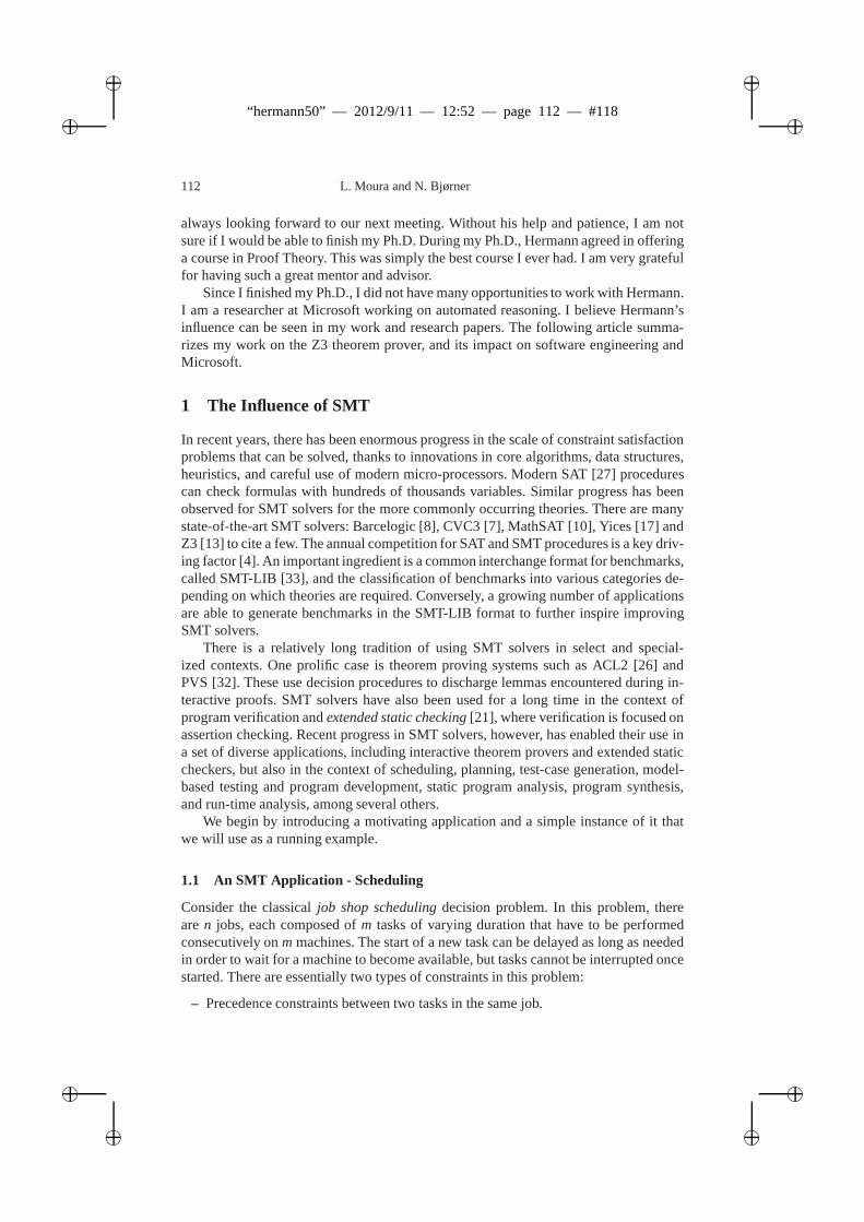
ii

“hermann50” — 2012/9/11 — 12:52 — page 112 — #118 ii

ii

ii

112 L. Moura and N. Bjørner

always looking forward to our next meeting. Without his helpand patience, I am notsure if I would be able to finish my Ph.D. During my Ph.D., Hermann agreed in offeringa course in Proof Theory. This was simply the best course I ever had. I am very gratefulfor having such a great mentor and advisor.

Since I finished my Ph.D., I did not have many opportunities towork with Hermann.I am a researcher at Microsoft working on automated reasoning. I believe Hermann’sinfluence can be seen in my work and research papers. The following article summa-rizes my work on the Z3 theorem prover, and its impact on software engineering andMicrosoft.

1 The Influence of SMT

In recent years, there has been enormous progress in the scale of constraint satisfactionproblems that can be solved, thanks to innovations in core algorithms, data structures,heuristics, and careful use of modern micro-processors. Modern SAT [27] procedurescan check formulas with hundreds of thousands variables. Similar progress has beenobserved for SMT solvers for the more commonly occurring theories. There are manystate-of-the-art SMT solvers: Barcelogic [8], CVC3 [7], MathSAT [10], Yices [17] andZ3 [13] to cite a few. The annual competition for SAT and SMT procedures is a key driv-ing factor [4]. An important ingredient is a common interchange format for benchmarks,called SMT-LIB [33], and the classification of benchmarks into various categories de-pending on which theories are required. Conversely, a growing number of applicationsare able to generate benchmarks in the SMT-LIB format to further inspire improvingSMT solvers.

There is a relatively long tradition of using SMT solvers in select and special-ized contexts. One prolific case is theorem proving systems such as ACL2 [26] andPVS [32]. These use decision procedures to discharge lemmasencountered during in-teractive proofs. SMT solvers have also been used for a long time in the context ofprogram verification andextended static checking[21], where verification is focused onassertion checking. Recent progress in SMT solvers, however, has enabled their use ina set of diverse applications, including interactive theorem provers and extended staticcheckers, but also in the context of scheduling, planning, test-case generation, model-based testing and program development, static program analysis, program synthesis,and run-time analysis, among several others.

We begin by introducing a motivating application and a simple instance of it thatwe will use as a running example.

1.1 An SMT Application - Scheduling

Consider the classicaljob shop schedulingdecision problem. In this problem, therearen jobs, each composed ofm tasks of varying duration that have to be performedconsecutively onm machines. The start of a new task can be delayed as long as neededin order to wait for a machine to become available, but tasks cannot be interrupted oncestarted. There are essentially two types of constraints in this problem:

– Precedence constraints between two tasks in the same job.

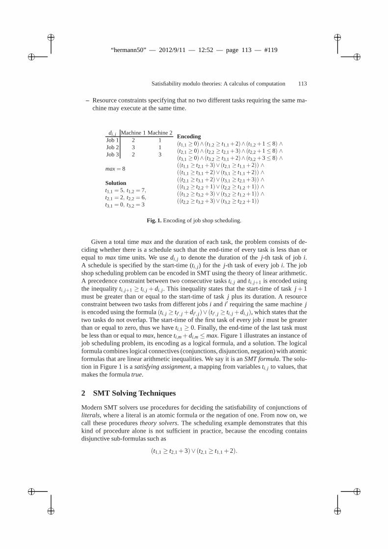
ii

“hermann50” — 2012/9/11 — 12:52 — page 113 — #119 ii

ii

ii

Satisfiability modulo theories: A calculus of computation 113

– Resource constraints specifying that no two different tasks requiring the same ma-chine may execute at the same time.

di, j Machine 1 Machine 2Job 1 2 1Job 2 3 1Job 3 2 3

max= 8

Solutiont1,1 = 5, t1,2 = 7,t2,1 = 2, t2,2 = 6,t3,1 = 0, t3,2 = 3

Encoding(t1,1 ≥ 0)∧ (t1,2 ≥ t1,1+2)∧ (t1,2+1≤ 8) ∧(t2,1 ≥ 0)∧ (t2,2 ≥ t2,1+3)∧ (t2,2+1≤ 8) ∧(t3,1 ≥ 0)∧ (t3,2 ≥ t3,1+2)∧ (t3,2+3≤ 8) ∧((t1,1 ≥ t2,1+3)∨ (t2,1 ≥ t1,1+2)) ∧((t1,1 ≥ t3,1+2)∨ (t3,1 ≥ t1,1+2)) ∧((t2,1 ≥ t3,1+2)∨ (t3,1 ≥ t2,1+3)) ∧((t1,2 ≥ t2,2+1)∨ (t2,2 ≥ t1,2+1)) ∧((t1,2 ≥ t3,2+3)∨ (t3,2 ≥ t1,2+1)) ∧((t2,2 ≥ t3,2+3)∨ (t3,2 ≥ t2,2+1))

Fig. 1.Encoding of job shop scheduling.

Given a total timemaxand the duration of each task, the problem consists of de-ciding whether there is a schedule such that the end-time of every task is less than orequal tomax time units. We usedi, j to denote the duration of thej-th task of jobi.A schedule is specified by the start-time (ti, j ) for the j-th task of every jobi. The jobshop scheduling problem can be encoded in SMT using the theory of linear arithmetic.A precedence constraint between two consecutive tasksti, j andti, j+1 is encoded usingthe inequalityti, j+1 ≥ ti, j +di, j . This inequality states that the start-time of taskj +1must be greater than or equal to the start-time of taskj plus its duration. A resourceconstraint between two tasks from different jobsi andi′ requiring the same machinejis encoded using the formula(ti, j ≥ ti′, j +di′, j)∨ (ti′, j ≥ ti, j +di, j), which states that thetwo tasks do not overlap. The start-time of the first task of every job i must be greaterthan or equal to zero, thus we haveti,1 ≥ 0. Finally, the end-time of the last task mustbe less than or equal tomax, henceti,m+di,m≤max. Figure 1 illustrates an instance ofjob scheduling problem, its encoding as a logical formula, and a solution. The logicalformula combines logical connectives (conjunctions, disjunction, negation) with atomicformulas that are linear arithmetic inequalities. We say itis anSMT formula. The solu-tion in Figure 1 is asatisfying assignment, a mapping from variablesti, j to values, thatmakes the formulatrue.

2 SMT Solving Techniques

Modern SMT solvers use procedures for deciding the satisfiability of conjunctions ofliterals, where a literal is an atomic formula or the negation of one. From now on, wecall these procedurestheory solvers. The scheduling example demonstrates that thiskind of procedure alone is not sufficient in practice, because the encoding containsdisjunctive sub-formulas such as

(t1,1≥ t2,1+3)∨ (t2,1≥ t1,1+2).

ii

“hermann50” — 2012/9/11 — 12:52 — page 114 — #120 ii

ii

ii


SMT solvers handle sub-formulas like this one by performingcase-analysis. Case-analysis is in the core of most automated deduction tools. Most SMT solvers rely onefficient satisfiability procedures for propositional logic (SAT solvers) for performingcase-analysis efficiently. A standard technique for integrating SAT solvers and theorysolvers has been developed [1,5,14,20,30]. We describe this technique next.

2.1 SAT - A Propositional Core

Propositional logic is a special case of predicate logic. Inpropositional logic, formu-las are built fromBoolean variables, calledatoms, and composed using logical con-nectives such as conjunction, disjunction and negation. The satisfiability problem forpropositional logic is famously known as an NP-complete problem [11], and thereforein principle computationally intractable. Yet, recent advances in efficient propositionallogic algorithms have moved the boundaries for what is intractable when it comes topractical applications [27].

Most successful SAT solvers are based on an approach calledsystematic search.The search space is a tree with each vertex representing a Boolean variable and the outedges representing the two choices (i.e.,true andfalse) for this variable. For a formulacontainingn Boolean variables, there are 2n leaves in this tree. Each path from theroot to a leaf corresponds to a truth assignment. Amodel is a truth assignment thatmakes the formulatrue. We also say the model satisfies the formula, and the formula issatisfiable. Most search based SAT solvers are based on the DPLL approach[12]. TheDPLL algorithm tries to build a model using three main operations:decide, propagateandbacktrack. The algorithm benefits from a restricted representation offormulas inconjunctive normal form (CNF). CNF formulas are restrictedto be conjunctions ofclauses, each clause is, in turn, a disjunction of literals. Recall that a literal is an atomor the negation of an atom. For example, the formula¬p∧ (p∨ q), is in CNF. Theoperationdecide heuristically chooses an unassigned atom and assigns it totrue orfalse. This operation is also calledbranchingor case-splitting. The operationpropagatededuces the consequences of a partial truth assignment using deduction rules. The mostwidely used deduction rule is theunit-clause rule, which states that if a clause has all butone literal assigned tofalseand the remaining literall is unassigned, then the only wayfor this clause to evaluate to true is to assignl to true. LetC be the clausep∨¬q∨¬r,andM the partial truth assignmentp 7→ false, r 7→ true, then the only way forC toevaluate totrue is by assigningq to false. Given a partial truth assignmentM and aclauseC in the CNF formula such that all literals ofC are assigned tofalsein M, thenthere is no way to extendM to a complete modelM′ that satisfies the given formula.We say this is aconflict, andC is aconflicting clause. A conflict indicates that some ofthe earlier decisions cannot lead to a truth assignment thatsatisfies the given formula,and the DPLL procedure mustbacktrack and try a different branch value. If aconflict isdetected and there are no decisions to backtrack, then the formula is unsatisfiable, thatis, it does not have a model. Many significant improvements ofthis basic procedurehave been proposed over the years. The main improvements are: lemma learning, non-chronological backtracking, efficient indexing techniquesfor applying the unit-clauserule andpreprocessingtechniques [27].

ii

“hermann50” — 2012/9/11 — 12:52 — page 115 — #121 ii

ii

ii


2.2 A Solver for Difference Arithmetic

The job shop scheduling decision problem can be solved by combining a SAT solverwith a theory solver fordifference arithmetic. Difference arithmetic is a fragment oflinear arithmetic where predicates are restricted to be of the form t − s≤ c, wheretands are variables andc a numeric constant such as 1 or 3. Every atom in Figure 1can be put into this form. For example, the atomt3,1 ≥ t2,1 + 3 is equivalent to theatomt2,1− t3,1 ≤ −3. For atoms of the forms≤ c ands≥ c, a special fresh variablez is used. We sayz is thezero variable, and these atoms are represented in differencearithmetic ass− z≤ c andz− s≤ −c respectively. For example, the atomt3,2+3≤ 8is represented in difference arithmetic ast3,2− z≤ 5. A set of difference arithmeticatoms can be checked very efficiently for satisfiability by searching for negative cyclesin weighted directed graphs. In the graph representation, each variable corresponds toa node, and an inequality of the formt− s≤ c corresponds to an edge froms to t withweight c. Figure 2 shows a subset of atoms (in difference arithmetic form) from ourexample in Figure 1, and the corresponding graph. The negative cycle, with weight−2,is shown by dashed lines. This cycle corresponds to the following schedule that cannotbe completed in 8 time units:

task 1/job 1→ task 1/job 2→ task 1/job 3→ task 2/job 3

Recall that the scheduling problem from Figure 1 is satisfiable, but it requires assigninga different combination of atoms to true.

z − t1,1≤ 0z − t2,1≤ 0z − t3,1≤ 0t3,2− z ≤ 5t3,1− t3,2≤−2t2,1− t3,1≤−3t1,1− t2,1≤−2 t3,2 t3,1

t2,1

t1,1

z

0

0

0-2

-3

-2

5

Fig. 2. Difference arithmetic example

2.3 Interfacing Solvers with SAT

We summarized how a theory solver for difference arithmeticworks. Now, we de-scribe how a SAT procedure interacts with this theory solver. The key idea is to cre-ate an abstraction that maps the atoms in an SMT formula into fresh Boolean vari-ablesp1, . . . , pn. For example, the formula¬(a≥ 3)∧ (a≥ 3∨a≥ 5) is translated into¬p1∧(p1∨ p2), where the atomsa≥ 3 anda≥ 5 are replaced by the Boolean variablesp1 and p2 respectively. The new abstract formula can then be processed by a regular

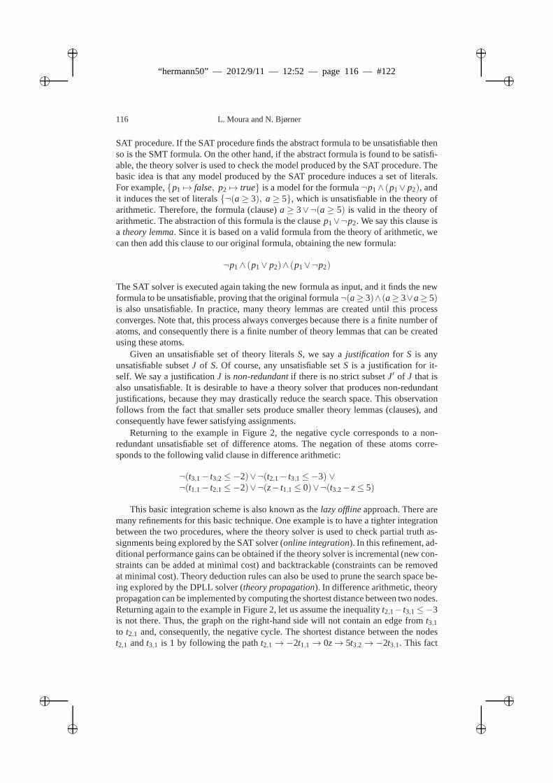
ii

“hermann50” — 2012/9/11 — 12:52 — page 116 — #122 ii

ii

ii


SAT procedure. If the SAT procedure finds the abstract formula to be unsatisfiable thenso is the SMT formula. On the other hand, if the abstract formula is found to be satisfi-able, the theory solver is used to check the model produced bythe SAT procedure. Thebasic idea is that any model produced by the SAT procedure induces a set of literals.For example,p1 7→ false, p2 7→ true is a model for the formula¬p1∧ (p1∨ p2), andit induces the set of literals¬(a≥ 3), a≥ 5, which is unsatisfiable in the theory ofarithmetic. Therefore, the formula (clause)a≥ 3∨¬(a≥ 5) is valid in the theory ofarithmetic. The abstraction of this formula is the clausep1∨¬p2. We say this clause isa theory lemma. Since it is based on a valid formula from the theory of arithmetic, wecan then add this clause to our original formula, obtaining the new formula:

¬p1∧ (p1∨ p2)∧ (p1∨¬p2)

The SAT solver is executed again taking the new formula as input, and it finds the newformula to be unsatisfiable, proving that the original formula¬(a≥ 3)∧(a≥ 3∨a≥ 5)is also unsatisfiable. In practice, many theory lemmas are created until this processconverges. Note that, this process always converges because there is a finite number ofatoms, and consequently there is a finite number of theory lemmas that can be createdusing these atoms.

Given an unsatisfiable set of theory literalsS, we say ajustification for S is anyunsatisfiable subsetJ of S. Of course, any unsatisfiable setS is a justification for it-self. We say a justificationJ is non-redundantif there is no strict subsetJ′ of J that isalso unsatisfiable. It is desirable to have a theory solver that produces non-redundantjustifications, because they may drastically reduce the search space. This observationfollows from the fact that smaller sets produce smaller theory lemmas (clauses), andconsequently have fewer satisfying assignments.

Returning to the example in Figure 2, the negative cycle corresponds to a non-redundant unsatisfiable set of difference atoms. The negation of these atoms corre-sponds to the following valid clause in difference arithmetic:

¬(t3,1− t3,2≤−2)∨¬(t2,1− t3,1≤−3) ∨¬(t1,1− t2,1≤−2)∨¬(z− t1,1≤ 0)∨¬(t3,2− z≤ 5)

This basic integration scheme is also known as thelazy offlineapproach. There aremany refinements for this basic technique. One example is to have a tighter integrationbetween the two procedures, where the theory solver is used to check partial truth as-signments being explored by the SAT solver (online integration). In this refinement, ad-ditional performance gains can be obtained if the theory solver is incremental (new con-straints can be added at minimal cost) and backtrackable (constraints can be removedat minimal cost). Theory deduction rules can also be used to prune the search space be-ing explored by the DPLL solver (theory propagation). In difference arithmetic, theorypropagation can be implemented by computing the shortest distance between two nodes.Returning again to the example in Figure 2, let us assume the inequalityt2,1− t3,1≤−3is not there. Thus, the graph on the right-hand side will not contain an edge fromt3,1to t2,1 and, consequently, the negative cycle. The shortest distance between the nodest2,1 andt3,1 is 1 by following the patht2,1→−2t1,1→ 0z→ 5t3,2→−2t3,1. This fact

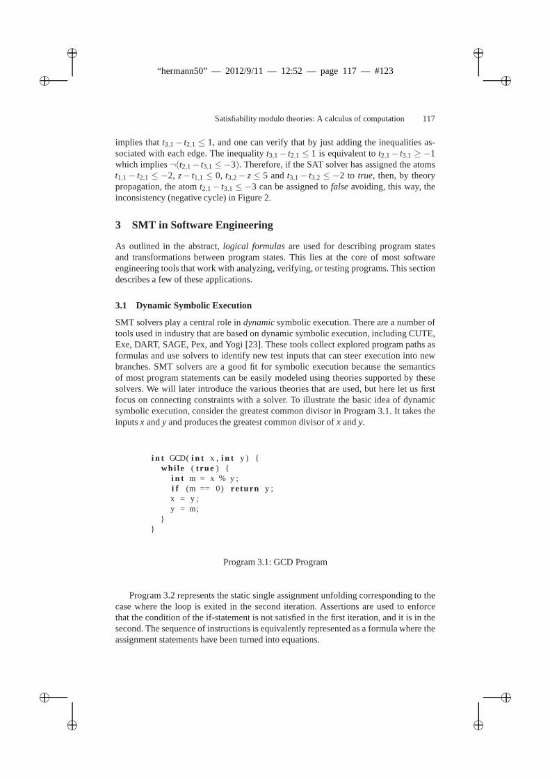
ii

“hermann50” — 2012/9/11 — 12:52 — page 117 — #123 ii

ii

ii


implies thatt3,1− t2,1 ≤ 1, and one can verify that by just adding the inequalities as-sociated with each edge. The inequalityt3,1− t2,1 ≤ 1 is equivalent tot2,1− t3,1 ≥ −1which implies¬(t2,1− t3,1 ≤−3). Therefore, if the SAT solver has assigned the atomst1,1− t2,1 ≤ −2, z− t1,1 ≤ 0, t3,2− z≤ 5 andt3,1− t3,2 ≤ −2 to true, then, by theorypropagation, the atomt2,1− t3,1 ≤ −3 can be assigned tofalseavoiding, this way, theinconsistency (negative cycle) in Figure 2.

3 SMT in Software Engineering

As outlined in the abstract,logical formulasare used for describing program statesand transformations between program states. This lies at the core of most softwareengineering tools that work with analyzing, verifying, or testing programs. This sectiondescribes a few of these applications.

3.1 Dynamic Symbolic Execution

SMT solvers play a central role indynamicsymbolic execution. There are a number oftools used in industry that are based on dynamic symbolic execution, including CUTE,Exe, DART, SAGE, Pex, and Yogi [23]. These tools collect explored program paths asformulas and use solvers to identify new test inputs that cansteer execution into newbranches. SMT solvers are a good fit for symbolic execution because the semanticsof most program statements can be easily modeled using theories supported by thesesolvers. We will later introduce the various theories that are used, but here let us firstfocus on connecting constraints with a solver. To illustrate the basic idea of dynamicsymbolic execution, consider the greatest common divisor in Program 3.1. It takes theinputsx andy and produces the greatest common divisor ofx andy.

i n t GCD( i n t x , i n t y ) whi le ( t rue )

i n t m = x % y ;i f (m == 0) re tu rn y ;x = y ;y = m;

Program 3.1: GCD Program

Program 3.2 represents the static single assignment unfolding corresponding to thecase where the loop is exited in the second iteration. Assertions are used to enforcethat the condition of the if-statement is not satisfied in thefirst iteration, and it is in thesecond. The sequence of instructions is equivalently represented as a formula where theassignment statements have been turned into equations.

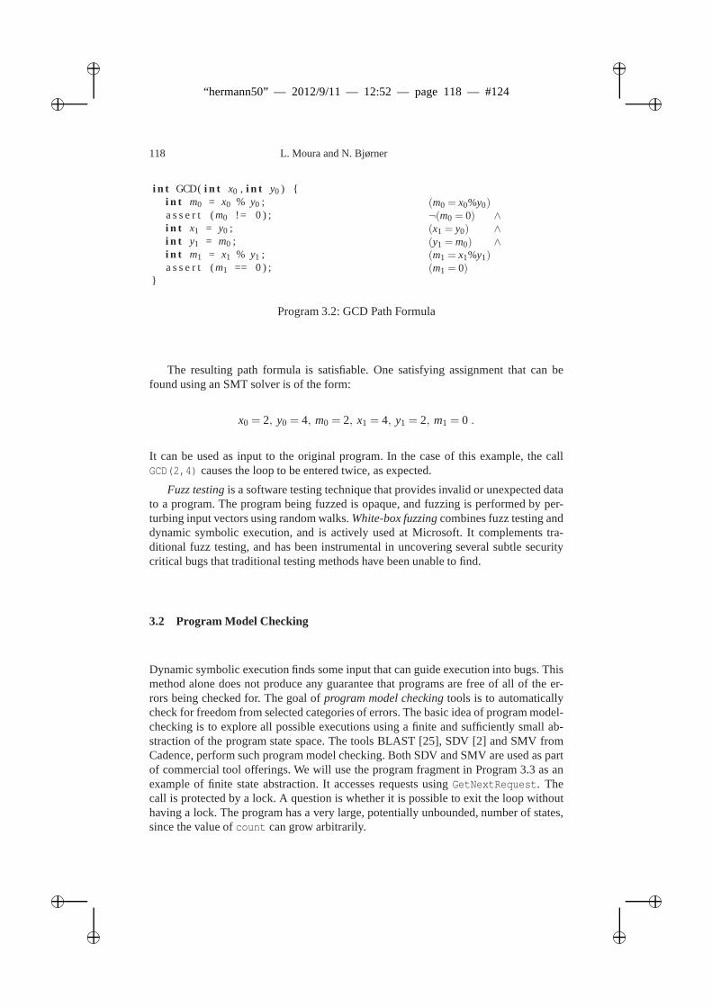
ii

“hermann50” — 2012/9/11 — 12:52 — page 118 — #124 ii

ii

ii


i n t GCD( i n t x0 , i n t y0 ) i n t m0 = x0 % y0 ;a s s e r t (m0 != 0 ) ;i n t x1 = y0 ;i n t y1 = m0 ;i n t m1 = x1 % y1 ;a s s e r t (m1 == 0 ) ;

(m0 = x0%y0)¬(m0 = 0) ∧(x1 = y0) ∧(y1 = m0) ∧(m1 = x1%y1)(m1 = 0)

Program 3.2: GCD Path Formula

The resulting path formula is satisfiable. One satisfying assignment that can befound using an SMT solver is of the form:

x0 = 2, y0 = 4, m0 = 2, x1 = 4, y1 = 2, m1 = 0 .

It can be used as input to the original program. In the case of this example, the callGCD(2,4) causes the loop to be entered twice, as expected.

Fuzz testingis a software testing technique that provides invalid or unexpected datato a program. The program being fuzzed is opaque, and fuzzingis performed by per-turbing input vectors using random walks.White-box fuzzingcombines fuzz testing anddynamic symbolic execution, and is actively used at Microsoft. It complements tra-ditional fuzz testing, and has been instrumental in uncovering several subtle securitycritical bugs that traditional testing methods have been unable to find.

3.2 Program Model Checking

Dynamic symbolic execution finds some input that can guide execution into bugs. Thismethod alone does not produce any guarantee that programs are free of all of the er-rors being checked for. The goal ofprogram model checkingtools is to automaticallycheck for freedom from selected categories of errors. The basic idea of program model-checking is to explore all possible executions using a finiteand sufficiently small ab-straction of the program state space. The tools BLAST [25], SDV [2] and SMV fromCadence, perform such program model checking. Both SDV and SMV are used as partof commercial tool offerings. We will use the program fragment in Program 3.3 as anexample of finite state abstraction. It accesses requests using GetNextRequest. Thecall is protected by a lock. A question is whether it is possible to exit the loop withouthaving a lock. The program has a very large, potentially unbounded, number of states,since the value ofcount can grow arbitrarily.

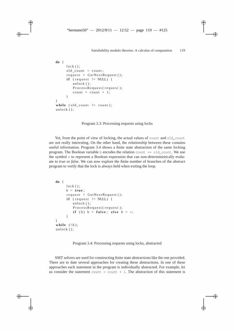
ii

“hermann50” — 2012/9/11 — 12:52 — page 119 — #125 ii

ii

ii


do l ock ( ) ;o l d_coun t = coun t ;r e q u e s t = GetNextRequest ( ) ;i f ( r e q u e s t != NULL)

un lock ( ) ;P r o c e s s R e q u e s t ( r e q u e s t ) ;coun t = coun t + 1 ;

whi le ( o l d_coun t != coun t ) ;un lock ( ) ;

Program 3.3: Processing requests using locks

Yet, from the point of view of locking, the actual values ofcount andold_countare not really interesting. On the other hand, therelationshipbetween these containsuseful information. Program 3.4 shows a finite state abstraction of the same lockingprogram. The Boolean variableb encodes the relationcount == old_count. We usethe symbol∗ to represent a Boolean expression that can non-deterministically evalu-ate totrue or false. We can now explore the finite number of branches of the abstractprogram to verify that the lock is always held when exiting the loop.

do l ock ( ) ;b = t rue ;r e q u e s t = GetNextRequest ( ) ;i f ( r e q u e s t != NULL)

un lock ( ) ;P r o c e s s R e q u e s t ( r e q u e s t ) ;i f ( b ) b = f a l s e ; e l s e b = ∗ ;

whi le ( ! b ) ;un lock ( ) ;

Program 3.4: Processing requests using locks, abstracted

SMT solvers are used for constructing finite state abstractions like the one provided.There are to date several approaches for creating these abstractions. In one of theseapproaches each statement in the program is individually abstracted. For example, letus consider the statementcount = count + 1. The abstraction of this statement is

ii

“hermann50” — 2012/9/11 — 12:52 — page 120 — #126 ii

ii

ii


essentially a relation between the current and new values ofthe Boolean variableb.SMT solvers are used to compute this relation by proving theorems such as

count == old_count→ count+1 != old_count

which is dual to checking unsatisfiability of the negation:

count == old_count ∧ count+1 == old_count.

The theorem says that if the current value ofb is true, then after executing the statementcount = count + 1 it will be false. Note that ifb is false, then neither of the followingconjectures is valid.

count != old_count→ count+1 == old_count

count != old_count→ count+1 != old_count

In both cases, an SMT solver will produce a model for the negation of the conjecture.Therefore, the model is acounter-examplefor the conjecture. Therefore, when the cur-rent value ofb is false, nothing can be said about its value after the execution of thestatement. The result of these three proof attempts is then used to replace the statementcount = count + 1; by if (b) b = false; else b = *;. A finite state modelchecker can now be used on the Boolean program. It will establish thatb is alwaystruewhen control reaches this statement, verifying that calls to lock() are balanced withcalls tounlock() in the original program.

3.3 Static Program Analysis

Static program analysis tools work in a similar way as dynamic symbolic executiontools. They also check feasibility of program paths. On the other hand they never requireexecuting programs and they can analyze software librariesand utilities independentlyof how they are used. One advantage of using modern SMT solvers in static programanalysis is that SMT solvers nowadays accurately capture the semantics of most basicoperations used by mainstream programming languages. We use the program in Pro-gram 3.5 to illustrate the need for static program analysis to use bit-precise reasoning.The program searches for an index in a sorted arrayarr that contains a key.

The assert statement is apre-condition, for the procedure. It restricts the inputto fall within the bounds of the arrayarr. The program performs several operationsinvolving arithmetic, so a theory and corresponding solverthat understands arithmeticappears to be a good match. It is important, however, to take into account that languages,such as Java, C# and C/C++ all use fixed-width bit-vectors as the representation forvalues of typeint. This means that the accurate theory forint is two-complementsmodular arithmetic. Assuming a bit-width of 32 bits, the maximal positive 32-bit integeris 231− 1 and the smallest negative 32-bit integer is−231. If both low andhigh are230, low + high evaluates to 231, which is treated as the negative number−231. Thepresumed assertion 0≤mid< high therefore does not hold.

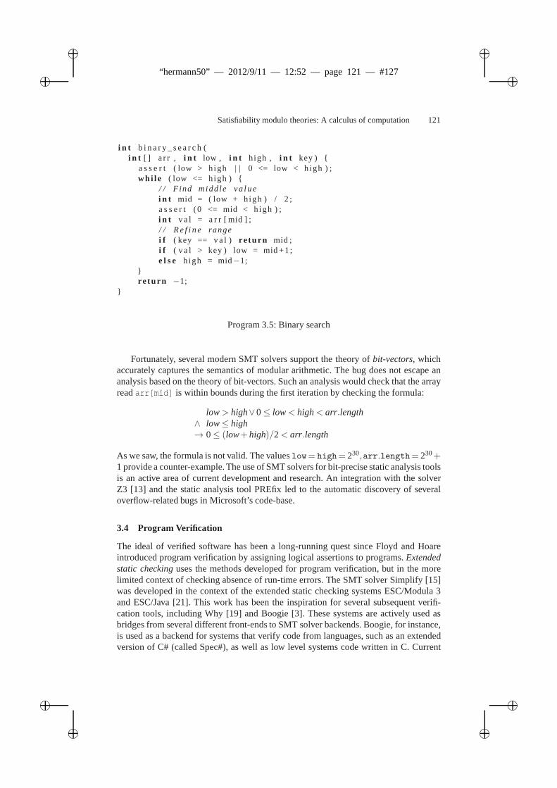
ii

“hermann50” — 2012/9/11 — 12:52 — page 121 — #127 ii

ii

ii


i n t b i n a r y _ s e a r c h (i n t [ ] a r r , i n t low , i n t high , i n t key )

a s s e r t ( low > high | | 0 <= low < high ) ;whi le ( low <= high )

/ / F ind midd le va luei n t mid = ( low + high ) / 2 ;a s s e r t (0 <= mid < high ) ;i n t v a l = a r r [ mid ] ;/ / R e f i n e rangei f ( key == v a l ) re tu rn mid ;i f ( v a l > key ) low = mid +1;e l s e high = mid−1;

re tu rn −1;

Program 3.5: Binary search

Fortunately, several modern SMT solvers support the theoryof bit-vectors, whichaccurately captures the semantics of modular arithmetic. The bug does not escape ananalysis based on the theory of bit-vectors. Such an analysis would check that the arrayreadarr[mid] is within bounds during the first iteration by checking the formula:

low> high∨0≤ low< high< arr.length∧ low≤ high→ 0≤ (low+high)/2< arr.length

As we saw, the formula is not valid. The valueslow= high= 230,arr.length= 230+1 provide a counter-example. The use of SMT solvers for bit-precise static analysis toolsis an active area of current development and research. An integration with the solverZ3 [13] and the static analysis tool PREfix led to the automatic discovery of severaloverflow-related bugs in Microsoft’s code-base.

3.4 Program Verification

The ideal of verified software has been a long-running quest since Floyd and Hoareintroduced program verification by assigning logical assertions to programs.Extendedstatic checkinguses the methods developed for program verification, but in the morelimited context of checking absence of run-time errors. TheSMT solver Simplify [15]was developed in the context of the extended static checkingsystems ESC/Modula 3and ESC/Java [21]. This work has been the inspiration for several subsequent verifi-cation tools, including Why [19] and Boogie [3]. These systems are actively used asbridges from several different front-ends to SMT solver backends. Boogie, for instance,is used as a backend for systems that verify code from languages, such as an extendedversion of C# (called Spec#), as well as low level systems code written in C. Current

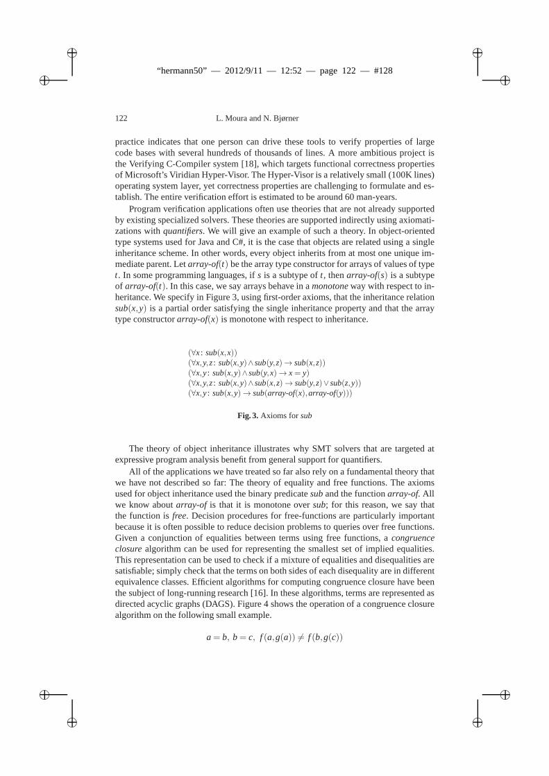
ii

“hermann50” — 2012/9/11 — 12:52 — page 122 — #128 ii

ii

ii


practice indicates that one person can drive these tools to verify properties of largecode bases with several hundreds of thousands of lines. A more ambitious project isthe Verifying C-Compiler system [18], which targets functional correctness propertiesof Microsoft’s Viridian Hyper-Visor. The Hyper-Visor is a relatively small (100K lines)operating system layer, yet correctness properties are challenging to formulate and es-tablish. The entire verification effort is estimated to be around 60 man-years.

Program verification applications often use theories that are not already supportedby existing specialized solvers. These theories are supported indirectly using axiomati-zations withquantifiers. We will give an example of such a theory. In object-orientedtype systems used for Java and C#, it is the case that objects are related using a singleinheritance scheme. In other words, every object inherits from at most one unique im-mediate parent. Letarray-of(t) be the array type constructor for arrays of values of typet. In some programming languages, ifs is a subtype oft, thenarray-of(s) is a subtypeof array-of(t). In this case, we say arrays behave in amonotoneway with respect to in-heritance. We specify in Figure 3, using first-order axioms,that the inheritance relationsub(x,y) is a partial order satisfying the single inheritance property and that the arraytype constructorarray-of(x) is monotone with respect to inheritance.

(∀x: sub(x,x))(∀x,y,z: sub(x,y)∧sub(y,z)→ sub(x,z))(∀x,y: sub(x,y)∧sub(y,x)→ x= y)(∀x,y,z: sub(x,y)∧sub(x,z)→ sub(y,z)∨sub(z,y))(∀x,y: sub(x,y)→ sub(array-of(x),array-of(y)))

Fig. 3. Axioms for sub

The theory of object inheritance illustrates why SMT solvers that are targeted atexpressive program analysis benefit from general support for quantifiers.

All of the applications we have treated so far also rely on a fundamental theory thatwe have not described so far: The theory of equality and free functions. The axiomsused for object inheritance used the binary predicatesuband the functionarray-of. Allwe know aboutarray-of is that it is monotone oversub; for this reason, we say thatthe function isfree. Decision procedures for free-functions are particularlyimportantbecause it is often possible to reduce decision problems to queries over free functions.Given a conjunction of equalities between terms using free functions, acongruenceclosurealgorithm can be used for representing the smallest set of implied equalities.This representation can be used to check if a mixture of equalities and disequalities aresatisfiable; simply check that the terms on both sides of eachdisequality are in differentequivalence classes. Efficient algorithms for computing congruence closure have beenthe subject of long-running research [16]. In these algorithms, terms are represented asdirected acyclic graphs (DAGS). Figure 4 shows the operation of a congruence closurealgorithm on the following small example.

a= b, b= c, f (a,g(a)) 6= f (b,g(c))

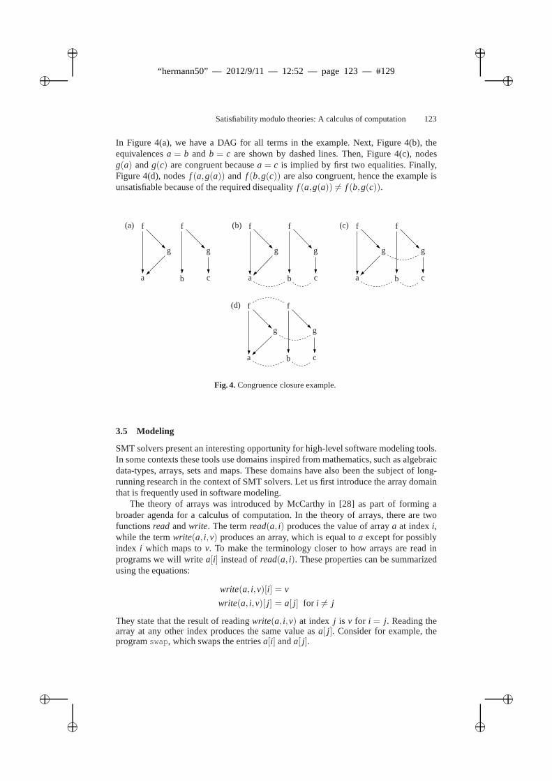
ii

“hermann50” — 2012/9/11 — 12:52 — page 123 — #129 ii

ii

ii


In Figure 4(a), we have a DAG for all terms in the example. Next, Figure 4(b), theequivalencesa = b and b = c are shown by dashed lines. Then, Figure 4(c), nodesg(a) andg(c) are congruent becausea = c is implied by first two equalities. Finally,Figure 4(d), nodesf (a,g(a)) and f (b,g(c)) are also congruent, hence the example isunsatisfiable because of the required disequalityf (a,g(a)) 6= f (b,g(c)).

(a) f

g

a

f

g

b c

(b) f

g

a

f

g

b c

(c) f

g

a

f

g

b c

(d) f

g

a

f

g

b c

Fig. 4. Congruence closure example.

3.5 Modeling

SMT solvers present an interesting opportunity for high-level software modeling tools.In some contexts these tools use domains inspired from mathematics, such as algebraicdata-types, arrays, sets and maps. These domains have also been the subject of long-running research in the context of SMT solvers. Let us first introduce the array domainthat is frequently used in software modeling.

The theory of arrays was introduced by McCarthy in [28] as part of forming abroader agenda for a calculus of computation. In the theory of arrays, there are twofunctionsread andwrite. The termread(a, i) produces the value of arraya at indexi,while the termwrite(a, i,v) produces an array, which is equal toa except for possiblyindex i which maps tov. To make the terminology closer to how arrays are read inprograms we will writea[i] instead ofread(a, i). These properties can be summarizedusing the equations:

write(a, i,v)[i] = v

write(a, i,v)[ j] = a[ j] for i 6= j

They state that the result of readingwrite(a, i,v) at index j is v for i = j. Reading thearray at any other index produces the same value asa[ j]. Consider for example, theprogramswap, which swaps the entriesa[i] anda[ j].

ii

“hermann50” — 2012/9/11 — 12:52 — page 124 — #130 ii

ii

ii


void swap(int[] a, int i, int j)

int tmp = a[i];a[i] = a[j];a[j] = tmp;

The statement thata[i] contains the previous value ofa[j] can be expressed as

a[ j] = write(write(a, i,a[ j]), j,a[i])[i]

We here summarize a few of the areas in the context of softwaremodeling whereSMT solvers are used.Model programsare behavioral specifications that can be de-scribed succinctly and at a high-level of abstraction. These descriptions are state ma-chines that use abstract domains. SMT solvers are used to perform bounded model-checkingof such descriptions. The main idea of bounded model-checking is to explorea bounded symbolic execution of a program or model. Thus, given a bound, such as 17,the transitions of the state machines are unrolled into a logical formula that describes allpossible executions using 17 steps.Model-based designsuse high-level languages fordescribing software systems. Implementations are derivedby refinements. Modelinglanguages present an advantage as they allow exploring a design space without com-mitting all design decisions up front. SMT solvers play various roles in model-baseddesigns. They are used for type-checking designs and they are useful in the search fordifferent consistent choices in a design space.Model-based testinguses high-level mod-els of software systems, including network protocols, to derive test oracles. SMT solvershave been used in this context for exploring the models usinga symbolic execution andsearch. Model-based testing is used on a large scale at Microsoft in the context of thedisclosure and documentation of Microsoft network protocols [24]. The model-basedtools use SMT solvers for generating combinations of test inputs as well as symbolicexploration of models.

4 Combining Theory Solvers

The combination of several theory solvers is one of the fundamental problems for SMTsolvers. As the previous sections illustrated, applications ranging from test-case genera-tion to software verification, require a combination of theories. For example, a combina-tion of arithmetic and arrays is needed to reason about Program 3.5. Many fundamentalquestions arise: is the union of two decidable theories still decidable? Is the union con-sistent? How can we combine different theory solvers? In general, this is a very difficultproblem. However, useful special cases have good answers. An established frameworkfor combining theory solvers is known as the Nelson-Oppen combination method [29].This framework assumes theories do not share symbols, except the equality relation. Inthis case, we say the theories aredisjoint. For example, the theory of linear arithmeticuses the constants, functions and relations+,0,1,≤, and the theory of arrays uses thedisjoint setread,write. It should also be possible to merge the models from the two the-ory solvers into one without contradicting assumptions onetheory may have about thesize of models. A condition that guarantees that solutions can be combined is known as

ii

“hermann50” — 2012/9/11 — 12:52 — page 125 — #131 ii

ii

ii


stable infiniteness: a theoryT is stably infinite if whenever a (quantifier-free) formulais satisfiable inT, then it is satisfiable in a model ofT with an infinite universe (size).

In many practical cases, thedisjointnessandstable infinitenessconditions are easyto satisfy when combining theory solvers. Of course not all theory combinations satisfythese side conditions and more recent research has been devoted to generalizing theframework where signatures are non-disjoint or where theories are non-stably infinite[22,34].

4.1 Convexity, Complexity and Propositional Search

An important notion in the context of combining theories isconvexity. A theory iscon-vexif for all sets of ground literalsSand all sets of equalities between variablesE if Simplies the disjunction ofE, then it also implies at least one equation ofE. For example,the theory of free functions is convex, but difference arithmetic over integers is not.

Convexity plays an important role in operations research aswell as in SMT be-cause efficient, polynomial time, techniques exist for combining solvers for convextheories [31]. The key property is that the equalities can bededuced, without back-tracking, instead ofguessed, with backtracking. Non-convex theories on the other handincur a potential exponential time combination overhead. It therefore becomes an ad-ditional requirement on solvers in the Nelson-Oppen combination framework that theyalso indicate which variables are implied equal based on a set of assertions.

The advent of efficient methods for propositional search allowed viewing the theorycombination problem from a different perspective. Thedelayed theory combination[9]method creates one atomic equality for every pair of variables shared between solvers.These additional atomic equalities are assigned totrue or false by a SAT solver. Inthis approach, the SAT solver is used to guess the correct equalities between sharedvariables. If the theory solvers disagree with the (dis)equalities, then they cause theSAT solver to backtrack. This approach is oblivious to whether theories are convexor not. Delayed theory combination potentially pollutes the search space with a largenumber of mostly useless new atomic equalities. TheModel-based theory combinationmethod [13] allows a more efficient handling of convex and non-convex theories: it asksthe solvers for amodel. The atomic equality predicates are only created if two sharedvariables are equal in a model.

5 Conclusions

In the last few years, SMT has become the core engine underlying a wide range ofpowerful technologies. SMT is an active and exciting area ofresearch with many prac-tical applications. We have presented some of the basic ideas, but we did not cover alarge number of details and heuristics. There are also several other exciting recent topicsin SMT research [6], including proof checking, integrationwith first-order quantifiers,quantifier elimination methods, and extraction of so-called Craig interpolant formulasfrom proofs. There are several existing and emerging applications we have not covered.These include sophisticated run-time analysis of real-time embedded systems, estimat-ing asymptotic run-time bounds of programs, and program synthesis.

ii

“hermann50” — 2012/9/11 — 12:52 — page 126 — #132 ii

ii

ii


SMT solving technologies are already making a profound impact on a number ofapplication areas and the application areas are providing rich feedback in terms of ex-perimental data. Recent progress has relied heavily on experimental evaluations thathave uncovered new theoretical challenges. The theoretical challenges include betterrepresentations and algorithms, efficient methods for combining procedures, theoriesfor quantifier reasoning, and various extensions to the basic search method.

References

1. G. Audemard, P. Bertoli, A. Cimatti, A. Kornilowicz, and R. Sebastiani. A sat based approachfor solving formulas over boolean and linear mathematical propositions. InCADE, volume2392 ofLNCS. Springer, 2002.

2. T. Ball and S. K. Rajamani. The SLAM project: debugging system software via static anal-ysis. SIGPLAN Not., 37(1):1–3, 2002.

3. M. Barnett, K. R. M. Leino, and W. Schulte. The Spec# Programming System: An Overview.In CASSIS 2004, LNCS 3362, pages 49–69. Springer, 2005.

4. C. Barrett, L. de Moura, and A. Stump. Design and Results ofthe 1st Satisfiability ModuloTheories Competition.JAR, 2005.

5. C. Barrett, D. Dill, and A. Stump. Checking satisfiabilityof first-order formulas by incre-mental translation to SAT. InCAV, 2002.

6. C. Barrett, R. Sebastiani, S. A. Seshia, and C. Tinelli.Satisfiability Modulo Theories, volume185 ofFrontiers in Artificial Intelligence and Applications, chapter 26, pages 825–885. IOSPress, February 2009.

7. C. Barrett and C. Tinelli. CVC3. In W. Damm and H. Hermanns,editors,Proceedings ofthe19th International Conference on Computer Aided Verification (CAV ’07), volume 4590of LNCS, pages 298–302. Springer-Verlag, July 2007. Berlin, Germany.

8. M. Bofill, R. Nieuwenhuis, A. Oliveras, E. Rodríguez Carbonell, and A. Rubio. The Barcel-ogic SMT Solver. In A. Gupta and S. Malik, editors,20th International Conference on Com-puter Aided Verification, CAV’08, volume 5123 ofLNCS, pages 294–298. Springer, 2008.

9. M. Bozzano, R. Bruttomesso, A. Cimatti, T. A. Junttila, S.Ranise, P. van Rossum, and R. Se-bastiani. Efficient satisfiability modulo theories via delayed theory combination. In K. Etes-sami and S. K. Rajamani, editors,CAV, volume 3576 ofLNCS, pages 335–349. Springer,2005.

10. R. Bruttomesso, A. Cimatti, A. Franzén, A. Griggio, and R. Sebastiani. The MathSAT 4 SMTSolver. InProceedings of the18th International Conference on Computer Aided Verification(CAV ’08), volume 5123 ofLNCS. Springer-Verlag, 2008.

11. S. A. Cook. The complexity of theorem-proving procedures. In STOC, pages 151–158.ACM, 1971.

12. M. Davis, G. Logemann, , and D. Loveland. A machine program for theorem proving.Communications of the ACM, 1962.

13. L. de Moura and N. Bjørner. Z3: An Efficient SMT Solver. In C. R. Ramakrishnan andJ. Rehof, editors,TACAS 08, volume 4963 ofLNCS. Springer, 2008.

14. L. de Moura and H. Rueß. Lemmas on Demand for Satisfiability Solvers. InSAT, 2002.15. D. Detlefs, G. Nelson, and J. B. Saxe. Simplify: a theoremprover for program checking.J.

ACM, 52(3):365–473, 2005.16. P. J. Downey, R. Sethi, and R. E. Tarjan. Variations on thecommon subexpression problem.

J. ACM, 27(4):758–771, 1980.17. B. Dutertre and L. de Moura. A Fast Linear-Arithmetic Solver for DPLL(T). InProceedings

of the 16th International Conference on Computer Aided Verification (CAV ’06), volume4144 ofLNCS, pages 81–94. Springer-Verlag, 2006.

ii

“hermann50” — 2012/9/11 — 12:52 — page 127 — #133 ii

ii

ii


18. E. Cohen and M. Dahlweid and M. Hillebrand and D. Leinenbach and M. Moskal and T.Santen and W. Schulte and S. Tobies. VCC: A Practical System for Verifying Concurrent C.In TPHOL, 2009.

19. J.-C. Filliâtre. Why: a multi-language multi-prover verification tool. Technical Report 1366,LRI, Université Paris Sud, 2003.

20. C. Flanagan, R. Joshi, X. Ou, and J. B. Saxe. Theorem Proving Using Lazy Proof Explica-tion. In CAV, 2003.

21. C. Flanagan, K. R. M. Leino, M. Lillibridge, G. Nelson, J.B. Saxe, and R. Stata. ExtendedStatic Checking for Java. InPLDI, pages 234–245, 2002.

22. S. Ghilardi, E. Nicolini, and D. Zucchelli. A comprehensive framework for combined deci-sion procedures. In Bernhard Gramlich, editor,FroCos, volume 3717 ofLNCS, pages 1–30.Springer, 2005.

23. P. Godefroid, J. de Halleux, A. V. Nori, S. K. Rajamani, W.Schulte, N. Tillmann, and M. Y.Levin. Automating Software Testing Using Program Analysis. IEEE Software, 25(5):30–37,2008.

24. W. Grieskamp, N. Kicillof, D. MacDonald, A. Nandan, K. Stobie, and F. L. Wurden. Model-Based Quality Assurance of Windows Protocol Documentation. In ICST, pages 502–506.IEEE Computer Society, 2008.

25. T. A. Henzinger, R. Jhala, R. Majumdar, and G. Sutre. Software verification with blast. InSPIN, pages 235–239, 2003.

26. M. Kaufmann, P. Manolios, and J. S. Moore.Computer-Aided Reasoning: An Approach.Kluwer Academic, June 2000.

27. S. Malik and L. Zhang. Boolean satisfiability from theoretical hardness to practical success.Commun. ACM, 52(8):76–82, 2009.

28. J. McCarthy. Towards a mathematical science of computation. In IFIP Congress, pages21–28, 1962.

29. G. Nelson and D. C. Oppen. Simplification by cooperating decision procedures.ACMTransactions on Programming Languages and Systems, 1(2):245–257, 1979.

30. R. Nieuwenhuis, A. Oliveras, and C. Tinelli. Solving SATand SAT Modulo Theories: Froman abstract Davis–Putnam–Logemann–Loveland procedure toDPLL(T). J. ACM, 53(6),2006.

31. D. C. Oppen. Complexity, convexity and combinations of theories. Theor. Comput. Sci.,12:291–302, 1980.

32. S. Owre, J. M. Rushby, and N. Shankar. PVS: A prototype verification system. In11thInternational Conference on Automated Deduction (CADE), June 1992.

33. S. Ranise and C. Tinelli. The Satisfiability Modulo Theories Library (SMT-LIB).www.SMT-LIB.org, 2006.

34. C. Tinelli and C. G. Zarba. Combining nonstably infinite theories. J. Autom. Reasoning,34(3):209–238, 2005.

ii

“hermann50” — 2012/9/11 — 12:52 — page 128 — #134 ii

ii

ii

A discussion on compressing proofs throughproof-theoretical techniques

Edward Hermann Haeusler1 and Vaston Gonçalves da Costa2

1 Departamento de Informática, Pontifícia Universidade Católica do Rio de Janeiro, Av.Marquês de São Vicente, 225. CEP.: 24130-000. Rio de Janeiro-RJ, Brasil.

E-mail:[email protected] Departamento de Ciência da Computação, Universidade Federal de Goiás - Catalão, Av. Dr.

Lamartine P. de Avelar, 1120. CEP.: 75.704-020. Catalão-GO, Brasil.E-mail:[email protected]

Abstract. Sometimes during the elaboration of a paper we face some problemsinvolving the proof of the results. That is the case of this article.The intent was present two methods to compact proofs. The first, a vertical one,that finds the most general unifier (mgu) between two parallelbranches of a proof.The second, a horizontal one, consists in replacing, consistently, a minimal (non-atomic) formula in a branch of the proof for a new variable. Asthe reader willsee, this is not a complete article, adjust e complementations must be made.

Preamble

The goal in sending this "article" to this book is to present what I consider to be thegreatest contribution that Hermann has given to me: "To learn from my mistakes andnot be ashamed of them".

We did a lot of thinking on the assertions presented is this text. However, we neverfinished them properly.

This is a work in progress... one in so many.Hermann was my PhD adviser, my postdoctoral supervisor, my ANUBIS research

project coordinator and, since 2002, a great friend.In the beginning I didn’t agree with Hermann’s way of advising his students... To-

day, I do the same with my students, expecting them to be grateful to me as I am tohim.

I would like to thank Hermann for trusting on me, all this years, and for the valuablelessons and advices.

Happy Birthday Hermann! You can always count on me.

1 Introduction

There are some worth of mentioning interconnections between Proof-Theory and Com-puter Science. One can mention programming languages typing disciplines, programgeneration by means of extracting computational content from logical proofs, compu-tational complexity and estimations on the size of Normal Proofs in certain systems of

ii

“hermann50” — 2012/9/11 — 12:52 — page 129 — #135 ii

ii

ii

Compressing proofs through proof-theoretical techniques129

logic, and more. On the other hand, it is quite well-known thecomputational analysishierarchy provided by logical decision problems. For each complexity class one canprovide a complete problem stated in logical form. Some of these problems concernsvalidity of a formula in a given logic, and hence implies proof existence. It is well-known that the size of a proof is a question of theoretical as well practical relevance.

Short proofs are the proof-theoretical counterpart of feasible computation. A shortproof is a proof that has polynomial sized proof length regarded its conclusion length.The length of a formula or a proof is the number of symbols usedto write them down.The fact that every classical tautology possesses a short proof implies thatCoNP= NP,and the existence of tautologies not possessing this property in any proof-system im-pliesCoNP 6= NP, and henceNP 6= P, according Cook’s Theorem. For intuitionisticlogic the existence of short proofs for each tautology impliesNP= PSPACE. More-over, Seldin has shown that in the Natural Deduction (ND) proof system, any classicaltautology can be proved with at most one application of the classical absurdity rule.This fact is proved by providing a transformation from an arbitrary ND proof ofα intoa proof ofα in ND having at most one application of the classical absurdity rule, andif present this application is the last one. Besides that, itcan be verified that the later is

polynomial on the length ofα whenever the former is. In this way,⊢Poly(|α|)Cla α if and

only if ⊢Poly(|α|)Int ¬α→⊥. Thus, the existence of polynomial proofs for every intuition-

istic tautology implies the existence of polynomial proofsfor every classical tautology,hence in this caseCoNP= PSPACE= NP. Summarizing, the existence of polynomialproofs for every intuitionistic tautology is equivalent toNP=CoNP= PSPACEwhilefor the classical caseNP= CoNP. These proofs must be carried out in proof-systemsthat polynomially simulate known deductive systems, such as Natural Deduction orSequent-Calculus.

The decision whetherCoNP= PSPACE, NP= PSPACEandNP= CoNPor notare known to be hard tasks. They are quite instigating and theoretical questions. Onthe other hand, while it is not known the answer to these questions, there are knownexamples of huge lower bounds on proofs of a specific kind carried out in certain proofsystem. A worth of mentioning case is the super-polynomial lower bound on the proofof the propositional Pigeon-Hole Principle whenever carried out in the Resolution proofsystem. This lower bound happens to be the same for cut-free Sequent Calculus. Thisexample has been quite useful to argue in favor of the cut-rule when providing proofsin Propositional Logic, since such huge lower bound is not known for any propositionaltautology in the Sequent Calculus with the cut-rule. On the other hand, given a proofΠ in ND, its corresponding normal proofΠ′ has known hyper-polynomial upper-boundon the size ofΠ as well some examples with hyper-polynomial lower-bound onΠalso. On of these later examples is due to Troelstra (see [8, 215]) and uses the typedrepresentation of Church numerals in order to build a polynomially-length proof of atautology that has a corresponding normal proof which cannot be bound any elementaryfunction. For first-order logic, Orekov has provided examples of formulas with linear-length non-normal proofs for which any normal proof has a hyper-polynomial lower-bound.

All the above discussion points out for the need of mechanisms to compress proofs.One may argue on the use of known compressing algorithm for that. However, their

ii

“hermann50” — 2012/9/11 — 12:52 — page 130 — #136 ii

ii

ii

130 E. Hermann and V. Costa

use is based on the fact that a proof is already at hand. The cut-rule is commonly putaside in any implementation of theorem-provers, and of course this is the problem withhuge problems. The same can be said about Natural Deduction theorem provers that aredriven to build normal proofs. To include the cut-rule in theimplementation as well toallow it to build non-normal proofs, the implementer shouldconsider a huge amount ofalternatives in every step of the proof. This would turn the implementation quite inef-fective. On the other hand, if one knows in advance strategicpoints to allow the cut-rule(a maximal formula in N.D. terminology) the implementationwould be better than theprevious case and is able to present short cases, whenever this is possible. This articledescribes two methods that can be used to produce short proofs in cases that the cut-free implementation cannot. The methods are based on introducing maximal formulas,since it is presented for Natural Deduction. Adapting the methods for Sequent Calculusis a quite routine exercise. The article firstly presents themethods as the proofs wereat hand, so to say, applying (automatically) them to a normalproof. Section 2 presentsthe basic terminology used in the article. Section 3 presents the Vertical Method, it isdesigned based on the Pigeon-Hole Principle. The horizontal method is based on theChurch numerals example above cited and is presented in Section 5. The main mod-ifications to be considered in a N.D. theorem prover to apply these methods “on thefly” are discussed in Section 6 with corresponding estimations on efficiency. Finallywe conclude this article point out in which way it can contribute for practical theoremprover on N.D. and Sequent Calculus.

2 Basic concepts

In order to fix the notation, we present some basic definitionsthat are going to be usedthroughout this paper.

A propositional formula is constructed from propositionalvariablesp,q, r, . . ., in-terpreted as ranging over the truth values⊥ and⊤, and from a propositional unary andbinary connective such as¬,∨,∧ and→. The set of variables in a propositional formulaH will be denoted byV(H).

We will use as proof system the Natural Deduction System (N.D.) as in Prawitz [5].And we will use the standard convention in displaying proof trees, placing the majorpremises of elimination rule applications in leftmost position.

To count the total number of symbols, we shall assume that thepropositional vari-able pi are written as ap followed by digits in base 10. Thus proofs are written as astring in a finite alphabet containing,p,0, . . . ,9,∨,∧,¬,→,(,) and comma.

The size of a proof is defined to be the total number of symbols in the proof.The size of a formula is defined to be the total number of symbols appearing in the

formula.

3 The Vertical Method

In this section we will present a method to reduce the size of apropositional proof. Insummary, this method looks for similarities in the proof andreplaces them by a newvariable that do not appears in the proof.

ii

“hermann50” — 2012/9/11 — 12:52 — page 131 — #137 ii

ii

ii


A particular kind of propositional proof will receive our attention, proofU-similar.In what follows we present the definitions that are going to use to formalize this concept.

Definition 1 (U-similar Formulae). We say that two propositional formulae, H1 andH2 such that V(H1)⊆V(H2), are U-similar if and only if

1. |H1|= 1 (or |H2|= 1). In this case, we say that theU-axiomset of H1 and H2 is theunary setH1↔H2, and

2. H1 = h11 h1

2 and H2 = h21⋄ h2

2 with ≡ ⋄, h11 is U-similar to h1

2(or h12 is U-similar

to h11) and h2

1 is U-similar to h22(or h2

2 is U-similar to h21). In this case theU-axiom

set of H1 and H2 is the set U1∪U2 where U1 is theU-axiomset of h11 and h12 and U2

is theU-axiomof h21 and h2

2.

Definition 2 (Axiom degree).Let U = h1, . . . ,hn be the U-axiom set of H1 and H2

we define the degree of U, denoted by deg(U) as

deg(U) = |1−min|hi|; i ∈ 1. . .n|

Example 1.Consider the following propositional formulaeH1 andH2.

H1 =(p00∧ p10)∨ (p00∧ p20)∨ (p00∧ p30)∨ (p01∧ p11)∨ (p01∧ p21)∨ (p01∧ p31)∨

(p02∧ p12)∨ (p02∧ p22)∨ (p02∧ p32)∨ (p10∧ p20)∨ (p10∧ p30)∨ (p11∧ p21)∨

(p11∧ p31)∨ (p12∧ p22)∨ (p13∧ p32)∨ (p20∧ p30)∨ (p21∧ p31)∨ (p22∧ p32)

H2 =[(p00∨ (p02∧ p20))∧ (p10∨ (p12∧ p20))]∨

[(p00∨ (p02∧ p20))∧ (p20∨ (p22∧ p20))]∨

[(p01∨ (p02∧ p21))∧ (p11∨ (p12∧ p21))]∨

[(p00∨ (p02∧ p20))∧ (p10∨ (p12∧ p20))]∨

[(p10∨ (p12∧ p20))∧ (p20∨ (p22∧ p20))]∨

[(p11∨ (p12∧ p21))∧ (p21∨ (p22∧ p21))]

We have thatp00 is U-similar to p00∨ (p02∧ p20), p10 isU-similar to p10∨ (p12∧ p20)and so on. The U-axiom set is

U = p00↔ p00∨ (p02∧ p20), p10↔ p10∨ (p12∧ p20),

p01↔ p01∨ (p02∧ p21), p11↔ p11∨ (p12∧ p21),

p20↔ p20∨ (p22∧ p20), p21↔ p21∨ (p22∧ p21)

In this example the deg(U)=|1-4|=3.

The definition ofU-similar proof follows.

Definition 3 (U-similar proof). A proof as in figure 1 is said to be U-similar if andonly if H1 and H2 are U-similar.

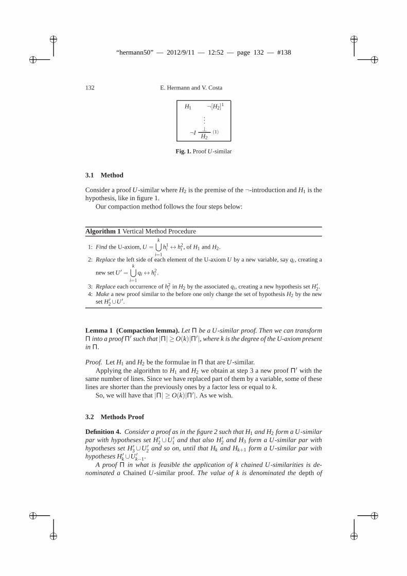
ii

“hermann50” — 2012/9/11 — 12:52 — page 132 — #138 ii

ii

ii


H1 ¬[H2]1

...⊥

¬I (1)H2

Fig. 1.ProofU-similar

3.1 Method

Consider a proofU-similar whereH2 is the premise of the¬-introduction andH1 is thehypothesis, like in figure 1.

Our compaction method follows the four steps below:

Algorithm 1 Vertical Method Procedure

1: Find the U-axiom,U =k⋃

i=1

h1i ↔ h2

i , of H1 andH2.

2: Replacethe left side of each element of the U-axiomU by a new variable, sayqi , creating a

new setU ′ =k⋃

i=1

qi ↔ h2i .

3: Replaceeach occurrence ofh2i in H2 by the associatedqi , creating a new hypothesis setH ′2.

4: Makea new proof similar to the before one only change the set of hypothesisH2 by the newsetH ′2∪U ′.

Lemma 1 (Compaction lemma).Let Π be a U-similar proof. Then we can transformΠ into a proofΠ′ such that|Π| ≥O(k)|Π′|, where k is the degree of the U-axiom presentin Π.

Proof. Let H1 andH2 be the formulae inΠ that areU-similar.Applying the algorithm toH1 andH2 we obtain at step 3 a new proofΠ′ with the

same number of lines. Since we have replaced part of them by a variable, some of theselines are shorter than the previously ones by a factor less orequal tok.

So, we will have that|Π| ≥O(k)|Π′|. As we wish.

3.2 Methods Proof

Definition 4. Consider a proof as in the figure 2 such that H1 and H2 form a U-similarpar with hypotheses set H′2∪U ′1 and that also H′2 and H3 form a U-similar par withhypotheses set H′3∪U ′2 and so on, until that Hk and Hk+1 form a U-similar par withhypotheses H′k∪U ′k−1.

A proof Π in what is feasible the application of k chained U-similarities is de-nominated aChainedU-similar proof. The value of k is denominated thedepthof

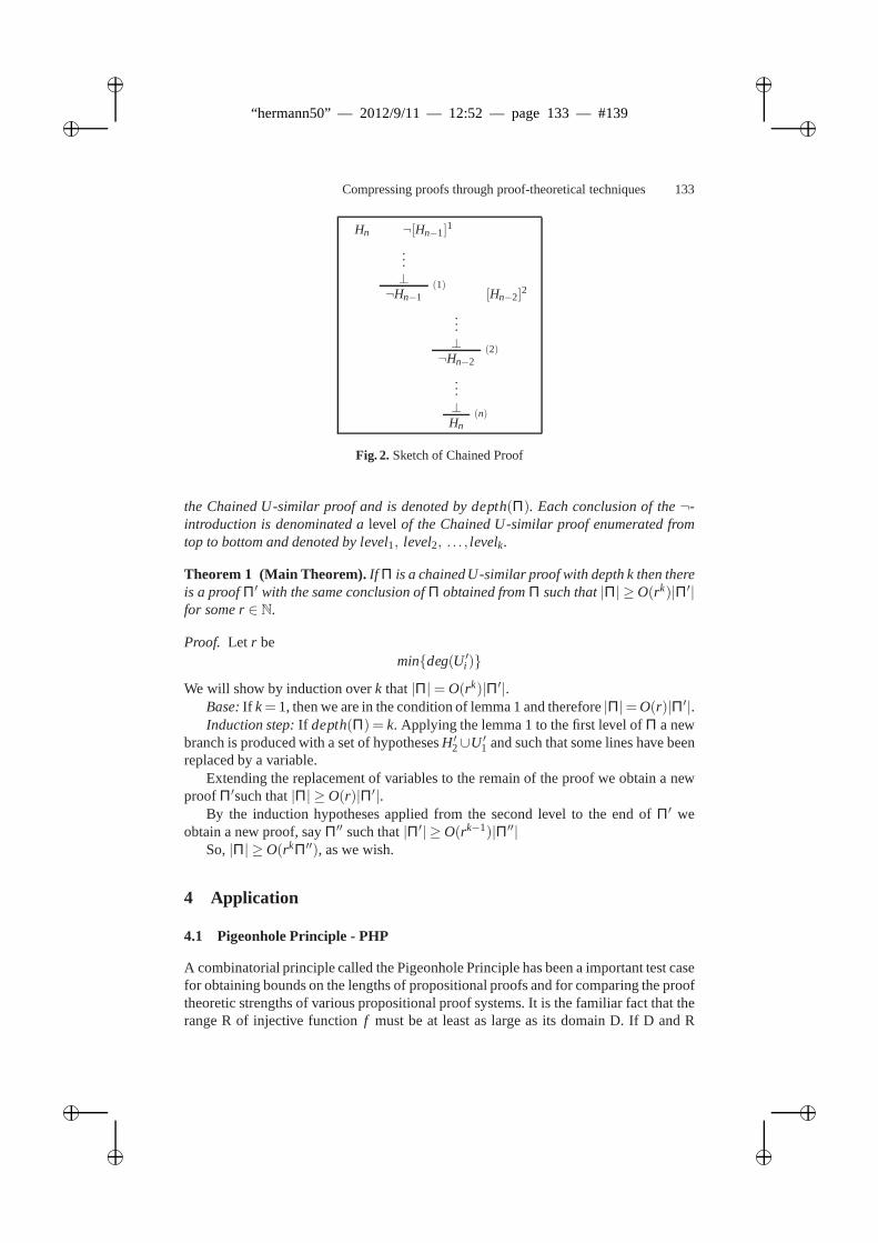
ii

“hermann50” — 2012/9/11 — 12:52 — page 133 — #139 ii

ii

ii


Hn ¬[Hn−1]1

...⊥ (1)

¬Hn−1 [Hn−2]2

...⊥ (2)

¬Hn−2

...⊥ (n)Hn

Fig. 2. Sketch of Chained Proof

the Chained U-similar proof and is denoted by depth(Π). Each conclusion of the¬-introduction is denominated alevel of the Chained U-similar proof enumerated fromtop to bottom and denoted by level1, level2, . . . , levelk.

Theorem 1 (Main Theorem).If Π is a chainedU-similar proof with depth k then thereis a proofΠ′ with the same conclusion ofΠ obtained fromΠ such that|Π| ≥O(rk)|Π′|for some r∈ N.

Proof. Let r bemindeg(U ′i )

We will show by induction overk that|Π|= O(rk)|Π′|.Base:If k= 1, then we are in the condition of lemma 1 and therefore|Π|=O(r)|Π′|.Induction step:If depth(Π) = k. Applying the lemma 1 to the first level ofΠ a new

branch is produced with a set of hypothesesH ′2∪U ′1 and such that some lines have beenreplaced by a variable.

Extending the replacement of variables to the remain of the proof we obtain a newproofΠ′such that|Π| ≥O(r)|Π′|.

By the induction hypotheses applied from the second level tothe end ofΠ′ weobtain a new proof, sayΠ′′ such that|Π′| ≥O(rk−1)|Π′′|

So,|Π| ≥O(rkΠ′′), as we wish.

4 Application

4.1 Pigeonhole Principle - PHP

A combinatorial principle called the Pigeonhole Principlehas been a important test casefor obtaining bounds on the lengths of propositional proofsand for comparing the prooftheoretic strengths of various propositional proof systems. It is the familiar fact that therange R of injective functionf must be at least as large as its domain D. If D and R

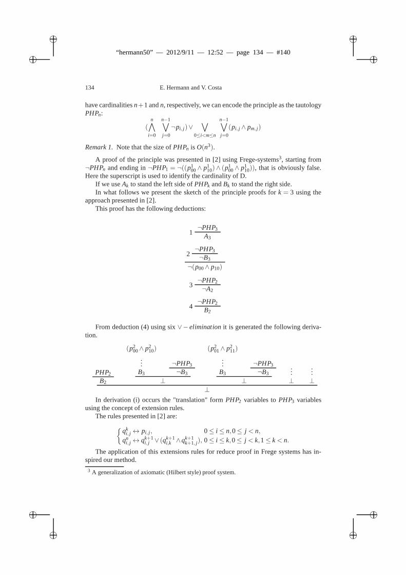
ii

“hermann50” — 2012/9/11 — 12:52 — page 134 — #140 ii

ii

ii


have cardinalitiesn+1 andn, respectively, we can encode the principle as the tautologyPHPn:

(n∧

i=0

n−1∨

j=0

¬pi, j )∨∨

0≤i<m≤n

n−1∨

j=0

(pi, j ∧ pm, j)

Remark 1.Note that the size ofPHPn is O(n3).

A proof of the principle was presented in [2] using Frege-systems3, starting from¬PHPn and ending in¬PHP1 = ¬((p1

00∧ p110)∧ (p

100∧ p1

10)), that is obviously false.Here the superscript is used to identify the cardinality of D.

If we useAk to stand the left side ofPHPk andBk to stand the right side.In what follows we present the sketch of the principle proofsfor k = 3 using the

approach presented in [2].This proof has the following deductions:

¬PHP31

A3

¬PHP32¬B3

¬(p00∧ p10)

¬PHP23¬A2

¬PHP24 B2

From deduction (4) using six∨−eliminationit is generated the following deriva-tion.

PHP2

B2

(p200∧ p2

10)

...B3

¬PHP3

¬B3

⊥

(p201∧ p2

11)

...B3

¬PHP3

¬B3

⊥

...⊥

...⊥

⊥

In derivation (i) occurs the "translation" formPHP2 variables toPHP3 variablesusing the concept of extension rules.

The rules presented in [2] are:

qk

i, j ↔ pi, j , 0≤ i ≤ n,0≤ j < n,qn

i, j ↔ qk+1i, j ∨ (q

k+1i,k ∧qk+1

k+1, j), 0≤ i ≤ k,0≤ j < k,1≤ k< n.

The application of this extensions rules for reduce proof inFrege systems has in-spired our method.

3 A generalization of axiomatic (Hilbert style) proof system.

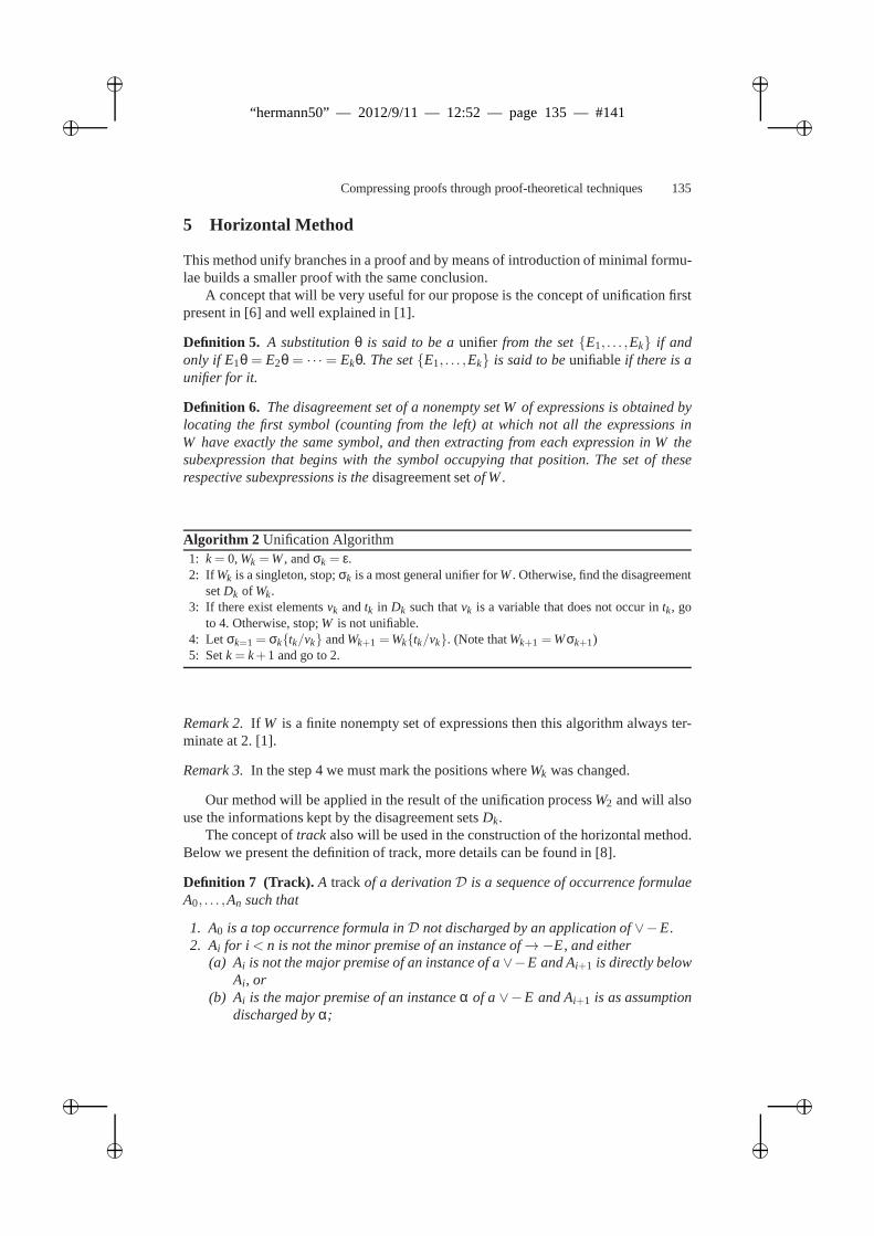
ii

“hermann50” — 2012/9/11 — 12:52 — page 135 — #141 ii

ii

ii


5 Horizontal Method

This method unify branches in a proof and by means of introduction of minimal formu-lae builds a smaller proof with the same conclusion.

A concept that will be very useful for our propose is the concept of unification firstpresent in [6] and well explained in [1].

Definition 5. A substitutionθ is said to be aunifier from the setE1, . . . ,Ek if andonly if E1θ = E2θ = · · · = Ekθ. The setE1, . . . ,Ek is said to beunifiableif there is aunifier for it.

Definition 6. The disagreement set of a nonempty set W of expressions is obtained bylocating the first symbol (counting from the left) at which not all the expressions inW have exactly the same symbol, and then extracting from eachexpression in W thesubexpression that begins with the symbol occupying that position. The set of theserespective subexpressions is thedisagreement setof W.

Algorithm 2 Unification Algorithm1: k= 0,Wk =W, andσk = ε.2: If Wk is a singleton, stop;σk is a most general unifier forW. Otherwise, find the disagreement

setDk of Wk.3: If there exist elementsvk andtk in Dk such thatvk is a variable that does not occur intk, go

to 4. Otherwise, stop;W is not unifiable.4: Let σk=1 = σktk/vk andWk+1 =Wktk/vk. (Note thatWk+1 =Wσk+1)5: Setk= k+1 and go to 2.

Remark 2.If W is a finite nonempty set of expressions then this algorithm always ter-minate at 2. [1].

Remark 3.In the step 4 we must mark the positions whereWk was changed.

Our method will be applied in the result of the unification processW2 and will alsouse the informations kept by the disagreement setsDk.

The concept oftrack also will be used in the construction of the horizontal method.Below we present the definition of track, more details can be found in [8].

Definition 7 (Track). A trackof a derivationD is a sequence of occurrence formulaeA0, . . . ,An such that

1. A0 is a top occurrence formula inD not discharged by an application of∨−E.2. Ai for i < n is not the minor premise of an instance of→−E, and either

(a) Ai is not the major premise of an instance of a∨−E and Ai+1 is directly belowAi , or

(b) Ai is the major premise of an instanceα of a∨−E and Ai+1 is as assumptiondischarged byα;

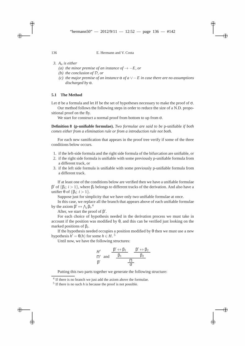
ii

“hermann50” — 2012/9/11 — 12:52 — page 136 — #142 ii

ii

ii


3. An is either(a) the minor premise of an instance of→−E, or(b) the conclusion ofD, or(c) the major premise of an instanceα of a∨−E in case there are no assumptions

discharged byα.

5.1 The Method

Let σ be a formula and letH be the set of hypotheses necessary to make the proof ofσ.Our method follows the following steps in order to reduce thesize of a N.D. propo-

sitional proof on the fly.We start for construct a normal proof from bottom to up fromσ.

Definition 8 (p-unifiable formulae). Two formulae are said to bep-unifiableif bothcomes either from a elimination rule or from a introduction rule not both.

For each new ramification that appears in the proof tree verify if some of the threeconditions below occurs.

1. if the left-side formula and the right side formula of the bifurcation are unifiable, or2. if the right side formula is unifiable with some previouslyp-unifiable formula from

a different track, or3. if the left side formula is unifiable with some previously p-unifiable formula from

a different track.

If at least one of the conditions below are verified then we have a unifiable formulaeβ′ of βi ; i > 1, whereβi belongs to different tracks of the derivation. And also haveaunifier θ of βi; i > 1.

Suppose just for simplicity that we have only two unifiable formulae at once.In this case, we replace all the branch that appears above of each unifiable formulae

by the axiomβ′↔∧

i βi.4

After, we start the proof ofβ′.For each choice of hypothesis needed in the derivation process we must take in

account if the position was modified byθ, and this can be verified just looking on themarked positions ofβi .

If the hypothesis needed occupies a position modified byθ then we must use a newhypothesish′ = θ(h) for someh∈ H. 5

Until now, we have the following structures:

H ′

Π′β′

and

β′↔ β1

β1

β′↔ β2

β2

Πσ

Putting this two parts together we generate the following structure:

4 If there is no branch we just add the axiom above the formulae.5 If there is no suchh is because the proof is not possible.

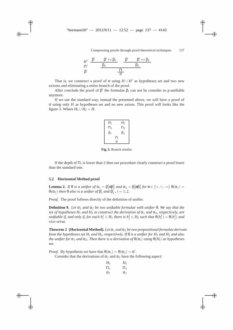
ii

“hermann50” — 2012/9/11 — 12:52 — page 137 — #143 ii

ii

ii


H ′

Π′β′

β′ β′↔ β1

β1

β′ β′↔ β2

β2

Πσ

That is, we construct a proof ofσ using H ∪H ′ as hypotheses set and two newaxioms and eliminating a entire branch of the proof.

After conclude the proof ofβ′ the formulaeβi can not be consider as p-unifiableanymore.

If we use the standard way, instead the presented above, we will have a proof ofσ using onlyH as hypotheses set and no new axiom. This proof will looks likethefigure 3. WhereH1∪H2 = H.

H1

Π1

β1

H2

Π2

β2

Πσ

Fig. 3. Branch similar

If the depth ofΠi is lower than 2 then our procedure clearly construct a proof lowerthan the standard one.

5.2 Horizontal Method proof

Lemma 2. If θ is a unifier ofα1 = β11 β2

1 andα2 = β12 β2

2 for ∈ ∨,∧,→ θ(α1) =θ(α2) thenθ also is a unifier ofβi

1 andβi2 , i = 1,2.

Proof. The proof follows directly of the definition of unifier.

Definition 9. Let α1 andα2 be two unifiable formulae with unifierθ. We say that theset of hypotheses H1 and H2 to construct the derivation ofα1 andα2, respectively, areunifiable if, and only if, for each h1i ∈ H1 there is h2j ∈ H2 such thatθ(h1

i ) = θ(h2j ) and

vice-versa.

Theorem 2 (Horizontal Method).Letα1 andα2 be two propositional formulae derivatefrom the hypotheses set H1 and H2, respectively. Ifθ is a unifier for H1 and H2 and alsothe unifier forα1 andα2. Then there is a derivation ofθ(αi) usingθ(Hi) as hypothesesset.

Proof. By hypothesis we have thatθ(α1) = θ(α2) = α′.Consider that the derivations ofα1 andα2 have the following aspect:

H1

Π1α1

H1

Π1α1

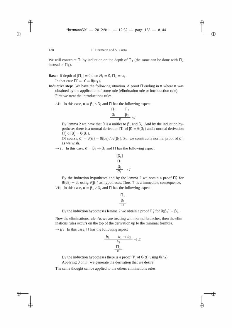
ii

“hermann50” — 2012/9/11 — 12:52 — page 138 — #144 ii

ii

ii


We will constructΠ′ by induction on the depth ofΠ1 (the same can be done withΠ2

instead ofΠ1).

Base: If depth of|Π1|= 0 thenH1 = /0, Π1 = α1.In that caseΠ′ = α′ = θ(α1).

Inductive step: We have the following situation. A proofΠ ending inα whereα wasobtained by the application of some rule (elimination rule or introduction rule).First we treat the introductions rule:

∧I : In this case,α = β1∧β2 andΠ has the following aspect

Π1

β1

Π2

β2∧Iα

By lemma 2 we have thatθ is a unifier toβ1 andβ2. And by the induction hy-potheses there is a normal derivationΠ′1 of β′1 = θ(β1) and a normal derivationΠ′2 of β′2 = θ(β2).Of course,α′ = θ(α) = θ(β1)∧θ(β2). So, we construct a normal proof ofα′,as we wish.

→ I : In this case,α = β1→ β2 andΠ has the following aspect

[β1]

Π1

β2→ Iα1

By the induction hypotheses and by the lemma 2 we obtain a proof Π′1 forθ(β2) = β′2 usingθ(β1) as hypotheses. ThusΠ′ is a immediate consequence.

∨I : In this case,α = β1∨β2 andΠ has the following aspect

Π1

β1α

By the induction hypotheses lemma 2 we obtain a proofΠ′1 for θ(β1) = β′1.

Now the eliminations rule. As we are treating with normal branches, then the elim-inations rules occurs on the top of the derivation up to the minimal formula.

→ E: In this case,Π has the following aspect

h1 h1→ h2→ E

h2

Π1α

By the induction hypotheses there is a proofΠ′1 of θ(α) usingθ(h2).Applying θ onh1 we generate the derivation that we desire.

The same thought can be applied to the others eliminations rules.

ii

“hermann50” — 2012/9/11 — 12:52 — page 139 — #145 ii

ii

ii


6 Final Considerations

The methods presented in the previous sections received those names due the directionwe need to walk in the proof in order to find the structure needed to apply.

A lot of word must be done to make this a fully complete article. For those readersthat has the interests in help us in this matter, we recommendto read some works related.In [3] it is presented some new results involving reduction of proofs, with examples.

Lew Gordeev, a special friend of TecMF, collaborates revising [3] and writing [4].In [4] is presented more results evolving proof compaction.

However, in order to be used in an automatic theorem prover, we still need to presentresults that prove the computational efficiency of the two methods.

References

1. C.-L. Chang and R.C.-T. Lee.Symbolic Logic and mechanical Theorem Proving. AcademicPress, 1973.

2. S. A. Cook and R. A. Reckhow. The relative efficiency of propositional proof systems.Journal of Symbolic Logic, 44(1):36–50, March 1979.

3. Vaston G. Costa.Compactação de Provas Lógicas. Phd Thesis - Departamento de Infor-mática, Pontifícia Universidade Católica do Rio de Janeiro. Rio de Janeiro. 2007. 66p.

4. Lew Gordeev, Edward Hermann Haeusler, Luiz Carlos Pereira. Propositional proof com-pressions and DNF logic.Logic Journal of the IGPL, 19(1): 62-86, 2011.

5. Dag Prawitz.Natural Deduction, A Proof-Theoretical Study. Almqvist & Wiksell, 1965.6. J.A. Robinson. New directions in mechanical theorem proving. In International Federation

for Information Processing Congress, North-Holland, pages 63–68, 1968.7. Jonathan P. Seldin. Normalization and excluded middle I.Studia Logica, 48:193–217, 1989.8. A. S. Troelstra and H. Schwichtenberg.Basic Proof Theory. Cambridge University Press,

Cambridge, England, 2 edition, 2000.

ii

“hermann50” — 2012/9/11 — 12:52 — page 140 — #146 ii

ii

ii

Intuitionistic description logic and legal reasoning

Edward Hermann Haeusler1, Valeria de Paiva2, and Alexandre Rademaker3

1 Dep. Informática PUC-Rio2 C.S. Univ. of Birmingham

3 EMAp/FGV

Abstract. Classical Logic has been used as a basis for knowledge representationand reasoning in many domains. Legal Knowledge Representation is interestingdue to the natural occurrences of conflicts among law systems, individual lawsand cases, usually taken as logical inconsistencies. Due toits inherently norma-tive feature, coherence (consistency) in legal ontologiesis more subtle than inother domains. An adequate intuitionistic semantics for negation in a legal do-main comes to the fore when we consider laws as individuals instead of proposi-tions. This paper presents a version of Intuitionistic Description Logic designedfor legal knowledge representation. The paper discusses a logical coherence anal-ysis of “Conflict of Laws in Space”, using our logic, and briefly compares thisanalysis to other logical approaches to Legal Reasoning.

Preamble

In 2010 I finished my PhD under supervision of Edward Hermann Haeusler at PUC-Rio. I first met Hermann on the first semester of 2004 when I attended his Logics andSpecifications course. At that time I was doing my Masters at UFF. The course wasoutstanding! We learned a lot with Hermann and his singular way of teaching: randomtopics trailing a certain fuzzy syllabus that ends with a very deep overview of the wholesubject under study. The course changed my mind and it convinced me to start my PhDwith Hermann right after I completed my Masters. I remember that I asked Hermann tobe my advisor during my doctoral studies in the end of that same semester.

In 2005 I started my PhD with Hermann. During that year, it didn’t take too muchtime to realize that I had made an excellent choice by having Hermann as my advisor.He was always available for long conversations and to answerthe same questions overand over again. He never tried to impose a research topic to me. On the other hand, hedrove my interests showing me problems and exposing me to research opportunities.He taught me to learn, to study and to use my time.

Around 2007, I had faced big changes in my life. Hermann was there to make hisbest to keep my focus on my studies. I remember the opportunity that he provided mewhen he let me present a poster in the ER 2007 in New Zealand. That travel has hadprofound impact on me. That was my first conference abroad andmotivated me a lot.The poster was about the paper [1] and was the starting point for my interest in thesubject. Later, Hermann and Isabel kindly invited me to jointhem in the research andwe wrote [2–4] together.

In the beginning of 2008 I engaged in the ANUBIS research project. A joinedproject of TecMF-PUC with Modulo Security Systems for the formalization and rea-soning about security policies. It was during our work in that project that I chose proof

ii

“hermann50” — 2012/9/11 — 12:52 — page 141 — #147 ii

ii

ii

Intuitionistic description logic and legal reasoning 141

theory for Description Logics as my research topic. Once again, Hermann drove myattention to the right opportunity showing to me the direction that I should follow.

During the next years until 2010, we have kept expanding our friendship. We notonly met each other during the week professionally but I alsostarted to surf with him onSaturdays. After the surf, we always spent around 1 or 2 hoursof conversation duringthe breakfasts.

In April 2010 I presented my thesis [5] and obtained my PhD. Atthat time anotherbig change happened in my life. At FGV, I had the opportunity to start a new positionas a professor at the Applied Mathematics School. At the end of 2010 I was a littledisoriented about what direction should I take in my career.What topics should I studyand invest my time? I recognized then how much I still needed Hermann’s advice. Itwas during that time that Hermann started a new research and invited me to join him.It was about using intuitionistic logic for legal reasoning. It is somehow and naturalextension of my thesis given that we proposed a intuitionistic version of one of thededuction systems presented in my thesis. That was the topicof this paper.

Before moving on, I would like to thank Hermann for his friendship and alwaysvaluable advices and lessons. I am also thankful to Christiano for giving me the op-portunity to write these words about my great friend Hermann. This paper was firstpublished as [6]. Section 3.1 was submitted to the pos-proceedings of EBL 2011 to bepublished in a special volume of IGPL.

1 Introduction

This article proposes an alternative logical basis for Legal Reasoning (LR) in the contextof AI. There are many aspects to be considered whenever we pose such a foundationalquestion as what constitutes the logical basis for representingLR. It seems clear that thewayLR is conceived is strongly related to the way laws (or “The Law”) are represented.LR is strongly interconnected to Legal Knowledge Representation, i.e, to the LegalOntology chosen, in a wider sense of the termontology. What we see is thatLR musthaveontological commitments; it cannot be simply based on a “legal” logic. It must alsomake a commitment as how do we get to know what we are reasoningabout. Our maingoal here is to show how an intuitionistic version of the Description LogicALC [7] canbe used to handle adequately certain incoherent situationsin LR.

In [8], Knowledge RepresentationKR is taken as a kind ofsurrogate, a substitutefor the represented knowledge itself. According to that seminal work some fundamen-tal roles thatKR plays inAI are: (1) It is a set ofontological commitments; (2) It is afragmentary theory of intelligent reasoning; (3) It is a medium for efficient computa-tion; and finally (4) It is a medium ofhuman expression. Applying these principles weconclude that:

1. LR should be based on logic. We focus onreasoningrather than on learning ordata-mining. We want to generate human readable explanations for the reason whya statement is a valid legal statement about a given legal system.

2. The ontological commitments ofLR should be guided by the underlying jurispru-dence theory and judicial practice. But fundamentally, these ontological commit-ments need to pay attention to computational efficiency and feasibility.

ii

“hermann50” — 2012/9/11 — 12:52 — page 142 — #148 ii

ii

ii

142 A. Rademaker et al.

When dealing withKR, questions about the adequacy of thesurrogatearise. Thesurrogate must substitute the “real thing” as faithfully aspossible. Considering princi-ple 1, there cannot be inconsistencies in the set of sentences describing our knowledge.An inconsistent theory has no model, and hence, describes/represents nothing. Incon-sistency is usually associated with formal versions of negation. The concept of logicalnegation is also essential when representing legal knowledge. Consistency seems to bemore difficult to maintain when more than one coherentlaw systemcan judge a case.This is also called aconflict of laws. There are some traditional legal mechanisms tosolve these conflicts; some of them state privileged fori, others consider jurisdiction,or law hierarchy or precedence between laws. Even using these legal mechanisms, co-herence is still a major concern. As consistency is stronglyrelated to logical negation,negation’s role inLR is more subtle than it is in other domains. In this article we mainlyinvestigate some inconsistencies that arise from the use ofthe excluded middle in Clas-sicalALC, a core description logic. Description Logics (DLs) have been widely used inKR. DLs are basically conceptual languages. A DL knowledge base is defined on top ofa set of concept terms plus a set of binary-relations, some statements about individuals(theABOX), and a set of subsumption assertions between concepts (theTBOX). EntityRelationship models, UML specifications, and many other frameworks in ComputerScience can be adequately represented by DL theories. Most of the DLs used are de-cidable. Althouth the computational complexity of DL satisfiability is at least PSPACE,there are good commercial reasoners to test satisfaction (truth) of a DL formula, andthey can be used to test logical consequence of subsumptionswith respect to a theory.Following principle 2, we want to use the expertise from the DL community to improveLR.

In section 2, we show that our underlying jurisprudence theory is better served bythe use of an intuitionistic version ofALC. The tailoring of this version, which we writeas iALC for intuitionistic ALC, is also a contribution of this work. We show howiALCcan be adequately used inLR.

Explained to a modal logician,ALC is formally equivalent to multimodalK [9].Using the modern modal logic perspective,ALC with ABOXes can be taken as a hy-brid logic. The assertionpl : BR, expressing the fact thatpl is a nominal denoting anindividual (law) inhabiting the extension of the conceptBR, is modally taken as “thepropositionBR holds at worldpl”. Keeping both readings ofALC in mind (as multi-modal and as a hybrid system) helps to understand our definition of iALC and its use inLR. In this article, each individual law will be taken as a possible world (in a Kripkestructure) and the collection of all individual laws (validlegal statements) forms our le-gal world. We choose “Conflict of Laws in Space”,4 to show how intuitionistic negation(in iALC) can help us deal with incoherent laws.

As discussed in [10], there are several possible ways of defining constructivede-scription logics. Here we use a constructive version ofALC, based on the frameworkfor constructive modal logics developed by Simpson in [11].Our system is also simi-

4 This legal term is used to mean that the laws of different countries (or different jurisdictions),on the subject-matter to be decided, are in opposition to each other; or that certain laws of thesame country are contradictory.

ii

“hermann50” — 2012/9/11 — 12:52 — page 143 — #149 ii

ii

ii


lar to the constructive framework developed in [12] for Hybrid Logics, its immediateinspiration. A shorter version of this work was presented in[13].

2 Jurisprudence and Intuitionism

To know what should be the basic unit of law is a fundamental open question in jurispru-dence theory. Any approach to law classification requires first answering this question( [14]). There are two main approaches to the question: (1) one can take all normativestatements, as a whole, as “the law”, or (2) one can take any legally valid statement asan individual law. The approach (1) carries the hard task of ruling a perfect world. Theapproach (2) seems to be nowadays predominant in legal philosophy and jurisprudenceand owes its significance to the Legal Positivism tradition initiated by Hans Kelsen( [15]). The coherence of laws plays a central role in both. The main debate on whethercoherence is built-in by the restrictions induced by Naturein an evolutionary way, orwhether coherence should be the object of knowledge management, seems to favor thelatter. The approach (1), in essence, is harder to be shared with jurisprudence princi-ples, since it is mainly concerned in morally justify the law. The approach (2) seems tobe more suitable to Legal AI. In fact, some Knowledge Engineering groups pursue thelatter as a basis for defining legal ontologies. We follow this route. In what follows weshall use “valid legal statement” (VLS) to denote an individual law holding in our uni-verse of discourse. Following Kelsen’s jurisprudence, ouruniverse of discourse is onlyinhabited byVLSs. For instance, if “Mary is liable” is aVLS it has to be an elementof our legal world. Concepts denote particular legal systems or situations (collectionsof individual laws). For example, we can useBR to denode the set ofVLS holding inBrazil. In particular, we may haveml : BRmeaning “Mary is liable” is aVLS in the setof Brazilian individual laws (BR).

In the sequel we discuss the role of the negation in Legal Knowledge Representa-tion. We will take valid legal statements as individuals of alegal universe, instead oftaking them as (deontic) propositions. We will compare classical negation to intuition-istic negation. The natural precedence between valid legalstatements is the pre-orderrelationship that characterizes the Kripke Semantics for Intuitionistic Logic. In orderto find out what happens in (classical)ALC, we check the simple task of negating anALC concept. First recall that in classicalALC the formulai : C⊔ i : ¬C is valid, for anynominal i and conceptC. Consider Peter, a young man, who is not yet 18 years old.If pl is “Peter is liable” thenpl : BR cannot be the case, since the legal age in Brazilis 18. From the negation ofpl : BRandpl : BR⊔ pl : ¬BRwe havepl : ¬BR. Since inclassicalALC the negation of a concept is interpreted as its set theoretical complement,this conclusion is too strong, it says that “Peter is liable”is a VLS that holds outsideBrazil. For, ifBRis interpreted as the set ofVLS holding in Brazil then¬BRis the com-plement of this set, that is the set ofVLS that holds outside Brazil. Butpl : ¬BR is notalways the case, there might be no Peter at all, outside Brazil. Thus, as is well-known,negation in classicalALC presents problems forLR. Now considering an intuitionisticversion ofALC, we do not have thatpl : ¬BR is a logical consequence of the aboveformalization. The semantics of negation in intuitionistic logic uses possible worlds,as the one for modal logic, and an hereditary relationship between worlds. In terms of

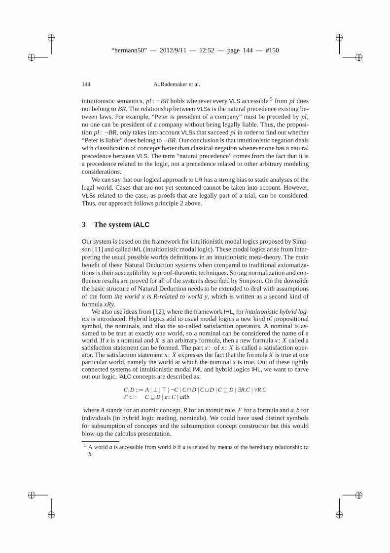
ii

“hermann50” — 2012/9/11 — 12:52 — page 144 — #150 ii

ii

ii


intuitionistic semantics,pl : ¬BRholds whenever everyVLS accessible5 from pl doesnot belong toBR. The relationship betweenVLSs is the natural precedence existing be-tween laws. For example, “Peter is president of a company” must be preceded bypl,no one can be president of a company without being legally liable. Thus, the proposi-tion pl : ¬BR, only takes into accountVLSs that succeedpl in order to find out whether“Peter is liable” does belong to¬BR. Our conclusion is that intuitionistic negation dealswith classification of concepts better than classical negation whenever one has a naturalprecedence betweenVLS. The term “natural precedence” comes from the fact that it isa precedence related to the logic, not a precedence related to other arbitrary modelingconsiderations.

We can say that our logical approach toLR has a strong bias to static analyses of thelegal world. Cases that are not yet sentenced cannot be takeninto account. However,VLSs related to the case, as proofs that are legally part of a trial, can be considered.Thus, our approach follows principle 2 above.

3 The systemiALC

Our system is based on the framework for intuitionistic modal logics proposed by Simp-son [11] and calledIML (intuitionistic modal logic). These modal logics arise from inter-preting the usual possible worlds definitions in an intuitionistic meta-theory. The mainbenefit of these Natural Deduction systems when compared to traditional axiomatiza-tions is their susceptibility to proof-theoretic techniques. Strong normalization and con-fluence results are proved for all of the systems described bySimpson. On the downsidethe basic structure of Natural Deduction needs to be extended to deal with assumptionsof the form the world x is R-related to world y, which is written as a second kind offormulaxRy.

We also use ideas from [12], where the frameworkIHL, for intuitionistic hybrid log-ics is introduced. Hybrid logics add to usual modal logics a new kind of propositionalsymbol, the nominals, and also the so-called satisfaction operators. A nominal is as-sumed to be true at exactly one world, so a nominal can be considered the name of aworld. If x is a nominal andX is an arbitrary formula, then a new formulax: X called asatisfaction statement can be formed. The partx: of x: X is called a satisfaction oper-ator. The satisfaction statementx: X expresses the fact that the formulaX is true at oneparticular world, namely the world at which the nominalx is true. Out of these tightlyconnected systems of intuitionistic modalIML and hybrid logicsIHL, we want to carveout our logic.iALC concepts are described as:

C,D ::= A | ⊥ | ⊤ | ¬C |C⊓D |C⊔D |C⊑ D | ∃R.C | ∀R.CF ::= C⊑ D | a: C | aRb

whereA stands for an atomic concept,R for an atomic role,F for a formula anda,b forindividuals (in hybrid logic reading, nominals). We could have used distinct symbolsfor subsumption of concepts and the subsumption concept constructor but this wouldblow-up the calculus presentation.

5 A world a is accessible from worldb if a is related by means of the hereditary relationship tob.

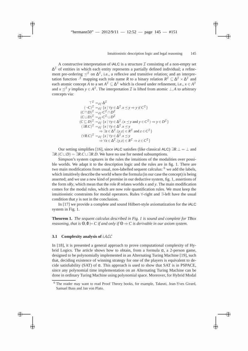
ii

“hermann50” — 2012/9/11 — 12:52 — page 145 — #151 ii

ii

ii


A constructive interpretation ofiALC is a structureI consisting of a non-empty set∆I of entities in which each entity represents a partially defined individual; a refine-ment pre-orderingI on ∆I , i.e., a reflexive and transitive relation; and an interpre-tation function·I mapping each role nameR to a binary relationRI ⊆ ∆I ×∆I andeach atomic conceptA to a setAI ⊆ ∆I which is closed under refinement, i.e.,x∈ AI

andxI y impliesy∈ AI . The interpretationI is lifted from atomic⊥,A to arbitraryconcepts via:

⊤I =d f ∆I

(¬C)I =d f x | ∀y∈ ∆I .x y⇒ y 6∈CI

(C⊓D)I =d f CI ∩DI

(C⊔D)I =d f CI ∪DI

(C⊑ D)I =d f x | ∀y∈ ∆I .(x y andy∈CI)⇒ y∈ DI

(∃R.C)I =d f x | ∀y∈ ∆I .x y⇒∃z∈ ∆I .(y,z) ∈ RI andz∈CI

(∀R.C)I =d f x | ∀y∈ ∆I .x y⇒∀z∈ ∆I .(y,z) ∈ RI ⇒ z∈CI

Our setting simplifies [16], sinceiALC satisfies (like classicalALC) ∃R.⊥ = ⊥ and∃R.(C⊔D) = ∃R.C⊔∃R.D. We have no use for nested subsumptions.

Simpson’s system captures in the rules the intuitions of themodalities over possi-ble worlds. We adapt it to the description logic and the rulesare in fig. 1. There aretwo main modifications from usual, non-labelled sequent calculus:6 we add the labels,which intuitively describe the world where the formula (in our case the concept) is beingasserted; and we use a new kind of premise in our deductive system, fig. 1, assertions ofthe formxRy, which mean that the roleR relates worldsx andy. The main modificationcomes for the modal rules, which are now role quantification rules. We must keep theintuitionistic constraints for modal operators. Rules∀-right and∃-left have the usualcondition thaty is not in the conclusion.

In [17] we provide a complete and sound Hilbert-style axiomatization for theiALCsystem in Fig. 1.

Theorem 1. The sequent calculus described in Fig. 1 is sound and complete for TBoxreasoning, that isΘ, /0 |=C if and only ifΘ⇒C is derivable in our axiom system.

3.1 Complexity analysis ofiALC

In [18], it is presented a general approach to prove computational complexity of Hy-brid Logics. The article shows how to obtain, from a formulaα, a 2-person game,designed to be polynomially implemented in an Alternating Turing Machine [19], suchthat, deciding existence of winning strategy for one of the players is equivalent to de-cide satisfiability (SAT) ofα. This approach is used to show that SAT is in PSPACE,since any polynomial time implementation on an AlternatingTuring Machine can bedone in ordinary Turing Machine using polynomial space. Moreover, for Hybrid Modal

6 The reader may want to read Proof Theory books, for example, Takeuti, Jean-Yves Girard,Samuel Buss and Jan von Plato.

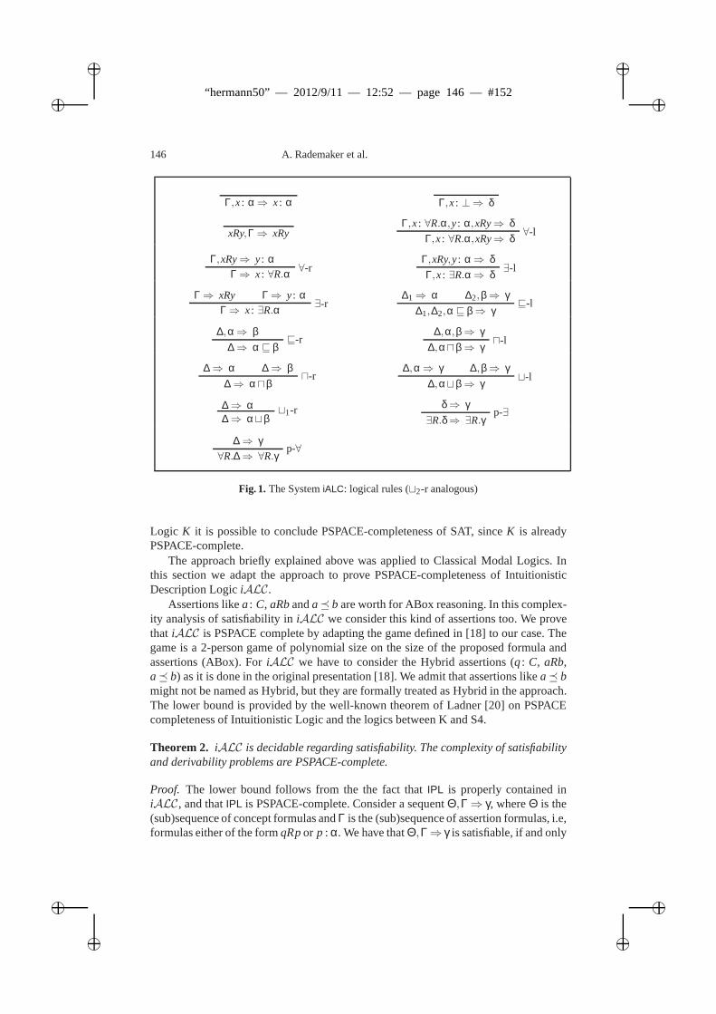
ii

“hermann50” — 2012/9/11 — 12:52 — page 146 — #152 ii

ii

ii


Γ,x: α⇒ x: α Γ,x: ⊥⇒ δ

xRy,Γ⇒ xRyΓ,x: ∀R.α,y: α,xRy⇒ δ

∀-lΓ,x: ∀R.α,xRy⇒ δ

Γ,xRy⇒ y: α∀-rΓ⇒ x: ∀R.α

Γ,xRy,y: α⇒ δ∃-lΓ,x: ∃R.α⇒ δ

Γ⇒ xRy Γ⇒ y: α∃-rΓ⇒ x: ∃R.α

∆1⇒ α ∆2,β⇒ γ⊑-l

∆1,∆2,α⊑ β⇒ γ

∆,α⇒ β⊑-r

∆⇒ α⊑ β∆,α,β⇒ γ

⊓-l∆,α⊓β⇒ γ

∆⇒ α ∆⇒ β⊓-r

∆⇒ α⊓β∆,α⇒ γ ∆,β⇒ γ

⊔-l∆,α⊔β⇒ γ

∆⇒ α ⊔1-r∆⇒ α⊔β

δ⇒ γp-∃

∃R.δ⇒ ∃R.γ

∆⇒ γp-∀

∀R.∆⇒ ∀R.γ

Fig. 1. The SystemiALC: logical rules (⊔2-r analogous)

Logic K it is possible to conclude PSPACE-completeness of SAT, since K is alreadyPSPACE-complete.

The approach briefly explained above was applied to Classical Modal Logics. Inthis section we adapt the approach to prove PSPACE-completeness of IntuitionisticDescription LogiciALC.

Assertions likea: C, aRbanda b are worth for ABox reasoning. In this complex-ity analysis of satisfiability iniALC we consider this kind of assertions too. We provethat iALC is PSPACE complete by adapting the game defined in [18] to our case. Thegame is a 2-person game of polynomial size on the size of the proposed formula andassertions (ABox). ForiALC we have to consider the Hybrid assertions (q: C, aRb,a b) as it is done in the original presentation [18]. We admit that assertions likea bmight not be named as Hybrid, but they are formally treated asHybrid in the approach.The lower bound is provided by the well-known theorem of Ladner [20] on PSPACEcompleteness of Intuitionistic Logic and the logics between K and S4.

Theorem 2. iALC is decidable regarding satisfiability. The complexity of satisfiabilityand derivability problems are PSPACE-complete.

Proof. The lower bound follows from the the fact thatIPL is properly contained iniALC, and thatIPL is PSPACE-complete. Consider a sequentΘ,Γ⇒ γ, whereΘ is the(sub)sequence of concept formulas andΓ is the (sub)sequence of assertion formulas, i.e,formulas either of the formqRpor p : α. We have thatΘ,Γ⇒ γ is satisfiable, if and only

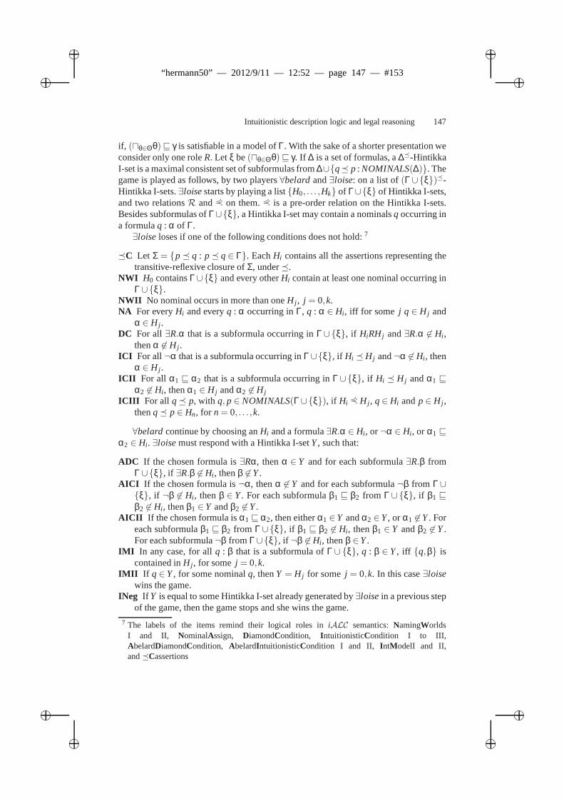
ii

“hermann50” — 2012/9/11 — 12:52 — page 147 — #153 ii

ii

ii


if, (⊓θ∈Θθ)⊑ γ is satisfiable in a model ofΓ. With the sake of a shorter presentation weconsider only one roleR. Let ξ be(⊓θ∈Θθ)⊑ γ. If ∆ is a set of formulas, a∆-HintikkaI-set is a maximal consistent set of subformulas from∆∪q p : NOMINALS(∆). Thegame is played as follows, by two players∀belard and∃loise: on a list of(Γ∪ξ)-Hintikka I-sets.∃loisestarts by playing a listH0, . . . ,Hk of Γ∪ξ of Hintikka I-sets,and two relationsR and2 on them.2 is a pre-order relation on the Hintikka I-sets.Besides subformulas ofΓ∪ξ, a Hintikka I-set may contain a nominalsq occurring ina formulaq : α of Γ.∃loise loses if one of the following conditions does not hold:7

C Let Σ = p q : p q∈ Γ. EachHi contains all the assertions representing thetransitive-reflexive closure ofΣ, under.

NWI H0 containsΓ∪ξ and every otherHi contain at least one nominal occurring inΓ∪ξ.

NWII No nominal occurs in more than oneH j , j = 0,k.NA For everyHi and everyq : α occurring inΓ, q : α ∈ Hi , iff for some j q ∈ H j and

α ∈ H j .DC For all ∃R.α that is a subformula occurring inΓ∪ξ, if HiRHj and∃R.α 6∈ Hi ,

thenα 6∈ H j .ICI For all¬α that is a subformula occurring inΓ∪ξ, if Hi H j and¬α 6∈Hi , then

α ∈ H j .ICII For all α1 ⊑ α2 that is a subformula occurring inΓ∪ξ, if Hi H j andα1 ⊑

α2 6∈ Hi , thenα1 ∈ H j andα2 6∈H jICIII For all q p, with q, p∈ NOMINALS(Γ∪ξ), if Hi 2 H j , q∈ Hi andp∈ H j ,

thenq p∈ Hn, for n= 0, . . . ,k.

∀belardcontinue by choosing anHi and a formula∃R.α ∈ Hi , or¬α ∈ Hi , or α1 ⊑α2 ∈ Hi . ∃loisemust respond with a Hintikka I-setY, such that:

ADC If the chosen formula is∃Rα, thenα ∈ Y and for each subformula∃R.β fromΓ∪ξ, if ∃R.β 6∈Hi , thenβ 6∈Y.

AICI If the chosen formula is¬α, thenα 6∈ Y and for each subformula¬β from Γ∪ξ, if ¬β 6∈ Hi , thenβ ∈ Y. For each subformulaβ1 ⊑ β2 from Γ∪ξ, if β1 ⊑β2 6∈ Hi , thenβ1 ∈Y andβ2 6∈Y.

AICII If the chosen formula isα1⊑ α2, then eitherα1 ∈Y andα2 ∈Y, or α1 6∈Y. Foreach subformulaβ1 ⊑ β2 from Γ∪ξ, if β1 ⊑ β2 6∈ Hi , thenβ1 ∈ Y andβ2 6∈ Y.For each subformula¬β from Γ∪ξ, if ¬β 6∈Hi , thenβ ∈Y.

IMI In any case, for allq : β that is a subformula ofΓ∪ ξ, q : β ∈ Y, iff q,β iscontained inH j , for somej = 0,k.

IMII If q∈Y, for some nominalq, thenY = H j for some j = 0,k. In this case∃loisewins the game.

INeg If Y is equal to some Hintikka I-set already generated by∃loisein a previous stepof the game, then the game stops and she wins the game.

7 The labels of the items remind their logical roles iniALC semantics:NamingWorldsI and II, NominalAssign, DiamondCondition, IntuitionisticCondition I to III,AbelardDiamondCondition, AbelardIntuitionisticCondition I and II, IntModelI and II,andCassertions

ii

“hermann50” — 2012/9/11 — 12:52 — page 148 — #154 ii

ii

ii


The game stops and∀belard wins, if ∃loise cannot find anY as above. If she canfind suchY, it is added to the list of Hintikka I-sets and the2-relation is updated to2 ∪(Hi ,Y) and the match continues by∀belard choosing another formula from therecently updated list of Hintikka I-sets, considering the (possibly) updated2-relation,leaving to her the task of finding anotherY, and so on.

At roundm, ∀belard can only choose either a formula of modal depth less than orequal to the modal depth ofΓ∪ξ minusm, or a formula with number of¬ occur-rences less than or equal to the¬ occurrences ofΓ∪ξminusm. Finally,∃loisewinsif she survive all attacks of∀belard. Since each attack of him is performed on a for-mula of less or equal complexity than the last one, the maximum length of a match isbounded by the number of subformulas occurring inΓ∪ξ plus the number of nom-inals occurring in the sequent, this is a polynomial bound onthe length of the match,and hence the game. Using Lemma 1 we have that satisfiability of the sequent is equiv-alent to existence of a winning strategy for∃loise. As existence of winning strategiesis a PTIME decision problem in Alternating Turing Machines,we conclude thatiALCsatisfiability is PSPACE-complete.

Lemma 1. ∃loise has a winning strategy, if and only ifΓ,Θ⇒ γ is satisfiable.

Proof. If Γ,Θ ⇒ γ is satisfiable, thenΓ∪ ξ also is and the existence of a modelthat satisfies it allows the definition of an initial list of Hintikka I-sets to∃loise playher winning strategy.∃loisehas only to provide the Hintikka I-sets associated to eachworld in this model ofΓ∪ξ. For the other direction, let us suppose that∃loisehas awinning strategy. This winning strategy will provide us with model forΓ∪ξ. Since∃loisehas a winning strategy, she has answered to each possible move of∀belard, shealso has a winning starting list of Hintikka I-sets. Thus,∃loisecan produce a HintikkaI-set for each attack of her opponent. LetM be this collection of all Hintikka I-setspossible to be generated by the winning strategy of∃loise. The model〈M,R,2,V〉 issuch that:

– R is such that, given Hintikka I-setsMi ,M j ∈ M, MiRMj , if and only if for everysubformula∃R.β, if ∃R.β 6∈Mi , thenβ 6∈M j .

– is the relation onM obtained by the winning strategy of∃loise, defined by thegame.

– V(A) = Mi : A∈Mi.– The assertionq : α is true atMi , if and only if,q,α is contained inMi .– The assertionq p is true atMi , if and only if,H j 2 Mi andq p∈ H j , for some

H j belonging to the initial Hintikka I-sets provided by∃loise.

From Lemma 2 we can see that if∃loisehas a winning strategy, thenΓ∪ξ has amodel. This finishes the remaining direction of this proof.

Lemma 2. For every subformula ofΓ∪ξ, 〈M,R,2,V〉 |=Mi α, if and only if,α ∈Mi .

Proof. We proceed by induction on the number of symbols inα. For assertionsq p,p : α and for atomic conceptsC it is a straightforward application of the definition of〈M,R,2,V〉 |=Mi α. Considerα of the formα1⊓α2 and〈M,R,2,V〉 |=Mi α1⊓α2. By

ii

“hermann50” — 2012/9/11 — 12:52 — page 149 — #155 ii

ii

ii


definition of|= we have〈M,R,2,V〉 |=Mi αk, k= 1,2. By inductive hypothesis, we haveαk ∈Mi . As Mi is maximal and consistent,α1⊓α2 ∈Mi . For the other direction, if wesuppose thatα1⊓α2 ∈Mi , thenαk ∈Mi , k= 1,2, sinceMi is a maximal consistent setof subformulas ofΓ∪ξ. By inductive hypothesis and the definition of|= we concludethat〈M,R,2,V〉 |=Mi α1⊓α2. If α is of the formα1⊑α2 Suppose thatα1⊑α2 6∈Mi , asMi 2M j and by fact 2 we haveα1∈M j andα2 6∈M j , and hence by inductive hypothesis〈M,R,2,V〉 |=M j α1 and〈M,R,2,V〉 6|=M j α2, hence〈M,R,2,V〉 6|=Mi α1⊑ α2. On theother hand, consider thatα1⊑ α2 ∈Mi . We know that∃loisehas a winning strategy, so,if ∀belardchooses to attackα1 ⊑ α2 in Mi , ∃loise is able to provide an answerY, suchthatMi 2 Y, by construction, and eitherα1 ∈ Y andα2 ∈ Y, or α1 6∈ Y.By fact 4, thisalso holds for every otherY, such thatMi 2Y, thus, we have〈M,R,2,V〉 |=Mi α1⊑ α2.The cases for¬α and∃R.α are analogous to this last case. This finishes the proof of thelemma.

The following facts are used in the proof of Lemma 2.

Fact 2 If M i 2M j , then for every subformulaα1⊑ α2 of Γ∪ξ, if α1⊑ α2 6∈Mi , thenα1 ∈M j andα2 6∈M j .

Proof. By definition of the model in Lemma 1.

Fact 3 If M i 2 M j , then for every subformula¬α of Γ∪ξ, if ¬α 6∈Mi , thenα ∈M j .

Proof. By definition of the model in Lemma 1.

Fact 4 If α1 ⊑ α2 ∈ Mi , then for each Y∈ M, such that, Mi 2 Y, eitherα1 ∈ Y andα2 ∈Y, orα1 6∈Y.

Proof. If there isY, such that,Mi 2 Y andα1 ∈ Y andα2 6∈ Y, thenα1 ⊑ α2 is notattacked by∀belard. This means thatM does not contain every possible choice of the∃loisewinning strategy. This contradicts the definition ofM.

4 Private International Law

A concept symbolC, in a description logic language, is associated to a subset of legalstatementsrepresenting akind oflegal situation. Roles in the description logic languageare associated to relations between theselegal situations, imposed by the relationshipbetween pairs of validlegal statements.

We provide some details of how we model the legal situation known as “Conflict ofLaws in Space” within the scope ofPrivate International Law.

Consider the following situation:Peter and Maria signed a renting contract. Thesubject of the contract is an apartment in Rio de Janeiro. Thecontract states that anydispute will go to court in Rio de Janeiro. Peter is 17 and Maria is 20 years old. Peterlives in Edinburgh and Maria lives in Rio.

In order to proceed with our formal reasoning, the legal statement (1)Maria andPeter have contractual obligations and rights to each otherconcerning an apartment inRio de Janeirohas to be valid. VLSs are the only individuals. There is no invalid legal

ii

“hermann50” — 2012/9/11 — 12:52 — page 150 — #156 ii

ii

ii


statement. This follows from the foundations of jurisprudence assumed in this article.We will denote bycmp the legal statement (1) above. As before, let us denote byBRthe set of (valid) individual legal statements in Brazil, and, bySCthe set correspondingto Scotland. Since 18 years old is the legal age in Brazil, there is no individual legalstatement about Peter in Brazil. Thus, the statementMaria is of legal age, mla for short,is in BR, andpla (Peter is of legal age) is in SC. There is a natural precedence relationbetween legal statements, only legally capable individuals have civil obligations. Inother words,pla cmpandmla cmp. Let PILBR be the set of legal statements inBrazil describing itsPrivate International Law. Of course we havePILBR⊑ BR. Byits very nature,PILBR is a disjunction of concepts of legal statements that subsumes∃LexDomicilium.Abroad.

It is worth noticing thatPrivate International Law(PIL) relates legal statementsin different contexts, locations, time, etc. Thus each member of PIL corresponds toa specific context, here a geographical living place.Abroad is the union of the legalstatements holding in each country, but Brazil.LexDomiciliumis a legal connection,a relationship between laws in jurisprudence terminology,written LexD in the proof.The pair of legal statements〈pla, pla〉 is in LexDomicilium, since Peter lives in Scot-land, abroad as far as Brazil is concerned. Summing up, we have the following set ofaxioms:8

∆ = mla: BR, pla: SC, pla cmp,mla cmp, pla LexDom pla

Ω = PILBR⇒ BR,SC⇒ Abroad, pla: BR⇒ cmp: BR

∃LexDom.Abroad ⊔ . . .⇒ PILBR,mla: BR

Ω displays the axioms stated in sequent form, whilst∆ is the set of concepts that weuse to prove thatcmp: BR. We start with the derivation presented in Fig. 2, where thesequents inΩ are used freely. The name of the concepts were shortened due to spacelimitations for displaying the proof tree.

We already know that∆⇒mla: BR, sincemla: BRoccurs in∆. Naming asΠ theproof of Fig. 2, and, using the axioms from∆, we conclude thatcmp: BR, Fig. 3.

We conclude thatcontract∈ BR, for each legal statement generalizingcontract,with regard to, namelypla andmla, is in BR. For the interesting case we note thatpla: ∃LexDomicilium.SC⊑ PILBR⊑ BR, by the definition of∃R.C concepts. This ar-gumentation can be obtained from the proof. In fact it reflects each step in the proof.

If one usesALC instead ofiALC in the example formalization, one needs to considera legal ontology involving non-validLegal Statements, and hence anad hocontology re-garding jurisprudence main concepts. Dealing with non-valid legal statements will alsoincrease the complexity of the ontology considered. Of course we simplified our exam-ple, since it only considerspla andmlaas succeedingcontract. In a real ontology, manymore statements would have to be considered, for exampleMaria-owns-the-apartmentamong them. This, we believe, would turn much more complex the classicALC case.

The sequent calculus foriALC is inspired by [21] where labels are used for contextcontrolling. This mechanism is shown ( [22]) to be useful when defining a Natural

8 The axiommla: BR, pla: BR⇒ cmp: BRstates that the contract is valid in Brazil wheneverboth agents are liable in Brazil. In fact, this is an instanceof a general law principle.

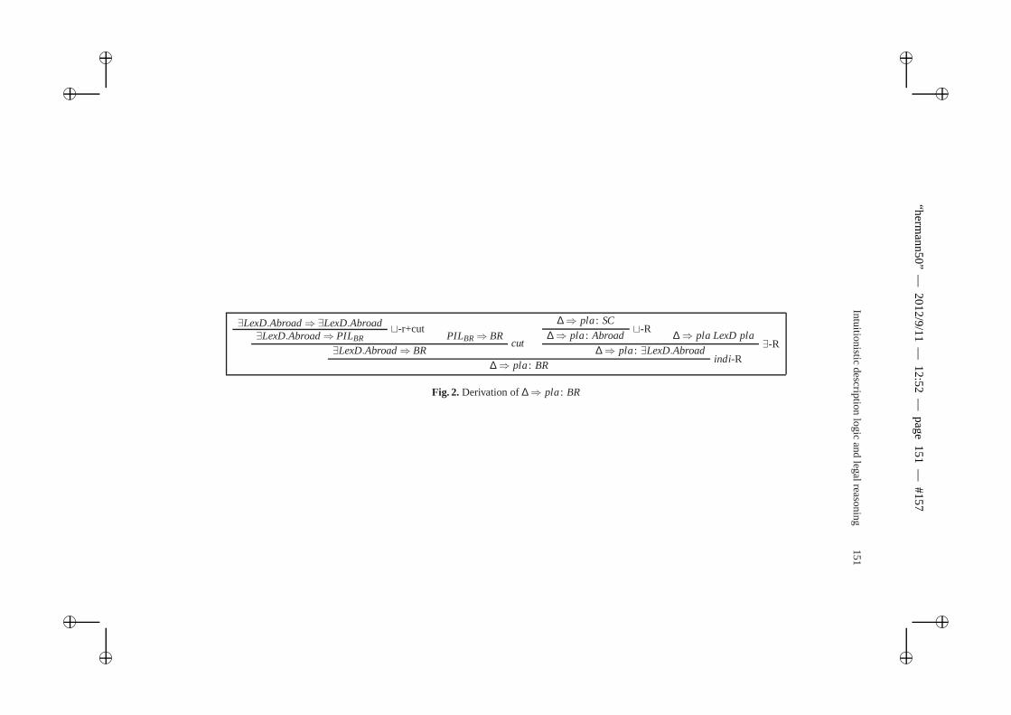
ii

“herm

ann

50

”—

20

12

/9/1

1—

12

:52

—p

age

15

1—

#1

57

ii

ii

ii

Intuitionisticdescription

logicand

legalreasoning151

∃LexD.Abroad⇒∃LexD.Abroad⊔-r+cut

∃LexD.Abroad⇒ PILBR PILBR⇒ BRcut

∃LexD.Abroad⇒ BR

∆⇒ pla: SC⊔-R∆⇒ pla: Abroad ∆⇒ pla LexD pla

∃-R∆⇒ pla: ∃LexD.Abroadindi-R∆⇒ pla: BR

Fig. 2.Derivation of∆⇒ pla: BR

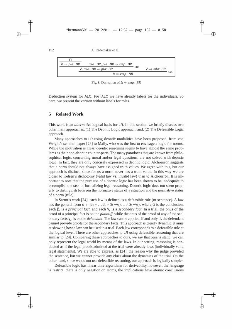
ii

“hermann50” — 2012/9/11 — 12:52 — page 152 — #158 ii

ii

ii


Π∆⇒ pla: BR mla: BR, pla: BR⇒ cmp: BR

cut∆,mla: BR⇒ pla: BR ∆⇒mla: BR

cut∆⇒ cmp: BR

Fig. 3.Derivation of∆⇒ cmp: BR

Deduction system forALC. For iALC we have already labels for the individuals. Sohere, we present the version without labels for roles.

5 Related Work

This work is analternativelogical basis forLR. In this section we briefly discuss twoother main approaches: (1) The Deontic Logic approach, and,(2) The Defeasible Logicapproach.

Many approaches toLR using deontic modalities have been proposed, from vonWright’s seminal paper [23] to Mally, who was the first to envisage a logic for norms.While the motivation is clear, deontic reasoning seems to have almost the same prob-lems as their non-deontic counter-parts. The many paradoxes that are known from philo-sophical logic, concerning moral and/or legal questions, are not solved with deonticlogic. In fact, they are only concisely expressed in deonticlogic. Alchourrón suggeststhat a norm should not always have assigned truth values. We agree with this, but ourapproach is distinct, since for us a norm never has a truth value. In this way we arecloser to Kelsen’s dichotomy (valid law vs. invalid law) than to Alchourrón. It is im-portant to note that the pure use of a deontic logic has been shown to be inadequate toaccomplish the task of formalizing legal reasoning. Deontic logic does not seem prop-erly to distinguish between the normative status of a situation and the normative statusof a norm (rule).

In Sartor’s work [24], each law is defined as a defeasible rule(or sentence). A lawhas the general formα← β1∧ . . .βn∧S(¬γ1) . . .∧S(¬γk), whereα is the conclusion,eachβi is a principal fact, and eachγ j is a secondary fact. In a trial, the onus of theproof of a principal fact is on theplaintiff, while the onus of the proof of any of the sec-ondary factsγ j , is on thedefendant. The law can be applied, if and only if, the defendantcannot provide proofs for the secondary facts. This approach is clearly dynamic, it aimsat showing how a law can be used in a trial. Each law corresponds to a defeasible rule atthe logical level. There are other approaches toLR using defeasible reasoning that aresimilar to [24]. Comparing these approaches to ours, we say that ours is static, we canonly represent the legal world by means of the laws. In our setting, reasoning is con-ducted as if the legal proofs admitted at the trial were already laws (individually validlegal statements). We are able to express, as [24], the reason why the judge providedthe sentence, but we cannot provide any clues about the dynamics of the trial. On theother hand, since we do not use defeasible reasoning, our approach is logically simpler.

Defeasible logic has linear time algorithms for derivability, however, the languageis restrict, there is only negation on atoms, the implications have atomic conclusions

ii

“hermann50” — 2012/9/11 — 12:52 — page 153 — #159 ii

ii

ii


and there is no disjunction. For this language, there are also linear time algorithms forALC. But ALC is not a defeasible logic. Anyway, it is worth noting that no linear timedefeasible logic exists for dealing with the full propositional language since classicalpropositional logic is NP-complete. Our calculus takes care of cyclic TBoxes, since theaxioms of a given theory will appear as additional (non-logical) top-sequents in a proof.

6 Conclusions

We usediALC to provide an alternative, and, we claim, more appropriate,definition ofsubsumption in the legal reasoning domain. The systemiALC deals with the jurispru-dence approach which consists of considering all (possible) legally valid individualsstatements as laws. Conflict of laws is formalized by means ofiALC, by showing itsadequacy to perform coherence analysis in legal AI. The sequent calculus helps in thistask. Our approach is different from [25], where the reasoning is by means of argumen-tation and opposition of propositions. Our basis is quite distinct, since we do not con-sider “laws” as propositions. Our approach is static while Sartor’s approach is dynamic,but this also means that our logical basis is simpler, and consequently, computationalsupport should be easier.

Our calculus first appeared in [17]. The example shown here was roughly modeledby the authors in [26]. Its use in formalizing the situation of conflict of laws in space isthe novelty of this paper. In future work we intend to compareour results to the onesof [27–29] and [30].

References

1. Cafezeiro, I., Haeusler, E.H.: Semantic interoperability via category theory. Conferences inResearch and Practice in Information Technology83 (2006)

2. Cafezeiro, I., Haeusler, E.H., Rademaker, A.: Ontology and context. In: IEEE InternationalConference on Pervasive Computing and Communications, LosAlamitos, CA, USA, IEEEComputer Society (2008)

3. Cafezeiro, I., Viterbo, J., Rademaker, A., Haeusler, E.H., Endler, M.: A formal frameworkfor modeling context-aware behavior in ubiquitous computing. In: Third International Sym-posium, ISoLA 2008, Proceddings, Heidelberg, Springer Berlin (2008)

4. Cafezeiro, I., Viterbo, J., Rademaker, A., Haeusler, E.H., Endler, M.: Designing ubiquitousapplications: proposal of a specification environment. In:MUCS ’09: Proceedings of the 6thinternational workshop on Managing ubiquitous communications and services, New York,NY, USA, ACM (2009)

5. Rademaker, A.: A Proof Theory for Description Logics. Springer Briefs in CS. Springer(2012)

6. Haeusler, E.H., Paiva, V.d., Rademaker, A.: Intuitionistic description logic and legal reason-ing. In: 2011 Database and Expert Systems Applications, DEXA, International Workshops,Toulouse, IEEE Computer Society (2011)

7. Baader, F., Calvanese, D., McGuinness, D., Nardi, D., Patel-Schneider, P., eds.: The De-scription Logic Handbook. Cambridge Univ. Press (2003)

8. Davis, R., Shrobe, H., Szolovits, P.: What is a knowledge representation? AI Magazine14(1)(1993) 17

ii

“hermann50” — 2012/9/11 — 12:52 — page 154 — #160 ii

ii

ii


9. Schild, K.: A correspondence theory for terminological logics: preliminary report. In: Proc.of the 12th IJCAI, IJCAI’91, San Francisco, CA, USA, Morgan Kaufmann Publishers Inc.(1991) 466–471

10. de Paiva, V.: Constructive description logics: what, why and how. Technical report, XeroxParc (2003)

11. Simpson, A.: The Proof Theory and Semantics of Intuitionistic Modal Logic. PhD thesis,University of Edinburgh (December 1993)

12. Braüner, T., de Paiva, V.: Intuitionistic hybrid logic.JAL 4(3) (2006) 231–25513. Haeusler, E.H., de Paiva, V., Rademaker, A.: Intuitionistic logic and legal ontologies. In:

Proc. JURIX 2010, IOS Press (2010) 155–15814. Raz, J.: Legal principles and the limits of law. YLJ81 (1972) 823–85415. Kelsen, H.: General theory of norms. Oxford Univ. Press,USA (1991)16. Mendler, M., Scheele, S.: Towards constructive DL for abstraction and refinement. JAR

44(3) (2010) 207–243 Proc. 21st Intl. DL Workshop.17. de Paiva, V., Hausler, E.H., Rademaker, A.: Constructive description logic: Hybrid-style. In:

Proc. HyLo’2010. (2010)18. Areces, C., Blackburn, P., Marx, M.: A road-map on complexity for hybrid logics. In: LNCS,

1683. (1999) 307–32119. Papadimitriou, C.: Computational complexity. John Wiley and Sons Ltd. (2003)20. Ladner, R.: The Computational Complexity of Provability in Systems of Modal Logics.

SIAM Journal on Computing6 (1977) 467–48021. Rademaker, A., Haeusler, E.H., Pereira, L.C.: On the proof theory ofALC. In: The Many

Sides of Logic. Proc of 15th EBL. Volume 21. College Publications, London (2008) 273–28522. Rademaker, A., Haeusler, E.: Providing a proof-theoretical basis for explanation: A case

study on uml and alcqi reasoning. JUCS16 (2010) 3016–304223. von Wright, G.: Deontic logic. Mind60(237) (1951) 1–1524. Sartor, G.: The structure of norm conditions and nonmonotonic reasoning in law. In: Proc.

3rd ICAIL, ACM, ACM Press (1991) 155–16425. Dung, P.M., Sartor, G.: A Logical Model of Private International Law. Deontic Logic in CS,

LNAI 6181 (2010) 229–24626. Haeusler, E.H., de Paiva, V., Rademaker, A.: Using intuitionistic logic as a basis for legal

ontologies. In: Proc. of the 4th LOAIT Workshop, Fiesole, Florence, Italy, European Univ.Institute (2010) 69–76

27. Alchourron, C.E., Martino, A.A.: Logic without truth. Ratio Juris3(1) (Jun 1990) 46–4728. Carmo, J., Jones, A.: Deontic logic and contrary-to-duties. Handbook of Philosophical Logic

8 (2002) 265–34329. Van Der Torre, L.: Deontic redundancy: a fundamental challenge for deontic logic. Deontic

Logic in Computer Science (2010) 11–3230. Klarman, S., Gutiérrez-Basulto, V.: Alcalc: a context description logic. In: Proceedings of

the 12th JELIA. JELIA’10, Berlin, Heidelberg, Springer-Verlag (2010) 208–220

Documents

“hermann50” — 2012/9/11 — 12:52 — page 1 — #1cbraga/hermann50/hermann50.pdf · “hermann50” — 2012/9/11 — 12:52 — page 2 — #2 ... – Luis Fernando Gomes Soares