Herding Behavior on mutual fund investors in Brazil - Cass Business

Herding Behavior on mutual fund investors in Brazil

Eric Kutchukian Escola de Administracao de Empresas – Fundacao Getulio Vargas – Sao Paulo – Brazil

William Eid Jr. Escola de Administracao de Empresas – Fundacao Getulio Vargas – Sao Paulo – Brazil

Samy Dana Escola de Administracao de Empresas – Fundacao Getulio Vargas – Sao Paulo – Brazil

ABSTRACT

By using a sample of Brazilian stock, money market and fixed income mutual funds daily

transactions and a methodology based on the direction of net flows of fund-raising for a high

number of mutual funds – aggregated in groups of investors according to the average size of

its investments (rich and poor), strong evidence was found that there is a herd behavior

heterogeneously among different groups of investors; and the intensity of such behavior

varies according to the investor’s size, the type of fund and the period. A heuristics bias test

was also carried out: price anchoring, which supposes that after a new historical maximum or

minimum stock index level, there will be an abnormal movement of investors believing it is

an indicator of future prices. It was possible to notice that such a phenomenon occurs in

different types of investments and not only in stock mutual funds, and that its impact is

greater when a new minimum level is reached than when there is a record in the Ibovespa

stock index. However, such a bias has little explaining power on the herd behavior, and there

many variables that may better explain it but have not yet been studied. Therefore, this study

has found evidence that suggests that the validity of the behavioral finance assumption that

the investors’ information and expectations are not homogeneous and that investors are

influenced by other investor’s decisions; nevertheless, there is weak evidence that the

heuristics bias of price anchoring plays a relevant role in investors’ behavior.

Keywords: mutual funds; behavioral finance; herd behavior.

1. INTRODUCTION

The several crises in financial markets, such as the recent subprime crisis, have caused great

fluctuations and losses in global financial markets, besides having impacted economies all

over the world. In these moments, market efficiency and, thus, asset pricing models based on

such assumptions are questioned. The relatively new field of behavioral finance tries to shed

light upon the flaws of these assumptions when its implications in capital markets are

empirically tested. Furthermore, the growing volume of money invested in Brazilian mutual

funds, including stock funds, becomes a source of concern: in case of a mass escape from

stock funds, i.e., a general movement of investors (herd behavior), could the asset selling

pressure lead to disequilibrium?

Correspondence to: Eric Kutchukian. [email protected]. 55 11 9625-1125 / 3885-0651

mailto:[email protected]

2. OBJECTIVES

The aim of this study is to empirically detect the occurrence of herd behavior in mutual fund

flows in Brazil in order to test an investor’s behavior that is not in accordance with the

assumptions of market efficiency, stated in the modern finance theory (MFT), but explained

by assumptions supported by behavioral finance (BF).

The following behaviors were tested:

I. Ocurrence of Herd Behavior The herd behavior is a positively correlated movement, in block, by investors. In case it does

happen, two assumptions of MFT are contradicted, as follows:

a. Agents maximize their expected utility as a function of their risk aversion, wich is

individual and should not lead to individuals deciding in groups.

b. The price reflects all available information: since there is a correlated movement of

investors, they may probably not believe that the current price is fair.

At the same time, the incidence of such a phenomenon supports the BF assumptions that there

may be under and overreaction and that investors do not make decisions based only on

expected utility and expectations of future cash flow, but also based on the decision of other

investors.

II. Heterogeneous Occurrence of Herd Behavior

Such an occurrence means that there is herd behavior, on average, in some groups of investors,

but not in others, in funds with assets of similar risk/return levels. It contradicts the MFT

assumption of homogeneous expectations and homogeneous information.

III. Price Anchoring Heuristics Causes Herd Behavior

Testing whether investors make decisions based on historical price – when Ibovespa price

rises over its maximum level or falls under its minimum level in a one-year historical horizon,

investors react. In case it is true, there is evidence that investors use heuristics (heuristic bias –

BF) instead of being rational (according to MFT) simply taking into account their evaluations

about the present value of future cash flows of Ibovespa stocks. This study does not aim to

test all herd behavior determinants, but to contribute to further research on this subject in

Brazil.

3. LITERATURE REVIEW

3.1 Modern Finance Theory and Behavioral Finance

In the opposite direction of the modern finance theory on asset pricing, in which information

and expectations are homogeneous, BF argues that information is not available to everyone,

and it has a cost of acquisition or research, and may have different interpretations. In some

cases, such a cost may top the benefit of information for some agents, but not for others. This

fact by itself causes information heterogeneity between agents. At the same time, BF admits

that agents may not have all the information, nor attach due importance to them, on account of

the representativeness bias proposed by Kahneman and Tversky (1974). These authors argue

that agents attach more importance to more recent information or information that seems more

clear to them and not necessarily more relevant, besides ignoring relevant information that

they do not have.

Another aspect stated by MFT is that economic agents are rational, whereas there is a counter-

argument in BF: rationality is limited and there are several ways for people to interpret the

market, according to Daft and Weick (1984).

MFT supports the concept of total asset divisibility. This is relevant because it presumes wide

access to market assets for agents from all wealth levels. When it comes to finance, such

barriers may be the minimum investment amount, eligibility, information and regulation.

MFT also presupposes that there are no consistent opportunities for arbitrage or abnormal

profits, suggesting that the market adjusts itself, wich agrees with the view of Adam Smith

about the “invisible hand”. In BF, De Long et al (1990) present a counter-argument, stating

that there are noise traders, i.e., investors whose behavior is neither rational nor predictable.

Rational agents fear negotiating in order to benefit from such an imbalance, because the

unpredictability of such noise traders may lead to greater imbalance, wich could cause

damage to rational agents that had bet against the imbalance hoping to profit when it was

gone.

3.2 The Herd Behavior

Herd behavior is not yet fully studied in behavioral finance, and its incidence among Brazilian

mutual funds investors is a theme which has not been published yet in Brazil. It differs from

the MFT in the efficient market assumptions that investors are rational (using all available

information about assets in the market), that information is homogeneous between the agents,

that all agents are price takers and that agents maximize their expected utility taking into

account the risk / return relationship, according to their level of risk aversion.

According to Bikhchandani and Sharma (2001), herd behavior is the correlated movement of

investors.

What causes such behavior is still subject to controversy. There are two possibilities:

1 – It may be explained by investor’s similar reactions to shocks and new information. In this

case, if it happens homogeneously and simultaneously in any group of agents, the MFT

assumption of homogeneous expectations and information is confirmed. In case it happens

heterogeneously, such assumption shows itself to be invalid.

2 – There is another possible explanation of this effect: imitation. One conjectures that

investors imitate other investors by observing their attitudes, as they believe there might be

some implicit information. Though it may be considered a rational behavior, it denies the

assumption of homogeneous information. Besides, when investors make decisions based on

what another investor did, they disregard the information available so far, its own utility

function and its level of risk aversion; these are counter-arguments to the presupposition that

all available information are reflected on the price. While Lakonishok, Schleifer and Vishny

(1992) - from now on “LSV” - found only weak evidence to the occurrence of herd behavior,

Shapira and Venezia (2006), in their study about transactions made by amateur and

Professional investors in an asset in Israel from 1994 until 1998, came to the conclusion that

herd behavior happens both with both type of investors, but such effect is greater among

amateurs. This is in conformity with what MFT postulates about homogeneous expectative

between agents. There are also several other studies that verify the existence of a relation

between herd behavior and stock returns, such as Cont and Bouchaud (2000), Who concluded

that amateur investors show herd behavior, and such behavior affects stock prices, increasing

the kurtosis of stock returns, but it does not happen with professional investors. Teh and

DeBondt (1997), based on a sample of stock returns from 1980 until 1990, observed that herd

behavior has additional might to explain stock returns variance, by using the same

methodology as Fama e French (1992). That suggests that the herd behaves inefficiently for

the market and for itself. For instance, if the herd wants to quit the market (i.e., sell stocks), it

will increase the supply of the asset and probably cause a pressure to diminish the price; that

damages the herd itself as the asset will be sold for less that it is fair; besides, it could unleash

more sells (imitation behaviour). On the other hand, professional investors may be more

aware of the power that their operations have regarding the prices; thus, they are more

cautious when doing great trades and may do they little by little. There are several authors

who studied, based on LSV methodology, whether there is herd or imitation behaviour among

mutual funds managers. For instance, Lobão and Serra (2002) found strong evidence of herd

behavior in fund managers’ investment decisions in the Portuguese stock investment funds

market.

Nevertheless, in this work, instead of measuring herd behaviour among fund managers, the

aim is to measure investors herd behaviour when buying or selling mutual funds quotas.

3.3 Price Anchoring

Price anchoring is related to the heuristics bias and to the investor’s memory. It is based on

the presupposition that an investor evaluates the price and the market expectative regarding an

asset’s price based on its historical information.

Though such idea has no theoretical validity, it is widely known in the so-called “technical

analysis” or “graphical analysis”, in a section popularly called “Dow theory”. It states that

prices vary in a range delimited by a maximum and minimum price in the long run: In case

the price falls more that the minimum price (support), it shall sharply decrease; on the other

hand, in case it rises above the historical maximum price (resistance), the price shall sharply

increase, and the former level (resistance) becomes the new minimum price (support). The

occurrence of new maximum or minimum prices is widely broadcasted in newspapers and

magazines, with headlines such as “Ibovespa breaks a new record…”.

The use of such sort of information in decision-making has no theoretical or rational validity.

There are several authors who test such idea in stock prices or prices index. Borges (2007),

for example, based on a study of weekly stock trades volume in Bovespa from January, 2000

to July, 2006, found evidence that there are abnormal trading volumes when there are new

maximum or minimum prices regarding a up to one-year period before the decision moment.

According to MFT, it should not happen, because it presupposes that investors make decisions

based on the expected utility hypothesis. Authors such as Kahneman and Tversky (1979)

showed that investors evaluate an investment’s risk taking into account loss and profit based

on a reference point (anchoring), which may be its initial capital or some level the price has

reached.

In this study, it was possible to verify that such behavior happens, measured by herd behavior,

not in stocks as observed by Borges (2007), but in mutual funds, and if it is linked to the

occurrence of new maximum and minimum level of the Ibovespa.

4. DATA

The main data used in this paper was a daily series of mutual fund flows, in a sample of the

non-exclusive and open mutual funds, in the period between 1st January 2005 and 30th June

2009. The data includes total assets, net flow, fund id, number of investors, institution,

management fee, manager and type (classified by AMBIMA). The data was from AMBIMA

(the Brazilian Financial and Capital Market Entities Association).

We also used daily Ibovespa (the main stock index in the Brazilian stock market – Bovespa)

quotes. These were collected at the Economatica data bank.

4.1 Sample Exclusions

Were excluded from the sample

Small funds: any record of a fund with total assets of less than 10 million BRL (Brazilian

Real, the Brazilian currency. As a reference to the reader, 1 USD = 1,80 BRL);

Enormous changes on the total assets: records with an asset variation of more than 10%

in a day. These records refer to funds being created or ended, not investment decisions);

Automatic investment funds from banks: by classification or management fee over

20% per year;

Foreign Exchange funds;

Consolidating Funds. Some institutions use one or more consolidating funds for each

kind of investment, but many other funds for market segmentation, which in turn invest in

a consolidating fund. To avoid double-counting and yet keep the segmentation of

investors, we chose to exclude from our sample the consolidating funds.

Pension funds. Pension funds were excluded because of the many restrictions that the

investors face regarding withdrawal of their money. They are not comparable to standard

mutual funds.

4.2 Fund classification

For fund classification, are needed two basic data: the size of the investors, in terms of

volume invested, and investment policy. First we calculate the Average Equity of the Investor

(from now on, AEI), given by the following formula:

AEI = Total Assets of the fund / number of investors;

Using that information, we divided the sample of funds in “classes”, a more synthetic

classification than the AMBIMA’s. The result is five classes of funds: Stock – Active Strategy,

Stock – Passive Strategy, Hedge, Fixed Income and Fixed Income Leveraged.

1) Aggregation in groups. Seeking to aggregate the behavior of fund investors, regarding to

risk and return (fund class) and size of investor (riches and poors), practice corroborated

by Jackson (2003) and Cesari and Panetta (2002), the funds were divided in five quantiles

for each fund class, being AEI the measure for the quintiles.

During the period comprehended in the sample, there were new funds, and some funds

ceased to exist, or changed their market positioning. To avoid survivorship bias (Elton,

Gruber e Blake, 1996) and distortions about the positioning changes, the groups were

rebalanced every year, always using the fund data available for each year beginning.

The choice of the number of groups is in accord with the main reference of this paper:

LSV (1992). See the Table 4.4.2 for the descriptive statistics of the different groups

generated.

2) Dummies. Dummy variables generated as stimuli variables, regarding to the anchoring

behavior, to be tested in this paper.

The softwares used for calculations and data management in this paper were MS Access,

MS Excel and Stata 10. Part of the tests of this research uses time series statistics, in panel

regressions. Stationarity tests were done, both Dickey and Fuller (1979) and Phillips-

Perron (1988). The tests rejected the unit root hypothesis, which suggest the stationarity of

the series.

the poorest the richest

Grupos: 1 2 3 4 5 Class

48.60 48.60 48.60 48.20 47.40 241.40

Avg 10,043 43,377 178,027 505,087 3,821,457 897,807

Std. Dev 6,794 17,447 63,421 139,309 6,810,717 3,347,058

Min 19 21,785 81,711 302,651 820,055 19

Max 21,759 80,818 302,440 819,763 57,495,972 57,495,972

Avg 78,255 82,733 52,386 74,980 152,635 87,899

Std. Dev 139,875 119,967 93,427 106,471 314,139 176,827

Total Assets 19,015,877 20,104,124 12,729,876 18,070,170 36,174,401 106,094,447



10.80 10.80 10.80 10.80 10.60 53.80

Avg 8,610 13,473 18,207 30,544 447,277 102,345

Std. Dev 2,191 1,048 1,972 7,969 776,918 382,737

Min 3,696 11,624 15,216 22,014 52,650 3,696

Max 11,572 15,199 22,006 52,413 3,535,681 3,535,681

Avg 37,565 66,810 119,833 97,779 241,590 112,236

Std. Dev 46,115 62,233 136,579 118,671 691,208 324,444

Total Assets 2,028,521 3,607,740 6,471,006 5,280,091 12,804,259 30,191,618



81.20 81.00 80.20 80.40 79.60 402.40

Avg 18,937 93,632 334,247 1,227,509 19,589,109 4,209,526

Std. Dev 12,410 36,175 108,622 469,556 76,506,463 34,843,950

Min 358 43,667 171,328 554,777 2,283,944 358

Max 43,666 170,771 553,731 2,280,692 951,200,000 951,200,000

Avg 373,151 420,526 541,580 277,742 714,765 464,768

Std. Dev 671,927 892,455 1,073,330 513,378 1,618,604 1,035,598

Total Assets 151,499,237 170,312,836 217,173,485 111,652,142 284,476,513 935,114,214



113.20 111.20 110.00 110.00 112.00 556.40

Avg 58,681 205,436 410,700 802,191 5,568,222 1,413,634

Std. Dev 31,302 42,849 78,149 166,535 11,111,562 5,407,309

Min 6,533 127,566 286,242 564,260 1,128,614 6,533

Max 127,191 285,831 564,072 1,127,907 130,800,000 130,800,000

Avg 98,007 99,824 82,141 133,626 241,932 131,246

Std. Dev 166,101 231,392 126,484 258,161 531,536 304,571

Total Assets 55,471,775 55,501,936 45,177,355 73,494,063 135,481,763 365,126,892



59.40 59.60 58.80 58.60 55.60 292.00

Avg 16,697 68,761 212,908 761,474 9,602,649 2,041,571

Std. Dev 9,737 22,253 73,957 315,411 22,819,485 10,602,377

Min 883 37,030 113,312 365,228 1,518,993 883

Max 36,904 112,884 364,363 1,516,279 247,800,000 247,800,000

Avg 411,708 617,184 861,102 298,474 468,096 532,154

Std. Dev 990,930 1,473,952 1,634,430 773,538 763,905 1,202,689

Total Assets 122,277,198 183,920,760 253,164,079 87,452,769 130,130,553 776,945,358

Total Assets of the

Funds

Stock Funds - Active Strategy

Stock Funds - Passive Strategy

Fixed Income Funds - Leveraged

Hedge Funds

Fixed Income Funds

Average Number of Funds




Total Assets of the

Funds

AIE

Total Assets of the

Funds

AIE


Total Assets of the

Funds

AIE

AIE

Total Assets of the

Funds

AIE

Table 4.4.2

Descriptive Statistics of the fund groups, divided by quintiles of the AIE, by group and class of funds. The data are relative to

the first working day of the years from 2005 to 2009.

5. METHODOLOGY

5.1 Herd Effect

On this section, the idea is to verify the existence of herd behavior within the investors of

mutual funds. As on many of the researches about herd behavior, LSV (1992) measure vas

used. Their work tested the existence of herd behavior within stock fund managers. Their herd

mesure measures the proportion of buys/sells of each given stock in a set of mutual funds. So,

in a given period, they counted how many funds diminished the proportion of the share A in

their portfolio, and how many augmented it. The funds that didn’t change it were not counted.

LSV says that, given zero growth in the long term, the proportion should tend to 50% funds

buying and 50% funds selling. The main idea of this statistic is to find if there are assets or a

specific time when the proportion is, for a long time, above or below the expected average of

50%. In this study, such a method is applied in a slightly different way: instead of testing the

fund managers’ behavior, the fund investors’ behavior is tested.

The LSV measure, tiH , , can be described as follows:

tittiti AFppH ,,, Equation 5.1.1

Being:

tip , the proportion of funds with positive net flow on group i, at time t;

tp the proportion of funds with positive net flow on all groups at time t;

tiAF , the adjustment factor, wich consists on the expectation of ttiti ppH ,, under the null

hypothesis (no herd effect), given that such expectation, when the number of funds for a given

group in a given time is small, is not zero. The Adjustment Factor compensates such a bias.

For the calculation of the tiAF , , Monte Carlo simulation was used, with 250 simulations made

on the Stata 10 software, under a normal distribution, for each observation (combination of

each group to each day on the sample). Then, the random numbers generated were

unstandardized to assume the average and standard deviation of tp in the whole sample.

The statistic was constructed by the following method:

1. Counting of the number of funds with positive and negative net flow for each group i

on each time t;

2. Calculation of tip , , tp ;

3. Monte Carlo simulation and calculation of tiAF , ;

4. Calculation of for each group i and time t;

5. Calculation of averages and standard-errors of the statistic for the whole sample

and for shares of the sample, divided by class, group and year, in a daily basis;

6. Hypothesis tests of the herd behavior. They are:

H0: There is no herd behavior H0: tiH , <= 0

Ha: There is herd behavior Ha: tiH , > 0

5.2 The relation between price anchoring and herd behavior

tiH ,

tiH ,

This test is based on the study made by Borges (2007), wich tests, with weekly data, if there is

abnormal volume traded when the price of a given stock reaches a new low or high on the last

year (52 weeks). If that happens, an abnormal volume of trading is expected when there is a

new high or low. In this study, Borges’ test is replicated, but with some major differences:

The asset tested, stocks in Borges’ study, is now groups of mutual funds, seeking to

verify if the behavior of investors that buy stock is comparable to the behavior of

investors that buy mutual funds;

The basis now is daily, not weekly, and subject to the test with lags, to consider the

time taken by investors to make a decision after new highs or lows.

Are made to assumptions, instead of one, for the memory of the investor: not just one

year (252 working days), but also three months (63 working days). Both are tested.

Interaction with the characteristics of each group, for testing the differences of

behavior between different segments of investors, on different investment policies.

The intuition behind the test is the hypothesis that the investors react to new high or lows

on the main Brazilian stock index, the Ibovespa, which are frequently on newspaper and

television news programs.

For this test, that consists of fixed effects panel regressions, were created four dummy

variables, called stimuli dummies, described as follows:

252maxD : assumes the value 1 when the Ibovespa reaches a new high in the last

252 days, and 0 on every other case.

252minD : assumes the value 1 when the Ibovespa reaches a new low in the last

252 days, and 0 on every other case.

63maxD : assumes the value 1 when the Ibovespa reaches a new high in the last 63

days, and 0 on every other case.

63minD : assumes the value 1 when the Ibovespa reaches a new low in the last 63

days, and 0 on every other case.

The panel regression tests the assumption that the event of a new high or low in the stock

index has relation with the investment flow on the groups of funds, being withdrawals or

new investments on the funds, instantaneously or with a lag. The equation 5.3.1 describes

the model.

tiji

k

k j

jtkjkti DgrpBDAncBH

.,

1

5

1

,,, Equation 5.3.1

Being:

tiH , the herd measure of the groups i at time t;

the expected H on the sample period;

jtkDAnc , the four price anchoring dummies, with lags up to five days (one

working week);

iDgrp the group dummies, used for the fixed effects panel regressions;

t The error term.

6.RESULTS

6.1 Herd Behavior

The table 6.6.1 presents the results of the average and tests on the herd measure, as well as

LSV have done. As the sample is large (1126 obs.), most results are statistically significant. It

is important to mention that negative averages of H(i) are possible, since the Adjustment

Factor is calculated on the expectation of H(i) under the null hypothesis for all groups on the

period. In case the herd effect in a given group is null and the average and standard deviation

of tip , of that group are smaller than those of tp , the value of tiAF , may lead to a slightly

negative value of H(i). On such a case, it is clear that the herd behavior is not significantly

different from zero.

Analyzing the results, it is important noticing that the average of H(i) for the whole period

was 0.0388. This means that if p, the average fraction of the net flows that are positive, was

0.5, than 53.88% of the mutual funds in general had flow in one direction, and 46.22% in the

opposite way. The median is even smaller: 0.0146. This suggests that there is very small herd

behavior in a typical day in a typical group of funds. However, there are large differences on

the H(i) average between groups and classes of funds. For example, on all years, the stock –

passive funds had herd behavior statistically different of zero.

The second class of funds with major occurrence of herd behavior was the stock – active

strategy funds. Considering all years, groups 4 and 5 (the richest) had more herd behavior

than the poorest. Another interesting point is that during 2007, all groups of this class show

herd behavior. Such a year had a long rise on the stock market.

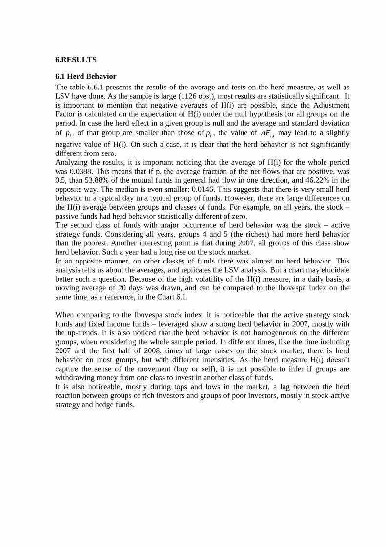
In an opposite manner, on other classes of funds there was almost no herd behavior. This

analysis tells us about the averages, and replicates the LSV analysis. But a chart may elucidate

better such a question. Because of the high volatility of the H(i) measure, in a daily basis, a

moving average of 20 days was drawn, and can be compared to the Ibovespa Index on the

same time, as a reference, in the Chart 6.1.

When comparing to the Ibovespa stock index, it is noticeable that the active strategy stock

funds and fixed income funds – leveraged show a strong herd behavior in 2007, mostly with

the up-trends. It is also noticed that the herd behavior is not homogeneous on the different

groups, when considering the whole sample period. In different times, like the time including

2007 and the first half of 2008, times of large raises on the stock market, there is herd

behavior on most groups, but with different intensities. As the herd measure H(i) doesn’t

capture the sense of the movement (buy or sell), it is not possible to infer if groups are

withdrawing money from one class to invest in another class of funds.

It is also noticeable, mostly during tops and lows in the market, a lag between the herd

reaction between groups of rich investors and groups of poor investors, mostly in stock-active

strategy and hedge funds.

Average Equity of the Investor Smaller Greater

Year Group 1 2 3 4 5 Class

Average (standard error) 0.0631 (0.0064) 0.0464 (0.0061) 0.0559 (0.0065) 0.0739 (0.0077) 0.0958 (0.0082) 0.0670 (0.0032)

Standard Deviation 0,1011 0,0964 0,1028 0,1219 0,1289 0,1120

Average Hypothesis Test 9.888 (0.000) 7.621 (0.000) 8.626 (0.000) 9.606 (0.000) 11.753 (0.000) 21.177 (0.000)

Minimum and Maximum -0.2299 e 0.3514 -0.1443 e 0.3862 -0.1709 e 0.3964 -0.1980 e 0.4533 -0.1442 e 0.6055 -0.2299 e 0.6055















































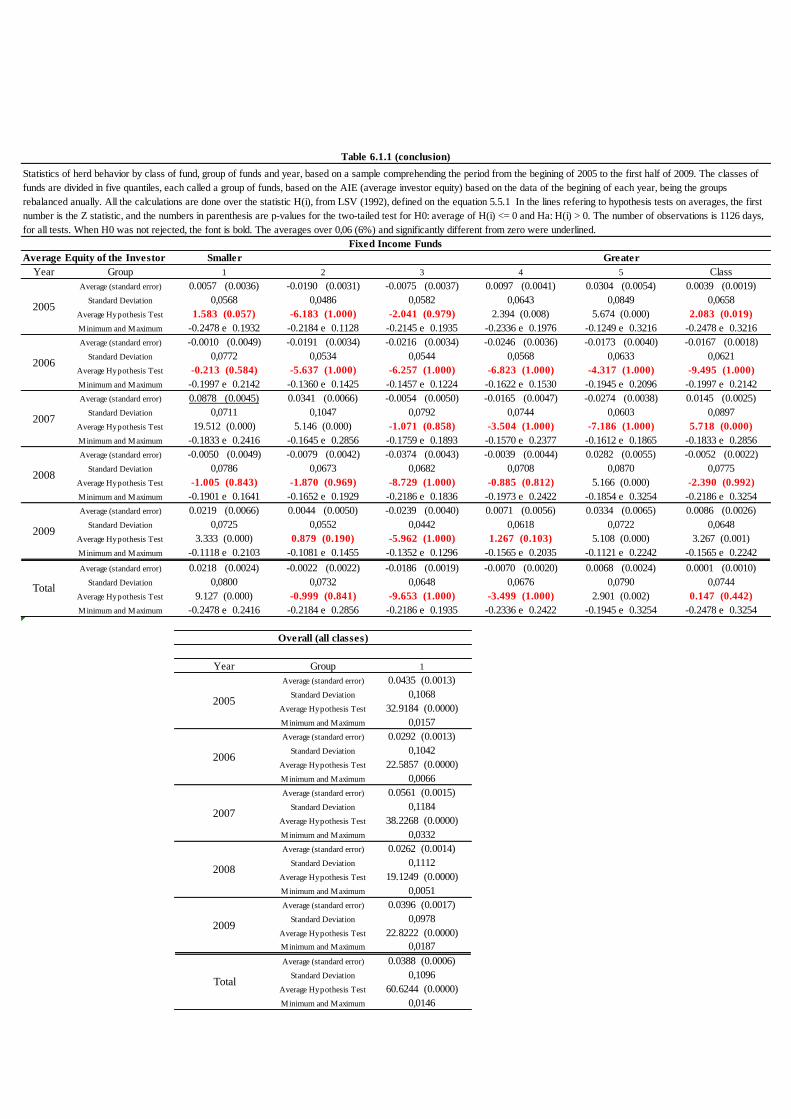
Statistics of herd behavior by class of fund, group of funds and year, based on a sample comprehending the period from the begining of 2005 to the first half of 2009. The classes of

funds are divided in five quantiles, each called a group of funds, based on the AIE (average investor equity) based on the data of the begining of each year, being the groups

rebalanced anually. All the calculations are done over the statistic H(i), from LSV (1992), defined on the equation 5.5.1 In the lines refering to hypothesis tests on averages, the first

number is the Z statistic, and the numbers in parenthesis are p-values for the two-tailed test for H0: average of H(i) <= 0 and Ha: H(i) > 0. The number of observations is 1126 days,

for all tests. When H0 was not rejected, the font is bold. The averages over 0,06 (6%) and significantly different from zero were underlined.

Table 6.1.1 (continues)



2005

2006

2009

Total

2005

2006

2007

2008

2009

Total

2007

2008

31 32 33 34 35 31



Average (standard error) -0.0224 (0.0028) -0.0014 (0.0036) 0.0321 (0.0047) 0.0094 (0.0041) 0.0540 (0.0055) 0.0143 (0.0020)


Average Hypothesis Test -7.957 (1.000) -0.398 (0.655) 6.774 (0.000) 2.291 (0.011) 9.822 (0.000) 7.042 (0.000)


Average (standard error) 0.0146 (0.0052) 0.0331 (0.0047) -0.0075 (0.0046) 0.0001 (0.0046) 0.0009 (0.0043) 0.0082 (0.0021)


Average Hypothesis Test 2.802 (0.003) 6.978 (0.000) -1.627 (0.948) 0.031 (0.488) 0.203 (0.419) 3.850 (0.000)


Average (standard error) 0.1096 (0.0057) 0.0689 (0.0055) 0.0215 (0.0051) 0.0137 (0.0048) -0.0093 (0.0048) 0.0409 (0.0026)


Average Hypothesis Test 19.332 (0.000) 12.472 (0.000) 4.204 (0.000) 2.830 (0.002) -1.939 (0.974) 15.605 (0.000)


Average (standard error) -0.0302 (0.0041) -0.0207 (0.0044) 0.0021 (0.0048) 0.0263 (0.0053) 0.0482 (0.0059) 0.0051 (0.0023)


Average Hypothesis Test -7.437 (1.000) -4.714 (1.000) 0.428 (0.334) 4.982 (0.000) 8.161 (0.000) 2.186 (0.014)


Average (standard error) 0.0587 (0.0072) 0.0032 (0.0055) -0.0139 (0.0044) -0.0090 (0.0052) 0.0018 (0.0059) 0.0081 (0.0028)


Average Hypothesis Test 8.096 (0.000) 0.576 (0.282) -3.149 (0.999) -1.743 (0.959) 0.302 (0.381) 2.940 (0.002)








Average (standard error) 0.0556 (0.0045) -0.0176 (0.0033) 0.0077 (0.0040) 0.0033 (0.0043) 0.0005 (0.0041) 0.0099 (0.0019)


Average Hypothesis Test 12.331 (0.000) -5.394 (1.000) 1.958 (0.025) 0.784 (0.216) 0.113 (0.455) 5.135 (0.000)


Average (standard error) -0.0137 (0.0041) 0.0370 (0.0061) 0.0120 (0.0047) -0.0136 (0.0044) 0.0107 (0.0049) 0.0065 (0.0022)


Average Hypothesis Test -3.328 (1.000) 6.095 (0.000) 2.565 (0.005) -3.116 (0.999) 2.191 (0.014) 2.889 (0.002)


Average (standard error) -0.0406 (0.0033) 0.0432 (0.0046) -0.0176 (0.0042) -0.0161 (0.0036) -0.0075 (0.0040) -0.0077 (0.0019)


Average Hypothesis Test -12.122 (1.000) 9.379 (0.000) -4.238 (1.000) -4.439 (1.000) -1.850 (0.968) -3.979 (1.000)


Average (standard error) 0.0187 (0.0042) -0.0087 (0.0037) -0.0218 (0.0038) -0.0082 (0.0040) -0.0406 (0.0038) -0.0121 (0.0018)


Average Hypothesis Test 4.506 (0.000) -2.372 (0.991) -5.746 (1.000) -2.035 (0.979) -10.727 (1.000) -6.661 (1.000)


Average (standard error) 0.0198 (0.0061) -0.0105 (0.0048) 0.0516 (0.0062) 0.0400 (0.0062) 0.0311 (0.0070) 0.0264 (0.0029)


Average Hypothesis Test 3.242 (0.001) -2.178 (0.985) 8.343 (0.000) 6.424 (0.000) 4.414 (0.000) 9.240 (0.000)


Average (standard error) 0.0067 (0.0022) 0.0107 (0.0022) 0.0011 (0.0021) -0.0034 (0.0020) -0.0050 (0.0021) 0.0021 (0.0010)


Average Hypothesis Test 3.094 (0.001) 4.834 (0.000) 0.546 (0.293) -1.684 (0.954) -2.334 (0.990) 2.156 (0.016)


Total

Hedge Funds

2005

2006

2007

2008

2008

2009

2009

Total


2005






Table 6.1.1 (continues)

2006

2007



Average (standard error) 0.0057 (0.0036) -0.0190 (0.0031) -0.0075 (0.0037) 0.0097 (0.0041) 0.0304 (0.0054) 0.0039 (0.0019)


Average Hypothesis Test 1.583 (0.057) -6.183 (1.000) -2.041 (0.979) 2.394 (0.008) 5.674 (0.000) 2.083 (0.019)


Average (standard error) -0.0010 (0.0049) -0.0191 (0.0034) -0.0216 (0.0034) -0.0246 (0.0036) -0.0173 (0.0040) -0.0167 (0.0018)


Average Hypothesis Test -0.213 (0.584) -5.637 (1.000) -6.257 (1.000) -6.823 (1.000) -4.317 (1.000) -9.495 (1.000)


Average (standard error) 0.0878 (0.0045) 0.0341 (0.0066) -0.0054 (0.0050) -0.0165 (0.0047) -0.0274 (0.0038) 0.0145 (0.0025)


Average Hypothesis Test 19.512 (0.000) 5.146 (0.000) -1.071 (0.858) -3.504 (1.000) -7.186 (1.000) 5.718 (0.000)


Average (standard error) -0.0050 (0.0049) -0.0079 (0.0042) -0.0374 (0.0043) -0.0039 (0.0044) 0.0282 (0.0055) -0.0052 (0.0022)


Average Hypothesis Test -1.005 (0.843) -1.870 (0.969) -8.729 (1.000) -0.885 (0.812) 5.166 (0.000) -2.390 (0.992)


Average (standard error) 0.0219 (0.0066) 0.0044 (0.0050) -0.0239 (0.0040) 0.0071 (0.0056) 0.0334 (0.0065) 0.0086 (0.0026)


Average Hypothesis Test 3.333 (0.000) 0.879 (0.190) -5.962 (1.000) 1.267 (0.103) 5.108 (0.000) 3.267 (0.001)


Average (standard error) 0.0218 (0.0024) -0.0022 (0.0022) -0.0186 (0.0019) -0.0070 (0.0020) 0.0068 (0.0024) 0.0001 (0.0010)


Average Hypothesis Test 9.127 (0.000) -0.999 (0.841) -9.653 (1.000) -3.499 (1.000) 2.901 (0.002) 0.147 (0.442)


#REF!

2 3 4

Year Group 1

Average (standard error) 0.0435 (0.0013)

Standard Deviation 0,1068

Average Hypothesis Test 32.9184 (0.0000)

Minimum and Maximum 0,0157





















2009

Total

2007

2008

Overall (all classes)

2005

Total

2006

2007

2008

2006

2009

Fixed Income Funds

2005

Table 6.1.1 (conclusion)








Hedge Funds

Fixed Income Funds

Chart 6.1 - Mean average (20) for each group, on each investor's size class, and the Ibovespa Stock Index (in points). Source: Economatica.


Ibovespa Stock Index

-0.10

-0.05

0.00

0.05

0.10

0.15

0.20

0.25

0.30

28/1/2005 16/8/2005 4/3/2006 20/9/2006 8/4/2007 25/10/2007 12/5/2008 28/11/2008 16/6/2009

Group 1(poor)

Group 2

Group 3

Group 4

Group 5(rich)

-0.10

-0.05

0.00

0.05

0.10

0.15

0.20

0.25

0.30

0.35

28/1/2005 16/8/2005 4/3/2006 20/9/2006 8/4/2007 25/10/2007 12/5/2008 28/11/2008 16/6/2009

Group 1(poor)

Group 2

Group 3

Group 4

Group 5(rich)

-0.11

-0.06

-0.01

0.04

0.09

0.14

0.19

28/1/2005 16/8/2005 4/3/2006 20/9/2006 8/4/2007 25/10/2007 12/5/2008 28/11/2008 16/6/2009

Group 1(poor)

Group 2

Group 3

Group 4

Group 5(rich)

-0.12

-0.07

-0.02

0.03

0.08

0.13

28/1/2005 16/8/2005 4/3/2006 20/9/2006 8/4/2007 25/10/2007 12/5/2008 28/11/2008 16/6/2009

Group 1(poor)

Group 2

Group 3

Group 4

Group 5(rich)

Ibovespa Index

20000

30000

40000

50000

60000

70000

80000

28/1/2005 28/5/2005 28/9/2005 28/1/2006 28/5/2006 28/9/2006 28/1/2007 28/5/2007 28/9/2007 28/1/2008 28/5/2008 28/9/2008 28/1/2009 28/5/2009

IbovespaIndex

-0.12

-0.07

-0.02

0.03

0.08

0.13

0.18

0.23

0.28

28/1/2005 16/8/2005 4/3/2006 20/9/2006 8/4/2007 25/10/2007 12/5/2008 28/11/2008 16/6/2009

Group 1(poor)

Group 2

Group 3

Group 4

Group 5(rich)

6.2. The relation between price anchoring and the herd behavior

For this test, a fixed effects panel regression was used, in order to control and measure the

effect of the characteristic of each group, as well as count for the time effect, and to isolate the

effect of the price anchoring on herd behavior. Six regressions were done, five of them

considering the groups on each class of funds, and a sixth for all classes of funds. The results

can be seen on the Table 6.3.1.

First, some analysis about the R2 is appropriated: the R2 within groups, the explain power of

the dummy variables over the herd behavior, is quite low, varying according to the fund

classes, between 1.6% and 3.7%. High figures were not expected, since the explaining

variables are dummies. However, the R2 between groups, ie the explaining power of the non-

observed characteristics of each group that do not vary with time, is high (except in the

passive strategy stock funds). That suggests that the influence of the event of new highs and

lows over the herd effect, ie the mutual fund investors in Brazil, yet may exist, has little

relevance.

New highs, in a year and in three months

The results achieved suggests that new highs in a period of one year have positive

contemporaneous with the herd effect on stock – active strategy funds, and a lagged negative

relation with hedge and leveraged fixed income funds.

However, in a period of three months, there is no evidence of a significant impact of new

highs on stock funds. Some effect is observed on hedge funds, being it negative in the one-

year horizon, but positive on the three months time. No theoretical support was found for

explaining such a result, in the research made.

New lows, in a year and in three months

In a general way, the results on new lows are more consistent and with larger coefficients than

with new highs. The new lows in one year had larger coefficients than in three months, which

is a more consistent result.

On the one-year term, new lows are related to smaller figures of the measure of herd behavior,

in all classes of funds, both one and four days lagged from the event.

No theoretical support was found for explaining such a result, in the research made.

Future studies may test if there is a greater volume of trading, after new lows, but without a

market consensus.

From the regression, it is possible to infer that the price anchoring, although has some

influence, has little explaining power on the herd behavior, but there are a set of non-observed

variables related to the groups, captured by the panel regression, which explains the herd

behavior.

7. CONCLUSIONS

This study aimed to detect, empirically, by means of statistical inference, the occurrence of

herd behavior in mutual fund flows in Brazil, as well as one of its possible causes: the price

anchoring.

Different from the LSV study, that found weak evidence of herd behavior among fund

managers, strong evidence of herd behavior was found among groups of investors in stock

mutual funds with an active strategy, in a heterogeneous way, and among investors of stock

(passive strategy) mutual funds.

Besides detecting the herd behavior, as did LSV in 1992, it was possible, by means of charts,

to verify that there is a great variance in that effect, although it follows trends, according to

the time, and sometimes there is a consensus between different groups, but most of the time

the herd behavior is heterogeneous between groups. This heterogeneity supports the

behavioral finance assumption that information (or rationality) is not homogeneous.

In a second test, it was possible to detect a small explaining power of event dummies related

to new price anchors, ie. new highs and lows in the Ibovespa stock index.

Stimulli Stock - active Stock - passive Fixed Income Lev. Hedge Fixed Income All

0.025** 0.003 0.011 0.001 0.008 0.010*

Lag 1 0.008 0.015 0.009 -0.008 -0.003 0.004

Lag 2 0.006 -0.004 0.007 -0.015* 0.004 0.000

Lag 3 0.010 -0.001 0.017* -0.004 0.007 0.007

Lag 4 0.016 -0.013 0.008 -0.011 0.002 0.001

Lag 5 0.015 0.002 -0.024** -0.033** 0.001 -0.008*

-0.044* -0.025 -0.008 0.005 -0.016 -0.016*

Lag 1 -0.044* -0.087** -0.055** -0.053** -0.036* -0.055**Lag 2 -0.016 -0.050 -0.005 -0.022 0.004 -0.015

Lag 3 -0.021 0.046 0.031 0.016 0.002 0.015

Lag 4 -0.029 -0.066* -0.070** -0.042** -0.047** -0.053**

Lag 5 -0.045* -0.001 0.023 0.011 -0.006 -0.003

-0.007 -0.001 0.000 0.002 -0.005 -0.002

Lag 1 0.003 -0.007 0.001 0.006 0.001 0.001

Lag 2 -0.009 0.002 0.004 0.022** 0.001 0.003

Lag 3 -0.013 -0.001 -0.009 0.004 -0.008 -0.007*

Lag 4 -0.007 0.007 -0.003 0.005 -0.006 -0.002

Lag 5 -0.004 -0.013 0.018** 0.014* -0.007 0.002

-0.010 0.007 -0.010 -0.013* -0.014* -0.008

Lag 1 0.012 0.008 0.033** 0.007 0.004 0.018**

Lag 2 -0.015 -0.007 0.014 -0.007 -0.018* -0.007

Lag 3 -0.005 -0.022 -0.029** -0.010 -0.009 -0.016**

Lag 4 0.010 0.035* 0.035** 0.026** 0.025** 0.029**

Lag 5 0.005 -0.002 -0.018* -0.008 -0.023** -0.009

R2 within groups 3.2% 1.6% 2.4% 3.7% 2.9% 1.4%

< < < < < <R2 between groups 59.2% 5.1% 75.5% 13.8% 76.2% 16.9%

general R2 3.1% 1.6% 2.4% 3.7% 2.8% 1.2%

average of obs. 1115.8 1106.2 1116.0 1116.0 1116.0 1114.0

Table 6.2.1

The resulting coefficients and R2 of the panel regressions of the herding measure (H(i)) explained by the dummy anchoring variables on the different

mutual fund classes. The variables mean: Dmax252 is 1 when there is a new high over the period of one year. Dmin252 is the same for new lows. The

Dmax 63 and Dmin63 variables are the same as those above. but for a 3-month period. Each column reffers to one regression. All regressions were

statistically significant.

* significant at 5% confidence level Source: the author

252maxD

252minD

63maxD

63minD

By those results, it was found that there is no strong evidence that investors use the price

anchoring heuristics in their investment decisions. Such a result is different from the results

found by Borges (2002), who tested this effect over the volume of stock traded on the

Bovespa Stock Exchange (Brazilian stock exchange) and with such heuristics bias, mentioned

by many authors in the Behavioral Finance line of research, i.e. Shefrin (2000).

This study had the following caveats, that are topics for future research:

The sample, although it has a large number of observations, comprehends a small period of

time, only four and a half years. That was due to a restriction on data availability. With such a

caveat, it is not possible to test the relation between herd behavior and the stock market crisis.

A study comprehending a larger sample, and other markets around the world, could lead to a

better comprehension of this fenomena among investors.

Also, the herd measure is not perfect, since it is not possible to know the exact number of

people that are deciding to buy or sell quotes of the fund.

Although this study is not conclusive on the matter, there are many factors that may induce

the herd behavior, not yet researched, but with great relevance for the comprehension of the

investors’ behavior, leading to questions such as:

Is there a sequential dissemination of the herd effect, maybe induced by a sequential, lagged

dissemination of the information between groups of investors? Does the herd behavior

influences the stock market returns?

8. REFERENCES

ANBID – Associação Nacional dos Bancos de Investimento Database. (n.d.). Consulted on

August 13th, 2009. (From October 21st, 2009 on, ANBID is called ANBIMA – Associação

Brasileira das Entidades dos Mercados Financeiro e de Capitais.

Baker, M., Ruback, R. S. & Wurgler, J. (2007). Behavioral corporate finance: A survey. In: B.

E. Eckbo (Ed.). Handbook of Corporate Finance: Empirical Corporate Finance, (Vol. 1).

Amsterdam: North-Holland.

Barberis, N. & Thaler, R. H. (2003). A survey of behavioral finance. In: G. Constantinides, M.

Harris, & R. Stultz (Eds.). The Handbook of the Economics of Finance, (Vol. 1B). Amsterdam:

North-Holland.

Bikhchandani, S. & Sharma, S. (2000). Herd behavior in financial markets. IMF Staff Papers,

47(3), 279-310.

Cesari, R. & Panetta, F. (2002). The performance of Italian equity funds. Journal of Banking

& Finance, 26, 99-126.

Cont, R. & Bouchaud, J. P. (2000). Herd behavior and aggregate fluctuations in financial

markets. Microeconomic Dynamics, 4, 170-196.

Cruz, L. F. B., Kimura, H. & Krauter, E. (2003). Finanças comportamentais: investigação do

comportamento decisório dos agentes brasileiros de acordo com a teoria do prospecto de

Kahneman & Tversky. In: XXXVIII Assembléia do Conselho Latino-Americano das Escolas

de Administração, 38, Lima, Peru.

Dickey, D. A. & Fuller, W. A. (1979). Distribution of the estimators for autoregressive time

series with a unit root. Journal of the American Statistical Association, 74(366), 427–431.

Economatica - Tools for Investment Analysis (n.d.). Consulted on August 13, 2009 at Getulio

Vargas Foundation’s Library.

Elton, E. J., Gruber, M. J., & Blake, C. R. (1996). Survivorship bias and mutual fund

performance. The Review of Financial Studies, 9(4), 1097-1120.

Fama, E. F. & French, K. R. (1992). The cross-section of expected stock returns. Journal of

Finance, 47, 427-465.

Fama, E. (1970). Efficient capital markets: a review of theory and empirical work. Journal of

Finance, 25(2), 383-417.

Fama, E. (1991). Efficient capital markets: II. Journal of Finance, 66(5), 1575-1617.

Jackson, A. (2003). The aggregate behavior of individual investors [Working Paper].

Available at SSRN: http://ssrn.com/abstract=536942.

Kahneman, D. & Tversky, A. (1979). Prospect theory: an analysis of decision under risk.

Econometrica, 47(2), 263-291.

Lakonishok, J., Shleifer, A. & Vishny, R. W. (1992). The impact of institutional trading on

stock prices. Journal of Financial Economics, 32(l), 23-43.

Lintner, J. (1965). The valuation of risk assets and the selection of risky investments in stock

portfolios and capital budgets. Review of Economics and Statistics, 47(1), 13-37.

Lobão, J. & Serra, A. P. (2002). Herding behavior – evidence from Portuguese mutual funds

[Working Paper]. Instituto de Estudos Financeiros e Fiscais, Portugal.

Markowitz, H. (1952). Portfolio selection. Journal of Finance, 7(1), 77-91.

Mossin, J. (1966). Equilibrium in a capital asset market. Econometrica, 34(4), 768-783.

Phillips, P. C. B. & Perron, P. (1988). Testing for a unit root in time series regression.

Biometrika, 75(2), 335-346.

Rochman, R. R. & Eid Jr., W. (2007). Insiders conseguem retornos anormais? Estudos de

eventos sobre as operações de insiders das empresas de governança corporativa diferenciada

da Bovespa. In: 7º Encontro Brasileiro de Finanças, São Paulo, Brasil.

Rogers, P., Securato, J. R. & Ribeiro, K. C. S. (2007). Finanças comportamentais no Brasil:

um estudo comparativo. Revista de Economia e Administração, 6(1), 49-68.

Sharpe, W. (1964). Capital asset prices: a theory of market equilibrium under conditions of

risk. Journal of Finance, 19(3), 425-442.

Shefrin, H. (2000). Beyond greed and fear: Understanding behavioral finance and the

psychology of investing. Boston MA: Harvard Business School Press.

Shefrin, H. (2001). Behavioral corporate finance. Journal of Applied Corporate Finance,

14(3), 113-124.

Shefrin, H. (2006). Behavioral corporate finance. McGraw-Hill/Irwin.

Schiller, R. J. (2000). Irrational exuberance. Princeton, NJ: Princeton University Press.

Teh, L. & Debondt, W. F. M. (1997). Herding behavior and stock returns: An exploratory

investigation. Swiss Journal of Economics and Statistics, 133(2), 293-324.

Thaler, R. H. (1987). Anomalies: The January effect. The Journal of Economic Perspectives,

1(1), 197 - 201.

Tversky, A. & Kahneman, D. (1974). Judgment under uncertainty: Heuristics and biases.

Science, 185(4157), 1124–31.

Documents

Herding Behavior on mutual fund investors in Brazil - Cass Business