Embed Size (px)
DESCRIPTION
many body physics
Citation preview

Introduction to
Many-body quantum theory incondensed matter physics
Henrik Bruus and Karsten Flensberg
Ørsted Laboratory, Niels Bohr Institute, University of CopenhagenMikroelektronik Centret, Technical University of Denmark
Copenhagen, 15 August 2002

ii
Preface
Preface for the 2001 editionThis introduction to quantum field theory in condensed matter physics has emerged fromour courses for graduate and advanced undergraduate students at the Niels Bohr Institute,University of Copenhagen, held between the fall of 1999 and the spring of 2001. We havegone through the pain of writing these notes, because we felt the pedagogical need fora book which aimed at putting an emphasis on the physical contents and applicationsof the rather involved mathematical machinery of quantum field theory without loosingmathematical rigor. We hope we have succeeded at least to some extend in reaching thisgoal.
We would like to thank the students who put up with the first versions of this book andfor their enumerable and valuable comments and suggestions. We are particularly gratefulto the students of Many-particle Physics I & II, the academic year 2000-2001, and to NielsAsger Mortensen and Brian Møller Andersen for careful proof reading. Naturally, we aresolely responsible for the hopefully few remaining errors and typos.
During the work on this book H.B. was supported by the Danish Natural Science Re-search Council through Ole Rømer Grant No. 9600548.
Ørsted Laboratory, Niels Bohr Institute Karsten Flensberg1 September, 2001 Henrik Bruus
Preface for the 2002 editionAfter running the course in the academic year 2001-2002 our students came up with morecorrections and comments so that we felt a new edition was appropriate. We would liketo thank our ever enthusiastic students for their valuable help in improving this book.
Karsten Flensberg Henrik BruusØrsted Laboratory Mikroelektronik CentretNiels Bohr Institute Technical University of Denmark
iii

iv PREFACE
Contents
List of symbols xii
1 First and second quantization 11.1 First quantization, single-particle systems . . . . . . . . . . . . . . . . . . . 21.2 First quantization, many-particle systems . . . . . . . . . . . . . . . . . . . 4
1.2.1 Permutation symmetry and indistinguishability . . . . . . . . . . . . 51.2.2 The single-particle states as basis states . . . . . . . . . . . . . . . . 61.2.3 Operators in first quantization . . . . . . . . . . . . . . . . . . . . . 7
1.3 Second quantization, basic concepts . . . . . . . . . . . . . . . . . . . . . . 91.3.1 The occupation number representation . . . . . . . . . . . . . . . . . 101.3.2 The boson creation and annihilation operators . . . . . . . . . . . . 101.3.3 The fermion creation and annihilation operators . . . . . . . . . . . 131.3.4 The general form for second quantization operators . . . . . . . . . . 141.3.5 Change of basis in second quantization . . . . . . . . . . . . . . . . . 161.3.6 Quantum field operators and their Fourier transforms . . . . . . . . 17
1.4 Second quantization, specific operators . . . . . . . . . . . . . . . . . . . . . 181.4.1 The harmonic oscillator in second quantization . . . . . . . . . . . . 181.4.2 The electromagnetic field in second quantization . . . . . . . . . . . 191.4.3 Operators for kinetic energy, spin, density, and current . . . . . . . . 211.4.4 The Coulomb interaction in second quantization . . . . . . . . . . . 231.4.5 Basis states for systems with different kinds of particles . . . . . . . 24
1.5 Second quantization and statistical mechanics . . . . . . . . . . . . . . . . . 251.5.1 The distribution function for non-interacting fermions . . . . . . . . 281.5.2 Distribution functions for non-interacting bosons . . . . . . . . . . . 29
1.6 Summary and outlook . . . . . . . . . . . . . . . . . . . . . . . . . . . . . . 29
2 The electron gas 312.1 The non-interacting electron gas . . . . . . . . . . . . . . . . . . . . . . . . 32
2.1.1 Bloch theory of electrons in a static ion lattice . . . . . . . . . . . . 332.1.2 Non-interacting electrons in the jellium model . . . . . . . . . . . . . 352.1.3 Non-interacting electrons at finite temperature . . . . . . . . . . . . 38
2.2 Electron interactions in perturbation theory . . . . . . . . . . . . . . . . . . 392.2.1 Electron interactions in 1st order perturbation theory . . . . . . . . 41
v
vi CONTENTS
2.2.2 Electron interactions in 2nd order perturbation theory . . . . . . . . 432.3 Electron gases in 3, 2, 1, and 0 dimensions . . . . . . . . . . . . . . . . . . . 44
2.3.1 3D electron gases: metals and semiconductors . . . . . . . . . . . . . 452.3.2 2D electron gases: GaAs/Ga1−xAlxAs heterostructures . . . . . . . . 462.3.3 1D electron gases: carbon nanotubes . . . . . . . . . . . . . . . . . . 482.3.4 0D electron gases: quantum dots . . . . . . . . . . . . . . . . . . . . 49
3 Phonons; coupling to electrons 513.1 Jellium oscillations and Einstein phonons . . . . . . . . . . . . . . . . . . . 523.2 Electron-phonon interaction and the sound velocity . . . . . . . . . . . . . . 533.3 Lattice vibrations and phonons in 1D . . . . . . . . . . . . . . . . . . . . . 533.4 Acoustical and optical phonons in 3D . . . . . . . . . . . . . . . . . . . . . 563.5 The specific heat of solids in the Debye model . . . . . . . . . . . . . . . . . 593.6 Electron-phonon interaction in the lattice model . . . . . . . . . . . . . . . 613.7 Electron-phonon interaction in the jellium model . . . . . . . . . . . . . . . 633.8 Summary and outlook . . . . . . . . . . . . . . . . . . . . . . . . . . . . . . 64
4 Mean field theory 654.1 The art of mean field theory . . . . . . . . . . . . . . . . . . . . . . . . . . . 684.2 Hartree–Fock approximation . . . . . . . . . . . . . . . . . . . . . . . . . . . 694.3 Broken symmetry . . . . . . . . . . . . . . . . . . . . . . . . . . . . . . . . . 714.4 Ferromagnetism . . . . . . . . . . . . . . . . . . . . . . . . . . . . . . . . . . 73
4.4.1 The Heisenberg model of ionic ferromagnets . . . . . . . . . . . . . . 734.4.2 The Stoner model of metallic ferromagnets . . . . . . . . . . . . . . 75
4.5 Superconductivity . . . . . . . . . . . . . . . . . . . . . . . . . . . . . . . . 784.5.1 Breaking of global gauge symmetry and its consequences . . . . . . . 784.5.2 Microscopic theory . . . . . . . . . . . . . . . . . . . . . . . . . . . . 81
4.6 Summary and outlook . . . . . . . . . . . . . . . . . . . . . . . . . . . . . . 85
5 Time evolution pictures 875.1 The Schrodinger picture . . . . . . . . . . . . . . . . . . . . . . . . . . . . . 875.2 The Heisenberg picture . . . . . . . . . . . . . . . . . . . . . . . . . . . . . 885.3 The interaction picture . . . . . . . . . . . . . . . . . . . . . . . . . . . . . . 885.4 Time-evolution in linear response . . . . . . . . . . . . . . . . . . . . . . . . 915.5 Time dependent creation and annihilation operators . . . . . . . . . . . . . 915.6 Summary and outlook . . . . . . . . . . . . . . . . . . . . . . . . . . . . . . 93
6 Linear response theory 956.1 The general Kubo formula . . . . . . . . . . . . . . . . . . . . . . . . . . . . 956.2 Kubo formula for conductivity . . . . . . . . . . . . . . . . . . . . . . . . . 986.3 Kubo formula for conductance . . . . . . . . . . . . . . . . . . . . . . . . . 1006.4 Kubo formula for the dielectric function . . . . . . . . . . . . . . . . . . . . 102
6.4.1 Dielectric function for translation-invariant system . . . . . . . . . . 1046.4.2 Relation between dielectric function and conductivity . . . . . . . . 104
CONTENTS vii
6.5 Summary and outlook . . . . . . . . . . . . . . . . . . . . . . . . . . . . . . 104
7 Transport in mesoscopic systems 1077.1 The S-matrix and scattering states . . . . . . . . . . . . . . . . . . . . . . . 108
7.1.1 Unitarity of the S-matrix . . . . . . . . . . . . . . . . . . . . . . . . 1117.1.2 Time-reversal symmetry . . . . . . . . . . . . . . . . . . . . . . . . . 112
7.2 Conductance and transmission coefficients . . . . . . . . . . . . . . . . . . . 1137.2.1 The Landauer-Buttiker formula, heuristic derivation . . . . . . . . . 1137.2.2 The Landauer-Buttiker formula, linear response derivation . . . . . . 115
7.3 Electron wave guides . . . . . . . . . . . . . . . . . . . . . . . . . . . . . . . 1167.3.1 Quantum point contact and conductance quantization . . . . . . . . 1167.3.2 Aharonov-Bohm effect . . . . . . . . . . . . . . . . . . . . . . . . . . 120
7.4 Disordered mesoscopic systems . . . . . . . . . . . . . . . . . . . . . . . . . 1217.4.1 Statistics of quantum conductance, random matrix theory . . . . . . 1217.4.2 Weak localization in mesoscopic systems . . . . . . . . . . . . . . . . 1237.4.3 Universal conductance fluctuations . . . . . . . . . . . . . . . . . . . 124
7.5 Summary and outlook . . . . . . . . . . . . . . . . . . . . . . . . . . . . . . 125
8 Green’s functions 1278.1 “Classical” Green’s functions . . . . . . . . . . . . . . . . . . . . . . . . . . 1278.2 Green’s function for the one-particle Schrodinger equation . . . . . . . . . . 1288.3 Single-particle Green’s functions of many-body systems . . . . . . . . . . . 131
8.3.1 Green’s function of translation-invariant systems . . . . . . . . . . . 1328.3.2 Green’s function of free electrons . . . . . . . . . . . . . . . . . . . . 1328.3.3 The Lehmann representation . . . . . . . . . . . . . . . . . . . . . . 1348.3.4 The spectral function . . . . . . . . . . . . . . . . . . . . . . . . . . 1358.3.5 Broadening of the spectral function . . . . . . . . . . . . . . . . . . . 136
8.4 Measuring the single-particle spectral function . . . . . . . . . . . . . . . . 1378.4.1 Tunneling spectroscopy . . . . . . . . . . . . . . . . . . . . . . . . . 1378.4.2 Optical spectroscopy . . . . . . . . . . . . . . . . . . . . . . . . . . . 141
8.5 Two-particle correlation functions of many-body systems . . . . . . . . . . . 1418.6 Summary and outlook . . . . . . . . . . . . . . . . . . . . . . . . . . . . . . 144
9 Equation of motion theory 1459.1 The single-particle Green’s function . . . . . . . . . . . . . . . . . . . . . . 145
9.1.1 Non-interacting particles . . . . . . . . . . . . . . . . . . . . . . . . . 1479.2 Anderson’s model for magnetic impurities . . . . . . . . . . . . . . . . . . . 147
9.2.1 The equation of motion for the Anderson model . . . . . . . . . . . 1499.2.2 Mean-field approximation for the Anderson model . . . . . . . . . . 1509.2.3 Solving the Anderson model and comparison with experiments . . . 1519.2.4 Coulomb blockade and the Anderson model . . . . . . . . . . . . . . 1539.2.5 Further correlations in the Anderson model: Kondo effect . . . . . . 153
9.3 The two-particle correlation function . . . . . . . . . . . . . . . . . . . . . . 1539.3.1 The Random Phase Approximation (RPA) . . . . . . . . . . . . . . 153

viii CONTENTS
9.4 Summary and outlook . . . . . . . . . . . . . . . . . . . . . . . . . . . . . . 156
10 Imaginary time Green’s functions 15710.1 Definitions of Matsubara Green’s functions . . . . . . . . . . . . . . . . . . 160
10.1.1 Fourier transform of Matsubara Green’s functions . . . . . . . . . . 16110.2 Connection between Matsubara and retarded functions . . . . . . . . . . . . 161
10.2.1 Advanced functions . . . . . . . . . . . . . . . . . . . . . . . . . . . 16310.3 Single-particle Matsubara Green’s function . . . . . . . . . . . . . . . . . . 164
10.3.1 Matsubara Green’s function for non-interacting particles . . . . . . . 16410.4 Evaluation of Matsubara sums . . . . . . . . . . . . . . . . . . . . . . . . . 165
10.4.1 Summations over functions with simple poles . . . . . . . . . . . . . 16710.4.2 Summations over functions with known branch cuts . . . . . . . . . 168
10.5 Equation of motion . . . . . . . . . . . . . . . . . . . . . . . . . . . . . . . . 16910.6 Wick’s theorem . . . . . . . . . . . . . . . . . . . . . . . . . . . . . . . . . . 17010.7 Example: polarizability of free electrons . . . . . . . . . . . . . . . . . . . . 17310.8 Summary and outlook . . . . . . . . . . . . . . . . . . . . . . . . . . . . . . 174
11 Feynman diagrams and external potentials 17711.1 Non-interacting particles in external potentials . . . . . . . . . . . . . . . . 17711.2 Elastic scattering and Matsubara frequencies . . . . . . . . . . . . . . . . . 17911.3 Random impurities in disordered metals . . . . . . . . . . . . . . . . . . . . 181
11.3.1 Feynman diagrams for the impurity scattering . . . . . . . . . . . . 18211.4 Impurity self-average . . . . . . . . . . . . . . . . . . . . . . . . . . . . . . . 18411.5 Self-energy for impurity scattered electrons . . . . . . . . . . . . . . . . . . 189
11.5.1 Lowest order approximation . . . . . . . . . . . . . . . . . . . . . . . 19011.5.2 1st order Born approximation . . . . . . . . . . . . . . . . . . . . . . 19011.5.3 The full Born approximation . . . . . . . . . . . . . . . . . . . . . . 19311.5.4 The self-consistent Born approximation and beyond . . . . . . . . . 194
11.6 Summary and outlook . . . . . . . . . . . . . . . . . . . . . . . . . . . . . . 197
12 Feynman diagrams and pair interactions 19912.1 The perturbation series for G . . . . . . . . . . . . . . . . . . . . . . . . . . 19912.2 infinite perturbation series!Matsubara Green’s function . . . . . . . . . . . . 19912.3 The Feynman rules for pair interactions . . . . . . . . . . . . . . . . . . . . 201
12.3.1 Feynman rules for the denominator of G(b, a) . . . . . . . . . . . . . 20112.3.2 Feynman rules for the numerator of G(b, a) . . . . . . . . . . . . . . 20212.3.3 The cancellation of disconnected Feynman diagrams . . . . . . . . . 203
12.4 Self-energy and Dyson’s equation . . . . . . . . . . . . . . . . . . . . . . . . 20512.5 The Feynman rules in Fourier space . . . . . . . . . . . . . . . . . . . . . . 20612.6 Examples of how to evaluate Feynman diagrams . . . . . . . . . . . . . . . 208
12.6.1 The Hartree self-energy diagram . . . . . . . . . . . . . . . . . . . . 20912.6.2 The Fock self-energy diagram . . . . . . . . . . . . . . . . . . . . . . 20912.6.3 The pair-bubble self-energy diagram . . . . . . . . . . . . . . . . . . 210
12.7 Summary and outlook . . . . . . . . . . . . . . . . . . . . . . . . . . . . . . 211
CONTENTS ix
13 The interacting electron gas 21313.1 The self-energy in the random phase approximation . . . . . . . . . . . . . 213
13.1.1 The density dependence of self-energy diagrams . . . . . . . . . . . . 21413.1.2 The divergence number of self-energy diagrams . . . . . . . . . . . . 21513.1.3 RPA resummation of the self-energy . . . . . . . . . . . . . . . . . . 215
13.2 The renormalized Coulomb interaction in RPA . . . . . . . . . . . . . . . . 21713.2.1 Calculation of the pair-bubble . . . . . . . . . . . . . . . . . . . . . . 21813.2.2 The electron-hole pair interpretation of RPA . . . . . . . . . . . . . 220
13.3 The ground state energy of the electron gas . . . . . . . . . . . . . . . . . . 22013.4 The dielectric function and screening . . . . . . . . . . . . . . . . . . . . . . 22313.5 Plasma oscillations and Landau damping . . . . . . . . . . . . . . . . . . . 227
13.5.1 Plasma oscillations and plasmons . . . . . . . . . . . . . . . . . . . . 22813.5.2 Landau damping . . . . . . . . . . . . . . . . . . . . . . . . . . . . . 230
13.6 Summary and outlook . . . . . . . . . . . . . . . . . . . . . . . . . . . . . . 231
14 Fermi liquid theory 23314.1 Adiabatic continuity . . . . . . . . . . . . . . . . . . . . . . . . . . . . . . . 233
14.1.1 The quasiparticle concept and conserved quantities . . . . . . . . . . 23514.2 Semi-classical treatment of screening and plasmons . . . . . . . . . . . . . . 237
14.2.1 Static screening . . . . . . . . . . . . . . . . . . . . . . . . . . . . . . 23814.2.2 Dynamical screening . . . . . . . . . . . . . . . . . . . . . . . . . . . 238
14.3 Semi-classical transport equation . . . . . . . . . . . . . . . . . . . . . . . . 24014.3.1 Finite life time of the quasiparticles . . . . . . . . . . . . . . . . . . 243
14.4 Microscopic basis of the Fermi liquid theory . . . . . . . . . . . . . . . . . . 24514.4.1 Renormalization of the single particle Green’s function . . . . . . . . 24514.4.2 Imaginary part of the single particle Green’s function . . . . . . . . 24814.4.3 Mass renormalization? . . . . . . . . . . . . . . . . . . . . . . . . . . 251
14.5 Outlook and summary . . . . . . . . . . . . . . . . . . . . . . . . . . . . . . 251
15 Impurity scattering and conductivity 25315.1 Vertex corrections and dressed Green’s functions . . . . . . . . . . . . . . . 25415.2 The conductivity in terms of a general vertex function . . . . . . . . . . . . 25915.3 The conductivity in the first Born approximation . . . . . . . . . . . . . . . 26115.4 The weak localization correction to the conductivity . . . . . . . . . . . . . 26415.5 Combined RPA and Born approximation . . . . . . . . . . . . . . . . . . . . 273
16 Green’s functions and phonons 27516.1 The Green’s function for free phonons . . . . . . . . . . . . . . . . . . . . . 27516.2 Electron-phonon interaction and Feynman diagrams . . . . . . . . . . . . . 27616.3 Combining Coulomb and electron-phonon interactions . . . . . . . . . . . . 279
16.3.1 Migdal’s theorem . . . . . . . . . . . . . . . . . . . . . . . . . . . . . 27916.3.2 Jellium phonons and the effective electron-electron interaction . . . 280
16.4 Phonon renormalization by electron screening in RPA . . . . . . . . . . . . 28116.5 The Cooper instability and Feynman diagrams . . . . . . . . . . . . . . . . 284
x CONTENTS
17 Superconductivity 28717.1 The Cooper instability . . . . . . . . . . . . . . . . . . . . . . . . . . . . . . 28717.2 The BCS groundstate . . . . . . . . . . . . . . . . . . . . . . . . . . . . . . 28717.3 BCS theory with Green’s functions . . . . . . . . . . . . . . . . . . . . . . . 28717.4 Experimental consequences of the BCS states . . . . . . . . . . . . . . . . . 288
17.4.1 Tunneling density of states . . . . . . . . . . . . . . . . . . . . . . . 28817.4.2 specific heat . . . . . . . . . . . . . . . . . . . . . . . . . . . . . . . . 288
17.5 The Josephson effect . . . . . . . . . . . . . . . . . . . . . . . . . . . . . . . 288
18 1D electron gases and Luttinger liquids 28918.1 Introduction . . . . . . . . . . . . . . . . . . . . . . . . . . . . . . . . . . . . 28918.2 First look at interacting electrons in one dimension . . . . . . . . . . . . . . 289
18.2.1 One-dimensional transmission line analog . . . . . . . . . . . . . . . 28918.3 The Luttinger-Tomonaga model - spinless case . . . . . . . . . . . . . . . . 289
18.3.1 Interacting one dimensional electron system . . . . . . . . . . . . . . 28918.3.2 Bosonization of Tomonaga model-Hamiltonian . . . . . . . . . . . . 28918.3.3 Diagonalization of bosonized Hamiltonian . . . . . . . . . . . . . . . 28918.3.4 Real space formulation . . . . . . . . . . . . . . . . . . . . . . . . . . 28918.3.5 Electron operators in bosonized form . . . . . . . . . . . . . . . . . . 289
18.4 Luttinger liquid with spin . . . . . . . . . . . . . . . . . . . . . . . . . . . . 29018.5 Green’s functions . . . . . . . . . . . . . . . . . . . . . . . . . . . . . . . . . 29018.6 Tunneling into spinless Luttinger liquid . . . . . . . . . . . . . . . . . . . . 290
18.6.1 Tunneling into the end of Luttinger liquid . . . . . . . . . . . . . . . 29018.7 What is a Luttinger liquid? . . . . . . . . . . . . . . . . . . . . . . . . . . . 29018.8 Experimental realizations of Luttinger liquid physics . . . . . . . . . . . . . 290
18.8.1 Edge states in the fractional quantum Hall effect . . . . . . . . . . . 29018.8.2 Carbon Nanotubes . . . . . . . . . . . . . . . . . . . . . . . . . . . . 290
A Fourier transformations 291A.1 Continuous functions in a finite region . . . . . . . . . . . . . . . . . . . . . 291A.2 Continuous functions in an infinite region . . . . . . . . . . . . . . . . . . . 292A.3 Time and frequency Fourier transforms . . . . . . . . . . . . . . . . . . . . 292A.4 Some useful rules . . . . . . . . . . . . . . . . . . . . . . . . . . . . . . . . . 292A.5 Translation invariant systems . . . . . . . . . . . . . . . . . . . . . . . . . . 293
B Exercises 295
C Index 326
List of symbols
Symbol Meaning Definition
♥ operator ♥ in the interaction picture Sec. 5.3♥ time derivative of ♥|ν〉 Dirac ket notation for a quantum state ν Chap. 1〈ν| Dirac bra notation for an adjoint quantum state ν Chap. 1|0〉 vacuum state
a annihilation operator for particle (fermion or boson)a† creation operator for particle (fermion or boson)aν , a
†ν annihilation/creation operators (state ν)
a±n amplitudes of wavefunctions to the left Sec. 7.1a0 Bohr radius Eq. (2.36)A(r, t) electromagnetic vector potential Sec. 1.4.2A(ν, ω) spectral function in frequency domain (state ν) Sec. 8.3.4A(r, ω), A(k, ω) spectral function (real space, Fourier space) Sec. 8.3.4A0(r, ω), A0(k, ω) spectral function for free particles Sec. 8.3.4A,A† phonon annihilation and creation operator Sec. 16.1
b annihilation operator for particle (boson, phonon)b† creation operator for particle (boson, phonon)b±n amplitudes of wavefunctions to the right Sec. 7.1B magnetic field
c annihilation operator for particle (fermion, electron)c† creation operator for particle (fermion, electron)cν , c
†ν annihilation/creation operators (state ν)
CRAB(t, t′) retarded correlation function between A and B (time) Sec. 6.1
CAAB(t, t′) advanced correlation function between A and B (time) Sec. 10.2.1
CRII(ω) retarded current-current correlation function (frequency) Sec. 6.3
CAB Matsubara correlation function Sec. 10.1C(Q, ikn, ikn + iqn) Cooperon in the Matsubara domain Sec. 15.4CR(Q, ε, ε) Cooperon in the real time domain Sec. 15.4C ion
V specific heat for ions (constant volume)
xi
xii LIST OF SYMBOLS
Symbol Meaning Definition
d(ε) density of states (including spin degeneracy for electrons) Eq. (2.31)δ(r) Dirac delta function Eq. (1.11)DR(rt, rt′) retarded phonon propagator Chap. 16DR(q, ω) retarded phonon propagator (Fourier space) Chap. 16D(rτ, rτ ′) Matsubara phonon propagator Chap. 16D(q, iqn) Matsubara phonon propagator (Fourier space) Chap. 16DR(νt, ν ′t′) retarded many particle Green’s function Eq. (9.9b)Dαβ(r) phonon dynamical matrix Sec. 3.4)∆k superconducting orderparameter Eq. (4.58b)
e elementary chargee20 electron interaction strength Eq. (1.101)
E(r, t) electric fieldE total energy of the electron gasE(1) interaction energy of the electron gas, 1st order perturbationE(2) interaction energy of the electron gas, 2nd order perturbationE0 Rydberg energy Eq. (2.36)Ek dispersion relation for BCS quasiparticles Eq. (4.64)ε energy variableε0 the dielectric constant of vacuumεk dispersion relationεν energy of quantum state νεF Fermi energyεkλ phonon polarization vector Eq. (3.20)ε(rt, rt′) dielectric function in real space Sec. 6.4ε(k, ω) dielectric function in Fourier space Sec. 6.4
F free energy Sec. 1.5|FS〉 the filled Fermi sea N -particle quantum stateφ(r, t) electric potentialφext external electric potentialφind induced electric potentialφ, φ wavefunctions with different normalizations Eq. (7.4)φ±LnE , φ±RnE wavefunctions in the left and right leads Sec. 7.1
gqλ electron-phonon coupling constant (lattice model)gq electron-phonon coupling constant (jellium model)G conductance
LIST OF SYMBOLS xiii
Symbol Meaning Definition
G(rt, r′t′) Green’s function for the Schrodinger equation Sec. 8.2G0(rt, r
′t′) unperturbed Green’s function for Schrodingers eq. Sec. 8.2G<
0 (rt, r′t′) free lesser Green’s function Sec. 8.3.1G>
0 (rt, r′t′) free grater Green’s function Sec. 8.3.1GA
0 (rt, r′t′) free advanced Green’s function Sec. 8.3.1GR
0 (rt, r′t′) free retarded Green’s function Sec. 8.3.1GR
0 (k, ω) free retarded Green’s function (Fourier space) Sec. 8.3.1G<(rt, r′t′) lesser Green’s function Sec. 8.3G>(rt, r′t′) greater Green’s function Sec. 8.3GA(rt, r′t′) advanced Green’s function Sec. 8.3GR(rt, r′t′) retarded Green’s function (real space) Sec. 8.3GR(k, ω) retarded Green’s function in Fourier space Sec. 8.3GR(k, ω) retarded Green’s function (Fourier space) Sec. 8.3.1GR(νt, ν ′t′) retarded single-particle Green’s function (ν basis) Eq. (8.32)G(rστ, r′σ′τ ′) Matsubara Green’s function (real space) Sec. 10.3G(ντ, ν ′τ ′) Matsubara Green’s function (ν basis) Sec. 10.3G(1, 1′) Matsubara Green’s function (real space four-vectors) Sec. 11.1G(k, k′) Matsubara Green’s function (four-momentum notation) Sec. 12.5G0(rστ, r′σ′τ ′) Matsubara Green’s function (real space, free particles) Sec. 10.3.1G0(ντ, ν′τ ′) Matsubara Green’s function (ν basis, free particles) Sec. 10.3.1G0(k, ikn) Matsubara Green’s function (Fourier space, free particles) Sec. 10.3G0(ν, ikn) Matsubara Green’s function (free particles ) Sec. 10.3G(n)
0 n-particle Green’s function (free particles) Sec. 10.6G(k, ikn) Matsubara Green’s function (Fourier space) Sec. 10.3G(ν, ikn) Matsubara Green’s function (ν basis, frequency domain) Sec. 10.3γ, γRA scalar vertex function Sec. 15.3Γ imaginary part of self-energyΓx(k, k + q) vertex function (x-component, four vector notation) Eq. (15.20b)Γ0,x free (undressed) vertex function
H a general HamiltonianH0 unperturbed part of an HamiltonianH ′ perturbative part of an HamiltonianHext external potential part of an HamiltonianHint interaction part of an HamiltonianHph phonon part of an Hamiltonianη positive infinitisimal
I current operator (particle current) Sec. 6.3Ie electrical current (charge current) Sec. 6.3
xiv LIST OF SYMBOLS
Symbol Meaning Definition
Jσ(r) current density operator Eq. (1.99a)J∆
σ (r) current density operator, paramagnetic term Eq. (1.99a)JA
σ (r) current density operator, diamagnetic term Eq. (1.99a)Jσ(q) current density operator (momentum space)Je(r, t) electric current density operatorJij interaction strength in the Heisenberg model Sec. 4.4.1
kn Matsubara frequency (fermions)kF Fermi wave numberk general momentum or wave vector variable
` mean free path or scattering length`0 mean free path (first Born approximation)`φ phase breaking mean free path`in inelastic scattering lengthL normalization length or system size in 1DλF Fermi wave lengthΛirr irreducible four-point function Eq. (15.17)
m mass (electrons and general particles)m∗ effective interaction renormalized mass Sec. 14.4.1µ chemical potentialµ general quantum number label
n particle densitynF(ε) Fermi-Dirac distribution function Sec. 1.5.1nB(ε) Bose-Einstein distribution function Sec. 1.5.2nimp impurity densityN number of particlesNimp number of impuritiesν general quantum number label
ω frequency variableωq phonon dispersion relationωn Matsubara frequency Chap. 10Ω thermodynamic potential Sec. 1.5
p general momentum or wave number variablepn Matsubara frequency (fermion)ΠR
αβ(rt, r′t′) retarded current-current correlation function Eq. (6.26)ΠR
αβ(q, ω) retarded current-current correlation functionΠαβ(q, iωn) Matsubara current-current correlation function Chap. 15Π0(q, iqn) free pair-bubble diagram Eq. (12.34)
LIST OF SYMBOLS xv
Symbol Meaning Definition
q general momentum variableqn Matsubara frequency (bosons)
r general space variabler reflection matrix coming from left Sec. 7.1r′ reflection matrix coming from right Sec. 7.1rs electron gas density parameter Eq. (2.37)ρ density matrix Sec. 1.5ρ0 unperturbed density matrixρσ(r) particle density operator (real space) Eq. (1.96)ρσ(q) particle density opetor (momentum space) Eq. (1.96)
S entropyS scattering matrix Sec. 7.1σ general spin indexσαβ(rt, r′t′) conductivity tensor Sec. 6.2ΣR(q, ω) retarded self-energy (Fourier space)Σ(q, ikn) Matsubara self-energyΣk impurity scattering self-energy Sec. 11.5Σ1BA
k first Born approximation Sec. 11.5.1ΣFBA
k full Born approximation Sec. 11.5.3ΣSCBA
k self-consistent Born approximation Sec. 11.5.4Σ(l, j) general electron self-energyΣσ(k, ikn) general electron self-energyΣF
σ (k, ikn) Fock self-energy Sec. 12.6ΣH
σ (k, ikn) Hartree self-energy Sec. 12.6ΣP
σ (k, ikn) pair-bubble self-energy Sec. 12.6ΣRPA
σ (k, ikn) RPA electron self-energy Eq. (13.10)
t general time variablet tranmission matrix coming from left Sec. 7.1t′ transmission matrix coming from right Sec. 7.1T kinetic energyτ general imaginary time variableτ tr transport scattering time Eq. (14.39)τ0, τk life-time in the first Born approximation
uj ion displacement (1D)u(R0) ion displacement (3D)uk BCS coherence factor Sec. 4.5.2U general unitary matrixU(t, t′) real time-evolution operator, interaction pictureU(τ, τ ′) imaginary time-evolution operator, interaction picture
xvi LIST OF SYMBOLS
Symbol Meaning Definition
vk BCS coherence factor Sec. 4.5.2V (r), V (q) general single impurity potentialV (r), V (q) Coulomb interactionVeff combined Coulomb and phonon-mediated interaction Sec. 13.2V normalization volume
W pair interaction HamiltonianW (r),W (q) general pair interactionW (r),W (q) Coulomb interactionWRPA RPA-screened Coulomb interaction Sec. 13.2
ξk εk − µξν εν − µχ(q, iqn) Matsubara charge-charge correlation function Sec. 13.4χRPA(q, iqn) RPA Matsubara charge-charge correlation function Sec. 13.4χirr(q, iqn) irreducible Matsubara charge-charge correlation function Sec. 13.4χ0(rt, r
′t′) free retarded charge-charge correlation functionχ0(q, iqn) free Matsubara charge-charge correlation function Sec. 13.4χR(rt, r′t′) retarded charge-charge correlation function Eq. (6.39)χR(q, ω) retarded charge-charge correlation function (Fourier)χn(y) transverse wavefunction Sec. 7.1
ψν(r) single-particle wave function, quantum number νψ±nE single-particle scattering states Sec. 7.1ψ(r1, r2, . . . , rn) n-particle wave function (first quantization)Ψσ(r) quantum field annihilation operator Sec. 1.3.6Ψ†
σ(r) quantum field creation operator Sec. 1.3.6
θ(x) Heaviside’s step function Eq. (1.12)

Chapter 1
First and second quantization
Quantum theory is the most complete microscopic theory we have today describing thephysics of energy and matter. It has successfully been applied to explain phenomenaranging over many orders of magnitude, from the study of elementary particles on thesub-nucleonic scale to the study of neutron stars and other astrophysical objects on thecosmological scale. Only the inclusion of gravitation stands out as an unsolved problemin fundamental quantum theory.
Historically, quantum physics first dealt only with the quantization of the motion ofparticles leaving the electromagnetic field classical, hence the name quantum mechanics(Heisenberg, Schrodinger, and Dirac 1925-26). Later also the electromagnetic field wasquantized (Dirac, 1927), and even the particles themselves got represented by quantizedfields (Jordan and Wigner, 1928), resulting in the development of quantum electrodynam-ics (QED) and quantum field theory (QFT) in general. By convention, the original form ofquantum mechanics is denoted first quantization, while quantum field theory is formulatedin the language of second quantization.
Regardless of the representation, be it first or second quantization, certain basic con-cepts are always present in the formulation of quantum theory. The starting point isthe notion of quantum states and the observables of the system under consideration.Quantum theory postulates that all quantum states are represented by state vectors ina Hilbert space, and that all observables are represented by Hermitian operators actingon that space. Parallel state vectors represent the same physical state, and one thereforemostly deals with normalized state vectors. Any given Hermitian operator A has a numberof eigenstates |ψα〉 that up to a real scale factor α is left invariant by the action of theoperator, A|ψα〉 = α|ψα〉. The scale factors are denoted the eigenvalues of the operator.It is a fundamental theorem of Hilbert space theory that the set of all eigenvectors of anygiven Hermitian operator forms a complete basis set of the Hilbert space. In general theeigenstates |ψα〉 and |φβ〉 of two different Hermitian operators A and B are not the same.By measurement of the type B the quantum state can be prepared to be in an eigenstate|φβ〉 of the operator B. This state can also be expressed as a superposition of eigenstates|ψα〉 of the operator A as |φβ〉 =
∑α |ψα〉Cαβ. If one in this state measures the dynamical
variable associated with the operator A, one cannot in general predict the outcome with
1
2 CHAPTER 1. FIRST AND SECOND QUANTIZATION
certainty. It is only described in probabilistic terms. The probability of having any given|ψα〉 as the outcome is given as the absolute square |Cαβ|2 of the associated expansioncoefficient. This non-causal element of quantum theory is also known as the collapse ofthe wavefunction. However, between collapse events the time evolution of quantum statesis perfectly deterministic. The time evolution of a state vector |ψ(t)〉 is governed by thecentral operator in quantum mechanics, the Hamiltonian H (the operator associated withthe total energy of the system), through Schrodinger’s equation
i~∂t|ψ(t)〉 = H|ψ(t)〉. (1.1)
Each state vector |ψ〉 is associated with an adjoint state vector (|ψ〉)† ≡ 〈ψ|. One canform inner products, “bra(c)kets”, 〈ψ|φ〉 between adjoint “bra” states 〈ψ| and “ket” states|φ〉, and use standard geometrical terminology, e.g. the norm squared of |ψ〉 is given by〈ψ|ψ〉, and |ψ〉 and |φ〉 are said to be orthogonal if 〈ψ|φ〉 = 0. If |ψα〉 is an orthonormalbasis of the Hilbert space, then the above mentioned expansion coefficient Cαβ is foundby forming inner products: Cαβ = 〈ψα|φβ〉. A further connection between the direct andthe adjoint Hilbert space is given by the relation 〈ψ|φ〉 = 〈φ|ψ〉∗, which also leads to thedefinition of adjoint operators. For a given operator A the adjoint operator A† is definedby demanding 〈ψ|A†|φ〉 = 〈φ|A|ψ〉∗ for any |ψ〉 and |φ〉.
In this chapter we will briefly review standard first quantization for one and many-particle systems. For more complete reviews the reader is refereed to the textbooks byDirac, Landau and Lifshitz, Merzbacher, or Shankar. Based on this we will introducesecond quantization. This introduction is not complete in all details, and we refer theinterested reader to the textbooks by Mahan, Fetter and Walecka, and Abrikosov, Gorkov,and Dzyaloshinskii.
1.1 First quantization, single-particle systems
For simplicity consider a non-relativistic particle, say an electron with charge −e, movingin an external electromagnetic field described by the potentials ϕ(r, t) and A(r, t). Thecorresponding Hamiltonian is
H =1
2m
(~i∇r + eA(r, t)
)2
− eϕ(r, t). (1.2)
An eigenstate describing a free spin-up electron travelling inside a box of volume Vcan be written as a product of a propagating plane wave and a spin-up spinor. Using theDirac notation the state ket can be written as |ψk,↑〉 = |k, ↑〉, where one simply lists therelevant quantum numbers in the ket. The state function (also denoted the wave function)and the ket are related by
ψk,σ(r) = 〈r|k, σ〉 = 1√V eik·rχσ (free particle orbital), (1.3)
i.e. by the inner product of the position bra 〈r| with the state ket.The plane wave representation |k, σ〉 is not always a useful starting point for calcu-
lations. For example in atomic physics, where electrons orbiting a point-like positively
1.1. FIRST QUANTIZATION, SINGLE-PARTICLE SYSTEMS 3
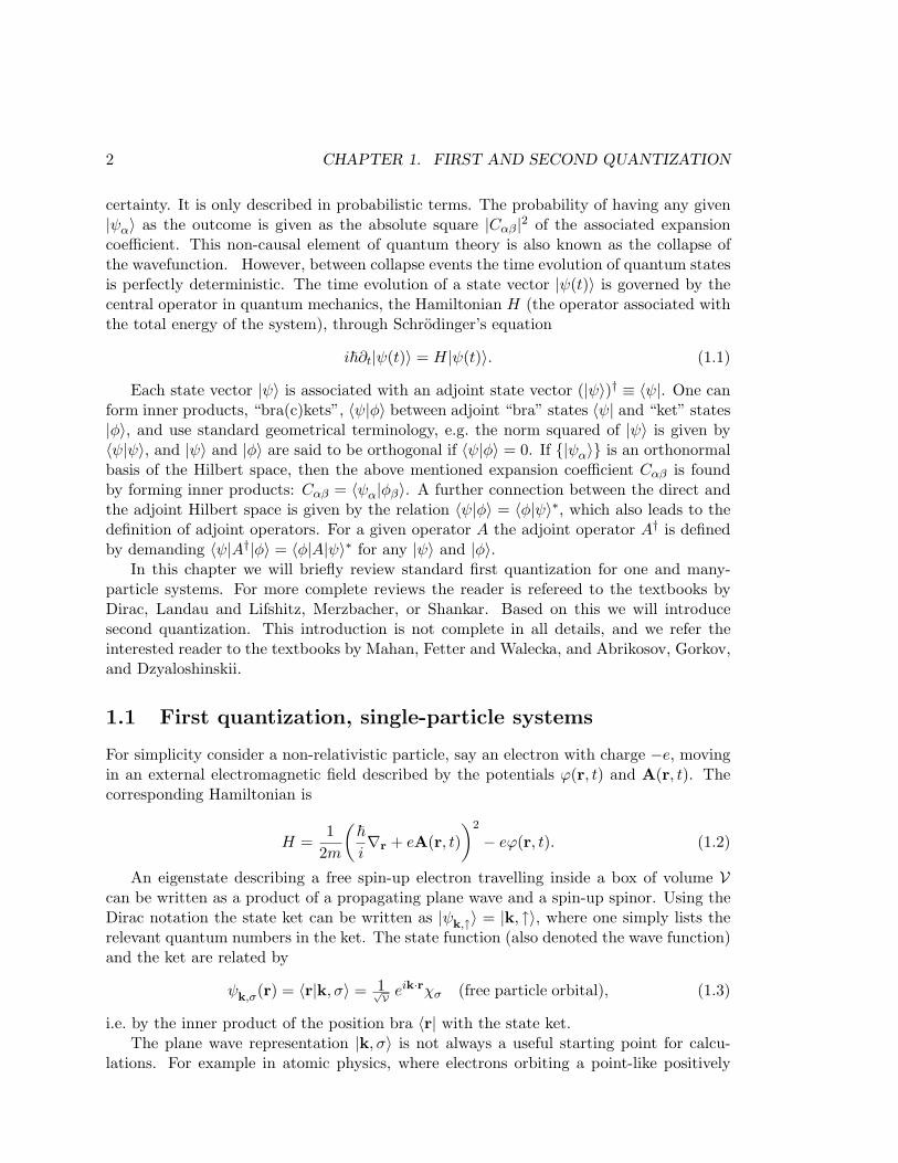
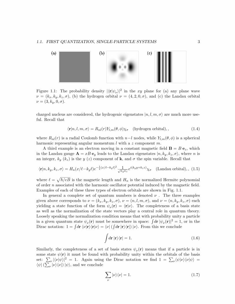
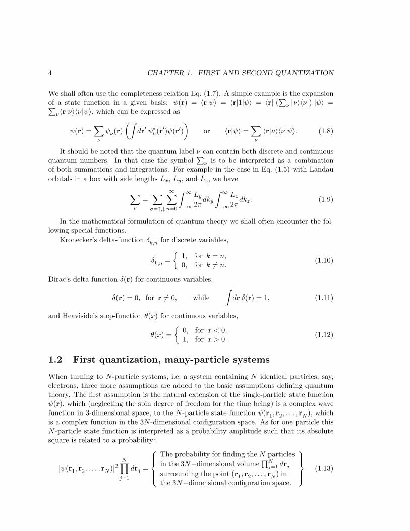
Figure 1.1: The probability density |〈r|ψν〉|2 in the xy plane for (a) any plane waveν = (kx, ky, kz, σ), (b) the hydrogen orbital ν = (4, 2, 0, σ), and (c) the Landau orbitalν = (3, ky, 0, σ).
charged nucleus are considered, the hydrogenic eigenstates |n, l,m, σ〉 are much more use-ful. Recall that
〈r|n, l, m, σ〉 = Rnl(r)Yl,m(θ, φ)χσ (hydrogen orbital), , (1.4)
where Rnl(r) is a radial Coulomb function with n−l nodes, while Yl,m(θ, φ) is a sphericalharmonic representing angular momentum l with a z component m.
A third example is an electron moving in a constant magnetic field B = B ez, whichin the Landau gauge A = xB ey leads to the Landau eigenstates |n, ky, kz, σ〉, where n isan integer, ky (kz) is the y (z) component of k, and σ the spin variable. Recall that
〈r|n, ky, kz, σ〉 = Hn(x/`−ky`)e−12(x/`−ky`)2 1√
LyLzei(kyy+kzz)χσ (Landau orbital), , (1.5)
where ` =√~/eB is the magnetic length and Hn is the normalized Hermite polynomial
of order n associated with the harmonic oscillator potential induced by the magnetic field.Examples of each of these three types of electron orbitals are shown in Fig. 1.1.
In general a complete set of quantum numbers is denoted ν . The three examplesgiven above corresponds to ν = (kx, ky, kz, σ), ν = (n, l,m, σ), and ν = (n, ky, kz, σ) eachyielding a state function of the form ψν(r) = 〈r|ν〉. The completeness of a basis stateas well as the normalization of the state vectors play a central role in quantum theory.Loosely speaking the normalization condition means that with probability unity a particlein a given quantum state ψν(r) must be somewhere in space:
∫dr |ψν(r)|2 = 1, or in the
Dirac notation: 1 =∫
dr 〈ν|r〉〈r|ν〉 = 〈ν| (∫ dr |r〉〈r|) |ν〉. From this we conclude∫
dr |r〉〈r| = 1. (1.6)
Similarly, the completeness of a set of basis states ψν(r) means that if a particle is insome state ψ(r) it must be found with probability unity within the orbitals of the basisset:
∑ν |〈ν|ψ〉|2 = 1. Again using the Dirac notation we find 1 =
∑ν〈ψ|ν〉〈ν|ψ〉 =
〈ψ| (∑ν |ν〉〈ν|) |ψ〉, and we conclude∑
ν
|ν〉〈ν| = 1. (1.7)
4 CHAPTER 1. FIRST AND SECOND QUANTIZATION
We shall often use the completeness relation Eq. (1.7). A simple example is the expansionof a state function in a given basis: ψ(r) = 〈r|ψ〉 = 〈r|1|ψ〉 = 〈r| (
∑ν |ν〉〈ν|) |ψ〉 =∑
ν〈r|ν〉〈ν|ψ〉, which can be expressed as
ψ(r) =∑
ν
ψν(r)(∫
dr′ ψ∗ν (r′)ψ(r′))
or 〈r|ψ〉 =∑
ν
〈r|ν〉〈ν|ψ〉. (1.8)
It should be noted that the quantum label ν can contain both discrete and continuousquantum numbers. In that case the symbol
∑ν is to be interpreted as a combination
of both summations and integrations. For example in the case in Eq. (1.5) with Landauorbitals in a box with side lengths Lx, Ly, and Lz, we have
∑ν
=∑
σ=↑,↓
∞∑
n=0
∫ ∞
−∞
Ly
2πdky
∫ ∞
−∞
Lz
2πdkz. (1.9)
In the mathematical formulation of quantum theory we shall often encounter the fol-lowing special functions.
Kronecker’s delta-function δk,n for discrete variables,
δk,n =
1, for k = n,0, for k 6= n.
(1.10)
Dirac’s delta-function δ(r) for continuous variables,
δ(r) = 0, for r 6= 0, while∫
dr δ(r) = 1, (1.11)
and Heaviside’s step-function θ(x) for continuous variables,
θ(x) =
0, for x < 0,1, for x > 0.
(1.12)
1.2 First quantization, many-particle systems
When turning to N -particle systems, i.e. a system containing N identical particles, say,electrons, three more assumptions are added to the basic assumptions defining quantumtheory. The first assumption is the natural extension of the single-particle state functionψ(r), which (neglecting the spin degree of freedom for the time being) is a complex wavefunction in 3-dimensional space, to the N -particle state function ψ(r1, r2, . . . , rN ), whichis a complex function in the 3N -dimensional configuration space. As for one particle thisN -particle state function is interpreted as a probability amplitude such that its absolutesquare is related to a probability:
|ψ(r1, r2, . . . , rN )|2N∏
j=1
drj =
The probability for finding the N particlesin the 3N−dimensional volume
∏Nj=1 drj
surrounding the point (r1, r2, . . . , rN ) inthe 3N−dimensional configuration space.
(1.13)

1.2. FIRST QUANTIZATION, MANY-PARTICLE SYSTEMS 5
1.2.1 Permutation symmetry and indistinguishability
A fundamental difference between classical and quantum mechanics concerns the conceptof indistinguishability of identical particles. In classical mechanics each particle can beequipped with an identifying marker (e.g. a colored spot on a billiard ball) without influ-encing its behavior, and moreover it follows its own continuous path in phase space. Thusin principle each particle in a group of identical particles can be identified. This is notso in quantum mechanics. Not even in principle is it possible to mark a particle withoutinfluencing its physical state, and worse, if a number of identical particles are brought tothe same region in space, their wavefunctions will rapidly spread out and overlap with oneanother, thereby soon render it impossible to say which particle is where.
The second fundamental assumption for N -particle systems is therefore that identicalparticles, i.e. particles characterized by the same quantum numbers such as mass, chargeand spin, are in principle indistinguishable.
From the indistinguishability of particles follows that if two coordinates in an N -particle state function are interchanged the same physical state results, and the corre-sponding state function can at most differ from the original one by a simple prefactor λ.If the same two coordinates then are interchanged a second time, we end with the exactsame state function,
ψ(r1, .., rj , .., rk, .., rN ) = λψ(r1, .., rk, .., rj , .., rN ) = λ2ψ(r1, .., rj , .., rk, .., rN ), (1.14)
and we conclude that λ2 = 1 or λ = ±1. Only two species of particles are thus possible inquantum physics, the so-called bosons and fermions1:
ψ(r1, . . . , rj , . . . , rk, . . . , rN ) = +ψ(r1, . . . , rk, . . . , rj , . . . , rN ) (bosons), (1.15a)
ψ(r1, . . . , rj , . . . , rk, . . . , rN ) = −ψ(r1, . . . , rk, . . . , rj , . . . , rN ) (fermions). (1.15b)
The importance of the assumption of indistinguishability of particles in quantumphysics cannot be exaggerated, and it has been introduced due to overwhelming experi-mental evidence. For fermions it immediately leads to the Pauli exclusion principle statingthat two fermions cannot occupy the same state, because if in Eq. (1.15b) we let rj = rk
then ψ = 0 follows. It thus explains the periodic table of the elements, and consequentlythe starting point in our understanding of atomic physics, condensed matter physics andchemistry. It furthermore plays a fundamental role in the studies of the nature of starsand of the scattering processes in high energy physics. For bosons the assumption is nec-essary to understand Planck’s radiation law for the electromagnetic field, and spectacularphenomena like Bose–Einstein condensation, superfluidity and laser light.
1This discrete permutation symmetry is always obeyed. However, some quasiparticles in 2D exhibitany phase eiφ, a so-called Berry phase, upon adiabatic interchange. Such exotic beasts are called anyons
6 CHAPTER 1. FIRST AND SECOND QUANTIZATION
1.2.2 The single-particle states as basis states
We now show that the basis states for the N -particle system can be built from any completeorthonormal single-particle basis ψν(r),
∑ν
ψ∗ν(r′)ψν(r) = δ(r− r′),
∫dr ψ∗ν(r)ψν′(r) = δν,ν′ . (1.16)
Starting from an arbitrary N -particle state ψ(r1, . . . , rN ) we form the (N −1)-particlefunction Aν1(r2, . . . , rN ) by projecting onto the basis state ψν1
(r1):
Aν1(r2, . . . , rN ) ≡∫
dr1 ψ∗ν1(r1)ψ(r1, . . . , rN ). (1.17)
This can be inverted by multiplying with ψν1(r1) and summing over ν1,
ψ(r1, r2, . . . , rN ) =∑ν1
ψν1(r1)Aν1(r2, . . . , rN ). (1.18)
Now define analogously Aν1,ν2(r3, . . . , rN ) from Aν1(r2, . . . , rN ):
Aν1,ν2(r3, . . . , rN ) ≡∫
dr2 ψ∗ν2(r2)Aν1(r2, . . . , rN ). (1.19)
Like before, we can invert this expression to give Aν1 in terms of Aν1,ν2 , which uponinsertion into Eq. (1.18) leads to
ψ(r1, r2, r3 . . . , rN ) =∑ν1,ν2
ψν1(r1)ψν2
(r2)Aν1,ν2(r3, . . . , rN ). (1.20)
Continuing all the way through rN (and then writing r instead of r) we end up with
ψ(r1, r2, . . . , rN ) =∑
ν1,...,νN
Aν1,ν2,...,νN ψν1(r1)ψν2
(r2) . . . ψνN(rN ), (1.21)
where Aν1,ν2,...,νN is just a complex number. Thus any N -particle state function can bewritten as a (rather complicated) linear superposition of product states containing Nfactors of single-particle basis states.
Even though the product states∏N
j=1 ψνj(rj) in a mathematical sense form a perfectly
valid basis for the N -particle Hilbert space, we know from the discussion on indistin-guishability that physically it is not a useful basis since the coordinates have to appear ina symmetric way. No physical perturbation can ever break the fundamental fermion or bo-son symmetry, which therefore ought to be explicitly incorporated in the basis states. Thesymmetry requirements from Eqs. (1.15a) and (1.15b) are in Eq. (1.21) hidden in the coef-ficients Aν1,...,νN . A physical meaningful basis bringing the N coordinates on equal footingin the products ψν1
(r1)ψν2(r2) . . . ψνN
(rN ) of single-particle state functions is obtained by
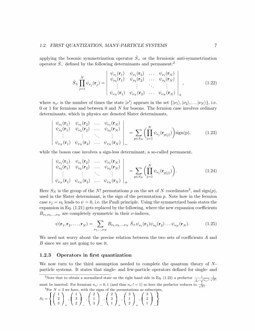
1.2. FIRST QUANTIZATION, MANY-PARTICLE SYSTEMS 7
applying the bosonic symmetrization operator S+ or the fermionic anti-symmetrizationoperator S− defined by the following determinants and permanent:2
S±N∏
j=1
ψνj(rj) =
∣∣∣∣∣∣∣∣∣
ψν1(r1) ψν1
(r2) . . . ψν1(rN )
ψν2(r1) ψν2
(r2) . . . ψν2(rN )
......
. . ....
ψνN(r1) ψνN
(r2) . . . ψνN(rN )
∣∣∣∣∣∣∣∣∣±
, (1.22)
where nν′ is the number of times the state |ν ′〉 appears in the set |ν1〉, |ν2〉, . . . |νN 〉, i.e.0 or 1 for fermions and between 0 and N for bosons. The fermion case involves ordinarydeterminants, which in physics are denoted Slater determinants,
∣∣∣∣∣∣∣∣∣
ψν1(r1) ψν1
(r2) . . . ψν1(rN )
ψν2(r1) ψν2
(r2) . . . ψν2(rN )
......
. . ....
ψνN(r1) ψνN
(r2) . . . ψνN(rN )
∣∣∣∣∣∣∣∣∣−
=∑
p∈SN
( N∏
j=1
ψνj(rp(j))
)sign(p), (1.23)
while the boson case involves a sign-less determinant, a so-called permanent,∣∣∣∣∣∣∣∣∣
ψν1(r1) ψν1
(r2) . . . ψν1(rN )
ψν2(r1) ψν2
(r2) . . . ψν2(rN )
......
. . ....
ψνN(r1) ψνN
(r2) . . . ψνN(rN )
∣∣∣∣∣∣∣∣∣+
=∑
p∈SN
( N∏
j=1
ψνj(rp(j))
). (1.24)
Here SN is the group of the N ! permutations p on the set of N coordinates3, and sign(p),used in the Slater determinant, is the sign of the permutation p. Note how in the fermioncase νj = νk leads to ψ = 0, i.e. the Pauli principle. Using the symmetrized basis states theexpansion in Eq. (1.21) gets replaced by the following, where the new expansion coefficientsBν1,ν2,...,νN are completely symmetric in their ν-indices,
ψ(r1, r2, . . . , rN ) =∑
ν1,...,νN
Bν1,ν2,...,νN S±ψν1(r1)ψν2
(r2) . . . ψνN(rN ). (1.25)
We need not worry about the precise relation between the two sets of coefficients A andB since we are not going to use it.
1.2.3 Operators in first quantization
We now turn to the third assumption needed to complete the quantum theory of N -particle systems. It states that single- and few-particle operators defined for single- and
2Note that to obtain a normalized state on the right hand side in Eq. (1.22) a prefactor 1Qν′√
nν′ !1√N !
must be inserted. For fermions nν′ = 0, 1 (and thus nν′ ! = 1) so here the prefactor reduces to 1√N !
.3For N = 3 we have, with the signs of the permutations as subscripts,
S3 =
8<:0@ 1
23
1A+
,
0@ 132
1A−
,
0@ 213
1A−
,
0@ 231
1A+
,
0@ 312
1A+
,
0@ 321
1A−
9=;

8 CHAPTER 1. FIRST AND SECOND QUANTIZATION
few-particle states remain unchanged when acting on N -particle states. In this course wewill only work with one- and two-particle operators.
Let us begin with one-particle operators defined on single-particle states described bythe coordinate rj . A given local one-particle operator Tj = T (rj ,∇rj
), say e.g. the kinetic
energy operator − ~22m∇2
rjor an external potential V (rj), takes the following form in the
|ν〉-representation for a single-particle system:
Tj =∑νa,νb
Tνbνa |ψνb(rj)〉〈ψνa
(rj)|, (1.26)
where Tνbνa =∫
drj ψ∗νb(rj) T (rj ,∇rj
) ψνa(rj). (1.27)
In an N -particle system all N particle coordinates must appear in a symmetrical way,hence the proper kinetic energy operator in this case must be the total (symmetric) kineticenergy operator Ttot associated with all the coordinates,
Ttot =N∑
j=1
Tj , (1.28)
and the action of Ttot on a simple product state is
Ttot|ψνn1(r1)〉|ψνn2
(r2)〉 . . . |ψνnN(rN )〉 (1.29)
=N∑
j=1
∑νaνb
Tνbνaδνa,νnj|ψνn1
(r1)〉 . . . |ψνb(rj)〉 . . . |ψνnN
(rN )〉.
Here the Kronecker delta comes from 〈νa|νnj 〉 = δνa,νnj. It is straight forward to extend
this result to the proper symmetrized basis states.We move on to discuss symmetric two-particle operators Vjk, such as the Coulomb
interaction V (rj−rk) = e2
4πε0
1|rj−rk| between a pair of electrons. For a two-particle sys-
tem described by the coordinates rj and rk in the |ν〉-representation with basis states|ψνa
(rj)〉|ψνb(rk)〉 we have the usual definition of Vjk:
Vjk =∑νaνb
νcνd
Vνcνd,νaνb|ψνc
(rj)〉|ψνd(rk)〉〈ψνa
(rj)|〈ψνb(rk)| (1.30)
where Vνcνd,νaνb=
∫drjdrk ψ∗νc
(rj)ψ∗νd
(rk)V (rj−rk)ψνa(rj)ψνb
(rk). (1.31)
In the N -particle system we must again take the symmetric combination of the coordinates,i.e. introduce the operator of the total interaction energy Vtot,
Vtot =N∑
j>k
Vjk =12
N∑
j,k 6=j
Vjk, (1.32)
1.3. SECOND QUANTIZATION, BASIC CONCEPTS 9
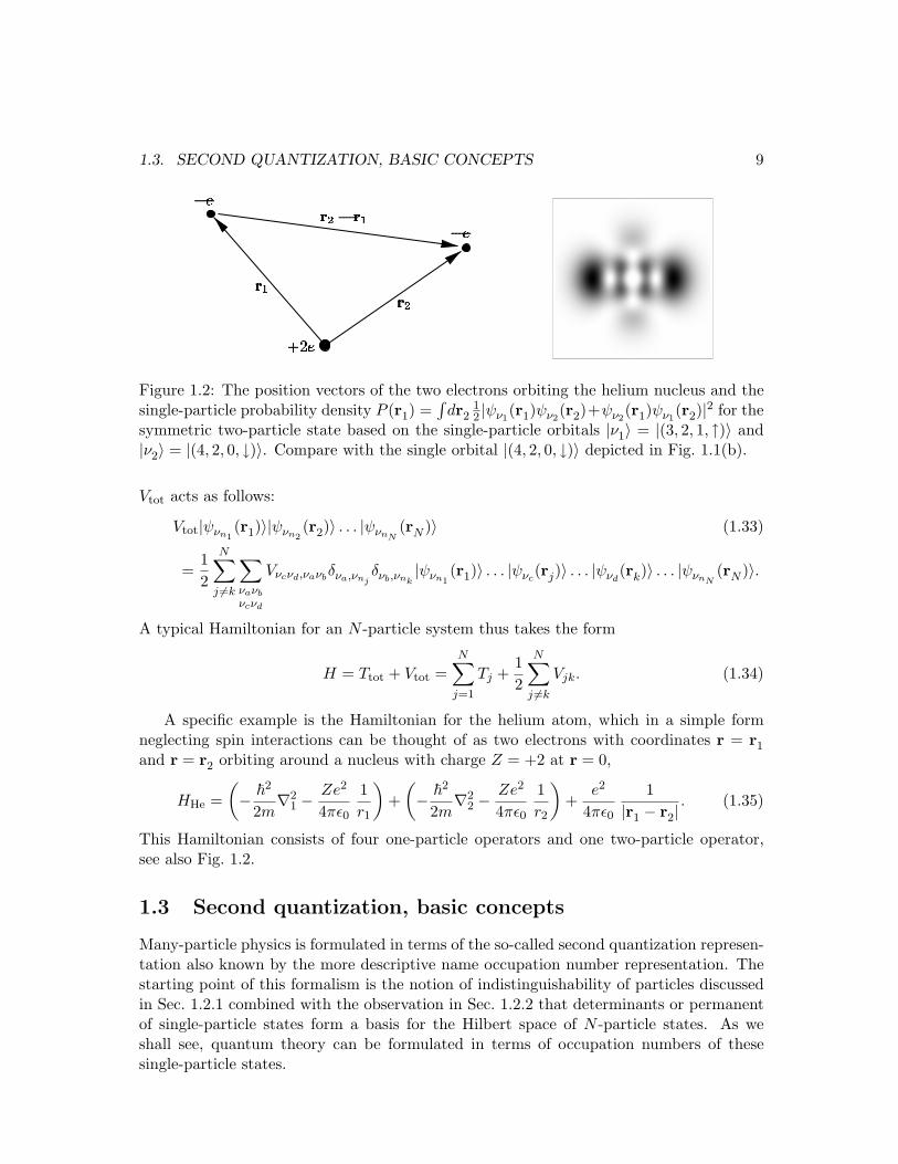
Figure 1.2: The position vectors of the two electrons orbiting the helium nucleus and thesingle-particle probability density P (r1) =
∫dr2
12 |ψν1
(r1)ψν2(r2)+ψν2
(r1)ψν1(r2)|2 for the
symmetric two-particle state based on the single-particle orbitals |ν1〉 = |(3, 2, 1, ↑)〉 and|ν2〉 = |(4, 2, 0, ↓)〉. Compare with the single orbital |(4, 2, 0, ↓)〉 depicted in Fig. 1.1(b).
Vtot acts as follows:
Vtot|ψνn1(r1)〉|ψνn2
(r2)〉 . . . |ψνnN(rN )〉 (1.33)
=12
N∑
j 6=k
∑νaνb
νcνd
Vνcνd,νaνbδνa,νnj
δνb,νnk|ψνn1
(r1)〉 . . . |ψνc(rj)〉 . . . |ψνd
(rk)〉 . . . |ψνnN(rN )〉.
A typical Hamiltonian for an N -particle system thus takes the form
H = Ttot + Vtot =N∑
j=1
Tj +12
N∑
j 6=k
Vjk. (1.34)
A specific example is the Hamiltonian for the helium atom, which in a simple formneglecting spin interactions can be thought of as two electrons with coordinates r = r1
and r = r2 orbiting around a nucleus with charge Z = +2 at r = 0,
HHe =(− ~
2
2m∇2
1 −Ze2
4πε0
1r1
)+
(− ~
2
2m∇2
2 −Ze2
4πε0
1r2
)+
e2
4πε0
1|r1 − r2|
. (1.35)
This Hamiltonian consists of four one-particle operators and one two-particle operator,see also Fig. 1.2.
1.3 Second quantization, basic concepts
Many-particle physics is formulated in terms of the so-called second quantization represen-tation also known by the more descriptive name occupation number representation. Thestarting point of this formalism is the notion of indistinguishability of particles discussedin Sec. 1.2.1 combined with the observation in Sec. 1.2.2 that determinants or permanentof single-particle states form a basis for the Hilbert space of N -particle states. As weshall see, quantum theory can be formulated in terms of occupation numbers of thesesingle-particle states.
10 CHAPTER 1. FIRST AND SECOND QUANTIZATION
1.3.1 The occupation number representation
The first step in defining the occupation number representation is to choose any orderedand complete single-particle basis |ν1〉, |ν2〉, |ν3〉, . . ., the ordering being of paramountimportance for fermions. It is clear from the form S±ψνn1
(r1)ψνn2(r2) . . . ψνnN
(rN ) of thebasis states in Eq. (1.25) that in each term only the occupied single-particle states |νnj 〉play a role. It must somehow be simpler to formulate a representation where one justcounts how many particles there are in each orbital |ν〉. This simplification is achievedwith the occupation number representation.
The basis states for an N -particle system in the occupation number representation areobtained simply by listing the occupation numbers of each basis state,
N−particle basis states : |nν1 , nν2 , nν3 , . . .〉,∑
j
nνj = N. (1.36)
It is therefore natural to define occupation number operators nνj which as eigenstates havethe basis states |nνj 〉, and as eigenvalues have the number nνj of particles occupying thestate νj ,
nνj |nνj 〉 = nνj |nνj 〉. (1.37)
We shall show later that for fermions nνj can be 0 or 1, while for bosons it can be anynon-negative number,
nνj =
0, 1 (fermions)0, 1, 2, . . . (bosons).
(1.38)
Naturally, the question arises how to connect the occupation number basis Eq. (1.36) withthe first quantization basis Eq. (1.23). This will be answered in the next section.
The space spanned by the occupation number basis is denoted the Fock space F . Itcan be defined as F = F0⊕F1⊕F2⊕ . . ., where FN = span|nν1 , nν2 , . . .〉 |
∑j nνj = N.
In Table. 1.1 some of the fermionic and bosonic basis states in the occupation numberrepresentation are shown. Note how by virtue of the direct sum, states containing adifferent number of particles are defined to be orthogonal.
1.3.2 The boson creation and annihilation operators
To connect first and second quantization we first treat bosons. Given the occupation num-ber operator it is natural to introduce the creation operator b†νj that raises the occupationnumber in the state |νj〉 by 1,
b†νj| . . . , nνj−1 , nνj , nνj+1 , . . .〉 = B+(nνj ) | . . . , nνj−1 , nνj + 1, nνj+1 , . . .〉, (1.39)
where B+(nνj ) is a normalization constant to be determined. The only non-zero matrixelements of b†νj are 〈nνj+1|b†νj |nνj 〉, where for brevity we only explicitly write the occupationnumber for νj . The adjoint of b†νj is found by complex conjugation as 〈nνj + 1|b†νj |nνj 〉∗ =〈nνj |(b†νj )†|nνj +1〉. Consequently, one defines the annihilation operator bνj
≡ (b†νj )†, whichlowers the occupation number of state |νj〉 by 1,
bνj| . . . , nνj−1 , nνj , nνj+1 , . . .〉 = B−(nνj ) | . . . , nνj−1 , nνj − 1, nνj+1 , . . .〉. (1.40)

1.3. SECOND QUANTIZATION, BASIC CONCEPTS 11
Table 1.1: Some occupation number basis states for N -particle systems.
N fermion basis states |nν1 , nν2 , nν3 , . . .〉0 |0, 0, 0, 0, ..〉1 |1, 0, 0, 0, ..〉, |0, 1, 0, 0, ..〉, |0, 0, 1, 0, ..〉, ..
2 |1, 1, 0, 0, ..〉, |0, 1, 1, 0, ..〉, |1, 0, 1, 0, ..〉, |0, 0, 1, 1, ..〉, |0, 1, 0, 1, ..〉, |1, 0, 0, 1, ..〉, .....
......
......
N boson basis states |nν1 , nν2 , nν3 , . . .〉0 |0, 0, 0, 0, ..〉1 |1, 0, 0, 0, ..〉, |0, 1, 0, 0, ..〉, |0, 0, 1, 0, ..〉, ..
2 |2, 0, 0, 0, ..〉, |0, 2, 0, 0, ..〉, |1, 1, 0, 0, ..〉, |0, 0, 2, 0, ..〉, |0, 1, 1, 0, ..〉, |1, 0, 1, 0, ..〉, .....
......
......
The creation and annihilation operators b†νj and bνjare the fundamental operators in the
occupation number formalism. As we will demonstrate later any operator can be expressedin terms of them.
Let us proceed by investigating the properties of b†νj and bνjfurther. Since bosons
are symmetric in the single-particle state index νj we of course demand that b†νj and b†νk
must commute, and hence by Hermitian conjugation that also bνjand bνk
commute. Thecommutator [A,B] for two operators A and B is defined as
[A,B] ≡ AB −BA, so that [A,B] = 0 ⇒ BA = AB. (1.41)
We demand further that if j 6= k then bνjand b†νk commute. However, if j = k we must
be careful. It is evident that since an unoccupied state can not be emptied further wemust demand bνj
| . . . , 0, . . .〉 = 0, i.e. B−(0) = 0. We also have the freedom to normalize
the operators by demanding b†νj | . . . , 0, . . .〉 = | . . . , 1, . . .〉, i.e. B+(0) = 1. But since〈1|b†νj |0〉∗ = 〈0|bνj
|1〉, it also follows that bνj| . . . , 1, . . .〉 = | . . . , 0, . . .〉, i.e. B−(1) = 1.
It is clear that bνjand b†νj do not commute: bνj
b†νj |0〉 = |0〉 while b†νjbνj|0〉 = 0, i.e.
we have [bνj, b†νj ] |0〉 = |0〉. We assume this commutation relation, valid for the state |0〉,
also to be valid as an operator identity in general, and we calculate the consequences ofthis assumption. In summary, we define the operator algebra for the bosonic creation andannihilation operators by the following three commutation relations:
[b†νj, b†νk
] = 0, [bνj, bνk
] = 0, [bνj, b†νk
] = δνj ,νk. (1.42)
By definition b†ν and bν are not Hermitian. However, the product b†νbν is, and byusing the operator algebra Eq. (1.42) we show below that this operator in fact is the
12 CHAPTER 1. FIRST AND SECOND QUANTIZATION
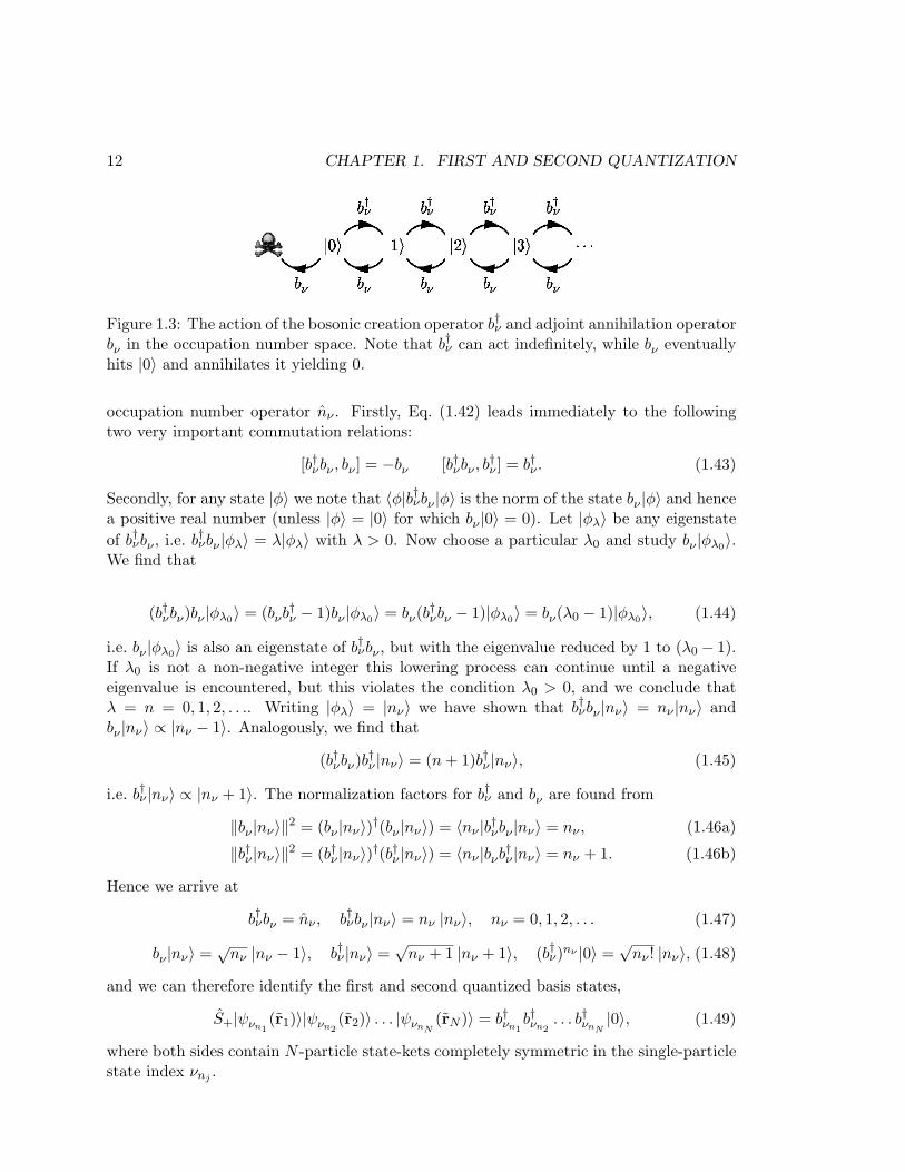
Figure 1.3: The action of the bosonic creation operator b†ν and adjoint annihilation operatorbν in the occupation number space. Note that b†ν can act indefinitely, while bν eventuallyhits |0〉 and annihilates it yielding 0.
occupation number operator nν . Firstly, Eq. (1.42) leads immediately to the followingtwo very important commutation relations:
[b†νbν , bν ] = −bν [b†νbν , b†ν ] = b†ν . (1.43)
Secondly, for any state |φ〉 we note that 〈φ|b†νbν |φ〉 is the norm of the state bν |φ〉 and hencea positive real number (unless |φ〉 = |0〉 for which bν |0〉 = 0). Let |φλ〉 be any eigenstateof b†νbν , i.e. b†νbν |φλ〉 = λ|φλ〉 with λ > 0. Now choose a particular λ0 and study bν |φλ0〉.We find that
(b†νbν)bν |φλ0〉 = (bνb†ν − 1)bν |φλ0〉 = bν(b
†νbν − 1)|φλ0〉 = bν(λ0 − 1)|φλ0〉, (1.44)
i.e. bν |φλ0〉 is also an eigenstate of b†νbν , but with the eigenvalue reduced by 1 to (λ0 − 1).If λ0 is not a non-negative integer this lowering process can continue until a negativeeigenvalue is encountered, but this violates the condition λ0 > 0, and we conclude thatλ = n = 0, 1, 2, . . .. Writing |φλ〉 = |nν〉 we have shown that b†νbν |nν〉 = nν |nν〉 andbν |nν〉 ∝ |nν − 1〉. Analogously, we find that
(b†νbν)b†ν |nν〉 = (n + 1)b†ν |nν〉, (1.45)
i.e. b†ν |nν〉 ∝ |nν + 1〉. The normalization factors for b†ν and bν are found from
‖bν |nν〉‖2 = (bν |nν〉)†(bν |nν〉) = 〈nν |b†νbν |nν〉 = nν , (1.46a)
‖b†ν |nν〉‖2 = (b†ν |nν〉)†(b†ν |nν〉) = 〈nν |bνb†ν |nν〉 = nν + 1. (1.46b)
Hence we arrive at
b†νbν = nν , b†νbν |nν〉 = nν |nν〉, nν = 0, 1, 2, . . . (1.47)
bν |nν〉 =√
nν |nν − 1〉, b†ν |nν〉 =√
nν + 1 |nν + 1〉, (b†ν)nν |0〉 =√
nν ! |nν〉, (1.48)
and we can therefore identify the first and second quantized basis states,
S+|ψνn1(r1)〉|ψνn2
(r2)〉 . . . |ψνnN(rN )〉 = b†νn1
b†νn2. . . b†νnN
|0〉, (1.49)
where both sides contain N -particle state-kets completely symmetric in the single-particlestate index νnj .
1.3. SECOND QUANTIZATION, BASIC CONCEPTS 13
1.3.3 The fermion creation and annihilation operators
Also for fermions it is natural to introduce creation and annihilation operators, now de-noted c†νj and cνj
, being the Hermitian adjoint of each other:
c†νj| . . . , nνj−1 , nνj , nνj+1 , . . .〉 = C+(nνj ) | . . . , nνj−1 , nνj +1, nνj+1 , . . .〉, (1.50)
cνj| . . . , nνj−1 , nνj , nνj+1 , . . .〉 = C−(nνj ) | . . . , nνj−1 , nνj−1, nνj+1 , . . .〉. (1.51)
But to maintain the fundamental fermionic antisymmetry upon exchange of orbitals ap-parent in Eq. (1.23) it is in the fermionic case not sufficient just to list the occupationnumbers of the states, also the order of the occupied states has a meaning. We musttherefore demand
| . . . , nνj = 1, . . . , nνk= 1, . . .〉 = −| . . . , nνk
= 1, . . . , nνj = 1, . . .〉. (1.52)
and consequently we must have that c†νj and c†νk anti-commute, and hence by Hermitianconjugation that also cνj
and cνkanti-commute. The anti-commutator A,B for two
operators A and B is defined as
A,B ≡ AB + BA, so that A,B = 0 ⇒ BA = −AB. (1.53)
For j 6= k we also demand that cνjand c†νk anti-commute. However, if j = k we again must
be careful. It is evident that since an unoccupied state can not be emptied further wemust demand cνj
| . . . , 0, . . .〉 = 0, i.e. C−(0) = 0. We also have the freedom to normalize
the operators by demanding c†νj | . . . , 0, . . .〉 = | . . . , 1, . . .〉, i.e. C+(0) = 1. But since〈1|c†νj |0〉∗ = 〈0|cνj
|1〉 it follows that cνj| . . . , 1, . . .〉 = | . . . , 0, . . .〉, i.e. C−(1) = 1.
It is clear that cνjand c†νj do not anti-commute: cνj
c†νj |0〉 = |0〉 while c†νjcνj|0〉 = 0,
i.e. we have cνj, c†νj |0〉 = |0〉. We assume this anti-commutation relation to be valid as
an operator identity and calculate the consequences. In summary, we define the operatoralgebra for the fermionic creation and annihilation operators by the following three anti-commutation relations:
c†νj, c†νk
= 0, cνj, cνk
= 0, cνj, c†νk
= δνj ,νk. (1.54)
An immediate consequence of the anti-commutation relations Eq. (1.54) is
(c†νj)2 = 0, (cνj
)2 = 0. (1.55)
Now, as for bosons we introduce the Hermitian operator c†νcν , and by using the operatoralgebra Eq. (1.54) we show below that this operator in fact is the occupation numberoperator nν . In analogy with Eq. (1.43) we find
[c†νcν , cν ] = −cν [c†νcν , c†ν ] = c†ν , (1.56)
so that c†ν and cν steps the eigenvalues of c†νcν up and down by one, respectively. FromEqs. (1.54) and (1.55) we have (c†νcν)
2 = c†ν(cνc†ν)cν = c†ν(1 − c†νcν)cν = c†νcν , so that

14 CHAPTER 1. FIRST AND SECOND QUANTIZATION
Figure 1.4: The action of the fermionic creation operator c†ν and the adjoint annihilationoperator cν in the occupation number space. Note that both c†ν and cν can act at mosttwice before annihilating a state completely.
c†νcν(c†νcν − 1) = 0, and c†νcν thus only has 0 and 1 as eigenvalues leading to a simple
normalization for c†ν and cν . In summary, we have
c†νcν = nν , c†νcν |nν〉 = nν |nν〉, nν = 0, 1 (1.57)
cν |0〉 = 0, c†ν |0〉 = |1〉, cν |1〉 = |0〉, c†ν |1〉 = 0, (1.58)
and we can readily identify the first and second quantized basis states,
S−|ψνn1(r1)〉|ψνn2
(r2)〉 . . . |ψνnN(rN )〉 = c†νn1
c†νn2. . . c†νnN
|0〉, (1.59)
where both sides contain normalized N -particle state-kets completely anti-symmetric inthe single-particle state index νnj in accordance with the Pauli exclusion principle.
1.3.4 The general form for second quantization operators
In second quantization all operators can be expressed in terms of the fundamental creationand annihilation operators defined in the previous two sections. This rewriting of the firstquantized operators in Eqs. (1.29) and (1.33) into their second quantized form is achievedby using the basis state identities Eqs. (1.49) and (1.59) linking the two representations.
For simplicity, let us first consider the single-particle operator Ttot from Eq. (1.29)acting on a bosonic N -particle system. In this equation we then act with the bosonicsymmetrization operator S+ on both sides. Utilizing that Ttot and S+ commute andinvoking the basis state identity Eq. (1.49) we obtain
Ttotb†νn1
. . . b†νnN|0〉 =
∑νaνb
Tνbνa
N∑
j=1
δνa,νnjb†νn1
. . .
site nj︷︸︸︷b†νb
. . . b†νnN|0〉, (1.60)
where on the right hand side of the equation the operator b†νb stands on the site nj . Tomake the kets on the two sides of the equation look alike, we would like to reinsert theoperator b†νnj
at site nj on the right. To do this we focus on the state ν ≡ νnj . Originally,i.e. on the left hand side, the state ν may appear, say, p times leading to a contribution(b†ν)p|0〉. We have p > 0 since otherwise both sides would yield zero. On the right hand
1.3. SECOND QUANTIZATION, BASIC CONCEPTS 15
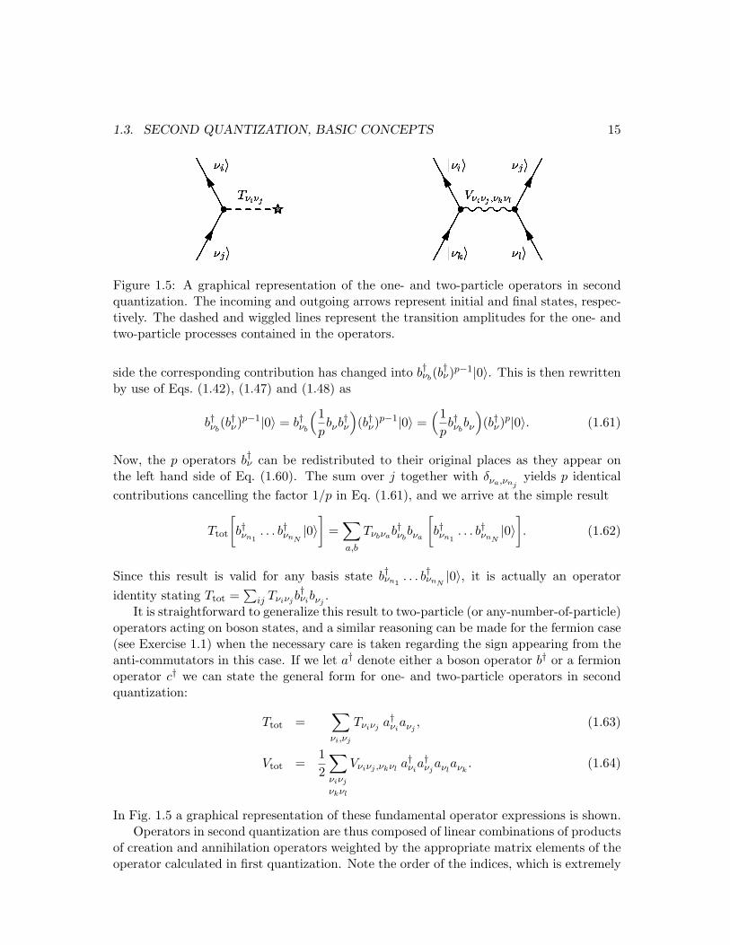
Figure 1.5: A graphical representation of the one- and two-particle operators in secondquantization. The incoming and outgoing arrows represent initial and final states, respec-tively. The dashed and wiggled lines represent the transition amplitudes for the one- andtwo-particle processes contained in the operators.
side the corresponding contribution has changed into b†νb(b†ν)p−1|0〉. This is then rewritten
by use of Eqs. (1.42), (1.47) and (1.48) as
b†νb(b†ν)
p−1|0〉 = b†νb
(1pbνb
†ν
)(b†ν)
p−1|0〉 =(1
pb†νb
bν
)(b†ν)
p|0〉. (1.61)
Now, the p operators b†ν can be redistributed to their original places as they appear onthe left hand side of Eq. (1.60). The sum over j together with δνa,νnj
yields p identicalcontributions cancelling the factor 1/p in Eq. (1.61), and we arrive at the simple result
Ttot
[b†νn1
. . . b†νnN|0〉
]=
∑
a,b
Tνbνab†νb
bνa
[b†νn1
. . . b†νnN|0〉
]. (1.62)
Since this result is valid for any basis state b†νn1. . . b†νnN
|0〉, it is actually an operatoridentity stating Ttot =
∑ij Tνiνjb
†νibνj
.It is straightforward to generalize this result to two-particle (or any-number-of-particle)
operators acting on boson states, and a similar reasoning can be made for the fermion case(see Exercise 1.1) when the necessary care is taken regarding the sign appearing from theanti-commutators in this case. If we let a† denote either a boson operator b† or a fermionoperator c† we can state the general form for one- and two-particle operators in secondquantization:
Ttot =∑νi,νj
Tνiνj a†νiaνj
, (1.63)
Vtot =12
∑νiνj
νkνl
Vνiνj ,νkνla†νi
a†νjaνl
aνk. (1.64)
In Fig. 1.5 a graphical representation of these fundamental operator expressions is shown.Operators in second quantization are thus composed of linear combinations of products
of creation and annihilation operators weighted by the appropriate matrix elements of theoperator calculated in first quantization. Note the order of the indices, which is extremely
16 CHAPTER 1. FIRST AND SECOND QUANTIZATION
important in the case of two-particle fermion operators. The first quantization matrixelement can be read as a transition induced from the initial state |νkνl〉 to the final state|νiνj〉. In second quantization the initial state is annihilated by first annihilating state|νk〉 and then state |νl〉, while the final state is created by first creating state |νj〉 and thenstate |νi〉:
|0〉 = aνlaνk|νkνl〉, |νiνj〉 = a†νi
a†νj|0〉. (1.65)
Note how all the permutation symmetry properties are taken care of by the operatoralgebra of a†ν and aν . The matrix elements are all in the simple non-symmetrized form ofEq. (1.31).
1.3.5 Change of basis in second quantization
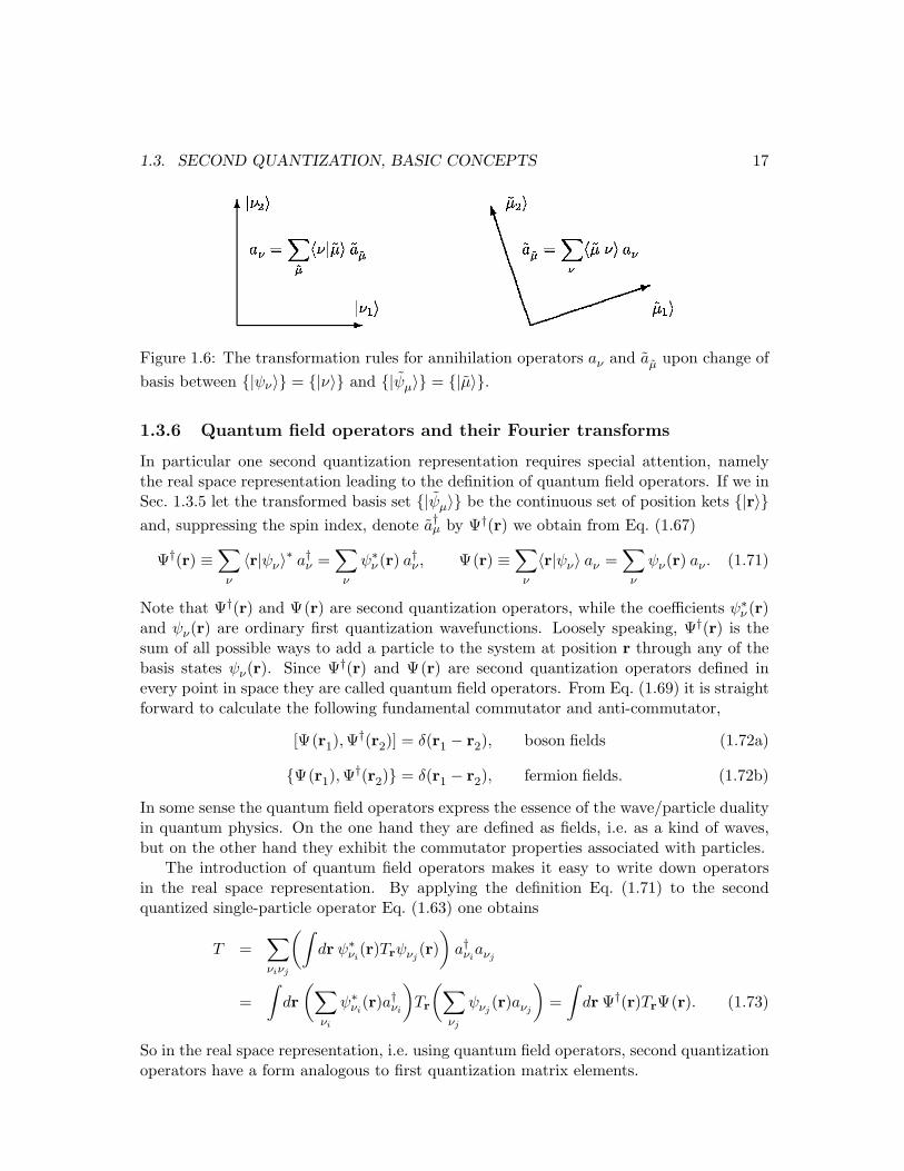
Different quantum operators are most naturally expressed in different representations mak-ing basis changes a central issue in quantum physics. In this section we give the generaltransformation rules which are to be exploited throughout this course.
Let |ψν1〉, |ψν2
〉, . . . and |ψµ1〉, |ψµ2
〉, . . . be two different complete and orderedsingle-particle basis sets. From the completeness condition Eq. (1.7) we have the basictransformation law for single-particle states:
|ψµ〉 =∑
ν
|ψν〉〈ψν |ψµ〉 =∑
ν
〈ψµ|ψν〉∗ |ψν〉. (1.66)
In the case of single-particle systems we define quite naturally creation operators a†µ anda†ν corresponding to the two basis sets, and find directly from Eq. (1.66) that a†µ|0〉 =|ψµ〉 =
∑ν〈ψµ|ψν〉∗ a†ν |0〉, which guides us to the transformation rules for creation and
annihilation operators (see also Fig. 1.6):
a†µ =∑
ν
〈ψµ|ψν〉∗ a†ν , aµ =∑
ν
〈ψµ|ψν〉 aν . (1.67)
The general validity of Eq. (1.67) follows from applying the first quantization single-particleresult Eq. (1.66) to the N -particle first quantized basis states S±|ψνn1
. . . ψνnN〉 leading to
a†µn1a†µn2
. . . a†µnN|0〉 =
(∑νn1
〈ψµn1|ψνn1
〉∗a†νn1
). . .
(∑νnN
〈ψµnN|ψνnN
〉∗a†νnN
)|0〉. (1.68)
The transformation rules Eq. (1.67) lead to two very desirable results. Firstly, that thebasis transformation preserves the bosonic or fermionic particle statistics,
[aµ1 , a†µ2
]± =∑νjνk
〈ψµ1|ψνj
〉〈ψµ2|ψνk
〉∗[aνj, a†νk
]± (1.69)
=∑νjνk
〈ψµ1|ψνj
〉〈ψνk|ψµ2
〉δνj ,νk=
∑νj
〈ψµ1|ψνj
〉〈ψνj|ψµ2
〉 = δµ1,µ2 ,
and secondly, that it leaves the total number of particles unchanged,∑
µ
a†µaµ =∑
µ
∑νjνk
〈ψνj|ψµ〉〈ψµ|ψνk
〉a†νjaνk
=∑νjνk
〈ψνj|ψνk
〉a†νjaνk
=∑νj
a†νjaνj
. (1.70)
1.3. SECOND QUANTIZATION, BASIC CONCEPTS 17
Figure 1.6: The transformation rules for annihilation operators aν and aµ upon change ofbasis between |ψν〉 = |ν〉 and |ψµ〉 = |µ〉.
1.3.6 Quantum field operators and their Fourier transforms
In particular one second quantization representation requires special attention, namelythe real space representation leading to the definition of quantum field operators. If we inSec. 1.3.5 let the transformed basis set |ψµ〉 be the continuous set of position kets |r〉and, suppressing the spin index, denote a†µ by Ψ†(r) we obtain from Eq. (1.67)
Ψ†(r) ≡∑
ν
〈r|ψν〉∗ a†ν =∑
ν
ψ∗ν (r) a†ν , Ψ(r) ≡∑
ν
〈r|ψν〉 aν =∑
ν
ψν(r) aν . (1.71)
Note that Ψ†(r) and Ψ(r) are second quantization operators, while the coefficients ψ∗ν (r)and ψν(r) are ordinary first quantization wavefunctions. Loosely speaking, Ψ†(r) is thesum of all possible ways to add a particle to the system at position r through any of thebasis states ψν(r). Since Ψ†(r) and Ψ(r) are second quantization operators defined inevery point in space they are called quantum field operators. From Eq. (1.69) it is straightforward to calculate the following fundamental commutator and anti-commutator,
[Ψ(r1),Ψ†(r2)] = δ(r1 − r2), boson fields (1.72a)
Ψ(r1), Ψ†(r2) = δ(r1 − r2), fermion fields. (1.72b)
In some sense the quantum field operators express the essence of the wave/particle dualityin quantum physics. On the one hand they are defined as fields, i.e. as a kind of waves,but on the other hand they exhibit the commutator properties associated with particles.
The introduction of quantum field operators makes it easy to write down operatorsin the real space representation. By applying the definition Eq. (1.71) to the secondquantized single-particle operator Eq. (1.63) one obtains
T =∑νiνj
(∫dr ψ∗νi
(r)Trψνj(r)
)a†νi
aνj
=∫
dr(∑
νi
ψ∗νi(r)a†νi
)Tr
(∑νj
ψνj(r)aνj
)=
∫dr Ψ†(r)TrΨ(r). (1.73)
So in the real space representation, i.e. using quantum field operators, second quantizationoperators have a form analogous to first quantization matrix elements.
18 CHAPTER 1. FIRST AND SECOND QUANTIZATION
Finally, when working with homogeneous systems it is often desirable to transformbetween the real space and the momentum representations, i.e. to perform a Fourier trans-formation. Substituting in Eq. (1.71) the |ψν〉 basis with the momentum basis |k〉 yields
Ψ†(r) =1√V
∑
k
e−ik·r a†k, Ψ(r) =1√V
∑
k
eik·r ak. (1.74)
The inverse expressions are obtained by multiplying by e±iq·r and integrating over r,
a†q =1√V
∫dr eiq·r Ψ†(r), aq =
1√V
∫dr e−iq·r Ψ(r). (1.75)
1.4 Second quantization, specific operators
In this section we will use the general second quantization formalism to derive some ex-pressions for specific second quantization operators that we are going to use repeatedly inthis course.
1.4.1 The harmonic oscillator in second quantization
The one-dimensional harmonic oscillator in first quantization is characterized by two con-jugate variables appearing in the Hamiltonian: the position x and the momentum p,
H =1
2mp2 +
12mω2x2, [p, x] =
~i. (1.76)
This can be rewritten in second quantization by identifying two operators a† and a satis-fying the basic boson commutation relations Eq. (1.42). By inspection it can be verifiedthat the following operators do the job,
a ≡ 1√2
(x
`+ i
p
~/`
)
a† ≡ 1√2
(x
`− i
p
~/`
)
⇒
x ≡ `1√2(a† + a),
p ≡ ~`
i√2(a† − a),
(1.77)
where x is given in units of the harmonic oscillator length ` =√~/mω and p in units of
the harmonic oscillator momentum ~/`. Mnemotechnically, one can think of a as beingthe (1/
√2-normalized) complex number formed by the real part x/` and the imaginary
part p/(~/`), while a† is found as the adjoint operator to a . From Eq. (1.77) we obtainthe Hamiltonian, H, and the eigenstates |n〉:
H = ~ω(a†a +
12
)and |n〉 =
(a†)n
√n!|0〉, with H|n〉 = ~ω
(n +
12
)|n〉. (1.78)
The excitation of the harmonic oscillator can thus be interpreted as filling the oscillatorwith bosonic quanta created by the operator a†. This picture is particularly useful in thestudies of the photon and phonon fields, as we shall see during the course. If we as a
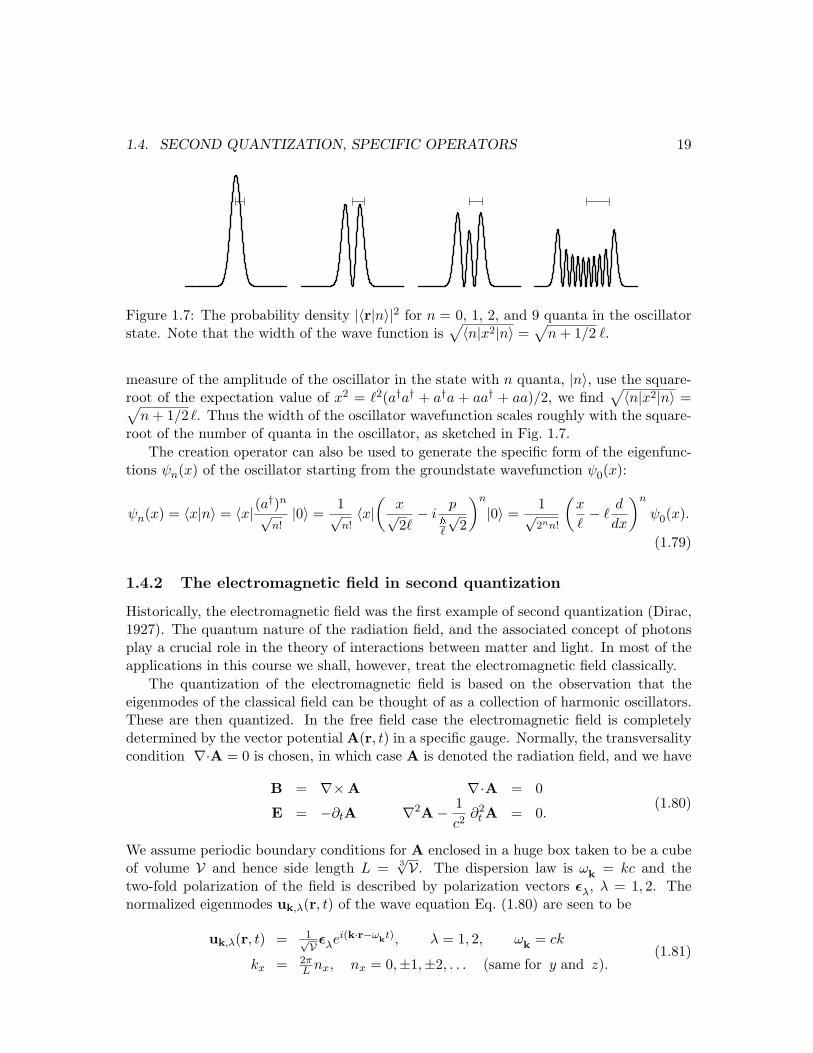
1.4. SECOND QUANTIZATION, SPECIFIC OPERATORS 19
Figure 1.7: The probability density |〈r|n〉|2 for n = 0, 1, 2, and 9 quanta in the oscillatorstate. Note that the width of the wave function is
√〈n|x2|n〉 =
√n + 1/2 `.
measure of the amplitude of the oscillator in the state with n quanta, |n〉, use the square-root of the expectation value of x2 = `2(a†a† + a†a + aa† + aa)/2, we find
√〈n|x2|n〉 =√
n + 1/2 `. Thus the width of the oscillator wavefunction scales roughly with the square-root of the number of quanta in the oscillator, as sketched in Fig. 1.7.
The creation operator can also be used to generate the specific form of the eigenfunc-tions ψn(x) of the oscillator starting from the groundstate wavefunction ψ0(x):
ψn(x) = 〈x|n〉 = 〈x|(a†)n
√n!|0〉 =
1√n!〈x|
(x√2`− i
p~`
√2
)n
|0〉 =1√2nn!
(x
`− `
d
dx
)n
ψ0(x).
(1.79)
1.4.2 The electromagnetic field in second quantization
Historically, the electromagnetic field was the first example of second quantization (Dirac,1927). The quantum nature of the radiation field, and the associated concept of photonsplay a crucial role in the theory of interactions between matter and light. In most of theapplications in this course we shall, however, treat the electromagnetic field classically.
The quantization of the electromagnetic field is based on the observation that theeigenmodes of the classical field can be thought of as a collection of harmonic oscillators.These are then quantized. In the free field case the electromagnetic field is completelydetermined by the vector potential A(r, t) in a specific gauge. Normally, the transversalitycondition ∇·A = 0 is chosen, in which case A is denoted the radiation field, and we have
B = ∇×A ∇·A = 0
E = −∂tA ∇2A− 1c2
∂2t A = 0.
(1.80)
We assume periodic boundary conditions for A enclosed in a huge box taken to be a cubeof volume V and hence side length L = 3
√V. The dispersion law is ωk = kc and thetwo-fold polarization of the field is described by polarization vectors ελ, λ = 1, 2. Thenormalized eigenmodes uk,λ(r, t) of the wave equation Eq. (1.80) are seen to be
uk,λ(r, t) = 1√V ελei(k·r−ωkt), λ = 1, 2, ωk = ck
kx = 2πL nx, nx = 0,±1,±2, . . . (same for y and z).
(1.81)
20 CHAPTER 1. FIRST AND SECOND QUANTIZATION
The set ε1, ε2,k/k forms a right-handed orthonormal basis set. The field A takes onlyreal values and hence it has a Fourier expansion of the form
A(r, t) =1√V
∑
k
∑
λ=1,2
(Ak,λei(k·r−ωkt) + A∗k,λe−i(k·r−ωkt)
)ελ, (1.82)
where Ak,λ are the complex expansion coefficients. We now turn to the Hamiltonian Hof the system, which is simply the field energy known from electromagnetism. UsingEq. (1.80) we can express H in terms of the radiation field A,
H =12
∫dr
(ε0|E|2 +
1µ0|B|2
)=
12ε0
∫dr (ω2
k|A|2 + c2k2|A|2) = ε0ω2k
∫dr |A|2. (1.83)
In Fourier space, using Parceval’s theorem and the notation Ak,λ = ARk,λ + iAI
k,λ for thereal and imaginary part of the coefficients, we have
H = ε0ω2k
∑
k,λ
2|Ak,λ|2 = 4ε0ω2k
12
∑
k,λ
(|AR
k,λ|2 + |AIk,λ|2
). (1.84)
If in Eq. (1.82) we merge the time dependence with the coefficients, i.e. Ak,λ(t) =Ak,λe−iωkt, the time dependence for the real and imaginary parts are seen to be
ARk,λ = +ωk AI
k,λ AIk,λ = −ωk AR
k,λ. (1.85)
From Eqs. (1.84) and (1.85) it thus follows that, up to some normalization constants, ARk,λ
and AIk,λ are conjugate variables: ∂H
∂ARk,λ
= −4ε0ωkAIk,λ and ∂H
∂AIk,λ
= +4ε0ωkARk,λ. Proper
normalized conjugate variables Qk,λ and Pk,λ are therefore introduced:
Qk,λ ≡ 2√
ε0ARk,λ
Pk,λ ≡ 2ωk
√ε0A
Ik,λ
⇒
H =∑
k,λ
12
(P 2
k,λ + ω2kQ2
k,λ
)
Qk,λ = Pk,λ, Pk,λ = −ω2kQk,λ
∂H
∂Qk,λ= −Pk,λ,
∂H
∂Pk,λ= Qk,λ.
(1.86)
This ends the proof that the radiation field A can thought of as a collection of harmonicoscillator eigenmodes, where each mode are characterized by the conjugate variable Qk,λ
and Pk,λ. Quantization is now obtained by imposing the usual condition on the commu-tator of the variables, and introducing the second quantized Bose operators a†k,λ for eachquantized oscillator:
[Pk,λ, Qk,λ] =~i⇒
H =∑
k,λ
~ωk(a†k,λak,λ +12), [ak,λ, a†k,λ] = 1,
Qk,λ =
√~
2ωk
(a†k,λ + ak,λ), Pk,λ =
√~ωk
2i(a†k,λ − ak,λ).
(1.87)
1.4. SECOND QUANTIZATION, SPECIFIC OPERATORS 21
To obtain the final expression for A in second quantization we simply express Ak,λ interms of Pk,λ and Qk,λ, which in turn is expressed in terms of a†k,λ and ak,λ:
Ak,λ = ARk,λ + iAI
k,λ →Qk,λ
2√ε0+ i
Pk,λ
2ωk√
ε0=
√~
2ε0ωk
ak,λ, and A∗k,λ →√
~2ε0ωk
a†k,λ.
(1.88)Substituting this into the expansion Eq. (1.82) our final result is:
A(r, t) =1√V
∑
k
∑
λ=1,2
√~
2ε0ωk
(ak,λei(k·r−ωkt) + a†k,λe−i(k·r−ωkt)
)ελ. (1.89)
1.4.3 Operators for kinetic energy, spin, density, and current
In the following we establish the second quantization representation of the four importantsingle-particle operators associated with kinetic energy, spin, particle density, and particlecurrent density.
First, we study the kinetic energy operator T , which is independent of spin and hencediagonal in the spin indices. In first quantization it has the representations
Tr,σ′σ = − ~2
2m∇2
r δσ′,σ, real space representation, (1.90a)
〈k′σ′|T |kσ〉 =~2k2
2mδk′,k δσ′,σ, momentum representation. (1.90b)
Its second quantized forms with spin indices follow directly from Eqs. (1.63) and (1.73)
T =∑
k,σ
~2k2
2ma†k,σak,σ = − ~
2
2m
∑σ
∫dr Ψ†
σ(r)(∇2
rΨσ(r))
. (1.91)
The second equality can also be proven directly by inserting Ψ†(r) and Ψ(r) from Eq. (1.74).For particles with charge q a magnetic field can be included in the expression for the ki-netic energy by substituting the canonical momentum p with the kinetic momentum4
p− qA,
TA =1
2m
∑σ
∫dr Ψ†
σ(r)(~i∇r − qA
)2
Ψσ(r). (1.92)
Next, we treat the spin operator s for electrons. In first quantization it is given bythe Pauli matrices
s =~2τ , with τ =
(0 11 0
),
(0 −ii 0
),
(1 00 −1
). (1.93)
4In analytical mechanics A enters through the Lagrangian: L = 12mv2 − V + qv ·A, since this by the
Euler-Lagrange equations yields the Lorentz force. But then p = ∂L/∂v = mv + qA, and via a Legendretransform we get H(r,p) = p ·v − L(r,v) = 1
2mv2 + V = 1
2m(p − qA)2 + V . Considering infinitesimal
variations δA we get δH = H(A + δA)−H(A) = −qv·δA = −qR
dr J·δA, an expression used to find J.
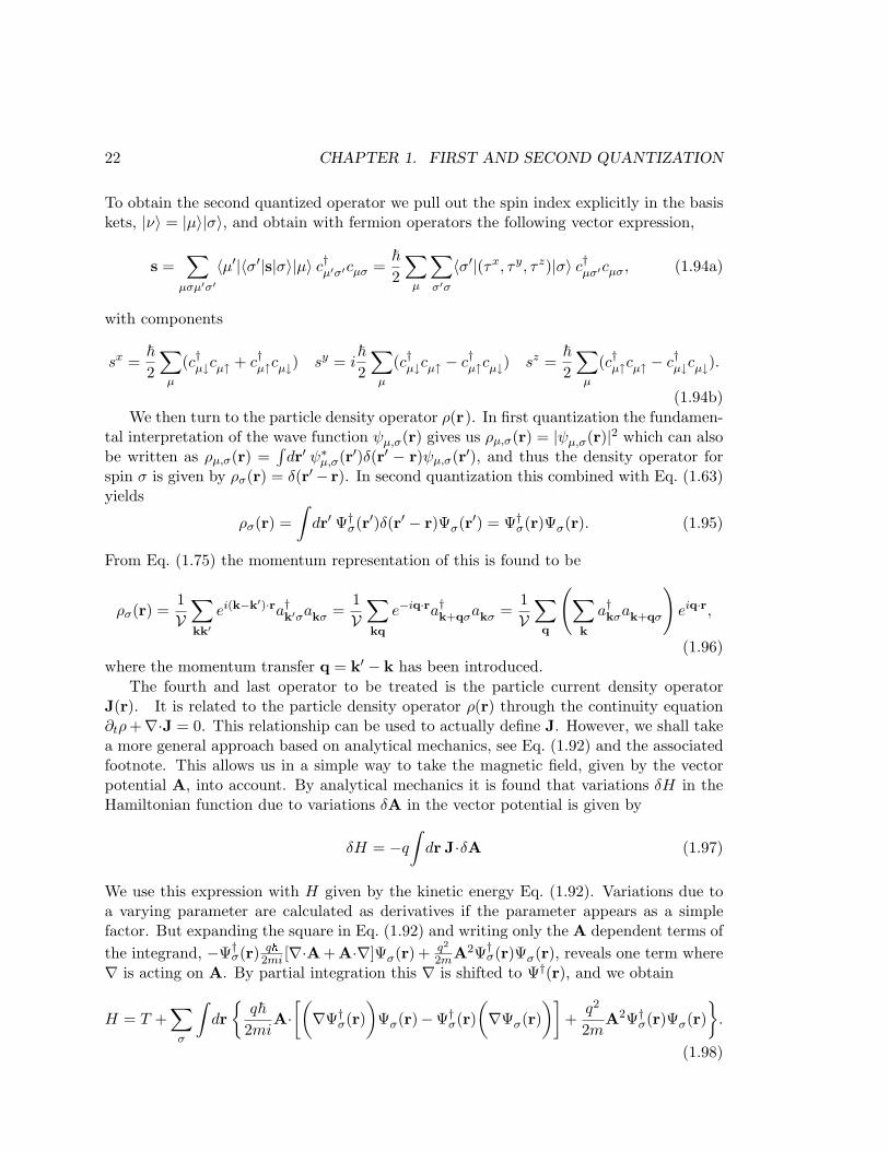
22 CHAPTER 1. FIRST AND SECOND QUANTIZATION
To obtain the second quantized operator we pull out the spin index explicitly in the basiskets, |ν〉 = |µ〉|σ〉, and obtain with fermion operators the following vector expression,
s =∑
µσµ′σ′〈µ′|〈σ′|s|σ〉|µ〉 c†µ′σ′cµσ =
~2
∑µ
∑
σ′σ
〈σ′|(τx, τy, τ z)|σ〉 c†µσ′cµσ, (1.94a)
with components
sx =~2
∑µ
(c†µ↓cµ↑ + c†µ↑cµ↓) sy = i~2
∑µ
(c†µ↓cµ↑ − c†µ↑cµ↓) sz =~2
∑µ
(c†µ↑cµ↑ − c†µ↓cµ↓).
(1.94b)We then turn to the particle density operator ρ(r). In first quantization the fundamen-
tal interpretation of the wave function ψµ,σ(r) gives us ρµ,σ(r) = |ψµ,σ(r)|2 which can alsobe written as ρµ,σ(r) =
∫dr′ ψ∗µ,σ(r′)δ(r′ − r)ψµ,σ(r′), and thus the density operator for
spin σ is given by ρσ(r) = δ(r′− r). In second quantization this combined with Eq. (1.63)yields
ρσ(r) =∫
dr′ Ψ†σ(r′)δ(r′ − r)Ψσ(r′) = Ψ†
σ(r)Ψσ(r). (1.95)
From Eq. (1.75) the momentum representation of this is found to be
ρσ(r) =1V
∑
kk′ei(k−k′)·ra†k′σakσ =
1V
∑
kq
e−iq·ra†k+qσakσ =1V
∑q
(∑
k
a†kσak+qσ
)eiq·r,
(1.96)where the momentum transfer q = k′ − k has been introduced.
The fourth and last operator to be treated is the particle current density operatorJ(r). It is related to the particle density operator ρ(r) through the continuity equation∂tρ +∇·J = 0. This relationship can be used to actually define J. However, we shall takea more general approach based on analytical mechanics, see Eq. (1.92) and the associatedfootnote. This allows us in a simple way to take the magnetic field, given by the vectorpotential A, into account. By analytical mechanics it is found that variations δH in theHamiltonian function due to variations δA in the vector potential is given by
δH = −q
∫dr J·δA (1.97)
We use this expression with H given by the kinetic energy Eq. (1.92). Variations due toa varying parameter are calculated as derivatives if the parameter appears as a simplefactor. But expanding the square in Eq. (1.92) and writing only the A dependent terms ofthe integrand, −Ψ†
σ(r) q~2mi [∇·A+A·∇]Ψσ(r) + q2
2mA2Ψ†σ(r)Ψσ(r), reveals one term where
∇ is acting on A. By partial integration this ∇ is shifted to Ψ†(r), and we obtain
H = T +∑
σ
∫dr
q~
2miA·
[(∇Ψ†
σ(r))
Ψσ(r)−Ψ†σ(r)
(∇Ψσ(r)
)]+
q2
2mA2Ψ†
σ(r)Ψσ(r)
.
(1.98)

1.4. SECOND QUANTIZATION, SPECIFIC OPERATORS 23
The variations of Eq. (1.97) can in Eq. (1.98) be performed as derivatives and J is imme-diately read off as the prefactor to δA. The two terms in the current density operator aredenoted the paramagnetic and the diamagnetic term, J∇ and JA, respectively:
Jσ(r) = J∇σ (r) + JAσ (r), (1.99a)
paramagnetic : J∇σ (r) =~
2mi
[Ψ†
σ(r)(∇Ψσ(r)
)−
(∇Ψ†
σ(r))
Ψσ(r)], (1.99b)
diamagnetic : JAσ (r) = − q
mA(r)Ψ†
σ(r)Ψσ(r). (1.99c)
The momentum representation of J is found in complete analogy with that of ρ
J∇σ (r) =~
mV∑
kq
(k +12q)eiq·ra†kσak+q,σ, JA
σ (r) =−q
mVA(r)∑
kq
eiq·ra†kσak+q,σ.
(1.100)The expression for J in an arbitrary basis is treated in Exercise 1.2.
1.4.4 The Coulomb interaction in second quantization
The Coulomb interaction operator V is a two-particle operator not involving spin andthus diagonal in the spin indices of the particles. Using the same reasoning that led fromEq. (1.63) to Eq. (1.73) we can go directly from Eq. (1.64) to the following quantum fieldoperator form of V :
V (r2 − r1) =12
∑σ1σ2
∫dr1dr2
e20
|r2 − r1|Ψ†
σ1(r1)Ψ
†σ2
(r2)Ψσ2(r2)Ψσ1
(r1). (1.101)
Here we have introduced the abbreviation e20 = e2/4πε0.We can also write the Coulomb
interaction directly in the momentum basis by using Eq. (1.31) and Eq. (1.64) with|ν〉 = |k, σ〉 and ψk,σ(r) = 1√V eik·rχσ. We can interpret the Coulomb matrix elementas describing a transition from an initial state |k1σ1,k2σ2〉 to a final state |k3σ1,k4σ2〉without flipping any spin, and we obtain
V =12
∑σ1σ2
∑
k1k2k3k4
〈k3σ1,k4σ2|V |k1σ1,k2σ2〉 a†k3σ1a†k4σ2
ak2σ2ak1σ1
(1.102)
=12
∑σ1σ2
∑
k1k2k3k4
(e20
V2
∫dr1dr2
ei(k1·r1+k2·r2−k3·r1−k4·r2)
|r2 − r1|)
a†k3σ1a†k4σ2
ak2σ2ak1σ1
.
Since r2 − r1 is the relevant variable for the interaction, the exponential is rewritten as
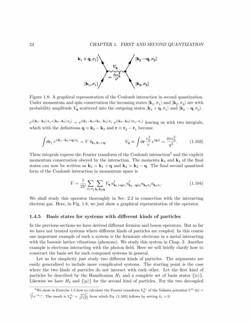
24 CHAPTER 1. FIRST AND SECOND QUANTIZATION
Figure 1.8: A graphical representation of the Coulomb interaction in second quantization.Under momentum and spin conservation the incoming states |k1, σ1〉 and |k2, σ2〉 are withprobability amplitude Vq scattered into the outgoing states |k1 + q, σ1〉 and |k2 − q, σ2〉.
ei[(k1−k3)·r1+(k2−k4)·r2] = ei(k1−k3+k2−k4)·r1 ei(k2−k4)·(r2−r1) leaving us with two integrals,which with the definitions q ≡ k2 − k4 and r ≡ r2 − r1 become
∫dr1 ei(k1−k3+q)·r1 = V δk3,k1+q, Vq ≡
∫dr
e20
reiq·r =
4πe20
q2. (1.103)
These integrals express the Fourier transform of the Coulomb interaction5 and the explicitmomentum conservation obeyed by the interaction. The momenta k3 and k4 of the finalstates can now be written as k3 = k1 + q and k4 = k2 − q. The final second quantizedform of the Coulomb interaction in momentum space is
V =1
2V∑σ1σ2
∑
k1k2q
Vq a†k1+qσ1a†k2−qσ2
ak2σ2ak1σ1
. (1.104)
We shall study this operator thoroughly in Sec. 2.2 in connection with the interactingelectron gas. Here, in Fig. 1.8, we just show a graphical representation of the operator.
1.4.5 Basis states for systems with different kinds of particles
In the previous sections we have derived different fermion and boson operators. But so farwe have not treated systems where different kinds of particles are coupled. In this courseone important example of such a system is the fermionic electrons in a metal interactingwith the bosonic lattice vibrations (phonons). We study this system in Chap. 3. Anotherexample is electrons interacting with the photon field. Here we will briefly clarify how toconstruct the basis set for such composed systems in general.
Let us for simplicity just study two different kinds of particles. The arguments areeasily generalized to include more complicated systems. The starting point is the casewhere the two kinds of particles do not interact with each other. Let the first kind ofparticles be described by the Hamiltonian H1 and a complete set of basis states |ν〉.Likewise we have H2 and |µ〉 for the second kind of particles. For the two decoupled
5We show in Exercise 1.5 how to calculate the Fourier transform V ksq of the Yukawa potential V ks(r) =
e20r
e−ksr. The result is V ksq =
4πe20
q2+k2s
from which Eq. (1.103) follows by setting ks = 0.
1.5. SECOND QUANTIZATION AND STATISTICAL MECHANICS 25
systems an example of separate occupation number basis sets is
|ψ(1)〉 = |nν1 , nν2 , . . . , nνj , . . .〉 (1.105a)
|ψ(2)〉 = |nµ1 , nµ2 , . . . , nµj , . . .〉 (1.105b)
When a coupling H12 between the two system is introduced, we need to enlarge the Hilbertspace. The natural definition of basis states is the outer product states written as
|ψ〉 = |ψ(1)〉|ψ(2)〉= |nν1 , nν2 , . . . , nνj , . . .〉|nµ1 , nµ2 , . . . , nµl
, . . .〉= |nν1 , nν2 , . . . , nνj , . . . ; nµ1 , nµ2 , . . . , nµl
, . . .〉 (1.106)
In the last line all the occupation numbers are simply listed within the same ket butthe two groups are separated by a semicolon. A general state |Φ〉 can of course be anysuperposition of the basis states:
|Φ〉 =∑
νjµlCνj,µl |nν1 , nν2 , . . . , nνj , . . . ; nµ1 , nµ2 , . . . , nµl
, . . .〉. (1.107)
As a concrete example we can write down the basis states for interacting electrons andphotons in the momentum representation. The electronic basis states are the plane waveorbitals |kσ〉 of Eq. (1.3), and the photon states are |qλ〉 given in Eq. (1.81). We let nkσ
and Nqλ denote the occupation numbers for electrons and photons, respectively. A basisstate |ψ〉 in this representation has the form:
|ψ〉 = |nk1σ1 , nk2σ2 , . . . , nkjσj , . . . ; Nq1λ1 , Nq2λ2 , . . . , Nqlλl, . . .〉. (1.108)
1.5 Second quantization and statistical mechanics
The basic assumption of statistical mechanics is the ergodicity assumption. It states thatas time evolves a system assume all possible states complying with the given externalconstraints, e.g. with a given total energy E. In other words, because of the randomnessof the system all of the available phase space is covered. The time it takes for the systemto visit all of the phase is the ergodicity time, which is assumed to be smaller than typicaltime scales of the observation.
Suppose we are interested in some small system connected to the outside world, theso-called reservoir, and assume that, taken as a whole, they constitute a closed system withtotal energy ET . Let us call the energy of the small system Es and that of the reservoirEr, i.e. ET = Es + Er. Based on the ergodicity assumption it is natural to conjecturethat the probability for a subsystem to have a definite energy Es is proportional to thenumber of ways that the subsystem can have that energy. The density of states is definedas d(E) = dN(E)/dE, where N(E) is the number of states with an energy less thanE. We denote the density of states of the total system at a given total energy d(ET ),while the small system and the reservoir have the densities of states ds(Es) and dr(Er),
26 CHAPTER 1. FIRST AND SECOND QUANTIZATION
respectively. Since for a given small energy interval ∆E the number of states in thereservoir is much larger than the number states in smaller subsystem, the total densityof states is dominated by that of the reservoir and hence d(ET ) ≈ dr(ET ). From theassumption about the probability being proportional to the number of states, we have forthe probability for the subsystem to have energy Es that
P (Es) ∝ dr(ET − Es) ∆E. (1.109)
Now, we do not expect this probability to be dependent on the size of the reservoir,i.e. if we make it smaller by cutting it in half by some wall, nothing should happen to thestate of the small system, provided of course that it is still much smaller than the newreservoir. This means that if we consider the ratio of two probabilities
P (Es)P (E′
s)=
dr(ET − Es)dr(ET − E′
s), (1.110)
it must only depend on the energies Es and E′s and neither on the total energy ET nor
on dr. But because the energy is only defined up to an additive constant, it can thus onlydepend on the difference Es − E′
s. The only function P (E) that satisfies the condition
P (Es)P (E′
s)=
dr(ET − Es)dr(ET − E′
s)= f(Es − E′
s), (1.111)
isP (E) ∝ e−βE . (1.112)
We have thus arrived at the famous Boltzmann or Gibbs distribution which of courseshould be normalized. In conclusion: from statistical mechanics we know that both forclassical and a quantum mechanical systems which are connected to a heat bath theprobability for a given state s with energy Es to be occupied is given by the Boltzmanndistribution
P (Es) =1Z
exp(−βEs), (1.113)
where β is the inverse temperature, β = 1/kBT , and where the normalization factor, Z,is the partition function
Z =∑
s
exp(−βEs). (1.114)
When we sum over states, we must sum over a set of states which cover the entirespace of possible states, i.e. the basis set that we use to compute the energy must be acomplete set. For a quantum system with many particles, the states s are, as we haveseen, in general quite complicated to write down, and it is therefore an advantage to havea form which is independent of the choice of basis states. Also for a quantum system it isnot clear what is meant by the energy of a given state, unless of course it is an eigenstateof the Hamiltonian. Therefore the only meaningful interpretation of Eq. (1.114) is thatthe sum of states runs over eigenstates of the Hamiltonian. Using the basis states |ν〉defined by
H|ν〉 = Eν |ν〉, (1.115)
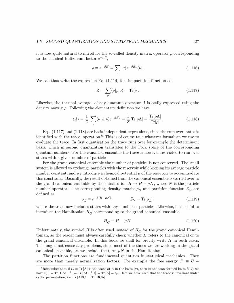
1.5. SECOND QUANTIZATION AND STATISTICAL MECHANICS 27
it is now quite natural to introduce the so-called density matrix operator ρ correspondingto the classical Boltzmann factor e−βE ,
ρ ≡ e−βH =∑
ν
|ν〉e−βEν 〈ν|. (1.116)
We can thus write the expression Eq. (1.114) for the partition function as
Z =∑
ν
〈ν|ρ|ν〉 = Tr[ρ]. (1.117)
Likewise, the thermal average of any quantum operator A is easily expressed using thedensity matrix ρ. Following the elementary definition we have
〈A〉 =1Z
∑ν
〈ν|A|ν〉e−βEν =1Z
Tr[ρA] =Tr[ρA]Tr[ρ]
. (1.118)
Eqs. (1.117) and (1.118) are basis-independent expressions, since the sum over states isidentified with the trace operation.6 This is of course true whatever formalism we use toevaluate the trace. In first quantization the trace runs over for example the determinantbasis, which in second quantization translates to the Fock space of the correspondingquantum numbers. For the canonical ensemble the trace is however restricted to run overstates with a given number of particles.
For the grand canonical ensemble the number of particles is not conserved. The smallsystem is allowed to exchange particles with the reservoir while keeping its average particlenumber constant, and we introduce a chemical potential µ of the reservoir to accommodatethis constraint. Basically, the result obtained from the canonical ensemble is carried over tothe grand canonical ensemble by the substitution H → H − µN , where N is the particlenumber operator. The corresponding density matrix ρG and partition function ZG aredefined as:
ρG ≡ e−β(H−µN), ZG = Tr[ρG]. (1.119)
where the trace now includes states with any number of particles. Likewise, it is useful tointroduce the Hamiltonian HG corresponding to the grand canonical ensemble,
HG ≡ H − µN. (1.120)
Unfortunately, the symbol H is often used instead of HG for the grand canonical Hamil-tonian, so the reader must always carefully check whether H refers to the canonical or tothe grand canonical ensemble. In this book we shall for brevity write H in both cases.This ought not cause any problems, since most of the times we are working in the grandcanonical ensemble, i.e. we include the term µN in the Hamiltonian.
The partition functions are fundamental quantities in statistical mechanics. Theyare more than merely normalization factors. For example the free energy F ≡ U −
6Remember that if tν = Tr [A] is the trace of A in the basis |ν〉, then in the transformed basis U |ν〉 wehave tUν = Tr
UAU−1
= Tr
AU−1U
= Tr [A] = tν . Here we have used that the trace is invariant under
cyclic permutation, i.e. Tr [ABC] = Tr [BCA].
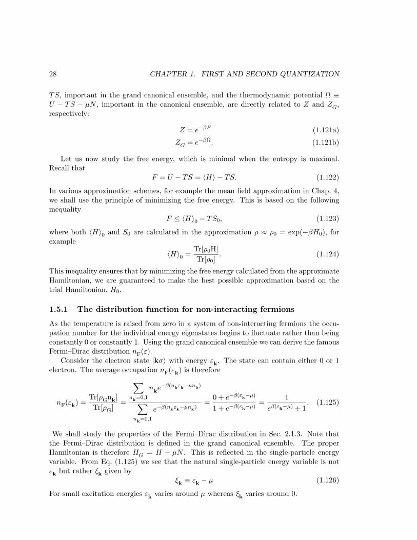
28 CHAPTER 1. FIRST AND SECOND QUANTIZATION
TS, important in the grand canonical ensemble, and the thermodynamic potential Ω ≡U − TS − µN , important in the canonical ensemble, are directly related to Z and ZG,respectively:
Z = e−βF (1.121a)
ZG = e−βΩ. (1.121b)
Let us now study the free energy, which is minimal when the entropy is maximal.Recall that
F = U − TS = 〈H〉 − TS. (1.122)
In various approximation schemes, for example the mean field approximation in Chap. 4,we shall use the principle of minimizing the free energy. This is based on the followinginequality
F ≤ 〈H〉0 − TS0, (1.123)
where both 〈H〉0 and S0 are calculated in the approximation ρ ≈ ρ0 = exp(−βH0), forexample
〈H〉0 =Tr[ρ0H]Tr[ρ0]
. (1.124)
This inequality ensures that by minimizing the free energy calculated from the approximateHamiltonian, we are guaranteed to make the best possible approximation based on thetrial Hamiltonian, H0.
1.5.1 The distribution function for non-interacting fermions
As the temperature is raised from zero in a system of non-interacting fermions the occu-pation number for the individual energy eigenstates begins to fluctuate rather than beingconstantly 0 or constantly 1. Using the grand canonical ensemble we can derive the famousFermi–Dirac distribution nF(ε).
Consider the electron state |kσ〉 with energy εk. The state can contain either 0 or 1electron. The average occupation nF(εk) is therefore
nF(εk) =Tr[ρGnk]Tr[ρG]
=
∑
nk=0,1
nke−β(nkεk−µnk)
∑
nk=0,1
e−β(nkεk−µnk)=
0 + e−β(εk−µ)
1 + e−β(εk−µ)=
1eβ(εk−µ) + 1
. (1.125)
We shall study the properties of the Fermi–Dirac distribution in Sec. 2.1.3. Note thatthe Fermi–Dirac distribution is defined in the grand canonical ensemble. The properHamiltonian is therefore HG = H − µN . This is reflected in the single-particle energyvariable. From Eq. (1.125) we see that the natural single-particle energy variable is notεk but rather ξk given by
ξk ≡ εk − µ (1.126)
For small excitation energies εk varies around µ whereas ξk varies around 0.
1.6. SUMMARY AND OUTLOOK 29
1.5.2 Distribution functions for non-interacting bosons
Next we find the distribution function for non-interacting bosons. Again using the grandcanonical ensemble we derive the equally famous Bose–Einstein distribution nB(ε). It isderived like its fermionic counterpart, the Fermi–Dirac distribution nF(ε).
Consider a bosonic state characterized by its fundamental energy εk. The occupationnumber of the state can be any non-negative integer nk = 0, 1, 2, . . .. In the grand canonicalensemble the average occupation number nB(εk) is found by writing λk = e−β(εk−µ) andusing the formulas
∑∞n=0 nλn = λ d
dλ
∑∞n=0 λn and
∑∞n=0 λn = 1
1−λ :
nB(εk) =
∞∑
nk=0
nk e−β(nkεk−µnk)
∞∑
nk=0
e−β(nkεk−µnk)
=
λk
d
dλk
∞∑
nk=0
λnkk
∞∑
nk=0
λnkk
=
λk(1−λk)2
11−λk
=1
eβ(εk−µ) − 1. (1.127)
The Bose–Einstein distribution differs from the Fermi–Dirac distribution by having −1 inthe denominator instead of +1. Both distributions converge towards the classical Maxwell–Boltzmann distribution, nk = e−β(εk−µ), for very small occupation numbers, where theparticular particle statistics is not felt very strongly.
1.6 Summary and outlook
In this chapter we have introduced second quantization, the representation of quantummechanics we are going to use throughout this course. The basic concepts are the oc-cupation number basis states and the fundamental creation and annihilation operators,b†ν and bν in the bosonic case (see Eq. (1.42)), and c†ν and cν in the fermionic case (seeEq. (1.54)). The intricate permutation symmetries are manifestly ensured by the basic(anti-)commutator relations of these fundamental operators. The main result of the chap-ter is the derivation of the general form of one- and two-particle operators, Eqs. (1.63)and (1.64) and Fig. 1.5. In fact, perhaps after some measure of acquaintance, this mainresult appears so simple and intuitively clear that one could choose to define quantum the-ory directly in second quantization rather than going the cumbersome way from first tosecond quantization. However, students usually learn basic quantum theory in first quanti-zation, so for pedagogical reasons we have chosen to start from the usual first quantizationrepresentation.
In Sec. 1.4 we presented a number of specific examples of second quantization operators,and we got a first glimpse of how second quantization leads to a formulation of quantumphysics in terms of creation and annihilation of particles and field quanta. In the followingthree chapters we shall get more acquainted with second quantization through studiesof simplified stationary problems for non-interacting systems or systems where a givenparticle only interacts with the mean field of the other particles. First in Chap. 5 will thequestion be raised of how to treat time evolution in second quantization. With an answerto that question we can proceed with the very interesting but also rather difficult studiesof the full time dependent dynamics of many-particle quantum systems.

30 CHAPTER 1. FIRST AND SECOND QUANTIZATION
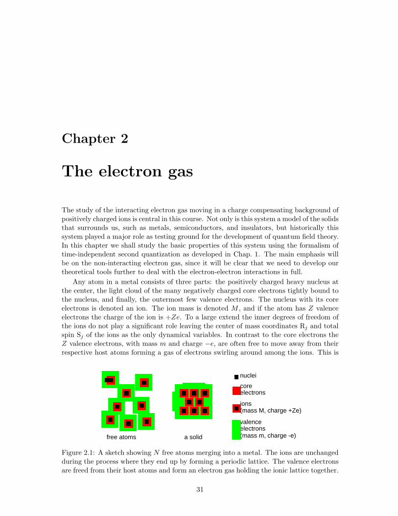
Chapter 2
The electron gas
The study of the interacting electron gas moving in a charge compensating background ofpositively charged ions is central in this course. Not only is this system a model of the solidsthat surrounds us, such as metals, semiconductors, and insulators, but historically thissystem played a major role as testing ground for the development of quantum field theory.In this chapter we shall study the basic properties of this system using the formalism oftime-independent second quantization as developed in Chap. 1. The main emphasis willbe on the non-interacting electron gas, since it will be clear that we need to develop ourtheoretical tools further to deal with the electron-electron interactions in full.
Any atom in a metal consists of three parts: the positively charged heavy nucleus atthe center, the light cloud of the many negatively charged core electrons tightly bound tothe nucleus, and finally, the outermost few valence electrons. The nucleus with its coreelectrons is denoted an ion. The ion mass is denoted M , and if the atom has Z valenceelectrons the charge of the ion is +Ze. To a large extend the inner degrees of freedom ofthe ions do not play a significant role leaving the center of mass coordinates Rj and totalspin Sj of the ions as the only dynamical variables. In contrast to the core electrons theZ valence electrons, with mass m and charge −e, are often free to move away from theirrespective host atoms forming a gas of electrons swirling around among the ions. This is
free atoms
!!!!!!!!!!!!!!!!!!!!!!!!!!!!!!!!!!!!!!!!""""""""""""""""""""""""""""""""""""""""
################################################$$$$$$$$$$$$$$$$$$$$$$$$$$$$$$$$$$$$$$$$$$$$$$$$
%%%%%%%%%%%%%%%%%%%%%%%%%%%%%%%%%%%%%%%%%%%%%%%%%%%%%%%%
&&&&&&&&&&&&&&&&&&&&&&&&&&&&&&&&&&&&&&&&&&&&&&&&&&&&&&&&
''''''''''''''''''''''''''''''''''''''''''
((((((((((((((((((((((((((((((((((((((((((
a solid
nuclei
electronsvalence
(mass m, charge -e)
ions(mass M, charge +Ze)
electronscore
)*))*)+*++*+,*,,*,-*--*-
.*..*./*//*/
0*00*01*11*1
2*22*23*33*3
4*44*45*55*5
6*66*67*77*7
8*88*89*99*9:*::*:;*;;*; <*<<*<=*==*= >*>>*>?*??*?@*@@*@A*AA*A B*BB*BC*CC*CD*DD*DE*EE*EF*FF*FG*GG*G H*HH*HI*II*I
J*JJ*JK*KK*K
L*LL*LM*MM*M
NO
PQ
RS
T*TU*U
VW
XY
Z[
\]
^_ `a bcde fghijk lm
no
pq
rrrrrrrrrrrrrrrrrrrrrrrrrrrrrrrrrrrrrrrrrr
ssssssssssssssssssssssssssssssssssssssssss
Figure 2.1: A sketch showing N free atoms merging into a metal. The ions are unchangedduring the process where they end up by forming a periodic lattice. The valence electronsare freed from their host atoms and form an electron gas holding the ionic lattice together.
31
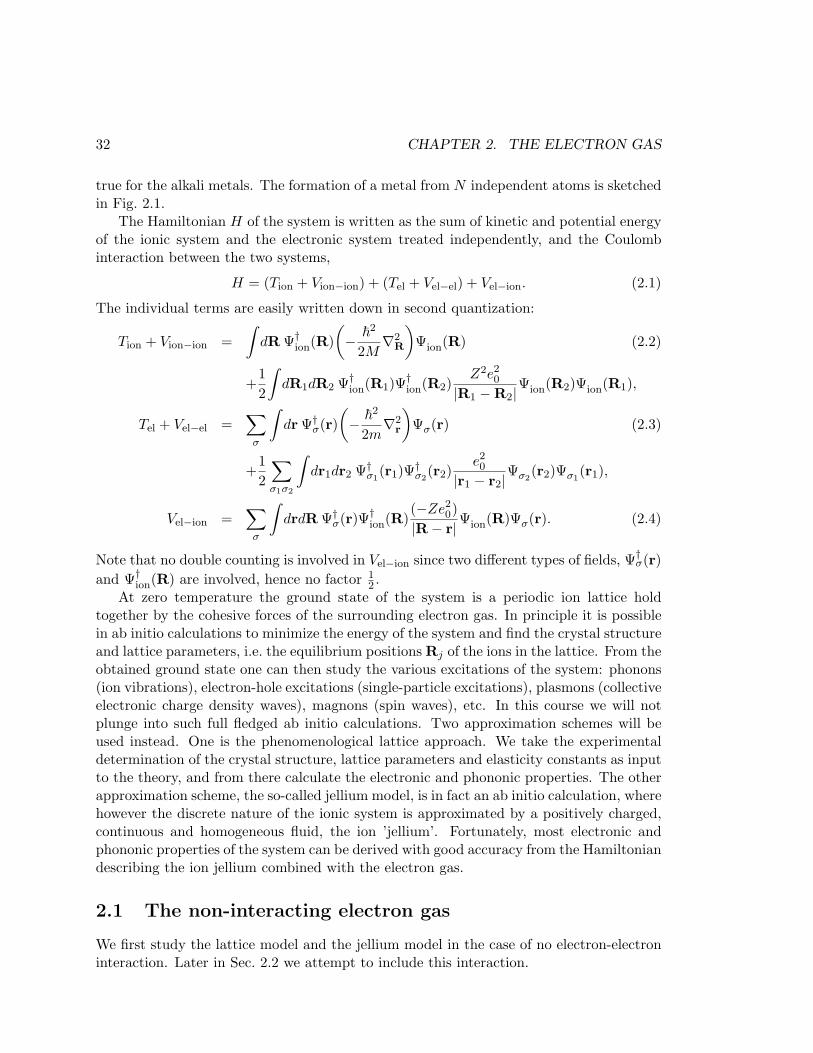
32 CHAPTER 2. THE ELECTRON GAS
true for the alkali metals. The formation of a metal from N independent atoms is sketchedin Fig. 2.1.
The Hamiltonian H of the system is written as the sum of kinetic and potential energyof the ionic system and the electronic system treated independently, and the Coulombinteraction between the two systems,
H = (Tion + Vion−ion) + (Tel + Vel−el) + Vel−ion. (2.1)
The individual terms are easily written down in second quantization:
Tion + Vion−ion =∫
dR Ψ†ion(R)
(− ~2
2M∇2
R
)Ψion(R) (2.2)
+12
∫dR1dR2 Ψ†
ion(R1)Ψ†ion(R2)
Z2e20
|R1 −R2|Ψion(R2)Ψion(R1),
Tel + Vel−el =∑
σ
∫dr Ψ†
σ(r)(− ~
2
2m∇2
r
)Ψσ(r) (2.3)
+12
∑σ1σ2
∫dr1dr2 Ψ†
σ1(r1)Ψ†
σ2(r2)
e20
|r1 − r2|Ψσ2(r2)Ψσ1
(r1),
Vel−ion =∑
σ
∫drdR Ψ†
σ(r)Ψ†ion(R)
(−Ze20)
|R− r|Ψion(R)Ψσ(r). (2.4)
Note that no double counting is involved in Vel−ion since two different types of fields, Ψ†σ(r)
and Ψ†ion(R) are involved, hence no factor 1
2 .At zero temperature the ground state of the system is a periodic ion lattice hold
together by the cohesive forces of the surrounding electron gas. In principle it is possiblein ab initio calculations to minimize the energy of the system and find the crystal structureand lattice parameters, i.e. the equilibrium positions Rj of the ions in the lattice. From theobtained ground state one can then study the various excitations of the system: phonons(ion vibrations), electron-hole excitations (single-particle excitations), plasmons (collectiveelectronic charge density waves), magnons (spin waves), etc. In this course we will notplunge into such full fledged ab initio calculations. Two approximation schemes will beused instead. One is the phenomenological lattice approach. We take the experimentaldetermination of the crystal structure, lattice parameters and elasticity constants as inputto the theory, and from there calculate the electronic and phononic properties. The otherapproximation scheme, the so-called jellium model, is in fact an ab initio calculation, wherehowever the discrete nature of the ionic system is approximated by a positively charged,continuous and homogeneous fluid, the ion ’jellium’. Fortunately, most electronic andphononic properties of the system can be derived with good accuracy from the Hamiltoniandescribing the ion jellium combined with the electron gas.
2.1 The non-interacting electron gas
We first study the lattice model and the jellium model in the case of no electron-electroninteraction. Later in Sec. 2.2 we attempt to include this interaction.
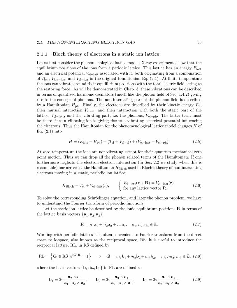
2.1. THE NON-INTERACTING ELECTRON GAS 33
2.1.1 Bloch theory of electrons in a static ion lattice
Let us first consider the phenomenological lattice model. X-ray experiments show that theequilibrium positions of the ions form a periodic lattice. This lattice has an energy Elatt
and an electrical potential Vel−latt associated with it, both originating from a combinationof Tion, Vion−ion, and Vel−ion in the original Hamiltonian Eq. (2.1). At finite temperaturethe ions can vibrate around their equilibrium positions with the total electric field acting asthe restoring force. As will be demonstrated in Chap. 3, these vibrations can be describedin terms of quantized harmonic oscillators (much like the photon field of Sec. 1.4.2) givingrise to the concept of phonons. The non-interacting part of the phonon field is describedby a Hamiltonian Hph. Finally, the electrons are described by their kinetic energy Tel,their mutual interaction Vel−el, and their interaction with both the static part of thelattice, Vel−latt, and the vibrating part, i.e. the phonons, Vel−ph. The latter term mustbe there since a vibrating ion is giving rise to a vibrating electrical potential influencingthe electrons. Thus the Hamiltonian for the phenomenological lattice model changes H ofEq. (2.1) into
H = (Elatt + Hph) + (Tel + Vel−el) + (Vel−latt + Vel−ph). (2.5)
At zero temperature the ions are not vibrating except for their quantum mechanical zeropoint motion. Thus we can drop all the phonon related terms of the Hamiltonian. If onefurthermore neglects the electron-electron interaction (in Sec. 2.2 we study when this isreasonable) one arrives at the Hamiltonian HBloch used in Bloch’s theory of non-interactingelectrons moving in a static, periodic ion lattice:
HBloch = Tel + Vel−latt(r),
Vel−latt(r + R) = Vel−latt(r)for any lattice vector R.
(2.6)
To solve the corresponding Schrodinger equation, and later the phonon problem, we haveto understand the Fourier transform of periodic functions.
Let the static ion lattice be described by the ionic equilibrium positions R in terms ofthe lattice basis vectors a1,a2,a3:
R = n1a1 + n2a2 + n3a3, n1, n2, n3 ∈ Z. (2.7)
Working with periodic lattices it is often convenient to Fourier transform from the directspace to k-space, also known as the reciprocal space, RS. It is useful to introduce thereciprocal lattice, RL, in RS defined by
RL =G ∈ RS
∣∣∣eiG ·R = 1
⇒ G = m1b1 +m2b2 +m3b3, m1,m2,m3 ∈ Z, (2.8)
where the basis vectors b1,b2,b3 in RL are defined as
b1 = 2πa2 × a3
a1 · a2 × a3
, b2 = 2πa3 × a1
a2 · a3 × a1
, b3 = 2πa1 × a2
a3 · a1 × a2
. (2.9)
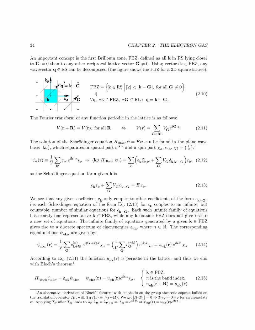
34 CHAPTER 2. THE ELECTRON GAS
An important concept is the first Brillouin zone, FBZ, defined as all k in RS lying closerto G = 0 than to any other reciprocal lattice vector G 6= 0. Using vectors k ∈ FBZ, anywavevector q ∈ RS can be decomposed (the figure shows the FBZ for a 2D square lattice):
FBZ =k ∈ RS
∣∣∣ |k| < |k−G |, for all G 6= 0
⇓∀q, ∃k ∈ FBZ, ∃G ∈ RL : q = k + G .
(2.10)
The Fourier transform of any function periodic in the lattice is as follows:
V (r + R) = V (r), for all R ⇔ V (r) =∑
G∈RL
VGeiG ·r. (2.11)
The solution of the Schrodinger equation HBlochψ = Eψ can be found in the plane wavebasis |kσ〉, which separates in spatial part eik·r and a spin part χσ, e.g. χ↑ =
(10
):
ψσ(r) ≡ 1V
∑
k′ck′ e
ik′·rχσ ⇒ 〈kσ|HBloch|ψσ〉 =∑
k′
(εkδk,k′ +
∑
G
VG δk,k′+G
)ck′ , (2.12)
so the Schrodinger equation for a given k is
ckεk +∑
G
VG ck−G = E ck. (2.13)
We see that any given coefficient ck only couples to other coefficients of the form ck+G ,i.e. each Schrodinger equation of the form Eq. (2.13) for ck couples to an infinite, butcountable, number of similar equations for ck−G . Each such infinite family of equationshas exactly one representative k ∈ FBZ, while any k outside FBZ does not give rise toa new set of equations. The infinite family of equations generated by a given k ∈ FBZgives rise to a discrete spectrum of eigenenergies εnk, where n ∈ N. The correspondingeigenfunctions ψnkσ are given by:
ψnkσ(r) =1V
∑
G
c(n)k+G ei(G+k)·rχσ =
( 1V
∑
G
c(nk)G
)eik·rχσ ≡ unk(r) eik·r χσ. (2.14)
According to Eq. (2.11) the function unk(r) is periodic in the lattice, and thus we endwith Bloch’s theorem1:
HBlochψnkσ = εnkψnkσ, ψnkσ(r) = unk(r)eik·rχσ,
k ∈ FBZ,n is the band index,unk(r + R) = unk(r).
(2.15)
1An alternative derivation of Bloch’s theorem with emphasis on the group theoretic aspects builds onthe translation operator TR, with TRf(r) ≡ f(r+R). We get [H, TR] = 0 ⇒ TRψ = λRψ for an eigenstateψ. Applying TP after TR leads to λP λR = λP+R ⇒ λR = eik·R ⇒ ψnk(r) = unk(r)eik·r.
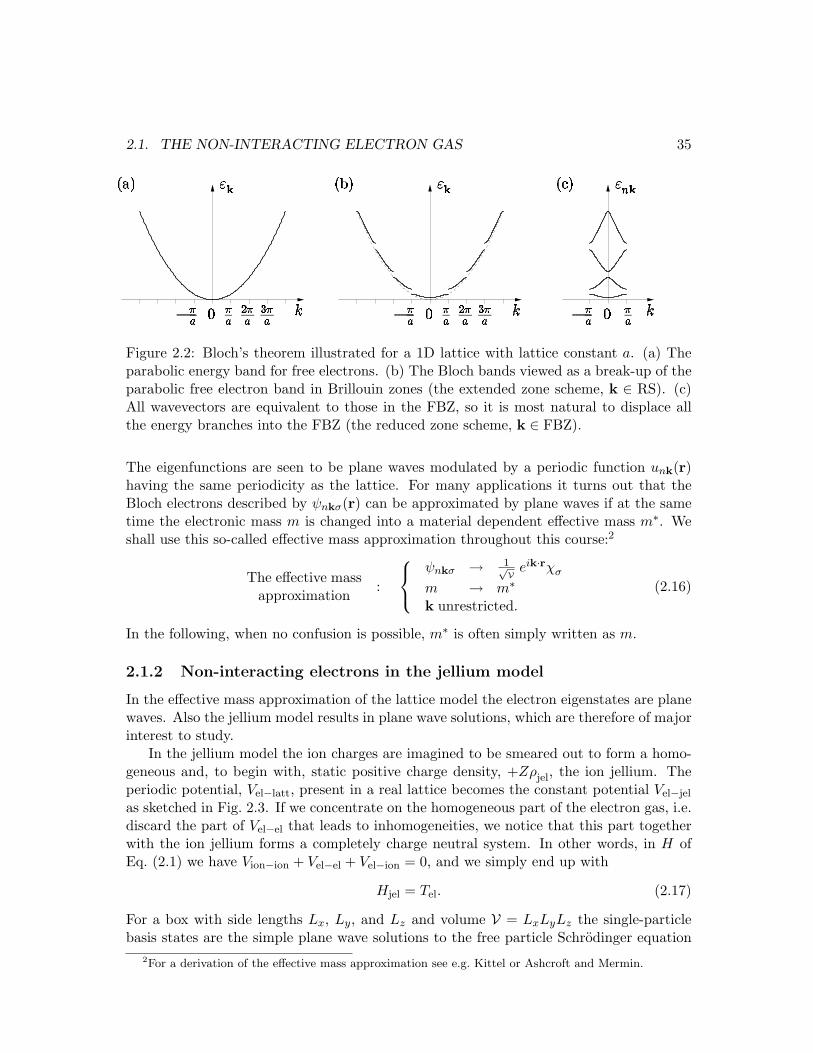
2.1. THE NON-INTERACTING ELECTRON GAS 35
Figure 2.2: Bloch’s theorem illustrated for a 1D lattice with lattice constant a. (a) Theparabolic energy band for free electrons. (b) The Bloch bands viewed as a break-up of theparabolic free electron band in Brillouin zones (the extended zone scheme, k ∈ RS). (c)All wavevectors are equivalent to those in the FBZ, so it is most natural to displace allthe energy branches into the FBZ (the reduced zone scheme, k ∈ FBZ).
The eigenfunctions are seen to be plane waves modulated by a periodic function unk(r)having the same periodicity as the lattice. For many applications it turns out that theBloch electrons described by ψnkσ(r) can be approximated by plane waves if at the sametime the electronic mass m is changed into a material dependent effective mass m∗. Weshall use this so-called effective mass approximation throughout this course:2
The effective massapproximation
:
ψnkσ → 1√V eik·rχσ
m → m∗
k unrestricted.
(2.16)
In the following, when no confusion is possible, m∗ is often simply written as m.
2.1.2 Non-interacting electrons in the jellium model
In the effective mass approximation of the lattice model the electron eigenstates are planewaves. Also the jellium model results in plane wave solutions, which are therefore of majorinterest to study.
In the jellium model the ion charges are imagined to be smeared out to form a homo-geneous and, to begin with, static positive charge density, +Zρjel, the ion jellium. Theperiodic potential, Vel−latt, present in a real lattice becomes the constant potential Vel−jel
as sketched in Fig. 2.3. If we concentrate on the homogeneous part of the electron gas, i.e.discard the part of Vel−el that leads to inhomogeneities, we notice that this part togetherwith the ion jellium forms a completely charge neutral system. In other words, in H ofEq. (2.1) we have Vion−ion + Vel−el + Vel−ion = 0, and we simply end up with
Hjel = Tel. (2.17)
For a box with side lengths Lx, Ly, and Lz and volume V = LxLyLz the single-particlebasis states are the simple plane wave solutions to the free particle Schrodinger equation
2For a derivation of the effective mass approximation see e.g. Kittel or Ashcroft and Mermin.
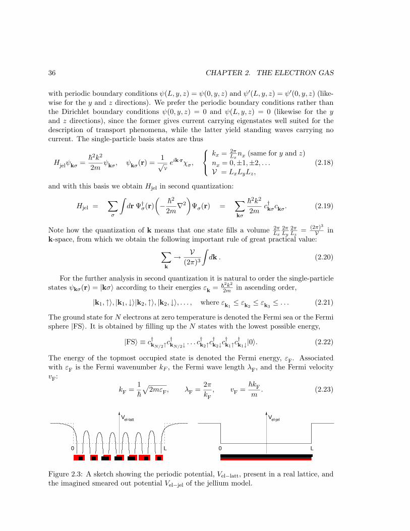
36 CHAPTER 2. THE ELECTRON GAS
with periodic boundary conditions ψ(L, y, z) = ψ(0, y, z) and ψ′(L, y, z) = ψ′(0, y, z) (like-wise for the y and z directions). We prefer the periodic boundary conditions rather thanthe Dirichlet boundary conditions ψ(0, y, z) = 0 and ψ(L, y, z) = 0 (likewise for the yand z directions), since the former gives current carrying eigenstates well suited for thedescription of transport phenomena, while the latter yield standing waves carrying nocurrent. The single-particle basis states are thus
Hjelψkσ =~2k2
2mψkσ, ψkσ(r) =
1√V
eik·rχσ,
kx = 2πLx
nx (same for y and z)nx = 0,±1,±2, . . .V = LxLyLz,
(2.18)
and with this basis we obtain Hjel in second quantization:
Hjel =∑
σ
∫dr Ψ†
σ(r)(− ~
2
2m∇2
)Ψσ(r) =
∑
kσ
~2k2
2mc†kσckσ. (2.19)
Note how the quantization of k means that one state fills a volume 2πLx
2πLy
2πLz
= (2π)3
V ink-space, from which we obtain the following important rule of great practical value:
∑
k
→ V(2π)3
∫dk . (2.20)
For the further analysis in second quantization it is natural to order the single-particlestates ψkσ(r) = |kσ〉 according to their energies εk = ~2k2
2m in ascending order,
|k1, ↑〉, |k1, ↓〉|k2, ↑〉, |k2, ↓〉, . . . , where εk1≤ εk2
≤ εk3≤ . . . (2.21)
The ground state for N electrons at zero temperature is denoted the Fermi sea or the Fermisphere |FS〉. It is obtained by filling up the N states with the lowest possible energy,
|FS〉 ≡ c†kN/2↑c†kN/2↓ . . . c†k2↑c
†k2↓c
†k1↑c
†k1↓|0〉. (2.22)
The energy of the topmost occupied state is denoted the Fermi energy, εF. Associatedwith εF is the Fermi wavenumber kF , the Fermi wave length λF, and the Fermi velocityvF:
kF =1~√
2mεF, λF =2π
kF
, vF =~kF
m. (2.23)
Vel-latt
0 L
Vel-jel
0 L
!!!!!!!!!!!!!!!!!!!!!!!!!!!!!!!!!!!!!
Figure 2.3: A sketch showing the periodic potential, Vel−latt, present in a real lattice, andthe imagined smeared out potential Vel−jel of the jellium model.
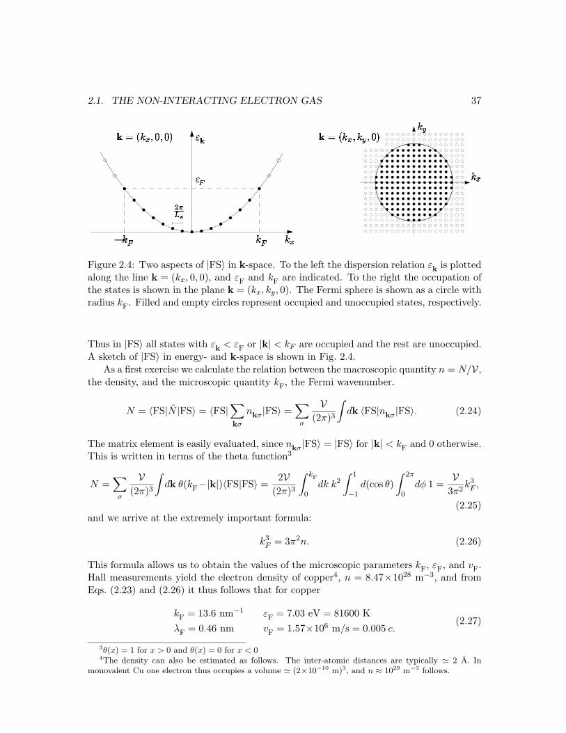
2.1. THE NON-INTERACTING ELECTRON GAS 37
Figure 2.4: Two aspects of |FS〉 in k-space. To the left the dispersion relation εk is plottedalong the line k = (kx, 0, 0), and εF and kF are indicated. To the right the occupation ofthe states is shown in the plane k = (kx, ky, 0). The Fermi sphere is shown as a circle withradius kF. Filled and empty circles represent occupied and unoccupied states, respectively.
Thus in |FS〉 all states with εk < εF or |k| < kF are occupied and the rest are unoccupied.A sketch of |FS〉 in energy- and k-space is shown in Fig. 2.4.
As a first exercise we calculate the relation between the macroscopic quantity n = N/V,the density, and the microscopic quantity kF, the Fermi wavenumber.
N = 〈FS|N |FS〉 = 〈FS|∑
kσ
nkσ|FS〉 =∑
σ
V(2π)3
∫dk 〈FS|nkσ|FS〉. (2.24)
The matrix element is easily evaluated, since nkσ|FS〉 = |FS〉 for |k| < kF and 0 otherwise.This is written in terms of the theta function3
N =∑
σ
V(2π)3
∫dk θ(kF−|k|)〈FS|FS〉 =
2V(2π)3
∫ kF
0dk k2
∫ 1
−1d(cos θ)
∫ 2π
0dφ 1 =
V3π2
k3F ,
(2.25)and we arrive at the extremely important formula:
k3F = 3π2n. (2.26)
This formula allows us to obtain the values of the microscopic parameters kF, εF, and vF.Hall measurements yield the electron density of copper4, n = 8.47×1028 m−3, and fromEqs. (2.23) and (2.26) it thus follows that for copper
kF = 13.6 nm−1 εF = 7.03 eV = 81600 KλF = 0.46 nm vF = 1.57×10⁶ m/s = 0.005 c.
(2.27)
3θ(x) = 1 for x > 0 and θ(x) = 0 for x < 04The density can also be estimated as follows. The inter-atomic distances are typically ' 2 A. In
monovalent Cu one electron thus occupies a volume ' (2×10⁻¹⁰ m)3, and n ≈ 1029 m−3 follows.
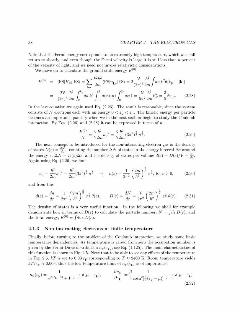
38 CHAPTER 2. THE ELECTRON GAS
Note that the Fermi energy corresponds to an extremely high temperature, which we shallreturn to shortly, and even though the Fermi velocity is large it is still less than a percentof the velocity of light, and we need not invoke relativistic considerations.
We move on to calculate the ground state energy E(0):
E(0) = 〈FS|Hjel|FS〉 =∑
kσ
~2k2
2m〈FS|nkσ|FS〉 = 2
V(2π)3
~2
2m
∫dk k2θ(kF − |k|)
=2V
(2π)3~2
2m
∫ kF
0dk k4
∫ 1
−1d(cos θ)
∫ 2π
0dφ 1 =
V5π2
~2
2mk5
F =35NεF. (2.28)
In the last equation we again used Eq. (2.26). The result is reasonable, since the systemconsists of N electrons each with an energy 0 < εk < εF. The kinetic energy per particlebecomes an important quantity when we in the next section begin to study the Coulombinteraction. By Eqs. (2.26) and (2.28) it can be expressed in terms of n:
E(0)
N=
35~2
2mkF
2 =35~2
2m(3π2)
23 n
23 . (2.29)
The next concept to be introduced for the non-interacting electron gas is the densityof states D(ε) = dN
dε , counting the number ∆N of states in the energy interval ∆ε aroundthe energy ε, ∆N = D(ε)∆ε, and the density of states per volume d(ε) = D(ε)/V = dn
dε .Again using Eq. (2.26) we find
εF =~2
2mkF
2 =~2
2m(3π2)
23 n
23 ⇒ n(ε) =
13π2
(2m
~2
) 32
ε32 , for ε > 0, (2.30)
and from this
d(ε) =dn
dε=
12π2
(2m
~2
) 32
ε12 θ(ε), D(ε) =
dN
dε=
V2π2
(2m
~2
) 32
ε12 θ(ε). (2.31)
The density of states is a very useful function. In the following we shall for exampledemonstrate how in terms of D(ε) to calculate the particle number, N =
∫dε D(ε), and
the total energy, E(0) =∫
dε ε D(ε).
2.1.3 Non-interacting electrons at finite temperature
Finally, before turning to the problem of the Coulomb interaction, we study some basictemperature dependencies. As temperature is raised from zero the occupation number isgiven by the Fermi-Dirac distribution nF(εk), see Eq. (1.125). The main characteristics ofthis function is shown in Fig. 2.5. Note that to be able to see any effects of the temperaturein Fig. 2.5, kT is set to 0.03 εF corresponding to T ≈ 2400 K. Room temperature yieldskT/εF ≈ 0.003, thus the low temperature limit of nF(εk) is of importance:
nF(εk) =1
eβ(εk−µ) + 1−→T→0
θ(µ− εk), −∂nF
∂εk
=β
41
cosh2[β2 (εk − µ)]
−→T→0
δ(µ− εk).
(2.32)
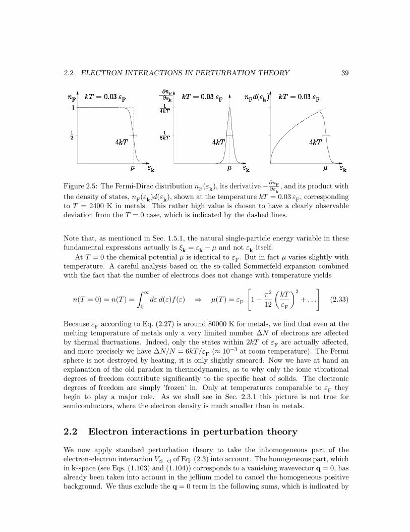
2.2. ELECTRON INTERACTIONS IN PERTURBATION THEORY 39
Figure 2.5: The Fermi-Dirac distribution nF(εk), its derivative −∂nF∂εk
, and its product withthe density of states, nF(εk)d(εk), shown at the temperature kT = 0.03 εF, correspondingto T = 2400 K in metals. This rather high value is chosen to have a clearly observabledeviation from the T = 0 case, which is indicated by the dashed lines.
Note that, as mentioned in Sec. 1.5.1, the natural single-particle energy variable in thesefundamental expressions actually is ξk = εk − µ and not εk itself.
At T = 0 the chemical potential µ is identical to εF. But in fact µ varies slightly withtemperature. A careful analysis based on the so-called Sommerfeld expansion combinedwith the fact that the number of electrons does not change with temperature yields
n(T = 0) = n(T ) =∫ ∞
0dε d(ε)f(ε) ⇒ µ(T ) = εF
[1− π2
12
(kT
εF
)2
+ . . .
](2.33)
Because εF according to Eq. (2.27) is around 80000 K for metals, we find that even at themelting temperature of metals only a very limited number ∆N of electrons are affectedby thermal fluctuations. Indeed, only the states within 2kT of εF are actually affected,and more precisely we have ∆N/N = 6kT/εF (≈ 10−3 at room temperature). The Fermisphere is not destroyed by heating, it is only slightly smeared. Now we have at hand anexplanation of the old paradox in thermodynamics, as to why only the ionic vibrationaldegrees of freedom contribute significantly to the specific heat of solids. The electronicdegrees of freedom are simply ’frozen’ in. Only at temperatures comparable to εF theybegin to play a major role. As we shall see in Sec. 2.3.1 this picture is not true forsemiconductors, where the electron density is much smaller than in metals.
2.2 Electron interactions in perturbation theory
We now apply standard perturbation theory to take the inhomogeneous part of theelectron-electron interaction Vel−el of Eq. (2.3) into account. The homogeneous part, whichin k-space (see Eqs. (1.103) and (1.104)) corresponds to a vanishing wavevector q = 0, hasalready been taken into account in the jellium model to cancel the homogeneous positivebackground. We thus exclude the q = 0 term in the following sums, which is indicated by
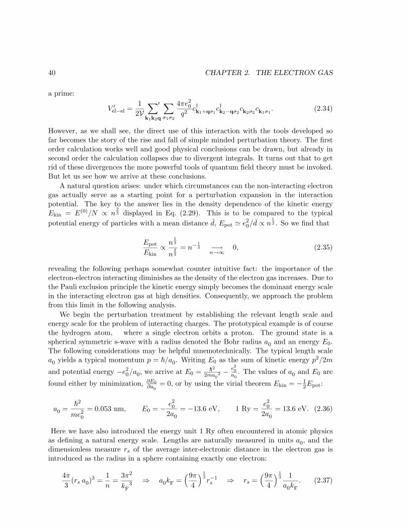
40 CHAPTER 2. THE ELECTRON GAS
a prime:
V ′el−el =
12V
∑
k1k2q
′ ∑σ1σ2
4πe20
q2c†k1+qσ1
c†k2−qσ2ck2σ2
ck1σ1. (2.34)
However, as we shall see, the direct use of this interaction with the tools developed sofar becomes the story of the rise and fall of simple minded perturbation theory. The firstorder calculation works well and good physical conclusions can be drawn, but already insecond order the calculation collapses due to divergent integrals. It turns out that to getrid of these divergences the more powerful tools of quantum field theory must be invoked.But let us see how we arrive at these conclusions.
A natural question arises: under which circumstances can the non-interacting electrongas actually serve as a starting point for a perturbation expansion in the interactionpotential. The key to the answer lies in the density dependence of the kinetic energyEkin = E(0)/N ∝ n
23 displayed in Eq. (2.29). This is to be compared to the typical
potential energy of particles with a mean distance d, Epot ' e20/d ∝ n
13 . So we find that
Epot
Ekin∝ n
13
n23
= n−13 −→
n→∞ 0, (2.35)
revealing the following perhaps somewhat counter intuitive fact: the importance of theelectron-electron interacting diminishes as the density of the electron gas increases. Due tothe Pauli exclusion principle the kinetic energy simply becomes the dominant energy scalein the interacting electron gas at high densities. Consequently, we approach the problemfrom this limit in the following analysis.
We begin the perturbation treatment by establishing the relevant length scale andenergy scale for the problem of interacting charges. The prototypical example is of coursethe hydrogen atom, where a single electron orbits a proton. The ground state is aspherical symmetric s-wave with a radius denoted the Bohr radius a0 and an energy E0.The following considerations may be helpful mnemotechnically. The typical length scalea0 yields a typical momentum p = ~/a0. Writing E0 as the sum of kinetic energy p2/2m
and potential energy −e20/a0, we arrive at E0 = ~2
2ma02 − e2
0a0
. The values of a0 and E0 are
found either by minimization, ∂E0∂a0
= 0, or by using the virial theorem Ekin = −12Epot:
a0 =~2
me20
= 0.053 nm, E0 = − e20
2a0
= −13.6 eV, 1 Ry =e20
2a0
= 13.6 eV. (2.36)
Here we have also introduced the energy unit 1 Ry often encountered in atomic physicsas defining a natural energy scale. Lengths are naturally measured in units a0, and thedimensionless measure rs of the average inter-electronic distance in the electron gas isintroduced as the radius in a sphere containing exactly one electron:
4π
3(rs a0)
3 =1n
=3π2
kF3 ⇒ a0kF =
(9π
4
) 13r−1s ⇒ rs =
(9π
4
) 13 1a0kF
. (2.37)
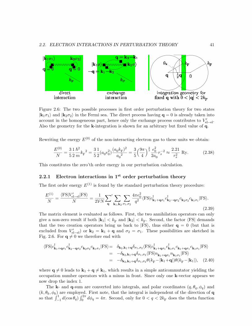
2.2. ELECTRON INTERACTIONS IN PERTURBATION THEORY 41
! " "
#%$'&(#%$'&
) *
+ , - . / 0, 1 0 . - 2 / 0 , 3 1
"
4 #%$ 4 "
#5$ " 4
) *
. 6 / 7 2 1 8 ., 1 0 . - 2 / 0 , 3 1
9 :;) *<) *
#" # &
, 1 0 . 8 - 2 0 , 3 1%8 . 3 = . 0 - >@? 3 -A 6 . + #5B , 0 7 & C # C'D ) *
Figure 2.6: The two possible processes in first order perturbation theory for two states|k1σ1〉 and |k2σ2〉 in the Fermi sea. The direct process having q = 0 is already taken intoaccount in the homogeneous part, hence only the exchange process contributes to V ′
el−el.Also the geometry for the k-integration is shown for an arbitrary but fixed value of q.
Rewriting the energy E(0) of the non-interacting electron gas to these units we obtain:
E(0)
N=
35
12~2
mkF
2 =35
12(a0e
20)
(a0kF)2
a02
=35
(9π
4
) 23 e2
0
2a0
r−2s ≈ 2.21
r2s
Ry. (2.38)
This constitutes the zero’th order energy in our perturbation calculation.
2.2.1 Electron interactions in 1st order perturbation theory
The first order energy E(1) is found by the standard perturbation theory procedure:
E(1)
N=〈FS|V ′
el−el|FS〉N
=1
2VN
∑q
′ ∑
k1,k2
∑σ1,σ2
4πe20
q2〈FS|c†k1+qσ1
c†k2−qσ2ck2σ2
ck1σ1|FS〉.
(2.39)The matrix element is evaluated as follows. First, the two annihilation operators can onlygive a non-zero result if both |k1| < kF and |k2| < kF. Second, the factor 〈FS| demandsthat the two creation operators bring us back to |FS〉, thus either q = 0 (but that isexcluded from V ′
el−el) or k2 = k1 + q and σ2 = σ1. These possibilities are sketched inFig. 2.6. For q 6= 0 we therefore end with
〈FS|c†k1+qσ1c†k2−qσ2
ck2σ2ck1σ1
|FS〉= δk2,k1+qδσ1,σ2〈FS|c†k1+qσ1c†k1σ1
ck1+qσ1ck1σ1
|FS〉= −δk2,k1+qδσ1,σ2〈FS|nk1+qσ1
nk1σ1|FS〉
= −δk2,k1+qδσ1,σ2θ(kF−|k1+q|)θ(kF−|k1|), (2.40)
where q 6= 0 leads to k1 + q 6= k1, which results in a simple anticommutator yielding theoccupation number operators with a minus in front. Since only one k-vector appears wenow drop the index 1.
The k- and q-sum are converted into integrals, and polar coordinates (q, θq, φq) and(k, θk, φk) are employed. First note, that the integral is independent of the direction of qso that
∫ 1−1 d(cos θq)
∫ 2π0 dφq = 4π. Second, only for 0 < q < 2kF does the theta function
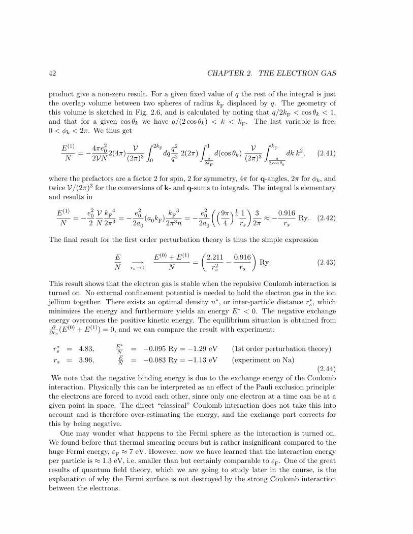
42 CHAPTER 2. THE ELECTRON GAS
product give a non-zero result. For a given fixed value of q the rest of the integral is justthe overlap volume between two spheres of radius kF displaced by q. The geometry ofthis volume is sketched in Fig. 2.6, and is calculated by noting that q/2kF < cos θk < 1,and that for a given cos θk we have q/(2 cos θk) < k < kF. The last variable is free:0 < φk < 2π. We thus get
E(1)
N= −4πe2
0
2VN2(4π)
V(2π)3
∫ 2kF
0dq
q2
q22(2π)
∫ 1
q2k
F
d(cos θk)V
(2π)3
∫ kF
q2 cos θk
dk k2, (2.41)
where the prefactors are a factor 2 for spin, 2 for symmetry, 4π for q-angles, 2π for φk, andtwice V/(2π)3 for the conversions of k- and q-sums to integrals. The integral is elementaryand results in
E(1)
N= −e2
0
2VN
kF4
2π3= − e2
0
2a0
(a0kF)kF
3
2π3n= − e2
0
2a0
((9π
4
) 13 1rs
)32π
≈ −0.916rs
Ry. (2.42)
The final result for the first order perturbation theory is thus the simple expression
E
N−→rs→0
E(0) + E(1)
N=
(2.211
r2s
− 0.916rs
)Ry. (2.43)
This result shows that the electron gas is stable when the repulsive Coulomb interaction isturned on. No external confinement potential is needed to hold the electron gas in the ionjellium together. There exists an optimal density n∗, or inter-particle distance r∗s , whichminimizes the energy and furthermore yields an energy E∗ < 0. The negative exchangeenergy overcomes the positive kinetic energy. The equilibrium situation is obtained from∂
∂rs(E(0) + E(1)) = 0, and we can compare the result with experiment:
r∗s = 4.83, E∗N = −0.095 Ry = −1.29 eV (1st order perturbation theory)
rs = 3.96, EN = −0.083 Ry = −1.13 eV (experiment on Na)
(2.44)We note that the negative binding energy is due to the exchange energy of the Coulombinteraction. Physically this can be interpreted as an effect of the Pauli exclusion principle:the electrons are forced to avoid each other, since only one electron at a time can be at agiven point in space. The direct “classical” Coulomb interaction does not take this intoaccount and is therefore over-estimating the energy, and the exchange part corrects forthis by being negative.
One may wonder what happens to the Fermi sphere as the interaction is turned on.We found before that thermal smearing occurs but is rather insignificant compared to thehuge Fermi energy, εF ≈ 7 eV. However, now we have learned that the interaction energyper particle is ≈ 1.3 eV, i.e. smaller than but certainly comparable to εF. One of the greatresults of quantum field theory, which we are going to study later in the course, is theexplanation of why the Fermi surface is not destroyed by the strong Coulomb interactionbetween the electrons.
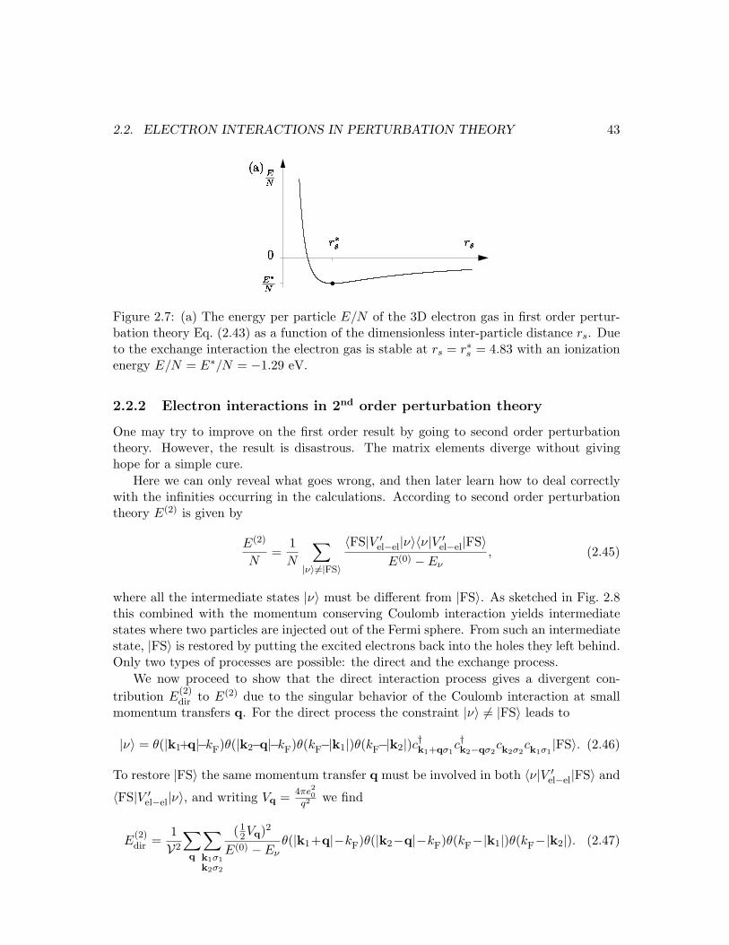
2.2. ELECTRON INTERACTIONS IN PERTURBATION THEORY 43
Figure 2.7: (a) The energy per particle E/N of the 3D electron gas in first order pertur-bation theory Eq. (2.43) as a function of the dimensionless inter-particle distance rs. Dueto the exchange interaction the electron gas is stable at rs = r∗s = 4.83 with an ionizationenergy E/N = E∗/N = −1.29 eV.
2.2.2 Electron interactions in 2nd order perturbation theory
One may try to improve on the first order result by going to second order perturbationtheory. However, the result is disastrous. The matrix elements diverge without givinghope for a simple cure.
Here we can only reveal what goes wrong, and then later learn how to deal correctlywith the infinities occurring in the calculations. According to second order perturbationtheory E(2) is given by
E(2)
N=
1N
∑
|ν〉6=|FS〉
〈FS|V ′el−el|ν〉〈ν|V ′
el−el|FS〉E(0) −Eν
, (2.45)
where all the intermediate states |ν〉 must be different from |FS〉. As sketched in Fig. 2.8this combined with the momentum conserving Coulomb interaction yields intermediatestates where two particles are injected out of the Fermi sphere. From such an intermediatestate, |FS〉 is restored by putting the excited electrons back into the holes they left behind.Only two types of processes are possible: the direct and the exchange process.
We now proceed to show that the direct interaction process gives a divergent con-tribution E
(2)dir to E(2) due to the singular behavior of the Coulomb interaction at small
momentum transfers q. For the direct process the constraint |ν〉 6= |FS〉 leads to
|ν〉 = θ(|k1+q|−kF)θ(|k2−q|−kF)θ(kF−|k1|)θ(kF−|k2|)c†k1+qσ1c†k2−qσ2
ck2σ2ck1σ1
|FS〉. (2.46)
To restore |FS〉 the same momentum transfer q must be involved in both 〈ν|V ′el−el|FS〉 and
〈FS|V ′el−el|ν〉, and writing Vq = 4πe2
0q2 we find
E(2)dir =
1V2
∑q
∑
k1σ1k2σ2
(12Vq)2
E(0) − Eνθ(|k1+q|−kF)θ(|k2−q|−kF)θ(kF−|k1|)θ(kF−|k2|). (2.47)
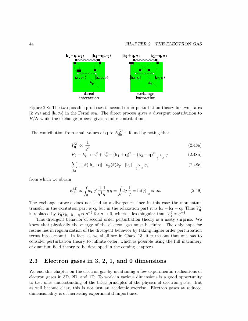
44 CHAPTER 2. THE ELECTRON GAS
! " #$ % & ! " % #
! " #' % ! " % #( )
* + , - . /+ 0 / - , 1 . / + 2 0
! " #3 % & ! " #
! " #4 % ! " #( )
- 5 . 6 1 0 7 -+ 0 / - , 1 . / + 2 0
Figure 2.8: The two possible processes in second order perturbation theory for two states|k1σ1〉 and |k2σ2〉 in the Fermi sea. The direct process gives a divergent contribution toE/N while the exchange process gives a finite contribution.
The contribution from small values of q to E(2)dir is found by noting that
V 2q ∝ 1
q4(2.48a)
E0 −Eν ∝ k21 + k2
2 − (k1 + q)2 − (k2 − q)2 ∝q→0
q (2.48b)∑
k1
. . . θ(|k1+q|−kF)θ(kF−|k1|) ∝q→0
q, (2.48c)
from which we obtain
E(2)dir ∝
∫
0dq q2 1
q4
1q
q q =∫
0dq
1q
= ln(q)∣∣∣0∝ ∞. (2.49)
The exchange process does not lead to a divergence since in this case the momentumtransfer in the excitation part is q, but in the relaxation part it is k2 − k1 − q. Thus V 2
q
is replaced by VqVk2−k1−q ∝ q−2 for q → 0, which is less singular than V 2q ∝ q−4.
This divergent behavior of second order perturbation theory is a nasty surprise. Weknow that physically the energy of the electron gas must be finite. The only hope forrescue lies in regularization of the divergent behavior by taking higher order perturbationterms into account. In fact, as we shall see in Chap. 13, it turns out that one has toconsider perturbation theory to infinite order, which is possible using the full machineryof quantum field theory to be developed in the coming chapters.
2.3 Electron gases in 3, 2, 1, and 0 dimensions
We end this chapter on the electron gas by mentioning a few experimental realizations ofelectron gases in 3D, 2D, and 1D. To work in various dimensions is a good opportunityto test ones understanding of the basic principles of the physics of electron gases. Butas will become clear, this is not just an academic exercise. Electron gases at reduceddimensionality is of increasing experimental importance.
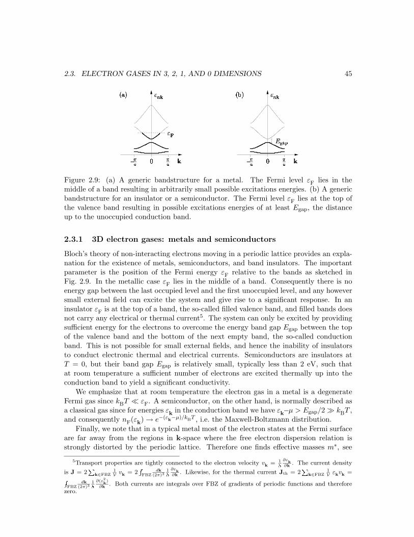
2.3. ELECTRON GASES IN 3, 2, 1, AND 0 DIMENSIONS 45
Figure 2.9: (a) A generic bandstructure for a metal. The Fermi level εF lies in themiddle of a band resulting in arbitrarily small possible excitations energies. (b) A genericbandstructure for an insulator or a semiconductor. The Fermi level εF lies at the top ofthe valence band resulting in possible excitations energies of at least Egap, the distanceup to the unoccupied conduction band.
2.3.1 3D electron gases: metals and semiconductors
Bloch’s theory of non-interacting electrons moving in a periodic lattice provides an expla-nation for the existence of metals, semiconductors, and band insulators. The importantparameter is the position of the Fermi energy εF relative to the bands as sketched inFig. 2.9. In the metallic case εF lies in the middle of a band. Consequently there is noenergy gap between the last occupied level and the first unoccupied level, and any howeversmall external field can excite the system and give rise to a significant response. In aninsulator εF is at the top of a band, the so-called filled valence band, and filled bands doesnot carry any electrical or thermal current5. The system can only be excited by providingsufficient energy for the electrons to overcome the energy band gap Egap between the topof the valence band and the bottom of the next empty band, the so-called conductionband. This is not possible for small external fields, and hence the inability of insulatorsto conduct electronic thermal and electrical currents. Semiconductors are insulators atT = 0, but their band gap Egap is relatively small, typically less than 2 eV, such thatat room temperature a sufficient number of electrons are excited thermally up into theconduction band to yield a significant conductivity.
We emphasize that at room temperature the electron gas in a metal is a degenerateFermi gas since kBT ¿ εF. A semiconductor, on the other hand, is normally described asa classical gas since for energies εk in the conduction band we have εk−µ > Egap/2 À kBT ,and consequently nF(εk) → e−(εk−µ)/kBT , i.e. the Maxwell-Boltzmann distribution.
Finally, we note that in a typical metal most of the electron states at the Fermi surfaceare far away from the regions in k-space where the free electron dispersion relation isstrongly distorted by the periodic lattice. Therefore one finds effective masses m∗, see
5Transport properties are tightly connected to the electron velocity vk = 1~
∂εk
∂k. The current density
is J = 2P
k∈FBZ1V vk = 2
RFBZ
dk(2π)3
1~
∂εk
∂k. Likewise, for the thermal current Jth = 2
Pk∈FBZ
1V εkvk =R
FBZdk
(2π)31~
∂(ε2k)
∂k. Both currents are integrals over FBZ of gradients of periodic functions and therefore
zero.
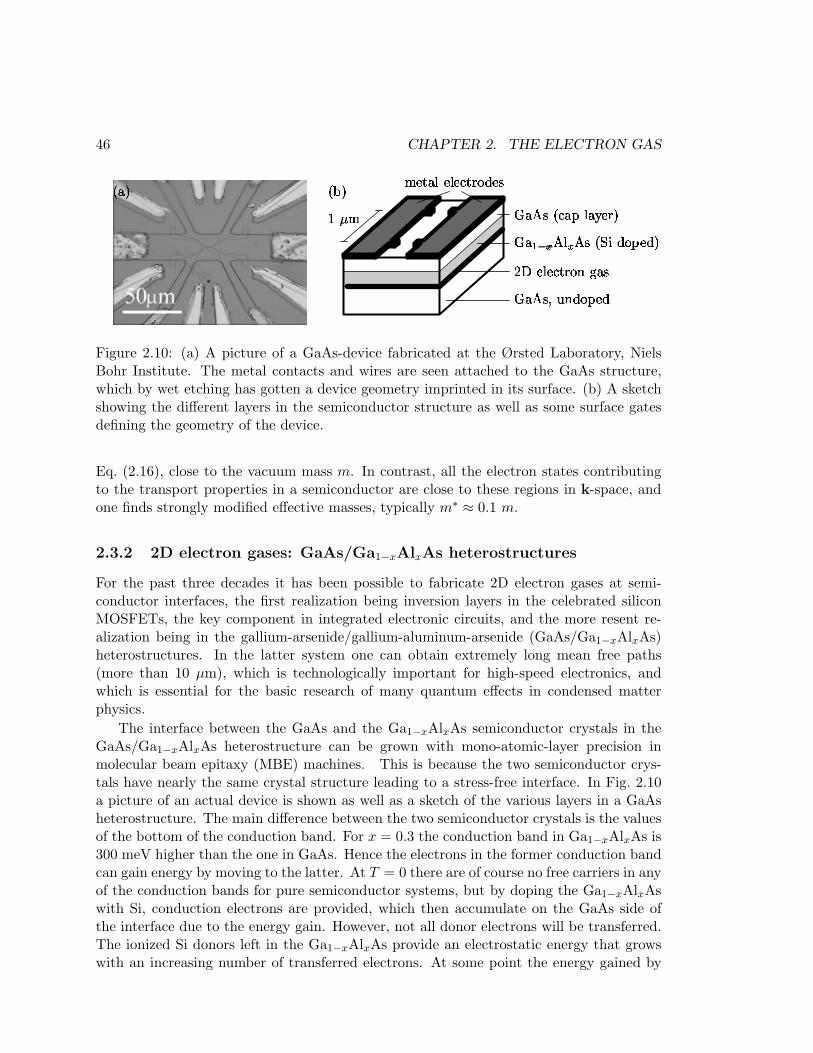
46 CHAPTER 2. THE ELECTRON GAS
Figure 2.10: (a) A picture of a GaAs-device fabricated at the Ørsted Laboratory, NielsBohr Institute. The metal contacts and wires are seen attached to the GaAs structure,which by wet etching has gotten a device geometry imprinted in its surface. (b) A sketchshowing the different layers in the semiconductor structure as well as some surface gatesdefining the geometry of the device.
Eq. (2.16), close to the vacuum mass m. In contrast, all the electron states contributingto the transport properties in a semiconductor are close to these regions in k-space, andone finds strongly modified effective masses, typically m∗ ≈ 0.1 m.
2.3.2 2D electron gases: GaAs/Ga1−xAlxAs heterostructures
For the past three decades it has been possible to fabricate 2D electron gases at semi-conductor interfaces, the first realization being inversion layers in the celebrated siliconMOSFETs, the key component in integrated electronic circuits, and the more resent re-alization being in the gallium-arsenide/gallium-aluminum-arsenide (GaAs/Ga1−xAlxAs)heterostructures. In the latter system one can obtain extremely long mean free paths(more than 10 µm), which is technologically important for high-speed electronics, andwhich is essential for the basic research of many quantum effects in condensed matterphysics.
The interface between the GaAs and the Ga1−xAlxAs semiconductor crystals in theGaAs/Ga1−xAlxAs heterostructure can be grown with mono-atomic-layer precision inmolecular beam epitaxy (MBE) machines. This is because the two semiconductor crys-tals have nearly the same crystal structure leading to a stress-free interface. In Fig. 2.10a picture of an actual device is shown as well as a sketch of the various layers in a GaAsheterostructure. The main difference between the two semiconductor crystals is the valuesof the bottom of the conduction band. For x = 0.3 the conduction band in Ga1−xAlxAs is300 meV higher than the one in GaAs. Hence the electrons in the former conduction bandcan gain energy by moving to the latter. At T = 0 there are of course no free carriers in anyof the conduction bands for pure semiconductor systems, but by doping the Ga1−xAlxAswith Si, conduction electrons are provided, which then accumulate on the GaAs side ofthe interface due to the energy gain. However, not all donor electrons will be transferred.The ionized Si donors left in the Ga1−xAlxAs provide an electrostatic energy that growswith an increasing number of transferred electrons. At some point the energy gained by
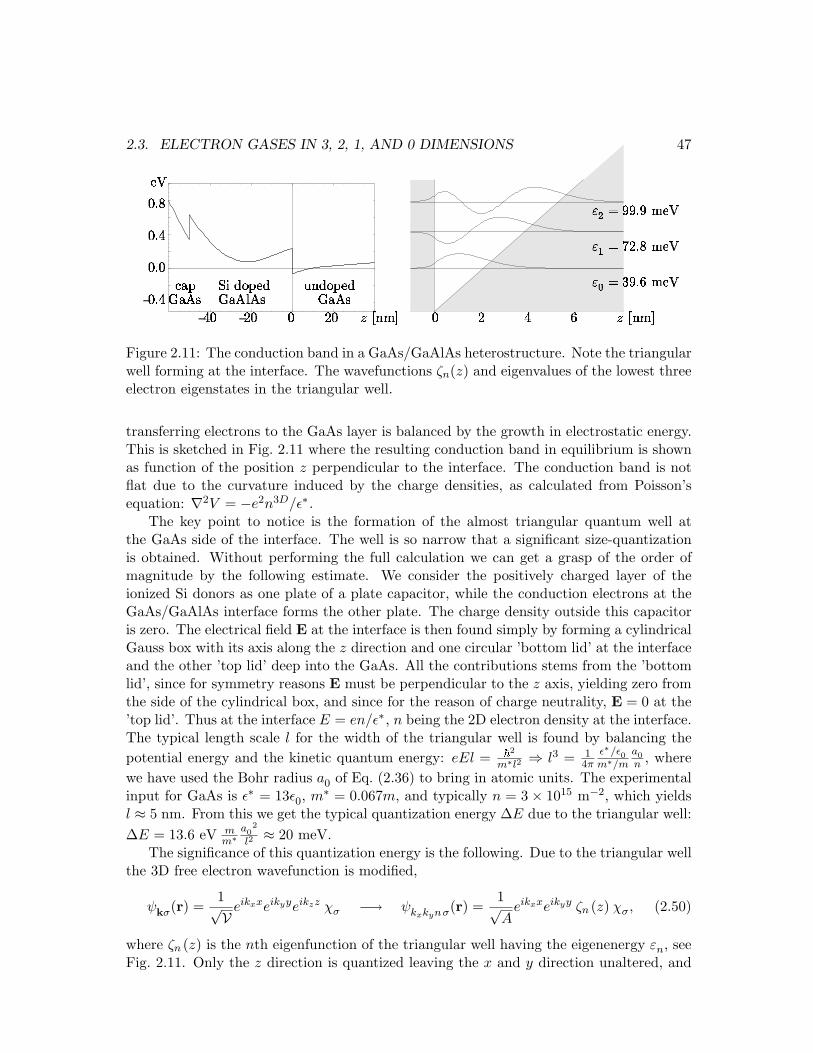
2.3. ELECTRON GASES IN 3, 2, 1, AND 0 DIMENSIONS 47
!
" # !
$ % ! &
&
Figure 2.11: The conduction band in a GaAs/GaAlAs heterostructure. Note the triangularwell forming at the interface. The wavefunctions ζn(z) and eigenvalues of the lowest threeelectron eigenstates in the triangular well.
transferring electrons to the GaAs layer is balanced by the growth in electrostatic energy.This is sketched in Fig. 2.11 where the resulting conduction band in equilibrium is shownas function of the position z perpendicular to the interface. The conduction band is notflat due to the curvature induced by the charge densities, as calculated from Poisson’sequation: ∇2V = −e2n3D/ε∗ .
The key point to notice is the formation of the almost triangular quantum well atthe GaAs side of the interface. The well is so narrow that a significant size-quantizationis obtained. Without performing the full calculation we can get a grasp of the order ofmagnitude by the following estimate. We consider the positively charged layer of theionized Si donors as one plate of a plate capacitor, while the conduction electrons at theGaAs/GaAlAs interface forms the other plate. The charge density outside this capacitoris zero. The electrical field E at the interface is then found simply by forming a cylindricalGauss box with its axis along the z direction and one circular ’bottom lid’ at the interfaceand the other ’top lid’ deep into the GaAs. All the contributions stems from the ’bottomlid’, since for symmetry reasons E must be perpendicular to the z axis, yielding zero fromthe side of the cylindrical box, and since for the reason of charge neutrality, E = 0 at the’top lid’. Thus at the interface E = en/ε∗ , n being the 2D electron density at the interface.The typical length scale l for the width of the triangular well is found by balancing thepotential energy and the kinetic quantum energy: eEl = ~2
m∗l2 ⇒ l3 = 14π
ε∗/ε0m∗/m
a0n , where
we have used the Bohr radius a0 of Eq. (2.36) to bring in atomic units. The experimentalinput for GaAs is ε∗ = 13ε0, m∗ = 0.067m, and typically n = 3× 10¹⁵ m−2, which yieldsl ≈ 5 nm. From this we get the typical quantization energy ∆E due to the triangular well:∆E = 13.6 eV m
m∗a0
2
l2≈ 20 meV.
The significance of this quantization energy is the following. Due to the triangular wellthe 3D free electron wavefunction is modified,
ψkσ(r) =1√V eikxxeikyyeikzz χσ −→ ψkxkynσ(r) =
1√A
eikxxeikyy ζn (z) χσ, (2.50)
where ζn (z) is the nth eigenfunction of the triangular well having the eigenenergy εn, seeFig. 2.11. Only the z direction is quantized leaving the x and y direction unaltered, and

48 CHAPTER 2. THE ELECTRON GAS
the total energy for all three spatial directions is
εkx,ky ,n =~2
2m∗(k2
x + k2y
)+ εn, kF
2 = 2πn ⇒ εF ≈ 10 meV, (2.51)
where we have given the 2D version of the fundamental relation between kF and n (seeExercise 2.4 and compare to Eq. (2.26) for the 3D case). The highest occupied state hasthe energy E0 + εF while the lowest unoccupied state has the energy E1. The differenceis E1 − (E0 + εF) = ∆E − εF ≈ 10 meV ≈ 100 K, and we arrive at our conclusion:At temperatures T ¿ 100 K all occupied electron states have the same orbital in thez direction, ζ0(z). Any changes of this orbital requires an excitation energy of at least10 meV. If this is not provided the system has effectively lost one spatial degree of freedomand is dynamically a 2D system. This means that theoretical studies of 2D electron gasesis far from an academic exercise; 2D systems do indeed exist in reality.
2.3.3 1D electron gases: carbon nanotubes
Since the mid-nineties a new research field has developed involving studies of the cylindri-cally shaped carbon based molecule, the so-called carbon nanotube. The carbon nanotubecan be viewed as a normal graphite sheet rolled up into a cylinder with a radius R0 ≈ 2 nmand a length more than a thousand times R0, see Fig. 2.12. These long and thin carbonmolecules have some extraordinary material characteristics. They are believed to be thestrongest material in the world, and depending on the specific way the cylinder is rolled upthe nanotubes are either metallic, semiconducting or insulating. In the same dynamicalsense as the GaAs heterostructure is a 2D metal sheet, a metallic nanotube is a nearlyideal 1D wire, i.e. two of the three spatial degrees of freedom are frozen in. We brieflysketch how this comes about.
The cylindrical symmetry of the nanotube makes it natural to change the basis func-tions from the 3D (x, y, z) plane waves to cylindrical (x, r, φ) wavefunctions:
ψkσ(r) =1√V eikxxeikyyeikzz χσ −→ ψkx,n,l,σ(r) =
1√L
eikxx Rnl(r) Yl(φ) χσ. (2.52)
This is of course more than just a mathematical transformation. The electrons are stronglybound to the surface of the cylinder in quantum states arising from the original π-bondsof the graphite system. This means that the extension ∆R of the radial wave functionRnl(r) around the mean value R0 is of atomic scale, i.e. ∆R ≈ 0.1 nm, resulting in a radialconfinement energy ER
0 ∼ ~22m∆R2 ∼ 10 eV. Likewise, in the azimuthal angle coordinate
φ, there is a strong confinement, since the perimeter must contain an integer numberof electron wavelengths λn, i.e. λn = 2πR0/n < 2 nm. The corresponding confinementenergy is Eφ
n ∼ ~22mλ2
n∼ 1 eV n. There are no severe constraints along the cylinder axis,
i.e. in the x direction. We therefore end up with a total energy
εkx,n,l = ER0 + Eφ
n +~2
2mk2
x, (2.53)

2.3. ELECTRON GASES IN 3, 2, 1, AND 0 DIMENSIONS 49
Figure 2.12: (a) Carbon atoms forming a sheet of graphite with a characteristic hexagonallattice. (b) A carbon nanotube molecule is formed by rolling up a graphite sheet into acylindrical geometry. (c) An atomic force micrograph taken at the Ørsted Laboratory,Niels Bohr Institute, showing a bundle of carbon nanotubes placed across a gap betweentwo metal electrodes, thereby connecting them and allowing for electrical measurementson single molecules.
with a considerable gap ∆E from the center of the (n, l) = (0, 0) band (the position of εF
for the metallic case) to the bottom of the (n, l) = (0, 1) band:
∆E =12(Eφ
1 − Eφ0 ) ≈ 1 eV ∼ 12000 K. (2.54)
Thus at room temperature the only available degree of freedom is the axial one describedby the continuous quantum number kx and the associated plan waves eikxx.
Not only are the nanotube very interesting from an experimental point of view, alsofrom a pure theoretical point of view do they play an important role. The nanotubes isone of only a couple of systems exhibiting a nearly ideal 1D behavior. In particular thatmakes the nanotubes a key testing ground for the diagonizable so-called Luttinger liquidmodel, a central quantum model for describing interacting electrons in 1D.
2.3.4 0D electron gases: quantum dots
Naturally one can think of confining the electrons in all three spatial dimensions. Thishas been realized experimentally in the so-called quantum dot systems, for example byusing the device shown in Fig. 2.10(b). A simplified model of a quantum dot is studied inExercise 8.4.
This section will be expanded in the next edition of these notes.

50 CHAPTER 2. THE ELECTRON GAS
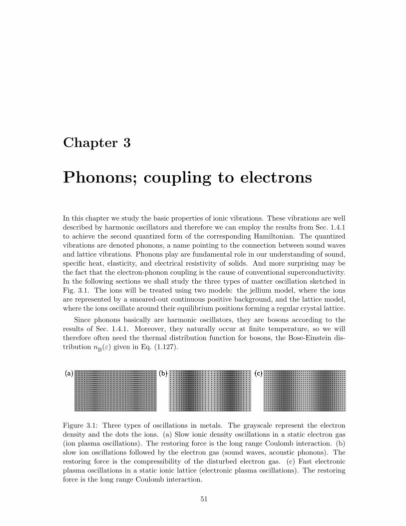
Chapter 3
Phonons; coupling to electrons
In this chapter we study the basic properties of ionic vibrations. These vibrations are welldescribed by harmonic oscillators and therefore we can employ the results from Sec. 1.4.1to achieve the second quantized form of the corresponding Hamiltonian. The quantizedvibrations are denoted phonons, a name pointing to the connection between sound wavesand lattice vibrations. Phonons play are fundamental role in our understanding of sound,specific heat, elasticity, and electrical resistivity of solids. And more surprising may bethe fact that the electron-phonon coupling is the cause of conventional superconductivity.In the following sections we shall study the three types of matter oscillation sketched inFig. 3.1. The ions will be treated using two models: the jellium model, where the ionsare represented by a smeared-out continuous positive background, and the lattice model,where the ions oscillate around their equilibrium positions forming a regular crystal lattice.
Since phonons basically are harmonic oscillators, they are bosons according to theresults of Sec. 1.4.1. Moreover, they naturally occur at finite temperature, so we willtherefore often need the thermal distribution function for bosons, the Bose-Einstein dis-tribution nB(ε) given in Eq. (1.127).
Figure 3.1: Three types of oscillations in metals. The grayscale represent the electrondensity and the dots the ions. (a) Slow ionic density oscillations in a static electron gas(ion plasma oscillations). The restoring force is the long range Coulomb interaction. (b)slow ion oscillations followed by the electron gas (sound waves, acoustic phonons). Therestoring force is the compressibility of the disturbed electron gas. (c) Fast electronicplasma oscillations in a static ionic lattice (electronic plasma oscillations). The restoringforce is the long range Coulomb interaction.
51
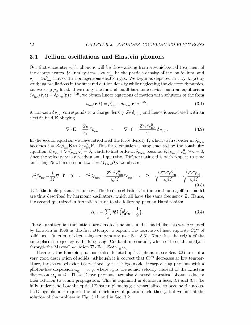
52 CHAPTER 3. PHONONS; COUPLING TO ELECTRONS
3.1 Jellium oscillations and Einstein phonons
Our first encounter with phonons will be those arising from a semiclassical treatment ofthe charge neutral jellium system. Let ρ0
ion be the particle density of the ion jellium, andρel = Zρ0
ion that of the homogeneous electron gas. We begin as depicted in Fig. 3.1(a) bystudying oscillations in the smeared out ion density while neglecting the electron dynamics,i.e. we keep ρel fixed. If we study the limit of small harmonic deviations from equilibriumδρion(r, t) = δρion(r)e−iΩt, we obtain linear equations of motion with solutions of the form
ρion(r, t) = ρ0ion + δρion(r) e−iΩt. (3.1)
A non-zero δρion corresponds to a charge density Ze δρion and hence is associated with anelectric field E obeying
∇ ·E =Ze
ε0δρion ⇒ ∇ · f =
Z2e2ρ0ion
ε0δρion. (3.2)
In the second equation we have introduced the force density f , which to first order in δρion
becomes f = ZeρionE ≈ Zeρ0ionE. This force equation is supplemented by the continuity
equation, ∂tρion+∇·(ρionv) = 0, which to first order in δρion becomes ∂tδρion+ρ0ion∇·v = 0,
since the velocity v is already a small quantity. Differentiating this with respect to timeand using Newton’s second law f = Mρion∂tv we obtain
∂2t δρion+
1M∇ · f = 0 ⇒ Ω2δρion =
Z2e2ρ0ion
ε0Mδρion ⇒ Ω =
√Z2e2ρ0
ion
ε0M=
√Ze2ρel
ε0M.
(3.3)Ω is the ionic plasma frequency. The ionic oscillations in the continuous jellium model
are thus described by harmonic oscillators, which all have the same frequency Ω. Hence,the second quantization formalism leads to the following phonon Hamiltonian:
Hph =∑q
~Ω(b†qbq +
12
). (3.4)
These quantized ion oscillations are denoted phonons, and a model like this was proposedby Einstein in 1906 as the first attempt to explain the decrease of heat capacity C ion
V ofsolids as a function of decreasing temperature (see Sec. 3.5). Note that the origin of theionic plasma frequency is the long-range Coulomb interaction, which entered the analysisthrough the Maxwell equation ∇ ·E = Zeδρion/ε0.
However, the Einstein phonons (also denoted optical phonons, see Sec. 3.3) are not avery good description of solids. Although it is correct that C ion
V decreases at low temper-ature, the exact behavior is described by the Debye-model incorporating phonons with aphoton-like dispersion ωq = vs q, where vs is the sound velocity, instead of the Einsteindispersion ωq = Ω. These Debye phonons are also denoted acoustical phonons due totheir relation to sound propagation. This is explained in details in Secs. 3.3 and 3.5. Tofully understand how the optical Einstein phonons get renormalized to become the acous-tic Debye phonons requires the full machinery of quantum field theory, but we hint at thesolution of the problem in Fig. 3.1b and in Sec. 3.2.
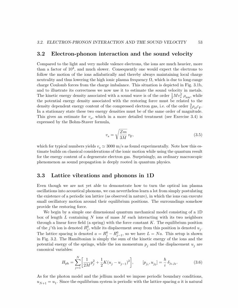
3.2. ELECTRON-PHONON INTERACTION AND THE SOUND VELOCITY 53
3.2 Electron-phonon interaction and the sound velocity
Compared to the light and very mobile valence electrons, the ions are much heavier, morethan a factor of 104, and much slower. Consequently one would expect the electrons tofollow the motion of the ions adiabatically and thereby always maintaining local chargeneutrality and thus lowering the high ionic plasma frequency Ω, which is due to long-rangecharge Coulomb forces from the charge imbalance. This situation is depicted in Fig. 3.1b,and to illustrate its correctness we now use it to estimate the sound velocity in metals.The kinetic energy density associated with a sound wave is of the order 1
2Mv2s ρion, while
the potential energy density associated with the restoring force must be related to thedensity dependent energy content of the compressed electron gas, i.e. of the order 3
5ρelεF.In a stationary state these two energy densities must be of the same order of magnitude.This gives an estimate for vs, which in a more detailed treatment (see Exercise 3.4) isexpressed by the Bohm-Staver formula,
vs =
√Zm
3MvF, (3.5)
which for typical numbers yields vs ' 3000 m/s as found experimentally. Note how this es-timate builds on classical considerations of the ionic motion while using the quantum resultfor the energy content of a degenerate electron gas. Surprisingly, an ordinary macroscopicphenomenon as sound propagation is deeply rooted in quantum physics.
3.3 Lattice vibrations and phonons in 1D
Even though we are not yet able to demonstrate how to turn the optical ion plasmaoscillations into acoustical phonons, we can nevertheless learn a lot from simply postulatingthe existence of a periodic ion lattice (as observed in nature), in which the ions can executesmall oscillatory motion around their equilibrium positions. The surroundings somehowprovide the restoring force.
We begin by a simple one dimensional quantum mechanical model consisting of a 1Dbox of length L containing N ions of mass M each interacting with its two neighborsthrough a linear force field (a spring) with the force constant K. The equilibrium positionof the j’th ion is denoted R0
j , while its displacement away from this position is denoted uj .The lattice spacing is denoted a = R0
j − R0j−1, so we have L = Na. This setup is shown
in Fig. 3.2. The Hamiltonian is simply the sum of the kinetic energy of the ions and thepotential energy of the springs, while the ion momentum pj and the displacement uj arecanonical variables:
Hph =N∑
j=1
[1
2Mp2
j +12K(uj − uj−1)
2
], [pj1
, uj2] =
~i
δj1,j2 . (3.6)
As for the photon model and the jellium model we impose periodic boundary conditions,uN+1 = u1. Since the equilibrium system is periodic with the lattice spacing a it is natural
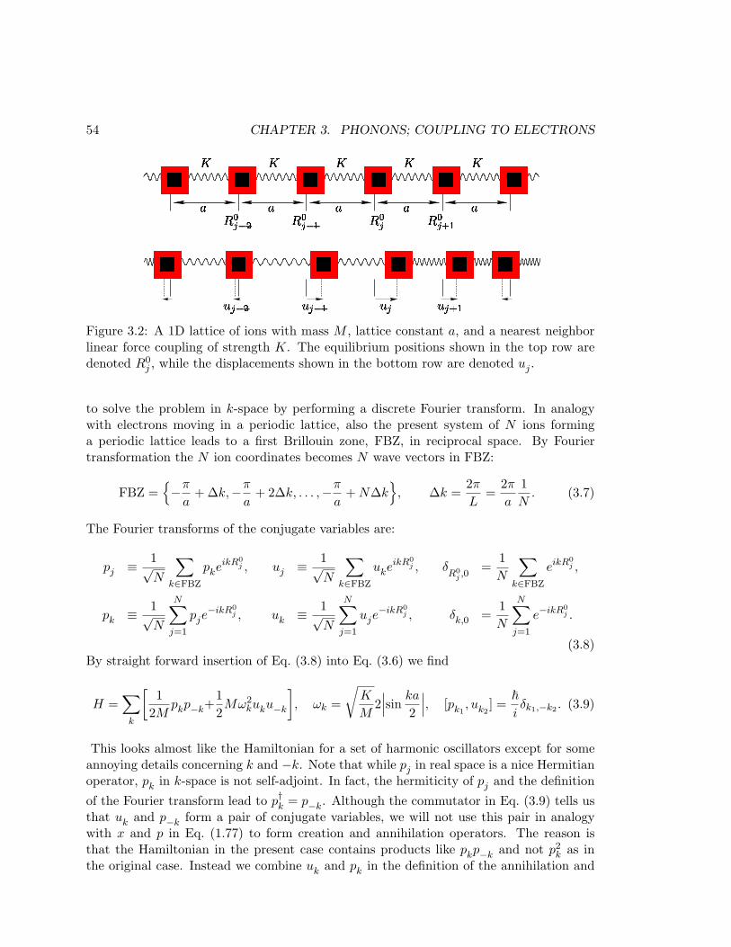
54 CHAPTER 3. PHONONS; COUPLING TO ELECTRONS
!"#$
%& '( )* +, -. /0
1 23 4 5 1 23 4 6 1 23 1 23 7 6
8 3 4 5 8 3 4 6 8 3 8 3 7 6
9:9;9:9:9
<:<;<:<:<
Figure 3.2: A 1D lattice of ions with mass M , lattice constant a, and a nearest neighborlinear force coupling of strength K. The equilibrium positions shown in the top row aredenoted R0
j , while the displacements shown in the bottom row are denoted uj .
to solve the problem in k-space by performing a discrete Fourier transform. In analogywith electrons moving in a periodic lattice, also the present system of N ions forminga periodic lattice leads to a first Brillouin zone, FBZ, in reciprocal space. By Fouriertransformation the N ion coordinates becomes N wave vectors in FBZ:
FBZ =−π
a+ ∆k,−π
a+ 2∆k, . . . ,−π
a+ N∆k
, ∆k =
2π
L=
2π
a
1N
. (3.7)
The Fourier transforms of the conjugate variables are:
pj ≡ 1√N
∑
k∈FBZ
pkeikR0
j , uj ≡ 1√N
∑
k∈FBZ
ukeikR0
j , δR0
j ,0=
1N
∑
k∈FBZ
eikR0j ,
pk ≡ 1√N
N∑
j=1
pje−ikR0
j , uk ≡ 1√N
N∑
j=1
uje−ikR0
j , δk,0 =1N
N∑
j=1
e−ikR0j .
(3.8)By straight forward insertion of Eq. (3.8) into Eq. (3.6) we find
H =∑
k
[1
2Mpkp−k+
12Mω2
kuku−k
], ωk =
√K
M2∣∣∣sin ka
2
∣∣∣, [pk1, uk2
] =~iδk1,−k2 . (3.9)
This looks almost like the Hamiltonian for a set of harmonic oscillators except for someannoying details concerning k and −k. Note that while pj in real space is a nice Hermitianoperator, pk in k-space is not self-adjoint. In fact, the hermiticity of pj and the definition
of the Fourier transform lead to p†k = p−k. Although the commutator in Eq. (3.9) tells usthat uk and p−k form a pair of conjugate variables, we will not use this pair in analogywith x and p in Eq. (1.77) to form creation and annihilation operators. The reason isthat the Hamiltonian in the present case contains products like pkp−k and not p2
k as inthe original case. Instead we combine uk and pk in the definition of the annihilation and
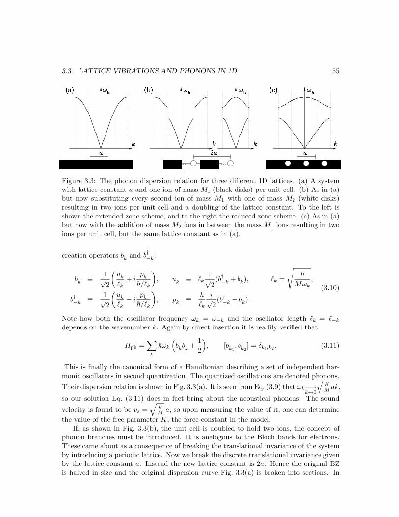
3.3. LATTICE VIBRATIONS AND PHONONS IN 1D 55
Figure 3.3: The phonon dispersion relation for three different 1D lattices. (a) A systemwith lattice constant a and one ion of mass M1 (black disks) per unit cell. (b) As in (a)but now substituting every second ion of mass M1 with one of mass M2 (white disks)resulting in two ions per unit cell and a doubling of the lattice constant. To the left isshown the extended zone scheme, and to the right the reduced zone scheme. (c) As in (a)but now with the addition of mass M2 ions in between the mass M1 ions resulting in twoions per unit cell, but the same lattice constant as in (a).
creation operators bk and b†−k:
bk ≡ 1√2
(uk
`k+ i
pk
~/`k
), uk ≡ `k
1√2(b†−k + bk), `k =
√~
Mωk,
b†−k ≡ 1√2
(uk
`k− i
pk
~/`k
), pk ≡ ~
`k
i√2(b†−k − bk).
(3.10)
Note how both the oscillator frequency ωk = ω−k and the oscillator length `k = `−k
depends on the wavenumber k. Again by direct insertion it is readily verified that
Hph =∑
k
~ωk
(b†kbk +
12
), [bk1
, b†k2] = δk1,k2 . (3.11)
This is finally the canonical form of a Hamiltonian describing a set of independent har-monic oscillators in second quantization. The quantized oscillations are denoted phonons.
Their dispersion relation is shown in Fig. 3.3(a). It is seen from Eq. (3.9) that ωk−→k→0
√KM ak,
so our solution Eq. (3.11) does in fact bring about the acoustical phonons. The sound
velocity is found to be vs =√
KM a, so upon measuring the value of it, one can determine
the value of the free parameter K, the force constant in the model.If, as shown in Fig. 3.3(b), the unit cell is doubled to hold two ions, the concept of
phonon branches must be introduced. It is analogous to the Bloch bands for electrons.These came about as a consequence of breaking the translational invariance of the systemby introducing a periodic lattice. Now we break the discrete translational invariance givenby the lattice constant a. Instead the new lattice constant is 2a. Hence the original BZis halved in size and the original dispersion curve Fig. 3.3(a) is broken into sections. In
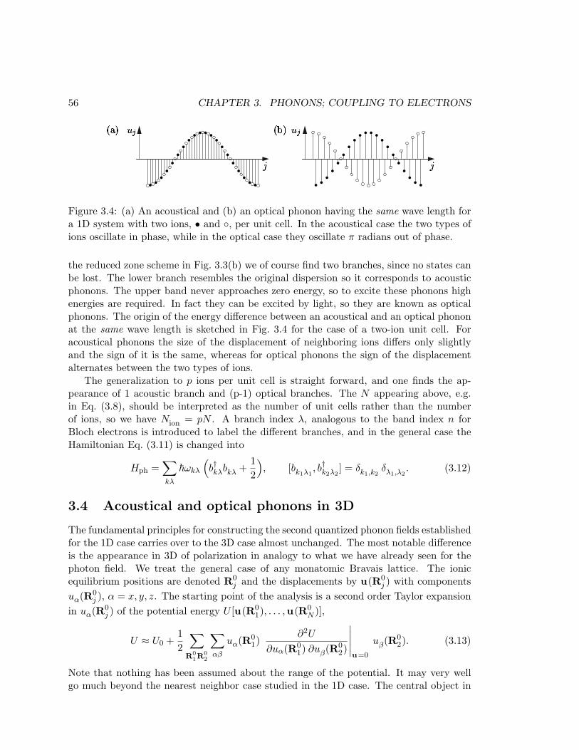
56 CHAPTER 3. PHONONS; COUPLING TO ELECTRONS
Figure 3.4: (a) An acoustical and (b) an optical phonon having the same wave length fora 1D system with two ions, • and , per unit cell. In the acoustical case the two types ofions oscillate in phase, while in the optical case they oscillate π radians out of phase.
the reduced zone scheme in Fig. 3.3(b) we of course find two branches, since no states canbe lost. The lower branch resembles the original dispersion so it corresponds to acousticphonons. The upper band never approaches zero energy, so to excite these phonons highenergies are required. In fact they can be excited by light, so they are known as opticalphonons. The origin of the energy difference between an acoustical and an optical phononat the same wave length is sketched in Fig. 3.4 for the case of a two-ion unit cell. Foracoustical phonons the size of the displacement of neighboring ions differs only slightlyand the sign of it is the same, whereas for optical phonons the sign of the displacementalternates between the two types of ions.
The generalization to p ions per unit cell is straight forward, and one finds the ap-pearance of 1 acoustic branch and (p-1) optical branches. The N appearing above, e.g.in Eq. (3.8), should be interpreted as the number of unit cells rather than the numberof ions, so we have Nion = pN . A branch index λ, analogous to the band index n forBloch electrons is introduced to label the different branches, and in the general case theHamiltonian Eq. (3.11) is changed into
Hph =∑
kλ
~ωkλ
(b†kλbkλ +
12
), [bk1λ1
, b†k2λ2] = δk1,k2
δλ1,λ2. (3.12)
3.4 Acoustical and optical phonons in 3D
The fundamental principles for constructing the second quantized phonon fields establishedfor the 1D case carries over to the 3D case almost unchanged. The most notable differenceis the appearance in 3D of polarization in analogy to what we have already seen for thephoton field. We treat the general case of any monatomic Bravais lattice. The ionicequilibrium positions are denoted R0
j and the displacements by u(R0j ) with components
uα(R0j ), α = x, y, z. The starting point of the analysis is a second order Taylor expansion
in uα(R0j ) of the potential energy U [u(R0
1), . . . ,u(R0N )],
U ≈ U0 +12
∑
R01R
02
∑
αβ
uα(R01)
∂2U
∂uα(R01) ∂uβ(R0
2)
∣∣∣∣∣u=0
uβ(R02). (3.13)
Note that nothing has been assumed about the range of the potential. It may very wellgo much beyond the nearest neighbor case studied in the 1D case. The central object in
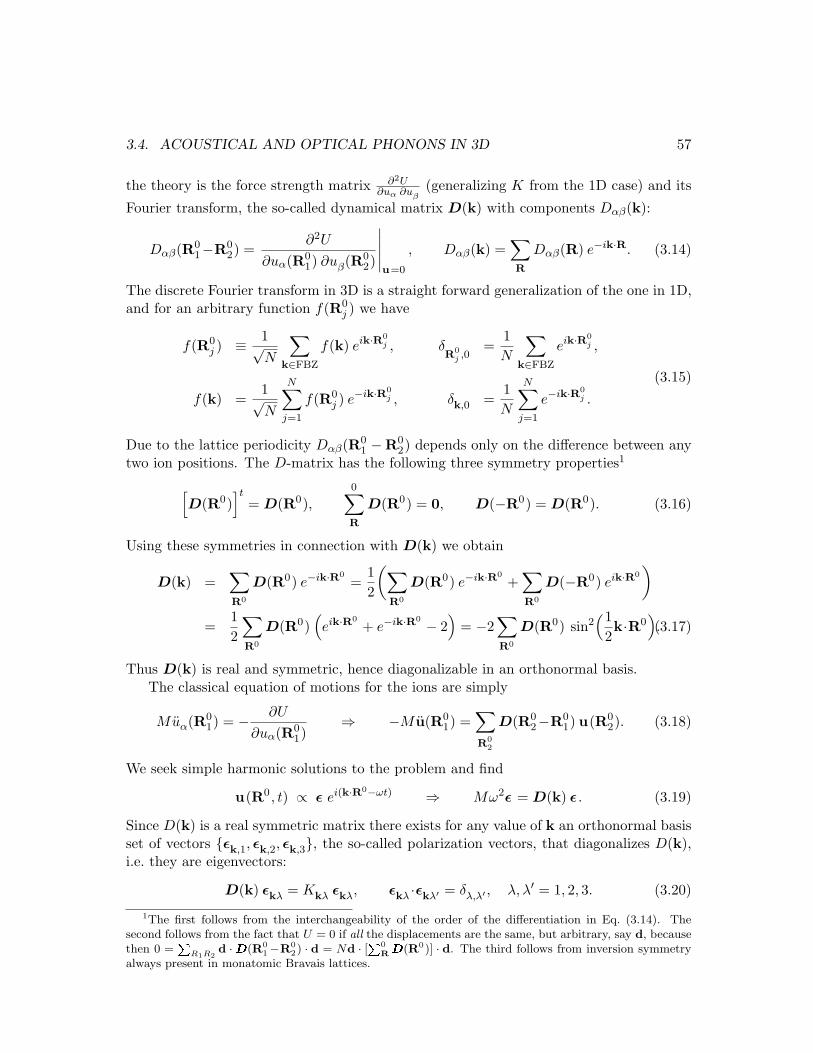
3.4. ACOUSTICAL AND OPTICAL PHONONS IN 3D 57
the theory is the force strength matrix ∂2U∂uα ∂uβ
(generalizing K from the 1D case) and its
Fourier transform, the so-called dynamical matrix D(k) with components Dαβ(k):
Dαβ(R01−R0
2) =∂2U
∂uα(R01) ∂uβ(R0
2)
∣∣∣∣∣u=0
, Dαβ(k) =∑
R
Dαβ(R) e−ik·R. (3.14)
The discrete Fourier transform in 3D is a straight forward generalization of the one in 1D,and for an arbitrary function f(R0
j ) we have
f(R0j ) ≡ 1√
N
∑
k∈FBZ
f(k) eik·R0j , δ
R0j ,0
=1N
∑
k∈FBZ
eik·R0j ,
f(k) =1√N
N∑
j=1
f(R0j ) e−ik·R0
j , δk,0 =1N
N∑
j=1
e−ik·R0j .
(3.15)
Due to the lattice periodicity Dαβ(R01 −R0
2) depends only on the difference between anytwo ion positions. The D-matrix has the following three symmetry properties1
[D(R0)
]t= D(R0),
0∑
R
D(R0) = 0, D(−R0) = D(R0). (3.16)
Using these symmetries in connection with D(k) we obtain
D(k) =∑
R0
D(R0) e−ik·R0=
12
(∑
R0
D(R0) e−ik·R0+
∑
R0
D(−R0) eik·R0
)
=12
∑
R0
D(R0)(eik·R0
+ e−ik·R0 − 2)
= −2∑
R0
D(R0) sin2(1
2k·R0
).(3.17)
Thus D(k) is real and symmetric, hence diagonalizable in an orthonormal basis.The classical equation of motions for the ions are simply
Muα(R01) = − ∂U
∂uα(R01)
⇒ −M u(R01) =
∑
R02
D(R02−R0
1) u(R02). (3.18)
We seek simple harmonic solutions to the problem and find
u(R0 , t) ∝ ε ei(k·R0−ωt) ⇒ Mω2ε = D(k) ε . (3.19)
Since D(k) is a real symmetric matrix there exists for any value of k an orthonormal basisset of vectors εk,1, εk,2, εk,3, the so-called polarization vectors, that diagonalizes D(k),i.e. they are eigenvectors:
D(k) εkλ = Kkλ εkλ, εkλ ·εkλ′ = δλ,λ′ , λ, λ′ = 1, 2, 3. (3.20)
1The first follows from the interchangeability of the order of the differentiation in Eq. (3.14). Thesecond follows from the fact that U = 0 if all the displacements are the same, but arbitrary, say d, becausethen 0 =
PR1R2
d ·D(R01−R0
2) · d = Nd · [P0RD(R0)] · d. The third follows from inversion symmetry
always present in monatomic Bravais lattices.
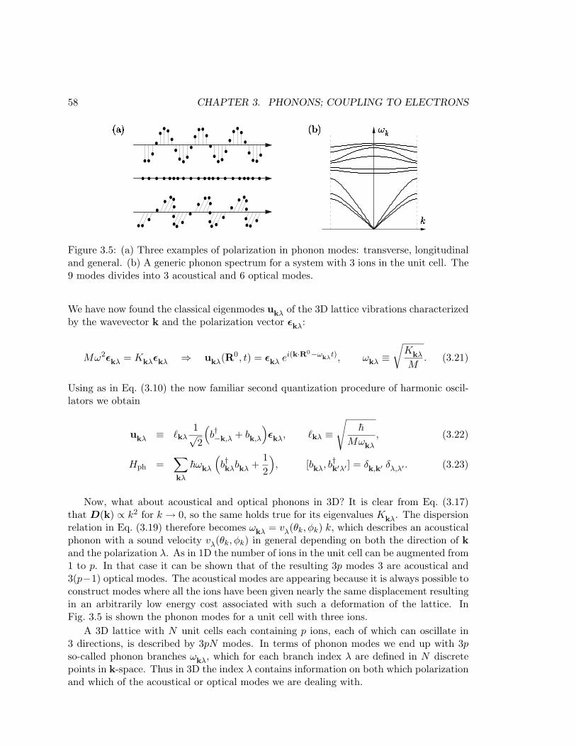
58 CHAPTER 3. PHONONS; COUPLING TO ELECTRONS
Figure 3.5: (a) Three examples of polarization in phonon modes: transverse, longitudinaland general. (b) A generic phonon spectrum for a system with 3 ions in the unit cell. The9 modes divides into 3 acoustical and 6 optical modes.
We have now found the classical eigenmodes ukλ of the 3D lattice vibrations characterizedby the wavevector k and the polarization vector εkλ:
Mω2εkλ = Kkλεkλ ⇒ ukλ(R0 , t) = εkλ ei(k·R0−ωkλt), ωkλ ≡√
Kkλ
M. (3.21)
Using as in Eq. (3.10) the now familiar second quantization procedure of harmonic oscil-lators we obtain
ukλ ≡ `kλ1√2
(b†−k,λ + bk,λ
)εkλ, `kλ ≡
√~
Mωkλ
, (3.22)
Hph =∑
kλ
~ωkλ
(b†kλbkλ +
12
), [bkλ, b†k′λ′ ] = δk,k′ δλ,λ′ . (3.23)
Now, what about acoustical and optical phonons in 3D? It is clear from Eq. (3.17)that D(k) ∝ k2 for k → 0, so the same holds true for its eigenvalues Kkλ. The dispersionrelation in Eq. (3.19) therefore becomes ωkλ = vλ(θk, φk) k, which describes an acousticalphonon with a sound velocity vλ(θk, φk) in general depending on both the direction of kand the polarization λ. As in 1D the number of ions in the unit cell can be augmented from1 to p. In that case it can be shown that of the resulting 3p modes 3 are acoustical and3(p−1) optical modes. The acoustical modes are appearing because it is always possible toconstruct modes where all the ions have been given nearly the same displacement resultingin an arbitrarily low energy cost associated with such a deformation of the lattice. InFig. 3.5 is shown the phonon modes for a unit cell with three ions.
A 3D lattice with N unit cells each containing p ions, each of which can oscillate in3 directions, is described by 3pN modes. In terms of phonon modes we end up with 3pso-called phonon branches ωkλ, which for each branch index λ are defined in N discretepoints in k-space. Thus in 3D the index λ contains information on both which polarizationand which of the acoustical or optical modes we are dealing with.
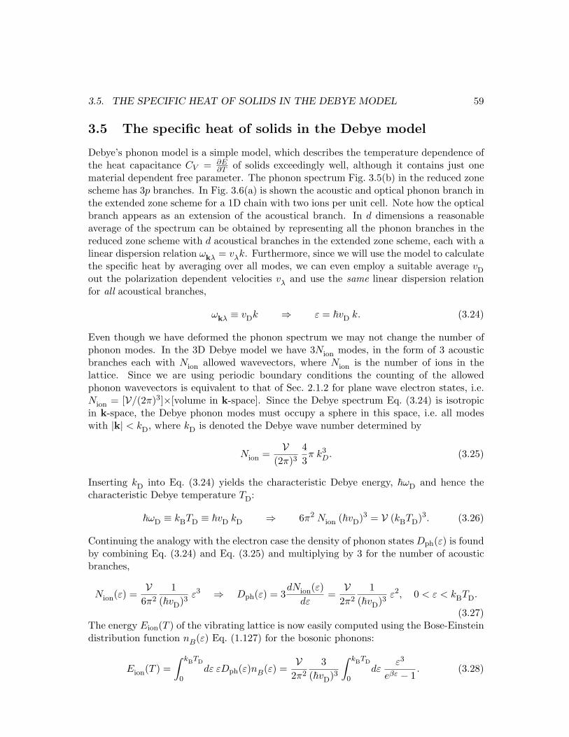
3.5. THE SPECIFIC HEAT OF SOLIDS IN THE DEBYE MODEL 59
3.5 The specific heat of solids in the Debye model
Debye’s phonon model is a simple model, which describes the temperature dependence ofthe heat capacitance CV = ∂E
∂T of solids exceedingly well, although it contains just onematerial dependent free parameter. The phonon spectrum Fig. 3.5(b) in the reduced zonescheme has 3p branches. In Fig. 3.6(a) is shown the acoustic and optical phonon branch inthe extended zone scheme for a 1D chain with two ions per unit cell. Note how the opticalbranch appears as an extension of the acoustical branch. In d dimensions a reasonableaverage of the spectrum can be obtained by representing all the phonon branches in thereduced zone scheme with d acoustical branches in the extended zone scheme, each with alinear dispersion relation ωkλ = vλk. Furthermore, since we will use the model to calculatethe specific heat by averaging over all modes, we can even employ a suitable average vD
out the polarization dependent velocities vλ and use the same linear dispersion relationfor all acoustical branches,
ωkλ ≡ vDk ⇒ ε = ~vD k. (3.24)
Even though we have deformed the phonon spectrum we may not change the number ofphonon modes. In the 3D Debye model we have 3Nion modes, in the form of 3 acousticbranches each with Nion allowed wavevectors, where Nion is the number of ions in thelattice. Since we are using periodic boundary conditions the counting of the allowedphonon wavevectors is equivalent to that of Sec. 2.1.2 for plane wave electron states, i.e.Nion = [V/(2π)3]×[volume in k-space]. Since the Debye spectrum Eq. (3.24) is isotropicin k-space, the Debye phonon modes must occupy a sphere in this space, i.e. all modeswith |k| < kD, where kD is denoted the Debye wave number determined by
Nion =V
(2π)343π k3
D. (3.25)
Inserting kD into Eq. (3.24) yields the characteristic Debye energy, ~ωD and hence thecharacteristic Debye temperature TD:
~ωD ≡ kBTD ≡ ~vD kD ⇒ 6π2 Nion (~vD)3 = V (kBTD)3. (3.26)
Continuing the analogy with the electron case the density of phonon states Dph(ε) is foundby combining Eq. (3.24) and Eq. (3.25) and multiplying by 3 for the number of acousticbranches,
Nion(ε) =V
6π2
1(~vD)3
ε3 ⇒ Dph(ε) = 3dNion(ε)
dε=
V2π2
1(~vD)3
ε2, 0 < ε < kBTD.
(3.27)The energy Eion(T ) of the vibrating lattice is now easily computed using the Bose-Einsteindistribution function nB(ε) Eq. (1.127) for the bosonic phonons:
Eion(T ) =∫ kBTD
0dε εDph(ε)nB(ε) =
V2π2
3(~vD)3
∫ kBTD
0dε
ε3
eβε − 1. (3.28)
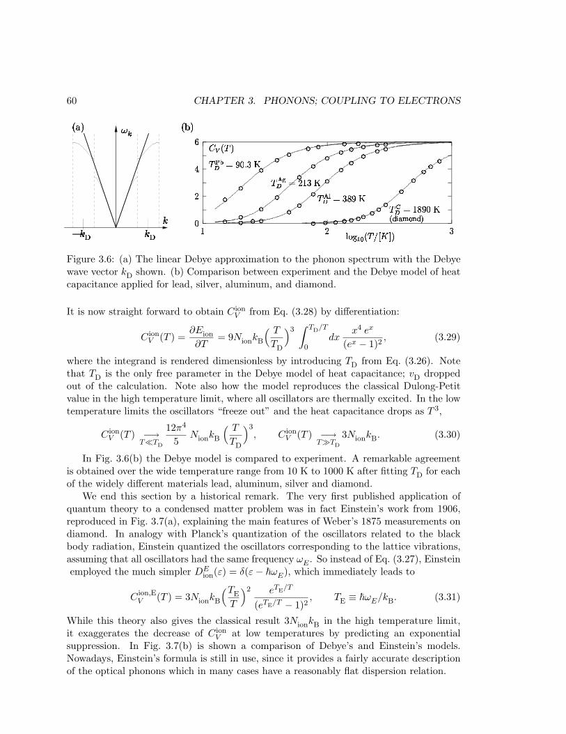
60 CHAPTER 3. PHONONS; COUPLING TO ELECTRONS
! " # $ % & ' ( # )
**** *
* * * *
* ***
** *
* * * * *
* * ** *
*** *
* * *
* * * * * * ** ***** **
+ , - + . -/ 0
11 23
4 1 23
Figure 3.6: (a) The linear Debye approximation to the phonon spectrum with the Debyewave vector kD shown. (b) Comparison between experiment and the Debye model of heatcapacitance applied for lead, silver, aluminum, and diamond.
It is now straight forward to obtain C ionV from Eq. (3.28) by differentiation:
C ionV (T ) =
∂Eion
∂T= 9NionkB
( T
TD
)3∫ TD/T
0dx
x4 ex
(ex − 1)2, (3.29)
where the integrand is rendered dimensionless by introducing TD from Eq. (3.26). Notethat TD is the only free parameter in the Debye model of heat capacitance; vD droppedout of the calculation. Note also how the model reproduces the classical Dulong-Petitvalue in the high temperature limit, where all oscillators are thermally excited. In the lowtemperature limits the oscillators “freeze out” and the heat capacitance drops as T 3,
C ionV (T ) −→
T¿TD
12π4
5NionkB
( T
TD
)3, C ion
V (T ) −→TÀTD
3NionkB. (3.30)
In Fig. 3.6(b) the Debye model is compared to experiment. A remarkable agreementis obtained over the wide temperature range from 10 K to 1000 K after fitting TD for eachof the widely different materials lead, aluminum, silver and diamond.
We end this section by a historical remark. The very first published application ofquantum theory to a condensed matter problem was in fact Einstein’s work from 1906,reproduced in Fig. 3.7(a), explaining the main features of Weber’s 1875 measurements ondiamond. In analogy with Planck’s quantization of the oscillators related to the blackbody radiation, Einstein quantized the oscillators corresponding to the lattice vibrations,assuming that all oscillators had the same frequency ωE . So instead of Eq. (3.27), Einsteinemployed the much simpler DE
ion(ε) = δ(ε− ~ωE), which immediately leads to
C ion,EV (T ) = 3NionkB
(TE
T
)2 eTE/T
(eTE/T − 1)2, TE ≡ ~ωE/kB. (3.31)
While this theory also gives the classical result 3NionkB in the high temperature limit,it exaggerates the decrease of C ion
V at low temperatures by predicting an exponentialsuppression. In Fig. 3.7(b) is shown a comparison of Debye’s and Einstein’s models.Nowadays, Einstein’s formula is still in use, since it provides a fairly accurate descriptionof the optical phonons which in many cases have a reasonably flat dispersion relation.
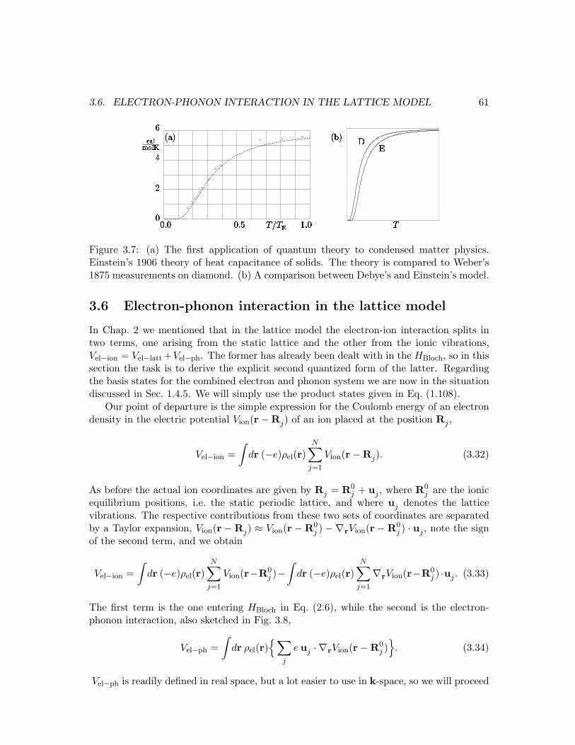
3.6. ELECTRON-PHONON INTERACTION IN THE LATTICE MODEL 61
Figure 3.7: (a) The first application of quantum theory to condensed matter physics.Einstein’s 1906 theory of heat capacitance of solids. The theory is compared to Weber’s1875 measurements on diamond. (b) A comparison between Debye’s and Einstein’s model.
3.6 Electron-phonon interaction in the lattice model
In Chap. 2 we mentioned that in the lattice model the electron-ion interaction splits intwo terms, one arising from the static lattice and the other from the ionic vibrations,Vel−ion = Vel−latt +Vel−ph. The former has already been dealt with in the HBloch, so in thissection the task is to derive the explicit second quantized form of the latter. Regardingthe basis states for the combined electron and phonon system we are now in the situationdiscussed in Sec. 1.4.5. We will simply use the product states given in Eq. (1.108).
Our point of departure is the simple expression for the Coulomb energy of an electrondensity in the electric potential Vion(r−Rj) of an ion placed at the position Rj ,
Vel−ion =∫
dr (−e)ρel(r)N∑
j=1
Vion(r−Rj). (3.32)
As before the actual ion coordinates are given by Rj = R0j + uj , where R0
j are the ionicequilibrium positions, i.e. the static periodic lattice, and where uj denotes the latticevibrations. The respective contributions from these two sets of coordinates are separatedby a Taylor expansion, Vion(r −Rj) ≈ Vion(r −R0
j ) −∇rVion(r −R0j ) · uj , note the sign
of the second term, and we obtain
Vel−ion =∫
dr (−e)ρel(r)N∑
j=1
Vion(r−R0j )−
∫dr (−e)ρel(r)
N∑
j=1
∇rVion(r−R0j ) ·uj . (3.33)
The first term is the one entering HBloch in Eq. (2.6), while the second is the electron-phonon interaction, also sketched in Fig. 3.8,
Vel−ph =∫
dr ρel(r)∑
j
e uj · ∇rVion(r−R0j )
. (3.34)
Vel−ph is readily defined in real space, but a lot easier to use in k-space, so we will proceed
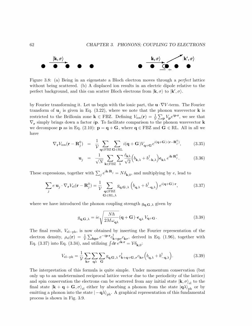
62 CHAPTER 3. PHONONS; COUPLING TO ELECTRONS
Figure 3.8: (a) Being in an eigenstate a Bloch electron moves through a perfect latticewithout being scattered. (b) A displaced ion results in an electric dipole relative to theperfect background, and this can scatter Bloch electrons from |k, σ〉 to |k′, σ〉.
by Fourier transforming it. Let us begin with the ionic part, the u ·∇V -term. The Fouriertransform of uj is given in Eq. (3.22), where we note that the phonon wavevector k isrestricted to the Brillouin zone k ∈ FBZ. Defining Vion(r) = 1
V∑
p Vpeip·r, we see that∇r simply brings down a factor ip. To facilitate comparison to the phonon wavevector kwe decompose p as in Eq. (2.10): p = q + G , where q ∈ FBZ and G ∈ RL. All in all wehave
∇rVion(r−R0j ) =
1V
∑
q∈FBZ
∑
G∈RL
i(q + G)Vq+Gei(q+G )·(r−R0j ), (3.35)
uj =1√N
∑
k∈FBZ
∑
λ
`kλ√2
(bk,λ + b†−k,λ
)εkλ eik·R0
j . (3.36)
These expressions, together with∑
j eik·Rj = Nδk,0, and multiplying by e, lead to
∑
j
e uj · ∇rVel(r−R0j ) =
1V
∑
q∈FBZ
G∈RL,λ
gq,G ,λ
(bq,λ + b†−q,λ
)ei(q+G )·r, (3.37)
where we have introduced the phonon coupling strength gq,G ,λ given by
gq,G ,λ = ie
√N~
2Mωqλ
(q + G)·εqλ Vq+G . (3.38)
The final result, Vel−ph, is now obtained by inserting the Fourier representation of theelectron density, ρel(r) = 1
V∑
kpσ e−ip·rc†k+pσckσ, derived in Eq. (1.96), together withEq. (3.37) into Eq. (3.34), and utilizing
∫dr eik·r = Vδk,0:
Vel−ph =1V
∑
kσ
∑
qλ
∑
G
gq,G ,λ c†k+q+G ,σckσ
(bq,λ + b†−q,λ
). (3.39)
The interpretation of this formula is quite simple. Under momentum conservation (butonly up to an undetermined reciprocal lattice vector due to the periodicity of the lattice)and spin conservation the electrons can be scattered from any initial state |k, σ〉el to thefinal state |k + q + G , σ〉el either by absorbing a phonon from the state |qλ〉ph or byemitting a phonon into the state |−qλ〉ph. A graphical representation of this fundamentalprocess is shown in Fig. 3.9.

3.7. ELECTRON-PHONON INTERACTION IN THE JELLIUM MODEL 63
Figure 3.9: A graphical representation of the fundamental electron-phonon coupling. Theelectron states are represented by the straight lines, the phonon states by curly spring-likelines, and the coupling strength by a dot. To the left the electron is scattered by absorbinga phonon, to the right by emitting a phonon.
The normal processes, i.e. processes where per definition G = 0, often tend to dominateover the so-called umklapp processes, where G 6= 0, so in the following we shall completelyneglect the latter.2 Moreover, we shall treat only isotropic media, where εqλ is eitherparallel to or perpendicular to q, i.e. q·εqλ in gq,G=0,λ is only non-zero for longitudinallypolarized phonons. So in the Isotropic case for Normal phonon processes we have
V INel−ph =
1V
∑
kσ
∑
qλl
gq,λlc†k+q,σckσ
(bq,λl
+ b†−q,λl
). (3.40)
Finally, the most significant physics of the electron-phonon coupling can often be extractedfrom considering just the acoustical modes. Due to their low energies they are excitedsignificantly more than the high energy optical phonons at temperatures lower than theDebye temperature. Thus in the Isotropic case for Normal Acoustical phonon processesonly the longitudinal acoustical branch enters and we have
V INAel−ph =
1V
∑
kσ
∑q
gq c†k+q,σckσ
(bq + b†−q
). (3.41)
If we for ions with charge +Ze approximate Vq by a Yukawa potential, Vq = Zeε0
1q2+k2
s(see
Exercise 1.5), the explicit form of the coupling constant gq is particularly simple:
gq = iZe2
ε0
q
q2 + k2s
√N~
2Mωq. (3.42)
3.7 Electron-phonon interaction in the jellium model
Finally, we return to the case of Einstein phonons in the jellium model treated in Sec. 3.1.The electron-phonon interaction in this case is derived in analogy with the that of normal
2There are mainly two reasons why the umklapp processes often can be neglected: (1) Vq+G is small
due to the 1/(q + G)2 dependence, and (2) At low temperatures the phase space available for umklappprocesses is small.
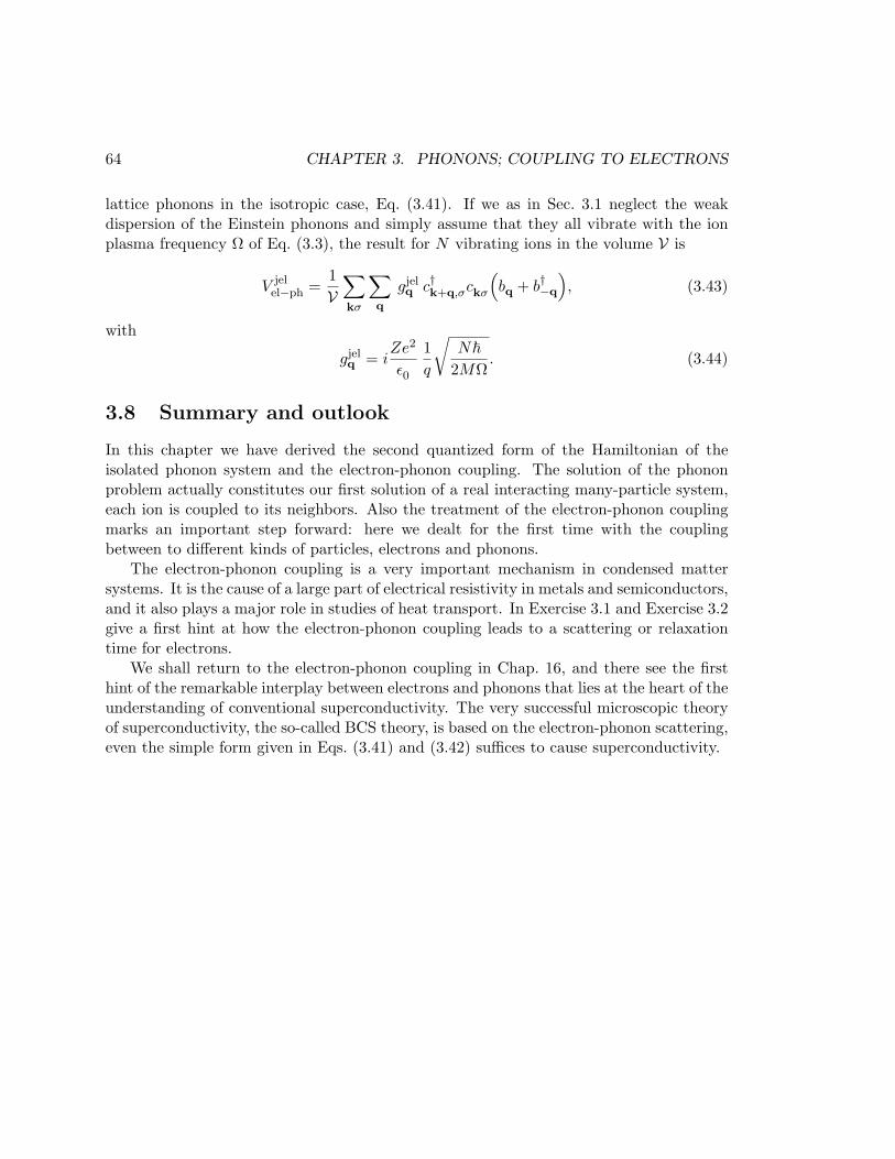
64 CHAPTER 3. PHONONS; COUPLING TO ELECTRONS
lattice phonons in the isotropic case, Eq. (3.41). If we as in Sec. 3.1 neglect the weakdispersion of the Einstein phonons and simply assume that they all vibrate with the ionplasma frequency Ω of Eq. (3.3), the result for N vibrating ions in the volume V is
V jelel−ph =
1V
∑
kσ
∑q
gjelq c†k+q,σckσ
(bq + b†−q
), (3.43)
with
gjelq = i
Ze2
ε0
1q
√N~
2MΩ. (3.44)
3.8 Summary and outlook
In this chapter we have derived the second quantized form of the Hamiltonian of theisolated phonon system and the electron-phonon coupling. The solution of the phononproblem actually constitutes our first solution of a real interacting many-particle system,each ion is coupled to its neighbors. Also the treatment of the electron-phonon couplingmarks an important step forward: here we dealt for the first time with the couplingbetween to different kinds of particles, electrons and phonons.
The electron-phonon coupling is a very important mechanism in condensed mattersystems. It is the cause of a large part of electrical resistivity in metals and semiconductors,and it also plays a major role in studies of heat transport. In Exercise 3.1 and Exercise 3.2give a first hint at how the electron-phonon coupling leads to a scattering or relaxationtime for electrons.
We shall return to the electron-phonon coupling in Chap. 16, and there see the firsthint of the remarkable interplay between electrons and phonons that lies at the heart of theunderstanding of conventional superconductivity. The very successful microscopic theoryof superconductivity, the so-called BCS theory, is based on the electron-phonon scattering,even the simple form given in Eqs. (3.41) and (3.42) suffices to cause superconductivity.
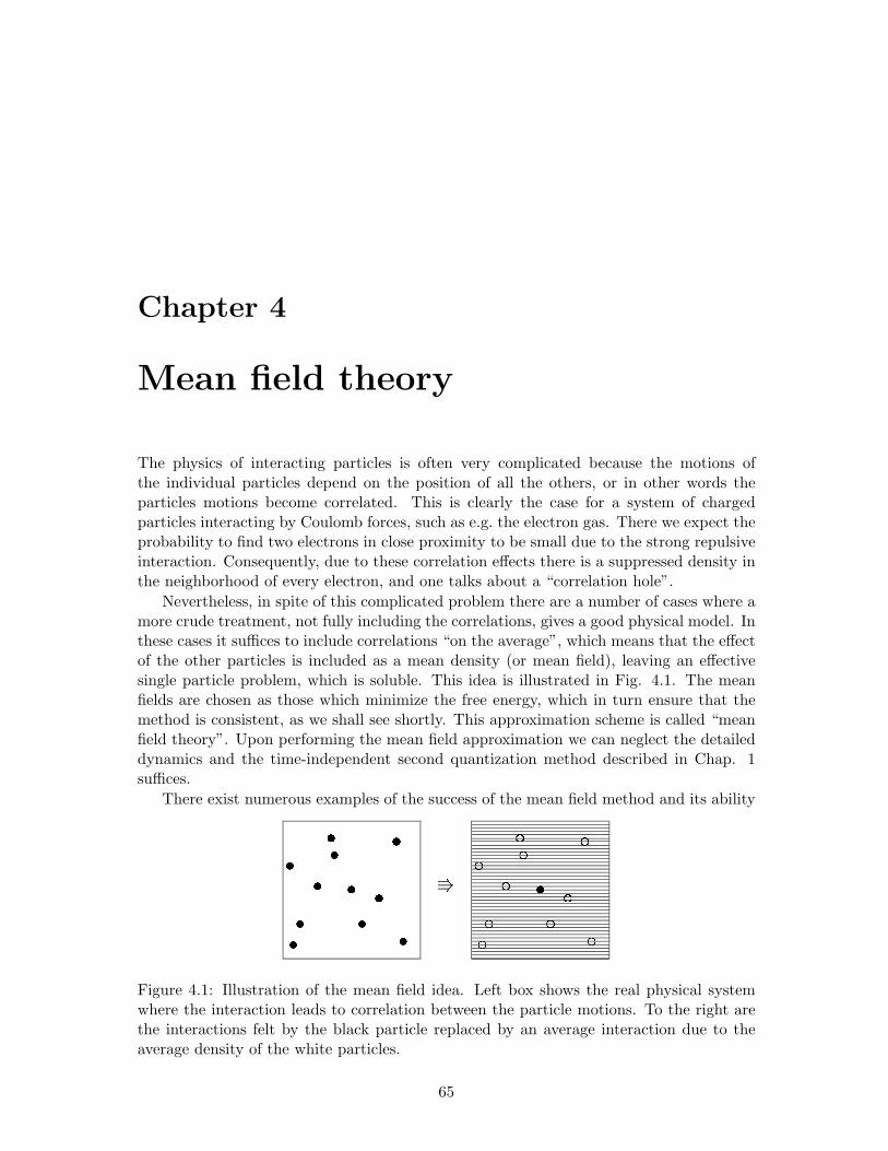
Chapter 4
Mean field theory
The physics of interacting particles is often very complicated because the motions ofthe individual particles depend on the position of all the others, or in other words theparticles motions become correlated. This is clearly the case for a system of chargedparticles interacting by Coulomb forces, such as e.g. the electron gas. There we expect theprobability to find two electrons in close proximity to be small due to the strong repulsiveinteraction. Consequently, due to these correlation effects there is a suppressed density inthe neighborhood of every electron, and one talks about a “correlation hole”.
Nevertheless, in spite of this complicated problem there are a number of cases where amore crude treatment, not fully including the correlations, gives a good physical model. Inthese cases it suffices to include correlations “on the average”, which means that the effectof the other particles is included as a mean density (or mean field), leaving an effectivesingle particle problem, which is soluble. This idea is illustrated in Fig. 4.1. The meanfields are chosen as those which minimize the free energy, which in turn ensure that themethod is consistent, as we shall see shortly. This approximation scheme is called “meanfield theory”. Upon performing the mean field approximation we can neglect the detaileddynamics and the time-independent second quantization method described in Chap. 1suffices.
There exist numerous examples of the success of the mean field method and its ability
Figure 4.1: Illustration of the mean field idea. Left box shows the real physical systemwhere the interaction leads to correlation between the particle motions. To the right arethe interactions felt by the black particle replaced by an average interaction due to theaverage density of the white particles.
65
66 CHAPTER 4. MEAN FIELD THEORY
to explain various physical phenomena. In this chapter, we shall discuss a few examplesfrom condensed matter physics , but before going to specific examples let us discuss themathematical structure of the mean field theory.
First we consider a system with two kinds of particles, described by operators aν andbµ, respectively. Let us assume that only interactions between different kind of particlesare important. The Hamiltonian is
H = H0 + Vint, (4.1a)
H0 =∑
ν
ξaνa†νaν +
∑µ
ξbµb†µbµ, (4.1b)
Vint =∑
νν′,µµ′Vνµ,ν′µ′a
†νb†µbµ′aν′ . (4.1c)
Now suppose that we expect, based on physical arguments, that the density operatorsa†νaν′ and b†µbµ′ deviate only little from their average values, 〈a†νaν′〉 and 〈b†µbµ′〉. It is thennatural to use this deviation as a small parameter and perform an expansion. In order todo so we define the deviation operators
dνν′ = a†νaν′ − 〈a†νaν′〉, (4.2a)
eµµ′ = b†µbµ′ − 〈b†µbµ′〉, (4.2b)
and insert them into (4.1a), which gives
H = H0 + VMF +
neglected in mean field︷ ︸︸ ︷∑
νν′,µµ′Vνµ,ν′µ′dνν′eµµ′ , (4.3)
where
VMF =∑
νν′,µµ′Vνµ,ν′µ′
(a†νaν′〈b†µbµ′〉+ b†µbµ′〈a†νaν′〉
)−
∑
νν′,µµ′Vνµ,ν′µ′〈a†νaν′〉〈b†µbµ′〉, (4.4)
Because dνν′ and eµµ′ are assumed to be small the second term in Eq. (4.3) is neglected,and the interaction Vint is approximated by the mean field interaction VMF resulting inthe so-called mean field Hamiltonian HMF given by
HMF = H0 + VMF. (4.5)
The mean field Hamiltonian HMF contains only single-particle operators, and thus theoriginal many-body problem has been reduced to a single-particle problem, which in prin-ciple is always soluble.1
1To see that a single-particle problem or a quadratic Hamiltonian can always be diagonalized, write Has H =
Pij a†i hijaj . Now since h is a hermitian matrix there exists a transformation, αi =
Pj Uijaj , with
U being a unitary matrix, such that h is diagonal,P
kk′ U†ikhkk′Uk′j = δijεi. In terms of the new basis
the Hamiltonian then becomes H =P
i α†i εiαi, and εi are thus the eigenvalues of h.
67
Looking at Eq. (4.4) we can formulate the mean field procedure in a different way: Ifwe have an interaction term involving two operators A and B given by a product of thetwo
HAB = AB, (4.6)
then the mean field approximation is given by A coupled to the mean field of B plus Bcoupled to the mean field of A and finally to avoid double counting subtracted by theproduct of the mean fields (such that 〈HMF
AB 〉 = 〈A〉〈B〉):HMF
AB = A〈B〉+ 〈A〉B − 〈A〉〈B〉. (4.7)
The question is however how to find the averages 〈a†νaν′〉 and 〈b†µbµ′〉. There are twopossible routes which in fact are equivalent. Method 1: The average is to be determinedself-consistently, i.e. when calculating the averages
naνν′ ≡ 〈a†νaν′〉, (4.8a)
nbµµ′ ≡ 〈b†µbµ′〉, (4.8b)
using the new mean field Hamiltonian, the same answer should come out. This means forna (and similarly for nb) that
naνν′ ≡ 〈a†νaν′〉MF =
1ZMF
Tr(e−βHMFa†νaν′
), (4.9)
where ZMF is the mean field partition function given by
ZMF = Tr(e−βHMF
). (4.10)
Eq. (4.9) and the similar one for nb are called the self-consistency equations (because na
and nb are given in terms of HMF and ZMF, which themselves depend on na and nb).Next we turn to the alternative route. Method 2: Use the nνν′ that minimizes the free
energy FMF of the mean field Hamiltonian. Using the expression for the free energy givenin Sec. 1.5, we get
0 =d
dnaνν′
FMF =d
dnaνν′
(− 1
βlnZMF
)
=1
ZMFTr
(e−βHMF
d
dnaνν′
HMF
)
=1
ZMFTr
e−βHMF
∑
µµ′Vνµ,ν′µ′
(b†µbµ′ − nb
µµ′)
=∑
µµ′Vνµ,ν′µ′
(〈b†µbµ′〉MF − nb
µµ′)
. (4.11)
This should hold for any pair (ν, ν ′) and hence the last parenthesis has to vanish and wearrive at the self-consistency equation for nb. Similarly by minimizing with respect to nb
we get Eq. (4.9). Thus the two methods are equivalent.
68 CHAPTER 4. MEAN FIELD THEORY
We can gain some more understanding of the physical content of the mean field approx-imation if we look at average interaction energy 〈Vint〉. A natural approximation wouldbe to evaluate the expectation value of a and b operator separately,
〈Vint〉 ≈∑
νν′,µµ′Vνµ,µ′ν′〈a†νaν′〉〈b†µbµ′〉, (4.12)
which is equivalent to assuming that the a and b particles are uncorrelated2. This is inessence the approximation done in the mean field approach. To see this let us evaluate〈Vint〉 using the mean field Hamiltonian
〈Vint〉MF =1
ZMFTr
(e−βHMFVint
). (4.13)
Because the mean field Hamiltonian can be separated into a part containing only a-operators and a part containing only b-operators, HMF = Ha
MF + HbMF, the average fac-
torizes exactly as in Eq. (4.12), and we get
〈Vint〉MF =∑
νν′,µµ′Vνµ,ν′µ′〈a†νaν′〉MF〈b†µbµ′〉MF. (4.14)
The mean field approach hence provides a consistent and physically sensible methodto study interacting systems where correlations are less important. Here “less important”should be quantified by checking the validity of the mean field approximation. That is,one should check that d indeed is small by calculating 〈d〉, using the neglected term in(4.3) as a perturbation, and then compare the result to 〈a†νaν′〉. If it is not small, one haseither chosen the wrong mean field parameter, or the method simply fails and other toolsmore adequate to deal with the problem at hand must be applied.
4.1 The art of mean field theory
In practice one has to assume something about the averages 〈a†νaν′〉 and 〈b†µbµ′〉 becauseeven though (4.9) gives a recipe on how to find which averages are important, there aresimply too many possible combinations. Suppose we have N different quantum numbers,then there are in principle N2 different combinations, which gives N2 coupled non-linearequations, which of course is only tractable for small systems. With modern computersone can treat hundreds of particles in this way, but for a condensed matter system, itis out of the question. Therefore, one must provide some physical insight to reduce thenumber of mean field parameters.
Often symmetry arguments can help reducing the number of parameters. Suppose forexample that the Hamiltonian that we are interested in has translational symmetry, suchthat momentum space is a natural choice. For a system of particles described by operatorsc and c†, we then have
〈c†kck′〉 =1V
∫dr
∫dr′e−ik′·r′eik·r〈Ψ†(r)Ψ(r′)〉. (4.15)
2Remember from usual statistics that the correlation function between two stochastic quantities X andY is defined by 〈XY 〉 − 〈X〉〈Y 〉.
4.2. HARTREE–FOCK APPROXIMATION 69
It is natural to assume that the system is homogeneous, which means
〈Ψ†(r)Ψ(r′)〉 = f(r− r′) ⇒ 〈c†kck′〉 = 〈nk〉δk,k′ . (4.16)
This assumption about homogeneity is however not always true, because in some cases thesymmetry of the system is lower than that of the Hamiltonian. For example if the systemspontaneously orders into a state with a spatial density variation, like a wave formationthen the average 〈Ψ†(r)Ψ(r′)〉 is not function of the r− r′ only. Instead it has a lower andmore restricted symmetry, namely that
〈Ψ†(r)Ψ(r′)〉 = h(r, r′), h(r, r′) = h(r + R, r′ + R) (4.17)
with R being a lattice vector. The kind of crystal structure of course exists in Natureand when it happens we talk about phenomena with broken symmetry. It is important torealize that this solution cannot be found if we assumed Eq. (4.16) from line one. Insteadwe should have started by assuming Eq. (4.17) leading to the possibility of 〈c†kck+Q〉 beingfinite, where R ·Q = 2π. Thus the choice of the proper mean field parameters requiresphysical motivation about which possible states one expects.
4.2 Hartree–Fock approximation
Above we discussed the mean field theory for interactions between different particles. Herewe go on to formulate the method for like particles. For the interaction term in Eq. (4.1a)we use the approximation to replace a†νaν′ and b†µbµ′ by their average values plus smallcorrections. For interactions between identical particles this, however, does not exhaustthe possibilities and only includes the so-called Hartree term and now we discuss the moregeneral approximation scheme, called the Hartree–Fock approximation. Suppose we havea system of interacting particles described by the Hamiltonian
H = H0 + Vint, (4.18a)
H0 =∑
ν
ξνc†νcν , (4.18b)
Vint =12
∑
νν′,µµ′Vνµ,ν′µ′c
†νc†µcµ′cν′ . (4.18c)
The basic idea behind the mean field theory was that the operator
ρµµ′ = c†µcµ′ , (4.19)
is large only when the average 〈ρµµ′〉 is non-zero. For most of the combinations νν ′ theaverage 〈ρνν′〉 is zero. We therefore use the same strategy as in the introduction and writethe four operators in the interaction term in terms of a deviation from the average value
c†ν(c†µcµ′ − 〈c†µcµ′〉
)cν′ + c†νcν′〈c†µcµ′〉. (4.20)
70 CHAPTER 4. MEAN FIELD THEORY
If the quantum number ν ′ is different from µ we can commute cν′ with the parenthesis.This is true except in a set of measure zero. With this assumption we again write c†νcν′ asits average value plus a deviation, which gives
(c†νcν′ − 〈c†νcν′〉
)(c†µcµ′ − 〈c†µcµ′〉
)+ c†νcν′〈c†µcµ′〉+ c†µcµ′〈c†νcν′〉 − 〈c†µcµ′〉〈c†νcν′〉. (4.21)
If we neglect the first term, which is proportional to the deviation squared, we have arrivedat the Hartree approximation for interactions
V Hartreeint =
12
∑Vνµ,ν′µ′ nµµ′c
†νcν′ +
12
∑Vνµ,ν′µ′ nνν′c
†µcµ′ −
12
∑Vνµ,ν′µ′ nνν′ nµµ′ . (4.22)
This is the same result we would get if we considered the operators with (ν, ν ′) and(µ, µ′) to be different kinds of particles and used the formula from the previous section.However, this is not the full result because here the operators labelled by µ and ν representidentical, indistinguishable particles and there is therefore one combination we is missedbe the Hartree approximation, namely the so-called exchange or Fock term. This new termappears because the product of four operators in Eq. (4.18c) also gives a large contributionwhen 〈c†νcµ′〉 is finite. To derive the mean field contribution from this possibility we thushave to first replace c†νcµ′ by its average value and following the principle in Eq. (4.7)do the same with the combination c†µcν′ . The mean field result for the Fock term thusbecomes
V Fockint = −1
2
∑Vνµ,ν′µ′ nνµ′c
†µcν′ −
12
∑Vνµ,ν′µ′ nµν′c
†νcµ′ +
12
∑Vνµ,ν′µ′ nνµ′ nµν′ . (4.23)
The final mean field Hamiltonian within the Hartree–Fock approximation is
HHF = H0 + V Fockint + V Hartree
int (4.24)
Consider now the example of a homogeneous electron gas which is translation invariant,which means that the expectation value 〈c†kck′〉 is diagonal. We can now read off thecorresponding Hartree–Fock Hamiltonian, see Exercise 4.1 from Eq. (1.104). The result is
HHF =∑
kσ
ξHFk c†kσckσ, (4.25a)
ξHFk = ξk +
∑
k′σ′
[V (0)− δσσ′V (k− k′)
]nk′σ′ ,
= ξk + V (0)N −∑
k′σ′V (k− k′)nk′σ′ . (4.25b)
The second term is the interaction with the average electron charge. As explained inChap. 2 in condensed matter systems it is normally cancelled out by an equally large termdue to the positively charged ionic background. The third term is the exchange correction.
Again we emphasize that the Hartree–Fock approximation depends crucially on whataverages we assume to be finite, and these assumptions must be based on physical knowl-edge or clever guess-work. In deriving Eq. (4.25b) we assumed for example that the spin
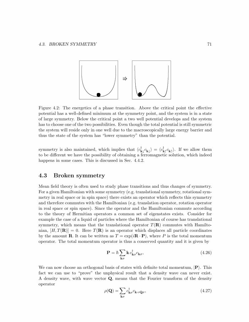
4.3. BROKEN SYMMETRY 71
Figure 4.2: The energetics of a phase transition. Above the critical point the effectivepotential has a well-defined minimum at the symmetry point, and the system is in a stateof large symmetry. Below the critical point a two well potential develops and the systemhas to choose one of the two possibilities. Even though the total potential is still symmetricthe system will reside only in one well due to the macroscopically large energy barrier andthus the state of the system has “lower symmetry” than the potential.
symmetry is also maintained, which implies that 〈c†k↓ck↓〉 = 〈c†k↑ck↑〉. If we allow themto be different we have the possibility of obtaining a ferromagnetic solution, which indeedhappens in some cases. This is discussed in Sec. 4.4.2.
4.3 Broken symmetry
Mean field theory is often used to study phase transitions and thus changes of symmetry.For a given Hamiltonian with some symmetry (e.g. translational symmetry, rotational sym-metry in real space or in spin space) there exists an operator which reflects this symmetryand therefore commutes with the Hamiltonian (e.g. translation operator, rotation operatorin real space or spin space). Since the operator and the Hamiltonian commute accordingto the theory of Hermitian operators a common set of eigenstates exists. Consider forexample the case of a liquid of particles where the Hamiltonian of course has translationalsymmetry, which means that the translational operator T (R) commutes with Hamilto-nian, [H,T (R)] = 0. Here T (R) is an operator which displaces all particle coordinatesby the amount R. It can be written as T = exp(iR ·P), where P is the total momentumoperator. The total momentum operator is thus a conserved quantity and it is given by
P = ~∑
kσ
k c†kσckσ, (4.26)
We can now choose an orthogonal basis of states with definite total momentum, |P〉. Thisfact we can use to “prove” the unphysical result that a density wave can never exist.A density wave, with wave vector Q, means that the Fourier transform of the densityoperator
ρ(Q) =∑
kσ
c†kσck+Qσ, (4.27)

72 CHAPTER 4. MEAN FIELD THEORY
Phenomena Order parameter Order parameterphysical mathematical
crystal density wave∑
k〈c†kck+Q〉ferromagnet magnetization
∑k〈c†k↑ck↑ − c†k↓ck↓〉
Bose-Einstein condensate population of k = 0 state 〈a†k=0〉superconductor pair condensate 〈ck↑c−k↓〉
Table 4.1: Typical examples of spontaneous symmetry breakings and their correspondingorder parameters.
has a finite expectation value, but
〈c†kσck+Qσ〉 =1Z
∑
P
e−βEP
⟨P
∣∣∣c†kσck+Qσ
∣∣∣P⟩
= 0, (4.28)
because c†kck+Q|P〉 has momentum P−Q and is thus orthogonal to |P〉. We have there-fore reached the senseless result that crystals do not exist. In the same way, we could“prove” that magnetism, superconductivity, and other well-known physical phenomenacannot happen. What is wrong?
The proof above breaks down if the sum of states in the thermodynamical average isrestricted. Even though crystals with different spatial reference points (or ferromagnetswith magnetization in different directions) have formally the same energy, they are effec-tively decoupled due to the large energy barrier it takes to melt and then recrystallizeinto a new state with a shifted reference (or direction of magnetization). In those caseswhere many states of the system are degenerate but separated by large energy barriers,it does not make sense to include them on equal footing in the statistical average as inEq. (4.28) because they correspond to macroscopically totally different configurations. Weare therefore forced to refrain from the fundamental ergodicity postulate of statistical me-chanics, also discussed in Sec. 1.5, and built into the description that the phase space ofthe system falls into physically separated sections. This is often illustrated by the doublebarrier model of phase transitions shown in Fig. 4.2.
When at some critical temperature the thermodynamical state of the system developsa non-zero expectation value of some macroscopic quantity which has a symmetry lowerthan the original Hamiltonian it is called spontaneous breaking of symmetry. The quantitywhich signals that a phase transition has occurred is called the order parameter. Typicalexamples are listed in Table 4.1.
In order to arrive at the new phase in a calculation and to avoid the paradox inEq. (4.28), one has to built in the possibility of the new phase into the theory. In themean field approach the trick is to include the order parameter in the choice of finitemean fields and, of course, show that the resulting mean field Hamiltonian leads to aself-consistent finite result. Next we study in some detail examples of symmetry breakingphenomena and their corresponding order parameters.

4.4. FERROMAGNETISM 73
Figure 4.3: The left figure shows the Heisenberg model in the disordered state where thereis no preferred direction for spins, while in the ferromagnetic state, shown in the middle,the spins form a collective state with a finite macroscopic moment along one direction.The model discussed here includes interactions between adjacent spins only, as shown inthe right panel.
4.4 Ferromagnetism
4.4.1 The Heisenberg model of ionic ferromagnets
In ionic magnetic crystals the interaction between the magnetic ions is due to the exchangeinteractions originating from the Coulomb interactions. Here we will not go into the detailsof this interaction but simply give the effective Hamiltonian3, known as the Heisenbergmodel for interaction between spins in a crystal. It reads
H = −2∑
ij
Jij Si · Sj , (4.29)
where Si is the spin operator for the ion on site i and Jij is the strength of the interaction,between the magnetic moment of the ions on sites i and j. It depends only on the distancebetween the ions. The interaction is generally short ranged and we truncate it so that it,as in Fig. 4.3, is only non-zero for nearest neighbors
Jij =
J0 if i and j are neighbors,0 otherwise.
(4.30)
We immediately see that if J < 0, the spins tend to become antiparallel whereas forJ > 0, it is energetically favorable to for the spins to be parallel. The first case correspondsto the antiferromagnetic case, while the latter to the ferromagnetic case. Here we consideronly the ferromagnetic case, J > 0.
As the model Hamiltonian stands, although simple looking, it is immensely complicatedand cannot be solved in general, the spins of the individual ions being strongly correlated.However, it is a good example where a mean field solution gives an easy and also physicalcorrect answer. The mean field decomposition then gives
H ≈ HMF = −2∑
ij
Jij 〈Si〉 · Sj − 2∑
ij
Jij Si · 〈Sj〉+ 2∑
ij
Jij 〈Si〉 · 〈Sj〉. (4.31)
3The term “effective Hamiltonian” has a well-defined meaning. It means the Hamiltonian describingthe important degrees of freedom on the relevant low energy scale.
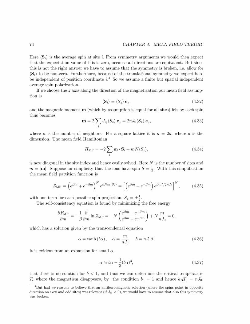
74 CHAPTER 4. MEAN FIELD THEORY
Here 〈Si〉 is the average spin at site i. From symmetry arguments we would then expectthat the expectation value of this is zero, because all directions are equivalent. But sincethis is not the right answer we have to assume that the symmetry is broken, i.e. allow for〈Si〉 to be non-zero. Furthermore, because of the translational symmetry we expect it tobe independent of position coordinate i.4 So we assume a finite but spatial independentaverage spin polarization.
If we choose the z axis along the direction of the magnetization our mean field assump-tion is
〈Si〉 = 〈Sz〉 ez, (4.32)
and the magnetic moment m (which by assumption is equal for all sites) felt by each spinthus becomes
m = 2∑
j
Jij〈Sz〉 ez = 2nJ0〈Sz〉 ez, (4.33)
where n is the number of neighbors. For a square lattice it is n = 2d, where d is thedimension. The mean field Hamiltonian
HMF = −2∑
i
m · Si + mN〈Sz〉, (4.34)
is now diagonal in the site index and hence easily solved. Here N is the number of sites andm = |m|. Suppose for simplicity that the ions have spin S = 1
2 . With this simplificationthe mean field partition function is
ZMF =(eβm + e−βm
)NeβNm〈Sz〉 =
[(eβm + e−βm
)eβm2/2nJ0
]N, (4.35)
with one term for each possible spin projection, Sz = ±12 .
The self-consistency equation is found by minimizing the free energy
∂FMF
∂m= − 1
β
∂
∂mln ZMF = −N
(eβm − e−βm
eβm + e−βm
)+ N
m
nJ0= 0,
which has a solution given by the transcendental equation
α = tanh (bα) , α =m
nJ0, b = nJ0β. (4.36)
It is evident from an expansion for small α,
α ≈ bα− 13(bα)3, (4.37)
that there is no solution for b < 1, and thus we can determine the critical temperatureTc where the magnetism disappears, by the condition bc = 1 and hence kBTc = nJ0.
4But had we reasons to believe that an antiferromagnetic solution (where the spins point in oppositedirection on even and odd sites) was relevant (if Jij < 0), we would have to assume that also this symmetrywas broken.
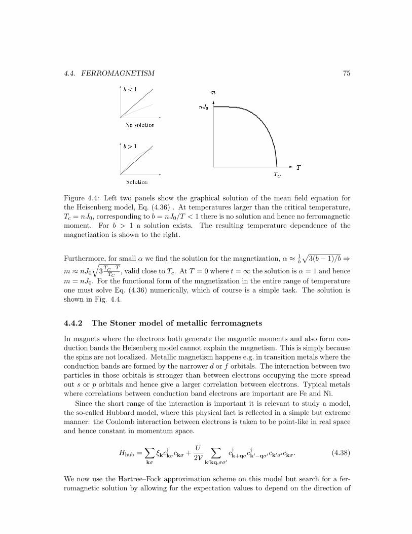
4.4. FERROMAGNETISM 75
Figure 4.4: Left two panels show the graphical solution of the mean field equation forthe Heisenberg model, Eq. (4.36) . At temperatures larger than the critical temperature,Tc = nJ0, corresponding to b = nJ0/T < 1 there is no solution and hence no ferromagneticmoment. For b > 1 a solution exists. The resulting temperature dependence of themagnetization is shown to the right.
Furthermore, for small α we find the solution for the magnetization, α ≈ 1b
√3(b− 1)/b ⇒
m ≈ nJ0
√3TC−T
TC, valid close to Tc. At T = 0 where t = ∞ the solution is α = 1 and hence
m = nJ0. For the functional form of the magnetization in the entire range of temperatureone must solve Eq. (4.36) numerically, which of course is a simple task. The solution isshown in Fig. 4.4.
4.4.2 The Stoner model of metallic ferromagnets
In magnets where the electrons both generate the magnetic moments and also form con-duction bands the Heisenberg model cannot explain the magnetism. This is simply becausethe spins are not localized. Metallic magnetism happens e.g. in transition metals where theconduction bands are formed by the narrower d or f orbitals. The interaction between twoparticles in those orbitals is stronger than between electrons occupying the more spreadout s or p orbitals and hence give a larger correlation between electrons. Typical metalswhere correlations between conduction band electrons are important are Fe and Ni.
Since the short range of the interaction is important it is relevant to study a model,the so-called Hubbard model, where this physical fact is reflected in a simple but extrememanner: the Coulomb interaction between electrons is taken to be point-like in real spaceand hence constant in momentum space.
Hhub =∑
kσ
ξkc†kσckσ +U
2V∑
k′kq,σσ′c†k+qσc†k′−qσ′ck′σ′ckσ. (4.38)
We now use the Hartree–Fock approximation scheme on this model but search for a fer-romagnetic solution by allowing for the expectation values to depend on the direction of
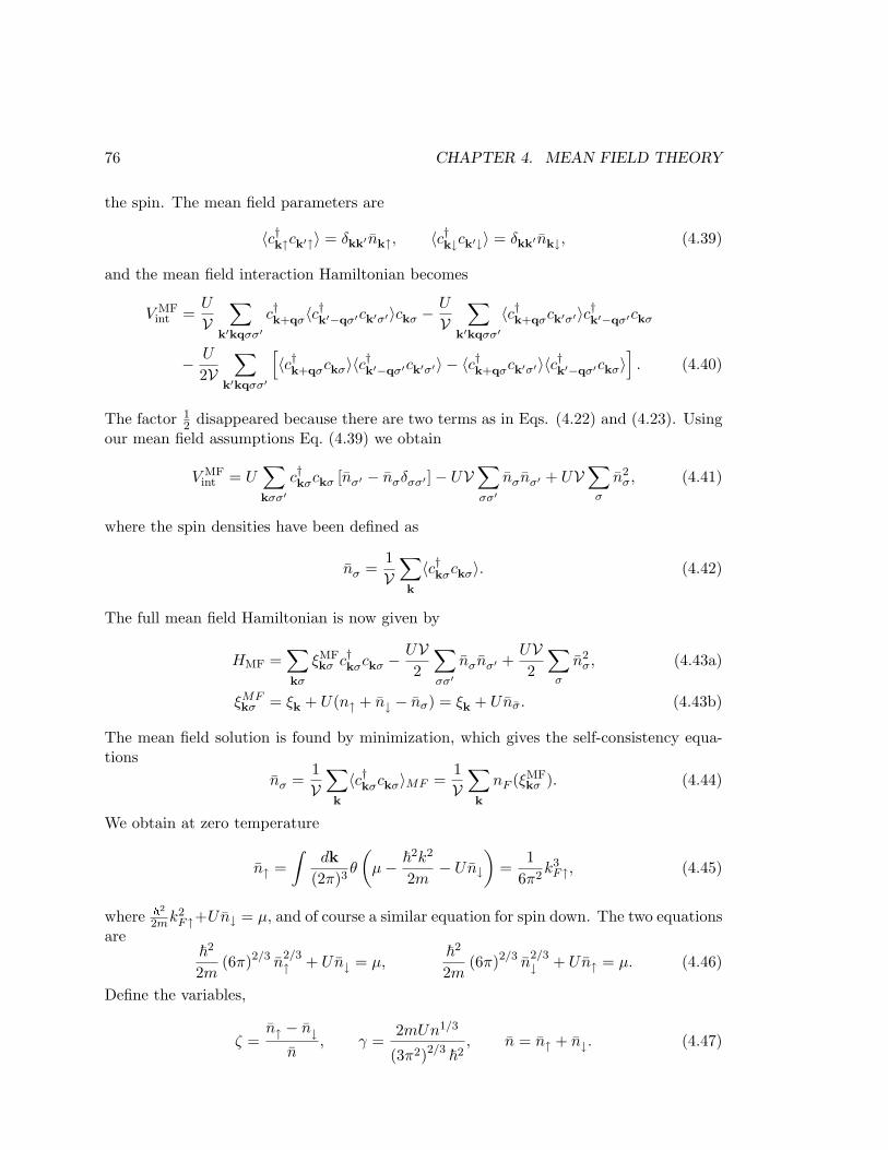
76 CHAPTER 4. MEAN FIELD THEORY
the spin. The mean field parameters are
〈c†k↑ck′↑〉 = δkk′ nk↑, 〈c†k↓ck′↓〉 = δkk′ nk↓, (4.39)
and the mean field interaction Hamiltonian becomes
V MFint =
U
V∑
k′kqσσ′c†k+qσ〈c†k′−qσ′ck′σ′〉ckσ −
U
V∑
k′kqσσ′〈c†k+qσck′σ′〉c†k′−qσ′ckσ
− U
2V∑
k′kqσσ′
[〈c†k+qσckσ〉〈c†k′−qσ′ck′σ′〉 − 〈c†k+qσck′σ′〉〈c†k′−qσ′ckσ〉
]. (4.40)
The factor 12 disappeared because there are two terms as in Eqs. (4.22) and (4.23). Using
our mean field assumptions Eq. (4.39) we obtain
V MFint = U
∑
kσσ′c†kσckσ [nσ′ − nσδσσ′ ]− UV
∑
σσ′nσnσ′ + UV
∑σ
n2σ, (4.41)
where the spin densities have been defined as
nσ =1V
∑
k
〈c†kσckσ〉. (4.42)
The full mean field Hamiltonian is now given by
HMF =∑
kσ
ξMFkσ c†kσckσ −
UV2
∑
σσ′nσnσ′ +
UV2
∑σ
n2σ, (4.43a)
ξMFkσ = ξk + U(n↑ + n↓ − nσ) = ξk + Unσ. (4.43b)
The mean field solution is found by minimization, which gives the self-consistency equa-tions
nσ =1V
∑
k
〈c†kσckσ〉MF =1V
∑
k
nF (ξMFkσ ). (4.44)
We obtain at zero temperature
n↑ =∫
dk(2π)3
θ
(µ− ~
2k2
2m− Un↓
)=
16π2
k3F↑, (4.45)
where ~22mk2
F↑+Un↓ = µ, and of course a similar equation for spin down. The two equationsare
~2
2m(6π)2/3 n
2/3↑ + Un↓ = µ,
~2
2m(6π)2/3 n
2/3↓ + Un↑ = µ. (4.46)
Define the variables,
ζ =n↑ − n↓
n, γ =
2mUn1/3
(3π2)2/3 ~2, n = n↑ + n↓. (4.47)
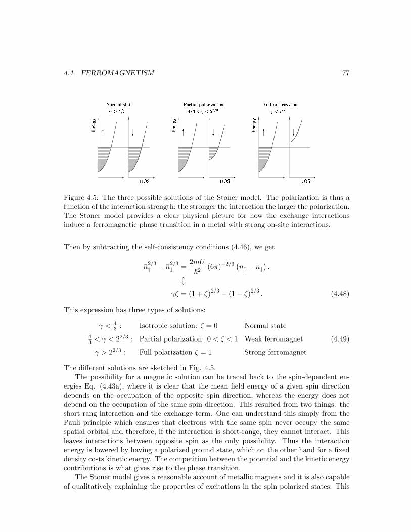
4.4. FERROMAGNETISM 77
! "
# $ % # $ % # $ %
& & &' ' '
Figure 4.5: The three possible solutions of the Stoner model. The polarization is thus afunction of the interaction strength; the stronger the interaction the larger the polarization.The Stoner model provides a clear physical picture for how the exchange interactionsinduce a ferromagnetic phase transition in a metal with strong on-site interactions.
Then by subtracting the self-consistency conditions (4.46), we get
n2/3↑ − n
2/3↓ =
2mU
~2(6π)−2/3 (
n↑ − n↓),
mγζ = (1 + ζ)2/3 − (1− ζ)2/3 . (4.48)
This expression has three types of solutions:
γ < 43 : Isotropic solution: ζ = 0 Normal state
43 < γ < 22/3 : Partial polarization: 0 < ζ < 1 Weak ferromagnet
γ > 22/3 : Full polarization ζ = 1 Strong ferromagnet
(4.49)
The different solutions are sketched in Fig. 4.5.The possibility for a magnetic solution can be traced back to the spin-dependent en-
ergies Eq. (4.43a), where it is clear that the mean field energy of a given spin directiondepends on the occupation of the opposite spin direction, whereas the energy does notdepend on the occupation of the same spin direction. This resulted from two things: theshort rang interaction and the exchange term. One can understand this simply from thePauli principle which ensures that electrons with the same spin never occupy the samespatial orbital and therefore, if the interaction is short-range, they cannot interact. Thisleaves interactions between opposite spin as the only possibility. Thus the interactionenergy is lowered by having a polarized ground state, which on the other hand for a fixeddensity costs kinetic energy. The competition between the potential and the kinetic energycontributions is what gives rise to the phase transition.
The Stoner model gives a reasonable account of metallic magnets and it is also capableof qualitatively explaining the properties of excitations in the spin polarized states. This
78 CHAPTER 4. MEAN FIELD THEORY
is however outside the scope of this section and the interested reader should consult forexample the book by Yosida.
4.5 Superconductivity
One of the most striking examples of symmetry breaking is the superconducting phasetransition. Below the critical temperature the metal which turns superconducting has noresistance what so ever, and it exhibits perfect diamagnetism (called Meissner effect),which means that magnetic fields are totally expelled from the interior of the material.These astonishing phenomena result from the superconducting state having a new form ofsymmetry breaking, namely loss of global gauge invariance. Besides the superconductivityitself and the Meissner effect superconductors show a number of other characteristics,e.g. distinct single particle properties, which result from the appearance of a gap in theexcitation spectrum.
Both the new type of phase and the appearance of an excitation gap are explained bythe Bardeen-Cooper-Schrieffer (BCS) theory from 1957. It is probably the most successfultheory in condensed matter physics and it has found application in other branches ofphysics as well, e.g. to explain the stability of nuclei with an even number of nucleons andalso in the standard model of high-energy physics.
In this section, we give a short introduction to the BCS theory, which in its spirit isvery much like the Hartree–Fock theory presented above. It is a mean field theory butwith a quite unusual mean field and therefore we begin by discussing the nature of thesuperconducting phase.
4.5.1 Breaking of global gauge symmetry and its consequences
Let us start by understanding what kind of broken symmetry could give rise to a super-conducting state. As was said above, the relevant symmetry is the global gauge symmetry,which means that we can give all electrons the same extra constant phase and still leavethe Hamiltonian invariant. The analog to this in the case of a ferromagnet, is that all spinscan be rotated by some angle without changing the Hamiltonian, which therefore has aglobal SO(3) symmetry. In that case a broken SO(3) symmetry means that the expecta-tion value 〈S〉 is not invariant under the rotation, because it will change the direction ofthe magnetization. In the same way the phase rotation also changes the superconductingorder parameter, which is of the form 〈cνcν′〉. The order parameter for the supercon-ductor thus involves an expectation value of two annihilation operators. Of course, thenumber of particles is conserved, but this is not a problem here where we discuss onlysuperconductors connected to electron reservoirs. Schematically the analogies betweensuperconductors and ferromagnets are as shown in Table 4.2.
While it is clear why the finite expectation 〈S〉 gives a magnetization in the caseof a ferromagnet, it is not so clear why broken symmetry in the superconducting caseleads to a system without resistance. We have argued that the superconducting state issensitive to a change of global phase, but it is also clear that a constant phase cannothave any measurable effect because all expectation values are given by the absolute square

4.5. SUPERCONDUCTIVITY 79
Global U(1) gauge symmetry, superconductor Global SO(3), ferromagnet
cν → cνeiϕ ⇒ H → H S → US ⇒ H → H
Broken symmetry: 0 6= 〈cνcν′〉 → 〈cνcν′〉e2iϕ Broken symmetry: 0 6= 〈S〉 → U〈S〉
Table 4.2: The analogy between the broken symmetries of a superconductor and a ferro-magnet.
of the wave function. However, phase gradients can have an effect. Let us thereforeassume that we ascribe a phase to the superconducting state which depends on position,ϕ (r), but varies extremely slowly, such that it takes a macroscopic distance to see anysignificant changes in ϕ (r). For any other non-superconducting system it would not makesense to talk about a quantum mechanical phase difference over macroscopic distances,simply because quantum coherence is destroyed by all sorts of scattering events on rathershort length scales, maybe of the order of 10 nm or less in metals. To argue that thesuperconducting state depends on phase differences over macroscopic distances is thereforevery unusual and tells us that superconductivity is a macroscopic quantum phenomenon.
In order to study the consequences of the phase change let us introduce a unitarytransformation which changes the phase
U = exp(
i
∫dr ρ(r)ϕ (r)
), (4.50)
(recall that ρ, is the density operator ρ (r) = Ψ† (r)Ψ (r)) because it has the followingproperties when applied to quantum field operators
Ψ(r) = UΨ(r)U−1 = exp(
i
∫dr ρ(r)ϕ (r)
)Ψ(r) exp
(−i
∫dr ρ(r)ϕ (r)
)
= Ψ(r) exp (−iϕ (r)) , (4.51a)
Ψ†(r) = UΨ†(r)U−1 = Ψ†(r) exp (iϕ (r)) . (4.51b)
These equations follow from the differential equation (together with the boundary condi-tion Ψϕ=0 = Ψ)
δ
δϕ (r′)Ψ(r) = iU [ρ(r′), Ψ(r)]U−1 = iΨ(r)δ
(r− r′
). (4.52)
(See also Eq. (5.24) in Chap. 5 which is derived in the same way.) If we transform thedensity operator and calculate the transformed partition function, we get
Z = Tr′[Ue−βHU−1
]= Tr′
[e−βH
]. (4.53)
Note here that if we had used the cyclic properties of the trace, U would have disappearedall together. However, we learned above that when dealing with systems with broken
80 CHAPTER 4. MEAN FIELD THEORY
symmetry, the sum-over-states has to be restricted so that the cyclic properties doesnot necessarily hold. This we have anticipated by the symbol Tr′ which means thatthe trace is restricted due to the spontaneous symmetry breaking. The transformationonly changes in the kinetic energy term of the Hamiltonian, because both the Coulombinteraction term, the impurity scattering term, and the phonon coupling term, only involvethe electron density operator ρ(r) which according to (4.51) is unchanged under the phaseshift transformation. The kinetic part reads
H =1
2me
∫drΨ†(r)eiϕ(r)
(~i∇+ eA
)2
e−iϕ(r)Ψ(r)
=1
2me
∫drΨ†(r)
(~i∇+ eA− ~∇ϕ(r)
)2
Ψ(r),
= H − ~∫
dr∇ϕ(r) · J(r)+~2
2me
∫dr ρ(r)(∇ϕ(r))2, (4.54)
where the last step closely follows the derivation of the current operator in Sec. 1.4.3.The claim above was that contrary to the non-superconducting state in the supercon-
ductor the phase is a macroscopic quantity. Let us therefore minimize the free energy withrespect to the phase in order to find the condition for the lowest free energy. It is clearfrom (4.54) that the energy doesn’t depend on ϕ itself, but only on the gradient of ϕ. Weobtain
δF
δ∇ϕ= −〈J(r)〉+ ~
me〈ρ(r)〉∇ϕ(r) = 0, (4.55)
and hence the energy is minimized if it carries a current, even in equilibrium, given by
〈J〉=~ρ0
me∇ϕ. (4.56)
The meaning of this result is that by forcing a phase gradient onto the system itminimizes its energy by carrying a current even in thermodynamical equilibrium, meaninga dissipationless current5. In the normal state of metals a current is always associated witha non-equilibrium state, where energy is constantly dissipated from the driving source andabsorbed in the conductor. Of course there is an energy cost for the system to carry thecurrent, but as long as this cost is smaller than the alternative which is to go out of thesuperconducting state, the current carrying state is chosen. The critical current is reachedwhen the energies are equal, and then the superconductor goes into the normal state.
What we have done so far is to show that if a phase gradient is imposed on a system,where the energy is assumed to depend on phase differences on a macroscopic scale, itunavoidably leads to the conclusion that the system will carry a dissipationless current inorder to minimize the energy cost of the phase gradient.
Finally, it should be noted that the appearance of the excitation gap is not the reasonfor the superconductivity itself. The superconductivity is, as we have argued, due to thelack of gauge invariance, and in fact gapless superconductors do exist.
5In reality the electron density appearing in Eq. (4.56) should only be the electrons participating in thesuperconducting condensate, the so-called superfluid. However, the simple minded derivation presentedhere assumes that all electrons participates.
4.5. SUPERCONDUCTIVITY 81
4.5.2 Microscopic theory
The understanding that superconductivity was closely related to the electron-phonon cou-pling was clear from the early 1950’ies when for example the isotope effect was discovered.Also the idea that the superconductivity was somehow similar to Bose-Einstein condensa-tion, with the bosons being electron pairs, had been tried and in fact was the underlyingidea of London’s theory in 1935. However, only in 1956 Cooper showed that the Fermisurface of the normal metal state was unstable towards formation of bound pairs of elec-trons (see Chap. 16). Subsequently in 1957 when the superconducting state was derivedusing a variational wavefunction by BCS, were the principles fully understood. Here wegive an outline of the main principles in the BCS theory.
In Chap. 16 we will see that the phonon mediated electron-electron interaction (derivedfrom the electron-phonon interaction found in Sec. 3.6) in fact has a range in frequency andmomentum space where it is negative, i.e. attractive. This happens for energy exchangesof order the Debye energy, ωD, which as we saw in Chap. 3 for metals is much smaller thanthe Fermi energy, ωD ¿ EF . Furthermore, from the Cooper instability we know that thephonon-mediated interaction tends to pair electrons with opposite spin and momentum.We define a Cooper pair operator
bk = ck↓c−k↑.
These two physical inputs led BCS to suggest the following remarkably successful modelHamiltonian to explain the superconducting state. The BCS effective Hamiltonian modelis
HBCS =∑
kσ
ξkc†kσckσ +∑
kk′Vkk′c
†k↑c
†−k↓c−k′↓ck′↑, (4.57)
where Vkk′ is the coupling strength which is only non-zero for states with energy ξk withinξ
F±ωD and furthermore constant and negative, Vkk′ = −V0, in this range. The interaction
includes only pair interactions and the remaining interaction is supposed to be includedin ξk via a Hartree–Fock term. The origin of the attractive interaction can intuitivelybe thought of in the following way: when an electron propagates through the crystal itattracts the positive ions and thus effectively creates a positive trace behind it. This traceis felt by the other electrons as an attractive interaction. It turns out that this effectiveinteraction is most important for electrons occupying time reversed states and in fact theycan form a bound state which is the Cooper pair. The Cooper pair is thus a bound stateof an electron in state ψν (r) and an electron in state ψ∗ν (r) or in the homogeneous caseelectrons in state k and −k.
Because the typical energy exchange due to the attractive interaction is the Debyeenergy, ωD, one would naively expect that the energy scale for the superconducting tran-sition temperature would be of the order ωD/k. This is however far from the truth becausewhile ωD/k is typically of the order of several hundred kelvin, the critical temperaturesfound in “conventional” low superconductors are in most cases less than 10 K and nevermore than 30 K. It therefore seems that a new energy scale is generated and we shallindeed see that this is the case.
82 CHAPTER 4. MEAN FIELD THEORY
The mean field assumption made by BCS, is that the pair operator has a finite ex-pectation value and that it varies only little from its average value. The BCS mean fieldHamiltonian is derived in full analogy with Hartree–Fock mean field theory describedabove
HMFBCS =
∑
kσ
ξkc†kσckσ −∑
k
∆kc†k↑c†−k↓
−∑
k
∆∗kck↓c−k↑ +
∑
kk′Vkk′〈c†k↑c†−k↓〉〈ck′↓c−k′↑〉, (4.58a)
∆k = −∑
kk′Vkk′〈c−k′↓ck′↑〉 (4.58b)
The mean field Hamiltonian is quadratic in electron operators and should be readily solv-able. It is however somewhat unusual in that terms like c†c† and cc appear. The way tosolve it is by a so-called Bogoliubov transformation. For this purpose it is convenient towrite the Hamiltonian in matrix notation
HMFBCS =
∑
k
(c†k↑ c−k↓
)(ξk ∆k
∆∗k −ξk
) (ck↑c†−k↓
)
+∑
k
ξk +∑
kk′Vkk′〈c†k↑c†−k↓〉〈ck′↓c−k′↑〉,
=∑
k
A†kHkAk + constant, (4.59)
where
Ak =
(ck↑c†−k↓
), Hk =
(ξk ∆k
∆∗k −ξk
). (4.60)
To bring the Hamiltonian into a diagonal form, we introduce the unitary transformation
Bk =
(γk↑γ†−k↓
)= U−1
k Ak, Uk =(
uk −vk
v∗k u∗k
), (4.61)
which diagonalizes the problem if
U†kHkUk =
(Ek 00 Ek
). (4.62)
After some algebra, we find the following solution for u, v and the energies, E and E
|uk|2 =12
(1 +
ξkEk
), |vk|2 =
12
(1− ξk
Ek
), (4.63)
Ek =√
ξ2k + |∆k|2 = −Ek. (4.64)
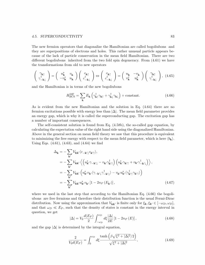
4.5. SUPERCONDUCTIVITY 83
The new fermion operators that diagonalize the Hamiltonian are called bogoliubons andthey are superpositions of electrons and holes. This rather unusual particle appears be-cause of the lack of particle conservation in the mean field Hamiltonian. There are twodifferent bogoliubons inherited from the two fold spin degeneracy. From (4.61) we havethe transformations from old to new operators(
γk↑γ†−k↓
)=
(u∗k vk
−v∗k uk
)(ck↑c†−k↓
)⇔
(ck↑c†−k↓
)=
(uk −vk
v∗k u∗k
)(γk↑γ†−k↓
), (4.65)
and the Hamiltonian is in terms of the new bogoliubons
HMFBCS =
∑
k
Ek
(γ†k↑γk↑ + γ†k↓γk↓
)+ constant. (4.66)
As is evident from the new Hamiltonian and the solution in Eq. (4.64) there are nofermion excitations possible with energy less than |∆|. The mean field parameter providesan energy gap, which is why it is called the superconducting gap. The excitation gap hasa number of important consequences.
The self-consistent solution is found from Eq. (4.58b), the so-called gap equation, bycalculating the expectation value of the right hand side using the diagonalized Hamiltonian.Above in the general section on mean field theory we saw that this procedure is equivalentto minimizing the free energy with respect to the mean field parameter, which is here 〈bk〉.Using Eqs. (4.61), (4.63), and (4.64) we find
∆k = −∑
k′Vkk′〈c−k′↓ck′↑〉,
= −∑
k′Vkk′
⟨(u∗k′γ−k′↓ − vk′γ
†k′↑
)(u∗k′γk′↑ + vk′γ
†−k′↓
)⟩,
= −∑
k′Vkk′
(u∗k′vk′〈γ−k′↓γ
†−k′↓〉 − vk′u
∗k′〈γ†k′↑γk′↑〉
)
= −∑
k′Vkk′u
∗k′vk′ [1− 2nF (Ek′)] , (4.67)
where we used in the last step that according to the Hamiltonian Eq. (4.66) the bogoli-ubons are free fermions and therefore their distribution function is the usual Fermi-Diracdistribution. Now using the approximation that Vkk′ is finite only for ξk, ξk′ ∈ [−ωD, ωD],and that ωD ¿ EF , such that the density of states is constant in the energy interval inquestion, we get
|∆| = V0d(EF )
2
∫ ωD
−ωD
dξ|∆|2E
[1− 2nF (E)] , (4.68)
and the gap |∆| is determined by the integral equation,
2V0d(EF )
=∫ ωD
0dξ
tanh(β√
ξ2 + |∆|2/2)
√ξ2 + |∆|2 , (4.69)
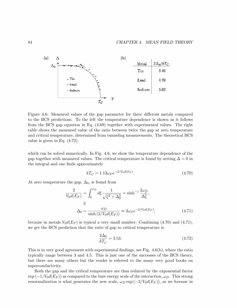
84 CHAPTER 4. MEAN FIELD THEORY
! "# $ % &' " & ! ( )
Figure 4.6: Measured values of the gap parameter for three different metals comparedto the BCS predictions. To the left the temperature dependence is shown as it followsfrom the BCS gap equation in Eq. (4.69) together with experimental values. The righttable shows the measured value of the ratio between twice the gap at zero temperatureand critical temperature, determined from tunneling measurements. The theoretical BCSvalue is given in Eq. (4.72).
which can be solved numerically. In Fig. 4.6, we show the temperature dependence of thegap together with measured values. The critical temperature is found by setting ∆ = 0 inthe integral and one finds approximately
kTC = 1.13ωDe−2/V0d(EF ). (4.70)
At zero temperature the gap, ∆0, is found from
2V0d(EF )
=∫ ωD
0dξ
1√ξ2 + ∆2
0
= sinh−1 2ωD
∆20
,
⇓∆0 =
ωD
sinh (2/V0d(EF ))≈ 2ωDe−2/V0d(EF ), (4.71)
because in metals V0d(EF ) is typical a very small number. Combining (4.70) and (4.71),we get the BCS prediction that the ratio of gap to critical temperature is
2∆0
kTC
= 3.53. (4.72)
This is in very good agreement with experimental findings, see Fig. 4.6(b), where the ratiotypically range between 3 and 4.5. This is just one of the successes of the BCS theory,but there are many others but the reader is referred to the many very good books onsuperconductivity.
Both the gap and the critical temperature are thus reduced by the exponential factorexp (−1/V0d(EF )) as compared to the bare energy scale of the interaction, ωD. This strongrenormalization is what generates the new scale, ωD exp (−2/V0d(EF )), as we foresaw in
4.6. SUMMARY AND OUTLOOK 85
the discussion above. Note that the interaction strength appears in a non-perturbativefashion in this expression, because the function exp (−1/x) has no Taylor expansion atx = 0. This tells us that the result could never have been derived using perturbation theoryin the interaction, no matter how many orders where included. This is in fact a generalfeature of phase transitions. It is not possible by perturbation expansions to cross a phasetransition line, because the two states have no analytic connection. Once again we see thatthere is no automatic way to predict the phase diagram of a given physical system, andone must rely on a combination of technical skill and most importantly physical intuition.
The BCS theory has provided an excellent model for the behavior of low tempera-ture superconductors. It is however not clear to what extend the theory can be usedto explain the superconductivity of high temperature superconductors and other exoticsuperconducting materials. This is still a very active and interesting area of research.
4.6 Summary and outlook
Mean field theories are widely used to study phase transitions in matter and also ine.g. atomic physics to compute the energetics of a finite size systems. The mean fieldapproximation is in many cases sufficient to understand the important physical features,at least those that has to do with static properties. We have seen examples of this in thecase of magnets and superconductors, where the important concept of symmetry breakingwas introduced. It means that the state of the system choose to have a lower symmetrythat the original Hamiltonian, e.g. all spins point in the same direction. Of course wehave not covered the vast fields of both magnetism and superconductivity in detail andthe interested reader should consult the book by Yosida to learn more about magnetism,and the books by Schrieffer, Tinkham and de Gennes to learn about superconductivity.
In the remaining part of this course we shall deal with the dynamical properties ofmany-particle systems. Also for the time-dependent case Hartree–Fock type approxima-tions will be invoked, e.g. for the so-called Random Phase Approximation treatment ofthe dielectric function in Sec. 8.5. The RPA result will later be derived later based on amore rigorous quantum field theoretical approach in Chap. 12.

86 CHAPTER 4. MEAN FIELD THEORY
Chapter 5
Time evolution pictures
Using the second quantization procedure, we have so far only treated energy eigenstateswith a trivial time dependence eiω t, instant processes at a single time t = 0, and systemswhere interactions are approximated by time-independent mean field theory. But howdoes one then treat the general case of time dependence in second quantization? Thatquestion will be addressed in this chapter, where time evolution is discussed using threerepresentations, or “pictures”: the Schrodinger picture, the Heisenberg picture, and theinteraction picture. These representations are used in the following chapters to developgeneral methods for treating many-particle systems.
5.1 The Schrodinger picture
The Schrodinger picture is useful when dealing with a time-independent Hamiltonian H,i.e. ∂tH = 0. Any other operator A may or may not depend on time. The state vectors|ψ(t)〉 does depend on time, and their time evolution is governed by Schrodinger’s equation.The time-independence of H leads to a simple formal solution:
i~∂t |ψ(t)〉 = H |ψ(t)〉 ⇒ |ψ(t)〉 = e−i~Ht |ψ0〉. (5.1)
In the following we will measure the energy in units of frequency, such that ~ drops outof the time-evolution equations: ε/~ → ε and H/~ → H. At the end of the calculationsone can easily convert frequencies back to energies. With this notation we can summarizethe Schrodinger picture with its states |ψ(t)〉 and operators A as:
The Schrodinger picture
states : |ψ(t)〉 = e−iHt |ψ0〉,operators : A, may or may not depend on time.
H, does not depend on time.(5.2)
To interpret the operator e−iHt we recall that a function f(B) of any operator B is definedby the Taylor expansion of f ,
f(B) =∞∑
n=0
f (n)(0)n!
Bn. (5.3)
87

88 CHAPTER 5. TIME EVOLUTION PICTURES
While the Schrodinger picture is quite useful for time-independent operators A, it maysometimes be preferable to collect all time dependencies in the operators and work withtime-independent state vectors. We can do that using the Heisenberg picture.
5.2 The Heisenberg picture
The central idea behind the Heisenberg picture is to obtain a representation where all thetime dependence is transferred to the operators, A(t), leaving the state vectors |ψ0〉 timeindependent. The Hamiltonian H remains time-independent in the Heisenberg picture.If the matrix elements of any operator between any two states are identical in the tworepresentations, then the two representations are fully equivalent. By using Eq. (5.2) weobtain the identity
〈ψ′(t)|A|ψ(t)〉 = 〈ψ′0|eiHtAe−iHt|ψ0〉 ≡ 〈ψ′0|A(t)|ψ0〉. (5.4)
Thus we see that the correspondence between the Heisenberg picture with time-independentstate vectors |ψ0〉, but time-dependent operators A(t), and the Schrodinger picture is givenby the unitary transformation operator exp(iHt),
The Heisenberg picture
states : |ψ0〉 ≡ eiHt |ψ(t)〉,operators : A(t) ≡ eiHtA e−iHt.
H does not depend on time.(5.5)
As before the original operator A may be time dependent. The important equation ofmotion governing the time evolution of A(t) is easily established. Since H is time inde-pendent, the total time derivative of A in the Heisenberg picture is denoted with a dot,A, while the explicit time derivative of the original Schrodinger operator is denoted ∂tA:
A(t) = eiHt(iHA− iAH + ∂tA
)e−iHt ⇒ A(t) = i
[H, A(t)
]+ (∂tA)(t), (5.6)
where X(t) always means eiHtXe−iHt for any symbol X, in particular for X = ∂tA. Inthis way an explicit time-dependence of A is taken into account. Note how carefully theorder of the operators is kept during the calculation.
Both the Schrodinger and the Heisenberg picture require a time-independent Hamil-tonian. In the general case of time-dependent Hamiltonians, we have to switch to theinteraction picture.
5.3 The interaction picture
The third and last representation, the interaction picture, is introduced to deal with thesituation where a system described by a time-independent Hamiltonian H0, with knownenergy eigenstates |n0〉, is perturbed by some, possibly time-dependent, interaction V (t),
H = H0 + V (t), with H0|n0〉 = εn0|n0〉. (5.7)
5.3. THE INTERACTION PICTURE 89
The key idea behind the interaction picture is to separate the trivial time evolution dueto H0 from the intricate one due to V (t). This is obtained by using only H0, not the fullH, in the unitary transformation Eq. (5.5). As a result, in the interaction picture boththe state vectors |ψ (t)〉 and the operators A(t) depend on time. The defining equationsfor the interaction picture are
The interaction picture
states : |ψ (t)〉 ≡ eiH0t |ψ(t)〉,operators : A(t) ≡ eiH0tA e−iH0t.
H0 does not depend on time.
(5.8)
The interaction picture and the Heisenberg picture coincide when V = 0; i.e., in the non-perturbed case. If V (t) is a weak perturbation, then one can think of Eq. (5.8) as a wayto pull out the fast, but trivial, time dependence due to H0, leaving states that vary onlyslowly in time due to V (t).
The first hint of the usefulness of the interaction picture comes from calculating thetime derivative of |ψ (t)〉 using the definition Eq. (5.8):
i∂t|ψ (t)〉 =(i∂te
iH0t)|ψ(t)〉+ eiH0t
(i∂t|ψ(t)〉
)= eiH0t(−H0 + H)|ψ(t)〉, (5.9)
which by Eq. (5.8) is reduced to
i∂t|ψ (t)〉 = V (t) |ψ (t)〉. (5.10)
The resulting Schrodinger equation for |ψ (t)〉 thus contains explicit reference only to theinteraction part V (t) of the full Hamiltonian H. This means that in the interaction picturethe time evolution of a state |ψ (t0)〉 from time t0 to t must be given in terms of a unitaryoperator U(t, t0) which also only depends on V (t). U(t, t0) is completely determined by
|ψ (t)〉 = U(t, t0) |ψ (t0)〉. (5.11)
When V and thus H are time-independent, an explicit form for U(t, t0) is obtained byinserting |ψ (t)〉 = eiH0t |ψ(t)〉 = eiH0t e−iHt |ψ0〉 and |ψ (t0)〉 = eiH0t0 e−iHt0 |ψ0〉 intoEq. (5.11),
eiH0t e−iHt |ψ0〉 = U(t, t0) eiH0t0 e−iHt0 |ψ0〉 ⇒ U(t, t0) = eiH0t e−iH(t−t0) e−iH0t0 .(5.12)
From this we observe that U−1 = U †, i.e. U is indeed a unitary operator.In the general case with a time-dependent V (t) we must rely on the differential equation
appearing when Eq. (5.11) is inserted in Eq. (5.10). We remark that Eq. (5.11) naturallyimplies the boundary condition U(t0, t0) = 1, and we obtain:
i∂t U(t, t0) = V (t) U(t, t0), U(t0, t0) = 1. (5.13)
By integration of this differential equation we get the integral equation
U(t, t0) = 1 +1i
∫ t
t0
dt′ V (t′) U(t′, t0), (5.14)
90 CHAPTER 5. TIME EVOLUTION PICTURES
which we can solve iteratively for U(t, t0) starting from U(t′, t0) = 1. The solution is
U(t, t0) = 1 +1i
∫ t
t0
dt1 V (t1) +1i2
∫ t
t0
dt1 V (t1)∫ t1
t0
dt2 V (t2) + . . . (5.15)
Note that in the iteration the ordering of all operators is carefully kept. A more compactform is obtained by the following rewriting. Consider for example the second order term,paying special attention to the dummy variables t1 and t2:
∫ t
t0
dt1 V (t1)∫ t1
t0
dt2 V (t2)
=12
∫ t
t0
dt1 V (t1)∫ t1
t0
dt2 V (t2) +12
∫ t
t0
dt2 V (t2)∫ t2
t0
dt1 V (t1)
=12
∫ t
t0
dt1
∫ t
t0
dt2 V (t1)V (t2)θ(t1 − t2) +12
∫ t
t0
dt2
∫ t
t0
dt1 V (t2)V (t1)θ(t2 − t1)
=12
∫ t
t0
dt1
∫ t
t0
dt2
[V (t1)V (t2)θ(t1 − t2) + V (t2)V (t1)θ(t2 − t1)
]
≡ 12
∫ t
t0
dt1
∫ t
t0
dt2 Tt[V (t1)V (t2)], (5.16)
where we have introduced the time ordering operator Tt. Time ordering is easily general-ized to higher order terms. In n-th order, where n factors V (tj) appear, all n! permutationsp ∈ Sn of the n times tj are involved, and we define1
Tt[V (t1)V (t2) . . . V (tn)] ≡∑
p∈Sn
V (tp(1))V (tp(2)) . . . V (tp(n)) × (5.17)
θ(tp(1) − tp(2)) θ(tp(2) − tp(3)) . . . θ(tp(n−1) − tp(n)).
Using the time ordering operator, we obtain the final compact form (see also Exercise 5.2):
U(t, t0) =∞∑
n=0
1n!
(1i
)n∫ t
t0
dt1 . . .
∫ t
t0
dtn Tt
(V (t1) . . . V (tn)
)= Tt
(e−iR t
t0dt′ V (t′)
). (5.18)
Note the similarity with a usual time evolution factor e−iε t. This expression for U(t, t0) isthe starting point for infinite order perturbation theory and for introducing the conceptof Feynman diagrams; it is therefore one of the central equations in quantum field theory.A graphical sketch of the contents of the formula is given in Fig. 5.1.
1For n = 3 we have Tt[V (t1)V (t2)V (t3)] =V (t1)V (t2)V (t3)θ(t1−t2)θ(t2−t3)+V (t1)V (t3)V (t2)θ(t1−t3)θ(t3−t2)+V (t2)V (t3)V (t1)θ(t2−t3)θ(t3−t1)+V (t2)V (t1)V (t3)θ(t2−t1)θ(t1−t3)+V (t3)V (t1)V (t2)θ(t3−t1)θ(t1−t2)+V (t3)V (t2)V (t1)θ(t3−t2)θ(t2−t1).
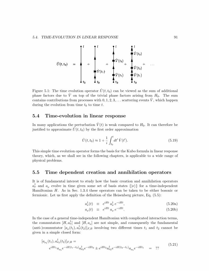
5.4. TIME-EVOLUTION IN LINEAR RESPONSE 91
Figure 5.1: The time evolution operator U(t, t0) can be viewed as the sum of additionalphase factors due to V on top of the trivial phase factors arising from H0. The sumcontains contributions from processes with 0, 1, 2, 3, . . . scattering events V , which happenduring the evolution from time t0 to time t.
5.4 Time-evolution in linear response
In many applications the perturbation V (t) is weak compared to H0. It can therefore bejustified to approximate U(t, t0) by the first order approximation
U(t, t0) ≈ 1 +1i
∫ t
t0
dt′ V (t′). (5.19)
This simple time evolution operator forms the basis for the Kubo formula in linear responsetheory, which, as we shall see in the following chapters, is applicable to a wide range ofphysical problems.
5.5 Time dependent creation and annihilation operators
It is of fundamental interest to study how the basic creation and annihilation operatorsa†ν and aν evolve in time given some set of basis states |ν〉 for a time-independentHamiltonian H. As in Sec. 1.3.4 these operators can be taken to be either bosonic orfermionic. Let us first apply the definition of the Heisenberg picture, Eq. (5.5):
a†ν(t) ≡ eiHt a†ν e−iHt, (5.20a)aν(t) ≡ eiHt aν e−iHt. (5.20b)
In the case of a general time-independent Hamiltonian with complicated interaction terms,the commutators [H, a†ν ] and [H, aν ] are not simple, and consequently the fundamental(anti-)commutator [aν(t1), a
†ν(t2)]F,B involving two different times t1 and t2 cannot be
given in a simple closed form:
[aν1(t1), a
†ν2(t2)]F,B =
eiHt1aν1e−iH(t1−t2)a†ν2e
−iHt2 ± eiHt2a†ν2e−iH(t2−t1)aν1
e−iHt1 = ??(5.21)
92 CHAPTER 5. TIME EVOLUTION PICTURES
No further reduction is possible in the general case. In fact, as we shall see in the followingchapters, calculating (anti-)commutators like Eq. (5.21) is the problem in many-particlephysics.
But let us investigate some simple cases to get a grasp of the time evolution pictures.Consider first a time-independent Hamiltonian H which is diagonal in the |ν〉-basis,
H =∑
ν
ενa†νaν . (5.22)
The equation of motion, Eq. (5.6), is straightforward:2
aν(t) = i[H, aν(t)] = ieiHt[H, aν ]e−iHt
= ieiHt∑
ν′εν′
[a†ν′aν′ , aν
]e−iHt = ieiHt
∑
ν′εν′
(−δν,ν′
)aν′e
−iHt
= −iενeiHtaνe
−iHt = −iενaν(t). (5.23)
By integration we obtainaν(t) = e−iενtaν , (5.24)
which by Hermitian conjugation leads to
a†ν(t) = e+iενta†ν . (5.25)
In this very simple case the basic (anti-)commutator Eq. (5.21) can be evaluated directly:
[aν1(t1), a†ν2
(t2)]F,B = e−iεν1(t1−t2) δν1,ν2
. (5.26)
For the diagonal Hamiltonian the time evolution is thus seen to be given by trivial phasefactors e±iε t.
We can also gain some insight into the interaction picture by a trivial extension of thesimple model. Assume that
H = H0 + γH0, γ ¿ 1, (5.27)
where H0 is diagonalized in the basis |ν〉 with the eigenenergies εν . Obviously, the fullHamiltonian H is also diagonalized in the same basis, but with the eigenenergies (1+γ)ε .Let us however try to treat γH0 as a perturbation V to H0, and then use the interactionpicture of Sec. 5.3. From Eq. (5.8) we then obtain
|ν(t)〉 = eiενt |ν(t)〉. (5.28)
But we actually know the time evolution of the Schrodinger state on the right-hand sideof the equation, so
|ν(t)〉 = eiενt e−i(1+γ)ενt|ν〉 = e−iγενt|ν〉. (5.29)2We are using the identities [AB, C] = A[B, C] + [A, C]B and [AB, C] = AB, C − A, CB, which
are valid for any set of operators. Note that the first identity is particularly useful for bosonic operatorsand the second for fermionic operators (see Exercise 5.4).

5.6. SUMMARY AND OUTLOOK 93
Here we clearly see that the fast Schrodinger time dependence given by the phase factoreiενt, is replaced in the interaction picture by the slow phase factor eiγενt. The reader cantry to obtain Eq. (5.29) directly from Eq. (5.18).
Finally, we briefly point to the complications that arise when the interaction is givenby a time-independent operator V not diagonal in the same basis as H0. Consider forexample the Coulomb-like interaction written symbolically as
H = H0 + V =∑
ν′εν′a
†ν′aν′ +
∑ν1ν2
∑q
Vq a†ν1+qa†ν2−qaν2
aν1. (5.30)
The equation of motion for aν(t) is:
aν(t) = i[H, aν(t)] = −iεν aν(t) + i∑ν1ν2q
Vq
[a†ν1+q(t) a†ν2−q(t), aν(t)
]aν2
(t) aν1(t)
= −iεν aν(t) + i∑ν1ν2
(Vν2−ν − Vν−ν1)a†ν1+ν2−ν(t) aν2
(t) aν1(t). (5.31)
The problem in this more general case is evident. The equation of motion for the singleoperator aν(t) contains terms with both one and three operators, and we do not knowthe time evolution of the three-operator product a†ν1+ν2−ν(t) aν2
(t) aν1(t). If we write
down the equation of motion for this three-operator product we discover that terms aregenerated involving five operator products. This feature is then repeated over and overagain generating a never-ending sequence of products containing seven, nine, eleven, etc.operators. In the following chapters we will learn various approximate methods to dealwith this problem.
5.6 Summary and outlook
In this chapter we have introduced the fundamental representations used in the descrip-tion of time evolution in many-particle systems: the Schrodinger picture, Eq. (5.2), theHeisenberg picture, Eq. (5.5), and the interaction picture, Eq. (5.8). The first two picturesrely on a time-independent Hamiltonian H, while the interaction picture involves a time-dependent Hamiltonian H of the form H = H0 + V (t), where H0 is a time-independentHamiltonian with known eigenstates. Which picture to use depends on the problem athand.
We have derived an explicit expression, Eq. (5.18), for the time evolution operatorU(t, t0) describing the evolution of an interaction picture state |ψ (t0)〉 at time t0 to |ψ (t)〉at time t. We shall see in the following chapters how the operator U(t, t0) plays animportant role in the formulation of infinite order perturbation theory and the introductionof Feynman diagrams, and how its linearized form Eq. (5.19) forms the basis of the widelyused linear response theory and the associated Kubo formalism.
Finally, by studying the basic creation and annihilation operators we have gotten afirst glimpse of the problems we are facing, when we are trying to study the full timedependence, or equivalently the full dynamics, of interacting many-particle systems.

94 CHAPTER 5. TIME EVOLUTION PICTURES

Chapter 6
Linear response theory
Linear response theory is an extremely widely used concept in all branches of physics.It simply states that the response to a weak external perturbation is proportional to theperturbation, and therefore all one needs to understand is the proportionality constant.Below we derive the general formula for the linear response of a quantum system exertedby a perturbation. The physical question we ask is thus: supposing some perturbation H ′,what is the measured consequence for an observable quantity, A. In other words, what is〈A〉 to linear order in H ′?
Among the numerous applications of the linear response formula, one can mentioncharge and spin susceptibilities of e.g. electron systems due to external electric or magneticfields. Responses to external mechanical forces or vibrations can also be calculated usingthe very same formula. Here we utilize the formalism to derive a general expression forthe electrical conductivity and briefly mention other applications.
6.1 The general Kubo formula
Consider a quantum system described by the (time independent) Hamiltonian H0 in ther-modynamic equilibrium. According to Sec. 1.5 this means that an expectation value of aphysical quantity, described by the operator A, can be evaluated as
〈A〉 =1Z0
Tr [ρ0A] =1Z0
∑n
〈n|A|n〉e−βEn , (6.1a)
ρ0 = e−βH0 =∑
n
|n〉〈n|e−βEn , (6.1b)
where ρ0 is the density operator and Z0 =Tr[ρ0] is the partition function. Here as inSec. 1.5, we write the density operator in terms of a complete set of eigenstates, |n〉, ofthe Hamiltonian, H0, with eigenenergies En.
Suppose now that at some time, t = t0, an external perturbation is applied to thesystem, driving it out of equilibrium. The perturbation is described by an additional timedependent term in the Hamiltonian
H(t) = H0 + H ′(t)θ(t− t0). (6.2)
95
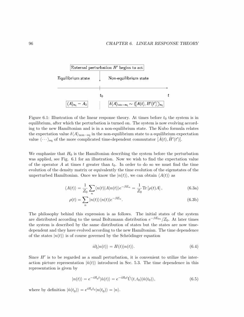
96 CHAPTER 6. LINEAR RESPONSE THEORY
!#" $ % $ & ' (#)* + !-, . / , . 0 " ' ( !#" ' (#12!
Figure 6.1: Illustration of the linear response theory. At times before t0 the system is inequilibrium, after which the perturbation is turned on. The system is now evolving accord-ing to the new Hamiltonian and is in a non-equilibrium state. The Kubo formula relatesthe expectation value δ〈A〉non−eq in the non-equilibrium state to a equilibrium expectationvalue 〈· · · 〉eq of the more complicated time-dependent commutator [A(t), H ′(t′)].
We emphasize that H0 is the Hamiltonian describing the system before the perturbationwas applied, see Fig. 6.1 for an illustration. Now we wish to find the expectation valueof the operator A at times t greater than t0. In order to do so we must find the timeevolution of the density matrix or equivalently the time evolution of the eigenstates of theunperturbed Hamiltonian. Once we know the |n(t)〉, we can obtain 〈A(t)〉 as
〈A(t)〉 =1Z0
∑n
〈n(t)|A|n(t)〉e−βEn =1Z0
Tr [ρ(t)A] , (6.3a)
ρ(t) =∑
n
|n(t)〉〈n(t)|e−βEn . (6.3b)
The philosophy behind this expression is as follows. The initial states of the systemare distributed according to the usual Boltzmann distribution e−βE0n/Z0. At later timesthe system is described by the same distribution of states but the states are now time-dependent and they have evolved according to the new Hamiltonian. The time dependenceof the states |n(t)〉 is of course governed by the Schrodinger equation
i∂t|n(t)〉 = H(t)|n(t)〉. (6.4)
Since H ′ is to be regarded as a small perturbation, it is convenient to utilize the inter-action picture representation |n(t)〉 introduced in Sec. 5.3. The time dependence in thisrepresentation is given by
|n(t)〉 = e−iH0t|n(t)〉 = e−iH0tU(t, t0)|n(t0)〉, (6.5)
where by definition |n(t0)〉 = eiH0t0 |n(t0)〉 = |n〉.

6.1. THE GENERAL KUBO FORMULA 97
To linear order in H ′, Eq. (5.19) states that U(t, t0) = 1− i∫ tt0
dt′ H ′(t′). Inserting thisinto (6.3a), one obtains the expectation value of A up to linear order in the perturbation
〈A(t)〉 = 〈A〉0 − i
∫ t
t0
dt′1Z0
∑n
e−βEn〈n(t0)|A(t)H ′(t′)− H ′(t′)A(t)|n(t0)〉
= 〈A〉0 − i
∫ t
t0
dt′〈[A(t), H ′(t′)]〉0. (6.6)
The brackets 〈〉0 mean an equilibrium average with respect to the Hamiltonian H0. Thisis in fact a remarkable and very useful result, because the inherently non-equilibriumquantity 〈A(t)〉 has been expressed as a correlation function of the system in equilibrium.The physical reason for this is that the interaction between excitations created in thenon-equilibrium state is an effect to second order in the weak perturbation, and hence notincluded in linear response.
The correlation function that appears in Eq. (6.6), is called a retarded correlationfunction, and for later reference we rewrite the linear response result as
δ〈A(t)〉 ≡ 〈A(t)〉 − 〈A〉0 =∫ ∞
t0
dt′CRAH′(t, t′)e−η(t−t′), (6.7)
whereCR
AH′(t, t′) = −iθ(t− t′)⟨[
A(t), H ′(t′)]⟩
0. (6.8)
This is the famous Kubo formula which expresses the linear response to a perturbation,H ′. We have added a very important detail here: the factor e−η(t−t′), with an infinitesimalpositive parameter η, has been included to force the response at time t due to the influenceof H ′ at time t′ to decay when t À t′. In the end of a calculation we must therefore takethe limit η → 0+. For physical reasons the (retarded) effect of a perturbation must ofcourse decrease in time. You can think of the situation that one often has for differentialequations with two solutions: one which increases exponentially with time (physicallynot acceptable) and one which decreases exponentially with time; the factor e−η(t−t′) isthere to pick out the physically relevant solution by introducing an artificial relaxationmechanism.
Kubo formula in the frequency domain
It is often convenient to express the response to an external disturbance in the frequencydomain. Let us therefore write the perturbation in terms of its Fourier components
H ′(t) =∫
dω
2πe−iωtH ′
ω, (6.9)
such that CRAH′ becomes
CRAH′(t, t′) =
∫ ∞
−∞
dω
2πe−iωt′CR
AH′ω(t− t′), (6.10)
98 CHAPTER 6. LINEAR RESPONSE THEORY
because 〈[A(t), H ′ω(t′)]〉0 only depends on the difference between t and t′, which can easily
be proven using the definition of the expectation value. When inserted into the Kuboformula, one gets (after setting t0 = −∞, because we are not interested in the transientbehavior)
δ〈A(t)〉 =∫ ∞
−∞dt′
∫ ∞
−∞
dω
2πe−iωte−i(ω+iη)(t′−t)CR
AH′ω(t− t′)
=∫ ∞
−∞
dω
2πe−iωtCR
AH′ω(ω), (6.11)
and therefore the final result reads in frequency domain
δ〈Aω〉 = CRAH′
ω(ω), (6.12a)
CRAH′
ω(ω) =
∫ ∞
−∞dteiωte−ηtCR
AH′ω(t). (6.12b)
Note again that the infinitesimal η is incorporated in order to ensure the correct physicalresult, namely that the retarded response function decays at large times.
6.2 Kubo formula for conductivity
Consider a system of charged particles, electrons say, which is subjected to an externalelectromagnetic field. The electromagnetic field induces a current, and the conductivityis the linear response coefficient. In the general case the conductivity may be non-local inboth time and space, such that the electric current Je at some point r at time t dependson the electric field at points r′ at times t′
Jαe (r, t) =
∫dt′
∫dr′
∑
β
σαβ(rt, r′t′) Eβ(r′, t′) (6.13)
where σαβ(r, r′; t, t′) is the conductivity tensor which describes the current response indirection eα to an applied electric field in direction eβ.
The electric field E is given by the electric potential φext and the vector potential Aext
E(r, t) = −∇rφext(r, t)− ∂tAext(r, t). (6.14)
The current density operator of charged particles in the presence of an electromagneticfield was given in Chap. 1. For simplicity we assume only one kind of particles, electronssay, but generalization to more kinds of charge carrying particles is straightforward bysimple addition of more current components.1 For electrons Je = −e〈J〉. The perturbingterm in the Hamiltonian due to the external electromagnetic field is given by the coupling
1With more carriers the operator for the electrical current becomes Je(r) =P
i qiJi(r), where qi arethe charges of the different carriers. Note that in this case the currents of the individual species are notnecessarily independent.

6.2. KUBO FORMULA FOR CONDUCTIVITY 99
of the electrons to the scalar potential and the vector potential. To linear order in theexternal potential
Hext = −e
∫dr ρ(r)φext(r, t) + e
∫dr J(r) ·Aext(r, t), (6.15)
where the latter term was explained in Sec. 1.4.3. Let A0 denote the vector potentialin the equilibrium, i.e. prior to the onset of the perturbation Aext, and let A denote thetotal vector potential. Then we have
A = A0+Aext, (6.16)
Again according to Sec. 1.4.3, the current operator has two components, the diamagneticterm and the paramagnetic term
J(r) = J∇(r) +e
mA(r)ρ(r), (6.17)
In order to simplify the expressions, we can choose a gauge where the external electricalpotential is zero, φext = 0. This is always possible by a suitable choice of A(r, t) as youcan see in Eq. (6.14). The final result should of course not depend on the choice ofgauge. The conductivity is most easily expressed in the frequency domain, and thereforewe Fourier transform the perturbation. Since ∂t becomes −iω in the frequency domain wehave Aext(r, ω) = (1/iω)Eext(r, ω), and therefore the external perturbation in Eq. (6.15)becomes in the Fourier domain
Hext,ω =e
iω
∫dr J(r) ·Eext(r, ω). (6.18)
In order to exploit the frequency domain formulation of linear response we want to writethe definition of the conductivity tensor in Eq. (6.13) in frequency domain. Because we areonly considering linear response the conductivity tensor is a property of the equilibriumsystem and can thus only depend on time differences σαβ(rt, r′t′) = σαβ(r, r′, t− t′). Thefrequency transform of Eq. (6.13) is therefore simply that of a convolution and hence
Jαe (r, ω) =
∫dr′
∑
β
σαβ(r, r′, ω) Eβ(r′, ω). (6.19)
Now since Eq. (6.18) is already linear in the external potential Eext and since we areonly interested in the linear response, we can replace J in Eq. (6.18) by J0 = J∇+ e
mA0ρ,thus neglecting the term proportional to Eext ·Aext. Eq. (6.18) is therefore replaced by
Hext,ω =e
iω
∫dr J0(r) ·Eext(r, ω). (6.20)
To find the expectation value of the current we write
〈J(r, ω)〉 = 〈J0(r, ω)〉+ 〈 e
mAext(r, ω)ρ(r)〉. (6.21)
100 CHAPTER 6. LINEAR RESPONSE THEORY
For the last term in Eq. (6.21) we use that to linear order in Aext the expectation valuecan be evaluated in the equilibrium state
〈 e
mAext(r, ω)ρ(r)〉 =
e
mAext(r, ω)〈ρ(r)〉0 =
e
iωEext(r, ω)〈ρ(r)〉0. (6.22)
For the first term in Eq. (6.21) we use the general Kubo formula in Eq. (6.7). Since theequilibrium state does not carry any current, i.e. 〈J0〉0 = 0, we conclude that 〈J0〉 = δ〈J0〉.In frequency domain we should use the results Eq. (6.12a) and substitute J0(r) for theoperator “A”, and Hext,ω for “H ′
ω”, which leads to 〈J0(r, ω)〉 = CRJ0(r)Hext,ω
(ω). Collectingthings we now have
〈J(r, ω)〉 = CRJ0(r)Hext,ω
(ω) +e
m〈ρ(r)〉0Aext(r,ω). (6.23)
Writing out the first term
CRJ0(r)Hext,ω
(ω) =∫
dr′∑
β
CRJ0(r)Jβ
0 (r′)(ω)
e
iωEβ(r′, ω). (6.24)
Comparing with the definition of the non-local conductivity in Eq. (6.19), we can now col-lect the two contributions to the conductivity tensor. The first term comes from Eq. (6.24)and it is seen to of the same form as (6.12a), in particular the response is non-local inspace. In contrast, the second term in Eq. (6.22) stemming from the diamagnetic partof the current operator is local in space. Now collecting the two terms and using thatJe = −e〈J〉, we finally arrive at the linear response formula for the conductivity tensor
σαβ(r, r′, ω) =ie2
ωΠR
αβ(r, r′, ω) +ie2n(r)iωm
δ(r− r′)δαβ, (6.25)
where we have used the symbol ΠR = CRJ0J0
for the retarded current-current correlationfunction. In the time domain it is given by
ΠRαβ(r, r′, t− t′) = CR
Jα0 (r)Jβ
0 (r′)(t− t′) = −iθ(t− t′)
⟨[Jα
0 (r, t), Jβ0 (r′, t′)
]⟩0. (6.26)
Finding the conductivity of a given system has thus been reduced to finding theretarded current-current correlation function. This formula will be used extensively inChap. 14.
6.3 Kubo formula for conductance
The conductivity σ is the proportionality coefficient between the electric field E and thecurrent density J, and it is an intrinsic property of a material. The conductance on theother hand is the proportionality coefficient between the current I through a sample andthe voltage V applied to it, i.e. a sample specific quantity. The conductance G is definedby the usual Ohm’s law
I = GV. (6.27)
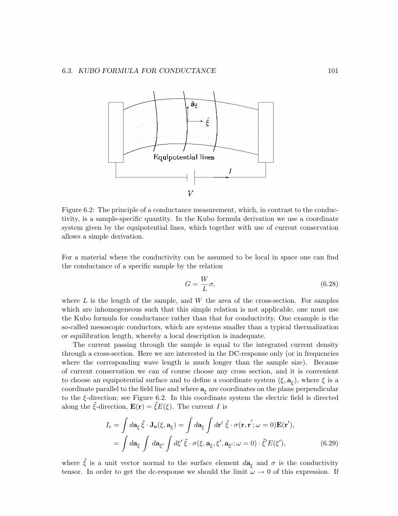
6.3. KUBO FORMULA FOR CONDUCTANCE 101
Figure 6.2: The principle of a conductance measurement, which, in contrast to the conduc-tivity, is a sample-specific quantity. In the Kubo formula derivation we use a coordinatesystem given by the equipotential lines, which together with use of current conservationallows a simple derivation.
For a material where the conductivity can be assumed to be local in space one can findthe conductance of a specific sample by the relation
G =W
Lσ, (6.28)
where L is the length of the sample, and W the area of the cross-section. For sampleswhich are inhomogeneous such that this simple relation is not applicable, one must usethe Kubo formula for conductance rather than that for conductivity. One example is theso-called mesoscopic conductors, which are systems smaller than a typical thermalizationor equilibration length, whereby a local description is inadequate.
The current passing through the sample is equal to the integrated current densitythrough a cross-section. Here we are interested in the DC-response only (or in frequencieswhere the corresponding wave length is much longer than the sample size). Becauseof current conservation we can of course choose any cross section, and it is convenientto choose an equipotential surface and to define a coordinate system (ξ,aξ), where ξ is acoordinate parallel to the field line and where aξ are coordinates on the plane perpendicularto the ξ-direction; see Figure 6.2. In this coordinate system the electric field is directedalong the ξ-direction, E(r) = ξE(ξ). The current I is
Ie =∫
daξ ξ · Je(ξ,aξ) =∫
daξ
∫dr′ ξ · σ(r, r
′;ω = 0)E(r′),
=∫
daξ
∫daξ′
∫dξ′ ξ · σ(ξ,aξ, ξ
′,aξ′ ; ω = 0) · ξ′E(ξ′), (6.29)
where ξ is a unit vector normal to the surface element daξ and σ is the conductivitytensor. In order to get the dc-response we should the limit ω → 0 of this expression. If

102 CHAPTER 6. LINEAR RESPONSE THEORY
we furthermore take the real part of (6.29) we see that what determines the dc-current isthe real part of the first term in Eq. (6.25) and hence the retarded correlation functionof the current densities. Since the total particle current at the coordinate ξ is given byI(ξ) =
∫daξ ξ · J , the conductance can instead be written as
Ie(ξ) = limω→0
∫dξ′Re
[ie2
ωCR
I(ξ)I(ξ′)(ω)]
E(ξ′) ≡∫
dξ′G(ξ, ξ′)E(ξ′), (6.30)
where CRI(ξ)I(ξ′) is the correlation function between total currents. Because of current
conservation the dc-current may be calculated at any point ξ and thus the result cannotdepend on ξ. Consequently the function in side the square brackets in Eq. (6.30) cannotdepend on ξ. Furthermore, since the conductance function G(ξ, ξ′) can be shown to bea symmetric function is cannot depend on ξ′ either. This simplification is the reason forchoosing the skew coordinate system defined by the field lines. We can therefore performthe integration over ξ′ which is just the voltage difference V =
∫dξ′E(ξ′) = φ(−∞)−φ(∞),
and we finally arrive at the for linear response formula for the conductance
G = limω→0
ie2
ωCR
II(ω). (6.31)
Here CRII is the retarded current-current function. In the time domain it is
CRII(t− t′) = −iθ(t− t′)〈[I(t), I(t′)]〉, (6.32)
where the current operator I denote the current through an arbitrary cross section alongthe sample.
6.4 Kubo formula for the dielectric function
When dealing with systems containing charged particles, as for example the electron gas,one is often interested in the dielectric properties of the system, and in particular thelinear response properties. When such a system is subjected to an external electromagneticperturbation the charge is redistributed and the system gets polarized. This in turn affectsthe measurements. The typical experiment is to exert an external potential, φext, andmeasure the resulting total potential, φtot. The total potential is the sum of the externalone and the potential created by the induced polarization, φind,
φtot = φext + φind. (6.33)
Alternatively to working with the potentials we can work with electric fields or charges.The charges are related to the potentials through a set of Poisson equations
ρtot = ρext + ρind,
∇2φtot = − 1ε0
ρe,tot
∇2φext = − 1ε0
ρe,ext
∇2φind = − 1ε0
ρe,ind
, (6.34)
6.4. KUBO FORMULA FOR THE DIELECTRIC FUNCTION 103
and likewise for electric fields, Etot, Eext, and Eind, which are related to the correspondingcharges by a set of Gauss laws, ∇ · E = ρe/ε0. Here we have used the symbols ρe for thecharge density, where ρ as defined in Chap. 1 defines particle densities.
The ratio between the external and the total potential is the dielectric response func-tion, also called the relative permittivity ε
φtot = ε−1φext, (6.35)
which is well-known from classical electrodynamics.2 However, in reality the permittivityis non-local both in time and space and the general relations between the total and theexternal potentials are
φtot(r, t) =∫
dr′∫
dt′ ε−1(rt, r′t′) φext(r′, t′), (6.36a)
φext(r, t) =∫
dr′∫
dt′ ε(rt, r′t′) φtot(r′, t′). (6.36b)
Our present task is to find the dielectric function ε(rt, r′t′), or rather its inverse ε−1(rt, r′t′)assuming linear response theory and for this purpose the induced potential is needed.
The external perturbation is represented as the following term to the Hamiltonian
H ′ =∫
dr ρe (r) φext(r, t). (6.37)
The induced charge density follows from linear response theory (if we assume that thesystem is charge neutral in equilibrium, i.e. 〈ρe(r, t)〉0 = 0) as
ρe,ind(r, t) = 〈ρe(r, t)〉 =∫
dr′∫ ∞
t0
dt′CRρeρe
(rt, r′t′)e−η(t−t′) φext(r′, t′), (6.38)
CRρeρe
(rt, r′t′) ≡ χRe (rt, r′t′) = −iθ(t− t′)〈[ρe(r, t), ρe(r′, t′)]〉0. (6.39)
The charge-charge correlation function, χRe , is called the polarizability function and it is
an important function which we will encounter many times. Once the induced charge isknown the potential follows from the Coulomb interaction Vc(r− r′) = 1/(ε0|r− r′|) as
φind(r) =∫
dr ′ Vc(r− r′) ρe,eind(r′), (6.40)
and hence
φtot(r, t) = φext(r, t) +∫
dr ′∫
dr ′′∫ ∞
t0
dt′Vc(r− r′)χR(r′t, r′′t′) φext(r′′, t′). (6.41)
From this expression we read off the inverse of the dielectric function as
ε−1(rt, r′t′) = δ(r− r′)δ(t− t′) +∫
dr ′′Vc(r− r′′)χR(r′′t, r′t′), (6.42)
2In electrodynamics the permittivity is defined as the proportionality constant between the electricdisplacement field, D, and the electric field, D = εE. In the present formulation, Eext plays the role of theD-field, i.e. D = ε0Eext, while Etot is the E-field
104 CHAPTER 6. LINEAR RESPONSE THEORY
which ends our derivation. In later chapters we will make extensive use of the dielectricfunction ε and the polarizability χ. The dielectric function expressed in Eq. (6.42) in-cludes all correlation effects, but often we must use some approximation to compute thepolarizability.
6.4.1 Dielectric function for translation-invariant system
In the translation-invariant case the polarizability can only depend on the differences of thearguments, i.e. χR(rt, r′t′) = χR(r− r′; t− t′), and therefore the problem is considerablysimplified by going to frequency and momentum space, where both Eqs. (6.36) have theform of convolutions. After Fourier transformation they become products
φtot(q,ω) = ε−1(q, ω)φext(q, ω), or φext(q,ω) = ε(q, ω)φtot(q, ω), (6.43)
with the dielectric function being
ε−1(q, ω) = 1 + Vc(q)χRe (q, ω) . (6.44)
6.4.2 Relation between dielectric function and conductivity
Both ε and σ give the response of a system to an applied electromagnetic field, and oneshould therefore expect that they were related, and of course they are. Here we consideragain the translational-invariant case, and using the definition of conductivity
J(q, ω) = σ(q, ω)Eext(q, ω) = −iσ(q, ω)qφext(q, ω), (6.45)
and the continuity equation,
−iωρ(q, ω) + iq · J(q, ω) = 0, (continuity equation), (6.46)
we obtain−iq · σ(q, ω)qφext(q, ω) = ωρe(q, ω) = ωχR
e (q, ω) φext(q, ω). (6.47)
Finally, using Eq. (6.44) and knowing that for a homogeneous system, the conductivitytensor is diagonal, we arrive at the relation
ε−1(q, ω) = 1− iq2
ωVc(q)σ(q, ω). (6.48)
So if we know the conductivity we can find the dielectric response and vice versa. Thisformula also tells us what information about the interactions within a given system canbe extracted from measurements of the dielectric properties.
6.5 Summary and outlook
We have developed a general method for calculating the response to weak perturbations.This method, called linear response theory, is widely used because many experimental
6.5. SUMMARY AND OUTLOOK 105
investigations are done in the linear response regime. In this regime the lack of equilibriumis not important, and one can think of this as probing the individual excitations of thesystems. Because the perturbation is weak it is not necessary to include interactionsbetween these excitations.
The general formula is a correlation function of the quantity that we measure and thequantity to which the weak external perturbation couples. In the case of conductivitywe saw that it was the current-current correlation function, and the dielectric responsereduces to a charge-charge correlation. These two will be used later in Chaps. 12 and 14.Also in the next chapter we will make use of the linear response result, when discussingtunneling current between two conductors.

106 CHAPTER 6. LINEAR RESPONSE THEORY
Chapter 7
Transport in mesoscopic systems
In this chapter we give an introduction to electronic transport in mesoscopic structuresand it is our first in-depth use of the Kubo formalism. The physics of mesoscopic systemsis a vast field, and we shall concentrate on the Landauer-Buttiker single-particle approachto conductance of small nanometer-sized coherent systems. By coherent we mean that thequantum mechanical coherence length is longer than the sample size, and the phenomenathat we discuss in the following all rely on quantum effects. They are all clear manifesta-tions of the wave propagation of electrons through the structures. The field of mesoscopictransport is interesting in that it combines physics on many length scales.
The important length scales are the coherence length `φ, the energy relaxation length,`in, the elastic mean free path, `0, the Fermi wave length of the electron, λF , the atomicBohr radius, a0, and of course the sample size, L. Typical mesoscopic structures that wehave mind are those which are fabricated on semiconductor chips, e.g. by electrostaticconfinement of two dimensional electron gases (see e.g. Sec. 2.3.2). At low temperatures,typically the range from 50 mK to 4 K, the length scales for these system are related as
a0 ¿ λF . `0 < L < `φ . `in. (7.1)
Metallic systems are more difficult to bring into the mesoscopic regime because of theirsmall Fermi wave length, λF ≈ a0. However, there is one relatively simple experimentinvolving a narrow metallic wire where the conductance as a clear signature of quantumtransport decreases in pronounced steps of size 2e2/h as the wire is stretched and pulledapart. This even happens at room temperature, whereas the more high-tech devices basedon semiconductor nanostructures only show quantum effects at low temperatures (see e.g.Fig. 7.2).
This chapter deals with the physics of quantum transport which can be understood byinvoking the Fermi liquid picture of non-interacting electrons to be discussed in Chap. 14.When interactions are important another rich field of physics appears, but this we willhave to study at some other time.
107
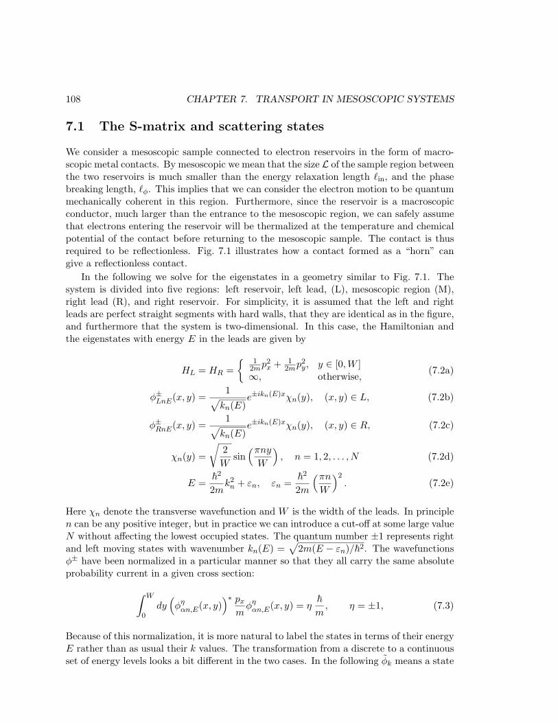
108 CHAPTER 7. TRANSPORT IN MESOSCOPIC SYSTEMS
7.1 The S-matrix and scattering states
We consider a mesoscopic sample connected to electron reservoirs in the form of macro-scopic metal contacts. By mesoscopic we mean that the size L of the sample region betweenthe two reservoirs is much smaller than the energy relaxation length `in, and the phasebreaking length, `φ. This implies that we can consider the electron motion to be quantummechanically coherent in this region. Furthermore, since the reservoir is a macroscopicconductor, much larger than the entrance to the mesoscopic region, we can safely assumethat electrons entering the reservoir will be thermalized at the temperature and chemicalpotential of the contact before returning to the mesoscopic sample. The contact is thusrequired to be reflectionless. Fig. 7.1 illustrates how a contact formed as a “horn” cangive a reflectionless contact.
In the following we solve for the eigenstates in a geometry similar to Fig. 7.1. Thesystem is divided into five regions: left reservoir, left lead, (L), mesoscopic region (M),right lead (R), and right reservoir. For simplicity, it is assumed that the left and rightleads are perfect straight segments with hard walls, that they are identical as in the figure,and furthermore that the system is two-dimensional. In this case, the Hamiltonian andthe eigenstates with energy E in the leads are given by
HL = HR =
12mp2
x + 12mp2
y, y ∈ [0,W ]∞, otherwise,
(7.2a)
φ±LnE(x, y) =1√
kn(E)e±ikn(E)xχn(y), (x, y) ∈ L, (7.2b)
φ±RnE(x, y) =1√
kn(E)e±ikn(E)xχn(y), (x, y) ∈ R, (7.2c)
χn(y) =
√2W
sin(πny
W
), n = 1, 2, . . . , N (7.2d)
E =~2
2mk2
n + εn, εn =~2
2m
(πn
W
)2. (7.2e)
Here χn denote the transverse wavefunction and W is the width of the leads. In principlen can be any positive integer, but in practice we can introduce a cut-off at some large valueN without affecting the lowest occupied states. The quantum number ±1 represents rightand left moving states with wavenumber kn(E) =
√2m(E − εn)/~2. The wavefunctions
φ± have been normalized in a particular manner so that they all carry the same absoluteprobability current in a given cross section:
∫ W
0dy
(φη
αn,E(x, y))∗ px
mφη
αn,E(x, y) = η~m
, η = ±1, (7.3)
Because of this normalization, it is more natural to label the states in terms of their energyE rather than as usual their k values. The transformation from a discrete to a continuousset of energy levels looks a bit different in the two cases. In the following φk means a state
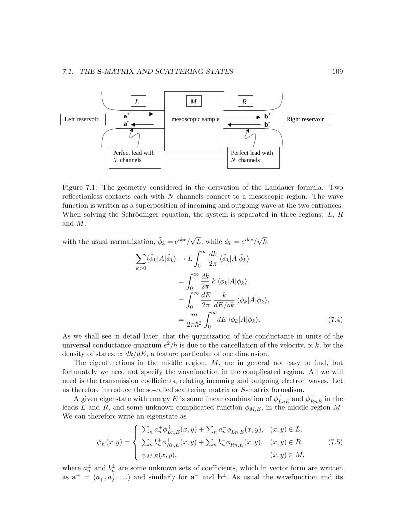
7.1. THE S-MATRIX AND SCATTERING STATES 109
b+
b-a-a+
Perfect lead withN channels
Right reservoirLeft reservoir mesoscopic sample
L M R
Perfect lead withN channels
Figure 7.1: The geometry considered in the derivation of the Landauer formula. Tworeflectionless contacts each with N channels connect to a mesoscopic region. The wavefunction is written as a superposition of incoming and outgoing wave at the two entrances.When solving the Schrodinger equation, the system is separated in three regions: L, Rand M .
with the usual normalization, φk = eikx/√
L, while φk = eikx/√
k.∑
k>0
〈φk|A|φk〉 → L
∫ ∞
0
dk
2π〈φk|A|φk〉
=∫ ∞
0
dk
2πk 〈φk|A|φk〉
=∫ ∞
0
dE
2π
k
dE/dk〈φk|A|φk〉,
=m
2π~2
∫ ∞
0dE 〈φk|A|φk〉. (7.4)
As we shall see in detail later, that the quantization of the conductance in units of theuniversal conductance quantum e2/h is due to the cancellation of the velocity, ∝ k, by thedensity of states, ∝ dk/dE, a feature particular of one dimension.
The eigenfunctions in the middle region, M , are in general not easy to find, butfortunately we need not specify the wavefunction in the complicated region. All we willneed is the transmission coefficients, relating incoming and outgoing electron waves. Letus therefore introduce the so-called scattering matrix or S-matrix formalism.
A given eigenstate with energy E is some linear combination of φ±LnE and φ±RnE in theleads L and R, and some unknown complicated function φM,E , in the middle region M .We can therefore write an eigenstate as
ψE(x, y) =
∑n a+
n φ+Ln,E(x, y) +
∑n a−n φ−Ln,E(x, y), (x, y) ∈ L,
∑n b+
n φ+Rn,E(x, y) +
∑n b−n φ−Rn,E(x, y), (x, y) ∈ R,
ψM,E(x, y), (x, y) ∈ M,
(7.5)
where a±n and b±n are some unknown sets of coefficients, which in vector form are writtenas a+ = (a+
1 , a+2 , . . .) and similarly for a− and b±. As usual the wavefunction and its

110 CHAPTER 7. TRANSPORT IN MESOSCOPIC SYSTEMS
derivative must be continuous. For a given ψM,E in the middle region this condition gives4×N linearly independent equations to determine a±n and b±n . These equations are
(a+
n + a−n)
=√
kn(E)∫
dy χn(y)ψM,E(0, y),(b+n eikn(E)L + b−n e−ikn(E)L
)=
√kn(E)
∫dy χn(y)ψM,E(L, y),
(a+
n − a−n)
=1
i√
kn(E)
∫dy χn(y)
(∂xψM (x, y)
)x=0
,
(b+n eikn(E)L − b−n e−ikn(E)L
)=
1i√
kn(E)
∫dy χn(y)
(∂xψM,E(x, y)
)x=L
.
Fortunately, we will not have to solve such a system of equations unless we want an exactexpression for the wavefunction. It is merely written down in order to illustrate the lineardependence of the coefficients, a±n and b±n . A particular useful way of representing thelinear dependence is through the so-called scattering matrix, or S-matrix, which relatesthe amplitudes of outgoing waves, φ−L and φ+
R, to incoming waves, φ+L and φ−R,
cout ≡(
a−
b+
)=
(r t′
t r′
)(a+
b−
)≡ S
(a+
b−
)≡ S cin. (7.7)
Here we have defined the important S-matrix to be a matrix of size 2N × 2N with theN ×N reflection and transmission matrices as block elements
S =(
r t′
t r′
). (7.8)
Here the matrix element tnn′ represents the transmission amplitude for an incoming wavefrom the left in state n′ to be transmitted into state n on the right hand side. The ampli-tude for transmission in the opposite direction is given by t′nn′ . Similarly the element rnn′
gives the amplitude for being reflected back into the left lead in state n. The coefficientsof the scattering matrix are of course energy dependent. Most of the time, we suppressthis dependence in the notation.
We now define the so-called scattering states, which are states with an incoming wavein one particular lead state, i.e. cin = (0, . . . 0, 1, 0, . . .). The scattering states are denotedψ±, where the superscript ± refers to the direction from which the incoming wave comes.In the plus direction (an incoming wave from the left) the scattering states are
ψ+nE(x, y) =
φ+Ln,E(x, y) +
∑n′ rn′nφ−Ln′,E(x, y), (x, y) ∈ L,∑
n′ tn′nφ+Rn′,E(x, y), (x, y) ∈ R,
? (x, y) ∈ M.
(7.9)
and in the minus direction (an electron incoming from the right hand side)
ψ−nE(x, y) =
φ−Rn,E(x, y) +∑
n′ r′n′nφ+
Rn′,E(x, y), (x, y) ∈ R,∑n′ t
′n′nφ−Ln′,E(x, y), (x, y) ∈ L,
? (x, y) ∈ M.
(7.10)

7.1. THE S-MATRIX AND SCATTERING STATES 111
The wavefunction in the scattering region is not specified, because to find the conductanceall we need is the transmission probabilities of electrons, and that we can get from theS-matrix.
7.1.1 Unitarity of the S-matrix
Before we calculate the transport properties of a mesoscopic system, let us look at someproperties of the S-matrix. First of all, it must be unitary, i.e. S−1 = S†. This is aconsequence of probability current conservation. The incoming electron flux
∑n |cin|2 =
|cin|2 must equal the outgoing flux∑
n |cout|2 = |cout|2 and therefore
c†outcout = c†incin ⇒ c†in (1− S†S) cin = 0, (7.11)
and hence S† = S−1. From the unitarity follows some properties of r and t, which we willmake use of below:
S†S = 1 ⇔
1 = r†r + t†t = r′†r′ + t′†t′,0 = r†t′ + t†r′ = t′†r + r′†t, , (7.12)
and furthermore
SS† = 1 ⇔
1 = r′r′†+tt† = rr† + t′t′†,0 = rt† + t′r′† = tr†+r′t′†.
(7.13)
We also show the unitarity in a bit more explicit way by calculating the currents onthe left and right hand sides of the system. This we do because we will need the currentslater on anyway. The current through a cross section for a given state is, cf. Eq. (1.99b),
I(x) =∫ W
0dy Ψ∗(x, y)
↔JxΨ(x, y),
↔Jx =
~2mi
(→∂ x −
←∂ x
), (7.14)
where the arrows indicate to which side the differential operators are acting. For a station-ary state, i.e. an eigenstate with energy E, the continuity equation gives ∂xJ = −ρ = 0,i.e. I(x) cannot depend on x. Let us compute I(x) for a state with incoming coefficientscin = (a+,b−). First calculate the current in region L
IL(x) =∫ W
0dy
(a+ · φ+
L,E + a− · φ−L,E
)∗ ↔Jx
(a+ · φ+
L,E + a− · φ−L,E
)
=~m
(|a+|2 −
∣∣ra+ + t′b−∣∣2
), (7.15)
where φ+L,E = (φ+
L,1E , φ+L,2E , . . .) and φ−L,E = (φ−L,1E , φ−L,2E , . . .). In the same way for R we
obtain
IR(x) =~m
(−|b−|2 +
∣∣ta+ + r′b−∣∣2
), (7.16)
112 CHAPTER 7. TRANSPORT IN MESOSCOPIC SYSTEMS
or more detailed
IL =~m
[(a+
)† (1− r†r) · a+ − (b−
)† (t′†t′
)b− − 2Re[
(a+
)† r†t′b−]
](7.17a)
IR =~m
[(b+
)† (−1 + r′†r′)b+ +(a+
)† (t†t
)a+ − 2Re[
(a+
)† t†r′b−]
]. (7.17b)
From the continuity equation we know that the current on the two sides must be equal,IL = IR, and we obtain Eq. (7.12) and hence S is unitary.
7.1.2 Time-reversal symmetry
Time-reversal symmetry means that H = H∗, because if Ψ(r, t) is a solution to theShrodinger equation so is Ψ∗(r,−t). In that case the scattering matrix is not only unitaryit is also symmetric, S = ST . This has some important consequences for the statistics ofS-matrices in disordered systems, which can be seen experimentally by studying transportwith and without an applied magnetic field.
A non-zero magnetic field B = ∇×A breaks time-reversal symmetry, and in this casethe Schrodinger equation is
HB ΨB(r) =[− ~
2
2m
(∇r + i
e
~A
)2+ V (r)
]ΨB(r) = E ΨB(r). (7.18)
Now, since HB = H∗−B we see that
HB ΨB(r) = E ΨB(r) ⇔ H∗−B Ψ∗
−B(r) = E Ψ∗−B(r), (7.19)
or in short: if ΨB(r) is a solution so is Ψ∗−B(r). We can therefore construct new eigen-
states by complex conjugation followed by reversal of the magnetic field. Suppose we havean eigenstate which is a linear combination of incoming and outgoing waves ΨB(r) =(cinφin, coutφout), then we can make a new eigenstate by Ψnew
−B (r) = Ψ∗B(r), which is a
solution for −B. However, because complex conjugation reverses the direction of propa-gation, the new in- and outgoing wave functions are cnew
in = c∗out, and cnewout = c∗in. Since
Ψnew is a solution for −B, we have
cnewout = S−Bcnew
in ⇒ c*in = S−Bc∗out = S−BS∗Bc*
in, (7.20)
which shows that
S−BS∗B = 1 ⇒ S∗−B = S†B ⇒ SB = ST−B. (7.21)
In case of time-reversal symmetry, the scattering matrix therefore has an additional sym-metry besides being unitary: it is also a symmetric matrix. This will be of importancewhen we look at disordered systems below.
7.2. CONDUCTANCE AND TRANSMISSION COEFFICIENTS 113
7.2 Conductance and transmission coefficients
Next we calculate the conductance. This will be done in two different ways: first wewill argue on physical grounds that the population of the scattering state is given bythe equilibrium distribution function of the reservoir, which allows us to calculate thecurrent directly. Secondly, we calculate the conductance using linear response theory,and, fortunately, we find the same result. While the first method is more physicallyappealing, one could get in doubt if the Pauli principle is treated correctly. The linearresponse result shows that indeed the first method gave the right answer, at least in thelinear response limit.
The answer we find, the celebrated Landauer-Buttiker formula, is very simple andphysically sensible: the conductance of a mesoscopic sample is given by the sum of all thetransmission possibilities a given electron has, i.e. by the sum of transmission probabilities
G =2e2
h
∑n
Tn =2e2
hTr[t†t], (7.22)
where Tn are the eigenvalues of the matrix t†t. This should not be confused with thetransmission probabilities, i.e. the probability that an electron in a given incoming state,n, ends up on the other side. This probability is Tn =
(t†t
)nn
, but when summing overall incoming states n we in fact get,
∑n Tn =
∑n Tn. So we can write Eq. (7.22) in terms
of Tn or Tn as we please.The Landauer-Buttiker formula tells us that the conductance of a mesoscopic sample
is quantized in units of 2e2/h. The number of quanta will be the number of channelsconnecting the two sides. However, since Tn is a number between 0 and 1 one expect thisquantization to show up only for some special geometries where Tn is either 0 or 1. This isin fact what happens for the quantum point contact, which is discussed below in Sec. 7.3.1.There a particular smooth interface between the two reservoirs ensures that Tn changes ina well-controlled manner between 0 and 1. However, there are other examples where theconductance quantum e2/h shows up, namely in the fluctuations of conductance. Thesefluctuations are universal in the sense that they have an amplitude of the order e2/hindependent of the average conductance. This is discussed in Sec. 7.4.3.
7.2.1 The Landauer-Buttiker formula, heuristic derivation
We argued above that if the reservoirs are much wider than the mesoscopic region andits leads, then we can assume reflectionless transmission from the leads to the reservoirs,i.e. the electrons entering the reservoir from the sample are thermalized before returning.Thus all electrons entering from the contacts are distributed according to the Fermi-Dirac distribution nF of the given reservoirs. Furthermore, since the mesoscopic regionis defined to be phase coherent, no energy relaxation takes place there, and consequentlyelectrons originating from, say, the left reservoir maintain their distribution function equalto that of that reservoir. Therefore it is natural to express the occupation of the scatteringeigenstates ψ±nε by two different distribution functions f± and the chemical potentials µL/R
114 CHAPTER 7. TRANSPORT IN MESOSCOPIC SYSTEMS
of the relevant reservoirs,
f+(ε) = nF(ε− µL), f−(ε) = nF(ε− µR). (7.23)
Now it is a simple matter to calculate the current through the mesoscopic system. Becauseof current conservation, we can calculate it in either of the regions L, R, or M . Naturally,we choose to do so in the perfect leads L or R where the wavefunctions are known. Letus look at the current in the left lead:
I = IL = e∑
nk
[I+nkf
+(Enk) + I−nkf−(Enk)
]. (7.24)
The currents carried by a scattering state ψ±nε can be read off from Eqs. (7.17a) and (7.17b)by substituting (a+)n′ = δnn′ for a state moving in the positive direction and (b−)n′ = δnn′
for a state moving in the negative direction. We get
I+nk =
~m
[1−
(r†r
)nn
]=~m
(t†t
)nn
, (7.25)
I−nk = − ~m
(t′†t′
)nn
=~m
[−1 +
(r′†r′
)nn
]. (7.26)
Transforming to an energy integral as in Eq. (7.4), the current is therefore simply
I =e
2π~∑
n
∫ ∞
0dE
[(t†t
)nn
nF(E − µL)−(t′†t′
)nn
nF(E − µR)]. (7.27)
The sum over diagonal elements of(t†t
)is nothing but the trace. The unitarity condition
Eq. (7.13), then leads to Tr[t′†t′] =Tr[t†t], and the current can be written as
I =e
2π~
∫ ∞
0dE Tr
[t†EtE
] [nF(E − µL)− nF(E − µR)
]. (7.28)
In Eq. (7.28), we have stressed the energy dependence of the transmission matrix, but atlow voltages V and temperatures T we can assume Tn to be energy independent and theintegral can be done. For |eV | = |µR−µL| ¿ µ, where µ is the equilibrium electrochemicalpotential, we Taylor expand around µ and find after integration
I =
From spin︷︸︸︷2
e2
hV Tr
[t†EtE
]⇒ G =
2e2
hTr
[t†t
]=
2e2
h
∑n
Tn. (7.29)
This is the famous Landauer-Buttiker formula. Here we have assumed that the spindegrees of freedom are degenerate which gives rise to a simple factor of two. If they arenot degenerate the trace must also include a trace over the spin degrees of freedom.
The expression Eq. (7.27) for current relies on the fact that the scattering states areeigenstates of the system, which means that we should not include any kind of blockingfactors (1 − nF) to ensure that the final state is empty, as one would normally do in aBoltzmann equation. Once a state is occupied in one lead, it is automatically also occupiedin the other. Thus we are not talking about a scattering event from one reservoir to theother, but rather about the thermal population of eigenmodes. In order to dismiss anyconcern about this point, the next section is devoted to a derivation of Eq. (7.22) fromfirst principles using the linear response formalism of Chap. 6.

7.2. CONDUCTANCE AND TRANSMISSION COEFFICIENTS 115
7.2.2 The Landauer-Buttiker formula, linear response derivation
Our starting point is Eq. (6.31) expressing the conductance G in terms of the current-current correlation function,
G(ω) = −2e2
~ωIm
∫ ∞
−∞dt ei(ω+iη)t(−i)Θ(t) 〈[I(x, t), I(x, 0)]〉0 , (7.30)
where the current operator I(x) due to current conservation can be evaluated at any crosssection x in the perfect leads, rendering G independent of x. (Again we consider the spindegenerate case which is the reason for the factor of two.) In second quantization thecurrent operator is given by
I(x) =∑
λλ′jλλ′(x) c†λcλ′ , (7.31)
jλλ′(x) =~
2mi
∫dy ψ∗λ(x, y)
(→∂ x −
←∂ x
)ψλ′(x, y), (7.32)
where we choose ψλ as a set of eigenstates, and where jλλ′ is a matrix element of thecurrent operator. We will of course use the scattering states that we found above as ourbasis, which means that the quantum number λ is specified by λ = E, n, η = ±. Westart by calculating the commutator in Eq. (7.30)
⟨[I(x′, t), I(x′, 0)
]⟩0
=∑
νν′jνν′(x′)
∑
λλ′jλλ′(x′)ei(Eλ−Eλ′ )t/~
⟨[c†λcλ′ , c
†νcν′
]⟩0
=∑
λλ′|jλλ′(x
′)|2 ei(Eλ−Eλ′ )t/~[nF(Eλ)− nF(Eλ′)
], (7.33)
where we used that 〈c†λcλ′〉0 = δλλ′nF(Eλ), and that jλλ′(x′) = (jλ′λ(x′))∗ . Inserting thisinto Eq. (7.30) yields
G(ω) = −2e2
ωIm
∑
λλ′
|jλλ′(x′)|2
(~ω + iη + Eλ − Eλ′)
[nF(Eλ)− nF(Eλ′)
], (7.34)
and in the dc-limit, ω → 0, one has
G(0) = −2~e2π∑
λλ′|jλλ′(x
′)|2(−∂nF(Eλ)
∂Eλ
)δ (Eλ −Eλ′) . (7.35)
Changing the sum over eigenstates to integrals over energy, i.e.∑
λ →∑
nηm
2π~2∫
dE,and setting T = 0 such that
(−∂nF(E)/∂E)
= δ(E − EF ), the conductance becomes
G(0) = −2~e2π( m
2π~2
)2 ∑
nn′,ηη′|jnηEF ,n′η′EF
(x′)|2, (7.36)
116 CHAPTER 7. TRANSPORT IN MESOSCOPIC SYSTEMS
Due to current conservation the current matrix elements jnηEF ,n′η′EF(x′) are independent
of x′, and we evaluate them in the L or R region at our convenience. We obtain
jnηEF ,n′η′EF(x′) =
~m
( (t†t
)nn′
(t†r′
)nn′
− (t′†r
)nn′
(−t′†t′)nn′
)≡ ~
mj, (7.37)
where the rows and columns correspond to η = +1 and −1, respectively. Hence we get
∑
nn′,ηη′|jnηEF ,n′η′EF
(x′)|2 =(~m
)2
Tr[j†j
]
=(~m
)2
Tr[(
t†t)2
+(t′†t′
)2+ r′†tt†r′ + r†t′t′†r
]
= 2(~m
)2
Tr[t†t
], (7.38)
after using the result Eq. (7.13). The final result is therefore
I = −2e2
hTr
[t†t
] ∫dx′ E(x′) =
2e2
hTr
[t†t
]V, (7.39)
which again is the Landauer-Buttiker formula. We have thus seen that it can be derivedmicroscopically, and any doubt about the validity of the treatment of the occupation factorin the heuristic derivation, has been removed.
7.3 Electron wave guides
7.3.1 Quantum point contact and conductance quantization
One of the most striking consequences of the Landauer-Buttiker formula for conductance isthat the conductance of a perfect channel is 2e2/h, and if there are N “perfect” channelsit is N2e2/h. This has been experimentally tested in numerous experiments and it isnow a well-established fact. The first experiments showing this was done by groups inDelft (Holland) and Cambridge (England) in 1988. The technique they used was a so-called splitgate geometry where a set of metallic gate electrodes was put on top of a two-dimensional electron gas such that a narrow contact between the two sides of the 2DEGwas formed, see Fig. 2.10b. By applying voltage to the gates the width of the constrictioncould be controlled very accurately. As the width decreases quantum channels are squeezedout one by one, until only one remains, leading to a staircase of conductance, each stepbeing of height 2e2/h, see Fig. 7.2. We will now see how this nice effect can happen.
Suppose there is a smooth constriction between two electron reservoirs. Smooth heremeans a horn-like shape were the curvature at all points is large compared to the wave-length of the wave which is going to be transmitted through the horn. The relevant waveequation for an electron horn is of course the Schrodinger equation, but there is in prin-ciple no difference between the electron wave guide and horn wave guides used in loud
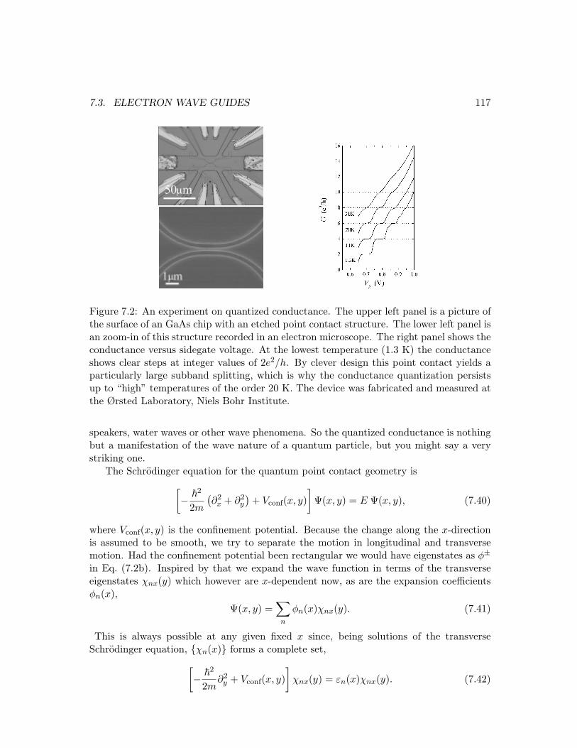
7.3. ELECTRON WAVE GUIDES 117
Figure 7.2: An experiment on quantized conductance. The upper left panel is a picture ofthe surface of an GaAs chip with an etched point contact structure. The lower left panel isan zoom-in of this structure recorded in an electron microscope. The right panel shows theconductance versus sidegate voltage. At the lowest temperature (1.3 K) the conductanceshows clear steps at integer values of 2e2/h. By clever design this point contact yields aparticularly large subband splitting, which is why the conductance quantization persistsup to “high” temperatures of the order 20 K. The device was fabricated and measured atthe Ørsted Laboratory, Niels Bohr Institute.
speakers, water waves or other wave phenomena. So the quantized conductance is nothingbut a manifestation of the wave nature of a quantum particle, but you might say a verystriking one.
The Schrodinger equation for the quantum point contact geometry is[− ~
2
2m
(∂2
x + ∂2y
)+ Vconf(x, y)
]Ψ(x, y) = E Ψ(x, y), (7.40)
where Vconf(x, y) is the confinement potential. Because the change along the x-directionis assumed to be smooth, we try to separate the motion in longitudinal and transversemotion. Had the confinement potential been rectangular we would have eigenstates as φ±
in Eq. (7.2b). Inspired by that we expand the wave function in terms of the transverseeigenstates χnx(y) which however are x-dependent now, as are the expansion coefficientsφn(x),
Ψ(x, y) =∑n
φn(x)χnx(y). (7.41)
This is always possible at any given fixed x since, being solutions of the transverseSchrodinger equation, χn(x) forms a complete set,
[− ~
2
2m∂2
y + Vconf(x, y)]
χnx(y) = εn(x)χnx(y). (7.42)
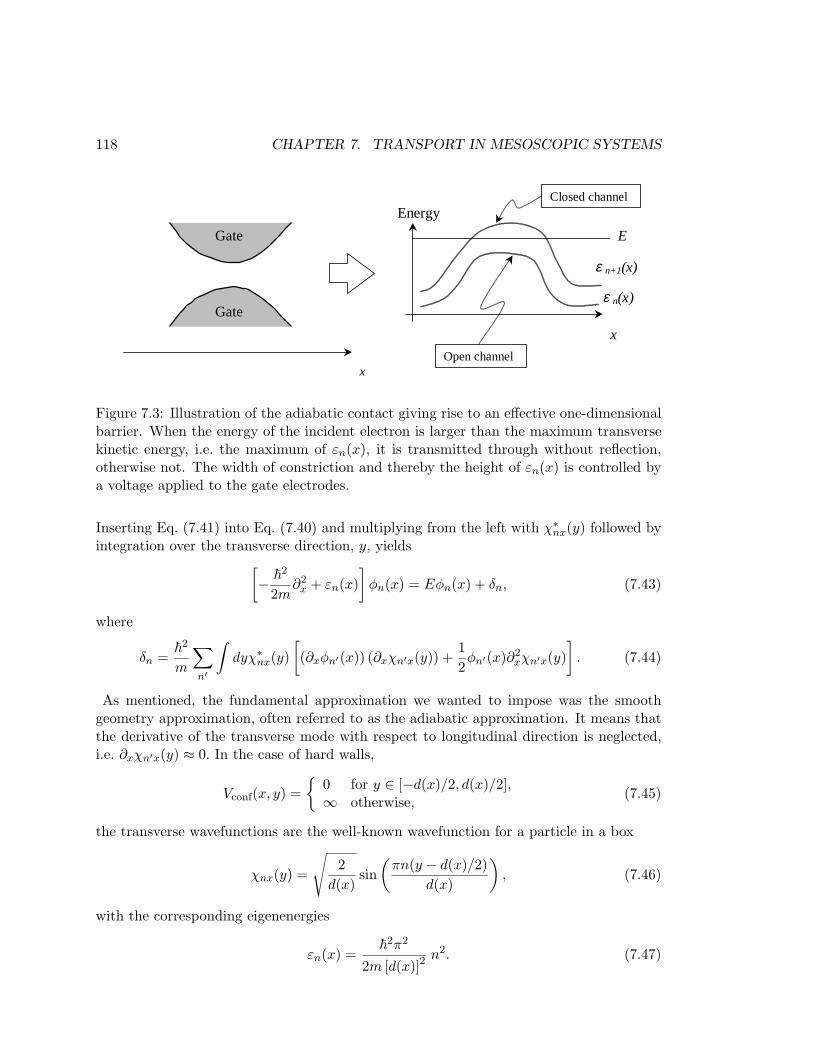
118 CHAPTER 7. TRANSPORT IN MESOSCOPIC SYSTEMS
ε n+1(x)
x
Energy
x
E
Open channel
Closed channel
ε n(x)Gate
Gate
Figure 7.3: Illustration of the adiabatic contact giving rise to an effective one-dimensionalbarrier. When the energy of the incident electron is larger than the maximum transversekinetic energy, i.e. the maximum of εn(x), it is transmitted through without reflection,otherwise not. The width of constriction and thereby the height of εn(x) is controlled bya voltage applied to the gate electrodes.
Inserting Eq. (7.41) into Eq. (7.40) and multiplying from the left with χ∗nx(y) followed byintegration over the transverse direction, y, yields
[− ~
2
2m∂2
x + εn(x)]
φn(x) = Eφn(x) + δn, (7.43)
where
δn =~2
m
∑
n′
∫dyχ∗nx(y)
[(∂xφn′(x)) (∂xχn′x(y)) +
12φn′(x)∂2
xχn′x(y)]
. (7.44)
As mentioned, the fundamental approximation we wanted to impose was the smoothgeometry approximation, often referred to as the adiabatic approximation. It means thatthe derivative of the transverse mode with respect to longitudinal direction is neglected,i.e. ∂xχn′x(y) ≈ 0. In the case of hard walls,
Vconf(x, y) =
0 for y ∈ [−d(x)/2, d(x)/2],∞ otherwise,
(7.45)
the transverse wavefunctions are the well-known wavefunction for a particle in a box
χnx(y) =
√2
d(x)sin
(πn(y − d(x)/2)
d(x)
), (7.46)
with the corresponding eigenenergies
εn(x) =~2π2
2m [d(x)]2n2. (7.47)
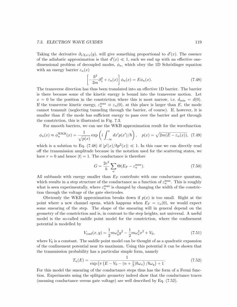
7.3. ELECTRON WAVE GUIDES 119
Taking the derivative ∂xχn′x(y), will give something proportional to d′(x). The essenceof the adiabatic approximation is that d′(x) ¿ 1, such we end up with an effective one-dimensional problem of decoupled modes, φn, which obey the 1D Schrodinger equationwith an energy barrier εn(x)
[− ~
2
2m∂2
x + εn(x)]
φn(x) = Eφn(x). (7.48)
The transverse direction has thus been translated into an effective 1D barrier. The barrieris there because some of the kinetic energy is bound into the transverse motion. Letx = 0 be the position in the constriction where this is most narrow, i.e. dmin = d(0).If the transverse kinetic energy, εmax
n ≡ εn(0), at this place is larger than E, the modecannot transmit (neglecting tunneling through the barrier, of course). If, however, it issmaller than E the mode has sufficient energy to pass over the barrier and get throughthe constriction, this is illustrated in Fig. 7.3.
For smooth barriers, we can use the WKB approximation result for the wavefunction
φn(x) ≈ φWKBn (x) =
1√p(x)
exp(
i
∫ x
−∞dx′p(x′)/~
), p(x) =
√2m(E − εn(x)), (7.49)
which is a solution to Eq. (7.48) if |p′(x)/~p2(x)| ¿ 1. In this case we can directly readoff the transmission amplitude because in the notation used for the scattering states, wehave r = 0 and hence |t| = 1. The conductance is therefore
G =2e2
h
∑n
Θ(EF − εmaxn ). (7.50)
All subbands with energy smaller than EF contribute with one conductance quantum,which results in a step structure of the conductance as a function of εmax
n . This is roughlywhat is seen experimentally, where εmax
n is changed by changing the width of the constric-tion through the voltage of the gate electrodes.
Obviously the WKB approximation breaks down if p(x) is too small. Right at thepoint where a new channel opens, which happens when EF = εn(0), we would expectsome smearing of the step. The shape of the smearing will in general depend on thegeometry of the constriction and is, in contrast to the step heights, not universal. A usefulmodel is the so-called saddle point model for the constriction, where the confinementpotential is modelled by
Vconf(x, y) =12mω2
yy2 − 1
2mω2
xx2 + V0, (7.51)
where V0 is a constant. The saddle point model can be thought of as a quadratic expansionof the confinement potential near its maximum. Using this potential it can be shown thatthe transmission probability has a particular simple form, namely
Tn(E) =1
exp(π
(E − V0 − (n + 1
2)~ωx
)/~ωy
)+ 1
. (7.52)
For this model the smearing of the conductance steps thus has the form of a Fermi func-tion. Experiments using the splitgate geometry indeed show that the conductance traces(meaning conductance versus gate voltage) are well described by Eq. (7.52).
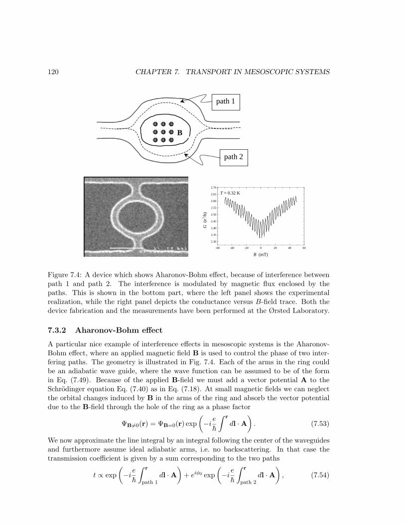
120 CHAPTER 7. TRANSPORT IN MESOSCOPIC SYSTEMS
B
path 1
path 2
-60 -40 -20 0 20 40 60
2.30
2.35
2.40
2.45
2.50
2.55
2.60
2.65
2.70
T = 0.32 K
G (
e 2 /h)
B (mT)
Figure 7.4: A device which shows Aharonov-Bohm effect, because of interference betweenpath 1 and path 2. The interference is modulated by magnetic flux enclosed by thepaths. This is shown in the bottom part, where the left panel shows the experimentalrealization, while the right panel depicts the conductance versus B-field trace. Both thedevice fabrication and the measurements have been performed at the Ørsted Laboratory.
7.3.2 Aharonov-Bohm effect
A particular nice example of interference effects in mesoscopic systems is the Aharonov-Bohm effect, where an applied magnetic field B is used to control the phase of two inter-fering paths. The geometry is illustrated in Fig. 7.4. Each of the arms in the ring couldbe an adiabatic wave guide, where the wave function can be assumed to be of the formin Eq. (7.49). Because of the applied B-field we must add a vector potential A to theSchrodinger equation Eq. (7.40) as in Eq. (7.18). At small magnetic fields we can neglectthe orbital changes induced by B in the arms of the ring and absorb the vector potentialdue to the B-field through the hole of the ring as a phase factor
ΨB 6=0(r) = ΨB=0(r) exp(−i
e
~
∫ r
dl ·A)
. (7.53)
We now approximate the line integral by an integral following the center of the waveguidesand furthermore assume ideal adiabatic arms, i.e. no backscattering. In that case thetransmission coefficient is given by a sum corresponding to the two paths
t ∝ exp(−i
e
~
∫ r
path 1dl ·A
)+ eiφ0 exp
(−i
e
~
∫ r
path 2dl ·A
), (7.54)
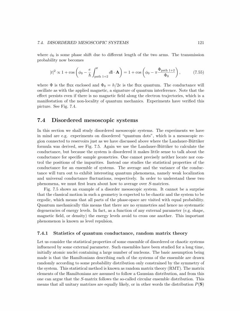
7.4. DISORDERED MESOSCOPIC SYSTEMS 121
where φ0 is some phase shift due to different length of the two arms. The transmissionprobability now becomes
|t|2 ∝ 1 + cos(
φ0 − e
~
∫ r
path 1+2dl ·A
)= 1 + cos
(φ0 − π
Φpath 1+2
Φ0
), (7.55)
where Φ is the flux enclosed and Φ0 = h/2e is the flux quantum. The conductance willoscillate as with the applied magnetic, a signature of quantum interference. Note that theeffect persists even if there is no magnetic field along the electron trajectories, which is amanifestation of the non-locality of quantum mechanics. Experiments have verified thispicture. See Fig. 7.4.
7.4 Disordered mesoscopic systems
In this section we shall study disordered mesoscopic systems. The experiments we havein mind are e.g. experiments on disordered “quantum dots”, which is a mesoscopic re-gion connected to reservoirs just as we have discussed above where the Landauer-Buttikerformula was derived, see Fig. 7.5. Again we use the Landauer-Buttiker to calculate theconductance, but because the system is disordered it makes little sense to talk about theconductance for specific sample geometries. One cannot precisely neither locate nor con-trol the positions of the impurities. Instead one studies the statistical properties of theconductance for an ensemble of systems. The average and the variance of the conduc-tance will turn out to exhibit interesting quantum phenomena, namely weak localizationand universal conductance fluctuations, respectively. In order to understand these twophenomena, we must first learn about how to average over S-matrices.
Fig. 7.5 shows an example of a disorder mesoscopic system. It cannot be a surprisethat the classical motion in such a geometry is expected to be chaotic and the system to beergodic, which means that all parts of the phase-space are visited with equal probability.Quantum mechanically this means that there are no symmetries and hence no systematicdegeneracies of energy levels. In fact, as a function of any external parameter (e.g. shape,magnetic field, or density) the energy levels avoid to cross one another. This importantphenomenon is known as level repulsion.
7.4.1 Statistics of quantum conductance, random matrix theory
Let us consider the statistical properties of some ensemble of disordered or chaotic systemsinfluenced by some external parameter. Such ensembles have been studied for a long time,initially atomic nuclei containing a large number of nucleons. The basic assumption beingmade is that the Hamiltonians describing each of the systems of the ensemble are drawnrandomly according to some probability distribution only constrained by the symmetry ofthe system. This statistical method is known as random matrix theory (RMT). The matrixelements of the Hamiltonians are assumed to follow a Gaussian distribution, and from thisone can argue that the S-matrix follows the so-called circular ensemble distribution. Thismeans that all unitary matrixes are equally likely, or in other words the distribution P (S)
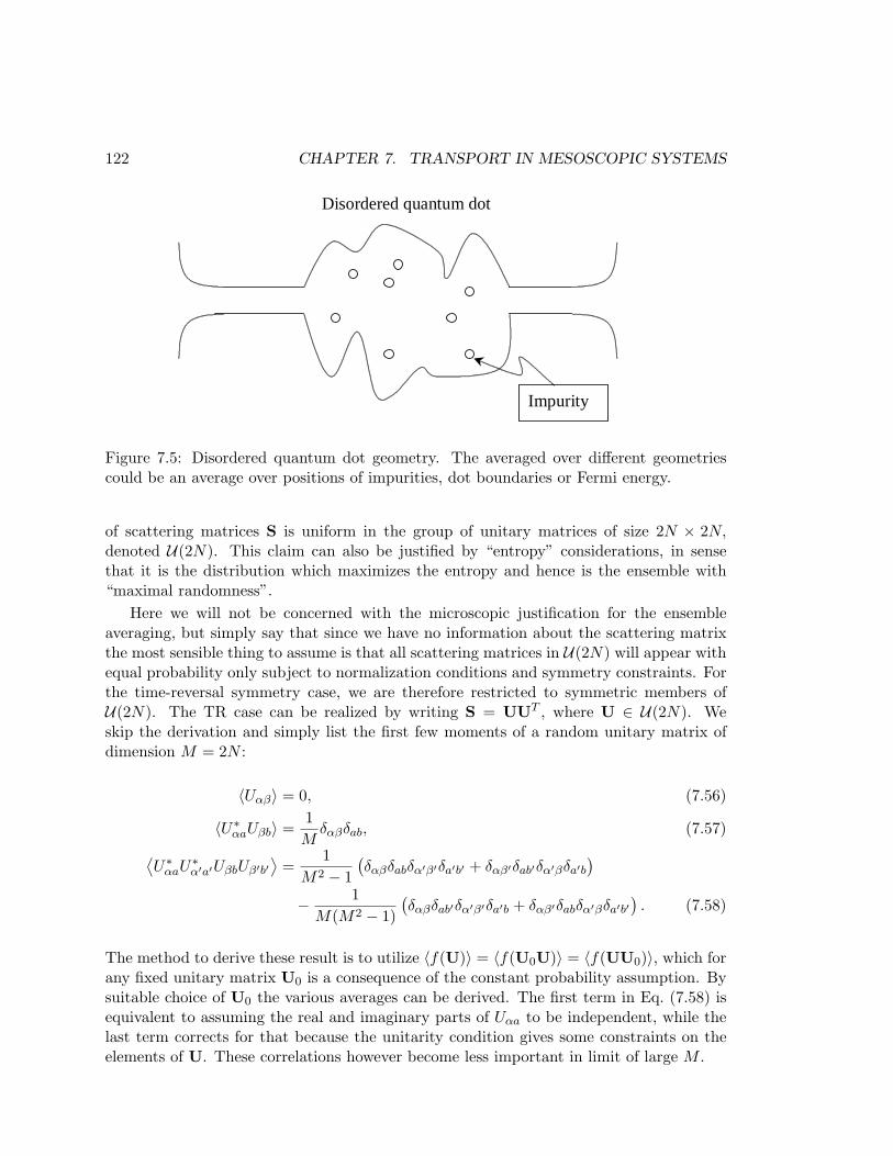
122 CHAPTER 7. TRANSPORT IN MESOSCOPIC SYSTEMS
Disordered quantum dot
Impurity
Figure 7.5: Disordered quantum dot geometry. The averaged over different geometriescould be an average over positions of impurities, dot boundaries or Fermi energy.
of scattering matrices S is uniform in the group of unitary matrices of size 2N × 2N,denoted U(2N). This claim can also be justified by “entropy” considerations, in sensethat it is the distribution which maximizes the entropy and hence is the ensemble with“maximal randomness”.
Here we will not be concerned with the microscopic justification for the ensembleaveraging, but simply say that since we have no information about the scattering matrixthe most sensible thing to assume is that all scattering matrices in U(2N) will appear withequal probability only subject to normalization conditions and symmetry constraints. Forthe time-reversal symmetry case, we are therefore restricted to symmetric members ofU(2N). The TR case can be realized by writing S = UUT , where U ∈ U(2N). Weskip the derivation and simply list the first few moments of a random unitary matrix ofdimension M = 2N :
〈Uαβ〉 = 0, (7.56)
〈U∗αaUβb〉 =
1M
δαβδab, (7.57)
⟨U∗
αaU∗α′a′UβbUβ′b′
⟩=
1M2 − 1
(δαβδabδα′β′δa′b′ + δαβ′δab′δα′βδa′b
)
− 1M(M2 − 1)
(δαβδab′δα′β′δa′b + δαβ′δabδα′βδa′b′
). (7.58)
The method to derive these result is to utilize 〈f(U)〉 = 〈f(U0U)〉 = 〈f(UU0)〉, which forany fixed unitary matrix U0 is a consequence of the constant probability assumption. Bysuitable choice of U0 the various averages can be derived. The first term in Eq. (7.58) isequivalent to assuming the real and imaginary parts of Uαa to be independent, while thelast term corrects for that because the unitarity condition gives some constraints on theelements of U. These correlations however become less important in limit of large M .

7.4. DISORDERED MESOSCOPIC SYSTEMS 123
7.4.2 Weak localization in mesoscopic systems
In Sec. 14.4 studied the weak localization in self-averaging macroscopic samples. Theorigin of this effect was found to be the constructive interference between time-reversedpairs of paths beginning and ending in the same point in space. Also mesoscopic systemsexhibit weak localization. In this case the coherence length is larger than the sample,hence the conductance is given by the S-matrix through the Landauer-Buttiker formula,and we can find the weak localization correction not for an individual sample but for anensemble of samples using random matrix theory of the S-matrix.
It is important to realize that the weak localization correction survives ensemble aver-aging. The average conductance is therefore
〈G〉 =2e2
h
⟨Tr
[t†t
]⟩=
2e2
h
N∑
n=1
2N∑
m=N+1
〈S∗mnSmn〉 . (7.59)
The result now depends on whether time-reversal symmetry is present or not, i.e. if aB-field is applied or not. First take the case of broken time-reversal symmetry, B 6= 0. Inthis case there is no other constraints on S than that it is unitary and there we can useEq. (7.57) directly
〈G〉B 6=0 =2e2
hN2 1
2N=
2e2
h
N
2. (7.60)
The case B = 0 means that in addition to unitarity S is also symmetric. Writing S = UUT
we get
〈G〉B=0 =2e2
h
N∑
n=1
2N∑
m=N+1
2N∑
i=1
2N∑
j=1
〈U∗miU
∗niUmjUnj〉 , (7.61)
and now applying Eq. (7.58), we have
〈G〉B=0 =2e2
h
N∑
n=1
2N∑
m=N+1
2N∑
i=1
2N∑
j=1
(δij + δmnδij)(
1− 12N
)1
4N2 − 1(7.62)
=2e2
h
14N2 − 1
(2N3
)(1− 1
2N
)=
2e2
h
N2
2N + 1, (7.63)
which is smaller than the B 6= 0 result. It is natural to compare the conductance with theclassical conductance i.e. the series connection between two leads with N channels
〈δG〉2e2/h
=〈G〉
2e2/h− N
2=
− N
2(2N+1) , for B = 0,
0 , for B 6= 0.(7.64)
This result clearly shows that quantum corrections, which comes from the last term inEq. (7.58), give a reduced conductance and that the quantum coherence is destroyed bya magnetic field. Of course in reality the transition from the B = 0 to the finite B-fieldcase is a smooth transition. The transition happens when the flux enclosed by a typicaltrajectory is of order the flux quantum, which we saw from the arguments leading toEq. (7.55).
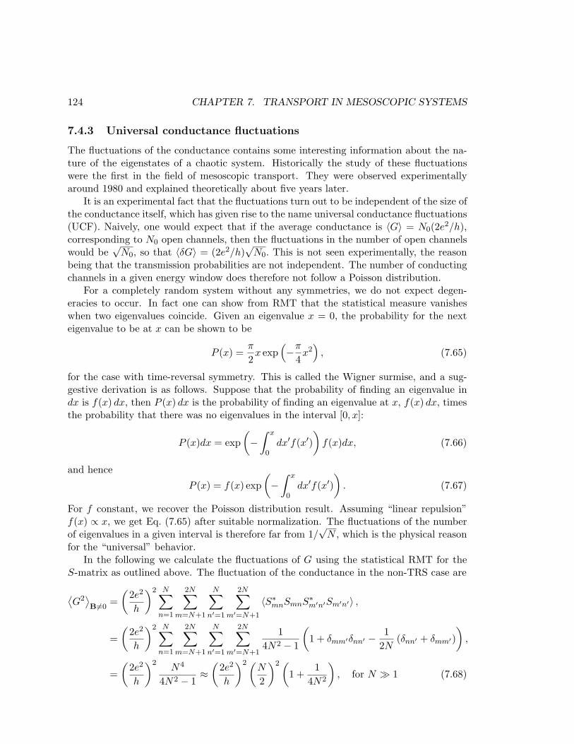
124 CHAPTER 7. TRANSPORT IN MESOSCOPIC SYSTEMS
7.4.3 Universal conductance fluctuations
The fluctuations of the conductance contains some interesting information about the na-ture of the eigenstates of a chaotic system. Historically the study of these fluctuationswere the first in the field of mesoscopic transport. They were observed experimentallyaround 1980 and explained theoretically about five years later.
It is an experimental fact that the fluctuations turn out to be independent of the size ofthe conductance itself, which has given rise to the name universal conductance fluctuations(UCF). Naively, one would expect that if the average conductance is 〈G〉 = N0(2e2/h),corresponding to N0 open channels, then the fluctuations in the number of open channelswould be
√N0, so that 〈δG〉 = (2e2/h)
√N0. This is not seen experimentally, the reason
being that the transmission probabilities are not independent. The number of conductingchannels in a given energy window does therefore not follow a Poisson distribution.
For a completely random system without any symmetries, we do not expect degen-eracies to occur. In fact one can show from RMT that the statistical measure vanisheswhen two eigenvalues coincide. Given an eigenvalue x = 0, the probability for the nexteigenvalue to be at x can be shown to be
P (x) =π
2x exp
(−π
4x2
), (7.65)
for the case with time-reversal symmetry. This is called the Wigner surmise, and a sug-gestive derivation is as follows. Suppose that the probability of finding an eigenvalue indx is f(x) dx, then P (x) dx is the probability of finding an eigenvalue at x, f(x) dx, timesthe probability that there was no eigenvalues in the interval [0, x]:
P (x)dx = exp(−
∫ x
0dx′f(x′)
)f(x)dx, (7.66)
and hence
P (x) = f(x) exp(−
∫ x
0dx′f(x′)
). (7.67)
For f constant, we recover the Poisson distribution result. Assuming “linear repulsion”f(x) ∝ x, we get Eq. (7.65) after suitable normalization. The fluctuations of the numberof eigenvalues in a given interval is therefore far from 1/
√N , which is the physical reason
for the “universal” behavior.In the following we calculate the fluctuations of G using the statistical RMT for the
S-matrix as outlined above. The fluctuation of the conductance in the non-TRS case are
⟨G2
⟩B6=0
=(
2e2
h
)2 N∑
n=1
2N∑
m=N+1
N∑
n′=1
2N∑
m′=N+1
〈S∗mnSmnS∗m′n′Sm′n′〉 ,
=(
2e2
h
)2 N∑
n=1
2N∑
m=N+1
N∑
n′=1
2N∑
m′=N+1
14N2 − 1
(1 + δmm′δnn′ − 1
2N(δnn′ + δmm′)
),
=(
2e2
h
)2N4
4N2 − 1≈
(2e2
h
)2 (N
2
)2 (1 +
14N2
), for N À 1 (7.68)

7.5. SUMMARY AND OUTLOOK 125
Figure 7.6: Variance of the conductance of a quantum dot as a function of magnetic field.The trace is taken at 30 mK. The decrease of the variance when the time-reversal symmetryis broken by the magnetic field is clearly seen and the decreases by approximately a factorof 2 is in agreement with the theory. The inset shows the geometry of the quantum dot,which has additional gates by which the shape can be changed. After Chan et al., Phys.Rev. Lett. 74, 3876 (1995).
and the variance is ⟨δG2
⟩B 6=0
(2e2/h)2≈ 1
16, for N À 1. (7.69)
A similar calculation for the B = 0 case gives⟨δG2
⟩B=0
(2e2/h)2≈ 1
8, for N À 1. (7.70)
The variance is thus independent of the average value of G and furthermore it is expectedto decrease by a factor of 2 when a magnetic field is applying. Indeed this is what is seenexperimentally for example as shown in Fig. 7.6.
7.5 Summary and outlook
Below we list a few text books and review papers about mesoscopic physics.
Text books:
1. Electronic transport in mesoscopic systems,S. Datta, (Cambridge University Press), 1995.
126 CHAPTER 7. TRANSPORT IN MESOSCOPIC SYSTEMS
2. Transport in nanostructures,D.K. Ferry and S.M. Goodnick, (Cambridge University Press), 1995.
Review papers:
1. Quantum transport in semiconductor nanostructures,C.W.J. Beenakker and H. van Houten,Solid State Physics 44, eds. H. Ehrenreich and D. Turnbull, (Academic Press), 1991.
2. Random-matrix theory of quantum transport,C.W.J. Beenakker, Review of Modern Physics 69, 731 (1997).
3. Conductance quantisation in metallic point contacts,J.M. van Ruitenbeek, cond-mat/9910394.
4. The statistical theory of quantum dots,Y. Alhassid, Review of Modern Physics 72, 895 (2000)

Chapter 8
Green’s functions
8.1 “Classical” Green’s functions
The Green’s function method is a very useful method in the theory of ordinary and partialdifferential equations. It has a long history with numerous applications.
To illustrate the idea of the method let us consider the familiar problem of finding theelectrical potential φ given a fixed charge distribution, ρe, i.e. we want to solve Poisson’sequation
∇2φ(r) = − 1ε0
ρe(r). (8.1)
It turns out to be a good idea instead to look for the solution G of a related but simplerdifferential equation
∇2rG(r) = δ(r), (8.2)
where δ(r) is the Dirac delta function. G(r) is called the Green’s function for the Laplaceoperator, ∇2
r. This is a good idea because once we have found G(r), the electrical potentialfollows as
φ(r) = − 1ε0
∫dr′G(r− r′)ρe(r′). (8.3)
That this is a solution to Eq. (8.1) is easily verified by letting ∇2r act directly on the
integrand and then use Eq. (8.2).The easiest way to find G(r) is by Fourier transformation, which immediately gives
−k2G(k) = 1 ⇒ G(k) = − 1k2
, (8.4)
and hence
G(r) =∫
dk(2π)3
eik·rG(k) = −∫
dk(2π)3
eik·r
k2= − 1
4πr. (8.5)
When inserting this into (8.3) we obtain the well-known potential created by a chargedistribution
φ(r) =1
4πε0
∫dr′
ρe(r′)|r− r′| . (8.6)
127
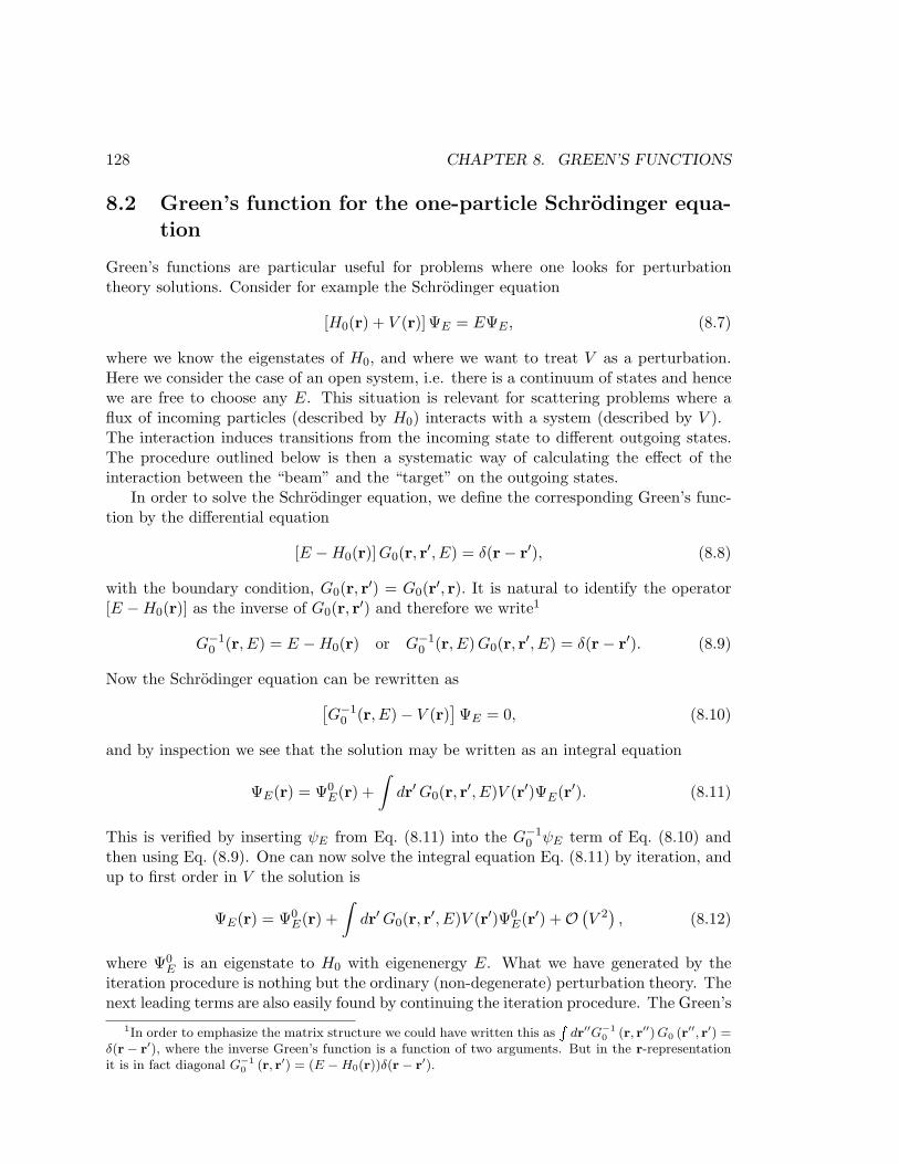
128 CHAPTER 8. GREEN’S FUNCTIONS
8.2 Green’s function for the one-particle Schrodinger equa-tion
Green’s functions are particular useful for problems where one looks for perturbationtheory solutions. Consider for example the Schrodinger equation
[H0(r) + V (r)]ΨE = EΨE , (8.7)
where we know the eigenstates of H0, and where we want to treat V as a perturbation.Here we consider the case of an open system, i.e. there is a continuum of states and hencewe are free to choose any E. This situation is relevant for scattering problems where aflux of incoming particles (described by H0) interacts with a system (described by V ).The interaction induces transitions from the incoming state to different outgoing states.The procedure outlined below is then a systematic way of calculating the effect of theinteraction between the “beam” and the “target” on the outgoing states.
In order to solve the Schrodinger equation, we define the corresponding Green’s func-tion by the differential equation
[E −H0(r)]G0(r, r′, E) = δ(r− r′), (8.8)
with the boundary condition, G0(r, r′) = G0(r′, r). It is natural to identify the operator[E −H0(r)] as the inverse of G0(r, r′) and therefore we write1
G−10 (r, E) = E −H0(r) or G−1
0 (r, E) G0(r, r′, E) = δ(r− r′). (8.9)
Now the Schrodinger equation can be rewritten as[G−1
0 (r, E)− V (r)]ΨE = 0, (8.10)
and by inspection we see that the solution may be written as an integral equation
ΨE(r) = Ψ0E(r) +
∫dr′G0(r, r′, E)V (r′)ΨE(r′). (8.11)
This is verified by inserting ψE from Eq. (8.11) into the G−10 ψE term of Eq. (8.10) and
then using Eq. (8.9). One can now solve the integral equation Eq. (8.11) by iteration, andup to first order in V the solution is
ΨE(r) = Ψ0E(r) +
∫dr′G0(r, r′, E)V (r′)Ψ0
E(r′) +O (V 2
), (8.12)
where Ψ0E is an eigenstate to H0 with eigenenergy E. What we have generated by the
iteration procedure is nothing but the ordinary (non-degenerate) perturbation theory. Thenext leading terms are also easily found by continuing the iteration procedure. The Green’s
1In order to emphasize the matrix structure we could have written this asR
dr′′G−10 (r, r′′) G0 (r′′, r′) =
δ(r− r′), where the inverse Green’s function is a function of two arguments. But in the r-representationit is in fact diagonal G−1
0 (r, r′) = (E −H0(r))δ(r− r′).
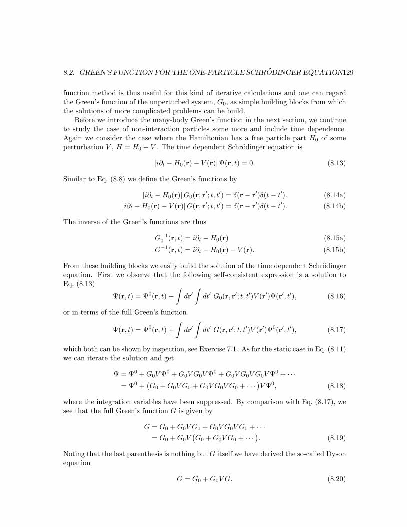
8.2. GREEN’S FUNCTION FOR THE ONE-PARTICLE SCHRODINGER EQUATION129
function method is thus useful for this kind of iterative calculations and one can regardthe Green’s function of the unperturbed system, G0, as simple building blocks from whichthe solutions of more complicated problems can be build.
Before we introduce the many-body Green’s function in the next section, we continueto study the case of non-interaction particles some more and include time dependence.Again we consider the case where the Hamiltonian has a free particle part H0 of someperturbation V , H = H0 + V . The time dependent Schrodinger equation is
[i∂t −H0(r)− V (r)]Ψ(r, t) = 0. (8.13)
Similar to Eq. (8.8) we define the Green’s functions by
[i∂t −H0(r)]G0(r, r′; t, t′) = δ(r− r′)δ(t− t′). (8.14a)[i∂t −H0(r)− V (r)]G(r, r′; t, t′) = δ(r− r′)δ(t− t′). (8.14b)
The inverse of the Green’s functions are thus
G−10 (r, t) = i∂t −H0(r) (8.15a)
G−1(r, t) = i∂t −H0(r)− V (r). (8.15b)
From these building blocks we easily build the solution of the time dependent Schrodingerequation. First we observe that the following self-consistent expression is a solution toEq. (8.13)
Ψ(r, t) = Ψ0(r, t) +∫
dr′∫
dt′ G0(r, r′; t, t′)V (r′)Ψ(r′, t′), (8.16)
or in terms of the full Green’s function
Ψ(r, t) = Ψ0(r, t) +∫
dr′∫
dt′ G(r, r′; t, t′)V (r′)Ψ0(r′, t′), (8.17)
which both can be shown by inspection, see Exercise 7.1. As for the static case in Eq. (8.11)we can iterate the solution and get
Ψ = Ψ0 + G0V Ψ0 + G0V G0V Ψ0 + G0V G0V G0V Ψ0 + · · ·= Ψ0 +
(G0 + G0V G0 + G0V G0V G0 + · · · )V Ψ0, (8.18)
where the integration variables have been suppressed. By comparison with Eq. (8.17), wesee that the full Green’s function G is given by
G = G0 + G0V G0 + G0V G0V G0 + · · ·= G0 + G0V
(G0 + G0V G0 + · · · ). (8.19)
Noting that the last parenthesis is nothing but G itself we have derived the so-called Dysonequation
G = G0 + G0V G. (8.20)
130 CHAPTER 8. GREEN’S FUNCTIONS
This equation will play and important role when we introduce the Feynman diagramslater in the course. The Dyson equation can also be derived directly from Eqs. (8.14) bymultiplying Eq. (8.14b) with G0 from the left.
The Green’s function G(r, t) we have defined here is the non-interaction version of theretarded single particle Green’s function that will be introduced in the following section.It is also often called a propagator because it propagates the wavefunction, i.e. if thewavefunction is know at some time then the wavefunction at later times is given by
Ψ(r, t) =∫
dr′∫
dt′G(rt, r′t′)Ψ(r′, t′), (8.21)
which can be checked by inserting Eq. (8.21) into the Schrodinger equation and using thedefinition Eq. (8.14b).
That the Green’s function is nothing but a propagator is immediately clear when wewrite is it as
G(rt, r′t′) = −iθ(t− t′)〈r|e−iH(t−t′)|r′〉, (8.22)
which indeed is a solution of the partial differential equation defining the Green’s function,Eq. (8.14b), the proof being left as an exercise; see Exercise 7.2. Looking at Eq. (8.22)the Green’s function expresses the amplitude for the particle to be in state |r〉 at time t,given that it was in the state |r′〉 at time t′. We could of course calculate the propagatorin a different basis, e.g. suppose it was in a state |φn′〉 and time t′ then the propagator forending in state |φn〉 is
G(nt, n′t′) = −iθ(t− t′)〈φn|e−iH(t−t′)|φn′〉. (8.23)
The Green’s function are related by a simple change of basis
G(rt, r′t′) =∑
nn′〈r|φn〉G(nt, n′t′)〈φn′ |r′〉. (8.24)
If we choose the basis state |φn〉 as the eigenstates of the Hamiltonian, then the Green’sfunction becomes
G(rt, r′t′) = −iθ(t− t′)∑
n
〈r|φn〉〈φn|r′〉e−iEn(t−t′). (8.25)
Propagation from one point to another in quantum mechanics is generally expressedin terms of transmission amplitudes. As a simple example we end this section by a typicalscattering problem in one dimension. Consider an electron incident on a barrier, locatedbetween x > 0 and x < L, the incoming wave is for x < 0 given by exp(ikx) while theoutgoing wave on the other side x > L is given t exp(ikx). Here t is the transmissionamplitude. The eigenstates are for this example thus given by
ψ(k) =
exp(ikx), for x < 0,t exp(ikx), for x > L.
(8.26)
8.3. SINGLE-PARTICLE GREEN’S FUNCTIONS OF MANY-BODY SYSTEMS 131
When this is inserted into Eq. (8.25) we see that the Green’s function for the x > L andx′ < 0 precisely describes propagator across the scattering region becomes
G(xt, x′t′) = t G0(x, x′; t, t′), x > L and x′ < 0. (8.27)
where G0 is the Green’s function in the absence of the scattering potential. From thisexample it is evident that the Green’s function contains information about the transmissionamplitudes for the particle. See also Exercise 10.2.
8.3 Single-particle Green’s functions of many-body systems
In many-particle physics we adopt the Green’s function philosophy and define some simplebuilding blocks, also called Green’s functions, from which we obtain solutions to ourproblems. The Green’s functions contain only part of the full information carried by thewave functions of the systems but they include the relevant information for the givenproblem. When we define the many-body Green’s functions it is not immediately clearthat they are solutions to differential equations as for the Schrodinger equation Green’sfunctions defined above. But as you will see later they are in fact solutions of equationsof motions with similar structure justifying calling them Green’s functions. Let us simplycarry on and define the different types of Green’s functions that we will be working with.
There are various types of single-particle Green’s functions. The retarded Green’sfunction is defined as
GR(rσt, r′σ′t′) = −iθ(t− t′
) 〈[Ψσ(rt), Ψ†σ′(r
′t′)]B,F 〉,
B : bosonsF : fermions
(8.28)
where the (anti-) commutator [· · · , · · · ]B,F is defined as
[A,B]B = [A, B] = AB −BA,[A,B]F = A, B = AB + BA.
(8.29)
Notice the similarity between the many-body Green’s function Eq. (8.28) and the onefor the propagator for the one particle wavefunction, in Eq. (8.22). For non-interactingparticles they are indeed identical.
The second type of single-particle Green’s functions is the so-called greater and lesserGreen’s functions
G>(rσt, r′σ′t′) = −i〈Ψσ(rt)Ψ†σ′(r
′t′)〉, (8.30a)
G<(rσt, r′σ′t′) = −i (±1) 〈Ψ†σ′(r
′t′)Ψσ(rt)〉. (8.30b)
We see that the retarded Green’s function can be written in terms of these two functionsas
GR(rσt, r′σ′t′) = θ(t− t′
) [G>(rσt, r′σ′t′)−G<(rσt, r′σ′t′)
].
Even though we call these Green’s functions for “single-particle Green’s functions”,they are truly many-body objects because they describe the propagation of single particles
132 CHAPTER 8. GREEN’S FUNCTIONS
governed by the full many-body Hamiltonian. Therefore the single-particle functions caninclude all sorts of correlation effects.
The Green’s functions in Eqs. (8.28), (8.30a), and (8.30b) are often referred to aspropagators. The reason is that they give the amplitude of a particle inserted in point r′
at time t′ to propagate to position r at time t. In this sense GR has its name “retarded”because it is required that t > t′.
The relation between the real space retarded Green’s function and the correspondingone in a general |ν〉-basis as defined in Eq. (1.71) is
GR(σrt, σr′t′) =∑
νν′ψν(σr)GR(νσt, ν′σ′t′)ψ∗ν′(σ
′r′), (8.31)
whereGR(νσt, ν′σ′t′) = −iθ
(t− t′
) 〈[aνσ(t), a†ν′σ′(t′)]B,F 〉, (8.32)
and similarly for G> and G<.
8.3.1 Green’s function of translation-invariant systems
For a system with translation-invariance the usual k-representation is a natural basis set.Since the system is translation-invariant G(r, r′) can only depend on the difference r− r′
and in this case
GR(r− r′, σt, σ′t′) =1V
∑
kk′eik·rGR(kσt,k′σ′t′)e−ik′·r′ ,
=1V
∑
kk′eik·(r−r′)GR(kσt,k′σ′t′)ei(k−k′)·r′ . (8.33)
However, because the right hand side cannot explicitly dependent on the origin and on r′,it follows that G(k,k′) = δk,k′G(k), allowing us to write
GR(r− r′, σt, σ′t′) =1V
∑
k
eik·(r−r′)GR(k, σt, σ′t′), (8.34a)
GR(k, σt, σ′t′) = −iθ(t− t′
) 〈[akσ(t), a†kσ′(t′)]B,F 〉. (8.34b)
The other types of Green’s functions have similar forms.
8.3.2 Green’s function of free electrons
A particular case often encountered in the theory of quantum liquids is the simple case offree particles. Consider therefore the Hamiltonian for free electrons (or other fermions)
H =∑
kσ
ξkσc†kσckσ, (8.35)
8.3. SINGLE-PARTICLE GREEN’S FUNCTIONS OF MANY-BODY SYSTEMS 133
and the corresponding greater function in k-space, which we denote G>0 to indicate that
it is the propagator of free electrons. Because the Hamiltonian is diagonal in the quantumnumbers k and σ so is the Green’s function and therefore
G>0 (kσ, t− t′) = −i
⟨ckσ(t)c†kσ(t′)
⟩. (8.36)
Because of the simple form of the Hamiltonian we are able to find the time dependence ofthe c-operators (see Eq. (5.24))
ckσ(t) = eiHtckσe−iHt = ckσe−iξkt, (8.37)
and similarly c†k(t) = c†keiξkt. An easy way to remember this is to realize that the factore−iHt to the right of ck must have one more electron in state k than eiHt to the left of ck.
Now G> becomes
G>0 (kσ; t− t′) = −i〈ckσc†kσ〉e−iξk(t−t′), (8.38)
and because the Hamiltonian is diagonal in k and the occupation of free electrons is givenby the Fermi-Dirac distribution, we of course have 〈ckσc†kσ〉 = 1− nF (ξk). In exactly thesame way, we can evaluate G<
0 and finally GR0
G>0 (kσ, t− t′) = −i(1− nF (ξk))e−iξk(t−t′), (8.39a)
G<0 (kσ, t− t′) = inF (ξk)e−iξk(t−t′), (8.39b)
GR0 (kσ, t− t′) = −iθ(t− t′)e−iξk(t−t′). (8.39c)
We see that G> gives the propagation of electrons, because it requires an empty state whileG< gives the propagation of holes, because it is proportional to the number of electrons.This is perhaps more clearly seen if we write the T = 0 definition of for example G>
0
G>0 (k,k′, t− t′) = −i〈G|ck(t)c†k′(t
′)|0〉 = −i〈G|cke−iH(t−t′)c†k′ |G〉eiE0(t−t′), (8.40)
which precisely is the overlap between a state with an added electron in state k′ and witha state with an added electron in k and allowing time to evolve from t′ to t. Here |G〉denotes the groundstate of the free electrons, i.e. the filled Fermi sea, |G〉 = |FS〉.
By Fourier transforming from the time domain to the frequency domain, we get infor-mation about the possible energies of the propagating particle. This is intuitively clearfrom Eqs. (8.39) because the propagators evolve periodically in time with the period givenby the energy of the electron. For example, the electron propagator is in the frequencydomain
G>0 (kσ, ω) = −2πi [1− nF (ξk)] δ (ξk − ω) . (8.41)
The corresponding r-dependent propagator, which expresses propagation of a particle inreal space is given by
G>0 (r− r ′, ω)−2πi
=∫
dk(2π)3
(1− nF (ξk))eik·(r−r′)δ (ξk − ω)
= d(ω) (1− nF (ω))sin(kωρ)
kωρ,
k2ω
2m= ω, ρ = |r− r′|, (8.42)
134 CHAPTER 8. GREEN’S FUNCTIONS
where d(ε) = m3/2√
ε/2/π2 is the density of states per spin in three dimensions, seealso Eq. (2.31). The propagation from point r′ to r of a particle with energy ω is thusdetermined by the density of states, d, the availability of an empty state (1 − nF ), theinterference function sin (x) /x that gives the amplitude of a spherical wave spreading outfrom the point r′. See also Exercise 7.3.
8.3.3 The Lehmann representation
A method we will often be using when proving formal results is the so-called Lehmannrepresentation, which is just another name for using the set of eigenstates, |n〉, of thefull Hamiltonian, H, as basis set. Let us for example study the diagonal Green’s function,G>(νtνt′). If we insert 1 =
∑n |n〉〈n| we get
G>(ν; t, t′) = −i〈cν(t)c†ν(t′)〉 = −i
1Z
∑n
〈n|e−βHaν(t)a†ν(t′)|n〉
= −i1Z
∑
nn′e−βEn〈n|cν |n′〉〈n′|a†ν |n〉ei(En−En′ )(t−t′). (8.43)
In the frequency domain, we obtain
G>(ν; ω) =−2πi
Z
∑
nn′e−βEn〈n|aν |n′〉〈n′|c†ν |n〉δ(En − En′ + ω). (8.44)
In the same way we have (for fermions, c)
G<(ν; ω) =2πi
Z
∑
nn′e−βEn〈n|c†ν |n′〉〈n′|cν |n〉δ(En − En′ − ω),
=2πi
Z
∑
nn′e−βEn′ 〈n′|c†ν |n〉〈n|cν |n′〉δ(En′′ − En − ω),
=2πi
Z
∑
nn′e−β(En+ω)〈n′|c†ν |n〉〈n|cν |n′〉δ(En′ − En − ω),
= −G>(ν;ω)e−βω. (8.45)
The retarded Green’s function becomes (again for fermions)
GR(ν, ω) = −i
∫ ∞
0dt ei(ω+iη)t 1
Z
∑
nn′e−βEn
(〈n|cν |n′〉〈n′|c†ν |n〉ei(En−En′ )t
+ 〈n|c†ν |n′〉〈n′|cν |n〉e−i(En−En′ )t)
=1Z
∑
nn′e−βEn
(〈n|cν |n′〉〈n′|c†ν |n〉ω + En −En′ + iη
+〈n|c†ν |n′〉〈n′|cν |n〉ω − En + En′ + iη
)
=1Z
∑
nn′
〈n|cν |n′〉〈n′|c†ν |n〉ω + En − En′ + iη
(e−βEn + e−βEn′
). (8.46)
8.3. SINGLE-PARTICLE GREEN’S FUNCTIONS OF MANY-BODY SYSTEMS 135
Taking the imaginary part of this and using (ω + iη)−1 = P 1ω − iπδ(ω), we get
2 ImGR(ν, ω) = −2π
Z
∑
nn′〈n|cν |n′〉〈n′|c†ν |n〉
(e−βEn + e−βEn′
)δ (ω + En −En′) (8.47)
= −2π
Z
∑
nn′〈n|cν |n′〉〈n′|c†ν |n〉e−βEn(1 + e−βω)δ (ω + En − En′) ,
= −i(1 + e−βω)G>(ν, ω), (8.48)
Defining the spectral function A as
A(ν, ω) = −2 Im GR(ν, ω), (8.49)
we have derived the important general relations
iG>(ν, ω) = A(ν, ω) [1− nF (ω)] , (8.50a)−iG<(ν, ω) = A(ν, ω)nF (ω). (8.50b)
Similar relations hold for bosons, see Exercise 7.4
8.3.4 The spectral function
The spectral function A(ν, ω) can be thought of as either the quantum state resolution ofa particle with given energy ω or as the energy resolution for a particle in a given quantumnumber ν. It gives an indication of how well the excitation created by adding a particlein state ν can be described by a free non-interacting particle. For example if we look atthe retarded propagator for free electrons in Eq. (8.39c)
GR0 (kσ, ω) = −i
∫ ∞
−∞dtθ(t− t′)eiω(t−t′)e−iξk(t−t′)η(t−t′)
=1
ω − ξk + iη, (8.51)
the corresponding spectral function is
A0(kσ, ω) = −2 ImGR0 (kσ, ω) = 2πδ(ω − ξk). (8.52)
Thus for the idealized case of non-interaction free electrons, the spectral function is a deltafunction, which tells us that an excitation with energy ω can only happen by adding anelectron to the state k given by ξk = ω, as expected.
This result is true for any quadratic Hamiltonian, i.e. non-interacting system. If wefor example have
H0 =∑
ν
ξνc†νcν , (8.53)
where ν labels the eigenstates of the system. Again the spectral function is given by asimple delta function
A0(ν, ω) = 2πδ(ω − ξν). (8.54)
136 CHAPTER 8. GREEN’S FUNCTIONS
Generally, due to interactions the spectral function differs from a delta function, butit may still be a peaked function, which then indicates that the non-interacting approxi-mation is not too far from the truth. In Chap. 13 this is discussed in much more detail.
We will now show that the spectral function is a like a probability distribution. Firstly,it is always positive as one must require. This follows from Eq. (8.46), the definition of thespectral function, Eq. (8.49) and the fact that 〈n′|cν |n′〉〈n′|c†ν |n〉 = |〈n′|cν |n′〉|2. Secondly,it obeys the sum rule ∫ ∞
−∞
dω
2πA(ν, ω) = 1. (8.55)
This formula is easily derived by considering the Lehmann representation of −2 Im GR inEq. (8.47)
∫ ∞
−∞
dω
2πA(ν, ω) = −
∫ ∞
−∞
dω
2π2 ImGR(ν, ω)
=∫ ∞
−∞dω
1Z
∑
nn′〈n|cν |n′〉〈n′|c†ν |n〉
(e−βEn + e−βEn′
)
× δ (ω + En −En′)
=1Z
∑
nn′〈n|cν |n′〉〈n′|c†ν |n〉
(e−βEn + e−βEn′
)
= 〈cνc†ν〉+ 〈c†νcν〉 = 〈cνc
†ν + c†νcν〉 = 1, (8.56)
where the last equality follows from the Fermi operator commutation relations.Furthermore, the spectral function is similar to the density of states at a given energy.
This is evident since the occupation nν of a given state ν is for fermions given by (8.50b)
nν = 〈c†νcν〉 = −iG<(ν, t = 0)
= −i
∫ ∞
−∞
dω
2πG<(ν, ω)
=∫ ∞
−∞
dω
2πA(ν, ω)nF (ω). (8.57)
The physical interpretation is that the occupation of a quantum state |ν〉 is an energyintegral of the spectral density of single particle states projected onto the state |ν〉 andweighted by the occupation at the given energy. We of course expect that if the state |ν〉is far below the Fermi surface, e.g. εν ¿ EF , then 〈c†νcν〉 ≈ 1. This in fact follows fromthe sum rule, because if εν ¿ EF and the width of A(ν, ω) is also small compared to EF
then the Fermi function in (8.57) is approximately unity and since A(ν, ω) integrates to2π, see above, the expected result follows.
8.3.5 Broadening of the spectral function
When interactions are present the spectral function changes from the ideal delta function toa broadened profile. One possible mechanism of broadening in a metal is by e.g. electron-phonon interaction, which redistributes the spectral weight because of energy exchange

8.4. MEASURING THE SINGLE-PARTICLE SPECTRAL FUNCTION 137
between the electron and the phonon system. Another mechanism for broadening is theelectron-electron interaction. See Chap. 13.
As a simple example we consider a Green’s function which decays in time due toprocesses that scatters the particle out of the state ν. In this situation the retardedGreen’s function becomes
GR(ν, t) ≈ −iθ(t)e−iξνte−t/τ , (8.58)
where τ is the characteristic decay time. Such a decaying Green’s function corresponds toa finite width of the spectral function
A(ν, ω) = −2 Im∫ ∞
−∞dteiωtGR(ν, t) ≈ 2 Im i
∫ ∞
0dteiωte−iξνte−t/τ =
2/τ
(ω − ξν)2 + (1/τ)2.
(8.59)Thus the width in energy space is given by τ−1.
The simple notion of single electron propagators becomes less well defined for inter-acting systems, which is reflected in a broadening of the spectral function. Amazingly, thefree electron picture is still a good distribution in many cases and in particular for metals,which is quite surprising since the Coulomb interaction between the electrons is a ratherstrong interaction. The reason for this will be discussed later in the Chap. 13 on Fermiliquid theory.
8.4 Measuring the single-particle spectral function
In order to probe the single-particle properties of a many-body system, a solid state samplesay, one must have a way of measuring how the electrons propagate as a function of energy.In practice this means taking out or inserting a particle with definite energy. There arenot too many ways for doing this because most experiments measure density or othertwo-particle properties. For example the response to an electromagnetic field couples tothe charge or current, which, as we saw in the previous chapter, measures charge-chargeor current-current correlation functions, both being two particle propagators.
In principle there is only one way to measure the single particle properties, which isto insert/remove a single electron into/out of a many-body system. This can be achievedby a so-called tunnel junction device or by subjecting the sample to a beam of electrons.However, in some cases also optical experiments approximately measures the single particledensity of states. For example when a photon is absorbed and an electron is kicked outfrom an occupied state to e.g. a freely propagating state outside the material.
In the following we study in detail the tunneling case where an electron tunnels fromone material to the other and show how the tunneling current is expressed in terms of thespectral functions and thus provides a direct measurement of these.
8.4.1 Tunneling spectroscopy
The tunnel experiment set-up consists of two conducting materials brought into closecontact such that electrons can tunnel from one to the other. This is illustrated in Fig. 8.1.
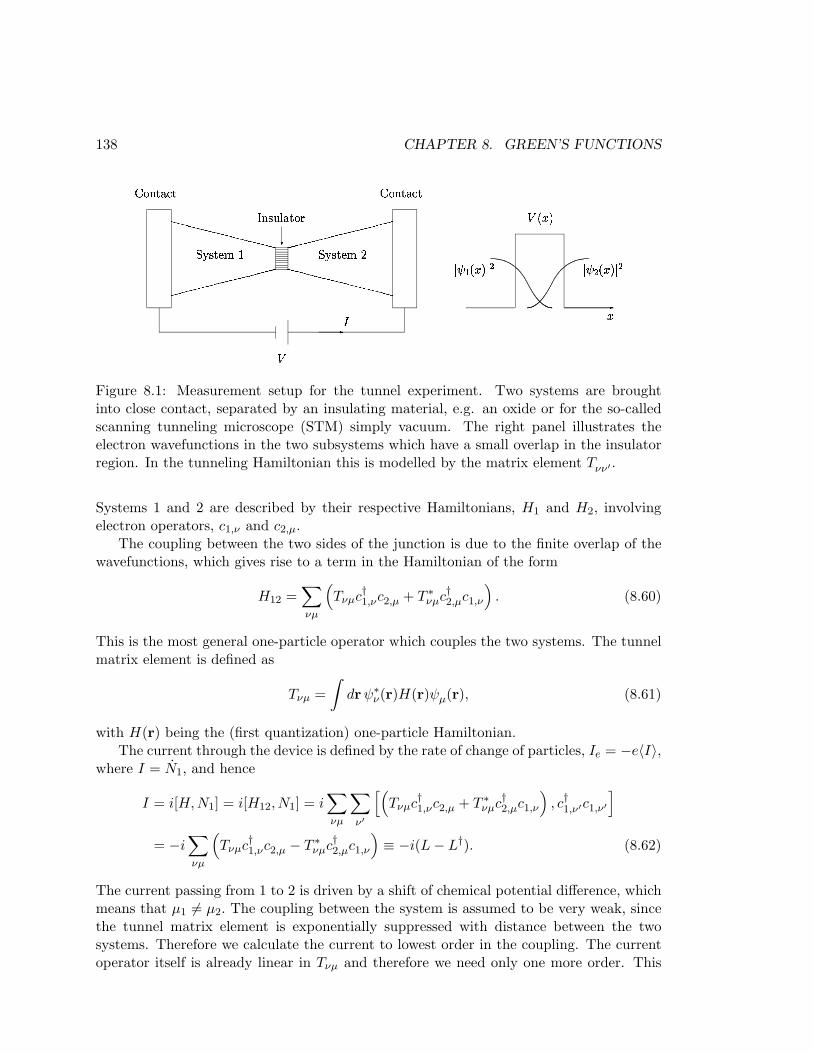
138 CHAPTER 8. GREEN’S FUNCTIONS
!
"
Figure 8.1: Measurement setup for the tunnel experiment. Two systems are broughtinto close contact, separated by an insulating material, e.g. an oxide or for the so-calledscanning tunneling microscope (STM) simply vacuum. The right panel illustrates theelectron wavefunctions in the two subsystems which have a small overlap in the insulatorregion. In the tunneling Hamiltonian this is modelled by the matrix element Tνν′ .
Systems 1 and 2 are described by their respective Hamiltonians, H1 and H2, involvingelectron operators, c1,ν and c2,µ.
The coupling between the two sides of the junction is due to the finite overlap of thewavefunctions, which gives rise to a term in the Hamiltonian of the form
H12 =∑νµ
(Tνµc†1,νc2,µ + T ∗νµc†2,µc1,ν
). (8.60)
This is the most general one-particle operator which couples the two systems. The tunnelmatrix element is defined as
Tνµ =∫
drψ∗ν(r)H(r)ψµ(r), (8.61)
with H(r) being the (first quantization) one-particle Hamiltonian.The current through the device is defined by the rate of change of particles, Ie = −e〈I〉,
where I = N1, and hence
I = i[H, N1] = i[H12, N1] = i∑νµ
∑
ν′
[(Tνµc†1,νc2,µ + T ∗νµc†2,µc1,ν
), c†1,ν′c1,ν′
]
= −i∑νµ
(Tνµc†1,νc2,µ − T ∗νµc†2,µc1,ν
)≡ −i(L− L†). (8.62)
The current passing from 1 to 2 is driven by a shift of chemical potential difference, whichmeans that µ1 6= µ2. The coupling between the system is assumed to be very weak, sincethe tunnel matrix element is exponentially suppressed with distance between the twosystems. Therefore we calculate the current to lowest order in the coupling. The currentoperator itself is already linear in Tνµ and therefore we need only one more order. This
8.4. MEASURING THE SINGLE-PARTICLE SPECTRAL FUNCTION 139
means that linear response theory is applicable. According to the general Kubo formuladerived in chap. 6 the particle current is to first order in H12 given by
〈I〉(t) =∫ ∞
−∞dt′CR
IpH12(t, t′), (8.63a)
CRIpH12
(t− t′) = −iθ(t− t′)〈[Ip(t), H12(t′)]〉eq (8.63b)
where the time development is governed by H = H1 + H2. The correlation function CIH12
can be simplified a bit as
CRIpH12
(t− t′) = −θ(t− t′)⟨[
L(t)− L†(t), L(t′) + L†(t′)]⟩
eq
= −θ(t− t′)[⟨[
L(t), L(t′)]⟩
eq−
⟨[L†(t), L(t′)
]⟩eq
+ c.c.]
. (8.64)
Now the combination⟨[
L(t), L(t′)]⟩
involves terms of the form
⟨(c†1,νc2,µ
)(t)
(c†1,νc2,µ
) (t′)⟩
eq,
with two electrons created in system 1 and two electrons annihilated in system 2 andtherefore is does not conserve the number of particles in each system. Naturally thenumber of particles is a conserved quantity and matrix elements of this type must vanish.2
We are therefore left with
Ip(t) = 2Re∫ ∞
−∞dt′θ(t− t′)
⟨[L†(t), L(t′)
]⟩eq
= 2 Re∫ ∞
−∞dt′θ(t− t′)
∑νµ
∑
ν′µ′T ∗νµTν′µ′
⟨[c†2,µ(t)c1,ν(t), c
†1,ν′(t
′)c2,µ′(t′)]⟩
eq
= 2 Re∫ ∞
−∞dt′θ(t− t′)
∑νµ
∑
ν′µ′T ∗νµTν′µ′
(⟨c1,ν(t)c
†1,ν′(t
′)⟩
eq
⟨c†2,µ(t)c2,µ′(t
′)⟩
eq
−⟨c†1,ν′(t
′)c1,ν(t)⟩
eq
⟨c2,µ′(t
′)c†2,µ(t)⟩
eq
). (8.65)
Now the time dependence due to the shift in energy by the applied voltages is explicitlypulled out such that
c1(t) = c1(t)e−i(−e)V1t, (8.66a)
c2(t) = c2(t)e−i(−e)V2t, (8.66b)
with the time dependence of c being given by the Hamiltonian with a common chemicalpotential µ. Furthermore, we are of course allowed to choose a basis set where the Green’s
2This is in fact not true for superconductors which are characterized by having a spontaneous breakingof the symmetry corresponding to the conservation of particles and therefore such two-particle tunnelprocesses are allowed and give rise to the so-called Josephson current.
140 CHAPTER 8. GREEN’S FUNCTIONS
function of the decoupled system (i.e. without H12) is diagonal, G>νν′ = δνν′G
>ν . The
particle current then becomes (after change of variable t′ → t′ + t)
Ip = 2Re∫ 0
−∞dt′
∑νµ
|Tνµ|2ei(−e)(V1−V2)t′ [G>1 (ν;−t′)G<
2 (µ; t′)−G<1 (ν;−t′)G>
2 (µ; t′)].
(8.67)After Fourier transformation (and reinsertion of the convergence factor eηt′) this expressionbecomes
Ip =∫ ∞
−∞
dω
2π
∑νµ
|Tνµ|2[G>
1 (ν; ω)G<2 (µ; ω + eV )−G<
1 (ν; ω)G>2 (µ; ω + eV )
], (8.68)
with the voltage given by V = V2 − V1. The lesser and greater Green’s functions are nowwritten in terms of the spectral function, see Eq. (8.50), and we finally arrive at
Ip =∫ ∞
−∞
dω
2π
∑νµ
|Tνµ|2A1 (ν, ω) A2(µ, ω + eV )[nF (ω + eV )− nF (ω)]. (8.69)
In Eq. (8.69) we see that the current is determined by two factors: the availability ofstates, given by the difference of occupation functions, and by the density of states at agiven energy. Therefore by sweeping the voltage across the junction one gets informationabout A(ν, ω). This is a widely used spectroscopic principle in for example the studyof superconductors where it was used to verify the famous prediction of the BCS theoryof superconductivity that there is an excitation gap in the superconductor, and that thedensity of states peaks near the gap, see Exercise 4.3 and Exercise 7.5. Also it is used tostudy small structures such as quantum dots where the individual quantum levels becomevisible due to size quantization.
The tunnel spectroscopy technique amounts to a sweep of an external voltage whichcontrols the chemical potential while measuring the differential conductance dI/dV . Ifthe other material is a simple material where one can assume the density of states to bemore or less constant, i.e.
∑µ
|Tνµ|2A2 (ν, ω + eV ) ≈ const. (8.70)
thendI
dV∝
∫ ∞
−∞dω
(−∂nF (ω + eV )
∂ω
)∑ν
A1(ν, ω). (8.71)
At low temperatures where the derivative of the Fermi function tends to a delta functionand (8.71) becomes
dI
dV∝
∑ν
A1(ν,−eV ). (8.72)
So the spectral function can in fact be measured in a rather direct way, which is illustratedin Fig. 8.2.

8.5. TWO-PARTICLE CORRELATION FUNCTIONS OF MANY-BODY SYSTEMS141
Figure 8.2: The principle used in tunneling spectroscopy. The left panel shows the twodensity of states in the two materials. The right one is metal, where there is little variationswith energy and the experiment can therefore be used to get information about the densityof states of the left material. The two right most panels show the resulting current andthe differential conductance trace. It is seen how the differential conductance is a directmeasure of
∑ν A1(ν, ω).
8.4.2 Optical spectroscopy
While the response to an electromagnetic field in principle is always given by the dielectricfunction, which was shown in Chap. 6, there are cases where it is well approximated bythe one-particle spectral function. Such an example is photo emission spectroscopy.
8.5 Two-particle correlation functions of many-body sys-tems
While the single-particle Green’s functions defined above measure the properties of indi-vidual particles the higher order Green’s functions give the response of the quantum systemto processes involving several particles. One important type of higher order Green’s func-tions are the correlation functions, which was encountered in the linear response chapter.For example, we saw that the response to electromagnetic radiation was determined by theauto correlation function of the charge and current densities. Typical correlation functionsthat we will meet are of the type
CAA(t, t′) = −iθ(t− t′)⟨[
A(t), A(t′)]⟩
, (8.73)
where A is some two particle operator.In order to treat a specific case, we evaluate the polarization function χ = Cρρ for a
non-interacting electron gas (see Eq. (6.39)). This function gives for example informationabout the dissipation due to an applied field, because the dissipation, which is the realpart of the conductivity3, is according to Eq. (6.48) given by (take for simplicity the
3Because the power dissipated at any given point in space and time is P (r,t) = Je(r, t) · E(r, t), the
142 CHAPTER 8. GREEN’S FUNCTIONS
translation-invariant case)
Re σ (q, ω) = −ωe2
q2ImχR(q, ω). (8.74)
In momentum space the polarization is given by
χR(q, t− t′) =∫
drχ(r− r′, t− t′)e−iq·(r−r′),
= −iθ(t− t′)∫
dr⟨[
ρ(r, t), ρ(r′, t′)]⟩
e−iq·(r−r′),
= −iθ(t− t′)∫
dr1V2
∑q1q2
⟨[ρ(q1, t), ρ(q2, t
′)]⟩
eiq1·r+iq2·r′e−iq·(r−r′),
= −iθ(t− t′)1V
∑q2
⟨[ρ(q, t), ρ(q2, t
′)]⟩
ei(q2+q)·r′ . (8.75)
Due to the translation-invariance the result cannot depend on r′ and one sees that q2 = −q(or formally one can integrate over r′ and divide by volume to get a delta function, δq2+q,0)and thus
χR(q, t− t′) = −iθ(t− t′)e2 1V
⟨[ρ(q, t), ρ(−q, t′)
]⟩. (8.76)
The Fourier transform of the charge operator was derived in Eq. (1.96)
ρ(q) =∑
kσ
c†kσck+qσ. (8.77)
For free electrons, the time dependence is given by (see Eq. (8.37))
ρ(q, t) =∑
kσ
c†kσck+qσei(ξk−ξk+q)t, (8.78)
which, when inserted into (8.76), yields
χR0 (q, t− t′) = −iθ(t− t′)e2 1
V∑
kk′σσ′〈[c†kσck+qσ, c†k′σ′ck′−q′σ′ ]〉ei(ξk−ξk+q)te
i(ξk′−ξ
k′−q)t′
,
(8.79)where the subindex “0” indicates that we are using the free electron approximation. Thecommutator is easily evaluated using the formula, [c†νcµ, c†ν′cµ′ ] = c†νcµ′δµ,ν′ − c†ν′cµδν′,µ,and we find
χR0 (q, t− t′) = −iθ(t− t′)e2 1
V∑
kσ
[nF (ξk)− nF (ξk+q)
]ei(ξk−ξk+q)(t−t′), (8.80)
total energy being dissipated is
W =
ZdrdtE(r, t) · Je(r, t)=
Zdω
2π
1
V
Xq
E∗(q, ω) · Je(q, ω) =
Zdω
2π
1
V
Xq
|E(q, ω)|2σ(q, ω)
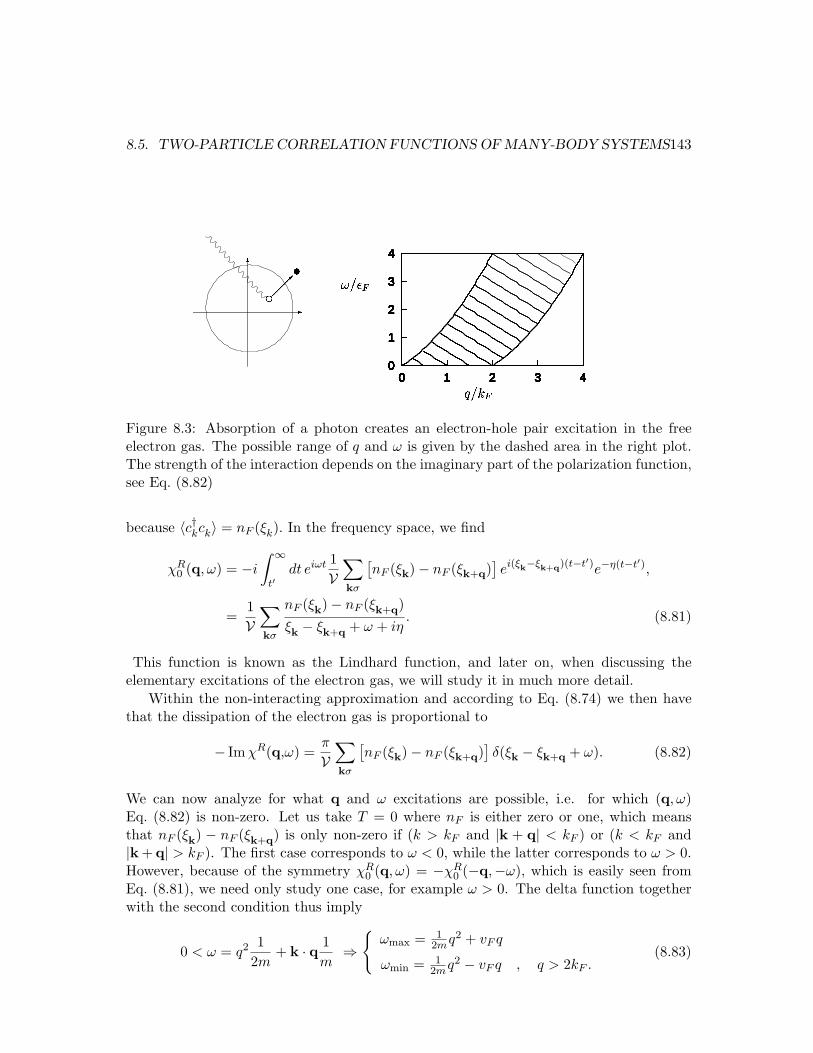
8.5. TWO-PARTICLE CORRELATION FUNCTIONS OF MANY-BODY SYSTEMS143
0
1
2
3
4
0 1 2 3 40
1
2
3
4
0 1 2 3 40
1
2
3
4
0 1 2 3 40
1
2
3
4
0 1 2 3 40
1
2
3
4
0 1 2 3 40
1
2
3
4
0 1 2 3 40
1
2
3
4
0 1 2 3 40
1
2
3
4
0 1 2 3 40
1
2
3
4
0 1 2 3 40
1
2
3
4
0 1 2 3 40
1
2
3
4
0 1 2 3 40
1
2
3
4
0 1 2 3 40
1
2
3
4
0 1 2 3 40
1
2
3
4
0 1 2 3 40
1
2
3
4
0 1 2 3 40
1
2
3
4
0 1 2 3 40
1
2
3
4
0 1 2 3 4
Figure 8.3: Absorption of a photon creates an electron-hole pair excitation in the freeelectron gas. The possible range of q and ω is given by the dashed area in the right plot.The strength of the interaction depends on the imaginary part of the polarization function,see Eq. (8.82)
because 〈c†kck〉 = nF (ξk). In the frequency space, we find
χR0 (q, ω) = −i
∫ ∞
t′dt eiωt 1
V∑
kσ
[nF (ξk)− nF (ξk+q)
]ei(ξk−ξk+q)(t−t′)e−η(t−t′),
=1V
∑
kσ
nF (ξk)− nF (ξk+q)ξk − ξk+q + ω + iη
. (8.81)
This function is known as the Lindhard function, and later on, when discussing theelementary excitations of the electron gas, we will study it in much more detail.
Within the non-interacting approximation and according to Eq. (8.74) we then havethat the dissipation of the electron gas is proportional to
− ImχR(q,ω) =π
V∑
kσ
[nF (ξk)− nF (ξk+q)
]δ(ξk − ξk+q + ω). (8.82)
We can now analyze for what q and ω excitations are possible, i.e. for which (q, ω)Eq. (8.82) is non-zero. Let us take T = 0 where nF is either zero or one, which meansthat nF (ξk) − nF (ξk+q) is only non-zero if (k > kF and |k + q| < kF ) or (k < kF and|k + q| > kF ). The first case corresponds to ω < 0, while the latter corresponds to ω > 0.However, because of the symmetry χR
0 (q, ω) = −χR0 (−q,−ω), which is easily seen from
Eq. (8.81), we need only study one case, for example ω > 0. The delta function togetherwith the second condition thus imply
0 < ω = q2 12m
+ k · q 1m
⇒
ωmax = 12mq2 + vF q
ωmin = 12mq2 − vF q , q > 2kF .
(8.83)
144 CHAPTER 8. GREEN’S FUNCTIONS
The possible range of excitations in (q,ω)-space is shown in Fig.8.3. The excitations whichgive rise to the dissipation are electron-hole pair excitations, where an electron within theFermi sea is excited to a state outside the Fermi sea. There is a continuum of suchexcitations given by conditions in (8.83).
While the electron-hole pair excitations are the only possible source of dissipation in thenon-interacting electron gas, this is certainly not true for the interacting case which is morecomplicated. There is one particular type of excitation which is immensely important,namely the plasmon excitation. This we study in great detail later in this course.
The excitation of the electrons gas can be measured by for example inelastic lightscattering (Raman scattering), where the change of momentum and energy of an incomingphoton is measured. The process discussed here where an electron within the Fermi seais scattering to an empty state outside the Fermi sea, is illustrated in the hand side ofFig. 8.3.
8.6 Summary and outlook
The concept of Green’s functions in many-body physics has been introduced in this chap-ters, and we will use Green’s functions in practically all discussions in the remaining partof the course. The Green’s functions describe the dynamical properties of excitations.We have so far seen two examples of this: the density of states is related to the spectralfunction and it can be measured for example in a tunneling experiment, and secondly theabsorption of electromagnetic radiation is given by the charge-charge correlation function.
The physical picture to remember is that the Green’s function G (rσt, r′σ′t′) gives theamplitude for propagation from the space-time point r′t′ to rt, with initial spin σ′ andfinal spin σ.
In this chapter we have defined the following many-body Green’s functions
GR(rσt, r′σ′t′) = −iθ (t− t′) 〈[Ψσ(rt),Ψ†σ′(r
′t′)]B,F 〉 retarded Green’s functionG>(rσt, σ′r′t′) = −i〈Ψσ(rt)Ψ†
σ′(r′t′)〉 greater Green’s function
G<(rσt, σ′r′t′) = −i (±1) 〈Ψ†σ′(r
′t′)Ψσ(rt)〉 lesser Green’s function
and their corresponding Fourier transforms. The important spectral function is in thefrequency domain and in a diagonal basis given by
A(ν, ω) = −2 ImGR(ν, ω) spectral function
The spectral function is related to the density of states. For non-interacting electrons thespectral function is given by a Dirac delta function
A0(ν, ω) = 2πδ(ξν − ω) non-interacting case

Chapter 9
Equation of motion theory
In the previous chapters we saw how various physical observables can be expressed interms of retarded Green’s functions and correlation functions. In many cases we need tocalculate the time-dependence of these functions. There are several ways of attacking thisproblem, one of which is the equation of motion technique. The basic idea of this methodis to generate a series of coupled differential equations by differentiating the correlationfunction at hand a number of times. If these equations close the problem is in principlesolvable, and if not, one needs to invoke physical arguments to truncate the set of equationsin a reasonable fashion. For example one can neglect certain correlations. We shall studyexamples of both situations in this chapter.
9.1 The single-particle Green’s function
Let us consider the retarded Green’s function GR for either fermions or bosons, Eq. (8.28)
GR(rt, r′t′) = −iθ(t− t′
) 〈[Ψ(rt),Ψ†(r′t′)]B,F 〉. (9.1)
We find the equation of motion for GR as the derivative with respect to the first timeargument
i∂tGR(rt, r′t′) = (−i)
(i∂tθ(t− t′)
) 〈[Ψ(rt), Ψ†(r′t′)]B,F 〉+ (−i) θ(t− t′)〈[i∂tΨ(rt), Ψ†(r′t′)]B,F 〉,
= δ(t− t′)δ(r− r′)+
+ (−i) θ(t− t′)〈[i∂tΨ(rt), Ψ†(r′t′)]B,F 〉. (9.2)
Here we used that the derivative of a step function is a delta function and the commutationrelations for field operators at equal times
[Ψ(r), Ψ†(r′)
]B,F
= δ(r− r′). Next, let us studythe time-derivative of the annihilation operator (throughout this chapter we assume thatH is time independent)
i∂tΨ(rt) = − [H, Ψ(r)] (t) = −[H0, Ψ(r)](t)− [Vint, Ψ(r)](t), (9.3)
145
146 CHAPTER 9. EQUATION OF MOTION THEORY
where the interaction part of the Hamiltonian includes all the interactions in the givenproblem, while H0 describes the quadratic part of the Hamiltonian, for example the kineticenergy. If H0 is the usual kinetic energy Hamiltonian of free particles, we have
−[H0,Ψ(r)] =1
2m
∫dr
[Ψ†(r′)∇2
r′Ψ(r′), Ψ(r)]
= − 12m
∇2rΨ(r). (9.4)
In this case the equation of motion becomes(
i∂t +1
2m∇2
r
)GR(rt, r′t′) = δ(t− t′)δ(r− r′) + DR(rt, r′t′), (9.5a)
DR(rt, r′t′) = −iθ(t− t′)⟨[−[Vint, Ψ(r)](t),Ψ†(r′t′)
]B,F
⟩. (9.5b)
The function DR thus equals the corrections to the free particle Green’s function. Af-ter evaluating [Vint,Ψ(r)] we can, as in Sec. 5.5, continue the generation of differentialequations. It is now evident why the many-body functions, GR, are called Green’s func-tions. The equation in (9.5a) has the structure of the classical Green’s function we sawin Sec. 8.1, where the Green’s function of a differential operator, L, was defined as LG =delta function.
Often it is convenient to work in some other basis, say ν. The Hamiltonian is againwritten as H = H0 + Vint, where the quadratic part of the Hamiltonian is
H0 =∑
νν′tν′νa
†ν′aν . (9.6)
The differential equation for the Green’s function in this basis
GR(νt, ν ′t′) = −iθ(t− t′)〈[aν(t), a†ν′(t
′)]B,F 〉 (9.7)
is found in exactly the same way as above. By differentiation the commutator with H0 isgenerated
−[H0, aν ] =∑
ν′′tνν′′aν′′ , (9.8)
and hence∑
ν′′(iδνν′′∂t − tνν′′) GR(ν ′′t, ν ′t′) = δ(t− t′)δνν′ + DR(νt, ν ′t′), (9.9a)
DR(νt, ν ′t′) = −iθ(t− t′)⟨[−[Vint, aν ](t), a
†ν′(t
′)]B,F
⟩. (9.9b)
In this course we will mainly deal with problems where the Hamiltonian does not dependexplicitly on time (linear response was an exception, but even there the time dependentproblem was transformed into a correlation function of a time independent problem).Therefore the Green’s function can only depend on the time difference t−t′ and in this case

9.2. ANDERSON’S MODEL FOR MAGNETIC IMPURITIES 147
it is always useful to work with the Fourier transforms. Recalling that when performingthe Fourier transformation of the derivative it becomes ∂t → −iω, and that the Fouriertransform of a delta function is unity, δ(t) → 1. We can write the equation of motion infrequency domain
∑
ν′′[δνν′′(ω + iη)− tνν′′ ] GR(ν ′′ν ′;ω) = δνν′ + DR(ν, ν ′;ω), (9.10a)
DR(ν, ν ′; ω) = −i
∫ ∞
−∞dtei(ω+iη)(t−t′)θ(t− t′)
⟨[−[Vint, aν ](t), a
†ν′(t
′)]B,F
⟩. (9.10b)
Here it is important to remember that the frequency of the retarded functions must carrya small positive imaginary part, η, to ensure proper convergence.
9.1.1 Non-interacting particles
For non-interacting particles, which means that the Hamiltonian is bilinear in annihilationor creation operators, we can in fact solve for the Green’s function1. In this case we have
∑
ν′′(δνν′′(ω + iη)− tνν′′)GR
0 (ν ′′ν ′; ω) = δνν′ (9.11)
where the subindex 0 on GR0 indicates that it is the Green’s function corresponding to a
non-interacting Hamiltonian. As in Sec. 8.1 we define the inverse Green’s function as
(GR
0
)−1(νν ′; ω) = δνν′(ω + iη)− tνν′ ≡
(GR
0
)−1
νν′ (9.12)
and in matrix notation Eq. (9.11) becomes
(GR
0
)−1GR
0 = 1. (9.13)
Therefore, in order to find the Green’s function all we need to do is to invert the matrix(GR
0
)−1
νν′ . For a diagonal basis, i.e. tνν′ = δνν′εν , the solution is
(GR
0
)νν′ = GR
0 (ν, ω) δνν′ =1
ω − εν + iηδνν′ , (9.14)
which of course agrees with the result found in Eq. (8.51).
9.2 Anderson’s model for magnetic impurities
In order to exemplify the usefulness of the equation of motion technique, we proceed bysolving a famous model for the appearance of a magnetic moment of impurities of certain
1Here we only consider terms of the form c†c but also anomalous terms like cc could be included.In Chap. 4 we saw that such a term is indeed relevant for superconductors. For the Green’s functionin a superconductor we should therefore solve the linear problem in a way similar to the Bogoliubovtransformation introduced in Chap. 4. We return to this in Chap. 15.
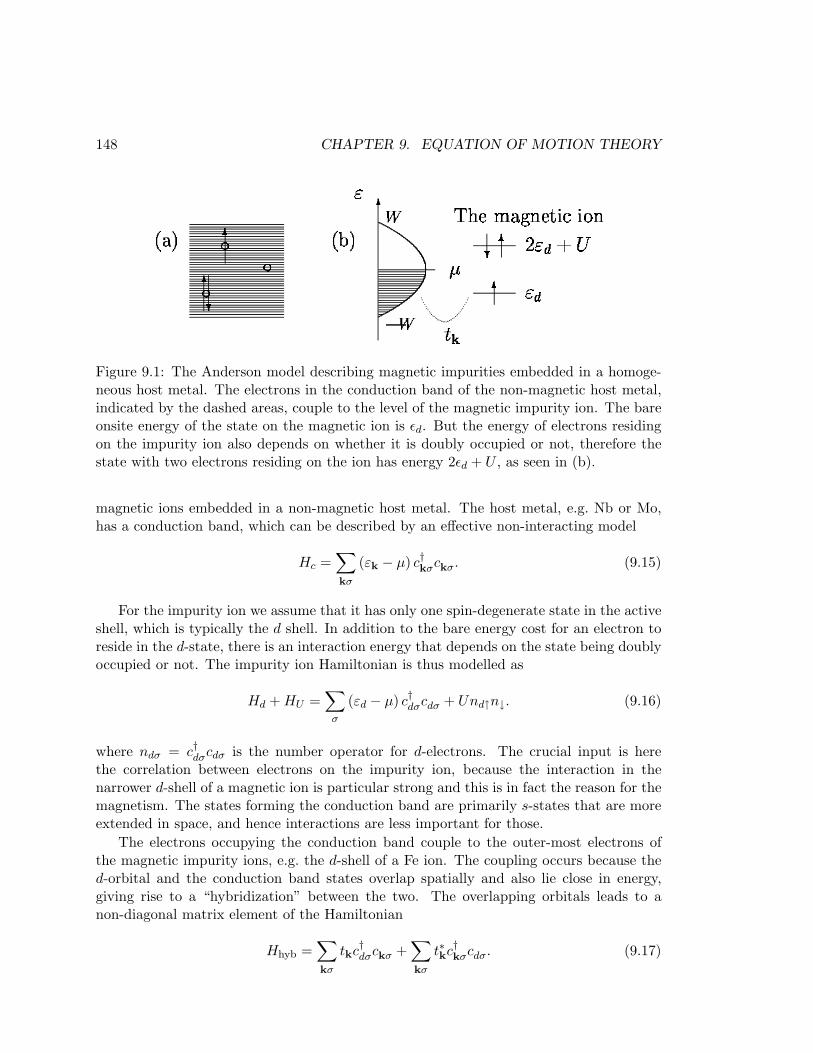
148 CHAPTER 9. EQUATION OF MOTION THEORY
Figure 9.1: The Anderson model describing magnetic impurities embedded in a homoge-neous host metal. The electrons in the conduction band of the non-magnetic host metal,indicated by the dashed areas, couple to the level of the magnetic impurity ion. The bareonsite energy of the state on the magnetic ion is εd. But the energy of electrons residingon the impurity ion also depends on whether it is doubly occupied or not, therefore thestate with two electrons residing on the ion has energy 2εd + U , as seen in (b).
magnetic ions embedded in a non-magnetic host metal. The host metal, e.g. Nb or Mo,has a conduction band, which can be described by an effective non-interacting model
Hc =∑
kσ
(εk − µ) c†kσckσ. (9.15)
For the impurity ion we assume that it has only one spin-degenerate state in the activeshell, which is typically the d shell. In addition to the bare energy cost for an electron toreside in the d-state, there is an interaction energy that depends on the state being doublyoccupied or not. The impurity ion Hamiltonian is thus modelled as
Hd + HU =∑
σ
(εd − µ) c†dσcdσ + Und↑n↓. (9.16)
where ndσ = c†dσcdσ is the number operator for d-electrons. The crucial input is herethe correlation between electrons on the impurity ion, because the interaction in thenarrower d-shell of a magnetic ion is particular strong and this is in fact the reason for themagnetism. The states forming the conduction band are primarily s-states that are moreextended in space, and hence interactions are less important for those.
The electrons occupying the conduction band couple to the outer-most electrons ofthe magnetic impurity ions, e.g. the d-shell of a Fe ion. The coupling occurs because thed-orbital and the conduction band states overlap spatially and also lie close in energy,giving rise to a “hybridization” between the two. The overlapping orbitals leads to anon-diagonal matrix element of the Hamiltonian
Hhyb =∑
kσ
tkc†dσckσ +∑
kσ
t∗kc†kσcdσ. (9.17)
9.2. ANDERSON’S MODEL FOR MAGNETIC IMPURITIES 149
The bare d-electron energy, εd, is below the chemical potential and from the kineticenergy point of view, it is favorable to fill the orbital by two electrons. However, this costspotential energy, U , and it is not possible if 2εd + U > 2µ. Furthermore, the system gainsfurther kinetic energy by the hybridization, which on the other hand is complicated bythe fact that the hopping in and out of the impurity orbital with, say, spin up electronsdepends on the occupation of spin down electrons. The hybridization therefore seems torandomize the spin on the magnetic ion. The sum of these three energy contributions
H = Hc + Hd + HU + Hhyb (9.18)
is known as the Anderson model. See Fig. 9.1 for an illustration. Although the Andersonmodel looks simple, its full solution is very complicated and in fact the model has a veryrich phase diagram. The Anderson model has been used to describe numerous effects inthe physics of strongly correlated electron systems.2
It turns out that for certain values of the parameters it is energetically favorable for thesystem to have a magnetic moment (and thus minimizing the on-site interaction energy)while for other values there is no magnetic moment (thus gaining maximum hybridizationenergy). The physical question we try to answer here is: Under which circumstances isthe material magnetic?
9.2.1 The equation of motion for the Anderson model
The magnetization in the z-direction is given by the expectation value of the differencen↑ − n↓ between spin up and down occupancy. The occupation of a quantum state wasfound in Eq. (8.57) in terms of the spectral function. For the d-electron occupation wetherefore have
ndσ =∫
dω
2πnF (ω) A(dσ, ω), (9.19)
where A(dσ, ω) is the spectral function, which follows from the retarded Green’s function,GR, see Eq. (8.49). All we need to find is then
GR(dσ; t− t′) = −iθ(t− t′
) ⟨cdσ (t) , c†dσ
(t′)
⟩. (9.20)
Let us write the equation of motion of this function using Eq. (9.10 ). Due to thehybridization term the Hamiltonian is not diagonal in the d-operators and the equationsof motion will involve another Green’s function, namely
GR(kσ, dσ, t− t′) = −iθ(t− t′
) 〈ckσ (t) , c†dσ
(t′)〉. (9.21)
The equation of motion are thus found by letting ν ′′ in Eq. (9.10) run over both d and kand we obtain the coupled equations
(ω + iη − εd + µ) GR(dσ, ω)−∑
k
tkGR(kσ, dσ, ω) = 1 + UDR(dσ, ω), (9.22)
(ω + iη − εk + µ) GR(kσ, dσ, ω)− t∗kGR(dσ, ω) = 0, (9.23)
2The model in fact has a known exact solution, but the solution fills an entire book, and it is hard toextract useful physical information from this solution.
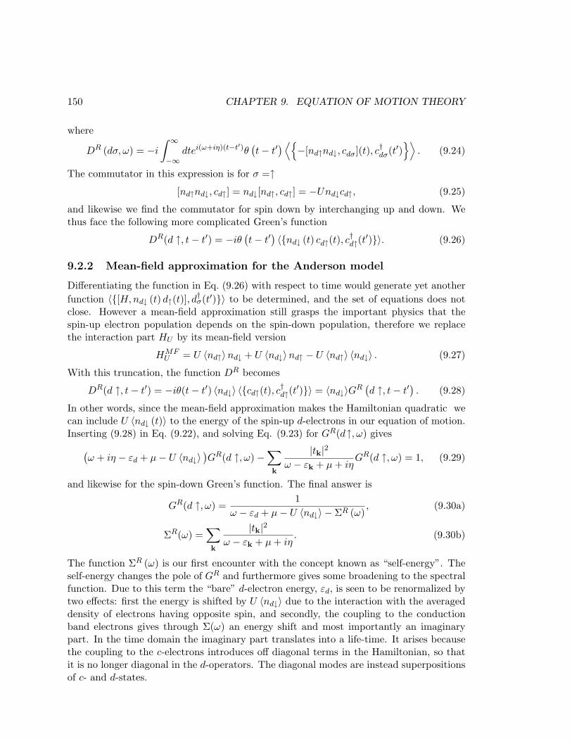
150 CHAPTER 9. EQUATION OF MOTION THEORY
where
DR (dσ, ω) = −i
∫ ∞
−∞dtei(ω+iη)(t−t′)θ
(t− t′
) ⟨−[nd↑nd↓, cdσ](t), c†dσ(t′)
⟩. (9.24)
The commutator in this expression is for σ =↑[nd↑nd↓, cd↑] = nd↓[nd↑, cd↑] = −Und↓cd↑, (9.25)
and likewise we find the commutator for spin down by interchanging up and down. Wethus face the following more complicated Green’s function
DR(d ↑, t− t′) = −iθ(t− t′
) 〈nd↓ (t) cd↑(t), c†d↑(t
′)〉. (9.26)
9.2.2 Mean-field approximation for the Anderson model
Differentiating the function in Eq. (9.26) with respect to time would generate yet anotherfunction 〈[H, nd↓ (t) d↑(t)], d
†σ(t′)〉 to be determined, and the set of equations does not
close. However a mean-field approximation still grasps the important physics that thespin-up electron population depends on the spin-down population, therefore we replacethe interaction part HU by its mean-field version
HMFU = U 〈nd↑〉nd↓ + U 〈nd↓〉nd↑ − U 〈nd↑〉 〈nd↓〉 . (9.27)
With this truncation, the function DR becomes
DR(d ↑, t− t′) = −iθ(t− t′) 〈nd↓〉 〈cd↑(t), c†d↑(t
′)〉 = 〈nd↓〉GR(d ↑, t− t′
). (9.28)
In other words, since the mean-field approximation makes the Hamiltonian quadratic wecan include U 〈nd↓ (t)〉 to the energy of the spin-up d-electrons in our equation of motion.Inserting (9.28) in Eq. (9.22), and solving Eq. (9.23) for GR(d↑, ω) gives
(ω + iη − εd + µ− U 〈nd↓〉
)GR(d ↑, ω)−
∑
k
|tk|2ω − εk + µ + iη
GR(d ↑, ω) = 1, (9.29)
and likewise for the spin-down Green’s function. The final answer is
GR(d ↑, ω) =1
ω − εd + µ− U 〈nd↓〉 − ΣR (ω), (9.30a)
ΣR(ω) =∑
k
|tk|2ω − εk + µ + iη
. (9.30b)
The function ΣR (ω) is our first encounter with the concept known as “self-energy”. Theself-energy changes the pole of GR and furthermore gives some broadening to the spectralfunction. Due to this term the “bare” d-electron energy, εd, is seen to be renormalized bytwo effects: first the energy is shifted by U 〈nd↓〉 due to the interaction with the averageddensity of electrons having opposite spin, and secondly, the coupling to the conductionband electrons gives through Σ(ω) an energy shift and most importantly an imaginarypart. In the time domain the imaginary part translates into a life-time. It arises becausethe coupling to the c-electrons introduces off diagonal terms in the Hamiltonian, so thatit is no longer diagonal in the d-operators. The diagonal modes are instead superpositionsof c- and d-states.
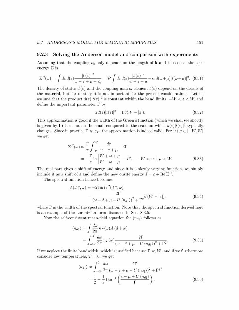
9.2. ANDERSON’S MODEL FOR MAGNETIC IMPURITIES 151
9.2.3 Solving the Anderson model and comparison with experiments
Assuming that the coupling tk only depends on the length of k and thus on ε, the self-energy Σ is
ΣR(ω) =∫
dε d(ε)|t (ε) |2
ω − ε + µ + iη= P
∫dε d(ε)
|t (ε) |2ω − ε + µ
−iπd(ω+µ)|t(ω+µ)|2. (9.31)
The density of states d (ε) and the coupling matrix element t (ε) depend on the details ofthe material, but fortunately it is not important for the present considerations. Let usassume that the product d(ε)|t(ε)|2 is constant within the band limits, −W < ε < W, anddefine the important parameter Γ by
πd(ε)|t(ε)|2 = Γθ(W − |ε|). (9.32)
This approximation is good if the width of the Green’s function (which we shall see shortlyis given by Γ) turns out to be small compared to the scale on which d(ε)|t(ε)|2 typicallychanges. Since in practice Γ ¿ εF , the approximation is indeed valid. For ω+µ ∈ [−W,W ]we get
ΣR(ω) ≈ Γπ
∫ W
−W
dε
ω − ε + µ− iΓ
= −Γπ
ln∣∣∣∣W + ω + µ
W − ω − µ
∣∣∣∣− iΓ, −W < ω + µ < W. (9.33)
The real part gives a shift of energy and since it is a slowly varying function, we simplyinclude it as a shift of ε and define the new onsite energy ε = ε + ReΣR.
The spectral function hence becomes
A(d ↑, ω) = −2 ImGR(d ↑, ω)
=2Γ
(ω − ε + µ− U 〈nd↓〉)2 + Γ2θ (W − |ε|) , (9.34)
where Γ is the width of the spectral function. Note that the spectral function derived hereis an example of the Lorentzian form discussed in Sec. 8.3.5.
Now the self-consistent mean-field equation for 〈nd↑〉 follows as
〈nd↑〉 =∫
dω
2πnF (ω)A (d ↑, ω)
=∫ W
−W
dω
2πnF (ω)
2Γ(ω − ε + µ− U 〈nd↓〉)2 + Γ2
. (9.35)
If we neglect the finite bandwidth, which is justified because Γ ¿ W , and if we furthermoreconsider low temperatures, T = 0, we get
〈nd↑〉 ≈∫ 0
−∞
dω
2π
2Γ(ω − ε + µ− U 〈nd↓〉)2 + Γ2
,
=12− 1
πtan−1
(ε− µ + U 〈nd↓〉
Γ
). (9.36)
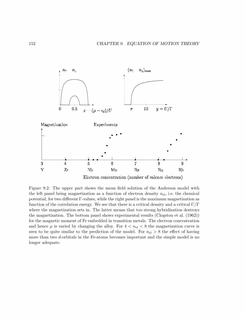
152 CHAPTER 9. EQUATION OF MOTION THEORY
! ! ! " # !%$ ! &' ( ) " ! ! * +
" , ! # - " # ! . / # &' ! *
0 1 20 3 $ 0 1 2%0 3 + 4 5 6
78 $ 9 2;: < + = >?@? A B 8 > = CD ?E
Figure 9.2: The upper part shows the mean field solution of the Anderson model withthe left panel being magnetization as a function of electron density nel, i.e. the chemicalpotential, for two different Γ-values, while the right panel is the maximum magnetization asfunction of the correlation energy. We see that there is a critical density and a critical U/Γwhere the magnetization sets in. The latter means that too strong hybridization destroysthe magnetization. The bottom panel shows experimental results (Clogston et al. (1962))for the magnetic moment of Fe embedded in transition metals. The electron concentrationand hence µ is varied by changing the alloy. For 4 < nel < 8 the magnetization curve isseen to be quite similar to the prediction of the model. For nel > 8 the effect of havingmore than two d-orbitals in the Fe-atoms becomes important and the simple model is nolonger adequate.
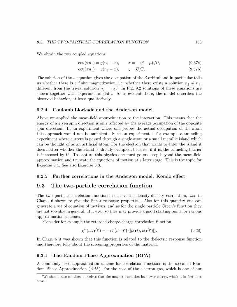
9.3. THE TWO-PARTICLE CORRELATION FUNCTION 153
We obtain the two coupled equations
cot (πn↑) = y(n↓ − x), x = − (ε− µ) /U, (9.37a)cot (πn↓) = y(n↑ − x), y = U/Γ. (9.37b)
The solution of these equation gives the occupation of the d-orbital and in particular tellsus whether there is a finite magnetization, i.e. whether there exists a solution n↓ 6= n↑,different from the trivial solution n↓ = n↑.3 In Fig. 9.2 solutions of these equations areshown together with experimental data. As is evident there, the model describes theobserved behavior, at least qualitatively.
9.2.4 Coulomb blockade and the Anderson model
Above we applied the mean-field approximation to the interaction. This means that theenergy of a given spin direction is only affected by the average occupation of the oppositespin direction. In an experiment where one probes the actual occupation of the atomthis approach would not be sufficient. Such an experiment is for example a tunnelingexperiment where current is passed through a single atom or a small metallic island whichcan be thought of as an artificial atom. For the electron that wants to enter the island itdoes matter whether the island is already occupied, because, if it is, the tunneling barrieris increased by U . To capture this physics one must go one step beyond the mean-fieldapproximation and truncate the equations of motion at a later stage. This is the topic forExercise 8.4. See also Exercise 8.3.
9.2.5 Further correlations in the Anderson model: Kondo effect
9.3 The two-particle correlation function
The two particle correlation functions, such as the density-density correlation, was inChap. 6 shown to give the linear response properties. Also for this quantity one cangenerate a set of equation of motions, and as for the single particle Green’s function theyare not solvable in general. But even so they may provide a good starting point for variousapproximation schemes.
Consider for example the retarded charge-charge correlation function
χR(rt, r′t′) = −iθ(t− t′
) 〈[ρ(rt), ρ(r′t′)]〉. (9.38)
In Chap. 6 it was shown that this function is related to the dielectric response functionand therefore tells about the screening properties of the material.
9.3.1 The Random Phase Approximation (RPA)
A commonly used approximation scheme for correlation functions is the so-called Ran-dom Phase Approximation (RPA). For the case of the electron gas, which is one of our
3We should also convince ourselves that the magnetic solution has lower energy, which it in fact doeshave.
154 CHAPTER 9. EQUATION OF MOTION THEORY
main topics in this course, RPA is exact in some limits, but also in general gives a decentdescription of the interacting electron gas. In Chap.12 RPA is derived using Feynman dia-grams, but here we derive it using the equation of motion technique. The two derivationsgive complementary insight into the physical content of the approximation.
We will for simplicity work with the translation-invariant electron gas with the Hamil-tonian given by the usual kinetic energy plus interaction energy (here we disregard thespin degree of freedom because it is not important)
H =∑
k
ξkc†kck +12
∑
kk′q6=0
V (q)c†k+qc†k−qck′ck = H0 + Vint. (9.39)
Furthermore, the q = 0 component is cancelled by the positively charged background.The charge-charge correlation function is
χR(q, t− t′) = −iθ(t− t′
) 1V
⟨[ρ (q,t) , ρ
(−q,t′)]⟩
, ρ (q) =∑
k
c†kck+q. (9.40)
However, it turns out to be better to work with the function
χR(kq, t− t′) = −iθ(t− t′
) 〈[(c†kck+q) (t) , ρ(−q,t′
)]〉, (9.41)
from which we can easily obtain χ(q) by summing over k, χR(q) =∑
k χR(kq). Let usfind the equation of motion
i∂tχR(kq, t− t′) = δ(t− t′)〈[(c†kck+q)(t), ρ(−q,t′)]〉
− iθ(t− t′)〈[−[H, c†kck+q] (t) , ρ(−q, t′)]〉, (9.42)
and for this purpose we need the following commutators
[c†kck+q, ρ (−q)
]=
∑[c†kck+q, c†k′ck′−q
]= c†kck − c†k+qck+q, (9.43)
[H0, c†kck+q] = (ξk − ξk+q) c†kck+q, (9.44)
[Vint, c†kck+q] = −1
2
∑
k′q′V (q′)
c†k+q′c
†k′−q′ck′ck+q + c†k′+q′c
†k−q′ck+qck′
− c†k′+q′c†kck+q+q′ck′ − c†kc†k′−qck′ck+q−q′
. (9.45)
When this is inserted into Eq. (9.42) a new 6-particle Green’s function is generated. Fur-thermore for each level of the equation of motion a Green’s function with two more electronoperators pops up. At this stage we truncate this series by the random phase approxima-tion which says that the right hand side of (9.45) is replaced by a mean-field expressionwhere pairs of operators are replaced by their average values. Using the recipe from Chap.
9.3. THE TWO-PARTICLE CORRELATION FUNCTION 155
4, we get
[Vint, c†kck+q] ≈ −1
2
∑
k′q′ 6=0
V (q′)
c†k+q′ck+q
⟨c†k′−q′ck′
⟩+
⟨c†k+q′ck+q
⟩c†k′−q′ck′
+⟨c†k−q′ck+q
⟩c†k′+q′ck′ + c†
k−q′ck+q
⟨c†k′+q′ck′
⟩
−c†k′+q′ck′⟨c†kck+q+q′
⟩−
⟨c†k′+q′ck′
⟩c†kck+q+q′
− c†kck+q−q′⟨c†k′−qck′
⟩−
⟨c†kck+q−q′
⟩c†k′−qck′ + const.
=∑
k′V (q)
(⟨nk+q
⟩− 〈nk〉)c†k′−q′ck′ , (9.46)
where we used that 〈c†kck′〉 = 〈nk〉δk,k′ . Note that the exchange pairings which we includedin the Hartree-Fock approximation is not included here.
Collecting everything and going to the frequency domain the equation of motion be-comes,
(ω + iη + ξk − ξk+q) χR(kq, ω) =(⟨
nk+q
⟩− 〈nk〉)(
1− V (q)∑
k′χR(k′q, ω)
), (9.47)
which, when summed over k, allows us to find an equation for χR(q, ω)
χR(q, ω) =1V
∑
k
χR(kq, ω) =1V
∑ 〈nk+q〉 − 〈nk〉ω + ξk − ξk+q + iδ
(1 + V (q) χR(q, ω)
), (9.48)
and hence
χR,RPA(q, ω) =χR
0 (q, ω)1− V (q)χR
0 (q, ω). (9.49)
This is the RPA result of the polarizability function. The free particle polarizabilityχR
0 (q, ω) was derived in Sec. 8.5. The RPA dielectric function becomes
εRPA(q,ω) =[1 + V (q)χR(q, ω)
]−1= 1− V (q) χR
0 (q, ω). (9.50)
Replacing the expectation values, nk, by the Fermi-Dirac distribution function, werecognize the Lindhard function studied in Sec. 8.5. There we studied a non-interactingelectron gas and found that χR(q, ω) indeed was equal to the numerator in (9.49) and thetwo results therefore agree nicely.
In Sec. 8.5 we also analyzed the excitation of the non-interacting electrons gas and theanalysis there is basically still correct. The excitations which were shown in Sec. 8.5 to berelated to the imaginary part of χR(q, ω) and therefore the structure of the electron-holeexcitations of the non-interacting gas (depicted in Fig. 8.3) is preserved here, but of coursethe strength is modified by the real part of the denominator of (9.49).
However, the interactions add other fundamental excitations, namely collective modes,and in the case of a charge liquid these modes are the plasmon modes. The additional

156 CHAPTER 9. EQUATION OF MOTION THEORY
modes are given by the part where the imaginary part of χR0 (q, ω) is zero because then
there is a possibility of a pole in the polarizability. If we set ImχR0 (q, ω) = −iδ, we have
− ImχR(q, ω) =δ[
1− V (q)Re χR0 (q, ω)
]2 + δ2= πδ
(1− V (q)Re χR
0 (q, ω)). (9.51)
This means that there is a well-defined mode when 1 − V (q) ReχR0 (q, ω) = 0 and this
is the plasma oscillation mode, also called a plasmon. The plasmon is studied in detailin Chap. 12, here we just mention that the condition for the mode turns out to beω ∝
√ω2
pl + const. q2.
9.4 Summary and outlook
In this chapter we have seen a method to deal with the dynamical aspects of interactingmany-body systems, namely the equation of motion method applied to the Green’s func-tions. The set of differential equation is not soluble in general, and in fact only a very smallset of Hamiltonians describing interacting systems can be solved exactly. Therefore ap-proximations are necessary and we saw particular examples of this, namely the mean-fieldsolution of a magnetic impurity embedded in a metallic host, and the RPA approximationfor the charge auto correlation function.
In the following chapter we use the equation of motion to derive the Green’s functionsin the imaginary time formalism and to derive the famous Wick’s theorem. Wick’s theoremwill then pave the way for introducing the Feynman diagrams.

Chapter 10
Imaginary time Green’s functions
We have seen that physical observables often have the form of Green’s functions, or thatthey can be derived in a simple way from the Green’s functions. In all the situations wehave studied so far the physical observables have been related to the retarded Green’sfunctions, which in general are defined as
CRAB(t, t′) = −iθ(t− t′)
⟨[A(t), B(t′)
]B,F
⟩,
B : for bosonsF : for fermions
, (10.1)
When A and B are single particle annihilation and creation operators, it is the singleparticle Green’s function defined in Eq. (8.28) from which one could derive the density ofstates. When A and B are two-particle operators, e.g. the density or current operators,CR has the form of a retarded correlation function that was shown to give the linearresponse results of Chap. 6. In Eq. (10.1) boson operators mean either single particleoperators like b or b† or an even number of fermion operators such as c†c appearing in forexample the density operator ρ. The important thing that distinguishes the boson casefrom the fermion case is the sign change that is obtained upon interchange.
In this chapter, we introduce a mathematical method to work out the retarded Green’sfunctions. For technical reasons it is convenient to use a mapping to a more general Green’sfunction, where the time and frequency arguments are imaginary quantities. This has noreal physical meaning, and is only a clever mathematical trick, which we need to learn.This is much like treating electrical circuit theory with complex numbers even thoughall currents and voltages are real. The present chapter concentrates on the mathematicaldetails of the technique and applications are left for later. The imaginary time formalism isparticularly useful when we want to perform perturbation theory, and this will eventuallylead us to the Feynman diagrams.
Let us for example look at the definition of the following correlation function
CAB(t, t′) = − ⟨A(t)B(t′)
⟩, (10.2)
from which we can find the retarded function as CR = iθ(t−t′)(CAB∓CBA). By definitionwe have
CAB(t, t′) = − 1Z
Tr(e−βHA(t)B(t′)). (10.3)
157

158 CHAPTER 10. IMAGINARY TIME GREEN’S FUNCTIONS
Suppose the Hamiltonian is H = H0 + V , where V is the perturbation. Then we saw inChap. 5 that the interaction picture provides a systematic way of expanding in powers ofV. We could try to utilize this and write CAB as
CAB(t, t′) = − 1Z
Tr[e−βHU(0, t)A(t)U(t, t′)B(t′)U(t′, 0)
], (10.4)
In Eq. (5.18) we saw also how a single U operator could be expanded as a time-orderedexponential. This would in Eq. (10.4) result in three time-ordered exponentials, whichcould be collected into a single time-ordered exponential. But the trouble arises for thedensity matrix e−βH , which should also be expanded in powers of the interaction. Tomake a long story short: this is a mess and a new idea is therefore needed. The solutionto this problem is to use imaginary times instead of real times, but bare in mind that thisis purely a mathematical trick without physical contents.
To employ imaginary time is not as far fetched as it might look, because both the den-sity operator ρ = e−βH/Z and the time evolution operator U(t) = e−iHt are both expo-nential functions of the Hamiltonian.1 They therefore satisfy similar differential equations:U satisfies the Schrodinger equation, i∂tU = HU while ρ is the solution to ∂βρ = −Hρ,which is known as the Bloch equation. In order to treat both U and ρ in one go, onereplaces the time argument by a imaginary quantity t → −iτ , where τ is real and hasthe dimension time. In the end this means that both U and ρ can be treated in just oneexpansion in powers of V . Furthermore, we will see that there is a well-defined methodto obtain the physically relevant quantity, i.e. to go back to physical real times from theimaginary time function.
As for real time we can define an imaginary time Heisenberg picture by substitutingit by τ . We define
A(τ) = eτHAe−τH , τ a Greek letter. (10.5)
In this notation, you should use the imaginary time definitions when the time argumentis a Greek letter and the usual definition when the times are written with roman letters,so
A(t) = eitHAe−itH , t a Roman letter. (10.6)
Similar to the interaction picture defined for real times, we can define the interactionpicture for imaginary times as
A(τ) = eτH0Ae−τH0 . (10.7)
Letting H = H0 + V , the relation between the Heisenberg and the interaction picturein imaginary time follows the arguments in Chap. 5. If we consider a product of oper-ators A(τ)B(τ ′) and write it in terms of the corresponding operators in the interactionrepresentation, we get
A(τ)B(τ ′) = U(0, τ)A(τ)U(τ, τ ′)B(τ ′)U(τ ′, 0), (10.8)1Note that we consider only time-independent Hamiltonians in this section. If they are not time-
independent, one cannot use the ordinary equilibrium statistical mechanics but instead one must use anon-equilibrium formalism. This we did in the linear response limit in Chap. 6, but we will not cover themore general case of non-linear time dependent response in this course.
159
where, like in Eq. (5.12), the time-evolution operator U in the interaction picture is
U(τ, τ ′) = eτH0e−(τ−τ ′)He−τ ′H0 . (10.9)
From this it follows directly that
U(τ, τ ′′)U(τ ′′, τ ′) = U(τ, τ ′). (10.10)
An explicit expression for U(τ, τ ′) is found in analogy with the derivation of Eq. (5.18).First we differentiate Eq. (10.9) with respect to τ and find
∂τ U(τ, τ ′) = eτH0(H0 −H)e−(τ−τ ′)He−τ ′H0 = −V (τ)U(τ, τ ′). (10.11)
This is analogous to Eq. (5.13) and the boundary condition, U(τ, τ) = 1, is of course thesame. Now the same iterative procedure is applied and we end with
U(τ, τ ′) =∞∑
n=0
1n!
(−1)n
∫ τ
τ ′dτ1 · · ·
∫ τ
τ ′dτn Tτ
(V (τ1) · · · V (τn)
)
= Tτ exp(−
∫ τ
τ ′dτ1V (τ1)
). (10.12)
The time ordering is again the same as defined in Sec. 5.3, i.e. the operators are orderedsuch that Tτ (A(τ)B(τ ′)) is equal to A(τ)B(τ ′) for τ > τ ′ and B(τ ′)A(τ) when τ ′ > τ .
Above it was argued that the density operator naturally can be treated within theimaginary time formalism, and indeed it can, because by combining Eqs. (10.9) and (10.12)we obtain
e−βH = e−βH0 U(β, 0) = e−βH0 Tτ exp(−
∫ β
0dτ1V (τ1)
). (10.13)
Consider now the time ordered expectation value of the pair of operators in Eq. (10.8)⟨TτA(τ)B(τ ′)
⟩=
1Z
Tr[e−βHTτA(τ)B(τ ′)
]. (10.14)
Utilizing Eqs. (10.8) and (10.13) we can immediately expand in powers of V
⟨TτA(τ)B(τ ′)
⟩=
1Z
Tr[e−βH0U(β, 0) Tτ (U(0, τ)A(τ)U(τ, τ ′)B(τ ′)U(τ ′, 0))
]. (10.15)
This can be written in a much more compact way relying on the properties of Tτ andEq. (10.10)
⟨TτA(τ)B(τ ′)
⟩=
1Z
Tr[e−βH0Tτ U(β, 0)A(τ)B(τ ′)
]=
⟨Tτ U(β, 0)A(τ)B(τ ′)
⟩0⟨
U(β, 0)⟩
0
, (10.16)
where we have used Z = Tr[e−βH
]= Tr
[e−βH0U(β, 0)
], and where the averages 〈· · · 〉0
depending on e−βH0 appear after normalizing with 1/Z0 = 1/Tr[e−βH0
]. This result
demonstrates that the trick of using imaginary time indeed allows for a systematic expan-sion of the complicated looking expression in Eq. (10.4). However, before we can see theusefulness fully, we need to relate the correlation functions written in imaginary time andthe correlation function with real time arguments.
160 CHAPTER 10. IMAGINARY TIME GREEN’S FUNCTIONS
10.1 Definitions of Matsubara Green’s functions
The imaginary time Green’s functions, also called Matsubara Green’s function, is definedin the following way
CAB(τ, τ ′) ≡ − ⟨Tτ
(A(τ)B(τ ′)
)⟩, (10.17)
where the time-ordering symbol in imaginary time has been introduced. It means thatoperators are ordered according to history and just like the time-ordering operator seenin Chap. 5 with the later “times” to the left
Tτ
(A(τ)B(τ ′)
)= θ(τ − τ ′)A(τ)B(τ ′)± θ
(τ ′ − τ
)B(τ ′)A(τ),
+ for bosons,− for fermions.
(10.18)The next question is: What values can τ have? From the definition in Eq. (10.17)
three things are clear. Firstly, CAB(τ, τ ′) is a function of the time difference only, i.e.CAB(τ, τ ′) = CAB(τ − τ ′). This follows from the cyclic properties of the trace. We havefor τ > τ ′
CAB(τ, τ ′) =−1Z
Tr[e−βHeτHAe−τHeτ ′HBe−τ ′H
]
=−1Z
Tr[e−βHe−τ ′HeτHAe−τHeτ ′HB
]
=−1Z
Tr[e−βHe(τ−τ ′)HAe−(τ−τ ′)HB
]
= CAB(τ − τ ′), (10.19)
and of course likewise for τ ′ > τ . Secondly, convergence of CAB(τ, τ ′) is guaranteed onlyif −β < τ − τ ′ < β. For τ > τ ′ the equality τ − τ ′ < β is clearly seen if one usesthe Lehmann representation in Eq. (10.19) to get a factor exp (− [β − τ + τ ′] En) , and,likewise, the second equality is obtained if τ < τ ′. Thirdly, we have the property
CAB(τ) = ±CAB(τ + β), for τ < 0, (10.20)
which again follows from the cyclic properties of the trace. The proof of Eq. (10.20) forτ < 0 is
CAB(τ + β) =−1Z
Tr[e−βHe(τ+β)HAe−(τ+β)HB
]
=−1Z
Tr[eτHAe−τHe−βHB
]
=−1Z
Tr[e−βHBeτHAe−τH
]
=−1Z
Tr[e−βHBA(τ)
]
= ±−1Z
Tr[e−βHTτ (A(τ)B)
]
= ±CAB(τ), (10.21)
and similarly for τ > 0.
10.2. CONNECTION BETWEEN MATSUBARA AND RETARDED FUNCTIONS161
10.1.1 Fourier transform of Matsubara Green’s functions
Next we wish to find the Fourier transforms with respect to the “time” argument τ .Because of the properties above, we take CAB(τ) to be defined in the interval −β < τ < β,and thus according to the theory of Fourier transformations we have a discrete Fourierseries on that interval given by
CAB(n) ≡ 12
∫ β
−βdτ eiπnτ/βCAB(τ), (10.22a)
CAB(τ) =1β
∞∑n=−∞
e−iπnτ/βCAB(n). (10.22b)
However, due to the symmetry property (10.21) this can be simplified as
CAB(n) =12
∫ β
0dτ eiπnτ/βCAB(τ) +
12
∫ 0
−βdτ eiπnτ/βCAB(τ),
=12
∫ β
0dτ eiπnτ/βCAB(τ) + e−iπn 1
2
∫ β
0dτ eiπnτ/βCAB(τ − β),
=12
(1± e−iπn
) ∫ β
0dτ eiπnτ/βCAB(τ), (10.23)
and since the factor(1± e−iπn
)is zero for plus sign and n odd or for minus sign and n
even and 2 otherwise, we obtain
CAB(n) =∫ β
0dτ eiπnτ/βCAB(τ),
n is even for bosons,n is odd for fermions.
(10.24)
From now on we use the following notation for the Fourier transforms of the MatsubaraGreen’s functions
CAB(iωn) =∫ β
0dτ eiωnτCAB(τ),
ωn = 2nπ
β , for bosons,
ωn = (2n+1)πβ , for fermions.
(10.25)
The frequency variable ωn is denoted a Matsubara frequency. Note how the informationabout the temperature is contained in the Matsubara frequencies through β.
Finally, we remark that the boundaries of the integral∫ β0 dτ in Eq. (10.25) leads to
a minor ambiguity of how to treat the boundary τ = 0, for example if CAB(τ) includesa delta function δ(τ). A consistent choice is always to move the time argument into theinterior of the interval [0, β], e.g replace δ(τ) by δ(τ − 0+).
10.2 Connection between Matsubara and retarded functions
We shall now see why the Matsubara Green’s functions have been introduced at all. Inthe frequency domain they are in fact the same analytic function as the usual real times
162 CHAPTER 10. IMAGINARY TIME GREEN’S FUNCTIONS
Green’s functions. In other words, there exists an analytic function CAB(z), where zis a complex frequency argument in the upper half plane, that equals CAB(iωn) on theimaginary axis and CR
AB(ω) on the real axis. This means that once we have one of thetwo, the other one follows by analytic continuation. Since it is in many cases much easierto compute the Matsubara function, CAB(iωn), this is a powerful method for finding thecorresponding retarded function. Indeed we shall now show that the appropriate analyticcontinuation is CR
AB(ω) = CAB(iωn → ω + iη),where η is a positive infinitesimal.The relation between the two functions CAB and CR
AB is proven by use of the Lehmannrepresentation. In Sec. 8.3.3 we calculated the retarded single particle Green’s functionand the result Eq. (8.46) can be carried over for fermions. In the general case we get2
CRAB(ω) =
1Z
∑
nn′
〈n |A|n′〉 〈n′ |B|n〉ω + En −En′ + iη
(e−βEn − (±)e−βE
n′)
, (10.26)
The Matsubara function is calculated in a similar way. For τ > 0, we have
CAB(τ) =−1Z
Tr[e−βHeτHAe−τHB
]
=−1Z
∑
nn′e−βEn
⟨n |A|n′⟩ ⟨
n′ |B|n⟩eτ(En−En′ ), (10.27)
and hence
CAB(iωn) =∫ β
0dτ eiωnτ −1
Z
∑
nn′e−βEn
⟨n |A|n′⟩ ⟨
n′ |B|n⟩eτ(En−En′ ),
=−1Z
∑
nn′e−βEn
〈n |A|n′〉 〈n′ |B|n〉iωn + En − En′
(eiωnβeβ(En−En′ ) − 1
),
=−1Z
∑
nn′e−βEn
〈n |A|n′〉 〈n′ |B|n〉iωn + En − En′
(±eβ(En−En′ ) − 1
)
=1Z
∑
nn′
〈n |A|n′〉 〈n′ |B|n〉iωn + En − En′
(e−βEn − (±)e−βEn′
), (10.28)
Eqs. (10.26) and (10.28) show that CAB(iωn) and CRAB(ω) coincide and that they are just
special cases of the same function, because we can generate both CAB(iωn) and CRAB(ω)
from the following function defined in the entire complex plane except for the real axis
CAB(z) =1Z
∑
nn′
〈n |A|n′〉 〈n′ |B|n〉z + En −En′
(e−βEn − (±) e−βE
n′)
. (10.29)
This function is analytic in the upper (or lower) half plane, but has a series of poles atEn′−En along the real axis. According to the theory of analytic functions: if two functions
2Note that it is assumed that the grand canonical ensemble is being used because the complete setof states includes states with any number of particles. Therefore the connection between imaginary timefunctions and retarded real time functions derived here is only valid in this ensemble.
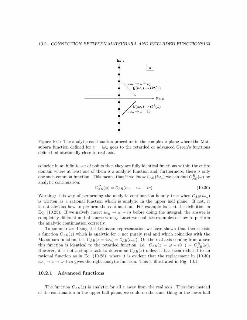
10.2. CONNECTION BETWEEN MATSUBARA AND RETARDED FUNCTIONS163
Figure 10.1: The analytic continuation procedure in the complex z-plane where the Mat-subara function defined for z = iωn goes to the retarded or advanced Green’s functionsdefined infinitesimally close to real axis.
coincide in an infinite set of points then they are fully identical functions within the entiredomain where at least one of them is a analytic function and, furthermore, there is onlyone such common function. This means that if we know CAB(iωn) we can find CR
AB(ω) byanalytic continuation:
CRAB(ω) = CAB(iωn → ω + iη). (10.30)
Warning: this way of performing the analytic continuation is only true when CAB(iωn)is written as a rational function which is analytic in the upper half plane. If not, itis not obvious how to perform the continuation. For example look at the definition inEq. (10.25). If we naıvely insert iωn → ω + iη before doing the integral, the answer iscompletely different and of course wrong. Later we shall see examples of how to performthe analytic continuation correctly.
To summarize: Using the Lehmann representation we have shown that there existsa function CAB(z) which is analytic for z not purely real and which coincides with theMatsubara function, i.e. CAB(z = iωn) = CAB(iωn). On the real axis coming from abovethis function is identical to the retarded function, i.e. CAB(z = ω + i0+) = CR
AB(ω).However, it is not a simple task to determine CAB(z) unless it has been reduced to anrational function as in Eq. (10.28), where it is evident that the replacement in (10.30)iωn → z → ω + iη gives the right analytic function. This is illustrated in Fig. 10.1.
10.2.1 Advanced functions
The function CAB(z) is analytic for all z away from the real axis. Therefore insteadof the continuation in the upper half plane, we could do the same thing in the lower half
164 CHAPTER 10. IMAGINARY TIME GREEN’S FUNCTIONS
plane iωn → z → ω − iη, which gives the so-called advanced Green’s function,
CAAB(ω) = CAB(iωn → ω − iη). (10.31)
The advanced Green’s function is in the time domain defined as
CAAB(t, t′) = iθ(t′ − t)
⟨[A(t), B(t′)
]B,F
⟩. (10.32)
The term “advanced” means that it gives the state of the system at previous timesbased on the state of system at present times. The retarded one, as was explained inChap. 6, gives the present state of the system as it has evolved from the state at previoustimes, i.e. the effect of retardation.
10.3 Single-particle Matsubara Green’s function
An important type of Matsubara functions are the single-particle Green’s function G. Theyare defined as
G(rστ, r′στ ′) = −⟨Tτ
(Ψσ(r,τ)Ψ†
σ(r′, τ ′))⟩
, real space, (10.33a)
G(ντ, ν ′τ ′) = −⟨Tτ
(cν(τ)c†ν′(τ
′))⟩
, ν representation. (10.33b)
10.3.1 Matsubara Green’s function for non-interacting particles
For non-interacting particles the Matsubara Green’s functions can be evaluated in thesame way we found the retarded Green’s function in Sec. 8.3.2. Suppose the Hamiltonianis diagonal in the ν-quantum numbers
H0 =∑
ν
ξνc†νcν , (10.34)
so that
cν(τ) = eτH0cνe−τH0 = e−ξντ cν , c†ν(τ) = eτH0c†νe
−τH0 = eξντ c†ν , (10.35)
which gives
G0(ν, τ − τ ′) = −⟨Tτ
(cν(τ)c†ν(τ
′))⟩
,
= −θ(τ − τ ′)〈cν(τ)c†ν(τ′)〉 − (±) θ(τ ′ − τ)〈c†ν(τ ′)cν(τ)〉
= −[θ(τ − τ ′)〈cνc
†ν〉(±)θ(τ ′ − τ)〈c†νcν〉
]e−ξν(τ−τ ′), (10.36)
For fermions this is
G0,F (ν, τ − τ ′) = − [θ(τ − τ ′)(1− nF (ξν))− θ(τ ′ − τ)nF (ξν)
]e−ξν(τ−τ ′) (10.37)

10.4. EVALUATION OF MATSUBARA SUMS 165
while the bosonic free particle Green’s function reads
G0,B(ν, τ − τ ′) = − [θ(τ − τ ′) (1 + nB(ξν)) + θ(τ ′ − τ)nB(ξν)
]e−ξν(τ−τ ′). (10.38)
In the frequency representation, the fermionic Green’s function is
G0,F (ν, ikn) =∫ β
0dτ eiknτG0,F (ν, τ), kn = (2n + 1)π/β
= − (1− nF (ξν))∫ β
0dτ eiknτe−ξντ ,
= − (1− nF (ξν))1
ikn − ξν
(eiknβe−ξνβ − 1
),
=1
ikn − ξν, (10.39)
because eiknβ = −1 and 1− nF (ε) =(e−βε + 1
)−1, while the bosonic one becomes
G0,B(ν, iqn) =∫ β
0dτ eiqnτG0,B(ν, τ), qn = 2nπ/β
= − (1 + nB(ξν))∫ β
0dτ eiqnτe−ξντ ,
= − (1 + nB(ξν))1
iqn − ξν
(eiqnβe−ξνβ − 1
),
=1
iqn − ξν, (10.40)
because eiqnβ = 1 and 1+nB(ε) = − (e−βε − 1
)−1. Here we have anticipated the notationthat is used later: Matsubara frequencies ikn and ipn are used for fermion frequencies,while iqn and iωn are used for boson frequencies.
According to our recipe Eq. (10.30), the retarded free particles Green’s functions arefor both fermions and bosons
GR0 (ν, ω) =
1ω − ξν + iη
, (10.41)
in agreement with Eq. (8.51).
10.4 Evaluation of Matsubara sums
When working with Matsubara Green’s functions we will often encounter sums over Mat-subara frequencies, similar to integrals over frequencies in the real time language. Forexample sums of the type
S1(ν, τ) =1β
∑
ikn
G(ν, ikn)eiknτ , τ > 0, (10.42)
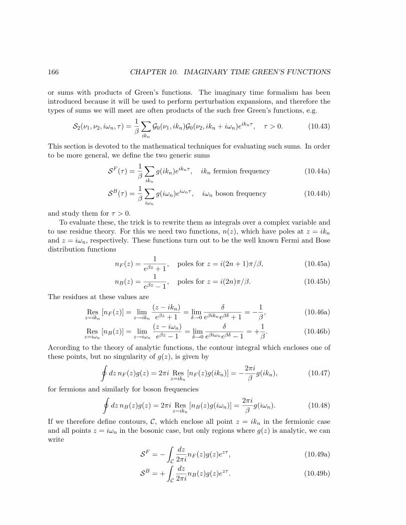
166 CHAPTER 10. IMAGINARY TIME GREEN’S FUNCTIONS
or sums with products of Green’s functions. The imaginary time formalism has beenintroduced because it will be used to perform perturbation expansions, and therefore thetypes of sums we will meet are often products of the such free Green’s functions, e.g.
S2(ν1, ν2, iωn, τ) =1β
∑
ikn
G0(ν1, ikn)G0(ν2, ikn + iωn)eiknτ , τ > 0. (10.43)
This section is devoted to the mathematical techniques for evaluating such sums. In orderto be more general, we define the two generic sums
SF (τ) =1β
∑
ikn
g(ikn)eiknτ , ikn fermion frequency (10.44a)
SB(τ) =1β
∑
iωn
g(iωn)eiωnτ , iωn boson frequency (10.44b)
and study them for τ > 0.To evaluate these, the trick is to rewrite them as integrals over a complex variable and
to use residue theory. For this we need two functions, n(z), which have poles at z = ikn
and z = iωn, respectively. These functions turn out to be the well known Fermi and Bosedistribution functions
nF (z) =1
eβz + 1, poles for z = i(2n + 1)π/β, (10.45a)
nB(z) =1
eβz − 1, poles for z = i(2n)π/β. (10.45b)
The residues at these values are
Resz=ikn
[nF (z)] = limz→ikn
(z − ikn)eβz + 1
= limδ→0
δ
eβikneβδ + 1= − 1
β, (10.46a)
Resz=iωn
[nB(z)] = limz→iωn
(z − iωn)eβz − 1
= limδ→0
δ
eβiωneβδ − 1= +
1β
. (10.46b)
According to the theory of analytic functions, the contour integral which encloses one ofthese points, but no singularity of g(z), is given by
∮dz nF (z)g(z) = 2πi Res
z=ikn
[nF (z)g(ikn)] = −2πi
βg(ikn), (10.47)
for fermions and similarly for boson frequencies∮
dz nB(z)g(z) = 2πi Resz=ikn
[nB(z)g(iωn)] =2πi
βg(iωn). (10.48)
If we therefore define contours, C, which enclose all point z = ikn in the fermionic caseand all points z = iωn in the bosonic case, but only regions where g(z) is analytic, we canwrite
SF = −∫
C
dz
2πinF (z)g(z)ezτ , (10.49a)
SB = +∫
C
dz
2πinB(z)g(z)ezτ . (10.49b)
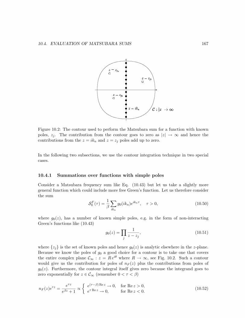
10.4. EVALUATION OF MATSUBARA SUMS 167
Figure 10.2: The contour used to perform the Matsubara sum for a function with knownpoles, zj . The contribution from the contour goes to zero as |z| → ∞ and hence thecontributions from the z = ikn and z = zj poles add up to zero.
In the following two subsections, we use the contour integration technique in two specialcases.
10.4.1 Summations over functions with simple poles
Consider a Matsubara frequency sum like Eq. (10.43) but let us take a slightly moregeneral function which could include more free Green’s function. Let us therefore considerthe sum
SF0 (τ) =
1β
∑
ikn
g0(ikn)eiknτ , τ > 0, (10.50)
where g0(z), has a number of known simple poles, e.g. in the form of non-interactingGreen’s functions like (10.43)
g0(z) =∏
j
1z − zj
, (10.51)
where zj is the set of known poles and hence g0(z) is analytic elsewhere in the z-plane.Because we know the poles of g0 a good choice for a contour is to take one that coversthe entire complex plane C∞ : z = R eiθ where R → ∞, see Fig. 10.2. Such a contourwould give us the contribution for poles of nF (z) plus the contributions from poles ofg0(z). Furthermore, the contour integral itself gives zero because the integrand goes tozero exponentially for z ∈ C∞ (remember 0 < τ < β)
nF (z)eτz =eτz
eβz + 1∝
e(τ−β)Re z → 0, for Re z > 0,eτ Re z → 0, for Re z < 0.
(10.52)
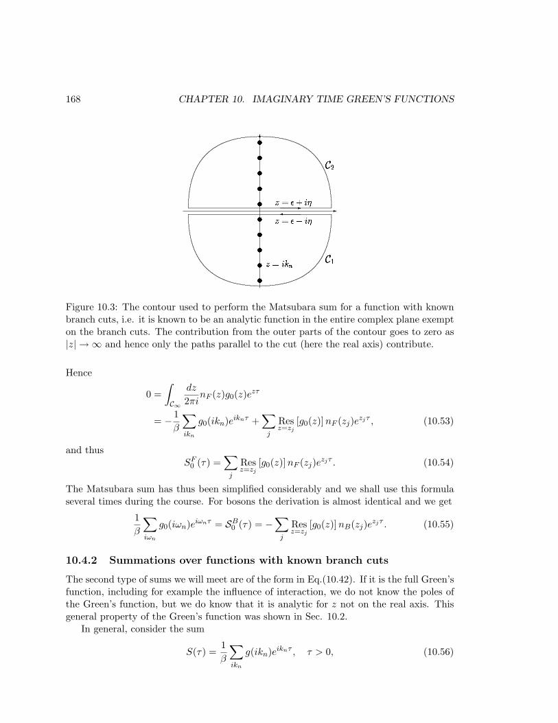
168 CHAPTER 10. IMAGINARY TIME GREEN’S FUNCTIONS
Figure 10.3: The contour used to perform the Matsubara sum for a function with knownbranch cuts, i.e. it is known to be an analytic function in the entire complex plane exempton the branch cuts. The contribution from the outer parts of the contour goes to zero as|z| → ∞ and hence only the paths parallel to the cut (here the real axis) contribute.
Hence
0 =∫
C∞
dz
2πinF (z)g0(z)ezτ
= − 1β
∑
ikn
g0(ikn)eiknτ +∑
j
Resz=zj
[g0(z)]nF (zj)ezjτ , (10.53)
and thusSF
0 (τ) =∑
j
Resz=zj
[g0(z)]nF (zj)ezjτ . (10.54)
The Matsubara sum has thus been simplified considerably and we shall use this formulaseveral times during the course. For bosons the derivation is almost identical and we get
1β
∑
iωn
g0(iωn)eiωnτ = SB0 (τ) = −
∑
j
Resz=zj
[g0(z)]nB(zj)ezjτ . (10.55)
10.4.2 Summations over functions with known branch cuts
The second type of sums we will meet are of the form in Eq.(10.42). If it is the full Green’sfunction, including for example the influence of interaction, we do not know the poles ofthe Green’s function, but we do know that it is analytic for z not on the real axis. Thisgeneral property of the Green’s function was shown in Sec. 10.2.
In general, consider the sum
S(τ) =1β
∑
ikn
g(ikn)eiknτ , τ > 0, (10.56)
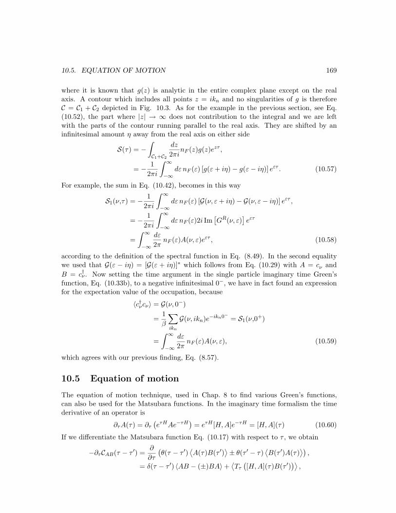
10.5. EQUATION OF MOTION 169
where it is known that g(z) is analytic in the entire complex plane except on the realaxis. A contour which includes all points z = ikn and no singularities of g is thereforeC = C1 + C2 depicted in Fig. 10.3. As for the example in the previous section, see Eq.(10.52), the part where |z| → ∞ does not contribution to the integral and we are leftwith the parts of the contour running parallel to the real axis. They are shifted by aninfinitesimal amount η away from the real axis on either side
S(τ) = −∫
C1+C2
dz
2πinF (z)g(z)ezτ ,
= − 12πi
∫ ∞
−∞dε nF (ε) [g(ε + iη)− g(ε− iη)] eετ . (10.57)
For example, the sum in Eq. (10.42), becomes in this way
S1(ν,τ) = − 12πi
∫ ∞
−∞dε nF (ε) [G(ν, ε + iη)− G(ν, ε− iη)] eετ ,
= − 12πi
∫ ∞
−∞dε nF (ε)2i Im
[GR(ν, ε)
]eετ
=∫ ∞
−∞
dε
2πnF (ε)A(ν, ε)eετ , (10.58)
according to the definition of the spectral function in Eq. (8.49). In the second equalitywe used that G(ε − iη) = [G(ε + iη)]∗ which follows from Eq. (10.29) with A = cν andB = c†ν . Now setting the time argument in the single particle imaginary time Green’sfunction, Eq. (10.33b), to a negative infinitesimal 0−, we have in fact found an expressionfor the expectation value of the occupation, because
〈c†νcν〉 = G(ν, 0−)
=1β
∑
ikn
G(ν, ikn)e−ikn0− = S1(ν,0+)
=∫ ∞
−∞
dε
2πnF (ε)A(ν, ε), (10.59)
which agrees with our previous finding, Eq. (8.57).
10.5 Equation of motion
The equation of motion technique, used in Chap. 8 to find various Green’s functions,can also be used for the Matsubara functions. In the imaginary time formalism the timederivative of an operator is
∂τA(τ) = ∂τ
(eτHAe−τH
)= eτH [H, A]e−τH = [H, A](τ) (10.60)
If we differentiate the Matsubara function Eq. (10.17) with respect to τ , we obtain
−∂τCAB(τ − τ ′) =∂
∂τ
(θ(τ − τ ′)
⟨A(τ)B(τ ′)
⟩± θ(τ ′ − τ)⟨B(τ ′)A(τ)
⟩),
= δ(τ − τ ′) 〈AB − (±)BA〉+⟨Tτ
([H,A](τ)B(τ ′)
)⟩,
170 CHAPTER 10. IMAGINARY TIME GREEN’S FUNCTIONS
where the minus sign in 〈AB − (±)BA〉 is for fermion operators, whereas the plus signshould be used for boson operators.
For the single-particle Green’s functions defined in Eqs. (10.33), we then get for bothfermion and boson Green’s functions
−∂τG(rτ, r′τ ′) = δ(τ − τ ′)δ(r− r′) +⟨Tτ ([H, Ψ(r)](τ)Ψ†(r′, τ ′))
⟩, (10.61a)
−∂τG(ντ, ν′τ ′) = δ(τ − τ ′)δνν′ +⟨Tτ ([H, cν ](τ)c†ν′(τ
′))⟩
. (10.61b)
For non-interacting electrons the Hamiltonian is quadratic, i.e. of the general form
H0 =∫
dr∫
dr′Ψ†(r)h0(r, r′)Ψ(r′), (10.62a)
H0 =∑
νν′tνν′c
†νcν′ . (10.62b)
In this case, the equations of motion therefore in the two representations reduce to
−∂τG0(rτ, r′τ ′)−∫
dr ′′ h0(r, r′′)G0(r′′τ, r′τ ′) = δ(τ − τ ′)δ(r− r′), (10.63a)
−∂τG0(ντ, ν′τ ′)−∑
ν′′tνν′′G0(ν ′′τ, ν ′τ ′) = δ(τ − τ ′)δνν′ , (10.63b)
or in matrix formG−1
0 G0 = 1, G−10 = −∂τ −H0. (10.64)
This equation together with the boundary condition G(τ) = ±G(τ + β) gives the solution.For example for free particle those given in Eqs. (10.37) and (10.38).
10.6 Wick’s theorem
We end this rather technical part by proving an extremely useful theorem, which we willneed later when doing perturbation theory, and which is used in the example ending thischapter. The theorem - called Wick’s theorem - states that for non-interacting particles,i.e. when the Hamiltonian is quadratic, higher order Green’s function involving more thanone particle can be factorized into products of single-particle Green’s functions.
Consider an n-particle Green’s function defined as
G(n)0 (ν1τ1, . . . , νnτn; ν ′1τ
′1, . . . , ν
′nτ ′n)
= (−1)n⟨Tτ
[cν1
(τ1) · · · cνn(τn)c†ν′n(τ ′n) · · · c†
ν′1(τ ′1)
]⟩0. (10.65)
The average is taken with respect to a non-interacting Hamiltonian H0 (like Eq. (10.62)),which we have indicated by the subscript 0. The time-evolution is also with respect to H0
and it is given byc(τ) = eτH0c e−τH0 . (10.66)
10.6. WICK’S THEOREM 171
The expression in (10.65) is indeed quite complicated to look at if we write out all thepossible orderings and the conditions for that particular ordering. For example if n = 2,there are 4 time arguments which can be ordered in 4! different ways. Let us simplify thewriting by defining one operator symbol for both creation and annihilation operators
dj(σj) =
cνj
(τj), j ∈ [1, n],
c†ν′(2n+1−j)
(τ ′(2n+1−j)), j ∈ [n + 1, 2n], (10.67)
and furthermore define the permutations of the 2n operators as
P (d1(σ1) · · · d2n(σ2n)) = dP1(σP1
) · · · dP2n(σP2n
), (10.68)
where Pj denotes the j’th variable in the permutation P (e.g. define the list (a, b, c) andthe permutation (c, a, b) then P = (3, 1, 2)). Which permutation is the correct one ofcourse depends on how the time arguments in (10.65) are really ordered. Therefore if wesum over all permutations and include the corresponding conditions, we can rewrite G(n)
0
as
G(n)0 (j1, . . . , j2n) = (−1)n
∑
P∈S2n
(±1)P θ(σP1− σP2
) · · · θ(σPn−1− σPn
)
×⟨dP1
(σP1) · · · dP2n
(σP2n)⟩
0, (10.69)
where the factor (±1)P takes into account that for fermions (minus sign) it costs a signchange every time a pair of operators are commuted.
The easiest way to show Wick’s theorem is through the equation of motion for the n-particle Green’s function. Thus we differentiate G(n)
0 with respect to one of time arguments,τ1, . . . , τn. This gives two kinds of contributions: the terms coming from the derivative ofthe theta functions and one term from the derivative of the expectation value itself. Thelast one gives for example for τ1
[− ∂
∂τ1
G(n)0
]
last term
= − (−1)n⟨Tτ
[[H0, cν1
](τ1) · · · cνn(τn)c†ν′n(τ ′n) · · · c†
ν′1(τ ′1)
]⟩, (10.70)
which is similar to the derivation that lead to Eqs. (10.63) and (10.64), so that we have
G−10i G(n)
0 = −∂θτiG(n)
0 , (10.71)
where G−10i means that it works on the coordinate νi, τi. On the right hand side the
derivative only acts on the theta functions in Eq. (10.69).Take now for example the case where τi is next to τ ′j . There are two such terms in
(10.69), corresponding to τi being either smaller or larger than τ ′j , and they will havedifferent order of the permutation. In this case G(n) has the structure
G(n)0 =
[· · · θ(τi − τ ′j) · · ·] ⟨· · · cνi
(τi)c†ν′j
(τ ′j) · · ·⟩
± [· · · θ(τ ′j − τi) · · ·] ⟨· · · c†
ν′j(τ ′j)cνi
(τi) · · ·⟩
, (10.72)
172 CHAPTER 10. IMAGINARY TIME GREEN’S FUNCTIONS
and when this is differentiated with respect to τi it gives two delta functions, and hence
−∂θτiG(n)
0 =([· · · ]
⟨· · · cνi
(τi)c†ν′j
(τ ′j) · · ·⟩∓ [· · · ]
⟨· · · c†
ν′j(τ ′j)cνi
(τi) · · ·⟩)
δ(τi − τ ′j).
(10.73)We can pull out the equal time commutator or anti-commutator for boson or fermions,respectively [
cνi(τi), c
†ν′j
(τi)]B,F
= δνi,ν′j. (10.74)
If τi is next to τj instead of τ ′j , we get in the same manner the (anti-)commutator[cνi
(τi), cνj(τi)
]B,F
= 0, (10.75)
which therefore does not contribute. The number of creation and annihilation operatorshas thus both been reduced by one, and it leaves a Green’s function which is no longer ann-particle Green’s function but an (n− 1)-Green’s function. In fact, we saw a special caseof this in Eq. (10.63) where a one-particle Green’s function was reduced to a zero-particleGreen’s function, i.e. a constant. What we have not determined is the sign of the new(n − 1)-Green’s function, and this sign denoted (−1)x will (for fermions) depend on theτ ′j in question. Besides this undetermined sign, our equation of motion (10.71) now lookslike
G−10i G(n)
0 =n∑
j=1
δνi,ν′jδ(τi − τ ′j) (−1)x G(n−1)
0 (ν1τ1, . . . , νnτn︸ ︷︷ ︸without i
; ν ′1τ′1, . . . , ν
′nτ ′n︸ ︷︷ ︸
without j
). (10.76)
Let us collect the signs that go into (−1)x: (−1) from (−∂τ ), (−1)n from the definitionin (10.65) [(−1)n−1]−1 from the definition of G(n−1), and for fermions (−1)n−i+n−j frommoving c†
ν′jnext to cνi
. Hence
fermions: (−1)x = − (−1)n (−1)1−n (−1)2n−i−j = (−1)j+i , (10.77a)
bosons : (−1)x = − (−1)n (−1)1−n = 1, (10.77b)
Now Eq. (10.76) can be integrated and because G(n)0 has the same boundary conditions
as G0, i.e. periodic in the time arguments, it gives the same result and hence
G(n)0 =
n∑
j=1
(±)j+i G0
(νiτi, ν
′jτ′j
)G(n−1)0 (ν1τ1, . . . , νnτn︸ ︷︷ ︸
without i
; ν ′1τ′1, . . . , ν
′nτ ′n︸ ︷︷ ︸
without j
). (10.78)
By recalling the definition of a determinants this formula is immediately recognized as thedeterminant in the case where the minus sign should be used. With the plus sign it iscalled a permanent. We therefore end up with
G(n)0 (1, . . . , n; 1′, . . . , n′) =
∣∣∣∣∣∣∣
G0(1, 1′) · · · G0(1, n′)...
. . ....
G0(n, 1′) · · · G0(n, n′)
∣∣∣∣∣∣∣B,F
, i ≡ (νi, τi) (10.79)
10.7. EXAMPLE: POLARIZABILITY OF FREE ELECTRONS 173
where we used a shorthand notation with the orbital and the time arguments being col-lected into one variable, and where the determinant |·|B,F means that for fermions it isthe usual determinant, while for bosons it should be understood as a permanent where allhave terms come with a plus sign; this is Wick’s theorem.
10.7 Example: polarizability of free electrons
In Sec. 8.5 we calculated the polarizability of non-interacting free electrons. In order toillustrate the working principle of the imaginary time formalism, we do it again here.
The starting point is the physical quantity which is needed: the frequency dependentretarded charge-charge correlation function, χR(q, ω), which follows from the correspond-ing Matsubara function by
χR(q, ω) = χ(q, iqn → ω + iη). (10.80)
In order to find χ (q, iqn) we start from the time-dependent χ
χ0(q, τ) = − 1V 〈Tτ (ρ (q, τ) ρ (−q))〉0 , (10.81)
and expresses it as a two-particle Green’s function
χ0(q, τ) = − 1V
∑
k,k′σσ′
⟨Tτ
(c†kσ (τ) ck+qσ (τ) c†k′σ′ck′−qσ′
)⟩0. (10.82)
By Wick’s theorem this is given by a product of single-particle Green’s functions withall possible pairings and with the sign given by the number of times we interchange twofermion operators, i.e.
χ0(q, τ) =1V
∑
k,k′,σ,σ′
⟨Tτ
(ck+qσ (τ) c†k′σ′
)⟩0
⟨Tτ
(ck′−qσ′ (0) c†kσ (τ)
)⟩0− 1V
=0 for q 6=0︷ ︸︸ ︷〈ρ (q)〉0 〈ρ (−q)〉0,
=1V
∑
kσ
G0(k + qσ, τ)G0(kσ,−τ). (10.83)
where we consider only q 6= 0 and use that G0(k,k′) ∝ δk,k′ .The next step is to calculate the frequency dependent function, i.e. to Fourier trans-
form the product (10.83). The Fourier transform of a product in the time domain is aconvolution in the frequency domain. Because one function has argument τ while theother has argument −τ , the internal frequencies in the two come with the same sign
χ0(q, iqn) =1β
∑
ikn
1V
∑
kσ
G0(k + qσ, ikn + iqn)G0(kσ, ikn). (10.84)
The sum over Matsubara frequencies has exactly the form studied in Sec. 10.4.1.Remembering that G0(kσ, ikn) = 1/ (ikn − ξk), we can read off the answer from Eq.(10.54)
174 CHAPTER 10. IMAGINARY TIME GREEN’S FUNCTIONS
by inserting the poles of the two G0(kσ, z) (z = ξk and z = ξk+q − iqn) and obtain
χ0(q, iqn) =1V
∑
k
nF (ξk)G0(k + qσ, ξk + iqn) + nF (ξk+q − iqn)G0(kσ, ξk+q − iqn)
=1V
∑
kσ
nF (ξk)− nF (ξk+q)iqn + ξk − ξk+q
. (10.85)
Here we used that
nF (ξk+q − iqn) =1
eβξk+qe−βiqn + 1=
1
eβξk+q + 1, (10.86)
because iqn is a bosonic frequency. After the substitution (10.80) Eq. (10.85) gives theresult we found in Eq. (8.81).
10.8 Summary and outlook
When performing calculations of physical quantities at finite temperatures it turns outthat the easiest way to find the “real time” introduced in Chap. 7 is often to go via theimaginary time formalism. This formalism has been introduced in this chapter, and in thefollowing chapters on Feynman diagrams it is a necessary tool. There you will see why itis more natural to use the imaginary time Green’s function, also called Matsubara Green’sfunction. The reason is that the time evolution operator and the Boltzmann weight factorcan be treated on an equal footing and one single perturbation expansion suffices. In thereal time formalism there is no simple way of doing this.
We have also derived some very useful relations concerning sums over Matsubara fre-quencies. The things to remember are the following.
Non-interacting particle Green’s function, valid for both bosons and fermions
G0(ν, iωn) =1
iωn − ξv. (10.87)
Matsubara frequency sum over products of non-interacting Green’s functions (for τ > 0)
SF (τ) =1β
∑
ikn
g0(ikn)eiknτ =∑
j
Res (g0(zj))nF (zj)ezjτ , ikn fermion frequency,
(10.88a)
SB(τ) =1β
∑
iωn
g0(iωn)eiωnτ = −∑
j
Res (g0(zj))nB(zj)ezjτ , iωn boson frequency,
(10.88b)
with g0(z) =∏
i 1/ (z − ξi) . If we perform a sum over functions where the poles areunknown but where the branch cuts are known, we can use a contour depicted in Fig.
10.8. SUMMARY AND OUTLOOK 175
10.3. For example if g(ikn) is known to be analytic everywhere but on the real axis we get
SF (τ) =1β
∑
ikn
g(ikn)eiknτ = −∫ ∞
−∞
dε
2πinF (ε) [g(ε + iη)− g(ε− iη)]
= −∫ ∞
−∞
dε
2πinF (ε)
[gR(ε)− gA(ε)
]. (10.89)
Finally, we proved an important theorem, Wick’s theorem, which says that for non-interacting an n-particle Green’s function is equal to a sum of products of single-particleGreen’s functions, where all possible pairings should be included in the sum. For fermionswe must furthermore keep track of the number of factors −1, because each time we inter-change two fermion operators we must include a factor -1. The end result was
G(n)0 (1, . . . , n; 1′, . . . , n′) =
∣∣∣∣∣∣∣
G0(1, 1′) · · · G0(1, n′)...
. . ....
G0(n, 1′) · · · G0(n, n′)
∣∣∣∣∣∣∣B,F
, i ≡ (νi, τi) , (10.90)
where
G(n)0 (1, . . . , n; 1′, . . . , n′) = (−1)n
⟨Tτ
[c(1) · · · c(n)c†(n′) · · · c†(1′)
]⟩0. (10.91)

176 CHAPTER 10. IMAGINARY TIME GREEN’S FUNCTIONS
Chapter 11
Feynman diagrams and externalpotentials
From the previous chapters on linear response theory and Green’s functions, it is clearthat complete calculations of thermal averages of time-dependent phenomena in quantumfield theory are a rather formidable task. Even the basic imaginary time evolution oper-ator U(τ) itself is an infinite series to all orders in the interaction V (r, τ). One simplyfaces the problem of getting lost in the myriads of integrals, and not being able to main-tain a good physical intuition of which terms are important. In 1948 Feynman solvedthis problem as part of his seminal work on quantum electrodynamics by inventing theingenious diagrams that today bear his name. The Feynman diagrams are both an exactmathematical representation of perturbation theory to infinite order and a powerful pic-torial method that elucidate the physical content of the complicated expressions. In thischapter we introduce the Feynman diagrams for the case of non-interacting particles in anexternal potential. Our main example of their use will be the analysis of electron-impurityscattering in disordered metals.
11.1 Non-interacting particles in external potentials
Consider a time-independent Hamiltonian H in the space representation describing non-interacting fermions in an external spin-diagonal single-particle potential Vσ(r):
H = H0 + V =∑
σ
∫dr Ψ†
σ(r)H0(r)Ψσ(r) +∑
σ
∫dr Ψ†
σ(r)Vσ(r)Ψσ(r). (11.1)
As usual we assume that the unperturbed system described by the time-independentHamiltonian H0 is solvable, and that we know the corresponding eigenstates |ν〉 andGreen’s functions G0
ν . In the following it will prove helpful to introduce the short-handnotation
(r1, σ1, τ1) = (1) and∫
d1 =∑σ1
∫dr1
∫ β
0dτ1 (11.2)
177
178 CHAPTER 11. FEYNMAN DIAGRAMS AND EXTERNAL POTENTIALS
for points and integrals in space-time.We want to study the full Green’s function, G(b, a) = −〈Tτ Ψ(b)Ψ†(a)〉, governed by
H, and the bare one, G0(b, a) = −〈Tτ Ψ(b)Ψ†(a)〉0, governed by H0. We note that sinceno particle-particle interaction is present in Eq. (11.1) both the full Hamiltonian H andthe bare H0 have the simple form of Eq. (10.62), and the equations of motion for the twoGreen’s functions have the same form as Eq. (10.63):
[−∂τb−H0(b)] G0(b, a) = δ(b−a) ⇔ [−∂τb
−H(b)+V (b)] G0(b, a) = δ(b−a) (11.3a)
[−∂τb−H(b) ] G(b, a) = δ(b−a) ⇔ G(b, a) = [−∂τb
−H(b)]−1 δ(b−a), (11.3b)
where we have also given the formal solution of G, which is helpful in acquiring the actualsolution for G. Substituting δ(b − a) in Eq. (11.3b) by the expression from Eq. (11.3a)yields:
[−∂τb−H(b)] G(b, a) = [−∂τb
−H(b) + V (b)] G0(b, a)
= [−∂τb−H(b)] G0(b, a) + V (b) G0(b, a) (11.4)
= [−∂τb−H(b)] G0(b, a) +
∫d1 δ(b− 1) V (1) G0(1, a).
Acting from the left with [−∂τb−H(b)]−1 gives an integral equation for G, the so-called
Dyson equation,
G(b, a) = G0(b, a) +∫
d1 G(b, 1) V (1) G0(1, a), (11.5)
where we have used the second expression in Eq. (11.3b) to introduce G in the integrand.By iteratively inserting G itself in the integrand on the left-hand side we obtain the infiniteperturbation series
G(b, a) = G0(b, a) +∫
d1 G0(b, 1) V (1) G0(1, a)
+∫
d1∫
d2 G0(b, 1) V (1) G0(1, 2) V (2) G0(2, a) (11.6)
+∫
d1∫
d2∫
d3 G0(b, 1) V (1) G0(1, 2) V (2) G0(2, 3) V (3) G0(3, a) + . . . .
The solutions Eqs. (11.5) and (11.6) for G are easy to interpret. The propagator, G, ofa fermion in an external potential is given as the sum of all possible processes involvingunperturbed propagation, described by G0 , intersected by any number of scattering eventsV . So in this simple case there is really no need for further elucidation, but we will anywayproceed by introducing the corresponding Feynman diagrams.
The first step is to define the basic graphical vocabulary, i.e. to define the pictogramsrepresenting the basic quantities G, G0 , and V of the problem. This vocabulary is known
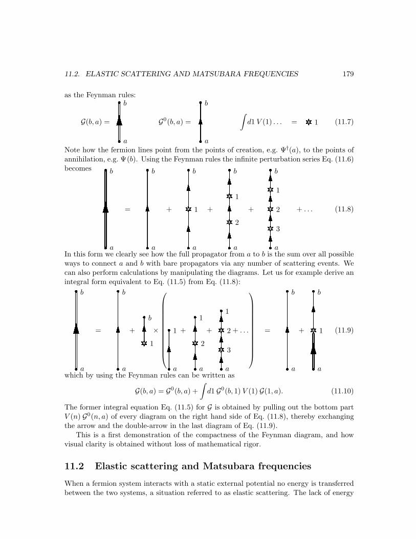
11.2. ELASTIC SCATTERING AND MATSUBARA FREQUENCIES 179
as the Feynman rules:
G(b, a) = ab G0(b, a) = ab ∫d1 V (1) . . . = 1 (11.7)
Note how the fermion lines point from the points of creation, e.g. Ψ†(a), to the points ofannihilation, e.g. Ψ(b). Using the Feynman rules the infinite perturbation series Eq. (11.6)becomes
ab
= ab
+ a1b
+ a21
b
+ a321
b
+ . . . (11.8)
In this form we clearly see how the full propagator from a to b is the sum over all possibleways to connect a and b with bare propagators via any number of scattering events. Wecan also perform calculations by manipulating the diagrams. Let us for example derive anintegral form equivalent to Eq. (11.5) from Eq. (11.8):
ab
= ab
+ 1b×a1 + a2
1
+ a321
+ . . .
= ab
+ a1b
(11.9)
which by using the Feynman rules can be written as
G(b, a) = G0(b, a) +∫
d1 G0(b, 1) V (1) G(1, a). (11.10)
The former integral equation Eq. (11.5) for G is obtained by pulling out the bottom partV (n) G0(n, a) of every diagram on the right hand side of Eq. (11.8), thereby exchangingthe arrow and the double-arrow in the last diagram of Eq. (11.9).
This is a first demonstration of the compactness of the Feynman diagram, and howvisual clarity is obtained without loss of mathematical rigor.
11.2 Elastic scattering and Matsubara frequencies
When a fermion system interacts with a static external potential no energy is transferredbetween the two systems, a situation referred to as elastic scattering. The lack of energy
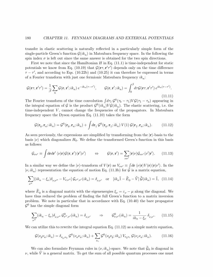
180 CHAPTER 11. FEYNMAN DIAGRAMS AND EXTERNAL POTENTIALS
transfer in elastic scattering is naturally reflected in a particularly simple form of thesingle-particle Green’s function G(ikn) in Matsubara frequency space. In the following thespin index σ is left out since the same answer is obtained for the two spin directions.
First we note that since the Hamiltonian H in Eq. (11.1) is time-independent for staticpotentials we know from Eq. (10.19) that G(rτ, r′τ ′) depends only on the time differenceτ − τ ′, and according to Eqs. (10.22b) and (10.25) it can therefore be expressed in termsof a Fourier transform with just one fermionic Matsubara frequency ikn:
G(rτ, r′τ ′) =1β
∑n
G(r, r′; ikn) e−ikn(τ−τ ′), G(r, r′; ikn) =∫ β
0dτG(rτ, r′τ ′) eikn(τ−τ ′).
(11.11)The Fourier transform of the time convolution
∫dτ1 G0(τb − τ1)V G(τ1 − τa) appearing in
the integral equation of G is the product G0(ikn)V G(ikn). The elastic scattering, i.e. thetime-independent V , cannot change the frequencies of the propagators. In Matsubarafrequency space the Dyson equation Eq. (11.10) takes the form
G(rb, ra; ikn) = G0(rb, ra; ikn) +∫
dr1 G0(rb, r1; ikn) V (1) G(r1, ra; ikn). (11.12)
As seen previously, the expressions are simplified by transforming from the |r〉-basis to thebasis |ν〉 which diagonalizes H0. We define the transformed Green’s function in this basisas follows:
Gνν′ ≡∫
drdr′ 〈ν|r〉G(r, r′)〈r′|ν ′〉 ⇔ G(r, r′) =∑
νν′〈r|ν〉Gνν′〈ν ′|r′〉. (11.13)
In a similar way we define the |ν〉-transform of V (r) as Vνν′ ≡∫
dr 〈ν|r〉V (r)〈r|ν ′〉. In the|ν, ikn〉 representation the equation of motion Eq. (11.3b) for G is a matrix equation,
∑
ν′′[(ikn − ξν)δν,ν′′ − Vν,ν′′ ] Gν′′,ν′(ikn) = δν,ν′ or [ikn
¯1− ¯E0 − ¯V ] ¯G(ikn) = ¯1, (11.14)
where ¯E0 is a diagonal matrix with the eigenenergies ξν = εν − µ along the diagonal. Wehave thus reduced the problem of finding the full Green’s function to a matrix inversionproblem. We note in particular that in accordance with Eq. (10.40) the bare propagatorG0 has the simple diagonal form
∑
ν′′(ikn − ξν)δν,ν′′ G0
ν′′,ν′(ikn) = δν,ν′ ⇒ G0ν,ν′(ikn) =
1ikn − ξν
δν,ν′ . (11.15)
We can utilize this to rewrite the integral equation Eq. (11.12) as a simple matrix equation,
G(νbνa; ikn) = δνb,νaG0(νaνa; ikn) +
∑νc
G0(νbνb; ikn) Vνbνc G(νcνa; ikn). (11.16)
We can also formulate Feynman rules in (ν, ikn)-space. We note that ¯G0 is diagonal inν, while ¯V is a general matrix. To get the sum of all possible quantum processes one must

11.3. RANDOM IMPURITIES IN DISORDERED METALS 181
sum over all matrix indices different from the externally given νa and νb. The frequencyargument is suppressed, since the Green’s functions are diagonal in ikn. .
Gνbνa = νa
νb
G0νb,νa
= δνb,νaνa
νb
=δνa,νb
ikn − ξνa
Vνν′ = νν ′ (11.17)
Using these Feynman rules in (ν, ikn)-space we can express Dyson’s equation Eq. (11.16)diagrammatically: νa
νb
= δνb,νaνa
νa
+ νa
νb
νc
νb
(11.18)
11.3 Random impurities in disordered metals
An important example of elastic scattering by external potentials is the case of randomimpurities in a disordered metal. One well-controlled experimental realization of this isprovided by a perfect metal Cu lattice with MgII ions substituting a small number ofrandomly chosen CuI ions. The valence of the impurity ions is one higher than the hostions, and as a first approximation an impurity ion at site Pj gives rise to a simple screened
mono-charge Coulomb potential uj(r) = −(e20/|r − Pj |) e−|r−Pj |/a. The screening is due
to the electrons in the system trying to neutralize the impurity charge, and as a resultthe range of the potential is finite, given by the so-called screening length a. This will bediscussed in detail in Chap. 13.
In Fig. 11.1(a) is sketched a number of randomly positioned impurities in an otherwiseperfect metal lattice. The presence of the impurities can be detected by measuring the(longitudinal) resistivity ρxx of the metal as a function of temperature. At high tempera-ture the resistivity is mainly due to electron-phonon scattering, and since the vibrational
Figure 11.1: (a) A disordered metal consisting of an otherwise perfect metal lattice witha number of randomly positioned impurities giving rise to elastic electron-impurity scat-tering. (b) The electrical resistivity ρxx(T ) of the disordered metal as a function of tem-perature. At high T the electron-phonon scattering dominates giving rise to a linearbehavior, while at low T only the electron-impurity scattering is effective and gives rise tothe non-zero value ρ0
xx of ρxx at T = 0.
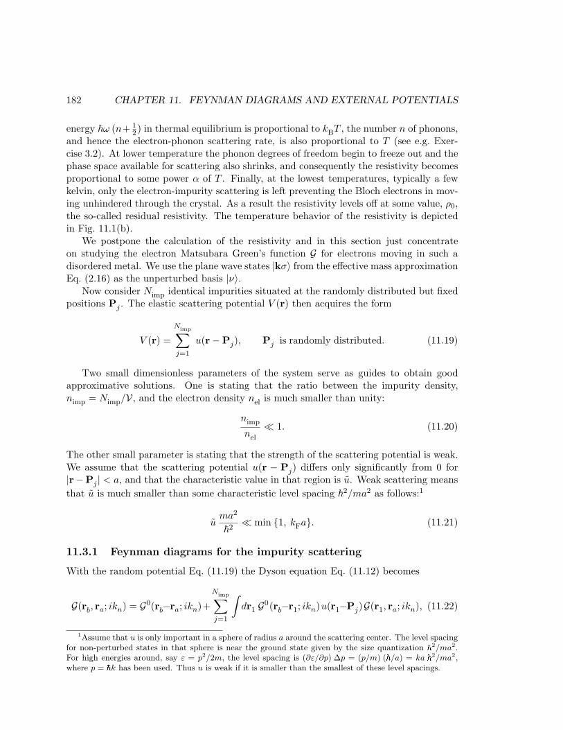
182 CHAPTER 11. FEYNMAN DIAGRAMS AND EXTERNAL POTENTIALS
energy ~ω (n+ 12) in thermal equilibrium is proportional to kBT , the number n of phonons,
and hence the electron-phonon scattering rate, is also proportional to T (see e.g. Exer-cise 3.2). At lower temperature the phonon degrees of freedom begin to freeze out and thephase space available for scattering also shrinks, and consequently the resistivity becomesproportional to some power α of T . Finally, at the lowest temperatures, typically a fewkelvin, only the electron-impurity scattering is left preventing the Bloch electrons in mov-ing unhindered through the crystal. As a result the resistivity levels off at some value, ρ0,the so-called residual resistivity. The temperature behavior of the resistivity is depictedin Fig. 11.1(b).
We postpone the calculation of the resistivity and in this section just concentrateon studying the electron Matsubara Green’s function G for electrons moving in such adisordered metal. We use the plane wave states |kσ〉 from the effective mass approximationEq. (2.16) as the unperturbed basis |ν〉.
Now consider Nimp identical impurities situated at the randomly distributed but fixedpositions Pj . The elastic scattering potential V (r) then acquires the form
V (r) =Nimp∑
j=1
u(r−Pj), Pj is randomly distributed. (11.19)
Two small dimensionless parameters of the system serve as guides to obtain goodapproximative solutions. One is stating that the ratio between the impurity density,nimp = Nimp/V, and the electron density nel is much smaller than unity:
nimp
nel
¿ 1. (11.20)
The other small parameter is stating that the strength of the scattering potential is weak.We assume that the scattering potential u(r − Pj) differs only significantly from 0 for|r−Pj | < a, and that the characteristic value in that region is u. Weak scattering meansthat u is much smaller than some characteristic level spacing ~2/ma2 as follows:1
uma2
~2¿ min 1, kFa. (11.21)
11.3.1 Feynman diagrams for the impurity scattering
With the random potential Eq. (11.19) the Dyson equation Eq. (11.12) becomes
G(rb, ra; ikn) = G0(rb−ra; ikn)+Nimp∑
j=1
∫dr1 G0(rb−r1; ikn)u(r1−Pj)G(r1, ra; ikn), (11.22)
1Assume that u is only important in a sphere of radius a around the scattering center. The level spacingfor non-perturbed states in that sphere is near the ground state given by the size quantization ~2/ma2.For high energies around, say ε = p2/2m, the level spacing is (∂ε/∂p) ∆p = (p/m) (~/a) = ka ~2/ma2,where p = ~k has been used. Thus u is weak if it is smaller than the smallest of these level spacings.
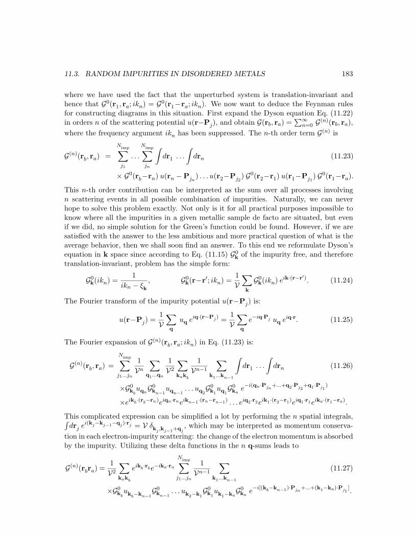
11.3. RANDOM IMPURITIES IN DISORDERED METALS 183
where we have used the fact that the unperturbed system is translation-invariant andhence that G0(r1, ra; ikn) = G0(r1−ra; ikn). We now want to deduce the Feynman rulesfor constructing diagrams in this situation. First expand the Dyson equation Eq. (11.22)in orders n of the scattering potential u(r−Pj), and obtain G(rb, ra) =
∑∞n=0 G(n)(rb, ra),
where the frequency argument ikn has been suppressed. The n-th order term G(n) is
G(n)(rb, ra) =Nimp∑
j1
. . .
Nimp∑
jn
∫dr1 . . .
∫drn (11.23)
× G0(rb−rn) u(rn −Pjn) . . . u(r2−Pj2
) G0(r2−r1) u(r1−Pj1) G0(r1−ra).
This n-th order contribution can be interpreted as the sum over all processes involvingn scattering events in all possible combination of impurities. Naturally, we can neverhope to solve this problem exactly. Not only is it for all practical purposes impossible toknow where all the impurities in a given metallic sample de facto are situated, but evenif we did, no simple solution for the Green’s function could be found. However, if we aresatisfied with the answer to the less ambitious and more practical question of what is theaverage behavior, then we shall soon find an answer. To this end we reformulate Dyson’sequation in k space since according to Eq. (11.15) G0
k of the impurity free, and thereforetranslation-invariant, problem has the simple form:
G0k(ikn) =
1ikn − ξk
, G0k(r−r′; ikn) =
1V
∑
k
G0k(ikn) eik·(r−r′). (11.24)
The Fourier transform of the impurity potential u(r−Pj) is:
u(r−Pj) =1V
∑q
uq eiq·(r−Pj) =1V
∑q
e−iq·Pj uq eiq·r. (11.25)
The Fourier expansion of G(n)(rb, ra; ikn) in Eq. (11.23) is:
G(n)(rb, ra) =Nimp∑
j1...jn
1Vn
∑q1...qn
1V2
∑
kakb
1Vn−1
∑
k1...kn−1
∫dr1 . . .
∫drn (11.26)
×G0kb
uqnG0kn−1
uqn−1. . . uq2
G0k1
uq1G0ka
e−i(qn·Pjn
+...+q2·Pj2+q1·Pj1
)
×eikb·(rb−rn)eiqn·rneikn−1·(rn−rn−1) . . . eiq2·r2eik1·(r2−r1)eiq1·r1eika·(r1−ra).
This complicated expression can be simplified a lot by performing the n spatial integrals,∫drj ei(kj−kj−1−qj)·rj = V δkj ,kj−1+qj
, which may be interpreted as momentum conserva-tion in each electron-impurity scattering: the change of the electron momentum is absorbedby the impurity. Utilizing these delta functions in the n q-sums leads to
G(n)(rbra) =1V2
∑
kakb
eikb·rbe−ika·ra
Nimp∑
j1...jn
1Vn−1
∑
k1...kn−1
(11.27)
×G0kb
ukb−kn−1G0kn−1
. . . uk2−k1G0k1
uk1−kaG0ka
e−i[(kb−kn−1)·Pjn
+...+(k1−ka)·Pj1].
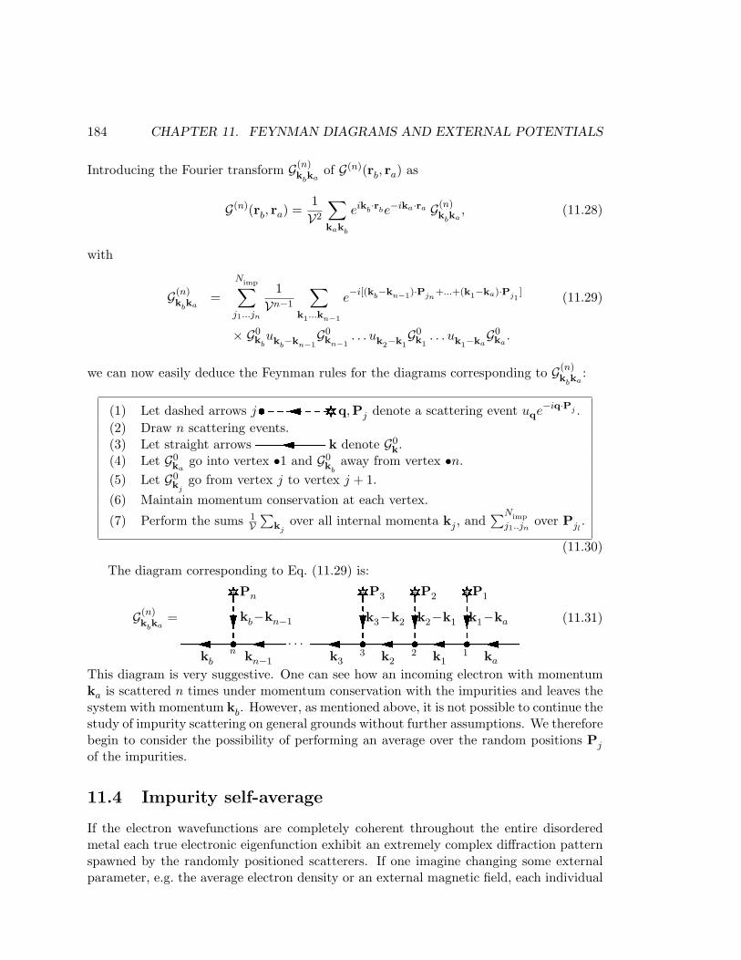
184 CHAPTER 11. FEYNMAN DIAGRAMS AND EXTERNAL POTENTIALS
Introducing the Fourier transform G(n)kbka
of G(n)(rb, ra) as
G(n)(rb, ra) =1V2
∑
kakb
eikb·rbe−ika·ra G(n)kbka
, (11.28)
with
G(n)kbka
=Nimp∑
j1...jn
1Vn−1
∑
k1...kn−1
e−i[(kb−kn−1)·Pjn
+...+(k1−ka)·Pj1] (11.29)
× G0kb
ukb−kn−1G0kn−1
. . . uk2−k1G0k1
. . . uk1−kaG0ka
.
we can now easily deduce the Feynman rules for the diagrams corresponding to G(n)kbka
:
(1) Let dashed arrows j q,Pj denote a scattering event uqe−iq·Pj .(2) Draw n scattering events.(3) Let straight arrows k denote G0
k.(4) Let G0
kago into vertex •1 and G0
kbaway from vertex •n.
(5) Let G0kj
go from vertex j to vertex j + 1.(6) Maintain momentum conservation at each vertex.
(7) Perform the sums 1V
∑kj
over all internal momenta kj , and∑Nimp
j1..jnover Pjl
.
(11.30)
The diagram corresponding to Eq. (11.29) is:
G(n)kbka
=Pn
n· · ·
kb kn−1
kb−kn−1 P3 P2 P1
3 2 1k3 k2 k1 ka
k3−k2 k2−k1 k1−ka (11.31)
This diagram is very suggestive. One can see how an incoming electron with momentumka is scattered n times under momentum conservation with the impurities and leaves thesystem with momentum kb. However, as mentioned above, it is not possible to continue thestudy of impurity scattering on general grounds without further assumptions. We thereforebegin to consider the possibility of performing an average over the random positions Pj
of the impurities.
11.4 Impurity self-average
If the electron wavefunctions are completely coherent throughout the entire disorderedmetal each true electronic eigenfunction exhibit an extremely complex diffraction patternspawned by the randomly positioned scatterers. If one imagine changing some externalparameter, e.g. the average electron density or an external magnetic field, each individual
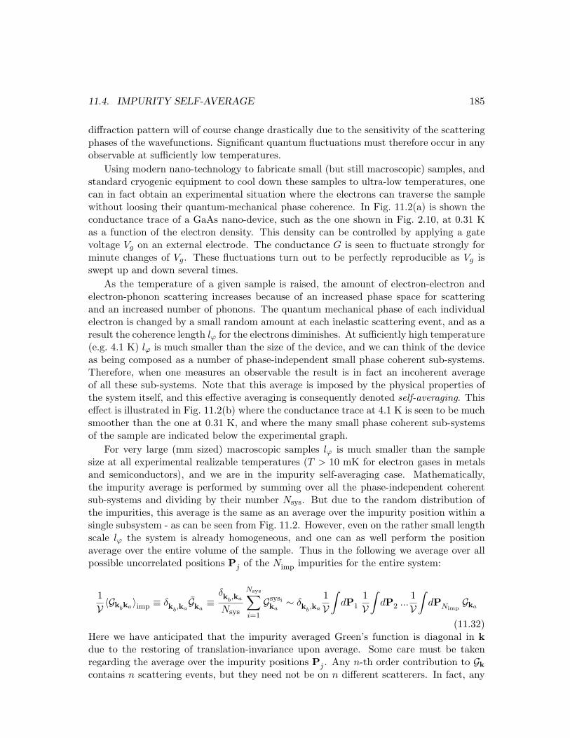
11.4. IMPURITY SELF-AVERAGE 185
diffraction pattern will of course change drastically due to the sensitivity of the scatteringphases of the wavefunctions. Significant quantum fluctuations must therefore occur in anyobservable at sufficiently low temperatures.
Using modern nano-technology to fabricate small (but still macroscopic) samples, andstandard cryogenic equipment to cool down these samples to ultra-low temperatures, onecan in fact obtain an experimental situation where the electrons can traverse the samplewithout loosing their quantum-mechanical phase coherence. In Fig. 11.2(a) is shown theconductance trace of a GaAs nano-device, such as the one shown in Fig. 2.10, at 0.31 Kas a function of the electron density. This density can be controlled by applying a gatevoltage Vg on an external electrode. The conductance G is seen to fluctuate strongly forminute changes of Vg. These fluctuations turn out to be perfectly reproducible as Vg isswept up and down several times.
As the temperature of a given sample is raised, the amount of electron-electron andelectron-phonon scattering increases because of an increased phase space for scatteringand an increased number of phonons. The quantum mechanical phase of each individualelectron is changed by a small random amount at each inelastic scattering event, and as aresult the coherence length lϕ for the electrons diminishes. At sufficiently high temperature(e.g. 4.1 K) lϕ is much smaller than the size of the device, and we can think of the deviceas being composed as a number of phase-independent small phase coherent sub-systems.Therefore, when one measures an observable the result is in fact an incoherent averageof all these sub-systems. Note that this average is imposed by the physical properties ofthe system itself, and this effective averaging is consequently denoted self-averaging. Thiseffect is illustrated in Fig. 11.2(b) where the conductance trace at 4.1 K is seen to be muchsmoother than the one at 0.31 K, and where the many small phase coherent sub-systemsof the sample are indicated below the experimental graph.
For very large (mm sized) macroscopic samples lϕ is much smaller than the samplesize at all experimental realizable temperatures (T > 10 mK for electron gases in metalsand semiconductors), and we are in the impurity self-averaging case. Mathematically,the impurity average is performed by summing over all the phase-independent coherentsub-systems and dividing by their number Nsys. But due to the random distribution ofthe impurities, this average is the same as an average over the impurity position within asingle subsystem - as can be seen from Fig. 11.2. However, even on the rather small lengthscale lϕ the system is already homogeneous, and one can as well perform the positionaverage over the entire volume of the sample. Thus in the following we average over allpossible uncorrelated positions Pj of the Nimp impurities for the entire system:
1V 〈Gkbka
〉imp ≡ δkb,kaGka
≡δkb,ka
Nsys
Nsys∑
i=1
Gsysika
∼ δkb,ka
1V
∫dP1
1V
∫dP2 ...
1V
∫dPNimp
Gka
(11.32)Here we have anticipated that the impurity averaged Green’s function is diagonal in kdue to the restoring of translation-invariance upon average. Some care must be takenregarding the average over the impurity positions Pj . Any n-th order contribution to Gk
contains n scattering events, but they need not be on n different scatterers. In fact, any
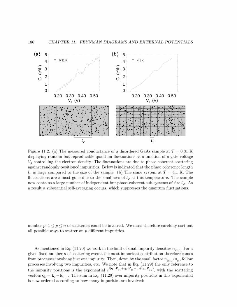
186 CHAPTER 11. FEYNMAN DIAGRAMS AND EXTERNAL POTENTIALS
0.20 0.30 0.40 0.50Vg (V)
0
1
2
3
4
5
G (
e2 /h)
T = 0.31 K
0.20 0.30 0.40 0.50Vg (V)
0
1
2
3
4
5
G (
e2 /h)
T = 4.1 K
Figure 11.2: (a) The measured conductance of a disordered GaAs sample at T = 0.31 Kdisplaying random but reproducible quantum fluctuations as a function of a gate voltageVg controlling the electron density. The fluctuations are due to phase coherent scatteringagainst randomly positioned impurities. Below is indicated that the phase coherence lengthlϕ is large compared to the size of the sample. (b) The same system at T = 4.1 K. Thefluctuations are almost gone due to the smallness of lϕ at this temperature. The samplenow contains a large number of independent but phase-coherent sub-systems of size lϕ. Asa result a substantial self-averaging occurs, which suppresses the quantum fluctuations.
number p, 1 ≤ p ≤ n of scatterers could be involved. We must therefore carefully sort outall possible ways to scatter on p different impurities.
As mentioned in Eq. (11.20) we work in the limit of small impurity densities nimp. For agiven fixed number n of scattering events the most important contribution therefore comesfrom processes involving just one impurity. Then, down by the small factor nimp/nel, followprocesses involving two impurities, etc. We note that in Eq. (11.29) the only reference tothe impurity positions is the exponential e
i(q1·Pj1+q2·Pj2
+...+qn·Pjn), with the scattering
vectors qi = ki−ki−1. The sum in Eq. (11.29) over impurity positions in this exponentialis now ordered according to how many impurities are involved:
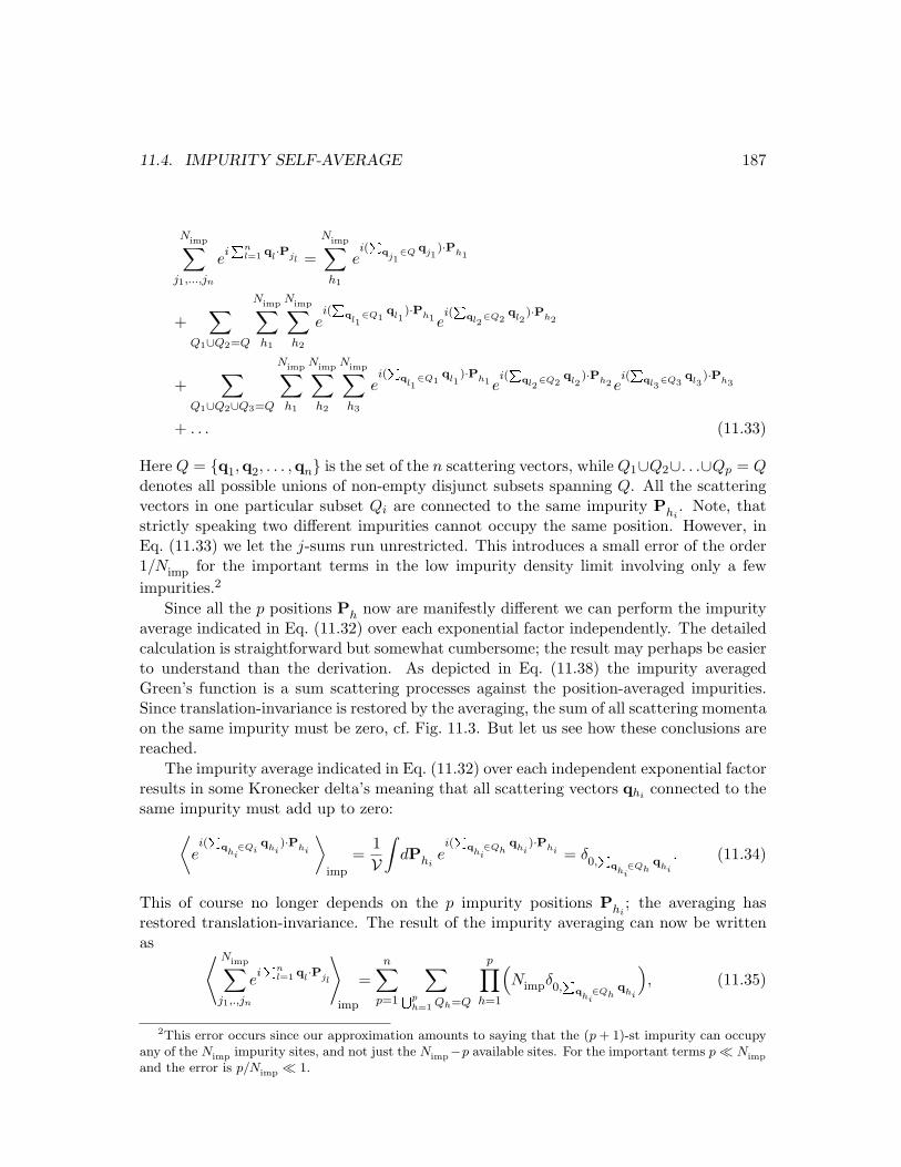
11.4. IMPURITY SELF-AVERAGE 187
Nimp∑
j1,...,jn
eiPn
l=1 ql·Pjl =Nimp∑
h1
ei(P
qj1∈Q qj1
)·Ph1
+∑
Q1∪Q2=Q
Nimp∑
h1
Nimp∑
h2
ei(P
ql1∈Q1
ql1)·Ph1e
i(P
ql2∈Q2
ql2)·Ph2
+∑
Q1∪Q2∪Q3=Q
Nimp∑
h1
Nimp∑
h2
Nimp∑
h3
ei(P
ql1∈Q1
ql1)·Ph1e
i(P
ql2∈Q2
ql2)·Ph2e
i(P
ql3∈Q3
ql3)·Ph3
+ . . . (11.33)
Here Q = q1,q2, . . . ,qn is the set of the n scattering vectors, while Q1∪Q2∪. . .∪Qp = Qdenotes all possible unions of non-empty disjunct subsets spanning Q. All the scatteringvectors in one particular subset Qi are connected to the same impurity Phi
. Note, thatstrictly speaking two different impurities cannot occupy the same position. However, inEq. (11.33) we let the j-sums run unrestricted. This introduces a small error of the order1/Nimp for the important terms in the low impurity density limit involving only a fewimpurities.2
Since all the p positions Ph now are manifestly different we can perform the impurityaverage indicated in Eq. (11.32) over each exponential factor independently. The detailedcalculation is straightforward but somewhat cumbersome; the result may perhaps be easierto understand than the derivation. As depicted in Eq. (11.38) the impurity averagedGreen’s function is a sum scattering processes against the position-averaged impurities.Since translation-invariance is restored by the averaging, the sum of all scattering momentaon the same impurity must be zero, cf. Fig. 11.3. But let us see how these conclusions arereached.
The impurity average indicated in Eq. (11.32) over each independent exponential factorresults in some Kronecker delta’s meaning that all scattering vectors qhi connected to thesame impurity must add up to zero:
⟨ei(P
qhi∈Qi
qhi)·Phi
⟩
imp
=1V
∫dPhi
ei(P
qhi∈Qh
qhi)·Phi = δ0,
Pq
hi∈Qh
qhi
. (11.34)
This of course no longer depends on the p impurity positions Phi; the averaging has
restored translation-invariance. The result of the impurity averaging can now be writtenas ⟨ Nimp∑
j1,.,jn
eiPn
l=1 ql·Pjl
⟩
imp
=n∑
p=1
∑Sph=1 Qh=Q
p∏
h=1
(Nimpδ0,
Pq
hi∈Qh
qhi
), (11.35)
2This error occurs since our approximation amounts to saying that the (p + 1)-st impurity can occupyany of the Nimp impurity sites, and not just the Nimp−p available sites. For the important terms p ¿ Nimp
and the error is p/Nimp ¿ 1.
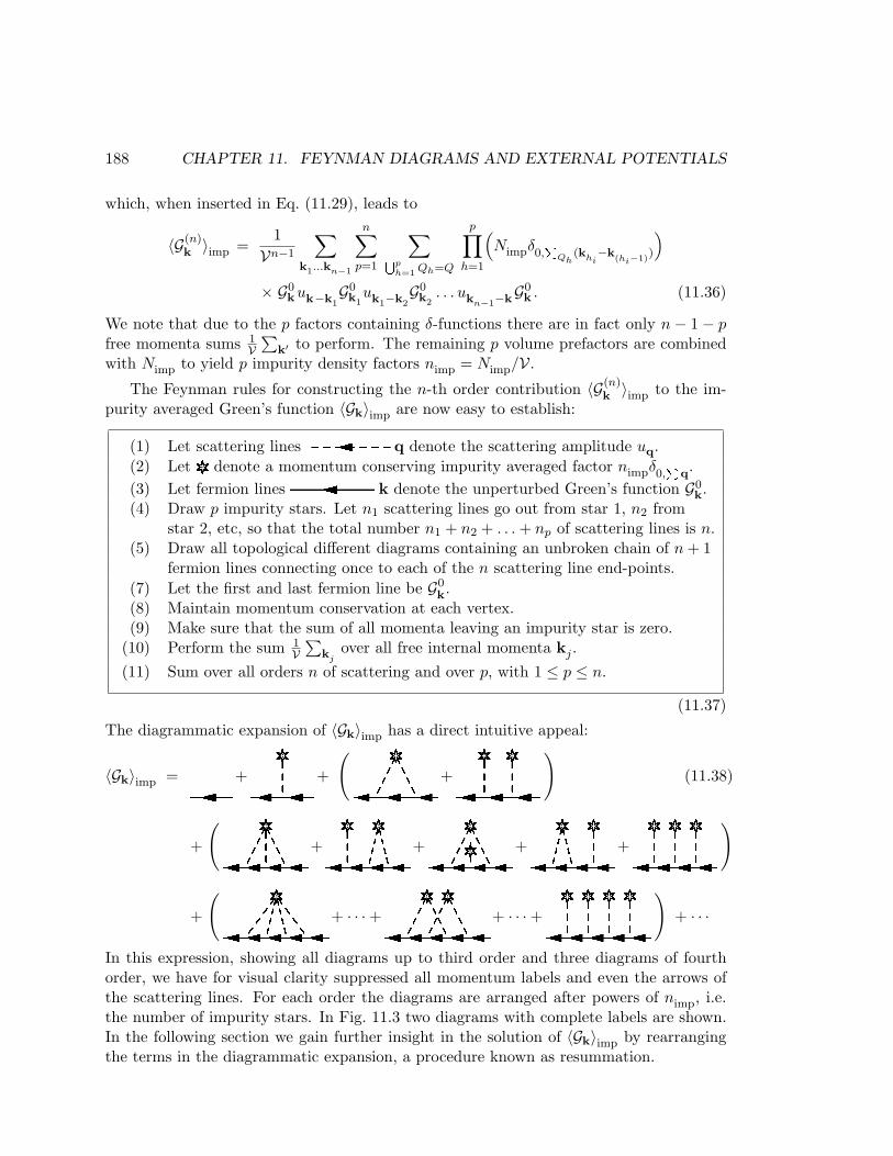
188 CHAPTER 11. FEYNMAN DIAGRAMS AND EXTERNAL POTENTIALS
which, when inserted in Eq. (11.29), leads to
〈G(n)k 〉imp =
1Vn−1
∑
k1...kn−1
n∑
p=1
∑Sph=1 Qh=Q
p∏
h=1
(Nimpδ0,
PQh
(khi−k
(hi−1))
)
× G0kuk−k1
G0k1
uk1−k2G0k2
. . . ukn−1−kG0k . (11.36)
We note that due to the p factors containing δ-functions there are in fact only n − 1 − pfree momenta sums 1
V∑
k′ to perform. The remaining p volume prefactors are combinedwith Nimp to yield p impurity density factors nimp = Nimp/V.
The Feynman rules for constructing the n-th order contribution 〈G(n)k 〉imp to the im-
purity averaged Green’s function 〈Gk〉imp are now easy to establish:
(1) Let scattering lines q denote the scattering amplitude uq.(2) Let denote a momentum conserving impurity averaged factor nimpδ0,
Pq.
(3) Let fermion lines k denote the unperturbed Green’s function G0k.
(4) Draw p impurity stars. Let n1 scattering lines go out from star 1, n2 fromstar 2, etc, so that the total number n1 + n2 + . . . + np of scattering lines is n.
(5) Draw all topological different diagrams containing an unbroken chain of n + 1fermion lines connecting once to each of the n scattering line end-points.
(7) Let the first and last fermion line be G0k.
(8) Maintain momentum conservation at each vertex.(9) Make sure that the sum of all momenta leaving an impurity star is zero.
(10) Perform the sum 1V
∑kj
over all free internal momenta kj .(11) Sum over all orders n of scattering and over p, with 1 ≤ p ≤ n.
(11.37)
The diagrammatic expansion of 〈Gk〉imp has a direct intuitive appeal:
〈Gk〉imp =++
( +!)(11.38)
+
("+#+$+%+&)
+
('+ · · ·+(+ · · ·+))+ · · ·
In this expression, showing all diagrams up to third order and three diagrams of fourthorder, we have for visual clarity suppressed all momentum labels and even the arrows ofthe scattering lines. For each order the diagrams are arranged after powers of nimp, i.e.the number of impurity stars. In Fig. 11.3 two diagrams with complete labels are shown.In the following section we gain further insight in the solution of 〈Gk〉imp by rearrangingthe terms in the diagrammatic expansion, a procedure known as resummation.
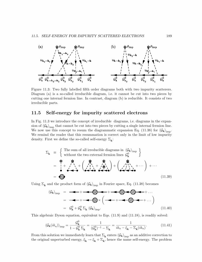
11.5. SELF-ENERGY FOR IMPURITY SCATTERED ELECTRONS 189
Figure 11.3: Two fully labelled fifth order diagrams both with two impurity scatterers.Diagram (a) is a so-called irreducible diagram, i.e. it cannot be cut into two pieces bycutting one internal fermion line. In contrast, diagram (b) is reducible. It consists of twoirreducible parts.
11.5 Self-energy for impurity scattered electrons
In Fig. 11.3 we introduce the concept of irreducible diagrams, i.e. diagrams in the expan-sion of 〈Gk〉imp that cannot be cut into two pieces by cutting a single internal fermion line.We now use this concept to resum the diagrammatic expansion Eq. (11.38) for 〈Gk〉imp.We remind the reader that this resummation is correct only in the limit of low impuritydensity. First we define the so-called self-energy Σk:
Σk ≡
The sum of all irreducible diagrams in 〈Gk〉imp
without the two external fermion lines G0k
= *+++
(,+- )+
(.+ · · ·)
+ · · ·
= / (11.39)
Using Σk and the product form of 〈Gk〉imp in Fourier space, Eq. (11.38) becomes
〈Gk〉imp = 0+1+2+ . . .
= 3+4×(5+6+ . . .
)
= G0k + G0
k Σk 〈Gk〉imp. (11.40)
This algebraic Dyson equation, equivalent to Eqs. (11.9) and (11.18), is readily solved:
〈Gk(ikn)〉imp =G0k
1− G0k Σk
=1
(G0k)−1 − Σk
=1
ikn − ξk − Σk(ikn). (11.41)
From this solution we immediately learn that Σk enters 〈Gk〉imp as an additive correction tothe original unperturbed energy, ξk → ξk + Σk, hence the name self-energy. The problem
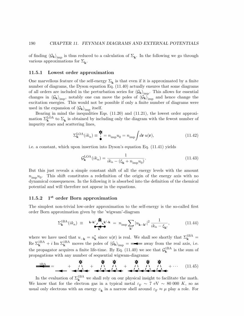
190 CHAPTER 11. FEYNMAN DIAGRAMS AND EXTERNAL POTENTIALS
of finding 〈Gk〉imp is thus reduced to a calculation of Σk. In the following we go throughvarious approximations for Σk.
11.5.1 Lowest order approximation
One marvellous feature of the self-energy Σk is that even if it is approximated by a finitenumber of diagrams, the Dyson equation Eq. (11.40) actually ensures that some diagramsof all orders are included in the perturbation series for 〈Gk〉imp. This allows for essentialchanges in 〈Gk〉imp, notably one can move the poles of 〈Gk〉imp and hence change theexcitation energies. This would not be possible if only a finite number of diagrams wereused in the expansion of 〈Gk〉imp itself.
Bearing in mind the inequalities Eqs. (11.20) and (11.21), the lowest order approxi-mation ΣLOA
k to Σk is obtained by including only the diagram with the fewest number ofimpurity stars and scattering lines,
ΣLOAk (ikn) ≡ 7 = nimpu0 = nimp
∫dr u(r), (11.42)
i.e. a constant, which upon insertion into Dyson’s equation Eq. (11.41) yields
GLOAk (ikn) =
1ikn − (ξk + nimpu0)
. (11.43)
But this just reveals a simple constant shift of all the energy levels with the amountnimpu0. This shift constitutes a redefinition of the origin of the energy axis with nodynamical consequences. In the following it is absorbed into the definition of the chemicalpotential and will therefore not appear in the equations.
11.5.2 1st order Born approximation
The simplest non-trivial low-order approximation to the self-energy is the so-called firstorder Born approximation given by the ’wigwam’-diagram
Σ1BAk (ikn) ≡8
k′
k−k′ k′−k = nimp
∑
k′|uk−k′ |2
1ikn − ξk′
, (11.44)
where we have used that u−k = u∗k since u(r) is real. We shall see shortly that Σ1BAk =
Re Σ1BAk + i Im Σ1BA
k moves the poles of 〈Gk〉imp =9 away from the real axis, i.e.the propagator acquires a finite life-time. By Eq. (11.40) we see that G1BA
k is the sum ofpropagations with any number of sequential wigwam-diagrams::1BA =;+<+=+>+ · · · (11.45)
In the evaluation of Σ1BAk we shall rely on our physical insight to facilitate the math.
We know that for the electron gas in a typical metal εF ∼ 7 eV ∼ 80 000 K, so asusual only electrons with an energy εk in a narrow shell around εF ≈ µ play a role. For

11.5. SELF-ENERGY FOR IMPURITY SCATTERED ELECTRONS 191
Figure 11.4: (a) The functions nimp|uk|2 and (ω −εk +µ)/[(ω −εk +µ)2 +η2] appearing inthe expression for ReΣ1BA
k (ikn). (b) The functions nimp|uk|2 and |kn|/[(ω − εk +µ)2 +η2]appearing in the expression for Im Σ1BA
k (ikn).
T < 800 K we have kBT/εF < 10−2, and for applied voltage drops Vext less than 70 mVover the coherence length lϕ < 10−5 m (the typical size we are looking at), i.e. appliedelectrical fields less than 7000 V/m, we have eVext/εF < 10−2. Thus we are only interestedin Σ1BA
k (ikn) for
|k| ∼ kF and |ikn → ω + i sgn(kn)η| ¿ εF. (11.46)
Here we have also anticipated that at the end of the calculation, as sketched in Fig. 10.1,we need to perform an analytical continuation down to the real axis, either from the upperhalf-plane, where kn > 0, as ikn → ω + iη, or from the lower half-plane, where kn < 0, asikn → ω − iη.
Furthermore, as we shall study in great detail later, the electron gas redistributes itselfto screen out the external charges from the impurities, and as a result uk−k′ varies in asmooth and gentle way for 0 < |k− k′| < 2kF.
With this physical input in mind we continue:
Σ1BAk (ω + i sgn(kn)η) = nimp
∑
k′|uk−k′ |2
1(ω − ξk′) + i sgn(kn)η
(11.47)
=∑
k′nimp|uk−k′ |2
[ω − ξk′
(ω − ξk′)2 + η2
− i sgn(kn) πδ(ω − ξk′)]
.
Since |uk−k′ |2 vary smoothly and |ω −ξk′ | ¿ εF ≈ µ we get the functional behavior shownin Fig. 11.4. Since (ω − ξk′)/((ω − ξk′)
2 + η2) is an odd function of ω − ξk′ and the widthη is small, we have3 Re Σ1BA
k (ikn) ≈ 0; For the imaginary part of Σ1BA we obtain theusual delta function for η → 0. Finally, since the spectral function for the unperturbedsystem forces ω to equal ξk, we obtain:
Σ1BAk (ikn) = −iπ sgn(kn)
∑
k′nimp|uk−k′ |2 δ(ξk − ξk′) = −i sgn(kn)
12τk
, (11.48)
3Strictly speaking, we only get vanishing real part if the slope of |uk−k′ |2 is zero near µ. If this is not
the case we do get a non-zero real part. However, since |uk−k′ |2 is slowly varying near µ we get the samereal part for all k and k′ near kF. This contribution can be absorbed into the definition of µ.
192 CHAPTER 11. FEYNMAN DIAGRAMS AND EXTERNAL POTENTIALS
where we have introduced the impurity scattering time τk defined as
1τk≡ 2π
∑
k′nimp|uk−k′ |2 δ(ξk − ξk′). (11.49)
This result can also be found using Fermi’s golden rule. Now we have obtained the 1storder Born approximation for Gk(ikn) in Eq. (11.41) and the analytic continuation ikn → zthereof into the entire complex plane:
G1BAk (ikn) =
1
ikn − ξk + i sgn(kn)2τk
−→ikn→z
G1BAk (z) =
1z−ξk+ i
2τk
, Im z > 0
1z−ξk− i
2τk
, Im z < 0.(11.50)
We see that G1BAk (z) has a branch cut along the real axis, but that it is analytic separately
in the upper and the lower half-plane. This is a property that will play an important rolelater, when we calculate the electrical resistivity of disordered metals. Note that thisbehavior is in accordance with the general results obtained in Sec. 9.2 concerning theanalytic properties of Matsubara Green’s functions.
We close this section by remarking three properties summarized in Fig. 11.5 relatedto the retarded Green’s function GR,1BA(ω ) = G1BA(ω + iη). First, it is seen by Fouriertransforming to the time domain that G
R,1BAk (t) decays exponentially in time with τk as
the typical time scale:
GR,1BAk (t) ≡
∫dω
2π
e−i(ω+iη)t
ω − ξk + i/2τk= −i θ(t) e−iξkt e−t/2τk . (11.51)
Second, exploiting that ω, τ−1k ¿ εF, it is seen by Fourier transforming back to real space
that GR,1BA(r, ω ) decays exponentially in space with lk ≡ vFτk as the typical length scale:
GR,1BA(r, ω ) ≡∫
dk(2π)3
eik·r
ω − ξk + i/2τk=
πd(εF)kF|r|
eikF|r| e−|r|/2lk . (11.52)
Thirdly, the spectral function A1BAk (ω ) is a Lorentzian of width 2τk:
A1BAk (ω ) ≡ −2 Im G1BA
k (ω + iη) =1/τk
(ω − ξk)2 + 1/4τ2k
(11.53)
In conclusion the impurity averaged 1st Born approximation has resulted in a self-energy with a non-zero imaginary part. The poles of the Matsubara Green’s functionG1BAk (ikn) are therefore shifted away from the real axis, resulting in a both temporal and
spatial exponential decay of the retarded Green’s function. This is interpreted as follows:the impurity scattering transforms the free electrons into quasiparticles with a finite lifetime given by the scattering time τk and a finite mean free path given by lk = vFτk.The finite life time of the quasiparticles is also reflected in the broadening of the spectralfunction. The characteristic sharp δ-function for free electrons, Ak(ω ) = 2πδ(ω − ξk), is
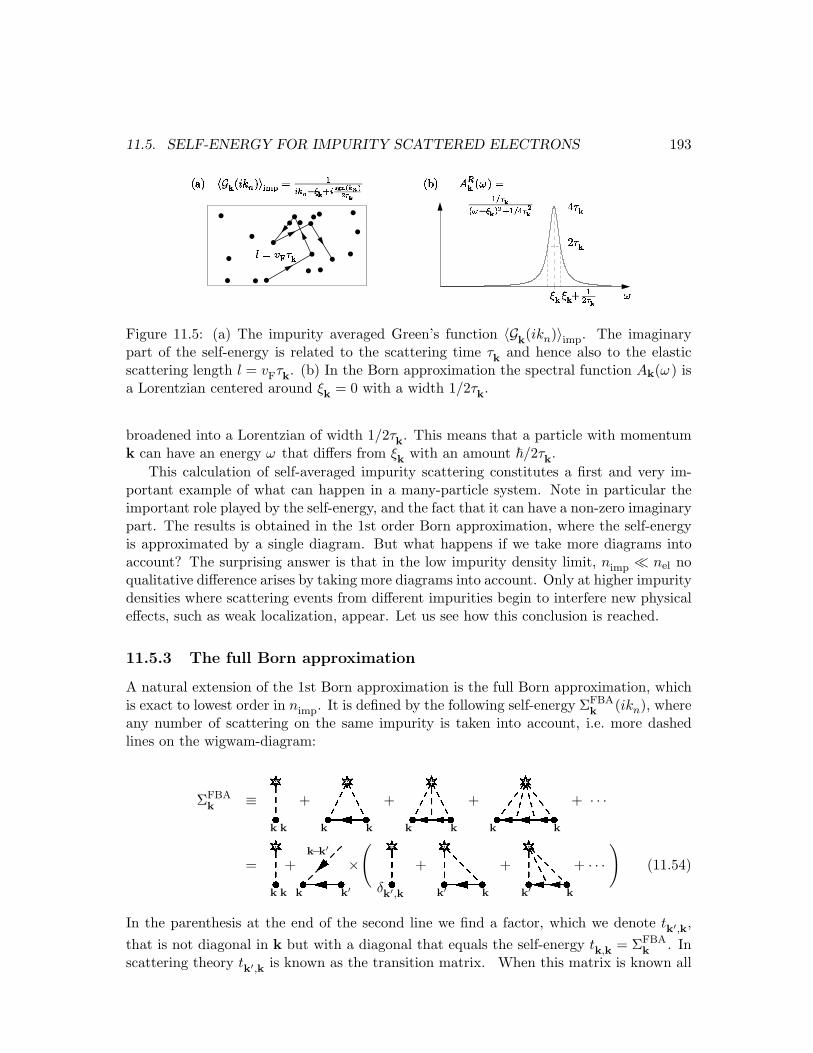
11.5. SELF-ENERGY FOR IMPURITY SCATTERED ELECTRONS 193
!" # $ &% ' (
) * + , - " ) . * "0/
1
2 2 345 * (
Figure 11.5: (a) The impurity averaged Green’s function 〈Gk(ikn)〉imp. The imaginarypart of the self-energy is related to the scattering time τk and hence also to the elasticscattering length l = vFτk. (b) In the Born approximation the spectral function Ak(ω ) isa Lorentzian centered around ξk = 0 with a width 1/2τk.
broadened into a Lorentzian of width 1/2τk. This means that a particle with momentumk can have an energy ω that differs from ξk with an amount ~/2τk.
This calculation of self-averaged impurity scattering constitutes a first and very im-portant example of what can happen in a many-particle system. Note in particular theimportant role played by the self-energy, and the fact that it can have a non-zero imaginarypart. The results is obtained in the 1st order Born approximation, where the self-energyis approximated by a single diagram. But what happens if we take more diagrams intoaccount? The surprising answer is that in the low impurity density limit, nimp ¿ nel noqualitative difference arises by taking more diagrams into account. Only at higher impuritydensities where scattering events from different impurities begin to interfere new physicaleffects, such as weak localization, appear. Let us see how this conclusion is reached.
11.5.3 The full Born approximation
A natural extension of the 1st Born approximation is the full Born approximation, whichis exact to lowest order in nimp. It is defined by the following self-energy ΣFBA
k (ikn), whereany number of scattering on the same impurity is taken into account, i.e. more dashedlines on the wigwam-diagram:
ΣFBAk ≡ ?
k k
+ @k k
+ Ak k
+ Bk k
+ · · ·
= Ck k
+Dk k′
k−k′×
( Eδk′,k
+ Fk′ k
+ Gk′ k
+ · · ·)
(11.54)
In the parenthesis at the end of the second line we find a factor, which we denote tk′,k,that is not diagonal in k but with a diagonal that equals the self-energy tk,k = ΣFBA
k . Inscattering theory tk′,k is known as the transition matrix. When this matrix is known all
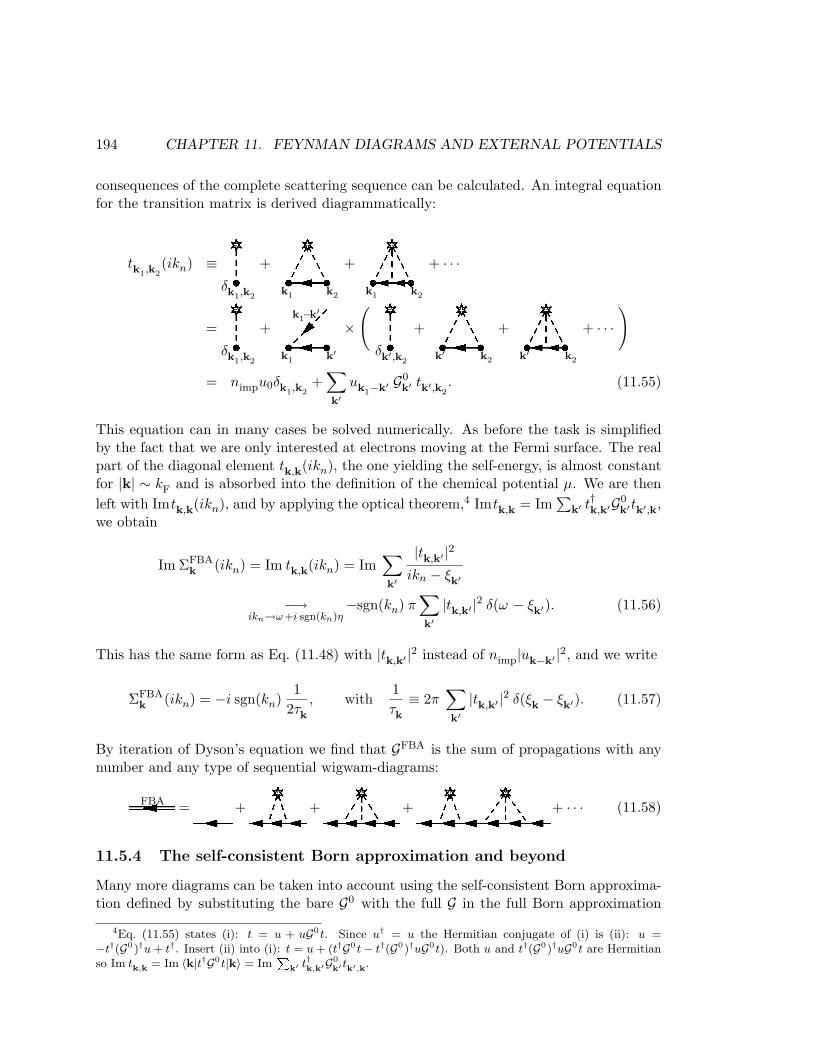
194 CHAPTER 11. FEYNMAN DIAGRAMS AND EXTERNAL POTENTIALS
consequences of the complete scattering sequence can be calculated. An integral equationfor the transition matrix is derived diagrammatically:
tk1,k2(ikn) ≡ H
δk1,k2
+ Ik1 k2
+ Jk1 k2
+ · · ·
= Kδk1,k2
+ Lk1 k′
k1−k′ ×( M
δk′,k2
+ Nk′ k2
+ Ok′ k2
+ · · ·)
= nimpu0δk1,k2+
∑
k′uk1−k′ G0
k′ tk′,k2. (11.55)
This equation can in many cases be solved numerically. As before the task is simplifiedby the fact that we are only interested at electrons moving at the Fermi surface. The realpart of the diagonal element tk,k(ikn), the one yielding the self-energy, is almost constantfor |k| ∼ kF and is absorbed into the definition of the chemical potential µ. We are thenleft with Imtk,k(ikn), and by applying the optical theorem,4 Imtk,k = Im
∑k′ t
†k,k′G0
k′tk′,k,we obtain
Im ΣFBAk (ikn) = Im tk,k(ikn) = Im
∑
k′
|tk,k′ |2ikn − ξk′
−→ikn→ω+i sgn(kn)η
−sgn(kn) π∑
k′|tk,k′ |2 δ(ω − ξk′). (11.56)
This has the same form as Eq. (11.48) with |tk,k′ |2 instead of nimp|uk−k′ |2, and we write
ΣFBAk (ikn) = −i sgn(kn)
12τk
, with1τk≡ 2π
∑
k′|tk,k′ |2 δ(ξk − ξk′). (11.57)
By iteration of Dyson’s equation we find that GFBA is the sum of propagations with anynumber and any type of sequential wigwam-diagrams:PFBA =Q+R+S+T+ · · · (11.58)
11.5.4 The self-consistent Born approximation and beyond
Many more diagrams can be taken into account using the self-consistent Born approxima-tion defined by substituting the bare G0 with the full G in the full Born approximation
4Eq. (11.55) states (i): t = u + uG0t. Since u† = u the Hermitian conjugate of (i) is (ii): u =−t†(G0)†u + t†. Insert (ii) into (i): t = u + (t†G0t− t†(G0)†uG0t). Both u and t†(G0)†uG0t are Hermitianso Im tk,k = Im 〈k|t†G0t|k〉 = Im
Pk′ t
†k,k′G0
k′tk′,k.

11.5. SELF-ENERGY FOR IMPURITY SCATTERED ELECTRONS 195
Eqs. (11.54) and (11.55) yields:
ΣSCBAk ≡ U +V +W +X + · · ·
= nimpu0δk,k +∑
k′uk−k′ Gk′ tk′,k, (11.59)
a self-consistent equation in ΣSCBAk since Gk′ = (ikn − ξk′ − ΣSCBA
k′ )−1. We again utilizethat tk,k is only weakly dependent on energy for |k| ≈ kF and ω ¿ εF, and if furthermorethe scattering strength is moderate, i.e. |ΣSCBA
k | ¿ εF we obtain almost the same resultas in Eq. (11.56). Only the imaginary part Σi
k of ΣSCBAk = ΣR
k + iΣik plays a role, since
the small real part ΣRk can be absorbed into µ.
Σik = Im tk,k = Im
∑
k′
|tk,k′ |2ikn−ξk′−iΣi
k′≈ −sgn(kn−Σi
k) π∑
k′|tk,k′ |2 δ(ω−ξk′). (11.60)
The only self-consistency requirement is thus connected with the sign of the imaginarypart. But this requirement is fulfilled by taking Im ΣSCBA(ikn) ∝ −sgn(kn) as seen bydirect substitution. The only difference between the full Born and the self-consistentBorn approximation is in the case of strong scattering, where the limiting δ-function inEq. (11.60) may acquire a small renormalization. The final result is
ΣSCBAk (ikn) = −i sgn(kn)
12τk
, with1τk≈ 2π
∑
k′|tk,k′ |2 δ(ω − ξk′). (11.61)
By iteration of Dyson’s equation we find that GSCBA is the sum of propagations withany number and any type of sequential wigwam-diagrams inside wigwam-diagrams butwithout crossings of any scattering lines:YSCBA = Z+[+\+]+ · · ·
+^+_+ · · · (11.62)
+`+ · · ·+a+ · · ·
We have now resummed most of the diagrams in the diagrammatic expansion of 〈Gk〉imp
with the exception of wigwam-diagrams with crossing lines. In Fig. 11.6 are shown twodifferent types of irreducible diagrams of the same order in both nimp and uk. Alsosketched is the phase space Ω available for the internal momenta k1 and k2 in the twocases. At zero temperature the energy broadening around the Fermi energy εF is given by
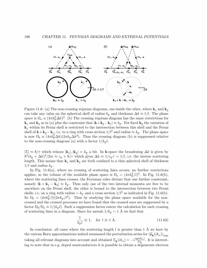
196 CHAPTER 11. FEYNMAN DIAGRAMS AND EXTERNAL POTENTIALS
!
"# !
Figure 11.6: (a) The non-crossing wigwam diagrams, one inside the other, where k1 and k2
can take any value on the spherical shell of radius kF and thickness ∆k ≈ 1/l. The phasespace is Ωa ∝ (4πk2
F∆k)2. (b) The crossing wigwam diagram has the same restrictions fork1 and k2 as in (a) plus the constraint that |k+k2−k1| ≈ kF. For fixed k2 the variation ofk1 within its Fermi shell is restricted to the intersection between this shell and the Fermishell of k+k2−k1, i.e. to a ring with cross section 1/l2 and radius ≈ kF. The phase spaceis now Ωb ∝ (4πk2
F∆k)(2πkF∆k2). Thus the crossing diagram (b) is suppressed relativeto the non-crossing diagram (a) with a factor 1/kFl.
|Σ| ≈ ~/τ which relaxes |k1|, |k2| = kF a bit. In k-space the broadening ∆k is given by~2(kF + ∆k)2/2m ≈ εF + ~/τ which gives ∆k ≈ 1/vFτ = 1/l, i.e. the inverse scatteringlength. This means that k1 and k2 are both confined to a thin spherical shell of thickness1/l and radius kF.
In Fig. 11.6(a), where no crossing of scattering lines occurs, no further restrictionsapplies, so the volume of the available phase space is Ωa = (4πk2
F/l)2. In Fig. 11.6(b),where the scattering lines crosses, the Feynman rules dictate that one further constraint,namely |k + k1 − k2| ≈ kF. Thus only one of the two internal momenta are free to beanywhere on the Fermi shell, the other is bound to the intersection between two Fermishells, i.e. on a ring with radius ∼ kF and a cross section 1/l2 as indicated in Fig. 11.6(b).So Ωb = (4πk2
F/l)(2πkF/l2). Thus by studying the phase space available for the non-crossed and the crossed processes we have found that the crossed ones are suppressed by afactor Ωb/Ωa ≈ 1/(kFl). Such a suppression factor enters the calculation for each crossingof scattering lines in a diagram. Since for metals 1/kF ∼ 1 A we find that
1kFl
¿ 1, for l À 1 A. (11.63)
In conclusion: all cases where the scattering length l is greater than 1 A we have bythe various Born approximations indeed resummed the perturbation series for 〈Gk(ikn)〉imp
taking all relevant diagrams into account and obtained Σk(ikn) = −i sgn(kn)2τk
. It is interest-ing to note that in e.g. doped semiconductors it is possible to obtain a degenerate electron

11.6. SUMMARY AND OUTLOOK 197
gas with a very low density. In these systems 1/kF or the Fermi wavelength is muchlarger than in metals, and the condition in Eq. (11.63) is violated. In this case one maytherefore observe deviations from the simple theory presented here. One example is theobservation of weak localization, which is an increase in the resistivity due to quantuminterference between scattering events involving several impurities at the same time. Theweak localization effect is studied in Sec. 15.4.
11.6 Summary and outlook
In this chapter we have introduced the Feynman diagrams for elastic impurity scattering.We have applied the diagrammatic technique to an analysis of the single-particle Matsub-ara Green’s function for electron propagation in disordered metals. The main result wasthe determination of the self-energy Σk(ikn) in terms of the scattering time τk,
ΣFBAk (ikn) = −i sgn(kn)
12τk
, with1τk≡ 2π
∑
k′|tk,k′ |2 δ(ξk − ξk′),
and the scattering-time broadened spectral function
A1BAk (ω ) =
1/τk(ω − ξk)2 + 1/4τ2
k
.
The structure in the complex plane of the Green’s function was found to be:
G1BAk (ikn) =
1
ikn − ξk + i sgn(kn)2τk
−→ikn→z
G1BAk (z) =
1z−ξk+ i
2τk
, Im z > 0
1z−ξk− i
2τk
, Im z < 0.
These results will be employed in Chap. 15 in the study of the residual resistivity of metals.The theory presented here provides in combination with the Kubo formalism the foun-
dation for a microscopic quantum theory of resistivity. The technique can be extendedto the study of quantum effects like weak localization (see Sec. 15.4) and universal con-ductance fluctuations (see Fig. 11.2). These more subtle quantum effects are fundamentalparts of the modern research field known as mesoscopic physics. They can be explainedwithin the theoretical framework presented here, by taking higher order correlations intoaccount. For example is weak localization explained by treating crossed diagrams like theone in Fig. 11.6(b), which was neglected in calculation presented in this chapter.

198 CHAPTER 11. FEYNMAN DIAGRAMS AND EXTERNAL POTENTIALS
Chapter 12
Feynman diagrams and pairinteractions
It is in the case of interacting particles and fields that the power of quantum field theoryand Feynman diagrams really comes into play. Below we develop the Feynman diagramtechnique for a system of fermions with pair interactions. The time-independent Hamil-tonian H0 of the unperturbed or non-interacting system is
H0 =∑
σ
∫dr Ψ†(r)H0Ψ(r), (12.1)
while the interaction Hamiltonian W is given by
W =12
∑σ1,σ2
∫dr1dr2 Ψ†(σ1, r1)Ψ
†(σ2, r2) W (σ2, r2; σ1, r1) Ψ(σ2, r2)Ψ(σ1, r1). (12.2)
We have specialized to the case where no spin flip processes occur at the vertices, thisbeing the case for our coming main examples: electron-electron interactions mediated byCoulomb or by phonon interactions. The total Hamiltonian H governing the dynamics ofthe system is as usual given by H = H 0+W . The main goal of this chapter is to derive theFeynman rules for the diagrammatic expansion in orders of W of the full single-particleMatsubara Green’s function Eq. (10.33a)
G(σb, rb, τb; σa, ra, τa) ≡ −⟨TτΨ(σb, rb, τb)Ψ
†(σa, ra, τa)⟩. (12.3)
12.1 The perturbation series for G12.2 infinite perturbation series!Matsubara Green’s func-
tion
The field operators in Eq. (12.3) defining G are of course given in the Heisenberg pic-ture, but using Eq. (10.16) we can immediately transform the expression for G into the
199
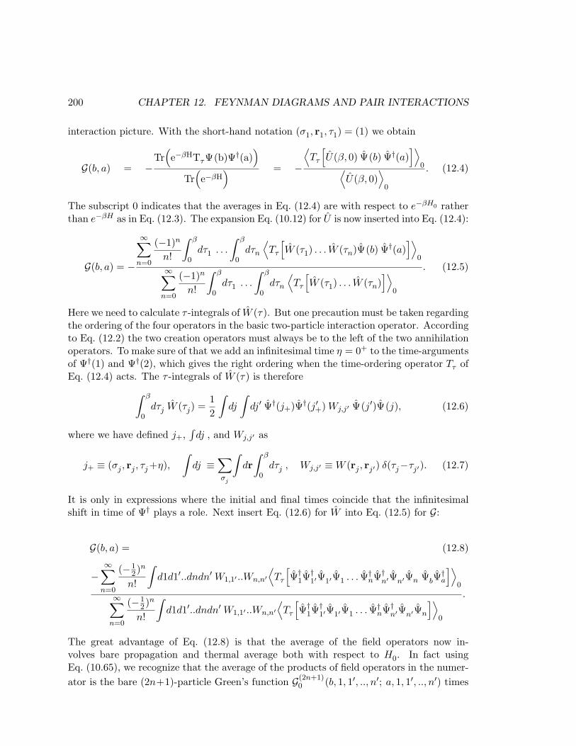
200 CHAPTER 12. FEYNMAN DIAGRAMS AND PAIR INTERACTIONS
interaction picture. With the short-hand notation (σ1, r1, τ1) = (1) we obtain
G(b, a) = −Tr
(e−βHTτΨ(b)Ψ†(a)
)
Tr(e−βH
) = −
⟨Tτ
[U(β, 0) Ψ(b) Ψ†(a)
]⟩0⟨
U(β, 0)⟩
0
. (12.4)
The subscript 0 indicates that the averages in Eq. (12.4) are with respect to e−βH0 ratherthan e−βH as in Eq. (12.3). The expansion Eq. (10.12) for U is now inserted into Eq. (12.4):
G(b, a) = −
∞∑
n=0
(−1)n
n!
∫ β
0dτ1 . . .
∫ β
0dτn
⟨Tτ
[W (τ1) . . . W (τn)Ψ(b) Ψ†(a)
]⟩0
∞∑
n=0
(−1)n
n!
∫ β
0dτ1 . . .
∫ β
0dτn
⟨Tτ
[W (τ1) . . . W (τn)
]⟩0
. (12.5)
Here we need to calculate τ -integrals of W (τ). But one precaution must be taken regardingthe ordering of the four operators in the basic two-particle interaction operator. Accordingto Eq. (12.2) the two creation operators must always be to the left of the two annihilationoperators. To make sure of that we add an infinitesimal time η = 0+ to the time-argumentsof Ψ†(1) and Ψ†(2), which gives the right ordering when the time-ordering operator Tτ ofEq. (12.4) acts. The τ -integrals of W (τ) is therefore
∫ β
0dτj W (τj) =
12
∫dj
∫dj′ Ψ†(j+)Ψ†(j′+) Wj,j′ Ψ(j′)Ψ(j), (12.6)
where we have defined j+,∫
dj , and Wj,j′ as
j+ ≡ (σj , rj , τj+η),∫
dj ≡∑σj
∫dr
∫ β
0dτj , Wj,j′ ≡ W (rj , rj′) δ(τj−τj′). (12.7)
It is only in expressions where the initial and final times coincide that the infinitesimalshift in time of Ψ† plays a role. Next insert Eq. (12.6) for W into Eq. (12.5) for G:
G(b, a) = (12.8)
−∞∑
n=0
(−12)n
n!
∫d1d1′..dndn′ W1,1′ ..Wn,n′
⟨Tτ
[Ψ†
1Ψ†1′Ψ1′Ψ1 . . . Ψ†
nΨ†n′Ψn′Ψn ΨbΨ
†a
]⟩0
∞∑
n=0
(−12)n
n!
∫d1d1′..dndn′ W1,1′ ..Wn,n′
⟨Tτ
[Ψ†
1Ψ†1′Ψ1′Ψ1 . . . Ψ†
nΨ†n′Ψn′Ψn
]⟩0
.
The great advantage of Eq. (12.8) is that the average of the field operators now in-volves bare propagation and thermal average both with respect to H0. In fact usingEq. (10.65), we recognize that the average of the products of field operators in the numer-ator is the bare (2n+1)-particle Green’s function G(2n+1)
0 (b, 1, 1′, .., n′; a, 1, 1′, .., n′) times

12.3. THE FEYNMAN RULES FOR PAIR INTERACTIONS 201
(−1)2n+1 = −1, while in the denominator it is the bare (2n)-particle Green’s functionG(2n)
0 (1, 1′, .., n′; 1, 1′, .., n′) times (−1)2n = 1. The resulting sign, −1, thus cancels thesign in Eq. (12.8). Now is the time for our main use of Wick’s theorem Eq. (10.79): thebare many-particle Green’s functions in the expression for the full single-particle Green’sfunction are written in terms of determinants containing the bare single-particle Green’sfunctions G0(l, j):
G(b, a) = (12.9)
∞∑
n=0
(−12)n
n!
∫d1d1′..dndn′ W1,1′ ..Wn,n′
∣∣∣∣∣∣∣∣∣∣∣
G0(b, a) G0(b, 1) G0(b, 1′) . . . G0(b, n′)G0(1, a) G0(1, 1) G0(1, 1′) . . . G0(1, n′)G0(1′, a) G0(1′, 1) G0(1′, 1′) . . . G0(1′, n′)
.... . .
...G0(n′, a) G0(n′, 1) G0(n′, 1′) . . . G0(n′, n′)
∣∣∣∣∣∣∣∣∣∣∣
∞∑
n=0
(−12)n
n!
∫d1d1′..dndn′ W1,1′ ..Wn,n′
∣∣∣∣∣∣∣∣∣
G0(1, 1) G0(1, 1′) . . . G0(1, n′)G0(1′, 1) G0(1′, 1′) . . . G0(1′, n′)
.... . .
...G0(n′, 1) G0(n′, 1′) . . . G0(n′, n′)
∣∣∣∣∣∣∣∣∣
This voluminous formula is the starting point for defining the Feynman rules for thediagrammatic expansion of G in terms of the pair interaction W . We have suppressed,but not forgotten, the fact that the initial time τj in G0(l, j) according to Eqs. (12.6)and (12.7) is to be shifted infinitesimally to τj + η.
12.3 The Feynman rules for pair interactions
We formulate first a number of basic Feynman rules that are derived directly from Eq. (12.9).However, it turns out that using these basic rules leads to a proof that the denominatorcancels out. This in turn leads to the formulation of the final Feynman rules to be usedin all later calculations.
12.3.1 Feynman rules for the denominator of G(b, a)
The basic Feynman rules for n’th order term in the denominator of G(b, a) are
(1) Fermion lines: j2 j1 ≡ G0(j2, j1), τ1 → τ1 + η.(2) Interaction lines: j j′ ≡ Wj,j′ .(3) Vertices: j• ≡ ∫
dj δσinj ,σout
j, i.e. sum over internal variables, no spin flip.
(4) Draw (2n)! sets of n interaction lines j j′.(5) For each set connect the 2n vertices with 2n fermion lines: one entering
and one leaving each vertex. This can be done in (2n)! ways.
(12.10a)
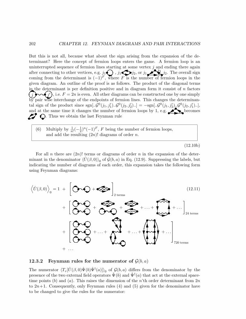
202 CHAPTER 12. FEYNMAN DIAGRAMS AND PAIR INTERACTIONS
But this is not all, because what about the sign arising from the expansion of the de-terminant? Here the concept of fermion loops enters the game. A fermion loop is anuninterrupted sequence of fermion lines starting at some vertex j and ending there againafter connecting to other vertices, e.g. j1 , j1 j2, or j1j3 j2. The overall signcoming from the determinant is (−1)F , where F is the number of fermion loops in thegiven diagram. An outline of the proof is as follows. The product of the diagonal termsin the determinant is per definition positive and in diagram form it consist of n factorsj j′ , i.e. F = 2n is even. All other diagrams can be constructed one by one simplyby pair wise interchange of the endpoints of fermion lines. This changes the determinan-tal sign of the product since sgn[..G0(j1, j
′1)..G0(j2, j
′2)..] = −sgn[..G0(j1, j
′2)..G0(j2, j
′1)..],
and at the same time it changes the number of fermion loops by 1, e.g. becomes . Thus we obtain the last Feynman rule
(6) Multiply by 1n!(−1
2)n(−1)F , F being the number of fermion loops,and add the resulting (2n)! diagrams of order n.
(12.10b)
For all n there are (2n)! terms or diagrams of order n in the expansion of the deter-minant in the denominator 〈U(β, 0)〉0 of G(b, a) in Eq. (12.9). Suppressing the labels, butindicating the number of diagrams of each order, this expansion takes the following formusing Feynman diagrams:
⟨U(β, 0)
⟩0
= 1 +
[ + ]
2 terms
(12.11)
+
[ + + + . . . + + . . .
]
24 terms
+
+ . . . + + . . . + + . . .
720 terms
+ . . .
12.3.2 Feynman rules for the numerator of G(b, a)
The numerator 〈Tτ [U(β, 0)Ψ(b)Ψ†(a)]〉0 of G(b, a) differs from the denominator by thepresence of the two external field operators Ψ(b) and Ψ†(a) that act at the external space-time points (b) and (a). This raises the dimension of the n’th order determinant from 2nto 2n+1. Consequently, only Feynman rules (4) and (5) given for the denominator haveto be changed to give the rules for the numerator:
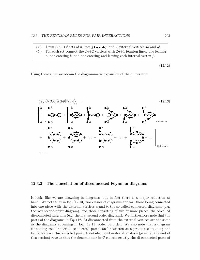
12.3. THE FEYNMAN RULES FOR PAIR INTERACTIONS 203
(4’) Draw (2n+1)! sets of n lines j j′ and 2 external vertices •a and •b.(5’) For each set connect the 2n+2 vertices with 2n+1 fermion lines: one leaving
a, one entering b, and one entering and leaving each internal vertex j.
(12.12)
Using these rules we obtain the diagrammatic expansion of the numerator:
⟨Tτ [U(β, 0)Ψ(b)Ψ†(a)]
⟩0
= (12.13)
ba+ba +ba +ba +ba +ba +ba
6 terms
+
b
a
+!b
a
+ . . . +"b
a
+ . . . +#b
a
+ . . .
120 terms
+ . . .
12.3.3 The cancellation of disconnected Feynman diagrams
It looks like we are drowning in diagrams, but in fact there is a major reduction athand. We note that in Eq. (12.13) two classes of diagrams appear: those being connectedinto one piece with the external vertices a and b, the so-called connected diagrams (e.g.the last second-order diagram), and those consisting of two or more pieces, the so-calleddisconnected diagrams (e.g. the first second order diagram). We furthermore note that theparts of the diagrams in Eq. (12.13) disconnected from the external vertices are the sameas the diagrams appearing in Eq. (12.11) order by order. We also note that a diagramcontaining two or more disconnected parts can be written as a product containing onefactor for each disconnected part. A detailed combinatorial analysis (given at the end ofthis section) reveals that the denominator in G cancels exactly the disconnected parts of
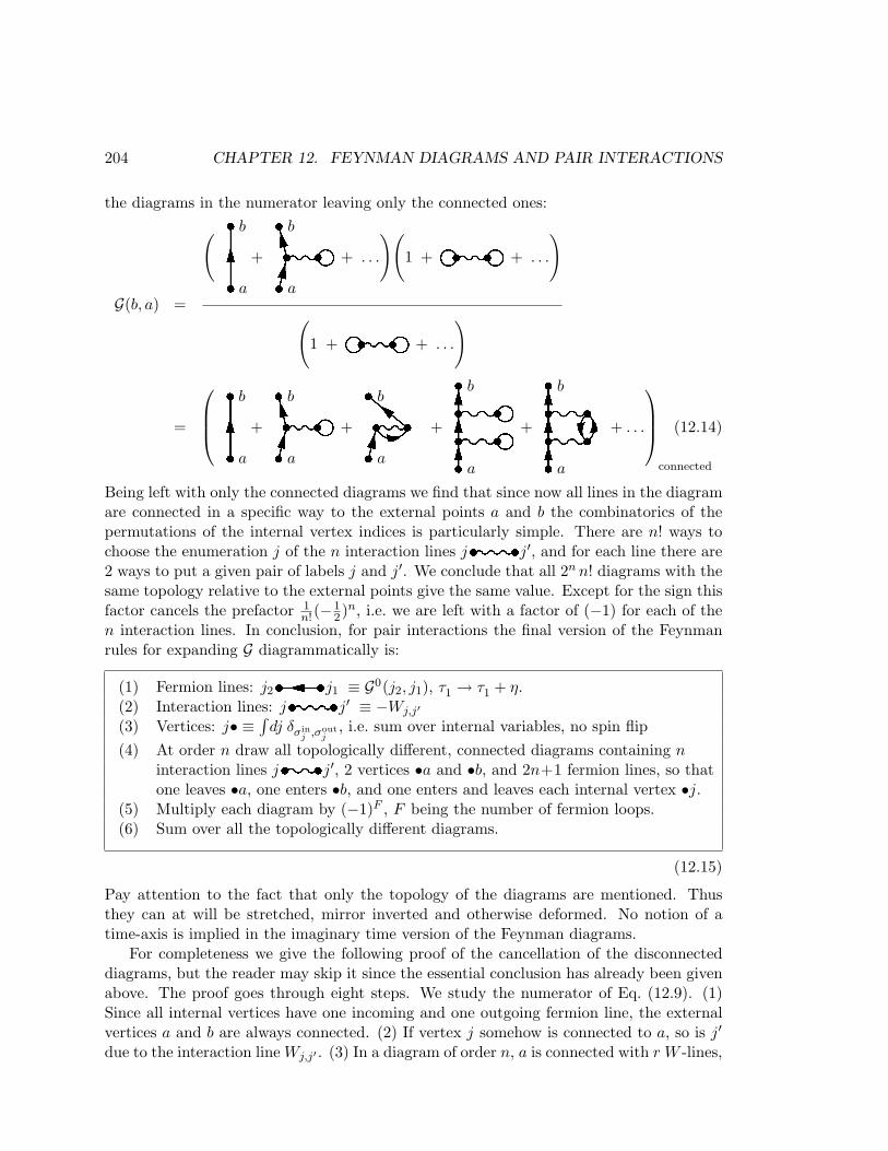
204 CHAPTER 12. FEYNMAN DIAGRAMS AND PAIR INTERACTIONS
the diagrams in the numerator leaving only the connected ones:
G(b, a) =
( $ba +%ba + . . .
)(1 +& + . . .
)
(1 +' + . . .
)
=
(ba +)ba +*ba ++
b
a
+,b
a
+ . . .
connected
(12.14)
Being left with only the connected diagrams we find that since now all lines in the diagramare connected in a specific way to the external points a and b the combinatorics of thepermutations of the internal vertex indices is particularly simple. There are n! ways tochoose the enumeration j of the n interaction lines j- j′, and for each line there are2 ways to put a given pair of labels j and j′. We conclude that all 2n n! diagrams with thesame topology relative to the external points give the same value. Except for the sign thisfactor cancels the prefactor 1
n!(−12)n, i.e. we are left with a factor of (−1) for each of the
n interaction lines. In conclusion, for pair interactions the final version of the Feynmanrules for expanding G diagrammatically is:
(1) Fermion lines: j2. j1 ≡ G0(j2, j1), τ1 → τ1 + η.(2) Interaction lines: j/ j′ ≡ −Wj,j′
(3) Vertices: j• ≡ ∫dj δσin
j ,σoutj
, i.e. sum over internal variables, no spin flip(4) At order n draw all topologically different, connected diagrams containing n
interaction lines j0 j′, 2 vertices •a and •b, and 2n+1 fermion lines, so thatone leaves •a, one enters •b, and one enters and leaves each internal vertex •j.
(5) Multiply each diagram by (−1)F , F being the number of fermion loops.(6) Sum over all the topologically different diagrams.
(12.15)
Pay attention to the fact that only the topology of the diagrams are mentioned. Thusthey can at will be stretched, mirror inverted and otherwise deformed. No notion of atime-axis is implied in the imaginary time version of the Feynman diagrams.
For completeness we give the following proof of the cancellation of the disconnecteddiagrams, but the reader may skip it since the essential conclusion has already been givenabove. The proof goes through eight steps. We study the numerator of Eq. (12.9). (1)Since all internal vertices have one incoming and one outgoing fermion line, the externalvertices a and b are always connected. (2) If vertex j somehow is connected to a, so is j′
due to the interaction line Wj,j′ . (3) In a diagram of order n, a is connected with r W -lines,
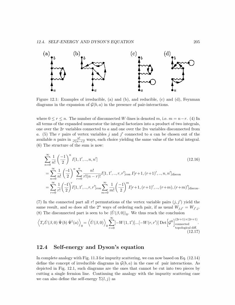
12.4. SELF-ENERGY AND DYSON’S EQUATION 205
Figure 12.1: Examples of irreducible, (a) and (b), and reducible, (c) and (d), Feynmandiagrams in the expansion of G(b, a) in the presence of pair-interactions.
where 0 ≤ r ≤ n. The number of disconnected W -lines is denoted m, i.e. m = n−r. (4) Inall terms of the expanded numerator the integral factorizes into a product of two integrals,one over the 2r variables connected to a and one over the 2m variables disconnected froma. (5) The r pairs of vertex variables j and j′ connected to a can be chosen out of theavailable n pairs in n!
r!(n−r)! ways, each choice yielding the same value of the total integral.(6) The structure of the sum is now:
∞∑
n=0
1n!
(−12
)n
I[1, 1′, .., n, n′] (12.16)
=∞∑
n=0
1n!
(−12
)n n∑
r=0
n!r!(n− r)!
I[1, 1′, .., r, r′]con I[r+1, (r+1)′, .., n, n′]discon
=∞∑
r=0
1r!
(−12
)r
I[1, 1′, .., r, r′]con
∞∑
m=0
1m!
(−12
)m
I[r+1, (r+1)′, .., (r+m), (r+m)′]discon.
(7) In the connected part all r! permutations of the vertex variable pairs (j, j′) yield thesame result, and so does all the 2n ways of ordering each pair, if as usual Wj,j′ = Wj′,j .(8) The disconnected part is seen to be 〈U(β, 0)〉0. We thus reach the conclusion⟨Tτ U(β, 0) Ψ(b) Ψ†(a)
⟩0=
⟨U(β, 0)
⟩0
∞∑
r=0
[−W (1, 1′)]...[−W (r, r′)] Det[G0
](2r+1)×(2r+1)
connectedtopological diff.
.
(12.17)
12.4 Self-energy and Dyson’s equation
In complete analogy with Fig. 11.3 for impurity scattering, we can now based on Eq. (12.14)define the concept of irreducible diagrams in G(b, a) in the case of pair interactions. Asdepicted in Fig. 12.1, such diagrams are the ones that cannot be cut into two pieces bycutting a single fermion line. Continuing the analogy with the impurity scattering casewe can also define the self-energy Σ(l, j) as
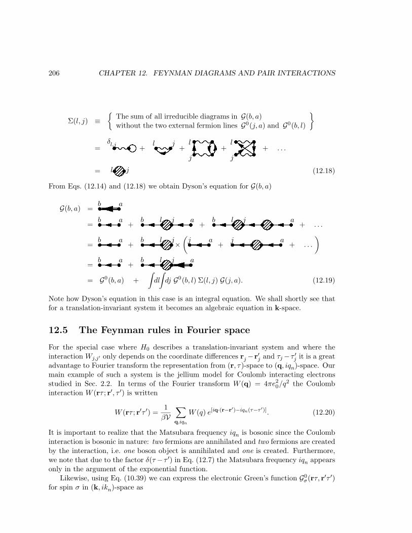
206 CHAPTER 12. FEYNMAN DIAGRAMS AND PAIR INTERACTIONS
Σ(l, j) ≡
The sum of all irreducible diagrams in G(b, a)without the two external fermion lines G0(j, a) and G0(b, l)
=1δl,j +2l j+3jl +4jl + . . .
= 5l j (12.18)
From Eqs. (12.14) and (12.18) we obtain Dyson’s equation for G(b, a)
G(b, a) = 6b a
= 7b a+ 8b l j a
+ 9b l j a+ . . .
= :b a+ ;b l j×
(<j a+ =j a
+ . . .
)
= >b a+ ?b l j a
= G0(b, a) +∫
dl
∫dj G0(b, l) Σ(l, j) G(j, a). (12.19)
Note how Dyson’s equation in this case is an integral equation. We shall shortly see thatfor a translation-invariant system it becomes an algebraic equation in k-space.
12.5 The Feynman rules in Fourier space
For the special case where H0 describes a translation-invariant system and where theinteraction Wj,j′ only depends on the coordinate differences rj−r′j and τj−τ ′j it is a greatadvantage to Fourier transform the representation from (r, τ)-space to (q, iqn)-space. Ourmain example of such a system is the jellium model for Coulomb interacting electronsstudied in Sec. 2.2. In terms of the Fourier transform W (q) = 4πe2
0/q2 the Coulombinteraction W (rτ ; r′, τ ′) is written
W (rτ ; r′τ ′) =1
βV∑
q,iqn
W (q) e[iq·(r−r′)−iqn(τ−τ ′)]. (12.20)
It is important to realize that the Matsubara frequency iqn is bosonic since the Coulombinteraction is bosonic in nature: two fermions are annihilated and two fermions are createdby the interaction, i.e. one boson object is annihilated and one is created. Furthermore,we note that due to the factor δ(τ −τ ′) in Eq. (12.7) the Matsubara frequency iqn appearsonly in the argument of the exponential function.
Likewise, using Eq. (10.39) we can express the electronic Green’s function G0σ(rτ, r′τ ′)
for spin σ in (k, ikn)-space as
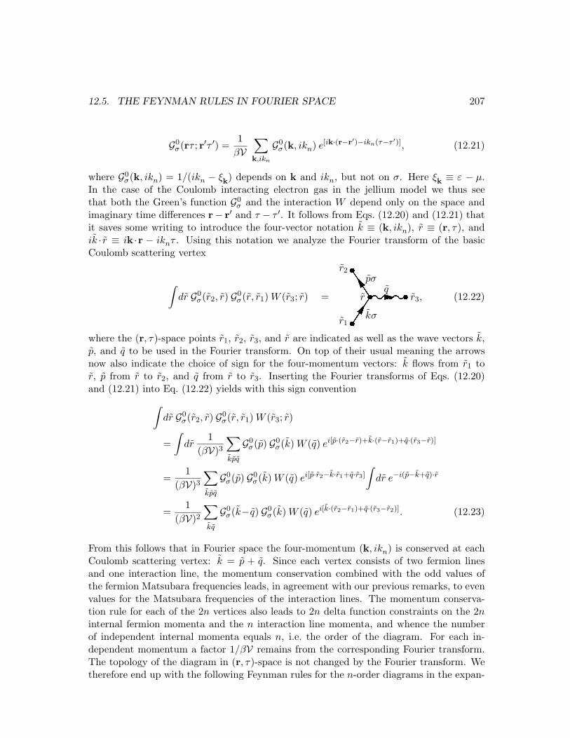
12.5. THE FEYNMAN RULES IN FOURIER SPACE 207
G0σ(rτ ; r′τ ′) =
1βV
∑
k,ikn
G0σ(k, ikn) e[ik·(r−r′)−ikn(τ−τ ′)], (12.21)
where G0σ(k, ikn) = 1/(ikn − ξk) depends on k and ikn, but not on σ. Here ξk ≡ ε − µ.
In the case of the Coulomb interacting electron gas in the jellium model we thus seethat both the Green’s function G0
σ and the interaction W depend only on the space andimaginary time differences r− r′ and τ − τ ′. It follows from Eqs. (12.20) and (12.21) thatit saves some writing to introduce the four-vector notation k ≡ (k, ikn), r ≡ (r, τ), andik · r ≡ ik ·r − iknτ . Using this notation we analyze the Fourier transform of the basicCoulomb scattering vertex
∫dr G0
σ(r2, r) G0σ(r, r1) W (r3; r) = @pσ
kσ
q
r1
r
r2
r3, (12.22)
where the (r, τ)-space points r1, r2, r3, and r are indicated as well as the wave vectors k,p, and q to be used in the Fourier transform. On top of their usual meaning the arrowsnow also indicate the choice of sign for the four-momentum vectors: k flows from r1 tor, p from r to r2, and q from r to r3. Inserting the Fourier transforms of Eqs. (12.20)and (12.21) into Eq. (12.22) yields with this sign convention
∫dr G0
σ(r2, r) G0σ(r, r1) W (r3; r)
=∫
dr1
(βV)3∑
kpq
G0σ(p) G0
σ(k) W (q) ei[p·(r2−r)+k·(r−r1)+q·(r3−r)]
=1
(βV)3∑
kpq
G0σ(p) G0
σ(k) W (q) ei[p·r2−k·r1+q·r3]
∫dr e−i(p−k+q)·r
=1
(βV)2∑
kq
G0σ(k−q) G0
σ(k) W (q) ei[k·(r2−r1)+q·(r3−r2)]. (12.23)
From this follows that in Fourier space the four-momentum (k, ikn) is conserved at eachCoulomb scattering vertex: k = p + q. Since each vertex consists of two fermion linesand one interaction line, the momentum conservation combined with the odd values ofthe fermion Matsubara frequencies leads, in agreement with our previous remarks, to evenvalues for the Matsubara frequencies of the interaction lines. The momentum conserva-tion rule for each of the 2n vertices also leads to 2n delta function constraints on the 2ninternal fermion momenta and the n interaction line momenta, and whence the numberof independent internal momenta equals n, i.e. the order of the diagram. For each in-dependent momentum a factor 1/βV remains from the corresponding Fourier transform.The topology of the diagram in (r, τ)-space is not changed by the Fourier transform. Wetherefore end up with the following Feynman rules for the n-order diagrams in the expan-
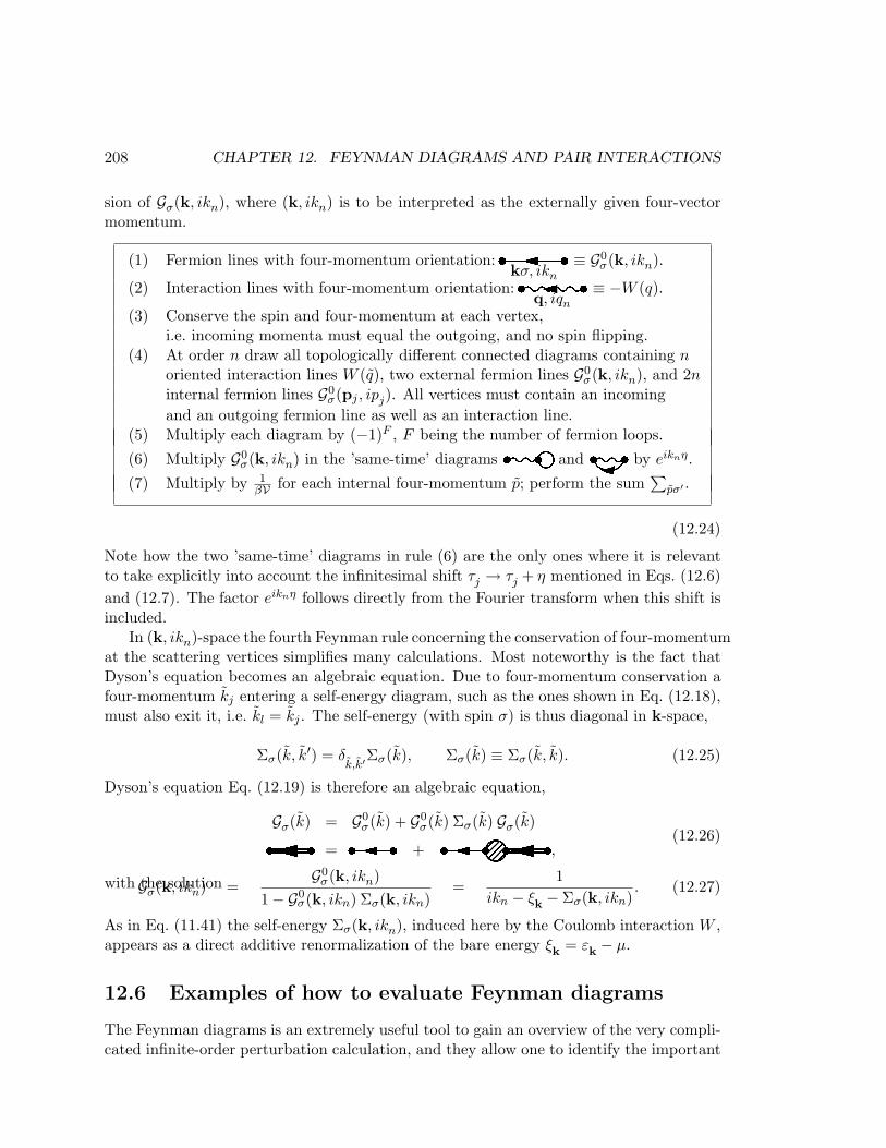
208 CHAPTER 12. FEYNMAN DIAGRAMS AND PAIR INTERACTIONS
sion of Gσ(k, ikn), where (k, ikn) is to be interpreted as the externally given four-vectormomentum.
(1) Fermion lines with four-momentum orientation:Akσ, ikn≡ G0
σ(k, ikn).
(2) Interaction lines with four-momentum orientation:Bq, iqn≡ −W (q).
(3) Conserve the spin and four-momentum at each vertex,i.e. incoming momenta must equal the outgoing, and no spin flipping.
(4) At order n draw all topologically different connected diagrams containing noriented interaction lines W (q), two external fermion lines G0
σ(k, ikn), and 2ninternal fermion lines G0
σ(pj , ipj). All vertices must contain an incomingand an outgoing fermion line as well as an interaction line.
(5) Multiply each diagram by (−1)F , F being the number of fermion loops.
(6) Multiply G0σ(k, ikn) in the ’same-time’ diagramsC andDby eiknη.
(7) Multiply by 1βV for each internal four-momentum p; perform the sum
∑pσ′ .
(12.24)
Note how the two ’same-time’ diagrams in rule (6) are the only ones where it is relevantto take explicitly into account the infinitesimal shift τj → τj + η mentioned in Eqs. (12.6)and (12.7). The factor eiknη follows directly from the Fourier transform when this shift isincluded.
In (k, ikn)-space the fourth Feynman rule concerning the conservation of four-momentumat the scattering vertices simplifies many calculations. Most noteworthy is the fact thatDyson’s equation becomes an algebraic equation. Due to four-momentum conservation afour-momentum kj entering a self-energy diagram, such as the ones shown in Eq. (12.18),must also exit it, i.e. kl = kj . The self-energy (with spin σ) is thus diagonal in k-space,
Σσ(k, k′) = δk,k′
Σσ(k), Σσ(k) ≡ Σσ(k, k). (12.25)
Dyson’s equation Eq. (12.19) is therefore an algebraic equation,
Gσ(k) = G0σ(k) + G0
σ(k) Σσ(k) Gσ(k)E = F + G ,(12.26)
with the solutionGσ(k, ikn) =G0
σ(k, ikn)1− G0
σ(k, ikn) Σσ(k, ikn)=
1ikn − ξk − Σσ(k, ikn)
. (12.27)
As in Eq. (11.41) the self-energy Σσ(k, ikn), induced here by the Coulomb interaction W ,appears as a direct additive renormalization of the bare energy ξk = εk − µ.
12.6 Examples of how to evaluate Feynman diagrams
The Feynman diagrams is an extremely useful tool to gain an overview of the very compli-cated infinite-order perturbation calculation, and they allow one to identify the important
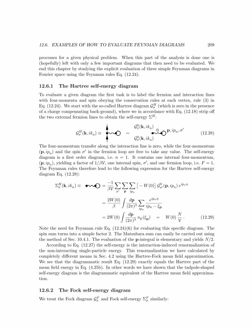
12.6. EXAMPLES OF HOW TO EVALUATE FEYNMAN DIAGRAMS 209
processes for a given physical problem. When this part of the analysis is done one is(hopefully) left with only a few important diagrams that then need to be evaluated. Weend this chapter by studying the explicit evaluation of three simple Feynman diagrams inFourier space using the Feynman rules Eq. (12.24).
12.6.1 The Hartree self-energy diagram
To evaluate a given diagram the first task is to label the fermion and interaction lineswith four-momenta and spin obeying the conservation rules at each vertex, rule (3) inEq. (12.24). We start with the so-called Hartree diagram GH
σ (which is zero in the presenceof a charge compensating back-ground), where we in accordance with Eq. (12.18) strip offthe two external fermion lines to obtain the self-energy ΣH :
GHσ (k, ikn) ≡H = IG0
σ(k, ikn)
G0σ(k, ikn)
0 p, ipn, σ′(12.28)
The four-momentum transfer along the interaction line is zero, while the four-momentum(p, ipn) and the spin σ′ in the fermion loop are free to take any value. The self-energydiagram is a first order diagram, i.e. n = 1. It contains one internal four-momentum,(p, ipn), yielding a factor of 1/βV, one internal spin, σ′, and one fermion loop, i.e. F = 1.The Feynman rules therefore lead to the following expression for the Hartree self-energydiagram Eq. (12.28):
ΣHσ (k, ikn) ≡J =
−1βV
∑
σ′
∑p
∑
ipn
[−W (0)] G0
σ′(p, ipn) eipnη
=2W (0)
β
∫dp
(2π)3∑
ipn
eipnη
ipn − ξp
= 2W (0)∫
dp(2π)3
nF(ξp) = W (0)N
V . (12.29)
Note the need for Feynman rule Eq. (12.24)(6) for evaluating this specific diagram. Thespin sum turns into a simple factor 2. The Matsubara sum can easily be carried out usingthe method of Sec. 10.4.1. The evaluation of the p-integral is elementary and yields N/2.
According to Eq. (12.27) the self-energy is the interaction-induced renormalization ofthe non-interacting single-particle energy. This renormalization we have calculated bycompletely different means in Sec. 4.2 using the Hartree-Fock mean field approximation.We see that the diagrammatic result Eq. (12.29) exactly equals the Hartree part of themean field energy in Eq. (4.25b). In other words we have shown that the tadpole-shapedself-energy diagram is the diagrammatic equivalent of the Hartree mean field approxima-tion.
12.6.2 The Fock self-energy diagram
We treat the Fock diagram GFσ and Fock self-energy ΣF
σ similarly:
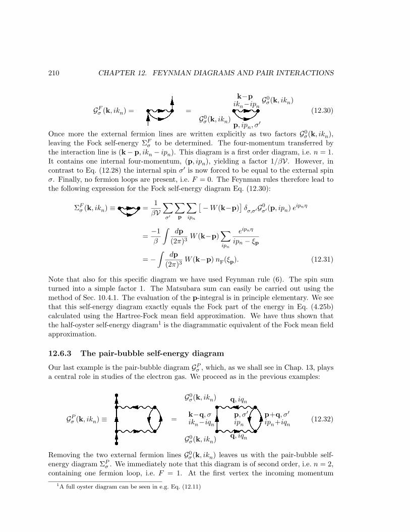
210 CHAPTER 12. FEYNMAN DIAGRAMS AND PAIR INTERACTIONS
GFσ (k, ikn) =K= LG0
σ(k, ikn)
G0σ(k, ikn)k−p
ikn−ipn
p, ipn, σ′
(12.30)
Once more the external fermion lines are written explicitly as two factors G0σ(k, ikn),
leaving the Fock self-energy ΣFσ to be determined. The four-momentum transferred by
the interaction line is (k− p, ikn − ipn). This diagram is a first order diagram, i.e. n = 1.It contains one internal four-momentum, (p, ipn), yielding a factor 1/βV. However, incontrast to Eq. (12.28) the internal spin σ′ is now forced to be equal to the external spinσ. Finally, no fermion loops are present, i.e. F = 0. The Feynman rules therefore lead tothe following expression for the Fock self-energy diagram Eq. (12.30):
ΣFσ (k, ikn) ≡M =
1βV
∑
σ′
∑p
∑
ipn
[−W (k−p)]δσ,σ′G0
σ′(p, ipn) eipnη
=−1β
∫dp
(2π)3W (k−p)
∑
ipn
eipnη
ipn − ξp
= −∫
dp(2π)3
W (k−p) nF(ξp). (12.31)
Note that also for this specific diagram we have used Feynman rule (6). The spin sumturned into a simple factor 1. The Matsubara sum can easily be carried out using themethod of Sec. 10.4.1. The evaluation of the p-integral is in principle elementary. We seethat this self-energy diagram exactly equals the Fock part of the energy in Eq. (4.25b)calculated using the Hartree-Fock mean field approximation. We have thus shown thatthe half-oyster self-energy diagram1 is the diagrammatic equivalent of the Fock mean fieldapproximation.
12.6.3 The pair-bubble self-energy diagram
Our last example is the pair-bubble diagram GPσ , which, as we shall see in Chap. 13, plays
a central role in studies of the electron gas. We proceed as in the previous examples:
GPσ (k, ikn) ≡ N = OG0
σ(k, ikn)
G0σ(k, ikn)
q, iqn
q, iqn
k−q, σikn−iqn
p, σ′ipn
p+q, σ′ipn+iqn
(12.32)
Removing the two external fermion lines G0σ(k, ikn) leaves us with the pair-bubble self-
energy diagram ΣPσ . We immediately note that this diagram is of second order, i.e. n = 2,
containing one fermion loop, i.e. F = 1. At the first vertex the incoming momentum1A full oyster diagram can be seen in e.g. Eq. (12.11)
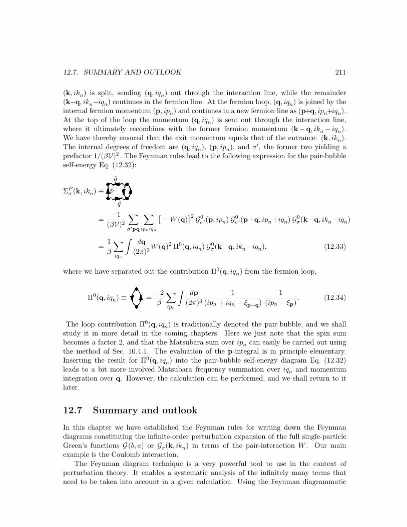
12.7. SUMMARY AND OUTLOOK 211
(k, ikn) is split, sending (q, iqn) out through the interaction line, while the remainder(k−q, ikn−iqn) continues in the fermion line. At the fermion loop, (q, iqn) is joined by theinternal fermion momentum (p, ipn) and continues in a new fermion line as (p+q, ipn+iqn).At the top of the loop the momentum (q, iqn) is sent out through the interaction line,where it ultimately recombines with the former fermion momentum (k−q, ikn− iqn).We have thereby ensured that the exit momentum equals that of the entrance: (k, ikn).The internal degrees of freedom are (q, iqn), (p, ipn), and σ′, the former two yielding aprefactor 1/(βV)2. The Feynman rules lead to the following expression for the pair-bubbleself-energy Eq. (12.32):
ΣPσ (k, ikn) ≡ Pqp
q
=−1
(βV)2∑
σ′pq
∑
ipniqn
[−W (q)]2 G0
σ′(p, ipn) G0σ′(p+q, ipn+iqn) G0
σ(k−q, ikn−iqn)
=1β
∑
iqn
∫dq
(2π)3W (q)2 Π0(q, iqn) G0
σ(k−q, ikn−iqn), (12.33)
where we have separated out the contribution Π0(q, iqn) from the fermion loop,
Π0(q, iqn) ≡ Q =−2β
∑
ipn
∫dp
(2π)31
(ipn + iqn − ξp+q)1
(ipn − ξp). (12.34)
The loop contribution Π0(q, iqn) is traditionally denoted the pair-bubble, and we shallstudy it in more detail in the coming chapters. Here we just note that the spin sumbecomes a factor 2, and that the Matsubara sum over ipn can easily be carried out usingthe method of Sec. 10.4.1. The evaluation of the p-integral is in principle elementary.Inserting the result for Π0(q, iqn) into the pair-bubble self-energy diagram Eq. (12.32)leads to a bit more involved Matsubara frequency summation over iqn and momentumintegration over q. However, the calculation can be performed, and we shall return to itlater.
12.7 Summary and outlook
In this chapter we have established the Feynman rules for writing down the Feynmandiagrams constituting the infinite-order perturbation expansion of the full single-particleGreen’s functions G (b, a) or Gσ(k, ikn) in terms of the pair-interaction W . Our mainexample is the Coulomb interaction.
The Feynman diagram technique is a very powerful tool to use in the context ofperturbation theory. It enables a systematic analysis of the infinitely many terms thatneed to be taken into account in a given calculation. Using the Feynman diagrammatic
212 CHAPTER 12. FEYNMAN DIAGRAMS AND PAIR INTERACTIONS
analysis one can, as we shall see in the following chapters, identify which sub-classes ofdiagrams that give the most important contributions. We have already given explicitexamples of how to evaluate some of the diagrams that are going to play an importantrole. Indeed, we show in Chap. 13 that the diagrams analyzed in Eqs. (12.31) and (12.34)are the ones that dominate the physics of the interacting electron gas in the high densitylimit. We shall learn how these diagrams determine the ground state energy of the systemas well as its dielectric properties such as static and dynamic screening.
Chapter 13
The interacting electron gas
In Sec. 2.2 we studied the Coulomb interaction as a perturbation to the non-interactingelectron gas in the jellium model. This was expected to be a valid procedure in thehigh density limit, where according to Eq. (2.35) the interaction energy is negligible.Nevertheless, the second order perturbation analysis of Sec. 2.2.2 revealed a divergence inthe contribution E
(2)dir from the direct processes, see Eq. (2.49).
In this chapter we reanalyze the Coulomb-interacting electron gas in the jellium modelusing the Feynman diagram technique, and we show how a meaningful finite ground stateenergy can be found. To ensure well-behaved finite integrals during our analysis we workwith the Yukawa-potential with an artificial range 1/α instead of the pure long rangeCoulomb potential, see Eq. (1.103) and the associated footnote,
W (r− r′) =e20
|r− r′| e−α|r−r′|, W (q) =4πe2
0
q2 + α2. (13.1)
The range 1/α has no physical origin. At the end at the calculation we take the limitα → 0 to recover the Coulomb interaction. For example, with the Yukawa potential wecan obtain a finite value for E
(2)dir in Eq. (2.49) if α is finite, but the divergence reappears
as soon as we take the limit α → 0,
E(2)dir ∝
∫
0dq q2 1
(q2 + α2)21q
q q ∼ − ln(α) −→α→0
∞. (13.2)
The main result of the following diagrammatic calculation is that the dynamics of theinteracting system by itself creates a renormalization of the pure Coulomb interaction intoa Yukawa-like potential independent of the value of α, which then without problems canbe taken to zero. The starting point of the theory is the self-energy Σσ(k, ikn).
13.1 The self-energy in the random phase approximation
To construct the diagrammatic expansion of the self-energy Σσ(k, ikn) in (k, ikn)-spacewe use the Feynman rules Eq. (12.24). In analogy with Eq. (12.18) the self-energy is givenby the sum of all the irreducible diagrams in Gσ(k, ikn) removing the two external fermion
213
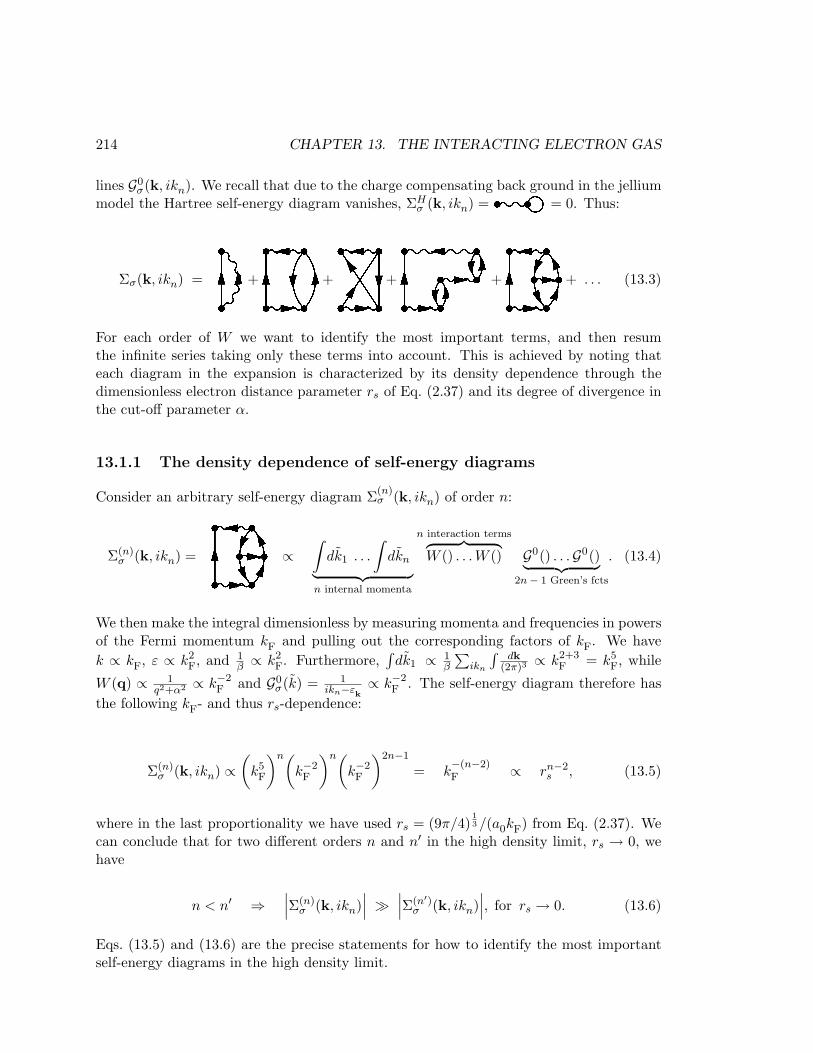
214 CHAPTER 13. THE INTERACTING ELECTRON GAS
lines G0σ(k, ikn). We recall that due to the charge compensating back ground in the jellium
model the Hartree self-energy diagram vanishes, ΣHσ (k, ikn) = = 0. Thus:
Σσ(k, ikn) = + + + + + . . . (13.3)
For each order of W we want to identify the most important terms, and then resumthe infinite series taking only these terms into account. This is achieved by noting thateach diagram in the expansion is characterized by its density dependence through thedimensionless electron distance parameter rs of Eq. (2.37) and its degree of divergence inthe cut-off parameter α.
13.1.1 The density dependence of self-energy diagrams
Consider an arbitrary self-energy diagram Σ(n)σ (k, ikn) of order n:
Σ(n)σ (k, ikn) = ∝
∫dk1 . . .
∫dkn
︸ ︷︷ ︸n internal momenta
n interaction terms︷ ︸︸ ︷W () . . . W () G0() . . .G0()︸ ︷︷ ︸
2n− 1 Green’s fcts
. (13.4)
We then make the integral dimensionless by measuring momenta and frequencies in powersof the Fermi momentum kF and pulling out the corresponding factors of kF. We havek ∝ kF, ε ∝ k2
F, and 1β ∝ k2
F. Furthermore,∫
dk1 ∝ 1β
∑ikn
∫dk
(2π)3∝ k2+3
F = k5F, while
W (q) ∝ 1q2+α2 ∝ k−2
F and G0σ(k) = 1
ikn−εk∝ k−2
F . The self-energy diagram therefore hasthe following kF- and thus rs-dependence:
Σ(n)σ (k, ikn) ∝
(k5
F
)n(k−2
F
)n(k−2
F
)2n−1
= k−(n−2)F ∝ rn−2
s , (13.5)
where in the last proportionality we have used rs = (9π/4)13 /(a0kF) from Eq. (2.37). We
can conclude that for two different orders n and n′ in the high density limit, rs → 0, wehave
n < n′ ⇒∣∣∣Σ(n)
σ (k, ikn)∣∣∣ À
∣∣∣Σ(n′)σ (k, ikn)
∣∣∣, for rs → 0. (13.6)
Eqs. (13.5) and (13.6) are the precise statements for how to identify the most importantself-energy diagrams in the high density limit.
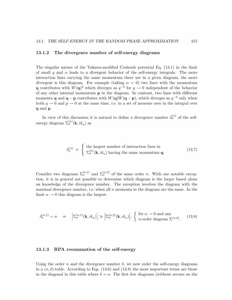
13.1. THE SELF-ENERGY IN THE RANDOM PHASE APPROXIMATION 215
13.1.2 The divergence number of self-energy diagrams
The singular nature of the Yukawa-modified Coulomb potential Eq. (13.1) in the limitof small q and α leads to a divergent behavior of the self-energy integrals. The moreinteraction lines carrying the same momentum there are in a given diagram, the moredivergent is this diagram. For example (taking α = 0) two lines with the momentumq contributes with W (q)2 which diverges as q−4 for q → 0 independent of the behaviorof any other internal momentum p in the diagram. In contrast, two lines with differentmomenta q and q− p contributes with W (q)W (q− p), which diverges as q−4 only whenboth q → 0 and p → 0 at the same time, i.e. in a set of measure zero in the integral overq and p.
In view of this discussion it is natural to define a divergence number δ(n)σ of the self-
energy diagram Σ(n)σ (k, ikn) as
δ(n)σ ≡
the largest number of interaction lines inΣ(n)
σ (k, ikn) having the same momentum q.(13.7)
Consider two diagrams Σ(n,1)σ and Σ(n,2)
σ of the same order n. With one notable excep-tion, it is in general not possible to determine which diagram is the larger based aloneon knowledge of the divergence number. The exception involves the diagram with themaximal divergence number, i.e. when all n momenta in the diagram are the same. In thelimit α → 0 this diagram is the largest:
δ(n,1)σ = n ⇒
∣∣∣Σ(n,1)σ (k, ikn)
∣∣∣ À∣∣∣Σ(n,2)
σ (k, ikn)∣∣∣,
for α → 0 and anyn-order diagram Σ(n,2).
(13.8)
13.1.3 RPA resummation of the self-energy
Using the order n and the divergence number δ, we now order the self-energy diagramsin a (n, δ)-table. According to Eqs. (13.6) and (13.8) the most important terms are thosein the diagonal in this table where δ = n. The first few diagrams (without arrows on the

216 CHAPTER 13. THE INTERACTING ELECTRON GAS
interaction lines for graphical clarity) are
Σσ(k) n = 1 n = 2 n = 3 n = 4
δ = 1 δ = 2 − δ = 3 − − δ = 4 − − −
(13.9)
It is clear that the most important diagrams in the high density limit are those having alow order. For each given order the diagrams with the highest divergence number are themost important. The self-energy in the random phase approximation (RPA) is an infinitesum containing diagrams of all orders n, but only the most divergent one for each n:
ΣRPAσ (k) ≡ k−q
q
+ k−q
q
q
p
p+q+ k−q
q
q
q+ k−q
q
q
q
q + . . .
(13.10)Below we are going to analyze parts of the diagrams individually. This is straightfor-
ward to do, since the Feynman rules Eq. (12.24) are still valid for each part. An importantpart of the self-energy diagrams in Eq. (13.10) is clearly the pair-bubble Π0(q, iqn) ≡ already introduced in Sec. 12.6.3. It plays a crucial role, because it ensures that all inter-action lines W (q) carry the same momentum q. To make the fermion-loop sign from thepair-bubble appear explicitly we prefer to work with χ0 ≡ −Π0 , i.e.
≡ −χ0(q, iqn), χ0(q, iqn) =2β
∑
ipn
∫dp
(2π)31
(ipn + iqn − ξp+q)1
(ipn − ξp).
(13.11)In fact, this χ0 is the same correlation function as the one introduced for other reasons inSec. 10.7.
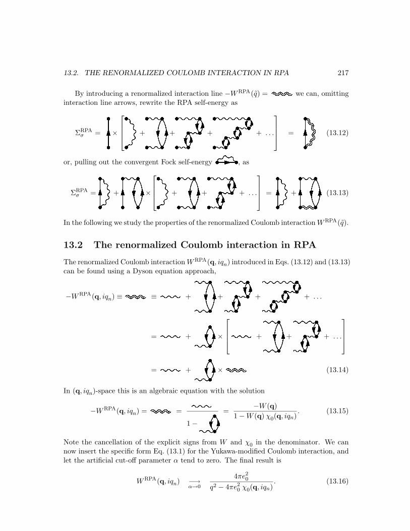
13.2. THE RENORMALIZED COULOMB INTERACTION IN RPA 217
By introducing a renormalized interaction line −WRPA(q) = we can, omittinginteraction line arrows, rewrite the RPA self-energy as
ΣRPAσ = ×
+ + +! + . . .
= " (13.12)
or, pulling out the convergent Fock self-energy# , as
ΣRPAσ = $ +% ×
& +' +( + . . .
= ) +* (13.13)
In the following we study the properties of the renormalized Coulomb interaction WRPA(q).
13.2 The renormalized Coulomb interaction in RPA
The renormalized Coulomb interaction WRPA(q, iqn) introduced in Eqs. (13.12) and (13.13)can be found using a Dyson equation approach,
−WRPA(q, iqn) ≡+ ≡, +- +. +/ + . . .
=0 +1 ×
2 +3 +4 + . . .
=5 +6 ×7 (13.14)
In (q, iqn)-space this is an algebraic equation with the solution
−WRPA(q, iqn) =8 = 91−: =
−W (q)1−W (q) χ0(q, iqn)
. (13.15)
Note the cancellation of the explicit signs from W and χ0 in the denominator. We cannow insert the specific form Eq. (13.1) for the Yukawa-modified Coulomb interaction, andlet the artificial cut-off parameter α tend to zero. The final result is
WRPA(q, iqn) −→α→0
4πe20
q2 − 4πe20 χ0(q, iqn)
. (13.16)
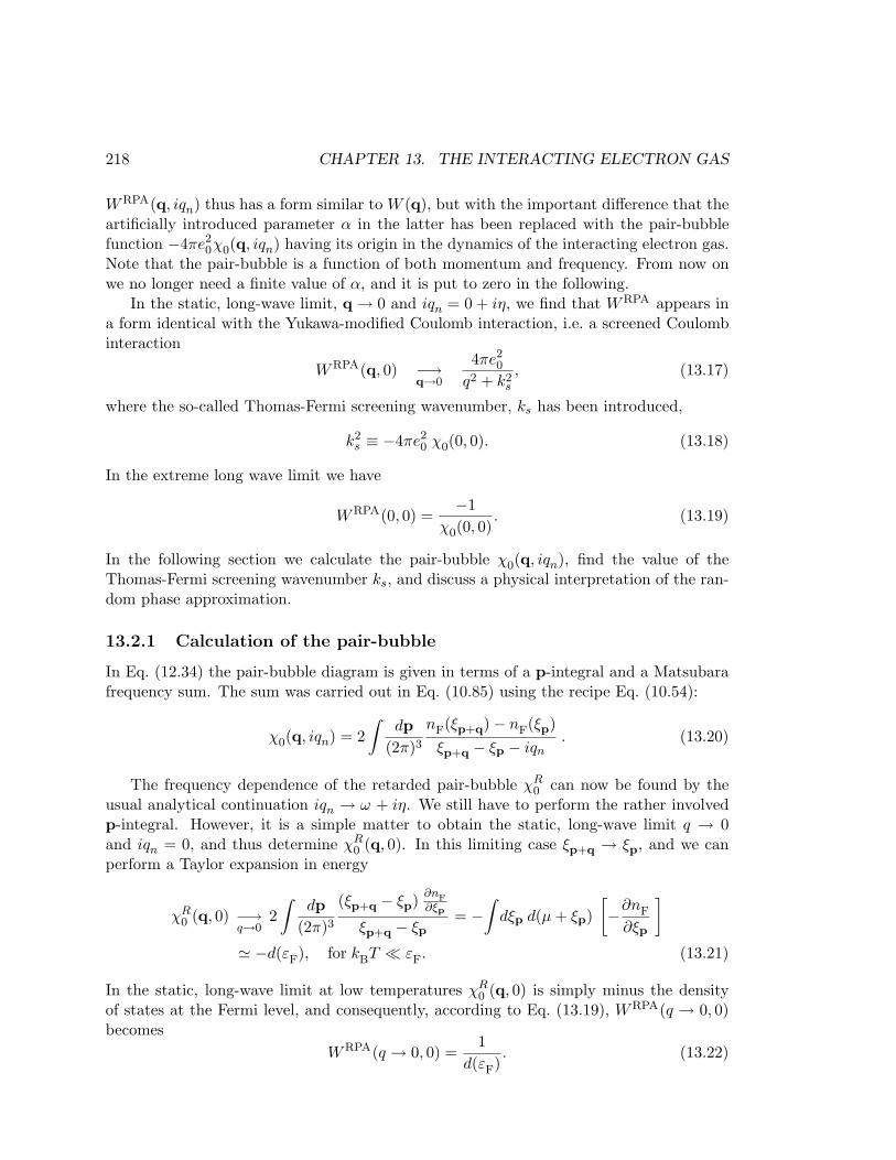
218 CHAPTER 13. THE INTERACTING ELECTRON GAS
WRPA(q, iqn) thus has a form similar to W (q), but with the important difference that theartificially introduced parameter α in the latter has been replaced with the pair-bubblefunction −4πe2
0χ0(q, iqn) having its origin in the dynamics of the interacting electron gas.Note that the pair-bubble is a function of both momentum and frequency. From now onwe no longer need a finite value of α, and it is put to zero in the following.
In the static, long-wave limit, q → 0 and iqn = 0 + iη, we find that WRPA appears ina form identical with the Yukawa-modified Coulomb interaction, i.e. a screened Coulombinteraction
WRPA(q, 0) −→q→0
4πe20
q2 + k2s
, (13.17)
where the so-called Thomas-Fermi screening wavenumber, ks has been introduced,
k2s ≡ −4πe2
0 χ0(0, 0). (13.18)
In the extreme long wave limit we have
WRPA(0, 0) =−1
χ0(0, 0). (13.19)
In the following section we calculate the pair-bubble χ0(q, iqn), find the value of theThomas-Fermi screening wavenumber ks, and discuss a physical interpretation of the ran-dom phase approximation.
13.2.1 Calculation of the pair-bubble
In Eq. (12.34) the pair-bubble diagram is given in terms of a p-integral and a Matsubarafrequency sum. The sum was carried out in Eq. (10.85) using the recipe Eq. (10.54):
χ0(q, iqn) = 2∫
dp(2π)3
nF(ξp+q)− nF(ξp)ξp+q − ξp − iqn
. (13.20)
The frequency dependence of the retarded pair-bubble χR0 can now be found by the
usual analytical continuation iqn → ω + iη. We still have to perform the rather involvedp-integral. However, it is a simple matter to obtain the static, long-wave limit q → 0and iqn = 0, and thus determine χR
0 (q, 0). In this limiting case ξp+q → ξp, and we canperform a Taylor expansion in energy
χR0 (q, 0) −→
q→02
∫dp
(2π)3(ξp+q − ξp) ∂nF
∂ξp
ξp+q − ξp= −
∫dξp d(µ + ξp)
[−∂nF
∂ξp
]
' −d(εF), for kBT ¿ εF. (13.21)
In the static, long-wave limit at low temperatures χR0 (q, 0) is simply minus the density
of states at the Fermi level, and consequently, according to Eq. (13.19), WRPA(q → 0, 0)becomes
WRPA(q → 0, 0) =1
d(εF). (13.22)

13.2. THE RENORMALIZED COULOMB INTERACTION IN RPA 219
The Thomas-Fermi screening wavenumber ks is found by combining Eq. (13.18) withEqs. (2.31) and (2.36),
k2s = −4πe2
0 χR0 (0, 0) = 4π e2
0 d(εF) =4π
kF
a0
, (13.23)
a0 being the Bohr radius. This result is very important, because it relates the screen-ing length 1/ks to microscopic parameters of the electron gas. It is therefore useful fornumerous applications. For metals ks ≈ 0.1 nm−1.
We now turn to the more general case, but limit the calculation of χ0(q, ω + iη) to thelow temperature regime kBT ¿ εF. Finite temperature effects can be obtained by usingthe Sommerfeld expansion or by numerical integration. In the low temperature limit ananalytical expression is obtained by a straightforward but rather tedious calculation. Inthe p-integral the only angular dependence of the integrand is through cos θ, and we have
λ ≡ cos θ,
∫dp
(2π)3=
∫ ∞
0
dp
4π2p2
∫ 1
−1dλ, ξp−q − ξp =
12m
(q2 − 2pqλ). (13.24)
In the low temperature limit the Fermi-Dirac distribution is a step-function, and thereal part of χ0 is most easily calculated by splitting Eq. (13.20) in two terms, substitutingp with p− q in the first term, and collecting the terms again:
Re χ0(q, ω +iη) = −P∫ kF
0
dp
2π2p2
∫ 1
−1dλ nF(ξp)
[1
12m (q2−2pqλ)+ω
+1
12m (q2+2pqλ)−ω
].
(13.25)The integrand is now made dimensionless by measuring all momenta in units of kF andall frequencies and energies in units of εF, such as
x ≡ q
2kF
and x0 ≡ ω
4εF
, (13.26)
and then the λ-integral followed by the p-integral is carried out using standard logarithmicintegrals1. The final result for the retarded function χR
0 is
Re χR0 (q, ω ) = −2 d(εF)
(12
+f(x, x0) + f(x,−x0)
8x
), (13.27a)
where
f(x, x0) ≡[1− (x0
x− x
)2]
ln∣∣∣∣x + x2 − x0
x− x2 + x0
∣∣∣∣ . (13.27b)
The imaginary part of χ0 in Eq. (13.20) is
Im χ0(q, ω + iη) =∫ kF
0
dp
2πp2
∫ 1
−1dλ [nF(ξp+q)− nF(ξp)] δ(ξp+q − ξp−ω ). (13.28)
1Useful integrals areR
dx 1ax+b
= 1a
ln(ax + b) andR
dx ln(ax + b) = 1a[(ax + b) ln(ax + b)− ax].
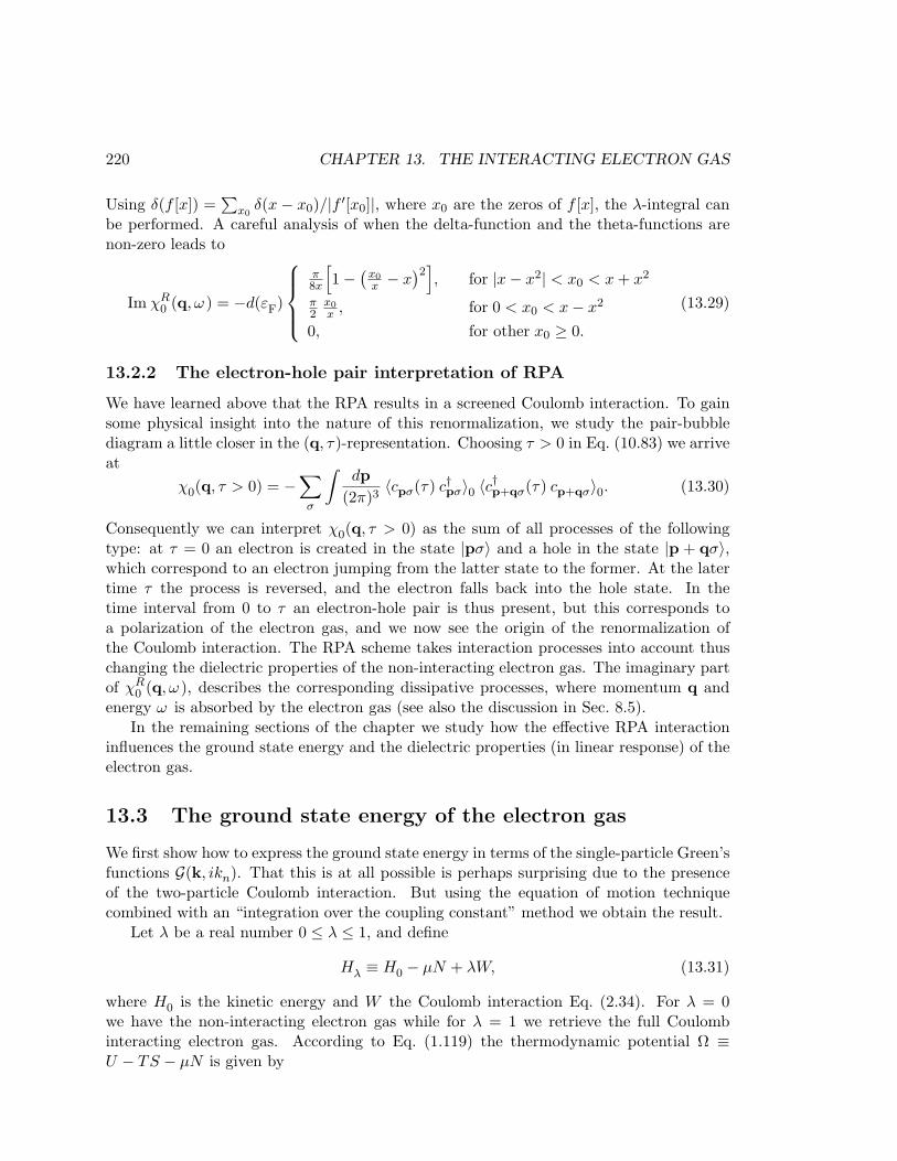
220 CHAPTER 13. THE INTERACTING ELECTRON GAS
Using δ(f [x]) =∑
x0δ(x− x0)/|f ′[x0]|, where x0 are the zeros of f [x], the λ-integral can
be performed. A careful analysis of when the delta-function and the theta-functions arenon-zero leads to
Im χR0 (q, ω ) = −d(εF)
π8x
[1− (
x0x − x
)2], for |x− x2| < x0 < x + x2
π2
x0x , for 0 < x0 < x− x2
0, for other x0 ≥ 0.
(13.29)
13.2.2 The electron-hole pair interpretation of RPA
We have learned above that the RPA results in a screened Coulomb interaction. To gainsome physical insight into the nature of this renormalization, we study the pair-bubblediagram a little closer in the (q, τ)-representation. Choosing τ > 0 in Eq. (10.83) we arriveat
χ0(q, τ > 0) = −∑
σ
∫dp
(2π)3〈cpσ(τ) c†pσ〉0 〈c†p+qσ(τ) cp+qσ〉0. (13.30)
Consequently we can interpret χ0(q, τ > 0) as the sum of all processes of the followingtype: at τ = 0 an electron is created in the state |pσ〉 and a hole in the state |p + qσ〉,which correspond to an electron jumping from the latter state to the former. At the latertime τ the process is reversed, and the electron falls back into the hole state. In thetime interval from 0 to τ an electron-hole pair is thus present, but this corresponds toa polarization of the electron gas, and we now see the origin of the renormalization ofthe Coulomb interaction. The RPA scheme takes interaction processes into account thuschanging the dielectric properties of the non-interacting electron gas. The imaginary partof χR
0 (q, ω ), describes the corresponding dissipative processes, where momentum q andenergy ω is absorbed by the electron gas (see also the discussion in Sec. 8.5).
In the remaining sections of the chapter we study how the effective RPA interactioninfluences the ground state energy and the dielectric properties (in linear response) of theelectron gas.
13.3 The ground state energy of the electron gas
We first show how to express the ground state energy in terms of the single-particle Green’sfunctions G(k, ikn). That this is at all possible is perhaps surprising due to the presenceof the two-particle Coulomb interaction. But using the equation of motion techniquecombined with an “integration over the coupling constant” method we obtain the result.
Let λ be a real number 0 ≤ λ ≤ 1, and define
Hλ ≡ H0 − µN + λW, (13.31)
where H0 is the kinetic energy and W the Coulomb interaction Eq. (2.34). For λ = 0we have the non-interacting electron gas while for λ = 1 we retrieve the full Coulombinteracting electron gas. According to Eq. (1.119) the thermodynamic potential Ω ≡U − TS − µN is given by
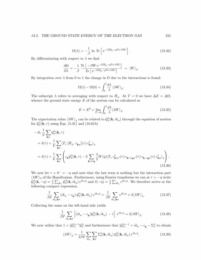
13.3. THE GROUND STATE ENERGY OF THE ELECTRON GAS 221
Ω(λ) = − 1β
ln Tr[
e−β(H0−µN+λW)]. (13.32)
By differentiating with respect to λ we find
∂Ω∂λ
= − 1β
Tr[−βW e−β(H0−µN+λW)
]
Tr[e−β(H0−µN+λW)
] = 〈W 〉λ. (13.33)
By integration over λ from 0 to 1 the change in Ω due to the interactions is found:
Ω(1)− Ω(0) =∫ 1
0
dλ
λ〈λW 〉λ. (13.34)
The subscript λ refers to averaging with respect to Hλ. At T = 0 we have ∆E = ∆Ω,whence the ground state energy E of the system can be calculated as
E = E0 + limT→0
∫ 1
0
dλ
λ〈λW 〉λ. (13.35)
The expectation value 〈λW 〉λ can be related to Gλσ(k, ikn) through the equation of motion
for Gλσ(k, τ) using Eqs. (5.31) and (10.61b)
− ∂τ1V
∑
kσ
Gλσ(k, τ)
= δ(τ) +1V
∑
kσ
〈Tτ [Hλ, ckσ](τ) c†kσ〉λ
= δ(τ) +1V
∑
kσ
εkGλ
σ(k, τ)− 2∑
k′σ′q
λ
2W (q)〈Tτ c†k′σ′(τ) ck′+qσ′(τ) ck−qσ(τ) c†kσ〉λ
.
(13.36)
We now let τ = 0− = −η and note that the last term is nothing but the interaction part〈λW 〉λ of the Hamiltonian. Furthermore, using Fourier transforms we can at τ = −η writeGλ
σ(k,−η) = 1β
∑iknGλ
σ(k, ikn) eiknη and δ(−η) = 1β
∑ikn
eiknη. We therefore arrive at thefollowing compact expression,
1βV
∑
iknkσ
(ikn − εk) Gλσ(k, ikn) eiknη =
1βV
∑
iknkσ
eiknη + 2〈λW 〉λ. (13.37)
Collecting the sums on the left-hand side yields
1βV
∑
iknkσ
[(ikn − εk)Gλ
σ(k, ikn) − 1]
eiknη = 2〈λW 〉λ. (13.38)
We now utilize that 1 = [Gλσ ]−1Gλ
σ and furthermore that [Gλσ ]−1 = ikn − εk −Σλ
σ to obtain
〈λW 〉λ =1
2βV∑
ikn
∑
kσ
Σλσ(k, ikn) Gλ
σ(k, ikn) eiknη, (13.39)
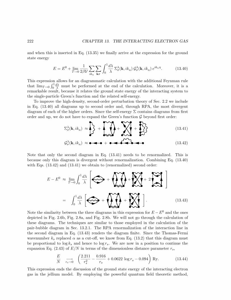
222 CHAPTER 13. THE INTERACTING ELECTRON GAS
and when this is inserted in Eq. (13.35) we finally arrive at the expression for the groundstate energy
E = E0 + limT→0
12βV
∑
ikn
∑
kσ
∫ 1
0
dλ
λΣλ
σ(k, ikn) Gλσ(k, ikn) eiknη. (13.40)
This expression allows for an diagrammatic calculation with the additional Feynman rulethat limT→0
∫ 10
dλλ must be performed at the end of the calculation. Moreover, it is a
remarkable result, because it relates the ground state energy of the interacting system tothe single-particle Green’s function and the related self-energy.
To improve the high-density, second-order perturbation theory of Sec. 2.2 we includein Eq. (13.40) all diagrams up to second order and, through RPA, the most divergentdiagram of each of the higher orders. Since the self-energy Σ contains diagrams from firstorder and up, we do not have to expand the Green’s function G beyond first order:
Σλσ(k, ikn) ≈ ; + < += + > (13.41)
Gλσ(k, ikn) ≈? +@ (13.42)
Note that only the second diagram in Eq. (13.41) needs to be renormalized. This isbecause only this diagram is divergent without renormalization. Combining Eq. (13.40)with Eqs. (13.42) and (13.41) we obtain to (renormalized) second order:
E − E0 ≈ limT→0
∫ 1
0
dλ
λ
A + B +C + 2D
=∫ 1
0
dλ
λ
[E + F + G]
. (13.43)
Note the similarity between the three diagrams in this expression for E−E0 and the onesdepicted in Fig. 2.6b, Fig. 2.8a, and Fig. 2.8b. We will not go through the calculation ofthese diagrams. The techniques are similar to those employed in the calculation of thepair-bubble diagram in Sec. 13.2.1. The RPA renormalization of the interaction line inthe second diagram in Eq. (13.43) renders the diagram finite. Since the Thomas-Fermiwavenumber ks replaced α as a cut-off, we know from Eq. (13.2) that this diagram mustbe proportional to log ks and hence to log rs. We are now in a position to continue theexpansion Eq. (2.43) of E/N in terms of the dimensionless distance parameter rs,
E
N−→rs→0
(2.211
r2s
− 0.916rs
+ 0.0622 log rs − 0.094)
Ry. (13.44)
This expression ends the discussion of the ground state energy of the interacting electrongas in the jellium model. By employing the powerful quantum field theoretic method,
13.4. THE DIELECTRIC FUNCTION AND SCREENING 223
in casu resummation of the Feynman diagram series for the single-electron self-energyand Green’s function, we could finally solve the problem posed by the failed second orderperturbation theory.
Having achieved this solution, we will also be able to study other aspects of the inter-acting electron gas. In the following we focus on the dielectric properties of the system.
13.4 The dielectric function and screening
Already from Eq. (13.15) it is clear that the internal dynamics of the interacting electrongas lead to a screening of the pure Coulomb interaction. One suspects that also externalpotentials φext will be screened similarly; and indeed, as we shall see below, this is in factthe case. As in Sec. 6.4 we study the linear response of the interacting system due to theperturbation H ′ caused by φext,
H ′ =∫
dr [−e ρ(r)] φext(r, t), (13.45)
where ρ(r) is the particle density and not, as in Sec. 6.4, the charge density. Since theunperturbed system even with its Coulomb interacting electrons is translation-invariant,we write all expressions in Fourier (q, ω )-space. The external potential φext(q, ω ) createsan induced charge density −eρind(q, ω ). Through the Coulomb interaction this in turncorresponds to an induced potential
φind(r, t) =∫
dr′−eρind(r′, t)4πε0|r− r′| ⇒ φind(q, ω ) =
1e2
W (q) [−e ρind(q, ω )]. (13.46)
We divide with e2 since W (q) by definition contains this factor. Next step is to usethe Kubo formula, which relates [−e ρind(r, ω)] with the external potential and with theretarded density-density correlator
[−e ρind(q, ω)] = (−e)2 CRρρ(q,−q, ω) φext(q, ω) ≡ e2 χR(q, ω) φext(q, ω). (13.47)
Collecting our partial results we have
φind(q, ω ) = W (q) χR(q, ω ) φext(q, ω ), (13.48)
where χR(q, ω ) is the Fourier transform of the retarded Kubo density-density correlationfunction χR(q, t− t′), see Eqs. (8.75) and (8.76),
χR(q, t− t′) ≡ CRρρ(qt,−qt′) = −iθ(t− t′)
1V
⟨[ρ(qt), ρ(−qt′)
]⟩eq
. (13.49)
Here the subscript ’eq’ refers to averaging in equilibrium, i.e. with respect to H = H0 +Womitting H ′. Using Eq. (13.48) the total potential φtot(q, ω ) can be written in terms ofthe polarization function χR,
φtot(q, ω ) = φext(q, ω ) + φind(q, ω ) =[1 + W (q) χR(q, ω )
]φext(q, ω ). (13.50)
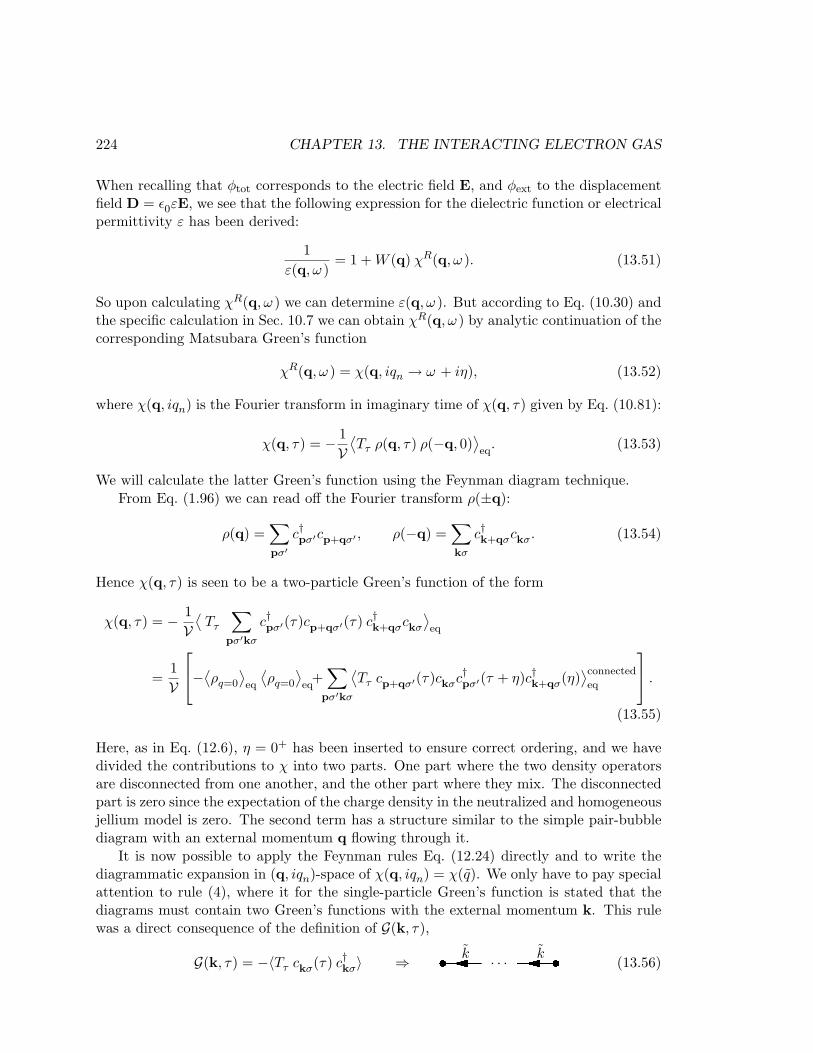
224 CHAPTER 13. THE INTERACTING ELECTRON GAS
When recalling that φtot corresponds to the electric field E, and φext to the displacementfield D = ε0εE, we see that the following expression for the dielectric function or electricalpermittivity ε has been derived:
1ε(q, ω )
= 1 + W (q) χR(q, ω ). (13.51)
So upon calculating χR(q, ω ) we can determine ε(q, ω ). But according to Eq. (10.30) andthe specific calculation in Sec. 10.7 we can obtain χR(q, ω ) by analytic continuation of thecorresponding Matsubara Green’s function
χR(q, ω ) = χ(q, iqn → ω + iη), (13.52)
where χ(q, iqn) is the Fourier transform in imaginary time of χ(q, τ) given by Eq. (10.81):
χ(q, τ) = − 1V
⟨Tτ ρ(q, τ) ρ(−q, 0)
⟩eq
. (13.53)
We will calculate the latter Green’s function using the Feynman diagram technique.From Eq. (1.96) we can read off the Fourier transform ρ(±q):
ρ(q) =∑
pσ′c†pσ′cp+qσ′ , ρ(−q) =
∑
kσ
c†k+qσckσ. (13.54)
Hence χ(q, τ) is seen to be a two-particle Green’s function of the form
χ(q, τ) = − 1V
⟨Tτ
∑
pσ′kσ
c†pσ′(τ)cp+qσ′(τ) c†k+qσckσ
⟩eq
=1V
−⟨
ρq=0
⟩eq
⟨ρq=0
⟩eq
+∑
pσ′kσ
⟨Tτ cp+qσ′(τ)ckσc†pσ′(τ + η)c†k+qσ(η)
⟩connected
eq
.
(13.55)
Here, as in Eq. (12.6), η = 0+ has been inserted to ensure correct ordering, and we havedivided the contributions to χ into two parts. One part where the two density operatorsare disconnected from one another, and the other part where they mix. The disconnectedpart is zero since the expectation of the charge density in the neutralized and homogeneousjellium model is zero. The second term has a structure similar to the simple pair-bubblediagram with an external momentum q flowing through it.
It is now possible to apply the Feynman rules Eq. (12.24) directly and to write thediagrammatic expansion in (q, iqn)-space of χ(q, iqn) = χ(q). We only have to pay specialattention to rule (4), where it for the single-particle Green’s function is stated that thediagrams must contain two Green’s functions with the external momentum k. This rulewas a direct consequence of the definition of G(k, τ),
G(k, τ) = −〈Tτ ckσ(τ) c†kσ〉 ⇒ Hk · · ·Ik(13.56)
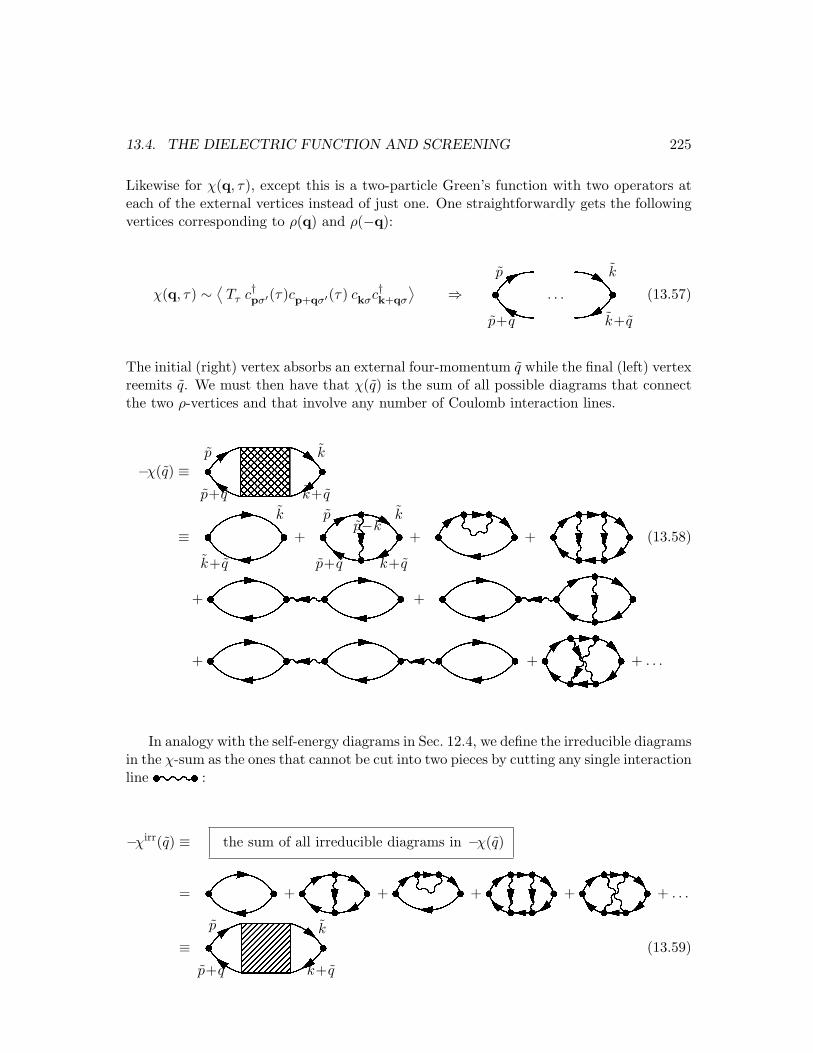
13.4. THE DIELECTRIC FUNCTION AND SCREENING 225
Likewise for χ(q, τ), except this is a two-particle Green’s function with two operators ateach of the external vertices instead of just one. One straightforwardly gets the followingvertices corresponding to ρ(q) and ρ(−q):
χ(q, τ) ∼ ⟨Tτ c†pσ′(τ)cp+qσ′(τ) ckσc†k+qσ
⟩ ⇒ Jp+q
p
. . . Kk+q
k
(13.57)
The initial (right) vertex absorbs an external four-momentum q while the final (left) vertexreemits q. We must then have that χ(q) is the sum of all possible diagrams that connectthe two ρ-vertices and that involve any number of Coulomb interaction lines.
−χ(q) ≡ Lp+q
p
k+q
k
≡ Mk+q
k
+ Np+q k+q
p kp−k
+ O + P (13.58)
+Q + R+S +T + . . .
In analogy with the self-energy diagrams in Sec. 12.4, we define the irreducible diagramsin the χ-sum as the ones that cannot be cut into two pieces by cutting any single interactionlineU :
−χirr(q) ≡ the sum of all irreducible diagrams in −χ(q)
= V +W +X +Y +Z + . . .
≡ [p+q
p
k+q
k
(13.59)
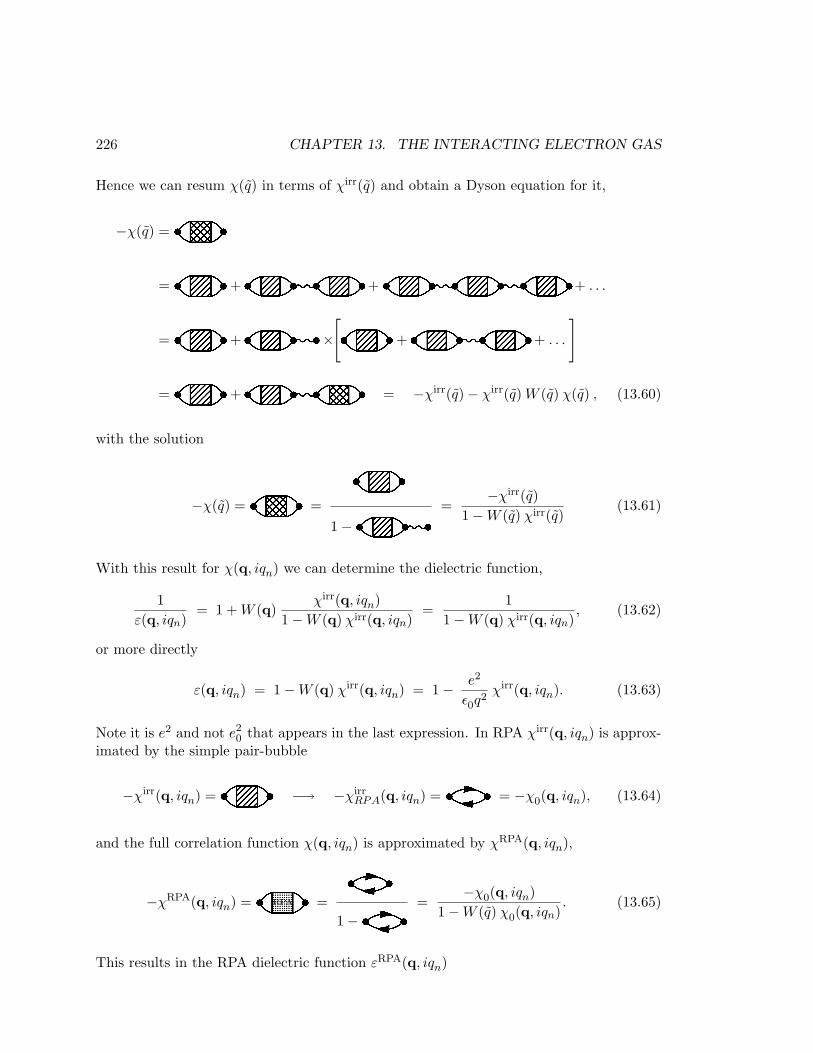
226 CHAPTER 13. THE INTERACTING ELECTRON GAS
Hence we can resum χ(q) in terms of χirr(q) and obtain a Dyson equation for it,
−χ(q) =\=] +^ +_ + . . .
=` +a ×[
b +c + . . .
]
=d +e = −χirr(q)− χirr(q) W (q) χ(q) , (13.60)
with the solution
−χ(q) =f = g1−h =
−χirr(q)1−W (q) χirr(q)
(13.61)
With this result for χ(q, iqn) we can determine the dielectric function,
1ε(q, iqn)
= 1 + W (q)χirr(q, iqn)
1−W (q) χirr(q, iqn)=
11−W (q) χirr(q, iqn)
, (13.62)
or more directly
ε(q, iqn) = 1−W (q) χirr(q, iqn) = 1− e2
ε0q2
χirr(q, iqn). (13.63)
Note it is e2 and not e20 that appears in the last expression. In RPA χirr(q, iqn) is approx-
imated by the simple pair-bubble
−χirr(q, iqn) =i −→ −χirrRPA(q, iqn) =j = −χ0(q, iqn), (13.64)
and the full correlation function χ(q, iqn) is approximated by χRPA(q, iqn),
−χRPA(q, iqn) =kRPA = l1−m =
−χ0(q, iqn)1−W (q) χ0(q, iqn)
. (13.65)
This results in the RPA dielectric function εRPA(q, iqn)
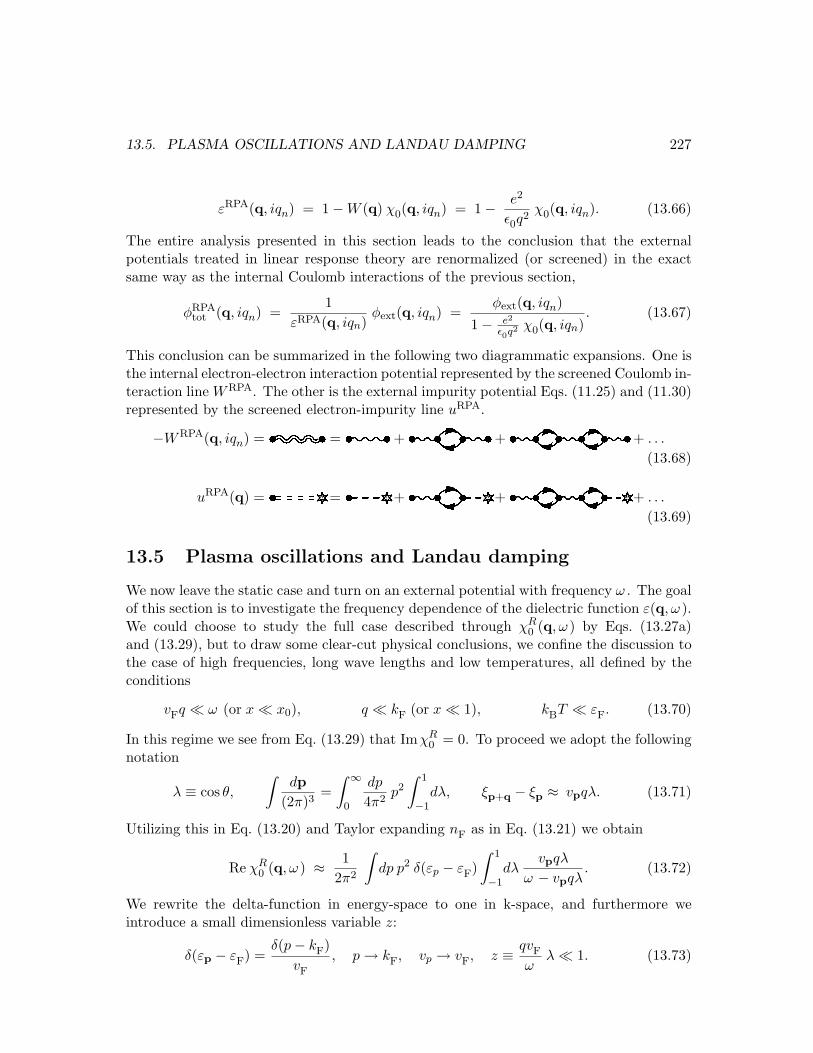
13.5. PLASMA OSCILLATIONS AND LANDAU DAMPING 227
εRPA(q, iqn) = 1−W (q) χ0(q, iqn) = 1− e2
ε0q2
χ0(q, iqn). (13.66)
The entire analysis presented in this section leads to the conclusion that the externalpotentials treated in linear response theory are renormalized (or screened) in the exactsame way as the internal Coulomb interactions of the previous section,
φRPAtot (q, iqn) =
1εRPA(q, iqn)
φext(q, iqn) =φext(q, iqn)
1− e2
ε0q2 χ0(q, iqn). (13.67)
This conclusion can be summarized in the following two diagrammatic expansions. One isthe internal electron-electron interaction potential represented by the screened Coulomb in-teraction line WRPA. The other is the external impurity potential Eqs. (11.25) and (11.30)represented by the screened electron-impurity line uRPA.
−WRPA(q, iqn) =n =o +p +q + . . .
(13.68)
uRPA(q) =r =s +t +u + . . .
(13.69)
13.5 Plasma oscillations and Landau damping
We now leave the static case and turn on an external potential with frequency ω . The goalof this section is to investigate the frequency dependence of the dielectric function ε(q, ω ).We could choose to study the full case described through χR
0 (q, ω ) by Eqs. (13.27a)and (13.29), but to draw some clear-cut physical conclusions, we confine the discussion tothe case of high frequencies, long wave lengths and low temperatures, all defined by theconditions
vFq ¿ ω (or x ¿ x0), q ¿ kF (or x ¿ 1), kBT ¿ εF. (13.70)
In this regime we see from Eq. (13.29) that ImχR0 = 0. To proceed we adopt the following
notation
λ ≡ cos θ,
∫dp
(2π)3=
∫ ∞
0
dp
4π2p2
∫ 1
−1dλ, ξp+q − ξp ≈ vpqλ. (13.71)
Utilizing this in Eq. (13.20) and Taylor expanding nF as in Eq. (13.21) we obtain
Re χR0 (q, ω ) ≈ 1
2π2
∫dp p2 δ(εp − εF)
∫ 1
−1dλ
vpqλ
ω − vpqλ. (13.72)
We rewrite the delta-function in energy-space to one in k-space, and furthermore weintroduce a small dimensionless variable z:
δ(εp − εF) =δ(p− kF)
vF
, p → kF, vp → vF, z ≡ qvF
ωλ ¿ 1. (13.73)
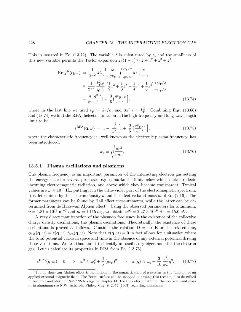
228 CHAPTER 13. THE INTERACTING ELECTRON GAS
This in inserted in Eq. (13.72). The variable λ is substituted by z, and the smallness ofthis new variable permits the Taylor expansion z/(1− z) ≈ z + z2 + z3 + z4.
Re χR0 (q, ω ) ≈ 1
2π2k2
F
1vF
ω
qvF
∫ qvF/ω
−qvF/ωdz
z
1− z
≈ 12π2
k2Fω
qv2F
[12z2 +
13z3 +
14z4 +
15z5
]+qvF/ω
−qvF/ω
=n
m
q2
ω2
[1 +
35(qvF
ω
)2], (13.74)
where in the last line we used vF = kF/m and 3π2n = k3F. Combining Eqs. (13.66)
and (13.74) we find the RPA dielectric function in the high-frequency and long-wavelengthlimit to be
εRPA(q, ω ) = 1− ω2p
ω2
[1 +
35
(qvF
ω
)2], (13.75)
where the characteristic frequency ωp, well known as the electronic plasma frequency, hasbeen introduced,
ωp ≡√
ne2
mε0. (13.76)
13.5.1 Plasma oscillations and plasmons
The plasma frequency is an important parameter of the interacting electron gas settingthe energy scale for several processes, e.g. it marks the limit below which metals reflectsincoming electromagnetic radiation, and above which they become transparent. Typicalvalues are ω ≈ 1016 Hz, putting it in the ultra-violet part of the electromagnetic spectrum.It is determined by the electron density n and the effective band-mass m of Eq. (2.16). Theformer parameter can be found by Hall effect measurements, while the latter can be de-termined from de Haas-van Alphen effect2. Using the observed parameters for aluminum,n = 1.81× 1029 m−2 and m = 1.115 m0, we obtain ωAl
p = 2.27× 10¹⁶ Hz = 15.0 eV.A very direct manifestation of the plasmon frequency is the existence of the collective
charge density oscillations, the plasma oscillations. Theoretically, the existence of theseoscillations is proved as follows. Consider the relation D = ε ε0E or the related one,φext(q, ω ) = ε(q, ω ) φtot(q, ω ). Note that ε(q, ω ) = 0 in fact allows for a situation wherethe total potential varies in space and time in the absence of any external potential drivingthese variations. We are thus about to identify an oscillatory eigenmode for the electrongas. Let us calculate its properties in RPA from Eq. (13.75).
εRPA(q, ω ) = 0 ⇒ ω2 ≈ ω2p +
35
(qvF)2 ⇒ ω (q) ≈ ωp +310
v2F
ωpq2. (13.77)
2The de Haas-van Alphen effect is oscillations in the magnetization of a system as the function of anapplied external magnetic field. The Fermi surface can be mapped out using this technique as describedin Ashcroft and Mermin, Solid State Physics, chapter 14. For the determination of the electron band massm in aluminum see N.W. Ashcroft, Philos. Mag. 8, 2055 (1963) regarding aluminum.
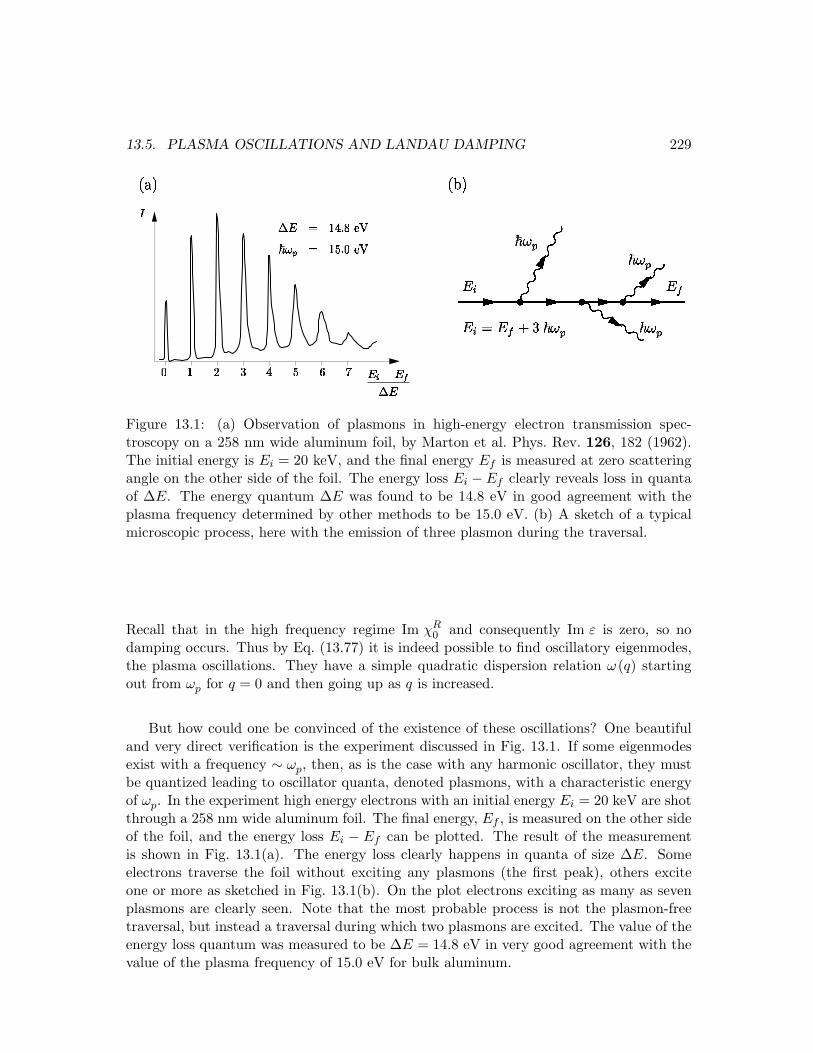
13.5. PLASMA OSCILLATIONS AND LANDAU DAMPING 229
! " ! "
! "
#
$% # &(' ! "
Figure 13.1: (a) Observation of plasmons in high-energy electron transmission spec-troscopy on a 258 nm wide aluminum foil, by Marton et al. Phys. Rev. 126, 182 (1962).The initial energy is Ei = 20 keV, and the final energy Ef is measured at zero scatteringangle on the other side of the foil. The energy loss Ei − Ef clearly reveals loss in quantaof ∆E. The energy quantum ∆E was found to be 14.8 eV in good agreement with theplasma frequency determined by other methods to be 15.0 eV. (b) A sketch of a typicalmicroscopic process, here with the emission of three plasmon during the traversal.
Recall that in the high frequency regime Im χR0 and consequently Im ε is zero, so no
damping occurs. Thus by Eq. (13.77) it is indeed possible to find oscillatory eigenmodes,the plasma oscillations. They have a simple quadratic dispersion relation ω (q) startingout from ωp for q = 0 and then going up as q is increased.
But how could one be convinced of the existence of these oscillations? One beautifuland very direct verification is the experiment discussed in Fig. 13.1. If some eigenmodesexist with a frequency ∼ ωp, then, as is the case with any harmonic oscillator, they mustbe quantized leading to oscillator quanta, denoted plasmons, with a characteristic energyof ωp. In the experiment high energy electrons with an initial energy Ei = 20 keV are shotthrough a 258 nm wide aluminum foil. The final energy, Ef , is measured on the other sideof the foil, and the energy loss Ei − Ef can be plotted. The result of the measurementis shown in Fig. 13.1(a). The energy loss clearly happens in quanta of size ∆E. Someelectrons traverse the foil without exciting any plasmons (the first peak), others exciteone or more as sketched in Fig. 13.1(b). On the plot electrons exciting as many as sevenplasmons are clearly seen. Note that the most probable process is not the plasmon-freetraversal, but instead a traversal during which two plasmons are excited. The value of theenergy loss quantum was measured to be ∆E = 14.8 eV in very good agreement with thevalue of the plasma frequency of 15.0 eV for bulk aluminum.
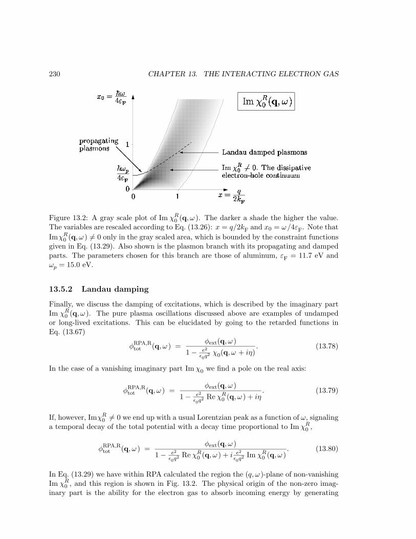
230 CHAPTER 13. THE INTERACTING ELECTRON GAS
! "# %$ &%' ( ) * ! + !! ! , - * ! , "
. /10 234 5 6 798
Figure 13.2: A gray scale plot of Im χR0 (q, ω ). The darker a shade the higher the value.
The variables are rescaled according to Eq. (13.26): x = q/2kF and x0 = ω/4εF. Note thatImχR
0 (q, ω ) 6= 0 only in the gray scaled area, which is bounded by the constraint functionsgiven in Eq. (13.29). Also shown is the plasmon branch with its propagating and dampedparts. The parameters chosen for this branch are those of aluminum, εF = 11.7 eV andωp = 15.0 eV.
13.5.2 Landau damping
Finally, we discuss the damping of excitations, which is described by the imaginary partIm χR
0 (q, ω ). The pure plasma oscillations discussed above are examples of undampedor long-lived excitations. This can be elucidated by going to the retarded functions inEq. (13.67)
φRPA,Rtot (q, ω ) =
φext(q, ω )1− e2
ε0q2 χ0(q, ω + iη). (13.78)
In the case of a vanishing imaginary part Im χ0 we find a pole on the real axis:
φRPA,Rtot (q, ω ) =
φext(q, ω )1− e2
ε0q2 Re χR0 (q, ω ) + iη
. (13.79)
If, however, ImχR0 6= 0 we end up with a usual Lorentzian peak as a function of ω, signaling
a temporal decay of the total potential with a decay time proportional to Im χR0 ,
φRPA,Rtot (q, ω ) =
φext(q, ω )1− e2
ε0q2 Re χR0 (q, ω ) + i e2
ε0q2 Im χR0 (q, ω )
. (13.80)
In Eq. (13.29) we have within RPA calculated the region the (q, ω )-plane of non-vanishingIm χR
0 , and this region is shown in Fig. 13.2. The physical origin of the non-zero imag-inary part is the ability for the electron gas to absorb incoming energy by generating
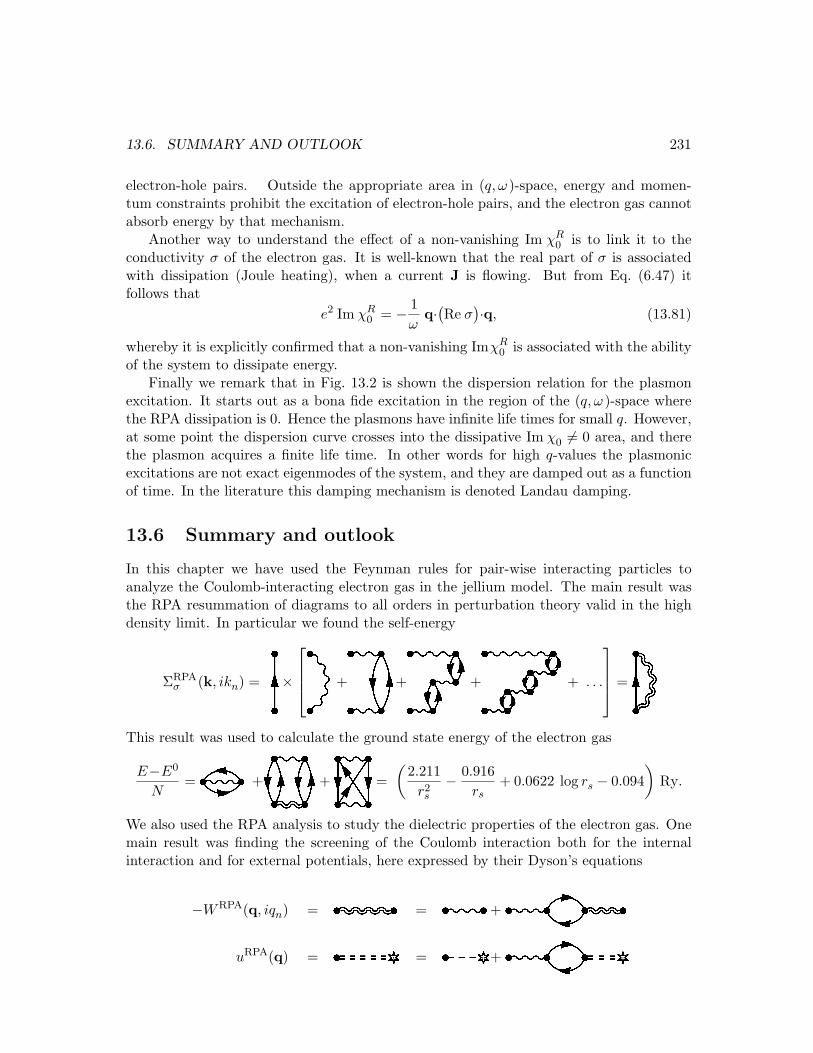
13.6. SUMMARY AND OUTLOOK 231
electron-hole pairs. Outside the appropriate area in (q, ω )-space, energy and momen-tum constraints prohibit the excitation of electron-hole pairs, and the electron gas cannotabsorb energy by that mechanism.
Another way to understand the effect of a non-vanishing Im χR0 is to link it to the
conductivity σ of the electron gas. It is well-known that the real part of σ is associatedwith dissipation (Joule heating), when a current J is flowing. But from Eq. (6.47) itfollows that
e2 Im χR0 = − 1
ωq·(Re σ
)·q, (13.81)
whereby it is explicitly confirmed that a non-vanishing ImχR0 is associated with the ability
of the system to dissipate energy.Finally we remark that in Fig. 13.2 is shown the dispersion relation for the plasmon
excitation. It starts out as a bona fide excitation in the region of the (q, ω )-space wherethe RPA dissipation is 0. Hence the plasmons have infinite life times for small q. However,at some point the dispersion curve crosses into the dissipative Im χ0 6= 0 area, and therethe plasmon acquires a finite life time. In other words for high q-values the plasmonicexcitations are not exact eigenmodes of the system, and they are damped out as a functionof time. In the literature this damping mechanism is denoted Landau damping.
13.6 Summary and outlook
In this chapter we have used the Feynman rules for pair-wise interacting particles toanalyze the Coulomb-interacting electron gas in the jellium model. The main result wasthe RPA resummation of diagrams to all orders in perturbation theory valid in the highdensity limit. In particular we found the self-energy
ΣRPAσ (k, ikn) = v ×
w +x +y +z + . . .
=
This result was used to calculate the ground state energy of the electron gas
E−E0
N=| + +~ =
(2.211
r2s
− 0.916rs
+ 0.0622 log rs − 0.094)
Ry.
We also used the RPA analysis to study the dielectric properties of the electron gas. Onemain result was finding the screening of the Coulomb interaction both for the internalinteraction and for external potentials, here expressed by their Dyson’s equations
−WRPA(q, iqn) = = +uRPA(q) = = +
232 CHAPTER 13. THE INTERACTING ELECTRON GAS
Explicit expressions for the dielectric function ε(q, ω ) was found in two cases, (i) thestatic, long-wave limit and (ii) the high frequency, long-wave limit,
εRPA(q, 0) = 1 +k2
s
q2, where k2
s =4π
kF
a0
εRPA(q, ω À qvF) = 1− ω2p
ω2
[1 +
35
(qvF
ω
)2].
Finally, we studied the plasma oscillations of the electron gas found from the conditionεRPA(q, ω ) = 0, and found the dispersion relation involving the plasma frequency ωp,
ω (q) = ωp +310
v2F
ωpq2, where ωp ≡
√ne2
mε0.
The RPA analysis has already given us a good insight in some central physical proper-ties of the electron gas. Moreover, it plays a crucial role in the studies of electron-impurityscattering, electron-phonon interaction, superconductivity, and of many other physicalphenomena involving the electron gas.
Chapter 14
Fermi liquid theory
The concept of Fermi liquid theory was developed by Landau in 1957-59 and later refinedby others1. The basic conclusion is that a gas of interacting particles can be described bya system of almost non-interacting “quasiparticles”. These quasiparticles are approximateexcitations of the system at sufficiently short time scales. What we mean by “sufficientlyshort” of course has to be quantified, and this condition will set the limits for the appli-cability of the theory.
The Fermi liquid theory is conceptually extremely important, because it explains whythe apparently immensely complicated system of for example interacting electrons in ametal can be regarded as a gas of non-interacting particles. This is of course an enormoussimplification, and it gives the theoretical explanation of why all the results that one getsfrom the widely used free electron model work so well.
The quasiparticle concept furthermore gives the theoretical foundation of the semi-classical description. The quasiparticle distribution function satisfies a kinetic equation,which may include scattering from one state to another for example due to impurity scat-tering. This equation is known as the Landau transport equation, and it is equivalentto the well-known Boltzmann equation from kinetic gas theory. In this description thepotential is allowed to vary in space due to some external perturbation or due to inter-actions with the inhomogeneous density of quasiparticles. Using the Landau transportequation we shall see that the collective modes derived in the previous chapter also comeout naturally from a semi-classical description and, furthermore, the conductivity, which iscalculated from microscopic considerations in Chap. 15, also is easily understood in termsof scattering of quasiparticles.
14.1 Adiabatic continuity
The Fermi liquid theory is based on the assumption that starting from the non-interactingsystem of particles one can analyze the interacting case by applying perturbation theory.This is in fact a rather stringent criterion, because it means that one cannot cross a phase
1See for example the collection of reprints in the book: D. Pines The Many-body problem, Addison-Wesley (1961,1997).
233
234 CHAPTER 14. FERMI LIQUID THEORY
boundary line. This is because a phase transition, such as for example the ferromagnetictransition discussed in Chap. 4, cannot be reached by perturbation theory starting fromthe paramagnetic phase.2
If the excitations of the non-interacting system are connected to the excitations ofthe interacting system by a one-to-one correspondence (at least on short time scales asexplained below) the two cases are said to be connected by “adiabatic continuity”. If youimagine that we start from the non-interacting system excited in some state and thenturn on the interaction adiabatically, i.e. so slowly that the occupation numbers are notchanged, then we would end up in a corresponding excited state of the interacting system.What we really are claiming is that the excited states of the interacting system can belabelled by the same quantum numbers as those we used to label the non-interactingsystem by.
As a simple example of adiabatic continuity we now consider a particle trapped in aone-dimensional potential. The one-dimensional potential will have a number of boundstates with discrete eigenenergies and a continuum of eigenenergies corresponding to thedelocalized states. We now imagine changing the potential slowly. As an example considera potential of the form
V (x, t) = −V0(t) exp(−x2/2x2
0
), (14.1)
where the depth of the well is time dependent, and let us suppose that it is changingfrom an initial value V01 to a final value V02. If this change is slow the solution of theSchrodinger equation
i∂tψ(x, t) = H(t)ψ(x, t) =(
p2
2m+ V (x, t)
)ψ(x, t), (14.2)
can be approximated by the adiabatic solution
ψadia(x, t) ≈ ψV0(t)(x) exp(−iE
V0(t)t)
, (14.3)
where ψV0(t)(x) is the solution of the static (or instantaneous) Schrodinger equation, withenergy E
V0(t)
H(t)ψV0(t)(x) = EV0(t)
ψV0(t)(x). (14.4)
Note that both ψV0(t)(x) and EV0(t) depend parametrically on the time through V0(t). Theaccuracy of the solution in Eq. (14.3) is estimated by inserting Eq. (14.3) into Eq. (14.2),which yields
i∂tψadia(x, t) = EV0(t)
ψadia(x, t) +(
∂ψadia(x, t)∂V0(t)
)(∂V0(t)
∂t
)= Hψadia(x, t). (14.5)
Thus we have an approximate solution if the first term dominates over the second term.Thus apparently our conclusion is that if the rate of change of V0(t) is small enough
the solution for the new value of V0 = V02 can be found be by starting from the solution2This fact you can understand from the concept of broken symmetry explained in Sec. 4.3. The phase
with broken symmetry can only occur if the ensemble of states in the statistical average is truncated.
14.1. ADIABATIC CONTINUITY 235
with the old value of V0 = V01 and “adiabatically” changing it to its new value. Forexample if the first excited state is a bound state, it will change to a somewhat modifiedstate with a somewhat modified energy, but most importantly it is still the first excitedstate and it is still a bound state. This may sound completely trivial, but it is not, and itis not always true. For example if the real solution during this change of V0 from V01 toV02 changes from a bound state to an un-bound state (if V02 is small enough there is onlyone bound state), then it does not matter how slowly we change V0. The two states cansimply not be connected through small changes of V0, because one is a decaying functionand one is an oscillatory function. This is an example where perturbation theory to anyorder would never give the right answer. The important message is, however, that if weavoid these transitions between different kinds of states, adiabatic continuity does work.In the following this idea is applied to the case of interacting particles.
14.1.1 The quasiparticle concept and conserved quantities
The principle of adiabatic continuity is now utilized to study a system of interactingparticles. It is used to bring the excitations of the interacting case back to the well-knownexcitations of the non-interacting case, thus making computation possible. In doing sowe gain the fundamental understanding that the interacting and the non-interacting caseshave a lot in common at least under some restricting circumstances. This turns out to berealized in many systems. The following arguments are meant to be the full theoreticalexplanation for the applicability of Fermi liquid theory, but rather to give a physicalintuition for the reason why the quasiparticle picture is valid.
When calculating physical quantities, such as response functions or occupation num-bers we are facing matrix elements between different states, for example between stateswith added particles or added particle-hole pairs. Since we are dealing with the low energyproperties of the system, let us consider states with single particles or single electron-holepairs added to the groundstate
|(kσ)p〉 = c†kσ|G〉, |(kσ)p; (k′σ′)h〉 = c†kσck′σ′ |G〉, etc. (14.6)
where |G〉 is the groundstate of the interacting system. The first term inserts a particlewhile the second term creates both a particle and hole. If we now imagine letting timeevolve according to a Hamiltonian where the interaction is gradually switched off at a rateζ
Hζ = H0 + Hinte−ζt, t > 0, (14.7)
then according to Eq. (5.18) the time evolution with the time dependent Hamiltonian is
|kσ〉(t) = e−iH0tTt exp(−i
∫ t
0dt′Hζ(t′)
)|kσ〉 ≡ Uζ(t, 0)|kσ〉. (14.8)
If, under the conditions of adiabaticity, we can bring the states (|(kσ)p〉, |(kσ)p; (kσ′)h〉,etc) all the way back to the non-interacting case, then the matrix elements are identicalto those of the non-interacting case. For example
〈(k′σ′)p|(kσ)p〉 = 〈(k′σ′)p|U †ζ (t, 0)Uζ(t, 0)|(kσ)p〉 −→
t→∞ 〈(k′σ′)p|(kσ)p〉0. (14.9)
236 CHAPTER 14. FERMI LIQUID THEORY
There are two important assumptions built into this construction:
1. The adiabatic procedure is valid when the energy of the state is large com-pared to the rate of change, i.e. εkσ À ζ, or, since typical excitation energiesare of order of the temperature, this is equivalent to assuming kBT À ζ.
2. The interactions do not induce transitions of the states in question, or inother words the life-time τlife of the state is long compared to ζ−1, that isτlife À ζ−1.
This apparently leaves an energy window where the idea makes sense, namely whenwe can choose a switch-off rate ζ such that
τ−1life ¿ ζ ¿ kBT. (14.10)
The last condition can in principle always be met at high enough temperatures, whereasthe first one is not necessarily possible. Below we shall see that it is indeed possible to makethe approximations consistent, because the life-time turns out to be inversely proportionalto the square of the temperature, τ−1
life ∝ T 2. Thus there is always a temperature range atlow temperature where Eq. (14.10) is fulfilled.
Next we discuss the properties of the state with an added particle, |(kσ)p〉. It is clearthat the state where the interaction is switched off Uζ(∞, 0)|kσ〉 has a number of propertiesin common with the initial state |(kσ)p〉, namely those that are conserved by the Hamil-tonian: (1) it has an excess charge e (compared to the groundstate), (2) it carries current−e~k/m, and (3) it has excess spin σ. Here −e and m are charge and mass of the electrons,respectively. These properties are all conserved quantities because the corresponding op-erators (1) the total charge Q = −eN , (2) the total current Je = −e
∑kσ vknkσ, and (3)
the total spin S =∑
kσ σnkσ all commute with the Hamiltonian. Most importantly, theadiabatic continuity principle can also be used to calculate the distribution function, andtherefore the distribution function 〈c†k′σ′ckσ〉 = 〈(k′σ′)p|(kσ)p〉 7−→ 〈(k′σ′)p|(kσ)p〉0 is aFermi-Dirac distribution function. This leads us to the definition of quasiparticles:
14.2. SEMI-CLASSICAL TREATMENT OF SCREENING AND PLASMONS 237
Quasiparticles are the excitations of the interacting system corresponding tothe creation or annihilation of particles (for example particle-hole pair state|(kσ)p; (k′σ′)h〉). The quasiparticles can be labelled by the same quantum num-bers as the non-interacting case, provided that the corresponding operators com-mute with the Hamiltonian. For a translation-invariant system of electrons inter-acting through the Coulomb interaction, the quasiparticles quantum numbers arethus k and σ and they carry charge−e and velocity vk = ~k/m. The quasiparticleconcept only makes sense on time scales shorter than the quasiparticle life time.The quasiparticle are thus not to be thought of as the exact eigenstates. At lowtemperatures there are only a few quasiparticles, and they therefore constitute adilute gas. Finally the quasiparticles are in equilibrium distributed according tothe Fermi-Dirac distribution function.
In the following we make use of the quasiparticle concept to calculate the screeningand the transport properties of an electron gas.
14.2 Semi-classical treatment of screening and plasmons
In Chap. 12 we saw how the collective modes of a charged Fermi gas came out of arigorous diagrammatical analysis. Here we shall rederive some of this using a less rigorousbut maybe physically more appealing approach. Consider a uniform electron gas which issubject to an external potential φext(r, t). We can include the external potential as a localchange of the potential felt by the charged quasiparticles.3 Now, if the local potential ofthe quasiparticles is space and time dependent so is then the density of quasiparticles,because they will of course tend to move towards the low potential regions. This in turnchanges the electrical potential because the quasiparticles are charged and therefore thetotal potential φtot is given by the sum of the external potential φext and the inducedpotential φind. The induced potential is caused by the excess or deficit of quasiparticles.Thus we write the resulting local potential φtot(r, t) as
φtot(r, t) = φext(r, t) + φind(r, t). (14.11)
The induced potential φind created by the induced density ρind, which in turn depends onthe total potential, must be determined self-consistently.
3Note that we are here invoking a new concept namely local equilibrium, because otherwise we couldnot talk about a local potential. Clearly, this only makes sense on length scales larger than a typicalthermalization length. The thermalization length is the length scale on which thermal equilibrium isestablished.
238 CHAPTER 14. FERMI LIQUID THEORY
14.2.1 Static screening
First we consider linear static screening. To linear order in the local total potential andat low temperatures the induced charge density is given by
ρind(r) =2V
∑
k
[nF
(ξk + (−e)φtot(r)
)− nF
(ξk
)]
≈ −(−e)φtot(r)2V
∑
k
(−∂nF (ξk)
∂ξk
)≈ −(−e)φtot(r)d(εF ), (14.12)
where ξk is quasiparticle energy measured relative to the equilibrium chemical potentialand d(εF ) is the density of states at the Fermi level. From this we get the induced potentialin real space and in q-space as
φind(r) =1−e
∫dr′W (r−r′)ρind(r) ⇔ φind(q) =
1−e
W (q)ρind(q) = −W (q)φtot(q)d(εF ),
(14.13)which when inserted into (14.11) yields
φtot(r) = φext(r, t)−W (q)d(εF )φtot(q) ⇒ φtot(q) =φext(q)
1 + W (q)d(εF ), (14.14)
and henceε(q) = 1 + W (q) d(εF ), (14.15)
in full agreement with the conclusions of the RPA results Eqs. (13.66 ) and (13.67) usingχR
0 = −d(εF ) from Eq. (13.21).
14.2.2 Dynamical screening
In the dynamical case, we expect to find collective excitations similar to the plasmonsfound in Sec. 13.5. In order to treat this case we need to refine the analysis a bit to allowfor the time it takes the charge to adjust to the varying external potential. Consequently,the induced charge density at point r at time t now depends on the total potential at someother point r′ and at some other (previous) time t′. The way to describe this is to lookat the deviation of the distribution function nk of a quasiparticle with a given momentump = ~k (below we as usual use ~ = 1). This depends on both r and t, so that
nk = nk(t)(r, t). (14.16)
The dynamics are controlled by two things: the conservation of charge and the changeof momentum with time. The first dependence arises from the flow of the distributionfunction. Because we are interested in times shorter than the life time of the quasiparticles,the number of quasiparticles in each state is conserved. The conservation of particles instate k is expressed in the continuity equation
nk +∇r · jk = 0, (14.17)
14.2. SEMI-CLASSICAL TREATMENT OF SCREENING AND PLASMONS 239
where the current carried of quasiparticles in state k is given by jk = vknk = (~k/m)nk,and hence we get
∂t(nk) + k · ∇knk + vk · ∇rnk = 0, (14.18)
which is known as the collision-free Boltzmann equation4.The second dependence follows from how a negatively charged particle is accelerated
in a field, i.e. simply from Newton’s law
p = −(−e)∇rφtot(r, t). (14.19)
Again it is convenient to use Fourier space and introducing the Fourier transform nk(q, ω).Using Eq. (14.19) we find
(−iω + iq · vk)nk(q, ω) = −ie (q · ∇knk) φtot(q, ω) = ie (q·∇kξk)(−∂nk
∂ξk
)φtot(q, ω).
(14.20)To linear order in the potential φtot we can replace the nk on the righthand side by theequilibrium distribution n0
k = nF (ξk) and hence we find
nk(q, ω) =q·∇kξk
ω − q · vk
(−∂nF (ξk)
∂ξk
)(−eφtot(q, ω)). (14.21)
From this expression we easily get the induced density by summation over k
ρind(q, ω) =2V
∑
k
q·∇kξkω − q · vk
(−∂nF (ξk)
∂ξk
)(−eφtot(q, ω)), (14.22)
where the factor 2 comes from to spin degeneracy. This is inserted into Eqs. (14.13) and(14.11) and we obtain the dielectric function ε = φext/φtot in the dynamical case
ε(q) = 1−W (q)2V
∑
k
q·∇kξkω − q · vk
(−∂nF (ξk)
∂ξk
). (14.23)
At ω = 0 we recover the static case in Eq. (14.15), because∇kξk = vk. At long wavelengthsor large frequencies qv ¿ ω, we find by expanding in powers of q that
ε(q) ≈ 1− W (q)ω2
2V
∑(q · vk)2
(−∂nF (ξk)
∂ξk
)= 1−
(ωp
ω
)2, (14.24)
which agrees with Eq. (13.75) in Sec. 13.5. Note that q drops out because W (q) ∝ q−2.We have thus shown that in the long wavelength limit the semi-classical treatment,
which relies on the Fermi liquid theory, gives the same result as the fully microscopic theory,based on renormalization by summation of the most important diagrams. We have alsogained some physical understanding of this renormalization, because we saw explicitly howit was due to the screening of the external potential by the mobile quasiparticles.
4Here r and t are independent space and time variables in contrast to the sometimes used fluid dynamicalformulation where r = r(t) follows the particle motion.
240 CHAPTER 14. FERMI LIQUID THEORY
14.3 Semi-classical transport equation
Our last application of the semi-classical approach is the calculation of conductivity ofa uniform electron gas with some embedded impurities. This will in fact lead us to thefamous Drude formula. Historically, the Drude formula was first derived in an incorrectway, namely by assuming that the charge carriers form a classical gas. We know now thatthey follow a Fermi-Dirac distribution, but amazingly the result turns out to be the same.In Sec. 15 we will furthermore see how the very same result can be derived in a microscopicquantum theory starting from the Kubo formula and using a diagrammatic approach.
As explained in Chap. 10, the finite resistivity of metals at low temperatures is dueto scattering against impurities or other imperfections in the crystal structure. Thesecollisions take momentum out of the electron system, thus introducing a mechanism formomentum relaxation and hence resistivity. A simple minded approach to conductivitywould be to say that the forces acting on a small volume of charge is the sum of theexternal force and a friction force that is taken to be proportional to the velocity of thefluid at the given point. In steady state these forces are in balance and hence
−(−e)E+mv
τp−relax= 0 ⇒ J = −env =
e2nτp−relax
mE ⇒ σ =
ne2τp−relax
m, (14.25)
where σ is the conductivity and τp−relax is the momentum relaxation time.Microscopically the momentum relaxation corresponds to scattering of quasiparticles
from one state |kσ〉 with momentum ~k to another state |k′σ′〉 with momentum ~k′. Fornon-magnetic impurities, the ones considered here, the spin is conserved and thus σ = σ′.The new scattering process thus introduced means that the number of quasiparticles ina given k-state is no longer conserved and we have to modify Eq. (14.17) to take intoaccount the processes that change the occupation number nk. The rate of change is givenby the rate, Γ(k′σ← kσ), at which scattering from the state |kσ〉 to some other state |k′σ′〉occurs. It can be found from Fermi’s golden rule
Γ(k′σ← kσ) = 2π∣∣⟨k′σ|Vimp|kσ
⟩∣∣2 δ(ξk − ξk′), (14.26)
where Vimp is the impurity potential. The fact that the scattering on an external potentialis an elastic scattering is reflected in the energy-conserving delta function. The totalimpurity potential is a sum over single impurity potentials situated at positions Ri (seealso Chap. 11)
Vimp(r) =∑
i
u(r−Ri) (14.27)
We can then find the rate Γ by the adiabatic procedure where the matrix element 〈k′σ|Vimp|kσ〉is identified with non-interacting counterpart 〈k′σ|Vimp|kσ〉0 , where |kσ〉0 = eik·r/
√V, andwe get
Γ(k′σ← kσ) = Γk′σ,kσ =2π
V2
∣∣∣∣∣∣∑
j
∫dr e−ik′·ru(r−Rj)e+ik·r
∣∣∣∣∣∣
2
δ(ξk − ξk′). (14.28)
14.3. SEMI-CLASSICAL TRANSPORT EQUATION 241
Of course we do not know the location of the impurities exactly and therefore we performa positional average. The average is done assuming only lowest order scattering, i.e. leav-ing out interference between scattering on different impurities. Therefore we can simplyreplace the sum over impurities by the number of scattering centers, Nimp = nimpV, andmultiplied by the impurity potential for a single impurity u(r). We obtain
Γk′,k = 2πnimp
V
∣∣∣∣∫
dr ei(k−k′)·ru(r)∣∣∣∣2
δ(ξk − ξk′) ≡ nimp
V Wk′,k. (14.29)
Now the change of nk due to collisions is included in the differential equation Eq. (14.17)as an additional term. The time derivative of nk becomes
nk(t)(r, t) =(
d
dtnk
)
flow−force
+(
∂
∂tnk
)
collisions
, (14.30)
where the change due to “flow and force” is given by the left hand side in Eq. (14.18).The new collision term is not a derivative but an integral functional of nk
(∂
∂tnk
)
collisions
= −nimp
V∑
k′
[nk(1− nk′)Wk′,k − nk′(1− nk)Wk,k′
]. (14.31)
The first term in the sum represents the rate for being scattered out of the state k and thesecond term represents the rate for being scattered into to state k from the state k′. Thetotal rate is obtained from the Fermi golden rule expression (14.29) times the probabilityfor the initial state to be filled and the final state to be empty. Because Wk,k′ = Wk′,k,we have (
∂
∂tnk
)
collisions
= −nimp
V∑
k′Wk′,k (nk − nk′) , (14.32)
and the full Boltzmann transport equation in the presence of impurity scattering nowreads
∂t(nk) + k · ∇knk + vk · ∇rnk = −nimp
V∑
k′Wk′,k (nk − nk′) . (14.33)
The Boltzmann equation for impurity scattering is rather easily solved in the linearresponse regime. First we note that p = −eE, and therefore to linear order in E theterm ∇knk multiplying k can be replaced by the equilibrium occupation, which at zerotemperature becomes ∇kn0
k = ∇kθ(kF − k) = −kδ(kF − k), where k is a unit vectororiented along k. Let us furthermore concentrate on the long wave-length limit such that∇rnk ≈ 0. By going to the frequency domain, we obtain
−iωnk + eE · k δ(kF − k) = −nimp
V∑
k′Wk′,k (nk − nk′) . (14.34)
Without the nk′-term on the right hand side this equation is simple to solve, because theright hand side is then of the form τ−1nk similar to −iωnk on the left hand side. This

242 CHAPTER 14. FERMI LIQUID THEORY
hints that we can obtain the full solution by some imaginary shift of ω, so let us try theansatz
nk(ω) =1
iω − 1/τ treE · kδ (kF − k), (14.35)
where the relaxation time τ tr needs to be determined. That this is in fact a solution isseen by substitution
−iω
iω − 1/τ treE · kδ(kF − k) + eE · k δ(kF − k)
=−e
iω − 1/τ tr
nimp
V∑
|k′|Wk′,k
(kδ(kF − k)−k
′δ(kF − k′)
)·E. (14.36)
Since Wk′,k includes an energy conserving delta function, we can set k = k′ = kF andremove the common factor δ(kF − k) to get
−iω
iω − 1/τ treE · k + eE · k =
−e
iω − 1/τ tr
nimp
V∑
|k′|=kF
Wk′,k(k− k′) ·E. (14.37)
which is solved by
cos θk1
τ tr=
nimp
V∑
k′=kF
Wk′,k(cos θk − cos θk′). (14.38)
Here θk is angle between the vector k and the electric field E. For a uniform system theresult cannot depend on the direction of the electric field, and therefore we can put Eparallel to k, and get
1τ tr
=nimp
V∑
k′=kF
Wk′,k(1− cos θk,k′). (14.39)
The time τ tr is known as the transport time, because it is the time that enters theexpression for the conductivity, as we see by calculating the current density
J = −2e
V∑
k
nkvk
= −2e
V∑
k
[eδ(kF − k)iω − 1/τ tr
k ·E]
km
=2e2
(2π)2E
−iω + 1/τ tr
1m
∫ ∞
0dk k3δ(kF − k)
∫ 1
−1d(cos θ) cos2 θ
=2e2E
−iω + 1/τ tr
1(2π)2m
k3F
23
=e2n
(−iω + 1/τ tr) mE, (14.40)
where we have used the relation between density and kF , n = k3F /3π2. The result for the
conductivity is
σ = σ01
1− iωτ tr; σ0 =
ne2τ tr
m, (14.41)
14.3. SEMI-CLASSICAL TRANSPORT EQUATION 243
which agrees with Eq. (14.25) found by the simplified analysis. The reason that the twoapproaches give the same result is that we can treat the quasiparticle as independent,and the analysis that was applied in the fluid dynamical picture in Eq. (14.25) is indeedapplicable to each quasiparticle separately.
Often one uses an even simpler approximation for the collision term, namely the so-called relaxation time approximation. In this approximation the collision is replaced by
(∂
∂tnk
)
collisions
= −nk − n0k
τ0, (14.42)
where n0k is the equilibrium distribution function, and τ0 is the relaxation time. This
approximation in fact gives the correct answer if the relaxation time is identified with thetransport time τ0 = τ tr. At first sight, it is tempting to think of the τ0 as the time forscattering out of the state k, i.e. the life time of the state k. This would however only givethe first term in the right hand side of Eq. (14.32) and it is therefore incorrect. The lifetime, which was also calculated in Eq. (11.49 ), is given by the first Born approximation
1τlife
=nimp
V∑
k′Wk′,k. (14.43)
This time expresses the rate for scattering out of a given state k, but it does not tell ushow much the momentum is degraded by the scattering process. This is precisely what theadditional cosine-term in Eq. (14.39) accounts for. If the quasiparticle scatters forward,i.e. cos θ ≈ 1, the state k is destroyed but the momentum is almost conserved and sucha process therefore does not effect the conductivity. On the contrary when the particle isscattered backward, i.e. cos θ ≈ −1, there is a large change in momentum, correspondingto a large momentum relaxation. Therefore the transport time is precisely the momentumrelaxation time defined in the simple fluid dynamical picture in Eq. (14.25).
14.3.1 Finite life time of the quasiparticles
Above we first assumed that the quasiparticles have an infinite life time. Then we includedsome finite life time induced by scattering against impurities. But we never includedscattering of quasiparticle on other quasiparticles. Here we investigate the validity of thisapproach by studying the rate of quasiparticle-quasiparticle scattering. Clearly there is amechanism for quasiparticle scattering against quasiparticles because they are charged andtherefore interact through the Coulomb interaction. The interaction between the particlesis screened by the other particles and we should use the RPA result for the interaction.The Coulomb interactions thus introduces a two-particle scattering where momentum andenergy are exchanged, but of course both total momentum and total energy are conservedin the scattering event. If two particles in states |kσ;k′σ′〉 scatter, the final state willbe a state |k + qσ;k′ − qσ′〉, such that the initial and the final energies are the sameεk + εk′ = εk+q + εk′−q or counting from the chemical potential ξk + ξk′ = ξk+q + ξk′−q.The rate for quasiparticle-quasiparticle scattering can be calculated using Fermi’s golden
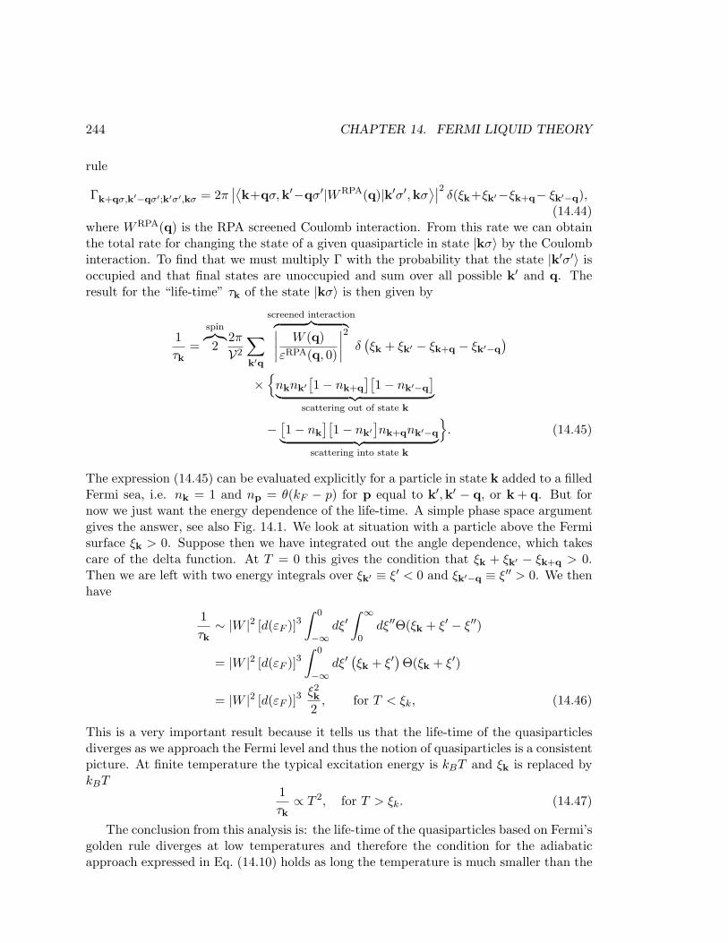
244 CHAPTER 14. FERMI LIQUID THEORY
rule
Γk+qσ,k′−qσ′;k′σ′,kσ = 2π∣∣⟨k+qσ,k′−qσ′|WRPA(q)|k′σ′,kσ
⟩∣∣2 δ(ξk+ξk′−ξk+q− ξk′−q),(14.44)
where WRPA(q) is the RPA screened Coulomb interaction. From this rate we can obtainthe total rate for changing the state of a given quasiparticle in state |kσ〉 by the Coulombinteraction. To find that we must multiply Γ with the probability that the state |k′σ′〉 isoccupied and that final states are unoccupied and sum over all possible k′ and q. Theresult for the “life-time” τk of the state |kσ〉 is then given by
1τk
=
spin︷︸︸︷2
2π
V2
∑
k′q
screened interaction︷ ︸︸ ︷∣∣∣∣W (q)
εRPA(q, 0)
∣∣∣∣2
δ(ξk + ξk′ − ξk+q − ξk′−q
)
×
nknk′[1− nk+q
][1− nk′−q
]︸ ︷︷ ︸
scattering out of state k
− [1− nk
][1− nk′
]nk+qnk′−q︸ ︷︷ ︸
scattering into state k
. (14.45)
The expression (14.45) can be evaluated explicitly for a particle in state k added to a filledFermi sea, i.e. nk = 1 and np = θ(kF − p) for p equal to k′,k′ − q, or k + q. But fornow we just want the energy dependence of the life-time. A simple phase space argumentgives the answer, see also Fig. 14.1. We look at situation with a particle above the Fermisurface ξk > 0. Suppose then we have integrated out the angle dependence, which takescare of the delta function. At T = 0 this gives the condition that ξk + ξk′ − ξk+q > 0.Then we are left with two energy integrals over ξk′ ≡ ξ′ < 0 and ξk′−q ≡ ξ′′ > 0. We thenhave
1τk∼ |W |2 [d(εF )]3
∫ 0
−∞dξ′
∫ ∞
0dξ′′Θ(ξk + ξ′ − ξ′′)
= |W |2 [d(εF )]3∫ 0
−∞dξ′
(ξk + ξ′
)Θ(ξk + ξ′)
= |W |2 [d(εF )]3ξ2k
2, for T < ξk, (14.46)
This is a very important result because it tells us that the life-time of the quasiparticlesdiverges as we approach the Fermi level and thus the notion of quasiparticles is a consistentpicture. At finite temperature the typical excitation energy is kBT and ξk is replaced bykBT
1τk∝ T 2, for T > ξk. (14.47)
The conclusion from this analysis is: the life-time of the quasiparticles based on Fermi’sgolden rule diverges at low temperatures and therefore the condition for the adiabaticapproach expressed in Eq. (14.10) holds as long the temperature is much smaller than the
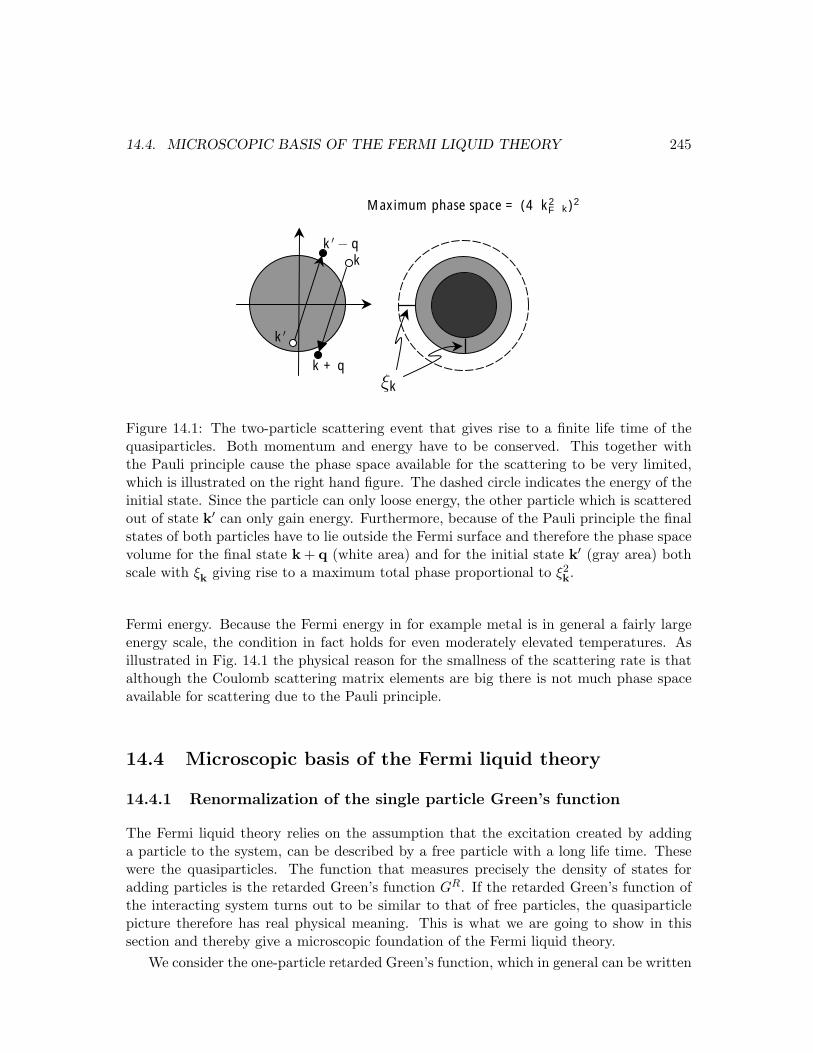
14.4. MICROSCOPIC BASIS OF THE FERMI LIQUID THEORY 245
ξk
k
k + q
k′
k′− q
Maximum phase space = (4k2
Fk)
2
Figure 14.1: The two-particle scattering event that gives rise to a finite life time of thequasiparticles. Both momentum and energy have to be conserved. This together withthe Pauli principle cause the phase space available for the scattering to be very limited,which is illustrated on the right hand figure. The dashed circle indicates the energy of theinitial state. Since the particle can only loose energy, the other particle which is scatteredout of state k′ can only gain energy. Furthermore, because of the Pauli principle the finalstates of both particles have to lie outside the Fermi surface and therefore the phase spacevolume for the final state k + q (white area) and for the initial state k′ (gray area) bothscale with ξk giving rise to a maximum total phase proportional to ξ2
k.
Fermi energy. Because the Fermi energy in for example metal is in general a fairly largeenergy scale, the condition in fact holds for even moderately elevated temperatures. Asillustrated in Fig. 14.1 the physical reason for the smallness of the scattering rate is thatalthough the Coulomb scattering matrix elements are big there is not much phase spaceavailable for scattering due to the Pauli principle.
14.4 Microscopic basis of the Fermi liquid theory
14.4.1 Renormalization of the single particle Green’s function
The Fermi liquid theory relies on the assumption that the excitation created by addinga particle to the system, can be described by a free particle with a long life time. Thesewere the quasiparticles. The function that measures precisely the density of states foradding particles is the retarded Green’s function GR. If the retarded Green’s function ofthe interacting system turns out to be similar to that of free particles, the quasiparticlepicture therefore has real physical meaning. This is what we are going to show in thissection and thereby give a microscopic foundation of the Fermi liquid theory.
We consider the one-particle retarded Green’s function, which in general can be written
246 CHAPTER 14. FERMI LIQUID THEORY
asGR(kσ, ω) =
1ω − ξk − ΣR(kσ, ω)
, (14.48)
where ξk = k2/2m −µ is the free electron energy measured with the respect to the chemicalpotential µ, and where ΣR(k, ω) is the irreducible retarded self-energy. To calculate theself-energy we should in principle include all possible diagrams, which of course is notdoable in the general case. Fortunately, important conclusions can be drawn from thefirst non-trivial approximation, namely the RPA which in Chap. 12 was shown to givethe exact answer in the high density limit. Let us first write the general form of GR byseparating the self-energy in real and imaginary parts
GR(kσ, ω) =1
ω − [ξk + Re ΣR(k, ω)]− i ImΣR(k, ω). (14.49)
We then anticipate the quasiparticle picture by looking at k-values close to the kF , meaningclose to the renormalized Fermi-energy. The renormalized Fermi wave number kF is definedby the condition that the real part of the energy vanishes ξkF
+ Re Σ(kF , 0) = 0. At smallenergies and for k close to kF , we can expand (GR)−1 in powers of k − kF and ω, whichleads to
GR(k, ω) ≈[ω − ω∂ω Re ΣR − (k − kF )∂k(ξ + Re ΣR)− i ImΣR
]−1
≡ Z
[ω − ξk +
i
2τk(ω)
]−1
(14.50)
where
Z−1 = 1− ∂
∂ωReΣ(kF , ω)
∣∣∣∣ω=0
, (14.51)
ξk = (k − kF )Z∂
∂k(ξk + Re Σ(k, 0))k=kF
, (14.52)
1τk(ω)
= −2Z ImΣR(k, ω). (14.53)
The imaginary part of ΣR(k, ω) is not expanded because we look at its form later. Theeffective energy ξk is usually expressed as
ξk = (k − kF )kF /m∗, (14.54)
where the effective mass by Eq. (14.52) is seen to be
m
m∗ = Z
(1 +
m
kF
∂
∂kReΣ(k, 0)
∣∣∣∣k=kF
). (14.55)
In Sec. 14.3.1 we saw that the life-time goes to infinity at low temperatures. If this alsoholds here the spectral function therefore has a Lorentzian shape near k = kF . For a very
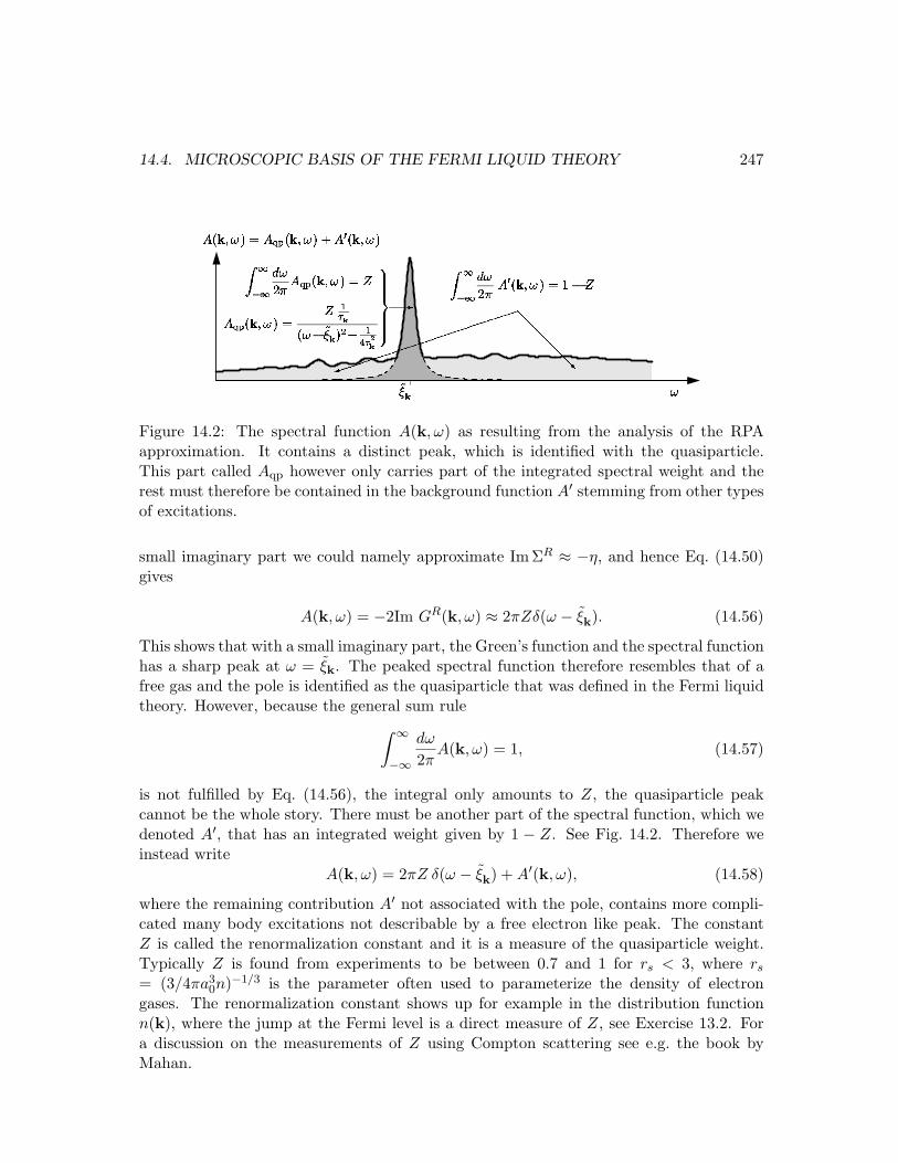
14.4. MICROSCOPIC BASIS OF THE FERMI LIQUID THEORY 247
! "
# $$$$%$$$$&
' )(
* + + + + + ,---------------- .
Figure 14.2: The spectral function A(k, ω) as resulting from the analysis of the RPAapproximation. It contains a distinct peak, which is identified with the quasiparticle.This part called Aqp however only carries part of the integrated spectral weight and therest must therefore be contained in the background function A′ stemming from other typesof excitations.
small imaginary part we could namely approximate Im ΣR ≈ −η, and hence Eq. (14.50)gives
A(k, ω) = −2Im GR(k, ω) ≈ 2πZδ(ω − ξk). (14.56)
This shows that with a small imaginary part, the Green’s function and the spectral functionhas a sharp peak at ω = ξk. The peaked spectral function therefore resembles that of afree gas and the pole is identified as the quasiparticle that was defined in the Fermi liquidtheory. However, because the general sum rule
∫ ∞
−∞
dω
2πA(k, ω) = 1, (14.57)
is not fulfilled by Eq. (14.56), the integral only amounts to Z, the quasiparticle peakcannot be the whole story. There must be another part of the spectral function, which wedenoted A′, that has an integrated weight given by 1 − Z. See Fig. 14.2. Therefore weinstead write
A(k, ω) = 2πZ δ(ω − ξk) + A′(k, ω), (14.58)
where the remaining contribution A′ not associated with the pole, contains more compli-cated many body excitations not describable by a free electron like peak. The constantZ is called the renormalization constant and it is a measure of the quasiparticle weight.Typically Z is found from experiments to be between 0.7 and 1 for rs < 3, where rs
= (3/4πa30n)−1/3 is the parameter often used to parameterize the density of electron
gases. The renormalization constant shows up for example in the distribution functionn(k), where the jump at the Fermi level is a direct measure of Z, see Exercise 13.2. Fora discussion on the measurements of Z using Compton scattering see e.g. the book byMahan.
248 CHAPTER 14. FERMI LIQUID THEORY
We still need to show that the assumption of a large τk is valid and we now turn toevaluating the imaginary part of the self-energy.
14.4.2 Imaginary part of the single particle Green’s function
We base our analysis on the most important diagram, the RPA self-energy
, inEq. (13.12). In the Matsubara frequency domain it is given by
ΣRPAσ (kσ, ikn) = − 1
β
∑
iωn
1V
∑q
W (q)εRPA(q, iωn)
G0(k + q, σ; ikn + iωn). (14.59)
where W/εRPA is the screened interaction. As usual we perform the Matsubara summationby a contour integration
ΣRPAσ (kσ, ikn) = −
∫
C
dz
2πinB(z)
1V
∑q
W (q)εRPA(q, z)
G0(k + q, σ; ikn + z), (14.60)
where C is a suitable contour that encloses all the bosonic Matsubara frequencies z = iωn.The integrand in analytic everywhere but in z = ξk+q − ikn and for z purely real. If wetherefore make a contour which is like the one in Fig. (10.3) C = C1 + C2 then we includeall the Matsubara frequencies except the one in origin (note that the points shown inFig. (10.3) are the fermionic Matsubara frequencies). Therefore we include a loop aroundthe origin so that the contour C = C1 + C2 + C3 shown in Fig. 14.3 includes all bosonMatsubara frequencies z = iωn. The small loop C3 shown in Fig. 14.3 is now seen tocancel parts of the counters C1 and C2 so that they are modified to run between ]−∞,−δ]and [δ,∞[ only, and this is equivalent to stating that the integration are replaced by theprincipal part, when letting δ → 0+. As seen in Fig. 14.3 we, however, also enclose thepole in z = ξk+q − ikn, which we therefore have to subtract again. We now get
ΣRPA(kσ, ikn) = − 1V
∑q
P∫ ∞
−∞
dω
2πinB(ω)
×[
W (q)εRPA(q, ω + iη)
G0(k + q, σ; ikn + ω)− (η → −η)]
+1V
∑q
nB(ξk+q − ikn)[
W (q)εRPA(q, ξk+q − ikn)
]. (14.61)
In the last term we should use that nB(ξk+q− ikn) = −nF (ξk+q) because ikn is a fermionfrequency. Now that we have performed the Matsubara sum, we are allowed to get the
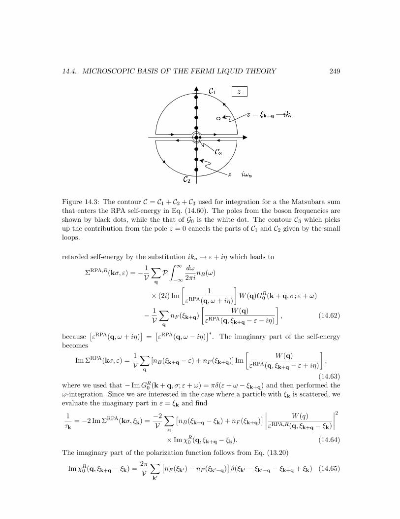
14.4. MICROSCOPIC BASIS OF THE FERMI LIQUID THEORY 249
Figure 14.3: The contour C = C1 + C2 + C3 used for integration for a the Matsubara sumthat enters the RPA self-energy in Eq. (14.60). The poles from the boson frequencies areshown by black dots, while the that of G0 is the white dot. The contour C3 which picksup the contribution from the pole z = 0 cancels the parts of C1 and C2 given by the smallloops.
retarded self-energy by the substitution ikn → ε + iη which leads to
ΣRPA,R(kσ, ε) = − 1V
∑q
P∫ ∞
−∞
dω
2πinB(ω)
× (2i) Im[
1εRPA(q, ω + iη)
]W (q)GR
0 (k + q, σ; ε + ω)
− 1V
∑q
nF (ξk+q)[
W (q)εRPA(q, ξk+q − ε− iη)
], (14.62)
because[εRPA(q, ω + iη)
]=
[εRPA(q, ω − iη)
]∗. The imaginary part of the self-energybecomes
ImΣRPA(kσ, ε) =1V
∑q
[nB(ξk+q − ε) + nF (ξk+q)] Im[
W (q)εRPA(q, ξk+q − ε + iη)
],
(14.63)where we used that − ImGR
0 (k + q, σ; ε + ω) = πδ(ε + ω − ξk+q) and then performed theω-integration. Since we are interested in the case where a particle with ξk is scattered, weevaluate the imaginary part in ε = ξk and find
1τk
= −2 Im ΣRPA(kσ, ξk) =−2V
∑q
[nB(ξk+q − ξk) + nF (ξk+q)
] ∣∣∣∣W (q)
εRPA,R(q, ξk+q − ξk)
∣∣∣∣2
× ImχR0 (q, ξk+q − ξk). (14.64)
The imaginary part of the polarization function follows from Eq. (13.20)
ImχR0 (q, ξk+q − ξk) =
2π
V∑
k′
[nF (ξk′)− nF (ξk′−q)
]δ(ξk′ − ξk′−q − ξk+q + ξk) (14.65)
250 CHAPTER 14. FERMI LIQUID THEORY
(here we shifted k′ → k′−q as compared with Eq. (13.20)) and when this is inserted backinto Eq. (14.64), we obtain
1τk
= −2 Im ΣRPA(kσ, ε) = −4π
V∑
qk′[nB(ξk+q − ξk) + nF (ξk+q)]
[nF (ξk′)− nF (ξk′−q)
]
×∣∣∣∣
W (q)εRPA,R(q, ξk+q − ξk)
∣∣∣∣2
δ(ξk′ − ξk′−q − ξk+q + ξk).
(14.66)
Let us study the occupation factors in this expression and compare with the Fermi’s goldenrule expression Eq. (14.45). For the first term in the first parenthesis we use the identity
nB(ε1 − ε2)[nF (ε2)− nF (ε2)] = nF (ε1)[1− nF (ε2)],
combined with ξk− ξk+q = −ξk′ + ξk′−q. For the second term we use the obvious identity
nF (ε1)[1− nF (ε2)]− nF (ε2)[1− nF (ε2] = nF (ε1)− nF (ε2)
and nF (−ε) = 1 − nF (ε). All together this allows us to write the occupation factors inEq. (14.66) as
−nF (ξk′)[1− nF (ξk+q)][1− nF (ξk′−q′)
]− [1− nF (ξk′)]nF (ξk+q)nF (ξk′−q) (14.67)
At low temperature the first term is due to the energy conservation condition non-zero forξk > 0, while the last term is non-zero for ξk < 0. The first term thus corresponds to thescattering out term in Eq. (14.45), while the second term corresponds to the scatteringin term. If we furthermore approximate ξk − ξk+q ≈ 0 in εRPA we now see that the lifetime in Eq. (14.66) is equivalent to the Fermi’s golden rule expression Eq. (14.45). Wehave thus verified that the imaginary part of the retarded Green’s function indeed goes tozero. At least when employing the RPA approximation for the self-energy, but the RPAapproximation in Chap. 12 was shown to be exact in the high density limit. An explicitcalculation of Eq. (14.66) was done by Quinn and Ferrell5 who got
1τk
=√
3π2
128ωp
(ξk
εF
)2
. (14.68)
Going beyond RPA, it can in fact be shown that the imaginary part vanishes to all ordersin the interaction. This was done by Luttinger6 who proved that the imaginary part of anydiagram for the self-energy goes to zero as ξ2 or faster. The derivation is rather lengthy andwe do not give it here. It is however not hard to imagine that more complicated scatteringevents than the simple one depicted in Fig. 14.1 will have even more constrains on theenergies. Hence after integration, they will result in higher powers of ξk. This concludesour analysis of the single particle Green’s function. The analysis indeed confirmed thephysical picture put forward by Landau in his Fermi liquid theory.
5J. J. Quinn and R. A. Ferrell, Phys. Rev 112, 812 (1958).6J.M. Luttinger, Phys. Rev. 121, 942 (1961).
14.5. OUTLOOK AND SUMMARY 251
14.4.3 Mass renormalization?
In the previous section we saw how the assumption of weakly interacting quasiparticles wasjustified by the long life time of the single particle Green’s function. We also found that theeffective mass of the quasiparticle was renormalized due to the interactions. This seems tocontradict the postulate of the Fermi liquid theory that the current of the quasiparticlesis independent of interactions, i.e. it is given by k/m and not k/m∗. The bare velocityof the quasiparticles was important for obtaining the Drude formula for the conductivity,σ = ne2τ tr/m. How come the renormalized mass m∗ appears in the Green’s functionwhereas the physically observable conductivity contains the bare mass m? The answer tothis question in found by studying how the conductivity is calculated diagrammatically.The conductivity is as we remember from the Kubo formula related to the current-currentcorrelation function. The calculation has to be done in a consistent way such that thediagrams included in the irreducible self-energy is also included in the diagrams for thetwo-particle correlation function. When the same type of diagrams are included bothin the self-energy and in the lines that cross the two-particle “bubble” then the massrenormalization exactly cancels. In Chap. 15 we shall see an explicit example of this bycalculating diagrammatically the finite resistance due to impurity scattering starting fromthe fully microscopic theory. See also Exercise 14.4
14.5 Outlook and summary
We have developed the semi-classical Fermi liquid theory of interacting particles. Thetheory is valid whenever perturbation theory is valid, i.e. when the interaction does notinduce a phase transition. Miraculously, the interacting system of particles can be de-scribed by a gas of non-interacting particles. These particles we call quasiparticles andthey can be labelled by the same quantum numbers of those of the non-interacting system,provided that the corresponding operators also commute with the full Hamiltonian. Fora translation-invariant system the quantum numbers are k and σ.
On long length and time scales we can use a semi-classical approach to study variousproperties. This approach is based on the Boltzmann equation
∂t(nk) + k · ∇knk + vk · ∇rnk =(
∂nk
∂t
)
collisions
. (14.69)
This equation is extremely useful since it in many situations gives a sufficiently accu-rate description of the physics. It has been widely used to explain numerous transportphenomena in gases and solids. One can include both electric and magnetic fields driv-ing the system out of equilibrium. The driving fields enter through the Lorentz force asp = ~k = (−e)(E + v ×B). On the right hand side of Eq. (14.69) we have included colli-sions due to impurities and particle-particle collisions . One can also include for exampleparticle-phonon scattering in solids and thus explain the temperature dependence of thedifferent transport coefficients.
Landau’s phenomenological theory was shown to be justified by a rigors microscopiccalculation, using the random phase approximation result for the self-energy. The result
252 CHAPTER 14. FERMI LIQUID THEORY
of this analysis was that even in the presence of interactions does the Fermi surface persistand near the Fermi surface the imaginary part of the single particle Green’s functionrapidly vanish as
ImΣR(kF , ε) ∝ max(ε2, T 2). (14.70)
This explains why the Fermi liquid theory works: when the imaginary part goes to zerothe single particle Green’s function is identical to that of a free particle.
Chapter 15
Impurity scattering andconductivity
We now return to the problem of calculating the resistance of a metallic conductor dueto scattering against impurities. The basic physics of impurity scattering was discussedin Chap. 10, where we saw how the single-particle Green’s function acquired a finite lifetime after averaging over the positions of the impurities. In Chap. 13 the conductivitywas calculated within the Boltzmann equation approach. We now rederive the Boltzmannequation result starting from a microscopic quantum approach. The advantage of thismicroscopic approach, besides giving a first principle justification of the Boltzmann equa-tion, is that it can be extended to include correlation and coherence effects that cannot bedescribed in the semiclassical Boltzmann approach. In order to get familiar with the tech-niques, we therefore start by deriving the semiclassical result. Then we go on to includethe quantum mechanical effect known as weak localization, which is due to interferencebetween time reversed paths. Weak localization involves coherent scattering on manyimpurities, and it can therefore not be explained semiclassically.
In 1979 the weak localization correction to resistivity was observed experimentally inlarge 2D samples at low temperatures. It was explained theoretically later the same year,and an extended research was initiated on the role of quantum coherence in transportproperties. A few years later another low-temperature interference effect, the so-calleduniversal conductance fluctuations, was discovered in small (∼ µm) phase-coherent struc-tures. This discovery started the modern field of mesoscopic physics. To understand thesesmaller systems one must take into account the finite size of the conductors, which is thetopic in Chap. 15. In this chapter we deal with extended systems and discuss the mostimportant disorder-induced quantum corrections. The leading quantum correction is pre-cisely the weak localization effect, at least in two dimensions. In one dimension, thingsare more complicated because there all states are localized and one cannot talk abouta conductivity that scales in a simple fashion with the length of the system. In threedimensions, the situation is again different in that at some critical amount of impurityscattering there exists a metal-insulator transition known as the Anderson localization.This is however outside the scope this book.
253
254 CHAPTER 15. IMPURITY SCATTERING AND CONDUCTIVITY
Based on the physical picture that emerged from the Fermi liquid description inChap. 13, we assume in the first part of this chapter that we can describe the electrons asnon-interacting. In the second part of the chapter we include electron-electron interactionstogether with impurity scattering and explicitly demonstrate that the non-interacting ap-proximation is valid. This means that we shall see how the mass renormalization discussedin Sec. 14.4.3 is cancelled out. Furthermore, we shall see that in order to obtain meaning-ful results, it is absolutely imperative to include vertex corrections to the current-currentcorrelation bubble diagrams. These corrections cannot be treated evaluating only single-particle Green’s functions. They are thus genuine two-particle correlation effects, whichcan be described by diagrams where interaction lines “cross” the bubble diagrams.
15.1 Vertex corrections and dressed Green’s functions
Let us start by the Kubo formula for the electrical conductivity tensor σαβ given inEq. (6.25) in terms of the retarded current-current correlation function Eq. (6.26). Herewe shall only look at the dissipative part of the conductivity, and therefore we take thereal part of Eq. (6.25)
Re σαβ(r, r′;ω) = −e2
ωImΠR
αβ(r, r′, ω). (15.1)
Note that the last, so-called “diamagnetic”, term of σ in Eq. (6.25) drops out of the realpart. In the following we therefore only include the first, so-called “paramagnetic”, termin Eq. (6.25), denoted σ∇. For a translation-invariant system we consider as usual theFourier transform
σ∇αβ(q; ω) =ie2
ωΠR
αβ(q, ω). (15.2)
The dc-conductivity is then found by letting1 q → 0 and then ω → 0. The dc-response atlong wavelengths is thus obtained as
Re σαβ = −e2 limω→0
limq→0
1ω
ImΠRαβ(q, ω). (15.3)
In this chapter we consider only homogeneous translation-invariant systems, i.e. the con-ductivity tensor is isotropic and therefore diagonal, σαβ = σ δαβ . In particular we haveno magnetic field and take A = 0. In the computation we can choose α to be the x direc-tion. Note that the system is translation-invariant even in the presence of impurities afterperforming the position average described in Chap. 10.
As usual we calculate the retarded function starting from the corresponding Matsubarafunction. The Matsubara current-current correlation function is
Πxx(q, τ − τ ′) = − 1V
⟨TτJx(q, τ)Jx(−q, τ ′)
⟩. (15.4)
1If in doubt always perform the limit q → 0 first, because having a electric field E(q,ω) where ω = 0and q finite is unphysical, since it would give rise to an infinite charge built up.
15.1. VERTEX CORRECTIONS AND DRESSED GREEN’S FUNCTIONS 255
In the frequency domain it is
Πxx(q, iqn) = − 1V
∫ β
0d(τ − τ ′)eiqn(τ−τ ′) ⟨
Jx(q, τ)Jx(−q, τ ′)⟩, (15.5)
where the time-ordering operator Tτ is omitted, because τ > τ ′. We can now expressJx(q, τ) in terms of Jx(q, iqn) and obtain
Πxx(q, iqn) = − 1V
∫ β
0d(τ − τ ′)eiqn(τ−τ ′) 1
β
∑
iql
1β
∑
iqm
〈Jx(q, iql)Jx(−q, iqm)〉 e−iqlτe−iqmτ ′ .
(15.6)The integration with respect to τ leads to iqn = iql. Finally, since the result cannot dependon τ ′, we must have iqn = −iqm, and whence
Πxx(q, iqn) = − 1Vβ
〈Jx(q, iqn)Jx(−q,−iqn)〉 . (15.7)
This we conveniently rewrite using the four-vector notation q = (iqn,q)
Πxx(q) = − 1Vβ
〈Jx(q)Jx(−q)〉 . (15.8)
In order to begin the diagrammatical analysis we write the current density Jx(q) infour-vector notation
Jx(q) =∫ β
0dτeiqnτ 1
2m
1V
∑
kσ
(2k + q)xc†kσ(τ)ck+qσ(τ)
=1
2m
1β
∑
ikn
1V
∑
kσ
(2k + q)xc†kσ(ikn)ck+qσ(ikn + iqn),
≡ 12m
1β
1V
∑
k
∑σ
(2kx+qx)c†σ(k)cσ(k + q), (15.9)
which we draw diagrammatically as a vertex
Jx(q) = k+q
k
(15.10)
The vertex conserves four-momentum, and thus has the momentum q = (iqn,q) flowingout from it to the left.
We can now draw diagrams for the current-current correlation function using the Feyn-man rules. The procedure is analogous to that for the charge-charge correlation functionin Chap. 12, however, here we include both the impurity lines from Chap. 10 and
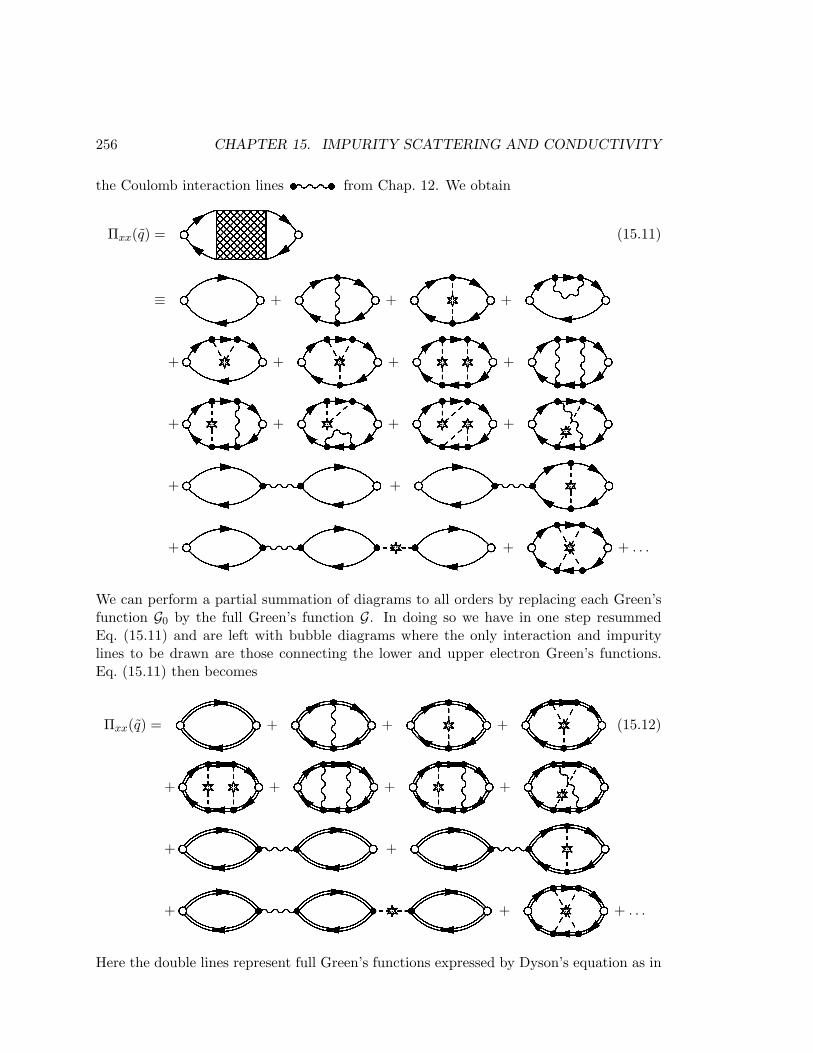
256 CHAPTER 15. IMPURITY SCATTERING AND CONDUCTIVITY
the Coulomb interaction lines from Chap. 12. We obtain
Πxx(q) = (15.11)
≡ + + ++ + + ++ + + ++ ++ + + . . .
We can perform a partial summation of diagrams to all orders by replacing each Green’sfunction G0 by the full Green’s function G. In doing so we have in one step resummedEq. (15.11) and are left with bubble diagrams where the only interaction and impuritylines to be drawn are those connecting the lower and upper electron Green’s functions.Eq. (15.11) then becomes
Πxx(q) = + + + (15.12)
+ + + ++ ++ + + . . .
Here the double lines represent full Green’s functions expressed by Dyson’s equation as in
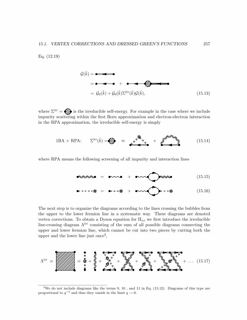
15.1. VERTEX CORRECTIONS AND DRESSED GREEN’S FUNCTIONS 257
Eq. (12.19)
G(k) =!=" +#= G0(k) + G0(k)Σirr(k)G(k), (15.13)
where Σirr = $ is the irreducible self-energy. For example in the case where we includeimpurity scattering within the first Born approximation and electron-electron interactionin the RPA approximation, the irreducible self-energy is simply
1BA + RPA: Σirr(k) =% ≈ & + ' (15.14)
where RPA means the following screening of all impurity and interaction lines
( = ) +* (15.15)
+ = , +- (15.16)
The next step is to organize the diagrams according to the lines crossing the bubbles fromthe upper to the lower fermion line in a systematic way. These diagrams are denotedvertex corrections. To obtain a Dyson equation for Πxx we first introduce the irreducibleline-crossing diagram Λirr consisting of the sum of all possible diagrams connecting theupper and lower fermion line, which cannot be cut into two pieces by cutting both theupper and the lower line just once2,
Λirr ≡.≡ / + 0 +1 +2 +3 +4 + . . . (15.17)
2We do not include diagrams like the terms 9, 10 , and 11 in Eq. (15.12). Diagrams of this type areproportional to q−2 and thus they vanish in the limit q → 0.
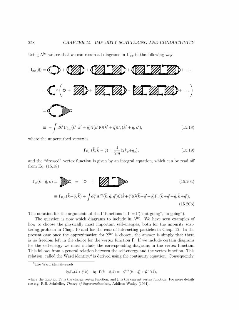
258 CHAPTER 15. IMPURITY SCATTERING AND CONDUCTIVITY
Using Λirr we see that we can resum all diagrams in Πxx in the following way
Πxx(q) =5 +6 +7 +8 + . . .
= 9 ×(
: +; +< += + . . .
)
≡>≡ −
∫dk′ Γ0,x(k′, k′ + q)G(k′)G(k′ + q)Γx(k′ + q, k′), (15.18)
where the unperturbed vertex is
Γ0,x(k, k + q) =1
2m(2kx+qx), (15.19)
and the “dressed” vertex function is given by an integral equation, which can be read offfrom Eq. (15.18)
Γx(k+q, k) ≡? = @ +A (15.20a)
≡ Γ0,x(k+q, k) +∫
dq′Λirr(k, q, q′)G(k+q′)G(k+q′+q)Γx(k+q′+q, k+q′),
(15.20b)
The notation for the arguments of the Γ functions is Γ = Γ(“out going”,“in going”).The question is now which diagrams to include in Λirr. We have seen examples of
how to choose the physically most important self-energies, both for the impurity scat-tering problem in Chap. 10 and for the case of interacting particles in Chap. 12. In thepresent case once the approximation for Σirr is chosen, the answer is simply that thereis no freedom left in the choice for the vertex function ΓΓ. If we include certain diagramsfor the self-energy we must include the corresponding diagrams in the vertex function.This follows from a general relation between the self-energy and the vertex function. Thisrelation, called the Ward identity,3 is derived using the continuity equation. Consequently,
3The Ward identity reads
iq0Γ0(k + q, k)− iq · ΓΓ(k + q, k) = −G−1(k + q) + G−1(k),
where the function Γ0 is the charge vertex function, and ΓΓ is the current vertex function. For more detailssee e.g. R.B. Schrieffer, Theory of Superconductivity, Addison-Wesley (1964).
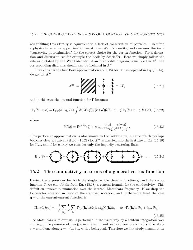
15.2. THE CONDUCTIVITY IN TERMS OF A GENERAL VERTEX FUNCTION259
not fulfilling this identity is equivalent to a lack of conservation of particles. Thereforea physically sensible approximation must obey Ward’s identity, and one uses the term“conserving approximation” for the correct choice for the vertex function. For a deriva-tion and discussion see for example the book by Schrieffer. Here we simply follow therule as dictated by the Ward identity: if an irreducible diagram is included in Σirr thecorresponding diagrams should also be included in Λirr.
If we consider the first Born approximation and RPA for Σirr as depicted in Eq. (15.14),we get for Λirr
Λirr =B≈ C + D ≡ W , (15.21)
and in this case the integral function for Γ becomes
Γx(k+ q, k) = Γ0,x(k+ q, k)+∫
dq′W (q′)G(k+ q′)G(k+ q′+ q)Γx(k+ q′+ q, k+ q′), (15.22)
where
W (q) = WRPA(q) + nimpu(q)
εRPA(q)u(−q)
εRPA(−q). (15.23)
This particular approximation is also known as the ladder sum, a name which perhapsbecomes clear graphically if Eq. (15.21) for Λirr is inserted into the first line of Eq. (15.18)for Πxx, and if for clarity we consider only the impurity scattering lines:
Πxx(q) =E +F +G +H + . . . (15.24)
15.2 The conductivity in terms of a general vertex function
Having the expressions for both the single-particle Green’s function G and the vertexfunction Γ, we can obtain from Eq. (15.18) a general formula for the conductivity. Thisdefinition involves a summation over the internal Matsubara frequency. If we drop thefour-vector notation in favor of the standard notation, and furthermore treat the caseq = 0, the current-current function is
Πxx(0, iqn) = − 1β
∑
ikn
1V
∑
k
Γ0,x(k,k)G(k, ikn)G(k,ikn + iqn)Γx(k,k;ikn + iqn, ikn).
(15.25)The Matsubara sum over ikn is performed in the usual way by a contour integration overz = ikn. The presence of two G’s in the summand leads to two branch cuts; one alongz = ε and one along z = −iqn +ε, with ε being real. Therefore we first study a summation
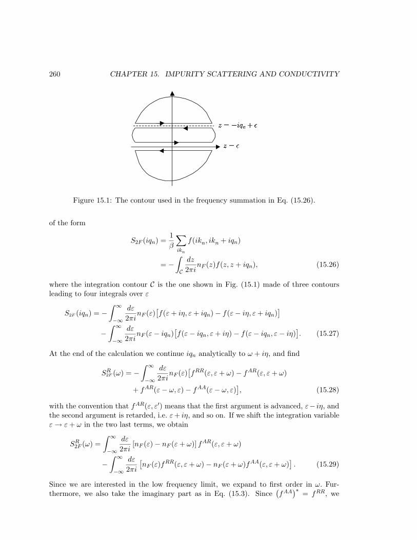
260 CHAPTER 15. IMPURITY SCATTERING AND CONDUCTIVITY
Figure 15.1: The contour used in the frequency summation in Eq. (15.26).
of the form
S2F (iqn) =1β
∑
ikn
f(ikn, ikn + iqn)
= −∫
C
dz
2πinF (z)f(z, z + iqn), (15.26)
where the integration contour C is the one shown in Fig. (15.1) made of three contoursleading to four integrals over ε
S2F (iqn) = −∫ ∞
−∞
dε
2πinF (ε)
[f(ε + iη, ε + iqn)− f(ε− iη, ε + iqn)
]
−∫ ∞
−∞
dε
2πinF (ε− iqn)
[f(ε− iqn, ε + iη)− f(ε− iqn, ε− iη)
]. (15.27)
At the end of the calculation we continue iqn analytically to ω + iη, and find
SR2F (ω) = −
∫ ∞
−∞
dε
2πinF (ε)
[fRR(ε, ε + ω)− fAR(ε, ε + ω)
+ fAR(ε− ω, ε)− fAA(ε− ω, ε)], (15.28)
with the convention that fAR(ε, ε′) means that the first argument is advanced, ε− iη, andthe second argument is retarded, i.e. ε + iη, and so on. If we shift the integration variableε → ε + ω in the two last terms, we obtain
SR2F (ω) =
∫ ∞
−∞
dε
2πi[nF (ε)− nF (ε + ω)] fAR(ε, ε + ω)
−∫ ∞
−∞
dε
2πi
[nF (ε)fRR(ε, ε + ω)− nF (ε + ω)fAA(ε, ε + ω)
]. (15.29)
Since we are interested in the low frequency limit, we expand to first order in ω. Fur-thermore, we also take the imaginary part as in Eq. (15.3). Since
(fAA
)∗ = fRR, we
15.3. THE CONDUCTIVITY IN THE FIRST BORN APPROXIMATION 261
find
Im SR2F (ω) = −ω Im
∫ ∞
−∞
dε
2πi
(−∂nF (ε)
∂ε
) [fAR(ε, ε)− fRR(ε, ε)
]. (15.30)
At low temperatures, we can approximate the derivative of the Fermi-Dirac function by adelta function (
−∂nF (ε)∂ε
)≈ δ(ε) (15.31)
and henceIm SR
2F (ω) =ω
2πRe
[fAA(0, 0)− fAR(0, 0)
]. (15.32)
By applying this to Eq. (15.25) and then inserting into Eq. (15.3) one obtains
Reσxx = 2 Ree2
2π
1V
∑
k
Γ0,x(k,k)[GA(k, 0)GR(k, 0)ΓRA
x (k,k; 0, 0)
−GA(k, 0)GA(k, 0)ΓAAx (k,k; 0, 0)
], (15.33)
where we have included a factor of 2 due to spin degeneracy. This is how far one can goon general principles. To proceed further, one must look at the specific physical cases andthen solve for the vertex function satisfying Eq. (15.20b) and insert the result into (15.33).In the following we consider various cases. We will consider only cases where the disorderis weak and for this case it is shown in the next section that the product GRGA exceedsGAGA by a factor of order 1/τEF , where τ is the scattering time for impurity scattering.Hence in the weak disorder limit, we may replace the general formula in Eq. (15.33) bythe first term only.
15.3 The conductivity in the first Born approximation
The conductivity was calculated in Sec. 14.3 using a semiclassical approximation for thescattering against the impurities. The semiclassical approximation is similar to the firstBorn approximation in that it only includes scattering against a single impurity and ne-glects interference effects. Therefore we expect to reproduce the semiclassical result if weonly include the first Born approximation in our diagrammatical calculation. The startingpoint in this section is non-interacting electrons scattering on impurities. The RPA partof the self-energy in Eq. (15.14) is not included in this section. Later we discuss whathappens if interactions are included.
The vertex function is now solved using the first Born approximation, i.e. the firstdiagram in Eq. (15.21). In this case, again taking q = 0, the integral equation Eq. (15.22)becomes
Γx(k,k;ikn + iqn, ikn) = Γ0,x(k,k) +1V
∑
q′nimp
∣∣uRPA(q′)∣∣2 G(k + q′, ikn) (15.34)
× G(k + q′,ikn + iqn)Γx(k + q′,k+q′;ikn + iqn, ikn),
262 CHAPTER 15. IMPURITY SCATTERING AND CONDUCTIVITY
where the second term in Eq. (15.23) has been inserted and where uRPA = u/εRPA. TheGreen’s functions G are, as we learned from the Ward identity, also those obtained inthe first Born approximation. Note that there is no internal Matsubara sum because theimpurity scattering conserves energy. Since we do not expect the dynamical screeningto be important for the elastic scattering, we set the frequency in εRPA(q, 0) to zero.Remembering that Γx is a component of a vector function ΓΓ and that the unperturbedvertex is ΓΓ0(k,k) = k/m, we define for convenience a scalar function γ(k, ε) definedas ΓΓ(k, ε) = k γ(k, ε)/m. In doing so we in fact use that the system is isotropic whichmeans that only the vector k can give the direction. When inserting this into Eq. (15.34),multiplying by (1/k2)k·, and shifting the variable q′ to q′ = k′ − k, we get
γ(k,k;ikn + iqn, ikn) = 1 +1V
∑
k′nimp
∣∣uRPA(k′ − k)∣∣2 G(k′, ikn)
× G(k′,ikn + iqn)k · k′k2
γ1BA(k′,k′;ikn + iqn, ikn), (15.35)
In the formula Eq. (15.33) for the conductivity both ΓRAx and ΓRR
x appear (or ratherΓRR
x = (ΓAAx )∗. They satisfy two different integral equations, which we obtain from
Eq. (15.35) by letting iqn → ω + iη and ikn → ε ± iη, and subsequently taking thedc-limit ω → 0. We arrive at
γRX(k, ε) = 1 +1V
∑
k′nimp
∣∣uRPA(k′ − k)∣∣2 GX(k′, ε)GR(k′, ε)
k · k′k2
γRX(k′, ε), (15.36)
where X = A or R. One immediately sees that the small factor nimp tends to kill thesum, and in the weak scattering limit one should expect the solution of this equation tobe simply γRX(k, ε) ≈ 1. It is immediately seen that this is a consistent solution for theimaginary part of both γRA and γRR but it turns out that for the real part of γRA a factor1/nimp is contained in the Green’s function. The lesson we learn here is that we have tobe rather careful with products of Green’s function carrying the same arguments, becausein the limit of small nimp, ImGX tends to a delta function, and the product of two deltafunctions has to be defined with care. Let us look more carefully into the products GAGR
and GRGR, which also appear in Eq. (15.33). This first combination is
GA(k, ε)GR(k, ε) =∣∣GR(k, ε)
∣∣2 ≡∣∣∣∣
1ε− ξk − ΣR(k, ε)
∣∣∣∣2
=1
ImΣR(k, ε)Im
1ε− ξk − ΣR(k, ε)
≡ 1−2 ImΣR(k, ε)
A(k, ε) ≡ τA(k, ε), (15.37)
where A = −2 Im GR is the spectral function, and where as before the life-time τ is definedby τ−1 = −2 Im ΣR(k, ε). For the case of weak impurity scattering the scattering rate τ−1
is small, whence the spectral function is approximately a delta function. In the case ofsmall nimp we therefore get
GA(k, ε)GR(k, ε) ≈ τ2πδ(ε− ξk). (15.38)
15.3. THE CONDUCTIVITY IN THE FIRST BORN APPROXIMATION 263
Because τ ∝ n−1imp, the product nimpG
AGR in Eq. (15.36) is finite in the limit nimp → 0.The combination GRGR on the other hand is not divergent and in fact nimpG
RGR → 0as nimp → 0. That GRGR is finite is seen as follows
GR(k, ε)GR(k, ε) ≈(
ε− ξk − i2τ(
ε− ξk)2 +
(12τ
)2
)2
=(ε− ξk)2 − (
12τ
)2
((ε− ξk
)2 +(
12τ
)2)2 + i (ε− ξk) A(k, ε). (15.39)
The last term clearly goes to zero when τ is large and when A is approximated by a deltafunction. The first term is a peaked function at ε− ξk = 0, but the integrated weight is infact zero as can be checked by performing an integration over ε. From these arguments itfollows that the terms with GRGR can be omitted and only terms with GRGA are kept. Asexplained above, we use the first Born approximation for the self-energy. In the followingwe therefore approximate τ with the first Born approximation life time τ0
τ−1 ≈ τ−10 ≡ 2πnimp
∑
k′|u(k− k′)|2δ(ξk − ξk′). (15.40)
Because all energies are at the Fermi energy, this life time is independent of k.The conductivity Eq. (15.33) then becomes
Re σxx = 2e2 Re1V
∑
k
Γ0,x(k,k)τ0δ(ξk)ΓRAx (k,k; 0, 0)
= 2e2τ0 Re1V
∑
k
kx
mδ(ξk)
kx
mγRA(k,k; 0, 0) =
e2n
mτ0γ
RA(kF , kF ; 0, 0) (15.41)
The remaining problem is to find γRA(k,k; 0,0) for |k| = kF . The solution follows fromthe integral equation Eq. (15.35)
γRA(k) = 1 +2π
V∑
k′nimp
∣∣uRPA(k′ − k)∣∣2 τ0δ(ξk′)
k · k′k2
γRA(k′). (15.42)
Since this equation has no dependence on the direction of k, and since the lengths of bothk and k′ are given by kF , γRA depends only on kF . But kF is constant, and we get
γRA = 1 +
[2π
V∑
k′nimp
∣∣uRPA(k′ − k)∣∣2 δ(ξk′)
k · k′k2
]τ0γ
RA. (15.43)
The solution is thus simply
γRA =1
1− λ τ0, (15.44)
where
λ =2π
V∑
k′nimp
∣∣uRPA(k′ − k)∣∣2 δ(ξk′)
k · k′k2
= (τ0)−1 − (
τ tr)−1
. (15.45)
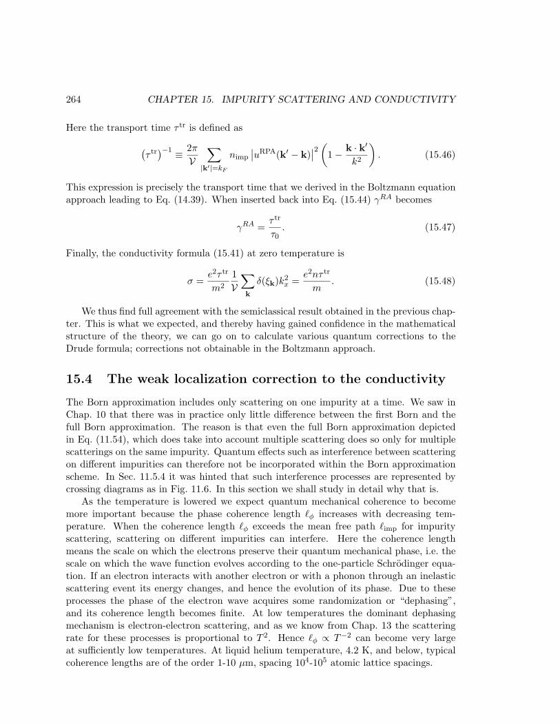
264 CHAPTER 15. IMPURITY SCATTERING AND CONDUCTIVITY
Here the transport time τ tr is defined as
(τ tr
)−1 ≡ 2π
V∑
|k′|=kF
nimp
∣∣uRPA(k′ − k)∣∣2
(1− k · k′
k2
). (15.46)
This expression is precisely the transport time that we derived in the Boltzmann equationapproach leading to Eq. (14.39). When inserted back into Eq. (15.44) γRA becomes
γRA =τ tr
τ0. (15.47)
Finally, the conductivity formula (15.41) at zero temperature is
σ =e2τ tr
m2
1V
∑
k
δ(ξk)k2x =
e2nτ tr
m. (15.48)
We thus find full agreement with the semiclassical result obtained in the previous chap-ter. This is what we expected, and thereby having gained confidence in the mathematicalstructure of the theory, we can go on to calculate various quantum corrections to theDrude formula; corrections not obtainable in the Boltzmann approach.
15.4 The weak localization correction to the conductivity
The Born approximation includes only scattering on one impurity at a time. We saw inChap. 10 that there was in practice only little difference between the first Born and thefull Born approximation. The reason is that even the full Born approximation depictedin Eq. (11.54), which does take into account multiple scattering does so only for multiplescatterings on the same impurity. Quantum effects such as interference between scatteringon different impurities can therefore not be incorporated within the Born approximationscheme. In Sec. 11.5.4 it was hinted that such interference processes are represented bycrossing diagrams as in Fig. 11.6. In this section we shall study in detail why that is.
As the temperature is lowered we expect quantum mechanical coherence to becomemore important because the phase coherence length `φ increases with decreasing tem-perature. When the coherence length `φ exceeds the mean free path `imp for impurityscattering, scattering on different impurities can interfere. Here the coherence lengthmeans the scale on which the electrons preserve their quantum mechanical phase, i.e. thescale on which the wave function evolves according to the one-particle Schrodinger equa-tion. If an electron interacts with another electron or with a phonon through an inelasticscattering event its energy changes, and hence the evolution of its phase. Due to theseprocesses the phase of the electron wave acquires some randomization or “dephasing”,and its coherence length becomes finite. At low temperatures the dominant dephasingmechanism is electron-electron scattering, and as we know from Chap. 13 the scatteringrate for these processes is proportional to T 2. Hence `φ ∝ T−2 can become very largeat sufficiently low temperatures. At liquid helium temperature, 4.2 K, and below, typicalcoherence lengths are of the order 1-10 µm, spacing 104-105 atomic lattice spacings.
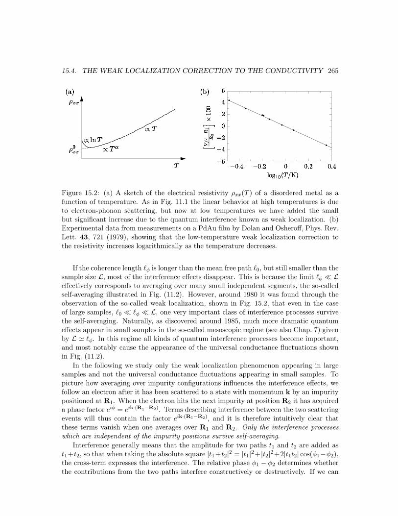
15.4. THE WEAK LOCALIZATION CORRECTION TO THE CONDUCTIVITY 265
! " # #
" $# #% & ' (%)( *
%)(
(
Figure 15.2: (a) A sketch of the electrical resistivity ρxx(T ) of a disordered metal as afunction of temperature. As in Fig. 11.1 the linear behavior at high temperatures is dueto electron-phonon scattering, but now at low temperatures we have added the smallbut significant increase due to the quantum interference known as weak localization. (b)Experimental data from measurements on a PdAu film by Dolan and Osheroff, Phys. Rev.Lett. 43, 721 (1979), showing that the low-temperature weak localization correction tothe resistivity increases logarithmically as the temperature decreases.
If the coherence length `φ is longer than the mean free path `0, but still smaller than thesample size L, most of the interference effects disappear. This is because the limit `φ ¿ Leffectively corresponds to averaging over many small independent segments, the so-calledself-averaging illustrated in Fig. (11.2). However, around 1980 it was found through theobservation of the so-called weak localization, shown in Fig. 15.2, that even in the caseof large samples, `0 ¿ `φ ¿ L, one very important class of interference processes survivethe self-averaging. Naturally, as discovered around 1985, much more dramatic quantumeffects appear in small samples in the so-called mesoscopic regime (see also Chap. 7) givenby L ' `φ. In this regime all kinds of quantum interference processes become important,and most notably cause the appearance of the universal conductance fluctuations shownin Fig. (11.2).
In the following we study only the weak localization phenomenon appearing in largesamples and not the universal conductance fluctuations appearing in small samples. Topicture how averaging over impurity configurations influences the interference effects, wefollow an electron after it has been scattered to a state with momentum k by an impuritypositioned at R1. When the electron hits the next impurity at position R2 it has acquireda phase factor eiφ = eik·(R1−R2). Terms describing interference between the two scatteringevents will thus contain the factor eik·(R1−R2), and it is therefore intuitively clear thatthese terms vanish when one averages over R1 and R2. Only the interference processeswhich are independent of the impurity positions survive self-averaging.
Interference generally means that the amplitude for two paths t1 and t2 are added ast1+t2, so that when taking the absolute square |t1+t2|2 = |t1|2+|t2|2+2|t1t2| cos(φ1−φ2),the cross-term expresses the interference. The relative phase φ1 − φ2 determines whetherthe contributions from the two paths interfere constructively or destructively. If we can
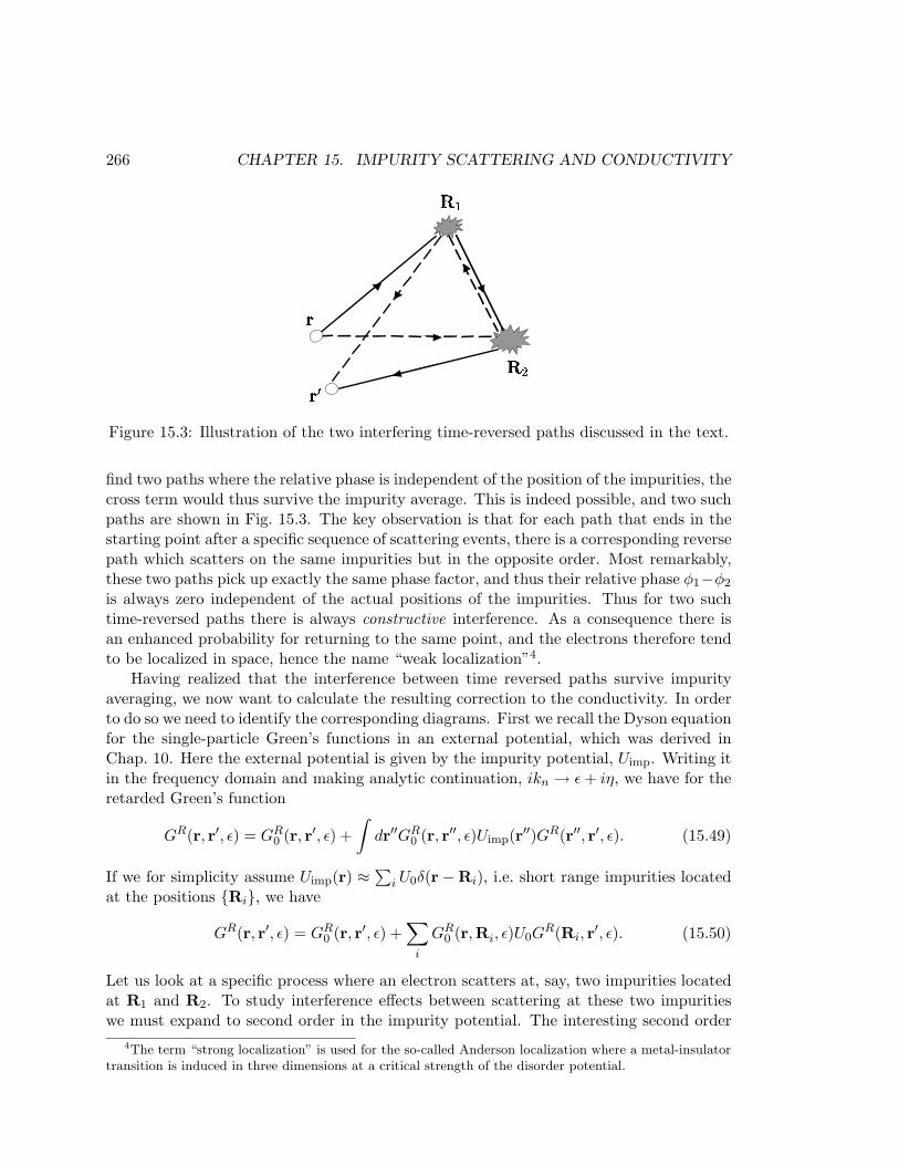
266 CHAPTER 15. IMPURITY SCATTERING AND CONDUCTIVITY
Figure 15.3: Illustration of the two interfering time-reversed paths discussed in the text.
find two paths where the relative phase is independent of the position of the impurities, thecross term would thus survive the impurity average. This is indeed possible, and two suchpaths are shown in Fig. 15.3. The key observation is that for each path that ends in thestarting point after a specific sequence of scattering events, there is a corresponding reversepath which scatters on the same impurities but in the opposite order. Most remarkably,these two paths pick up exactly the same phase factor, and thus their relative phase φ1−φ2
is always zero independent of the actual positions of the impurities. Thus for two suchtime-reversed paths there is always constructive interference. As a consequence there isan enhanced probability for returning to the same point, and the electrons therefore tendto be localized in space, hence the name “weak localization”4.
Having realized that the interference between time reversed paths survive impurityaveraging, we now want to calculate the resulting correction to the conductivity. In orderto do so we need to identify the corresponding diagrams. First we recall the Dyson equationfor the single-particle Green’s functions in an external potential, which was derived inChap. 10. Here the external potential is given by the impurity potential, Uimp. Writing itin the frequency domain and making analytic continuation, ikn → ε + iη, we have for theretarded Green’s function
GR(r, r′, ε) = GR0 (r, r′, ε) +
∫dr′′GR
0 (r, r′′, ε)Uimp(r′′)GR(r′′, r′, ε). (15.49)
If we for simplicity assume Uimp(r) ≈∑
i U0δ(r−Ri), i.e. short range impurities locatedat the positions Ri, we have
GR(r, r′, ε) = GR0 (r, r′, ε) +
∑
i
GR0 (r,Ri, ε)U0G
R(Ri, r′, ε). (15.50)
Let us look at a specific process where an electron scatters at, say, two impurities locatedat R1 and R2. To study interference effects between scattering at these two impuritieswe must expand to second order in the impurity potential. The interesting second order
4The term “strong localization” is used for the so-called Anderson localization where a metal-insulatortransition is induced in three dimensions at a critical strength of the disorder potential.
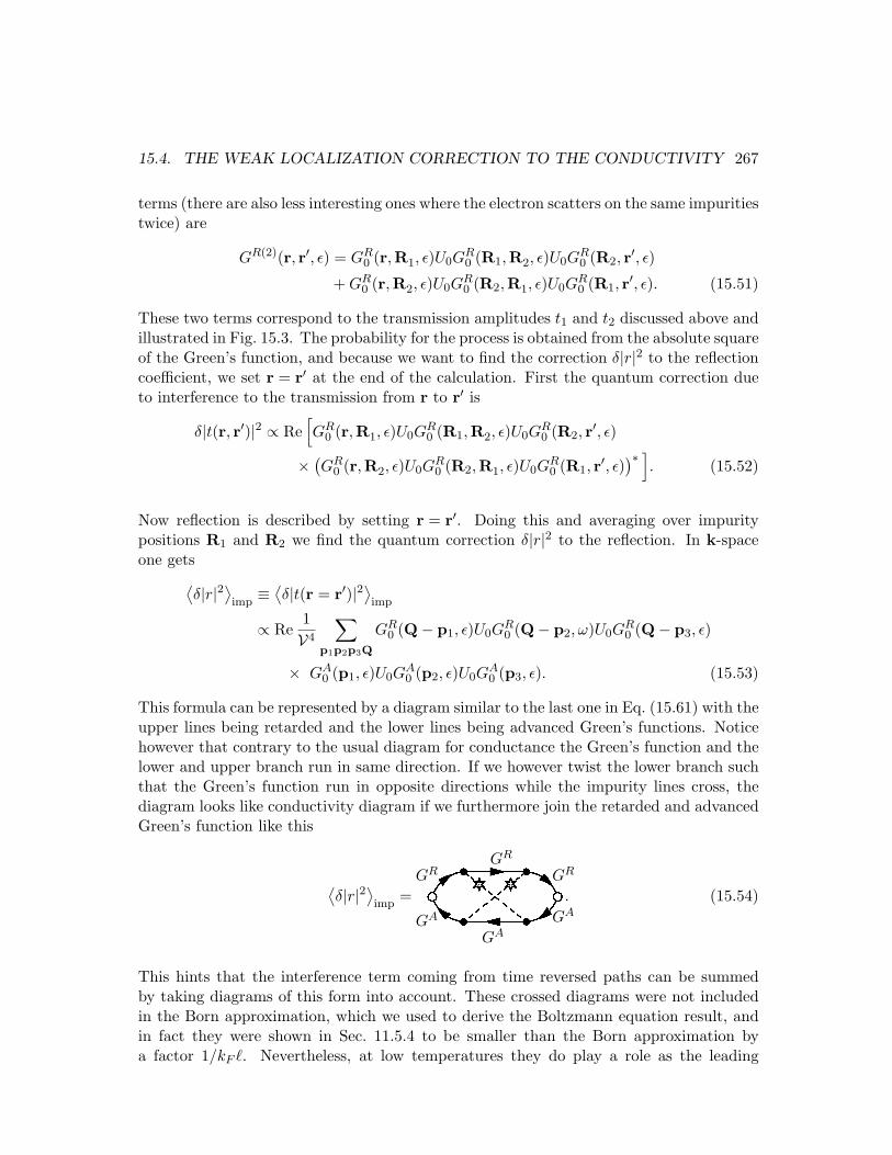
15.4. THE WEAK LOCALIZATION CORRECTION TO THE CONDUCTIVITY 267
terms (there are also less interesting ones where the electron scatters on the same impuritiestwice) are
GR(2)(r, r′, ε) = GR0 (r,R1, ε)U0G
R0 (R1,R2, ε)U0G
R0 (R2, r′, ε)
+ GR0 (r,R2, ε)U0G
R0 (R2,R1, ε)U0G
R0 (R1, r′, ε). (15.51)
These two terms correspond to the transmission amplitudes t1 and t2 discussed above andillustrated in Fig. 15.3. The probability for the process is obtained from the absolute squareof the Green’s function, and because we want to find the correction δ|r|2 to the reflectioncoefficient, we set r = r′ at the end of the calculation. First the quantum correction dueto interference to the transmission from r to r′ is
δ|t(r, r′)|2 ∝ Re[GR
0 (r,R1, ε)U0GR0 (R1,R2, ε)U0G
R0 (R2, r′, ε)
× (GR
0 (r,R2, ε)U0GR0 (R2,R1, ε)U0G
R0 (R1, r′, ε)
)∗ ]. (15.52)
Now reflection is described by setting r = r′. Doing this and averaging over impuritypositions R1 and R2 we find the quantum correction δ|r|2 to the reflection. In k-spaceone gets
⟨δ|r|2⟩
imp≡ ⟨
δ|t(r = r′)|2⟩imp
∝ Re1V4
∑
p1p2p3Q
GR0 (Q− p1, ε)U0G
R0 (Q− p2, ω)U0G
R0 (Q− p3, ε)
× GA0 (p1, ε)U0G
A0 (p2, ε)U0G
A0 (p3, ε). (15.53)
This formula can be represented by a diagram similar to the last one in Eq. (15.61) with theupper lines being retarded and the lower lines being advanced Green’s functions. Noticehowever that contrary to the usual diagram for conductance the Green’s function and thelower and upper branch run in same direction. If we however twist the lower branch suchthat the Green’s function run in opposite directions while the impurity lines cross, thediagram looks like conductivity diagram if we furthermore join the retarded and advancedGreen’s function like this
⟨δ|r|2⟩
imp=IGR
GR
GR
GA
GA
GA
. (15.54)
This hints that the interference term coming from time reversed paths can be summedby taking diagrams of this form into account. These crossed diagrams were not includedin the Born approximation, which we used to derive the Boltzmann equation result, andin fact they were shown in Sec. 11.5.4 to be smaller than the Born approximation bya factor 1/kF `. Nevertheless, at low temperatures they do play a role as the leading
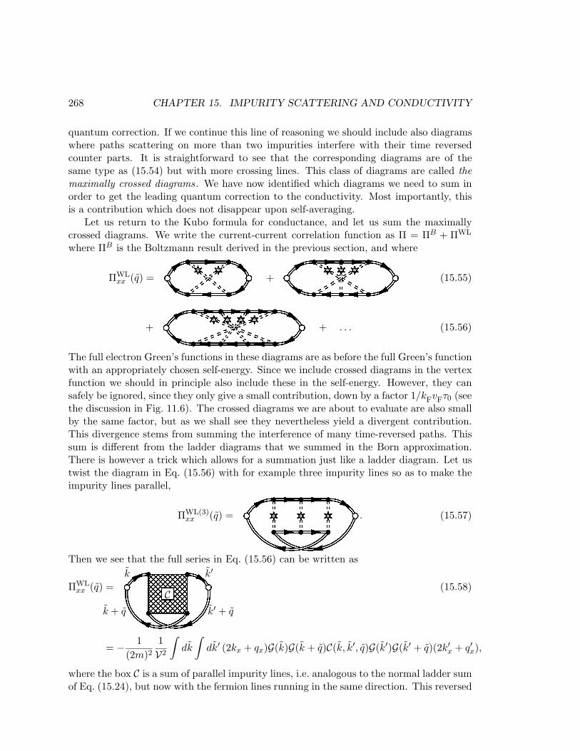
268 CHAPTER 15. IMPURITY SCATTERING AND CONDUCTIVITY
quantum correction. If we continue this line of reasoning we should include also diagramswhere paths scattering on more than two impurities interfere with their time reversedcounter parts. It is straightforward to see that the corresponding diagrams are of thesame type as (15.54) but with more crossing lines. This class of diagrams are called themaximally crossed diagrams. We have now identified which diagrams we need to sum inorder to get the leading quantum correction to the conductivity. Most importantly, thisis a contribution which does not disappear upon self-averaging.
Let us return to the Kubo formula for conductance, and let us sum the maximallycrossed diagrams. We write the current-current correlation function as Π = ΠB + ΠWL
where ΠB is the Boltzmann result derived in the previous section, and where
ΠWLxx (q) =J +K (15.55)
+L + . . . (15.56)
The full electron Green’s functions in these diagrams are as before the full Green’s functionwith an appropriately chosen self-energy. Since we include crossed diagrams in the vertexfunction we should in principle also include these in the self-energy. However, they cansafely be ignored, since they only give a small contribution, down by a factor 1/kFvFτ0 (seethe discussion in Fig. 11.6). The crossed diagrams we are about to evaluate are also smallby the same factor, but as we shall see they nevertheless yield a divergent contribution.This divergence stems from summing the interference of many time-reversed paths. Thissum is different from the ladder diagrams that we summed in the Born approximation.There is however a trick which allows for a summation just like a ladder diagram. Let ustwist the diagram in Eq. (15.56) with for example three impurity lines so as to make theimpurity lines parallel,
ΠWL(3)xx (q) =M . (15.57)
Then we see that the full series in Eq. (15.56) can be written as
ΠWLxx (q) =NC
k
k + q
k′
k′ + q
(15.58)
= − 1(2m)2
1V2
∫dk
∫dk′ (2kx + qx)G(k)G(k + q)C(k, k′, q)G(k′)G(k′ + q)(2k′x + q′x),
where the box C is a sum of parallel impurity lines, i.e. analogous to the normal ladder sumof Eq. (15.24), but now with the fermion lines running in the same direction. This reversed
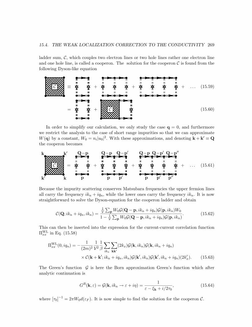
15.4. THE WEAK LOCALIZATION CORRECTION TO THE CONDUCTIVITY 269
ladder sum, C, which couples two electron lines or two hole lines rather one electron lineand one hole line, is called a cooperon. The solution for the cooperon C is found from thefollowing Dyson-like equation
OC ≡ P +Q +R + . . . (15.59)
= S +TC U (15.60)
In order to simplify our calculation, we only study the case q = 0, and furthermorewe restrict the analysis to the case of short range impurities so that we can approximateW (q) by a constant, W0 = ni|u0|2. With these approximations, and denoting k + k′ ≡ Qthe cooperon becomes
VCk k′
k′ k
= WQ−p
p
+XQ−p
p
Q−p′
p′
+YQ−p
p
Q−p′
p′
Q−p′′
p′′
+ . . . (15.61)
Because the impurity scattering conserves Matsubara frequencies the upper fermion linesall carry the frequency ikn + iqn, while the lower ones carry the frequency ikn. It is nowstraightforward to solve the Dyson-equation for the cooperon ladder and obtain
C(Q; ikn + iqn, ikn) =1V
∑p W0G(Q− p, ikn + iqn)G(p, ikn)W0
1− 1V
∑p W0G(Q− p, ikn + iqn)G(p, ikn)
. (15.62)
This can then be inserted into the expression for the current-current correlation functionΠWL
xx in Eq. (15.58)
ΠWLxx (0, iqn) = − 1
(2m)21V2
1β
∑
ikn
∑
kk′(2kx)G(k, ikn)G(k, ikn + iqn)
× C(k + k′; ikn + iqn, ikn)G(k′, ikn)G(k′, ikn + iqn)(2k′x). (15.63)
The Green’s function G is here the Born approximation Green’s function which afteranalytic continuation is
GR(k, ε) = G(k, ikn → ε + iη) =1
ε− ξk + i/2τ0, (15.64)
where [τ0]−1 = 2πW0d(εF ). It is now simple to find the solution for the cooperon C.
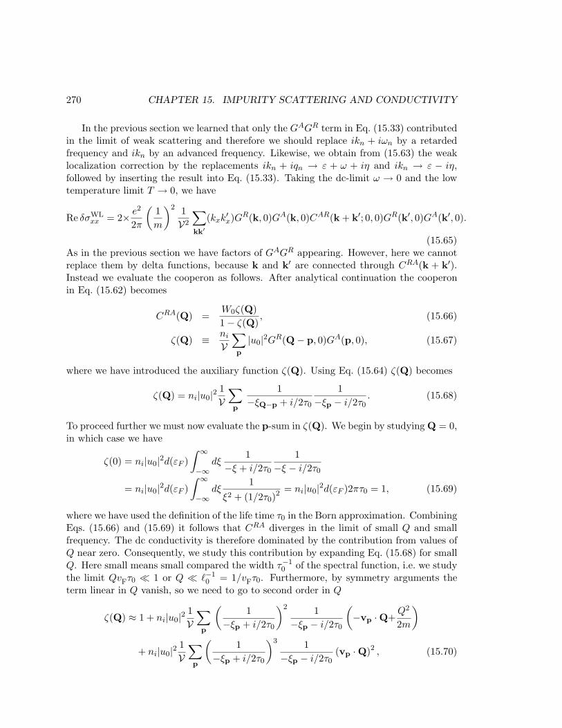
270 CHAPTER 15. IMPURITY SCATTERING AND CONDUCTIVITY
In the previous section we learned that only the GAGR term in Eq. (15.33) contributedin the limit of weak scattering and therefore we should replace ikn + iωn by a retardedfrequency and ikn by an advanced frequency. Likewise, we obtain from (15.63) the weaklocalization correction by the replacements ikn + iqn → ε + ω + iη and ikn → ε − iη,followed by inserting the result into Eq. (15.33). Taking the dc-limit ω → 0 and the lowtemperature limit T → 0, we have
Re δσWLxx = 2× e2
2π
(1m
)2 1V2
∑
kk′(kxk′x)GR(k, 0)GA(k, 0)CAR(k + k′; 0, 0)GR(k′, 0)GA(k′, 0).
(15.65)As in the previous section we have factors of GAGR appearing. However, here we cannotreplace them by delta functions, because k and k′ are connected through CRA(k + k′).Instead we evaluate the cooperon as follows. After analytical continuation the cooperonin Eq. (15.62) becomes
CRA(Q) =W0ζ(Q)1− ζ(Q)
, (15.66)
ζ(Q) ≡ ni
V∑p
|u0|2GR(Q− p, 0)GA(p, 0), (15.67)
where we have introduced the auxiliary function ζ(Q). Using Eq. (15.64) ζ(Q) becomes
ζ(Q) = ni|u0|2 1V
∑p
1−ξQ−p + i/2τ0
1−ξp − i/2τ0
. (15.68)
To proceed further we must now evaluate the p-sum in ζ(Q). We begin by studying Q = 0,in which case we have
ζ(0) = ni|u0|2d(εF )∫ ∞
−∞dξ
1−ξ + i/2τ0
1−ξ − i/2τ0
= ni|u0|2d(εF )∫ ∞
−∞dξ
1ξ2 + (1/2τ0)
2 = ni|u0|2d(εF )2πτ0 = 1, (15.69)
where we have used the definition of the life time τ0 in the Born approximation. CombiningEqs. (15.66) and (15.69) it follows that CRA diverges in the limit of small Q and smallfrequency. The dc conductivity is therefore dominated by the contribution from values ofQ near zero. Consequently, we study this contribution by expanding Eq. (15.68) for smallQ. Here small means small compared the width τ−1
0 of the spectral function, i.e. we studythe limit QvFτ0 ¿ 1 or Q ¿ `−1
0 = 1/vFτ0. Furthermore, by symmetry arguments theterm linear in Q vanish, so we need to go to second order in Q
ζ(Q) ≈ 1 + ni|u0|2 1V
∑p
(1
−ξp + i/2τ0
)2 1−ξp − i/2τ0
(−vp ·Q+
Q2
2m
)
+ ni|u0|2 1V
∑p
(1
−ξp + i/2τ0
)3 1−ξp − i/2τ0
(vp ·Q)2 , (15.70)
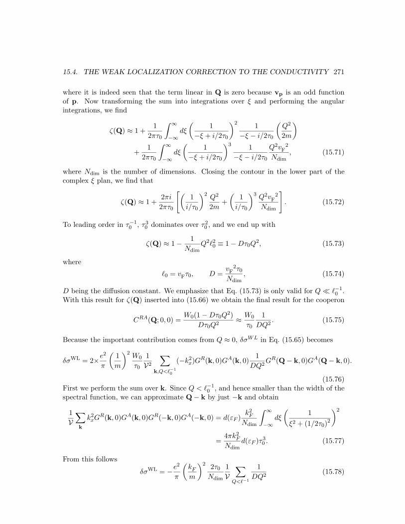
15.4. THE WEAK LOCALIZATION CORRECTION TO THE CONDUCTIVITY 271
where it is indeed seen that the term linear in Q is zero because vp is an odd functionof p. Now transforming the sum into integrations over ξ and performing the angularintegrations, we find
ζ(Q) ≈ 1 +1
2πτ0
∫ ∞
−∞dξ
(1
−ξ + i/2τ0
)2 1−ξ − i/2τ0
(Q2
2m
)
+1
2πτ0
∫ ∞
−∞dξ
(1
−ξ + i/2τ0
)3 1−ξ − i/2τ0
Q2vF2
Ndim, (15.71)
where Ndim is the number of dimensions. Closing the contour in the lower part of thecomplex ξ plan, we find that
ζ(Q) ≈ 1 +2πi
2πτ0
[(1
i/τ0
)2 Q2
2m+
(1
i/τ0
)3 Q2vF2
Ndim
]. (15.72)
To leading order in τ−10 , τ3
0 dominates over τ20 , and we end up with
ζ(Q) ≈ 1− 1Ndim
Q2`20 ≡ 1−Dτ0Q
2, (15.73)
where
`0 = vFτ0, D =vF
2τ0
Ndim, (15.74)
D being the diffusion constant. We emphasize that Eq. (15.73) is only valid for Q ¿ `−10 .
With this result for ζ(Q) inserted into (15.66) we obtain the final result for the cooperon
CRA(Q; 0, 0) =W0(1−Dτ0Q
2)Dτ0Q2
≈ W0
τ0
1DQ2
. (15.75)
Because the important contribution comes from Q ≈ 0, δσWL in Eq. (15.65) becomes
δσWL = 2×e2
π
(1m
)2 W0
τ0
1V2
∑
k,Q<`−10
(−k2x)GR(k, 0)GA(k, 0)
1DQ2
GR(Q− k, 0)GA(Q− k, 0).
(15.76)First we perform the sum over k. Since Q < `−1
0 , and hence smaller than the width of thespectral function, we can approximate Q− k by just −k and obtain
1V
∑
k
k2xGR(k, 0)GA(k, 0)GR(−k, 0)GA(−k, 0) = d(εF )
k2F
Ndim
∫ ∞
−∞dξ
(1
ξ2 + (1/2τ0)2
)2
=4πk2
F
Ndimd(εF )τ3
0 . (15.77)
From this follows
δσWL = −e2
π
(kF
m
)2 2τ0
Ndim
1V
∑
Q<`−1
1DQ2
(15.78)
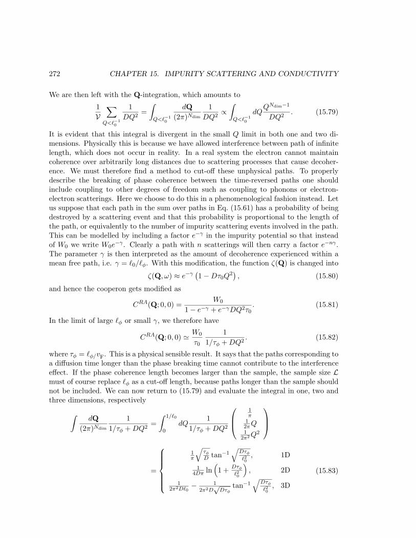
272 CHAPTER 15. IMPURITY SCATTERING AND CONDUCTIVITY
We are then left with the Q-integration, which amounts to
1V
∑
Q<`−10
1DQ2
=∫
Q<`−10
dQ(2π)Ndim
1DQ2
∝∫
Q<`−10
dQQNdim−1
DQ2. (15.79)
It is evident that this integral is divergent in the small Q limit in both one and two di-mensions. Physically this is because we have allowed interference between path of infinitelength, which does not occur in reality. In a real system the electron cannot maintaincoherence over arbitrarily long distances due to scattering processes that cause decoher-ence. We must therefore find a method to cut-off these unphysical paths. To properlydescribe the breaking of phase coherence between the time-reversed paths one shouldinclude coupling to other degrees of freedom such as coupling to phonons or electron-electron scatterings. Here we choose to do this in a phenomenological fashion instead. Letus suppose that each path in the sum over paths in Eq. (15.61) has a probability of beingdestroyed by a scattering event and that this probability is proportional to the length ofthe path, or equivalently to the number of impurity scattering events involved in the path.This can be modelled by including a factor e−γ in the impurity potential so that insteadof W0 we write W0e
−γ . Clearly a path with n scatterings will then carry a factor e−nγ .The parameter γ is then interpreted as the amount of decoherence experienced within amean free path, i.e. γ = `0/`φ. With this modification, the function ζ(Q) is changed into
ζ(Q, ω) ≈ e−γ(1−Dτ0Q
2), (15.80)
and hence the cooperon gets modified as
CRA(Q; 0, 0) =W0
1− e−γ + e−γDQ2τ0. (15.81)
In the limit of large `φ or small γ, we therefore have
CRA(Q; 0, 0) ' W0
τ0
11/τφ + DQ2
. (15.82)
where τφ = `φ/vF. This is a physical sensible result. It says that the paths corresponding toa diffusion time longer than the phase breaking time cannot contribute to the interferenceeffect. If the phase coherence length becomes larger than the sample, the sample size Lmust of course replace `φ as a cut-off length, because paths longer than the sample shouldnot be included. We can now return to (15.79) and evaluate the integral in one, two andthree dimensions, respectively
∫dQ
(2π)Ndim
11/τφ + DQ2
=∫ 1/`0
0dQ
11/τφ + DQ2
1π
12πQ1
2π2 Q2
=
1π
√τφ
D tan−1√
Dτφ
`20, 1D
14Dπ ln
(1 + Dτφ
`20
), 2D
12π2D`0
− 1
2π2D√
Dτφtan−1
√Dτφ
`20, 3D
(15.83)
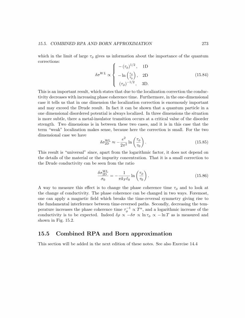
15.5. COMBINED RPA AND BORN APPROXIMATION 273
which in the limit of large τφ gives us information about the importance of the quantumcorrections:
δσWL ∝
− (τφ)1/2 , 1D
− ln(
τφ
τ0
), 2D
(τφ)−1/2 , 3D.
(15.84)
This is an important result, which states that due to the localization correction the conduc-tivity decreases with increasing phase coherence time. Furthermore, in the one-dimensionalcase it tells us that in one dimension the localization correction is enormously importantand may exceed the Drude result. In fact it can be shown that a quantum particle in aone dimensional disordered potential is always localized. In three dimensions the situationis more subtle, there a metal-insulator transition occurs at a critical value of the disorderstrength. Two dimensions is in between these two cases, and it is in this case that theterm “weak” localization makes sense, because here the correction is small. For the twodimensional case we have
δσWL2D ≈ − e2
2π2ln
(τφ
τ0
). (15.85)
This result is “universal” since, apart from the logarithmic factor, it does not depend onthe details of the material or the impurity concentration. That it is a small correction tothe Drude conductivity can be seen from the ratio
δσWL2D
σ0= − 1
πkF `0ln
(τφ
τ0
). (15.86)
A way to measure this effect is to change the phase coherence time τφ and to look atthe change of conductivity. The phase coherence can be changed in two ways. Foremost,one can apply a magnetic field which breaks the time-reversal symmetry giving rise tothe fundamental interference between time-reversed paths. Secondly, decreasing the tem-perature increases the phase coherence time τ−1
φ ∝ Tα, and a logarithmic increase of theconductivity is to be expected. Indeed δρ ∝ −δσ ∝ ln τφ ∝ − ln T as is measured andshown in Fig. 15.2.
15.5 Combined RPA and Born approximation
This section will be added in the next edition of these notes. See also Exercise 14.4

274 CHAPTER 15. IMPURITY SCATTERING AND CONDUCTIVITY
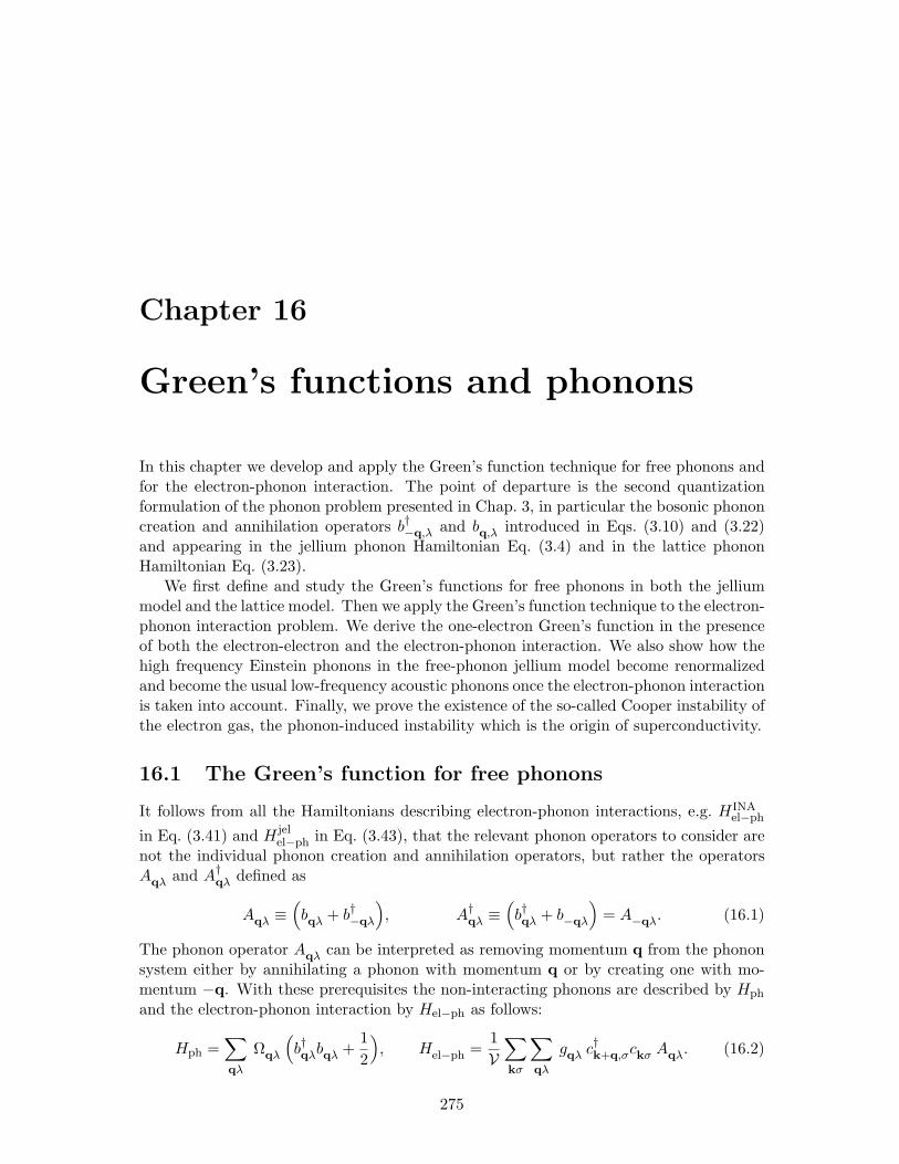
Chapter 16
Green’s functions and phonons
In this chapter we develop and apply the Green’s function technique for free phonons andfor the electron-phonon interaction. The point of departure is the second quantizationformulation of the phonon problem presented in Chap. 3, in particular the bosonic phononcreation and annihilation operators b†−q,λ and bq,λ introduced in Eqs. (3.10) and (3.22)and appearing in the jellium phonon Hamiltonian Eq. (3.4) and in the lattice phononHamiltonian Eq. (3.23).
We first define and study the Green’s functions for free phonons in both the jelliummodel and the lattice model. Then we apply the Green’s function technique to the electron-phonon interaction problem. We derive the one-electron Green’s function in the presenceof both the electron-electron and the electron-phonon interaction. We also show how thehigh frequency Einstein phonons in the free-phonon jellium model become renormalizedand become the usual low-frequency acoustic phonons once the electron-phonon interactionis taken into account. Finally, we prove the existence of the so-called Cooper instability ofthe electron gas, the phonon-induced instability which is the origin of superconductivity.
16.1 The Green’s function for free phonons
It follows from all the Hamiltonians describing electron-phonon interactions, e.g. HINAel−ph
in Eq. (3.41) and H jelel−ph in Eq. (3.43), that the relevant phonon operators to consider are
not the individual phonon creation and annihilation operators, but rather the operatorsAqλ and A†qλ defined as
Aqλ ≡(bqλ + b†−qλ
), A†qλ ≡
(b†qλ + b−qλ
)= A−qλ. (16.1)
The phonon operator Aqλ can be interpreted as removing momentum q from the phononsystem either by annihilating a phonon with momentum q or by creating one with mo-mentum −q. With these prerequisites the non-interacting phonons are described by Hph
and the electron-phonon interaction by Hel−ph as follows:
Hph =∑
qλ
Ωqλ
(b†qλbqλ +
12
), Hel−ph =
1V
∑
kσ
∑
qλ
gqλ c†k+q,σckσ Aqλ. (16.2)
275
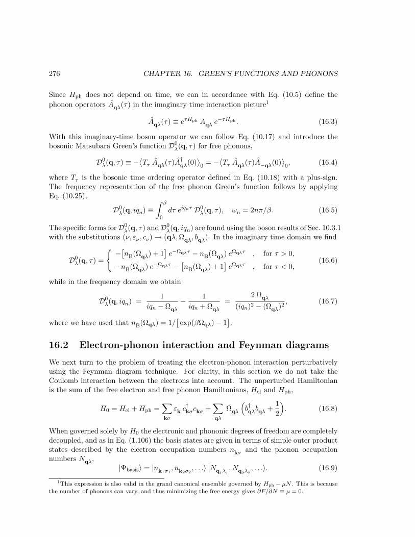
276 CHAPTER 16. GREEN’S FUNCTIONS AND PHONONS
Since Hph does not depend on time, we can in accordance with Eq. (10.5) define thephonon operators Aqλ(τ) in the imaginary time interaction picture1
Aqλ(τ) ≡ eτHph Aqλ e−τHph . (16.3)
With this imaginary-time boson operator we can follow Eq. (10.17) and introduce thebosonic Matsubara Green’s function D0
λ(q, τ) for free phonons,
D0λ(q, τ) ≡ −⟨
Tτ Aqλ(τ)A†qλ(0)⟩0
= −⟨Tτ Aqλ(τ)A−qλ(0)
⟩0, (16.4)
where Tτ is the bosonic time ordering operator defined in Eq. (10.18) with a plus-sign.The frequency representation of the free phonon Green’s function follows by applyingEq. (10.25),
D0λ(q, iqn) ≡
∫ β
0dτ eiqnτ D0
λ(q, τ), ωn = 2nπ/β. (16.5)
The specific forms forD0λ(q, τ) andD0
λ(q, iqn) are found using the boson results of Sec. 10.3.1with the substitutions (ν, εν , cν) → (qλ,Ωqλ, bqλ). In the imaginary time domain we find
D0λ(q, τ) =
−[nB(Ωqλ) + 1
]e−Ωqλτ − nB(Ωqλ) eΩqλτ , for τ > 0,
−nB(Ωqλ) e−Ωqλτ − [nB(Ωqλ) + 1
]eΩqλτ , for τ < 0,
(16.6)
while in the frequency domain we obtain
D0λ(q, iqn) =
1iqn − Ωqλ
− 1iqn + Ωqλ
=2 Ωqλ
(iqn)2 − (Ωqλ)2, (16.7)
where we have used that nB(Ωqλ) = 1/[exp(βΩqλ)− 1
].
16.2 Electron-phonon interaction and Feynman diagrams
We next turn to the problem of treating the electron-phonon interaction perturbativelyusing the Feynman diagram technique. For clarity, in this section we do not take theCoulomb interaction between the electrons into account. The unperturbed Hamiltonianis the sum of the free electron and free phonon Hamiltonians, Hel and Hph,
H0 = Hel + Hph =∑
kσ
εk c†kσckσ +∑
qλ
Ωqλ
(b†qλbqλ +
12
). (16.8)
When governed solely by H0 the electronic and phononic degrees of freedom are completelydecoupled, and as in Eq. (1.106) the basis states are given in terms of simple outer productstates described by the electron occupation numbers nkσ and the phonon occupationnumbers Nqλ,
|Ψbasis〉 = |nk1σ1, nk2σ2
, . . .〉 |Nq1λ1, Nq2λ2
, . . .〉. (16.9)
1This expression is also valid in the grand canonical ensemble governed by Hph − µN . This is becausethe number of phonons can vary, and thus minimizing the free energy gives ∂F/∂N ≡ µ = 0.
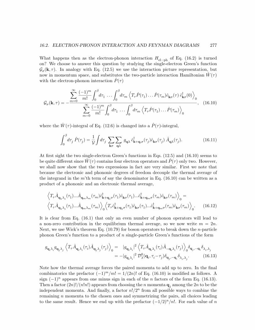
16.2. ELECTRON-PHONON INTERACTION AND FEYNMAN DIAGRAMS 277
What happens then as the electron-phonon interaction Hel−ph of Eq. (16.2) is turnedon? We choose to answer this question by studying the single-electron Green’s functionGσ(k, τ). In analogy with Eq. (12.5) we use the interaction picture representation, butnow in momentum space, and substitutes the two-particle interaction Hamiltonian W (τ)with the electron-phonon interaction P (τ)
Gσ(k, τ) = −
∞∑
m=0
(−1)m
m!
∫ β
0dτ1 . . .
∫ β
0dτm
⟨Tτ P (τ1) . . . P (τm)ckσ(τ) c†kσ(0)
⟩0
∞∑
m=0
(−1)m
m!
∫ β
0dτ1 . . .
∫ β
0dτm
⟨Tτ P (τ1) . . . P (τm)
⟩0
, (16.10)
where the W (τ)-integral of Eq. (12.6) is changed into a P (τ)-integral,
∫ β
0dτj P (τj) =
1V
∫dτj
∑
kσ
∑
qλ
gqλ c†k+q,σ(τj)ckσ(τj) Aqλ(τj). (16.11)
At first sight the two single-electron Green’s functions in Eqs. (12.5) and (16.10) seems tobe quite different since W (τ) contains four electron operators and P (τ) only two. However,we shall now show that the two expressions in fact are very similar. First we note thatbecause the electronic and phononic degrees of freedom decouple the thermal average ofthe integrand in the m’th term of say the denominator in Eq. (16.10) can be written as aproduct of a phononic and an electronic thermal average,
⟨Tτ Aq1λ1
(τ1)...Aqmλm(τm)c†k+q1σ(τ1)ckσ(τ1)...c
†k+qmσ(τm)ckσ(τm)
⟩0
=⟨Tτ Aq1λ1
(τ1)...Aqmλm(τm)
⟩0
⟨Tτ c
†k+q1σ(τ1)ckσ(τ1)...c
†k+qmσ(τm)ckσ(τm)
⟩0. (16.12)
It is clear from Eq. (16.1) that only an even number of phonon operators will lead toa non-zero contribution in the equilibrium thermal average, so we now write m = 2n.Next, we use Wick’s theorem Eq. (10.79) for boson operators to break down the n-particlephonon Green’s function to a product of n single-particle Green’s functions of the form
gqiλigqjλj
⟨Tτ Aqiλi
(τi)Aqjλj(τj)
⟩0
= |gqiλi|2
⟨Tτ Aqiλi
(τi)A−qiλi(τj)
⟩0δqj ,−qi
δλi,λj
= −|gqiλi|2 D0
λ(qi, τi−τj)δqj ,−qiδλi,λj
. (16.13)
Note how the thermal average forces the paired momenta to add up to zero. In the finalcombinatorics the prefactor (−1)m/m! = 1/(2n)! of Eq. (16.10) is modified as follows. Asign (−1)n appears from one minus sign in each of the n factors of the form Eq. (16.13).Then a factor (2n)!/(n!n!) appears from choosing the n momenta qj among the 2n to be theindependent momenta. And finally, a factor n!/2n from all possible ways to combine theremaining n momenta to the chosen ones and symmetrizing the pairs, all choices leadingto the same result. Hence we end up with the prefactor (−1/2)n/n!. For each value of n
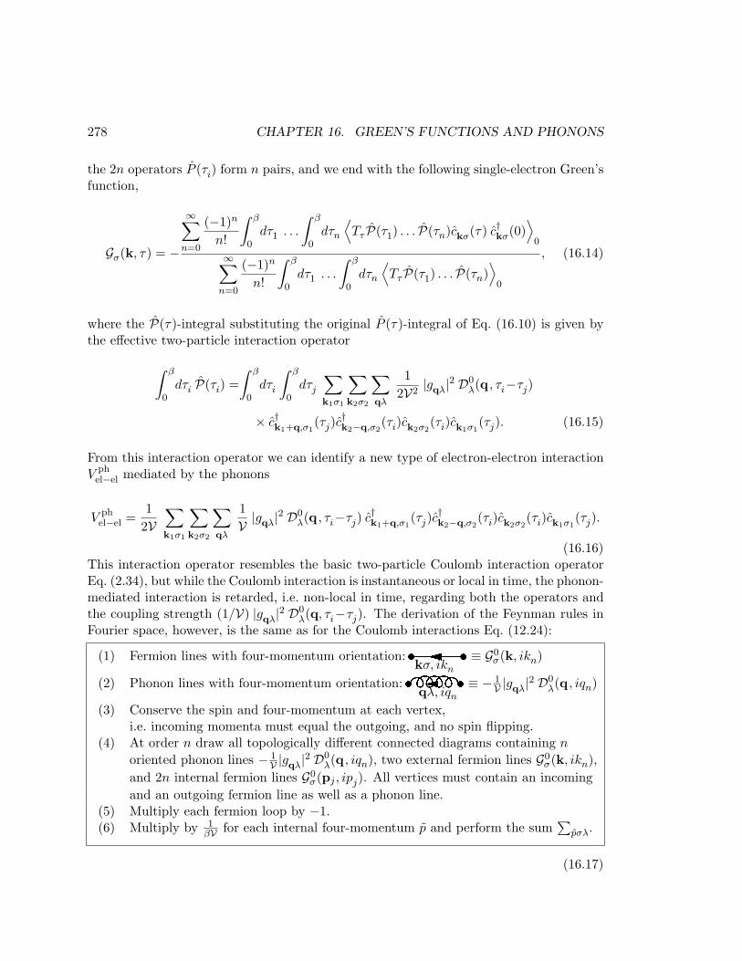
278 CHAPTER 16. GREEN’S FUNCTIONS AND PHONONS
the 2n operators P (τi) form n pairs, and we end with the following single-electron Green’sfunction,
Gσ(k, τ) = −
∞∑
n=0
(−1)n
n!
∫ β
0dτ1 . . .
∫ β
0dτn
⟨Tτ P(τ1) . . . P(τn)ckσ(τ) c†kσ(0)
⟩0
∞∑
n=0
(−1)n
n!
∫ β
0dτ1 . . .
∫ β
0dτn
⟨Tτ P(τ1) . . . P(τn)
⟩0
, (16.14)
where the P(τ)-integral substituting the original P (τ)-integral of Eq. (16.10) is given bythe effective two-particle interaction operator
∫ β
0dτi P(τi) =
∫ β
0dτi
∫ β
0dτj
∑
k1σ1
∑
k2σ2
∑
qλ
12V2
|gqλ|2 D0λ(q , τi−τj)
× c†k1+q,σ1(τj)c
†k2−q,σ2
(τi)ck2σ2(τi)ck1σ1
(τj). (16.15)
From this interaction operator we can identify a new type of electron-electron interactionV ph
el−el mediated by the phonons
V phel−el =
12V
∑
k1σ1
∑
k2σ2
∑
qλ
1V |gqλ|2 D0
λ(q , τi−τj) c†k1+q,σ1(τj)c
†k2−q,σ2
(τi)ck2σ2(τi)ck1σ1
(τj).
(16.16)This interaction operator resembles the basic two-particle Coulomb interaction operatorEq. (2.34), but while the Coulomb interaction is instantaneous or local in time, the phonon-mediated interaction is retarded, i.e. non-local in time, regarding both the operators andthe coupling strength (1/V) |gqλ|2 D0
λ(q, τi−τj). The derivation of the Feynman rules inFourier space, however, is the same as for the Coulomb interactions Eq. (12.24):
(1) Fermion lines with four-momentum orientation:kσ, ikn≡ G0
σ(k, ikn)
(2) Phonon lines with four-momentum orientation:qλ, iqn≡ − 1
V |gqλ|2 D0λ(q , iqn)
(3) Conserve the spin and four-momentum at each vertex,i.e. incoming momenta must equal the outgoing, and no spin flipping.
(4) At order n draw all topologically different connected diagrams containing n
oriented phonon lines − 1V |gqλ|2 D0
λ(q , iqn), two external fermion lines G0σ(k, ikn),
and 2n internal fermion lines G0σ(pj , ipj). All vertices must contain an incoming
and an outgoing fermion line as well as a phonon line.(5) Multiply each fermion loop by −1.(6) Multiply by 1
βV for each internal four-momentum p and perform the sum∑
pσλ.
(16.17)

16.3. COMBINING COULOMB AND ELECTRON-PHONON INTERACTIONS 279
16.3 Combining Coulomb and electron-phonon interactions
We now discuss the effect of the long range Coulomb interactions between electrons andions and between electrons themselves. For simplicity we henceforth study only longitu-dinal phonons and hence drop all reference to the polarization index λ. In Fig. 3.1 wehave already sketched the ion plasma oscillation that occurs, if we consider the interactionbetween the ions and the electron gas assuming the latter to be homogeneous and com-pletely inert, i.e. disregarding all the dynamics of the electrons. A complete calculation israther tedious, but in Sec. 3.1 we studied the ion plasma oscillations in the jellium modelneglecting the electron dynamics. In the case of an ion density ρ0
ion = N/V we found thedispersion-less jellium phonon modes in the long wave length limit,
Ωq = Ω =
√Z2e2N
ε0MV . (16.18)
The coupling constant for the electron-electron interaction mediated by these jelliumphonons is found by combining Eqs. (3.44) and (16.18),
1V |gq|2 =
1V
(Ze2
qε0
)2 N~2MΩ
=e2
ε0q2
~Ω2
=12
W (q) Ω, (16.19)
which not surprisingly is proportional to the Coulomb interaction W (q). Note that we havedropped ~ in the last equality in accordance with the convention introduced in Sec. 5.1.The resulting, bare, phonon-mediated electron-electron interaction is
1V |gq|2 D0(q, iqn) = W (q)
Ω2
(iqn)2 − Ω2. (16.20)
To discuss the role of the electron dynamics we now add the electron-electron Coulombinteraction Vel−el of Eq. (2.34) and study the full Hamiltonian H for the electronic andphononic system,
H = Hel + Vel−el + Hph + Hel−ph. (16.21)
16.3.1 Migdal’s theorem
When the electron-phonon coupling Hel−ph is added, the question naturally arises ofwhether to study the influence of the electrons on the ions before that of the ions onthe electrons, or vice versa. The answer is provided by Migdal’s theorem. This theoremis the condensed matter physics analogue to the well-known Born-Oppenheimer approxi-mation of molecular physics. The latter states that it is a good approximation to considerthe coordinates Ri of the slowly moving, heavy ions as parameters in the Schrodingerequation for the fast moving, light electrons, which is then solved. In the second stage thevalues of Ri are then changed adiabatically. Likewise, it can be proven by phase spacearguments that renormalization of the electron-phonon vertex is suppressed at least by a
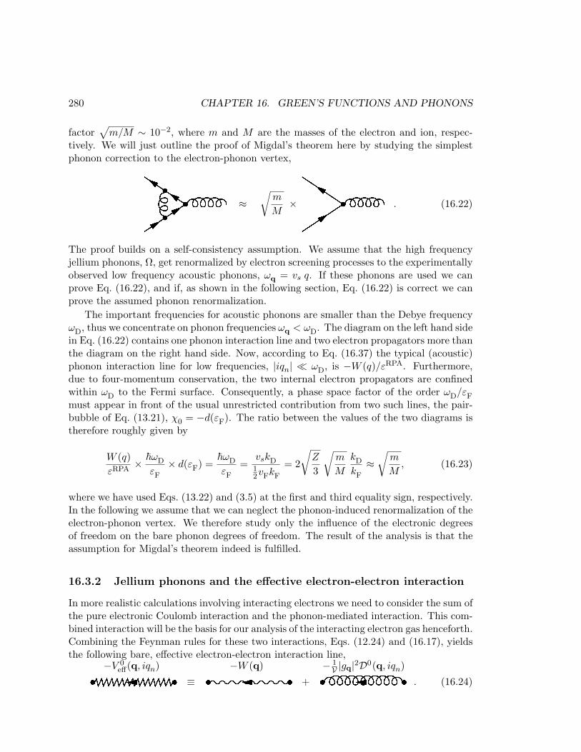
280 CHAPTER 16. GREEN’S FUNCTIONS AND PHONONS
factor√
m/M ∼ 10−2, where m and M are the masses of the electron and ion, respec-tively. We will just outline the proof of Migdal’s theorem here by studying the simplestphonon correction to the electron-phonon vertex,
≈√
m
M× . (16.22)
The proof builds on a self-consistency assumption. We assume that the high frequencyjellium phonons, Ω, get renormalized by electron screening processes to the experimentallyobserved low frequency acoustic phonons, ωq = vs q. If these phonons are used we canprove Eq. (16.22), and if, as shown in the following section, Eq. (16.22) is correct we canprove the assumed phonon renormalization.
The important frequencies for acoustic phonons are smaller than the Debye frequencyωD, thus we concentrate on phonon frequencies ωq < ωD. The diagram on the left hand sidein Eq. (16.22) contains one phonon interaction line and two electron propagators more thanthe diagram on the right hand side. Now, according to Eq. (16.37) the typical (acoustic)phonon interaction line for low frequencies, |iqn| ¿ ωD, is −W (q)/εRPA. Furthermore,due to four-momentum conservation, the two internal electron propagators are confinedwithin ωD to the Fermi surface. Consequently, a phase space factor of the order ωD/εF
must appear in front of the usual unrestricted contribution from two such lines, the pair-bubble of Eq. (13.21), χ0 = −d(εF). The ratio between the values of the two diagrams istherefore roughly given by
W (q)εRPA
× ~ωD
εF
× d(εF) =~ωD
εF
=vskD12vFkF
= 2
√Z
3
√m
M
kD
kF
≈√
m
M, (16.23)
where we have used Eqs. (13.22) and (3.5) at the first and third equality sign, respectively.In the following we assume that we can neglect the phonon-induced renormalization of theelectron-phonon vertex. We therefore study only the influence of the electronic degreesof freedom on the bare phonon degrees of freedom. The result of the analysis is that theassumption for Migdal’s theorem indeed is fulfilled.
16.3.2 Jellium phonons and the effective electron-electron interaction
In more realistic calculations involving interacting electrons we need to consider the sum ofthe pure electronic Coulomb interaction and the phonon-mediated interaction. This com-bined interaction will be the basis for our analysis of the interacting electron gas henceforth.Combining the Feynman rules for these two interactions, Eqs. (12.24) and (16.17), yieldsthe following bare, effective electron-electron interaction line,
−V 0eff(q, iqn)
≡−W (q)
+− 1V |gq|2D0(q, iqn)
. (16.24)
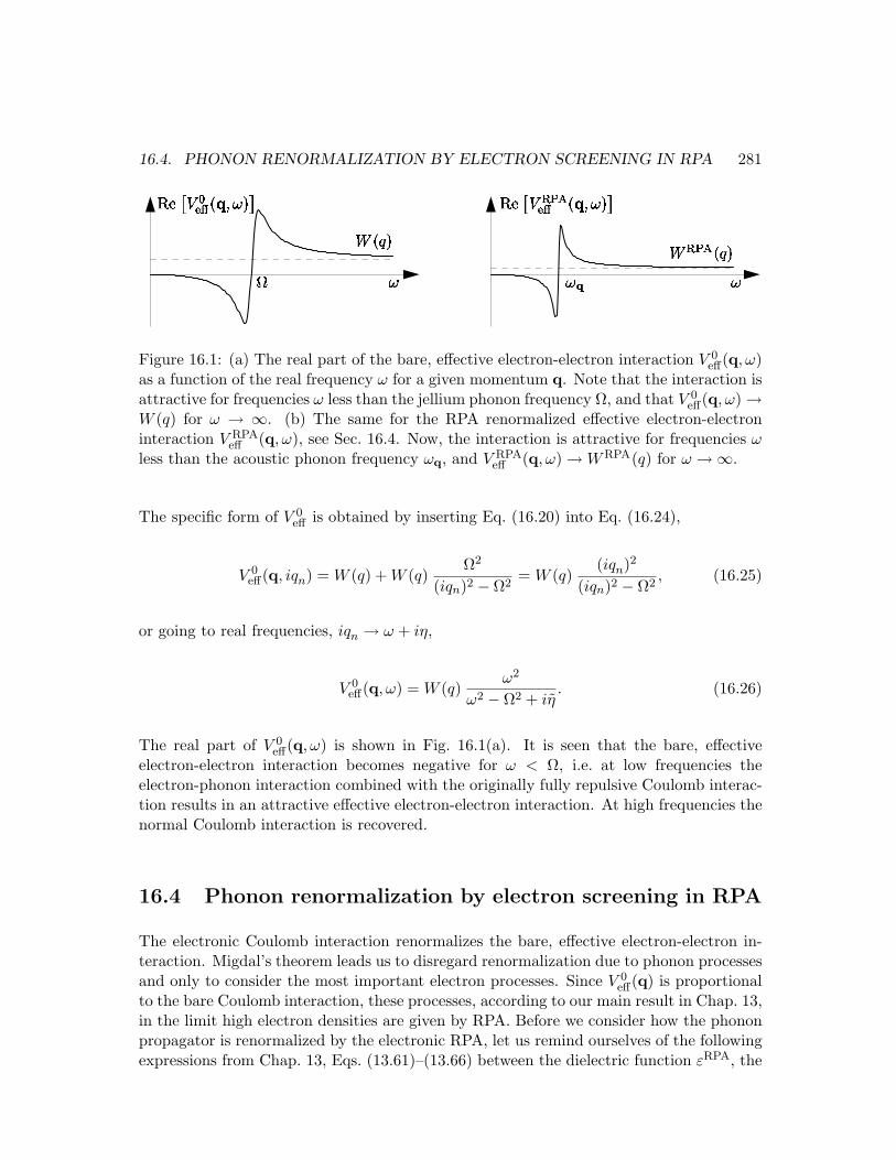
16.4. PHONON RENORMALIZATION BY ELECTRON SCREENING IN RPA 281
Figure 16.1: (a) The real part of the bare, effective electron-electron interaction V 0eff(q, ω)
as a function of the real frequency ω for a given momentum q. Note that the interaction isattractive for frequencies ω less than the jellium phonon frequency Ω, and that V 0
eff(q, ω) →W (q) for ω → ∞. (b) The same for the RPA renormalized effective electron-electroninteraction V RPA
eff (q, ω), see Sec. 16.4. Now, the interaction is attractive for frequencies ωless than the acoustic phonon frequency ωq, and V RPA
eff (q, ω) → WRPA(q) for ω →∞.
The specific form of V 0eff is obtained by inserting Eq. (16.20) into Eq. (16.24),
V 0eff(q, iqn) = W (q) + W (q)
Ω2
(iqn)2 − Ω2= W (q)
(iqn)2
(iqn)2 − Ω2, (16.25)
or going to real frequencies, iqn → ω + iη,
V 0eff(q, ω) = W (q)
ω2
ω2 − Ω2 + iη. (16.26)
The real part of V 0eff(q, ω) is shown in Fig. 16.1(a). It is seen that the bare, effective
electron-electron interaction becomes negative for ω < Ω, i.e. at low frequencies theelectron-phonon interaction combined with the originally fully repulsive Coulomb interac-tion results in an attractive effective electron-electron interaction. At high frequencies thenormal Coulomb interaction is recovered.
16.4 Phonon renormalization by electron screening in RPA
The electronic Coulomb interaction renormalizes the bare, effective electron-electron in-teraction. Migdal’s theorem leads us to disregard renormalization due to phonon processesand only to consider the most important electron processes. Since V 0
eff(q) is proportionalto the bare Coulomb interaction, these processes, according to our main result in Chap. 13,in the limit high electron densities are given by RPA. Before we consider how the phononpropagator is renormalized by the electronic RPA, let us remind ourselves of the followingexpressions from Chap. 13, Eqs. (13.61)–(13.66) between the dielectric function εRPA, the
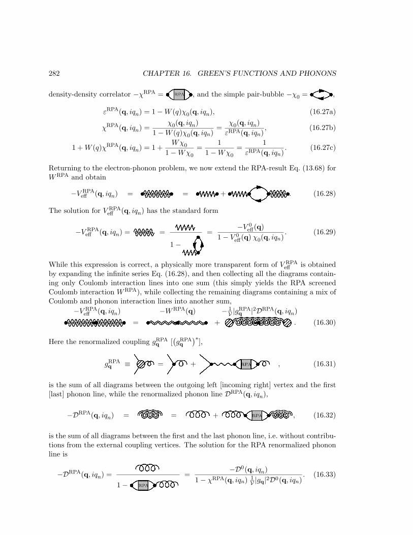
282 CHAPTER 16. GREEN’S FUNCTIONS AND PHONONS
density-density correlator −χRPA =RPA , and the simple pair-bubble −χ0 = ,
εRPA(q, iqn) = 1−W (q)χ0(q, iqn), (16.27a)
χRPA(q, iqn) =χ0(q, iqn)
1−W (q)χ0(q, iqn)=
χ0(q, iqn)εRPA(q, iqn)
, (16.27b)
1 + W (q)χRPA(q, iqn) = 1 +Wχ0
1−Wχ0
=1
1−Wχ0
=1
εRPA(q, iqn). (16.27c)
Returning to the electron-phonon problem, we now extend the RPA-result Eq. (13.68) forWRPA and obtain
−V RPAeff (q, iqn) = = + . (16.28)
The solution for V RPAeff (q, iqn) has the standard form
−V RPAeff (q, iqn) = =
1− =−V 0
eff(q)1− V 0
eff(q) χ0(q, iqn). (16.29)
While this expression is correct, a physically more transparent form of V RPAeff is obtained
by expanding the infinite series Eq. (16.28), and then collecting all the diagrams contain-ing only Coulomb interaction lines into one sum (this simply yields the RPA screenedCoulomb interaction WRPA), while collecting the remaining diagrams containing a mix ofCoulomb and phonon interaction lines into another sum,
−V RPAeff (q, iqn)
=−WRPA(q)
+− 1V |gRPA
q |2DRPA(q, iqn)
. (16.30)
Here the renormalized coupling gRPAq [
(gRPAq
)∗],
gRPAq ≡ = +RPA , (16.31)
is the sum of all diagrams between the outgoing left [incoming right] vertex and the first[last] phonon line, while the renormalized phonon line DRPA(q, iqn),
−DRPA(q, iqn) = = +RPA , (16.32)
is the sum of all diagrams between the first and the last phonon line, i.e. without contribu-tions from the external coupling vertices. The solution for the RPA renormalized phononline is
−DRPA(q, iqn) = 1−RPA
=−D0(q, iqn)
1− χRPA(q, iqn) 1V |gq|2D0(q, iqn)
. (16.33)
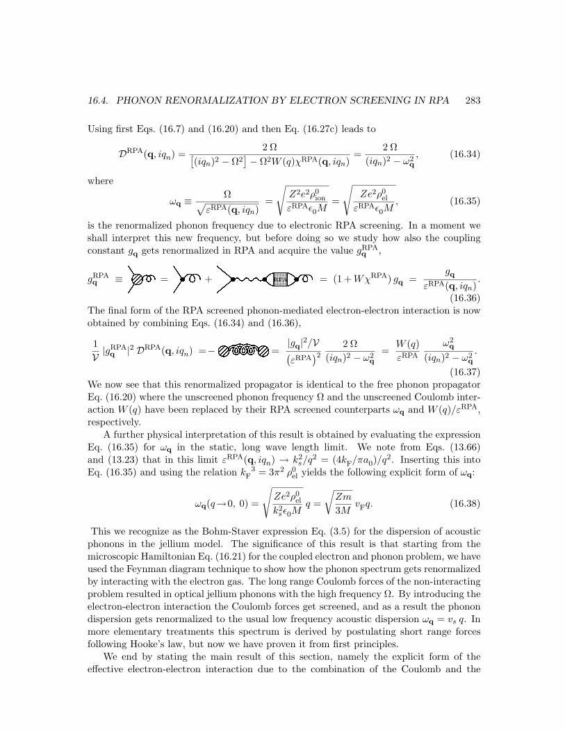
16.4. PHONON RENORMALIZATION BY ELECTRON SCREENING IN RPA 283
Using first Eqs. (16.7) and (16.20) and then Eq. (16.27c) leads to
DRPA(q, iqn) =2 Ω[
(iqn)2 − Ω2]− Ω2W (q)χRPA(q, iqn)
=2 Ω
(iqn)2 − ω2q
, (16.34)
where
ωq ≡ Ω√εRPA(q, iqn)
=
√Z2e2ρ0
ion
εRPAε0M=
√Ze2ρ0
el
εRPAε0M, (16.35)
is the renormalized phonon frequency due to electronic RPA screening. In a moment weshall interpret this new frequency, but before doing so we study how also the couplingconstant gq gets renormalized in RPA and acquire the value gRPA
q ,
gRPAq ≡ = +RPA = (1 + WχRPA) gq =
gq
εRPA(q, iqn).
(16.36)The final form of the RPA screened phonon-mediated electron-electron interaction is nowobtained by combining Eqs. (16.34) and (16.36),
1V |g
RPAq |2 DRPA(q, iqn) =− =
|gq|2/V(εRPA
)2
2 Ω(iqn)2 − ω2
q
=W (q)εRPA
ω2q
(iqn)2 − ω2q
.
(16.37)We now see that this renormalized propagator is identical to the free phonon propagatorEq. (16.20) where the unscreened phonon frequency Ω and the unscreened Coulomb inter-action W (q) have been replaced by their RPA screened counterparts ωq and W (q)/εRPA,respectively.
A further physical interpretation of this result is obtained by evaluating the expressionEq. (16.35) for ωq in the static, long wave length limit. We note from Eqs. (13.66)and (13.23) that in this limit εRPA(q, iqn) → k2
s/q2 = (4kF/πa0)/q2. Inserting this intoEq. (16.35) and using the relation kF
3 = 3π2 ρ0el yields the following explicit form of ωq:
ωq(q→0, 0) =
√Ze2ρ0
el
k2sε0M
q =
√Zm
3MvFq. (16.38)
This we recognize as the Bohm-Staver expression Eq. (3.5) for the dispersion of acousticphonons in the jellium model. The significance of this result is that starting from themicroscopic Hamiltonian Eq. (16.21) for the coupled electron and phonon problem, we haveused the Feynman diagram technique to show how the phonon spectrum gets renormalizedby interacting with the electron gas. The long range Coulomb forces of the non-interactingproblem resulted in optical jellium phonons with the high frequency Ω. By introducing theelectron-electron interaction the Coulomb forces get screened, and as a result the phonondispersion gets renormalized to the usual low frequency acoustic dispersion ωq = vs q. Inmore elementary treatments this spectrum is derived by postulating short range forcesfollowing Hooke’s law, but now we have proven it from first principles.
We end by stating the main result of this section, namely the explicit form of theeffective electron-electron interaction due to the combination of the Coulomb and the
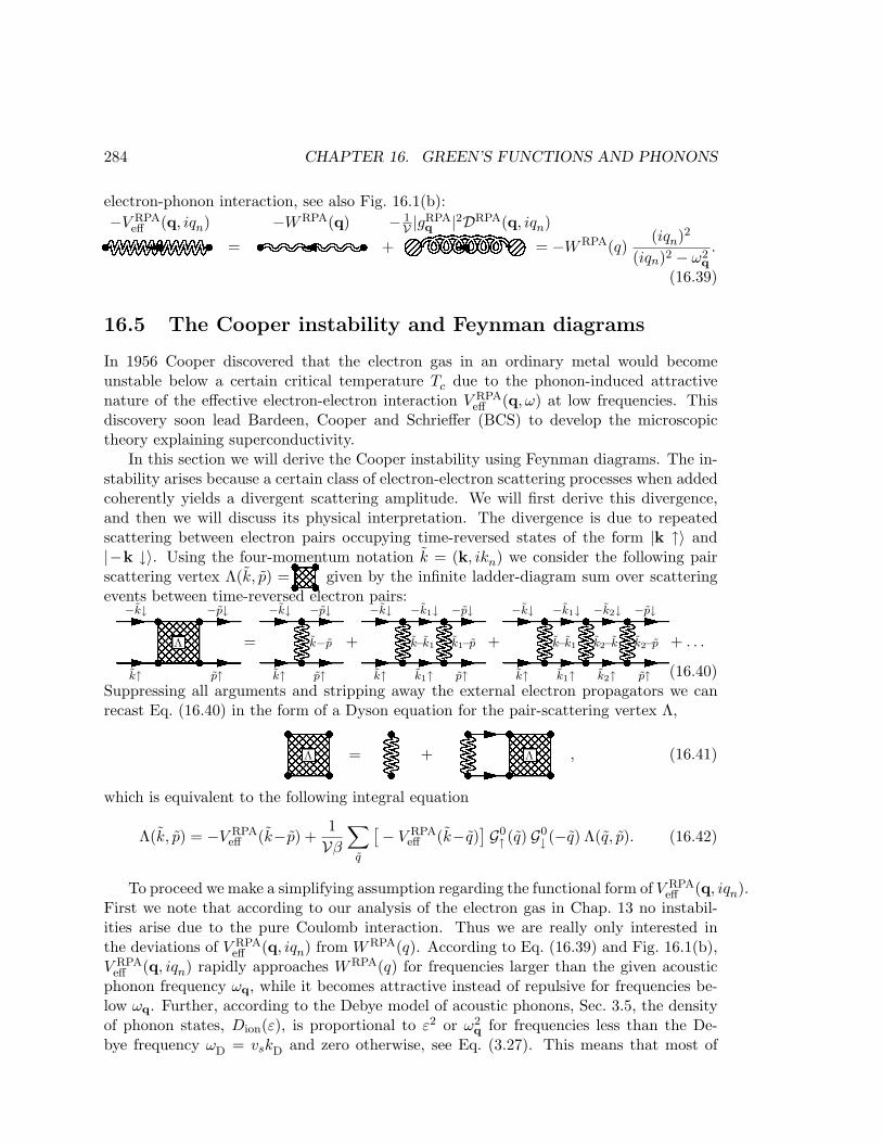
284 CHAPTER 16. GREEN’S FUNCTIONS AND PHONONS
electron-phonon interaction, see also Fig. 16.1(b):
−V RPAeff (q, iqn)
= −WRPA(q)
+!− 1V |gRPA
q |2DRPA(q, iqn)
= −WRPA(q)(iqn)2
(iqn)2 − ω2q
.
(16.39)
16.5 The Cooper instability and Feynman diagrams
In 1956 Cooper discovered that the electron gas in an ordinary metal would becomeunstable below a certain critical temperature Tc due to the phonon-induced attractivenature of the effective electron-electron interaction V RPA
eff (q, ω) at low frequencies. Thisdiscovery soon lead Bardeen, Cooper and Schrieffer (BCS) to develop the microscopictheory explaining superconductivity.
In this section we will derive the Cooper instability using Feynman diagrams. The in-stability arises because a certain class of electron-electron scattering processes when addedcoherently yields a divergent scattering amplitude. We will first derive this divergence,and then we will discuss its physical interpretation. The divergence is due to repeatedscattering between electron pairs occupying time-reversed states of the form |k ↑〉 and|−k ↓〉. Using the four-momentum notation k = (k, ikn) we consider the following pairscattering vertex Λ(k, p) =" given by the infinite ladder-diagram sum over scatteringevents between time-reversed electron pairs:
#−k↓ −p↓
k↑ p↑
Λ =$−k↓ −p↓
k↑ p↑
k−p +%−k↓ −k1↓ −p↓
k↑ k1↑ p↑
k−k1 k1−p +&−k↓ −k1↓ −k2↓ −p↓
k↑ k1↑ k2↑ p↑
k−k1 k2−k1 k2−p + . . .
(16.40)Suppressing all arguments and stripping away the external electron propagators we canrecast Eq. (16.40) in the form of a Dyson equation for the pair-scattering vertex Λ,
'Λ = ( + )Λ , (16.41)
which is equivalent to the following integral equation
Λ(k, p) = −V RPAeff (k−p) +
1Vβ
∑
q
[− V RPAeff (k−q)
] G0↑ (q) G0
↓ (−q) Λ(q, p). (16.42)
To proceed we make a simplifying assumption regarding the functional form of V RPAeff (q, iqn).
First we note that according to our analysis of the electron gas in Chap. 13 no instabil-ities arise due to the pure Coulomb interaction. Thus we are really only interested inthe deviations of V RPA
eff (q, iqn) from WRPA(q). According to Eq. (16.39) and Fig. 16.1(b),V RPA
eff (q, iqn) rapidly approaches WRPA(q) for frequencies larger than the given acousticphonon frequency ωq, while it becomes attractive instead of repulsive for frequencies be-low ωq. Further, according to the Debye model of acoustic phonons, Sec. 3.5, the densityof phonon states, Dion(ε), is proportional to ε2 or ω2
q for frequencies less than the De-bye frequency ωD = vskD and zero otherwise, see Eq. (3.27). This means that most of
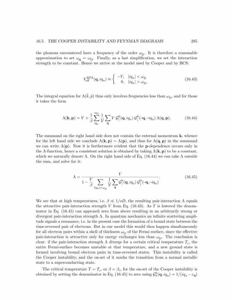
16.5. THE COOPER INSTABILITY AND FEYNMAN DIAGRAMS 285
the phonons encountered have a frequency of the order ωD. It is therefore a reasonableapproximation to set ωq = ωD. Finally, as a last simplification, we set the interactionstrength to be constant. Hence we arrive at the model used by Cooper and by BCS:
V RPAeff (q, iqn) ≈
−V, |iqn| < ωD
0, |iqn| > ωD.(16.43)
The integral equation for Λ(k, p) thus only involves frequencies less than ωD, and for thoseit takes the form
Λ(k,p) = V +1β
ωD∑
iqn
1V
∑q
V G0↑ (q, iqn) G0
↓ (−q,−iqn) Λ(q,p). (16.44)
The summand on the right hand side does not contain the external momentum k, whencefor the left hand side we conclude Λ(k,p) = Λ(p), and thus for Λ(q,p) in the summandwe can write Λ(p). Now it is furthermore evident that the p-dependence occurs only inthe Λ-function, hence a consistent solution is obtained by taking Λ(k,p) to be a constant,which we naturally denote Λ. On the right hand side of Eq. (16.44) we can take Λ outsidethe sum, and solve for it:
Λ =V
1− V
β
∑
|iqn|<ωD
1V
∑q
G0↑ (q, iqn) G0
↓ (−q,−iqn). (16.45)
We see that at high temperatures, i.e. β ¿ 1/oD, the resulting pair-interaction Λ equalsthe attractive pair-interaction strength V from Eq. (16.43). As T is lowered the denom-inator in Eq. (16.45) can approach zero from above resulting in an arbitrarily strong ordivergent pair-interaction strength Λ. In quantum mechanics an infinite scattering ampli-tude signals a resonance, i.e. in the present case the formation of a bound state between thetime-reversed pair of electrons. But in our model this would then happen simultaneouslyfor all electron pairs within a shell of thickness ωD of the Fermi surface, since the effectivepair-interaction is attractive only for energy exchanges less than ωD. The conclusion isclear: if the pair-interaction strength Λ diverge for a certain critical temperature Tc, theentire Fermi-surface becomes unstable at that temperature, and a new ground state isformed involving bound electron pairs in time-reversed states. This instability is calledthe Cooper instability, and the on-set of it marks the transition from a normal metallicstate to a superconducting state.
The critical temperature T = Tc, or β = βc, for the on-set of the Cooper instability isobtained by setting the denominator in Eq. (16.45) to zero using G0
σ(q, iqn) = 1/(iqn− εq)

286 CHAPTER 16. GREEN’S FUNCTIONS AND PHONONS
and qn = 2πβc
(n + 1
2
):
1 =V
βc
∑
|iqn|<ωD
1V
∑q
1iqn − εq
1−iqn − εq
=V
βc
∑
|iqn|<ωD
d(εF)2
∫ ∞
−∞dε
1q2n + ε2
=V d(εF)
2βc
∑
|iqn|<ωD
π
|qn| =12
V d(εF)
12π
βcωD∑
n=0
1n + 1
2
− 2
≈ V d(εF)2
ln(4
βcωD
2π
), βcωD À 1, (16.46)
where we use the density of states per spin, d(εF)/2. From this equation Tc is found to be
kBTc ≈ ~ωD e− 2
V d(εF
) . (16.47)
Two important comments can be made at this stage. The first is that although thecharacteristic phonon energy ~ωD is of the order 100 K, see e.g. Fig. 3.6b, the criticaltemperature Tc for the Cooper instability is lowered to about 1 K by the exponentialfactor. The second comment is that Tc is a non-analytic function of the pair-interactionstrength V , since Tc(V ) ∝ exp(−const/V ). Consequently, it is not possible to reach thenew ground state resulting from the Cooper instability by perturbation theory in V ofthe normal metallic Fermi sea. These problems will be treated in some of the exercise ofthis chapter and in much greater detail in the next chapter concerning the BCS theory ofsuperconductivity.
Chapter 17
Superconductivity
17.1 The Cooper instability
17.2 The BCS groundstate
17.3 BCS theory with Green’s functions
287
288 CHAPTER 17. SUPERCONDUCTIVITY
17.4 Experimental consequences of the BCS states
17.4.1 Tunneling density of states
17.4.2 specific heat
17.5 The Josephson effect
Chapter 18
1D electron gases and Luttingerliquids
18.1 Introduction
18.2 First look at interacting electrons in one dimension
18.2.1 One-dimensional transmission line analog
18.3 The Luttinger-Tomonaga model - spinless case
18.3.1 Interacting one dimensional electron system
18.3.2 Bosonization of Tomonaga model-Hamiltonian
18.3.3 Diagonalization of bosonized Hamiltonian
18.3.4 Real space formulation
18.3.5 Electron operators in bosonized form
289
290 CHAPTER 18. 1D ELECTRON GASES AND LUTTINGER LIQUIDS
18.4 Luttinger liquid with spin
18.5 Green’s functions
18.6 Tunneling into spinless Luttinger liquid
18.6.1 Tunneling into the end of Luttinger liquid
18.7 What is a Luttinger liquid?
18.8 Experimental realizations of Luttinger liquid physics
18.8.1 Edge states in the fractional quantum Hall effect
18.8.2 Carbon Nanotubes
Appendix A
Fourier transformations
Fourier transformation is useful to employ in the case of homogeneous systems or tochange linear differential equations into linear algebraic equations. The idea is to resolvethe quantity f(r, t) under study on plane wave components,
fk,ω ei(k·r−ωt), (A.1)
travelling at the speed v = ω/|k|.
A.1 Continuous functions in a finite region
Consider a rectangular box in 3D with side lengths Lx, Ly, Lz and a volume V = LxLyLz.The central theorem in Fourier analysis states that any well-behaved function fulfilling theperiodic boundary conditions,
f(r + Lxex) = f(r + Lyey) = f(r + Lzez) = f(r) (A.2)
can be written as a Fourier series
f(r) =1V
∑
k
fk eik·r,
kx = 2πnxLx
, nx = 0,±1,±2, . . .
likewise for y and z,(A.3)
where
fk =∫
Vdr f(r) e−ik·r. (A.4)
Note the prefactor 1/V in Eq. (A.3). It is our choice to put it there. Another choice wouldbe to put it in Eq. (A.4), or to put 1/
√V in front of both equations. In all cases theproduct of the normalization constants should be 1/V.
An extremely important and very useful theorem states∫
dr e−ik·r = V δk,0,1V
∑
k
eik·r = δ(r). (A.5)
291
292 APPENDIX A. FOURIER TRANSFORMATIONS
Note the dimensions in these two expressions so that you do not forget where to putthe factors of V and 1/V. Note also that by using Eq. (A.5) you can prove that Fouriertransforming from r to k and then back brings you back to the starting point: insert fk
from Eq. (A.4) into the expression for f(r) in Eq. (A.3) an reduce by use of Eq. (A.5).
A.2 Continuous functions in an infinite region
If we let V tend to infinity the k-vectors become quasi-continuous variables, and the k-sumin Eq. (A.3) is converted into an integral,
f(r) =1V
∑
k
fk eik·r −→V→∞
1V
V(2π)3
∫dk fk eik·r =
∫dk
(2π)3fk eik·r. (A.6)
Now you see why we choose to put 1/V in front of∑
k. We have
f(r) =∫
dk(2π)3
fk eik·r, fk =∫
dr f(r)e−ik·r, (A.7)
and also ∫dk
(2π)3eik·r = δ(r),
∫dr e−ik·r = (2π)3 δ(k). (A.8)
Note that the dimensions are okay. Again it is easy to use these expression to verify thatFourier transforming twice brings you back to the starting point.
A.3 Time and frequency Fourier transforms
The time t and frequency ω transforms can be thought of as an extension of functionsperiodic with the finite period T , to the case where this period tends to infinity. Thus tplays the role of r and ω that of k, and in complete analogy with Eq. (A.7) – but withthe opposite sign of i due to Eq. (A.1) – we have
f(t) =∫ ∞
−∞
dω
2πfω e−iωt, fω =
∫ ∞
−∞dt f(t)eiωt, (A.9)
and also ∫ ∞
−∞
dω
2πe−iωt = δ(t),
∫ ∞
−∞dt eiωt = 2π δ(ω). (A.10)
Note again that the dimensions are okay.
A.4 Some useful rules
We can think of Eqs. (A.5), (A.8) and (A.10) as the Fourier transform of the constantfunction f = 1 to delta functions (and back):
1r ←→ V δk,0, 1k ←→ δ(r), discrete k, (A.11a)
1r ←→ (2π)3 δ(k), 1k ←→ δ(r), continuous k, (A.11b)1t ←→ 2π δ(ω), 1ω ←→ δ(t), continuous ω. (A.11c)
A.5. TRANSLATION INVARIANT SYSTEMS 293
Another useful rule is the rule for Fourier transforming convolution integrals. By directapplication of the definitions and Eq. (A.8) we find
f(r) =∫
ds h(r−s) g(s) =∫
ds1V2
∑
k,k′hkeik·(r−s)gk′e
ik′·s =1V
∑
k
hkgk eik·r, (A.12)
or in words: a convolution integral in r-space becomes a product in k-space.∫
ds h(r−s) g(s) ←→ hk gk. (A.13)
A related rule, the invariance of inner products going from r to k, is derived in a similarway (and here given in three different versions):
∫dr h(r) g∗(r) =
∫dk
(2π)3hkg∗k, (A.14)
∫dr h(r) g(r) =
∫dk
(2π)3hkg−k, (A.15)
∫dr h(r) g(−r) =
∫dk
(2π)3hkgk. (A.16)
Finally we mention the Fourier transformation of differential operators. For the gra-dient operator we have
∇rf(r) = ∇r1V
∑
k
fk eik·r =1V
∑
k
fk ∇reik·r =
1V
∑
k
ikfk eik·r. (A.17)
Similarly for ∇2, ∇×, and ∂t (remember the sign change of i in the latter):
∇r ←→ ik, ∂t ←→ −iω, (A.18)
∇2 ←→ −k2, ∇× ←→ ik× . (A.19)
A.5 Translation invariant systems
We study a translation invariant system. Any physical observable f(r, r′) of two spatialvariables r and r′ can only depend on the difference between the coordinates and not onthe absolute position of any of them,
f(r, r′) = f(r−r′). (A.20)
The consequences in k-space from this constraint are:
f(r, r′) =∫
dk(2π)3
∫dk′
(2π)3fk,k′ e
ik·reik′·r′ =∫
dk(2π)3
∫dk′
(2π)3fk,k′ e
ik·(r−r′)ei(k′+k)·r′ .
(A.21)Since this has to be a function of r − r′, it is obvious from the factor ei(k′+k)·r′ that anyreference to the absolute value of r′ only can vanish if k′ = −k, and thus fk,k′ ∝ δ(k+k′).

294 APPENDIX A. FOURIER TRANSFORMATIONS
To find the proportionality constant, we can also find the Fourier transform of f byexplicitly using that f only depends on the difference r− r′
f(r, r′) = f(r− r′) =∫
dk(2π)3
fk eik·(r−r′), (A.22)
and by comparing the two expressions Eqs. (A.21) and (A.22) we read off that
fk,k′ = (2π)3δ(k + k′)fk, (A.23)
or in shortf(r, r′) ←→ fk,−k, translation−invariant systems. (A.24)
For the discrete case, we can go through the same arguments or use the formulae fromabove to get
fk,k′ = Vδk,−k′ fk. (A.25)
This result is used several times in the main text when we consider correlation functionsof the form
g(r, r′) = 〈A(r)B(r′)〉, (A.26)
where A and B are some operators. For a translation-invariant system we now thatg(r, r′) = g(r− r′), and by using the result in Eq. (A.25) for k = −k′ we get that
g(k) =1V 〈A(k)B(−k)〉. (A.27)
Appendix B
Exercises
Exercises for Chapter 1
Exercise 1.1
Prove Eq. (1.63) for fermions: Ttot =∑
νi,νjTνiνj c†νicνj
. Hints: write Eq. (1.60) with
fermion operators c†ν . Argue why in this case one has c†νb = c†νbcνnjc†νnj
. Obtain the
fermion analogue of Eq. (1.62) by moving the pair c†νbcνnjto the left. What about the
fermion anti-commutator sign?
Exercise 1.2
Find the current density operator J in terms of the arbitrary single particle basis statesψν and the corresponding creation and annihilation operators a†ν and aν . Hint: use thebasis transformations Eq. (1.67) in the real space representation Eq. (1.99a).
Exercise 1.3
In some crystals the valence electrons are rather tightly bound to their host ions. A goodstarting point for analyzing such systems is to describe the kinetic energy by hoppingprocesses, where with the probability amplitude t one valence electron can hop from anion j to one of the nearest neighbor ions j + δ (as usual c†j , cj′ = δj,j′):
H = −t∑
jδ
c†j+δcj ,
This Hamiltonian is known as the tight-binding Hamiltonian.(a) Consider a 1D lattice with N sites, periodic boundary conditions, and a lattice
constant a. Here j = 1, 2, . . . , N and δ = ±1. Use the discrete Fourier transformationcj = (1/
√N)
∑k eikja ck to diagonalize H in k-space and plot the eigenvalues εk as a
function of k.
295
296 EXERCISES FOR CHAPTER 2
(b) In the high-temperature superconductors the conduction electrons are confined toparallel CuO-planes, where the ions form a 2D square lattice. In this case the 2D tight-binding model is applicable. Generalize the 1D model to a 2D square lattice also with thelattice constant a and plot contours of constant energy εkxky
in the kxky plane.
Exercise 1.4
Consider a bosonic particle moving in 1D with the Hamiltonian
H = ~ω(
a†a +12
)+ ~ω0
(a† + a
),
where [a, a†] = 1, while ω and ω0 are positive constants. Diagonalize H by introducing theoperator α ≡ a + ω0/ω and its Hermitian conjugate α†, and determine the eigenenergies.What might be the physical origin of the second term in H (see Sec. 1.4.1)? Compare theresult to a classical and a first quantized treatment of the problem.
Exercise 1.5
The Yukawa potential is defined as V ks(r) = e20r e−ksr, with ks being some real positive
constant with the dimensions of a wavevector. Prove that the Fourier transform is V ksq =
4πe20
q2+ks2 . Relate the result to the Coulomb potential. Hints: work in polar coordinates
r = (r, θ, φ), and perform the∫ 2π0 dφ and
∫ +1−1 d(cos θ) integrals first. The remaining
∫∞0 r2dr
integral is a simple integral of the sum of two exponential functions.
Exercises for Chapter 2
Exercise 2.1
Iron (Fe) in its metallic state has valence II, and X-ray measurements have revealed thatit forms a body-centered-cubic (BCC) crystal with side length a = 0.287 nm. Calculatethe density n of the resulting gas of valence electrons, and use this value to determine themicroscopic parameters kF, εF, vF, and λF.
Exercise 2.2
Use the variational principle to argue that although the expression Eq. (2.43) is not exactnear the energy minimum density rs = r∗s = 4.83, the result E∗/N = −1.29 eV neverthelessensures the stability of the electron gas.
Exercise 2.3
Starting from Eqs. (2.34) and (2.45) derive the expression Eq. (2.47) for the contributionsfrom the direct Coulomb interaction processes to the interaction energy in second orderperturbation theory.
EXERCISES FOR CHAPTER 3. 297
Exercise 2.4
In Sec. 2.3.2 we saw an example of the existence of 2D electron gases in GaAs/Ga1−xAlxAsheterostructures. Derive, in analogy with the 3D case, the relation between the 2D Fermiwave vector kF and the 2D electron density: kF
2 = 2πn. Use the result to derive the 2Ddensity of states per area, d(ε).
Exercise 2.5
In Sec. 2.3.3 we saw an example of the existence of 1D electron gases in carbon nanotubes.Derive, in analogy with the 3D case, the relation between the 1D Fermi wave vector kF
and the 1D density of states per length, d(ε). Use the result to derive the 1D electrondensity: kF = 2n/π.
Exercises for Chapter 3
Exercise 3.1
We want to study the influence of electron-phonon scattering on a given electron state|kσ〉 using the simple Hamiltonian HINA
el−ph of Eq. (3.41). For simplicity we restrict ourstudy to processes that scatter electrons out of |kσ〉.
(a) Argue that in this case we need only consider the simple phonon absorption andemission processes given by
Hel−ph = Habsel−ph + Hemi
el−ph =∑q
gq c†k+q,σckσbq +∑q
gq c†k+q,σckσb†−q.
(b) The scattering rate corresponding to the emission processes is denoted τ emik . It
can be estimated using Fermi’s Golden Rule (suppressing the unimportant spin index):
1τ emik
=2π
~∑
f
∣∣∣〈f |Hemiel−ph|i〉
∣∣∣2δ(Ef − Ei),
involving a sum over all possible final states with energy Ef = Ei, and an initial state|i〉 having the energy Ei and being specified by the occupation numbers nkσ and Nq forelectron states |kσ〉 and phonon states |q〉 (see Eq. (1.108)). Assume that |i〉 is a simple but
unspecified product state, i.e. |i〉 =(∏
kσic†kσ
)(∏qi
1√Nq!
[b†q
]Nq)|0〉, and show that
for a given q 6= 0 in Hemiel−ph the only possible normalized final states is 1√
Nq+1c†k+qckb†q|i〉.
(c) Show for the state |i〉 that
1τ emik
=2π
~∑q
|gq|2 (N iq + 1) (1− ni
k+q) nik δ(εk+q − εk + ~ωq).
Derive the analogous expression for the scattering rate 1/τabsk due to absorption.
298 EXERCISES FOR CHAPTER 3
(d) Keeping nk = 1 fixed for our chosen state, argue why thermal averaging leads to
1τ emik
=2π
~∑q
|gq|2 [nB(ωq) + 1] [1− nF(εk+q)] δ(εk+q − εk + ~ωq).
Exercise 3.2
We now determine the temperature dependence of the scattering rate τ emik in the high and
low temperature limits. This immediately gives us the behavior of the total scatteringrate 1/τk = 1/τ emi
k + 1/τabsk , since at low T , due to the lack of phonons, 1/τabs
k ≈ 0, whileat high T we have 1/τ emi
k ≈ 1/τabsk .
(a) To obtain realistic results we need to use the screened Coulomb or Yukawa potentialfor the ionic potential Vq (see Eq. (3.42) and Exercise 1.5). The electrons redistribute inan attempt to neutralize the ionic potential. As we shall see in Chap. 13 they succeed todo so for distances further away than 1/ks from the ion. Show by dimensional analysisinvolving the Fourier component e2/(ε0k
2s), the Fermi energy εF, and the electron density
n that k2s ≈ kF/a0.
(b) Show how Eq. (3.42) together with k′ = k + q change 1τemik
from Exercise 3.1d to
1τ emik
∝ 2π
~∑
k′ωq [nB(ωq) + 1] [1− nF(εk′)]δ(εk′ − εk + ~ωq),
where we here and in the following do not care about the numerical prefactors.(c) As usual, we are mainly interested in electrons moving relatively close to the
Fermi surface (why?), i.e. k′, k ≈ kF. Furthermore, we employ the Debye model of thephonon spectrum (see Sec. 3.5): ωq = vDq. We note that since k′ and k are tied to theFermi surface the largest q is 2kF, and the corresponding largest phonon energy is denoted~ωmax ≡ 2vDkF. Now use polar coordinates to obtain
∑k′ ∝
∫dεk′
∫ 1−1 d(cos θ), and show
using q2 = |k′ − k|2 that d(cos θ) ∝ q dq. With this prove that
∫ 1
−1d(cos θ)δ(εk′ − εk + ~ωq) ∝
∫ 2kF
0q dq δ(εk′ − εk + ~ωq) ∝
ωq, εk − εk′ < ~ωmax
0, εk − εk′ > ~ωmax
Since dεk′ = ~ dωq show in the limit ~ωmax ¿ εk−εF ¿ εF how to obtain
1τ emik
∝∫ ωmax
0dωq ω2
q [nB(ωq) + 1] [1− nF(εk′)] ≈∫ ωmax
0dωq ω2
q [nB(ωq) + 1].
(d) Show that the result in (c) leads to the following temperature dependencies:
1τ emik
∝
T, for T À ~ωmax/kB
T 3 + const., for T ¿ ~ωmax/kB.

EXERCISES FOR CHAPTER 3 299
Exercise 3.3
In analogy with the homogeneous 1D chain of Sec. 3.3 we now want to find the eigenmodesof the linear 1D chain with lattice constant a mentioned in Fig. 3.3(c). The ionic latticehas a unit cell with two different ions • and , respectively. All spring constants are thesame, namely K. The masses, the momenta, and the displacements of the • ions aredenoted m, pj and uj , while for the ions they are denoted M , Pj and Uj . The sites arenumbered by j as . . . , uj−1, Uj−1, uj , Uj , uj+1, Uj+1, . . ..
(a) Verify that the Hamiltonian of the two-atoms-per-unit-cell chain is
H =∑
j
[1
2mp2
j +1
2MP 2
j +12K(uj − Uj−1)2 +
12K(Uj − uj)2
]
(b) Use Hamilton’s equations uj = ∂H∂pj
and pj = − ∂H∂uj
(similar for Uj and Pj), to
obtain the equations for uj and Uj .(c) Assume the harmonic solutions uj ≡ uke
i(kja−ω t) and Uj ≡ Ukei(kja−ω t) to derive
a 2× 2 matrix eigenvalue equation for (uk, Uk). Verify the dispersion curve ωk displayedin Fig. 3.3(c) and the eigenmode displayed in Fig. 3.4.
(d) Check that in the limit M = m the dispersion ωk in Eq. (3.9) of the one-atom-per-unit-cell is recovered.
Exercise 3.4
The task is to prove the Bohm-Staver expression Eq. (3.5). We study the situation de-scribed in Sec. 3.2, where the light and mobile electrons always follow the motion of theslow and heavy ions to maintain local charge neutrality. The ions are treated as the jelliumof Sec. 3.1.
(a) Multiply the continuity equation by the ion mass M to obtain
M∂tρion +∇ · π = 0,
where π is the momentum density.(b) Take the time derivative and note that π is the force density f , which on the other
hand is equal to the pressure gradient −∇P due to the compression of the electron gasfollowing the ionic motion:
π = f = −∇P = ∇( ∂E(0)
∂V
∣∣∣∣∣N
),
where the electron gas ground state energy E(0) is given in Eq. (2.28).(c) Combine the equations and derive the wave equation for ρion, from which the
(square of the) sound velocity vs is read off:
M∂2t ρion −
2Z
3εF ∇2ρion = 0.
300 EXERCISES FOR CHAPTER 3
Exercise 3.5
Electrons and phonons in the jellium model In this exercise we quantize the jelliummodel of the ion system in a solid and derive the electron phonon interaction in a waywhich is somewhat different from the method used in the main text.
We take the case of a monovalent metal, i.e. each ion has charge +e. Because thesystem is charge neutral as a whole, we need only take into account interactions betweendeviations from equilibrium. We define
ρion(r)=ρ0ion + δρion(r) ≡ ρ0
ion+ρ0ion∇ · u(r),
ρ(r)=ρ0ion + δρ(r),
where u is a displacement field describing the deviation of the ion density from equilibrium,and ρ(r) is the electron density. The potential energy contributions which involves theionic system are the ion-ion interaction and the electron-ion interaction
Eion−ionpot =
12
∫drdr′ δρion(r)V (r− r′)δρion(r
′),
Eion−elpot = −
∫drdr′ δρ(r)V (r− r′)δρion(r
′),
with the usual definition
Eel−elpot =
12
∫drdr′ δρ(r)V (r− r′)δρ(r′).
We have not explicitly included the electron-electron interaction here. When included itgives rise to the term in Eq. (2.34).
First we quantize the ion system and we start by looking at the isolated ion system.The classical Lagrangian for this system is
L0ion = Tion − Vion
T 0ion =
12
∫drMρion(r)v2(r)
Vion = Eion−ionpot ,
where v is the velocity field of the ions. Because we are interested in the low energyexcitations we linearize the kinetic such that
T =12
∫drMρ0
ionv2(r).
Using particle conservation show that
v(r) = −u(r)
and using this, derive the Lagrangian as a functional of u
L0ion[u] =
12
∫drMρ0
ion|u(r)|2 −(ρ0ion
)2
2
∫drdr′ [∇ · u(r)]V (r− r′)
[∇ · u(r′)].
EXERCISES FOR CHAPTER 3 301
Because the Lagrangian is quadratic in u it is equivalent to a set of harmonic oscillatorsthat describe sound waves of the ion system. What dispersion relation do you expect?
Next you should quantize the ion system and find the Hamiltonian. First show thatthe canonical momentum corresponding to the field u is
p(r) = Mρ0ionu(r),
and show, using the well known relation H =∫
p · u− L, that
H0ion =
12
∫dr
p2(r)Mρ0
ion
+
(ρ0ion
)2
2
∫drdr′ [∇ · u(r)]V (r− r′)
[∇ · u(r′)]
=1
2V∑q
p(q) · p(−q)Mρ0
ion
+
(ρ0ion
)2
2V∑q
V (q) [q · u(q)] [q · u(−q)] .
The system is quantized by the condition (canonical quantization)
[ui(r),pj(r′)] = iδijδ(r− r′).
Show that in k-space this becomes
[ui(q),pj(−q′)] = iδijV δqq′ .
Now follow the standard scheme for diagonalization of the phonons modes. Define
uq = εq
√V
2Mρ0ionΩ
(bq + b†−q
), p−q = iεq
√VMρ0
ionΩ2
(b†q − b−q
),
where the polarization vector has the property that εq = ε−q, i.e. one must choose apositive polarization direction. The polarization is here parallel to q i.e. only longitudinalmodes exist in the jellium model1. Furthermore, Ω is chosen such that H is diagonal.Verify that
H =∑q
Ω0
(b†qbq +
12
); Ω0 =
√4πe2
0ρ0ion
M.
Explain the physics of this result.
Exercise 3.6
Bare electron- phonon interaction in the jellium model. Using the quantizationfrom the previous exercise verify that the Hamiltonian describing the electron-phonon
1In the general non-jellium case the polarization vectors are eigenvectors of the dynamical matrix D(q)in Eq. (3.14). In the jellium case, one thus has Dαβ(q) = qaqβ V (q) which only has one eigenvector withnon-zero eigenvalue, namely εq, which you can easily check.
302 EXERCISES FOR CHAPTER 4
interaction is given by
Hion−el =∫
drdr′ δρ(r)V (r− r′)δρion(r′)
=ρ0ion
V∑
q
ρ(−q)V (q)(iq · u(q))
=1√V
∑q
g(q)ρ(−q)Aq, (B.1)
where
g(q) = iqV (q)
√ρ0ion
2MΩ0
, (B.2)
andAq = bq + b†−q. (B.3)
Exercises for Chapter 4
Exercise 4.1
(a) Consider the Hartree-Fock solution of the homogeneous electron gas in a positivebackground. After the mean-field approximation the Hamiltonian can be written as
HHF =∑
k
εHFk c†kσckσ + constant. (1)
Argue why it is that in this case the Hartree-Fock energy follows from Eq. (4.25b) and isgiven by
εHFk = εk + VHF (k) , VHF (k) = −
∑
k′V (k− k′)nk′σ, V (q) =
4πe20
q2(2)
The occupation numbers should of course be solved self-consistently. What is the self-consistency condition?(b) Consider the zero temperature limit, and assume that nk′σ = θ (kF − k′), which thengives
VHF (k) = −e20kF
π
(1 +
k2F − k2
2kF kln
∣∣∣∣k + kF
k − kF
∣∣∣∣)
. (3)
VHF (k) is increasing monotonously with k (which you might check, e.g. graphically). Usethis to argue that the guess nk′σ = θ (kF − k′) is in fact the correct solution.(c) Now find the energy of the electron gas in the Hartree-Fock approximation. Is it givenby
EHF?=
∑
k
εHFk nF
(εHFk
), (4)
and why not? Hint: show that the correct energy reduces to E(1) given in Eq. (2.39).(d) The conclusion is so far that Hartree–Fock and first order perturbation theory are inthis case identical. Is that true as well for the mean field solution of the Stoner model?
EXERCISES FOR CHAPTER 4 303
Exercise 4.2
The Hartree–Fock energies derived in the previous exercise have however some unphysicalfeatures. Show that the density of states as derived from Eq. (2) diverge at the Fermilevel.
This conclusion contradicts both experiments and the Fermi liquid theory discussedin Chap. 14. It also warns us that the single-particle energies derived from a mean-fieldHamiltonian are not necessary a good approximation of the excitation energies of thesystem, even if the mean-field approach gives a good estimate of the groundstate energy.
Exercise 4.3
In this exercise we calculate the density of states in the superconducting state. Firstgo through the arguments that give the so-called coherence factors, uk and vk, and theexcitation energies, E, Eqs. (4.63) and (4.64). You can assume that ∆ is real. Secondly,find the density of states for the excitations in energy space, d(E). Show that it diverges atthe “gap-edge”, near d(∆). Hint: start with the density of states in k space and translateto a density in energy space. The square root singularity that you find, has been confirmedin great detail by experiments and is one of the many successes of the BCS theory. Seealso Table 4.6.
Exercise 4.4
In 1937 Landau developed a general phenomenological theory of symmetry breaking phasetransitions. The basic idea is to expand the free energy in powers of the order parameter.Consider a transition to a state with a finite order parameter, η. For second order phasetransitions only even terms are present in the free energy expansion
F (T, η) = F0 (T ) + A (T ) η2 + C (T ) η4.
At the transition point η vanishes. Use this to argue that A also vanishes at the transitionpoint, T = TC , and that A < 0 for T < TC , and A > 0 for T > TC . Then write A and Cas
A (T ) = (T − TC) α, C (T ) = C,
and use the principle of minimal free energy to show that
η =
√−A
2C=
√(TC − T )
TCη (0) , η (0) =
√Tcα
2C.
Finally, make a sketch of the specific heat of the system and show that it is discontinuousat the transition point. Hint: recall that
CV = −T∂2F
∂T 2.
304 EXERCISES FOR CHAPTER 5
Exercises for Chapter 5
Exercise 5.1
We return to the bosonic particle described by the Hamiltonian of Exercise 1.4. Write downthe Heisenberg equations of motion for a† and a . Solve these equations by introducingthe operator α† ≡ a† + ω0/ω . Express H in terms of α†(t) and α(t). Interpret the changeof the zero point energy.
Exercise 5.2
Show that the third-order term U3(t, t0) of U(t, t0) in Eq. (5.18) indeed has the form
U3(t, t0) =13!
(1i
)3∫ t
t0
dt1
∫ t
t0
dt2
∫ t
t0
dt3 Tt
(V (t1)V (t2)V (t3)
).
Hint: study Eqs. (5.16) and (5.17) and the associated footnote.
Exercise 5.3
Use the Heisenberg picture to show that for the diagonal Hamiltonian H of Eq. (5.22) wehave
H =∑
ν′εν′a
†ν′aν′ ⇒ H(t) =
∑
ν′εν′a
†ν′(t)aν′(t).
Exercise 5.4
Due to the equation of motion for operators Eq. (5.6) we will often need to calculate com-mutators of the form [AB, C], for some operators A, B, and C. Show the very importantrelations
[AB, C] = A[B ,C] + [A , C]B, useful for boson operators,[AB, C] = AB,C − A,CB, useful for fermion operators.
Exercise 5.5
In the jellium model of metals the kinetic energy of the electrons is described by the Hamil-tonian Hjel of Eq. (2.19), while the interaction energy is given by V ′
el−el of Eq. (2.34). Inthe Heisenberg picture the time evolution of the electron creation and annihilation opera-tors c†kσ and ckσ is governed by the total Hamiltonian H = Hjel + V ′
el−el. In analogy withEq. (5.31) derive the equation of motion for ckσ(t). Apply the Hartree–Fock approximationto the result.
EXERCISES FOR CHAPTER 6. 305
Exercises for Chapter 6
Exercise 6.1
As in Exercise 5.1 we consider a harmonic oscillator influenced by an external force f(t),but now we treat this force as a time-dependent perturbation
H ′ = f(t) x.
Express x in terms of a and a† and calculate the linear response result for the expectationvalue 〈x(t)〉. Argue that this result is in fact exact, for example by considering the equationof motion for 〈x(t)〉.
Exercise 6.2
The spin susceptibility measures the response to a magnetic field. Suppose that a pieceof some material is perturbed by external magnetic moments. These moments could forexample be in the form of a neutron beam in a neutron scattering experiment. Theperturbation is in this case given by
H ′ = −gµB
∫dr Bext(r, t) · S(r),
where S is the spin density operator S(r) = Ψ†(r)sΨ(r), see Sec. 1.4.3. Find the responseto linear order in B for the induced spin density in the material, 〈S(r, t)〉. Express yourresult in both real space and momentum space.
Neutron scattering experiments are the main source for obtaining experimental infor-mation about the distribution of spins in condensed matter systems.
Exercise 6.3
We study integrals of the form∫∞−∞dx 1
x+iη f(x), where f(x) is any function with a wellbehaved Taylor expansion around x = 0, and η = 0+ is a positive infinitesimal. Show thatin this context 1
x+iη can be decomposed as the following real and imaginary parts
1x + iη
= P 1x− iπ δ(x).
Here P means Cauchy principle part:
P∫ ∞
−∞dx
1x
f(x) ≡∫ −η
−∞dx
1x
f(x) +∫ ∞
ηdx
1x
f(x).
Exercise 6.4
In this exercise we consider the conductivity of a translation- and rotational-invariantsystem. This means that the conductivity σ(r, r′) is a function of r− r′ only and that
306 EXERCISES FOR CHAPTER 7
the conductivity tensor is diagonal with identical diagonal components. Show that in theFourier domain
Je(q, ω) = σ(q, ω)E(q, ω).
Find the relation between the conductivity, i.e. σ(q, ω) and the correlation function
〈[Jα(q, t), Jα(−q, 0)]〉 ,
where J(q) is the particle current operator in momentum space.
Exercise 6.5
Consider again the conductivity of a translation-invariant and rotational-invariant system.First consider the conductivity of a non-interacting electron gas at long wave lengths,
q → 0. Derive the expression for the particle current operator in this limit,
J(0, t) =1m
∑
kσ
k c†kσ(t) ckσ(t),
and show that it is time-independent in the Heisenberg picture. From this you can deriveobtain the long wavelength conductivity
σαβ(0, ω) = iδαβne2
ωm.
How does this fit with the Drude result (13.42) in the clean limit, where the impurityinduced scattering time τ tends to infinity (i.e. ωτ → ∞)? How does the conclusionschange for an interacting translation-invariant system?
Exercises for Chapter 7
Exercise 7.1
Verify that the self-consistent equations in Eqs. (8.16) and (8.17) both are solution to theSchrodinger equation in Eq. (8.13).
Exercise 7.2
In this exercise we prove that the propagator in Eq. (8.22) in fact is identical to the Green’sfunction by showing that it obey the same differential equation, namely Eq. (8.14b). Hint:differentiate (8.22) with respect to time using that the derivative of the theta function isa delta function, and that
〈r|H|φ〉 = H(r)〈r|φ〉Which you can see for example by inserting a complete set of eigenstates of H.
EXERCISES FOR CHAPTER 7 307
Exercise 7.3
Find the greater propagator, G>(r, r′; ω) similar to Eq. (8.42), but now in one- and twodimensions. Can you suggest an experiment (at least in principle) that measures thispropagator.
Exercise 7.4
Eqs. (8.50) are valid for fermions. Show that the corresponding results for bosons are
iG>(ν, ω) = A(ν, ω) [1 + nB(ω)] ,iG<(ν, ω) = A(ν, ω) nB(ω).
Exercise 7.5
The tunneling density of states for a superconductor has a characteristic shape which youfind in this exercise. First find the retarded Green’s function
GR(k ↑, t) = −iθ(t)〈ck↑(t), c†k↑〉
by expressing the c and c† operators in terms of the diagonal γ-operators called bogoliubonsgiven in Eq. (4.65). Once you have done that the problem is reduced to finding the Green’sfunction of a free particle, which you see from the Hamiltonian Eq. (4.66). Now calculatethe tunneling current-voltage characteristics, assuming the tunneling matrix element tobe approximately constant. Plot the results of I and dI/dV versus V .
Exercise 7.6
In this exercise we shall calculate the dc conductance of a perfect one-dimensional wire.From Sec. 6.3 we have that the conductance is given by
G =ie2
ωΠR(ω), ΠR(x− x′; t− t′) = −iθ(t− t′)
⟨[Ip(xt), Ip(x′t′)
]⟩
where Ip is the operator for the particle current through the wire. Hints: use the one-dimensional version of the particle current operator
Ip(x) =~
mL
∑
kqσ
(k +
q
2
)c†kσck+qσ eiqx.
The result for the dc conductance does not depend on where the current is evaluated(why?). Now you can use the method in Sec. 8.5 to find that
ΠR(x− x′; t− t′) =− iθ(t− t′)(~
mL
)2 ∑
kqσ
(nF (εk)− nF (εk+q)
)
×(k +
q
2
)2ei(εk−εk+q)(t−t′) eiq(x−x′).
308 EXERCISES FOR CHAPTER 8
Setting x = x′ find ΠR(0, ω) and study it in the low frequency limit. Show that
limω→0
ImΠR(ω) = ~ωπ
(~
mL
)2 ∑
kqσ
[−∂nF (∂εk)
εk
]δ(εk − εk+q)
(k +
q
2
)2.
Do the q-integral first and find
limω→0
ImΠR(ω) = ~ωπ
(~m
)2 (m
~2
) 12πL
∑
kσ
(− ∂
∂εk
nF (εk))
k2
|k|
=ω
~π1
e−βµ + 1.
In the limit µ À kT , you find the famous result for the conductance G of a perfect 1Dchannel
G =2e2
h.
Exercise 7.7
Consider a 2D electron gas in the xy plane confined to the strip 0 < x < L. What is theelectron density as a function of the distance x from the left edge? Take for simplicityT = 0. What will change at larger temperatures? The oscillations that you will find arecalled Friedel oscillations.
Hints: Use standing waves in the x-direction fulfilling the proper boundary conditions,and assume quasi-continuous states with periodic boundary conditions in the y direc-tion. Find the x-dependent density as n(x) =
∫dy
∑ν〈c†νcν〉|〈xy|ν〉|2, where the ν-sum
runs over the appropriately normalized states |ν〉. You may need to know the integral∫ds√
1− s2 sin2(xs) = π8x [x− J1(2x)].
Exercises for Chapter 8
Exercise 8.1
Consider a physical system consisting of fermions allowed to occupy two orbitals. TheHamiltonian is given by
H = E1c†1c1 + E2c
†2c2 + tc†1c2 + t∗c†2c1.
Find the Green’s function GR(ij, ω), where i and j can be both be either 1 or 2 and whereGR(ij, t − t′) = −iθ(t − t′)〈ci(t), c†j(t
′)〉. Use the equation of motion method. Don’tforget to interpret the result.
Exercise 8.2
Derive Eqs. (9.22) and (9.23) by differentiating the Green’s functions in (9.20) and (9.21).
EXERCISES FOR CHAPTER 8 309
Exercise 8.3
Consider an atom on a metal surface. The electronic states of the atom will hybridize withthe conduction electrons in the metal. If we assume that only a single orbital couples tothe metal states, then the atom and the metal can be described by the Anderson modelHamiltonian Eq. (9.18).
When a scanning tunneling microscope (STM) is placed near the atom current willflow from the STM tip through the atom to the metal. Since the atom is strongly coupledto the metal surface the bottleneck for the current is the tunneling from STM to atom,which we can describe by a tunneling Hamiltonian as in Eq. (8.60), and not the tunnelingbetween atom and metal, described by Eq. (9.17). It is therefore a good approximationto assume that the atom is in equilibrium with the metal, and to use tunneling theory forthe current between tip and atom.
Sketch the resulting dI/dV using the expression derived in Chap. 8 for the tunnelcurrent and the mean field expression for the d electron Green’s function, derived inSec. 9.2.
Exercise 8.4
In this exercise we improve the solution of the Anderson model presented in Secs. 9.2.2and 9.2.3. Start by combining Eqs. (9.22), (9.23), and (9.30b) to obtain the followingequation of motion for GR(d ↑, ω):
[ω + iη − εd + µ− ΣR(ω)
]GR(d ↑, ω) = 1 + IUDR(d ↑, ω).
The two-particle Green’s function DR(d ↑, t) is defined in Eq. (9.26). In Eq. (9.28) it wasapproximated by a product of two single-particle Green’s functions, and the model wasthen solved at the level of single-particle Green’s functions.
Here we go one step further and derive an equation of motion for DR(d ↑, t) andtruncate it at the two-particle Green’s function level. Thus we get a better approximationwhich takes pair correlations into account. First find the differential equation for DR bydifferentiation with respect to t. When you do that the difficult commutator is
[Hhyb, nd↓d↑] = nd↓ [Hhyb, d↑] + [Hhyb, nd↓] d↑
= nd↓[Hhyb, d↑] +∑
kσ
(t∗kc†k↓d↓ − tkd†↓ck↓
)d↑,
The last term contains a new type of processes giving rise to higher order correlations(corresponding to spin flips), and it is therefore omitted. This constitutes our new andimproved approximation. The first term generates a two-particle Green’s function denotedFR given by
FR(kd ↑, t− t′) = −iθ(t− t′)〈(nd↓ck↑)(t), d†↑(t′)〉.
Note the similarity between FR and the single-particle function GRkd(kdσ) of Eq. (9.21).
Derive the equation of motion for FR, and show that if you again neglect the term[Hhyb, nd↓] no new Green’s functions are generated. Instead FR is coupled back to DR.
310 EXERCISES FOR CHAPTER 10
Inset this result into the equation of motion you derived for DR above, and show that theresulting equation for DR is
[ω + iη − εd + µ− U − Σ(ω)
]DR(d ↑) = 〈nd↓〉.
Finally, solve for GR and show that the result is
GR(d ↑) =1− 〈nd↓〉
ω + iη − εd + µ− ΣR(ω)+
〈nd↓〉ω + iη − εd − U + µ− ΣR(ω)
.
Interpret this result physically, for example by considering how the result of Exercise 8.3is changed.
Exercises for Chapter 9
Exercise 9.1
Find the Fermi-Dirac distribution by starting from the Matsubara Green’s function andsetting τ = 0−. Then show that
〈c†νcν〉 = G0σ(ν, τ = 0−) =
1β
∑
ikn
e−ikn0− G0σ(ν, ikn) = nF (εν)
How would you calculate 〈cνc†ν〉?
Exercise 9.2
Repeat Exercise 7.6 but this time using the imaginary time formalism. Use the proceduregoing from Eq. (10.80) to Eq. (10.85).
Exercise 9.3
According to Eq. (10.63) the equation of motion for the Matsubara Green’s function of afree particle is
(−∂τ − p2
2m+ µ
)G0
σ(r− r′, τ − τ ′) = δ(r− r′) δ(τ − τ ′).
Show (10.39) by Fourier transforming this equation. Note that both τ and τ ′ are greaterthan zero.
Exercises for Chapter 10
Exercise 10.1
Single impurity scattering. The Dyson equation for otherwise free electrons scatteringagainst an external potential is written in Eqs. (11.5) and (11.9). Suppose now that the
EXERCISES FOR CHAPTER 10 311
electrons are confined to move in one dimension and that the external potential can berepresented by a delta-function impurity potential, U(x) = U0δ(x). Show that in this casethe solution of the Dyson equation becomes
Gσ(xx′, ikn) = G0σ(xx′, ikn) + G0
σ(x0, ikn)U0
1− G0σ(00, ikn) U0
G0σ(0x′, ikn).
Hint: solve for G(0x′, ikn) first and insert that in the Dyson equation for G(xx′, ikn). Tofind the retarded Green’s we thus need the unperturbed Green’s function, which is
G0Rσ (xx′, ω) = G0
σ(xx′, ω + iη) =1L
∑
k
eik(x−x′)
ω − εk + µ + iη=
1ivω
eikω |x−x′|,
(do you agree?) where kω =√
2m(ω + µ) and v =ω ∂εk/∂k|k=kω . Since the retardedGreen’s function tells us about the amplitude for propagation from point x′ to point x,we can in fact extract the transmission and reflection amplitudes t and r. For x′ < 0 wehave
GRσ (xx′, ω) = t G0R
σ (xx′, ω) θ(x) +[1 + reiφ(x,x′)
]G0R
σ (xx′, ω) θ(−x),
where eiφ(x,x′) is a phase factor, which is determined by the calculation. Find r and t anddiscuss the phase shifts that the electrons acquire when they are scattered.
Exercise 10.2
Resonant tunneling. In for example semiconductor heterostructures one can makequantum-well systems which to a good approximation can be described by a one-dimen-sional model of free electrons with two tunneling barriers. Here we simplify it somewhatfurther by representing the tunneling barriers by delta-function potentials situated at a1
and a2. The Hamiltonian is then given by
H = H0 +∫ ∞
−∞dx ρ(x) U0
[δ(x− a1) + δ(x− a2)
],
where H0 is the Hamiltonian for free electrons in one dimension. Write H in x−spaceand find a formal expression for the Matsubara Green’s function using Dyson’s equation.From the Dyson equation find the retarded Green’s function for x′ < a1 < a2 < x:
GRσ (xx′, ω) =
eik(x−x′)
ivω
[1 + α
(e−ika1 , e−ika2
) ·(
1− α −αeiθ
−αeiθ 1− α
)−1
·(
eika1
eika2
)],
where k = kω (see previous exercise) and where α = U0/iv and θ = k(a2 − a1). Use thisto show that the transmission is unity for the particular values of θ satisfying
α = i cot θ.
Derive the same result using the following simple argument involving two paths for anelectron to go from x′ to x: (1) x′ → a1 → a2 → x, and (2) x′ → a1 → a2 → a1 → a2 → x.The transmission is unity when these two paths interfere constructively – as does pathswith any number of trips back and forth in the “cavity”.
312 EXERCISES FOR CHAPTER 11
Exercises for Chapter 11
Exercise 11.1
Matsubara frequency summation. Use the rule Eq. (10.54) for summing over func-tions with simple poles to perform the Matsubara frequency summation appearing in thefollowing diagrams of Eqs. (12.30) and (12.34):
ΣFσ (k, ikn) ≡ Π0(q, iqn) ≡
Exercise 11.2
The cancellation of disconnected diagrams in G(b, a). We study the one-particleGreen’s function, which in the interaction picture in the presence of the particle-particleinteraction W (r− r′) becomes:
G(b, a) = −
⟨Tτ
[U(β, 0) Ψ(b) Ψ†(a)
]⟩0⟨
U(β, 0)⟩
0
, with U(β, 0) = Tτ exp(−
∫ β
0dτ W (τ)
).
As in Eq. (12.14) use the Feynman rules to expand the denominator and the numerator,but now to second order in W , and show explicitly the cancellation of the disconnecteddiagrams. Hints. (1) Start with the simpler denominator (how many terms?). (2) Drawtopologically identical diagrams only once and multiply with the number of them. (3) Getmost of the diagrams in the numerator by cutting open and stretching out a Fermion linein the diagrams from the denominator (how many terms?).
Exercise 11.3
Feynman diagrams and Dyson’s equation for the Anderson model. We return toAnderson’s model for localized magnetic moments in metals, see Sec. 9.2. We wish to derivethe Dyson equation Eq. (9.29) using Feynman diagrams. The unperturbed Hamiltonianis given by H0 =
∑σ(εd − µ) d†σdσ +
∑kσ(εk − µ) c†kσckσ, while the interaction part is
given by Hint = Hhyb+HMFU , the sum of the hybridization Eq. (9.17) and on-site repulsion
Eq. (9.27). We employ the mean-field approximation given by Eq. (9.27) where the σ spinsonly interact with the average density 〈ndσ〉 of the opposite σ spins.
We introduce the following rather obvious diagrammatic notation for the MatsubaraGreen’s functions and interactions:
≡ G0(dσ) tk ≡∑
k
tk ≡ G (dσ) ≡ G0(kσ) U ≡ U
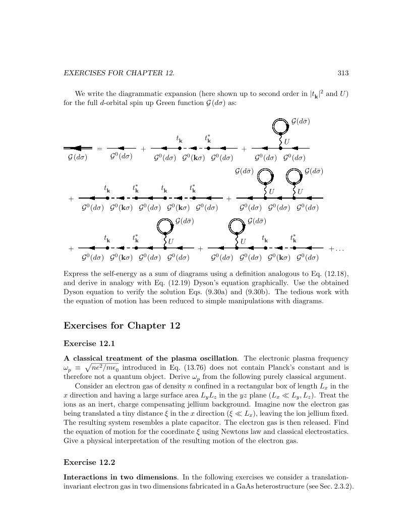
EXERCISES FOR CHAPTER 12. 313
We write the diagrammatic expansion (here shown up to second order in |tk|2 and U)for the full d-orbital spin up Green function G (dσ) as:
G (dσ)
=G0(dσ)
+G0(dσ)
tk
G0(kσ)
t∗k
G0(dσ)+
G0(dσ)
U
G0(dσ)
G(dσ)
+G0(dσ)
tk
G0(kσ)
t∗k
G0(dσ)
tk
G0(kσ)
t∗k
G0(dσ)+
G0(dσ)
U
G0(dσ)
U
G0(dσ)
G(dσ) G(dσ)
+G0(dσ)
tk
G0(kσ)
t∗k
G0(dσ)
U
G0(dσ)
G(dσ)
+G0(dσ)
U
G0(dσ)
tk
G0(kσ)
t∗k
G0(dσ)
G(dσ)
+ . . .
Express the self-energy as a sum of diagrams using a definition analogous to Eq. (12.18),and derive in analogy with Eq. (12.19) Dyson’s equation graphically. Use the obtainedDyson equation to verify the solution Eqs. (9.30a) and (9.30b). The tedious work withthe equation of motion has been reduced to simple manipulations with diagrams.
Exercises for Chapter 12
Exercise 12.1
A classical treatment of the plasma oscillation. The electronic plasma frequencyωp ≡ √
ne2/mε0 introduced in Eq. (13.76) does not contain Planck’s constant and istherefore not a quantum object. Derive ωp from the following purely classical argument.
Consider an electron gas of density n confined in a rectangular box of length Lx in thex direction and having a large surface area LyLz in the yz plane (Lx ¿ Ly, Lz). Treat theions as an inert, charge compensating jellium background. Imagine now the electron gasbeing translated a tiny distance ξ in the x direction (ξ ¿ Lx), leaving the ion jellium fixed.The resulting system resembles a plate capacitor. The electron gas is then released. Findthe equation of motion for the coordinate ξ using Newtons law and classical electrostatics.Give a physical interpretation of the resulting motion of the electron gas.
Exercise 12.2
Interactions in two dimensions. In the following exercises we consider a translation-invariant electron gas in two dimensions fabricated in a GaAs heterostructure (see Sec. 2.3.2).
314 EXERCISES FOR CHAPTER 12
The electron mass for this material is m∗ = 0.067 m, the relative permittivity is εr = 13,while the electron density ranges from n2D = 1× 10¹⁵ m−2 to 5×10¹⁵ m−2.
The electron wave function for the two dimensional electron gas is restricted to be
ψk(r, z) =1√
LxLy
eik·rζ0(z),
where k = (kx, ky) and r = (x, y), while ζ0(z) is the lowest eigenstate in the z direction,i.e. n = 0 in Eq. (2.50). Write down the interaction part of the Hamiltonian and showthat it is of the form
H2D =1
2A∑
kk′q
∑
σσ′W 2D(q) c†k+q,σc†k′−q,σ′ck′,σ′ck,σ
where q = (qx, qy). For a strictly 2D system, i.e. |ζ0(z)|2 = δ(z), show that
W 2D(q) =e2
2εrε0 q.
Hint: use∫ π0 dθ cos (α cos θ) = πJ0(α), where J0 is the Bessel function of the first kind of
order zero.
Exercise 12.3
Plasmons in two dimensions. Consider a translation-invariant electron gas in twodimensions fabricated in a GaAs heterostructure. The electron mass for this material ism∗ = 0.067 m, the relative permittivity is εr = 13, while the electron density ranges fromn2D = 1× 10¹⁵ m−2 to 5×10¹⁵ m−2.
For such a system the RPA dielectric function is given by
ε2DRPA(q, iqn) = 1−W 2D(q) χ2D
0 (q, iqn),
with q = (qx, qy) and where χ2D0 (q, iqn) is the 2D version of the 3D pair bubble χ0
given in Eq. (13.20). Show that at low temperatures, kBT ¿ εF, and long wave lengths,q ¿ ω/vF , the plasmon dispersion relation is ω = vF
√k2D
s q/2, where k2Ds is the Thomas-
Fermi screening wavenumber in 2D. Find the relation between kF and the electron density,n2D. Express k2D
s in terms of the parameters of the electron gas. Is it larger or smallerthan kF for n2D = 2× 10¹⁵ m−2?
Exercise 12.4
Static screening in two dimensions. Show that in 2D the static RPA screened inter-action at small wavevectors, q ¿ kF, and low temperatures, kBT ¿ εF, is given by
W 2DRPA(q, 0) ≡ W 2D(q)
ε2DRPA(q, 0)
=e2
2εrε0 (q + k2Ds )
.
EXERCISES FOR CHAPTER 13. 315
Exercise 12.5
Damping of two dimensional plasmons. The electron-hole pair continuum is theregion in q − ω space where Im χ2D
0 6= 0. Find the condition for the plasmons not to bedamped by single-particle excitations for q < kF. In the estimate you can use the small-qexpressions for the plasmon frequency and the polarization, that you found above. Arethe plasmons damped in the region q < kF in GaAs with the parameters given above?
Exercise 12.6
Deriving the Feynman diagrams for χ(q). The task is to understand the argumentsleading to the diagrammatic expansion for χ(q) given in Eq. (13.58). We are not askingfor detailed calculations.
In the real space formulation χ(b, a)≡−⟨Tτ ρ(b)ρ(a)
⟩eq
=−⟨Tτ Ψ†(b)Ψ(b)Ψ†(a)Ψ(a)
⟩eq
.Write down the expression for χ(b, a) analogous to Eq. (12.8) for G(b, a). Then applyWick’s theorem to obtain the analogue of Eq. (12.9). Following arguments similar tothose of Eq. (12.16) it can be shown that the numerator also cancels in the case of χ(b, a)(you do not have to show that). Finally, argue with the help of Appendix A that for atranslation-invariant system χ(q, τ) = − 1
V⟨Tτ ρ(q, τ) ρ(−q, 0)
⟩eq
as stated in Eq. (13.53),see also the form of σ(q, ω ) in Exercise 6.4. Please note that
⟨ρ⟩eq
= 0 due to chargeneutrality.
Alternatively, you may start with χ(q, τ) for a translation-invariant system, and writethis in a form analogous to Eq. (12.8). Then apply Wick’s theorem in this situation toobtain the starting point for the diagrammatic expansion directly in q-space.
Exercises for Chapter 13
Exercise 13.1
Semi-classical motion. We study Eqs. (14.17), (14.18), and (14.19). If the quasiparticlesbehaves like non-interacting particles why is then the number of quasiparticles conservedon the semi-classical level?
To answer this question we introduce the concept of a wave packet, i.e. a wave functionfairly localized in both space and momentum space:
ψ(r, t) =∫
dk f(k−k0) ei[k·r−ω (k)t], e.g. with f(k−k0) = exp
(−(k−k0)
2
2 (∆k)2
).
Taylor expand ω (k) to first order and show that the wave packet can be written as
ψ(r, t) ≈ ei[k0·r−ω (k0)t] F (r− ∂kω (k0) t),
where F is some envelope function. What is the physical interpretation of ∂kω (k0)? Inconclusion, the wave packet has the energy εk and the velocity vk given by
εk = ~ ωk, vk = ∂kωk =1~
∂kεk.
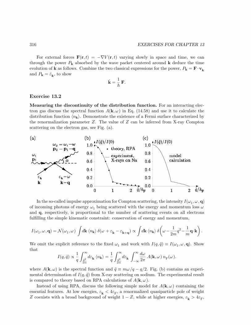
316 EXERCISES FOR CHAPTER 13
For external forces F(r, t) = −∇V (r, t) varying slowly in space and time, we canthrough the power Pk absorbed by the wave packet centered around k deduce the timeevolution of k as follows. Combine the two classical expressions for the power, Pk = F ·vk
and Pk = εk, to show
k =1~
F.
Exercise 13.2
Measuring the discontinuity of the distribution function. For an interacting elec-tron gas discuss the spectral function A(k, ω ) in Eq. (14.58) and use it to calculate thedistribution function 〈nk〉. Demonstrate the existence of a Fermi surface characterized bythe renormalization parameter Z. The value of Z can be inferred from X-ray Comptonscattering on the electron gas, see Fig. (a).
! " # $ % & ' ( ) *
# + , # % - . # / ! '0 1 % 2 & 3 $ /54 2
6 7
. $ 8 # 9: 2 9 : ; 9 2 ! - $ /
In the so-called impulse approximation for Compton scattering, the intensity I(ω1, ω ,q)of incoming photons of energy ω1 being scattered with the energy and momentum loss ωand q, respectively, is proportional to the number of scattering events on all electronsfulfilling the simple kinematic constraint: conservation of energy and momentum,
I(ω1, ω ,q) = N (ω1, ω )∫
dk 〈nk〉 δ(ω + εk − εk+q) ∝∫
dk 〈nk〉 δ
(ω− 1
2mq2− 1
mq·k
).
We omit the explicit reference to the fixed ω1 and work with I(q, q) ≡ I(ω1, ω ,q). Showthat
I(q, q) ∝ 1q
∫ ∞
q2
2m
dεk 〈nk〉 =1q
∫ ∞
q2
2m
dεk
∫ ∞
−∞
dω
2πA(k, ω ) nF(ω ).
where A(k, ω) is the spectral function and q ≡ mω/q − q/2. Fig. (b) contains an experi-mental determination of I(q, q) from X-ray scattering on sodium. The experimental resultis compared to theory based on RPA calculations of A(k, ω ).
Instead of using RPA, discuss the following simple model for A(k, ω ) containing theessential features. At low energies, εk < 4εF, a renormalized quasiparticle pole of weightZ coexists with a broad background of weight 1− Z, while at higher energies, εk > 4εF,
EXERCISES FOR CHAPTER 14. 317
no renormalization occurs, and the quasiparticle is in fact the bare electron:
A(k, ω ) = Zk 2πδ(ω−ξk) + (1−Zk)π
Wθ(W−|ω |), Zk =
Z, for k < 2kF
1, for k > 2kF.
Here W is the large but unspecified band width of the conduction band. Explain Fig. (c).
Exercise 13.3
Detailed balance. The scattering life time in Eq. (14.45) expresses the time betweenscatterings assuming some unknown distribution function n(k). The Boltzmann equationwith inclusion of e-e scattering therefore reads
∂t(nk) + k · ∇knk + vk · ∇rnk = −(
1τk
)
collisions
.
In the homogenous and static case, i.e. absence of external forces, the left hand side isexpected to be zero. Show that the usual Fermi-Dirac equation solves the Boltzmannequation in this case, i.e. that the right hand side is also zero if we use n = nF . Hint:show and use that nF (ε) [1− nF (ε′)] exp (β(ε− ε′)) = [1− nF (ε)]nF (ε′).
Exercise 13.4
Why are metals shiny? According to Eq. (13.75) we have in the semiclassical highfrequency, long wave limit that ε(0, ω) = 1 − ω2
p/ω2. Consider a monochromatic electro-magnetic wave with E = E(x)e−iωtez incident on a metal occupying the half-space x > 0.Use the high-frequency limit of Maxwell’s equations in matter. Set D = ε0ε(0, ω)E and
prove that ∇2E(x) = ω2p−ω2
c2E(x). Hint: you may need ∇×∇×E = −∇2E. For which
frequencies does the wave propagate through the metal, and for which is it reflected?From X-ray diffraction we know that the unit-cell of Na is body-centered cubic (i.e.
one atom in each corner and one in the center of the cube) with a side-length of 4.23 A.It is observed that Na is transparent for UV-light with a wavelength shorter than 206 nm.Explain this, and explain why (polished) metals appear shiny. Hint: Each Na atom donatesone electron to the conduction band.
Exercises for Chapter 14
Exercise 14.1
The integral equation for the vertex function in the Born approximation. Thisexercise deals with the Kubo formula method applied to impurity scattering in metals.The conductivity is in the weak scattering limit given by
σxx =e2
π
1V
∑
k
(kx
m
)GR(k, 0)GA(k, 0)ΓRA
x (k,k; 0, 0).
318 EXERCISES FOR CHAPTER 14
In the Born approximation the Dyson equation for the vertex function is
ΓRAx (k,k; 0, 0) =
kx
m+
1V
∑
k′nimp|u(k− k′)|2GR(k′, 0)GA(k′, 0)ΓRA
x (k′,k′; 0, 0).
1. If the impurity potential is short ranged argue that we can approximate it by aconstant |u(k− k′)|2 ≈ |u0|2. Prove that in this case
ΓRAx =
kx
m,
and use this to find that
σ =e2nτ0
m,
where τ0 is the Born approximation life time
τ−10 = 2πd(εF )nimp|u0|2.
2. Now relax the assumption of short range scatterers but assume instead that u(k− k′)is slowly varying on the scale given by the width of the spectral function, i.e. τ−1
0 .In this more realistic case, you will find for |k| = kF that
~ΓRA(k) =km
+d(εF )
2
∫dΩ′ |u(k− k′)|2~ΓRA(k′),
with |k′| = kF and∫
dΩ′ =∫
dφ′dθ′ sin θ′ is an integration over the angle of k′. Nowshow that
σ =e2nτ tr
m,
where(τ tr
)−1 = 2πd(εF )nimp
∫dΩ′
4π|u(k− k′)|2
(1− k · k′
k2F
).
Hint: use the ansatz ~ΓRA(k) = (k/m)γ.
Explain the physical meaning of the last term and why it does not appear in the resultfor point-like impurities.
Exercise 14.2
Life time of the Green’s function in the Born approximation. Show that theretarded impurity averaged Green’s function in the Born approximation decays exponen-tially in time and given a physical interpretation of this result.
EXERCISES FOR CHAPTER 14 319
Exercise 14.3
Weak localization at finite frequency. Here we consider the weak localization cor-rection at finite frequency. The only change in the formula for the weak localization isthrough the Cooperon which becomes instead
CRA(Q, ω) =W0ζ(Q, ω)1− ζ(Q, ω)
,
ζ(Q, ω) =1V
∑p
|u0|2GR(p−Q, ω)GA(p, 0).
Show that in this case, the low frequency ωτ0 ¿ 1 and long wavelength QvF τ0 ¿ 1 limitof ζ(Q, ω) is
ζ(Q, ω) ≈ 1 + iωτ0 −Dτ0Q2.
Show that the frequency provide a small Q cut-off in the conductivity correction and tryto explain why.
Exercise 14.4
Mass renormalization in Drude formula? The mass that appears in the Drude for-mula is the bare electron mass (possibly including bandstructure effects). The impuritiesonly enter in the scattering time. The Drude formula can be derived from e.g. the Boltz-mann equation, where the mass enters through the velocity, vk = ~k/m and the impuritypotential in the collision term.
If we think about impurity scattering from a microscopic point of view the self energyhas both a real and an imaginary part. Let us for instance consider the lowest orderself-consistent Born approximation. In this case the self-energy reads
∑1SCBA(k, ikn) = nimp
∑
k′|uk−k′ |2G
(k′, ikn
). (B.4)
Note that it is G and not G0 that enters in the self-consistent approximation. The realpart leads to a renormalization of the mass and to a renormalization of the spectral weightat the Fermi surface, i.e. when expanding the Green’s function near the Fermi surface wecan write
GR(k, ε) ≈ Z
ω − ξ∗k + i 2τ∗
. (B.5)
If we include the real part in this way (contrary to Sec. 14.3 and Exercise 5, where it isneglected) does it lead to a renormalization of the Drude formula?
320 EXERCISES FOR CHAPTER 15
Exercises for Chapter 15
Exercise 15.1
Conductance of a delta function barrierAs a model system of a mesoscopic 1Dchannel take the following Hamiltonian
H = − ~2
2m
∂2
∂x2+ V0δ (x) .
Consider a scattering state
ψ+k (x) =
1√L
(eikx + re−ikx
), x < 0,
1√Lteikx, x > 0,
and likewise for ψ−. Show that
ψ′(0+)− ψ′(0−) =2m
~2V0ψ(0)
and use it to find r and t. Suppose now that the two ends of the wire have differentchemical potential, so that the distribution function for electrons in the states ψ+
k is givenby nF (εk − µL), while the distribution function for electrons in states ψ−k is nF (εk − µR).Show that the current at low temperature becomes
I = 2e∑
k>0
(v+k nF (εk − µL)− v−k nF (εk − µR)
)=
2e2
h
11 + (V0/~vF )2
V,
where V = µR−µLe ¿ εF .
Hints: v+k = ~
2mi((ψ+
k
)∗∂xψ+
k − c.c.) = |t|2 = 1− |r|2 with t = (1 + iz)−1, z = mV0/~k.
Exercise 15.2
Landauer-Buttiker formula at finite temperatures. For a general mesoscopic systemshow that the linear conductance at finite temperature is generalized to
G =2e2
h
∑n
∫ ∞
0dE
(−∂nF (E − µ)
∂E
)Tn(E),
where Tn(E) is the transmission probability of a given mode Tn(E) =∑
n′ t∗nn′tn′n.
Using a model electron waveguide, where the potential in the transverse direction is aparabolic confinement, the transmission coefficient is supposed to be
Tn(E) = Θ(E −En) = Θ(E − (n +12)~ωT ),
where ωT is the frequency of transverse oscillation. Find an expression for the conductanceG and plot the G as a function of µ. Plot for example G(h/2e2) versus µ/~ωT for twodifferent temperatures: kT = (0.05, 0.15)~ωT . How would the result look if the transverseconfinement was given by a square well?
EXERCISES FOR CHAPTER 16. 321
Exercises for Chapter 16
Exercise 16.1
Phonon Green’s function Prove Eq. (16.7).
Exercise 16.2
Cooper’s instability In this exercise we shall see that an attractive electron-electroninteraction leads to an instability of the Fermi surface.
BCS model Hamiltonian. In Chap. 16 it is shown that the electron-phonon interactionleads to an effective electron-electron interaction. It is attractive for small frequencies, i.e.for energies smaller than qvs, where q is the exchanged momentum and vs is the soundvelocity. The scale of this energy is given by the Debye energy. This observation leadCooper to study the following model Hamiltonian, which is also the starting point usedby BCS,
H = H0 + H ′ (1a)
H0 =∑
kσ
(εk − µ) c†kσckσ, (1b)
H ′ = −V0
2
∑ ′c†k+qσc†k′−qσ′ck′σ′ckσ. (1c)
Here the sum is restricted such that all initial and final states lie in an interval givenby [µ − ωD, µ + ωD], i.e. in a shell around the Fermi surface. Anticipating the physicalidea that the electrons due to the attractive interaction will form pairs with zero totalmomentum and spin, we look specifically at the interaction between such pairs. The pairsare thus supposed to consist of electrons with opposite momentum, which means that wechoose k′ = −k and σ = −σ′. After relabelling we have
H ′ = −V0
∑ ′c†k′↑c†−k′↓c−k↓ck↑. (2)
Variational calculation of FS with an added pair of electrons. We wish to find theenergy of a pair of electrons added to a filled Fermi sea state, and with interactionsaccording to (2). In order to separate the effect of the interaction on the Fermi sea and onthe extra pair of electrons, the
∑′ sum is further restricted to involve only states outsidethe Fermi sea. Thus Eq. (2) becomes
H ′ = −V0
∑
k,k′>kF .
′c†k′↑c
†−k′↓c−k↓ck↑. (3)
We look at the difference between the two situations: 1) The electron pair is added tothe Fermi surface, i.e. with |k|, |k′| = kF and energy equal to zero. 2) The electron pairforms a coherent superposition of pairs not necessary at the Fermi surface. According tothe variational principle the lowest energy of the two is closest to the groundstate energy.
322 EXERCISES FOR CHAPTER 17
For situation 2 we start by an Ansatz wavefunction, which is a superposition of so-called Cooper pairs
|ψ〉 =∑
k
αkc†k↑c†−k↓|FS〉. (4)
Show that αk satisfies the following equation.
αk(2εk −EF )− V0
∑
k′>kF
′αk′ = Eαk, (5)
and that this leads to a condition for E given by
1 = V0
∑
k′>kF
′ 1(2εk −EF )− E
. (6)
In order to find the energy E you should make use of the following hierarchy of energyscales
E ¿ ωD ¿ EF , (7)
where the validity of the first one of course must be checked at the of the calculation. Findthat (reinserting ~)
E = −2~ωD exp (−1/V0d(EF )) . (8)
Discuss the following two important issues:
• Why does this result indicate an instability of the Fermi surface
• Could this result have been reached by perturbation theory in V0?
Exercises for Chapter 17
Exercise 17.1
The Josephson effect. This exercise deals with the supercurrent across a tunnel junc-tion, the so-called Josephson effect. We apply the relations to study the current-voltagecharacteristic of a tunnel junction in the so-called resistively shunted Josephson junctionmodel.
Supercurrent in the equilibrium state. Consider a tunnel junction between two super-conductors, i.e. two superconductors separated by an insulator. The tunnel Hamiltonianis
HT =∑
kp
(tkpc†kσfpσ + t∗kpf †pσckσ
), (1)
where the electron operators for the two sides are called c and f , respectively. In thefollowing we assume for simplicity that in the energy range of interest the tunnel matrixelement depends weakly on the states k and p, therefore
tkp ≈ t (2)
EXERCISES FOR CHAPTER 17 323
The Hamiltonian for the two sides are the usual BCS Hamiltonians
Hc =∑
kσ
ξkc†kσckσ −∆eiφc
∑
k
c†k↑c†−k↓ −∆e−iφc
∑
k
c−k↓ck↑, (3a)
Hf =∑
kσ
ξkf†kσfkσ −∆eiφf
∑
k
f †k↑f†−k↓ −∆e−iφf
∑
k
f−k↓fk↑, (3b)
where the two superconductors are assumed to be equal. The order parameter of eachside of the junction have different phases, φc and φf , and ∆ is here taking to be real.The phase difference between the two side can be absorbed as a phase shift of the tunnelmatrix
t → e−i(φc−φf)/2t, (4)
by the transformationc → eiφc/2c, f → eiφf /2f. (5)
Show that the equilibrium current running between the two superconductors is
IJ = 〈I〉 = (−2e) 〈 ∂
∂φHT 〉 = (−2e)
∂F
∂φ, (6)
where I is the operator for the electrical current I = (−e) Nc, F is the free energy andφ = φc − φf is the phase difference.
This is a current which runs in thermodynamical equilibrium and hence is dissipation-less in the sense that it runs without an applied bias (the chemical potential of the twosides is per definition identical in equilibrium). In the following we calculate this so-calledsupercurrent to second order in the tunneling amplitude.
Show that to second order in HT
〈 ∂
∂φHT 〉 ≈ −
∫ β
0dτ〈TτHT (τ)
∂
∂φHT 〉0 = −1
2∂
∂φ
∫ β
0dτ〈TτHT (τ)HT 〉0, (7)
where the expectation value 〈〉0 means taken with respect to Eqs. (2). Then show that
12
∂
∂φ
∫ β
0dτ〈TτHT (τ)HT 〉0 =
∂
∂φ
∫ β
0dτ
∑
kp
t2eiφG21(k, τ)G12(p,−τ) + c.c.
=∂
∂φ
1
β
∑
ikn
∑
kp
t2eiφG21(k, ikn)G12(p, ikn) + c.c.
(8)
where G12 and G21 are the off-diagonal Nambu Green’s functions defined in Exercise 3.Verify the following steps
∑
k
G21(k, ikn) =∑p
G12(p, ikn)
=∆d(εF )
2
∫ ∞
−∞dξ
(1
(ikn)2 − E2
)
= −∆d(εF )2
π√k2
n + ∆2, (9)
324 EXERCISES FOR CHAPTER 17
and use it to find that
IJ = −(
π∆d(εF )t2
)2 1β
∑
ikn
1k2
n + ∆2
= sin φe (πd(εF )t)2
2∆ tanh
(∆β
2
)
= sin φ∆π
2eRNtanh
(∆β
2
), (10)
where the normal state tunnel resistance is given by R−1N = πe2d2t2/~.
Exercise 17.2
RSJ model of a Josephson junction. With a finite bias voltage across the junction,one can still have a supercurrent running, i.e. a current carried by Cooper pairs and therelation
IJ = IC sinφ, (1)
is still valid. This is known as the first Josephson relation. The finite voltage changes theenergy of electrons of the two sides and hence their phase. We can simply include thisphase change in the time dependence of by the following substitution
c(t) → c(t)eiV t/2, f(t) → f(t)e−iV t/2, (2)
which corresponds toφ → φ + 2eV t, (3)
orφ =
2e
~V, (4)
which is called the second Josephson relations.The second Josephson relation adds interesting dynamics to the Josephson junction
because of the intrinsic frequency 2eV/~. One can measure this frequency by applyingexternal RF radiation to the junction. The Josephson junction thus acts as a voltage tofrequency converter, which has many applications.
Now we look at the current-voltage characteristic of a Josephson junction in the RSJmodel. The current is carried by two kinds of electrons: those that are paired and thosethat are not. The pair current is described by the Josephson relations while the normalcurrent is supposed to be given by Ohm’s law.
Consider a current biased setup, i.e. a junction with a fixed current, I. This currentis made up by the sum of the supercurrent and the normal current. Thus
I = IN + IJ =1R
V + IC sinφ =~
2eRφ + IC sinφ. (5)
Write this equation in the dimensionless form
η =I
IC
=dφ
dτ+ sin φ, τ =
2eIcR
~t. (6)
EXERCISES FOR CHAPTER 17 325
The voltage is time dependent, but in a dc measurement one measures the average voltage.Integrate Eq. (6) and show that the average voltage becomes
〈V 〉 =
0, I < IC
RIc
√(I/IC)2 − 1. I > IC
(7)
Hint: first find solutions for φ = 0 and then a “running” solution where φ 6= 0. For thelast situation the average voltage is 〈V 〉 = 1
T
∫ T0 dtdφ
dt = 2πT . Here T is the period of the
voltage or the time it takes to increase φ by 2π.
Index
acoustic phononsDebye phonons, 52graphical representation, 51, 56in second quantization, 55
adiabatic continuity, 233advanced function, 163Aharonov-Bohm effect, 120analytic continuation, 162analytic function, 161Anderson’s model for magnetic impurities, 147annihilation operators
1D phonons, 55bosons, 10fermions, 13time dependence, 91time-derivative, 145
anti-commutator, 13anti-symmetrization operator, 7antiferromagnetism, 73art, the art of mean field theory, 68atom
artificial, 153Bohr radius a0, 40electron orbitals, 3ground state energy E0, 40in metal, 31
attractive pair-interaction, 281
bandstructure diagramextended zone scheme, 35metal, semiconductor, insulator, 45
Bardeen-Cooper-Schrieffer (see BCS), 78basis states
change in second quantization, 16complete basis set, 3Green’s function, 130many-particle boson systems, 12many-particle fermion systems, 14orthonormal basis set, 2systems with different particles, 24
BCS theoryeffective Hamiltonian, 81interaction potential model, 285mean field Hamiltonian, 82self-consistent gap equation, 83tunneling spectroscopy, 140
BlochBloch theory of lattice electrons, 33bandstructure, 35Bloch’s equation, density matrix, 158Bloch’s theorem, 34
Bogoliubov transformation, 82Bohm-Staver sound velocity
from RPA-screened phonons, 283semi-classical, 53
Bohr radius a0, 40Boltzmann distribution, 26Boltzmann equation
collision free, 239introduction, 233with impurity scattering, 241
Born approximationfirst Born approximation, 190, 259full Born approximation, 193in conductivity, 261self-consistent Born approximation, 194spectral function, 1st order, 192
Born-Oppenheimer approximation, 279Bose-Einstein distribution, 29, 51boson
creation/annihilation operators, 10defining commutators, 11definition, 5frequency, 161, 165many-particle basis, 12
bra state, 2Brillouin zone
bandstructure diagram, 35definition, 34for 1D phonons, 54
326
INDEX 327
broadening of the spectral function, 136broken symmetry, 71
canonicalensemble, 27momentum, 21partition function, 26
carbon nanotubes, 48charge-charge correlation function, 103chemical potential
definition, 27temperature dependence, 39
collapse of wavefunction, 2commutator
[AB, C] = A[B, C] + [A, C]B, 92[AB, C] = AB, C − A,CB, 92defining bosons, 11defining fermions, 13general definition, 11
completebasis states, 3set of quantum numbers ν, 3
conductanceconductance fluctuations, 186Kubo formalism, 100mesoscopic system, 113universal fluctuations, 121
conductance quantization, 116conductivity
cooperons, 269introduction, 253Kubo formalism, 98relation to dielectric function, 104semi-classical approach, 240
connected Feynman diagrams, 203conservation of four-momentum, 208conserving approximation, 259continuity equation
for ions in the jellium model, 52for quasiparticles, 238
contour integral, 166convergence of Matsubara functions, 160Cooper
Cooper pairs, 81instability of the Fermi surface, 81instability, Feynman diagrams, 284
cooperons in conductivity, 269core electron, 31correlation function
charge-charge correlation, 103current-current correlation, 100, 254general Kubo formalism, 97
correlation hole around electrons, 65Coulomb blockade, 153Coulomb interaction
combined with phonons, 279direct process, 43divergence, 44, 213exchange process, 44in conductivity, 256RPA renormalization, 217, 227screened impurity scattering, 181second quantization, 23Yukawa potential, RPA-screening, 218
coupling constantelectron interaction strength e2
0 , 23electron-phonon, general, 62electron-phonon, jellium model, 64electron-phonon, lattice model, 63electron-phonon, RPA-renormalized, 283integration over, 220
creation operators1D phonons, 55bosons, 10fermions, 13time dependence, 91
critical temperatureCooper instability, 285ferromagnetism, 74superconductivity, 84
crossed diagramdefinition, 267maximally crossed, 268
crossing diagramsdefinition, 264suppressed in the Born approx., 196
current density operatordia- and paramagnetic terms, 99second quantization, 22
current-current correlation function, Πdefinition, 100diagrammatics, 254
d-shell, 148Debye
acoustical Debye phonons, 52Debye energy or frequency ωD, 59Debye model, 52, 59, 284
328 INDEX
Debye temperature TD, 59Debye wave number kD, 59density of states, Debye model, 59frequency cut-off, BCS, 285
delta function δ(r), 4density in second quantization, 22density matrix operator, 27density of states
measured by tunneling, 140non-interacting electrons, 38phonons, Debye model, 59spectral function, 136
density waves, 72density-density correlation function
the pair-bubble χ0 ≡ −Π0 , 216the RPA-bubble χRPA, 226the RPA-bubble and phonons, 282
dephasing, 108, 264, 272determinant
first quantization, 7in Wick’s theorem, 172Slater, 7
diagonal Hamiltonian, 133diamagnetic term in current density, 99dielectric function ε
equation of motion derivation, 155irreducible polarization function χirr, 226Kubo formalism, 102relation to polarization function χ, 223relation to conductivity, 104
differential conductance, 140differential equation
classical Green’s function, 127many-body Green’s function, 131single-particle Green’s function, 146
Diracbra(c)ket notation for quantum states, 2delta function δ(r), 4
disconnected Feynman diagrams, 203disorder, mesoscopic systems, 121dissipation
due to electron-hole pairs, 144, 231of electron gas, 143
distribution functionBoltzmann, 26non-interacting bosons, 29non-interacting fermions, 28Boltzmann, Gibbs, 26Bose-Einstein, 29
electron reservoir, 113Fermi-Dirac, 28Maxwell-Boltzmann, 45
donor atoms, 46Drude formula, 240, 251, 264Dulong-Petit value for specific heat, 60dynamical matrix D(k), 57Dyson equation
Feynman diag., external potential, 179first Born approximation, 190for Πxx, 257for cooperon, 269full Born approximation, 193impurity and interaction, 256impurity averaged electrons, 189pair interactions in Fourier space, 208pair interactions in real space, 205pair-scattering vertex Λ, 284polarization function χ, 226self-consistent Born approximation, 194single-particle in external potential, 178
effective electron-electron interactionCoulomb and phonons, jellium, 280Coulomb and phonons, RPA, 283phonon mediated, RPA, 283
effective mass approximation, 35effective mass, renormalization, 246, 251eigenmodes
electromagnetic field, 19lattice vibrations, 58
eigenstatedefinition, 1superposition, 1
eigenvalue, definition of, 1Einstein model of specific heat, 60Einstein phonons
in the jellium model, 52optical phonons, 52
elastic scatteringMatsubara Green’s function, 179
electric potentialclassical theory, 127external and induced, 237
electroncore electrons, 31density of states, 38phase coherence, 184valence electrons, 31
INDEX 329
electron gas, in general0D: quantum dots, 491D: carbon nanotubes, 482D: GaAs heterostructures, 463D: metals and semiconductors, 45introduction, 31
electron gas, interactingattractive interaction, 281dielectric properties and screening, 223first order perturbation, 41, 43full self-energy diagram, 214full theory, 213general considerations, 39ground state energy, 220, 222Hartree–Fock mean field Hamiltonian, 70infinite perturbation series, 214, 222Landau damping, 230plasma oscillations, 228second order perturbation, 43thermodynamic potential Ω, 220
electron gas, non-interactingBloch theory, 33density of states, 38Feynman diagrams, 177finite temperature, 38ground state energy, 38jellium model, 35motion in external potentials, 177static ion lattice, 33
electron interaction strength e20 , 23
electron wave guides, 116electron-electron scattering
attractive interaction, 281Cooper instability, 284dephasing, 264, 272life-time, 243
electron-hole pairsexcitations, 144, 155interpretation of RPA, 220Landau damping, 231
electron-phonon interactionadiabatic electron motion, 53basis states, 276combined with Coulomb interaction, 279Feynman diagrams, 276general introduction, 51graphical representation, 63the jellium model, 63, 275the lattice model, 61, 275
the sound velocity, 53umklapp process, 63
electronic plasma oscillationsgraphical representation, 51
equation of motionAnderson’s model, 149derivation of RPA, 153for ions, 57frequency domain, 147Heisenberg operators, 88in proof of Wick’s theorem, 171introduction, 145Matsubara Green’s function, 169non-interacting particles, 147single-particle Green’s function, 145
ergodic, 121ergodicity assumption, 25extended zone scheme, 35
FermiFermi energy εF, 36Fermi sea diagrams, 37Fermi sea with interactions, 42Fermi sea, Cooper instability, 286Fermi sea, definition, 36Fermi sea, excitations, 144Fermi velocity vF, 36Fermi wave length λF, 36Fermi wavenumber kF , 36Fermi’s golden rule, 240, 244, 250Thomas-Fermi screening, 218, 219
Fermi liquid theoryintroduction, 233microscopic basis, 245
Fermi-Dirac distribution, 28, 237fermion
definition, 5creation/annihilation operators, 13defining commutators, 13frequency, 161, 165many-particle basis, 14
fermion loop, 202ferromagnetism
critical temperature, 74introduction, 73order parameter, 72Stoner model, 75
Feynman diagramscancellation of disconnected diagrams, 203
330 INDEX
Cooper instability, 284electron-impurity scattering, 182electron-phonon interaction, 276external potential scattering, 179first Born approximation, 190full Born approximation, 193impurity averaged single-particle, 188interaction line in Fourier space, 208interaction line in real space, 204irreducible diagrams, imp. scattering, 189irreducible diagrams, pair interaction, 205pair interactions, 199polarization function χ, 225self-consistent Born approximation, 194single-particle, external potential, 177topologically different diagrams, 204
Feynman ruleselectron-impurity scattering, 184external potential scattering, 179impurity averaged Green’s function, 188pair interactions in Fourier space, 208pair interactions in real space, 204pair interactions, G denominator, 201pair interactions, G numerator, 202phonon mediated pair interaction, 278
first quantizationmany-particle systems, 4name, 1single-particle systems, 2
Fockapproximation for interactions, 70Fock self-energy for pair interactions, 209Fock space, 10, 27Hartree–Fock approximation, 69
four-vector/four-momentum notation, 207, 255Fourier transformation
1D ion vibrations, 54basic theory, 291Coulomb interaction, Matsubara, 206equation of motion, 147Matsubara functions, 161
free energydefiniton, 27in mean field theory, 67
GaAs/Ga1−xAlxAs heterostructures, 46gauge
breaking of gauge symmetry, 78Landau gauge, 3
radiation field, 19transversality condition, 19
Gauss box, 47Gibbs distribution, 26grand canonical
density matrix, 27ensemble, 27partition function, 27
gravitation, 1Greek letters, 158Green’s function
n-particle, 170classical, 127dressed, 254free electrons, 132free phonons, 275greater and lesser, 131imaginary time, 160introduction, 127Lehmann representation, 134Poisson’s equation, 127renormalization, 245retarded, equation of motion, 145retarded, many-body system, 131retarded, one-body system, 130RPA-screened phonons, 282Schrodinger equation, 128single-particle, many-body system, 131translation-invariant system, 132two particle, 141
Hamiltoniandiagonal, 133non-interacting particles, 135quadratic, 135, 146, 150, 170
harmonic oscillatorlength, 18second quantization, 18
Hartreeapproximation for interactions, 70Hartree self-energy, pair interactions, 209Hartree–Fock approximation, 69
Hartree–Fock approximationintroduction, 69mean field Hamiltonian, 70the interacting electron gas, 70
heat capacityfor electrons, 39for ions, 52
INDEX 331
Heaviside’s step function θ(x), 4Heisenberg
Heisenberg picture, 88model of ferromagnetism, 73
helium, Hamiltonian, 9heterostructures, GaAs/Ga1−xAlxAs, 46Hilbert space, 1hopping, 149Hubbard model, 75hybridization, 148hydrogen atom
Bohr radius a0, 40electron orbitals, 3ground state energy E0, 40
imaginary timediscussion, 158Greek letters, 158Green’s function, 160
impurities, magnetic, 148impurity scattering, conductivity, 253impurity self-average, 184impurity-scattering line
Feynman rules, 188in conductivity, 255renormalization by RPA-screening, 227
inelastic light scattering, 144infinite perturbation series
breakdown at phase transistions, 85electron gas ground state energy, 222self-energy for interacting electrons, 214single-particle Green’s function, 178time-evolution operator U(t, t0), 90
infinitesimal shift η, 162integration over the coupling constant, 220interaction line
general pair interaction in real space, 204pair interaction in Fourier space, 208RPA screened Coulomb line, 217, 227RPA screened impurity line, 227
interaction pictureimaginary time, 159introduction, 88real space Matsubara Green’s fct., 200
interference, 264, 265ions
ionic plasma oscillations, 51forming a static lattice, 33Heisenberg model, ionic ferromagnets, 73
in a metal, 31irreducible Feynman diagrams
impurity scattering, 189pair interaction, 205polarization function χirr, 225
iterative solution, integral eqs., 90, 128
jellium modeleffective electron-electron interaction, 280Einstein phonons, 52electron-phonon interaction, 63full electronic self-energy, 214oscillating background, 52static case, 35
ket state, 2kinetic energy operator
including a vector potential, 21second quantization, 21
kinetic momentum, 21Kronecker’s delta function δk,n, 4Kubo formalism
conductance, 100conductivity, 98, 254correlation function, 97dielectric function, 102general introduction, 95Landauer-Buttiker formula, 115RPA-screening in the electron gas, 223time evolution, 97tunnel current, 139
ladder diagram, 259Landau
and Fermi liquid theory, 233damping and plasma oscillations, 230eigenstates, 3gauge, 3
Landauer-Buttiker formulaheuristic derivation, 113linear response derivation, 115
lattice modelbasis in real space, 33basis in reciprocal space, 33Hamiltonian, 33
lattice vibrations1D phonon Hamiltonian, 53electron-phonon interaction, 61
Lehmann representationdefinition, 134
332 INDEX
for G>, G<, and GR, 134Matsubara function, 162
life-time, 150, 236, 243, 262Lindhard function, 143, 155linear response theory
introduction, 95Landauer-Buttiker formula, 115mesoscopic system, 113time evolution, 91tunnel current, 139
magnetic impurities, 148magnetic length, 3magnetic moment, 74, 147, 149magnetization, 72, 149many-body system
single-particle Green’s function, 131first quantization, 2second quantization, 9
mass renormalization, 254Matsubara
function, equation of motion, 169convergence of, 160Fourier transformation, 161frequency, 161Green’s function, 160relation to retarded function, 161sums, evaluation of, 165sums, simple poles, 167sums, with branch cuts, 168
Matsubara Green’s functionelastic scattering, 179electron-impurity scattering, 182first Born approximation, 190free phonons, 275full Born approximation, 193impurity averaged single-particle, 188interacting elec. in Fourier space, 208interacting electrons in Fourier space, 206interacting electrons in real space, 199RPA-screened phonons, 282self-consistent Born approximation, 194two-particle polarization function χ, 224
maximally crossed diagrams, 268MBE, molecular beam epitaxy, 46mean field theory
Anderson’s model, 150BCS mean field Hamiltonian, 82broken symmetry, phase transistions, 71
general Hamiltonian HMF, 66Hartree–Fock mean field Hamiltonian, 70introduction, 65mean field approximation, 67partition function ZMF, 67the art of mean field theory, 68
mean free path, 107measuring the spectral function, 137Meissner effect, 78mesoscopic
disordered systems, 121physics, 253regime, 265systems, introduction, 107
metaldisordering and random impurities, 181electrical resistivity, 181general description, 31Hamiltonian, 32observation of plasmons, 229Thomas-Fermi screening in metals, 219
Migdal’s theorem, 279molecular beam epitaxy, MBE, 46momentum
canonical, 21kinetic, 21relaxation, 240, 243
MOSFET, 46
Newton’s second lawfor ions in the jellium model, 52
non-interacting particlesdistribution functions, 28equation of motion, 147Green’s functions, 132Hamiltonian, 135in conductivity, 261Matsubara Green’s function, 164quasiparticles, 233retarded Green’s function GR(kσ, ω), 135spectral function A0(kσ, ω), 135
normalization of quantum states, 3normalization, scattering state, 108nucleus, 31
occupation number operatorbosons, 12fermions, 14introduction, 10
INDEX 333
occupation number representation, 10operator
adjoint, 2boson creation/annihilation, 10electromagnetic field, 19expansion of e−iHt, 87fermion creation/annihilation, 13first quantization, 7Heisenberg equation of motion, 88Hermitian, 1real time ordering Tt, 90second quantization, 14time evolution operator U(t, t0), 89trace Tr, 27
optical phononsEinstein phonons, 52graphical representation, 56
optical spectroscopy, 141optical theorem, scattering theory, 194order parameter
definition, 72list of order parameters, 72
overlap of wavefunctionslocalized/extended states, 148particle propagation, 133tunneling, 138
pair condensate, 72pair interactions
Dyson equation in Fourier space, 208Dyson equation in real space, 205Feynman diagrams, 199Feynman rules in Fourier space, 208Feynman rules in real space, 204self-energy in Fourier space, 208self-energy in real space, 205
pair-bubblecalculation of the pair-bubble, 218Feynman diagram Π0(q, iqn), 211in the RPA self-energy, 216self-energy diagram, 210the correlation function χ0 ≡ −Π0 , 216
paramagnetic term in current density, 99particle-particle scattering
in the collision term, 251life-time, 243
partition functioncanonical ensemble, 26grand canonical ensemble, 27
in mean field theory, 67Pauli
exclusion principle, 5, 40spin matrices, 21
periodic boundary conditions1D phonons, 53electrons, 36photons, 19
permanentfor bosons, 7in first quantization, 7in Wick’s theorem, 172
permutation, 171permutation group SN , 7, 90perturbation theory
first order, electron gas, 41infinite order, Green’s function, 178infinite order, ground state energy, 222infinite order, interacting electrons, 214linear response, Kubo formula, 95second order, electron gas, 43single particle wavefunction, 128time-evolution operator U(t, t0), 90
phase coherence, 264phase coherence for electrons, 184phase coherence length lϕ, 186phase space, 244, 245phase transition
breakdown of perturbation theory, 85broken symmetry, 71order parameters, 72
phonons1D annihilation/creation operators, 551D lattice vibrations, 53density of states, Debye model, 59dephasing, 264, 272eigenmodes in 3D, 58Einstein model of specific heat, 60free Green’s function, 275general introduction, 51Hamiltonian for jellium phonons, 52phonon branches, 55relevant operator Aqλ, 275RPA renormalization, 281RPA-renormalized Green’s function, 282second quantization, 55, 58
plasma frequencyfor electron gases in a metals, 228ionic plasma frequency, 52
334 INDEX
plasma oscillationselectronic plasma oscillations, 51interacting electron gas in RPA, 228ionic plasma oscillations, 51Landau damping, 230plasmons, 228
plasmonsdynamical screening, 238experimental observation in metals, 229plasma oscillations, 228semi-classical treatment, 237
Poisson’s equationGaAs heterostructures, 47Green’s function, 127
polarization function χDyson equation, 226Feynman diagrams, 225free electrons, 143, 173irreducible Feynman diagrams, 225Kubo formalism, 103momentum space, 142relation to dielectric function ε, 223two-particle Matsubara Green’s fct., 224
polarization vectorsphonons, 57photons, 19
probability current conservation, 111probability distribution, 136propagator
Green’s function, 130single-particle in external potential, 178
quadratic Hamiltonian, 135, 146, 150, 170quantum coherence
macroscopic in superconductivity, 79single electrons, 184
quantum correction, 253, 264, 273quantum dots
introduction, 49tunneling spectroscopy, 140
quantum effects, 107quantum field operator
definition, 17Fourier transform, 17
quantum fluctuationsin conductance, 186
quantum number νFeynman rules, Dyson equation, 181general introduction, 3
sum over, 4quantum point contact, 116quantum state
bra and ket state, 2free particle, 2hydrogen, 3Landau states, 3orthogonal, 2time evolution, 2
quasiparticledefinition, 236discussion, 235introduction, 233life-time, 243
quasiparticle-quasiparticle scattering, 243
radiation field, 19Raman scattering, 144random impurities, 181random matrix theory, 121random phase approximation (see RPA), 213rational function, 163reciprocal lattice basis, 33reciprocal space, 33reduced zone scheme, 35reflection amplitude, 110reflectionless contact, 108, 113relaxation time approximation, 243renormalization
constant Z, 247effective mass, 246, 251Green’s function, 245of phonons by RPA-screening, 281
reservoir, 25, 108resistivity (see conductivity), 240resummation of diagrams
current-current correlation, 256impurity scattering, 188the RPA self-energy, 215
retarded functionconvergence factor, 147Green’s function, 131, 132relation to Matsubara function, 161
Roman letters, 158RPA for the electron gas
Coulomb and impurity lines, 257deriving the equation of motion, 153electron-hole pair interpretation, 220Fermi liquid theory, 238, 246
INDEX 335
plasmons and Landay damping, 227renormalized Coulomb interaction, 217resummation of the self-energy, 215the dielectric function εRPA, 226the polarization function χRPA, 226vertex corrections, 259
Rydberg, unit of energy (Ry), 40
scattering length, 193scattering matrix, S, 108scattering state, 108scattering theory
optical theorem, 194Schrodinger equation, 128transition matrix, 193
Schrodinger equationGreen’s function, 128quantum point contact, 117scattering theory, 128time reversal symmetry, 112time-dependent, 2
Schrodinger picture, 87screening
dieelectric properties of the elec. gas, 223RPA-screened Coulomb interaction, 218semiclassical, dynamical, 238semiclassical, static, 238Thomas-Fermi screening, 218
second quantizationbasic concepts, 9basis for different particles, 24change of basis, 16Coulomb interaction, 23electromagnetic field, 19electron-phonon interaction, 61free phonons in 1D, 55free phonons in 3D, 58harmonic oscillator, 18kinetic energy, 21name, 1operators, 14particle current density, 22particle density, 22spin, 21statistical mechanics, 25thermal average, 27
self-average for impurity scatteringbasic concepts, 184weak localization, 265
self-consistent equationAnderson’s model, 151general mean-field theory, 67
self-energydue to hybridization, 150first Born approximation, 190Fock diagram for pair interactions, 209full Born approximation, 193Hartree diagram for pair interactions, 209impurity averaged electrons, 189interacting electrons, jellium model, 214irreducible, 257pair interactions in Fourier space, 208pair interactions in real space, 205pair-bubble diag., pair interactions, 210RPA self-energy, interacting electrons, 216self-consistent Born approximation, 194
semi-classicalapproximation, 261screening, 237transport equation, 240
single-particle statesas N -particle basis, 6free particle state, 2hydrogen orbital, 3Landau state, 3
Slater determinant, fermions, 7Sommerfeld expansion, 39sound velocity
Bohm-Staver formula, RPA, 283Bohm-Staver formula, semi-classical, 53Debye model, 52
sounds waves, 51space-time, points and integrals, 177spectral function
Anderson’s model, 151broadening, 136definition, 135first Born approximation, 192in sums with branch cuts, 169measurement, 137non-interacting particles, 135physical interpretation, 135
spectroscopyoptical, 141tunneling, 137
spinPauli matrices, 21second quantization, 21
336 INDEX
spontaneous symmetry breakingbreaking of gauge symmetry, 78introduction, 72
statistical mechanicssecond quantization, 25
step function θ(x), 4STM, 138Stoner model of metallic ferromagnetism, 75superconductivity
critical temperature, 84introduction, 78Meissner effect, 78microscopic BCS theory, 81order parameter, 72
symmetrization operator, 7
thermal average, 27thermodynamic potential Ω
definition, 28for the interacting electron gas, 220
Thomas-Fermi screening, 218, 219, 222time dependent Hamiltonian, 95time evolution
creation/annihilation operators, 91Heisenberg picture, 88in linear response, 91interaction picture, 88linear response, Kubo, 97operator, imaginary time, 159Schrodinger picture, 87unitary operator U(t, t0), 89
time-ordering operatorimaginary time Tτ , 160real time Tt, 90
time-reversal symmetry, 112time-reversed paths, 266, 268, 272topologically different diagrams, 204trace of operators, 27transition matrix, scattering theory, 193translation-invariant system
conductivity, 254Green’s function, 132
transmission amplitude, 110, 130, 267transmission coefficients, 113transport equation, 233transport time, 242transversality condition, 19triangular potential well, 47truncation
Anderson’s model, 150, 153derivation of RPA, 154discussion, 145
tunnelingscanning microscope, 138BCS superconductor, 140current, 138spectroscopy, 137
umklapp process, 63unit cell, 55unitarity, S-matrix, 111universal conductance fluctuations, 121, 124
valenceelectrons, 31
vector potentialelectromagnetic field, 19kinetic energy, 21Kubo formalism, 99
vertexcurrent vertex, 255dressed vertex function, 258electron-phonon vertex, 280pair-scattering vertex Λ, 284vertex correction, 254, 257vertex function, 268
Ward identity, 258, 262wavefunction collapse, 2weak localization
and conductivity, 264introduction, 253mesoscopic systems, 121, 123
Wick’s theoremderivation, 170interacting electrons, 201phonon Green’s function, 277
WKB approximation, 119
Yukawa potentialdefinition, 24, 213RPA-screened Coulomb interaction, 218


![[Henrik Bruus, Karsten Flensberg] Many-Body Quantum Theory in Condensed Matter Physics](https://img.pdfslide.us/doc/110x75/54518fd5af79591d308b48fd/henrik-bruus-karsten-flensberg-many-body-quantum-theory-in-condensed-matter-physics.jpg)