Embed Size (px)
Citation preview

Heights of prespecial points of Shimura varieties Article
Accepted Version
Daw, C. and Orr, M. (2016) Heights of prespecial points of Shimura varieties. Mathematische Annalen, 365 (34). pp. 13051357. ISSN 00255831 doi: https://doi.org/10.1007/s0020801513283 Available at http://centaur.reading.ac.uk/70364/
It is advisable to refer to the publisher’s version if you intend to cite from the work. Published version at: http://dx.doi.org/10.1007/s0020801513283
To link to this article DOI: http://dx.doi.org/10.1007/s0020801513283
Publisher: Springer
All outputs in CentAUR are protected by Intellectual Property Rights law, including copyright law. Copyright and IPR is retained by the creators or other copyright holders. Terms and conditions for use of this material are defined in the End User Agreement .
www.reading.ac.uk/centaur
CentAUR
Central Archive at the University of Reading

Reading’s research outputs online

Heights of pre-special points of Shimura varieties
Christopher Daw Martin Orr
May 15, 2017
Abstract
Let s be a special point on a Shimura variety, and x a pre-image of sin a fixed fundamental set of the associated Hermitian symmetric domain.We prove that the height of x is polynomially bounded with respect to thediscriminant of the centre of the endomorphism ring of the correspondingZ-Hodge structure. Our bound is the final step needed to complete a proofof the André–Oort conjecture under the conjectural lower bounds for thesizes of Galois orbits of special points, using a strategy of Pila and Zannier.
1 IntroductionOur aim in this paper is to prove a bound for the height of a pre-special point ina fundamental set of a Hermitian symmetric domain covering a Shimura variety.This generalises a theorem of Pila and Tsimerman ([PT13] Theorem 3.1) concern-ing the heights of pre-images of CM points in a fundamental set of the Siegelupper half-space. Our motivation for considering this bound is that it completes astrategy, originating in the work [PZ08] of Pila and Zannier, for a new proof of theAndré–Oort conjecture under the conjectural lower bounds for the sizes of Galoisorbits of special points, known to hold under the Generalised Riemann Hypothesis(GRH).
The following is the precise statement of our primary bound, comparing theheight of a pre-special point x with the discriminant of the centre of the endomor-phism ring of the Z-Hodge structure associated with x. Note that the associationof Z-Hodge structures with points of X depends on the choice of a representation
Christopher Daw, Institut des Hautes Études Scientifiques, Bures-sur-Yvette, FranceMartin Orr, Dept. of Mathematics, Imperial College, South Kensington, London, UK2010 Mathematics Subject Classification: 11G18
1

of the group G and of a lattice in this representation – this is the only purpose ofρ and EZ in the theorem.
Theorem 1.1. Let (G, X) be a Shimura datum with G being an adjoint group. Letρ : G→ GL(E) be a faithful self-dual Q-representation, and fix a lattice EZ ⊂ E.
Let Γ ⊂ G(Q) be a congruence subgroup and let F ⊂ X be a fundamental setfor Γ as in Théorème 13.1 of [Bor69], with respect to a pre-special base point x0.
Choose a realisation of X such that the action of G(Qalg ∩R) on X is semial-gebraic and defined over Qalg ∩ R. Let H(x) denote the multiplicative Weil heightof a point in X(Qalg) with respect to this realisation.
There are constants C1, C2 (depending on G, X, F , ρ and the choice of arealisation for X) such that for all pre-special points x ∈ F ,
H(x) ≤ C1 |discRx|C2 ,
where Rx is the centre of the endomorphism ring of the Z-Hodge structure ρ ◦ x.
Our motivation for proving this theorem was to apply it to the André–Oort con-jecture. In order to do this, we prove an additional bound (Theorem 4.1) comparingthe discriminant of Rx with certain invariants associated with the Mumford–Tategroup of the pre-special point. These invariants are the same invariants whichappear in lower bounds for the sizes of Galois orbits of special points.
The upshot of Theorems 1.1 and 4.1 is that the absence of lower bounds forGalois orbits of special points becomes the only remaining obstacle to an uncon-ditional proof of the André–Oort conjecture. Specifically, the combination of The-orems 1.1 and 4.1 together with [PW06], [PT14], [Ull14], [KUY] and the strategyof [PZ08] implies the following.
Theorem 1.2. Let (G, X) be a Shimura datum and K a compact open subgroupof G(Af ).
Assume that there exist positive constants C3, C4, C5, C6 (depending only onG, X and K) such that, for each pre-special point x ∈ X, its image [x, 1] in theShimura variety ShK(G, X) satisfies∣∣∣Gal(Qalg/Lx) · [x, 1]
∣∣∣ ≥ C3Ci(M)4 [Km
M : KM]C5 |discLx|C6
(where we use notations (a)–(d) from Theorem 1.4).Then the André–Oort conjecture (Conjecture 1.3) holds for ShK(G, X).
It is known that the Generalised Riemann Hypothesis for CM fields impliesthe Galois bounds assumed in Theorem 1.2 (see [UY15]). Thus Theorem 1.2gives a new proof of the André–Oort conjecture assuming the GRH for CM fields.
2

The André–Oort conjecture is already known under the GRH due to the work ofKlingler, Ullmo and Yafaev (see [KY14] and [UY14a]).
However, Theorem 1.2 is stronger than simply “GRH implies André–Oort” be-cause it is conceivable that the necessary Galois bounds could be proved withoutusing the GRH. Tsimerman has recently proved these bounds for the case of themoduli space of principally polarised abelian varieties Ag (see [Tsi]). This repre-sents an advantage of Theorem 1.2 over the proof of the André–Oort conjectureunder the GRH by Klingler, Ullmo and Yafaev, as their proof depends much moreheavily on the GRH.
The Ag case of Theorem 1.1 was proved by Pila and Tsimerman (see [PT13]Theorem 3.1). Earlier known cases of Theorem 1.1 included modular curves(see [Pil09]) and Hilbert modular surfaces (see [DY11]). The analogous boundfor abelian varieties in place of Shimura varieties, used in Pila and Zanner’s proofof the Manin–Mumford conjecture, is trivial.
It is not difficult to deduce Theorem 1.1 for all Shimura varieties of abeliantype from the case of Ag, so the new contribution of this paper is that it holds forShimura varieties which are not of abelian type. Our proof works uniformly forall Shimura varieties, but as we explain later in the introduction, moving beyondShimura varieties of abelian type introduced substantial new difficulties.
1.1 The Pila–Zannier strategy for proving André–OortWe will outline the various ingredients used in Pila and Zannier’s strategy forproving the André–Oort conjecture, and how Theorem 1.1 fits into this. There areseveral expositions available on how this strategy is implemented once one has thenecessary ingredients (see, for example, [PT13] for the case of A2, the moduli spaceof principally polarised abelian surfaces, [Ull14] for the case of Ang and [Daw15] forthe case of a general Shimura variety).
We begin by recalling the statement of the André–Oort Conjecture.
Conjecture 1.3. Let S be a Shimura variety and let Σ be a set of special pointsin S. Every irreducible component of the Zariski closure of Σ in S is a specialsubvariety.
The most appealing feature of the Pila–Zannier strategy is the manner in whichit combines a number of independent ingredients to deliver a relatively simple proofof the conjecture. The ingredients themselves are substantially more complicatedand belong to various branches of mathematics. The primordial result is the so-called Pila–Wilkie counting theorem (see [PW06]), yielding strong upper boundson the number of algebraic points of bounded height and degree away from thealgebraic part of a set definable in an o-minimal structure.
3

The fact that Shimura varieties are amenable to tools from o-minimality is dueto the second ingredient, which states that, if we write S := Γ\X+, the restrictionof the uniformisation map X+ → S to F is definable in the o-minimal structureRan,exp. For the moduli space Ag of principally polarised abelian varieties this is atheorem of Peterzil and Starchenko (see [PS10]). It has since been demonstratedfor any Shimura variety in the work [KUY] of Klingler, Ullmo and Yafaev.
The third ingredient is the so-called hyperbolic Ax-Lindemann-Weierstrass con-jecture, which is a statement in functional transcendence regarding the uniformi-sation map. This was first proved for products of modular curves by Pila in hisseminal work [Pil11], then for compact Shimura varieties by Ullmo and Yafaevin [UY14b] and for Ag by Pila and Tsimerman in [PT14]. The case of a generalShimura variety has recently been demonstrated by Klingler, Ullmo and Yafaev(see [KUY]).
The final two ingredients are arithmetic in nature and serve as opposing forces.The goal of these two ingredients is to show that there are constants C7 and C8,such that for every pre-special point x ∈ F with image [x, 1] in the Shimura variety,
H(x) ≤ C7
∣∣∣Gal(Qalg/Lx) · [x, 1]∣∣∣C8
.
This is broken down into two parts. The first is the lower bound for the sizes ofGalois orbits of special points. As we discussed previously, this is known uncondi-tionally for Ag and under the GRH for all Shimura varieties. Without the GRH,this bound remains an open problem in general. The second of the final ingredientsis the upper bound for the heights of pre-special points in the fundamental domainF , which is the subject of this paper. We have already discussed previous workon special cases of these final two ingredients.
Gao has generalised the Pila–Zannier strategy to the mixed André–Oort con-jecture (see [Gaob]). In the note [Gaoa], he shows that Theorems 1.1 and 4.1 implythe mixed André–Oort conjecture for all mixed Shimura varieties, conditional onthe same Galois bounds for pure Shimura varieties as Theorem 1.2.
1.2 Pre-special points and realisationsWe emphasise that we are talking about the heights of pre-special points, namelypoints belonging to X+, rather than special points, which in our terminology areprecisely the images of pre-special points in S. Recall that X is a G(R)-conjugacyclass of morphisms S → GR, where S is the Deligne torus. An element x ∈ X issaid to be pre-special if it factors through a subtorus of G defined over Q. In theclassical setting, where X+ is realised as the upper half-plane or the Siegel upperhalf-space Hg, points of X+ are often referred to as period matrices. The periodmatrices corresponding to CM abelian varieties always have algebraic entries. The
4

theorem of Pila and Tsimerman, which we are generalising, bounds the height ofthe period matrices of CM abelian varieties.
In general, in order to define the height H(x) of a point x ∈ X, we must choosea realisation X of X. By this we mean an analytic subset of a quasi-projectivecomplex variety, equipped with a transitive action of G(R) by holomorphic auto-morphisms of X and with an isomorphism of G(R)-homogeneous spaces X → Xsuch that, for every x0 ∈ X , the map
G(R)→ X : g 7→ g · x0
is semi-algebraic (regarding X as a subset of a real algebraic variety by taking realand imaginary parts of the coordinates). A morphism of realisations is definedto be a G(R)-equivariant biholomorphism commuting with the respective isomor-phisms with X. By [Ull14] Lemme 2.1, every realisation is a semialgebraic set andevery morphism of realisations is semialgebraic.
We restrict ourselves to realisations X for which the the action of G(Qalg ∩R)is semialgebraic over Qalg ∩ R. By this, we mean that:
(i) X is an analytic subset of the complex points of a quasi-projective varietydefined over Qalg, and
(ii) for each Qalg-point x0 ∈ X , the map g 7→ g · x0 is definable in the languageof ordered rings with constants Qalg ∩ R. (In other words, the graph of thismap is a semialgebraic set which can be defined by equations and inequalitieswhose coefficients are in Qalg ∩ R.)
Note that throughout this paper, Qalg denotes the subfield of algebraic numbersin C, so Qalg ∩R is unambiguously defined. The Borel realisation is an example ofa realisation which is semialgebraic over Qalg ∩ R (see [UY11]) and any two suchrealisations are related by an isomorphism which is semialgebraic over Qalg ∩ R.
By [UY11] Proposition 3.7, pre-special points in such a realisation have coor-dinates in Qalg. Alternatively, this fact follows from the fact that each pre-specialpoint in X is the unique fixed point of some element of G(Q) (see [DH] Theo-rem 2.3). Therefore, we can write H(x) for a pre-special point x ∈ X to mean itsmultiplicative Weil height in a chosen realisation X . Henceforth, for any Shimuradatum (G, X), we tacitly assume the choice of a realisation for X.
In order for the Pila–Zannier strategy to work, it is necessary that pre-specialpoints in X are not only algebraic but are defined over number fields of uniformlybounded degree. In the case of the Borel realisation, it follows from the proofof [UY11] Lemma 3.8 that, given a faithful representation ρ : G → GLn, a pre-special point x ∈ X is defined over the splitting field L of a maximal torus in GLn
containing the Mumford-Tate group of x. The rank d of this torus is of course
5

bounded by n, and the Galois action on its group of characters is given by anembedding
Gal(L/Q) ↪→ GLd(Z).
Therefore, it follows from a classical result of Minkowksi on finite subgroups ofGLd(Z) that the degree [L : Q] is bounded by a constant depending only on n.The fact that any two realisations semialgebraic over Qalg ∩ R are related by anisomorphism which is semialgebraic over Qalg ∩ R implies that this holds for allsuch realisations.
1.3 Precise statement of our final bound and minor re-marks
For convenience, we include here a precise statement of our final bound for heightsof pre-special points (i.e. the combination of Theorem 1.1 and Theorem 4.1). Theform of the bound in Theorem 1.4 matches the form of the conjectural Galoisbounds (as mentioned in Theorem 1.2). Hence the invariants which appear seemto be the natural invariants of a (pre-)special point of a general Shimura variety.
Theorem 1.4. Let (G, X) be a Shimura datum in which G is an adjoint group.Choose a realisation of X such that the action of G(Qalg ∩R) on X is semial-
gebraic and defined over Qalg ∩ R. Let H(x) denote the multiplicative Weil heightof a point in X(Qalg) with respect to this realisation.
Let K be a compact open subgroup of G(Af ) and let F be a fundamental setin X for K ∩G(Q), as in Théorème 13.1 of [Bor69], with respect to a pre-specialbase point x0.
There exist constants C9, C10 > 0 such that for all C11 > 0, there exists C12 > 0(where C9 and C10 depend only on G, X, F and the realisation of X, while C12depends on these data and also C11) such that:
For each pre-special point x ∈ F :
(a) Let M denote the Mumford–Tate group of x (which is a torus because x ispre-special).
(b) Let KM = K∩M(Af ) and let KmM be the maximal compact subgroup of M(Af ).
(c) Let i(M) be the number of primes p for which K ∩M(Qp) is strictly containedin the maximal compact subgroup of M(Qp).
(d) Let Lx be the splitting field of M.
ThenH(x) ≤ C12C
i(M)11 [Km
M : KM]C9 |discLx|C10 .
6

The quantifiers associated with the constants in Theorem 1.4 are complicated.In particular, why is C11 universally quantified while the others are existentiallyquantified? The reason for this is the need to compare Theorem 1.4 with theGalois bound
C3Ci(M)4 [Km
M : KM]C5 |discLx|C6 ≤∣∣∣Gal(Qalg/Lx) · [x, 1]
∣∣∣from the assumption of Theorem 1.2 and end up with a conclusion
H(x) ≤ C7
∣∣∣Gal(Qalg/Lx) · [x, 1]∣∣∣C8
. (*)
The difficulty in comparing these two bounds is that C4 might be less than 1.We will need to choose a large value for C8 in order for the [Km
M : KM] and |discLx|factors on the right hand side of (*) to be larger than the corresponding factorson the left. In order for the i(M) factors in (*) to work out, we need
C11 ≤ CC84 . (†)
But if C4 < 1, then we cannot achieve (†) by making C8 large. Instead we need thefreedom to choose C11 in Theorem 1.4. Furthermore, our choice of C11 depends onC8 which in turn depends on C9 and C10 so the quantifiers of these constants mustbe ordered as in the statement of the theorem. Meanwhile, “there exists C12” hasto come last due to the proof of Theorem 1.4.
In the statements of Theorems 1.1 and 1.4 we assume that G is an adjointgroup i.e. it has trivial centre. In the context of the André–Oort conjecture this isentirely inconsequential (see [EY03] §2). The fact that G is adjoint ensures thatthe Hodge structures induced by any representation of G are of pure weight, whichis essential to our proof (indeed, it ensures that these Hodge structures are pureof weight 0, but this is not essential). We have taken advantage of the hypothesisthat G is adjoint to make some other, non-essential, simplifications.
Note that it is a trivial observation that Theorems 1.1 and 1.4 fail if one doesnot restrict to a fundamental set in X.
1.4 Comparison with Theorem 3.1 of [PT13]In essence, the proof of [PT13] Theorem 3.1 has three steps: studying the rela-tionship between polarisations of a CM abelian variety and its endomorphism ring,choosing a suitable symplectic basis and reduction theory for matrices in the Siegelupper half-space Hg. (The division between the cases of simple and non-simpleabelian varieties which appears in [PT13] affects only the first of these steps. It istrue that our paper could be greatly simplified if we could ignore the case of non-irreducible isotypic Hodge structures, but given the final structure of our proof,
7

we cannot easily separate it into parts dealing with irreducible and non-irreducibleHodge structures.)
We use polarisations in the same way as [PT13] (Proposition 2.9). We also usereduction theory (section 2.6), although in dealing with general Shimura varieties,our calculations are necessarily less explicit.
The main additional difficulty for general Shimura varieties concerns the sec-ond of these steps. Instead of a symplectic basis, we must find a basis havingthe property we call G-admissibility, which we can describe using a multilinearform Φ on our Hodge structure whose stabiliser is equal to G (the existence of Φis guaranteed by Chevalley’s theorem). In the case of Ag, G = GSp2g and thismultilinear form is the standard symplectic form. (Of course, GSp2g is the groupof similitudes of the standard symplectic form, rather than its stabiliser, but thisis an unimportant technical difference.) It is much easier to manipulate symplec-tic forms than general multilinear forms, and this leads to the most importantdifficulties in this paper (sections 2.5 and 3).
It is perhaps worth saying a word about why this issue of G-admissibilityis so important. Throughout the paper, we work with a faithful representationG ↪→ GLn and we embed X ⊂ Hom(S,G) in a GLn(C)-conjugacy class XGLnof morphisms SC → GLn,C. A basis is said to be G-admissible if it lies in theG(R)-orbit of some fixed reference basis. Thus G-admissibility has two parts: therelevant matrix must be both real and in G. The requirement that this matrix bereal is the purpose of section 3 while the requirement that it be in G is the coreof the difficulties in section 2.
In earlier attempts to prove our theorem, we ignored G-admissibility andattempted to use reduction theory directly in GLn(R) rather than in G(R).This fails because reduction theory in GLn(R) works with the symmetric spaceGLn(R)/R×On(R), which is not the same as XGLn .
1.5 Outline of paperThe proof of Theorem 1.1 is found in section 2. In order to attach Hodge structuresto points of X, we have to choose a representation of the group G. Of course,the constants we get depend on which representation we choose but the fact thatthere always exists some representation satisfying the conditions of Theorem 1.1means that this is sufficient for proving Theorem 1.4.
In section 3 we prove the following theorem, saying that an affine variety definedover Qalg∩R has a (Qalg∩R)-point whose height is polynomially bounded relativeto the coefficients of polynomials defining the variety. A version of this withQalg∩R replaced by Qalg is straightforward, but we need the version with Qalg∩Rin section 2.
8

Theorem 1.5. For all positive integers m, n, D, there are constants C13 and C14depending on m, n and D such that:
For every affine algebraic set V ⊂ An defined over Qalg ∩ R by polynomialsf1, . . . , fm ∈ (Qalg ∩ R)[X1, . . . , Xn] of degree at most D and height at most H, ifV (R) is non-empty, then V (Qalg ∩R) contains a point of height at most C13H
C14.
Most of this section is elementary, based on the proof of the Noether normal-isation lemma. However in some cases, in order to prove the Qalg ∩ R version ofTheorem 1.5, we need to show that if we have bounds for the heights of polynomialsdefining a variety V , then we can find a proper algebraic subset V ′ ⊂ V such thatSing V ⊂ V ′ and the heights of polynomials defining V ′ are also bounded. Theproof of this uses Philippon’s arithmetic Bézout theorem ([Phi95]), Nesterenko’sstudy of the Chow form ([Nes77]) and an idea of Bombieri, Masser and Zannier([BMZ07]) to use the Chow form in studying the singular locus.
Finally in section 4 we relate the bound in terms of the discriminant of thecentre of the endomorphism ring which appears in Theorem 1.1 to the bound interms of invariants of the Mumford–Tate torus which appears in Theorem 1.4.This generalises arguments of Tsimerman for the Ag case (see [Tsi12] section 7.2).
Let us say a little more about the proof of Theorem 1.1. This proof is inspiredby the proof of [PT13] Theorem 3.1 but turns out to be significantly more difficult,as explained above (and we have found it convenient to write it in a very differentway). We fix a pre-special base point x0 for X, and we aim to find an element(which we will call g4) in G(Qalg ∩ R) such that
g4x0 = x and the height of g4 is polynomially bounded.
In order to construct g4, we first construct several different elements of GL(EC)which map x0 to x (by conjugation in Hom(SC,GL(EC)) but which do not satisfyall the conditions we want for g4: they are not always in G(R) and they satisfyweaker bounds than a straightforward height bound. (Note: in section 2, we talkabout bases for EC rather than elements of GL(EC). These are equivalent oncewe have fixed a reference basis.) These constructions use Minkowski’s theorem,the theory of maximal tori and some calculations with Hermitian forms.
We then use Theorem 1.5 to construct g4 itself. Initially we do not get a heightbound for g4, only for the matrix relating g3 and g4. However up to this point wehave not used the fact that x is in the fundamental set F . We use the definitionof the fundamental set, together with our various other bounds for g4, to concludethat the height of g4 is bounded.
Some explanatory paragraphs of this preprint are omitted in the publishedversion.
9

2 Height bound in terms of the discriminant ofthe endomorphism ring
In this section we show that the heights of pre-special points in suitable fundamen-tal sets are polynomially bounded with respect to the discriminant of the centreof the endomorphism ring of the associated Hodge structure. In other words, weprove Theorem 1.1.
To prove Theorem 1.1, we construct an element g4 ∈ G(Qalg ∩ R) such that
g4x0 = x
and g4 has polynomially bounded height. (Throughout this section, polynomiallybounded means bounded above by an expression of the form C |discRx|C
′.) This
suffices to prove the theorem because the action of G(R) on X is semialgebraic.On the way to constructing g4, we will need to talk about gx0 not just for
g ∈ G(R) but also for g ∈ GL(EC). In order for this to make sense, we enlarge
X = a G(R)-conjugacy class in Hom(S,GR)
to a GL(EC)-conjugacy class in Hom(SC,GL(EC)). Whenever we write gx0 forg ∈ GL(EC) we always refer to the action of GL(EC) on Hom(SC,GL(EC)) byconjugation.
Rather than talking about elements of GL(EC), we will often talk about basesfor EC. Since GL(EC) acts simply transitively on the set of bases, this is purelya matter of language. It is more convenient to use the language of bases because,while we are ultimately interested in how a general basis B is related to B(0) (afixed basis linked to the base point x0), for our computations we shall want toconsider the coordinates of B relative to BZ (a fixed basis for the lattice BZ).
We shall define a number of adjectives to describe special types of (ordered)bases for EC. For now, we omit certain technical complications from these defini-tions; the full details will appear in section 2.1.4.
1. A basis B for EC is a Hodge basis for x ∈ X if every vector in B is aneigenvector for the Hodge parameter x (and B is ordered in a correct way).The purpose of this definition is to relate bases to elements of x ∈ X: B willbe a Hodge basis for x if and only if the element g ∈ GL(EC) mapping B(0)
to B satisfies gx0 = x.
2. A basis B for EC is a diagonal basis for Ex if each vector in B is aneigenvector for the centre of EndQ-HS Ex, and B is a Hodge basis. (If x ispre-special, then the condition that B is a Hodge basis serves only to controlthe ordering of B).
10

3. A basis B for EC is G-admissible if the element g ∈ GL(EC) which mapsB(0) to B is in G(R).
4. A diagonal basis B for Ex is Galois-compatible if the action of Aut(C) oncoordinates permutes the vectors of B in a suitable way.The benefit of Galois-compatibility is that, if we have a Galois-compatiblebasis and we can bound the absolute values and the denominators of itscoordinates, then we can deduce a bound for the heights of the coordinates.
5. A basis B for EC is weakly bounded if all its coordinates are algebraicnumbers with polynomially bounded denominators and its covolume is poly-nomially bounded.
Using these adjectives, we can translate our search for g4 into the following:we construct a G-admissible Hodge basis B(4) for the pre-special point x whosecoordinates are algebraic numbers with polynomially bounded height. In order todo this, we will first construct a series of other bases satisfying some but not all ofthe properties we want:
1. B(1), a G-admissible diagonal basis with no bounds at all;
2. B(2), a Galois-compatible weakly bounded diagonal basis which need not beG-admissible;
3. B(3), a Galois-compatible weakly bounded diagonal basis on which the valuesof a polarisation are bounded;
4. B(4), a weakly bounded G-admissible diagonal basis, such that the coor-dinates of B(4) with respect to B(3) are algebraic numbers of polynomiallybounded height.
Once we have obtained B(4) as above, we will then prove that B(4) has coor-dinates of polynomially bounded height (relative to BZ). The point of boundingthe height of the coordinates of B(4) relative to B(3) is that it allows us to passbounds back and forth between B(3) and B(4). In particular this means that wecan exploit the Galois-compatibility of B(3) while bounding B(4) (which is notGalois-compatible).
The constructions of B(1), B(2) and B(3) are fairly straightforward. B(1) is con-structed geometrically using maximal tori, while B(2) is constructed arithmeticallyusing the Minkowski bound. B(3) is obtained from B(2) by some calculations withpositive-definite Hermitian forms.
11

The hardest part of the proof is to obtain B(4) from B(3). To do this we willuse Chevalley’s theorem: we can choose a multilinear form Φ: E⊗kZ → Z such that
G = {g ∈ GL(E) | Φ(gv1, . . . , gvk) = Φ(v1, . . . , vk) for all vj ∈ E}.
Then a basis B is G-admissible if and only if the values of Φ on B are the same asits values on B(0).
We can use the bound for the polarisation on B(3) together with the Galois-compatibility of B(3) to show that the values of the multilinear form Φ on B(3) arealgebraic numbers of polynomially bounded height. This allows us to concludethat the following algebraic set is defined by equations of polynomially boundedheight:
V = {h ∈ GLn(C) | B(3)h is diagonal and G-admissible}.Here we write B(3)h with h on the right to mean the basis whose coordinatesrelative to B(3) are given by the columns of h. This is different from gB(3) with alinear map g on the left, which means the basis obtained by applying g to eachelement of B(3).
We can apply Theorem 3.1 to V to obtain B(4) (the existence of B(1) ensuresthat V (R) is non-empty).
Finally we have to bound the height of B(4). In order to do this we will use thefact that x is in the fundamental domain F – this fact has not been used so farin the construction of B(4). In particular, this means that the element g4 ∈ G(R)mapping B(0) to B(4) is contained in a Siegel set. Using the definition of Siegel setstogether with bounds for B(4) deduced from the fact that B(3) is weakly boundedand Galois-compatible, we prove that the coordinates of B(4) have polynomiallybounded absolute values. Using again the height bound for the relation betweenB(3) and B(4) and the fact that B(3) is Galois-compatible, we deduce that thecoordinates of B(4) have polynomially bounded height.
2.1 NotationIn the first three parts of this section, we define notation for data which depend onlyon the Shimura datum (G, X) and the representation ρ (when we say “choose”something, we choose it once depending on (G, X, ρ) and thereafter regard itas fixed). In particular these data do not depend on the special point x. Insection 2.1.3, we define notation for data which does depend on x.
Choose a basis BZ for EZ. Whenever we talk about the coordinates of a basisin EC, we mean with respect to BZ.
Let n = dimE.If B and B′ are two bases of the vector space E, we define
Vol(B : B′) = covol(B′)/ covol(B).
12

2.1.1 Multilinear forms
By Chevalley’s theorem, we can choose a multilinear form Φ: E⊗kZ → Z such that
G = {g ∈ GL(E) | Φ(gv1, . . . , gvk) = Φ(v1, . . . , vk) for all vj ∈ E}.
(By Deligne’s extension of Chevalley’s theorem, because G is reductive, we canrequire that g exactly preserves Φ rather than just up to a scalar. Because of thehypothesis that ρ is self-dual, we can say that Φ is in E∨⊗kZ rather than a mixtureof E∨Z and EZ.)
Let Ψ: EQ×EQ → Q denote a G-invariant C-polarisation as in [Del79] 1.1.15and 1.1.18(b).
By the definition of a C-polarisation, for each x ∈ X, the bilinear form on ECdefined by
Θx(u, v) = ΨC(u, x(i)v)is Hermitian and positive definite, where ΨC denotes the C-bilinear extension of Ψ.
2.1.2 Base point
Choose a pre-special point x0 ∈ F such that the fundamental set F is a finiteunion of G(Q)-translates of S.x0, where S is a Siegel set for G over Q.
Let T0 be a maximal torus of G defined over Qalg∩R which contains the imageof the Hodge parameter x0.
Choose a basis B(0) for EC which satisfies the following conditions:
(a) every vector in B(0) is an eigenvector for T0;
(b) for each v ∈ B(0), the complex conjugate v is also in B(0);
(c) each vector of B(0) has coordinates in Qalg (relative to BZ).
Note that each eigenspace of T0 is contained in one of the Hodge componentsEp,−px0 , so condition (a) implies that B(0) consists of eigenvectors for the Hodge
parameter x0. In condition (b), v may be equal to v.To construct such a basis B(0), observe that each eigenspace of T0 is defined
over Qalg, and that the complex conjugate of an eigenspace of T0 is also eigenspaceof T0 (perhaps the same one). So we simply take the union of the following:
(i) for each pair of distinct complex conjugate eigenspaces Eχ, Eχ of T0, chooseone of these eigenspaces Eχ and choose a basis for Eχ defined over Qalg;
(ii) the complex conjugates of (i);
(iii) for each real eigenspace of T0, choose any basis for the eigenspace which isdefined over Qalg ∩ R.
13

2.1.3 Variable data
Let Fx denote the centre of EndQ-HS Ex and Rx the centre of EndZ-HS Ex. We candecompose Fx as a direct product of fields:
Fx =s∏i=1
Fi
where each Fi is either a CM field or Q (Q appears if E0,0x 6= {0}).
Let Σ = Hom(Fx,C), and let Σi = Hom(Fi,C) for 1 ≤ i ≤ s. Then Σ is thedisjoint union of the Σi.
For each σ ∈ Σ, let rσ denote the dimension of the eigenspace in Ex on whichFx acts via σ. Then rσ is the same for all σ in the same Σi, and we also denotethis value ri.
2.1.4 Types of basis
We will define a number of adjectives which we will use to describe bases of EC.Implicitly, our bases will be ordered, so that given two bases B and B′, the “linearmap g such that gB′ = B” is well-defined. However we will never explicitly writedown the ordering of a basis except during the definition of a Hodge basis – indeed,most of our bases will be diagonal bases labelled as explained in the definition ofa diagonal basis.
Choose and fix an ordering of the basis B(0) which we have already chosen.
1. An ordered basis B = {v1, . . . , vn} of EC is a Hodge basis for Ex if:
(a) every vector in B is an eigenvector for the Hodge parameter x; and(b) the Hodge type (in Ex) of each vj is the same as the Hodge type (in Ex0)
of the corresponding v(0)j ∈ B(0).
Equivalently, a basis B is a Hodge basis for Ex if and only if the linear mapg ∈ GL(EC) defined by gB(0) = B satisfies
gx0 = x in Hom(SC,GL(EC)).
2. An ordered basis B of EC is a diagonal basis for Vx if it is a Hodge basisand every vector in B is an eigenvector for the centre of EndQ-HS Ex.If x is pre-special (which is the only case we care about), every eigenvector ofthe centre of EndQ-HS Ex is automatically an eigenvector for x, so requiringthat B be a Hodge basis only adds conditions (b), that B is ordered so thatits Hodge types match those of B(0).
14
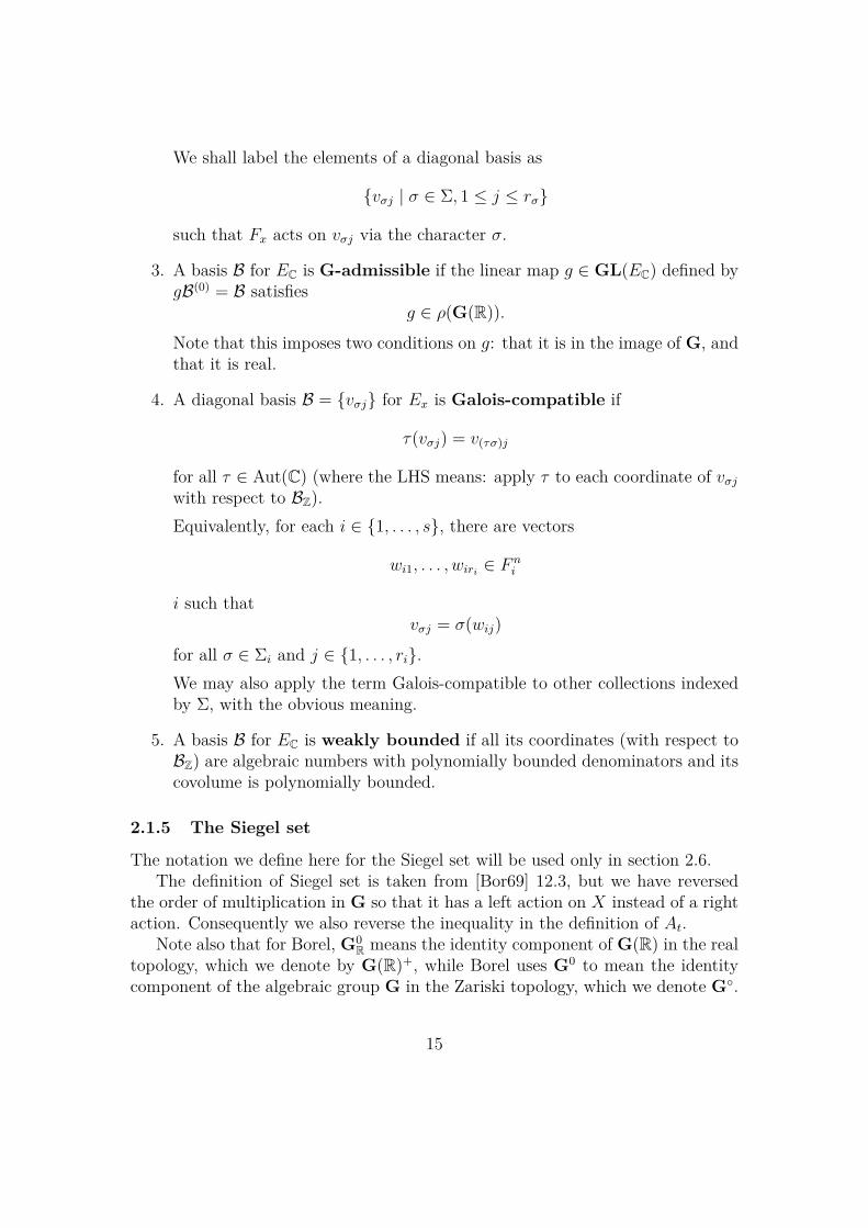
We shall label the elements of a diagonal basis as
{vσj | σ ∈ Σ, 1 ≤ j ≤ rσ}
such that Fx acts on vσj via the character σ.
3. A basis B for EC is G-admissible if the linear map g ∈ GL(EC) defined bygB(0) = B satisfies
g ∈ ρ(G(R)).
Note that this imposes two conditions on g: that it is in the image of G, andthat it is real.
4. A diagonal basis B = {vσj} for Ex is Galois-compatible if
τ(vσj) = v(τσ)j
for all τ ∈ Aut(C) (where the LHS means: apply τ to each coordinate of vσjwith respect to BZ).Equivalently, for each i ∈ {1, . . . , s}, there are vectors
wi1, . . . , wiri ∈ F ni
i such thatvσj = σ(wij)
for all σ ∈ Σi and j ∈ {1, . . . , ri}.We may also apply the term Galois-compatible to other collections indexedby Σ, with the obvious meaning.
5. A basis B for EC is weakly bounded if all its coordinates (with respect toBZ) are algebraic numbers with polynomially bounded denominators and itscovolume is polynomially bounded.
2.1.5 The Siegel set
The notation we define here for the Siegel set will be used only in section 2.6.The definition of Siegel set is taken from [Bor69] 12.3, but we have reversed
the order of multiplication in G so that it has a left action on X instead of a rightaction. Consequently we also reverse the inequality in the definition of At.
Note also that for Borel, G0R means the identity component of G(R) in the real
topology, which we denote by G(R)+, while Borel uses G0 to mean the identitycomponent of the algebraic group G in the Zariski topology, which we denote G◦.
15

By definition, the Siegel set S has the form
S = ωAtK
where
(i) K is the stabiliser of x0 in G(R),
(ii) At = {a ∈ S(R)+ | ϕ(a) ≥ t for all simple Q-roots ϕ of G w.r.t. U} forsome t ∈ R>0,
(iii) ω is a compact neighbourhood of the identity in U(R)M(R)+,
(iv) S is a maximal Q-split torus in G,
(v) M is the maximal Q-anisotropic subgroup of ZG(S)◦, and
(vi) U is the unipotent radical of a minimal Q-parabolic subgroup of G contain-ing S.
Without loss of generality, we may assume that ρ(S) is contained in the set ofdiagonal matrices and ρ(U) in the set of upper triangular matrices of GL(E) withrespect to BZ – this simply requires us to replace BZ by a fixed GL(EQ)-conjugate,which makes a bounded change to |discRx|.
By [Bor69] 13.1, our fundamental set F has the form
F = C.S.x0
for some finite set C ⊂ G(Q).
2.2 A G-admissible diagonal basisWe prove that there exists a G-admissible diagonal basis for Ex. First we constructg1 ∈ G(R) which maps x0 to x and which conjugates the fixed maximal torus T0to a maximal torus containing the Mumford–Tate group of x. Then we let B(1) =g1B(0). This is automatically a G-admissible Hodge basis which diagonalises theMumford–Tate group of x, and we prove that this implies that it is a diagonalbasis.
Lemma 2.1. There exists g1 ∈ G(R) such that g1x0 = x and g1T0g−11 contains
the Mumford–Tate group of Ex.
16

Proof. First choose any g ∈ G(R) such that gx0 = x. Then gT0g−1 is a maximal
R-torus of G containing the image of x, but it might not contain the Mumford–Tate group of Ex.
Choose any maximal torus T ⊂ G defined over R which contains the Mumford–Tate group of Ex. Then gT0g
−1 and T are both maximal R-tori in Kx, the sta-biliser of x in G(R). Since Kx is compact, there is some g′ ∈ Kx which conjugatesgT0g
−1 into T.Taking g1 = g′g proves the lemma (g1x0 = x because g′ stabilises x).
Lemma 2.2. Let B be a Hodge basis for Ex. If B diagonalises the Mumford–Tategroup of Ex, then B is a diagonal basis for Ex.
Proof. Let M ⊂ G be the Mumford–Tate group of Ex.We write End ρ|M for the endomorphism algebra of theQ-representation ρ|M : M→
GL(E), considered as a subalgebra of End(EQ). It is a standard property ofMumford–Tate groups that
End ρ|M = EndQ-HS Ex
and hence the centre of End ρ|M is Fx.Let Z denote the centre of the centraliser of M in GL(E). Since the Q-points of
the centraliser of M in GL(E) are the same as the invertible elements of End ρ|M,we deduce that Z(Q) = F×x (as subgroups of GL(EQ)).
Since M is commutative, M ⊂ Z and so each eigenspace for Z in EC iscontained in an eigenspace for M in EC. We need to establish the inclusion ofeigenspaces in the opposite direction.
The isotypic decomposition of the Q-Hodge structure Ex is
Ex =⊕
iEx,i (*)
where Ex,i is isomorphic to the ri-th power of an irreducible Q-Hodge structurewith endomorphism algebra Fi. Because sub-Q-Hodge structures are the same assubrepresentations of the Mumford–Tate group, this is the same as the isotypicdecomposition of the Q-representation ρ|M. Since M is a torus, it follows thateach eigenspace of M in EC is contained in one of the Ex,i and has dimension ri.
By looking at the action of End ρ|M, we see that (*) is also the isotypic decom-position of the Q-representation ρ|Z, and hence that every eigenspace of Z in ECis contained in one of the Ex,i and has dimension ri.
Thus each eigenspace of Z in EC has the same dimension ri as the eigenspaceof M which contains it, so the eigenspaces of Z are equal to the eigenspaces ofM. Thus the fact that B diagonalises M implies that it also diagonalises Z (or inother words, it diagonalises the action of Fx on Ex).
17

Proposition 2.3. There exists a G-admissible diagonal basis B(1) = {v(1)σj } for Ex.
Proof. Choose g1 as in Lemma 2.1, and let B(1) = g1B(0). Since g1x0 = x, thisgives a Hodge basis for Ex.
Since B(0) diagonalises T0, B(1) diagonalises g1T0g−11 and hence a fortiori M.
Lemma 2.2 implies that B(1) is a diagonal basis for Ex.Finally B(1) is G-admissible because g1 ∈ G(R).
2.3 A weakly bounded diagonal basisIn order to prove the existence of a weakly bounded diagonal basis, we need ageneralisation of Minkowski’s bound to arbitrary lattices in a module over a prod-uct of number fields. This is essentially Claim 3.1 from [PT13] (the generalisationof Minkowski’s bound from ideals in a ring of integers to lattices), but we haveincluded all the generalisations we will need in a single statement: working in avector space over a number field rather than in the field itself, and working witha product of number fields rather than just a single field.
The deduction of Proposition 2.5 from Lemma 2.4 is essentially just bookkeep-ing. The construction gives us Galois-compatibility for free.
Lemma 2.4. For all positive integers d, s and r1, . . . , rs, there are constants C15and C16 depending on d, s and r1, . . . , rs such that:
For all number fields F1, . . . , Fs of degree at most d and all Z-lattices
L ⊂∏i
F rii ,
if we let F = ∏i Fi, R = StabF L and L0 = ∏
iOriFi, then there exists ν ∈∏i GLri(Fi) such that
νL ⊂ L0 and [L0 : νL] ≤ C15 |discR|C16 .
Proof. Let OF = ∏iOFi ⊂ F , and let eR = [OF : R]. Then
discR = e2R
∏i
discFi.
Let L′ = OF .L. Then L′ is an OF -module such that
eRL′ ⊂ L ⊂ L′.
This implies that [L′ : L] ≤ erkZ LR .
Since L′ is an OF -module, it splits as a direct sum
L′ =⊕i
L′i
18

where each L′i ⊂ F rii is an OFi-module of rank ri. Furthermore since OFi is
a Dedekind domain, L′i is isomorphic (as an OFi-module) to Ori−1Fi⊕ Ji for some
ideal Ji ⊂ OFi . By Minkowski’s first theorem, we can choose Ji such that [OFi : Ji]is bounded above by |discFi|1/2 times a constant depending only on d.
In other words, there exists νi ∈ GLri(Fi) such that νiL′i = Ori−1Fi⊕ Ji, which
is contained in OriFi with index bounded by a constant times |discFi|1/2.Letting ν = (ν1, . . . , νs) ∈
∏i GLri(Fi), we get that
νL ⊂ νL′ ⊂ L0 and [L0 : νL] = [L′ : L]∏i
[OriFi : νL′i]
and these indices are bounded relative to |discR| as required.
Proposition 2.5. There exists a Galois-compatible weakly bounded diagonal basisB(2) = {v(2)
σj } for Ex.
Proof. Choose an isomorphism of Fx-modules ι : ∏i Frii → EQ. Choose ν as in
Lemma 2.4 applied to L = ι−1(EZ), and replace ι by ι ◦ ν−1. Then
EZ ⊂ ι(L0) and [ι(L0) : EZ] is polynomially bounded.
There is a natural isomorphism of C-vector spaces∏i
F rii ⊗Q C→ Cn
built using all the embeddings Fi → C on each copy of Fi. Let BF be the basis for∏i F
rii which maps to the standard basis of Cn under this isomorphism, and let
B(2) = ι(BF ).
This consists of eigenvectors for the action of Fx on Ex. If we order the vectorsof B(2) appropriately, then it will satisfy the condition on Hodge types to be aHodge basis for Ex, giving us a diagonal basis for Ex.
Let P denote the matrix giving the coordinates of BZ with respect to B(2), inother words
ej′ =∑σ∈Σ
rσ∑j=1
Pσjj′v(2)σj
where the rows of P are indexed by (σ, j) ∈ ⋃si=1 Σi×{1, . . . , ri} and the columnsare indexed by j′ ∈ {1, . . . , n}.
Because BZ ⊂ ι(L0), the entries of P are algebraic integers and Aut(C) per-mutes the rows of P in the natural way i.e.
τ(Pσjj′) = P(τσ)jj′ .
19

Furthermore
detP = Vol(B(2) : BZ) = Vol(BF : L0) Vol(L0 : EZ) =(∏i
|discFi|ri/2)[L0 : EZ]
so (detP )2 is a polynomially bounded rational integer.Hence P−1 has entries which are algebraic numbers with polynomially bounded
denominators and its determinant is polynomially bounded (indeed detP−1 ≤ 1).Since P−1 gives the coordinates of B(2) with respect to BZ, this says that B(2) isweakly bounded.
Since Aut(C) permutes the rows of P , it permutes the columns of P−1 in thenatural way, and thus B(2) is Galois-compatible.
2.4 A weakly bounded diagonal basis with polynomiallybounded polarisation
In order to construct B(3), we perform a long calculation with Hermitian forms.The key step is Lemma 3.5 from [PT13]. Essentially we want to apply this lemmato the values of the positive definite Hermitian form
Θx(u, v) = ΨC(u, x(i)v)
on B(2), but we have to tweak these values slightly (by using ζ constructed usingLemma 2.6) to get a set of values which are Galois-compatible.
Lemma 2.6. For all positive integers d, there exist constants C17 and C18 suchthat:
For every totally real number field F of degree d and every collection of signssσ ∈ {±1} indexed by the embeddings σ : F → R, there exists an element ζ ∈ F×such that
H(ζ) ≤ C17 |discF |C18
and for each σ : F → R, the sign of σ(ζ) is sσ.
Proof. Consider the lattice of integers OF in F ⊗Q R ∼= Rd. Minkowski’s sec-ond theorem implies that the covering radius µ of this lattice is bounded by apolynomial in |discF | (with the polynomial depending only on d).
Consider a ball B in F ⊗Q R which has radius greater than µ and which iscontained in the hypercube
{z ∈ F ⊗Q R | 0 < sσσ(z) < 3µ for all σ : F → R}.
20

By the definition of the covering radius, B contains an element ζ of the lat-tice OF . By our choice of B, σ(ζ) has the correct sign for each σ : F → R. Sinceζ is an algebraic integer, its height satisfies
H(ζ) ≤∏
σ : F→R|σ(ζ)| < (3µ)d
which is bounded by a polynomial in |discF | as required.
Lemma 2.7. The determinant of the Hermitian matrix
Θx(B(2),B(2))
is polynomially bounded.
Proof. We have
det Θx(B(2),B(2)) =∣∣∣Vol(B(1) : B(2))
∣∣∣2 det Θx(B(1),B(1)).
NowVol(B(0) : B(1)) = 1
because B(1) is G-admissible and G is semisimple (so det ρ(G) must be trivial).Hence
Vol(B(1) : B(2)) = Vol(B(0) : B(2))
is polynomially bounded because B(2) is weakly bounded. Also
Θx(B(1),B(1)) = Θx0(B(0),B(0))
is constant, so the lemma is proved.
The following lemma is proved in the same way as Lemma 3.5 of [PT13], butfor convenience we have written it down as a general statement with the preciselist of conditions required.
Lemma 2.8. For all positive integers d and r, there are constants C19 and C20depending on d and r such that:
For every number field F of degree at most d and every matrix A ∈ Mr(F ), if
(i) the entries of A have denominator at most D,
(ii) NmF/Q detA ≤ D, and
(iii) for every σ : F → C, σ(A) is Hermitian and positive definite,
21

then there exists Q ∈ GLr(F ) such that the entries of Q are algebraic integers andthe entries xij of Q†AQ satisfy
|σ(xij)| ≤ C19(D |discF |)C20
for all σ : F → C.
Proposition 2.9. There exists a Galois-compatible weakly bounded diagonal basisB(3) = {v(3)
σj } for Ex such that the complex numbers
Θx(v(3)σj , v
(3)σj′)
are polynomially bounded for all σ ∈ Σ, 1 ≤ j, j′ ≤ rσ.
Proof. Since the Hodge structure Ex has weight 0, ρx(i) has eigenvalues ±1. ByLemma 2.6, we can choose an element ζ ∈ F×x which is totally real, such that σ(ζ)has the same sign as the eigenvalue of ρx(i) on v(2)
σ1 for all σ ∈ Σ, and whose heightis polynomially bounded.
DefineAσjj′ = σ(ζ) ΨC(v(2)
σj , v(2)σj′)
for each σ ∈ Σ and 1 ≤ j, j′ ≤ rσ.The way we chose the signs of σ(ζ) implies that
Aσjj′ = |σ(ζ)| Θx(v(2)σj , v
(2)σj′).
Since Θx is a positive definite Hermitian form, we deduce that the square matrix Aσis Hermitian and positive definite for each σ ∈ Σ.
Observe that, for every τ ∈ Aut(C) and σ ∈ Σ, we have τ σ = τσ because Fxis a product of CM fields and Q. Since Ψ is defined over Q, we deduce that
τ(Aσjj′) = A(τσ)jj′
or in other words there are matrices Ai ∈ Mri(Fi) such that
Aσjj′ = σ(Aijj′)
for all 1 ≤ i ≤ s, σ ∈ Σi, 1 ≤ j, j′ ≤ ri.Because B(2) has polynomially bounded denominators and ζ has polynomially
bounded height, the entries of the Ai have polynomially bounded denominators.Furthermore
s∏i=1
NmFi/Q detAi =∏σ∈Σ
detAσ =∏σ∈Σ|σ(ζ)|
det Θx(B(2),B(2)).
22

(We are using the fact that the eigenspaces of Fx are orthogonal to each other withrespect to Θx, so the matrix Θx(B(2),B(2)) is block diagonal with one block foreach σ.) The values |σ(ζ)| are polynomially bounded because ζ has polynomiallybounded height. Using Lemma 2.7, we conclude that
s∏i=1
NmFi/Q detAi
is polynomially bounded.Each value (NmFi/Q detAi)−1 is polynomially bounded because the denomina-
tors of Ai are polynomially bounded. Hence
NmFi/Q detAi
is polynomially bounded for each i.Hence Ai ∈ Mri(Fi) satisfies the conditions of Lemma 2.8 (with D being poly-
nomial in |disc(R)|). So we can choose Qi ∈ GLri(Fi) as in the conclusion of thatlemma.
Letv
(3)σj =
rσ∑j′=1
σ(Qij′j)v(2)σj′
for all 1 ≤ i ≤ s, σ ∈ Σi and 1 ≤ j ≤ rσ.Now B(3) = {v(3)
σj } is a diagonal basis because each v(3)σj is a linear combination
of σ-eigenvectors for Fx. Clearly it is also Galois-compatible.Because the archimedean absolute values of entries of Q†iAiQi are polynomially
bounded,NmFi/Q detQ†iAiQi
is polynomially bounded. As remarked above, (NmFi/Q detAi)−1 is polynomiallybounded. Hence∣∣∣NmFi/Q detQi
∣∣∣2 = (NmFi/Q detQ†iAiQi)(NmFi/Q detAi)−1
is polynomially bounded. We deduce that the covolume of B(3), namely(s∏i=1
NmFi/Q detQi
)Vol(BZ : B(2)),
is polynomially bounded.Furthermore B(3) has bounded denominators because B(2) had bounded denom-
inators and the entries of Qi are algebraic integers. Hence B(3) is weakly bounded.Finally the values
|σ(ζ)| Θx(v(3)σj , v
(3)σj′)
23

are the entries of σ(Q†iAiQi) and so are polynomially bounded. Since ζ has poly-nomially bounded height, we conclude that
Θx(v(3)σj , v
(3)σj′)
are polynomially bounded.
2.5 A G-admissible diagonal basis whose height is boundedrelative to B(3)
In this section we will construct the basis B(4) which is G-admissible, diagonal,and whose coordinates with respect to B(3) have polynomially bounded height.
We begin by considering the coordinates of B(3) with respect to B(1). Usingthe fact that Θx is polynomially bounded on B(3), we show that these coordinatesare polynomially bounded, and deduce that the multilinear form Φ is polynomiallybounded on B(3). Because B(3) is Galois-compatible and has polynomially boundeddenominators, the bound on (the standard absolute value of) the values of Φ on B(3)
implies a bound for the heights of these values.The set of coordinates (with respect to B(3)) of G-admissible diagonal bases
forms an affine algebraic set V0 defined over Qalg ∩ R. Because G is precisely thestabiliser of Φ, we can use Φ to write down equations for V0,Qalg , and then describea suitable (Qalg ∩ R)-form of this algebraic set. The bound for the heights ofvalues of Φ on B(3) implies that these equations have coefficients of polynomiallybounded height, and the existence of a G-admissible diagonal basis B(1) impliesthat V0(R) is non-empty. We can therefore use Theorem 3.1 to obtain an elementof V0(Qalg ∩ R) of polynomially bounded height, and thus B(4).
Lemma 2.10. For each σ ∈ Σ, let Rσ be the matrix in GLrσ(C) such that
v(3)σj =
rσ∑j′=1
Rσj′jv(1)σj′ .
(Such matrices exist because B(1) and B(3) are both diagonal bases for Ex.)The entries of Rσ are polynomially bounded.
Proof. Consider the rσ × rσ matrices
Bσjj′ = Θx(v(1)σj , v
(1)σj′)
andB′σjj′ = Θx(v(3)
σj , v(3)σj′).
24

These matrices are Hermitian positive definite, so they can be diagonalised byunitary matrices:
Bσ = U †σDσUσ and B′σ = U ′†σ D′σU′σ
where Uσ, U′σ are unitary matrices and Dσ, D
′σ are diagonal with positive real
entries. We can then choose further diagonal matrices Λσ with positive real entriessuch that
Λ2σDσ = D′σ.
Observe thatBσjj′ = Θx0(v(0)
σj , v(0)σj )
and hence does not depend on x. Thus Dσ and Uσ are constant.The entries of U ′σ are bounded by 1 because it is a unitary matrix. The entries
of B′σ are polynomially bounded by the construction of B(3). Hence the entries ofD′σ, and therefore also Λσ, are polynomially bounded.
LetR′σ = U †σΛσU
′σ ∈ GLrσ(C).
This has polynomially bounded entries and satisfies
B′σ = R′†σBσR
′σ.
But by the definition of R,B′σ = R†σBσRσ.
Hence RσR′−1σ lies in the compact group of Bσ-unitary matrices. Because Bσ is
constant, there is a uniform bound for entries of the entries of Bσ-unitary matrices.Combining this bound for RσR
′−1σ with the polynomial bound for R′σ, we deduce
that Rσ has polynomially bounded entries.
Lemma 2.11. The valuesΦ(v(3)
σ1j1 , . . . , v(3)σkjk
)
are algebraic numbers of polynomially bounded height for all
((σ1, j1), . . . , (σk, jk)) ∈ (⋃i
Σi × {1, . . . , ri})k.
Proof. The definition of Rσ implies that we can express the values of Φ on B(3) interms of its values on B(1) as follows:
Φ(v(3)σ1j1 , . . . , v
(3)σkjk
) =rσ1∑j′1=1· · ·
rσk∑j′k=1Rσ1j′1j1
· · ·Rσkj′kjkΦ(v(1)
σ1j′1, . . . , v
(1)σkj′k).
25

The facts that B(1) is G-admissible and Φ is G-invariant imply that the values ofΦ on B(1) are equal to its values on B(0) and hence constant. Thus Lemma 2.10implies that the values
Φ(v(3)σ1j1 , . . . , v
(3)σkjk
)
are polynomially bounded.The facts that B(3) is Galois-compatible and that Φ is defined over Q imply
thatτ(Φ(v(3)
σ1j1 , . . . , v(3)σkjk
)) = Φ(v(3)(τσ1)j1 , . . . , v
(3)(τσk)jk)
for all τ ∈ Aut(C). Hence the values of Φ on B(3) are algebraic numbers.Because each Φ(v(3)
σ1j1 , . . . , v(3)σkjk
) is polynomially bounded and because thesevalues are Galois-compatible, all Galois conjugates of Φ(v(3)
σ1j1 , . . . , v(3)σkjk
) are poly-nomially bounded. Furthermore the denominators of Φ(v(3)
σ1j1 , . . . , v(3)σkjk
) are poly-nomially bounded because B(3) is weakly bounded. The combination of boundeddenominators and all Galois conjugates being bounded implies that the heightsare polynomially bounded.
Proposition 2.12. There exist matrices Sσ ∈ GLri(C) whose entries are algebraicnumbers of polynomially bounded height and such that the diagonal basis B(4) ={v(4)
σj } defined by
v(4)σj =
rσ∑j′=1
Sσj′jv(3)σj′
is G-admissible.
Proof. Let V denote the Qalg-algebraic set consisting of those elements
S := (Sσ)σ∈Σ ∈∏σ∈Σ
GLrσ
which satisfy the equationsr1∑j1=1· · ·
rk∑jk=1
Sσ1j′1j1· · ·Sσkj′kjkΦ(v(3)
σ1j′1, . . . , v
(3)σkj′k) = Φ(v(1)
σ1j1 , . . . , v(1)σkjk
) (*)
for all tuples((σ1, j1), . . . , (σk, jk)) ∈
(⋃i
Σi × {1, . . . , ri})k.
Observe that the basis
B(3)S ={ rσ∑j′=1
Sσj′jv(3)σj′ | σ ∈ Σ, 1 ≤ j ≤ rσ
}
26

is always diagonal. The purpose of the algebraic set V is that the basis B(3)S is ofthe form gB(0) for some g ∈ G(C) if and only if S ∈ V (C).
We will now construct a (Qalg∩R)-form V0 of V such that B(3)S is G-admissibleif and only if S ∈ V0(R).
Recall that, when choosing B(0), we required that for each v ∈ B(0), its complexconjugate is also in B(0). Since B(1) = g1B(0) for some real linear map g1, it followsthat B(1) has the same property. Clearly, if Fx acts on v via the character σ, thenit acts on v via the character σ. Hence for each σ ∈ Σ, there is a permutationβ(σ,−) of {1, . . . , rσ} defined by
v(1)σj = v
(1)σβ(σ,j).
(The subscript on the right hand side of that equation might be hard to read: itis σβ(σ, j).) On the other hand, because B(3) is Galois-compatible, we have
v(3)σj = v
(3)σj .
Define a semilinear involution θ of ∏σ∈Σ GLrσ ,Qalg by
θ(S)σj′j = Sσj′β(σ,j).
By construction, a tuple of matrices S ∈ ∏Σ GLrσ(C) satisfies θ(S) = S if andonly if the basis B(3)S is permuted by complex conjugation in the same fashion asB(1), or in other words, if and only if the linear map transforming B(1) into thisbasis is defined over R. Thus B(3)S is G-admissible if and only if S ∈ V (C) andθ(S) = S.
Because Φ is defined over Q (so a fortiori over R), composing one of theequations (*) with θ transforms it into another of the equations (*). Hence thereis a (Qalg ∩ R)-form V0 of V on which the action of complex conjugation is givenby θ. In particular
V0(R) = {S ∈ V (C) | θ(S) = S}
and thus B(3)S is G-admissible if and only if S ∈ V0(R).The (Qalg ∩ R)-variety V0 is defined by the equations
f + θ(f), i(f − θ(f))
as f runs over the equations (*). The number of equations (*) depends only on thecombinatorial data s, r1, . . . , rs (for which there are finitely many possibilities), andtheir degrees are fixed. By Lemma 2.11, their coefficients are algebraic numbersof polynomially bounded height. Hence V0 is defined by a finite set of polynomialssuch that the number of polynomials in the set is uniformly bounded, the degree
27

of each of the polynomials is uniformly bounded and their coefficients are elementsof Qalg ∩ R of polynomially bounded height.
Furthermore V0(R) is non-empty because R−1 ∈ V0(R) (recall that R wasdefined in Lemma 2.10 as the tuple of matrices such that B(3) = B(1)R).
Thus we can apply Theorem 3.1 to V0, to deduce that V0(Qalg ∩ R) contains apoint S of polynomially bounded height. This is the S whose existence is assertedby the proposition.
2.6 Bounding the height of B(4)
The main work in this section is showing that the coordinates of B(4) (with respectto BZ) are polynomially bounded in absolute value. We will then (by going to B(3)
and back) deduce that these coordinates have polynomially bounded height.Notation-wise, we shall consider E∨C as a space of row vectors and write ‖·‖ for
the standard Hermitian norm on E∨C with respect to the basis dual to BZ. For anymatrix M ∈ GLn(C), we shall write λmin(M) for the minimum of the absolutevalues of eigenvalues of M .
Let g0, g3, g4 ∈ GL(EC) be the linear maps such that
B(0) = g0BZ, B(3) = g3B(0) and B(4) = g4B(0).
We will interpret these linear maps as matrices in GLn(C) with respect to thebasis BZ. Then the coordinates of B(3) and B(4) (with respect to BZ) are given bythe columns of g3g0 and g4g0 respectively.
Let S ′ denote the matrix in GL(EC) which expresses the coordinates of B(4)
with respect to B(3). In other words,
g4g0 = g3g0S′.
By the construction of B(4), S ′ can be obtained by taking the block diagonal matrixwith blocks Sσ from Proposition 2.12, and permuting the rows and columns tomatch the orderings of the bases B(3) and B(4).
Since B(4) is G-admissible, we have g4 ∈ G(R). Since B(4) is diagonal for Ex,we have g4x0 = x in the symmetric space X. Since x4 is in the fundamental setF = C.S.x0, we have g4 ∈ C.S. We can therefore write
g4 = γνακ
with γ ∈ C, ν ∈ ω, α ∈ At and κ ∈ K.
Lemma 2.13. For all e∨ ∈ E∨Z − {0},
‖e∨g4‖−1
is polynomially bounded.
28

Proof. We have
‖e∨g4‖ = ‖e∨g3 g0S′g−1
0 ‖ ≥ λmin(S ′g−10 )‖e∨g3g0‖.
By Proposition 2.12, the entries of S ′ are algebraic numbers with polynomiallybounded height, while g0 is a constant matrix whose entries are algebraic num-bers. Hence the entries of S ′g−1
0 are algebraic numbers with polynomially boundedheight, so the same is true of its eigenvalues. Hence λmin(S ′g−1
0 )−1 is polynomiallybounded.
The row vector e∨g3g0 is a Z-linear combination of rows of g3g0. Since B(3) isGalois-compatible and weakly bounded, the coordinates of e∨g3g0 are a set of al-gebraic numbers which are closed under Galois conjugation and have polynomiallybounded denominators. Hence ‖e∨g3g0‖2 is a rational number with polynomiallybounded denominator.
Furthermore ‖e∨g3g0‖2 6= 0 because g3g0 is invertible. A non-zero rational num-ber with polynomially bounded denominator has polynomially bounded inverse,so ‖e∨g3g0‖−1 is polynomially bounded.
Lemma 2.14. For 1 ≤ j ≤ n,‖e∨j να‖−1
is polynomially bounded.
Proof. By definition, να = γ−1g4κ−1.
Since κ is contained in the constant compact set K, for any v∨ ∈ E∨C , ‖v∨κ−1‖is bounded between constant multiples of ‖v∨‖. Hence it will suffice to prove that‖e∨j γ−1g4‖−1 is polynomially bounded.
Since γ lies in the constant finite set C ⊂ G(Q), there is a uniform bound forthe denominator of γ−1. Thus e∨j γ−1 lies in a constant rational multiple of E∨Z ,and so Lemma 2.13 implies that ‖e∨j γ−1g4‖−1 is polynomially bounded.
Lemma 2.15. There exists a positive integer ` depending only on G such that:For any ν ∈ U(R)M(R)+ and α ∈ At, if νjj′ 6= 0, then
αjj ≥ min(1, t`)αj′j′ .
Proof. Let ν = um with u ∈ U(R) and m ∈M(R)+.Since νjj′ 6= 0, there exists i ∈ {1, . . . , n} such that ujimij′ 6= 0.Since U(R) is unipotent, its Lie algebra is the vector subspace of GLn(R)
spanned by {u− 1 | u ∈ U(R)}. In particular, since uji 6= 0, either i = j or thereis some U ∈ Lie U(R) such that Uji 6= 0.
Suppose that there is U ∈ Lie U(R) such that Uji 6= 0. Since the conjugationaction of the Q-split torus S on U is diagonalisable over Q, we may assume thatU is an eigenvector for S, while still satisfying Uji 6= 0.
29

Let ϕ be the Q-root of G specifying how S acts on U . Because S is containedin the diagonal torus of GLn, for every s ∈ S,
((Ad s)U)ji = (sjj/sii)Uji
and so ϕ(s) = sjj/sii.By definition, ϕ is a positive root with respect to U, so it can be expressed as
a sum of at most ` positive simple Q-roots of G, for some constant ` dependingonly on G. Since α ∈ At, we conclude that ϕ(α) ≥ t`.
Thus we get αjj/αii ≥ t` whenever i 6= j. Combining with the trivial casei = j, we get that
αjj ≥ min(1, t`)αii.Since M centralises S and S is diagonal,
αiimij′ = mij′αj′j′ .
Since mij′ 6= 0, we deduce that αii = αj′j′ so the lemma is proved.
Lemma 2.16. The values α−1jj are polynomially bounded.
Proof. We have‖e∨j να‖2 =
n∑j′=1
(νjj′αj′j′)2.
Using Lemma 2.15, we deduce that
‖e∨j να‖2 ≤n∑
j′=1ν2jj′ min(1, t`)−2α2
jj.
Since ν is in the fixed compact set ω, there is a uniform upper bound for |νjj′ |.Hence αjj is bounded below by a uniform constant multiple of ‖e∨j να‖. Com-
bining with Lemma 2.14, we deduce that α−1jj is polynomially bounded.
Proposition 2.17. The coordinates of B(4) with respect to BZ are polynomiallybounded in absolute value.
Proof. Since S ′ has determinant of polynomially bounded height and B(3) is weaklybounded, g4 has polynomially bounded determinant. Now
n∏j=1
αjj = detα = |det γ|−1 |det g4|
because det ν = |detκ| = 1. Since γ is in the fixed finite set C, ∏αjj is polynomi-ally bounded.
30

Combining this bound for ∏αjj with the bound for all α−1jj from Lemma 2.16,
we deduce that each αjj is polynomially bounded.Since each of γ, ν and κ is contained in a fixed finite set, this implies that the
entries of g4 = γνακ are polynomially bounded.Since the coordinates of B(4) are given by g4g0, they are also polynomially
bounded.
Proposition 2.18. The coordinates of B(4) with respect to BZ are algebraic num-bers of polynomially bounded height.
Proof. Since S ′ gives the coordinates of B(4) with respect to B(3) and has entriesof polynomially bounded height, Proposition 2.17 implies that the coordinates ofB(3) with respect to BZ are polynomially bounded in absolute value.
Since B(3) is Galois-compatible, this tells us that each coordinate of a vectorin B(3) in fact has all its Galois conjugates polynomially bounded. Furthermoreits denominator is polynomially bounded, because B(3) is weakly bounded. Hencethe heights of the coordinates of B(3) are polynomially bounded.
Again using the fact that S ′ has polynomially bounded height, we concludethat the heights of the coordinates of B(4) are polynomially bounded.
Proof of Theorem 1.1. Proposition 2.18 implies that the entries of g4 are algebraicnumbers of polynomially bounded height. Since x = g4x0 and the action of G(R)on X is semialgebraic over Qalg ∩ R, it follows that the coordinates of x ∈ X alsoare algebraic with polynomially bounded height.
3 Points of small height on real affine varietiesLet V be an affine algebraic set defined overQalg. Suppose that V can be defined bya fixed number of polynomials in a fixed number of variables and of fixed degrees,such that the coefficients of these polynomials have height at most H. Then thearithmetic Bézout theorem and Zhang’s theorem on the essential minimum implythat V has a Qalg-point whose height is bounded by a polynomial in H.
For our application to pre-special points, we need a variant of this result: weassume that V is defined over Qalg ∩ R and we need to show that V (Qalg ∩ R)contains a point of polynomially bounded height. (For us, Qalg means the set ofalgebraic numbers in C rather than an abstract algebraic closure of Q, so Qalg ∩Ris well-defined.) To avoid trivial counter-examples, we must also assume that V (R)is non-empty.
Theorem 3.1. For all positive integers m, n, D, there are constants C13 and C14depending on m, n and D such that:
31

For every affine algebraic set V ⊂ An defined over Qalg ∩ R by polynomialsf1, . . . , fm ∈ (Qalg ∩ R)[X1, . . . , Xn] of degree at most D and height at most H, ifV (R) is non-empty, then V (Qalg ∩R) contains a point of height at most C13H
C14.
We will prove the theorem by an elementary argument, using a quantitativeversion of the Noether normalisation lemma. The proof is by induction on n.
Given an algebraic set in An, the following lemma constructs an algebraic set inAn−1 satisfying appropriate bounds, which we can then study inductively. Part (i)of the lemma is simply the inductive step of the Noether normalisation lemma,without any height bound. Parts (ii) to (iv) allow us to find a point of small heightin V , once we have got such a point in πφ(V ). Part (v) ensures that as we carryout the induction, replacing V ⊂ An by πφ(V ) ⊂ An−1, the number, degrees andheights of the defining polynomials remain controlled. (Parts (i) to (iii) work whenk is any field of characteristic zero. For (iv) and (v) the field must be containedin Qalg so that we have a notion of height.)
Lemma 3.2. Let V ⊂ An be an affine algebraic set defined over a field k ⊂ Qalg.Suppose that V can be defined by m polynomials with coefficients in k, each ofdegree at most D and height at most H.
If V 6= An, then there exists a linear automorphism φ of kn such that:
(i) (πφ)|V : V → An−1 is a finite morphism (where π : An → An−1 means projec-tion onto the first n− 1 coordinates);
(ii) the matrix representing φ w.r.t. the standard basis has entries in Z withabsolute values at most D;
(iii) there exists a polynomial g ∈ k[X1, . . . , Xn−1][Xn] which vanishes on φ(V )and which is monic of degree at most D in Xn (we do not require that φ(V ) ={x | π(x) ∈ πφ(V ) and g(x) = 0});
(iv) the height of g is bounded by a polynomial in H;
(v) the image πφ(V ) can be defined by polynomials in k[X1, . . . , Xn−1] such thatthe number and degree of these polynomials are bounded by bounds dependingon m and D only, and their heights are bounded by a polynomial in H.
Here “bounded by a polynomial in H” means bounded by an expression of the formC21H
C22 where C21 and C22 are constants which depend on n, m and D only.
Using Lemma 3.2, we can directly prove the simplified version of Theorem 3.1which only concerns Qalg-points. Indeed, by induction on n we get a point
x = (x1, . . . , xn−1) ∈ πφ(V )(Qalg)
32

of polynomially bounded height. Parts (iii) and (iv) of the lemma imply thatany point in the fibre π−1(x) ∩ φ(V )(Qalg) also has polynomially bounded height,because its xn-coordinate must be a root of g(x1, . . . , xn−1)(Xn). Then part (ii)allows us to transform this into a point of polynomially bounded height in V .
This argument is not sufficient to obtain a (Qalg ∩ R)-point of small heighton V . This is because the fibre π−1(x) ∩ φ(V ) at our chosen x is not guaranteedto contain any real points.
In order to deal with this, we will strengthen the inductive hypothesis slightlyas follows:
Theorem 3.3. In the setting of Theorem 3.1, each connected component Z ofV (R) (in the real topology) contains a (Qalg ∩R)-point of height at most C13H
C14.
We then consider the boundary of πφ(Z), viewed as a subset of πφ(V )(R).If πφ(Z) is an entire connected component of πφ(V )(R), then by the inductivehypothesis it contains a (Qalg ∩ R)-point of polynomially bounded height and wecan apply the same argument as above to get a (Qalg ∩ R)-point of small heightin Z.
So the interesting case is when πφ(Z) has non-empty boundary in πφ(V )(R).At a point (x1, . . . , xn−1) on the boundary of πφ(Z), an analytic argument impliesthat either g(x1, . . . , xn−1)(Xn) has a double root, or πφ(V ) is singular. In eithercase we can find an algebraic subset V ′ ⊂ V , of smaller dimension and defined bypolynomials satisfying the appropriate bounds on number, degree and height, suchthat Z ∩V ′(R) is non-empty, so we can replace V by V ′ and repeat the argument.
If g(x1, . . . , xn−1)(Xn) has a double root at some point of πφ(Z), then it isstraightforward to construct V ′. In order to construct V ′ when πφ(V ) has asingular point, we use Proposition 3.11, which we prove using the Chow form andan idea of Bombieri, Masser and Zannier.
3.1 DefinitionsThroughout this section, k denotes a field of characteristic 0.
We will denote by π the linear map An → An−1 given by projection onto thefirst n− 1 coordinates.
We identify an algebraic set over k with its set of kalg-points. When we saythat an algebraic set V is defined by polynomials f1, . . . , fm, we mean simply that
V (kalg) = {(x1, . . . , xn) ∈ An(kalg) | fi(x1, . . . , xn) = 0 for all i}.
In particular, we do not require the ideal (f1, . . . , fm) ⊂ k[X1, . . . , Xm] to be aradical ideal.
33

Symbols Ci will denote constants; the first time we introduce each constant wewill specify the parameters on which it depends. Usually Ci depends on degreesbut not heights.
We define the height of a point (x1, . . . , xn) ∈ An(Qalg) to be the multiplicativeabsolute Weil height of [x1 : · · · : xn : 1] ∈ Pn(Qalg), that is
H(x1, . . . , xn) =∏v
max(|x1|v , . . . , |xn|v , 1)dv/[K:Q]
where K is any number field containing x1, . . . , xn, the product is over all placesof K and dv = [Kv : Qp] or [Kv : R] as appropriate, with the absolute valuesnormalised so that they agree with the standard absolute value when restricted toQp or R.
The height of a polynomial in Qalg[X1, . . . , Xn] means the multiplicative ab-solute Weil height of the point in projective space whose homogeneous coordinatesare the coefficients of the polynomial.
Lemma 3.4. If f ∈ Qalg[X] is a monic polynomial in one variable of degree d andx is a root of f , then
H(x) ≤ dH(f).
Proof. Letf(X) = Xd + ad−1X
d−1 + · · ·+ a0.
and let K be a number field containing a0, . . . , ad−1, x.For each absolute value |·| of K,
max(|x| , 1)d = max(∣∣∣ad−1x
d−1 + · · ·+ a0
∣∣∣ , 1)
≤ dmax(∣∣∣ad−1x
d−1∣∣∣ , . . . , |a0| , 1)
≤ dmax(|ad−1| , . . . , |a0| , 1) max(|x| , 1)d−1
so thatmax(|x| , 1) ≤ dmax(|ad−1| , . . . , |a0| , 1)
and the factor of d (coming from the triangle inequality) can be replaced by 1 fornon-archimedean absolute values.
Taking the product over all places of K gives the result.
3.2 Bounded normalisation lemmaWe will now prove parts (i) to (iv) of Lemma 3.2. Our proof is based on the proofof the Noether normalisation lemma in exercise 5.16 of [AM69].
34

Let us remark that the bound in part (ii) is stronger than most of our bounds:the height of φ is bounded only in terms of the degrees of the defining equationsfor V , independent of the height of these equations. We do not need this extrastrength. In order to obtain this bound in part (ii), we will use the followinglemma.
Lemma 3.5. Let f ∈ k[X1, . . . , Xn] be a non-zero polynomial of degree at most D(over any field k of characteristic zero). There exist integers λ1, . . . , λn, such that|λi| ≤ D for all i, λi 6= 0 for all i and
f(λ1, . . . , λn) 6= 0.
Proof. The proof is by induction on n. Write
f(X1, . . . , Xn) =D∑i=0
gi(X1, . . . , Xn−1)X in.
The gi are polynomials in k[X1, . . . , Xn−1] of degree at most D.Choose some i such that gi 6= 0. By induction, there are non-zero integers
λ1, . . . , λn−1, with absolute value at most D, such that
gi(λ1, . . . , λn−1) 6= 0.
Then f(λ1, . . . , λn−1, Xn) is a non-zero polynomial in one variable Xn. It hasdegree at most D, so it has �most D roots.
Hence the set of D + 1 values {−1, 1, 2, . . . , D} contains at least one non-rootof f(λ1, . . . , λn−1, Xn), as required.
Proof of Lemma 3.2 (i)–(iv). Let f = f1. This is a polynomial in k[X1, . . . , Xn]of degree at most D which vanishes on V , and without loss of generality f 6= 0.
Let F denote the homogeneous polynomial consisting of the terms of f withhighest total degree. By Lemma 3.5, we can find non-zero integers λ1, . . . , λn, withabsolute value at most D, such that
F (λ1, . . . , λn) 6= 0.
Let φ : An → An be the k-linear map with matrixλn −λ1
. . . ...λn −λn−1
1
This is invertible because λn 6= 0. It satisfies (ii) by construction.
35

Let g ∈ k[X1, . . . , Xn] be the polynomial
g(X1, . . . , Xn) = f(φ−1(X1, . . . , Xn)).
Observe that g vanishes on φ(V ).Let G be the homogeneous polynomial consisting of the terms of g with highest
total degree. Then
G(0, . . . , 0, λn) = F (φ−1(0, . . . , 0, λn)) = F (λ1, . . . , λn) 6= 0.
Since G is homogeneous and λn 6= 0, we deduce that
G(0, . . . , 0, 1) 6= 0.
Let d denote the total degree of G. Then G(0, . . . , 0, 1) is the coefficient of theXdn term of g, and all other terms in g have a lower power ofXn. Hence after scaling
by G(0, . . . , 0, 1)−1, g(X1, . . . , Xn) is monic of degree d ≤ D as a polynomial in theone variable Xn with coefficients in k[X1, . . . , Xn−1]. Thus (iii) is satisfied.
The coordinate ring k[φ(V )] is generated as a k[X1, . . . , Xn−1]-algebra by Xn.Furthermore, since g is monic in Xn and vanishes on φ(V ), we deduce that Xn
(viewed as an element of k[φ(V )]) is integral over k[X1, . . . , Xn−1]. Hence k[φ(V )]is finite as a k[X1, . . . , Xn−1]-algebra. In other words, the morphism π|φ(V ) is finite.Since φ is invertible, (i) is satisfied.
Since f , φ and G(0, . . . , 0, 1) all have height bounded by a polynomial in H,the same is true of g, so (iv) holds.
3.3 Bounding the image of normalisationWe wish to prove part (v) of Lemma 3.2, i.e. that the image πφ(V ) has polyno-mially bounded height–complexity. Note first that πφ(V ) is indeed Zariski-closedbecause πφ|V is finite.
Take the polynomials f1 ◦ φ−1, . . . , fm ◦ φ−1 which define V ′ = φ(V ), andlabel them g1, . . . , gr, h1, . . . , hs such that the gi all contain Xn while the hi do notcontain Xn. A point (x1, . . . , xn−1) ∈ An−1(kalg) is in πφ(V ) if and only if all the hivanish at (x1, . . . , xn−1) and all the one-variable polynomials gi(x1, . . . , xn−1)(Xn)have a common root xn. So the problem is to write down algebraic conditionson the coefficients which recognise when a set of one-variable polynomials withvarying coefficients has a common root.
Given two one-variable polynomials, we can recognise when they have a com-mon root using the resultant. More precisely: for each pair of integers (d, e),there is a universal polynomial Resd,e ∈ Z[a0, . . . , ad, b0, . . . , be] such that for allone-variable polynomials u of degree d and v of degree e, Resd,e vanishes on thecoefficients of u and v if and only if u and v have a common root in kalg.
36

We must take care about what happens when we plug polynomials into Resd,ewhose degrees are smaller than the expected degrees d and e. It turns out that, ifboth deg u < d and deg v < e, then Resd,e(u, v) is always zero. If deg u = d anddeg v < e (or vice versa), then as usual, Resd,e(u, v) = 0 if and only if u and v havea common root. Essentially, in the case where both deg u < d and deg v < e, thefact that Resd,e(u, v) = 0 is telling us that the degree-d homogenisation of u andthe degree-e homogenisation of v have a common root at ∞ ∈ P1(kalg).
To determine whether a set of more than two polynomials have a common root,we just have to look at the resultants of sufficiently many linear combinations ofthem.
Lemma 3.6. Let g1, . . . , gr ∈ k[X] be polynomials in one variable, with degree atmost D. Let d = deg g1.
The polynomials g1, . . . , gr share a common root in kalg if and only if
Resd,D(g1, λ2g2 + λ3g3 + · · ·+ λr−1gr−1 + gr) = 0
for all (λ2, . . . , λr−1) ∈ {0, . . . , d}r−2.
Proof. The “only if” direction is clear: if g1, . . . , gr all share a common root, thenevery linear combination of them also vanishes at that point.
For the “if” direction, the proof is by induction on r. For r = 2, this is justthe definition of the resultant. We know that g1 has exactly degree d, so even ifdeg g2 < D the resultant still tells us whether they have a common root.
For r > 2: Suppose that the given resultants are all zero. By induction, forevery λ ∈ {0, . . . , d}, the polynomials
g1, g2, . . . , gr−2, λgr−1 + gr
share a common root αλ. Since each αλ is a root of g1, and g1 has at most d roots,there must be two distinct values λ, µ ∈ {0, . . . , d} such that
αλ = αµ.
Then by construction
λgr−1(αλ) + gr(αλ) = µgr−1(αλ) + gr(αλ) = 0
which implies thatgr−1(αλ) = gr(αλ) = 0.
Thus αλ is the required common root of g1, . . . , gr.
37

The following lemma establishes part (v) of Lemma 3.2. For defining equationsof V ′ = φ(V ), we take f1◦φ−1, . . . , fm◦φ−1 as well as g from part (iii) of Lemma 3.2.Since g vanishes on V ′ by construction, adding it to the set of defining polynomialsdoes not change V ′; g ensures that the condition that one of the polynomials shouldbe monic in Xn is satisfied.
Lemma 3.7. For all positive integers m, n, D, there are constants C23, C24 andC25 depending on m, n and D such that:
For every affine algebraic set V ′ ⊂ An defined over k ⊂ Qalg by at most mpolynomials of degree at most D and height at most H, such that one of thesepolynomials is monic in Xn, the image under projection
π(V ′) ⊂ An−1
is defined by at most C23 polynomials over k, each of degree at most C23 and heightat most C24H
C25.
Proof. Take the polynomials defining V ′, and label them
g1, . . . , gr, h1, . . . , hs
such that the gi all containXn while the hi do not containXn. Choose the labellingsuch that g1 is monic in Xn.
A point (x1, . . . , xn−1) ∈ An−1(kalg) is in π(V ′) if and only if all the hi vanishat (x1, . . . , xn−1) and the one-variable polynomials gi(x1, . . . , xn−1)(Xn) have acommon root.
Let d be the degree of g1 with respect to Xn. Because g1 is monic in Xn, d isequal to deg g1(x1, . . . , xn−1)(Xn) for every (x1, . . . , xn−1) ∈ An−1(kalg).
Hence we can apply Lemma 3.6 at each point of An−1(kalg), the polynomialsgi(x1, . . . , xn−1)(Xn) have a common root if and only if
Resd,D(g1, λ2g2 + λ3g3 + · · ·+ λr−1gr−1 + gr) = 0
at (x1, . . . , xn−1) for all (λ2, . . . , λm−1) ∈ {0, . . . , d}r−2.These resultants give us a set of (d+1)r−2 polynomials in k[X1, . . . , Xn−1] which,
together with h1, . . . , hs, define π(V ′). Because these polynomials are constructedas universal polynomials in the coefficients of g1, . . . , gr, their degrees are boundedby a constant depending on n and D and their heights by a polynomial in H.
We have completed the proof of Lemma 3.2 and, as remarked below the state-ment of Lemma 3.2, it is straightforward to deduce a version of Theorem 3.1 whichonly concerns Qalg-points.
38

3.4 Behaviour of real points under projectionIn order to obtain (Qalg ∩ R)-points of small height, and not just Qalg-points, welook at the image of a single connected component of V (R) under πφ. As explainedin the introduction to the section the difficult case is when this image is strictlycontained in a connected component of πφ(V )(R).
The principle we use to deal with this is that, in a smoothly varying familyof monic one-variable polynomials such as g(x1, . . . , xn−1)(Xn), real roots cannotdisappear spontaneously: whenever a real root disappears, there must be either arepeated root or a singular point in the base. The condition that the polynomialsare monic ensures that a root cannot disappear off to infinity (such as occurs inx1X2 − 1 = 0 when x1 → 0).
The set of points of πφ(V ) at which g(x1, . . . , xn−1)(Xn) has a repeated root isitself an algebraic set, which is (usually) of smaller dimension than πφ(V ) itself,defined by adding ∂g/∂Xn to the set of polynomials defining πφ(V ). Thus clearlyit is still defined by polynomials of bounded height, and we can apply the inductionhypothesis to this set.
The singular locus of πφ(V ) is likewise an algebraic set of smaller dimension.Controlling the height of polynomials defining the singular locus is more difficult.Indeed, instead of using the singular locus directly, we use Proposition 3.11 toobtain an algebraic set which sits in between πφ(V ) and its singular locus, andwhose height we can control.
It is convenient to restrict attention to irreducible algebraic sets in the followinglemma. Lemmas 3.9 and 3.10 ensure that we can take irreducible components ofV while retaining control of the heights of defining polynomials.
Proposition 3.8. Let W ⊂ An be an irreducible affine algebraic set defined overR such that π|W is finite. Let g ∈ R[X1, . . . , Xn−1][Xn] be a polynomial which ismonic in Xn and which vanishes on W .
Let Z be a connected component of W (R) (in the real topology).Then at least one of the following holds:
(i) π(Z) is a connected component of π(W )(R);
(ii) there is a point (x1, . . . , xn) ∈ Z such that xn is a repeated root of the one-variable polynomial g(x1, . . . , xn−1)(Xn);
(iii) π(Z) contains a point at which π(W ) is singular.
Proof. Assume for contradiction that none of the statements of the lemma hold.Since π|W is proper and Z is a closed subset of W (R), π(Z) is a closed subset
of π(W )(R). Furthermore π(Z) is connected because Z is connected. Because(i) does not hold, π(Z) is not open in π(W )(R). Hence there exists some point
39

(x1, . . . , xn−1) which is contained in the intersection of π(Z) with the closure ofπ(W )(R)− π(Z).
Consider the algebraic set
Σ = {(z1, . . . , zn) ∈ An | (z1, . . . , zn−1) ∈ π(W ) and g(z1, . . . , zn) = 0}.
W is an irreducible Zariski closed subset of Σ of the same dimension, so is anirreducible component of Σ.
Since (iii) does not hold, π(W ) is smooth at (x1, . . . , xn−1). Hence there isan open neighbourhood U of (x1, . . . , xn−1) in π(W )(C) which is isomorphic (as acomplex manifold) to a complex ball.
Since (x1, . . . , xn−1) ∈ π(Z) we can find some xn ∈ R such that
(x1, . . . , xn) ∈ Z.
Since (ii) does not hold, xn is a simple root of g(x1, . . . , xn−1)(Xn). Thus thepartial derivative ∂g/∂Xn is non-zero at (x1, . . . , xn). We can therefore applythe implicit function theorem to get a holomorphic function α : U → Σ(C) whichinduces a bijection between U and some open neighbourhood U of (x1, . . . , xn) inΣ(C), such that α is inverse to π|U .
It follows that Σ is smooth at (x1, . . . , xn) and so (x1, . . . , xn) is contained inonly one irreducible component of Σ, namely W . Thus U ⊂ W (C).
Furthermore, α is the only continously differentiable function which induces abijection U → U with inverse π. But since Σ and (x1, . . . , xn) are defined overR, the continuously differentiable function α = c ◦ α ◦ c (where c denotes complexconjugation) also induces a bijection U → U with inverse π. So the uniqueness ofα implies that
α = α.
Hence αmaps U∩π(W )(R) intoW (R), and indeed induces a homemomorphism
U ∩ π(W )(R)→ U ∩W (R).
Since W (R) is a real algebraic set, it is locally connected and Z is open inW (R). Hence U ∩ Z is open in W (R). Thanks to the above homeomorphism,π(U ∩ Z) is open in π(W )(R).
Hence π(U ∩Z) is an open neighbourhood of (x1, . . . , xn−1) in π(W )(R) whichis contained in π(Z). But the existence of such a neighbourhood contradicts thefact that (x1, . . . , xn−1) is in the closure of π(W )(R)− π(Z).
We are now ready to finish the proof of Theorem 3.3, and hence that of Theo-rem 3.1.
40

Proof of Theorem 3.3. We prove Theorem 3.3 by induction on n+ dim V .Choose a (Qalg∩R)-irreducible component V1 of V whose real points intersect Z.There are two cases, depending on whether V1 is geometrically irreducible or
not. First consider the case in which it is not geometrically irreducible. ThenV1 = V2 ∪ V2 for some geometrically irreducible algebraic set V2 defined over Qalg,and V1(R) is contained in the intersection V2∩V2. By Lemmas 3.9 and 3.10, V2 canbe defined by polynomials P1, . . . , Pt with coefficients in Qalg whose number anddegree are bounded and whose heights are polynomially bounded. Then V2 ∩V2 isdefined by the real and imaginary parts
ReP1, ImP1, . . . ,RePt, ImPt ∈ (Qalg ∩ R)[X1, . . . , Xn]
which again are bounded in number and degree and polynomially bounded inheight. Since dim(V2 ∩ V2) < dim V , we can apply the induction hypothesis toV2 ∩ V2 and a connected component of (V2 ∩ V2)(R) ∩ Z, proving the theorem inthis case.
Otherwise V1 is geometrically irreducible. Acording to Lemmas 3.9 and 3.10,V1 can be defined by polynomials with coefficients in Qalg ∩ R whose number anddegree are bounded and whose heights are polynomially bounded, so we can replaceV by V1 and Z by a connected component of V1(R) ∩ Z.
Choose φ and g as in Lemma 3.2 (with k = Qalg ∩ R) and let W = φ(V ). Wewill need to assume that ∂g/∂Xn does not vanish identically on W : to achievethis, simply replace g by ∂rg/∂Xr
n for the largest r < deg g such that this vanishesidentically on W (scaled to remain monic).
If we are in case (i) of Proposition 3.8, then πφ(Z) is equal to a connectedcomponent Z ′ of π(W )(R). By part (v) of Lemma 3.2, π(W ) is defined by polyno-mials over (Qalg ∩ R) which are bounded in number and degree and polynomiallybounded in height. Hence by induction Z ′ contains a Qalg∩R-point (x1, . . . , xn−1)of polynomially-bounded height. Choose xn such that (x1, . . . , xn) ∈ Z; then xnmust also have bounded height because it is a root of g(x1, . . . , xn−1)(Xn) and thetheorem is proved for this case.
If we are in case (ii) of Proposition 3.8, let
W ′ = {x ∈ W | (∂g/∂Xn)(x) = 0}.
Because we have assumed that ∂g/∂Xn does not vanish identically on W , andbecause W is irreducible, W ′ is a subset of W of smaller dimension. Clearly W ′
is defined by equations of polynomially bounded height. Because we are in case(ii) of Proposition 3.8, W ′(R) ∩ Z is non-empty. Hence by induction W ′(R) ∩ Zcontains a (Qalg ∩ R)-point of small height.
If we are in case (iii) of Proposition 3.8, chooseW ′ ⊂ W as in Proposition 3.11.By construction, W ′ is defined by polynomials of bounded height and has smaller
41

dimension than W . By case (iii) of Proposition 3.8, W ′(R) ∩ Z is non-empty.Hence by induction W ′(R) ∩ Z contains a (Qalg ∩ R)-point of small height.
3.5 Height bounds for varieties and the singular locusWe will use Chow polynomials, together with an idea of Bombieri, Masser andZannier, to prove that the singular locus of an irreducible affine algebraic varietyis contained in an algebraic subset of positive codimension and which is definedby equations of bounded height. Along the way, we also get for free a bound forthe height of polynomials defining an irreducible component of an affine algebraicset, a necessary reduction in the proof of Theorem 3.1.
LetW be an irreducible algebraic variety defined over Qalg. We define a certainpolynomial associated withW , theChow form ofW , and define the height H(W )of the variety W to be the height of its Chow form. (Because we are working withmultiplicative heights, H(W ) is exp h(W ) where h(W ) is the height defined byPhilippon.) From the Chow form, we can obtain a special set of polynomialsdefining W , which we call the Chow polynomials of W .
Our first two lemmas show that, given any set of equations defining W , theheight of the Chow form is polynomially bounded with respect to the height ofthese equations, and in the other direction, the heights of the Chow polynomialsare polynomially bounded with respect to the height of the Chow form. Combin-ing these two lemmas gives us a bound for the heights of equations defining anirreducible component of an affine algebraic set. Note that some care is requiredwhen we consider irreducible components and when we allow arbitrary affine al-gebraic sets because Chow forms are only defined for irreducible varieties, and thearithmetic Bézout theorem only talks about geometrically irreducible components.
The Chow polynomials do not necessarily generate a radical ideal, and so thealgebraic set W ′ defined by applying the Jacobian criterion to the Chow polyno-mials may be bigger than SingW . Following an idea of Bombieri, Masser andZannier, we show that this W ′ is strictly contained in W , and this is enough forus to deal with case (iii) of Proposition 3.8.
We believe that it should be possible to show that SingW itself can be definedby equations of bounded number and degree and polynomially bounded height byusing the theory of Gröbner bases.
Philippon and Nesterenko work with projective rather than affine algebraicsets, but we can turn our affine sets into projective ones simply by embeddingAn ↪→ Pn and replacing W by its Zariski closure (i.e. homogenising the definingpolynomials).
Lemma 3.9. For all positive integers m, n, D, there are constants C26, C27 andC28 depending on m, n and D such that:
42

For every affine algebraic set V ⊂ An defined over Qalg by at most m polyno-mials of degree at most D and height at most H, each irreducible component of Vhas degree at most C26 and height at most C27H
C28.
Proof. Note that V is equal to the intersection V (f1) ∩ · · · ∩ V (fm), where V (fi)is the variety defined by
V (fi) = {(x1, . . . , xn) ∈ An | fi(x1, . . . , xn) = 0}.
For an irreducible component W of V we may choose an irreducible factor gi ofeach fi such that W is contained in V (g1) ∩ · · · ∩ V (gm).
By [Hab08] §2, there exists a constant C29(D) such that the height of V (gi)is at most C29H. Of course, the degree of V (gi) is at most D. Therefore, by thearithmetic Bézout theorem (see [Hab08] Theorem 3), there exist constants C30(D)and C31(D) such that the multiplicative height of any irreducible component ofthe intersection of any two of the V (gi) is at most C30H
C31 . Similarly, the stan-dard Bézout theorem (see [RU09] Lemme 3.4) implies that there exists a constantC32(D) which bounds the degree of such a component.
Reiterating this procedure we eventually reachW itself (after at mostm steps).
Lemma 3.10. For all positive integers n and D, there are constants C33, C34 andC35 depending on n and D such that:
For every irreducible affine variety W ⊂ An defined over a field k ⊂ Qalg suchthat W has degree at most D and height at most H, the Chow polynomials of Ware a set of at most C33 polynomials in k[X1, . . . , Xn] defining W , each of degreeat most C33 and height at most C34H
C35.
Proof. We follow [Nes77] §1. Let A = k[X] be the ring of polynomials over k inthe variables X0, . . . , Xn, let r = dim(W ) + 1 and let Ui,j for i ∈ {1, . . . , r} andj ∈ {0, . . . , n} be algebraically independent variables over A. We introduce thelinear forms
Li(X) =n∑j=0
Ui,jXj
and let I be the homogeneous prime ideal of A corresponding to the Zariski closureW ′ of W in Pn. We let χ denote the ideal in A[U] = A[U1,0, . . . , Ur,n] generatedby X0, . . . , Xn and define the ideals
I =⋃k≥0
((I, L1, . . . , Lr) : χk) ⊂ A[U],
I = I ∩ k[U].
43

By [Nes77] Lemma 5 (3), I is a principal ideal and we choose a generatorF ∈ k[U] for I. We refer to this polynomial as a Chow form of W ′ (it is uniqueup to scalar). The height of W is, by definition, H(F ). In particular, this does notdepend on the choice of F .
We consider the variables
S(i)j,k, j, k ∈ {0, . . . , n}, i ∈ {1, . . . , r},
algebraically independent over A except for the skew symmetry
S(i)j,k + S
(i)k,j = 0.
We define an A-algebra homomorphism
θ : A[U]→ A[S] := A[S(1)0,0 , . . . , S
(r)n,n]
by sending Ui,j to ∑nk=0 S
(i)j,kXk. The Chow ideal J of W ′ is the ideal of k[X]
generated by the coefficients P ′1, . . . , P ′m of θ(F ) as a polynomial in the S(i)jk (j < k).
We refer to these coefficients as Chow polynomials of W ′ and, by [Nes77] Lemma11, they define W ′. Therefore, if we set X0 = 1, we obtain polynomials P1, . . . , PMdefiningW and we refer to these as Chow polynomials. The numberM of Chowpolynomials is clearly bounded by a constant depending only on n and D.
Consider the diagram
Γ ⊂ Pn × (Pn)r ϕ−→ (Pn)r,
where Γ is the variety defined by the ideal generated by I and the Li. By definition,this is a projective and hence proper morphism. By the proof of [Nes77] Lemma 4,the image ϕ(Γ) is precisely the hypersurface H defined by F . Therefore, we havea proper, surjective morphism
Γ ⊂ Pn × (Pn)r ϕ−→ H,
which is clearly generically finite. By the projection formula, the degree of H is atmost the degree of Γ and, therefore, so is the degree of the Chow form F .
Note that the degree of the subvariety ΓW of Pn × (Pn)r defined by the idealgenerated by I in A[U] is precisely the degree of W . Therefore, we can calculatethe degree of Γ by applying the standard Bézout theorem to the intersection ofΓW with the subvarieties defined by the Li. We conclude that the degree of F and,hence, the degrees of the Chow polynomials are bounded by a constant C33(n,D).Furthermore, given the explicit nature of θ, there exist constants C34(n,D) andC35(n,D) such that the heights of the Chow polynomials are at most C34H
C35 .
44

Proposition 3.11. For all positive integers m, n, D, there are constants C36, C37and C38 depending on m, n and D such that:
For every geometrically irreducible affine algebraic set W ⊂ An defined over afield k ⊂ Qalg by at most m polynomials of degree at most D and height at most H,if SingW (Qalg) 6= ∅, then there exists an algebraic set W ′ ⊂ An satisfying:
(i) SingW ⊂ W ′ ⊂ W ;
(ii) W ′ 6= W ;
(iii) W ′ can be defined by at most C36 polynomials, each of degree at most C36and having coefficients in k of height at most C37H
C38.
Proof. We follow the argument of [BMZ07] pp. 9–10.The hypothesis thatW is geometrically irreducible allows us to apply Lemma 3.9.
We can then also apply Lemma 3.10 to deduce that the number and degree of theChow polynomials of W are bounded by constants depending only on m, n andD, and that the heights of the Chow polynomials are polynomially bounded withrespect to H.
Let J be the Chow ideal of W , which is generated by the Chow polynomialsP1, . . . , PM . Let I denote the prime ideal of W , and let Q1, . . . , QM ′ be generatorsfor I. We shall study the rank of the Jacobian matrix
Jac(P1, . . . , PM) =(∂Pi∂Xj
)i,j
∈ MM,n(k[W ])
and compare it with the rank of the analogous matrix Jac(Q1, . . . , QM ′).According to [Nes77] Lemma 11, I is an isolated primary component of J (in
fact it is the only isolated primary component). Hence we can find a minimalprimary decomposition
J = I ∩ I2 ∩ · · · ∩ It.
Because this decomposition is minimal, I2 ∩ · · · ∩ It 6⊂ I so we can choose somef ∈ I2 ∩ · · · ∩ It which is not in I. We thus have f 6∈ I but fI ⊂ J .
Because fI ⊂ J ⊂ I, and because all polynomials in I vanish on W , a calcu-lation shows that
rk Jac(fQ1, . . . , fQM ′) ≤ rk Jac(P1, . . . , PM) ≤ rk Jac(Q1, . . . , QM ′)
at each point of W .A similar calculation shows that
Jac(fQ1, . . . , fQM ′) = f Jac(Q1, . . . , QM ′) in MM ′,n(k[W ]).
45

Since f 6∈ I, it is invertible in the function field k(W ). We conclude that
rk Jac(fQ1, . . . , fQM ′) = rk Jac(Q1, . . . , QM ′)
at the generic point of W . It is well-known that
rk Jac(Q1, . . . , QM ′) = n− dim(W )
at the generic point, and we deduce that the same is true of rk Jac(P1, . . . , PM).It follows that the inequality
rk Jac(P1, . . . , PM) < n− dim(W )
defines a proper subsetW ′ ofW . This subset can be defined as the subset on whichall (n−dim(W ))× (n−dim(W )) minors of Jac(P1, . . . , PM) vanish, and so it is analgebraic subset defined by polynomials satisfying the bounds of condition (iii).
On the other hand, at any point in SingW , the Jacobian criterion for singularpoints tells us that
rk Jac(P1, . . . , PM) ≤ rk Jac(Q1, . . . , QM ′) < n− dim(W )
and so SingW ⊂ W ′.
4 Discriminants and toriThe bound for the height of a pre-special point x in Theorem 1.1 is relative to thediscriminant of the centre of the endomorphism ring of the Hodge structure Ex,while the bound in Theorem 1.4 (as required to obtain Theorem 1.2) is relative tocertain invariants of the Mumford–Tate torus of x. In this section, we prove thefollowing theorem which links these bounds together.
Theorem 4.1. Let (G, X) be a Shimura datum, ρ : G → GL(E) a faithful Q-representation and EZ a lattice in EQ. Let K be a compact open subgroup of G(Af ).
There exist constants C39, C40 > 0 such that for all C41 > 0, there existsC42 > 0 (where C39 and C40 depend only on G, X, F and the realisation of X,while C42 depends on these data and also C41) such that:
For every pre-special point x ∈ X:
(a) Let M denote the Mumford–Tate group of x (which is a torus because x ispre-special).
(b) Let KM = K∩M(Af ) and let KmM be the maximal compact subgroup of M(Af ).
46

(c) Let i(M) be the number of primes p for which KM,p := K ∩M(Qp) is strictlycontained in the maximal compact subgroup Km
M,p of M(Qp).
(d) Let L be the splitting field of M.
(e) Let Fx be the centre of EndQ-HS Ex, let Rx the centre of EndZ-HS Ex, and letOx be the maximal order in Fx.
Then[Ox : Rx] ≤ C42C
i(M)41 [Km
M : KM]C39 |discL|C40 .
For an explanation of the quantifiers associated with the constants in the abovetheorem, see section 1. Throughout this section, constants which depend only onG, X, ρ and K will be referred to as uniform.
Our proof is based on Tsimerman’s proof of this theorem for the special caseof Ag ([Tsi12] Lemma 7.2). Our only changes to Tsimerman’s argument are thatin section 4.2, we consider general CM Hodge structures instead of CM Hodgestructures of type (−1, 0) + (0,−1) (which is only a minor change), and that wegive a proof for Proposition 4.11 which is used tacitly by Tsimerman but whichappears to us to be a non-trivial statement.
We will reduce to the case in which the compact open subgroup K ⊂ G(Af )is a direct product of compact open subgroups Kp ⊂ G(Qp), so that
[KmM : KM] =
∏p
[KmM,p : KM,p].
We then study the p-part of [Ox : Rx], one prime at a time. We use the factthat tori splitting over unramified local fields have nice integral models to showthat, outside a fixed finite set of bad primes, if p divides [Ox : Rx] then either p isramified in L (i.e. p divides discL) or Km
M,p 6= KM,p.Note that, even if Km
M,p 6= KM,p, it need not be true that p divides [KmM,p :
KM,p]. We will deal with this by using [UY14a] Proposition 3.15 which says that,outside the bad primes and those ramified in L, if Km
M,p 6= KM,p then [KmM,p :
KM,p]� p.The hardest parts of the proof (section 4.2 and Proposition 4.12) control which
power of p divides [Ox : Rx], relative to the power of p which divides [KmM,p : KM,p].
4.1 Generating Q-algebrasLet x ∈ X be a pre-special point, M its Mumford–Tate group and L the splittingfield of M. We can naturally embed M(Q) as a subgroup of F×x . Hence thereciprocity morphism
r : ResL/QGm →M
47

induces a homomorphism
L× = ResL/Q Gm(Q)→ F×x .
We will use Goursat’s lemma for algebras to show that the image of L× generatesF×x as a Q-algebra.
We will reuse the notation from the proof of Lemma 2.2: the isotypic decom-position of the Q-Hodge structure E is
Ex =s⊕i=1
Ex,i
where Ex,i is isomorphic to a power of an irreducible Q-Hodge structure withendomorphism algebra Fi, the centre of EndQ-HS Ex is
Fx =s∏i=1
Fi,
and the centre of the centraliser of the Mumford–Tate group M in GL(E) isdenoted Z. We recall that Z(Q) is the image of F×x ↪→ GL(EQ), and so
Z ∼=s∏i=1
ResFi/Q Gm,
and that M ⊂ Z because M is commutative. Hence we get an injective homomor-phism M(Q)→ F×x .
Now the image of M(Q) generates Fx as a Q-algebra. This is an instance ofthe general fact that for any semisimple representation of a commutative group,the group generates the centre of its endomorphism algebra, but we will give moredetails of the proof below.
Lemma 4.2. Suppose that the image of M under the projection
Z→ ResFi/Q Gm
is contained in a subtorus ResF ′/QGm ⊂ ResFi/Q Gm for some subfield F ′ of Fi.Then F ′ = Fi.
Proof. Consider an irreducible M-subrepresentation E ′ ⊂ Ex,i. This is an Fi-vector space of dimension 1, and hence an F ′-vector space of dimension [Fi : F ′].Since M(Q) ⊂ F ′, every F ′-subspace of E ′ is an M-subrepresentation. But sinceE ′ is irreducible, we must have [Fi : F ′] = 1.
48

Lemma 4.3. Suppose the map from M to ResFi/QGm×ResFj/Q Gm factors throughthe map
ResFi/Q Gm → ResFi/Q Gm × ResFj/QGm : x 7→ (x, ϕ(x)),
induced by a field isomorphism ϕ : Fi → Fj. Then i = j.
Proof. Let E ′x,i and E ′x,j denote irreducible M-subrepresentations of Ex,i and Ex,jrespectively. The field isomorphism ϕ induces an isomorphism of M-representationsE ′x,i → E ′x,j and hence these are both in the same isotypic component i.e. i = j.
These properties yield the following conclusion:
Proposition 4.4. The image of M(Q) generates the Q-algebra Fx = ∏i Fi.
Proof. Consider the image of M(Q) in ResFi/Q Gm(Q) for each i. The Q-algebragenerated by these elements constitutes a subfield F ′ of Fi. However, by Lemma 4.2,F ′ = Fi. Therefore, the image of M(Q) in Fx generates a Q-algebra that surjectson to each factor Fi. Furthermore, however, by Lemma 4.3 the projection of M(Q)to Fi × Fj for any distinct i, j is not contained in the graph of an isomorphismFi ∼= Fj. Therefore, the proposition follows from the following lemma.
Lemma 4.5. Let A = ⊕ri=1Ki be a direct sum of finite field extensions Ki of a
field k. Let Θ be a subset of A. Then Θ generates A as a k-algebra if and only if
(1) for each projection πi : A→ Ki, the image πi(Θ) is not contained in a propersubfield of Ki and
(2) for each projection πi,j : A→ Ki⊕Kj, the image πi,j(Θ) is not contained inthe graph of a k-isomorphism Ki
∼= Kj.
Proof. This is an immediate consequence of Goursat’s lemma for algebras.
We will now consider the reciprocity morphism r : ResL/Q Gm → M. Let usbriefly recall its definition. Extending x : S→ GR to a morphism over C yields
G2m,C∼= SC
hC−→MC
and we denote by µ the cocharacter obtained by pre-composing with the em-bedding Gm,C ↪→ G2
m,C sending z to (z, 1). As a cocharacter of M, µ is nec-essarily defined over L i.e. µ : Gm,L → ML and restricting scalars to Q yieldsResL/Q Gm → ResL/Q ML. The morphism r is obtained by composing with thenorm map ResL/Q ML → M. Since r is surjective (as a morphism of algebraicgroups) we deduce the following corollary:
49

Corollary 4.6. The image of ResL/Q Gm(Q) generates the Q-algebra Fx.
Proof. If the corollary did not hold then the algebra generated by the image ofResL/Q Gm(Q) in Fx would violate one of the conditions of Lemma 4.5. This wouldimply that the image of ResL/Q Gm in the product of the ResFi/QGm would factornon-trivially in one of the two ways referred to in Lemmas 4.2 and 4.3. However,since r is surjective (as a morphism of algebraic groups) and the Q-points ofResL/Q Gm(Q) are Zariski dense in ResL/Q Gm, this would be a contradiction.
4.2 Generators of small indexWe have seen that the reciprocity map induces a homomorphism L× → F×x whoseimage generates Fx as a Q-algebra. We will construct a Q-linear map S : L→ Fxwhich can be interpreted as the logarithm of this homomorphism (this interpreta-tion can be made precise p-adically). We then show that, for each prime p, thereis an element zp ∈ OL ⊗ Zp such that S(zp) generates a Zp-algebra whose indexin the maximal order of Fx ⊗Qp is a bounded power of p. We will later use S(zp)to bound the power of p dividing [Ox : Rx] relative to the power of p dividing[Km
M,p : KM,p].The morphism L× →M(Q) defined by r is given explicitly by
z 7→∏
σ∈Gal(L/Q)µσ(σ(z)) =
∏σ∈Gal(L/Q)
σ(µ(z)).
For i = 1, . . . , s, let µi denote the composition of µ : Gm,L →ML with the projec-tion to (ResFi/Q Gm)×QL. Since M is split over L, the fields Fi are all isomorphicto subfields of the Galois field L and so
(ResFi/QGm)×Q L ∼=∏
τ : Fi→LGm,L.
Let (−ni,τ ,−n′i,τ ) denote the Hodge type of the Fi-eigenspace in Ex,L on whichFi acts via τ . Then the definition of the cocharacter µ of M implies that
µi(z) = (zni,τ )τ : Fi→L in∏
τ : Fi→LGm,L.
Therefore, the projection ri of r to ResFi/Q Gm sends z ∈ L× to the element
∏σ∈Gal(L/Q)
σ(µi(z)) = ∏σ∈Gal(L/Q)
σ(z)ni,σ−1τ
τ : Fi→L
in ResFi/Q Gm(L) ∼=∏τ : Fi→L L
×, for uniform integers ni,τ . Observe that this valueis Gal(L/Q)-invariant, so in fact it is an element of ResFi/Q Gm(Q) = F×i .
50

We define a Q-linear map S : L→ Fx by
S(z)⊗ 1 = ∑σ∈Gal(L/Q)
ni,σ−1τ σ(z)i,τ
in Fx ⊗Q L ∼=s∏i=1
∏τ : Fi→L
L×.
Observe that the right hand side of the above expression is invariant under theaction of Gal(L/Q) on Fx ⊗Q L, so it does indeed give us values in Fx ⊗ 1. Thismap S is the same as the map from the tangent space of ResL/QGm to the tangentspace of Z induced by r.
Lemma 4.7. The image of S generates the full Q-algebra Fx.
Proof. By Corollary 4.6, we know that ri : ResL/Q Gm → ResFi/Q Gm does notfactor through ResF ′/Q Gm for any proper subfield F ′ ⊂ Fi. Since ri is a morphismof algebraic groups over a field of characteristic zero, it follows that the inducedmap of tangent spaces does not factor through the tangent space of the algebraicsubgroup ResF ′/QGm. In other words, the projection of S onto Fi does not factorthrough any proper subfield F ′ ⊂ Fi.
A similar argument shows that the projection of S onto Fi×Fj does not factorthrough the graph of any isomorphism Fi → Fj (when i 6= j).
By Lemma 4.5, these properties imply the statement of the lemma.
For each prime p, the elements of Gal(L/Q) extend Qp-linearly to the Qp-algebra L⊗Q Qp and so the map S also extends Qp-linearly to L⊗Qp. Providedn > 1 (to ensure convergence), we have
r(exp pnz) = exp pnS(z)
as maps OL ⊗ Zp → (Ox ⊗ Zp)×.
Proposition 4.8. There is a uniform constant C43 such that, for every prime p,there exists z ∈ OL ⊗ Zp such that the index of Zp[S(z)] in
Ox,p := Ox ⊗Z Zp =s∏i=1OFi ⊗Z Zp
is at most pC43.
Proof. Enumerate the complete set of ring homomorphisms ψi from Ox,p to a fixedp-adic completion Lv of L. Let vp be the p-adic valuation on Q and its extensionto Lv. For z ∈ OL ⊗ Zp the index of Zp[S(z)] in Ox,p is given by p raised to thevalue of vp on the Vandermonde determinant
ι(z) :=∏i 6=j
(ψi(S(z))− ψj(S(z))),
51

divided by the discriminant of Ox,p.To find a suitable z we first choose a Zp-basis {βj} of OL⊗Zp such that vp(βj)
is bounded by a uniform positive integer. To see that this is possible, first chooseany Zp-basis {βj} of OL⊗Zp and recall that, if we enumerate the automorphismsσi of L⊗Qp, then the discriminant of L⊗Qp is p raised to the value of vp on thedeterminant of the matrix (σi(βj)). This discriminant is uniformly bounded andso we conclude that vp(βj) is uniformly bounded for one of the βj. However, by theproperties of vp we can therefore obtain our desired basis by, if necessary, takingsums of the form βj + βj′ . Since the value of vp is preserved under automorphism,vp(ι(βj)) is uniformly bounded for any βj.
Writingz =
∑j
ajβj (for aj ∈ Zp),
we can express ι as a polynomial over Zp of uniformly bounded degree in the aj. ByLemma 4.7, this polynomial is not identically zero. Hence by Lemma 3.5, we canfind a linear combination z of the βj whose coefficients have uniformly boundedp-adic valuation such that ι(z) 6= 0.
4.3 Generating the maximal orderIn this section we show that, for all primes p outside of a uniformly fixed finite setΣ, if p divides [Ox : Rx] then either p is ramified in L (and hence divides discL) orKM,p is strictly contained in Km
M,p. Note that, once we know that KM,p 6= KmM,p,
[UY14a] Proposition 3.15 implies that
[KmM,p : KM,p]� p.
The uniform finite set which we have to omit is the following: let Σ be the setof primes p for which the compact open subgroup Kp ⊂ G(Qp) is not containedin GL(EZp).
Lemma 4.9. If p is unramified in L, the group KmM,p generates the ring Ox,p.
Proof. Recall that ResL/Q Gm, M and ResFi/Q Gm possess smooth models RL, Tand RFi over Zp whose generic fibres are (ResL/Q Gm)Qp , MQp and (ResFi/Q Gm)Qp ,respectively. Furthermore, since p is unramified in L, we may insist that the specialfibres of these models are tori over Fp and that their Zp-points are the respectiveunique hyperspecial (maximal) compact open subgroups. The extension of r overQp then extends uniquely to a morphism
RL → T →s∏i=1RFi
52
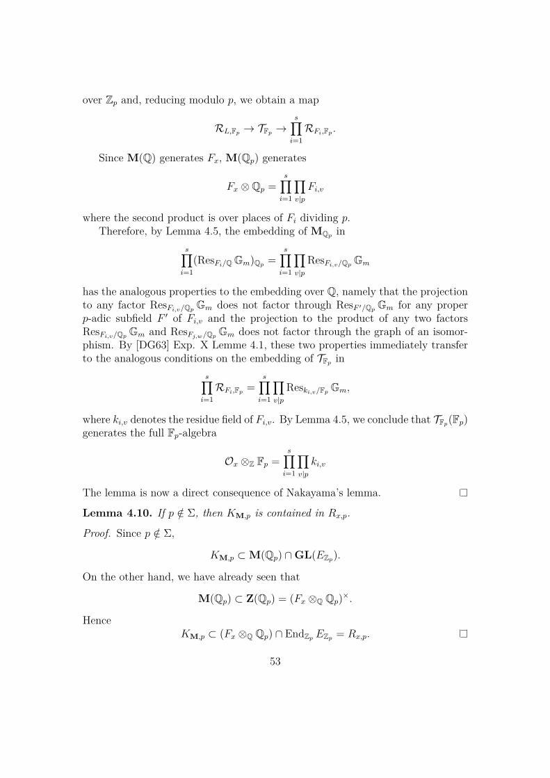
over Zp and, reducing modulo p, we obtain a map
RL,Fp → TFp →s∏i=1RFi,Fp .
Since M(Q) generates Fx, M(Qp) generates
Fx ⊗Qp =s∏i=1
∏v|pFi,v
where the second product is over places of Fi dividing p.Therefore, by Lemma 4.5, the embedding of MQp in
s∏i=1
(ResFi/Q Gm)Qp =s∏i=1
∏v|p
ResFi,v/Qp Gm
has the analogous properties to the embedding over Q, namely that the projectionto any factor ResFi,v/Qp Gm does not factor through ResF ′/Qp Gm for any properp-adic subfield F ′ of Fi,v and the projection to the product of any two factorsResFi,v/Qp Gm and ResFj,w/Qp Gm does not factor through the graph of an isomor-phism. By [DG63] Exp. X Lemme 4.1, these two properties immediately transferto the analogous conditions on the embedding of TFp in
s∏i=1RFi,Fp =
s∏i=1
∏v|p
Reski,v/Fp Gm,
where ki,v denotes the residue field of Fi,v. By Lemma 4.5, we conclude that TFp(Fp)generates the full Fp-algebra
Ox ⊗Z Fp =s∏i=1
∏v|pki,v
The lemma is now a direct consequence of Nakayama’s lemma.
Lemma 4.10. If p /∈ Σ, then KM,p is contained in Rx,p.
Proof. Since p /∈ Σ,
KM,p ⊂M(Qp) ∩GL(EZp).
On the other hand, we have already seen that
M(Qp) ⊂ Z(Qp) = (Fx ⊗Q Qp)×.
HenceKM,p ⊂ (Fx ⊗Q Qp) ∩ EndZp EZp = Rx,p.
53

Proposition 4.11. If p /∈ Σ is unramified in L and p divides [Ox : Rx] then KM,p
is strictly contained in KmM,p.
Proof. Suppose KM,p = KmM,p. By Lemma 4.9, Km
M,p generates the ring Ox,p.However, by Lemma 4.10, Km
M,p is contained in the ring Rx,p. Hence Rx,p =Ox,p.
4.4 Proof of Theorem 4.1The following proposition is the final ingredient in the proof of Theorem 4.1. Weuse it in two different ways: if p divides [Km
M,p : KM,p], then the proposition tellsus that the p-part of [Ox : Rx] is bounded by a suitable power of the p-part of[Km
M,p : KM,p], while if p does not divide [KmM,p : KM,p], then the proposition tells
us that the power of p dividing [Ox : Rx] is uniformly bounded.Proposition 4.12. There is a uniform integer C44 such that, if pn is the maximumpower of p dividing [Km
M,p : KM,p], then
pC44(n+1) - [Ox : Rx].
Proof. Choose z ∈ OL ⊗ Zp as in Proposition 4.8 so that the index of Zp[S(z)] inOx,p is at most pC43 . Let h be the dimension of Ox,p as a free module over Zp anddefine yj := exp jpNS(z) for j ∈ {0, ..., h − 1} and N > 1 an integer. Note thatyj = r(exp jz)pN is an element of Km
M,p. However, it also lies in the image I of thep-adic exponential on p2Ox,p, which is a pro-p group. Therefore, the quotient ofKm
M,p∩I by KM,p∩I is a p-group contained in the finite abelian group KmM,p/KM,p.
In particular, its order divides pn and, if n divides N , we conclude that yj ∈ KM,p.If p /∈ Σ we conclude that yj ∈ Rx,p. If p ∈ Σ, we can replace N by a uniformlybounded multiple of n to obtain the same result.
By definition, modulo pNh−h,
yj ≡ 1 + jpNS(z) + j2p2NS(z)2
2! + · · ·+ jh−1pN(h−1)S(z)h−1
(h− 1)! .
Therefore, the span Λ of the elements yj in Zp[pNS(z)] modulo pNh−h is of indexbounded by the maximum power pmh of p dividing the (non-zero) determinant ofthe matrix (
jk
k!
)j,k∈{0,...,h−1}
.
On the other hand, Zp[pNS(z)] certainly contains pN(h−1)+C43Ox,p, so we concludethat Λ contains
pN(h−1)+C43+mhOx,p/pNh−hOx,p,
54

which is non-trivial if N > h+C43+mh. In particular, if all of the above conditionson N hold then Λ contains the quotient
pNh−h−1Ox,p/pNh−hOx,p
and so, by Nakayama’s lemma, the span of the yj in Ox,p contain pNh−h−1Ox,p.Since the yj ∈ Rx,p, we conclude
[Ox,p : Rx,p] ≤ pNh2−h2−h,
which finishes the proof.
Now we are ready to finish the proofs of Theorems 1.4 and 4.1.
Proof of Theorem 4.1. We begin by reducing to the case in which K ⊂ G(Af ) isa direct product of compact open subgroups Kp ⊂ G(Qp). To see that this issufficient, first note that an arbitrary compact open subgroup K ⊂ G(Af ) alwayscontains such a subgroup K ′ = ∏
pK′p. Replacing K by K ′ changes i(M) by at
most the (finite) number of primes for which
K ∩G(Qp) 6= K ′ ∩G(Qp),
and multiplies [KmM : KM] by [KM : K ′M], which is at most [K : K ′]. Hence
replacing K by K ′ changes the right hand side of the bound in Theorem 4.1 by auniformly bounded quantity, so it suffices to prove the theorem with K ′ in placeof K.
We may therefore assume that K = ∏pKp, so
[KmM : KM] =
∏p
[KmM,p : KM,p].
For any integer x and any prime p, let [x]p denote the largest power of p whichdivides x i.e.
[x]p = pvp(x).
We will show that we can choose constants C39 and C40 uniformly and a con-stant C45 depending on G, X, ρ, K, C41 such that for every prime p, either
p and [Ox : Rx]p are both less than C45
or[Ox : Rx]p ≤ C
i(M,p)41 [Km
M,p : KM,p]C39 [discL]C40p (*)
where i(M, p) = 1 if KmM,p 6= KM,p and 0 if Km
M,p = KM,p. The bound in Theo-rem 4.1 follows by taking the product over all primes p (the first case leads to theconstant C42).
55

• If p divides [KmM,p : KM,p] then Proposition 4.12 implies that
[Ox : Rx]p ≤ [KmM,p : KM,p]2C44 .
– If we suppose further that pC44 ≥ C−141 , then
[Ox : Rx]p ≤ C41[KmM,p : KM,p]3C44
and so taking C39 ≥ 3C44 suffices.
• If p does not divide [KmM,p : KM,p] then by Proposition 4.12,
[Ox : Rx]p ≤ pC44 .
– If [KmM,p : KM,p] > 1, then by [UY14a] Proposition 3.15 there exists a
uniform constant C46 ≤ 1 such that
C46p ≤ [KmM,p : KM,p].
If also p is large enough that pC44 ≥ C−2C4446 C−1
41 , we deduce that
[Ox : Rx]p ≤ C41[KmM,p : KM,p]2C44 .
Thus in this case, C39 ≥ 2C44 suffices.– If [Km
M,p : KM,p] = 1 and p is ramified in L then p divides discL andi(M, p) = 0. Thus
[Ox : Rx]p ≤ Ci(M,p)41 [discL]C44
p
and so C40 ≥ C44 suffices.– If [Km
M,p : KM,p] = 1, p is unramified in L and p /∈ Σ, then Proposi-tion 4.11 implies that [Ox : Rx] = 1. Again i(M, p) = 0 so both sidesof (*) are equal to 1.
• We are left with the cases
p ∈ Σ or pC44 < C−2C4446 C−1
41
(note that this includes pC44 < C−141 because C46 ≤ 1). In these cases we have
an upper bound for p depending on uniform data and on C41 (recall thatΣ is finite and uniform). The fact that [Ox : Rx]p ≤ pC44 implies a similarbound for [Ox : Rx]p.
56

Proof of Theorem 1.4. By Theorem 1.1, there are constants C1 and C2 dependingonly on G, X, F and ρ such that
H(x) ≤ C1 |discRx|C2 .
anddiscRx = [Ox : Rx]2 discOx = [Ox : Rx]2
s∏i=1
discFi.
Since each Fi is isomorphic to a subfield of L, we know that |discFi| is at most|discL|. Clearly, the number of isotypic components s is at most the dimensionof E. Therefore, Theorem 1.4 follows from Theorem 4.1.
AcknowledgementsBoth authors would like to thank Emmanuel Ullmo and Andrei Yafaev for sug-gesting that they work together on this problem and for numerous conversationsregarding the subject of this paper. The authors also owe a special thank you toPhilipp Habegger who suggested the use of Chow polynomials to prove Proposi-tion 3.11. They are grateful to Ziyang Gao for pointing out the issue with quan-tifiers in Theorem 1.4 which is needed for it to imply Theorem 1.2. Both authorswould like to thank the referee for their reading of the manuscript and their helpfulcomments.
The first author is indebted to the Engineering and Physical Sciences ResearchCouncil and the Institut des Hautes Études Scientifiques for their financial support.The second author was funded by European Research Council grant 307364 “Someproblems in Geometry of Shimura varieties.”
References[AM69] M. F. Atiyah and I. G. Macdonald. Introduction to commutative alge-
bra. Addison-Wesley Publishing Co., Reading, Mass.-London-Don Mills,Ont., 1969.
[BMZ07] E. Bombieri, D. Masser, and U. Zannier. Anomalous subvarieties—structure theorems and applications. International Mathematics Re-search Notices, 2007, 2007.
[Bor69] A. Borel. Introduction aux groupes arithmétiques. Publications del’Institut de Mathématique de l’Université de Strasbourg, XV. Actu-alités Scientifiques et Industrielles, No. 1341. Hermann, Paris, 1969.
57

[Daw15] C. Daw. The André-Oort conjecture via o-minimality. In G. O. Jones andA. J. Wilkie, editors, O-minimality and Diophantine Geometry, LondonMathematical Society Lecture Note Series 421. Cambridge UniversityPress, 2015.
[Del79] P. Deligne. Variétés de Shimura: interprétation modulaire, et techniquesde construction de modèles canoniques. In Automorphic forms, represen-tations and L-functions (Part 2), Proc. Sympos. Pure Math., XXXIII,pages 247–289. Amer. Math. Soc., Providence, R.I., 1979.
[DG63] M. Demazure and A. Grothendieck. Schémas en groupes, SGA 3. IHES,1963. Exp. VIII–XIV, Fasc. 4.
[DH] C. Daw and A. Harris. Categoricity of modular and Shimura curves. Toappear in J. Inst. Math. Jussieu.
[DY11] C. Daw and A. Yafaev. An unconditional proof of the André–Oort con-jecture for Hilbert modular surfaces. Manuscripta Math., 135:263–271,2011.
[EY03] B. Edixhoven and A. Yafaev. Subvarieties of Shimura varieties. Ann. ofMath., 157(2):621–645, 2003.
[Gaoa] Z. Gao. About the mixed André–Oort conjecture: reduction to a lowerbound for the pure case. Unpublished note, available at www.math.u-psud.fr/~gao.
[Gaob] Z. Gao. Towards the André–Oort conjecture for mixed Shimura vari-eties: The Ax–Lindemann theorem and lower bounds for Galois orbitsof special points. To appear in J. Reine Angew. Math..
[Hab08] P. Habegger. Intersecting subvarieties of Gnm with algebraic subgroups.
Math. Ann., 342(2):449–466, 2008.
[KUY] B. Klingler, E. Ullmo, and A. Yafaev. The hyperbolic Ax–Lindemann–Weierstrass conjecture. Preprint, available at arxiv.org/abs/1307.3965.
[KY14] B. Klingler and A. Yafaev. The André-Oort conjecture. Ann. of Math.(2), 180(3):867–925, 2014.
[Nes77] Ju V. Nesterenko. Estimates for the orders of zeros of functions of acertain class and applications in the theory of transcendental numbers.Math. USSR Izv., 11(2):239–270, 1977.
58

[Phi95] P. Philippon. Sur des hauteurs alternatives. III. J. Math. Pures Appl.(9), 74(4):345–365, 1995.
[Pil09] J. Pila. Algebraic points of definable sets and results of André–Oort–Manin–Mumford type. IMRN, 13:2476–2507, 2009.
[Pil11] J. Pila. O-minimality and the André–Oort conjecture for Cn. Ann. ofMath., 173(3):1779–1840, 2011.
[PS10] Y. Peterzil and S. Starchenko. Tame complex analysis and o-minimality.In Proceedings of the ICM, Hyderabad, 2010.
[PT13] J. Pila and J. Tsimerman. The André–Oort conjecture for the modulispace of abelian surfaces. Compositio Math., 149(2):204–216, 2013.
[PT14] J. Pila and J. Tsimerman. Ax–Lindemann for Ag. Ann. of Math. (2),179(2):659–681, 2014.
[PW06] J. Pila and A. Wilkie. The rational points of a definable set. Duke Math.J., 133:591–616, 2006.
[PZ08] J. Pila and U. Zannier. Rational points in periodic analytic sets and theManin–Mumford conjecture. Rend. Mat. Acc. Lincei, 19:149–162, 2008.
[RU09] N. Ratazzi and E. Ullmo. Galois+equidistribution=Manin–Mumford.In Ecole d’été arithmetic geometry, Clay Math. Proc. Amer. Math. Soc.,2009.
[Tsi] J. Tsimerman. A proof of the André-Oort conjecture for Ag. Preprint,available at arxiv.org/abs/1506.01466.
[Tsi12] J. Tsimerman. Brauer-Siegel for arithmetic tori and lower bounds forGalois orbits of special points. J. Amer. Math. Soc., 25:1091–1117, 2012.
[Ull14] E. Ullmo. Applications du théorème d’Ax-Lindemann hyperbolique.Compos. Math., 150(2):175–190, 2014.
[UY11] E. Ullmo and A. Yafaev. A characterisation of special subvarieties. Math-ematika, 57(2):263–273, 2011.
[UY14a] E. Ullmo and A. Yafaev. Galois orbits and equidistribution of specialsubvarieties: towards the André-Oort conjecture. Ann. of Math. (2),180(3):823–865, 2014.
[UY14b] E. Ullmo and A. Yafaev. The hyperbolic Ax–Lindemann theorem in thecompact case. Duke Math. J., 163(2):267–463, 2014.
59

[UY15] E. Ullmo and A. Yafaev. Nombre de classes des tores de multiplicationcomplexe et bornes inférieures pour les orbites galoisiennes de pointsspéciaux. Bull. Soc. Math. France, 143(1):197–228, 2015.
60


![Shimura Varieties and the Mumford–Tate conjecture, part I · 2018. 11. 24. · arXiv:math/0109094v1 [math.NT] 14 Sep 2001 Shimura Varieties and the Mumford–Tate conjecture, part](https://img.pdfslide.us/doc/110x75/606be3d5bd366d74a156014c/shimura-varieties-and-the-mumfordatate-conjecture-part-i-2018-11-24-arxivmath0109094v1.jpg)