Heightened Hydro-morphological Activity Reaches ... · hydromorphology team and requires the development of Sediment Transport: Reach the Equilibrium Assessment Method (ST:REAM) model

\\sepa-fp-01\Projects\WFD\Characterisation, Monitoring and Classification\Science Task Teams\Hydromorphology\Chris Bromley\Sediment budget\01 ST_REAM\heather\Final outputs\Layers

1

Heightened Hydro-morphological Activity Reaches

Explanatory Note V.2

V.2- 17th October 2013:

Updated/incorporated items: - New transport equation (Recking, 2013). - “R” table. - Categories and thresholds. - Blind test of classes. - Categories distribution. - Hydro-coding and QA. - Tributary network


2

Contents

1 Background ......................................................................................................................... 3

2 ST:REAM model ................................................................................................................. 3

3 Model assessment and validation ...................................................................................... 5

3.1 Field survey: reaches and observations ..................................................................... 5

3.2 Field survey: sediment ................................................................................................ 6

3.3 Model parameters ....................................................................................................... 6

3.4 Assessment ................................................................................................................. 6

3.5 Version selection ......................................................................................................... 7

4 CSR classes: depositional, balance and erosional reaches .............................................. 9

5 Modelling of catchments ................................................................................................... 11

6 Mapping ............................................................................................................................ 13

6.1 Tributaries and mapping ........................................................................................... 13

6.2 Data outputs and hydro-coding ................................................................................. 14

7 Outputs delivered ............................................................................................................. 14

7.1 Point dataset fields: ................................................................................................... 14

7.2 Line dataset fields: .................................................................................................... 15

7.3 Use of the datasets ................................................................................................... 15

8 Categories distribution across Scotland ........................................................................... 16

8.1 Categories distribution by length .............................................................................. 16

8.2 Categories distribution by number of reaches (by Advisory Group) ........................ 17

8.3 Categories distribution by % of number of reaches (by Advisory Group) ................ 18

8.4 Categories distribution by number of reaches (by region) ....................................... 19

9 Appendix-1 ........................................................................................................................ 20


3

1 Background In early 2012, SEPA commissioned Halcrow to identify approaches to screen and quantify natural flood management effects. Based on the approach recommended by Halcrow, SEPA committed to undertaking a national screening process to identify areas within catchments with Potentially Vulnerable Areas that have natural flood management opportunities. The main outputs of the screening process will be the identification of:

• areas of high runoff generation;

• areas of floodplain storage potential;

• areas of estuarine surge attenuation potential;

• areas of wave energy attenuation potential; and

• areas of heightened hydromorphological activity Identification of areas of heightened morphological activity is being undertaken by the hydromorphology team and requires the development of the Sediment Transport: Reach Equilibrium Assessment Method (ST:REAM) model. In addition to identifying areas at risk from flooding due to in-channel sediment deposition, this model will also help to assess the impacts of climate change on flood risk and develop catchment-scale approaches to in-channel sediment management.

2 ST:REAM model The ST:REAM model was developed by Dr Chris Parker during his PhD at the University of Nottingham. This thesis came about as a result of the Flood Risk Management Research Consortium’s (FRMRC), Priority Area 8 (Morphology and Habitat). PA8 was identified as a necessity since existing flood management techniques rarely account for sediment transfer in river systems, despite the fact that disruptions to this transfer is known to impact future flood risk and the quality of in-channel habitat (FRMRC, 2004). The thesis recognised that there was no tool currently capable of delivering a nationwide, quantitative or semi-quantitative assessment of sediment source, transfer and deposition zones at the catchment scale. ST:REAM was thus created to provide quantitative, catchment-scale assessments of in-channel coarse-sediment dynamics using existing, national level, datasets.

ST:REAM requires up to four different data inputs in order to generate outcomes: - Flows: Flow Duration Curves (FDC) generated using Low Flow Enterprise (LFE) or

bankfull discharge (Qmed) values generated using the Flood Estimation Handbook (FEH) methodology, both at 50m intervals along the entire river network.

- Channel slope and bankfull channel width at 50m intervals along the river network.

- A representative sediment grain size for the river catchment was tested in some versions of the model.

All rivers can transport sediment. When a river’s sediment transport capacity exceeds the amount of sediment supplied to it, net erosion is likely to occur. When sediment supply exceeds transport capacity, net sediment deposition is likely to occur. When sediment


4

transport capacity roughly equals sediment supply, a balance is struck between erosion and deposition.

Using the data inputs, ST:REAM can estimate the sediment transport capacity in two different ways:

1. Using a sediment transport equation that predicts transport capacity for every 50m section of the river network (calculated using grain size); or

2. Using stream power for every 50m section of the river network (calculated without using grain size) to infer transport capacity.

The transport capacity using the sediment transport equation or stream power is then divided by that of the upstream section to produce capacity supply ratios (CSR) for every 50m section. ST:REAM then uses an algorithm to group together adjacent 50m sections with very similar CSRs, so that a smaller number of longer river reaches is created.

In this way, reaches where net sediment deposition occurs (CSR <1), can be distinguished from those where net erosion occurs (CSR >1), or where there is a balance between erosion and deposition (CSR approximately equals 1).

The original version of ST:REAM has been modified to fulfil the purposes of SEPA. The present version can process massive data generating 8 different outputs. The assessment of the model will allow selecting which version performs better compared to field observations.

The different versions of the model are shown in table-1:

These outputs can feed into analyses of areas at risk from flooding; can be used for regulating sediment removal activities; and for looking at potential impacts of climate changes on river flows, flood risk and channel morphology.

Table 1 Tree of outcome types produced by ST:REAM

FDC: Flow Duration Curves

- Qmed and Stream Power SP_Q_SP - Qmed and Transport Capacity SP_Q_TC - FDC and Stream Power SP_FDC_SP - FDC and Transport Capacity SP_FDC_TC

- Qmed and Stream Power TC_Q_SP - Qmed and Transport Capacity TC_Q_TC - FDC and Stream Power TC_FDC_SP - FDC and Transport Capacity TC_FDC_TC

Stream Power:

Transport Capacity:

Reaches calculated by: CSR calculated by Version name:


5

3 Model assessment and validation The model assessment and validation will allow, firstly, selecting the best output version from ST:REAM and, secondly, assessing the level of confidence of the model by comparing model predictions to field observations.

3.1 Field survey: reaches and observations

The assessment and validation of the model has been carried out against field observations from four trial catchments:

- Isla (WB ID 23181, 23179, 23176) - Farnack (WB ID 20312) - Charnaig (WB ID 20072) - Bervie (WB ID 23262, 23264)

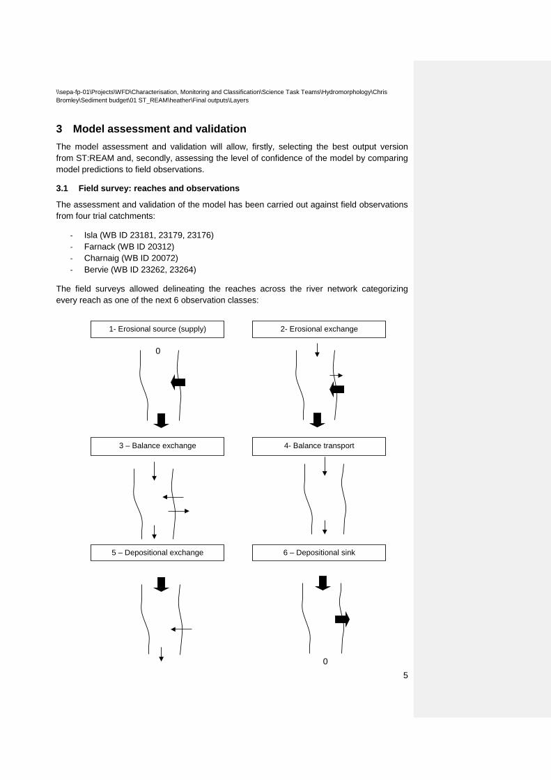
The field surveys allowed delineating the reaches across the river network categorizing every reach as one of the next 6 observation classes:

1- Erosional source (supply)

2- Erosional exchange

3 – Balance exchange

4- Balance transport

5 – Depositional exchange

6 – Depositional sink

0

0


6

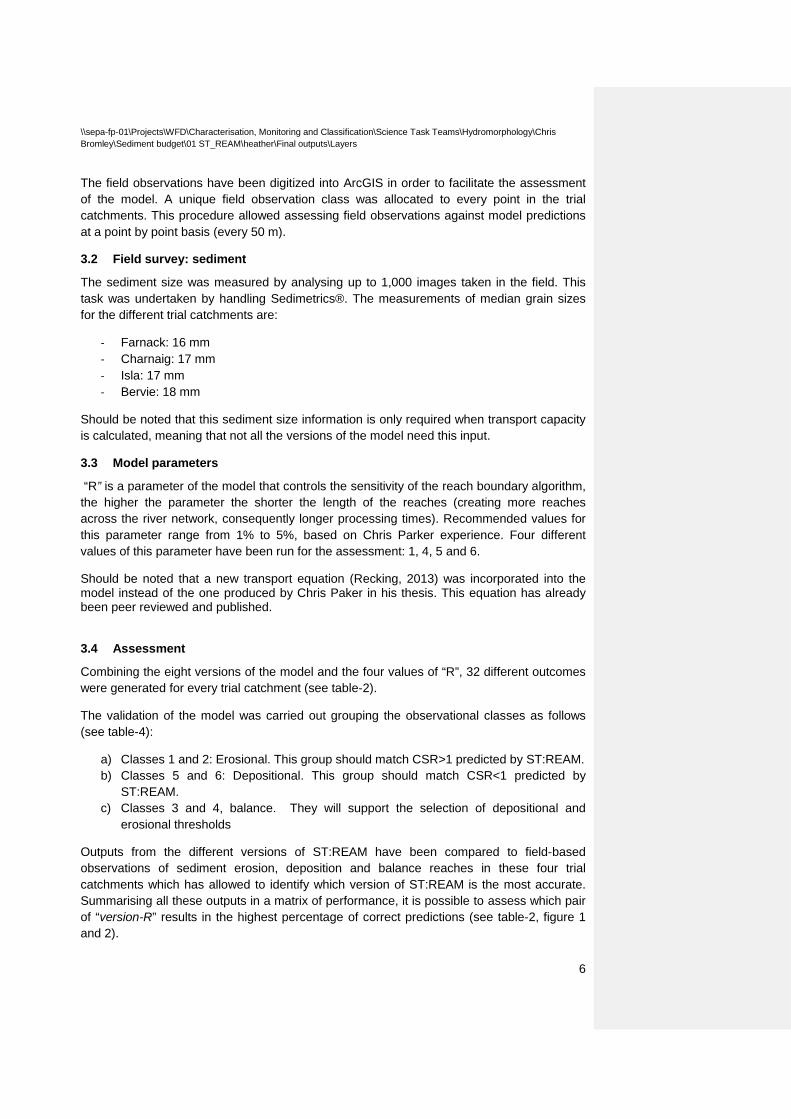
The field observations have been digitized into ArcGIS in order to facilitate the assessment of the model. A unique field observation class was allocated to every point in the trial catchments. This procedure allowed assessing field observations against model predictions at a point by point basis (every 50 m).

3.2 Field survey: sediment

The sediment size was measured by analysing up to 1,000 images taken in the field. This task was undertaken by handling Sedimetrics®. The measurements of median grain sizes for the different trial catchments are:

- Farnack: 16 mm - Charnaig: 17 mm - Isla: 17 mm - Bervie: 18 mm

Should be noted that this sediment size information is only required when transport capacity is calculated, meaning that not all the versions of the model need this input.

3.3 Model parameters

“R” is a parameter of the model that controls the sensitivity of the reach boundary algorithm, the higher the parameter the shorter the length of the reaches (creating more reaches across the river network, consequently longer processing times). Recommended values for this parameter range from 1% to 5%, based on Chris Parker experience. Four different values of this parameter have been run for the assessment: 1, 4, 5 and 6.

Should be noted that a new transport equation (Recking, 2013) was incorporated into the model instead of the one produced by Chris Paker in his thesis. This equation has already been peer reviewed and published.

3.4 Assessment

Combining the eight versions of the model and the four values of “R”, 32 different outcomes were generated for every trial catchment (see table-2).

The validation of the model was carried out grouping the observational classes as follows (see table-4):

a) Classes 1 and 2: Erosional. This group should match CSR>1 predicted by ST:REAM. b) Classes 5 and 6: Depositional. This group should match CSR<1 predicted by

ST:REAM. c) Classes 3 and 4, balance. They will support the selection of depositional and

erosional thresholds

Outputs from the different versions of ST:REAM have been compared to field-based observations of sediment erosion, deposition and balance reaches in these four trial catchments which has allowed to identify which version of ST:REAM is the most accurate. Summarising all these outputs in a matrix of performance, it is possible to assess which pair of “version-R” results in the highest percentage of correct predictions (see table-2, figure 1 and 2).


7

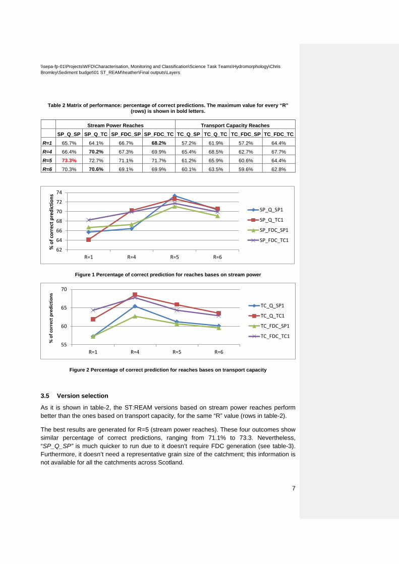
Table 2 Matrix of performance: percentage of correct predictions. The maximum value for every “R” (rows) is shown in bold letters.

Stream Power Reaches Transport Capacity Reaches

SP_Q_SP SP_Q_TC SP_FDC_SP SP_FDC_TC TC_Q_SP TC_Q_TC TC_FDC_SP TC_FDC_TC

R=1 65.7% 64.1% 66.7% 68.2% 57.2% 61.9% 57.2% 64.4%

R=4 66.4% 70.2% 67.3% 69.9% 65.4% 68.5% 62.7% 67.7%

R=5 73.3% 72.7% 71.1% 71.7% 61.2% 65.9% 60.6% 64.4%

R=6 70.3% 70.6% 69.1% 69.9% 60.1% 63.5% 59.6% 62.8%

Figure 1 Percentage of correct prediction for reaches bases on stream power

Figure 2 Percentage of correct prediction for reaches bases on transport capacity

3.5 Version selection

As it is shown in table-2, the ST:REAM versions based on stream power reaches perform better than the ones based on transport capacity, for the same “R” value (rows in table-2).

The best results are generated for R=5 (stream power reaches). These four outcomes show similar percentage of correct predictions, ranging from 71.1% to 73.3. Nevertheless, “SP_Q_SP” is much quicker to run due to it doesn’t require FDC generation (see table-3). Furthermore, it doesn’t need a representative grain size of the catchment; this information is not available for all the catchments across Scotland.

62

64

66

68

70

72

74

R=1 R=4 R=5 R=6

% o

f cor

rect

pre

dict

ions

SP_Q_SP1

SP_Q_TC1

SP_FDC_SP1

SP_FDC_TC1

55

60

65

70

R=1 R=4 R=5 R=6

% o

f cor

rect

pre

dict

ions

TC_Q_SP1

TC_Q_TC1

TC_FDC_SP1

TC_FDC_TC1


8

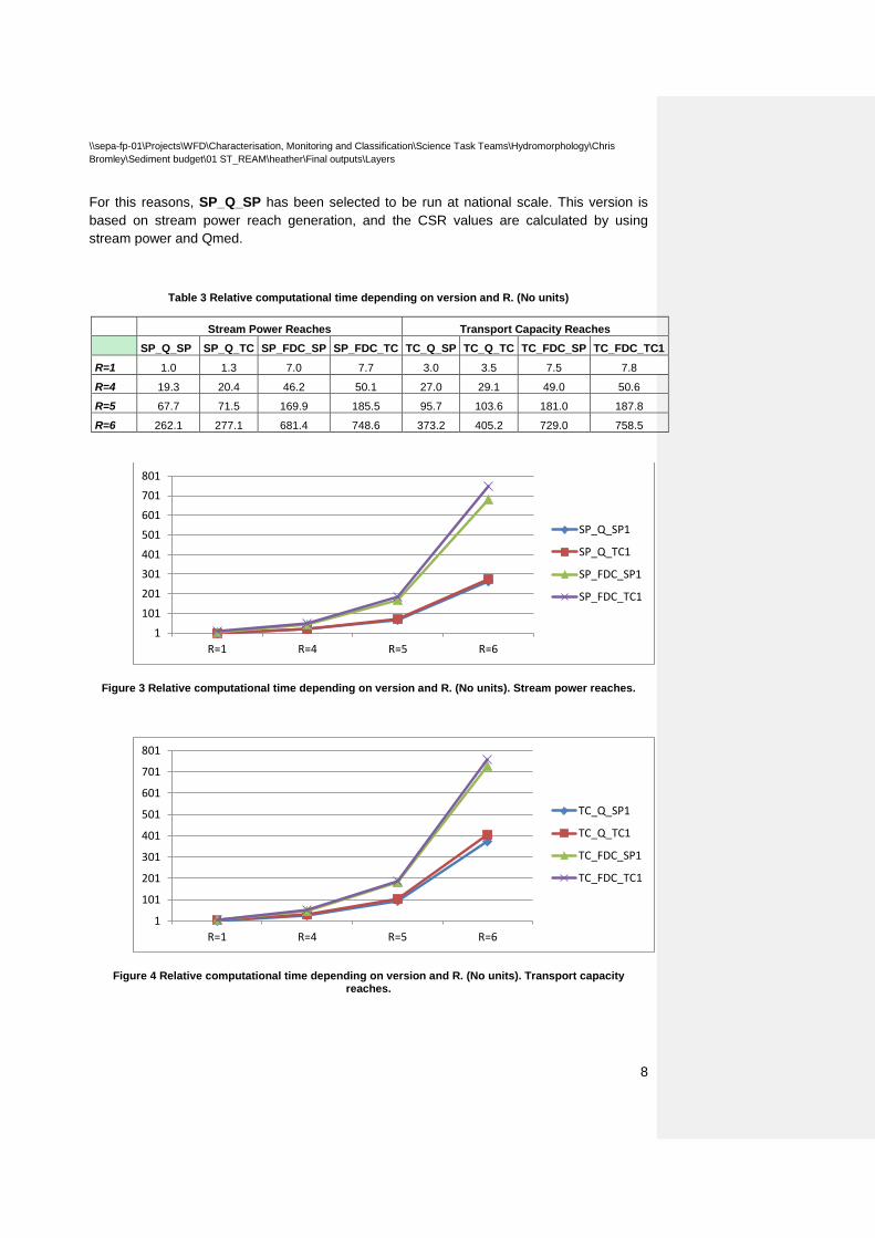
For this reasons, SP_Q_SP has been selected to be run at national scale. This version is based on stream power reach generation, and the CSR values are calculated by using stream power and Qmed.

Table 3 Relative computational time depending on version and R. (No units)

Stream Power Reaches Transport Capacity Reaches

SP_Q_SP SP_Q_TC SP_FDC_SP SP_FDC_TC TC_Q_SP TC_Q_TC TC_FDC_SP TC_FDC_TC1

R=1 1.0 1.3 7.0 7.7 3.0 3.5 7.5 7.8

R=4 19.3 20.4 46.2 50.1 27.0 29.1 49.0 50.6

R=5 67.7 71.5 169.9 185.5 95.7 103.6 181.0 187.8

R=6 262.1 277.1 681.4 748.6 373.2 405.2 729.0 758.5

Figure 3 Relative computational time depending on version and R. (No units). Stream power reaches.

Figure 4 Relative computational time depending on version and R. (No units). Transport capacity reaches.

1

101

201

301

401

501

601

701

801

R=1 R=4 R=5 R=6

SP_Q_SP1

SP_Q_TC1

SP_FDC_SP1

SP_FDC_TC1

1

101

201

301

401

501

601

701

801

R=1 R=4 R=5 R=6

TC_Q_SP1

TC_Q_TC1

TC_FDC_SP1

TC_FDC_TC1


9

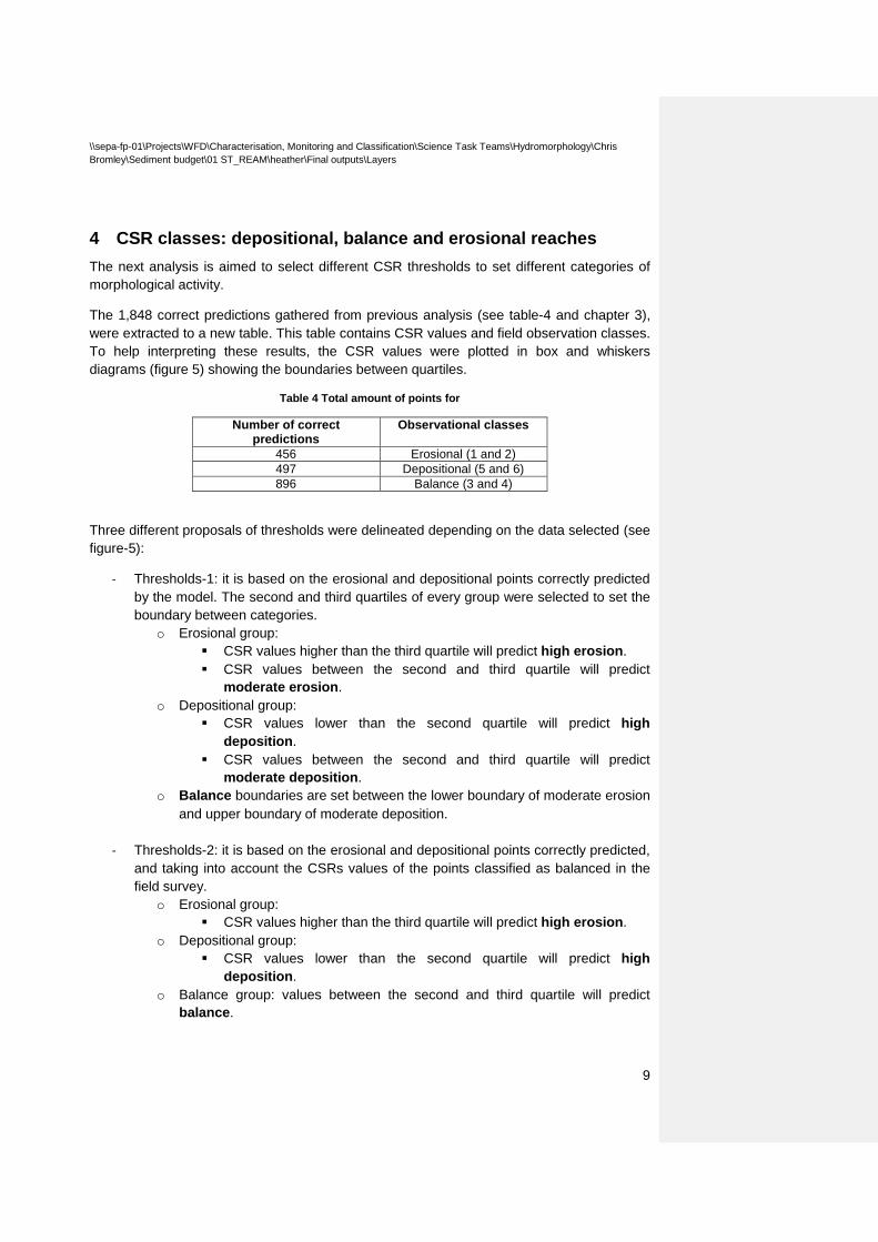
4 CSR classes: depositional, balance and erosional reaches The next analysis is aimed to select different CSR thresholds to set different categories of morphological activity.

The 1,848 correct predictions gathered from previous analysis (see table-4 and chapter 3), were extracted to a new table. This table contains CSR values and field observation classes. To help interpreting these results, the CSR values were plotted in box and whiskers diagrams (figure 5) showing the boundaries between quartiles.

Table 4 Total amount of points for

Number of correct predictions

Observational classes

456 Erosional (1 and 2) 497 Depositional (5 and 6) 896 Balance (3 and 4)

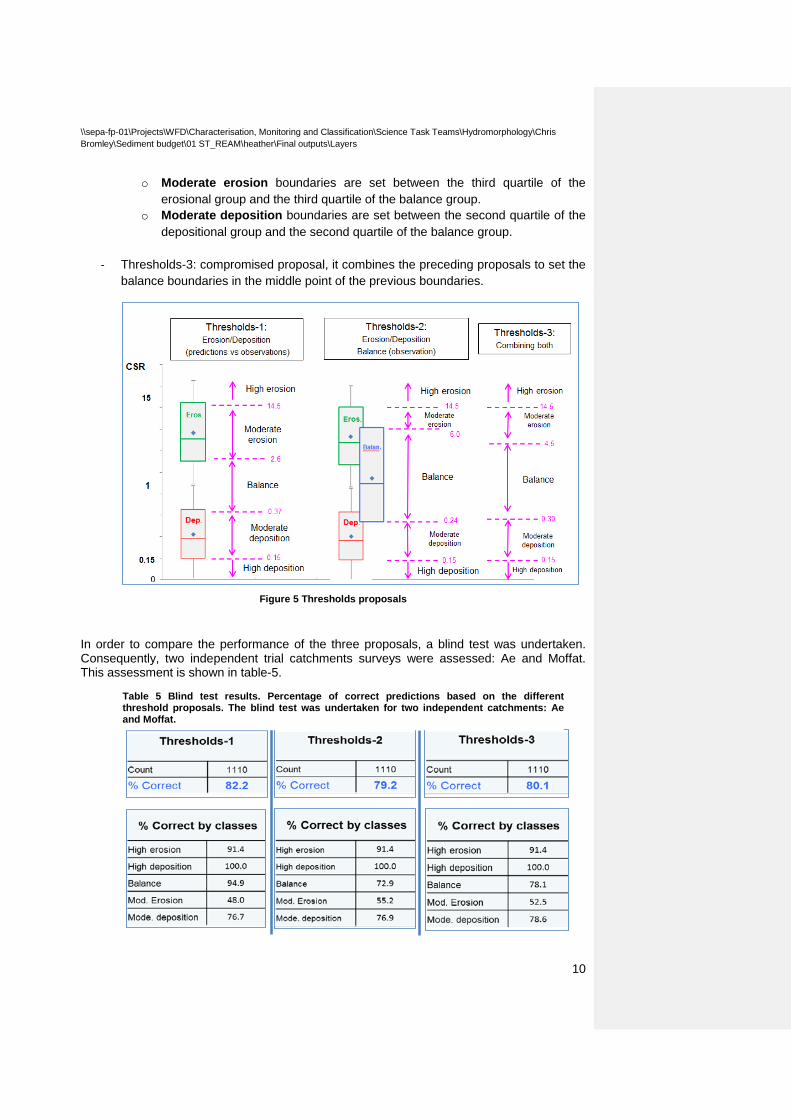
Three different proposals of thresholds were delineated depending on the data selected (see figure-5):

- Thresholds-1: it is based on the erosional and depositional points correctly predicted by the model. The second and third quartiles of every group were selected to set the boundary between categories.

o Erosional group: CSR values higher than the third quartile will predict high erosion. CSR values between the second and third quartile will predict

moderate erosion. o Depositional group:

CSR values lower than the second quartile will predict high deposition.

CSR values between the second and third quartile will predict moderate deposition.

o Balance boundaries are set between the lower boundary of moderate erosion and upper boundary of moderate deposition.

- Thresholds-2: it is based on the erosional and depositional points correctly predicted, and taking into account the CSRs values of the points classified as balanced in the field survey.

o Erosional group: CSR values higher than the third quartile will predict high erosion.

o Depositional group: CSR values lower than the second quartile will predict high

deposition. o Balance group: values between the second and third quartile will predict

balance.


10

o Moderate erosion boundaries are set between the third quartile of the erosional group and the third quartile of the balance group.

o Moderate deposition boundaries are set between the second quartile of the depositional group and the second quartile of the balance group.

- Thresholds-3: compromised proposal, it combines the preceding proposals to set the

balance boundaries in the middle point of the previous boundaries.

Figure 5 Thresholds proposals

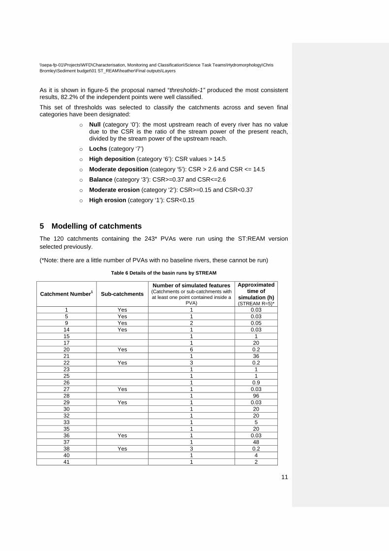
In order to compare the performance of the three proposals, a blind test was undertaken. Consequently, two independent trial catchments surveys were assessed: Ae and Moffat. This assessment is shown in table-5.

Table 5 Blind test results. Percentage of correct predictions based on the different threshold proposals. The blind test was undertaken for two independent catchments: Ae and Moffat.


11

As it is shown in figure-5 the proposal named “thresholds-1” produced the most consistent results, 82.2% of the independent points were well classified.

This set of thresholds was selected to classify the catchments across and seven final categories have been designated:

o Null (category ‘0’): the most upstream reach of every river has no value due to the CSR is the ratio of the stream power of the present reach, divided by the stream power of the upstream reach.

o Lochs (category ‘7’)

o High deposition (category ‘6’): CSR values > 14.5

o Moderate deposition (category ‘5’): CSR > 2.6 and CSR <= 14.5

o Balance (category ‘3’): CSR>=0.37 and CSR<=2.6

o Moderate erosion (category ‘2’): CSR>=0.15 and CSR<0.37

o High erosion (category ‘1’): CSR<0.15

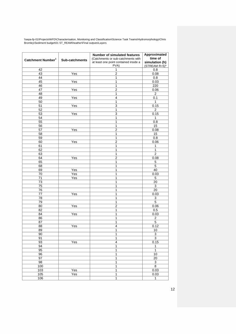
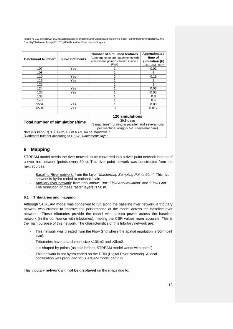
5 Modelling of catchments The 120 catchments containing the 243* PVAs were run using the ST:REAM version selected previously.

(*Note: there are a little number of PVAs with no baseline rivers, these cannot be run)

Table 6 Details of the basin runs by STREAM

Catchment Number1 Sub-catchments Number of simulated features

(Catchments or sub-catchments with at least one point contained inside a

PVA)

Approximated time of

simulation (h) (STREAM R=5)*

1 Yes 1 0.03 5 Yes 1 0.03 9 Yes 2 0.05 14 Yes 1 0.03 15 1 1 17 1 20 20 Yes 6 0.2 21 1 36 22 Yes 3 0.2 23 1 1 25 1 1 26 1 0.9 27 Yes 1 0.03 28 1 96 29 Yes 1 0.03 30 1 20 32 1 20 33 1 5 35 1 20 36 Yes 1 0.03 37 1 48 38 Yes 3 0.2 40 1 4 41 1 2


12



PVA)



42 1 0.8 43 Yes 2 0.08 44 1 0.8 45 Yes 1 0.03 46 1 220 47 Yes 2 0.06 48 1 2 49 Yes 4 0.1 50 1 1 51 Yes 3 0.15 52 1 2 53 Yes 3 0.15 54 1 1 55 1 0.8 56 1 15 57 Yes 2 0.08 58 1 15 59 1 0.8 60 Yes 2 0.06 61 1 1 62 1 1 63 1 2 64 Yes 2 0.08 65 1 5 68 1 5 69 Yes 1 40 70 Yes 1 0.03 71 Yes 1 5 73 1 20 75 1 3 76 1 20 77 Yes 1 0.03 78 1 3 79 1 5 80 Yes 2 0.06 82 1 0.5 84 Yes 1 0.03 86 1 2 87 1 5 88 Yes 4 0.12 89 1 10 90 1 3 91 1 3 93 Yes 4 0.15 94 1 1 95 1 1 96 1 10 97 1 20 98 1 3 100 1 8 103 Yes 1 0.03 105 Yes 1 0.03 106 1 1


13



PVA)



107 Yes 1 0.03 108 1 6 110 Yes 2 0.15 115 Yes 1 2 123 1 1 124 Yes 1 0.03 136 Yes 1 0.03 138 1 0.8 140 1 0.4 5564 Yes 1 0.03 6584 Yes 3 0.012

Total number of simulations/time 120 simulations

30,5 days (3 machines* running in parallel, and several runs

per machine, roughly 5-10 days/machine) *Intel(R) Xeon(R) 3.30 GHz, 16GB RAM, 64 bit. Windows 7 1Cathment number according to GI_02_Catchments layer

6 Mapping STREAM model needs the river network to be converted into a river-point network instead of a river-line network (points every 50m). This river-point network was constructed from the next sources:

- Baseline River network: from the layer “Mastermap Sampling Points 50m”. This river network is hydro coded at national scale.

- Auxiliary river network: from “IoH inflow”, “IoH Flow Accumulation” and “Flow Grid”. The resolution of these raster layers is 50 m.

6.1 Tributaries and mapping

Although ST:REAM model was conceived to run along the baseline river network, a tributary network was created to improve the performance of the model across the baseline river network. These tributaries provide the model with stream power across the baseline network (in the confluence with tributaries), making the CSR values more accurate. This is the main purpose of this network. The characteristics of this tributary network are:

- This network was created from the Flow Grid where the spatial resolution is 50m (cell size).

- Tributaries have a catchment size <10km2 and >3km2.

- It is shaped by points (as said before, STREAM model works with points).

- This network is not hydro coded on the DRN (Digital River Network). A local codification was produced for STREAM model can run.

This tributary network will not be displayed on the maps due to:

http://stir-app-gis04/gis/apps/Meta_app/details.asp?id=753


14

- The target of the project is to categorize the baseline river network.

- The tributary network is a ST:REAM input not an outcome.

- The tributaries are “short” water courses. They usually have a “null” CSR because they are too short for the model to split them into more than one reach.

- It will not align the background. Problems associated with showing the baseline and non-baseline layers, which are mapped to different scales, on the same output map.

- The output showing the different categories must be self-explanatory.

6.2 Data outputs and hydro-coding

The thresholds selected in chapter 4 were applied to the model outputs. The preliminary outcome is a point dataset where a unique category has been allocated to every point.

These points were converted into continuous line features by a process of hydro coding for display on the 1:50k DRN. (This task was undertaken by Dominic Habron, GIS Team).

After the conversion a QA was carried out to assess the fidelity of the line dataset against the original point dataset. The result of this conversion was highly accurate. Just 0.63% of the less favourable reaches analysed needed correction. (See Appendix-1)

7 Outputs delivered Maps display the “hydromorphological activity categories” along the baseline river network contained in PVAs catchments. There are a small number of PVAs that don’t contain any baseline river reach, therefore there is not ST:REAM information in those sub-catchments.

Folder Location: \\sepa-fp-01\Projects\WFD\Characterisation, Monitoring and Classification\Science Task Teams\Hydromorphology\Chris Bromley\Sediment budget\01 ST_REAM\heather\Final outputs\Layers

Datasets delivered:

- 3 sets of maps excluding the catchment 46 (Tay): a) Point dataset: whole river network. b) Point dataset: reaches contained inside PVAs. c) Line dataset: hydro coded line dataset of the whole river network.

- 3 sets of maps for the Catchment 46 (Tay).

a) Point dataset: Tay river network. b) Point dataset: Tay reaches contained inside PVAs. c) Line dataset: hydro coded line dataset of the Tay river network.

7.1 Point dataset fields:

The Heightened Hydromorphological Activity layer includes the next main fields:

- “CSR”: it is the capacity supply ratio corresponding to SP_Q (reaches base on stream power and R=5). It is a double data field.


15

- “Morpho_Act”: It is an integer field. Every point has been allocated to one of the next categories (same than line datasets below):

o 0: Null, the most upstream reach of every river has no value due to the CSR is the ratio of the stream power of the present reach, divided by the stream power of the upstream reach.

o 7: Lochs

o 6: High deposition, CSR values > 14.5

o 5: Moderate deposition, CSR > 2.6 and CSR <= 14.5

o 3: Balance, CSR>=0.37 and CSR<=2.6

o 2: Moderate erosion, CSR>=0.15 and CSR<0.37

o 1: High erosion, CSR<0.15

7.2 Line dataset fields:

Both line datasets (Tay and National) include these key fields:

- Reach_ID: it is the river reach ID formed by: Catchment number/River ID/ Reach ID. Every reach has a unique hydro morphological activity category.

- Category: every reach has been allocated to one of the next categories (same than point datasets above):

o 0: Null, the most upstream reach of every river has no value due to the CSR is the ratio of the stream power of the present reach, divided by the stream power of the upstream reach.

o 7: Lochs

o 6: High deposition, CSR values > 14.5

o 5: Moderate deposition, CSR > 2.6 and CSR <= 14.5

o 3: Balance, CSR>=0.37 and CSR<=2.6

o 2: Moderate erosion, CSR>=0.15 and CSR<0.37

o 1: High erosion, CSR<0.15

7.3 Use of the datasets

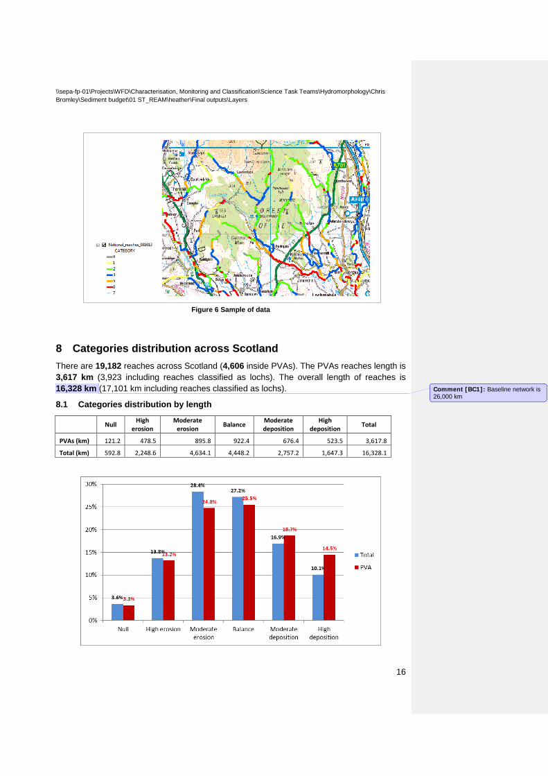
The preliminary point dataset should be just used for investigative purposes. The final line datasets have been hydro coded according to the DRN, constituting the definitive outcome of this project. (see sample, figure-6)


16

Figure 6 Sample of data

8 Categories distribution across Scotland There are 19,182 reaches across Scotland (4,606 inside PVAs). The PVAs reaches length is 3,617 km (3,923 including reaches classified as lochs). The overall length of reaches is 16,328 km (17,101 km including reaches classified as lochs).

8.1 Categories distribution by length

Null High erosion

Moderate erosion Balance Moderate

deposition High

deposition Total

PVAs (km) 121.2 478.5 895.8 922.4 676.4 523.5 3,617.8

Total (km) 592.8 2,248.6 4,634.1 4,448.2 2,757.2 1,647.3 16,328.1

Comment [BC1]: Baseline network is 26,000 km


17

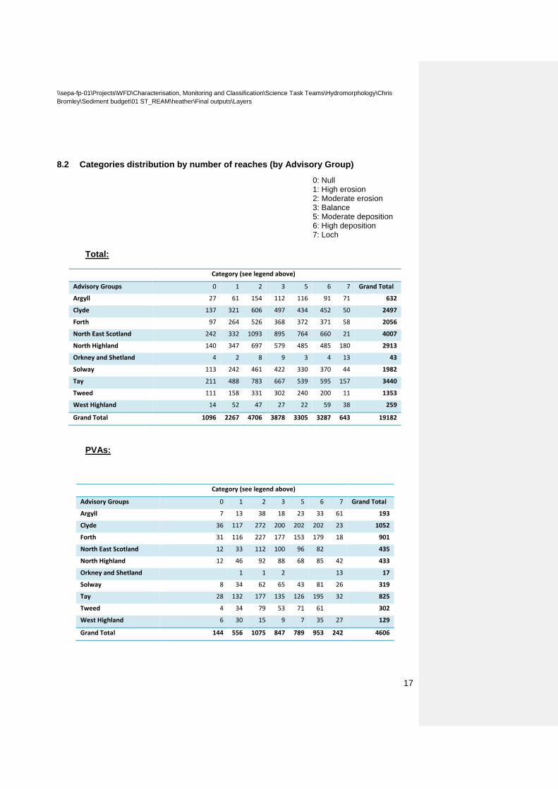
8.2 Categories distribution by number of reaches (by Advisory Group)

0: Null 1: High erosion 2: Moderate erosion 3: Balance 5: Moderate deposition 6: High deposition 7: Loch

Total:

Category (see legend above)

Advisory Groups 0 1 2 3 5 6 7 Grand Total

Argyll 27 61 154 112 116 91 71 632

Clyde 137 321 606 497 434 452 50 2497

Forth 97 264 526 368 372 371 58 2056

North East Scotland 242 332 1093 895 764 660 21 4007

North Highland 140 347 697 579 485 485 180 2913

Orkney and Shetland 4 2 8 9 3 4 13 43

Solway 113 242 461 422 330 370 44 1982

Tay 211 488 783 667 539 595 157 3440

Tweed 111 158 331 302 240 200 11 1353

West Highland 14 52 47 27 22 59 38 259

Grand Total 1096 2267 4706 3878 3305 3287 643 19182

PVAs:


Advisory Groups 0 1 2 3 5 6 7 Grand Total

Argyll 7 13 38 18 23 33 61 193

Clyde 36 117 272 200 202 202 23 1052

Forth 31 116 227 177 153 179 18 901

North East Scotland 12 33 112 100 96 82 435

North Highland 12 46 92 88 68 85 42 433

Orkney and Shetland 1 1 2 13 17

Solway 8 34 62 65 43 81 26 319

Tay 28 132 177 135 126 195 32 825

Tweed 4 34 79 53 71 61 302

West Highland 6 30 15 9 7 35 27 129

Grand Total 144 556 1075 847 789 953 242 4606


18

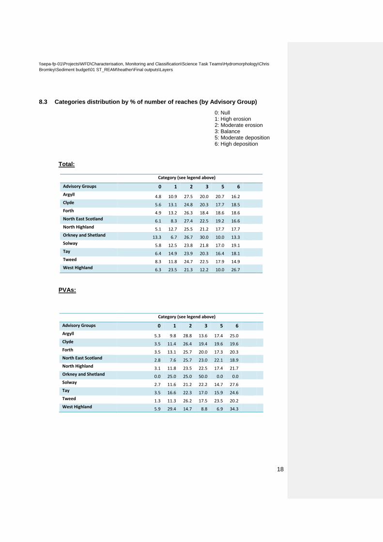
8.3 Categories distribution by % of number of reaches (by Advisory Group)

0: Null 1: High erosion 2: Moderate erosion 3: Balance 5: Moderate deposition 6: High deposition

Total:


Advisory Groups 0 1 2 3 5 6

Argyll 4.8 10.9 27.5 20.0 20.7 16.2

Clyde 5.6 13.1 24.8 20.3 17.7 18.5

Forth 4.9 13.2 26.3 18.4 18.6 18.6

North East Scotland 6.1 8.3 27.4 22.5 19.2 16.6

North Highland 5.1 12.7 25.5 21.2 17.7 17.7

Orkney and Shetland 13.3 6.7 26.7 30.0 10.0 13.3

Solway 5.8 12.5 23.8 21.8 17.0 19.1

Tay 6.4 14.9 23.9 20.3 16.4 18.1

Tweed 8.3 11.8 24.7 22.5 17.9 14.9

West Highland 6.3 23.5 21.3 12.2 10.0 26.7

PVAs:


Advisory Groups 0 1 2 3 5 6

Argyll 5.3 9.8 28.8 13.6 17.4 25.0

Clyde 3.5 11.4 26.4 19.4 19.6 19.6

Forth 3.5 13.1 25.7 20.0 17.3 20.3

North East Scotland 2.8 7.6 25.7 23.0 22.1 18.9

North Highland 3.1 11.8 23.5 22.5 17.4 21.7

Orkney and Shetland 0.0 25.0 25.0 50.0 0.0 0.0

Solway 2.7 11.6 21.2 22.2 14.7 27.6

Tay 3.5 16.6 22.3 17.0 15.9 24.6

Tweed 1.3 11.3 26.2 17.5 23.5 20.2

West Highland 5.9 29.4 14.7 8.8 6.9 34.3


19

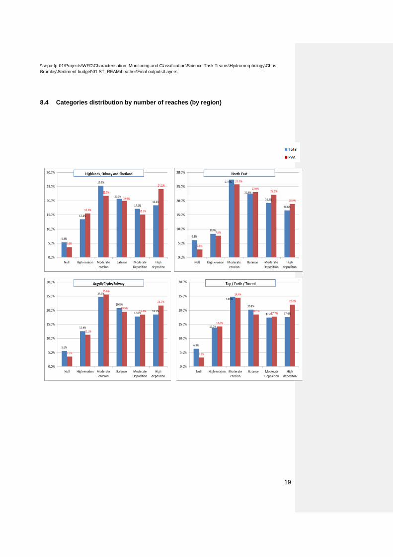
8.4 Categories distribution by number of reaches (by region)


20

9 Appendix-1

Hydro coded network check:

The hydro-coded networks (supplied by Dominic Habron) are two line datasets, one for the Tay catchment, the other covering the rest of the PVAs.

The purpose of this work is to assess the original point dataset from the ST:REAM model against the hydro-coded line dataset.

The present procedure is designed to locate substantial disparities between the original point dataset and the new line dataset. The potential mismatches are due to scale differences between the source data and the DRN.

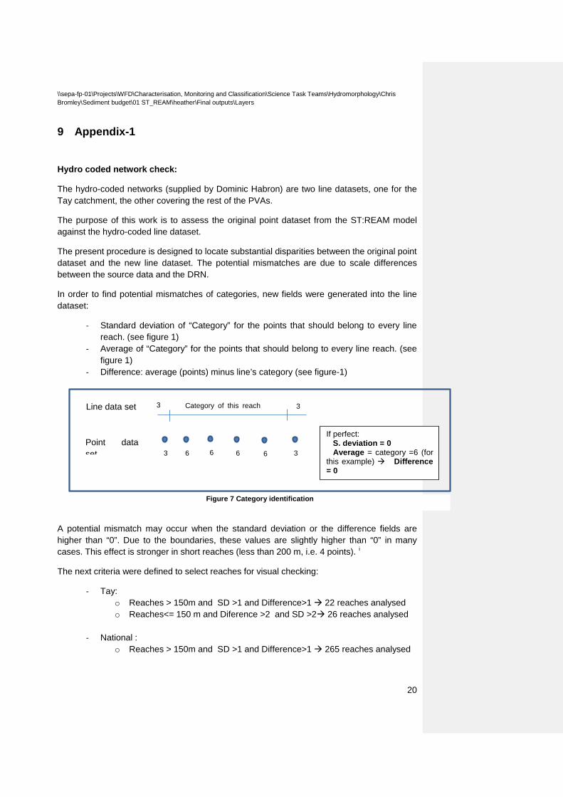
In order to find potential mismatches of categories, new fields were generated into the line dataset:

- Standard deviation of “Category” for the points that should belong to every line reach. (see figure 1)

- Average of “Category” for the points that should belong to every line reach. (see figure 1)

- Difference: average (points) minus line’s category (see figure-1)

A potential mismatch may occur when the standard deviation or the difference fields are higher than “0”. Due to the boundaries, these values are slightly higher than “0” in many cases. This effect is stronger in short reaches (less than 200 m, i.e. 4 points). i

The next criteria were defined to select reaches for visual checking:

- Tay: o Reaches > 150m and SD >1 and Difference>1 22 reaches analysed o Reaches<= 150 m and Diference >2 and SD >2 26 reaches analysed

- National :

o Reaches > 150m and SD >1 and Difference>1 265 reaches analysed

Category of this reach

3 3 Line data set

Point data set 3 6 6 6 6 3

If perfect: S. deviation = 0 Average = category =6 (for this example) Difference = 0

Figure 7 Category identification


21

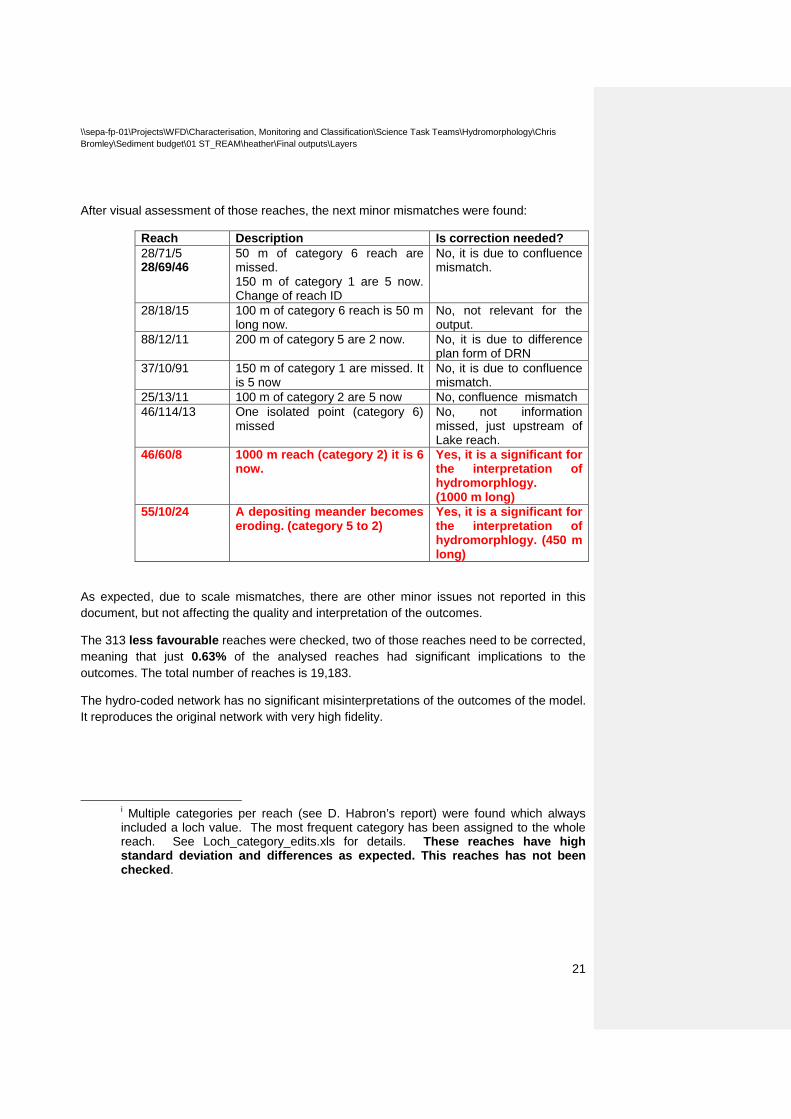
After visual assessment of those reaches, the next minor mismatches were found:

Reach Description Is correction needed? 28/71/5 28/69/46

50 m of category 6 reach are missed. 150 m of category 1 are 5 now. Change of reach ID

No, it is due to confluence mismatch.

28/18/15 100 m of category 6 reach is 50 m long now.

No, not relevant for the output.

88/12/11 200 m of category 5 are 2 now. No, it is due to difference plan form of DRN

37/10/91 150 m of category 1 are missed. It is 5 now

No, it is due to confluence mismatch.

25/13/11 100 m of category 2 are 5 now No, confluence mismatch 46/114/13 One isolated point (category 6)

missed No, not information missed, just upstream of Lake reach.

46/60/8 1000 m reach (category 2) it is 6 now.

Yes, it is a significant for the interpretation of hydromorphlogy. (1000 m long)

55/10/24 A depositing meander becomes eroding. (category 5 to 2)

Yes, it is a significant for the interpretation of hydromorphlogy. (450 m long)

As expected, due to scale mismatches, there are other minor issues not reported in this document, but not affecting the quality and interpretation of the outcomes.

The 313 less favourable reaches were checked, two of those reaches need to be corrected, meaning that just 0.63% of the analysed reaches had significant implications to the outcomes. The total number of reaches is 19,183.

The hydro-coded network has no significant misinterpretations of the outcomes of the model. It reproduces the original network with very high fidelity.

i Multiple categories per reach (see D. Habron’s report) were found which always included a loch value. The most frequent category has been assigned to the whole reach. See Loch_category_edits.xls for details. These reaches have high standard deviation and differences as expected. This reaches has not been checked.

Documents

Heightened Hydro-morphological Activity Reaches ... · hydromorphology team and requires the development of Sediment Transport: Reach the Equilibrium Assessment Method (ST:REAM) model