Available online at www.sciencedirect.com

www.elsevier.com/locate/asr

ScienceDirect

Advances in Space Research 60 (2017) 1797–1806

Height-dependent sunrise and sunset: Effects and implications ofthe varying times of occurrence for local ionospheric processes

and modelling

Tobias G.W. Verhulst ⇑, Stanimir M. Stankov

Royal Meteorological Institute (RMI), Ringlaan 3, B-1180 Brussels, Belgium

Received 29 March 2017; received in revised form 4 May 2017; accepted 29 May 2017Available online 29 July 2017

Abstract

It is well established that the sunrise and sunset periods are of particular importance to ionospheric research and modelling because ofthe rapid changes in the ionospheric plasma density, temperature, and dynamics. In particular, the sharp increase in the ionisation fol-lowing sunrise results in a quick increase in the ionospheric peak density, NmF 2, and a decrease in the peak height, hmF 2. Changes inplasma temperature, scale height and transport processes add further complexity which makes it difficult to investigate and model theionospheric behaviour during this transitional period from night to day. One of the aspects contributing to this difficulty is that notall ionospheric altitudes are exposed to the first sunlight of the day at the same time. During sunrise, the upper part of the ionosphereis illuminated prior to the lower part which is still in the dark. The boundary between sunlit and dark regions moves downwards until itreaches the surface of the Earth, which is commonly taken as the moment of sunrise at certain geographical coordinates. This means thatthe sunrise at surface level does not occur until after the entire ionosphere has been illuminated. During sunset, the same process happensin reverse order. This paper addresses the issue of these altitude-dependent times of sunrise and sunset and reports on our study of someof the effects on the diurnal variations in the ionospheric characteristics.� 2017 COSPAR. Published by Elsevier Ltd. All rights reserved.

Keywords: Ionospheric modelling; Geometrical astronomy; Sunrise/sunset

1. Introduction

The ionisation of the neutral particles in the upperatmosphere is primarily the result of photoionisationcaused by solar irradiation. The contribution of transportprocesses to the ion and electron density depends stronglyon altitude. At higher altitudes, transport processes havesufficient influence to maintain of the F layer throughoutthe night, while at lower altitudes, in the E and D regions,the transport processes are rather insignificant and are

http://dx.doi.org/10.1016/j.asr.2017.05.042

0273-1177/� 2017 COSPAR. Published by Elsevier Ltd. All rights reserved.

⇑ Corresponding author.E-mail addresses: tobias.verhulst@oma.be (T.G.W. Verhulst), s.stan-

kov@meteo.be (S.M. Stankov).

usually ignored. The amount of local photoionisation iscommonly described by the Chapman production function,which is well known in the literature—see, for example,Schunk and Nagy (2000). This production functiondepends, among other things, on the solar elevation angle.

The LIEDR (Local Ionospheric Electron Density profileReconstruction) model has been developed and used toreconstruct the local electron density profile for the entireionosphere (see Fig. 1), including the topside (Stankovet al., 2011). This is a real time model, based on the iono-sonde characteristics automatically scaled from ionograms,as well as GNSS derived total electron content (TEC). Inthe current work, we use this model to reconstruct the elec-tron density above the Dourbes ionosphere observatory,

Fig. 1. Panel (A): Schematic of the vertical ionospheric ion and electron density profiles, indicating key characteristics such as peak density (NmF 2), peakdensity height (hmF 2), plasma scale height (Hsc), and the ionospheric slab thickness. Panel (B): Comparison between vertical density profiles obtained withbasic analytical models for a given scale height of 100 km. Panel (C): A sample of five profilograms produced in the course of one hour; each profilogramshows the electron density, Ne (colour-coded, logarithmic scale on right) as a function of altitude (vertical axis) and time (horizontal axis). (Forinterpretation of the references to color in this figure legend, the reader is referred to the web version of this article.)

1798 T.G.W. Verhulst, S.M. Stankov / Advances in Space Research 60 (2017) 1797–1806

located at 50.1�N and 4.6�E. The LIEDR operational resultscan be found on the web-page http://ionosphere.meteo.be/ionosphere/liedr. At the Dourbes observatory, a DigisondeDPS4D digital ionosonde (Reinisch et al., 2009) and aNovAtel GPStation-6 GNSS receiver are co-located, pro-viding all the necessary input data for the LIEDR model.

A major problem for the reconstruction of the completeelectron density profile is that, while the ionosonde can beused to obtain the bottom-side characteristics, little infor-mation is directly available for the topside ionosphere(Fig. 1). The topside TEC can be calculated from the totalGNSS-derived TEC by subtracting the bottom-side TEC

estimated from the bottom-side electron density profilereconstructed from ionosonde measurements. However,to be able to deduce the topside electron density profilefrom the topside TEC, a suitable profiler function mustbe chosen. In the LIEDR model, a Chapman profile, Epsteinprofile, and exponential profile are available to model thetopside. The model can switch between different profilerfunctions depending on various parameters like time ofday, season, geomagnetic conditions, etc. (Verhulst andStankov, 2014, 2015).

However, at different altitudes, the ionosphere is notonly exposed to the solar irradiation at different zenithangles but is also exposed to the irradiation at differenttimes during the sunrise and sunset periods. Simply switch-ing between different, fixed topside profiles for day andnight might therefore not be sufficient to accurately modelthe ionosphere. Some proposed improvements are to use acombination of various profiles, with different scale heightsat different altitudes (Fonda et al., 2005; Kutiev et al.,2006), or to use a profile with an altitude dependent scaleheight (Reinisch et al., 2007; Nsumei et al., 2012). The gen-eral idea of those methods is to improve the topside mod-elling by using a different profile function at different

altitudes. In this work we demonstrate a different, but con-ceptually similar, approach: we switch between the fixedprofiles available in the LIEDR model, but we use differentprofiles for the parts of the ionosphere which are sunlitand the parts that are in darkness. This means that ourmethod, too, is using different profiles at different altitudes.The main distinction with the methods described in theaforementioned literature is that we base our choice of pro-file function on the position of the sun alone, instead of his-torical or real-time data.

This paper is organised as follows. First, we derive therelevant mathematical formulas and computational algo-rithms than can be used to calculate which part of the iono-sphere is irradiated by the sun at a given time and place.After this, we show various ionosonde observations, anddiscuss their relation to the varying times of sunrise at dif-ferent altitudes. Finally, we show how the LIEDR model canbe improved by adapting the topside profiles to the heightdependent sunrise and sunset.

2. Theoretical considerations

2.1. Height of the permanently sunlit region above a certain

location

At a certain altitude above the Earth’s surface, depend-ing on the day of year and the latitude, the solar nadir isabove the horizon. If this height (h�) is in the ionosphere,i.e. below the upper O+/H+ ion transition level (UTL), apart of the ionosphere would remain sunlit throughoutthe night. This means that photoionisation, and plasmatransport, would continue to take place in the ionospheresimilarly to the daytime conditions. This is particularlyimportant if h� is at (lower) altitudes where the photoion-ization becomes more significant. The issue is of

Fig. 2. An observer at point P, at some altitude above the Earth’s surface at latitude u, sees the sun exactly on the horizon (ignoring breaking of light inthe atmosphere, which is not very important for the ionising fraction of the spectrum). For an observer at the same latitude at sea level, the sun is below thehorizon.

Fig. 3. Panel A: The lowest height of the permanently sunlit atmospherefor equinox and for winter and summer solstices as a function of latitude(Ref. Northern Hemisphere). Panel B: The lowest height of the perma-nently sunlit atmosphere above Dourbes, as calculated with formulas (7)(blue) and (9) (red), for each day of the year (DOY). (For interpretation ofthe references to color in this figure legend, the reader is referred to theweb version of this article.)

T.G.W. Verhulst, S.M. Stankov / Advances in Space Research 60 (2017) 1797–1806 1799

importance with regard to modelling the topside iono-sphere, since it is the topside ionosphere that remainsexposed to the solar irradiation for much longer periods.

At midnight during summer solstice, assuming that thesunlight arrives at the Earth parallel to the ecliptic and thatthe Earth is spherical, the height h� above the Earth’s sur-face can be derived from the following equation:

R þ h�� �

cos/ ¼ R ð1Þ

where R is the Earth’s radius and / ¼ p2� h (see Fig. 2).

From this equation, it follows that

h� ¼ R1� cos/cos/

ð2Þ

¼ R1� sin hsin h

ð3Þ

or, with h ¼ uþ e (where u is the latitude ande ¼ 22:44� ¼ 0:3917 is the obliquity angle):

h�ðuÞ ¼ R1� sinðuþ eÞsinðuþ eÞ ð4Þ

In order to obtain a formula for days other than at sum-mer solstice, the solar declination d� needs to be usedinstead of the obliquity angle. If assuming the orbitaleccentricity of the Earth to be zero, and using the followingapproximation

arcsinðsin a cos bÞ � a cos b; ð5Þthe result would be the following formula for h�:

h� ¼ R1� sin uþ e cos �� p

2

� �� �

sin uþ e cos �� p2

� �� � ; ð6Þ

in which � is the ecliptic longitude. The ecliptic longitude isgiven (approximately) by

�� p2¼ f � n

with n the number of days past winter solstice andf ¼ 2p

365:24. Thus,

h�ðu; nÞ ¼ R1� sinðuþ e cosðf � nÞÞsinðuþ e cosðf � nÞÞ ð7Þ

Fig. 3A shows this height as a function of latitude forthe summer and winter solstices in the Northern Hemi-sphere. The summer curve reaches an altitude of zero at66.56�, which is indeed the latitude of the polar circle.

A slightly more accurate formula can be obtained by notusing the above approximation (5) but instead using thefollowing expression for the solar declination d�:

1800 T.G.W. Verhulst, S.M. Stankov / Advances in Space Research 60 (2017) 1797–1806

d� ¼ arcsin sin e � cos fnþ 2e sin f ðn� 12Þð Þð Þð Þ ð8Þ

(where n is the days past winter solstice and e ¼ 0:0167 isthe eccentricity of the Earth’s orbit). The height of the per-manent sunlight is then given by

h�ðu; nÞ ¼ R1� sin uþ arcsin sin e � cos fnþ 2e sin f ðn� 12Þð Þð Þð Þð Þsin uþ arcsin sin e � cos fnþ 2e sin f ðn� 12Þð Þð Þð Þð Þ

ð9Þ

In Fig. 3B both, the approximate height given by (7) andthe more accurate height given by (9), are plotted for thelocation of the Dourbes ionosonde station (50.1�N, 4.6�E). It can be seen from the figure that the differencebetween both versions is negligible, which justifies the useof the simpler expression (7).

2.2. Sunrise and sunset as a function of height

The next issue to consider is at what times, given the dayof year, the sun will appear and disappear at a given alti-tude above sea-level. We call this the altitudinal solar ter-minator. Algorithms exist to calculate at what times thesun is at a certain angle above or below the geometric hori-zon (Nautical Almanac Office, 1990; Meeus, 1985, 1998;Jenkins, 2013). Besides the definition of sunrise and sunsetas the moment when the midpoint of the sun is 90� fromzenith, several other angles have historically been used.The official twilight is considered to be the moment whenthe centre of the sun is 90.83� from zenith, which is themoment when the entire solar disk is below the horizon.Civil, nautical and astronomical twilight are defined as

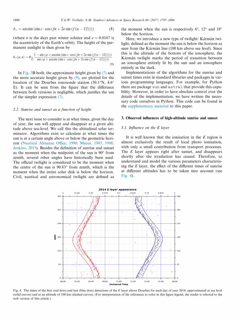
Fig. 4. The times of the first (red dots) and last (blue dots) detections of the E(solid curves) and at an altitude of 100 km (dashed curves). (For interpretationweb version of this article.)

the moment when the sun is respectively 6�, 12� and 18�below the horizon.

Here, we introduce a new type of twilight: Karman twi-light, defined as the moment the sun is below the horizon asseen from the Karman line (100 km above sea level). Sincethis is the altitude of the bottom of the ionosphere, theKarman twilight marks the period of transition betweenan ionosphere entirely lit by the sun and an ionosphereentirely in the dark.

Implementations of the algorithms for the sunrise andsunset times exist in standard libraries and packages in var-ious programming languages. For example, for Pythonthere are package sun and astral that provide this capa-bility. However, in order to have absolute control over thedetails of the implementation, we have written the neces-sary code ourselves in Python. This code can be found inthe supplementary material to this paper.

3. Observed influences of high-altitude sunrise and sunset

3.1. Influence on the E layer

It is well known that the ionisation in the E region isalmost exclusively the result of local photo ionisation,with only a small contribution from transport processes.The E layer appears right after sunset, and disappearsshortly after the irradiation has ceased. Therefore, tounderstand and model the various parameters characteris-ing the E layer, the effect of the different times of sunriseat different altitudes has to be taken into account (seeFig. 4).

layer above Dourbes for each day of year 2014, approximated at sea levelof the references to color in this figure legend, the reader is referred to the

T.G.W. Verhulst, S.M. Stankov / Advances in Space Research 60 (2017) 1797–1806 1801

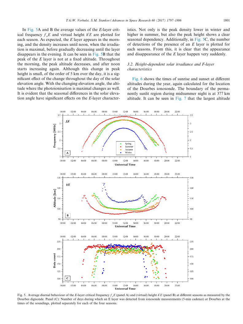
In Fig. 5A and B the average values of the E-layer crit-ical frequency f oE and virtual height h0E are plotted foreach season. As expected, the E layer appears in the morn-ing, and the density increases until noon, when the irradia-tion is maximal, before gradually decreasing until the layerdisappears in the evening. It can be seen in Fig. 5B that thepeak of the E layer is not at a fixed altitude. Throughoutthe morning, the peak altitude decreases, and after noonstarts increasing again. Although this change in peakheight is small, of the order of 5 km over the day, it is a sig-nificant effect of the change throughout the day of the solarelevation angle. With the changing elevation angle, the alti-tude where the photoionisation is maximal changes as well.It is evident that the seasonal differences in the solar eleva-tion angle have significant effects on the E-layer character-

Fig. 5. Average diurnal behaviour of the E-layer critical frequency f oE (panel ADourbes digisonde. Panel (C): Number of days during which an E layer was dtimes of the soundings, plotted separately for each of the four seasons.

istics. Not only is the peak density lower in winter andhigher in summer, but also the peak height shows a clearseasonal dependency. Additionally, in Fig. 5C, the numberof detections of the presence of an E layer is plotted foreach seasons. From this, it is clear that the appearanceand disappearance of the E layer happen very suddenly.

3.2. Height-dependent solar irradiance and F-layer

characteristics

Fig. 6 shows the times of sunrise and sunset at differentaltitudes during the year, again calculated for the locationof the Dourbes ionosonde. The boundary of the perma-nently sunlit region during midsummer night is at 377 kmaltitude. It can be seen in Fig. 7 that the largest altitude

) and (virtual) height h0E (panel B) at different seasons as measured by theetected from ionosonde measurements (5-min cadence) at Dourbes at the

Fig. 6. Sunrise and sunset times as a function of DOY at different altitudes above Dourbes (50.1�N,4.6�E), as calculated for year 2014.

Fig. 7. The daily maximal height of the F 2 peak (black dots) and the boundary of the permanent sunlight (red line) during 2014. (For interpretation of thereferences to color in this figure legend, the reader is referred to the web version of this article.)

1802 T.G.W. Verhulst, S.M. Stankov / Advances in Space Research 60 (2017) 1797–1806

of the F 2 peak during the night is around 400 km. It is evi-dent from this same figure that for several months aroundthe summer solstice the topside ionosphere is for a largepart, or even in its entirety, being irradiated by the sunthroughout the entire day. Nevertheless, there is no evi-dence of the maximal peak height itself being influencedby the seasonal variation of the solar terminator height.The daily maximum is stable around the same altitude of400 km throughout the entire year.

In Fig. 8 the time of the first appearance of the E layerand the time of the minimum in the critical frequency f oF 2

are shown, throughout one year. Since the electron densitydecreases throughout the night, until photoionisationresumes at sunrise, the minimum in the critical frequencycan be expected to occur shortly before sunrise. As alreadymentioned, the E layer is almost exclusively produced bylocal photoionisation and is therefore expected to appearjust after sunrise. Nevertheless, it is clear from the picture

Fig. 8. The times of the daily minima for the critical frequency f oF 2 (bluedots) and the first appearances of the E layer (red dots) during 2014. Thesolid lines show the time of sunrise at 90 km (green) and 1100 km (blue).(For interpretation of the references to color in this figure legend, thereader is referred to the web version of this article.)

T.G.W. Verhulst, S.M. Stankov / Advances in Space Research 60 (2017) 1797–1806 1803

that, on most days, the appearance of the E layer happensbefore the critical frequency reaches its minimum.

4. Adaptation of the LIEDR model

Ionospheric characteristics, scaled automatically fromionosonde measurements together with vertical TEC valuescalculated from GNSS measurements, are used as input forthe RMI Local Ionospheric Electron Density Reconstruc-tion (LIEDR) system (Stankov et al., 2011). LIEDR usesf oF 2; f oE;Mð3000ÞF 2 and TEC as input parameters, aswell as solar radio flux and geomagnetic measurements.It acquires and processes in real time the concurrent andcollocated ionosonde and GNSS TEC measurements, andultimately, deduces a full-height electron density profilebased on a reconstruction technique (Stankov et al.,2003) utilising different ionospheric profiles (Exponential,Epstein, Chapman) and empirically-modelled values ofthe O+–H+ ion transition height. In this way, the topsideprofile is more adequately represented because of the useof independent additional information about the topsideionosphere. The retrieval of the electron density distribu-tion is performed in two main stages: construction of thebottomside electron profile (below hmF 2) and constructionof the topside profiles (above hmF 2). The ionosonde mea-surements are used for directly obtaining the lower partof the electron density profile. The corresponding bottom-side part of TEC is calculated from this profile and is thensubtracted from the entire TEC in order to obtain the

unknown portion of TEC in the upper part. The topsideTEC is used in the next stage for deducing the topsideion and electron profiles. The result is a full-height profileof the electron density distribution, from 90 km up toabout 1100 km, which can be easily put on display (profilo-gram) for a close-up analysis (Fig. 1).

The choice of an appropriate topside profile for use inthe LIEDR is an important issue, which is still the subjectof ongoing research (Verhulst and Stankov, 2013, 2014,2015). In the currently operational version of the model,different profile functions are selected for use during day-time and night-time, respectively: an exponential profile isused during the day, while the Epstein profile is used atnight. However, if the time of change between two topsideprofiles is based on the time of sunrise and sunset at sea-level, artefacts appear in the reconstructed profilograms.In practice, the most obvious discontinuities appear inthe evening, when switching to the nigh-time profile—seeFig. 9, top panel. A possible solution is to switch the top-side profile at the times of sunrise and sunset at the Kar-man altitude. An example of this is shown in the middlepanel of Fig. 9. The discontinuity clearly visible in thetop panel is not so obvious in this case, and also happensslightly later (since the sun sets later at higher altitude).

Another possibility is switching the profiles not based onthe sunrise and sunset at a fixed altitude, but at the altitudeof the F 2 peak. This way, regular variations of the iono-spheric conditions with season and solar activity, as wellas exceptional conditions due to geomagnetic storms, canautomatically be taken into consideration in determiningthe time of the switch. This is the method currently imple-mented in the operational LIEDR model, and an example isshown in the bottom panel of Fig. 9.

Fig. 10 shows the output of the LIEDR model for a weekin each season, as well as the altitude of the solar termina-tor during these periods. It is evident from this figure thatthe effect of the height dependency of the solar terminatorat this location is most important during the summer.Depending on the exact altitude of the F 2 peak, there canbe some nights during which there will be no transitionto the night-time profile at all.

5. Discussion

Sunrise and sunset periods are of particular importanceto ionospheric research and modelling because of the rapidchanges in the key ionospheric plasma characteristics, suchas the ion/electron densities and temperature, as well as inthe dynamics of the plasma transport processes. In partic-ular, the sharp increase in the ionisation following sunriseleads to a prompt and substantial increase in the iono-spheric peak density, NmF 2, and a decrease in the peakheight, hmF 2. Changes in the temperatures and scale heightsfor both the neutral and ionised components, accompaniedby active plasma transport, add further complexity whichmakes it difficult to investigate and model the ionosphericbehaviour during these transitional periods from night to

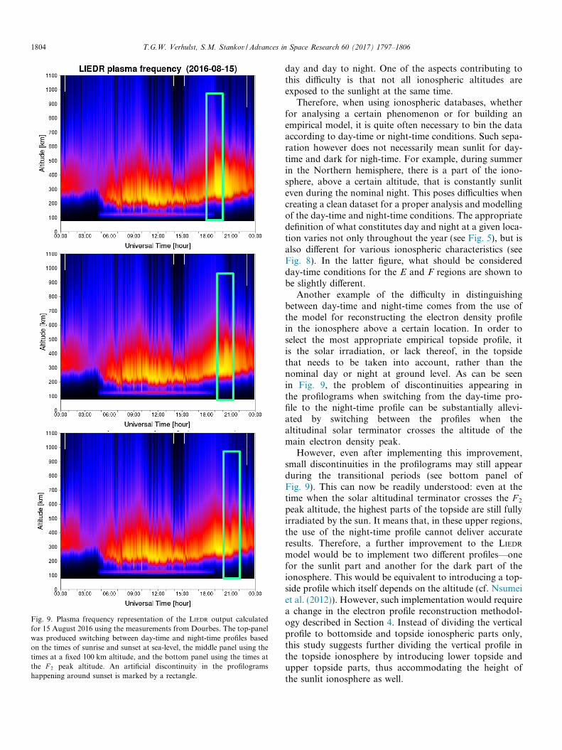
Fig. 9. Plasma frequency representation of the LIEDR output calculatedfor 15 August 2016 using the measurements from Dourbes. The top-panelwas produced switching between day-time and night-time profiles basedon the times of sunrise and sunset at sea-level, the middle panel using thetimes at a fixed 100 km altitude, and the bottom panel using the times atthe F 2 peak altitude. An artificial discontinuity in the profilogramshappening around sunset is marked by a rectangle.

1804 T.G.W. Verhulst, S.M. Stankov / Advances in Space Research 60 (2017) 1797–1806

day and day to night. One of the aspects contributing tothis difficulty is that not all ionospheric altitudes areexposed to the sunlight at the same time.

Therefore, when using ionospheric databases, whetherfor analysing a certain phenomenon or for building anempirical model, it is quite often necessary to bin the dataaccording to day-time or night-time conditions. Such sepa-ration however does not necessarily mean sunlit for day-time and dark for nigh-time. For example, during summerin the Northern hemisphere, there is a part of the iono-sphere, above a certain altitude, that is constantly sunliteven during the nominal night. This poses difficulties whencreating a clean dataset for a proper analysis and modellingof the day-time and night-time conditions. The appropriatedefinition of what constitutes day and night at a given loca-tion varies not only throughout the year (see Fig. 5), but isalso different for various ionospheric characteristics (seeFig. 8). In the latter figure, what should be consideredday-time conditions for the E and F regions are shown tobe slightly different.

Another example of the difficulty in distinguishingbetween day-time and night-time comes from the use ofthe model for reconstructing the electron density profilein the ionosphere above a certain location. In order toselect the most appropriate empirical topside profile, itis the solar irradiation, or lack thereof, in the topsidethat needs to be taken into account, rather than thenominal day or night at ground level. As can be seenin Fig. 9, the problem of discontinuities appearing inthe profilograms when switching from the day-time pro-file to the night-time profile can be substantially allevi-ated by switching between the profiles when thealtitudinal solar terminator crosses the altitude of themain electron density peak.

However, even after implementing this improvement,small discontinuities in the profilograms may still appearduring the transitional periods (see bottom panel ofFig. 9). This can now be readily understood: even at thetime when the solar altitudinal terminator crosses the F 2

peak altitude, the highest parts of the topside are still fullyirradiated by the sun. It means that, in these upper regions,the use of the night-time profile cannot deliver accurateresults. Therefore, a further improvement to the LIEDR

model would be to implement two different profiles—onefor the sunlit part and another for the dark part of theionosphere. This would be equivalent to introducing a top-side profile which itself depends on the altitude (cf. Nsumeiet al. (2012)). However, such implementation would requirea change in the electron profile reconstruction methodol-ogy described in Section 4. Instead of dividing the verticalprofile to bottomside and topside ionospheric parts only,this study suggests further dividing the vertical profile inthe topside ionosphere by introducing lower topside andupper topside parts, thus accommodating the height ofthe sunlit ionosphere as well.

Fig. 10. Plasma frequency profilograms reconstructed using the improved LIEDR model above Dourbes for seven day around the equinoxes and solstices(top to bottom: spring, summer, fall, winter). The green line shows variation of the altitudinal solar terminator with time. (For interpretation of thereferences to color in this figure legend, the reader is referred to the web version of this article.)

T.G.W. Verhulst, S.M. Stankov / Advances in Space Research 60 (2017) 1797–1806 1805

As pointed out earlier in the discussion, the actual posi-tion of the altitudinal solar terminator is just one of severalfactors contributing to the difficulties in modelling theionosphere during the dawn and dusk periods. In termsof ionospheric dynamics (Kelley, 2009), the mid-latitudeF-layer is exposed to the complex interplay of plasma pro-duction and loss (dominant during day), neutral atmo-sphere winds, gravity and electromagnetic forces(dominant during night). Changes in dominance duringthe transitional periods, add further complexity to themodelling task. The ionospheric plasma drifts, both verti-cal and horizontal, are known to play a role in the plasma

redistribution processes occurring during these transitionperiods. Gravity and pressure gradients are mostly respon-sible for the vertical motion, while the neutral winds andelectric fields are for the horizontal motion.

6. Conclusion

This paper is concerned with the complex issue of thesolar illumination of the ionosphere at middle latitudesfor different altitudes, time of day, and day of year. A com-mon misconception is that above a certain location, night-time conditions are equivalent to dark conditions. There

1806 T.G.W. Verhulst, S.M. Stankov / Advances in Space Research 60 (2017) 1797–1806

are instances when, even at mid-latitudes, a part of the top-side ionosphere remains sunlit, at least partially and forvarious periods of time, during the statutory night (at mid-dle latitudes, the period from sunset to sunrise at sea level).The lowest altitude above which the atmosphere is sunlitduring night we termed as altitudinal solar terminator. Ofparticular concern are the sunrise and sunset periods whenrapid changes occur in the ionospheric plasma compositionand dynamics. Although the issue has always been known,it is still often overlooked or poorly handled most probablybecause of the complexities associated with calculating theexact position of the altitudinal solar terminator and imple-menting a relevant algorithm to minimise the errors causedby disregarding this issue.

The behaviour of the altitudinal solar terminator for thelocation of the Dourbes Observatory has been thoroughlyinvestigated and the influence of the height-dependent sun-rise and sunset on the ionospheric E and F layers presentedhere. Mathematical formulae have been deduced, and analgorithm developed, for calculating the height of the ter-minator as a function of the geographic latitude and theday of year. The algorithm has been successfully imple-mented in the operational LIEDR model that is used forreconstructing and imaging in real time the local iono-spheric electron density profile. The implementationproved to be efficient in substantially improving the recon-struction by minimising, and in many cases even eliminat-ing, the discrepancies between consecutive profiles thatused to occur during sunset when switching from the LIEDR

day-time to night-time profiles.Several applications are envisaged for the formulae and

algorithm presented. Perhaps the most important applica-tion would be in theoretical and empirical ionosphericmodels as demonstrated here. Another possible applicationwould be in the development and use of comprehensiveionospheric/atmospheric databases. Scientific research canalso be helped by ensuring the use of clean datasets leadingto more reliable analyses.

Acknowledgement

This work is funded by the Royal Meteorological Insti-tute (RMI) via the Belgian Solar-Terrestrial Centre ofExcellence (STCE).

Appendix A. Supplementary material

Supplementary data associated with this article can befound, in the online version, at http://dx.doi.org/10.1016/j.asr.2017.05.042.

References

Fonda, C., Coısson, P., Nava, B., Radicella, S.M., 2005. Comparison ofanalytical functions used to describe topside electron density profileswith satellite data. Ann. Geophys. 48 (3), 491–495.

Jenkins, A., 2013. The Sun’s position in the Sky. Eur. J. Phys 34, 633–652.Available from: <1208.1043v3>.

Kelley, M.C., 2009. The Earth’s Ionosphere: Plasma Physics andElectrodynamics, second ed. Academic Press, San Diego CA, USA.

Kutiev, I., Marinov, S., Watanabe, S., 2006. Model of topside ionospherescale height based on topside sounder data. Adv. Space Res. 37 (5),943–950.

Meeus, J., 1985. Astronomical Formulæ for Calculators, third ed.Willmann-Bell, Richmond VA, USA.

Meeus, J., 1998. Astronomical Algorithms, second ed. Willmann-Bell,Richmond VA, USA.

Nautical Almanac Office, 1990. Almanac For Computers. United StatesNaval Observatory, Washington DC, USA.

Nsumei, P., Reinisch, B.W., Huang, X., Bilitza, D., 2012. New Vary-Chapprofile of the topside ionosphere electron density distribution for usewith the IRI model and the GIRO real time data. Radio Sci. 47,RS0L16. http://dx.doi.org/10.1029/2012RS004989.

Reinisch, B.X., Nsumei, P., Huang, X., Bilitza, D.K., 2007. Modelling theF2 topside and plasmasphere for IRI using IMAGE/RPI and ISISdata. Adv. Space Res. 39 (5), 731–738.

Reinisch, B.W., Galkin, I.A., Khmyrov, G.M., Kozlov, A.V., Bibl, K.,Lisysyan, I.A., Cheney, G.P., Huang, X., Kitrosser, D.F., Paznukhov,V.V., Luo, Y., Jones, W., Stelmash, S., Hamel, R., Grochmal, J., 2009.New Digisonde for research and monitoring applications. Radio Sci.44, RS0A24. http://dx.doi.org/10.1029/2008RS004115.

Schunk, R., Nagy, A., 2000. Ionospheres – Physics, Plasma Physics, andChemistry. Cambridge University Press, Cambridge, UK.

Stankov, S.M., Jakowski, N., Heise, S., Muhtarov, P., Kutiev, I.,Warnant, R., 2003. A new method for reconstruction of the verticalelectron density distribution in the upper ionosphere and plasmas-phere. J. Geophys. Res. 108 (A5), 1164. http://dx.doi.org/10.1029/2002JA009570.

Stankov, S.M., Stegen, K., Muhtarov, P., Warnant, R., 2011. Localionospheric electron density profile reconstruction in real time fromsimultaneous ground-based GNSS and ionosonde measurements. Adv.Space Res. 47 (7), 1172–1180. http://dx.doi.org/10.1016/j.asr.2010.11.039.

Verhulst, T., Stankov, S.M., 2013. The topside sounder database – datascreening and systematic biases. Adv. Space Res. 51 (11), 2010–2017.http://dx.doi.org/10.1016/j.asr.2012.12.023.

Verhulst, T., Stankov, S.M., 2014. Evaluation of ionospheric profilersusing topside sounding data. Radio Sci. 49 (3), 181–195. http://dx.doi.org/10.1002/2013RS005263.

Verhulst, T., Stankov, S.M., 2015. Ionospheric specification with analyt-ical profilers: evidences of non-Chapman electron density distributionin the upper ionosphere. Adv. Space Res. 55 (8), 2058–2069. http://dx.doi.org/10.1016/j.asr.2014.10.017.