Embed Size (px)
Citation preview

Hedging Strategies To Manage Commodity Price Risk
Karen Ósk Finsen
Thesis of 30 ECTS credits Master of Science in Financial Engineering
June 2018
Hedging Strategies To Manage Commodity Price Risk
by
Karen Ósk Finsen
Thesis of 30 ECTS credits submitted to the School of Science and Engineeringat Reykjavík University in partial fulfillment
of the requirements for the degree ofMaster of Science (M.Sc.) in Financial Engineering
June 2018
Supervisor:
Dr. Sverrir Ólafsson, SupervisorProfessor, Reykjavík University, Iceland
Examiner:
Dr. Sigurur Pétur Magnússon, ExaminerArion Banki, Reykjavík, Iceland
i

CopyrightKaren Ósk Finsen
June 2018
ii

Hedging Strategies To Manage Commodity Price RiskKaren Ósk Finsen
June 2018
Abstract
Price fluctuations in commodity markets can have a significant impact on potential profits,both for those who use and produce that commodity. Commodity prices, which are basedon the supply and demand of a market, are very volatile and it is nearly impossible to predictexactly which way a price will move in the future. Companies that are impacted by unexpectedcommodity price movements should consider managing these risks and minimizing theire�ects through the use of financial market instruments. The purpose of this thesis is to use riskmanagement strategies and derivatives to hedge risks faced by an Icelandic manufacturer thatuses gold as an input. Fluctuating gold prices and foreign exchange rates are causing changesin cash flows and a�ecting the company’s profitability. To reduce these risks, the companycan hedge its exposure through the use of derivatives, such as futures contracts, forwardcontracts, options and swaps. Historical data on gold prices and foreign exchange rates areused to predict future prices and to calculate Value at Risk. Black Scholes model and MonteCarlo simulation are used for option pricing. In conclusion, risk management strategies andderivatives reduce price uncertainty and stabilize future cash flow. But considerable risk canalso accompany the use of risk management, whereby the price of the underlying asset candevelop in a di�erent direction to what was predicted.
iii

Áhættuvarnir Gegn Versveiflum á HrávörumarkaiKaren Ósk Finsen
júní 2018
Útdráttur
Versveiflur á hrávörumörkuum geta haft veruleg áhrif á fjárhagslegan ávinning fyrirtækjasem stunda viskipti me hrávörur. Mikil óvissa ríkir almennt á �essum mörkuum og getur�ví áhættan veri mikil bæi fyrir �au fyrirtæki sem nota og framleia hrávörur. Til �essa verjast �essum óvæntu versveiflum á markai er hægt a nota aferir áhættust˝ringarog tryggja �ar af leiandi stöugra tekjustreymi í framtíinni. Markmi �essara ritgerarer a s˝na hvernig íslenskt fyrirtæki sem notar gull í framleislu sinni getur nota áhætt-urvarnir og afleiusamninga til �ess a verja sig fyrir áhættum sem a �a stendur frammifyrir. Helstu áhættu�ættir sem hafa áhrif á tekjustreymi fyrirtækisins eru verbreytingar águlli, gjaldeyrishreyfingar og vaxtabreytingar. Skoa er hvernig fyrirtæki getur n˝tt sérframvirka samninga, valrétti og skiptasamninga til �ess a draga úr �essum helstu áhættu-�áttum. Notast var vi söguleg gögn um ver á gulli og gengis�róun krónunnar gagnvartbandaríkjadal til a spá fyrir um framtíarver og til �ess a reikna áhættuviri sem segirtil um hugsanleg tap fyrirtækisins á ákvenu tímabili í framtíinni. Black-Scholes aferinog Monte Carlo hermun eru notaar til �ess a verleggja valréttina. Helstu niurstöureru �ær a áhættust˝ring og notkun afleiusamninga dregur úr helstu áhættum me �ví astula a stöugum tekjum og minnka verulega óvæntar versveiflur í rekstri fyrirtækisins.En �a getur líka fylgt �ví töluver áhætta a notast vi áhættust˝ringu �ar sem veri áundirliggjandi eign getur �róast í ara átt en búi var a spá fyrir um.
iv
Hedging Strategies To Manage Commodity Price Risk
Karen Ósk Finsen
Thesis of 30 ECTS credits submitted to the School of Science and Engineeringat Reykjavík University in partial fulfillment of
the requirements for the degree ofMaster of Science (M.Sc.) in Financial Engineering
June 2018
Student:
Karen Ósk Finsen
Supervisor:
Dr. Sverrir Ólafsson
Examiner:
Dr. Sigurur Pétur Magnússon
v

The undersigned hereby grants permission to the Reykjavík University Library to reproducesingle copies of this Thesis entitled Hedging Strategies To Manage Commodity PriceRisk and to lend or sell such copies for private, scholarly or scientific research purposes only.The author reserves all other publication and other rights in association with the copyrightin the Thesis, and except as herein before provided, neither the Thesis nor any substantialportion thereof may be printed or otherwise reproduced in any material form whatsoeverwithout the author’s prior written permission.
date
Karen Ósk FinsenMaster of Science
vi

vii
Acknowledgements
I would like to thank my supervisor Dr. Sverrir Ólafsson for all his help andguidance through this research. I would also like thank my family and friendsfor all the support over the last years.
viii
Contents
Acknowledgements viii
Contents ix
List of Figures xi
List of Tables xiii
List of Abbreviations xiv
1 Introduction 1
2 Risk and risk management 22.1 What is risk? . . . . . . . . . . . . . . . . . . . . . . . . . . . . . . . . . 22.2 Financial risk . . . . . . . . . . . . . . . . . . . . . . . . . . . . . . . . . 22.3 Risk management . . . . . . . . . . . . . . . . . . . . . . . . . . . . . . . 22.4 Why manage risk? . . . . . . . . . . . . . . . . . . . . . . . . . . . . . . . 3
3 Types of risk faced by corporations 43.1 Foreign exchange risk . . . . . . . . . . . . . . . . . . . . . . . . . . . . . 43.2 Interest rate risk . . . . . . . . . . . . . . . . . . . . . . . . . . . . . . . . 43.3 Commodity price risk . . . . . . . . . . . . . . . . . . . . . . . . . . . . . 4
4 How to quantify risk? 64.1 Risk as spread in returns . . . . . . . . . . . . . . . . . . . . . . . . . . . 64.2 Value at Risk . . . . . . . . . . . . . . . . . . . . . . . . . . . . . . . . . 74.3 Risk from foreign investment . . . . . . . . . . . . . . . . . . . . . . . . . 74.4 Monte Carlo . . . . . . . . . . . . . . . . . . . . . . . . . . . . . . . . . . 8
5 Instruments available for risk management purpose 95.1 Forward contracts . . . . . . . . . . . . . . . . . . . . . . . . . . . . . . . 95.2 Futures contracts . . . . . . . . . . . . . . . . . . . . . . . . . . . . . . . 9
5.2.1 Payo�s from forward and future contracts . . . . . . . . . . . . . . 105.2.2 Forward contracts on currencies . . . . . . . . . . . . . . . . . . . 10
5.3 Vanilla options . . . . . . . . . . . . . . . . . . . . . . . . . . . . . . . . 115.3.1 Options positions . . . . . . . . . . . . . . . . . . . . . . . . . . . 11
5.4 Asian options . . . . . . . . . . . . . . . . . . . . . . . . . . . . . . . . . 125.5 Swaps . . . . . . . . . . . . . . . . . . . . . . . . . . . . . . . . . . . . . 125.6 Hedging strategies using derivatives . . . . . . . . . . . . . . . . . . . . . 13
ix
6 Valuing and pricing derivatives 146.1 Valuing European options . . . . . . . . . . . . . . . . . . . . . . . . . . . 146.2 Valuing currency options . . . . . . . . . . . . . . . . . . . . . . . . . . . 146.3 Implied volatility . . . . . . . . . . . . . . . . . . . . . . . . . . . . . . . 156.4 Monte Carlo methods . . . . . . . . . . . . . . . . . . . . . . . . . . . . . 156.5 Ornstein-Uhlenbeck process . . . . . . . . . . . . . . . . . . . . . . . . . 166.6 Valuing a commodity swap . . . . . . . . . . . . . . . . . . . . . . . . . . 166.7 Valuing a fixed-floating currency swap . . . . . . . . . . . . . . . . . . . . 17
7 Description of the risks the firm faces 197.1 Description of the firm to be discussed . . . . . . . . . . . . . . . . . . . . 197.2 Commodity price risk . . . . . . . . . . . . . . . . . . . . . . . . . . . . . 197.3 Instruments available to manage commodity price risk . . . . . . . . . . . . 27
7.3.1 Commodity futures . . . . . . . . . . . . . . . . . . . . . . . . . . 277.3.2 Commodity options . . . . . . . . . . . . . . . . . . . . . . . . . . 277.3.3 Commodity swaps . . . . . . . . . . . . . . . . . . . . . . . . . . 27
7.4 Foreign exchange risk . . . . . . . . . . . . . . . . . . . . . . . . . . . . . 277.5 Instruments available to manage foreign exchange risk . . . . . . . . . . . 31
7.5.1 Forward exchange contract . . . . . . . . . . . . . . . . . . . . . . 317.5.2 Currency options . . . . . . . . . . . . . . . . . . . . . . . . . . . 317.5.3 Currency swaps . . . . . . . . . . . . . . . . . . . . . . . . . . . . 31
7.6 Comparison of the two risk types . . . . . . . . . . . . . . . . . . . . . . . 31
8 Implementation of risk management strategies 358.1 Hedging gold price with a future contract . . . . . . . . . . . . . . . . . . 358.2 Hedging foreign exchange rate with a forward contract . . . . . . . . . . . . 368.3 Pricing a European call option . . . . . . . . . . . . . . . . . . . . . . . . 388.4 Pricing Asian call option . . . . . . . . . . . . . . . . . . . . . . . . . . . 418.5 Pricing a currency call option . . . . . . . . . . . . . . . . . . . . . . . . . 428.6 Pricing a gold swap . . . . . . . . . . . . . . . . . . . . . . . . . . . . . . 448.7 Pricing a currency swap . . . . . . . . . . . . . . . . . . . . . . . . . . . . 468.8 Summary . . . . . . . . . . . . . . . . . . . . . . . . . . . . . . . . . . . 48
9 Discussion and Conclusion 52
Bibliography 53
x
List of Figures
2.1 Risk management planning process . . . . . . . . . . . . . . . . . . . . . . . . 32.2 Risk management implementation process . . . . . . . . . . . . . . . . . . . . 3
5.1 Payo� from a longposition at maturity. . . . . . . . . . . . . . . . . . . . . . . . . . . . . . . . . 10
5.2 Payo� from a shortposition at maturity. . . . . . . . . . . . . . . . . . . . . . . . . . . . . . . . . 10
5.3 Payo� from a longposition in a call option. . . . . . . . . . . . . . . . . . . . . . . . . . . . . . . 12
5.4 Payo� from a shortposition in a call option. . . . . . . . . . . . . . . . . . . . . . . . . . . . . . . 12
5.5 Payo� from a longposition in a put option. . . . . . . . . . . . . . . . . . . . . . . . . . . . . . 12
5.6 Payo� from a shortposition in a put option. . . . . . . . . . . . . . . . . . . . . . . . . . . . . . . 12
7.1 Historical data of gold prices between 4 December 2015 and 4 December 2017. 207.2 The daily gold price change . . . . . . . . . . . . . . . . . . . . . . . . . . . . 217.3 Probability density function for the returns. . . . . . . . . . . . . . . . . . . . 227.4 Cumulative probability function for daily gold price changes . . . . . . . . . . 237.5 VaR as a function of time . . . . . . . . . . . . . . . . . . . . . . . . . . . . . 247.6 Simulated 10,000 price paths for gold using the Ornstein-Uhlenbeck process. . 257.7 Profit loss probability density function for June 2018 . . . . . . . . . . . . . . 267.8 Profit-and-loss probability density function for December 2018 . . . . . . . . . 267.9 Historical data of the foreign exchange rate. . . . . . . . . . . . . . . . . . . . 287.10 Daily change in exchange rate . . . . . . . . . . . . . . . . . . . . . . . . . . . 297.11 Probability density function for daily rate returns . . . . . . . . . . . . . . . . 307.12 Cumulative probability function for daily rate change . . . . . . . . . . . . . . 307.13 Daily gold price in ISK/oz. . . . . . . . . . . . . . . . . . . . . . . . . . . . . 327.14 VaR calculations for given months . . . . . . . . . . . . . . . . . . . . . . . . 34
8.1 The profit diagram for the long Gold futures contract with maturity in June 2018. 368.2 The profit diagram for the long foreign exchange rate forward contract with
maturity in June 2018. . . . . . . . . . . . . . . . . . . . . . . . . . . . . . . 378.3 10,000 simulated price paths 252 days into the future. . . . . . . . . . . . . . . 388.4 The profit from a long position in a call option with strike 1280 in June 2018. . 408.5 Simulated price paths for foreign exchange rate . . . . . . . . . . . . . . . . . 438.6 Payo� from a long currency call option . . . . . . . . . . . . . . . . . . . . . . 448.7 The present value of the swap contract at di�erent maturities. . . . . . . . . . . 46
xi

8.8 The present value of the currency swap contract at di�erent maturities. . . . . . 488.9 The probability density function for the present value of option payments . . . . 50
xii

List of Tables
7.1 The USD Libor rates, required quantities of gold, the future price and the expectedexposure for gold based on information on 4 December 2017. . . . . . . . . . . 20
7.2 Theoretical and Empirical probabilities . . . . . . . . . . . . . . . . . . . . . . 227.3 The 95% VaR risk for the gold price. . . . . . . . . . . . . . . . . . . . . . . . 237.4 Gold price forecast from January 2018 and December 2018. . . . . . . . . . . 257.5 The 95% VaR for the gold price. . . . . . . . . . . . . . . . . . . . . . . . . . 277.6 The calculated forward exchange rate . . . . . . . . . . . . . . . . . . . . . . . 287.7 Theoretical and Empirical probabilities . . . . . . . . . . . . . . . . . . . . . . 297.8 Forward exchange rate and gold future price in USD per oz and ISK per oz. . . 327.9 Correlation between the return of gold price and foreign exchange rate . . . . . 337.10 The 95% VaR risk for the gold price in ISK. . . . . . . . . . . . . . . . . . . . 33
8.1 The future price for gold ($/oz). . . . . . . . . . . . . . . . . . . . . . . . . . 358.2 Calculated forward exchange rate . . . . . . . . . . . . . . . . . . . . . . . . . 378.3 Valuation of call options . . . . . . . . . . . . . . . . . . . . . . . . . . . . . 398.4 Valuation of call options . . . . . . . . . . . . . . . . . . . . . . . . . . . . . 398.5 Valuation of call options . . . . . . . . . . . . . . . . . . . . . . . . . . . . . 398.6 Valuation of call options . . . . . . . . . . . . . . . . . . . . . . . . . . . . . 408.7 Probabilities for monthly gold price to be greater than the strike price . . . . . 418.8 Valuations of Asian call options . . . . . . . . . . . . . . . . . . . . . . . . . 418.9 Valuations of Asian call options . . . . . . . . . . . . . . . . . . . . . . . . . 418.10 Valuations of Asian call options . . . . . . . . . . . . . . . . . . . . . . . . . 428.11 Calculated Monte Carlo price and Black Scholes price for currency call option . 438.12 The Swap Contract . . . . . . . . . . . . . . . . . . . . . . . . . . . . . . . . 458.13 The Currency Swap Contract . . . . . . . . . . . . . . . . . . . . . . . . . . . 478.14 Compared hedging strategies for gold prices . . . . . . . . . . . . . . . . . . . 498.15 Compared hedging strategies for exchange rate . . . . . . . . . . . . . . . . . . 518.16 Compared hedging strategies for exchange rate . . . . . . . . . . . . . . . . . . 51
xiii

List of Abbreviations
VaR Value at RiskOTC Over the counterSDE Stochastic di�erential equationPV Present Valuepdf Probability density functioncdf Cumulative density function
xiv
Chapter 1
Introduction
Uncertainty in commodity prices poses a huge risk to producers, manufactures and con-sumers, who are all a�ected by fluctuations in the market prices. Prices are based on supplyand demand of a market and therefore it can be di�cult to predict future price movements.A business operating in the commodity markets should consider managing these risks wherefluctuations in commodity prices may impact business profitability.
Companies that are exposed to commodity risk may also be exposed to foreign exchangerisk, since most commodities are quoted in US dollars. Managing only commodity risk willleave the company exposed to adverse movements in foreign exchange rates. When lockingthe price in US dollars, the foreign exchange risk remains. With fluctuating commodityprices, foreign exchange rate risk can be complicated to manage. By using appropriate riskmanagement strategies, the risk of unexpected price movements can be reduced.
Risk management is not always profitable because there can be risk and potential loss ifthe price of the underlying asset develops in a di�erent direction to what was predicted or ifthe company chooses an inappropriate risk management tool. Therefore, a risk managementplan must be appropriately implemented if it is to be successful.
The objective of this research is to reduce market price risk and foreign exchange riskof a company operating in the jewelry industry by implementing risk management strategies.The aim is to find the best way for the company to manage these risks. This thesis willanswer the following main questions:
• What is the purpose of implementing risk management strategies?
• What are the reasons firms seek to manage risk?
The outline of this thesis is as follows. Chapter 2 begins with a description of risk and riskmanagement. Chapter 3 discusses the description of risks faced by corporations, commodityprice risk, foreign exchange risk and interest rate risk. Chapter 4 introduces methods toquantify risks. Derivatives are introduced as instruments available for risk management inChapter 5 while Chapter 6 demonstrates methods for valuing and pricing these derivatives.Chapters 7 describe the firm and the risks the firm faces. In Chapter 8, implementation of riskstrategies for the firm is described. Finally, Chapter 9 presents discussion and conclusions.
Chapter 2
Risk and risk management
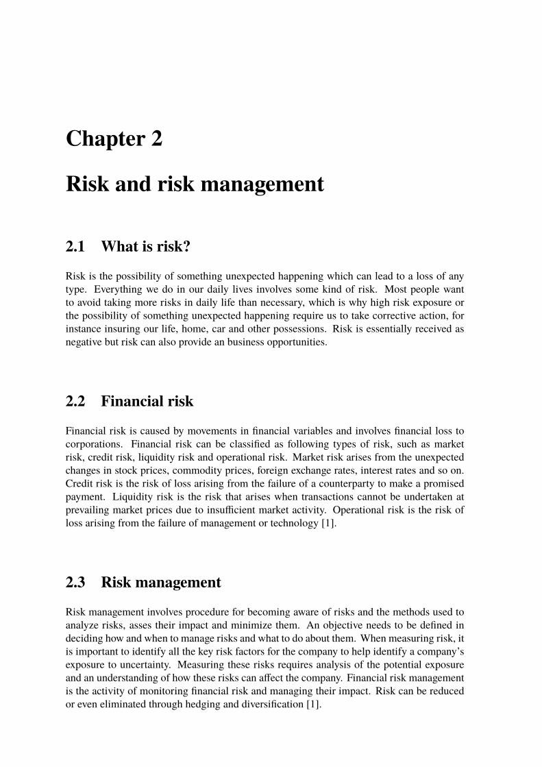
2.1 What is risk?
Risk is the possibility of something unexpected happening which can lead to a loss of anytype. Everything we do in our daily lives involves some kind of risk. Most people wantto avoid taking more risks in daily life than necessary, which is why high risk exposure orthe possibility of something unexpected happening require us to take corrective action, forinstance insuring our life, home, car and other possessions. Risk is essentially received asnegative but risk can also provide an business opportunities.
2.2 Financial risk
Financial risk is caused by movements in financial variables and involves financial loss tocorporations. Financial risk can be classified as following types of risk, such as marketrisk, credit risk, liquidity risk and operational risk. Market risk arises from the unexpectedchanges in stock prices, commodity prices, foreign exchange rates, interest rates and so on.Credit risk is the risk of loss arising from the failure of a counterparty to make a promisedpayment. Liquidity risk is the risk that arises when transactions cannot be undertaken atprevailing market prices due to insu�cient market activity. Operational risk is the risk ofloss arising from the failure of management or technology [1].
2.3 Risk management
Risk management involves procedure for becoming aware of risks and the methods used toanalyze risks, asses their impact and minimize them. An objective needs to be defined indeciding how and when to manage risks and what to do about them. When measuring risk, itis important to identify all the key risk factors for the company to help identify a company’sexposure to uncertainty. Measuring these risks requires analysis of the potential exposureand an understanding of how these risks can a�ect the company. Financial risk managementis the activity of monitoring financial risk and managing their impact. Risk can be reducedor even eliminated through hedging and diversification [1].
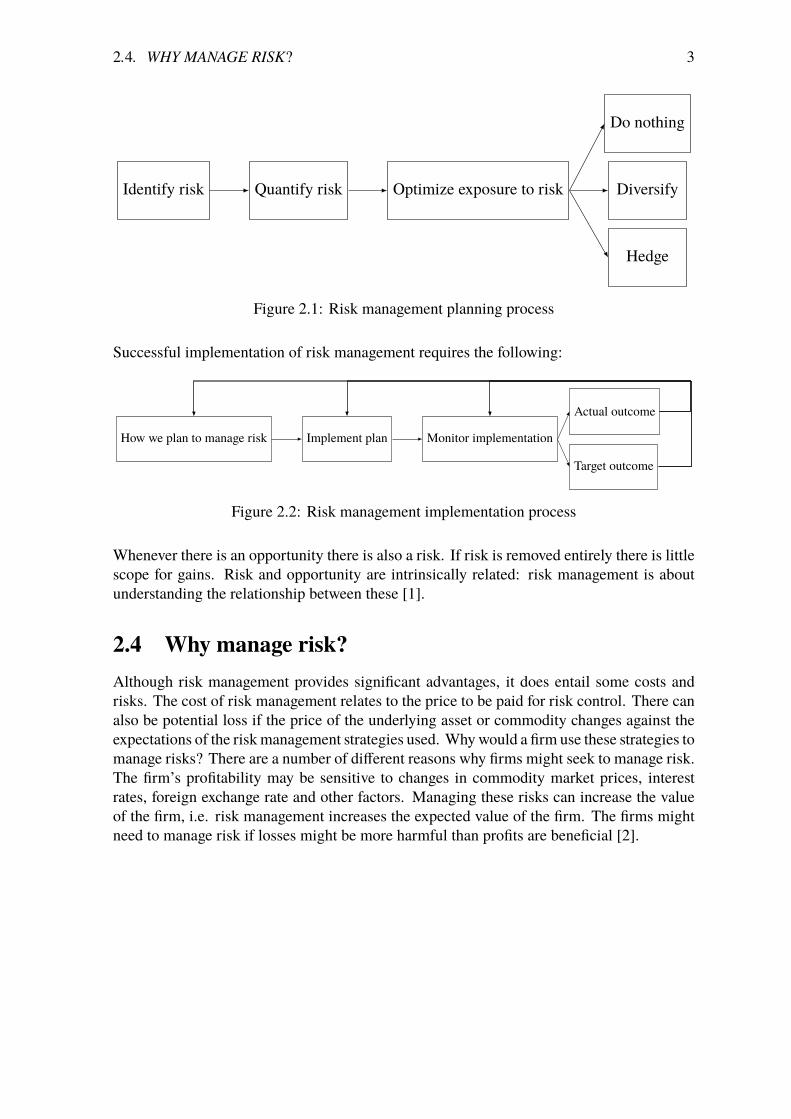
�.�. WHY MANAGE RISK� 3
Identify risk Quantify risk Optimize exposure to risk Diversify
Hedge
Do nothing
Figure 2.1: Risk management planning process
Successful implementation of risk management requires the following:
How we plan to manage risk Implement plan Monitor implementation
Target outcome
Actual outcome
Figure 2.2: Risk management implementation process
Whenever there is an opportunity there is also a risk. If risk is removed entirely there is littlescope for gains. Risk and opportunity are intrinsically related: risk management is aboutunderstanding the relationship between these [1].
2.4 Why manage risk?Although risk management provides significant advantages, it does entail some costs andrisks. The cost of risk management relates to the price to be paid for risk control. There canalso be potential loss if the price of the underlying asset or commodity changes against theexpectations of the risk management strategies used. Why would a firm use these strategies tomanage risks? There are a number of di�erent reasons why firms might seek to manage risk.The firm’s profitability may be sensitive to changes in commodity market prices, interestrates, foreign exchange rate and other factors. Managing these risks can increase the valueof the firm, i.e. risk management increases the expected value of the firm. The firms mightneed to manage risk if losses might be more harmful than profits are beneficial [2].
Chapter 3
Types of risk faced by corporations
There are many di�erent types of risks that corporations and financial institutions might faceand need to overcome. Identifying and managing these risks has become a focus point withinmost corporations to minimize their losses and maximize their profit. Before understandingthe techniques to control risk and perform risk management, it is very important to realizewhat risk is and what the types of risks are.
3.1 Foreign exchange riskForeign exchange risk is the risk that the value of one currency changes against another.Fluctuations in exchange rates will a�ect companies that export or import their goods andservices and can have a big impact on company income. Companies importing their goodsand services may end up paying more than expected. Companies that export their goodsand services may be at risk of getting paid less than planned. This is a big risk factor forbusinesses that deal in more than one currency but other businesses can also be exposed toforeign exchange risk if for example their business relies on imported products or services[3].
3.2 Interest rate riskInterest rate risk is the risk of fluctuations in interest rates on borrowed or invested money thatcan have a big impact on company’s profitability. Cash flows of the borrower or lender area�ected by the changes in interest rates whereby the borrower can face increased costs wheninterest costs fluctuate according to interest rate movements during the life of a loan. Anadverse movement in interest rate may potentially increase borrowing costs for borrowers andreduce returns for investors. When borrowers are generally concerned about rising interestrates, investors are concerned about falling rates [4].
3.3 Commodity price riskCommodity price risk is the risk arising from changes in commodity prices that impactthe firms that both use and produce a commodity. Commodities is a term for a basicgood which can generally be classified into three categories: soft commodities, metals andenergy commodities. Soft commodities include agricultural products such as wheat, co�ee,sugar and fruit. Metals include gold, silver, copper and aluminum. Energy commodities
�.�. COMMODITY PRICE RISK 5
include gas, oil and coal. Commodity price risk is a significant problem for some firmsthat use commodities in their manufacturing process and for consumers in general, bothbecause consuming firms that use raw materials for their production may face increasedproduction costs due to fluctuations in commodity prices and because producing firms thatsell commodities are exposed to price falls which mean they will receive less revenue for thecommodities they produce [5].
Chapter 4
How to quantify risk?
Measuring risk is important and helps the company to recognize the impact of the risksinvolved in the business. When measuring risk, a company can identify which risk factorsare most important and can therefore prepare for the damage these can cause. By identifyingthe amount of risk involved, the company can make a decision to either accept or mitigatethe risk. The firms then need to make a decision about how much risk may be acceptableand how much exposure can be tolerated. This should lead the firm to make strategic choicesabout what risks to accept and how risks are to be managed. The most common way ofmeasuring risk factors is to evaluate the likelihood that events will occur and what theirimpact would be. Risk is the volatility of presently unknown future outcomes, for examplereturns. This uncertainty implies possible good or bad outcomes. One popular way toquantify risk exposure is in terms of Value at Risk (VaR).
4.1 Risk as spread in returnsReturns are changes in price that are relative to some initial price. The return series canvisualize the price volatility better than the price series. The percent change in value (returns)in the time period from t-1 to t is:
rt =St � St�1
St�1100 (4.1)
where St is the price of an asset at time t. The return series provides the data for a volatilitymodeling. By modeling the return distribution, probabilistic quantification of losses andgains can be calculated and compared between di�erent investments [6]. VaR can be calcu-lated from the probability distribution for asset values or returns.
In favor of normally distributed historical data of some security returns, their probabilitydistribution can be presented by:
p(r) = 1p
2⇡�2exp(� (µ � r)2
2�2 ) (4.2)
where µ is the mean and � is the standard deviation of the historical returns. Cumulativenormal distribution is:
F(x0) = Pr(x x0 |µ,�) =π x0
�1f (y |µ,�) dy (4.3)
�.�. VALUE AT RISK 7
The probability that a return events is below some fixed value a is:
P(x a) = 12(1 + er f (a � µ
p2�
)) (4.4)
P(x � a) = 12(1 � er f (a � µ
p2�
)) (4.5)
where the error function and the complementary error function are defined as:
er f (x) = 2p⇡
π x
0exp(�w2) dw (4.6)
er f (x) = 1 � 2p⇡
π 1
xexp(�w2) dw (4.7)
4.2 Value at RiskValue at Risk (VaR) measures the worst loss expected over a given time interval at a givenconfidence level. VaR is defined by the following statement: "I am c percent certain that I
will not loose more than X dollars in the next T days” where the variable X is the VaR ofthe portfolio and c is the confidence level. VaR is a popular measure because it provides asingle number summarizing the total risk and it is easy to understand. Given the historicalprobability distribution for returns, VaR calculates the probability of su�ering certain lossesover a fixed time period. Following the assumption that returns are normally distributed, thevalue at risk for the time period of T days is [6]:
VaR(↵,�R,T,T,V0) = ↵V0�R,T (4.8)
where �R,T is the standard deviation for T days calculated as follows:
�R,T = �R,1p
T (4.9)
where �R,1 is the standard deviation of daily returns. Then the VaR for longer time period ofT days is:
VaR(↵,�R,T,V0) = ↵V0�R,1p
T (4.10)
One popular approach to calculate VaR is historical simulation. Historical simulation involvesusing past data as a guide to what will happen in the future by creating a database consistingof the daily movements in all market variables over a period of time. The change inthe portfolio value is calculated for each simulation trial and the VaR is calculated as theappropriate percentile of the probability distribution of �P [7].
4.3 Risk from foreign investmentThe risk from foreign investments is a�ected by returns in the security’s home market andchanges in exchange rates. It is important to understand the relationship between these tworisk factors. The exchange rate X f ,d(t) at time t measures the amount of foreign currency
8 CHAPTER �. HOW TO QUANTIFY RISK�
per unit of domestic currency [6]. When investing Qd(t) in a foreign security Q f (t) at timet, the investor buys foreign currency as follows:
Q f (t) = X f ,d(t)Qd(t) (4.11)
The value of the investment in foreign currency at time T is:
Q f (T) = (1 + Rf (t,T))Q f (t) (4.12)
and the domestic value of the foreign currency at time T is:
Qd(T) = Xd, f (T)Q f (T) (4.13)
where Xd, f is the amount of domestic currency per unit of foreign currency.
The percent change (returns) in the exchange rate is:
�Xd, f (t,T) =Xd, f (T) � Xd, f (t)
Xd, f (t)(4.14)
and the standard deviation of returns:
�d = (�2f + �
2X + 2� f ⇢ f ,X�X)
12 (4.15)
4.4 Monte CarloMonte Carlo simulation can be used to create a distribution based on the assumption of certainstochastic processes for the underlying variables. Monte Carlo simulation is a numericalprocedure that gives potential outcomes of a scenario using stochastic processes to give anestimate of the range and likelihood of possible future outcomes.

Chapter 5
Instruments available for riskmanagement purpose
A derivative is a financial instrument whose value depends on, or is derived from, the valuesof other underlying variables. These underlying variables can be dependent on almost anyvariable, e.g. interest rates, commodities, stocks, bonds or weather. Derivatives play a keyrole in transferring risks in the economy. Derivatives are either traded on exchange, suchas the Chicago Board Options Exchange, or over-the-counter (OTC) markets where tradersworking for banks, fund managers and corporate treasurers contact each other directly. Threemain types of traders can be identified: hedgers, speculators and arbitrageurs. Hedgers usederivatives to reduce the risk from a future movement in a market variable. Speculatorsuse derivatives to bet on the future direction of a market variable to get extra leverage.Arbitrageurs take a position in two or more markets to lock in a riskless profit. The mostcommon types of derivatives are forward contracts, future contracts, swaps and options [7].
5.1 Forward contracts
Forward contract is an agreement to buy or sell an asset or commodity at a specific time in thefuture for a certain price. The time at which the contract settles is called the expiration date.The asset or the commodity on which the forward contract is based is called the underlyingasset. A forward contract is traded in the over-the-counter market so the contract can becustomized between any two parties. One party agrees to buy the underlying asset on acertain future date for a certain price and the other party agrees to sell the asset on the samedate for the same price. The party that agrees to buy has a long position and the party thatagrees to sell has a short position [7].
5.2 Futures contracts
Future contract is an agreement between two parties to buy or sell an asset at a certain timein the future for certain price. Futures contracts are standardized and traded on exchanges[7].
10 CHAPTER �. INSTRUMENTS AVAILABLE FOR RISK MANAGEMENT PURPOSE
5.2.1 Payo�s from forward and future contractsThe fair or arbitrage free forward price for an asset that pays no dividend or has storage cost,presently priced at S(t) and to be received at the future time T, is:
F(t,T) = S(t)eR(t,T)(T�t) (5.1)
where R(t,T) is the rate for maturity T-t. The ratio between the forward price F(T,t) and thespot price S(t) is called the forward premium for maturity T-t:
FP(t,T) = F(t,T)S(t) = eR(t,T)(T�t) (5.2)
The forward price for an asset that pays annualized dividend yield � [8] is:
F(t,T) = S(t)e��(T�t)eR(t,T)(T�t) = S(t)e(R(t,T)��)(T�t) (5.3)
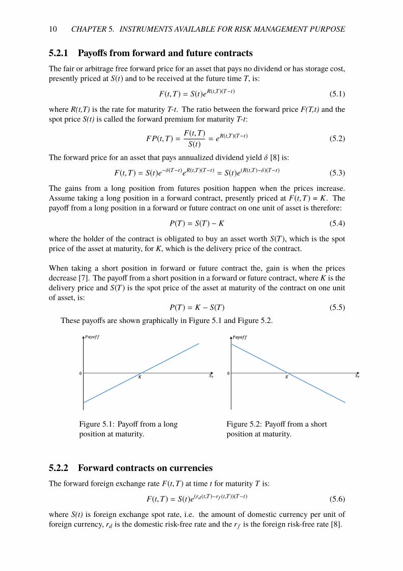
The gains from a long position from futures position happen when the prices increase.Assume taking a long position in a forward contract, presently priced at F(t,T) = K . Thepayo� from a long position in a forward or future contract on one unit of asset is therefore:
P(T) = S(T) � K (5.4)
where the holder of the contract is obligated to buy an asset worth S(T), which is the spotprice of the asset at maturity, for K, which is the delivery price of the contract.
When taking a short position in forward or future contract the, gain is when the pricesdecrease [7]. The payo� from a short position in a forward or future contract, where K is thedelivery price and S(T) is the spot price of the asset at maturity of the contract on one unitof asset, is:
P(T) = K � S(T) (5.5)These payo�s are shown graphically in Figure 5.1 and Figure 5.2.
Figure 5.1: Payo� from a longposition at maturity.
Figure 5.2: Payo� from a shortposition at maturity.
5.2.2 Forward contracts on currenciesThe forward foreign exchange rate F(t,T) at time t for maturity T is:
F(t,T) = S(t)e(rd(t,T)�rf (t,T))(T�t) (5.6)
where S(t) is foreign exchange spot rate, i.e. the amount of domestic currency per unit offoreign currency, rd is the domestic risk-free rate and the r f is the foreign risk-free rate [8].
�.�. VANILLA OPTIONS 11
5.3 Vanilla optionsThere are two types of option: call options and put options. A call option gives the holderthe right to buy the underlying asset by a certain date for a certain price. A put option givesthe holder the right to sell the underlying asset by a certain date for a certain price. Sincean option gives the holder the right and not the obligation to buy or sell an asset, a cost isincurred when entering an option [7]. This initial cost that the option buyer must pay whenentering into the contract is called the option price or premium. The strike price or theexercise price is the fixed price at which the option holder can either buy or sell the asset. Acall option is said to be in-the-money if the asset price at maturity S(T) exceeds the strikeprice K and out-of-the money if the asset price at maturity is less than the strike price. A putoption is said to be in-the-money if the asset price at maturity is less than the strike price andout-of-the-money if the asset price at maturity is more than the strike price. If the asset priceat maturity is equal to the strike price, the option is said to be at-the-money. In-the-moneyoptions are exercised but out-of-the-money options are never exercised [2].
5.3.1 Options positionsThere are two sides to every option contract. The party agreeing to buy an options is saidto have a long option position and the party agreeing to sell an option has a short optionposition. There are four types of option position:
• A long position in a call option is the right to buy
• A short position in a call option is the obligation to sell
• A long position in a put option is the right to sell
• A short position in a put option is the obligation to buy
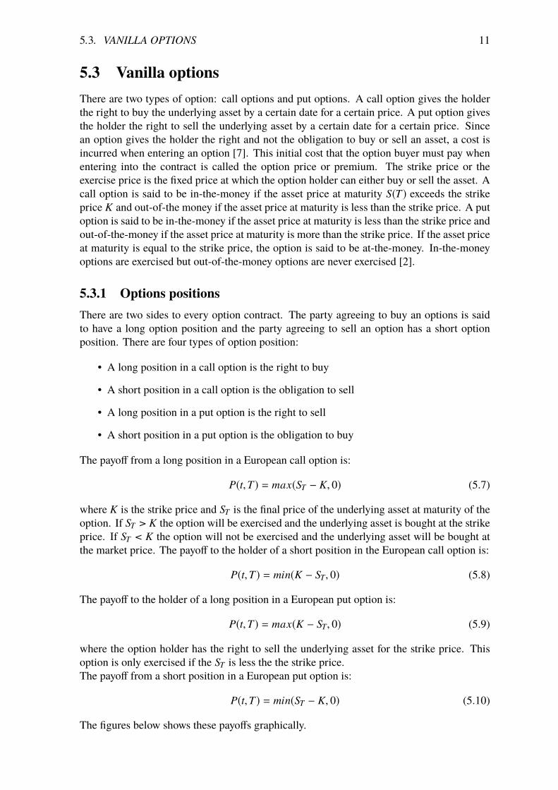
The payo� from a long position in a European call option is:
P(t,T) = max(ST � K, 0) (5.7)
where K is the strike price and ST is the final price of the underlying asset at maturity of theoption. If ST > K the option will be exercised and the underlying asset is bought at the strikeprice. If ST < K the option will not be exercised and the underlying asset will be bought atthe market price. The payo� to the holder of a short position in the European call option is:
P(t,T) = min(K � ST, 0) (5.8)
The payo� to the holder of a long position in a European put option is:
P(t,T) = max(K � ST, 0) (5.9)
where the option holder has the right to sell the underlying asset for the strike price. Thisoption is only exercised if the ST is less the the strike price.The payo� from a short position in a European put option is:
P(t,T) = min(ST � K, 0) (5.10)
The figures below shows these payo�s graphically.
12 CHAPTER �. INSTRUMENTS AVAILABLE FOR RISK MANAGEMENT PURPOSE
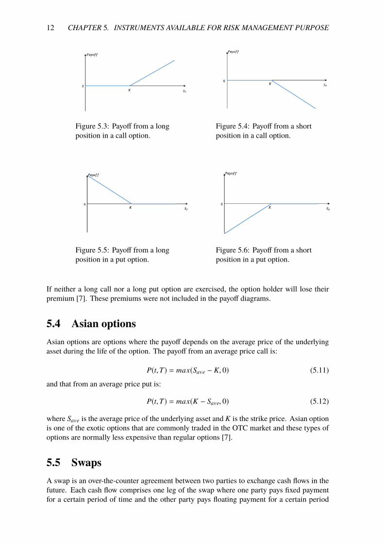
Figure 5.3: Payo� from a longposition in a call option.
Figure 5.4: Payo� from a shortposition in a call option.
Figure 5.5: Payo� from a longposition in a put option.
Figure 5.6: Payo� from a shortposition in a put option.
If neither a long call nor a long put option are exercised, the option holder will lose theirpremium [7]. These premiums were not included in the payo� diagrams.
5.4 Asian optionsAsian options are options where the payo� depends on the average price of the underlyingasset during the life of the option. The payo� from an average price call is:
P(t,T) = max(Save � K, 0) (5.11)
and that from an average price put is:
P(t,T) = max(K � Save, 0) (5.12)
where Save is the average price of the underlying asset and K is the strike price. Asian optionis one of the exotic options that are commonly traded in the OTC market and these types ofoptions are normally less expensive than regular options [7].
5.5 SwapsA swap is an over-the-counter agreement between two parties to exchange cash flows in thefuture. Each cash flow comprises one leg of the swap where one party pays fixed paymentfor a certain period of time and the other party pays floating payment for a certain period
�.�. HEDGING STRATEGIES USING DERIVATIVES 13
of time. Fixed payments are determined at the beginning of the contract but the floatingpayment depends on the level of market variables such as commodity price or interest ratesat the time when the payment is made [9].
5.6 Hedging strategies using derivativesThe purpose of hedging is to reduce or eliminate risk by locking in the prices today andtherefore minimizing the unexpected loss. Forward contracts neutralize risk by fixing theprice that the hedger will pay or receive for the underlying asset. Option contracts provideinsurance whereby investors can protect themselves against market movements in the future,where the option gives the holder the right to exercise but not the obligation to do so. A swapcontract can be used to hedge a stream of risky payments. By entering into a swap, the buyerconfronting a stream of uncertain payments can lock in a fixed price for a period of time.A short hedge is a hedge that involves a short position in future contracts. A short hedge isappropriate when the hedge already owns an asset and expects to sell it at some time in thefuture. Long hedge is a hedge that involves taking a long position in a futures contract. Along hedge is appropriate when a company knows it will have to purchase a certain asset inthe future and wants to lock in a price now. Hedging is not always profitable and can lead to apotential loss if the underlying asset changes against the hedger’s expectations, and thereforechoosing a correct derivative for a risk management strategy is very important [7].
Chapter 6
Valuing and pricing derivatives
6.1 Valuing European optionsThe value of options can be calculated in various ways. The best known formula for theoptions pricing model is the Black Scholes formulas for the prices of European call and putoptions. These formulas are:
c = S0N(d1) � Ke�rT N(d2) (6.1)and
p = Ke�rT N(�d2) � S0N(�d1) (6.2)where
d1 =ln( S0
K ) + (r + �2
2 )T�p
T(6.3)
d2 =ln( S0
K ) + (r � �2
2 )T�p
T= d1 � �
pT (6.4)
The function N(x) is the cumulative probability distribution function for a variable with astandard normal distribution. It is the probability that a normally distributed variable is lessthan x. The variables c and p are the European call and European put prices. S0 is the valueof the underlying asset at time zero, K is the strike price, r is the risk-free rate, � is the stockvolatility, and T is the time to maturity of the option, which is measured in years [7].
6.2 Valuing currency optionsThe pricing of currency options depends on the risk-free interest rate in both currency zones,rd and r f , where rd is the interest rate in domestic currency and r f is the interest rate inforeign currency [10]. The holder of foreign currency receives yield equal to the interest ratein the foreign currency zones.
c = S0e�rf T N(d1) � Ke�rdT N(d2) (6.5)and
p = Ke�rdT N(�d2) � S0e�rf T N(�d1) (6.6)where
d1 =ln( S0
K ) + (rd � r f +�2
2 )T�p
T(6.7)
d2 = d1 � �p
T (6.8)
�.�. IMPLIED VOLATILITY 15
6.3 Implied volatilityThe implied volatility is the value of volatility for which the Black Scholes price equals themarket price of the option. When the option market price is known, the implied volatilitycan be calculated by implying it to the option pricing formula, given that the other inputs areknown. The other inputs are the Spot price of underlying asset S, the strike price K, interestrates r and the actual market value of the options c or p [7].
6.4 Monte Carlo methodsThe Monte Carlo approach to asset pricing is based on the simulation of asset prices usinga program. When used to value an option, Monte Carlo simulation uses the risk-neutralvaluation result. Risk-neutrality means that the expected return of the stock is the risk-freerate and the expected payo� of an option will be discounted with the risk-free rate. Aderivative dependent on a single market variable S provides a payo� at time T . Monte Carlosimulation involves the following steps when used to value a derivative:
1. Simulate a random path for the stock price starting at today’s value of the asset S0 overthe required time horizon. Each price is then generated using:
ST = S0e(µ��22 )T+�✏
pT (6.9)
2. Calculate the payo� of the stock prices.
3. Repeat steps 1 and 2 many times to get many sample values of the payo�s.
4. The mean of all the sample payo�s is calculated to get an estimate of the expectedpayo� in a risk-neutral world.
5. The mean of the payo� is then discounted at the risk-free rate to get an estimate of thevalue of the stock prices.
The process for the underlying market variable in a risk-neutral world is:
dS = µSdt + �Sdz (6.10)
where dz is a Wiener process, µ is the expected return in a risk-neutral world and � isvolatility. To simulate the path followed by S,
S(t + �t) � S(t) = µS(t)�t + �S(t)✏p�t (6.11)
where S(t) is the value of S at time t, ✏ is a random sample from a normal distribution with0 mean and 1 standard deviation. By using Ito’s Lemma the process is:
d ln S = (µ � �2
2)dt + �dz (6.12)
so thatln S(t + �t) � ln S(t) = (µ � �
2
2)�t + �✏
p�t (6.13)
or equivalentlyS(t + �t) � S(t) = S(t)e(µ��2
2 )�t+�✏p�t (6.14)
16 CHAPTER �. VALUING AND PRICING DERIVATIVES
This equation is used to construct a path for S. If µ and � are constant then:
ln S(T) � ln S(0) = (µ � �2
2)T + �✏
pT (6.15)
It follows thatS(T) = S(0)e(µ��2
2 )T+�✏p
T (6.16)
This equation can be used to value derivatives that provide a nonstandard payo� at time T .If S is the price of a non-dividend stock then µ = r , if it is an exchange rate then µ = rd � r f[7].
6.5 Ornstein-Uhlenbeck processMost commodity prices follow a mean-reverting process where they tend to get pulled backto a central value [7]. The long-term mean can be a constant but it can also follow a deter-ministic or even a stochastic process.
Stochastic processes are often used for risk analysis and pricing derivatives. The evolutionof log series is usually modeled and the result is exponentiated. In the Ornstein-Uhlenbeckprocess the evolution of the price St satisfies the following stochastic di�erential equation(SDE):
dSt = �(µ � St)dt + �dWt (6.17)
where � is the mean reversion rate, µ is the mean price, � is the volatility and Wt is theWiener process. If the price St is higher than the mean price the price level is pulled downat a rate determined by the reversion rate. The exact solution of the above SDE is:
Si+1 = Sie��� + µ(1 � e���) + �r
1 � e�2��
2�N0,1 (6.18)
where � is the time step and N0,1 is a Gaussian random variable with 0 mean and 1 standarddeviation [11].
6.6 Valuing a commodity swapCommodity swaps are in essence a series of forward contracts on a commodity with di�erentmaturity dates and the same delivery prices. Swap contracts have one party to the contractwhich pays fixed while the other party pays floating. When entering into a swap contract thefixed payer knows exactly how much needs to be paid at the maturity of the contract but thefloating rate payer needs to pay the market spot price at the maturity of the contract. Whenentering into a swap contract at time t, the fixed payer pays fixed amount x at the future timesT1, T2,.....,TN for a certain quantities of commodities Qi given at each time. The discountfactors D(t,Ti), i = 1, 2, .., N are used for the calculation of the present values of the cashflow [9]. The present value for the fixed payment is:
PV(t) f x =
N’i=1
xQiD(t,Ti) (6.19)
�.�. VALUING A FIXED-FLOATING CURRENCY SWAP 17
The present value for the floating payers is:
PV(t) f l =
N’j=1
F(t,Tj)Q j D(t,Tj) (6.20)
where F(t,T1), F(t,T2),..., F(t,TN ) is the forward price at the future time T.From the condition PV(t) f l = PV(t) f x
N’i=1
xQiD(t,Ti) =N’
j=1F(t,Tj)Q j D(t,Tj) (6.21)
then solving for x gives:
x =
ÕNj=1 F(t,Tj)Q j D(t,Tj)ÕN
i=1 QiD(t,Tj)(6.22)
and this can be written as:
x =N’
k=1wk F(t,Tk) (6.23)
where the swap fixed price x is the weighted average of the forward prices, where the weightsare given by formula:
wk =Qk D(t,Tk)ÕNi=1 QiD(t,Ti)
(6.24)
6.7 Valuing a fixed-floating currency swapIn these contracts there is an initial exchange of principals Qd and Q f . The relationshipbetween the exchanged amounts is defined by the exchange rate X(t) (amount of domesticcurrency per unit of foreign currency) between the two currencies at the time t [9].
Qd = X(t)Q f (6.25)
Following this exchange of principals the interest payments take place at a future time asdictated by the contract. One party pays fixed rate SR and other party pays floating rate. Thepresent value of the fixed and floating payments is:
PV(t) f ixed = SRN’
i=1Qie�rd(Ti�t) (6.26)
PV(t) f loating =
N’i=1
FX(t,Ti)Qie�rd(Ti�t) (6.27)
where Qi is the principal amount in foreign currency at time Ti and FX(t,Ti) is the forwardexchange rate calculated by the formula:
FX(t,Ti) = X(t)e(rd�rf )(Ti�t) (6.28)
The exchanged cash flows needs to satisfy the condition that the present values of bothpayment schedules be equal:
PV(t) f ixed = PV(t) f loating (6.29)
18 CHAPTER �. VALUING AND PRICING DERIVATIVES
after solving for SR we find:
SR =ÕN
i=1 FX(t,Ti)Qie�rd(Ti�t)ÕNj=1 Q je�rd(Tj�t) (6.30)
Chapter 7
Description of the risks the firm faces
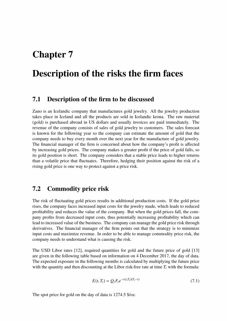
7.1 Description of the firm to be discussed
Zano is an Icelandic company that manufactures gold jewelry. All the jewelry productiontakes place in Iceland and all the products are sold in Icelandic krona. The raw material(gold) is purchased abroad in US dollars and usually invoices are paid immediately. Therevenue of the company consists of sales of gold jewelry to customers. The sales forecastis known for the following year so the company can estimate the amount of gold that thecompany needs to buy every month over the next year for the manufacture of gold jewelry.The financial manager of the firm is concerned about how the company’s profit is a�ectedby increasing gold prices. The company makes a greater profit if the price of gold falls, soits gold position is short. The company considers that a stable price leads to higher returnsthan a volatile price that fluctuates. Therefore, hedging their position against the risk of arising gold price is one way to protect against a price risk.
7.2 Commodity price risk
The risk of fluctuating gold prices results in additional production costs. If the gold pricerises, the company faces increased input costs for the jewelry made, which leads to reducedprofitability and reduces the value of the company. But when the gold prices fall, the com-pany profits from decreased input costs, thus potentially increasing profitability which canlead to increased value of the business. The company can manage the gold price risk throughderivatives. The financial manager of the firm points out that the strategy is to minimizeinput costs and maximize revenue. In order to be able to manage commodity price risk, thecompany needs to understand what is causing the risk.
The USD Libor rates [12], required quantities for gold and the future price of gold [13]are given in the following table based on information on 4 December 2017, the day of data.The expected exposure in the following months is calculated by multiplying the future pricewith the quantity and then discounting at the Libor risk-free rate at time Ti with the formula:
E(t,Ti) = QiFie�r(t,Ti)(Ti�t) (7.1)
The spot price for gold on the day of data is 1274.5 $/oz.
20 CHAPTER �. DESCRIPTION OF THE RISKS THE FIRM FACES
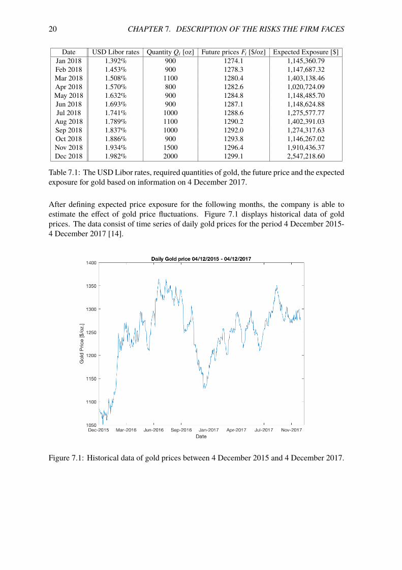
Date USD Libor rates Quantity Qi [oz] Future prices Fi [$/oz] Expected Exposure [$]Jan 2018 1.392% 900 1274.1 1,145,360.79Feb 2018 1.453% 900 1278.3 1,147,687.32Mar 2018 1.508% 1100 1280.4 1,403,138.46Apr 2018 1.570% 800 1282.6 1,020,724.09May 2018 1.632% 900 1284.8 1,148,485.70Jun 2018 1.693% 900 1287.1 1,148,624.88Jul 2018 1.741% 1000 1288.6 1,275,577.77Aug 2018 1.789% 1100 1290.2 1,402,391.03Sep 2018 1.837% 1000 1292.0 1,274,317.63Oct 2018 1.886% 900 1293.8 1,146,267.02Nov 2018 1.934% 1500 1296.4 1,910,436.37Dec 2018 1.982% 2000 1299.1 2,547,218.60
Table 7.1: The USD Libor rates, required quantities of gold, the future price and the expectedexposure for gold based on information on 4 December 2017.
After defining expected price exposure for the following months, the company is able toestimate the e�ect of gold price fluctuations. Figure 7.1 displays historical data of goldprices. The data consist of time series of daily gold prices for the period 4 December 2015-4 December 2017 [14].
Figure 7.1: Historical data of gold prices between 4 December 2015 and 4 December 2017.
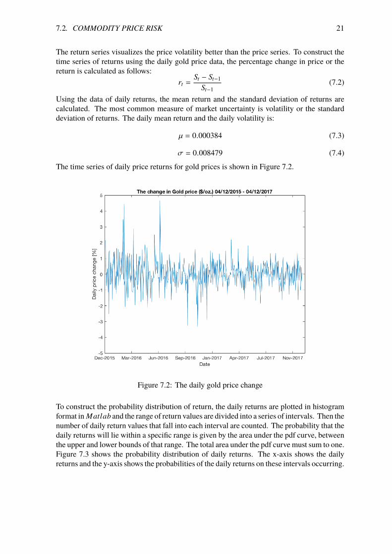
�.�. COMMODITY PRICE RISK 21
The return series visualizes the price volatility better than the price series. To construct thetime series of returns using the daily gold price data, the percentage change in price or thereturn is calculated as follows:
rt =St � St�1
St�1(7.2)
Using the data of daily returns, the mean return and the standard deviation of returns arecalculated. The most common measure of market uncertainty is volatility or the standarddeviation of returns. The daily mean return and the daily volatility is:
µ = 0.000384 (7.3)
� = 0.008479 (7.4)
The time series of daily price returns for gold prices is shown in Figure 7.2.
Figure 7.2: The daily gold price change
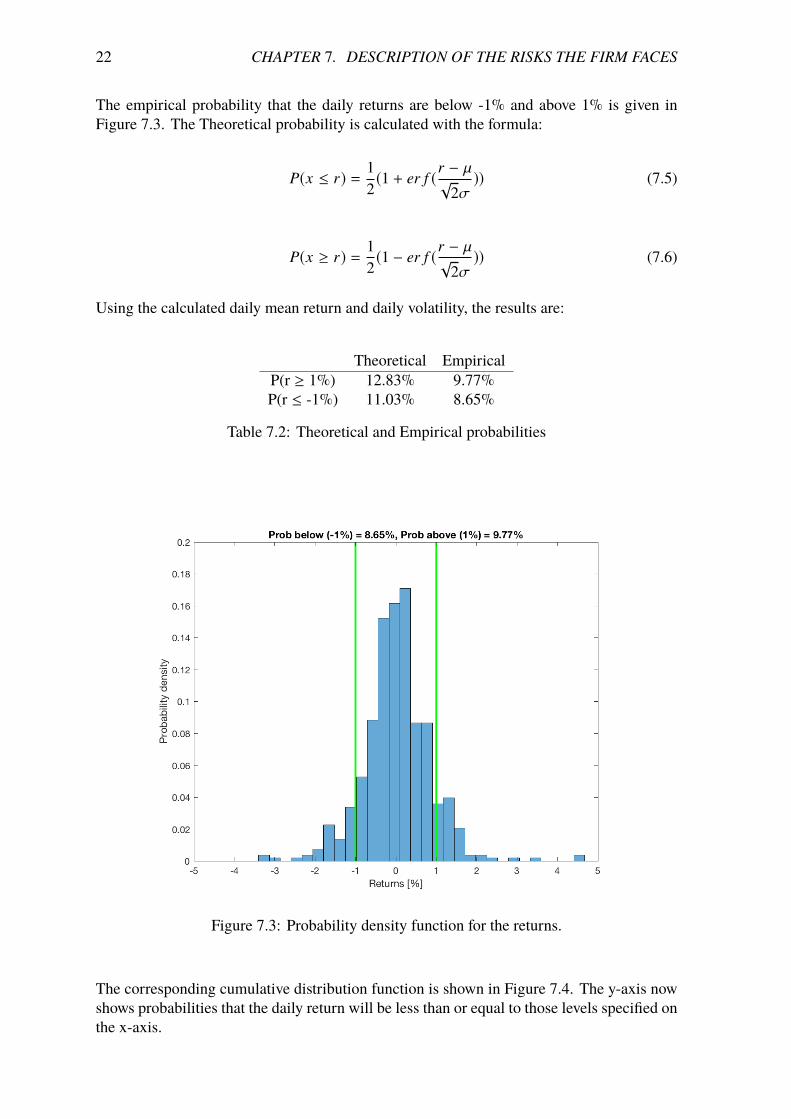
To construct the probability distribution of return, the daily returns are plotted in histogramformat in Matlab and the range of return values are divided into a series of intervals. Then thenumber of daily return values that fall into each interval are counted. The probability that thedaily returns will lie within a specific range is given by the area under the pdf curve, betweenthe upper and lower bounds of that range. The total area under the pdf curve must sum to one.Figure 7.3 shows the probability distribution of daily returns. The x-axis shows the dailyreturns and the y-axis shows the probabilities of the daily returns on these intervals occurring.
22 CHAPTER �. DESCRIPTION OF THE RISKS THE FIRM FACES
The empirical probability that the daily returns are below -1% and above 1% is given inFigure 7.3. The Theoretical probability is calculated with the formula:
P(x r) = 12(1 + er f (r � µp
2�)) (7.5)
P(x � r) = 12(1 � er f (r � µp
2�)) (7.6)
Using the calculated daily mean return and daily volatility, the results are:
Theoretical EmpiricalP(r � 1%) 12.83% 9.77%P(r -1%) 11.03% 8.65%
Table 7.2: Theoretical and Empirical probabilities
Figure 7.3: Probability density function for the returns.
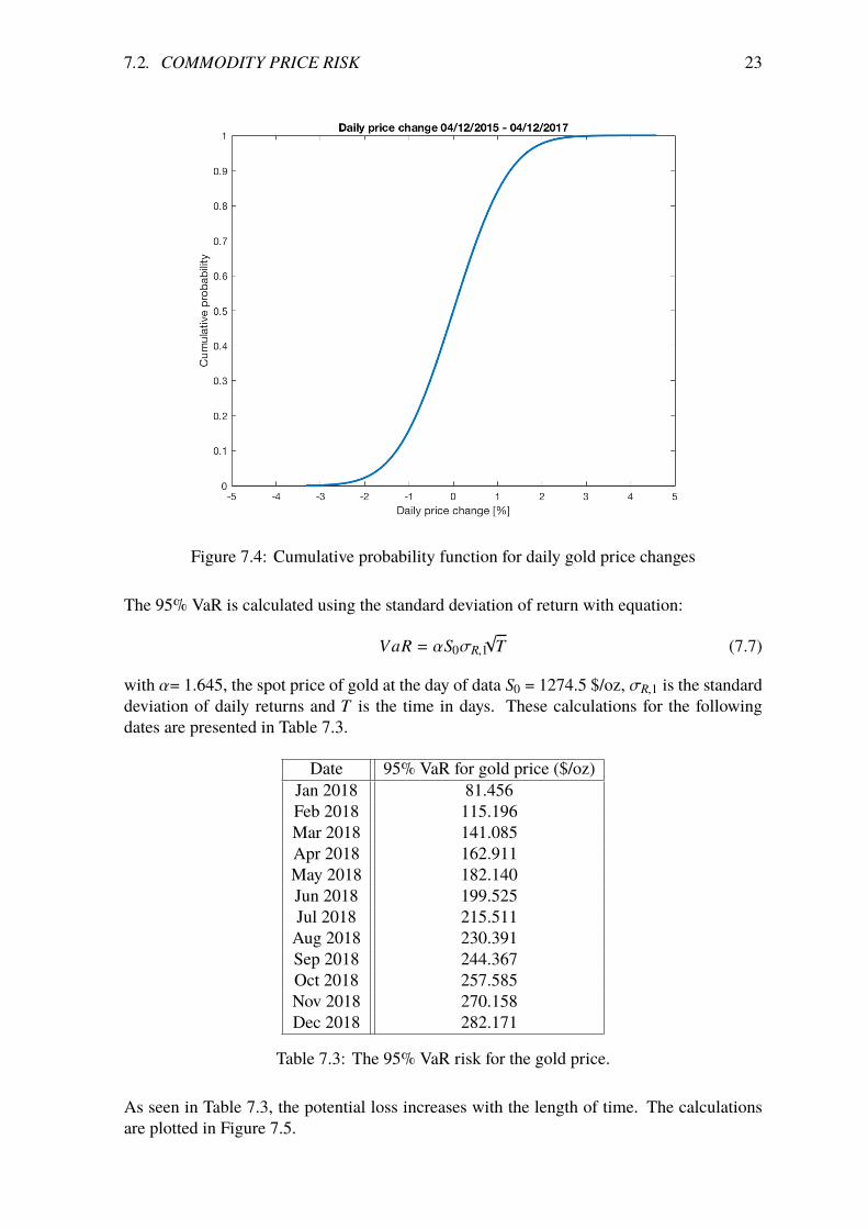
The corresponding cumulative distribution function is shown in Figure 7.4. The y-axis nowshows probabilities that the daily return will be less than or equal to those levels specified onthe x-axis.
�.�. COMMODITY PRICE RISK 23
Figure 7.4: Cumulative probability function for daily gold price changes
The 95% VaR is calculated using the standard deviation of return with equation:
VaR = ↵S0�R,1p
T (7.7)
with ↵= 1.645, the spot price of gold at the day of data S0 = 1274.5 $/oz, �R,1 is the standarddeviation of daily returns and T is the time in days. These calculations for the followingdates are presented in Table 7.3.
Date 95% VaR for gold price ($/oz)Jan 2018 81.456Feb 2018 115.196Mar 2018 141.085Apr 2018 162.911May 2018 182.140Jun 2018 199.525Jul 2018 215.511Aug 2018 230.391Sep 2018 244.367Oct 2018 257.585Nov 2018 270.158Dec 2018 282.171
Table 7.3: The 95% VaR risk for the gold price.
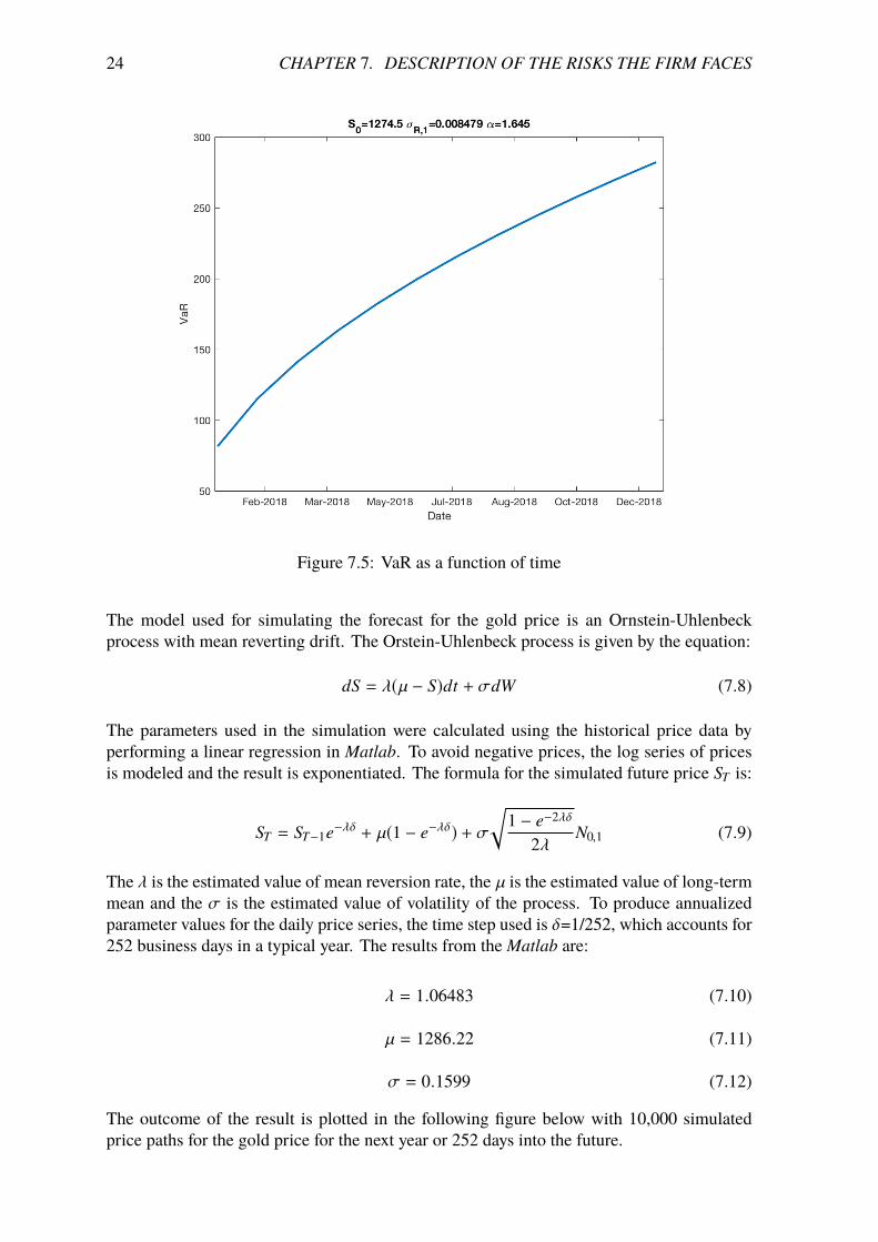
As seen in Table 7.3, the potential loss increases with the length of time. The calculationsare plotted in Figure 7.5.
24 CHAPTER �. DESCRIPTION OF THE RISKS THE FIRM FACES
Figure 7.5: VaR as a function of time
The model used for simulating the forecast for the gold price is an Ornstein-Uhlenbeckprocess with mean reverting drift. The Orstein-Uhlenbeck process is given by the equation:
dS = �(µ � S)dt + �dW (7.8)
The parameters used in the simulation were calculated using the historical price data byperforming a linear regression in Matlab. To avoid negative prices, the log series of pricesis modeled and the result is exponentiated. The formula for the simulated future price ST is:
ST = ST�1e��� + µ(1 � e���) + �r
1 � e�2��
2�N0,1 (7.9)
The � is the estimated value of mean reversion rate, the µ is the estimated value of long-termmean and the � is the estimated value of volatility of the process. To produce annualizedparameter values for the daily price series, the time step used is �=1/252, which accounts for252 business days in a typical year. The results from the Matlab are:
� = 1.06483 (7.10)
µ = 1286.22 (7.11)
� = 0.1599 (7.12)
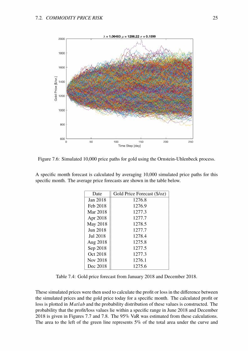
The outcome of the result is plotted in the following figure below with 10,000 simulatedprice paths for the gold price for the next year or 252 days into the future.
�.�. COMMODITY PRICE RISK 25
Figure 7.6: Simulated 10,000 price paths for gold using the Ornstein-Uhlenbeck process.
A specific month forecast is calculated by averaging 10,000 simulated price paths for thisspecific month. The average price forecasts are shown in the table below.
Date Gold Price Forecast ($/oz)Jan 2018 1276.8Feb 2018 1276.9Mar 2018 1277.3Apr 2018 1277.7May 2018 1278.5Jun 2018 1277.7Jul 2018 1278.4Aug 2018 1275.8Sep 2018 1277.5Oct 2018 1277.3Nov 2018 1276.1Dec 2018 1275.6
Table 7.4: Gold price forecast from January 2018 and December 2018.
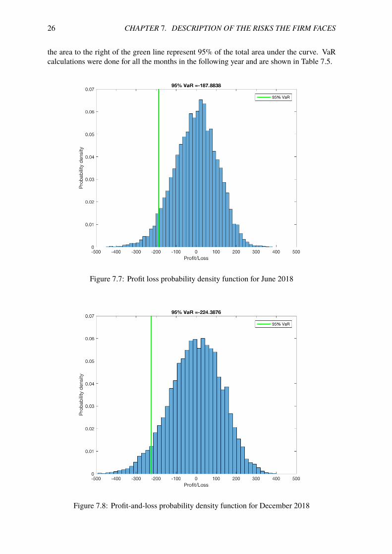
These simulated prices were then used to calculate the profit or loss in the di�erence betweenthe simulated prices and the gold price today for a specific month. The calculated profit orloss is plotted in Matlab and the probability distribution of these values is constructed. Theprobability that the profit/loss values lie within a specific range in June 2018 and December2018 is given in Figures 7.7 and 7.8. The 95% VaR was estimated from these calculations.The area to the left of the green line represents 5% of the total area under the curve and
26 CHAPTER �. DESCRIPTION OF THE RISKS THE FIRM FACES
the area to the right of the green line represent 95% of the total area under the curve. VaRcalculations were done for all the months in the following year and are shown in Table 7.5.
Figure 7.7: Profit loss probability density function for June 2018
Figure 7.8: Profit-and-loss probability density function for December 2018
�.�. INSTRUMENTS AVAILABLE TO MANAGE COMMODITY PRICE RISK 27
Date 95% VaR for gold price ($/oz)Jan 2018 -56.640Feb 2018 -105.794Mar 2018 -138.253Apr 2018 -153.545May 2018 -177.984Jun 2018 -187.884Jul 2018 -199.713Aug 2018 -207.699Sep 2018 -214.015Oct 2018 -219.108Nov 2018 -220.429Dec 2018 -224.388
Table 7.5: The 95% VaR for the gold price.
7.3 Instruments available to manage commodity price risk
7.3.1 Commodity futuresCommodity futures are standardized agreements to purchase or sell a specific amount of acommodity on a fixed future date for a certain price. These contracts enable the company tolock in a fixed price for a future delivery of the gold and provide protection against adversemovements in the gold price.
7.3.2 Commodity optionsOptions are agreements between two parties that give the holder the right but not the obligationto purchase or sell the commodity at a certain date for a certain price. The buyer of acommodity option pays a premium to the seller of the option. Commodity option insuresagainst adverse movements of the gold price.
7.3.3 Commodity swapsCommodity swap is an agreement between two parties to exchange cash flows. With swaps,the company can lock in the price they have to pay for the gold during the contract periodand guarantee a long-term income stream.
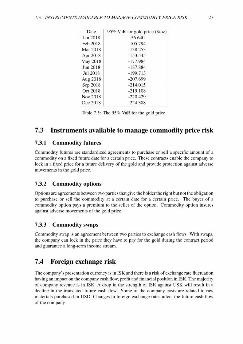
7.4 Foreign exchange riskThe company’s presentation currency is in ISK and there is a risk of exchange rate fluctuationhaving an impact on the company cash flow, profit and financial position in ISK. The majorityof company revenue is in ISK. A drop in the strength of ISK against USK will result in adecline in the translated future cash flow. Some of the company costs are related to rawmaterials purchased in USD. Changes in foreign exchange rates a�ect the future cash flowof the company.
28 CHAPTER �. DESCRIPTION OF THE RISKS THE FIRM FACES
The forward exchange rate is calculated for the following months with the formula:
F(t,Ti) = Xd, f (t)e(rd(t,Ti)�rf (t,Ti))(Ti�t) (7.13)
where Xd, f (t) is the exchange rate at the day of data, rd is the ISK Reibor rate [15] and r f isthe USD Libor rate at time Ti. The spot exchange rate, Xd, f (t) on 4 December 2017, the dayof data, is 103.59. The calculations for the following months are given in Table 7.6.
Date USD Libor rates ISK Reibor rates Exchange rate [ISK/USD]Jan 2018 1.392% 4.350% 103.8457Feb 2018 1.453% 4.650% 104.1434Mar 2018 1.508% 4.650% 104.4068Apr 2018 1.570% 4.650% 104.6590May 2018 1.632% 4.650% 104.9011Jun 2018 1.693% 4.650% 105.1329Jul 2018 1.741% 4.667% 105.3729Aug 2018 1.789% 4.683% 105.6080Sep 2018 1.837% 4.700% 105.8381Oct 2018 1.886% 4.717% 106.0631Nov 2018 1.934% 4.733% 106.2830Dec 2018 1.982% 4.750% 106.4978
Table 7.6: The calculated forward exchange rate
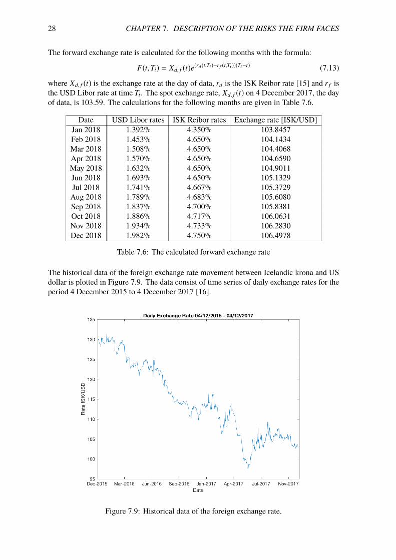
The historical data of the foreign exchange rate movement between Icelandic krona and USdollar is plotted in Figure 7.9. The data consist of time series of daily exchange rates for theperiod 4 December 2015 to 4 December 2017 [16].
Figure 7.9: Historical data of the foreign exchange rate.
�.�. FOREIGN EXCHANGE RISK 29
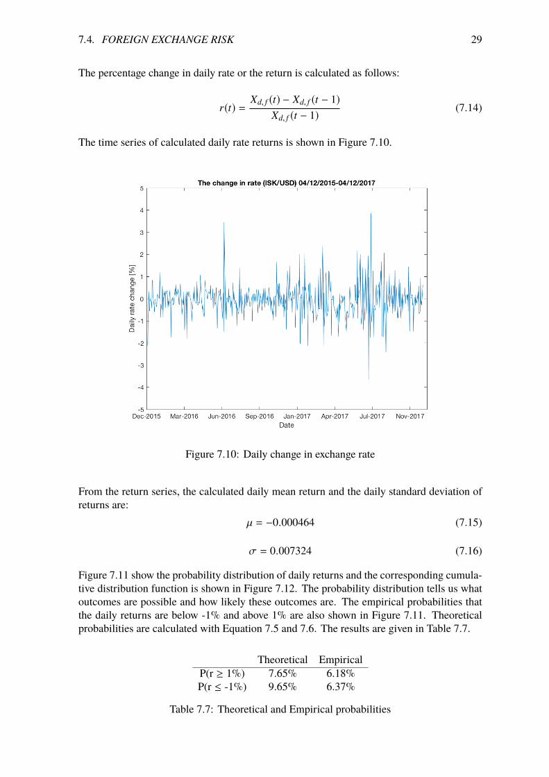
The percentage change in daily rate or the return is calculated as follows:
r(t) =Xd, f (t) � Xd, f (t � 1)
Xd, f (t � 1) (7.14)
The time series of calculated daily rate returns is shown in Figure 7.10.
Figure 7.10: Daily change in exchange rate
From the return series, the calculated daily mean return and the daily standard deviation ofreturns are:
µ = �0.000464 (7.15)
� = 0.007324 (7.16)
Figure 7.11 show the probability distribution of daily returns and the corresponding cumula-tive distribution function is shown in Figure 7.12. The probability distribution tells us whatoutcomes are possible and how likely these outcomes are. The empirical probabilities thatthe daily returns are below -1% and above 1% are also shown in Figure 7.11. Theoreticalprobabilities are calculated with Equation 7.5 and 7.6. The results are given in Table 7.7.
Theoretical EmpiricalP(r � 1%) 7.65% 6.18%P(r -1%) 9.65% 6.37%
Table 7.7: Theoretical and Empirical probabilities

30 CHAPTER �. DESCRIPTION OF THE RISKS THE FIRM FACES
Figure 7.11: Probability density function for daily rate returns
Figure 7.12: Cumulative probability function for daily rate change

�.�. INSTRUMENTS AVAILABLE TO MANAGE FOREIGN EXCHANGE RISK 31
7.5 Instruments available to manage foreign exchange risk
7.5.1 Forward exchange contract
Enables the company to protect itself from adverse movement in exchange rates by lockingin an agreed exchange rate until an agreed date. The company can enter a forward currencycontract for the ISK/USD rate. By entering this contract the uncertainty caused by possiblecurrency fluctuations can be removed.
7.5.2 Currency options
The company can enter into a currency option to purchase foreign currency under an agree-ment that allows for the right but not the obligation to undertake the transaction at an agreedfuture date. The foreign currency option, which includes the price of a premium, will protectthe company from downward movements in the value of the ISK against the USD and thecompany will also benefit from increases in the ISK against the USD.
7.5.3 Currency swaps
The company can enter into a currency swap where the company exchanges a fixed amountof ISK for USD.
7.6 Comparison of the two risk types
Both commodity price risk and foreign exchange risk have a direct impact on the companycash flow. Managing both these risks at the same time can be di�cult. When locking inthe gold price in US dollars, the company is still exposed to foreign exchange risk. Foreignexchange risk is complicated to manage when the risk exposure is based on fluctuating goldprices. Based on previous calculations in this chapter, the gold price is slightly more volatilethan the foreign exchange rate.
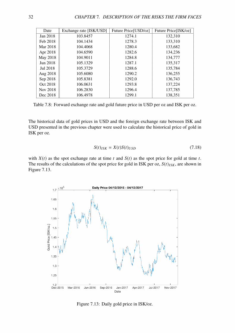
The future price in ISK per ounce is calculated by multiplying the future price for gold($/oz) with the calculated forward exchange rate.
FISK(t,Ti) = FUSD(t,Ti)FISK/USD(t,Ti) (7.17)
where FISK is the future price for gold in ISK per oz, FUSD is the future price for gold in USDper oz, o�ered by the COMEX division of the CME group, and FISK/USD is the calculatedforward exchange rate. The results of these calculations are given in Table 7.8.
32 CHAPTER �. DESCRIPTION OF THE RISKS THE FIRM FACES
Date Exchange rate [ISK/USD] Future Price[USD/oz] Future Price[ISK/oz]Jan 2018 103.8457 1274.1 132,310Feb 2018 104.1434 1278.3 133,310Mar 2018 104.4068 1280.4 133,682Apr 2018 104.6590 1282.6 134,236May 2018 104.9011 1284.8 134,777Jun 2018 105.1329 1287.1 135,317Jul 2018 105.3729 1288.6 135,784Aug 2018 105.6080 1290.2 136,255Sep 2018 105.8381 1292.0 136,743Oct 2018 106.0631 1293.8 137,224Nov 2018 106.2830 1296.4 137,785Dec 2018 106.4978 1299.1 138,351
Table 7.8: Forward exchange rate and gold future price in USD per oz and ISK per oz.
The historical data of gold prices in USD and the foreign exchange rate between ISK andUSD presented in the previous chapter were used to calculate the historical price of gold inISK per oz.
S(t)ISK = X(t)S(t)USD (7.18)
with X(t) as the spot exchange rate at time t and S(t) as the spot price for gold at time t.The results of the calculations of the spot price for gold in ISK per oz, S(t)ISK , are shown inFigure 7.13.
Figure 7.13: Daily gold price in ISK/oz.

�.�. COMPARISON OF THE TWO RISK TYPES 33
The total risk in ISK, �ISK , is calculated as follows:
�ISK = (�2USD + �
2FX + 2�USD⇢(USD,FX)�FX)
12 (7.19)
The one day standard deviations of returns are �USD and �FX and the correlation betweentheir returns is ⇢(USD,FX). �USD is the standard deviation of gold price in USD and �FX isthe standard deviation of foreign exchange rate. The information is given in Table 7.9.
Risk (�) CorrelationGold Price [$/oz] 0.008479 1.00 -0.0866
Exchange Rate [ISK/USD] 0.007324 -0.0866 1
Table 7.9: Correlation between the return of gold price and foreign exchange rate
The correlation between the returns of gold price and foreign exchange rate is negative, whichmeans that their returns tend to move in opposite directions. Using information in Table 7.9,the total risk or the daily volatility in ISK is:
�ISK = 0.010713595 (7.20)
Value at Risk (VaR) for the gold price in ISK is given by the formula:
VaRISK = ↵�ISK S0p
T (7.21)
where ↵ is 1.645, the spot price for gold today in ISK per oz is S0 = 132,025.46 ISK/oz andT is the time measured in days. VaR was calculated for the following months and the resultsare shown in Table 7.10 and plotted in Figure 7.14.
Date 95% VaR for gold price (ISK/oz)Jan 2018 10661.78Feb 2018 15078.04Mar 2018 18466.75Apr 2018 21323.56May 2018 23840.47Jun 2018 26115.93Jul 2018 28208.42Aug 2018 30156.07Sep 2018 31985.35Oct 2018 33715.51Nov 2018 35361.13Dec 2018 36933.50
Table 7.10: The 95% VaR risk for the gold price in ISK.
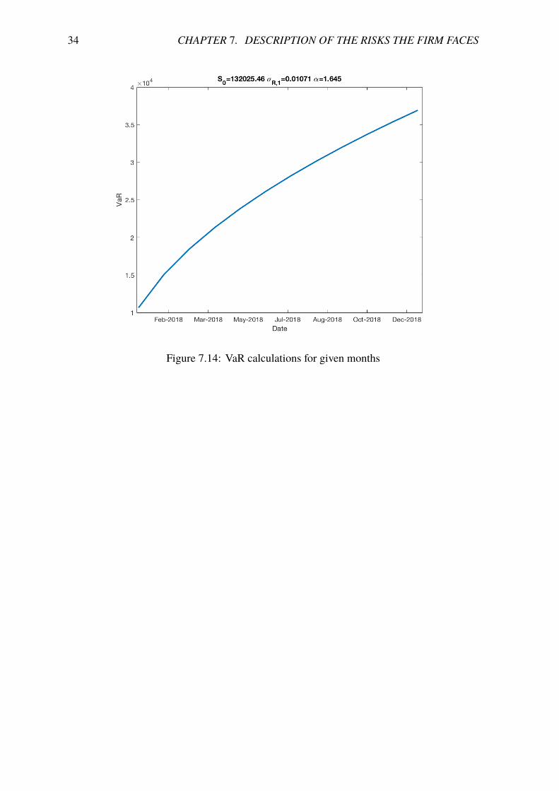
34 CHAPTER �. DESCRIPTION OF THE RISKS THE FIRM FACES
Figure 7.14: VaR calculations for given months
Chapter 8
Implementation of risk managementstrategies
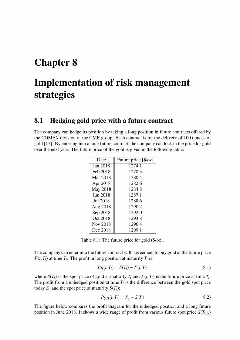
8.1 Hedging gold price with a future contractThe company can hedge its position by taking a long position in future contracts o�ered bythe COMEX division of the CME group. Each contract is for the delivery of 100 ounces ofgold [17]. By entering into a long future contract, the company can lock in the price for goldover the next year. The future price of the gold is given in the following table:
Date Future price [$/oz]Jan 2018 1274.1Feb 2018 1278.3Mar 2018 1280.4Apr 2018 1282.6May 2018 1284.8Jun 2018 1287.1Jul 2018 1288.6Aug 2018 1290.2Sep 2018 1292.0Oct 2018 1293.8Nov 2018 1296.4Dec 2018 1299.1
Table 8.1: The future price for gold ($/oz).
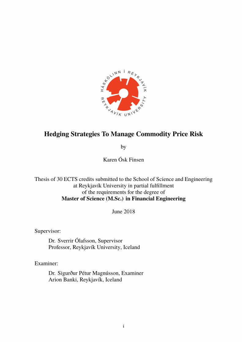
The company can enter into the future contract with agreement to buy gold at the future priceF(t,Ti) at time Ti. The profit in long position at maturity Ti is:
PH(t,Ti) = S(Ti) � F(t,Ti) (8.1)
where S(Ti) is the spot price of gold at maturity Ti and F(t,Ti) is the future price at time Ti.The profit from a unhedged position at time Ti is the di�erence between the gold spot pricetoday S0 and the spot price at maturity S(Ti):
PUH(t,Ti) = S0 � S(Ti) (8.2)
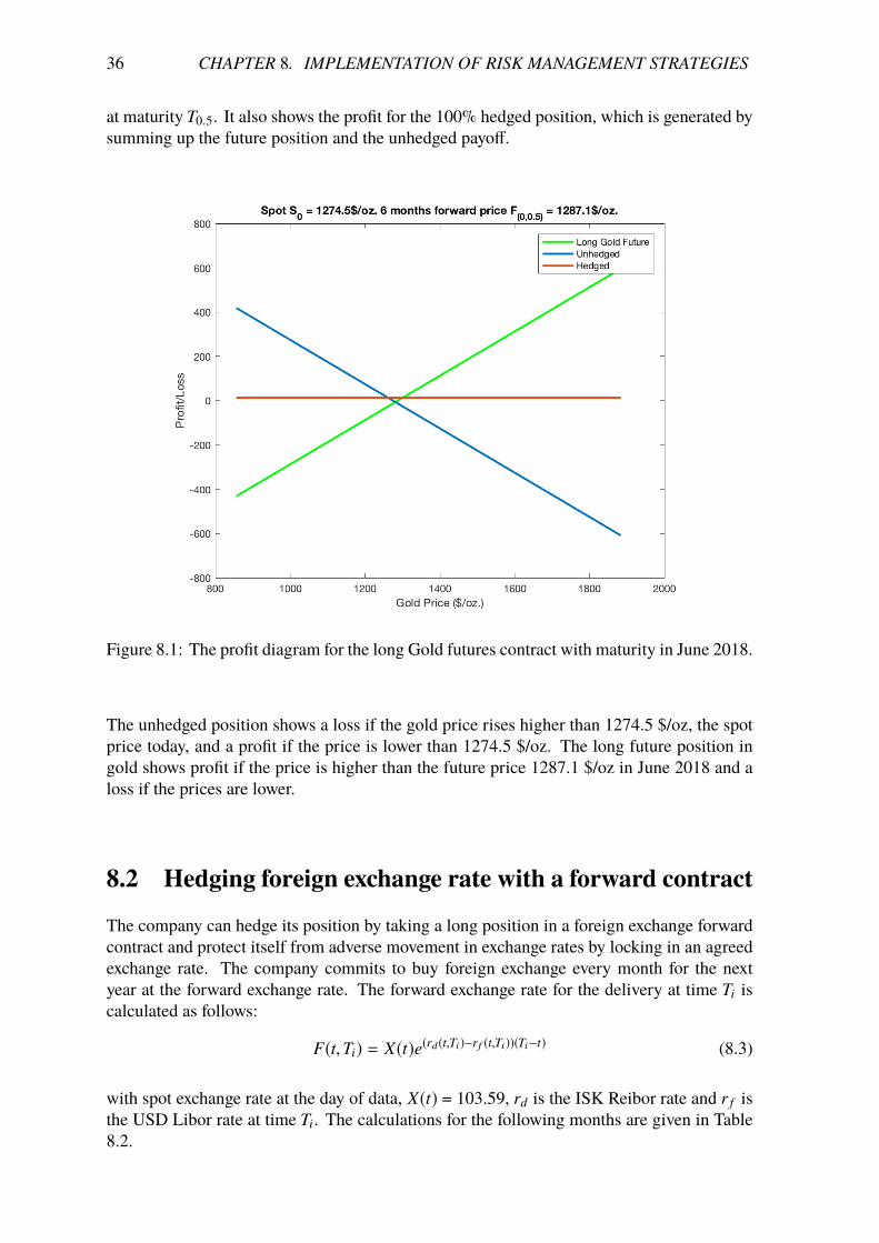
The figure below compares the profit diagram for the unhedged position and a long futureposition in June 2018. It shows a wide range of profit from various future spot price S(T0.5)
36 CHAPTER �. IMPLEMENTATION OF RISK MANAGEMENT STRATEGIES
at maturity T0.5. It also shows the profit for the 100% hedged position, which is generated bysumming up the future position and the unhedged payo�.
Figure 8.1: The profit diagram for the long Gold futures contract with maturity in June 2018.
The unhedged position shows a loss if the gold price rises higher than 1274.5 $/oz, the spotprice today, and a profit if the price is lower than 1274.5 $/oz. The long future position ingold shows profit if the price is higher than the future price 1287.1 $/oz in June 2018 and aloss if the prices are lower.
8.2 Hedging foreign exchange rate with a forward contract
The company can hedge its position by taking a long position in a foreign exchange forwardcontract and protect itself from adverse movement in exchange rates by locking in an agreedexchange rate. The company commits to buy foreign exchange every month for the nextyear at the forward exchange rate. The forward exchange rate for the delivery at time Ti iscalculated as follows:
F(t,Ti) = X(t)e(rd(t,Ti)�rf (t,Ti))(Ti�t) (8.3)
with spot exchange rate at the day of data, X(t) = 103.59, rd is the ISK Reibor rate and r f isthe USD Libor rate at time Ti. The calculations for the following months are given in Table8.2.
�.�. HEDGING FOREIGN EXCHANGE RATE WITH A FORWARD CONTRACT 37
Date USD Libor rates ISK Reibor rates Exchange rate [ISK/USD]Jan 2018 1.392% 4.350% 103.8457Feb 2018 1.453% 4.650% 104.1434Mar 2018 1.508% 4.650% 104.4068Apr 2018 1.570% 4.650% 104.6590May 2018 1.632% 4.650% 104.9011Jun 2018 1.693% 4.650% 105.1329Jul 2018 1.741% 4.667% 105.3729Aug 2018 1.789% 4.683% 105.6080Sep 2018 1.837% 4.700% 105.8381Oct 2018 1.886% 4.717% 106.0631Nov 2018 1.934% 4.733% 106.2830Dec 2018 1.982% 4.750% 106.4978
Table 8.2: Calculated forward exchange rate
The profit in long position at maturity Ti is:
PH(t,Ti) = X(Ti) � F(t,Ti) (8.4)
where X(Ti) is the spot exchange rate at maturity Ti and F(t,Ti) is forward exchange rate attime Ti. The profit from a unhedged position at time Ti is:
PUH(t,Ti) = X(t) � X(Ti) (8.5)
Figure 8.2: The profit diagram for the long foreign exchange rate forward contract withmaturity in June 2018.
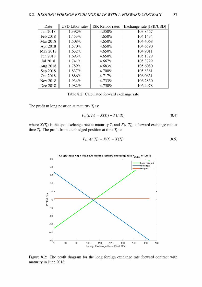
38 CHAPTER �. IMPLEMENTATION OF RISK MANAGEMENT STRATEGIES
The profit diagram for the the unhedged position and a long future position in June 2018is shown in Figure 8.2. It shows a wide range of profit from various future exchange ratesX(T0.5). at maturity T0.5. The figure also shows 100% hedged position.
The unhedged position shows a loss if the exchange rate rises higher than 103.59 and aprofit if the exchange rate is lower than 103.59. The long future position in gold shows profitif the exchange rate is higher than 105.13 in June 2018 and a loss if the exchange rate islower.
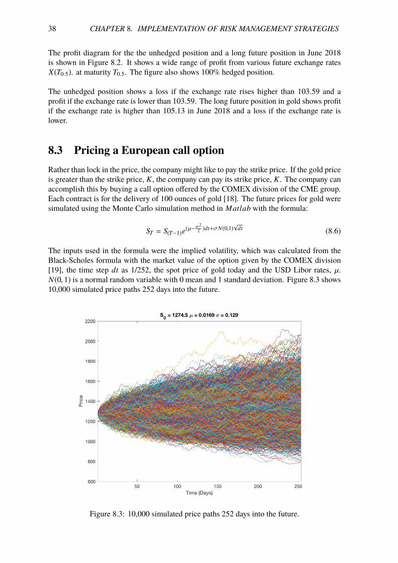
8.3 Pricing a European call optionRather than lock in the price, the company might like to pay the strike price. If the gold priceis greater than the strike price, K , the company can pay its strike price, K . The company canaccomplish this by buying a call option o�ered by the COMEX division of the CME group.Each contract is for the delivery of 100 ounces of gold [18]. The future prices for gold weresimulated using the Monte Carlo simulation method in Matlab with the formula:
ST = S(T�1)e(µ��22 )dt+�N(0,1)
pdt (8.6)
The inputs used in the formula were the implied volatility, which was calculated from theBlack-Scholes formula with the market value of the option given by the COMEX division[19], the time step dt as 1/252, the spot price of gold today and the USD Libor rates, µ.N(0, 1) is a normal random variable with 0 mean and 1 standard deviation. Figure 8.3 shows10,000 simulated price paths 252 days into the future.
Figure 8.3: 10,000 simulated price paths 252 days into the future.
�.�. PRICING A EUROPEAN CALL OPTION 39
These 10,000 samples of future prices are used to compute the payo� of the option and theMonte Carlo price is given by the mean of these payo�s. The Monte Carlo price is:
Call price = e�rT mean(max(ST � K, 0)) (8.7)
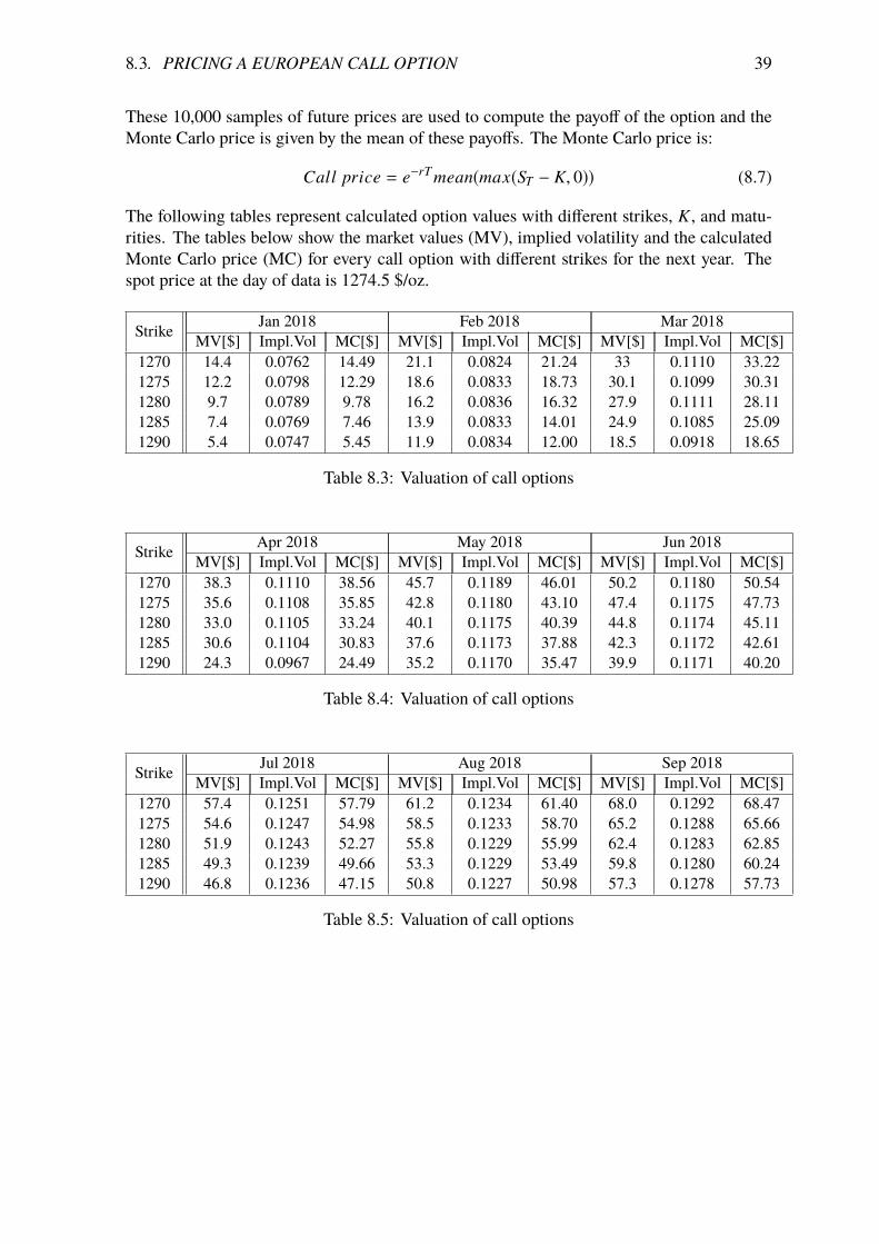
The following tables represent calculated option values with di�erent strikes, K , and matu-rities. The tables below show the market values (MV), implied volatility and the calculatedMonte Carlo price (MC) for every call option with di�erent strikes for the next year. Thespot price at the day of data is 1274.5 $/oz.
Strike Jan 2018 Feb 2018 Mar 2018MV[$] Impl.Vol MC[$] MV[$] Impl.Vol MC[$] MV[$] Impl.Vol MC[$]
1270 14.4 0.0762 14.49 21.1 0.0824 21.24 33 0.1110 33.221275 12.2 0.0798 12.29 18.6 0.0833 18.73 30.1 0.1099 30.311280 9.7 0.0789 9.78 16.2 0.0836 16.32 27.9 0.1111 28.111285 7.4 0.0769 7.46 13.9 0.0833 14.01 24.9 0.1085 25.091290 5.4 0.0747 5.45 11.9 0.0834 12.00 18.5 0.0918 18.65
Table 8.3: Valuation of call options
Strike Apr 2018 May 2018 Jun 2018MV[$] Impl.Vol MC[$] MV[$] Impl.Vol MC[$] MV[$] Impl.Vol MC[$]
1270 38.3 0.1110 38.56 45.7 0.1189 46.01 50.2 0.1180 50.541275 35.6 0.1108 35.85 42.8 0.1180 43.10 47.4 0.1175 47.731280 33.0 0.1105 33.24 40.1 0.1175 40.39 44.8 0.1174 45.111285 30.6 0.1104 30.83 37.6 0.1173 37.88 42.3 0.1172 42.611290 24.3 0.0967 24.49 35.2 0.1170 35.47 39.9 0.1171 40.20
Table 8.4: Valuation of call options
Strike Jul 2018 Aug 2018 Sep 2018MV[$] Impl.Vol MC[$] MV[$] Impl.Vol MC[$] MV[$] Impl.Vol MC[$]
1270 57.4 0.1251 57.79 61.2 0.1234 61.40 68.0 0.1292 68.471275 54.6 0.1247 54.98 58.5 0.1233 58.70 65.2 0.1288 65.661280 51.9 0.1243 52.27 55.8 0.1229 55.99 62.4 0.1283 62.851285 49.3 0.1239 49.66 53.3 0.1229 53.49 59.8 0.1280 60.241290 46.8 0.1236 47.15 50.8 0.1227 50.98 57.3 0.1278 57.73
Table 8.5: Valuation of call options
40 CHAPTER �. IMPLEMENTATION OF RISK MANAGEMENT STRATEGIES
Strike Oct 2018 Nov 2018 Dec 2018MV[$] Impl.Vol MC[$] MV[$] Impl.Vol MC[$] MV[$] Impl.Vol MC[$]
1270 71.2 0.1268 71.69 78.0 0.1323 78.53 80.9 0.1297 81.451275 68.4 0.1264 68.88 75.2 0.1320 75.72 78.1 0.1294 78.641280 65.7 0.1262 66.17 72.5 0.1317 73.01 75.4 0.1292 75.931285 63.1 0.1260 63.56 69.9 0.1315 70.41 72.7 0.1288 73.221290 60.6 0.1258 61.05 67.4 0.1314 67.90 70.1 0.1286 70.61
Table 8.6: Valuation of call options
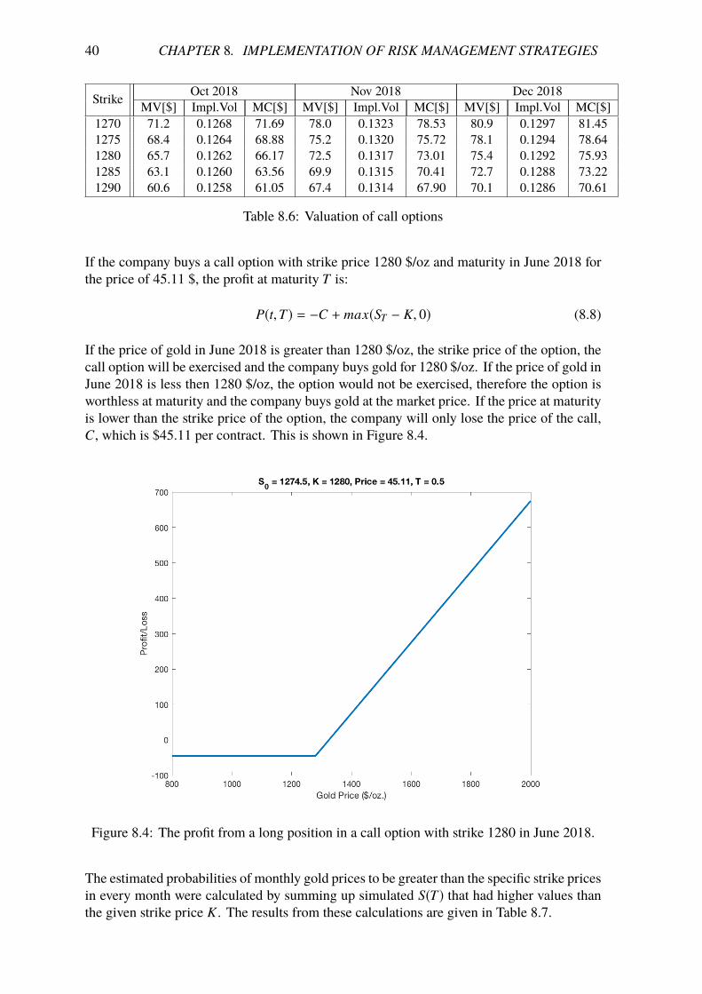
If the company buys a call option with strike price 1280 $/oz and maturity in June 2018 forthe price of 45.11 $, the profit at maturity T is:
P(t,T) = �C + max(ST � K, 0) (8.8)
If the price of gold in June 2018 is greater than 1280 $/oz, the strike price of the option, thecall option will be exercised and the company buys gold for 1280 $/oz. If the price of gold inJune 2018 is less then 1280 $/oz, the option would not be exercised, therefore the option isworthless at maturity and the company buys gold at the market price. If the price at maturityis lower than the strike price of the option, the company will only lose the price of the call,C, which is $45.11 per contract. This is shown in Figure 8.4.
Figure 8.4: The profit from a long position in a call option with strike 1280 in June 2018.
The estimated probabilities of monthly gold prices to be greater than the specific strike pricesin every month were calculated by summing up simulated S(T) that had higher values thanthe given strike price K . The results from these calculations are given in Table 8.7.
�.�. PRICING ASIAN CALL OPTION 41
Date P(S(T) > K)K=1270 K=1275 K=1280 K=1285 K=1290
Jan 2018 58.19% 51.02% 44.26% 37.28% 30.39%Feb 2018 56.65% 51.86% 47.34% 42.74% 38.37%Mar 2018 54.32% 51.54% 46.68% 45.91% 42.06%Apr 2018 54.35% 51.91% 45.92% 47.10% 44.20%May 2018 54.01% 51.99% 49.99% 47.96% 45.96%Jun 2018 54.24% 52.37% 50.53% 48.65% 46.81%Jul 2018 53.98% 52.35% 50.73% 49.13% 47.51%Aug 2018 54.16% 53.59% 51.05% 49.55% 48.01%Sep 2018 54.11% 52.71% 51.35% 49.99% 48.59%Oct 2018 54.48% 53.17% 51.83% 50.50% 49.16%Nov 2018 54.33% 53.11% 51.89% 50.66% 49.48%Dec 2018 54.75% 53.57% 52.37% 51.18% 50.03%
Table 8.7: Probabilities for monthly gold price to be greater than the strike price
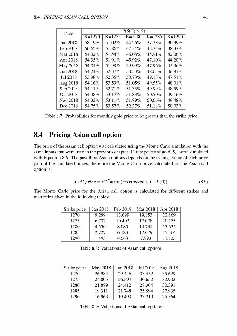
8.4 Pricing Asian call optionThe price of the Asian call option was calculated using the Monte Carlo simulation with thesame inputs that were used in the previous chapter. Future prices of gold, ST , were simulatedwith Equation 8.6. The payo� on Asian options depends on the average value of each pricepath of the simulated prices, therefore the Monte Carlo price calculated for the Asian calloption is:
Call price = e�rT mean(max(mean(ST ) � K, 0)) (8.9)
The Monte Carlo price for the Asian call option is calculated for di�erent strikes andmaturities given in the following tables:
Strike price Jan 2018 Feb 2018 Mar 2018 Apr 20181270 9.299 13.099 19.853 22.8691275 6.737 10.403 17.078 20.1551280 4.530 8.085 14.731 17.6351285 2.727 6.183 12.079 15.3641290 1.495 4.543 7.993 11.135
Table 8.8: Valuations of Asian call options
Strike price May 2018 Jun 2018 Jul 2018 Aug 20181270 26.984 29.446 33.452 35.6291275 24.005 26.597 30.652 32.9021280 21.889 24.412 28.304 30.3911285 19.311 21.748 25.594 27.9351290 16.963 19.499 23.219 25.564
Table 8.9: Valuations of Asian call options
42 CHAPTER �. IMPLEMENTATION OF RISK MANAGEMENT STRATEGIES
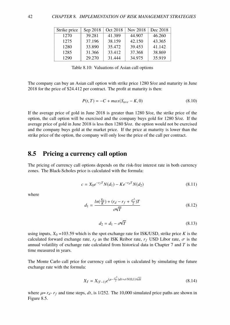
Strike price Sep 2018 Oct 2018 Nov 2018 Dec 20181270 39.281 41.389 44.907 46.2601275 37.196 38.159 42.150 43.3651280 33.890 35.472 39.453 41.1421285 31.366 33.412 37.368 38.8691290 29.270 31.444 34.975 35.919
Table 8.10: Valuations of Asian call options
The company can buy an Asian call option with strike price 1280 $/oz and maturity in June2018 for the price of $24.412 per contract. The profit at maturity is then:
P(t,T) = �C + max(Save � K, 0) (8.10)
If the average price of gold in June 2018 is greater than 1280 $/oz, the strike price of theoption, the call option will be exercised and the company buys gold for 1280 $/oz. If theaverage price of gold in June 2018 is less then 1280 $/oz. the option would not be exercisedand the company buys gold at the market price. If the price at maturity is lower than thestrike price of the option, the company will only lose the price of the call per contract.
8.5 Pricing a currency call optionThe pricing of currency call options depends on the risk-free interest rate in both currencyzones. The Black-Scholes price is calculated with the formula:
c = X0e�rf T N(d1) � Ke�rdT N(d2) (8.11)
where
d1 =ln( X0
K ) + (rd � r f +�2
2 )T�p
T(8.12)
d2 = d1 � �p
T (8.13)
using inputs, X0 =103.59 which is the spot exchange rate for ISK/USD, strike price K is thecalculated forward exchange rate, rd as the ISK Reibor rate, r f USD Libor rate, � is theannual volatility of exchange rate calculated from historical data in Chapter 7 and T is thetime measured in years.
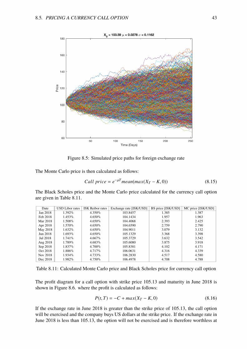
The Monte Carlo call price for currency call option is calculated by simulating the futureexchange rate with the formula:
XT = X(T�1)e(µ��22 )dt+�N(0,1)
pdt (8.14)
where µ= rd- r f and time steps, dt, is 1/252. The 10,000 simulated price paths are shown inFigure 8.5.
�.�. PRICING A CURRENCY CALL OPTION 43
Figure 8.5: Simulated price paths for foreign exchange rate
The Monte Carlo price is then calculated as follows:
Call price = e�µT mean(max(XT � K, 0)) (8.15)
The Black Scholes price and the Monte Carlo price calculated for the currency call optionare given in Table 8.11.
Date USD Libor rates ISK Reibor rates Exchange rate [ISK/USD] BS price [ISK/USD] MC price [ISK/USD]Jan 2018 1.392% 4.350% 103.8457 1.385 1.387Feb 2018 1.453% 4.650% 104.1434 1.957 1.963Mar 2018 1.508% 4.650% 104.4068 2.393 2.425Apr 2018 1.570% 4.650% 104.6590 2.759 2.790May 2018 1.632% 4.650% 104.9011 3.079 3.132Jun 2018 1.693% 4.650% 105.1329 3.368 3.398Jul 2018 1.741% 4.667% 105.3729 3.632 3.542Aug 2018 1.789% 4.683% 105.6080 3.875 3.918Sep 2018 1.837% 4.700% 105.8381 4.102 4.171Oct 2018 1.886% 4.717% 106.0631 4.316 4.339Nov 2018 1.934% 4.733% 106.2830 4.517 4.580Dec 2018 1.982% 4.750% 106.4978 4.708 4.788
Table 8.11: Calculated Monte Carlo price and Black Scholes price for currency call option
The profit diagram for a call option with strike price 105.13 and maturity in June 2018 isshown in Figure 8.6. where the profit is calculated as follows:
P(t,T) = �C + max(XT � K, 0) (8.16)
If the exchange rate in June 2018 is greater than the strike price of 105.13, the call optionwill be exercised and the company buys US dollars at the strike price. If the exchange rate inJune 2018 is less than 105.13, the option will not be exercised and is therefore worthless at
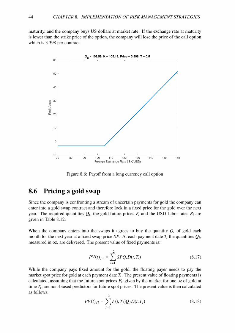
44 CHAPTER �. IMPLEMENTATION OF RISK MANAGEMENT STRATEGIES
maturity, and the company buys US dollars at market rate. If the exchange rate at maturityis lower than the strike price of the option, the company will lose the price of the call optionwhich is 3.398 per contract.
Figure 8.6: Payo� from a long currency call option
8.6 Pricing a gold swapSince the company is confronting a stream of uncertain payments for gold the company canenter into a gold swap contract and therefore lock in a fixed price for the gold over the nextyear. The required quantities Qi, the gold future prices Fi and the USD Libor rates Ri aregiven in Table 8.12.
When the company enters into the swaps it agrees to buy the quantity Qi of gold eachmonth for the next year at a fixed swap price SP. At each payment date Ti the quantities Qi,measured in oz, are delivered. The present value of fixed payments is:
PV(t) f x =
12’i=1
SPQiD(t,Ti) (8.17)
While the company pays fixed amount for the gold, the floating payer needs to pay themarket spot price for gold at each payment date Ti. The present value of floating payments iscalculated, assuming that the future spot prices Fi, given by the market for one oz of gold attime Ti, are non-biased predictors for future spot prices. The present value is then calculatedas follows:
PV(t) f l =
12’j=1
F(t,Tj)Q j D(t,Tj) (8.18)
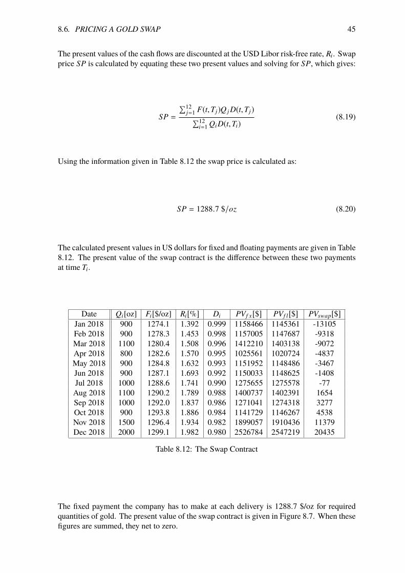
�.�. PRICING A GOLD SWAP 45
The present values of the cash flows are discounted at the USD Libor risk-free rate, Ri. Swapprice SP is calculated by equating these two present values and solving for SP, which gives:
SP =
Õ12j=1 F(t,Tj)Q j D(t,Tj)Õ12
i=1 QiD(t,Ti)(8.19)
Using the information given in Table 8.12 the swap price is calculated as:
SP = 1288.7 $/oz (8.20)
The calculated present values in US dollars for fixed and floating payments are given in Table8.12. The present value of the swap contract is the di�erence between these two paymentsat time Ti.
Date Qi[oz] Fi[$/oz] Ri[%] Di PVf x[$] PVf l[$] PVswap[$]Jan 2018 900 1274.1 1.392 0.999 1158466 1145361 -13105Feb 2018 900 1278.3 1.453 0.998 1157005 1147687 -9318Mar 2018 1100 1280.4 1.508 0.996 1412210 1403138 -9072Apr 2018 800 1282.6 1.570 0.995 1025561 1020724 -4837May 2018 900 1284.8 1.632 0.993 1151952 1148486 -3467Jun 2018 900 1287.1 1.693 0.992 1150033 1148625 -1408Jul 2018 1000 1288.6 1.741 0.990 1275655 1275578 -77Aug 2018 1100 1290.2 1.789 0.988 1400737 1402391 1654Sep 2018 1000 1292.0 1.837 0.986 1271041 1274318 3277Oct 2018 900 1293.8 1.886 0.984 1141729 1146267 4538Nov 2018 1500 1296.4 1.934 0.982 1899057 1910436 11379Dec 2018 2000 1299.1 1.982 0.980 2526784 2547219 20435
Table 8.12: The Swap Contract
The fixed payment the company has to make at each delivery is 1288.7 $/oz for requiredquantities of gold. The present value of the swap contract is given in Figure 8.7. When thesefigures are summed, they net to zero.
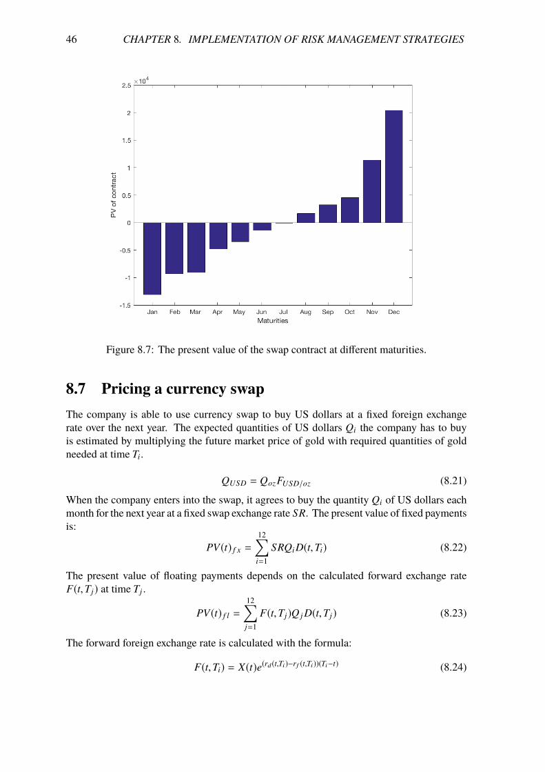
46 CHAPTER �. IMPLEMENTATION OF RISK MANAGEMENT STRATEGIES
Figure 8.7: The present value of the swap contract at di�erent maturities.
8.7 Pricing a currency swapThe company is able to use currency swap to buy US dollars at a fixed foreign exchangerate over the next year. The expected quantities of US dollars Qi the company has to buyis estimated by multiplying the future market price of gold with required quantities of goldneeded at time Ti.
QUSD = QozFUSD/oz (8.21)
When the company enters into the swap, it agrees to buy the quantity Qi of US dollars eachmonth for the next year at a fixed swap exchange rate SR. The present value of fixed paymentsis:
PV(t) f x =
12’i=1
SRQiD(t,Ti) (8.22)
The present value of floating payments depends on the calculated forward exchange rateF(t,Tj) at time Tj .
PV(t) f l =
12’j=1
F(t,Tj)Q j D(t,Tj) (8.23)
The forward foreign exchange rate is calculated with the formula:
F(t,Ti) = X(t)e(rd(t,Ti)�rf (t,Ti))(Ti�t) (8.24)

�.�. PRICING A CURRENCY SWAP 47
When a swap contract is entered into the present value of the fixed and floating payments areequal, so the swap rate can be calculated as:
SR =Õ12
i=1 QiD(t,Ti)Õ12j=1 F(t,Tj)Q j D(t,Tj)
(8.25)
The required quantities of US dollars Qi, forward exchange rate Fi, ISK Reibor rates Ri andthe discount factor Di, calculated using ISK Reibor rates, are given in Table 8.13. Using thisinformation, the swap rate is calculated:
SR = 105.38 (8.26)
Therefore the company has locked in the exchange rate at ISK 105.38 per USD for the requiredquantities of US dollars. The present value of fixed and floating payments calculated in ISKare given in the following table. The present value of the swap contract is the di�erencebetween fixed and floating payments at each payment date Ti.
Date Ri[%] Di Fi[ISK/USD] Qi[USD] PVf x[ISK] PVf l[ISK] PVswap[ISK]Jan 4.350 0.996 103.85 1146690 120402404 118647924 -1754480Feb 4.650 0.993 104.14 1150470 120302033 118888929 -1413104Mar 4.650 0.988 104.41 1408440 146707774 145351113 -1356661Apr 4.650 0.985 104.66 1026080 106466532 105736808 -729724May 4.650 0.981 104.90 1156320 119516271 118971633 -544637Jun 4.650 0.977 105.13 1158390 119267167 118986051 -281116Jul 4.667 0.973 105.37 1288600 132147551 132137101 -10450Aug 4.683 0.969 105.61 1419220 144961788 145273687 311899Sep 4.700 0.965 105.84 1292000 131436832 132006563 569731Oct 4.717 0.961 106.06 1164420 117978515 118741801 763287Nov 4.733 0.958 106.28 1944600 196223122 197902104 1678982Dec 4.750 0.954 106.50 2598200 261100102 263866375 2766273
Table 8.13: The Currency Swap Contract
The present values of the swap contract at time t are given in Figure 8.8. As seen in thefigure, the net value of the swap contract at time t is zero. The floating payment may changein time and change the net value of the swap contract. At any given time, the value of theswap contract is given by the di�erence in the present values of the remaining payments.When the spot exchange rate increases, the net payment goes to the fixed rate payer and whenthe spot exchange decreases, the net payment goes to the floating rate payer.

48 CHAPTER �. IMPLEMENTATION OF RISK MANAGEMENT STRATEGIES
Figure 8.8: The present value of the currency swap contract at di�erent maturities.
8.8 SummaryTo choose the best risk management strategies for the company to hedge its risk exposure,the derivatives contracts are compared.
In future contract, the company pays various future prices for the gold each month. Thepresent value at time t (today) of the payments made by purchasing required quantities ofgold Q(Ti)gold for a future price F(t,Ti) at time Ti is:
PV(t,Ti)Future = Q(Ti)goldF(t,Ti)D(t,Ti) (8.27)
In call option, a fixed strike price at 1270 $/oz or less for the gold is paid each month, plusthe cost of a premium for these contracts C(t,Ti)premium. If the spot price for gold at maturityis lower than 1270 $/oz, the company buys the gold at the market price. The present valueof the total cost of entering into a call options to buy required quantities Q(Ti)gold with strikeK=1270 $/oz at time Ti is:
PV(t,Ti)Option = Q(Ti)goldKD(t,Ti) + C(t,Ti)premium (8.28)
In swap contract, a fixed swap price of 1288.7 $/oz is paid for the gold price over the nextyear. The present value of the fixed payments in swap contract at time t with a fixed swapprice SP = 1288.7 $/oz is:
PV(t,Ti)Swap = SPQ(Ti)gold D(t,Ti) (8.29)
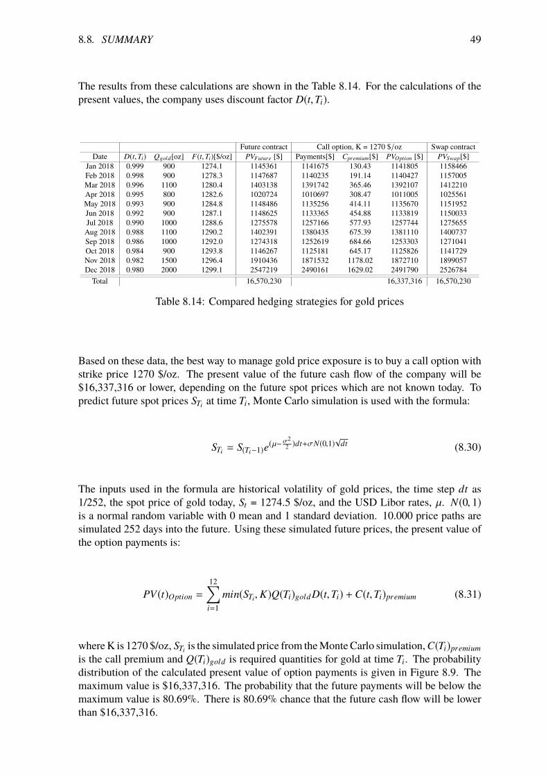
�.�. SUMMARY 49
The results from these calculations are shown in the Table 8.14. For the calculations of thepresent values, the company uses discount factor D(t,Ti).
Future contract Call option, K = 1270 $/oz Swap contractDate D(t,Ti) Qgold[oz] F(t,Ti)[$/oz] PVFuture [$] Payments[$] Cpremium[$] PVOption [$] PVSwap[$]
Jan 2018 0.999 900 1274.1 1145361 1141675 130.43 1141805 1158466Feb 2018 0.998 900 1278.3 1147687 1140235 191.14 1140427 1157005Mar 2018 0.996 1100 1280.4 1403138 1391742 365.46 1392107 1412210Apr 2018 0.995 800 1282.6 1020724 1010697 308.47 1011005 1025561May 2018 0.993 900 1284.8 1148486 1135256 414.11 1135670 1151952Jun 2018 0.992 900 1287.1 1148625 1133365 454.88 1133819 1150033Jul 2018 0.990 1000 1288.6 1275578 1257166 577.93 1257744 1275655Aug 2018 0.988 1100 1290.2 1402391 1380435 675.39 1381110 1400737Sep 2018 0.986 1000 1292.0 1274318 1252619 684.66 1253303 1271041Oct 2018 0.984 900 1293.8 1146267 1125181 645.17 1125826 1141729Nov 2018 0.982 1500 1296.4 1910436 1871532 1178.02 1872710 1899057Dec 2018 0.980 2000 1299.1 2547219 2490161 1629.02 2491790 2526784
Total 16,570,230 16,337,316 16,570,230
Table 8.14: Compared hedging strategies for gold prices
Based on these data, the best way to manage gold price exposure is to buy a call option withstrike price 1270 $/oz. The present value of the future cash flow of the company will be$16,337,316 or lower, depending on the future spot prices which are not known today. Topredict future spot prices STi at time Ti, Monte Carlo simulation is used with the formula:
STi = S(Ti�1)e(µ��22 )dt+�N(0,1)
pdt (8.30)
The inputs used in the formula are historical volatility of gold prices, the time step dt as1/252, the spot price of gold today, St = 1274.5 $/oz, and the USD Libor rates, µ. N(0, 1)is a normal random variable with 0 mean and 1 standard deviation. 10.000 price paths aresimulated 252 days into the future. Using these simulated future prices, the present value ofthe option payments is:
PV(t)Option =
12’i=1
min(STi,K)Q(Ti)gold D(t,Ti) + C(t,Ti)premium (8.31)
where K is 1270 $/oz, STi is the simulated price from the Monte Carlo simulation, C(Ti)premiumis the call premium and Q(Ti)gold is required quantities for gold at time Ti. The probabilitydistribution of the calculated present value of option payments is given in Figure 8.9. Themaximum value is $16,337,316. The probability that the future payments will be below themaximum value is 80.69%. There is 80.69% chance that the future cash flow will be lowerthan $16,337,316.

50 CHAPTER �. IMPLEMENTATION OF RISK MANAGEMENT STRATEGIES
Figure 8.9: The probability density function for the present value of option payments
Table 8.15 compares the best strategies to hedge foreign exchange rates for the company. Byentering into a forward contract, the company agrees to purchase US dollars at the forwardexchange rate each month. The present value at time t for these future payments to buyrequired quantities of US dollars Q(Ti)USD at time Ti is:
PV(t,Ti)Forward = Q(Ti)USDF(t,Ti)D(t,Ti) (8.32)
The quantities Q(Ti)USD of US dollars that the company have to purchase depends on theprice of gold at each payment date Ti. The expected quantities of US dollars purchased eachmonth are calculated with the future price of gold:
Q(Ti)USD = Q(Ti)ozF(t,Ti)USD/oz (8.33)
In swap contract, the company purchases US dollars at a fixed exchange swap rate SR=105.38.The present value of the fixed payments in the swap contract is:
PVSwap(t,Ti) = SRQ(Ti)USDD(t,Ti) (8.34)
The option contract gives the company the right to purchase US dollars at the calculatedforward exchange rate given today at time t. If the forward exchange rate at maturity is higherthan the spot exchange rate, the company can purchase US dollars at the market exchangerate. The present value of the payments made in option contract at each delivery Ti is:
PVOption(t,Ti) = Q(Ti)USDK(Ti)D(t,Ti) + C(t,Ti)premium (8.35)

�.�. SUMMARY 51
Forward contract Call option, K = F(t,Ti) Swap contractDate D(t,Ti) QUSD F(t,Ti) PVForward [ISK] Payments[ISK] Cpremium[ISK] PVOption [ISK] PVSwap[ISK]
Jan 2018 0.996 1146690 103.85 118647924 118647924 1588575 120236500 120402404Feb 2018 0.992 1150470 104.14 118888929 118888929 2251043 121139972 120302033Mar 2018 0.988 1408440 104.41 145351113 145351113 3370434 148721548 146707774Apr 2018 0.985 1026080 104.66 105736808 105736808 2831019 108567827 106466532May 2018 0.981 1156320 104.90 118971633 118971633 3561185 122532819 119516271Jun 2018 0.977 1158390 105.13 118986051 118986051 3901373 122887424 119267167Jul 2018 0.973 1288600 105.37 132137101 132137101 4679497 136816598 132147551Aug 2018 0.969 1419220 105.61 145273687 145273687 5499674 150773361 144961788Sep 2018 0.965 1292000 105.84 132006563 132006563 5300312 137306875 131436832Oct 2018 0.961 1164420 106.06 118741801 118741801 5025368 123767169 117978515Nov 2018 0.958 1944600 106.28 197902104 197902104 8783966 206686070 196223122Dec 2018 0.954 2598200 106.50 263866375 263866375 12232020 276098395 261100102
Total 1,716,510,091 1,775,534,558 1,716,510,091
Table 8.15: Compared hedging strategies for exchange rate
The best way to manage foreign exchange exposure is to enter into a swap contract to purchaseUS dollars at a fixed exchange rate of 105.38 or entering into a long future contract to lockin the future gold price for the next year.
If the company decides to manage gold price exposure with a long position in a call optionwith strike price K = 1270 $/oz, it guarantees that quantities of gold for the next year will bepurchased for 1270 $/oz or lower. The quantities of US dollars the company has to purchasecan now be calculated as:
Q(Ti)USD = Q(Ti)ozKUSD/oz (8.36)
The present value of payments for each contract is now calculated with the new quantities ofUS dollars and the results are shown in Table 8.16.
Forward contract Call option, K = F(t,Ti) Swap contractDate D(t,Ti) QUSD F(t,Ti) PVForward [ISK] Payments[ISK] Cpremium[ISK] PVOption [ISK] PVSwap[ISK]
Jan 2018 0.996 1143000 103.85 118266120 118266120 1583463 119849584 120009164Feb 2018 0.992 1143000 104.14 118116984 118116984 2236426 120353410 119515146Mar 2018 0.988 1397000 104.41 144170504 144170504 3343058 147513563 145509126Apr 2018 0.985 1016000 104.66 104698071 104698071 2803207 107501279 105415541May 2018 0.981 1143000 104.90 117601163 117601163 3520163 121121326 118133827Jun 2018 0.977 1143000 105.13 117405240 117405240 3849540 121254781 117676944Jul 2018 0.973 1270000 105.37 130229799 130229799 4611952 134841751 130233814Aug 2018 0.969 1397000 105.61 142999211 142999211 5413569 148412780 142685312Sep 2018 0.965 1270000 105.84 129758774 129758774 5210059 134968832 129192511Oct 2018 0.961 1143000 106.06 116557495 116557495 4932924 121490420 115802663Nov 2018 0.958 1905000 106.28 193872009 193872009 8605088 202477097 192217944Dec 2018 0.954 2540000 106.50 257955736 257955736 11958021 269913757 255239114
Total 1,691,631,106 1,749,698,580 1,691,631,106
Table 8.16: Compared hedging strategies for exchange rate
To summarize the results calculated, the best way to manage both gold price risk and foreignexchange rate risk is to take a long position in a call option to purchase gold at the strike priceK=1270 $/oz for delivery of the required ounces of gold each month. Now the companyknows that the gold price for the next year will be bought for 1270 $/oz, the company candecide how many US dollars they have to purchase. With this information, the company canenter into a swap contract with fixed swap exchange rate = 105.38 or enter into a forwardcontract with future prices bought at delivery. The company’s future payments for buyinggold and US dollars are now immune to upward movements in the market price.
Chapter 9
Discussion and Conclusion
Companies that use commodities as input should consider implementing risk managementstrategies to insure against a rise in prices, where the profit decreases when the price of theinput increases. Hedging strategies for such firms include buying forwards, buying futures,buying calls or entering into a swap contract. Many companies faced with commodity pricerisk can also face a foreign exchange rate risk since most commodities are quoted in USdollars. Managing both these risks at the same time can be challenging.
The main purpose of this thesis is to use risk management strategies and derivatives tohedge risks faced by an Icelandic manufacturer that uses gold as an input. The derivativesused are futures, forwards, options and swaps. Both gold price risk and foreign exchangerate risk have a great e�ect on the company’s profitability. Based on the risk-managementtools and analysis, the study shows that a good way to manage gold price risk is by taking along position in a call option with a strike price close to the present spot price. Entering intoa swap contract with a fixed foreign exchange rate over the next year can be considered ane�ective risk management strategy for the company to manage foreign exchange rate risk.
When implementing risk management strategies, it is important to choose appropriate strate-gies because there can also be a potential loss if the prices of the underlying commoditychange against risk management strategies and expectations of price fluctuations.
As a result, hedging against market price fluctuations in volatile commodity markets reducesprice uncertainty and stabilizes future cash flow. These non-predictable price fluctuations inthe commodity market can lead to big losses for companies that can be much more harmfulthan profits are beneficial.
Bibliography
[1] S. Ólafsson, “Introduction to risk management”, Reykjavik: Reykjavik University,2015.
[2] R. L. McDonald, Fundamentals of derivatives markets. Boston: Pearson Education,Inc., 2009.
[3] CPA Australia. (2009). A guide to managing foreign exchange risk, [Online]. Avail-able: https://www.cpaaustralia.com.au/~/media/corporate/allfiles/document/professional- resources/business/managing- foreign-
exchange-risk.pdf?la=en. Accessed: 15 Jan 2018.[4] ——, (2008). Understanding and managing interest rate risk, [Online]. Available:
https://www.cpaaustralia.com.au/~/media/corporate/allfiles/docu
ment/professional-resources/business/understanding-and-managing-
interest-rate-risk-guide.pdf?la=en,%20https://www.cpaaustralia.
com.au/~/media/corporate/allfiles/document/professional-resou
rces/business/understanding- and- managing- interest- rate- risk-
guide.pdf?la=en. Accessed: 15 Jan 2018.[5] ——, (2012). A guide to managing commodity risk, [Online]. Available: https:
//www.cpaaustralia.com.au/~/media/corporate/allfiles/document/
professional-resources/business/managing-commodity-risk.pdf?la=
en,%20https://www.cpaaustralia.com.au/~/media/corporate/allfil
es/document/professional-resources/business/managing-commodity-
risk.pdf?la=en. Accessed: 15 Jan 2018.[6] S. Ólafsson, “Risk quantification”, Reykjavik: Reykjavik University, 2015.[7] J. C. Hull, Options, futures and other derivatives. New Jersey: Pearson Education,
Inc., 2015.[8] S. Ólafsson, “Introduction to forward contracts and futures contracts”, Reykjavik:
Reykjavik University, 2015.[9] ——, “Introduction to swaps”, Reykjavik: Reykjavik University, Feb. 2014.
[10] ——, “Option valuation”, Reykjavik: Reykjavik University, 2015.[11] General Electric Company. (2016). Calibration of ornstein-uhlenbeck mean reverting
process, [Online]. Available: https://www.predix.io/api/catalog/analytics/artifacts/8699fe7b-5a67-48b1-9320-216ab2e57105/file?fileName=
Mean%20reversion%20model%20fit.pdf. Accessed: 15 Jan 2018.[12] Global Rates. (2017). Libor - current libor interest rates, [Online]. Available: http:
//www.global-rates.com/interest-rates/libor/libor.aspx. Accessed:04 Dec 2017.
54 BIBLIOGRAPHY
[13] CME Group. (2017). Gold futures quotes, [Online]. Available: http://www.cmegroup.com/trading/metals/precious/gold_quotes_globex.html. Accessed:04 Dec 2017.
[14] Investing. (2017). Gold historical data, [Online]. Available: https://www.investing.com/commodities/gold-historical-data. Accessed: 04 Dec 2017.
[15] Selabanki Íslands. (2017). Vextir selabankans og arir vextir, [Online]. Available:https://www.sedlabanki.is/annad- efni/vextir- sedlabankans- og-
adrir-vextir/. Accessed: 04 Dec 2017.[16] Central Bank of Iceland. (2017). O�cial exchange rate - time series, [Online].
Available: https : / / www . cb . is / ?PageId = 6909b7bd - 5189 - 45dd - bf5b -c76ea33496ef. Accessed: 04 Dec 2017.
[17] CME Group. (2017). Gold futures contract specs, [Online]. Available: http://www.cmegroup.com/trading/metals/precious/gold_contract_specification
s.html. Accessed: 04 Dec 2017.[18] ——, (2017). Gold options contract specs, [Online]. Available: http://www.cmegr
oup.com/trading/metals/precious/gold_contractSpecs_options.html?
ds_medium=cpc&ds_medium=cpc&gclid=CjwKCAjw_tTXBRBsEiwArqXyMlJm
SjhhuL9_CUCigyXwFqztLXD1F0trmz4OKLJSYIDPi96cMgE0DRoCUt8QAvD_BwE&
gclsrc=aw.ds. Accessed: 04 Dec 2017.[19] ——, (2017). Gold options quotes, [Online]. Available: http://www.cmegroup.
com/trading/metals/precious/gold_quotes_globex_options.html#
optionProductId=192&strikeRange=ATM. Accessed: 04 Dec 2017.


![E} ZvP rK ]}ví · 01/03/2021 · 4bo+vtup 3ftfswpjs 3jehfnbsl 5sft1jopt e} zvp rk ]}ví](https://img.pdfslide.us/doc/110x75/6138a82b0ad5d20676496439/e-zvp-rk-v-01032021-4bovtup-3ftfswpjs-3jehfnbsl-5sft1jopt-e-zvp-rk-v.jpg)