Hedging Multiperiod Forward Commitments: The Case of Period-by-Period Quantity Uncertainty

Review of Quantitative Finance and Accounting, 16, 171–181, 2001©C 2001 Kluwer Academic Publishers. Manufactured in The Netherlands.

Hedging Multiperiod Forward Commitments:The Case of Period-by-Period Quantity Uncertainty

DONALD LIENDepartment of Economics, Summerfield Hall, University of Kansas, Lawrence, KS 66045E-mail: [email protected]

DAVID R. SHAFFERVillanova University, College of Commerce and Finance, 800 Lancaster Avenue, Villanova, PA 19085-1678E-mail: [email protected]

Abstract. This article considers the hedging problem of a producer with a long-term forward commitmentto deliver a commodity at multiple future points in time. The aggregate quantity to be delivered over time isknown with certainty; however, the period-by-period quantity is determined by the customer and is unknown tothe producer. A minimum-variance multiperiod futures position that considers both price uncertainty and period-by-period quantity uncertainty is derived. The following results are obtained: The individual effects of priceuncertainty and quantity uncertainty on the multiperiod minimum-variance are separable. In the two-period case,if the spot price is expected to decrease over time, the risk-minimizing hedge considering both price and quantityuncertainties is greater than that which considers price uncertainty only. If the spot price is expected to increaseover time, then the hedger would be over-hedged if only price uncertainty were considered. Convenience yieldpromotes a larger risk-minimizing futures position, whereas storage costs and financial costs reduce the size ofthe risk-minimizing futures position. In the multiperiod case, if forward prices are unbiased estimators of futurespot prices, or if spot prices are expected to decrease over time, then quantity uncertainty increases the size ofthe risk-minimizing hedge. If spot prices are expected to increase, then the effect of period-by-period quantityuncertainty is indeterminate.

Key words: hedging, forward commitment, quantity uncertainty, variance minimization

JEL Classification: G11

1. Introduction

The case of Metallgesellschaft (MG) and its controversial hedging strategy has increasedacademic scrutiny of hedging long-term forward commitments with short-dated futurescontracts (e.g., see Brennan and Crew, 1997; Culp and Miller, 1994, 1995a, 1995b; Edwardsand Canter, 1995; Hilliard, 1997; Mello and Parsons, 1995; Pirrong, 1997). In the early1990s MG had large long-term forward commitments in which the maturity of the obliga-tions exceeded that of their hedging instruments. The result was a strategy of purchasing a“stack” of short-term futures contracts and rolling the stack forward as it neared expirationand repeating this procedure until the final delivery was made on the forward commitments.While a detailed description can of MG’s hedging strategy can be found in Culp and Miller

172 LIEN AND SHAFFER

(1994, 1995a, 1995b), Edwards and Canter (1995), and Mello and Parsons (1995), a briefrecounting is provided here.

MG tried to aggressively penetrate U.S. petroleum markets through its subsidiary, MGRefining and Marketing (MGRM), by offering independent dealers of energy-related prod-ucts long-term fixed-price supply contracts. These contracts were so popular that withintwo years, MGRM had sold nearly 160 million barrels of oil forward, most of which were10-year supply obligations. One type of contract, the “firm-fixed” contract, obligated MGRMto deliver a fixed amount of product each month at a fixed price for the duration of the con-tract. The other type of contract, the “firm-flexible” contract, was similar to the firm-fixedcontract except it contained a deferment option allowing customers to delay delivery of,and payment for, their supply.1 Nearly one-third of MGRM’s total forward commitmentwas subject to firm-flexible supply provisions. Thus, while the cumulative quantity to bedelivered over the life of the supply contracts was known, MGRM was uncertain how muchquantity had to be delivered each period.2

MGRM’s hedge consisted of over-the-counter swaps and exchange traded energy futures,although the futures hedge has received the greatest attention in the literature. Under theswap agreements, MGRM exchanged fixed for variable payments. The futures positionconsisted of a long “rolling stack” of short-dated futures contracts. The size of MGRM’shedge was almost identical to its forward commitment, implying a hedge ratio of 1:1. By theend of 1993, following adverse price movements and associated margin calls, MGRM wasfacing huge hedging-related losses on its futures position and apparent financial collapse.Only a $1.3 billion emergency cash infusion saved the parent company from bankruptcy.Explanations for the failed hedging program have been offered by Culp and Miller (1994,1995a) who defend the program as conceptually sound, but fault supervisory board membersfor abandoning the program when prices moved against MG; Mello and Parsons (1995)and Pirrong (1997) who view the strategy as conceptually flawed; and Edwards and Canter(1995) who highlight the potential risks and benefits of the program but are reserved in theirjudgement of MG. Hilliard (1997) developed a backward dynamic algorithm to calculatethe optimal hedge ratios.

This article considers the hedging problem of a producer with a long-term forward com-mitment to deliver a commodity at multiple future points in time. The total quantity com-mitment contracted for between the producer and the customer is known with certainty.However, the customer has discretion over when to take delivery of, and make paymentfor, this quantity. At the extremes, the customer could request the entire quantity in anysingle period, or instead, take delivery of an equal amount each period for the duration ofthe contract. Thus, the producer faces period-by-period quantity uncertainty, in addition toprice uncertainty.

A minimum-variance multiperiod futures position is derived that considers both period-by-period quantity uncertainty and price uncertainty.3 The contract examined in this papercan be viewed as a generalized form of MGRM’s firm-flexible contract. It is more gen-eral because the buyer has the option to either accelerate or defer delivery of its supply,whereas MGRM’s firm-flexible contract gave customers only the option to defer. This paperdevelops the following results. The effects of price uncertainty and period-by-period quan-tity uncertainty on the multiperiod minimum-variance hedge position are separable. In the

HEDGING MULTIPERIOD FORWARD COMMITMENTS 173

two-period case, if spot prices are expected to decrease over time, the risk-minimizing hedgeconsidering both price and quantity uncertainties is greater than that which considers priceuncertainty only. If spot prices are expected to increase over time, then the risk-minimizingfutures position considering both price and quantity uncertainties will be smaller than thatwhich considers price uncertainty only. The convenience yield of a commodity promotes alarger risk-minimizing futures position, whereas storage costs and financial costs depressthe size of the risk-minimizing futures position. In a multiperiod context, if forward pricesare unbiased estimators of future spot prices, or if spot prices are expected to decrease overtime, then period-by-period quantity uncertainty increases the size of the risk-minimizinghedge. Last, if spot prices are expected to increase, then the effect of period-by-periodquantity uncertainty is ambiguous.

The analysis of hedging in the presence of quantity or production uncertainty is not newto the literature (e.g., Anderson and Danthine, 1983; Baesel and Grant, 1982; Ho, 1984;McKinnon, 1967; Rolfo, 1980). However, these articles examine the case in which aggregatequantity is uncertain. This paper takes aggregate (cumulative) quantity as given and period-by-period quantity as unknown. The paper is organized as follows. Section 2 developsa model for the case of period-by-period quantity uncertainty and derives the minimumvariance futures position in a two-period setting. Section 3 discusses hedge ratio estimation.In Section 4, the hedger’s problem is generalized to a T -period context. Section 5 discussesthe implications of the results with respect to the case of MGRM and Section 6 concludesthe paper.

2. The hedger’s decision

This section lays out the hedger’s problem and derives the solution considering the effectsof both period-by-period quantity and price uncertainties. This model is cast in a three tradedate (two-period) setting. At t = 0 a producer commits to deliver Q units of a commodity toa buyer at a forward price of f . The buyer can choose to receive any quantity of the good att = 1 or t = 2 such that Q1 + Q2 = Q.4 While the buyer may solve for the optimal quantityof Q1, the hedger does not have complete information on certain parameters affecting thebuyer’s decision-making. As a result, the hedger treats Q1 as a random variable. The forwardobligation is completely settled at t = 2. The producer settles by purchasing the commodityin the spot market at the prevailing spot price, S2, and selling the good to the buyer at f .A futures contract is available at t = 0 that matures at t = 1 and another is available att = 1 that matures at t = 2. The producer is subject to both price and period-by-periodquantity uncertainties at t = 0. The hedger’s objective is to choose a futures position att = 0 and again at t = 1 so that the variance of his profit is minimized at t = 2. Whilethis problem is examined in a two-period setting, an extension of the model to an T -periodsetting is straightforward and is considered later in the paper. The following notation isemployed:

π = total profit earned by the hedger from t = 0 to t = 2.πt = profit earned by the hedger from time t − 1 to t , where t = 1, 2.


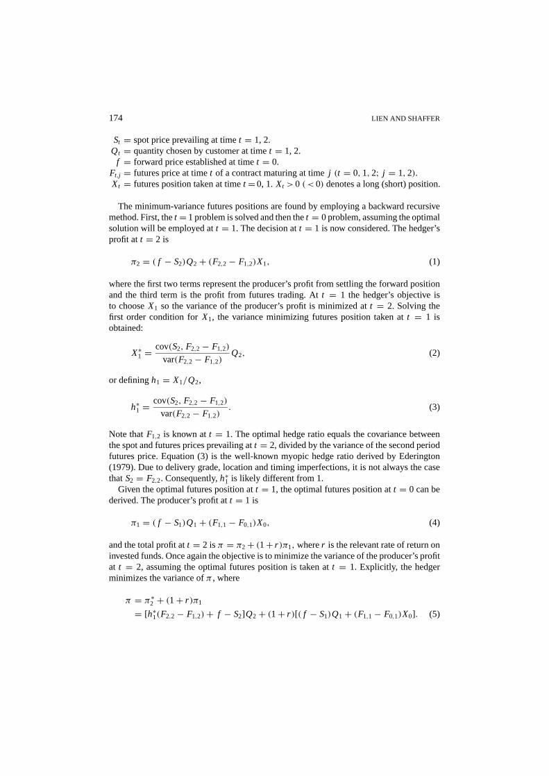
St = spot price prevailing at time t = 1, 2.Qt = quantity chosen by customer at time t = 1, 2.

f = forward price established at time t = 0.Ft,j = futures price at time t of a contract maturing at time j (t = 0, 1, 2; j = 1, 2).Xt = futures position taken at time t = 0, 1. Xt > 0 ( < 0) denotes a long (short) position.

The minimum-variance futures positions are found by employing a backward recursivemethod. First, the t = 1 problem is solved and then the t = 0 problem, assuming the optimalsolution will be employed at t = 1. The decision at t = 1 is now considered. The hedger’sprofit at t = 2 is

π2 = ( f − S2)Q2 + (F2,2 − F1,2)X1, (1)

where the first two terms represent the producer’s profit from settling the forward positionand the third term is the profit from futures trading. At t = 1 the hedger’s objective isto choose X1 so the variance of the producer’s profit is minimized at t = 2. Solving thefirst order condition for X1, the variance minimizing futures position taken at t = 1 isobtained:

X∗1 = cov(S2, F2,2 − F1,2)

var(F2,2 − F1,2)Q2, (2)

or defining h1 = X1/Q2,

h∗1 = cov(S2, F2,2 − F1,2)

var(F2,2 − F1,2). (3)

Note that F1,2 is known at t = 1. The optimal hedge ratio equals the covariance betweenthe spot and futures prices prevailing at t = 2, divided by the variance of the second periodfutures price. Equation (3) is the well-known myopic hedge ratio derived by Ederington(1979). Due to delivery grade, location and timing imperfections, it is not always the casethat S2 = F2,2. Consequently, h∗

1 is likely different from 1.Given the optimal futures position at t = 1, the optimal futures position at t = 0 can be

derived. The producer’s profit at t = 1 is

π1 = ( f − S1)Q1 + (F1,1 − F0,1)X0, (4)

and the total profit at t = 2 is π = π2 + (1 + r)π1, where r is the relevant rate of return oninvested funds. Once again the objective is to minimize the variance of the producer’s profitat t = 2, assuming the optimal futures position is taken at t = 1. Explicitly, the hedgerminimizes the variance of π , where

π = π∗2 + (1 + r)π1

= [h∗1(F2,2 − F1,2) + f − S2]Q2 + (1 + r)[( f − S1)Q1 + (F1,1 − F0,1)X0]. (5)


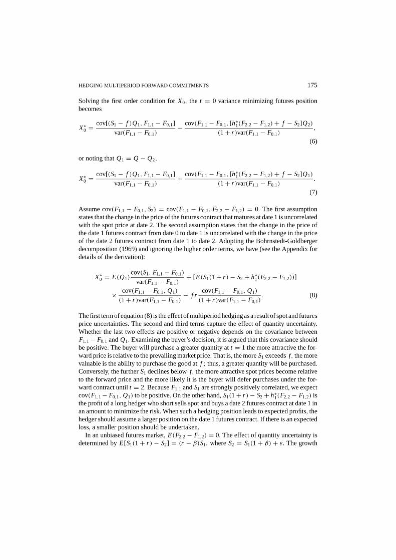
Solving the first order condition for X0, the t = 0 variance minimizing futures positionbecomes

X∗0 = cov[(S1 − f )Q1, F1,1 − F0,1]

var(F1,1 − F0,1)− cov(F1,1 − F0,1, [h∗

1(F2,2 − F1,2) + f − S2]Q2)

(1 + r)var(F1,1 − F0,1),

(6)

or noting that Q1 = Q − Q2,

X∗0 = cov[(S1 − f )Q1, F1,1 − F0,1]

var(F1,1 − F0,1)+ cov(F1,1 − F0,1, [h∗

1(F2,2 − F1,2) + f − S2]Q1)

(1 + r)var(F1,1 − F0,1).

(7)

Assume cov(F1,1 − F0,1, S2) = cov(F1,1 − F0,1, F2,2 − F1,2) = 0. The first assumptionstates that the change in the price of the futures contract that matures at date 1 is uncorrelatedwith the spot price at date 2. The second assumption states that the change in the price ofthe date 1 futures contract from date 0 to date 1 is uncorrelated with the change in the priceof the date 2 futures contract from date 1 to date 2. Adopting the Bohrnstedt-Goldbergerdecomposition (1969) and ignoring the higher order terms, we have (see the Appendix fordetails of the derivation):

X∗0 = E(Q1)

cov(S1, F1,1 − F0,1)

var(F1,1 − F0,1)+ [E(S1(1 + r) − S2 + h∗

1(F2,2 − F1,2))]

× cov(F1,1 − F0,1, Q1)

(1 + r)var(F1,1 − F0,1)− f r

cov(F1,1 − F0,1, Q1)

(1 + r)var(F1,1 − F0,1). (8)

The first term of equation (8) is the effect of multiperiod hedging as a result of spot and futuresprice uncertainties. The second and third terms capture the effect of quantity uncertainty.Whether the last two effects are positive or negative depends on the covariance betweenF1,1 − F0,1 and Q1. Examining the buyer’s decision, it is argued that this covariance shouldbe positive. The buyer will purchase a greater quantity at t = 1 the more attractive the for-ward price is relative to the prevailing market price. That is, the more S1 exceeds f, the morevaluable is the ability to purchase the good at f ; thus, a greater quantity will be purchased.Conversely, the further S1 declines below f, the more attractive spot prices become relativeto the forward price and the more likely it is the buyer will defer purchases under the for-ward contract until t = 2. Because F1,1 and S1 are strongly positively correlated, we expectcov(F1,1 − F0,1, Q1) to be positive. On the other hand, S1(1 + r) − S2 + h∗

1(F2,2 − F1,2) isthe profit of a long hedger who short sells spot and buys a date 2 futures contract at date 1 inan amount to minimize the risk. When such a hedging position leads to expected profits, thehedger should assume a larger position on the date 1 futures contract. If there is an expectedloss, a smaller position should be undertaken.

In an unbiased futures market, E(F2,2 − F1,2) = 0. The effect of quantity uncertainty isdetermined by E[S1(1 + r) − S2] = (r − β)S1, where S2 = S1(1 + β) + ε. The growth


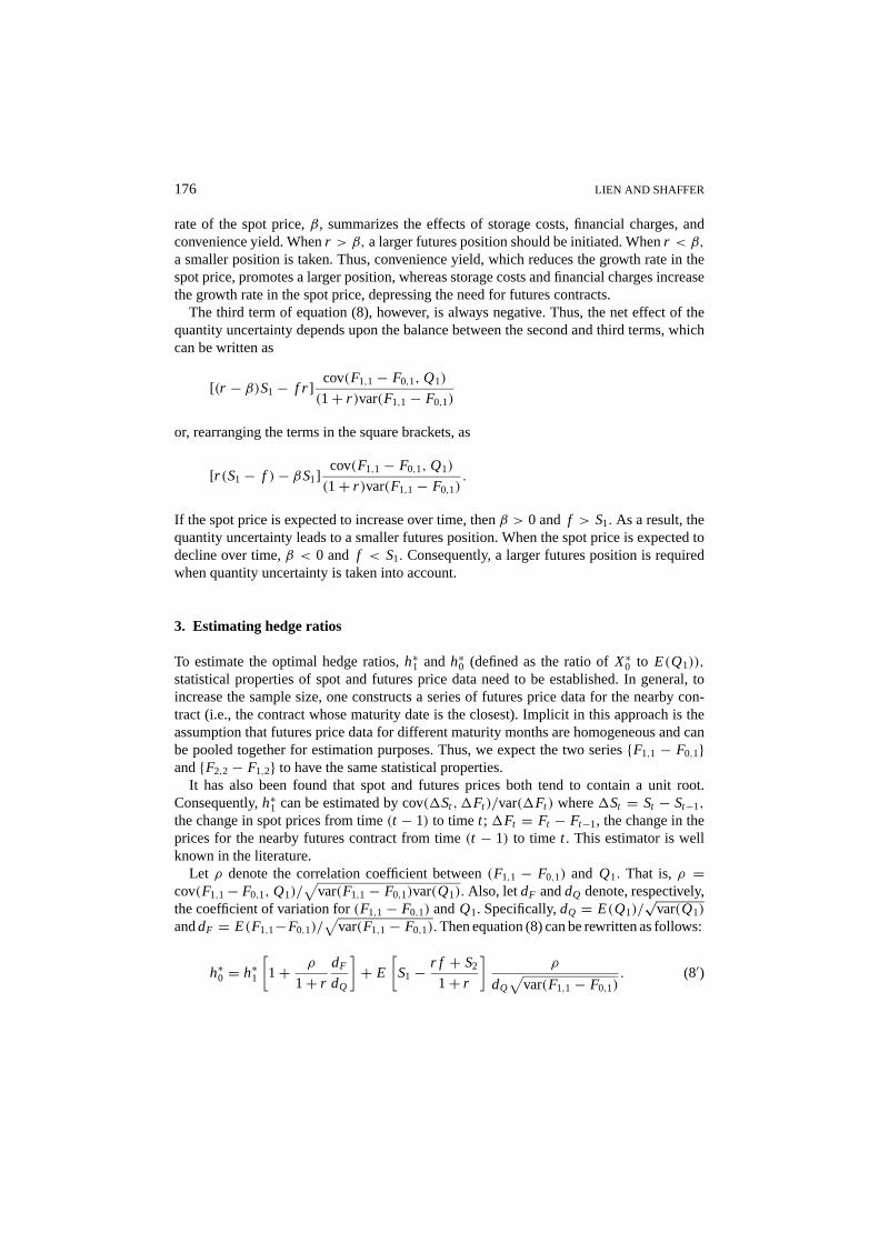
rate of the spot price, β, summarizes the effects of storage costs, financial charges, andconvenience yield. When r > β, a larger futures position should be initiated. When r < β,

a smaller position is taken. Thus, convenience yield, which reduces the growth rate in thespot price, promotes a larger position, whereas storage costs and financial charges increasethe growth rate in the spot price, depressing the need for futures contracts.

The third term of equation (8), however, is always negative. Thus, the net effect of thequantity uncertainty depends upon the balance between the second and third terms, whichcan be written as

[(r − β)S1 − f r ]cov(F1,1 − F0,1, Q1)

(1 + r)var(F1,1 − F0,1)

or, rearranging the terms in the square brackets, as

[r(S1 − f ) − βS1]cov(F1,1 − F0,1, Q1)

(1 + r)var(F1,1 − F0,1).

If the spot price is expected to increase over time, then β > 0 and f > S1. As a result, thequantity uncertainty leads to a smaller futures position. When the spot price is expected todecline over time, β < 0 and f < S1. Consequently, a larger futures position is requiredwhen quantity uncertainty is taken into account.

3. Estimating hedge ratios

To estimate the optimal hedge ratios, h∗1 and h∗

0 (defined as the ratio of X∗0 to E(Q1)),

statistical properties of spot and futures price data need to be established. In general, toincrease the sample size, one constructs a series of futures price data for the nearby con-tract (i.e., the contract whose maturity date is the closest). Implicit in this approach is theassumption that futures price data for different maturity months are homogeneous and canbe pooled together for estimation purposes. Thus, we expect the two series {F1,1 − F0,1}and {F2,2 − F1,2} to have the same statistical properties.

It has also been found that spot and futures prices both tend to contain a unit root.Consequently, h∗

1 can be estimated by cov(�St , �Ft )/var(�Ft ) where �St = St − St−1,

the change in spot prices from time (t − 1) to time t ; �Ft = Ft − Ft−1, the change in theprices for the nearby futures contract from time (t − 1) to time t . This estimator is wellknown in the literature.

Let ρ denote the correlation coefficient between (F1,1 − F0,1) and Q1. That is, ρ =cov(F1,1 − F0,1, Q1)/

√var(F1,1 − F0,1)var(Q1). Also, let dF and dQ denote, respectively,

the coefficient of variation for (F1,1 − F0,1) and Q1. Specifically, dQ = E(Q1)/√

var(Q1)

and dF = E(F1,1−F0,1)/√

var(F1,1 − F0,1). Then equation (8) can be rewritten as follows:

h∗0 = h∗

1

[1 + ρ

1 + r

dF

dQ

]+ E

[S1 − r f + S2

1 + r

]ρ

dQ

√var(F1,1 − F0,1)

. (8′)


Suppose that the spot price follows a martingale process. Then E(S2) = S1 and one alsoexpects f = S1. As a result, h∗

0 = h∗1[1 + (ρ/1 + r)(dF/dQ)]. While dF can be estimated

from the price data, ρ and dQ remain to be firm-specific. The difference between h∗0 and

h∗1 (i.e., the optimal hedge ratio in absence of quantity uncertainty) increases as ρ (or dF

increases) or dQ (or r ) decreases. In an unbiased future market, h∗0 = h∗

1 and quantityuncertainty has no effect on the optimal hedge ratio. Suppose that, instead, a backwarda-tion or a contango prevails in the futures market. Then the larger the quantity uncertainty,the bigger the difference between the two hedge ratios. On the other hand, the volatil-ity of the futures price depresses the impact of quantity uncertain on the optimal hedgeratio.

In the more general case, the last term in equation (8′) cannot be ignored. Herein we havethree firm-specific parameters, ρ, f, and dQ . The directions of the effect of each parameterdepend upon the sign of E[S1(1 + r) − S2 − r f ] . When this term is positive (or negative,respectively), the positive effects of quantity uncertainty and the correlation between thequantity and the futures price on hedge ratio are strengthened (or weakened, respectively).Similar conclusion applies to the negative effect of the futures price volatility.

4. The general case

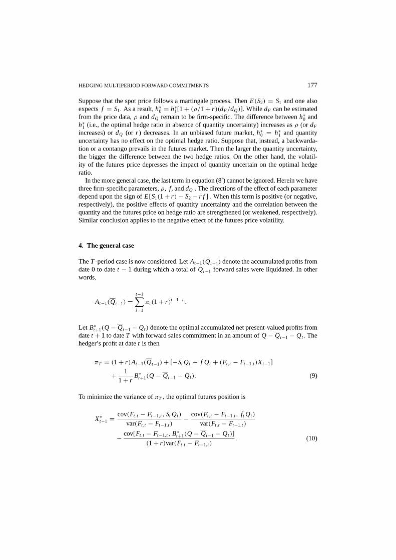
The T -period case is now considered. Let At−1(Qt−1) denote the accumulated profits fromdate 0 to date t − 1 during which a total of Qt−1 forward sales were liquidated. In otherwords,

At−1(Qt−1) =t−1∑i=1

πi (1 + r)t−1−i .

Let B∗t+1(Q − Qt−1 − Qt ) denote the optimal accumulated net present-valued profits from

date t + 1 to date T with forward sales commitment in an amount of Q − Qt−1 − Qt . Thehedger’s profit at date t is then

πT = (1 + r)At−1(Qt−1) + [−St Qt + f Qt + (Ft,t − Ft−1,t )Xt−1]

+ 1

1 + rB∗

t+1(Q − Qt−1 − Qt ). (9)

To minimize the variance of πT , the optimal futures position is

X∗t−1 = cov(Ft,t − Ft−1,t , St Qt )

var(Ft,t − Ft−1,t )− cov(Ft,t − Ft−1,t , ft Qt )

var(Ft,t − Ft−1,t )

− cov[Ft,t − Ft−1,t , B∗t+1(Q − Qt−1 − Qt )]

(1 + r)var(Ft,t − Ft−1,t ). (10)


Using Bohrnstedt and Goldberger (1969), we have

X∗t−1 = E(Qt )

cov(Ft,t − Ft−1,t , St )

var(Ft,t − Ft−1,t )+ [E(St ) − f ]

cov(Ft,t − Ft−1,t , Qt )

var(Ft,t − Ft−1,t )

− cov[Ft,t − Ft−1,t , B∗t+1(Q − Qt−1 − Qt )]

(1 + r)var(Ft,t − Ft−1,t ). (11)

The effect of quantity uncertainty is again summarized by the second and third terms.As before, cov(Ft,t − Ft−1,t , Qt ) is expected to be positive. Also, B∗

t+1(Q − Qt−1 − Qt )

is, in general, an increasing function of Q − Qt−1 − Qt , i.e., the more forward salesthat remain, the more profitable the future forward sales commitment is. Thus, cov[Ft,t −Ft−1,t , B∗

t+1(Q − Qt−1 − Qt )] is likely to be negative. When the spot price is expected todecline over time, E(St ) > f, both the second and third terms are positive. As a result,quantity uncertainty leads to a larger futures position. Also, if forward prices are unbiasedpredictors of expected future spot prices, i.e., E(St ) = f, then the second term is zeroand the last term is positive, leading to a larger futures position. Consequently, in the twocases above, the risk-minimizing futures position that considers both price and quantityuncertainties is greater than that which considers price uncertainty only. If the spot price isexpected to increase over time, E(St ) < f, the second term is negative whereas the thirdterm is positive. In this last case, the effect of quantity uncertainty is undetermined.

Note that, in deriving equation (11), we assume higher order terms in the Bohrnstedt-Goldberger decomposition are negligible. This approach is precise if all the underlyingvariables are jointly normally distributed or, more plausibly, when the correlation coeffi-cients between various prices are independent of the buyer’s quantity decisions (see theAppendix for mathematical details).

5. Implications

These results can be applied to the case of MGRM. Several authors have reported thatMGRM was substantially overhedged by employing a unit hedge ratio. Edwards and Canter(1995), for example, estimate that a hedge ratio on the order of 0.50 would have been morereasonable in terms of minimizing risk. Ignoring close-out options, Mello and Parsons(1995) suggest that an initial hedge ratio of 0.56 would have been more in line with theobjective of variance minimization for a ten-year forward supply program. Pirrong (1997)calculates a series of minimum variance hedge ratios and finds they are all substantially lessthan unity. However, the above results suggest that a traditional variance-minimizing hedgeratio would have been inappropriate since it ignores period-by-period quantity uncertainty.In all cases, T > 1, MGRM would have been underhedged with a price risk-minimizinghedge when the firm anticipated a decline in spot prices. In a two-period case, MGRMwould have been overhedged if spot prices were expected to increase. However, the effectof period-by-period quantity uncertainty would be ambiguous in the multiperiod case whereT > 2. While the optimal size of MGRM’s futures position is a matter of empirical analysis,


it appears unlikely the traditional variance-minimizing hedge ratio, which considers priceuncertainty only, would have been appropriate in all price environments faced by MGRM.

6. Conclusions

This paper considers the problem of a producer hedging a long-term forward commitmentto deliver a commodity at multiple points of time. A minimum variance multiperiod futuresposition is derived that considers both quantity and price uncertainties. It is shown that theindividual effects of quantity uncertainty and price uncertainty are separable. Moreover, inthe two-period case, if spot prices are expected to decrease over time, the risk-minimizinghedge considering both price and quantity uncertainties is greater than that which con-siders price uncertainty only. If spot prices are expected to increase over time, then therisk-minimizing futures position considering both price and quantity uncertainties will besmaller than that which considers price uncertainty only. A commodity’s convenience yieldencourages a larger risk-minimizing futures position, whereas storage costs and financialcosts diminish the size of the risk-minimizing futures position. In a multiperiod context,if forward prices are unbiased estimators of future spot prices, or if spot prices are ex-pected to decrease over time, then period-by-period quantity uncertainty increases the sizeof the risk-minimizing hedge. Last, if spot prices are expected to increase, then the effectof period-by-period quantity uncertainty is ambiguous

Appendix

To derive equation (8), note that by Bohrnstedt and Goldberger (1969) we have

cov((S1 − f )Q1, �F1) = E(S1 − f )cov(Q1, �F1) + E(Q1)cov(S1, �F1) + R,

where �F1 = F1,1 − F0,1 and R is a third order term:

R = E[(Q1 − E(Q1))(S1 − E(S1))(�F1 − E(�F1))].

When Q1, S1, and �F1 are jointly normally distributed, R = 0. On the other hand,

R = E{(Q1 − E(Q1))E[(S1 − E(S1))(�F1 − E(�F1)) | Q1]}= E{(Q1 − E(Q1))cov(S1, �F1 | Q1)}.

Therefore, R = 0 when the correlation between S1 and �F1 is independent of Q1. It seemsplausible that the correlation between spot and futures prices is independent of a buyer’squantity decision. In this paper, we assume that R is negligible.


The second term in equation (7) is the sum of h∗1 cov(�F1, Q1�F2) and cov(�F1,

( f − S2)Q1) where �F2 = F2,2 − F1,2. The latter term can be written as follows:

cov(( f − S2)Q1, �F1) = E( f − S2)cov(Q1, �F1) − E(Q1)cov(S2, �F1) + X,

where X = E[(Q1 − E(Q1))(S2 − E(S2))(�F1 − E(�F1))]. Again, X = 0 when Q1, S2,and �F1 are jointly normally distributed. Alternatively,

X = E{(Q1 − E(Q1))E[(S2 − E(S2))(�F1 − E(�F1)) | Q1]}= E{(Q1 − E(Q1))cov(S2, �F1 | Q1)}.

If the correlation between S2 and �F1 is independent of Q1, then X = 0. This seems aplausible assumption. Also, note that we assume cov(S2,�F1) = 0. As a consequence,

cov(( f − S2)Q1,�F1) = E( f − S2)cov(Q1, �F1).

Finally, cov(�F1, Q1�F2) can be written as:

cov(�F1, Q1�F2) = E(Q1)cov(�F1, �F2) + E(�F2)cov(�F1, Q1) + Y,

where Y = E[(Q1 − E(Q1))(�F1 − E(�F1))(�F2 − E(�F2))]. Thus Y = 0 whenQ1, �F2, and �F2 are jointly normally distributed. Alternatively, we have

Y = E{(Q1 − E(Q1))E[(�F1 − E(�F1))(�F2 − E(�F2)) | Q1]}= E{(Q1 − E(Q1))cov(�F1, �F2 | Q1)}.

When the correlation between �F1 and �F2 is independent of Q1, X = 0. The conditionseems reasonable. We also assume that cov(�F1, �F2) = 0. Consequently,

cov(�F1, Q1�F2) = E(�F2)cov(�F1, Q1).

Upon substituting the above results into equation (7), we derive equation (8).

Acknowledgments

The authors would like to thank Steve Black, the participants of the 1999 Midwest FinanceAssociation Meeting, Richard Torz, and the participants of the 2000 Eastern EconomicAssociation Meeting for their helpful comments and suggestions. Two anonymous refereesprovided helpful comments and suggestions.


Notes

1. MGRM also offered a third program, “guaranteed margin” contracts, to customers. These were short-termarrangements that gave customers a guaranteed profit margin on quantities they sold. However, since thesecontracts were short-term and renewable at MGRM’s discretion, they did not drive MGRM’s hedging activities.

2. Additionally, both the firm-fixed and firm-flexible contracts contained embedded “close-out” options givingcustomers the right to exercise, for cash, their forward contracts when they were in-the-money. These optionswere an additional source of quantity uncertainty for MGRM.

3. An alternative hedging objective is utility maximization. While variance-minimization is not, in general,equivalent to utility maximization, it is the most popular approach in the hedging literature.

4. The only source of quantity uncertainty considered in this model is that resulting from the customer’s optionto select the period-by-period quantity to be delivered. All other potential sources of quantity uncertainty, suchas counterparty default and “close-out” options, are ignored.

References

Anderson, R. W. and J. P. Danthine, “The Time Pattern of Hedging and the Volatility of Futures Prices.” Reviewof Economic Studies 50, 249–266, (1983).

Baesel, J. and D. Grant, “Optimal Sequential Futures Trading.” Journal of Financial and Quantitative Analysis17, 683–695, (1982).

Bohrnstedt, G. W. and A. S. Goldberger, “On the Exact Covariance of Products of Random Variables.” Journal ofthe American Statistical Association 64, 1439–1442, (1969).

Brennan, M. J. and N. I. Crew, “Hedging Long Maturity Commodity Commitments with Short-dated FuturesContracts.” in M. H. Michael Dempster, and Stanley R. Pliska (Eds), Mathematics of Derivative Securities,Cambridge University Press, 1997.

Culp, C. L. and M. H. Miller, “Hedging a Flow of Commodity Deliveries with Futures: Lessons from Metallge-sellschaft.” Derivatives Quarterly 1, 7–15, (1994).

Culp, C. L. and M. H. Miller, “Metallgesellschaft and the Economics of Synthetic Storage.” Journal of AppliedCorporate Finance 7, 62–76, (1995a).

Culp, C. L. and M. H. Miller, “Hedging and the Theory of Corporate Finance: A Reply to Our Critics.” Journalof Applied Corporate Finance 8, 121–127, (1995b).

Ederington, L. H., “The Hedging Performance of the New Futures Markets.” Journal of Finance 34, 157–170,(1979).

Edwards, F. R. and M. S. Canter, “The Collapse of Metallgesellschaft: Unhedgeable Risks, Poor Hedging Strategy,or Just Bad Luck?” Journal of Applied Corporate Finance 8, 86–105, (1995).

Hilliard, J. E., Analytics Underlying the Metallgesellschaft Hedge: Short Term Futures in a Multi-Period Environ-ment. Working Paper, University of Georgia, (1997).

Ho, T. S. Y., “Intertemporal Commodity Futures Hedging and the Production Decision.” Journal of Finance 39,351–376, (1984).

McKinnon, R. I., “Futures Markets, Buffer Stocks, and Income Stability for Primary Producers.” Journal ofPolitical Economy 75, 844–861, (1967).

Mello, A. S. and J. E. Parsons, “The Maturity Structure of a Hedge Matters: Lessons from the MetallgesellschaftDebacle.” Journal of Applied Corporate Finance 8, 106–120, (1995).

Neuberger, A., How Well Can You Hedge Long Term Exposures with Short Term Futures Contracts? IFA WorkingPaper 214-1996, London Business School, (1996).

Pirrong, S. C., “Metallgesellschaft: A Prudent Hedger Ruined, or a Wildcatter on NYMEX?” Journal of FuturesMarkets 17, 543–578, (1997).

Rolfo, J., “Optimal Hedging under Price and Quantity Uncertainty: The Case of a Cocoa Producer.” Journal ofPolitical Economy 88, 100–116, (1980).

Ross, S. A., Hedging long run commitments: Exercises in incomplete market pricing. Working Paper, Yale Schoolof Management, (1995).

Documents

Hedging Multiperiod Forward Commitments: The Case of Period-by-Period Quantity Uncertainty