Investments in hedge funds and other private investment funds involve a high degree of risk. You could lose all or a substantial amount of your investment. Check carefully the trading strategy that you are going to invest. Each fund is associated with different types of risks. When investing in a particular hedge fund, you should carefully read a fund’s offering materials and related information for specific risk and other important information regarding your investment. I have attached a monthly performance of a hedge fund and the related statistics.

Check the skill of the hedge fund manager or alpha defined as the intercept from the regression. Alpha, is used to measure the ability of managers to outperform the base index. A positive and statistically significant indicates a skilled fund manager whose decisions add value to the fund. Rhodes (2000) argued, that “persistent performance shows that some fund managers are able to outperform their peers. This implies that the fund managers must either have access to information that is insider or not widespread or make use of information in a speedier way than other managers. As markets become more efficient it will be more difficult for any fund manager to outperform the market continuously”(Rhodes,2000,p.7). On the other hand, negative values or statistically insignificant values represent inferior or neutral performance of the manager. In other words, a negative indicates a poorly performing manager whose decisions affect negatively the value of the fund. Check the risk premium which equal to the slope of the security market line. It is the difference between the expected return of the portfolio and the risk – free rate. Calculate monthly mean returns and standard deviations of different hedge funds categories and check the volatility of returns. The best fund is the one with high mean return and low standard deviation. Seventy percent of alphas come from the dynamic rebalancing of strategies. The other 30% comes from superior manager selection. The average manager that is employed in the fund has about $1 billion in assets under management. He/she has been in business five to seven years and has a five to seven year track record that has outperformed its own benchmark. In other words, if it were a distressed debt manager, it would be someone who would have outperformed the distressed debt sub-index of the Tremont index when the trading strategy is distressed securities. Usually, when balance sheets were stressed, we have an economic recovery which is forcing yield spreads to compress. Please analyze economic cycles along two dimensions, growth and interest rates, and break it into quadrants. All economic cycles begin with a low growth, low interest rate environment. Then proceed clockwise through a quadrant scenario, where we are moving to a higher growth, low interest rate area where the Fed is being supportive of growing the economy. Then we move into a high growth, high interest rate quadrant, and that is typically where the Fed is now beginning to be concerned or the central banks become concerned about inflation and overheating the economy. That forces the economy into the final stage, which is high interest rate and low growth type of environment where you have an inverted yield curve. Check the meaning of the invested yield curve in the fixed – income investments document.

1

Check the relationship between incentive and management fees. Select the fund with the lowest fees.

I have attached a table with a sample of hedge funds to show the structure and their performance in terms of trading strategy, assets under management, management fees, incentive, fees, high – water mark, hurdle rate, and lock-up period.

Please check the different ratios that are used in the hedge fund industry. I have added a sample of the funds that constitute each investment strategy and index.

Due to confidentiality reasons, I will not be able to disclose information and data related to the funds that constitute the various trading strategies. For example, I cannot disclose from the Credit Suisse site information related to the performance of the different indices. Please refer to the web site of Credit Suisse. www.hedgeindex.com

You will find information concerning monthly performance, indices and sub categories of the various trading strategies. In addition, it is listed the monthly standard deviation annualized and Sharpe ratio data. The Sharpe ratio is calculated through the use of the 90 day Treasury bill rate that represents the risk – free rate. You will also find Dow Jones indices and other information such as alternative beta indexes. After taking into consideration copyright agreement, you can e-mail them for a login account to download cumulative statistics, NAV prices in different currencies and for different indexes such as the Credit Suisse broad hedge fund index, the credit Suisse all hedge index, and the Credit Suisse blue chip hedge fund index. Finally, you will find information concerning the correlations matrix between an investment strategy and the relevant index, quarterly and monthly performance data. Good luck!

To solve my problem, I am going to use a past database that includes information concerning the individual funds that constitute the strategy, the lockup period, the hurdle rate, incentive and management fees and watermark provision. I would like to thanks Karen Henseleit sales manager for passing to me the data from Datafeeder. The Alternative Asset Center (AAC), the Fund of Hedge Funds Specialist and the Hedge Funds DataFeeder. I am trying to facilitate you to understand how the hedge funds industry is working. Thanks for the participation. The old database provide information concerning the fund name under different strategies, the management fees, the incentive fees, the high water mark provision, the hurdle rate, the lock-up period, the fund assets, monthly returns and monthly standard deviations.

I have added the introduction, a detailed section of the trading strategies, Excel and the computer programming in terms of C++, Java, VBA, Python, etc…

The book is under construction and it is lacking many sections. Hedge funds are very important in the investment industry. They are used to hedge different types of risk by using derivatives products. Hedge fund managers use call and put options, commodity futures, forward contracts, index, currency and fixed

2

income options and futures to hedge credit risk, market risk, country risk, sector risk, company risk, interest rate risk and currency risk. Thus, in addition to stocks and bonds they use their derivatives product to hedge or speculate according to the investment strategy, the market and political trend. They are used from wealthy investors that have a capital higher than 250,000 USD. In some cases the invested capital could be 1,000,000 USD or more than 10,000,000 USD.

Step – by - step introduction to Hedge funds. A practical guide for postgraduate, research students and investors.

Dr Michel Zaki Guirguis 19/01/2017

Bournemouth UniversityInstitute of Business and LawFern BarrowPoole, BH12 5BB, UKTel:0030-210-9841550Mobile:0030-6982044429Email: guirguismichel@gmail.com1

1 Τhe permanent address of the author’s is 94, Terpsichoris road, Palaio-Faliro, Post Code:17562, Athens, Greece.

3

Table of Contents

Preface

Acknowledgments

Chapter 1

Hedge funds categories and strategies

Introduction

Definition and purpose of the hedge funds industry Convertible arbitrage Emerging markets Equity market neutral Event driven Distressed securities Fixed income arbitrage Global macro Long/short equity Options Fund of funds Managed futures / CTAs Multi - strategy

Chapter 2

Hedge funds indices

Credit Suisse convertible arbitrage index Dow Jones world emerging markets index Equity market neutral S&P 500 index Credit Suisse event driven index Suisse high yield II and credit index distressed securities Citigroup world government bond index,WGBI, for fixed income arbitrage Credit Suisse global macro index Credit Suisse long/short equity index S&P Goldman Sachs commodities index options Credit Suisse all hedge fund index fund of funds Credit Suisse managed futures/CTAs index Dow Jones world index multi - strategy

4

Chapter 3

Performance measurement and attribution of hedge funds

Introduction to style analysis Rolling methodology of performance measurement Introduction to different types of ratios Passive management, tracking error, and the information ratio

Chapter 4

Fees structure interrelation to hedge funds

Management fees Incentive fees Water marks Hurdle rate Lock –up period

Chapter 5

Related articles of hedge funds. Application with industrial examples. An empirical analysis of the performance of Hedge Funds over the period

1998 to 2003 in terms of incentive fees, management fees, size, age, hurdle rate, high watermark provision and lockup period.

Application of a GARCH, TGARCH and EGARCH models to test the volatility of monthly returns of Credit Suisse All Hedge Market Neutral Funds.

Application of a linear Gaussian space model and the Kalman filter in estimating expectations of the natural logarithmic monthly returns of offshore strategic hedge funds.

Comparison of the census X12 and Tramo / Seats additive ARIMA (p,d,q) seasonal adjustment models applied to diversification of long/short equity hedge funds categories.

Measuring technical, allocative and overall cost efficiency of commodity hedge funds futures contracts by applying data envelopment analysis, (DEA).

Applying and comparing Sharpe style analysis versus a rolling methodology of loagarithmic monthly returns of long/short funds, market – neutral funds, global macro funds, event – driven funds and their related indices.

Chapter 6

5

Workshops of hedge funds in terms of Excel and other computer language programming

Workshop of functions application in Excel Workshop of functions application in Excel in terms of the

Decision tools and Stat tools Suite from Palisade organisation. http://www.palisade.com Workshop of language programming in terms of VBA in Excel Workshop of language programming in terms of C++ Workshop of language programming in terms of SQL Workshop of language programming in terms of Oracle Workshop of language programming in terms of Python Workshop of detailed explanation of Matlab Workshop of analysis of financial data, scientific programming

and simulation using R language programming Workshop of statistical analysis and applications by using Java

statistical program

References & Bibliography

Preface

6

This book is designed to provide an overview and introduction to the hedge funds industry. Hedge funds are not a complicated subject. To better understand them, please refer to my previous book introduction to financial derivatives. The reason is that hedge funds strategies are based on leveraged, long and short positions of derivatives products.

A lot of students and especially the one that do not have strong quantitative skills will feel vulnerable when taking this subject. If the level of mathematical sophistication is too high, the material is likely to be inaccessible to many students. If it is too low, some important issues will inevitable be treated in a rather superficial way. The book covers BA and BS, MA and MS in Risk Management, Business Administration, Financial Services, Computational Finance and International Business and Financial Derivatives.

Specifically, the book will have a lot of features that will distinguish it from the already published books. It provides a new approach of gaining some basic familiarity with the essential concepts of the hedge funds industry and the Orthodox Christianity. The aim of trading is to help the poors and the beggars. In addition, it is written in a very accessible style that will not frighten the students.

Most importantly, the book includes a range of materials to help the student, the practitioners and the investors to reinforce their learning skills. Each section offers a solid explanation of basic concepts, followed by examples for the reader to work through. Moreover, each chapter will include practical examples from Financial Times and visual representation of graphs in order to help the reader to combine the basic theoretical concepts with real situations examples from various companies. This book is aimed to cover the learning needs of a variety of readers. The basic needs of the above mentioned target group are similar in terms that both lack confidence about their numerical skills and both are motivated to learn basic knowledge. The average investor wants to learn how these products work but he/she cannot understand very easily the academic terminology. On the other hand, postgraduate students need to learn quickly the basic concepts in order to proceed to more advanced textbooks that deals with advanced stochastic calculus.

The market will be very responsive for our book especially that a lot of international students experience problem with their English and their numerical skills. It will cover the basic needs of postgraduate students and those who are interesting in alternative investments. The market in the next five years will become very complicated and would require the use of sophisticated risk management techniques in order to hedge market, operational, and credit risk. The use of derivatives and Hedge funds will be essential even for the average investor in terms of profit and protection from the highly competitive and hostile environment. This book will have a broader international appeal as it covers the UK, the European, and the US market.

In addition, we will include a variety of workshops related to language programming in terms of VBA for Excel, C++, SQL, Oracle, Python, R language programming, and Java. I will also include a mathematical and statistical software such as Matlab and the decision tools and stat tools suite from Palisade organisation. The aim is to facilitate the undergraduate, postgraduate and research students to proceed smoothly in their career in the investment banks without stress and confusion.

7

The investment industry will hire persons that possess practical expertise that sustain quality, spiritual integrity and efficiency in the financial market. Investment banks will hire applicants that are able to hedge different types of risk and achieve successful spiritual and therefore investment decisions. After reading this book, students of Bournemouth University could easily and in a relaxed way join the back and front office of alternative investments department of JP Morgan Chase or other investment bank.

Acknowledgments

First of all, I would like to thank my parents and especially my mother and father for giving me the opportunity to write this book and for their continued support, encouragement, and sacrifices during this period. I would also like to thank my supervisors Professor Philip Hardwick and Dr Geoff Willcocks for their continued

8

support and help. I would like to thank the Schweser Kaplan organisation for the professional education that covers the syllabus of the Chartered Financial Institute, (CFA). I would like to thank Mr Chandan Sengupta for helping me through his book to understand in detail how to apply financial analysis and modelling using Excel and VBA. I would like to thank Palisade organisation for issuing me demo academic software that shows the application of the decision tools and Stat tools Suite in Excel. I strongly recommend that you buy this software. Their website is http://www.palisade.com . I would like to thank Bloomberg Financial data and analysis. Their website is http://www.bloomberg.com

I would like to thank Matlab organization from providing free trial software in the past. I strongly recommend that you also subscribe to Matlab. Their website is http://www.mathworks.com.

Chapter 1

Definition and purpose of the hedge funds industry

9

Hedge funds are also known as alternative investments that are suited to institutional investors or wealthy investors with significant experience and knowledge in investment. They are used to hedge different types of risk by using derivatives products. Hedge fund managers use call and put options, commodity futures, forward contracts, index, currency and fixed income options and futures to hedge credit risk, market risk, country risk, sector risk, company risk, interest rate risk and currency risk. Thus, in addition to stocks and bonds they use their derivatives product to hedge or speculate according to the investment strategy, the market and political trend. Hedge funds are divided in several categories according to the investment strategy that is adopted by the fund manager. They use leverage through derivatives products, long and short position on securities, currencies, bonds and other investment products. They try to reduce risk, offset loses and positively increase the performance of the fund. They are not liquid as they use a lockup period for a certain period of time. They are used from wealthy investors that have a capital higher than 250,000 USD. In some cases the invested capital could be 1,000,000 USD or more than 10,000,000 USD.

The most interesting feature of hedge funds is the interrelation of their structure and their performance. As a result, the payroll structure which is based on three components namely performance fees, incentive fees and management fees are closely related to performance. Payroll structure is based on a minimum investment of $250.000, an annual fee of 1% - 2%, and an incentive fee of 5% to 25% of annual profits. This payroll structure usually includes another component known as high water mark that adds past performance to current ones. On the other hand, investors in hedge funds are often restricted with lockup periods which are the time period that initial investment cannot be redeemed from the fund. Limitations on cash withdrawals are a result of cash fluctuations and give fund managers more freedom in setting up long-term positions. This lockup period could have an adverse effect for active investors’.

Another factor that affects directly the performance of the fund is manager incentive fees which are related to the hurdle rate. The former are additional fees based on new profits from the funds according to the performance. The manager is rewarded only when the fund does well. The later is the return above which the manager begins to take incentive fees. For example, if the fund has a hurdle rate of 10% and the fund returns 25% for the year, the fund will take incentive fees on the 15% return above the hurdle rate. Thus, if the fund performance is below the high water mark limit, then the manager will be restricted to charge incentive fees which could lead to a consequent bad performance of the fund and finally liquidation of the fund. This incentive fee is generally subject to a high water mark provision. It is a benchmark used by funds to take fees only when profits are recorded from the positive performance of the fund. For example a $1 million investment is made in year 1 and the fund declines by 50%, leaving $500 thousand. In year 2, the fund returns 100% which equal to the initial investment. It will not take incentive fees on the return in year 2 as the initial investment was not increased. If the fund shows a negative performance, then the manager must cover the loss in the next year before the incentive fee becomes applicable. We relax the assumptions that if new investors have different high-water marks, then returns are not the same for all investors in the fund. Usually, databases report the returns for the initial or the average investor. Finally, management fees are taken by the manager on the entire asset level of the investment.

10

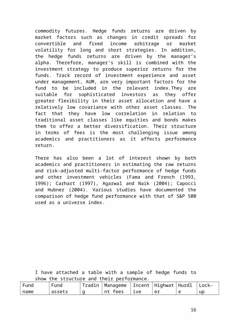
Hedge funds have been first created by Alfred Winslow Jones in (1949). It was a market neutral fund. Winslow strategy was to buy securities that were undervalued and to sell overvalued securities. The securities sold short provided a natural hedge against market risk and provided with positive return for his portfolio. As a matter of fact, there is no universally accepted definition of hedge funds. They are owned by private managers and wealthy individuals. Since the early 1990s, there has been a growing interest in the use of hedge funds. They are a growing business with more than $200 billion. The Assets under management in the hedge fund industry have grown from $25 billion in 1990 to more than $20 trillion in 2016. This growth has been due to new financial products as well as changes in technology that permit sophisticated investment strategies to be designed, implemented and offered to investors. Hedge funds offer a lot of advantages such as reduction of stock and bond portfolio volatility risk. They enhance portfolio returns in economic environments in which traditional stock and bond investments offer limited opportunities. They use a variety of long, short, spread, straddle options and commodity futures. Hedge funds returns are driven by market factors such as changes in credit spreads for convertible and fixed income arbitrage or market volatility for long and short strategies. In addition, the hedge funds returns are driven by the manager’s alpha. Therefore, manager’s skill is combined with the investment strategy to produce superior returns for the funds. Track record of investment experience and asset under management, AUM, are very important factors for the fund to be included in the relevant index.They are suitable for sophisticated investors as they offer greater flexibility in their asset allocation and have a relatively low covariance with other asset classes. The fact that they have low correlation in relation to traditional asset classes like equities and bonds makes them to offer a better diversification. Their structure in terms of fees is the most challenging issue among academics and practitioners as it affects performance return.

There has also been a lot of interest shown by both academics and practitioners in estimating the raw returns and risk-adjusted multi-factor performance of hedge funds and other investment vehicles (Fama and French (1993, 1996); Carhart (1997), Agarwal and Naik (2004); Capocci and Hubner (2004). Various studies have documented the comparison of hedge fund performance with that of S&P 500 used as a universe index.

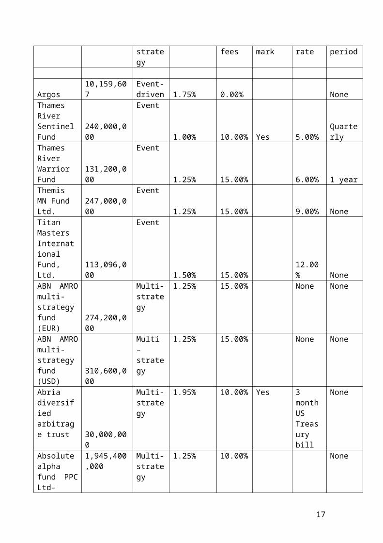
I have attached a table with a sample of hedge funds to show the structure and their performance.

Fund name Fund assets Trading strategy

Management fees

Incentive fees

Highwatermark

Hurdle rate

Lock-upperiod

Argos 10,159,607 Event- 1.75% 0.00% None

11

drivenThames River Sentinel Fund 240,000,000

Event

1.00% 10.00% Yes 5.00% QuarterlyThames River Warrior Fund 131,200,000

Event

1.25% 15.00% 6.00% 1 yearThemis MN Fund Ltd. 247,000,000

Event1.25% 15.00% 9.00% None

Titan Masters International Fund, Ltd. 113,096,000

Event

1.50% 15.00% 12.00% NoneABN AMRO multi-strategy fund (EUR) 274,200,000

Multi-strategy

1.25% 15.00% None None

ABN AMRO multi-strategy fund (USD) 310,600,000

Multi – strategy

1.25% 15.00% None None

Abria diversified arbitrage trust 30,000,000

Multi- strategy

1.95% 10.00% Yes 3 month US Treasury bill

None

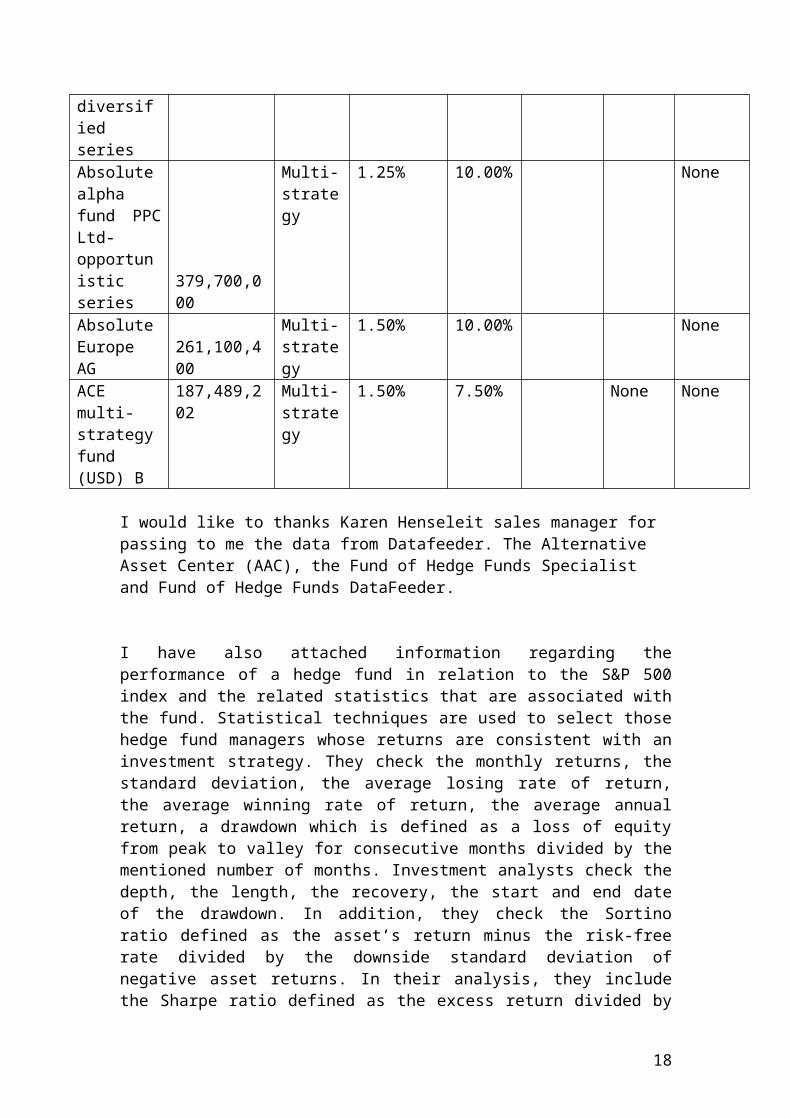
Absolute alpha fund PPC Ltd- diversified series 1,945,400,000

Multi- strategy

1.25% 10.00% None

Absolute alpha fund PPC Ltd- opportunistic series 379,700,000

Multi-strategy

1.25% 10.00% None

Absolute Europe AG 261,100,400

Multi-strategy

1.50% 10.00% None

ACE multi-strategy fund (USD) B

187,489,202 Multi-strategy

1.50% 7.50% None None

I would like to thanks Karen Henseleit sales manager for passing to me the data from Datafeeder. The Alternative Asset Center (AAC), the Fund of Hedge Funds Specialist and Fund of Hedge Funds DataFeeder.

12

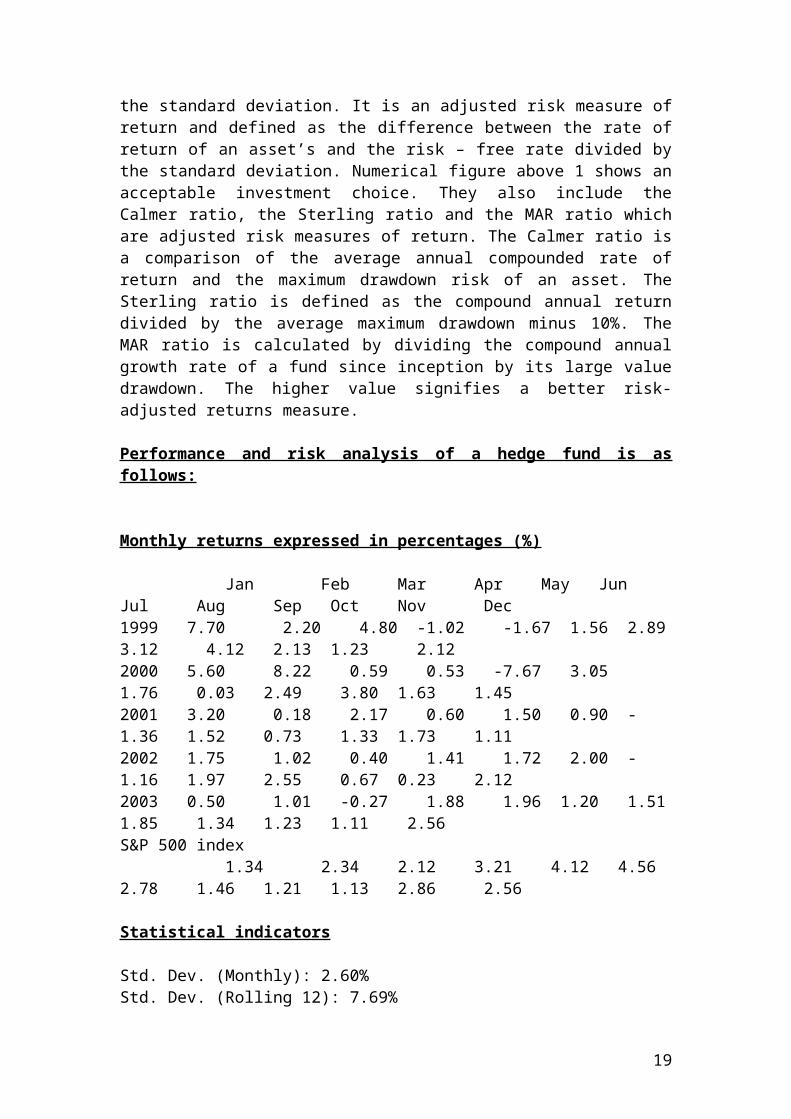
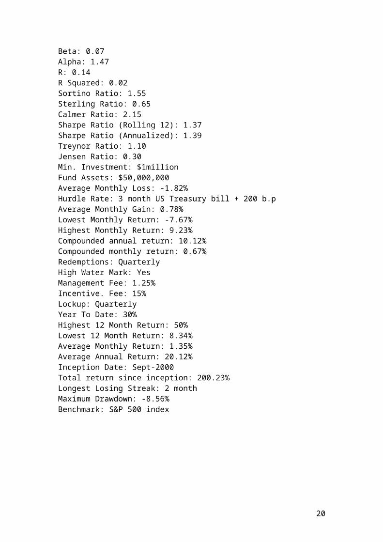
I have also attached information regarding the performance of a hedge fund in relation to the S&P 500 index and the related statistics that are associated with the fund. Statistical techniques are used to select those hedge fund managers whose returns are consistent with an investment strategy. They check the monthly returns, the standard deviation, the average losing rate of return, the average winning rate of return, the average annual return, a drawdown which is defined as a loss of equity from peak to valley for consecutive months divided by the mentioned number of months. Investment analysts check the depth, the length, the recovery, the start and end date of the drawdown. In addition, they check the Sortino ratio defined as the asset’s return minus the risk-free rate divided by the downside standard deviation of negative asset returns. In their analysis, they include the Sharpe ratio defined as the excess return divided by the standard deviation. It is an adjusted risk measure of return and defined as the difference between the rate of return of an asset’s and the risk – free rate divided by the standard deviation. Numerical figure above 1 shows an acceptable investment choice. They also include the Calmer ratio, the Sterling ratio and the MAR ratio which are adjusted risk measures of return. The Calmer ratio is a comparison of the average annual compounded rate of return and the maximum drawdown risk of an asset. The Sterling ratio is defined as the compound annual return divided by the average maximum drawdown minus 10%. The MAR ratio is calculated by dividing the compound annual growth rate of a fund since inception by its large value drawdown. The higher value signifies a better risk-adjusted returns measure.

Performance and risk analysis of a hedge fund is as follows:

Monthly returns expressed in percentages (%)

Jan Feb Mar Apr May Jun Jul Aug Sep Oct Nov Dec1999 7.70 2.20 4.80 -1.02 -1.67 1.56 2.89 3.12 4.12 2.13 1.23 2.12 2000 5.60 8.22 0.59 0.53 -7.67 3.05 1.76 0.03 2.49 3.80 1.63 1.452001 3.20 0.18 2.17 0.60 1.50 0.90 -1.36 1.52 0.73 1.33 1.73 1.11 2002 1.75 1.02 0.40 1.41 1.72 2.00 -1.16 1.97 2.55 0.67 0.23 2.122003 0.50 1.01 -0.27 1.88 1.96 1.20 1.51 1.85 1.34 1.23 1.11 2.56S&P 500 index 1.34 2.34 2.12 3.21 4.12 4.56 2.78 1.46 1.21 1.13 2.86 2.56

Statistical indicators

Std. Dev. (Monthly): 2.60%Std. Dev. (Rolling 12): 7.69%Beta: 0.07Alpha: 1.47R: 0.14R Squared: 0.02Sortino Ratio: 1.55Sterling Ratio: 0.65Calmer Ratio: 2.15Sharpe Ratio (Rolling 12): 1.37Sharpe Ratio (Annualized): 1.39Treynor Ratio: 1.10

13

Jensen Ratio: 0.30Min. Investment: $1millionFund Assets: $50,000,000 Average Monthly Loss: -1.82%Hurdle Rate: 3 month US Treasury bill + 200 b.pAverage Monthly Gain: 0.78%Lowest Monthly Return: -7.67%Highest Monthly Return: 9.23%Compounded annual return: 10.12%Compounded monthly return: 0.67%Redemptions: QuarterlyHigh Water Mark: YesManagement Fee: 1.25%Incentive. Fee: 15%Lockup: QuarterlyYear To Date: 30%Highest 12 Month Return: 50%Lowest 12 Month Return: 8.34%Average Monthly Return: 1.35%Average Annual Return: 20.12%Inception Date: Sept-2000Total return since inception: 200.23%Longest Losing Streak: 2 monthMaximum Drawdown: -8.56%Benchmark: S&P 500 index

14

Hedge funds categories and trading strategies

1. Convertible Arbitrage

The overall objective and aim of this category is the use of convertible securities. It is expected that the performance of the fund will be greater than the benchmark by using a long /short position than a traditional long only position. The hedge fund manager invests in convertible bonds, warrants and convertible preferred stock that could be exchanged by buying a stock. It is converted in a particular amount of shares to take advantage about stock price rises.

Usually, we purchase the bond and we sell the stock to anticipate market movements in terms of increase of the bond price or further decrease of the stock. The delta of a long position in the convertible security is typically hedged by selling the stock short. Ideally, the trader wants a delta neutral position. The risks that the trader tries to hedge are changes in the price of the stock, changes in expected volatility of the stock, and changes in the level of interest rates. The basic idea is to gain from pricing differences between the bond and the stock. This strategy is based on anticipating the changes of short – term interest rates. The trader will achieve positive returns if expected volatility rises, if stock prices increases and if the credit issuer rating is improved.Thus, when interest rates rise, the bond prices will fall and the stock prices increase. Specifically, the fund manager takes a long position in the stock that is expected to rise and a short position in the stock or option that is going to decrease in value by shortens his position in the bond. The fund targets overvalued or undervalued securities. In other words, he/she buys and sells securities according to their CAPM security market line. He/she could also use a strategy of buying and selling shares of companies in different markets that are going to acquire each other. The purpose of arbitrage is to profit from price discrepancy in two different markets.

2. Emerging markets

Emerging markets hedge funds invests primarily in countries that have a closed market economy and are in the process of developing and expanding its infrastructure such as Brazil, India, Latin America, Africa, Eastern Europe, Korea and China. Hedge funds use in addition to stocks and bond a mixture of derivatives products such as commodity futures, forward contracts, fixed-income instruments, currency and index options to take advantage from the leverage effect due to substantial increase or decrease of prices. Therefore, the risk in emerging economies is higher for potential losses and gains. Another difficulty that hedge funds face in emerging economies is transparency and lack of liquidity which increase the volatility of the prices. Therefore, the risk and return are significant high and requires significant capital and investment knowledge to trade in such markets.

3. Equity market neutral

A market neutral strategy combines both long and short positions. The net exposure is equal to zero. The purpose of using such strategy is to eliminate the market risk. The

15

hedge fund manager is trying to increase the positive return by opening a long position in a bull market and short positions in a bear market. The purpose is to hedge and decrease market volatility. The hedge fund manager is checking the correlation structure of different segment or industries and accordingly aligns his/her investment strategy to buy or sell the different shares according to the sector, industry and market capitalization. It aims to provide a stable and consistent return profile that has no correlation to either equity or bond market movements, and to produce a consistent return. The fund manager has equally the same long and short positions, so the net exposure is zero.

4. Event Driven

The fund manager primarily is targeting financial, micro and macro economic or political events that will affect positively the net asset value, NAV, performance of the fund. The portfolio is exposed in long and short positions in bonds and shares according to business events, merger, acquisition, restructuring, legislative changes, and political turmoil. He /she is trying to increase the value of the portfolio by taking into consideration event driven scenario. This strategy is based in public information of forthcoming events that will affect positively or negatively the performance of the hedge fund. The fund manager seeks to take advantage of the price spread between current market prices of corporate securities and their value when the takeover is completed. Merger arbitrage involves buying the stock of the target companies after a merger announcement and shorting the acquiring company’s stock. Hedge funds hedge this risk by holding a large portfolio of different probabilistic scenarios of merger prices to eliminate the discrepancy between the present value of the merger offer and the current stock price. The present value valuation model takes into consideration the possibility that the merger will fail. Hedge funds perform better when the economy is booming and there are positive news regarding the corporate business plan of the different companies. They could also take advantage of the political turmoil and instability and sell stocks or bonds by opening short positions. The investment vehicles that they use are equities, debt securities, options, futures and convertible bonds.

5. Distressed securities

Distressed securities are related to the corporate bonds of bankrupted companies that start to get out from the crisis and are trying to reduce their loan exposures in the market. It could be also trading in distressed companies that are going to bankrupt and their debt value are reduced. The corporate bonds and shares are traded in discounted values. Their price is low and the investors’ anticipate a change in the management in terms of paying the debtors obligations. The risk that the hedge manager is exposed is that the company could increase its liabilities instead its assets and finally bankrupt. The stocks and bonds have no monetary value and the fund will display a negative NAV return. Therefore, the investors will face losses. Hedge funds or institutional investors buy distressed securities to better access the liquidity and the effort of the companies trying to get out from bankruptcy. Hedge funds perform better when the economy is in recession and the companies are distressed. They examine the equity to debt ratio and accordingly they decide whether it is favourable to buy them at a discounted debt value and sell them at a higher price.

16

6. Multi-strategy

The objective of the multi-strategy fund is to achieve positive NAV return by investing in diversified and professionally managed investment funds of equities and bonds. He/she is trying to monitor and hedge market and credit risk. The hedge funds invests in alternative investment strategies such as merger arbitrage, equity short bias, mortgage arbitrage, statistical arbitrage, structural arbitrage, market neutral strategies, convertible arbitrage, global macro, and CTA Managers.

7. Fixed income arbitrage

These funds engage principally in arbitrage strategies in the global corporate debt securities markets taking advantage of mispricings. Fixed income arbitrage funds take advantage of mispricing between fixed – income securities. Hedge fund managers open two positions at the same time to eliminate losses. A short and a long position aim to take advantage for price differences in the traded fixed – income securities. Government or municipal, corporate bonds and credit default swap are used to leverage the fund’s return. They use derivatives product to hedge against credit risk. Another strategy is yield curve arbitrage and credit yield curve. The profit or loss is resulted from studying the difference between a short 3 month US bond and long term 10 year US bond yield curve. Sometimes, they use mortgage backed securities arbitrage.

8. Global m acro

Investment risks are spread over different asset classes and investment strategies. Global macro hedge fund managers’ focus to generate positive returns based on currency futures and options, fixed – income securities derivatives products or stock indices futures and options. They are trying to eliminate the market risk by examining carefully the macroeconomic indicators and the political trends. They are checking the appreciation or depreciation of currencies by using options and futures. They use spot and forward rates futures and options by checking the interest rates. They check the monetary policy of each country in relation to the macroeconomic indicators, related to employment, gross domestic product, inflation and production. In addition, they check changes in interest rates resulted from short and long – term US treasury fixed income products. Please check the document financial derivatives for more information related to currency and Eurodollar futures. Another strategy is to use index option and futures or commodity futures such as gold, silver, sugar, cocoa, oil to take advantage of inflation or deflation. For example, in an inflationary environment, commodity prices will rise and a long strategy will be profitable. In contrast, in a deflationary environment commodity prices will fall and therefore a short strategy will be profitable. The hedge fund portfolio is leveraged and the degree of risk is very high.

17

9. Long/Short Equity

The hedge fund primarily goal is to invest in long and short position of the security to take advantage from increase or decrease of the prices. Thus, he/she buys a security that is expected to rise and sell a security that is expected to fall. In other words, the hedge fund manager buys an undervalued share and sells an overvalued share. The main purpose is to minimize the market exposure and profit from the spread of a long/ short strategy between the shares. The net exposure should outweigh the long versus the short position or vice versa. The risk is still high because the market could move sharply in one direction and affect negatively the investment in the opposite direction. For example, if you invest 250,000 USD in a long position and 500,000 USD in a short position, the difference due to beta of the market direction could affect positively or negatively the entire investment. The fund manager could also use equity futures and options for small and large capitalization companies or blue chips companies.

10.Option strategies

Hedge funds are using different option strategies to hedge their portfolio from market risk. Options are a special type of financial asset that gives the holder the right but not the obligation to buy or sell an underlying security at a predetermined price. Options are of two types: put options and call options. A call option gives the right but not the obligation to buy, and a put option the right to sell at a specific price within a certain time period. American options give the right to the investors to exercise it before as well as on the expiry date. In contrast, European options give the right to exercise it only on the expiry date. The advantage of buying an option is that the initial outlay is smaller in comparison with buying a large number of shares. Furthermore, the downside risk is limited to a certain amount. In contrast, if the share price falls by a significant amount, then the investor’s could loose a large amount of his/her capital. Finally, the percentage positive return is greater due to the leverage effect. The investor can also take the position to as referred long or short straddle. Let’s take as an example the first case of buying a straddle. It involves taking a long position in a call and a long position in a put with the same strike, share price and expiration date. This strategy is appropriate when an investor is expecting a large move in a price on an underlying share, but does not know in which direction the move will be in the index (Traded options, investor chronicle, 1997, p.38). Selling straddle or taking a short position involves more risk for limited reward. To reduce the risk of large losses, a straddle seller may buy a put with a lower strike and a call with a higher strike. The resulting position looks similar to a butterfly spread (Ritchken, 1987,p.54)It involves taking a short position in a call and a short position in a put with the same strike price, share price and expiration or maturity date. This strategy is appropriate when an investor is expecting a minor move in a price on an underlying share, but does not know in which direction the move will be in the index. Another type of strategy which involves a combination in both call and puts is referred to as a strangle. There are two strategies which are buying and selling a strangle. The first strategy consists of a long position in a call and a put with different strike prices, the same maturity or expiration date and the same underlying share. The second strategy consists of a short position in a call and a put with different strike prices the same

18

maturity or expiration date and the same underlying share. Implied volatility is estimated when the current market price of the option is different from the theoretical pricing price that is calculated from the Black - Scholes formula. The deviation or difference in price is related to the volatility that is incorporated in the option pricing formula. The implied volatility is calculated in Excel by using the functions of Goal Seek. It applies trial and error test to find the accurate value of the volatility implied.

Check the implied volatility of the S&P 500 index which shows the estimated future movement of an asset. Therefore, high implied volatility signifies to sell the option of the specific share. Low implied volatility signifies to buy the option of the specific share. Check the Bollinger bands with a 2 standard deviations and a 30 day moving average.

11. Funds of funds

Funds of hedge funds invest solely in other hedge funds. The hedge fund manager selects funds based on a specific investment strategy or a combination of different investment strategies to achieve a better return. The benefit of combining different investment strategies is to achieve diversification and skilful management to reduce market risk. The disadvantages are the fees of asset management and the incentive fees that are charged to manage these funds. They charge a 2% fee and an incentive fee of 15% to 25 % from the profit that is generated. The double fee structure is a disadvantage of investing in funds of funds. The risk is that you could loose from your initial capital due to low return and high transaction fees. Fund of funds cannot as easily be liquidated. They have a withdrawal period of either monthly or quarterly. As an example, we can mention large cap equity stocks that are traded in the S&P500 index in the USA and government bonds. The equity benchmark rate waseither the S&P 500 or MSCI World while the government bonds benchmark rate is the Citigroup world government bond index,WGBI. Different funds of funds have different objectives and as a result different level of volatilities. Therefore, a diversified portfolio with negative correlations between various investment products reduces the level of market - beta risk and manager risk. Beta and alpha measures are compared to show the skilful capability of the hedge fund manager. Funds with monthly returns of five years showed an annual standard deviation of volatility equal to 50% whereas the lowest rate was 15%.

12. Managed futures / CTAs

CTA, commodity trading advisers, or managed futures managers’ trade in the commodity market. The hedge funds invest in commodity futures, currencies, bonds and shares. The portfolio is leveraged and the risk is quite high. Forward and futures contracts have similarities in terms that they involve two parties to exchange a commodity, a currency or a bond at a specified price in the future. The costs of carry that characterize these contracts are insurance, storage and interest costs. A standardized future contract is traded based on a specified amount at a fixed future date and at a fixed price. In contrast, in the forward contract the two parties negotiate the amount that will be traded. Futures contracts are exchanged on a stock exchange.

19

Forward contracts are done between the parties and they are over - the -counter contracts. The fact that there is a clearing house that regulate the settlements through a margin call make the standardized futures contract more safe by eliminating the credit risk of default. In contrast, forward contracts, as they are over - the - counter are not regulated by a clearing house of the futures exchange and the parties could experience large losses. The only advantage of over-the- counter contracts are that the involved parties could negotiate the quantity, the price and the expiration date. The biggest problem is the risk of default, the lack of liquidity and buying or selling in the wrong price. Standardized futures contract provide liquidity to the parties involved, as they can be sold to another party at any time of the contract until maturity. In contrast, forward contracts could not be sold to a third party, which makes them to lack liquidity. To sum up, the standardized futures contract are regulated, offer high liquidity, correct pricing and low credit risk. The forward contracts offer less pricing transparency, low liquidity, higher credit risk and they are traded over- the- counter. The characteristic of a future contract is the underlying, the standardized unit multiplied by the index points, the initial margin, the settlement method, the minimum price move, the minimum tick value and the time period expressed in months. For example, if you buy the Financial Times, (FT), newspaper and check a future contract for the FTSE - 100 Index, you will see a standardized value of 25 Pounds multiplied by the index point. Other characteristics of the index future contract is the time period expressed in months, open interest, the closing price for each trading day, the high, the low, the previous value and the settlement price. Settlement price refers to the closing price of the contract. Open interest refers to the total number of contracts in terms of buying or selling positions. Hedge funds use managed futures in terms of indices, treasuries, fixed –income securities and commodities such as gold, silver, oil , corn, cocoa, sugar etc.

20

Chapter 2

Hedge funds indices

Credit Suisse convertible arbitrage index Dow Jones world emerging markets index Equity market neutral S&P 500 index Credit Suisse event driven index Suisse high yield II and credit index distressed securities Citigroup world government bond index,WGBI, for fixed income arbitrage Credit Suisse global macro index Credit Suisse long/short equity index S&P Goldman Sachs commodities index options Credit Suisse all hedge fund index fund of funds Credit Suisse managed futures/CTAs index Dow Jones world index multi - strategy

Due to confidentiality reasons, I will not be able to disclose information and data related to the performance of the indices that constitute the various trading strategies. For example, I cannot disclose from the credit Suisse site information related to the performance of the different indices. Please refer to the web site of credit Suisse, www.hedgeindex.com

You will also find Dow Jones indices and other information such as alternative beta indexes. After taking into consideration copyright agreement, you can e-mail them for a login account to download cumulative statistics, NAV prices in different currencies and for different indexes such as the credit Suisse broad hedge fund index, the credit Suisse all hedge index, and the credit Suisse blue chip hedge fund index. Finally, you will find information concerning the correlations matrix between an investment strategy and the relevant index, quarterly and monthly performance data. Check the correlation matrix as we did in the seminar group between individual investment strategies and the relevant hedge fund index. Good luck!

Fund managers who satisfy institutional criteria for number of years, track record, assets under management, AUM, of 50 million USD and an audited financial statement are considered for inclusion in the hedge fund indices. Additional checks are made to ensure that performance is consistent with the manager’s investment style. An index committee is comprised from investment analysts who are responsible to review the methodology of index creation. This committee may propose additional criteria to or eliminate hedge fund managers to join the index. Statistical techniques are used to select those hedge fund managers whose returns are consistent with an investment strategy. They check the monthly returns, the standard deviation, the average losing rate of return, the average winning rate of return, the average annual return, a drawdown which is defined as a loss of equity from peak to valley for consecutive months divided by the mentioned number of months. Investment analysts check the depth, the length, the recovery, the start and end date of the drawdown. In addition, they check the Sortino ratio defined as the asset’s return minus the risk-free rate divided by the downside standard deviation of negative asset returns. In their

21

analysis, they include the Sharpe ratio defined as the excess return divided by the standard deviation. It is an adjusted risk measure of return and defined as the difference between the rate of return of an asset’s and the risk – free rate divided by the standard deviation. Numerical figure above 1 shows an acceptable investment choice. They also include the Calmer ratio, the Sterling ratio and the MAR ratio which are adjusted risk measures of return. The Calmer ratio is a comparison of the average annual compounded rate of return and the maximum drawdown risk of an asset. The Sterling ratio is defined as the compound annual return divided by the average maximum drawdown minus 10%. The MAR ratio is calculated by dividing the compound annual growth rate of a fund since inception by its large value drawdown. The higher value signifies a better risk-adjusted returns measure.They also check the correlation matrix of the investment strategy, for example, event driven funds and compare them with a Credit Suisse event driven index. Therefore, the indices methodology begins by identifying a set of candidate hedge fund managers who are selected by the index committee.

The returns for each style funds are entered into a database and each fund is then controlled by a number of screens in order to identify a subset of funds that satisfies the investment criteria’s. For example, the first criterion for inclusion in the hedge fund index is a two year performance track record. It is difficult to use statistically based style analysis with relatively few monthly returns. The second criterion is assets under management. The committee requires minimum 50 million USD as assets under management. The purpose of the minimum asset requirement is to ensure that hedge fund managers have a demonstrated organizational and managerial infrastructure and have a demonstrated ability to raise funds from wealthy investors.

The index methodology that is used is cluster analysis. The indices initially use a measure of correlation of the fund returns versus a benchmark. The first component that is checked is correlation matrix of returns by using Pearson correlation measure. The purpose is to check and compare the volatility of those returns versus a benchmark or an index. This technique shows also the degree of leverage of the portfolio. Low correlation levels monthly returns were determined to hedge against market risk and ensure high degree of diversification. Managers who did not satisfy the minimum correlation criteria were eliminated. For funds that do not meet these criteria, fund managers use non-parametric measures of correlation, such as Spearman rank correlation to check the ranking of each fund. Cluster-based classification is a statistical technique for choosing and collecting data into sets of similar members. Collection may be done either hierarchically or non-hierarchically, where each element is associated with a set, where the sets do not overlap. Clustering techniques were used to group managers and to check for consistency of returns and risk levels. Investment analysts use also x –y scatter plot to find in which quadrant the hedge funds returns show similarity or dissimilarity. Cluster analysis aims to minimize intra – group data variation. We group funds with the same investment strategy and level of leverage. Volatility is measured by the standard deviation or the mean absolute deviation in some cases and simulation and bootstrapping methods are employed. Variation in index returns can be explained by debt and swap spreads, bonds and equity volatility or implied volatility. For example, market neutral strategy groups funds with the same objectives. As an example, we can mention the Amazon market

22

neutral fund. Fund managers who satisfy the criteria were contacted and asked to provide historical monthly returns data

Each manager in the index is given equal weight. Indices are checked every three months with a 1-month lag. Inclusions or exclusions from an index will be determined by the index committee and are incorporated into the index at the start of each quarter.Hedge fund managers who have stopped trading are removed from the index after audited results. This helps us to eliminate survivor bias in the index or reporting dead fund performance that does not exist.

I have added a sample of the different funds that constitute the investment strategy and the elated index.

Convertible arbitrage

Emerging markets

Equity market neutral

Event driven Distressed securities

Alpine Associates

Black rock emerging frontiers fund limited

Abaco financials fund limited

AG eleven partners LP

Archer capital master fund LP

Basso Holdings Ltd

Black rock UK emerging companies fund

AlphaGen volantis fund Ltd

AG super fund Avenue Europe

Boussard & Gavaudan

Finisterre credit fund

Amazon market neutral fund

Candriam risk arbitrage

Avenue international

Candriam index arbitrage

GAM emerging markets hedge fund

Aphilion Blue mountain credit alternatives fund

Castle creek arbitrage

GAM star (Lux)- emerging alpha

Blue crest all blue limited fund

Copernico latin America strategic fund

Contrarian capital fund

CQS global convertible arbitrage

Hermitage global master

CC&L Q market neutral

Dynamic global growth opportunities fund

Golden tree credit opportunities

Gabelli associates

Spinnaker global emerging markets fund

Danske invest SICAV Europe long-short dynamic

ECF value fund Highland crusader offshore

GAM star (Lux)- convertible alpha

UFG Russia select fund

Fiera north American market neutral

King street capital

Knighthead master fund

Glazer capital GLG market neutral fund

MLIS – York event driven UCTIS fund

LibreMax capital

Palisade strategic fund

JL equity market neutral fund

Owl creek Marathon special opportunity fund

Pine river convertible fund

Midway market neutral international

Paulson event arbitrage

MKP opportunity fund

23

Silverback arbitrage master fund limited

MW market neutral tops fund

Paulson merger arbitrage

Paulson credit funds

SSI hedged convertible opportunity fund

Saemor Europe alpha fund

Scoggin capital

Tiedemann arbitrage associates

Third point

TIG securitized asset fund limitedUG hidden dragon special opportunity fundVertex fundWhitebox asymmetric partners LPYork capital managementYork select LP

Multi-strategy Fixed income arbitrage

Global macro Long/short equity Managed futures

Advent global partners

400 capital credit opportunities

Alphadyne international master fund.

Adelphi Europe fund

AQR managed futures

Alexandra global master fund Ltd

AG diversified credit strategies fund

Balestra capital partners LP

AlphaGen capella fund Ltd

Aspect diversified fund

Bennelong asia pacific multi

AG mortgage value partners

Blue crest strategic limited

AlphaGen Octanis fund Ltd

Athena UI fund

Black diamond Axonic credit opportunities

Brevan howard master fund Ltd

Alsback European absolute return fund

Black rock natural resources hedge fund

Blue crest capital international

Barnegat fund Ltd Bridgewater all weather 12% strategy

Arcus zensen fund Boronia diversified fund master limited

Brencourt multi-strategy fund

Black rock fixed income global alpha fund

Bridgewater pure alpha strategy

Bay resource partners

Campbell managed futures portfolio

Canyon value realization fund

Black rock obsidian CCP core macro fund

Strategy equity master fund Ltd

Candriam alternative return

Crabel multi-product program

Brummer & Partners Nektar

Forum global opportunities fund

Black rock health sciences master unit

DISCUS managed futures program

24

trustDeephaven global multi –strategy fund

Capula global relative value master fund

GAM global rates hedge fund

Black rock UK equity hedge fund

Eckhardt futures standard

Finisterre global opportunity fund

Danske invest hedge fixed income strategies fund

GAM star Keynes quantitative strategies

Braddock partners offshore LP

FORT global contrarian LP

Fir tree capital opportunity master fund LP

Drake absolute return fund Ltd

GAMut investments Inc

Chilton international LP

FTC futures fund classic

Fir tree value fund LP

Drake global opportunities master fund Ltd

Graham global investment fund

Clovis capital partners

Graham global investment fund

Fir Tree global opportunity fund

Ellington partners HSBC GIF – global macro

Eisenstat capital partners

ISAM systematic trend

Graham global investment fund

Elm ridge partners IRIS low volatility cell

GAM talentum Europe long/short fund

Legacy futures fund

Henderson credit alpha

HSBC GIF- DEM debt total return fund

Maverick fund LDC

Giano capital limited

Man AHL diversified programme

Highbridge multi-strategy

III fund Moore macro managers fund

GLG alpha select fund

Rivoil international fund

IKOS multi-strategy

III relative value credit strategies fund

Passport global strategy

GLG European long/short fund

SMN diversified futures fund

IRIS balanced cell IP all seasons asian credit fund

Quantedge global fund

Henderson gartmore united

Tremblant capital

Kellner catalyst fund LP

JLP credit opportunity fund

Quantitative global fund

Horesman global fund

Tulip trend fund Ltd

Kingdon capital management

Lispenard street credit master Ltd

Raptor global portfolio Ltd

Horesman europena select fund

Winton futures fund

LIM Asia multi-strategy fund Inc

Fund LP Tudor discretionary macro fund

Jupiter Europe fund

Mariner atlantic Ltd Absolute return fund

Wexford spectrum funds

Kinetics fund

O connor global multi-strategy alpha

MKP credit fund Lakewood capital partners LP

Pinpoint multi –strategy fund

Nordkinn fixed income

Lansdowne european equity fund

Platinum international fund

Northstar funds Lansdowne developed markets fund Ltd

Renaissance institutional diversified alpha fund

One William street capital

Macquarie Asian alpha fund

Rohatyn group Pine river China NB greater China

25

global opportunity fund

fund long/short equity fund

Segantii Asia –pacific equity multi – strategy fund

Pine river fixed income fund

Market neutral long/short master Ltd

Stratus multi -strategy

Pinpoint China fund OCCO Eastern European fund

QIC global fixed interest alpha fund

Orbis investment management

The Keynes multi asset value fund limited

Sabre style arbitrage fund

Platinum Asia fund

TT international fund Ltd

Southpaw credit opportunity master fund LP

Renaissance institutional equities

Tudor BVI global fund Ltd

Waterfall eden fund Rhenman healthcare equity L/S fund

UG greater China multi-strategy fund

York credit opportunities fund LP

SPARX long – short master fund limited

Whitebox multi-strategy partners LP

Thai focused equity fund

York Asian opportunities master fund LP

Tonga partners

Wexford catalyst fundsYork European opportunities fundZweig - dimennaZeal China

26

Chapter 3

Performance measurement and attribution of hedge funds

Introduction to Sharpe style analysis

In this section, a methodology of risk – adjusted performance of bonds is developed to take into account the style allocation that is suggested by Sharpe (1992). The return based style analysis of a multiple regression was developed to take into consideration how style analysis affects the return of the bond portfolio. The multiple regression equation is as follows:

Where: is the excess return of a bond portfolio. The returns minus the risk-free rate. wn is the style weights that is adopted by a fund manager. are the coefficients of the individual weights. is the error term. There are constraints that are imposed to the style weights. For example, the sum of the weights should add to 1 and be positive.

Input your data in an Excel file according to the asset classes, their weights and the benchmark. You should have return data, their standard deviation, the alpha, the beta, the covariance matrix and their weights. Calculate the expected return of bond portfolio and the expected standard deviation of the portfolio. The expected return of the portfolio is the output of the multiplication of the weights with the related returns. The standard deviation of the portfolio is the result of the multiplication of the variances with the weights, the individual standard deviations the weights and the correlation coefficients. Specifically, use the Solver add-in function in Excel. It is very important for a mutual bond fund investor to be sure that the manager’s selects the investment weights that will maximise the return on the portfolio. If the investor wants to consider all possible efficient portfolios that can be formed from n securities, it must be possible to determine the composition of each one of these portfolios.

The above can be achieved through Solver add – in Excel function, which is basically linear programming. But what is linear programming? It is a mathematical solution technique, which can make it possible to find the investment weights that will maximise the return of a portfolio. The investor must select a solution procedure that maximise the returns of the portfolio. Solver add - in model in Excel consists of three components. Set target cell. You select a formula cell in Excel. For example, expected return calculation, portfolio standard deviation, the alpha return or the Sharpe ratio measured as the excess return divided by the portfolio standard deviation. Excess return is the expected portfolio return minus the risk- free rate.

By changing cells select the cells of the weights that you want to maximize. Finally, subject to constraints, you press add and you select the cell that the constraints will be applied. Select the relationship you want to add or change ( <=, =, >=, int, or bin )

27

between the referenced cell and the constraint. Then enter for the constraint  a number the box to the right. For example, there are constraints that are imposed to the style weights. For example, the sum of the weights should add to 1 or equal to 1 and should be >= than 0. These two constraints are added for example when setting as a target cell the Sharpe ratio.

We assume that investors are risk averse. They prefer a low level of risk. The level of risk is measured by the beta of the bond portfolio. The weighted average of the expected returns on the individual bonds in the portfolio is the weights of the bonds expressed as a fraction of the total portfolio invested in each bond. The first constraint is beta or portfolio standard deviation. Beta is a risk measure of the tendency of a bond to move up or down with the market. In the case that =1, the portfolio moves according to the market index. A beta value greater than 2 indicated a high degree of market risk. The second constraint is the alpha value. The difference between the actual expected return and the expected return is known as the alpha value of a security. Alpha is the intercept of the regression equation and beta is the slope of the regression equation. The alpha value of a bond portfolio is the weighted average of the alpha value of the individual bonds that constitute the portfolio. Check the weight changes after optimisation to find if bond weighting was allocated appropriately and the resources were used efficiently.

I have selected the following asset classes and benchmark indexes

Asset Classes

Treasury bills less than 90 days to maturity.Medium - term government bonds with maturity less than 10 years. Long-term government bonds with a maturity greater than 10 years.High yield corporate bonds involves high credit riskHigh grade corporate bonds

Benchmark Indexes

JPM GBI SwedenNDEA Denmark government bond constant maturity 5YJPM GBI United KingdomJPM GBI United StatesBMAL European Union governmentJPM EMBI global diversifiesBAML blended high yield bondsBAML Euro corporate

28

Rolling methodology of performance measurement

The quality of mutual fund management has been investigated in the literature largely in relation to the ability to select stocks and market-timing ability. Their focus was to test the null hypothesis that fund managers cannot outperform the market and do not have market timing skills. The alternative hypothesis is that fund managers can outperform the market and have market timing skills which enable them to predict the movement of the market.

To test these hypotheses, we use a rolling methodology for the first, third, fifth and ninth years. The term ‘rolling’ means that the third year includes the first, second and third years and the fifth year includes all the previous years. We test the hypothesis of Hendricks, Patel, and Zeckhauser (1993), Goetzmann and Ibboston (1994), Brown and Goetzmann (1995), and Wermers (1996) who found evidence of persistence in mutual fund performance over relatively short-term horizons of one to three years and attribute the persistence to skilled and market timing fund managers. The ninth year includes observations that start from the fifth year. We test the hypothesis of Grinblatt and Titman (1992), Elton, Gruber, Das and Hlavha (1993), and Elton, Gruber, Das, and Blake (1996a) who documented mutual fund return persistence over longer horizons periods of five to ten years and attribute the persistence to skilled managerial performance. The rolling methodology approach is consistent with Gruber (1996), Fama and French (1993), and Carhart (1997).

Our first approach follows Fama and French’s (1993) three-factor model and aims to measure performance as the intercept from the regression that includes size, a book-to-market factor and the excess market return as independent variables. Our second approach is the Fama and French (1993) three-factor model extended to include a variable from the Treynor and Mazuy (1966) model related to market timing ability. This additional independent variable is the square of the market rate of return. The third approach is Carhart’s (1997) performance persistence theory which takes into consideration an additional anomaly referred to as momentum.

In terms of signs of the independent variables, we expect to find positive values for the coefficients of size, market and negative values are expected for the book-to-market effect. Positive or negative values are expected for momentum. In more detail, size effect was documented in Fama and French’s model in terms that small firms outperform big companies and therefore we expect a positive effect. Market effect has always played an important role in return explanation based on the CAPM. Book-to-market effect is expected to have a negative value based on the hypothesis of Pontiff (1997) who found that the book-to market effect is negative and insignificant and affects funds with low premiums and discounts. Momentum is expected to have a positive sign during the short-term according to the hypothesis of Jegadeesh and Titman (1993). In more detail, Jegadeesh and Titman (1993) show that buying past winners and selling past losers generates significant profits when returns are measured over three to twelve-month periods. This hypothesis is tested later by using deciles and trying to test the significance between rankings. In contrast, momentum is

29

expected to have a negative sign over the long term as we assume that information both private and public were incorporated in the prices of funds.

The model of Fama and French (1993) was constructed and implemented on various portfolios of shares to explain various anomalies in financial markets in terms of size and the book-to-market ratio. This led to the three-factor model. Gruber (1996) tested performance persistence by identifying four factors: the local equity market index, a size index, a bond index and an index which measures the performance of the difference between growth and value stocks. The last factor is used because of the importance of the book to market ratio in explaining returns (Fama and French, 1993). The bond index factor focuses on income funds that invest in bonds.

Following Gruber (1996) and Fama and French (1993), we define one, three, five and nine year managerial performance based on monthly returns which are defined as excess NAV returns for the period January 1990 to January 2003. The intercepts

from the regression equations for one, three, five and nine years respectively are used to measure the contribution of the manager to the performance of the fund. Thus, a positive and statistically significant alpha indicates superior performance of the fund, whereas negative values or statistically insignificant values represent inferior or neutral managerial performance.

The hypotheses to be tested are as follows:

H0 : ≤ 0, Fund managers have an inferior or neutral performanceH1: 0 Fund managers have a superior performance

We extend Fama and French’s model to include an additional independent variable following the Treynor and Mazuy (1966) model. The extra variable is the square of the market return which is included in an attempt to capture market timing ability. The intercepts from the regression equations for one, three, five and nine years respectively are used to measure the contribution of the manager to the performance of the fund. Thus, as before, a positive and statistically significant alpha indicates superior managerial performance of the fund, whereas negative values or statistically insignificant values represent inferior or neutral managerial performance. In their paper, Treynor and Mazuy (1966) assume that if a mutual fund is not engaged in market timing and maintains a constant fund beta, the relationship between the fund return and the return on the benchmark will be linear. However, if the fund is successful at market timing, the fund return will be higher than the benchmark return, and the relationship between the fund return and the return on the benchmark will be non-linear. Thus we can test for timing ability by testing for this nonlinearity. To do this, we include the square of the market return as an additional independent variable (with coefficient ). A negative or zero means that fund managers do not have market timing ability, whereas a positive would imply that fund managers have market timing ability.

The hypotheses to be tested are as follows:

H0 : ≤ 0, ≤ 0 Fund managers have an inferior or neutral performance

30

H1: 0, 0 Fund managers have a superior performance

Mutual fund persistence is well documented in the finance literature. Wermers (1996) suggests that it is momentum that generates short-term persistence. Carhart (1997) argues that persistence of returns can be attributed mainly to the difference in expenses charged. Much of the remaining persistence is driven by the one-year momentum effect of Jegadeesh and Titman (1993). In more detail, Jegadeesh and Titman (1993) show that buying past winners and selling past losers generates significant profits when returns are measured over three to twelve-month periods. They show, with NYSE and AMEX securities over the period 1965-1989, that a successful momentum strategy was buying the winners from the previous six months, (for example, the assets at the top of the rankings) and selling the losers from the previous six months. This shows that asset returns exhibit momentum, which means that the winners of the past continue to perform well and the losers of the past continue to perform badly. Fama and French (1993) stress that their model does not explain the short-term persistence of returns highlighted by Jegadeesh and Titman (1993). Carhart (1997), on the other hand, suggests that performance persistence is due to the use of momentum strategies by the fund managers, rather than the managers being particularly skilful at picking winning stocks.

Using our sample of 120 investment trusts funds, both alive and dead, and 30 US closed end funds, we test the hypothesis of managerial performance persistence and secondly, we test the hypothesis of discount persistence. Performance is defined as gross managerial performance less expenses charged by managers. Funds are grouped into portfolios ranked on the level of past performance and allocated to deciles. As before, past performance is measured over one, three five and nine year periods by using monthly data from 01/01/1990 to 01/01/2003. In the finance literature, the most frequent test that is used to test performance persistence is the Spearman rank correlation coefficient. The purpose for using the Spearman rank correlation coefficient is to break down the distribution into tenths in order to be able to detect persistence among the deciles through the various years. The weakness of this methodology is that author’s arbitrarily choose as a benchmark the past performance that will be compared with subsequent years. Dimson and Minio-Kozerski (2001) found that there is managerial performance persistence during the first two years of the life of the funds. Similarly, Allen and Tan (1999) used as a benchmark the first two-year period compared with the subsequent two-year period. Our approach is different in terms of the subsequent years. We test for short and long-term persistence by using as a benchmark the first two years measured as the average NAV return and test for persistence over the first, third, fifth, and ninth years thereafter.

Try to apply this methodology in bond portfolio management for bonds that are traded at a premium and others that are traded at a discount. The hypothesis test should focus on managerial performance persistence measured in terms of market timing and skill selection.

31

Introduction to different types of bond financial ratios It is also important to measure the value of the business before to make any investment. The most common measures that are used are gross dividend yield, current market price, and price/earnings ratio. In addition, check carefully the cash flows from investing and financing activities. Is there an increase in cash in the statement of cash flows that will be used in the subsequent years? On the other hand, please have a look to the profit and loss account. Check carefully that the revenues are exceeding the expenses and that you get a positive net income. In other words, the company is recording a gain and not a loss. Check the fixed and variables costs and make sure that they are covered from the sales that the company is doing. Don’t take blind risk that could destroy the capital of the client. Please pay particular attention to this point. Check the number of times interest earned to cover interest expenses from potential loans. Check the profit margin, the current ratio, the acid test ratio and the account receivable turnover, the earning per share and the dividends that are paid annually. In addition, check the earnings before interest, taxes, depreciation and amortization, EBITDA. Check the free cash flow after dividends, FCF, the operating margin, the debt / EBITDA, the EBITDA/interest, FCF/debt, EBITDA/interest expense and the debt/capital ratio. It is very important to find the percentage of capital that is financed by the debt. A lower ratio of debt / capital ratio indicates a lower credit risk. A high value of the debt / EBITDA ratio indicates that the company is leveraged and has a high credit risk. Check the variability of the EBITDA. Check the ratio EBITDA / interest expense. A high ratio value indicates that the company is facing low credit risk. Check the working capital which is equal to assets – liabilities and the net income of the company. To sum - up, check the liability side, current assets, short and long-term liabilities, the net income, the cash flow, the investing activities and the leverage ratio of the company before to buy a corporate bond.

The mathematical formulas are as follows:

Working capital = current assets – current liabilities

EBITDA = operating income + depreciation and amortization

FCF = cash flow from operations – capital expenditures – dividends

Operating margin = operating income / revenue

32

In the workshop, I will include practical examples from the account of companies listed in the stock exchange.

I have also included a table that shows the main accounts that you have to check very carefully in the balance sheet and especially the liability side

Balance SheetFixed assetsFixed assets at net book valueFurniture and buildingsCurrent assets Liabilities (current liabilities less than

a year)Cash and short term securities Account payablePrepayments Bank overdraftAccount receivable / Debtors CreditorsOther current assets Short-term debtShareholder’s equityShare capital Long-term liabilities (more than a

year)Retained earnings Long-term debt

Source: author’s illustration.

33

Active return, active risk and information ratio

Active return is the difference in returns between a portfolio and the index or benchmark that is measured.

Active return = rp - rb

Where: rp is the portfolio return. rb is the benchmark or index return.

If the portfolio return is 0.80 and the benchmark return of the index is 0.70 then, the active return is………

Please complete the calculation.

Active risk or tracking error is the standard deviation of the difference of returns between a portfolio and the benchmark or index.

If the portfolio return is 0.80, the number of assets is 10 and the benchmark return of the index is 0.40 then, the active risk is………

Please complete the calculation.

Information ratio shows the consistency of the fund manager towards the active return. The mathematical formula is as follows:

34

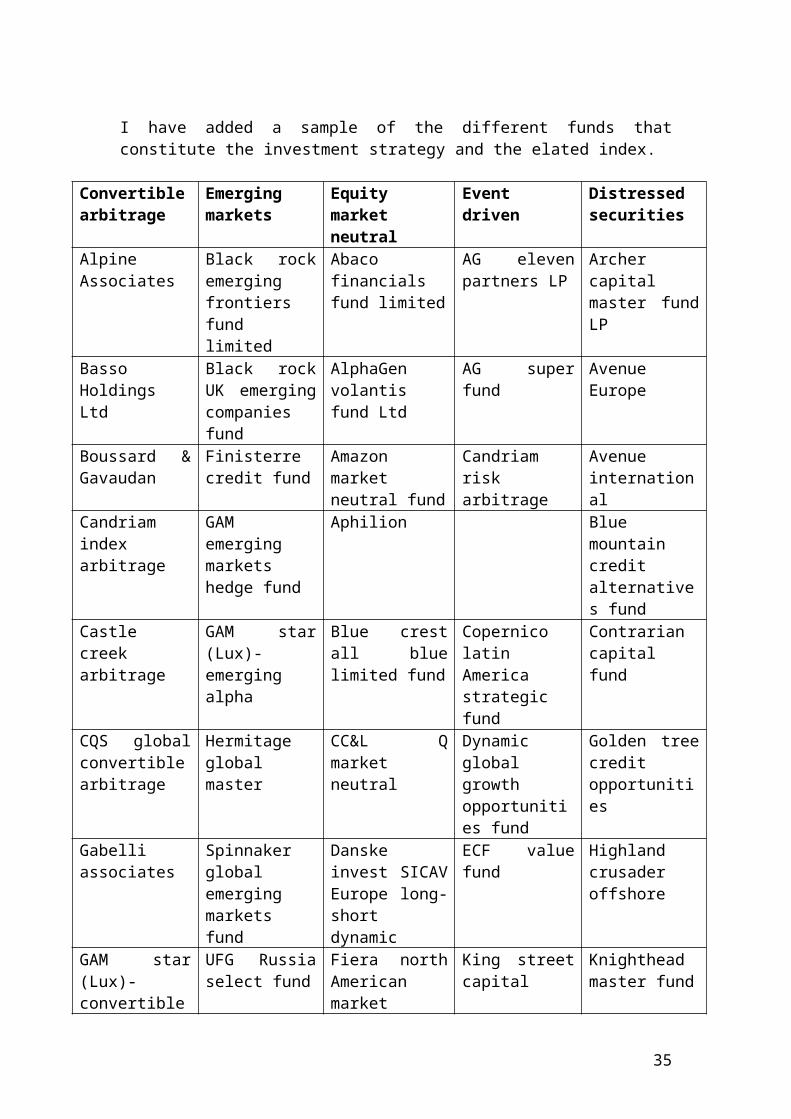
It could be calculated very easily in Excel software. I will illustrate a simple table with the relevant calculations.

Day rp rb rp - rb

1 0.03 0.02 0.012 0.02 0.014 0.0063 -0.04 0.034 -0.0744 0.05 0.067 -0.0175 0.08 0.012 0.0686 -0.01 -0.056 0.0467 0.07 0.031 0.0398 0.034 0.023 0.0119 -0.021 0.015 -0.03610 0.045 0.001 0.044

Average 0.0258 0.0161Standard deviation

0.043

Source: author’s calculation

By substituting the values that we have found in terms of rp =0.0258, rb = 0.0161 and standard deviation = 0.043 in the following equation we have:

But what is the interpretation of the information ratio of 0.23. It means that the fund manager gained around 23 basis points of active return per unit of active risk. The higher is this number, the better the manager is performing in relation to active risk.

35

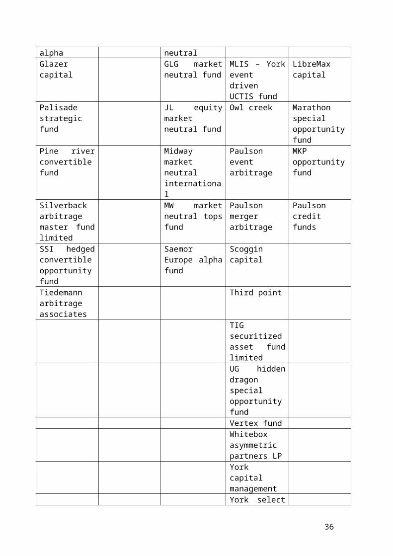
Chapter 4

Fees structure interrelation to hedge funds

Management fees Performance fees Incentive fees Water marks Hurdle rate Lock –up period

The most interesting feature of hedge funds is the interrelation of their structure and their performance. As a result, the payroll structure which is based on three components namely performance fees, incentive fees and management fees are closely related to performance. Payroll structure is based on a minimum investment of $250.000, an annual fee of 1% - 2%, and an incentive fee of 5% to 25% of annual profits. This payroll structure usually includes another component known as high water mark that adds past performance to current ones. On the other hand, investors in hedge funds are often restricted with lockup periods which are the time period that

36

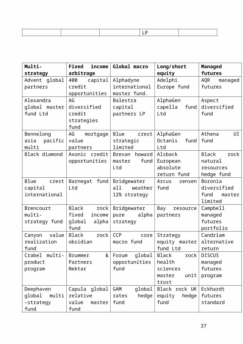
initial investment cannot be redeemed from the fund. Limitations on cash withdrawals are a result of cash fluctuations and give fund managers more freedom in setting up long-term positions. This lockup period could have an adverse effect for active investors’.

Another factor that affects directly the performance of the fund is manager incentive fees which are related to the hurdle rate. The former are additional fees based on new profits from the funds according to the performance. The manager is rewarded only when the fund does well. The later is the return above which the manager begins to take incentive fees. For example, if the fund has a hurdle rate of 10% and the fund returns 25% for the year, the fund will take incentive fees on the 15% return above the hurdle rate. Thus, if the fund performance is below the high water mark limit, then the manager will be restricted to charge incentive fees which could lead to a consequent bad performance of the fund and finally liquidation of the fund. This incentive fee is generally subject to a high water mark provision. It is a benchmark used by funds to take fees only when profits are recorded from the positive performance of the fund. For example a $1 million investment is made in year 1 and the fund declines by 50%, leaving $500 thousand. In year 2, the fund returns 100% which equal to the initial investment. It will not take incentive fees on the return in year 2 as the initial investment was not increased. If the fund shows a negative performance, then the manager must cover the loss in the next year before the incentive fee becomes applicable. We relax the assumptions that if new investors have different high-water marks, then returns are not the same for all investors in the fund. Usually, databases report the returns for the initial or the average investor. Finally, management fees are taken by the manager on the entire asset level of the investment.

Chapter 5

An empirical analysis of the performance of Hedge Funds over the period 1998 to 2003 in terms of incentive fees, management fees, size, age, hurdle rate, high watermark provision and lockup period.

37

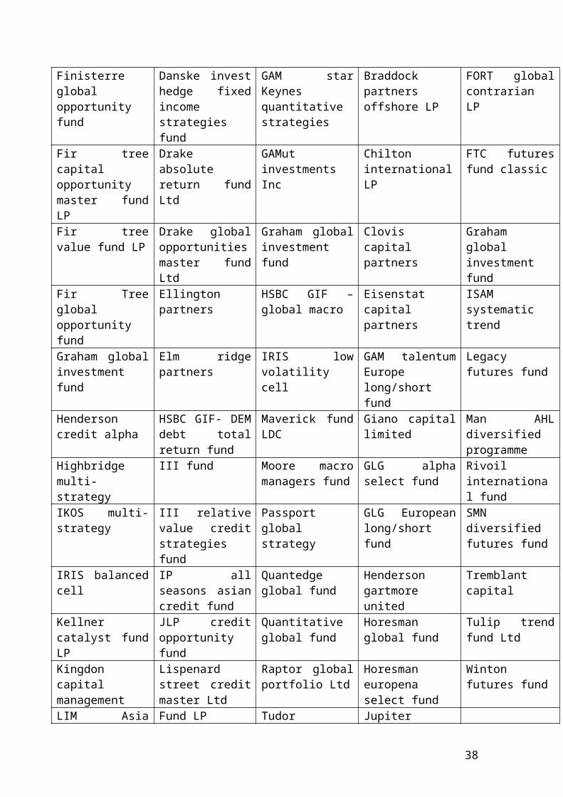
Abstract:

This paper aims at testing empirically the major building blocks that affect the performance of Hedge Funds: incentive fees, management fees, size, age, hurdle rate, high watermark provision and lockup period. The sample is provided from Data Feeder dataset. It is very comprehensive and includes 680 funds for the period 1998 to 2003. According to my findings the results are mixed. Management fees and age affect significantly the performance of Hedge Funds. My findings suggest that there are other factors that could contribute to this deviation such as lock-up periods, hurdle rate and high water mark. Dummy variables applied on the probit binary regression equation suggest that these three factors constitute a significant explanation of the performance persistence.

Keywords: incentive fees, management fees, hurdle rate, high watermark provision, lock up period, Data feeder2

Introduction

Hedge funds have been first created by Alfred Winslow Jones in (1949). As a matter

of fact, there is no universally accepted definition of hedge funds. They are owned by

private managers and wealthy individuals. Since the early 1990s, there has been a

2 I would like to thanks Karen Henseleit sales manager for passing to me the data from Datafeeder. The Alternative Asset Center (AAC), the Fund of Hedge Funds Specialist (www.aa-center.net) and Fund of Hedge Funds DataFeeder.

38

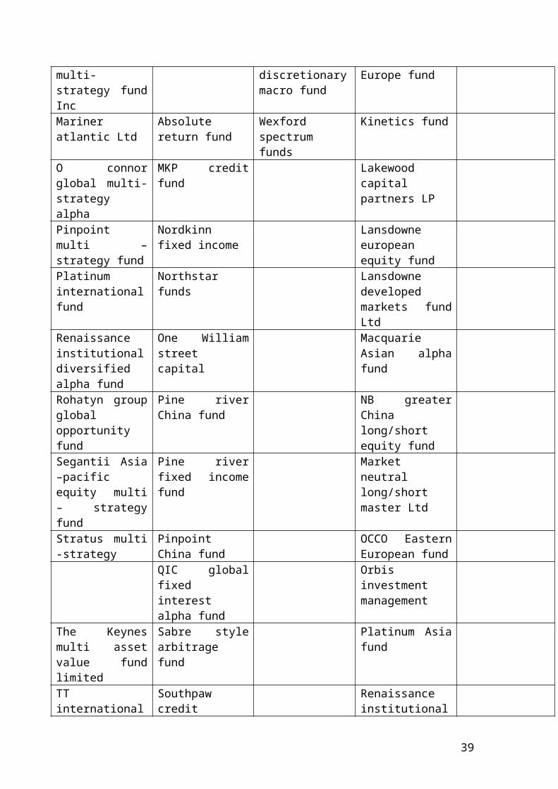
growing interest in the use of hedge funds. They are a growing business with more

than $200 billion. They are suitable for sophisticated investors as they offer greater

flexibility in their asset allocation and have a relatively low covariance with other

asset classes. The fact that they have low correlation in relation to traditional asset

classes like equities and bonds makes them to offer a better diversification. Their

structure in terms of fees is the most challenging issue among academics and

practitioners as it affects performance return.

There has also been a lot of interest shown by both academics and practitioners in

estimating the raw returns and risk-adjusted multi-factor performance of hedge funds

and other investment vehicles (Fama and French (1993, 1996); Carhart (1997),

Agarwal and Naik (2004); Capocci and Hubner (2004). Various studies have

documented the comparison of hedge fund performance with that of S&P 500 used as

a universe index. We are going to compare the performance of these funds with the

S&P 500 index.

This paper seeks to shed light on the complexity of the structure of hedge funds by

examining their performance in terms of management fees, hurdle rate, and

watermark provision. We look at these changing exposures for individual hedge

funds. Thus, we seek to provide empirical evidence on the type of fees or other factors

that sustain the fund and affect directly the fluctuations of return.

The paper is organized as follows. Section 2 describes the interrelation of structure

and performance. Section 3 provides information on data collection issues, sampling

and descriptive statistics. Section 4 presents methodological issues and empirical

results. Section 5 summarizes and concludes.

2. Structure and performance

The most interesting feature of hedge funds is the interrelation of their structure and

their performance. As a result, the payroll structure which is based on three axes

namely performance fees, incentive fees and management fees are closely related to

39

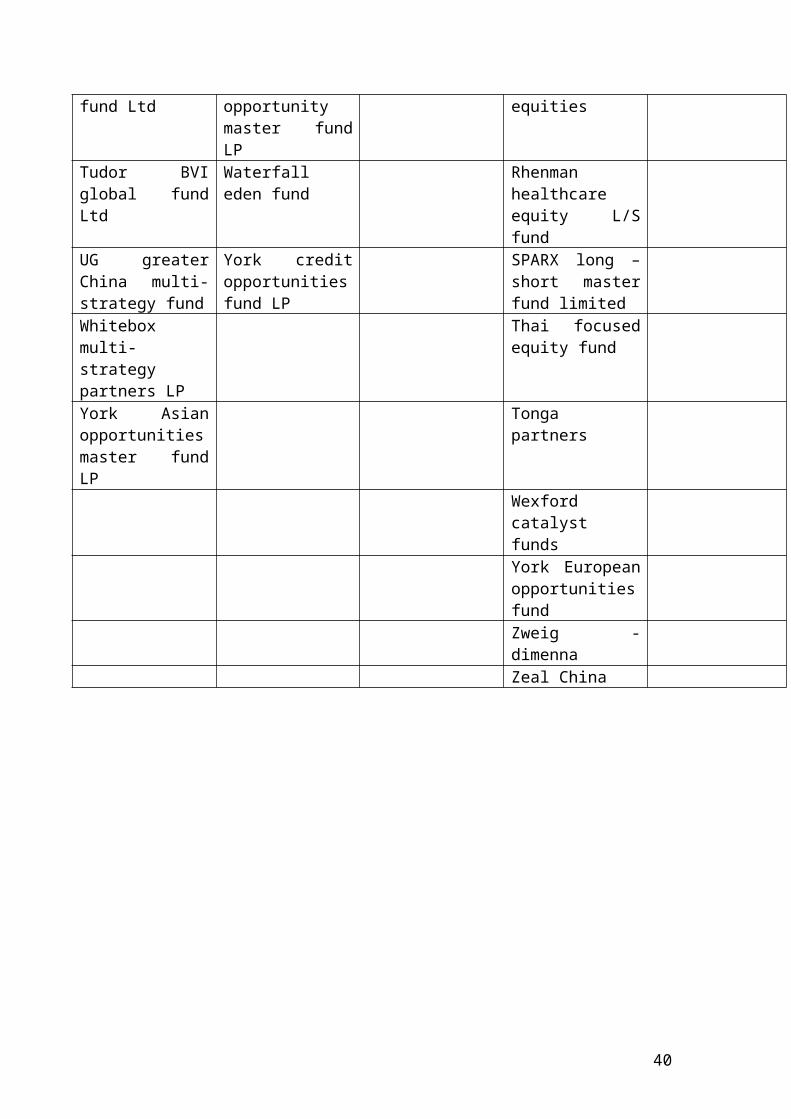
performance. Payroll structure is based on a minimum investment of $250.000, an

annual fee of 1% - 2%, and an incentive fee of 5% to 25% of annual profits. This

payroll structure usually includes another component known as high water mark that

adds past performance to current ones. On the other hand, investors in hedge funds are

often restricted with lockup periods which are the time period that initial investment

cannot be redeemed from the fund. Limitations on cash withdrawals are a result of

cash fluctuations and give fund managers more freedom in setting up long-term

positions. This lockup period could have an adverse effect for active investors’.

Another factor that affects directly the performance of the fund is manager incentive

fees which are related to the hurdle rate. The former are additional fees based on new

profits from the funds according to the performance. The manager is rewarded only

when the fund does well. The later is the return above which the manager begins to

take incentive fees. For example, if the fund has a hurdle rate of 10% and the fund

returns 25% for the year, the fund will take incentive fees on the 15% return above the

hurdle rate. Thus, if the fund performance is below the high water mark limit, then the

manager will be restricted to charge incentive fees which could lead to a consequent

bad performance of the fund and finally liquidation of the fund. This incentive fee is

generally subject to a high water mark provision. It is a benchmark used by funds to

take fees only when profits are recorded from the positive performance of the fund.

For example a $1 million investment is made in year 1 and the fund declines by 50%,

leaving $500 thousand. In year 2, the fund returns 100% which equal to the initial

investment. It will not take incentive fees on the return in year 2 as the initial

investment was not increased. If the fund shows a negative performance, then the

manager must cover the loss in the next year before the incentive fee becomes

applicable. We relax the assumptions that if new investors have different high-water

marks, then returns are not the same for all investors in the fund. Usually, databases

report the returns for the initial or the average investor. Finally, management fees are

taken by the manager on the entire asset level of the investment.

The investment styles and asset allocation of hedge funds have changed significantly

over time to reflect the performance of the fund. Due to the diversity of the industry,

there is no standard method to classify hedge funds. They can be classified either on

the basis of domicile or the nature of the trading strategies employed by them.

40

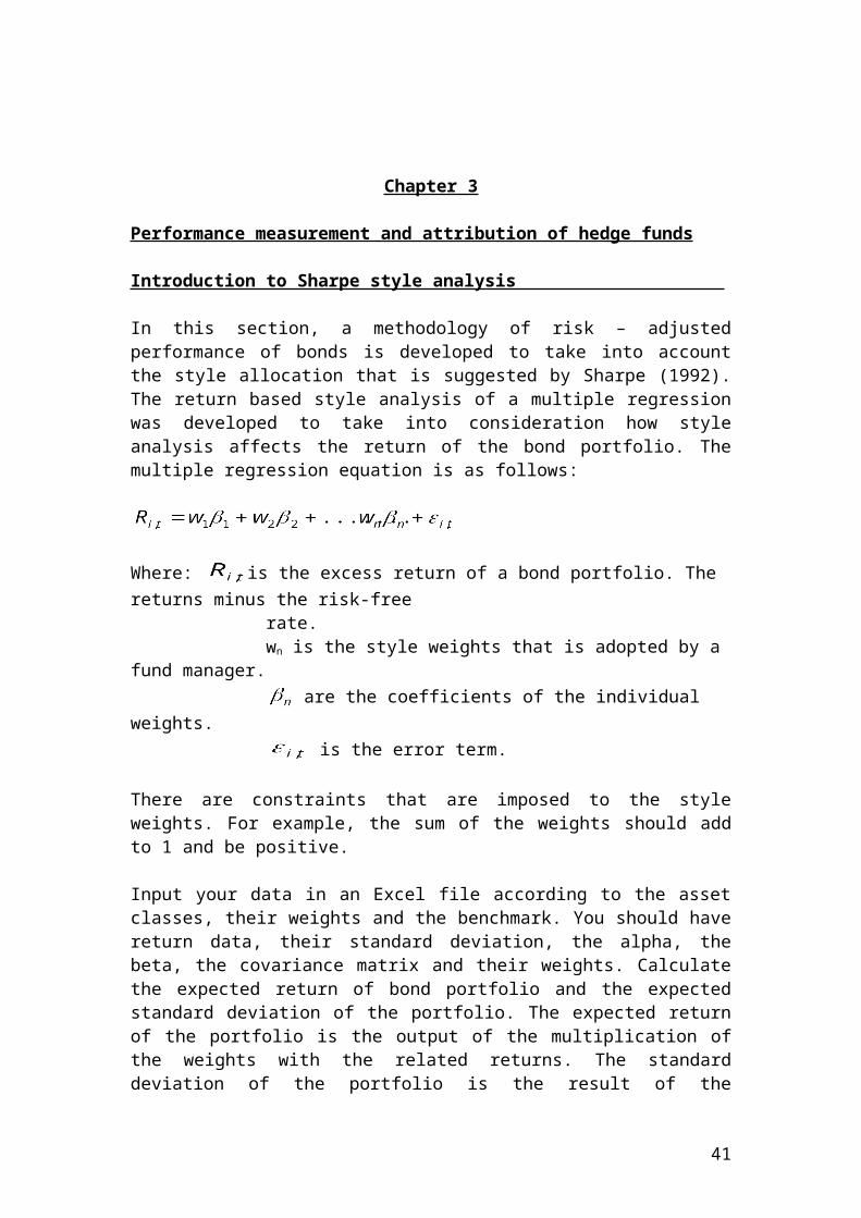
Based on domicile, hedge funds can be classified into two broad categories: onshore

and offshore. Onshore funds are domiciled in the US and are usually in the Limited

Partnership form, where the investors’ goals are aligned with fund managers’

incentives. In addition, they are free from regulatory controls imposed by the

Investment Company Act of 1940. In contrast, offshore funds are established in tax

neutral jurisdictions such as the British Virgin Islands, the Bahamas, Bermuda, the

Cayman Islands, Dublin and Luxembourg allowing the investors to minimize their tax

liabilities by investing outside their country. They are not regulated by the Securities

and Exchange Commission (SEC) so it is very interesting for practitioners to examine

their behaviour in terms of risk and return. The investors that focus on offshore funds

are generally non US or US tax exempt investors. In this paper, we focus on the whole

industry.

On the basis of nature of trading strategies followed by hedge funds, they can be

divided into two broad categories: Non-Directional and Directional. Non-directional

strategies do not depend on the direction of any specific market movement and are

commonly referred to as market neutral strategies. In contrast, directional strategies

aim to benefits from broad market movements.

Our perspective differs from that used from other researcher in terms of database,

methodology, and empirical results. Brown, Goetzmann, and Ibboston (1999)

examine the performance of offshore hedge funds. They attribute offshore hedge fund

performance to the style effects rather than manager skills. Ackermann, McEnally,

and Ravenscraft (1999) report that the comparison of hedge funds and market indexes

yields mixed findings. They conclude that hedge funds outperform mutual funds. The

above papers all use different hedge fund data. For example, Fung and Hsieh (1997)

use combined data from Paradigm LDC and TASS Management Limited. Brown,

Goetzmann, and Ibboston (1999) employ the hand-collected data from the US

Offshore Funds Directory. Ackermann, McEnally, and Ravenscraft (1999), utilize

combined data from Hedge Fund Research, Inc. (HFR) and Managed Account

Reports (MAR).

3. Data collection issues, sampling and descriptive statistics

41

Data are collected by a number of data vendors and fund advisors such as TASS and

Credit Suisse First Boston/Tremont (CSFB/Tremont) databases and Alternative Asset

Center Fund of Hedge Funds DataFeeder. Specifically, TASS and CSFB/Tremont

database track more than 3000 funds. There are strict rules for fund selection. The

universe consists only of funds with a minimum of USD 10m under management, a

minimum one-year track record, and current audited financial statements of more than

900 funds in the Index Universe. (www.hedgeindex.com).

We took our sample of 680 hedge funds from Alternative Asset Center Fund of

DataFeeder database. We use the data to investigate hedge fund performance and the

question of performance persistence among hedge fund managers. On the other hand,

the Alternative Asset Center (AAC) was formed in July 1999 as an independent

publishing company. In appendix 1, we present the various categories of hedge funds

according to the style mandate that we are doing in our analysis. The DataFeeder is

very powerful and includes general information of each of the 680 funds profiled in

terms of fund name/code, fund domicile, investment manager, fund NAV, redemption

frequency, management fee, performance fee, style mandate, investor type,

investment objective and many other information including monthly performances

since 1989. A major and important advantage of this database is that it keeps

historical information on defunct funds.

The use of monthly data has some strong advantages over annual returns used by

Brown et al. (1999). Monthly returns greatly enhance the accuracy of our standard

deviation measure of risk. The audited reports that hedge fund send to investors

generally include monthly returns and these are the same returns the funds supply to

the databases. Subscription and redemption opportunities typically do not correspond

to the incentive fee period.

The different strategies by funds, the total number of funds, descriptive statistics of

average NAV return Jarque-Bera test of normality and Sharpe ratio are presented in

Table 1. It is worth to mention that for the period 1998-2003 the funds did not have a

complete data history due to different inception periods.

42

Table 1 shows the descriptive statistics of the average NAV return Jarque-Bear statistic which is used to test if the series is normal or non-normal. This type of test uses the chi-squared distribution and specifically is a goodness-of-fit test. Sharpe ratio which is defined as the difference of the excess return over the standard deviation of the style categories. The whole sample consists of the 680 hedge funds covering the period January 1998 to January 2003.

AAC classifications of various style categories

Number of

Funds(N)

Mean(%)

StandardDeviation

(%)

Min(%)

Max(%)

Skew(%)

Kurt(%)

ADFtest

Jarque-Bear

Sharperatio

Alternative hedge and private equity investments

1 0.35 1.01 -2.20 3.37 0.03 2.99 -4.24* 0.001 2,54

Arbitrage 11 0.21 0.39 -0.80 1.15 0.16 3.32 -5,65* 0.51 6,23Arbitrage- Long/Short Equity

2 0.47 1.27 -2.21 4.61 1.36 6.25 -4,56* 38.85 2,12

Broad based but with larger allocation to Equity Hedged Strategies

2 0.81 0.64 -0.04 1.83 0.47 2.01 -5,39* 0.70 4,73

Conservative 131 0.47 1.27 -2.21 4.61 1.36 6.25 -4,56* 38.85 2,12Diversified 324 0.65 1.62 -6.45 5.80 -0.19 8.86 -4,22* 103.50 1,77Diversified across several strategies

1 0.56 1.30 -1.86 5.19 1.19 6.63 -3,83* 43.24 2,14

Equity 2 0.32 0.74 -1.61 2.30 0.09 4.25 -4,13* 4.05 3,43Equity Hedge 1 0.52 1.97 -6.44 6.04 -0.02 5.62 -4,73* 17.40 1,39Equity/Hedge/event 1 0.15 1.00 -1.44 2.84 0.79 3.62 -4,38* 2.62 2,37Equity/defensive 2 0.51 1.97 -6.44 6.04 -0.01 5.61 -4,71* 17.37 1,39Event driven 5 0.27 0.70 -1.67 2.76 0.26 4.86 -3,66* 9.47 3,56Global macro 1 0.35 1.98 -2.75 3.17 -0.17 1.74 -5,69* 0.92 1,30Global multi manager fund

3 0.19 1.08 -2.05 2.40 0.15 2.81 -4,50* 0.19 2,23

Hedged bond 2 0.71 1.56 -2.63 4.43 0.40 3.12 -3,92* 1.66 1,88Hedged equity 5 0.20 0.33 -0.94 0.90 -0.76 4.81 -5,54* 14.23 7,33Long/Short arbitrage 2 1.00 1.77 -3.92 5.12 0.45 3.64 -6,26* 3.11 1,82Long/Short equity 25 0.42 1.03 -2.70 -2.87 -0.12 4.52 -4,96* 4.84 2,56Macro/CTA 1 0.21 0.66 -0.95 1.82 0.45 3.34 -5,21* 0.72 3,68Market defensive 53 0.64 1.49 -5.76 4.54 -0.47 8.26 -3,84* 72.58 1,92Market neutral 10 0.70 1.40 -3.85 4.65 0.25 4.85 -3,82* 9.33 2,09Market neutral diversified

2 0.41 2.90 -9.94 8.25 -0.29 5.21 -4,59* 13.33 0,91

Multi-strategy 70 0.61 1.51 -6.56 4.41 -1.05 10.49 -4,32* 153.87 1,87Primarily arbitrage strategies

1 0.39 0.77 -0.76 2.23 0.66 3.00 -5,91* 1.653,39

Strategic 102 0.52 1.73 -6.54 5.65 -0.34 7.33 -3,61* 48.92 1,58Trading 2 0.36 0.50 -0.57 1.76 0.71 3.37 -5.93* 2.87 5,16Trading/Equity/Arbitrage 1 0.08 0.89 -2.94 2.66 -0.50 6.16 -4,33* 33.04 2,58Trading strategies 10 0.89 1.62 -3.38 6.60 0.71 5.76 -4,14* 24.52 1,92Source: calculated by the author* Significant at 1% level

According to table 1, the highest absolute return was achieved by Long/Short

arbitrage (1.00%), Broad based but with larger allocation to Equity Hedged Strategies

(0.81%), Hedged bond (0.71%), trading strategies (0.89%), market neutral (0.70%).

On the other hand, the lowest absolute return was achieved by hedged equity (0.20%),

global multi-manager fund (0.19%), equity, hedge event (0.15%), arbitrage (0.21%).

43

Almost all the style categories show a higher measure of standard deviation in relation

to their mean. It is interesting to see that the Sharpe ratio shows a different picture

when we take into consideration a risk adjusted measure in terms of US 3month

treasury bill risk free rate. After adjusting for the risk factor, arbitrage which was low

in terms of absolute return shows a high return of (6.23%) which is due to the fact that

we adjust our risk measure. Hedged equity shows the same results of (7.33%). The

Jarque-Bear test of normality shows a very different picture according to the style of

the category. For example, diversified style category shows a Jarque-Bear test of

103.50 which imply that the time series is not normally distributed. Global macro

shows a figure of 0.92 which is below the 5% significance level and therefore the

series is normally distributed. Most of the categories show a significant measure of

leptokurtic kurtosis and a mixed picture of positively or negatively skewed direction

of the normal distribution curve which imply that actual data are below or above the

mean according to the performance of the fund.

Table 2 displays descriptive statistics of Hedge fund independent variables that affect the performance measure

Table 2 shows the descriptive statistics of the variables that affect the performance of hedge funds in terms of management fees, incentive fees are the percentage of annual profits over high water mark provision or hurdle rate, size is the funds’ net assets under management, age is the number of months beginning from the inception of the fund. The whole sample is calculated for the period January 1998 to January 2003.

Variable Mean Median Standard deviation Range Minimum MaximumManagement fees (%) 1,37 1,50 0,69 12,00 0,00 12,00

Incentive fees (%) 7,75 10,00 6,44 30,00 0,00 30,00

Size ($million) 135,98 324,7 418,99 791,82 450 791,87

Age (months) 41,78 24,00 36,55 226,00 2,00 228,00

S&P 500 index -0,11 -0,46 5,31 23,32 -10,62 12,69

Source: calculated by the author.

According to table 2, management fees and incentive fees varies significantly

according to the various style categories of hedge funds. Managers of hedge funds get

strong incentives to manage properly the fund and get a return above a high water

mark provision. According to the table the incentive fees given to the managers have

a median of 10% and a mean of 7,75%. The maximum value that they can get is 30%.

44

Incentive fees constitute an important factor that could affect significantly the

performance of the fund. Annual Management fees charged in addition to incentive

fees are another variable which affect the attitude of the investors to increase their

shareholder in the fund assets. The range of different styles of hedge funds is 12 %.

The average manager get a fee of 1,37% charged on the assets and the median figure

is 1,50% while the maximum fees charged was 12%.

The age of the fund shows a median figure of 24 months and a range of 226 months

among the various funds. The average fund has an age of 41,78 months and a median

of 24 months. A consistent positive performance would have a direct influence on the

age of the fund as it is the source of survival and long-term existence in the database.

Finally, the S&P 500 index is used as a benchmark that will be compared with the

various style categories of hedge funds to identify if the funds are outperforming or

underperforming the universe index. According to table 2, the index shows a negative

performance of -0,11 percentage points for the period 1998-2003. The standard

deviation shows a wide dispersion of 5,31 percentage from the mean which indicate a

high dispersion from the actual data.

Table 3 shows the Augmented Dicky Fuller test statistic of the independent variable that are going to be used in the multiple regression equation.

Table 3 shows the results of the Augmented Dicky Fuller test statistic in terms of management fees, incentive fees defined as the percentage of annual profits over high water mark provision or hurdle rate, size calculated as the funds’ net assets under management, age the number of months beginning from the inception of the fund. The whole sample is calculated for the period January 1998 to January 2003.

Variable ADF test statisticManagement fees -8,40*Incentive fees -9,87*Size -11,26*Age -9,86*Source: calculated by the author* Significant at 1% level

From the ADF unit root test reported in table 3, it is clear that all independent

variables are at the 1% level of significance stationary. Since all variables are

stationary standard regression may be used.

Table 4 presents a Pearson correlation matrix of the dependent and independent variables for the major style categories for the period 1998 to 2003. The final sample consists of large style categories and the number of funds in each category ≥ 30. We

45

excluded the small style categories with limited number of funds such as 1 or 2 as they create multi-collinearity problems in our regression equation due to limited observations. We excluded funds with the acronyms Alternative Equity and private (AEP), arbitrage (A), arbitrage long/short equity (AL/SE), Broad based with larger allocation (BBWLA), Diversified across several strategies (DAST), Equity (E), Equity/Hedge (EH), Equity Hedge Event (EHE), Event driven (ED), Equity defensive (ED), Global macro (GM), Global multi manager (GMM), Hedged bond (HB), Hedged equity (HE), Long/Short Arbitrage (L/SA), Long/Short Equity (L/SE), Macro CTA (MC), Market defensive (MD), Market neutral (MN), Market neutral diversified (MND), Primarily arbitrage strategy (PAS), Trading (T), Trading Equity Arbitrage (TEA), Trading strategies (TS). We include a representative sample of 680 hedge funds that belongs in style categories with the acronyms of Conservative (C), Diversified (D), Market defensive (MD), Multi-strategy (MS), Strategic (S). The dependent variables are compared with the independent variables of age, size, management fees (MF), incentive fees (IF), and S&P 500 index.

C D MD MS S Age Size MF IFS&P500 INDEX

C 1D 0,09 1,00MD 0,10 0,10 1,00MS 0,09 0,09 0,10 1,00S 0,09 0,09 0,10 0,09 1,00Age -0,29 -0,32 -0,30 -0,30 -0,31 1,00Size -0,17 -0,18 -0,17 -0,20 -0,24 0,01 1,00MF 0,11 0,11 0,12 0,12 0,13 0,03 0,03 1,00IF 0,11 0,08 0,08 0,08 0,05 0,01 -0,09 0,11 1,00S&P500 INDEX 0,36 0,44 0,40 0,44 0,45 -0,33 -0,04 0,27 0,06 1,00

Source: calculated by the author

The correlation matrix shown in table 4 reveals no statistically significant relationship

between the independent and dependent variables. Most of the figures reveal negative

and insignificant values among the various categories and the independent variables.

There are no signs of multicollinearity among the variables and therefore we can use

them in our multiple regressions.

4. Methodological issues and empirical results.

In this paper we empirically analyze the persistence of hedge funds performance over

the period 1998 to 2003 by applying two methodologies. The first methodology is a

multiple regression that takes into consideration a range of independent variables such

as management fees, incentive fees, age and size of the fund. The statistical,

econometric and descriptive statistics of the independent and dependent variables

46

were examined in the previous section and concluded that there is no sign of

multicollinearity and the series are stationary.

The first methodology follows a multiple regression model of the followed form:

= a + b1(Rm-Rf) + b2(IF) + b3(MF) + b4(Age) + b5(Size) + εt

Where:

: is the excess NAV return of the style category and 3 month US treasury bill

Rm : is the return on an excess market return of S&P 500 index. The weighted value index such as Credit Suisse First Boston (CSFB) Tremont Hedge Fund Index

Rf : is the risk free rate of 3 months US Treasury Bill

IF: is the incentive fee

MF: is the management fee

Age: the number of months since fund inception.

Size: the assets of the fund under the management control.εt : is the random or tracking error.

The hypotheses to be tested are as follows:

H0 : ≤ 0, Fund managers have an inferior or neutral performance

H1: 0 Fund managers have a superior performance

In terms of signs of the independent variables, we expect to find positive values for

the coefficients of incentive fee, management fee, size, and age. Incentive and

management fees constitute a compensation structure that affect the skill of the

manager to outperform the index and the fund shows a positive performance. Size is

well documented in the literature by Fama and French (1993, 1996) that affect the

performance of the fund according to the fees structure. Finally, age is directly related

to the fees and performance of the fund.

47

Table 5 shows the results of the multiple regressions of the 680 hedge funds of the sample period starting from 1998 to 2003. We have regress the average NAV performance of each style categories against the excess market return, incentive fee, management fee, age and size. Excess market return is calculated as the difference of S&P 500 index and three month US treasury bill. Management fee is defined according to the style category of the hedge fund. Incentive fees defined as the percentage of annual profits over high water mark provision or hurdle rate, size calculated as the funds’ net assets under management, age the number of months beginning from the inception of the fund.

AAC style categories Rm – Rf IF MF Age SizeConservative 2.37

(21.01)*0.02

(1.56)-0.00

(-0.27)0.07

(1.84)*0.01

(3.28)*0.03

(0.61)Diversified 2.68

(18.76)*-0.00

(-0.15)0.01

(0.68)0.024(0.22)

0.00(1.58)

-0.03(-0.31)

Market defensive 2.42(23.23)*

0.00(0.27)

-0.01(-1.47)

0.21(3.01)*

0.00(4.15)*

-0.01(-1.26)

Multi-strategy 2.51(20.61)*

0.01(2.20)*

-0.01(-2.15)*

0.10(1.26)

0.00(2.18)*

-0.01(-0.27)

Strategic 2.39(4.32)*

0.01(0.75)

0.03(1.28)

0.13(0.45)

-0.00(-0.04)

-0.04(-0.24)

Source: calculated by the author

* represents t -value that is statistically significant at 5% significance level** represents t -value that is statistically significant at 1% significance level

According to table 5, indicates a skilled fund manager whose decisions add value

to the fund. On the other hand, negative values or statistically insignificant values

represent inferior or neutral performance of the manager. All style categories display

an that is positive and statistically significant at the 5% significance level. Two out

of five style categories display management fee variable that is positive and

statistically significant. Three out of five display the age variable as positive and

statistically significant.

The second methodology is a probit model which measures the relationship between a

binary variable strength such as lockup or hurdle rate over a number of other

variables. This technique helps us to measure how the binary variable affects

performance measure of our sample for the specified period of time. Specifically, we

are going to test the effect of lockup and hurdle rate upon the performance of the style

categories.

48

Lockup period = a + b1(Rm-Rf) + b2(IF) + b3(MF) + b4(Age) + b5(Size) + εt

Hurdle rate = a + b1(Rm-Rf) + b2(IF) + b3(MF) + b4(Age) + b5(Size) + εt

Watermark provision = a + b1(Rm-Rf) + b2(IF) + b3(MF) + b4(Age) + b5(Size) + εt

Where:

Lockup period, hurdle rate, watermark provision: are the binary variables

Rm : is the return on an excess market return of S&P 500 index. The weighted value index such as Credit Suisse First Boston (CSFB) Tremont Hedge Fund Index

Rf : is the risk free rate of 3 months US Treasury Bill

IF: is the incentive fee

MF: is the management fee

Age: the number of months since fund inception.

Size: the assets of the fund under the management control.εt : is the random or tracking error.

The hypotheses to be tested are as follows:

H0 : Lockup = 0 The performance of the style category is independent from the

lockup period.

H1: Lockup = 1 The performance of the style category is dependent from the lockup

period.

H0 : Hurdle rate = 0 The performance of the style category is independent from the

hurdle rate

H1: Hurdle rate = 1 The performance of the style category is dependent from the

hurdle rate.

H0 : Watermark provision = 0 The performance of the style category is independent

from the watermark provision.

H1: Watermark provision = 1 The performance of the style category is dependent

from the watermark provision.

49

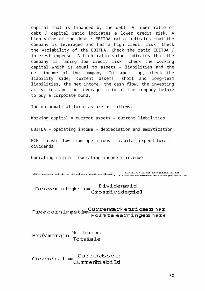
Table 6 shows the results of the probit regressions of the 680 hedge funds of the sample period starting from 1998 to 2003. We have regressed for each style categories three binary variables, watermark provision (WP), hurdle rate(HR), and lockup period (LP) against the performance of each category, the excess market return, incentive fee, management fee, age and size. Excess market return is calculated as the difference of S&P 500 index and three month US treasury bill. Management fee is defined according to the style category of the hedge fund. Incentive fees defined as the percentage of annual profits over high water mark provision or hurdle rate, size calculated as the funds’ net assets under management, age the number of months beginning from the inception of the fund.AAC style categories

Binary

VariableLR statistic

(6 df)Probability(LR stat)

Rm – Rf IF MF Age Size

Conservative WP 11.73 0.07 -0.05(0.12)

0.04(0.14)

0.26(0.26)

-0.00(0.92)

0.36(0.03)*

HR 14.13 0.03* 0.04(0.38)

0.08(0.06)

-0.62(0.16)

0.01(0.47)

0.24(0.24)

LP 15.91 0.01* 0.04(0.63)

-0.02(0.71)

-1.60(0.01)*

-0.03(0.26)

-0.09(0.79)

Diversified WP 15.75 0.02* 0.01(0.82)

0.09(0.01)*

0.09(0.81)

0.01(0.10)

-0.04(0.89)

HR 9.11 0.17 -0.02(0.63)

0.06(0.09)

0.16(0.69)

-0.00(0.72)

0.53(0.13)

LP N/A N/A N/A N/A N/A N/A N/A

Market defensive WP 23.09 0.00* 0.00(0.93)

0.14(0.00)*

-0.19(0.66)

0.01(0.33)

0.14(0.03)*

HR 7.56 0.27 0.07(0.01)*

0.07(0.08)

0.22(0.63)

-0.00(0.88)

0.06(0.43)

LP 2.19 0.90 0.06(0.50)

-0.17(0.49)

0.46(0.54)

0.01(0.72)

0.01(0.45)

Multi-strategy WP 4.45 0.62 0.04(0.23)

0.00(0.93)

0.25(0.52)

0.01(0.14)

-0.14(0.24)

HR 5.97 0.43 0.02(0.44)

0.02(0.59)

0.09(0.80)

0.01(0.33)

0.08(0.30)

LP 11.97 0.06 0.04(0.28)

-0.03(0.43)

0.51(0.20)

-0.00(0.70)

0.07(0.41)

Strategic WP 7.61 0.27 0.03(0.15)

0.01(0.74)

0.63(0.08)

0.00(0.84)

-0.28(0.21)

HR 13.44 0.04* -0.00(0.96)

0.07(0.03)*

-0.50(0.17)

0.01(0.25)

-0.50(0.08)

LP 6.71 0.35 -0.09(0.25)

-0.14(0.09)

-1.56(0.19)

0.00(0.82)

-0.24(0.67)

Source: calculated by the author* represents p - value that is statistically significant at 5% significance level

The above table shows that for 5% significance level the p-value is significant for

most binary variables which the sample evidence imply that we can reject the Null

50

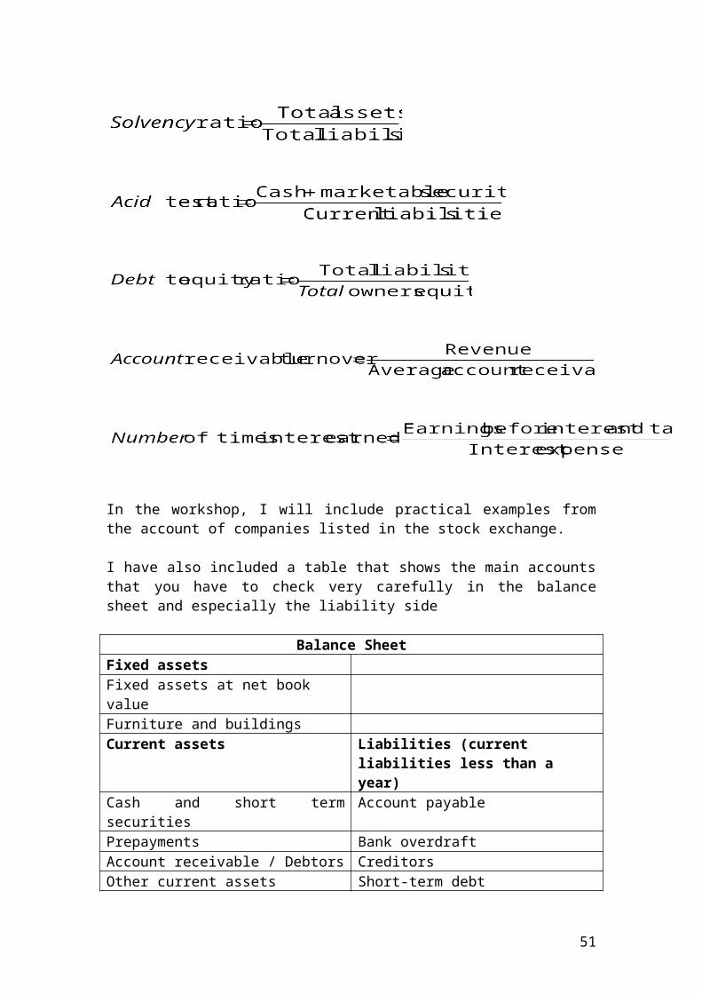
hypothesis. Specifically, the p-value for hurdle rate and lockup period is significant as

the LR statistic is greater than the critical value of 12.59. Hurdle rate and lockup

period affect significantly the performance of conservative style category. In contrast,

Watermark provision does not affect the performance of the conservative category

and this may be due to the fact that most of the observations in our sample are funds

that do not offer watermark. The diversified style category shows a different picture.

The watermark provision binary variable is significant as the test statistic for 6 degree

of freedom is greater than the critical value of 12.59. The sample evidence suggests

that we can reject the null hypothesis in favourite of the alternative one. The lockup

binary variable shows a N/A value as the matrix was near singular. The hurdle rate

shows an insignificant value. The third category which is market defensive style

category shows a significant p-value for watermark provision. The other two binary

variables show an insignificant p-value.

Multi-strategy style category did not show any significant p-value for any of the three

binary variables. Finally, strategic style category shows a significant p-value for

hurdle rate of 0.04. The other two binary variables namely lockup period and

watermark provision show an insignificant p-value. Thus, the sample evidence

suggests that only performance is dependent on the hurdle rate.

51

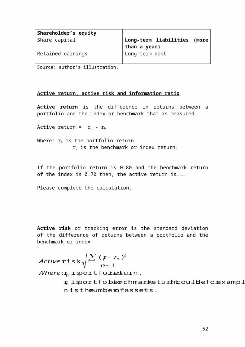
5. Conclusion

This paper examined the performance persistence of hedge funds in terms of

management fees, hurdle rate, incentive fees, size, age, high watermark provision and

lockup period. The sample under consideration was for the period 1998 to 2003 and

includes 680 funds. The first methodology applied was a multiple regression that

takes into consideration a range of independent variables such as management fees,

incentive fees, age and size of the fund.

According to the findings, all style categories display an that is positive and

statistically significant at the 5% significance level. Two out of five style categories

display management fee variable that is positive and statistically significant. Three

out of five display the age variable as positive and statistically significant.

52

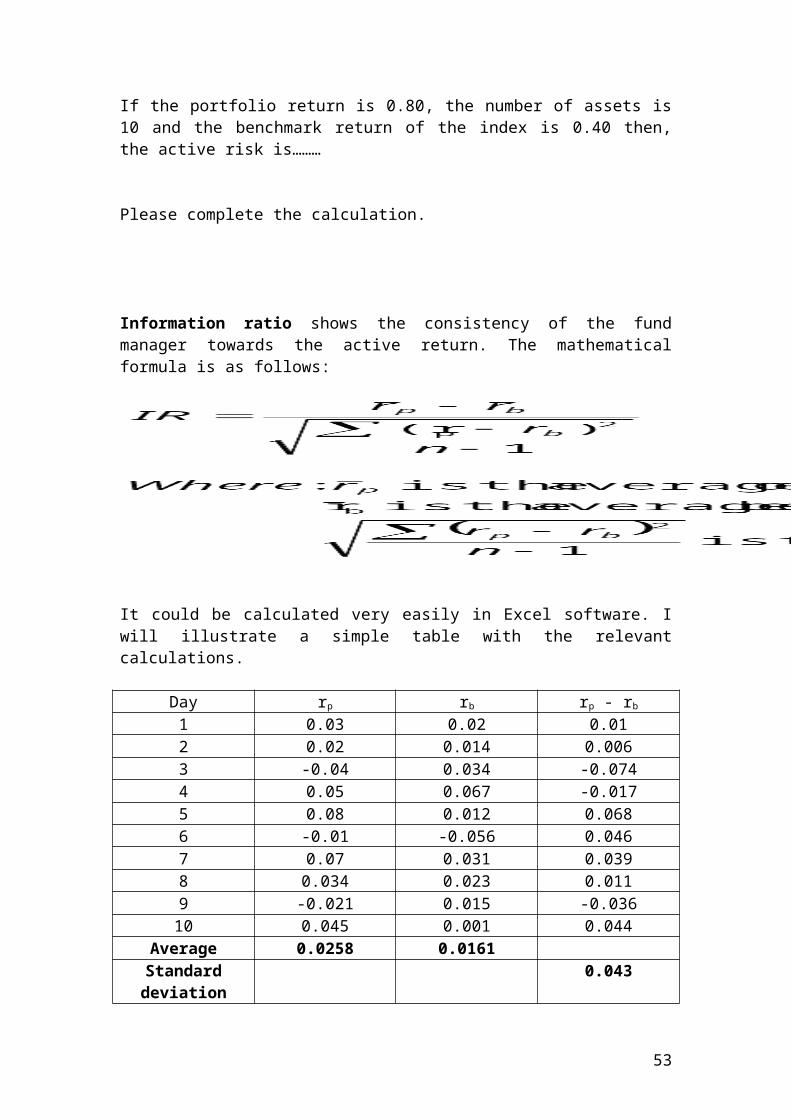
The second methodology is a probit model which measures the relationship between a

binary variable strength such as lockup or hurdle rate over a number of other

variables. According to the results, hurdle rate and lockup period affect significantly

the performance of conservative style category. The watermark provision binary

variable for the diversified style category is significant as the test statistic for 6 degree

of freedom is greater than the critical value of 12.59. The third category which is

market defensive style category shows a significant p-value for watermark provision.

Finally, strategic style category shows a significant p-value for hurdle rate of 0.04.

Thus dummy variables applied on the probit binary regression suggest a significant

explanation of performance persistence of hedge funds.

References

Alfred Winslow Jones (1949), “Creation of the first hedge fund”.

Ackermann, C., R. McEnally and Ravenscraft, (1999). “The Performance of Hedge Funds: Risk, Return, and Incentives”. The Journal of Finance. Volume 54, Issue 3, pages 833-874.

Agarwal, Vikas and Narayan Y. Naik (2004), “Risk and Portfolio Decisions Involving Hedge Funds”. Review of Financial Studies, 17, pp.63-98.

Brown and Goetzmann (1997), “Hedge Funds with Style”. NBER working paper No.8173.

Brown, Stephen, William N. Goetzmann and Roger G. Ibbotson, (1999), “Offshore Hedge Funds, Survival and Performance”. Journal of Business 72: (January #1) 91-118.

Carhart, M.(1997), “On Persistence in Mutual Fund Performance”. Journal of Finance, Vol 52. No 1.

Capocci and Hubner, (2004), “An Analysis of Hedge Fund Performance”. Journal of Empirical Finance. Vol.11, No 1, pp 55-89.

Fama, E. F., and K. R. French. (1993), “Common Risk Factors in the Returns on Stocks and Bonds.”Journal of Financial Economics 33, (1993): 3-56.

53

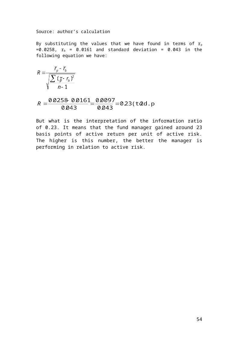
Fama, E. F., and K. R. French.(1996), “Multifactor Explanations of Asset

Pricing Anomalies.” Journal of Finance 51, (1996): 55-84.

Fung and Hsieh(1997), “Performance Characteristics of Hedge Funds and Commodity Funds: Natural versus Spurious Biases. Journal of Financial and Quantitative Analysis. Volume 35, pp.291-307.

Lavinio, Stefano (2000), Hedge fund handbook: a definitive guide for analyzing and evaluating alternative investments, New York: McGraw Hill.

Chapter 6

Excel Applications

Please check the attached Excel files, which show how, for example, call options could fit an asset allocation portfolio. I have included an Excel file, which shows the calculation of the Black and Scholes formula. Moreover, I have included an Excel file that shows a practical example of buying a call option on the Standard and Poor, S&P 500 stock index options in terms of breakeven, limitation of downside risk and gain or losses. In the same Excel file, I have included an example of a hedge portfolio by taking a short position in call in case of 1% rise or fall of stock prices. Finally, I have included an Excel example of how to hedge by using a Eurodollar contract and how to speculate using Euromark futures. In the same Excel file, I have included an example of applying a profit /loss of a long and short call in S&P 500 index by using real data.

Workshop of functions application in Excel

All the relevant functions for financial modelling and analysis will be found by following the Excel path:

Insert --------- function. Then, by pressing the arrow, you have the choice to select a category. The most common category that is used is:

A) Financial

54

B) StatisticalC) LogicalD) Lookup and referenceE) Scenario manager

Thus, this workshop will help you to understand the application of each function by using examples from the derivatives market.

A) Financial functions

The most common financial applications that are used by practitioners are as follows:

1. Present value, (PV)

The mathematical formula in Excel for the PV function is:

PV(rate, nper, pmt, fv, type).

Where: fv and type are not compulsory and if they are not included are assumed to be zeros. fv is used if the final future payment amount is changed. Rate is the annual interest rate. Nper is the number of payments that will be done. pmt is the amount to be paid each year.

The present value calculates the present cash flows based on a future payment. For example, the annual interest rate is 5%. The annual payments are 8. Each year will be paid the amount 500 Pounds and the final year the amount paid will be 300 Pounds. What is the present value of the investment?

By including the above data the mathematical formula will be as follows:

PV(0.05, 8,-500,-300,0). Or you can enter the formula as:PV(5%, 8, -500, -300,0)

You should get an answer of 3,435 Pounds.

2. Future value, (FV)

The FV function calculates the future value of the investment based on a present value principal.

The mathematical formula in Excel for the FV function is:

FV (rate, nper, pmt, pv, type).

Where: pv and type are not compulsory and if they are not included are assumed to be zeros. pv is used if the present payment amount is changed. Rate is the annual interest rate. Nper is the number of payments that will be done. pmt is the amount to be paid each year.

55

The future value calculates present cash flows. For example, the annual interest rate is 3%. The annual payments are 7. Each year the investor will pay the amount 300 Pounds and an additional amount paid will be 100 Pounds. How much money the investor will get at the end of the 7 years? In other words, what is the future value of the investment?

By including the above data the mathematical formula will be as follows:

FV(0.03, 7,-300,-100,0).

You should get an answer of 2,422 Pounds

3. Price of a bond

The mathematical formula for calculating the price of a bond based on a 100 Pounds face value is as follows:

Price(settlement, maturity, rate, yield, redemption, frequency, basis).

Settlement is the date that the bond is settled. For example, it is 16-Feb-14Maturity is the date that the bond expires. For example, it is 20-Mar-16.Rate is the annual coupon rate. For example, it is 2.71%.Yield is the return to maturity. For example, it is 4.32%.Redemption value based on a 100 Pounds face value. We assume 100 face value.Frequency is the number of coupon payments per year. For example, we assume that the coupon of the bond is paid twice per year.Basis is the number of days to use. It is optional.

By including the above data the mathematical formula will be as follows:

Price(16-Feb-14, 20-Mar-16, 2.71, 4.32,100, 2,0)

4. Yield of a bond

The mathematical formula for calculating the yield that a bond matures based on twice per year payment is as follows:

Yield(settlement, maturity, rate, pr, redemption, frequency, basis).

Settlement is the date that the bond is settled. For example, it is 16-Feb-14Maturity is the date that the bond expires. For example, it is 20-Mar-16Rate is the annual coupon rate. For example, it is 2.71%.Pr is the price per 100 Pounds. For example, the current bond price is 96.8066.Redemption value based on a 100 Pounds face value. We assume 100 face value.

56

Frequency is the number of coupon payments per year. For example, we assume that the coupon of the bond is paid twice per year.Basis is the number of days to use. It is optional.

By including the above data the mathematical formula will be as follows:

Yield(16-Feb-14, 20-Mar-16, 2.71, 96.8066,100, 2,0)

5. Duration of a bond

The mathematical formula for calculating the duration that a bond matures based on twice per year payment is as follows:

Duration(settlement, maturity, coupon, yield, frequency, basis).

Settlement is the date that the bond is settled. For example, it is 16-Feb-14Maturity is the date that the bond expires. For example, it is 20-Mar-16Coupon is the annual coupon rate. For example, it is 2.71%.Yield is the yield maturity. For example, it is 4.32%Frequency is the number of coupon payments per year. For example, we assume that the coupon of the bond is paid twice per year.Basis is the number of days to use. It is optional.

By including the above data the mathematical formula will be as follows:

Duration(16-Feb-14, 20-Mar-16, 2.71, 4.32, 2,0)

You should get an answer of duration of 2.03 years.

6. Net present value, (NPV)

The mathematical formula in Excel for the NPV function is as follows:

NPV(rate, value1, value2,…). The rate represents the discount rate and value 1, value 2, etc represents the cash flows or the principal that will be invested.

For example, the discount rate is 3%. The value 1 is 400 Pounds and the value 2 is 300 Pounds.

NPV(3%, 400,300). You should get an answer of 671.13

7. Internal rate of return, (IRR)

The mathematical formula in Excel for the IRR function is as follows:

IRR(values, guess).

57

Where IRR calculates the internal rate of return for various cash flows. The value represents the cash flow and the guess is an optional initial guess that the investors input.

For example, the values are the initial cash flows. The total principal has a negative value followed by the cash flows. For example, -100 90 80 70. They are all inserted in one row. Then, guess is an optional value. It could be 110 Pounds. By applying the data into the formula, we have the following results.

IRR(-100 90 80 70,110).

B) Statistical functions

The most common statistical functions that are used in the investment banks are as follows:

1. Descriptive statistics

Please input all the returns or cash flows in an array in Excel. Then, select the data. Then, press tools and then data analysis. Then descriptive statistics, then, you press OK. Then input the range of the data. Then, for output range, please select a cell that you want your output to be displayed. Do not forget to select summary statistics and then OK.

For example, we have the following cash flows.12,000 , 15,000, 17,000, 19,000, 25,000.

After plugging the data in a row or column, you should get the following output.

Mean 17600Standard Error 2181.742Median 17000Mode #N/AStandard Deviation 4878.524

58

Sample Variance 23800000Kurtosis 0.897182Skewness 0.769967Range 13000Minimum 12000Maximum 25000Sum 88000Count 5

Source: author’s calculation

The mean shows the average. The standard deviation shows the dispersion around the data. The median is the middle value. The range shows the maximum – minimum value. The kurtosis shows the peakdness of the distribution and the skewness shows the asymmetry of the distribution or the shift of the distribution from the mean. Thus, we have positive and negative skewness.

2. Cumulative frequency

It shows the total number of times that a value above or below a certain amount occur.

Class: value of revenues received after sales of options £ (m)

Frequency Cumulative Frequencies

% Cumulative Frequencies

Less than 65 10 10Less than 85 18 28 = (10+18)Less than 105 6Less than 125 4Less than 145 3Less than 165 2Less than 185 2Less than 205 4Less than 225 1Total 50 100Source: author’s calculation

Please complete the calculations ……………

59

3. Histogram

A histogram is a means of illustrating a frequency distribution and should give the reader an impression of the distribution of values between two datasets. For example,A practitioner in an investment bank has recorded the following cash flows for different classes in Excel:

Classes Cash flows 1 Cash flows 20 - 12,000 10,000 11,00012,000- 15,000 12,000 13,00015,000 - 16,000 15,000 14,00016,000 - 20,000 17,000 19,000

Select both data arrays, then, select chart wizard. Then, select bar chart, then OK. Then, chart options. In the chart title box input the name cash flows. In the x axis, please input number of transactions. In the y axis, please input cash flows and press OK. Finally, press format data series by right clicking on the chart. Press options. Select overlap and gap width to zero values. You should get the following graph.

Cash flows

0

5,000

10,000

15,000

20,000

0 - 12,000 12,000-15,000

15,000 -16,000

16,000 -20,000

Number of transactions

Cash

flow

s

Cash flows 1Cash flows 2

4. Normal cumulative distribution for a specified mean and standard deviation, (NORMDIST)

The mathematical formula in Excel for the NORMDIST function is as follows:

NORMDIST(x,mean,standard-dev,cumulative)

Where: NORMDIST is the normal cumulative distribution. x is the value that we want the normal cumulative distribution to calculate. mean is the average and it is given. The same for the standard deviation which shows the dispersion around the mean. Cumulative is a logical value. If, it is cumulative, then, then the value is True. If not, then, you input False.

60

This function calculates the cumulative normal distribution for a known mean and a standard deviation. Thus, what is the probability if the mean is 4, the standard deviation is 5, an x value less than 3 and a cumulative function.

NORMDIST(3,4,5,TRUE)

If we have two x values with the same mean and standard deviation, then, you will have to input two formulas. Thus, we have the following formulas:

=NORMDIST(x1,mean,standard deviation, TRUE)-NORMDIST(x2,mean,standard deviation, TRUE)

Please do not confuse the function NORMSINV () is used to convert the random number into a standard normal distribution number.

5. Scatter diagram, regression and correlation

A Scatter diagram

1 Input the dependent y values and the independent x values in two separate columns.

2 Highlight the columns containing the information.3 Go to the chart wizard icon 4 Select the x,y scatter5 Select the first scatter diagram i.e. the one with the points6 Click on Next7 Click on Series

In Name write the name of the chartMake sure that the cells in the x values and the cells in the y values correspond to what is in the worksheet

8 Click on nextIn the titles put in the titles for the (x) axis and the (y) axis

9 Click on finish and the diagram will appear

Calculation of the regression

1 Go to Tools2 Select Data Analysis 3 Select Regression4 In the field Input y range highlight the y values5 In the field Input x range highlight the x values

In output options

61

1 Make sure that the cursor is in the output range field2 Highlight the cell where you want the data to appear3 Make sure that the information in the filed input ranges has not changed

Calculation of the correlation

Multiple R = the correlation co-efficient for the 2 variablesR square is the square of the correlation co-efficient

6. Covariance

It is used to measure the degree to which two data sets affect each other. The mathematical formula is as follows:

COVAR(array1, array2)

Where: array 1 is the first data sets of cash flows. It could be for example, 10,000, 20,000, 30,000, 40,000 array 2 is the second data sets of cash flows. It could be for example, 5,000, 7,000, 10,000, 15,000.

Please plug the numbers into the formula and calculate the covariance.

7. Statistical tests in terms of, (TTEST) and, (FTEST)

The TTEST calculates the probability of a student t-test. The mathematical formula is as follows:

TTEST(array1, array2, tails, type) Where: array 1 is the first dataset. array 2 is the second dataset. tails could be 1 or 2 depending if it is one or two tailed distribution. type shows the type of t-test to be performed. If it is paired, then, it takes the value of 1. If it is two sample with equal variance, then, it takes the value of 2. If two ample with unequal variance, it takes the value of 3.

For example, we have the following data sets of cash flows with the formula:

10,000 11,00012,000 13,00015,000 14,00017,000 19,000

=TTEST(A3:A6,B3:B6,2,2) You should get a value of 0.76

62

The FTEST calculates the difference in variability between two data sets. For a two-tailed test, the F-test calculates that the variability between two data sets is not significant. The mathematical formula is as follows:

FTEST(array1,array2)

For example, we have the following data sets of cash flows with the formula:

10,000 11,00012,000 13,00015,000 14,00017,000 19,000

=FTEST(A3:A6,B3:B6)

You should get a value of 0.89.

8. Quartile and intrequartile range

The quartiles divide the area under the distribution into four equal partsExample:

Number of sales annually

Year Cash flows expressed in millions

1 6822 6903 6934 5735 7286 6627 7758 6469 73310 67311 71912 599

Source: author’s calculation

First of all, we arrange our data by size in ascending form

63

n.=12 573 599 646 662 673 682 690 693 719 728 733 775

1st M 3rd quartile quartile

The Median = (n+1) /2 = (12 +1) /2 = 6.5 th number so 682 +690 /2 = 686.0

Q1 = 1st quartile = 646 +662 / 2 = 654

Q3 = 3rd quartile = 719 + 728 / 2 = 723.5

Interquartile range = 723.5 - 654 = 69.5 m

n. =11 573 599 646 662 673 682 690 719 728 733 775

1 st quarter 3rd quarter

Median = (n+1) /2 = 6 th number. So it is the 682

Interquartile range = 728 - 646 = 82 mThe mathematical formula to calculate quartile in Excel is as follows:

Quartile(array,quart)

Where: array is the number values that you will insert in terms of cash flows. Quart is a number. The first quartile takes the value of 1, and the third quartile takes the value of 3.

Example, the practitioner has recorded the following cash flows:20,000 , 25,000, 27,000, 30,000, 35,000.

The formula in Excel will be as follows:=QUARTILE(B2:B6,1) and you should get the value of 25,000 for the first quartile. Where B2:B6 represent the array of numbers. 1 represents the first quartile.

The formula in Excel for the third quartile will be as follows:=QUARTILE(B2:B6,3) and you should get the value of 30,000 for the third quartile. Where B2:B6 represent the array of numbers. 3 represents the third quartile.

9. Geometric mean

It is defined to be the nth root of the product of n numbers. It is useful when we are trying to average percentages. It is also used with index numbers.

The formula is

64

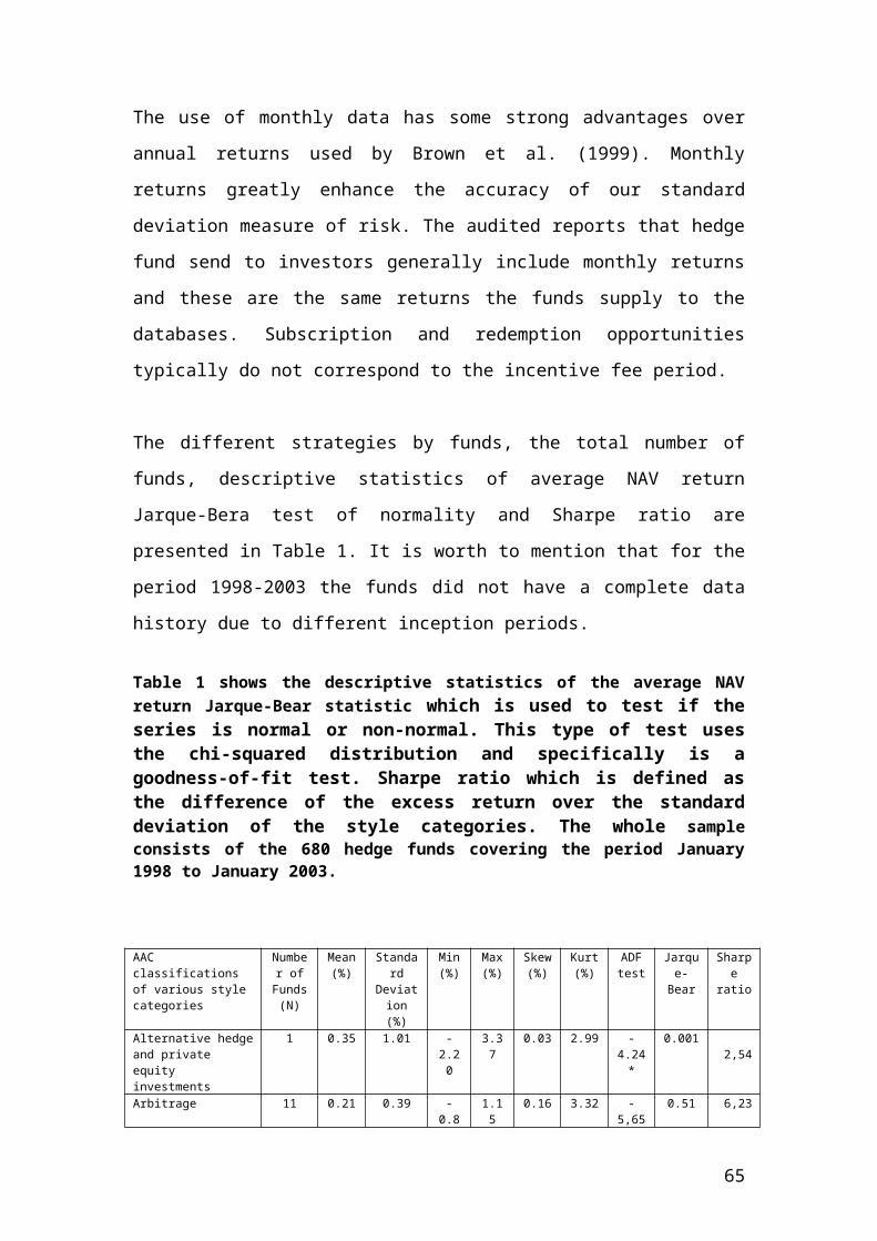
Example, given the percentage of time spent on a certain task we have the following data: 30% 20% 65%

A simple mean will be

Make a comparison between the two means.

The mathematical formula to calculate the geometric mean in Excel is as follows:

Geomean(number1, number2,…..)

By using the above numbers 30%, 20% and 65%, you should get 0.34 or 34%

10. Harmonic mean

The harmonic mean is used when we are looking at ratio data.

Example, we have the following data set:

23 25 26 27 23

First of all, you need to find their reciprocals.

Then find their average.

Then take the reciprocal of the answer

Then contrast with the simple mean.

The mathematical formula to calculate the harmonic mean in Excel is as follows:

Harmean(number1, number2,…..)

By using the above numbers 23, 25, 26, 27, 23 you should get 24.70.

65

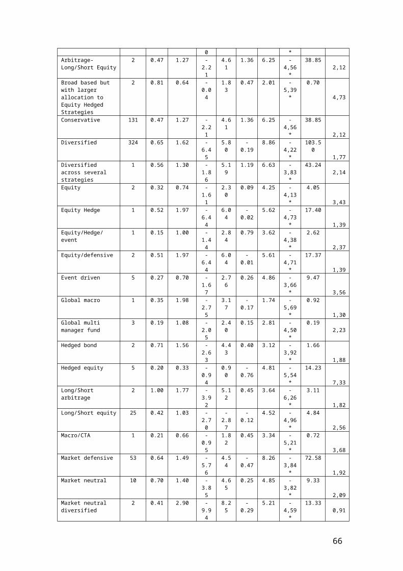
11. SUMPRODUCT

This function is very important in Excel to calculate the expected returns of call options and the variance - covariance matrix based on correlations and standard deviations. It returns the sum of the products of corresponding arrays. The syntax of this function is as follows:

=SUMPRODUCT(array1,array2,…..,etc).

For example, we have three call options, A, B, and C.

  A B C D  

Row numbers Call optionsExpected Returns ( r)

Standard deviation

Weights(w)

Portfolio return

1 A 0.06 0.05 0.35 0.0722 B 0.1 0.07 0.45 Standard

deviation or portfolio risk

3 C 0.03 0.02 0.2 0.42100%

Source: author’s calculation.

The mathematical formula for portfolio return is as follows:Rp = rA*wA + rB* wB + rC* wC

Rp = 0.06 *0.35 +0.1 *0.45 + 0.03 * 0.2 = 0.021 + 0.045 + 0.006 = 0.072

The mathematical syntax for portfolio returns in Excel is as follows:=SUMPRODUCT(B1:B3,D1:D3)

You should get the answer 0.072.

The risk of a portfolio of derivatives products is calculated by taking into consideration the correlation coefficients, the standard deviations, the variances and the weights of each option. The portfolio risk calculation in terms of variance is more complicated as it includes the correlation and the covariance matrix.

(1)

The formula of the correlation coefficient is as follows:

(2)

The correlation coefficient is calculated from the original time series dataset by clicking on Tools in Excel and then selecting correlation from data analysis in Excel.The correlation coefficients of the three portfolios of options are as follows:

.

66

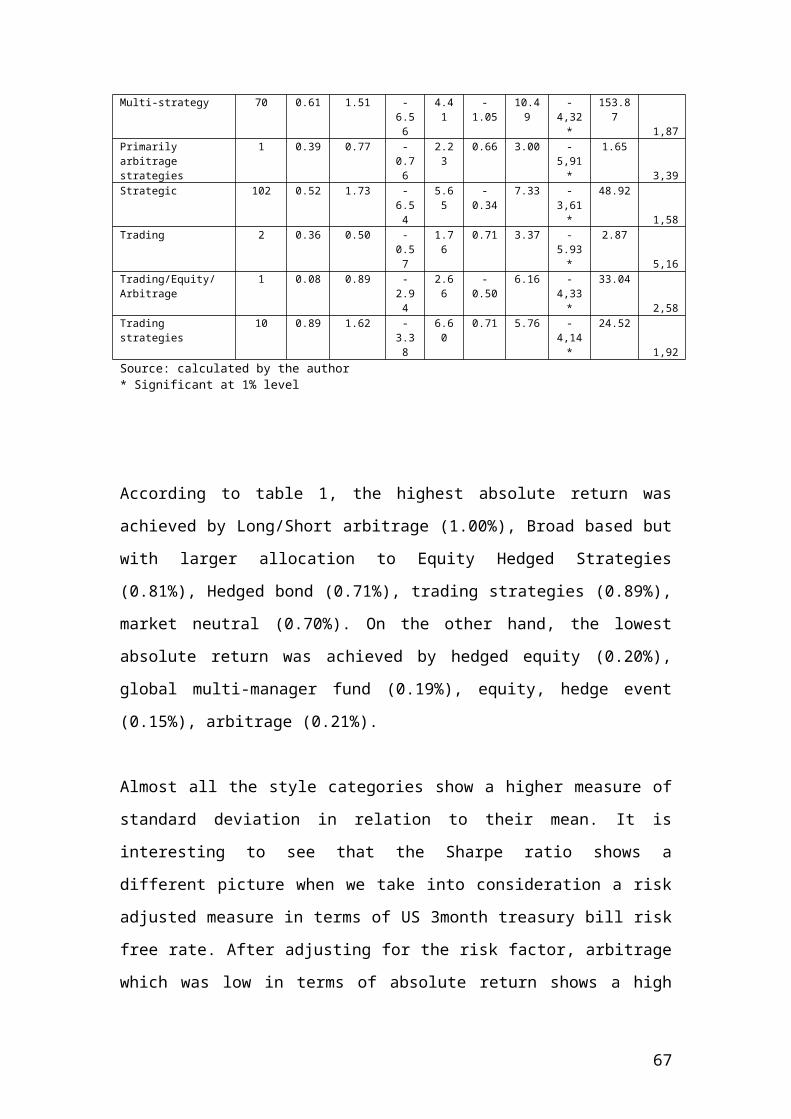
By substituting equation (2) into equation (1) and by inputting the numbers from the Table, we have the following derivation of the variance of the portfolio:

Please complete the calculations ……………………………….

You should get an answer of 0.0018 or 0.18%

After calculating the variance, you should be able to calculate the standard deviation or the risk of the portfolio by taking the square root of the variance.

Standard deviation or risk of the portfolio is as follows:

StDev = SQRT(0.18) = ………………

This is the basic procedure if you have three classes of investment products. If you have more classes of shares or options or futures, then, you need to use Excel software to perform the calculations, as the whole procedure become more complicated. But even with three classes, Excel could facilitate the calculations by using the SUMPRODUCT Function and the MMULT function for matrix multiplication. I will show how to calculate the variance and standard deviation or risk of the above portfolio using Excel software.

Correlation matrix

Standard deviation

A B CA 1 0.5 -0.4 0.05B 0.5 1 -0.1 0.07C -0.4 -0.1 1 0.02

Source: author’s calculation.

Variance - Covariance matrix Weights

0.0025 0.0018 -0.0004 0.350.0018 0.0049 -0.0001 0.45

-0.0004 -0.0001 0.0004 0.2Source: author’s calculation.

The variance – covariance matrix is calculated by using the SUMPRODUCT function

based on the equation . The calculations are based on the correlation

matrix and the standard deviations of call options A,B and C.

For example, 0.0025 is calculated by applying the formula =SUMPRODUCT(1,0.05,0.05) 0.0018 is calculated by applying the formula =SUMPRODUCT(0.5,0.05,0.07) -0.0004 is calculated by applying the formula =SUMPRODUCT(-0.4,0.05,0.02) 0.0018 0.0049

67

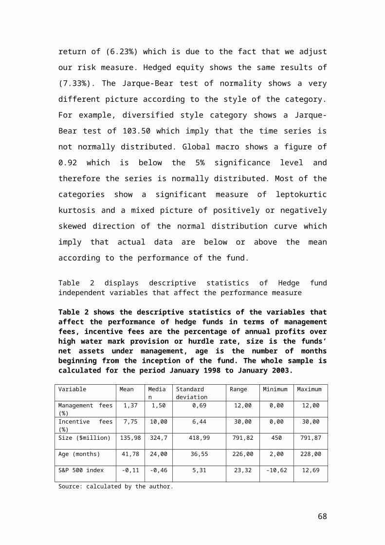
-0.0001 -0.0004 -0.0001 0.0004

Please practice by applying the same principle for the remaining numbers in the Variance – Covariance matrix.

Then, we use the Variance – Covariance matrix in relation to the weights to calculate the variance of the portfolio by applying the MMULT function found in math and trigonometry of fx function. The MMULT function is recorded by pressing simultaneously Ctrl+Shift+Enter.

Variance of the portfolio 0.002Variance percentage return of the portfolio 0.2Standard deviation or risk of the portfolio 0.42

Source: author’s calculation.

=MMULT(TRANSPOSE(weights),MMULT(Variance – Covariance matrix,weights))

Then, the variance percentage return is the variance multiplied by 100 and the standard deviation or the risk of the portfolio is the SQRT of the variance percentage return.

C) Logical functions

The most common logical functions that are used in the investment banks are as follows:

1. The IF function

The mathematical formula to calculate the IF function in Excel is as follows:

IF(logical-test, value-if-true, value-if-false)

For example, a broker would like to invest different cash flows in different interest rate futures. The range of the cash flows is 15,000 to 40,000 Pounds. For an amount less than 15,000, the interest rate is 4%. Between 15,000 to 30,000, the interest rate is 3%. Above 40,000 the future contract is getting a different interest rate of 5%. What is the appropriate interest rate according to the amounts invested?

For amount less than 15,000 Pounds, the interest rate is 4%Between 15,000 and 30,000 Pounds, the interest rate is 3%Above 40,000 Pounds, the interest rate is 5%

68

Source: author’s illustration

The mathematical formula will be as follows:

=IF(C15<C9,C12,IF(C15<C10,C13,IF(C15>C11,C14)))

OR

=IF(C15<15,000,0.04,IF(C15<30,000,0.03,IF(C15>40,000,0.05)))

You should get an interest rate of 0.04 or 4%.

Another example is to record for each cash flows gain or losses according to the actual and predicted returns after the sale of option contract.

Cash FlowsActual returns

(F)Predicted

returns (G)Gain /losses

10,000 3% 7% Gain20,000 6% 5% Loss25,000 8% 10% Gain30,000 10% 13% Gain35,000 15% 11% Loss

Source: author’s illustration

=IF(G10>F10,"Gain",) Gain

=IF(G11<F11,"Loss",) Loss

=IF(G12>F12,"Gain",) Gain

=IF(G13>F13,"Gain",) Gain

=IF(G14<F14,"Loss",) Loss

D) Lookup and reference functions

The most common Lookup and reference functions that are used in the investment banks are as follows:

1. The LOOKUP function

The mathematical formula to calculate the LOOKUP function in Excel is as follows:

LOOKUP(lookup-value, lookup-vector, result-vector)

69

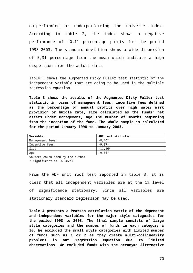
The LOOKUP function is used to look up a value either from a one – row or one - column range or from an array.

For example, we want to calculate or find the appropriate interest rate for different principal values.

Principal expressed in Pounds (D21:D26)

Interest rate (E21,E26)

Different principal rates

5,000 1% 7,00010,000 1.50% 12,00020,000 2.20% 25,00030,000 2.50%  40,000 3.50%  50,000 4.50%  

Source: author’s calculation

=LOOKUP(F21,D21:D26,E21:E26)

Where: F21 represents the suggested principal rate. In this case it is 7,000. D21:D26 represents the principal amounts of 5,000, 10,000, 20,000, 30,000, 40,000 and 50,000. E21,E26 represents the interest rates of 1%, 1.50%, 2.20%, 2.50%, 3.50%, 4.50%.

You should get an answer of 0.01 or 1%.

Similarly, the LOOKUP function for 12,000 and 25,000 will be as follows:

=LOOKUP(F22,$D$21:$D$26,$E$21:$E$26) Where: F22 represents 12,000.

You should get a value of 0.015 or 1.5%.

I have used the dollar sign or absolute cell reference because I don’t want that the formula is modified when I do copy and paste. I have left the cell F23 without dollar sign, as I want that the amount of principal to be changed.

=LOOKUP(F23,$D$21:$D$26,$E$21:$E$26) Where F23 represents 25,000

You should get a value of 0.022 or 2.2%.

2. The HLOOKUP function

The mathematical formula to calculate the HLOOKUP function in Excel is as follows:

HLOOKUP(lookup-value,table-array,row-index-num, range-lookup)

70

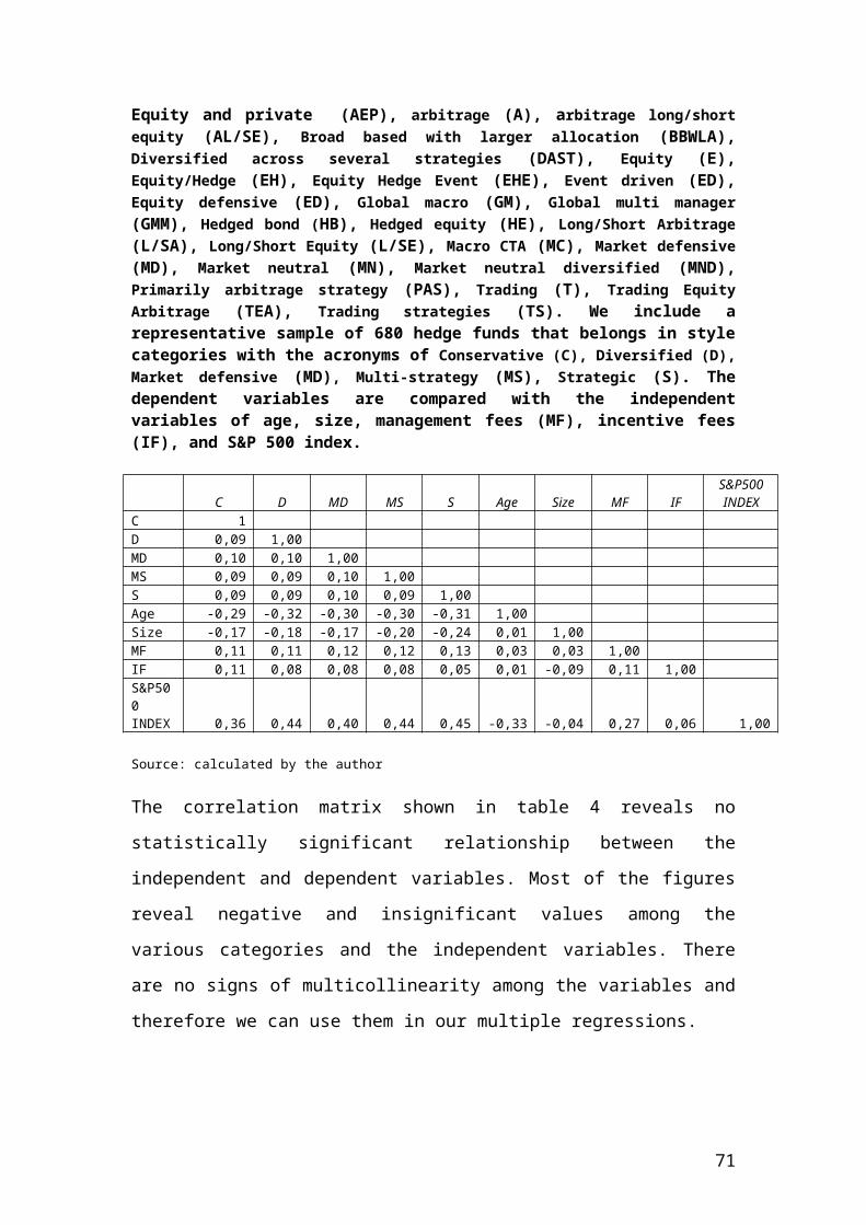
Where:HLLOKUP looks for a value in the leftmost column of a table, and then returns a value in the same row from a column you specify.Lookup value is the value to be found in the first row of the table. It could be a value, a reference or a text string.Table array is a table of information that is used for data to be looked up.Row-index-num is the row number in table-array from which the matching value will be returned.Range –lookup is a logical value that specifies if the HLOOKUP will find an exact or approximate match.

Example, calculate the appropriate principal to be invested by using the HLOOKUP function.

Principal expressed in Pounds (lower bound)

Principal expressed in Pounds (upper bound)

Interest rate Different principal rates

5,000 10,000 1% 7,00010,000 20,000 1.50% 12,00020,000 30,000 2.20% 25,00030,000 40,000 2.50%  40,000 50,000 3.50%  50,000 60,000 4.50%  

Source: author’s calculation

=HLOOKUP(F24,C24:E29,2,TRUE) Where F24 is the proposed principal rates, but we don’t know if it is the correct amount. C24:E29 represents the bolded area of the table. Row-index-num in this case is 2. Range lookup is set up as True. You have two options to select True or False. If False, HLOOKUP will look for an exact match. If True, then, an approximate match is found.

You should get 10000.

E) Scenario manager

Scenario manager tool is used to answer what if questions about possible scenarios. It is a useful tool that helps the practitioner or the investor to see the changes of the values of the dependent variable based on the changes of the values of the independent variable. The set of values that are derived from the changes of the inputs or the independent variables are called possible scenarios.

71

For example, we have the current share prices and we want to construct a scenario analysis to record the gain and losses.

Current share prices Gain Loss

100 110 90120 130 80130 140 70140 150 60150 160 50160 170 40170 180 30180 190 20190 200 10200 210 15

Source: author’s calculation

To use the scenario manager, open Excel and then press tools, scenarios. Then, press add scenario. In the scenario name, please write Gain. Then, in the changing cells input the current share prices. Then, press OK. You will be directed in a scenario values. Please input the values of each of the changing cells that represent gain. For example, in cell$A$2, you will input the value 110. It represents a gain as it is above 100 of the current value. To record a Loss, presses again add, then, in the scenario name record Loss. Then, in the changing cells input the current share prices. Then, press OK. You will be directed in a scenario values. Please input the values of each of the changing cells that represent loss. For example, in cell$A$2, you will input the value 90. It represents a loss as it is below 100 of the current value. The following table represents a scenario summary.

Scenario Summary    

    Current Values: Gain LossChanging Cells:        $A$2 100 110 90  $A$3 120 130 80  $A$4 130 140 70  $A$5 140 150 60  $A$6 150 160 50  $A$7 160 170 40  $A$8 170 180 30  $A$9 180 190 20  $A$10 190 200 10  $A$11 200 210 15Notes: Current Values column represents values of changing cells attime Scenario Summary Report was created. Changing cells for eachscenario are highlighted in gray.

Source: author’s calculation

72

Workshop of functions application in Excel in terms of the decision tools and Stat tools Suite from Palisade organisation. http://www.palisade.com

This statistical software tools that is offered from Palisade is integrated in Excel for further analysis of your dataset. I will apply the statistical analysis in the commodities market, call index options and Danish and Swedish equities. The purpose of using this software is to develop a financial model, to identify the uncertainty, to use simulation and probabilities and finally form a decision. I will display in each section the output from the analysis. Several of the options that the statistical software shows are as follows:

A) Stat Tools B) @ Risk 4.5C) BestFitD) Precision TreeE) Risk optimizerF) Top rank function

A) Stat Tools

This option helps you to analyze and summarize data in a descriptive or inferential manner. It provides options for summary graphs, time series and forecasting, normality tests, regression analysis, and quality control charts that are used in Six Sigma methodology. Please e-mail for more information concerning the mathematical formula of the quality charts that are used in quality assessment. My e-mail is guirguismichel@gmail.com. In the workshop, I will show how to use the Stat tools and the interpretation of the data according to the historical data that you have downloaded for an option or a future contract. At this stage, I am illustrating the layout of the graphs and the tables that are provided from Palisade statistical tools.

73

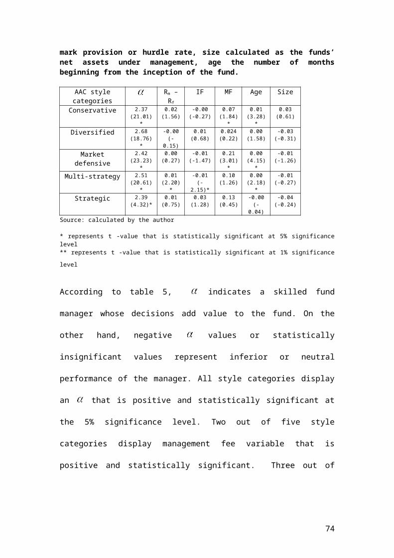
Time series graph (core analysis pack)

Time Series of a Danish stock - Danisco / Data Set #1

0

50

100

150

200

250

300

350

400

1 9 17 25 33 41 49 57 65 73 81 89 97 105 113 121 129 137 145 153

Observation #

StatTools Student VersionFor Academic Use Only

StatTools Student VersionFor Academic Use Only

StatTools Student VersionFor Academic Use Only

StatTools Student VersionFor Academic Use Only

StatTools Student VersionFor Academic Use Only

StatTools Student VersionFor Academic Use Only

StatTools Student VersionFor Academic Use Only

StatTools Student VersionFor Academic Use Only

StatTools Student VersionFor Academic Use Only

StatTools Student VersionFor Academic Use Only

Source: author’s calculation from Palisade software.

Confidence interval (core analysis pack)

Danisco EquityConf. Intervals (One-Sample) Data Set #1Sample Size 155Sample Mean 307.25Sample Std Dev 38.37Confidence Level (Mean) 95.0%Degrees of Freedom 154Lower Limit 301.16Upper Limit 313.34

Source: author’s calculation from Palisade software.

74

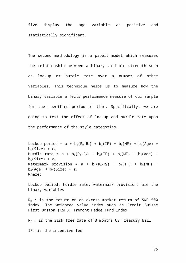
Histogram (core analysis pack)

Danisco Equity / Data Set #1Histogram Bin Min Bin Max Bin Midpoint Freq. Rel. Freq. Prb. DensityBin #1 186.60 205.33 195.97 6 0.0387 0.0021Bin #2 205.33 224.06 214.70 4 0.0258 0.0014Bin #3 224.06 242.80 233.43 6 0.0387 0.0021Bin #4 242.80 261.53 252.16 1 0.0065 0.0003Bin #5 261.53 280.26 270.90 9 0.0581 0.0031Bin #6 280.26 298.99 289.63 16 0.1032 0.0055Bin #7 298.99 317.73 308.36 35 0.2258 0.0121Bin #8 317.73 336.46 327.09 45 0.2903 0.0155Bin #9 336.46 355.19 345.82 33 0.2129 0.0114

75

Source: author’s calculation from Palisade software.

Correlation and covariance (core analysis pack)

Danisco Equity Correlation Table Data Set #1

1.000Sydbank 0.952Emerging Markets Equity 0.946Danske Bank 0.933Nordea Bank 0.976

Danisco EquityCovariance Table Data Set #1Sydbank 1472.55Emerging Markets Equity 1562.44Danske Bank 894.93Nordea Bank 2158.76

Source: author’s calculation from Palisade software.

Summary statistics of Danisco Equity.

Danisco EquityOne Variable Summary Data Set #1Mean 307.25Variance 1472.55Std. Dev. 38.37Skewness -1.4604Kurtosis 4.7004Median 318.52Mean Abs. Dev. 28.74Minimum 186.60Maximum 355.19

76

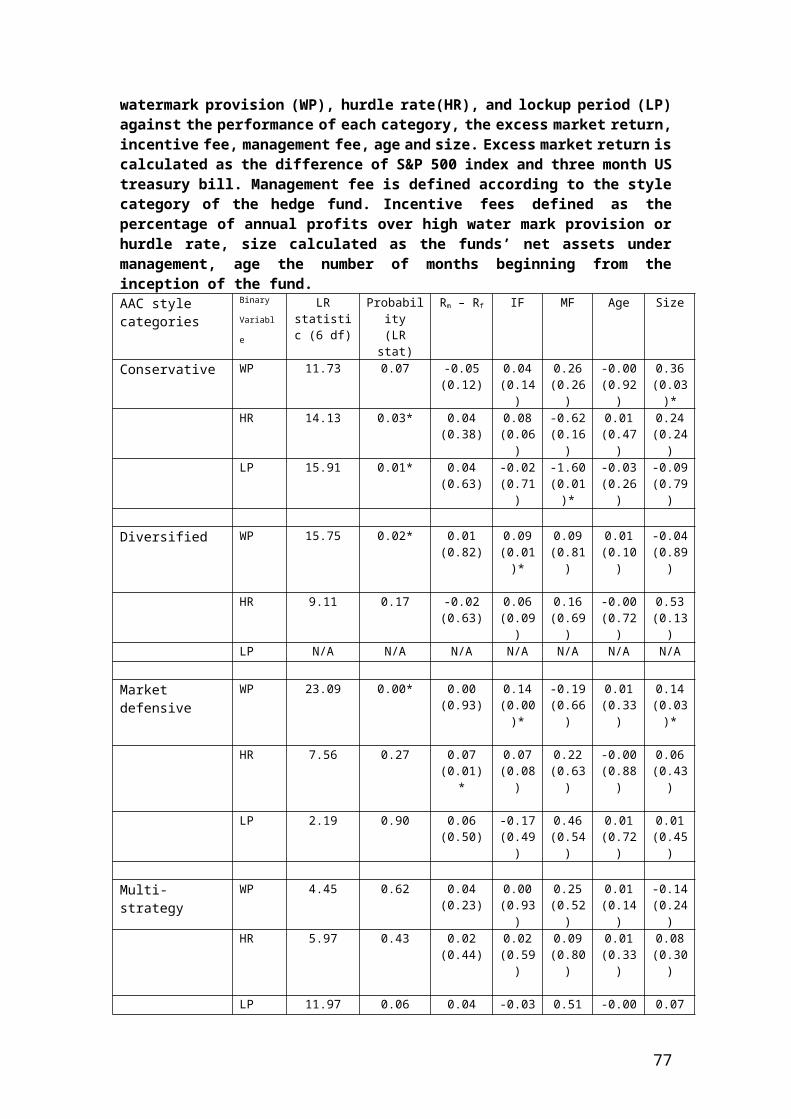
Range 168.59Count 155Sum 47623.891st Quartile 295.613rd Quartile 335.14Interquartile Range 39.53

Source: author’s calculation from Palisade software.

B) @ Risk 4.5

This option gives you the opportunity to perform Monte Carlo simulation, optimization, regression sensitivity graph, tornado graph. By checking the number of iterations as 100 or 500, you get the opportunity to simulate your data worksheet and get an output represented in different tab. The tabs give you the opportunity to check the distribution of the data, the percentiles and the descriptive statistics. By right clicking on the graph, you have the option to amend your graph and change the settings. You can select your data and then by right clicking you check the best distribution of your data by using for example a normal or a chi-square distribution. It gives you the possibility to do recalculation in your Excel file by selecting random values many times. The final result is a distribution related to the probability that the outcome will take place. It also includes sensitivity analysis and scenario analysis. In the workshop, I will show how to use the @Risk tools and the interpretation of the data according to the historical data that you have downloaded for an option or a future contract. At this stage, I am illustrating the layout of the graphs and the tables that are provided from Palisade statistical tools.

Let’s illustrate a simulation problem. For example, we assume that the current price of the Danisco share is 153 Danish Krone, (DK). We are expecting a bullish market and an increase of the share price around 50%. To increase our profitability, we have bought for a premium of 7,67 a European call option on Danisco with exercise price 160 DK and expiration date in three months. The mean is 30% and the standard deviation is 35%. The risk free rate is 4,879%

You are asked to calculate the value at risk, (VAR) of your portfolio by using the function @ Risk? Calculate the Danisco price at expiration and the percentage gain of your portfolio by including the call option of Danisco in addition to the share that is traded in the stock market. Value at risk is used to calculate the percentage of the loss position of the portfolio within a confidence level.

Hint: The mathematical formula is as follows:

Danisco price at expiration is calculated as follows:

77

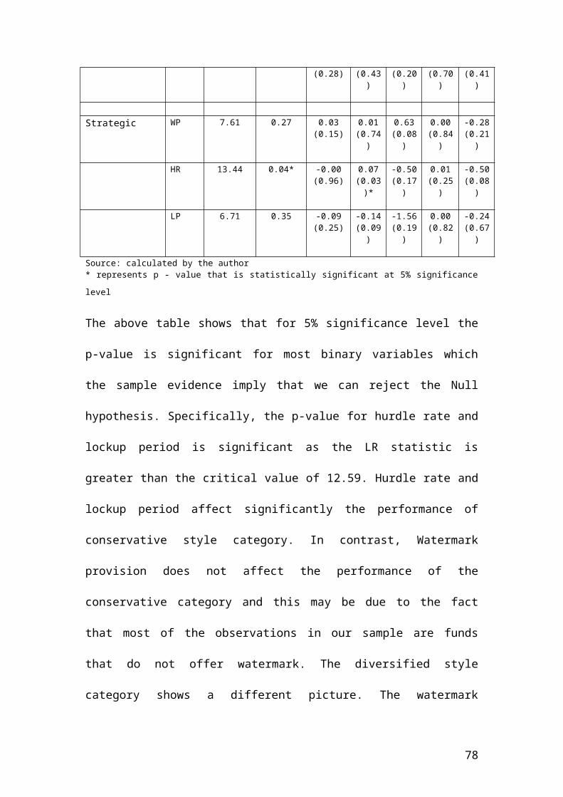
Danisco portfolio Total amounts

Current market price 153Call exercise price 160Call duration 90Risk free rate 0.04879Growth rate 0,30Volatility 0,35Call premium 7,67

Danisco price at expiration% gain by including the share + call optionSource: author’s illustration from Palisade software.

Please complete the table ………………

Then the @Risk software starts to calculate the Value at risk of the % gain of the share and the call for different iterations and for different confidence levels.

VAR % Probability5%10%15%20%25%30%35%Source: author’s illustration from Palisade software.

Sensitivity and Scenario analysis

Sensitivity and scenario analysis are used for successful investment decisions to determine how changes in the values of the independent variable will affect the dependent variable in case for example of 10% or -10% changes in the share, option of future prices. Another way, it will be to input in the window of the sensitivity analysis, in the base the value of the share or exercise price. Then, in the min and max value, we input the range of the prices that we expect the share or option or future will

78

fluctuate until the contract expires. Finally, in the steps window, we select the number of combinations.

Thus, these tools help us to determine the direction of the prices in case of changes in the market index direction of a bull or bear market. To do the sensitivity analysis, we click on the cell that we are going to test or analyze. Then, you have two options to use one way or two way analysis type according to the independent variables that we have. For example, if we have one variable, then, we use one way analysis. Then, we select the cells that are going to vary or the independent variables. By pressing the add button, we add them. Then, we suggest values in terms of min, max, base and steps. As an example, I will show the Danske Bank strike call option, the dependent variable is affected from the Danske Bank share price and the OMX Copenhagen 20 index. These both variables are the independent variables in the model.

Danske share price

Danske strike call option

Copenhagen index

142 150 710

120

134

148

162

176

190

640

7300

20406080

100120140160

Dec

isio

n an

alys

is

$L$5

$M$5

2-Way Sensitivity of Decision analysis

140-160

120-140

100-120

80-100

60-80

40-60

20-40

0-20

PrecisionTree Student VersionFor Academic Use Only

PrecisionTree Student VersionFor Academic Use Only

PrecisionTree Student VersionFor Academic Use Only

PrecisionTree Student VersionFor Academic Use Only

PrecisionTree Student VersionFor Academic Use Only

PrecisionTree Student VersionFor Academic Use Only

PrecisionTree Student VersionFor Academic Use Only

PrecisionTree Student VersionFor Academic Use Only

PrecisionTree Student VersionFor Academic Use Only

PrecisionTree Student VersionFor Academic Use Only

Decision analysis

Opt. Path

120 142127 142134 142141 142148 142155 142162 142169 142176 142183 142190 142

Decision analysis

Opt. Path

640 142

79

655 142670 142685 142700 142715 142730 142745 142760 142775 142790 142

Let’s illustrate a numerical example that shows the effect of changes of the independent variables in the forecast in terms of cash flows that were invested in an equity derivative. I will show how the Danske Bank strike call option, the dependent variable is affected from the Danske Bank share price and the OMX Copenhagen 20 index. These both variables are the independent variables in the model.

We assume that for year 0 the total cash invested is 200,000,000 Pounds. The first 4 months the cash flows for investing in Danske Bank strike option are as follows:

Months Pounds0 200,000,0001 50,000,0002 50,000,0003 50,000,0004 50,000,000

Source: author’s illustration

Months 0 1 2 3 4

(200,000,000) 50,000,000 50,000,000 50,000,000 50,000,000

The mathematical equation for total ending cash position will be as follows:

((- Initial investment + (monthly payment x (strike price – changes in share prices) x changes in stock index)).

Where: Initial investment and monthly payment is fixed amounts. Strike price that is bought is fixed and is the dependent variable. The share price and stock index prices are independent variables.

Thus, the values that we are going to change are the share prices and the stock index prices by inputting a minimum and a maximum value. By substituting the numbers, the formula becomes as follows:

((-200,000,000 + (50,000,000 x (150 – 142) x 710))

80

Thus, the values of the share prices are (120, 127, 134, 141, 148, 155, 162, 169, 176, 183, 190).The values of the stock index are, (640, 655, 670, 685, 700, 715, 730, 745, 760, 775, 790). C) BestFit

This option in the statistical package is used to find the distribution function that best describes your dataset. It offers an option of 26 distribution types integrated with optimized algorithms. The statistical software that I am using has a version of 4.5. In the workshop, I will show how to use the Best fit tools and the interpretation of the data according to the historical data that you have downloaded for an option or a future contract. At this stage, I am illustrating the layout of the graphs and the tables that are provided from Palisade statistical tools. I have used as an example a normal distribution of a call Bovespa index option.

Normal distribution graph of Bovespa call index option.

Normal(307.251, 38.374)

Val

ues

x 10

^-2

0.0

0.5

1.0

1.5

2.0

2.5

180

200

220

240

260

280

300

320

340

360

< >71.0% 29.0%328.5 +Infinity

BestFit Student VersionFor Academic Use Only

81

Source: author’s calculation from Palisade software.

The absolute error between the fitted distribution and the input data of Bovespa call index option.

BetaGeneral(16.049, 1.3752, -252.31, 355.19)

Val

ues

x 10

^-2

-1.0

-0.8

-0.6

-0.4

-0.2

0.0

0.2

0.4

0.6

0.8

1.0

180

200

220

240

260

280

300

320

340

360

BestFit Student VersionFor Academic Use Only

82

Source: author’s calculation from Palisade software.

D) Precision or decision tree

This option helps you to understand and decompose the sequence of a financial problem. It includes a statistical report and risk profile graph. It also includes a sensitivity analysis which displays which independent variables are the most important in order to formulate a decision. This is very helpful tool when designing a swap contract between two parties.

£20,000,000Investment bank Insurance company

$ 10,000,000 The most important tools of a precision or decision tree are tree name, decision node, chance node, end node, path probability. It helps you to take the best or optimum decision based on the data that you have. For example, Tree name is the investment bank and the insurance company. The decision node illustrates if the payment will be made through the logical expression true or false. The chance node shows that there is a variety of payment methods available to both institutions. Then, the probabilities of default or reliable payment will be assigned according to the credibility of the institution. By pressing decision analysis, the software will calculate descriptive statistics based on the whole decision tree or part of it. Then, the risk profile graph illustrates the possible probability defaults that will take place during the contract period. For example, you can have a swap contract of 5 to 8 years, thus, you would like to see the credibility and variation in the payment procedure between the two institutions in a probability of cumulative format. It is very interesting software and it worth to buy it. You are going to learn many things and it will facilitate your life in the investment bank.

Pay : True Amount paid

Not to pay False Amount not paid

Probability Probability of credible of default payment

E) risk optimizer

83

Investment Bank

Insurance Company

Decision node Outcome

Risk optimizer is very helpful function that is used to optimize the cell of the financial model that you have built. It uses a genetic algorithm optimization with Monte Carlo simulation to find for example, the best possible total return from a combination of different asset categories.

Cell A Cell B Cell C Cell DAsset categories

Portfolio weights %

Expected return

Total return

Stock funds 12% 0.1874 31%Bond funds 15% 0.2739 8%Commodities 20% 0.4387 10%Futures 20% 0.0922 15%Options 10% 0.3024 12%FX funds 23% 0.2866 3%

100%Total return Optimized cell

Source: authro’s illustration

In the example that I have mentioned, the expected return is calculated by using a normal bell shaped distribution function in Excel. The mathematical formula is as follows:

Risknormal(mean, standard deviation)

The mean and standard deviation values that are included in the formula have been extracted from historical data of the asset categories. The total return is the addition of the weight + expected return of each asset categories. So, how you optimize the total return from a given portfolio percentage weights? The first thing is to press the risk optimizer settings. Then, select the cell that you want to optimize. In this case, it is total return. Keep the mean as descriptive statistic that we want to optimize, as it is going to show us the mean % return from the different asset categories. Define the constraints by inputting the minimum and maximum values accompanied by the greater or small symbol. For example, we want the mean to have a minimum value of 0.2 and a maximum value of 0.4. Another constraint is to restrict the value of the risk or standard deviation of the portfolio. For example, the standard deviation will have a value of less than or equal to 0.05. In the sampling method, choose Monte Carlo and then OK. Then, press the blue button to start the optimization process. You can pause or press stop optimization. When you press stop, then, select the option of best values found so far and generate optimization summary worksheet.

F) Top rank function

Top rank is calculated and shown as an output cell for a given input of values such as cash flows of different call index options. In this example, it is used to show which call index options has generated the greatest positive cash flow after the liquidation of the investment.

Call index options 2008 2009 2010 2011 2012 2013

84

Hang Seng Index call option cash flow 10000 13000 -12000 19000 5000 -8000Bovespa Index call option cash flow 13000 -25000 11000 -20000 -10000 9000Hang Seng China Enterprise call option cash flow -15000 30000 -17000 22000 15000 12000FTSE 100 Index call option cash flow 19000 -40000 20000 26000 -20000 -14000S&P 500 Index call option cash flow -22000 50000 30000 -30000 22000 16000Dow Jones Industrial call option cash flow 25000 60000 -40000 33000 25000 20000S&P BSE Sensex index call option cash flow 30000 16000 50000 60000 29000 21000Top rank function

Source: author’s illustration

It checks the entire model by taking into consideration the cash flows input of the different years. It replaces original values with auto vary function in Excel by defining a lower and upper bound. The mathematical formula in Excel for autovary function is as follows:

=Riskautovary( expected value, low range, high range, range type, steps)

Where: expected value is the value returned by the function when a What –if – analysis is not underway.Low range is the minimum value in the range.High range is the maximum value in the range.Range type is optional. 0 shows a percentage range. 1 shows a +/- range. 2 shows that min and max values are actual values.Steps is optional and specify the number of steps in the input.

By pressing OK, you get a summary output that displays the greatest positive cash flow by year. Then, you have the option to run a what if analysis after adding a top rank functions and defining the relevant output. Then, what if analysis replaces each input values and recalculates the model and shows the output values in terms of hierarchy. Specifically, it shows the most important inputs at the top of the list with the maximum and minimum output values. In addition, it includes probability distribution functions that are used with the Vary function to show variations in the values. In more detail, a probability distribution function shows both the range of values possible for an input and the likelihood of occurrence of any value in the range.

Filter, pivot tables and pivot chart report.

By joining an investment bank, you will have to deal with large worksheets. Thus, the aim is to facilitate the flow of your work, enjoy it in a relaxed way. The first thing is to select your data and then press data and then filter and finally auto filter. Beside each variable you will see a dropdown arrow. Please, press it and it will display to you how you will want your data to be arranged.

Example

Principal expressed in Pounds Interest rate

85

10,000 0.0120,000 0.01530,000 0.02240,000 0.02550,000 0.03560,000 0.045

Source: author’s calculation

For example, if you have a range of different cash flows. The arrow will facilitate to choose the investment with the desired cash flow and interest rate. Thus, this function speed your work and eliminate the confusion from a large amount of numbers in your worksheet.

Pivot tables and pivot chart report are extremely useful in the industry of investment banks as you will deal with a large amount of data. They help the practitioner to extract, visualize, organize, and summarise the data in a tabular and graphical format. They are very helpful tool in the six – sigma methodology of correcting and modifying successful derivative contracts. For example, it is a helpful tool to select which options or futures you will choose for investment purposes. To design pivot tables and pivot chart report, you choose data and then pivot tables and pivot chart report. Then, select pivot chart report (with pivot table report). Then, next, then, layout. In the layout window select in the row the first variable by dragging and dropping it. Then, in the column select the second variable and press OK. You will get a Bar chart of the two variables in relation to the pivot table. Then, you have choices on how to rearrange the data. Right click on the pivot table and then select Field settings. Then, select sum, count or average according to the way that you want the data to be displayed. By pressing in the same box, the options, you can select if the data will be displayed in terms of percentage of rows or columns. In addition, by right clicking on the pivot table, you have the option to group the data in class intervals by pressing group and show detail. You have the option to select the starting interval class and the ending value. In addition, you have the option to choose the interval width of the class.

86

Simulate share prices in Excel by using the function rand () and NORMSINV

The function rand () is used in Excel to calculate a random number. This function gives uniform random numbers in the range of 0 and 1. The function NORMSINV () is used to convert the random number into a standard normal distribution number. This function converts the random numbers into standard normal variables between -3 and +3.By pressing f9 the random numbers and the standard normal ones are changed automatically.

Consider the following exercise related to share prices simulation. The following data are given:

Current share price : 25 USDTime period : 10Expected return: 5%Volatility: 25%

RequiredUsing the function rand() and NORMSINV construct simulated share prices for 10 observations. A B C D Current share price 25

Expected return 0.05

Volatility 0.25

Days Random Standard normal

Simulated share price

1 0.555495 0.139556938 25.40

2 0.456186 -0.110047819 24.943 0.410829 -0.225412798 24.614 0.96409 1.800250776 33.905 0.53459 0.086812363 26.036 0.417113 -0.20928523 24.747 0.676326 0.457450615 28.498 0.412777 -0.22040649 24.77

87

9 0.097506 -1.295896311 19.2310 0.814514 0.894654836 32.87

Insert in Excel in column B the function =rand() in each cell from 1 to 10. By pressing f9 the numbers change automatically. Insert in column C the function =NORMSINV(B1) to convert the random number into standard normal one. Use the same function for cells 1 to 10. Insert in column D the following equation for the first cell:

S = Share price * exp[(expected return*day1/10+sig* standard normal *sqrt(day1/10)]

Or

=$B$1*EXP($B$2*A5/10+$B$3*C5*SQRT(A5/10))

Then copy paste the equation for the remaining cells. Everytime you press f9, you will find that the numbers are changing. The same apply for the chart. You will get different layout everytime that you press f9.

The following chart shows the simulated share prices in relation to days.

Simulated share prices

05

10152025303540

1 2 3 4 5 6 7 8 9 10

Days

Shar

e pr

ices

Simulated shareprice

88

Please consider the following Monte Carlo simulation problem and compare the value with Black and Scholes call option value.

The formula to calculate the simulated share price is as follows:

S = Share price * exp[(r-q-0.5σ2)*T + ε*σ*sqrt(T)]

Where ε: is the standard normal value for each observation. The standard normal function is NORMSINV(rand) and the random function is rand(). You will get different numbers by pressing f9.

The drift is calculated from the formula (r-q-0.5σ2)*T and volatility from the formulaσ*sqrt(T).

The Monte Carlo value was found from the call option payoff table. The call option payoff for each observation is calculated as share price 1 – Exercise price, share price 2 – Exercise, etc… When the payoff is negative, it means that the call option has zero value and you input zero.

Once you have calculated the call option payoff table, you calculate the average and you multiply it by the discount factor to get the Monte Carlo value. The discount factor is calculated from the formula exp(-r*T).

89

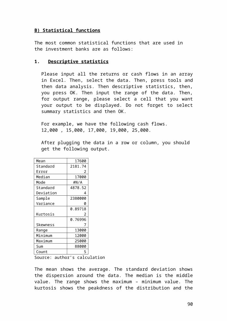
Share price 90      Exercise 80      Interest rate (r) 0.07      

Dividend yield (q) 0.02  

Black and Scholes call option 14.48 

Maturity (T) 0.5   Monte Carlo value 12.67Volatility (σ) 0.3               Simulations 40      Drift 0.0025      sig 0.2121      Discount factor 0.9656               

Simulations randomStandard normal Share price

Call option payoff

1.00 0.38 -0.30 84.58 4.582.00 0.69 0.50 100.38 20.383.00 0.61 0.27 95.48 0.004.00 0.38 -0.32 84.36 4.365.00 0.50 0.01 90.46 10.466.00 0.17 -0.95 73.79 0.007.00 0.54 0.11 92.39 12.398.00 0.03 -1.86 60.78 0.009.00 0.43 -0.17 86.94 6.94

10.00 0.79 0.79 106.79 26.7911.00 0.70 0.53 100.90 20.9012.00 0.84 1.01 111.83 31.8313.00 0.03 -1.84 61.05 0.0014.00 0.07 -1.49 65.76 0.0015.00 0.24 -0.70 77.78 0.0016.00 0.83 0.97 110.86 30.8617.00 0.79 0.80 106.85 26.8518.00 0.26 -0.66 78.48 0.0019.00 0.29 -0.54 80.44 0.4420.00 0.88 1.20 116.32 36.32

90

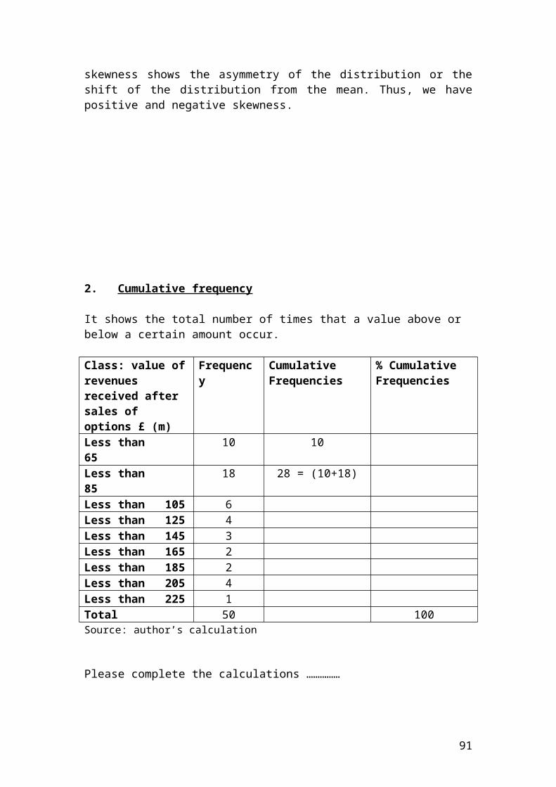
21.00 0.68 0.47 99.71 19.7122.00 0.56 0.14 92.98 12.9823.00 0.21 -0.82 75.81 0.0024.00 0.18 -0.91 74.33 0.0025.00 0.22 -0.77 76.69 0.0026.00 0.77 0.73 105.45 25.4527.00 0.43 -0.18 86.85 6.8528.00 0.69 0.49 100.07 20.0729.00 0.87 1.13 114.78 34.7830.00 0.87 1.12 114.49 34.4931.00 0.37 -0.34 83.90 3.9032.00 0.33 -0.43 82.29 2.2933.00 0.37 -0.33 84.17 4.1734.00 0.73 0.62 102.99 22.9935.00 0.06 -1.55 64.94 0.0036.00 0.69 0.48 99.98 19.9837.00 0.17 -0.97 73.45 0.0038.00 0.45 -0.12 88.04 8.0439.00 0.90 1.30 118.99 38.9940.00 0.89 1.23 117.14 37.14

      Average 13.12Source: author’s illustration

The following chart shows the simulated share prices in relation to days.

Simulated share prices

020406080

100120140

1 5 9 13 17 21 25 29 33 37

Days

Shar

e pr

ices

Share price

91

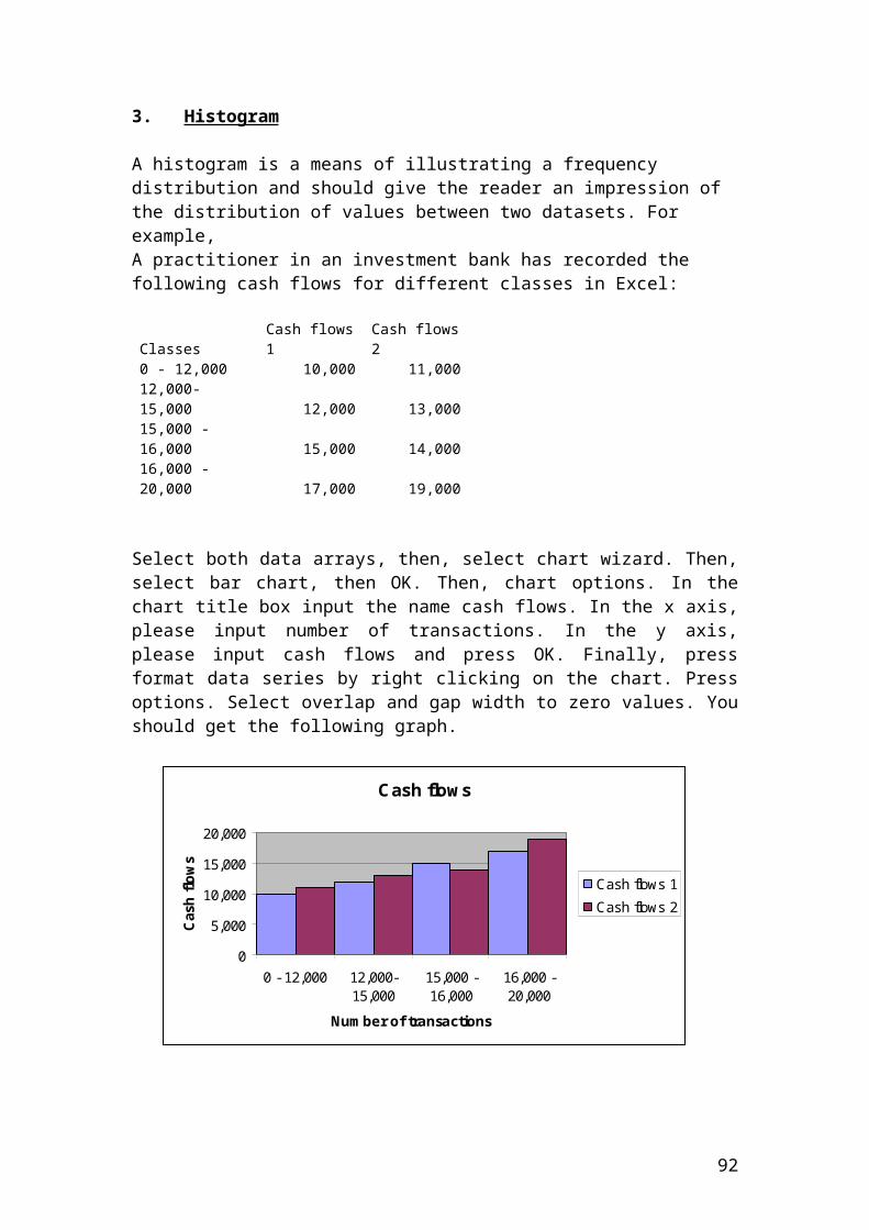
Please consider the following Monte Carlo simulation problem with antithetic variables and compare the value with Black and Scholes call option value.

The formulas to calculate the simulated share prices are as follows:

Share price 1 = Share price * exp[(r-q-0.5σ2)*T + ε*σ*sqrt(T)]Share price 2 = Share price * exp[(r-q-0.5σ2)*T - ε*σ*sqrt(T)]

Where ε: is the standard normal value for each observation. The standard normal function is NORMSINV(rand) and the random function is rand(). You will get different numbers by pressing f9.

The drift is calculated from the formula (r-q-0.5σ2)*T and volatility from the formulaσ*sqrt(T).

The Monte Carlo value was found from the average call option payoff table. The call option payoff for each observation is calculated as share price 1 – Exercise price, share price 2 – Exercise, etc…

Once you have calculated the call option payoff table, you calculate the average and you multiply it by the discount factor to get the Monte Carlo value. The discount factor is calculated from the formula exp(-r*T).

92

Share price 90            Exercise 80            Interest rate 0.07            

Dividend yield 0.02  

Black and Scholes call option 14.48       

Maturity 0.5  MC value

13.28     

Volatility 0.3                           Simulations 40            Drift 0.0025            sig 0.2121            Discount factor 0.9656                           

Simulations randomStandard normal

Share price1

Share price2

Call option payoff1 Call option payoff2 Average payoff

1 0.18 -0.90 80.45 103.75 0.45 23.75 12.102 0.49 -0.02 91.07 91.65 11.07 11.65 11.363 0.09 -1.36 75.41 110.68 0.00 30.68 15.344 0.80 0.83 102.75 81.23 22.75 1.23 11.995 0.87 1.12 107.11 77.93 27.11 0.00 13.556 0.43 -0.17 89.19 93.59 9.19 13.59 11.397 0.29 -0.54 84.62 98.64 4.62 18.64 11.638 0.19 -0.87 80.78 103.32 0.78 23.32 12.059 0.10 -1.26 76.41 109.23 0.00 29.23 14.62

10 0.15 -1.05 78.71 106.04 0.00 26.04 13.0211 0.89 1.25 109.06 76.53 29.06 0.00 14.5312 0.64 0.36 96.06 86.89 16.06 6.89 11.4813 1.00 2.79 135.49 61.60 55.49 0.00 27.7414 0.05 -1.66 72.24 115.53 0.00 35.53 17.7715 0.11 -1.25 76.57 109.01 0.00 29.01 14.5016 0.09 -1.31 75.87 110.01 0.00 30.01 15.0117 0.17 -0.95 79.89 104.48 0.00 24.48 12.2418 0.80 0.84 102.91 81.11 22.91 1.11 12.0119 0.55 0.14 93.14 89.61 13.14 9.61 11.38

93

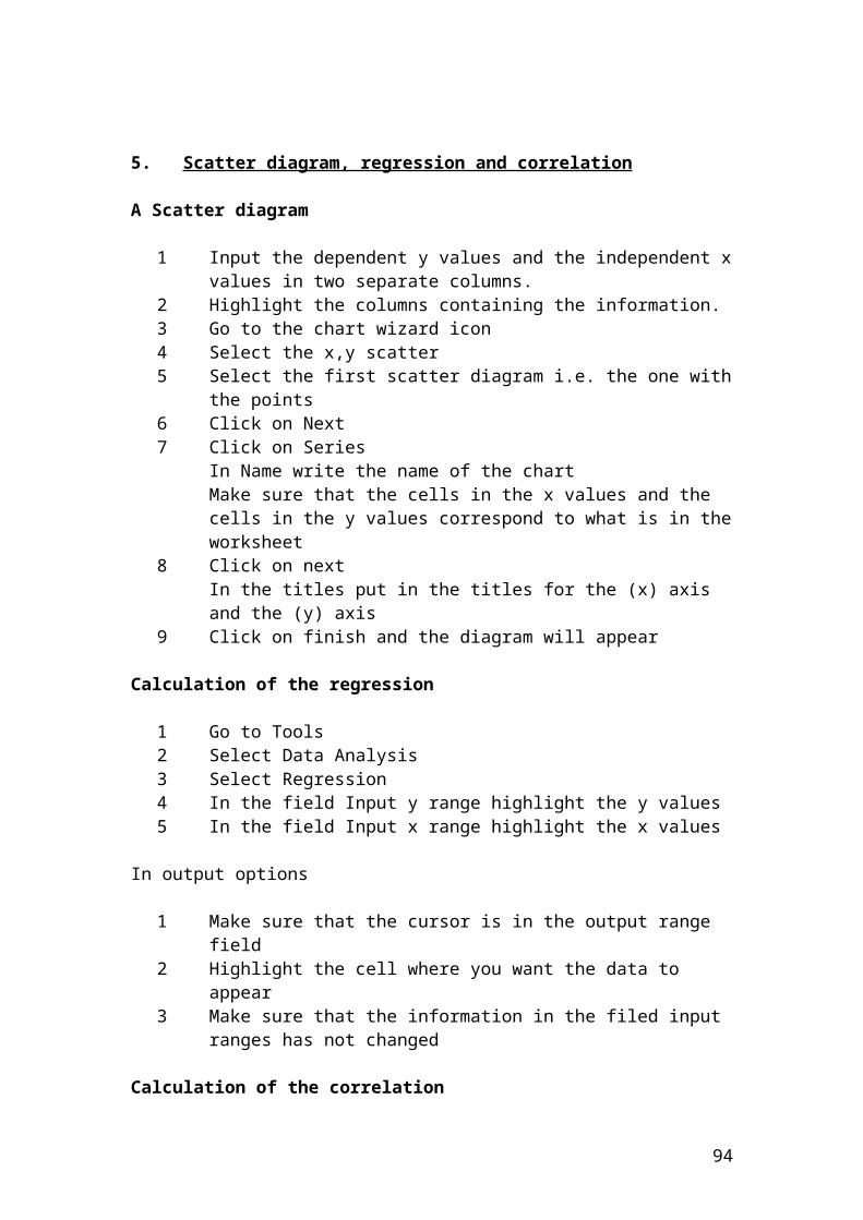
20 0.01 -2.33 65.67 127.11 0.00 47.11 23.5521 0.19 -0.87 80.80 103.30 0.80 23.30 12.0522 0.03 -1.92 69.59 119.93 0.00 39.93 19.9723 0.94 1.56 113.88 73.29 33.88 0.00 16.9424 0.04 -1.71 71.75 116.33 -8.25 36.33 14.0425 0.83 0.95 104.45 79.91 24.45 0.00 12.2226 0.75 0.68 100.65 82.93 20.65 2.93 11.7927 0.25 -0.66 83.18 100.35 3.18 20.35 11.7628 0.27 -0.62 83.73 99.69 3.73 19.69 11.7129 0.72 0.57 99.08 84.24 19.08 4.24 11.6630 0.72 0.59 99.30 84.05 19.30 4.05 11.6831 0.30 -0.51 84.98 98.22 4.98 18.22 11.6032 0.96 1.74 116.81 71.45 36.81 0.00 18.4133 0.25 -0.67 83.12 100.42 3.12 20.42 11.7734 0.65 0.39 96.50 86.50 16.50 6.50 11.5035 0.32 -0.46 85.58 97.53 5.58 17.53 11.5636 0.82 0.93 104.16 80.13 24.16 0.13 12.1537 0.06 -1.59 72.93 114.46 0.00 34.46 17.2338 0.37 -0.32 87.33 95.58 7.33 15.58 11.4539 0.20 -0.85 80.96 103.10 0.96 23.10 12.0340 0.52 0.05 91.96 90.76 11.96 10.76 11.36

            Average 13.75Source: author’s illustration

The following chart shows the simulated share prices in relation to days.

Simulated share prices

0

20

40

60

80

100

120

140

160

1 5 9 13 17 21 25 29 33 37

Days

Shar

e pr

ices

1 a

nd 2

Share price1Share price2

94

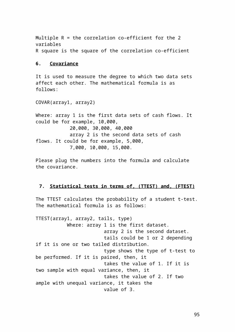
Workshop of language programming in terms of Visual Basic Application, (VBA), in Excel

Visual basic application, (VBA) is a language programming in Excel that facilitates the financial analyst to create successful and powerful models. To be successful with VBA, you should first in a piece of paper state the financial problem that you want to solve. Then, you have to design the appropriate strategy in terms of inputting the correct syntax in the module of VBA that will give instructions to Excel to execute the commands.

To access the visual basic editor, you have two options. The first one is to open Excel and then right click on the toolbar. Then, select visual basic. The second option is to click on Tools and then select macro and then visual basic editor. Once you open the visual basic editor, press insert and then module. Your module is the main page that you will write your VBA code. Explicit reference in terms of inputting the data value will take place in the module page. I will mention very helpful hint to facilitate the writing of the code.

The code always starts with:

Sub test()

The apostrophe signal ‘means the beginning of a comment. It is important to include such comments as they facilitate you to understand what you are going to do later.

The Dim statements list the variables that you are going to use.

Then, input the data.

Then, formula calculation for the different option positions.

End Sub means the end of inputting the code.

Finally, you press F8 to validate the code and check for errors. If there are errors, then, you will get a message of debugging and a yellow line will appear for the line that you have to correct in order to proceed with the validation. Please use the Help object menu in case that you get confused or e-mail me.

95

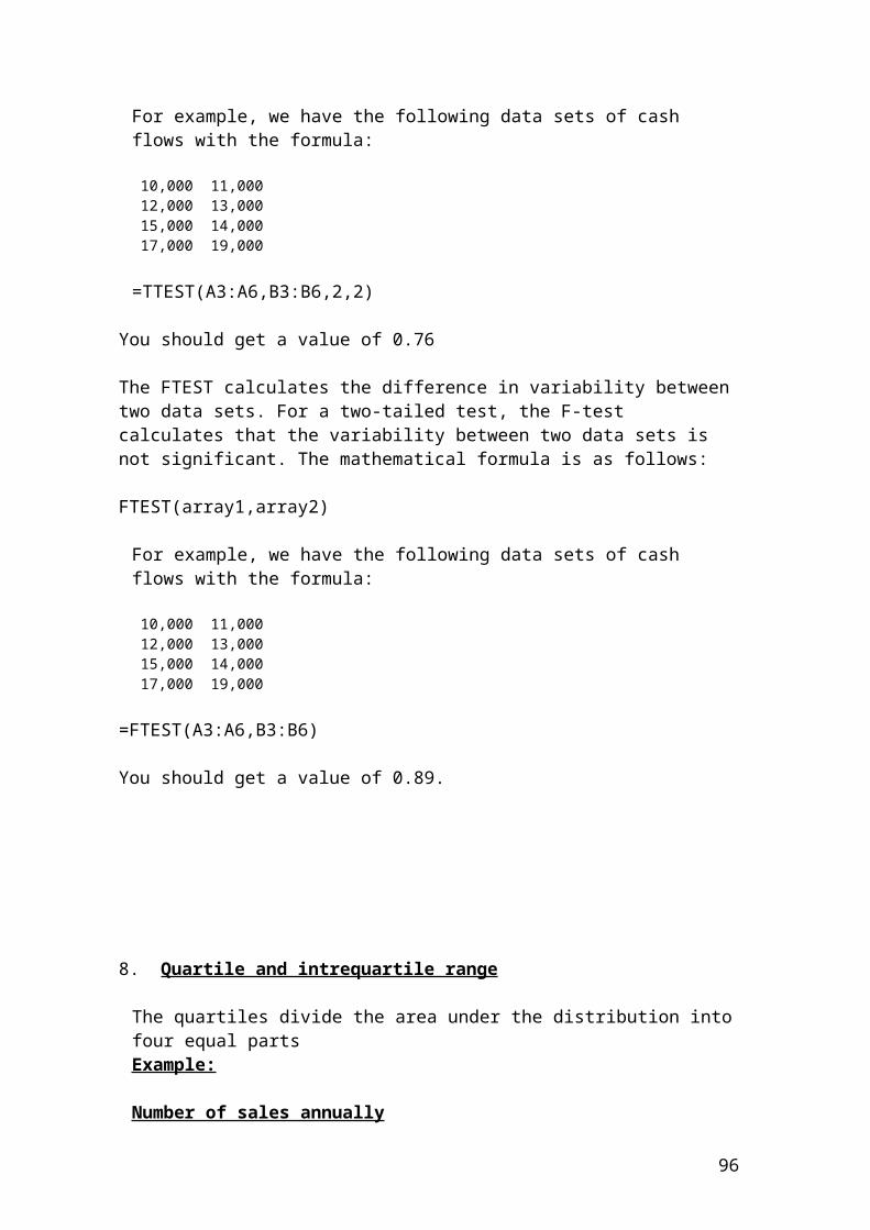
Then, you have the possibility to include other Sub test with other combinations of instructions according to the financial problem that you will be asked to prepare in the investment bank.

For example, Sub test1(), Subtest2() is to turn the font to bold.

End Sub and then again F8 to validate the code in Excel and make the necessary changes.

I have included an example how to create a chart in VBA in terms of Bar staked.Finally, I have included a macro button. By changing the numbers and by clicking on the macro button, it makes the calculations automatically.Sub createchart()End Sub

Example

'It is required to calculate the net result in terms of gains and losses expressed in Pounds from buying call and put options.

' Draw a stacked graph to show the total amounts of buying call and put contracts and the net results in terms of gains and losses expressed in Pounds.

'Data provided

'Share price = 100, 110, 120, 130, 140, 150, 160, 170, 180'Exercise price of a call = 90'Exercise price of a put = 190'Total number of shares = 100 Pounds'Premium of a call = 14'Premium of a put = 9'Total number of contracts = 10

Cell numbers

1

Share price

Cell (A)

Exercise price of a call

Cell (B)

Exercise price of a put

Cell ( C)

Profit or loss from buying a call

Cell (D)

Profit or loss from buying a put

Cell (E)

Net result in terms of gains and losses expressed in Pounds

Cell (F)2 100 90 190 -4000 81000 -850003 110 90 190 6000 71000 -650004 120 90 190 16000 61000 -450005 130 90 190 26000 51000 -250006 140 90 190 36000 41000 -50007 150 90 190 46000 31000 150008 160 90 190 56000 21000 350009 170 90 190 66000 11000 5500010 180 90 190 76000 1000 75000

96

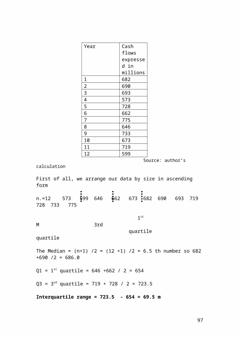
111213 Total number of

shares 10014 Premium of a

call 1415 Premium of a

put 916 Total number of

contracts 10

Source: author’s calculation

VBA code illustration of the above exampleSub test1()

'Question

'It is required to calculate the net result in terms of gains and losses expressed in Pounds from buying call and put options.

'Draw a stacked graph to show the total amounts of buying call and put contracts and the net results in terms of gains and losses expressed in Pounds.

'********************************************************************'Data provided'********************************************************************

'Share price = 100, 110, 120, 130, 140, 150, 160, 170, 180'Exercise price of a call = 90'Exercise price of a put = 190'Total number of shares = 100 Pounds'Premium of a call = 14'Premium of a put = 9'Total number of contracts = 10

'********************************************************************'Variables name that are used in the worksheet VBA for options.'********************************************************************

Dim sp 'Share priceDim exp 'Exercise priceDim bc 'Buy a callDim bp 'Buy a put

Application.Workbooks("VBA for options").Worksheets("sheet1").Range("A1") = "Share price"Application.Workbooks("VBA for options").Worksheets("sheet1").Range("A13") = "Total number of shares"Application.Workbooks("VBA for options").Worksheets("sheet1").Range("A14") = "Premium of a call"

97

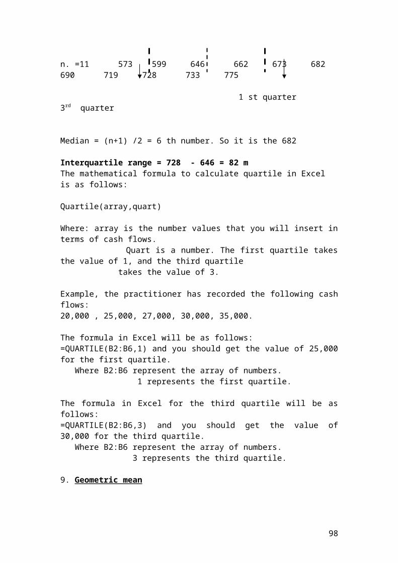
Application.Workbooks("VBA for options").Worksheets("sheet1").Range("A15") = "Premium of a put"Application.Workbooks("VBA for options").Worksheets("sheet1").Range("A16") = "Total number of contracts"Application.Workbooks("VBA for options").Worksheets("sheet1").Range("B1") = "Exercise price of a call"Application.Workbooks("VBA for options").Worksheets("sheet1").Range("C1") = "Exercise price of a put"Application.Workbooks("VBA for options").Worksheets("sheet1").Range("D1") = "Profit or loss from buying a call"Application.Workbooks("VBA for options").Worksheets("sheet1").Range("E1") = "Profit or loss from buying a put"Application.Workbooks("VBA for options").Worksheets("sheet1").Range("F1") = "Net result in terms of gains and losses expressed in Pounds"

'********************************************************************'Input data'********************************************************************Application.Workbooks("VBA for options").Worksheets("sheet1").Range("A2").Value = 100Application.Workbooks("VBA for options").Worksheets("sheet1").Range("A3").Value = 110Application.Workbooks("VBA for options").Worksheets("sheet1").Range("A4").Value = 120Application.Workbooks("VBA for options").Worksheets("sheet1").Range("A5").Value = 130Application.Workbooks("VBA for options").Worksheets("sheet1").Range("A6").Value = 140Application.Workbooks("VBA for options").Worksheets("sheet1").Range("A7").Value = 150Application.Workbooks("VBA for options").Worksheets("sheet1").Range("A8").Value = 160Application.Workbooks("VBA for options").Worksheets("sheet1").Range("A9").Value = 170Application.Workbooks("VBA for options").Worksheets("sheet1").Range("A10").Value = 180

Application.Workbooks("VBA for options").Worksheets("sheet1").Range("B2").Value = 90Application.Workbooks("VBA for options").Worksheets("sheet1").Range("B3").Value = 90Application.Workbooks("VBA for options").Worksheets("sheet1").Range("B4").Value = 90Application.Workbooks("VBA for options").Worksheets("sheet1").Range("B5").Value = 90Application.Workbooks("VBA for options").Worksheets("sheet1").Range("B6").Value = 90Application.Workbooks("VBA for options").Worksheets("sheet1").Range("B7").Value = 90

98

Application.Workbooks("VBA for options").Worksheets("sheet1").Range("B8").Value = 90Application.Workbooks("VBA for options").Worksheets("sheet1").Range("B9").Value = 90Application.Workbooks("VBA for options").Worksheets("sheet1").Range("B10").Value = 90Application.Workbooks("VBA for options").Worksheets("sheet1").Range("B13").Value = 100Application.Workbooks("VBA for options").Worksheets("sheet1").Range("B14").Value = 14Application.Workbooks("VBA for options").Worksheets("sheet1").Range("B15").Value = 9Application.Workbooks("VBA for options").Worksheets("sheet1").Range("B16").Value = 10

Application.Workbooks("VBA for options").Worksheets("sheet1").Range("C2").Value = 190Application.Workbooks("VBA for options").Worksheets("sheet1").Range("C3").Value = 190Application.Workbooks("VBA for options").Worksheets("sheet1").Range("C4").Value = 190Application.Workbooks("VBA for options").Worksheets("sheet1").Range("C5").Value = 190Application.Workbooks("VBA for options").Worksheets("sheet1").Range("C6").Value = 190Application.Workbooks("VBA for options").Worksheets("sheet1").Range("C7").Value = 190Application.Workbooks("VBA for options").Worksheets("sheet1").Range("C8").Value = 190Application.Workbooks("VBA for options").Worksheets("sheet1").Range("C9").Value = 190Application.Workbooks("VBA for options").Worksheets("sheet1").Range("C10").Value = 190

'********************************************************************' Formula calculation'*******************************************************************

Application.Workbooks("VBA for options").Worksheets("sheet1").Range("D2").Formula = "= B13*B16*(A2-B2-B14)"Application.Workbooks("VBA for options").Worksheets("sheet1").Range("D3").Formula = "= B13*B16*(A3-B14-B3)"Application.Workbooks("VBA for options").Worksheets("sheet1").Range("D4").Formula = "= B13*B16*(A4-B4-B14)"Application.Workbooks("VBA for options").Worksheets("sheet1").Range("D5").Formula = "= B13*B16*(A5-B5-B14)"Application.Workbooks("VBA for options").Worksheets("sheet1").Range("D6").Formula = "= B13*B16*(A6-B6-B14)"Application.Workbooks("VBA for options").Worksheets("sheet1").Range("D7").Formula = "= B13*B16*(A7-B7-B14)"

99

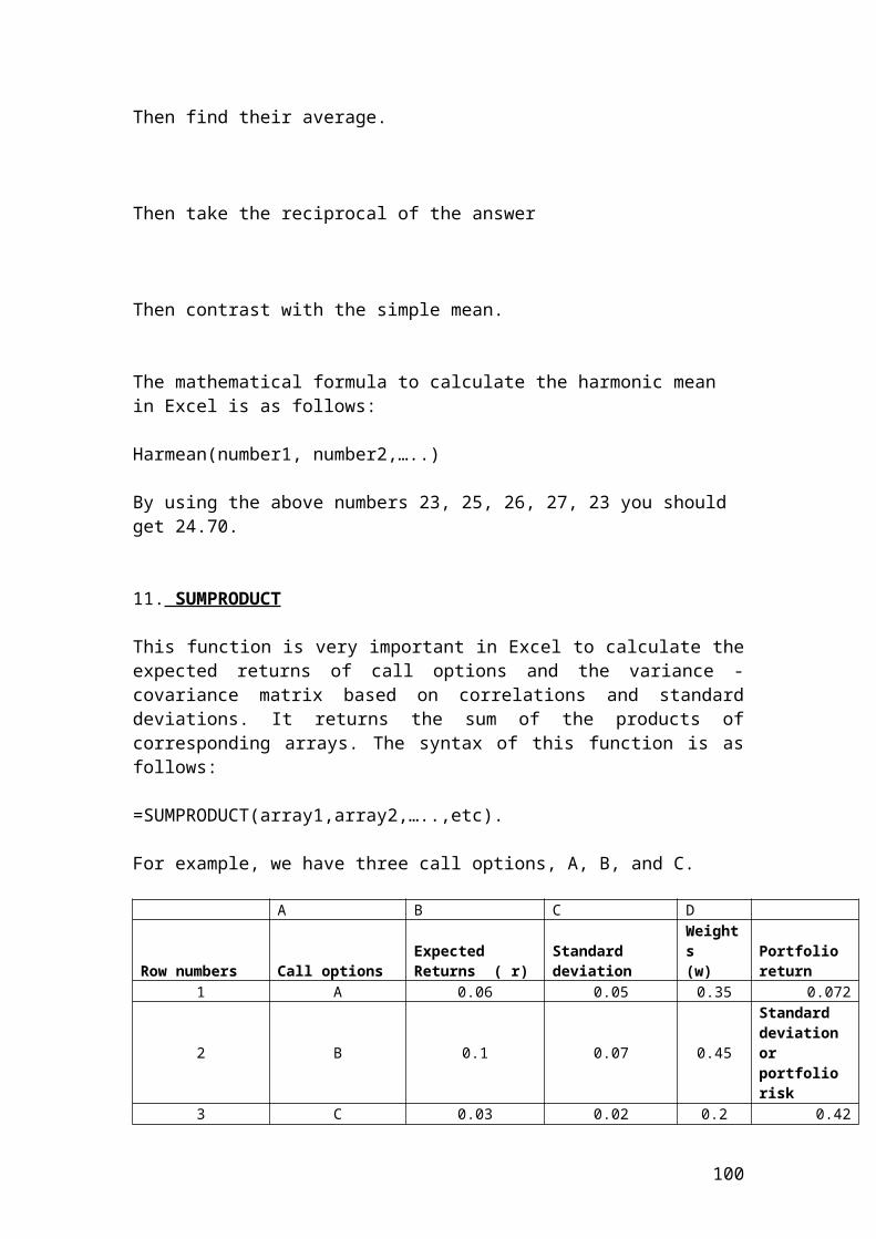
Application.Workbooks("VBA for options").Worksheets("sheet1").Range("D8").Formula = "= B13*B16*(A8-B8-B14)"Application.Workbooks("VBA for options").Worksheets("sheet1").Range("D9").Formula = "= B13*B16*(A9-B9-B14)"Application.Workbooks("VBA for options").Worksheets("sheet1").Range("D10").Formula = "= B13*B16*(A10-B10-B14)"Application.Workbooks("VBA for options").Worksheets("sheet1").Range("E2").Formula = "= B13*B16*(C2-A2-B15)"Application.Workbooks("VBA for options").Worksheets("sheet1").Range("E3").Formula = "= B13*B16*(C3-A3-B15)"Application.Workbooks("VBA for options").Worksheets("sheet1").Range("E4").Formula = "= B13*B16*(C4-A4-B15)"Application.Workbooks("VBA for options").Worksheets("sheet1").Range("E5").Formula = "= B13*B16*(C5-A5-B15)"Application.Workbooks("VBA for options").Worksheets("sheet1").Range("E6").Formula = "= B13*B16*(C6-A6-B15)"Application.Workbooks("VBA for options").Worksheets("sheet1").Range("E7").Formula = "= B13*B16*(C7-A7-B15)"Application.Workbooks("VBA for options").Worksheets("sheet1").Range("E8").Formula = "= B13*B16*(C8-A8-B15)"Application.Workbooks("VBA for options").Worksheets("sheet1").Range("E9").Formula = "= B13*B16*(C9-A9-B15)"Application.Workbooks("VBA for options").Worksheets("sheet1").Range("E10").Formula = "= B13*B16*(C10-A10-B15)"

Application.Workbooks("VBA for options").Worksheets("sheet1").Range("F2").Formula = "= D2-E2"Application.Workbooks("VBA for options").Worksheets("sheet1").Range("F3").Formula = "= D3-E3"Application.Workbooks("VBA for options").Worksheets("sheet1").Range("F4").Formula = "= D4-E4"Application.Workbooks("VBA for options").Worksheets("sheet1").Range("F5").Formula = "= D5-E5"Application.Workbooks("VBA for options").Worksheets("sheet1").Range("F6").Formula = "= D6-E6"Application.Workbooks("VBA for options").Worksheets("sheet1").Range("F7").Formula = "= D7-E7"Application.Workbooks("VBA for options").Worksheets("sheet1").Range("F8").Formula = "= D8-E8"Application.Workbooks("VBA for options").Worksheets("sheet1").Range("F9").Formula = "= D9-E9"Application.Workbooks("VBA for options").Worksheets("sheet1").Range("F10").Formula = "= D10-E10"

End Sub'********************************************************************

100

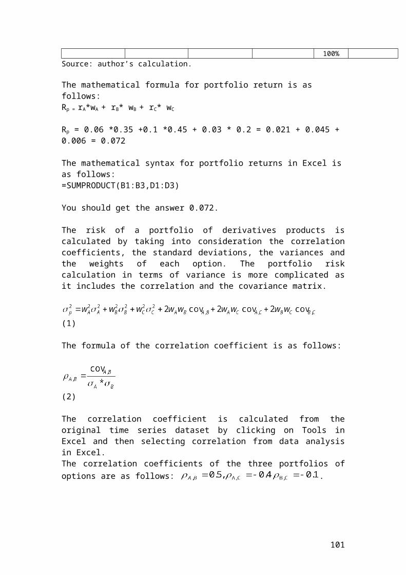
Sub test2()'********************************************************************'Turn font to bold'********************************************************************

ThisWorkbook.Worksheets("Sheet1").Range("A1").Font.Bold = TrueThisWorkbook.Worksheets("Sheet1").Range("B1").Font.Bold = TrueThisWorkbook.Worksheets("Sheet1").Range("C1").Font.Bold = TrueThisWorkbook.Worksheets("Sheet1").Range("D1").Font.Bold = TrueThisWorkbook.Worksheets("Sheet1").Range("E1").Font.Bold = TrueThisWorkbook.Worksheets("Sheet1").Range("F1").Font.Bold = TrueThisWorkbook.Worksheets("Sheet1").Range("A13").Font.Bold = TrueThisWorkbook.Worksheets("Sheet1").Range("A14").Font.Bold = TrueThisWorkbook.Worksheets("Sheet1").Range("A15").Font.Bold = TrueThisWorkbook.Worksheets("Sheet1").Range("A16").Font.Bold = True

End Sub

'********************************************************************Sub createchart()'Cretaing a chart in different Excel sheet.

Dim Chart As ChartSet Chart = Charts.AddChart.SetSourceData Source:=Worksheets("sheet2").Range("A2").CurrentRegion, PlotBy:=xlColumnsChart.ChartType = xl3DBarStacked

End Sub*********************************************************************

-1E+05

-50000 0 50000 100000

150000

200000

1

2

3

4

5

6

7

8

9

Profit or loss frombuying a call

Profit or loss frombuying a put

Net result in terms ofgains and lossesexpressed in Pounds

101

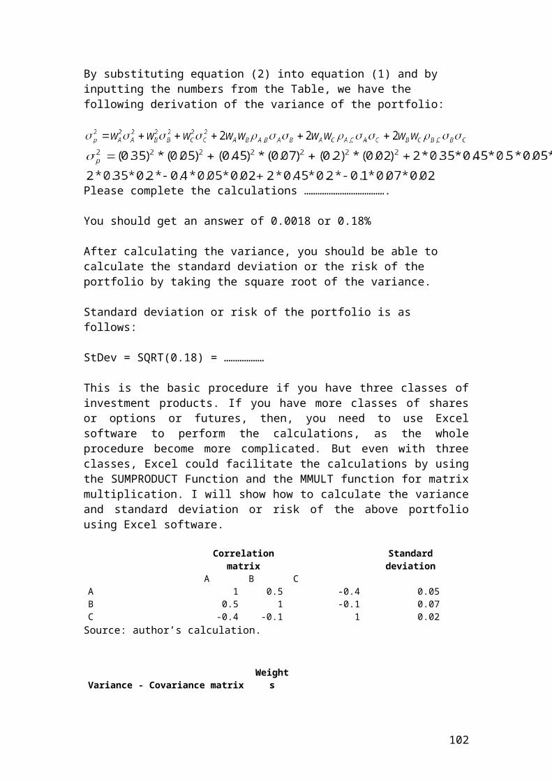
Sub createchart()'Defining the location of the chart and including it in the same Excel sheet.

Dim Chart As ChartSet Chart = Charts.AddSet Chart = Chart.Location(Where:=xlLocationAsObject, Name:="sheet2")Chart.SetSourceData Source:=Worksheets("sheet2").Range("A2:C10").CurrentRegion, PlotBy:=xlColumnsChart.ChartType = xl3DBarStacked

End Sub

-1E+05

-50000 0 50000 100000

150000

200000

1

2

3

4

5

6

7

8

9

Profit or loss frombuying a call

Profit or loss frombuying a put

Net result in terms ofgains and lossesexpressed in Pounds

102

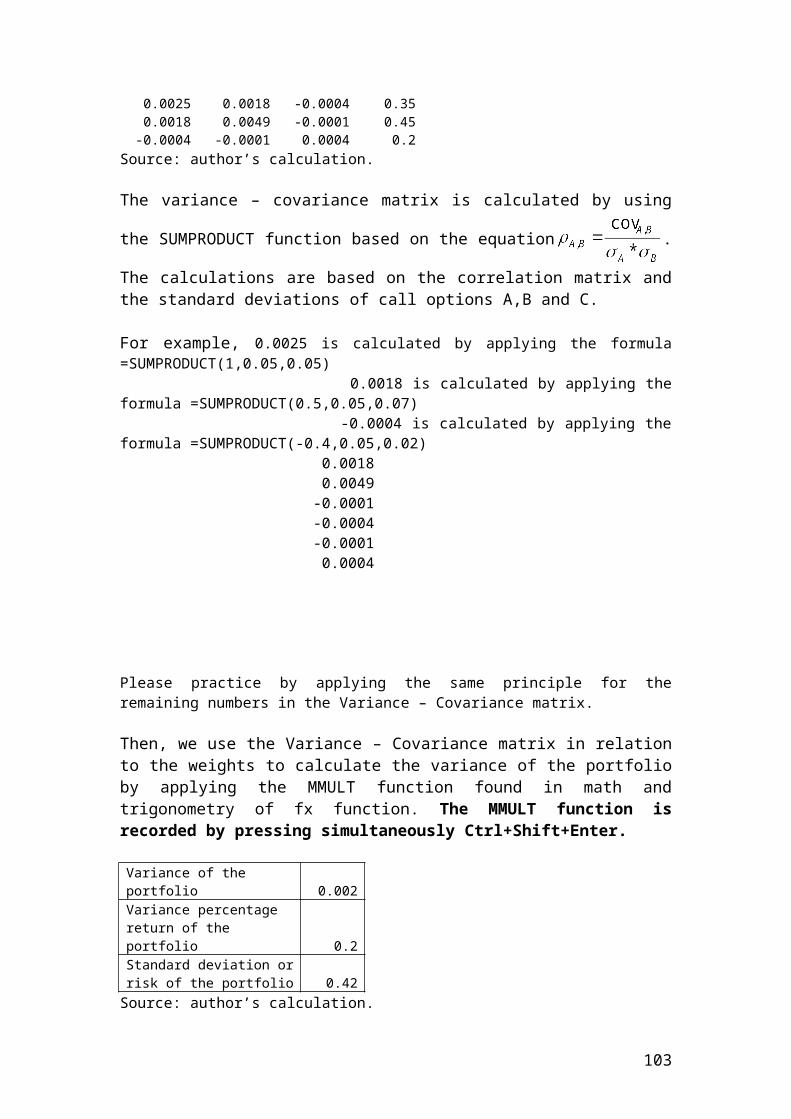
Sub test3()

'Insert of a macro button. By changing the numbers and by clicking on the macro button, it makes the calculations automatically. Application.Workbooks("VBA for options").Worksheets("sheet1").Range("D13") = "Amount of calls expressed in Pounds"Application.Workbooks("VBA for options").Worksheets("sheet1").Range("D18") = "Total"ThisWorkbook.Worksheets("Sheet1").Range("D13").Font.Bold = TrueThisWorkbook.Worksheets("Sheet1").Range("D18").Font.Bold = True

'input data

Sheets("Sheet1").SelectRange("D14").Selecta = ActiveCell.ValueRange("D15").Selectb = ActiveCell.ValueRange("D16").Selectc = ActiveCell.ValueRange("D17").Selectd = ActiveCell.Valuee = a + b + c + d

'output results

Range("D19").SelectActiveCell.Value = e

End Sub

' The VBA language for the CommandButon1 that will calculate automatically the amounts by changing the numbers. Private Sub CommandButton1_Click()

'input data

Sheets("Sheet1").SelectRange("D14").Selecta = ActiveCell.ValueRange("D15").Selectb = ActiveCell.ValueRange("D16").Selectc = ActiveCell.ValueRange("D17").Selectd = ActiveCell.Valuee = a + b + c + d

103

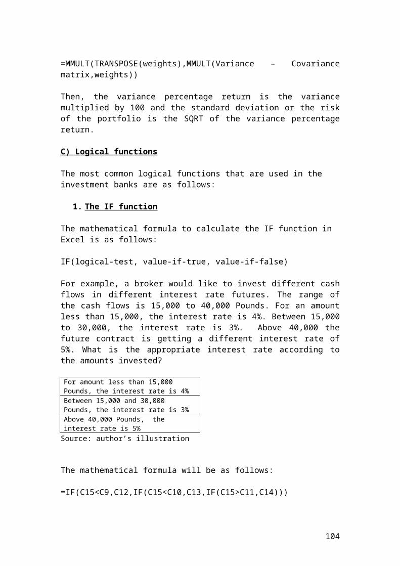
'output results

Range("D19").SelectActiveCell.Value = e

End Sub

Sub test()Worksheets("sheet3").Range("A1") = "Share price"Worksheets("Sheet3").Range("A1").Font.Bold = TrueWorksheets("Sheet3").Range("A2").Value = 40Worksheets("Sheet3").Range("A3").Value = 50Worksheets("Sheet3").Range("A4").Value = 60Worksheets("Sheet3").Range("A5").Value = 70Worksheets("Sheet3").Range("A6").Value = 80Worksheets("Sheet3").Range("A7").Value = 90Worksheets("Sheet3").Range("A8").Value = 95

Worksheets("sheet3").Range("B1") = "Premium of a call"Worksheets("Sheet3").Range("B1").Font.Bold = TrueWorksheets("Sheet3").Range("B2").Value = 4Worksheets("Sheet3").Range("B3").Value = 5Worksheets("Sheet3").Range("B4").Value = 6Worksheets("Sheet3").Range("B5").Value = 7Worksheets("Sheet3").Range("B6").Value = 8Worksheets("Sheet3").Range("B7").Value = 8.8Worksheets("Sheet3").Range("B8").Value = 8.4

Worksheets("sheet3").Range("C1") = "Premium of a put"Worksheets("Sheet3").Range("C1").Font.Bold = TrueWorksheets("Sheet3").Range("C2").Value = 2Worksheets("Sheet3").Range("C3").Value = 3Worksheets("Sheet3").Range("C4").Value = 4Worksheets("Sheet3").Range("C5").Value = 5Worksheets("Sheet3").Range("C6").Value = 6Worksheets("Sheet3").Range("C7").Value = 7.1Worksheets("Sheet3").Range("C8").Value = 7.2

Worksheets("sheet3").Range("D1") = "Volatility of a call"Worksheets("Sheet3").Range("D1").Font.Bold = TrueWorksheets("Sheet3").Range("D2").Value = 0.1Worksheets("Sheet3").Range("D3").Value = 0.14Worksheets("Sheet3").Range("D4").Value = 0.17Worksheets("Sheet3").Range("D5").Value = 0.12Worksheets("Sheet3").Range("D6").Value = 0.13Worksheets("Sheet3").Range("D7").Value = 0.15Worksheets("Sheet3").Range("D8").Value = 0.16

Worksheets("sheet3").Range("E1") = "Volatility of a put"Worksheets("Sheet3").Range("E1").Font.Bold = True

104

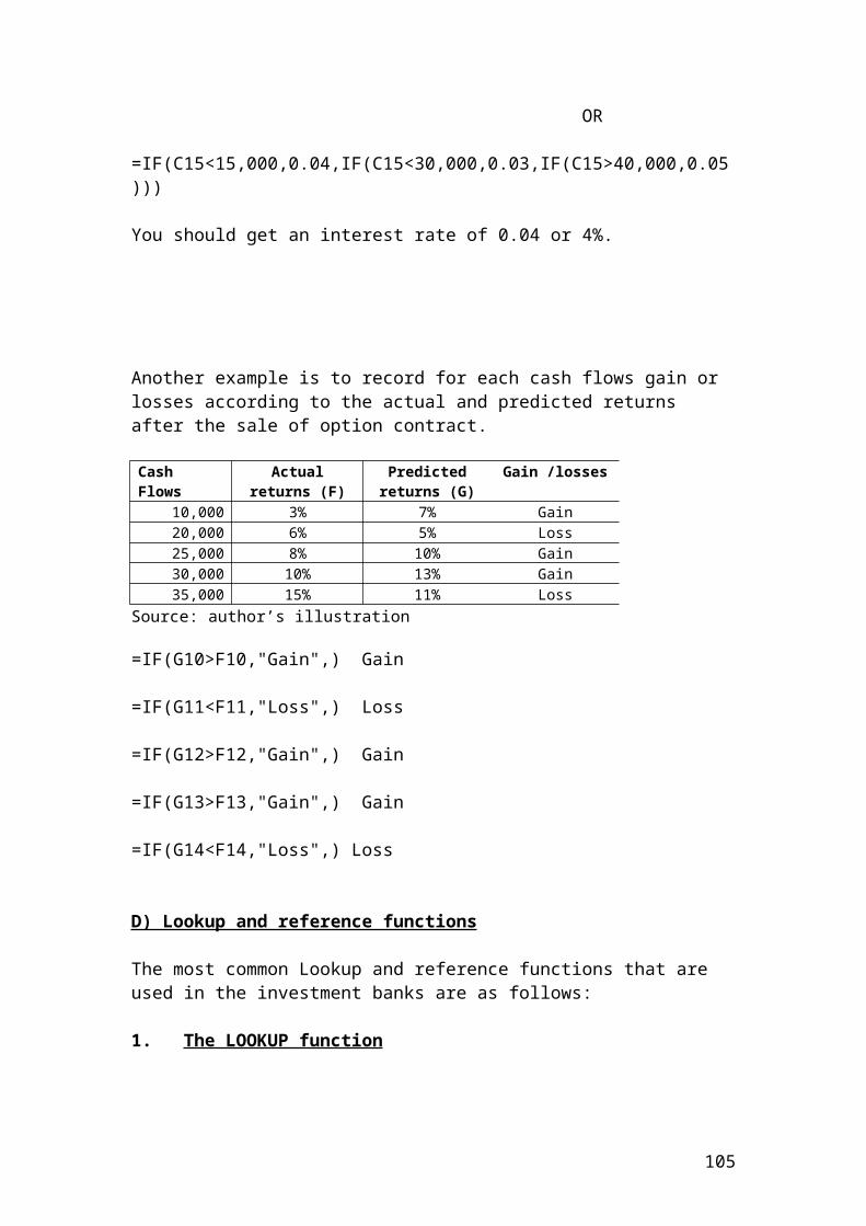
Worksheets("Sheet3").Range("E2").Value = 0.2Worksheets("Sheet3").Range("E3").Value = 0.21Worksheets("Sheet3").Range("E4").Value = 0.18Worksheets("Sheet3").Range("E5").Value = 0.25Worksheets("Sheet3").Range("E6").Value = 0.16Worksheets("Sheet3").Range("E7").Value = 0.19Worksheets("Sheet3").Range("E8").Value = 0.13End Sub

Sub Createchart2()Dim Chart As ChartSet Chart = Charts.AddSet Chart = Chart.Location(Where:=xlLocationAsObject, Name:="sheet3")Chart.SetSourceData Source:=Worksheets("sheet3").Range("A2:E8").CurrentRegion, PlotBy:=xlLineChart.ChartType = xlLineEnd SubSub Entries()

Range("A1") = "Share price returns"Range("A1").Font.Bold = TrueRange("A2").Value = 0.08Range("A3").Value = 0.05Range("A4").Value = 0.04Range("A5").Value = 0.07Range("A6").Value = 0.02Range("A7").Value = 0.03Range("A8") = "Average return"Range("A8").Font.Bold = TrueRange("A9").Formula = "=(A2+A3+A4+A5+A6+A7)/6"Range("A10") = "Harmonic mean"Range("A10").Font.Bold = TrueRange("A11").Formula = "=(1/((1/A2+1/A3+1/A4+1/A5+1/A6+1/A7)/6))"Range("A12") = "Range"Range("A12").Font.Bold = TrueRange("A13").Formula = "=(A2-A6)"Range("A14") = "Geometric mean"Range("A14").Font.Bold = TrueRange("A15").Formula = "=(A2*A3*A4*A5*A6*A7)^0.166666666"

Range("B1") = "Call option returns"Range("B1").Font.Bold = TrueRange("B2").Value = 0.01Range("B3").Value = 0.02Range("B4").Value = 0.04Range("B5").Value = 0.05Range("B6").Value = 0.06Range("B7").Value = 0.08Range("B8") = "Average return"Range("B8").Font.Bold = True

105

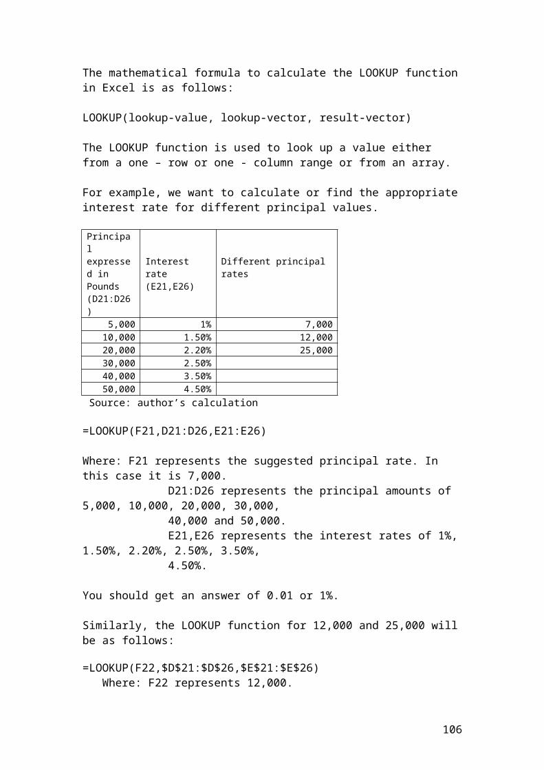
Range("B9").Formula = "=(B2+B3+B4+B5+B6+B7)/6"Range("B10") = "Harmonic mean"Range("B10").Font.Bold = TrueRange("B11").Formula = "=1/((1/B2+1/B3+1/B4+1/B5+1/B6+1/B7)/6)"Range("B12") = "Range"Range("B12").Font.Bold = TrueRange("B13").Formula = "=(B7-B2)"Range("B14") = "Geometric mean"Range("B14").Font.Bold = TrueRange("B15").Formula = "=(B2*B3*B4*B5*B6*B7)^0.166666666"

Range("C1") = "Put option returns"Range("C1").Font.Bold = TrueRange("C2").Value = 0.03Range("C3").Value = 0.07Range("C4").Value = 0.08Range("C5").Value = 0.09Range("C6").Value = 0.1Range("C7").Value = 0.02Range("C8") = "Average return"Range("C8").Font.Bold = TrueRange("C9").Formula = "=(C2+C3+C4+C5+C6+C7)/6"Range("C10") = "Harmonic mean"Range("C10").Font.Bold = TrueRange("C11").Formula = "=1/((1/C2+1/C3+1/C4+1/C5+1/C6+1/C7)/6)"Range("C12") = "Range"Range("C12").Font.Bold = TrueRange("C13").Formula = "=(C6-C7)"Range("C14") = "Geometric mean"Range("C14").Font.Bold = TrueRange("C15").Formula = "=(C2*C3*C4*C5*C6*C7)^0.166666666"

Range("D1") = "Index option returns"Range("D1").Font.Bold = TrueRange("D2").Value = 0.12Range("D3").Value = 0.23Range("D4").Value = 0.34Range("D5").Value = 0.15Range("D6").Value = 0.2Range("D7").Value = 0.11Range("D8") = "Average return"Range("D8").Font.Bold = TrueRange("D9").Formula = "=(D2+D3+D4+D5+D6+D7)/6"Range("D10") = "Harmonic mean"Range("D10").Font.Bold = TrueRange("D11").Formula = "=1/((1/D2+1/D3+1/D4+1/D5+1/D6+1/D7)/6)"Range("D12") = "Range"Range("D12").Font.Bold = TrueRange("D13").Formula = "=(D4-D7)"

106

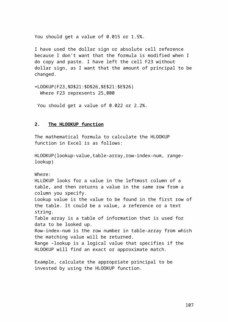
Range("D14") = "Geometric mean"Range("D14").Font.Bold = TrueRange("D15").Formula = "=(D2*D3*D4*D5*D6*D7)^0.166666666"

End Sub

107

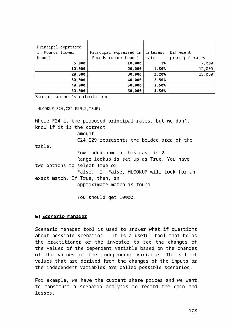
A detailed example of Black and Scholes formula for an European call, put option and the Greeks in Excel and VBA

(A) Parameter (B) Call option (C) Put option

1. S 130 1302. X 100 1003. r 0.08 0.084. σ 0.2 0.25. q 0.03 0.036. T 0.5 0.57. d1 2.1027

=((LN(B1/B2)+(B3-B5+B4^2/2)*B6)/(B4*SQRT(B6)))

2.1027

=((LN(C1/C2)+(C3-C5+C4^2/2)*C6)/(C4*SQRT(C6)))

8. d2 1.9613

=((LN(B1/B2)+(B3-B5-B4^2/2)*B6)/(B4*SQRT(B6)))

1.9613

=((LN(C1/C2)+(C3-C5-C4^2/2)*C6)/(C4*SQRT(C6)))

9. N'(d1) 0.0437=NORMDIST(B7,0,1,FALSE)

0.0437=NORMDIST(C7,0,1,FALSE)

10. N(d1) 0.9823=NORMSDIST(B7)

0.9823=NORMSDIST(C7)

11. N(d2) 0.9751=NORMSDIST(B8)

0.9751=NORMSDIST(C8)

12. N(-d1) 0.0177=NORMSDIST(-B7)

0.0177=NORMSDIST(-C7)

13. N(-d2) 0.0249=NORMSDIST(-B8)

0.0249=NORMSDIST(-C8)

14. Exp(-rT) 0.9608=EXP(-B3*B6)

0.9608=EXP(-C3*C6)

15. Exp(-qT) 0.9851=EXP(-B5*B6)

0.9851=EXP(-C5*C6)

BS value 32.11=B1*B15*B10-B2*B14*B11

0.12=C2*C14*C13-C1*C15*C12

Delta (Δ) is related to changes in share price

0.97

=B15*B10

-0.02

=(C15*(C10-1))Gamma(Γ) is related to changes of delta with respect to the share price

0.002

=((B9*B15)/(B1*B4*SQRT(B6)))

0.002

=((C9*C15)/(C1*C4*SQRT(C6)))

Vega is related 3.96 3.96

108

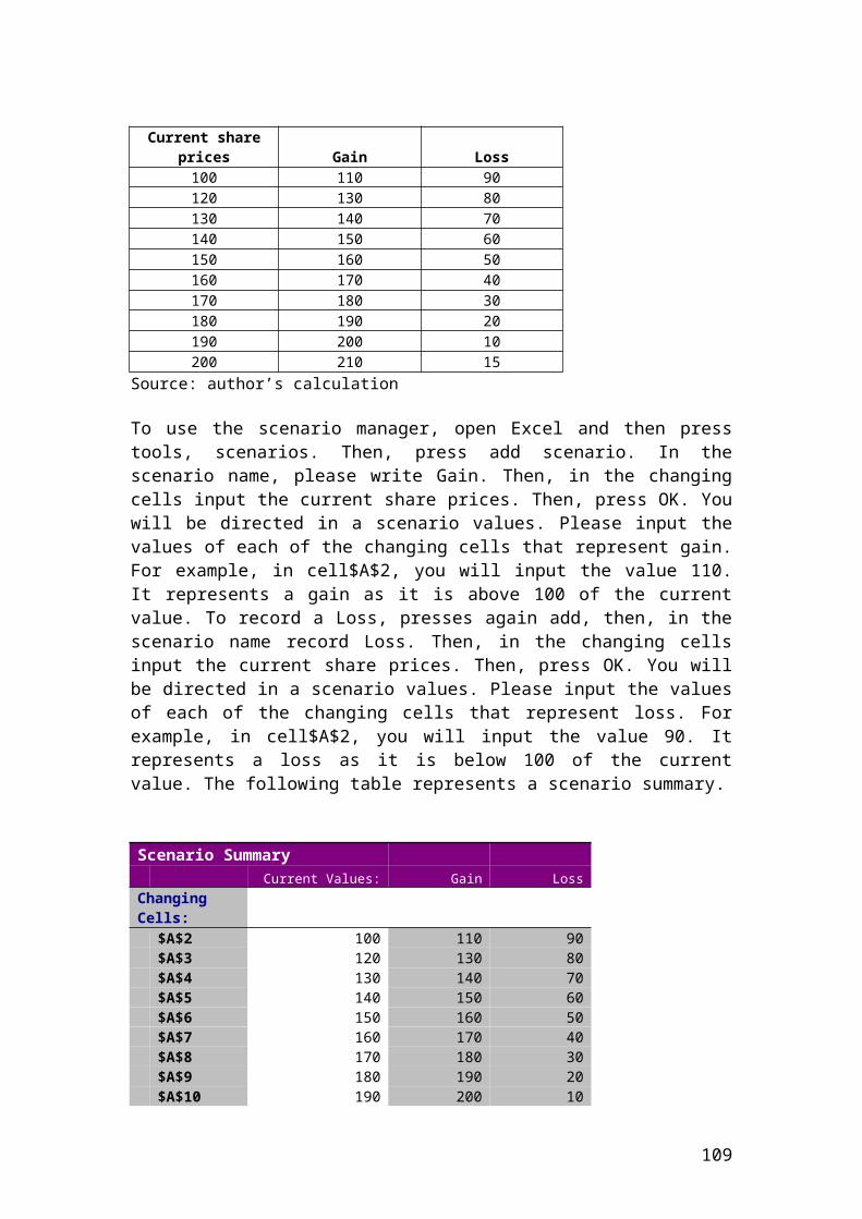
to changes in volatility =B1*SQRT(B6)*B9*B15 =C1*SQRT(C6)*C9*C15Rho (ρ) is related to changes in interest rate

46.84=B2*B6*B14*B11

-1.20

=-(C2*C6*C14*C13)

Theta (-Θ) is related for changes in option life

-4.51

=(B5*B1*B10*B15)-(B3*B2*B14*B11)-((B1*B9*B4*B15)/(2*SQRT(B6)))

-0.67

=-(C5*C1*C10*C15)+(C3*C2*C14*C11)-((C1*C9*C4*C15)/(2*SQRT(C6)))

Hedge ratio0.97

=B15*B100.97

=C15*C10

Source: author’s calculation.

(gamma), measures the change in an option’s delta for a small change in the share price. , (delta), means the change that will occur in the option price for a small change in the share price, when all other factors are constant. For example, a call option has a delta of 0.97. It means that for a small change in share price, the call price will change by 97%. Small Gamma means that changes in delta will be very small. In our case, it is 0.2% small changes and it measures the rate of change of delta in relation to the share price. Vega measures the option value in relation to the volatility. As the volatility increases, the option value increases. In our case, the Vega measure of call option volatility is 3.96%.

Rho is related to change in interest rates. An increase or decrease in interest rate will affect directly the derivative Rho. In our case, a Rho of 46.84 means that increase in percentage point in interest rate, the value of a call option increases by 46.84%. Theta is always negative as it measures the life of the option in relation to the time. As the time passes, the value of the option decreases and gets a negative value.

The following table and chart show the value of a call and a put option contract.

Value of a call option

Value of a put option

15 1418 1121 734 2123 1712 10

Source: author’s calculation.

109

BS model

05

10152025303540

1 2 3 4 5 6

Value of a call option

Valu

e of

a p

ut o

ptio

n

Value of a call optionValue of a put option

Source: author’s illustration.

Please complete the calculations in Excel of the Greek letters that are derived from the Black & Scholes model and interpret your results. Then construct a VBA code with the Greek letters and include a command button that will calculate the results automatically.

(21)

Where: Δ is a call delta option. e is the base of the natural logarithm and it equals 2.71828. In Excel, we use the EXP function. q is the dividend yield. T is time to maturity. N(d1) is the cumulative normal distribution function. In Excel the function of N(d1) is =NORMSDIST(d1).

(22)

Where: Δ is a put delta option. e is the base of the natural logarithm and it equals 2.71828. In Excel, we use the EXP function. q is the dividend yield. T is time to maturity. N(d1) is the cumulative normal distribution function. In Excel the function of N(d1) is =NORMSDIST(d1-1).

(23)

110

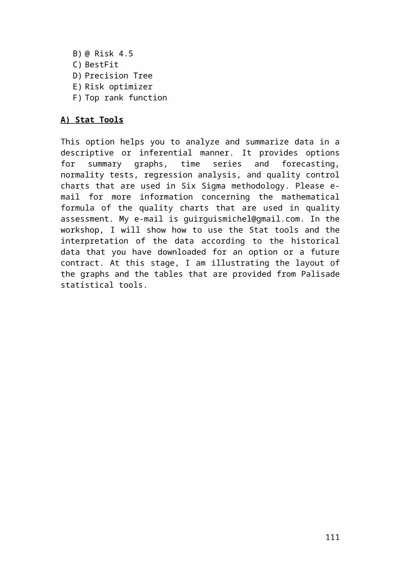
Where: Γ is the same for call and put option.

e is the base of the natural logarithm and it equals 2.71828. In Excel, we use the EXP function. q is the dividend yield. T is the time to maturity. S is the share price. σ is the standard deviation.

(24)

Where: Θ is the theta for call option.

e is the base of the natural logarithm and it equals 2.71828. In Excel, we use the EXP function. N(d1) is the cumulative normal distribution function for a standard normal random variable d1. In Excel the function of N(d1) is =NORMSDIST(d1). N(d2) is the cumulative normal distribution function for a standard normal random variable d2. In Excel the function of N(d2) is =NORMSDIST(d2). q is the dividend yield. T is the time to maturity. S is the share price. σ is the standard deviation.

(25)

Where: Θ is the theta for put option.

111

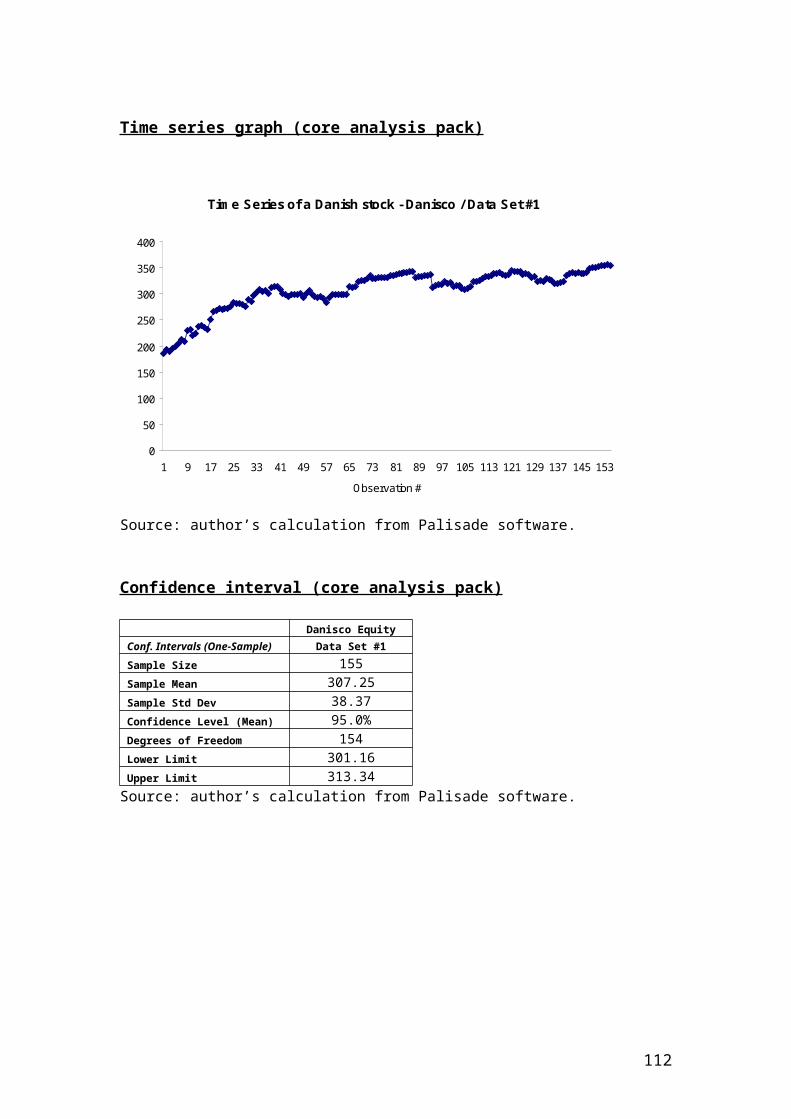
e is the base of the natural logarithm and it equals 2.71828. In Excel, we use the EXP function. N(-d1) is the cumulative normal distribution function for a standard normal random variable d1. In Excel the function of N(-d1) is =NORMSDIST(-d1). N(-d2) is the cumulative normal distribution function for a standard normal random variable d2. In Excel the function of N(-d2) is =NORMSDIST(-d2). q is the dividend yield. T is the time to maturity. S is the share price. σ is the standard deviation.

(26)

Where: Vega is the same for both call and put option. S is the share price. e is the base of the natural logarithm and it equals 2.71828. In Excel, we use the EXP function.

q is the dividend yield. T is the time to maturity.

(27)

Where: Rho is the derivative for call option. e is the base of the natural logarithm and it equals 2.71828. In Excel, we use the EXP function. N(d2) is the cumulative normal distribution function for a standard normal random variable d2. In Excel the function of N(d1) is =NORMSDIST(d2). r is the risk- free interest rate. T is the time to maturity. X is the exercise price.

(28)

Where: Rho is the derivative for put option. e is the base of the natural logarithm and it equals 2.71828. In Excel, we use the EXP function. N(-d2) is the cumulative normal distribution function for a standard normal random variable d2. In Excel the function of N(-d2) is =NORMSDIST(-d2).

112

r is the risk- free interest rate. T is the time to maturity. X is the exercise price.

Example of interpreting the Greek results

Delta The amount that the share price will change if the market moves up or down by 1 basis point or 0.01%.

Gamma The amount that the Delta will change if the market moves up or down by 1 basis point or 0.01%.

Theta The amount that the share price will change as the time decay.

Vega The amount that the share price will change if the volatility of the asset moves up or down by 1 percentage basis point.For example, 10 basis points of volatility are equivalent to 0.1%

Rho The amount that the share price will change if interest rates move up or down by 1 percentage basis point. For example, 20 basis points of interest rate are equivalent to 0.20%

Source: author’s illustration

Calculate the pricing formula of an European option call and put and the Greeks in VBA by including a command button to perform the calculations automatically for options with different prices. Then, calculate the profit / loss position of your trading day. Please use the following data. It is the same example as in page 100. You could check again the formulas.

Parameter(A)

Call option(B)

Parameter( C )

Put option(D)

113

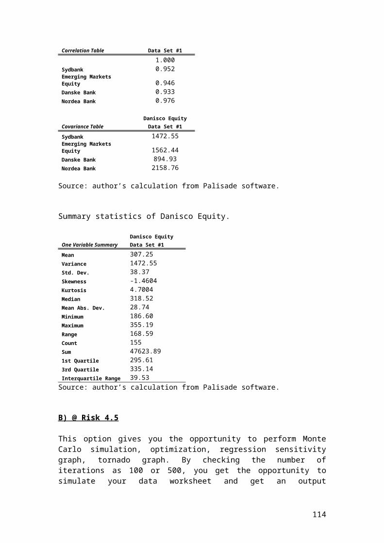
1 S 130 S 1302 X 100 X 1003 r 0.08 r 0.084 σ 0.2 σ 0.25 q 0.03 q 0.036 T 0.5 T 0.57 d1 d18 d2 d29 N'(d1) N'(d1)10 N(d1) N(d1)11 N(d2) N(d2)12 N(-d1) N(-d1)13 N(-d2) N(-d2)14 exp(-rT) exp(-rT)15 exp(-qT) exp(-qT)16 BS value BS value 17 Delta (Δ) is

related to changes in share price.

Delta (Δ) is related to changes in share price.

18 Gamma(Γ) is related to changes of delta with respect to the share price.

Gamma(Γ) is related to changes of delta with respect to the share price.

19 Vega is related to changes in volatility.

Vega is related to changes in volatility.

20Rho (ρ) is related to changes in interest rate.

Rho (ρ) is related to changes in interest rate.

21 Theta (-Θ) is related for changes in option life.

Theta (-Θ) is related for changes in option life.

22 Hedge ratio. Hedge ratio.Source: author’s calculation.

Example

' Calculate the pricing formula of an European option call and the Greeks in VBA' by including a command button to perform the calculations automatically for' options with different prices. Then, calculate the profit / loss position of your trading 'day.

'S Spot price or share price of the underlying security. 130'X Strike or exercise price of the option. 100

114

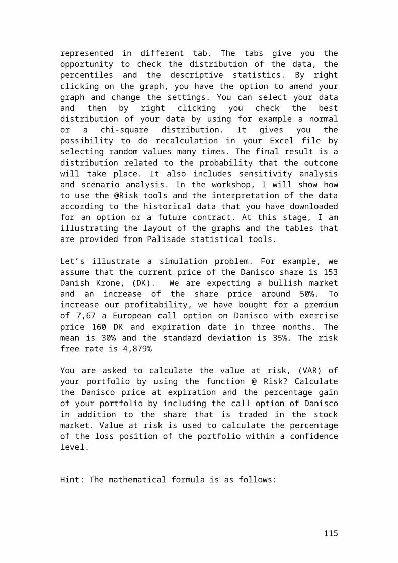
'r Risk - free interest rate. 0.08's Annual volatility for the underlying security. 0.2'd Dividend yield. 0.03'T Time left to maturity of the option. 0.5'********************************************************************Worksheets("sheet3").Range("A1") = "Share price"Worksheets("Sheet3").Range("A1").Font.Bold = TrueWorksheets("Sheet3").Range("B1").Value = 130Worksheets("Sheet3").Range("A2") = "Strike price"Worksheets("Sheet3").Range("A2").Font.Bold = TrueWorksheets("Sheet3").Range("B2").Value = 100Worksheets("Sheet3").Range("A3") = "Interest rate"Worksheets("Sheet3").Range("A3").Font.Bold = TrueWorksheets("Sheet3").Range("B3").Value = 0.08Worksheets("Sheet3").Range("A4") = "Sigma or volatility"Worksheets("Sheet3").Range("A4").Font.Bold = TrueWorksheets("Sheet3").Range("B4").Value = 0.2Worksheets("Sheet3").Range("A5") = "Dividend yield"Worksheets("Sheet3").Range("A5").Font.Bold = TrueWorksheets("Sheet3").Range("B5").Value = 0.03Worksheets("Sheet3").Range("A6") = "Time to maturity"Worksheets("Sheet3").Range("A6").Font.Bold = TrueWorksheets("Sheet3").Range("B6").Value = 0.5Worksheets("sheet3").Range("A7") = "d1"Worksheets("Sheet3").Range("A7").Font.Bold = TrueWorksheets("Sheet3").Range("B7").Formula = "=((LN(B1/B2)+(B3-B5+B4^2/2)*B6)/(B4*SQRT(B6)))"Worksheets("sheet3").Range("A8") = "d2"Worksheets("Sheet3").Range("A8").Font.Bold = TrueWorksheets("Sheet3").Range("B8").Formula = "=((LN(B1/B2)+(B3-B5-B4^2/2)*B6)/(B4*SQRT(B6)))"Worksheets("sheet3").Range("A9") = "N'(d1)"Worksheets("Sheet3").Range("A9").Font.Bold = TrueWorksheets("Sheet3").Range("B9").Formula = "=NORMDIST(B7,0,1,FALSE)"Worksheets("sheet3").Range("A10") = "N(d1)"Worksheets("Sheet3").Range("A10").Font.Bold = TrueWorksheets("Sheet3").Range("B10").Formula = "=NORMSDIST(B7)"Worksheets("sheet3").Range("A11") = "N(d2)"Worksheets("Sheet3").Range("A11").Font.Bold = TrueWorksheets("Sheet3").Range("B11").Formula = "=NORMSDIST(B8)"Worksheets("sheet3").Range("A12") = "N(-d1)"Worksheets("Sheet3").Range("A12").Font.Bold = TrueWorksheets("Sheet3").Range("B12").Formula = "=NORMSDIST(-B7)"Worksheets("sheet3").Range("A13") = "N(-d2)"Worksheets("Sheet3").Range("A13").Font.Bold = TrueWorksheets("Sheet3").Range("B13").Formula = "=NORMSDIST(-B8)"Worksheets("sheet3").Range("A14") = "exp(-rT)"Worksheets("Sheet3").Range("A14").Font.Bold = TrueWorksheets("Sheet3").Range("B14").Formula = "=EXP(-B3*B6)"Worksheets("sheet3").Range("A15") = "exp(-qT)"

115

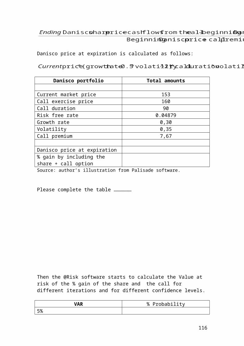
Worksheets("Sheet3").Range("A15").Font.Bold = TrueWorksheets("Sheet3").Range("B15").Formula = "=EXP(-B5*B6)"Worksheets("sheet3").Range("A16") = "BS value of a call option"Worksheets("Sheet3").Range("A16").Font.Bold = TrueWorksheets("Sheet3").Range("B16").Formula = "=(B1*B15*B10-B2*B14*B11)"Worksheets("sheet3").Range("A17") = "Delta"Worksheets("Sheet3").Range("A17").Font.Bold = TrueWorksheets("Sheet3").Range("B17").Formula = "=B15*B10"Worksheets("sheet3").Range("A18") = "Gamma"Worksheets("Sheet3").Range("A18").Font.Bold = TrueWorksheets("Sheet3").Range("B18").Formula = "=((B9*B15)/(B1*B4*SQRT(B6)))"Worksheets("sheet3").Range("A19") = "Vega"Worksheets("Sheet3").Range("A19").Font.Bold = TrueWorksheets("Sheet3").Range("B19").Formula = "=B1*SQRT(B6)*B9*B15"Worksheets("sheet3").Range("A20") = "Rho"Worksheets("Sheet3").Range("A20").Font.Bold = TrueWorksheets("Sheet3").Range("B20").Formula = "=B2*B6*B14*B11"Worksheets("sheet3").Range("A21") = "Theta"Worksheets("Sheet3").Range("A21").Font.Bold = TrueWorksheets("Sheet3").Range("B21").Formula = "=(B5*B1*B10*B15)-(B3*B2*B14*B11)-((B1*B9*B4*B15)/(2*SQRT(B6)))"Worksheets("sheet3").Range("A22") = "Hedge ratio"Worksheets("Sheet3").Range("A22").Font.Bold = TrueWorksheets("Sheet3").Range("B22").Formula = "=B15*B10"

' Calculate the pricing formula of an European option put and the Greeks in VBA' by including a command button to perform the calculations automatically for' options with different prices. Then, calculate the profit / loss position of your trading 'day.

'S Spot price or share price of the underlying security. 130'X Strike or exercise price of the option. 100'r Risk - free interest rate. 0.08

116

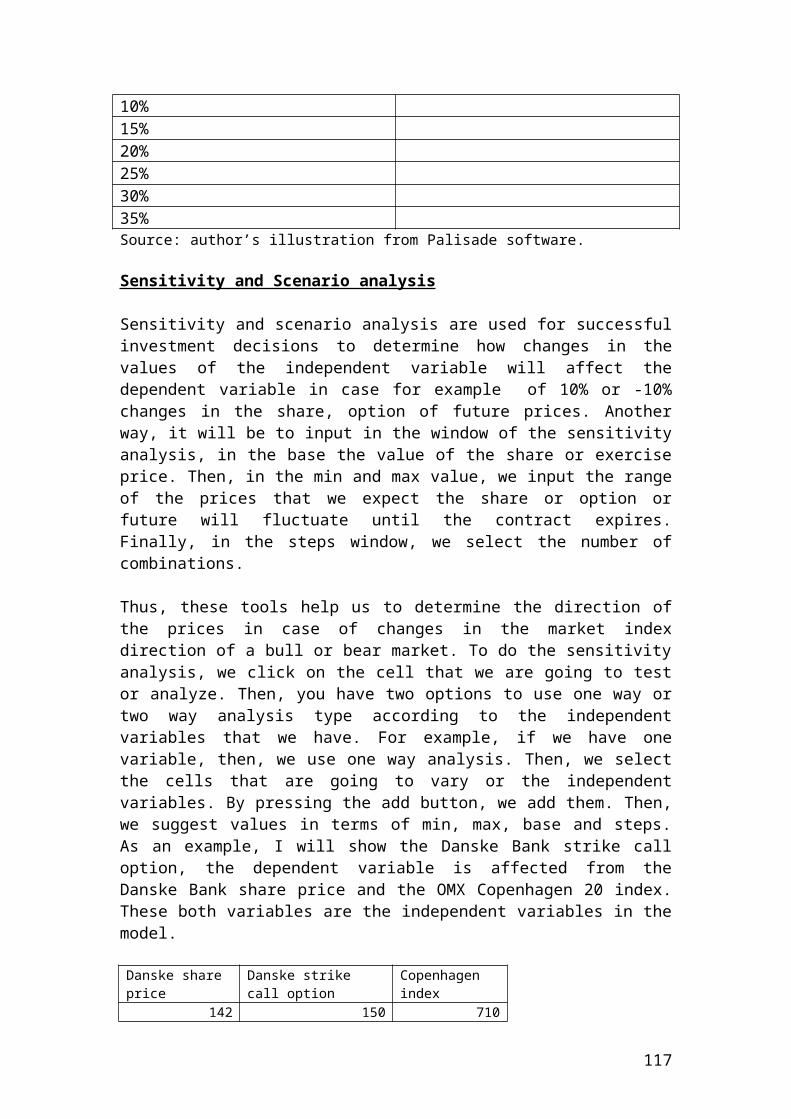
's Annual volatility for the underlying security. 0.2'd Dividend yield. 0.03'T Time left to maturity of the option. 0.5'********************************************************************Worksheets("sheet3").Range("C1") = "Share price"Worksheets("Sheet3").Range("C1").Font.Bold = TrueWorksheets("Sheet3").Range("D1").Value = 130Worksheets("Sheet3").Range("C2") = "Strike price"Worksheets("Sheet3").Range("C2").Font.Bold = TrueWorksheets("Sheet3").Range("D2").Value = 100Worksheets("Sheet3").Range("C3") = "Interest rate"Worksheets("Sheet3").Range("C3").Font.Bold = TrueWorksheets("Sheet3").Range("D3").Value = 0.08Worksheets("Sheet3").Range("C4") = "Sigma or volatility"Worksheets("Sheet3").Range("C4").Font.Bold = TrueWorksheets("Sheet3").Range("D4").Value = 0.2Worksheets("Sheet3").Range("C5") = "Dividend yield"Worksheets("Sheet3").Range("C5").Font.Bold = TrueWorksheets("Sheet3").Range("D5").Value = 0.03Worksheets("Sheet3").Range("C6") = "Time to maturity"Worksheets("Sheet3").Range("C6").Font.Bold = TrueWorksheets("Sheet3").Range("D6").Value = 0.5Worksheets("sheet3").Range("C7") = "d1"Worksheets("Sheet3").Range("C7").Font.Bold = TrueWorksheets("Sheet3").Range("D7").Formula = "=((LN(D1/D2)+(D3-D5+D4^2/2)*D6)/(D4*SQRT(D6)))"Worksheets("sheet3").Range("C8") = "d2"Worksheets("Sheet3").Range("C8").Font.Bold = TrueWorksheets("Sheet3").Range("D8").Formula = "=((LN(D1/D2)+(D3-D5-D4^2/2)*D6)/(D4*SQRT(D6)))"Worksheets("sheet3").Range("C9") = "N'(d1)"Worksheets("Sheet3").Range("C9").Font.Bold = TrueWorksheets("Sheet3").Range("D9").Formula = "=NORMDIST(D7,0,1,FALSE)"Worksheets("sheet3").Range("C10") = "N(d1)"Worksheets("Sheet3").Range("C10").Font.Bold = TrueWorksheets("Sheet3").Range("D10").Formula = "=NORMSDIST(D7)"Worksheets("sheet3").Range("C11") = "N(d2)"Worksheets("Sheet3").Range("C11").Font.Bold = TrueWorksheets("Sheet3").Range("D11").Formula = "=NORMSDIST(D8)"Worksheets("sheet3").Range("C12") = "N(-d1)"Worksheets("Sheet3").Range("C12").Font.Bold = TrueWorksheets("Sheet3").Range("D12").Formula = "=NORMSDIST(-D7)"Worksheets("sheet3").Range("C13") = "N(-d2)"Worksheets("Sheet3").Range("C13").Font.Bold = TrueWorksheets("Sheet3").Range("D13").Formula = "=NORMSDIST(-D8)"Worksheets("sheet3").Range("C14") = "exp(-rT)"Worksheets("Sheet3").Range("C14").Font.Bold = TrueWorksheets("Sheet3").Range("D14").Formula = "=EXP(-D3*D6)"Worksheets("sheet3").Range("C15") = "exp(-qT)"Worksheets("Sheet3").Range("C15").Font.Bold = True

117

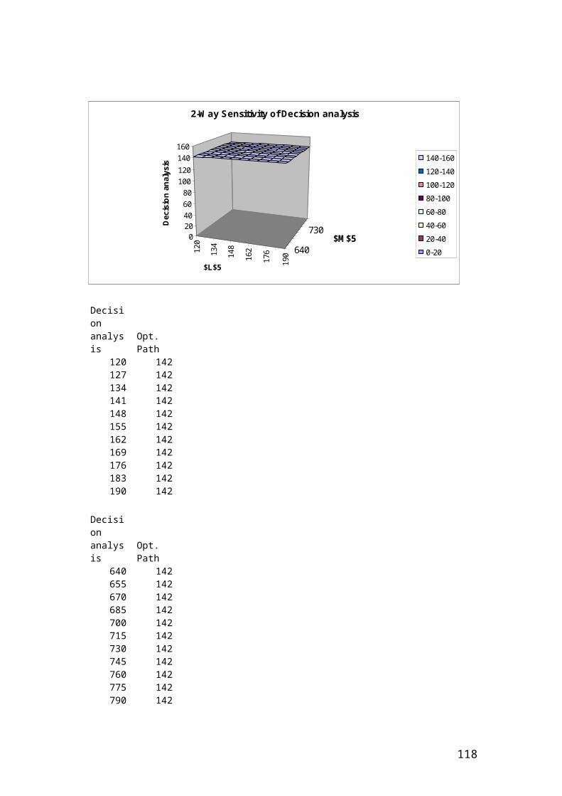
Worksheets("Sheet3").Range("D15").Formula = "=EXP(-D5*D6)"Worksheets("sheet3").Range("C16") = "BS value of a put option"Worksheets("Sheet3").Range("C16").Font.Bold = TrueWorksheets("Sheet3").Range("D16").Formula = "=(D2*D14*D13-D1*D12*D15)"Worksheets("sheet3").Range("C17") = "Delta"Worksheets("Sheet3").Range("C17").Font.Bold = TrueWorksheets("Sheet3").Range("D17").Formula = "=(D15*(D10-1))"Worksheets("sheet3").Range("C18") = "Gamma"Worksheets("Sheet3").Range("C18").Font.Bold = TrueWorksheets("Sheet3").Range("D18").Formula = "=((D9*D15)/(D1*D4*SQRT(D6)))"Worksheets("sheet3").Range("C19") = "Vega"Worksheets("Sheet3").Range("C19").Font.Bold = TrueWorksheets("Sheet3").Range("D19").Formula = "=(D1*SQRT(D6)*D9*D15)"Worksheets("sheet3").Range("C20") = "Rho"Worksheets("Sheet3").Range("C20").Font.Bold = TrueWorksheets("Sheet3").Range("D20").Formula = "=-(D2*D6*D14*D13)"Worksheets("sheet3").Range("C21") = "Theta"Worksheets("Sheet3").Range("C21").Font.Bold = TrueWorksheets("Sheet3").Range("D21").Formula = "=-(D5*D1*D12*D15)+(D3*D2*D14*D13)-((D1*D9*D4*D15)/(2*SQRT(D6)))"Worksheets("sheet3").Range("C22") = "Hedge ratio"Worksheets("Sheet3").Range("C22").Font.Bold = TrueWorksheets("Sheet3").Range("D22").Formula = "=D15*D10"

' Insert a macro command button to perform the calculations automatically.

Worksheets("sheet3").Range("A1") = "Share price"Worksheets("Sheet3").Range("A1").Font.Bold = TrueWorksheets("Sheet3").Range("B1").Value = 130Worksheets("Sheet3").Range("A2") = "Strike price"Worksheets("Sheet3").Range("A2").Font.Bold = TrueWorksheets("Sheet3").Range("B2").Value = 100Worksheets("Sheet3").Range("A3") = "Interest rate"Worksheets("Sheet3").Range("A3").Font.Bold = TrueWorksheets("Sheet3").Range("B3").Value = 0.08Worksheets("Sheet3").Range("A4") = "Sigma or volatility"Worksheets("Sheet3").Range("A4").Font.Bold = TrueWorksheets("Sheet3").Range("B4").Value = 0.2Worksheets("Sheet3").Range("A5") = "Dividend yield"Worksheets("Sheet3").Range("A5").Font.Bold = TrueWorksheets("Sheet3").Range("B5").Value = 0.03Worksheets("Sheet3").Range("A6") = "Time to maturity"Worksheets("Sheet3").Range("A6").Font.Bold = TrueWorksheets("Sheet3").Range("B6").Value = 0.5Worksheets("sheet3").Range("A7") = "d1"Worksheets("Sheet3").Range("A7").Font.Bold = TrueWorksheets("Sheet3").Range("B7").Formula = "=((LN(B1/B2)+(B3-B5+B4^2/2)*B6)/(B4*SQRT(B6)))"Worksheets("sheet3").Range("A8") = "d2"

118

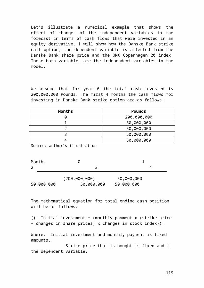
Worksheets("Sheet3").Range("A8").Font.Bold = TrueWorksheets("Sheet3").Range("B8").Formula = "=((LN(B1/B2)+(B3-B5-B4^2/2)*B6)/(B4*SQRT(B6)))"Worksheets("sheet3").Range("A9") = "N'(d1)"Worksheets("Sheet3").Range("A9").Font.Bold = TrueWorksheets("Sheet3").Range("B9").Formula = "=NORMDIST(B7,0,1,FALSE)"Worksheets("sheet3").Range("A10") = "N(d1)"Worksheets("Sheet3").Range("A10").Font.Bold = TrueWorksheets("Sheet3").Range("B10").Formula = "=NORMSDIST(B7)"Worksheets("sheet3").Range("A11") = "N(d2)"Worksheets("Sheet3").Range("A11").Font.Bold = TrueWorksheets("Sheet3").Range("B11").Formula = "=NORMSDIST(B8)"Worksheets("sheet3").Range("A12") = "N(-d1)"Worksheets("Sheet3").Range("A12").Font.Bold = TrueWorksheets("Sheet3").Range("B12").Formula = "=NORMSDIST(-B7)"Worksheets("sheet3").Range("A13") = "N(-d2)"Worksheets("Sheet3").Range("A13").Font.Bold = TrueWorksheets("Sheet3").Range("B13").Formula = "=NORMSDIST(-B8)"Worksheets("sheet3").Range("A14") = "exp(-rT)"Worksheets("Sheet3").Range("A14").Font.Bold = TrueWorksheets("Sheet3").Range("B14").Formula = "=EXP(-B3*B6)"Worksheets("sheet3").Range("A15") = "exp(-qT)"Worksheets("Sheet3").Range("A15").Font.Bold = TrueWorksheets("Sheet3").Range("B15").Formula = "=EXP(-B5*B6)"Worksheets("sheet3").Range("A16") = "BS value of a call option"Worksheets("Sheet3").Range("A16").Font.Bold = TrueWorksheets("Sheet3").Range("B16").Formula = "=(B1*B15*B10-B2*B14*B11)"Worksheets("sheet3").Range("A17") = "Delta"Worksheets("Sheet3").Range("A17").Font.Bold = TrueWorksheets("Sheet3").Range("B17").Formula = "=B15*B10"Worksheets("sheet3").Range("A18") = "Gamma"Worksheets("Sheet3").Range("A18").Font.Bold = TrueWorksheets("Sheet3").Range("B18").Formula = "=((B9*B15)/(B1*B4*SQRT(B6)))"Worksheets("sheet3").Range("A19") = "Vega"Worksheets("Sheet3").Range("A19").Font.Bold = TrueWorksheets("Sheet3").Range("B19").Formula = "=B1*SQRT(B6)*B9*B15"Worksheets("sheet3").Range("A20") = "Rho"Worksheets("Sheet3").Range("A20").Font.Bold = TrueWorksheets("Sheet3").Range("B20").Formula = "=B2*B6*B14*B11"Worksheets("sheet3").Range("A21") = "Theta"Worksheets("Sheet3").Range("A21").Font.Bold = TrueWorksheets("Sheet3").Range("B21").Formula = "=(B5*B1*B10*B15)-(B3*B2*B14*B11)-((B1*B9*B4*B15)/(2*SQRT(B6)))"Worksheets("sheet3").Range("A22") = "Hedge ratio"Worksheets("Sheet3").Range("A22").Font.Bold = TrueWorksheets("Sheet3").Range("B22").Formula = "=B15*B10"Worksheets("sheet3").Range("C1") = "Share price"Worksheets("Sheet3").Range("C1").Font.Bold = TrueWorksheets("Sheet3").Range("D1").Value = 130Worksheets("Sheet3").Range("C2") = "Strike price"

119

Worksheets("Sheet3").Range("C2").Font.Bold = TrueWorksheets("Sheet3").Range("D2").Value = 100Worksheets("Sheet3").Range("C3") = "Interest rate"Worksheets("Sheet3").Range("C3").Font.Bold = TrueWorksheets("Sheet3").Range("D3").Value = 0.08Worksheets("Sheet3").Range("C4") = "Sigma or volatility"Worksheets("Sheet3").Range("C4").Font.Bold = TrueWorksheets("Sheet3").Range("D4").Value = 0.2Worksheets("Sheet3").Range("C5") = "Dividend yield"Worksheets("Sheet3").Range("C5").Font.Bold = TrueWorksheets("Sheet3").Range("D5").Value = 0.03Worksheets("Sheet3").Range("C6") = "Time to maturity"Worksheets("Sheet3").Range("C6").Font.Bold = TrueWorksheets("Sheet3").Range("D6").Value = 0.5Worksheets("sheet3").Range("C7") = "d1"Worksheets("Sheet3").Range("C7").Font.Bold = TrueWorksheets("Sheet3").Range("D7").Formula = "=((LN(D1/D2)+(D3-D5+D4^2/2)*D6)/(D4*SQRT(D6)))"Worksheets("sheet3").Range("C8") = "d2"Worksheets("Sheet3").Range("C8").Font.Bold = TrueWorksheets("Sheet3").Range("D8").Formula = "=((LN(D1/D2)+(D3-D5-D4^2/2)*D6)/(D4*SQRT(D6)))"Worksheets("sheet3").Range("C9") = "N'(d1)"Worksheets("Sheet3").Range("C9").Font.Bold = TrueWorksheets("Sheet3").Range("D9").Formula = "=NORMDIST(D7,0,1,FALSE)"Worksheets("sheet3").Range("C10") = "N(d1)"Worksheets("Sheet3").Range("C10").Font.Bold = TrueWorksheets("Sheet3").Range("D10").Formula = "=NORMSDIST(D7)"Worksheets("sheet3").Range("C11") = "N(d2)"Worksheets("Sheet3").Range("C11").Font.Bold = TrueWorksheets("Sheet3").Range("D11").Formula = "=NORMSDIST(D8)"Worksheets("sheet3").Range("C12") = "N(-d1)"Worksheets("Sheet3").Range("C12").Font.Bold = TrueWorksheets("Sheet3").Range("D12").Formula = "=NORMSDIST(-D7)"Worksheets("sheet3").Range("C13") = "N(-d2)"Worksheets("Sheet3").Range("C13").Font.Bold = TrueWorksheets("Sheet3").Range("D13").Formula = "=NORMSDIST(-D8)"Worksheets("sheet3").Range("C14") = "exp(-rT)"Worksheets("Sheet3").Range("C14").Font.Bold = TrueWorksheets("Sheet3").Range("D14").Formula = "=EXP(-D3*D6)"Worksheets("sheet3").Range("C15") = "exp(-qT)"Worksheets("Sheet3").Range("C15").Font.Bold = TrueWorksheets("Sheet3").Range("D15").Formula = "=EXP(-D5*D6)"Worksheets("sheet3").Range("C16") = "BS value of a put option"Worksheets("Sheet3").Range("C16").Font.Bold = TrueWorksheets("Sheet3").Range("D16").Formula = "=(D2*D14*D13-D1*D12*D15)"Worksheets("sheet3").Range("C17") = "Delta"Worksheets("Sheet3").Range("C17").Font.Bold = TrueWorksheets("Sheet3").Range("D17").Formula = "=(D15*(D10-1))"Worksheets("sheet3").Range("C18") = "Gamma"

120

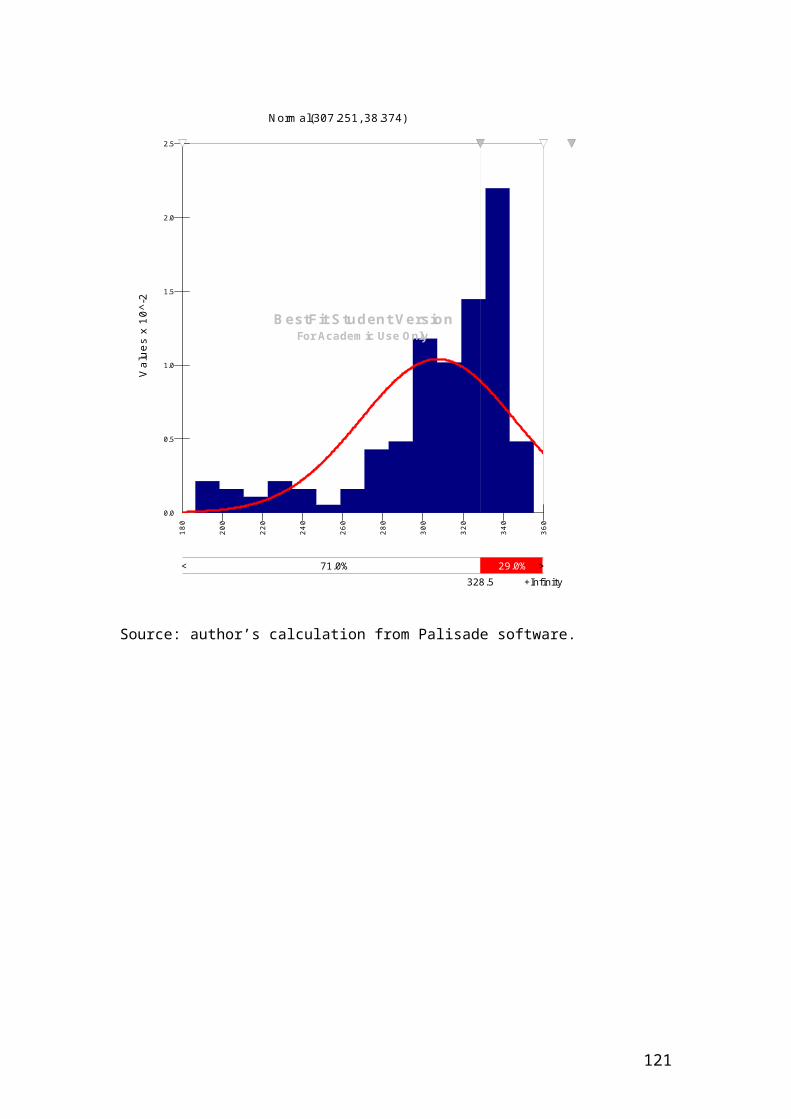
Worksheets("Sheet3").Range("C18").Font.Bold = TrueWorksheets("Sheet3").Range("D18").Formula = "=((D9*D15)/(D1*D4*SQRT(D6)))"Worksheets("sheet3").Range("C19") = "Vega"Worksheets("Sheet3").Range("C19").Font.Bold = TrueWorksheets("Sheet3").Range("D19").Formula = "=(D1*SQRT(D6)*D9*D15)"Worksheets("sheet3").Range("C20") = "Rho"Worksheets("Sheet3").Range("C20").Font.Bold = TrueWorksheets("Sheet3").Range("D20").Formula = "=-(D2*D6*D14*D13)"Worksheets("sheet3").Range("C21") = "Theta"Worksheets("Sheet3").Range("C21").Font.Bold = TrueWorksheets("Sheet3").Range("D21").Formula = "=-(D5*D1*D12*D15)+(D3*D2*D14*D13)-((D1*D9*D4*D15)/(2*SQRT(D6)))"Worksheets("sheet3").Range("C22") = "Hedge ratio"Worksheets("Sheet3").Range("C22").Font.Bold = TrueWorksheets("Sheet3").Range("D22").Formula = "=D15*D10"

End Sub

A detailed example of calculating historical volatility by using Excel and VBA

Historical volatility of a portfolio of options is calculated by using the standard deviation function in Excel. Firstly, we input the daily share prices, then we calculate their log values and finally the standard deviation and we multiply it by . 252 is the number of trading days per year. Historical volatility is based on historical prices and is different from implied volatility. We will discuss about implied volatility in the next section. The derivative’s trader should combine both historical and implied volatility to spot overvalued or undervalued options.

121

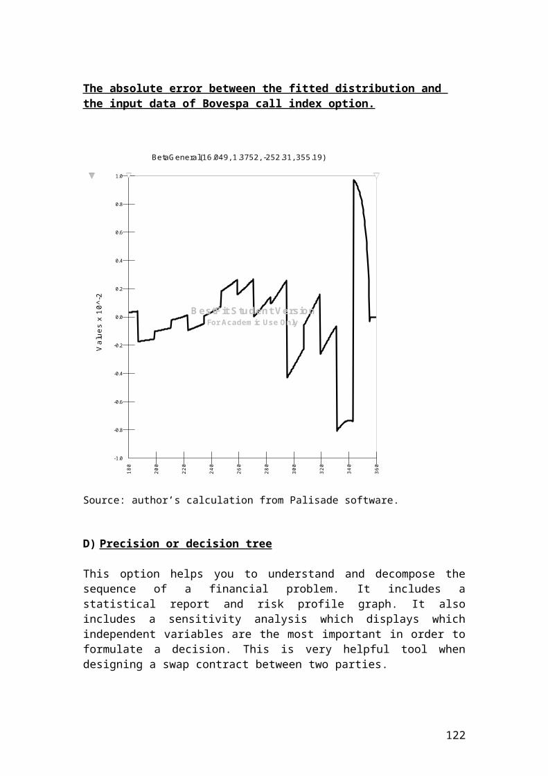
ExampleCalculate the historical volatility of the share prices for 30 days of XYZ option.

(A1) 1 Day (B1) Share price (C1) Ln(St/St-1) (A2) 2 20 (A3) 3 30 0.41 (A4) 4 40 0.29

(A5) 5 50 0.22(A6) 6 60 0.18(A7) 7 70 0.15(A8) 8 80 0.13(A9) 9 90 0.12(A10) 10 100 0.11(A11) 11 110 0.10(A12) 12 120 0.09(A13) 13 130 0.08(A14) 14 140 0.07(A15) 15 150 0.07(A16) 16 160 0.06(A17) 17 170 0.06(A18) 18 180 0.06(A19) 19 190 0.05(A20) 20 200 0.05(A21) 21 210 0.05(A22) 22 220 0.05(A23) 23 230 0.04(A24) 24 240 0.04(A25) 25 250 0.04(A26) 26 260 0.04(A27) 27 270 0.04(A28) 28 280 0.04(A29) 29 290 0.04(A30) 30 300 0.03(A31) 31 310 0.03

(A32)Standard deviation, (STDEV)

0.086

(A33) Daily standard deviation

=0.086*SQRT(252) =1.36

Source: author’s calculation

Example

Please use VBA code to calculate the historical volatility of XYZ option

' Calculate the historical volatility of the share prices for 30 days of XYZ option.'********************************************************************

122

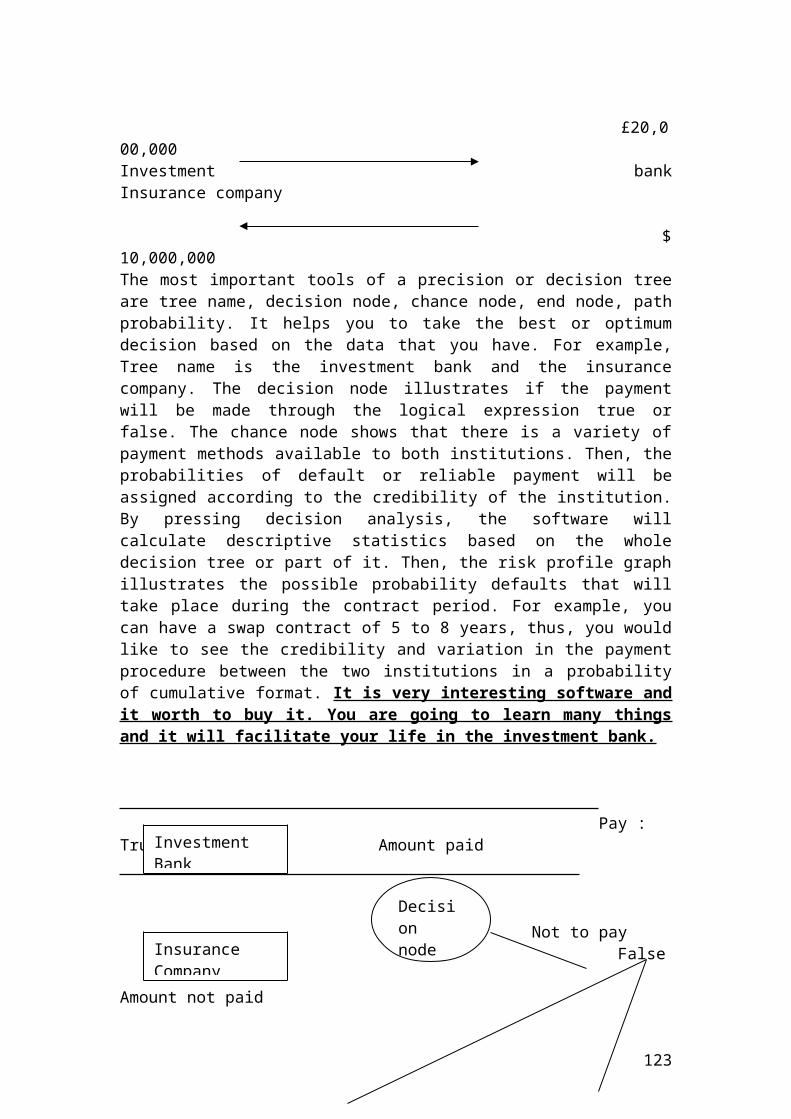
Sub Test()

' Input

Worksheets("sheet2").Range("A1") = "Day"Worksheets("Sheet2").Range("A1").Font.Bold = TrueWorksheets("sheet2").Range("B1") = "Share price"Worksheets("Sheet2").Range("B1").Font.Bold = TrueWorksheets("sheet2").Range("C1") = "ln(St-St-1)"Worksheets("Sheet2").Range("C1").Font.Bold = TrueWorksheets("Sheet2").Range("A2").Value = 1Worksheets("Sheet2").Range("A3").Value = 2Worksheets("Sheet2").Range("A4").Value = 3Worksheets("Sheet2").Range("A5").Value = 4Worksheets("Sheet2").Range("A6").Value = 5Worksheets("Sheet2").Range("A7").Value = 6Worksheets("Sheet2").Range("A8").Value = 7Worksheets("Sheet2").Range("A9").Value = 8Worksheets("Sheet2").Range("A10").Value = 9Worksheets("Sheet2").Range("A11").Value = 10Worksheets("Sheet2").Range("A12").Value = 11Worksheets("Sheet2").Range("A13").Value = 12Worksheets("Sheet2").Range("A14").Value = 13Worksheets("Sheet2").Range("A15").Value = 14Worksheets("Sheet2").Range("A16").Value = 15Worksheets("Sheet2").Range("A17").Value = 16Worksheets("Sheet2").Range("A18").Value = 17Worksheets("Sheet2").Range("A19").Value = 18Worksheets("Sheet2").Range("A20").Value = 19Worksheets("Sheet2").Range("A21").Value = 20Worksheets("Sheet2").Range("A22").Value = 21Worksheets("Sheet2").Range("A23").Value = 22Worksheets("Sheet2").Range("A24").Value = 23Worksheets("Sheet2").Range("A25").Value = 24Worksheets("Sheet2").Range("A26").Value = 25Worksheets("Sheet2").Range("A27").Value = 26Worksheets("Sheet2").Range("A28").Value = 27Worksheets("Sheet2").Range("A29").Value = 28Worksheets("Sheet2").Range("A30").Value = 29Worksheets("Sheet2").Range("A31").Value = 30Worksheets("Sheet2").Range("B2").Value = 20Worksheets("Sheet2").Range("B3").Value = 30Worksheets("Sheet2").Range("B4").Value = 40Worksheets("Sheet2").Range("B5").Value = 50Worksheets("Sheet2").Range("B6").Value = 60Worksheets("Sheet2").Range("B7").Value = 70Worksheets("Sheet2").Range("B8").Value = 80Worksheets("Sheet2").Range("B9").Value = 90Worksheets("Sheet2").Range("B10").Value = 100Worksheets("Sheet2").Range("B11").Value = 110

123

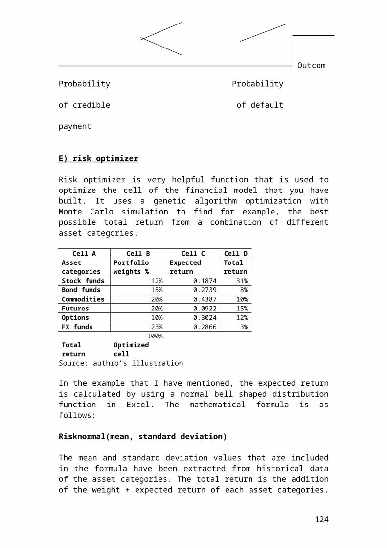
Worksheets("Sheet2").Range("B12").Value = 120Worksheets("Sheet2").Range("B13").Value = 130Worksheets("Sheet2").Range("B14").Value = 140Worksheets("Sheet2").Range("B15").Value = 150Worksheets("Sheet2").Range("B16").Value = 160Worksheets("Sheet2").Range("B17").Value = 170Worksheets("Sheet2").Range("B18").Value = 180Worksheets("Sheet2").Range("B19").Value = 190Worksheets("Sheet2").Range("B20").Value = 200Worksheets("Sheet2").Range("B21").Value = 210Worksheets("Sheet2").Range("B22").Value = 220Worksheets("Sheet2").Range("B23").Value = 230Worksheets("Sheet2").Range("B24").Value = 240Worksheets("Sheet2").Range("B25").Value = 250Worksheets("Sheet2").Range("B26").Value = 260Worksheets("Sheet2").Range("B27").Value = 270Worksheets("Sheet2").Range("B28").Value = 280Worksheets("Sheet2").Range("B29").Value = 290Worksheets("Sheet2").Range("B30").Value = 300Worksheets("Sheet2").Range("B31").Value = 310

'Formula

Worksheets("Sheet2").Range("C3").Formula = "=LN(B3/B2)"Worksheets("Sheet2").Range("C4").Formula = "=LN(B4/B3)"Worksheets("Sheet2").Range("C5").Formula = "=LN(B5/B4)"Worksheets("Sheet2").Range("C6").Formula = "=LN(B6/B5)"Worksheets("Sheet2").Range("C7").Formula = "=LN(B7/B6)"Worksheets("Sheet2").Range("C8").Formula = "=LN(B8/B7)"Worksheets("Sheet2").Range("C9").Formula = "=LN(B9/B8)"Worksheets("Sheet2").Range("C10").Formula = "=LN(B10/B9)"Worksheets("Sheet2").Range("C11").Formula = "=LN(B11/B10)"Worksheets("Sheet2").Range("C12").Formula = "=LN(B12/B11)"Worksheets("Sheet2").Range("C13").Formula = "=LN(B13/B12)"Worksheets("Sheet2").Range("C14").Formula = "=LN(B14/B13)"Worksheets("Sheet2").Range("C15").Formula = "=LN(B15/B14)"Worksheets("Sheet2").Range("C16").Formula = "=LN(B16/B15)"Worksheets("Sheet2").Range("C17").Formula = "=LN(B17/B16)"Worksheets("Sheet2").Range("C18").Formula = "=LN(B18/B17)"Worksheets("Sheet2").Range("C19").Formula = "=LN(B19/B18)"Worksheets("Sheet2").Range("C20").Formula = "=LN(B20/B19)"Worksheets("Sheet2").Range("C21").Formula = "=LN(B21/B20)"Worksheets("Sheet2").Range("C22").Formula = "=LN(B22/B21)"Worksheets("Sheet2").Range("C23").Formula = "=LN(B23/B22)"Worksheets("Sheet2").Range("C24").Formula = "=LN(B24/B23)"Worksheets("Sheet2").Range("C25").Formula = "=LN(B25/B24)"Worksheets("Sheet2").Range("C26").Formula = "=LN(B26/B25)"Worksheets("Sheet2").Range("C27").Formula = "=LN(B27/B26)"Worksheets("Sheet2").Range("C28").Formula = "=LN(B28/B27)"Worksheets("Sheet2").Range("C29").Formula = "=LN(B29/B28)"

124

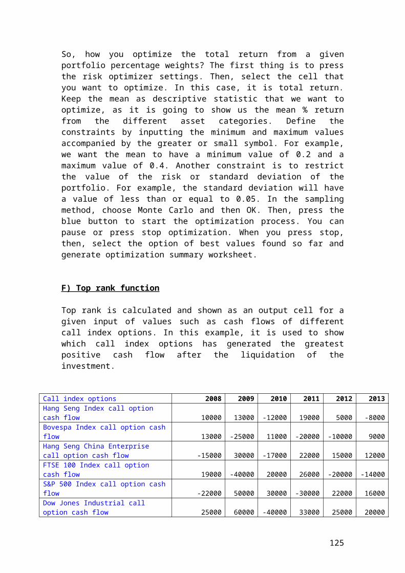
Worksheets("Sheet2").Range("C30").Formula = "=LN(B30/B29)"Worksheets("Sheet2").Range("C31").Formula = "=LN(B31/B30)"Worksheets("Sheet2").Range("C32").Formula = "=SQRT(((((((((((((((((((((((((((((((30*((C3)^2+(C4)^2+(C5)^2+(C6)^2+(C7)^2+(C8)^2+(C9)^2+(C10)^2+(C11)^2+(C12)^2+(C13)^2+(C14)^2+(C15)^2+(C16)^2+(C17)^2+(C18)^2+(C19)^2+(C20)^2+(C21)^2+(C22)^2+(C23)^2+(C24)^2+(C25)^2+(C26)^2+(C27)^2+(C28)^2+(C29)^2+(C30)^2+(C31)^2))-((C3+C4+C5+C6+C7+C8+C9+C10+C11+C12+C13+C14+C15+C16+C17+C18+C19+C20+C21+C22+C23+C24+C25+C26+C27+C28+C29+C30+C31)^2))/(30*(30-1)))))))))))))))))))))))))))))))"Worksheets("sheet2").Range("A32") = "Standard deviation"Worksheets("Sheet2").Range("A32").Font.Bold = TrueWorksheets("sheet2").Range("A33") = "Daily standard deviation"Worksheets("Sheet2").Range("A33").Font.Bold = TrueWorksheets("Sheet2").Range("C33").Formula = "=(C32*SQRT(252))"End Sub

Inserting a macro button to perform the calculations automatically

Private Sub CommandButton1_Click()'InputWorksheets("sheet2").Range("A1") = "Day"Worksheets("Sheet2").Range("A1").Font.Bold = TrueWorksheets("sheet2").Range("B1") = "Share price"Worksheets("Sheet2").Range("B1").Font.Bold = TrueWorksheets("sheet2").Range("C1") = "ln(St-St-1)"Worksheets("Sheet2").Range("C1").Font.Bold = TrueWorksheets("Sheet2").Range("A2").Value = 1Worksheets("Sheet2").Range("A3").Value = 2Worksheets("Sheet2").Range("A4").Value = 3Worksheets("Sheet2").Range("A5").Value = 4Worksheets("Sheet2").Range("A6").Value = 5Worksheets("Sheet2").Range("A7").Value = 6Worksheets("Sheet2").Range("A8").Value = 7Worksheets("Sheet2").Range("A9").Value = 8Worksheets("Sheet2").Range("A10").Value = 9Worksheets("Sheet2").Range("A11").Value = 10Worksheets("Sheet2").Range("A12").Value = 11Worksheets("Sheet2").Range("A13").Value = 12Worksheets("Sheet2").Range("A14").Value = 13Worksheets("Sheet2").Range("A15").Value = 14Worksheets("Sheet2").Range("A16").Value = 15Worksheets("Sheet2").Range("A17").Value = 16Worksheets("Sheet2").Range("A18").Value = 17Worksheets("Sheet2").Range("A19").Value = 18Worksheets("Sheet2").Range("A20").Value = 19Worksheets("Sheet2").Range("A21").Value = 20Worksheets("Sheet2").Range("A22").Value = 21Worksheets("Sheet2").Range("A23").Value = 22Worksheets("Sheet2").Range("A24").Value = 23

125

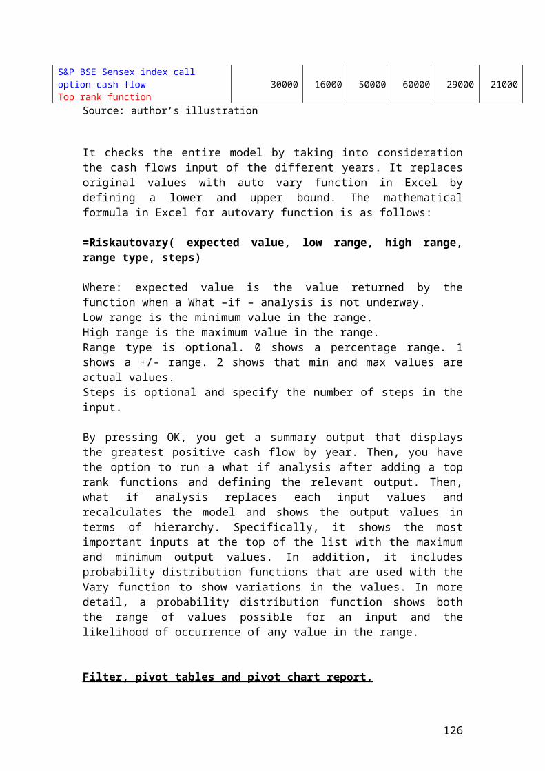
Worksheets("Sheet2").Range("A25").Value = 24Worksheets("Sheet2").Range("A26").Value = 25Worksheets("Sheet2").Range("A27").Value = 26Worksheets("Sheet2").Range("A28").Value = 27Worksheets("Sheet2").Range("A29").Value = 28Worksheets("Sheet2").Range("A30").Value = 29Worksheets("Sheet2").Range("A31").Value = 30Worksheets("Sheet2").Range("B2").Value = 20Worksheets("Sheet2").Range("B3").Value = 30Worksheets("Sheet2").Range("B4").Value = 40Worksheets("Sheet2").Range("B5").Value = 50Worksheets("Sheet2").Range("B6").Value = 60Worksheets("Sheet2").Range("B7").Value = 70Worksheets("Sheet2").Range("B8").Value = 80Worksheets("Sheet2").Range("B9").Value = 90Worksheets("Sheet2").Range("B10").Value = 100Worksheets("Sheet2").Range("B11").Value = 110Worksheets("Sheet2").Range("B12").Value = 120Worksheets("Sheet2").Range("B13").Value = 130Worksheets("Sheet2").Range("B14").Value = 140Worksheets("Sheet2").Range("B15").Value = 150Worksheets("Sheet2").Range("B16").Value = 160Worksheets("Sheet2").Range("B17").Value = 170Worksheets("Sheet2").Range("B18").Value = 180Worksheets("Sheet2").Range("B19").Value = 190Worksheets("Sheet2").Range("B20").Value = 200Worksheets("Sheet2").Range("B21").Value = 210Worksheets("Sheet2").Range("B22").Value = 220Worksheets("Sheet2").Range("B23").Value = 230Worksheets("Sheet2").Range("B24").Value = 240Worksheets("Sheet2").Range("B25").Value = 250Worksheets("Sheet2").Range("B26").Value = 260Worksheets("Sheet2").Range("B27").Value = 270Worksheets("Sheet2").Range("B28").Value = 280Worksheets("Sheet2").Range("B29").Value = 290Worksheets("Sheet2").Range("B30").Value = 300Worksheets("Sheet2").Range("B31").Value = 310

'Formula

Worksheets("Sheet2").Range("C3").Formula = "=LN(B3/B2)"Worksheets("Sheet2").Range("C4").Formula = "=LN(B4/B3)"Worksheets("Sheet2").Range("C5").Formula = "=LN(B5/B4)"Worksheets("Sheet2").Range("C6").Formula = "=LN(B6/B5)"Worksheets("Sheet2").Range("C7").Formula = "=LN(B7/B6)"Worksheets("Sheet2").Range("C8").Formula = "=LN(B8/B7)"Worksheets("Sheet2").Range("C9").Formula = "=LN(B9/B8)"Worksheets("Sheet2").Range("C10").Formula = "=LN(B10/B9)"Worksheets("Sheet2").Range("C11").Formula = "=LN(B11/B10)"Worksheets("Sheet2").Range("C12").Formula = "=LN(B12/B11)"

126

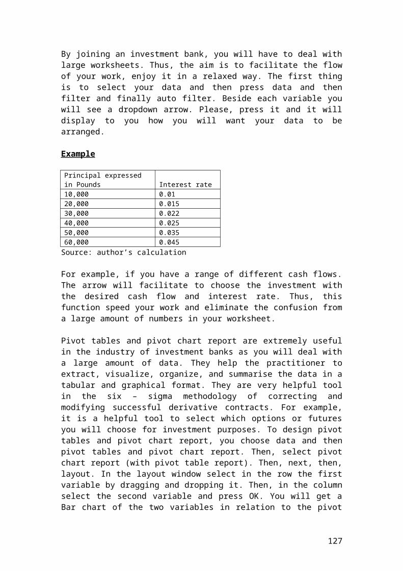
Worksheets("Sheet2").Range("C13").Formula = "=LN(B13/B12)"Worksheets("Sheet2").Range("C14").Formula = "=LN(B14/B13)"Worksheets("Sheet2").Range("C15").Formula = "=LN(B15/B14)"Worksheets("Sheet2").Range("C16").Formula = "=LN(B16/B15)"Worksheets("Sheet2").Range("C17").Formula = "=LN(B17/B16)"Worksheets("Sheet2").Range("C18").Formula = "=LN(B18/B17)"Worksheets("Sheet2").Range("C19").Formula = "=LN(B19/B18)"Worksheets("Sheet2").Range("C20").Formula = "=LN(B20/B19)"Worksheets("Sheet2").Range("C21").Formula = "=LN(B21/B20)"Worksheets("Sheet2").Range("C22").Formula = "=LN(B22/B21)"Worksheets("Sheet2").Range("C23").Formula = "=LN(B23/B22)"Worksheets("Sheet2").Range("C24").Formula = "=LN(B24/B23)"Worksheets("Sheet2").Range("C25").Formula = "=LN(B25/B24)"Worksheets("Sheet2").Range("C26").Formula = "=LN(B26/B25)"Worksheets("Sheet2").Range("C27").Formula = "=LN(B27/B26)"Worksheets("Sheet2").Range("C28").Formula = "=LN(B28/B27)"Worksheets("Sheet2").Range("C29").Formula = "=LN(B29/B28)"Worksheets("Sheet2").Range("C30").Formula = "=LN(B30/B29)"Worksheets("Sheet2").Range("C31").Formula = "=LN(B31/B30)"Worksheets("Sheet2").Range("C32").Formula = "=SQRT(((((((((((((((((((((((((((((((30*((C3)^2+(C4)^2+(C5)^2+(C6)^2+(C7)^2+(C8)^2+(C9)^2+(C10)^2+(C11)^2+(C12)^2+(C13)^2+(C14)^2+(C15)^2+(C16)^2+(C17)^2+(C18)^2+(C19)^2+(C20)^2+(C21)^2+(C22)^2+(C23)^2+(C24)^2+(C25)^2+(C26)^2+(C27)^2+(C28)^2+(C29)^2+(C30)^2+(C31)^2))-((C3+C4+C5+C6+C7+C8+C9+C10+C11+C12+C13+C14+C15+C16+C17+C18+C19+C20+C21+C22+C23+C24+C25+C26+C27+C28+C29+C30+C31)^2))/(30*(30-1)))))))))))))))))))))))))))))))"Worksheets("sheet2").Range("A32") = "Standard deviation"Worksheets("Sheet2").Range("A32").Font.Bold = TrueWorksheets("sheet2").Range("A33") = "Daily standard deviation"Worksheets("Sheet2").Range("A33").Font.Bold = TrueWorksheets("Sheet2").Range("C33").Formula = "=(C32*SQRT(252))"

End Sub

A detailed example of using Excel Goal Seek function to calculate implied volatility

Implied volatility is estimated when the current market price of the option is different from the theoretical pricing price that is calculated from the Black - Scholes formula. The deviation or difference in price is related to the volatility that is incorporated in the option pricing formula. The implied volatility is calculated in Excel by using the functions of Goal Seek. It applies trial and error test to find the accurate value of the volatility implied.

127

Example

It is given the following data for a Black – Scholes model. The days are calculated by using the networkdays as a function of today and expiry date. We calculate d1, d2, N(d1), N(d2), exp(-qT), exp(-rT) and the theoretical value of BS call option value. The mathematical formulas are as follows:

BS call formula = S exp(-qT)N(d1) - Xexp(-rT) N(d2) (29)d1 = [ln(S/X) + (r-d+σ^2/2)T] /[ σ*sqrtT] (30)d2 = [ln(S/X) + (r-d-σ^2/2)T] /[ σ*sqrtT] (31) N(d1) = NORMSDIST(d1) (32) N(d2) = NORMSDIST(d2) (33)exp(-qT) (34)exp(-rT) (35)

Then, we check the market price of the call option. For example, we have found that the market price is $40.45 and the calculated theoretical is $31.31. We want to find the exact value of the deviation through implied volatility by using the Goal Seek function. The steps are as follows:

Press Tools and then Goal Seek function. The opened window has three options. The first row is to set the cell. Select the calculated value of the BS value. The second row is to input the market value. In our case is $40.45. The third row is to select the volatility cell to find the right value. By pressing OK, you get the right value. Thus, the value of the volatility will change after doing the test.

Today 6/2/2014Expirydate 9/1/2014Networkdays 66Stock (S) 130Strike (X) 100

128

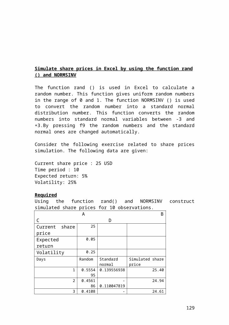
Risk - free rate (r) 8%Volatility 30%Dividend yield (q) 3%Time to maturity 0.26d1 1.871d2 1.717N(d1) 0.969N(d2) 0.957exp(-qT) 0.99exp(-rT) 0.98BS value 31.31Market value 40.45

Source: author’s calculation

After applying the Goal Seek function with the above data, the implied volatility will change to 94%, as shown to the following table. Thus, the adjustment took place to explain the price deviation between the theoretical BS value and the market price of the call option.

Today 6/2/2014Expirydate 9/1/2014Networkdays 66Stock 130Strike 100Risk - free rate 8%Volatility 94%Dividend yield 3%Time to maturity 0.26d1 0.813d2 0.332N(d1) 0.792N(d2) 0.630exp(-qT) 0.99exp(-rT) 0.98BS value 40.45Market value 40.45

Source: author’s calculationA detailed example of portfolio management application using Excel and VBA

We have three call options, A, B, and C and it is required to calculate the portfolio return and the standard deviation or risk of the portfolio.

  A B C D  

Row numbers Call optionsExpected Returns ( r)

Standard deviation

Weights(w)

Portfolio return

1 A 0.06 0.05 0.35

2 B 0.1 0.07 0.45Standard deviation orPortfolio risk

129

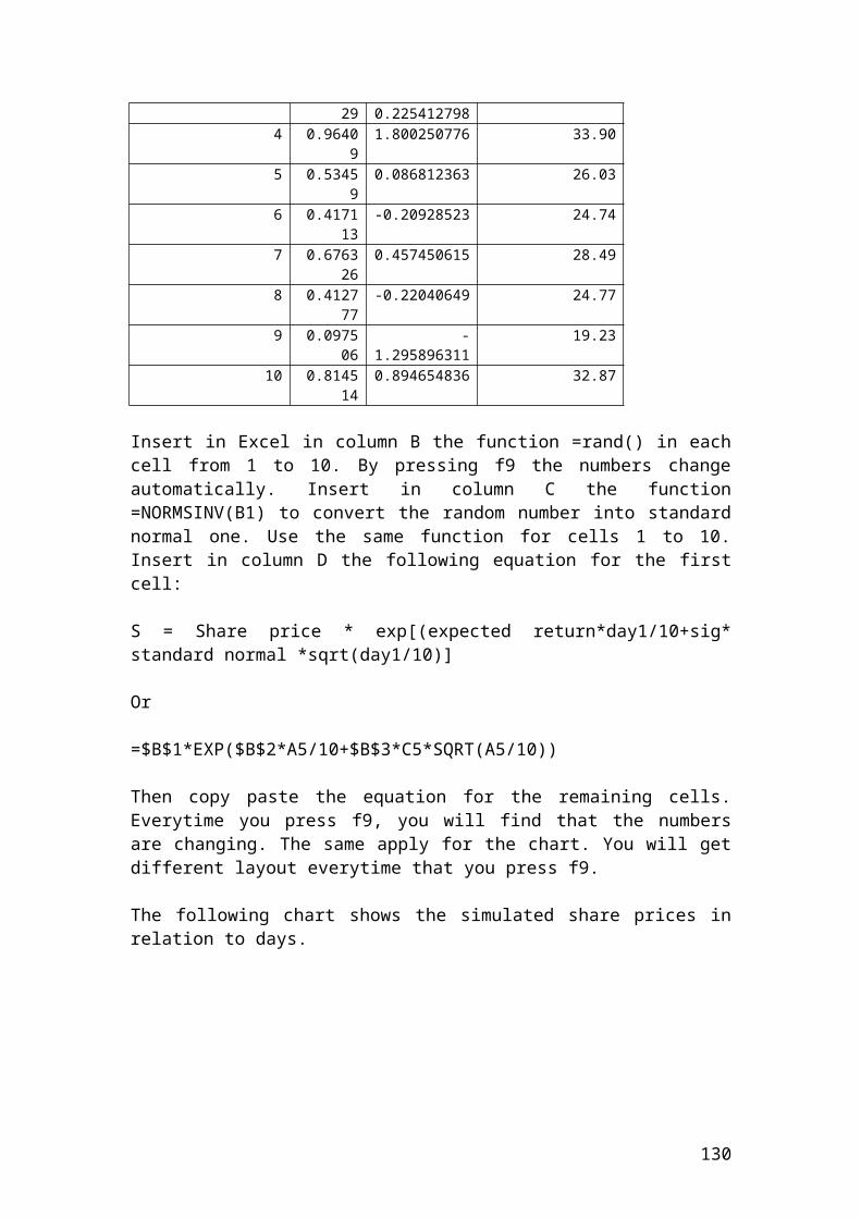
3 C 0.03 0.02 0.2100%

Source: author’s calculation.

'Calculate the portfolio returns and the standard deviation or risk of the portfolio in 'VBA by including a command button to perform the calculations automatically for 'options with different returns and standard deviations.'Calculate the portfolio return and the standard deviation?'Call option A expected return 0.06'Call option A standard deviation 0.05'Call option A weight 0.35'Correlation coefficient between A and B 0.5'Call option B expected return 0.1'Call option B standard deviation 0.07 'Call option B weight 0.45‘Correlation coefficient between B and C -0.1'Call option C expected return 0.03'Call option C standard deviation 0.02'Call option C weight 0.2‘ Correlation coefficient between A and C -0.4'********************************************************************Sub Test()

Worksheets("sheet2").Range("A1") = "Portfolio of options"Worksheets("Sheet2").Range("A1").Font.Bold = TrueWorksheets("sheet2").Range("A2") = "A"Worksheets("sheet2").Range("A3") = "B"Worksheets("sheet2").Range("A4") = "C"Worksheets("Sheet2").Range("A6")= "Variance of the portfolio"Worksheets("Sheet2").Range("A6").Font.Bold = TrueWorksheets("Sheet2").Range("A7").Formula = "= ((((((0.35^2*0.05^2)+(0.45^2*0.07^2)+(0.2^2*0.02^2)+(2*0.35*0.45*0.5*0.05*0.07)+(2*0.35*0.2*-0.4*0.05*0.02)+(2*0.45*0.2*-0.1*0.07*0.02))))))"Worksheets("Sheet2").Range("A8")= "Percentage return of the variance portfolio"Worksheets("Sheet2").Range("A8").Font.Bold = TrueWorksheets("Sheet2").Range("A9").Formula = "= (A7*100)"Worksheets("Sheet2").Range("A10")= "Standard deviation or risk of the portfolio"Worksheets("Sheet2").Range("A10").Font.Bold = TrueWorksheets("Sheet2").Range("A11").Formula = "= SQRT(A9)"Worksheets("Sheet2").Range("B1")= "Expected returns"Worksheets("Sheet2").Range("B1").Font.Bold = TrueWorksheets("Sheet2").Range("B2").Value = 0.06Worksheets("Sheet2").Range("B3").Value = 0.1Worksheets("Sheet2").Range("B4").Value = 0.03Worksheets("Sheet2").Range("C1")= "Standard deviation"Worksheets("Sheet2").Range("C1").Font.Bold = TrueWorksheets("Sheet2").Range("C2").Value = 0.05Worksheets("Sheet2").Range("C3").Value = 0.07Worksheets("Sheet2").Range("C4").Value = 0.02Worksheets("Sheet2").Range("C10")= "A"

130

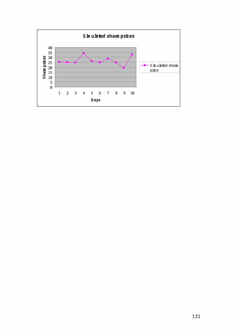
Worksheets("Sheet2").Range("C11")= "B"Worksheets("Sheet2").Range("C12")= "C"Worksheets("Sheet2").Range("C20")= "Variance"Worksheets("Sheet2").Range("C20").Font.Bold = TrueWorksheets("Sheet2").Range("C21")= "Variance percentage return"Worksheets("Sheet2").Range("C21").Font.Bold = TrueWorksheets("Sheet2").Range("C22")= "Standard deviation or risk of the portfolio"Worksheets("Sheet2").Range("C22").Font.Bold = TrueWorksheets("Sheet2").Range("D1")= "Weights"Worksheets("Sheet2").Range("D1").Font.Bold = TrueWorksheets("Sheet2").Range("D2").Value = 0.35Worksheets("Sheet2").Range("D3").Value = 0.45Worksheets("Sheet2").Range("D4").Value = 0.2Worksheets("Sheet2").Range("D5").Value = 1Worksheets("Sheet2").Range("D8")= "Correlation matrix"Worksheets("Sheet2").Range("D8").Font.Bold = TrueWorksheets("Sheet2").Range("D8").Font.Underline = TrueWorksheets("Sheet2").Range("D9")= "A"Worksheets("Sheet2").Range("D10").Value = 1Worksheets("Sheet2").Range("D11").Value = 0.5Worksheets("Sheet2").Range("D12").Value = -0.4Worksheets("Sheet2").Range("D15")= "Variance – Covariance matrix"Worksheets("Sheet2").Range("D15").Font.Bold = TrueWorksheets("Sheet2").Range("D15").Font.Underline = TrueWorksheets("Sheet2").Range("D16"). Formula = "= SUMPRODUCT(D10,G10,G10)"Worksheets("Sheet2").Range("D17"). Formula = "= SUMPRODUCT(D11,G10,G11)"Worksheets("Sheet2").Range("D18"). Formula = "= SUMPRODUCT(D12,G10,G12)"Worksheets("Sheet2").Range("D20").Formula = "= MMULT(TRANSPOSE(G16:G18),MMULT(D16:F18,G16:G18))"Worksheets("Sheet2").Range("D21").Formula = "= (D20*100)"Worksheets("Sheet2").Range("D22").Formula = "= SQRT(D21)"Worksheets("Sheet2").Range("E1")= "Portfolio return"Worksheets("Sheet2").Range("E1").Font.Bold = TrueWorksheets("Sheet2").Range("E2").Formula = "= SUMPRODUCT(B2:B4,D2:D4)"Worksheets("Sheet2").Range("E3")= "Portfolio risk"Worksheets("Sheet2").Range("E3").Font.Bold = TrueWorksheets("Sheet2").Range("E4").Formula = "= SQRT(A9)"Worksheets("Sheet2").Range("E9")= "B"Worksheets("Sheet2").Range("E10").Value = 0.5Worksheets("Sheet2").Range("E11").Value = 1Worksheets("Sheet2").Range("E12").Value = -0.1Worksheets("Sheet2").Range("E16"). Formula = "= SUMPRODUCT(E10,G10,G11)"Worksheets("Sheet2").Range("E17"). Formula = "= SUMPRODUCT(E11,G11,G11)"Worksheets("Sheet2").Range("E18"). Formula = "= SUMPRODUCT(E12,G11,G12)"Worksheets("Sheet2").Range("F9")= "C"Worksheets("Sheet2").Range("F10").Value = -0.4Worksheets("Sheet2").Range("F11").Value = -0.1

131

Worksheets("Sheet2").Range("F12").Value = 1Worksheets("Sheet2").Range("F16"). Formula = "= SUMPRODUCT(F10,G10,G12)"Worksheets("Sheet2").Range("F17"). Formula = "= SUMPRODUCT(F11,G11,G12)"Worksheets("Sheet2").Range("F18"). Formula = "= SUMPRODUCT(F12,G12,G12)"Worksheets("Sheet2").Range("G9")= "Standard deviation"Worksheets("Sheet2").Range("G9").Font.Bold = TrueWorksheets("Sheet2").Range("G9").Font.Underline = TrueWorksheets("Sheet2").Range("G10").Value = 0.05Worksheets("Sheet2").Range("G11").Value = 0.07Worksheets("Sheet2").Range("G12").Value = 0.02Worksheets("Sheet2").Range("G15")= "Weights"Worksheets("Sheet2").Range("G15").Font.Bold = TrueWorksheets("Sheet2").Range("G15").Font.Underline = TrueWorksheets("Sheet2").Range("G16").Value = 0.35Worksheets("Sheet2").Range("G17").Value = 0.45Worksheets("Sheet2").Range("G18").Value = 0.2End Sub

Solution

You should get the following results:

  A B C D  

Row numbers Call optionsExpected Returns ( r)

Standard deviation

Weights(w)

Portfolio return

1 A 0.06 0.05 0.35 0.0722 B 0.1 0.07 0.45

3 C 0.03 0.02 0.2100%

Source: author’s calculation.

Calculate the share and call option prices using a Cox, Ross, Rubinstein,(CRR) binomial 3 steps tree using VBA. The following data are given:

S = 60 share price K = 50 strike price r = 0.05 risk-free interest rate q = 0.02 dividend yield T = 0.5 life to maturity sig = 0.3 volatility n = 3 number of steps

Identify the variables

132

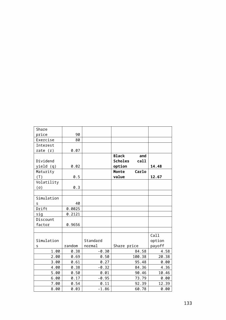
Steps expressed in years. Multiplier of upmove. Multiplier of downmove. Risk neutral probability of upmove. Discount factor. Insert the mathematical formulas Steps expressed in years = T/n Multiplier of upmove = exp(sig*sqrt(dt)) Multiplier of downmove = 1/u Discount factor = exp(-r*dt) Risk neutral probability of upmove = (exp((r-q)*dt)-d)/(u-d)

Application of Cox, Ross, Rubinstein,(CRR) binomial 3 steps tree using VBA

Sub test()

'S = 60 share price 'K = 50 strike price 'r = 0.05 risk-free interest rate 'q = 0.02 dividend yield 'T = 0.5 life to maturity 'sig = 0.3 volatility 'n = 3 number of steps'********************************************************************

' Identify the variable 'Steps expressed in years. 'Multiplier of upmove. 'Multiplier of downmove. 'Risk neutral probability of upmove. 'Discount factor.'********************************************************************

' Insert the mathematical formulas ' Steps expressed in years = T/n' Multiplier of upmove = exp(sig*sqrt(dt))' Multiplier of downmove = 1/u' Discount factor = Exp(-r * dt)' Risk neutral probability of upmove = (exp((r-q)*dt)-d)/(u-d)

'********************************************************************

Worksheets("sheet1").Range("A1") = "Share price"Worksheets("sheet1").Range("A1").Font.Bold = True

133

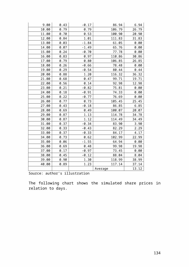
Worksheets("sheet1").Range("B1").Value = 60Worksheets("sheet1").Range("A2") = "Exercise price"Worksheets("sheet1").Range("A2").Font.Bold = TrueWorksheets("sheet1").Range("B2").Value = 50Worksheets("sheet1").Range("A3") = "Risk-free interest rate"Worksheets("sheet1").Range("A3").Font.Bold = TrueWorksheets("sheet1").Range("B3").Value = 0.05Worksheets("sheet1").Range("A4") = "Dividend yield"Worksheets("sheet1").Range("A4").Font.Bold = TrueWorksheets("sheet1").Range("B4").Value = 0.02Worksheets("sheet1").Range("A5") = "Life to maturity"Worksheets("sheet1").Range("A5").Font.Bold = TrueWorksheets("sheet1").Range("B5").Value = 0.5Worksheets("sheet1").Range("A6") = "Volatility"Worksheets("sheet1").Range("A6").Font.Bold = TrueWorksheets("sheet1").Range("B6").Value = 0.3Worksheets("sheet1").Range("A7") = "Number of steps"Worksheets("sheet1").Range("A7").Font.Bold = TrueWorksheets("sheet1").Range("B7").Value = 3Worksheets("sheet1").Range("A9") = "Steps expressed in years"Worksheets("sheet1").Range("A9").Font.Bold = TrueWorksheets("sheet1").Range("B9").Formula = "=(B5/B7)"Worksheets("sheet1").Range("A10") = "Multiplier of upmove"Worksheets("sheet1").Range("A10").Font.Bold = TrueWorksheets("sheet1").Range("B10").Formula = "=exp(B6*sqrt(B9))"Worksheets("sheet1").Range("A11") = "Multiplier of downmove"Worksheets("sheet1").Range("A11").Font.Bold = TrueWorksheets("sheet1").Range("B11").Formula = "=(1/B10)"Worksheets("sheet1").Range("A12") = "Discount factor"Worksheets("sheet1").Range("A12").Font.Bold = TrueWorksheets("sheet1").Range("B12").Formula = "=exp(-B3*B9)"Worksheets("sheet1").Range("A13") = "Risk neutral probability of upmove"Worksheets("sheet1").Range("A13").Font.Bold = TrueWorksheets("sheet1").Range("B13").Formula = "=(exp((B3-B4)*B9)-B11)/(B10-B11)"

Worksheets("sheet1").Range("D12").Value = 0Worksheets("sheet1").Range("D12").Font.Bold = TrueWorksheets("sheet1").Range("D17").Value = 60Worksheets("sheet1").Range("E11").Value = 1Worksheets("sheet1").Range("E11").Font.Bold = TrueWorksheets("sheet1").Range("F10").Value = 2Worksheets("sheet1").Range("F10").Font.Bold = TrueWorksheets("sheet1").Range("G9").Value = 3

Worksheets("sheet1").Range("E13").Formula = "=D17*B10"Worksheets("sheet1").Range("F13").Formula = "=D17*B10^2"Worksheets("sheet1").Range("G13").Formula = "=D17*B10^3"Worksheets("sheet1").Range("E23").Formula = "=D17*B11"Worksheets("sheet1").Range("F23").Formula = "=D17*B11^2"

134

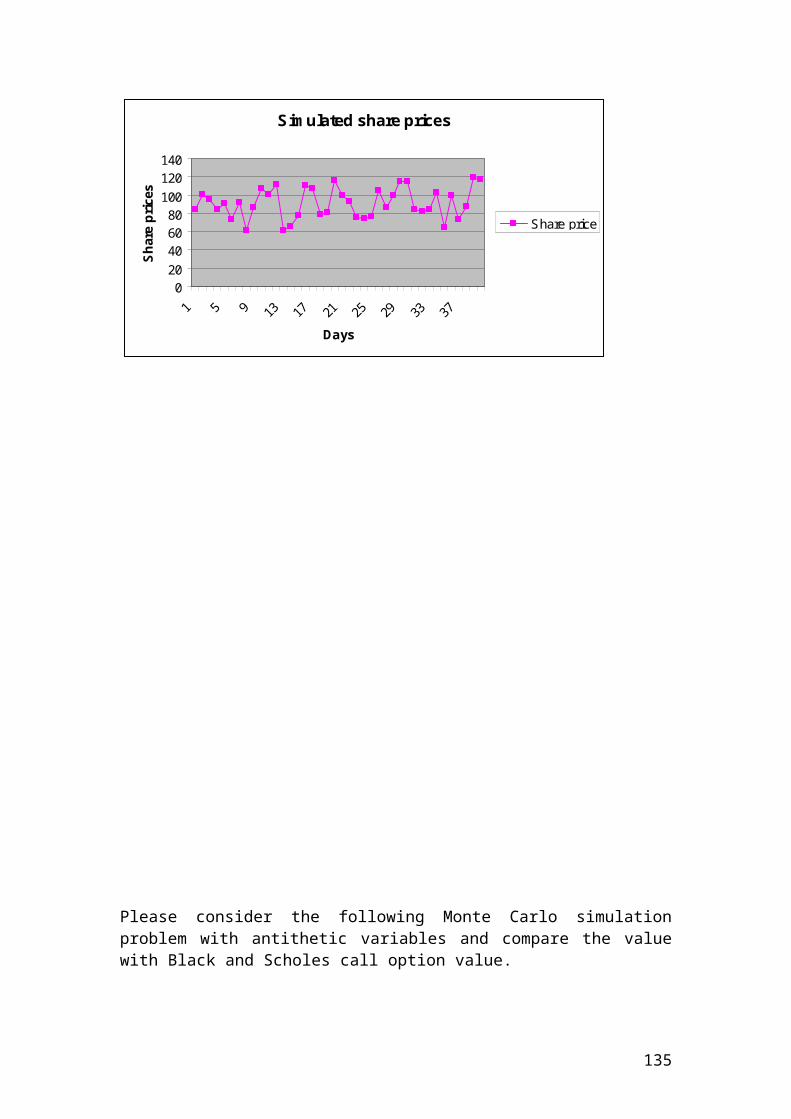
Worksheets("sheet1").Range("G23").Formula = "=D17*B11^3"Worksheets("sheet1").Range("F17").Formula = "=D17*B10*B11"Worksheets("sheet1").Range("G17").Formula = "=F17*B10"Worksheets("sheet1").Range("G19").Formula = "=F17*B11"

Worksheets("sheet1").Range("G14").Formula = "=G13-B2"Worksheets("sheet1").Range("G18").Formula = "=G17-B2"Worksheets("sheet1").Range("G20").Formula = "=G19-B2"Worksheets("sheet1").Range("G24").Value = 0

Worksheets("sheet1").Range("F14").Formula = "=$B$12*($B$13*G14)+(1-$B$13)*G18"Worksheets("sheet1").Range("F18").Formula = "=$B$12*($B$13*G18)+(1-$B$13)*G20"Worksheets("sheet1").Range("F24").Formula = "=$B$12*($B$13*G20)+(1-$B$13)*G24"Worksheets("sheet1").Range("E14").Formula = "=$B$12*($B$13*F14)+(1-$B$13)*F18"Worksheets("sheet1").Range("E24").Formula = "=$B$12*($B$13*F18)+(1-$B$13)*F24"Worksheets("sheet1").Range("D18").Formula = "=$B$12*($B$13*E14)+(1-$B$13)*E24"

End Sub

Calculate the share and put option prices using a Cox, Ross, Rubinstein,(CRR) binomial 3 steps tree using VBA. The following data are given:

S = 60 share price K = 70 strike price r = 0.02 risk-free interest rate q = 0.03 dividend yield T = 0.5 life to maturity sig = 0.2 volatility n = 3 number of steps

Identify the variables

135

Steps expressed in years. Multiplier of upmove. Multiplier of downmove. Risk neutral probability of upmove. Discount factor. Insert the mathematical formulas Steps expressed in years = T/n Multiplier of upmove = exp(sig*sqrt(dt)) Multiplier of downmove = 1/u Discount factor = exp(-r*dt) Risk neutral probability of upmove = (exp((r-q)*dt)-d)/(u-d)

Application of Cox, Ross, Rubinstein,(CRR) binomial 3 steps tree using VBA

Sub test()

'S = 60 share price 'K = 70 strike price 'r = 0.02 risk-free interest rate 'q = 0.03 dividend yield 'T = 0.5 life to maturity 'sig = 0.2 volatility 'n = 3 number of steps'******************************************************************** ' Identify the variable 'Steps expressed in years. 'Multiplier of upmove. 'Multiplier of downmove. 'Risk neutral probability of upmove. 'Discount factor.'********************************************************************

' Insert the mathematical formulas ' Steps expressed in years = T/n' Multiplier of upmove = exp(sig*sqrt(dt))' Multiplier of downmove = 1/u' Discount factor = Exp(-r * dt)' Risk neutral probability of upmove = (exp((r-q)*dt)-d)/(u-d)

'*******************************************************************

Worksheets("sheet1").Range("A1") = "Share price"Worksheets("sheet1").Range("A1").Font.Bold = TrueWorksheets("sheet1").Range("B1").Value = 60Worksheets("sheet1").Range("A2") = "Exercise price"Worksheets("sheet1").Range("A2").Font.Bold = True

136

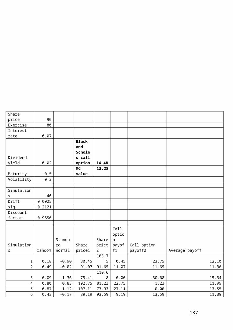
Worksheets("sheet1").Range("B2").Value = 70Worksheets("sheet1").Range("A3") = "Risk-free interest rate"Worksheets("sheet1").Range("A3").Font.Bold = TrueWorksheets("sheet1").Range("B3").Value = 0.02Worksheets("sheet1").Range("A4") = "Dividend yield"Worksheets("sheet1").Range("A4").Font.Bold = TrueWorksheets("sheet1").Range("B4").Value = 0.03Worksheets("sheet1").Range("A5") = "Life to maturity"Worksheets("sheet1").Range("A5").Font.Bold = TrueWorksheets("sheet1").Range("B5").Value = 0.5Worksheets("sheet1").Range("A6") = "Volatility"Worksheets("sheet1").Range("A6").Font.Bold = TrueWorksheets("sheet1").Range("B6").Value = 0.2Worksheets("sheet1").Range("A7") = "Number of steps"Worksheets("sheet1").Range("A7").Font.Bold = TrueWorksheets("sheet1").Range("B7").Value = 3Worksheets("sheet1").Range("A9") = "Steps expressed in years"Worksheets("sheet1").Range("A9").Font.Bold = TrueWorksheets("sheet1").Range("B9").Formula = "=(B5/B7)"Worksheets("sheet1").Range("A10") = "Multiplier of upmove"Worksheets("sheet1").Range("A10").Font.Bold = TrueWorksheets("sheet1").Range("B10").Formula = "=exp(B6*sqrt(B9))"Worksheets("sheet1").Range("A11") = "Multiplier of downmove"Worksheets("sheet1").Range("A11").Font.Bold = TrueWorksheets("sheet1").Range("B11").Formula = "=(1/B10)"Worksheets("sheet1").Range("A12") = "Discount factor"Worksheets("sheet1").Range("A12").Font.Bold = TrueWorksheets("sheet1").Range("B12").Formula = "=exp(-B3*B9)"Worksheets("sheet1").Range("A13") = "Risk neutral probability of upmove"Worksheets("sheet1").Range("A13").Font.Bold = TrueWorksheets("sheet1").Range("B13").Formula = "=(exp((B3-B4)*B9)-B11)/(B10-B11)"

Worksheets("sheet1").Range("D12").Value = 0Worksheets("sheet1").Range("D12").Font.Bold = TrueWorksheets("sheet1").Range("D17").Value = 60Worksheets("sheet1").Range("E11").Value = 1Worksheets("sheet1").Range("E11").Font.Bold = TrueWorksheets("sheet1").Range("F10").Value = 2Worksheets("sheet1").Range("F10").Font.Bold = TrueWorksheets("sheet1").Range("G9").Value = 3

Worksheets("sheet1").Range("E13").Formula = "=D17*B10"Worksheets("sheet1").Range("F13").Formula = "=D17*B10^2"Worksheets("sheet1").Range("G13").Formula = "=D17*B10^3"Worksheets("sheet1").Range("E23").Formula = "=D17*B11"Worksheets("sheet1").Range("F23").Formula = "=D17*B11^2"Worksheets("sheet1").Range("G23").Formula = "=D17*B11^3"Worksheets("sheet1").Range("F17").Formula = "=D17*B10*B11"Worksheets("sheet1").Range("G17").Formula = "=F17*B10"

137

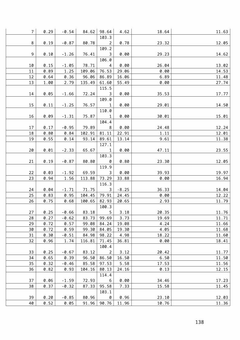
Worksheets("sheet1").Range("G19").Formula = "=F17*B11"

Worksheets("sheet1").Range("G14").Value = 0Worksheets("sheet1").Range("G18").Formula = "=B2-G17"Worksheets("sheet1").Range("G20").Formula = "=B2-G19"Worksheets("sheet1").Range("G24").Formula = "=B2-G23"

Worksheets("sheet1").Range("F14").Formula = "=$B$12*($B$13*G14)+(1-$B$13)*G18"Worksheets("sheet1").Range("F18").Formula = "=$B$12*($B$13*G18)+(1-$B$13)*G20"Worksheets("sheet1").Range("F24").Formula = "=$B$12*($B$13*G20)+(1-$B$13)*G24"Worksheets("sheet1").Range("E14").Formula = "=$B$12*($B$13*F14)+(1-$B$13)*F18"Worksheets("sheet1").Range("E24").Formula = "=$B$12*($B$13*F18)+(1-$B$13)*F24"Worksheets("sheet1").Range("D18").Formula = "=$B$12*($B$13*E14)+(1-$B$13)*E24"

End Sub

Workshop of language programming in terms of C++

C++ is very useful language programming in modeling financial derivatives and their related Greeks symbols. First of all, you should download the software as part of an integrated development environment, (IDE). A possible public domain is www. Bloodshed.net. You could download the software, (IDE) version 4.9.9.2.

You can start C++ by creating a source code in the text editor. Then, press execute and selects the C++ compiler to compile the code. Finally, press the debug or run button to get the output in a DOS window or console. You first have to do the compiling and then to run the console. During the compiling, the source code is translated into object code. Then, through the linker the object code is combined with other files into an executable program. The most common software is to use the

138

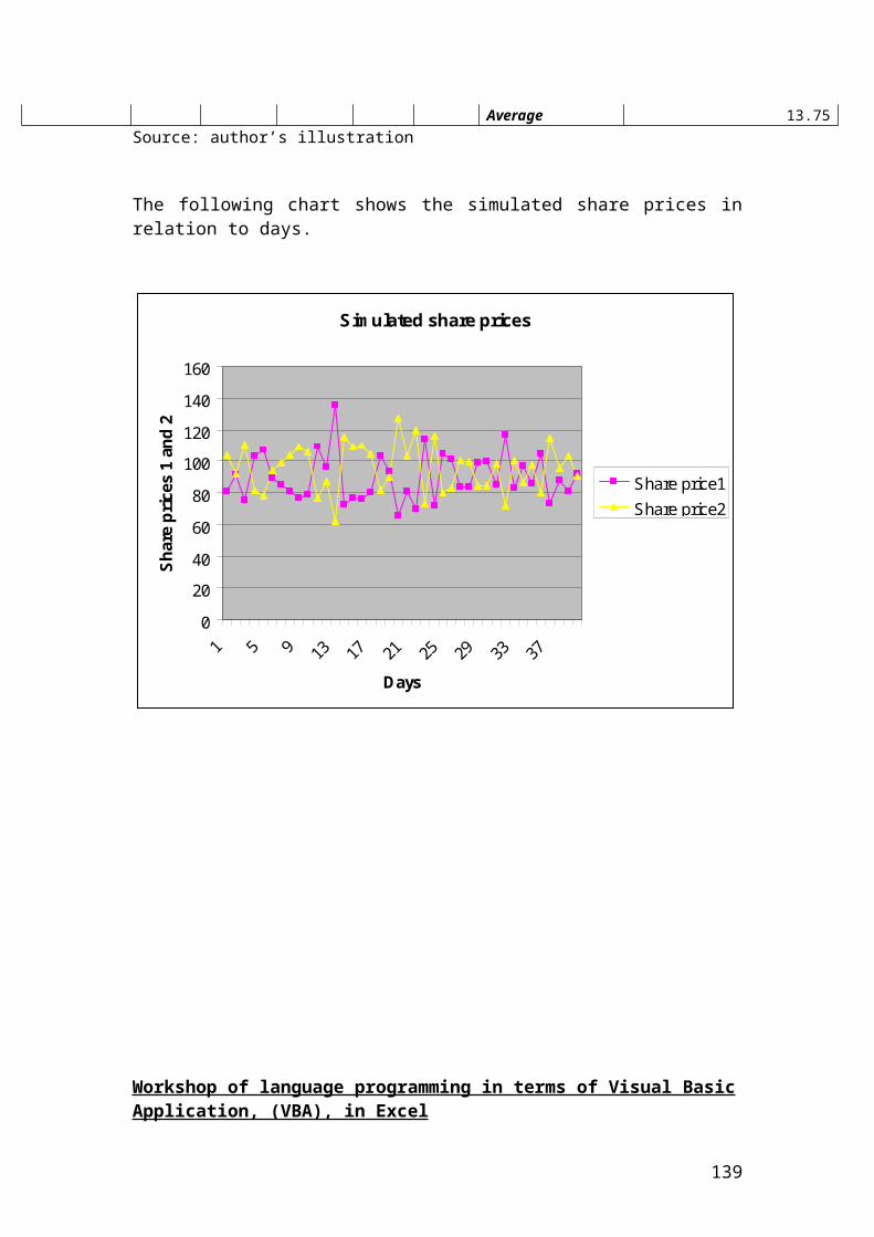
integrated development environment as part of a C++ compiler and a debugger to help you fix the errors or improve the code. Sometimes, you will get errors that are the reason of lacking to insert the correct header. For example, if you do not include the header #include <math.h> or # include <cmath>, the compiler will not recognize the mathematical functions such as exp, log and sqrt. It is very important to select the correct headers. For example, <cmath> means standard mathematical library.

If you do not have the right headers, then, you will not be able to do compiling and debug. In other words, you will not be able to get the output in the DOS window or console. You will get error messages as the computer cannot recognize the formulas.

The comments, variables, functions, and mathematical formulas have to be inserted to be able to get the output. We use the symbol // to show a single line comment. The lines that include statements should end with semicolon ; in C++ . We use numerical variables with fractional parts. In this case, the term double is inserted in front of each variable. Once you define a variable with capital or small letters, you can not change it with different layout as you move to the calculation part. Consistency is very important. Other types of data are integers, real numbers, characters, strings and Boolean values. Pay particular attention to the lower and upper case letters. For example, integer for interest rate is written as variable intRate. Another example that can be used is the integer value for the amount. It is written as intAmount.

Very important headers that we use in derivatives are the following:

# include <iostream># include <cmath> Or # include <math.h>#include < cstdlib> using namespace std;

The name of the header has to be enclosed between the symbols < >. You should use the header < cstdlib> for functions that will be used from the standard library,(STL). The header < iostream> is very important as it includes the input/output, (I/O) library. You should also use blank line for presentation purposes. The execution of the program starts with the statement int main()

Then, the code should be enclosed between two braces {}.

The main heading to start C++ is as follows:

# include <iostream>using namespace std;

int main()

139

{

/* Identify your given variables using double for numbers with fractions or int for integers numbers. Identify the variables that will be calculated. The symbols /* and */ are used for multiline comments.*/

// Insert the mathematical formula or formulas.

*/ Insert the output functions cout and the cin statement if needed. The cout statement is a prompt followed by the cin statement. For example, cout <<”Enter interest rate:”<<endl; cin>> interest rate;

You should used the extraction operator, >> and quotation marks for the cout function. This is the basic layout that I have used to convert most of the mathematical problems to C++.*/

system("PAUSE"); return 0; }

The data types that are incorporated into the C++ language are char, wchar-t, int, float, double, bool, and void. The available modifiers are signed, unsigned, long and short.The cin function tells the computer to use the input value from the keyboard and place it in the variable length that has been identified in the variable section.

The function cout is used to produce outputs. The symbol << is known as the output operator and the statement or message should be enclosed between quotation marks.

Messages should be enclosed between a pair of double quotation marks. You could use an escape character \n to tell the program to start a new line.

The statement system(″PAUSE″); tells the computer in DOS environment to display the message and wait until you press any key to close the console or the DOS window.

Finally the statement returns 0; tells the computer to end the program.

140

Calculations of European call and put prices by applying Black and Scholes model, (BSM)

/* Calculation of Euro call and put prices by applying Black and Scholes model, BSM. price of stock = 70, strike price = 70, interest rate = 0.08, dividend yield = 0.03, life to maturity = 0.5, and volatility = 0.2.*/

#include <iostream># include <math.h>using namespace std;

// Calculations of the European call and put prices.

double Call(double S, double K, double r, double q, double T,

141

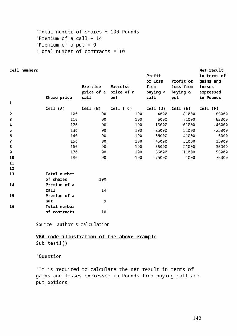
double sig);double Put(double S, double K, double r, double q, double T, double sig);

// Calculation of the cumulative normal distribution.

double NP(double x);double N(double x);

double NP(double x){ return (1.0/sqrt(2.0 * 3.1415)* exp(-x*x*0.5));} double N(double x){ double b1 = 0.319381530; double b2 = -0.356563782; double b3 = 1.781477937; double b4 = -1.821255978; double b5 = 1.330274429; double k; k = 1/(1+0.2316419*x); if (x >= 0.0) { return (1 - NP(x)*((b1*k) + (b2* k*k) + (b3*k*k*k) + (b4*k*k*k*k) + (b5*k*k*k*k*k))); } else { return (1-N(-x)); } }

// Mathematical formulas to calculate d1, d2 and the European call price.

double Call(double S, double K, double r, double q, double T, double sig){

double d1, d2; d1 = (log(S/K) + (r-q +(sig*sig)*0.5 ) * T ) / (sig * sqrt(T)); d2 = d1 - sig*sqrt(T); return S*exp(-q*T)*N(d1) - K*exp(-r*T)*N(d2) ; }

142

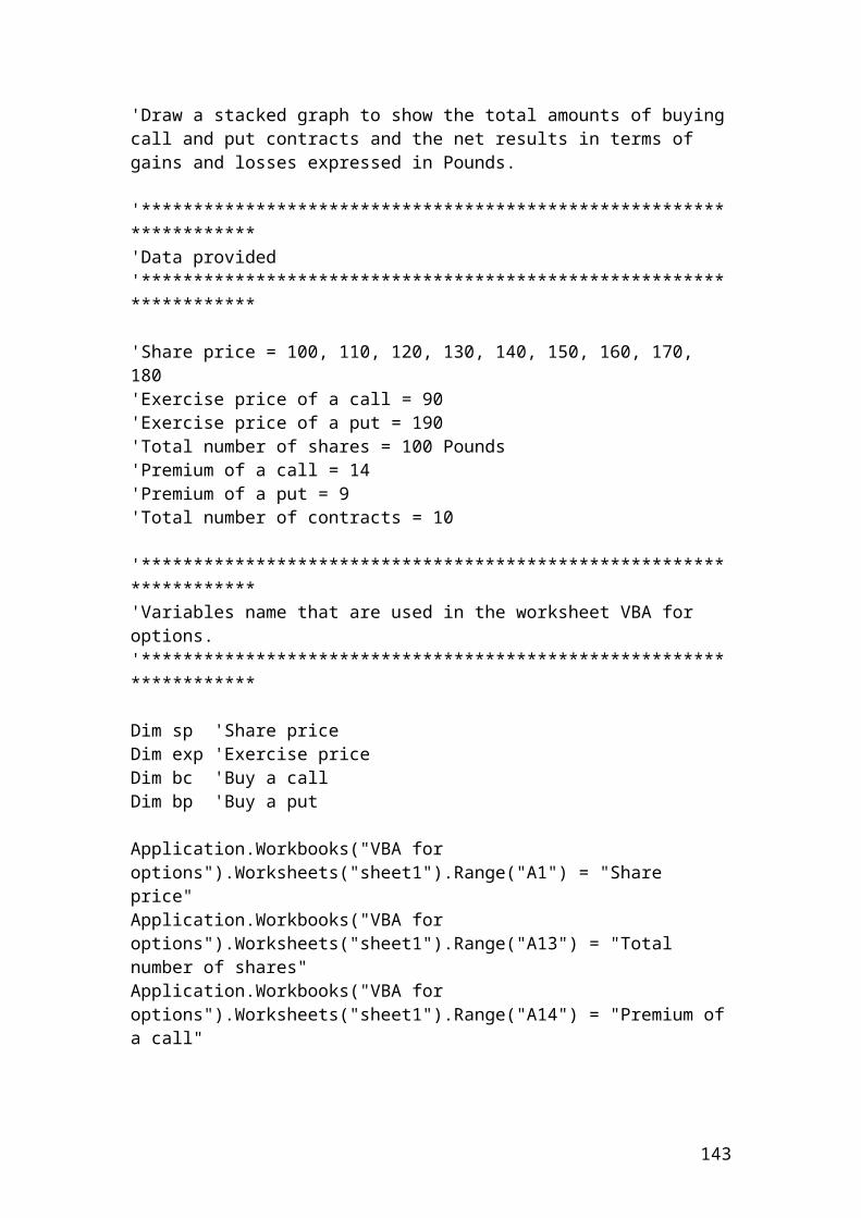
// Mathematical formulas to calculate d1, d2 and the European put price.

double Put(double S, double K, double r, double q, double T, double sig){

double d1, d2; d1 = (log(S/K) + (r-q +(sig*sig)*0.5 ) * T ) / (sig * sqrt(T)); d2 = d1 - sig*sqrt(T);

return K*exp(-r*T)*N(-d2) - S*exp(-q*T)*N(-d1) ; }

// Identification or declaration of the variables.

int main(){ double S = 70; // price of stock double K = 70; // strike price double r = 0.08; // interest rate double q = 0.03; // dividend yield double T = 0.5; // life to maturity double sig = 0.20; // volatility

/*Calculation of call and put prices in addition of showing the numerical values of the variables.*/

double callPrice, putPrice;

callPrice = Call (S,K,r,q,T,sig);putPrice = Put (S,K,r,q,T,sig);

std::cout<<"Price of stock: " <<S<<std::endl;std::cout<<"Strike price: " <<K<<std::endl;std::cout<<"Interest rate: " <<r<<std::endl;std::cout<<"Dividend yield: " <<q<<std::endl;std::cout<<"Life to maturity: " <<T<<std::endl;std::cout<<"Volatility: " <<sig<<std::endl;cout<<"Call price: " <<callPrice << endl;cout<<"Put price:" <<putPrice << endl;

system("PAUSE"); return 0;

}

143

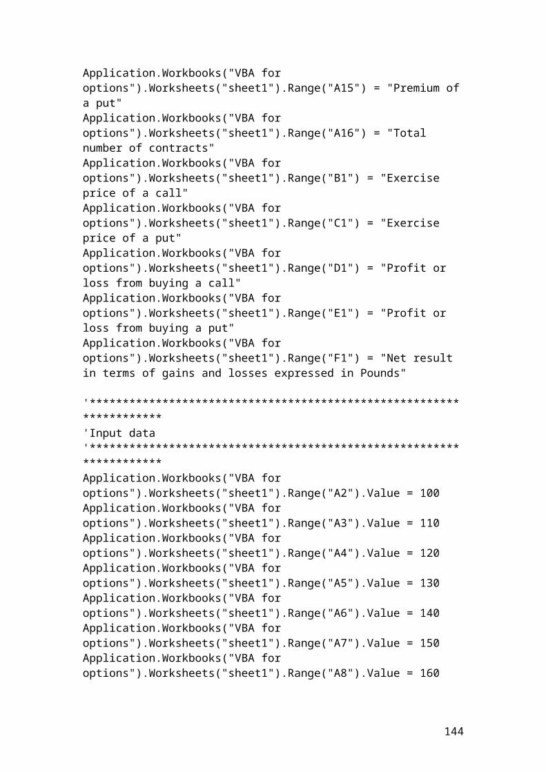
Output

After compiling and debugging, the DOS window or console will open and display the following results:

Price of stock: 70Strike price: 70Interest rate: 0.08Dividend yield: 0.03Life to maturity: 0.5Volatility: 0.2Call price: 4.75036Put price: 3.04778

Press any key to continue….

Calculations of European call and put prices by applying Black and Scholes model, (BSM). It is the same example as above. The difference is in calculating the cumulative normal distribution and inserting it in the mathematical formulas for call and put price. In addition, I have included other layout for call and put option calculations

/* Calculations of European call and put prices by applying Black and Scholes model, (BSM). price of stock = 70, strike price = 70, interest rate = 0.08, dividend yield = 0.03, life to maturity = 0.5, and volatility = 0.2.*/

#include <iostream># include <math.h>using namespace std;

144

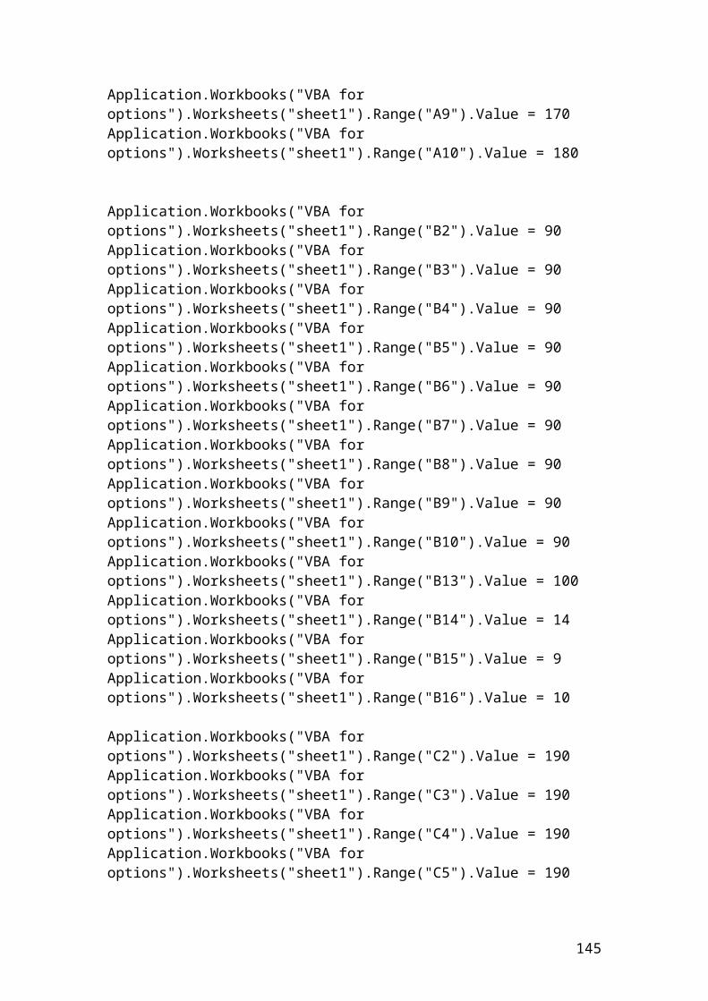
// Calculations of the European call and put price.

double Call(double S, double K, double r, double q, double T, double sig);double Put(double S, double K, double r, double q, double T, double sig);

// Calculation of the cumulative normal distribution.

double norm_cdf (const double& x) {

double k = 1/(1+0.2316419*x);double k_sum = k*(0.319381530 + k*(-0.356563782 + k*(1.781477937 + k*(-1.821255978 + k*(1.330274429))))); if (x >= 0.0) {return (1.0 - (1.0/(pow(2*M_PI, 0.5))) * exp(-0.5*x*x)* k_sum);} else {return 1.0 - norm_cdf(-x);}}

// Mathematical formulas to calculate d1, d2 and the European call price.

double Call( double S, // price of stock double K, // strike price double r, // interest rate double q, // dividend yield double T, // life to maturity double sig // volatility ) { double d1, d2; d1 = (log(S/K) + (r-q +(sig*sig)*0.5 ) * T ) / (sig * sqrt(T)); d2 = d1 - sig*sqrt(T); return S*exp(-q*T)*norm_cdf(d1) - K*exp(-r*T)*norm_cdf(d2) ; }

// Mathematical formulas to calculate d1, d2 and the European put price.

double Put( double S, // price of stock double K, // strike price double r, // interest rate

145

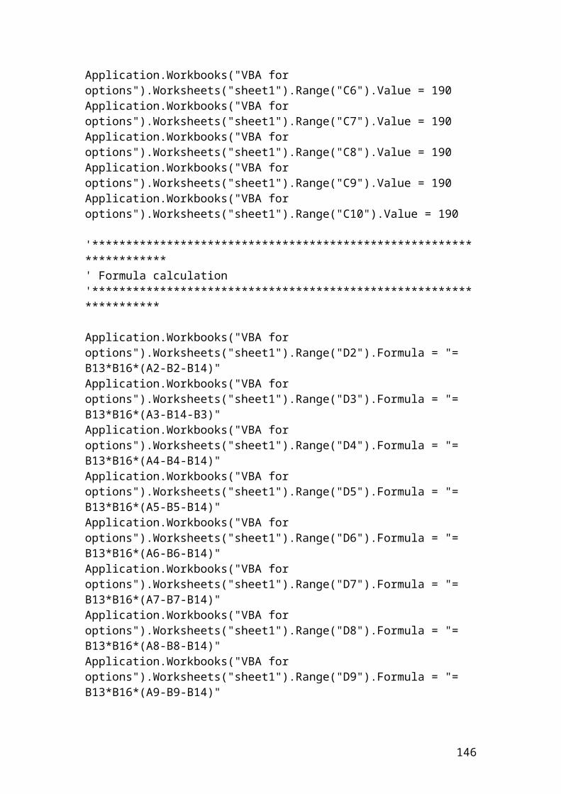
double q, // dividend yield double T, // life to maturity double sig // volatility )

{ double d1, d2; d1 = (log(S/K) + (r-q +(sig*sig)*0.5 ) * T ) / (sig * sqrt(T)); d2 = d1 - sig*sqrt(T);

return K*exp(-r*T)*norm_cdf(-d2) - S*exp(-q*T)*norm_cdf(-d1) ; }

// Identification or declaration of the variables.

int main(){ double S = 70; // price of stock double K = 70; // strike price double r = 0.08; // interest rate double q = 0.03; // dividend yield double T = 0.50; // life to maturity double sig = 0.20; // volatility /*Calculation of call and put prices in addition of showing the numerical values of the variables.*/

double callPrice, putPrice;

callPrice = Call (S,K,r,q,T,sig);putPrice = Put (S,K,r,q,T,sig);

std::cout<<"Price of stock: " <<S<<std::endl;std::cout<<"Strike price: " <<K<<std::endl;std::cout<<"Interest rate: " <<r<<std::endl;std::cout<<"Dividend yield: " <<q<<std::endl;std::cout<<"Life to maturity: " <<T<<std::endl;std::cout<<"Volatility: " <<sig<<std::endl;cout << "Call price: " << callPrice << endl;cout << "Put price: " << putPrice << endl;

system("PAUSE"); return 0;

}

146

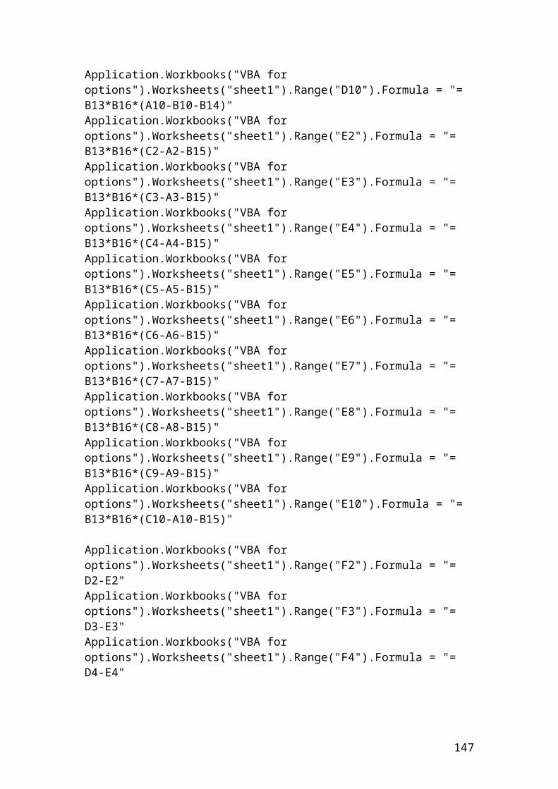
Output

After compiling and debugging, the DOS window or console will open and display the following results:

Price of stock: 70Strike price: 70Interest rate: 0.08Dividend yield: 0.03Life to maturity: 0.5Volatility: 0.2Call price: 4.75Put price: 3.05

Press any key to continue….

Calculations of European call and put prices and their related Greeks by applying Black and Scholes model, (BSM)

/*Calculations of Euro call and put prices by applying Black and Scholes model, BSM. price of stock = 70, strike price = 70, interest rate = 0.08, dividend yield = 0.03, life to maturity = 0.5, and volatility = 0.2.*/

#include <iostream># include <math.h>using namespace std;

// Calculation of the European call and put price.

double Call(double S, double K, double r, double q, double T,

147

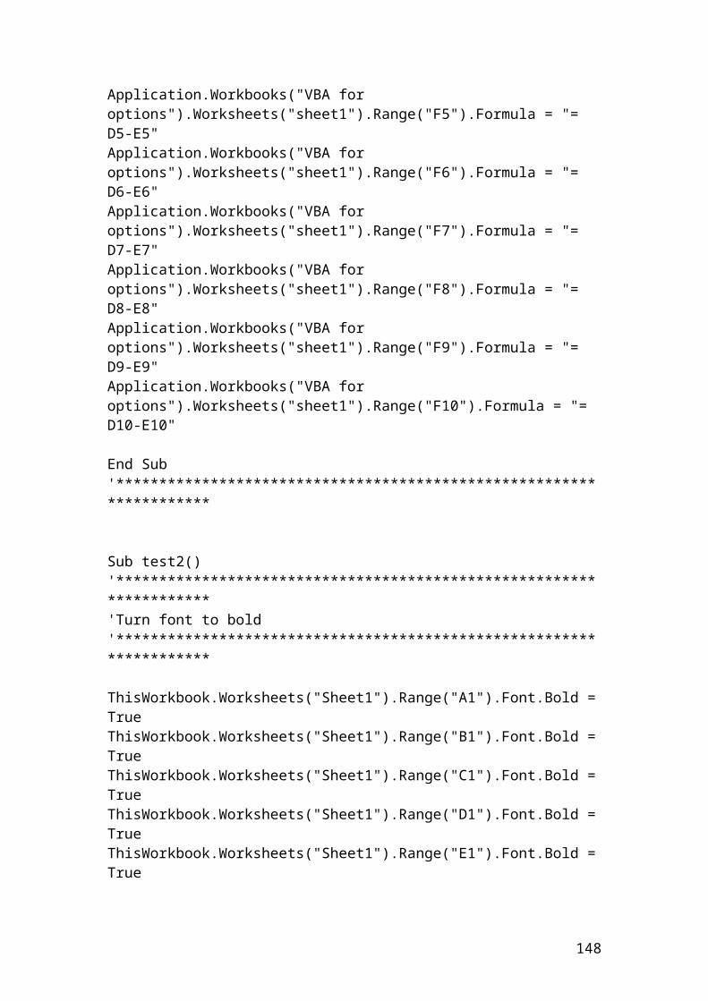
double sig);double Put(double S, double K, double r, double q, double T, double sig);double CallDelta(double S, double K, double r, double q, double T, double sig);double PutDelta(double S, double K, double r, double q, double T, double sig);double CallTheta(double S, double K, double r, double q, double T, double sig);double PutTheta(double S, double K, double r, double q, double T, double sig);double Gamma(double S, double K, double r, double q, double T, double sig);double Vega(double S, double K, double r, double q, double T, double sig);double CallRho(double S, double K, double r, double q, double T, double sig);double PutRho(double S, double K, double r, double q, double T, double sig);

// Calculation of the cumulative normal distribution.

double NP(double x);double N(double x);

double NP(double x){ return (1.0/sqrt(2.0 * 3.1415)* exp(-x*x*0.5));} double N(double x){ double b1 = 0.319381530; double b2 = -0.356563782; double b3 = 1.781477937; double b4 = -1.821255978; double b5 = 1.330274429; double k; k = 1/(1+0.2316419*x); if (x >= 0.0) { return (1 - NP(x)*((b1*k) + (b2* k*k) + (b3*k*k*k) + (b4*k*k*k*k) + (b5*k*k*k*k*k))); } else { return (1-N(-x)); }

148

}

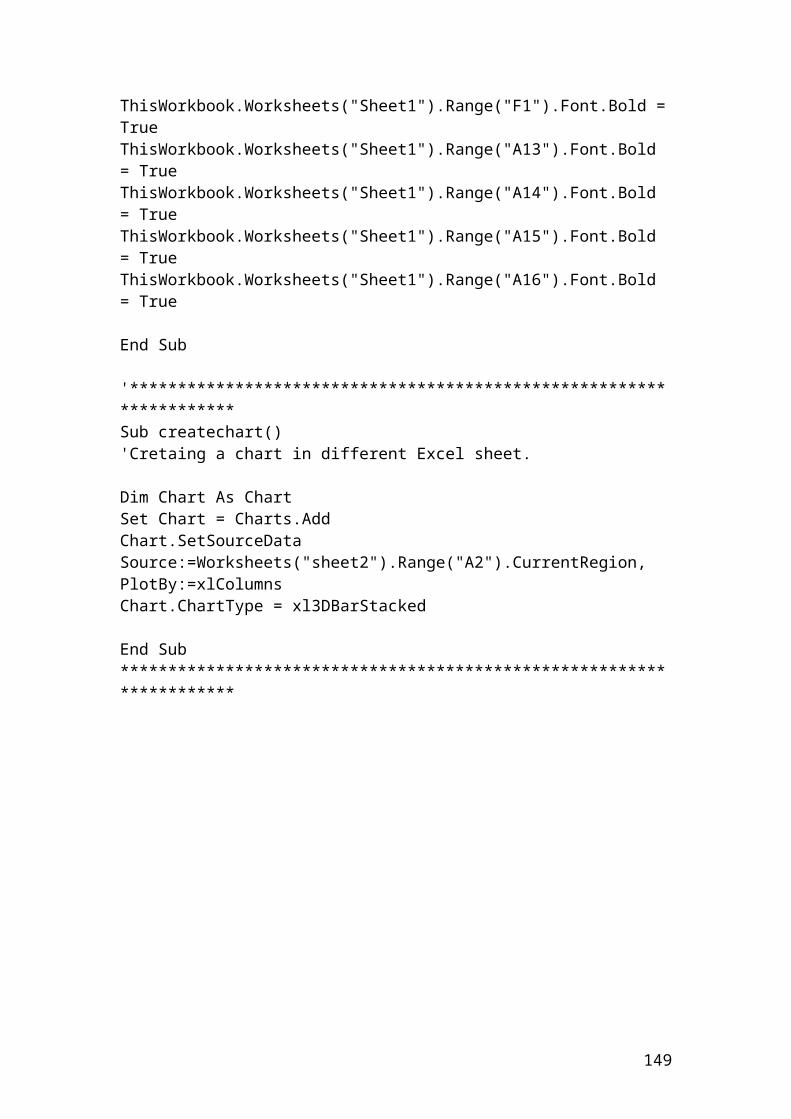
// Mathematical formulas to calculate d1, d2 and the European Call price.

double Call(double S, double K, double r, double q, double T, double sig){

double d1, d2; d1 = (log(S/K) + (r-q +(sig*sig)*0.5 ) * T ) / (sig * sqrt(T)); d2 = d1 - sig*sqrt(T); return S*exp(-q*T)*N(d1) - K*exp(-r*T)*N(d2) ; }

// Mathematical formulas to calculate d1, d2 and the CallDelta price.

double CallDelta(double S, double K, double r, double q, double T, double sig){

double d1, d2; d1 = (log(S/K) + (r-q +(sig*sig)*0.5 ) * T ) / (sig * sqrt(T)); d2 = d1 - sig*sqrt(T); return exp(-q*T)*N(d1); }

// Mathematical formulas to calculate d1, d2 and the CallTheta price.

double CallTheta(double S, double K, double r, double q, double T, double sig){

double d1, d2; d1 = (log(S/K) + (r-q +(sig*sig)*0.5 ) * T ) / (sig * sqrt(T)); d2 = d1 - sig*sqrt(T); return -(S*NP(d1)*sig*exp(-q*T))/(2*sqrt(T)) + (q*S*N(d1)*exp(-q*T)) - (r*K*exp(-r*T)*N(d2)); }

149

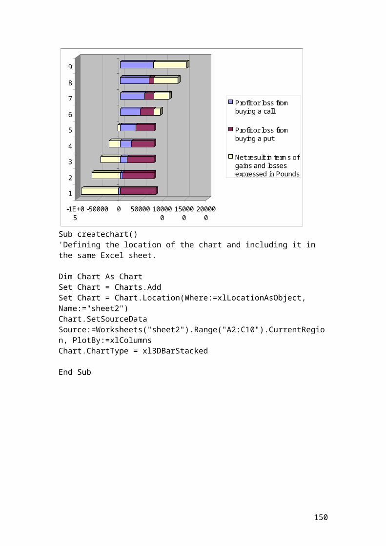
// Mathematical formulas to calculate d1, d2 and the CallRho price.

double CallRho(double S, double K, double r, double q, double T, double sig){

double d1, d2; d1 = (log(S/K) + (r-q +(sig*sig)*0.5 ) * T ) / (sig * sqrt(T)); d2 = d1 - sig*sqrt(T); return K*T*exp(-r*T)*N(d2);}

// Mathematical formulas to calculate d1, d2 and the Gamma price.

double Gamma(double S, double K, double r, double q, double T, double sig){

double d1, d2; d1 = (log(S/K) + (r-q +(sig*sig)*0.5 ) * T ) / (sig * sqrt(T)); d2 = d1 - sig*sqrt(T); return (NP(d1)*exp(-q*T))/(S*sig*sqrt(T));}

// Mathematical formulas to calculate d1, d2 and the Vega price.

double Vega(double S, double K, double r, double q, double T, double sig){

double d1, d2; d1 = (log(S/K) + (r-q +(sig*sig)*0.5 ) * T ) / (sig * sqrt(T)); d2 = d1 - sig*sqrt(T); return S*sqrt(T)*NP(d1)*exp(-q*T);}

150

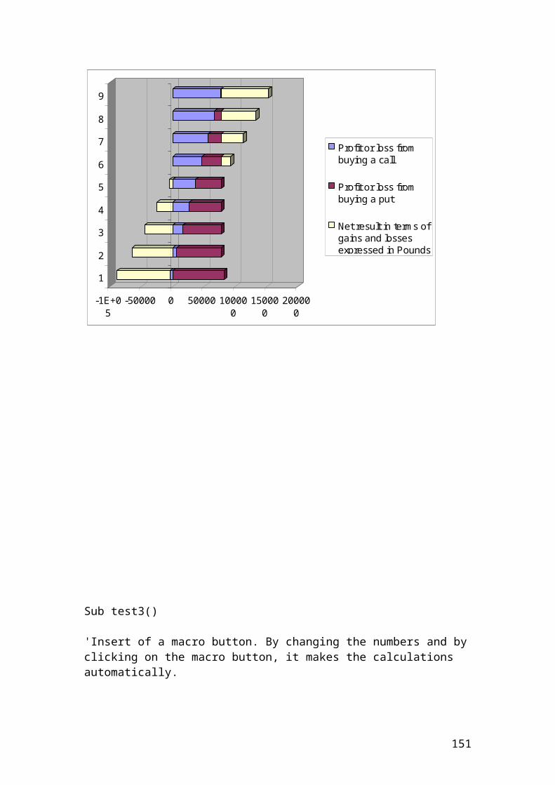
// Mathematical formulas to calculate d1, d2 and the European put price.

double Put(double S, double K, double r, double q, double T, double sig){

double d1, d2; d1 = (log(S/K) + (r-q +(sig*sig)*0.5 ) * T ) / (sig * sqrt(T)); d2 = d1 - sig*sqrt(T);

return K*exp(-r*T)*N(-d2) - S*exp(-q*T)*N(-d1) ; }

// Mathematical formulas to calculate d1, d2 and the European PutDelta.

double PutDelta(double S, double K, double r, double q, double T, double sig){

double d1, d2; d1 = (log(S/K) + (r-q +(sig*sig)*0.5 ) * T ) / (sig * sqrt(T)); d2 = d1 - sig*sqrt(T); return exp(-q*T)*(N(d1)-1); }

// Mathematical formulas to calculate d1, d2 and the European PutTheta.

double PutTheta(double S, double K, double r, double q, double T, double sig){

double d1, d2; d1 = (log(S/K) + (r-q +(sig*sig)*0.5 ) * T ) / (sig * sqrt(T)); d2 = d1 - sig*sqrt(T); return -(S*NP(d1)*sig*exp(-q*T))/(2*sqrt(T)) - (q*S*N(-d1)*exp(-q*T)) + (r*K*exp(-r*T)*N(-d2)); } // Mathematical formulas to calculate d1, d2 and the European PutRho.

double PutRho(double S, double K, double r, double q, double T, double sig){

double d1, d2;

151

d1 = (log(S/K) + (r-q +(sig*sig)*0.5 ) * T ) / (sig * sqrt(T)); d2 = d1 - sig*sqrt(T); return -K*T*exp(-r*T)*N(-d2);}

// Identification or declaration of the variables.

int main(){ double S = 70; // price of stock double K = 70; // strike price double r = 0.08; // interest rate double q = 0.03; // dividend yield double T = 0.5; // life to maturity double sig = 0.20; // volatility

/*Calculation of call and put prices in addition of showing the numerical values of the variables.*/

double callPrice, putPrice, callDelta, putDelta, callTheta, putTheta, callRho, putRho, gamma, vega;

callPrice = Call (S,K,r,q,T,sig);putPrice = Put (S,K,r,q,T,sig);callDelta = CallDelta (S, K, r, q, T, sig) ;putDelta = PutDelta(S, K, r, q, T, sig); callTheta = CallTheta(S, K, r, q, T, sig) ;putTheta = PutTheta(S, K, r, q, T, sig) ; callRho = CallRho(S, K, r, q, T, sig) ;putRho = PutRho(S, K, r, q, T, sig) ; gamma = Gamma(S, K, r, q, T, sig) ; vega = Vega(S, K, r, q, T, sig) ; std::cout<<"Price of stock: " <<S<<std::endl;std::cout<<"Strike price: " <<K<<std::endl;std::cout<<"Interest rate: " <<r<<std::endl;std::cout<<"Dividend yield: " <<q<<std::endl;std::cout<<"Life to maturity: " <<T<<std::endl;std::cout<<"Volatility: " <<sig<<std::endl;cout<<"Call price: " <<callPrice << endl;cout<<"Put price:" <<putPrice << endl;cout << "Call delta: "<<callDelta <<endl;cout << "Put delta: "<<putDelta <<endl; cout << "Call theta: "<<callTheta <<endl;cout << "Put theta: "<<putTheta <<endl; cout <<" Callrho:"<<callRho <<endl;cout <<" Putrho: "<<putRho <<endl;

152

cout << "Gamma: "<<gamma <<endl; cout << "Vega: "<<vega <<endl;

system("PAUSE"); return 0;

}OutputAfter compiling and debugging , the DOS window or console will open and display the following results:

Price of stock: 70Strike price: 70Interest rate: 0.08Dividend yield: 0.03Life to maturity: 0.5Volatility: 0.2Call price: 4.75Put price: 3.05Call delta: 0.589Put delta: -0.396 or -0.40Call theta: -5.45Put theta: -2.14Call rho: 18.23Put rho: -15.39Gamma: 0.0385 or 0.039Vega: 18.87Press any key to continue….

Calculation of the mean of stock price returns and inserting the function cin to allow us to write in the console or DOS window the numerical values of stock price returns

#include <iostream>using namespace std;int main(){double stockPrice[6];stockPrice[1] = 10;stockPrice[2] = 12;stockPrice[3] = 13;stockPrice[4] = 14;stockPrice[5] = 15;

153

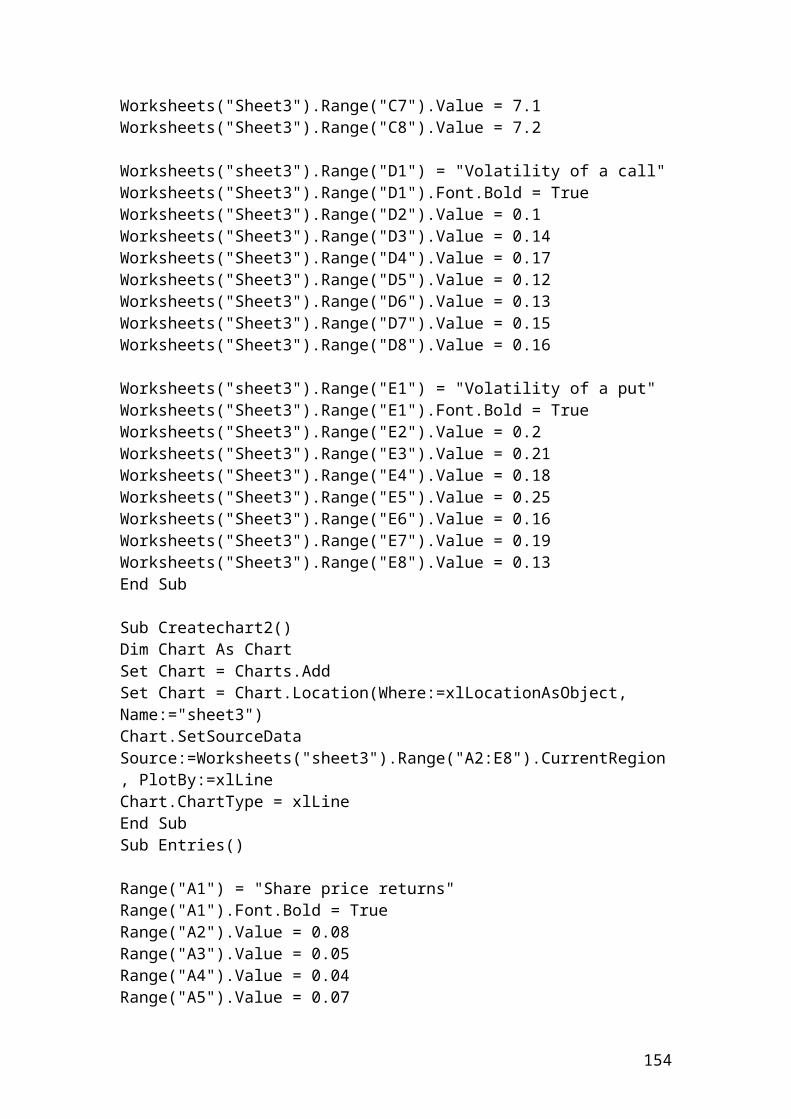
stockPrice[6] = 16;double average;

// Insert the mathematical formula.

average = (stockPrice[1] + stockPrice[2] + stockPrice[3] + stockPrice[4] + stockPrice[5] + stockPrice[6])/6;

// Output functions.

cout<<" The mean: "<<average<<endl;cout<< "Enter stockPrice" <<endl;cin>> stockPrice[1];cin>> stockPrice[2];cin>> stockPrice[3];cin>> stockPrice[4];cin>> stockPrice[5];cin>> stockPrice[6];system ("PAUSE");return 0;}

OutputAfter compiling and debugging , the DOS window or console will open and display the following results:

The mean : 13.3333Enter StockPrice (This command allows you to insert the stock price returns.You input 10. Then, press Enter.12 Press Enter.13 Press Enter14 Press Enter15 Press EnterPress any key to continue….

Repetition of the previous example by replacing the function double with int.Calculation of the mean of stock price returns and inserting the function cin to allow us to write in the console or DOS window the numerical values of stock price returns

I would like to make clear that we use the function double to include numbers with fractional parts. In contrast, we use the function int which is integers to include whole numbers. I repeat the above example, to show the difference. In Financial investment, we use the function double to include the decimals.

#include <iostream>using namespace std;int main(){int stockPrice[6];

154

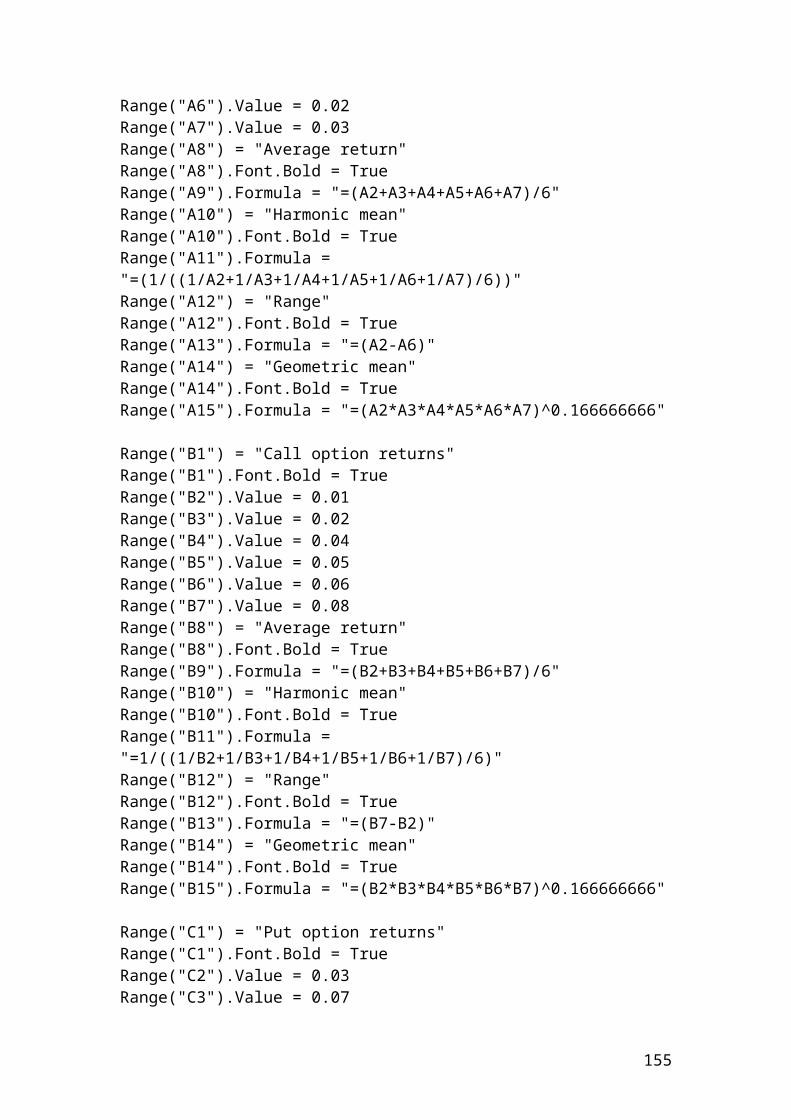
stockPrice[1] = 10;stockPrice[2] = 12;stockPrice[3] = 13;stockPrice[4] = 14;stockPrice[5] = 15;stockPrice[6] = 16;int average;

// Insert the mathematical formula.

average = (stockPrice[1] + stockPrice[2] + stockPrice[3] + stockPrice[4] + stockPrice[5] + stockPrice[6])/6;

// Output functions.

cout<<" The mean: "<<average<<endl;cout<< "Enter stockPrice:" <<endl;cin>> stockPrice[0];cin>> stockPrice[1];cin>> stockPrice[2];cin>> stockPrice[3];cin>> stockPrice[4];cin>> stockPrice[5];system ("PAUSE");return 0;}

OutputAfter compiling and debugging , the DOS window or console will open and display the following results:

The mean : 13Enter StockPrice (This command allows you to insert the stock price returns.You input 10. Then press Enter.12131415Press any key to continue….

155

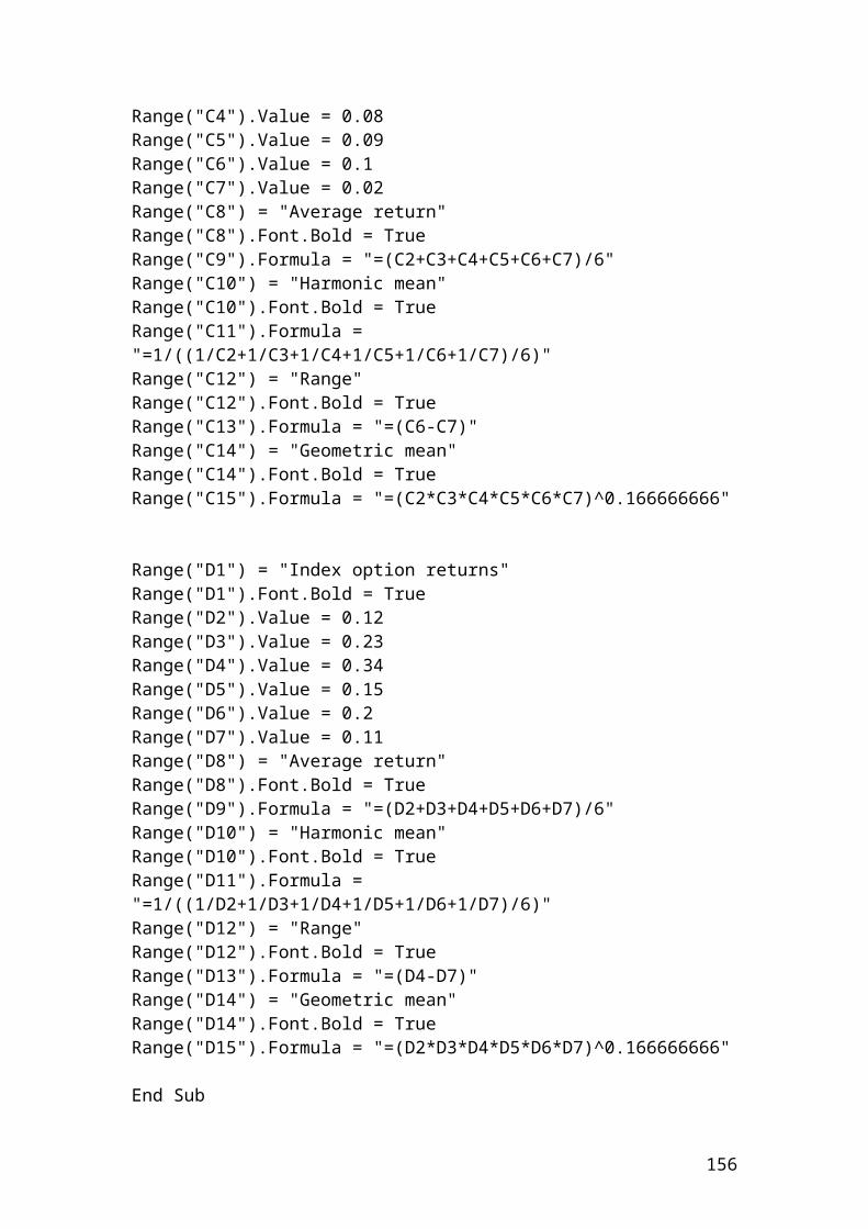
Calculations of the mean and the harmonic mean of share price returns, call option returns, put option returns and index option returns

#include <iostream>using namespace std;int main(){double SharePriceReturns[6];SharePriceReturns[1] = 0.08;SharePriceReturns[2] = 0.05;SharePriceReturns[3] = 0.04;SharePriceReturns[4] = 0.07;SharePriceReturns[5] = 0.02;SharePriceReturns[6] = 0.03;

156

double CallOptionPriceReturns[6];CallOptionPriceReturns[1] = 0.01;CallOptionPriceReturns[2] = 0.02;CallOptionPriceReturns[3] = 0.04;CallOptionPriceReturns[4] = 0.05;CallOptionPriceReturns[5] = 0.06;CallOptionPriceReturns[6] = 0.06;

double PutOptionPriceReturns[6];PutOptionPriceReturns[1] = 0.03;PutOptionPriceReturns[2] = 0.07;PutOptionPriceReturns[3] = 0.08;PutOptionPriceReturns[4] = 0.09;PutOptionPriceReturns[5] = 0.1;PutOptionPriceReturns[6] = 0.02;

double IndexOptionPriceReturns[6];IndexOptionPriceReturns[1] = 0.12;IndexOptionPriceReturns[2] = 0.23;IndexOptionPriceReturns[3] = 0.34;IndexOptionPriceReturns[4] = 0.15;IndexOptionPriceReturns[5] = 0.2;IndexOptionPriceReturns[6] = 0.11;

double averageSharePriceReturns;double averageCallOptionPriceReturns;double averagePutOptionPriceReturns;double averageIndexOptionPriceReturns;double harmonicaverageSharePriceReturns;double harmonicaverageCallOptionPriceReturns;double harmonicaveragePutOptionPriceReturns;double harmonicaverageIndexOptionPriceReturns;

averageSharePriceReturns = (SharePriceReturns[1] + SharePriceReturns[2] + SharePriceReturns[3] + SharePriceReturns[4] + SharePriceReturns[5] + SharePriceReturns[6])/6;

averageCallOptionPriceReturns = (CallOptionPriceReturns[1] + CallOptionPriceReturns[2] + CallOptionPriceReturns[3] + CallOptionPriceReturns[4] + CallOptionPriceReturns[5] + CallOptionPriceReturns[6])/6;

averagePutOptionPriceReturns = (PutOptionPriceReturns[1] + PutOptionPriceReturns[2] + PutOptionPriceReturns[3] + PutOptionPriceReturns[4] + PutOptionPriceReturns[5] + PutOptionPriceReturns[6])/6;

averageIndexOptionPriceReturns = (IndexOptionPriceReturns[1] + IndexOptionPriceReturns[2] + IndexOptionPriceReturns[3] + IndexOptionPriceReturns[4] + IndexOptionPriceReturns[5] + IndexOptionPriceReturns[6])/6;

157

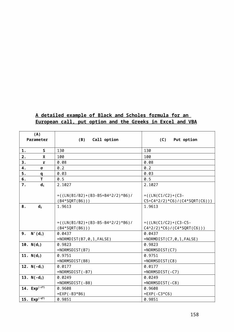
harmonicaverageSharePriceReturns = (1/((1/SharePriceReturns[1] + 1/SharePriceReturns[2] + 1/SharePriceReturns[3] + 1/SharePriceReturns[4] + 1/SharePriceReturns[5] + 1/SharePriceReturns[6])/6));

harmonicaverageCallOptionPriceReturns = (1/((1/CallOptionPriceReturns[1] + 1/CallOptionPriceReturns[2] + 1/CallOptionPriceReturns[3] + 1/CallOptionPriceReturns[4] + 1/CallOptionPriceReturns[5] + 1/CallOptionPriceReturns[6])/6));

harmonicaveragePutOptionPriceReturns = (1/((1/PutOptionPriceReturns[1] + 1/PutOptionPriceReturns[2] + 1/PutOptionPriceReturns[3] + 1/PutOptionPriceReturns[4] + 1/PutOptionPriceReturns[5] + 1/PutOptionPriceReturns[6])/6));

harmonicaverageIndexOptionPriceReturns = (1/((1/IndexOptionPriceReturns[1] + 1/IndexOptionPriceReturns[2] + 1/IndexOptionPriceReturns[3] + 1/IndexOptionPriceReturns[4] + 1/IndexOptionPriceReturns[5] + 1/IndexOptionPriceReturns[6])/6));

cout<<" The mean SharePriceReturns: "<<averageSharePriceReturns<<endl;cout<<" The mean CallOptionPriceReturns: "<<averageCallOptionPriceReturns<<endl;cout<<" The mean PutOptionPriceReturns: "<<averagePutOptionPriceReturns<<endl;cout<<" The mean IndexOptionPriceReturns: "<<averageIndexOptionPriceReturns<<endl;

cout<<" The harmonic mean SharePriceReturns: "<<harmonicaverageSharePriceReturns<<endl;cout<<" The harmonic mean CallOptionPriceReturns: "<<harmonicaverageCallOptionPriceReturns<<endl;cout<<" The harmonic mean PutOptionPriceReturns: "<<harmonicaveragePutOptionPriceReturns<<endl;cout<<" The harmonic mean IndexOptionPriceReturns: "<<harmonicaverageIndexOptionPriceReturns<<endl;system ("PAUSE");return 0;}

Output

After compiling and debugging , the DOS window or console will open and display the following results:

The mean SharePriceReturns: 0.048The mean CallOptionPriceReturns:0.04The mean PutOptionPriceReturns: 0.065The mean IndexOptionPriceReturns: 0.19The harmonic mean SharePriceReturns: 0.039The harmonic mean CallOptionPriceReturns: 0.026

158

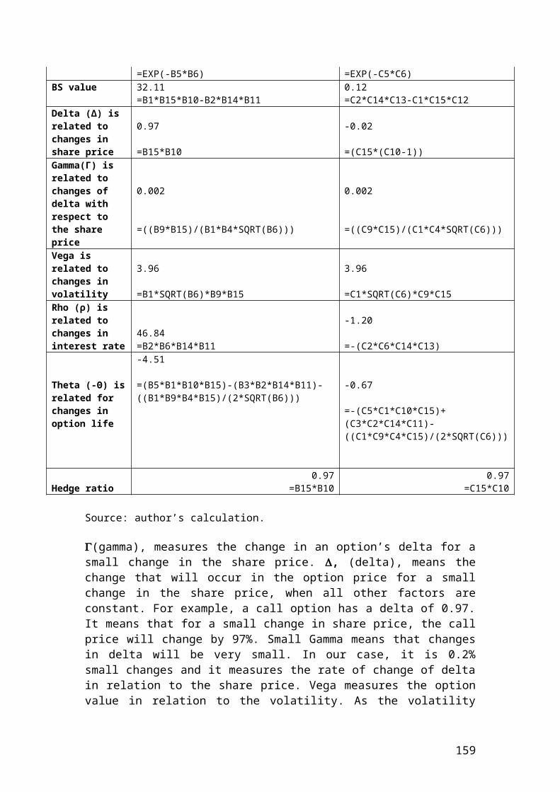
The harmonic mean PutOptionPriceReturns: 0.046The harmonic mean IndexOptionPriceReturns: 0.16

Press any key to continue….

Exercise of how to calculate the payoff of buying a call, a put and the net result or position of your investment position expressed in pounds

#include <iostream>using namespace std;

int main(){double SharePrice[6];SharePrice[1] = 105;SharePrice[2] = 110;SharePrice[3] = 120;SharePrice[4] = 130;SharePrice[5] = 140;SharePrice[6] = 150;

double ExercisePriceCall[6];ExercisePriceCall[1] = 90;

159

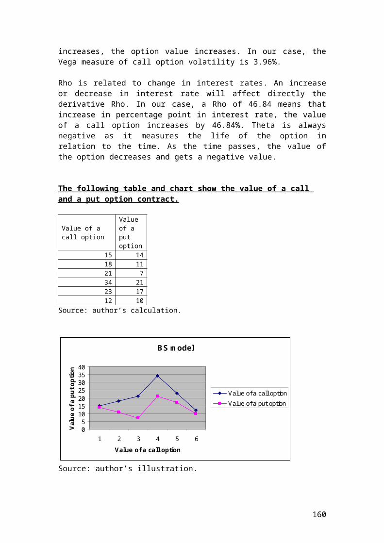
ExercisePriceCall[2] = 90;ExercisePriceCall[3] = 90;ExercisePriceCall[4] = 90;ExercisePriceCall[5] = 90;ExercisePriceCall[6] = 90;

double ExercisePricePut[6];ExercisePricePut[1] = 190;ExercisePricePut[2] = 190;ExercisePricePut[3] = 190;ExercisePricePut[4] = 190;ExercisePricePut[5] = 190;ExercisePricePut[6] = 190;

double PremiumofCall [1];PremiumofCall [1] = 14;

double PremiumofPut [1];PremiumofPut [1] = 9;

double TotalNumberofContracts [1];TotalNumberofContracts [1] = 10;

double totalNumberOfShares =100;

double payoffBuyaCall1;double payoffBuyaCall2;double payoffBuyaCall3;double payoffBuyaCall4;double payoffBuyaCall5;double payoffBuyaCall6;

double payoffBuyaPut1;double payoffBuyaPut2;double payoffBuyaPut3;double payoffBuyaPut4;double payoffBuyaPut5;double payoffBuyaPut6;

double NetResult1;double NetResult2;double NetResult3;double NetResult4;double NetResult5;double NetResult6;

payoffBuyaCall1 = (SharePrice[1]-(ExercisePriceCall[1]+PremiumofCall[1]))*TotalNumberofContracts[1]*totalNumberOfShares;

160

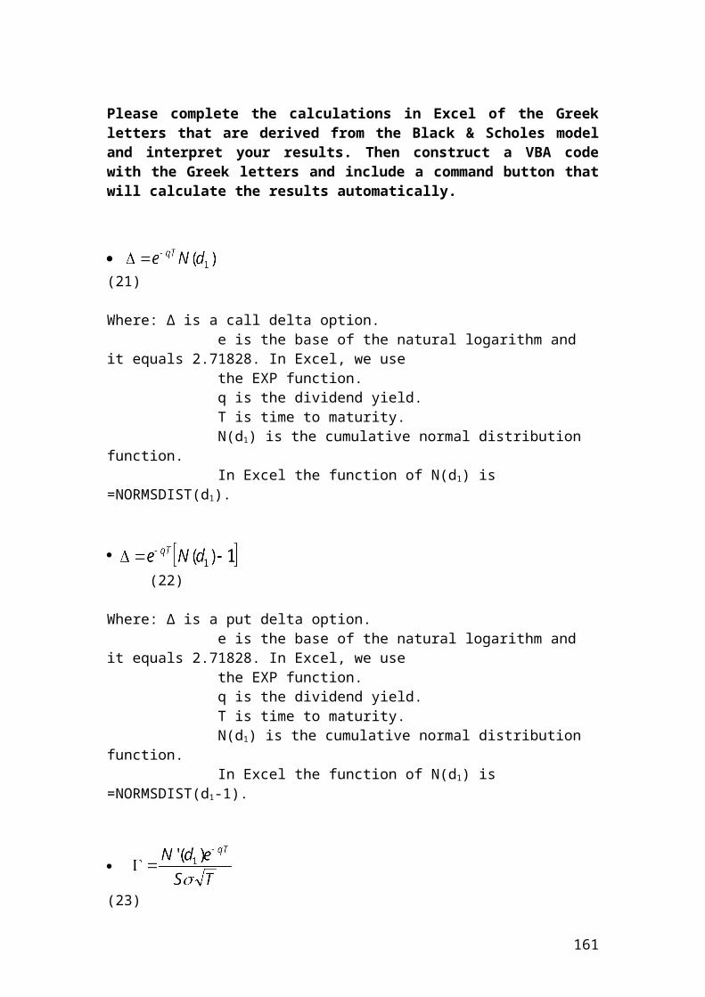
payoffBuyaCall2 = ( SharePrice[2]-(ExercisePriceCall[2]+PremiumofCall[1]))*TotalNumberofContracts[1]*totalNumberOfShares;payoffBuyaCall3 = ( SharePrice[3]-(ExercisePriceCall[3]+PremiumofCall[1]))*TotalNumberofContracts[1]*totalNumberOfShares;payoffBuyaCall4 = ( SharePrice[4]-(ExercisePriceCall[4]+PremiumofCall[1]))*TotalNumberofContracts[1]*totalNumberOfShares;payoffBuyaCall5 = ( SharePrice[5]-(ExercisePriceCall[5]+PremiumofCall[1]))*TotalNumberofContracts[1]*totalNumberOfShares;payoffBuyaCall6 = ( SharePrice[6]-(ExercisePriceCall[6]+PremiumofCall[1]))*TotalNumberofContracts[1]*totalNumberOfShares;

payoffBuyaPut1 = ( ExercisePricePut[1]-SharePrice[1]-PremiumofPut[1])*TotalNumberofContracts[1]*totalNumberOfShares;payoffBuyaPut2 = ( ExercisePricePut[2]-SharePrice[2]-PremiumofPut[1])*TotalNumberofContracts[1]*totalNumberOfShares;payoffBuyaPut3 = ( ExercisePricePut[3]-SharePrice[3]-PremiumofPut[1])*TotalNumberofContracts[1]*totalNumberOfShares;payoffBuyaPut4 = ( ExercisePricePut[4]-SharePrice[4]-PremiumofPut[1])*TotalNumberofContracts[1]*totalNumberOfShares;payoffBuyaPut5 = ( ExercisePricePut[5]-SharePrice[5]-PremiumofPut[1])*TotalNumberofContracts[1]*totalNumberOfShares;payoffBuyaPut6 = ( ExercisePricePut[6]-SharePrice[6]-PremiumofPut[1])*TotalNumberofContracts[1]*totalNumberOfShares;

NetResult1 = payoffBuyaCall1 - payoffBuyaPut1;NetResult2 = payoffBuyaCall2 - payoffBuyaPut2;NetResult3 = payoffBuyaCall3 - payoffBuyaPut3;NetResult4 = payoffBuyaCall4 - payoffBuyaPut4;NetResult5 = payoffBuyaCall5 - payoffBuyaPut5;NetResult6 = payoffBuyaCall6 - payoffBuyaPut6;

cout<<" Payoff of buy a call1: "<<payoffBuyaCall1<<endl;cout<<" Payoff of buy a call2: "<<payoffBuyaCall2<<endl;cout<<" Payoff of buy a call3: "<<payoffBuyaCall3<<endl;cout<<" Payoff of buy a call4: "<<payoffBuyaCall4<<endl;cout<<" Payoff of buy a call5: "<<payoffBuyaCall5<<endl;cout<<" Payoff of buy a call6: "<<payoffBuyaCall6<<endl;

cout<<" Payoff of buy a Put1: "<<payoffBuyaPut1<<endl;cout<<" Payoff of buy a Put2: "<<payoffBuyaPut2<<endl;cout<<" Payoff of buy a Put3: "<<payoffBuyaPut3<<endl;cout<<" Payoff of buy a Put4: "<<payoffBuyaPut4<<endl;cout<<" Payoff of buy a Put5: "<<payoffBuyaPut5<<endl;cout<<" Payoff of buy a Put6: "<<payoffBuyaPut6<<endl;

161

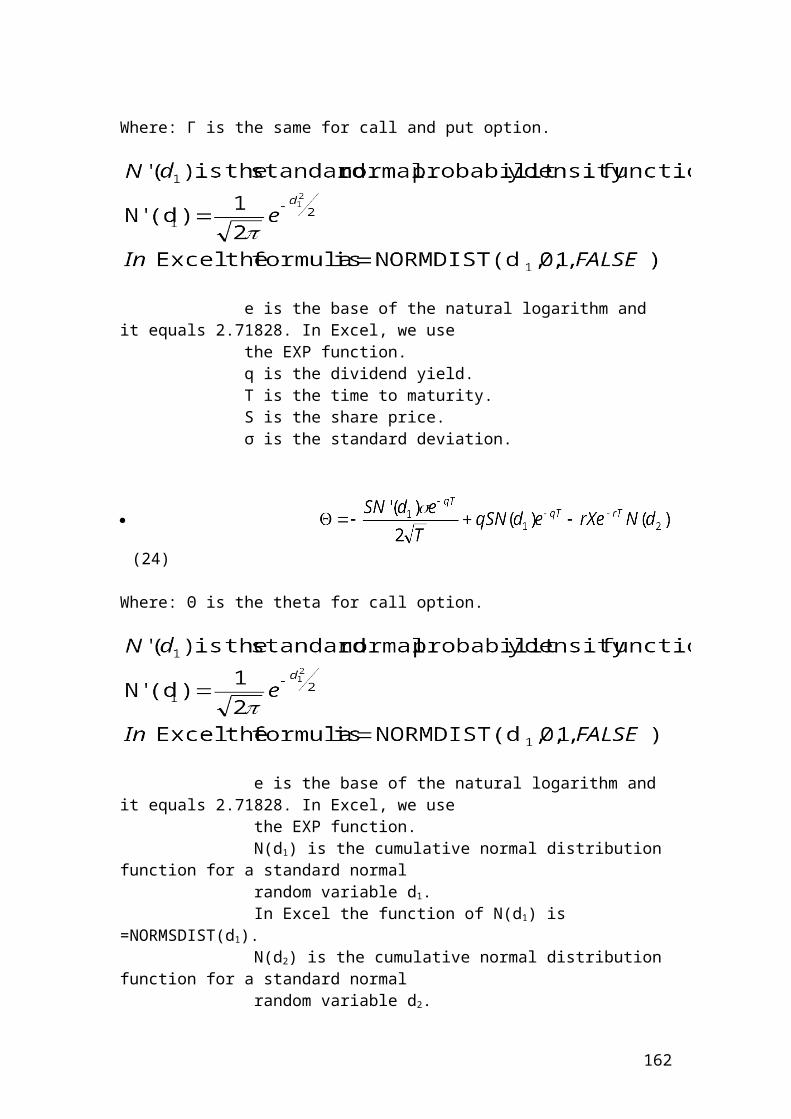
cout<<" NetResult1: "<<NetResult1<<endl;cout<<" NetResult2: "<<NetResult2<<endl;cout<<" NetResult3: "<<NetResult3<<endl;cout<<" NetResult4: "<<NetResult4<<endl;cout<<" NetResult5: "<<NetResult5<<endl;cout<<" NetResult6: "<<NetResult6<<endl;

system ("PAUSE");return 0;}

Output

The amounts are expressed in pounds. After compiling and debugging , the DOS window or console will open and display the following results:

Payoff of buy a call1 : 1000Payoff of buy a call2 : 6000Payoff of buy a call3 : 16000Payoff of buy a call4 : 26000Payoff of buy a call5 : 36000Payoff of buya call6 : 46000

Payoff of buy a put1 : 76000Payoff of buy a put2 : 71000Payoff of buy a put3 : 61000Payoff of buy a put4 : 51000Payoff of buy a put5 : 41000Payoff of buy a put6 : 31000

NetResult1 : -75000NetResult2 : -65000 NetResult3 : -45000NetResult4 : -25000NetResult5 : -5000NetResult6 : 15000

Press any key to continue….

Exercise

Please calculate the range based on different share prices.

Answer

#include <iostream>

162

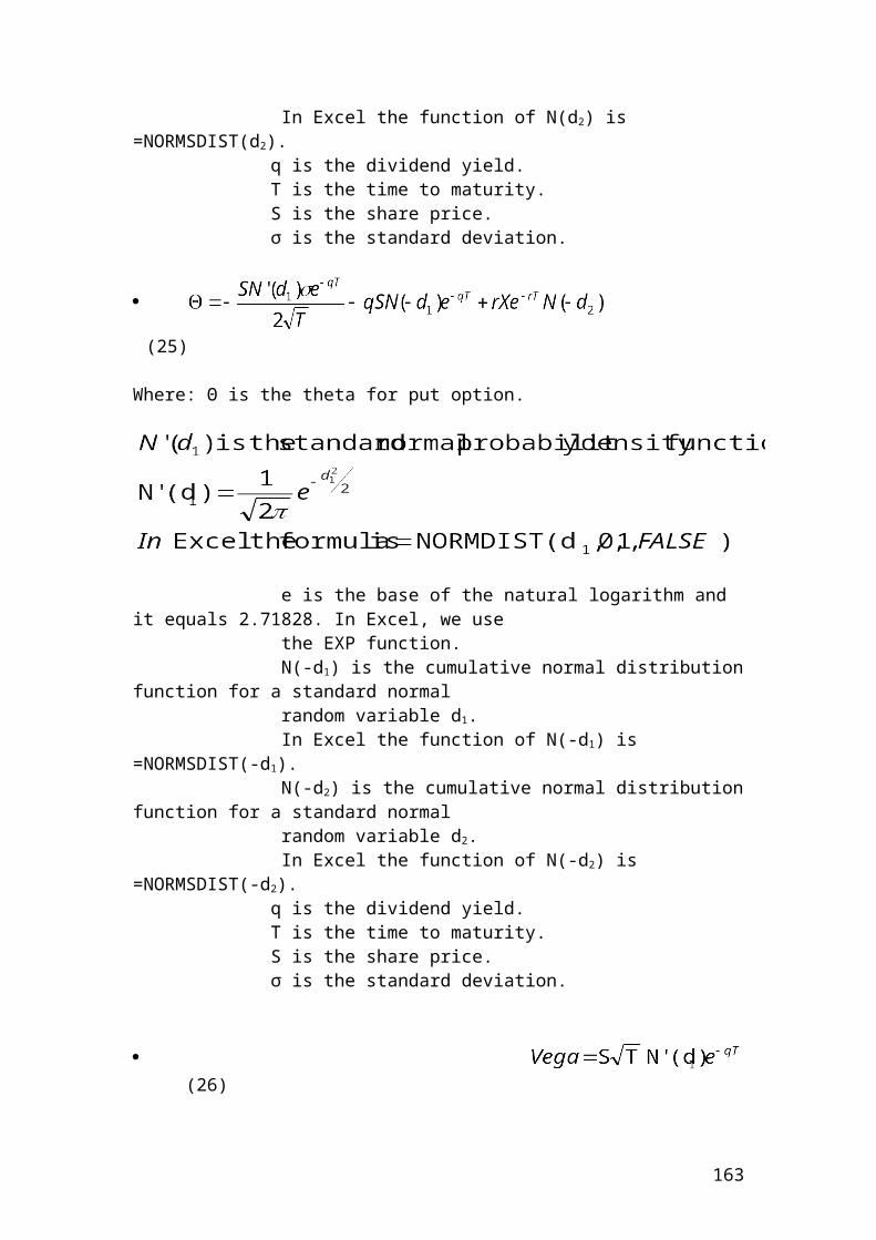
using namespace std;

int main(){double SharePrice[6];SharePrice[1] = 20;SharePrice[2] = 30;SharePrice[3] = 40;SharePrice[4] = 50;SharePrice[5] = 60;SharePrice[6] = 70;

double RangeSharePrice;

// Insert the mathematical formula.

RangeSharePrice = (SharePrice[6]-SharePrice[1]);

// Output function.

cout<<" The Range: "<<RangeSharePrice<<endl;system ("PAUSE");return 0;}

Output

After compiling and debugging , the DOS window or console will open and display the following results:

The Range: 50

Press any key to continue …Calculate the log returns and the average using actual share price returns expressed in pounds

#include <iostream>#include<cmath>

using namespace std;

int main(){

//Identify the variables.

double dailyret2;double dailyret3;double dailyret4;double dailyret5;

163

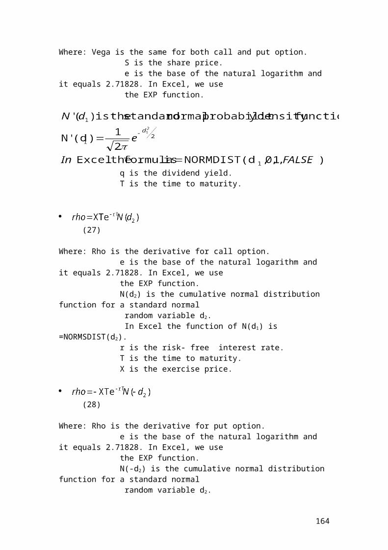
double average;

// Actual share prices.

double sharePrices[5];sharePrices[1] = 14.23;sharePrices[2] = 15.67;sharePrices[3] = 12.13;sharePrices[4] = 11.45;sharePrices[5] = 10.11;

/* Insert the mathematical formulas for ln returns. In C++ use the log function. In Excel use the ln function.*/

dailyret2 = log(sharePrices[2]/sharePrices[1]); dailyret3 = log(sharePrices[3]/ sharePrices[2]); dailyret4 = log(sharePrices[4]/ sharePrices[3]); dailyret5 = log (sharePrices[5]/ sharePrices[4]); // Average calculation. average = (dailyret2 + dailyret3+ dailyret4 + dailyret5)/4;

// Output functions.

cout.setf(ios::fixed); cout.setf(ios::showpoint); cout.precision(2); cout<<"dailyret2:"<<dailyret2<<endl;cout<<"dailyret3:"<<dailyret3<<endl;cout<<"dailyret4:"<<dailyret4<<endl;cout<<"dailyret5:"<<dailyret5<<endl;cout<< "Average:"<<average<<endl;

system ("PAUSE");return 0;}

Output

After compiling and debugging , the DOS window or console will open and display the following results:

dailyret2: 0.10dailyret3: -0.26dailyret4: -0.06dailyret5: -0.12Average: -0.09Press any key to continue …

164

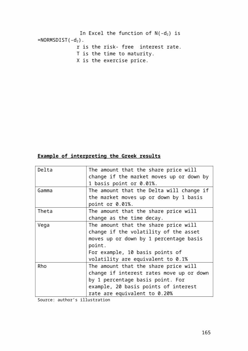
Calculation of daily and annual volatility of percentage returns measured by the sample standard deviation

/* Calculation of daily volatility of percentage returns measured by the sample standard deviation. Then, convert it toannual by multiplying the standard deviation by the square root of 250.*/

#include <iostream>#include<math.h>using namespace std;

int main(){

// Identify the variables.

165

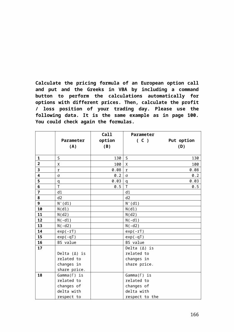
double sum ;double average; double sumDiffSqr;double DailystdDev;double AnnualstdDev;

double sharePrices[5] = {0.1423,0.1567,0.1213,0.1145,0.1011};

/* The following expression inserts a variable x that tells the computerthat the first observation 0 is 0.1423 and x is less than 5 to include all observations.*/

for (int x = 0; x < 5; x++)

//We insert the formula for summation.

sum += sharePrices[x];

// We insert the formula for average.average = sum/5;

/* We calculate the sumDiffSqr by inserting the expression for that tells the computer the numbers that will be included in the calculation. We calculate the difference between each number and the average. Then, we square it and we sum it.*/

sumDiffSqr = 0;for (int x = 0; x < 5; x++) { sumDiffSqr = sumDiffSqr + pow((sharePrices[x]-average),2); }/* Insert the formula of the sample standard deviation by taking into account the formual n-1.*/

DailystdDev = sqrt(sumDiffSqr/4);

//We use 250 trading days per year instead of 365 days.

AnnualstdDev = DailystdDev * sqrt(250);

// Output functions.

cout.setf(ios::fixed); cout.setf(ios::showpoint); cout.precision(4); cout<<"Daily sample standard deviation:"<<DailystdDev<<endl;cout<<"Annual standard deviation:"<<AnnualstdDev<<endl;system ("PAUSE");return 0;}

166

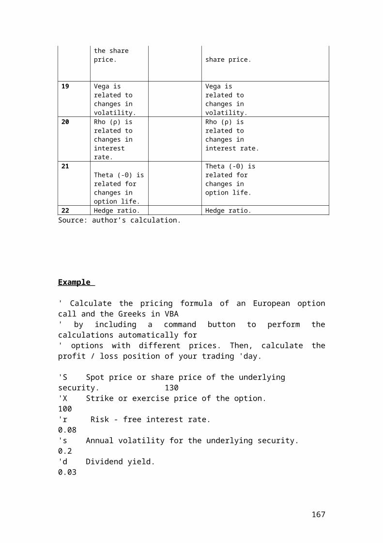
Output

After compiling and debugging , the DOS window or console will open and display the following results:

Daily sample standard deviation: 0.0222Annual standard deviation: 0.3514Press any key to continue …

Calculations of the sum, the average, the sum difference squares and the sample standard deviation of index price returns expressed as percentages from an array format. Please remember that we use the formula n-1. We have 5 observations. Thus, 5 – 1 = 4

#include <iostream>#include<math.h>using namespace std;

int main(){// Calculations of the sum and average function of index prices from an array format.

// Identify the variables.

double sum ;double average;

167

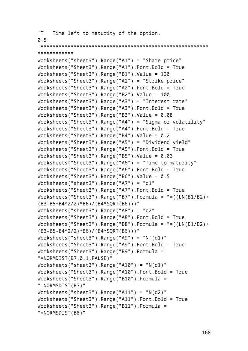
double stdDev;double sumDiffSqr;

/* Identify the array of index prices. We start with a bracket that includes the five observations followed by the numbers.*/

double arrayIndexPriceReturns[5] = {90.54,80.32,82.98,87.12,97.78};

/* The following expression inserts a variable x that tells the computerthat the first observation 0 is 90.54 and x is less than 5 to include all observations.*/

for (int x = 0; x < 5; x++)

//We insert the formula for summation.

sum += arrayIndexPriceReturns[x];

// We insert the formula for average.average = sum/5;

/* We calculate the sumDiffSqr by inserting the expression for that tells the computer the numbers that will be included in the calculation. We calculate the difference between each number and the average. Then, we square it and we sum it.*/

sumDiffSqr = 0;for (int x = 0; x < 5; x++) { sumDiffSqr = sumDiffSqr + pow((arrayIndexPriceReturns[x]-average),2); }/* Insert the formula of the sample standard deviation by taking into account the formual n-1.*/

stdDev = sqrt(sumDiffSqr/4);

// Output functions and conclusion.

cout<< "Sum:"<<sum<<endl;cout<< "Average:"<<average<<endl;cout<<"Standard deviation:"<<stdDev<<endl;

system ("PAUSE");return 0;}

Output

After compiling and debugging , the DOS window or console will open and display the following results:

168

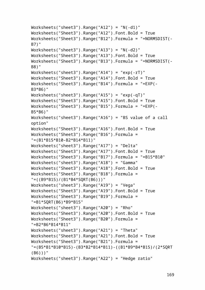
Sum: 438.74Average: 87.748Standard deviation: 6.83264

Press any key to continue …

Calculations of the sum, the average, the sum difference squares and the population standard deviation of index price returns expressed as percentages from an array format. In this case, we use n = 5

#include <iostream>#include<math.h>using namespace std;

int main(){// Calculations of the sum and average function of index prices from an array format.

// Identify the variables.

double sum ;double average; double sumDiffSqr;

169

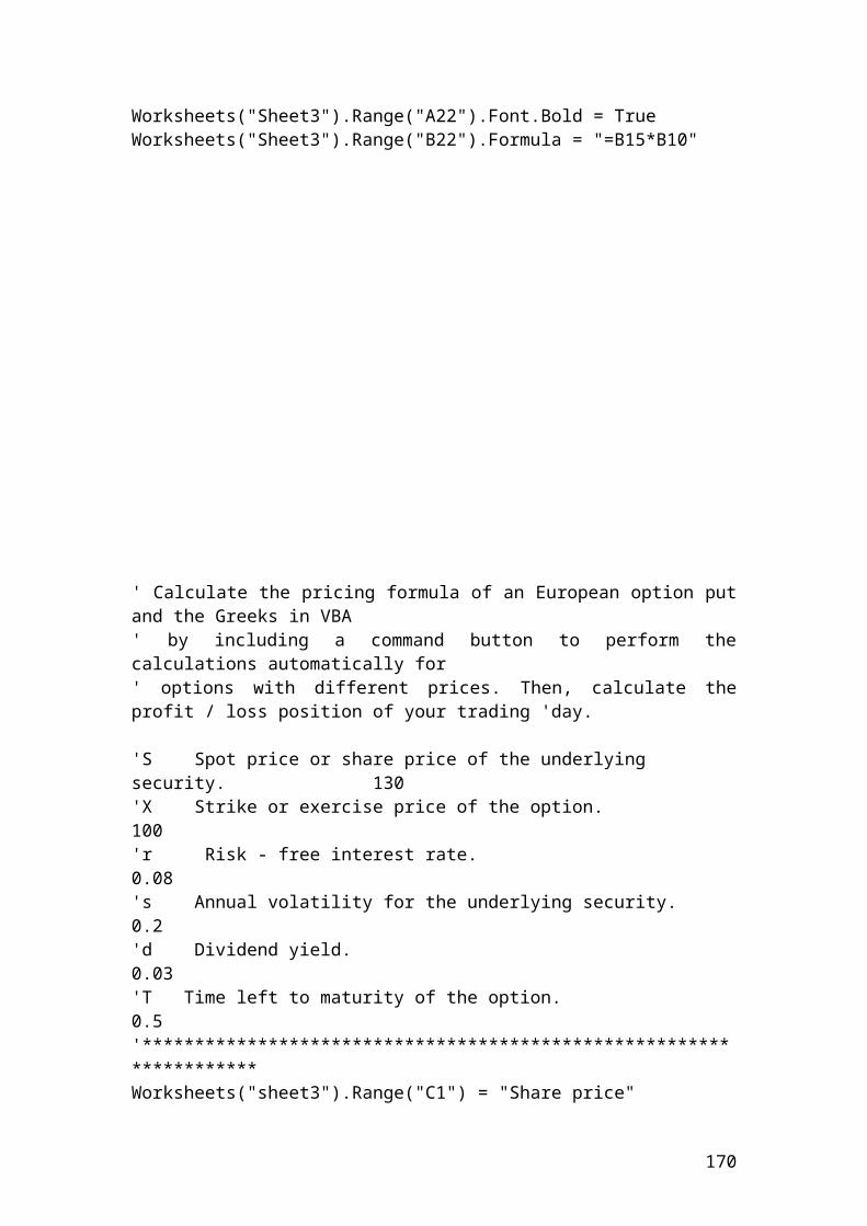
double stdDev;

/* Identify the array of index prices. We start with a bracket that includes the five observations followed by the numbers.*/

double arrayIndexPriceReturns[5] = {90.54,80.32,82.98,87.12,97.78};

/* The following expression inserts a variable x that tells the computerthat the first observation 0 is 90.54 and x is less than 5 to include all observations.*/

for (int x = 0; x < 5; x++)

//We insert the formula for summation.

sum += arrayIndexPriceReturns[x];

// We insert the formula for average.average = sum/5;

/* We calculate the sumDiffSqr by inserting the expression for that tells the computer the numbers that will be included in the calculation.*/

sumDiffSqr = 0;for (int x = 0; x < 5; x++) { sumDiffSqr = sumDiffSqr + pow((arrayIndexPriceReturns[x]-average),2); }// Insert the formula of the population standard deviation.stdDev = sqrt(sumDiffSqr/5);

// Output functions and conclusion.

/* By the function cin we tell the program to allow us to insert theindex price returns in the console by pressing Enter.*/

cout<< "Enter arrayIndexPriceReturns" <<endl;cin>> arrayIndexPriceReturns[1];cin>> arrayIndexPriceReturns[2];cin>> arrayIndexPriceReturns[3];cin>> arrayIndexPriceReturns[4];cin>> arrayIndexPriceReturns[5];cout<< "Sum:"<<sum<<endl;cout<< "Average:"<<average<<endl;cout<<"Standard deviation:"<<stdDev<<endl;system ("PAUSE");return 0;}

170

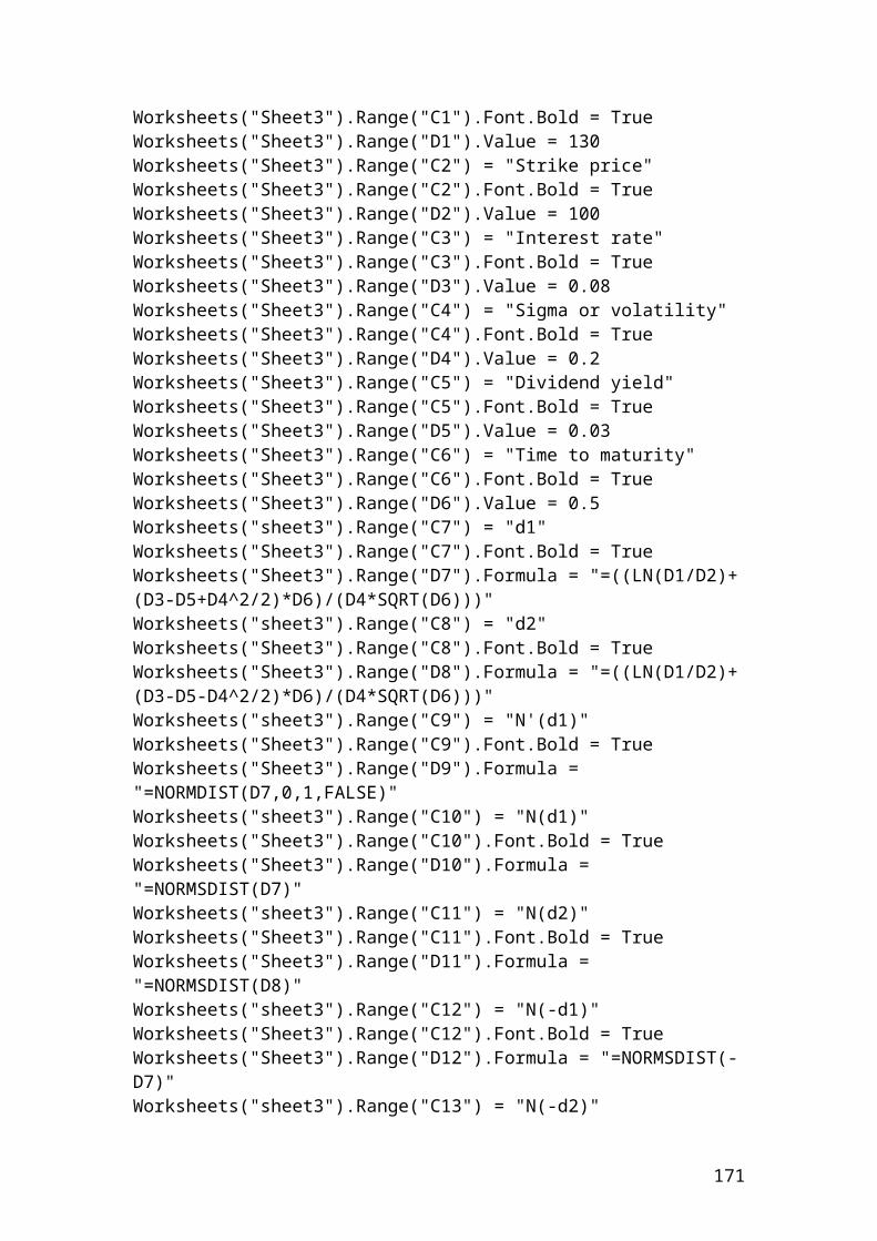
Output

After compiling and debugging , the DOS window or console will open and display the following results:

Enter arrayIndexPriceReturns90.54 Press Enter80.32 Press Enter82.98 Press Enter87.12 Press Enter97.78 Press Enter

Sum: 438.74Average: 87.748Standard deviation: 6.1113

Press any key to continue …

Calculations of the sum, average, sum difference squares and population standard deviation of call option returns from an array format. In this case, we use n = 5

#include <iostream>#include<math.h>using namespace std;

int main(){

/* Calculations of the sum, average, sum difference square and standard deviation functions of call option returns from an array format.*/

// Identify the variables.

double sum ;

171

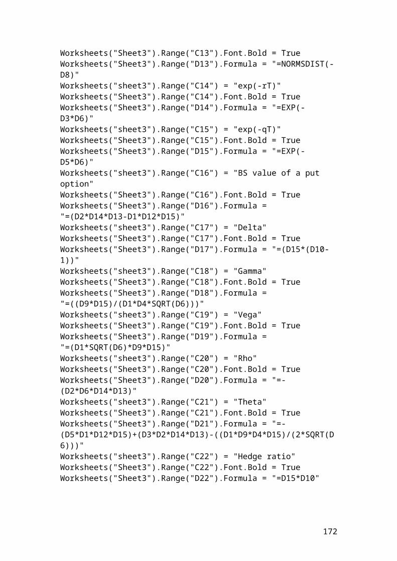
double average; double stdDev;double sumDiffSqr;

/* Identify the array of call option retunrs. We start with a bracket that includes the five observations followed by the numbers.*/

double arraycallreturn[5] = {3.56,4.78,5.65,6.43,8.56};

/* The following expression inserts a varoable x that tells the computerthat the first observation 0 is 3.56 and x is less than 5 to include all observations.*/

for (int x = 0; x < 5; x++)

//We insert the formula for summation.sum += arraycallreturn[x];

// We insert the formula for average.

average = sum/5;

/* We calculate the sumDiffSqr by inserting the expression for that tells the computer the numbers that will be included in the calculation.*/

sumDiffSqr = 0;

for (int x = 0; x < 5; x++) { sumDiffSqr = sumDiffSqr + pow((arraycallreturn[x]-average),2); }/* Insert the formula of the sample standard deviation by taking into account the formual n-1.*/

stdDev = sqrt(sumDiffSqr/5);

/* By the function cin we tell the program to allow us to insert thecall option retunrs in the console by pressing Enter.*/

cout<< "Enter arraycallreturn" <<endl;cin>> arraycallreturn[1];cin>> arraycallreturn[2];cin>> arraycallreturn[3];cin>> arraycallreturn[4];cin>> arraycallreturn[5];

//Output functions.

cout<< "Sum:"<<sum<<endl;cout<< "Average:"<<average<<endl;cout<<"Standard deviation:"<<stdDev<<endl;

172

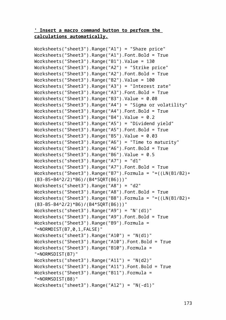
system ("PAUSE");return 0;}

Output

After compiling and debugging , the DOS window or console will open and display the following results:

Enter arraycallreturn3.56 Press Enter4.78 Press Enter5.65 Press Enter6.43 Press Enter8.56 Press Enter

Sum: 28.98Average: 5.796Standard deviation: 1.67898

Press any key to continue …

Calculations of the sum, the average, the sum difference squares and the population standard deviation of call option returns from an array format. In this case, we use n = 5. Demonstration of the high and low level of call option returns

#include <iostream>#include<math.h>using namespace std;

int main(){

/* Calculations of the sum, average, sum difference square and standard deviation functions of call option returns. Demonstration of the high and low level of call option returns. Insert observations as integer in the sum equation.*/

173

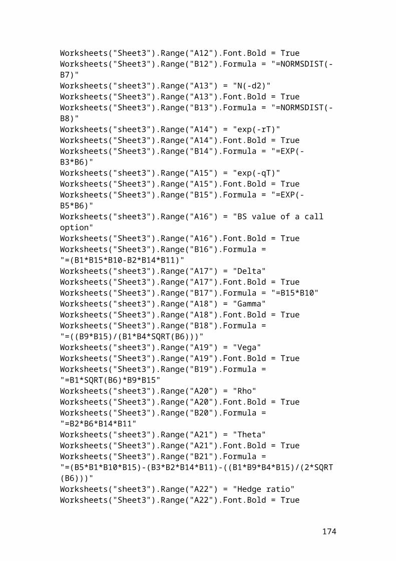
// from an array format.// Identify the variables.

double high = 10.032 ;double low = 1.56 ;double sum ;int observations = 5 ; double average; double sumDiffSqr;double stdDev;

/*Identify the array of call option retunrs. We start with a bracket that includes the five observations followed by the numbers.*/

double arraycallreturn[5] = {3.56,4.78,5.65,6.43,8.56};

/*The following expression inserts a varoable x that tells the computerthat the first observation 0 is 3.56 and x is less than 5 to include all observations.*/

for (int x = 0; x < 5; x++)

//We insert the formula for summation.

sum += arraycallreturn[x];

// We insert the formula for average.

average = sum/observations;

/* We calculate the sumDiffSqr by inserting the expression for that tells the computer the numbers that will be included in the calculation.*/

sumDiffSqr = 0;for (int x = 0; x < 5; x++) { sumDiffSqr = sumDiffSqr + pow((arraycallreturn[x]-average),2); }/* Insert the formula of the sample standard deviation by taking into account the formual n-1.*/

stdDev = sqrt(sumDiffSqr/5);

/* By the function cin we tell the program to allow us to insert thecall option retunrs in the console by pressing Enter.*/

cout<< "Enter arraycallreturn" <<endl;cin>> arraycallreturn[1];cin>> arraycallreturn[2];cin>> arraycallreturn[3];

174

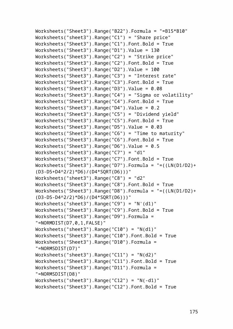
cin>> arraycallreturn[4];cin>> arraycallreturn[5];

//Output functions.

cout<<"High call option return:"<<high<<endl;cout<<"Low call option return:"<<low<<endl;cout<< "Sum:"<<sum<<endl;cout<< "Average:"<<average<<endl;cout<<"Standard deviation:"<<stdDev<<endl;system ("PAUSE");return 0;}

Output

After compiling and debugging , the DOS window or console will open and display the following results:

Enter arraycallreturn3.56 Press Enter4.78 Press Enter5.65 Press Enter6.43 Press Enter8.56 Press EnterHigh call option return: 10.032Low call option return: 1.56Sum: 28.98Average: 5.796Standard deviation: 1.67898

Press any key to continue …

Calculation of the geometric average based on percentages of stock prices

#include <iostream>#include <cmath>using namespace std;int main(){

/* The stock prices express percentages and we are trying to calculate the geometric mean or average. We insert the percentage values of each stock in an array format.*/

double stockPrice[6];stockPrice[1] = 10;stockPrice[2] = 12;stockPrice[3] = 13;

175

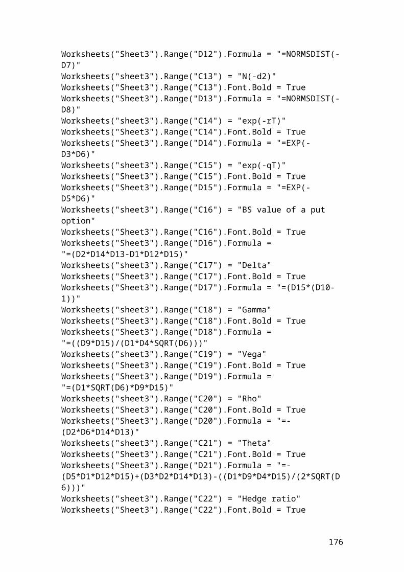
stockPrice[4] = 14;stockPrice[5] = 15;stockPrice[6] = 16;

// We define the variable that we want to calculate.

double Geometricaverage;

// We write the mathematical equation of the geometric mean.

Geometricaverage = pow(stockPrice[1]*stockPrice[2]*stockPrice[3]*stockPrice[4]*stockPrice[5]*stockPrice[6],0.166666);

// The output function.cout<<"The geometric average:"<<Geometricaverage<<endl;

system ("PAUSE");return 0;}

Output

After compiling and debugging , the DOS window or console will open and display the following results:

The geometric average: 13.18 ( to 2.d.p.).

Press any key to continue …

Calculation of the geometric average based on percentages of call option price returns

#include <iostream>#include <cmath>using namespace std;int main(){

/* The call option price returns are expressed in percentages and we are trying to calculate the geometric mean or average. We insert the percentage values of each call option in an array format.*/

double CallOptionPriceReturns[6];CallOptionPriceReturns[1] = 5;CallOptionPriceReturns[2] = 3;CallOptionPriceReturns[3] = 2;

176

CallOptionPriceReturns[4] = 4;CallOptionPriceReturns[5] = 7;CallOptionPriceReturns[6] = 8;

// We define the variable that we want to calculate.

double Geometricaverage;

// We write the mathematical equation of the geometric mean.

Geometricaverage = pow(CallOptionPriceReturns[1]*CallOptionPriceReturns[2]*CallOptionPriceReturns[3]*CallOptionPriceReturns[4]*CallOptionPriceReturns[5]*CallOptionPriceReturns[6],0.166666);

// The output.cout<<"The geometric average:"<<Geometricaverage<<endl;

system ("PAUSE");return 0;}

Output

After compiling and debugging , the DOS window or console will open and display the following results:

The geometric average: 4.34 ( to 2.d.p.).

Press any key to continue …

Calculation of the geometric average based on percentages of put option price returns

#include <iostream>#include <cmath>using namespace std;int main(){

/* The put option price returns are expressed in percentages and we are trying to calculate the geometric mean or average.*/

// We insert the percentage values of each put option in an array format.

double PutOptionPriceReturns[6];PutOptionPriceReturns[1] = 2;

177

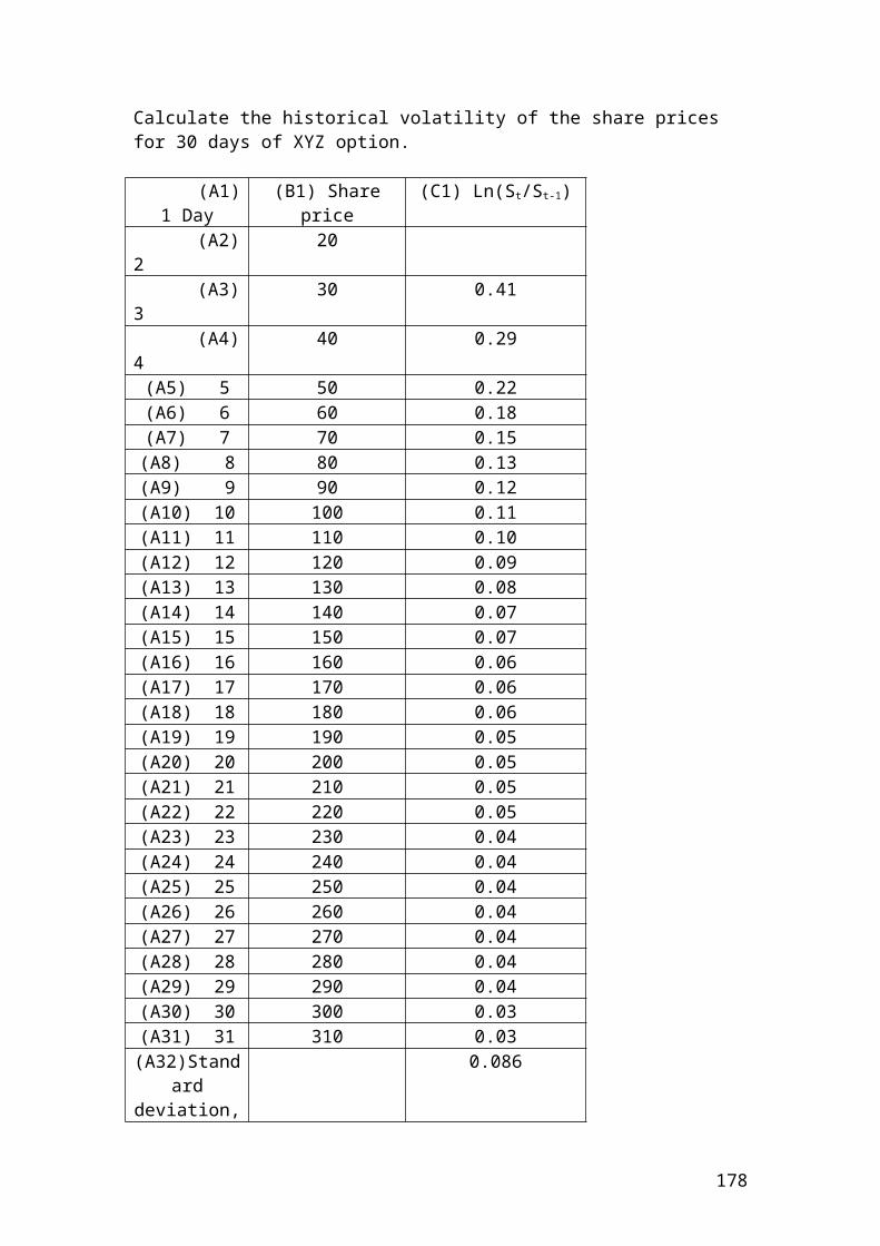
PutOptionPriceReturns[2] = 3.3;PutOptionPriceReturns[3] = 2.45;PutOptionPriceReturns[4] = 4.21;PutOptionPriceReturns[5] = 7.4;PutOptionPriceReturns[6] = 4.34;

// We define the variable that we want to calculate.

double Geometricaverage;

// We write the mathematical equation of the geometric mean.

Geometricaverage = pow(PutOptionPriceReturns[1]*PutOptionPriceReturns[2]*PutOptionPriceReturns[3]*PutOptionPriceReturns[4]*PutOptionPriceReturns[5]*PutOptionPriceReturns[6],0.166666);

// The output.

cout<<"The geometric average:"<<Geometricaverage<<endl;

system ("PAUSE");return 0;}

Output

After compiling and debugging , the DOS window or console will open and display the following results:

The geometric average: 3.60 ( to 2.d.p.).

Press any key to continue …

Calculation of the geometric average based on percentages of index option price returns

#include <iostream>#include <cmath>using namespace std;int main(){

/* The Index option price returns are expressed in percentages and we are trying to calculate the geometric mean or average. We insert the percentage values of each index option in an array format.*/

double IndexOptionPriceReturns[6];IndexOptionPriceReturns[1] = 2;IndexOptionPriceReturns[2] = 2.31;

178

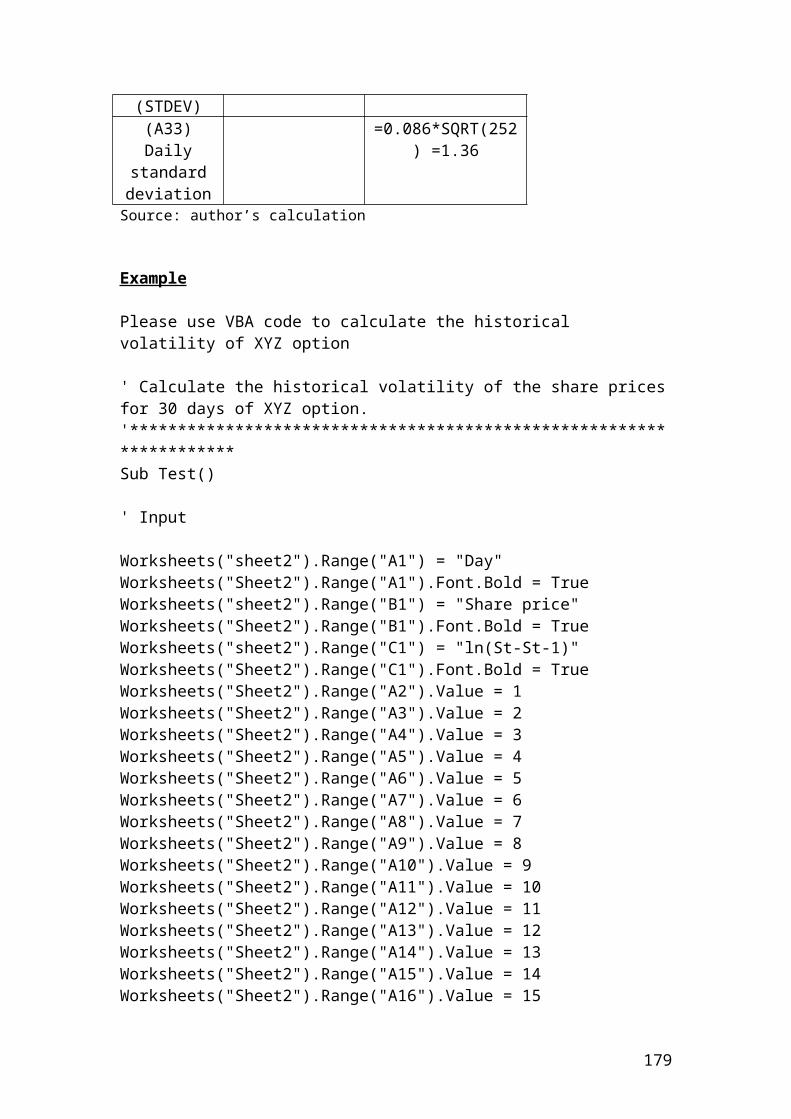
IndexOptionPriceReturns[3] = 2.35;IndexOptionPriceReturns[4] = 4.51;IndexOptionPriceReturns[5] = 7.56;IndexOptionPriceReturns[6] = 4.39;

// We define the variable that we want to calculate.

double Geometricaverage;

// We write the mathematical equation of the geometric mean.

Geometricaverage = pow(IndexOptionPriceReturns[1]*IndexOptionPriceReturns[2]*IndexOptionPriceReturns[3]*IndexOptionPriceReturns[4]*IndexOptionPriceReturns[5]*IndexOptionPriceReturns[6],0.166666);

// The output.cout<<"The geometric average:"<<Geometricaverage<<endl;system ("PAUSE");return 0;}

Output

After compiling and debugging , the DOS window or console will open and display the following results:

The geometric average: 3.43 ( to 2.d.p.).

Press any key to continue …

Calculate the portfolio return, the variance and the standard deviation in C++ for options with different returns and standard deviations

// Calculate the portfolio return, the variance and the standard deviation or risk of the // portfolio in C++ for options with different returns and standard deviations.// Call option A expected return 0.6// Call option A standard deviation 0.2// Call option A weight 0.35// Correlation coefficient between A and B 0.5// Call option B expected return 0.1// Call option B standard deviation 0.7 // Call option B weight 0.45//Correlation coefficient between B and C -0.1// Call option C expected return 0.3// Call option C standard deviation 0.4// Call option C weight 0.2//Correlation coefficient between A and C -0.4

#include <iostream>

179

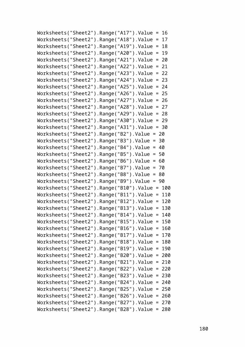
#include<cmath>using namespace std;

int main(){ //Insert the given information by using the double function as we have fractions.

double CalloptionAexpectedreturn = 0.6;double CalloptionAstandarddeviation = 0.2;double CalloptionAweight = 0.35;double CorrelationcoefficientbetweenAandB = 0.5;double CalloptionBexpectedreturn = 0.1;double CalloptionBstandarddeviation = 0.7;double CalloptionBweight = 0.45;double CorrelationcoefficientbetweenBandC = -0.1;double CalloptionCexpectedreturn = 0.3;double CalloptionCstandarddeviation = 0.4;double CalloptionCweight = 0.2;double CorrelationcoefficientbetweenAandC = -0.4;

/* Define the variables that we want to calculate. In other words, the portfolio return, variance and standard deviation.*/

double Portfolioreturn;double Portfoliovariance; double PortfoliostdDev;

// Write the formula of portfolio return.

Portfolioreturn = (CalloptionAexpectedreturn*CalloptionAweight)+(CalloptionBweight*CalloptionBexpectedreturn)+(CalloptionCexpectedreturn*CalloptionCweight);

// Write the formula for portfolio variance.

Portfoliovariance = pow(CalloptionAweight*CalloptionAstandarddeviation,2)+ pow(CalloptionBweight*CalloptionBstandarddeviation,2)+ pow(CalloptionCweight*CalloptionCstandarddeviation,2)+(2*CalloptionAweight*CalloptionBweight*CalloptionAstandarddeviation*CalloptionBstandarddeviation*CorrelationcoefficientbetweenAandB)+(2*CalloptionAweight*CalloptionCweight*CorrelationcoefficientbetweenAandC*CalloptionAstandarddeviation*CalloptionCstandarddeviation)+(2*CalloptionBweight*CalloptionCweight*CorrelationcoefficientbetweenBandC*CalloptionBstandarddeviation*CalloptionCstandarddeviation);

// Write the formula for portfolio standard deviation.

PortfoliostdDev = sqrt(Portfoliovariance);

// Output functions.

180

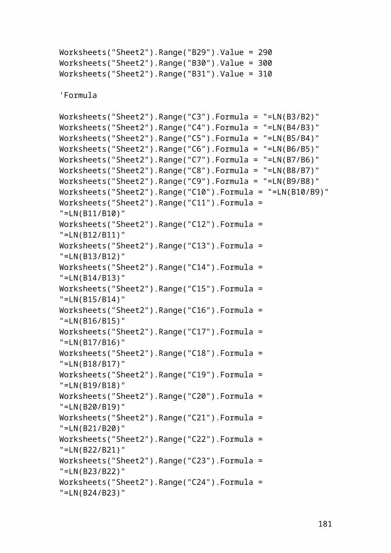
cout<< "Portfolio return:"<<Portfolioreturn<<endl;cout<< "Portfolio variance:"<<Portfoliovariance<<endl;cout<< "Portfolio standard deviation:"<<PortfoliostdDev<<endl;system ("PAUSE");return 0;}

Output

After compiling and debugging , the DOS window or console will open and display the following results:

Portfolio return: 0.315Portfolio variance:0.12 to (2.d.p.).Portfolio standard deviation: 0.35 to (2.d.p.).

Press any key to continue …

Calculate the portfolio return, the variance and the standard deviation or risk of the portfolio

/* Calculate the portfolio return, the variance and the standard deviation or risk of the portfolio.*/

// Share A expected return 0.11// Share A standard deviation 0.15// Share A amount 50000// Correlation coefficient between A and B 0.30// Share B expected return 0.25// Share standard deviation 0.20 // Share B amount 50000// The total amount of the portfolio is 100000

#include <iostream>#include<cmath>using namespace std;

int main()

181

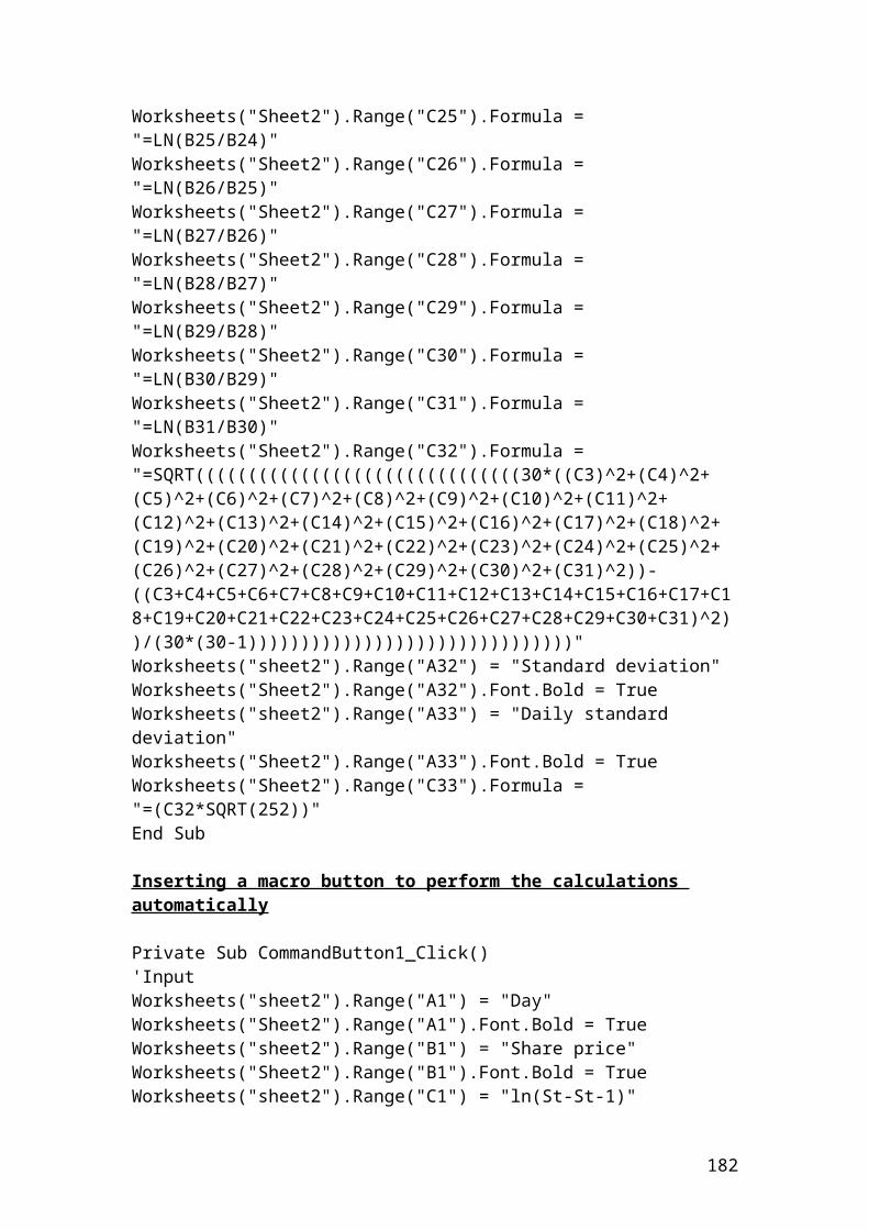
{ double shareAexpRet = 0.25;double shareAstddev = 0.10;double shareAamount = 50000;double correlationAB = 0.40;double shareBexpRet = 0.35;double shareBstddev = 0.18;double shareBamount = 50000;double totalportfoliovalue = 100000;

/* Define the variables that we want to calculate.In other words, the portfolio return, variance and the standard deviation.*/

double weightA;double weightB;double Portfolioreturn;double Portfoliovariance; double PortfoliostdDev;

// Calculate the weights for each share.

weightA = shareAamount / totalportfoliovalue;weightB = shareBamount / totalportfoliovalue;

// Write the formula of portfolio return.

Portfolioreturn = (shareAexpRet*weightA)+(shareBexpRet*weightB);

// Write the formula for portfolio variance.

Portfoliovariance = pow(weightA*shareAstddev,2)+ pow(weightB*shareBstddev,2)+(2*weightA*weightB*shareAstddev*shareBstddev*correlationAB);

// Write the formula for portfolio standard deviation.

PortfoliostdDev = sqrt(Portfoliovariance);

// Output functions.

cout<< "Portfolio return:"<<Portfolioreturn<<endl;cout<< "Portfolio variance:"<<Portfoliovariance<<endl;cout<< "Portfolio standard deviation:"<<PortfoliostdDev<<endl;//Wait for the user to read the output on the consolesystem ("PAUSE");return 0;}

Output

182

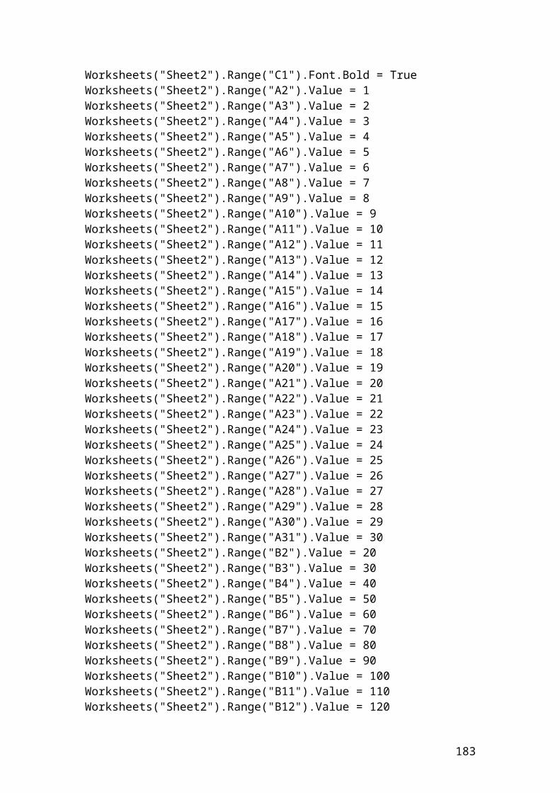
After compiling and debugging , the DOS window or console will open and display the following results:

Portfolio return: 0.3Portfolio variance:0.0142Portfolio standard deviation: 0.119164

Press any key to continue …

Exercise and solution

/*It is required to calculate the average return and the expected risk expressed as standard deviation. The following numbers represent percentage returns for each class of call, put and index options.*/

//Data provided

//Call option returns of Danske bank = 3.5, 4.7, 7.9, -4.2, 5.4, 10.3.//Put option returns of Danske bank = 2.7, 4.9, 5.7, 8.5, 9.3, 11.5./*Index option returns of OMX Copenhagen stockmarket = 3.7, 7.9, 8.9, 10.2,-6.8, 5.9.*/

#include <iostream>#include<math.h>using namespace std;

int main(){

183

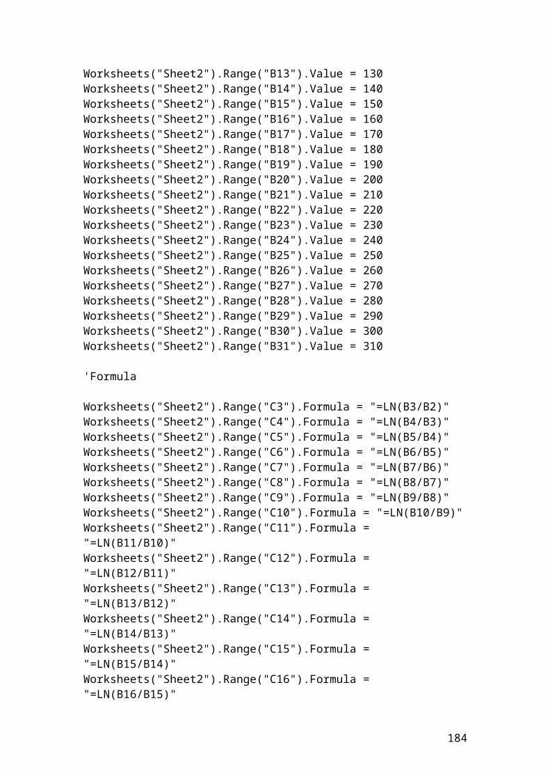
//Identify the variables.

double sum1;double sum2;double sum3;double average1;double average2;double average3; double sumDiffSqr1;double sumDiffSqr2;double sumDiffSqr3;double stdDev1;double stdDev2;double stdDev3;

// We insert the given numbers expressed in percentages in array format.

double arrayCalloptionreturns[6] = {3.5,4.7,7.9,-4.2,5.4,10.3}; double arrayPutoptionreturns[6] = {2.7, 4.9, 5.7, 8.5,9.3,11.5};double arrayIndexoptionreturns[6] ={3.7, 7.9, 8.9, 10.2, -6.8, 5.9};

/* The following expression inserts a variable x that tells the computerthat the first observation 0 is for example 3.5 and x is less than 6 to include all observations. We write the summation equation.*/

for (int x = 0; x < 6; x++)sum1 += arrayCalloptionreturns[x];for (int x = 0; x < 6; x++)sum2 += arrayPutoptionreturns[x];for (int x = 0; x < 6; x++)sum3 += arrayIndexoptionreturns[x];

// We insert the formula for the average of different classes.average1 = sum1/6;average2 = sum2/6;average3 = sum3/6;

/* We calculate the sumDiffSqr. We calculate the difference between each number and the average. Then, we square it and we sum it.*/

sumDiffSqr1 = 0;for (int x = 0; x < 6; x++) { sumDiffSqr1 = sumDiffSqr1 + pow((arrayCalloptionreturns[x]-average1),2); }

sumDiffSqr2 = 0;for (int x = 0; x < 6; x++) { sumDiffSqr2 = sumDiffSqr2 + pow((arrayPutoptionreturns[x]-average2),2);

184

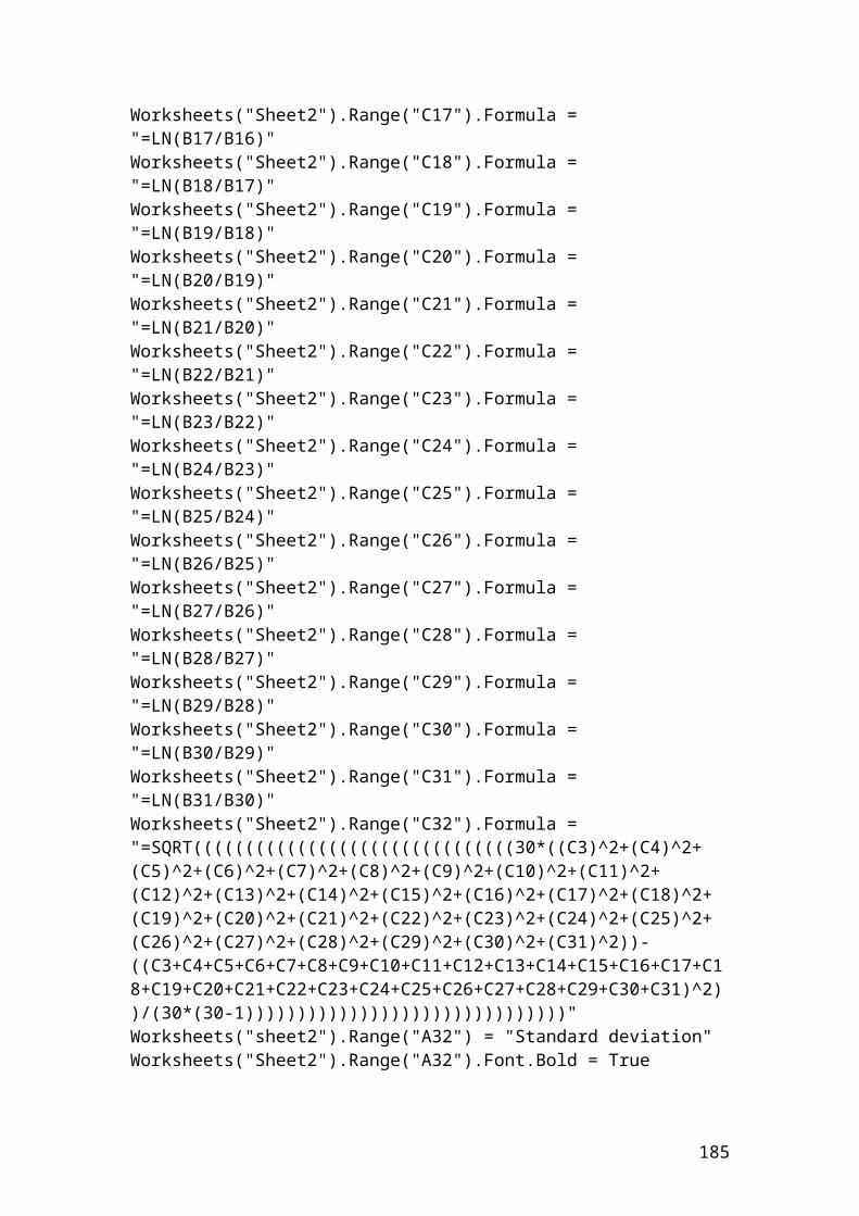
}sumDiffSqr3 = 0;for (int x = 0; x < 6; x++) { sumDiffSqr3 = sumDiffSqr3 + pow((arrayIndexoptionreturns[x]-average3),2); }

/* Insert the formula of the sample standard deviation by taking into account the formual n-1. We are taking the square root of the sumDiffSqr and divide by the totalnumber of observations less 1.*/

stdDev1 = sqrt(sumDiffSqr1/5);stdDev2 = sqrt(sumDiffSqr2/5);stdDev3 = sqrt(sumDiffSqr3/5);

/* By the function cin we tell the program to allow us to insert the numerical values of each class of call, put and index options in the console by pressing Enter. After entering the numbers the program will calculate automatically the sum, the average and the standard deviation.*/

// Output functions.cout<< "Enter arrayCalloptionretunrs" <<endl;cin>> arrayCalloptionreturns[0];cin>> arrayCalloptionreturns[1];cin>> arrayCalloptionreturns[2];cin>> arrayCalloptionreturns[3];cin>> arrayCalloptionreturns[4];cin>> arrayCalloptionreturns[5];cout<< "Sum:"<<sum1<<endl;cout<< "Average:"<<average1<<endl;cout<<" Sample standard deviation:"<<stdDev1<<endl;

cout<< "Enter arrayPutoptionretunrs" <<endl;cin>> arrayPutoptionreturns[0];cin>> arrayPutoptionreturns[1];cin>> arrayPutoptionreturns[2];cin>> arrayPutoptionreturns[3];cin>> arrayPutoptionreturns[4];cin>> arrayPutoptionreturns[5];cout<< "Sum:"<<sum2<<endl;cout<< "Average:"<<average2<<endl;cout<<"Sample standard deviation:"<<stdDev2<<endl;

cout<< "Enter arrayIndexoptionretunrs" <<endl;cin>> arrayIndexoptionreturns[0];cin>> arrayIndexoptionreturns[1];cin>> arrayIndexoptionreturns[2];cin>> arrayIndexoptionreturns[3];cin>> arrayIndexoptionreturns[4];cin>> arrayIndexoptionreturns[5];

185

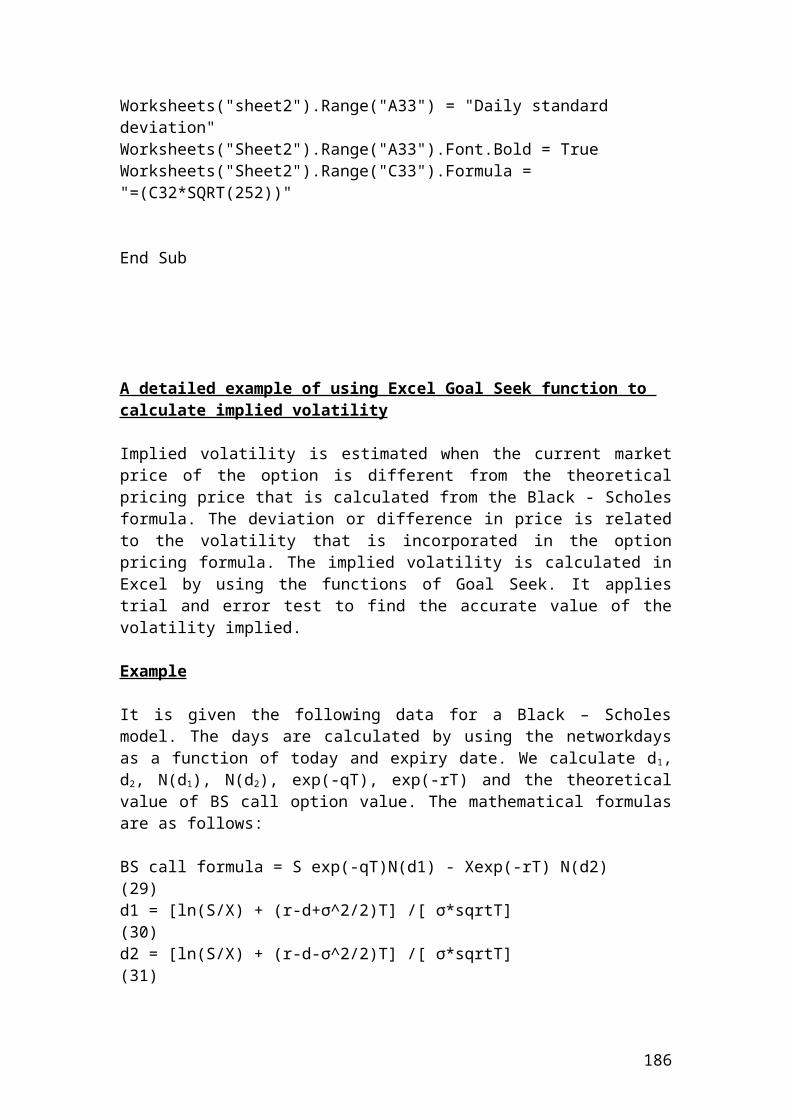
cout<< "Sum:"<<sum3<<endl;cout<< "Average:"<<average3<<endl;cout<<"Sample standard deviation:"<<stdDev3<<endl;

system ("PAUSE");return 0;}

Output

After compiling and debugging , the DOS window or console will open and display the following results:

Enter arrayCalloptionreturns3.5 Press Enter4.7 Press Enter7.9 Press Enter-4.2 Press Enter5.4 Press Enter10.3 Press Enter

Sum: 27.6Average: 4.6Sample standard deviation: 4.95 to (2.d.p.).

Enter arrayPutoptionreturns2.7 Press Enter4.9 Press Enter5.7 Press Enter8.5 Press Enter9.3 Press Enter11.5 Press Enter

Sum: 42.6Average: 7.1Sample standard deviation: 3.23 to (2.d.p.).

Enter arrayIndexoptionreturns3.7 Press Enter7.9 Press Enter8.9 Press Enter10.2 Press Enter-6.8 Press Enter5.9 Press Enter

Sum: 29.8

186

Average: 4.97 to (2.d.p.).Sample standard deviation: 6.20

Press any key to continue …

Example of pricing a forward contract and solution

A forward contract of 6 month has a market price of 52 Pounds when the spot price of the underlying commodity is 49 Pounds. There are no costs of carry and the discount rate is 7 percent. Calculate the value of the forward contract.

Solution

The current price of the forward contract (F0) should be equal to the value of the underlying commodity, (S0) at the discount rate r. Thus, the equation is as follows:

Application of pricing a forward contract in C++

//Pricing a forward contract.

#include <iostream>

187

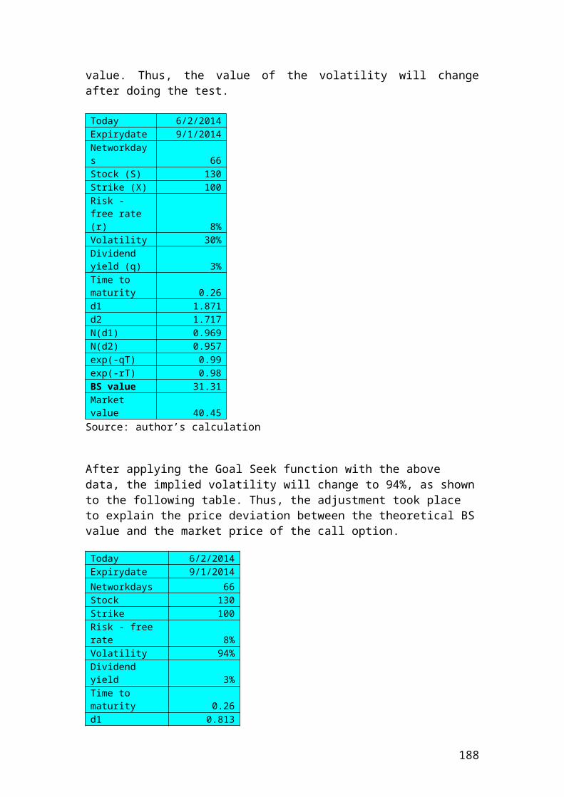
using namespace std;

int main(){ double valueforwardcontract; double spotprice = 49; double discountrate = 0.07; // Insert the mathematical formula.

valueforwardcontract = spotprice*(1+discountrate/2);

// Output functions.cout<< "Enter spotprice" <<endl;cin>> spotprice;cout<< "Enter discountrate" <<endl;cin>> discountrate;cout<< "Value forward contract:"<<valueforwardcontract<<endl;system ("PAUSE");return 0;}

Output

The numerical value is expressed in pounds. After compiling and debugging , the DOS window or console will open and display the following results:

Enter spot price49Enter discount rate0.07Value forward contract: 50.715Press any key to continue …

Example of interest rate payment and solution

A trader wants to calculate the interest amount that he / she will receive in three months from a forward contract of a Euribor deposit paying a Euro deposit rate of 3.55%. The principal amount is 300,000

The mathematical formula is as follows:

188

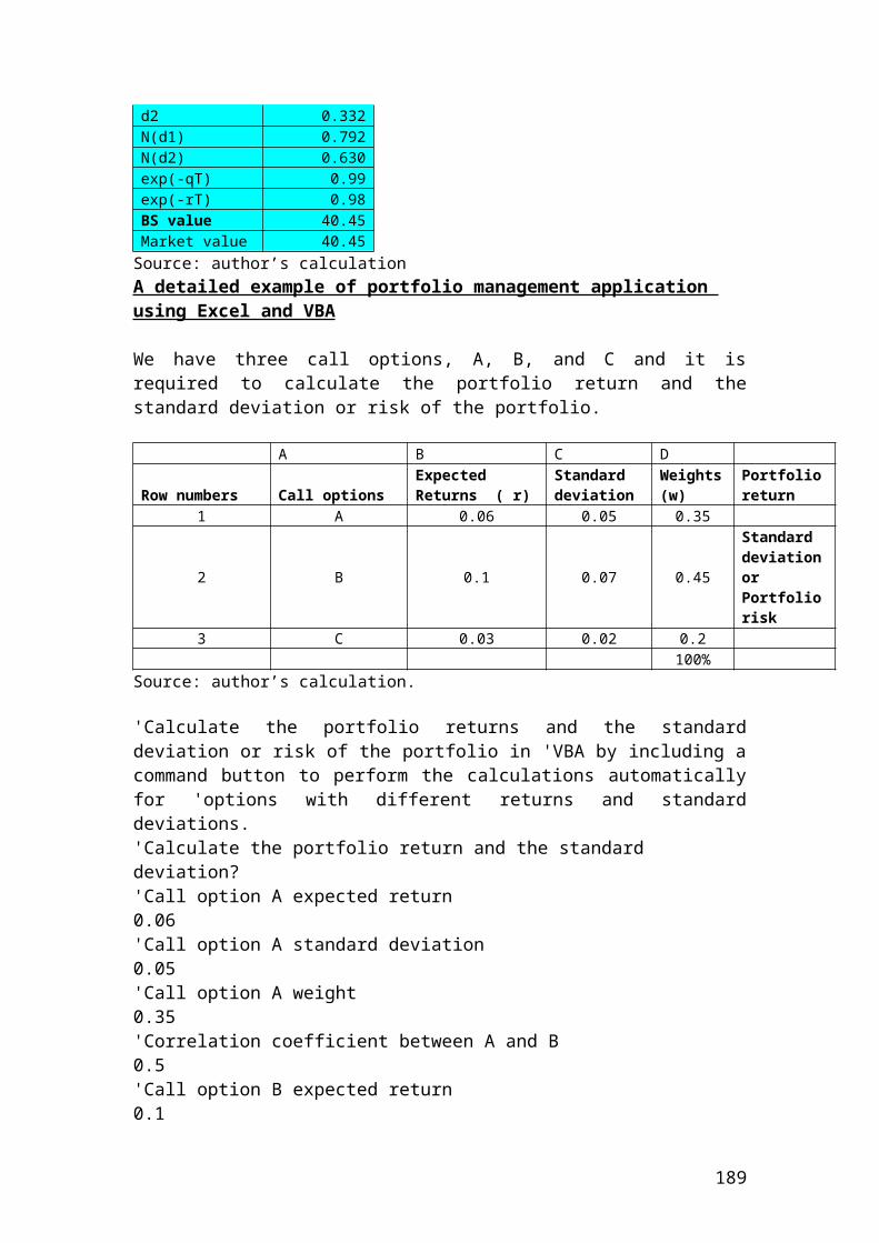
Interest payment = principal x [interest rate x (tdays / 360)]

Interest payment = 300,000 x [0.0355 x (90/360)]Interest payment = 2662.5 Euro.

First example: application of interest payment in C++

//Interest payment.

#include <iostream>using namespace std;

int main(){ double interestpayment; double principal = 300000; double interestrate = 0.0355; double days = 90;

// Insert the mathematical formula.

interestpayment = principal*(interestrate *days/360);

// Output functions.

cout<< "Enter principal" <<endl;cin>> principal;cout<< "Enter interestrate" <<endl;cin>> interestrate;cout<< "Interest payment:"<<interestpayment<<endl;system ("PAUSE");return 0;} Output

The numerical value is expressed in Euro. After compiling and debugging , the DOS window or console will open and display the following results:

Enter principal300000Enter interest rate0.0355Interest payment: 2662.5

Press any key to continue …

189

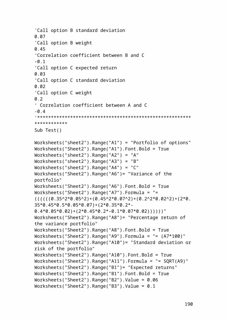
Second example: application of interest payment in C++ by changing the layout of the cout and cin function

//Interest payment.

#include <iostream>using namespace std;

int main(){ double interestpayment; double principal = 300000; double interestrate = 0.0355; int days = 90;

// Insert the mathematical formula.

interestpayment = principal*(interestrate *days/360);

// Output functions.

cout<< "Enter principal, interest rate" <<endl;cin>> principal >> interestrate;cout<< "Interest payment:"<<interestpayment<<endl;system ("PAUSE");return 0;}

Output

The numerical value is expressed in Euro. After compiling and debugging , the DOS window or console will open and display the following results:

Enter principal, interest rate300000 0.0355Interest payment: 2662.5

Press any key to continue …

190

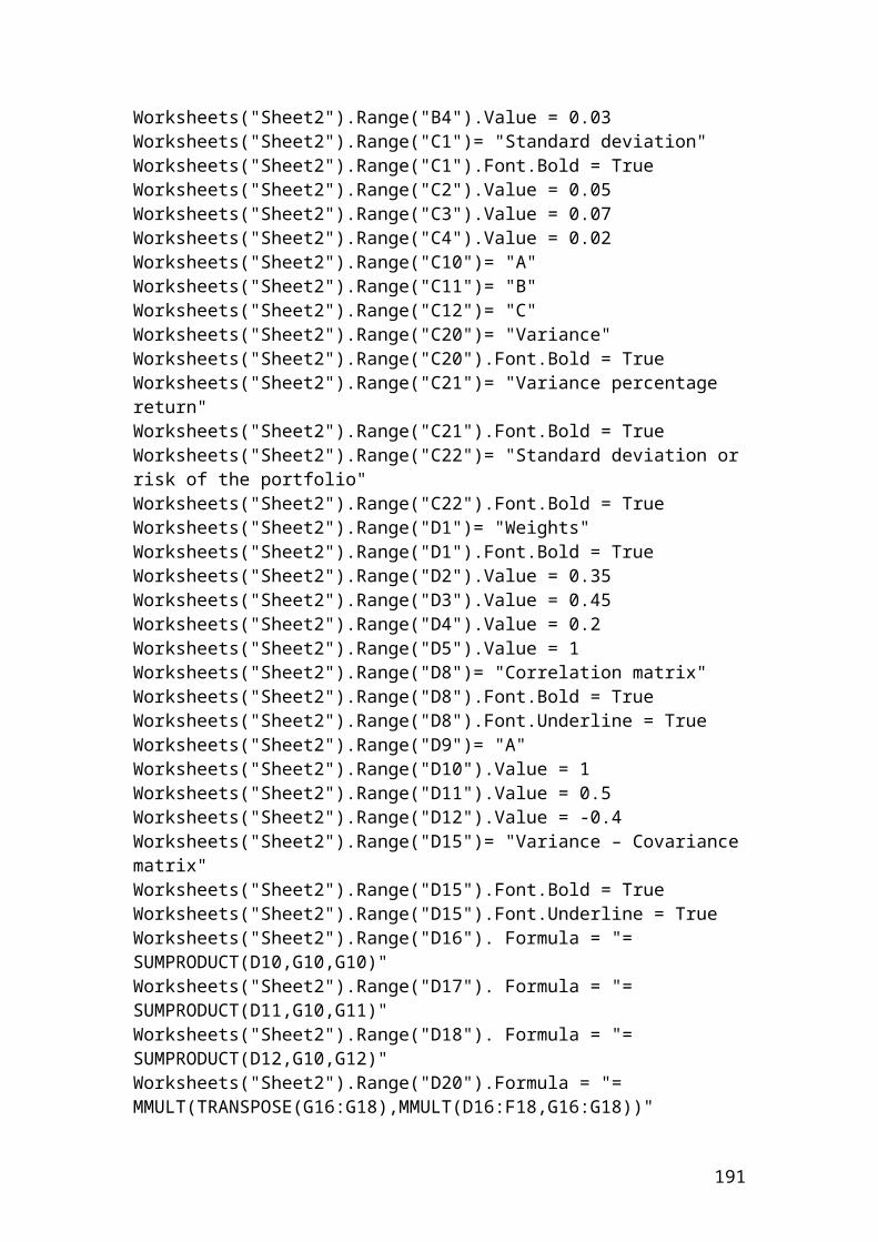
Third example: application of interest payment in C++ by adding formatting output values in the output functions

//Interest payment.

#include <iostream>using namespace std;

int main(){ double interestpayment; double principal = 300000; double interestrate = 0.0355; double days = 90; interestpayment = principal*(interestrate *days/360);

//Formating output values and output functions.

cout.setf(ios::fixed); // First statement.cout.setf(ios::showpoint); // Second statement.cout.precision(3); // Third statement. To show the final numerical

191

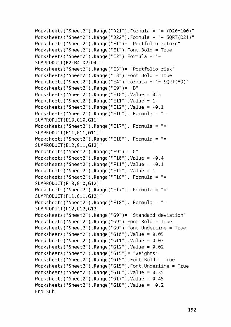
// value rounded to three decimal places.

cout<< "Enter principal, interest rate" <<endl;cin>> principal >> interestrate;cout<< "Interest payment:"<<interestpayment<<endl;system ("PAUSE");return 0;}

Output

The numerical value is expressed in Euro. After compiling and debugging , the DOS window or console will open and display the following results:

Enter principal, interest rate300000 0.0355Interest payment: 2662.500

Press any key to continue …

Fourth example: application of interest payment in C++ by adding the Euro currency in the output functions

//Interest payment.

#include <iostream>using namespace std;

int main(){ double interestpayment; double principal = 300000; double interestrate = 0.0355; double days = 90; interestpayment = principal*(interestrate *days/360);

//Formating output values and output functions.

cout.setf(ios::fixed); // First statement.cout.setf(ios::showpoint); // Second statement.cout.precision(3); // Third statement. To show the final numerical

192

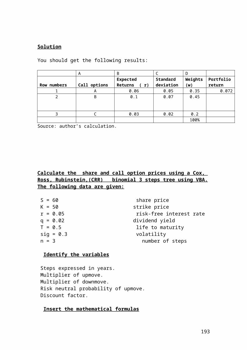
// value rounded to three decimal places.

cout<< "Enter principal, interest rate" <<endl;cin>> principal >> interestrate;cout<< "Interest payment in Euro:"<<interestpayment<<endl;system ("PAUSE");return 0;}

Output

The numerical value is expressed in Euro. After compiling and debugging , the DOS window or console will open and display the following results:

Enter principal, interest rate300000 0.0355Interest payment in Euro: 2662.500

Press any key to continue …

Example and solution of calculating profits and losses on futures contracts

An investor buys 8 S&P 500 futures contracts at $2189. He has closed the futures contract position with a price of $2236. The multiplier for S&P 500 futures contracts is 250 dollars. Did he record a profit or a loss?

Solution

The mathematical formula is as follows:

Where: fT is the final contract price. f0 is the initial contract price.

USD

Application of calculating profits and losses on futures contracts in C++

// calculating profits and losses on futures contracts.

193

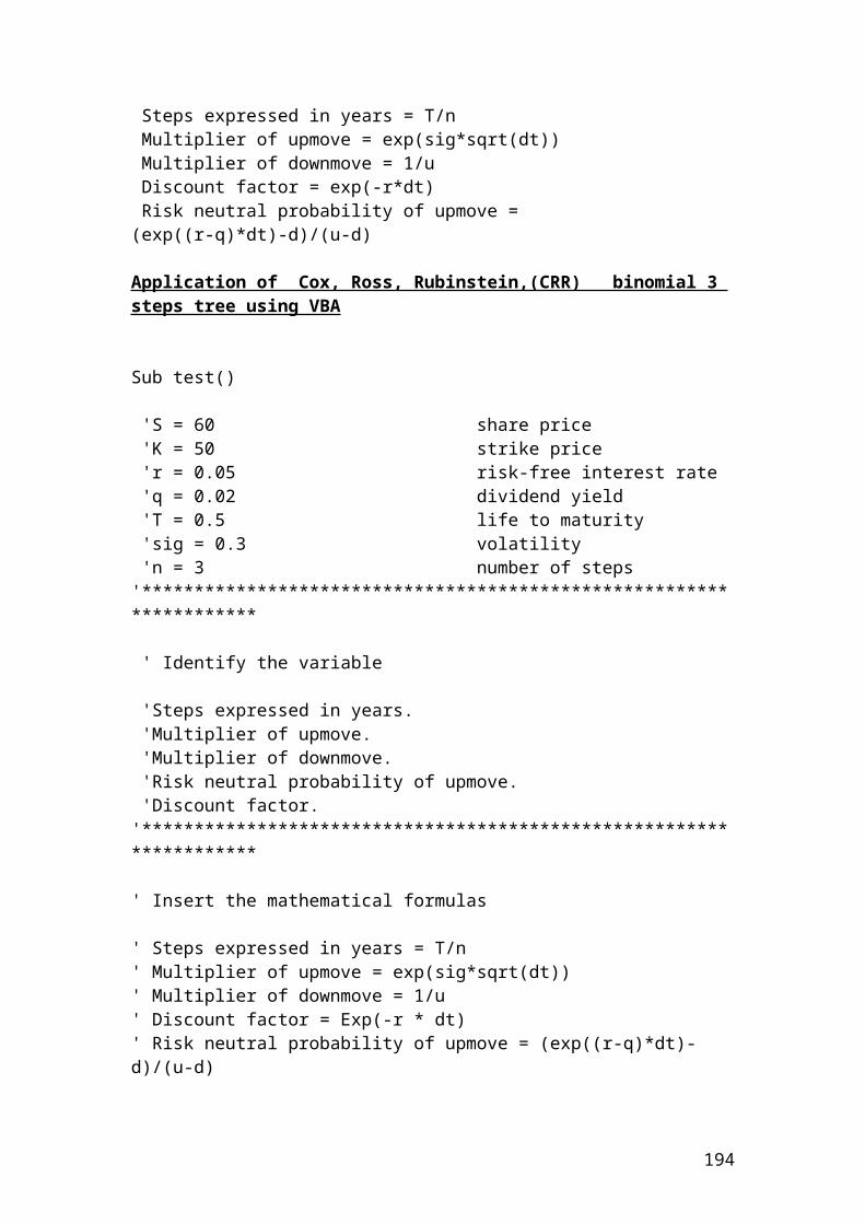
#include <iostream>using namespace std;

int main(){ double profitorloss ; int numberofcontracts =8; double buyingprice = 2189; double sellingprice = 2236; int multiplier = 250;

// Insert the mathematical formula.

profitorloss = numberofcontracts*multiplier*(sellingprice - buyingprice);

// Output functions.

cout<< "Enter number of contracts" <<endl;cin>> numberofcontracts;cout<< "Enter buying price" <<endl;cin>> buyingprice;cout<< "Enter selling price" <<endl;cin>> sellingprice;cout<< "Enter multiplier" <<endl;cin>> multiplier;cout<< "Profit or loss:"<<profitorloss<<endl;system ("PAUSE");return 0;} Output

The numerical value is expressed in USD. After compiling and debugging , the DOS window or console will open and display the following results:

Enter number of contracts8Enter buying price2189Enter selling price2236Enter multiplier250Profit or loss: 94000 ( In this case, we have profit or gain).

Press any key to continue …

194

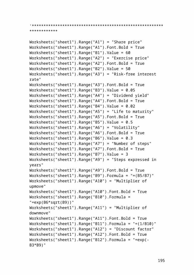
Example and solution of semiannually currency swap between an investment bank and an insurance company

The investment bank borrows 20,000,000 Pounds from the insurance company at a fixed rate of 5% for 1 year. The insurance company borrows from the investment bank 10,000,000 Euros at a fixed rate of 5% for 1 year. Calculate the interest payments for the three years, if we assume semiannual payments?

At the beginning of the contract

€10,000,000Investment bank Insurance company

£ 20,000,000

The insurance company pays the investment bank the following interest payment.

£20,000,000 x 0.05/2 = 500,000 Pounds.

The investment bank pays the insurance the following interest payment.

195

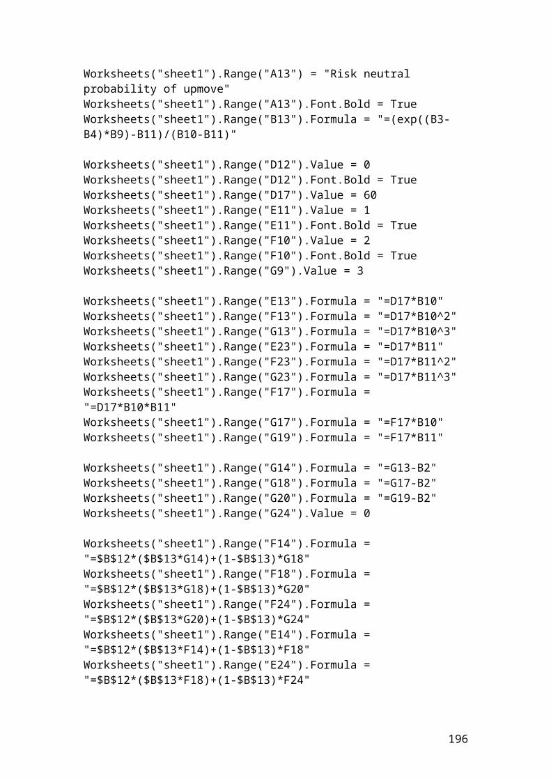
€10,000,000 x 0.05/2 =250,000 Euros.

The following arrows illustrate the interest payments.

€ 250,000Investment bank Insurance company

£ 500,000

At the end of the third year, the two parties exchange the principal amounts in addition to the final interest payments.

€10,250,000Investment bank Insurance company

£20,500,000

Application of semiannually currency swap between an investment bank and an insurance company in C++

//Semiannual swaps interest payments between an investment bank and an insurance //company.

#include <iostream>using namespace std;

int main(){ double bankpaysinsurance ; double insurancepaysbank ; double bankborrowsfrominsurance =20000000; double insuranceborrowsfrombank = 10000000; double interestrate = 0.05; int semiannualpayment = 2;

//Insert the mathematical formulas. bankpaysinsurance = insuranceborrowsfrombank *(interestrate/semiannualpayment);

196

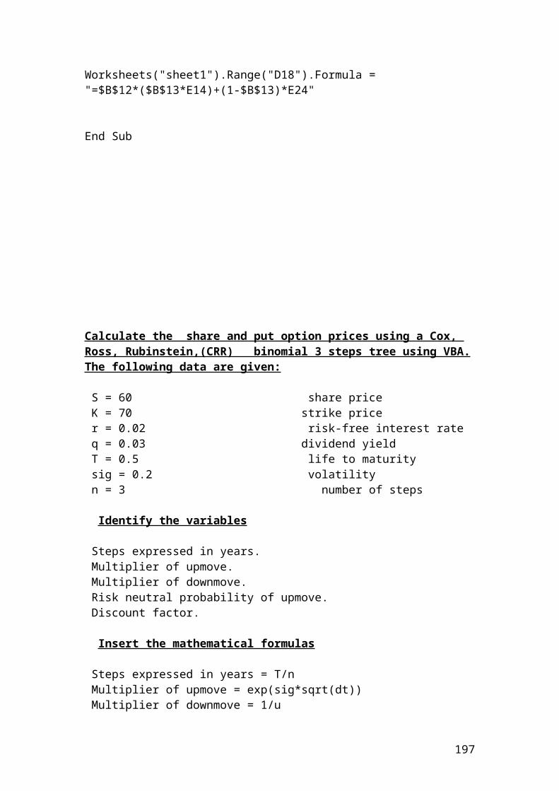
insurancepaysbank = bankborrowsfrominsurance *(interestrate/semiannualpayment);

// Output functions.

cout<< "Enter bank borrows from insurance" <<endl;cin>> bankborrowsfrominsurance ;cout<< "Enter insurance borrows from bank " <<endl;cin>> insuranceborrowsfrombank;cout<< "Enter interest rate" <<endl;cin>> interestrate;cout<< "Enter semi annual payment" <<endl;cin>> semiannualpayment;cout<< " Bank pays insurance:"<< bankpaysinsurance <<endl;cout<< " Insurance pays bank :"<< insurancepaysbank <<endl;

system ("PAUSE");return 0;}

Output

After compiling and debugging , the DOS window or console will open and display the following results:

Enter bank borrows from insurance20000000Enter insurance borrows from bank10000000Enter interest rate0.05Enter semi annual payment2Bank pays insurance: 250000Insurance pays bank: 500000

Press any key to continue …

197

Example and solution of interest rate swap

Interest rate swaps are very popular agreements between two parties in the debt or fixed-income department of the investment banks. The fixed income department of Bank A pays a fixed rate of 5.5% upon the principal of 50,000,000 Pounds. In contrast, Bank B pays a floating or reference rate of LIBOR accounted to 7.2%. The payment frequency is every 6 months for 2 years.

Fixed payment : £50,000,000 x 0.055/2 = 1,375,000 Bank A Bank B Floating payment: £50,000,000 x 0.072/2 = 1,800,000

Suppose in the second year that the LIBOR has increased by 12 basis points or 0.12%. Then, the floating payment will change and the calculation will be as follows:

198

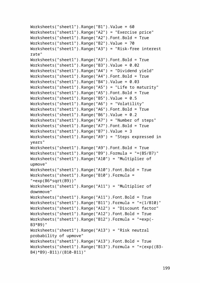
Second year floating payment for Bank B = 50,000,000 x 0.0732 / 2 = 1,830,000 Pounds.

Bank A will continue to pay the same fixed amount, namely, £50,000,000 x 0.055/2 = £1,375,000.

Application of interest rate swap in C++

//Semiannual swaps interest payments between two parties.

#include <iostream>using namespace std;

int main(){ double fixedpayment ; double floatingpayment1 ; double floatingpayment2 ; double principal = 50000000; double interestrate1 = 0.055; double interestrate2 = 0.072; double interestrate3 = 0.0732; int semiannualpayment = 2;

// Insert the mathematical formulas. fixedpayment = principal*(interestrate1/semiannualpayment);floatingpayment1 = principal*(interestrate2/semiannualpayment);floatingpayment2 = principal*(interestrate3/semiannualpayment);

// Output functions.

cout<< " Fixed payment:"<< fixedpayment <<endl;cout<< " Floating payment 1 :"<< floatingpayment1 <<endl;cout<< " Floating payment 2 :"<< floatingpayment2 <<endl;

system ("PAUSE");return 0;} Output

199

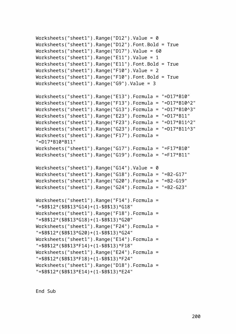
After compiling and debugging , the DOS window or console will open and display the following results:

Enter bank borrows from insuranceFixed payment: 1.375 e+006

Floating payment 1: 1.8 e+006

Floating payment 2: 1.83 e+006

Press any key to continue …

Delta – neutral hedge

Delta – neutral hedge is common used in risk management to keep the value of the portfolio neutral due to changes in the share price. It is achieved from a long position in a share and a short position in a call option. The mathematical formula to determine the number of options is as follows:

Thus, if the investment bank has bought 30,000 shares of Vodafone and the delta of the call option of the same company is 0.50, then the numbers of call options that are needed to purchase to form a delta-neutral hedge are as follows:

Delta hedge = 30,000 / 0.50 = 60,000 options or 600 option contracts.

Application of delta- neutral hedge in C++

200

// Delta neutral hedge.

#include <iostream>using namespace std;

int main(){ double deltaneutralhedge ; double numberofshares = 30000 ; double deltaofcalloption = 0.50 ; // Insert the mathematical equation.

deltaneutralhedge = numberofshares/deltacalloption;

// Output function.

cout<< " Delta neutral hedge:"<< deltaneutralhedge <<endl;system ("PAUSE");return 0;} OutputAfter compiling and debugging , the DOS window or console will open and display the following results:

Delta neutral hedge: 60000

Press any key to continue …Weighted mean price of a portfolio

Let’s assume that we have a portfolio of four options with their market prices and the number of shares bought. It is required to calculate the weighted mean price of the portfolio.

Options Price expressed in $

Number of shares

Weight Weight x Price

A 14.00 300 0.4 5.6B 12.00 200 0.3 3.6C 8.00 100 0.1 0.8D 5.00 150 0.2 1

Total 750 1Source: author’s calculation

The mathematical formula is as followed:

201

By substituting the numbers from the Table into the equation we have the following:

0.8 + 1 = 11.

Application of weighted mean price of a portfolio in C++

// Weighted mean price of a portfolio.

#include <iostream>using namespace std;

int main(){double portfoliomean ;

double price[4];price[1] = 14;price[2] = 12;price[3] = 8;price[4] = 5;

double weight[4];weight[1] = 0.4;weight[2] = 0.3;weight[3] = 0.1;weight[4] = 0.2;

// Insert the mathematical equation.

portfoliomean = (price[1]*weight[1]+price[2]*weight[2]+price[3]*weight[3]+price[4]*weight[4]);

// Output function.cout<<" Weighted mean of the portfolio:"<<portfoliomean<<endl;system ("PAUSE");return 0;}

Output

After compiling and debugging , the DOS window or console will open and display the following results:

202

Weighted mean of the portfolio: 11

Press any key to continue …

Example of Eurodollar futures

An investor wants to calculate the futures price of a 1-month Eurodollar time deposits based on a LIBOR rate of 3.40%. The initial principal is 1 million Pounds.

Solution

The price of the Eurodollar futures contract will be as follows:

203

Application of Eurodollar futures in C++

//The price of Eurodollar future.

#include <iostream>using namespace std;

int main(){ double Eurodollarfuture; double principal = 1000000; double interestrate = 0.034; int days = 30;

// Insert the mathematical formula.

Eurodollarfuture = principal*(1- interestrate *days/360);

// Output function.

cout.setf(ios::fixed); cout.setf(ios::showpoint); cout.precision(2); cout<< "Enter principal, interest rate" <<endl;cin>> principal >> interestrate;cout<< "Price of Eurodollar future:"<<Eurodollarfuture<<endl;system ("PAUSE");return 0;}

Output

The price of the Eurodollar future is expressed in pounds. After compiling and debugging , the DOS window or console will open and display the following results:

Enter principal, interest rate1000000 0.034Price of Eurodollar future: 997166.67 pounds

Press any key to continue …

204

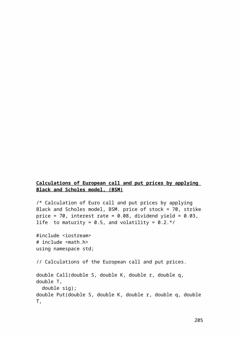
Example of forward rate agreement

An investment bank buys a 4 x 6 FRA from a building society in the UK for 4.0% by paying 2 million Pounds. 80 days latter, LIBOR is 5%. Who will receive the FRA payment and for how much?

Solution

The mathematical formula for Forward Rate Agreement, (FRA) is as follows:

The timeline schedule is as follows:

t = 0 4months 6 months

205

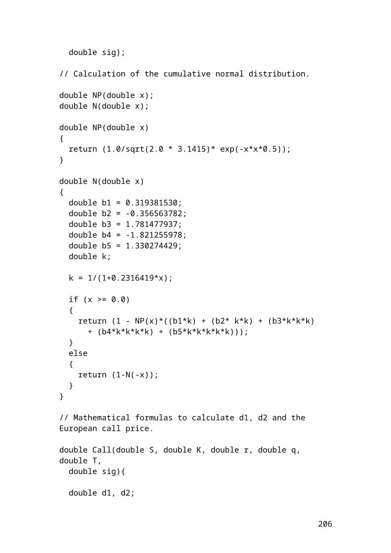
= ………. Please complete

the calculation.

Helpful hint: If the FRA payment is positive, then, the building society is the payer and the investment bank receives the FRA payment.

If the FRA payment is negative, then the investment bank is the payer and the building society receives the FRA payment.

Application of forward rate agreement in C++

//The price of forward rate agreement.

#include <iostream>using namespace std;

int main(){ double FRApayment; double principal = 2000000; double variablerate = 0.05; double fixedrate = 0.04;

// Insert the mathematical formula.FRApayment= principal*(variablerate - fixedrate)*0.333333333/1.011111111;

// Output function.

cout.setf(ios::fixed); cout.setf(ios::showpoint); cout.precision(1); cout<< "Forward rate payment:"<<FRApayment<<endl;system ("PAUSE");return 0;}

Output

The payment is expressed in pounds. After compiling and debugging , the DOS window or console will open and display the following results:

Forward rate payment: 6593.4 pounds

206

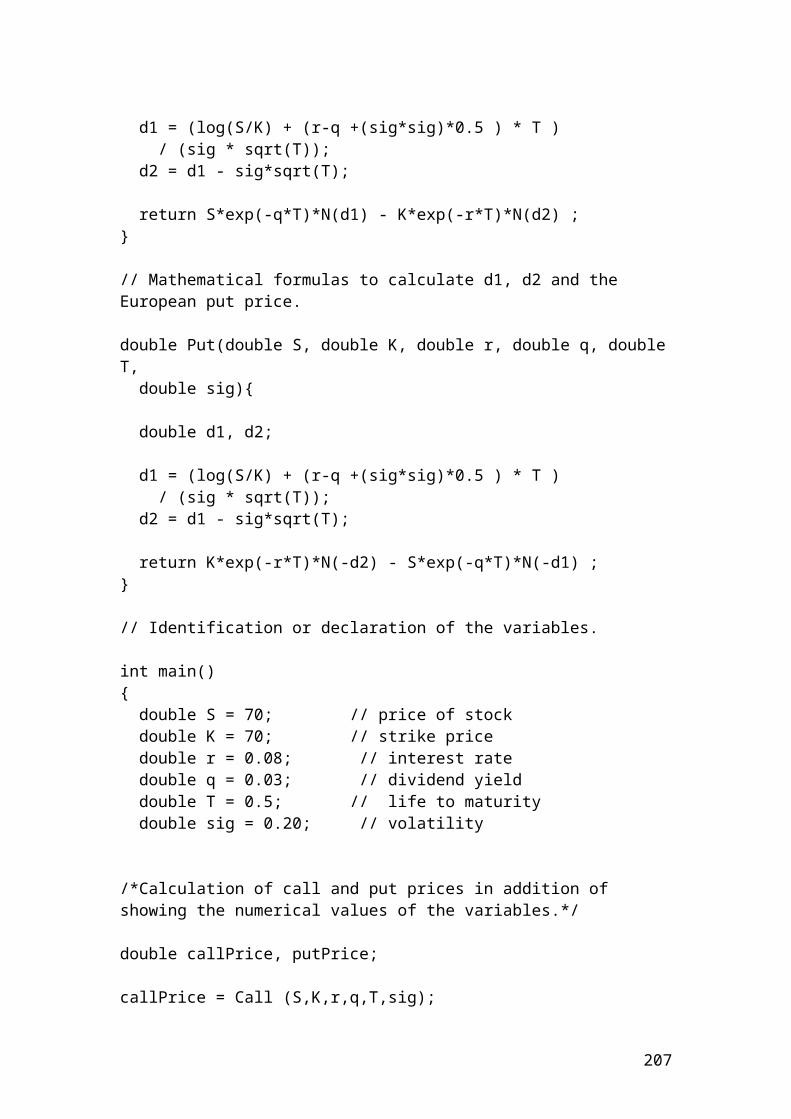
Press any key to continue …

Example of futures on Treasury bills

An investor wants to calculate the futures price of a 3-month Treasury bills. Treasury bills are short-term notes of limited period of 1- month, and 3 - month respectively. The initial principal is 5 million Pounds and the discount rate is 3.50%.

Solution

The price of the Treasury bill futures will be as follows:

Please complete the calculation …….

Application of futures on Treasury bills in C++

207

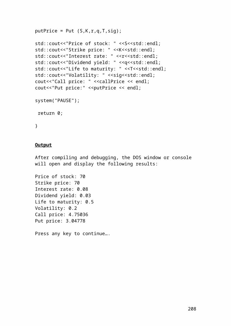
//The price of futures on Treasury bills.

#include <iostream>using namespace std;

int main(){ double futurestreasurybills; double principal = 5000000; double discountrate = 0.035; int days = 90;

// Insert the mathematical formula.

futurestreasurybills = principal*(1- discountrate *days/360);

// Output function.

cout<< "Enter principal, discount rate" <<endl;cin>> principal >> discountrate;cout<< "Price of futures on Treasury bills:"<<futurestreasurybills<<endl;system ("PAUSE");return 0;}

Output

After compiling and debugging , the DOS window or console will open and display the following results:

Enter principal, interest rate5000000 0.035Price of futures on Treasury bills: 4956250 or 4.95625 e+006

Press any key to continue …

208

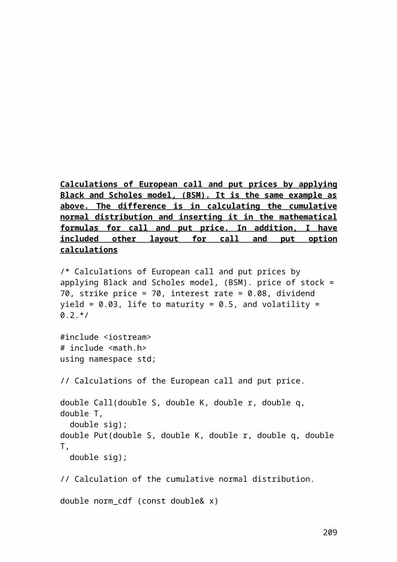
Example of stock index futures

For example, if you bought 10 contracts of the Dow Jones Industrial index at 10,000 and you expected an aggressive bull market that reaches the value of 16,000, then, the 6000 points increase are multiplied by the standardized value of 250. If the initial principal of investment is $100,000, the mathematical formula for the gains will be as follows:

10 x 100,000 x 6000 x 250 = 1.5 x 1012 Dollars

Application of stock index futures in C++

//The gains from stock index futures

#include <iostream>using namespace std;

209

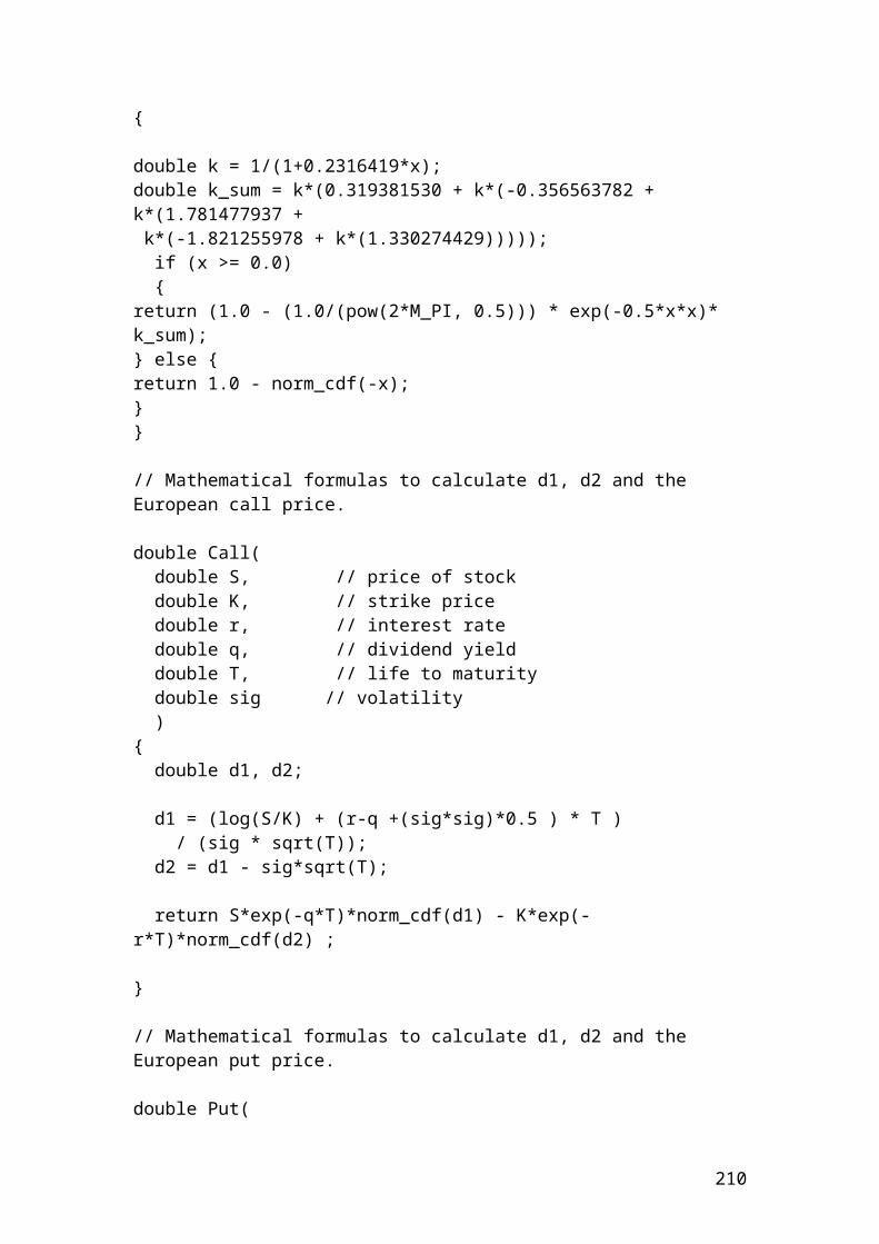
int main(){ double gains; double principal = 100000; double pointsincrease = 6000; int number_of_contracts = 10; int multiplier = 250;

// Insert the mathematical formula.

gains = principal*pointsincrease*multiplier*number_of_contracts;

// Output functions.

cout<< "Enter principal, pointsincrease, multiplier, number_of_contracts" <<endl;cin>> principal >> pointsincrease>>multiplier>>number_of_contracts;cout<< "Gains from stock index futures:"<<gains<<endl;system ("PAUSE");return 0;}

Output

After compiling and debugging , the DOS window or console will open and display the following results:

Enter principal, points increase, multiplier,number_of_contracts100000 600025010Gains from stock index futures: 1.5 e+012

Press any key to continue …

Example of currency futures

A manufacturer wants to calculate the currency futures price of EURO/USD traded in Frankfurt derivative market. For example, in August the contract is quoted as 1.35 EURO /USD and the contract size is 20,000. The principal is 300,000 Euro.

Solution

The contract price of 1 contract is as follows:

210

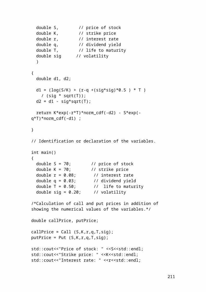
Application of currency futures in C++

//The futures price of currency.

#include <iostream>using namespace std;

int main(){ double futurespriceofcurrency; double principal = 300000; double quote = 1.35; int contractsize = 20000;

// Insert the mathematical formula.futurespriceofcurrency = principal*quote*contractsize ;

// Output functions.

cout<< "Enter principal, quote, contract size" <<endl;cin>> principal >> quote>> contractsize;cout<< "Futures price of currency:"<<futurespriceofcurrency<<endl;system ("PAUSE");return 0;}

Output

The result is in Euro. After compiling and debugging , the DOS window or console will open and display the following results:

Enter principal, quote, contract size300000 1.3520000

Futures price of currency: 8.1 e+009

Press any key to continue …

211

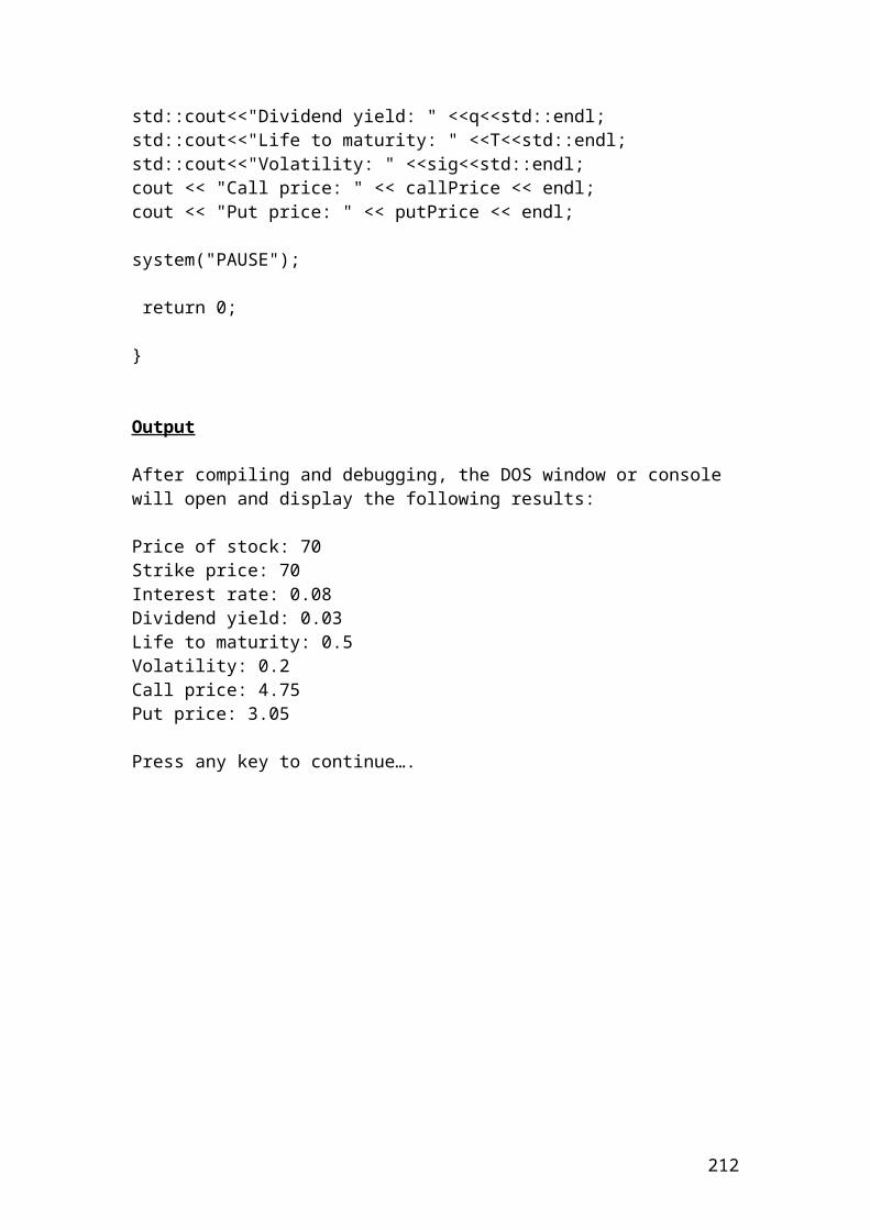
Example of calculating implied volatility and the new theoretical call option price due to volatility

# include<cmath>#include <iostream>using namespace std;

double Call(double S, double K, double r, double q, double T, double sig);

int main(){ double S =50.0, K=50.0 , r=0.04, q = 0.01, T = 0.50; double sig, optPrice, TheoreticalPrice, tolerance ; int i; optPrice = 8.34; // Option price. sig = 0;

212

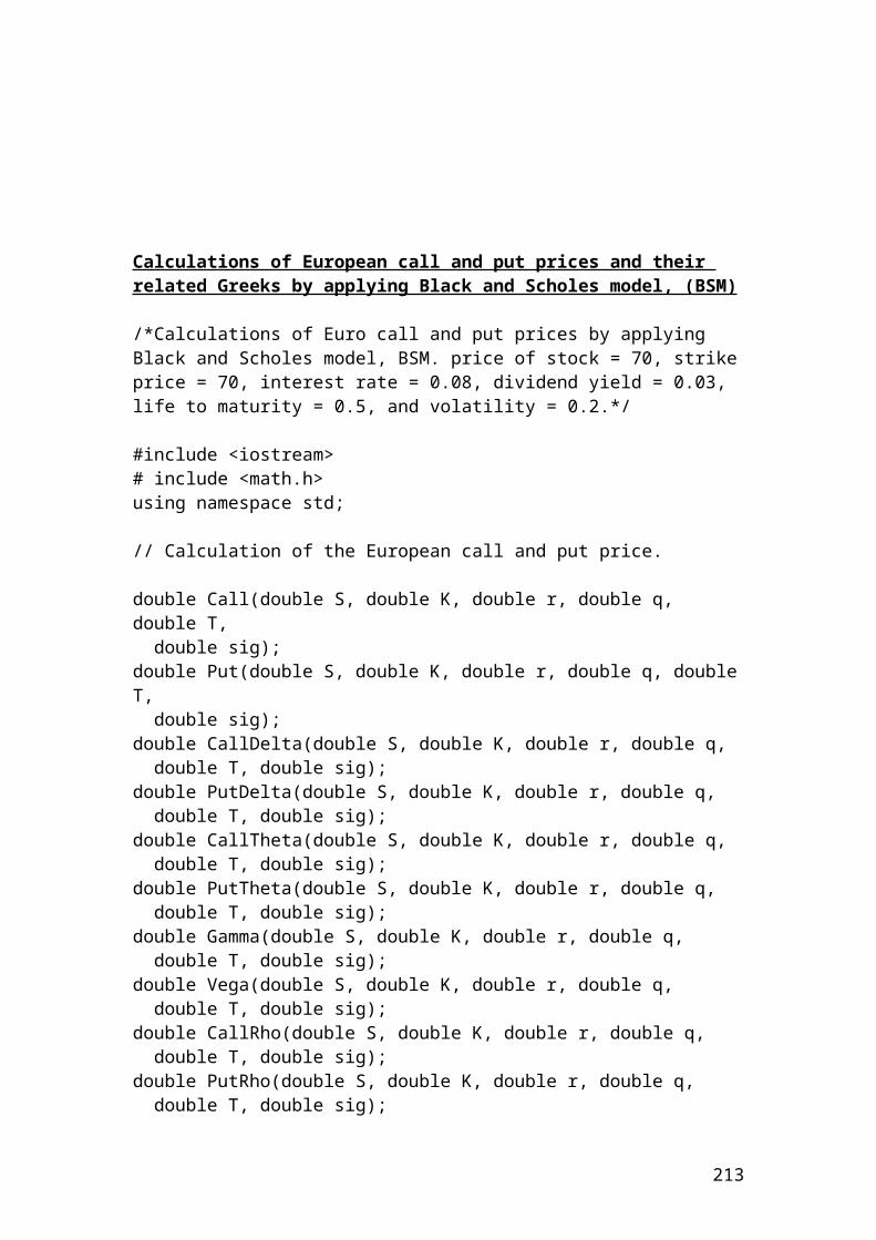
tolerance = 0.1; /* Specification for the sigma or volatility with tolerance level in relation with the theoretical and market option price.*/ for(i = 1; i < 50 ; i++) { sig += tolerance; TheoreticalPrice = Call(S, K, r, q, T, sig); if((TheoreticalPrice) > (optPrice)) { tolerance = -(tolerance * 0.1); tolerance = -tolerance; } } // Output functions. cout << "Implied volatility: " << sig << endl; cout << "Option price: " << optPrice << endl; cout << "Theoretical Price due to volatility:"<< TheoreticalPrice << endl; system("PAUSE"); return 0; } // Calculation of the cumulative normal distribution.

double norm_cdf (const double& x) {

double k = 1/(1+0.2316419*x);double k_sum = k*(0.319381530 + k*(-0.356563782 + k*(1.781477937 + k*(-1.821255978 + k*(1.330274429))))); if (x >= 0.0) {return (1.0 - (1.0/(pow(2*M_PI, 0.5))) * exp(-0.5*x*x)* k_sum);} else {return 1.0 - norm_cdf(-x);}}// Mathematical formulas to calculate d1, d2 and the European call price.

double Call(double S, double K, double r, double q, double T, double sig){

double d1, d2;

213

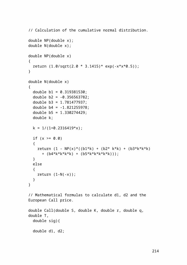
d1 = (log(S/K) + (r-q +(sig*sig)*0.5 ) * T ) / (sig * sqrt(T)); d2 = d1 - sig*sqrt(T); return S*exp(-q*T)*norm_cdf(d1) - K*exp(-r*T)*norm_cdf(d2); }

Output

After compiling and debugging , the DOS window or console will open and display the following results:

Implied volatility: 0.611 or 61.1%Option price: 8.34Theoretical price due to volatility: 8.82

Press any key to continue …

Example of calculating implied volatility and the new theoretical put option price due to volatility

# include<cmath>#include <iostream>using namespace std;

double Put(double S, double K, double r, double q, double T, double sig);

int main(){ double S =70.0, K=70.0 , r=0.04, q = 0.01, T = 0.50; double sig, optPrice, TheoreticalPrice, tolerance ; int i; optPrice = 5.25; // Option price. sig = 0; tolerance = 0.1;

214

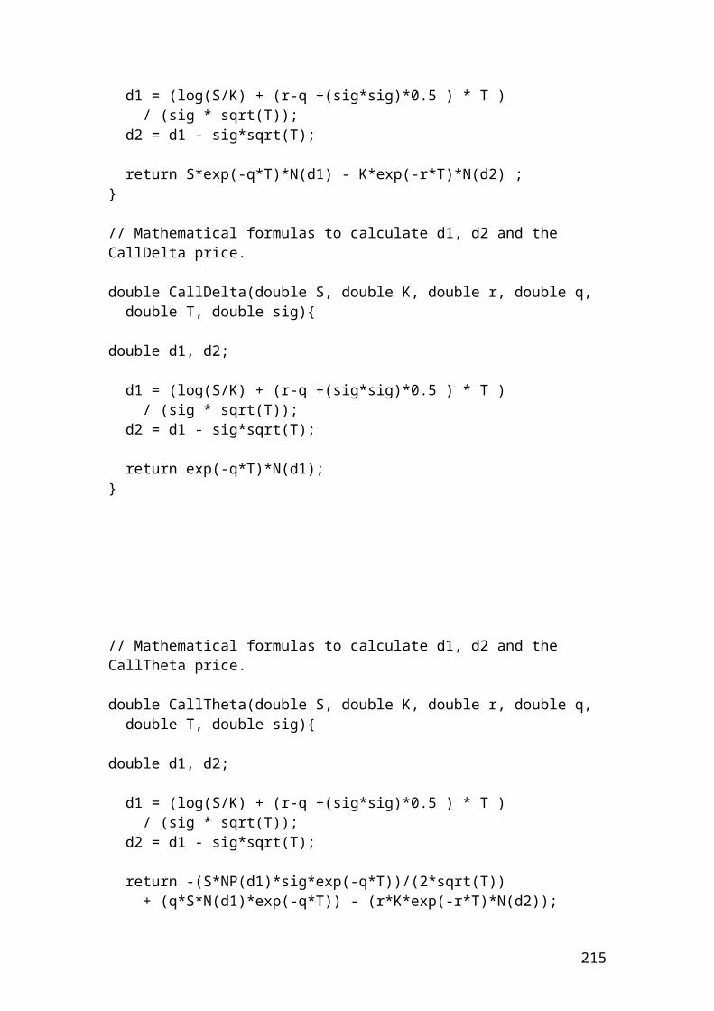
/* Specification for the sigma or volatility with tolerance level in relation with the theoretical and market option price.*/ for(i = 1; i < 70 ; i++) { sig += tolerance; TheoreticalPrice = Put(S, K, r, q, T, sig); if((TheoreticalPrice) > (optPrice)) { tolerance = -(tolerance * 0.1); tolerance = -tolerance; } } // Output functions. cout << "Implied volatility: " << sig << endl; cout << "Option price: " << optPrice << endl; cout << "Theoretical price due to volatility: "<<TheoreticalPrice<<endl; system("PAUSE"); return 0; }

// Calculation of the cumulative normal distribution.

double norm_cdf (const double& x) {

double k = 1/(1+0.2316419*x);double k_sum = k*(0.319381530 + k*(-0.356563782 + k*(1.781477937 + k*(-1.821255978 + k*(1.330274429))))); if (x >= 0.0) {return (1.0 - (1.0/(pow(2*M_PI, 0.5))) * exp(-0.5*x*x)* k_sum);} else {return 1.0 - norm_cdf(-x);}}// Mathematical formulas to calculate d1, d2 and the European put price.

double Put(double S, double K, double r, double q, double T, double sig){

double d1, d2;

215

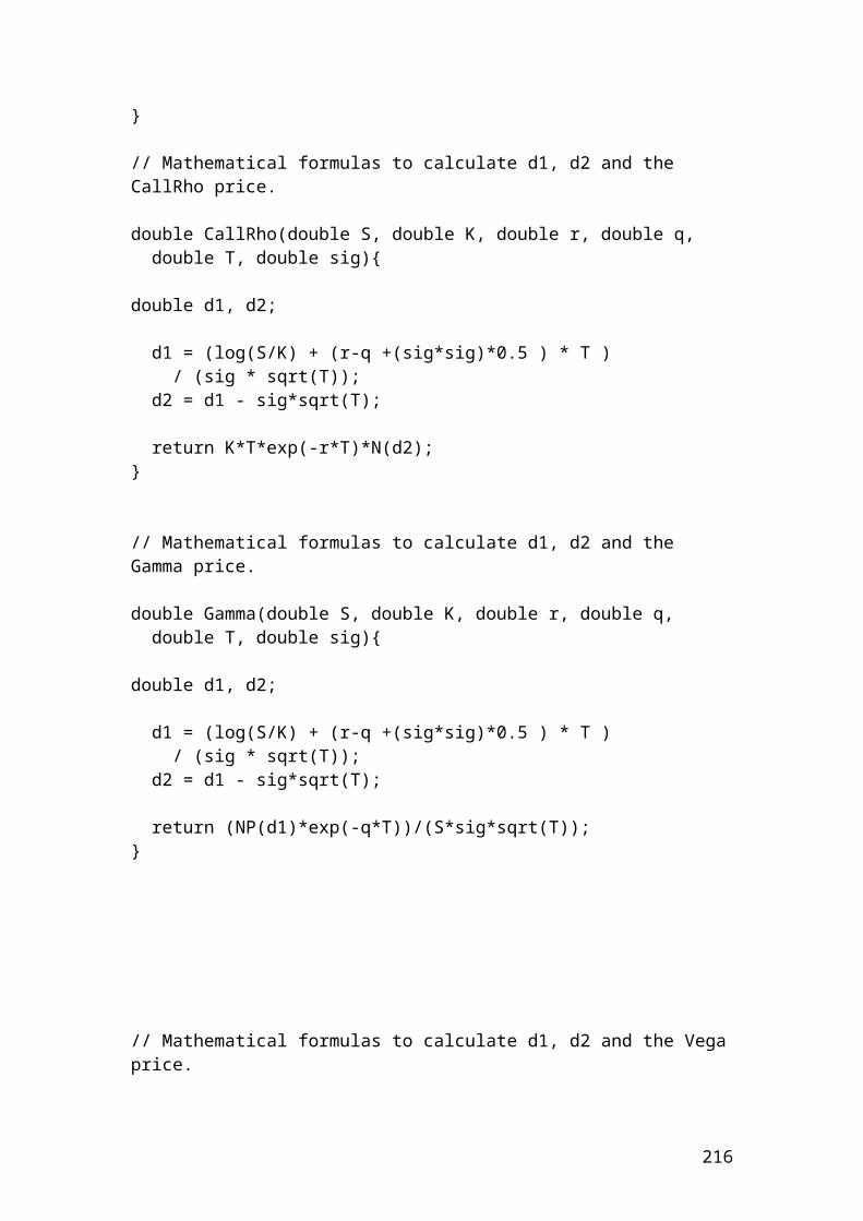
d1 = (log(S/K) + (r-q +(sig*sig)*0.5 ) * T ) / (sig * sqrt(T)); d2 = d1 - sig*sqrt(T); return K*exp(-r*T)*norm_cdf(-d2) - S*exp(-q*T)*norm_cdf(-d1) ; }

Output

After compiling and debugging , the DOS window or console will open and display the following results:

Implied volatility: 0.311 or 31.1%Option price: 5.25Theoretical price due to volatility: 5.55

Press any key to continue …

Please try based on the previous examples to illustrate the following example in C++. If you have difficulties e-mail me

Active return, active risk and information ratio

Active return is the difference in returns between a portfolio and the index or benchmark that is measured.

Active return = rp - rb

Where: rp is the portfolio return. rb is the benchmark or index return.

If the portfolio return is 0.80 and the benchmark return of the index is 0.70 then, the active return is………

Please complete the calculation.

216

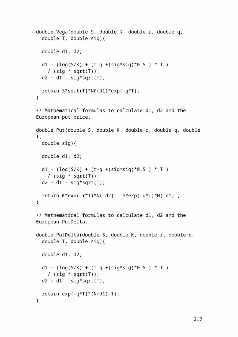
Active risk or tracking error is the standard deviation of the difference of returns between a portfolio and the benchmark or index.

If the portfolio return is 0.80, the number of assets is 10 and the benchmark return of the index is 0.40 then, the active risk is………

Please complete the calculation.

Information ratio shows the consistency of the fund manager towards the active return. The mathematical formula is as follows:

It could be calculated very easily in Excel software. I will illustrate a simple table with the relevant calculations.

Day rp rb rp - rb

1 0.03 0.02 0.012 0.02 0.014 0.0063 -0.04 0.034 -0.0744 0.05 0.067 -0.0175 0.08 0.012 0.0686 -0.01 -0.056 0.0467 0.07 0.031 0.0398 0.034 0.023 0.0119 -0.021 0.015 -0.03610 0.045 0.001 0.044

217

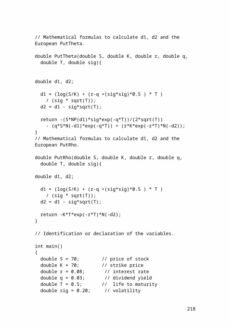
Average 0.0258 0.0161Standard deviation

0.043

Source: author’s calculation

By substituting the values that we have found in terms of rp =0.0258, rb = 0.0161 and standard deviation = 0.043 in the following equation we have:

But what is the interpretation of the information ratio of 0.23. It means that the fund manager gained around 23 basis points of active return per unit of active risk. The higher is this number, the better the manager is performing in relation to active risk.

Please convert the following exercise in C++ language programming

Calculate the balance at the end of the 5th day from changes in the futures prices from 90 to 89, 91, 95, 97, 99. The trader has bought 50 futures contract for settlement in May. The initial margin is $8.

Day Beginning balance

Futures price Gain or loss Ending balance

0 400 90 0 4001 400 89 (50)2 350 91 1003 450 95 2004 650 97 1005 750 99 100

Source: author’s illustration.

Beginning balance = initial margin x number of contracts.Beginning balance = 8 x 50 = $400

Please complete the values of the column ending balance.

218

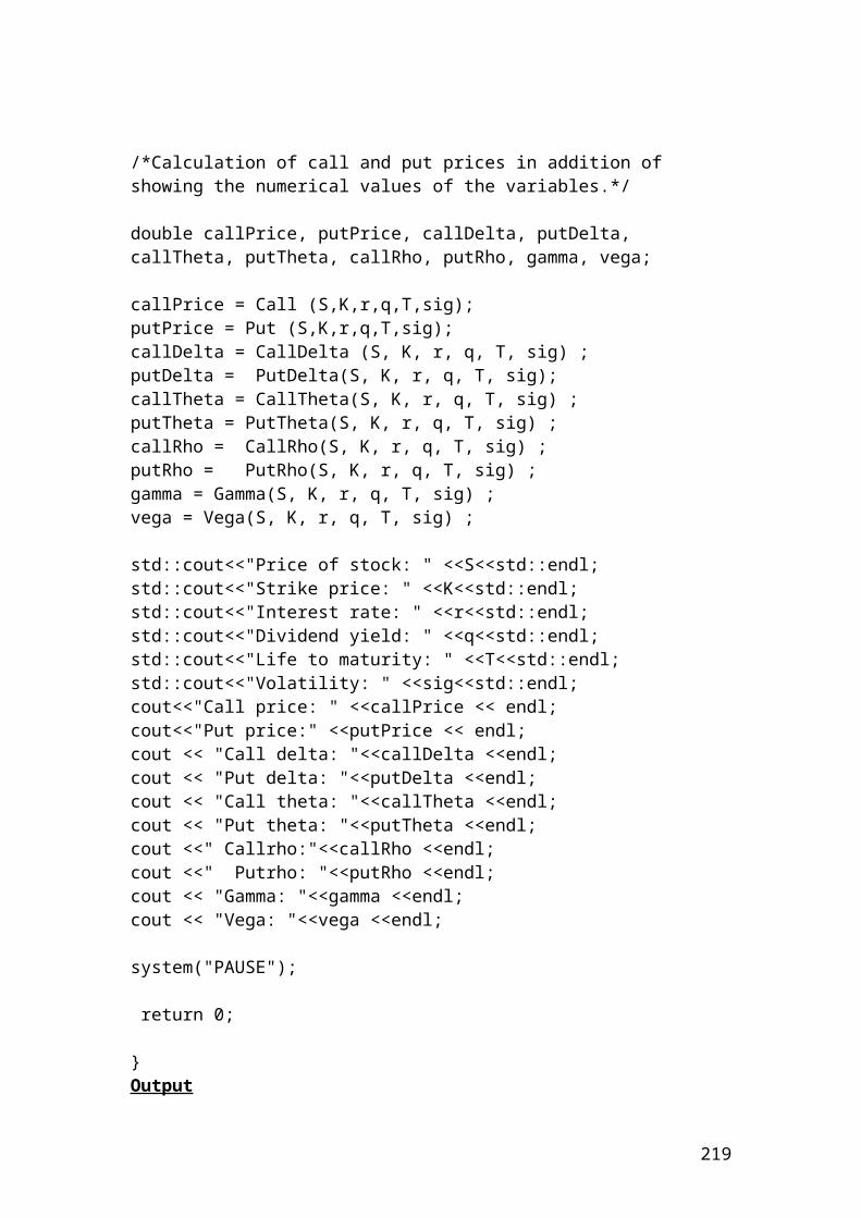
Application of the srand() rand() functions. The srand() function is related to the system time. The computer generates every time different random numbers. The function rand() is related to random numbers and is converting the numbers to the value between 0 and 199. It is very useful method that is used in simulations such as Monte Carlo simulation to price derivatives products

#include <iostream>#include <ctime>using namespace std;

int main(){ int k; int arraySize ; cout << "Enter array size: "<<endl; cin >> arraySize; int dataarray[arraySize]; // Generate the array with random numbers between 0 and 199 srand(time(0)); for(k = 0; k < arraySize; k++) { dataarray[k] = rand()%200; cout << dataarray[k] << endl;

219

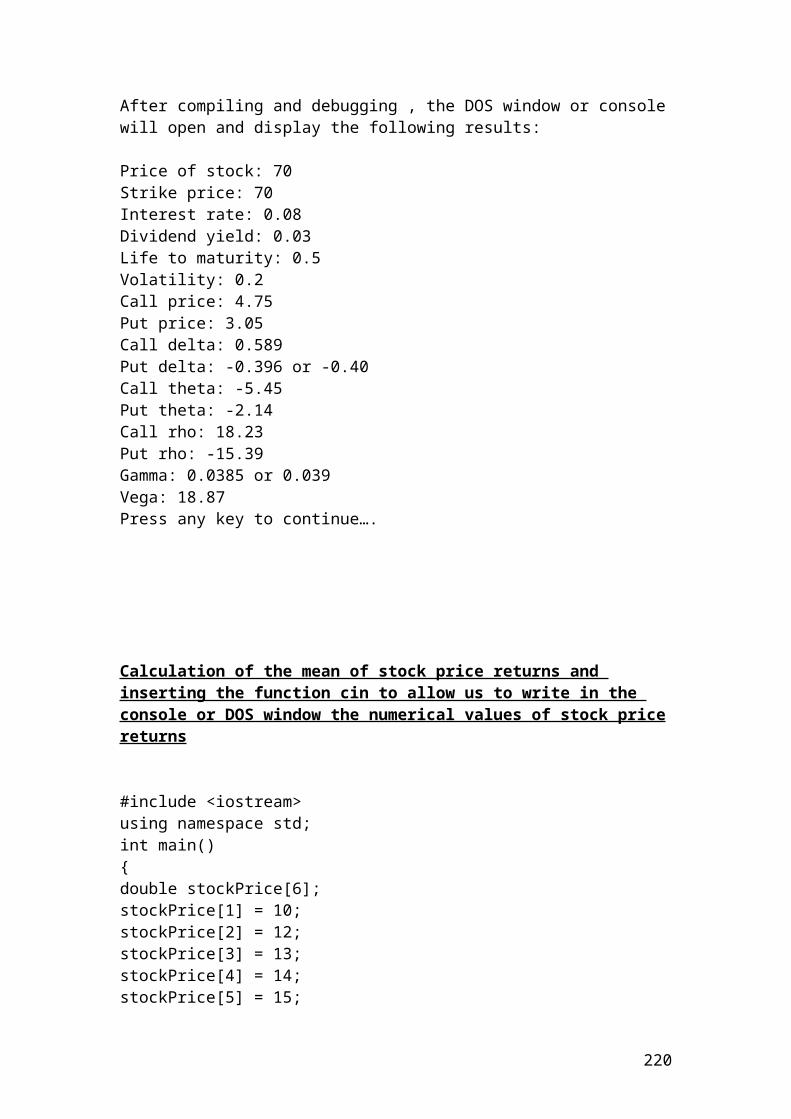
} system("PAUSE"); return 0; }

OutputAfter compiling and debugging , the DOS window or console will open and display the following results. Every time you will get different numbers by using the functions srand() and rand().

Enter array size:81341618312957242058Press any key to continue …

Example of profit or loss of a call option portfolio

// Profit or loss of a call option portfolio.

#include <iostream>using namespace std;

int main(){ double portfoliovalue1, portfoliovalue2, portfoliovalue3, portfoliovalue4, portfoliovalue5,portfoliovalue6,portfoliovalue7, portfoliovalue8,portfoliovalue9,portfoliovalue10 ; // portfolio value. double shareprice[10] ; // number of positions of share prices. double strikeprice[10]; // number of positions of strike prices. double optionpremium [10]; // Call option premiums. double contractsize = 100; // contract size.

/* Identifying the number of positions in relation to the share prices, strike prices and option premium.*/

shareprice[1] = 10.25; shareprice[2] = 20.13; shareprice[3] = 30.22; shareprice[4] = 40.56; shareprice[5] = 50.89;

220

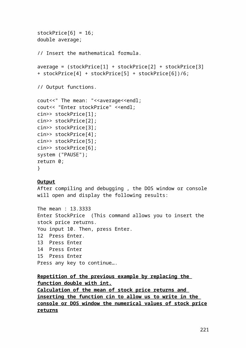
shareprice[6] = 51.23; shareprice[7] = 53.33; shareprice[8] = 54.63; shareprice[9] = 66.23; shareprice[10] = 68.23;

strikeprice[1] = 3.34; strikeprice[2] = 8.34; strikeprice[3] = 18.78; strikeprice[4] = 28.34; strikeprice[5] = 31.12; strikeprice[6] = 22.02; strikeprice[7] = 34.23; strikeprice[8] = 47.12; strikeprice[9] = 48.45; strikeprice[10] = 50.12; optionpremium[1] = 1.50; optionpremium[2] = 2.30; optionpremium[3] = 2.56; optionpremium[4] = 3.10; optionpremium[5] = 3.25; optionpremium[6] = 3.45; optionpremium[7] = 3.56; optionpremium[8] = 4.32; optionpremium[9] = 5.12; optionpremium[10] = 5.78; // Calculate the call option portfolio values. portfoliovalue1 = (shareprice[1]-(strikeprice[1]+ optionpremium[1]))* contractsize; portfoliovalue2 = (shareprice[2]-(strikeprice[2]+ optionpremium[2]))* contractsize; portfoliovalue3 = (shareprice[3]-(strikeprice[3]+ optionpremium[3]))* contractsize; portfoliovalue4 = (shareprice[4]-(strikeprice[4]+ optionpremium[4]))* contractsize; portfoliovalue5 = (shareprice[5]-(strikeprice[5]+ optionpremium[5]))* contractsize; portfoliovalue6 = (shareprice[6]-(strikeprice[6]+ optionpremium[6]))* contractsize; portfoliovalue7 = (shareprice[7]-(strikeprice[7]+ optionpremium[7]))* contractsize; portfoliovalue8 = (shareprice[8]-(strikeprice[8]+ optionpremium[8]))* contractsize; portfoliovalue9 = (shareprice[9]-(strikeprice[9]+ optionpremium[9]))* contractsize; portfoliovalue10 = (shareprice[10]-(strikeprice[10]+ optionpremium[10]))* contractsize; //Output functions.

cout <<"Portfolio value 1:"<< portfoliovalue1<<endl; cout <<"Portfolio value 2:"<< portfoliovalue2<<endl; cout <<"Portfolio value 3:"<< portfoliovalue3<<endl; cout <<"Portfolio value 4:"<< portfoliovalue4<<endl; cout <<"Portfolio value 5:"<< portfoliovalue5<<endl;

221

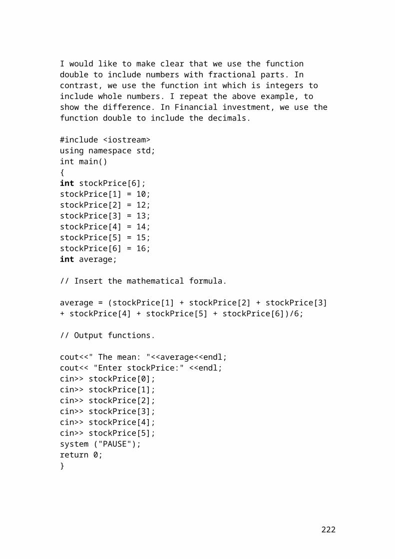
cout <<"Portfolio value 6:"<< portfoliovalue6<<endl; cout <<"Portfolio value 7:"<< portfoliovalue7<<endl; cout <<"Portfolio value 8:"<< portfoliovalue8<<endl; cout <<"Portfolio value 9:"<< portfoliovalue9<<endl; cout <<"Portfolio value 10:"<< portfoliovalue10<<endl; system("PAUSE"); return 0; }

Output

The figures are expressed in pounds. After compiling and debugging , the DOS window or console will open and display the following results:

Portfolio value 1: 541Portfolio value 2: 949Portfolio value 3: 888Portfolio value 4: 912Portfolio value 5: 1652Portfolio value 6: 2576Portfolio value 7: 1554Portfolio value 8: 319Portfolio value 9: 1266Portfolio value 10: 1233

Press any key to continue …

222

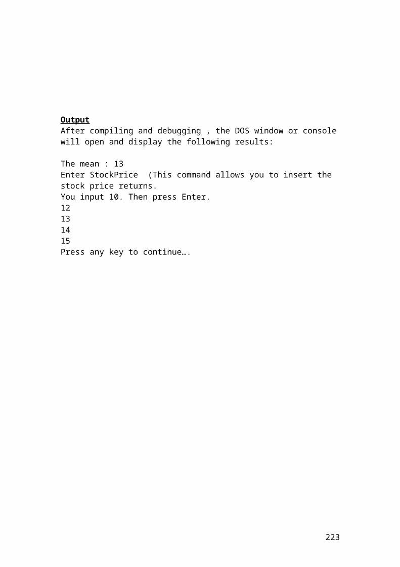
Example of profit or loss of a put option portfolio

// Profit or loss of a put option portfolio.

#include <iostream>using namespace std;

int main(){ double portfoliovalue1, portfoliovalue2, portfoliovalue3, portfoliovalue4, portfoliovalue5,portfoliovalue6,portfoliovalue7, portfoliovalue8,portfoliovalue9,portfoliovalue10 ; // portfolio value. double shareprice[10] ; // number of positions of share prices. double strikeprice[10]; // number of positions of strike prices. double optionpremium [10]; // Put option premiums. double contractsize = 100; // contract size.

/* Identifying the number of positions in relation to the share prices, strike prices and option premium.*/

shareprice[1] = 10.25; shareprice[2] = 20.13;

223

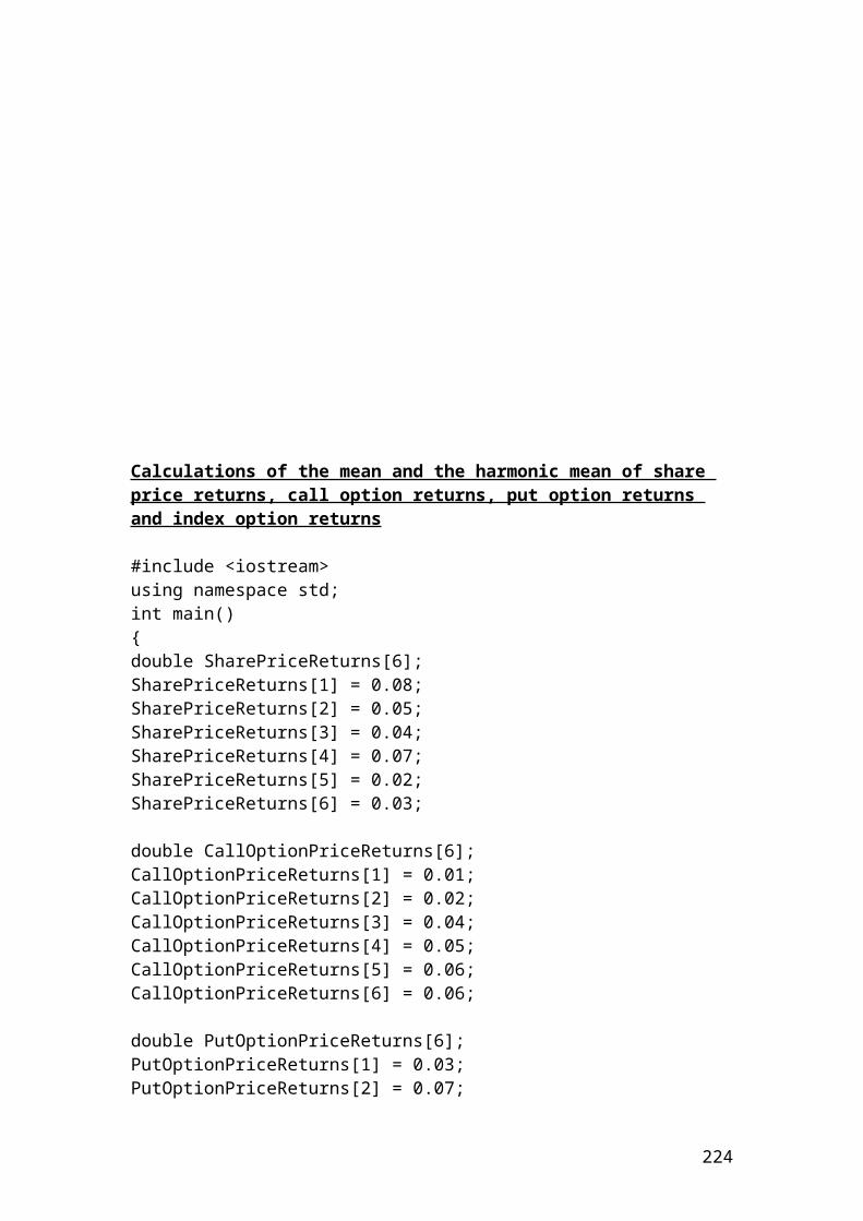
shareprice[3] = 30.22; shareprice[4] = 40.56; shareprice[5] = 50.89; shareprice[6] = 51.23; shareprice[7] = 53.33; shareprice[8] = 54.63; shareprice[9] = 66.23; shareprice[10] = 68.23;

strikeprice[1] = 3.34; strikeprice[2] = 8.34; strikeprice[3] = 18.78; strikeprice[4] = 28.34; strikeprice[5] = 31.12; strikeprice[6] = 22.02; strikeprice[7] = 34.23; strikeprice[8] = 47.12; strikeprice[9] = 48.45; strikeprice[10] = 50.12; optionpremium[1] = 1.50; optionpremium[2] = 2.30; optionpremium[3] = 2.56; optionpremium[4] = 3.10; optionpremium[5] = 3.25; optionpremium[6] = 3.45; optionpremium[7] = 3.56; optionpremium[8] = 4.32; optionpremium[9] = 5.12; optionpremium[10] = 5.78; // Calculate the call option portfolio values. portfoliovalue1 = (strikeprice[1]- optionpremium[1]-shareprice[1])* contractsize; portfoliovalue2 = (strikeprice[2]- optionpremium[2]- shareprice[2])* contractsize; portfoliovalue3 = (strikeprice[3]- optionpremium[3]- shareprice[3])* contractsize; portfoliovalue4 = (strikeprice[4]- optionpremium[4]- shareprice[4])* contractsize; portfoliovalue5 = (strikeprice[5]- optionpremium[5]- shareprice[5])* contractsize; portfoliovalue6 = (strikeprice[6]- optionpremium[6]- shareprice[6])* contractsize; portfoliovalue7 = (strikeprice[7]- optionpremium[7]- shareprice[7])* contractsize; portfoliovalue8 = (strikeprice[8]- optionpremium[8]- shareprice[8])* contractsize; portfoliovalue9 = (strikeprice[9]- optionpremium[9]- shareprice[9])* contractsize; portfoliovalue10 = (strikeprice[10]- optionpremium[10]- shareprice[10])* contractsize; cout <<"Portfolio value 1:"<< portfoliovalue1<<endl; cout <<"Portfolio value 2:"<< portfoliovalue2<<endl; cout <<"Portfolio value 3:"<< portfoliovalue3<<endl; cout <<"Portfolio value 4:"<< portfoliovalue4<<endl;

224

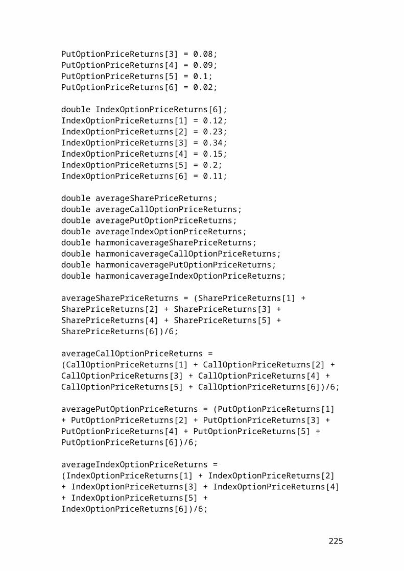
cout <<"Portfolio value 5:"<< portfoliovalue5<<endl; cout <<"Portfolio value 6:"<< portfoliovalue6<<endl; cout <<"Portfolio value 7:"<< portfoliovalue7<<endl; cout <<"Portfolio value 8:"<< portfoliovalue8<<endl; cout <<"Portfolio value 9:"<< portfoliovalue9<<endl; cout <<"Portfolio value 10:"<< portfoliovalue10<<endl; system("PAUSE"); return 0; }

Output

The figures are expressed in pounds. After compiling and debugging , the DOS window or console will open and display the following results:

Portfolio value 1: -841Portfolio value 2: -1409Portfolio value 3: -1400Portfolio value 4: -1532Portfolio value 5: -2302Portfolio value 6: -3266Portfolio value 7: -2266Portfolio value 8: -1183Portfolio value 9: -2290Portfolio value 10: -2389

Press any key to continue …

225

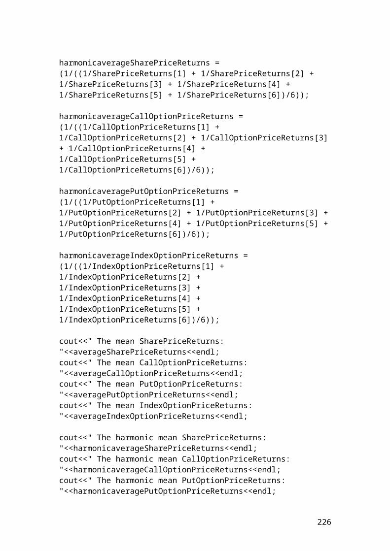
One – period binomial method

A share is traded in the Danish stock exchange at 50 DKK. First of all, we would like to calculate the possible price changes based on probabilities. The risk - free rate is 5% and the value of the call option has an exercise price of 50 DKK. It is required to calculate the expected value of the option at t =1. In addition, it is required to calculate the value of the option today discounted at the given risk-free rate.

We assume two scenarios. The first one is that the share will increase by 20% or by a factor of 1 + 0.20 = 1.20. The second one is that the share will decrease by 0.833. The number 0.833 is calculated as 1 / 1.20 = 0.833.

The mathematical formulas are as follows:

Down move = D = 1 / up move = 1 / 1.20 = 0.833

226

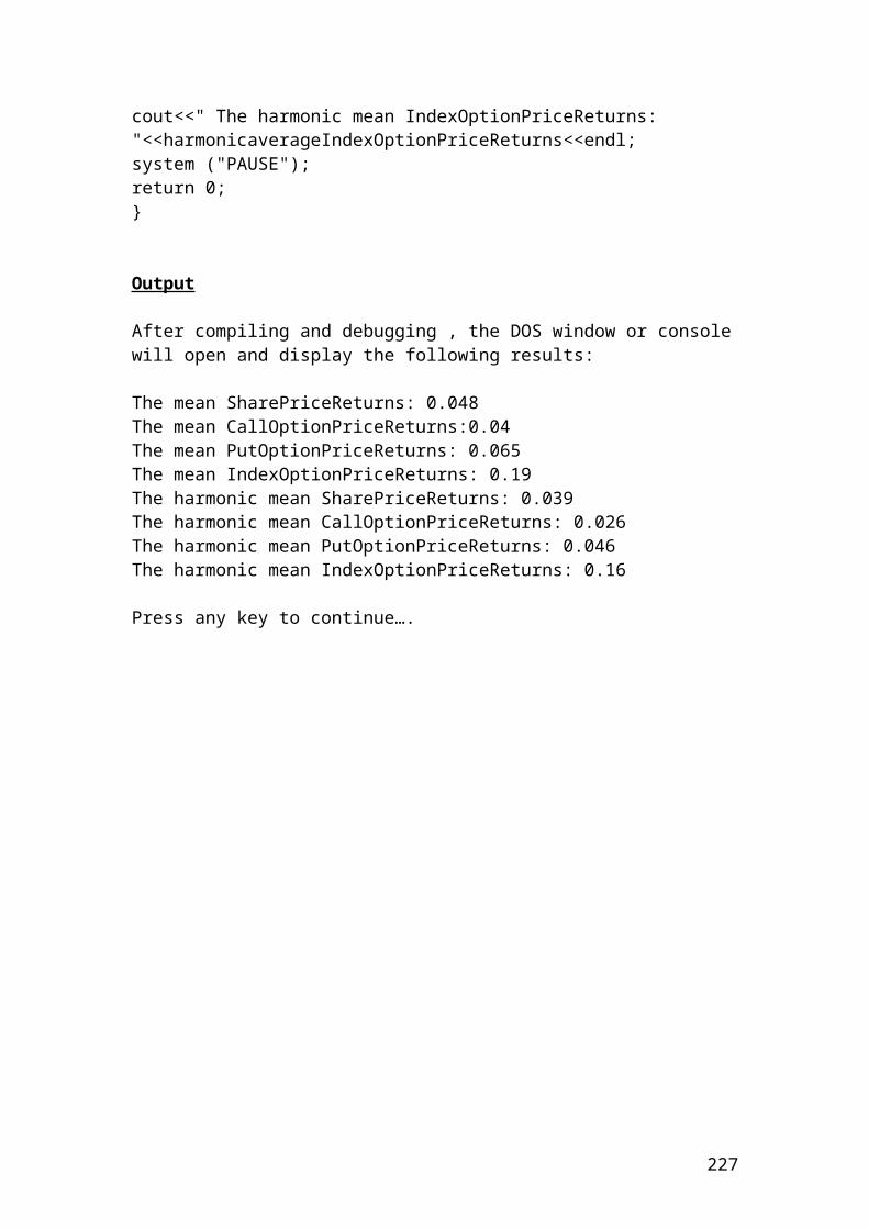
Thus, the payoff or the one-period binomial tree for share and option prices for the two possible scenarios will be as follows:

t = 0 t = 1

Probability Up = 0.59128 Share price = 50 x 1.20 = 60 DKK Call option = 60 – 50 = 10 DKK. 50 In this case, an increase of the share price will lead to the call option to pay back 10 DKK Probability Down =0.40872 Share price = 50 x 0.833 = 41.65 DKK Call option = 41.65 – 50 = -8.35 DKK = 0 DKK In this case the call option does not worth anything.

The expected value of the call option at t = 1 is as follows:

Expected call option = (10 x 0.59128) + ( 0 x 0.40872) = 5.9128 + 0 = 5.9128 DKK.

The value of the call option discounted at 5% risk – free rate is as follows:

Ctoday = 5.9128 / 1.05 = 5.63 DKK (to 2 d.p.).

Application of one – period binomial method in C++

//One - period binomial method.

#include <iostream>using namespace std;

int main(){ double shareprice = 50; double exerciseprice = 50; double upmove = 1.20; double downmove = 0.833; double riskfreerate = 0.05; double riskprobofupmove; double riskprobofdownmove; double shareprice1; double shareprice2; double calloptionprice1; double calloptionprice2; double expectedcalloption; double valueofcalldiscounted;

227

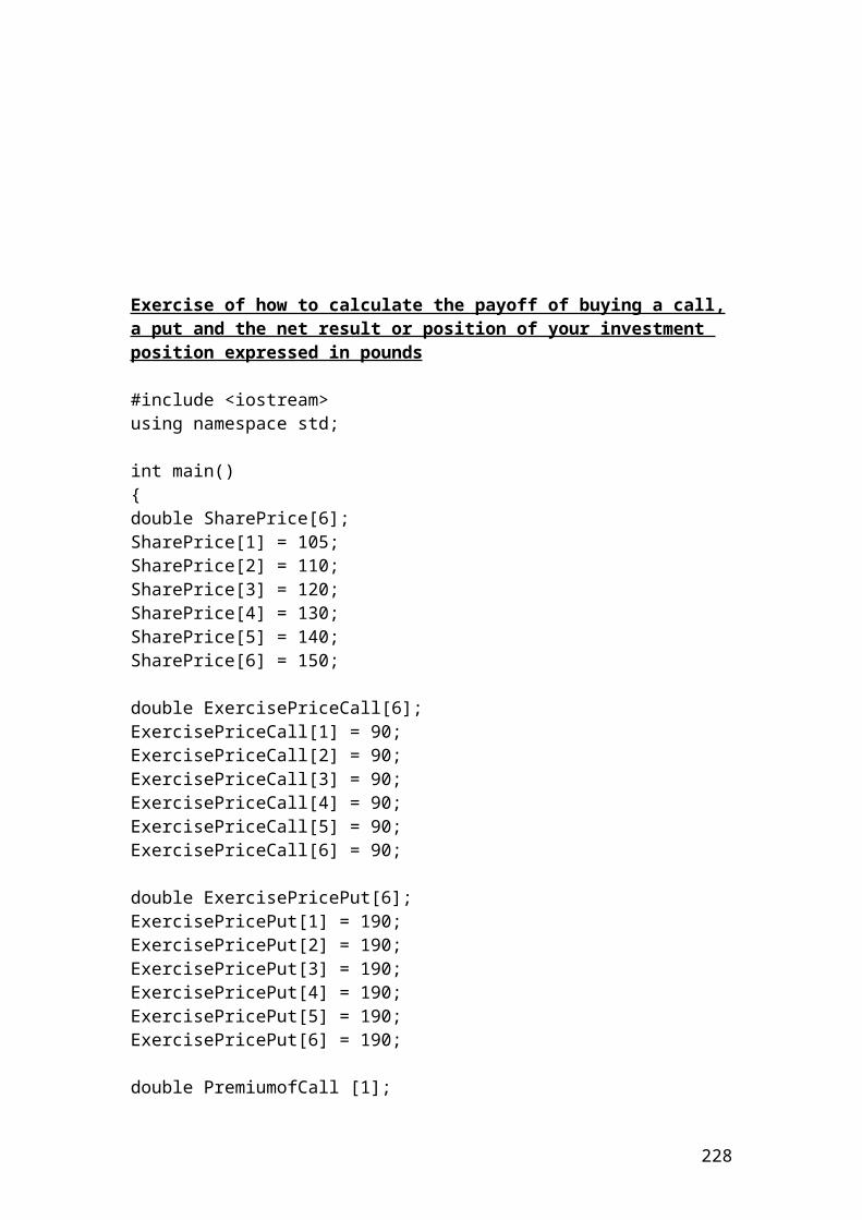
// Insert the mathematical formulas of risk probability of up and down move.

riskprobofupmove = (1+riskfreerate-downmove) / (upmove - downmove);riskprobofdownmove = 1 - riskprobofupmove;

// The payoff or one period binomial tree for share and option prices is as follows:

shareprice1 = shareprice * upmove;calloptionprice1 = shareprice1 - exerciseprice;

shareprice2 = shareprice *downmove;calloptionprice2 = shareprice2 - exerciseprice;calloptionprice2 =0;

// The expected value of the call option at t=1 is as follows:

expectedcalloption = (calloptionprice1* riskprobofupmove) + (calloptionprice2 * riskprobofdownmove);

// The value of the call option discounted at 5% risk - free rate is as follows:

valueofcalldiscounted = expectedcalloption / 1.05;// Output functions.

cout<< "Risk probability of up move:" <<riskprobofupmove<<endl;cout<< "Risk probability of down move:"<<riskprobofdownmove <<endl;cout<< "Share price 1:"<<shareprice1 <<endl;cout<< "Call option price 1:"<<calloptionprice1 <<endl;cout<< "Share price 2:"<<shareprice2 <<endl;cout<< "Call option price 2:"<< calloptionprice2<<endl;cout<< "Expected call option:"<<expectedcalloption <<endl;cout<< "Value of call option discounted:"<<valueofcalldiscounted <<endl;

system ("PAUSE");return 0;}

Output

After compiling and debugging , the DOS window or console will open and display the following results:

Risk probability of up move: 0.59128Risk probability of down move: 0.40872Share price 1: 60Call option price 1: 10Share price 2: 41.65Call option price 2: 0 Expected call option: 5.9128Value of call option discounted: 5.63

228

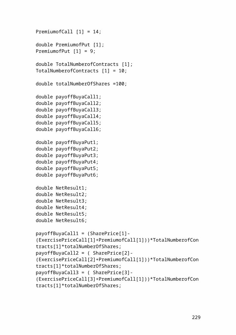
Press any key to continue …

Two – period binomial method

This method is based on the one – period binomial method, but it is extended to include a second period, t = 2. Thus, we have three periods. t = 0, t =1 and t =2. We use the same example of the previous section but extended to an additional period.

A share is traded in the Danish stock exchange at 50 DKK. First of all, we would like to calculate the possible price changes based on probabilities. The risk - free rate is 5% and the value of the call option has an exercise price of 50 DKK. It is required to calculate the expected value of the option. In addition, it is required to calculate the value of the option today discounted at the given risk-free rate.

We assume two scenarios. The first one is that the share will increase by 20% or by a factor of 1 + 0.20 = 1.20. The second one is that the share will decrease by 0.833. The number 0.833 is calculated as 1 / 1.20 = 0.833.

The mathematical formulas are as follows:

Down move = D = 1 / up move.

229

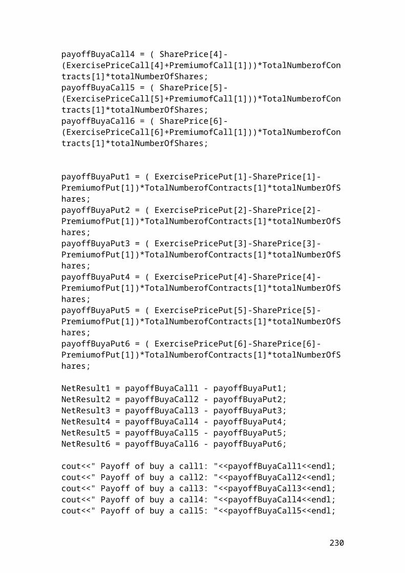
Thus, the payoff or the two-period binomial tree for share prices for the two possible scenarios will be as follows:

t = 0 t = 1 t =2 50*(1.20)2=72 DKKProbability Up = 0.59 S1 = 50 x 1.20 = 60 DKK S2 50*1.20*0.833 =49.98 50 DKK Probability Down =0.41 S1 = 50 x 0.833 = 41.65 DKK S2

50 * (0.833)2 = 34.69

The value of the call options for the period t =2 for both ups and downs are as follows:

Upside movementC1 = 72 – 50 = 22C2 = 49.98 – 50 = -0.02 =0 Negative values mean that the option does not worth.

Downside movementC1 = 49.98 -50 = -0.02 =0C2 = 34.69 -50 = -15.31 =0

The expected value of the call options for both movements for period t =1 are calculated based on the following equations:

Upside movement

Downside movement

The value of the call option today discounted is calculated based on the following formula:

230

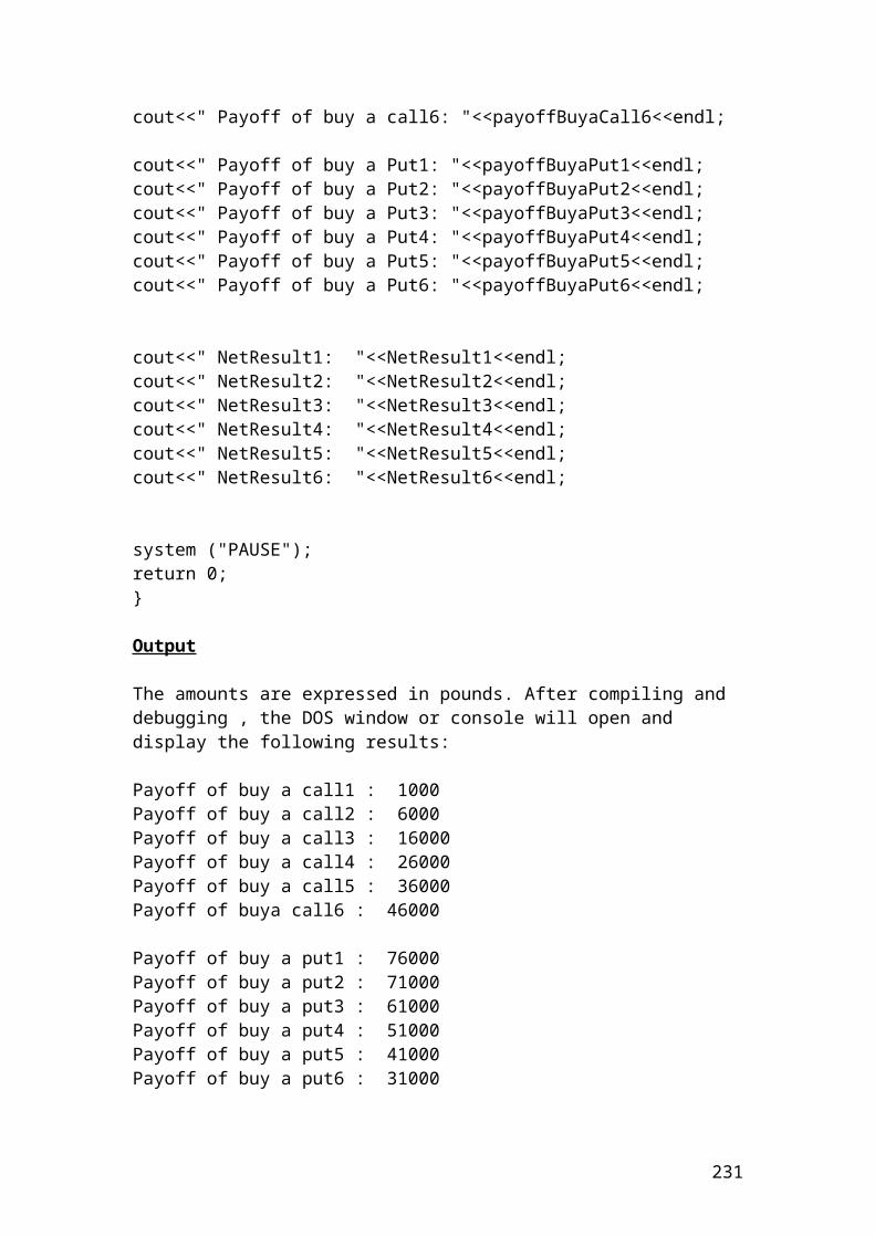
The final format of the two-period binomial tree for call options is as follows:

t = 0 t = 1 t = 2

22.00 DKK 12.3887DKK 06.976 DKK 0 0

Application of two – period binomial method in C++

//Two - period binomial method.

#include <iostream>#include<cmath>using namespace std;

int main(){ double shareprice = 50; double exerciseprice = 50; double upmove = 1.20; double downmove = 0.833; double riskfreerate = 0.05; double riskprobofupmove; double riskprobofdownmove; double shareprice1; double shareprice2; double shareprice3; double shareprice4; double shareprice5; double calloptionprice1; double calloptionprice2; double calloptionprice3; double calloptionprice4; double calloptionprice5; double expectedcalloptionupside; double expectedcalloptiondownside; double valueofcalldiscounted;

// Insert the mathematical formulas of risk probability of up and down move.

231

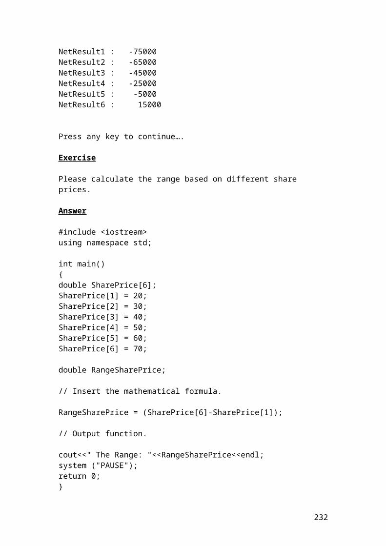
riskprobofupmove = (1+riskfreerate-downmove) / (upmove - downmove);riskprobofdownmove = 1 - riskprobofupmove;

// The payoff or two period binomial tree for share and option prices is as follows:

shareprice1 = shareprice * upmove;

shareprice2 = shareprice *downmove;

shareprice3 = shareprice * pow(upmove,2);calloptionprice3 = shareprice3 - exerciseprice;

shareprice4 = shareprice * pow(downmove,2);calloptionprice4 = shareprice4 - exerciseprice;calloptionprice4 =0;

shareprice5 = shareprice * upmove * downmove;calloptionprice5 = shareprice5 - exerciseprice;calloptionprice5 =0;

// The expected value of the call option at t=2 is as follows:expectedcalloptionupside = (riskprobofupmove * calloptionprice3+ riskprobofdownmove* calloptionprice5) / 1.05;

expectedcalloptiondownside = (riskprobofupmove *calloptionprice4+ riskprobofdownmove * calloptionprice5) / 1.05;

// The value of the call option discounted at 5% risk - free rate is as follows:

valueofcalldiscounted = (riskprobofupmove * expectedcalloptionupside+riskprobofdownmove* expectedcalloptiondownside)/ 1.05;

// Output functions.

cout<< "Risk probability of up move:" <<riskprobofupmove<<endl;cout<< "Risk probability of down move:"<<riskprobofdownmove <<endl;cout<< "Share price 1:"<<shareprice1 <<endl;cout<< "Share price 2:"<<shareprice2 <<endl;cout<<" Share price 3:"<<shareprice3<<endl;cout<<" Share price 4:"<<shareprice4<<endl;cout<<" Share price 5:"<<shareprice5<<endl;cout<< "Call option price 3:"<< calloptionprice3<<endl;cout<< "Call option price 4:"<< calloptionprice4<<endl;cout<< "Call option price 5:"<< calloptionprice5<<endl;cout<< "Expected call option upside:"<<expectedcalloptionupside <<endl;cout<< "Expected call option downside:"<<expectedcalloptiondownside <<endl;cout<< "Value of call option discounted:"<<valueofcalldiscounted <<endl;

system ("PAUSE");

232

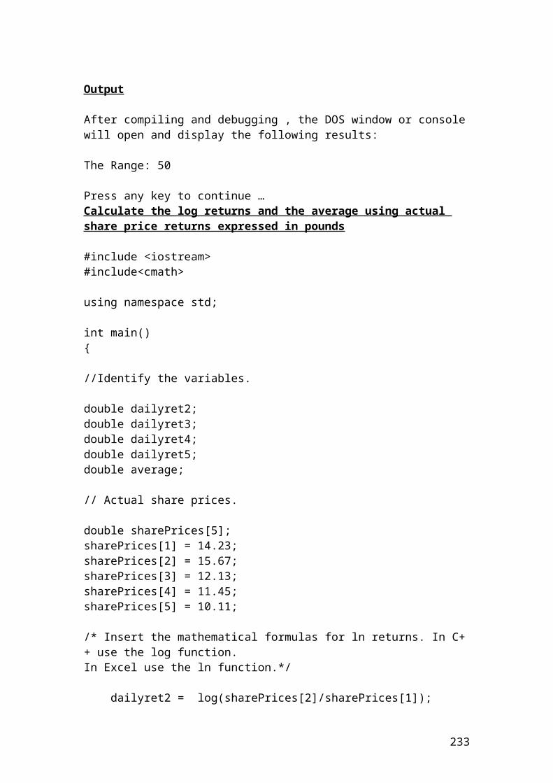
return 0;}

Output

After compiling and debugging , the DOS window or console will open and display the following results:

Risk probability of up move: 0.59128Risk probability of down move: 0.40872Share price 1: 60Share price 2: 41.65Share price 3: 72Share price 4: 34.69Share price 5: 49.98Call option price 3: 22Call option price 4: 0Call option price 5: 0Expected call option upside: 12.3887Expected call option downside: 0Value of call option discounted: 6.976

Press any key to continue …

233

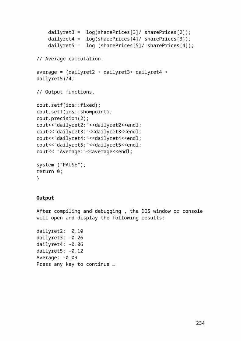
Stock index option

Let’s assume that a practitioner wants to buy a stock index call option that is related to the general movement of the S&P 500 index. The dollar multiplier for S&P 500 option contract is 250 dollars. The strike price of the index is 1240. The August premium is 20 index points.

Question

Calculate the cost of the August call and the net profit involved if the S&P 500 index reaches the price of 1540.

Solution

Cost of the August call = premium expressed in index points x dollar multiplier Cost of the August call = 20 x 250 = 5000 USD

The net profit incurred is calculated as follows:

(Ending index value – beginning index value x dollar multiplier ) – cost of the August call.

(1540 – 1240) x 250 – 5000 = 70,000 USD.

Application of stock index option in C++

//Cost of call and net profit of stock index option.

#include <iostream>using namespace std;

234

int main(){ double costofcall; double netprofit ; int premium = 20; int multiplier = 250; double endingindexvalue = 1540; double beginningindexvalue = 1240; // Insert the mathematical formula.

costofcall = premium * multiplier ;netprofit = (endingindexvalue - beginningindexvalue) * multiplier - costofcall;

// Output functions.

cout<< "Cost of call:"<<costofcall<<endl;cout<< "Net profit:"<<netprofit<<endl;

system ("PAUSE");return 0;}

Output

The figures are expressed in USD. After compiling and debugging , the DOS window or console will open and display the following results:

Cost of call: 5000Net profit: 70000

Press any key to continue …

235

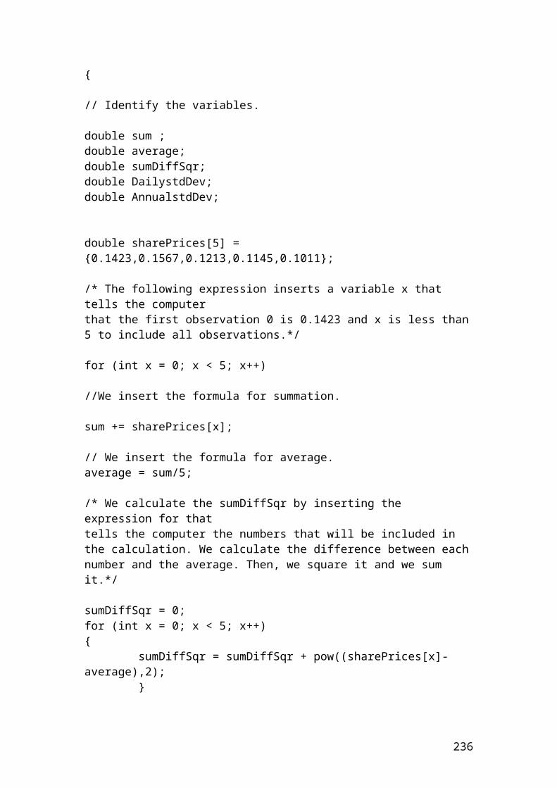
Exercise of an European interest rate option

Calculate the profit or loss of the interest rate difference between the actual and the strike rate of a call option. Let’s assume that an interest call option on a 6 –month Eurodollar has a strike rate of 4%. At expiration, the 6-month Eurodollar rate is 5%. The invested principal is 50,000,000 Euros. The duration of the contract is expressed in days divided by 360 days. Thus, 6 –months equal 180 days.

The mathematical formula for profit or loss is as follows:

Application of an European interest rate option in C++

//Profit or loss of call interest rate option.

#include <iostream>using namespace std;

int main(){ double profitorlosscallinterestrateoption; // call interest rate option. double principal = 50000000; double actualrate = 0.05; double strikerate = 0.04; double duration = 180; double days = 360;

236

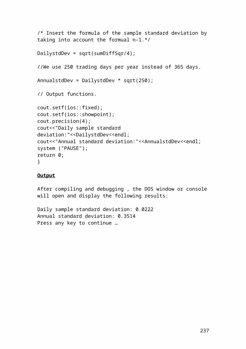
// Insert the mathematical formula.

profitorlosscallinterestrateoption = principal *(actualrate – strikerate)*duration/days;

// Output function.

cout<< "Profit or loss of call interest rate option:"<<profitorlosscallinterestrateoption <<endl;

system ("PAUSE");return 0;}

Output

The figure is expressed in Euros. After compiling and debugging , the DOS window or console will open and display the following results:

Profit or loss of call interest rate option: 250000

Press any key to continue …

237

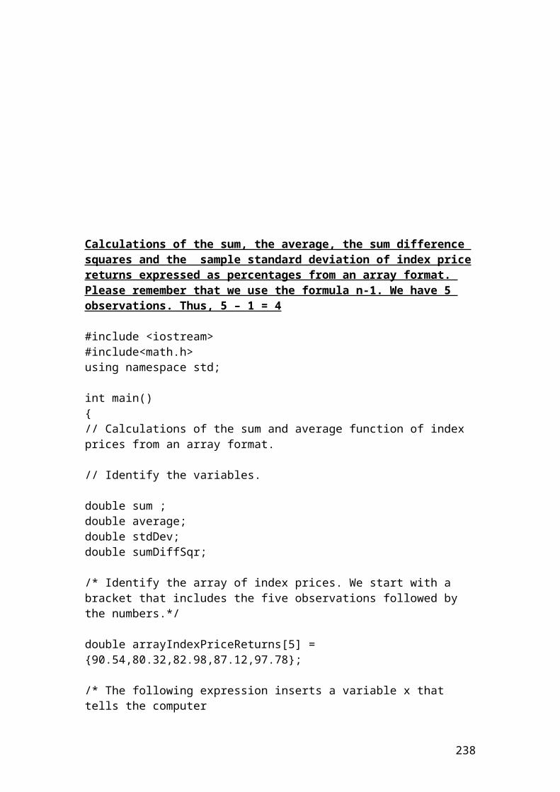
Currency option

Let’s assume that a wealthy investor buys a call currency option because it expects a rise in the exchange rate parity of the EURO against the USD, EURO/USD. The spot exchange rate is 1/1.3568. The strike price is 1.3568. The premium expressed as cents per Euro is 1.56. The initial principal is 100,000 USD.

Question

Calculate the net profit involved if the strike price increases to 1.3987.

Solution

The wealthy investor to record a profit, he or she should add to the strike price 1.3568 the premium expressed as cents per Euro. In our case, the breakeven point is1.3568 + 0.0156 = 1.3724. Above the price of 1.3724, he or she starts to record a profit. If the strike price reaches 1.3987, then the profit will be as follows:

Initial principal x (Ending strike price – beginning strike price – premium paid) =100,000 x (1.3987 – 1.3568 – 0.0156) = 2630 USD net profit

Application of currency option in C++

//Profit or loss of currency option.

#include <iostream>using namespace std;

int main(){ double netprofit; double principal = 100000; double endingstrikeprice = 1.3987; double beginningstrikeprice = 1.3568;

238

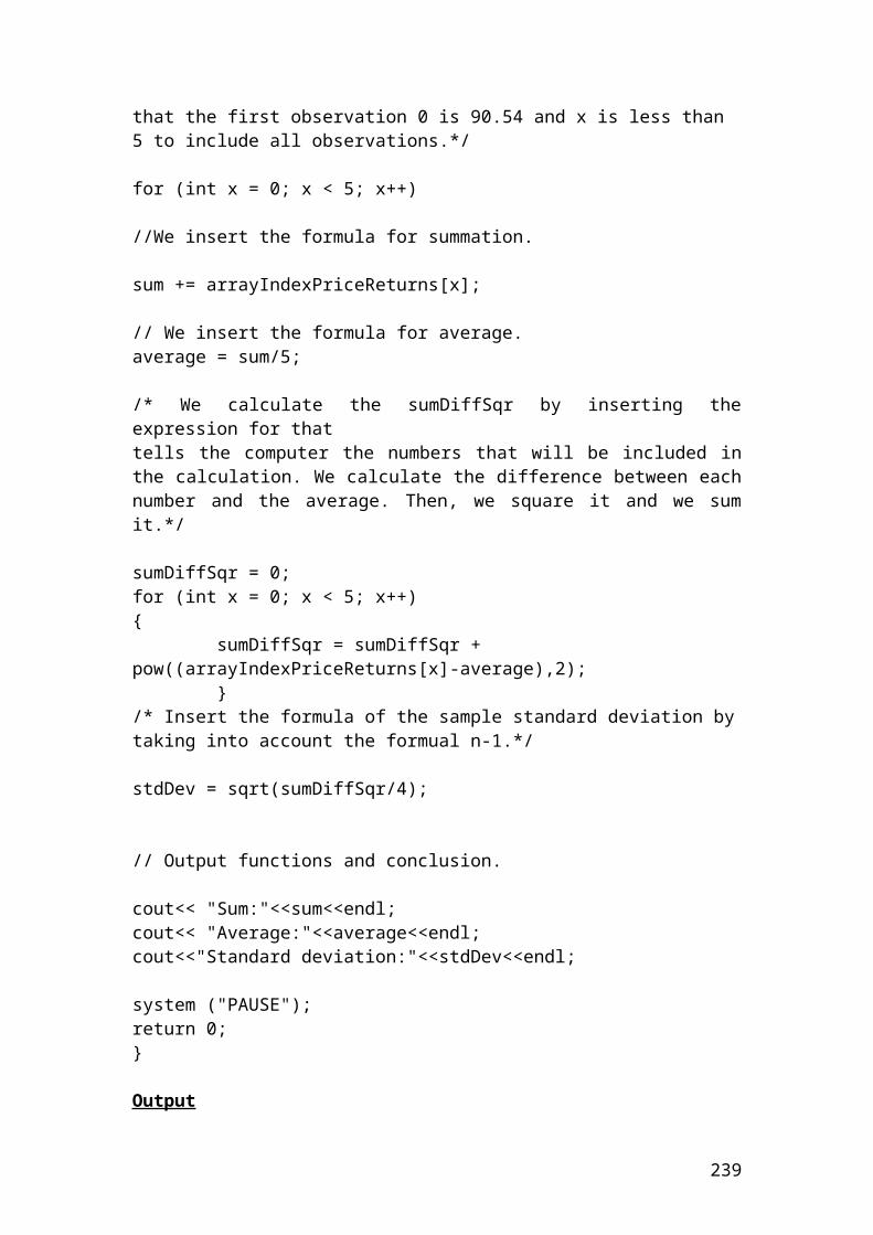
double premiumpaid = 0.0156; // Insert the mathematical formula.

netprofit = principal *(endingstrikeprice – beginningstrikeprice - premiumpaid);

// Output function.

cout<< "Net profit:"<<netprofit <<endl;

system ("PAUSE");return 0;}

Output

The figure is expressed in USD. After compiling and debugging , the DOS window or console will open and display the following results:

Net profit: 2630

Press any key to continue …

239

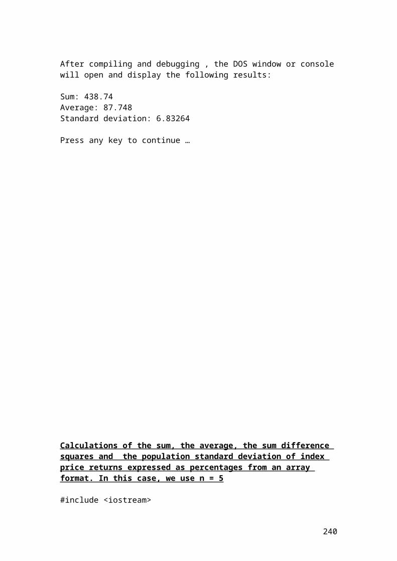
Example of calculating the payments of an interest rate cap based on different LIBOR rates

Interest rate cap is an agreement between two parties where one party pay the other at a specified period of time in which the interest rate or London interbank offered rate ,LIBOR, exceeds the strike price. It is used this contract to hedge against interest rate fluctuations. Let’s assume that an interest cap has a value of 5.5% and the LIBOR prices for the next three years are 7.5%, 8.3% and 4.65%. The principal is $50,000,000 and the payments take place semiannually.

The mathematical formula that is used to calculate the payments of each year is as follows:

Interest rate payment =[ principal x (LIBOR rate – cap rate)/0.5]

Therefore, the first year interest rate payment is as follows:

Year 1

Interest rate payment = [50,000,000 x (0.075 – 0.055)/2] = $ ………

Application of payments of an interest rate cap based on different LIBOR rates in C++

// Payments of an interest rate cap based on different LIBOR rates.

#include <iostream>using namespace std;

int main(){ double interestpay1; double interestpay2; double interestpay3; double principal = 50000000; double liborrate1 = 0.075;

240

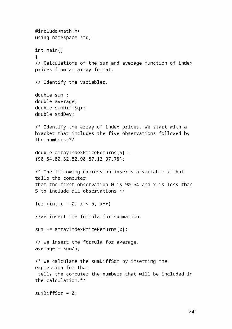
double liborrate2 = 0.083; double caprate = 0.055; double duration = 2; // Insert the mathematical formula.

interestpay1 = principal *(liborrate1 - caprate) /duration ;interestpay2 = principal *(liborrate2 - caprate) / duration ;

// Output functions.

cout<< "Interest rate payment 1:"<<interestpay1 <<endl;cout<< "Interest rate payment 2:"<<interestpay2 <<endl;system ("PAUSE");return 0;}

Output

The figures are expressed in USD. After compiling and debugging , the DOS window or console will open and display the following results:

Interest rate payment 1: 500000Interest rate payment 2: 700000

Press any key to continue …

241

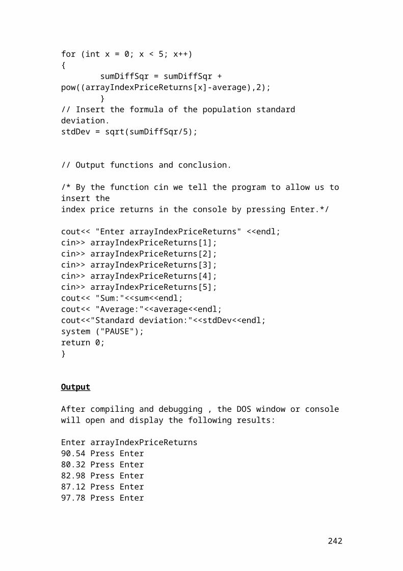
A six month interest rate cap has a rate of 0.08 and the principal is 20,000,000 USD. The settlements is done quarterly. The first quarter the 3 –month libor rate is 0.096 and the second quarter the rate is 0.087. Calculate the payoff for the cap the first and the second quarter?

Solution

Payoff the first quarter = 20,000,000 * = 80000 USD

Payoff the second quarter = 20,000,000 * =35000 USD

Application of payoff of interest rate cap in C++

//Payoff of interest rate cap.

#include <iostream>using namespace std;

int main(){ double payoff1; double payoff2; double principal = 20000000; double caprate = 0.08; double liborrate1 = 0.096; double liborrate2 = 0.087; double period = 4; // Insert the mathematical formulas. payoff1 = (principal*(liborrate1-caprate)/period);payoff2 = (principal*(liborrate2-caprate)/period);

// Output functions.cout<< "Payoff1:" <<payoff1<<endl;

242

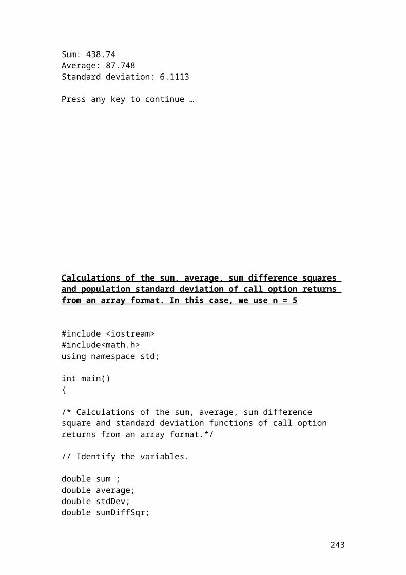
cout<< "Payoff2:" <<payoff2<<endl;system ("PAUSE");return 0;}

Output

The figures are expressed in USD. After compiling and debugging , the DOS window or console will open and display the following results:

Payoff1: 80000Payoff2: 35000

Press any key to continue …Swaption

An investor purchased a 1 year European swaption with exercise price 7.50%. The principal is 30,000,000USD. The floating rate payments are based on LIBOR. The 90, 180, 270, and 360 day annualized LIBOR rates and present value factors are as follows:

LIBOR Rate Present value factors90 day LIBOR 4% 0.990099180 day LIBOR 5.5% 0.973236270 day LIBOR 6% 0.956938360 day LIBOR 7% 0.934579

Calculate the semi-annual and annualized swap rate?Calculate the net cash flow at each payment and the value of swaption at maturity.

Solution

The present value factors are calculated as follows:

PV 90 days = 0.990099

PV 180 days = 0.973236

PV 270 days = 0.956938

243

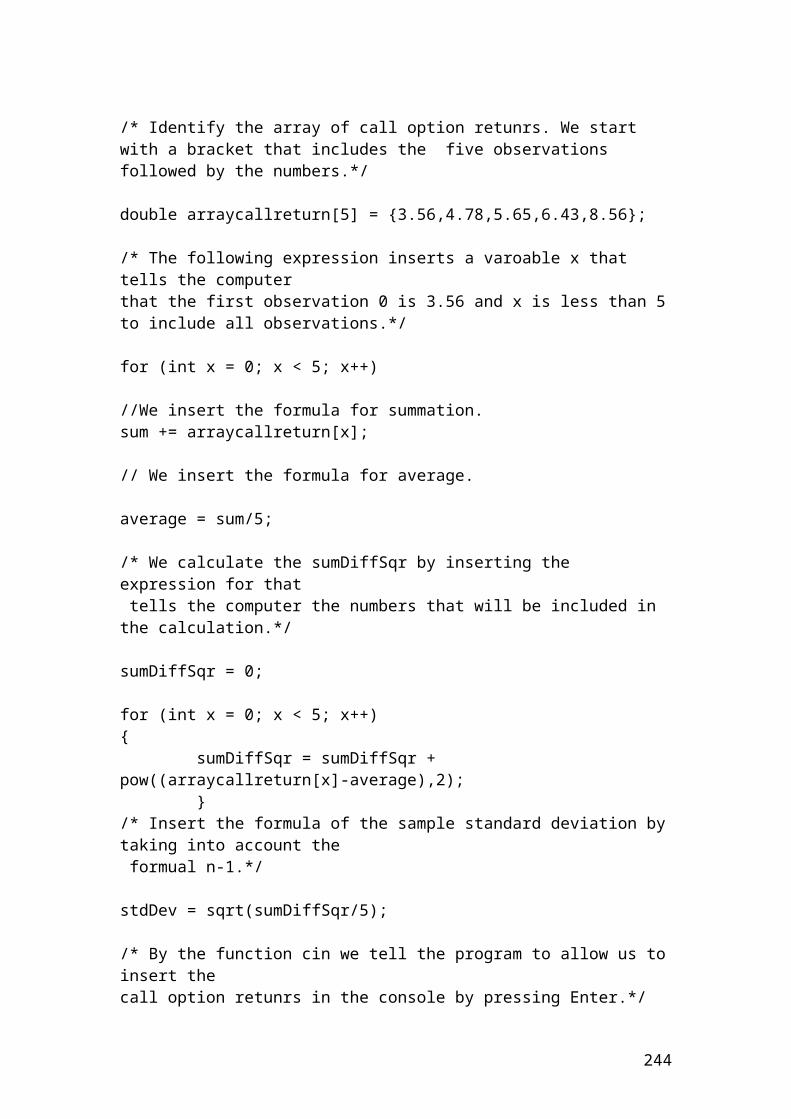
PV 360 days = 0.934579

Semi - annual swap rate =

Annulaized swap rate =

The swaption is in the money because the exercise price 7.50% is greater than the market annualized swap rate 6.788%.

The net cash flow is as follows:

netCashFlow = (0.075 – 0.06788)*90/360 * 30000000 = 53400 USD

The value of swaption at maturity is as follows:

valueSwaption = 53400 *( ) = 205,849.1 USD

Application of swaption in C++

//Swaption.

#include <iostream>using namespace std;

int main(){ double semiAnnualRate; double annualizedSwapRate; double netCashFlow; double valueSwaption; double exerciseRate = 0.075; double principal = 30000000; double PV90; double PV180; double PV270; double PV360; double rate90 = 0.04; double rate180 = 0.055; double rate270 = 0.06 ; double rate360 = 0.07;

244

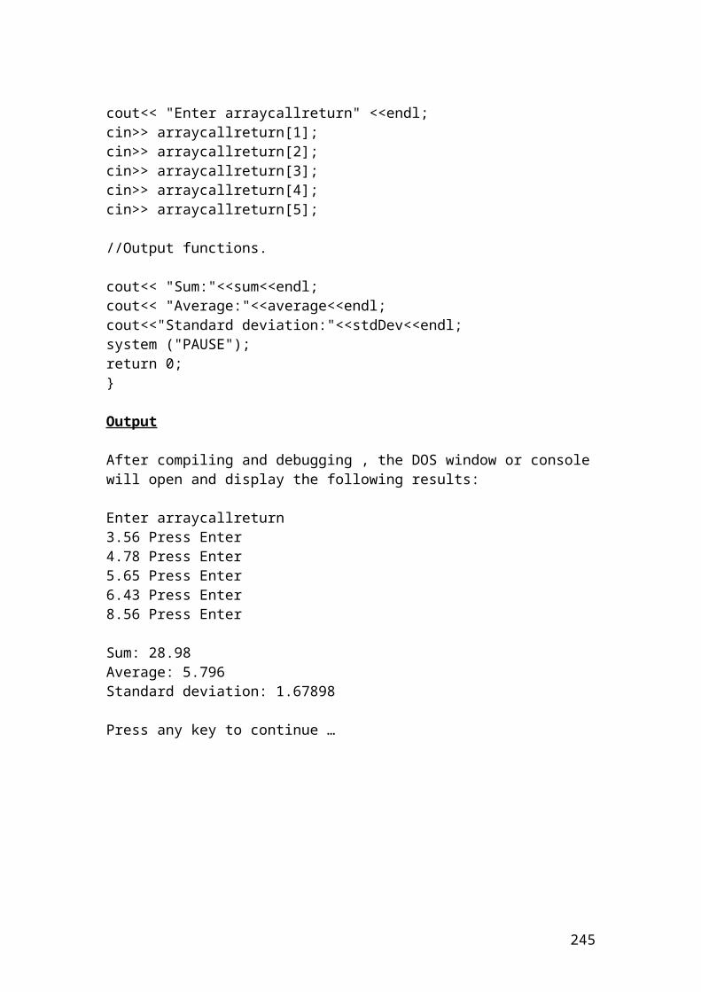
// Insert the mathematical formulas. PV90 = 1 /(1+(rate90 * 90/360));PV180 = 1/(1+(rate180 * 180/360));PV270 = 1/(1+(rate270 * 270/360));PV360 = 1/(1+(rate360* 360/360));

semiAnnualRate = (1-PV360)/(PV90 +PV180 +PV270 +PV360);annualizedSwapRate = semiAnnualRate * (360/90);

// Output functions.

cout.setf(ios::fixed); cout.setf(ios::showpoint); cout.precision(5); cout<< "Semi - annual rate:" <<semiAnnualRate<<endl;cout<< "Annualized swap rate:" <<annualizedSwapRate<<endl;

system ("PAUSE");return 0;}

Output

The figures are expressed in USD. After compiling and debugging , the DOS window or console will open and display the following results:

Semi – annual rate: 0.01697Annualized swap rate: 0.06788

Press any key to continue …

Please repeat the above swaption problem and calculate the net cash flow and the value of swaption at maturity.

245

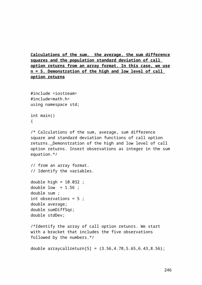
Put –call parity

The put – call parity shows the relationship between a call and a put option with the same expiration, strike and share prices. The mathematical formula is as follows:

Example

Calculate the price of a call if the price of a put is 5.34 Pounds, the share price is 94, the strike price is 97, the risk-free rate is 4% and the time to maturity, T=0.5. By rearranging formula (20) and solving for the price of a call, we have the following results:

Application of put - call parity in C++

// Put - call parity. Calculating the price of a call.

#include <iostream># include <cmath>using namespace std;

246

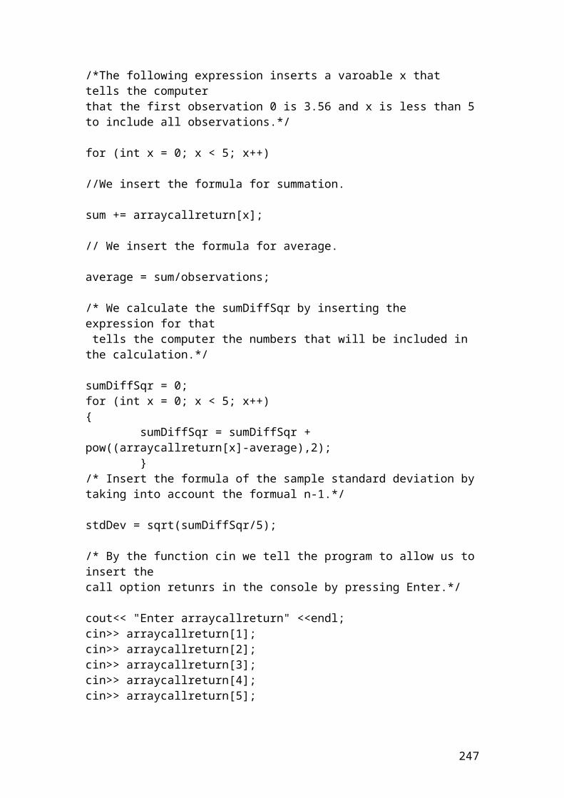
int main(){ double call; double put = 5.34; double shareprice = 94; double strikeprice = 97; double disriskfreerate = 1.04; double maturity = 0.5;

// Insert the mathematical formula.

call = put + shareprice - strikeprice / pow(disriskfreerate,maturity);

// Output function.

cout<< "Call :"<<call <<endl;system ("PAUSE");return 0;}

Output

The figure is expressed in pounds. After compiling and debugging , the DOS window or console will open and display the following results:

Call: 4.22

Press any key to continue …

247

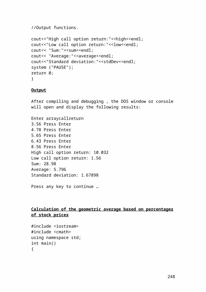
Example of margin payments in the clearinghouse

An investor open a margin account with a minimum initial margin of 5,200 dollars per contract. The maintenance margin is 1,500 dollars per contract. He/she buys 7 July wheat futures contracts with a standard contract size of 200 bushels priced at 230 dollars per bushel. The July contract size in the next 2 days recorded the prices of 220 and 210 dollars per bushel. Show the cash flows, gains and losses for the buyer and the seller?

Solution

Initial margin = 7 x 5,200 = 36,400 dollars

Maintenance margin = 7 x 1,500 = 10,500 dollars

The cash flows, gains and losses for the next two days will be as follows:

Day 1

Cash flows for the buyer’s: 36,400 + 14,000 = 50,400 dollars. The investor’s recorded a gain.

Cash flows for the seller’s: 36,400 – 14,000 = 22,400 dollars. The investor’s recorded a loss.

Helpful hint: the amount of 14,000 is calculated from the difference of the bushel prices, (f0-f) x number of contracts x standard contract size. Thus, we have: (230-220) x 7 x 200 = 14,000 dollars. The same principle applies for the second day but with different bushel price.

Day 2

Please do the calculations for the second day.

This is why I am stressing the importance that the investors should buy or sell ONLY when the market is aggressively increasing or falling. If he/she gets trapped in a market that is not strong bull or bear, then, he/she will have to compensate regularly for the losses or he/she will experience a very small profit. If the amounts as the days passes is below the maintenance margin, then, the investor’s will receive a margin call

248

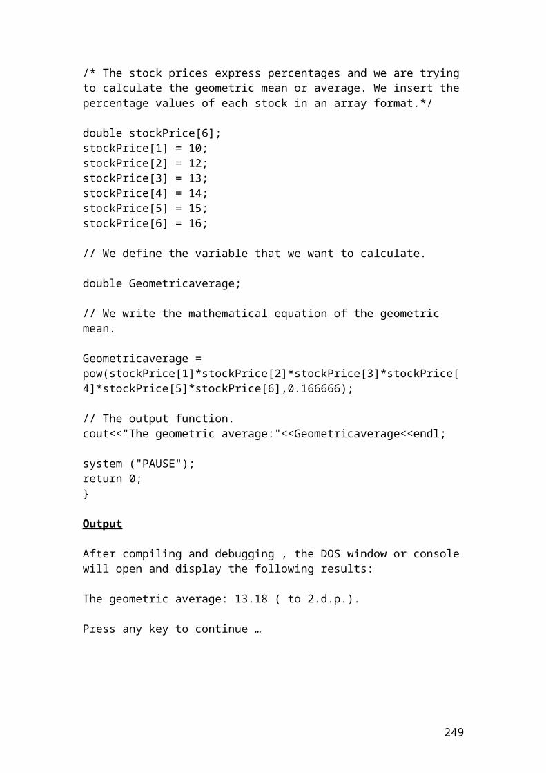
and he/she should add the capital required to proceed with the contract. If the investor’s is short of money, then, the position is closed with the incurred losses.

Application of margin payments in the clearinghouse in C++

// Margin payments.

#include <iostream>using namespace std;

int main(){ double cashflowbuyer ; double cashflowseller ; double initialmargin = 5200; double maintenancemargin = 1500; int contractnumber = 7; int bushelcontractsize = 200; double bushelprice1 = 230; double bushelprice2 = 220; double initialmarginwithcontract ; double maintenancemarginwithcontract; double bushelcontract ;

// Insert the mathematical formulas.

initialmarginwithcontract = initialmargin * contractnumber;maintenancemarginwithcontract = maintenancemargin * contractnumber;

bushelcontract = (bushelprice1 – bushelprice2) * bushelcontractsize * contractnumber;

cashflowbuyer = initialmarginwithcontract + bushelcontract; cashflowseller = initialmarginwithcontract – bushelcontract;

// Output functions.

cout<< "Initial margin with contract :"<<initialmarginwithcontract <<endl;cout<< "Maintenance margin with contract :"<<maintenancemarginwithcontract <<endl;cout<< "Bushel contract :"<<bushelcontract <<endl;cout<< "Cash flow buyer :"<<cashflowbuyer <<endl;cout<< "Cash flow seller :"<<cashflowseller <<endl;

249

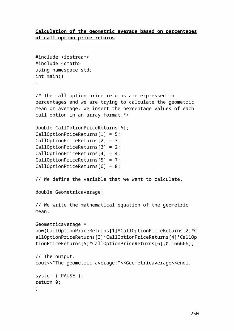
system ("PAUSE");return 0;}

Output

The figures are expressed in dollars. After compiling and debugging , the DOS window or console will open and display the following results:

Initial margin with contract: 36400Maintenance margin with contract: 10500 Bushel contract: 14000Cash flow buyer: 50400Cash flow seller: 22400

Press any key to continue …

250

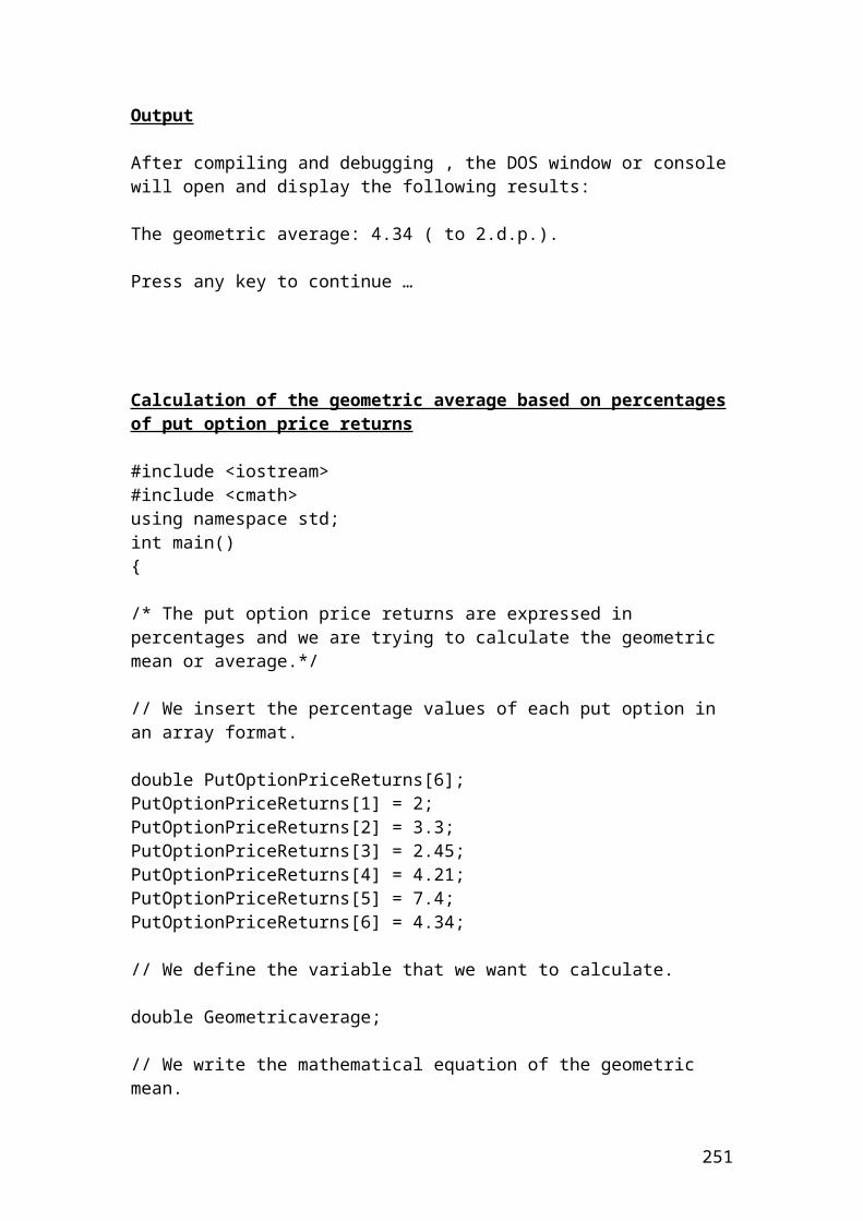
Example of calculating a margin call due to changes of price futures

An investor has opened a short position of 20 Soybean futures contract. The initial margin was 500 Pounds and the maintenance margin was 430 Pounds per contract. The price change that will create a margin call is as follows:

Solution

3.5

Application of margin call in C++

// Margin call.

#include <iostream>using namespace std;

int main(){ double initialmargin = 500; double maintenancemargin = 430; int futurescontract = 20; double margincall;

// Insert the mathematical formula.

margincall =( initialmargin – maintenancemargin) / futurescontract;

// Output function.

cout<< "Margin call created at a price :"<<margincall<<endl;system ("PAUSE");return 0;}

251

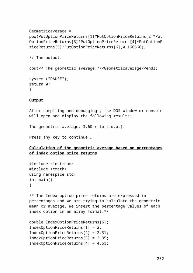
Output

The figure is expressed in pounds. After compiling and debugging , the DOS window or console will open and display the following results:

Margin call created at a price: 3.5

Press any key to continue …

252

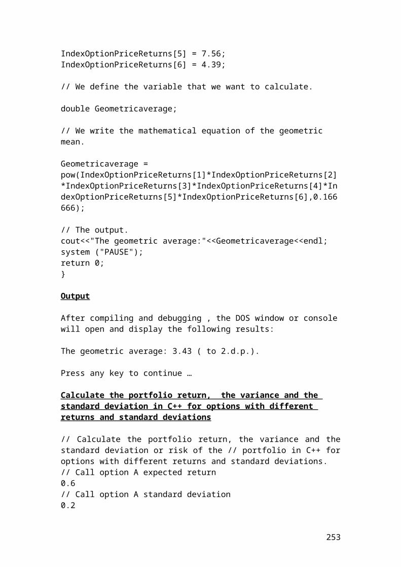
Example of simulating share prices by showing different price scenarios of the highest and the lowest value

/* Simulated share prices by showing different price scenarios of the highest and the lowest value.*/

#include <iostream>#include <ctime>#include<cmath>

using namespace std;

int main(){

int i ;int numberOfSimulation = 6;const int maxSize = 8;double normSamps[maxSize];double sharePrice[maxSize];double randomNumber[maxSize];

double S0 = 60; // initial share price.double r = 0.03; // risk – free interest rate.double q = 0.02; // dividend yield.double sig = 0.20; // volatility double dt = 1/250; // maturity expressed by 250 trading days. srand (time(0));for (i=0; i< maxSize; i++){ randomNumber[i] =((rand()%30000)+ 3000)/300;} for(i=0; i <maxSize; i++) { normSamps[i]=0; sharePrice[i] =0; }

253

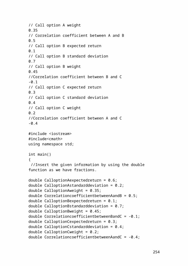
sharePrice[0]= S0;int numberofsteps = 2;cout.setf(ios::fixed); cout.setf(ios::showpoint); cout.precision(3); cout<<"Initial share price:"<<S0<<endl;

for (int i =0; i<1; i++) { sharePrice[i] = sharePrice[i-1] *exp((r-q-0.5*sig*sig)*dt + normSamps[i-1]*randomNumber[i]*sig *sqrt(dt)); // We simulate the share price by using random number. sharePrice[i-1] = sharePrice[i-2] *exp((r-q-0.5*sig*sig)*dt + normSamps[i-2]*randomNumber[i-2]*sig *sqrt(dt)); // We simulate the share price by using random number. //Output functions.

cout<<"Share price[i]:"<<sharePrice[i]<<endl; cout<<"Share price[i-1]:"<<sharePrice[i-1]<<endl; } system ("PAUSE"); return 0; }

Output

The figures are expressed in Euro. Everytime, you will get different figures as we have used random numbers without defining a Box-Muller algorithm. In my case, after compiling and debugging , the DOS window or console will open and display the following results:

Initial share price in Euro: 60Share price[i] in Euro: 42.000Share price[i-1] in Euro: 82.000Press any key to continue …

254

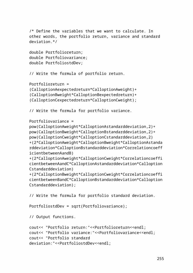
Example of simulating share prices by showing different price scenarios

// Simulated share prices by showing different price scenarios.

#include <iostream>#include <ctime>#include<cmath>

using namespace std;

int main(){

int i ;int numberOfSimulation = 6;const int maxSize = 8;double normSamps[maxSize];double sharePrice[maxSize];double randomNumber[maxSize];

double S0 = 60; // initial share price.double r = 0.03; // risk – free interest rate.double q = 0.02; // dividend yield.double sig = 0.20; // volatility double dt = 1/250; // maturity expressed by 250 trading days. srand (time(0));for (i=0; i< maxSize; i++){ randomNumber[i] =((rand()%30000)+ 3000)/300;} for(i=0; i <maxSize; i++) { normSamps[i]=0; sharePrice[i] =0; } sharePrice[0]= S0;int numberofsteps = 2;cout.setf(ios::fixed);

255

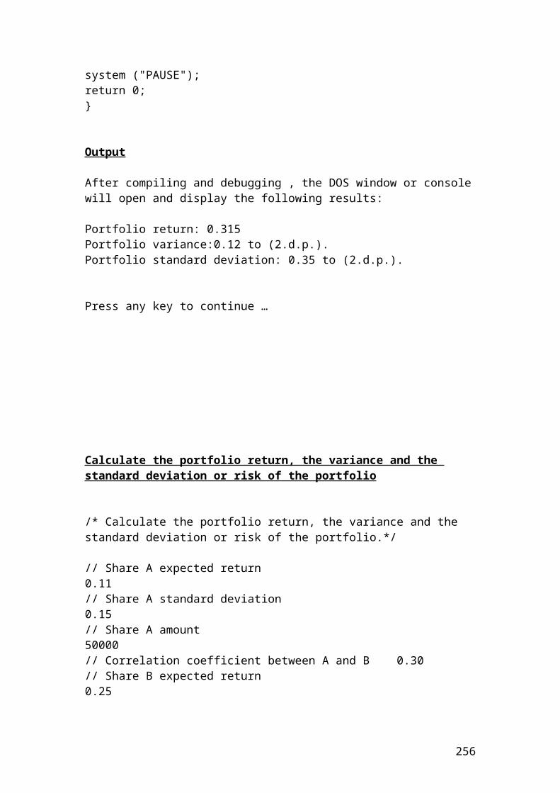
cout.setf(ios::showpoint); cout.precision(3); cout<<"Initial share price in Euro:"<<S0<<endl;

for (int i =0; i<1; i++) { sharePrice[i] = sharePrice[i-1] *exp((r-q-0.5*sig*sig)*dt + normSamps[i-1]*randomNumber[i-1]*sig *sqrt(dt)); // We simulate the share price by using random number. sharePrice[i-1] = sharePrice[i-2] *exp((r-q-0.5*sig*sig)*dt + normSamps[i-2]*randomNumber[i-2]*sig *sqrt(dt)); // We simulate the share price by using random number. sharePrice[i-2] = sharePrice[i-3] *exp((r-q-0.5*sig*sig)*dt + normSamps[i-3]*randomNumber[i-3]*sig *sqrt(dt)); // We simulate the share price by using random number. sharePrice[i-3] = sharePrice[i-4] *exp((r-q-0.5*sig*sig)*dt + normSamps[i-4]*randomNumber[i-4]*sig *sqrt(dt)); // We simulate the share price by using random number. sharePrice[i-4] = sharePrice[i-5] *exp((r-q-0.5*sig*sig)*dt + normSamps[i-5]*randomNumber[i-5]*sig *sqrt(dt)); // We simulate the share price by using random number. sharePrice[i-5] = sharePrice[i-6] *exp((r-q-0.5*sig*sig)*dt + normSamps[i-6]*randomNumber[i-6]*sig *sqrt(dt)); // We simulate the share price by using random number. //Output functions. cout<<"Share price[i]in Euro:"<<sharePrice[i]<<endl; cout<<"Share price[i-1] in Euro:"<<sharePrice[i-1]<<endl; cout<<"Share price[i-2] in Euro:"<<sharePrice[i-2]<<endl; cout<<"Share price[i-3] in Euro:"<<sharePrice[i-3]<<endl; cout<<"Share price[i-4] in Euro:"<<sharePrice[i-4]<<endl; cout<<"Share price[i-5] in Euro:"<<sharePrice[i-5]<<endl; } system ("PAUSE"); return 0; }

256

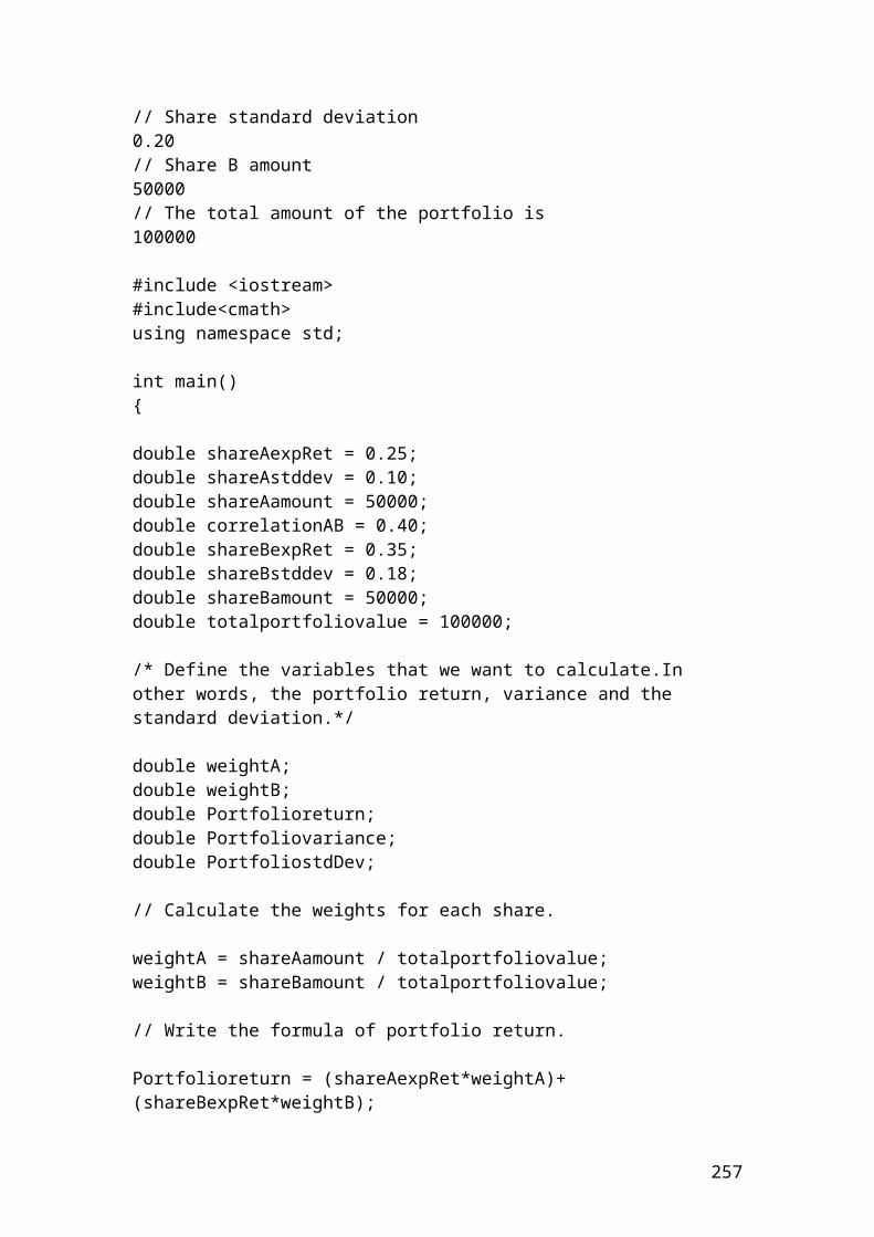
Output

The figures are expressed in Euro. Everytime, you will get different figures as we have used random numbers without defining a Box-Muller algorithm. In my case, after compiling and debugging , the DOS window or console will open and display the following results:

Initial share price in Euro: 60Share price[i] in Euro: 100.000Share price[i-1] in Euro: 85.000Share price[i-2] in Euro: 38.000Share price[i-3] in Euro: 49.000Share price[i-4] in Euro: 32.000Share price[i-5] in Euro: 17.000Press any key to continue …

257

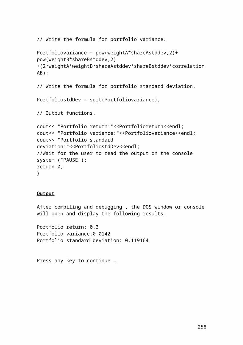
Example of calculating a call option using Monte Carlo simulation.Part of the formulas were taken from the book Financial Modeling using C++, p458

// Calculation of a call option using Monte Carlo simulation.

#include <iostream>#include <ctime>#include<cmath>using namespace std;

double termval( double K, double S0);

int main(){

int i ;int numberOfSimulation = 199999;const int maxSize = 200000;double normSamps[maxSize];double sharePrice;double optPrice;double payoff = 0 ;double randomNumber;

double S0 = 60; // initial share pricedouble K = 50; // strike pricedouble r = 0.05; // risk - free interest ratedouble q = 0.02; // dividend yielddouble sig = 0.45; // volatility double T = 0.5; // maturity

srand (time(0));

randomNumber = ((rand()%10000)+1000)/100;

for(i=0; i <maxSize; i++) { normSamps[i]=0; } for (int i = 0; i <= numberOfSimulation; i ++)

258

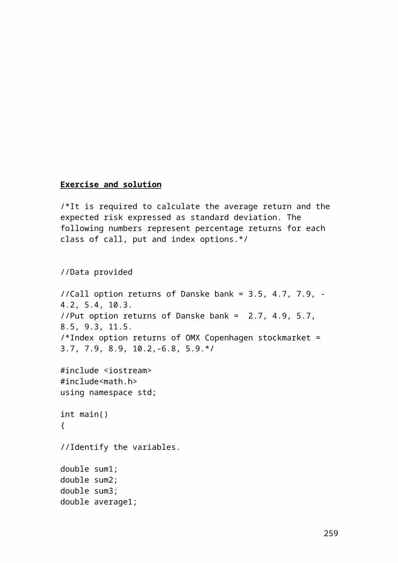
{ sharePrice = S0 *exp((r-q-0.5*sig*sig)*T + normSamps[i-1]*randomNumber*sig *sqrt(T)); // We simulate the share price by using random numbers. payoff += termval(K, sharePrice); /* We use the for loop to calculate the sum of payoffs for the given simulation number.*/ } optPrice = (payoff * exp(-r*T))/ numberOfSimulation; /* Calculate the price of the call option based on the payoff.*/ cout.setf(ios::fixed); cout.setf(ios::showpoint); cout.precision(3); cout<<"Call option price:"<<optPrice<<endl; system ("PAUSE"); return 0; }double termval( double K, double S0){ double val = 0; { if(S0>K) val = S0 - K; } return val; } Output

The figure is expressed in pounds. After compiling and debugging , the DOS window or console will open and display the following results:

Call option price: 7.705

Press any key to continue …

259

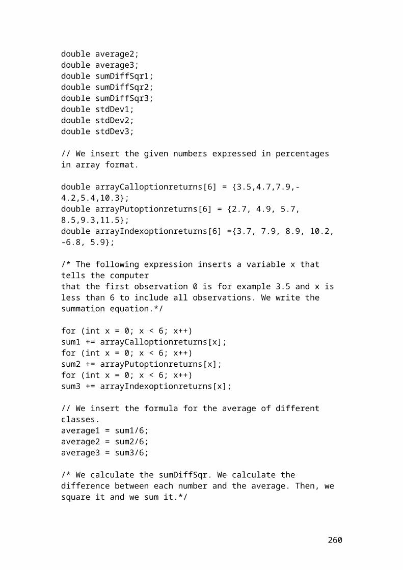
Example of calculating a put option using Monte Carlo simulation.Part of the formulas were taken from the book Financial Modeling using C++, p458

// Calculation of a put option using Monte Carlo simulation.

#include <iostream>#include <ctime>#include<cmath>using namespace std;

double termval( double K, double S0);

int main(){

int i ;int numberOfSimulation = 199999;const int maxSize = 200000;double normSamps[maxSize];double sharePrice;double optPrice;double payoff = 0 ;double randomNumber;

double S0 = 50; // initial share pricedouble K = 58; // strike pricedouble r = 0.05; // risk – free interest ratedouble q = 0.02; // dividend yield double sig = 0.45; // volatility double T = 0.5; // maturity

srand (time(0));

randomNumber = ((rand()%10000)+1000)/100;

for(i=0; i <maxSize; i++) { normSamps[i]=0; } for (int i = 0; i <= numberOfSimulation; i ++)

260

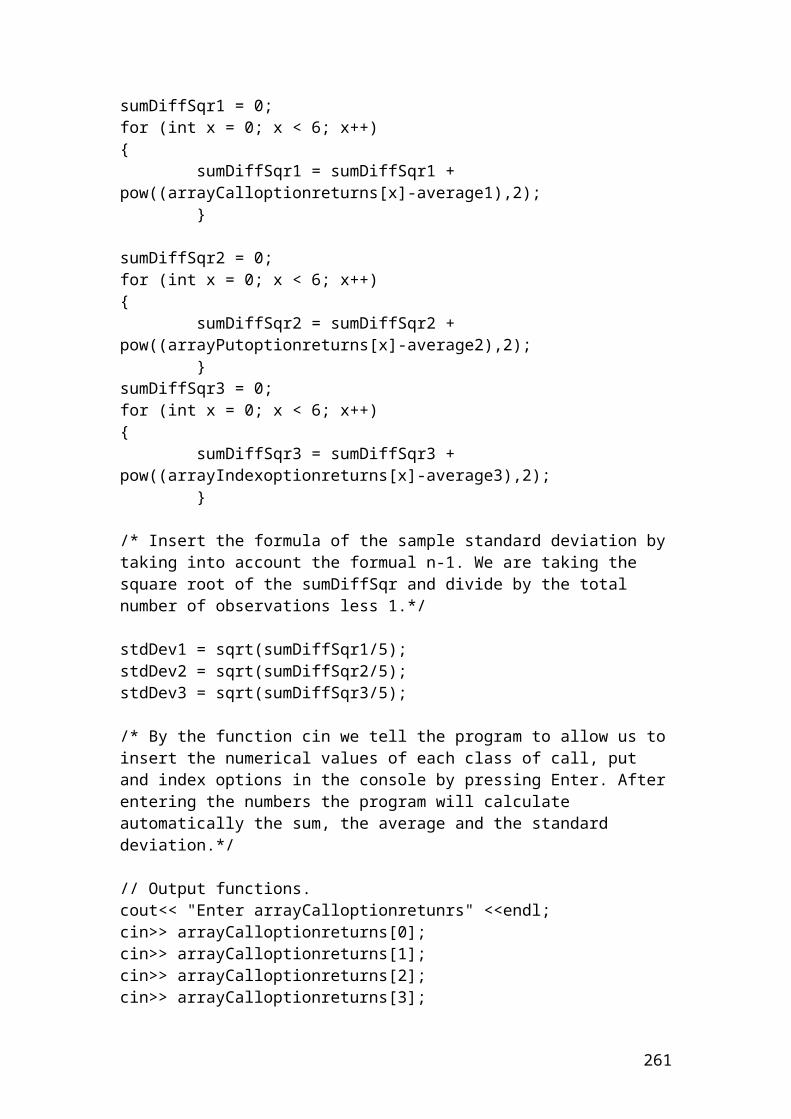
{ sharePrice = S0 *exp((r-q-0.5*sig*sig)*T + normSamps[i-1]*randomNumber*sig *sqrt(T)); // We simulate the share price by using random numbers. payoff += termval(K, sharePrice); /*We use the for loop to calculate the sum of payoffs for the given simulation number.*/ } optPrice = (payoff * exp(-r*T))/ numberOfSimulation; /* Calculate the price of the put option based on the payoff.*/ cout.setf(ios::fixed); cout.setf(ios::showpoint); cout.precision(3); cout<<"Put option price:"<<optPrice<<endl; system ("PAUSE"); return 0; }double termval( double K, double S0){ double val = 0; { if(S0<K) val = K - S0; } return val; }

Output

The figure is expressed in pounds. After compiling and debugging , the DOS window or console will open and display the following results:

Put option price: 9.509

Press any key to continue …

261

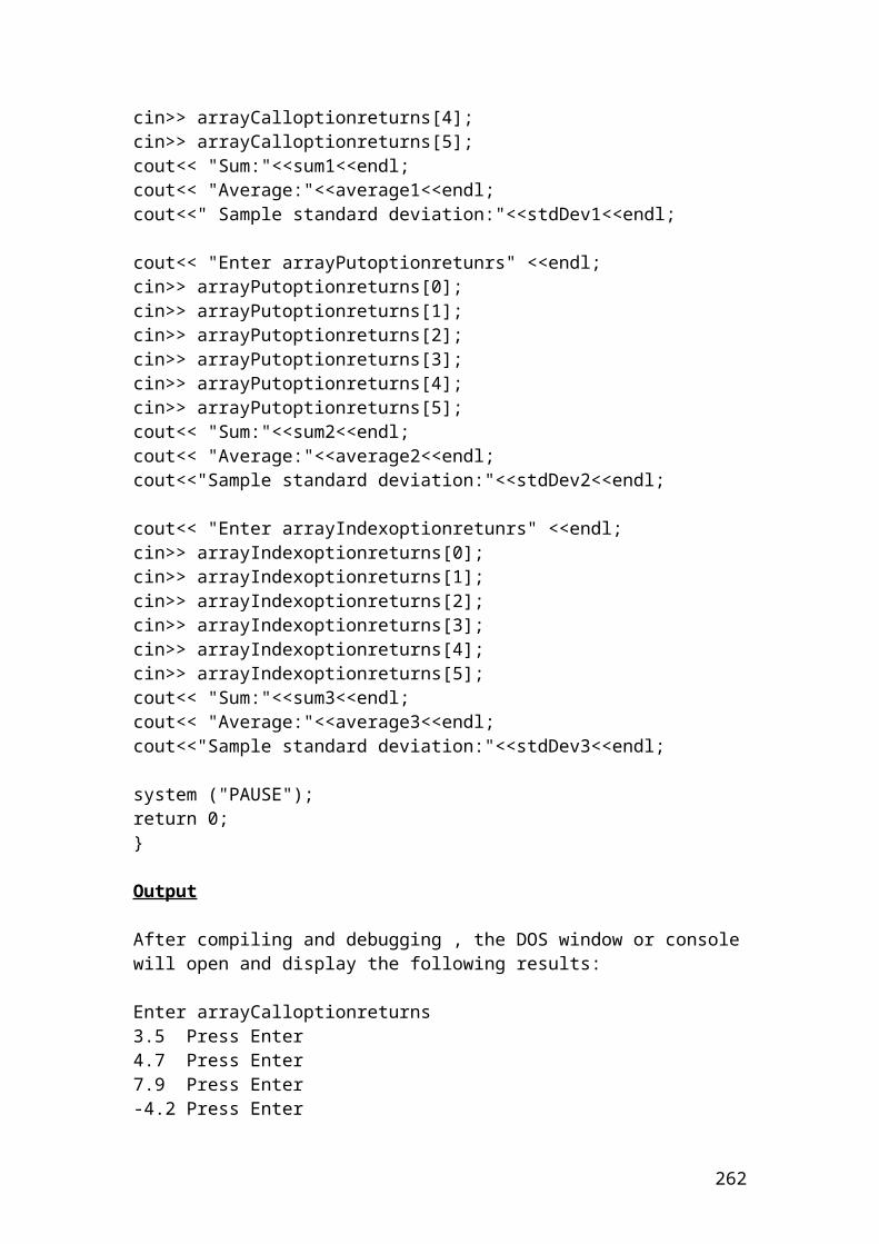
Example of calculating a call option using Monte Carlo simulation and comparing the numerical value with the Black and Scholes modelPart of the formulas were taken from the book Financial Modeling using C++, p458

/* Calculation of a call option using Monte Carlo simulation and comparing it with the Balck and Scholes model.*/

#include <iostream>#include <ctime>#include<cmath>using namespace std;

double Call(double S0, double K, double r, double q, double T,double sig);

double termval( double K, double S0);

// Calculation of the cumulative normal distribution.

double NP(double x);double N(double x);

double NP(double x){ return (1.0/sqrt(2.0 * 3.1415)* exp(-x*x*0.5));} double N(double x){ double b1 = 0.319381530; double b2 = -0.356563782; double b3 = 1.781477937; double b4 = -1.821255978; double b5 = 1.330274429; double k; k = 1/(1+0.2316419*x); if (x >= 0.0) {

262

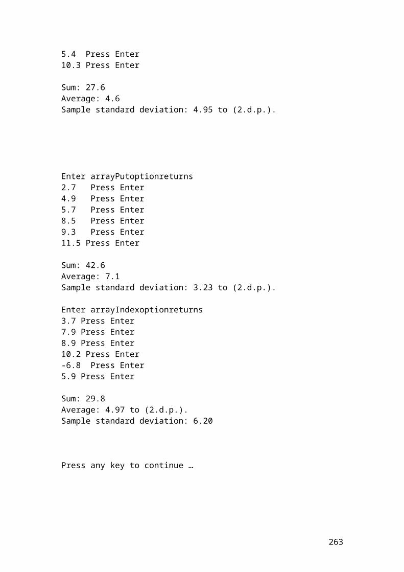
return (1 - NP(x)*((b1*k) + (b2* k*k) + (b3*k*k*k) + (b4*k*k*k*k) + (b5*k*k*k*k*k))); } else { return (1-N(-x)); } } // Mathematical formulas to calculate d1, d2 and the European call price.

double Call(double S0, double K, double r, double q, double T,double sig){

double d1, d2; d1 = (log(S0/K) + (r-q +(sig*sig)*0.5 ) * T ) / (sig * sqrt(T)); d2 = d1 - sig*sqrt(T); return S0*exp(-q*T)*N(d1) - K*exp(-r*T)*N(d2) ; }

int main(){

int i ;int numberOfSimulation = 199999;const int maxSize = 200000;double normSamps[maxSize];double sharePrice;double optPrice;double payoff = 0 ;double randomNumber;

double S0 = 60; // initial share pricedouble K = 50; // strike pricedouble r = 0.05; // risk –free interest ratedouble q = 0.02; // dividend yielddouble sig = 0.45; // volatility double T = 0.5; // maturity

srand (time(0)); randomNumber = ((rand()%10000)+1000)/100; for(i=0; i <maxSize; i++) { normSamps[i]=0; }

263

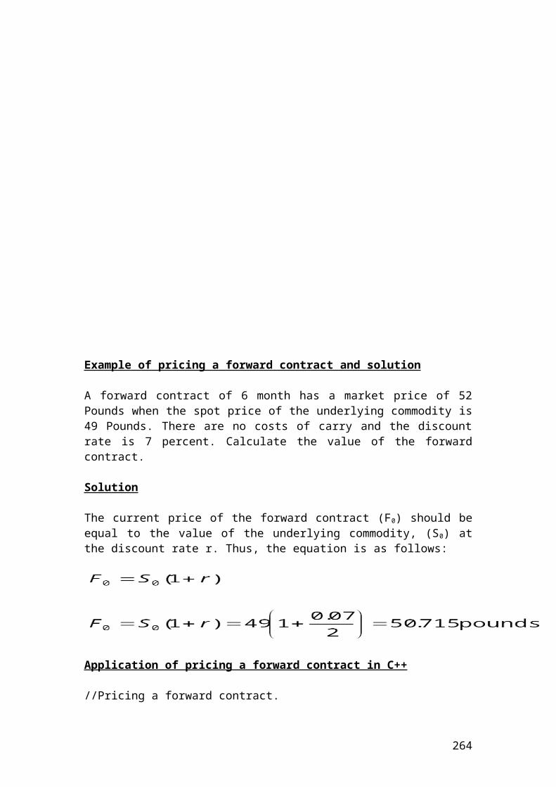
for (int i = 0; i <= numberOfSimulation; i ++) { sharePrice = S0 *exp((r-q-0.5*sig*sig)*T + normSamps[i-1]*randomNumber*sig *sqrt(T)); // We simulate the share price by using random numbers. payoff += termval(K, sharePrice); /* We use the for loop to calculate the sum of payoffs for the given simulation number.*/ } optPrice = (payoff * exp(-r*T))/ numberOfSimulation; /* Calculate the price of the call option based on the payoff.*/ //Calculation of the call price based on the Black and Scholes model.

double callPrice;

callPrice = Call (S0,K,r,q,T,sig); cout.setf(ios::fixed); cout.setf(ios::showpoint); cout.precision(3); cout<<"Monte Carlo call option price:"<<optPrice<<endl;cout<<"Black and Scholes call price: " <<callPrice << endl; system ("PAUSE"); return 0; }

double termval( double K, double S0){ double val = 0; { if(S0>K) val = S0 - K; } return val; } Output

The figures are expressed in Euro. After compiling and debugging , the DOS window or console will open and display the following results:

Monte Carlo call option price: 7.705Black and Scholes call price: 13.414

Press any key to continue …

Question

264

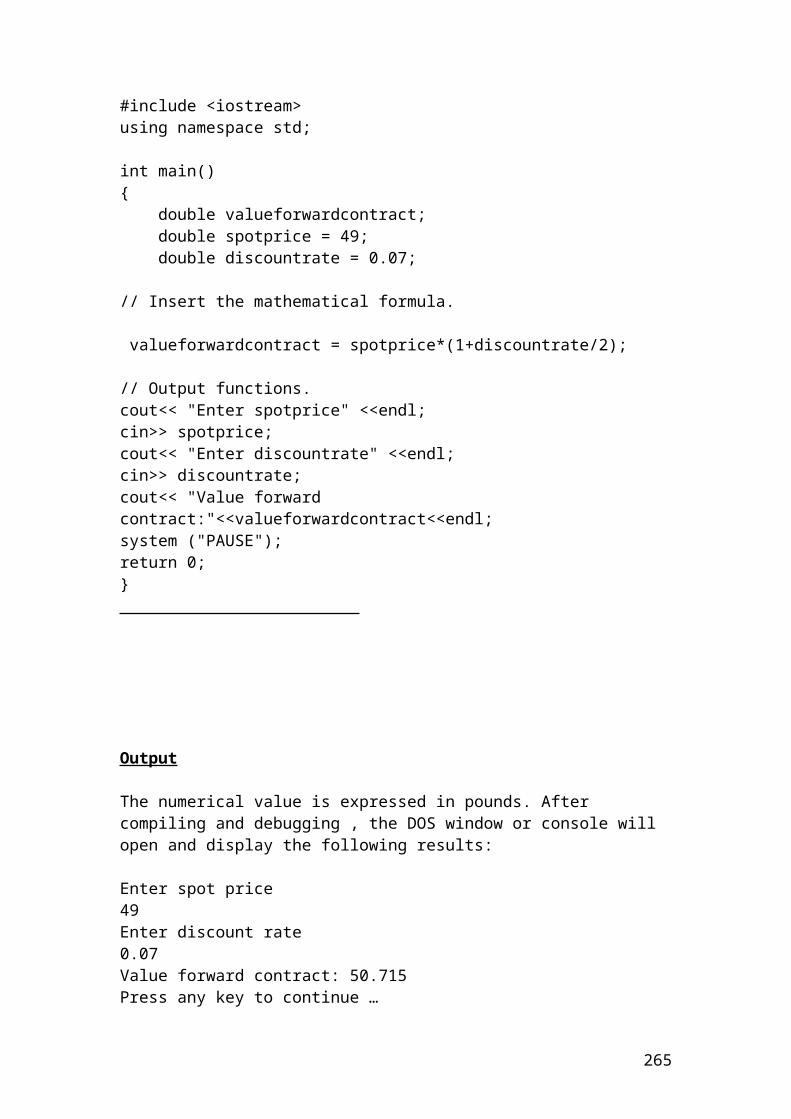
Could you please explain the deviation between the simulated price and the Black and Scholes price?

[Hint: It could be due to the random number definition or lack of algorithm. The standard error is quite high.]

Calculation of a Monte Carlo call option using antithetic variables and comparing it with the Balck and Scholes model. The purpose of using antithetic variables is to improve the estimation results by reducing the standard error of the simulation results. Part of the formulas were taken from the book Financial Modeling using C++, p461

/* Calculation of a Monte Carlo call option using antithetic variables and comparing it with the Balck and Scholes model. The purpose of using antithetic variables is to improve the estimation results by reducing the standard error of simulation results.*/

#include <iostream>#include <ctime>#include<cmath>using namespace std;

double Call(double S0, double K, double r, double q, double T,double sig);

double termval( double K, double S0);

// Calculation of the cumulative normal distribution.

double NP(double x);double N(double x);

double NP(double x){ return (1.0/sqrt(2.0 * 3.1415)* exp(-x*x*0.5));} double N(double x){ double b1 = 0.319381530; double b2 = -0.356563782; double b3 = 1.781477937; double b4 = -1.821255978; double b5 = 1.330274429; double k; k = 1/(1+0.2316419*x);

265

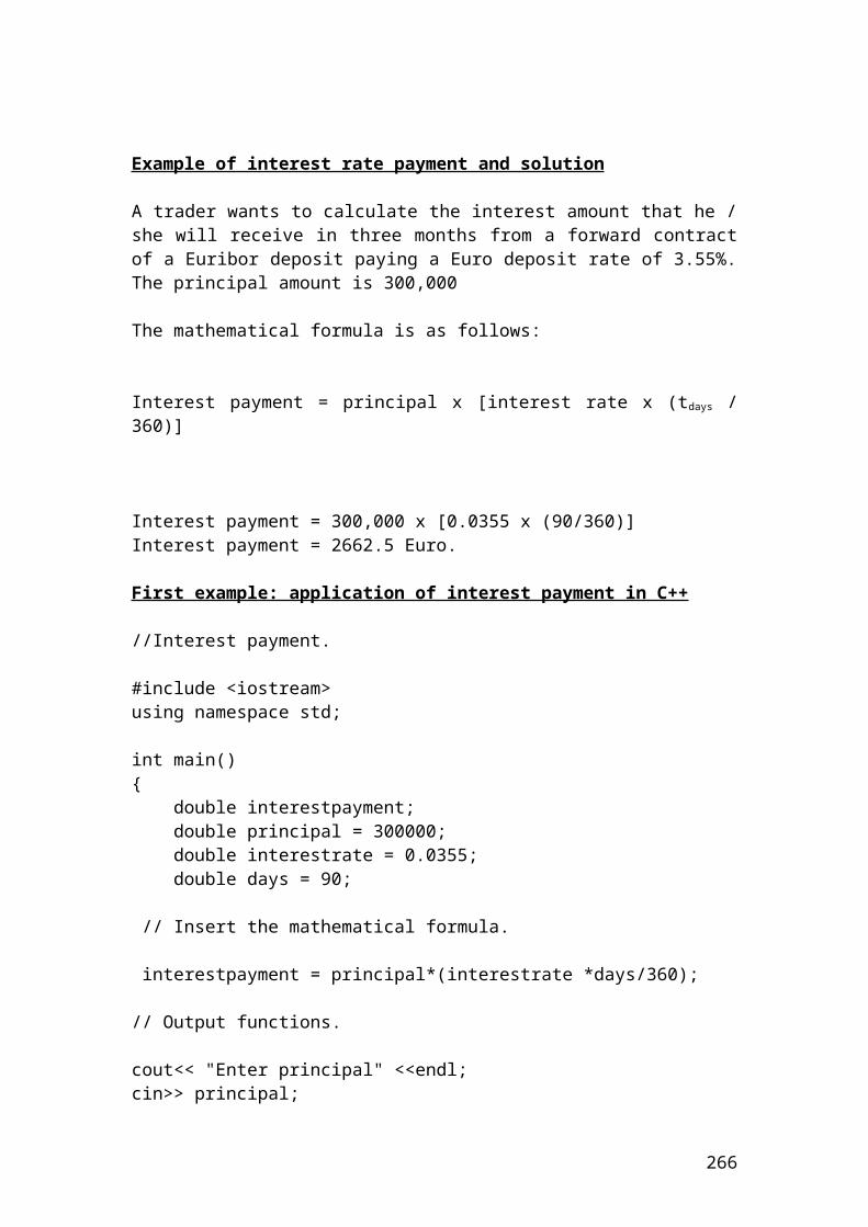
if (x >= 0.0) { return (1 - NP(x)*((b1*k) + (b2* k*k) + (b3*k*k*k) + (b4*k*k*k*k) + (b5*k*k*k*k*k))); } else { return (1-N(-x)); } } // Mathematical formulas to calculate d1, d2 and the European call price.

double Call(double S0, double K, double r, double q, double T,double sig){

double d1, d2; d1 = (log(S0/K) + (r-q +(sig*sig)*0.5 ) * T ) / (sig * sqrt(T)); d2 = d1 - sig*sqrt(T); return S0*exp(-q*T)*N(d1) - K*exp(-r*T)*N(d2) ; }

int main(){

int i ;int numberOfSimulation = 199999;const int maxSize = 200000;double normSamps[maxSize];double optPrice;double payoff = 0 ;double randomNumber;double sharePrice;

double S0 = 100; // initial share pricedouble K = 60; // strike pricedouble r = 0.07; // risk-free interest ratedouble q = 0.02; // dividend yielddouble sig = 0.10; // volatility double T = 0.5; // maturity

srand (time(0)); randomNumber = ((rand()%30000)+3000)/300; for(i=0; i <maxSize; i++)

266

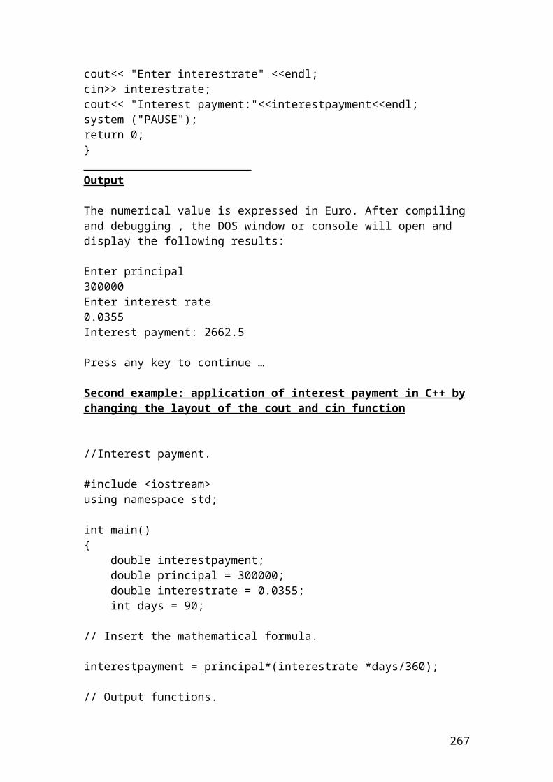
{ normSamps[i]=0; }

/* We calculate twice the stock price and the option payoffs to generate a better estimate. The first equation calculate the share price with a positive normal deviateWe want that the simulated call option price is close to the Black and Scholes price. In the second equation of the share price estimation, we deduct the normal deviates normSamps. We are creating perfectly negatively correlated simulation results to eliminate the standard error. The antithetic variables reduce the standard error. */

for (int i = 0; i <= numberOfSimulation; i ++) { sharePrice = S0 *exp((r-q-0.5*sig*sig)*T + normSamps[i-1]*randomNumber*sig *sqrt(T)); // We simulate the share price by using random numbers. payoff += termval(K, sharePrice); // We use the for loop to calculate the sum // of payoffs for the given simulation number.

sharePrice = S0 *exp((r-q-0.5*sig*sig)*T - normSamps[i-1]*randomNumber*sig *sqrt(T)); payoff += termval(K, sharePrice); } optPrice = (payoff * exp(-r*T))/ numberOfSimulation/2; // Calculate the price of //the call option based on the payoff. //Calculation of the call price based on Black and Scholes model.

double callPrice;

callPrice = Call (S0,K,r,q,T,sig); cout.setf(ios::fixed); cout.setf(ios::showpoint); cout.precision(3); cout<<"Call option price:"<<optPrice<<endl;cout<<"Black and Scholes call price: " <<callPrice << endl; system ("PAUSE"); return 0; }

double termval( double K, double S0){

267

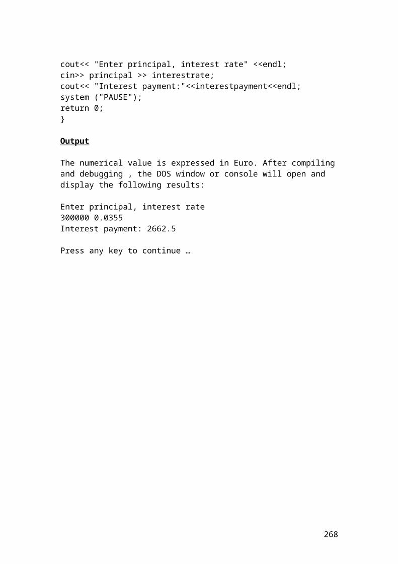
double val = 0; { if(S0>K) val = S0 - K; } return val; }

Output

The figures are expressed in Euro. After compiling and debugging , the DOS window or console will open and display the following results:

Call option price: 40.822Black and Scholes call price: 41.069

Press any key to continue …

268

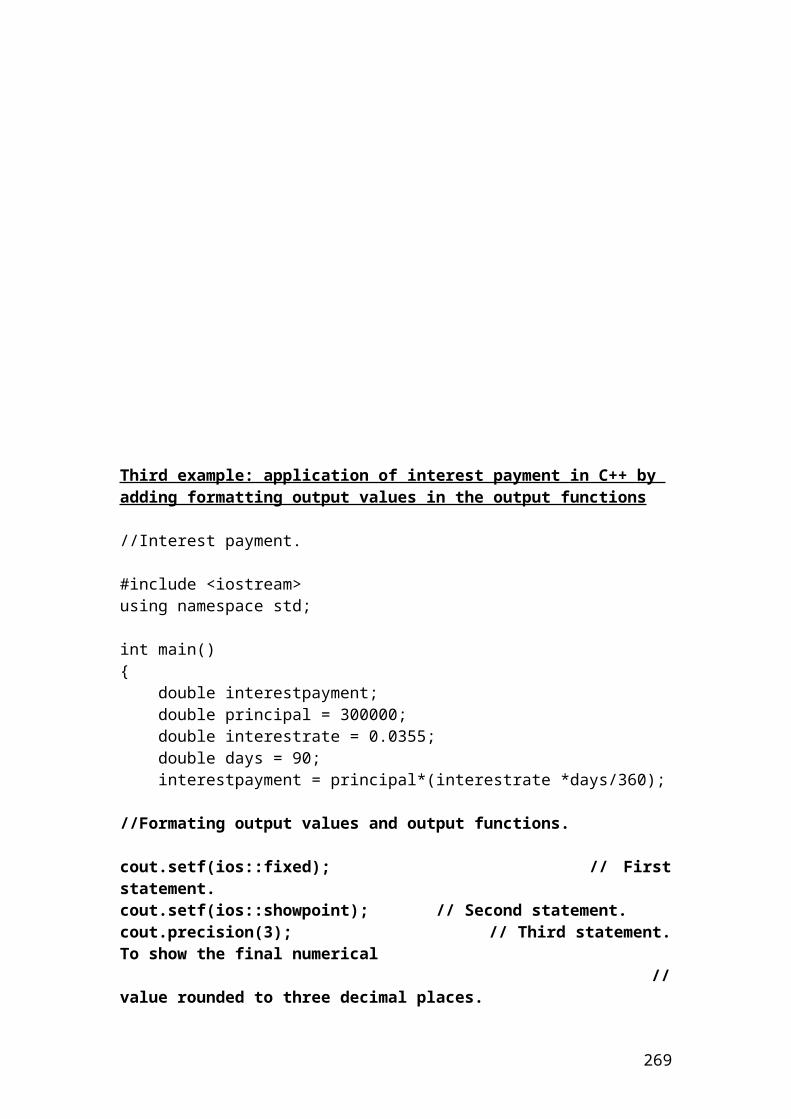
Example of calculating a put option using Monte Carlo simulation and comparing the numerical value with the Black and Scholes modelPart of the formulas were taken from the book Financial Modeling using C++, p458

/* Calculation of a put option using Monte Carlo simulation and comparing it with the Balck and Scholes model.*/

#include <iostream>#include <ctime>#include<cmath>using namespace std;

double Put(double S0, double K, double r, double q, double T, double sig);

double termval( double K, double S0);

// Calculation of the cumulative normal distribution.

double NP(double x);double N(double x);

double NP(double x){ return (1.0/sqrt(2.0 * 3.1415)* exp(-x*x*0.5));} double N(double x){ double b1 = 0.319381530; double b2 = -0.356563782; double b3 = 1.781477937; double b4 = -1.821255978; double b5 = 1.330274429; double k; k = 1/(1+0.2316419*x); if (x >= 0.0) {

269

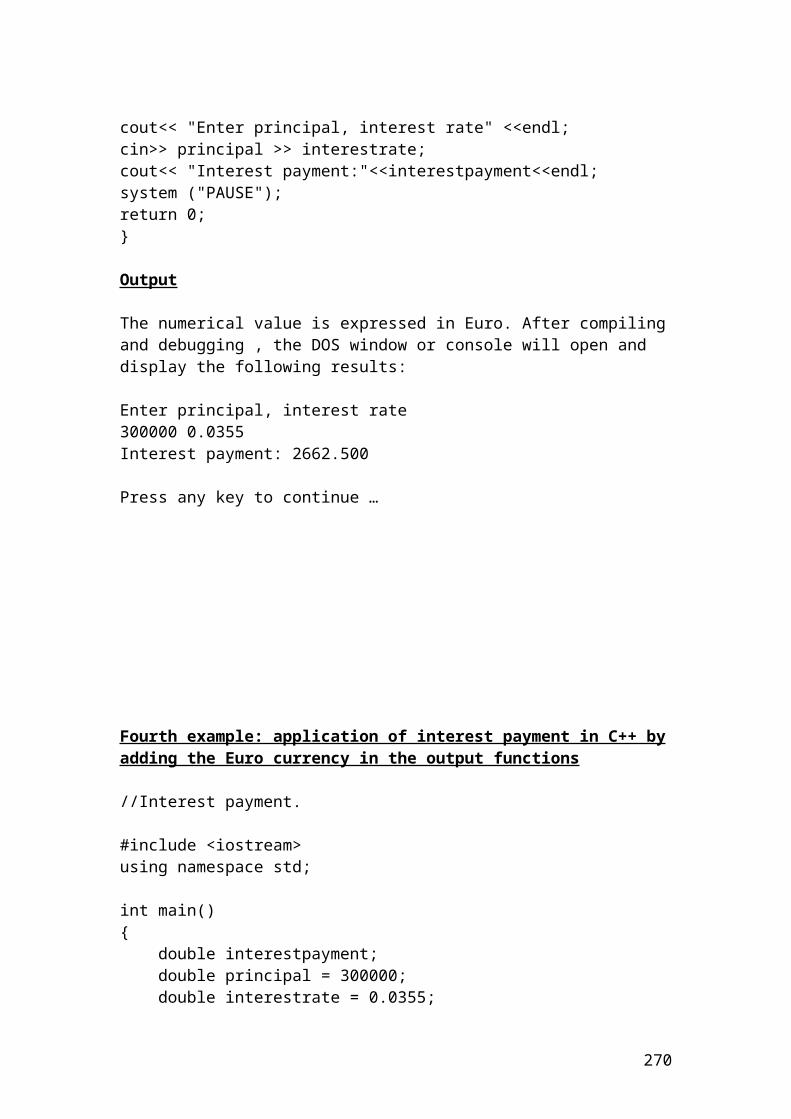
return (1 - NP(x)*((b1*k) + (b2* k*k) + (b3*k*k*k) + (b4*k*k*k*k) + (b5*k*k*k*k*k))); } else { return (1-N(-x)); } } // Mathematical formulas to calculate d1, d2 and the European put price.

double Put(double S0, double K, double r, double q, double T, double sig){

double d1, d2; d1 = (log(S0/K) + (r-q +(sig*sig)*0.5 ) * T ) / (sig * sqrt(T)); d2 = d1 - sig*sqrt(T);

return K*exp(-r*T)*N(-d2) – S0*exp(-q*T)*N(-d1) ; }

int main(){

int i ;int numberOfSimulation = 199999;const int maxSize = 200000;double normSamps[maxSize];double sharePrice;double optPrice;double payoff = 0 ;double randomNumber;

double S0 = 50; // initial share pricedouble K = 58; // strike pricedouble r = 0.05; // risk-free interest ratedouble q = 0.02; // dividend yielddouble sig = 0.45; // volatilitydouble T = 0.5; // maturity

srand (time(0));

randomNumber = ((rand()%10000)+1000)/100;

for(i=0; i <maxSize; i++) { normSamps[i]=0; }

270

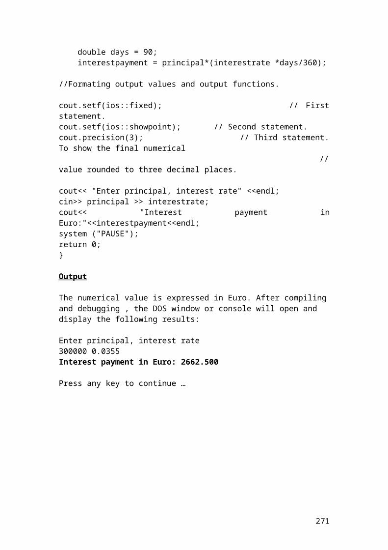
for (int i = 0; i <= numberOfSimulation; i ++) { sharePrice = S0 *exp((r-q-0.5*sig*sig)*T + normSamps[i-1]*randomNumber*sig *sqrt(T)); // We simulate the share price by using random numbers. payoff += termval(K, sharePrice); /* We use the for loop to calculate the sum of payoffs for the given simulation number.*/ } optPrice = (payoff * exp(-r*T))/ numberOfSimulation; /* Calculate the price of the put option based on the payoff.*/ //Calculation of the put price based on the Black and Scholes model.

double putPrice;

putPrice = Put (S0,K,r,q,T,sig); cout.setf(ios::fixed); cout.setf(ios::showpoint); cout.precision(3); cout<<"Monte Carlo put option price:"<<optPrice<<endl;cout<<"Black and Sholes put price: " <<putPrice << endl; system ("PAUSE"); return 0; }double termval( double K, double S0){ double val = 0; { if(S0<K) val = K - S0; } return val; }

Output

The figures are expressed in USD. After compiling and debugging , the DOS window or console will open and display the following results:

Monte Carlo put option price: 9.509Black and Scholes put price: 10.812

Press any key to continue …

Question

Could you please explain the deviation between the simulated price and the Black and Scholes price?

271

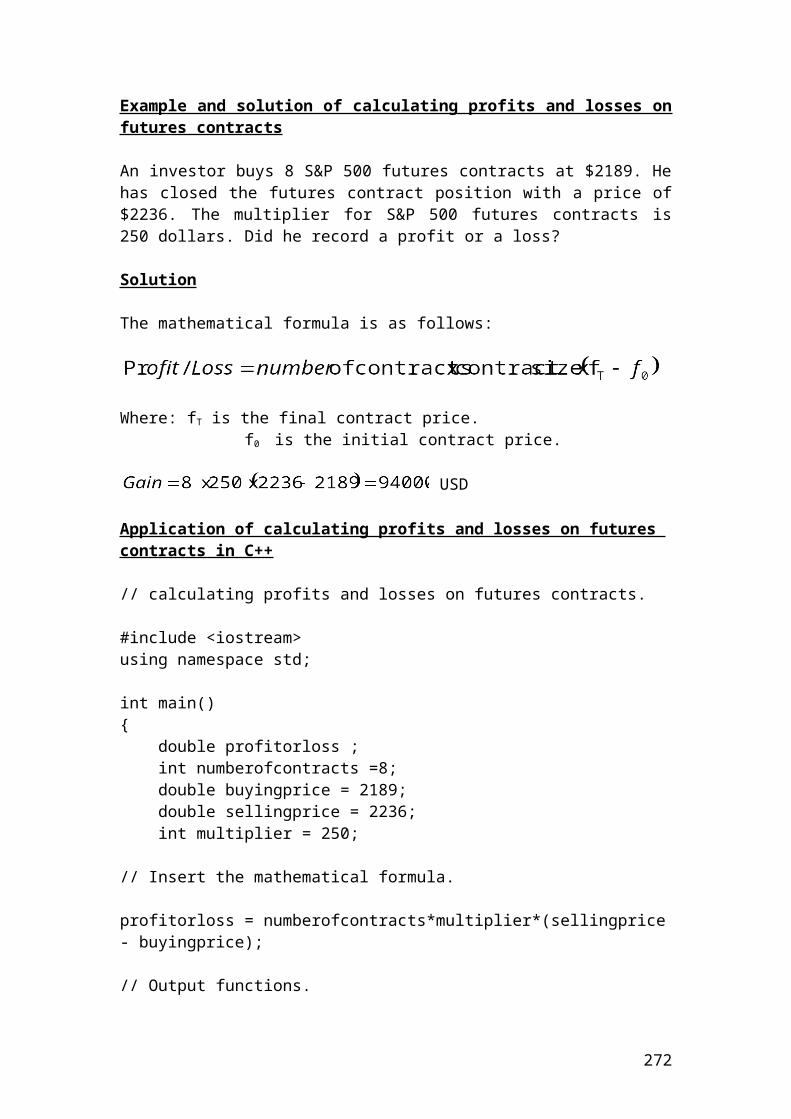
[Hint: It could be due to the random number definition or lack of algorithm.]

Calculation of a Monte Carlo put option using antithetic variables and comparing it with the Balck and Scholes model. The purpose of using antithetic variables is to improve the estimation results by reducing the standard errorof the simulation results. Part of the formulas were taken from the book Financial Modeling using C++, p461

/* Calculation of a Monte Carlo put option using antithetic variables and comparing it with the Balck and Scholes model. The purpose of using antithetic variables is to improve the estimation results by reducing the standard error of simulation results.*/

#include <iostream>#include <ctime>#include<cmath>using namespace std;

double Put(double S0, double K, double r, double q, double T,double sig);

double termval( double K, double S0);

// Calculation of the cumulative normal distribution.

double NP(double x);double N(double x);

double NP(double x){ return (1.0/sqrt(2.0 * 3.1415)* exp(-x*x*0.5));} double N(double x){ double b1 = 0.319381530; double b2 = -0.356563782; double b3 = 1.781477937; double b4 = -1.821255978; double b5 = 1.330274429; double k; k = 1/(1+0.2316419*x);

272

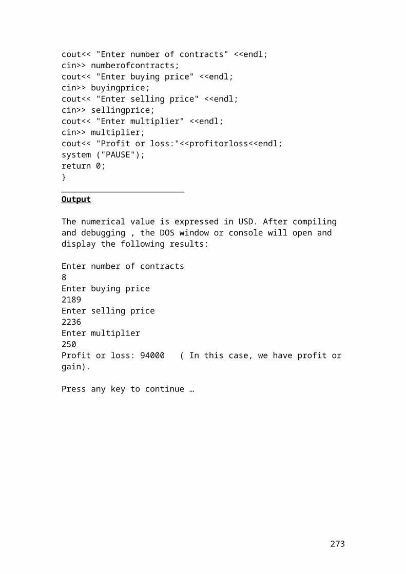
if (x >= 0.0) { return (1 - NP(x)*((b1*k) + (b2* k*k) + (b3*k*k*k) + (b4*k*k*k*k) + (b5*k*k*k*k*k))); } else { return (1-N(-x)); } } // Mathematical formulas to calculate d1, d2 and the European put price.

double Put(double S0, double K, double r, double q, double T, double sig){

double d1, d2; d1 = (log(S0/K) + (r-q +(sig*sig)*0.5 ) * T ) / (sig * sqrt(T)); d2 = d1 - sig*sqrt(T);

return K*exp(-r*T)*N(-d2) - S0*exp(-q*T)*N(-d1) ; }

int main(){

int i ;int numberOfSimulation = 199999;const int maxSize = 200000;double normSamps[maxSize];double optPrice;double payoff = 0 ;double randomNumber;double sharePrice;

double S0 = 70; // initial share pricedouble K = 100; // strike pricedouble r = 0.07; // risk –free interest ratedouble q = 0.02; // dividend yielddouble sig = 0.10; // volatility double T = 0.5; // maturity

srand (time(0)); randomNumber = ((rand()%30000)+3000)/300; for(i=0; i <maxSize; i++) { normSamps[i]=0;

273

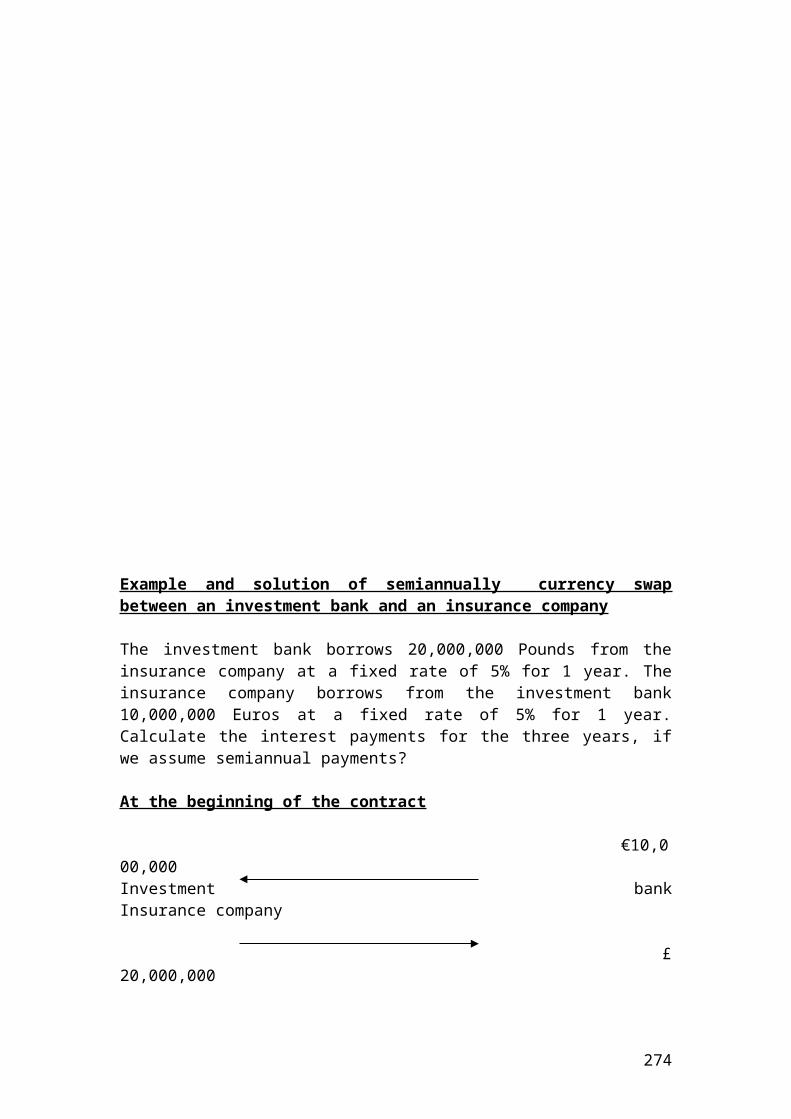
} /* We calculate twice the stock price and the option payoffs to generate a better estimate. The first equation calculate the share price with a positive normal deviate We want that the simulated call option price is close to the Black and Scholes price. In the second equation of the share price estimation, we deduct the normal deviates normSamps. We are creating perfectly negatively correlated simulation results to eliminate the standard error. The antithetic variables reduce the standard error. */ for (int i = 0; i <= numberOfSimulation; i ++) { sharePrice = S0 *exp((r-q-0.5*sig*sig)*T + normSamps[i-1]*randomNumber*sig *sqrt(T)); // We simulate the share price by using random numbers. payoff += termval(K, sharePrice); // We use the for loop to calculate the sum // of payoffs for the given simulation number.

sharePrice = S0 *exp((r-q-0.5*sig*sig)*T - normSamps[i-1]*randomNumber*sig *sqrt(T)); payoff += termval(K, sharePrice); } optPrice = (payoff * exp(-r*T))/ numberOfSimulation/2; // Calculate the price of //the call option based on the payoff. //Calculation of call price based on Black and Scholes model.

double putPrice;

putPrice = Put (S0,K,r,q,T,sig); cout.setf(ios::fixed); cout.setf(ios::showpoint); cout.precision(3); cout<<"Put option price:"<<optPrice<<endl;cout<<"Black and Scholes put price: " <<putPrice << endl; system ("PAUSE"); return 0; }

double termval( double K, double S0){ double val = 0; { if(S0<K) val = K-S0; } return val;

274

}

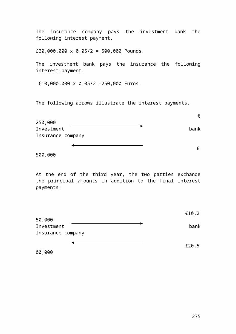
Output

The figures are expressed in USD. After compiling and debugging , the DOS window or console will open and display the following results:

Put option price: 27.430Black and Scholes put price: 27.257

Press any key to continue …

275

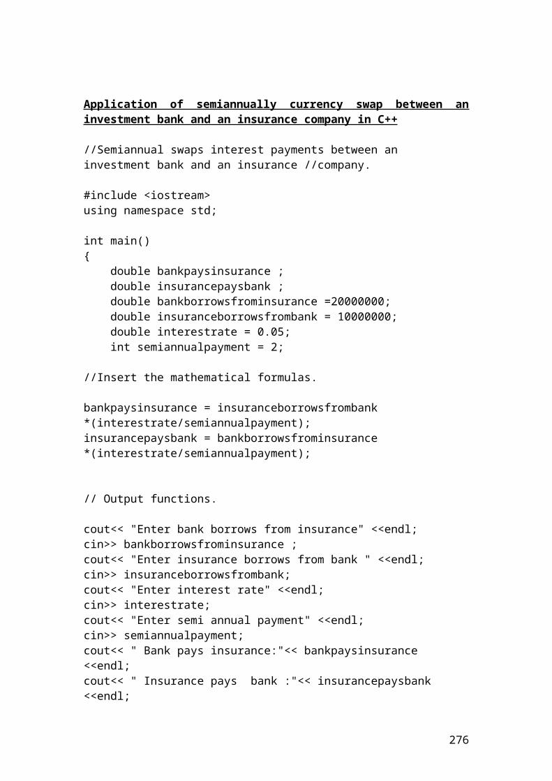
Calculate the share prices of a call option using a Cox, Ross, Rubinstein,(CRR) binomial 3 steps tree using a vector. The multipliers of up and down move depend on volatility and length of steps

/* Calculate the share prices of a call option using a Cox, Ross, Rubinstein,(CRR) binomial 3 steps tree. */

#include <iostream> #include<cmath> #include<vector>using namespace std;

int main() { double S = 60; //share price double K = 50; // strike price double r = 0.05; // risk –free interest rate double q = 0.02; // dividend yield double T = 0.5; // life to maturity double sig = 0.3; // volatility // Identify the variables. u = multiplier of upmove. //d = multiplier of downmove. dt = steps expressed in years. double u; double d; double dt; int i ,j; const int n = 3; // Identify tree steps binomial tree. // Insert the mathematical formulas. dt = T/n; u = exp(sig*sqrt(dt)); d = 1/u; double sharetree[i][j];int arraysize[10];vector<double> dataarray;for (i=0; i<=j; i++)

276

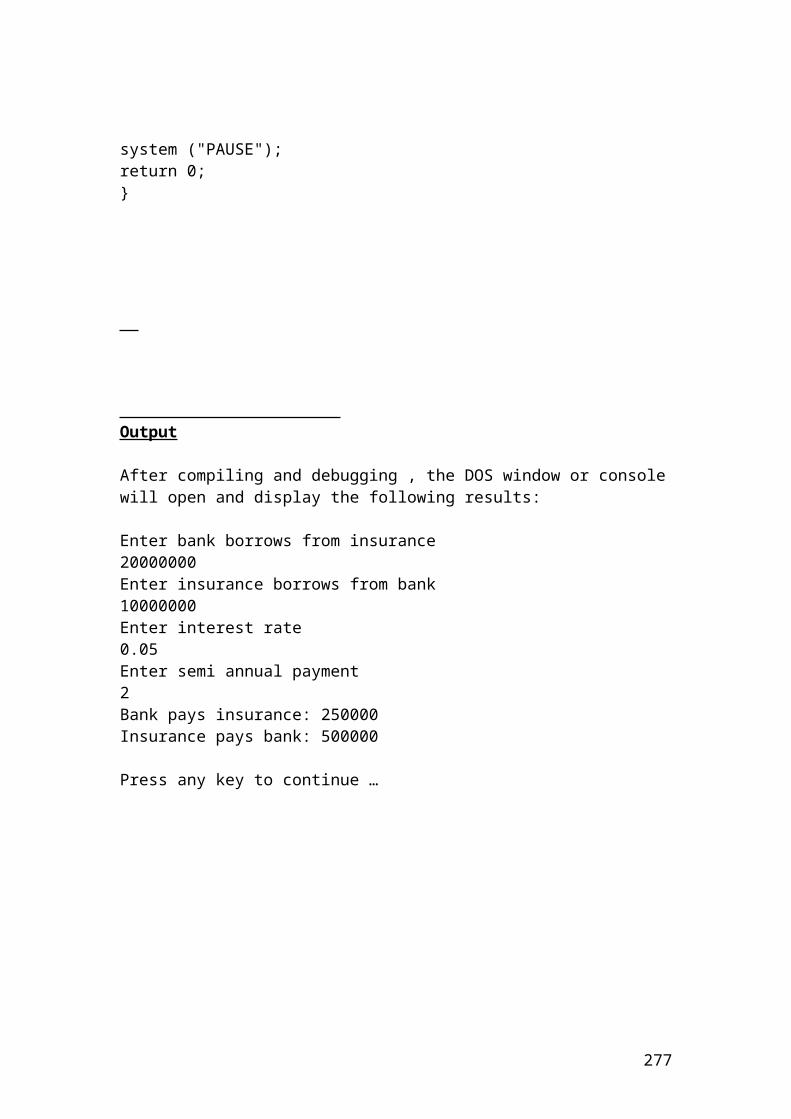
{ for (j=1; j<=n; j++) { if (i==0) sharetree[i][j] = S * u; else sharetree[i][j] = S* d; if (i==0) sharetree[i][j] = S * pow(u,2); else sharetree[i][j] = S* pow(d,2); if (i==0) sharetree[i][j] = S*u*d; if (i==0) sharetree[i][j] = S*pow(u,2)*d ; if (i==0) sharetree[i][j] = S* pow(d,2)*u; if (i==0) sharetree[i][j] = S * pow(u,3); else sharetree[i][j] = S* pow(d,3); }}

cout.setf(ios::fixed); cout.setf(ios::showpoint); cout.precision(5); cout<<"Steps expressed in years:"<< dt<<endl;cout<<"Multiplier of upmove:"<< u<<endl;cout<<"Multiplier of downmove:"<< d<<endl; cout<<"Enter array size:"<<endl;cin>> arraysize[10];

sharetree[i][j] = S ;cout.setf(ios::fixed); cout.setf(ios::showpoint); cout.precision(2); cout<<" Share price [0]:"<<sharetree[i][j]<<endl;

sharetree[i][j] = S * u;cout.setf(ios::fixed); cout.setf(ios::showpoint); cout.precision(2); cout<<" Share price upmove [1]:"<<sharetree[i][j]<<endl; sharetree[i][j] = S* d;cout.setf(ios::fixed); cout.setf(ios::showpoint); cout.precision(2); cout<<" Share price downmove[1]:"<<sharetree[i][j]<<endl; sharetree[i][j] = S * pow(u,2); cout.setf(ios::fixed);

277

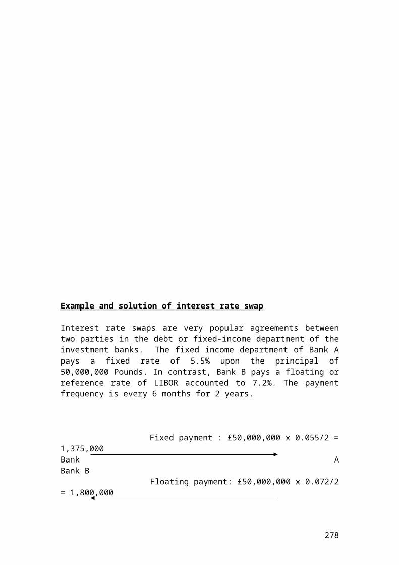
cout.setf(ios::showpoint); cout.precision(2); cout<<" Share price upmove [2]:"<<sharetree[i][j]<<endl; sharetree[i][j] = S*u*d;cout.setf(ios::fixed); cout.setf(ios::showpoint); cout.precision(2); cout<<" Share price up and downmove [2]:"<<sharetree[i][j]<<endl; sharetree[i][j] = S* pow(d,2);cout.setf(ios::fixed); cout.setf(ios::showpoint); cout.precision(2); cout<<" Share price downmove [2]:"<<sharetree[i][j]<<endl; sharetree[i][j] = S* pow (u,3);cout.setf(ios::fixed); cout.setf(ios::showpoint); cout.precision(2); cout<<" Share price upmove [3]:"<<sharetree[i][j]<<endl;

sharetree[i][j] = S*pow(u,2)*d ;cout.setf(ios::fixed); cout.setf(ios::showpoint); cout.precision(2); cout<<" Share price *upmove* downmove*upmove [3]:"<<sharetree[i][j]<<endl;

sharetree[i][j] = S* pow(d,2)*u;cout.setf(ios::fixed); cout.setf(ios::showpoint); cout.precision(2); cout<<" Share price *upmove * downmove*downmove [3]:"<<sharetree[i][j]<<endl;

sharetree[i][j] = S* pow(d,3);cout.setf(ios::fixed); cout.setf(ios::showpoint); cout.precision(2); cout<<" Share price downmove [3]:"<<sharetree[i][j]<<endl; system ("PAUSE");return 0;}

278

Output

The figures are expressed in pounds. After compiling and debugging , the DOS window or console will open and display the following results:

Steps expressed in years: 0.16667Multiplier of upmove: 1.13029Multiplier of downmove: 0.88473Enter array size:10Share price[0]: 60.00Share price upmove [1]: 67.82Share price downmove [1]: 53.08Share price upmove [2]: 76.65Share price up and downmove[2]:60.00Share price downmove [2]: 46.96Share price upmove [3]: 86.64Share price upmove*downmove* upmove [3]: 67.82Share price upmove*downmove*downmove[3]: 53.08Share price downmove [3]: 41.55

Press any key to continue …

279

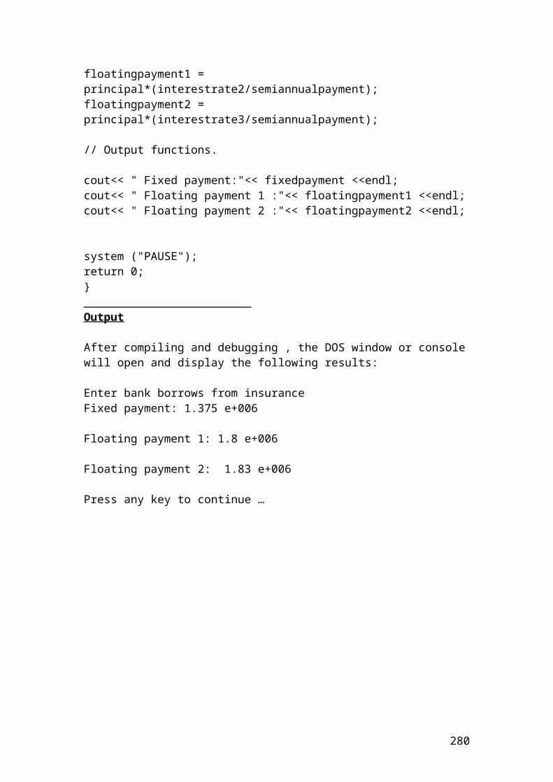
Calculate the call option prices using a Cox, Ross, Rubinstein,(CRR) binomial 3 steps tree. Please e-mail me to send you the binomial tree in Excel if this is complicated. I will also convert this example in VBA. Please check the VBA section in the document Financial Derivatives /* Calculate the call option prices using a Cox, Ross, Rubinstein,(CRR) binomial 3 steps tree. */

#include <iostream> #include<cmath> using namespace std;

int main() { double S = 60; //share price double K = 50; // strike price double r = 0.05; // risk-free interest rate double q = 0.02; // dividend yield. If the dividend is zero, then, it is // not included in the equation of risk neutral // probability of upmove. double T = 0.5; // life to maturity double sig = 0.3; // volatility // Identify the variables. // u = multiplier of upmove. //d = multiplier of downmove. dt = steps expressed in years. //riskprobofupmove = risk neutral probability of upmove. //disfact = discount factor. double u; double d; double dt; double riskprobofupmove; double disfact; const int n = 3; // Identify tree steps binomial tree. // Insert the mathematical formulas. dt = T/n; u = exp(sig*sqrt(dt)); d = 1/u;

280

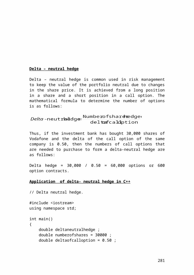
disfact = exp(-r*dt); riskprobofupmove = (exp((r-q)*dt)-d)/(u-d); double callpayoffupmovestep3; // (Shareprice * upmove^3)-Kdouble callpayoff3i; // (Shareprice * upmove^2 * downmove)-Kdouble callpayoff3ii; // (Shareprice * downmove^2*upmove)-K double callpayoffdownmovestep3; // (Shareprice * downmove^3) -K

// The option prices are calculated backwards.

callpayoffupmovestep3 = S*pow(u,3)-K;callpayoff3i = S * pow(u,2) * d -K;callpayoff3ii =S * pow(d,2)*u-K; callpayoffdownmovestep3 = S*pow(d,3)-K;callpayoffdownmovestep3 =0;

double callpriceupmovestep2;double callpriceupdownmovestep2;double callpricedownmovestep2;

callpriceupmovestep2 = (disfact*(riskprobofupmove*callpayoffupmovestep3)+(1-riskprobofupmove)*callpayoff3i);

callpriceupdownmovestep2 =(disfact*(riskprobofupmove*callpayoff3i)+(1-riskprobofupmove)*callpayoff3ii);

callpricedownmovestep2 =(disfact*(riskprobofupmove*callpayoff3ii)+(1-riskprobofupmove)*callpayoffdownmovestep3);

double callpriceupmovestep1;double callpricedownmovestep1;

callpriceupmovestep1 = (disfact*(riskprobofupmove*callpriceupmovestep2)+(1-riskprobofupmove)*callpriceupdownmovestep2);

callpricedownmovestep1=(disfact*(riskprobofupmove*callpriceupdownmovestep2)+(1-riskprobofupmove)*callpricedownmovestep2);

double callpricestep0;

callpricestep0= (disfact*(riskprobofupmove*callpriceupmovestep1)+(1-riskprobofupmove)*callpricedownmovestep1);

//Output functions.cout.setf(ios::fixed); cout.setf(ios::showpoint); cout.precision(4); cout<<"Steps expressed in years:"<< dt<<endl;

281

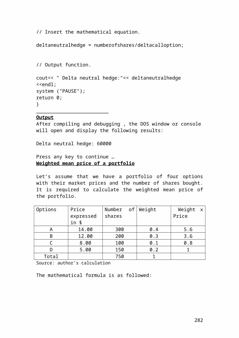
cout<<"Multiplier of upmove:"<< u<<endl;cout<<"Multiplier of downmove:"<< d<<endl;cout<<" Discount factor:"<<disfact<<endl;cout<< "Risk neutral probability of upmove:"<<riskprobofupmove<<endl;

cout<<"Call payoff upmove step [3]:"<<callpayoffupmovestep3<<endl;cout<<"Call payoff [3i]:"<<callpayoff3i<<endl;cout<<"Call payoff [3ii]:"<<callpayoff3ii<<endl;cout<<"Call payoff downmove step [3]:"<<callpayoffdownmovestep3<<endl;cout<<"Call price upmove step[2]:"<<callpriceupmovestep2<<endl;cout<<"Call price updownmove step [2]:"<<callpriceupdownmovestep2<<endl;cout<<"Call price downmove step [2]:"<<callpricedownmovestep2<<endl;cout<<"Call price upmove step [1]:"<<callpriceupmovestep1<<endl;cout<<"Call price downmove step [1]:"<<callpricedownmovestep1<<endl;cout<<"Call price step[0]:"<<callpricestep0<<endl;

system ("PAUSE");return 0;}

Output

The figures are expressed in pounds. After compiling and debugging , the DOS window or console will open and display the following results:

Steps expressed in years: 0.1667Multiplier of upmove: 1.1303Multiplier of downmove: 0.8847Disount factor: 0.9917Risk neutral probability of upmove: 0.4898Call payoff upmove step [3]: 36.6406Call payoff [3i]: 17.8174Call payoff [3ii]: 3.0837Call payoff downmove step [3]: 0.0000Call price upmove step [2]: 26.8887Call price updownmove step [2]: 10.2283Call price downmove step [2]: 1.4980Call price upmove step [1]: 18.2798Call price downmove step [1]: 5.7328Call price step [0]: 11.8044Press any key to continue …

282

Compare the call option price using a Cox,Ross, Rubinstein, (CRR), binomial 3 steps tree with the Black and Scholes model

/*Compare the call option price using a Cox,Ross, Rubinstein, (CRR), binomial 3 steps tree with the Black and Scholes model.*/

/* Calculate the call option prices using a Cox, Ross, Rubinstein,(CRR) binomial 3 steps tree. */

#include <iostream> #include<cmath> using namespace std; // Calculation of the cumulative normal distribution.

double norm_cdf (const double& x) {

double k = 1/(1+0.2316419*x);double k_sum = k*(0.319381530 + k*(-0.356563782 + k*(1.781477937 + k*(-1.821255978 + k*(1.330274429))))); if (x >= 0.0) {return (1.0 - (1.0/(pow(2*M_PI, 0.5))) * exp(-0.5*x*x)* k_sum);} else {return 1.0 - norm_cdf(-x);}}

// Mathematical formulas to calculate d1, d2 and the European call price.

double Call(double S, double K, double r, double q, double T, double sig){

double d1, d2; d1 = (log(S/K) + (r-q +(sig*sig)*0.5 ) * T ) / (sig * sqrt(T)); d2 = d1 - sig*sqrt(T); return S*exp(-q*T)*norm_cdf(d1) - K*exp(-r*T)*norm_cdf(d2) ; }

283

int main() { double S = 60; //share price double K = 50; // strike price double r = 0.05; // risk-free interest rate double q = 0.02; // dividend yield. If the dividend is zero, then, it is // not included in the equation of risk neutral // probability of upmove. double T = 0.5; // life to maturity double sig = 0.3; // volatility // Identify the variables. // u = multiplier of upmove. //d = multiplier of downmove. dt = steps expressed in years. //riskprobofupmove = risk neutral probability of upmove. //disfact = discount factor. double u; double d; double dt; double riskprobofupmove; double disfact; const int n = 3; // Identify tree steps binomial tree. // Insert the mathematical formulas. dt = T/n; u = exp(sig*sqrt(dt)); d = 1/u; disfact = exp(-r*dt); riskprobofupmove = (exp((r-q)*dt)-d)/(u-d); double callpayoffupmovestep3; // (Shareprice * upmove^3)-Kdouble callpayoff3i; // (Shareprice * upmove^2 * downmove)-Kdouble callpayoff3ii; // (Shareprice * downmove^2*upmove)-K double callpayoffdownmovestep3; // (Shareprice * downmove^3) -K

// The option prices are calculated backwards.

callpayoffupmovestep3 = S*pow(u,3)-K;callpayoff3i = S * pow(u,2) * d -K;callpayoff3ii =S * pow(d,2)*u-K;

284

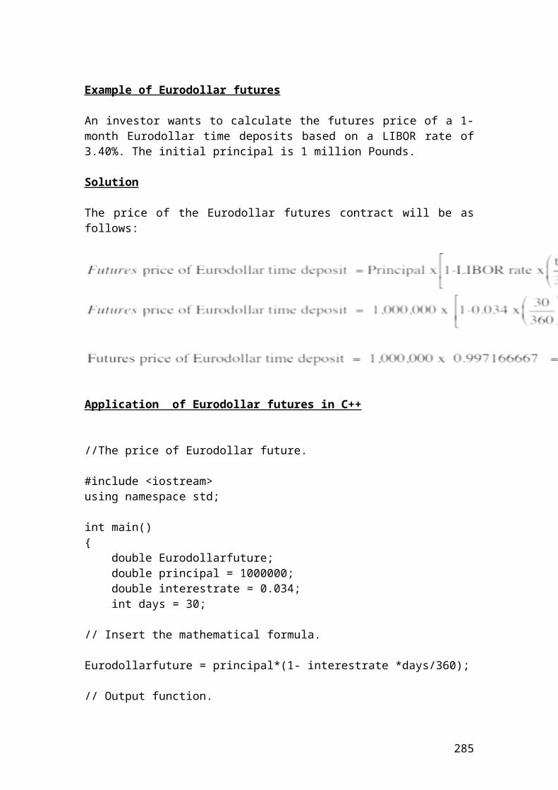
callpayoffdownmovestep3 = S*pow(d,3)-K;callpayoffdownmovestep3 =0;

double callpriceupmovestep2;double callpriceupdownmovestep2;double callpricedownmovestep2;

callpriceupmovestep2 = (disfact*(riskprobofupmove*callpayoffupmovestep3)+(1-riskprobofupmove)*callpayoff3i);

callpriceupdownmovestep2 =(disfact*(riskprobofupmove*callpayoff3i)+(1-riskprobofupmove)*callpayoff3ii);

callpricedownmovestep2 =(disfact*(riskprobofupmove*callpayoff3ii)+(1-riskprobofupmove)*callpayoffdownmovestep3);

double callpriceupmovestep1;double callpricedownmovestep1;

callpriceupmovestep1 = (disfact*(riskprobofupmove*callpriceupmovestep2)+(1-riskprobofupmove)*callpriceupdownmovestep2);

callpricedownmovestep1=(disfact*(riskprobofupmove*callpriceupdownmovestep2)+(1-riskprobofupmove)*callpricedownmovestep2);

double callpricestep0;

callpricestep0= (disfact*(riskprobofupmove*callpriceupmovestep1)+(1-riskprobofupmove)*callpricedownmovestep1);

//Calculation of call price based on the Black and Scholes model.

double callPrice;

callPrice = Call (S,K,r,q,T,sig);

//Output functions.cout.setf(ios::fixed); cout.setf(ios::showpoint); cout.precision(4); cout<<"Steps expressed in years:"<< dt<<endl;cout<<"Multiplier of upmove:"<< u<<endl;cout<<"Multiplier of downmove:"<< d<<endl;cout<<" Discount factor:"<<disfact<<endl;cout<< "Risk neutral probability of upmove:"<<riskprobofupmove<<endl;cout<<"Call payoff upmove step [3]:"<<callpayoffupmovestep3<<endl;cout<<"Call payoff [3i]:"<<callpayoff3i<<endl;cout<<"Call payoff [3ii]:"<<callpayoff3ii<<endl;cout<<"Call payoff downmove step [3]:"<<callpayoffdownmovestep3<<endl;

285

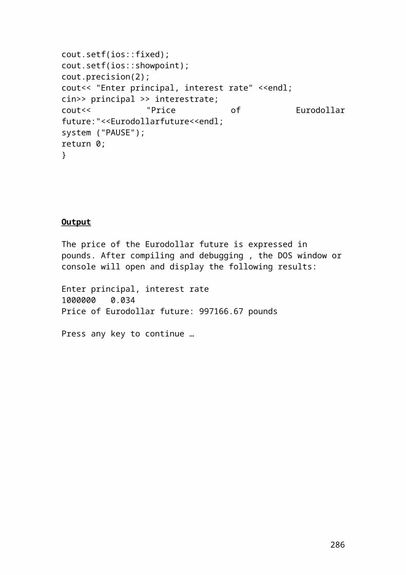
cout<<"Call price upmove step[2]:"<<callpriceupmovestep2<<endl;cout<<"Call price updownmove step [2]:"<<callpriceupdownmovestep2<<endl;cout<<"Call price downmove step [2]:"<<callpricedownmovestep2<<endl;cout<<"Call price upmove step [1]:"<<callpriceupmovestep1<<endl;cout<<"Call price downmove step [1]:"<<callpricedownmovestep1<<endl;cout<<"Call price step[0]:"<<callpricestep0<<endl;cout<<" Black and Scholes call price:"<<callPrice<<endl;system ("PAUSE");return 0;}

Output

The figures are expressed in pounds. After compiling and debugging , the DOS window or console will open and display the following results:

Steps expressed in years: 0.1667Multiplier of upmove: 1.1303Multiplier of downmove: 0.8847Disount factor: 0.9917Risk neutral probability of upmove: 0.4898Call payoff upmove step [3]: 36.6406Call payoff [3i]: 17.8174Call payoff [3ii]: 3.0837Call payoff downmove step [3]: 0.0000Call price upmove step [2]: 26.8887Call price updownmove step [2]: 10.2283Call price downmove step [2]: 1.4980Call price upmove step [1]: 18.2798Call price downmove step [1]: 5.7328Call price step [0]: 11.8044Black and Scholes call price: 11.7183Press any key to continue …

286

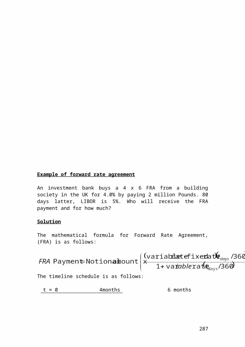
Calculate the put option prices using a Cox, Ross, Rubinstein,(CRR) binomial 3 steps tree. The multipliers of up and down move depend on volatility and the length of steps

/* Calculate the put option prices using a Cox, Ross, Rubinstein,(CRR) binomial 3 steps tree. */

#include <iostream> #include<cmath> using namespace std; int main() { double S = 60; // share price double K = 70; // strike price double r = 0.02; // risk-free interest rate double q = 0.03; // dividend yield double T = 0.5; // life to maturity double sig = 0.2; // volatility // Identify the variables. u = multiplier of upmove. //d = multiplier of downmove. dt = steps expressed in years. //riskprobofupmove = risk neutral probability of upmove. //disfact = discount factor. double u; double d; double dt; double riskprobofupmove; double disfact; const int n = 3; // Identify tree steps binomial tree. // Insert the mathematical formulas. dt = T/n; u = exp(sig*sqrt(dt)); d = 1/u; disfact = exp(-r*dt); riskprobofupmove = (exp((r-q)*dt)-d)/(u-d); double putpayoffupmovestep3; // K - (Shareprice * upmove^3)

287

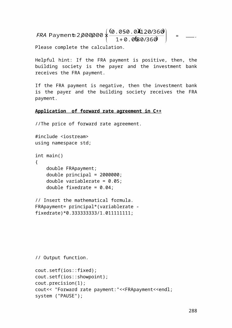
double putpayoff3i; // K- (Shareprice * upmove^2 * downmove)double putpayoff3ii; // K-(Shareprice * downmove^2*upmove) double putpayoffdownmovestep3; // K-(Shareprice * downmove^3)

// The option prices are calculated backwards.

putpayoffupmovestep3 = K-S*pow(u,3);putpayoffupmovestep3=0;putpayoff3i = K- S * pow(u,2) * d;putpayoff3ii =K- S * pow(d,2)*u; putpayoffdownmovestep3 = K - S*pow(d,3);

double putpriceupmovestep2;double putpriceupdownmovestep2;double putpricedownmovestep2;

putpriceupmovestep2 = (disfact*(riskprobofupmove*putpayoffupmovestep3)+(1-riskprobofupmove)*putpayoff3i);

putpriceupdownmovestep2 =(disfact*(riskprobofupmove*putpayoff3i)+(1-riskprobofupmove)*putpayoff3ii);

putpricedownmovestep2 =(disfact*(riskprobofupmove*putpayoff3ii)+(1-riskprobofupmove)*putpayoffdownmovestep3);

double putpriceupmovestep1;double putpricedownmovestep1;

putpriceupmovestep1 = (disfact*(riskprobofupmove*putpriceupmovestep2)+(1-riskprobofupmove)*putpriceupdownmovestep2);

putpricedownmovestep1=(disfact*(riskprobofupmove*putpriceupdownmovestep2)+(1-riskprobofupmove)*putpricedownmovestep2);

double putpricestep0;

putpricestep0= (disfact*(riskprobofupmove*putpriceupmovestep1)+(1-riskprobofupmove)*putpricedownmovestep1);

//Output functions.cout.setf(ios::fixed); cout.setf(ios::showpoint); cout.precision(4); cout<<"Steps expressed in years:"<< dt<<endl;cout<<"Multiplier of upmove:"<< u<<endl;cout<<"Multiplier of downmove:"<< d<<endl;

288

cout<<" Discount factor:"<<disfact<<endl;cout<< "Risk neutral probability of upmove:"<<riskprobofupmove<<endl;

cout<<"Put payoff upmove step[3]:"<<putpayoffupmovestep3<<endl;cout<<"Put payoff [3i]:"<<putpayoff3i<<endl;cout<<"Put payoff [3ii]:"<<putpayoff3ii<<endl;cout<<"Put payoff downmove step[3]:"<<putpayoffdownmovestep3<<endl;cout<<"Put price upmove step[2]:"<<putpriceupmovestep2<<endl;cout<<"Put price updownmove step[2]:"<<putpriceupdownmovestep2<<endl;cout<<"Put price downmove step[2]:"<<putpricedownmovestep2<<endl;cout<<"Put price upmove step[1]:"<<putpriceupmovestep1<<endl;cout<<"Put price downmove step[1]:"<<putpricedownmovestep1<<endl;cout<<"Put price step[0]:"<<putpricestep0<<endl;

system ("PAUSE");return 0;}

Output

The figures are expressed in USD. After compiling and debugging , the DOS window or console will open and display the following results:

Steps expressed in years: 0.1667Multiplier of upmove: 1.0851Multiplier of downmove: 0.9216Disount factor: 0.9967Risk neutral probability of upmove: 0.4694Put payoff upmove step [3]: 0.0000Put payoff [3i]: 4.8955Put payoff [3ii]: 14.7043Put payoff downmove step [3]: 23.0353Put price upmove step [2]: 2.5975Put price updownmove step [2]: 10.0923Put price downmove step [2]: 19.1017Put price upmove step [1]: 6.5701Put price downmove step [1]: 14.8568Put price step [0]: 10.9566Press any key to continue …

289

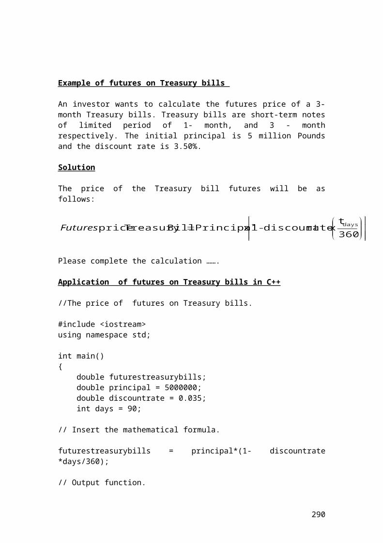
Compare the put option price using a Cox,Ross, Rubinstein, (CRR), binomial 3 steps tree with the Black and Scholes model

/*Compare the put option price using a Cox,Ross, Rubinstein, (CRR), binomial 3 steps tree with the Black and Scholes model.*/

/* Calculate the put option prices using a Cox, Ross, Rubinstein,(CRR) binomial 3 steps tree. */

#include <iostream> #include<cmath> using namespace std; // Calculation of the cumulative normal distribution.

double norm_cdf (const double& x) {

double k = 1/(1+0.2316419*x);double k_sum = k*(0.319381530 + k*(-0.356563782 + k*(1.781477937 + k*(-1.821255978 + k*(1.330274429))))); if (x >= 0.0) {return (1.0 - (1.0/(pow(2*M_PI, 0.5))) * exp(-0.5*x*x)* k_sum);} else {return 1.0 - norm_cdf(-x);}}// Mathematical formulas to calculate d1, d2 and the European put price.

double Put(double S, double K, double r, double q, double T, double sig){

double d1, d2; d1 = (log(S/K) + (r-q +(sig*sig)*0.5 ) * T ) / (sig * sqrt(T)); d2 = d1 - sig*sqrt(T);

return K*exp(-r*T)*norm_cdf(-d2) - S*exp(-q*T)*norm_cdf(-d1) ; }

290

int main() { double S = 60; // share price double K = 70; // strike price double r = 0.02; // risk-free interest rate double q = 0.03; // dividend yield double T = 0.5; // life to maturity double sig = 0.2; // volatility // Identify the variables. u = multiplier of upmove. //d = multiplier of downmove. dt = steps expressed in years. //riskprobofupmove = risk neutral probability of upmove. //disfact = discount factor. double u; double d; double dt; double riskprobofupmove; double disfact; const int n = 3; // Identify tree steps binomial tree. // Insert the mathematical formulas. dt = T/n; u = exp(sig*sqrt(dt)); d = 1/u; disfact = exp(-r*dt); riskprobofupmove = (exp((r-q)*dt)-d)/(u-d); double putpayoffupmovestep3; // K - (Shareprice * upmove^3)double putpayoff3i; // K- (Shareprice * upmove^2 * downmove)double putpayoff3ii; // K-(Shareprice * downmove^2*upmove) double putpayoffdownmovestep3; // K-(Shareprice * downmove^3)

// The option prices are calculated backwards.

putpayoffupmovestep3 = K-S*pow(u,3);putpayoffupmovestep3=0;putpayoff3i = K- S * pow(u,2) * d;putpayoff3ii =K- S * pow(d,2)*u; putpayoffdownmovestep3 = K - S*pow(d,3);

291

double putpriceupmovestep2;double putpriceupdownmovestep2;double putpricedownmovestep2;

putpriceupmovestep2 = (disfact*(riskprobofupmove*putpayoffupmovestep3)+(1-riskprobofupmove)*putpayoff3i);

putpriceupdownmovestep2 =(disfact*(riskprobofupmove*putpayoff3i)+(1-riskprobofupmove)*putpayoff3ii);

putpricedownmovestep2 =(disfact*(riskprobofupmove*putpayoff3ii)+(1-riskprobofupmove)*putpayoffdownmovestep3);

double putpriceupmovestep1;double putpricedownmovestep1;

putpriceupmovestep1 = (disfact*(riskprobofupmove*putpriceupmovestep2)+(1-riskprobofupmove)*putpriceupdownmovestep2);

putpricedownmovestep1=(disfact*(riskprobofupmove*putpriceupdownmovestep2)+(1-riskprobofupmove)*putpricedownmovestep2);

double putpricestep0;

putpricestep0= (disfact*(riskprobofupmove*putpriceupmovestep1)+(1-riskprobofupmove)*putpricedownmovestep1);

//Calculation of put price based on the Black and Scholes model.

double putPrice;

putPrice = Put (S,K,r,q,T,sig);

//Output functions.cout.setf(ios::fixed); cout.setf(ios::showpoint); cout.precision(4); cout<<"Steps expressed in years:"<< dt<<endl;cout<<"Multiplier of upmove:"<< u<<endl;cout<<"Multiplier of downmove:"<< d<<endl;cout<<" Discount factor:"<<disfact<<endl;cout<< "Risk neutral probability of upmove:"<<riskprobofupmove<<endl;cout<<"Put payoff upmove step[3]:"<<putpayoffupmovestep3<<endl;cout<<"Put payoff [3i]:"<<putpayoff3i<<endl;cout<<"Put payoff [3ii]:"<<putpayoff3ii<<endl;cout<<"Put payoff downmove step[3]:"<<putpayoffdownmovestep3<<endl;cout<<"Put price upmove step[2]:"<<putpriceupmovestep2<<endl;cout<<"Put price updownmove step[2]:"<<putpriceupdownmovestep2<<endl;

292

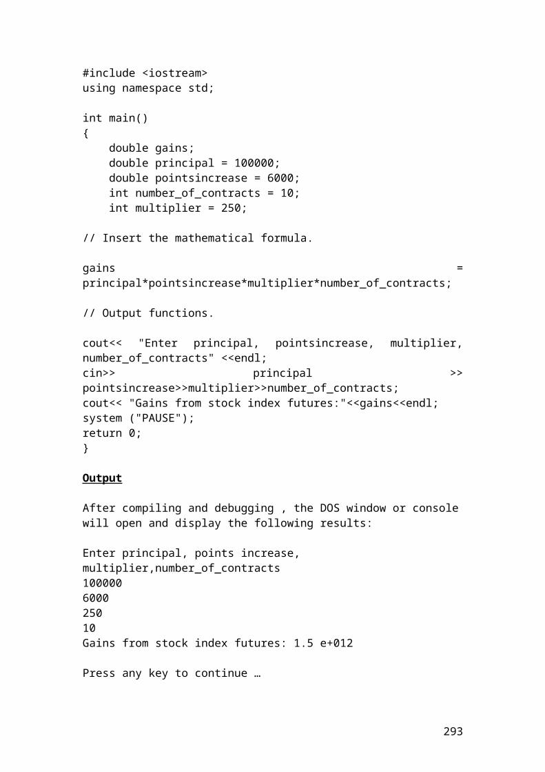
cout<<"Put price downmove step[2]:"<<putpricedownmovestep2<<endl;cout<<"Put price upmove step[1]:"<<putpriceupmovestep1<<endl;cout<<"Put price downmove step[1]:"<<putpricedownmovestep1<<endl;cout<<"Put price step[0]:"<<putpricestep0<<endl;cout<<" Black and Scholes put price:"<<putPrice<<endl;system ("PAUSE");return 0;}

Output

The figures are expressed in USD. After compiling and debugging , the DOS window or console will open and display the following results:

Steps expressed in years: 0.1667Multiplier of upmove: 1.0851Multiplier of downmove: 0.9216Disount factor: 0.9967Risk neutral probability of upmove: 0.4694Put payoff upmove step [3]: 0.0000Put payoff [3i]: 4.8955Put payoff [3ii]: 14.7043Put payoff downmove step [3]: 23.0353Put price upmove step [2]: 2.5975Put price updownmove step [2]: 10.0923Put price downmove step [2]: 19.1017Put price upmove step [1]: 6.5701Put price downmove step [1]: 14.8568Put price step [0]: 10.9566Black and Scholes put price: 10.7864Press any key to continue …

293

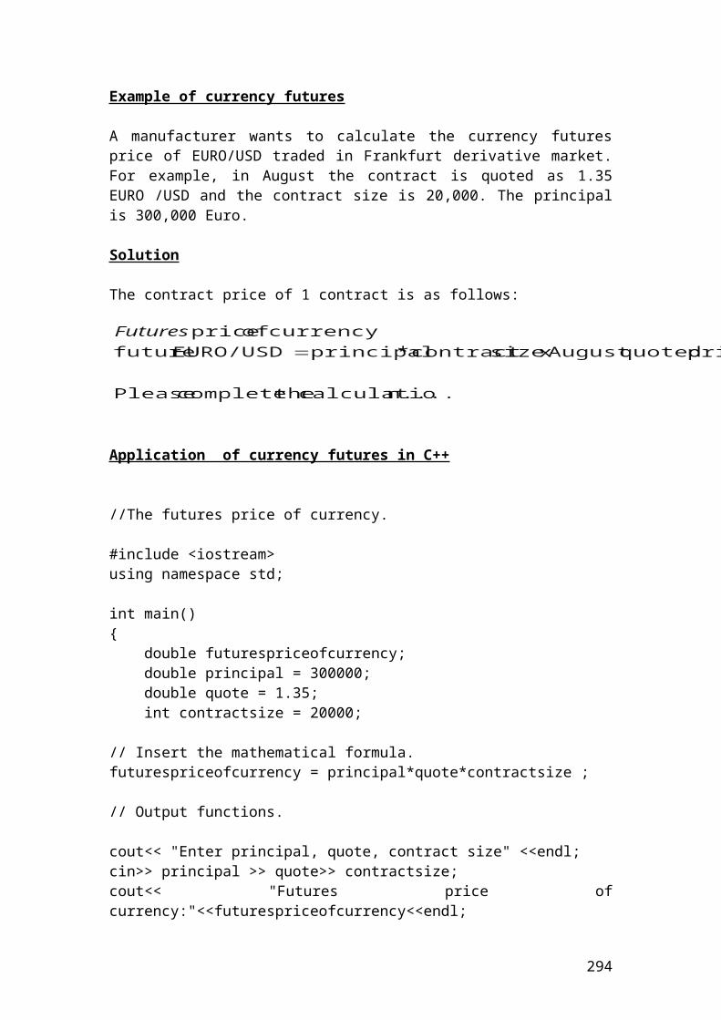
Calculate the share prices of a call option using a Jarrow – Rudd, (JR), binomial 3 steps tree using a vector. The key difference between the Cox, Ross, Rubinstein,(CRR) binomial tree and the Jarrow – Rudd, (JR), binomila tree is in defining the parmeters of the multiplier of up and down move. The multipliers depend on a drift in addition to volatility and length of steps

/* Calculate the share prices of a call option using Jarrow - Rudd, (JR), binomial 3 steps tree. */

#include <iostream> #include<cmath> #include<vector>using namespace std;

int main() { double S = 90; //share price double K = 85; // strike price double r = 0.04; // risk -free interest rate double q = 0.03; // dividend yield. If the dividend is zero, then, it is // not included in the equation of the multiplier of upmove // and downmove.

double T = 0.5; // life to maturity double sig = 0.2; // volatility // Identify the variables. u = multiplier of upmove. //d = multiplier of downmove. dt = steps expressed in years. double u; double d; double dt; int i,j ; const int n = 3; // Identify tree steps binomial tree. // Insert the mathematical formulas. dt = T/n; u = (exp((r-q -0.5*sig*sig)*dt + sig*sqrt(dt))); d = (exp((r-q -0.5*sig*sig)*dt - sig*sqrt(dt)));

294

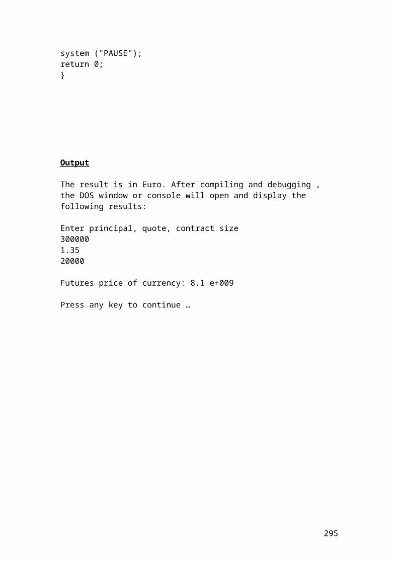
double sharetree[i][j];int arraysize[10];vector<double> dataarray;for (i=0; i<=j; i++){ for (j=1; j<=n; j++) { if (i==0) sharetree[i][j] = S * u; else sharetree[i][j] = S* d; if (i==0) sharetree[i][j] = S * pow(u,2); else sharetree[i][j] = S* pow(d,2); if (i==0) sharetree[i][j] = S*u*d; if (i==0) sharetree[i][j] = S*pow(u,2)*d ; if (i==0) sharetree[i][j] = S* pow(d,2)*u; if (i==0) sharetree[i][j] = S * pow(u,3); else sharetree[i][j] = S* pow(d,3); }}

cout.setf(ios::fixed); cout.setf(ios::showpoint); cout.precision(4); cout<<"Steps expressed in years:"<< dt<<endl;cout<<"Multiplier of upmove:"<< u<<endl;cout<<"Multiplier of downmove:"<< d<<endl; cout<<"Enter array size:"<<endl;cin>> arraysize[10];

sharetree[i][j] = S ;cout.setf(ios::fixed); cout.setf(ios::showpoint); cout.precision(2); cout<<" Share price [0]:"<<sharetree[i][j]<<endl;

sharetree[i][j] = S * u;cout.setf(ios::fixed); cout.setf(ios::showpoint); cout.precision(2); cout<<" Share price upmove [1]:"<<sharetree[i][j]<<endl; sharetree[i][j] = S* d;cout.setf(ios::fixed); cout.setf(ios::showpoint); cout.precision(2);

295

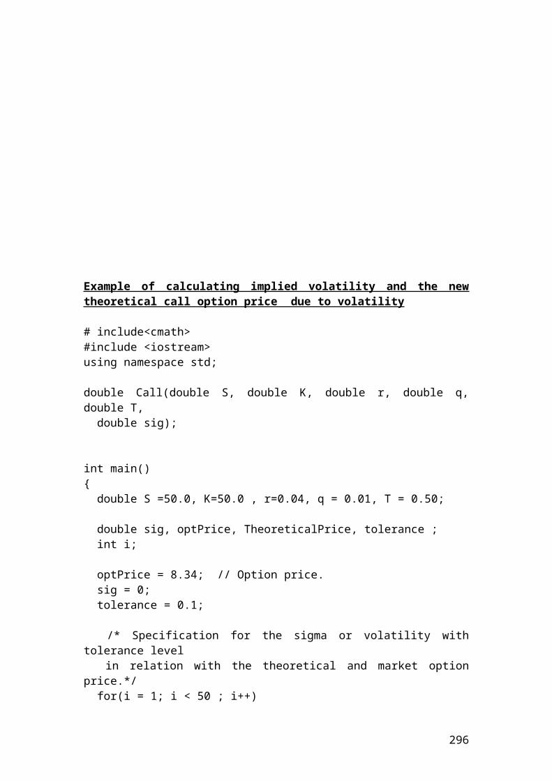
cout<<" Share price downmove[1]:"<<sharetree[i][j]<<endl; sharetree[i][j] = S * pow(u,2); cout.setf(ios::fixed); cout.setf(ios::showpoint); cout.precision(2); cout<<" Share price upmove [2]:"<<sharetree[i][j]<<endl; sharetree[i][j] = S*u*d;cout.setf(ios::fixed); cout.setf(ios::showpoint); cout.precision(2); cout<<" Share price up and downmove [2]:"<<sharetree[i][j]<<endl; sharetree[i][j] = S* pow(d,2);cout.setf(ios::fixed); cout.setf(ios::showpoint); cout.precision(2); cout<<" Share price downmove [2]:"<<sharetree[i][j]<<endl; sharetree[i][j] = S* pow (u,3);cout.setf(ios::fixed); cout.setf(ios::showpoint); cout.precision(2); cout<<" Share price upmove [3]:"<<sharetree[i][j]<<endl;

sharetree[i][j] = S*pow(u,2)*d ;cout.setf(ios::fixed); cout.setf(ios::showpoint); cout.precision(2); cout<<" Share price *upmove* downmove*upmove [3]:"<<sharetree[i][j]<<endl;

sharetree[i][j] = S* pow(d,2)*u;cout.setf(ios::fixed); cout.setf(ios::showpoint); cout.precision(2); cout<<" Share price *upmove * downmove*downmove [3]:"<<sharetree[i][j]<<endl;

sharetree[i][j] = S* pow(d,3);cout.setf(ios::fixed); cout.setf(ios::showpoint); cout.precision(2); cout<<" Share price downmove [3]:"<<sharetree[i][j]<<endl; system ("PAUSE");return 0;

296

}

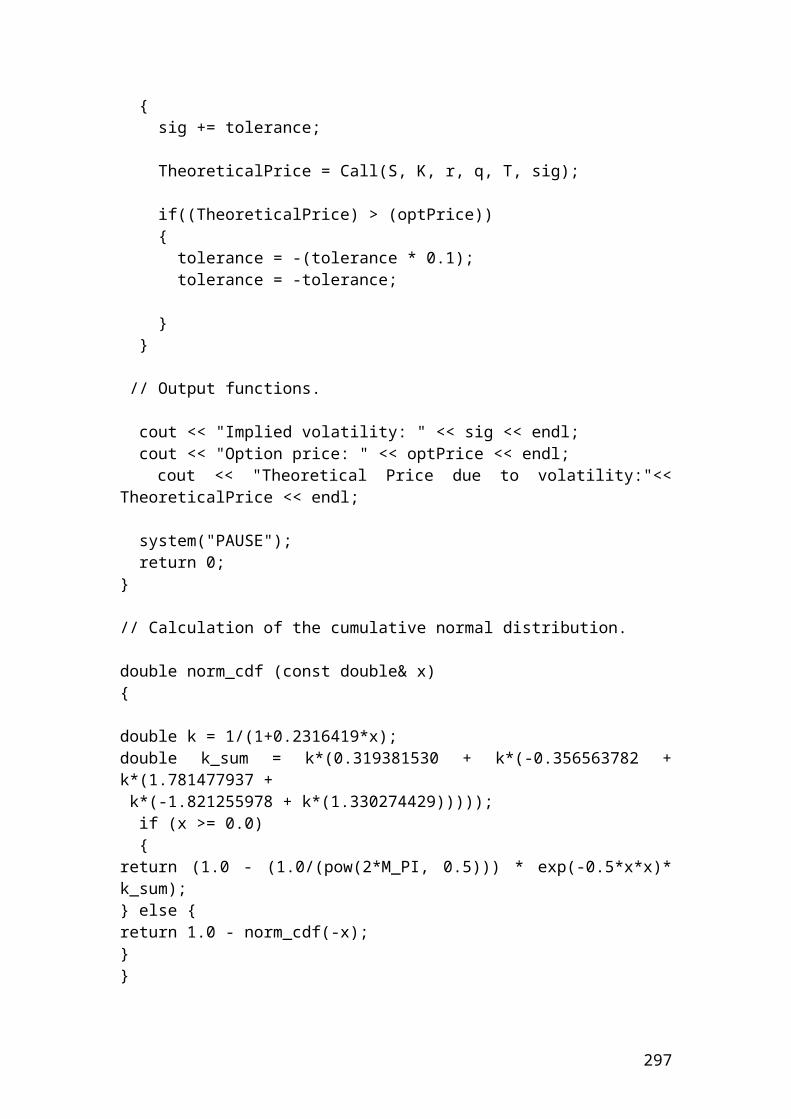
Output

The figures are expressed in pounds. After compiling and debugging , the DOS window or console will open and display the following results:

Steps expressed in years: 0.1667Multiplier of upmove: 1.0833Multiplier of downmove: 0.9201Enter array size:10Share price[0]: 90Share price upmove [1]:97.49 Share price downmove [1]: 82.81Share price upmove [2]: 105.61Share price up and downmove[2]:89.70Share price downmove [2]: 76.19Share price upmove [3]: 114.41Share price upmove*downmove* upmove [3]:97.17 Share price upmove*downmove*downmove[3]: 82.53Share price downmove [3]: 70.10Press any key to continue …

297

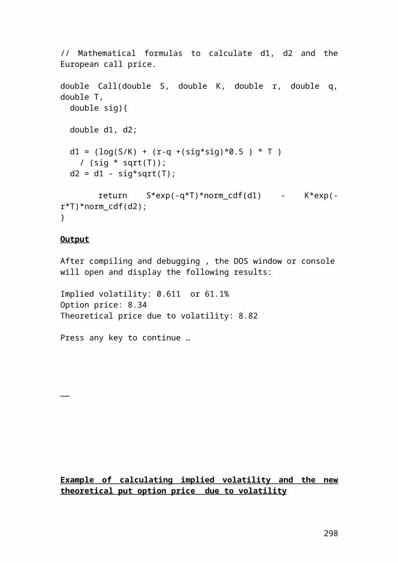
Calculate the call option prices using a Jarrow – Rudd, (JR), binomial 3 steps tree. The key difference between the Cox, Ross, Rubinstein,(CRR) binomial tree and the Jarrow – Rudd, (JR), binomila tree is in defining the parmeters of the multiplier of up and down move

/* Calculate the call option prices using Jarrrow and Rudd(J,R) binomial 3 steps tree. */

#include <iostream> #include<cmath> using namespace std;

int main() { double S = 90; // share price double K = 85; // strike price double r = 0.04; // risk – free interest rate double q = 0.03; // dividend yield. If the dividend is zero, then, it is // not included in the equation of the multiplier of // upmove and downmove. double T = 0.5; // life to maturity double sig = 0.2; // volatility // Identify the variables. u = multiplier of upmove. //d = multiplier of downmove. dt = steps expressed in years. //riskprobofupmove = risk neutral probability of upmove. //disfact = discount factor. double u; double d; double dt; double riskprobofupmove; double disfact; const int n = 3; // Identify tree steps binomial tree. // Insert the mathematical formulas. dt = T/n; u = (exp((r-q -0.5*sig*sig)*dt + sig*sqrt(dt))); d = (exp((r-q -0.5*sig*sig)*dt - sig*sqrt(dt))); disfact = exp(-r*dt); riskprobofupmove = (exp((r-q)*dt)-d)/(u-d);

298

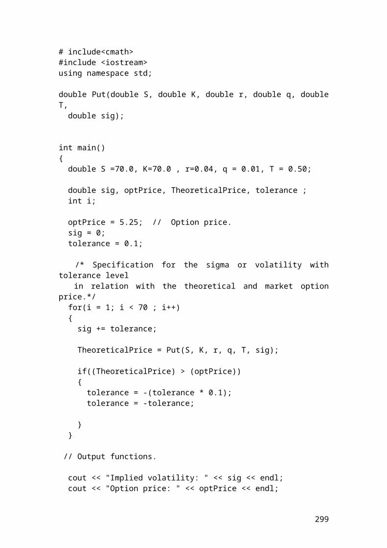
double callpayoffupmovestep3; // (Shareprice * upmove^3)-Kdouble callpayoff3i; // (Shareprice * upmove^2 * downmove)-Kdouble callpayoff3ii; // (Shareprice * downmove^2*upmove)-K double callpayoffdownmovestep3; // (Shareprice * downmove^3) -K

callpayoffupmovestep3 = S*pow(u,3)-K;callpayoff3i = S * pow(u,2) * d -K;callpayoff3ii =S * pow(d,2)*u-K; callpayoff3ii =0;callpayoffdownmovestep3 = S*pow(d,3)-K;callpayoffdownmovestep3 =0;

double callpriceupmovestep2;double callpriceupdownmovestep2;double callpricedownmovestep2;

callpriceupmovestep2 = (disfact*(riskprobofupmove*callpayoffupmovestep3)+(1-riskprobofupmove)*callpayoff3i);

callpriceupdownmovestep2 =(disfact*(riskprobofupmove*callpayoff3i)+(1-riskprobofupmove)*callpayoff3ii);

callpricedownmovestep2 =(disfact*(riskprobofupmove*callpayoff3ii)+(1-riskprobofupmove)*callpayoffdownmovestep3);

double callpriceupmovestep1;double callpricedownmovestep1;

callpriceupmovestep1 = (disfact*(riskprobofupmove*callpriceupmovestep2)+(1-riskprobofupmove)*callpriceupdownmovestep2);

callpricedownmovestep1=(disfact*(riskprobofupmove*callpriceupdownmovestep2)+(1-riskprobofupmove)*callpricedownmovestep2);

double callpricestep0;

callpricestep0= (disfact*(riskprobofupmove*callpriceupmovestep1)+(1-riskprobofupmove)*callpricedownmovestep1);

//Output functions.cout.setf(ios::fixed); cout.setf(ios::showpoint); cout.precision(2); cout<<"Steps expressed in years:"<< dt<<endl;cout<<"Multiplier of upmove:"<< u<<endl;cout<<"Multiplier of downmove:"<< d<<endl;

299

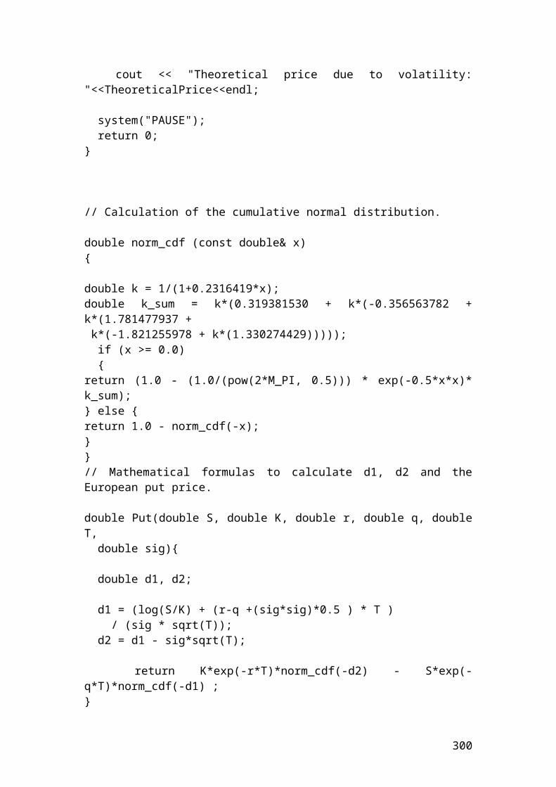
cout<<" Discount factor:"<<disfact<<endl;cout<< "Risk neutral probability of upmove:"<<riskprobofupmove<<endl;cout<<"Call payoff upmove step3:"<<callpayoffupmovestep3<<endl;cout<<"Call payoff 3i:"<<callpayoff3i<<endl;cout<<"Call payoff 3ii:"<<callpayoff3ii<<endl;cout<<"Call payoff downmove step3:"<<callpayoffdownmovestep3<<endl;cout<<"Call price upmove step2:"<<callpriceupmovestep2<<endl;cout<<"Call price up down move step2:"<<callpriceupdownmovestep2<<endl;cout<<"Call price down move step2:"<<callpricedownmovestep2<<endl;cout<<"Call price upmove step1:"<<callpriceupmovestep1<<endl;cout<<"Call price down movestep1:"<<callpricedownmovestep1<<endl;cout<<"Call price step0:"<<callpricestep0<<endl;

system ("PAUSE");return 0;}

Output

The figures are expressed in pounds. After compiling and debugging , the DOS window or console will open and display the following results:

Steps expressed in years: 0.17Multiplier of upmove: 1.08Multiplier of downmove: 0.92Disount factor: 0.99Risk neutral probability of upmove: 0.50Call payoff upmove step [3]: 29.41Call payoff [3i]: 12.17Call payoff [3ii]: 0Call payoff downmove step [3]: 0Call price upmove step [2]: 20.69Call price updownmove step [2]: 6.04Call price downmove step [2]: 0Call price upmove step [1]: 13.30Call price downmove step [1]: 3.00Call price step [0]: 8.11Press any key to continue …

300

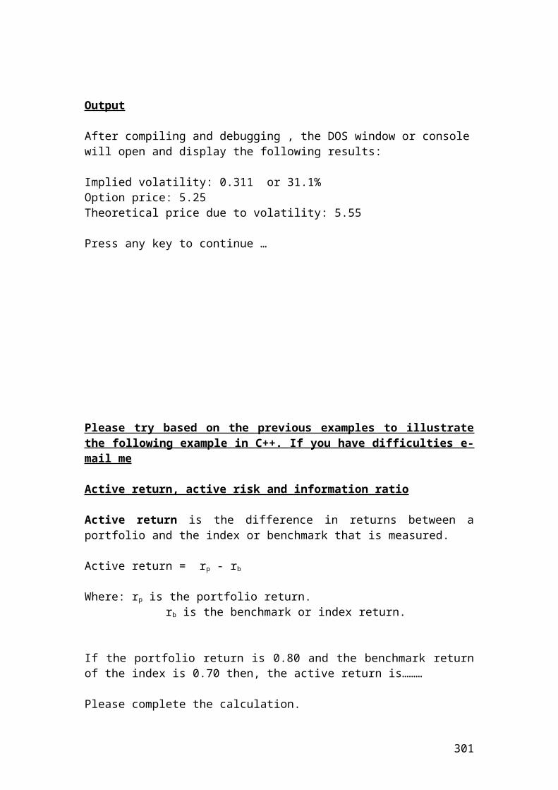
Compare the call option price using a Jarrow - Rudd, (JR), binomial 3 steps tree with the Black and Scholes model

/*Compare the call option price using a Jarrow - Rudd, (JR), binomial 3 steps tree with the Black and Scholes model.*/

/* Calculate the call option prices using Jarrrow and Rudd(J,R) binomial 3 steps tree. */

#include <iostream> #include<cmath> using namespace std; // Calculation of the cumulative normal distribution.

double norm_cdf (const double& x) {

double k = 1/(1+0.2316419*x);double k_sum = k*(0.319381530 + k*(-0.356563782 + k*(1.781477937 + k*(-1.821255978 + k*(1.330274429))))); if (x >= 0.0) {return (1.0 - (1.0/(pow(2*M_PI, 0.5))) * exp(-0.5*x*x)* k_sum);} else {return 1.0 - norm_cdf(-x);}}

// Mathematical formulas to calculate d1, d2 and the European call price.

double Call(double S, double K, double r, double q, double T, double sig){

double d1, d2; d1 = (log(S/K) + (r-q +(sig*sig)*0.5 ) * T ) / (sig * sqrt(T)); d2 = d1 - sig*sqrt(T); return S*exp(-q*T)*norm_cdf(d1) - K*exp(-r*T)*norm_cdf(d2) ; }

301

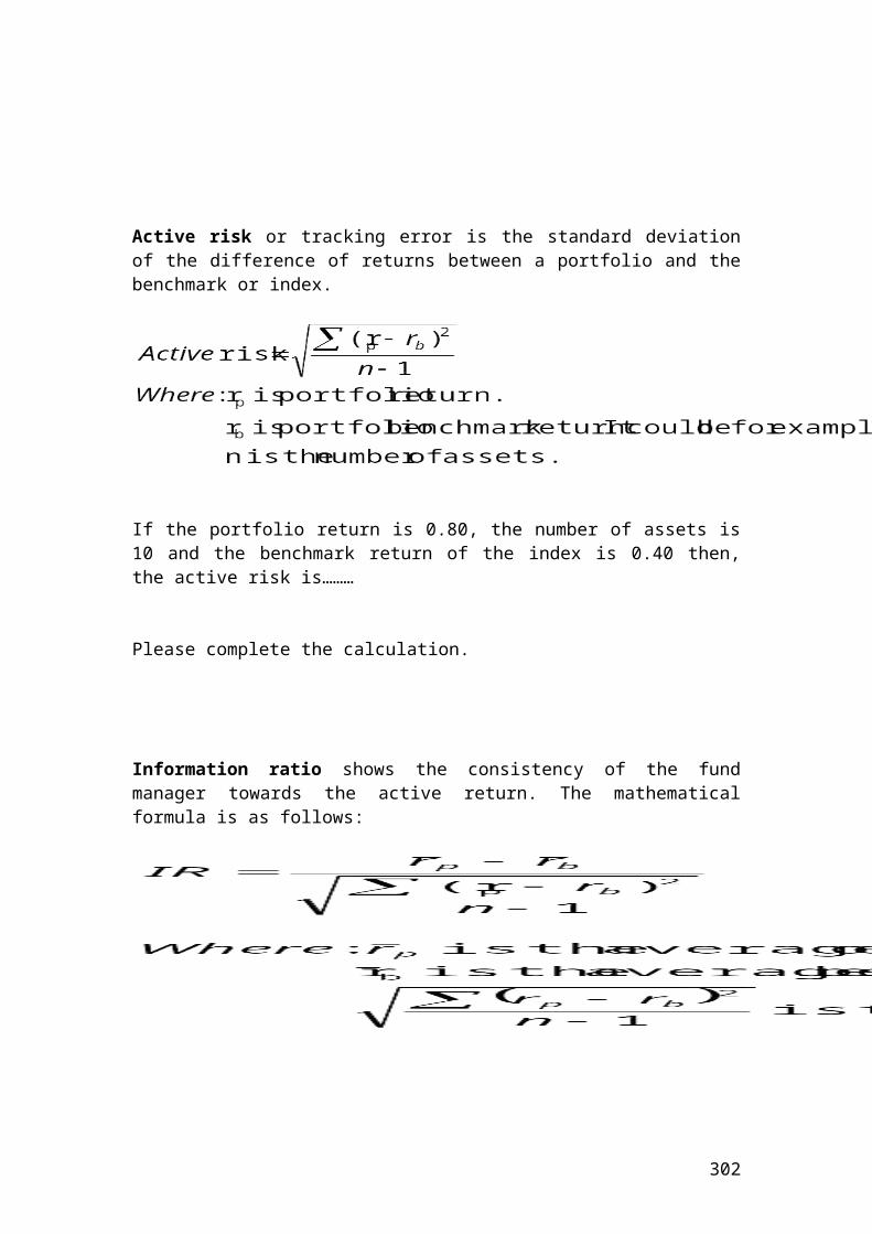
int main() { double S = 90; // share price double K = 85; // strike price double r = 0.04; // risk - free interest rate double q = 0.03; // dividend yield. If the dividend is zero, then, it is // not included in the equation of the multiplier of // upmove and downmove. double T = 0.5; // life to maturity double sig = 0.2; // volatility // Identify the variables. u = multiplier of upmove. //d = multiplier of downmove. dt = steps expressed in years. //riskprobofupmove = risk neutral probability of upmove. //disfact = discount factor. double u; double d; double dt; double riskprobofupmove; double disfact; const int n = 3; // Identify tree steps binomial tree. // Insert the mathematical formulas. dt = T/n; u = (exp((r-q -0.5*sig*sig)*dt + sig*sqrt(dt))); d = (exp((r-q -0.5*sig*sig)*dt - sig*sqrt(dt))); disfact = exp(-r*dt); riskprobofupmove = (exp((r-q)*dt)-d)/(u-d); double callpayoffupmovestep3; // (Shareprice * upmove^3)-Kdouble callpayoff3i; // (Shareprice * upmove^2 * downmove)-Kdouble callpayoff3ii; // (Shareprice * downmove^2*upmove)-K double callpayoffdownmovestep3; // (Shareprice * downmove^3) -K

callpayoffupmovestep3 = S*pow(u,3)-K;callpayoff3i = S * pow(u,2) * d -K;callpayoff3ii =S * pow(d,2)*u-K; callpayoff3ii =0;callpayoffdownmovestep3 = S*pow(d,3)-K;callpayoffdownmovestep3 =0;

302

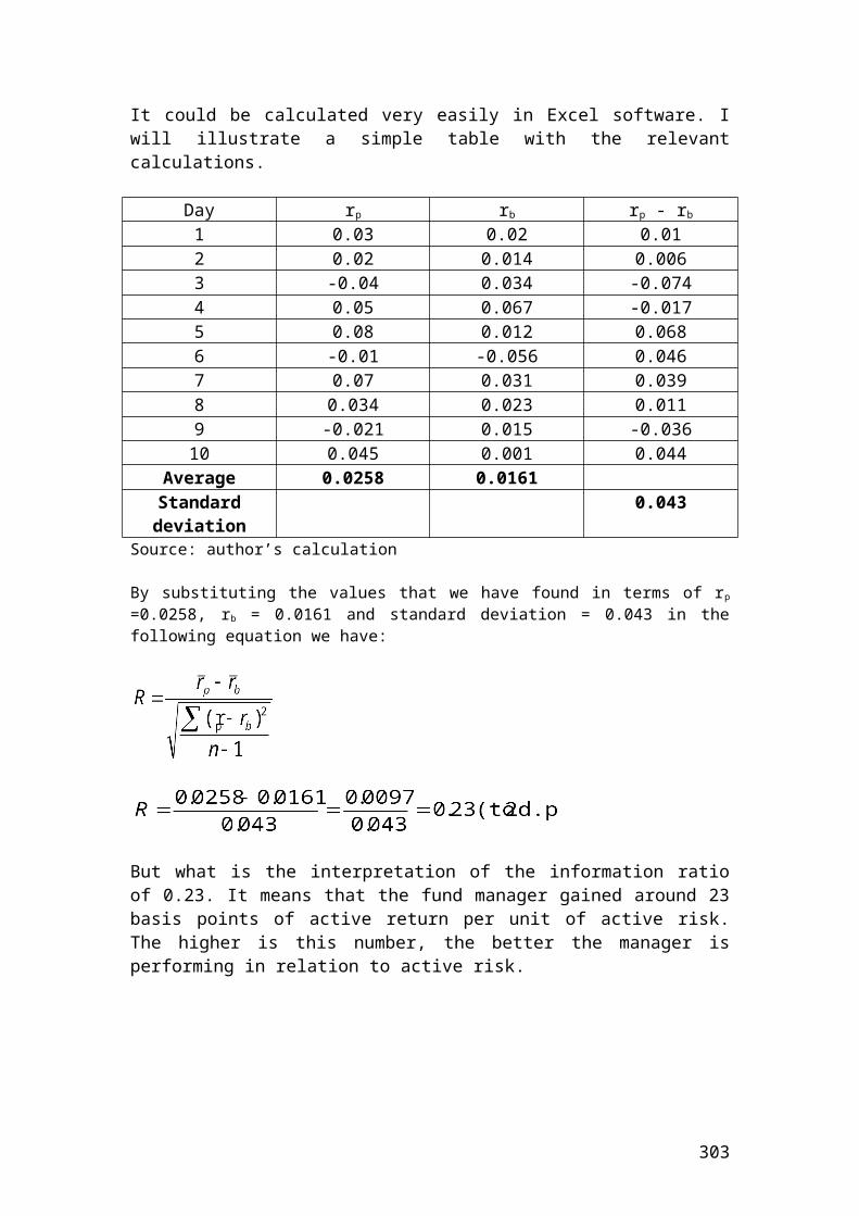
double callpriceupmovestep2;double callpriceupdownmovestep2;double callpricedownmovestep2;

callpriceupmovestep2 = (disfact*(riskprobofupmove*callpayoffupmovestep3)+(1-riskprobofupmove)*callpayoff3i);

callpriceupdownmovestep2 =(disfact*(riskprobofupmove*callpayoff3i)+(1-riskprobofupmove)*callpayoff3ii);

callpricedownmovestep2 =(disfact*(riskprobofupmove*callpayoff3ii)+(1-riskprobofupmove)*callpayoffdownmovestep3);

double callpriceupmovestep1;double callpricedownmovestep1;

callpriceupmovestep1 = (disfact*(riskprobofupmove*callpriceupmovestep2)+(1-riskprobofupmove)*callpriceupdownmovestep2);

callpricedownmovestep1=(disfact*(riskprobofupmove*callpriceupdownmovestep2)+(1-riskprobofupmove)*callpricedownmovestep2);

double callpricestep0;

callpricestep0= (disfact*(riskprobofupmove*callpriceupmovestep1)+(1-riskprobofupmove)*callpricedownmovestep1);

//Calculation of call price based on the Black and Scholes model.

double callPrice;

callPrice = Call (S,K,r,q,T,sig);

//Output functions.cout.setf(ios::fixed); cout.setf(ios::showpoint); cout.precision(2); cout<<"Steps expressed in years:"<< dt<<endl;cout<<"Multiplier of upmove:"<< u<<endl;cout<<"Multiplier of downmove:"<< d<<endl;cout<<" Discount factor:"<<disfact<<endl;cout<< "Risk neutral probability of upmove:"<<riskprobofupmove<<endl;

cout<<"Call payoff upmove step3:"<<callpayoffupmovestep3<<endl;cout<<"Call payoff 3i:"<<callpayoff3i<<endl;cout<<"Call payoff 3ii:"<<callpayoff3ii<<endl;cout<<"Call payoff downmove step3:"<<callpayoffdownmovestep3<<endl;cout<<"Call price upmove step2:"<<callpriceupmovestep2<<endl;cout<<"Call price up down move step2:"<<callpriceupdownmovestep2<<endl;

303

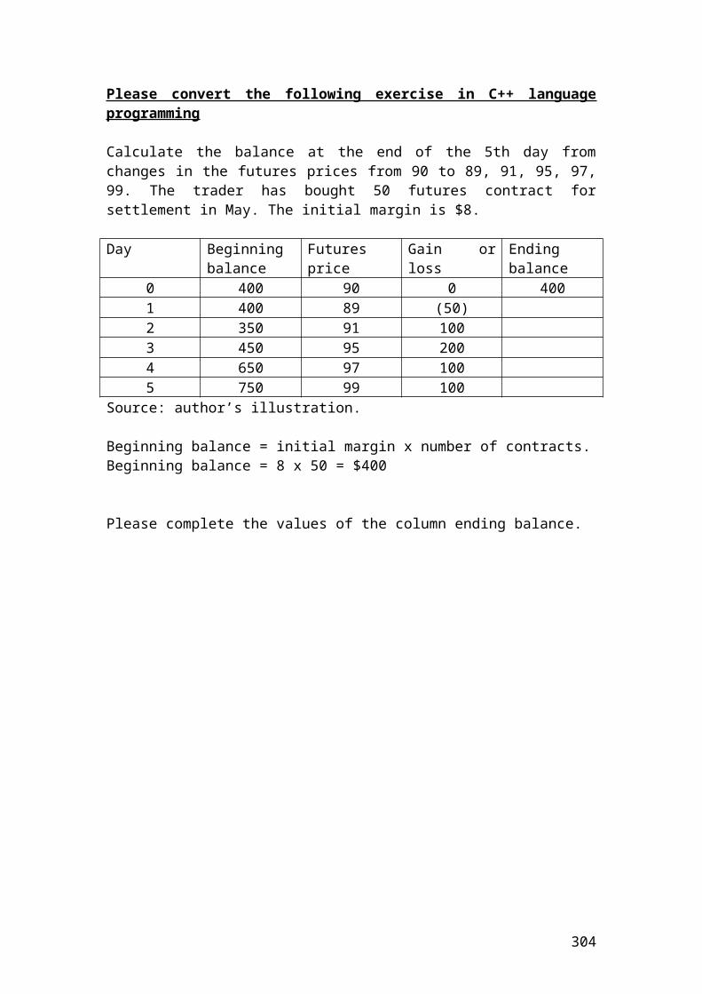
cout<<"Call price down move step2:"<<callpricedownmovestep2<<endl;cout<<"Call price upmove step1:"<<callpriceupmovestep1<<endl;cout<<"Call price down movestep1:"<<callpricedownmovestep1<<endl;cout<<"Call price step0:"<<callpricestep0<<endl;cout<<" Black and Scholes call price:"<<callPrice<<endl;system ("PAUSE");return 0;}

Output

The figures are expressed in pounds. After compiling and debugging , the DOS window or console will open and display the following results:

Steps expressed in years: 0.17Multiplier of upmove: 1.08Multiplier of downmove: 0.92Disount factor: 0.99Risk neutral probability of upmove: 0.50Call payoff upmove step [3]: 29.41Call payoff [3i]: 12.17Call payoff [3ii]: 0Call payoff downmove step [3]: 0Call price upmove step [2]: 20.69Call price updownmove step [2]: 6.04Call price downmove step [2]: 0Call price upmove step [1]: 13.30Call price downmove step [1]: 3.00Call price step [0]: 8.11Black and Scholes call price: 7.98Press any key to continue …

304

Calculate the put option prices using a Jarrow – Rudd, (JR), binomial 3 steps tree

/* Calculate the put option prices using Jarrow and Rudd, (J,R), binomial 3 steps tree. */

#include <iostream> #include<cmath> using namespace std;

int main() { double S = 60; double K = 70; double r = 0.02; double q = 0.03; double T = 0.5; double sig = 0.2; // Identify the variables. u = multiplier of upmove. //d = multiplier of downmove. dt = steps expressed in years. //riskprobofupmove = risk neutral probability of upmove. //disfact = discount factor. double u; double d; double dt; double riskprobofupmove; double disfact; const int n = 3; // Identify tree steps binomial tree. // Insert the mathematical formulas. dt = T/n; u = (exp((r-q -0.5*sig*sig)*dt + sig*sqrt(dt))); d = (exp((r-q -0.5*sig*sig)*dt - sig*sqrt(dt))); disfact = exp(-r*dt); riskprobofupmove = (exp((r-q)*dt)-d)/(u-d); double putpayoffupmovestep3; // K - (Shareprice * upmove^3)double putpayoff3i; // K- (Shareprice * upmove^2 * downmove)

305

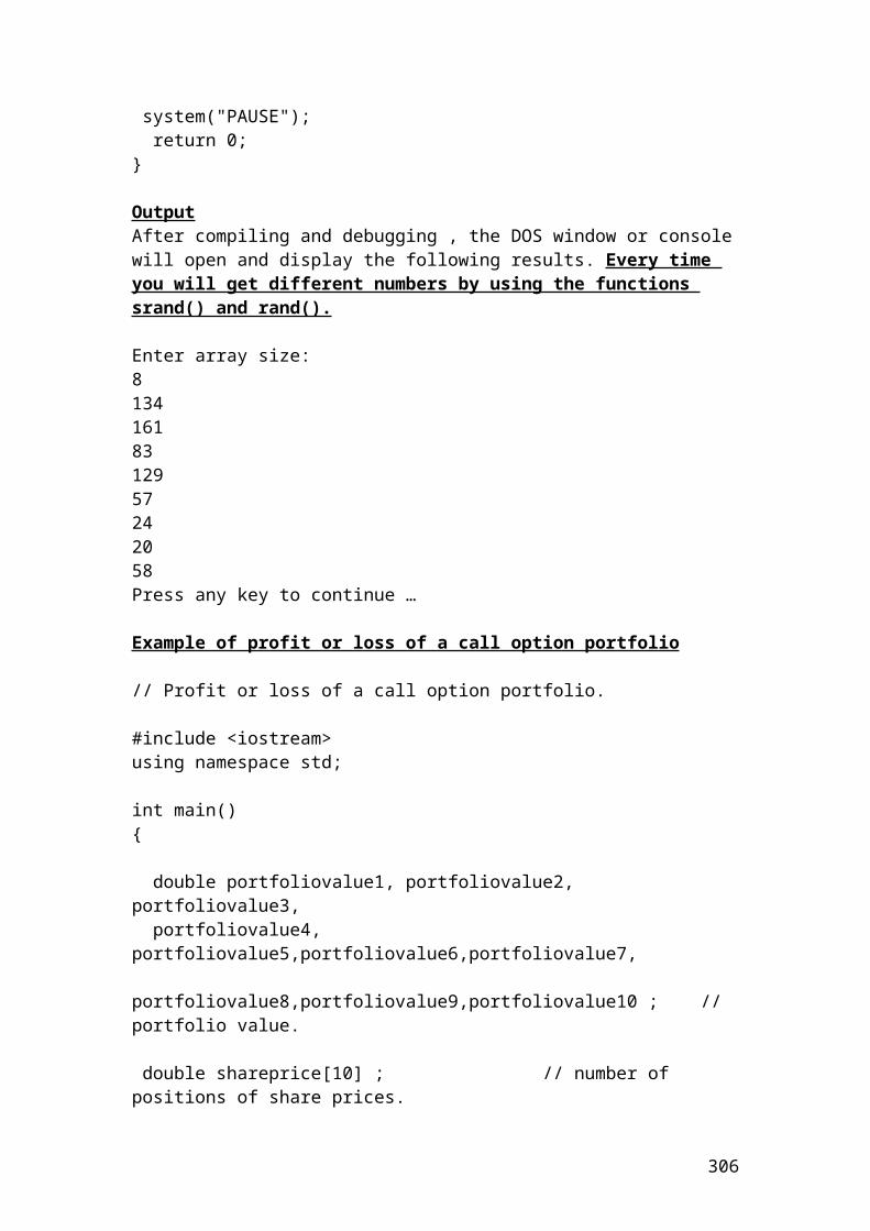
double putpayoff3ii; // K-(Shareprice * downmove^2*upmove) double putpayoffdownmovestep3; // K-(Shareprice * downmove^3)

// The option prices are calculated backwards.

putpayoffupmovestep3 = K-S*pow(u,3);putpayoffupmovestep3=0;putpayoff3i = K- S * pow(u,2) * d;putpayoff3ii =K- S * pow(d,2)*u; putpayoffdownmovestep3 = K - S*pow(d,3);

double putpriceupmovestep2;double putpriceupdownmovestep2;double putpricedownmovestep2;

putpriceupmovestep2 = (disfact*(riskprobofupmove*putpayoffupmovestep3)+(1-riskprobofupmove)*putpayoff3i);

putpriceupdownmovestep2 =(disfact*(riskprobofupmove*putpayoff3i)+(1-riskprobofupmove)*putpayoff3ii);

putpricedownmovestep2 =(disfact*(riskprobofupmove*putpayoff3ii)+(1-riskprobofupmove)*putpayoffdownmovestep3);

double putpriceupmovestep1;double putpricedownmovestep1;

putpriceupmovestep1 = (disfact*(riskprobofupmove*putpriceupmovestep2)+(1-riskprobofupmove)*putpriceupdownmovestep2);

putpricedownmovestep1=(disfact*(riskprobofupmove*putpriceupdownmovestep2)+(1-riskprobofupmove)*putpricedownmovestep2);

double putpricestep0;

putpricestep0= (disfact*(riskprobofupmove*putpriceupmovestep1)+(1-riskprobofupmove)*putpricedownmovestep1);

//Output functions.cout.setf(ios::fixed); cout.setf(ios::showpoint); cout.precision(2); cout<<"Steps expressed in years:"<< dt<<endl;cout<<"Multiplier of upmove:"<< u<<endl;cout<<"Multiplier of downmove:"<< d<<endl;cout<<" Discount factor:"<<disfact<<endl;cout<< "Risk neutral probability of upmove:"<<riskprobofupmove<<endl;

306

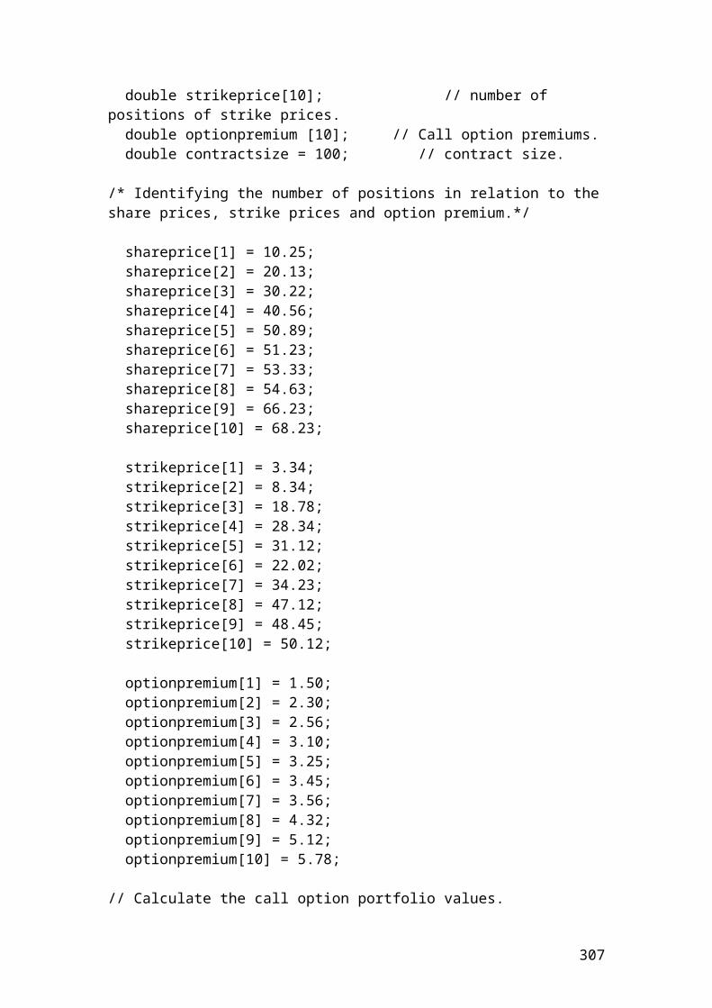
cout<<"Put payoff upmove step[3]:"<<putpayoffupmovestep3<<endl;cout<<"Put payoff [3i]:"<<putpayoff3i<<endl;cout<<"Put payoff [3ii]:"<<putpayoff3ii<<endl;cout<<"Put payoff downmove step[3]:"<<putpayoffdownmovestep3<<endl;cout<<"Put price upmove step[2]:"<<putpriceupmovestep2<<endl;cout<<"Put price updownmove step[2]:"<<putpriceupdownmovestep2<<endl;cout<<"Put price downmove step[2]:"<<putpricedownmovestep2<<endl;cout<<"Put price upmove step[1]:"<<putpriceupmovestep1<<endl;cout<<"Put price downmove step[1]:"<<putpricedownmovestep1<<endl;cout<<"Put price step[0]:"<<putpricestep0<<endl;

system ("PAUSE");return 0;}

Output

The figures are expressed in USD. After compiling and debugging , the DOS window or console will open and display the following results:

Steps expressed in years: 0.17Multiplier of upmove: 1.08Multiplier of downmove: 0.92Disount factor: 1.00Risk neutral probability of upmove: 0.50Put payoff upmove step [3]: 0.00Put payoff [3i]: 5.86Put payoff [3ii]: 15.53Put payoff downmove step [3]: 23.73Put price upmove step [2]: 2.93Put price updownmove step [2]: 10.69Put price downmove step [2]: 19.61Put price upmove step [1]: 6.80Put price downmove step [1]: 15.13Put price step [0]: 10.95Press any key to continue …

307

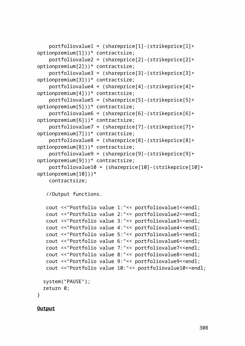
Compare the put option price using a Jarrow - Rudd, (JR), binomial 3 steps tree with the Black and Scholes model

/*Compare the put option price using a Jarrow - Rudd, (JR), binomial 3 steps tree with //the Black and Scholes model.*/

/* Calculate the put option prices using Jarrow and Rudd, (J,R), binomial 3 steps tree. */

#include <iostream> #include<cmath> using namespace std;

// Calculation of the cumulative normal distribution.

double norm_cdf (const double& x) {

double k = 1/(1+0.2316419*x);double k_sum = k*(0.319381530 + k*(-0.356563782 + k*(1.781477937 + k*(-1.821255978 + k*(1.330274429))))); if (x >= 0.0) {return (1.0 - (1.0/(pow(2*M_PI, 0.5))) * exp(-0.5*x*x)* k_sum);} else {return 1.0 - norm_cdf(-x);}}

// Mathematical formulas to calculate d1, d2 and the European put price.

double Put(double S, double K, double r, double q, double T, double sig){

double d1, d2; d1 = (log(S/K) + (r-q +(sig*sig)*0.5 ) * T ) / (sig * sqrt(T)); d2 = d1 - sig*sqrt(T);

return K*exp(-r*T)*norm_cdf(-d2) - S*exp(-q*T)*norm_cdf(-d1) ; }

308

int main() { double S = 60; double K = 70; double r = 0.02; double q = 0.03; double T = 0.5; double sig = 0.2; // Identify the variables. u = multiplier of upmove. //d = multiplier of downmove. dt = steps expressed in years. //riskprobofupmove = risk neutral probability of upmove. //disfact = discount factor. double u; double d; double dt; double riskprobofupmove; double disfact; const int n = 3; // Identify tree steps binomial tree. // Insert the mathematical formulas. dt = T/n; u = (exp((r-q -0.5*sig*sig)*dt + sig*sqrt(dt))); d = (exp((r-q -0.5*sig*sig)*dt - sig*sqrt(dt))); disfact = exp(-r*dt); riskprobofupmove = (exp((r-q)*dt)-d)/(u-d); double putpayoffupmovestep3; // K - (Shareprice * upmove^3)double putpayoff3i; // K- (Shareprice * upmove^2 * downmove)double putpayoff3ii; // K-(Shareprice * downmove^2*upmove) double putpayoffdownmovestep3; // K-(Shareprice * downmove^3)

// The option prices are calculated backwards.

putpayoffupmovestep3 = K-S*pow(u,3);putpayoffupmovestep3=0;putpayoff3i = K- S * pow(u,2) * d;putpayoff3ii =K- S * pow(d,2)*u; putpayoffdownmovestep3 = K - S*pow(d,3);

double putpriceupmovestep2;double putpriceupdownmovestep2;double putpricedownmovestep2;

putpriceupmovestep2 = (disfact*(riskprobofupmove*putpayoffupmovestep3)

309

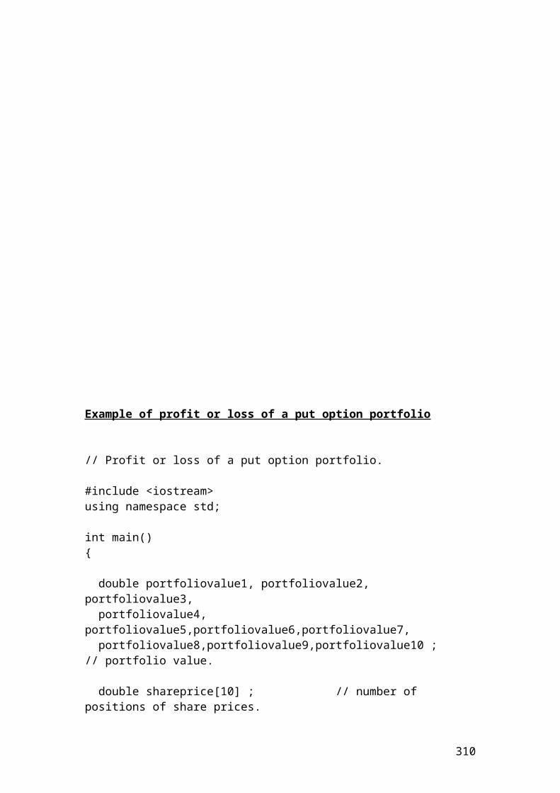
+(1-riskprobofupmove)*putpayoff3i);

putpriceupdownmovestep2 =(disfact*(riskprobofupmove*putpayoff3i)+(1-riskprobofupmove)*putpayoff3ii);

putpricedownmovestep2 =(disfact*(riskprobofupmove*putpayoff3ii)+(1-riskprobofupmove)*putpayoffdownmovestep3);

double putpriceupmovestep1;double putpricedownmovestep1;

putpriceupmovestep1 = (disfact*(riskprobofupmove*putpriceupmovestep2)+(1-riskprobofupmove)*putpriceupdownmovestep2);

putpricedownmovestep1=(disfact*(riskprobofupmove*putpriceupdownmovestep2)+(1-riskprobofupmove)*putpricedownmovestep2);

double putpricestep0;

putpricestep0= (disfact*(riskprobofupmove*putpriceupmovestep1)+(1-riskprobofupmove)*putpricedownmovestep1);

//Calculation of put price based on the Black and Scholes model.

double putPrice;

putPrice = Put (S,K,r,q,T,sig);

//Output functions.

cout.setf(ios::fixed); cout.setf(ios::showpoint); cout.precision(2); cout<<"Steps expressed in years:"<< dt<<endl;cout<<"Multiplier of upmove:"<< u<<endl;cout<<"Multiplier of downmove:"<< d<<endl;cout<<" Discount factor:"<<disfact<<endl;cout<< "Risk neutral probability of upmove:"<<riskprobofupmove<<endl;cout<<"Put payoff upmove step[3]:"<<putpayoffupmovestep3<<endl;cout<<"Put payoff [3i]:"<<putpayoff3i<<endl;cout<<"Put payoff [3ii]:"<<putpayoff3ii<<endl;cout<<"Put payoff downmove step[3]:"<<putpayoffdownmovestep3<<endl;cout<<"Put price upmove step[2]:"<<putpriceupmovestep2<<endl;cout<<"Put price updownmove step[2]:"<<putpriceupdownmovestep2<<endl;cout<<"Put price downmove step[2]:"<<putpricedownmovestep2<<endl;cout<<"Put price upmove step[1]:"<<putpriceupmovestep1<<endl;cout<<"Put price downmove step[1]:"<<putpricedownmovestep1<<endl;cout<<"Put price step[0]:"<<putpricestep0<<endl;cout<<" Black and Scholes put price:"<<putPrice<<endl;

310

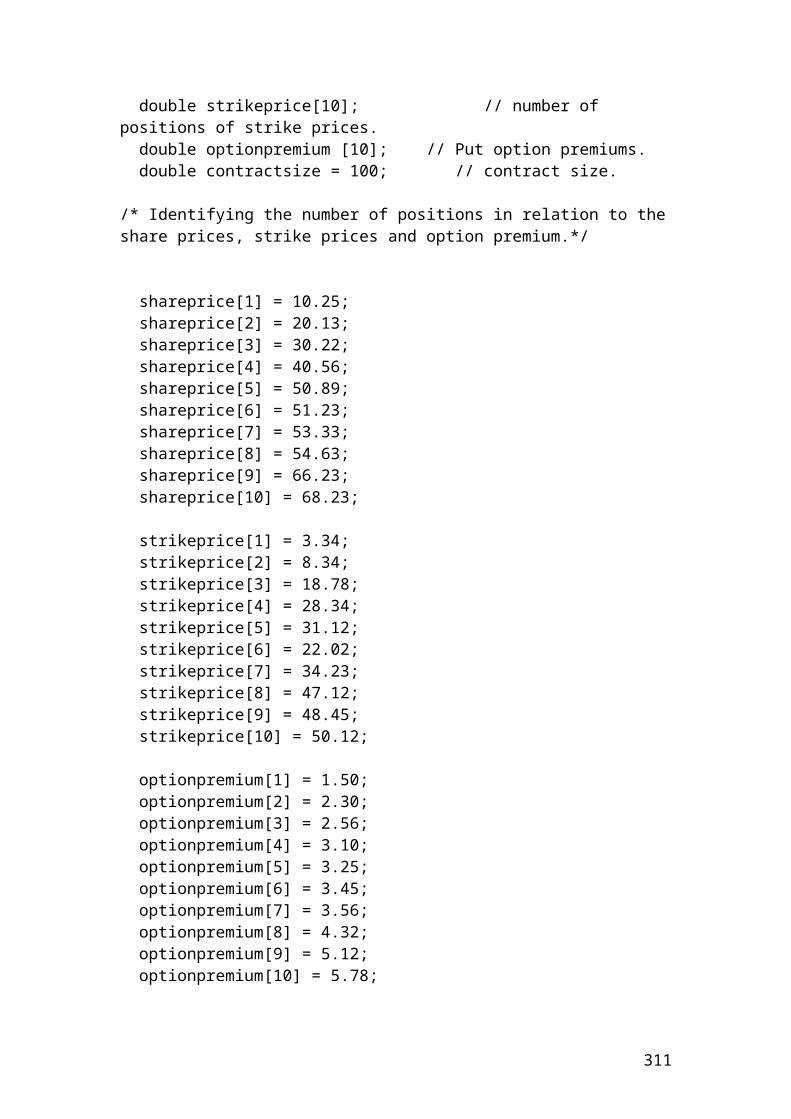
system ("PAUSE");return 0;}

Output

The figures are expressed in USD. After compiling and debugging , the DOS window or console will open and display the following results:

Steps expressed in years: 0.17Multiplier of upmove: 1.08Multiplier of downmove: 0.92Disount factor: 1.00Risk neutral probability of upmove: 0.50Put payoff upmove step [3]: 0.00Put payoff [3i]: 5.86Put payoff [3ii]: 15.53Put payoff downmove step [3]: 23.73Put price upmove step [2]: 2.93Put price updownmove step [2]: 10.69Put price downmove step [2]: 19.61Put price upmove step [1]: 6.80Put price downmove step [1]: 15.13Put price step [0]: 10.95Black and Scholes put price: 10.79Press any key to continue …

311

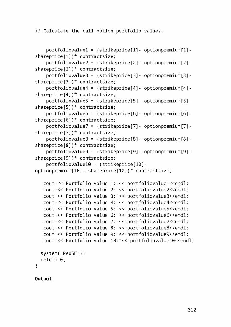
Calculate the interest rates of an option bond based on a two – period binomial tree. The risk – neutral probability of an up and down move in the interest rate tree is always 50% or 0.5

/* Calculate the interest rates of an option bond using binomial 2 steps tree. */

#include <iostream> #include<cmath> using namespace std;

int main() { double BP = 100; // bond price double strike = 100; // strike price double AC = 7; // annual coupon double T = 0.5; // maturity double sig = 0.3; // volatility double r = 4; // interest rate expressed in percentage. // Identify the variables. u = multiplier of upmove. //d = multiplier of downmove. dt = steps expressed in years. double u; double d; double dt; double p = 0.5; // risk -neutral probability of upmove. const int n = 2; // Identify two steps binomial tree. // Insert the mathematical formulas. dt = T/n; u = exp(sig*sqrt(dt)); d = 1/u;

// Identify the interest rates variables. double interestrate0;double interestrate1i;double interestrate1ii;double interestrate2i;double interestrate2ii;double interestrate2iii;

312

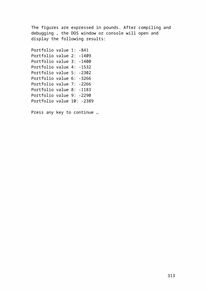
// Insert the mathematical formulas.

interestrate0 = r ;interestrate1i = r * u;interestrate1ii = r * d;interestrate2i = r * pow(u,2); interestrate2ii= r*u*d;interestrate2iii = r* pow(d,2);

cout.setf(ios::fixed); cout.setf(ios::showpoint); cout.precision(2); cout<<"Steps expressed in years:"<< dt<<endl;cout<<"Multiplier of upmove:"<< u<<endl;cout<<"Multiplier of downmove:"<< d<<endl;cout<<" Interest rate [0]:"<<interestrate0<<endl; cout<<" Interest rate upmove [1i]:"<<interestrate1i<<endl; cout<<" Interest rate downmove[1ii]:"<<interestrate1ii<<endl; cout<<" Interest rate upmove [2i]:"<<interestrate2i<<endl; cout<<" Interest rate up and downmove [2ii]:"<<interestrate2ii<<endl; cout<<" Interest rate downmove [2iii]:"<<interestrate2iii<<endl;

system ("PAUSE");return 0;}

Output

The figures are expressed in percentages. After compiling and debugging , the DOS window or console will open and display the following results:

Steps expressed in years: 0.25Multiplier of upmove: 1.16Multiplier of downmove: 0.86Interest rate [0]: 4.00Interest rate upmove [1i]: 4.65Interest rate downmove [1ii]: 3.44Interest rate upmove [2i]: 5.40Interest rate up and downmove[2ii]: 4.00Interest rate downmove [2iii]: 2.96Press any key to continue …

313

Calculate the bond prices of an option based on different interest rates using a binomial 2 steps tree

/* Calculate the bond prices of an optionbased on different interest rates using a binomial 2 steps tree. */

#include <iostream> #include<cmath> using namespace std;

int main() { double BP = 100; // bond price double strike =100; // strike price double AC = 7; // annual coupon double T = 0.5; // maturity double sig = 0.3; // volatility double r = 4; // interest rate // Identify the variables. u = multiplier of upmove. //d = multiplier of downmove. dt = steps expressed in years. double u; double d; double dt; double p = 0.5; // risk -neutral probability of up and down move. const int n = 2; // Identify two steps binomial tree. // Insert the mathematical formulas. dt = T/n; u = exp(sig*sqrt(dt)); d = 1/u;

// Identify the bond price variables. double bondPrice0;double bondPrice1i;double bondPrice1ii;double bondPrice2i;double bondPrice2ii;

314

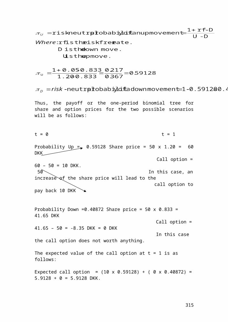
double bondPrice2iii;

// Identify the discounted interest rates.double disinterest0 = 1.04;double disinterest1i = 1.0465;double disinterest1ii = 1.0344;double disinterest2i = 1.054;double disinterest2ii = 1.04;double disinterest2iii = 1.0296;

// Insert the mathematical formulas. It is a backward induction methodology.

bondPrice2i = (BP+AC)*(1/disinterest2i) ; bondPrice2ii=(BP+AC)*(1/disinterest2ii) ;bondPrice2iii = (BP+AC)*(1/disinterest2iii);bondPrice1i = ((((bondPrice2i+AC)*p)+(bondPrice2ii+AC)*p)/disinterest1i);bondPrice1ii = ((((bondPrice2ii+AC)*p)+(bondPrice2iii+AC)*p)/disinterest1ii);bondPrice0 = ((((bondPrice1i+ AC)*p)+(bondPrice1ii+ AC)*p)/disinterest0);

cout.setf(ios::fixed); cout.setf(ios::showpoint); cout.precision(2); cout<<"Steps expressed in years:"<< dt<<endl;cout<<"Multiplier of upmove:"<< u<<endl;cout<<"Multiplier of downmove:"<< d<<endl;

cout<<" Bond price upmove [2i]:"<<bondPrice2i<<endl; cout<<" Bond price up and downmove [2ii]:"<<bondPrice2ii<<endl; cout<<" Bond price downmove [2iii]:"<<bondPrice2iii<<endl; cout<<" Bond price upmove [1i]:"<<bondPrice1i<<endl; cout<<" Bond price downmove[1ii]:"<<bondPrice1ii<<endl;cout<<" Bond price [0]:"<<bondPrice0<<endl; system ("PAUSE");return 0;}

Output

The figures are expressed in pounds. After compiling and debugging , the DOS window or console will open and display the following results:

Steps expressed in years: 0.25Multiplier of upmove: 1.16Multiplier of downmove: 0.86Bond price upmove [2i]: 101.52Bond price up and downmove[2ii]: 102.88Bond price downmove [2iii]: 103.92Bond price upmove [1i]: 104.35Bond price downmove [1ii]: 106.73Bond price [0]: 108.21

315

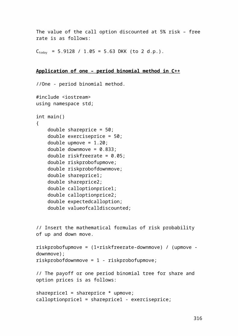
Press any key to continue …

Calculate the bond call option prices based on different interest rates using a binomial 2 steps tree

/* Calculate the bond call option prices based on different interest rates using a binomial 2 steps tree. */

#include <iostream> #include<cmath> using namespace std; int main() { double BP = 100; // bond price double strike = 100; // strike price double AC = 7; // annual coupon expressed in % double T = 0.5; // maturity double sig = 0.3; // volatility double r = 4; // interest rate // Identify the variables. u = multiplier of upmove. //d = multiplier of downmove. dt = steps expressed in years. double u; double d; double dt; double p = 0.5; // risk -neutral probability of up and down move. const int n = 2; // Identify two steps binomial tree. // Insert the mathematical formulas. dt = T/n; u = exp(sig*sqrt(dt)); d = 1/u;

// Identify the bond price variables. double bondPrice0;double bondPrice1i;double bondPrice1ii;double bondPrice2i;double bondPrice2ii;double bondPrice2iii;

// Identify the discounted interest rates.

316

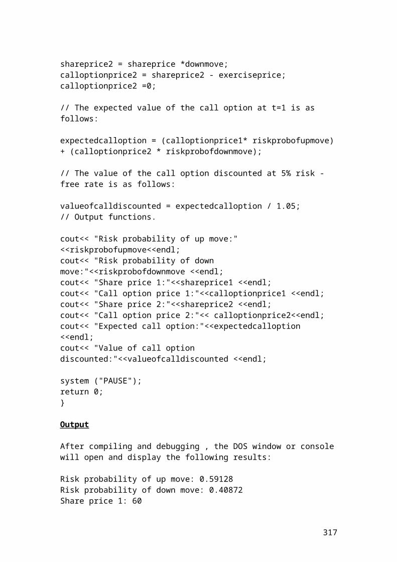
double disinterest0 = 1.04;double disinterest1i = 1.0465;double disinterest1ii = 1.0344;double disinterest2i = 1.054;double disinterest2ii = 1.04;double disinterest2iii = 1.0296;

// Insert the mathematical formulas. It is a backward induction methodology.

bondPrice2i = (BP+AC)*(1/disinterest2i) ; bondPrice2ii=(BP+AC)*(1/disinterest2ii) ;bondPrice2iii = (BP+AC)*(1/disinterest2iii);bondPrice1i = ((((bondPrice2i+AC)*p)+(bondPrice2ii+AC)*p)/disinterest1i);bondPrice1ii = ((((bondPrice2ii+AC)*p)+(bondPrice2iii+AC)*p)/disinterest1ii);bondPrice0 = ((((bondPrice1i+ AC)*p)+(bondPrice1ii+ AC)*p)/disinterest0);

double callPriceUpmovestep2i;double callPriceUpdownmovestep2ii; double callPriceDownmovestep2iii;double callPriceUpmovestep1i;double callPriceDownmovestep1ii;double callPricestep0;

callPriceUpmovestep2i = bondPrice2i - strike;callPriceUpdownmovestep2ii = bondPrice2ii - strike; callPriceDownmovestep2iii = bondPrice2iii - strike;callPriceUpmovestep1i= (((callPriceUpmovestep2i*p)+(callPriceUpdownmovestep2ii*p))/disinterest1i);

callPriceDownmovestep1ii= (((callPriceUpdownmovestep2ii*p)+(callPriceDownmovestep2iii*p))/disinterest1ii);

callPricestep0= (((callPriceUpmovestep1i*p)+(callPriceDownmovestep1ii*p))/disinterest0);

cout.setf(ios::fixed); cout.setf(ios::showpoint); cout.precision(2); cout<<"Steps expressed in years:"<< dt<<endl;cout<<"Multiplier of upmove:"<< u<<endl;cout<<"Multiplier of downmove:"<< d<<endl;

cout<<" Bond price upmove [2i]:"<<bondPrice2i<<endl; cout<<" Bond price up and downmove [2ii]:"<<bondPrice2ii<<endl; cout<<" Bond price downmove [2iii]:"<<bondPrice2iii<<endl; cout<<" Bond price upmove [1i]:"<<bondPrice1i<<endl; cout<<" Bond price downmove[1ii]:"<<bondPrice1ii<<endl;cout<<" Bond price [0]:"<<bondPrice0<<endl;

cout<<"Call price upmove step [2i]:"<<callPriceUpmovestep2i<<endl;

317

cout<<"Call price updownmove step [2ii]:"<<callPriceUpdownmovestep2ii<<endl; cout<<"Call price downmove step [2iii]:"<<callPriceDownmovestep2iii<<endl;cout<<"Call price upmove step [1i]:"<<callPriceUpmovestep1i<<endl; cout<<"Call price downmove step [1ii]:"<<callPriceDownmovestep1ii<<endl;cout<<"Call price step [0]:"<<callPricestep0<<endl;

system ("PAUSE");return 0;}

Output

The figures are expressed in pounds. After compiling and debugging , the DOS window or console will open and display the following results:

Steps expressed in years: 0.25Multiplier of upmove: 1.16Multiplier of downmove: 0.86Bond price upmove [2i]: 101.52Bond price up and downmove[2ii]: 102.88Bond price downmove [2iii]: 103.92Bond price upmove [1i]: 104.35Bond price downmove [1ii]: 106.73Bond price [0]: 108.21Call price upmove step [2i]: 1.52Call price updownmove step [2ii]: 2.88Call price downmove step [2iii]: 3.92Call price upmove step [1i]: 2.10Call price downmove step [1ii]: 3.29Call price step [0]: 2.59Press any key to continue …

318

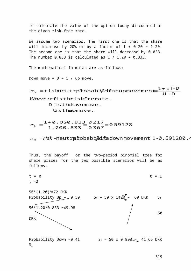
Calculate the bond put option prices based on different interest rates using a binomial 2 steps tree

/* Calculate the bond put option prices based on different interest rates using a binomial 2 steps tree. */

#include <iostream> #include<cmath> using namespace std; int main() { double BP = 100; // bond price double strike = 102; // strike price double AC = 7; // annual coupon expressed in % double T = 0.5; // maturity double sig = 0.3; // volatility double r = 4; // interest rate // Identify the variables. u = multiplier of upmove. //d = multiplier of downmove. dt = steps expressed in years. double u; double d; double dt; double p = 0.5; // risk -neutral probability of up and down move. const int n = 2; // Identify two steps binomial tree. // Insert the mathematical formulas. dt = T/n; u = exp(sig*sqrt(dt)); d = 1/u;

// Identify the bond price variables. double bondPrice0;double bondPrice1i;double bondPrice1ii;double bondPrice2i;double bondPrice2ii;double bondPrice2iii;

// Identify the discounted interest rates.

319

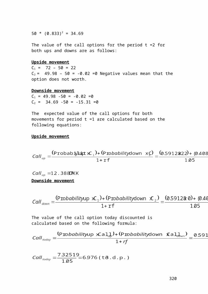
double disinterest0 = 1.04;double disinterest1i = 1.0465;double disinterest1ii = 1.0344;double disinterest2i = 1.054;double disinterest2ii = 1.04;double disinterest2iii = 1.0296;

// Insert the mathematical formulas. It is a backward induction methodology.

bondPrice2i = (BP+AC)*(1/disinterest2i) ; bondPrice2ii=(BP+AC)*(1/disinterest2ii) ;bondPrice2iii = (BP+AC)*(1/disinterest2iii);bondPrice1i = ((((bondPrice2i+AC)*p)+(bondPrice2ii+AC)*p)/disinterest1i);bondPrice1ii = ((((bondPrice2ii+AC)*p)+(bondPrice2iii+AC)*p)/disinterest1ii);bondPrice0 = ((((bondPrice1i+ AC)*p)+(bondPrice1ii+ AC)*p)/disinterest0);

double putPriceUpmovestep2i;double putPriceUpdownmovestep2ii; double putPriceDownmovestep2iii;double putPriceUpmovestep1i;double putPriceDownmovestep1ii;double putPricestep0;

putPriceUpmovestep2i = strike - bondPrice2i ;putPriceUpdownmovestep2ii = strike - bondPrice2ii; putPriceUpdownmovestep2ii = 0; // the put option has no intrinsic value. It is

//negative so, it has zero value.

putPriceDownmovestep2iii = strike - bondPrice2iii;putPriceDownmovestep2iii =0; // the put option has no intrinsic value. It is

//negative so, it has zero value.

putPriceUpmovestep1i= (((putPriceUpmovestep2i*p)+(putPriceUpdownmovestep2ii*p))/disinterest1i);

putPriceDownmovestep1ii= (((putPriceUpdownmovestep2ii*p)+(putPriceDownmovestep2iii*p))/disinterest1ii);

putPricestep0= (((putPriceUpmovestep1i*p)+(putPriceDownmovestep1ii*p))/disinterest0);

cout.setf(ios::fixed); cout.setf(ios::showpoint); cout.precision(2); cout<<"Steps expressed in years:"<< dt<<endl;cout<<"Multiplier of upmove:"<< u<<endl;cout<<"Multiplier of downmove:"<< d<<endl;

320

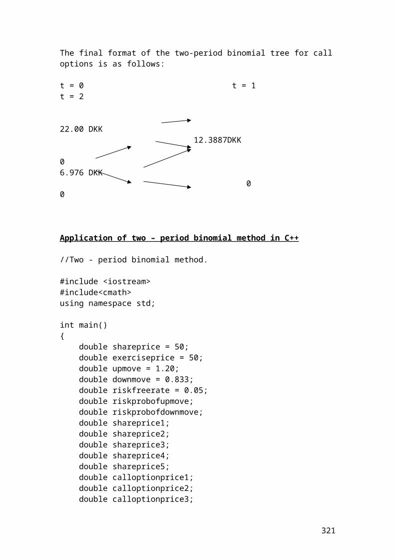
cout<<"Put price upmove step [2i]:"<<putPriceUpmovestep2i<<endl;cout<<"Put price updownmove step [2ii]:"<<putPriceUpdownmovestep2ii<<endl; cout<<"Put price downmove step [2iii]:"<<putPriceDownmovestep2iii<<endl;cout<<"Put price upmove step [1i]:"<<putPriceUpmovestep1i<<endl; cout<<"Put price downmove step [1ii]:"<<putPriceDownmovestep1ii<<endl;cout<<"Put price step [0]:"<<putPricestep0<<endl;

system ("PAUSE");return 0;}

Output

The figures are expressed in pounds. After compiling and debugging , the DOS window or console will open and display the following results:

Steps expressed in years: 0.25Multiplier of upmove: 1.16Multiplier of downmove: 0.86Put price upmove step [2i]: 0.48Put price updownmove step [2ii]: 0.00Put price downmove step [2iii]: 0.00Put price upmove step [1i]: 0.23Put price downmove step [1ii]: 0.00Put price step [0]: 0.11Press any key to continue …

321

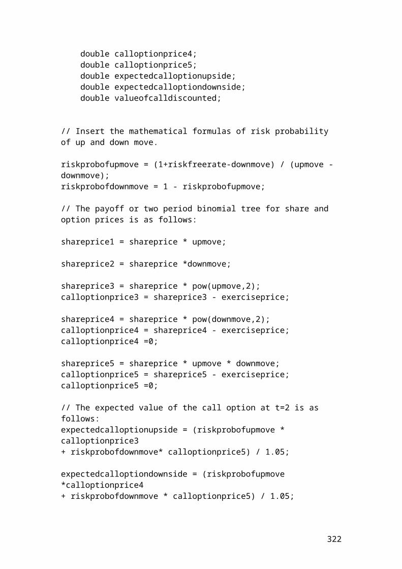
Calculate the caplet option payments based on different interest rates using a binomial 2 steps tree

/* Calculate the caplet values based on an interest rate cap using a binomial 2 steps tree. It is a similar example of a call option on interest rates. The payment is based on the difference between the current interest rate and the cap rate multiplied by the principal and divided by the discounted current interest rate. The buyer receives a payment when the current interest rate exceeds the cap strike price. */

#include <iostream> #include<cmath> using namespace std;

int main() { double strike = 0.02; // cap strike price double principal = 30000000; // principal double T = 0.5; // maturity double sig = 0.3; // volatility double r = 0.04; // interest rate // Identify the variables. u = multiplier of upmove. //d = multiplier of downmove. dt = steps expressed in years. double u; double d; double dt; double p = 0.5; // risk -neutral probability of up and down move. const int n = 2; // Identify two steps binomial tree. // Insert the mathematical formulas. dt = T/n; u = exp(sig*sqrt(dt)); d = 1/u;

// Identify the caplet price variables. double capletPrice0;double capletPrice1i;double capletPrice1ii;

322

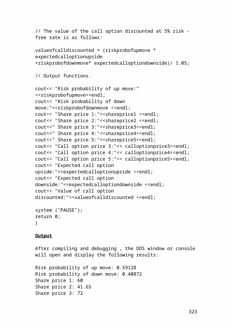
double capletPrice2i;double capletPrice2ii;double capletPrice2iii;

// Identify the interest rates in each node.double interest0 = 0.04;double interest1i = 0.0465;double interest1ii = 0.0344;double interest2i = 0.054;double interest2ii = 0.04;double interest2iii = 0.0296;

// Identify the discounted interest rates.double disinterest0 = 1.04;double disinterest1i = 1.0465;double disinterest1ii = 1.0344;double disinterest2i = 1.054;double disinterest2ii = 1.04;double disinterest2iii = 1.0296;

// Insert the mathematical formulas. It is a backward induction methodology.

capletPrice2i = (principal*(interest2i-strike)/disinterest2i) ; capletPrice2ii = (principal*(interest2ii-strike)/disinterest2ii) ;capletPrice2iii = (principal*(interest2iii-strike)/disinterest2iii) ;capletPrice1i = (((capletPrice2i*p)+(capletPrice2ii*p))/disinterest1i);capletPrice1ii = (((capletPrice2ii*p)+(capletPrice2iii*p))/disinterest1ii);capletPrice0 = (((capletPrice1i*p)+(capletPrice1ii*p))/disinterest0);

cout.setf(ios::fixed); cout.setf(ios::showpoint); cout.precision(2); cout<<"Steps expressed in years:"<< dt<<endl;cout<<"Multiplier of upmove:"<< u<<endl;cout<<"Multiplier of downmove:"<< d<<endl;

cout<<" Caplet price upmove [2i]:"<<capletPrice2i<<endl; cout<<" Caplet price up and downmove [2ii]:"<<capletPrice2ii<<endl; cout<<" Caplet price downmove [2iii]:"<<capletPrice2iii<<endl; cout<<" Caplet price upmove [1i]:"<<capletPrice1i<<endl; cout<<" Caplet price downmove[1ii]:"<<capletPrice1ii<<endl;cout<<" Caplet price [0]:"<<capletPrice0<<endl; system ("PAUSE");return 0;}

323

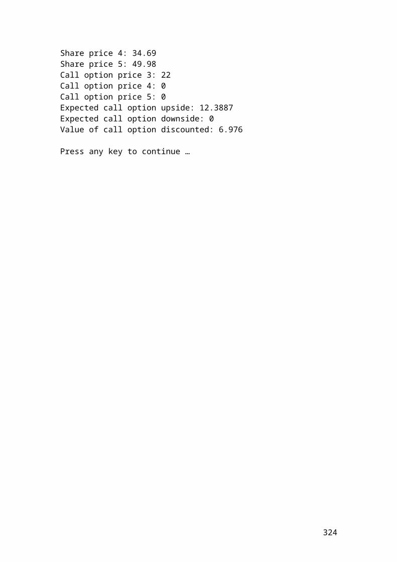
Output

The figures are expressed in pounds. After compiling and debugging , the DOS window or console will open and display the following results:

Steps expressed in years: 0.25Multiplier of upmove: 1.16Multiplier of downmove: 0.86Caplet price upmove [2i]: 967741.94Caplet price up and downmove[2ii]: 576923.08Caplet price downmove [2iii]: 279720.28Caplet price upmove [1i]: 738014.82Caplet price downmove [1ii]: 414077.42Caplet price [0]: 553890.50Press any key to continue …

324

Calculate the floorlet option payments based on different interest rates using a binomial 2 steps tree

/* Calculate the floorlet values based on an interest rate floor using a binomial 2 steps tree. It is a similar example of a put option on interest rates. It protects the holder from declining interest rates. The payment is based on the difference between the floor rate and the current interest rate multiplied by the principal and divided by the discounted current interest rate. */

#include <iostream> #include<cmath> using namespace std;

int main() { double strike = 0.056; // floor strike price double principal = 30000000; // principal double T = 0.5; // maturity double sig = 0.3; // volatility double r = 0.04; // interest rate // Identify the variables. u = multiplier of upmove. //d = multiplier of downmove. dt = steps expressed in years. double u; double d; double dt; double p = 0.5; // risk -neutral probability of up and down move. const int n = 2; // Identify two steps binomial tree. // Insert the mathematical formulas. dt = T/n; u = exp(sig*sqrt(dt)); d = 1/u;

// Identify the floorlet price variables. double floorletPrice0;double floorletPrice1i;double floorletPrice1ii;

325

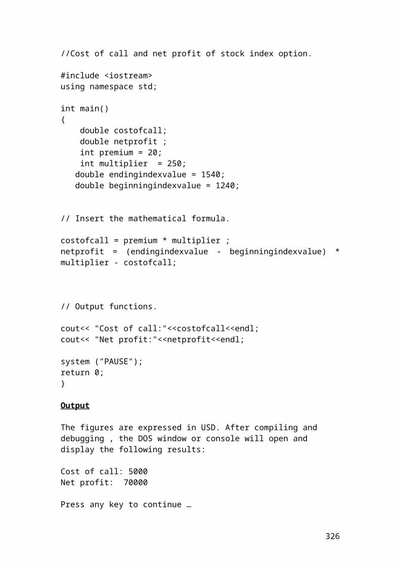
double floorletPrice2i;double floorletPrice2ii;double floorletPrice2iii;

// Identify the interest rates in each node.double interest0 = 0.04;double interest1i = 0.0465;double interest1ii = 0.0344;double interest2i = 0.054;double interest2ii = 0.04;double interest2iii = 0.0296;

// Identify the discounted interest rates.double disinterest0 = 1.04;double disinterest1i = 1.0465;double disinterest1ii = 1.0344;double disinterest2i = 1.054;double disinterest2ii = 1.04;double disinterest2iii = 1.0296;

// Insert the mathematical formulas. It is a backward induction methodology.

floorletPrice2i = (principal*(strike - interest2i)/disinterest2i) ; floorletPrice2ii = (principal*(strike - interest2ii)/disinterest2ii) ;floorletPrice2iii = (principal*(strike - interest2iii)/disinterest2iii) ;floorletPrice1i = (((floorletPrice2i*p)+(floorletPrice2ii*p))/disinterest1i);floorletPrice1ii = (((floorletPrice2ii*p)+(floorletPrice2iii*p))/disinterest1ii);floorletPrice0 = (((floorletPrice1i*p)+(floorletPrice1ii*p))/disinterest0);

cout.setf(ios::fixed); cout.setf(ios::showpoint); cout.precision(2); cout<<"Steps expressed in years:"<< dt<<endl;cout<<"Multiplier of upmove:"<< u<<endl;cout<<"Multiplier of downmove:"<< d<<endl;

cout<<" Floorlet price upmove [2i]:"<<floorletPrice2i<<endl; cout<<" Floorlet price up and downmove [2ii]:"<<floorletPrice2ii<<endl; cout<<" Floorlet price downmove [2iii]:"<<floorletPrice2iii<<endl; cout<<" Floorlet price upmove [1i]:"<<floorletPrice1i<<endl; cout<<" Floorlet price downmove[1ii]:"<<floorletPrice1ii<<endl;cout<<" Floorlet price [0]:"<<floorletPrice0<<endl; system ("PAUSE");return 0;}

326

Output

The figures are expressed in pounds. After compiling and debugging , the DOS window or console will open and display the following results:

Steps expressed in years: 0.25Multiplier of upmove: 1.16Multiplier of downmove: 0.86Floorlet price upmove [2i]: 56926.00Floorlet price up and downmove[2ii]: 461538.46 Floorlet price downmove [2iii]: 769230.77Floorlet price upmove [1i]: 247713.55Floorlet price downmove [1ii]: 594919.39Floorlet price [0]: 405111.99Press any key to continue …

327

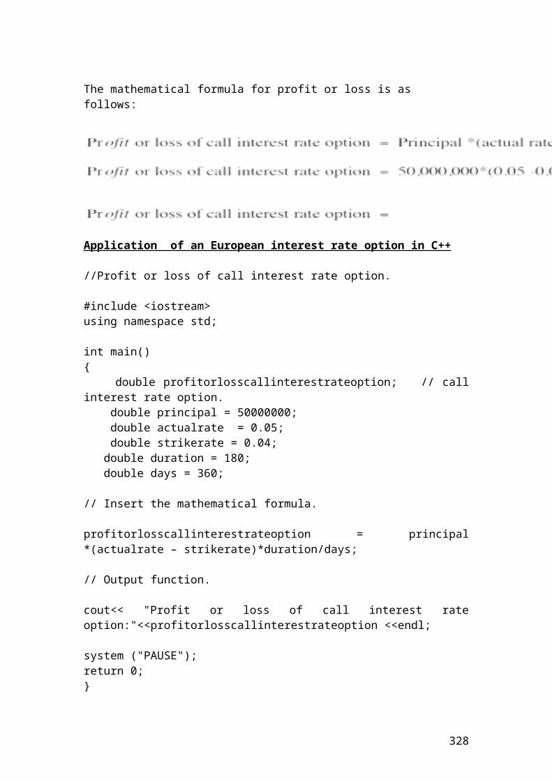
Solution of the above examples

Active return, active risk and information ratio

Active return is the difference in returns between a portfolio and the index or benchmark that is measured.

Active return = rp - rb

Where: rp is the portfolio return. rb is the benchmark or index return.

If the portfolio return is 0.80 and the benchmark return of the index is 0.70 then, the active return is………

Please complete the calculation.

Application of active return in C++

// Active return.

#include <iostream>using namespace std;

int main(){ double portfolioReturn = 0.8; double benchmarkReturn = 0.70; double activeReturn;

// Insert the mathematical formula.

activeReturn = portfolioReturn - benchmarkReturn;

// Output function.cout.setf(ios::fixed); cout.setf(ios::showpoint); cout.precision(2); cout<< "Active return :"<<activeReturn<<endl;system ("PAUSE");return 0;}

328

Output

After compiling and debugging , the DOS window or console will open and display the following results:

Active return : 0.10Press any key to continue …

329

Active risk or tracking error is the standard deviation of the difference of returns between a portfolio and the benchmark or index.

If the portfolio return is 0.80, the number of observations is 10 and the benchmark return of the index is 0.40 then, the active risk is………

Please complete the calculation.

Application of active risk in C++

// Active risk.

#include <iostream>#include <cmath>using namespace std;

int main(){ double portfolioReturn = 0.80; double benchmarkReturn = 0.40; int numberOfObservations = 10; // we use the formula n-1 = 10-1 =9. double activeRisk;

// Insert the mathematical formula.

activeRisk = sqrt(pow(portfolioReturn - benchmarkReturn,2)/9);

// Output function.cout.setf(ios::fixed); cout.setf(ios::showpoint); cout.precision(2); cout<< "Active risk :"<<activeRisk<<endl;

330

system ("PAUSE");return 0;} Output

After compiling and debugging , the DOS window or console will open and display the following results:

Active risk : 0.13Press any key to continue …

331

Information ratio shows the consistency of the fund manager towards the active return. The mathematical formula is as follows:

It could be calculated very easily in Excel software. I will illustrate a simple table with the relevant calculations.

Day rp rb rp - rb

1 0.03 0.02 0.012 0.02 0.014 0.0063 -0.04 0.034 -0.0744 0.05 0.067 -0.0175 0.08 0.012 0.0686 -0.01 -0.056 0.0467 0.07 0.031 0.0398 0.034 0.023 0.0119 -0.021 0.015 -0.03610 0.045 0.001 0.044

Average 0.0258 0.0161Standard deviation

0.043

Source: author’s calculation

By substituting the values that we have found in terms of rp =0.0258, rb = 0.0161 and standard deviation = 0.043 in the following equation we have:

But what is the interpretation of the information ratio of 0.23. It means that the fund manager gained around 23 basis points of active return per unit of active risk. The higher is this number, the better the manager is performing in relation to active risk.

332

Application of information ratio in C++

// Calculation of the information ratio.

#include <iostream>#include<cmath>using namespace std;int main(){

double informationRatio;

double portfolioReturn[10];portfolioReturn[1] = 0.03;portfolioReturn[2] = 0.02;portfolioReturn[3] = -0.04;portfolioReturn[4] = 0.05;portfolioReturn[5] = 0.08;portfolioReturn[6] = -0.01;portfolioReturn[7] = 0.07;portfolioReturn[8] = 0.034;portfolioReturn[9] = -0.021;portfolioReturn[10]= 0.045;

double average1;

// Insert the mathematical formula.

average1 = (portfolioReturn[1] + portfolioReturn[2] + portfolioReturn[3] + portfolioReturn[4] + portfolioReturn[5] + portfolioReturn[6]+ portfolioReturn[7] + portfolioReturn[8] + portfolioReturn[9]+ portfolioReturn[10])/10;

double benchmarkReturn[10];benchmarkReturn[1] = 0.02;benchmarkReturn[2] = 0.014;benchmarkReturn[3] = 0.034;benchmarkReturn[4] = 0.067;benchmarkReturn[5] = 0.012;benchmarkReturn[6] = -0.056;benchmarkReturn[7] = 0.031;benchmarkReturn[8] = 0.023;benchmarkReturn[9] = 0.015;benchmarkReturn[10]= 0.001;

double average2;

// Insert the mathematical formula.

333

average2 = (benchmarkReturn[1] + benchmarkReturn[2] + benchmarkReturn[3] + benchmarkReturn[4] + benchmarkReturn[5] + benchmarkReturn[6]+ benchmarkReturn[7] + benchmarkReturn[8] + benchmarkReturn[9]+ benchmarkReturn[10])/10;

/* Insert the mathematical formulas to calculate the differences between the portfolio and benchmark return and then square it.*/

double diff1, diff2, diff3, diff4, diff5, diff6, diff7, diff8, diff9,diff10;double sumDiff;double average3;

diff1 = portfolioReturn[1] - benchmarkReturn[1]; diff2 = portfolioReturn[2] - benchmarkReturn[2]; diff3 = portfolioReturn[3] - benchmarkReturn[3]; diff4 = portfolioReturn[4] - benchmarkReturn[4]; diff5 = portfolioReturn[5] - benchmarkReturn[5]; diff6 = portfolioReturn[6] - benchmarkReturn[6]; diff7 = portfolioReturn[7] - benchmarkReturn[7]; diff8 = portfolioReturn[8] - benchmarkReturn[8]; diff9 = portfolioReturn[9] - benchmarkReturn[9]; diff10 = portfolioReturn[10] - benchmarkReturn[10];

// Find the sum from the differences.

sumDiff = diff1 + diff2 + diff3 + diff4 + diff5 + diff6 + diff7 + diff8 +diff9 +diff10;

// Find the average from the differences.

average3 = sumDiff /10;

// The square functions.

double diff1Sq, diff2Sq, diff3Sq, diff4Sq, diff5Sq, diff6Sq, diff7Sq, diff8Sq, diff9Sq,diff10Sq;

diff1Sq = pow(portfolioReturn[1] - benchmarkReturn[1]-average3,2); diff2Sq = pow(portfolioReturn[2] - benchmarkReturn[2]-average3,2); diff3Sq = pow(portfolioReturn[3] - benchmarkReturn[3]-average3,2); diff4Sq = pow(portfolioReturn[4] - benchmarkReturn[4]-average3,2); diff5Sq = pow(portfolioReturn[5] - benchmarkReturn[5]-average3,2); diff6Sq = pow(portfolioReturn[6] - benchmarkReturn[6]-average3,2); diff7Sq = pow(portfolioReturn[7] - benchmarkReturn[7]-average3,2); diff8Sq = pow(portfolioReturn[8] - benchmarkReturn[8]-average3,2); diff9Sq = pow(portfolioReturn[9] - benchmarkReturn[9]-average3,2); diff10Sq = pow(portfolioReturn[10] - benchmarkReturn[10]-average3,2);

334

// The sum function of the differences squared.

double sumDiffSquare;

sumDiffSquare = diff1Sq + diff2Sq + diff3Sq + diff4Sq + diff5Sq + diff6Sq + diff7Sq + diff8Sq +diff9Sq +diff10Sq;

// Insert the formula for the sample standard deviation.

double Stdev;

Stdev = sqrt(sumDiffSquare/9);

//Insert the formula for the information ratio.

informationRatio = (average1 -average2)/Stdev;

// Output functions.cout.setf(ios::fixed); cout.setf(ios::showpoint); cout.precision(2); cout<<"Information ratio:"<<informationRatio<<endl;system ("PAUSE");return 0;}

Output

After compiling and debugging , the DOS window or console will open and display the following results:

Information ratio : 0.23Press any key to continue …

Please convert the following exercise in C++ language programming

335

Calculate the balance at the end of the 5th day from changes in the futures prices from 90 to 89, 91, 95, 97, 99. The trader has bought 50 futures contract for settlement in May. The initial margin is $8.

Day Beginning balance

Futures price Gain or loss Ending balance

0 400 90 0 4001 400 89 (50)2 350 91 1003 450 95 2004 650 97 1005 750 99 100

Source: author’s illustration.

Beginning balance = initial margin x number of contracts.Beginning balance = 8 x 50 = $400

Please complete the values of the column ending balance.

Solution

Day Beginning balance

Futures price Gain or loss Ending balance

0 400 90 0 4001 400 89 (50) 3502 350 91 100 4503 450 95 200 6504 650 97 100 7505 750 99 100 850

The ending balance at the 5th day in the margin account will be 850 USD.

Illustration of the volatility smile

336

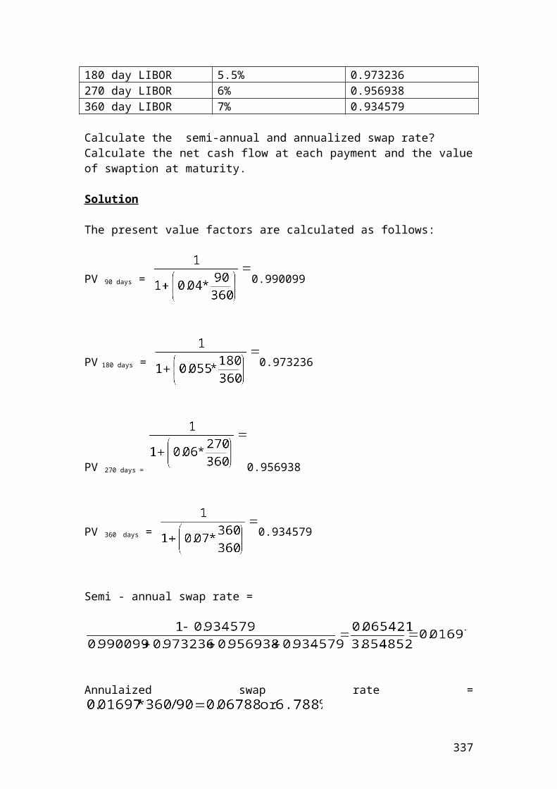
// Illustration of the volatility smile.

#include <iostream>using namespace std;int main(){

// The numerical values are expressed in USD.

double strikePrice[10];strikePrice[1] = 70.54;strikePrice[2] = 74.21;strikePrice[3] = 72.12;strikePrice[4] = 68.34;strikePrice[5] = 65.89;strikePrice[6] = 60.23;strikePrice[7] = 58.36;strikePrice[8] = 80.45;strikePrice[9] = 110.12;strikePrice[10]= 100.34;

// The numerical values are expressed in percentages.

double impliedVolatility[10];impliedVolatility[1] = 22.56;impliedVolatility[2] = 24.16;impliedVolatility[3] = 23.22;impliedVolatility[4] = 21.86;impliedVolatility[5] = 19.36;impliedVolatility[6] = 18.16;impliedVolatility[7] = 22.11;impliedVolatility[8] = 23.22;impliedVolatility[9] = 21.02;impliedVolatility[10] = 24.21;

// Output functions.

cout.setf(ios::fixed); cout.setf(ios::showpoint); cout.precision(2); std::cout<<"Strike price 1: " <<strikePrice[1]<<std::endl;std::cout<<"Strike price 2: " <<strikePrice[2]<<std::endl;std::cout<<"Strike price 3: " <<strikePrice[3]<<std::endl;std::cout<<"Strike price 4: " <<strikePrice[4]<<std::endl;std::cout<<"Strike price 5: " <<strikePrice[5]<<std::endl;std::cout<<"Strike price 6: " <<strikePrice[6]<<std::endl;std::cout<<"Strike price 7: " <<strikePrice[7]<<std::endl;std::cout<<"Strike price 8: " <<strikePrice[8]<<std::endl;

337

std::cout<<"Strike price 9: " <<strikePrice[9]<<std::endl;std::cout<<"Strike price 10: " <<strikePrice[10]<<std::endl;std::cout<<"Implied volatility 1: " <<impliedVolatility[1]<<std::endl;std::cout<<"Implied volatility 2: " <<impliedVolatility[2]<<std::endl;std::cout<<"Implied volatility 3: " <<impliedVolatility[3]<<std::endl;std::cout<<"Implied volatility 4: " <<impliedVolatility[4]<<std::endl;std::cout<<"Implied volatility 5: " <<impliedVolatility[5]<<std::endl;std::cout<<"Implied volatility 6: " <<impliedVolatility[6]<<std::endl;std::cout<<"Implied volatility 7: " <<impliedVolatility[7]<<std::endl;std::cout<<"Implied volatility 8: " <<impliedVolatility[8]<<std::endl;std::cout<<"Implied volatility 9: " <<impliedVolatility[9]<<std::endl;std::cout<<"Implied volatility 10: " <<impliedVolatility[10]<<std::endl;

system ("PAUSE");return 0;}

Output

After compiling and debugging , the DOS window or console will open and display the following results:

StrikePrice 1 = 70.54;StrikePrice 2 = 74.21;StrikePrice 3 = 72.12;StrikePrice 4= 68.34;StrikePrice 5 = 65.89;StrikePrice 6 = 60.23;StrikePrice 7 = 58.36;StrikePrice 8 = 80.45;StrikePrice 9 = 110.12;StrikePrice 10= 100.34;ImpliedVolatility 1 = 22.56;ImpliedVolatility 2 = 24.16;ImpliedVolatility 3 = 23.22;ImpliedVolatility 4 = 21.86;ImpliedVolatility 5 = 19.36;ImpliedVolatility 6 = 18.16;ImpliedVolatility 7 = 22.11;ImpliedVolatility 8 = 23.22;ImpliedVolatility 9 = 21.02;ImpliedVolatility 10 = 24.21;

The chart in Excel will be as follows:

338

Implied volatility smile

0

5

10

15

20

25

30

70.5 74.2 72.1 68.3 65.9 60.2 58.4 80.5 110 100

Strike prices

Impl

ied

vola

tility

Strike priceVolatility

339

Workshop of structured query language in terms of SQL

Both databases are servers that you construct and you can import the data in Excel in terms of pivot table, pivot chart and spreadsheet. To import the data, select data and, then, select import external data and then new SQL server connection or connect to new data source in case of Oracle database. Press open, then, write the name of the server, then, click on the user name and password and input the login and password. Thus, the whole procedure in Excel takes place in the data connection wizard. In addition, you can use the Query wizard to form a SQL query. In this case, you select data, and then import external data. Then, you form new query data. You have the options to choose columns, to filter data, and to sort or order the data in ascending or descending order. Then, by pressing import, you select existing data or data from a new worksheet. In the Query wizard, you have the option to apply multiple filters to sort your data in addition to string operators. It is a function that links Excel reports to SQL query. For example, we create an Excel file with futures contracts for different individuals and companies with monthly, annual returns and profit and loss position. Then, we export this file through new SQL server connection to form and filter different queries in order to form management reports. We then return the data to Excel reports by limiting or extracting the transactions that took place in the futures contract the last 6 months. String operators are used in terms of equals, does not equal, is greater then, is greater than or equal to, is lee than, is less than or equal to. These strings are used as filter value in the drop – down field. These, reports facilitate the derivatives portfolio management. Another example is JP Morgan investment bank that keeps data warehouses of client and company accounts and their related balance. Information related to portfolio management is used as a business intelligence tool in the Query wizard. The Query wizard is a very useful and intermediary tool between Excel and a database for applicants with limited SQL knowledge, as it provides a selection of existing database tables, views, formula creations, and applications of filter conditions.

To install the SQL server 5.0 edition, please check the web site www.mysql.com.Please download the software program MySQL through the set up wizard. Then, choose typical and then install it. Select the standard configuration. Then, select from the start up programs MySQL command line client. This procedure is for more advanced applicants that will insert the code and the syntax to construct the tables, the rows from scratch. In addition, please, download the driver Open Database Connectivity, (ODBC) and then WinSQL from the website www.mysql.com. Select zipped EXE and download it. The trader will get a setup wizard named My SQL connector / ODBC 3.51. Repeat again the same procedure of software installation by clicking on typical and then install it. The WinSQL is not a database server. It is a program to enter statements. It is not our main focus. We are focusing on creating Excel files and then exporting through Query wizard to form a SQL query and then returning back to Excel. For example, the trader would like to construct a Table 1 in a database format with the following information:

Column 1 2 3 4

340

Futures contracts Monthly returns Annual returns Profit / loss position denoted in USD

1 0.02% 2.56% 1,000

2 0.01% 3.01% (500)3 0.03% 4.5% 2,0004 0.021% 6.89% (800)5 0.032% 7.32% 1506 0.01% 5.32% 3697 0.022% 3.21% 3,0008 0.001% 1.45% (243)

Total functionAverage function

Source: author’s illustration

A more experienced trader should be familiar with the syntax of SQL. The basic statements are select, insert, update, delete, create, use and show. For example, the trader uses the command creates Table 1. Then, he/she specifies the name of the columns. For example, column 1 is futures contracts, column 2 is monthly returns, column three is annual returns and column 4 is profit / loss position. Then, in each column he/she specifies the datatype. For example, insert into Table 1 ( column 1, column 2,…… column n). Then, set column 1 = ( value1, value 2,…….value n). Set column 2 = (value 1, value 2,……, value n).

Thus, the syntax will be:

SQL> create Table 1 ( Futures contracts, Monthly returns, Annual returns, Profit / loss position denoted in USD);

Insert into Table 1 ( Futures contracts, monthly returns, annual returns, profit / loss position denoted in USD)Values (1, 0.02%, 2.56%, 1,000);

Insert into Table 1 ( Futures contracts, monthly returns, annual returns, profit / loss position)Values (2, 0.01%, 3,01%, (500);

Please complete the syntax……………………

Then, the trader selects column 2 of monthly returns from Table 1 and, then, he/she uses the where to specify the string condition. For example, monthly returns less than 0.05%.

Then, the trader has the option to perform various functions based on the table. For example, he/she could use the SQL count function, max function, average function, sum function, SQRT function, etc…

As an example, we will show the syntax of the total and average function. The average and total function for monthly returns will be as following:

341

SQL> SELECT AVG( monthly returns)-> FROM Table 1;

SQL> SELECT SUM( monthly returns)-> FROM Table 1;

The trader could use the select function to filter the data that should appear in the management report. For example, by using the following syntax, he/she could view the futures contracts in relation to annual returns and Profit/ loss position denoted in USD. The syntax will be as follows:

SQL> SELECT Futures contract, Annual returns, Profit / loss position denoted in USD;

Thus, the table that he/she should get will be as follows:

Futures contracts Annual returns Profit / loss position denoted in USD

1 2.56% 1,0002 3.01% (500)3 4.5% 2,0004 6.89% (800)5 7.32% 1506 5.32% 3697 3.21% 3,0008 1.45% (243)

Source: author’s illustration

342

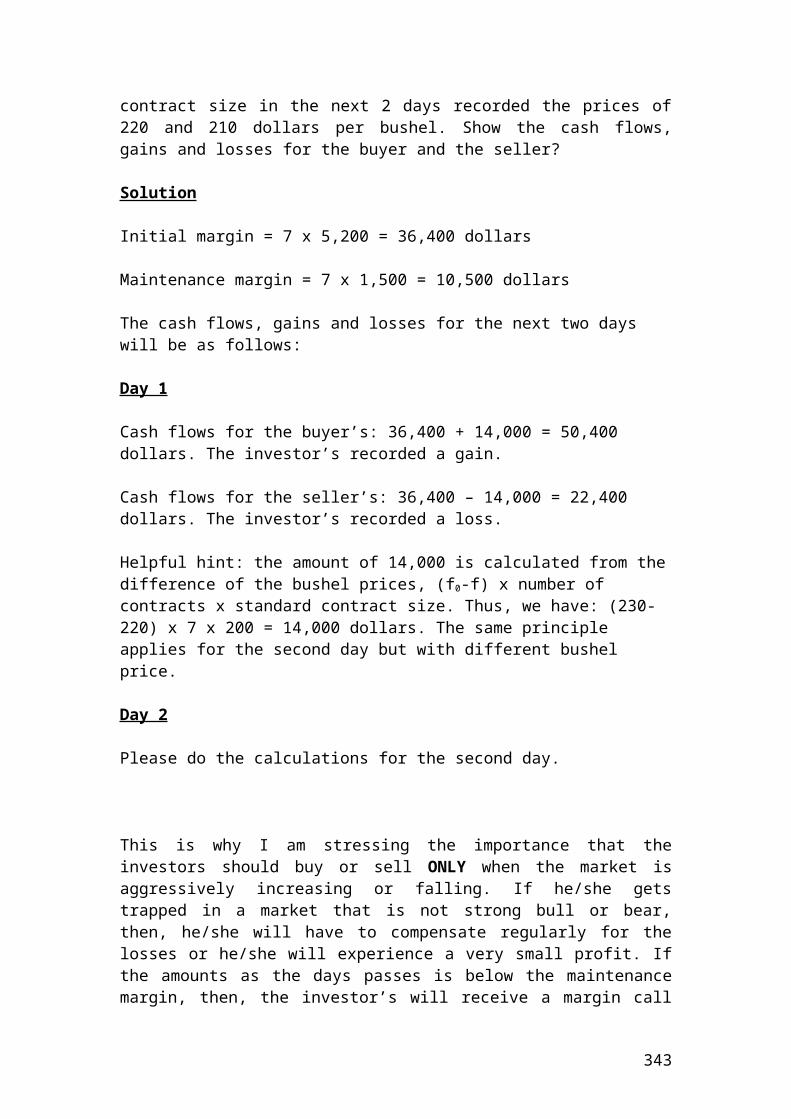
Workshop of language programming in terms of Python 3.4.1

Python version 3.4.1 Shell is very useful language programming for modeling financial derivatives. You can download and donate for the software by visiting the site www.python.org

The Python organization provides free download for the standard package version 3.4.1 Shell for windows or 3.5.

Python includes a math and a statistical library to import functions and perform basic calculations. Part of Python is the scientific Python package IPython. Components of IPyhton are scipy and Numpy. Scipy is used to calculate the cumulative normal distribution and generate random numbers. Numpy is used to construct array in matrix format which are used in statistics, econometrics and data analysis. We will focus on financial derivatives examples. IPython could be downloaded through the continuum analytics Anaconda website. www.continuum.io/downloads

Anaconda includes the standard Python software and the related libraries of IPython. You can download it for Windows, Linux and Macintosh. Please check for compatibility. version and memory space for fitness with your PC.

Please visit the site www.python.org and check the source code for mathematical statistics functions and the math library.

We will focus mainly on Python version 3.4.1 for doing simple calculations. We will use also the scientific Python package IPython to calculate call, put options and their related Greeks.

I have included basic examples that I have used in the Python version 3.4.1 Shell.

Variable names are written with underscore followed by the equal sign. For example,

>>> interest_rate = 0.03Variable names could also be written with small letters adjacent to each other. For example, interestrate = 0.03

It is better to use underscore to separate them and be able to read them clearly.

Another example that we can mention is if we have two variable values such as:>>> c = 5>>> d = 3>>> c+d 8>>> c*d15

343

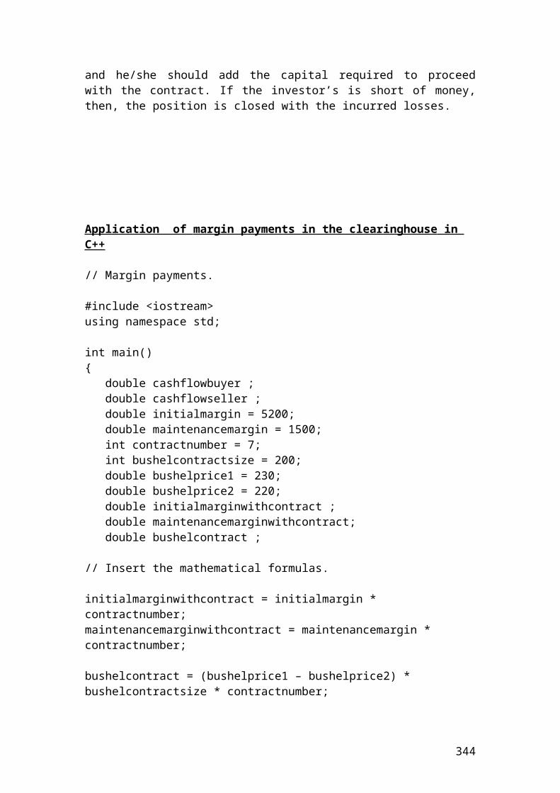
I have included another example that shows the multiplication of two interest rates. Then, I have added to the result the second interest rate by using the function >>>interest_rate2+_. Then, I have rounded the final figure to two decimal places.

>>> interest_rate1 = 0.02>>> interest_rate2 = 0.03>>> interest_rate1*interest_rate20.0006>>> interest_rate2+_0.0306>>> round(_,2)0.03

Powers are performed by using twice the symbol**. For example, >>>3**5 243

If you would like to add comments, then, use the symbol # in front of the variable name.The operator # is used to write comments. For example,

>>>sigma = 0.5 # volatility.

Please distinguish between the integer numbers, (int), such as (1,3,4,5,7) and the fractional ones such as (2.0, 1.3) that are float.

Division is performed using the sign / to get a float result. Use the symbol // to get an integer result without fractional part. For example,>>> 7.0 / 3.0 2.33333

In contrast, >>> 7 // 3 2

Lists could be written as numbers separated by commas in brackets. As an example, please consider the following:

>>> squares = [1,2,4,5]>>> squares[1, 2, 4, 5]

Strings should be enclosed in single or double quotes.

344

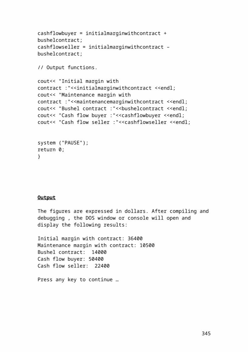
For example, ‘ volatility’

Use the function range to include numbers from 1 to 10. The function is as follows:

>>> range(1,10)[1, 2, 3, 4, 5, 6, 7, 8, 9]

It is worth to mention the headings that should be included in Python version 3.4.1 Shell and IPython.

The headings are as follows:

>>>from statistics import mean, median, variance, or stdev OR

>>>from statistics import*

>>>data = [1.2,3.4]>>> mean(data)>>>2.3>>> median(data)etc…..

If you want to round then use the function round(_,2)

The same logic applies for the math library related to sqrt, log, exp, etc…

from math import log, exp, sqrt OR

>>>from math import *>>> x =25>>> sqrt(x)>>>5

Alternatively, you can do in IPython the same calculations using the numpy function.

import numpy as np

x = np.array([1.2,3.4])

y = np.sum(x)

345

print(y) # It is used to find the sum function

4.6

mean(x)

2.2999999999999998

round(2.2999999999999998,2)

2.3

variance(x)

2.4199999999999999

stdev(x)

1.5556349186104046

Cumulative distribution function and probability density function in IPython. They are used in the derivatives equations

from scipy.stats import norm OR

cumdist = scipy.stats.norm.cdf

Thus, in the option equations we have norm.cdf and norm.pdf.

346

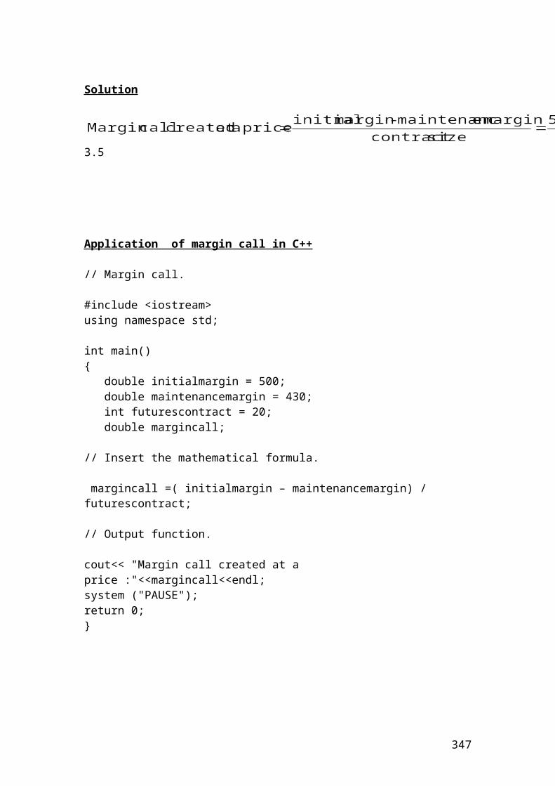
Calculations of European call and put prices and their related Greeks by applying Black and Scholes model, (BSM). I have used the IPython

In[1]: S=70 # share price

In[2]: K=70 # strike price

In[3]: r =0.08 # interest rate

In[4]: q = 0.03 # dividend yield

In[5]: sig = 0.20 # volatility

In[6]: T = 0.5 # life to maturity

In [7]:from math import *

In [8]: d1 = (log(S/K)+((r-q)+sig*sig/2)*T)/(sig*sqrt(T))

In [9]: d1Out[9]: 0.24748737341529162

In [10]: d2 = d1-sig*sqrt(T)

In [11]: d2Out[11]: 0.10606601717798209

In [12]:from scipy.stats import norm

In [13]:call =S*exp(-q*T)*norm.cdf(d1)-K*exp(-r*T)*norm.cdf(d2)

In [14]:callOut[14]: 4.7503181393906004

In [15]:round(_,2)Out[15]: 4.75

In[16]:put = K*exp(-r*T)*norm.cdf(-d2) - S*exp(-q*T)*norm.cdf(-d1)

In [17]:putOut[17]: 3.0477431078388406

In[18]:round(3.0477431078388406,2)Out[18]: 3.05

In[19]: calldelta = exp(-q*T)*norm.cdf(d1)

In[20]: calldeltaOut[20]: 0.58883536203399822

347

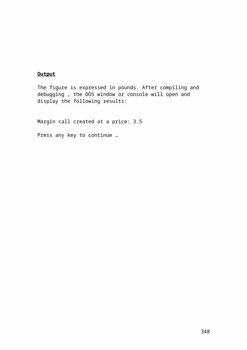
In[21]: round(0.58883536203399822, 2)In[21]: 0.59

In[22]:calltheta = -(S*norm.pdf(d1)*sig*exp(-q*T))/(2*sqrt(T)) +(q*S*norm.cdf(d1)*exp(-q*T)) - (r*K*exp(-r*T)*norm.cdf(d2))

In[23]:callthetaOut[23]: -5.4540860845449357

In[24]: round(-5.4540860845449357,2)Out[24]: -5.45

In[25]:callrho=K*T*exp(-r*T)*norm.cdf(d2)

In[26]:callrhoOut[26]: 18.234078601494634

In[27]:round(18.234078601494634,2)Out[27]: 18.23

In[28]:callandputgamma=(norm.pdf(d1)*exp(-q*T))/(S*sig*sqrt(T))

In[29]:callandputgammaOut[29]: 0.038501916005889703

In[30]:round(_,2)Out[30]: 0.040000000000000001

In[31]:callandputvega=S*sqrt(T)*norm.pdf(d1)*exp(-q*T)

In[32]:callandputvegaOut[32]: 18.865938842885953

In[33]:round(_,2)Out[33]: 18.870000000000001

In[34]:putdelta = exp(-q*T)*(norm.cdf(d1)-1)

In[35]:putdeltaOut[35]: -0.39627657756906448

In[36]:round(_,2)Out[36]: -0.40000000000000002

In[37]:puttheta =-(S*norm.pdf(d1)*sig*exp(-q*T))/(2*sqrt(T)) - (q*S*norm.cdf(-d1)*exp(-q*T)) + (r*K*exp(-r*T)*norm.cdf(-d2))

348

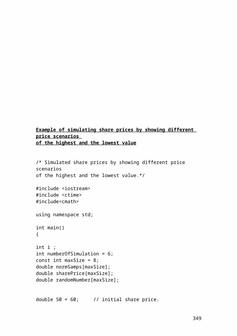
In[38]:putthetaOut[38]: -2.1424002984583579

In[39]:round(-2.1424002984583579,2)Out[39]: -2.14

In[40]:putrho = -K*T*exp(-r*T)*norm.cdf(-d2)

In[41]:putrhoOut[41]: -15.393551768836677

In[42]:round(_,2)Out[42]: -15.390000000000001

349

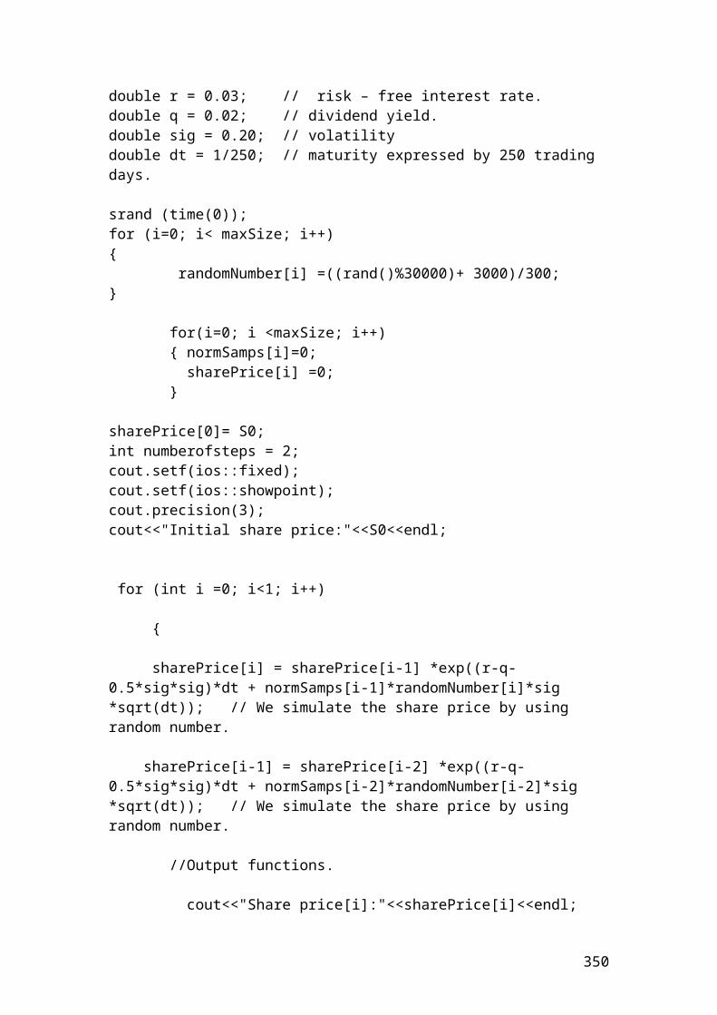
Calculation of the average of stock price returns expressed as percentages

>>> stock_price1 = 10.0>>> stock_price2 = 12.0>>> stock_price3 = 13.0>>> stock_price4 = 14.0>>> stock_price5 = 15.0>>> stock_price6 = 16.0>>> average = (stock_price1+stock_price2+stock_price3+stock_price4+stock_price5+stock_price6)/6>>> average13.333333333333334

Another way to find the average is as follows:

>>> stock_prices = [10.0,12.0,13.0,14.0,15.0,16.0]>>> n=6 # The number of observations.>>> sum(stock_prices)80.0>>> average=sum(stock_prices)/n>>> average13.333333333333334

Finally, you can use the mean function from the statistical library by including the appropriate heading

>>> from statistics import mean>>> stock_prices = [10.0,12.0,13.0,14.0,15.0,16.0]>>> mean(stock_prices)13.333333333333334

Repetition of the previous example to calculate the mean by getting an integer number without decimals. You exclude the decimal point. Returns are expressed as percentages

>>> stock_prices = [10,12,13,14,15,16]>>> n=6 # The number of observations.>>> sum(stock_prices)80>>> average=sum(stock_prices)//n>>> average13

350

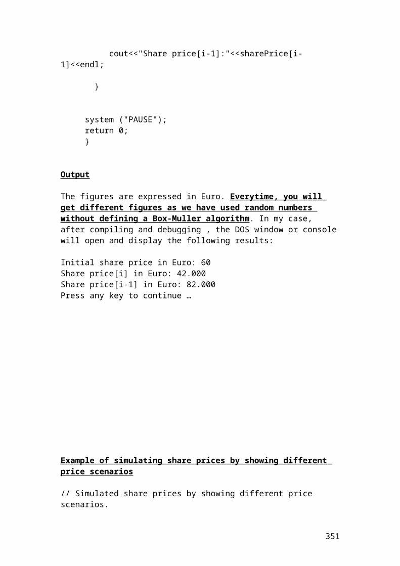
Calculations of the mean and the harmonic mean of share price returns, call option returns, put option returns and index option returns

>>> shareprice_return1 = 0.08>>> shareprice_return2 = 0.05>>> shareprice_return3 = 0.04>>> shareprice_return4 = 0.07>>> shareprice_return5 = 0.02>>> shareprice_return6 = 0.03>>>averageshareprice_returns=(shareprice_return1+shareprice_return2+shareprice_return3+shareprice_return4+shareprice_return5 + shareprice_return6)/6>>> averageshareprice_returns0.04833333333333334

You can use the mean function of share price returns from the statistical library by including the appropriate heading

>>> from statistics import mean>>> shareprice_returns = [0.08,0.05,0.04,0.07,0.02,0.03]>>> mean(shareprice_returns)0.04833333333333334

Calculation of the harmonic mean of share price returns

First of all, you need to find the reciprocals of shareprice_returns, then, find their average and finally take the reciprocal of the answer.

>>> shareprice_return1 = 0.08>>> shareprice_return2 = 0.05>>> shareprice_return3 = 0.04>>> shareprice_return4 = 0.07>>> shareprice_return5 = 0.02>>> shareprice_return6 = 0.03>>> harmonicaverageshareprice_returns = (1/((1/shareprice_return1 + 1/shareprice_return2 + 1/shareprice_return3 + 1/shareprice_return4 + 1/shareprice_return5 + 1/shareprice_return6)/6))>>> harmonicaverageshareprice_returns0.03867996930161166

Use the mean function to calculate call option returns from the statistical library by including the appropriate heading

>>> from statistics import mean>>> calloptionprice_returns = [0.01,0.02,0.04,0.05,0.06,0.06]>>> mean(calloptionprice_returns)0.04

351

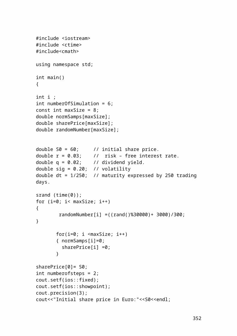
Calculation of the harmonic mean of call option price returns

>>> calloptionprice_return1 = 0.01>>> calloptionprice_return2 = 0.02>>> calloptionprice_return3 = 0.04>>> calloptionprice_return4 = 0.05>>> calloptionprice_return5 = 0.06>>> calloptionprice_return6 = 0.06>>> harmoniccalloptionprice_returns = (1/((1/calloptionprice_return1 + 1/calloptionprice_return2 + 1/calloptionprice_return3 + 1/calloptionprice_return4 + 1/calloptionprice_return5 + 1/calloptionprice_return6)/6))>>> harmoniccalloptionprice_returns0.026277372262773727>>> round(_,2)0.03

Use the mean function to calculate the put option returns from the statistical library by including the appropriate heading

>>> from statistics import mean>>> putoptionprice_returns = [0.03,0.07,0.08,0.09,0.1,0.02]>>> mean(putoptionprice_returns)0.065

Calculation of the harmonic mean of put option price returns

>>> putoptionprice_return1 = 0.03>>> putoptionprice_return2 = 0.07>>> putoptionprice_return3 = 0.08>>> putoptionprice_return4 = 0.09>>> putoptionprice_return5 = 0.1>>> putoptionprice_return6 = 0.02>>> harmonicputoptionprice_returns = (1/((1/putoptionprice_return1 + 1/putoptionprice_return2 + 1/putoptionprice_return3 + 1/putoptionprice_return4 + 1/putoptionprice_return5 + 1/putoptionprice_return6)/6))>>> harmonicputoptionprice_returns0.04572119745993347>>> round(_,2)0.05

352

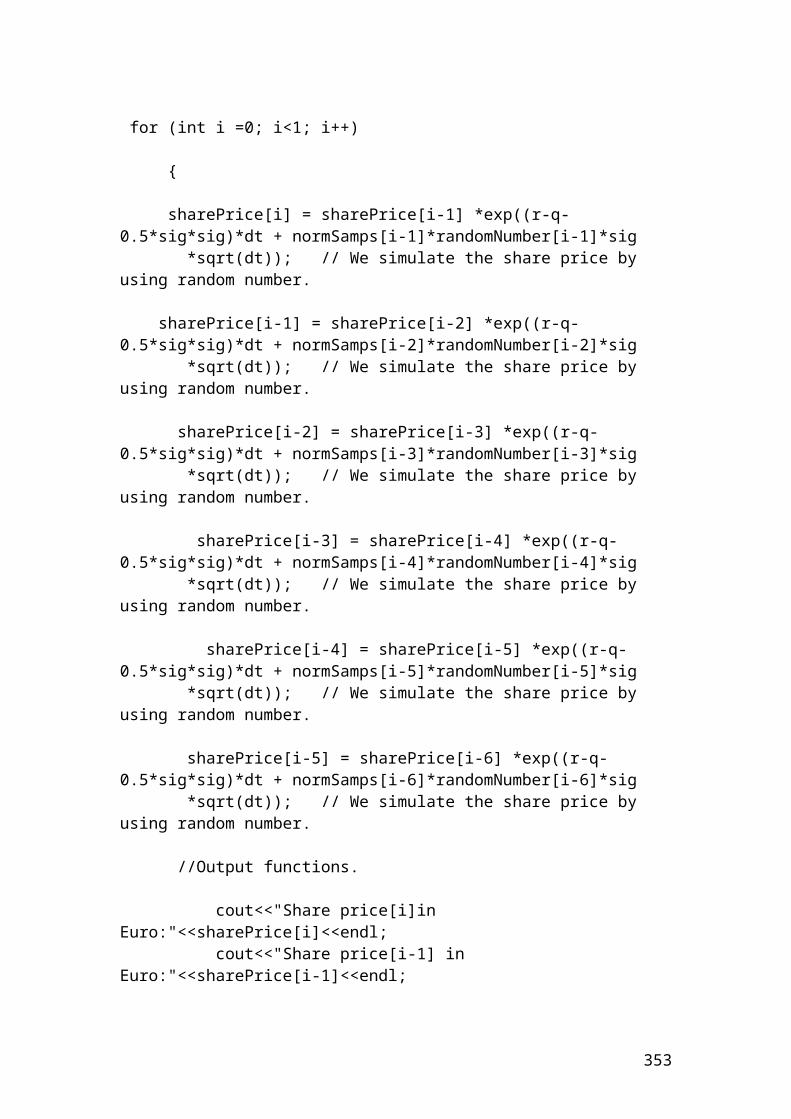
Use the mean function to calculate the index option returns from the statistical library by including the appropriate heading

>>> from statistics import mean>>> indexoptionprice_returns = [0.12,0.23,0.34,0.15,0.2,0.11]>>> mean(indexoptionprice_returns)0.19166666666666668>>> round(_,2)0.19

Calculation of the harmonic mean of index option price returns

>>> indexoptionprice_return1 = 0.12>>> indexoptionprice_return2 = 0.23>>> indexoptionprice_return3 = 0.34>>> indexoptionprice_return4 = 0.15>>> indexoptionprice_return5 = 0.2>>> indexoptionprice_return6 = 0.11>>> harmonicindexoptionprice_returns = (1/((1/indexoptionprice_return1 + 1/indexoptionprice_return2 + 1/indexoptionprice_return3 + 1/indexoptionprice_return4 + 1/indexoptionprice_return5 + 1/indexoptionprice_return6)/6))>>> harmonicindexoptionprice_returns0.1649261839330223>>> round(_,2)0.16

353

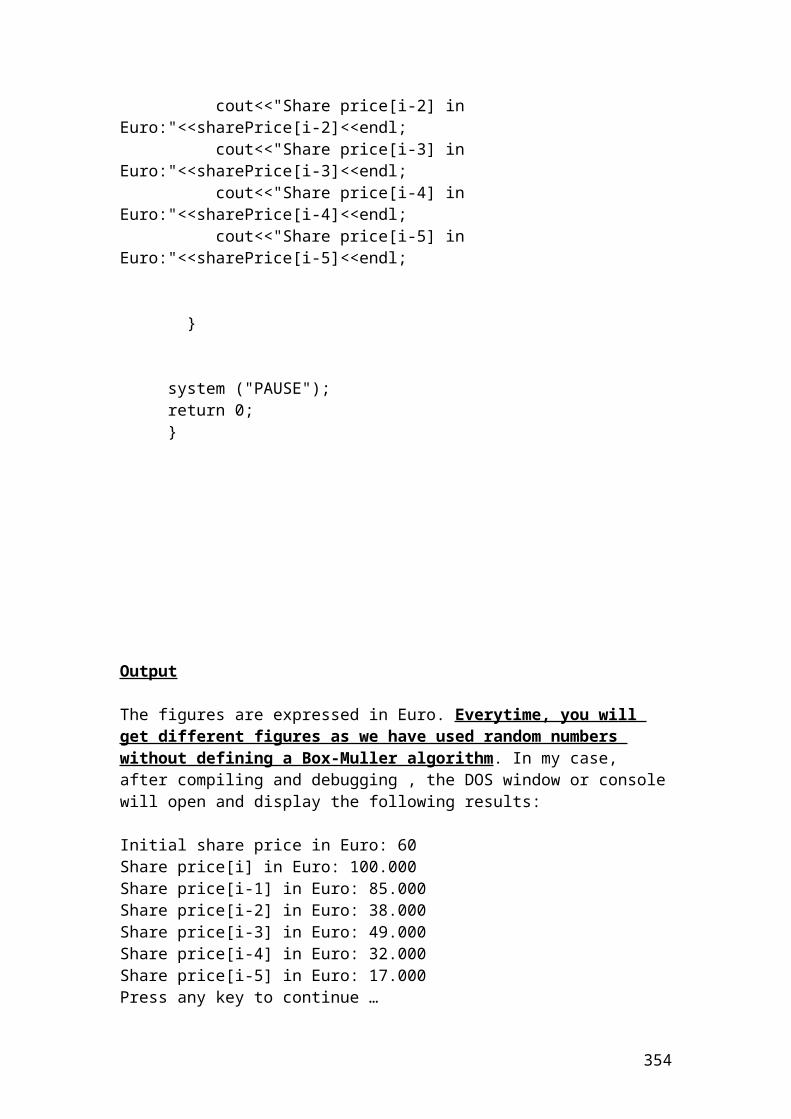
Exercise of how to calculate the payoff of buying a call, a put and the net result or position of your investment position expressed in pounds

Payoff of buying a call

>>> share_price1=105>>> share_price2=110>>> share_price3=120>>> share_price4=130>>> share_price5=140>>> share_price6=150>>> >>> exerciseprice_call1=90>>> exerciseprice_call2=90>>> exerciseprice_call3=90>>> exerciseprice_call4=90>>> exerciseprice_call5=90>>> exerciseprice_call6=90>>> >>> premium_call=14>>> totalnumber_contracts=10>>> totalnumber_shares=100>>> >>> payoffbuy_call1 = (share_price1-(exerciseprice_call1+premium_call))*totalnumber_contracts*totalnumber_shares>>> payoffbuy_call11000>>> payoffbuy_call2 = (share_price2-(exerciseprice_call2+premium_call))*totalnumber_contracts*totalnumber_shares>>> payoffbuy_call26000>>> payoffbuy_call3 = (share_price3-(exerciseprice_call3+premium_call))*totalnumber_contracts*totalnumber_shares>>> payoffbuy_call316000>>> payoffbuy_call4 = (share_price4-(exerciseprice_call4+premium_call))*totalnumber_contracts*totalnumber_shares>>> payoffbuy_call426000>>> payoffbuy_call5 = (share_price5-(exerciseprice_call5+premium_call))*totalnumber_contracts*totalnumber_shares>>> payoffbuy_call536000>>> payoffbuy_call6 = (share_price6-(exerciseprice_call6+premium_call))*totalnumber_contracts*totalnumber_shares>>> payoffbuy_call646000

354

Payoff of buying a put

>>> share_price1=105>>> share_price2=110>>> share_price3=120>>> share_price4=130>>> share_price5=140>>> share_price6=150

>>> exerciseprice_put1=190>>> exerciseprice_put2=190>>> exerciseprice_put3=190>>> exerciseprice_put4=190>>> exerciseprice_put5=190>>> exerciseprice_put6=190

>>> premiumof_put = 9>>> totalnumber_contracts=10>>> totalnumber_shares=100

>>> payoffbuya_put1 = (exerciseprice_put1-share_price1-premiumof_put)*totalnumber_contracts*totalnumber_shares>>> payoffbuya_put176000>>> payoffbuya_put2 = (exerciseprice_put2-share_price2-premiumof_put)*totalnumber_contracts*totalnumber_shares>>> payoffbuya_put271000>>> payoffbuya_put3 = (exerciseprice_put3-share_price3-premiumof_put)*totalnumber_contracts*totalnumber_shares>>> payoffbuya_put361000>>> payoffbuya_put4 = (exerciseprice_put4-share_price4-premiumof_put)*totalnumber_contracts*totalnumber_shares>>> payoffbuya_put451000>>> payoffbuya_put5 = (exerciseprice_put5-share_price5-premiumof_put)*totalnumber_contracts*totalnumber_shares>>> payoffbuya_put541000>>> payoffbuya_put6 = (exerciseprice_put6-share_price6-premiumof_put)*totalnumber_contracts*totalnumber_shares>>> payoffbuya_put631000>>>

355

Net result

>>> netresult1 = payoffbuy_call1 - payoffbuya_put1>>> netresult1-75000>>> netresult2 = payoffbuy_call2 - payoffbuya_put2>>> netresult2-65000>>> netresult3 = payoffbuy_call3 - payoffbuya_put3>>> netresult3-45000>>> netresult4 = payoffbuy_call4 - payoffbuya_put4>>> netresult4-25000>>> netresult5 = payoffbuy_call5 - payoffbuya_put5>>> netresult5-5000>>> netresult6 = payoffbuy_call6 - payoffbuya_put6>>> netresult615000>>>

Exercise

Please calculate the range based on different share prices.

>>> share_price1= 20>>> share_price2 = 30>>> share_price3 = 40>>> share_price4 = 50>>> share_price5 = 60>>> share_price6 = 70>>> range = share_price6 - share_price1>>> range50

356

Calculate the log returns and the average using actual share price returns expressed in pounds

>>> from math import*>>> share_price1 = 14.23>>> share_price2 = 15.67>>> share_price3 = 12.13>>> share_price4 = 11.45>>> share_price5 = 10.11>>> dailyret2 = log(share_price2/share_price1)>>> dailyret20.09639564426616845>>> dailyret3 = log(share_price3/share_price2)>>> dailyret3-0.25606633341197066>>> dailyret4 = log(share_price4/share_price3)>>> dailyret4-0.057691992955710175>>> dailyret5 = log(share_price5/share_price4)>>> dailyret5-0.12446469696786859>>> average = (dailyret2 + dailyret3 + dailyret4 + dailyret5)/4>>> average-0.08545684476734525>>> round(_,2)-0.09>>>

Calculation of the median, the variance and the sample standard deviation of share prices percentage returns

>>> from statistics import*share_prices = [0.1011, 0.1145, 0.1213, 0.1423, 0.1567]>>> median(share_prices)0.1213>>> variance(share_prices)0.0004938920000000002>>> stdev(share_prices)0.022223681063226232>>> round(_,2)0.02

357

Calculation of the geometric average based on percentages of stock prices

>>> stockprice_1 = 10>>> stockprice_2 = 12>>> stockprice_3 = 13>>> stockprice_4 = 14>>> stockprice_5 = 15>>> stockprice_6 = 16

>>> Geometricaverage = (stockprice_1*stockprice_2*stockprice_3*stockprice_4*stockprice_5*stockprice_6)**0.16666>>> Geometricaverage13.17849601334643>>> round(_,2)13.18

Calculation of the geometric average based on percentages of call option price returns

>>> Calloptionpricereturns_1 = 5>>> Calloptionpricereturns_2 = 3>>> Calloptionpricereturns_3 = 2>>> Calloptionpricereturns_4 = 4>>> Calloptionpricereturns_5 = 7>>> Calloptionpricereturns_6 = 8>>> Geometricaverage = (Calloptionpricereturns_1*Calloptionpricereturns_2*Calloptionpricereturns_3*Calloptionpricereturns_4*Calloptionpricereturns_5*Calloptionpricereturns_6)**0.16666>>> Geometricaverage4.3437954197862885>>> round(_,2)4.34

358

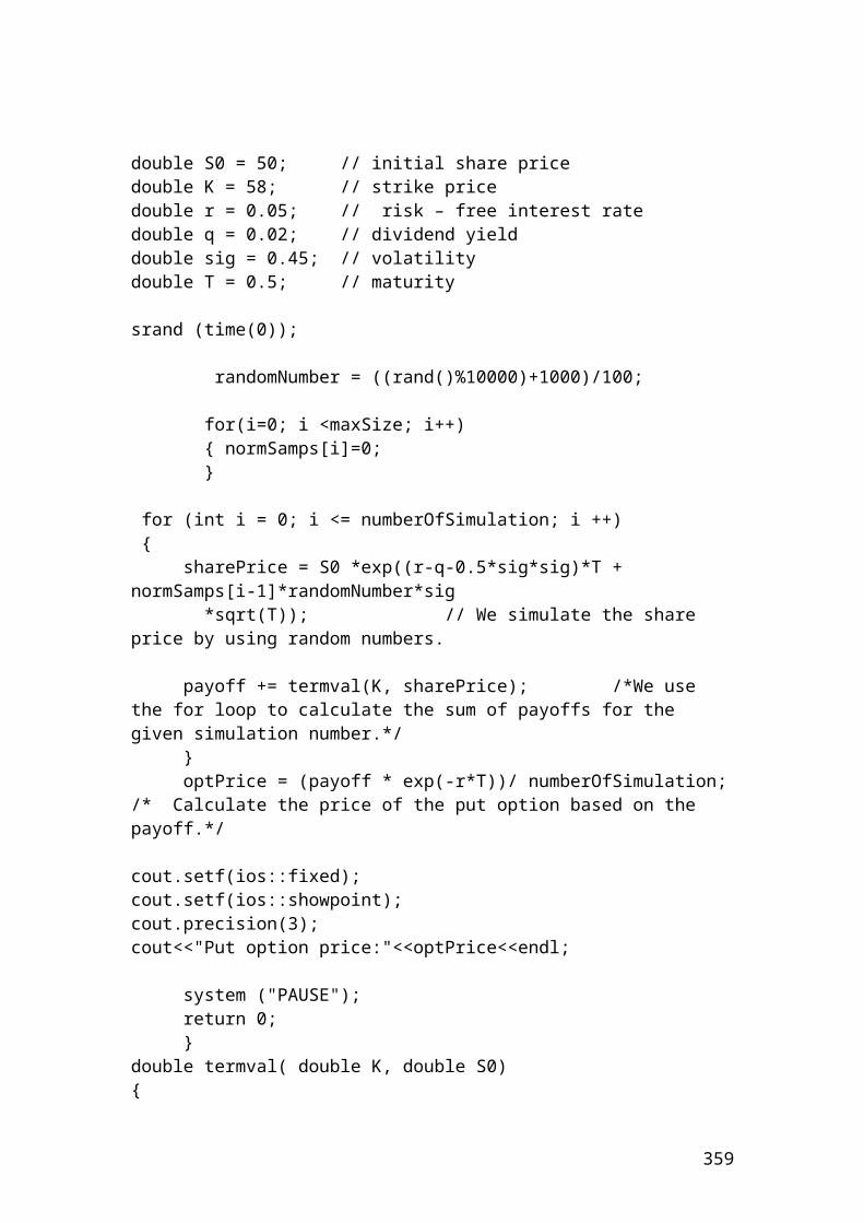
Calculation of the geometric average based on percentages of put option price returns

>>> Putoptionpricereturns_1 = 2>>> Putoptionpricereturns_2 = 3.3>>> Putoptionpricereturns_3 = 2.45>>> Putoptionpricereturns_4 = 4.21>>> Putoptionpricereturns_5 = 7.4>>> Putoptionpricereturns_6 = 4.34>>> Geometricaverage = (Putoptionpricereturns_1*Putoptionpricereturns_2*Putoptionpricereturns_3*Putoptionpricereturns_4*Putoptionpricereturns_5*Putoptionpricereturns_6)**0.16666>>> Geometricaverage3.6024392246983483>>> round(_,1)3.6

359

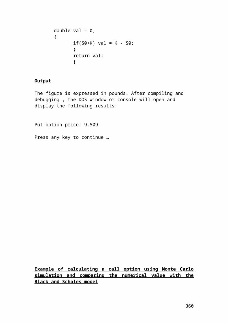
Calculation of the geometric average based on percentages of index option price returns

>>> Indexoptionpricereturns_1 = 2>>> Indexoptionpricereturns_2 = 2.31>>> Indexoptionpricereturns_3 = 2.35>>> Indexoptionpricereturns_4 = 4.51>>> Indexoptionpricereturns_5 = 7.56>>> Indexoptionpricereturns_6 = 4.39>>> Geometricaverage = (Indexoptionpricereturns_1*Indexoptionpricereturns_2*Indexoptionpricereturns_3*Indexoptionpricereturns_4*Indexoptionpricereturns_5*Indexoptionpricereturns_6)**0.16666>>> Geometricaverage3.4286570204871354>>> round(_,2)3.43

360

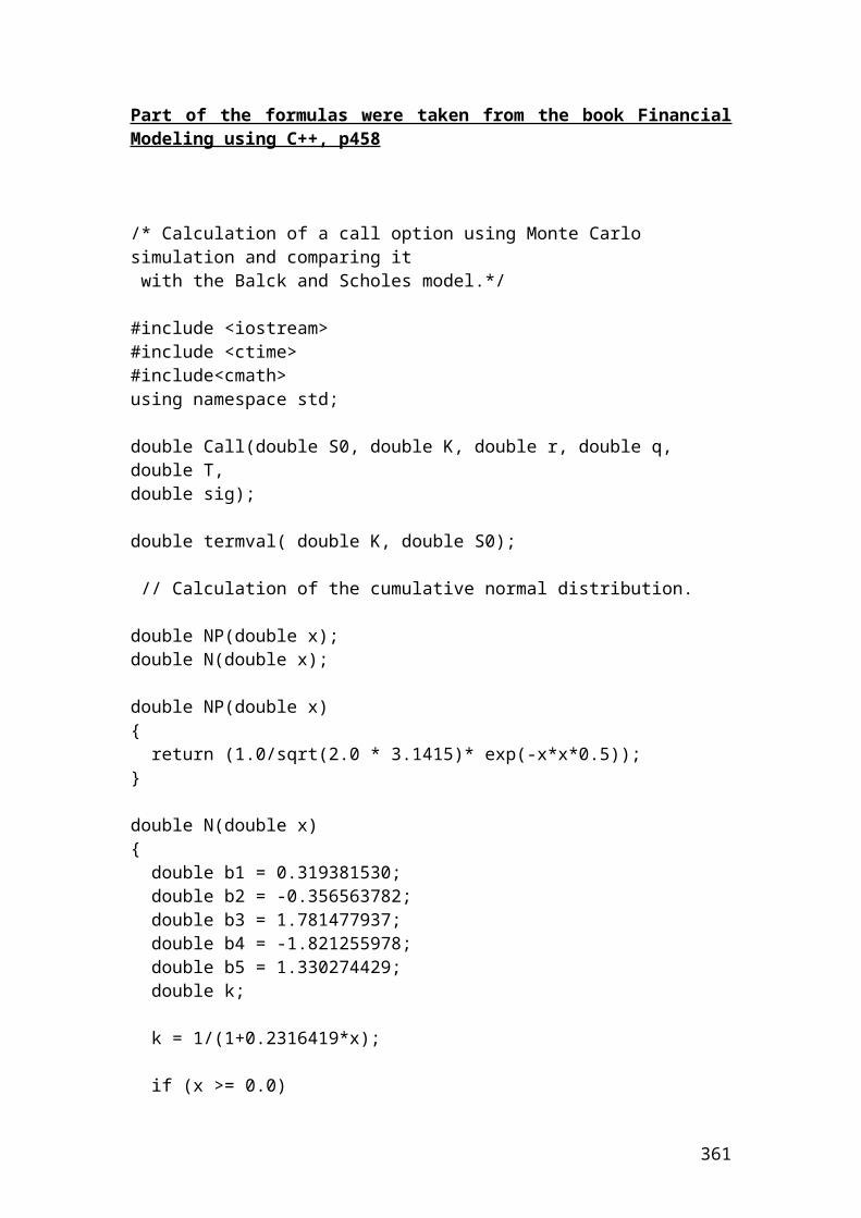
Calculate the portfolio return, the variance and the standard deviation in python for options with different returns and standard deviations

>>> CalloptionAexpectedreturn = 0.6>>> CalloptionAstandarddeviation = 0.2>>> CalloptionAweight = 0.35>>> CorrelationcoefficientbetweenAandB = 0.5>>> CalloptionBexpectedreturn = 0.1>>> CalloptionBstandarddeviation = 0.7>>> CalloptionBweight = 0.45>>> CorrelationcoefficientbetweenBandC = -0.1>>> CalloptionCexpectedreturn = 0.3>>> CalloptionCstandarddeviation = 0.4>>> CalloptionCweight = 0.2>>> CorrelationcoefficientbetweenAandC = -0.4

>>> Portfolioreturn = (CalloptionAexpectedreturn*CalloptionAweight)+(CalloptionBweight*CalloptionBexpectedreturn)+(CalloptionCexpectedreturn*CalloptionCweight)>>> Portfolioreturn0.315>>> round(_,2)0.32

You can omit the brackets from the Portfoliovariance. I have included them to show the different parts.

>>> Portfoliovariance = (CalloptionAweight**2*CalloptionAstandarddeviation**2)+ (CalloptionBweight**2*CalloptionBstandarddeviation**2)+(CalloptionCweight**2*CalloptionCstandarddeviation**2)+(2*CalloptionAweight*CalloptionBweight*CalloptionAstandarddeviation*CalloptionBstandarddeviation*CorrelationcoefficientbetweenAandB)+(2*CalloptionAweight*CalloptionCweight*CorrelationcoefficientbetweenAandC*CalloptionAstandarddeviation*CalloptionCstandarddeviation)+(2*CalloptionBweight*CalloptionCweight*CorrelationcoefficientbetweenBandC*CalloptionBstandarddeviation*CalloptionCstandarddeviation)>>> Portfoliovariance0.12305499999999998>>> round(_,2)0.12

>>> from math import*>>> PortfoliostdDev = sqrt(Portfoliovariance)>>> PortfoliostdDev0.35079196113936245>>> round(_,2)0.35

361

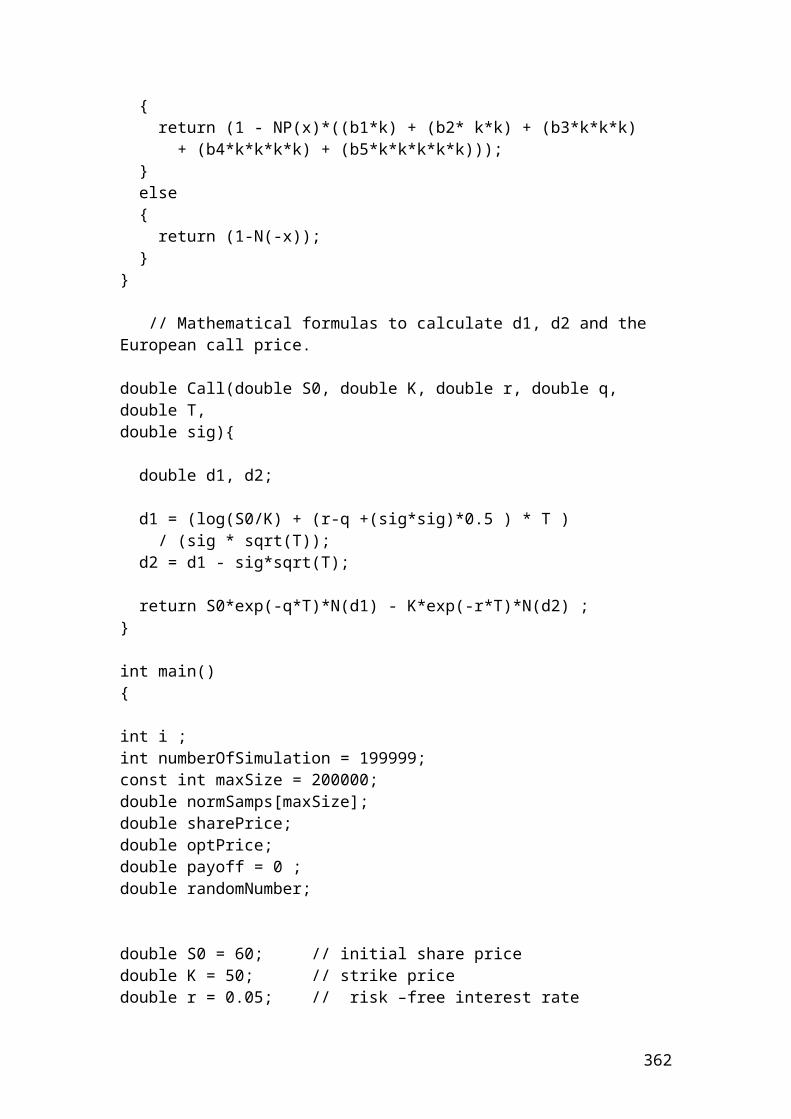
Calculate the portfolio return, the variance and the standard deviation or risk of the portfolio

>>>shareAexpRet = 0.25>>>shareAstddev = 0.10>>>shareAamount = 50000>>>correlationAB = 0.40>>>shareBexpRet = 0.35>>>shareBstddev = 0.18>>>shareBamount = 50000>>>totalportfoliovalue = 100000

>>># Calculate the weights for each share.

>>>weightA = shareAamount / totalportfoliovalue>>> weightA0.5

>>>weightB = shareBamount / totalportfoliovalue>>> weightB0.5

>>># Write the formula for portfolio return.

>>>Portfolioreturn = (shareAexpRet*weightA)+(shareBexpRet*weightB)>>> Portfolioreturn0.3

>>> # Write the formula for portfolio variance.

>>> Portfoliovariance = (weightA**2*shareAstddev**2)+(weightB**2*shareBstddev**2)+(2*weightA*weightB*shareAstddev*shareBstddev*correlationAB)>>> Portfoliovariance0.0142

>>># Write the formula for portfolio standard deviation.

>>>PortfoliostdDev = sqrt(Portfoliovariance)>>> PortfoliostdDev0.11916375287812986>>> round(_,2)0.12

362

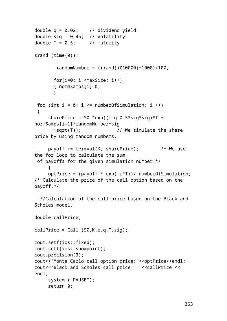
Exercise and solution

>>> # It is required to calculate the sum, and the average return.>>># The expected risk expressed as standard deviation of call, put and index options.

>>> Calloptionreturns = [3.5,4.7,7.9,-4.2,5.4,10.3]>>> Putoptionreturns = [2.7,4.9,5.7,8.5,9.3,11.5]>>> Indexoptionreturns = [3.7,7.9,8.9,10.2,-6.8,5.9]>>> n=6>>> sum(Calloptionreturns)27.600000000000005>>> average= sum(Calloptionreturns)/n>>> average4.6000000000000005>>> round(_,2)4.6>>> sum(Putoptionreturns)42.6>>> average = sum(Putoptionreturns)/n>>> average7.1000000000000005>>> round(_,2)7.1>>> sum(Indexoptionreturns)29.799999999999997>>> round(_,2)29.8>>> average = sum(Indexoptionreturns)/n>>> average4.966666666666666>>> round(_,2)4.97

>>> from statistics import stdev>>> stdev(Calloptionreturns)4.953382682571578>>> round(_,2)4.95>>> stdev(Putoptionreturns)3.234810659064917>>> round(_,2)3.23>>> stdev(Indexoptionreturns)6.203117495797308>>> round(_,2)6.2

363

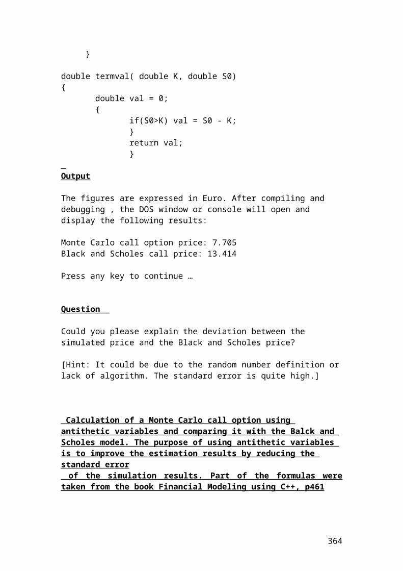
Example of pricing a forward contract and solution

A forward contract of 6 month has a market price of 52 Pounds when the spot price of the underlying commodity is 49 Pounds. There are no costs of carry and the discount rate is 7 percent. Calculate the value of the forward contract.

Solution

The current price of the forward contract (F0) should be equal to the value of the underlying commodity, (S0) at the discount rate r. Thus, the equation is as follows:

Application of pricing a forward contract in python

>>> spotprice = 49>>> discountrate = 0.07>>> valueforwardcontract = spotprice *(1+discountrate/2)>>> valueforwardcontract50.714999999999996>>> round(_,2)50.71 # Pounds

364

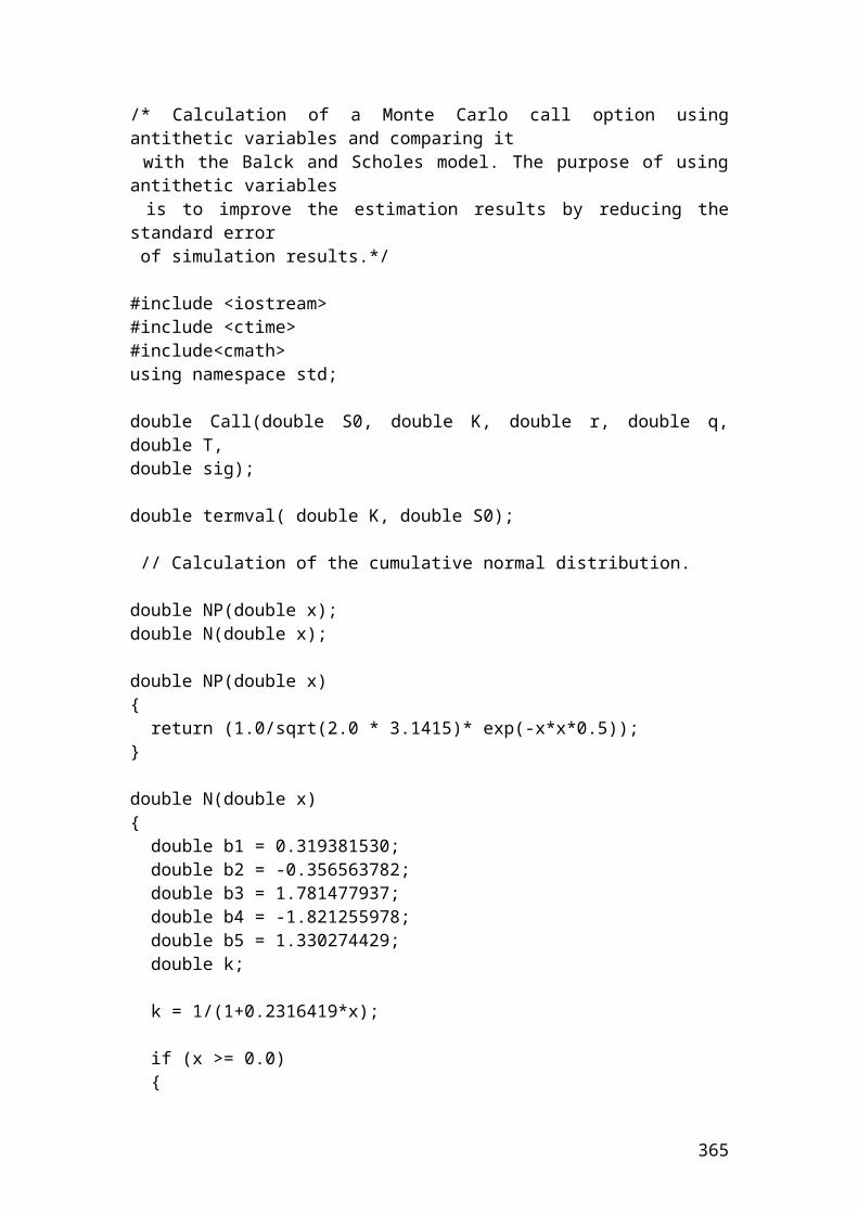
Example of interest rate payment and solution

A trader wants to calculate the interest amount that he / she will receive in three months from a forward contract of a Euribor deposit paying a Euro deposit rate of 3.55%. The principal amount is 300,000

The mathematical formula is as follows:

Interest payment = principal x [interest rate x (tdays / 360)]

Interest payment = 300,000 x [0.0355 x (90/360)]Interest payment = 2662.5 Euro.

Application of interest payment in python

>>> principal = 300000>>> interest_rate = 0.0355>>> days = 90>>> interestpayment = principal*(interest_rate *days/360)>>> interestpayment2662.4999999999995>>> round(_,2)2662.5 # Euro

365

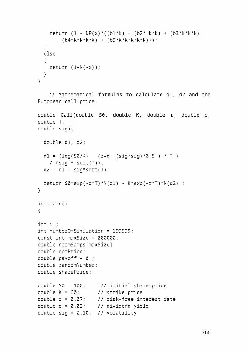
Example and solution of calculating profits and losses on futures contracts

An investor buys 8 S&P 500 futures contracts at $2189. He has closed the futures contract position with a price of $2236. The multiplier for S&P 500 futures contracts is 250 dollars. Did he record a profit or a loss?

Solution

The mathematical formula is as follows:

Where: fT is the final contract price. f0 is the initial contract price.

USD

When the prices move up, the investor will gain in long positions. When prices move down, the investor will gain in short positions.

Application of calculating profits and losses on futures contracts in python

>>> numberof_contracts = 8>>> buying_price = 2189>>> selling_price = 2236>>> multiplier = 250>>> profitorloss = numberof_contracts*multiplier*(selling_price - buying_price)>>> profitorloss94000 # USD

366

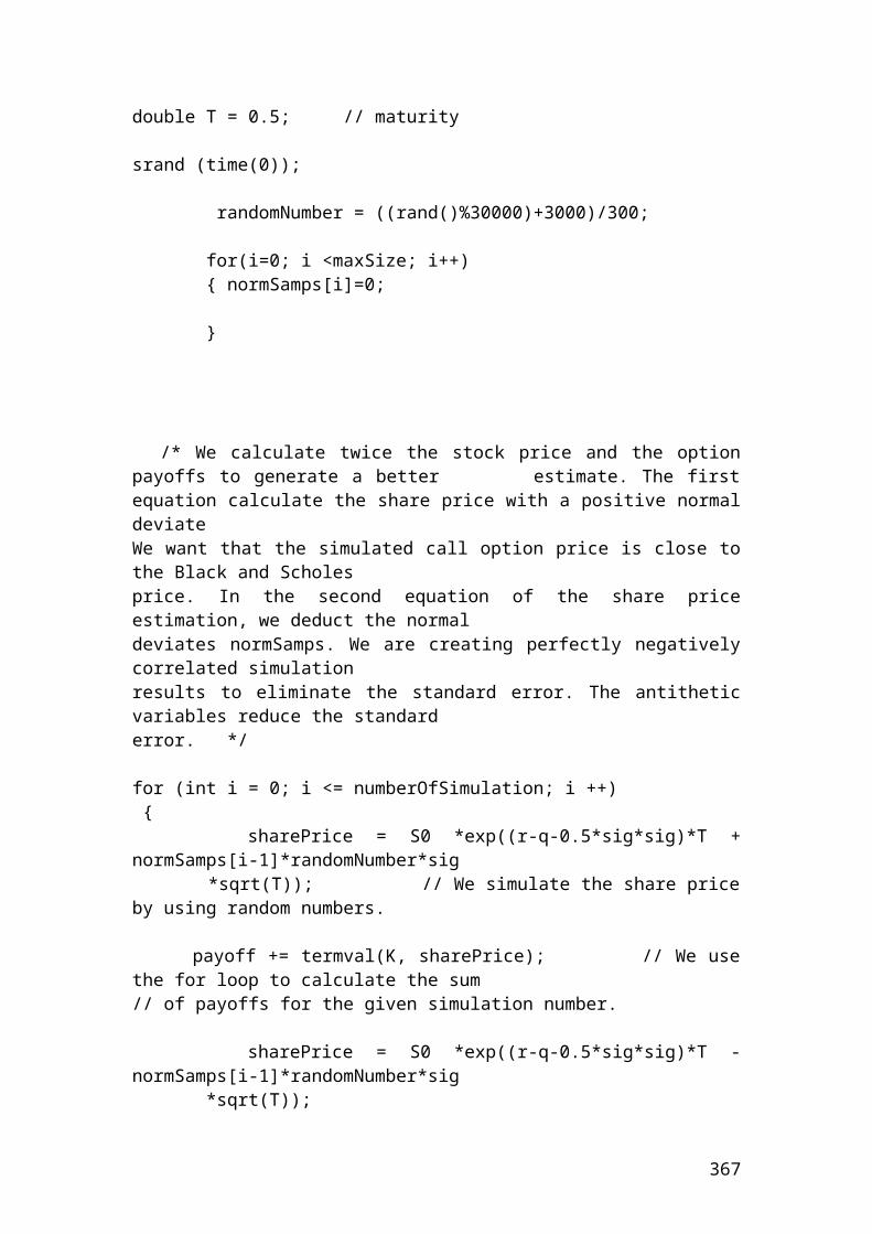
Example and solution of semiannually currency swap between an investment bank and an insurance company

The investment bank borrows 20,000,000 Pounds from the insurance company at a fixed rate of 5% for 1 year. The insurance company borrows from the investment bank 10,000,000 Euros at a fixed rate of 5% for 1 year. Calculate the interest payments for the three years, if we assume semiannual payments?

At the beginning of the contract

€10,000,000Investment bank Insurance company

£ 20,000,000

The insurance company pays the investment bank the following interest payment.

£20,000,000 x 0.05/2 = 500,000 Pounds.

The investment bank pays the insurance the following interest payment.

€10,000,000 x 0.05/2 =250,000 Euros.

The following arrows illustrate the interest payments.

€ 250,000Investment bank Insurance company

£ 500,000

At the end of the third year, the two parties exchange the principal amounts in addition to the final interest payments.

€10,250,000Investment bank Insurance company

£20,500,000

367

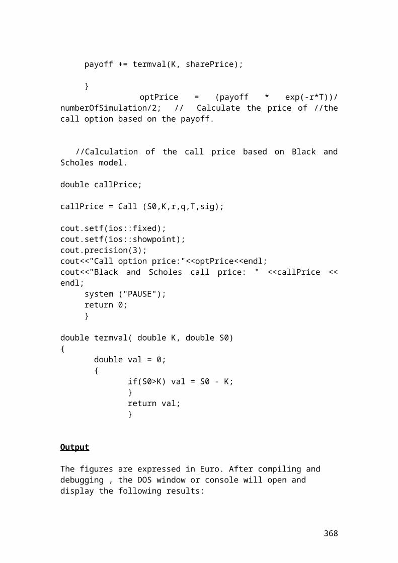
Application of semiannually currency swap between an investment bank and an insurance company in python

>>> bankborrowsfrom_insurance = 20000000>>> insuranceborrowsfrom_bank = 10000000>>> interest_rate = 0.05>>> semiannualpayment = 2>>> bankpaysinsurance = insuranceborrowsfrom_bank *(interest_rate/semiannualpayment)>>> bankpaysinsurance250000.0 # Euros>>> insurancepaysbank = bankborrowsfrom_insurance *(interest_rate/semiannualpayment)>>> insurancepaysbank500000.0 # Pounds

368

Example and solution of interest rate swap

Interest rate swaps are very popular agreements between two parties in the debt or fixed-income department of the investment banks. The fixed income department of Bank A pays a fixed rate of 5.5% upon the principal of 50,000,000 Pounds. In contrast, Bank B pays a floating or reference rate of LIBOR accounted to 7.2%. The payment frequency is every 6 months for 2 years.

Fixed payment : £50,000,000 x 0.055/2 = 1,375,000 Bank A Bank B Floating payment: £50,000,000 x 0.072/2 = 1,800,000

Suppose in the second year that the LIBOR has increased by 12 basis points or 0.12%. Then, the floating payment will change and the calculation will be as follows:

Second year floating payment for Bank B = 50,000,000 x 0.0732 / 2 = 1,830,000 Pounds.

Bank A will continue to pay the same fixed amount, namely, £50,000,000 x 0.055/2 = £1,375,000.

Application of interest rate swap in python

>>> principal = 50000000>>> interest_rate1 = 0.055>>> interest_rate2 = 0.072>>> interest_rate3 = 0.0732>>> semiannualpayment = 2>>> fixedpayment = principal*(interest_rate1/semiannualpayment)>>> fixedpayment1375000.0 # Pounds>>> floatingpayment1 = principal*(interest_rate2/semiannualpayment)>>> floatingpayment11799999.9999999998>>> round(_,2)1800000.0 # Pounds>>> floatingpayment2 = principal*(interest_rate3/semiannualpayment)>>> floatingpayment21830000.0 # Pounds

369

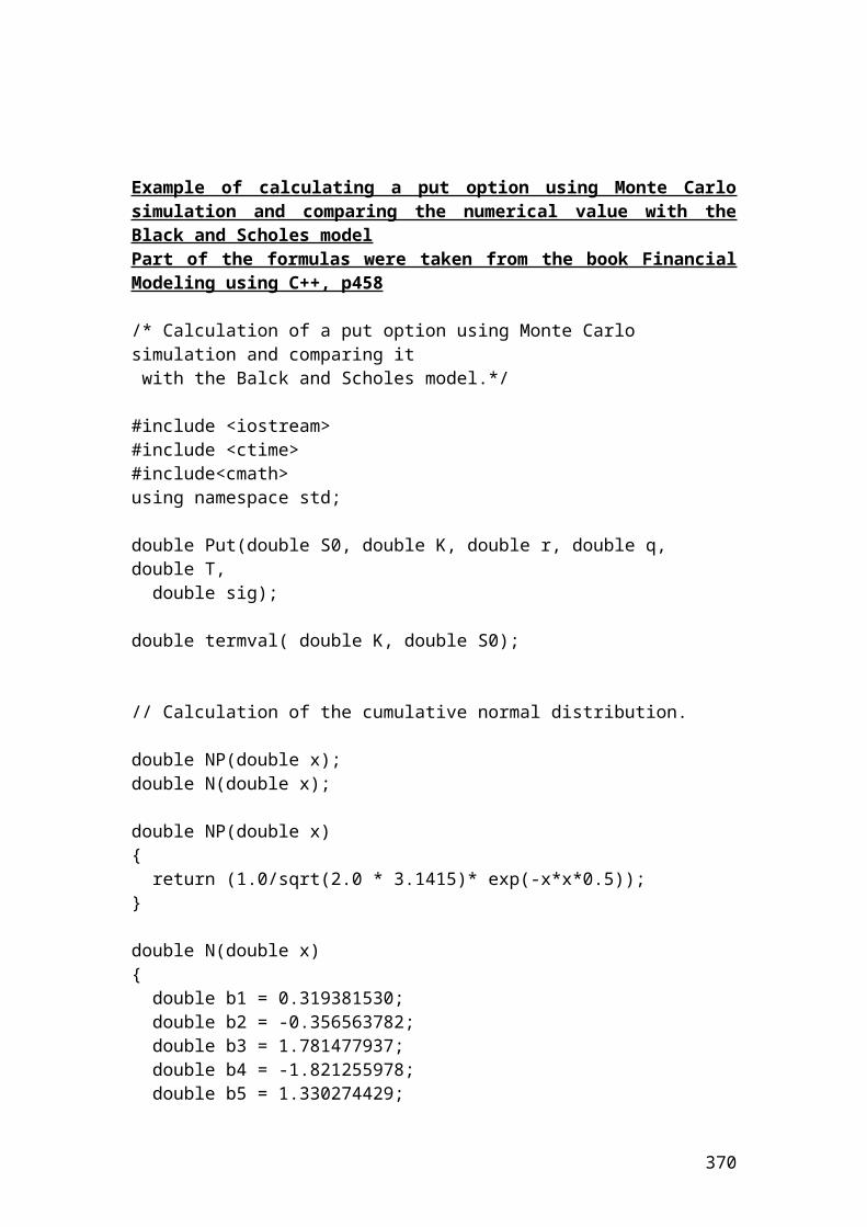
Delta – neutral hedge

Delta – neutral hedge is common used in risk management to keep the value of the portfolio neutral due to changes in the share price. It is achieved from a long position in a share and a short position in a call option. The mathematical formula to determine the number of options is as follows:

Thus, if the investment bank has bought 30,000 shares of Vodafone and the delta of the call option of the same company is 0.50, then the numbers of call options that are needed to purchase to form a delta-neutral hedge are as follows:

Delta hedge = 30,000 / 0.50 = 60,000 options or 600 option contracts.

Application of delta- neutral hedge in python

>>> numberof_shares = 30000>>> deltaofcall_option = 0.50>>> deltaneutralhedge = numberof_shares/deltaofcall_option>>> deltaneutralhedge60000.0

370

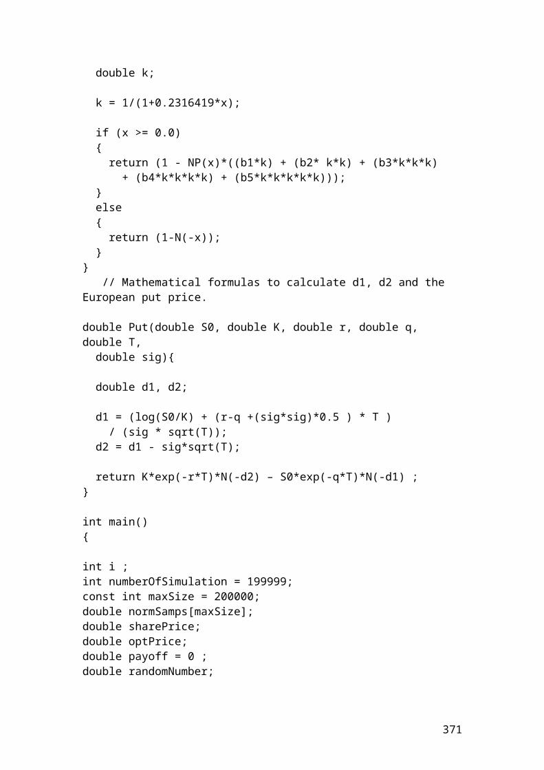
Weighted mean price of a portfolio

Let’s assume that we have a portfolio of four options with their market prices and the number of shares bought. It is required to calculate the weighted mean price of the portfolio.

Options Price expressed in $

Number of shares

Weight Weight x Price

A 14.00 300 0.4 5.6B 12.00 200 0.3 3.6C 8.00 100 0.1 0.8D 5.00 150 0.2 1

Total 750 1Source: author’s calculation

The mathematical formula is as followed:

By substituting the numbers from the Table into the equation we have the following:

0.8 + 1 = 11.

Application of weighted mean price of a portfolio in python

>>> price_1 = 14>>> price_2 = 12>>> price_3 = 8>>> price_4 = 5>>> weight_1 = 0.4>>> weight_2 = 0.3>>> weight_3 = 0.1>>> weight_4 = 0.2>>>portfoliomean=(price_1*weight_1+price_2*weight_2+price_3*weight_3+price_4*weight_4)>>> portfoliomean11.0 # Pounds

Example of Eurodollar futures

371

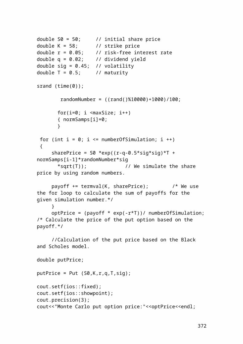
An investor wants to calculate the futures price of a 1-month Eurodollar time deposits based on a LIBOR rate of 3.40%. The initial principal is 1 million Pounds.

Solution

The price of the Eurodollar futures contract will be as follows:

Application of Eurodollar futures in python

>>> principal = 1000000>>> interest_rate = 0.034>>> days = 30>>> # Insert the mathematical formula.>>>Eurodollarfuture = principal*(1- interest_rate*(days/360))>>> Eurodollarfuture997166.67 # Pounds

Example of forward rate agreement

372

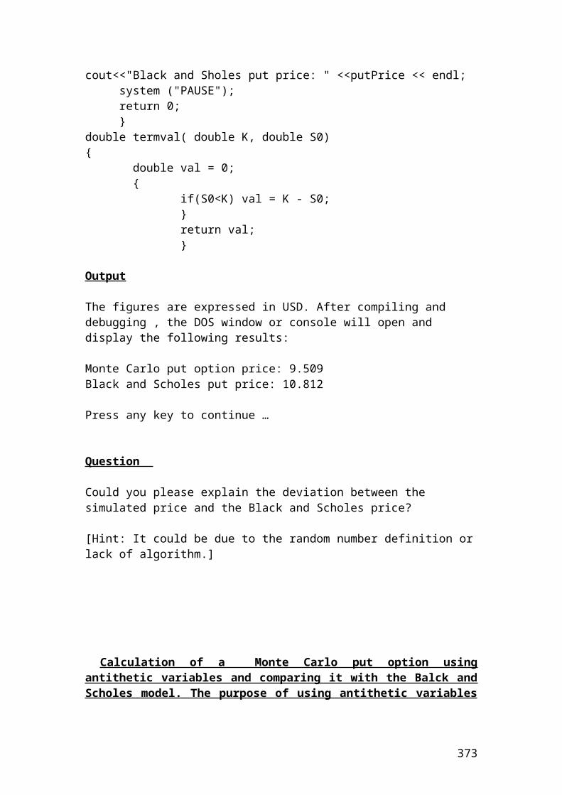
An investment bank buys a 4 x 6 FRA from a building society in the UK for 4.0% by paying 2 million Pounds. 80 days latter, LIBOR is 5%. Who will receive the FRA payment and for how much?

Solution

The mathematical formula for Forward Rate Agreement, (FRA) is as follows:

The timeline schedule is as follows:

t = 0 4months 6 months

= ………. Please complete

the calculation.

Helpful hint: If the FRA payment is positive, then, the building society is the payer and the investment bank receives the FRA payment.

If the FRA payment is negative, then the investment bank is the payer and the building society receives the FRA payment.

Application of forward rate agreement in python

>>> principal = 2000000>>> variable_rate = 0.05>>> fixed_rate = 0.04>>> FRApayment= principal*(variablerate - fixedrate)*0.333333333/1.011111111>>> FRApayment6593.4 # Pounds

Example of futures on Treasury bills

373

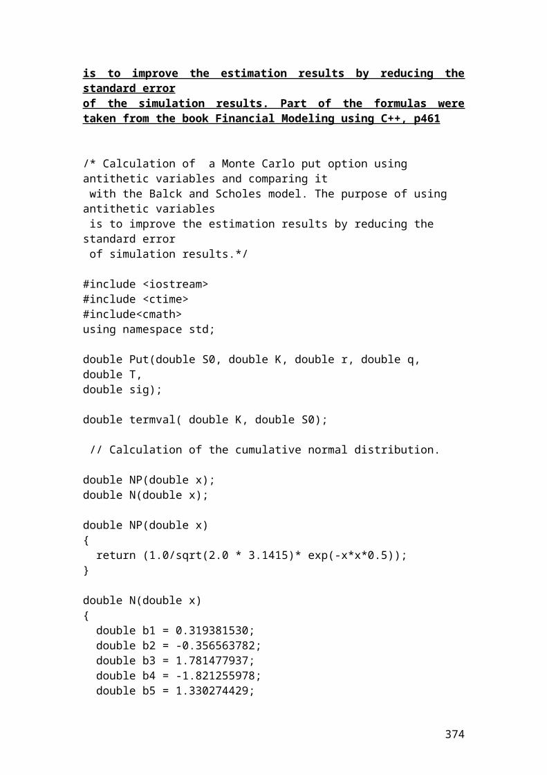
An investor wants to calculate the futures price of a 3-month Treasury bills. Treasury bills are short-term notes of limited period of 1- month, and 3 - month respectively. The initial principal is 5 million Pounds and the discount rate is 3.50%.

Solution

The price of the Treasury bill futures will be as follows:

Please complete the calculation …….

Application of futures on Treasury bills in python

>>> principal = 5000000>>> discount_rate = 0.035>>> days = 90>>> futurestreasurybills = principal*(1- discount_rate *days/360)>>> futurestreasurybills4956250 or 4.95625 e+006 # Pounds

Example of stock index futures

374

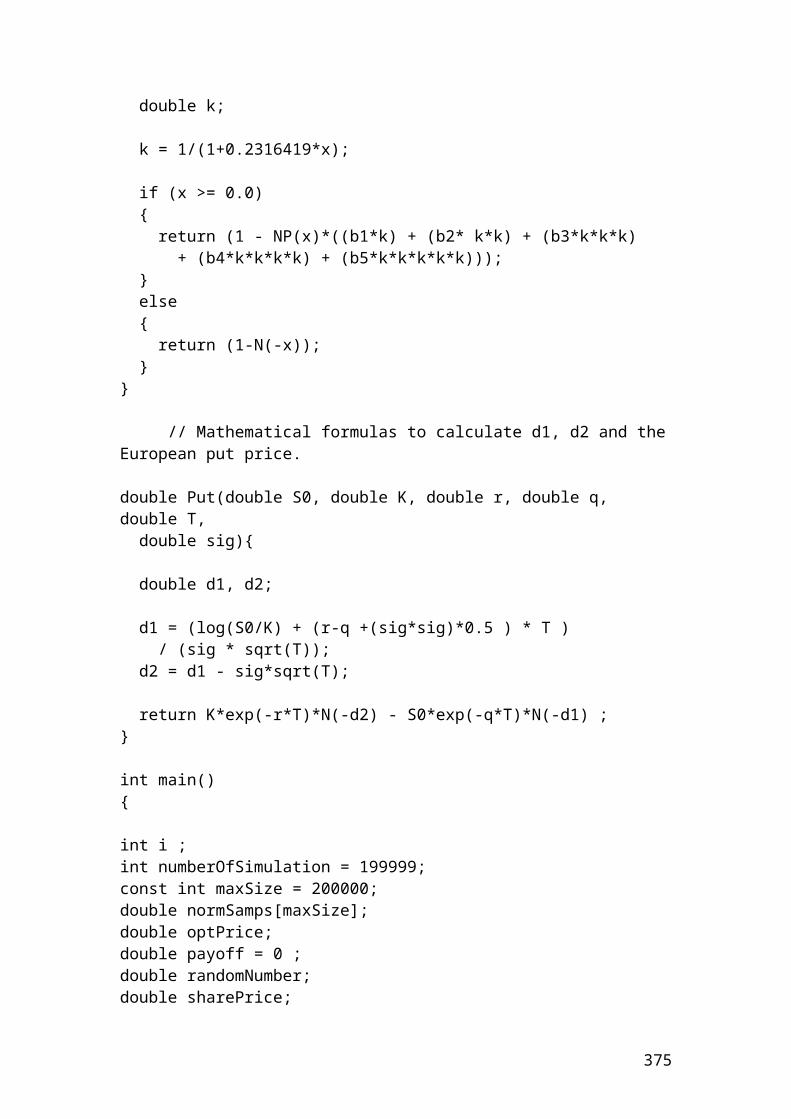
For example, if you bought 10 contracts of the Dow Jones Industrial index at 10,000 and you expected an aggressive bull market that reaches the value of 16,000, then, the 6000 points increase are multiplied by the standardized value of 250. If the initial principal of investment is $100,000, the mathematical formula for the gains will be as follows:

10 x 100,000 x 6000 x 250 = 1.5 x 1012 Dollars

Application of stock index futures in python

>>> principal = 100000>>> points_increase = 6000>>> multiplier = 250>>> number_of_contracts = 10>>> gains = principal*points_increase*multiplier>>> gains1.5 x 1012 # USD

Example of currency futures

375

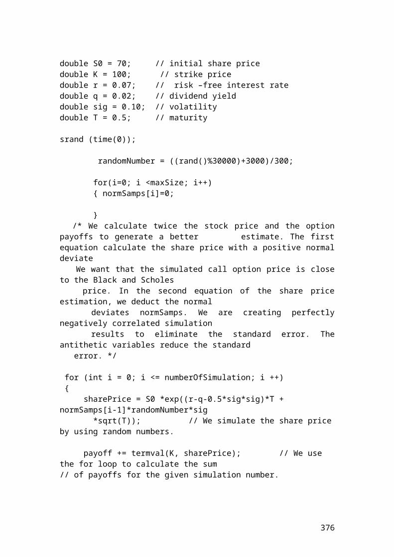
A manufacturer wants to calculate the currency futures price of EURO/USD traded in Frankfurt derivative market. For example, in August the contract is quoted as 1.35 EURO /USD and the contract size is 20,000. The principal is 300,000 Euro.

Solution

The contract price of 1 contract is as follows:

Application of currency futures in python

>>> principal = 300000>>> quote = 1.35>>> contract_size = 20000>>> futurespriceofcurrency = principal*quote*contract_size>>> futurespriceofcurrency8100000000.0 # Euro

Please try based on the previous examples to illustrate the following example in python. If you have difficulties e-mail me

Active return, active risk and information ratio

376

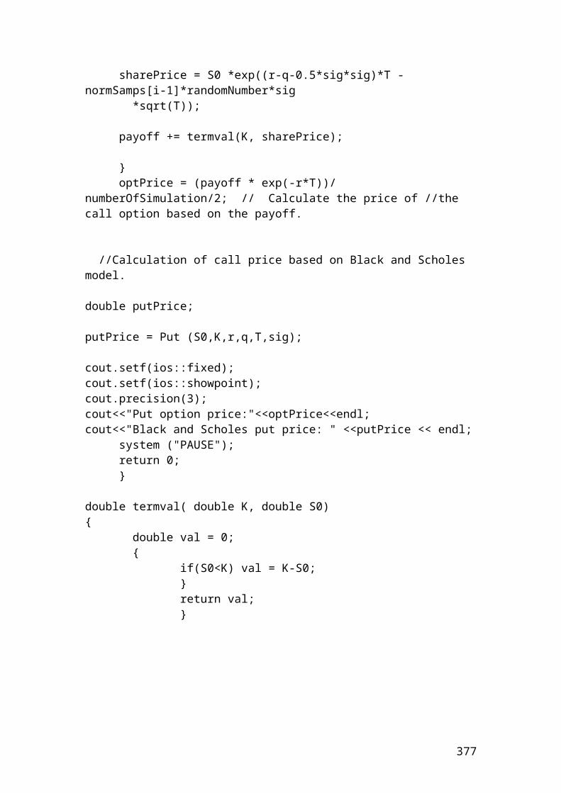
Active return is the difference in returns between a portfolio and the index or benchmark that is measured.

Active return = rp - rb

Where: rp is the portfolio return. rb is the benchmark or index return.

If the portfolio return is 0.80 and the benchmark return of the index is 0.70 then, the active return is………

Please complete the calculation.

Active risk or tracking error is the standard deviation of the difference of returns between a portfolio and the benchmark or index.

Error! Objects cannot be created from editing field codes.

If the portfolio return is 0.80, the number of assets is 10 and the benchmark return of the index is 0.40 then, the active risk is………

Please complete the calculation.

Information ratio shows the consistency of the fund manager towards the active return. The mathematical formula is as follows:

Error! Objects cannot be created from editing field codes.

It could be calculated very easily in Excel software. I will illustrate a simple table with the relevant calculations.

Day rp rb rp - rb

1 0.03 0.02 0.012 0.02 0.014 0.0063 -0.04 0.034 -0.0744 0.05 0.067 -0.0175 0.08 0.012 0.0686 -0.01 -0.056 0.046

377

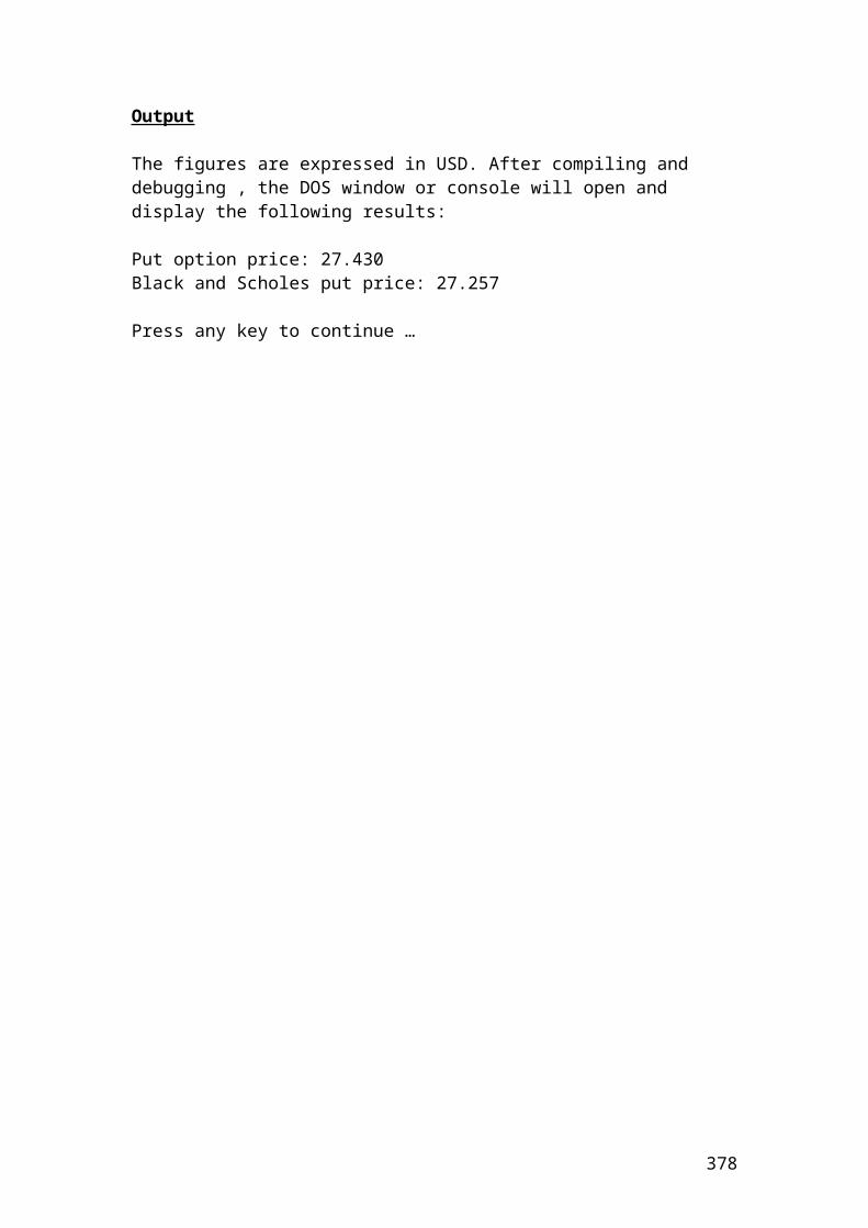
7 0.07 0.031 0.0398 0.034 0.023 0.0119 -0.021 0.015 -0.03610 0.045 0.001 0.044

Average 0.0258 0.0161Standard deviation

0.043

Source: author’s calculation

By substituting the values that we have found in terms of rp =0.0258, rb = 0.0161 and standard deviation = 0.043 in the following equation we have:

Error! Objects cannot be created from editing field codes.

Error! Objects cannot be created from editing field codes.

But what is the interpretation of the information ratio of 0.23. It means that the fund manager gained around 23 basis points of active return per unit of active risk. The higher is this number, the better the manager is performing in relation to active risk.

Please convert the following exercise in python language programming

Calculate the balance at the end of the 5th day from changes in the futures prices from 90 to 89, 91, 95, 97, 99. The trader has bought 50 futures contract for settlement in May. The initial margin is $8.

Day Beginning balance

Futures price Gain or loss Ending balance

0 400 90 0 4001 400 89 (50)2 350 91 1003 450 95 2004 650 97 1005 750 99 100

Source: author’s illustration.

Beginning balance = initial margin x number of contracts.Beginning balance = 8 x 50 = $400

Please complete the values of the column ending balance.

378

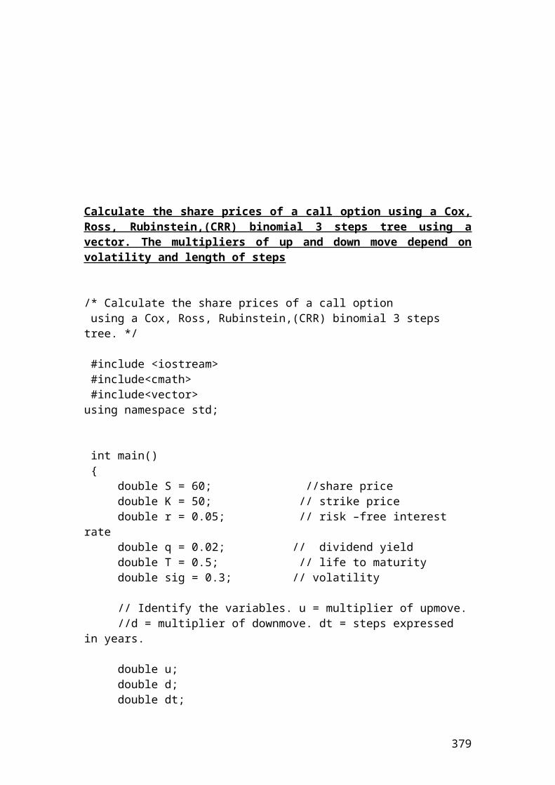
Application of the rand() function. It is very useful method that is used in simulations such as Monte Carlo simulation to price derivatives products

>>> import random>>> random.random()0.5972244221568863>>> random.uniform(1,10000)7872.215306401703>>> random.uniform(1,5000)2829.9563027875884>>> random.uniform(1,4000)2475.3647035985528

Example of profit or loss of a call option portfolio. The figures are expressed in Euros

>>> shareprice_1 = 10.25>>> shareprice_2 = 20.13>>> shareprice_3 = 30.22>>> shareprice_4 = 40.56>>> shareprice_5 = 50.89>>> shareprice_6 = 51.23>>> shareprice_7 = 53.33>>> shareprice_8 = 54.63>>> shareprice_9 = 66.23

379

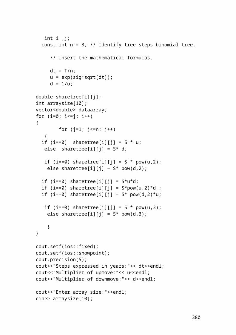
>>> shareprice_10 = 68.23>>> stikeprice_1 = 3.34>>> strikeprice_1 = 3.34>>> strikeprice_2 = 8.34>>> strikeprice_3 = 18.78>>> strikeprice_4 = 28.34>>> strikeprice_5 = 31.12>>> strikeprice_6 = 22.02>>> strikeprice_7 = 34.23>>> strikeprice_8 = 47.12>>> strikeprice_9 = 48.45>>> strikeprice_10 = 50.12>>> optionpremium_1 = 1.50>>> optionpremium_2 = 2.30>>> optionpremium_3 = 2.56>>> optionpremium_4 = 3.10>>> optionpremium_5 = 3.25>>> optionpremium_6 = 3.45>>> optionpremium_7 = 3.56>>> optionpremium_8 = 4.32>>> optionpremium_9 = 5.12>>> optionpremium_10 = 5.78>>> contractsize = 100

>>> portfoliovalue1 = (shareprice_1-(strikeprice_1+ optionpremium_1))* contractsize>>> portfoliovalue1541.0>>> portfoliovalue2 = (shareprice_2-(strikeprice_2+ optionpremium_2))* contractsize>>> portfoliovalue2948.9999999999999>>> round(_,2)949.0>>> portfoliovalue3 = (shareprice_3-(strikeprice_3+ optionpremium_3))* contractsize>>> portfoliovalue3887.9999999999999>>> round(_,2)888.0>>> portfoliovalue4 = (shareprice_4-(strikeprice_4+ optionpremium_4))* contractsize>>> portfoliovalue4912.0000000000001>>> round(_,2)912.0>>> portfoliovalue5 = (shareprice_5-(strikeprice_5+ optionpremium_5))* contractsize>>> portfoliovalue51651.9999999999995

380

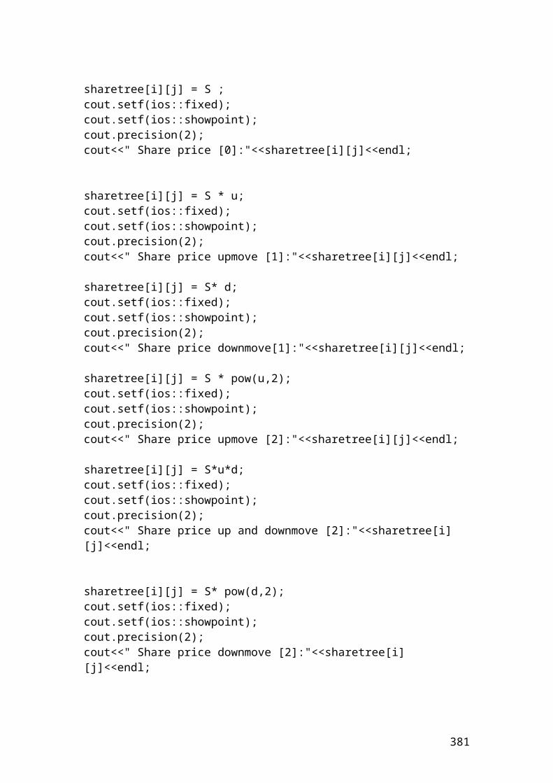
>>> round(_,2)1652.0>>> portfoliovalue6 = (shareprice_6-(strikeprice_6+ optionpremium_6))* contractsize>>> portfoliovalue62576.0>>> portfoliovalue7 = (shareprice_7-(strikeprice_7+ optionpremium_7))* contractsize>>> portfoliovalue71554.0>>> portfoliovalue8 = (shareprice_8-(strikeprice_8+ optionpremium_8))* contractsize>>> portfoliovalue8319.00000000000045>>> round(_,2)319.0>>> portfoliovalue9 = (shareprice_9-(strikeprice_9+ optionpremium_9))* contractsize>>> portfoliovalue91266.0000000000005>>> round(_,2)1266.0>>> portfoliovalue10 = (shareprice_10-(strikeprice_10+ optionpremium_10))* contractsize>>> portfoliovalue101233.0000000000005>>> round(_,2)1233.0

381

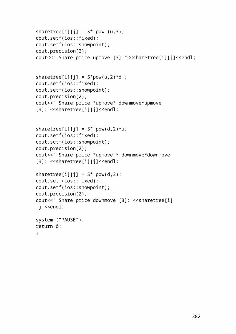
Example of profit or loss of a put option portfolio. The figures are expressed in Euro

>>> shareprice_1 = 10.25>>> shareprice_2 = 20.13>>> shareprice_3 = 30.22>>> shareprice_4 = 40.56>>> shareprice_5 = 50.89>>> shareprice_6 = 51.23>>> shareprice_7 = 53.33>>> shareprice_8 = 54.63>>> shareprice_9 = 66.23>>> shareprice_10 = 68.23>>> strikeprice_1 = 3.34>>> strikeprice_2 = 8.34>>> strikeprice_3 = 18.78>>> strikeprice_4 = 28.34>>> strikeprice_5 = 31.12>>> strikeprice_6 = 22.02>>> strikeprice_7 = 34.23>>> strikeprice_8 = 47.12>>> strikeprice_9 = 48.45>>> strikeprice_10 = 50.12>>> optionpremium_1 = 1.50>>> optionpremium_2 = 2.30>>> optionpremium_3 = 2.56>>> optionpremium_4 = 3.10

382

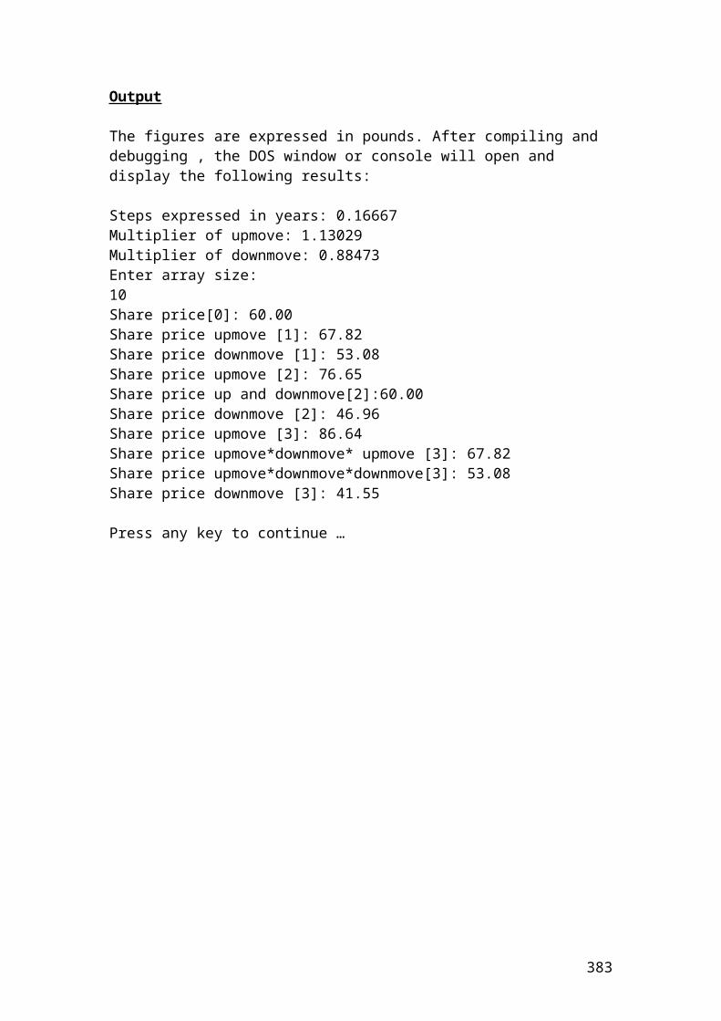
>>> optionpremium_5 = 3.25>>> optionpremium_6 = 3.45>>> optionpremium_7 = 3.45>>> optionpremium_8 = 4.32>>> optionpremium_9 = 5.12>>> optionpremium_10 = 5.78>>> contractsize =100>>> portfoliovalue1 = (strikeprice_1- optionpremium_1-shareprice_1)* contractsize>>> portfoliovalue1-841.0>>> portfoliovalue2 = (strikeprice_2- optionpremium_2- shareprice_2)* contractsize>>> portfoliovalue2-1409.0>>> portfoliovalue3 = (strikeprice_3- optionpremium_3- shareprice_3)* contractsize>>> portfoliovalue3-1399.9999999999995>>> round(_,2)-1400.0>>> portfoliovalue4 = (strikeprice_4 - optionpremium_4 - shareprice_4)* contractsize>>> portfoliovalue4-1532.0000000000005>>> round(_,2)-1532.0>>> portfoliovalue5 = (strikeprice_5- optionpremium_5- shareprice_5)* contractsize>>> portfoliovalue5-2302.0>>> portfoliovalue6 = (strikeprice_6- optionpremium_6- shareprice_6)* contractsize>>> portfoliovalue6-3265.9999999999995>>> round(_,2)-3266.0>>> portfoliovalue7 = (strikeprice_7- optionpremium_7- shareprice_7)* contractsize>>> portfoliovalue7-2255.0>>> portfoliovalue8 = (strikeprice_8- optionpremium_8- shareprice_8)* contractsize>>> portfoliovalue8-1183.0000000000005>>> round(_,2)-1183.0>>> portfoliovalue9 = (strikeprice_9- optionpremium_9- shareprice_9)* contractsize>>> portfoliovalue9-2290.0>>> portfoliovalue10 = (strikeprice_10- optionpremium_10- shareprice_10)* contractsize>>> portfoliovalue10-2389.000000000001>>> round(_,2)-2389.0

383

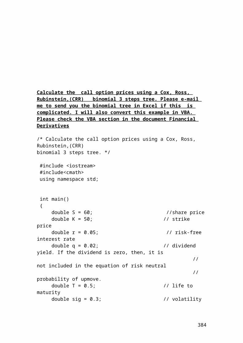
One – period binomial method

A share is traded in the Danish stock exchange at 50 DKK. First of all, we would like to calculate the possible price changes based on probabilities. The risk - free rate is 5% and the value of the call option has an exercise price of 50 DKK. It is required to calculate the expected value of the option at t =1. In addition, it is required to calculate the value of the option today discounted at the given risk-free rate.

We assume two scenarios. The first one is that the share will increase by 20% or by a factor of 1 + 0.20 = 1.20. The second one is that the share will decrease by 0.833. The number 0.833 is calculated as 1 / 1.20 = 0.833.

The mathematical formulas are as follows:

Down move = D = 1 / up move = 1 / 1.20 = 0.833

384

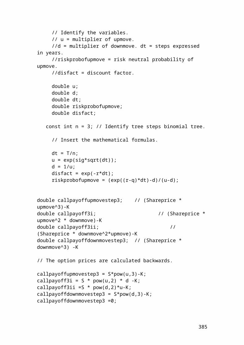
Thus, the payoff or the one-period binomial tree for share and option prices for the two possible scenarios will be as follows:

t = 0 t = 1

Probability Up = 0.59128 Share price = 50 x 1.20 = 60 DKK Call option = 60 – 50 = 10 DKK. 50 In this case, an increase of the share price will lead to the call option to pay back 10 DKK Probability Down =0.40872 Share price = 50 x 0.833 = 41.65 DKK Call option = 41.65 – 50 = -8.35 DKK = 0 DKK In this case the call option does not worth anything.

The expected value of the call option at t = 1 is as follows:

Expected call option = (10 x 0.59128) + ( 0 x 0.40872) = 5.9128 + 0 = 5.9128 DKK.

The value of the call option discounted at 5% risk – free rate is as follows:

Ctoday = 5.9128 / 1.05 = 5.63 DKK (to 2 d.p.).

Application of one – period binomial method in python. The figures are expressed in DKK

>>> share_price = 50>>> exercise_price = 50>>> upmove = 1.20>>> downmove = 0.833>>> risk_free_rate = 0.05>>> # Insert the mathematical formulas of risk probability of up and down move.>>> riskprobofupmove = (1+risk_free_rate-downmove) / (upmove - downmove)>>> riskprobofupmove0.5912806539509539>>> round(_,2)0.59>>> riskprobofdownmove = 1 - riskprobofupmove>>> riskprobofdownmove0.40871934604904614>>> round(_,2)0.41>>> # The payoffs are determined by the following equations.>>> shareprice1 = share_price * upmove>>> shareprice160.0>>> calloptionprice1 = shareprice1 - exercise_price>>> calloptionprice110.0

385

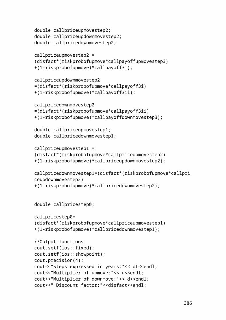
>>> shareprice2 = share_price *downmove>>> shareprice241.65>>> calloptionprice2 = shareprice2 - exercise_price>>> calloptionprice2-8.350000000000001>>> calloptionprice2 =0>>> calloptionprice20>>> #The expected value of the call option at t=1 is as follows:>>> expectedcalloption = (calloptionprice1* riskprobofupmove) + (calloptionprice2 * riskprobofdownmove)>>> expectedcalloption5.912806539509539>>> round(_,2)5.91>>># The value of the call option discounted at 5% risk - free rate is as follows:>>> valueofcalldiscounted = expectedcalloption / 1.05>>> valueofcalldiscounted5.631244323342418>>> round(_,2)5.63

386

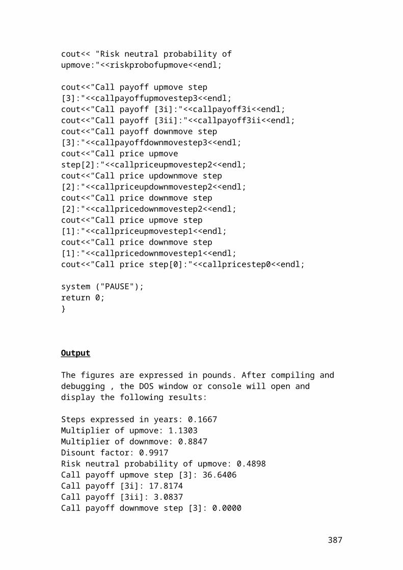
Two – period binomial method

This method is based on the one – period binomial method, but it is extended to include a second period, t = 2. Thus, we have three periods. t = 0, t =1 and t =2. We use the same example of the previous section but extended to an additional period.

A share is traded in the Danish stock exchange at 50 DKK. First of all, we would like to calculate the possible price changes based on probabilities. The risk - free rate is 5% and the value of the call option has an exercise price of 50 DKK. It is required to calculate the expected value of the option. In addition, it is required to calculate the value of the option today discounted at the given risk-free rate.

We assume two scenarios. The first one is that the share will increase by 20% or by a factor of 1 + 0.20 = 1.20. The second one is that the share will decrease by 0.833. The number 0.833 is calculated as 1 / 1.20 = 0.833.

The mathematical formulas are as follows:

Down move = D = 1 / up move.

387

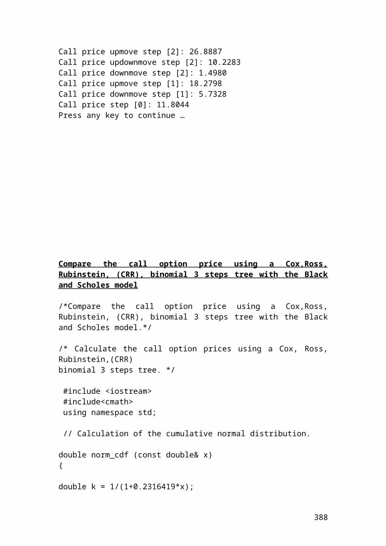
Thus, the payoff or the two-period binomial tree for share prices for the two possible scenarios will be as follows:

t = 0 t = 1 t =2 50*(1.20)2=72 DKKProbability Up = 0.59 S1 = 50 x 1.20 = 60 DKK S2 50*1.20*0.833 =49.98 50 DKK Probability Down =0.41 S1 = 50 x 0.833 = 41.65 DKK S2

50 * (0.833)2 = 34.69

The value of the call options for the period t =2 for both ups and downs are as follows:

Upside movementC1 = 72 – 50 = 22C2 = 49.98 – 50 = -0.02 =0 Negative values mean that the option does not worth.

Downside movementC1 = 49.98 -50 = -0.02 =0C2 = 34.69 -50 = -15.31 =0

The expected value of the call options for both movements for period t =1 are calculated based on the following equations:

Upside movement

Downside movement

The value of the call option today discounted is calculated based on the following formula:

388

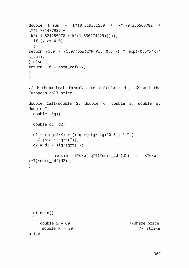
The final format of the two-period binomial tree for call options is as follows:

t = 0 t = 1 t = 2

22.00 DKK 12.3887DKK 06.976 DKK 0 0

Application of two – period binomial method in python. The figures are expressed in DKK

>>> share_price = 50>>> exercise_price = 50>>> upmove = 1.20>>> downmove = 0.833>>> risk_free_rate = 0.05>>> # Insert the mathematical formulas of risk probability of up and down move.>>> riskprobofupmove = (1+risk_free_rate-downmove) / (upmove - downmove)>>> riskprobofupmove0.5912806539509539>>> round(_,2)0.59>>> riskprobofdownmove = 1 - riskprobofupmove>>> riskprobofdownmove0.40871934604904614>>> round(_,2)0.41>>> # The payoffs are determined by the following equations.>>> shareprice1 = share_price * upmove>>> shareprice160.0>>> shareprice2 = share_price *downmove>>> shareprice241.65>>> shareprice3 = share_price * upmove**2>>> shareprice372.0>>> calloptionprice3 = shareprice3 - exercise_price>>> calloptionprice322.0>>> shareprice4 = share_price * downmove**2

389

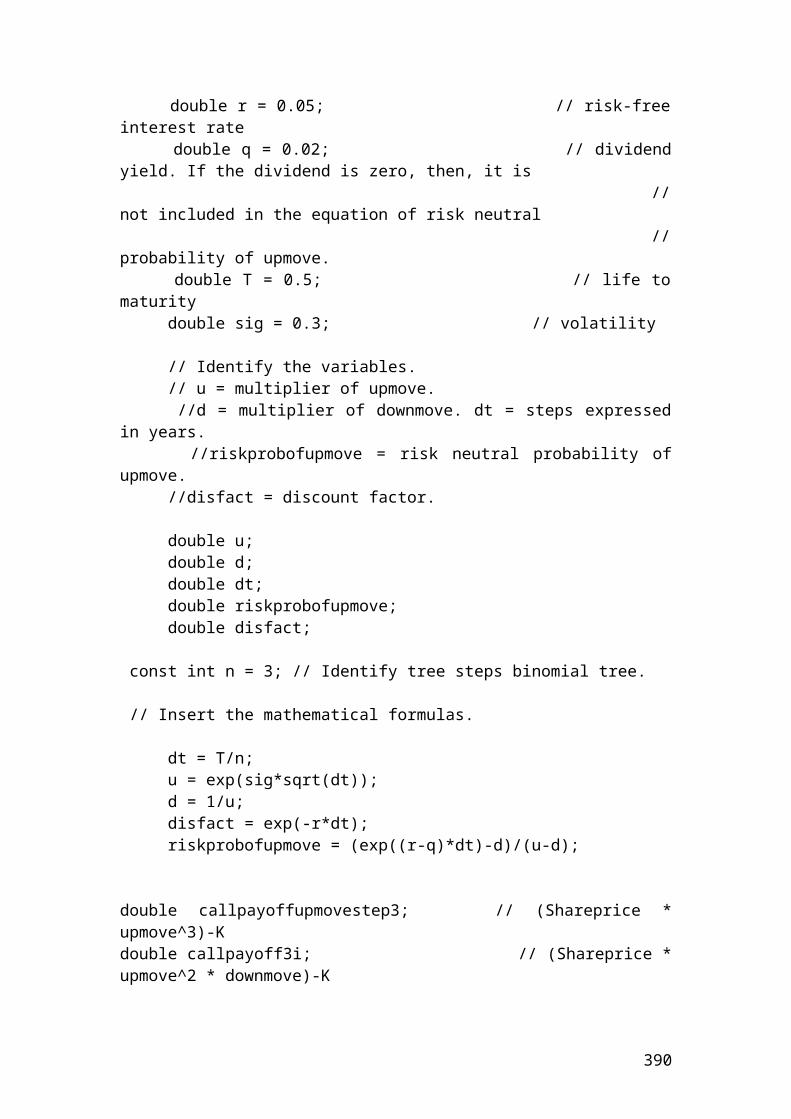
>>> shareprice434.694449999999996>>> round(_,2)34.69>>> calloptionprice4 = shareprice4 - exercise_price>>> calloptionprice4-15.305550000000004>>> round(_,2)-15.31>>> calloptionprice4 =0>>> calloptionprice40>>> shareprice5 = share_price * upmove * downmove>>> shareprice549.98>>> calloptionprice5 = shareprice5 - exercise_price>>> calloptionprice5-0.020000000000003126>>> round(_,2)-0.02>>> calloptionprice5 =0>>> calloptionprice50>>> #The expected value of the call option at t=2 is as follows:>>> expectedcalloptionupside = (riskprobofupmove * calloptionprice3+ riskprobofdownmove* calloptionprice5) / 1.05>>> expectedcalloptionupside12.388737511353318>>> round(_,2)12.39>>> expectedcalloptiondownside = (riskprobofupmove *calloptionprice4+ riskprobofdownmove * calloptionprice5) / 1.05>>> expectedcalloptiondownside0.0>>># The value of the call option discounted at 5% risk - free rate is as follows:>>> valueofcalldiscounted = (riskprobofupmove * expectedcalloptionupside+riskprobofdownmove* expectedcalloptiondownside)/ 1.05>>> valueofcalldiscounted6.976400778418764>>> round(_,2)6.98

390

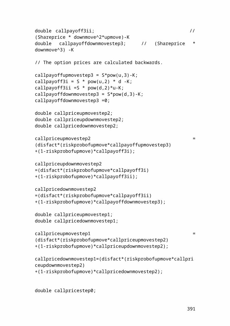
Stock index option

Let’s assume that a practitioner wants to buy a stock index call option that is related to the general movement of the S&P 500 index. The dollar multiplier for S&P 500 option contract is 250 dollars. The strike price of the index is 1240. The August premium is 20 index points.

Question

Calculate the cost of the August call and the net profit involved if the S&P 500 index reaches the price of 1540.

Solution

Cost of the August call = premium expressed in index points x dollar multiplier Cost of the August call = 20 x 250 = 5000 USD

The net profit incurred is calculated as follows:

(Ending index value – beginning index value x dollar multiplier ) – cost of the August call.

(1540 – 1240) x 250 – 5000 = 70,000 USD.

Application of stock index option in python

>>> beginning_index_value = 1240>>> ending_index_value = 1540>>> multiplier = 250>>> premium = 20>>> costofcall = premium * multiplier

391

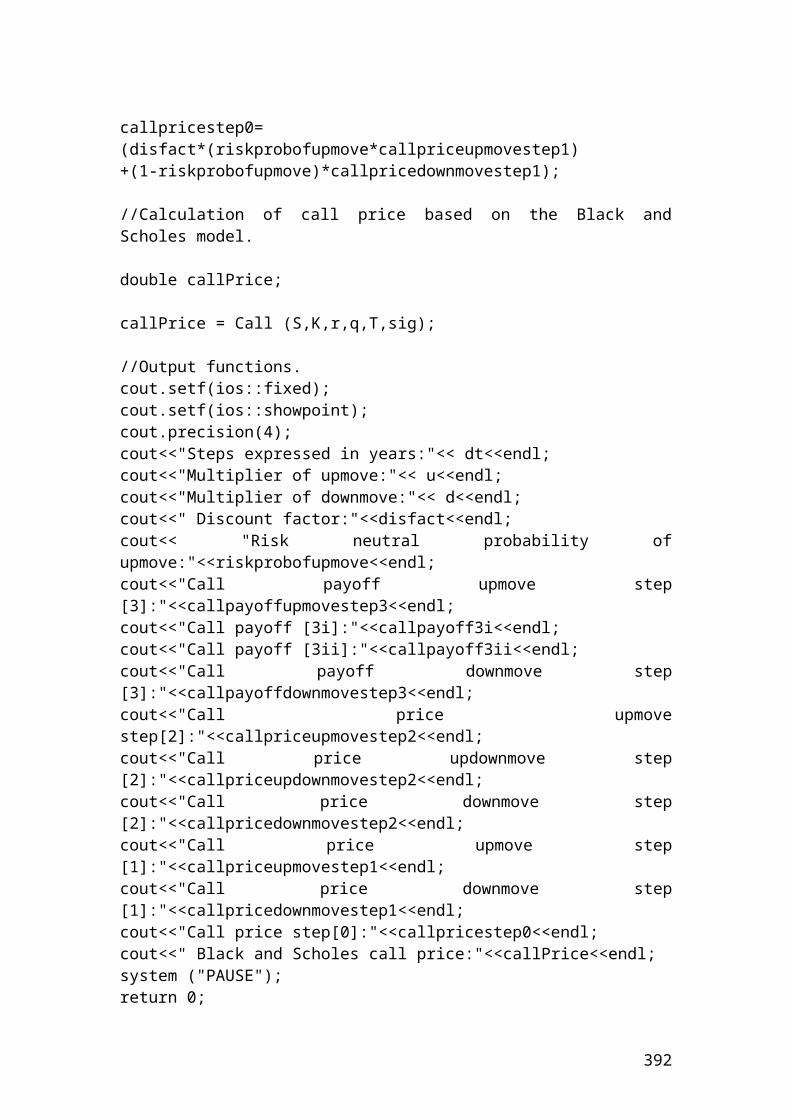
>>> costofcall5000 # USD>>> netprofit = (ending_index_value - beginning_index_value) * multiplier - costofcall>>> netprofit70000 # USD

Exercise of an European interest rate option

Calculate the profit or loss of the interest rate difference between the actual and the strike rate of a call option. Let’s assume that an interest call option on a 6 –month Eurodollar has a strike rate of 4%. At expiration, the 6-month Eurodollar rate is 5%. The invested principal is 50,000,000 Euros. The duration of the contract is expressed in days divided by 360 days. Thus, 6 –months equal 180 days.

The mathematical formula for profit or loss is as follows:

Application of an European interest rate option in python

>>> principal = 50000000>>> actual_rate = 0.05>>> strike_rate = 0.04>>> duration = 180>>> days = 360>>> # Insert the mathematical formula.>>> profitorloss =principal*(actual_rate - strike_rate)*duration/days>>> profitorloss250000.00000000003>>> round(_,2)250000.0 # Euros

392

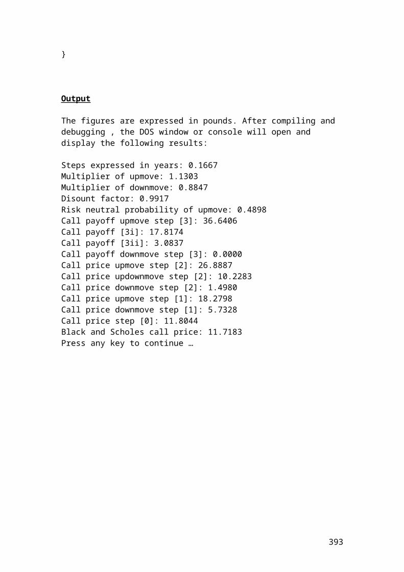
Currency option

Let’s assume that a wealthy investor buys a call currency option because it expects a rise in the exchange rate parity of the EURO against the USD, EURO/USD. The spot exchange rate is 1/1.3568. The strike price is 1.3568. The premium expressed as cents per Euro is 1.56. The initial principal is 100,000 USD.

Question

Calculate the net profit involved if the strike price increases to 1.3987.

Solution

The wealthy investor to record a profit, he or she should add to the strike price 1.3568 the premium expressed as cents per Euro. In our case, the breakeven point is1.3568 + 0.0156 = 1.3724. Above the price of 1.3724, he or she starts to record a profit. If the strike price reaches 1.3987, then the profit will be as follows:

Initial principal x (Ending strike price – beginning strike price – premium paid) =100,000 x (1.3987 – 1.3568 – 0.0156) = 2630 USD net profit

Application of currency option in python

>>> principal = 100000>>> ending_strike_price = 1.3987>>> beginning_strike_price = 1.3568>>> premiumpaid = 0.0156>>> netprofit = principal *(ending_strike_price-beginning_strike_price-premiumpaid)>>> netprofit2630.000000000005>>> round(_,2)2630.0 # USD

393

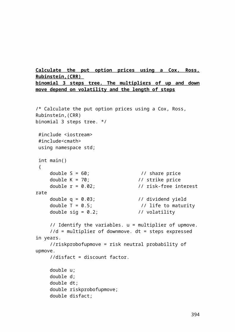
Example of calculating the payments of an interest rate cap based on different LIBOR rates

Interest rate cap is an agreement between two parties where one party pay the other at a specified period of time in which the interest rate or London interbank offered rate ,LIBOR, exceeds the strike price. It is used this contract to hedge against interest rate fluctuations. Let’s assume that an interest cap has a value of 5.5% and the LIBOR prices for the next three years are 7.5%, 8.3% and 4.65%. The principal is $50,000,000 and the payments take place semiannually.

The mathematical formula that is used to calculate the payments of each year is as follows:

Interest rate payment =[ principal x (LIBOR rate – cap rate)/0.5]

Therefore, the first year interest rate payment is as follows:

Year 1

Interest rate payment = [50,000,000 x (0.075 – 0.055)/2] = $ ………

Application of payments of an interest rate cap based on different LIBOR rates in python

>>> principal = 50000000>>> liborrate_1 = 0.075>>> liborrate_2 = 0.083>>> caprate = 0.055>>> duration = 2>>> interestpay1 = principal *(liborrate_1 - caprate) /duration>>> interestpay1499999.99999999994>>> round(_,2)

394

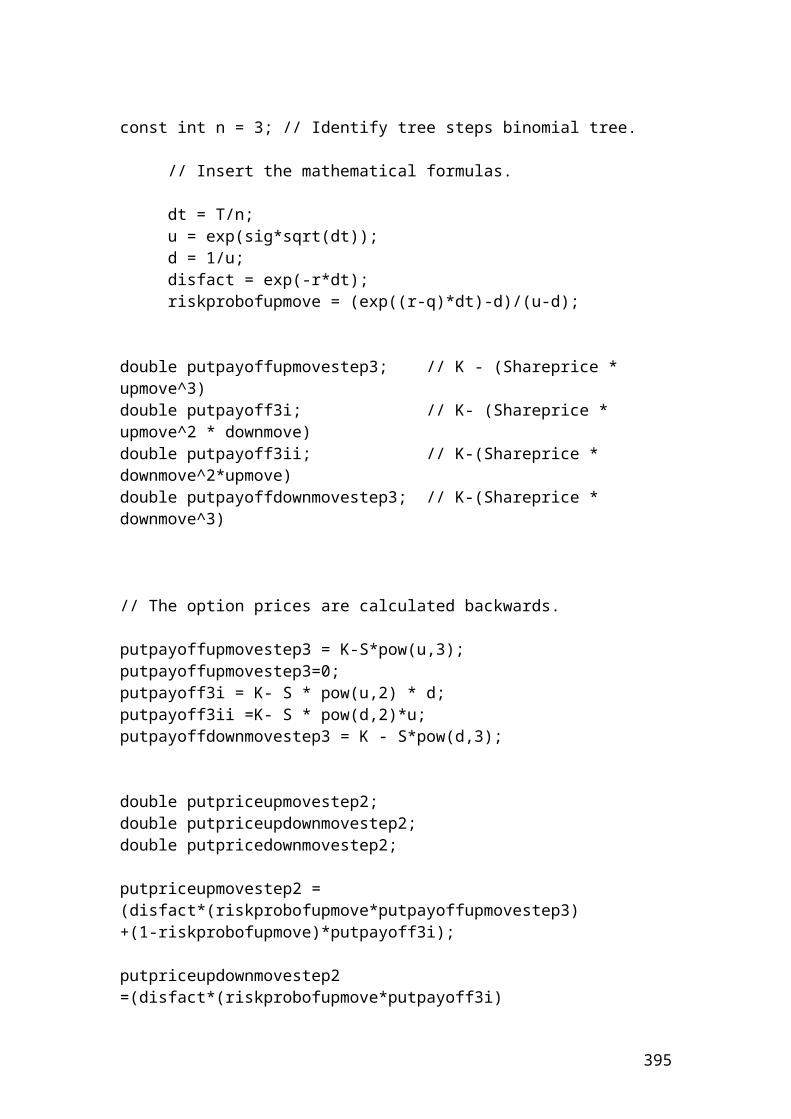
500000.0 # USD>>> interestpay2 = principal *(liborrate_2 - caprate) / duration>>> interestpay2700000.0000000001>>> round(_,2)700000.0 # USD

A six month interest rate cap has a rate of 0.08 and the principal is 20,000,000 USD. The settlements is done quarterly. The first quarter the 3 –month libor rate is 0.096 and the second quarter the rate is 0.087. Calculate the payoff for the cap the first and the second quarter?

Solution

Payoff the first quarter = 20,000,000 * = 80000 USD

Payoff the second quarter = 20,000,000 * 35000 USD

Application of payoff of interest rate cap in python

>>> principal = 20000000>>> caprate = 0.08>>> liborrate_1 = 0.096>>> liborrate_2 = 0.087>>> period = 4>>> # Insert the mathematical formulas.>>> payoff1 = (principal*(liborrate_1-caprate)/period)>>> payoff180000.0 # USD>>> payoff2 = (principal*(liborrate_2-caprate)/period)>>> payoff234999.99999999996>>> round(_,2)35000.0 # USD

395

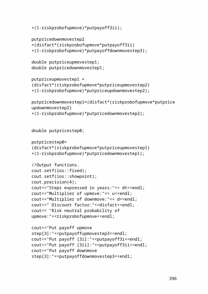
Swaption

An investor purchased a 1 year European swaption with exercise price 7.50%. The principal is 30,000,000USD. The floating rate payments are based on LIBOR. The 90, 180, 270, and 360 day annualized LIBOR rates and present value factors are as follows:

LIBOR Rate Present value factors90 day LIBOR 4% 0.990099180 day LIBOR 5.5% 0.973236270 day LIBOR 6% 0.956938360 day LIBOR 7% 0.934579

Calculate the semi-annual and annualized swap rate?Calculate the net cash flow at each payment and the value of swaption at maturity.

Solution

The present value factors are calculated as follows:

PV 90 days = Error! Objects cannot be created from editing field codes.0.990099

PV 180 days = Error! Objects cannot be created from editing field codes.0.973236

PV 270 days = Error! Objects cannot be created from editing field codes.0.956938

PV 360 days = Error! Objects cannot be created from editing field codes.0.934579

Semi - annual swap rate =

Error! Objects cannot be created from editing field codes.

396

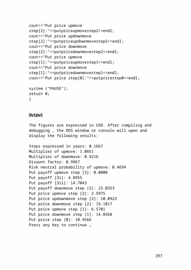
Annulaized swap rate = Error! Objects cannot be created from editing field codes.

The swaption is in the money because the exercise price 7.50% is greater than the market annualized swap rate 6.788%.

The net cash flow is as follows:

netCashFlow = (0.075 – 0.06788)*90/360 * 30000000 = 53400 USD

The value of swaption at maturity is as follows:

valueSwaption = 53400 *(Error! Objects cannot be created from editing field codes.) = 205,849.1 USD

Application of swaption in python

>>> principal = 30000000>>> exercise_rate = 0.075>>> rate90 = 0.04>>> rate180 = 0.055>>> rate270 = 0.06>>> rate360 = 0.07>>> # Insert the mathematical formulas.>>> PV90 = 1 /(1+(rate90 * 90/360))>>> PV900.9900990099009901>>> PV180 = 1/(1+(rate180 * 180/360))>>> PV1800.97323600973236>>> PV270 = 1/(1+(rate270 * 270/360))>>> PV2700.9569377990430623>>> PV360 = 1/(1+(rate360* 360/360))>>> PV3600.9345794392523364>>> semiAnnualRate = (1-PV360)/(PV90 +PV180 +PV270 +PV360)>>> semiAnnualRate0.01697096448070222>>> round(_,5)0.01697>>> annualizedSwapRate = semiAnnualRate * (360/90)>>> annualizedSwapRate0.06788385792280888>>> round(_,5)0.06788

397

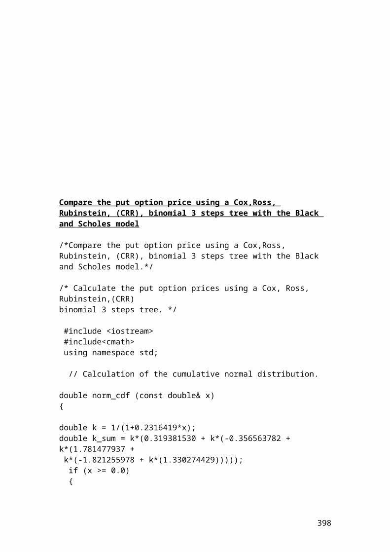
Please repeat the above swaption problem in python and calculate the net cash flow and the value of swaption at maturity.

Put –call parity

The put – call parity shows the relationship between a call and a put option with the same expiration, strike and share prices. The mathematical formula is as follows:

Error! Objects cannot be created from editing field codes.

Example

Calculate the price of a call if the price of a put is 5.34 Pounds, the share price is 94, the strike price is 97, the risk-free rate is 4% and the time to maturity, T=0.5. By rearranging formula (20) and solving for the price of a call, we have the following results:

Application of put - call parity in python

>>> put = 5.34>>> share_price = 94>>> strike_price = 97>>> disriskfreerate = 1.04>>> maturity = 0.5>>> # Insert the mathematical formula.>>> call = put + share_price - strike_price /(disriskfreerate**maturity)>>> call4.223674457980749>>> round(_,2)4.22 # Pounds

Example of margin payments in the clearinghouse

An investor open a margin account with a minimum initial margin of 5,200 dollars per contract. The maintenance margin is 1,500 dollars per contract. He/she buys 7 July wheat futures contracts with a standard contract size of 200 bushels priced at 230 dollars per bushel. The July contract size in the next 2 days recorded the prices of 220 and 210 dollars per bushel. Show the cash flows, gains and losses for the buyer and the seller?

398

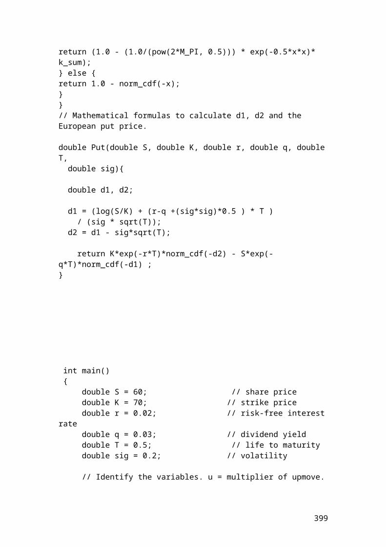
Solution

Initial margin = 7 x 5,200 = 36,400 dollars

Maintenance margin = 7 x 1,500 = 10,500 dollars

The cash flows, gains and losses for the next two days will be as follows:

Day 1

Cash flows for the buyer’s: 36,400 + 14,000 = 50,400 dollars. The investor’s recorded a gain.

Cash flows for the seller’s: 36,400 – 14,000 = 22,400 dollars. The investor’s recorded a loss.

Helpful hint: the amount of 14,000 is calculated from the difference of the bushel prices, (fT-f0) x number of contracts x standard contract size. Thus, we have: (220-230) x 7 x 200 = (14,000 dollars). The same principle applies for the second day but with different bushel prices. Thus, we have: (210 – 230) x 7 x 200 = (28000 dollars). Gains or losses depends if you are the buyer or seller.

Day 2

Please do the calculations for the second day.

This is why I am stressing the importance that the investors should buy or sell ONLY when the market is aggressively increasing or falling. If he/she gets trapped in a market that is not strong bull or bear, then, he/she will have to compensate regularly for the losses or he/she will experience a very small profit. If the amounts as the days passes is below the maintenance margin, then, the investor’s will receive a margin call and he/she should add the capital required to proceed with the contract. If the investor’s is short of money, then, the position is closed with the incurred losses.

Application of margin payments in the clearinghouse in python

>>> initialmargin = 5200>>> maintenancemargin = 1500>>> contractnumber = 7>>> bushelcontractsize = 200

399

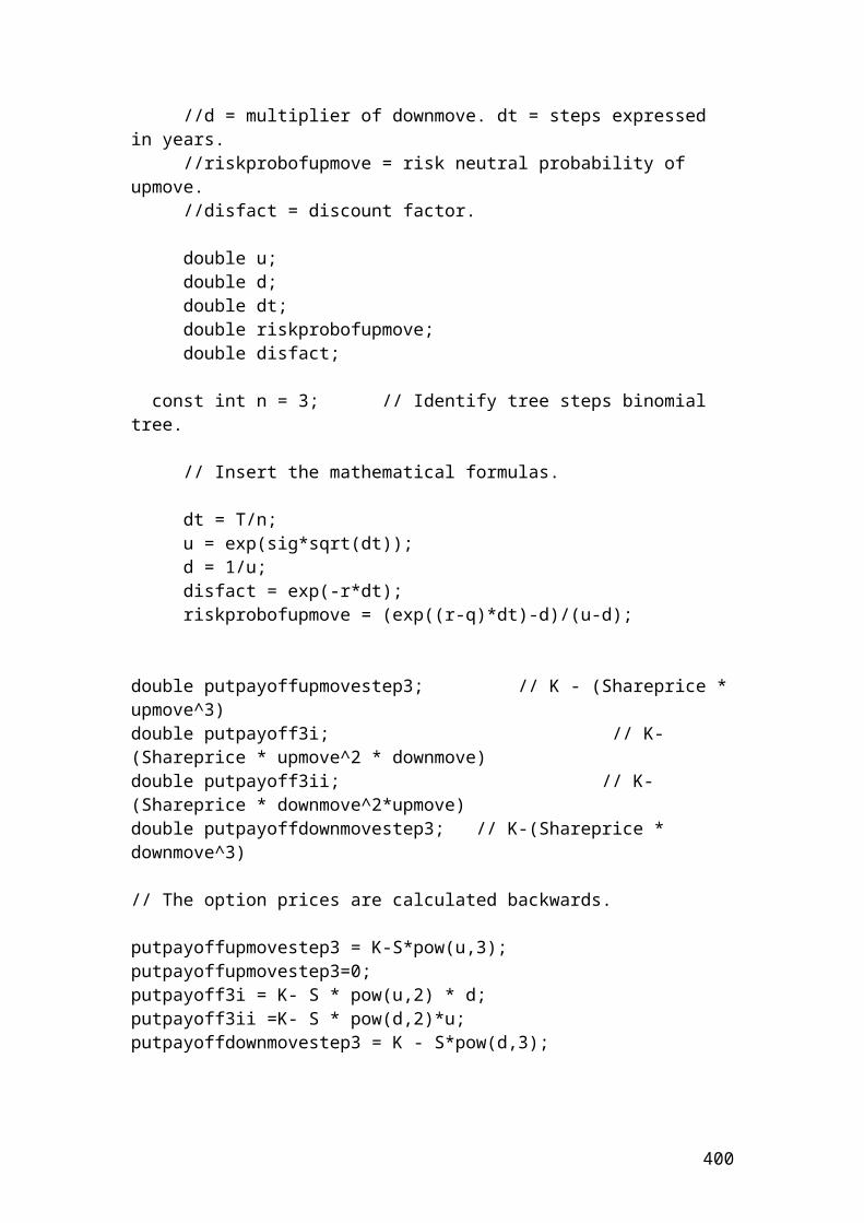
>>> bushelprice_1 = 230>>> bushelprice_2 = 220>>> # Insert the mathematical formulas.>>> initialmarginwithcontract = initialmargin * contractnumber>>> initialmarginwithcontract36400 # USD>>> maintenancemarginwithcontract = maintenancemargin * contractnumber>>> maintenancemarginwithcontract10500 # USD>>> bushelcontract = (bushelprice_1-bushelprice_2) * bushelcontractsize * contractnumber>>> bushelcontract14000 # USD>>> cashflowbuyer = initialmarginwithcontract + bushelcontract>>> cashflowbuyer50400 # USD>>> cashflowseller = initialmarginwithcontract - bushelcontract>>> cashflowseller22400 # USD

Please continue the calculations for the second day….

Example of calculating a margin call due to changes of price futures

An investor has opened a short position of 20 Soybean futures contract. The initial margin was 500 Pounds and the maintenance margin was 430 Pounds per contract. The price change that will create a margin call is as follows:

400

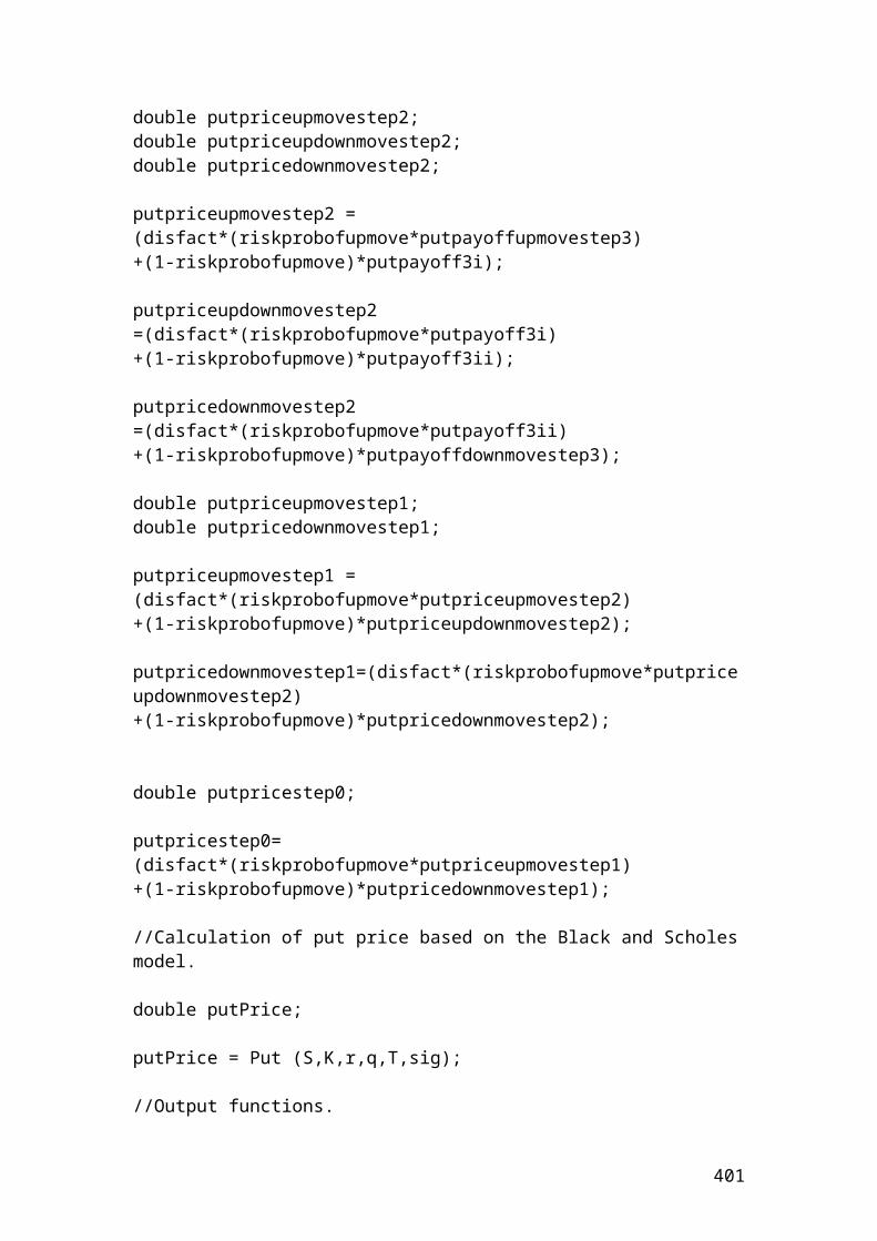
Solution

3.5

Pounds

Application of margin call in python

>>> initial_margin = 500>>> maintenance_margin = 430>>> futures_contract = 20>>> # Insert the mathematical formula.>>> margincall =(initial_margin-maintenance_margin) / futures_contract>>> margincall3.5 # Pounds

Solution of the above examples

Active return, active risk and information ratio

Active return is the difference in returns between a portfolio and the index or benchmark that is measured.

401

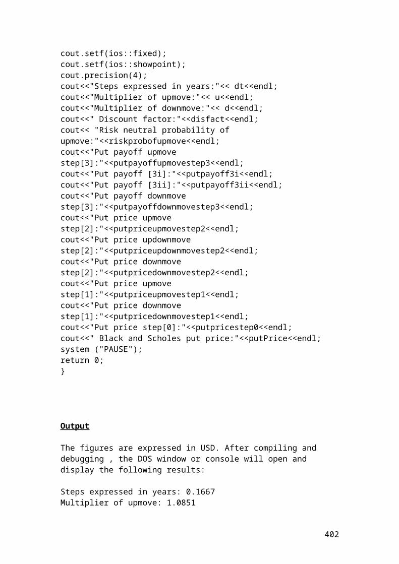
Active return = rp - rb

Where: rp is the portfolio return. rb is the benchmark or index return.

If the portfolio return is 0.80 and the benchmark return of the index is 0.70 then, the active return is………

Please complete the calculation.

Application of active return in python

>>> portfolio_return = 0.8>>> benchmark_return = 0.7>>> active_return = portfolio_return - benchmark_return>>> active_return0.10000000000000009>>> round(_,2)0.1

Active risk or tracking error is the standard deviation of the difference of returns between a portfolio and the benchmark or index.

402

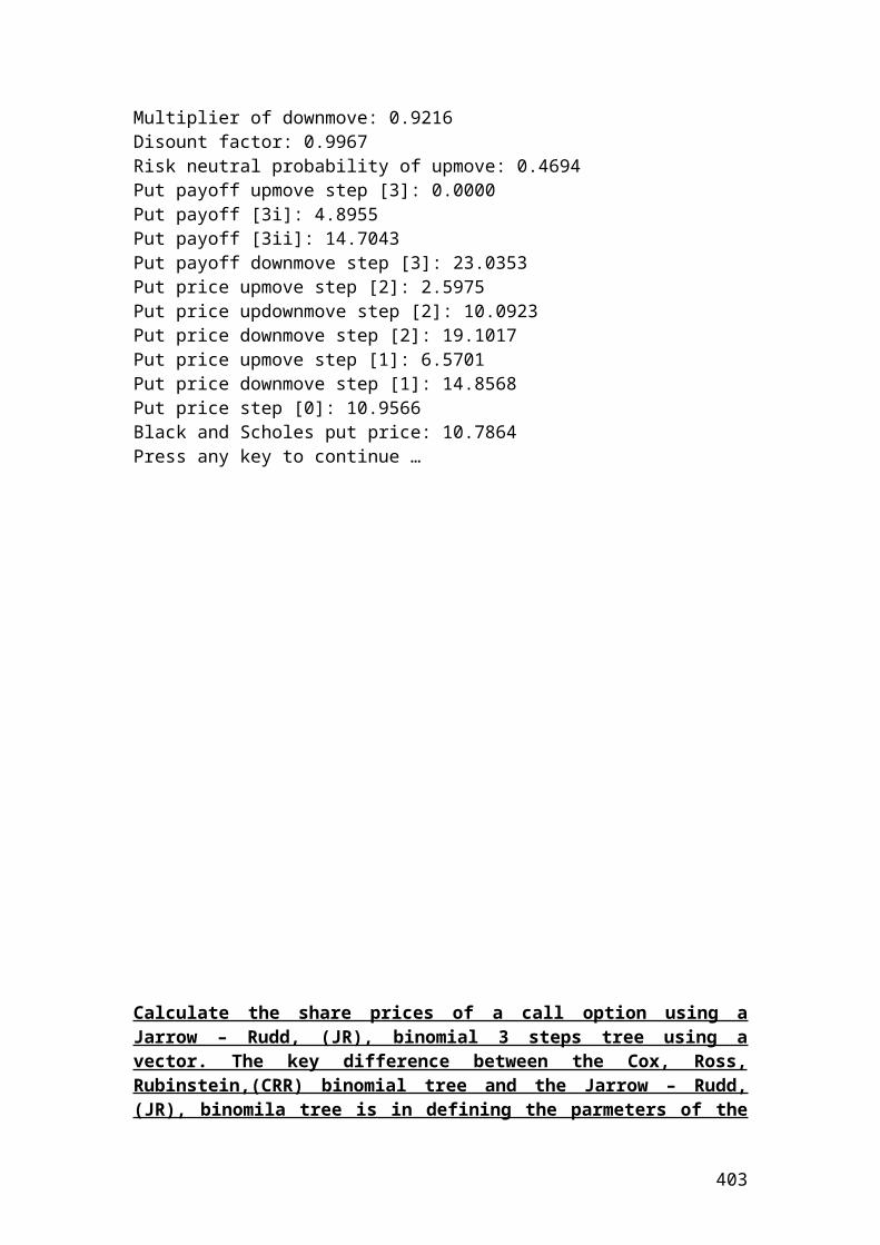
If the portfolio return is 0.80, the number of observations is 10 and the benchmark return of the index is 0.40 then, the active risk is………

Please complete the calculation.

Application of active risk in python

>>> portfolio_return = 0.80>>> benchmark_return = 0.40>>> n =10>>> # Insert the mathematical formula.>>> active_risk = sqrt((portfolio_return - benchmark_return)**2/9)>>> active_risk0.13333333333333336>>> round(_,2)0.13

Information ratio shows the consistency of the fund manager towards the active return. The mathematical formula is as follows:

Error! Objects cannot be created from editing field codes.

403

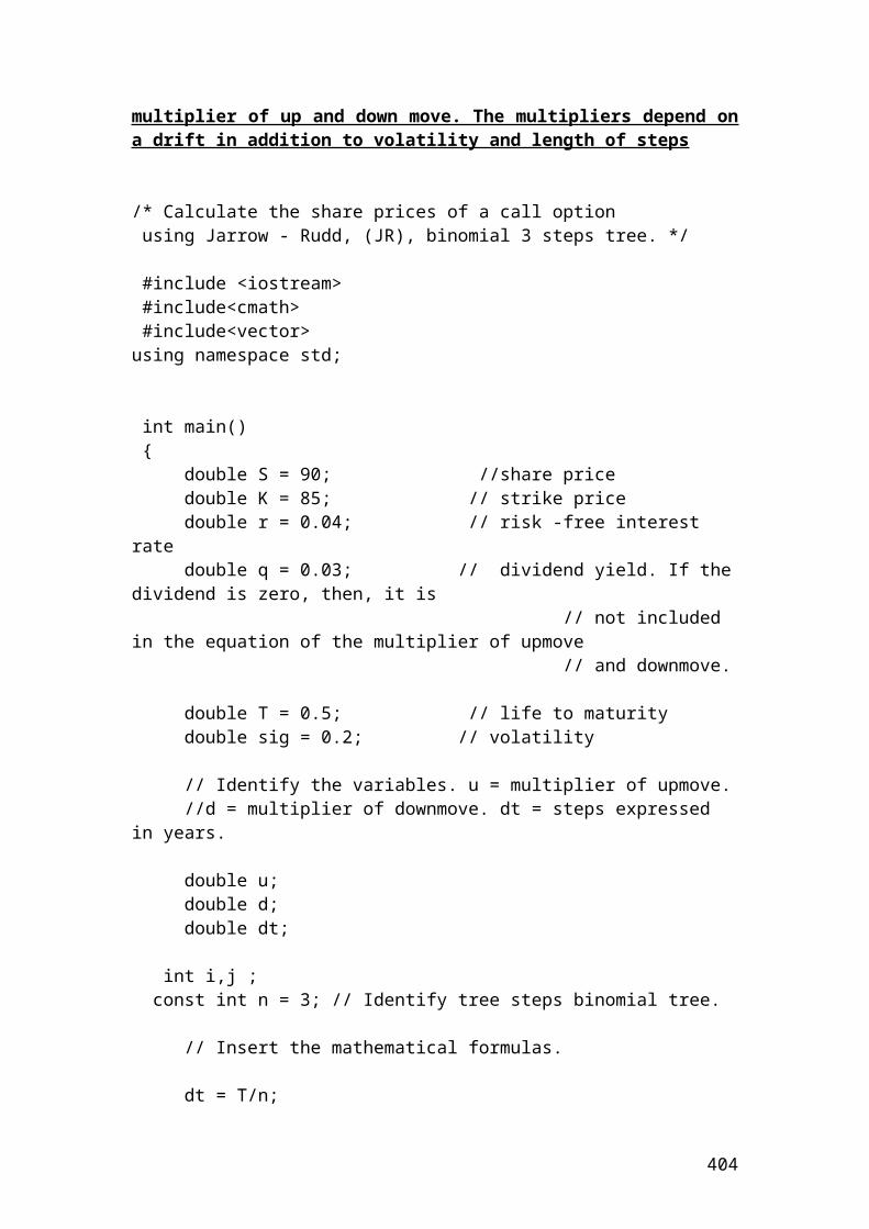
It could be calculated very easily in Excel software. I will illustrate a simple table with the relevant calculations.

Day rp rb rp - rb

1 0.03 0.02 0.012 0.02 0.014 0.0063 -0.04 0.034 -0.0744 0.05 0.067 -0.0175 0.08 0.012 0.0686 -0.01 -0.056 0.0467 0.07 0.031 0.0398 0.034 0.023 0.0119 -0.021 0.015 -0.03610 0.045 0.001 0.044

Average 0.0258 0.0161Standard deviation

0.043

Source: author’s calculation

By substituting the values that we have found in terms of rp =0.0258, rb = 0.0161 and standard deviation = 0.043 in the following equation we have:

Error! Objects cannot be created from editing field codes.

Error! Objects cannot be created from editing field codes.

But what is the interpretation of the information ratio of 0.23. It means that the fund manager gained around 23 basis points of active return per unit of active risk. The higher is this number, the better the manager is performing in relation to active risk.

Application of information ratio in python

>>> portfolio_return1 = 0.03>>> portfolio_return2 = 0.02>>> portfolio_return3 = -0.04>>> portfolio_return4 = 0.05>>> portfolio_return5 = 0.08>>> portfolio_return6 = -0.01>>> portfolio_return7 = 0.07>>> portfolio_return8 = 0.034>>> portfolio_return9 = -0.021>>> portfolio_return10 = 0.045>>> # Insert the mathematical formula.>>> average_1 = (portfolio_return1 + portfolio_return2 + portfolio_return3 + portfolio_return4 + portfolio_return5 + portfolio_return6+ portfolio_return7 + portfolio_return8 + portfolio_return9+ portfolio_return10)/10>>> average_10.0258

404

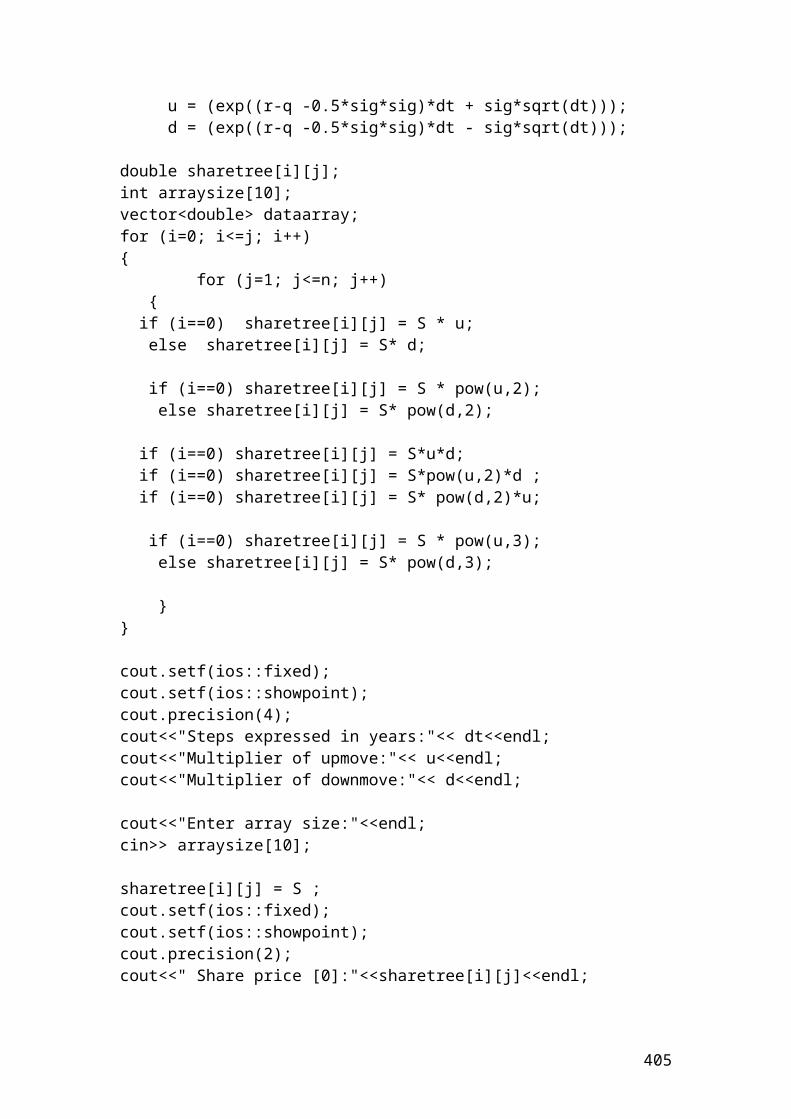
>>> benchmark_return1 = 0.02>>> benchmark_return2 = 0.014>>> benchmark_return3 = 0.034>>> benchmark_return4 = 0.067>>> benchmark_return5 = 0.012>>> benchmark_return6 = -0.056>>> benchmark_return7 = 0.031>>> benchmark_return8 = 0.023>>> benchmark_return9 = 0.015>>> benchmark_return10 = 0.001>>> average_2 = (benchmark_return1 + benchmark_return2 + benchmark_return3 + benchmark_return4 + benchmark_return5 + benchmark_return6 + benchmark_return7 + benchmark_return8 + benchmark_return9+ benchmark_return10)/10>>> average_20.016100000000000003>>># Insert the mathematical formulas to calculate the differences between the portfolioand benchmark return and then square it.>> diff1 = portfolio_return1 - benchmark_return1>>> diff10.009999999999999998>>> diff2 = portfolio_return2 - benchmark_return2>>> diff20.006>>> diff3 = portfolio_return3 - benchmark_return3>>> diff3-0.07400000000000001>>> diff4 = portfolio_return4 - benchmark_return4>>> diff4-0.017>>> diff5 = portfolio_return5 - benchmark_return5>>> diff50.068>>> diff6 = portfolio_return6 - benchmark_return6>>> diff60.046>>> diff7 = portfolio_return7 - benchmark_return7>>> diff70.03900000000000001>>> diff8 = portfolio_return8 - benchmark_return8>>> diff80.011000000000000003>>> diff9 = portfolio_return9 - benchmark_return9>>> diff9-0.036000000000000004>>> diff10 = portfolio_return10 - benchmark_return10>>> diff100.044>>> #Find the sum from the differences.>>> sumDiff = diff1 + diff2 + diff3 + diff4 + diff5 + diff6 + diff7 + diff8 +diff9 +diff10

405

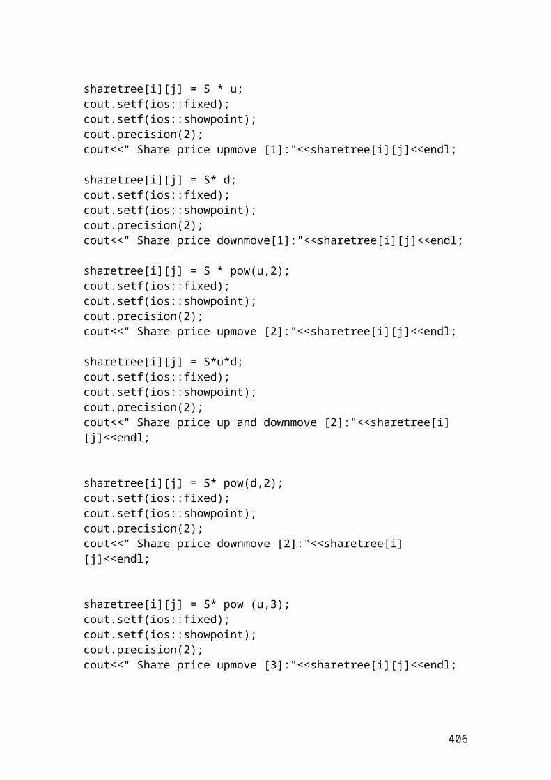
>>> sumDiff0.09699999999999999>>># Find the average from the differences.>>> average3 = sumDiff /10>>> average30.009699999999999999

Please complete the exercise……. If you have questions, then, please let me know.

Please convert the following exercise in python language programming

Calculate the balance at the end of the 5th day from changes in the futures prices from 90 to 89, 91, 95, 97, 99. The trader has bought 50 futures contract for settlement in May. The initial margin is $8.

Day Beginning balance

Futures price Gain or loss Ending balance

0 400 90 0 4001 400 89 (50)2 350 91 1003 450 95 2004 650 97 1005 750 99 100

Source: author’s illustration.

Beginning balance = initial margin x number of contracts.Beginning balance = 8 x 50 = $400

Please complete the values of the column ending balance.

406

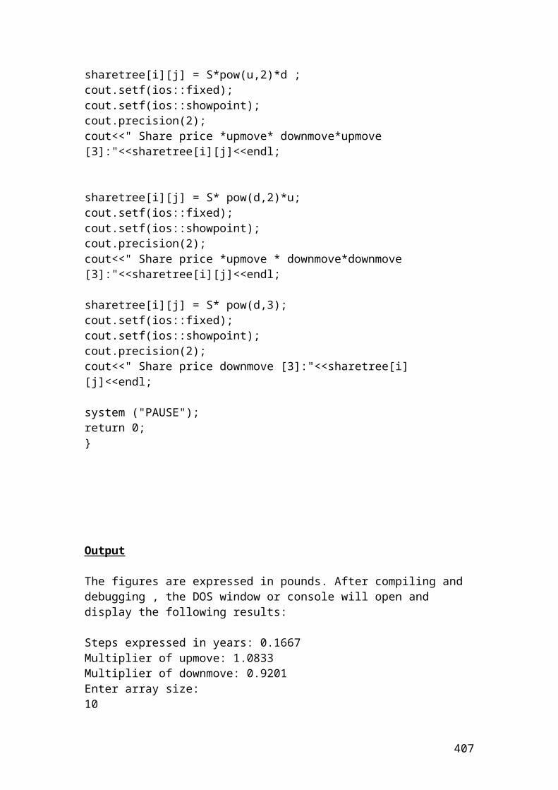
Solution

Day Beginning balance

Futures price Gain or loss Ending balance

0 400 90 0 4001 400 89 (50) 3502 350 91 100 4503 450 95 200 6504 650 97 100 7505 750 99 100 850

The ending balance at the 5th day in the margin account will be 850 USD.

Calculate the caplet option payments based on different interest rates using a binomial 2 steps tree. The figures are expressed in pounds

>>> # Calculate the caplet values based on an interest rate cap using a binomial 2 steps tree. It is a similar example of a call option on interest rates. The payment is based on the difference between the current interest rate and the cap rate multiplied by the principal and divided by the discounted current interest rate. The buyer receives a payment when the current interest rate exceeds the cap strike price.

>>> strike = 0.02>>> principal = 30000000>>> maturity = 0.5>>> sigma = 0.3>>> interest_rate = 0.04>>> n =2>>> p=0.5>>> # Insert the mathematical formulas.>>> dt = maturity/n # steps expressed in years.>>> dt0.25>>> from math import*>>> u = exp(sigma*sqrt(dt)) # multiplier of upmove.

407

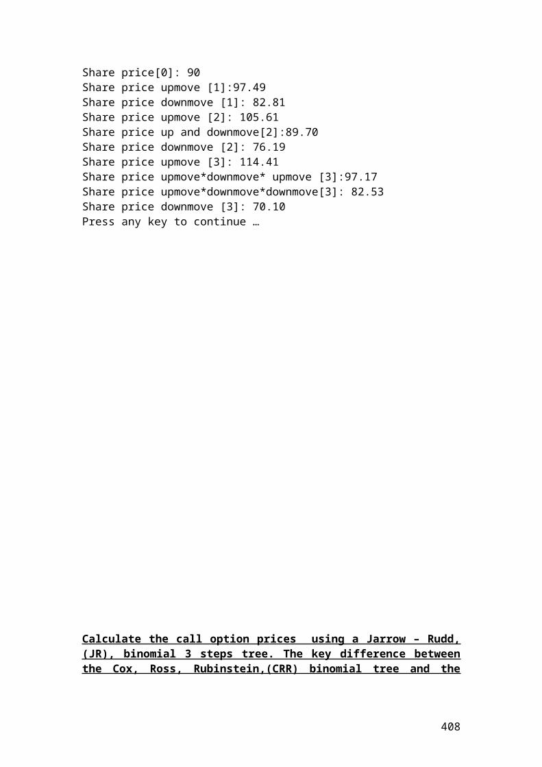
>>> u1.161834242728283>>> d = 1/u # multiplier of downmove.>>> d0.8607079764250578>>># Identify the interest rates in each node.>>> interest_0 = 0.04>>> interest_1i = 0.0465>>> interest_1ii = 0.0344>>> interest_2i = 0.054>>> interest_2ii = 0.04>>> interest_2iii = 0.0296>>># Identify the discounted interest rates.>>> disinterest_0 = 1.04>>> disinterest_1i = 1.0465>>> disinterest_1ii = 1.0344>>> disinterest_2i = 1.054>>> disinterest_2ii = 1.04>>> disinterest_2iii = 1.0296>>># Insert the mathematical formulas. It is a backward induction methodology.>>> capletPrice2i = (principal*(interest_2i-strike)/disinterest_2i)>>> capletPrice2i967741.935483871>>> capletPrice2ii = (principal*(interest_2ii-strike)/disinterest_2ii)>>> capletPrice2ii576923.0769230769>>> capletPrice2iii = (principal*(interest_2iii-strike)/disinterest_2iii)>>> capletPrice2iii279720.2797202797>>> capletPrice1i = (((capletPrice2i*p)+(capletPrice2ii*p))/disinterest_1i)>>> capletPrice1i738014.8172035108>>> capletPrice1ii = (((capletPrice2ii*p)+(capletPrice2iii*p))/disinterest_1ii)>>> capletPrice1ii414077.415237508>>> capletPrice0 = (((capletPrice1i*p)+(capletPrice1ii*p))/disinterest_0)>>> capletPrice0553890.4963658744>>> round(_,2)553890.5

408

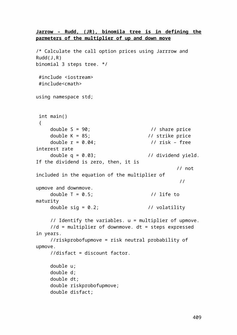
Calculate the floorlet option payments based on different interest rates using a binomial 2 steps tree. The figures are expressed in pounds

>>> # Calculate the floorlet values based on an interest rate floor using a binomial 2 steps tree. It is a similar example of a put option on interest rates. It protects the holder from declining interest rates. The payment is based on the difference between the floor rate and the current interest rate multiplied by the principal and divided by the discounted current interest rate.

>>> strike = 0.02>>> principal = 30000000>>> maturity = 0.5>>> sigma = 0.3>>> interest_rate = 0.04>>> n =2>>> p=0.5>>> # Insert the mathematical formulas.>>> dt = maturity/n # steps expressed in years.>>> dt0.25>>> from math import*>>> u = exp(sigma*sqrt(dt)) # multiplier of upmove.>>> u1.161834242728283

409

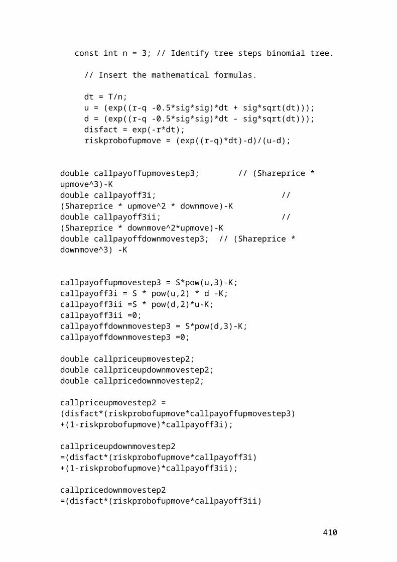
>>> d = 1/u # multiplier of downmove.>>> d0.8607079764250578>>># Identify the interest rates in each node.>>> interest_0 = 0.04>>> interest_1i = 0.0465>>> interest_1ii = 0.0344>>> interest_2i = 0.054>>> interest_2ii = 0.04>>> interest_2iii = 0.0296

>>># Identify the discounted interest rates.>>> disinterest_0 = 1.04>>> disinterest_1i = 1.0465>>> disinterest_1ii = 1.0344>>> disinterest_2i = 1.054>>> disinterest_2ii = 1.04>>> disinterest_2iii = 1.0296

>>># Insert the mathematical formulas. It is a backward induction methodology.>>> floorletPrice2i = (principal*(strike - interest_2i)/disinterest_2i)>>> floorletPrice2i56925.99620493363>>> floorletPrice2ii = (principal*(strike - interest_2ii)/disinterest_2ii)>>> floorletPrice2ii461538.4615384615>>> floorletPrice2iii = (principal*(strike - interest_2iii)/disinterest_2iii)>>> floorletPrice2iii769230.7692307691>>> floorletPrice1i = (((floorletPrice2i*p)+(floorletPrice2ii*p))/disinterest_1i)>>> floorletPrice1i247713.5488501649>>> floorletPrice1ii = (((floorletPrice2ii*p)+(floorletPrice2iii*p))/disinterest_1ii)>>> floorletPrice1ii594919.3884228686>>> floorletPrice0 = (((floorletPrice1i*p)+(floorletPrice1ii*p))/disinterest_0)>>> floorletPrice0405111.9890735737>>> round(_,2)405111.99

410

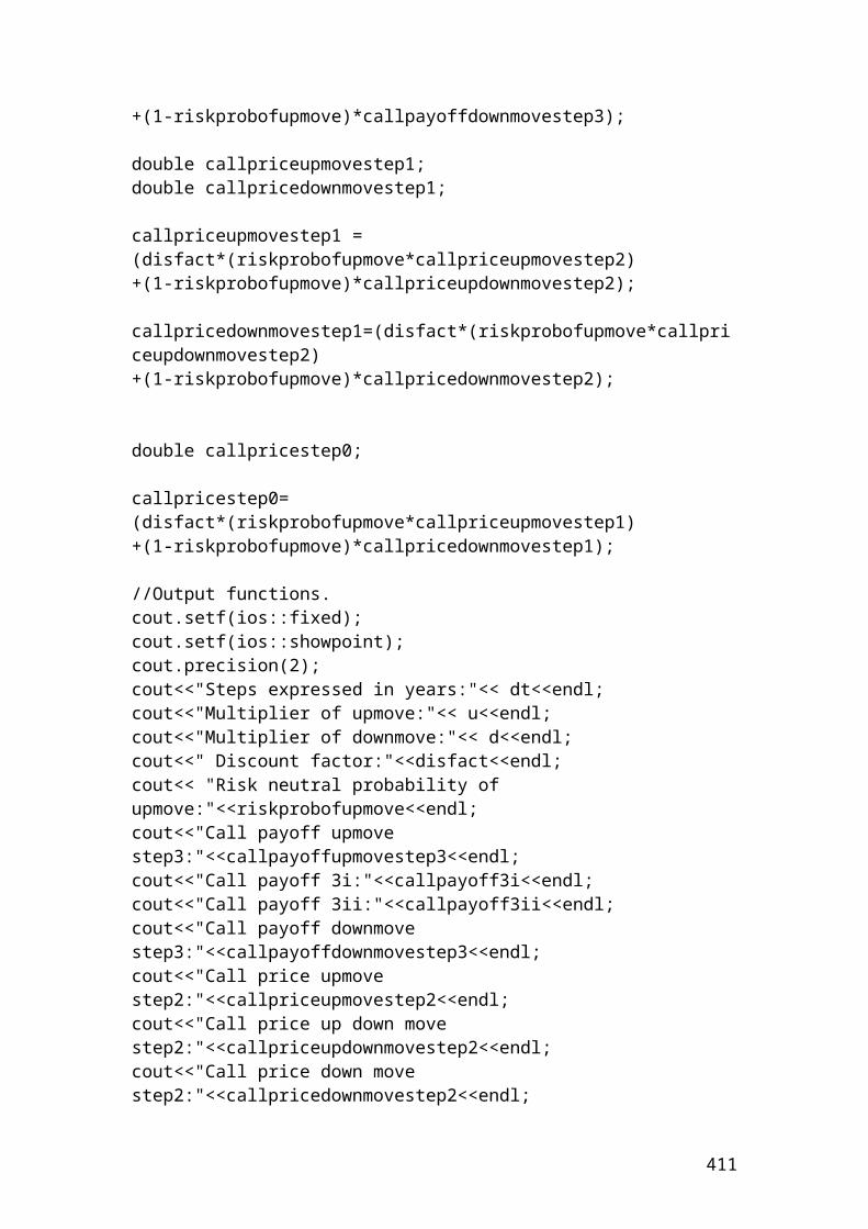
Calculate the bond put option prices based on different interest rates using a binomial 2 steps tree

>>> bond_price = 100>>> strike = 102>>> annual_coupon = 7>>> maturity = 0.5>>> sigma = 0.3>>> interest_rate = 4>>> n =2>>> p = 0.5>>> dt = maturity/n # steps expressed in years.>>> dt0.25>>> from math import*>>> u = exp(sigma*sqrt(dt)) # multiplier of upmove.>>> u1.161834242728283>>> d = 1/u # multiplier of downmove.>>> d0.8607079764250578>>># Insert the mathematical formulas. It is a backward induction methodology.>>> bondPrice2i = (bond_price+annual_coupon)*(1/disinterest_2i)

411

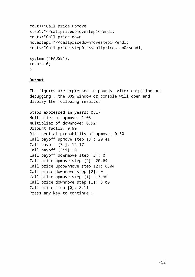
>>> bondPrice2i101.5180265654649>>> bondPrice2ii=(bond_price+annual_coupon)*(1/disinterest_2ii)>>> bondPrice2ii102.88461538461537>>> bondPrice2iii = (bond_price+annual_coupon)*(1/disinterest_2iii)>>> bondPrice2iii103.92385392385391>>> bondPrice1i = ((((bondPrice2i+annual_coupon)*p)+(bondPrice2ii+annual_coupon)*p)/disinterest_1i)>>> bondPrice1i104.3490883660202>>> bondPrice1ii = ((((bondPrice2ii+annual_coupon)*p)+(bondPrice2iii+annual_coupon)*p)/disinterest_1ii)>>> bondPrice1ii106.73263210966226>>> bondPrice0 = ((((bondPrice1i+ annual_coupon)*p)+(bondPrice1ii+ annual_coupon)*p)/disinterest_0)>>> bondPrice0108.21236561330888

>>> putPriceUpmovestep2i = strike - bondPrice2i>>> putPriceUpmovestep2i0.48197343453510655>>> putPriceUpdownmovestep2ii = strike - bondPrice2ii>>> putPriceUpdownmovestep2ii-0.8846153846153726>>> putPriceUpdownmovestep2ii = 0>>> putPriceUpdownmovestep2ii0>>> putPriceDownmovestep2iii = strike - bondPrice2iii>>> putPriceDownmovestep2iii-1.9238539238539119>>> putPriceDownmovestep2iii =0>>> putPriceDownmovestep2iii0>>> putPriceUpmovestep1i= (((putPriceUpmovestep2i*p)+(putPriceUpdownmovestep2ii*p))/disinterest_1i)>>> putPriceUpmovestep1i0.2302787551529415>>> putPriceDownmovestep1ii= (((putPriceUpdownmovestep2ii*p)+(putPriceDownmovestep2iii*p))/disinterest_1ii)>>> putPriceDownmovestep1ii0.0

412

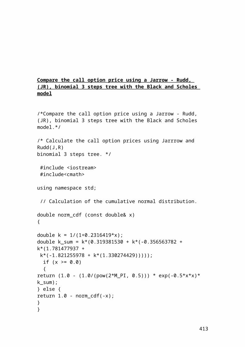
>>> putPricestep0= (((putPriceUpmovestep1i*p)+(putPriceDownmovestep1ii*p))/disinterest_0)>>> putPricestep00.11071093997737572

Calculate the bond call option prices based on different interest rates using a binomial 2 steps tree. The figures are expressed in pounds

>>> bond_price = 100>>> strike = 100>>> annual_coupon = 7>>> maturity = 0.5>>> sigma = 0.3>>> interest_rate = 4>>> n =2>>> p = 0.5>>> dt = maturity/n # steps expressed in years.>>> dt0.25>>> from math import*>>> u = exp(sigma*sqrt(dt)) # multiplier of upmove.>>> u1.161834242728283>>> d = 1/u # multiplier of downmove.>>> d0.8607079764250578

>>> #Identify the discounted interest rates.

413

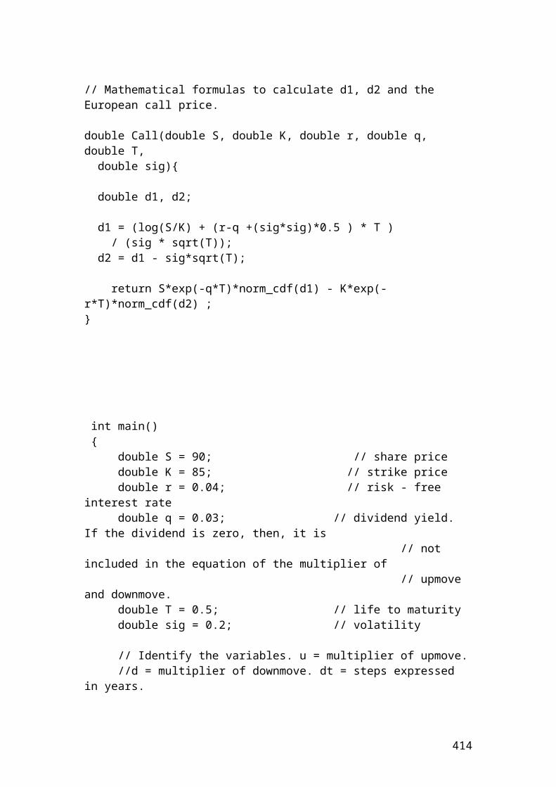
>>> disinterest_0 = 1.04>>> disinterest_1i = 1.0465>>> disinterest_1ii = 1.0344>>> disinterest_2i = 1.054>>> disinterest_2ii = 1.04>>> disinterest_2iii = 1.0296>>># Insert the mathematical formulas. It is a backward induction methodology.>>> bondPrice2i = (bond_price+annual_coupon)*(1/disinterest_2i)>>> bondPrice2i101.5180265654649>>> bondPrice2ii=(bond_price+annual_coupon)*(1/disinterest_2ii)>>> bondPrice2ii102.88461538461537>>> bondPrice2iii = (bond_price+annual_coupon)*(1/disinterest_2iii)>>> bondPrice2iii103.92385392385391>>> bondPrice1i = ((((bondPrice2i+annual_coupon)*p)+(bondPrice2ii+annual_coupon)*p)/disinterest_1i)>>> bondPrice1i104.3490883660202>>> bondPrice1ii = ((((bondPrice2ii+annual_coupon)*p)+(bondPrice2iii+annual_coupon)*p)/disinterest_1ii)>>> bondPrice1ii106.73263210966226>>> bondPrice0 = ((((bondPrice1i+ annual_coupon)*p)+(bondPrice1ii+ annual_coupon)*p)/disinterest_0)>>> bondPrice0108.21236561330888>>> callPriceUpmovestep2i = bondPrice2i - strike>>> callPriceUpmovestep2i1.5180265654648935>>> round(_,2)1.52>>> callPriceUpdownmovestep2ii = bondPrice2ii - strike>>> callPriceUpdownmovestep2ii2.8846153846153726>>> callPriceDownmovestep2iii = bondPrice2iii - strike>>> callPriceDownmovestep2iii3.923853923853912>>> callPriceUpmovestep1i= (((callPriceUpmovestep2i*p)+(callPriceUpdownmovestep2ii*p))/disinterest_1i)>>> callPriceUpmovestep1i2.103507859570122>>> callPriceDownmovestep1ii= (((callPriceUpdownmovestep2ii*p)+(callPriceDownmovestep2iii*p))/disinterest_1ii)>>> callPriceDownmovestep1ii3.291023447635965>>> callPricestep0= (((callPriceUpmovestep1i*p)+(callPriceDownmovestep1ii*p))/disinterest_0)>>> callPricestep0

414

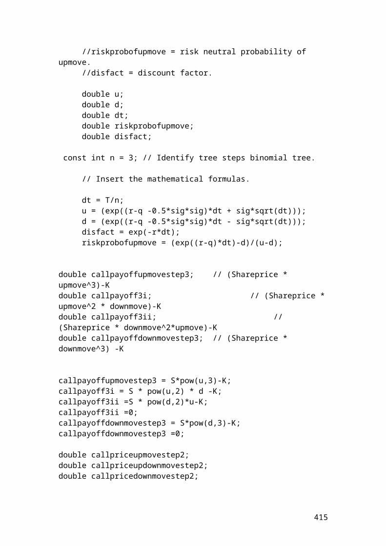
2.5935246669260033>>> round(_,2)2.59

Calculate the bond prices of an option based on different interest rates using a binomial 2 steps tree. The figures are expressed in pounds

>>> bond_price = 100>>> strike = 100>>> annual_coupon = 7>>> maturity = 0.5>>> sigma = 0.3>>> interest_rate = 4>>> n =2>>> p = 0.5>>> dt = maturity/n # steps expressed in years.>>> dt0.25>>> from math import*>>> u = exp(sigma*sqrt(dt)) # multiplier of upmove.>>> u1.161834242728283>>> d = 1/u # multiplier of downmove.>>> d0.8607079764250578

>>> #Identify the discounted interest rates.>>> disinterest_0 = 1.04>>> disinterest_1i = 1.0465>>> disinterest_1ii = 1.0344>>> disinterest_2i = 1.054

415

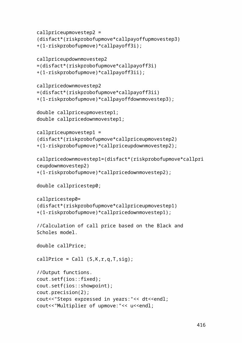
>>> disinterest_2ii = 1.04>>> disinterest_2iii = 1.0296

>>># Insert the mathematical formulas. It is a backward induction methodology.>>> bondPrice2i = (bond_price+annual_coupon)*(1/disinterest_2i)>>> bondPrice2i101.5180265654649>>> bondPrice2ii=(bond_price+annual_coupon)*(1/disinterest_2ii)>>> bondPrice2ii102.88461538461537>>> bondPrice2iii = (bond_price+annual_coupon)*(1/disinterest_2iii)>>> bondPrice2iii103.92385392385391>>> bondPrice1i = ((((bondPrice2i+annual_coupon)*p)+(bondPrice2ii+annual_coupon)*p)/disinterest_1i)>>> bondPrice1i104.3490883660202>>> bondPrice1ii = ((((bondPrice2ii+annual_coupon)*p)+(bondPrice2iii+annual_coupon)*p)/disinterest_1ii)>>> bondPrice1ii106.73263210966226>>> bondPrice0 = ((((bondPrice1i+ annual_coupon)*p)+(bondPrice1ii+ annual_coupon)*p)/disinterest_0)>>> bondPrice0108.21236561330888

416

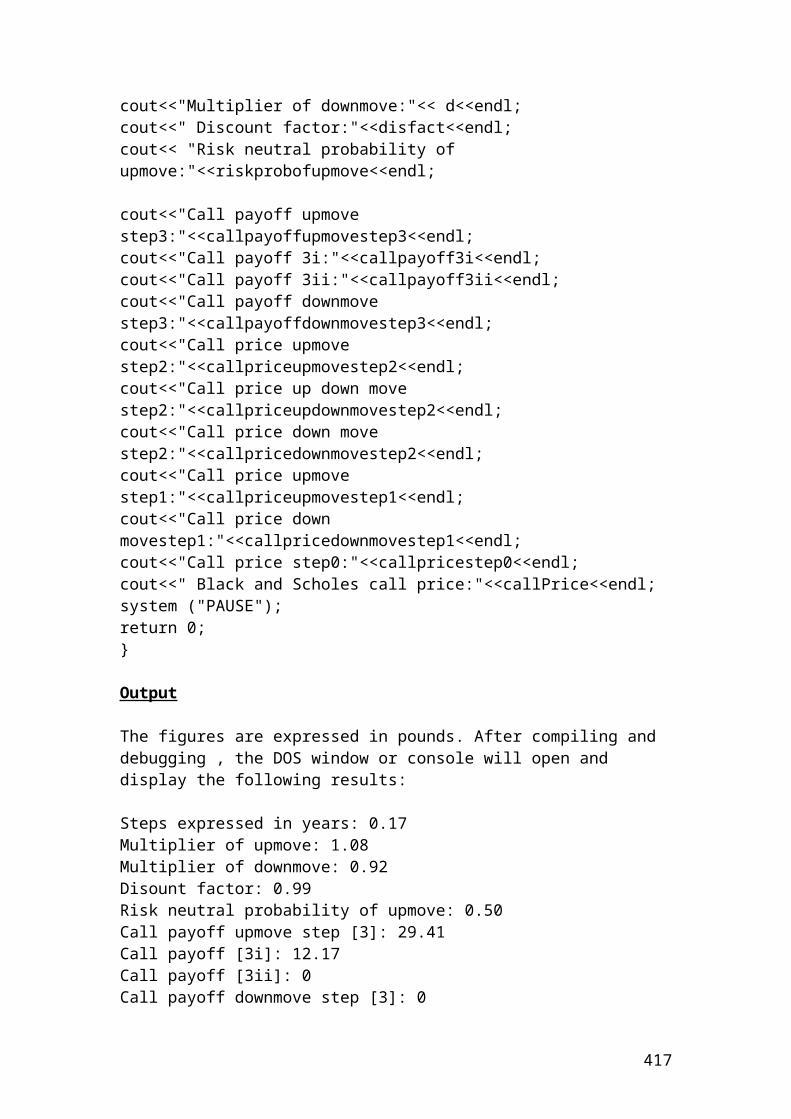
Calculate the interest rates of an option bond based on a two – period binomial tree. The risk – neutral probability of an up and down move in the interest rate tree is always 50% or 0.5. The figures are expressed in percentages

>>> bond_price =100>>> strike = 100>>> annual_coupon = 7>>> maturity = 0.5>>> volatility = 0.3>>> interest_rate = 4>>> p=0.5>>> n=2>>>interestrate0 = 4>>> interestrate1i = interest_rate * u>>> interestrate1i4.647336970913132>>> interestrate1ii = interest_rate * d>>> interestrate1ii3.4428319057002312>>> interestrate2i = interest_rate * u**2>>> interestrate2i5.399435230304012>>> interestrate2ii= interest_rate*u*d>>> interestrate2ii4.0>>> interestrate2iii= interest_rate* d**2>>> interestrate2iii2.9632728827268715>>> round(_,2)

417

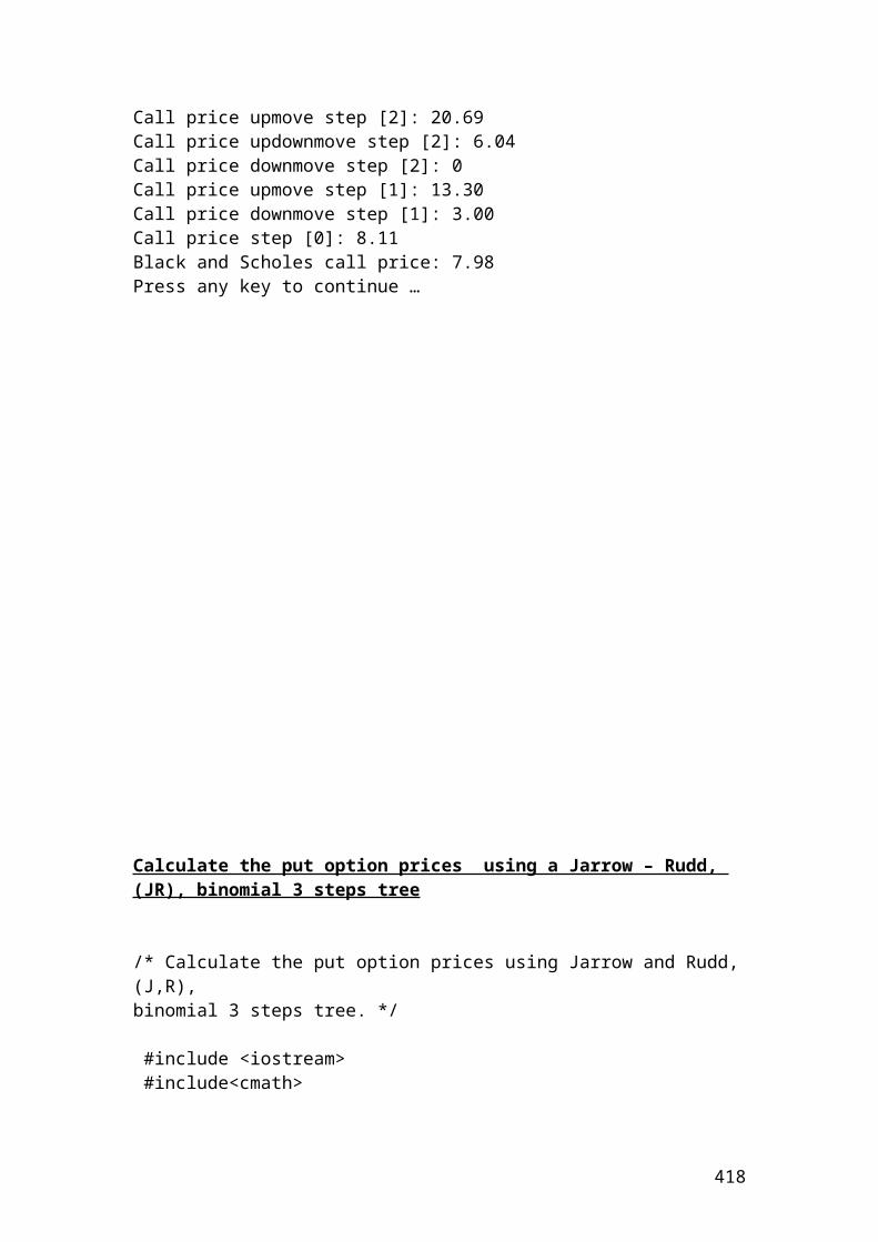
2.96

Calculate the share prices of a call option using a Cox, Ross, Rubinstein,(CRR) binomial 3 steps tree using a vector. The multipliers of up and down move depend on volatility and length of steps. The figures are expressed in pounds

S = 60 # share price K = 50 # strike price r = 0.05 # interest rateq = 0.02 # dividend yieldT = 0.5 # maturitysig = 0.3 # volatilityn = 3>>> dt = T/n>>> dt0.16666666666666666>>> u = exp(sig*sqrt(dt))>>> u1.1302902827674572>>> d = 1/u>>> d0.8847284766100544>>> share_price0 = S>>> share_price060>>> share_price_1upmove = S*u>>> share_price167.81741696604743>>> round(_,2)67.82>>> share_price_1downmove = S *d

418

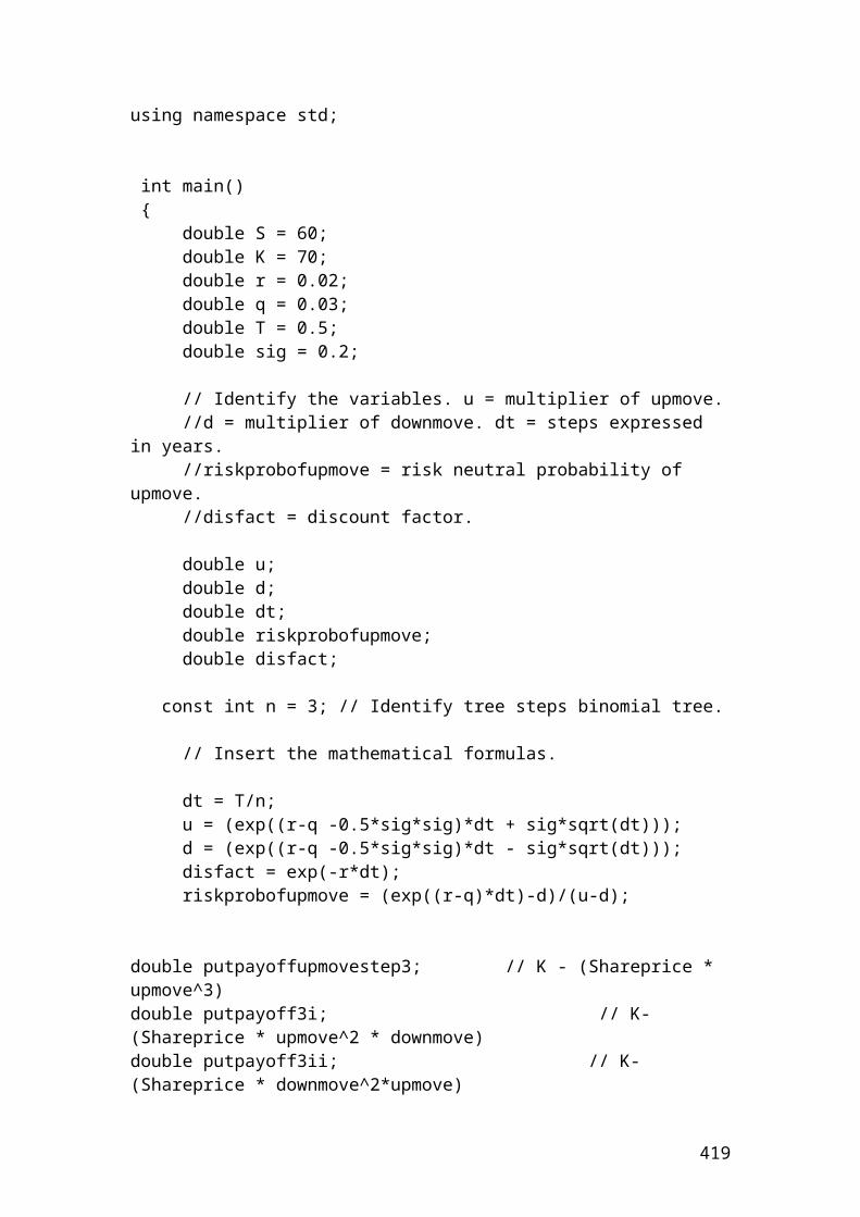
>>> share_price_1downmove53.083708596603266>>> round(_,2)53.08>>> share_price2upmove = S *u**2>>> share_price2upmove76.6533673991123>>> round(_,2)76.65>>> share_price2downmove = S*d**2>>> share_price2downmove46.96466863948485>>> round(_,2)46.96>>> share_price2upanddownmove = S*u*d>>> share_price2upanddownmove60.0>>> share_price3downmove = S*d**3>>> share_price3downmove41.55097973990743>>> round(_,2)41.55>>> share_price3upmove = S*u**3>>> share_price3upmove86.64055631262043>>> round(_,2)86.64>>> share_price3updowndown = S*u*d*d>>> share_price3updowndown53.083708596603266>>> round(_,2)53.08>>> share_price3upandupdown = S*u*u*d>>> share_price3upandupdown67.81741696604743>>> round(_,2)67.82

419

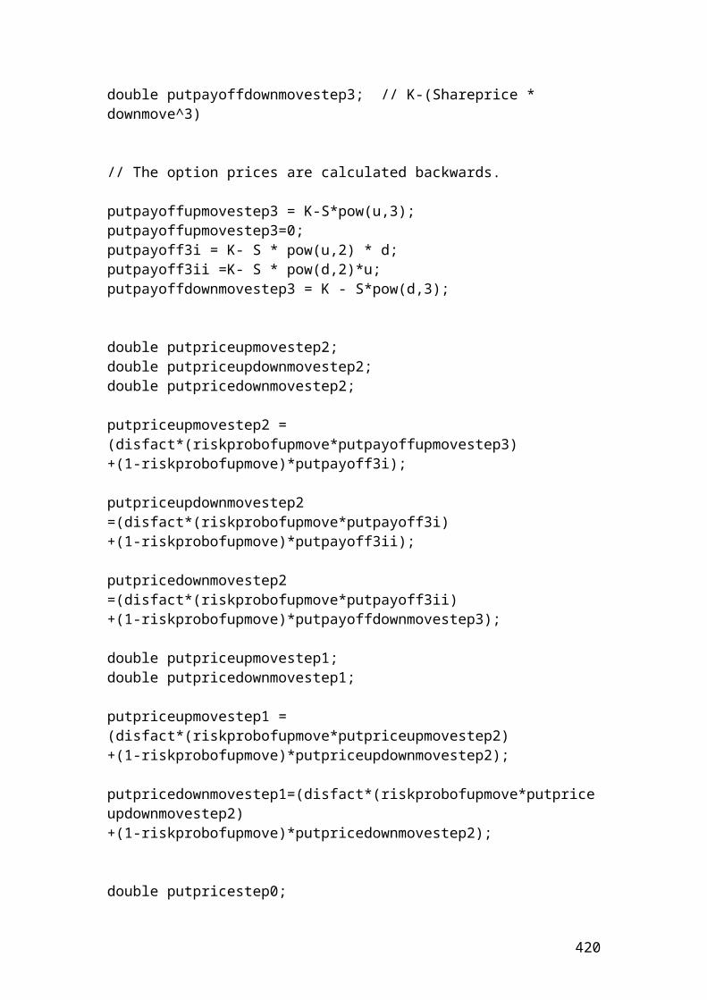
Calculate the call option prices using a Cox, Ross, Rubinstein,(CRR) binomial 3 steps tree. The figures are expressed in pounds

S = 60 # share price K = 50 # strike price r = 0.05 # interest rateq = 0.02 # dividend yieldT = 0.5 # maturitysig = 0.3 # volatilityn = 3>>> dt = T/n>>> dt0.16666666666666666>>> from math import*>>> u = exp(sig*sqrt(dt))>>> u1.1302902827674572>>> d = 1/u>>> d0.8847284766100544>>> disfact = exp(-r*dt)>>> disfact0.991701292638876>>> riskprobofupmove = (exp((r-q)*dt)-d)/(u-d)>>> riskprobofupmove0.48983205544695174>> #The option prices are calculated backwards.>>> callpayoffupmovestep3 = S*u**3-K>>> callpayoffupmovestep3

420

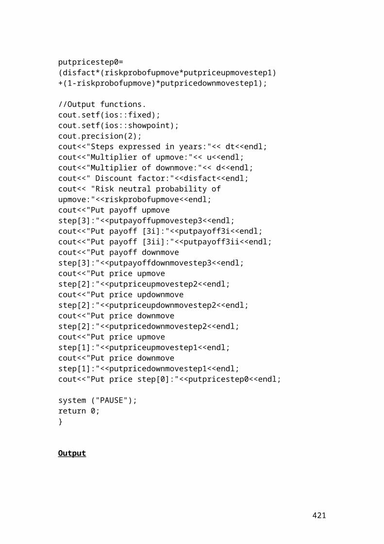
36.64055631262043>>> callpayoff3i = S * u**2 * d -K>>> callpayoff3i17.817416966047432>>> callpayoff3ii =S * d**2*u-K>>> callpayoff3ii3.083708596603259>>> callpayoffdownmovestep3 = S*d**3-K>>> callpayoffdownmovestep3-8.449020260092567>>> callpayoffdownmovestep3 =0>>> callpayoffdownmovestep30>>> callpriceupmovestep2 = (disfact*(riskprobofupmove*callpayoffupmovestep3)+(1-riskprobofupmove)*callpayoff3i)>>> callpriceupmovestep226.88865113426896>>> callpriceupdownmovestep2 =(disfact*(riskprobofupmove*callpayoff3i)+(1-riskprobofupmove)*callpayoff3ii)>>> callpriceupdownmovestep210.228323934729657>>> callpricedownmovestep2 =(disfact*(riskprobofupmove*callpayoff3ii)+(1-riskprobofupmove)*callpayoffdownmovestep3)>>> callpricedownmovestep21.4979641284454819>>> callpriceupmovestep1 = (disfact*(riskprobofupmove*callpriceupmovestep2)+(1-riskprobofupmove)*callpriceupdownmovestep2)>>> callpriceupmovestep118.279784613543832>>> callpricedownmovestep1=(disfact*(riskprobofupmove*callpriceupdownmovestep2)+(1-riskprobofupmove)*callpricedownmovestep2)>>> callpricedownmovestep15.732796357703088>>> callpricestep0= (disfact*(riskprobofupmove*callpriceupmovestep1)+(1-riskprobofupmove)*callpricedownmovestep1)>>> callpricestep011.804406575946299>>> round(_,2)11.8

421

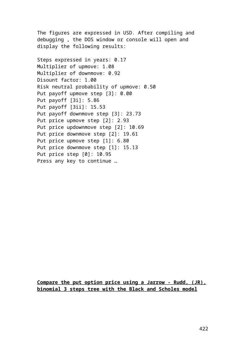
Calculate the put option prices using a Cox, Ross, Rubinstein,(CRR) binomial 3 steps tree. The figures are expressed in USD

>>> S = 60 # share price>>> K = 70 # strike price>>> r = 0.02 # interest rate>>> q = 0.03 # dividend yield>>> T = 0.5 # maturity>>> sig = 0.2 # volatility>>> n = 3>>> dt = T/n>>> dt0.16666666666666666>>> from math import*>>> u = exp(sig*sqrt(dt))>>> u1.0850755957772693>>> d = 1/u>>> d0.9215947754162443>>> disfact = exp(-r*dt)>>> disfact0.9966722160545233>>> riskprobofupmove = (exp((r-q)*dt)-d)/(u-d)>>> riskprobofupmove0.46941253331873867>>> #The option prices are calculated backwards.>>> putpayoffupmovestep3 = K-S*u**3

422

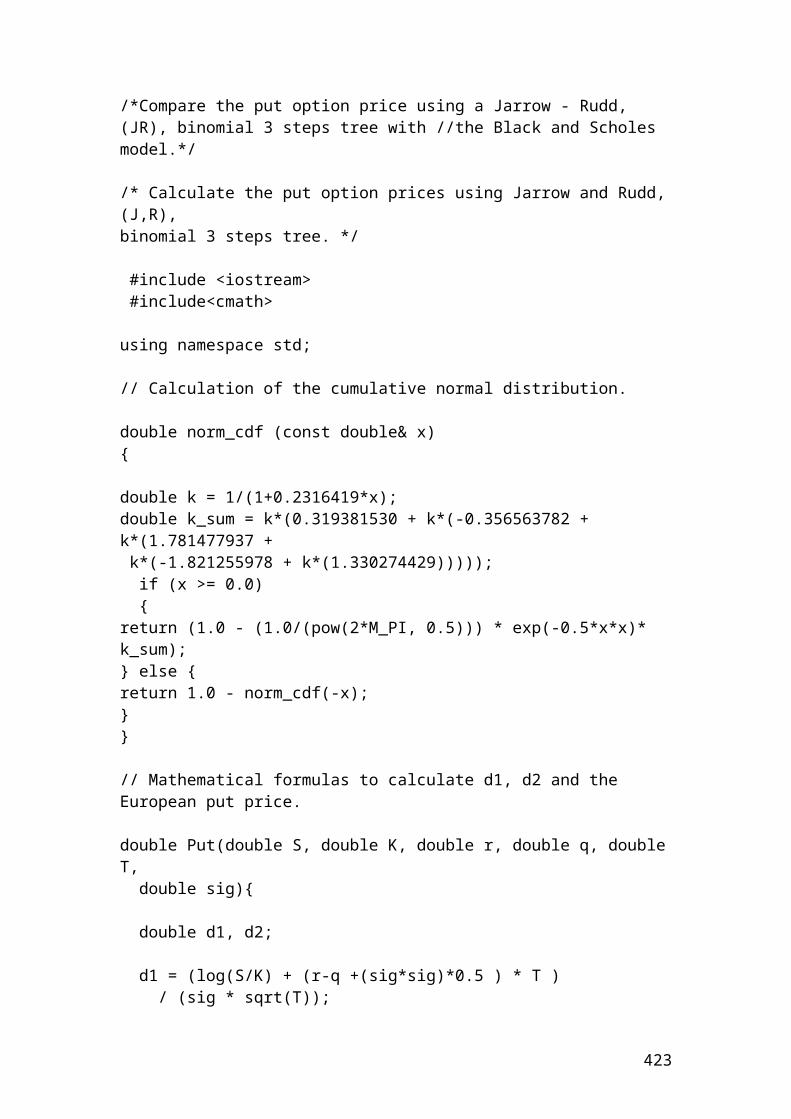
>>> putpayoffupmovestep3-6.653367399112284>>> putpayoffupmovestep3=0>>> putpayoffupmovestep30>>> putpayoff3i = K- S * u**2 * d>>> putpayoff3i4.895464253363841>>> putpayoff3ii =K- S * d**2*u>>> putpayoff3ii14.704313475025337>>> putpayoffdownmovestep3 = K - S*d**3>>> putpayoffdownmovestep323.035331360515137>>> putpriceupmovestep2 = (disfact*(riskprobofupmove*putpayoffupmovestep3)+(1-riskprobofupmove)*putpayoff3i)>>> putpriceupmovestep22.5974719764209926>>> putpriceupdownmovestep2 =(disfact*(riskprobofupmove*putpayoff3i)+(1-riskprobofupmove)*putpayoff3ii)>>> putpriceupdownmovestep210.092269491137635>>> putpricedownmovestep2 =(disfact*(riskprobofupmove*putpayoff3ii)+(1-riskprobofupmove)*putpayoffdownmovestep3)>>> putpricedownmovestep219.101677490334147>>> putpriceupmovestep1 = (disfact*(riskprobofupmove*putpriceupmovestep2)+(1-riskprobofupmove)*putpriceupdownmovestep2)>>> putpriceupmovestep16.5700600829982925>>> putpricedownmovestep1=(disfact*(riskprobofupmove*putpriceupdownmovestep2)+(1-riskprobofupmove)*putpricedownmovestep2)>>> putpricedownmovestep114.85678328831304>>> putpricestep0= (disfact*(riskprobofupmove*putpriceupmovestep1)+(1-riskprobofupmove)*putpricedownmovestep1)>>> putpricestep010.956628441795559>>> round(_,2)10.96

423

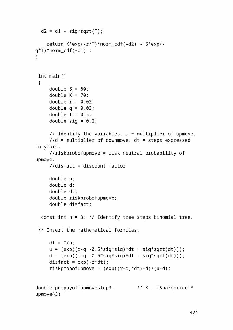
Calculation of a Monte Carlo put option using antithetic variables. The purpose of using antithetic variables is to improve the estimation results by reducing the standard error of the simulation results. The figures are expressed in USD

>>> number_of_simulation = 199999>>> max_size = 200000>>> initial_share_price = 80>>> strike_price = 110>>> interest_rate = 0.07>>> dividend_yield = 0.02>>> volatility = 0.10>>> maturity = 0.5>>> from math import*>>> normsamp = [i]>>> i =0>>> i<=number_of_simulationTrue>>> random.number = (30000+3000)/300>>> random.number110.0>>> sharePrice = initial_share_price *exp((interest_rate-dividend_yield-0.5*volatility*volatility)*maturity+normsamp[i]*random.number*volatility *sqrt(maturity))>>> sharePrice81.82040273315567>>> round(_,2)81.82

424

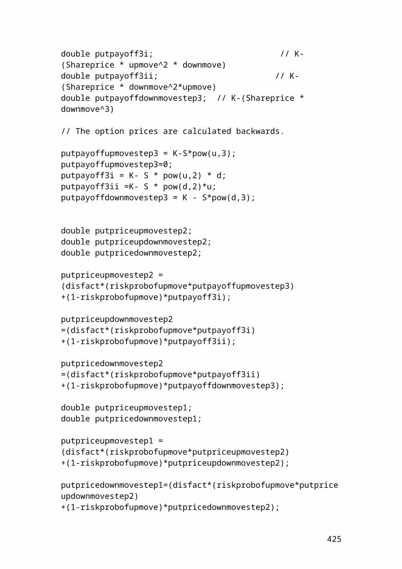
>>> sharePrice = initial_share_price *exp((interest_rate-dividend_yield-0.5*volatility*volatility)*maturity-normsamp[i]*random.number*volatility *sqrt(maturity))>>> sharePrice>>> payoff += value*strike*sharePrice*sharePrice>>> payoff35460314.4509055>>> optPrice = (payoff * exp(-r*T))/ Number_of_simulation/2>>> optPrice87.7691349127051>>> round(_,2)87.77

Calculate the put option prices using a Cox, Ross, Rubinstein,(CRR) binomial 3 steps tree. The figures are expressed in USD

>>> S = 60 # share price>>> K = 70 # strike price>>> r = 0.02 # interest rate>>> q = 0.03 # dividend yield>>> T = 0.5 # maturity>>> sig = 0.2 # volatility>>> n = 3>>> dt = T/n>>> dt0.16666666666666666>>> from math import*>>> u = exp(sig*sqrt(dt))>>> u1.0850755957772693>>> d = 1/u>>> d0.9215947754162443>>> disfact = exp(-r*dt)>>> disfact0.9966722160545233>>> riskprobofupmove = (exp((r-q)*dt)-d)/(u-d)>>> riskprobofupmove0.46941253331873867>>> #The option prices are calculated backwards.

425

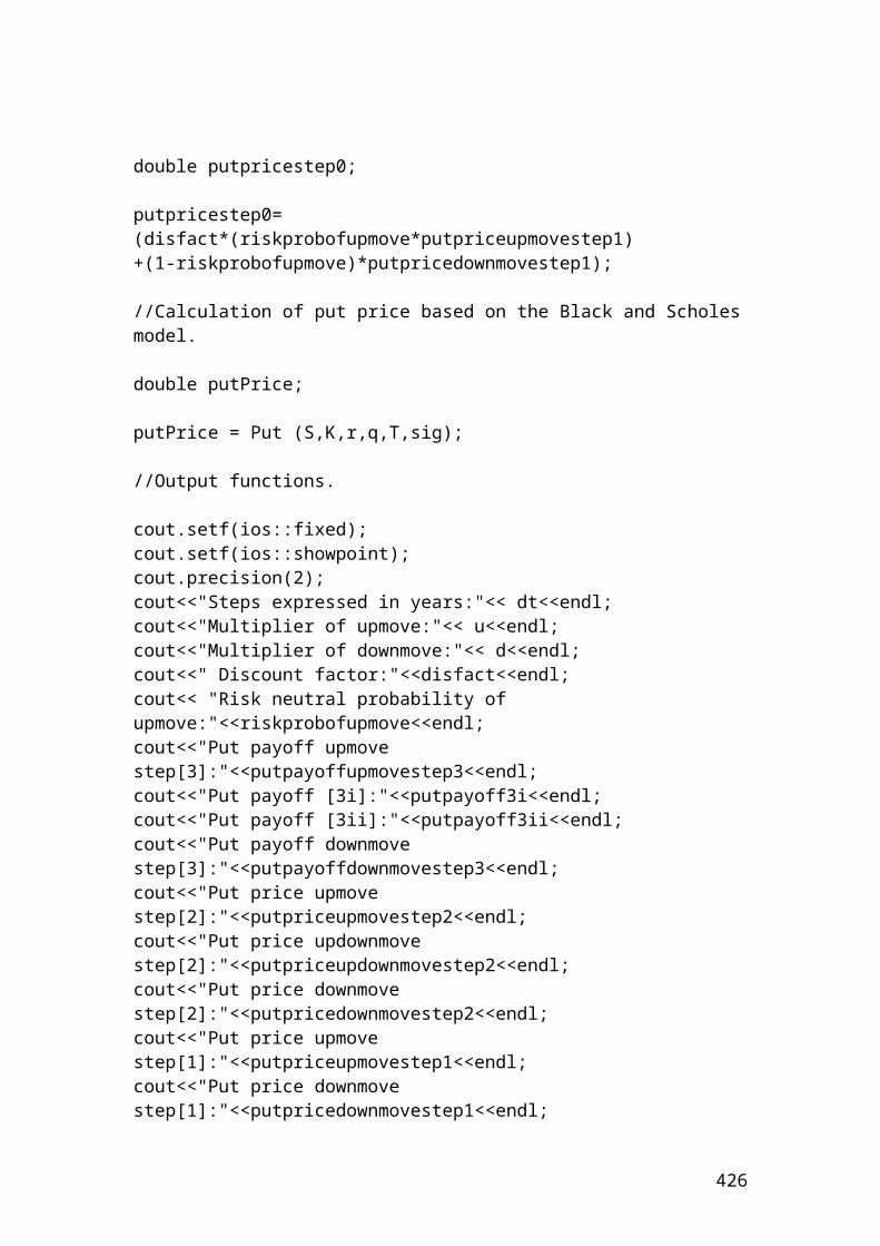
>>> putpayoffupmovestep3 = K-S*u**3>>> putpayoffupmovestep3-6.653367399112284>>> putpayoffupmovestep3=0>>> putpayoffupmovestep30>>> putpayoff3i = K- S * u**2 * d>>> putpayoff3i4.895464253363841>>> putpayoff3ii =K- S * d**2*u>>> putpayoff3ii14.704313475025337>>> putpayoffdownmovestep3 = K - S*d**3>>> putpayoffdownmovestep323.035331360515137>>> putpriceupmovestep2 = (disfact*(riskprobofupmove*putpayoffupmovestep3)+(1-riskprobofupmove)*putpayoff3i)>>> putpriceupmovestep22.5974719764209926>>> putpriceupdownmovestep2 =(disfact*(riskprobofupmove*putpayoff3i)+(1-riskprobofupmove)*putpayoff3ii)>>> putpriceupdownmovestep210.092269491137635>>> putpricedownmovestep2 =(disfact*(riskprobofupmove*putpayoff3ii)+(1-riskprobofupmove)*putpayoffdownmovestep3)>>> putpricedownmovestep219.101677490334147>>> putpriceupmovestep1 = (disfact*(riskprobofupmove*putpriceupmovestep2)+(1-riskprobofupmove)*putpriceupdownmovestep2)>>> putpriceupmovestep16.5700600829982925>>> putpricedownmovestep1=(disfact*(riskprobofupmove*putpriceupdownmovestep2)+(1-riskprobofupmove)*putpricedownmovestep2)>>> putpricedownmovestep114.85678328831304>>> putpricestep0= (disfact*(riskprobofupmove*putpriceupmovestep1)+(1-riskprobofupmove)*putpricedownmovestep1)>>> putpricestep010.956628441795559>>>>>> round(_,2)10.96

426

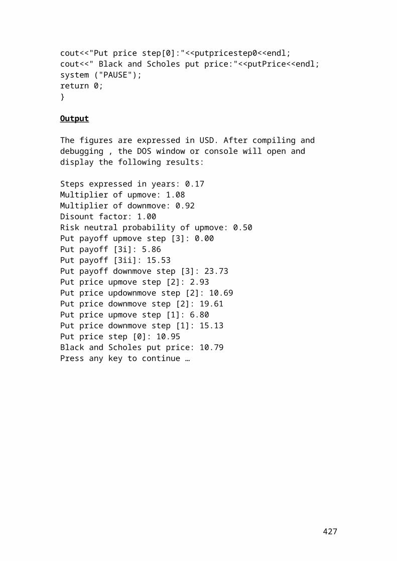
Calculation of a Monte Carlo call option using antithetic variables. The purpose of using antithetic variables is to improve the estimation results by reducing the standard error of the simulation results

>>> number_of_simulation = 199999>>> max_size = 200000>>> initial_share_price = 120>>> strike_price = 90>>> interest_rate = 0.07>>> dividend_yield = 0.02>>> volatility = 0.10>>> maturity = 0.5>>> from math import*>>> i =0>>> i<=number_of_simulationTrue>>> normsamp = [i]>>> random = (30000+3000)/300>>> random110.0>>> sharePrice = initial_share_price *exp((interest_rate-dividend_yield-0.5*volatility*volatility)*maturity+normsamp[i]*random*volatility *sqrt(maturity))>>> sharePrice122.73060409973353>>> round(_,2)122.73

427

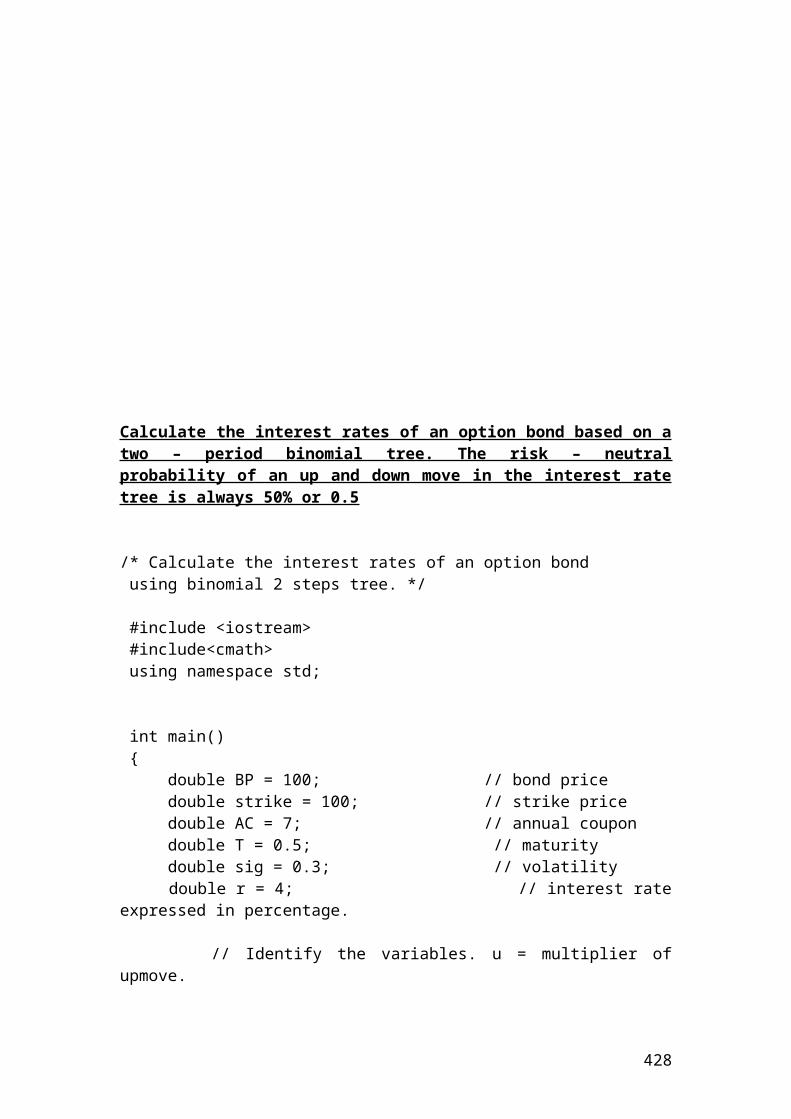
>>> sharePrice = initial_share_price *exp((interest_rate-dividend_yield-0.5*volatility*volatility)*maturity-normsamp[i]*random*volatility *sqrt(maturity))>>> sharePrice>>> value = initial_share_price – strike_price>>> value>>>30>>> payoff += value*strike*sharePrice*sharePrice>>> payoff

>>> optPrice = (payoff * exp(-r*T))/ Number_of_simulation/2>>> optPrice

Please continue the calculations related to payoff and optPrice….

Calculate the call option prices using a Jarrow – Rudd, (JR), binomial 3 steps tree. The key difference between the Cox, Ross, Rubinstein,(CRR) binomial tree and the Jarrow – Rudd, (JR), binomila tree is in defining the parmeters of the multiplier of up and down move. The figures are expressed in pounds

>>> S = 90 # share price>>> K = 85 # strike price>>> r = 0.04 # interest rate>>> q = 0.03 # dividend yield>>> T = 0.5 # maturity>>> sig = 0.2 # volatility>>> n = 3>>> from math import*>>> dt = T/n>>> dt = T/n # steps expressed in years.>>> dt0.16666666666666666>>> u = (exp((r-q -0.5*sig*sig)*dt + sig*sqrt(dt))) # multiplier of upmove.>>> u1.0832686426635116 >>> d = (exp((r-q -0.5*sig*sig)*dt - sig*sqrt(dt))) # multiplier of downmove.>>> d0.9200600634058166>>> disfact = exp(-r*dt) # discount factor.>>> disfact0.9933555062550344

428

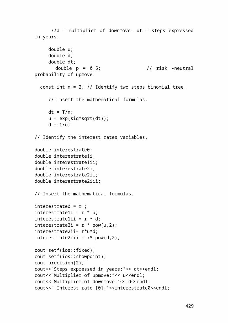
>>> riskprobofupmove = (exp((r-q)*dt)-d)/(u-d) # risk neutral probability of upmove.>>> riskprobofupmove0.5000226905523886>>> callpayoffupmovestep3 = S*u**3-K>>> callpayoffupmovestep329.406585701387428>>> callpayoff3i = S * u**2 * d -K>>> callpayoff3i12.169738279923607>>> callpayoff3ii =S*d**2*u-K>>> callpayoff3ii-2.470152793185349>>> callpayoff3ii =0>>> callpayoff3ii0>>> callpayoffdownmovestep3 = S*d**3-K>>> callpayoffdownmovestep3-14.904352933845047>>> callpayoffdownmovestep3 =0>>> callpayoffdownmovestep30>>> callpriceupmovestep2 = (disfact*(riskprobofupmove*callpayoffupmovestep3)+(1-riskprobofupmove)*callpayoff3i)>>> callpriceupmovestep220.690852733318547>>> callpriceupdownmovestep2 =(disfact*(riskprobofupmove*callpayoff3i)+(1-riskprobofupmove)*callpayoff3ii)>>> callpriceupdownmovestep26.044712568308618>>> callpricedownmovestep2 =(disfact*(riskprobofupmove*callpayoff3ii)+(1-riskprobofupmove)*callpayoffdownmovestep3)>>> callpricedownmovestep20.0>>> callpriceupmovestep1 = (disfact*(riskprobofupmove*callpriceupmovestep2)+(1-riskprobofupmove)*callpriceupdownmovestep2)>>> callpriceupmovestep113.299371739539392>>> callpricedownmovestep1=(disfact*(riskprobofupmove*callpriceupdownmovestep2)+(1-riskprobofupmove)*callpricedownmovestep2)>>> callpricedownmovestep13.0024105032518027>>> callpricestep0= (disfact*(riskprobofupmove*callpriceupmovestep1)+(1-riskprobofupmove)*callpricedownmovestep1)>>> callpricestep08.10693896385682>>> round(_,2)8.11

429

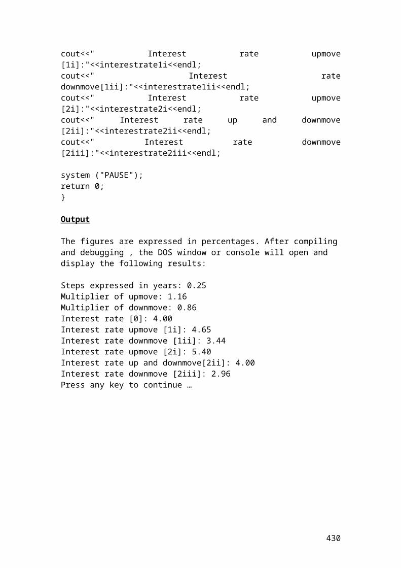
Calculate the share prices of a call option using a Jarrow – Rudd, (JR), binomial 3 steps tree. The prices are expressed in Euros

>>> S = 90>>> K = 85>>> r = 0.04>>> q = 0.03>>> T = 0.5>>> sig = 0.2>>> n =3>>> dt = T/n>>> dt0.16666666666666666>>> from math import*>>> u = (exp((r-q -0.5*sig*sig)*dt + sig*sqrt(dt)))>>> u1.0832686426635116>>> d = (exp((r-q -0.5*sig*sig)*dt - sig*sqrt(dt)))>>> d0.9200600634058166>>> share_price0 = S>>> share_price090>>> share_priceupmove1 = S*u>>> share_priceupmove97.49417783971604

430

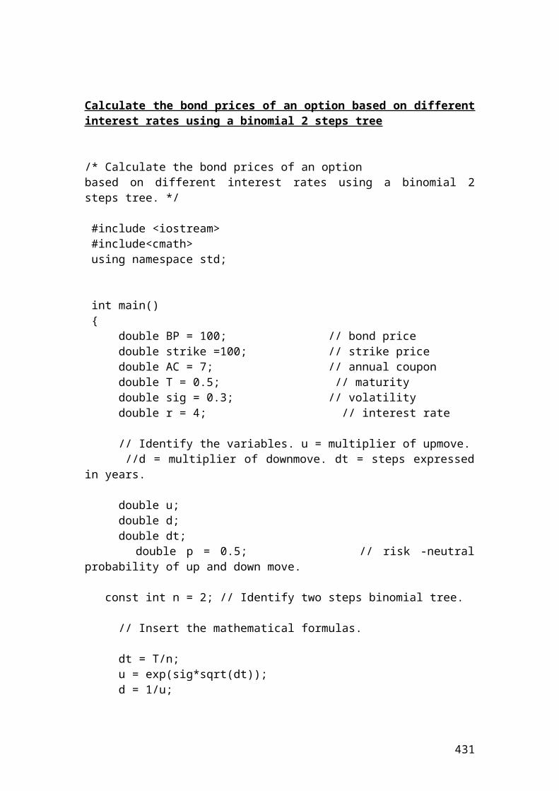
>>> round(_,2)97.49>>> share_pricedownmove1 = S*d>>> share_pricedownmove182.80540570652349>>> round(_,2)82.81>>> share_priceupmove2 = S*u**2>>> share_priceupmove2105.61238569602422>>> round(_,2)105.61>>> share_priceupmovedownmove = S*u*d>>> share_priceupmovedownmove89.70049944490711>>> round(_,2)89.7>>> share_pricedownmove2 = S*d**2>>> share_pricedownmove276.18594682468837>>> round(_,2)76.19>>> share_priceupmove3 = S*u**3>>> share_priceupmove3114.40658570138743>>> round(_,2)114.41

Please complete the remaining calculations……

431

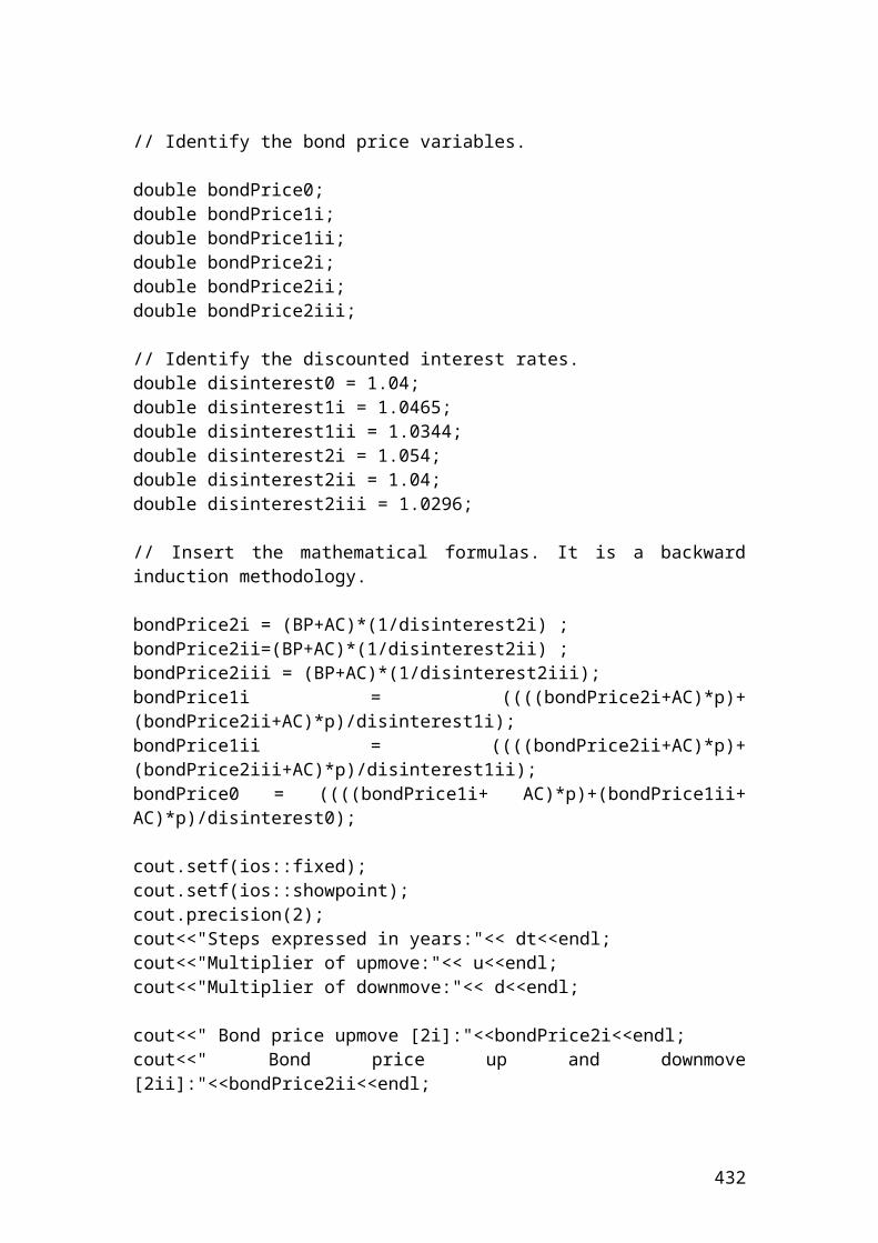
Example of simulating share prices by showing different price scenarios. The figure is expressed in pounds

>>> number_of_simulation = 6>>> max_size = 8>>> S0 = 60>>> r = 0.03>>> q = 0.02>>> sig = 0.20>>> dt = 1/250>>> dt0.004>>> from math import*>>> normsamp = [i]>>> i = 0>>> normsamp=[i]>>> i<=number_of_simulationTrue>>> random.number = (30000+3000)/300>>> random.number110.0>>> sharePrice=S0*exp((r-q-0.5*sig*sig)*dt+normsamp[i]*random.number*sig*sqrt(dt))>>> sharePrice59.99760004799936

432

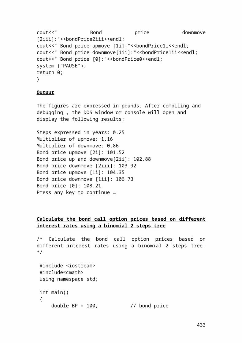
Please complete the calculations to get different share prices….

A manufacturing company sold a FRA contract expiring in 50 days with a principal of 30,000,000 USD. The underlying is 180 days LIBOR. The agreed rate on this FRA is 7%. At expiration, 90 days later, the actual rate on 180 days LIBOR is 8%. How much is the payoff of the manufacturing company at expiration?

Solution

The mathematical formula for Forward Rate Agreement, (FRA) is as follows:

FRA Payment = 30,000,000* ((0.08 – 0.07)*(180/360) / 1 + 0.08*(180/360)

FRA Payment = 30,000,000 * 0.005 / 1.04

FRA Payment = 144230.77 USD

Application of FRA payment in python

>>> principal = 30000000>>> actual_rate = 0.08

433

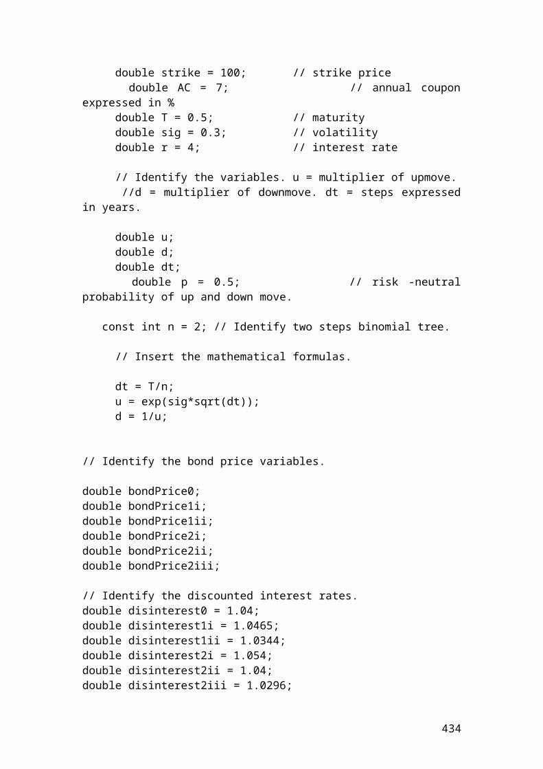
>>> agreed_rate = 0.07>>> days_1underlying = 180>>> days_2expiration = 180

Please complete the calculations using python ……..

Currency futures

Futures Price = contract size * exchange rate

If the contract size is 20,000 USD and the quoted price is 1.573 USD, then, the futures price is as follows:

Futures Price = 20,000 * 1.573 = 31460 USD

Application of currency futures in python

>>> contract_size = 20000>>> quoted_price = 1.573>>> FuturesPrice = contract_size * quoted_price>>> FuturesPrice31460.0 # USD>>>

434

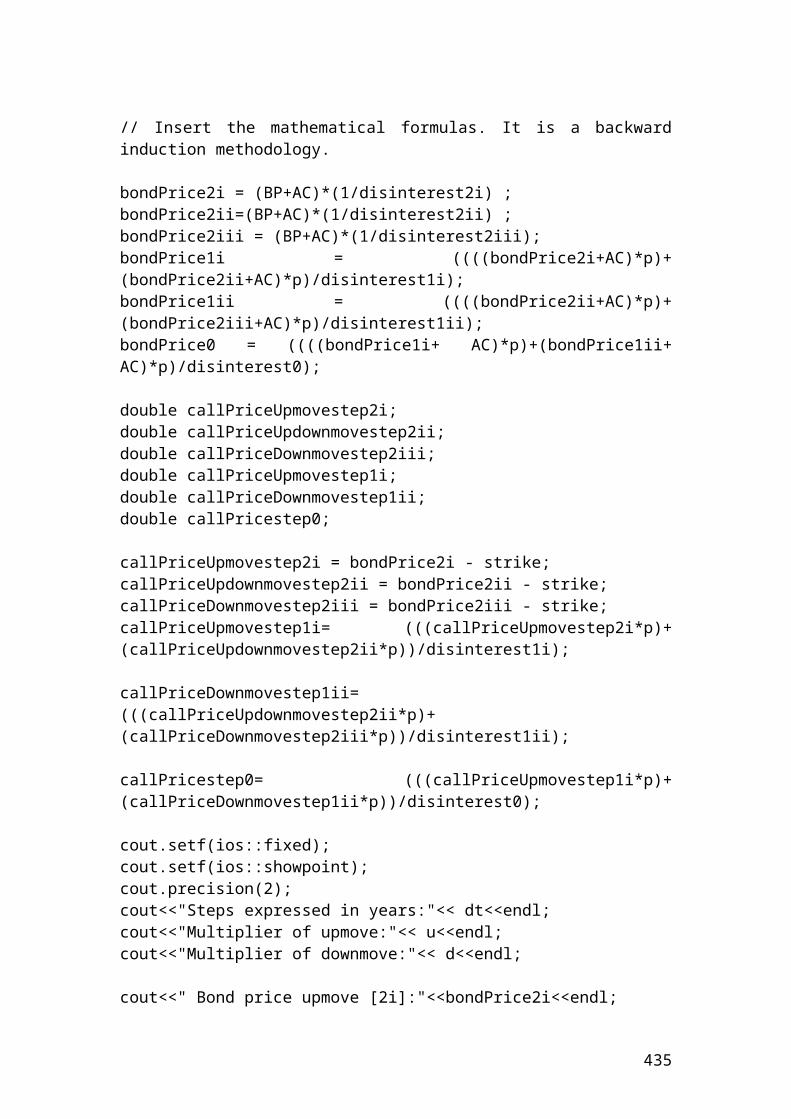
Minimum price required for a margin call

It is very important to check the maintenance margin level. The initial margin per contract for a gold futures contract is 1,500 USD. The maintenance margin per contract is 800 USD. The contract size is 5,000 ounces.

Solution

Minimum price required for a margin call = initial margin – maintenance margin / contract size

Minimum price required for a margin call = 1500 – 800 / 5000 = 0.14 USD.

Application of minimum price required for a margin call in python

>>> initial_margin_of_gold_futures = 1500>>> maintenance_margin_percontract = 800>>> contract_size = 5000>>> minimum_price_required_for_a_margin_call = (initial_margin_of_gold_futures - maintenance_margin_percontract) / contract_size>>> minimum_price_required_for_a_margin_call0.14 # USD

435

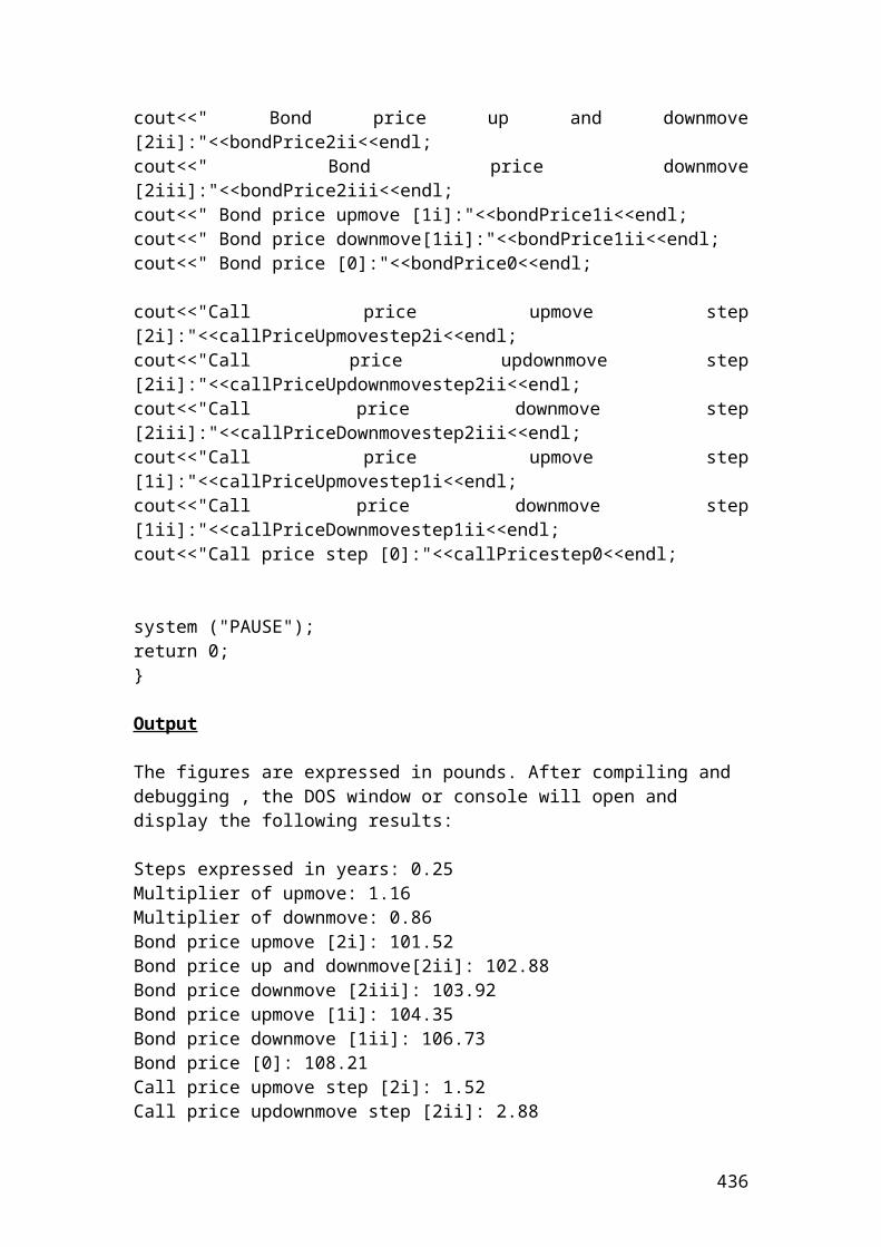
Loss on the futures position

Please consider a bond related to Eurodollar futures. The settlement price of the bond is 95.70 in December 2015. The principal is 2,000,000 Euros. The investor has adopted a long position of 100 contracts. The bond price has fallen to 90.15. Calculate the loss on the futures position.

Solution

Insert the mathematical formula.

Loss on the futures position = (settlement price – current price) / 100 * 100 contracts * 2,000,000

Loss on the futures position = (95.70 – 90.15) / 100 * 100 * 2,000,000 =

Loss on the futures position = 5.55 / 100 * 100 * 2000000 = 11,100,000 Euros.

Application of loss on the futures position in python

>>> settlement_price = 95.70>>> current_price = 90.15>>> principal = 2000000

436

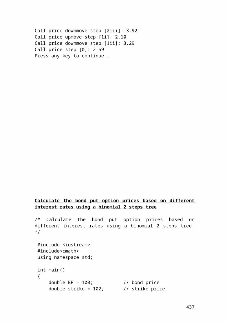
>>> contract_size = 100>>> Loss_on_the_futures_position =(settlement_price - current_price)/100*contract_size*principal>>> Loss_on_the_futures_position11099999.999999994>>> round(_,2)11100000.0 # Euros

Variation margin call

The amount of variation margin call is used in futures when the price of the asset price falls below a certain amount. For example, consider the bond price of Eurodollar futures.

Consider a trader that has bought a Eurodollar bond futures with a principal of 10,000,000 Euros. The settlement price is 97.14. The long position includes 100 contracts. The price of the bond has fallen to 95.78. The maintenance price is 96.45. The price of the bond has fallen below the maintenance price.

Variation margin = (settlement price – current price) / 100 * 100 contracts * 10,000,000

Variation margin = (97.14 – 95.78) / 100 * 100 *10,000,000 =

Variation margin = 1.36 / 100 * 100 * 10,000,000 = 13,600,000 Euros.

Application of variation margin call in python

>>> settlement_price = 97.14>>> current_price = 95.78>>> principal = 10000000

437

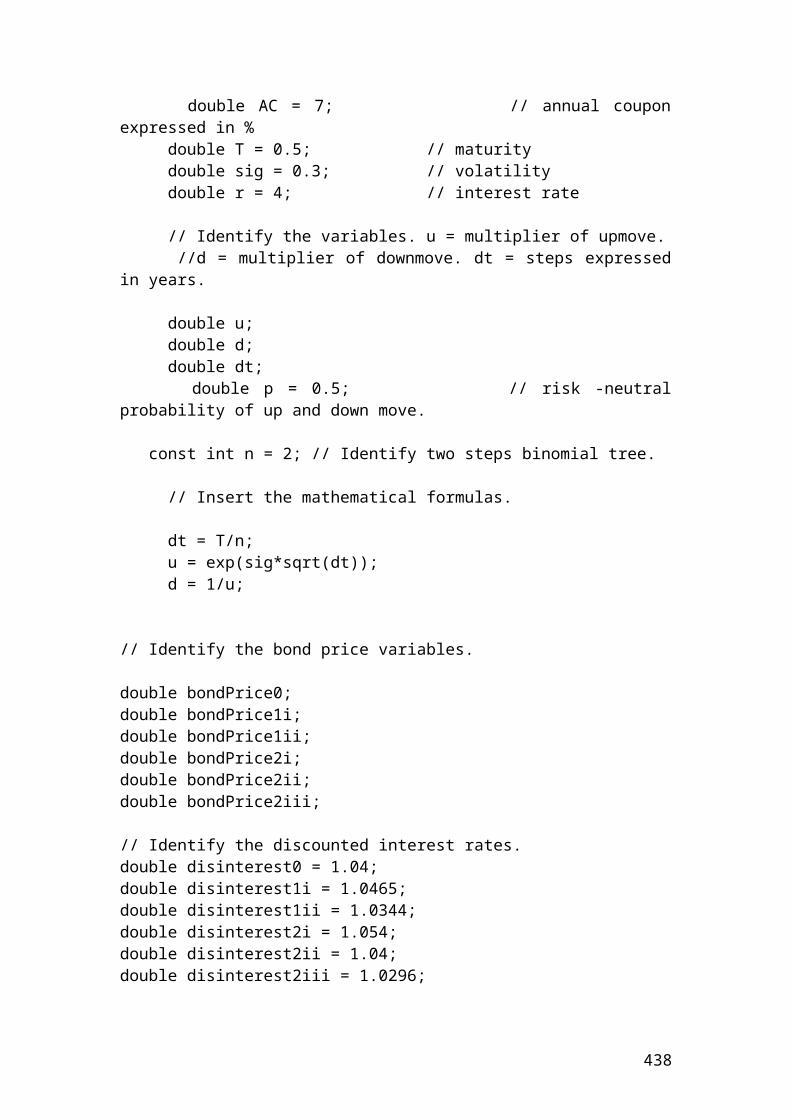
>>> contract_size = 100>>> variation_margin =(settlement_price-current_price)/100*contract_size*10000000>>> variation_margin13599999.999999994>>> round(_,2)13600000.0 # Euros

Calculate the volume and the open interest position in the July FTSE 100 index

Please consider 5 investors with the following short/long contract position.

First investor buys 3 contracts to open a long position.Second investor buys 5 contracts to open a long position.Third investor buys 2 contracts to open a long position.Fourth investor sells 7 contracts to close a long position.Fifth investor sells 4 contracts to close a long position.

If we assume that the initial open interest before the trades was 30 contracts. Calculate the volume and ending open interest.

Solution

Total volume = 3 + 5 + 2 + 7 + 4 = 21 contracts.

Ending open interest = initial open interest + opened positions - closed positions

Ending open interest = 30 + 3 + 5 + 2 - 7 – 4 = 29

438

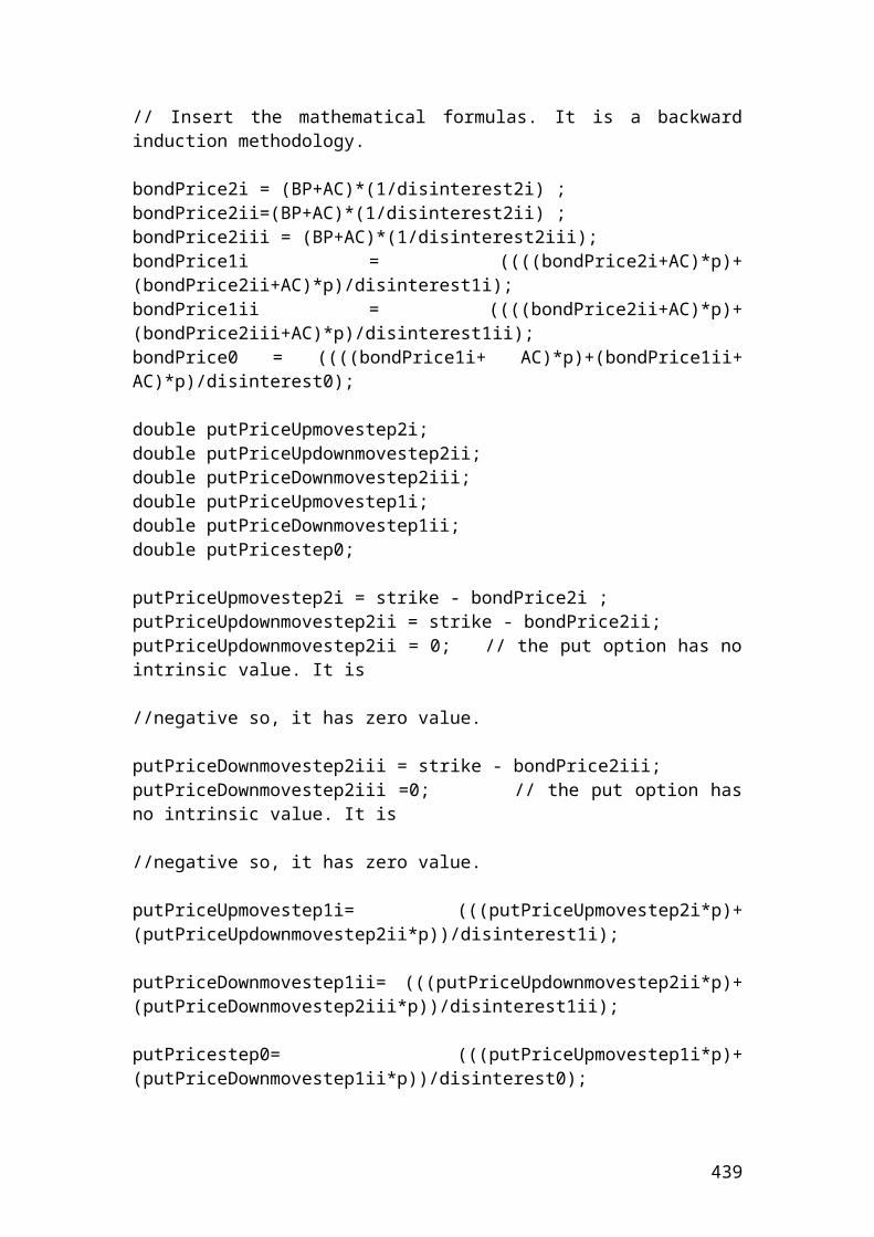
Application of calculation the volume and the open interest position in the July FTSE 100 index in python

>>> first_investor_buys_3contracts = 3>>> second_investor_buys_5contracts = 5>>> third_investor_buys_2contracts = 2>>> fourth_investor_sells_7contracts = 7>>> fifth_investor_sells_4contracts = 4>>> initial_open_interest = 30>>> Total_volume = 3+5+2+7+4>>> Total_volume21 # contracts>>> ending_open_interest = 30 + 3 + 5 + 2 - 7 -4>>> ending_open_interest29 # ending open interest>>>

Calculation of the minimum price per ounce before a margin call

Please consider the following terms of the silver contract:

Initial margin = $ 3,500 per contract.Maintenance margin = $ 2,500 per contract.20 silver contracts sold at a price equals $700 per ounce.Contract size = 100 ounces.

Solution

The initial margin = 3,500 * 20 = 70,000 USD. The maintenance margin = 2,500 * 20 = 50,000 USD.The difference between the initial and maintenance margin is the amount recorded before a margin call take place. Thus, 70,000 – 50,000 = 20,000 USD.

The price is 20,000 / 20*100 = 10 USD per ounce. This is the price before a margin call take place.

Application of calculating the minimum up or down ounce price before a margin call in python

>>> initial_margin = 3500

439

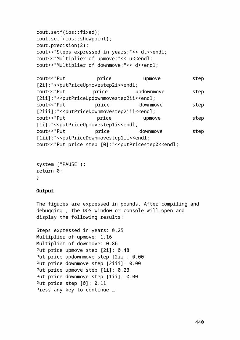
>>> maintenance_margin = 2500>>> silver_contracts = 20>>> contract_size = 100>>> minimum_price_required_for_a_margincall = (3500 - 2500) / 100>>> minimum_price_required_for_a_margincall10.0 # USD per ounce.

Calculate the intrinsic value of call share traded in Frankfurt stock exchange

The VW share is traded at 140 Euro in the Frankfurt stock exchange. The strike price is 130 Euro and the option market price is 7.70 Euro. The intrinsic value of the VW call is as calculate as follows:

Solution

The intrinsic value of the VW call is = Share price – strike price = 140 – 130 = 10 Euro.

Application of calculating the intrinsic value of call share traded in Frankfurt stock exchange

>>> share_price = 140>>> strike_price = 130>>> intrinsic_value = share_price - strike_price>>> intrinsic_value10 # Euro.>>>

440

Workshop and detailed explanation of Matlab

Matlab is a powerful mathematical and statistical package that covers Financial Derivatives. Once you open Matlab, you get a launch pad that includes Financial Derivatievs toolbox. By clicking on it you have a help and a demo function. By clicking on the demo function and selection Financial toolbox, you get a variety of financial functions and quantitative analysis options. You could select options as follows:

Equity options Portfolio optimization Capital allocation GARCH estimation Time series Financial charting Mean – Variance efficient frontier Call option sensitivity measures 1 Call option sensitivity measures 2

In this workshop, we will focus on capital allocation, call option sensitivity measures 1 and call option sensitivity measures 2.

By clicking on capital allocation, you have the option the change the inputs such as risk free rate, borrowing rate, and risk aversion coefficient. Once you input the numbers, you are provided with a chart that displays the expected return in relation to

441

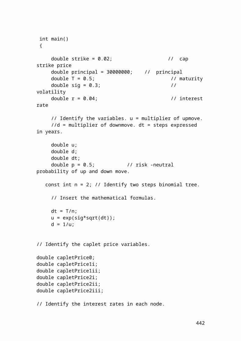
the risk or standard deviation. The chart shows the optimal overall portfolio and the optimal risky portfolio.

By clicking on capital option sensitivity measures 1 and 2, you are provided with a graph that shows the sensitivity of the Greek letter Gamma of the share option in relation to the time expressed in months. (gamma), measures the change in an option’s delta for a small change in the share price. , (delta), means the change that will occur in the option price for a small change in the share price, when all other factors are constant.

Once you have prepared the Excel datasheet with all the variables that you will describe and analyse, you then import the data in the Matalab software. For example, you have recorded the closing price, the open price the high and low of a future index contract for the last 5 years. You press file and then import data and then select the file type. The, select create vectors from each column using column names. Then, press workspace to work on your data individually or in aggregate format. By clicking on the variable or the group of variables, you are provided with graph selection. You have the option to use plot, surf, 2-Dgraphics and 3-D graphics. Once you have your chart, you press tools and you are provided with the option of basic fitting and data statistics. By clicking on the basic fitting, you have the option to click the shape that your data will take. For example, it will be linear, quadratic, cubic, etc… Thus, you have the option to explore different polynomials that fit your data. For example, you can try a linear or cubic polynomial to the data. You have also the option to select the equation and to plot the residuals. By plotting the residuals, you can evaluate the goodness of fit. You have also the option to interpolate or extrapolate the fit and shows the results. I have included an example of a Danske call equity option that is traded in the OMX Copenhagen 20 stock exchange index.

442

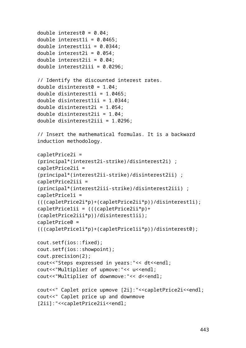
Source: author’s calculation

In this workshop we will cover in detail the following topics:

The command window of matrix algebra. Excel link used to exchange data between Matlab and Excel Microsoft. Financial Toolbox. Financial Time Series toolbox is used to analyze time series data. GARCH toolbox used to test the Generalized Autoregressive Conditional

Heteroskedasticity, (GARCH) volatility modelling. Matlab compiler is used to convert Matlab M-files to C++ computer language

programming. Statistics toolbox is used to analyze statistical historical data, model systems

and develop statistical algorithms. Financial derivatives toolbox is used to analyze options, futures and swaps. Quotes from the Gospel that are integrated in a Fuzzy logic function through a

spiritual advisor. Introduction to spectral analysis by using the covariance method, wavelet and

Fourier analysis. Introduction to Simulink.

Matrix algebra

In the command window, you have the options to calculate matrix algebra by inputting the correct syntax of Matlab command. For example, you want to construct a 3 x 3 matrix of a variable X. You write the following formula in the command window:

443

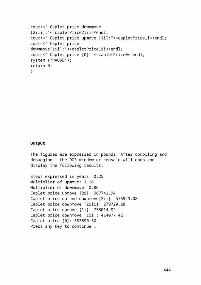
>>X = [2 4 5; 7 9 10; 3 5 8] Then, press enter in the command window. Matlab will arrange the numbers in a matrix format as follows:

X =

2 4 5 7 9 10 3 5 8

Now if you want to create a new variable Y = X + 3. Then, write the formula in the command window and press enter. Matlab will do the additions in the matrix as follows:

>>Y = X + 3

Y =

5 7 8 10 12 13 6 8 11

If you want to multiply the above matrices and create a new one, then use the formula as follows:

>>Z = X*Y

Z =

80 102 123 185 237 283 113 145 177

If you want to calculate the inverse function of Z, then type the formula as follows:Matlab will make the following calculation.

>>M = inv(Z).

M =

2.2850 -0.5475 -0.7125 -1.9150 0.6525 0.2875 0.1100 -0.1850 0.2250If you want to calculate the eigenvalue of M. Type the command eig(M). Matlab will do the following calculation.

>> eig(M)

444

ans =

2.7065 0.0020 0.4539

If you want to calculate the singular value decomposition of M. Type the command svd(M). Matlab will do the following calculation.

>>svd(M)

ans =

3.1837 0.4062 0.0019

You could calculate the poly function of M. It generates a vector containing the coefficients of the characteristic polynomial. Type the command P=round(poly(M)). Matlab will do the following calculation.

>> P=round(poly(M))

P =

1 -3 1 0

If you want to calculate the roots function of a polynomial. Type the command roots(P). Matlab will do the following calculation.

>> roots(P)

ans =

0 2.6180 0.3820

Excel link used to exchange data between Matlab and Excel Microsoft

To achieve a linkage between Excel and Matlab you have to do the following:

Start Microsoft Excel. Select Tools menu. Select Add-Ins and click Browse.

445

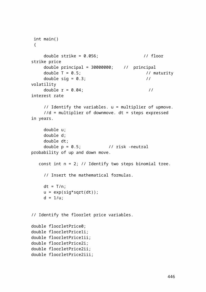
Find and select the Excel Link add-in excllink.xla under matlab/toolbox/exlink.

Press OK.

The function matlabinit start the Excel link in relation to the Matlab software. The function MLAutoStart start Matlab. The function MLClose stops Matlab from running. The function MLOpen initiate matlab software.

You can combine both softwares, namely, Excel and Matlab to build and solve financial derivatives problems.

For example, we want to calculate the expected risk expressed as a standard deviation based on historical return data that was collected from Metastock technical analysis for buying or going long on a call, put and index options. Then, we want to design the efficient frontier and decide which investment strategy is the most appropriate. Is it better to hold a call, a put or index options portfolio?

1 (A) Date (B) Call option return of Danske bank

( C) Put option return of

Danske bank

(D) Index option return

of OMX Copenhagen stockmarket

(E) Risk expressed

as standard deviation,

(STDEVA)

(F)Average

returns for call, put

and index options

2 2009 3.5% 2.7% 3.7%3 2010 4.7% 4.9% 7.9%4 2011 7.9% 5.7% 8.9%5 2012 -4.2% 8.5% 10.2%6 2013 5.4% 9.3% -6.8%7 2014 10.3% 11.5% 5.9%

Source: author’s calculation.

The first thing is to input the above data in a visual basic application, (VBA) format and then use Matlab syntax to transfer and exchange the data between the two softwares. The name of the Excel file is VBA for options.

Please complete the table ……………………………

VBA code illustration of the above example

Sub test1()

'Question

446

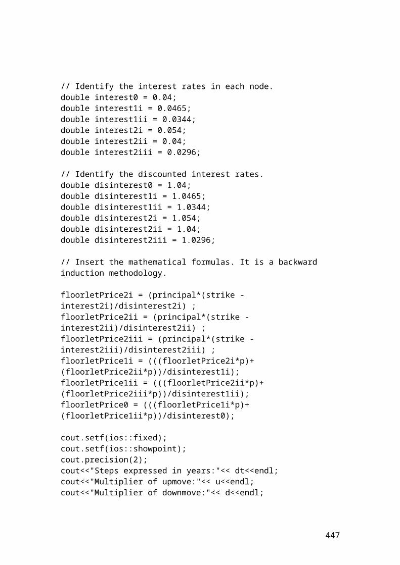
'It is required to calculate the expected risk expressed as a standard deviation based on historical return data that was collected from Metastock technical analysis for call, put and index options. The risk will be calculated for the three bands of investment for each year.

'Draw an efficient frontier and decide which investment strategy is the most suitable?

'********************************************************************'Data provided'********************************************************************

'Call option return of Danske bank = 3.5%, 4.7%, 7.9%, -4.2%, 5.4%, 10.3%'Put option return of Danske bank = 2.7%, 4.9%, 5.7%, 8.5%, 9.3%, 11.5%'Index option return of OMX Copenhagen stockmarket = 3.7%, 7.9%, 8.9%, 10.2%, -6.8%, 5.9%'********************************************************************'Variables name that are used in the worksheet VBA for options'********************************************************************Dim D 'DateDim COR 'Call option returnDim POR 'Put option returnDim IndexOptR 'Index option returnDim STDEVA 'Standard deviationDim Average 'Average return for call, put and index options

Application.Workbooks("VBA for options1").Worksheets("sheet1").Range("A1") = "Date"Application.Workbooks("VBA for options1").Worksheets("sheet1").Range("B1") = "Call option return"Application.Workbooks("VBA for options1").Worksheets("sheet1").Range("C1") = "Put option return"Application.Workbooks("VBA for options1").Worksheets("sheet1").Range("D1") = "Index option return"Application.Workbooks("VBA for options1").Worksheets("sheet1").Range("E1") = "Risk expressed as standard deviation"Application.Workbooks("VBA for options1").Worksheets("sheet1").Range("F1") = "Average return for call, put and index options"

'********************************************************************'Input data'********************************************************************

Application.Workbooks("VBA for options1").Worksheets("sheet1").Range("A2").Value = 2009Application.Workbooks("VBA for options1").Worksheets("sheet1").Range("A3").Value = 2010Application.Workbooks("VBA for options1").Worksheets("sheet1").Range("A4").Value = 2011

447

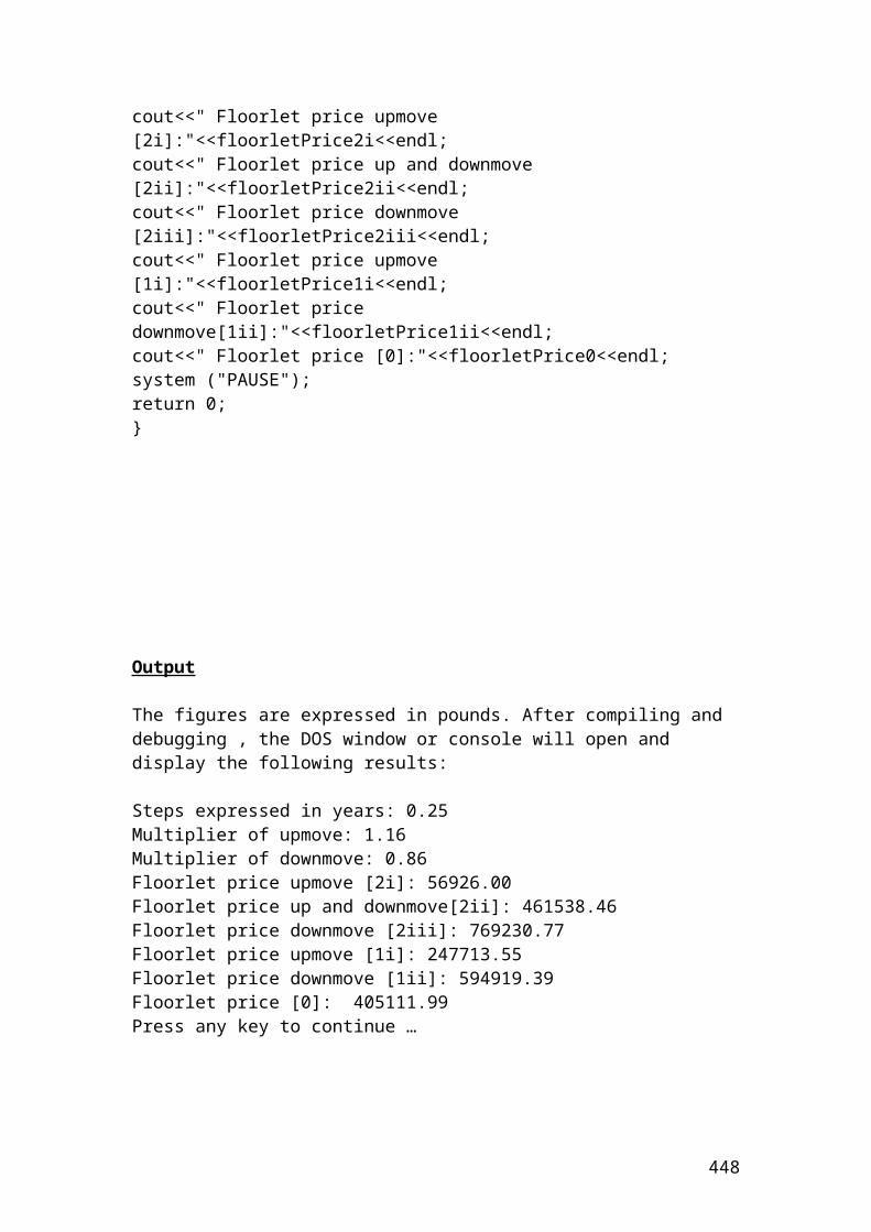
Application.Workbooks("VBA for options1").Worksheets("sheet1").Range("A5").Value = 2012Application.Workbooks("VBA for options1").Worksheets("sheet1").Range("A6").Value = 2013Application.Workbooks("VBA for options1").Worksheets("sheet1").Range("A7").Value = 2014

Application.Workbooks("VBA for options1").Worksheets("sheet1").Range("B2").Value = 0.035Application.Workbooks("VBA for options1").Worksheets("sheet1").Range("B3").Value = 0.047Application.Workbooks("VBA for options1").Worksheets("sheet1").Range("B4").Value = 0.079Application.Workbooks("VBA for options1").Worksheets("sheet1").Range("B5").Value = -0.042Application.Workbooks("VBA for options1").Worksheets("sheet1").Range("B6").Value = 0.054Application.Workbooks("VBA for options1").Worksheets("sheet1").Range("B7").Value = 0.103

Application.Workbooks("VBA for options1").Worksheets("sheet1").Range("C2").Value = 0.027Application.Workbooks("VBA for options1").Worksheets("sheet1").Range("C3").Value = 0.049Application.Workbooks("VBA for options1").Worksheets("sheet1").Range("C4").Value = 0.057Application.Workbooks("VBA for options1").Worksheets("sheet1").Range("C5").Value = 0.085Application.Workbooks("VBA for options1").Worksheets("sheet1").Range("C6").Value = 0.093Application.Workbooks("VBA for options1").Worksheets("sheet1").Range("C7").Value = 0.115

Application.Workbooks("VBA for options1").Worksheets("sheet1").Range("D2").Value = 0.037Application.Workbooks("VBA for options1").Worksheets("sheet1").Range("D3").Value = 0.079Application.Workbooks("VBA for options1").Worksheets("sheet1").Range("D4").Value = 0.089Application.Workbooks("VBA for options1").Worksheets("sheet1").Range("D5").Value = 0.102Application.Workbooks("VBA for options1").Worksheets("sheet1").Range("D6").Value = -0.068Application.Workbooks("VBA for options1").Worksheets("sheet1").Range("D7").Value = 0.059

'********************************************************************' Formula calculations'********************************************************************

448

Application.Workbooks("VBA for options1").Worksheets("sheet1").Range("E2").Formula = "=SQRT(((3*((B2)^2+(C2)^2+(D2)^2))-((B2+C2+D2)^2))/(3*(3-1))) "Application.Workbooks("VBA for options1").Worksheets("sheet1").Range("E3").Formula = "= SQRT(((3*((B3)^2+(C3)^2+(D3)^2))-((B3+C3+D3)^2))/(3*(3-1)))"Application.Workbooks("VBA for options1").Worksheets("sheet1").Range("E4").Formula = "= SQRT(((3*((B4)^2+(C4)^2+(D4)^2))-((B4+C4+D4)^2))/(3*(3-1)))"Application.Workbooks("VBA for options1").Worksheets("sheet1").Range("E5").Formula = "= SQRT(((3*((B5)^2+(C5)^2+(D5)^2))-((B5+C5+D5)^2))/(3*(3-1)))"Application.Workbooks("VBA for options1").Worksheets("sheet1").Range("E6").Formula = "= SQRT(((3*((B6)^2+(C6)^2+(D6)^2))-((B6+C6+D6)^2))/(3*(3-1)))"Application.Workbooks("VBA for options1").Worksheets("sheet1").Range("E7").Formula = "= SQRT(((3*((B7)^2+(C7)^2+(D7)^2))-((B7+C7+D7)^2))/(3*(3-1)))"

Application.Workbooks("VBA for options1").Worksheets("sheet1").Range("F2").Formula = "= (B2+C2+D2)/3"Application.Workbooks("VBA for options1").Worksheets("sheet1").Range("F3").Formula = "= (B3+C3+D3)/3"Application.Workbooks("VBA for options1").Worksheets("sheet1").Range("F4").Formula = "= (B4+C4+D4)/3"Application.Workbooks("VBA for options1").Worksheets("sheet1").Range("F5").Formula = "= (B5+C5+D5)/3"Application.Workbooks("VBA for options1").Worksheets("sheet1").Range("F6").Formula = "= (B6+C6+D6)/3"Application.Workbooks("VBA for options1").Worksheets("sheet1").Range("F7").Formula = "= (B7+C7+D7)/3"

End Sub'********************************************************************Sub createchart1()

Dim Chart1 As ChartSet Chart1 = Charts.AddChart1.SetSourceData Source:=Worksheets("sheet2").Range("A2").CurrentRegion, PlotBy:=xlColumnsChart1.ChartType = xl3DBarStackedEnd Sub'********************************************************************Sub createchart2()

Dim Chart1 As ChartSet Chart1 = Charts.AddChart1.SetSourceData Source:=Worksheets("sheet2").Range("A2").CurrentRegion, PlotBy:=xlColumns

449

Chart1.ChartType = xlLine

End Sub

Sub createchart3()Dim Chart As ChartSet Chart = Charts.AddChart.SetSourceData Source:=Sheet2.Range("A2:B7").CurrentRegion, PlotBy:=xlColumnsChart.ChartType = xlLineActiveChart.HasTitle = TrueActiveChart.ChartTitle.Font.Bold = TrueActiveChart.ChartTitle.Font.Size = 12ActiveChart.ChartTitle.Text = "Risk and average returns of options"ActiveChart.Axes(xlCategory, xlPrimary).HasTitle = TrueActiveChart.Axes(xlCategory, xlPrimary).AxisTitle.Text = "Risk expressed as standard deviation"ActiveChart.Axes(xlValue, xlPrimary).HasTitle = TrueActiveChart.Axes(xlValue, xlPrimary).AxisTitle.Text = "Average return for call, put and index options"

End Sub*********************************************************************Sub MsgBox_Test()Averagereturn = 0.05msgReply = MsgBox("The company expects increase of the average returns above 0.05")End Sub

Link functions between Excel and Matlab

A) After finishing with writing the VBA code and the Excel file is ready, then, you can transfer the data to Matlab.

= MLPutMatrix("retseries", B2:D7) <== MLPutMatrix("retseries", B2:D7)

B) Use Matlab Financial toolbox functions.

= MLEvalString("[ret, cov]= ewstats(retseries)") <== MLEvalString("[ret, cov] = ewstats(retseries)")

<== MLEvalString("[risk] = portopt(ret, cov, 6)")

C) Transfer the resulting output to Excel.

=MLGetMatrix("risk", "F2")<== MLGetMatrix("risk", "F2")

D) Draw the efficient frontier.

450

=MLEvalString("portopt (ret, cov, 6); grid on; xlabel('Risk'); ylabel('Return')") <== MLEvalString("portopt (ret, cov, 6); grid on; xlabel('Risk'); ylabel('Return')")

Financial Toolbox

In Matlab, Financial toolbox is very useful to perform mathematical and statistical analysis. It is used to display cash flows. It is used to compute, analyze, manage portfolios, measure risk and compute yields and sensitivities for the derivatives products.

The cash flows in the command window of Matlab could be displayed as follows:

>> Cash = [-2000 3000 5000 6000]

Cash =

-2000 3000 5000 6000

To transpose a matrix of cash flows, please use the following syntax:

>> Cash = [-2000 3000 5000 6000]'

Cash =

-2000 3000 5000 6000

Another example is if you have two portfolios of shares and you would like to calculate the NewPortfolios as an addition of portfolios A and B.

>> Portfolios_A = [400 300 200 400 200 250];

Portfolios_B = [375 425 400 300 100 400];

NewPortfolios = Portfolios_A + Portfolios_B

NewPortfolios =

775 725 600 700 300 650

451

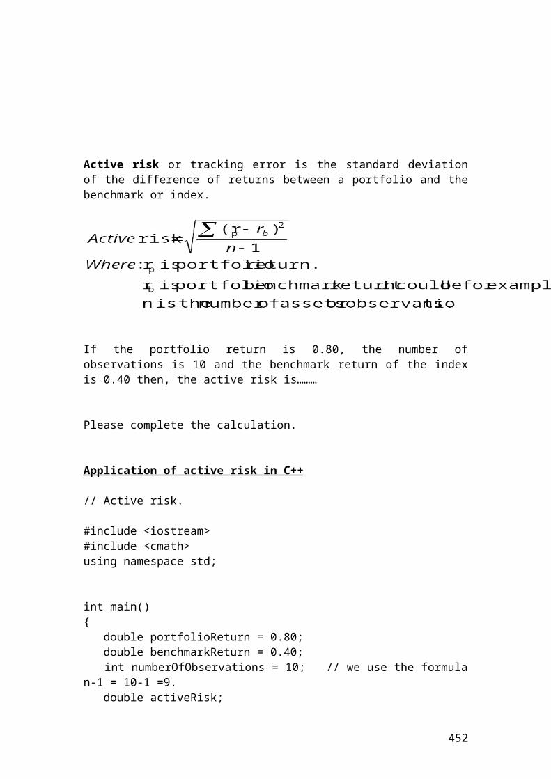
Another example that is used in portfolio management is to multiply closing prices with numbers of shares. The syntax of the closing prices for three shares and the number of shares of equity derivatives in the command window is as follows:

ClosePrices = [50 37 40]

NumShares = [200 300 400]

The portfolio total value is the multiplication of the vectors of ClosePrices and NumShares.

PortfValue = ClosePrices * NumShares

ClosePrices =

50 37 40

NumShares =

200 300 400

PortfValue =

37100

Solving simultaneous equations is another example. Let’s assume that we have two matrices.

A = [2 2 4 -3];

B = [12 -14];

X = A \ B

X =

0.5714 5.4286

Another example, it is how to calculate yields based on dividends and prices.

452

Dividends = [2.40 0.67 2.30 3.20];Prices = [30.14 12.89 16.78 54.20];Yields = Dividends ./ Prices

Yields =

0.0796 0.0520 0.1371 0.0590

Let’s assume that the initial capital that an investor has is 200 USD. The amount has been invested with a fixed rate and the investor received annual cash receipts of 30 USD, 50 USD, 60 USD, 75 USD, and 85 USD. Calculate the internal rate of return based on the cash flows. The transposed cash flows could be displayed in Matlab with the followed syntax:

>> CashFlows = [-200 30 50 60 75 85]'

CashFlows =

-200 30 50 60 75 85

>> Rate = irr(CashFlows)

Rate =

0.1290

>> Rate = 0.1290 * 100

Rate =

12.9 % . The internal rate of return based on the above cash flows is 12.9%

Financial Time Series toolbox is used to analyze time series data

Compute the Bollinger bands for Danisco share. It is a technical analysis indicator that is used to decide whether to buy or sell a call option. I have included the syntax that will be used in the command window and a figure that shows the three bands of the Bollinger indicator.

453

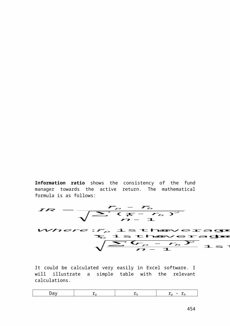
>> load danisco.mat[danisco_Mid,danisco_Uppr,danisco_Lowr]= bollinger(danisco);danisco_CloseBolling = [danisco_Mid, danisco_Uppr danisco_Lowr];plot (danisco_CloseBolling);title('Bollinger Bands for Danisco Closing Prices')

Source: author’s illustration.

GARCH toolbox used to test the Generalized Autoregressive Conditional Heteroskedasticity, (GARCH) volatility modelling

GARCH models are very important and show the volatility of asset returns by taking into consideration excess kurtosis or fat tails and volatility clustering. It provides timely forecasts of time varying conditional variances and covariances. They are important models for risk and portfolio managers who are involved in financial derivatives, portfolio management and asset allocation. They are also very important in designing successful strategies for short and long-term interest rate futures, currency options, and value-at-risk, (VaR) calculations. Thus, it is a useful tool that you can compare a Gaussian distribution with a distribution with excess kurtosis and spot the variations.

Suppose that we have the following autoregressive moving average, ARMA(2,2) model.

454

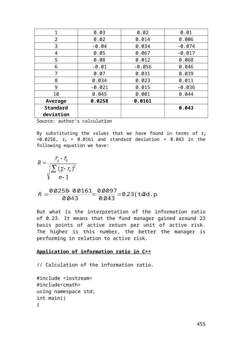
Use the function garchar to convert finite-order ARMA models to 5 infinite order auto-regressive (AR) models. The syntax in the command window of Matlab is as follows:

PI' or InfiniteAR = garchar(AR, MA, NumLags)

Where: garchar convert finite-order ARMA models to infinite order auto-regressive (AR) models.AR are autoregressive coefficients such as yt-1 and yt-2.MA are moving average coefficients such as NumLags is an integer scalar and determines the length of the infinite-order AR output vector. If it is not specified, the default is 10.

AR = [0.4 -0.6] MA = [-0.3 0.5]

PI = garchar([0.4 -0.6], [-0.3 0.5], 5);PI'

ans =

0.1000 -0.0700 -0.0710 0.0137 0.0396

Use the function garchma to convert finite-order ARMA models to 10 infinite order moving average (MA) models. The syntax in the command window of Matlab is as follows:

PI' or InfiniteMA = garchma(AR, MA, NumLags)

Where: garchma convert finite-order ARMA models to infinite order moving average (MA) models.AR are autoregressive coefficients such as yt-1 and yt-2.MA are moving average coefficients such as NumLags is an integer scalar and determines the length of the infinite-order AR output vector. If it is not specified, the default is 10.

Suppose that we have the following autoregressive moving average, ARMA(2,2) model.

455

AR = [0.4 -0.6] MA = [-0.3 0.5]

PI = garchma([0.4 -0.6], [-0.3 0.5], 10);PI'

ans =

0.1000 -0.0600 -0.0840 0.0024 0.0514 0.0191 -0.0232 -0.0207 0.0056 0.0147

Matlab compiler is used to convert Matlab mat-files to C++ computer language programming

Programming in C++ differs from programming in MATLAB in terms of syntax. Expression such as and ' is not valid syntax for C++. The mathematical symbols.*, .\, ./, .^ and \ are not valid C++ operators. The {} cell array indexing operator is unavailable. In Matlab, the syntax for the logical function is logical (). It could be a logical scalar or a variety of arrays of logical values. In C++, logical values are defined only as scalars.

Statistics toolbox is used to analyze statistical historical data and model systems

Statistical process control, (SPC) is very important tools that are used in Six Sigma analysis in order to improve the efficiency of the derivative product that is offered to the customer. I have included the syntax that is used in the command window and the xbar chart with 95% confidence level.

load partsconf = 0.95;spec = [-0.5 0.5];xbarplot(runout,conf,spec)

456

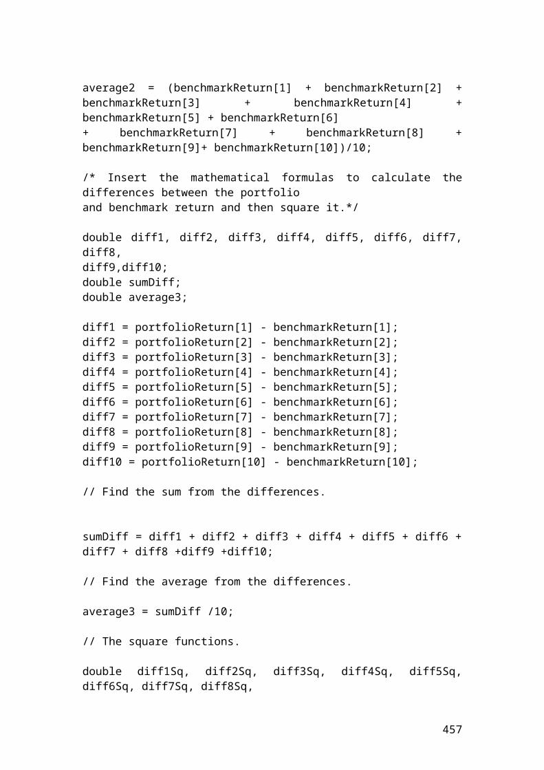
Source: author’s illustration.

I have included the syntax that is used in the command window for the exponentially weighted moving average, (EWMA), chart with 95% confidence level.

ewmaplot(runout,0.5,0.01,spec)

457

Source: author’s illustration.

I have included the syntax that is used in the command window for the distribution plots, quantile - quantile plot.

x = poissrnd(15,40,1);y = poissrnd(5,100,1);qqplot(x,y);

458

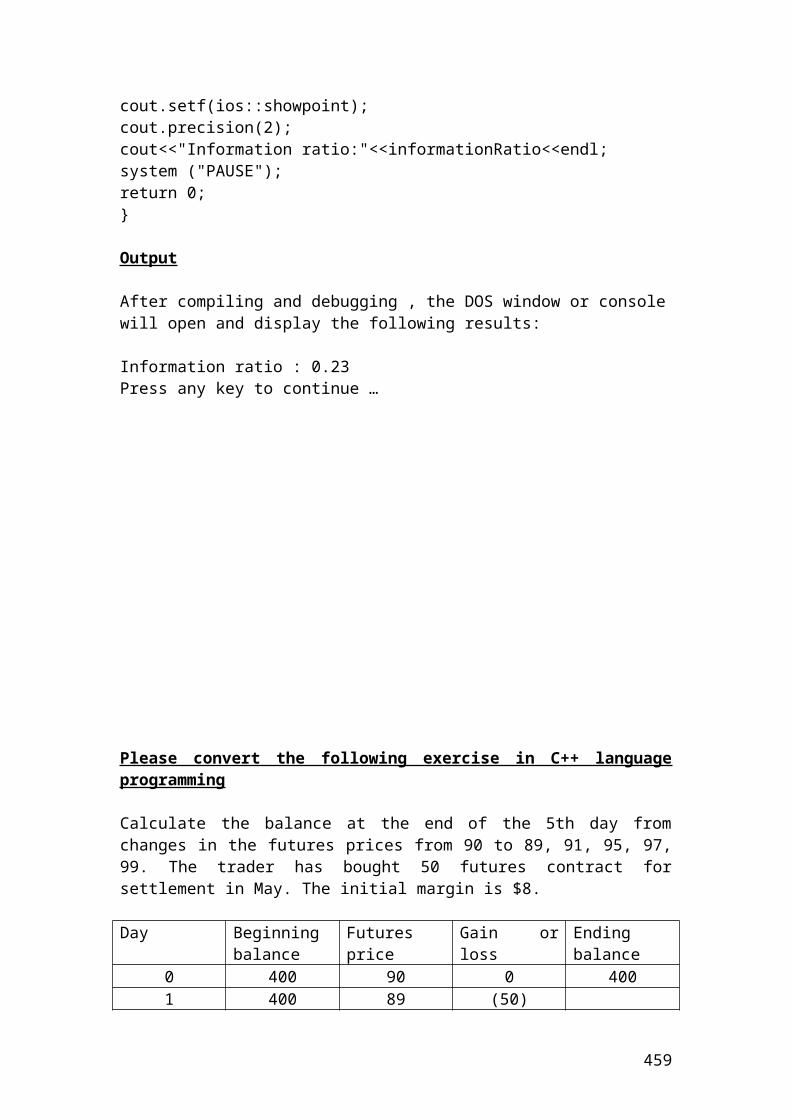
Source: author’s illustration.

I have included the syntax that is used in the command window for the normal distribution plots.

x = normrnd(15,1,35,1);normplot(x)

459

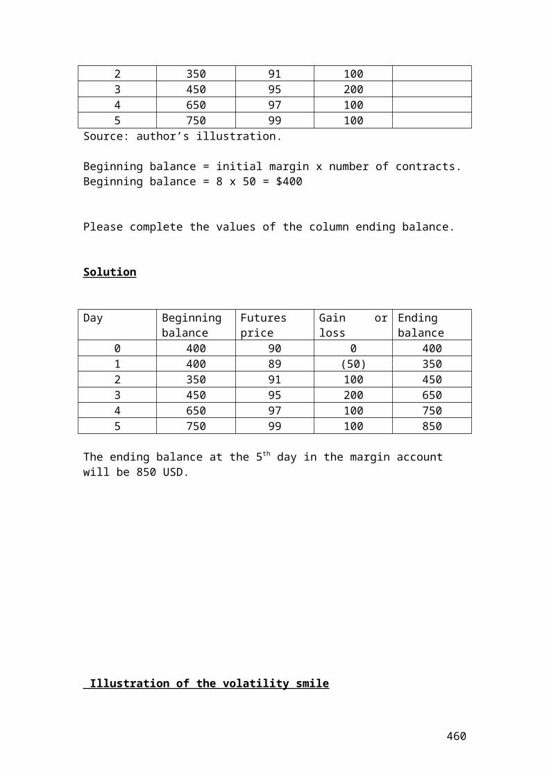
Source: author’s illustration.

I have included the syntax that is used in the command window for the box plot and analysis of variance, (ANOVA).

load data>> data

data =

203.6000 257.1000 181.0000 230.7000 279.5000 192.2000 235.9000 280.1000 197.5000 232.5000 262.8000 191.8000 235.6000 270.2000 193.8000 241.3000 273.1000 196.4000 [p,tbl,stats] = anova1(data);pp =

460

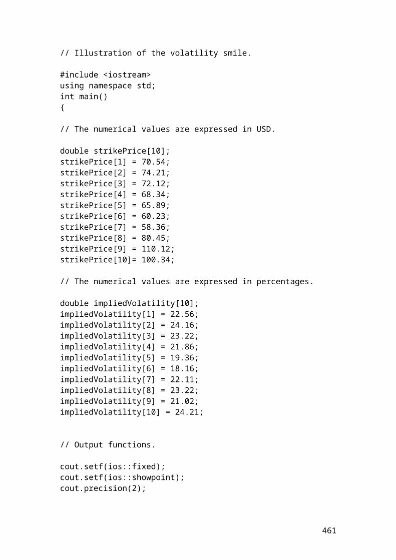
Source: author’s illustration.

Source: author’s illustration.

I have included the syntax that is used in the command window to calculate the mean.

>> A = [1 2 4 4 3 4 6 8];mean(A)ans =

461

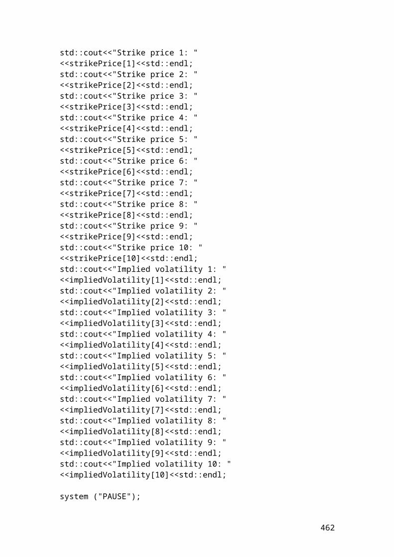
4

I have included the syntax that is used in the command window to calculate the geometric mean.

>> m = geomean(A)

m =

3.4135

I have included the syntax that is used in the command window to calculate the range. It calculates the difference between the maximum and the minimum value of a data sample such as A = [1 2 4 4 3 4 6 8];

>> y = range(A)

y =

7

I have included the syntax that is used in the command window to calculate the interquartile range. It calculates the difference between the 75th and the 25th

percentiles of a data sample such as A = [1 2 4 4 3 4 6 8];

>>

y = iqr(A)

y =

2.5000

I have included the syntax that is used in the command window to calculate the variance as a measure of dispersion by using a data sample such as A = [1 2 4 4 3 4 6 8];

>> var(A)

ans =

4.8571

Financial derivatives toolbox is used to analyze options, futures and swaps

462

Let’s consider a portfolio of options and future. Let’s consider a future contract that is traded in Frankfurt with a delivery date of 20-08-2014. The quoted price is $200.45. The layout of displaying the data in Matlab is as follows:

Type Strike Price Call Put Option 97 88 13.7 4.9 Option 102 97 8.2 7.9 Option 108 98 7.8 9.4 Type Delivery F Future 20-Aug-2014 200.45

Strike = (97;102;108); Price = (88;97;98);Call = [13.7; 8.2; 7.8];Put = [4.9; 7.9; 9.4]; Future = {20-Aug-2014; 200.45};

InstSet = instaddfield{Option;97;88;13.7;4.9};InstSet = instaddfield{Option;102;97;8.2;7.9};InstSet = instaddfield{Option;108;98;7.8;9.4};InstSet = instaddfield{future;20-Aug-2014;200.45};

Where:InstSet is a variable that contains a collection of data. The above data are expressed as a row vector.

Instaddfield is used to create or customize a portfolio of investment products according to the needs of the clients. For example, a portfolio of options and future.

The syntax for a swap contract is as follows:

InstSet = instswap(InstSet, LegRate, Settle, Maturity, LegReset, Basis, Principal, LegType)

Where:

InstSet is a function used when adding a swap to an existing portfolio set with other investment products.

LegRate is defined as [couponrate ;spread], where couponrate is the decimal annual rate and spread is the number of basis points.

Settle is the settlement date.

Maturity represents the maturity date for the swap contract.

463

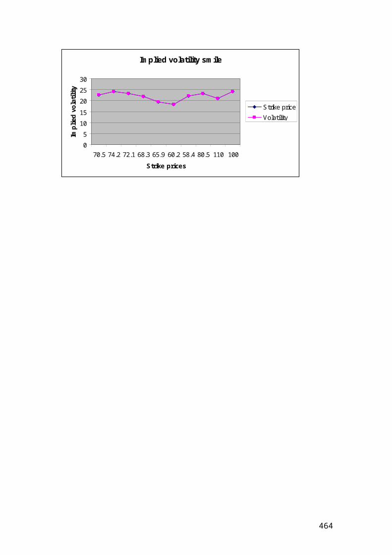
LegReset is optional and represents the frequency per year for each swap. The default function is default =[1 1].

Basis is optional and the Default = 0 (actual/actual).

Principal is optional and the Default = 100.

LegType is optional. It represents a matrix and each column indicates if thecorresponding leg is fixed (1) or floating (0). Default is [1,0] for each swap contract.

The syntax for a bond option is as follows:

InstSet = instoptbnd(InstSet, BondIndex, OptSpec, Strike, ExerciseDates, AmericanOpt or EuropenOpt )

Where:

InstSet is a function used when adding a bond option to an existing portfolio set with other investment products.

BondIndex is used to specify bond data.

OptSpec is used to specify if the option is a call or a put. The definition of the strike and exercise date depend if the option is American or European. If AmericanOpt = 1.

Strike shows the exercise price for each bond option.

ExerciseDates. There is only one exercise date, the option expiry date for an European option.

Sensitivity Measures or Greeks used in option pricing

The most common Greeks that are used in option pricing are:

Delta is the rate of change of its price relative to the price of the underlying asset. When delta is large, the derivative is sensitive to small changes in the price.

Gamma is the rate of change of delta relative to the price of the underlying asset. When gamma is small, the change in delta is small.

Lambda represents the percentage change in the price of an option. Rho is the rate of change in option price relative to the risk free rate. Theta is the rate of change in the price of the derivative instrument relative to

time. The value is small or negative as it reaches maturity. Vega is the rate of change in the price of the derivative instrument relative to

the volatility of the underlying security. Implied volatility helps the trader to determine the volatility of the stock and

according to the variance to hedge by using different strategies.

464

Let’s illustrate an example of a call European option and its delta, gamma, lambda, and implied volatility calculations. The asset price is 200 USD. The exercise price is150 USD. The risk-free rate is 8% and the time to maturity is 0.2 years, the volatility is 0.40, and the dividend rate is 0. By using the syntax in the command window of Matlab, we have the followed functions:

[CallPrice, PutPrice] = blsprice(200, 150, 0.08, 0.2, 0.40, 0)CallPrice; PutPrice =

CallPrice =

52.9446

PutPrice =

0.5637

[CallDelta, PutDelta] = blsdelta(200, 150, 0.08, 0.2, 0.40, 0)CallDelta; PutDelta =

CallDelta =

0.9630

PutDelta =

-0.0370

Gamma = blsgamma(200, 150, 0.08, 0.2, 0.40, 0)Gamma =

Gamma =

0.0023

[CallEl, PutEl] = blslambda(200, 150, 0.08, 0.2, 0.40, 0)CallEl; Put El =

CallEl =

3.6379

PutEl =

-13.1151

465

[CallRho, PutRho] = blsrho(200, 150, 0.08, 0.2, 0.40, 0)CallRho; PutRho =

CallRho =

27.9326

PutRho =

-1.5912

[CallTheta, PutTheta] = blstheta(200, 150, 0.08, 0.2, 0.40, 0)CallTheta; PutTheta =

CallTheta =

-18.4001

PutTheta =

-6.5906

Vega = blsvega(200, 150, 0.08, 0.2, 0.40, 0)Vega =

Vega =

7.2271

Quotes from the Gospel that are integrated in a Fuzzy logic function through a spiritual advisor

I have included two statements as follows:

“Wealth is not eternal and stable, but as a dream will disappear one day”.

“The spirit of the individual is strengthened from the Holy Spirit and not from the mammon or the money”.

Fuzzy logic is used to show the link between an input and an output space to find the best decision. The difference with the Christian Orthodox approach is that the best decision is offered from the strong faith that the individual has towards the Holy Trinity and the interaction with the Orthodox principles. Thus, the best decision is associated with the Holy gifts that he/she received from the Holy Trinity with always the help of the Virgin Mary.

466

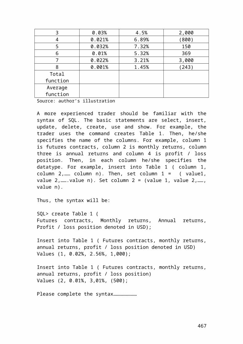
As an example of application of Fuzzy logic, we could mention the degree of wealth that an individual could dispose. The trend line starts from the extremely poor to reach the super rich. The amount that represents the different classes are expressed in Euros per month. The variables that sustain the Greek Christian Orthodox theology are expressed in a Likert scale from very weak to very strong. It is worth to mention that in practice these variables are sustained and increased according to the following parameters:

The faith. The good actions. The purity of the heart and the thoughts that the individual has towards

himself/herself and towards the fellow-persons.For example, Saint Nektarios metropolitan of pentapolis in Aegina has received all the spiritual gifts from heaven by keeping purity and maximum spiritual integrity in all his life. Aegina is an island situated in the Saronic Gulf of Greece. It is worth to visit the monastery and get blessing.

/ / / / / / Extremely poor Very Very poor Very poor Lower class Middle class Upper class

% Establish constantsextremely poor =200 ; very very poor=250 ; very poor=300; lower class=400; middle class=700; upper class=1000;Wealthrange =upper class - extremelypoor

Faith towards the Holy Trinityvery weak =0; weak=1; medium=2.5; strong=4; verystrong=5;faith towards the holy trinity=verystrong - veryweak

Repentancevery weak =0; weak=1; medium=2.5; strong=4; verystrong=5;repentance= verystrong - veryweak

Confessionvery weak =0; weak=1; medium=2.5; strong=4; verystrong=5;confession= verystrong - veryweak

HolyCommunionvery weak =0; weak=1; medium=2.5; strong=4; verystrong=5;holy communion= verystrong - veryweak

Prayervery weak =0; weak=1; medium=2.5; strong=4; verystrong=5;prayer= verystrong - veryweak

Fastveryweak =0; weak=1; medium=2.5; strong=4; verystrong=5;

467

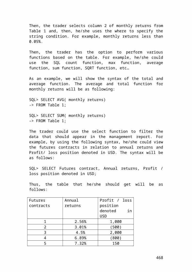
fast= verystrong - veryweak

Prostrationsveryweak =0; weak=1; medium=2.5; strong=4; verystrong=5;prostrations= verystrong - veryweak

Vigilveryweak =0; weak=1; medium=2.5; strong=4; verystrong=5;vigil= verystrong - veryweak

Almsgivingveryweak =0; weak=1; medium=2.5; strong=4; verystrong=5;almsgiving= verystrong - veryweak

Rejection of personal willveryweak =0; weak=1; medium=2.5; strong=4; verystrong=5;rejection of personal will= verystrong - veryweak

Appreciate Byzantine musicveryweak =0; weak=1; medium=2.5; strong=4; verystrong=5;appreciate byzantine music= verystrong – veryweak

Humilityveryweak =0; weak=1; medium=2.5; strong=4; verystrong=5;humility= verystrong – veryweak

Strong believe that Jesus Christ was resurrectedveryweak =0; weak=1; medium=2.5; strong=4; verystrong=5;strong believe that Jesus Christ was resurrected= verystrong - veryweak

% Wealth is not eternal and stable but as a dream will disappear one day.% The spiritual advisor suggest to focus on the spirit until the government finds a solution with the financial part.% He suggests that the spirit of the individual is strengthened from the Holy Spirit and not from the mammon or the money.Safeguard the spiritual integrity = faith towards the Holy Trinity* repentance* confession* Holy Communion* prayer* fast* prostrations* vigil* almsgiving* rejection of personal will* appreciate Byzantine music*humility* strong believe that Jesus Christ was resurrected

The result of the above or the gifts of the Holy Spirit after lifting a personal cross for all your life and the cross of the other person, if possible, is as follows:

1) Love plenty of honesty and free from hypocrisy. 2) Happiness.3) To be patient and control your temper in a way that reflects the Christian Orthodox principles. To love yourself, the other person and put yourself in his/her position.4) Control the desire of the body and strengthen the spiritual integrity.2) Sustainable faith towards the Holy Trinity and the help of Virgin Mary.

468

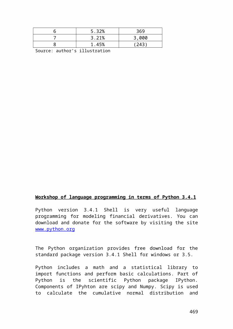
3) Solidarity to take care about the other person as yourself.4) Inner peace with yourself, the neighbor and the enemy.5) Virtuosity.6) Salvation of the soul.7) Gentleness

The above model should be combined with the letter to Galatas, Chapter E, pages 760-763 and verses 22-26.

end

Introduction to spectral analysis by using the covariance method, wavelet and Fourier analysis

The signal processing toolbox is used for spectral analysis to estimate random signals that can be used in investment for buying or selling derivatives instrument. To open the signal processing toolbox, type the syntax SPtool in the command window.

To open the Spectrum Viewer and create a power spectral density, (PSD) estimate from the SPTool is done as follows:

Select a signal from the Signal list box in SPTool. Press the Create button in the Spectra list. Press the Apply button in the Spectrum Viewer.

To select signals that display the volatility of the option or the future press shift and click on the noise and blnoise signals in the signals list of SPtool to select both signals. Then, press the View button under the signals list.

The purpose of spectral analysis is to describe and analyze the trend of the distribution of the equity option based on different signals that are extracted from a set of data. The power spectral density function is based on the covariance method. It represents a signal by using an autoregressive model. It is used to show the trend line in relation to an autoregressive filter function that isolates the buying from the selling signals. The power spectral density is calculated in units of power per radians per sample. For example, a first order autoregressive model defined as, (1,c) for returns of an equity option is as follows:

c = [1 -3.5678 4.5278 -1.4267 5.1267]; % AR filter coefficientsfreqz(1,c) % AR filter frequency responsetitle('AR System Frequency Response')

469

Source: author’s calculation.Let’s display the input signal x by filtering white noise by using the autoregressive filter. Estimate the power spectral density, (PSD) of x based on a third-order autoregressive prediction model of order three to show that the time span or life of the option decay or fall as we approach to maturity.

x = filter(1,a,randn(200,1)); % Signal generated from AR filter pcov(x,3) % Third-order estimate>>

470

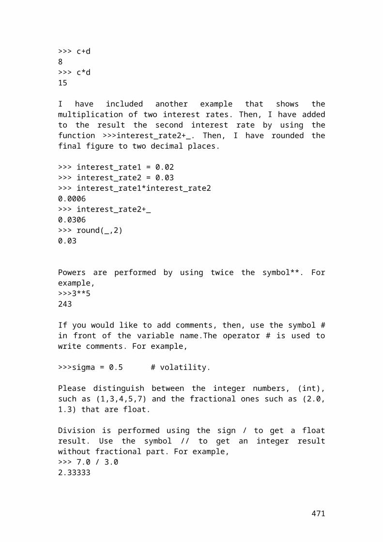
Source: author’s calculation.

Wavelet analysis is another tool that is used to analyze signals based on financial data.Wavelet analysis is characterized by two aspects, which are scale and time. Consequently every application has scale and time aspects. Financial data characterized by a time aspect are included in a list of domains to identify random signals when buying or selling an equity option, a swap contract or a future contract. This type of analysis helps the practitioner to use long time intervals in combination with precise low frequency data. On the other hand, it allows the practitioner to use shorter regions in combination with high frequency information.

For example, we want to plot complex Gaussian wavelets of order 3 for an equity option traded in the Eurex derivative market. The syntax is as follows:

[PSI,X] = cgauwavf(LB,UB,N,P)

% Set effective support and grid parameters.lb = -3; ub = 3; n = 2500;% Compute complex Gaussian wavelet of order 3.[psi,x] = cgauwavf(lb,ub,n,4);% Plot complex Gaussian wavelet of order 3.subplot(211)plot(x,real(psi)),title('Complex Gaussian wavelet of order 3')xlabel('Real part'), grid

471

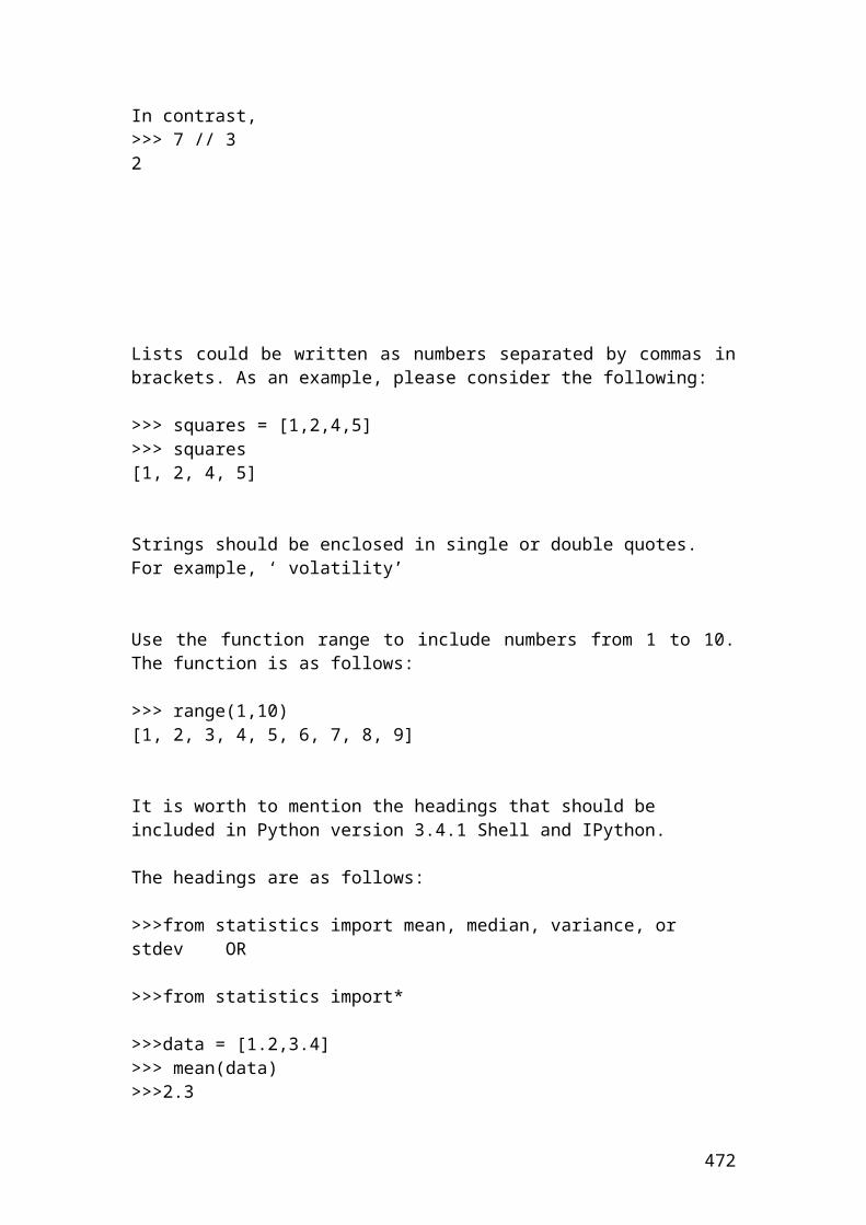
subplot(212)plot(x,imag(psi)) xlabel('Imaginary part'), grid

Source: author’s calculation.

Another toot of signal analysis is Fourier analysis. It decomposes a signal into parts of sinusoids of different frequencies. It is used to transform the signal from time to frequency mode. The problem with this transformation is that time information is omitted. Thus, you can not spot exactly the time that a particular macroeconomic event took place and show a buying or selling signal in the derivatives market. Different time series are non-stationary, random and erratic. Thus, by excluding the time factor through transformation, the prediction with Fourier analysis becomes less accurate and predictable.

Let’s assume an equity option that expires in 3 months. We want to plot the signal random noise in relation to the time by using Fourier analysis.

Please transform the signal from time to frequency mode by using the help menu of Matlab and comment about the accuracy of your results.

t = 1:2:3;x = sin(2*pi*30*t)+sin(2*pi*70*t);y = x + 2*randn(size(t));plot(y(1:30))title('Signal Random Noise')xlabel('period (months)')

472

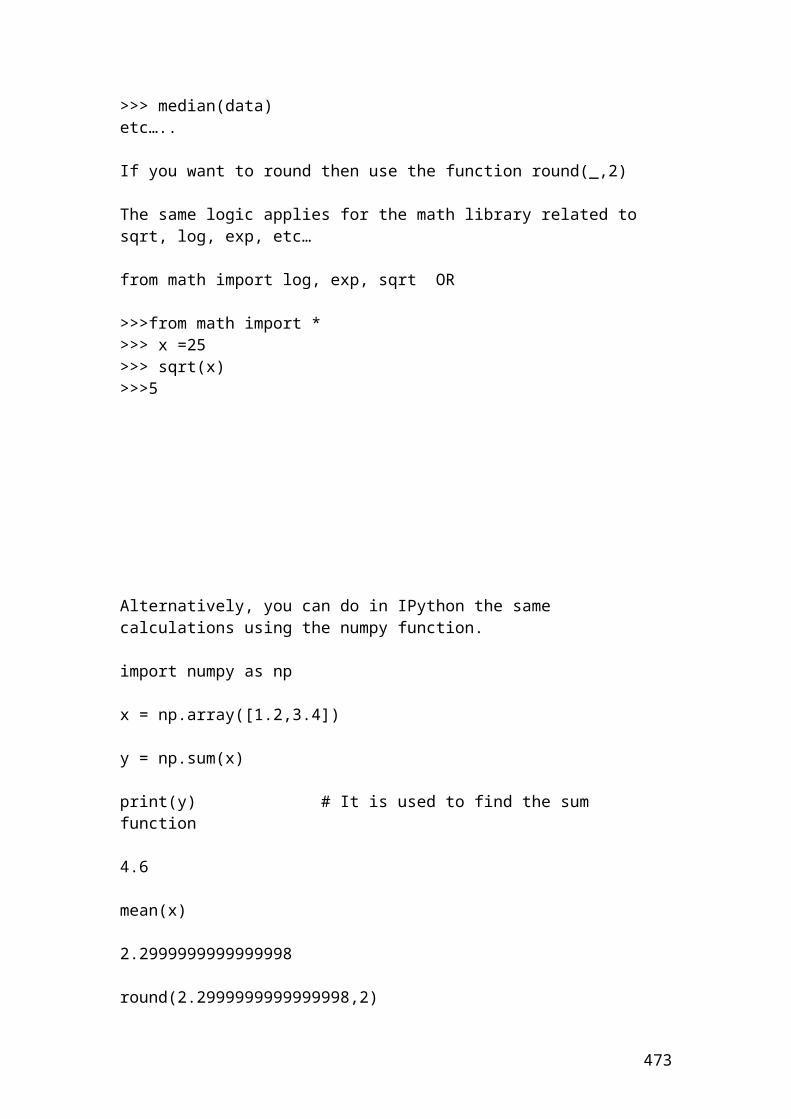
Source: author’s calculation.

473

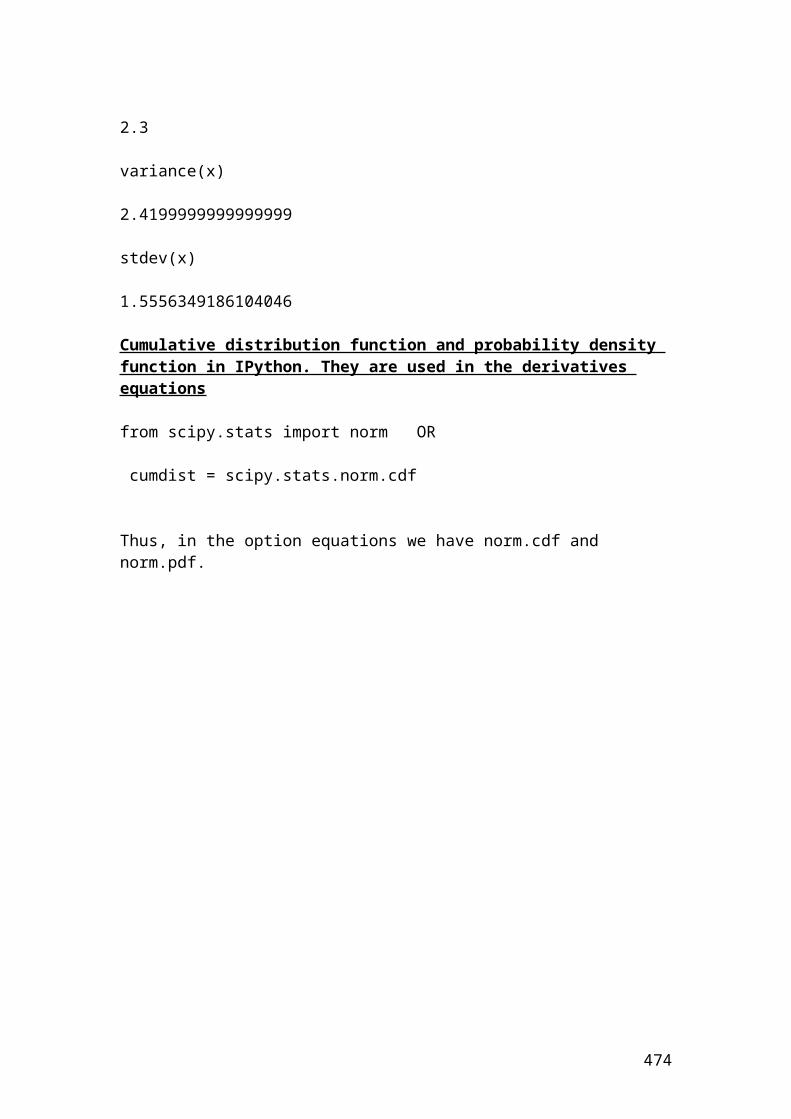
Simulink

Simulink is software that is used extensively in academia and in the industry to construct and build financial models. For example, it is used from the Federal Reserve Bank to model the effect of the fiscal and monetary policy. I have included a detailed example of Figure 1 with flow charts how Simulink could integrate the circular flow and effort of each individual with the fiscal and monetary policy of the Federal Reserve Bank and the derivatives market.

Monetary and fiscal policy of the circular flow of income J = I + G + X Firms

Households

W = S + T + M

Where:J is injections.W is withdrawals.S is net saving.T is taxes.M is import expenditure.I is investment.G is government expenditure.X is export expenditure.

The velocity of circulation determines the relationship between money and income. This velocity is integrated with the circular flow of spiritual effort in relation to the monetary and fiscal policy and the Financial Derivatives market. We have two types of monetary and fiscal policy. Tight and loose monetary policy, expansionary and contractionary fiscal policy. The optimum situation or equilibrium is to realign the different models with an ultimate objective to serve the household towards his/her spiritual integrity and salvation of the soul. Sinful actions are the result of hidden demons that restrict or delay the repentance and confession.

474

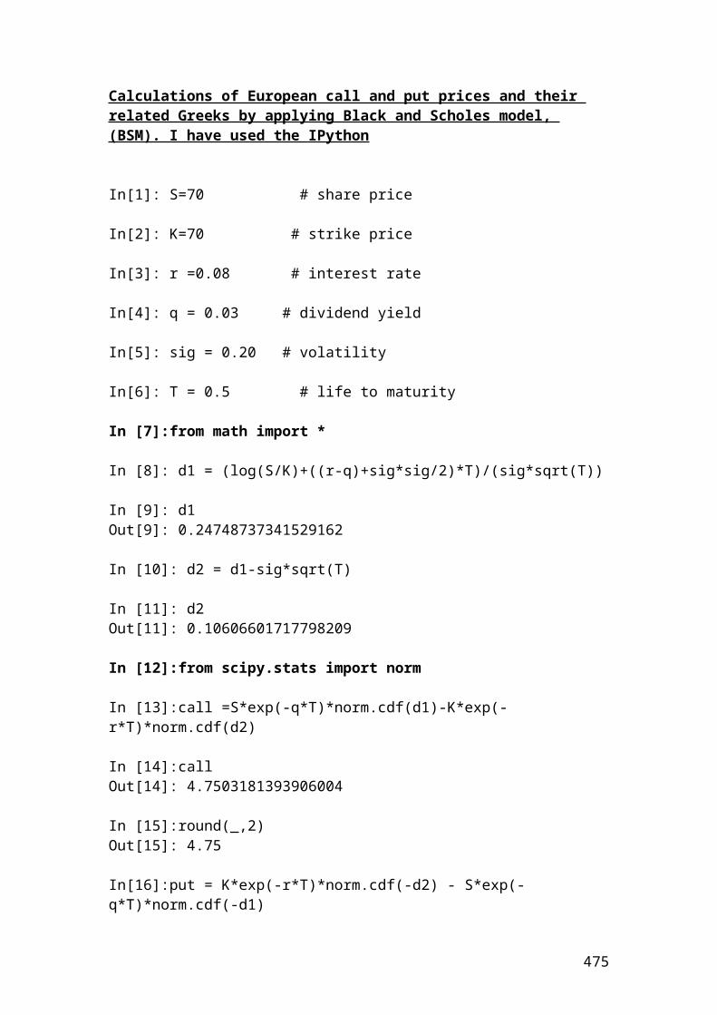
Tight monetary policy Loose monetary policy

Expansionary fiscal policy Contractionary fiscal policy

Financial Derivatives market

475

The Federal Reserve Bank buys treasury securities. This will affect short-term interest rates to go down. The central bank has more money to lend to the commercial banks, businesses and households. As an effect, there is an increase in employment and economic growth.

The Federal Reserve Bank sells treasury securities. This will affect short-term interest rates to go up. The central bank has less money to lend to the commercial banks, businesses and households. As an effect, there is a decrease in employment and economic growth.

Raising government expenditures.

Reducing taxes.

Increase aggregate demand.

Rise in national income.

Cutting government expenditures.

Raising taxes.

Decrease aggregate demand.

Decrease in national income.

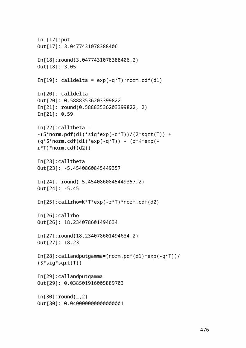
Buy very very low Never buy or sell in middle prices Sell very very high

The aim is to avoid psychological disorders, sustainable sinful condition and different illnesses.Source: Author’s illustration

To start the simulation, pull down the simulation menu and choose the start command. As the simulation runs, it will show that the accumulation of core values and additive variables reduce mortal, pardonable and sins of omission. In addition, it will show the interaction of the circular flow of income with the monetary, fiscal policy and the derivatives market.

476

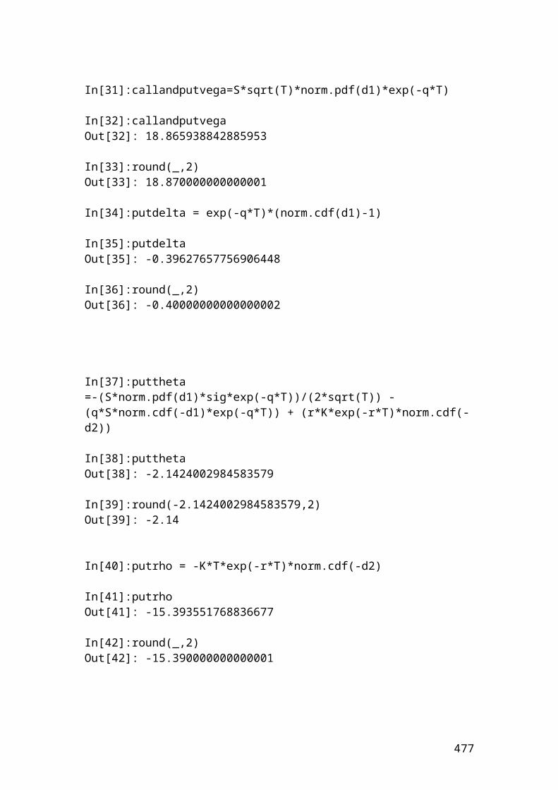
Workshop of analysis of financial data, scientific programming and simulation using R language programming

R is very useful language programming in modeling financial and statistical models. First of all, you should download the software for windows version R 3.2.2. A possible public domain is as follows:

Cran.r-project.org/bin/windows/base

Or

http://cran.ms.unimelb.edu.au

Please download R 3.3.3 for windows. Please read the instructions before to download the software. Once downloaded, then, open the R console and start to insert your variables, data and mathematical formulas.

Variable names are written with underscore followed by the equal sign. For example,

> interest_rate = 0.03Variable names could also be written with small letters adjacent to each other. For example, interestrate = 0.03

It is better to use underscore to separate them and be able to read them clearly.

> interest_rate =0.3> volatility = 0.5> interest_rate + volatility[1] 0.8>

In terms of arithmetic, R uses the symbols + for addition, - for subtraction, * for multiplication, / for division and ^ or ** for exponential functions. For example, powers are performed by using twice the symbol** or the exponential function ^.

For example, >3**5 243

Or >3 ^ 5243

If you would like to add comments, then, use the symbol # in front of the variable name.The operator # is used to write comments. For example,

>sigma = 0.5 # volatility.

I have included another example that shows the multiplication of two interest rates.

477

> interest_rate1 = 0.02> interest_rate2 = 0.03> interest_rate1*interest_rate2[1] 6e-04

Division is performed using the sign / to get a float result. Use the as.integer function to get an integer result without fractional part. For example,> 7.0 / 3.0 2.33333> as.integer(7/3)[1] 2Or> as.integer(2.33333)[1] 2

Ceiling or floor is used for round up purposes. They are used to round up or down respectively. Let’s try the above example.> floor(7/3)[1] 2> ceiling(7/3)[1] 3

Rounding of two or three decimals figures is used as follows:

> 7.5/2.45[1] 3.061224> round(3.061224,digits=2)[1] 3.06> round(3.061224,digits=3)[1] 3.061

For inputting your variables, you can use the sign = or <-. For example, please consider the following input.

share_price_1 <- 0.24share_price_2<- 0.56

Or

share_price_1 = 0.24share_price_2 = 0.56In the calculation part, insert the formula by using the sign <- or =For example, please consider the above example.

share_price_1 <- 0.24share_price_2 <- 0.56

total_share_price <- share_price_1 + share_price_2

478

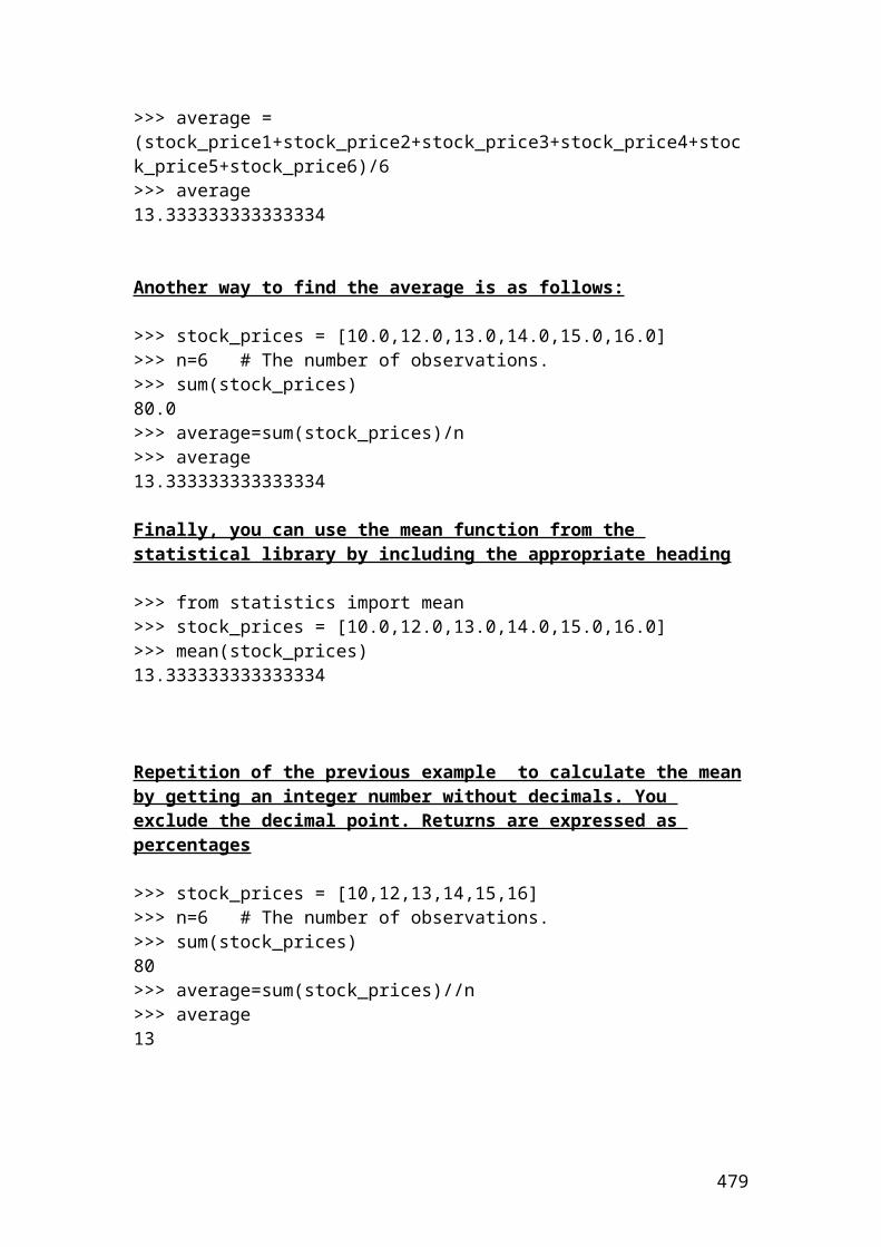
Calculation of the average of stock price returns expressed in percentages

> stock_price1 <- 10.0> stock_price2 <-12.0> stock_price3 <- 13.0> stock_price4 <- 14.0> stock_price5 <- 15.0> stock_price6 <- 16.0average<-(stock_price1+stock_price2+stock_price3+stock_price4+stock_price5+stock_price6)/6> average[1] 13.33333

Another way to find the average is as follows:

> x<-c(10,12,13,14,15,16)> sum(x)[1] 80> n = 6> average = sum(x)/n> average[1] 13.33333

479

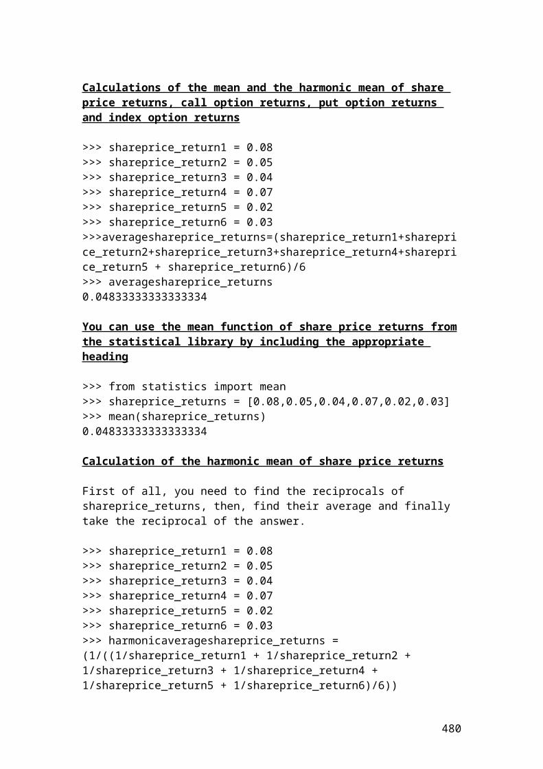
Repetition of the previous example to calculate the mean by getting an integer number without decimals. Returns are expressed as percentages

> stock_prices<-c(10,12,13,14,15,16)> n=6> sum(stock_prices)[1] 80> average = sum(stock_prices)/n> average[1] 13.33333> as.integer(average)[1] 13

Calculation of the mean, the variance and the standard deviation using the formulas that we have covered in the handout of measures of dispersion

> stock_prices<-c(10,12,13,14,15,16)> stock_prices[1] 10 12 13 14 15 16> n=6> sum(stock_prices)[1] 80> stock_prices.mean<-sum(x)/n # mean.> stock_prices.mean[1] 13.33333> sd<-sqrt(sum((stock_prices-mean(stock_prices))^2)/(n-1)) # standard deviation.> sd[1] 2.160247> stock_prices.var<-sum((stock_prices-stock_prices.mean)^2)/(n-1) # variance.> stock_prices.var[1] 4.666667

480

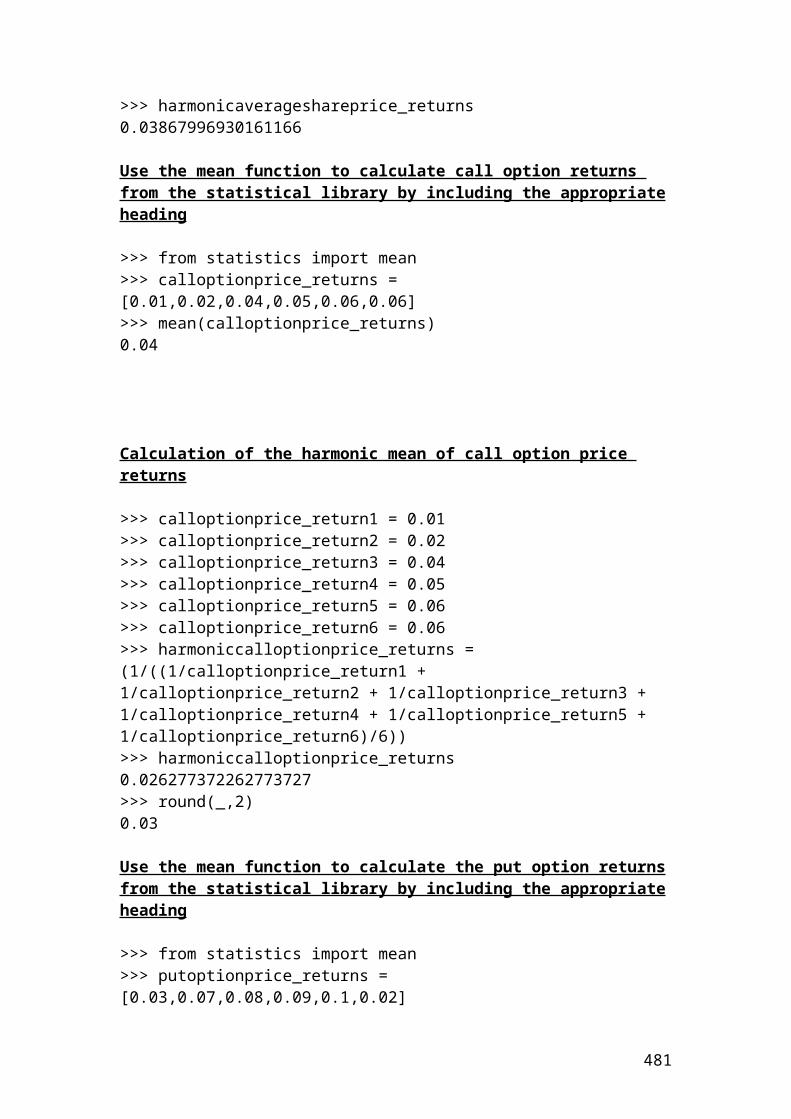
Calculations of European call and put prices and their related Greeks by applying Black and Scholes model, (BSM)

> S<- 70 # share price> K<- 70 # strike price> r <- 0.08 # interest rate> q <- 0.03 # dividend yield> sig <- 0.20 # volatility> T <- 0.5 # life to maturity> d1 <- (log(S/K)+((r-q)+sig*sig/2)*T)/(sig*sqrt(T))> d1[1] 0.2474874> d2 <-d1-sig*sqrt(T)> d2[1] 0.106066> call <-S*exp(-q*T)*pnorm(d1)-K*exp(-r*T)*pnorm(d2)> call[1] 4.750318> put <-K*exp(-r*T)*pnorm(-d2) - S*exp(-q*T)*pnorm(-d1)> put[1] 3.047743> round(3.047743,digits=2)[1] 3.05> calldelta <- exp(-q*T)*pnorm(d1)> calldelta[1] 0.5888354> round(0.5888354,digits=2)[1] 0.59> calltheta <- -(S*dnorm(d1)*sig*exp(-q*T))/(2*sqrt(T)) +(q*S*pnorm(d1)*exp(-q*T)) - (r*K*exp(-r*T)*pnorm(d2))> calltheta[1] -5.454086> callrho<- K*T*exp(-r*T)*pnorm(d2)> callrho[1] 18.23408> callandputgamma <- (dnorm(d1)*exp(-q*T))/(S*sig*sqrt(T))> callandputgamma[1] 0.03850192> callandputvega <- S*sqrt(T)*dnorm(d1)*exp(-q*T)> callandputvega[1] 18.86594> putdelta <- exp(-q*T)*(pnorm(d1)-1)> putdelta[1] -0.3962766> putrho<- -K*T*exp(-r*T)*pnorm(-d2)> putrho[1] -15.39355

481

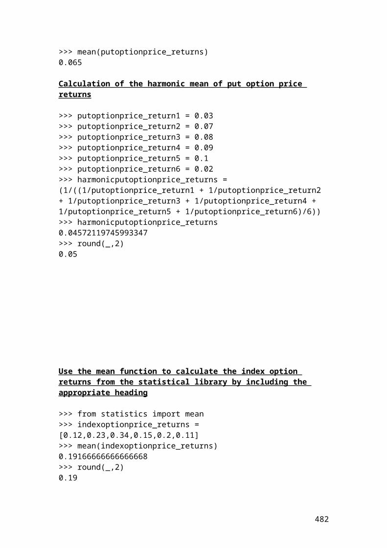
>puttheta <- -(S*pnorm(d1)*sig*exp(-q*T))/(2*sqrt(T)) – (q*S*dnorm(-d1)*exp(-q*T)) + (r*K*exp(-r*T)*dnorm(-d2))>puttheta[1] -2.1424002984583579

482

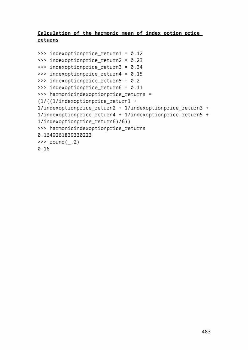
Calculations of the mean and the harmonic mean of share price returns, call option returns, put option returns and index option returns

> shareprice_return1<-0.08> shareprice_return2 <- 0.05> shareprice_return3 <- 0.04> shareprice_return4 <- 0.07> shareprice_return5 <- 0.02> shareprice_return6 <- 0.03>averageshareprice_returns<-(shareprice_return1+shareprice_return2+shareprice_return3+shareprice_return4+shareprice_return5 + shareprice_return6)/6> averageshareprice_returns[1] 0.04833333

You can use the mean function of share price returns from the statistical library bu using the appropriate heading

> stock_prices<-c(0.08,0.05,0.04,0.07,0.02,0.03)> sum(stock_prices)[1] 0.29> n=6> average = sum(stock_prices)/n> average[1] 0.04833333> round(average,digits=3)[1] 0.048

OR> stock_prices.mean<-sum(stock_prices)/n> stock_prices.mean[1] 0.04833333

Calculation of the harmonic mean of share price returns

First of all, you need to find the reciprocals of share price returns, then, find their average and finally take the reciprocal of the answer.

> shareprice_return1<-0.08> shareprice_return2 <- 0.05> shareprice_return3 <- 0.04> shareprice_return4 <- 0.07> shareprice_return5 <-0.02> shareprice_return6 <- 0.03>harmonicaverageshareprice_returns<-(1/((1/shareprice_return1+1/shareprice_return2 +1/shareprice_return3+1/shareprice_return4+1/shareprice_return5+1/shareprice_return6)/6))> harmonicaverageshareprice_returns[1] 0.03867997

483

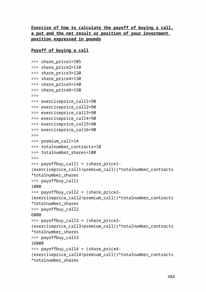
> round(harmonicaverageshareprice_returns,digits=3)[1] 0.039

Use the mean function to calculate call option returns from the statistical library by including the appropriate heading

> call_option_price_returns<-c(0.01,0.02,0.04,0.05,0.06,0.06)> n=6> sum(call_option_price_returns)[1] 0.24> call_option_price_returns.mean<-sum(call_option_price_returns)/n> call_option_price_returns.mean[1] 0.04

Calculation of the harmonic mean of call option price returns

> calloptionprice_return1 <- 0.01> calloptionprice_return2 <- 0.02> calloptionprice_return3 <- 0.04> calloptionprice_return4 <- 0.05> calloptionprice_return5 <- 0.06> calloptionprice_return6 <- 0.06> harmoniccalloptionprice_returns <- (1/((1/calloptionprice_return1 + 1/calloptionprice_return2 + 1/calloptionprice_return3 + 1/calloptionprice_return4 + 1/calloptionprice_return5 + 1/calloptionprice_return6)/6))> harmoniccalloptionprice_returns[1] 0.026277372262773727

Use the mean function to calculate the put option returns from the statistical library by including the appropriate heading

> put_option_price_returns<-c(0.03,0.07,0.08,0.09,0.1,0.02)> put_option_price_returns.mean<-sum(put_option_price_returns)/n> n=6> put_option_price_returns.mean[1] 0.065

Calculation of the harmonic mean of put option price returns

> put_option_price_return_1 <- 0.03> put_option_price_return_2 <- 0.07> put_option_price_return_3 <- 0.08> put_option_price_return_4 <- 0.09> put_option_price_return_5 <- 0.1> put_option_price_return_6 <- 0.02> harmonicputoptionprice_returns <- (1/((1/put_option_price_return_1 + 1/put_option_price_return_2 + 1/put_option_price_return_3 + 1/put_option_price_return_4 + 1/put_option_price_return_5 + 1/put_option_price_return_6)/6))> harmonicputoptionprice_returns

484

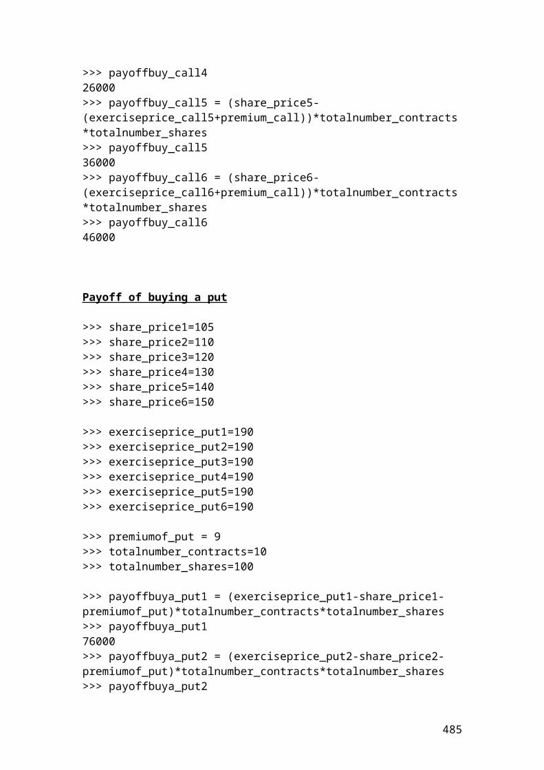
[1]0.04572119745993347

Use the mean function to calculate the index option returns from the statistical library by including the appropriate heading

> index_option_price_returns<-c(0.12,0.23,0.34,0.15,0.2,0.11)> index_option_price_returns.mean<-sum(index_option_price_returns)/n> n=6> index_option_price_returns.mean[1] 0.1916667

Calculation of the harmonic mean of index option price returns

> index_option_price_return_1 <- 0.12> index_option_price_return_2 <-0.23> index_option_price_return_3 <- 0.34> index_option_price_return_4 <- 0.15> index_option_price_return_5 <- 0.2> index_option_price_return_6 <-0.11> harmonicindexoptionprice_returns <- (1/((1/index_option_price_return_1 + 1/index_option_price_return_2 + 1/index_option_price_return_3 + 1/index_option_price_return_4 + 1/index_option_price_return_5 + 1/index_option_price_return_6)/6))> harmonicindexoptionprice_returns[1]0.1649261839330223

485

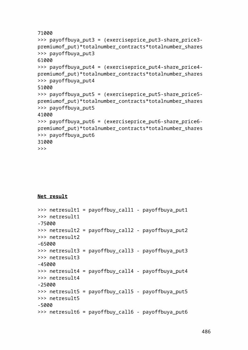
Exercise of how to calculate the payoff of buying a call, a put and the net result or position of your investment position expressed in pounds

Payoff of buying a call

> share_price_1<-105> share_price_2<-110> share_price_3<-120> share_price_4<-130> share_price_5<-140> share_price_6<-150> exercise_price_1<-90> exercise_price_2<-90> exercise_price_3<-90> exercise_price_4<-90> exercise_price_5<-90> exercise_price_6<-90> premium_call<-14> total_number_contracts<-10> total_number_shares<-100>payoffbuy_call1<-(share_price_1-(exercise_price_1+premium_call))*total_number_contracts*total_number_shares> payoffbuy_call1[1] 1000> payoffbuy_call2 <-(share_price_2-(exercise_price_2+premium_call))*total_number_contracts*total_number_shares> payoffbuy_call2[1]6000> payoffbuy_call3 <- (share_price_3-(exercise_price_3+premium_call))*total_number_contracts*total_number_shares> payoffbuy_call3[1]16000> payoffbuy_call4 <- (share_price_4-(exercise_price_4+premium_call))*total_number_contracts*total_number_shares> payoffbuy_call4[1]26000> payoffbuy_call5 <- (share_price_5-(exercise_price_5+premium_call))*total_number_contracts*total_number_shares> payoffbuy_call5[1]36000> payoffbuy_call6 <-(share_price_6-(exercise_price_6+premium_call))*total_number_contracts*total_number_shares> payoffbuy_call6[1]46000

486

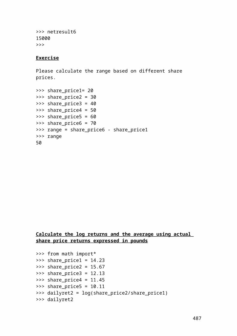
Payoff of buying a put

If you wish you can input underscore after each word to have a clear picture of your variables. For example, share_price_1 and exercise_price_put_1, etc…

> share_price1<-105> share_price2<-110> share_price3<-120> share_price4<-130> share_price5<-140> share_price6<-150

> exerciseprice_put1<-190> exerciseprice_put2<-190> exerciseprice_put3<-190> exerciseprice_put4<-190> exerciseprice_put5<-190> exerciseprice_put6<-190

> premiumof_put <- 9> totalnumber_contracts<-10> totalnumber_shares<-100

> payoffbuya_put1 <- (exerciseprice_put1-share_price1-premiumof_put)*totalnumber_contracts*totalnumber_shares> payoffbuya_put1[1]76000> payoffbuya_put2 <-(exerciseprice_put2-share_price2-premiumof_put)*totalnumber_contracts*totalnumber_shares> payoffbuya_put2[1]71000> payoffbuya_put3 <- (exerciseprice_put3-share_price3-premiumof_put)*totalnumber_contracts*totalnumber_shares> payoffbuya_put3[1]61000> payoffbuya_put4 <- (exerciseprice_put4-share_price4-premiumof_put)*totalnumber_contracts*totalnumber_shares> payoffbuya_put4[1]51000> payoffbuya_put5 <- (exerciseprice_put5-share_price5-premiumof_put)*totalnumber_contracts*totalnumber_shares> payoffbuya_put5[1]41000> payoffbuya_put6 <- (exerciseprice_put6-share_price6-premiumof_put)*totalnumber_contracts*totalnumber_shares> payoffbuya_put6[1]31000

487

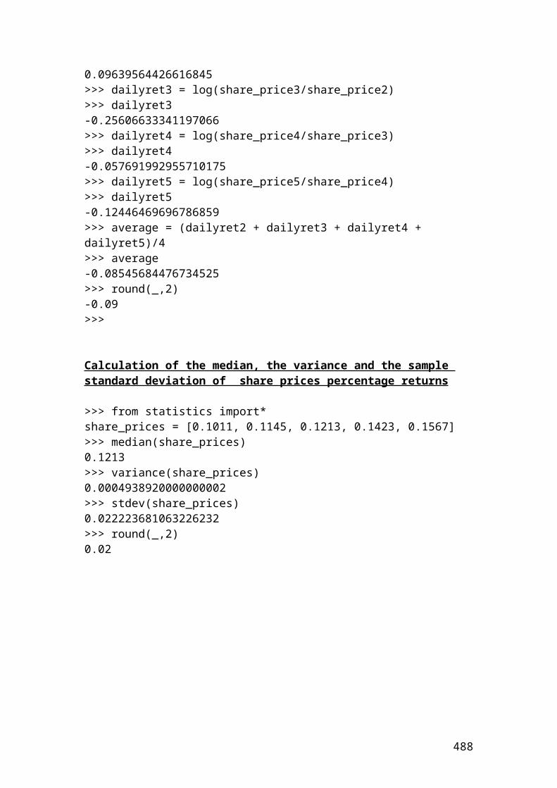
Net result

> netresult1 <- payoffbuy_call1 - payoffbuya_put1> netresult1[1]-75000> netresult2 <-payoffbuy_call2 - payoffbuya_put2> netresult2[1]-65000> netresult3 <- payoffbuy_call3 - payoffbuya_put3> netresult3[1]-45000> netresult4 <-payoffbuy_call4 - payoffbuya_put4> netresult4[1]-25000> netresult5 <-payoffbuy_call5 - payoffbuya_put5> netresult5[1]-5000> netresult6 <- payoffbuy_call6 - payoffbuya_put6> netresult6[1]15000

488

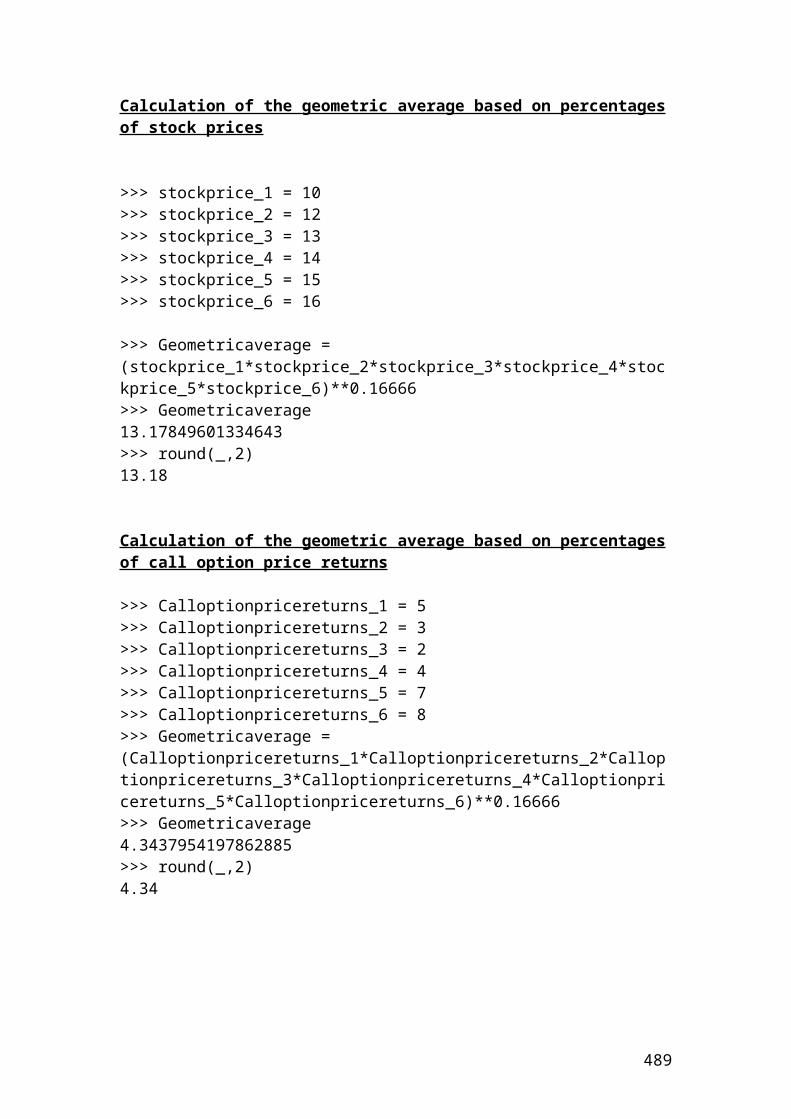
Exercise

Please calculate the range based on different share prices.

> share_price_1<- 20> share_price_2 <- 30> share_price_3 <- 40> share_price_4 <-50> share_price_5 <- 60> share_price_6 <-70> range <- share_price_6 - share_price_1> range[1] 50

489

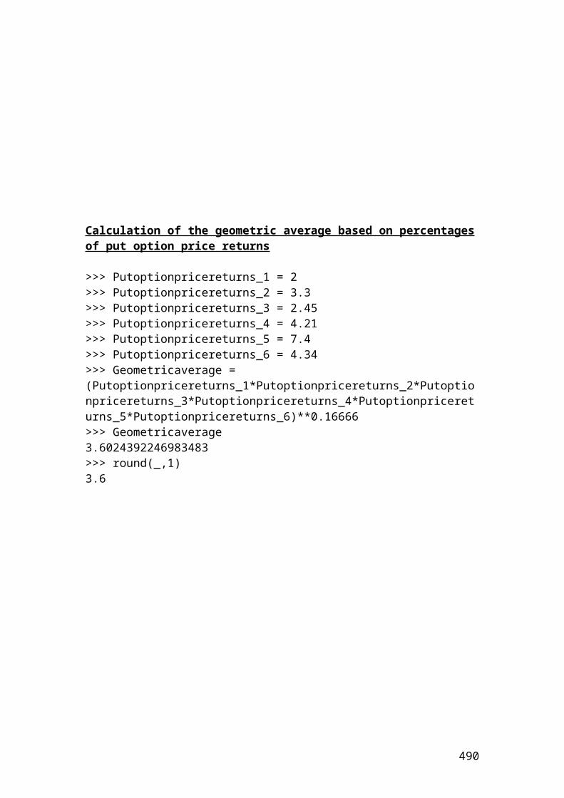
Calculate the log returns and the average using actual share price returns expressed in pounds

> share_price_1 <- 14.23> share_price_2 <- 15.67> share_price_3 <- 12.13> share_price_4 <- 11.45> share_price_5 <- 10.11> dailyret2 <- log(share_price_2/share_price_1)> dailyret2[1]0.09639564426616845> dailyret3 <- log(share_price_3/share_price_2)> dailyret3[1]-0.25606633341197066> dailyret4 <- log(share_price_4/share_price_3)> dailyret4[1]-0.057691992955710175> dailyret5 <- log(share_price_5/share_price_4)> dailyret5[1]-0.12446469696786859> average <- (dailyret2 + dailyret3 + dailyret4 + dailyret5)/4> average[1]-0.08545684476734525

490

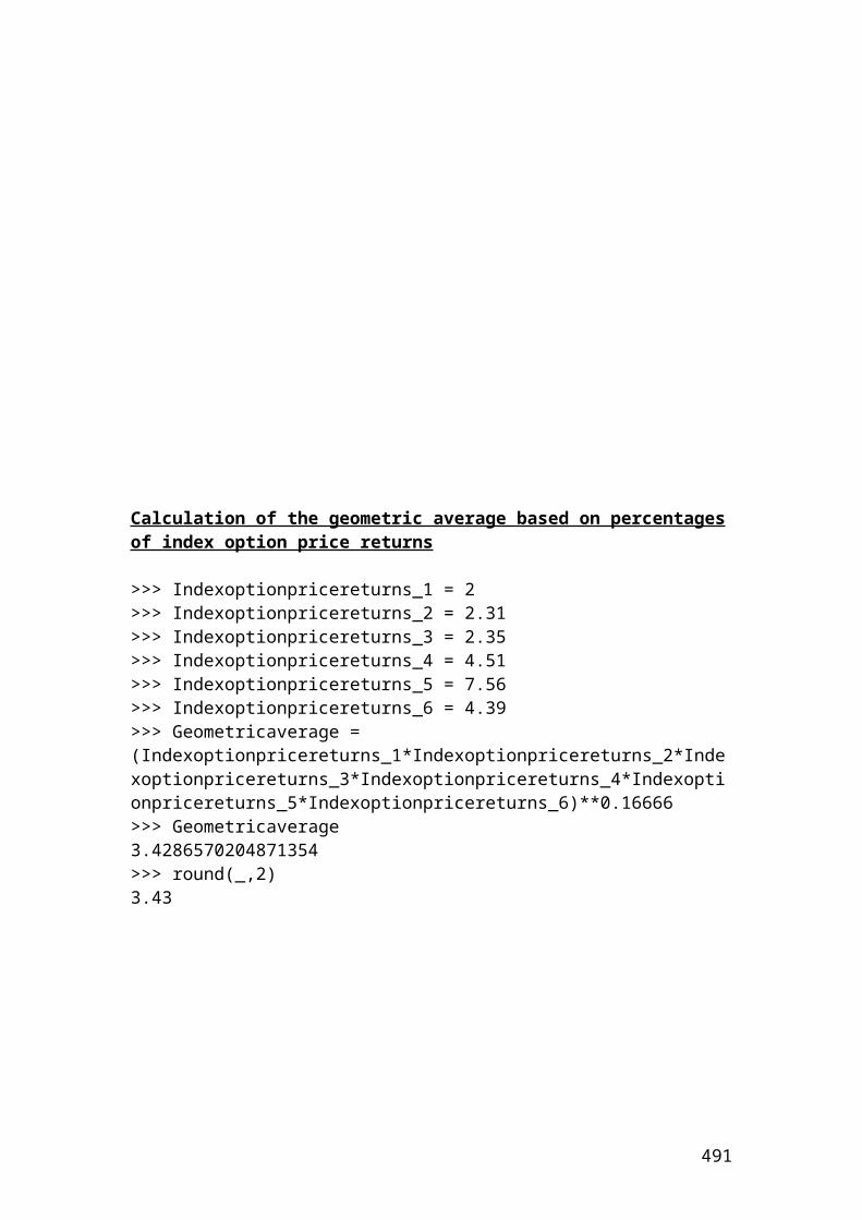
Calculation of the geometric average based on percentages of stock prices

> stock_price_1 <- 10> stock_price_2 <- 12> stock_price_3 <- 13> stock_price_4 <- 14> stock_price_5 <- 15> stock_price_6 <-16> Geometricaverage <- (stock_price_1*stock_price_2*stock_price_3*stock_price_4*stock_price_5*stock_price_6)**0.16666> Geometricaverage[1]13.17849601334643> round(Geometricaverage,digits =2)[1] 13.18

Calculation of the geometric average based on percentages of call option price returns

> Call_option_price_returns_1 <-5> Call_option_price_returns_2 <- 3> Call_option_price_returns_3 <- 2> Call_option_price_returns_4 <- 4> Call_option_price_returns_5 <- 7> Call_option_price_returns_6 <-8> Geometricaverage <- (Call_option_price_returns_1*Call_option_price_returns_2*Call_option_price_returns_3*Call_option_price_returns_4*Call_option_price_returns_5*Call_option_price_returns_6)**0.16666> Geometricaverage[1] 4.3437954197862885

491

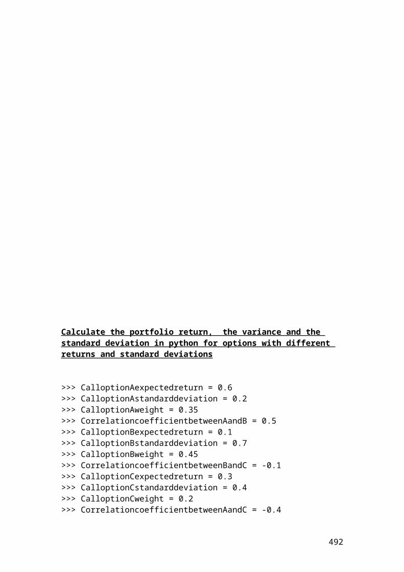
Calculation of the geometric average based on percentages of put option price returns

> Put_option_price_returns_1 <- 2> Put_option_price_returns_2 <- 3.3> Put_option_price_returns_3 <- 2.45> Put_option_price_returns_4 <- 4.21> Put_option_price_returns_5 <- 7.4> Put_option_price_returns_6 <- 4.34> Geometricaverage <- (Put_option_price_returns_1*Put_option_price_returns_2*Put_option_price_returns_3*Put_option_price_returns_4*Put_option_price_returns_5*Put_option_price_returns_6)**0.16666> Geometricaverage[1]3.6024392246983483

Calculation of the geometric average based on percentages of index option price returns

> Index_option_price_returns_1 <- 2> Index_option_price_returns_2 <- 2.31> Index_option_price_returns_3 <- 2.35> Index_option_price_returns_4 <- 4.51> Index_option_price_returns_5 <- 7.56> Index_option_price_returns_6 <- 4.39> Geometricaverage <- (Index_option_price_returns_1*Index_option_price_returns_2*Index_option_price_returns_3*Index_option_price_returns_4*Index_option_price_returns_5*Index_option_price_returns_6)**0.16666> Geometricaverage[1]3.4286570204871354

492

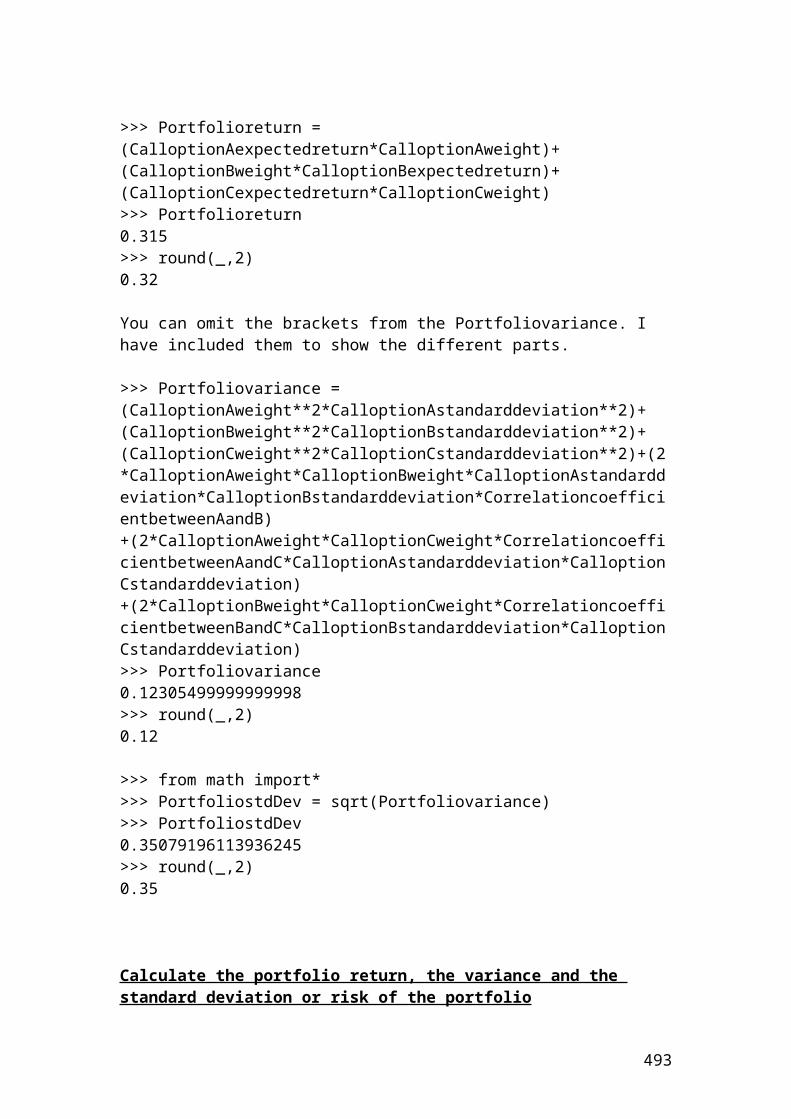
Calculate the portfolio return, the variance and the standard deviation in R for options with different returns and standard deviations

> CalloptionAexpectedreturn = 0.6> CalloptionAstandarddeviation = 0.2> CalloptionAweight = 0.35> CorrelationcoefficientbetweenAandB = 0.5> CalloptionBexpectedreturn = 0.1> CalloptionBstandarddeviation = 0.7> CalloptionBweight = 0.45> CorrelationcoefficientbetweenBandC = -0.1> CalloptionCexpectedreturn = 0.3> CalloptionCstandarddeviation = 0.4> CalloptionCweight = 0.2> CorrelationcoefficientbetweenAandC = -0.4

> Portfolioreturn = (CalloptionAexpectedreturn*CalloptionAweight)+(CalloptionBweight*CalloptionBexpectedreturn)+(CalloptionCexpectedreturn*CalloptionCweight)>>> Portfolioreturn[1] 0.315

You can omit the brackets from the Portfoliovariance. I have included them to show the different parts.

> Portfoliovariance = (CalloptionAweight**2*CalloptionAstandarddeviation**2)+ (CalloptionBweight**2*CalloptionBstandarddeviation**2)+(CalloptionCweight**2*CalloptionCstandarddeviation**2)+(2*CalloptionAweight*CalloptionBweight*CalloptionAstandarddeviation*CalloptionBstandarddeviation*CorrelationcoefficientbetweenAandB)+(2*CalloptionAweight*CalloptionCweight*CorrelationcoefficientbetweenAandC*CalloptionAstandarddeviation*CalloptionCstandarddeviation)+(2*CalloptionBweight*CalloptionCweight*CorrelationcoefficientbetweenBandC*CalloptionBstandarddeviation*CalloptionCstandarddeviation)> Portfoliovariance[1] 0.12305499999999998

> Portfolio_std = sqrt(Portfoliovariance)> Portfolio_std0.35079196113936245> round(Portfolio_std,digits=2)[1] 0.35

493

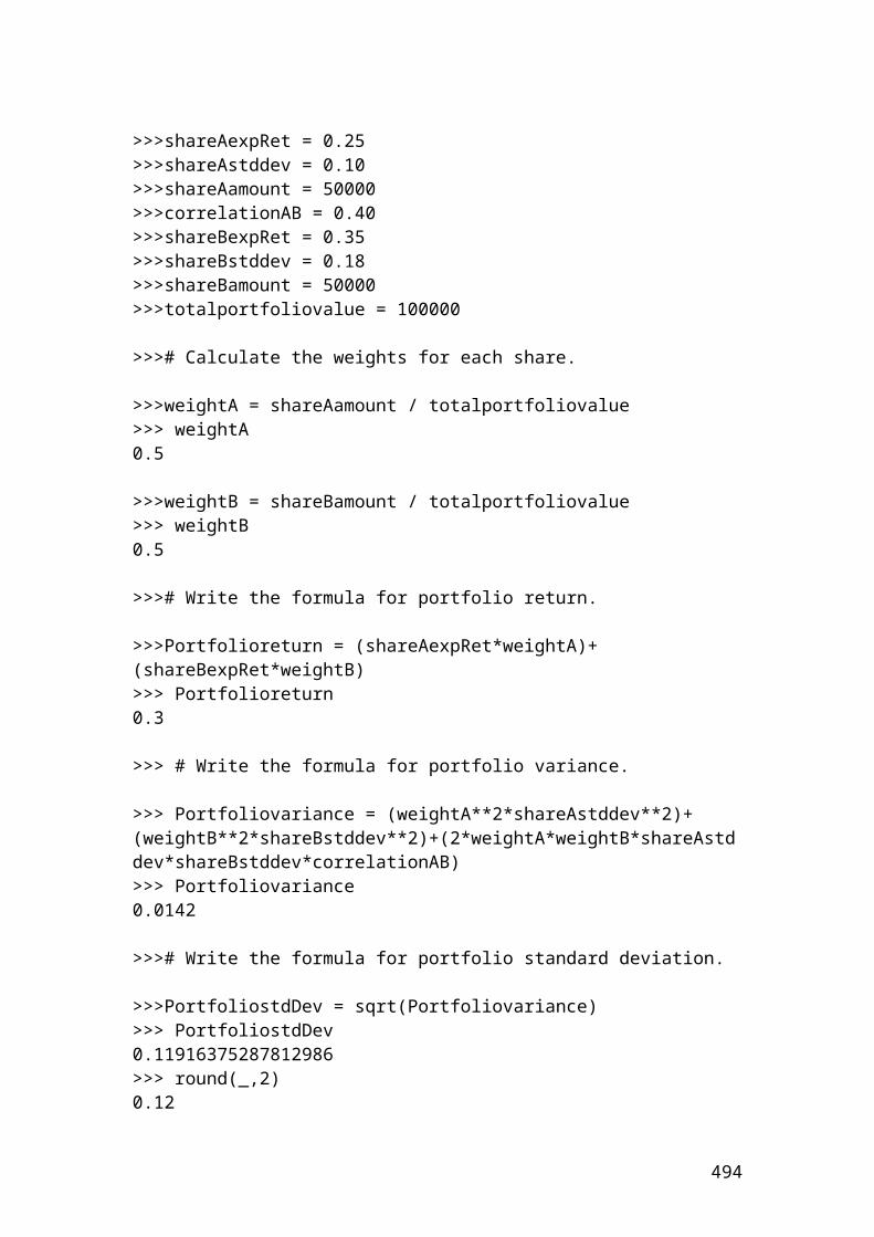
Calculate the portfolio return, the variance and the standard deviation or risk of the portfolio

>shareAexpRet <- 0.25>shareAstddev <- 0.10>shareAamount <- 50000>correlationAB <- 0.40>shareBexpRet <- 0.35>shareBstddev <- 0.18>shareBamount <- 50000>totalportfoliovalue <- 100000

># Calculate the weights for each share.

>weightA <- shareAamount / totalportfoliovalue> weightA[1]0.5

>weightB <-shareBamount / totalportfoliovalue> weightB[1]0.5

># Write the formula for portfolio return.

>Portfolioreturn <- (shareAexpRet*weightA)+(shareBexpRet*weightB)> Portfolioreturn[1]0.3

> # Write the formula for portfolio variance.

> Portfoliovariance <- (weightA**2*shareAstddev**2)+(weightB**2*shareBstddev**2)+(2*weightA*weightB*shareAstddev*shareBstddev*correlationAB)> Portfoliovariance[1]0.0142

># Write the formula for portfolio standard deviation.

>Portfolio_std <- sqrt(Portfoliovariance)> Portfolio_std[1]0.11916375287812986> round(Portfolio_std,digits=2)[1] 0.12

494

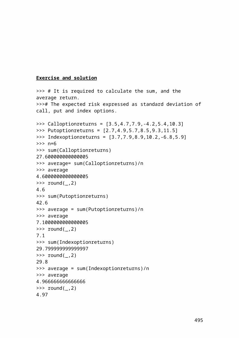
Exercise and solution

> # It is required to calculate the sum, and the average return.># The expected risk expressed as standard deviation of call, put and index options.># The figures represent percentages.

> call_option_returns <-c (3.5,4.7,7.9,-4.2,5.4,10.3)> put_option_returns <-c (2.7,4.9,5.7,8.5,9.3,11.5)> index_option_returns <-c (3.7,7.9,8.9,10.2,-6.8,5.9)> n<-6> sum(call_option_returns)[1] 27.600000000000005> average<- sum(call_option_returns)/n> average[1] 4.6000000000000005> sum(put_option_returns)[1] 42.6> average <-sum(put_option_returns)/n> average[1] 7.1000000000000005> sum(index_option_returns)[1] 29.799999999999997> average <- sum(index_option_returns)/n> average[1] 4.966666666666666> sd<-sqrt(sum((call_option_returns-mean(call_option_returns))^2)/(n-1))> sd[1] 4.953383> sd<-sqrt(sum((put_option_returns-mean(put_option_returns))^2)/(n-1))> sd[1] 3.234811> sd<-sqrt(sum((index_option_returns-mean(index_option_returns))^2)/(n-1))> sd[1] 6.203117> round(sd,digits=2)[1] 6.2

495

Example of pricing a forward contract and solution

A forward contract of 6 month has a market price of 52 Pounds when the spot price of the underlying commodity is 49 Pounds. There are no costs of carry and the discount rate is 7 percent. Calculate the value of the forward contract.

Solution

The current price of the forward contract (F0) should be equal to the value of the underlying commodity, (S0) at the discount rate r. Thus, the equation is as follows:

pounds 715.50207.0149)1(

)1(

00

00

rSF

rSF

Application of pricing a forward contract in R

> spot_price <- 49> discount_rate <- 0.07> # Insert the mathematical formula.> value_forward_contract <- spot_price *(1+discount_rate/2)> value_forward_contract50.714999999999996> round(50.715,digits=2)[1] 50.72 # Pounds

496

Example of interest rate payment and solution

A trader wants to calculate the interest amount that he / she will receive in three months from a forward contract of a Euribor deposit paying a Euro deposit rate of 3.55%. The principal amount is 300,000

The mathematical formula is as follows:

Interest payment = principal x [interest rate x (tdays / 360)]

Interest payment = 300,000 x [0.0355 x (90/360)]Interest payment = 2662.5 Euro.

Application of interest payment in R

> principal <- 300000> interest_rate <- 0.0355> days <- 90> # Insert the mathematical formula.> interest_payment <- principal*(interest_rate *days/360)> interest_payment[1] 2662.4999999999995> round(interest_payment,digits=2)[1] 2662.5 # Euro

497

Example and solution of calculating profits and losses on futures contracts

An investor buys 8 S&P 500 futures contracts at $2189. He has closed the futures contract position with a price of $2236. The multiplier for S&P 500 futures contracts is 250 dollars. Did he record a profit or a loss?

Solution

The mathematical formula is as follows:

Where: fT is the final contract price. f0 is the initial contract price.

9400021892236 x250 x 8 Gain USD

When the prices move up, the investor will gain in long positions. When prices move down, the investor will gain in short positions.

Application of calculating profits and losses on futures contracts in R

> number_of_contracts <- 8> buying_price <- 2189> selling_price <- 2236> multiplier <-250> # Insert the mathematical formula.> profit_or_loss <- number_of_contracts*multiplier*(selling_price - buying_price)> profit_or_loss[1] 94000 # USD

498

Example and solution of semiannually currency swap between an investment bank and an insurance company

The investment bank borrows 20,000,000 Pounds from the insurance company at a fixed rate of 5% for 1 year. The insurance company borrows from the investment bank 10,000,000 Euros at a fixed rate of 5% for 1 year. Calculate the interest payments for the three years, if we assume semiannual payments?

At the beginning of the contract

€10,000,000Investment bank Insurance company

£ 20,000,000

The insurance company pays the investment bank the following interest payment.

£20,000,000 x 0.05/2 = 500,000 Pounds.

The investment bank pays the insurance the following interest payment.

€10,000,000 x 0.05/2 =250,000 Euros.

The following arrows illustrate the interest payments.

€ 250,000Investment bank Insurance company

£ 500,000

At the end of the third year, the two parties exchange the principal amounts in addition to the final interest payments.

€10,250,000Investment bank Insurance company

£20,500,000

499

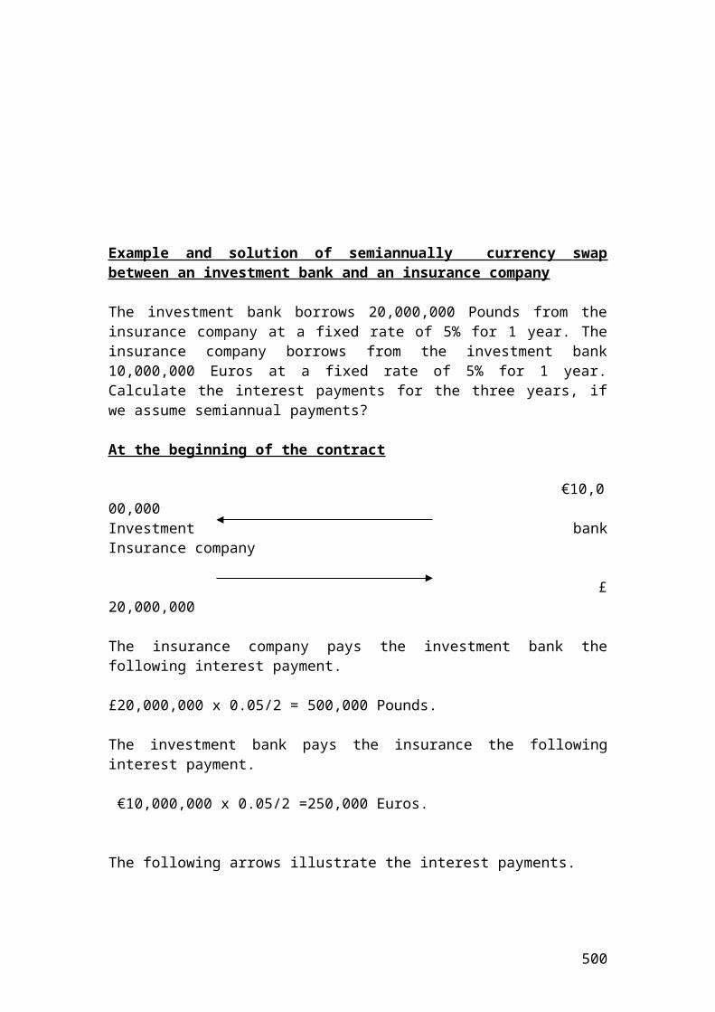
Application of semiannually currency swap between an investment bank and an insurance company in R

> bank_borrows_from_insurance <- 20000000> insurance_borrows_from_bank <-10000000> interest_rate <- 0.05> semiannual_payment <- 2> # Insert the mathematical formula.> bank_pays_insurance <- insurance_borrows_from_bank *(interest_rate/semiannual_payment)> bank_pays_insurance[1] 250000.0 # Euros> # Insert the mathematical formula.> insurance_pays_bank <- bank_borrows_from_insurance *(interest_rate/semiannual_payment)> insurance_pays_bank[1] 500000.0 # Pounds or[1] 5e+05 # Pounds

500

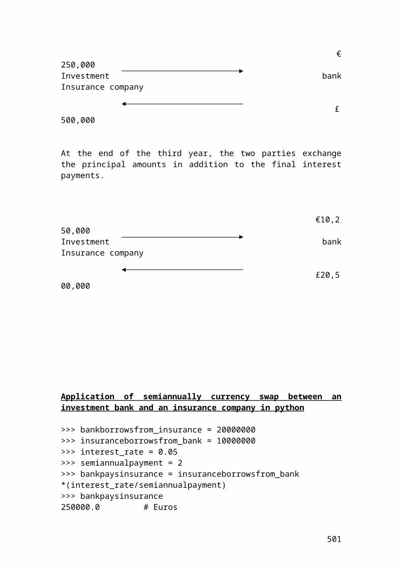
Example and solution of interest rate swap

Interest rate swaps are very popular agreements between two parties in the debt or fixed-income department of the investment banks. The fixed income department of Bank A pays a fixed rate of 5.5% upon the principal of 50,000,000 Pounds. In contrast, Bank B pays a floating or reference rate of LIBOR accounted to 7.2%. The payment frequency is every 6 months for 2 years.

Fixed payment : £50,000,000 x 0.055/2 = 1,375,000 Bank A Bank B Floating payment: £50,000,000 x 0.072/2 = 1,800,000

Suppose in the second year that the LIBOR has increased by 12 basis points or 0.12%. Then, the floating payment will change and the calculation will be as follows:

Second year floating payment for Bank B = 50,000,000 x 0.0732 / 2 = 1,830,000 Pounds.

Bank A will continue to pay the same fixed amount, namely, £50,000,000 x 0.055/2 = £1,375,000.

Application of interest rate swap in R

> principal <- 50000000> interest_rate1 <- 0.055> interest_rate2 <- 0.072> interest_rate3 <- 0.0732> semiannual_payment <- 2> # Insert the mathematical formula.> fixed_payment <- principal*(interest_rate1/semiannual_payment)> fixed_payment[1]1375000.0 # pounds> # Insert the mathematical formula.> floating_payment_1 <- principal*(interest_rate2/semiannual_payment)> floating_payment_1[1] 1800000.0 # pounds> # Insert the mathematical formula.> floating_payment_2 <- principal*(interest_rate3/semiannual_payment)> floating_payment_2[1]1830000.0 # Pounds

501

Delta – neutral hedge

Delta – neutral hedge is common used in risk management to keep the value of the portfolio neutral due to changes in the share price. It is achieved from a long position in a share and a short position in a call option. The mathematical formula to determine the number of options is as follows:

option call of deltahedged shares ofNumber hedge neutral - Delta

Thus, if the investment bank has bought 30,000 shares of Vodafone and the delta of the call option of the same company is 0.50, then the numbers of call options that are needed to purchase to form a delta-neutral hedge are as follows:

Delta hedge = 30,000 / 0.50 = 60,000 options or 600 option contracts.

Application of delta- neutral hedge in R

> number_of_shares <- 30000> delta_of_call_option <- 0.50> # Insert the mathematical formula.> delta_neutral_hedge <- number_of_shares/delta_of_call_option> delta_neutral_hedge[1] 60000.0

502

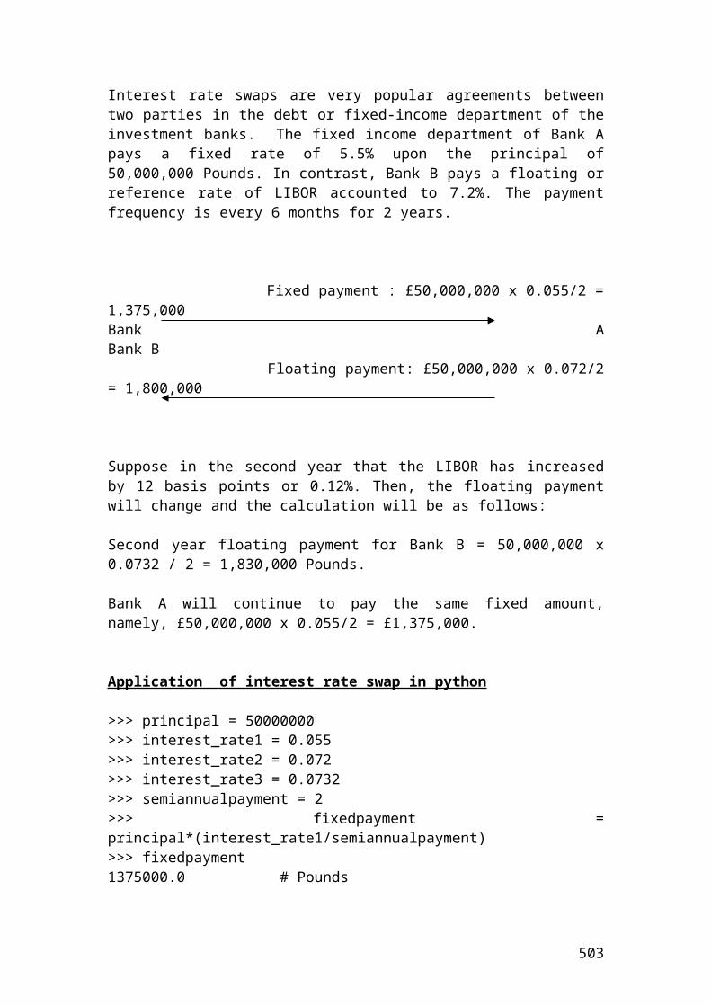
Weighted mean price of a portfolio

Let’s assume that we have a portfolio of four options with their market prices and the number of shares bought. It is required to calculate the weighted mean price of the portfolio.

Options Price expressed in $

Number of shares

Weight Weight x Price

A 14.00 300 0.4 5.6B 12.00 200 0.3 3.6C 8.00 100 0.1 0.8D 5.00 150 0.2 1

Total 750 1Source: author’s calculation

The mathematical formula is as followed:

prices. theare P weights. theare w

portfolio. theof pricemean weighted theis X :

i

i

wWhere

PwX iiw

By substituting the numbers from the Table into the equation we have the following:

3.6 5.6 wX 0.8 + 1 = 11.

Application of weighted mean price of a portfolio in R

> price_1 <-14> price_2 <- 12> price_3 <- 8> price_4 <- 5> weight_1 <- 0.4> weight_2 <- 0.3> weight_3 <- 0.1> weight_4 <- 0.2>portfoliomean<-(price_1*weight_1+price_2*weight_2+price_3*weight_3+price_4*weight_4)> portfoliomean[1] 11.0 # Pounds

503

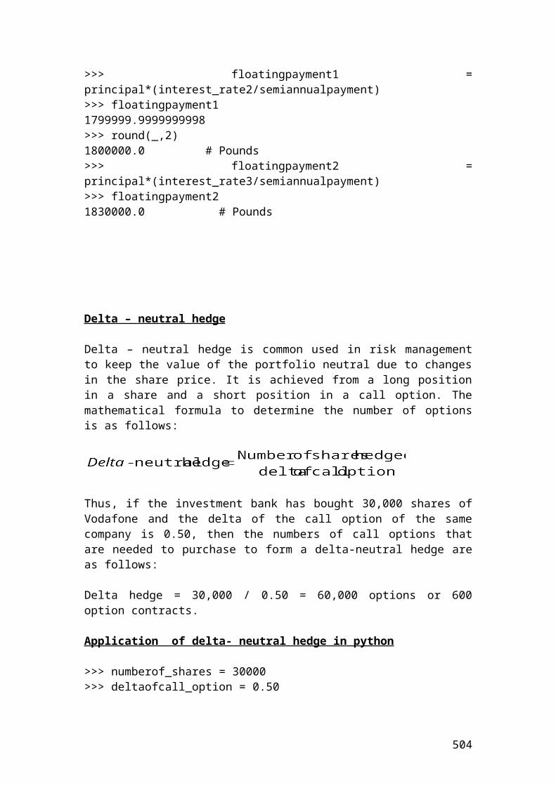
Example of Eurodollar futures

An investor wants to calculate the futures price of a 1-month Eurodollar time deposits based on a LIBOR rate of 3.40%. The initial principal is 1 million Pounds.

Solution

The price of the Eurodollar futures contract will be as follows:

Application of Eurodollar futures in R

> principal <- 1000000> interest_rate <- 0.034> days <- 30> Eurodollar_future <- principal*(1- interest_rate*(days/360))> Eurodollar_future[1] 997166.7 # Pounds

504

Example of forward rate agreement

An investment bank buys a 4 x 6 FRA from a building society in the UK for 4.0% by paying 2 million Pounds. 80 days latter, LIBOR is 5%. Who will receive the FRA payment and for how much?

Solution

The mathematical formula for Forward Rate Agreement, (FRA) is as follows:

360/trate var1360/rate fixed -rate variable

amount x NotionalPayment days

iablet

FRA days

The timeline schedule is as follows:

t = 0 4months 6 months

360/800.051

360/1200.04 -0.05 x000,000,2Payment FRA = ………. Please complete the

calculation.

Helpful hint: If the FRA payment is positive, then, the building society is the payer and the investment bank receives the FRA payment.

If the FRA payment is negative, then the investment bank is the payer and the building society receives the FRA payment.

Application of forward rate agreement in R

> principal <- 2000000> variable_rate <- 0.05> fixed_rate <- 0.04> FRA_payment <- principal*(variable_rate - fixed_rate)*0.333333333/1.011111111> FRA_payment[1] 6593.407> round(FRA_payment,digits=2)[1] 6593.41 # Pounds

505

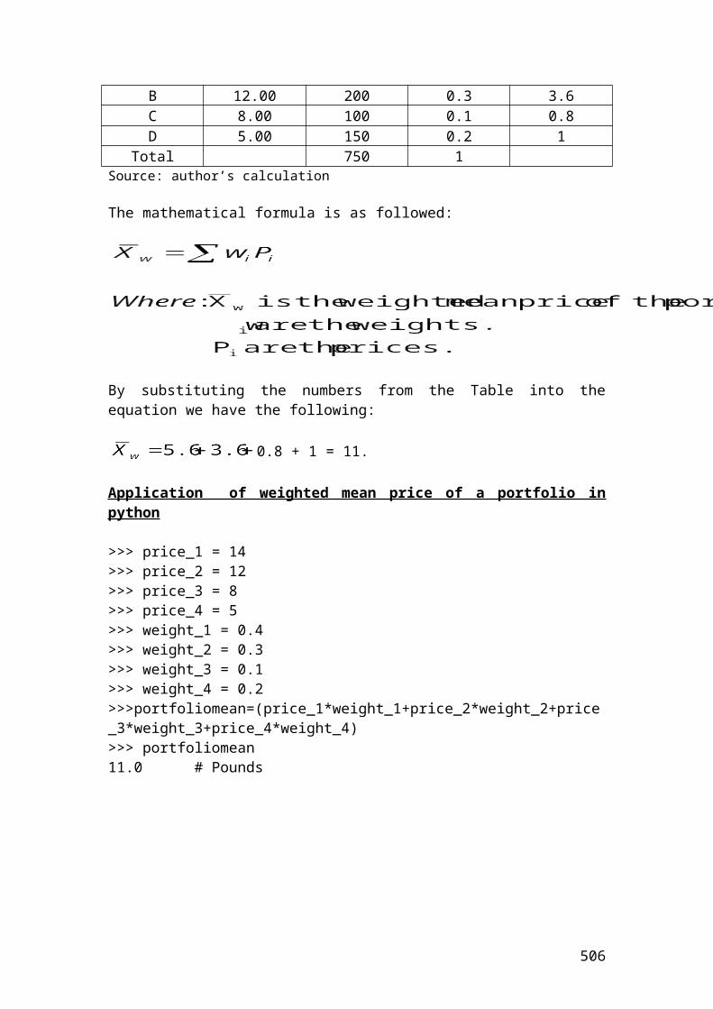
Example of futures on Treasury bills

An investor wants to calculate the futures price of a 3-month Treasury bills. Treasury bills are short-term notes of limited period of 1- month, and 3 - month respectively. The initial principal is 5 million Pounds and the discount rate is 3.50%.

Solution

The price of the Treasury bill futures will be as follows:

360t

xratediscount -1 x Principal BillTreasury price daysFutures

Please complete the calculation …….

Application of futures on Treasury bills in R

> principal <- 5000000> discount_rate <- 0.035> days <- 90< # Insert the mathematical formula.> futures_treasury_bills <- principal*(1- discount_rate *(days/360))> futures_treasury_bills [1] 4956250 # Pounds

506

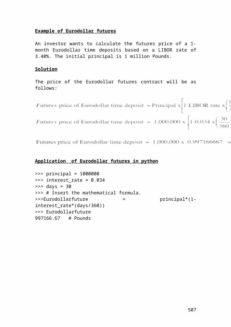
Example of stock index futures

For example, if you bought 10 contracts of the Dow Jones Industrial index at 10,000 and you expected an aggressive bull market that reaches the value of 16,000, then, the 6000 points increase are multiplied by the standardized value of 250. If the initial principal of investment is $100,000, the mathematical formula for the gains will be as follows:

10 x 100,000 x 6000 x 250 = 1.5 x 1012 Dollars

Application of stock index futures in R

> principal <- 100000> points_increase <- 6000> multiplier <- 250> number_of_contracts <- 10> gains <- principal*points_increase*multiplier*number_of_contracts> gains[1] 1.5e+12 # USD

507

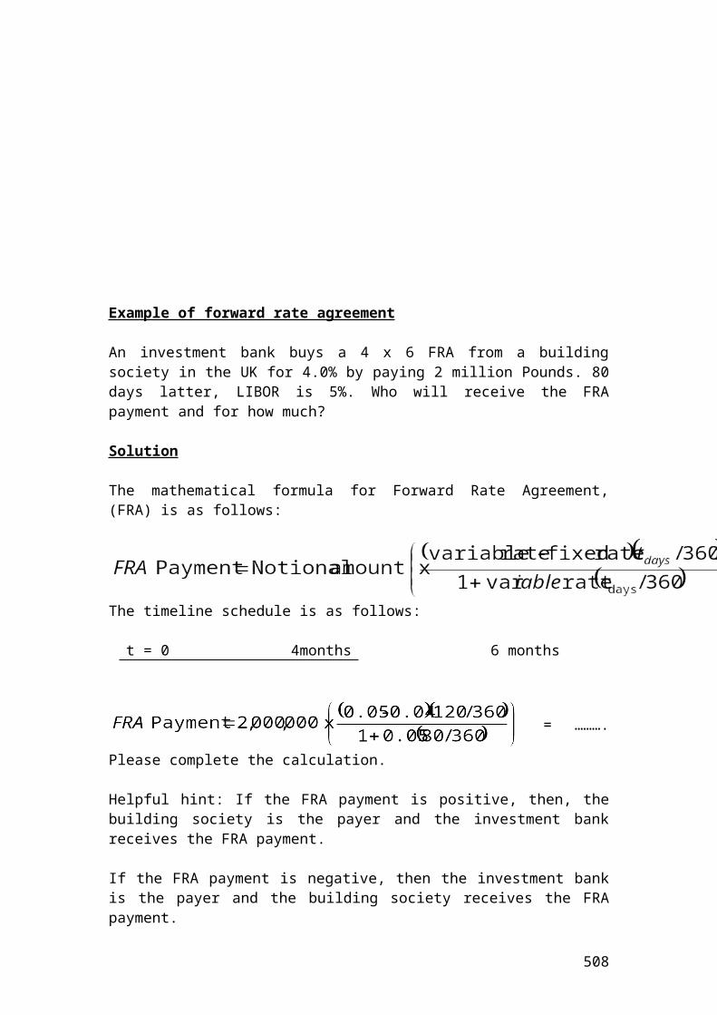
Example of currency futures

A manufacturer wants to calculate the currency futures price of EURO/USD traded in Frankfurt derivative market. For example, in August the contract is quoted as 1.35 EURO /USD and the contract size is 20,000. The principal is 300,000 Euro.

Solution

The contract price of 1 contract is as follows:

n....calculatio thecomplete Please

Euro .. ... price quotedAugust x sizecontract *principal EURO/USD futurecurrency of price

Futures

Application of currency futures in R

> principal =<-300000> quote <- 1.35> contract_size <- 20000> # Insert the mathematical formula.> futures_price_of_currency <- principal*quote*contract_size> futures_price_of_currency[1] 8.1e+09 # Euro

508

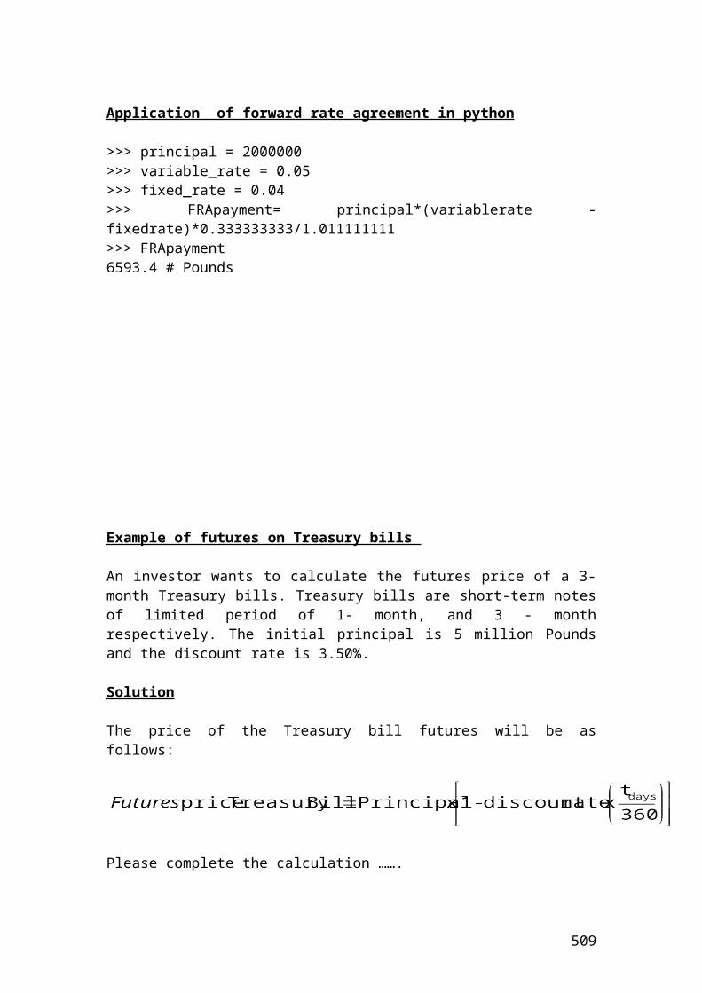
Please try based on the previous examples to illustrate the following example in R. If you have difficulties e-mail me.

Active return, active risk and information ratio

Active return is the difference in returns between a portfolio and the index or benchmark that is measured.

Active return = rp - rb

Where: rp is the portfolio return. rb is the benchmark or index return.

If the portfolio return is 0.80 and the benchmark return of the index is 0.70 then, the active return is………

Please complete the calculation.

Active risk or tracking error is the standard deviation of the difference of returns between a portfolio and the benchmark or index.

assets. ofnumber theisn index.an examplefor be couldIt return.benchmark portfolio is r

return. portfolio is r :

1

)(r risk

b

p

2p

Wheren

rActive b

If the portfolio return is 0.80, the number of assets is 10 and the benchmark return of the index is 0.40 then, the active risk is………

Please complete the calculation.

Information ratio shows the consistency of the fund manager towards the active return. The mathematical formula is as follows:

509

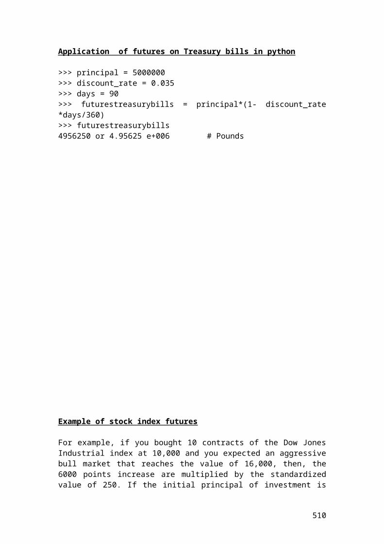
risk active theis

1

return.index or benchmark average theis r

return. portfolio of average theis :

1)(r

2

b

2p

nrr

rWhere

nr

rrIR

bp

p

b

bp

It could be calculated very easily in Excel software. I will illustrate a simple table with the relevant calculations.

Day rp rb rp - rb

1 0.03 0.02 0.012 0.02 0.014 0.0063 -0.04 0.034 -0.0744 0.05 0.067 -0.0175 0.08 0.012 0.0686 -0.01 -0.056 0.0467 0.07 0.031 0.0398 0.034 0.023 0.0119 -0.021 0.015 -0.03610 0.045 0.001 0.044

Average 0.0258 0.0161Standard deviation

0.043

Source: author’s calculation

By substituting the values that we have found in terms of rp =0.0258, rb = 0.0161 and standard deviation = 0.043 in the following equation we have:

1)(r 2

p

n

r

rrR

b

bp

2d.p.) (to 23.0043.0

0097.0043.0

0161.00258.0

R

But what is the interpretation of the information ratio of 0.23. It means that the fund manager gained around 23 basis points of active return per unit of active risk. The higher is this number, the better the manager is performing in relation to active risk.

510

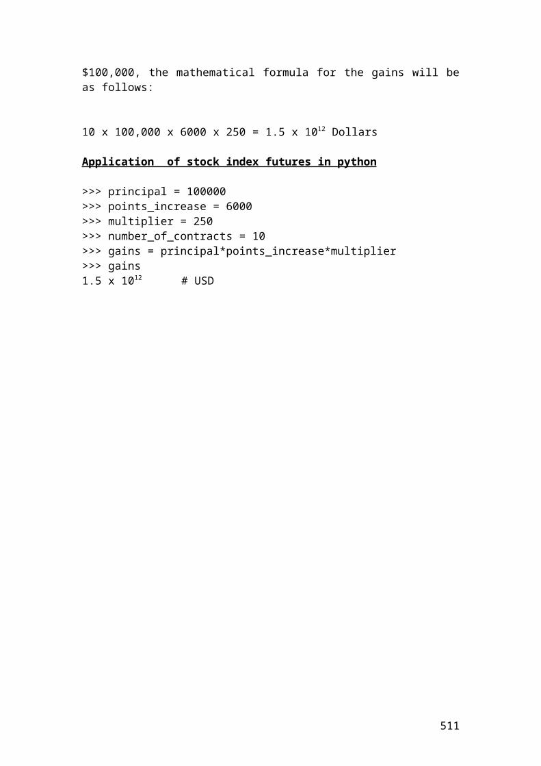
Please convert the following exercise in R language programming.

Calculate the balance at the end of the 5th day from changes in the futures prices from 90 to 89, 91, 95, 97, 99. The trader has bought 50 futures contract for settlement in May. The initial margin is $8.

Day Beginning balance

Futures price Gain or loss Ending balance

0 400 90 0 4001 400 89 (50)2 350 91 1003 450 95 2004 650 97 1005 750 99 100

Source: author’s illustration.

Beginning balance = initial margin x number of contracts.Beginning balance = 8 x 50 = $400

Please complete the values of the column ending balance.

511

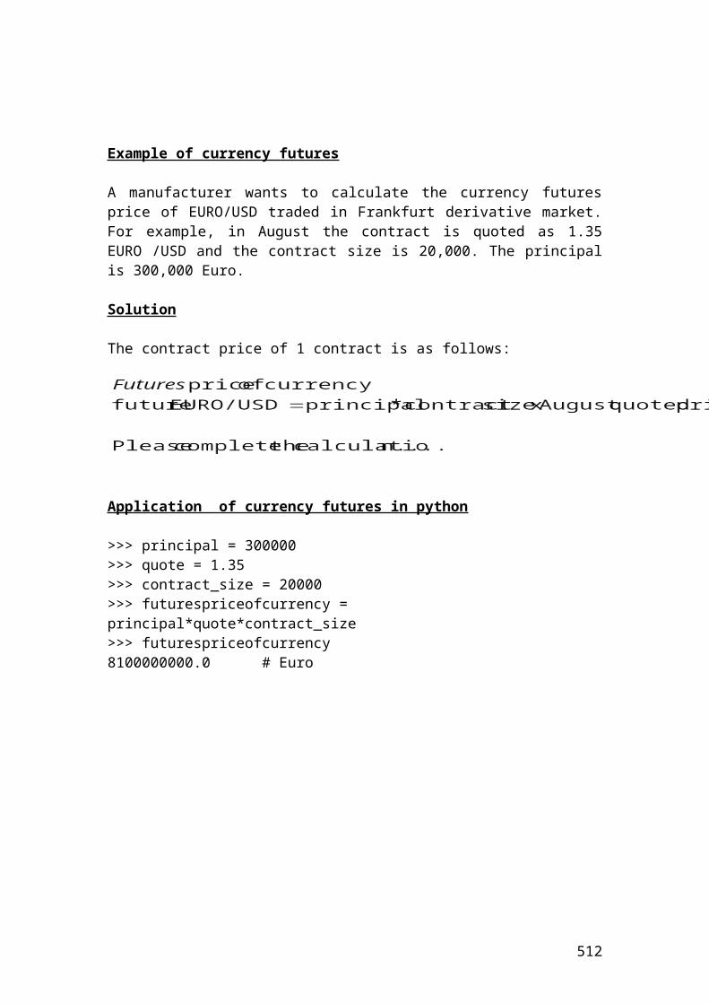
Application of the random function. It is very useful method that is used in simulations such as Monte Carlo simulation to price derivatives products

The uniform random function is given by the runif. Inside the brackets, there are three numbers. The first number symbolizes the total number of random numbers. The second number symbolizes the lower value and the third number symbolizes the upper value.

> rand.number<-runif(2,0,10000)> rand.number[1] 1848.823 7023.740> rand.number<-runif(5,0,10000)> rand.number[1] 5733.263 1680.519 9438.393 9434.750 1291.590

Other random functions available in R are related with different types of distributions. For example, the random number that is associated with a normal distribution is given by rnorm.The random number that is associated with an exponential distribution is given by rexp.

512

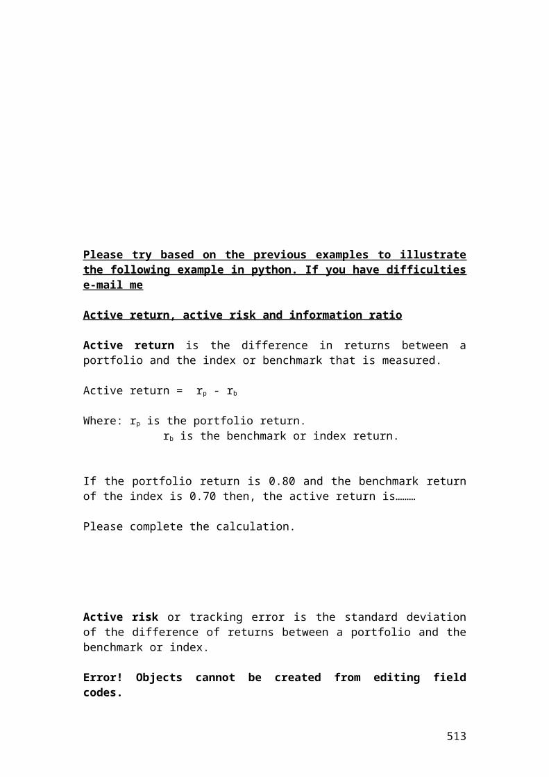
Example of profit or loss of a call option portfolio. The figures are expressed in Euros.

> shareprice_1 <-10.25> shareprice_2 <- 20.13> shareprice_3 <- 30.22> shareprice_4 <- 40.56> shareprice_5 <- 50.89> shareprice_6 <- 51.23> shareprice_7 <- 53.33> shareprice_8 <-54.63> shareprice_9 <- 66.23> shareprice_10 <- 68.23> strikeprice_1 <- 3.34> strikeprice_2 <- 8.34> strikeprice_3 <-18.78> strikeprice_4 <- 28.34> strikeprice_5 <- 31.12> strikeprice_6 <- 22.02> strikeprice_7 <- 34.23> strikeprice_8 <- 47.12> strikeprice_9 <- 48.45> strikeprice_10 <- 50.12> optionpremium_1 <- 1.50> optionpremium_2 <- 2.30> optionpremium_3 <- 2.56> optionpremium_4 <- 3.10> optionpremium_5 <- 3.25> optionpremium_6 <- 3.45> optionpremium_7 <- 3.56> optionpremium_8 <- 4.32> optionpremium_9 <- 5.12> optionpremium_10 <- 5.78> contractsize <- 100

> portfoliovalue1 <- (shareprice_1-(strikeprice_1+ optionpremium_1))* contractsize> portfoliovalue1[1] 541.0> portfoliovalue2 <- (shareprice_2-(strikeprice_2+ optionpremium_2))* contractsize> portfoliovalue2[1] 948.9999999999999> portfoliovalue3 <- (shareprice_3-(strikeprice_3+ optionpremium_3))* contractsize> portfoliovalue3[1] 887.9999999999999> portfoliovalue4 <- (shareprice_4-(strikeprice_4+ optionpremium_4))* contractsize> portfoliovalue4[1] 912.0000000000001> portfoliovalue5 <- (shareprice_5-(strikeprice_5+ optionpremium_5))* contractsize> portfoliovalue5

513

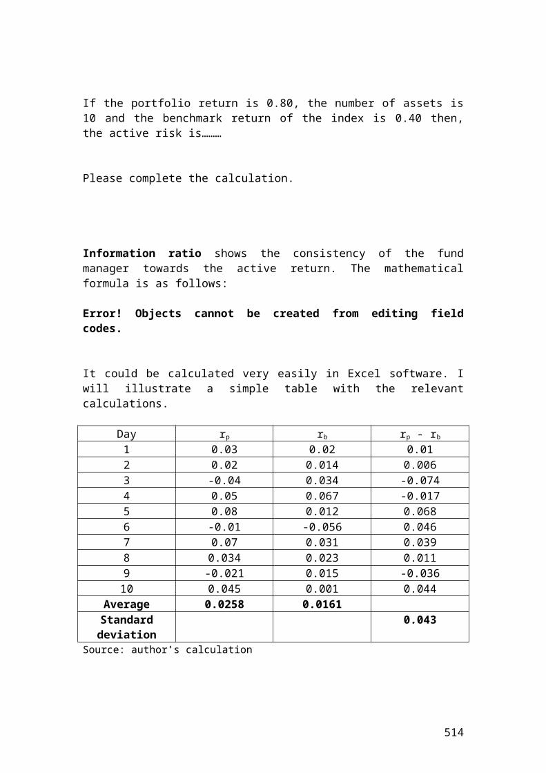
[1] 1651.9999999999995> portfoliovalue6 <- (shareprice_6-(strikeprice_6+ optionpremium_6))* contractsize> portfoliovalue6[1] 2576.0> portfoliovalue7 <- (shareprice_7-(strikeprice_7+ optionpremium_7))* contractsize> portfoliovalue7[1] 1554.0> portfoliovalue8 <- (shareprice_8-(strikeprice_8+ optionpremium_8))* contractsize> portfoliovalue8[1] 319.00000000000045> portfoliovalue9 <- (shareprice_9-(strikeprice_9+ optionpremium_9))* contractsize> portfoliovalue9[1] 1266.0000000000005> portfoliovalue10 <- (shareprice_10-(strikeprice_10+ optionpremium_10))* contractsize> portfoliovalue10[1] 1233.0000000000005

514

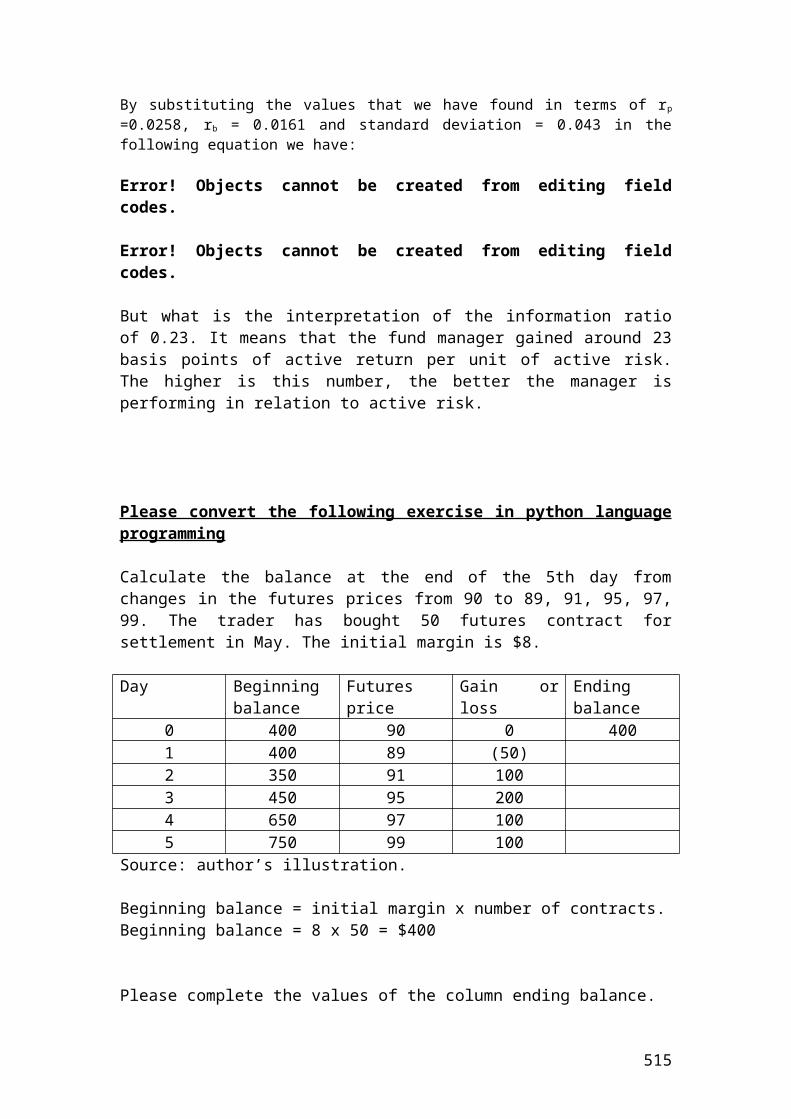
Example of profit or loss of a put option portfolio. The figures are expressed in Euro.

> shareprice_1 <- 10.25> shareprice_2 <- 20.13> shareprice_3 <- 30.22> shareprice_4 <- 40.56> shareprice_5 <- 50.89> shareprice_6 <- 51.23> shareprice_7 <- 53.33> shareprice_8 <- 54.63> shareprice_9 <- 66.23> shareprice_10 <- 68.23> strikeprice_1 <- 3.34> strikeprice_2 <- 8.34> strikeprice_3 <- 18.78> strikeprice_4 <- 28.34> strikeprice_5 <- 31.12> strikeprice_6 <- 22.02> strikeprice_7 <- 34.23> strikeprice_8 <- 47.12> strikeprice_9 <- 48.45> strikeprice_10 <- 50.12> optionpremium_1 <- 1.50> optionpremium_2 <- 2.30> optionpremium_3 <- 2.56> optionpremium_4 <- 3.10> optionpremium_5 <- 3.25> optionpremium_6 <- 3.45> optionpremium_7 <- 3.45> optionpremium_8 <- 4.32> optionpremium_9 <- 5.12> optionpremium_10 <- 5.78> contractsize <-100> portfoliovalue1 <- (strikeprice_1- optionpremium_1-shareprice_1)* contractsize> portfoliovalue1[1] -841.0> portfoliovalue2 <- (strikeprice_2- optionpremium_2- shareprice_2)* contractsize> portfoliovalue2[1] -1409.0> portfoliovalue3 <- (strikeprice_3- optionpremium_3- shareprice_3)* contractsize> portfoliovalue3[1] -1399.9999999999995> portfoliovalue4 <- (strikeprice_4 - optionpremium_4 - shareprice_4)* contractsize> portfoliovalue4[1] -1532.0000000000005> portfoliovalue5 <- (strikeprice_5- optionpremium_5- shareprice_5)* contractsize> portfoliovalue5[1] -2302.0

515

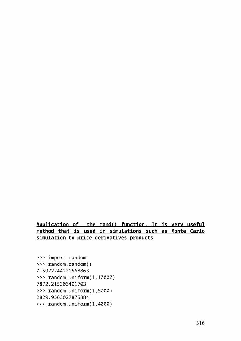
> portfoliovalue6 <- (strikeprice_6- optionpremium_6- shareprice_6)* contractsize> portfoliovalue6[1] -3265.9999999999995> portfoliovalue7 <- (strikeprice_7- optionpremium_7- shareprice_7)* contractsize> portfoliovalue7[1] -2255.0> portfoliovalue8 <- (strikeprice_8- optionpremium_8- shareprice_8)* contractsize> portfoliovalue8[1] -1183.0000000000005> portfoliovalue9 <- (strikeprice_9- optionpremium_9- shareprice_9)* contractsize> portfoliovalue9[1] -2290.0> portfoliovalue10 <- (strikeprice_10- optionpremium_10- shareprice_10)* contractsize> portfoliovalue10[1] -2389.000000000001

516

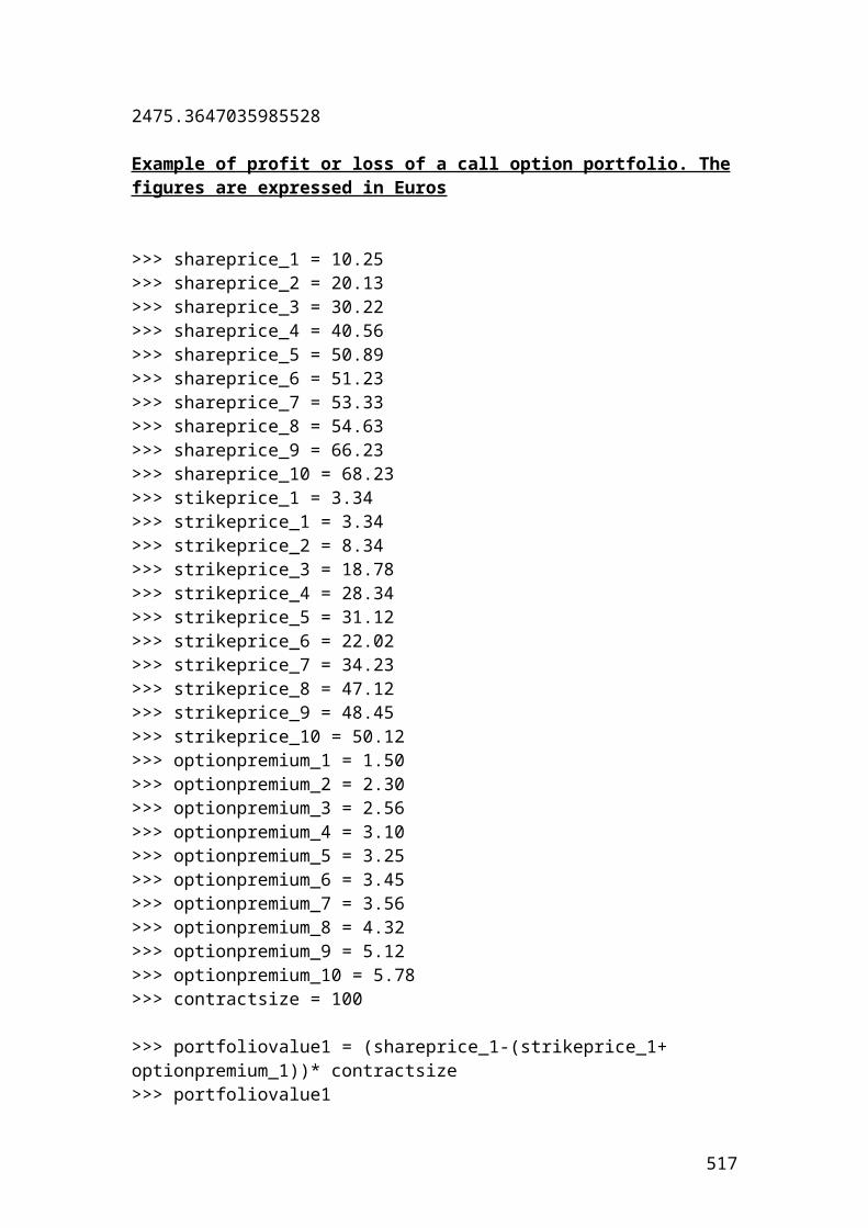
One – period binomial method

A share is traded in the Danish stock exchange at 50 DKK. First of all, we would like to calculate the possible price changes based on probabilities. The risk - free rate is 5% and the value of the call option has an exercise price of 50 DKK. It is required to calculate the expected value of the option at t =1. In addition, it is required to calculate the value of the option today discounted at the given risk-free rate.

We assume two scenarios. The first one is that the share will increase by 20% or by a factor of 1 + 0.20 = 1.20. The second one is that the share will decrease by 0.833. The number 0.833 is calculated as 1 / 1.20 = 0.833.

The mathematical formulas are as follows:

Down move = D = 1 / up move = 1 / 1.20 = 0.833

59128.0367.0217.0

0.833-1.200.833- 0.051

move. up theis U move.down theis D

rate. free-risk theis rf :

D-U

D-rf1 movement upan ofy probabilit neutral -risk

U

Where

U

0.40872 0.59128 - 1 movement down a ofy probabilit neutral - riskD

Thus, the payoff or the one-period binomial tree for share and option prices for the two possible scenarios will be as follows:

t = 0 t = 1

Probability Up = 0.59128 Share price = 50 x 1.20 = 60 DKK Call option = 60 – 50 = 10 DKK. 50 In this case, an increase of the share price will lead to the call option to pay back 10 DKK Probability Down =0.40872 Share price = 50 x 0.833 = 41.65 DKK Call option = 41.65 – 50 = -8.35 DKK = 0 DKK In this case the call option does not worth anything.

The expected value of the call option at t = 1 is as follows:

Expected call option = (10 x 0.59128) + ( 0 x 0.40872) = 5.9128 + 0 = 5.9128 DKK.

The value of the call option discounted at 5% risk – free rate is as follows:

517

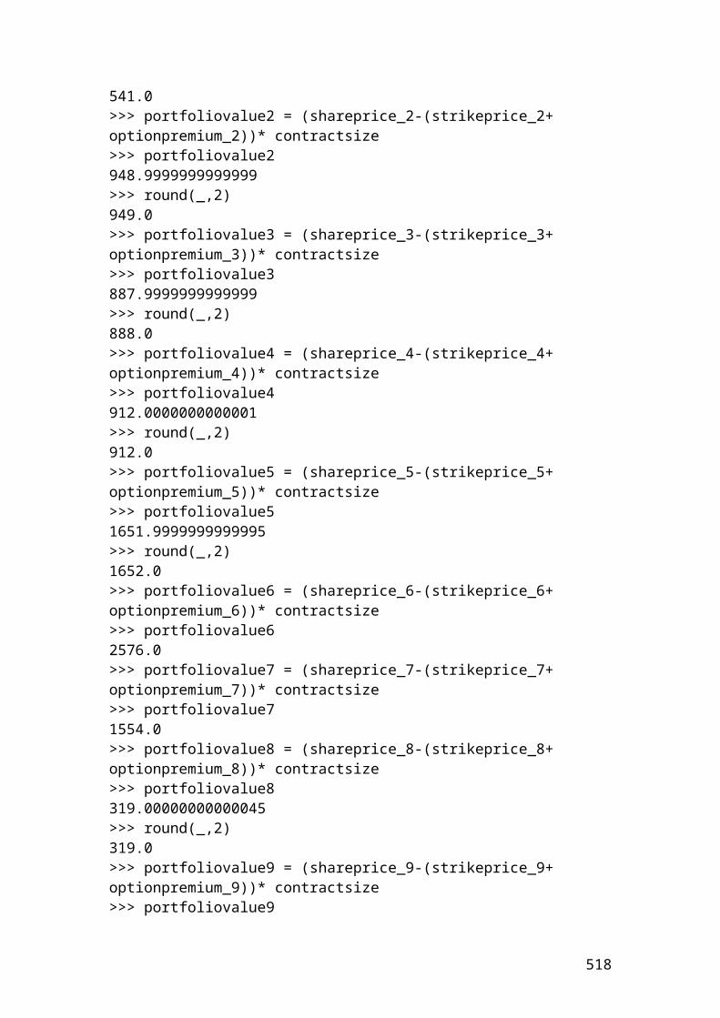
Ctoday = 5.9128 / 1.05 = 5.63 DKK (to 2 d.p.).Application of one – period binomial method in R. The figures are expressed in DKK.

> share_price <- 50> exercise_price <- 50> upmove <- 1.20> downmove <- 0.833> risk_free_rate <- 0.05> # Insert the mathematical formulas of risk probability of up and down move.> riskprobofupmove <- (1+risk_free_rate-downmove) / (upmove - downmove)> riskprobofupmove[1] 0.5912806539509539> round(riskprobofupmove,digits=2)[1] 0.59> riskprobofdownmove <- 1 - riskprobofupmove> riskprobofdownmove[1] 0.40871934604904614> round(riskprobofdownmove,digits=2)[1] 0.41> # The payoffs are determined by the following equations.> shareprice1 <- share_price * upmove> shareprice1[1] 60.0> calloptionprice1 <- shareprice1 - exercise_price> calloptionprice1[1] 10.0> shareprice2 <- share_price *downmove> shareprice2[1] 41.65> calloptionprice2 <- shareprice2 - exercise_price> calloptionprice2[1] -8.350000000000001> calloptionprice2 =0> calloptionprice2[1] 0> #The expected value of the call option at t=1 is as follows:> expectedcalloption <- (calloptionprice1* riskprobofupmove) + (calloptionprice2 * riskprobofdownmove)> expectedcalloption[1] 5.912806539509539> round(expectedcalloption,digits=2)[1] 5.91># The value of the call option discounted at 5% risk - free rate is as follows:> valueofcalldiscounted <- expectedcalloption / 1.05> valueofcalldiscounted[1] 5.631244323342418> round(valueofcalldiscounted, digits= 2)[1] 5.63

518

Two – period binomial method

This method is based on the one – period binomial method, but it is extended to include a second period, t = 2. Thus, we have three periods. t = 0, t =1 and t =2. We use the same example of the previous section but extended to an additional period.

A share is traded in the Danish stock exchange at 50 DKK. First of all, we would like to calculate the possible price changes based on probabilities. The risk - free rate is 5% and the value of the call option has an exercise price of 50 DKK. It is required to calculate the expected value of the option. In addition, it is required to calculate the value of the option today discounted at the given risk-free rate.

We assume two scenarios. The first one is that the share will increase by 20% or by a factor of 1 + 0.20 = 1.20. The second one is that the share will decrease by 0.833. The number 0.833 is calculated as 1 / 1.20 = 0.833.

The mathematical formulas are as follows:

Down move = D = 1 / up move.

59128.0367.0217.0

0.833-1.200.833- 0.051

move. up theis U move.down theis D

rate. free-risk theis rf :

D-U

D-rf1 movement upan ofy probabilit neutral -risk

U

Where

U

0.40872 0.59128 - 1 movement down a ofy probabilit neutral - riskD

Thus, the payoff or the two-period binomial tree for share prices for the two possible scenarios will be as follows:

t = 0 t = 1 t =2 50*(1.20)2=72 DKKProbability Up = 0.59 S1 = 50 x 1.20 = 60 DKK S2 50*1.20*0.833 =49.98 50 DKK Probability Down =0.41 S1 = 50 x 0.833 = 41.65 DKK S2

50 * (0.833)2 = 34.69

The value of the call options for the period t =2 for both ups and downs are as follows:

519

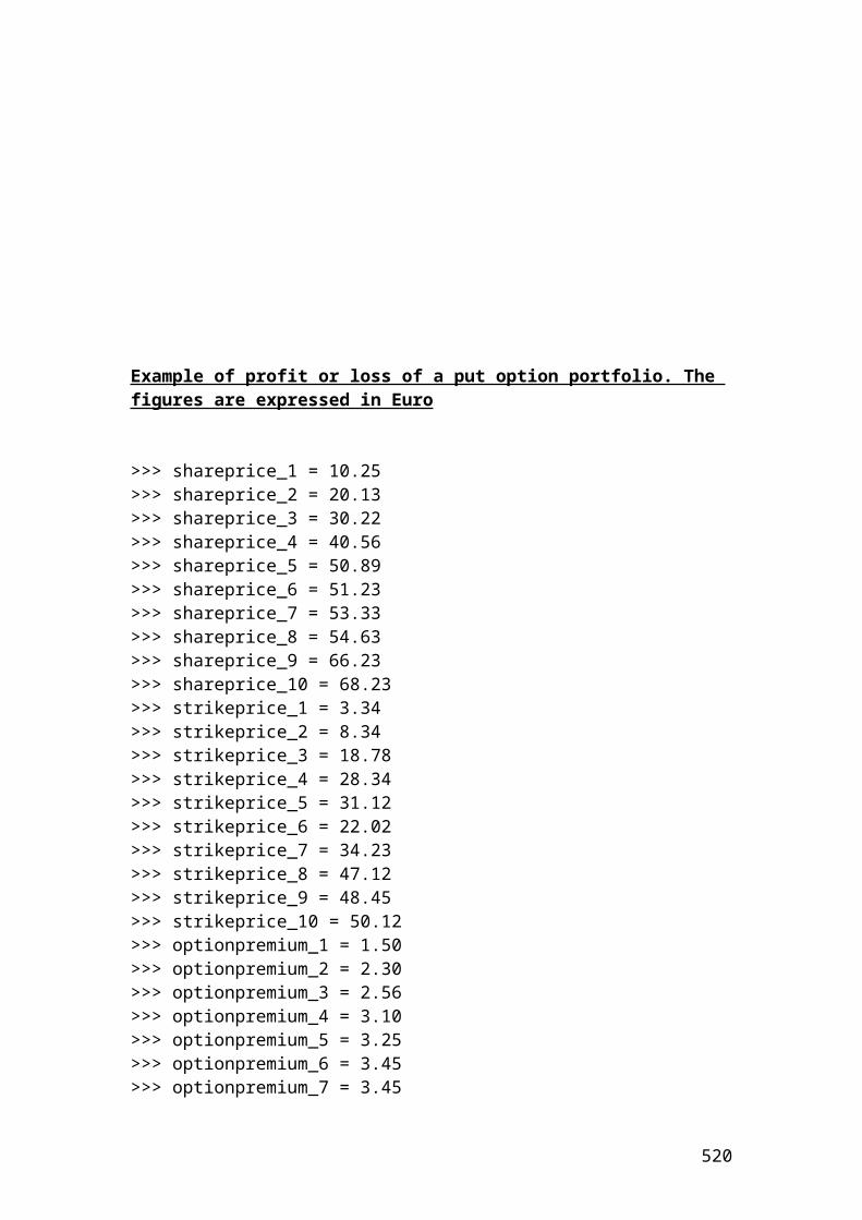
Upside movementC1 = 72 – 50 = 22C2 = 49.98 – 50 = -0.02 =0 Negative values mean that the option does not worth.

Downside movementC1 = 49.98 -50 = -0.02 =0C2 = 34.69 -50 = -15.31 =0

The expected value of the call options for both movements for period t =1 are calculated based on the following equations:

Upside movement

DKK 12.3887

05.1008.13

05.1)040872.0(2259128.0

rf 1down xC PrC x upy Probabilit 21

up

up

Call

xxobabilityCall

Downside movement

005.1

0) 40872.0(0 59128.0rf 1

Cdown x PrC x up Pr 21

xxobabilityobabilityCalldown

The value of the call option today discounted is calculated based on the following formula:

3.d.p.) (to 976.605.1

32519.7

05.10 12.3887 x 59128.0

1Calldown x PrCall x up Pr downup

today

today

Call

rfobabilityobability

Call

The final format of the two-period binomial tree for call options is as follows:

t = 0 t = 1 t = 2

22.00 DKK 12.3887DKK 06.976 DKK 0 0

520

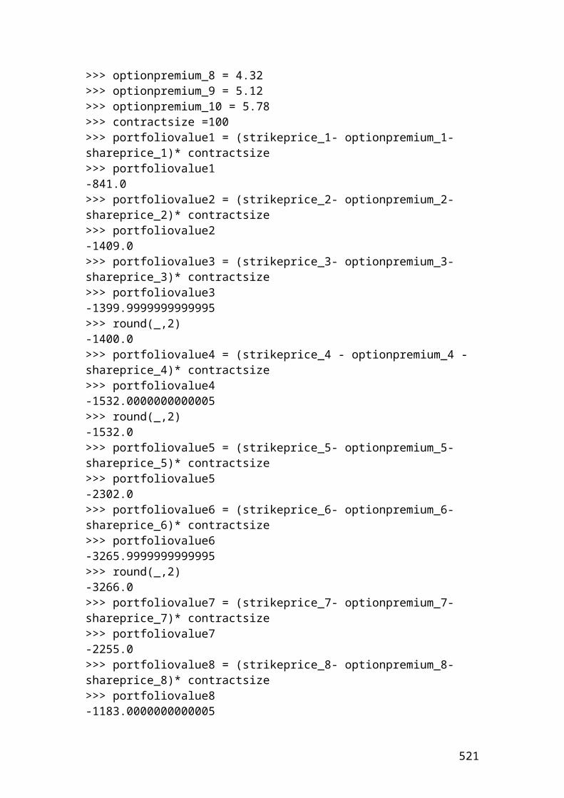
Application of two – period binomial method in R. The figures are expressed in DKK.

> share_price <- 50> exercise_price <- 50> upmove <- 1.20> downmove <- 0.833> risk_free_rate <- 0.05> # Insert the mathematical formulas of risk probability of up and down move.> riskprobofupmove <- (1+risk_free_rate-downmove) / (upmove - downmove)> riskprobofupmove[1] 0.5912806539509539> round(riskprobofupmove,digits=2)[1] 0.59> riskprobofdownmove <- 1 - riskprobofupmove> riskprobofdownmove[1] 0.40871934604904614> # The payoffs are determined by the following equations.> shareprice1 <- share_price * upmove> shareprice1[1] 60.0> shareprice2 <- share_price *downmove> shareprice2[1] 41.65> shareprice3 <-share_price * upmove**2> shareprice3[1] 72.0> calloptionprice3 <- shareprice3 - exercise_price> calloptionprice3[1] 22.0> shareprice4 <- share_price * downmove**2> shareprice4[1] 34.694449999999996> calloptionprice4 <- shareprice4 - exercise_price> calloptionprice4[1] -15.305550000000004> calloptionprice4 <-0> calloptionprice4[1] 0> shareprice5 <- share_price * upmove * downmove> shareprice5[1] 49.98> calloptionprice5 <- shareprice5 - exercise_price> calloptionprice5[1] -0.020000000000003126> calloptionprice5 <-0> calloptionprice5[1] 0

521

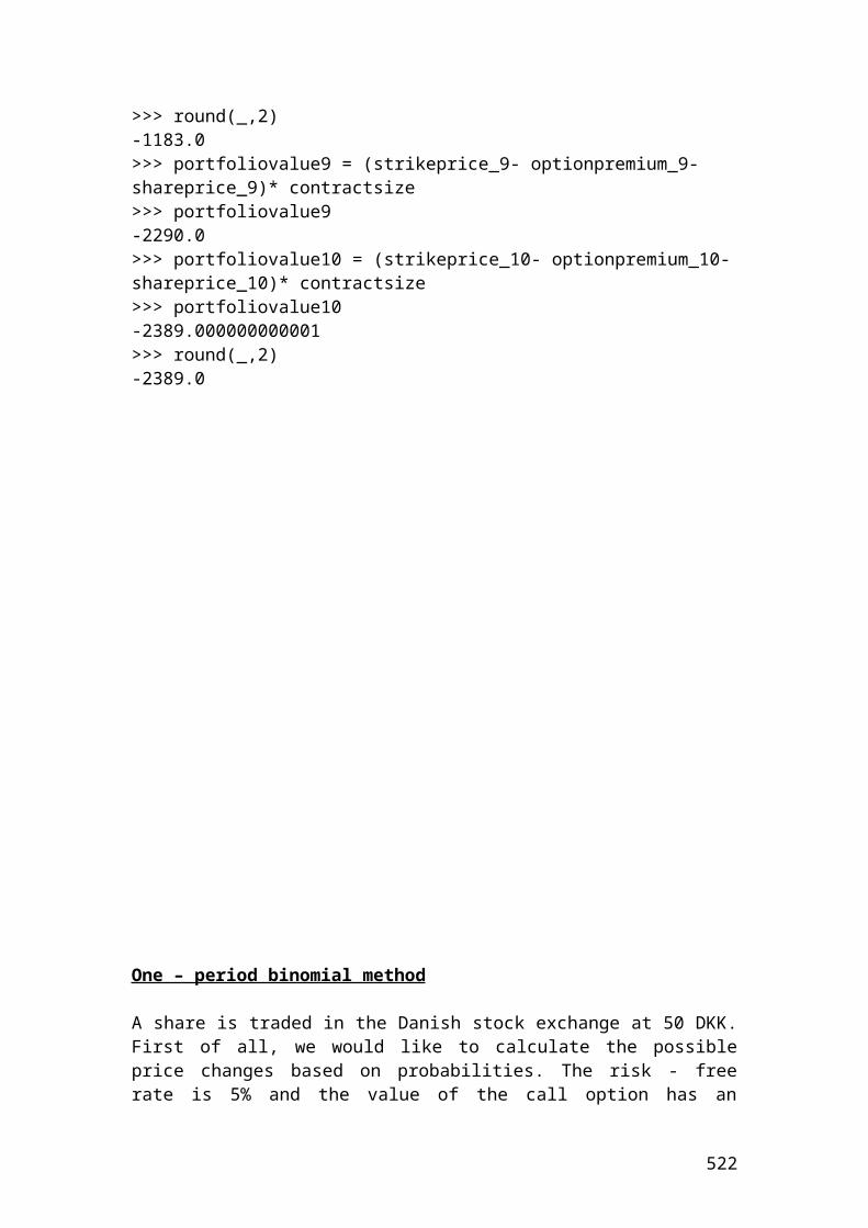
> #The expected value of the call option at t=2 is as follows:> expectedcalloptionupside <- (riskprobofupmove * calloptionprice3+ riskprobofdownmove* calloptionprice5) / 1.05> expectedcalloptionupside[1] 12.388737511353318> expectedcalloptiondownside <- (riskprobofupmove *calloptionprice4+ riskprobofdownmove * calloptionprice5) / 1.05> expectedcalloptiondownside[1] 0.0># The value of the call option discounted at 5% risk - free rate is as follows:> valueofcalldiscounted <- (riskprobofupmove * expectedcalloptionupside+riskprobofdownmove* expectedcalloptiondownside)/ 1.05> valueofcalldiscounted[1] 6.976400778418764> round(valueofcalldiscounted, digits=2)[1] 6.98

522

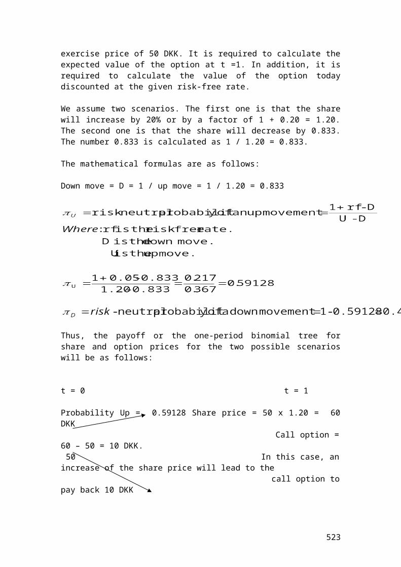
Stock index option

Let’s assume that a practitioner wants to buy a stock index call option that is related to the general movement of the S&P 500 index. The dollar multiplier for S&P 500 option contract is 250 dollars. The strike price of the index is 1240. The August premium is 20 index points.

Question

Calculate the cost of the August call and the net profit involved if the S&P 500 index reaches the price of 1540.

Solution

Cost of the August call = premium expressed in index points x dollar multiplier Cost of the August call = 20 x 250 = 5000 USD

The net profit incurred is calculated as follows:

(Ending index value – beginning index value x dollar multiplier ) – cost of the August call.

(1540 – 1240) x 250 – 5000 = 70,000 USD.

Application of stock index option in R

> beginning_index_value <- 1240> ending_index_value <- 1540> multiplier <- 250> premium <- 20> costofcall <- premium * multiplier> costofcall[1] 5000 # USD> netprofit <- (ending_index_value - beginning_index_value) * multiplier - costofcall> netprofit[1] 70000 # USD

523

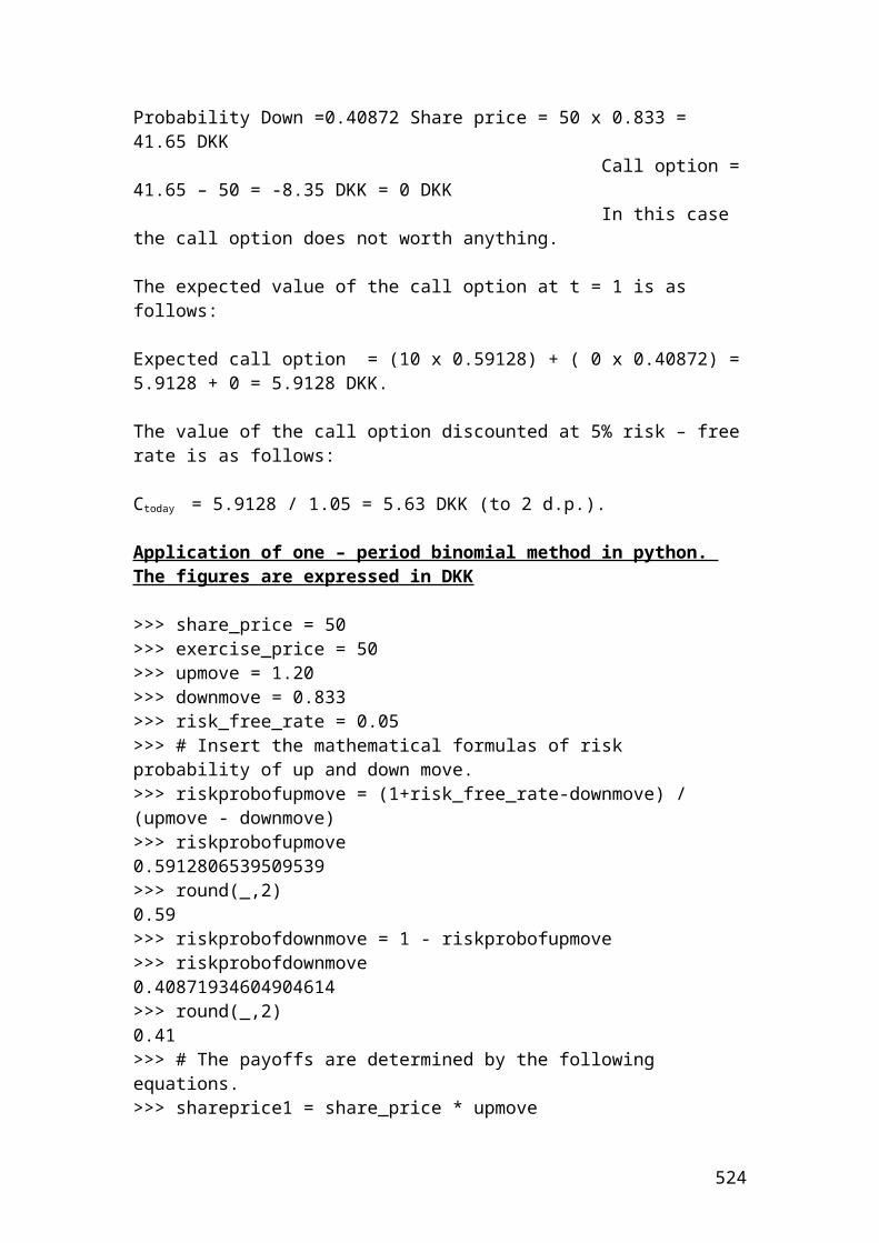
Exercise of an European interest rate option

Calculate the profit or loss of the interest rate difference between the actual and the strike rate of a call option. Let’s assume that an interest call option on a 6 –month Eurodollar has a strike rate of 4%. At expiration, the 6-month Eurodollar rate is 5%. The invested principal is 50,000,000 Euros. The duration of the contract is expressed in days divided by 360 days. Thus, 6 –months equal 180 days.

The mathematical formula for profit or loss is as follows:

Application of an European interest rate option in R

> principal <- 50000000> actual_rate <- 0.05> strike_rate <- 0.04> duration <- 180> days <- 360> # Insert the mathematical formula.> profitorloss <-principal*(actual_rate - strike_rate)*duration/days> profitorloss[1] 250000.0 # Euros

524

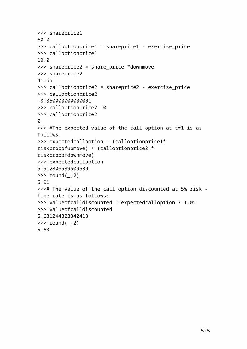
Currency option

Let’s assume that a wealthy investor buys a call currency option because it expects a rise in the exchange rate parity of the EURO against the USD, EURO/USD. The spot exchange rate is 1/1.3568. The strike price is 1.3568. The premium expressed as cents per Euro is 1.56. The initial principal is 100,000 USD.

Question

Calculate the net profit involved if the strike price increases to 1.3987.

Solution

The wealthy investor to record a profit, he or she should add to the strike price 1.3568 the premium expressed as cents per Euro. In our case, the breakeven point is1.3568 + 0.0156 = 1.3724. Above the price of 1.3724, he or she starts to record a profit. If the strike price reaches 1.3987, then the profit will be as follows:

Initial principal x (Ending strike price – beginning strike price – premium paid) =100,000 x (1.3987 – 1.3568 – 0.0156) = 2630 USD net profit

Application of currency option in R

> principal <- 100000> ending_strike_price <- 1.3987> beginning_strike_price <- 1.3568> premiumpaid <- 0.0156> netprofit <- principal *(ending_strike_price-beginning_strike_price-premiumpaid)> netprofit[1] 2630 # USD

525

Example of calculating the payments of an interest rate cap based on different LIBOR rates

Interest rate cap is an agreement between two parties where one party pay the other at a specified period of time in which the interest rate or London interbank offered rate ,LIBOR, exceeds the strike price. It is used this contract to hedge against interest rate fluctuations. Let’s assume that an interest cap has a value of 5.5% and the LIBOR prices for the next three years are 7.5%, 8.3% and 4.65%. The principal is $50,000,000 and the payments take place semiannually.

The mathematical formula that is used to calculate the payments of each year is as follows:

Interest rate payment =[ principal x (LIBOR rate – cap rate)/0.5]

Therefore, the first year interest rate payment is as follows:

Year 1

Interest rate payment = [50,000,000 x (0.075 – 0.055)/2] = $ ………

Application of payments of an interest rate cap based on different LIBOR rates in R

> principal <- 50000000> liborrate_1 <- 0.075> liborrate_2 <- 0.083> caprate <- 0.055> duration <- 2> interestpay1 <- principal *(liborrate_1 - caprate) /duration> interestpay1[1] 5e+05 or 500000 # USD> interestpay2 <- principal *(liborrate_2 - caprate) / duration> interestpay2[1] 7e+05 or 700000 # USD

526

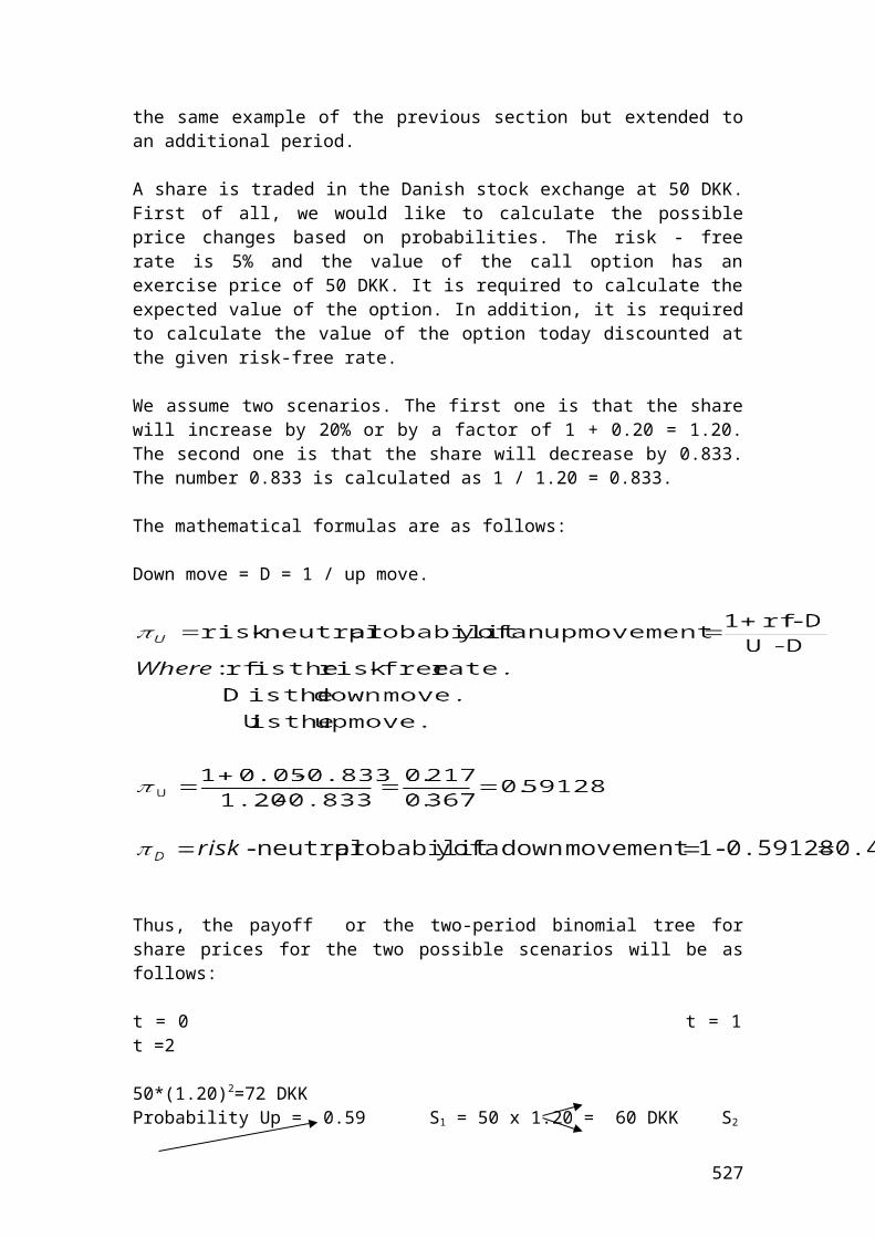
A six month interest rate cap has a rate of 0.08 and the principal is 20,000,000 USD. The settlements is done quarterly. The first quarter the 3 –month libor rate is 0.096 and the second quarter the rate is 0.087. Calculate the payoff for the cap the first and the second quarter?

Solution

Payoff the first quarter = 20,000,000 * = 80000 USD

Payoff the second quarter = 20,000,000 * 35000 USD

Application of payoff of interest rate cap in python

> principal <- 20000000> caprate <- 0.08> liborrate_1 <- 0.096> liborrate_2 <- 0.087> period <- 4> # Insert the mathematical formulas.> payoff1 <- (principal*(liborrate_1-caprate)/period)> payoff1[1] 80000 # USD> payoff2 <- (principal*(liborrate_2-caprate)/period)> payoff2[1] 35000 # USD

527

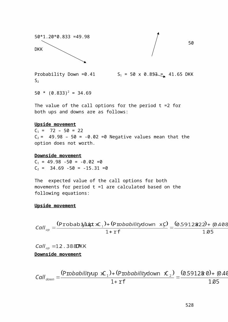
Swaption

An investor purchased a 1 year European swaption with exercise price 7.50%. The principal is 30,000,000USD. The floating rate payments are based on LIBOR. The 90, 180, 270, and 360 day annualized LIBOR rates and present value factors are as follows:

LIBOR Rate Present value factors90 day LIBOR 4% 0.990099180 day LIBOR 5.5% 0.973236270 day LIBOR 6% 0.956938360 day LIBOR 7% 0.934579

Calculate the semi-annual and annualized swap rate?Calculate the net cash flow at each payment and the value of swaption at maturity.

Solution

The present value factors are calculated as follows:

PV 90 days =

36090*04.01

10.990099

PV 180 days =

360180*055.01

10.973236

PV 270 days =

360270*06.01

1

0.956938

PV 360 days =

360360*07.01

10.934579

Semi - annual swap rate =

01697.0854852.3065421.0

934579.0956938.0973236.0990099.0934579.01

Annulaized swap rate = 6.788%or 06788.090/360*01697.0

528

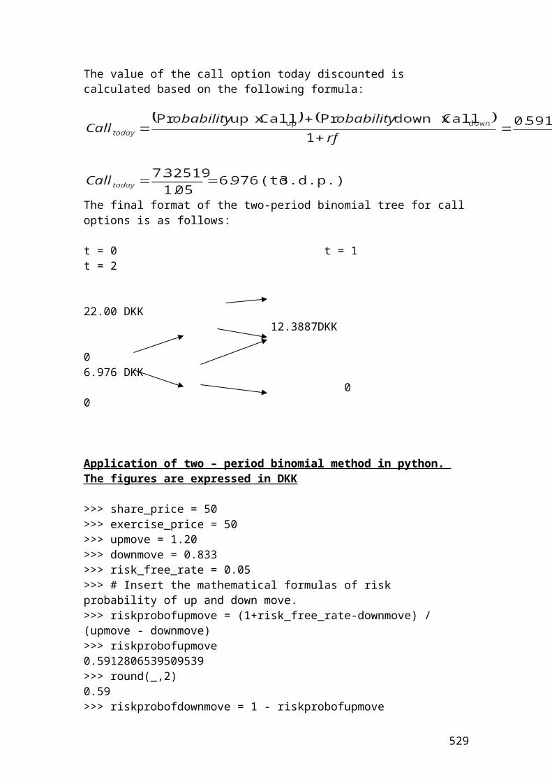
The swaption is in the money because the exercise price 7.50% is greater than the market annualized swap rate 6.788%.

The net cash flow is as follows:

netCashFlow = (0.075 – 0.06788)*90/360 * 30000000 = 53400 USD

The value of swaption at maturity is as follows:

valueSwaption = 53400 *( 934579.0956938.0973236.0990099.0 ) = 205,849.1 USD

Application of swaption in R

> principal = 30000000> exercise_rate = 0.075> rate90 = 0.04> rate180 = 0.055> rate270 = 0.06> rate360 = 0.07> # Insert the mathematical formulas.> PV90 = 1 /(1+(rate90 * 90/360))> PV90[1] 0.9900990099009901> PV180 = 1/(1+(rate180 * 180/360))> PV180[1] 0.97323600973236> PV270 = 1/(1+(rate270 * 270/360))> PV270[1] 0.9569377990430623> PV360 = 1/(1+(rate360* 360/360))> PV360[1] 0.9345794392523364> semiAnnualRate = (1-PV360)/(PV90 +PV180 +PV270 +PV360)> semiAnnualRate[1] 0.01697096448070222> round(semiAnnualRate ,digits=5)0.01697> annualizedSwapRate = semiAnnualRate * (360/90)> annualizedSwapRate[1] 0.06788385792280888> round(annualizedSwapRate, digits=5)0.06788

Please repeat the above swaption problem in python and calculate the net cash flow and the value of swaption at maturity.

529

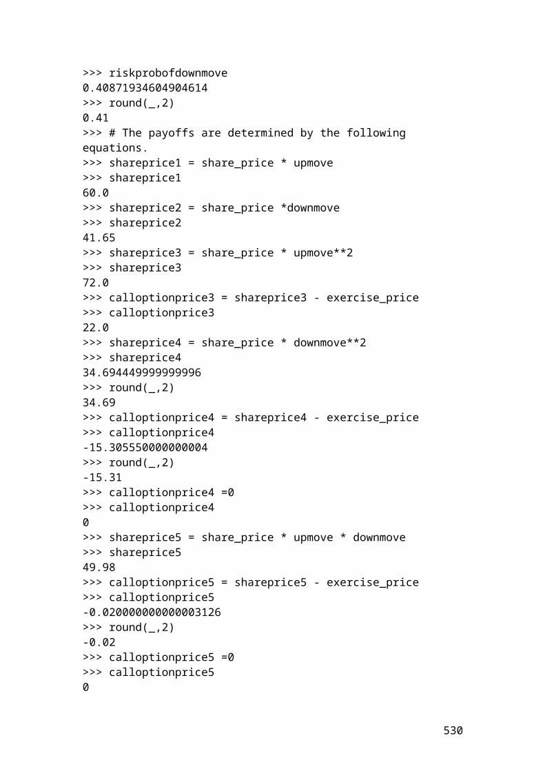
Put –call parity

The put – call parity shows the relationship between a call and a put option with the same expiration, strike and share prices. The mathematical formula is as follows:

option.put theand call both thefor price share theis S .expirationor maturity to time theis T

rate. free-rsik theis r call. theandput both the of price strike theis X

put. theof price theis P call. theof price theis C :

)1(

f

Where

SPrfXC T

Example

Calculate the price of a call if the price of a put is 5.34 Pounds, the share price is 94, the strike price is 97, the risk-free rate is 4% and the time to maturity, T=0.5. By rearranging formula (20) and solving for the price of a call, we have the following results:

Application of put - call parity in R

> put <- 5.34> share_price <- 94> strike_price <- 97> dis_risk_free_rate <-1.04> maturity <- 0.5> # Insert the mathematical formula.> call <- put + share_price - strike_price /(dis_risk_free_rate**maturity)> call4.223674457980749> round(call,digits=2)[1] 4.22 # Pounds

530

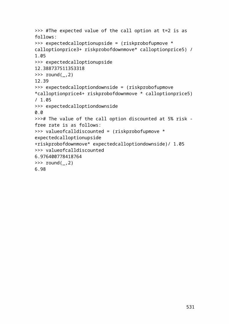
Example of margin payments in the clearinghouse

An investor open a margin account with a minimum initial margin of 5,200 dollars per contract. The maintenance margin is 1,500 dollars per contract. He/she buys 7 July wheat futures contracts with a standard contract size of 200 bushels priced at 230 dollars per bushel. The July contract size in the next 2 days recorded the prices of 220 and 210 dollars per bushel. Show the cash flows, gains and losses for the buyer and the seller?

Solution

Initial margin = 7 x 5,200 = 36,400 dollars

Maintenance margin = 7 x 1,500 = 10,500 dollars

The cash flows, gains and losses for the next two days will be as follows:

Day 1

Cash flows for the buyer’s: 36,400 + 14,000 = 50,400 dollars. The investor’s recorded a gain.

Cash flows for the seller’s: 36,400 – 14,000 = 22,400 dollars. The investor’s recorded a loss.

Helpful hint: the amount of 14,000 is calculated from the difference of the bushel prices, (fT-f0) x number of contracts x standard contract size. Thus, we have: (220-230) x 7 x 200 = (14,000 dollars). The same principle applies for the second day but with different bushel prices. Thus, we have: (210 – 230) x 7 x 200 = (28000 dollars). Gains or losses depends if you are the buyer or seller.

Day 2

Please do the calculations for the second day.

This is why I am stressing the importance that the investors should buy or sell ONLY when the market is aggressively increasing or falling. If he/she gets trapped in a market that is not strong bull or bear, then, he/she will have to compensate regularly for the losses or he/she will experience a very small profit. If the amounts as the days passes is below the maintenance margin, then, the investor’s will receive a margin call and he/she should add the capital required to proceed with the contract. If the investor’s is short of money, then, the position is closed with the incurred losses.

531

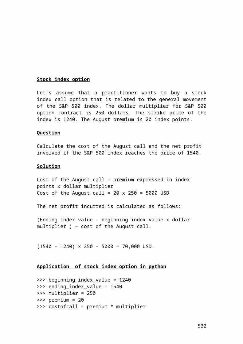
Application of margin payments in the clearinghouse in R

> initial_margin <- 5200> maintenance_margin <- 1500> contract_number <- 7> bushel_contract_size <- 200> bushel_price_1 <- 230> bushel_price_2 <- 220> # Insert the mathematical formulas.> initial_margin_with_contract <- initial_margin * contract_number> initial_margin_with_contract[1] 36400 # USD> maintenance_margin_with_contract <- maintenance_margin * contract_number> maintenance_margin_with_contract[1] 10500 # USD> bushel_contract <- (bushel_price_1-bushel_price_2) * bushel_contract_size * contract_number> bushel_contract[1] 14000 # USD> cash_flow_buyer <- initial_margin_with_contract + bushel_contract> cash_flow_buyer[1] 50400 # USD> cash_flow_seller <- initial_margin_with_contract – bushel_contract> cash_flow_seller[1] 22400 # USD

Please continue the calculations for the second day….

532

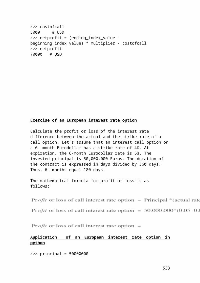
Example of calculating a margin call due to changes of price futures

An investor has opened a short position of 20 Soybean futures contract. The initial margin was 500 Pounds and the maintenance margin was 430 Pounds per contract. The price change that will create a margin call is as follows:

Solution

20

430- 500 sizecontract

margin emaintenanc -margin initial price aat created callMargin 3.5

Pounds

Application of margin call in R

> initial_margin <- 500> maintenance_margin <- 430> futures_contract <- 20> # Insert the mathematical formula.> margin_call <-(initial_margin-maintenance_margin) / futures_contract> margin_call[1] 3.5 # Pounds

533

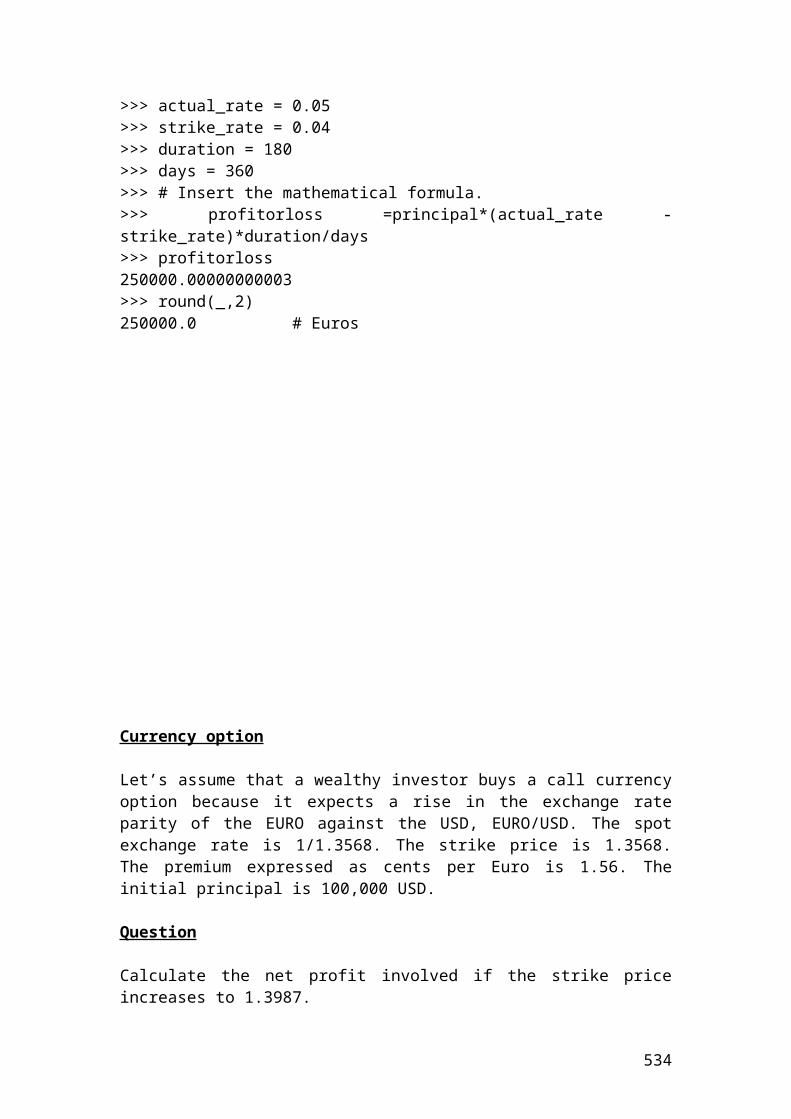
Solution of the above examples

Active return, active risk and information ratio

Active return is the difference in returns between a portfolio and the index or benchmark that is measured.

Active return = rp - rb

Where: rp is the portfolio return. rb is the benchmark or index return.

If the portfolio return is 0.80 and the benchmark return of the index is 0.70 then, the active return is………

Please complete the calculation.

Application of active return in R

> portfolio_return <- 0.8> benchmark_return <- 0.7> active_return <- portfolio_return - benchmark_return> active_return[1] 0.10000000000000009> round(active_return,digits=2)[1] 0.1

534

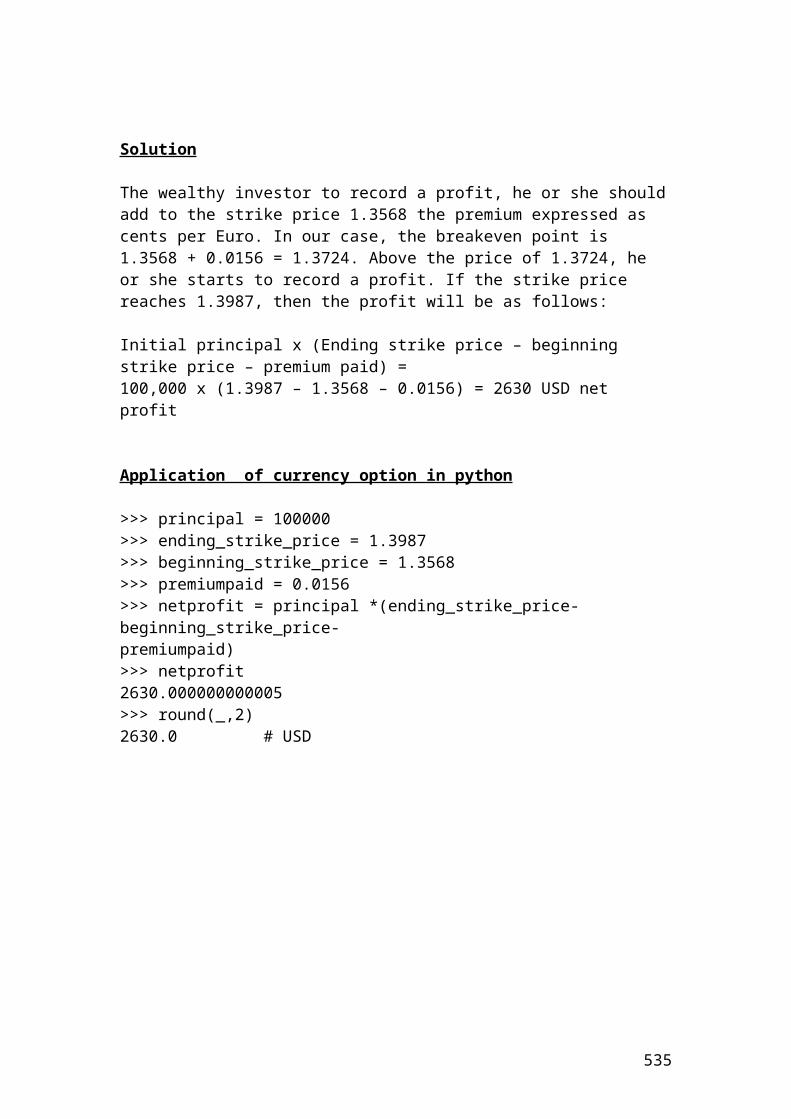
Active risk or tracking error is the standard deviation of the difference of returns between a portfolio and the benchmark or index.

ns.observatioor assets ofnumber theisn index.an examplefor be couldIt return.benchmark portfolio is r

return. portfolio is r :

1

)(r risk

b

p

2p

Wheren

rActive b

If the portfolio return is 0.80, the number of observations is 10 and the benchmark return of the index is 0.40 then, the active risk is………

Please complete the calculation.

Application of active risk in R

> portfolio_return <- 0.80> benchmark_return <- 0.40> n <-10> # Insert the mathematical formula.> active_risk <- sqrt((portfolio_return - benchmark_return)**2/9)> active_risk[1] 0.13333333333333336> round(active_risk,digits=2)[1] 0.13

535

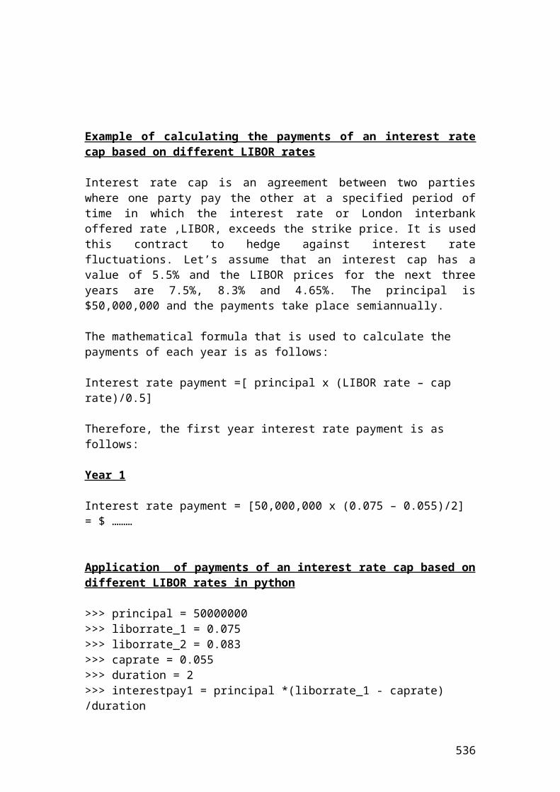
Information ratio shows the consistency of the fund manager towards the active return. The mathematical formula is as follows:

risk active theis

1

return.index or benchmark average theis r

return. portfolio of average theis :

1)(r

2

b

2p

nrr

rWhere

nr

rrIR

bp

p

b

bp

It could be calculated very easily in Excel software. I will illustrate a simple table with the relevant calculations.

Day rp rb rp - rb

1 0.03 0.02 0.012 0.02 0.014 0.0063 -0.04 0.034 -0.0744 0.05 0.067 -0.0175 0.08 0.012 0.0686 -0.01 -0.056 0.0467 0.07 0.031 0.0398 0.034 0.023 0.0119 -0.021 0.015 -0.03610 0.045 0.001 0.044

Average 0.0258 0.0161Standard deviation

0.043

Source: author’s calculation

By substituting the values that we have found in terms of rp =0.0258, rb = 0.0161 and standard deviation = 0.043 in the following equation we have:

1)(r 2

p

n

r

rrR

b

bp

2d.p.) (to 23.0043.0

0097.0043.0

0161.00258.0

R

But what is the interpretation of the information ratio of 0.23. It means that the fund manager gained around 23 basis points of active return per unit of active risk. The higher is this number, the better the manager is performing in relation to active risk.

536

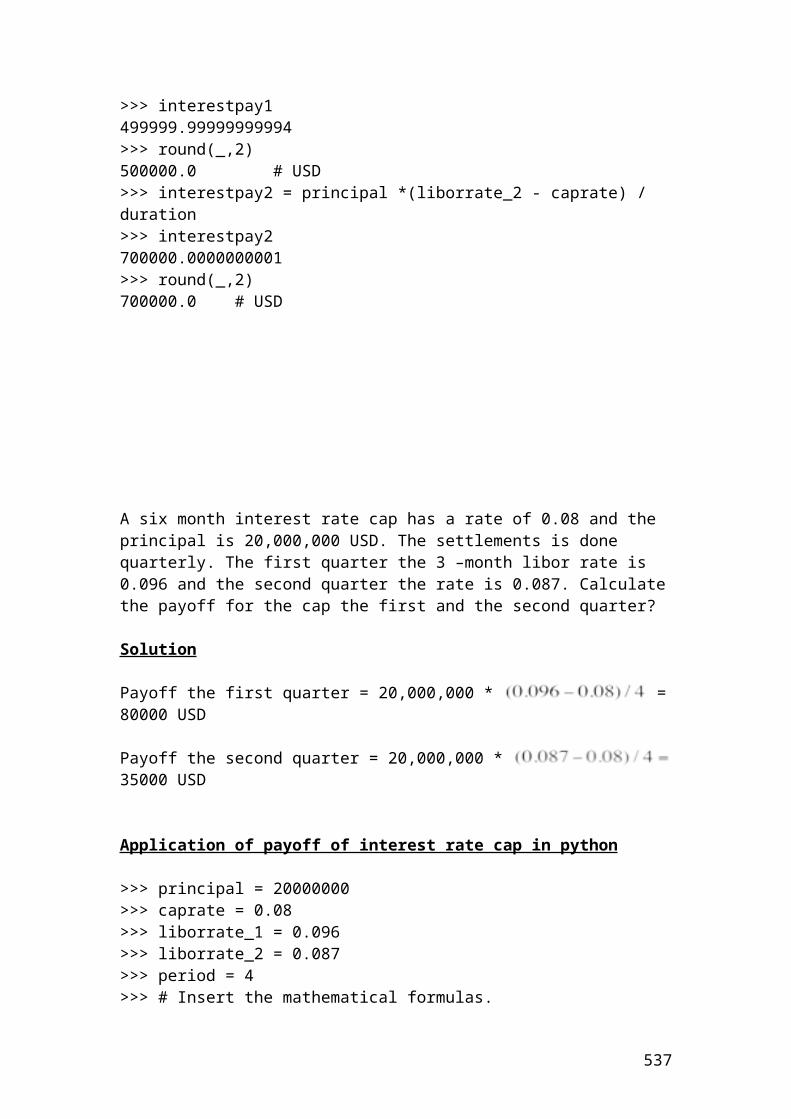
Application of information ratio in R

> portfolio_return1 = 0.03> portfolio_return2 = 0.02> portfolio_return3 = -0.04> portfolio_return4 = 0.05> portfolio_return5 = 0.08> portfolio_return6 = -0.01> portfolio_return7 = 0.07> portfolio_return8 = 0.034> portfolio_return9 = -0.021> portfolio_return10 = 0.045> # Insert the mathematical formula.> average_1 = (portfolio_return1 + portfolio_return2 + portfolio_return3 + portfolio_return4 + portfolio_return5 + portfolio_return6+ portfolio_return7 + portfolio_return8 + portfolio_return9+ portfolio_return10)/10> average_1[1] 0.0258> benchmark_return1 = 0.02> benchmark_return2 = 0.014> benchmark_return3 = 0.034> benchmark_return4 = 0.067> benchmark_return5 = 0.012> benchmark_return6 = -0.056> benchmark_return7 = 0.031> benchmark_return8 = 0.023> benchmark_return9 = 0.015> benchmark_return10 = 0.001> average_2 = (benchmark_return1 + benchmark_return2 + benchmark_return3 + benchmark_return4 + benchmark_return5 + benchmark_return6 + benchmark_return7 + benchmark_return8 + benchmark_return9+ benchmark_return10)/10> average_2[1] 0.016100000000000003># Insert the mathematical formulas to calculate the differences between the portfolioand benchmark return and then square it.> diff1 = portfolio_return1 - benchmark_return1> diff1[1] 0.009999999999999998> diff2 = portfolio_return2 - benchmark_return2> diff2[1] 0.006> diff3 = portfolio_return3 - benchmark_return3> diff3[1] -0.07400000000000001> diff4 = portfolio_return4 - benchmark_return4> diff4[1] -0.017> diff5 = portfolio_return5 - benchmark_return5> diff5[1] 0.068

537

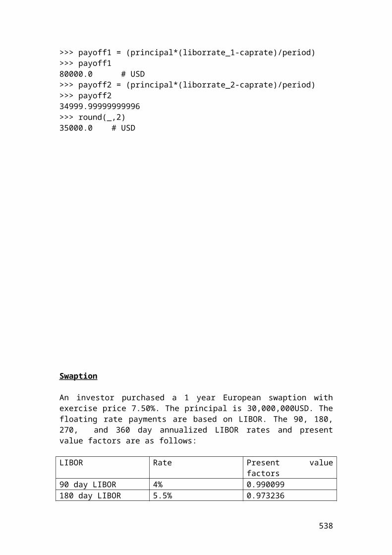
> diff6 = portfolio_return6 - benchmark_return6> diff6[1] 0.046> diff7 = portfolio_return7 - benchmark_return7> diff7[1] 0.03900000000000001> diff8 = portfolio_return8 - benchmark_return8> diff8[1] 0.011000000000000003> diff9 = portfolio_return9 - benchmark_return9> diff9[1] -0.036000000000000004> diff10 = portfolio_return10 - benchmark_return10> diff10[1] 0.044> #Find the sum from the differences.> sumDiff = diff1 + diff2 + diff3 + diff4 + diff5 + diff6 + diff7 + diff8 +diff9 +diff10> sumDiff[1] 0.09699999999999999># Find the average from the differences.> average3 = sumDiff /10> average3[1] 0.009699999999999999

Please complete the exercise……. If you have questions, then, please let me know.

538

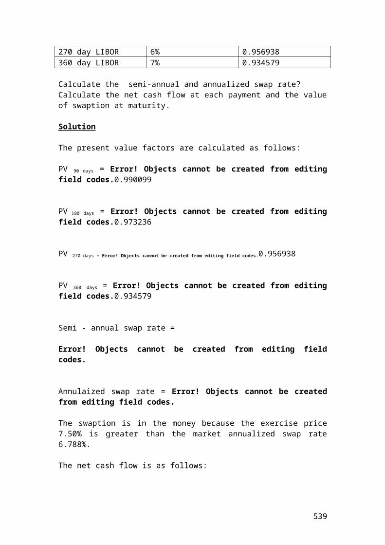
Please convert the following exercise in R language programming

Calculate the balance at the end of the 5th day from changes in the futures prices from 90 to 89, 91, 95, 97, 99. The trader has bought 50 futures contract for settlement in May. The initial margin is $8.

Day Beginning balance

Futures price Gain or loss Ending balance

0 400 90 0 4001 400 89 (50)2 350 91 1003 450 95 2004 650 97 1005 750 99 100

Source: author’s illustration.

Beginning balance = initial margin x number of contracts.Beginning balance = 8 x 50 = $400

Please complete the values of the column ending balance.

Solution

Day Beginning balance

Futures price Gain or loss Ending balance

0 400 90 0 4001 400 89 (50) 3502 350 91 100 4503 450 95 200 6504 650 97 100 7505 750 99 100 850

The ending balance at the 5th day in the margin account will be 850 USD.

539

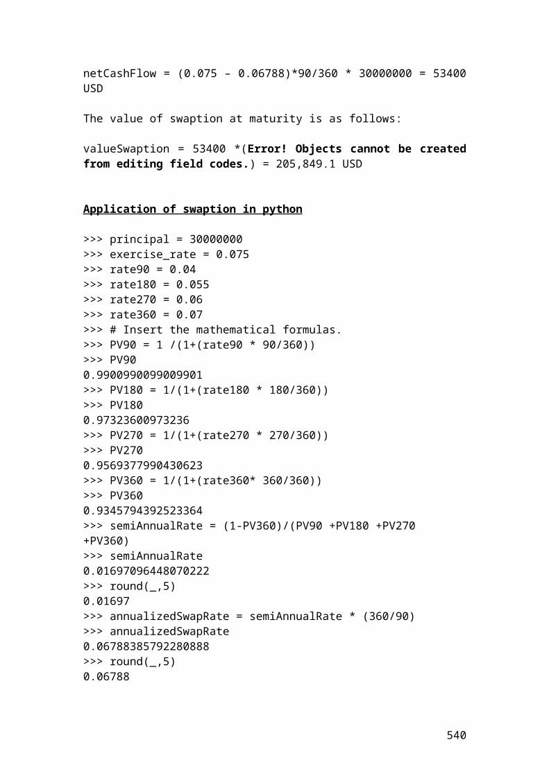
Calculate the caplet option payments based on different interest rates using a binomial 2 steps tree. The figures are expressed in pounds

> # Calculate the caplet values based on an interest rate cap using a binomial 2 steps tree. It is a similar example of a call option on interest rates. The payment is based on the difference between the current interest rate and the cap rate multiplied by the principal and divided by the discounted current interest rate. The buyer receives a payment when the current interest rate exceeds the cap strike price.

> strike <-0.02> principal <- 30000000> maturity <- 0.5> sigma <- 0.3> interest_rate <- 0.04> n <-2> p<-0.5> # Insert the mathematical formulas.> dt <- maturity/n # steps expressed in years.> dt[1] 0.25> u <- exp(sigma*sqrt(dt)) # multiplier of upmove.> u[1] 1.161834242728283> d <- 1/u # multiplier of downmove.> d[1] 0.8607079764250578># Identify the interest rates in each node.> interest_0 <- 0.04> interest_1i <- 0.0465> interest_1ii <- 0.0344> interest_2i <- 0.054> interest_2ii <- 0.04> interest_2iii <- 0.0296> #Identify the discounted interest rates.> disinterest_0 <- 1.04> disinterest_1i <- 1.0465> disinterest_1ii <- 1.0344> disinterest_2i <- 1.054> disinterest_2ii <- 1.04> disinterest_2iii <- 1.0296># Insert the mathematical formulas. It is a backward induction methodology.> capletPrice2i <- (principal*(interest_2i-strike)/disinterest_2i)> capletPrice2i[1] 967741.935483871> capletPrice2ii <- (principal*(interest_2ii-strike)/disinterest_2ii)> capletPrice2ii[1] 576923.0769230769> capletPrice2iii <- (principal*(interest_2iii-strike)/disinterest_2iii)> capletPrice2iii[1] 279720.2797202797

540

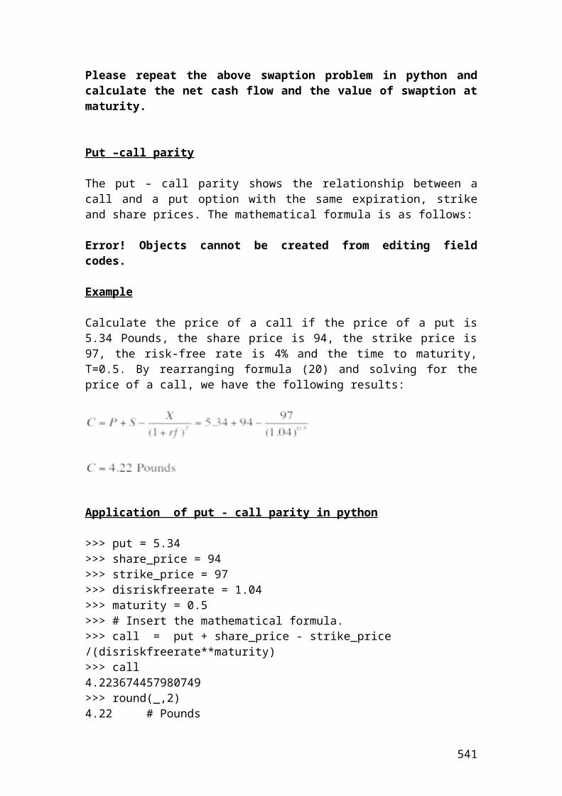
> capletPrice1i <- (((capletPrice2i*p)+(capletPrice2ii*p))/disinterest_1i)> capletPrice1i[1] 738014.8172035108> capletPrice1ii <- (((capletPrice2ii*p)+(capletPrice2iii*p))/disinterest_1ii)> capletPrice1ii[1] 414077.415237508> capletPrice0 <- (((capletPrice1i*p)+(capletPrice1ii*p))/disinterest_0)> capletPrice0[1] 553890.4963658744> round(capletPrice0,digits=1)[1] 553890.5

541

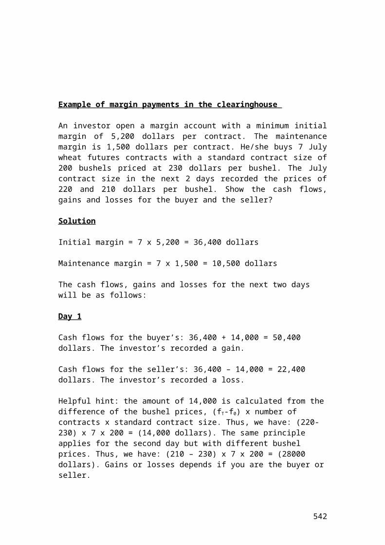
Calculate the floorlet option payments based on different interest rates using a binomial 2 steps tree. The figures are expressed in pounds

> # Calculate the floorlet values based on an interest rate floor using a binomial 2 steps tree. It is a similar example of a put option on interest rates. It protects the holder from declining interest rates. The payment is based on the difference between the floor rate and the current interest rate multiplied by the principal and divided by the discounted current interest rate.

> strike <- 0.02> principal <- 30000000> maturity <- 0.5> sigma <- 0.3> interest_rate <- 0.04> n <-2> p<-0.5> # Insert the mathematical formulas.> dt <- maturity/n # steps expressed in years.> dt[1] 0.25> from math import*> u <- exp(sigma*sqrt(dt)) # multiplier of upmove.> u[1] 1.161834242728283> d <-1/u # multiplier of downmove.> d[1] 0.8607079764250578># Identify the interest rates in each node.> interest_0 <- 0.04> interest_1i <- 0.0465> interest_1ii <- 0.0344> interest_2i <- 0.054> interest_2ii <- 0.04> interest_2iii <- 0.0296># Identify the discounted interest rates.> disinterest_0 <- 1.04> disinterest_1i <- 1.0465> disinterest_1ii <- 1.0344> disinterest_2i <- 1.054> disinterest_2ii <- 1.04> disinterest_2iii <- 1.0296># Insert the mathematical formulas. It is a backward induction methodology.> floorletPrice2i <- (principal*(strike - interest_2i)/disinterest_2i)> floorletPrice2i[1] 56925.99620493363> floorletPrice2ii <- (principal*(strike - interest_2ii)/disinterest_2ii)> floorletPrice2ii[1] 461538.4615384615> floorletPrice2iii <- (principal*(strike - interest_2iii)/disinterest_2iii)> floorletPrice2iii

542

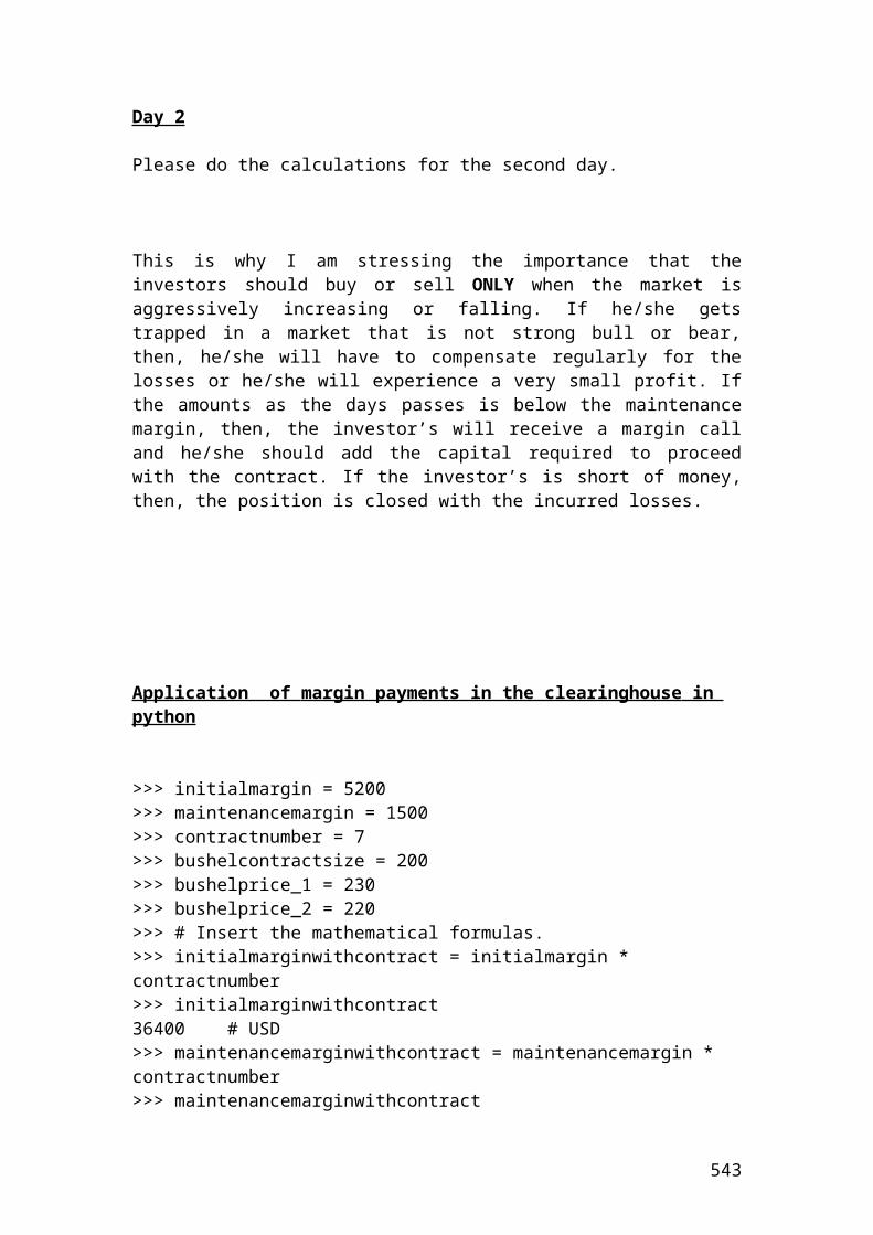
[1] 769230.7692307691> floorletPrice1i <- (((floorletPrice2i*p)+(floorletPrice2ii*p))/disinterest_1i)> floorletPrice1i[1] 247713.5488501649> floorletPrice1ii <- (((floorletPrice2ii*p)+(floorletPrice2iii*p))/disinterest_1ii)> floorletPrice1ii[1] 594919.3884228686> floorletPrice0 <- (((floorletPrice1i*p)+(floorletPrice1ii*p))/disinterest_0)> floorletPrice0[1] 405111.9890735737> round(floorletPrice0,digits=2)[1] 405111.99

543

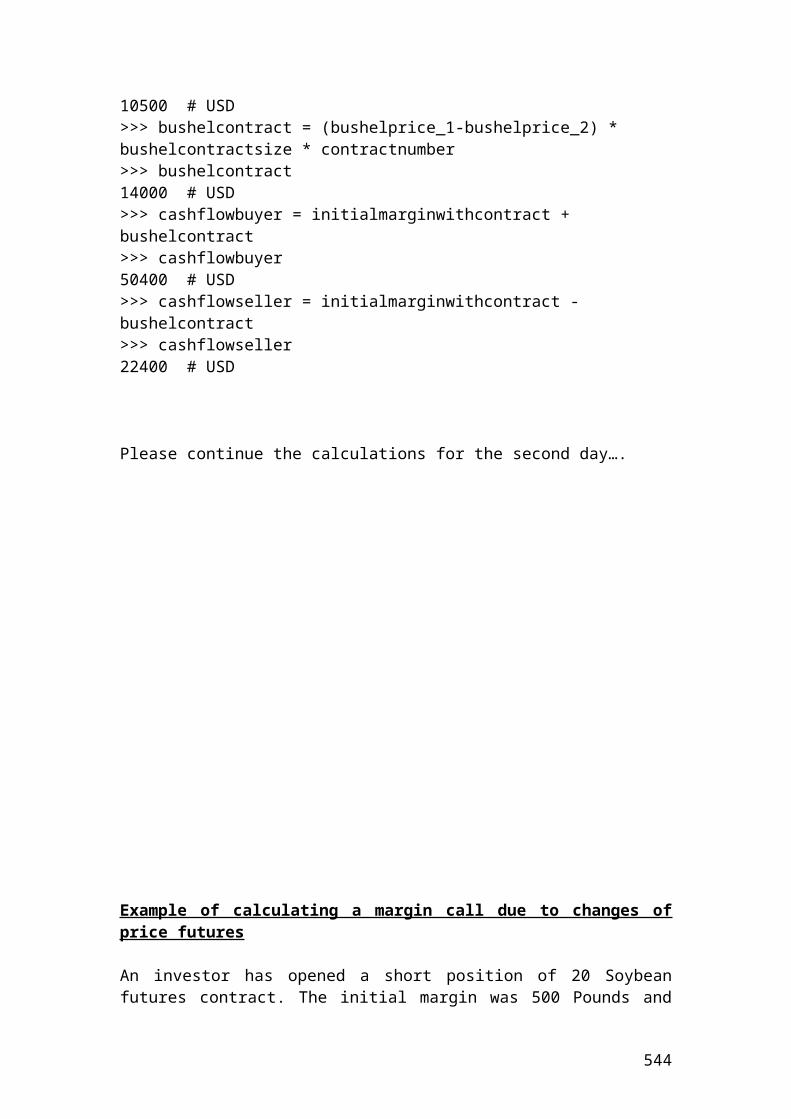
Calculate the bond put option prices based on different interest rates using a binomial 2 steps tree

> bond_price <- 100> strike <- 102> annual_coupon <- 7> maturity <- 0.5> sigma <- 0.3> interest_rate <- 4> n <-2> p <- 0.5> dt <- maturity/n # steps expressed in years.> dt[1] 0.25> u <- exp(sigma*sqrt(dt)) # multiplier of upmove.> u[1] 1.161834242728283> d <- 1/u # multiplier of downmove.> d[1] 0.8607079764250578># Insert the mathematical formulas. It is a backward induction methodology.> bondPrice2i <- (bond_price+annual_coupon)*(1/disinterest_2i)> bondPrice2i[1] 101.5180265654649> bondPrice2ii<-(bond_price+annual_coupon)*(1/disinterest_2ii)> bondPrice2ii[1] 102.88461538461537> bondPrice2iii <- (bond_price+annual_coupon)*(1/disinterest_2iii)> bondPrice2iii[1] 103.92385392385391> bondPrice1i <- ((((bondPrice2i+annual_coupon)*p)+(bondPrice2ii+annual_coupon)*p)/disinterest_1i)> bondPrice1i[1] 104.3490883660202> bondPrice1ii <- ((((bondPrice2ii+annual_coupon)*p)+(bondPrice2iii+annual_coupon)*p)/disinterest_1ii)> bondPrice1ii[1] 106.73263210966226> bondPrice0 <- ((((bondPrice1i+ annual_coupon)*p)+(bondPrice1ii+ annual_coupon)*p)/disinterest_0)> bondPrice0[1] 108.21236561330888

> putPriceUpmovestep2i <- strike - bondPrice2i> putPriceUpmovestep2i

544

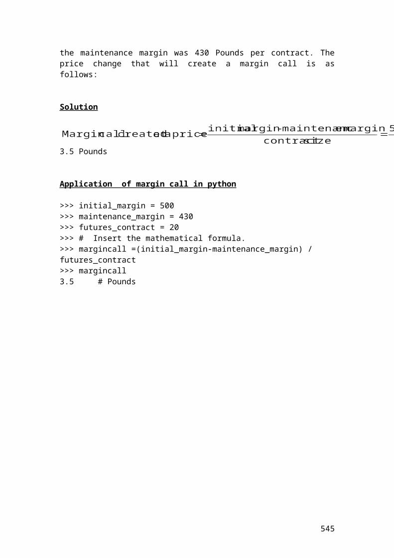
[1] 0.48197343453510655> putPriceUpdownmovestep2ii <- strike - bondPrice2ii> putPriceUpdownmovestep2ii[1] -0.8846153846153726> putPriceUpdownmovestep2ii <- 0> putPriceUpdownmovestep2ii[1] 0> putPriceDownmovestep2iii <- strike - bondPrice2iii> putPriceDownmovestep2iii[1]-1.9238539238539119> putPriceDownmovestep2iii <-0> putPriceDownmovestep2iii[1]0> putPriceUpmovestep1i<- (((putPriceUpmovestep2i*p)+(putPriceUpdownmovestep2ii*p))/disinterest_1i)> putPriceUpmovestep1i[1]0.2302787551529415> putPriceDownmovestep1ii<- (((putPriceUpdownmovestep2ii*p)+(putPriceDownmovestep2iii*p))/disinterest_1ii)> putPriceDownmovestep1ii[1]0.0> putPricestep0<- (((putPriceUpmovestep1i*p)+(putPriceDownmovestep1ii*p))/disinterest_0)> putPricestep0[1]0.11071093997737572

Calculate the bond call option prices based on different interest rates using a binomial 2 steps tree. The figures are expressed in pounds

545

> bond_price <- 100> strike <- 100> annual_coupon <- 7> maturity <- 0.5> sigma <- 0.3> interest_rate <- 4> n <-2> p <-0.5> dt <- maturity/n # steps expressed in years.> dt[1] 0.25> u <- exp(sigma*sqrt(dt)) # multiplier of upmove.> u[1] 1.161834242728283> d <- 1/u # multiplier of downmove.> d[1] 0.8607079764250578> #Identify the discounted interest rates.> disinterest_0 <- 1.04> disinterest_1i <- 1.0465> disinterest_1ii <- 1.0344> disinterest_2i <- 1.054> disinterest_2ii <- 1.04> disinterest_2iii <- 1.0296># Insert the mathematical formulas. It is a backward induction methodology.> bondPrice2i <- (bond_price+annual_coupon)*(1/disinterest_2i)> bondPrice2i[1] 101.5180265654649> bondPrice2ii<-(bond_price+annual_coupon)*(1/disinterest_2ii)> bondPrice2ii[1] 102.88461538461537> bondPrice2iii <- (bond_price+annual_coupon)*(1/disinterest_2iii)> bondPrice2iii[1] 103.92385392385391> bondPrice1i <- ((((bondPrice2i+annual_coupon)*p)+(bondPrice2ii+annual_coupon)*p)/disinterest_1i)> bondPrice1i[1] 104.3490883660202> bondPrice1ii <- ((((bondPrice2ii+annual_coupon)*p)+(bondPrice2iii+annual_coupon)*p)/disinterest_1ii)> bondPrice1ii[1] 106.73263210966226> bondPrice0 <- ((((bondPrice1i+ annual_coupon)*p)+(bondPrice1ii+ annual_coupon)*p)/disinterest_0)> bondPrice0[1] 108.21236561330888> callPriceUpmovestep2i <- bondPrice2i - strike> callPriceUpmovestep2i[1] 1.5180265654648935

546

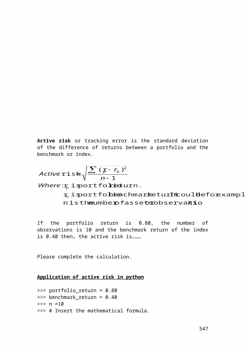
> callPriceUpdownmovestep2ii <- bondPrice2ii - strike> callPriceUpdownmovestep2ii[1] 2.8846153846153726> callPriceDownmovestep2iii <- bondPrice2iii - strike> callPriceDownmovestep2iii[1] 3.923853923853912> callPriceUpmovestep1i<- (((callPriceUpmovestep2i*p)+(callPriceUpdownmovestep2ii*p))/disinterest_1i)> callPriceUpmovestep1i[1] 2.103507859570122> callPriceDownmovestep1ii<- (((callPriceUpdownmovestep2ii*p)+(callPriceDownmovestep2iii*p))/disinterest_1ii)> callPriceDownmovestep1ii[1] 3.291023447635965> callPricestep0<- (((callPriceUpmovestep1i*p)+(callPriceDownmovestep1ii*p))/disinterest_0)> callPricestep0[1] 2.5935246669260033> round(callPricestep0,digits=2)[1] 2.59

Calculate the bond prices of an option based on different interest rates using a binomial 2 steps tree. The figures are expressed in pounds

> bond_price <- 100

547

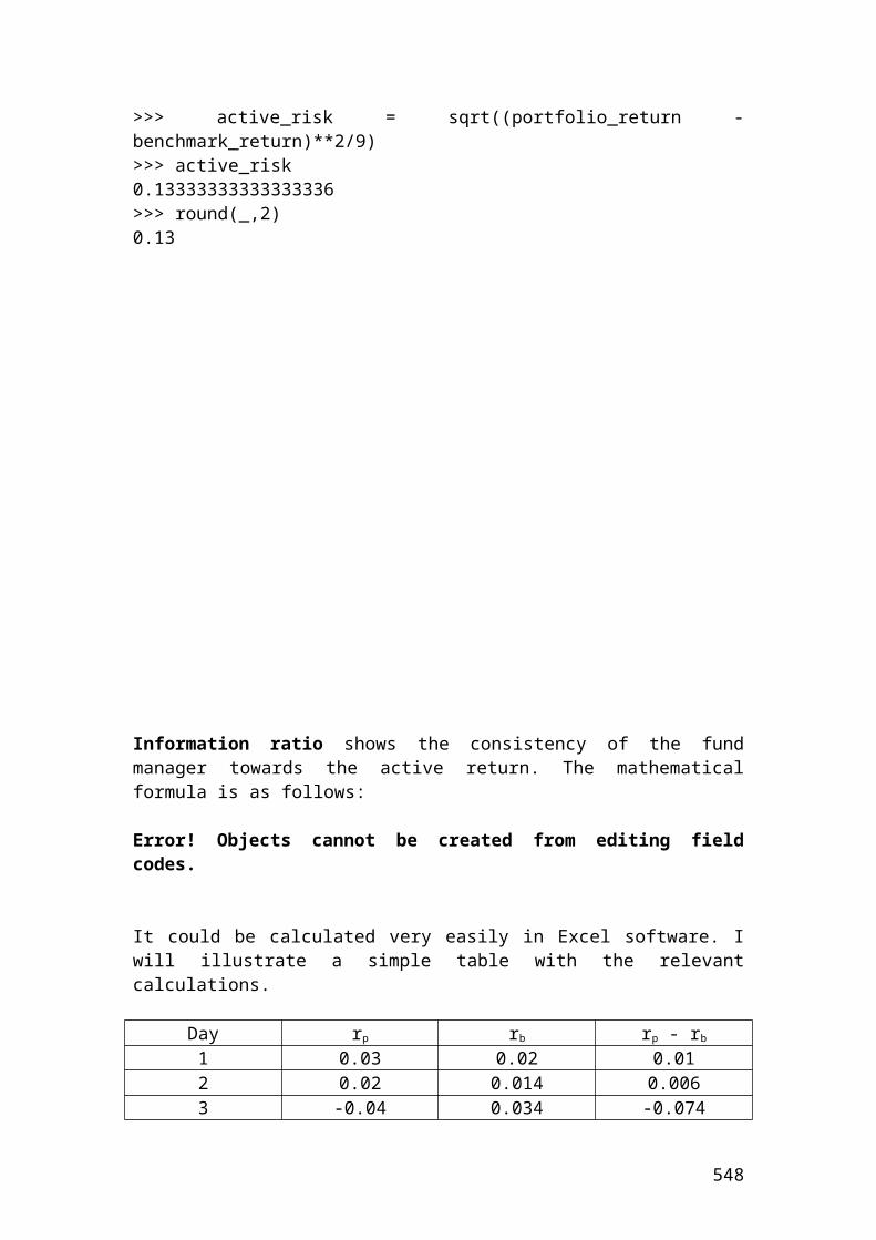
> strike <- 100> annual_coupon <- 7> maturity <- 0.5> sigma <- 0.3> interest_rate <- 4> n <-2> p <- 0.5> dt <- maturity/n # steps expressed in years.> dt[1] 0.25> u <- exp(sigma*sqrt(dt)) # multiplier of upmove.> u[1] 1.161834242728283> d <- 1/u # multiplier of downmove.> d[1] 0.8607079764250578> #Identify the discounted interest rates.> disinterest_0 <- 1.04> disinterest_1i <- 1.0465> disinterest_1ii <- 1.0344> disinterest_2i <- 1.054> disinterest_2ii <- 1.04> disinterest_2iii <- 1.0296># Insert the mathematical formulas. It is a backward induction methodology.> bondPrice2i <- (bond_price+annual_coupon)*(1/disinterest_2i)> bondPrice2i[1] 101.5180265654649> bondPrice2ii <-(bond_price+annual_coupon)*(1/disinterest_2ii)> bondPrice2ii[1] 102.88461538461537> bondPrice2iii <- (bond_price+annual_coupon)*(1/disinterest_2iii)> bondPrice2iii[1] 103.92385392385391> bondPrice1i <- ((((bondPrice2i+annual_coupon)*p)+(bondPrice2ii+annual_coupon)*p)/disinterest_1i)> bondPrice1i[1] 104.3490883660202> bondPrice1ii <- ((((bondPrice2ii+annual_coupon)*p)+(bondPrice2iii+annual_coupon)*p)/disinterest_1ii)> bondPrice1ii[1] 106.73263210966226> bondPrice0 <- ((((bondPrice1i+ annual_coupon)*p)+(bondPrice1ii+ annual_coupon)*p)/disinterest_0)> bondPrice0[1] 108.21236561330888

548

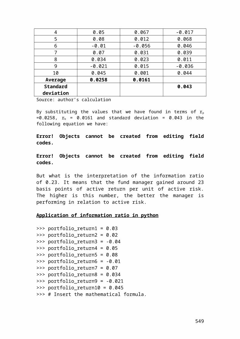
Calculate the interest rates of an option bond based on a two – period binomial tree. The risk – neutral probability of an up and down move in the interest rate tree is always 50% or 0.5. The figures are expressed in percentages

> bond_price <-100> strike <- 100

549

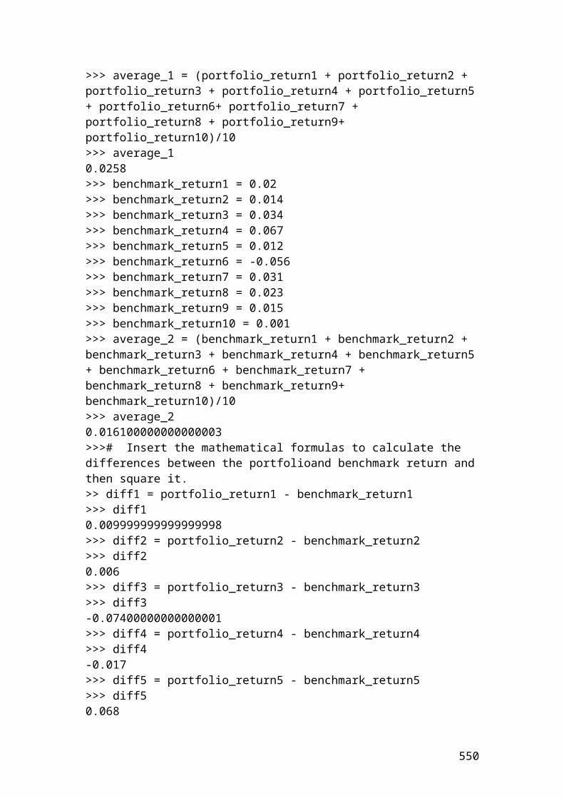
> annual_coupon <- 7> maturity <- 0.5> volatility <- 0.3> interest_rate <- 4> p<-0.5> n<-2>interestrate0 <- 4> interestrate1i <- interest_rate * u> interestrate1i[1] 4.647336970913132> interestrate1ii <- interest_rate * d> interestrate1ii[1] 3.4428319057002312> interestrate2i <- interest_rate * u**2> interestrate2i[1] 5.399435230304012> interestrate2ii<- interest_rate*u*d> interestrate2ii[1] 4.0> interestrate2iii<- interest_rate* d**2> interestrate2iii[1] 2.9632728827268715> round(interestrate2iii,digits=2)2.96

Calculate the share prices of a call option using a Cox, Ross, Rubinstein,(CRR) binomial 3 steps tree using a vector. The multipliers of up and down move depend on volatility and length of steps. The figures are expressed in pounds

S <- 60 # share price K <- 50 # strike price

550

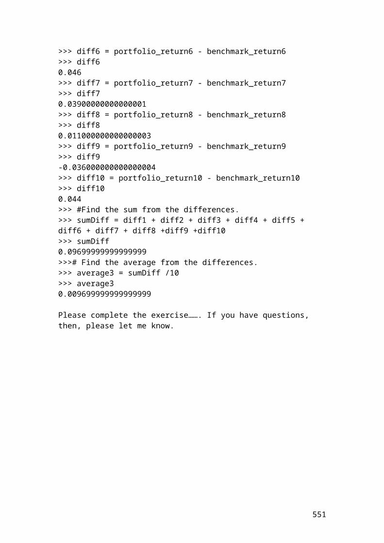
r <- 0.05 # interest rateq <- 0.02 # dividend yieldT <- 0.5 # maturitysig <- 0.3 # volatilityn <- 3> dt <- T/n> dt[1] 0.16666666666666666> u <- exp(sig*sqrt(dt))> u[1] 1.1302902827674572> d <- 1/u> d[1] 0.8847284766100544> share_price0 <- S> share_price0[1] 60> share_price_1upmove <- S*u> share_price1[1] 67.81741696604743> round(share_price1,digits=2)[1]67.82> share_price_1downmove <- S *d> share_price_1downmove[1] 53.083708596603266> share_price2upmove <- S *u**2> share_price2upmove[1] 76.6533673991123> share_price2downmove <- S*d**2> share_price2downmove[1] 46.96466863948485> share_price2upanddownmove <- S*u*d> share_price2upanddownmove[1] 60.0> share_price3downmove <- S*d**3> share_price3downmove41.55097973990743> share_price3upmove <- S*u**3> share_price3upmove[1] 86.64055631262043> share_price3updowndown <-S*u*d*d> share_price3updowndown[1] 53.083708596603266> share_price3upandupdown <- S*u*u*d> share_price3upandupdown[1] 67.81741696604743

551

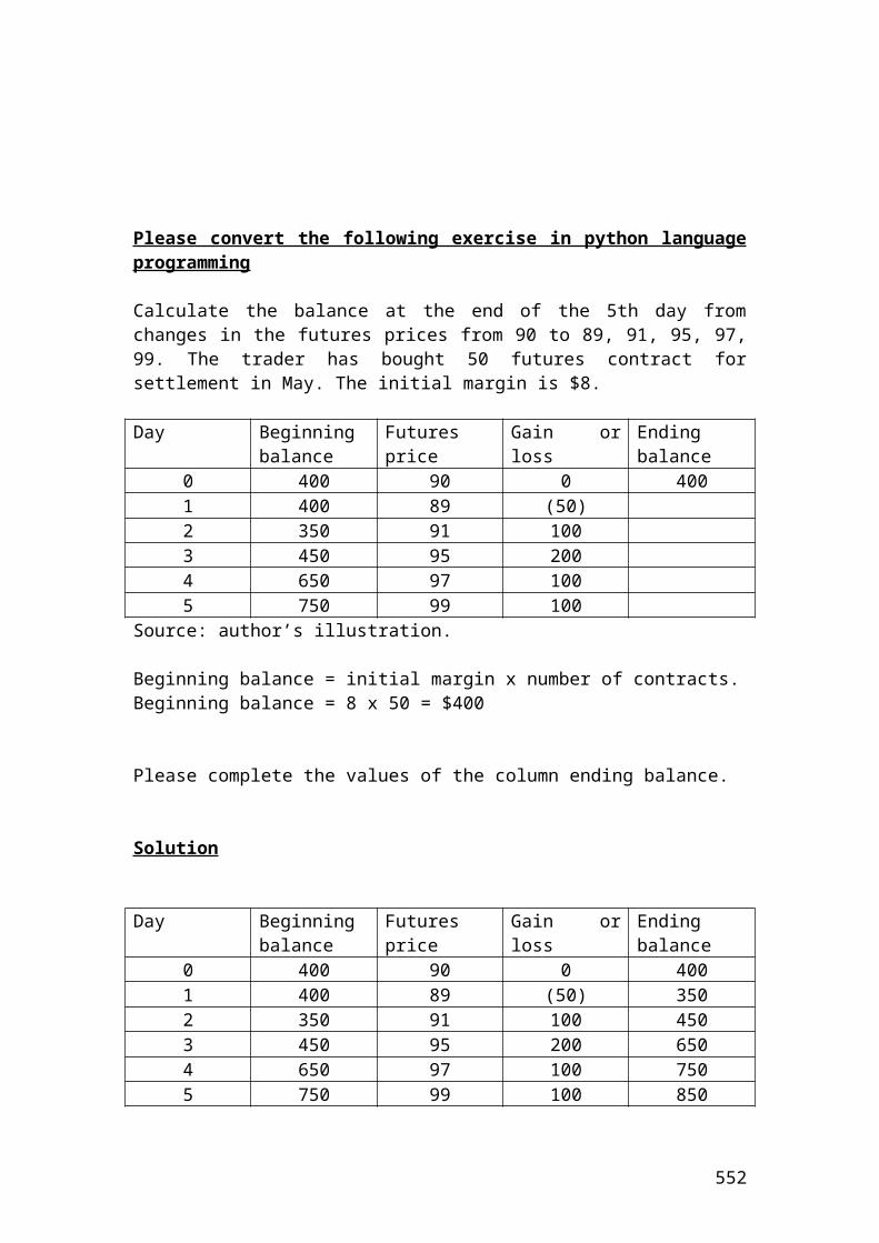
Calculate the call option prices using a Cox, Ross, Rubinstein,(CRR) binomial 3 steps tree. The figures are expressed in pounds

S <- 60 # share priceK <- 50 # strike pricer <- 0.05 # interest rate

552

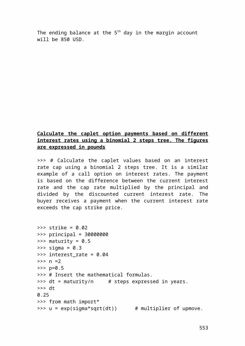
q <- 0.02 # dividend yieldT <- 0.5 # maturitysig <- 0.3 # volatilityn <- 3> dt <- T/n> dt[1] 0.16666666666666666> u <- exp(sig*sqrt(dt))> u[1] 1.1302902827674572> d <- 1/u> d[1] 0.8847284766100544> disfact <- exp(-r*dt)> disfact[1] 0.991701292638876> riskprobofupmove <- (exp((r-q)*dt)-d)/(u-d)> riskprobofupmove[1] 0.48983205544695174> #The option prices are calculated backwards.> callpayoffupmovestep3 <- S*u**3-K> callpayoffupmovestep3[1] 36.64055631262043> callpayoff3i <- S * u**2 * d -K> callpayoff3i[1] 17.817416966047432> callpayoff3ii <-S * d**2*u-K> callpayoff3ii[1] 3.083708596603259> callpayoffdownmovestep3 <- S*d**3-K> callpayoffdownmovestep3[1] -8.449020260092567> callpayoffdownmovestep3 <-0> callpayoffdownmovestep3[1] 0> callpriceupmovestep2 <- (disfact*(riskprobofupmove*callpayoffupmovestep3)+(1-riskprobofupmove)*callpayoff3i)> callpriceupmovestep2[1] 26.88865113426896> callpriceupdownmovestep2 <-(disfact*(riskprobofupmove*callpayoff3i)+(1-riskprobofupmove)*callpayoff3ii)> callpriceupdownmovestep2[1] 10.228323934729657> callpricedownmovestep2 <-(disfact*(riskprobofupmove*callpayoff3ii)+(1-riskprobofupmove)*callpayoffdownmovestep3)> callpricedownmovestep2[1] 1.4979641284454819> callpriceupmovestep1 <- (disfact*(riskprobofupmove*callpriceupmovestep2)+(1-riskprobofupmove)*callpriceupdownmovestep2)> callpriceupmovestep1

553

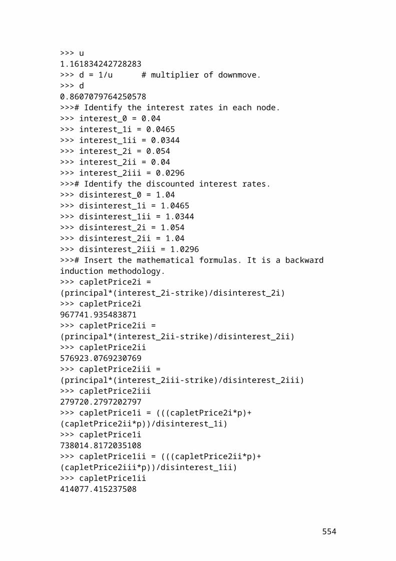
[1] 18.279784613543832>callpricedownmovestep1<-(disfact*(riskprobofupmove*callpriceupdownmovestep2)+(1-riskprobofupmove)*callpricedownmovestep2)> callpricedownmovestep1[1] 5.732796357703088> callpricestep0<- (disfact*(riskprobofupmove*callpriceupmovestep1)+(1-riskprobofupmove)*callpricedownmovestep1)> callpricestep0[1] 11.804406575946299>>> round(callpricestep0,digits=2)11.8

Calculate the put option prices using a Cox, Ross, Rubinstein,(CRR) binomial 3 steps tree. The figures are expressed in USD

> S <- 60 # share price> K <- 70 # strike price> r <- 0.02 # interest rate

554

> q <- 0.03 # dividend yield> T <- 0.5 # maturity> sig <- 0.2 # volatility> n <- 3> dt <- T/n> dt[1] 0.16666666666666666> u <- exp(sig*sqrt(dt))> u[1] 1.0850755957772693> d <- 1/u> d[1] 0.9215947754162443> disfact <- exp(-r*dt)> disfact[1] 0.9966722160545233> riskprobofupmove <- (exp((r-q)*dt)-d)/(u-d)> riskprobofupmove[1] 0.46941253331873867> #The option prices are calculated backwards.> putpayoffupmovestep3 <- K-S*u**3> putpayoffupmovestep3[1] -6.653367399112284> putpayoffupmovestep3<-0> putpayoffupmovestep3[1] 0> putpayoff3i <- K- S * u**2 * d> putpayoff3i[1] 4.895464253363841> putpayoff3ii <-K- S * d**2*u> putpayoff3ii[1] 14.704313475025337> putpayoffdownmovestep3 <- K - S*d**3> putpayoffdownmovestep3[1] 23.035331360515137> putpriceupmovestep2 <- (disfact*(riskprobofupmove*putpayoffupmovestep3)+(1-riskprobofupmove)*putpayoff3i)> putpriceupmovestep2[1] 2.5974719764209926> putpriceupdownmovestep2 <-(disfact*(riskprobofupmove*putpayoff3i)+(1-riskprobofupmove)*putpayoff3ii)> putpriceupdownmovestep2[1] 10.092269491137635> putpricedownmovestep2 <-(disfact*(riskprobofupmove*putpayoff3ii)+(1-riskprobofupmove)*putpayoffdownmovestep3)> putpricedownmovestep2[1] 19.101677490334147> putpriceupmovestep1 <- (disfact*(riskprobofupmove*putpriceupmovestep2)+(1-riskprobofupmove)*putpriceupdownmovestep2)> putpriceupmovestep1

555

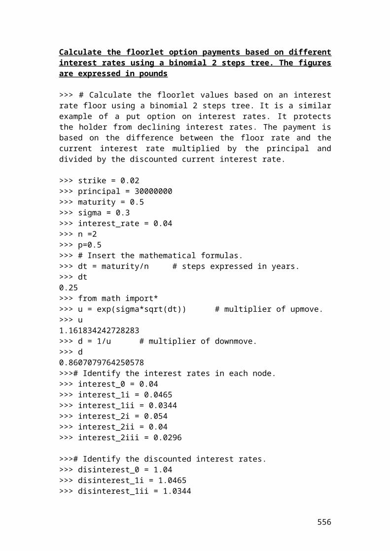
[1] 6.5700600829982925>putpricedownmovestep1<-(disfact*(riskprobofupmove*putpriceupdownmovestep2)+(1-riskprobofupmove)*putpricedownmovestep2)> putpricedownmovestep1[1] 14.85678328831304> putpricestep0<- (disfact*(riskprobofupmove*putpriceupmovestep1)+(1-riskprobofupmove)*putpricedownmovestep1)> putpricestep0[1] 10.956628441795559

Calculation of a Monte Carlo put option using antithetic variables. The purpose of using antithetic variables is to improve the estimation results by reducing the standard error of the simulation results. The figures are expressed in USD

> number_of_simulation <- 199999> max_size <- 200000

556

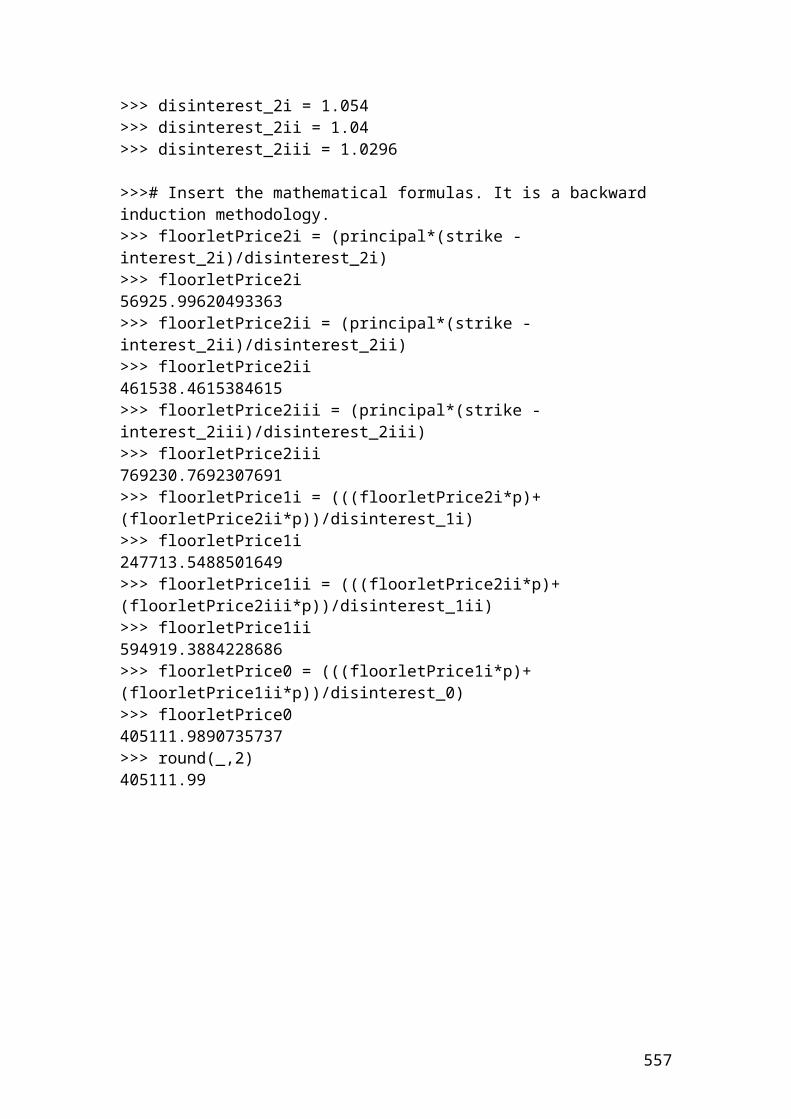
> initial_share_price <- 80> strike_price <- 110> interest_rate <- 0.07> dividend_yield <- 0.02> volatility <- 0.10> maturity <- 0.5> random.number <- (30000+3000)/300> random.number[1 110.0> sharePrice <- initial_share_price *exp((interest_rate-dividend_yield-0.5*volatility*volatility)*maturity*random.number*volatility *sqrt(maturity))> sharePrice[1] 95.30055> round(sharePrice,digits=2)[1] 95.30> value <- strike_price – initial_share_price> payoff <- (value*strike*sharePrice*sharePrice)^2> payoff[1] 29695052> optPrice <- (payoff * exp(-interest_rate*maturity))/ number_of_simulation/2> optPrice[1] 71.68462> round(optPrice,digits=2)[1] 71.68

Calculate the call option prices using a Jarrow – Rudd, (JR), binomial 3 steps tree. The key difference between the Cox, Ross, Rubinstein,(CRR) binomial tree and the Jarrow – Rudd, (JR), binomila tree is in defining the parmeters of the multiplier of up and down move. The figures are expressed in pounds

> S <- 90 # share price

557

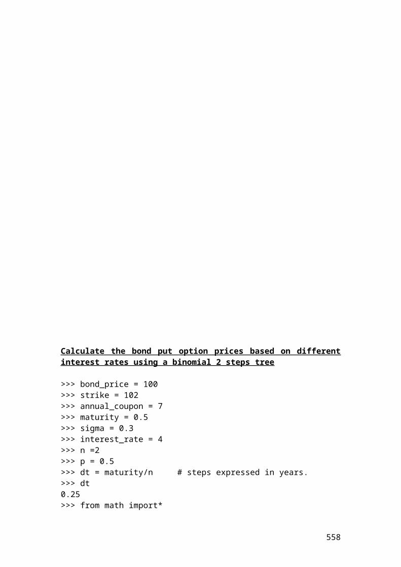
> K <- 85 # strike price> r <- 0.04 # interest rate> q <- 0.03 # dividend yield> T <- 0.5 # maturity> sig <- 0.2 # volatility> n <- 3> dt <- T/n> dt <- T/n # steps expressed in years.> dt[1] 0.16666666666666666> u <- (exp((r-q -0.5*sig*sig)*dt + sig*sqrt(dt))) # multiplier of upmove.> u[1] 1.0832686426635116 > d <- (exp((r-q -0.5*sig*sig)*dt - sig*sqrt(dt))) # multiplier of downmove.> d[1] 0.9200600634058166> disfact <- exp(-r*dt) # discount factor.> disfact[1] 0.9933555062550344> riskprobofupmove <- (exp((r-q)*dt)-d)/(u-d) # risk neutral probability of upmove.> riskprobofupmove[1] 0.5000226905523886> callpayoffupmovestep3 <- S*u**3-K> callpayoffupmovestep3[1] 29.406585701387428> callpayoff3i <- S * u**2 * d -K> callpayoff3i[1] 12.169738279923607> callpayoff3ii <-S*d**2*u-K> callpayoff3ii[1] -2.470152793185349> callpayoff3ii <-0> callpayoff3ii[1] 0> callpayoffdownmovestep3 <- S*d**3-K> callpayoffdownmovestep3[1] -14.904352933845047> callpayoffdownmovestep3 <-0> callpayoffdownmovestep3[1] 0> callpriceupmovestep2 <- (disfact*(riskprobofupmove*callpayoffupmovestep3)+(1-riskprobofupmove)*callpayoff3i)> callpriceupmovestep2[1] 20.690852733318547> callpriceupdownmovestep2 <-(disfact*(riskprobofupmove*callpayoff3i)+(1-riskprobofupmove)*callpayoff3ii)> callpriceupdownmovestep2[1] 6.044712568308618> callpricedownmovestep2 <-(disfact*(riskprobofupmove*callpayoff3ii)+(1-riskprobofupmove)*callpayoffdownmovestep3)

558

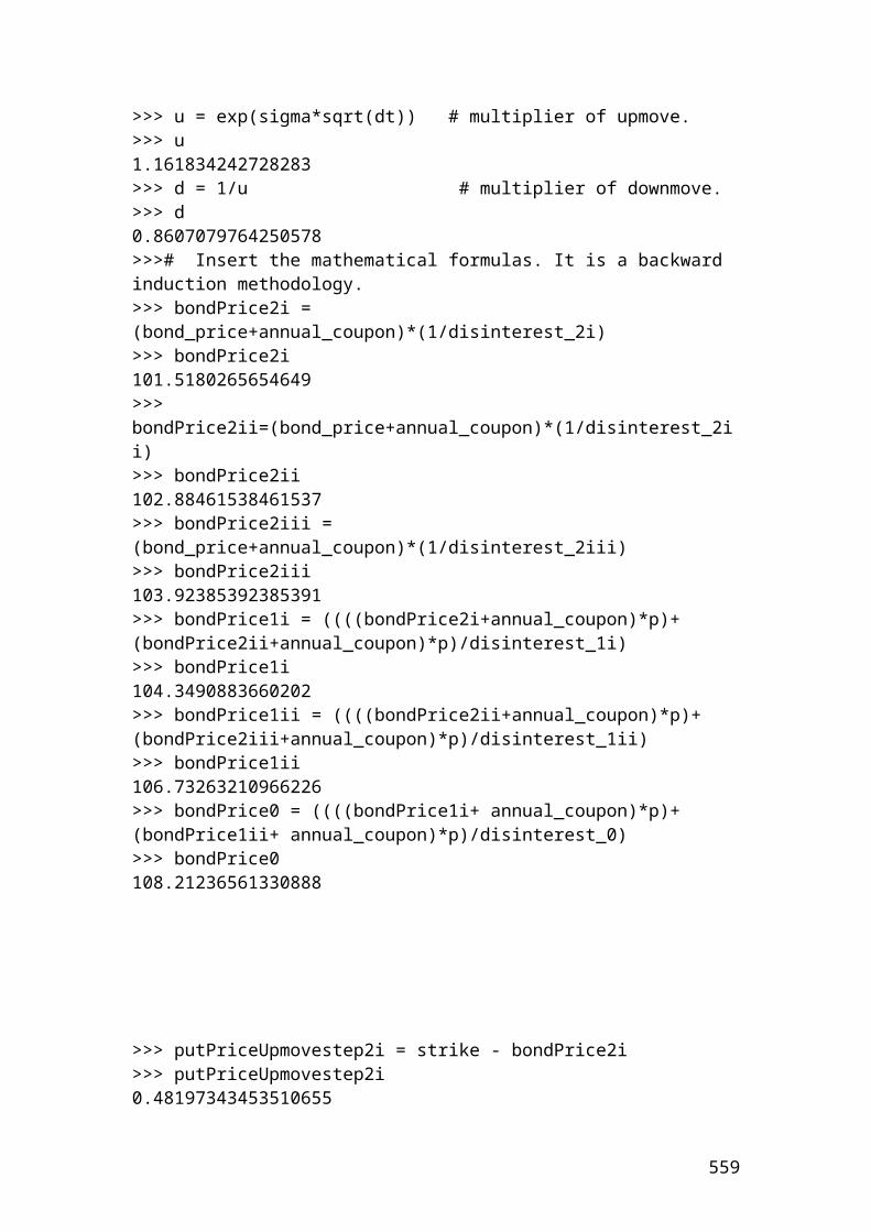
> callpricedownmovestep2[1] 0.0> callpriceupmovestep1 <- (disfact*(riskprobofupmove*callpriceupmovestep2)+(1-riskprobofupmove)*callpriceupdownmovestep2)> callpriceupmovestep1[1] 13.299371739539392> callpricedownmovestep1<-(disfact*(riskprobofupmove*callpriceupdownmovestep2)+(1-riskprobofupmove)*callpricedownmovestep2)> callpricedownmovestep1[1] 3.0024105032518027> callpricestep0<- (disfact*(riskprobofupmove*callpriceupmovestep1)+(1-riskprobofupmove)*callpricedownmovestep1)> callpricestep0[1] 8.10693896385682>>> round(callpricestep0,digits=2)8.11

Calculate the share prices of a call option using a Jarrow – Rudd, (JR), binomial 3 steps tree. The prices are expressed in Euros.

> S <- 90> K <- 85> r <- 0.04> q <-0.03

559

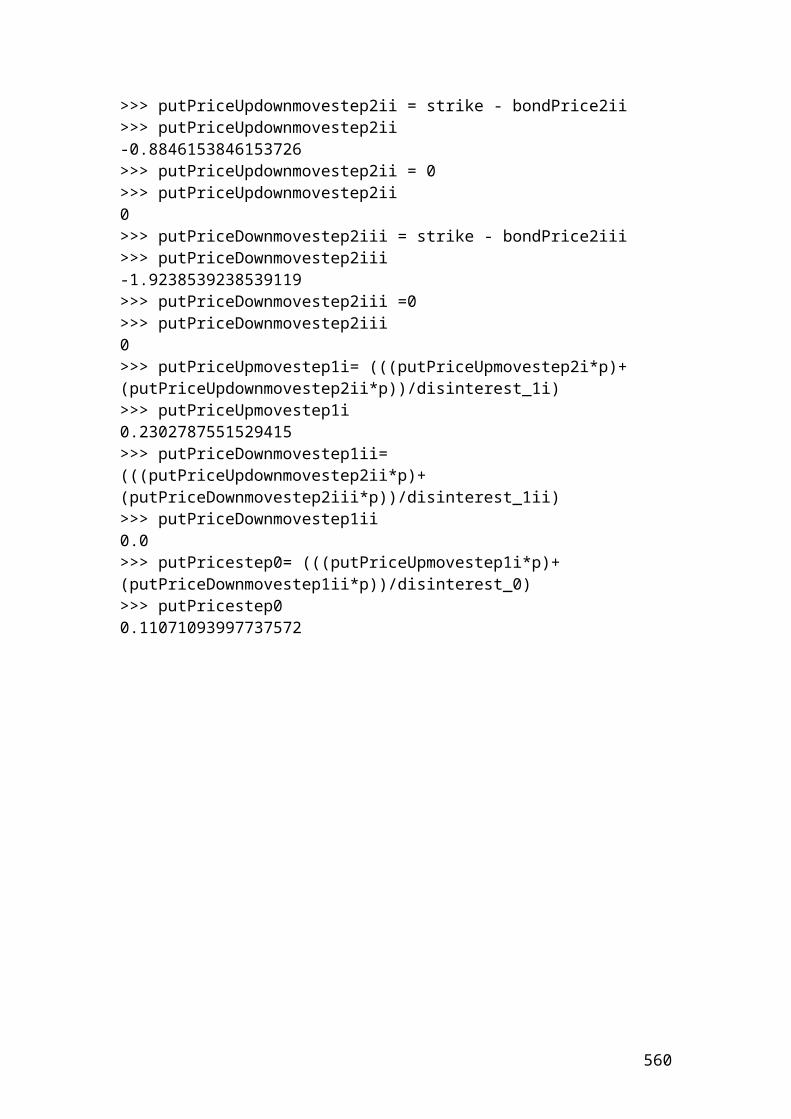
> T <- 0.5> sig <- 0.2> n <-3> dt <- T/n> dt[1] 0.16666666666666666> u <- (exp((r-q -0.5*sig*sig)*dt + sig*sqrt(dt)))> u[1] 1.0832686426635116> d <- (exp((r-q -0.5*sig*sig)*dt - sig*sqrt(dt)))> d[1] 0.9200600634058166> share_price0 <- S> share_price0[1] 90> share_priceupmove1 <- S*u> share_priceupmove[1] 97.49417783971604> share_pricedownmove1 <- S*d> share_pricedownmove1[1] 82.80540570652349> share_priceupmove2 <- S*u**2> share_priceupmove2[1] 105.61238569602422> share_priceupmovedownmove <- S*u*d> share_priceupmovedownmove[1] 89.70049944490711> share_pricedownmove2 <- S*d**2> share_pricedownmove2[1] 76.18594682468837> share_priceupmove3 <-S*u**3> share_priceupmove3[1] 114.40658570138743

Please complete the remaining calculations……

Example of simulating share prices by showing different price scenarios. The figure is expressed in pounds.

> number_of_simulation <- 6> S0 <- 60> r <- 0.03> q <- 0.02

560

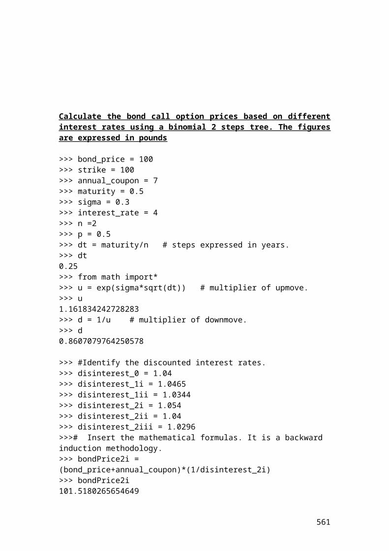
> sig <- 0.20> dt <- 1/250> dt[1] 0.004> random.number <- (30000+3000)/300> random.number110.0> sharePrice<-S0*exp((r-q-0.5*sig*sig)*dt*random.number*sig*sqrt(dt))> sharePrice59.99760004799936

Please complete the calculations to get different share prices….

A manufacturing company sold a FRA contract expiring in 50 days with a principal of 30,000,000 USD. The underlying is 180 days LIBOR. The agreed rate on this FRA is 7%. At expiration, 90 days later, the actual rate on 180 days LIBOR is 8%. How much is the payoff of the manufacturing company at expiration?

Solution

561

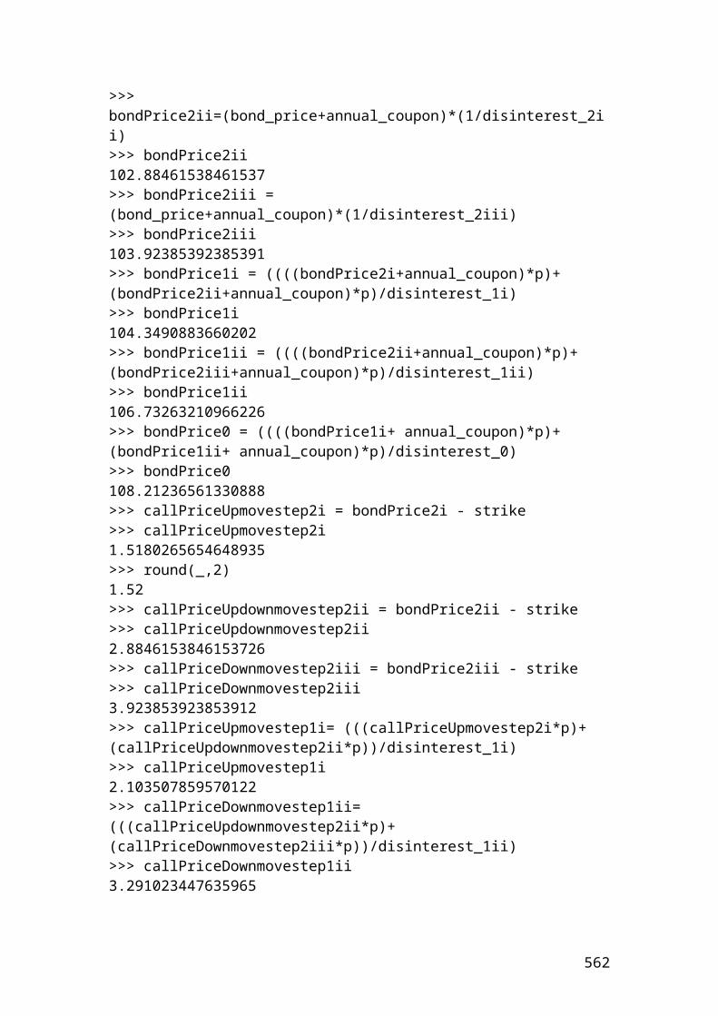
The mathematical formula for Forward Rate Agreement, (FRA) is as follows:

FRA Payment = 30,000,000* ((0.08 – 0.07)*(180/360) / 1 + 0.08*(180/360)

FRA Payment = 30,000,000 * 0.005 / 1.04

FRA Payment = 144230.77 USD

Application of FRA payment in R

> principal <- 30000000> actual_rate <- 0.08> agreed_rate <- 0.07> days_1_underlying <- 180> days_2_expiration <- 180

Please complete the calculations using R……..

Currency futures

Futures Price = contract size * exchange rate

If the contract size is 20,000 USD and the quoted price is 1.573 USD, then, the futures price is as follows:

562

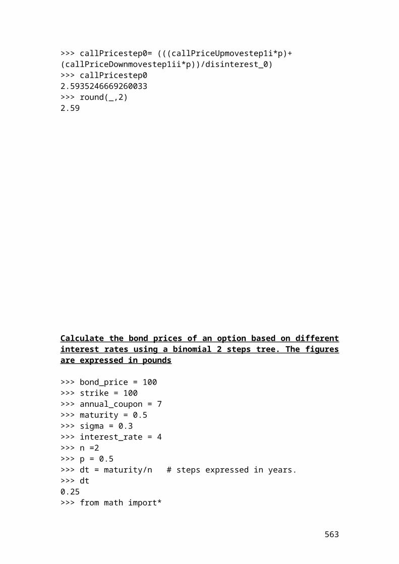
Futures Price = 20,000 * 1.573 = 31460 USD

Application of currency futures in R

> contract_size <- 20000> quoted_price <- 1.573> FuturesPrice <- contract_size * quoted_price> FuturesPrice[1] 31460.0 # USD

Minimum price required for a margin call

It is very important to check the maintenance margin level. The initial margin per contract for a gold futures contract is 1,500 USD. The maintenance margin per contract is 800 USD. The contract size is 5,000 ounces.

Solution

563

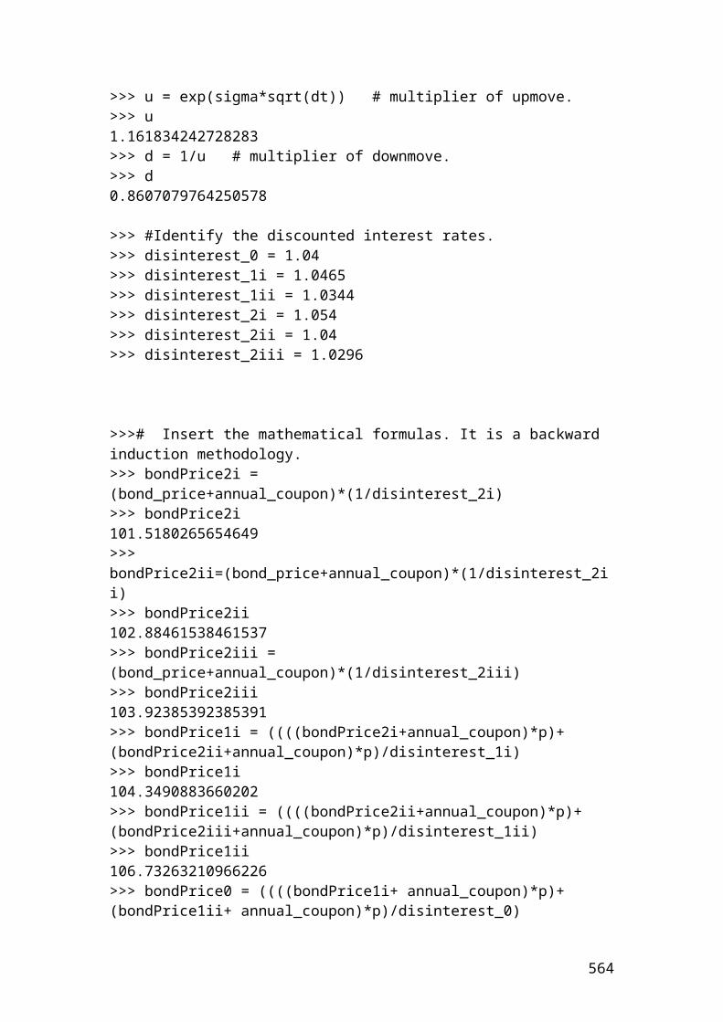
Minimum price required for a margin call = initial margin – maintenance margin / contract size

Minimum price required for a margin call = 1500 – 800 / 5000 = 0.14 USD.

Application of minimum price required for a margin call in R

> initial_margin_of_gold_futures <- 1500> maintenance_margin_percontract <- 800> contract_size <- 5000> minimum_price_required_for_a_margin_call <- (initial_margin_of_gold_futures - maintenance_margin_percontract) / contract_size> minimum_price_required_for_a_margin_call0.14 # USD

Loss on the futures position

Please consider a bond related to Eurodollar futures. The settlement price of the bond is 95.70 in December 2015. The principal is 2,000,000 Euros. The investor has adopted a long position of 100 contracts. The bond price has fallen to 90.15. Calculate the loss on the futures position.

564

Solution

Insert the mathematical formula.

Loss on the futures position = (settlement price – current price) / 100 * 100 contracts * 2,000,000

Loss on the futures position = (95.70 – 90.15) / 100 * 100 * 2,000,000 =

Loss on the futures position = 5.55 / 100 * 100 * 2000000 = 11,100,000 Euros.

Application of loss on the futures position in R

> settlement_price <- 95.70> current_price <- 90.15> principal <- 2000000> contract_size <- 100> Loss_on_the_futures_position <-(settlement_price - current_price)/100*contract_size*principal> Loss_on_the_futures_position11099999.999999994> round(Loss_on_the_futures_position, digits=2)11100000.0 # Euros

Variation margin call

The amount of variation margin call is used in futures when the price of the asset price falls below a certain amount. For example, consider the bond price of Eurodollar futures.

565

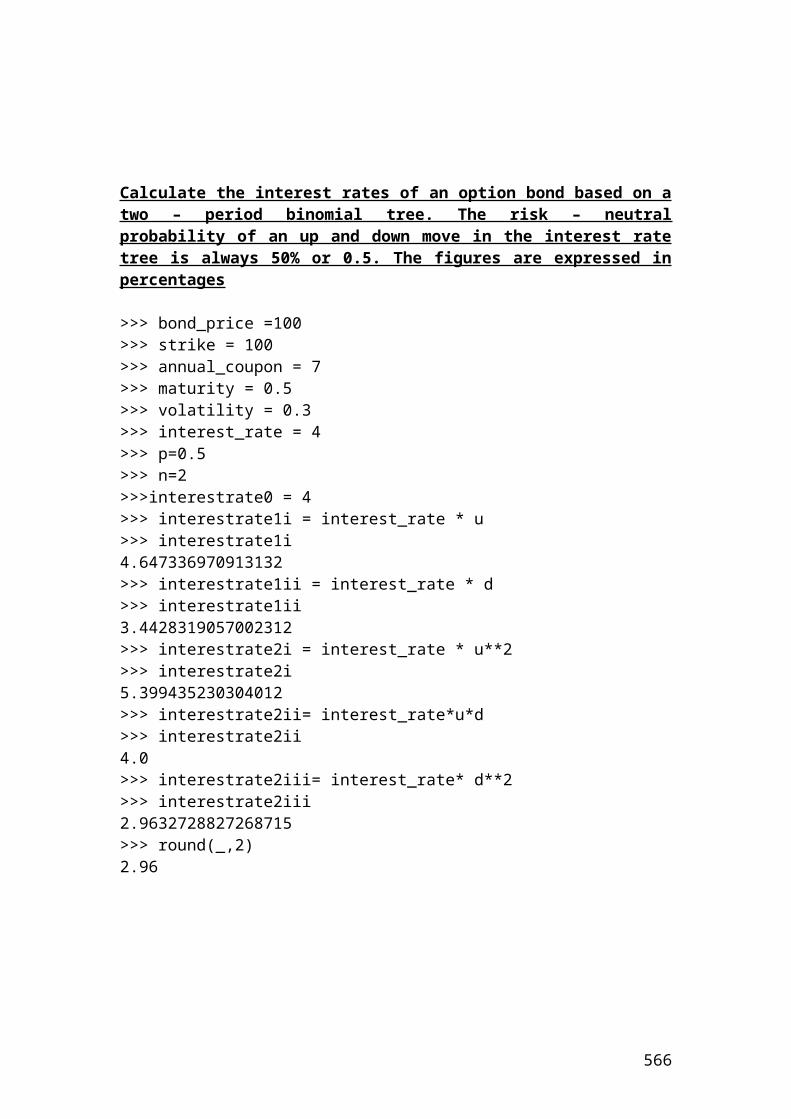
Consider a trader that has bought a Eurodollar bond futures with a principal of 10,000,000 Euros. The settlement price is 97.14. The long position includes 100 contracts. The price of the bond has fallen to 95.78. The maintenance price is 96.45. The price of the bond has fallen below the maintenance price.

Variation margin = (settlement price – current price) / 100 * 100 contracts * 10,000,000

Variation margin = (97.14 – 95.78) / 100 * 100 *10,000,000 =

Variation margin = 1.36 / 100 * 100 * 10,000,000 = 13,600,000 Euros.

Application of variation margin call in R

> settlement_price <- 97.14> current_price <- 95.78> principal <- 10000000> contract_size <- 100> variation_margin <-(settlement_price-current_price)/100*contract_size*10000000> variation_margin13599999.999999994> round(variation_margin,digits = 2)13600000.0 # Euros

Calculate the volume and the open interest position in the July FTSE 100 index

Please consider 5 investors with the following short/long contract position.

First investor buys 3 contracts to open a long position.

566

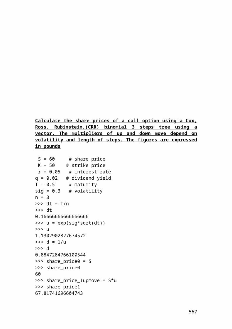
Second investor buys 5 contracts to open a long position.Third investor buys 2 contracts to open a long position.Fourth investor sells 7 contracts to close a long position.Fifth investor sells 4 contracts to close a long position.

If we assume that the initial open interest before the trades was 30 contracts. Calculate the volume and ending open interest.

Solution

Total volume = 3 + 5 + 2 + 7 + 4 = 21 contracts.

Ending open interest = initial open interest + opened positions - closed positions

Ending open interest = 30 + 3 + 5 + 2 - 7 – 4 = 29

Application of calculation the volume and the open interest position in the July FTSE 100 index in R

> first_investor_buys_3contracts <- 3> second_investor_buys_5contracts <- 5> third_investor_buys_2contracts <- 2> fourth_investor_sells_7contracts <- 7> fifth_investor_sells_4contracts <- 4> initial_open_interest <- 30> Total_volume <- 3+5+2+7+4> Total_volume21 # contracts> ending_open_interest <- 30 + 3 + 5 + 2 - 7 -4> ending_open_interest29 # ending open interest

Calculation of the minimum price per ounce before a margin call

Please consider the following terms of the silver contract:

Initial margin = $ 3,500 per contract.Maintenance margin = $ 2,500 per contract.

567

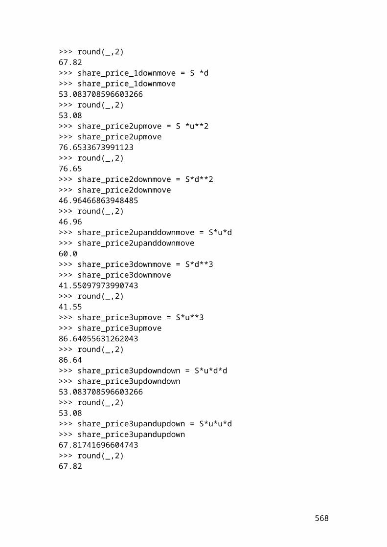
20 silver contracts sold at a price equals $700 per ounce.Contract size = 100 ounces.

Solution

The initial margin = 3,500 * 20 = 70,000 USD. The maintenance margin = 2,500 * 20 = 50,000 USD.The difference between the initial and maintenance margin is the amount recorded before a margin call take place. Thus, 70,000 – 50,000 = 20,000 USD.

The price is 20,000 / 20*100 = 10 USD per ounce. This is the price before a margin call take place.

Application of calculating the minimum up or down ounce price before a margin call in R

> initial_margin <- 3500> maintenance_margin <- 2500> silver_contracts <- 20> contract_size <- 100> minimum_price_required_for_a_margincall <- (3500 - 2500) / 100> minimum_price_required_for_a_margincall10.0 # USD per ounce.

Calculate the intrinsic value of call share traded in Frankfurt stock exchange

The VW share is traded at 140 Euro in the Frankfurt stock exchange. The strike price is 130 Euro and the option market price is 7.70 Euro. The intrinsic value of the VW call is as calculate as follows:

568

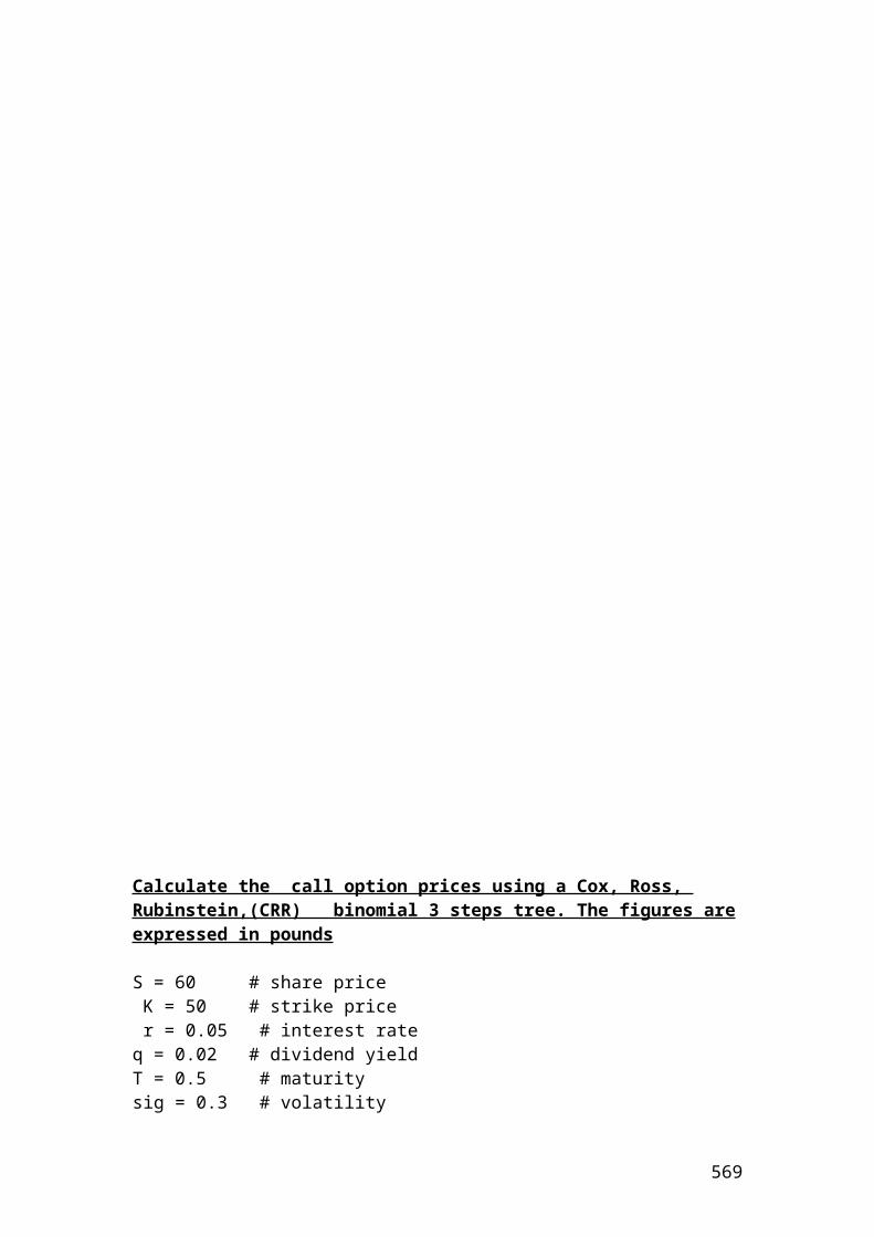
Solution

The intrinsic value of the VW call is = Share price – strike price = 140 – 130 = 10 Euro.

Application of calculating the intrinsic value of call share traded in Frankfurt stock exchange

> share_price <- 140> strike_price <- 130> intrinsic_value <- share_price - strike_price> intrinsic_value10 # Euro.

Workshop of analysis of financial data, scientific programming and simulation using Java language programming

569

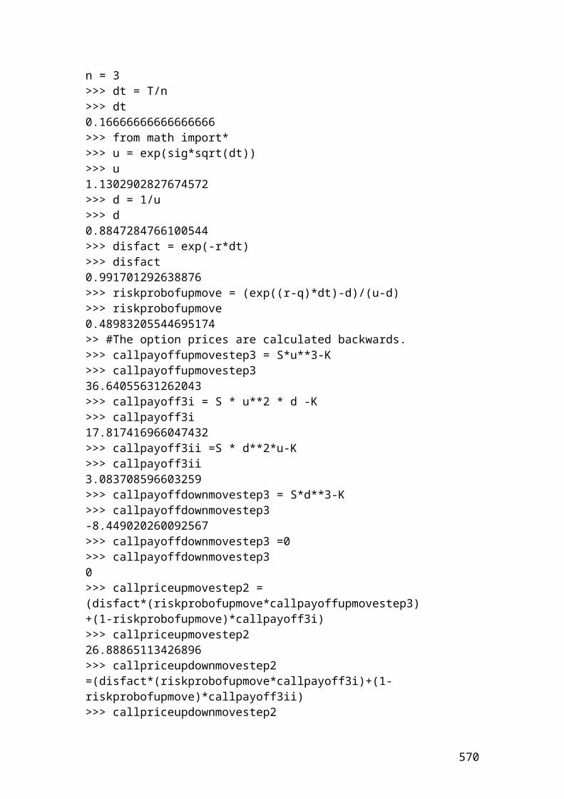
Java is very useful language programming in financial modeling. Please make yourself very familiar with C++. You will find a lot of similarities with Java. The main differences are in defining the headings and the output functions.

First of all, you should download the software as part of an integrated development environment, (IDE). A possible public domain is as follows:

www.drjava.org

You can start Java programming by creating a source code in the text editor. Then, press tools and select the compile current document to compile the code. Once compilation is completed, then, press run document from the tools section. At the bottom, you could see the output of the source code.

Press new to create a new text editor, then, in the header insert the title of the document to be saved. For example,

class Currency_futures

Press save and then insert the appropriate source code for financial calculation.

If you do not have the right headers, then, you will not be able to do compiling and run the document to see the output.

The comments, variables, functions, and mathematical formulas have to be inserted to be able to get the output. We use the symbol // to show a single line comment. The lines that include statements should end with semicolon ; in Java . We use numerical variables with fractional parts. In this case, the term double is inserted in front of each variable. Once you define a variable with capital or small letters, you can not change it with different layout as you move to the calculation part. Pay particular attention to the lower and upper case letters. For example, integer for interest rate is written as variable intRate or int_rate. Another example that can be used is the integer value for the amount. It is written as intAmount or int_amount. Use the symbols /* and */ for multiline comments. The symbol // is used for single comment.

Then, the source code should be enclosed between braces.

The main layout to start Java is as follows:

570

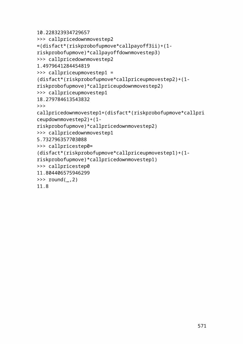
class name of the variable { public static void main (String[] args) {

/* Identify your given variables using double for numbers with fractions or int for integers numbers. Identify the variables that will be calculated. The symbols /* and */ are used for multiline comments.*/

// Insert the mathematical formula or formulas.

// Output functions.System.out.print ("type the sentence that will appear in the output before the calculated number")System.out.println(variable that is defined by a mathematical formula)You can add as many output functions as your mathematical formulas.

} }

A simple example to illustrate the above is as follows:

// Calculate the average

571

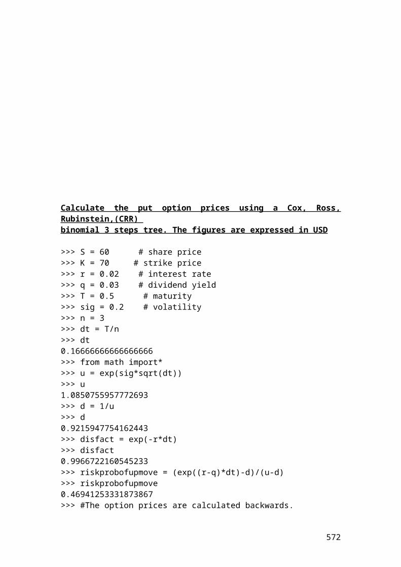
class Average

{public static void main (String[] args) {

// Identify the variables.

double stock_price1=3;double stock_price2=5;double stock_price3=9;double average;

// Insert the mathematical formula.

average = (stock_price1 + stock_price2 + stock_price3)/3;

// Output functions.System.out.print("The average in $");System.out.println(average);}}

After compiling the current document, press run document from Tools, you should get $ 5.66.

Calculations of the mean and the harmonic mean of share price returns, call option returns, put option returns and index option returns

572

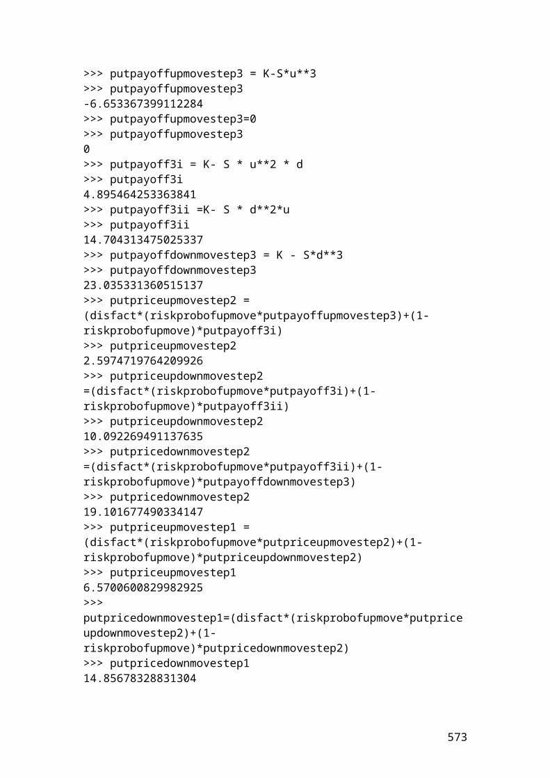
class average_and_harmonic_average

{public static void main(String[] args) {

/* Calculations of the mean and the harmonic mean of share price returns, call option returns, put option returns and index option returns.*/ double SharePriceReturns1 = 0.08;double SharePriceReturns2= 0.05;double SharePriceReturns3 = 0.04;double SharePriceReturns4 = 0.07;double SharePriceReturns5 = 0.02;double SharePriceReturns6 = 0.03;

double CallOptionPriceReturns1 = 0.01;double CallOptionPriceReturns2 = 0.02;double CallOptionPriceReturns3 = 0.04;double CallOptionPriceReturns4 = 0.05;double CallOptionPriceReturns5 = 0.06;double CallOptionPriceReturns6 = 0.06;

double PutOptionPriceReturns1 = 0.03;double PutOptionPriceReturns2 = 0.07;double PutOptionPriceReturns3 = 0.08;double PutOptionPriceReturns4 = 0.09;double PutOptionPriceReturns5 = 0.1;double PutOptionPriceReturns6 = 0.02;

double IndexOptionPriceReturns1 = 0.12;double IndexOptionPriceReturns2 = 0.23;double IndexOptionPriceReturns3 = 0.34;double IndexOptionPriceReturns4 = 0.15;double IndexOptionPriceReturns5 = 0.2;double IndexOptionPriceReturns6 = 0.11;

double averageSharePriceReturns;double averageCallOptionPriceReturns;double averagePutOptionPriceReturns;double averageIndexOptionPriceReturns;double harmonicaverageSharePriceReturns;double harmonicaverageCallOptionPriceReturns;double harmonicaveragePutOptionPriceReturns;double harmonicaverageIndexOptionPriceReturns;

averageSharePriceReturns = (SharePriceReturns1 + SharePriceReturns2 + SharePriceReturns3 + SharePriceReturns4 + SharePriceReturns5 + SharePriceReturns6)/6;

573

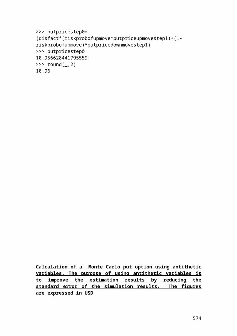
averageCallOptionPriceReturns = (CallOptionPriceReturns1 + CallOptionPriceReturns2 + CallOptionPriceReturns3 + CallOptionPriceReturns4 + CallOptionPriceReturns5 + CallOptionPriceReturns6)/6;

averagePutOptionPriceReturns = (PutOptionPriceReturns1 + PutOptionPriceReturns2 + PutOptionPriceReturns3 + PutOptionPriceReturns4 + PutOptionPriceReturns5 + PutOptionPriceReturns6)/6;

averageIndexOptionPriceReturns = (IndexOptionPriceReturns1 + IndexOptionPriceReturns2 + IndexOptionPriceReturns3 + IndexOptionPriceReturns4 + IndexOptionPriceReturns5 + IndexOptionPriceReturns6)/6;

harmonicaverageSharePriceReturns = (1/((1/SharePriceReturns1 + 1/SharePriceReturns2 + 1/SharePriceReturns3 + 1/SharePriceReturns4 + 1/SharePriceReturns5 + 1/SharePriceReturns6)/6));

harmonicaverageCallOptionPriceReturns = (1/((1/CallOptionPriceReturns1 + 1/CallOptionPriceReturns2 + 1/CallOptionPriceReturns3 + 1/CallOptionPriceReturns4 + 1/CallOptionPriceReturns5 + 1/CallOptionPriceReturns6)/6));

harmonicaveragePutOptionPriceReturns = (1/((1/PutOptionPriceReturns1 + 1/PutOptionPriceReturns2 + 1/PutOptionPriceReturns3 + 1/PutOptionPriceReturns4 + 1/PutOptionPriceReturns5 + 1/PutOptionPriceReturns6)/6));

harmonicaverageIndexOptionPriceReturns = (1/((1/IndexOptionPriceReturns1 + 1/IndexOptionPriceReturns2 + 1/IndexOptionPriceReturns3 + 1/IndexOptionPriceReturns4 + 1/IndexOptionPriceReturns5 + 1/IndexOptionPriceReturns6)/6));

System.out.print("The average is");System.out.println(averageSharePriceReturns);System.out.print("The average of call option price returns is");System.out.println(averageCallOptionPriceReturns);System.out.print("The average of put option price returns is");System.out.println(averagePutOptionPriceReturns);System.out.print("The average of index option price returns is");System.out.println(averageIndexOptionPriceReturns);System.out.print("The harmonic average of share price returns is");System.out.println(harmonicaverageSharePriceReturns);System.out.print("The harmonic average of call option price returns is");System.out.println(harmonicaverageCallOptionPriceReturns);System.out.print("The harmonic average of put option price returns is");System.out.println(harmonicaveragePutOptionPriceReturns);System.out.print("The harmonic average of index option price returns is");System.out.println(harmonicaverageIndexOptionPriceReturns);}}

574

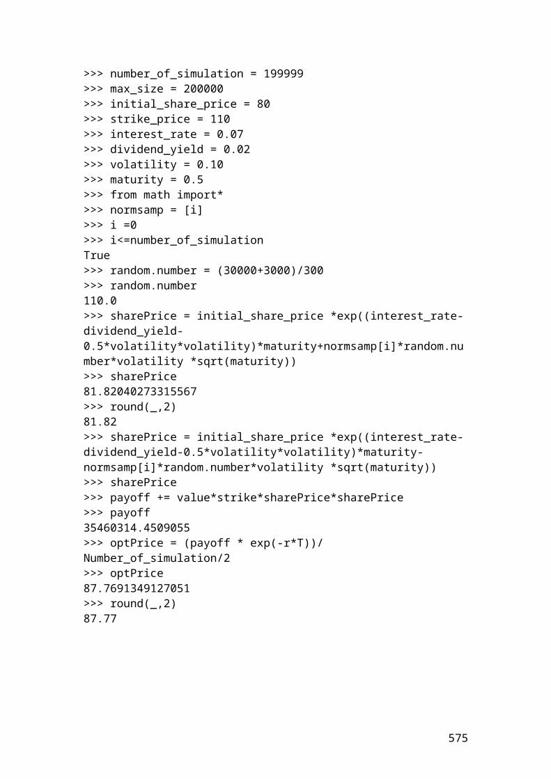
Output results

After compiling the current document from tools and pressing the run document you should get the following results:

Welcome to DrJava. Working directory is C:\Documents and Settings\Owner\Desktop\Java Compiler> run average_and_harmonic_averageThe average is 0.04833333333333334The average of call option price returns is 0.04The average of put option price returns is 0.065The average of index option price returns is 0.19166666666666668The harmonic average of share price returns is 0.03867996930161166The harmonic average of call option price returns is 0.026277372262773727The harmonic average of put option price returns is 0.04572119745993347The harmonic average of index option price returns is 0.1649261839330223

Repetition of calculating the mean and the harmonic mean of share price returns, call option returns, put option returns and index option returns. I will show how to use the rounding function in Java

575

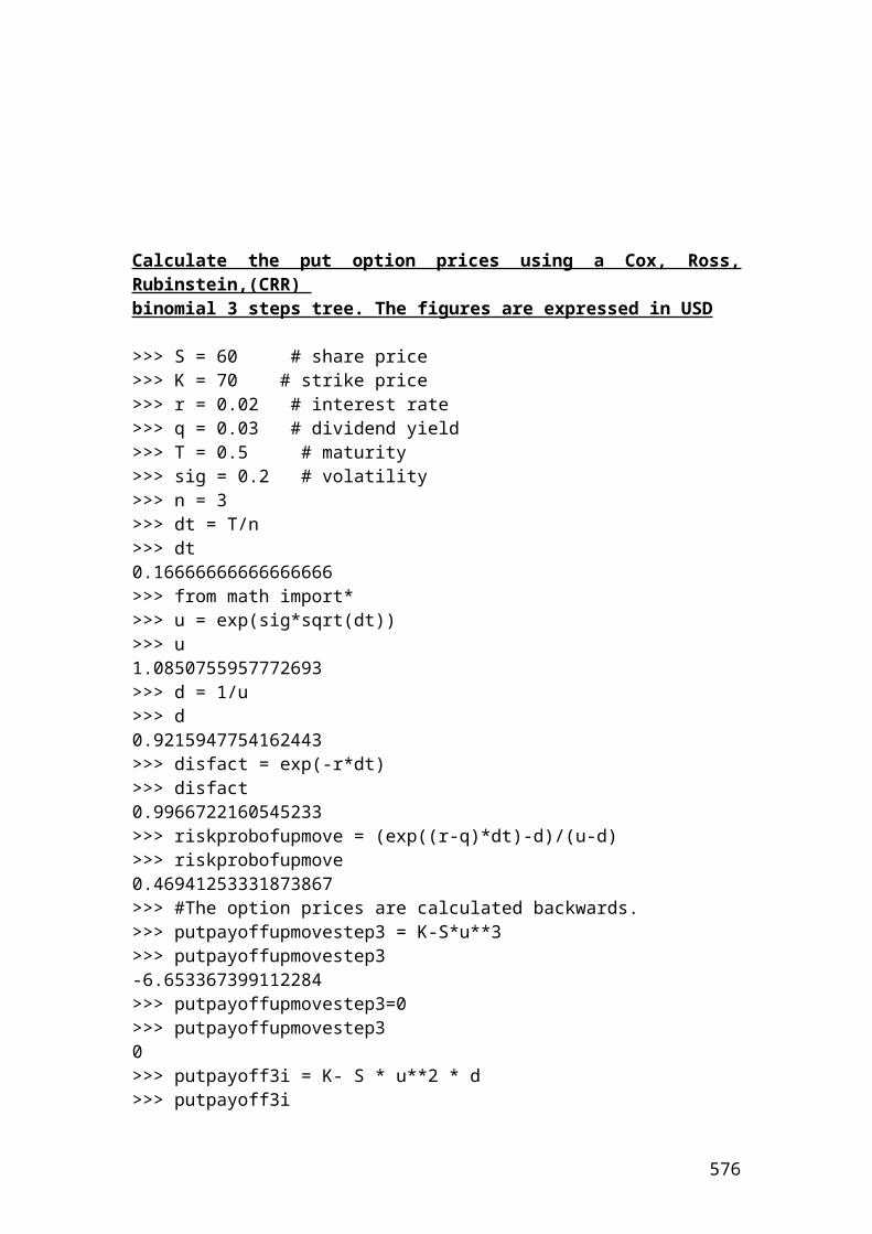
class average_and_harmonic_average {public static void main(String[] args) {

/* Calculations of the mean and the harmonic mean of share price returns, call option returns, put option returns and index option returns. */ double SharePriceReturns1 = 0.08;double SharePriceReturns2= 0.05;double SharePriceReturns3 = 0.04;double SharePriceReturns4 = 0.07;double SharePriceReturns5 = 0.02;double SharePriceReturns6 = 0.03;

double CallOptionPriceReturns1 = 0.01;double CallOptionPriceReturns2 = 0.02;double CallOptionPriceReturns3 = 0.04;double CallOptionPriceReturns4 = 0.05;double CallOptionPriceReturns5 = 0.06;double CallOptionPriceReturns6 = 0.06;

double PutOptionPriceReturns1 = 0.03;double PutOptionPriceReturns2 = 0.07;double PutOptionPriceReturns3 = 0.08;double PutOptionPriceReturns4 = 0.09;double PutOptionPriceReturns5 = 0.1;double PutOptionPriceReturns6 = 0.02;

double IndexOptionPriceReturns1 = 0.12;double IndexOptionPriceReturns2 = 0.23;double IndexOptionPriceReturns3 = 0.34;double IndexOptionPriceReturns4 = 0.15;double IndexOptionPriceReturns5 = 0.2;double IndexOptionPriceReturns6 = 0.11;

double averageSharePriceReturns;double averageCallOptionPriceReturns;double averagePutOptionPriceReturns;double averageIndexOptionPriceReturns;double harmonicaverageSharePriceReturns;double harmonicaverageCallOptionPriceReturns;double harmonicaveragePutOptionPriceReturns;double harmonicaverageIndexOptionPriceReturns;

averageSharePriceReturns = (SharePriceReturns1 + SharePriceReturns2 + SharePriceReturns3 + SharePriceReturns4 + SharePriceReturns5 + SharePriceReturns6)/6;

576

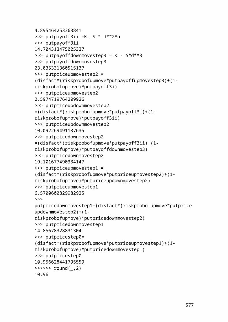
averageCallOptionPriceReturns = (CallOptionPriceReturns1 + CallOptionPriceReturns2 + CallOptionPriceReturns3 + CallOptionPriceReturns4 + CallOptionPriceReturns5 + CallOptionPriceReturns6)/6;

averagePutOptionPriceReturns = (PutOptionPriceReturns1 + PutOptionPriceReturns2 + PutOptionPriceReturns3 + PutOptionPriceReturns4 + PutOptionPriceReturns5 + PutOptionPriceReturns6)/6;

averageIndexOptionPriceReturns = (IndexOptionPriceReturns1 + IndexOptionPriceReturns2 + IndexOptionPriceReturns3 + IndexOptionPriceReturns4 + IndexOptionPriceReturns5 + IndexOptionPriceReturns6)/6;

harmonicaverageSharePriceReturns = (1/((1/SharePriceReturns1 + 1/SharePriceReturns2 + 1/SharePriceReturns3 + 1/SharePriceReturns4 + 1/SharePriceReturns5 + 1/SharePriceReturns6)/6));

harmonicaverageCallOptionPriceReturns = (1/((1/CallOptionPriceReturns1 + 1/CallOptionPriceReturns2 + 1/CallOptionPriceReturns3 + 1/CallOptionPriceReturns4 + 1/CallOptionPriceReturns5 + 1/CallOptionPriceReturns6)/6));

harmonicaveragePutOptionPriceReturns = (1/((1/PutOptionPriceReturns1 + 1/PutOptionPriceReturns2 + 1/PutOptionPriceReturns3 + 1/PutOptionPriceReturns4 + 1/PutOptionPriceReturns5 + 1/PutOptionPriceReturns6)/6));

harmonicaverageIndexOptionPriceReturns = (1/((1/IndexOptionPriceReturns1 + 1/IndexOptionPriceReturns2 + 1/IndexOptionPriceReturns3 + 1/IndexOptionPriceReturns4 + 1/IndexOptionPriceReturns5 + 1/IndexOptionPriceReturns6)/6));

System.out.print("The average is");System.out.println(averageSharePriceReturns);System.out.println(Math.round(averageSharePriceReturns*100.0)/100.0);System.out.print("The average of call option price returns is");System.out.println(averageCallOptionPriceReturns);System.out.println(Math.round(averageCallOptionPriceReturns*100.0)/100.0);System.out.print("The average of put option price returns is");System.out.println(averagePutOptionPriceReturns);System.out.println(Math.round(averagePutOptionPriceReturns*100.0)/100.0);System.out.print("The average of index option price returns is");System.out.println(averageIndexOptionPriceReturns);System.out.println(Math.round(averageIndexOptionPriceReturns*100.0)/100.0);System.out.print("The harmonic average of share price returns is");System.out.println(harmonicaverageSharePriceReturns);System.out.println(Math.round(harmonicaverageSharePriceReturns*100.0)/100.0);System.out.print("The harmonic average of call option price returns is");System.out.println(harmonicaverageCallOptionPriceReturns);System.out.println(Math.round(harmonicaverageCallOptionPriceReturns*100.0)/100.0);

577

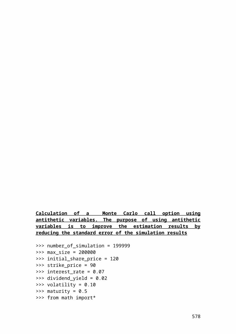
System.out.print("The harmonic average of put option price returns is");System.out.println(harmonicaveragePutOptionPriceReturns);System.out.println(Math.round(harmonicaveragePutOptionPriceReturns*100.0)/100.0);System.out.print("The harmonic average of index option price returns is");System.out.println(harmonicaverageIndexOptionPriceReturns);System.out.println(Math.round(harmonicaverageIndexOptionPriceReturns*100.0)/100.0);}}

Output results

After compiling the current document from tools and pressing the run document you should get the following results:

Welcome to DrJava. Working directory is C:\Documents and Settings\Owner\Desktop\Java Compiler> run average_and_harmonic_averageThe average is 0.048333333333333340.05The average of call option price returns is 0.040.04The average of put option price returns is 0.0650.07The average of index option price returns is 0.191666666666666680.19The harmonic average of share price returns is 0.038679969301611660.04The harmonic average of call option price returns is 0.0262773722627737270.03The harmonic average of put option price returns is 0.045721197459933470.05The harmonic average of index option price returns is 0.16492618393302230.16>

Exercise of how to calculate the payoff of buying a call, a put and the net result or position of your investment position expressed in pounds

class payoff

578

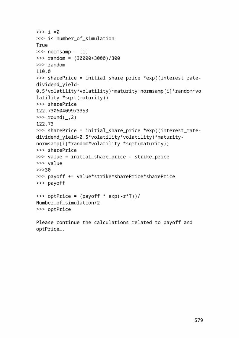
{public static void main(String[] args) {

/*payoff of buying a call, a put and the net result or position of your investment position expressed in pounds. */

double SharePrice1 = 105;double SharePrice2 = 110;double SharePrice3 = 120;double SharePrice4 = 130;double SharePrice5 = 140;double SharePrice6 = 150;

double ExercisePriceCall1 = 90;double ExercisePriceCall2 = 90;double ExercisePriceCall3 = 90;double ExercisePriceCall4 = 90;double ExercisePriceCall5 = 90;double ExercisePriceCall6 = 90;

double ExercisePricePut1 = 190;double ExercisePricePut2 = 190;double ExercisePricePut3 = 190;double ExercisePricePut4 = 190;double ExercisePricePut5 = 190;double ExercisePricePut6 = 190;

double PremiumofCall= 14;

double PremiumofPut =9;

double TotalNumberofContracts = 10;

double totalNumberOfShares =100;

double payoffBuyaCall1;double payoffBuyaCall2;double payoffBuyaCall3;double payoffBuyaCall4;double payoffBuyaCall5;double payoffBuyaCall6;

double payoffBuyaPut1;double payoffBuyaPut2;double payoffBuyaPut3;double payoffBuyaPut4;double payoffBuyaPut5;double payoffBuyaPut6;

double NetResult1;

579

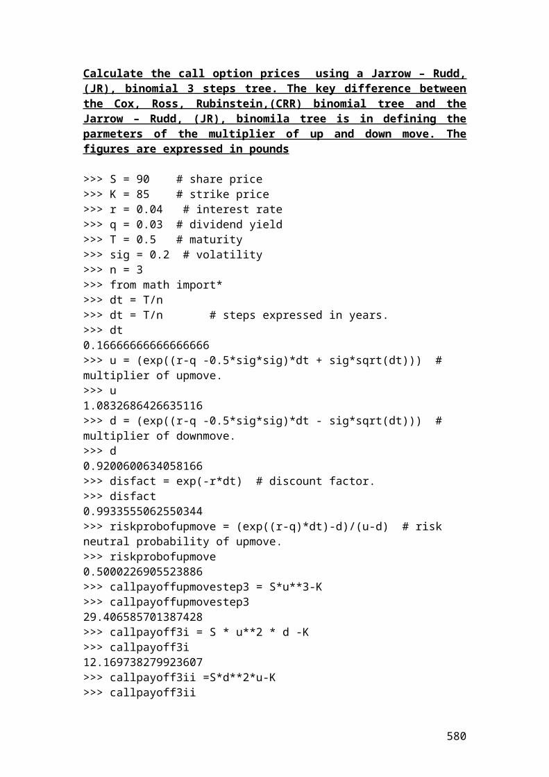
double NetResult2;double NetResult3;double NetResult4;double NetResult5;double NetResult6;

payoffBuyaCall1 = (SharePrice1-(ExercisePriceCall1+PremiumofCall))*TotalNumberofContracts*totalNumberOfShares;payoffBuyaCall2 = ( SharePrice2-(ExercisePriceCall2+PremiumofCall))*TotalNumberofContracts*totalNumberOfShares;payoffBuyaCall3 = ( SharePrice3-(ExercisePriceCall3+PremiumofCall))*TotalNumberofContracts*totalNumberOfShares;payoffBuyaCall4 = ( SharePrice4-(ExercisePriceCall4+PremiumofCall))*TotalNumberofContracts*totalNumberOfShares;payoffBuyaCall5 = ( SharePrice5-(ExercisePriceCall5+PremiumofCall))*TotalNumberofContracts*totalNumberOfShares;payoffBuyaCall6 = ( SharePrice6-(ExercisePriceCall6+PremiumofCall))*TotalNumberofContracts*totalNumberOfShares;

payoffBuyaPut1 = ( ExercisePricePut1-SharePrice1-PremiumofPut)*TotalNumberofContracts*totalNumberOfShares;payoffBuyaPut2 = ( ExercisePricePut2-SharePrice2-PremiumofPut)*TotalNumberofContracts*totalNumberOfShares;payoffBuyaPut3 = ( ExercisePricePut3-SharePrice3-PremiumofPut)*TotalNumberofContracts*totalNumberOfShares;payoffBuyaPut4 = ( ExercisePricePut4-SharePrice4-PremiumofPut)*TotalNumberofContracts*totalNumberOfShares;payoffBuyaPut5 = ( ExercisePricePut5-SharePrice5-PremiumofPut)*TotalNumberofContracts*totalNumberOfShares;payoffBuyaPut6 = ( ExercisePricePut6-SharePrice6-PremiumofPut)*TotalNumberofContracts*totalNumberOfShares;

NetResult1 = payoffBuyaCall1 - payoffBuyaPut1;NetResult2 = payoffBuyaCall2 - payoffBuyaPut2;NetResult3 = payoffBuyaCall3 - payoffBuyaPut3;NetResult4 = payoffBuyaCall4 - payoffBuyaPut4;NetResult5 = payoffBuyaCall5 - payoffBuyaPut5;NetResult6 = payoffBuyaCall6 - payoffBuyaPut6; System.out.print("The payoff buy a call 1 in pounds is");System.out.println(payoffBuyaCall1);System.out.print("The payoff buy a call 2 in pounds is");

580

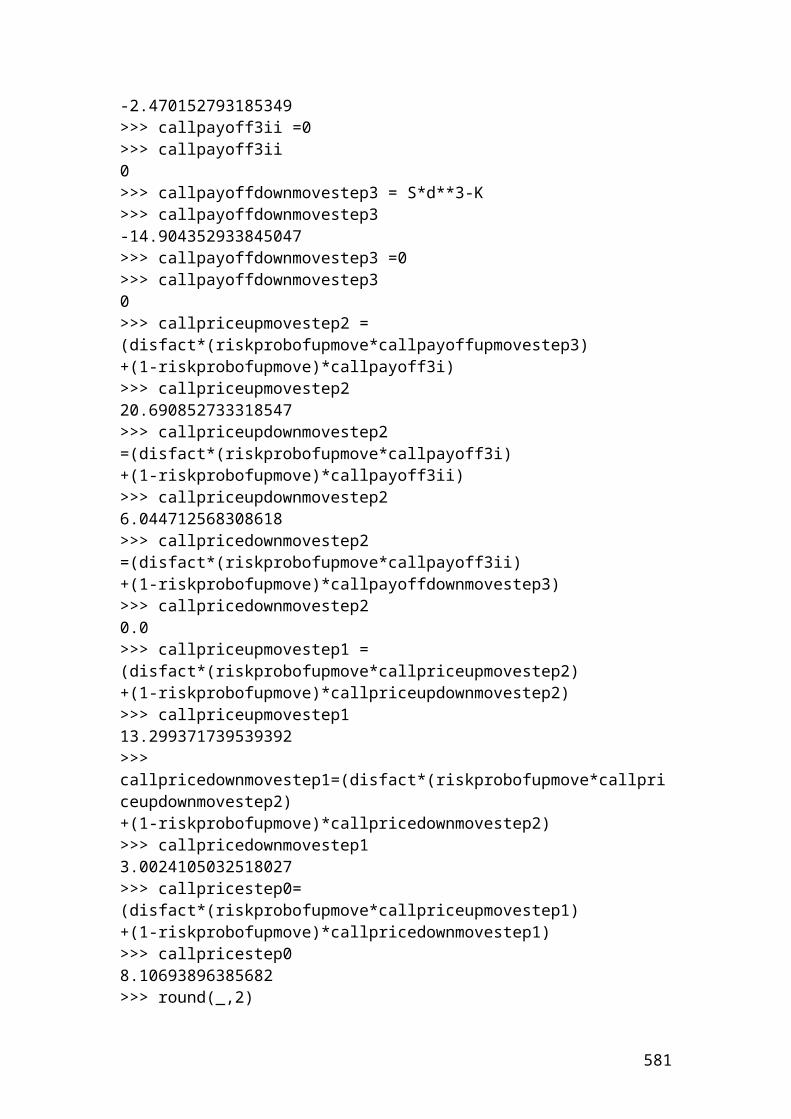
System.out.println(payoffBuyaCall2);System.out.print("The payoff buy a call 3 in pounds is");System.out.println(payoffBuyaCall3);System.out.print("The payoff buy a call 4 in pounds is");System.out.println(payoffBuyaCall4);System.out.print("The payoff buy a call 5 in pounds is");System.out.println(payoffBuyaCall5);System.out.print("The payoff buy a call 6 in pounds is");System.out.println(payoffBuyaCall6);System.out.print("The payoff buy a put 1 in pounds is");System.out.println(payoffBuyaPut1);System.out.print("The payoff buy a put 2 in pounds is");System.out.println(payoffBuyaPut2);System.out.print("The payoff buy a put 3 in pounds is");System.out.println(payoffBuyaPut3);System.out.print("The payoff buy a put 4 in pounds is");System.out.println(payoffBuyaPut4);System.out.print("The payoff buy a put 5 in pounds is");System.out.println(payoffBuyaPut5);System.out.print("The payoff buy a put 6 in pounds is");System.out.println(payoffBuyaPut6);System.out.print("The net result 1 in pounds is");System.out.println(NetResult1);System.out.print("The net result 2 in pounds is");System.out.println(NetResult2);System.out.print("The net result 3 in pounds is");System.out.println(NetResult3);System.out.print("The net result 4 in pounds is");System.out.println(NetResult4);System.out.print("The net result 5 in pounds is");System.out.println(NetResult5);System.out.print("The net result 6 in pounds is");System.out.println(NetResult6);}}

Output results

After compiling the current document from tools and pressing the run document you should get the following results:

581

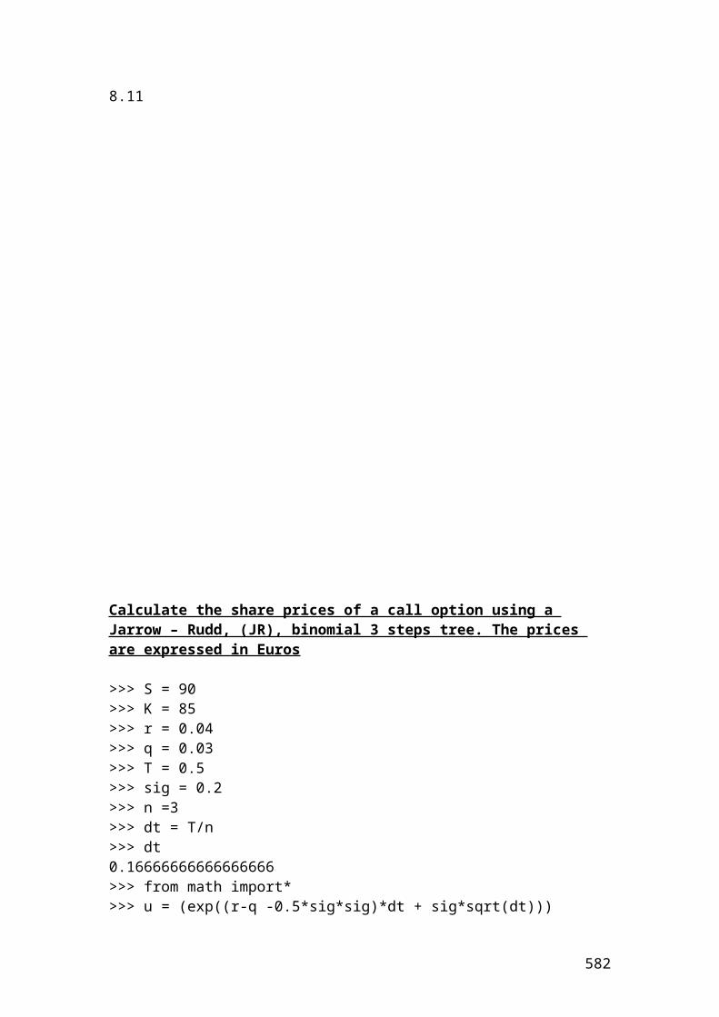
Welcome to DrJava. Working directory is C:\Documents and Settings\Owner\Desktop\Java Compiler> run payoff

The payoff buy a call 1 in pounds is1000.0The payoff buy a call 2 in pounds is6000.0The payoff buy a call 3 in pounds is16000.0The payoff buy a call 4 in pounds is26000.0The payoff buy a call 5 in pounds is36000.0The payoff buy a call 6 in pounds is46000.0The payoff buy a put 1 in pounds is76000.0The payoff buy a put 2 in pounds is71000.0The payoff buy a put 3 in pounds is61000.0The payoff buy a put 4 in pounds is51000.0The payoff buy a put 5 in pounds is41000.0The payoff buy a put 6 in pounds is31000.0The net result 1 in pounds is-75000.0The net result 2 in pounds is-65000.0The net result 3 in pounds is-45000.0The net result 4 in pounds is-25000.0The net result 5 in pounds is-5000.0The net result 6 in pounds is15000.0

Exercise

Please calculate the range in Java based on different share prices. The figures are nominated in USD.

582

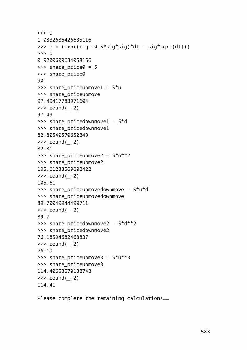
class range{public static void main(String[] args) {

// Calculate the range.

double share_price_1 = 20;double share_price_2 = 30;double share_price_3 = 40;double share_price_4 = 50;double share_price_5 = 60;double share_price_6 = 70;

double range_share_price;

// Insert the mathematical formula.

range_share_price = (share_price_6-share_price_1);

// Output function.System.out.print("The range of share price in $ is ");System.out.println(range_share_price);}}

Output result

After compiling the current document from tools and pressing the run document you should get the following result:

Welcome to DrJava. Working directory is C:\Documents and Settings\Owner\Desktop\Java Compiler> run rangeThe range of share price in $ is 50.0>

Calculate the log returns and the average using actual share price returns expressed in USD

class log_returns{

583

public static void main(String[] args) {

//Identify the variables.

double dailyret2;double dailyret3;double dailyret4;double dailyret5;double average;

// Actual share prices.

double share_price1 = 14.23;double share_price2 = 15.67;double share_price3 = 12.13;double share_price4 = 11.45;double share_price5 = 10.11;

// Insert the mathematical formulas. dailyret2 = (share_price2/share_price1);dailyret3 =(share_price3/ share_price2);dailyret4 =(share_price4/ share_price3);dailyret5 =(share_price5/ share_price4); // Output functions.System.out.print("The dailyret2 is ");System.out.println("Math.log("+ dailyret2 +")="+Math.log(dailyret2));System.out.println(Math.round(Math.log(dailyret2)*100.0)/100.0);System.out.print("The dailyret3 is ");System.out.println("Math.log("+ dailyret3 +")="+Math.log(dailyret3));System.out.println(Math.round(Math.log(dailyret3)*100.0)/100.0);System.out.print("The dailyret4 is ");System.out.println("Math.log("+ dailyret4 +")="+Math.log(dailyret4));System.out.println(Math.round(Math.log(dailyret4)*100.0)/100.0);System.out.print("The dailyret5 is ");System.out.println("Math.log("+ dailyret5 +")="+Math.log(dailyret5));System.out.println(Math.round(Math.log(dailyret5)*100.0)/100.0);}}

Output results

After compiling the current document from tools and pressing the run document you should get the following results:

584

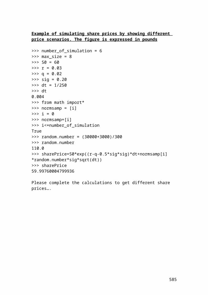
Welcome to DrJava. Working directory is C:\Documents and Settings\Owner\Desktop\Java Compiler> run log_returns

The dailyret2 is Math.log(1.101194659170766)=0.096395644266168450.1The dailyret3 is Math.log(0.7740906190172304)=-0.25606633341197066-0.26The dailyret4 is Math.log(0.9439406430338004)=-0.057691992955710175-0.06The dailyret5 is Math.log(0.8829694323144105)=-0.12446469696786859-0.12>

Calculation of the average, the daily and the annual volatility of percentage returns measured by the sample standard deviation

class average_and_standard_deviations

585

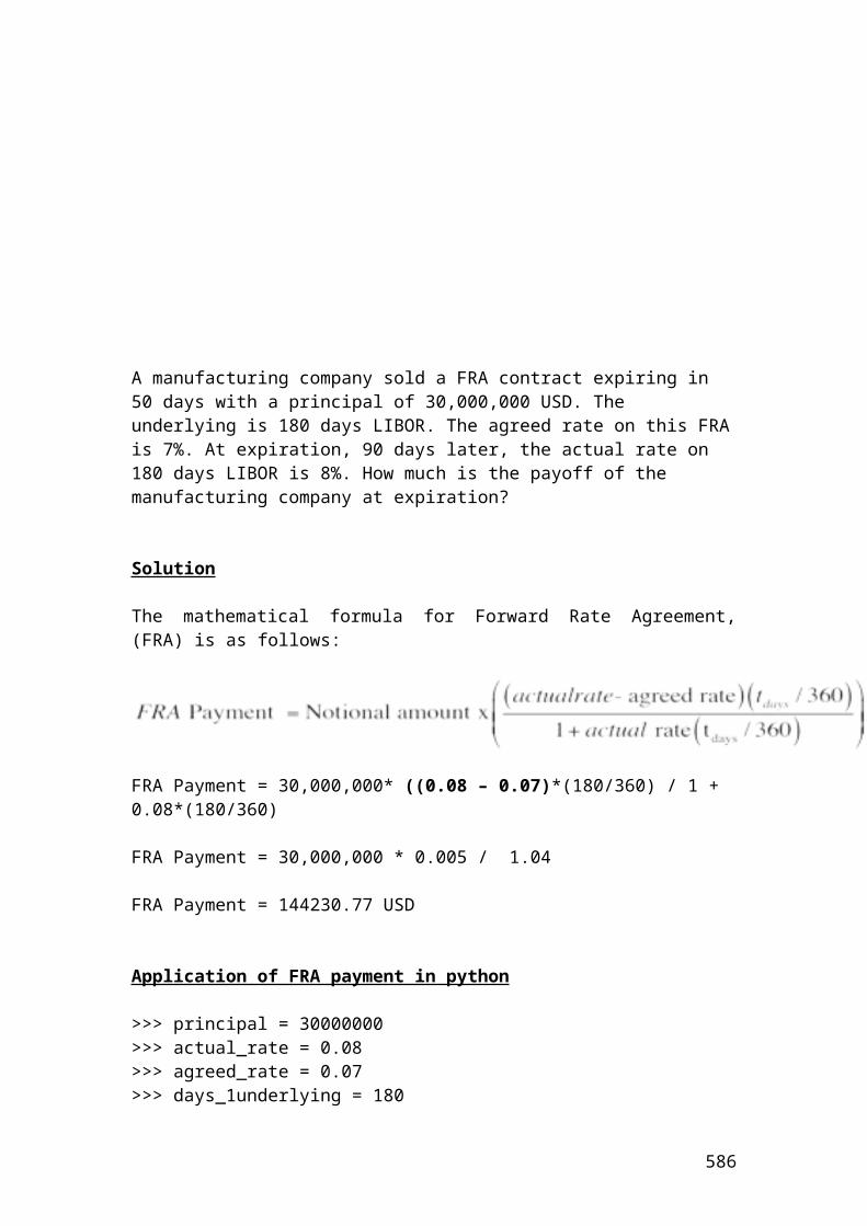
{public static void main(String[] args) {

// Identify the variables.

double sum=0 ;double average; double sumDiffSqr;double DailystdDev;double AnnualstdDev;

double[]sharePrices = new double[]{0.1423,0.1567,0.1213,0.1145,0.1011};

/* The following expression inserts a variable x that tells the computerthat the first observation 0 is 0.1423 and x is less than 5 to include all observations.*/

for (int x = 0; x < 5; x++)

//We insert the formula for summation.

sum += sharePrices[x];

// We insert the formula for average.average = sum/5;

/* We calculate the sumDiffSqr by inserting the expression for that tells the computer the numbers that will be included in the calculation. We calculate the difference between each number and the average. Then, we square it and we sum it.*/

sumDiffSqr = 0;for (int x = 0; x < 5; x++) { sumDiffSqr = sumDiffSqr + Math.pow((sharePrices[x]-average),2); }/* Insert the formula of the sample standard deviation by taking into account the formual n-1.*/

DailystdDev = Math.sqrt(sumDiffSqr/4);

//We use 250 trading days per year instead of 365 days.

AnnualstdDev = DailystdDev * Math.sqrt(250);

// Output functions.

System.out.print("The average is ");System.out.println(average);System.out.println(Math.round(average*100.0)/100.0);

586

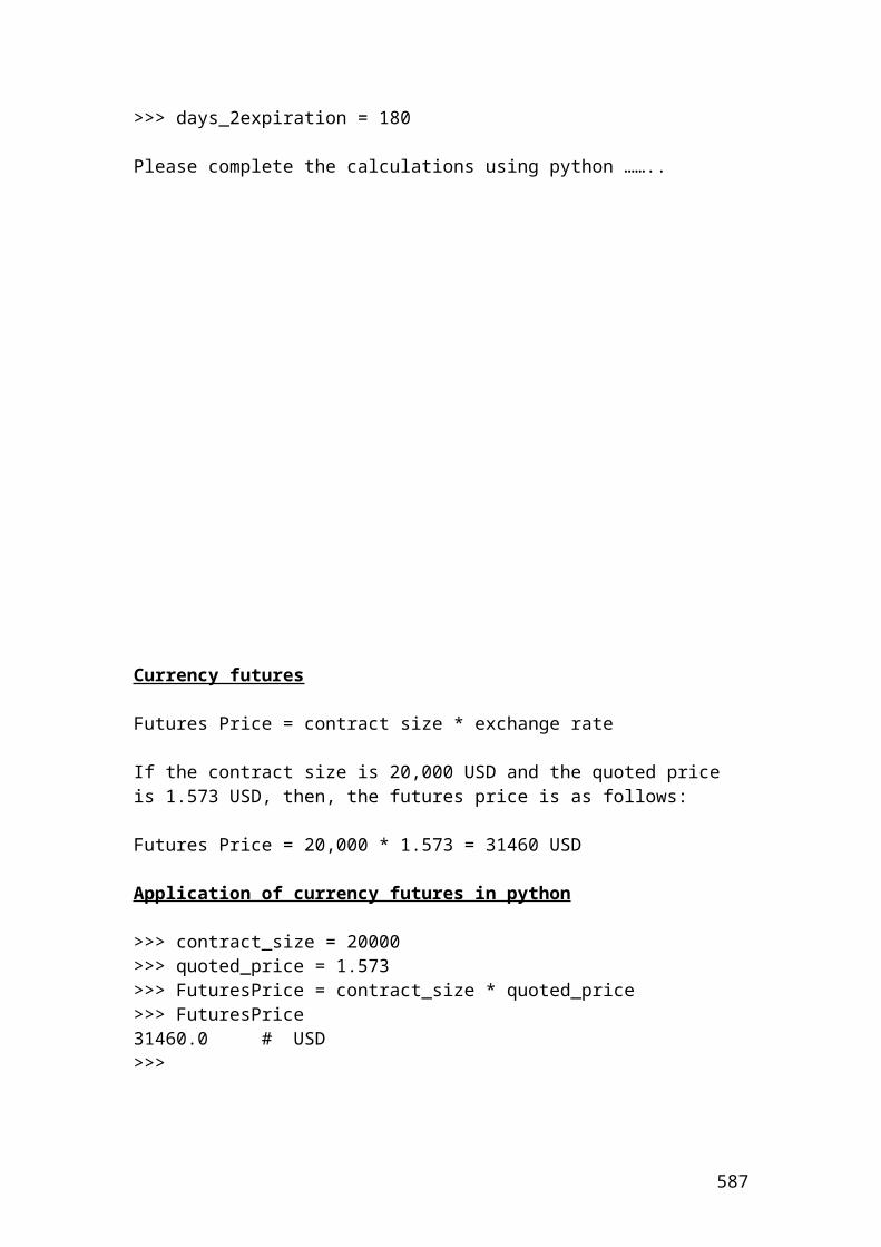
System.out.print("The daily standard deviation is ");System.out.println(DailystdDev);System.out.println(Math.round(DailystdDev*100.0)/100.0);System.out.print("The annual standard deviation is ");System.out.println(AnnualstdDev);System.out.println(Math.round(AnnualstdDev*100.0)/100.0);}}

Output results

After compiling the current document from tools and pressing the run document you should get the following results:

Welcome to DrJava. Working directory is C:\Documents and Settings\Owner\Desktop\Java Compiler> run average_and_standard_deviationsThe average is 0.127180000000000020.13The daily standard deviation is 0.022223681063226230.02The annual standard deviation is 0.351387250764736760.35>

Calculation of the geometric average based on percentages of call option price returns

class geometric_average_call_option_price_returns{

587

public static void main(String[] args) {

/* The call option price returns are expressed in percentages and we are trying to calculate the geometric mean or average. We insert the percentage values of each call option in an array format.*/

double call_option_price_return_1 = 5;double call_option_price_return_2 = 3;double call_option_price_return_3 = 2;double call_option_price_return_4 = 4;double call_option_price_return_5 = 7;double call_option_price_return_6 = 8;

// We define the variable that we want to calculate.double geometric_average;

// We write the mathematical equation of the geometric mean.

geometric_average = Math.pow(call_option_price_return_1*call_option_price_return_2*call_option_price_return_3*call_option_price_return_4*call_option_price_return_5*call_option_price_return_6,0.16666);

// Output functions.

System.out.println("Pow(" + call_option_price_return_1 + ", " + 0.16666 + ") = " + geometric_average);System.out.println(Math.round(geometric_average*100.0)/100.0); }}

Output result

After compiling the current document from tools and pressing the run document you should get the following result:

Welcome to DrJava. Working directory is C:\Documents and Settings\Owner\Desktop\Java Compiler> geometric_average_call_option_price_returnsPow(5.0, 0.16666) = 4.34379541978628854.34

Calculation of the geometric average based on percentages of stock prices returns

class geometric_average_share_prices_returns{

588

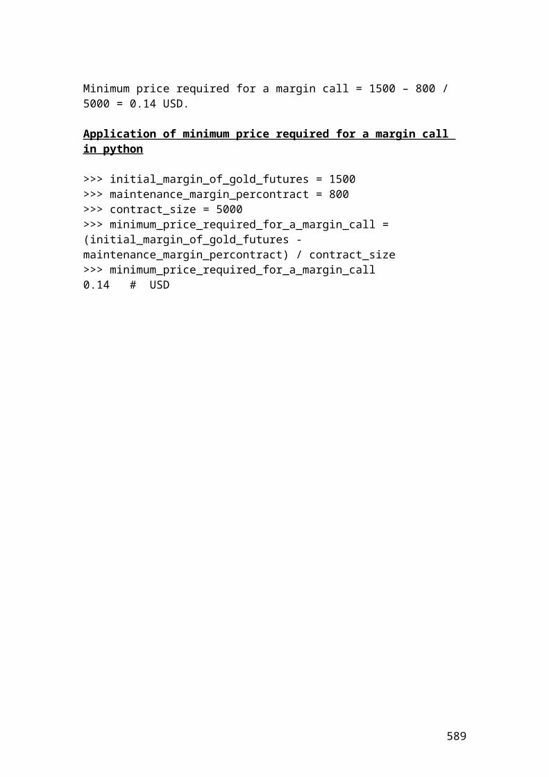
public static void main(String[] args) {

/* The stock prices express percentages and we are trying to calculate the geometric mean or average. We insert the percentage values of each stock in an array format.*/

double stock_price_1 = 10;double stock_price_2 = 12;double stock_price_3 = 13;double stock_price_4 = 14;double stock_price_5 = 15;double stock_price_6 = 16;

// We define the variable that we want to calculate.double geometric_average;

// We write the mathematical equation of the geometric mean.geometric_average = Math.pow(stock_price_1*stock_price_2*stock_price_3*stock_price_4*stock_price_5*stock_price_6,0.166666);

// Output functions.

System.out.println("Pow(" + stock_price_1 + ", " + 0.16666 + ") = " + geometric_average);System.out.println(Math.round(geometric_average*100.0)/100.0); }}

Output result

After compiling the current document from tools and pressing the run document you should get the following result:

Welcome to DrJava. Working directory is C:\Documents and Settings\Owner\Desktop\Java Compiler> geometric_average_share_prices_returnsPow(10.0, 0.16666) = 13.1797194671364513.18>

Calculation of the geometric average based on percentages of put option price returns

class geometric_average_put_option_price_returns{public static void main(String[] args) {

589

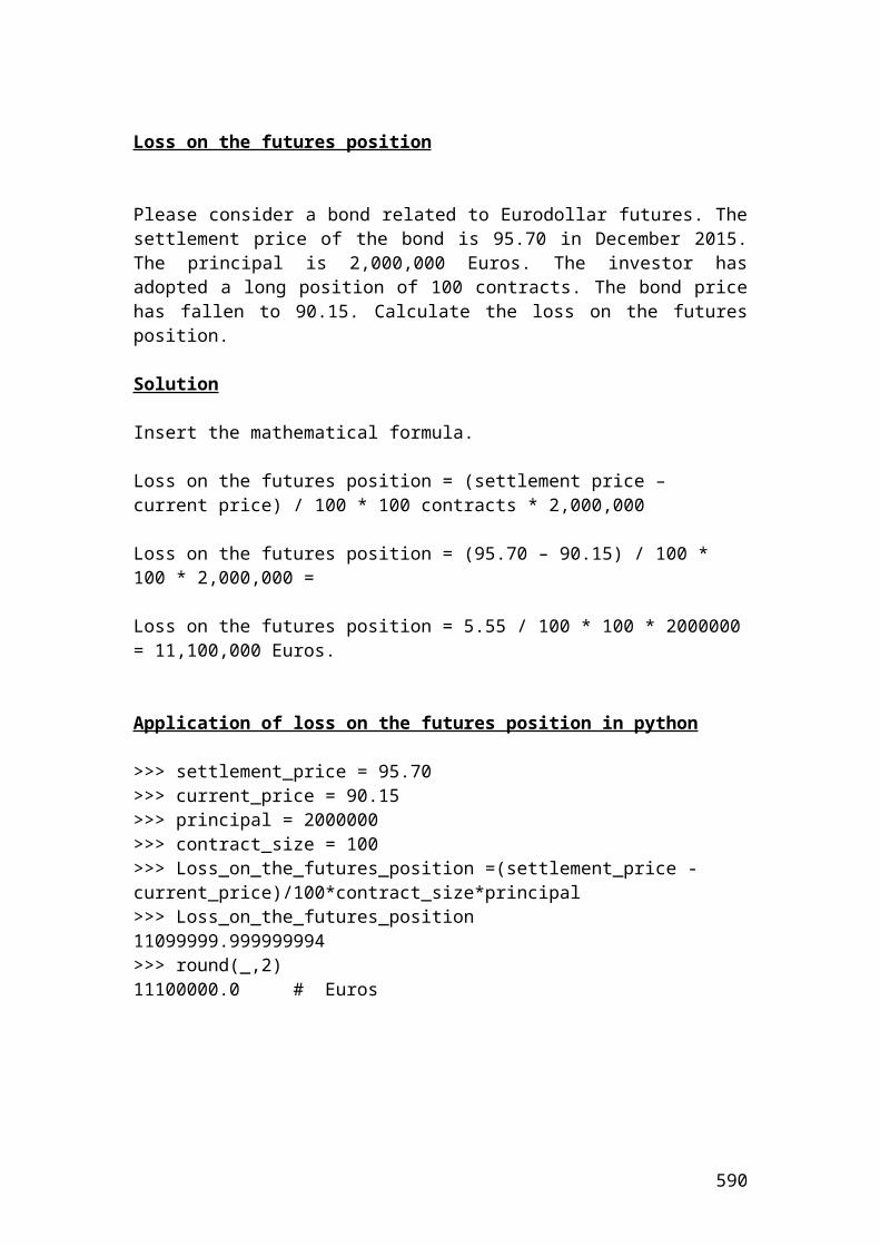
/* The put option price returns are expressed in percentages and we are trying to calculate the geometric mean or average.*/ // We insert the percentage values of each put option in an array format.

double put_option_price_return_1 = 2;double put_option_price_return_2 = 3.3;double put_option_price_return_3 = 2.45;double put_option_price_return_4 = 4.21;double put_option_price_return_5 = 7.4;double put_option_price_return_6 = 4.34;

// We define the variable that we want to calculate.double geometric_average;

// We write the mathematical equation of the geometric mean.

geometric_average = Math.pow(put_option_price_return_1*put_option_price_return_2*put_option_price_return_3*put_option_price_return_4*put_option_price_return_5*put_option_price_return_6,0.16666);

// Output functions.System.out.println("Pow(" + put_option_price_return_1 + ", " + 0.16666 + ") = " + geometric_average);System.out.println(Math.round(geometric_average*100.0)/100.0); }}

Output result

After compiling the current document from tools and pressing the run document you should get the following result:

Welcome to DrJava. Working directory is C:\Documents and Settings\Owner\Desktop\Java Compiler> geometric_average_put_option_price_returnsPow(2.0, 0.16666) = 3.60243922469834833.6>

Calculation of the geometric average based on percentages of index option price returns

class geometric_average_index_option_price_returns{

590

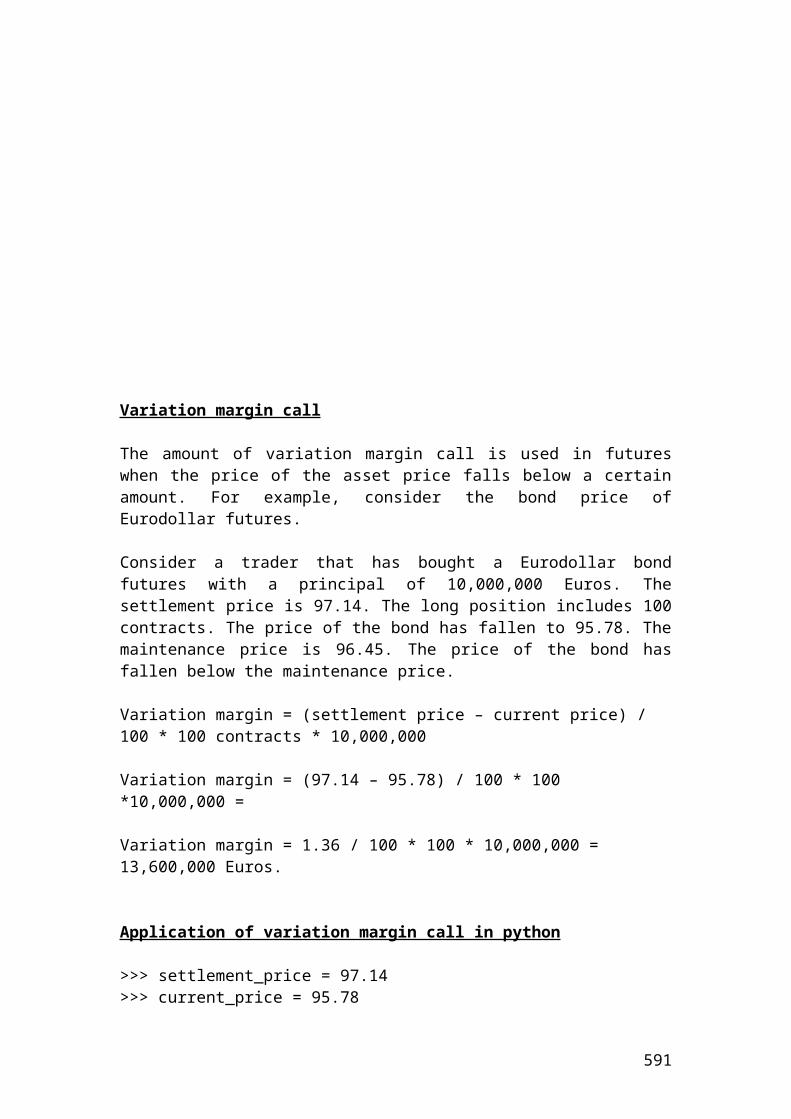
public static void main(String[] args) {

/* The Index option price returns are expressed in percentages and we are trying to //calculate the geometric mean or average. We insert the percentage values of each index option in an array format.*/

double index_option_price_return_1 = 2;double index_option_price_return_2 = 2.31;double index_option_price_return_3 = 2.35;double index_option_price_return_4 = 4.51;double index_option_price_return_5 = 7.56;double index_option_price_return_6 = 4.39;

// We define the variable that we want to calculate.double geometric_average;

// We write the mathematical equation of the geometric mean.

geometric_average = Math.pow(index_option_price_return_1*index_option_price_return_2*index_option_price_return_3*index_option_price_return_4*index_option_price_return_5*index_option_price_return_6,0.16666);

// Output functions.System.out.println("Pow(" + index_option_price_return_1 + ", " + 0.16666 + ") = " + geometric_average);System.out.println(Math.round(geometric_average*100.0)/100.0); }}

Output result

After compiling the current document from tools and pressing the run document you should get the following result:

Welcome to DrJava. Working directory is C:\Documents and Settings\Owner\Desktop\Java Compiler> run geometric_average_index_option_price_returnsPow(2.0, 0.16666) = 3.42865702048713543.43>

Calculate the portfolio return, the variance and the standard deviation in C++ for options with different returns and standard deviations

class portfolio_return_variance_and_standard_deviation{

591

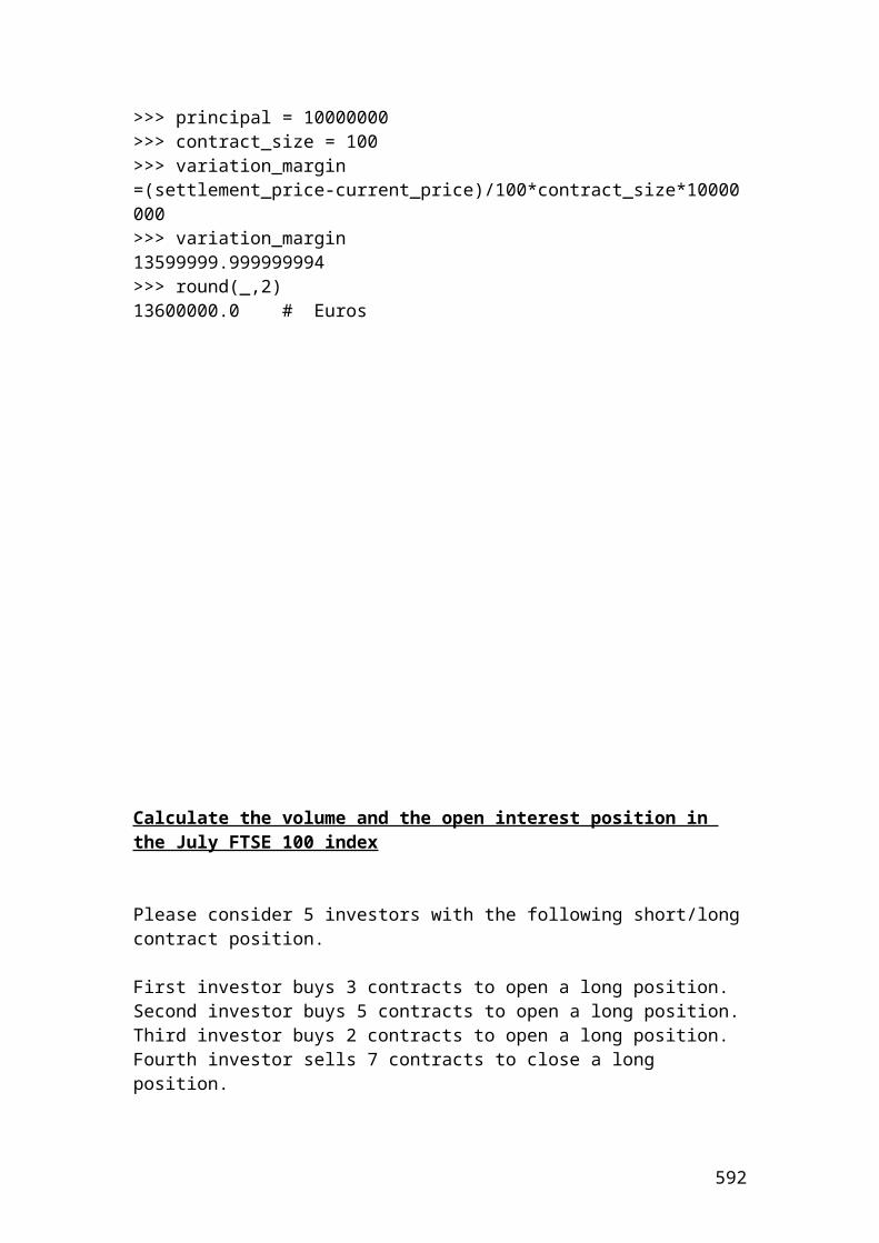
public static void main(String[] args) {

/* Calculate the portfolio return, the variance and the standard deviation or risk of theportfolio for options with different returns and standard deviations.*/

// Call option A expected return 0.6// Call option A standard deviation 0.2// Call option A weight 0.35// Correlation coefficient between A and B 0.5// Call option B expected return 0.1// Call option B standard deviation 0.7 // Call option B weight 0.45//Correlation coefficient between B and C -0.1// Call option C expected return 0.3// Call option C standard deviation 0.4// Call option C weight 0.2//Correlation coefficient between A and C -0.4

//Insert the given information by using the double function as we have fractions.

double CalloptionAexpectedreturn = 0.6;double CalloptionAstandarddeviation = 0.2;double CalloptionAweight = 0.35;double CorrelationcoefficientbetweenAandB = 0.5;double CalloptionBexpectedreturn = 0.1;double CalloptionBstandarddeviation = 0.7;double CalloptionBweight = 0.45;double CorrelationcoefficientbetweenBandC = -0.1;double CalloptionCexpectedreturn = 0.3;double CalloptionCstandarddeviation = 0.4;double CalloptionCweight = 0.2;double CorrelationcoefficientbetweenAandC = -0.4; /*Define the variables that we want to calculate. In other words, the portfolio return,variance and standard deviation.*/

double Portfolioreturn;double Portfoliovariance; double PortfoliostdDev;

// Write the formula of portfolio return.

Portfolioreturn = (CalloptionAexpectedreturn*CalloptionAweight)+(CalloptionBweight*CalloptionBexpectedreturn)+(CalloptionCexpectedreturn*CalloptionCweight);// Write the formula for portfolio variance.

Portfoliovariance = Math.pow(CalloptionAweight*CalloptionAstandarddeviation,2)+ Math.pow(CalloptionBweight*CalloptionBstandarddeviation,2)+ Math.pow(CalloptionCweight*CalloptionCstandarddeviation,2)

592

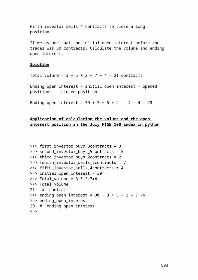
+(2*CalloptionAweight*CalloptionBweight*CalloptionAstandarddeviation*CalloptionBstandarddeviation*CorrelationcoefficientbetweenAandB)+(2*CalloptionAweight*CalloptionCweight*CorrelationcoefficientbetweenAandC*CalloptionAstandarddeviation*CalloptionCstandarddeviation)+(2*CalloptionBweight*CalloptionCweight*CorrelationcoefficientbetweenBandC*CalloptionBstandarddeviation*CalloptionCstandarddeviation);

// Write the formula for portfolio standard deviation.

PortfoliostdDev = Math.sqrt(Portfoliovariance);

//Output functions. System.out.print("The portfolio return is");System.out.println(Portfolioreturn);System.out.println(Math.round(Portfolioreturn*100.0)/100.0);System.out.print("The portfolio variance is");System.out.println(Portfoliovariance);System.out.println(Math.round(Portfoliovariance*100.0)/100.0);System.out.print("The portfolio standard deviation is");System.out.println(PortfoliostdDev);System.out.println(Math.round(PortfoliostdDev*100.0)/100.0);}}

Output results

After compiling the current document from tools and pressing the run document you should get the following results:

Welcome to DrJava. Working directory is C:\Documents and Settings\Owner\Desktop\Java Compiler> run portfolio_return_variance_and_standard_deviation

The portfolio return is0.3150.32The portfolio variance is0.123054999999999980.12The portfolio standard deviation is0.350791961139362450.35>

Calculate the portfolio return, the variance and the standard deviation or risk of the portfolio

class portfolio_return_variance_and_standard_deviation_of_portfolio{public static void main(String[] args) {

/* Calculate the portfolio return, the variance and the standard deviation or risk of the

593

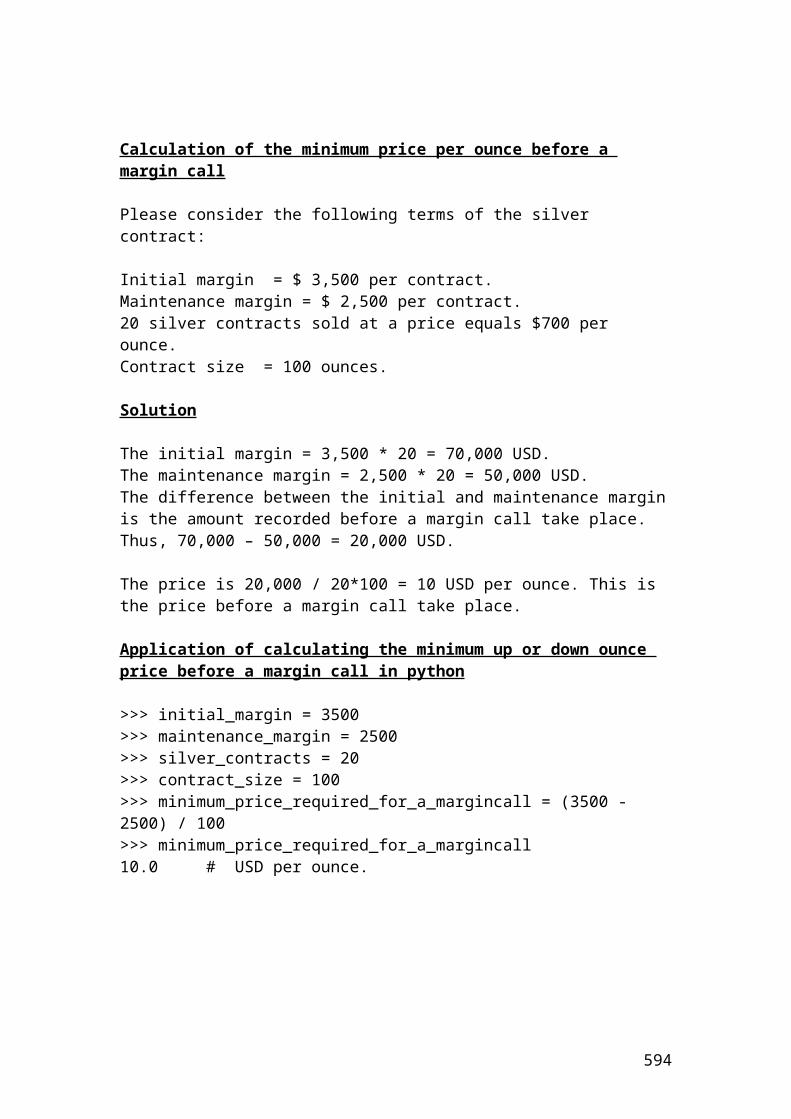
portfolio.*/

// Share A expected return 0.11// Share A standard deviation 0.15// Share A amount 50000// Correlation coefficient between A and B 0.30// Share B expected return 0.25// Share standard deviation 0.20 // Share B amount 50000// The total amount of the portfolio is 100000

double shareAexpRet = 0.25;double shareAstddev = 0.10;double shareAamount = 50000;double correlationAB = 0.40;double shareBexpRet = 0.35;double shareBstddev = 0.18;double shareBamount = 50000;double totalportfoliovalue = 100000;

/* Define the variables that we want to calculate.In other words, the portfolio return, variance and the standard deviation.*/

double weightA;double weightB;double Portfolioreturn;double Portfoliovariance; double PortfoliostdDev;

// Calculate the weights for each share.

weightA = shareAamount / totalportfoliovalue;weightB = shareBamount / totalportfoliovalue;

// Write the formula of portfolio return.

Portfolioreturn = (shareAexpRet*weightA)+(shareBexpRet*weightB);

// Write the formula for portfolio variance.

Portfoliovariance = Math.pow(weightA*shareAstddev,2)+ Math.pow(weightB*shareBstddev,2)+(2*weightA*weightB*shareAstddev*shareBstddev*correlationAB);

// Write the formula for portfolio standard deviation.

PortfoliostdDev = Math.sqrt(Portfoliovariance);

//Output functions.

594

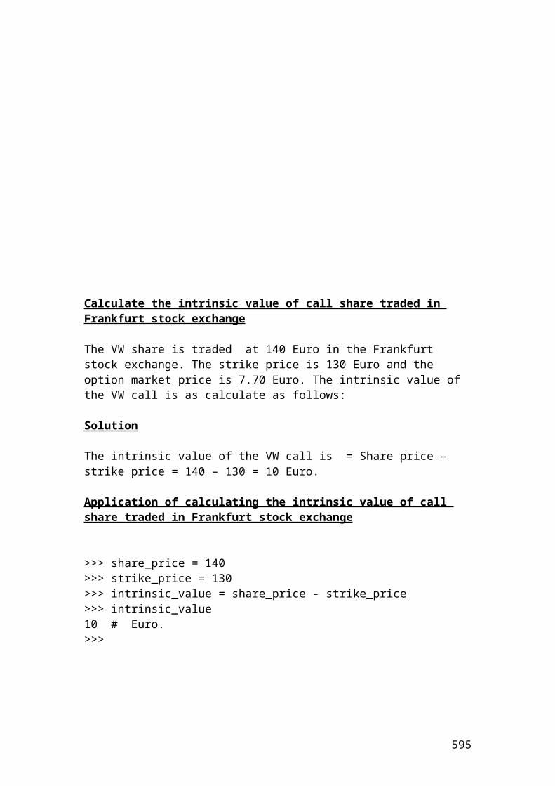
System.out.print("The portfolio return is");System.out.println(Portfolioreturn);System.out.println(Math.round(Portfolioreturn*100.0)/100.0);System.out.print("The portfolio variance is");System.out.println(Portfoliovariance);System.out.println(Math.round(Portfoliovariance*100.0)/100.0);System.out.print("The portfolio standard deviation is");System.out.println(PortfoliostdDev);System.out.println(Math.round(PortfoliostdDev*100.0)/100.0);}}

Output results

After compiling the current document from tools and pressing the run document you should get the following results:

Welcome to DrJava. Working directory is C:\Documents and Settings\Owner\Desktop\Java Compiler> run portfolio_return_variance_and_standard_deviation_of_portfolioThe portfolio return is0.30.3The portfolio variance is0.01420.01The portfolio standard deviation is0.119163752878129860.12>

Example of pricing a forward contract and solution

A forward contract of 6 month has a market price of 52 Pounds when the spot price of the underlying commodity is 49 Pounds. There are no costs of carry and the discount rate is 7 percent. Calculate the value of the forward contract.

Solution

595

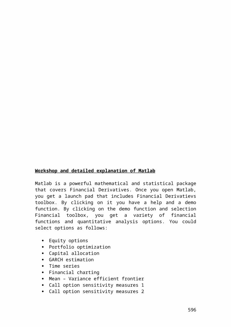
The current price of the forward contract (F0) should be equal to the value of the underlying commodity, (S0) at the discount rate r. Thus, the equation is as follows:

Application of pricing a forward contract in Java

class pricing_forward_contract{public static void main(String[] args) {

//Pricing a forward contract.

double Value_forward_contract;double spot_price = 49;double discount_rate = 0.07; // Insert the mathematical formula.

Value_forward_contract = spot_price*(1+discount_rate/2);

//Output function. System.out.print("The value of a forward contract in pounds is");System.out.println(Value_forward_contract);System.out.println(Math.round(Value_forward_contract*100.0)/100.0);

}}

Output result

After compiling the current document from tools and pressing the run document you should get the following result:

Welcome to DrJava. Working directory is C:\Documents and Settings\Owner\Desktop\Java Compiler> run pricing_forward_contractThe value of a forward contract in pounds is50.714999999999996

596

50.72>

Example of interest rate payment and solution

A trader wants to calculate the interest amount that he / she will receive in three months from a forward contract of a Euribor deposit paying a Euro deposit rate of 3.55%. The principal amount is 300,000

The mathematical formula is as follows:

597

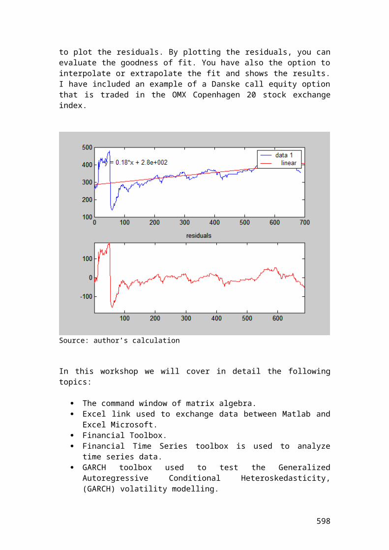
Interest payment = principal x [interest rate x (tdays / 360)]

Interest payment = 300,000 x [0.0355 x (90/360)]Interest payment = 2662.5 Euro.

First example: application of interest payment in Java

class interest_rate_payment{public static void main(String[] args) {

//Interest rate payment.

double interest_payment;double principal = 300000;double interest_rate = 0.0355;double days = 90;

// Insert the mathematical formula.

interest_payment = principal*(interest_rate *days/360);

//Output function. System.out.print("interest rate payment in euro is");System.out.println(interest_payment);System.out.println(Math.round(interest_payment*100.0)/100.0);}}

Output result

After compiling the current document from tools and pressing the run document you should get the following result:

Welcome to DrJava. Working directory is C:\Documents and Settings\Owner\Desktop\Java Compiler> run interest_rate_payment

598

interest rate payment in euro is 2662.49999999999952662.5>

Example and solution of calculating profits and losses on futures contracts

An investor buys 8 S&P 500 futures contracts at $2189. He has closed the futures contract position with a price of $2236. The multiplier for S&P 500 futures contracts is 250 dollars. Did he record a profit or a loss?

Solution

The mathematical formula is as follows:

599

Where: fT is the final contract price. f0 is the initial contract price.

USD

Application of calculating profits and losses on futures contracts in Java

class profits_losses_futures_contracts{public static void main(String[] args) {

// calculating profits and losses on futures contracts.

double profit_or_loss ; int number_of_contracts =8;double buying_price = 2189;double selling_price = 2236;int multiplier = 250;

// Insert the mathematical formula. profit_or_loss = number_of_contracts*multiplier*(selling_price - buying_price);

//Output function. System.out.print("Profit or loss on futures contract in USD is");System.out.println(profit_or_loss);System.out.println(Math.round(profit_or_loss*100.0)/100.0);

}}

Output result

After compiling the current document from tools and pressing the run document you should get the following result:

Welcome to DrJava. Working directory is C:\Documents and Settings\Owner\Desktop\Java Compiler> run profits_losses_futures_contractsProfit or loss on futures contract in USD is94000.0

600

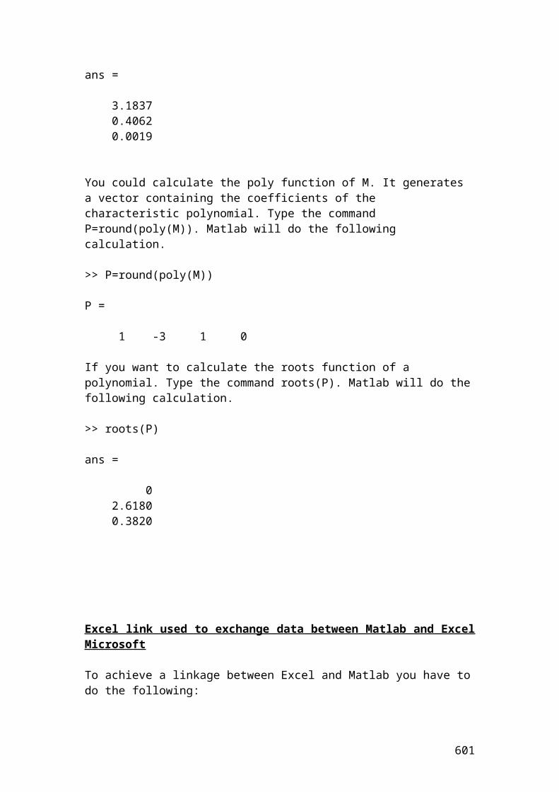
94000.0>

Example and solution of semiannually currency swap between an investment bank and an insurance company

The investment bank borrows 20,000,000 Pounds from the insurance company at a fixed rate of 5% for 1 year. The insurance company borrows from the investment bank 10,000,000 Euros at a fixed rate of 5% for 1 year. Calculate the interest payments for the three years, if we assume semiannual payments?

At the beginning of the contract

601

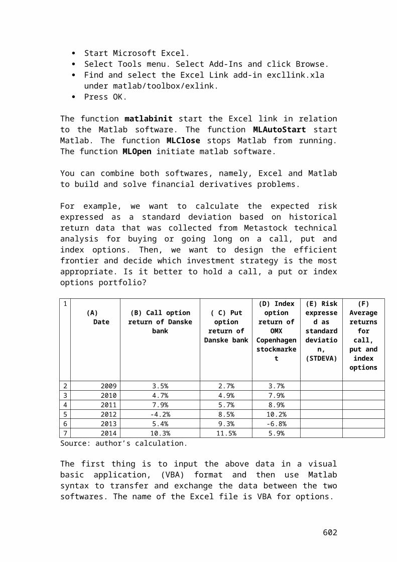
€10,000,000Investment bank Insurance company

£ 20,000,000

The insurance company pays the investment bank the following interest payment.

£20,000,000 x 0.05/2 = 500,000 Pounds.

The investment bank pays the insurance the following interest payment.

€10,000,000 x 0.05/2 =250,000 Euros.

The following arrows illustrate the interest payments.

€ 250,000Investment bank Insurance company

£ 500,000

At the end of the third year, the two parties exchange the principal amounts in addition to the final interest payments.

€10,250,000Investment bank Insurance company

£20,500,000

Application of semiannually currency swap between an investment bank and an insurance company in Java

class semiannual_currency_swap{public static void main(String[] args) {

//Semiannual swaps interest payments between an investment bank and an insurance company.

602

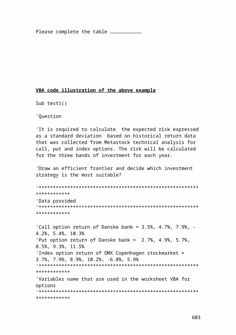
double bank_pays_insurance ;double insurance_pays_bank ;double bank_borrows_from_insurance =20000000;double insurance_borrows_from_bank = 10000000;double interest_rate = 0.05;int semi_annual_payment = 2;

//Insert the mathematical formulas. bank_pays_insurance = insurance_borrows_from_bank *(interest_rate/semi_annual_payment);insurance_pays_bank = bank_borrows_from_insurance *(interest_rate/semi_annual_payment);

//Output function. System.out.print("bank pays insurance in euros is");System.out.println(bank_pays_insurance);System.out.print("insurance pays bank in pounds is");System.out.println(insurance_pays_bank);}}

Output results

After compiling the current document from tools and pressing the run document you should get the following result:

Welcome to DrJava. Working directory is C:\Documents and Settings\Owner\Desktop\Java Compiler> run semiannual_currency_swapbank pays insurance in euros is 250000.0insurance pays bank in pounds is 500000.0>

Example and solution of interest rate swap

Interest rate swaps are very popular agreements between two parties in the debt or fixed-income department of the investment banks. The fixed income department of Bank A pays a fixed rate of 5.5% upon the principal of 50,000,000 Pounds. In contrast, Bank B pays a floating or reference rate of LIBOR accounted to 7.2%. The payment frequency is every 6 months for 2 years.

603

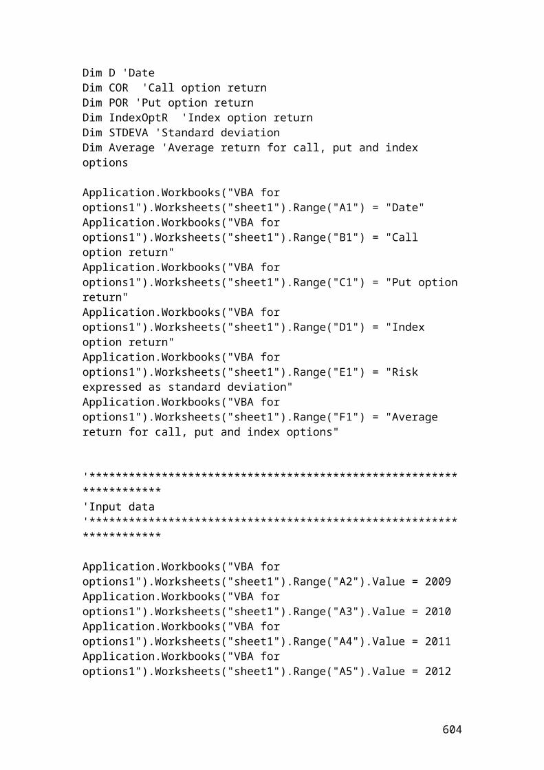
Fixed payment : £50,000,000 x 0.055/2 = 1,375,000 Bank A Bank B Floating payment: £50,000,000 x 0.072/2 = 1,800,000

Suppose in the second year that the LIBOR has increased by 12 basis points or 0.12%. Then, the floating payment will change and the calculation will be as follows:

Second year floating payment for Bank B = 50,000,000 x 0.0732 / 2 = 1,830,000 Pounds.

Bank A will continue to pay the same fixed amount, namely, £50,000,000 x 0.055/2 = £1,375,000.

Application of interest rate swap in Java

class interest_rate_swap{public static void main(String[] args) {//Semiannual swaps interest payments between two parties.

double fixed_payment ;double floating_payment_1 ;

604

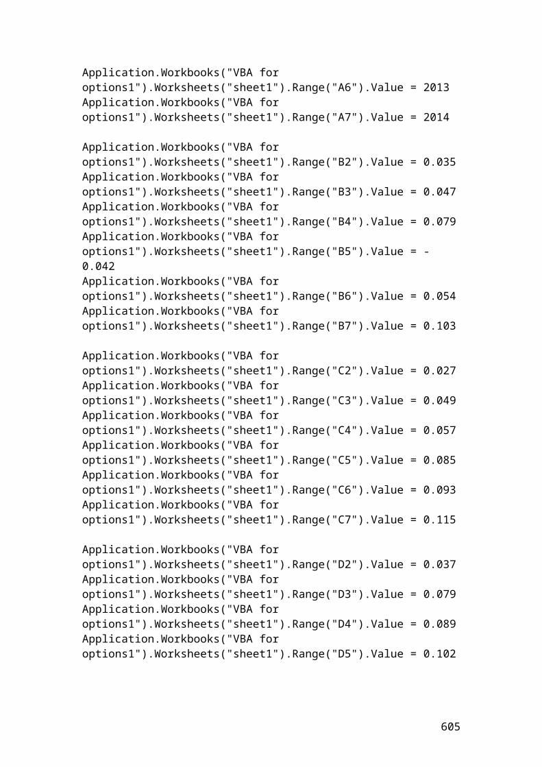
double floating_payment_2 ;double principal = 50000000;double interest_rate_1 = 0.055;double interest_rate_2 = 0.072;double interest_rate_3 = 0.0732;int semiannual_payment = 2;

// Insert the mathematical formulas. fixed_payment = principal*(interest_rate_1/semiannual_payment);floating_payment_1 = principal*(interest_rate_2/semiannual_payment);floating_payment_2 = principal*(interest_rate_3/semiannual_payment);

//Output functions.System.out.print("The value of a fixed payment in pounds is");System.out.println(fixed_payment);System.out.println(Math.round(fixed_payment*100.0)/100.0);System.out.print("The value of a floating payment 1 in pounds is");System.out.println(floating_payment_1);System.out.println(Math.round(floating_payment_1*100.0)/100.0);System.out.print("The value of a floating payment 2 in pounds is");System.out.println(floating_payment_2);System.out.println(Math.round(floating_payment_2*100.0)/100.0);}}

Output results

After compiling the current document from tools and pressing the run document you should get the following results:

Welcome to DrJava. Working directory is C:\Documents and Settings\Owner\Desktop\Java Compiler> run interest_rate_swapThe value of a fixed payment in pounds is1375000.01375000.0The value of a floating payment 1 in pounds is1799999.99999999981800000.0The value of a floating payment 2 in pounds is1830000.01830000.0>Delta – neutral hedge

Delta – neutral hedge is common used in risk management to keep the value of the portfolio neutral due to changes in the share price. It is achieved from a long position in a share and a short position in a call option. The mathematical formula to determine the number of options is as follows:

605

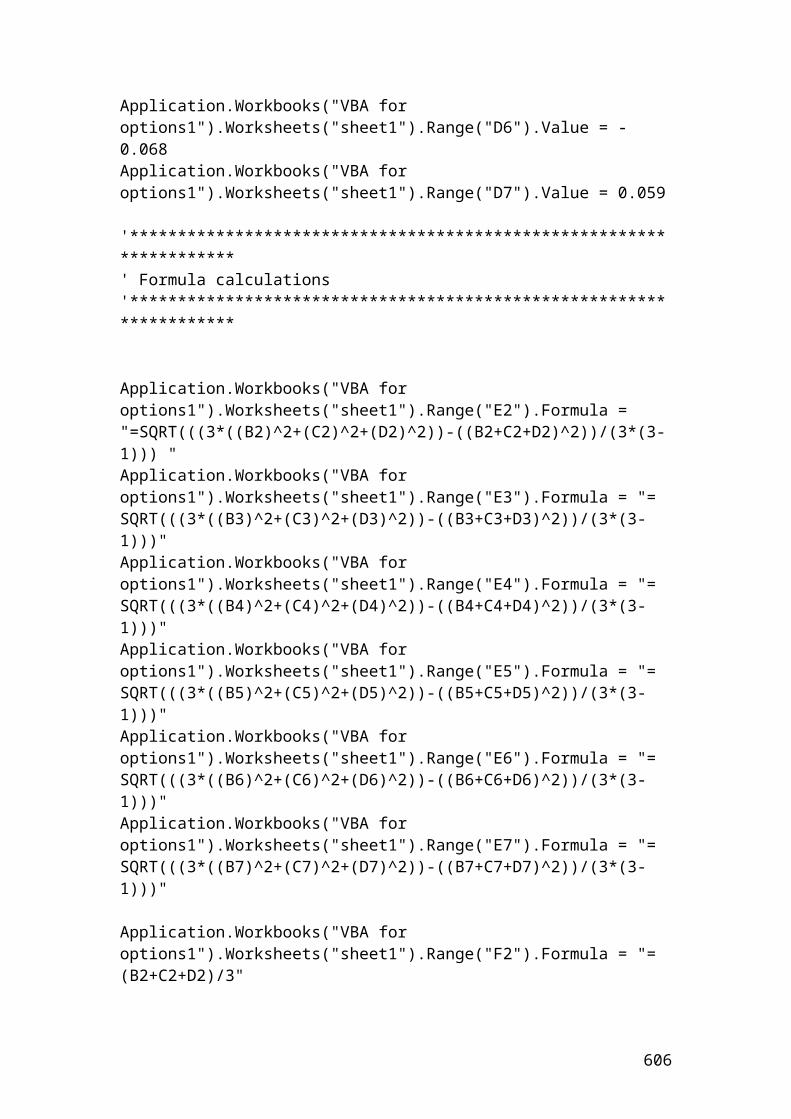
Thus, if the investment bank has bought 30,000 shares of Vodafone and the delta of the call option of the same company is 0.50, then the numbers of call options that are needed to purchase to form a delta-neutral hedge are as follows:

Delta hedge = 30,000 / 0.50 = 60,000 options or 600 option contracts.

Application of delta- neutral hedge in Java

class delta_neutral_hedge{public static void main(String[] args) { // Delta neutral hedge.

double delta_neutral_hedge ;double number_of_shares = 30000 ;double delta_call_option = 0.50 ; // Insert the mathematical equation.

delta_neutral_hedge = number_of_shares/delta_call_option;

// Output function.

System.out.print("The delta neutral hedge is");System.out.println(delta_neutral_hedge);System.out.println(Math.round(delta_neutral_hedge*100.0)/100.0);

}}

Output result

After compiling the current document from tools and pressing the run document you should get the following result:

Welcome to DrJava. Working directory is C:\Documents and Settings\Owner\Desktop\Java Compiler> run delta_neutral_hedge

606

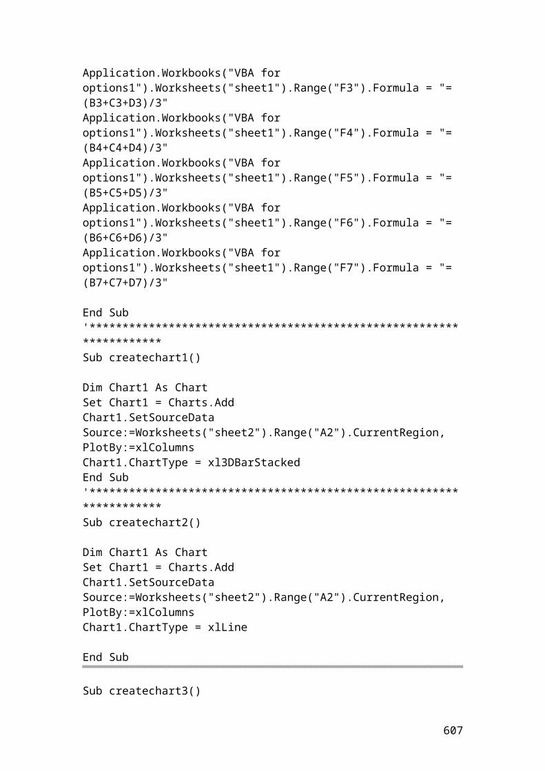
The delta neutral hedge is60000.060000.0>

Weighted mean price of a portfolio

Let’s assume that we have a portfolio of four options with their market prices and the number of shares bought. It is required to calculate the weighted mean price of the portfolio.

Options Price expressed in $

Number of shares

Weight Weight x Price

A 14.00 300 0.4 5.6

607

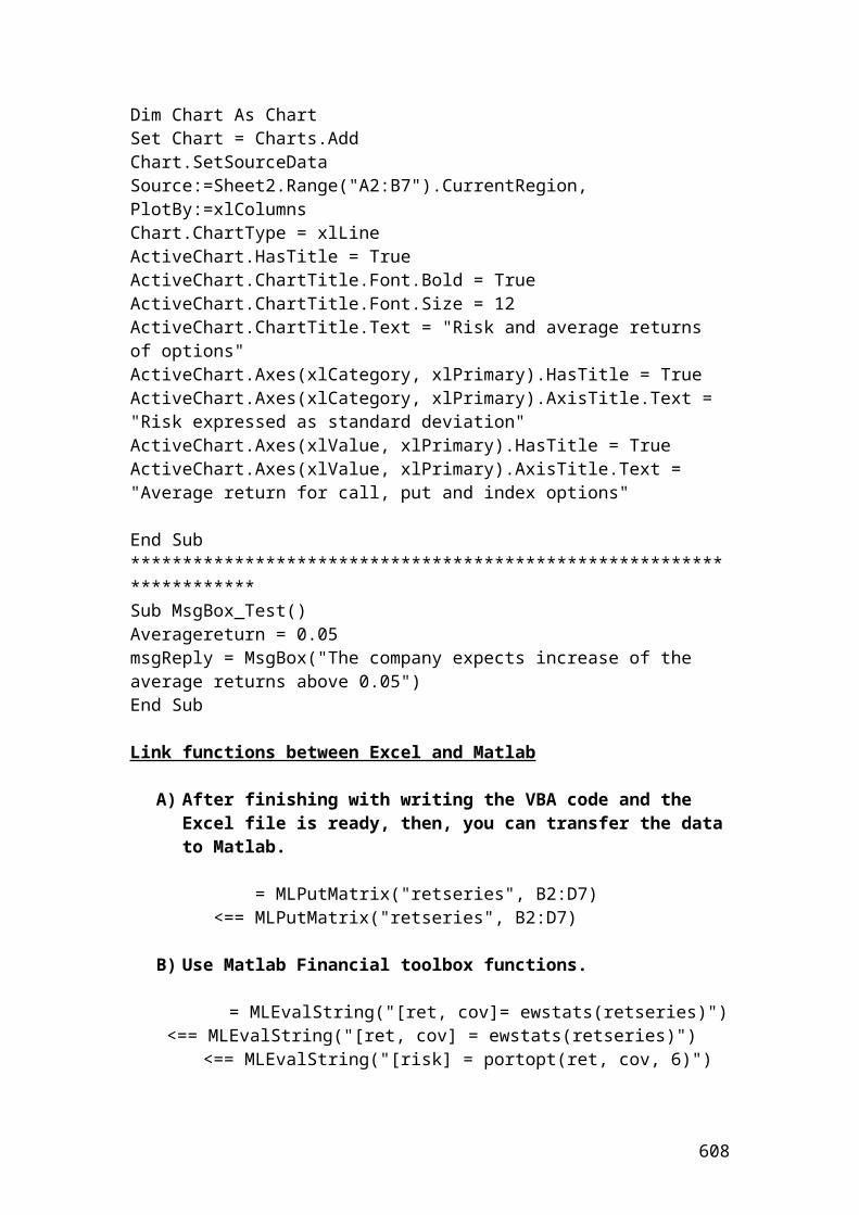
B 12.00 200 0.3 3.6C 8.00 100 0.1 0.8D 5.00 150 0.2 1

Total 750 1Source: author’s calculation

The mathematical formula is as followed:

By substituting the numbers from the Table into the equation we have the following:

0.8 + 1 = 11.

Application of weighted mean price of a portfolio in Java

class weighted_mean_price_portfolio{public static void main(String[] args) {

// Weighted mean price of a portfolio. double portfolio_mean ;

double price_1 = 14;double price_2 = 12;double price_3 = 8;double price_4 = 5;

double weight_1 = 0.4;double weight_2 = 0.3;double weight_3 = 0.1;double weight_4 = 0.2;

// Insert the mathematical equation.

portfolio_mean = (price_1*weight_1 + price_2*weight_2 + price_3*weight_3 + price_4*weight_4) ;

//Output function. System.out.print("The weighted mean price of a portfolio in USD is");System.out.println(portfolio_mean);}

608

}

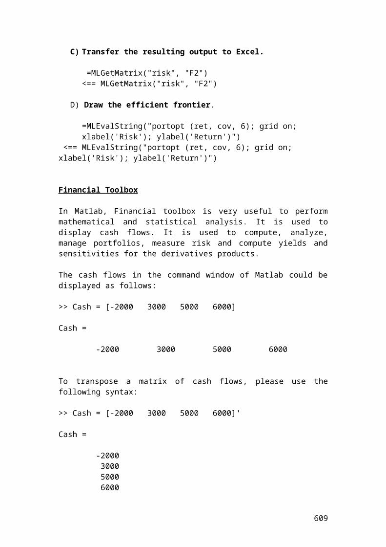
Output result

After compiling the current document from tools and pressing the run document you should get the following result:

Welcome to DrJava. Working directory is C:\Documents and Settings\Owner\Desktop\Java Compiler> run weighted_mean_price_portfolioThe weighted mean price of a portfolio in USD is11.0>

Example of Eurodollar futures

An investor wants to calculate the futures price of a 1-month Eurodollar time deposits based on a LIBOR rate of 3.40%. The initial principal is 1 million Pounds.

Solution

The price of the Eurodollar futures contract will be as follows:

609

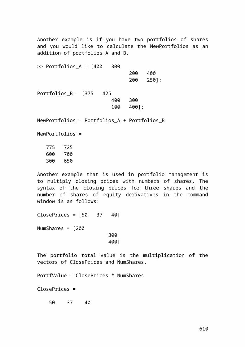
Application of Eurodollar futures in Java

class Eurodollar_futures{public static void main(String[] args) {

double Eurodollar_futures;double principal = 1000000;double interest_rate = 0.034;int days = 30;

// Insert the mathematical formula.

Eurodollar_futures = principal*(1- interest_rate *days/360);

//Output function. System.out.print("Eurodollar futures in pounds is");System.out.println(Eurodollar_futures);System.out.println(Math.round(Eurodollar_futures*100.0)/100.0);}}

Output result

After compiling the current document from tools and pressing the run document you should get the following result:

Welcome to DrJava. Working directory is C:\Documents and Settings\Owner\Desktop\Java Compiler> run Eurodollar_futuresEurodollar futures in pounds is997166.6666666666997166.67

610

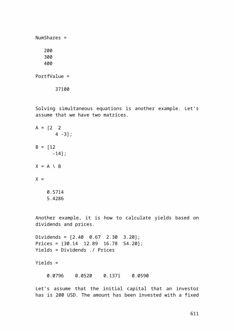
Example of forward rate agreement

An investment bank buys a 4 x 6 FRA from a building society in the UK for 4.0% by paying 2 million Pounds. 80 days latter, LIBOR is 5%. Who will receive the FRA payment and for how much?

Solution

The mathematical formula for Forward Rate Agreement, (FRA) is as follows:

The timeline schedule is as follows:

t = 0 4months 6 months

= ………. Please complete

the calculation.

Helpful hint: If the FRA payment is positive, then, the building society is the payer and the investment bank receives the FRA payment.

If the FRA payment is negative, then the investment bank is the payer and the building society receives the FRA payment.

Application of forward rate agreement in Java

class Forward_rate_agreement{public static void main(String[] args) {

double FRApayment;double principal = 2000000;double variable_rate = 0.05;double fixed_rate = 0.04;

611

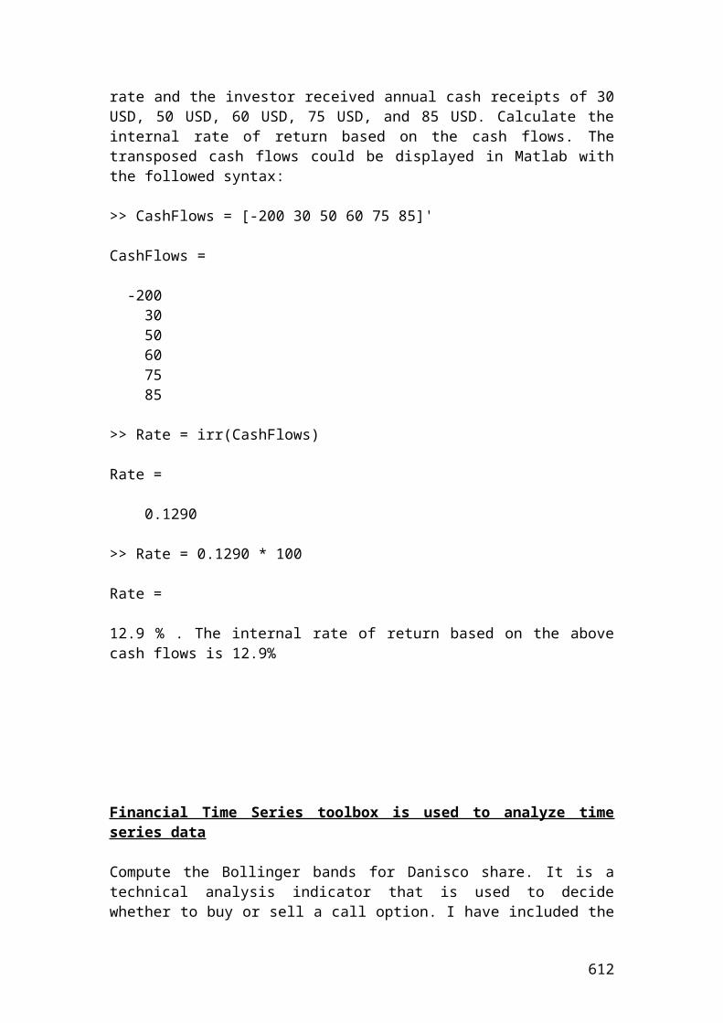
// Insert the mathematical formula.FRApayment= principal*(variable_rate - fixed_rate)*0.333333333/1.011111111;

// Output function.

System.out.print("Forward rate agreement in pounds is");System.out.println(FRApayment);System.out.println(Math.round(FRApayment*100.0)/100.0);}}

Output result

After compiling the current document from tools and pressing the run document you should get the following result:

Welcome to DrJava. Working directory is C:\Documents and Settings\Owner\Desktop\Java Compiler> run Forward_rate_agreementForward rate agreement in pounds is6593.4065875377396593.41>

Example of futures on Treasury bills

An investor wants to calculate the futures price of a 3-month Treasury bills. Treasury bills are short-term notes of limited period of 1- month, and 3 - month respectively. The initial principal is 5 million Pounds and the discount rate is 3.50%.

Solution

The price of the Treasury bill futures will be as follows:

612

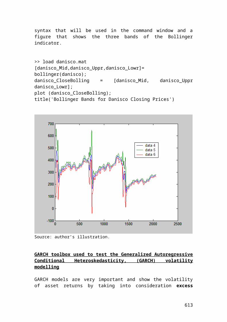
Please complete the calculation …….

Application of futures on Treasury bills in Java

class Futures_Treasury_bills{public static void main(String[] args) {

double Futures_treasury_bills;double principal = 5000000;double discount_rate = 0.035;int days = 90;

//Insert the mathematical formula.

Futures_treasury_bills = principal*(1- discount_rate *days/360);

//Output function.

System.out.print("Futures on treasury bills in pounds is");System.out.println(Futures_treasury_bills);System.out.println(Math.round(Futures_treasury_bills*100.0)/100.0);}}

Output result

After compiling the current document from tools and pressing the run document you should get the following result:

Welcome to DrJava. Working directory is C:\Documents and Settings\Owner\Desktop\Java Compiler> run Futures_Treasury_billsFutures on treasury bills in pounds is4956250.04956250.0>

Example of stock index futures

For example, if you bought 10 contracts of the Dow Jones Industrial index at 10,000 and you expected an aggressive bull market that reaches the value of 16,000, then, the 6000 points increase are multiplied by the standardized value of 250. If the initial principal of investment is $100,000, the mathematical formula for the gains will be as follows:

613

10 x 100,000 x 6000 x 250 = 1.5 x 1012 Dollars

Application of stock index futures in Java

class Stock_index_futures{public static void main(String[] args) { //The gains from stock index futures. double gains;double principal = 100000;double pointsincrease = 6000; int number_of_contracts = 10;int multiplier = 250;

// Insert the mathematical formula.

gains = principal*pointsincrease*multiplier*number_of_contracts;

// Output function.

System.out.print("The gains from stock index futures in USD are");System.out.println(gains);System.out.println(Math.round(gains*100.0)/100.0);

}}

Output result

After compiling the current document from tools and pressing the run document you should get the following result:

Welcome to DrJava. Working directory is C:\Documents and Settings\Owner\Desktop\Java Compiler> run Stock_index_futuresThe gains from stock index futures in USD are1.5E121.5E12>

Example of currency futures

A manufacturer wants to calculate the currency futures price of EURO/USD traded in Frankfurt derivative market. For example, in August the contract is quoted as 1.35 EURO /USD and the contract size is 20,000. The principal is 300,000 Euro.

Solution

The contract price of 1 contract is as follows:

614

Application of currency futures in Java

class Currency_futures{public static void main(String[] args) {

double Futures_price_of_currency;double principal = 300000;double quote = 1.35;int contract_size = 20000;

// Insert the mathematical formula.Futures_price_of_currency = principal*quote*contract_size ;

// Output function.

System.out.print("Futures price of currency in euro is");System.out.println(Futures_price_of_currency);System.out.println(Math.round(Futures_price_of_currency*100.0)/100.0);}}

Output result

After compiling the current document from tools and pressing the run document you should get the following result:

Welcome to DrJava. Working directory is C:\Documents and Settings\Owner\Desktop\Java Compiler> run Currency_futuresFutures price of currency in euro is8.1E98.1E9

615

Example of calculating implied volatility of a call option price due to volatility

class Implied_volatility{public static void main(String[] args) { double S = 80.0; double K = 80.0; double r = 0.04; double q = 0.01;

616

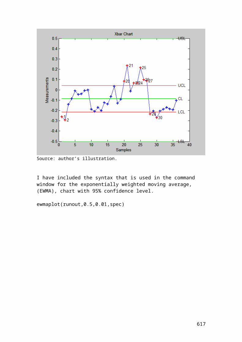
double T = 0.50; double sig, optPrice,tolerance ; int i;

optPrice = 8.34; // Option price. sig = 0; tolerance = 0.01; // Specification for the sigma or volatility with tolerance level //in relation with the theoretical and market option price. for(i = 1; i < 80 ; i++) { sig += tolerance; } // Output functions. System.out.print("Implied volatility is");System.out.println(sig);System.out.println(Math.round(sig*100.0)/100.0);System.out.print("Current option pricein USD is ");System.out.println(optPrice);}} Output results

After compiling the current document from tools and pressing the run document you should get the following results:

Welcome to DrJava. Working directory is C:\Documents and Settings\Owner\Desktop\Java Compiler> run Implied_volatilityImplied volatility is0.79000000000000050.79Current option price in USD is 8.34>

Example of calculating implied volatility of a put option price due to volatility

class Implied_volatility{public static void main(String[] args) { double S = 50.0; double K = 50.0; double r = 0.04; double q = 0.01; double T = 0.50;

617

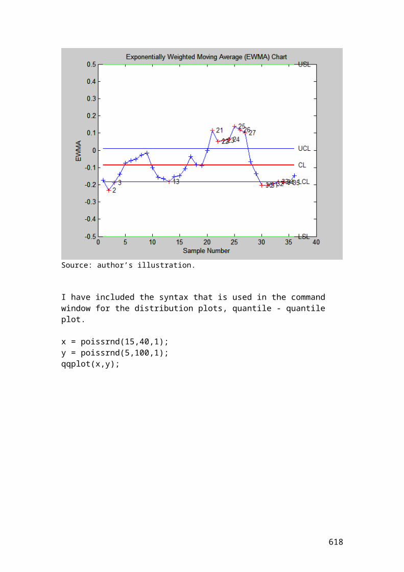
double sig, optPrice,tolerance ; int i;

optPrice = 5.34; // Put option price. sig = 0; tolerance = 0.01; /* Specification for the sigma or volatility with tolerance level in relation with the theoretical and market option price.*/ for(i = 1; i < 50 ; i++) { sig += tolerance; } // Output functions. System.out.print("Implied volatility is");System.out.println(sig);System.out.println(Math.round(sig*100.0)/100.0);System.out.print("Current option price in USD is ");System.out.println(optPrice);}}

Output results

After compiling the current document from tools and pressing the run document you should get the following results:

> run Implied_volatilityImplied volatility is0.490000000000000270.49Current option price in USD is 5.34>

Please try based on the previous examples to illustrate the following example in Java. If you have difficulties e-mail me

Active return, active risk and information ratio

Active return is the difference in returns between a portfolio and the index or benchmark that is measured.

Active return = rp - rb

Where: rp is the portfolio return.

618

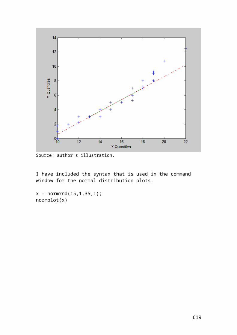
rb is the benchmark or index return.

If the portfolio return is 0.80 and the benchmark return of the index is 0.70 then, the active return is………

Please complete the calculation.

Active risk or tracking error is the standard deviation of the difference of returns between a portfolio and the benchmark or index.

If the portfolio return is 0.80, the number of assets is 10 and the benchmark return of the index is 0.40 then, the active risk is………

Please complete the calculation.

Information ratio shows the consistency of the fund manager towards the active return. The mathematical formula is as follows:

It could be calculated very easily in Excel software. I will illustrate a simple table with the relevant calculations.

Day rp rb rp - rb

1 0.03 0.02 0.012 0.02 0.014 0.006

619

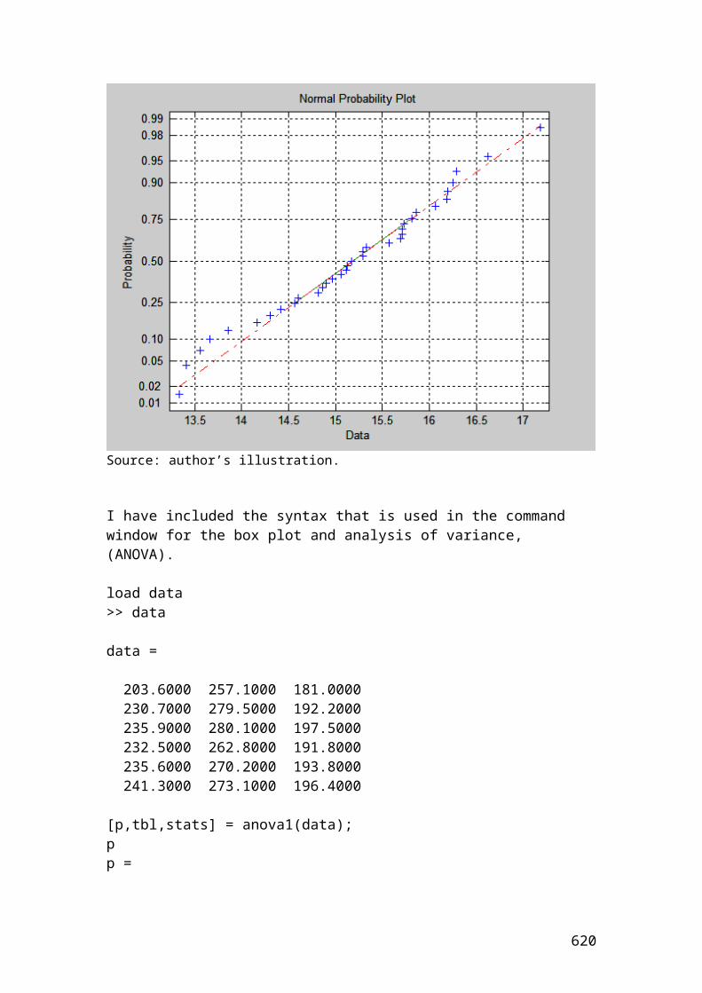
3 -0.04 0.034 -0.0744 0.05 0.067 -0.0175 0.08 0.012 0.0686 -0.01 -0.056 0.0467 0.07 0.031 0.0398 0.034 0.023 0.0119 -0.021 0.015 -0.03610 0.045 0.001 0.044

Average 0.0258 0.0161Standard deviation

0.043

Source: author’s calculation

By substituting the values that we have found in terms of rp =0.0258, rb = 0.0161 and standard deviation = 0.043 in the following equation we have:

But what is the interpretation of the information ratio of 0.23. It means that the fund manager gained around 23 basis points of active return per unit of active risk. The higher is this number, the better the manager is performing in relation to active risk.

Please convert the following exercise in Java language programming

Calculate the balance at the end of the 5th day from changes in the futures prices from 90 to 89, 91, 95, 97, 99. The trader has bought 50 futures contract for settlement in May. The initial margin is $8.

Day Beginning balance

Futures price Gain or loss Ending balance

0 400 90 0 4001 400 89 (50)2 350 91 1003 450 95 2004 650 97 1005 750 99 100

Source: author’s illustration.

Beginning balance = initial margin x number of contracts.Beginning balance = 8 x 50 = $400

620

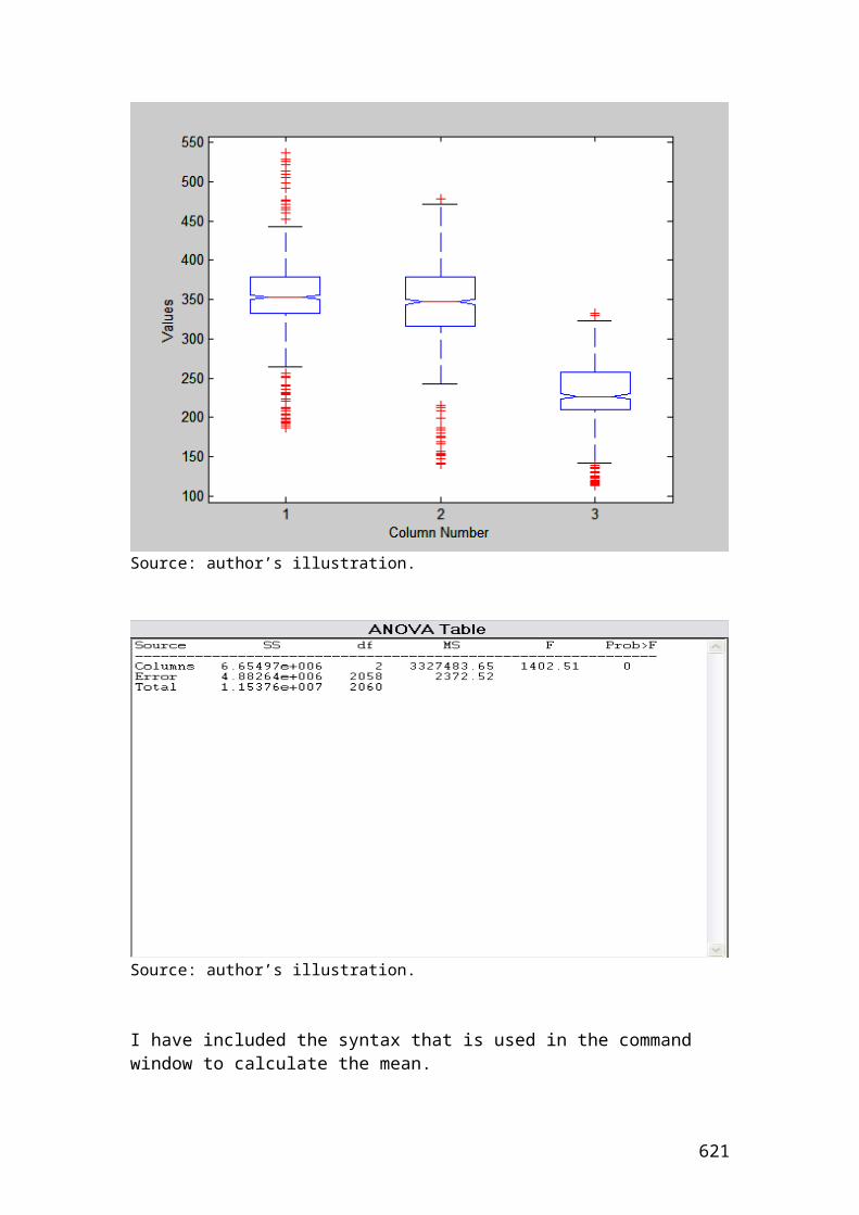
Please complete the values of the column ending balance.

Example of profit or loss of a call option portfolio

class profit_or_loss_call_option_portfolio {public static void main(String[] args) {

double portfoliovalue1, portfoliovalue2, portfoliovalue3, portfoliovalue4, portfoliovalue5,portfoliovalue6,portfoliovalue7, portfoliovalue8,portfoliovalue9,portfoliovalue10 ; // portfolio value. double shareprice=10 ; // number of positions of share prices. double strikeprice=10; // number of positions of strike prices. double optionpremium=10; // Call option premiums. double contractsize = 100; // contract size.

/* Identifying the number of positions in relation to the share prices, strike prices and option premium.*/

621

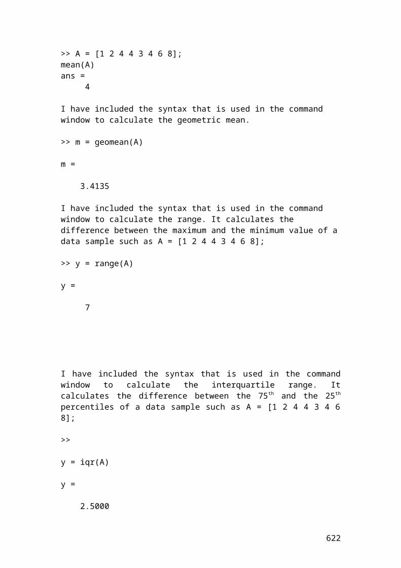
double shareprice1 = 10.25; double shareprice2 = 20.13; double shareprice3 = 30.22; double shareprice4 = 40.56; double shareprice5 = 50.89; double shareprice6 = 51.23; double shareprice7 = 53.33; double shareprice8 = 54.63; double shareprice9 = 66.23; double shareprice10 = 68.23;

double strikeprice1 = 3.34; double strikeprice2 = 8.34; double strikeprice3 = 18.78; double strikeprice4 = 28.34; double strikeprice5 = 31.12; double strikeprice6 = 22.02; double strikeprice7 = 34.23; double strikeprice8 = 47.12; double strikeprice9 = 48.45; double strikeprice10 = 50.12; double optionpremium1 = 1.50; double optionpremium2 = 2.30; double optionpremium3 = 2.56; double optionpremium4 = 3.10; double optionpremium5 = 3.25; double optionpremium6 = 3.45; double optionpremium7 = 3.56; double optionpremium8 = 4.32; double optionpremium9 = 5.12; double optionpremium10 = 5.78; // Calculate the call option portfolio values. portfoliovalue1 = (shareprice1-(strikeprice1+ optionpremium1))* contractsize; portfoliovalue2 = (shareprice2-(strikeprice2+ optionpremium2))* contractsize; portfoliovalue3 = (shareprice3-(strikeprice3+ optionpremium3))* contractsize; portfoliovalue4 = (shareprice4-(strikeprice4+ optionpremium4))* contractsize; portfoliovalue5 = (shareprice5-(strikeprice5+ optionpremium5))* contractsize; portfoliovalue6 = (shareprice6-(strikeprice6+ optionpremium6))* contractsize; portfoliovalue7 = (shareprice7-(strikeprice7+ optionpremium7))* contractsize; portfoliovalue8 = (shareprice8-(strikeprice8+ optionpremium8))* contractsize; portfoliovalue9 = (shareprice9-(strikeprice9+ optionpremium9))* contractsize; portfoliovalue10 = (shareprice10-(strikeprice10+ optionpremium10))* contractsize;

System.out.print("The portfoliovalue1 in pounds is");System.out.println(portfoliovalue1);System.out.println(Math.round(portfoliovalue1*100.0)/100.0);

622

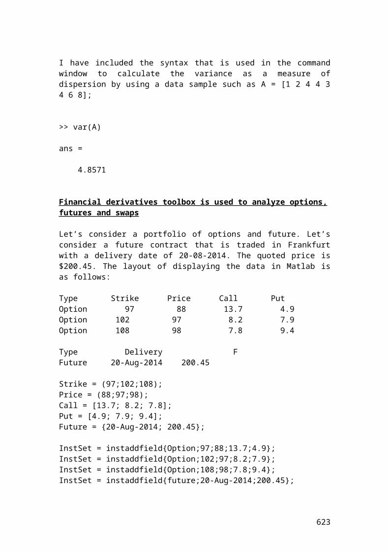
System.out.print("The portfoliovalue2 in pounds is");System.out.println(portfoliovalue2);System.out.println(Math.round(portfoliovalue2*100.0)/100.0);System.out.print("The portfoliovalue3 in pounds is");System.out.println(portfoliovalue3);System.out.println(Math.round(portfoliovalue3*100.0)/100.0);System.out.print("The portfoliovalue4 in pounds is");System.out.println(portfoliovalue4);System.out.println(Math.round(portfoliovalue4*100.0)/100.0);System.out.print("The portfoliovalue5 in pounds is");System.out.println(portfoliovalue5);System.out.println(Math.round(portfoliovalue5*100.0)/100.0);System.out.print("The portfoliovalue6 in pounds is");System.out.println(portfoliovalue6);System.out.println(Math.round(portfoliovalue6*100.0)/100.0);System.out.print("The portfoliovalue7 in pounds is");System.out.println(portfoliovalue7);System.out.println(Math.round(portfoliovalue7*100.0)/100.0);System.out.print("The portfoliovalue8 in pounds is");System.out.println(portfoliovalue8);System.out.println(Math.round(portfoliovalue8*100.0)/100.0);System.out.print("The portfoliovalue9 in pounds is");System.out.println(portfoliovalue9);System.out.println(Math.round(portfoliovalue9*100.0)/100.0);System.out.print("The portfoliovalue10 in pounds is");System.out.println(portfoliovalue10);System.out.println(Math.round(portfoliovalue10*100.0)/100.0);}}

Output results

After compiling the current document from tools and pressing the run document you should get the following results:

Welcome to DrJava. Working directory is C:\Documents and Settings\Owner\Desktop\Java Compiler> run profit_or_loss_call_option_portfolioThe portfoliovalue1 in pounds is541.0541.0The portfoliovalue2 in pounds is948.9999999999999949.0The portfoliovalue3 in pounds is887.9999999999999888.0The portfoliovalue4 in pounds is912.0000000000001912.0The portfoliovalue5 in pounds is1651.99999999999951652.0The portfoliovalue6 in pounds is2576.0

623

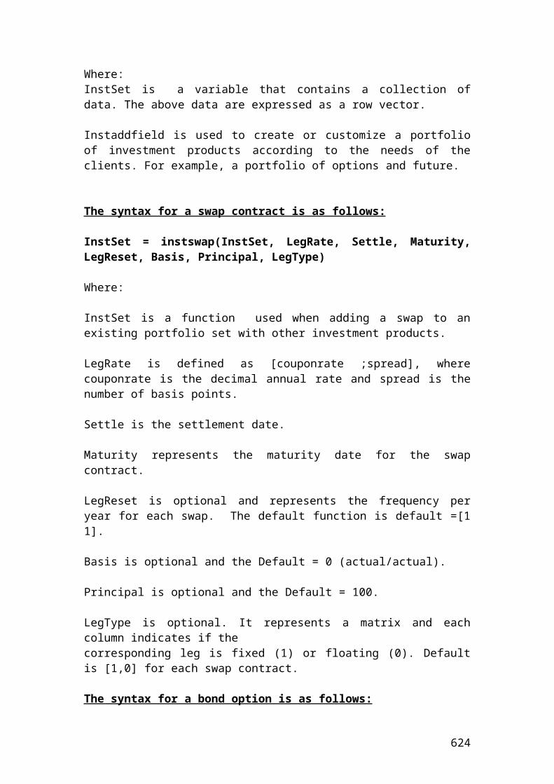
2576.0The portfoliovalue7 in pounds is1554.01554.0The portfoliovalue8 in pounds is319.00000000000045319.0The portfoliovalue9 in pounds is1266.00000000000051266.0The portfoliovalue10 in pounds is1233.00000000000051233.0>

Example of profit or loss of a put option portfolio

class profit_or_loss_put_option_portfolio {public static void main(String[] args) {

double portfoliovalue1, portfoliovalue2, portfoliovalue3, portfoliovalue4, portfoliovalue5,portfoliovalue6,portfoliovalue7, portfoliovalue8,portfoliovalue9,portfoliovalue10 ; // portfolio value. double shareprice=10 ; // number of positions of share prices. double strikeprice=10; // number of positions of strike prices. double optionpremium=10; // Call option premiums. double contractsize = 100; // contract size.

/* Identifying the number of positions in relation to the share prices, strike prices and option premium.*/

624

double shareprice1 = 10.25; double shareprice2 = 20.13; double shareprice3 = 30.22; double shareprice4 = 40.56; double shareprice5 = 50.89; double shareprice6 = 51.23; double shareprice7 = 53.33; double shareprice8 = 54.63; double shareprice9 = 66.23; double shareprice10 = 68.23;

double strikeprice1 = 3.34; double strikeprice2 = 8.34; double strikeprice3 = 18.78; double strikeprice4 = 28.34; double strikeprice5 = 31.12; double strikeprice6 = 22.02; double strikeprice7 = 34.23; double strikeprice8 = 47.12; double strikeprice9 = 48.45; double strikeprice10 = 50.12; double optionpremium1 = 1.50; double optionpremium2 = 2.30; double optionpremium3 = 2.56; double optionpremium4 = 3.10; double optionpremium5 = 3.25; double optionpremium6 = 3.45; double optionpremium7 = 3.56; double optionpremium8 = 4.32; double optionpremium9 = 5.12; double optionpremium10 = 5.78; // Calculate the call option portfolio values. portfoliovalue1 = (strikeprice1-optionpremium1-shareprice1)* contractsize; portfoliovalue2 = (strikeprice2-optionpremium2-shareprice2)* contractsize; portfoliovalue3 = (strikeprice3-optionpremium3-shareprice3)* contractsize; portfoliovalue4 = (strikeprice4-optionpremium4-shareprice4)* contractsize; portfoliovalue5 = (strikeprice5-optionpremium5-shareprice5)* contractsize; portfoliovalue6 = (strikeprice6-optionpremium6-shareprice6)* contractsize; portfoliovalue7 = (strikeprice7-optionpremium7-shareprice7)* contractsize; portfoliovalue8 = (strikeprice8-optionpremium8-shareprice8)* contractsize; portfoliovalue9 = (strikeprice9-optionpremium9-shareprice9)* contractsize; portfoliovalue10 = (strikeprice10-optionpremium10-shareprice10)* contractsize;

System.out.print("The portfoliovalue1 in pounds is");System.out.println(portfoliovalue1);System.out.println(Math.round(portfoliovalue1*100.0)/100.0);

625

System.out.print("The portfoliovalue2 in pounds is");System.out.println(portfoliovalue2);System.out.println(Math.round(portfoliovalue2*100.0)/100.0);System.out.print("The portfoliovalue3 in pounds is");System.out.println(portfoliovalue3);System.out.println(Math.round(portfoliovalue3*100.0)/100.0);System.out.print("The portfoliovalue4 in pounds is");System.out.println(portfoliovalue4);System.out.println(Math.round(portfoliovalue4*100.0)/100.0);System.out.print("The portfoliovalue5 in pounds is");System.out.println(portfoliovalue5);System.out.println(Math.round(portfoliovalue5*100.0)/100.0);System.out.print("The portfoliovalue6 in pounds is");System.out.println(portfoliovalue6);System.out.println(Math.round(portfoliovalue6*100.0)/100.0);System.out.print("The portfoliovalue7 in pounds is");System.out.println(portfoliovalue7);System.out.println(Math.round(portfoliovalue7*100.0)/100.0);System.out.print("The portfoliovalue8 in pounds is");System.out.println(portfoliovalue8);System.out.println(Math.round(portfoliovalue8*100.0)/100.0);System.out.print("The portfoliovalue9 in pounds is");System.out.println(portfoliovalue9);System.out.println(Math.round(portfoliovalue9*100.0)/100.0);System.out.print("The portfoliovalue10 in pounds is");System.out.println(portfoliovalue10);System.out.println(Math.round(portfoliovalue10*100.0)/100.0);}}

Output results

After compiling the current document from tools and pressing the run document you should get the following results:

Welcome to DrJava. Working directory is C:\Documents and Settings\Owner\Desktop\Java Compiler> run profit_or_loss_put_option_portfolioThe portfoliovalue1 in pounds is-841.0-841.0The portfoliovalue2 in pounds is-1409.0-1409.0The portfoliovalue3 in pounds is-1399.9999999999995-1400.0The portfoliovalue4 in pounds is-1532.0000000000005-1532.0The portfoliovalue5 in pounds is-2302.0-2302.0The portfoliovalue6 in pounds is-3265.9999999999995

626

-3266.0The portfoliovalue7 in pounds is-2266.0-2266.0The portfoliovalue8 in pounds is-1183.0000000000005-1183.0The portfoliovalue9 in pounds is-2290.0-2290.0The portfoliovalue10 in pounds is-2389.000000000001-2389.0>

One – period binomial method

A share is traded in the Danish stock exchange at 50 DKK. First of all, we would like to calculate the possible price changes based on probabilities. The risk - free rate is 5% and the value of the call option has an exercise price of 50 DKK. It is required to calculate the expected value of the option at t =1. In addition, it is required to calculate the value of the option today discounted at the given risk-free rate.

We assume two scenarios. The first one is that the share will increase by 20% or by a factor of 1 + 0.20 = 1.20. The second one is that the share will decrease by 0.833. The number 0.833 is calculated as 1 / 1.20 = 0.833.

The mathematical formulas are as follows:

Down move = D = 1 / up move = 1 / 1.20 = 0.833

627

59128.0367.0217.0

0.833-1.200.833- 0.051

move. up theis U move.down theis D

rate. free-risk theis rf :

D-U

D-rf1 movement upan ofy probabilit neutral -risk

U

Where

U

0.40872 0.59128 - 1 movement down a ofy probabilit neutral - riskD

Thus, the payoff or the one-period binomial tree for share and option prices for the two possible scenarios will be as follows:

t = 0 t = 1

Probability Up = 0.59128 Share price = 50 x 1.20 = 60 DKK Call option = 60 – 50 = 10 DKK. 50 In this case, an increase of the share price will lead to the call option to pay back 10 DKK Probability Down =0.40872 Share price = 50 x 0.833 = 41.65 DKK Call option = 41.65 – 50 = -8.35 DKK = 0 DKK In this case the call option does not worth anything.

The expected value of the call option at t = 1 is as follows:

Expected call option = (10 x 0.59128) + ( 0 x 0.40872) = 5.9128 + 0 = 5.9128 DKK.

The value of the call option discounted at 5% risk – free rate is as follows:

Ctoday = 5.9128 / 1.05 = 5.63 DKK (to 2 d.p.).

Application of one – period binomial method in Java

class One_period_binomial_method{public static void main(String[] args) { //One - period binomial method. double shareprice = 50; double exerciseprice = 50; double upmove = 1.20; double downmove = 0.833;

628

double riskfreerate = 0.05; double riskprobofupmove; double riskprobofdownmove; double shareprice1; double shareprice2; double calloptionprice1; double calloptionprice2; double expectedcalloption; double valueofcalldiscounted;

// Insert the mathematical formulas of risk probability of up and down move.

riskprobofupmove = (1+riskfreerate-downmove) / (upmove - downmove);riskprobofdownmove = 1 - riskprobofupmove;

// The payoff or one period binomial tree for share and option prices is as follows:

shareprice1 = shareprice * upmove;calloptionprice1 = shareprice1 - exerciseprice;

shareprice2 = shareprice *downmove;calloptionprice2 = shareprice2 - exerciseprice;calloptionprice2 =0;

// The expected value of the call option at t=1 is as follows:

expectedcalloption = (calloptionprice1* riskprobofupmove) + (calloptionprice2 * riskprobofdownmove);

// The value of the call option discounted at 5% risk - free rate is as follows:

valueofcalldiscounted = expectedcalloption / 1.05;

System.out.print("The risk probability of up move is");System.out.println(riskprobofupmove);System.out.println(Math.round(riskprobofupmove*100.0)/100.0);System.out.print("The risk probability of down move is");System.out.println(riskprobofdownmove);System.out.println(Math.round(riskprobofdownmove*100.0)/100.0);System.out.print("The share price 1 is");System.out.println(shareprice1);System.out.print("The share price 2 is");System.out.println(shareprice2);System.out.print("The call option price 1 is");System.out.println(calloptionprice1);System.out.print("The call option price 2 is");System.out.println(calloptionprice2);System.out.print("The expected call option is");System.out.println(expectedcalloption);

629

System.out.println(Math.round(expectedcalloption*100.0)/100.0);System.out.print("The value of call option discounted is");System.out.println(valueofcalldiscounted);System.out.println(Math.round(valueofcalldiscounted*100.0)/100.0);}}

Output results

After compiling the current document from tools and pressing the run document you should get the following results:

Welcome to DrJava. Working directory is C:\Documents and Settings\Owner\Desktop\Java Compiler> run One_period_binomial_methodThe risk probability of up move is0.59128065395095390.59The risk probability of down move is0.408719346049046140.41The share price 1 in DKK is60.0The share price 2 in DKK is41.65The call option price 1 in DKK is10.0The call option price 2 in DKK is0.0The expected call option in DKK is5.9128065395095395.91The value of call option discounted in DKK is5.6312443233424185.63>

Two – period binomial method

This method is based on the one – period binomial method, but it is extended to include a second period, t = 2. Thus, we have three periods. t = 0, t =1 and t =2. We use the same example of the previous section but extended to an additional period.

A share is traded in the Danish stock exchange at 50 DKK. First of all, we would like to calculate the possible price changes based on probabilities. The risk - free rate is 5% and the value of the call option has an exercise price of 50 DKK. It is required to calculate the expected value of the option. In addition, it is required to calculate the value of the option today discounted at the given risk-free rate.

We assume two scenarios. The first one is that the share will increase by 20% or by a factor of 1 + 0.20 = 1.20. The second one is that the share will decrease by 0.833. The number 0.833 is calculated as 1 / 1.20 = 0.833.

630

The mathematical formulas are as follows:

Down move = D = 1 / up move.

59128.0367.0217.0

0.833-1.200.833- 0.051

move. up theis U move.down theis D

rate. free-risk theis rf :

D-U

D-rf1 movement upan ofy probabilit neutral -risk

U

Where

U

0.40872 0.59128 - 1 movement down a ofy probabilit neutral - riskD

Thus, the payoff or the two-period binomial tree for share prices for the two possible scenarios will be as follows:

t = 0 t = 1 t =2 50*(1.20)2=72 DKKProbability Up = 0.59 S1 = 50 x 1.20 = 60 DKK S2 50*1.20*0.833 =49.98 50 DKK Probability Down =0.41 S1 = 50 x 0.833 = 41.65 DKK S2

50 * (0.833)2 = 34.69

The value of the call options for the period t =2 for both ups and downs are as follows:

Upside movementC1 = 72 – 50 = 22C2 = 49.98 – 50 = -0.02 =0 Negative values mean that the option does not worth.

Downside movementC1 = 49.98 -50 = -0.02 =0C2 = 34.69 -50 = -15.31 =0

The expected value of the call options for both movements for period t =1 are calculated based on the following equations:

Upside movement

631

DKK 12.3887

05.1008.13

05.1)040872.0(2259128.0

rf 1down xC PrC x upy Probabilit 21

up

up

Call

xxobabilityCall

Downside movement

005.1

0) 40872.0(0 59128.0rf 1

Cdown x PrC x up Pr 21

xxobabilityobabilityCalldown

The value of the call option today discounted is calculated based on the following formula:

3.d.p.) (to 976.605.1

32519.7

05.10 12.3887 x 59128.0

1Calldown x PrCall x up Pr downup

today

today

Call

rfobabilityobability

Call

The final format of the two-period binomial tree for call options is as follows:

t = 0 t = 1 t = 2

22.00 DKK 12.3887DKK 06.976 DKK 0 0

Application of two – period binomial method in Java

class Two_period_binomial_method{public static void main(String[] args) { //Two - period binomial method. double shareprice = 50; double exerciseprice = 50; double upmove = 1.20; double downmove = 0.833; double riskfreerate = 0.05; double riskprobofupmove; double riskprobofdownmove; double shareprice1; double shareprice2; double shareprice3;

632

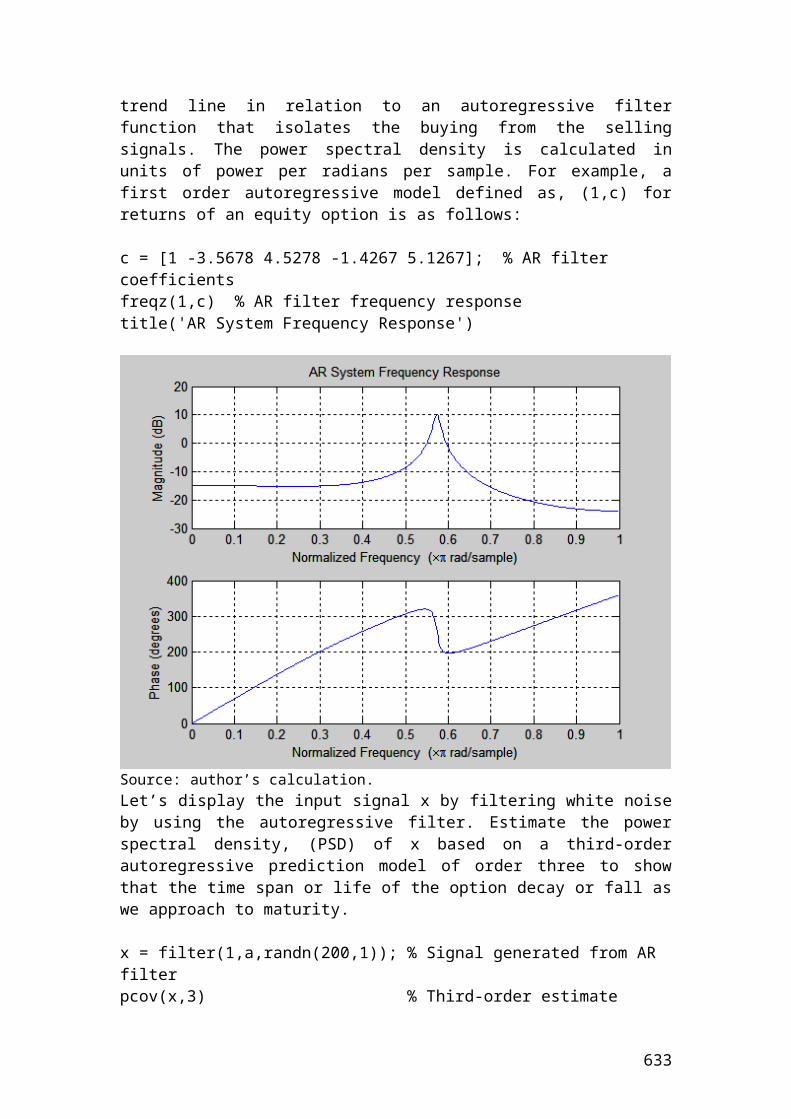
double shareprice4; double shareprice5; double calloptionprice1; double calloptionprice2; double calloptionprice3; double calloptionprice4; double calloptionprice5; double expectedcalloptionupside; double expectedcalloptiondownside; double valueofcalldiscounted; // Insert the mathematical formulas of risk probability of up and down move.

riskprobofupmove = (1+riskfreerate-downmove) / (upmove - downmove);riskprobofdownmove = 1 - riskprobofupmove;

// The payoff or two period binomial tree for share and option prices is as follows:

shareprice1 = shareprice * upmove;

shareprice2 = shareprice *downmove;

shareprice3 = shareprice * Math.pow(upmove,2);calloptionprice3 = shareprice3 - exerciseprice;

shareprice4 = shareprice * Math.pow(downmove,2);calloptionprice4 = shareprice4 - exerciseprice;calloptionprice4 =0;

shareprice5 = shareprice * upmove * downmove;calloptionprice5 = shareprice5 - exerciseprice;calloptionprice5 =0;

// The expected value of the call option at t=2 is as follows:expectedcalloptionupside = (riskprobofupmove * calloptionprice3+ riskprobofdownmove* calloptionprice5) / 1.05;

expectedcalloptiondownside = (riskprobofupmove *calloptionprice4+ riskprobofdownmove * calloptionprice5) / 1.05;

// The value of the call option discounted at 5% risk - free rate is as follows:

valueofcalldiscounted = (riskprobofupmove * expectedcalloptionupside+riskprobofdownmove* expectedcalloptiondownside)/ 1.05;

// Output functions.System.out.print("The risk probability of up move is");System.out.println(riskprobofupmove);System.out.println(Math.round(riskprobofupmove*100.0)/100.0);System.out.print("The risk probability of down move is");

633

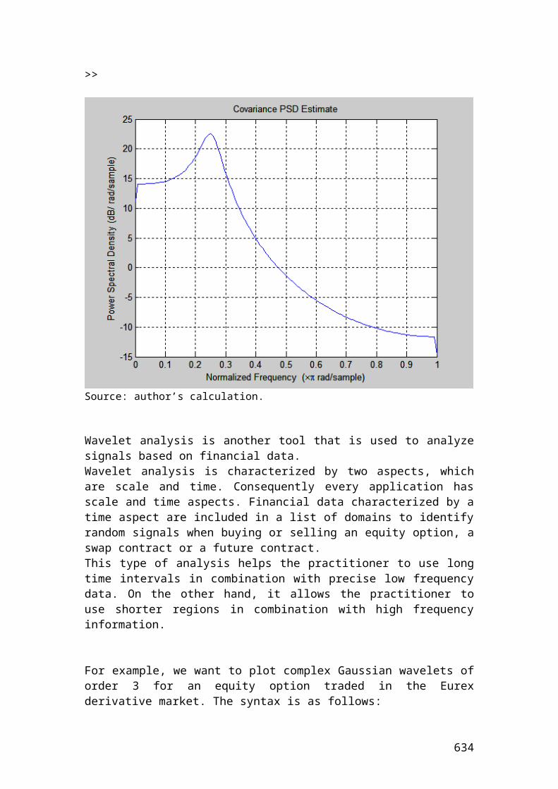
System.out.println(riskprobofdownmove);System.out.println(Math.round(riskprobofdownmove*100.0)/100.0);System.out.print("The share price 1 in DKK is");System.out.println(shareprice1);System.out.print("The share price 2 in DKK is");System.out.println(shareprice2);System.out.print("The share price 3 in DKK is");System.out.println(shareprice3);System.out.print("The share price 4 in DKK is");System.out.println(shareprice4);System.out.print("The share price 5 in DKK is");System.out.println(shareprice5);System.out.print("The call option price 3 in DKK is");System.out.println(calloptionprice3);System.out.print("The call option price 4 in DKK is");System.out.println(calloptionprice4);System.out.print("The call option price 5 in DKK is");System.out.println(calloptionprice5);System.out.print("The expected call option upside in DKK is");System.out.println(expectedcalloptionupside);System.out.println(Math.round(expectedcalloptionupside*100.0)/100.0);System.out.print("The expected call option downside in DKK is");System.out.println(expectedcalloptiondownside);System.out.println(Math.round(expectedcalloptiondownside*100.0)/100.0);System.out.print("The value of call option discounted in DKK is");System.out.println(valueofcalldiscounted);System.out.println(Math.round(valueofcalldiscounted*100.0)/100.0);}}

Output results

After compiling the current document from tools and pressing the run document you should get the following results:

Welcome to DrJava. Working directory is C:\Documents and Settings\Owner\Desktop\Java Compiler> run Two_period_binomial_methodThe risk probability of up move is0.59128065395095390.59The risk probability of down move is0.408719346049046140.41The share price 1 in DKK is60.0The share price 2 in DKK is41.65The share price 3 in DKK is72.0The share price 4 in DKK is34.694449999999996The share price 5 in DKK is49.98The call option price 3 in DKK is22.0

634

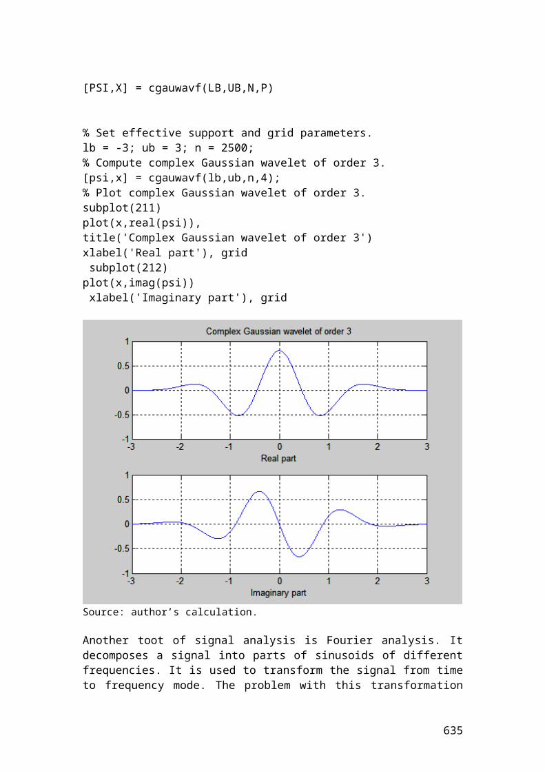
The call option price 4 in DKK is0.0The call option price 5 in DKK is0.0The expected call option upside in DKK is12.38873751135331812.39The expected call option downside in DKK is0.00.0The value of call option discounted in DKK is6.9764007784187646.98>

Stock index option

Let’s assume that a practitioner wants to buy a stock index call option that is related to the general movement of the S&P 500 index. The dollar multiplier for S&P 500 option contract is 250 dollars. The strike price of the index is 1240. The August premium is 20 index points.

Question

Calculate the cost of the August call and the net profit involved if the S&P 500 index reaches the price of 1540.

Solution

Cost of the August call = premium expressed in index points x dollar multiplier Cost of the August call = 20 x 250 = 5000 USD

The net profit incurred is calculated as follows:

635

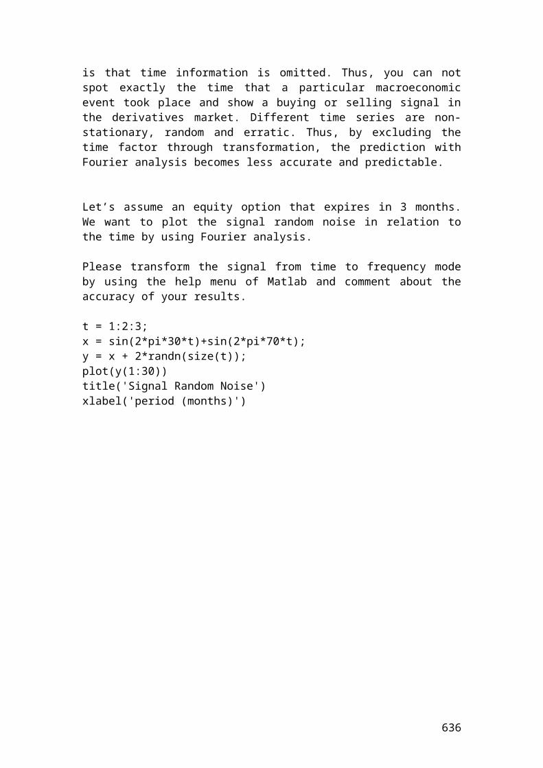
(Ending index value – beginning index value x dollar multiplier ) – cost of the August call.

(1540 – 1240) x 250 – 5000 = 70,000 USD.

Application of stock index option in Java

class Stock_index_option{public static void main(String[] args) {

double cost_of_call;double net_profit ;int premium = 20;int multiplier = 250;double ending_index_value = 1540;double beginning_index_value = 1240; // Insert the mathematical formula.

cost_of_call = premium * multiplier ;net_profit = (ending_index_value - beginning_index_value) * multiplier - cost_of_call;

// Output functions.

System.out.print("The cost of call in USD is");System.out.println(cost_of_call);System.out.println(Math.round(cost_of_call*100.0)/100.0);System.out.print("The net profit in USD is");System.out.println(net_profit);System.out.println(Math.round(net_profit*100.0)/100.0);}}

Output result

After compiling the current document from tools and pressing the run document you should get the following result:

Welcome to DrJava. Working directory is C:\Documents and Settings\Owner\Desktop\Java Compiler> run Stock_index_optionThe cost of call in USD is 5000.05000.0The net profit in USD is 70000.070000.0

636

>

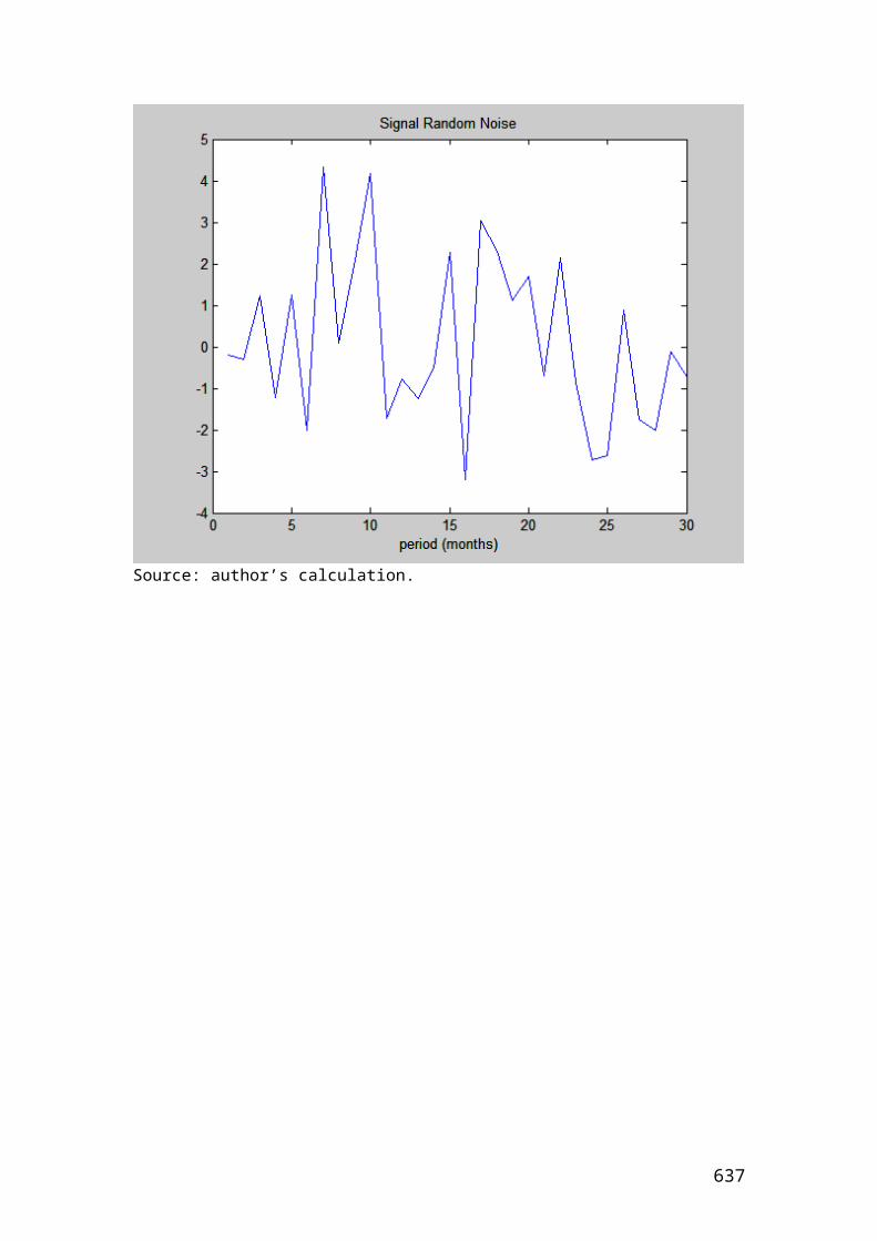
Exercise of an European interest rate option

Calculate the profit or loss of the interest rate difference between the actual and the strike rate of a call option. Let’s assume that an interest call option on a 6 –month Eurodollar has a strike rate of 4%. At expiration, the 6-month Eurodollar rate is 5%. The invested principal is 50,000,000 Euros. The duration of the contract is expressed in days divided by 360 days. Thus, 6 –months equal 180 days.

The mathematical formula for profit or loss is as follows:

637

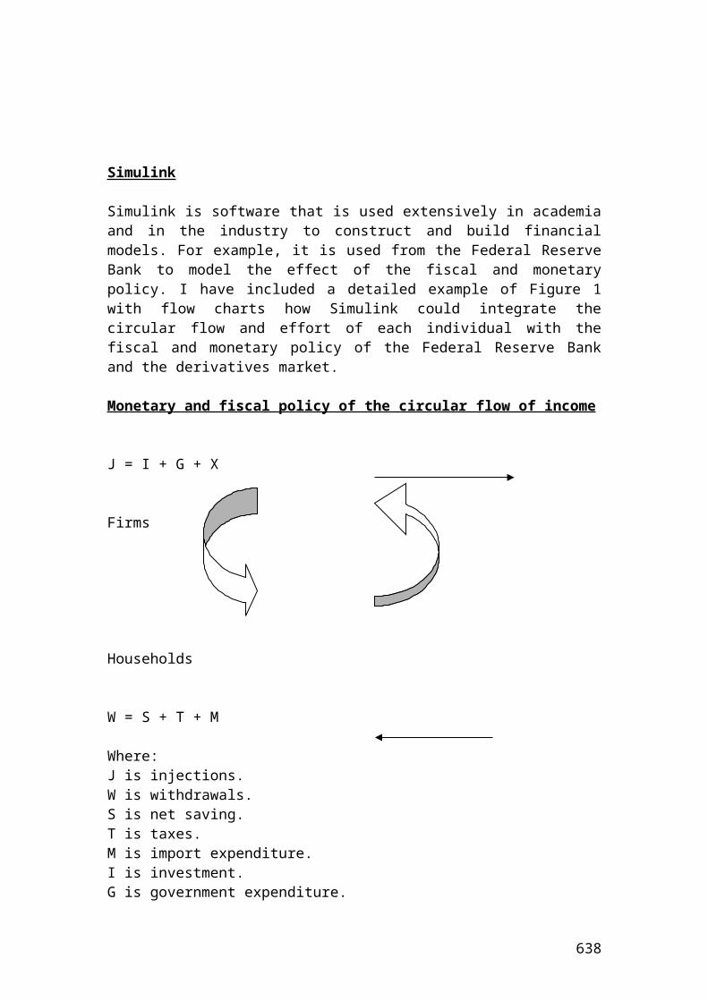
Application of an European interest rate option in Java

class European_interest_option{public static void main(String[] args) {

//Profit or loss of call interest rate option. double Profit_or_loss_call_interest_rate_option; // call interest rate option.double principal = 50000000;double actual_rate = 0.05;double strike_rate = 0.04;double duration = 180;double days = 360; // Insert the mathematical formula.

Profit_or_loss_call_interest_rate_option = principal *(actual_rate-strike_rate)*duration/days;

// Output function.

System.out.print("Profit_or_loss_call_interest_rate_option in euros is");System.out.println(Profit_or_loss_call_interest_rate_option);System.out.println(Math.round(Profit_or_loss_call_interest_rate_option*100.0)/100.0);}}

Output result

After compiling the current document from tools and pressing the run document you should get the following result:

Welcome to DrJava. Working directory is C:\Documents and Settings\Owner\Desktop\Java Compiler> run European_interest_optionProfit_or_loss_call_interest_rate_option in euros is250000.00000000003250000.0>

638

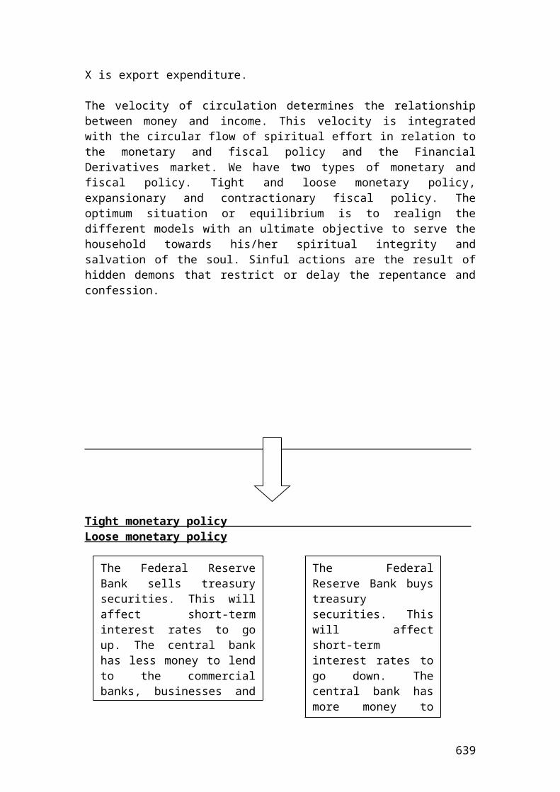
Currency option

Let’s assume that a wealthy investor buys a call currency option because it expects a rise in the exchange rate parity of the EURO against the USD, EURO/USD. The spot exchange rate is 1/1.3568. The strike price is 1.3568. The premium expressed as cents per Euro is 1.56. The initial principal is 100,000 USD.

Question

Calculate the net profit involved if the strike price increases to 1.3987.

Solution

The wealthy investor to record a profit, he or she should add to the strike price 1.3568 the premium expressed as cents per Euro. In our case, the breakeven point is1.3568 + 0.0156 = 1.3724. Above the price of 1.3724, he or she starts to record a profit. If the strike price reaches 1.3987, then the profit will be as follows:

639

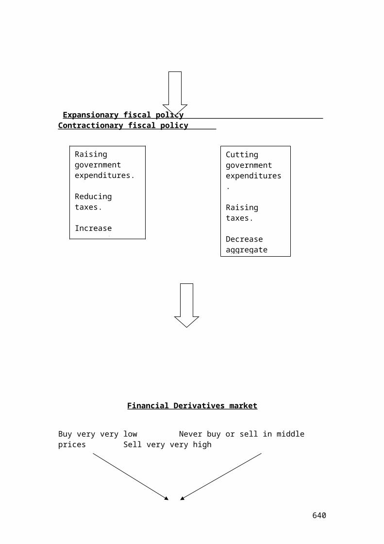
Initial principal x (Ending strike price – beginning strike price – premium paid) =100,000 x (1.3987 – 1.3568 – 0.0156) = 2630 USD net profit

Application of currency option in Java

class Currency_option{public static void main(String[] args) { //Profit or loss of currency option. double net_profit;double principal = 100000;double ending_strike_price = 1.3987;double beginning_strike_price = 1.3568;double premium_paid = 0.0156; // Insert the mathematical formula.

net_profit = principal *(ending_strike_price-beginning_strike_price - premium_paid);

// Output function.

System.out.print("net profit in USD is");System.out.println(net_profit);System.out.println(Math.round(net_profit*100.0)/100.0);}}

Output result

After compiling the current document from tools and pressing the run document you should get the following result:

Welcome to DrJava. Working directory is C:\Documents and Settings\Owner\Desktop\Java Compiler> run Currency_optionnet profit in USD is2630.0000000000052630.0>

640

Example of calculating the payments of an interest rate cap based on different LIBOR rates

Interest rate cap is an agreement between two parties where one party pay the other at a specified period of time in which the interest rate or London interbank offered rate ,LIBOR, exceeds the strike price. It is used this contract to hedge against interest rate fluctuations. Let’s assume that an interest cap has a value of 5.5% and the LIBOR prices for the next three years are 7.5%, 8.3% and 4.65%. The principal is $50,000,000 and the payments take place semiannually.

The mathematical formula that is used to calculate the payments of each year is as follows:

Interest rate payment =[ principal x (LIBOR rate – cap rate)/0.5]

Therefore, the first year interest rate payment is as follows:

Year 1

641

Interest rate payment = [50,000,000 x (0.075 – 0.055)/2] = $ ………

Application of payments of an interest rate cap based on different LIBOR rates in Java

class Payments_interest_rate_cap{public static void main(String[] args) {

// Payments of an interest rate cap based on different LIBOR rates. double interest_pay_1;double interest_pay_2;double interest_pay_3;double principal = 50000000;double libor_rate_1 = 0.075;double libor_rate_2 = 0.083;double cap_rate = 0.055;double duration = 2; // Insert the mathematical formula.

interest_pay_1 = principal *(libor_rate_1 - cap_rate) /duration ;interest_pay_2 = principal *(libor_rate_2 - cap_rate) / duration ;

//Output functions.

System.out.print("interest_pay_1 in USD is");System.out.println(interest_pay_1);System.out.println(Math.round(interest_pay_1*100.0)/100.0);System.out.print("interest_pay_2 in USD is");System.out.println(interest_pay_2);System.out.println(Math.round(interest_pay_2*100.0)/100.0);}}

Output result

After compiling the current document from tools and pressing the run document you should get the following result:

Welcome to DrJava. Working directory is C:\Documents and Settings\Owner\Desktop\Java Compiler> run Payments_interest_rate_capinterest_pay_1 in USD is499999.99999999994500000.0interest_pay_2 in USD is700000.0000000001700000.0>

642

A six month interest rate cap has a rate of 0.08 and the principal is 20,000,000 USD. The settlements is done quarterly. The first quarter the 3 –month libor rate is 0.096 and the second quarter the rate is 0.087. Calculate the payoff for the cap the first and the second quarter?

Solution

Payoff the first quarter = 20,000,000 * = 80000 USD

Payoff the second quarter = 20,000,000 * =35000 USD

Application of payoff of interest rate cap in Java

class Payoff_interest_rate_cap{public static void main(String[] args) { //Payoff of interest rate cap.

643

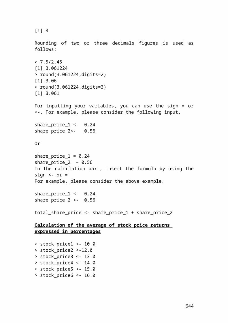
double payoff_1;double payoff_2;double principal = 20000000;double cap_rate = 0.08;double libor_rate_1 = 0.096;double libor_rate_2 = 0.087;double period = 4; // Insert the mathematical formulas. payoff_1 = (principal*(libor_rate_1-cap_rate)/period);payoff_2 = (principal*(libor_rate_2-cap_rate)/period);

// Output functions.

System.out.print("payoff_1 in USD is");System.out.println(payoff_1);System.out.println(Math.round(payoff_1*100.0)/100.0);System.out.print("payoff_2 in USD is");System.out.println(payoff_2);System.out.println(Math.round(payoff_2*100.0)/100.0);}}

Output results

After compiling the current document from tools and pressing the run document you should get the following results:

Welcome to DrJava. Working directory is C:\Documents and Settings\Owner\Desktop\Java Compiler> run Payoff_interest_rate_cappayoff_1 in USD is80000.080000.0payoff_2 in USD is34999.9999999999635000.0>

644

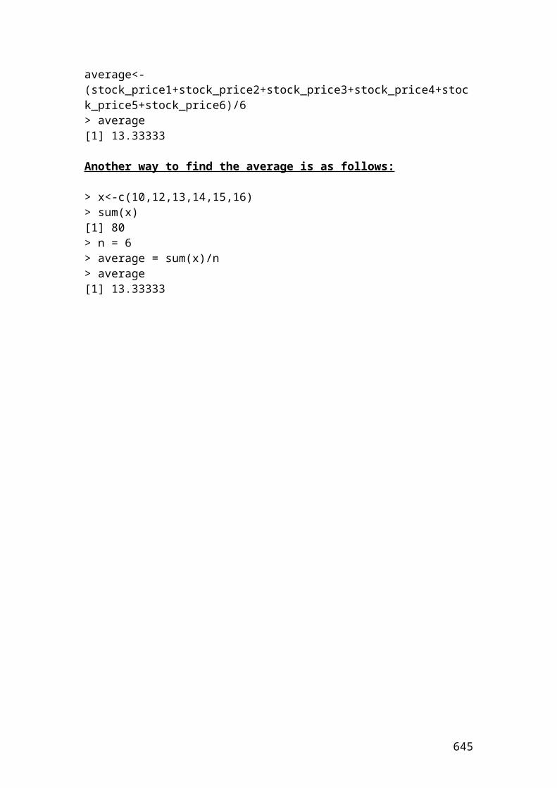
Swaption

An investor purchased a 1 year European swaption with exercise price 7.50%. The principal is 30,000,000USD. The floating rate payments are based on LIBOR. The 90, 180, 270, and 360 day annualized LIBOR rates and present value factors are as follows:

LIBOR Rate Present value factors90 day LIBOR 4% 0.990099180 day LIBOR 5.5% 0.973236270 day LIBOR 6% 0.956938360 day LIBOR 7% 0.934579

Calculate the semi-annual and annualized swap rate?Calculate the net cash flow at each payment and the value of swaption at maturity.

Solution

The present value factors are calculated as follows:

645

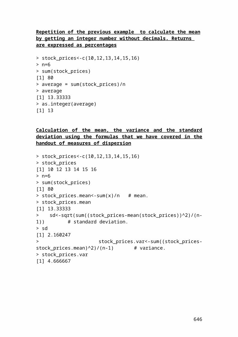
PV 90 days =

36090*04.01

10.990099

PV 180 days =

360180*055.01

10.973236

PV 270 days =

360270*06.01

1

0.956938

PV 360 days =

360360*07.01

10.934579

Semi - annual swap rate =

01697.0854852.3065421.0

934579.0956938.0973236.0990099.0934579.01

Annulaized swap rate = 6.788%or 06788.090/360*01697.0

The swaption is in the money because the exercise price 7.50% is greater than the market annualized swap rate 6.788%.

The net cash flow is as follows:

netCashFlow = (0.075 – 0.06788)*90/360 * 30000000 = 53400 USD

The value of swaption at maturity is as follows:

valueSwaption = 53400 *( 934579.0956938.0973236.0990099.0 ) = 205,849.1 USD

Application of swaption in Java

class Swaption{public static void main(String[] args) {

646

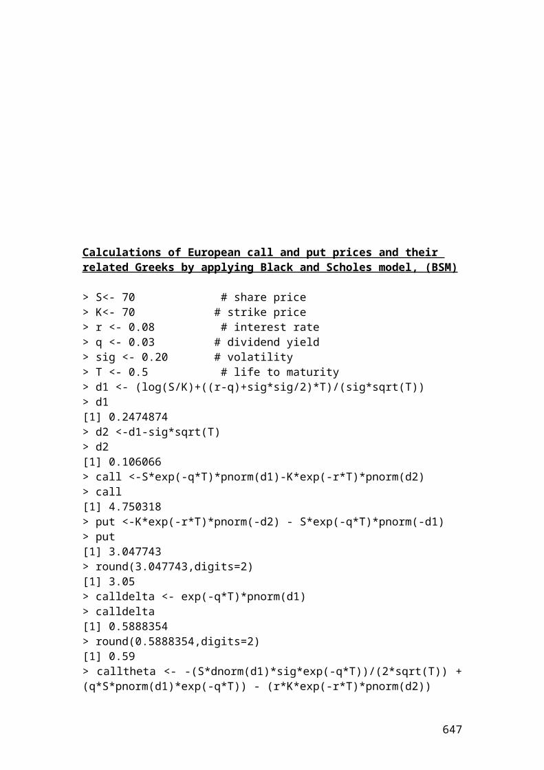
double Semi_annual_rate;double Annualized_swap_rate;double Net_cash_flow;double Value_swaption;double Exercise_rate = 0.075;double principal = 30000000;double PV90;double PV180;double PV270;double PV360;double rate_90 = 0.04;double rate_180 = 0.055;double rate_270 = 0.06 ;double rate_360 = 0.07; // Insert the mathematical formulas. PV90 = 1 /(1+(rate_90 * 90/360));PV180 = 1/(1+(rate_180 * 180/360));PV270 = 1/(1+(rate_270 * 270/360));PV360 = 1/(1+(rate_360* 360/360));

Semi_annual_rate = (1-PV360)/(PV90 +PV180 +PV270 +PV360);Annualized_swap_rate = Semi_annual_rate * (360/90);

// Output functions.

System.out.print("Semi_annual_rate is");System.out.println(Semi_annual_rate);System.out.println(Math.round(Semi_annual_rate*100.0)/100.0);System.out.print("Annualized_swap_rate is");System.out.println(Annualized_swap_rate);System.out.println(Math.round(Annualized_swap_rate*100.0)/100.0);}}

Output results

After compiling the current document from tools and pressing the run document you should get the following results:

Welcome to DrJava. Working directory is C:\Documents and Settings\Owner\Desktop\Java Compiler> run SwaptionSemi_annual_rate is0.016970964480702220.02Annualized_swap_rate is0.067883857922808880.07>

647

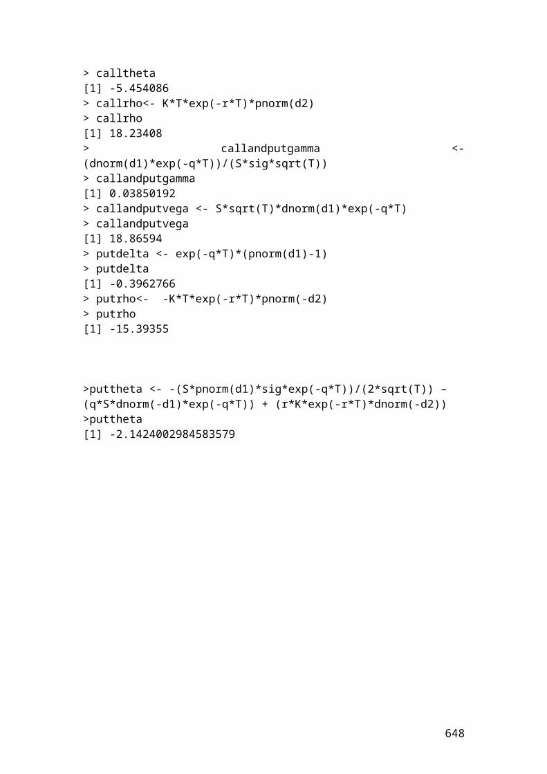
Please repeat the above swaption problem and calculate the net cash flow and the value of swaption at maturity expressed in USD.

Put –call parity

The put – call parity shows the relationship between a call and a put option with the same expiration, strike and share prices. The mathematical formula is as follows:

option.put theand call both thefor price share theis S .expirationor maturity to time theis T

rate. free-rsik theis r call. theandput both the of price strike theis X

put. theof price theis P call. theof price theis C :

)1(

f

Where

SPrfXC T

Example

648

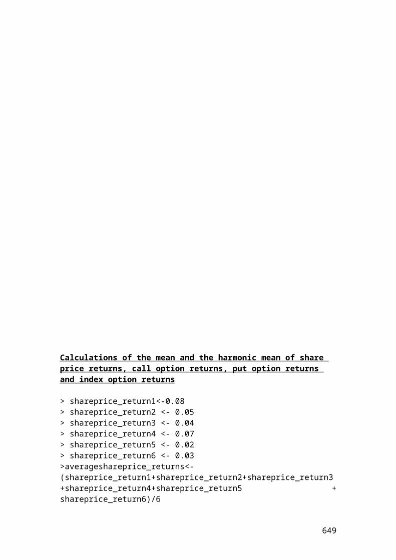
Calculate the price of a call if the price of a put is 5.34 Pounds, the share price is 94, the strike price is 97, the risk-free rate is 4% and the time to maturity, T=0.5. By rearranging formula (20) and solving for the price of a call, we have the following results:

pounds 22.4

)04.1(979434.5

)1( 5.0

C

rfXSPC T

Application of put - call parity in Java

class Put_call_parity{public static void main(String[] args) { // Put - call parity. Calculating the price of a call. double Call;double put = 5.34;double share_price = 94;double strike_price = 97;double dis_risk_free_rate = 1.04;double maturity = 0.5;

// Insert the mathematical formula.

Call= put + share_price - strike_price / Math.pow(dis_risk_free_rate,maturity);

// Output function.

System.out.print("Call in pounds is");System.out.println(Call);System.out.println(Math.round(Call*100.0)/100.0);

}}

Output result

After compiling the current document from tools and pressing the run document you should get the following result:

Welcome to DrJava. Working directory is C:\Documents and Settings\Owner\Desktop\Java Compiler> run Put_call_parityCall in pounds is4.223674457980749

649

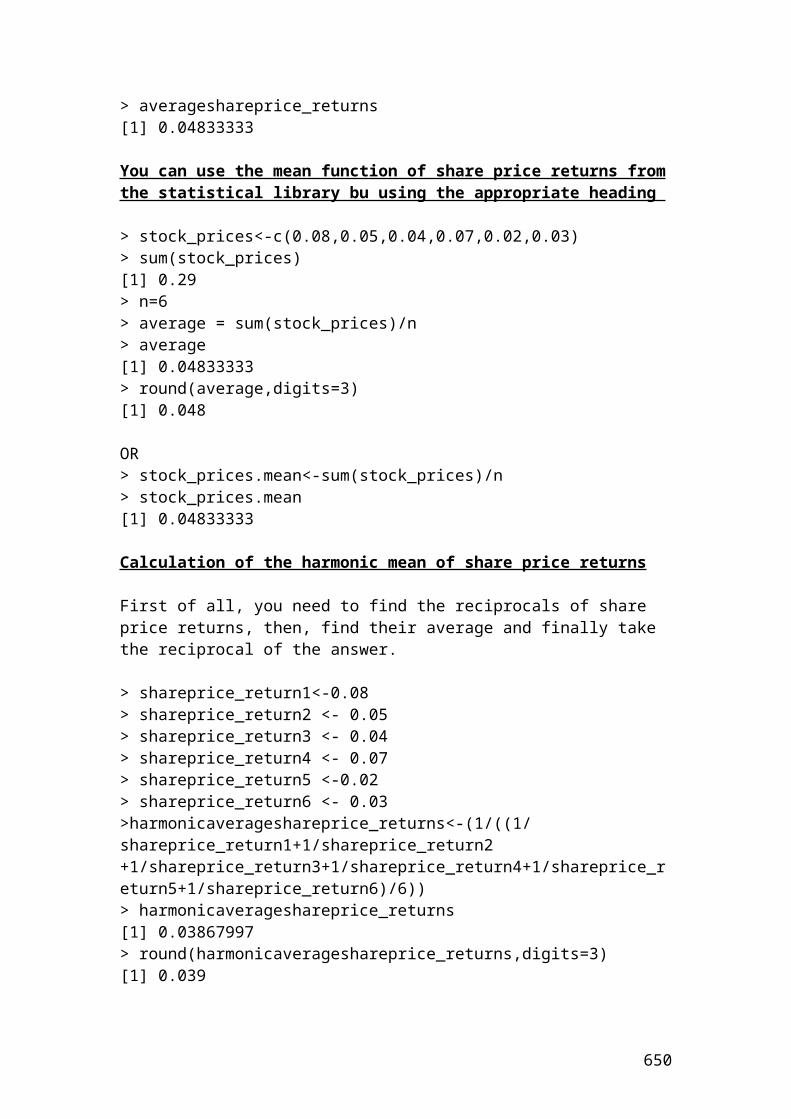
4.22>

Example of margin payments in the clearinghouse

An investor open a margin account with a minimum initial margin of 5,200 dollars per contract. The maintenance margin is 1,500 dollars per contract. He/she buys 7 July wheat futures contracts with a standard contract size of 200 bushels priced at 230 dollars per bushel. The July contract size in the next 2 days recorded the prices of 220 and 210 dollars per bushel. Show the cash flows, gains and losses for the buyer and the seller?

Solution

Initial margin = 7 x 5,200 = 36,400 dollars

Maintenance margin = 7 x 1,500 = 10,500 dollars

The cash flows, gains and losses for the next two days will be as follows:

Day 1

650

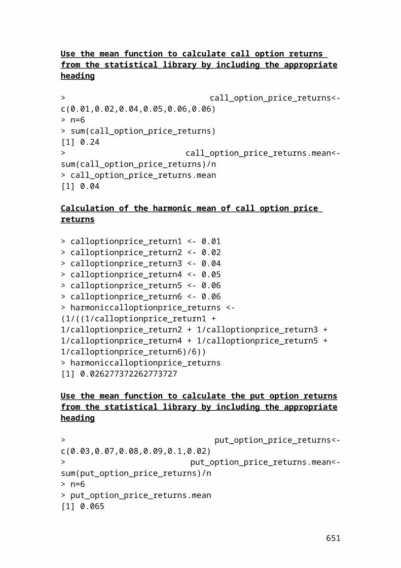
Cash flows for the buyer’s: 36,400 + 14,000 = 50,400 dollars. The investor’s recorded a gain.

Cash flows for the seller’s: 36,400 – 14,000 = 22,400 dollars. The investor’s recorded a loss.

Helpful hint: the amount of 14,000 is calculated from the difference of the bushel prices, (f0-f) x number of contracts x standard contract size. Thus, we have: (230-220) x 7 x 200 = 14,000 dollars. The same principle applies for the second day but with different bushel price.

Day 2

Please do the calculations for the second day.

This is why I am stressing the importance that the investors should buy or sell ONLY when the market is aggressively increasing or falling. If he/she gets trapped in a market that is not strong bull or bear, then, he/she will have to compensate regularly for the losses or he/she will experience a very small profit. If the amounts as the days passes is below the maintenance margin, then, the investor’s will receive a margin call and he/she should add the capital required to proceed with the contract. If the investor’s is short of money, then, the position is closed with the incurred losses.

Application of margin payments in the clearinghouse in Java

class Margin_payments{public static void main(String[] args) {

// Margin payments. double Cash_flow_buyer ;double Cash_flow_seller ;double initial_margin = 5200;double maintenance_margin = 1500;int contract_number = 7;int bushel_contract_size = 200;double bushel_price_1 = 230;double bushel_price_2 = 220;double Initial_margin_with_contract ;double Maintenance_margin_with_contract;double Bushel_contract ;

651

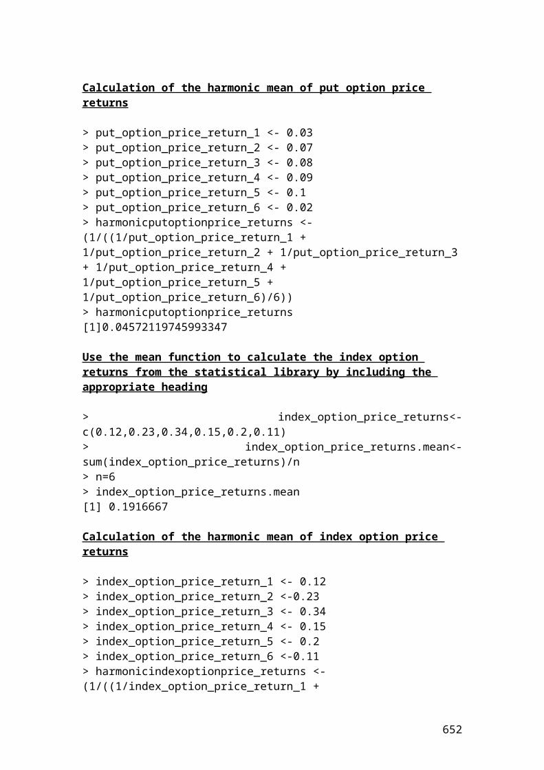
// Insert the mathematical formulas.

Initial_margin_with_contract = initial_margin * contract_number;Maintenance_margin_with_contract = maintenance_margin * contract_number;

Bushel_contract =(bushel_price_1-bushel_price_2)*bushel_contract_size*contract_number;

Cash_flow_buyer = Initial_margin_with_contract + Bushel_contract; Cash_flow_seller = Initial_margin_with_contract-Bushel_contract;

// Output functions.

System.out.print(" Initial_margin_with_contract in USD is");System.out.println(Initial_margin_with_contract);System.out.print(" Maintenance_margin_with_contract in USD is");System.out.println(Maintenance_margin_with_contract);System.out.print(" Bushel_contract in USD is");System.out.println(Bushel_contract);System.out.print(" Cash_flow_buyer in USD is");System.out.println(Cash_flow_buyer);System.out.print(" Cash_flow_seller in USD is");System.out.println(Cash_flow_seller);}}

Output results

After compiling the current document from tools and pressing the run document you should get the following results:

Welcome to DrJava. Working directory is C:\Documents and Settings\Owner\Desktop\Java Compiler> run Margin_payments Initial_margin_with_contract in USD is36400.0 Maintenance_margin_with_contract in USD is10500.0 Bushel_contract in USD is14000.0 Cash_flow_buyer in USD is50400.0 Cash_flow_seller in USD is22400.0>

652

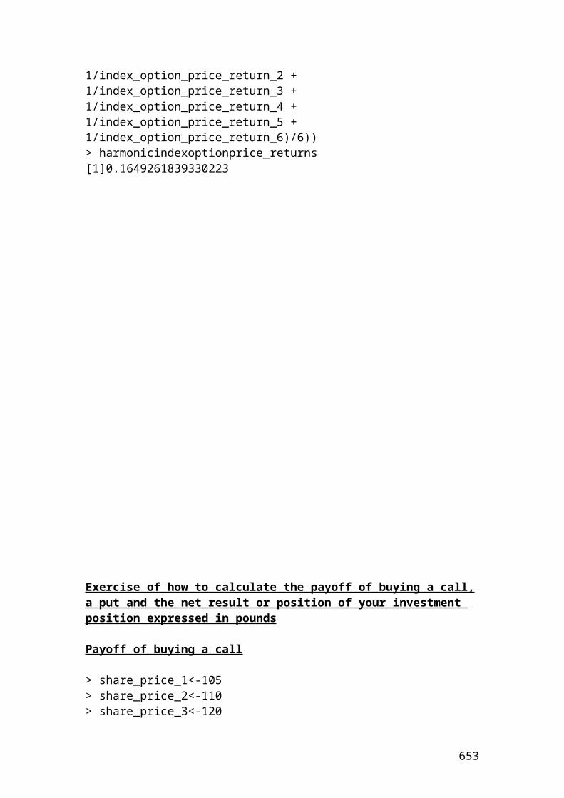
Example of calculating a margin call due to changes of price futures

An investor has opened a short position of 20 Soybean futures contract. The initial margin was 500 Pounds and the maintenance margin was 430 Pounds per contract. The price change that will create a margin call is as follows:

Solution

20

430- 500 sizecontract

margin emaintenanc -margin initial price aat created callMargin 3.5

Application of margin call in Java

class Margin_call {public static void main(String[] args) {

653

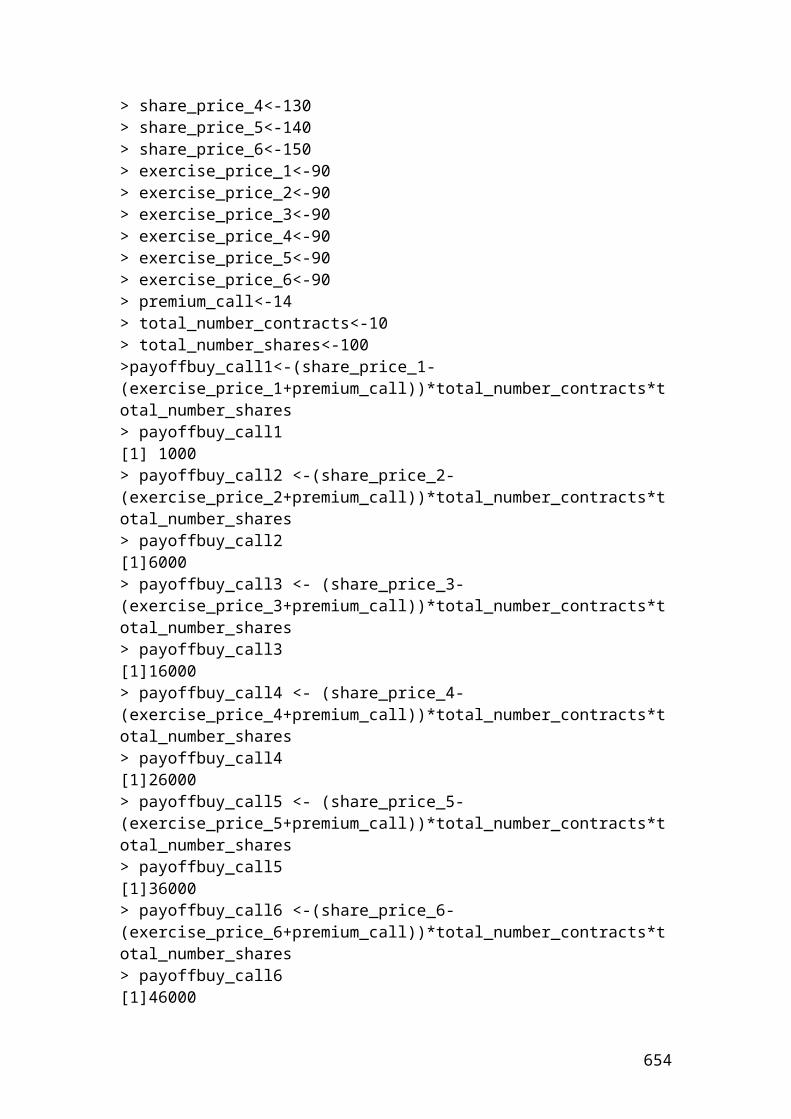
// Margin call. double initial_margin = 500;double maintenance_margin = 430;int futures_contract = 20;double margin_call;

// Insert the mathematical formula.

margin_call =( initial_margin-maintenance_margin) / futures_contract;

// Output function.

System.out.print(" margin_call in pounds is");System.out.println(margin_call);}}

Output result

After compiling the current document from tools and pressing the run document you should get the following result:

Welcome to DrJava. Working directory is C:\Documents and Settings\Owner\Desktop\Java Compiler> run Margin_call margin_call in pounds is3.5>

Calculate the call option prices using a Cox, Ross, Rubinstein,(CRR) binomial 3 steps tree. Please e-mail me to send you the binomial tree in Excel if this is complicated. I will also convert this example in VBA. Please check the VBA section in the document Financial Derivatives

class Cox_Ross_Rubinstein_call_option_calculations {public static void main(String[] args) { /* Calculate the call option prices using a Cox, Ross, Rubinstein,(CRR) binomial 3 steps tree. */ double S = 60; //share price double K = 50; // strike price double r = 0.05; // risk-free interest rate double q = 0.02; // dividend yield. If the dividend is zero, then, it is // not included in the equation of risk neutral // probability of upmove. double T = 0.5; // life to maturity

654

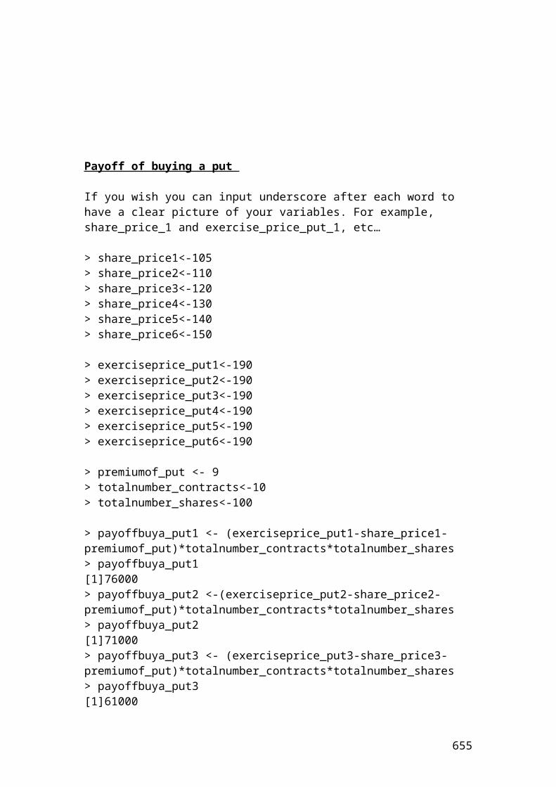
double sig = 0.3; // volatility // Identify the variables. // u = multiplier of upmove. //d = multiplier of downmove. dt = steps expressed in years. //riskprobofupmove = risk neutral probability of upmove. //disfact = discount factor. double u; double d; double dt; double riskprobofupmove; double disfact; int n = 3; // Identify tree steps binomial tree. // Insert the mathematical formulas. dt = T/n; u = Math.exp(sig*Math.sqrt(dt)); d = 1/u; disfact = Math.exp(-r*dt); riskprobofupmove = (Math.exp((r-q)*dt)-d)/(u-d); double callpayoffupmovestep3; // (Shareprice * upmove^3)-Kdouble callpayoff3i; // (Shareprice * upmove^2 * downmove)-Kdouble callpayoff3ii; // (Shareprice * downmove^2*upmove)-K double callpayoffdownmovestep3; // (Shareprice * downmove^3) -K

// The option prices are calculated backwards.

callpayoffupmovestep3 = S*Math.pow(u,3)-K;callpayoff3i = S * Math.pow(u,2) * d -K;callpayoff3ii =S * Math.pow(d,2)*u-K; callpayoffdownmovestep3 = S*Math.pow(d,3)-K;callpayoffdownmovestep3 =0;

double callpriceupmovestep2;double callpriceupdownmovestep2;double callpricedownmovestep2;

callpriceupmovestep2 = (disfact*(riskprobofupmove*callpayoffupmovestep3)+(1-riskprobofupmove)*callpayoff3i);

callpriceupdownmovestep2 =(disfact*(riskprobofupmove*callpayoff3i)+(1-riskprobofupmove)*callpayoff3ii);

callpricedownmovestep2 =(disfact*(riskprobofupmove*callpayoff3ii)+(1-riskprobofupmove)*callpayoffdownmovestep3);

655

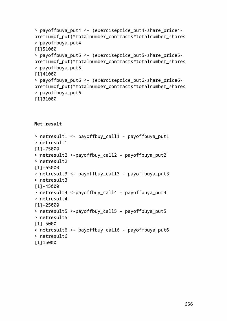
double callpriceupmovestep1;double callpricedownmovestep1;

callpriceupmovestep1 = (disfact*(riskprobofupmove*callpriceupmovestep2)+(1-riskprobofupmove)*callpriceupdownmovestep2);

callpricedownmovestep1=(disfact*(riskprobofupmove*callpriceupdownmovestep2)+(1-riskprobofupmove)*callpricedownmovestep2);

double callpricestep0;

callpricestep0= (disfact*(riskprobofupmove*callpriceupmovestep1)+(1-riskprobofupmove)*callpricedownmovestep1);

//Output functions.

System.out.print("Steps expressed in years is ");System.out.println(dt);System.out.println(Math.round(dt*100.0)/100.0);System.out.print("Multiplier of upmove is ");System.out.println(u);System.out.println(Math.round(u*100.0)/100.0);System.out.print("Multiplier of downmove is ");System.out.println(d);System.out.println(Math.round(d*100.0)/100.0);System.out.print("Discount factor is ");System.out.println(disfact);System.out.println(Math.round(disfact*100.0)/100.0);System.out.print("Risk neutral probability of upmove is ");System.out.println(riskprobofupmove);System.out.println(Math.round(riskprobofupmove*100.0)/100.0);System.out.print("Call payoff upmove step [3] in pounds is ");System.out.println(callpayoffupmovestep3);System.out.println(Math.round(callpayoffupmovestep3*100.0)/100.0);System.out.print("Call payoff [3i] in pounds is ");System.out.println(callpayoff3i);System.out.println(Math.round(callpayoff3i*100.0)/100.0);System.out.print("Call payoff [3ii] in pounds is ");System.out.println(callpayoff3ii);System.out.println(Math.round(callpayoff3ii*100.0)/100.0);System.out.print("Call payoff downmove step [3] in pounds is ");System.out.println(callpayoffdownmovestep3);System.out.println(Math.round(callpayoffdownmovestep3*100.0)/100.0);System.out.print("Call price upmove step[2] in pounds is ");System.out.println(callpriceupmovestep2);System.out.println(Math.round(callpriceupmovestep2*100.0)/100.0);System.out.print("Call price updownmove step [2] in pounds is ");System.out.println(callpriceupdownmovestep2);

656

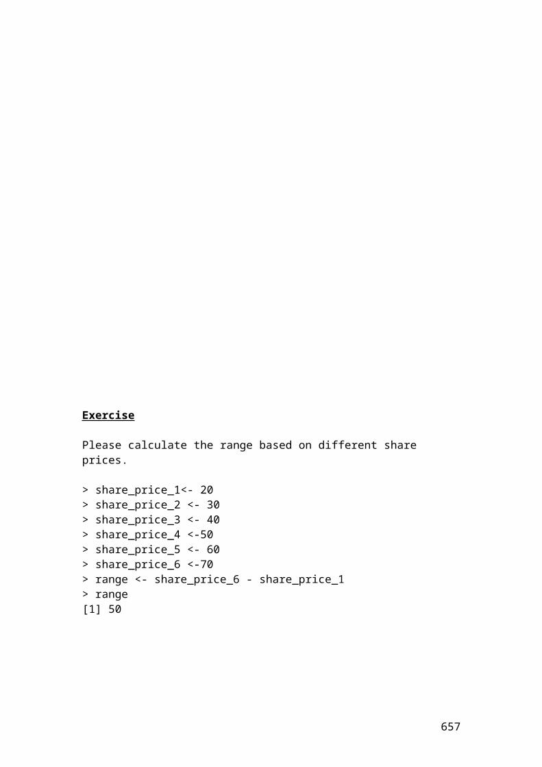
System.out.println(Math.round(callpriceupdownmovestep2*100.0)/100.0);System.out.print("Call price downmove step [2] in pounds is ");System.out.println(callpricedownmovestep2);System.out.println(Math.round(callpricedownmovestep2*100.0)/100.0);System.out.print("Call price upmove step [1] in pounds is ");System.out.println(callpriceupmovestep1);System.out.println(Math.round(callpriceupmovestep1*100.0)/100.0);System.out.print("Call price downmove step [1] in pounds is ");System.out.println(callpricedownmovestep1);System.out.println(Math.round(callpricedownmovestep1*100.0)/100.0);System.out.print("Call price step[0] in pounds is ");System.out.println(callpricestep0);System.out.println(Math.round(callpricestep0*100.0)/100.0);}}

Output results

After compiling the current document from tools and pressing the run document you should get the following results:

Welcome to DrJava. Working directory is C:\Documents and Settings\Owner\Desktop\Java Compiler> run Cox_Ross_Rubinstein_call_option_calculationsSteps expressed in years is 0.166666666666666660.17Multiplier of upmove is 1.13029028276745721.13Multiplier of downmove is 0.88472847661005440.88Discount factor is 0.9917012926388760.99Risk neutral probability of upmove is 0.489832055446951740.49Call payoff upmove step [3] in pounds is 36.6405563126204336.64Call payoff [3i] in pounds is 17.81741696604743217.82Call payoff [3ii] in pounds is 3.0837085966032593.08Call payoff downmove step [3] in pounds is 0.00.0Call price upmove step[2] in pounds is 26.8886511342689626.89Call price updownmove step [2] in pounds is 10.22832393472965710.23Call price downmove step [2] in pounds is 1.49796412844548191.5Call price upmove step [1] in pounds is 18.27978461354383218.28

657

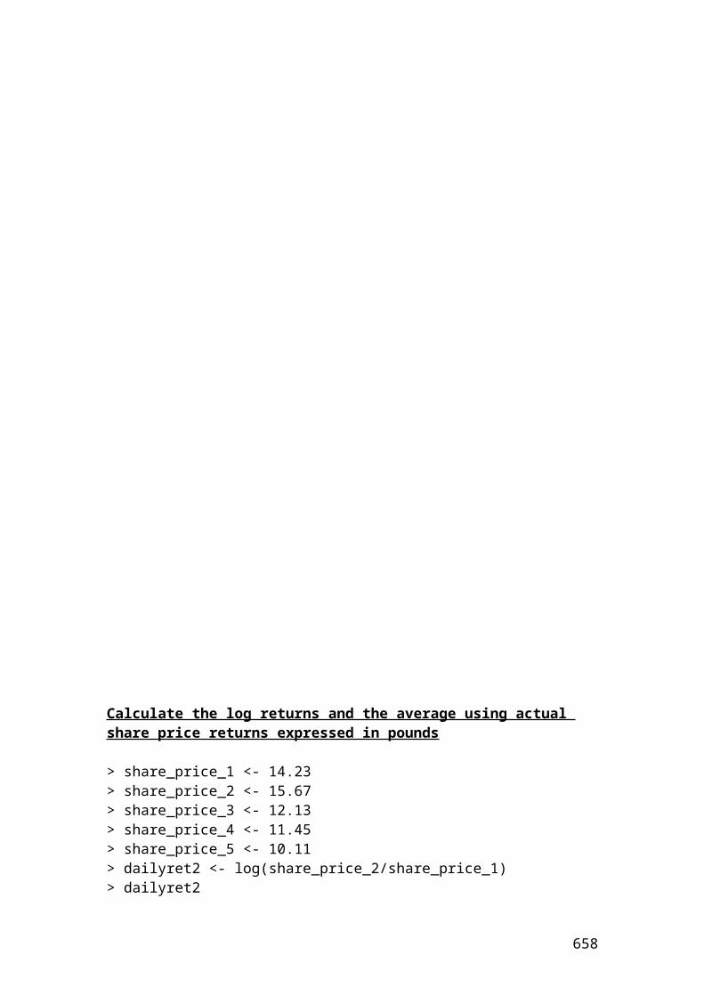
Call price downmove step [1] in pounds is 5.7327963577030885.73Call price step[0] in pounds is 11.80440657594629911.8>

Calculate the put option prices using a Cox, Ross, Rubinstein,(CRR) binomial 3 steps tree. The multipliers of up and down move depend on volatility and the length of steps

class Cox_Ross_Rubinstein_put_option_calculations {public static void main(String[] args) {

/* Calculate the put option prices using a Cox, Ross, Rubinstein,(CRR) binomial 3 steps tree. */

double S = 60; // share price double K = 70; // strike price double r = 0.02; // risk-free interest rate double q = 0.03; // dividend yield double T = 0.5; // life to maturity double sig = 0.2; // volatility // Identify the variables. u = multiplier of upmove.

658

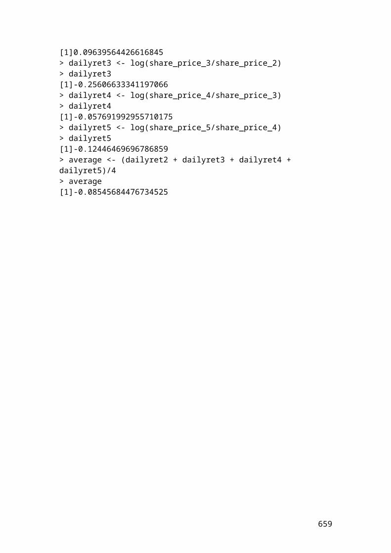
//d = multiplier of downmove. dt = steps expressed in years. //riskprobofupmove = risk neutral probability of upmove. //disfact = discount factor. double u; double d; double dt; double riskprobofupmove; double disfact; int n = 3; // Identify tree steps binomial tree. // Insert the mathematical formulas. dt = T/n; u = Math.exp(sig*Math.sqrt(dt)); d = 1/u; disfact = Math.exp(-r*dt); riskprobofupmove = (Math.exp((r-q)*dt)-d)/(u-d); double putpayoffupmovestep3; // K - (Shareprice * upmove^3)double putpayoff3i; // K- (Shareprice * upmove^2 * downmove)double putpayoff3ii; // K-(Shareprice * downmove^2*upmove) double putpayoffdownmovestep3; // K-(Shareprice * downmove^3)

// The option prices are calculated backwards.

putpayoffupmovestep3 = K-S*Math.pow(u,3);putpayoffupmovestep3=0;putpayoff3i = K- S * Math.pow(u,2) * d;putpayoff3ii =K- S * Math.pow(d,2)*u; putpayoffdownmovestep3 = K - S*Math.pow(d,3);

double putpriceupmovestep2;double putpriceupdownmovestep2;double putpricedownmovestep2;

putpriceupmovestep2 = (disfact*(riskprobofupmove*putpayoffupmovestep3)+(1-riskprobofupmove)*putpayoff3i);

putpriceupdownmovestep2 =(disfact*(riskprobofupmove*putpayoff3i)+(1-riskprobofupmove)*putpayoff3ii);

putpricedownmovestep2 =(disfact*(riskprobofupmove*putpayoff3ii)+(1-riskprobofupmove)*putpayoffdownmovestep3);

double putpriceupmovestep1;double putpricedownmovestep1;

659

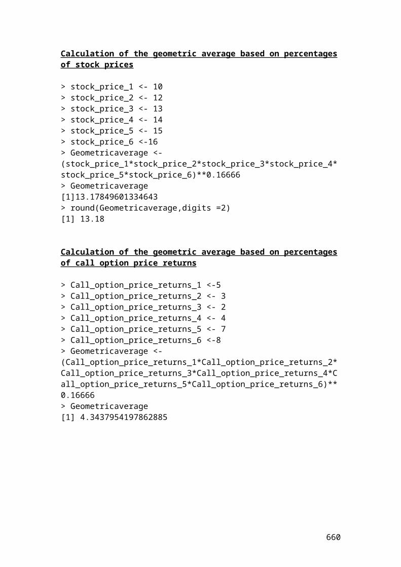
putpriceupmovestep1 = (disfact*(riskprobofupmove*putpriceupmovestep2)+(1-riskprobofupmove)*putpriceupdownmovestep2);

putpricedownmovestep1=(disfact*(riskprobofupmove*putpriceupdownmovestep2)+(1-riskprobofupmove)*putpricedownmovestep2);

double putpricestep0;

putpricestep0= (disfact*(riskprobofupmove*putpriceupmovestep1)+(1-riskprobofupmove)*putpricedownmovestep1);

//Output functions.System.out.print("Steps expressed in years is ");System.out.println(dt);System.out.println(Math.round(dt*100.0)/100.0);System.out.print("Multiplier of upmove is ");System.out.println(u);System.out.println(Math.round(u*100.0)/100.0);System.out.print("Multiplier of downmove is ");System.out.println(d);System.out.println(Math.round(d*100.0)/100.0);System.out.print("Discount factor is ");System.out.println(disfact);System.out.println(Math.round(disfact*100.0)/100.0);System.out.print("Risk neutral probability of upmove is ");System.out.println(riskprobofupmove);System.out.println(Math.round(riskprobofupmove*100.0)/100.0);System.out.print("Put payoff upmove step [3] in pounds is ");System.out.println(putpayoffupmovestep3);System.out.println(Math.round(putpayoffupmovestep3*100.0)/100.0);System.out.print("Put payoff [3i] in pounds is ");System.out.println(putpayoff3i);System.out.println(Math.round(putpayoff3i*100.0)/100.0);System.out.print("Put payoff [3ii] in pounds is ");System.out.println(putpayoff3ii);System.out.println(Math.round(putpayoff3ii*100.0)/100.0);System.out.print("Put payoff downmove step [3] in pounds is ");System.out.println(putpayoffdownmovestep3);System.out.println(Math.round(putpayoffdownmovestep3*100.0)/100.0);System.out.print("Put price upmove step[2] in pounds is ");System.out.println(putpriceupmovestep2);System.out.println(Math.round(putpriceupmovestep2*100.0)/100.0);System.out.print("Put price updownmove step [2] in pounds is ");System.out.println(putpriceupdownmovestep2);System.out.println(Math.round(putpriceupdownmovestep2*100.0)/100.0);System.out.print("Put price downmove step [2] in pounds is ");System.out.println(putpricedownmovestep2);System.out.println(Math.round(putpricedownmovestep2*100.0)/100.0);

660

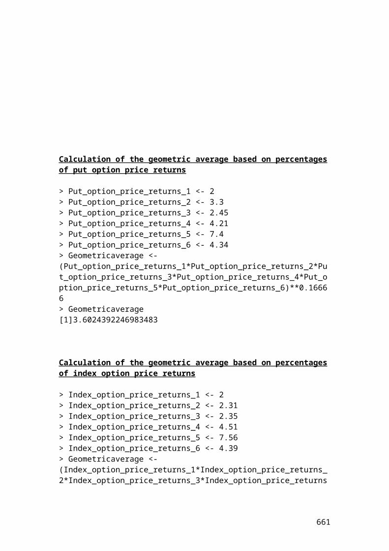
System.out.print("Put price upmove step [1] in pounds is ");System.out.println(putpriceupmovestep1);System.out.println(Math.round(putpriceupmovestep1*100.0)/100.0);System.out.print("Put price downmove step [1] in pounds is ");System.out.println(putpricedownmovestep1);System.out.println(Math.round(putpricedownmovestep1*100.0)/100.0);System.out.print("Put price step[0] in pounds is ");System.out.println(putpricestep0);System.out.println(Math.round(putpricestep0*100.0)/100.0);}}

Output results

After compiling the current document from tools and pressing the run document you should get the following results:

Welcome to DrJava. Working directory is C:\Documents and Settings\Owner\Desktop\Java Compiler> run Cox_Ross_Rubinstein_put_option_calculationsSteps expressed in years is 0.166666666666666660.17Multiplier of upmove is 1.08507559577726931.09Multiplier of downmove is 0.92159477541624430.92Discount factor is 0.99667221605452331.0Risk neutral probability of upmove is 0.469412533318738670.47Put payoff upmove step [3] in pounds is 0.0

661

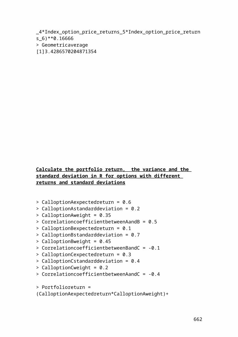
0.0Put payoff [3i] in pounds is 4.8954642533638414.9Put payoff [3ii] in pounds is 14.70431347502533714.7Put payoff downmove step [3] in pounds is 23.03533136051513723.04Put price upmove step[2] in pounds is 2.59747197642099262.6Put price updownmove step [2] in pounds is 10.09226949113763510.09Put price downmove step [2] in pounds is 19.10167749033414719.1Put price upmove step [1] in pounds is 6.57006008299829256.57Put price downmove step [1] in pounds is 14.8567832883130414.86Put price step[0] in pounds is 10.95662844179555910.96>

References

Alfred Winslow Jones (1949), “Creation of the first hedge fund”.

Ackermann, C., R. McEnally and Ravenscraft, (1999). “The Performance of Hedge Funds: Risk, Return, and Incentives”. The Journal of Finance. Volume 54, Issue 3, pages 833-874.

Agarwal, Vikas and Narayan Y. Naik (2004), “Risk and Portfolio Decisions Involving Hedge Funds”. Review of Financial Studies, 17, pp.63-98.

Brown and Goetzmann (1997), “Hedge Funds with Style”. NBER working paper No.8173.

Brown, Stephen, William N. Goetzmann and Roger G. Ibbotson, (1999), “Offshore Hedge Funds, Survival and Performance”. Journal of Business 72: (January #1) 91-118.

662

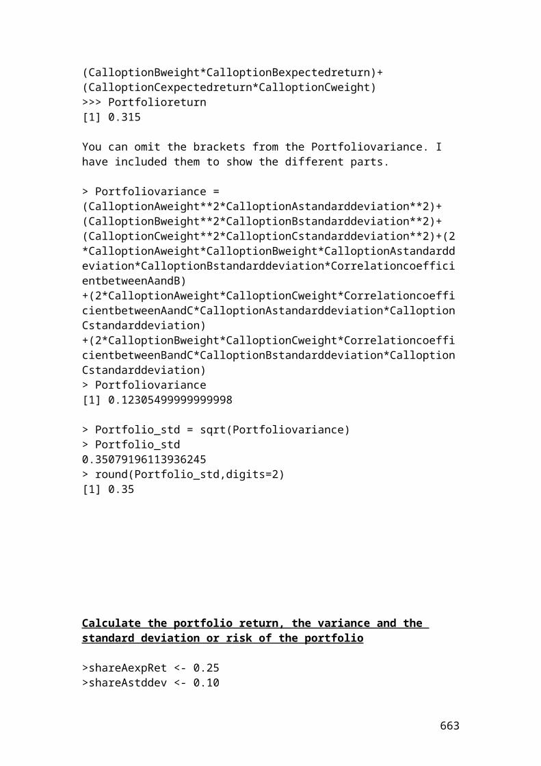
Carhart, M.(1997), “On Persistence in Mutual Fund Performance”. Journal of Finance, Vol 52. No 1.

Capocci and Hubner, (2004), “An Analysis of Hedge Fund Performance”. Journal of Empirical Finance. Vol.11, No 1, pp 55-89.

Fama, E. F., and K. R. French. (1993), “Common Risk Factors in the Returns on Stocks and Bonds.”Journal of Financial Economics 33, (1993): 3-56.

Fama, E. F., and K. R. French.(1996), “Multifactor Explanations of Asset Pricing Anomalies.” Journal of Finance 51, (1996): 55-84.

Fung and Hsieh(1997), “Performance Characteristics of Hedge Funds and Commodity Funds: Natural versus Spurious Biases. Journal of Financial and Quantitative Analysis. Volume 35, pp.291-307.

Lavinio, Stefano (2000), Hedge fund handbook: a definitive guide for analyzing and evaluating alternative investments, New York: McGraw Hill.

663

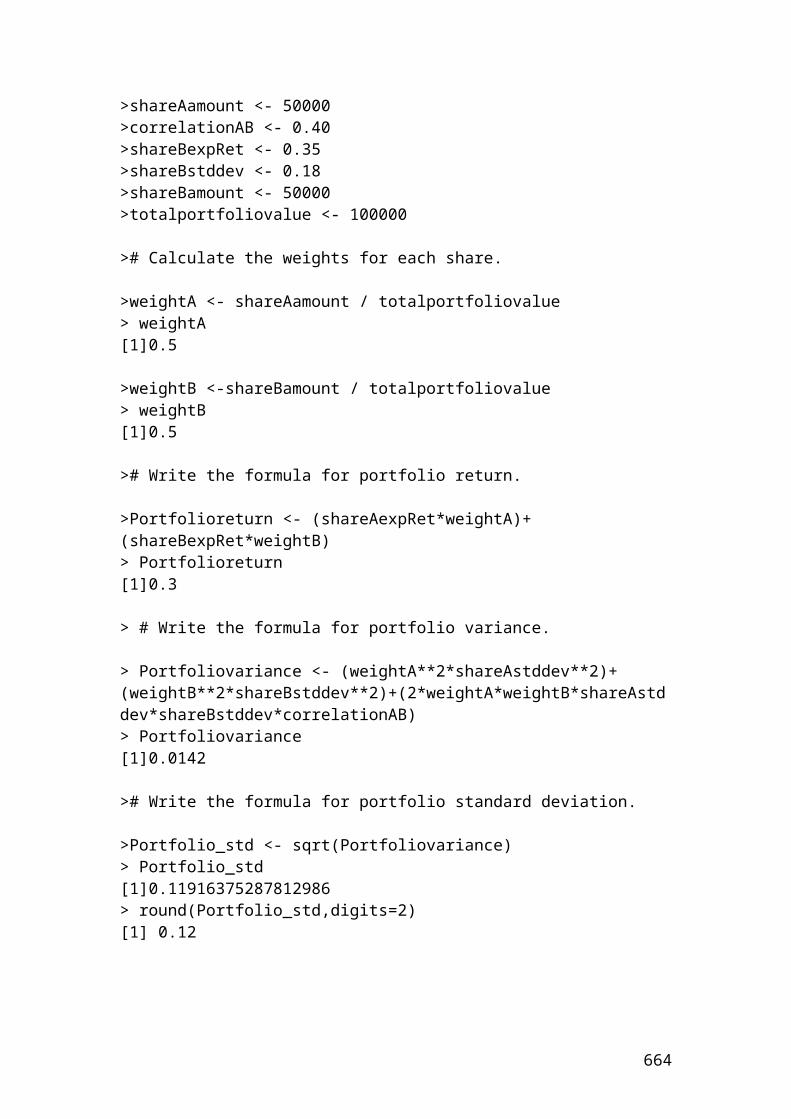
664