Hedge Fund Tail Risk�

Tobias Adriany

Federal Reserve Bank of New York

Markus K. Brunnermeierz

Princeton University

Version: September 21, 2007

- Preliminary and Incomplete -

Abstract

This paper uses quantile regressions to document the increase in hedge funds'Value-at-Risk (VaR) conditional on other styles being under distress and (pre-dictable) spill-over e�ects to the banking sector. This increase of conditional VaRis due to an increase in bivariate dependencies in times of stress. We identify sixcommon factors that explain the tail dependence across hedge fund styles. Thisset of risk factors also explains a large part of hedge funds' expected returns,which unlike the Value-at-Risk, a�ect ows into and out of hedge funds style.

Keywords: Hedge Funds, Tail Risk, Asset Pricing, Systemic Risk, Value-at-RiskJEL classi�cation: G10, G12

�The authors would like to thank Ren�e Carmona, Xavier Gabaix, Beverly Hirtle, John Kambhu,Burton Malkiel, Maureen O'Hara, Matt Pritsker, Jos�e Scheinkman, Kevin Stiroh and seminar par-ticipants at Columbia University, Princeton University, Cornell University, Rutgers University, andthe Federal Reserve Bank of New York for helpful comments. Brunnermeier acknowledges �nancialsupport from the Alfred P. Sloan Foundation.The views expressed in this paper are those of the authors and do not necessarily represent those

of the Federal Reserve Bank of New York or the Federal Reserve System.yFederal Reserve Bank of New York, Capital Markets, 33 Liberty Street, New York, NY 10045,

http://nyfedeconomists.org/adrian/, email: tobias.adrian@ny.frb.orgzPrinceton University, Department of Economics, Bendheim Center for Finance, Prince-

ton, NJ 08540-5296, NBER, CEPR, CESIfo, http://www.princeton.edu/�markus, e-mail:markus@princeton.edu

1

1 Introduction

Our �nancial architecture underwent a dramatic transformation in the last two decades

with hedge funds taking on an ever increasing role. Hedge funds' assets under man-

agement { after adjusting for leverage { are now comparable to the total size of US

investment banks' balance sheets and represent nearly 25% of GDP. The emergence

of hedge funds as key �nancial intermediaries is intimately linked to this continuous

process of �nancial innovation. In today's markets the risk of individual assets is

repackaged and tranched into di�erent components using derivatives. With this ever

increasing tradability and securitization of �nancial assets such as loan portfolios, cor-

porate debt, credit card payables, mortgages etc., hedge funds now take on risks that

have traditionally been kept on banks' balance sheets.

The collapse of Long Term Capital Management (LTCM) in 1998 made clear that

the failure of a hedge fund can threaten the stability of the �nancial system. The

opaqueness of hedge funds' exposures and lack of regulatory oversight further raises

the question whether hedge funds increase the likelihood of systemic crisis. In a liquid-

ity spiral, initial losses in some asset class lead to higher margins, rapid asset sales, and

reduction in mark-to-market wealth, which in turn leads to additional losses and po-

tential spillovers into other asset classes (Brunnermeier and Pedersen (2007)).1 Banks

and particularly prime brokers, who have credit risk exposure to hedge funds, suf-

fer potentially large losses if many hedge funds experience distress at the same time.

Therefore from a �nancial stability point of view, it is important to understand which

hedge fund styles tend to experience simultaneous large losses and to what extent the

banking sector is shielded from hedge fund distress.

1The liquidity spiral of July/August 2007 that lead to a systematic unwinding of factor basedportfolios among quant funds suggests a high comovement in quant fund returns in times of crisis.See Wall Street Journal August 24, 2007 \How the Quant Playbook Failed".

2

In this paper, we use quantile regression, which naturally yield our measure of tail

risk { the Value-at-Risk (VaR) { to empirically study the interdependencies between

di�erent hedge fund styles at times of crisis, and analyze the spillover e�ects to the

banking system. We present �ve main results: (i) our new tail risk dependence measure,

CoVaR { de�ned as hedge funds' VaR conditional on the fact that some other hedge

fund style is in distress { is signi�cantly higher than the (unconditional) VaR, (ii) \tail

dependence" sensitivities are higher in times of distress, (iii) low returns of �xed income

hedge funds predict a higher Value-at-Risk for investment banks in the subsequent

months. To document this (delayed) spill-over e�ect to the banking sector, we introduce

a \Granger-tail causality test". Furthermore, (iv) we identify six risk factors that

explain the tail dependence across hedge fund styles and the banking sector and argue

that (v) these risk factors also explain a large part of hedge funds' expected returns.

We also �nd { consistent with existing literature { that past returns a�ect capital ows

across strategies and over time, but { surprisingly { the Value-at-Risk does not a�ect

capital ows. Hedge fund managers thus have incentives to load on tail risk for two

reasons: it increases both the managers' incentive fee (percentage of the fund's pro�t)

and the management fee (percentage of assets under management).

Our paper contributes to the growing literature that sheds light on the link between

hedge funds and the risk of a systemic crisis. Boyson, Stahel, and Stulz (2006) also doc-

ument contagion across hedge fund styles using logit regressions on daily and monthly

returns. However, they do not �nd evidence of contagion between hedge fund returns

and equity, �xed income and foreign exchange returns. In contrast, we show that our

pricing factors explain the increase in comovement among hedge fund styles in times

of stress. Chan, Getmansky, Haas, and Lo (2006) document an increase in correlation

across hedge funds, especially prior to the LTCM crisis and after 2003. Adrian (2007)

3

points out that the increase in correlation since 2003 is due to a reduction in volatility

{ a phenomenon that occurred across many �nancial assets { rather than an increase

in covariance.

Asness, Krail, and Liew (2001) and Agarwal and Naik (2004) document that hedge

funds load on tail risk in order to boost their CAPM-�. Agarwal and Naik (2004)

capture the tail exposure of equity hedge funds with non-linear market factors that take

the shape of out-of-the-money put options. Patton (2007) develops several \neutrality

tests" including a test for tail and VaR neutrality and �nds that many so-called market

neutral funds are in fact not market neutral. Bali, Gokcan, and Liang (2007) and Liang

and Park (2007) �nd that hedge funds that take on high left-tail risk outperform funds

with less risk exposure. In addition, there is a large and growing number of papers

that explain average returns of hedge funds using asset pricing factors (see e.g. Fung

and Hsieh (2001, 2002, 2003), Hasanhodzic and Lo (2007)). Our approach is di�erent

in the sense that we study factors that explain the co-dependence across the tails of

di�erent hedge fund styles.

The paper is organized in �ve sections. In Section 2, we study the pairwise relation-

ships between the returns to di�erent hedge fund styles, and the relationships between

hedge fund styles and other �nancial intermediaries. In Section 3, we estimate a risk

factor model for the hedge fund returns. We document that six commonly traded risk

factors explain hedge fund returns well, and that they particularly explain the increase

of CoVaR relative to unconditional VaR. In Section 4, we study the incentives of hedge

funds to take on tail risk. Finally, Section 6 concludes.

4

2 q-Sensitivities and CoVaR

In this section, we document that pairwise dependence of the returns to hedge fund

styles is signi�cantly higher in times of stress. As a result, the Values-at-Risk of fund

styles conditional on other funds is higher in times of stress than in normal times. We

also study the relation between hedge fund returns and the returns to other �nancial

institutions in times of stress, both contemporaneously and in a predictive sense.

2.1 Hedge Fund Return Data

Hedge funds are private investment partnerships that are largely unregulated. Studying

hedge funds is more challenging than the analysis of regulated �nancial institutions

such as mutual funds, banks, or insurance companies, as only very limited data on

hedge funds is made available through regulatory �lings. Consequently, most studies

of hedge funds thus rely on self-reported return data.2 We follow this approach and

use the hedge fund style indices by Credit Suisse/Tremont.

There are several papers that compare the self-reported returns of di�erent vendors

(see e.g. Agarwal and Naik (2005)), and some research compares the return charac-

teristics of hedge fund indices with the returns of individual funds (Malkiel and Saha

(2005)). The literature also investigates biases such as survivorship bias (Brown, Goet-

zmann, and Ibbotson (1999) and Liang (2000)), termination and self-selection bias

(Ackermann, McEnally, and Ravenscraft (1999)), back�lling bias, and illiquidity bias

(Asness, Krail, and Liew (2001) and Getmansky, Lo, and Makarov (2004)). We take

from this literature that hedge fund return indices do not constitute ideal sources of

2A notable exception is a study by Brunnermeier and Nagel (2004) who use quarterly 13F �lings tothe SEC and show that hedge funds were riding the tech-bubble rather than acting as price-correctingforce.

5

data, but that their study is useful, and the best that is available. In addition, there is

some evidence that the Credit Suisse/Tremont indices appear to be the least a�ected

by various biases (Malkiel and Saha (2005)).

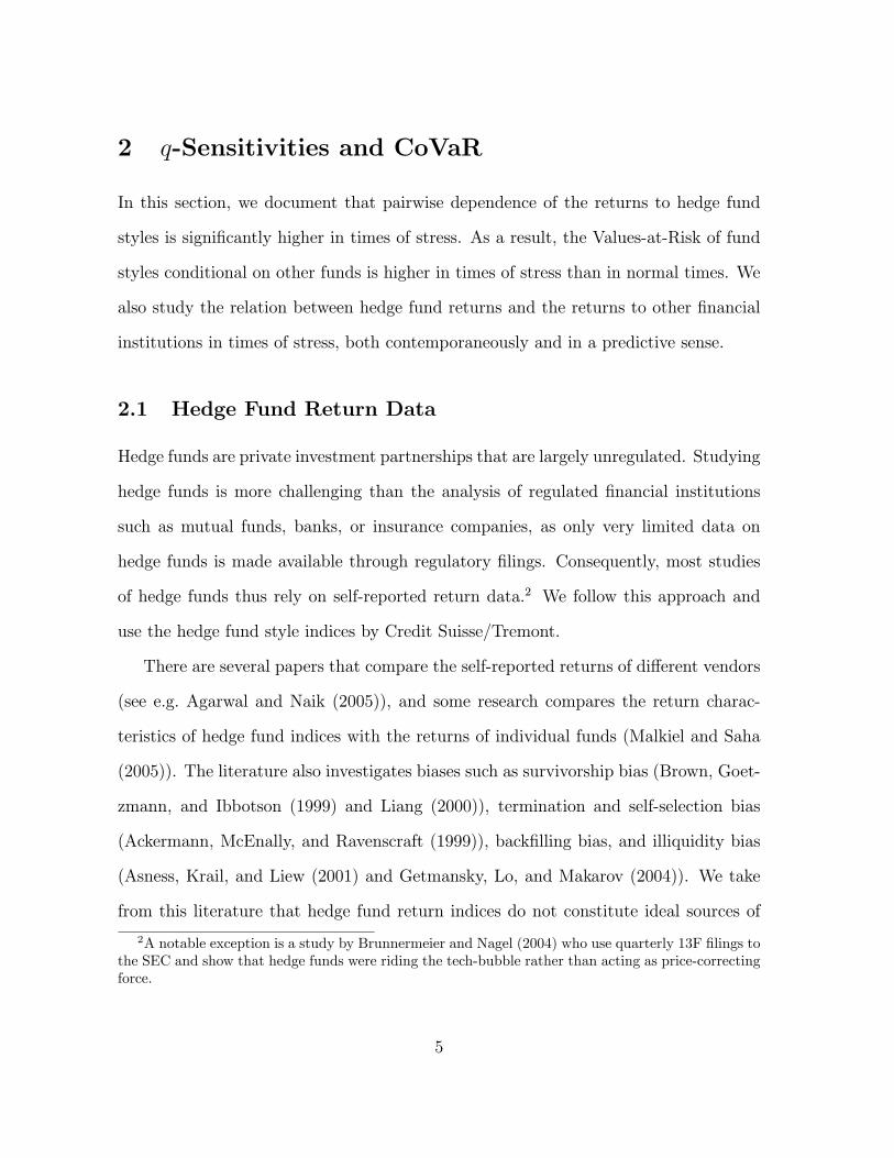
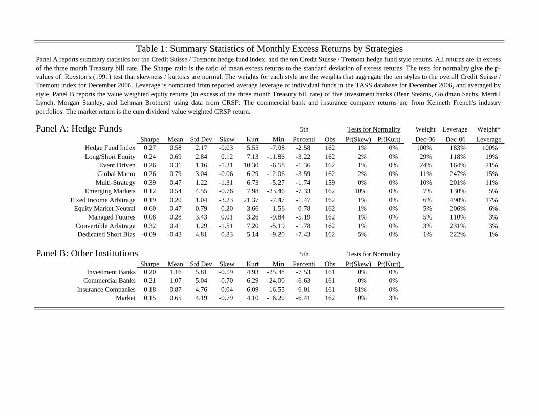
[Table 1]

Summary statistics for January 1994 - June 2006 of the monthly excess returns of the

overall hedge fund index and the ten style indices are given in Table 1 (Panel A). These

styles have been extensively described in the literature (see Agarwal and Naik (2005)

for a survey), and characterizations can also be found on the Credit Suisse/Tremont

website (www.hedgeindex.com). We report the hedge fund returns in the order of their

weights in the overall index as of December 2006. These weights are also reported in the

third to last column of Panel A in Table 1. We also report the returns of three additional

�nancial institutions in Panel B: commercial banks, investment banks, insurance com-

panies. In addition, we report the summary statistics of the return CRSP market excess

return, which we sometimes interpret as a proxy to a well diversi�ed mutual fund. The

commercial bank and insurance company returns are from the 49 industry portfolios of

Ken French's website (http://mba.tuck.dartmouth.edu/pages/faculty/ken.french/data library.html).

The investment bank returns are the value weighted returns of Morgan Stanley, Mer-

rill Lynch, Goldman Sachs, Bear Sterns, and Lehman Brothers from CRSP. Note that

traditional �nancial intermediaries are traded and hence their returns { unlike the ac-

counting returns used in hedge fund indices { also re ect expected changes in goodwill

and reputation.

The Sharpe ratio of the hedge fund index (0.27 monthly) is nearly twice as high as

the Sharpe ratio of the market index (0.15 monthly). It is also higher than the Sharpe

ratio of the other �nancial institutions (0.20 for investment banks, 0.21 for commercial

6

banks, and 0.18 for insurance companies). There is a wide disparity of Sharpe ratios

across styles: equity market neutral achieves the highest Sharpe ratio (0.60), while

dedicated short has a negative Sharpe ratio (-0.09). Sharpe ratios and the December

2006 sectoral weights do not appear to be highly correlated (the correlation is in fact

15% and statistically insigni�cant), but average returns over the 1994-2006 period are

highly and signi�cantly correlated with the December 2006 weights (the correlation is

56%). Since hedge funds invest part of their wealth in highly illiquid instruments with

stale or \managed" prices, they can smooth their returns and manipulate Sharpe ratios

(see e.g. Asness, Krail, and Liew (2001) and Getmansky, Lo, and Makarov (2004)).

The hedge fund index has less negative skewness than the market return (-0.03

versus -0.79), but higher kurtosis (5.55 versus 4.93). There is also large variation of

skewness and kurtosis across styles. Styles with higher leverage generally appear to

have more negative skewness. Normality is rejected on the basis of either skewness or

kurtosis for all styles, as well as the other �nancial institutions and the market return.

Thus, consistent with previous �ndings, the returns to hedge funds have both skewed

and fat tailed returns relative to normality.

The most negative monthly returns are lower for the overall hedge fund index than

for the market or other �nancial institutions. This �nding is also con�rmed by looking

at the 5% percentile: it is -2.58% monthly for the hedge fund index, versus -6.41% for

the market. The �nding that the left tail of hedge fund returns has excess skewness

and kurtosis relative to a normal distribution, but lower skewness and kurtosis than the

market is consistent with Brunnermeier and Nagel's (2004) �nding that hedge funds

are good market timers.

7

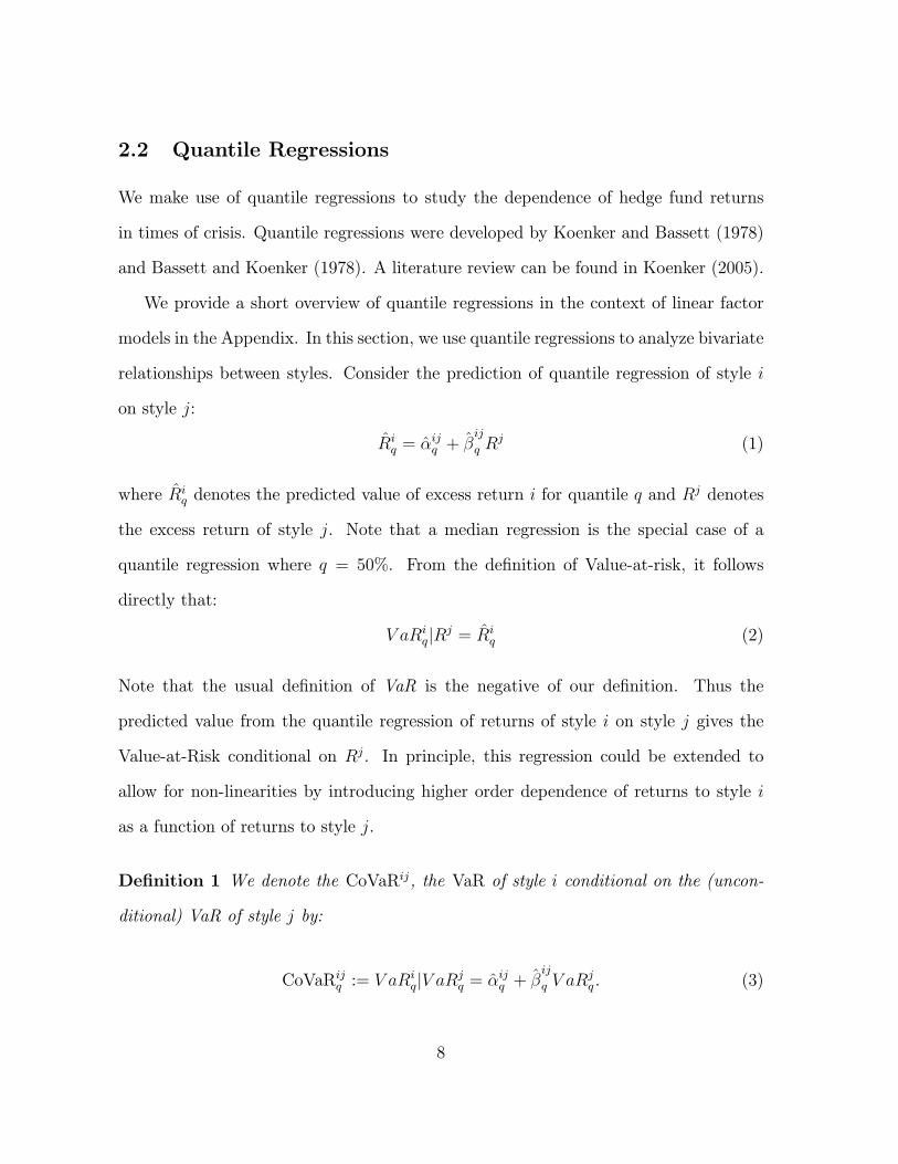
2.2 Quantile Regressions

We make use of quantile regressions to study the dependence of hedge fund returns

in times of crisis. Quantile regressions were developed by Koenker and Bassett (1978)

and Bassett and Koenker (1978). A literature review can be found in Koenker (2005).

We provide a short overview of quantile regressions in the context of linear factor

models in the Appendix. In this section, we use quantile regressions to analyze bivariate

relationships between styles. Consider the prediction of quantile regression of style i

on style j:

Riq = �ijq + �

ij

q Rj (1)

where Riq denotes the predicted value of excess return i for quantile q and Rj denotes

the excess return of style j. Note that a median regression is the special case of a

quantile regression where q = 50%. From the de�nition of Value-at-risk, it follows

directly that:

V aRiqjRj = Riq (2)

Note that the usual de�nition of VaR is the negative of our de�nition. Thus the

predicted value from the quantile regression of returns of style i on style j gives the

Value-at-Risk conditional on Rj. In principle, this regression could be extended to

allow for non-linearities by introducing higher order dependence of returns to style i

as a function of returns to style j.

De�nition 1 We denote the CoVaRij, the VaR of style i conditional on the (uncon-

ditional) VaR of style j by:

CoVaRijq := V aRiqjV aRjq = �ijq + �

ij

q V aRjq. (3)

8

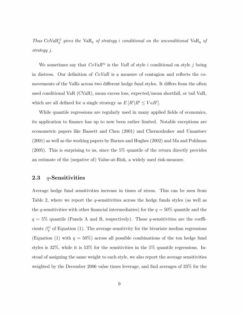
Thus CoVaRijq gives the VaRq of strategy i conditional on the unconditional VaRq of

strategy j.

We sometimes say that CoVaRij is the VaR of style i conditional on style j being

in distress. Our de�nition of CoVaR is a measure of contagion and re ects the co-

movements of the VaRs across two di�erent hedge fund styles. It di�ers from the often

used conditional VaR (CVaR), mean excess loss, expected/mean shortfall, or tail VaR,

which are all de�ned for a single strategy as E [RijRi � V aRi].

While quantile regressions are regularly used in many applied �elds of economics,

its application to �nance has up to now been rather limited. Notable exceptions are

econometric papers like Bassett and Chen (2001) and Chernozhukov and Umantsev

(2001) as well as the working papers by Barnes and Hughes (2002) and Ma and Pohlman

(2005). This is surprising to us, since the 5% quantile of the return directly provides

an estimate of the (negative of) Value-at-Risk, a widely used risk-measure.

2.3 q-Sensitivities

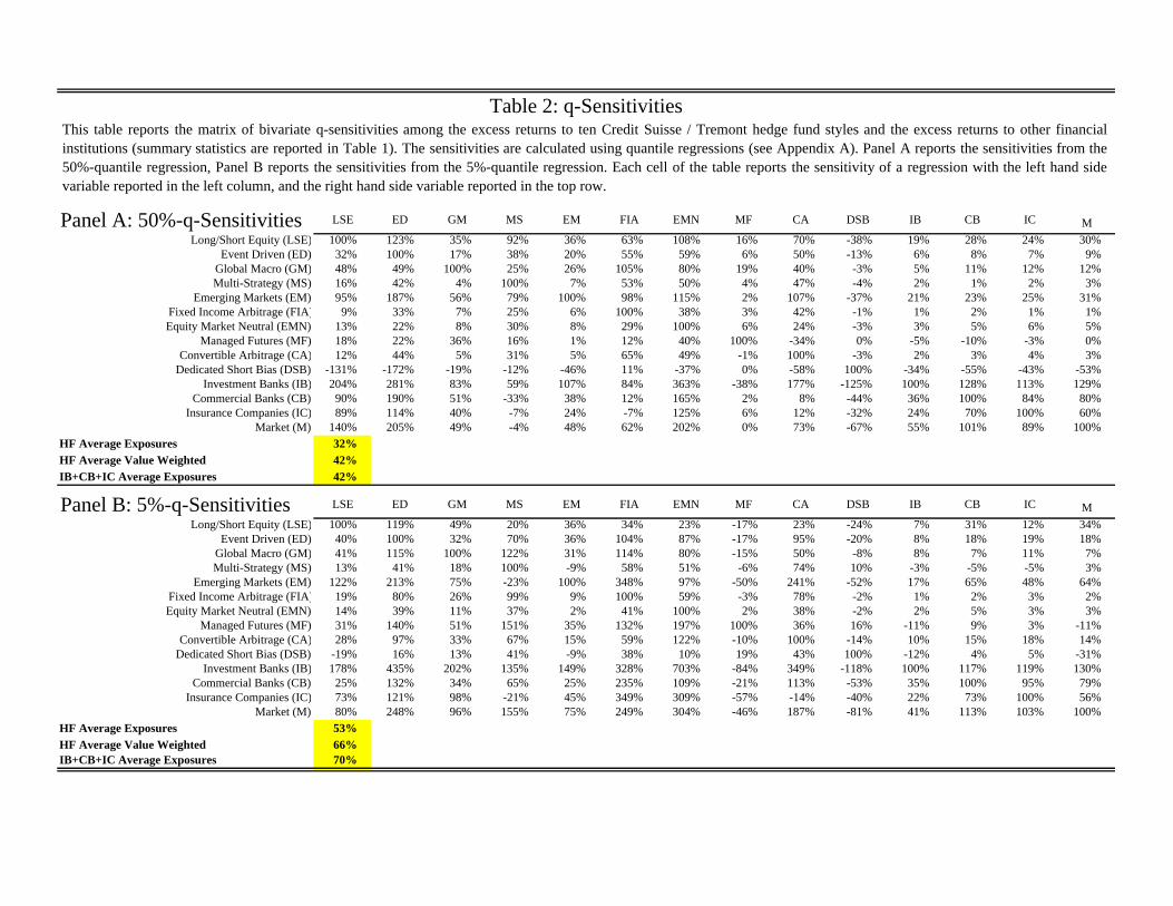
Average hedge fund sensitivities increase in times of stress. This can be seen from

Table 2, where we report the q-sensitivities across the hedge funds styles (as well as

the q-sensitivities with other �nancial intermediaries) for the q = 50% quantile and the

q = 5% quantile (Panels A and B, respectively). These q-sensitivities are the coe�-

cients �ijq of Equation (1). The average sensitivity for the bivariate median regressions

(Equation (1) with q = 50%) across all possible combinations of the ten hedge fund

styles is 32%, while it is 53% for the sensitivities in the 5% quantile regressions. In-

stead of assigning the same weight to each style, we also report the average sensitivities

weighted by the December 2006 value times leverage, and �nd averages of 33% for the

9

50% sensitivities (median regressions), versus 56% for the 5% sensitivities. Average

sensitivities are thus more than two thirds higher in times of stress (as proxied by the

5% sensitivities) compared to normal times (as proxied by the 50% sensitivities).

[Table 2]

We can also see that the q-sensitivities between the hedge fund styles and other

�nancial intermediaries increases in the left tails of the return distributions. In partic-

ular, the average exposures between the ten hedge fund styles, and the other �nancial

intermediaries is 42% for the median regression, and 70% for the 5% quantile regres-

sions.

Table 2 also reveals interesting patterns across individual styles. Each column of

the table gives a particular right hand side variable of the quantile regressions, while

the styles in the �rst column of the table correspond to the left hand side returns. For

example, the sensitivity of global macro returns with respect to �xed income arbitrage

is 7% in the median regression, but increases to 26% in the 5% regression. Conversely,

the sensitivity of �xed income arbitrage with respect to global macro is 105% in normal

times, but increases to 114% in times of stress.

The increase in sensitivities among hedge fund styles in times of stress has previously

been noted by Boyson, Stahel, and Stulz (2006). Boyson, Stahel, and Stulz (2006) do

not use quantile regressions, but produce dummies for the worst 5% of returns of the

left hand side return in an OLS regression, and refer to this increase in dependencies

as \contagion".

10

2.4 Increases in CoVaRs

As a consequence of the increase in average sensitivities among hedge fund styles,

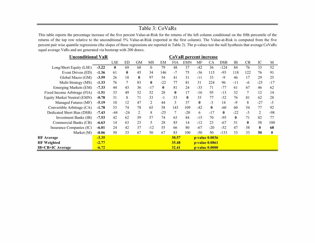
the CoVaRs increase. This can be seen in Table 3, where we report the matrix of

percentage increases in CoVaRs, relative to their unconditional values:

CoV aRij � V aRiV aRi

Reporting the percentage increase relative to the unconditional VaRs instead of the

CoVaR itself has the advantage that it normalizes data across strategies with di�erent

unconditional VaRs. The unconditional VaRs are reported in the �rst column of the

table and corresponds to the 5th percentile of the return distribution, also reported in

Table 1. The average unconditional VaR of the di�erent hedge fund styles is �3:35%

(it is �2:77% for the value weighted average), and �6:72% for the other �nancial

intermediaries. The average percentage increase of the CoVaRs is 30:57, thus the

average CoVaR is �3:35% � (1 + 30:57%) = �4:38%.

[Table 3]

As one would expect, these e�ects are not totally symmetric. For example, �xed

income funds and multi-strategy funds have roughly the same (unconditional) VaR of

�1:51, �1:33 respectively. However, when multi-strategy funds are in distress, the VaR

of �xed income funds is 52% higher, while in periods of distress for �xed-income funds,

the VaR of multi-strategy is increased by roughly 77%.

11

2.5 Forecasting Distress - Tail Granger Causality Test

So far we focused on contemporaneous relationship between returns. Next, we incorpo-

rate quantile regressions into a Granger causality test to determine whether hedge fund

returns predict distress in other �nancial intermediaries (in the sense of an increased

Value-at-Risk), and vice versa. More speci�cally, we \quantile regress"

Riq = �ijq + �

ijq R

jt�1 + qR

it�1 + u

ijt

and test whether �ijq for q = 5% are signi�cantly di�erent from zero.

[Table 4]

Our �ndings, presented in Table 4, show that multi-strategy, �xed-income, con-

vertible arbitrage and dedicated short funds predict a statistically signi�cantly higher

Value-at-Risk in the investment banking sector. The converse and a link to the com-

mercial banking sector is not statistically signi�cant, which is most likely due the fact

that at the beginning of our data sample 1994, the interdependence between hedge

funds and commercial banks was weaker than it is today. As commercial banks are

entering more and more into the investment banking business (whose trading resem-

bles to a large extent that of hedge funds), we would expect that the \tail Granger

causality" that we document for investment banks might also show up for commercial

banks.

3 Identifying Tail Factors

Having established that Value-at-Risk of hedge fund style i or of banks increases when

the return of style j is in distress, in this section we identify factors that explain this

12

\tail dependence". We argue that a factor structure explains this tail dependence, if the

CoVaR after o�oading the risk associated with these factors roughly coincides with the

unconditional o�oaded VaR, that is, if the excess tail dependence for residuals is much

lower compared to the dependence of the raw returns. We �rst outline our six factors,

before creating o�oaded returns. We distinguish between two o�oaded returns: (i)

the residuals of an OLS regression whose conditional expectation is independent of the

realization of the factor returns and (ii) the residuals of a 5% quantile regression, whose

5% VaR does not depend on the factor returns.

3.1 Tail Factors - Description and Data

We select six factors that capture the increase in co-movement across hedge fund styles'

VaRs. All of them have solid theoretical foundations, capturing certain aspects of risks

and hence, are not simply due to data mining. They are also liquid and easily tradable.

We restrict ourselves to a small set of six risk factors to avoid over�tting the data. Our

factors are:

(i) CRSP market return in excess to the 3-month bill rate re ecting the equity

market risk. The Center for Research in Security Prices (CRSP) market index is a

broad benchmark re ecting the value weighted of all publicly traded securities;

(ii) VIX straddle excess return to capture the implied future volatility in the stock

market. This implied volatility index is available on Chicago Board Options Exchange's

website. To get a tradable excess return series we calculate the straddle return of a

hypothetical at-the-money straddle position that is based on the VIX implied volatility

and substract the 3-month bill rate.

(iii) the variance swap return to capture the associated risk premium for risky shifts

in volatility. The variance swap contract pays o� the di�erence between the realized

13

variance over the coming months and its delivery price at the beginning of the month.

Since the delivery price is not commonly observable over our whole sample period, we

use { as is common practice { the VIX squared normalized to 21 trading days, i.e.

(VIX*21/360)2. The realization of the index variance is computed from daily S&P 500

index data for each month. Note also since the initial price of the swap contract is

zero, returns are automatically excess returns.

(iv) a short term \liquidity spread", de�ned as the di�erence between the 1-month

repo rate and the 1-month bill rate measures the short-term counterparty liquidity risk.

We use the 1-month general collateral repo rate that is available on Bloomberg, and

obtain the 1-month Treasury rate from the Federal Reserve Bank of New York.

In addition we consider the following two �xed-income factors that are known to

be indicators in forecasting the business cycle and also predict excess stock returns

(Estrella and Hardouvelis (1991), Campbell (1987), and Fama and French (1989)).

(v) the slope of the yield curve, measured by the yield-spread between the 10-year

Treasury rate and the 3-months bill rate.

(vi) the credit spread between BAA rated bonds and the Treasury rate (with same

maturity of 10 years).

The last three factors are from the Federal Reserve Board's H.15 release. All data

are monthly from 01:1994 to 07:2007.

The literature has studied related factors. Boyson, Stahel, and Stulz (2006) use the

S&P500, Russell 3000, change in VIX, FRB dollar index, Lehman US bond index and

the 3-Month Bill return as factors, but { unlike our study { they do not �nd a link

between these factors and contagion. Agarwal and Naik (2004) also focus on tail risk.

In addition to out of the money put and call market factors they use the Russell 3000,

MSCI excluding US (bonds), MSCI emerging markets, HML, SMB, MOM, Salomon

14

Government and corporate bonds, Salomon world government bonds, Lehman high

yield, Federal Reserve trade weighted dollar index, GS commodity index and change

in default spread. Factors used in Fung and Hsieh (1997, 2001, 2002, 2003) di�er

depending on the hedge fund style they analyze. An innovative feature of their fac-

tor structure is to incorporate lookback options factors that are intended to capture

momentum e�ects. We opted not to include this factor since restricted ourselves only

to highly liquid factors. Fung, Hsieh, Naik, and Ramadorai (2008) try to understand

performance of fund of fund managers. They employ the S&P 500 index as factor; a

small minus big factor; the excess returns on portfolios of lookback straddle options on

currencies, commodities and bonds; the yield spread { our factor (v) { and the credit

spread { our factor (vi). Finally, Chan, Getmansky, Haas, and Lo (2006) use the S&P

500 total return, bank equity return index, the �rst di�erence in the 6-months LIBOR,

the return on the U.S. Dollar spot rate, the return to a gold spot price index, the Dow

Jones / Lehman Brothers bond index, Dow-Jones large cap - small cap index, Dow

Jones value minus growth index, the KDP high yield minus U.S. 1-year Treasury yield,

the 10-year Swap / 6-month Libor spread, and the change in CBOE's VIX implied

volatility index. Bondarenko (2004) introduced the Variance swap contract as a new

factor.

In our robustness section we show whether our results change for these alternative

factor speci�cations .

3.2 O�-loaded Returns

After having speci�ed our factors, we study next how o�oading the tail risk that is

associated with these a�ects the returns. We consider two di�erent ways to construct

o�oaded returns. As an intermediate step we �rst look at \OLS o�oaded returns"

15

which are the residual of the OLS regression of raw returns on our six factors. Then,

we look at the \quantile o�oaded returns" we are primarily interested in, the residuals

of the 5%-quantile regression of raw returns on our six factors. Note that VaR of the

quantile o�oaded returns is independent of the realization of the factors.

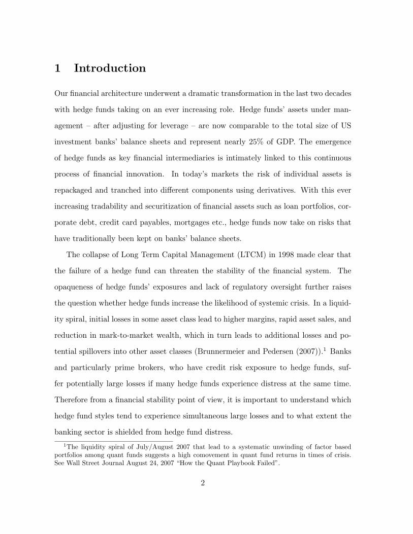
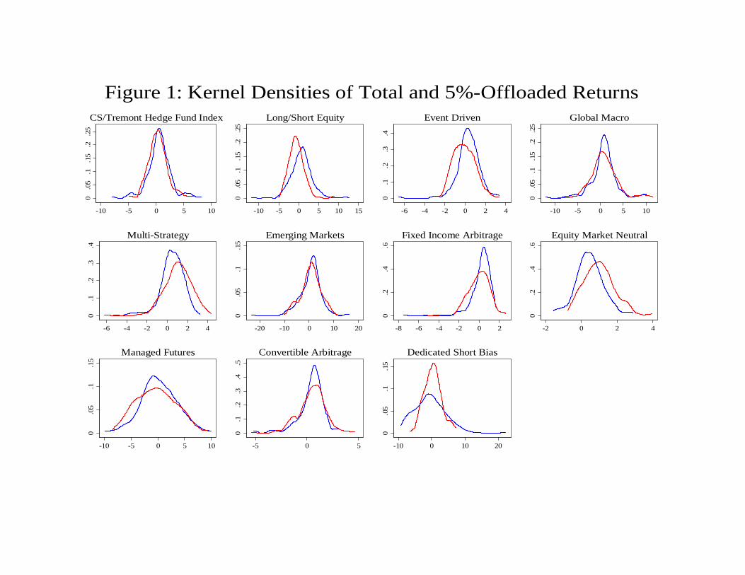
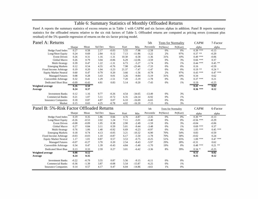
Panel A of Table 6 repeats the raw returns listed in Table 1 to facilitate the com-

parison with the quantile o�oaded returns reported in Panel B.

[Table 6]

The following di�erences between Panel A and B stand out: First, o�oading the

risk associated with our factors signi�cantly reduces the average mean return and

Sharpe ratio if one weights each strategy by its size. The reduction is small if fund

style are equally weighted. However, this is primarily driven by the overrepresentation

of dedicated short-specialists { a hedge fund style that comprises only 1 percent of the

fund size universe { since their quantile o�oading returns is relatively high. Looking

at individual styles, one notes that some o�-leaded mean returns and Sharpe ratio even

enter negative territory. Our model's �s are not very large { and they are by de�nition

the same for the raw returns and o�oaded returns. The CAPM-�, using CRSP excess

market returns, also drops notably after o�oading the risk associated with our factors.

The average CAPM declines from .35 to .11. Note that we take the simple average of

�s instead of the average of the absolute amounts of �s, since it is not easy to short

a hedge fund style. Finally, note that hedge fund and bank returns are not normally

distributed. Most styles and the index exhibit negative skewness and positive excess

kurtosis. The Royston's (1991) tests for normality con�rms this. It give the p-values

whether skewness is zero and kurtosis is three { the values for the normal distribution.

The kernel densities of Figure 1 reveal that o�oading reduces the fat left tail, while it

16

doesn't a�ect the right tail much.

[Figure 1]

3.3 q-Sensitivities of O�-loaded Returns

As we did for the raw returns in Section 2, we replicate the bivariate 5%-quantile

regressions for the o�oaded returns. In other words, we quantile regress the o�oaded

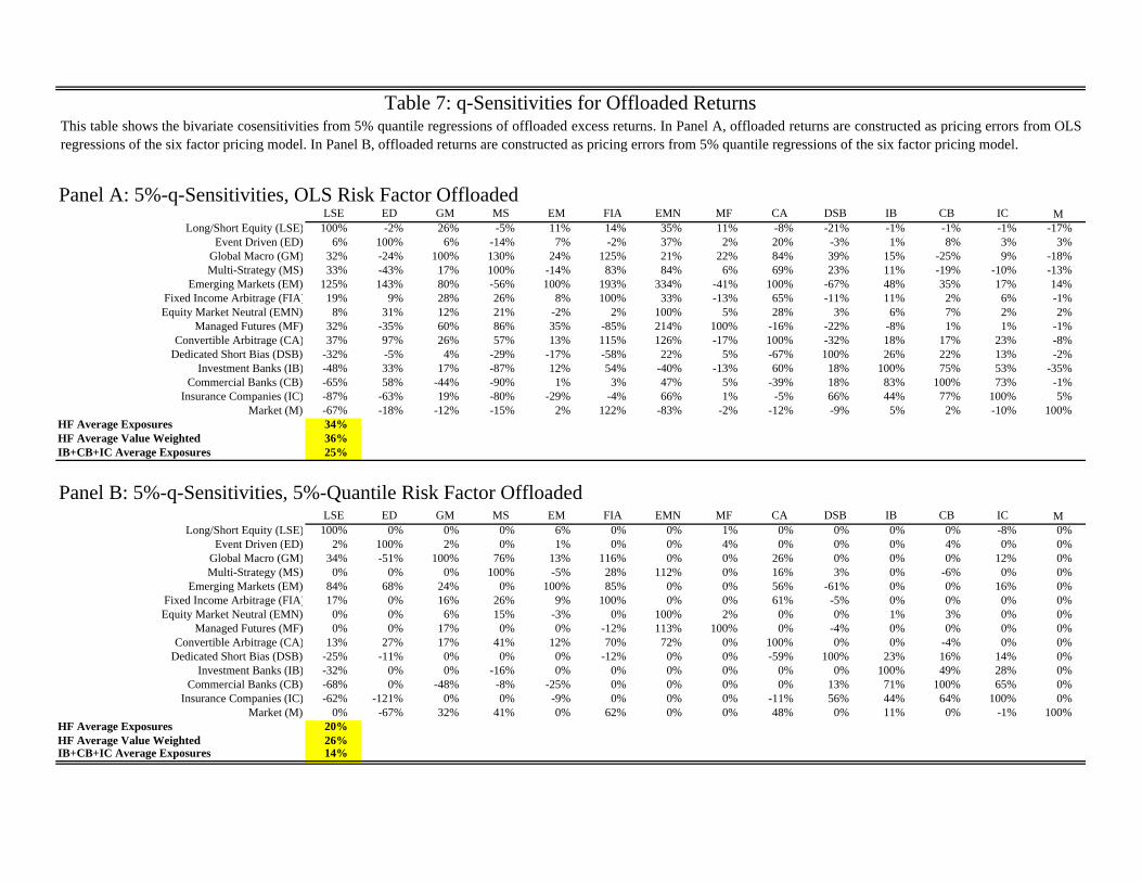
returns of style i on the o�oaded returns of style j. Table 8 reports quantile regression

coe�cients, our sensitivity measures for the o�oaded returns for q = 5%. O�-loaded

returns are residuals of the OLS factor regression in Panel A and the residual of the

quantile factor regression constructed in Panel B.

[Table 7]

Ultimately, we are interested in whether our six factors capture the tail dependence

among hedge funds' raw returns. They do so, if the bivariate-sensitivities of the of-

oaded returns in Table 8 are signi�cantly lower than the ones for the raw returns

reported in Table 2, Panel B in Section 2. The average bivariate 5%-sensitivity de-

creases from 53% to 34% for the OLS o�oaded returns and to 20% for the quantile

o�oaded returns. The decline is even more pronounced for the banking and insurance

sector. The average cosensitivity drops from 70% to 25%, 14% respectively.

Another striking feature of Table 7 is that there are many negative entries in the

Commercial bank row. That is, the o�oaded VaR of commercial banks seems to

improve as returns of various, especially the large, hedge fund styles worsen. This

�nding is surprising at �rst sight but is consistent with \reintermediation phenomenon"

caused by ight to quality. As investors shed risky assets in times of crisis, cash pours

17

into commercial banks and hence, banks' funding liquidity improves. Hence, they are

natural liquidity providers at these times (Gatev and Strahan (2006)), which seems to

boost their o�oaded returns. However, their overall returns still su�er since they are

also adversely a�ected by our risk factors. The coe�cients for insurance companies

point in a similar direction, but they di�er in magnitude.

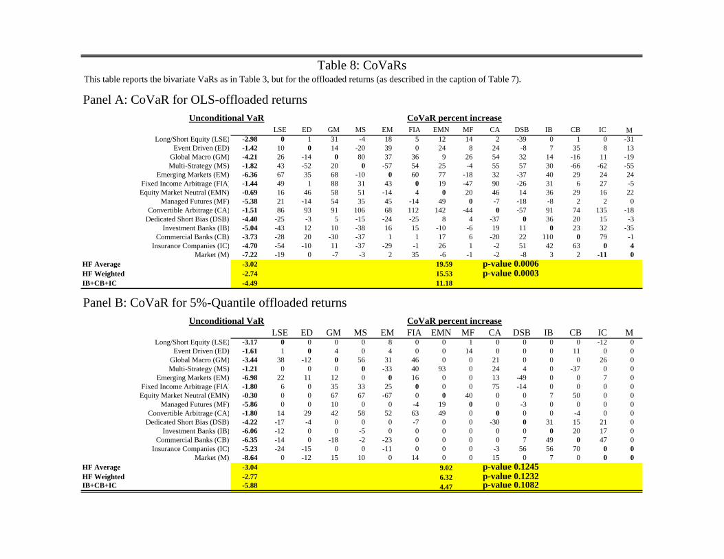
3.4 CoVaRs of O�-loaded Returns

q-Sensitivities give a good sense about the directional impact of conditioning, but they

do not allow a good comparison across more and less volatile hedge fund styles. The

percentage increase in CoVaR over the unconditional VaR provides the right normal-

ization and hence more information on the extent to which our factors reduce the tail

dependence. Table 8 reports percentage increases in CoVaR over the unconditional

VaR. In Panel A o�oaded returns are the residual of the OLS regression of returns on

our six factors. In Panel B we use the residual of the 5% quantile regression as the of-

oaded returns. After o�oading risks associated with these factors, the Value-at-Risk

of the residual monthly returns is in fact only -3.02% (Panel A) and -3.04% (Panel B).

[Table 8]

Our factors capture the co-dependence among hedge fund styles and other �nan-

cial intermediaries if the percentage increase in CoVaRs for the o�oaded returns is

markedly smaller than the one reported for raw returns in Table 3. Indeed, the average

percentage increase due to conditioning on other fund styles being in trouble is only

19.59% of the -3.02% (Panel A), 9.02% of -3.04% (Panel B). Recall without o�oading

the tail dependence is much higher { conditioning on some other fund style being in

distress on average increased the Value-at-Risk on average by 38.15% (Table 3). Taking

18

the weighted average instead of the simple average, the drop is from 30.57% for raw

returns (Table 3) to 15.53% for OLS o�oaded returns (Panel A) or 6.32% quantile

o�oaded returns (Panel B). The drop is more dramatic for the banking and insurance

sector.

Also note that the hedge fund strategy Equity Market Neutral (EMN) has the

lowest unconditional VaR, which explains why the percentage increase in CoVaR is

high after conditioning on certain hedge fund styles.

4 Incentives to Load on Tail Risk

Section 2 documents that tail risk of hedge funds and other �nancial institutions in-

creases during times of distress. Section 3 identi�es tradable factors that explain a large

part of this increase in tail risk. We next ask whether hedge funds have an incentive

to o�oad this tail risk.

4.1 Cost of o�oading factor risks

Hedge fund managers, investors, banks, or fund of fund managers can o�oad the risk

associated with these factors without incurring large trading costs since our factors

tradable and highly liquid. Consequently o�oading is �-neutral within our model.

However, the comparison of Panels A and B of Table 6 show that o�oading signi�cantly

reduces the weighted average monthly return from .26 to 0.08. Stated di�erently, a large

extent of hedge funds' outperformance relative to the market index is a direct result of

their loading on these \tail" factors, especially the variance swap factor. In short, there

appears to be a risk-return trade-o� between returns and conditional Value-at-Risk in

hedge fund returns.

19

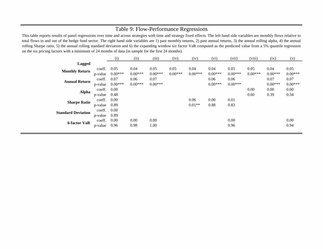
4.2 Flow analysis

If reducing sensitivity to these \tail risk factors" substantially lowers hedge funds'

expected return, the question arises whether hedge fund managers have an incentive

to do so. A typical hedge fund manager receives a performance fee of 20% of the

realized pro�ts plus 2% of the value of assets under management. Hence, limiting his

risk-sensitivity to these (high-return) factors lowers his expected compensation except

if it leads to signi�cant in ows into his fund. We study these ows and �nd that ows

are sensitive to past monthly and annual returns or past (annual rolling) Sharpe ratios,

but not to the hedge funds' VaR or the standard deviation of its returns. The standard

deviation is calculated with an annual rolling window, while the VaR is computed as

the predicted value from a 5% quantile regression on the six pricing factors with a

minimum of 24 months of data.

[Table 9]

The lack of sensitivity of fund ow with respect to two risk measures { standard

deviation and VaR { gives the fund manager no incentive to o�oad the risks associated

with our factors. This suggests that investors either expect hedge fund managers to

take on this risk or investors are naive and hedge fund managers take advantage of this

fact.

5 Robustness

5.1 Alternative measures of dependency

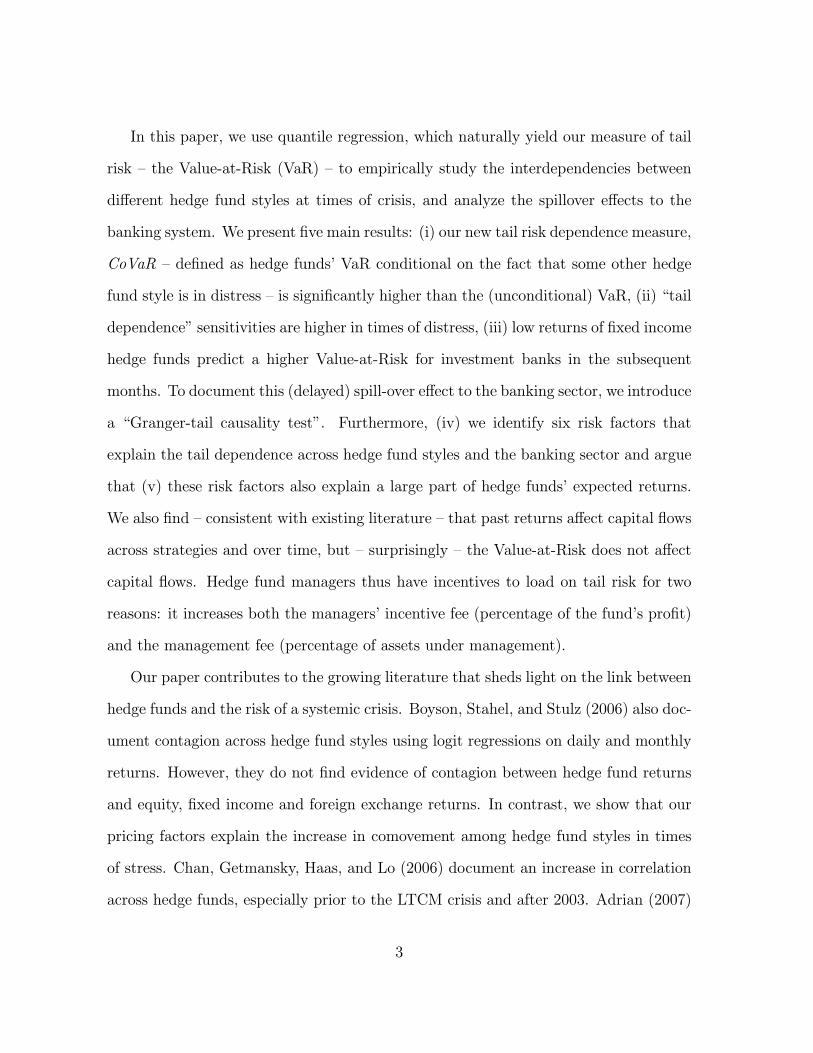
The comparison of q-sensitivities from the 5%- and 50%-quantile regressions of Table

2 can be interpreted as a comparison of sensitivities across states of the world. Table

20

2 shows that average sensitivities are higher in bad times (the average 5% quantile

sensitivity is 52%) than in normal times (the average 50%-quantile sensitivity is 32%).

In Figure 2, we plot the average sensitivities across the hedge fund styles for all quantiles

between 5% and 95% for total returns, OLS o�oaded returns, and 5% o�oaded returns.

The plot shows that the sensitivities across quantiles is relatively at for the 5%-

o�oaded returns. In contrast, average sensitivities are sharply decreasing along the

quantiles for the total returns, and are also decreasing for the OLS o�oaded returns.

[Figure 2]

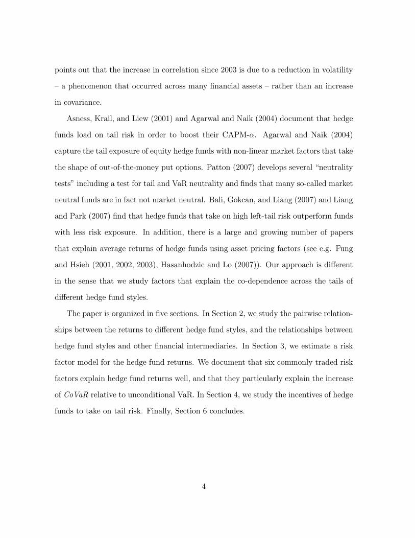
Instead of looking at sensitivities across states of the world, we can also investigate

the evolution of sensitivities over time. To do so, we estimate a multivariate BEKK-

ARCH(12) model, and extract the evolution of covariances across the strategies over

time. We plot the average of the covariances across the ten strategies in Figure 3.

[Figure 3]

The covariances for the 5%-o�oaded returns are clearly less volatile than for the

total returns. In particular, estimated average covariances spiked during the LTCM

crisis in the third quarter of 1998, and in January 2000. In contrast, the average

covariances of 5%-o�oaded returns increased much less during those volatile times.

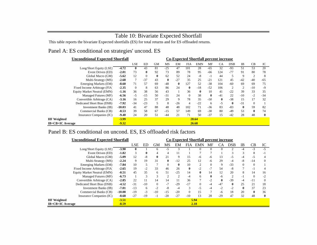
5.2 Alternative measures of tail risk

Value-at-Risk { our main measure of tail risk { is only one possible characterization of

tail risk. Many alternative measures have been proposed. First of all, Value-at-Risk

at lower quantiles can be used. Second, other measures of tail risk can be used. A

particularly appealing measure of tail risk that has been proposed in the literature

21

Artzner, Delbaen, Eber, and Heath (1999) is the expected shortfall. It is de�ned as

the average loss below the VaR. In order to make sure that our results are robust to

this measure, we computed the expected shortfall of returns as the average CoVaR for

1%, 2%, 3%, 4%, and 5%, and report the results in Table 10.

[Table 10]

By comparing the two panels, we see that the unconditional expected shortfall is

-3.99% for total returns of hedge funds, and -3.51% for the 5% o�oaded returns. The

increase of expected shortfall conditional on the other strategies is 28% higher for total

returns, and only 5.94% higher for the o�oaded returns.

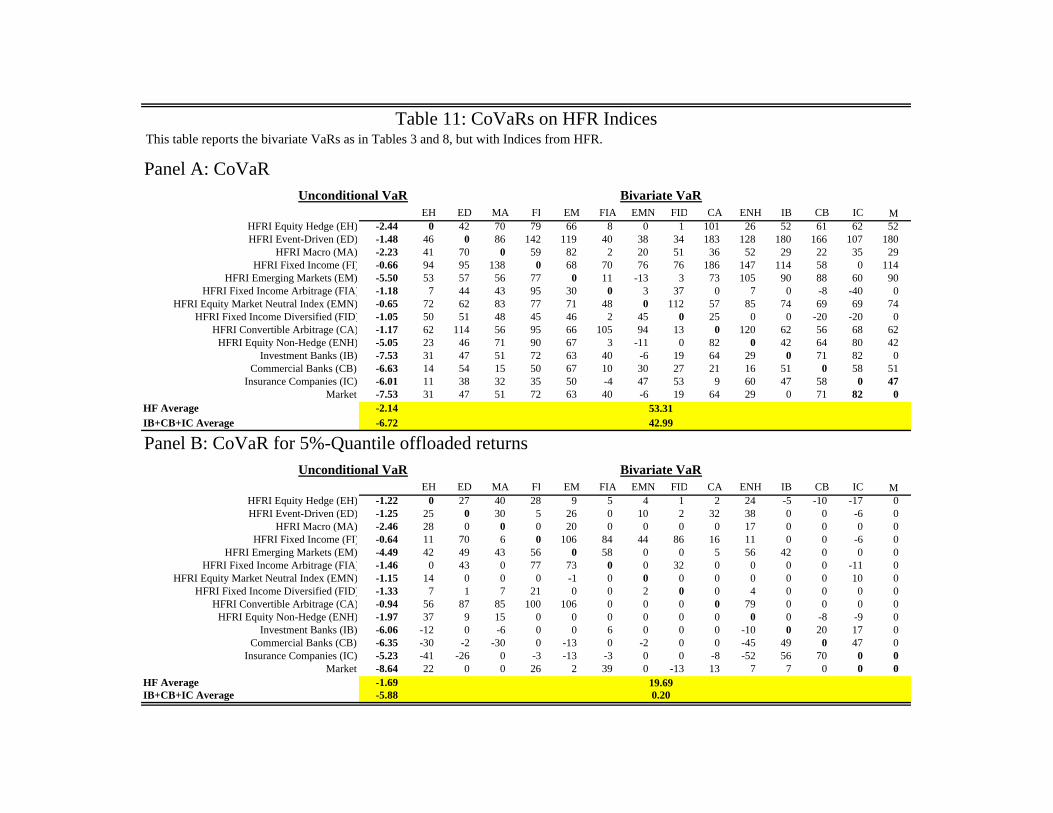
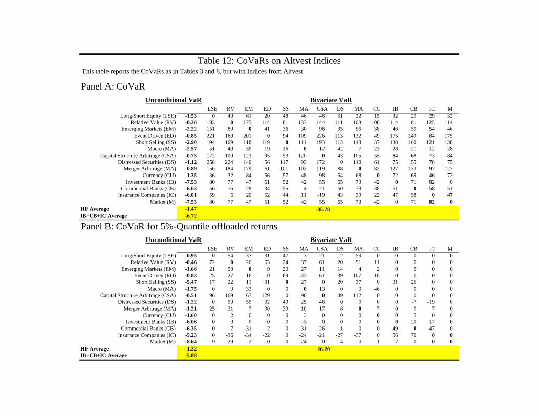
5.3 Alternative hedge fund data

There are several providers of hedge fund indices that use di�erent hedge funds and

di�erent methodologies to compute style indices. Two alternative data providers are

Hedge Fund Research (HFR, at www.hedgefundresearch.com), and Morningstar/Altvest

(at www.altvest.com). Tables 11 and 12 report the CoVaRs for these two alternative

databases.

[Table 11] [Table 12]

Our main result that the increase of CoVaRs conditional on distress of the other

strategies or institutions is higher than the unconditional VaRs holds for these alter-

native datasets. We can also see that o�oaded returns have a markedly lower increase

in CoVaRs. A striking feature of the alternative datasets is that they have generally

lower unconditional VaRs, but more pronounced increases in the CoVaR relative to the

unconditional VaR in comparison to the Credit Suisse / Tremont indices.

22

5.4 Alternative factors

{ To be written {

6 Conclusion

{ To be written {

23

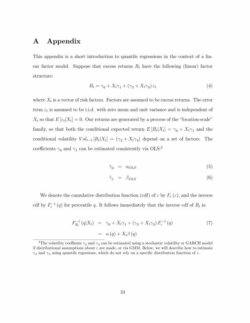
A Appendix

This appendix is a short introduction to quantile regressions in the context of a lin-

ear factor model. Suppose that excess returns Rt have the following (linear) factor

structure:

Rt = 0 +Xt 1 + ( 2 +Xt 3) "t (4)

where Xt is a vector of risk factors. Factors are assumed to be excess returns. The error

term "t is assumed to be i.i.d. with zero mean and unit variance and is independent of

Xt so that E ["tjXt] = 0. Our returns are generated by a process of the \location-scale"

family, so that both the conditional expected return E [RtjXt] = 0 + Xt 1 and the

conditional volatility V olt�1 [RtjXt] = ( 2 +Xt 3) depend on a set of factors. The

coe�cients 0 and 1 can be estimated consistently via OLS:3

0 = �OLS (5)

1 = �OLS (6)

We denote the cumulative distribution function (cdf) of " by F" ("), and the inverse

cdf by F�1" (q) for percentile q. It follows immediately that the inverse cdf of Rt is:

F�1Rt (qjXt) = 0 +Xt 1 + ( 2 +Xt 3)F�1" (q) (7)

= � (q) +Xt� (q)

3The volatility coe�ents 2 and 3 can be estimated using a stochastic volatility or GARCH modelif distributional assumptions about " are made, or via GMM. Below, we will describe how to estimate 2 and 3 using quantile regessions, which do not rely on a speci�c distribution function of ".

24

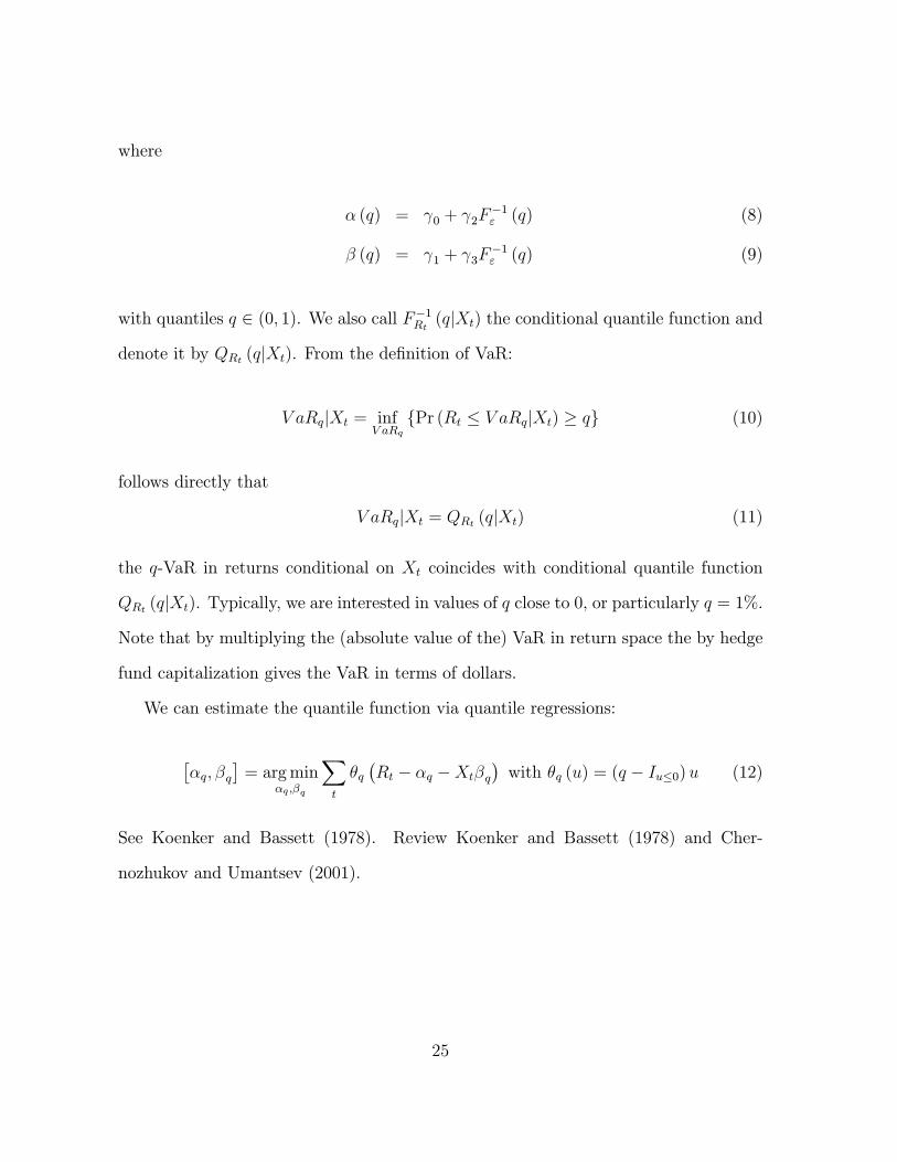
where

� (q) = 0 + 2F�1" (q) (8)

� (q) = 1 + 3F�1" (q) (9)

with quantiles q 2 (0; 1). We also call F�1Rt (qjXt) the conditional quantile function and

denote it by QRt (qjXt). From the de�nition of VaR:

V aRqjXt = infV aRq

fPr (Rt � V aRqjXt) � qg (10)

follows directly that

V aRqjXt = QRt (qjXt) (11)

the q-VaR in returns conditional on Xt coincides with conditional quantile function

QRt (qjXt). Typically, we are interested in values of q close to 0, or particularly q = 1%.

Note that by multiplying the (absolute value of the) VaR in return space the by hedge

fund capitalization gives the VaR in terms of dollars.

We can estimate the quantile function via quantile regressions:

��q; �q

�= argmin

�q ;�q

Xt

�q�Rt � �q �Xt�q

�with �q (u) = (q � Iu�0)u (12)

See Koenker and Bassett (1978). Review Koenker and Bassett (1978) and Cher-

nozhukov and Umantsev (2001).

25

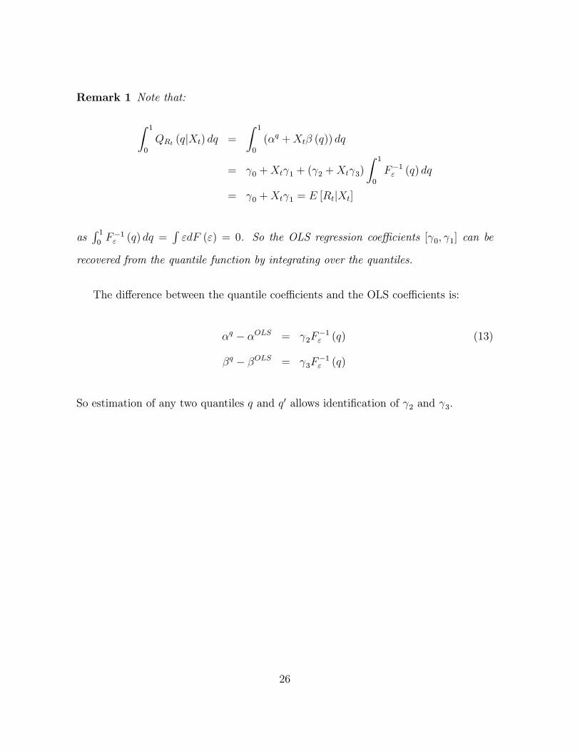
Remark 1 Note that:

Z 1

0

QRt (qjXt) dq =

Z 1

0

(�q +Xt� (q)) dq

= 0 +Xt 1 + ( 2 +Xt 3)

Z 1

0

F�1" (q) dq

= 0 +Xt 1 = E [RtjXt]

asR 10F�1" (q) dq =

R"dF (") = 0. So the OLS regression coe�cients [ 0; 1] can be

recovered from the quantile function by integrating over the quantiles.

The di�erence between the quantile coe�cients and the OLS coe�cients is:

�q � �OLS = 2F�1" (q) (13)

�q � �OLS = 3F�1" (q)

So estimation of any two quantiles q and q0 allows identi�cation of 2 and 3.

26

References

Ackermann, C., R. McEnally, and D. Ravenscraft (1999): \The Performance

of Hedge Funds: Risk, Return, and Incentives," Journal of Finance, 54(3), 833{874.

Adrian, T. (2007): \Measuring Risk in the Hedge Fund Sector," Current Issues in

Economics and Finance by the Federal Reserve Bank of New York, 13(3), 1{7.

Agarwal, V., and N. Y. Naik (2004): \Risks and Portfolio Decisions Involving

Hedge Funds," Review of Financial Studies, 17(1), 63{98.

(2005): \Hedge Funds," in Foundations and Trends in Finance, ed. by

L. Jaeger, vol. 1.

Artzner, P., F. Delbaen, J.-M. Eber, and D. Heath (1999): \Coherent Mea-

sures of Risk," Mathematical Finance, 9(3), 203{228.

Asness, C. S., R. Krail, and J. M. Liew (2001): \Do Hedge Funds Hedge?,"

Journal of Portfolio Management, 28(1), 6{19.

Bali, T. G., S. Gokcan, and B. Liang (2007): \Value at Risk and the Cross-

Section of Hedge Fund Returns," Journal of Banking and Finance.

Barnes, M. L., and A. W. Hughes (2002): \A Quantile Regression Analysis of the

Cross Section of Stock Market Returns," Working Paper, Federal Reserve Bank of

Boston.

Bassett, G. W., and H.-L. Chen (2001): \Portfolio Style: Return-based Attribu-

tion Using Quantile Regression," Empirical Economics, 26(1), 293{305.

27

Bassett, G. W., and R. Koenker (1978): \Asymptotic Theory of Least Absolute

Error Regression," Journal of the American Statistical Association, 73(363), 618{

622.

Bondarenko, O. (2004): \Market Price of Variance Risk and Performance of Hedge

Funds," SSRN Working Paper 542182.

Boyson, N. M., C. W. Stahel, and R. M. Stulz (2006): \Is there Hedge Fund

Contagion," NBER Working Paper 12090.

Brown, S. J., W. N. Goetzmann, and R. G. Ibbotson (1999): \O�shore Hedge

Funds: Survival and Performance 1989-1995," Journal of Business, 72(1), 91{117.

Brunnermeier, M. K., and S. Nagel (2004): \Hedge Funds and the Technology

Bubble," Journal of Finance, 59(5), 2013{2040.

Brunnermeier, M. K., and L. H. Pedersen (2007): \Market Liquidity and Fund-

ing Liquidity," Princeton University, Working Paper.

Campbell, J. Y. (1987): \Stock Returns and the Term Structure," Journal of Fi-

nancial Economics, 18(2), 373{399.

Chan, N., M. Getmansky, S. Haas, and A. W. Lo (2006): \Systemic Risk and

Hedge Funds," in The Risks of Financial Institutions and the Financial Sector, ed.

by M. Carey, and R. M. Stulz. The University of Chicago Press: Chicago, IL.

Chernozhukov, V., and L. Umantsev (2001): \Conditional Value-at-Risk: As-

pects of Modeling and Estimation," Empirical Economics, 26(1), 271{292.

28

Engle, R. F., and S. Manganelli (2004): \CAViaR: Conditional Autoregressive

Value at Risk by Regression Quantiles," Journal of Business and Economic Satistics,

22, 367{381.

Estrella, A., and G. A. Hardouvelis (1991): \The Term Structure as a Pedictor

of Real Economic Activity," Journal of Finance, 46(2), 555{567.

Fama, E. F., and K. R. French (1989): \Business Conditions and Expected Re-

turns on Stocks and Bonds," Journal of Financial Economics, 25(1), 23{49.

Fund, W., and D. A. Hsieh (2003): \The Risk in Hedge Fund Strategies: Alternative

Alphas and Alternative Betas," in Managing the Risks of Alternative 40 Investment

Strategies, ed. by L. Jaeger. Euromoney.

Fung, W., and D. A. Hsieh (1997): \Empirical Characteristics of Dynamic Trading

Strategies: The Case of Hedge," Review of Financial Studies, 10(2), 275{302.

(2001): \The Risk in Hedge Fund Strategies: Theory and Evidence from

Trend Followers," Review of Financial Studies, 14(2), 313{341.

(2002): \The Risk in Fixed-Income Hedge Fund Styles," Journal of Fixed

Income, 12, 6{27.

Fung, W., D. A. Hsieh, N. Y. Naik, and T. Ramadorai (2008): \Hedge Funds:

Performance, Risk and Capital Formation," Journal of Finance (forthcoming).

Gatev, E., and P. E. Strahan (2006): \Banks' Advantage in Hedging Liquid-

ity Risk: Theory and Evidence from the Commerical Paper Market," Journal of

Finance, 61(2), 867{892.

29

Getmansky, M., A. W. Lo, and I. Makarov (2004): \An Econometric Model

of Serial Correlation and Illiquidity in Hedge Fund Returns," Journal of Financial

Economics, 74(3), 529{609.

Hasanhodzic, J., and A. W. Lo (2007): \Can Hedge-Fund Returns be Replicated?:

The Linear Case," Journal of Investment Management, 5(2), 5{45.

Koenker, R. (2005): Quantile Regression. Cambridge University Press: Cambridge,

UK.

Koenker, R., and G. W. Bassett (1978): \Regression Quantiles," Econometrica,

46(1), 33{50.

Liang, B. (2000): \Hedge Funds: The Living and the Dead," Journal of Financial

and Quantitative Analysis, 35(3), 309{326.

Liang, B., and H. Park (2007): \Risk Measures for Hedge Funds," European Fi-

nancial Management, 13(2), 333{370.

Ma, L., and L. Pohlman (2005): \Return Forecasts and Optimal Portfolio Con-

struction: A Quantile Regression Approach," SSRN Working Paper 880478.

Malkiel, B. G., and A. Saha (2005): \Hedge Funds: Risk and Return," Financial

Analysts Journal, 61(6), 80{88.

Patton, A. (2007): \Are `Market Neutral' Hedge Funds Really Market Neutral?,"

SSRN Working Paper 557096.

Royston, P. (1991): \Estimating Departure from Normality," Statistics in Medicine,

10(8), 1283{1293.

30

0.0

5.1

.15

.2.2

5

-10 -5 0 5 10

CS/Tremont Hedge Fund Index

0.0

5.1

.15

.2.2

5

-10 -5 0 5 10 15

Long/Short Equity

0.1

.2.3

.4

-6 -4 -2 0 2 4

Event Driven

0.0

5.1

.15

.2.2

5

-10 -5 0 5 10

Global Macro

0.1

.2.3

.4

-6 -4 -2 0 2 4

Multi-Strategy0

.05

.1.1

5

-20 -10 0 10 20

Emerging Markets

0.2

.4.6

-8 -6 -4 -2 0 2

Fixed Income Arbitrage

0.2

.4.6

-2 0 2 4

Equity Market Neutral

0.0

5.1

.15

-10 -5 0 5 10

Managed Futures

0.1

.2.3

.4.5

-5 0 5

Convertible Arbitrage

0.0

5.1

.15

-10 0 10 20

Dedicated Short Bias

Figure 1: Kernel Densities of Total and 5%-Offloaded Returns

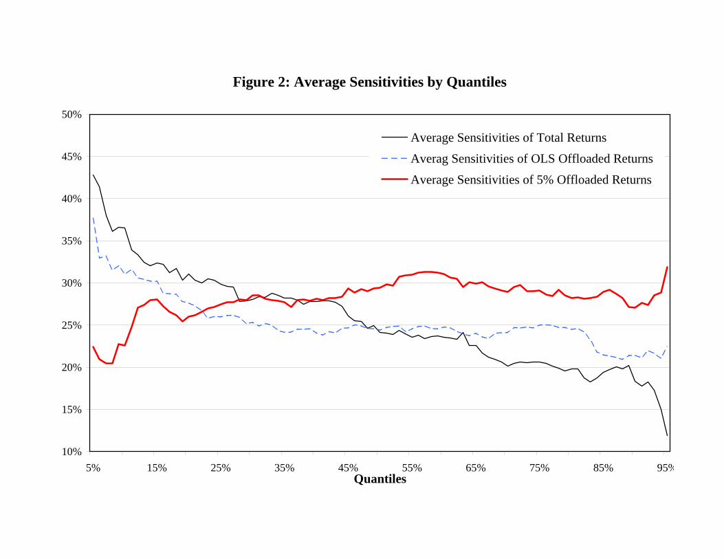
Figure 2: Average Sensitivities by Quantiles

10%

15%

20%

25%

30%

35%

40%

45%

50%

5% 15% 25% 35% 45% 55% 65% 75% 85% 95%Quantiles

Average Sensitivities of Total Returns

Averag Sensitivities of OLS Offloaded Returns

Average Sensitivities of 5% Offloaded Returns

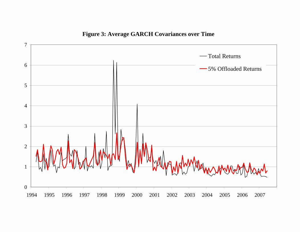
Figure 3: Average GARCH Covariances over Time

0

1

2

3

4

5

6

7

1994 1995 1996 1997 1998 1999 2000 2001 2002 2003 2004 2005 2006 2007

Total Returns

5% Offloaded Returns

5th Weight Leverage Weight*Sharpe Mean Std Dev Skew Kurt Min Percenti Obs Pr(Skew) Pr(Kurt) Dec-06 Dec-06 Leverage

Hedge Fund Index 0.27 0.58 2.17 -0.03 5.55 -7.98 -2.58 162 1% 0% 100% 183% 100%Long/Short Equity 0.24 0.69 2.84 0.12 7.13 -11.86 -3.22 162 2% 0% 29% 118% 19%

Event Driven 0.26 0.31 1.16 -1.31 10.30 -6.58 -1.36 162 1% 0% 24% 164% 21%Global Macro 0.26 0.79 3.04 -0.06 6.29 -12.06 -3.59 162 2% 0% 11% 247% 15%Multi-Strategy 0.39 0.47 1.22 -1.31 6.73 -5.27 -1.74 159 0% 0% 10% 201% 11%

Emerging Markets 0.12 0.54 4.55 -0.76 7.98 -23.46 -7.33 162 10% 0% 7% 130% 5%Fixed Income Arbitrage 0.19 0.20 1.04 -3.23 21.37 -7.47 -1.47 162 1% 0% 6% 490% 17%

Equity Market Neutral 0.60 0.47 0.79 0.20 3.66 -1.56 -0.78 162 1% 0% 5% 206% 6%Managed Futures 0.08 0.28 3.43 0.01 3.26 -9.84 -5.19 162 1% 0% 5% 110% 3%

Convertible Arbitrage 0.32 0.41 1.29 -1.51 7.20 -5.19 -1.78 162 1% 0% 3% 231% 3%Dedicated Short Bias -0.09 -0.43 4.81 0.83 5.14 -9.20 -7.43 162 5% 0% 1% 222% 1%

5thSharpe Mean Std Dev Skew Kurt Min Percenti Obs Pr(Skew) Pr(Kurt)

Investment Banks 0.20 1.16 5.81 -0.59 4.93 -25.38 -7.53 161 0% 0%Commercial Banks 0.21 1.07 5.04 -0.70 6.29 -24.00 -6.63 161 0% 0%

Insurance Companies 0.18 0.87 4.76 0.04 6.09 -16.55 -6.01 161 81% 0%Market 0.15 0.65 4.19 -0.79 4.10 -16.20 -6.41 162 0% 3%

Table 1: Summary Statistics of Monthly Excess Returns by Strategies

Panel A: Hedge Funds

Panel B: Other Institutions

Tests for Normality

Tests for Normality

Panel A reports summary statistics for the Credit Suisse / Tremont hedge fund index, and the ten Credit Suisse / Tremont hedge fund style returns. All returns are in excessof the three month Treasury bill rate. The Sharpe ratio is the ratio of mean excess returns to the standard deviation of excess returns. The tests for normality give the p-values of Royston's (1991) test that skewness / kurtosis are normal. The weights for each style are the weights that aggregate the ten styles to the overall Credit Suisse /Tremont index for December 2006. Leverage is computed from reported average leverage of individual funds in the TASS database for December 2006, and averaged bystyle. Panel B reports the value weighted equity returns (in excess of the three month Treasury bill rate) of five investment banks (Bear Stearns, Goldman Sachs, MerrillLynch, Morgan Stanley, and Lehman Brothers) using data from CRSP. The commercial bank and insurance company returns are from Kenneth French's industryportfolios. The market return is the cum dividend value weighted CRSP return.

Panel A: 50%-q-Sensitivities LSE ED GM MS EM FIA EMN MF CA DSB IB CB IC MLong/Short Equity (LSE) 100% 123% 35% 92% 36% 63% 108% 16% 70% -38% 19% 28% 24% 30%

Event Driven (ED) 32% 100% 17% 38% 20% 55% 59% 6% 50% -13% 6% 8% 7% 9%Global Macro (GM) 48% 49% 100% 25% 26% 105% 80% 19% 40% -3% 5% 11% 12% 12%Multi-Strategy (MS) 16% 42% 4% 100% 7% 53% 50% 4% 47% -4% 2% 1% 2% 3%

Emerging Markets (EM) 95% 187% 56% 79% 100% 98% 115% 2% 107% -37% 21% 23% 25% 31%Fixed Income Arbitrage (FIA) 9% 33% 7% 25% 6% 100% 38% 3% 42% -1% 1% 2% 1% 1%Equity Market Neutral (EMN) 13% 22% 8% 30% 8% 29% 100% 6% 24% -3% 3% 5% 6% 5%

Managed Futures (MF) 18% 22% 36% 16% 1% 12% 40% 100% -34% 0% -5% -10% -3% 0%Convertible Arbitrage (CA) 12% 44% 5% 31% 5% 65% 49% -1% 100% -3% 2% 3% 4% 3%

Dedicated Short Bias (DSB) -131% -172% -19% -12% -46% 11% -37% 0% -58% 100% -34% -55% -43% -53%Investment Banks (IB) 204% 281% 83% 59% 107% 84% 363% -38% 177% -125% 100% 128% 113% 129%

Commercial Banks (CB) 90% 190% 51% -33% 38% 12% 165% 2% 8% -44% 36% 100% 84% 80%Insurance Companies (IC) 89% 114% 40% -7% 24% -7% 125% 6% 12% -32% 24% 70% 100% 60%

Market (M) 140% 205% 49% -4% 48% 62% 202% 0% 73% -67% 55% 101% 89% 100%HF Average Exposures 32%HF Average Value Weighted 42%IB+CB+IC Average Exposures 42%

Panel B: 5%-q-Sensitivities LSE ED GM MS EM FIA EMN MF CA DSB IB CB IC MLong/Short Equity (LSE) 100% 119% 49% 20% 36% 34% 23% -17% 23% -24% 7% 31% 12% 34%

Event Driven (ED) 40% 100% 32% 70% 36% 104% 87% -17% 95% -20% 8% 18% 19% 18%Global Macro (GM) 41% 115% 100% 122% 31% 114% 80% -15% 50% -8% 8% 7% 11% 7%Multi-Strategy (MS) 13% 41% 18% 100% -9% 58% 51% -6% 74% 10% -3% -5% -5% 3%

Emerging Markets (EM) 122% 213% 75% -23% 100% 348% 97% -50% 241% -52% 17% 65% 48% 64%Fixed Income Arbitrage (FIA) 19% 80% 26% 99% 9% 100% 59% -3% 78% -2% 1% 2% 3% 2%Equity Market Neutral (EMN) 14% 39% 11% 37% 2% 41% 100% 2% 38% -2% 2% 5% 3% 3%

Managed Futures (MF) 31% 140% 51% 151% 35% 132% 197% 100% 36% 16% -11% 9% 3% -11%Convertible Arbitrage (CA) 28% 97% 33% 67% 15% 59% 122% -10% 100% -14% 10% 15% 18% 14%

Dedicated Short Bias (DSB) -19% 16% 13% 41% -9% 38% 10% 19% 43% 100% -12% 4% 5% -31%Investment Banks (IB) 178% 435% 202% 135% 149% 328% 703% -84% 349% -118% 100% 117% 119% 130%

Commercial Banks (CB) 25% 132% 34% 65% 25% 235% 109% -21% 113% -53% 35% 100% 95% 79%Insurance Companies (IC) 73% 121% 98% -21% 45% 349% 309% -57% -14% -40% 22% 73% 100% 56%

Market (M) 80% 248% 96% 155% 75% 249% 304% -46% 187% -81% 41% 113% 103% 100%HF Average Exposures 53%HF Average Value Weighted 66%IB+CB+IC Average Exposures 70%

Table 2: q-SensitivitiesThis table reports the matrix of bivariate q-sensitivities among the excess returns to ten Credit Suisse / Tremont hedge fund styles and the excess returns to other financialinstitutions (summary statistics are reported in Table 1). The sensitivities are calculated using quantile regressions (see Appendix A). Panel A reports the sensitivities from the50%-quantile regression, Panel B reports the sensitivities from the 5%-quantile regression. Each cell of the table reports the sensitivity of a regression with the left hand sidevariable reported in the left column, and the right hand side variable reported in the top row.

Unconditional VaRLSE ED GM MS EM FIA EMN MF CA DSB IB CB IC M

Long/Short Equity (LSE) -3.22 0 69 68 0 79 48 37 -42 36 -124 84 76 33 52Event Driven (ED) -1.36 61 0 45 34 146 -7 75 -36 115 -93 118 122 76 91

Global Macro (GM) -3.59 26 18 0 97 54 41 31 -11 33 -9 46 17 29 25Multi-Strategy (MS) -1.33 76 7 83 0 -22 77 81 31 224 96 -11 -6 -25 -17

Emerging Markets (EM) -7.33 44 43 36 -17 0 81 24 -33 71 -77 61 67 46 62Fixed Income Arbitrage (FIA) -1.51 33 49 52 52 28 0 17 -16 95 -13 32 7 12 14Equity Market Neutral (EMN) -0.78 31 8 71 33 -1 53 0 33 77 -32 76 81 62 28

Managed Futures (MF) -5.19 10 12 47 2 44 3 37 0 -3 14 -9 8 -27 -5Convertible Arbitrage (CA) -1.78 53 74 78 65 58 143 109 -42 0 -60 60 54 77 92

Dedicated Short Bias (DSB) -7.43 -44 -24 2 8 -25 7 -20 6 -17 0 -22 -3 2 -98Investment Banks (IB) -7.53 42 62 59 57 74 63 84 -15 70 -95 0 71 82 77

Commercial Banks (CB) -6.63 14 63 23 5 28 85 14 -12 23 -67 51 0 58 100Insurance Companies (IC) -6.01 24 42 37 -12 55 66 80 -67 -20 -52 47 58 0 68

Market (M) -0.06 50 33 67 50 67 83 100 -50 50 -133 33 33 50 0HF Average -3.35 30.57 p-value 0.0036HF Weighted -2.77 35.48 p-value 0.0861IB+CB+IC Average -6.72 32.41 p-value 0.0000

Table 3: CoVaRs

CoVaR percent increase

This table reports the percentage increase of the five percent Value-at-Risk for the returns of the left column conditional on the fifth percentile of thereturns of the top row relative to the unconditional 5% Value-at-Risk (reported in the first column). The Value-at-Risk is computed from the fivepercent pair wise quantile regressions (the slopes of these regressions are reported in Table 2). The p-values test the null hyothesis that average CoVaRsequal average VaRs and are generated via bootsrap with 200 draws.

I-Banks C-Banks Insur I-Banks C-Banks InsurHedge Fund IndexLong/Short Equity

Event DrivenGlobal MacroMulti-Strategy **

Emerging MarketsFixed Income Arbitrage **

Equity Market NeutralManaged Futures

Convertible Arbitrage ** *Dedicated Short Bias ***

A: Hedge Funds Forecasting Banks B: Banks Forecasting Hedge Funds

Table 4: Quantile Granger CausalityThis table reports the significance of five percent quantile regressions. In Columns A, the left hand side excess return is reported in the first column,and is regressed on its own lag, as well as the lagged excess return of the variable in the top row of columns A. The significance refers to the coefficientof the top row, * denotes significance at the 10% level, ** at the 5% level, and *** at the 1% level.

5thMean Std Dev Skew Kurt Min Percentil Pr(Skew) Pr(Kurt) Obs

Repo - Treasury Rate 0.02 0.05 -0.85 6.04 -0.20 -0.06 50% 0% 16210 Year - 3 Month Treasury Return 0.16 2.24 -0.34 2.73 -6.25 -3.67 7% 55% 162

Moody's BAA - 10 Year Treasury Return 0.24 2.36 -0.13 3.47 -7.47 -3.28 47% 18% 162CRSP Market Excess Return 0.65 4.19 -0.79 4.10 -16.20 -6.41 0% 2% 162VIX Straddle Excess Return 1.01 11.57 0.94 4.76 -24.63 -15.26 0% 0% 162

Variance Swap Return -0.39 0.41 2.38 10.30 -0.86 -0.77 0% 0% 162

Table 5: Summary Statistics of Risk Factors

Tests for Normality

This table reports summary statistics for excess returns of six risk factors. The repo Treasury spread is the difference between the one monthgeneral collateral Treasury repo rate (from ICAP) and the one month Treasury bill rate (from Federal Reserve Board's H.15 releases). The 10year - 3 month Treasury return is the return to the 10-year constant maturity Treasury bond (from H.15) in excess of the 3-month Treasury Bill.Moody's BAA - 10-year Treasury return is the return to Moody's BAA bond portfolio in excess of the return to the 10-year constant maturityTreasury return. The CRSP market excess return is in excess of the 3-month Treasury bill and is from the Center of Research in Security Prices.The VIX straddle return is computed from the Black-Scholes (1973) formula using CBOE's VIX implied volatility index, the return to theS&P500, and the 3-month Treasury rate. The variance swap return is the difference between realized S&P500 variance from daily closing dataand the VIX implied variance. The tests for normality give the p-values of Royston's (1991) test that skewness / kurtosis are normal.

Panel A: Returns 5thSharpe Mean Std Dev Skew Kurt Min Percentile Pr(Skew) Pr(Kurt)

Hedge Fund Index 0.27 0.58 2.17 -0.03 5.55 -7.98 -2.58 0% 0% 0.39 *** -0.13Long/Short Equity 0.24 0.69 2.84 0.12 7.13 -11.86 -3.22 2% 97% 0.37 ** -0.29

Event Driven 0.26 0.31 1.16 -1.31 10.30 -6.58 -1.36 31% 10% 0.49 *** -0.06Global Macro 0.26 0.79 3.04 -0.06 6.29 -12.06 -3.59 0% 3% 0.66 *** 0.37

Multi-Strategy 0.39 0.47 1.22 -1.31 6.73 -5.27 -1.74 0% 1% 0.44 *** 0.45 **Emerging Markets 0.12 0.54 4.55 -0.76 7.98 -23.46 -7.33 0% 0% 0.16 -0.59

Fixed Income Arbitrage 0.19 0.20 1.04 -3.23 21.37 -7.47 -1.47 0% 0% 0.19 ** 0.24 *Equity Market Neutral 0.60 0.47 0.79 0.20 3.66 -1.56 -0.78 2% 97% 0.43 *** 0.47 ***

Managed Futures 0.08 0.28 3.43 0.01 3.26 -9.84 -5.19 31% 10% 0.34 0.62Convertible Arbitrage 0.32 0.41 1.29 -1.51 7.20 -5.19 -1.78 0% 3% 0.37 *** 0.21Dedicated Short Bias -0.09 -0.43 4.81 0.83 5.14 -9.20 -7.43 0% 1% 0.19 -0.25

Weighted average 0.26 0.50 0.41 *** 0.02Average 0.24 0.37 0.36 *** 0.12

Investment Banks 0.12 1.16 9.77 -0.26 4.54 -34.65 -13.49 0% 3%Commercial Banks 0.21 1.07 5.11 -0.72 6.35 -24.14 -6.92 0% 1%

Insurance Companies 0.18 0.87 4.87 0.07 6.10 -16.69 -6.65 0% 0%Market 0.15 0.65 4.25 -0.78 4.02 -16.20 -7.15 0% 3%

Panel B: 5%-Risk Factor Offloaded Returns 5thSharpe Mean Std Dev Skew Kurt Min Percentile Pr(Skew) Pr(Kurt)

Hedge Fund Index 0.19 0.35 1.86 0.66 4.76 -4.87 -2.35 0% 0% 0.30 ** -0.13Long/Short Equity -0.26 -0.53 2.02 1.24 7.11 -5.01 -3.40 0% 0% -0.56 *** -0.29

Event Driven -0.08 -0.09 1.05 0.38 2.90 -2.49 -1.59 0% 3% -0.04 -0.06Global Macro 0.27 0.84 3.11 0.59 5.01 -9.44 -3.48 0% 1% 0.69 *** 0.37

Multi-Strategy 0.76 1.06 1.40 -0.92 6.69 -6.23 -0.97 0% 0% 1.05 *** 0.45 ***Emerging Markets 0.18 0.74 4.13 -0.05 3.21 -10.32 -6.90 70% 54% 0.83 -0.59

Fixed Income Arbitrage -0.03 -0.03 1.10 -0.87 6.17 -5.50 -1.78 70% 58% -0.02 0.24Equity Market Neutral 1.17 1.01 0.87 0.57 3.53 -0.75 -0.25 51% 65% 1.00 *** 0.47 ***

Managed Futures -0.07 -0.27 3.70 0.20 2.54 -8.43 -5.97 29% 28% -0.31 0.62Convertible Arbitrage 0.34 0.47 1.39 -0.43 4.84 -5.40 -1.70 19% 0% 0.48 *** 0.21 **Dedicated Short Bias 0.13 0.33 2.59 0.27 3.01 -6.42 -3.36 8% 39% 0.34 * -0.25

Weighted average 0.08 0.12 0.11 0.02Average 0.24 0.35 0.35 0.12

Investment Banks -0.22 -0.79 3.55 0.87 5.56 -9.15 -6.11 0% 0%Commercial Banks -0.36 -1.39 3.87 -0.08 5.54 -15.87 -6.25 0% 1%

Insurance Companies 0.14 0.57 4.17 0.47 6.04 -14.86 -4.61 1% 0%

Table 6: Summary Statistics of Monthly Offloaded Returns

CAPM 7-Factoralpha alpha

alpha alpha

Tests for Normality

Tests for Normality CAPM 6-Factor

Panel A reports the summary statistics of excess returns as in Table 1 with CAPM and six factors alphas in addition. Panel B reports summarystatistics for the offloaded returns relative to the six risk factors of Table 5. Offloaded returns are computed as pricing errors (constant plusresidual) of the 5% quantile regression of returns on the six factor pricing model.

Panel A: 5%-q-Sensitivities, OLS Risk Factor OffloadedLSE ED GM MS EM FIA EMN MF CA DSB IB CB IC M

Long/Short Equity (LSE) 100% -2% 26% -5% 11% 14% 35% 11% -8% -21% -1% -1% -1% -17%Event Driven (ED) 6% 100% 6% -14% 7% -2% 37% 2% 20% -3% 1% 8% 3% 3%

Global Macro (GM) 32% -24% 100% 130% 24% 125% 21% 22% 84% 39% 15% -25% 9% -18%Multi-Strategy (MS) 33% -43% 17% 100% -14% 83% 84% 6% 69% 23% 11% -19% -10% -13%

Emerging Markets (EM) 125% 143% 80% -56% 100% 193% 334% -41% 100% -67% 48% 35% 17% 14%Fixed Income Arbitrage (FIA) 19% 9% 28% 26% 8% 100% 33% -13% 65% -11% 11% 2% 6% -1%Equity Market Neutral (EMN) 8% 31% 12% 21% -2% 2% 100% 5% 28% 3% 6% 7% 2% 2%

Managed Futures (MF) 32% -35% 60% 86% 35% -85% 214% 100% -16% -22% -8% 1% 1% -1%Convertible Arbitrage (CA) 37% 97% 26% 57% 13% 115% 126% -17% 100% -32% 18% 17% 23% -8%

Dedicated Short Bias (DSB) -32% -5% 4% -29% -17% -58% 22% 5% -67% 100% 26% 22% 13% -2%Investment Banks (IB) -48% 33% 17% -87% 12% 54% -40% -13% 60% 18% 100% 75% 53% -35%

Commercial Banks (CB) -65% 58% -44% -90% 1% 3% 47% 5% -39% 18% 83% 100% 73% -1%Insurance Companies (IC) -87% -63% 19% -80% -29% -4% 66% 1% -5% 66% 44% 77% 100% 5%

Market (M) -67% -18% -12% -15% 2% 122% -83% -2% -12% -9% 5% 2% -10% 100%HF Average Exposures 34%HF Average Value Weighted 36%IB+CB+IC Average Exposures 25%

Panel B: 5%-q-Sensitivities, 5%-Quantile Risk Factor OffloadedLSE ED GM MS EM FIA EMN MF CA DSB IB CB IC M

Long/Short Equity (LSE) 100% 0% 0% 0% 6% 0% 0% 1% 0% 0% 0% 0% -8% 0%Event Driven (ED) 2% 100% 2% 0% 1% 0% 0% 4% 0% 0% 0% 4% 0% 0%

Global Macro (GM) 34% -51% 100% 76% 13% 116% 0% 0% 26% 0% 0% 0% 12% 0%Multi-Strategy (MS) 0% 0% 0% 100% -5% 28% 112% 0% 16% 3% 0% -6% 0% 0%

Emerging Markets (EM) 84% 68% 24% 0% 100% 85% 0% 0% 56% -61% 0% 0% 16% 0%Fixed Income Arbitrage (FIA) 17% 0% 16% 26% 9% 100% 0% 0% 61% -5% 0% 0% 0% 0%Equity Market Neutral (EMN) 0% 0% 6% 15% -3% 0% 100% 2% 0% 0% 1% 3% 0% 0%

Managed Futures (MF) 0% 0% 17% 0% 0% -12% 113% 100% 0% -4% 0% 0% 0% 0%Convertible Arbitrage (CA) 13% 27% 17% 41% 12% 70% 72% 0% 100% 0% 0% -4% 0% 0%

Dedicated Short Bias (DSB) -25% -11% 0% 0% 0% -12% 0% 0% -59% 100% 23% 16% 14% 0%Investment Banks (IB) -32% 0% 0% -16% 0% 0% 0% 0% 0% 0% 100% 49% 28% 0%

Commercial Banks (CB) -68% 0% -48% -8% -25% 0% 0% 0% 0% 13% 71% 100% 65% 0%Insurance Companies (IC) -62% -121% 0% 0% -9% 0% 0% 0% -11% 56% 44% 64% 100% 0%

Market (M) 0% -67% 32% 41% 0% 62% 0% 0% 48% 0% 11% 0% -1% 100%HF Average Exposures 20%HF Average Value Weighted 26%IB+CB+IC Average Exposures 14%

Table 7: q-Sensitivities for Offloaded ReturnsThis table shows the bivariate cosensitivities from 5% quantile regressions of offloaded excess returns. In Panel A, offloaded returns are constructed as pricing errors from OLSregressions of the six factor pricing model. In Panel B, offloaded returns are constructed as pricing errors from 5% quantile regressions of the six factor pricing model.

Panel A: CoVaR for OLS-offloaded returnsUnconditional VaR

LSE ED GM MS EM FIA EMN MF CA DSB IB CB IC MLong/Short Equity (LSE) -2.98 0 1 31 -4 18 5 12 14 2 -39 0 1 0 -31

Event Driven (ED) -1.42 10 0 14 -20 39 0 24 8 24 -8 7 35 8 13Global Macro (GM) -4.21 26 -14 0 80 37 36 9 26 54 32 14 -16 11 -19Multi-Strategy (MS) -1.82 43 -52 20 0 -57 54 25 -4 55 57 30 -66 -62 -55

Emerging Markets (EM) -6.36 67 35 68 -10 0 60 77 -18 32 -37 40 29 24 24Fixed Income Arbitrage (FIA) -1.44 49 1 88 31 43 0 19 -47 90 -26 31 6 27 -5Equity Market Neutral (EMN) -0.69 16 46 58 51 -14 4 0 20 46 14 36 29 16 22

Managed Futures (MF) -5.38 21 -14 54 35 45 -14 49 0 -7 -18 -8 2 2 0Convertible Arbitrage (CA) -1.51 86 93 91 106 68 112 142 -44 0 -57 91 74 135 -18

Dedicated Short Bias (DSB) -4.40 -25 -3 5 -15 -24 -25 8 4 -37 0 36 20 15 -3Investment Banks (IB) -5.04 -43 12 10 -38 16 15 -10 -6 19 11 0 23 32 -35

Commercial Banks (CB) -3.73 -28 20 -30 -37 1 1 17 6 -20 22 110 0 79 -1Insurance Companies (IC) -4.70 -54 -10 11 -37 -29 -1 26 1 -2 51 42 63 0 4

Market (M) -7.22 -19 0 -7 -3 2 35 -6 -1 -2 -8 3 2 -11 0HF Average -3.02 19.59 p-value 0.0006HF Weighted -2.74 15.53 p-value 0.0003IB+CB+IC -4.49 11.18

Panel B: CoVaR for 5%-Quantile offloaded returnsUnconditional VaR

LSE ED GM MS EM FIA EMN MF CA DSB IB CB IC MLong/Short Equity (LSE) -3.17 0 0 0 0 8 0 0 1 0 0 0 0 -12 0

Event Driven (ED) -1.61 1 0 4 0 4 0 0 14 0 0 0 11 0 0Global Macro (GM) -3.44 38 -12 0 56 31 46 0 0 21 0 0 0 26 0Multi-Strategy (MS) -1.21 0 0 0 0 -33 40 93 0 24 4 0 -37 0 0

Emerging Markets (EM) -6.98 22 11 12 0 0 16 0 0 13 -49 0 0 7 0Fixed Income Arbitrage (FIA) -1.80 6 0 35 33 25 0 0 0 75 -14 0 0 0 0Equity Market Neutral (EMN) -0.30 0 0 67 67 -67 0 0 40 0 0 7 50 0 0

Managed Futures (MF) -5.86 0 0 10 0 0 -4 19 0 0 -3 0 0 0 0Convertible Arbitrage (CA) -1.80 14 29 42 58 52 63 49 0 0 0 0 -4 0 0

Dedicated Short Bias (DSB) -4.22 -17 -4 0 0 0 -7 0 0 -30 0 31 15 21 0Investment Banks (IB) -6.06 -12 0 0 -5 0 0 0 0 0 0 0 20 17 0

Commercial Banks (CB) -6.35 -14 0 -18 -2 -23 0 0 0 0 7 49 0 47 0Insurance Companies (IC) -5.23 -24 -15 0 0 -11 0 0 0 -3 56 56 70 0 0

Market (M) -8.64 0 -12 15 10 0 14 0 0 15 0 7 0 0 0HF Average -3.04 9.02 p-value 0.1245HF Weighted -2.77 6.32 p-value 0.1232IB+CB+IC -5.88 4.47 p-value 0.1082

Table 8: CoVaRs

CoVaR percent increase

CoVaR percent increase

This table reports the bivariate VaRs as in Table 3, but for the offloaded returns (as described in the caption of Table 7).

(i) (ii) (iii) (iv) (iv) (vi) (vii) (viii) (ix) (x)Lagged

coeff. 0.05 0.04 0.05 0.05 0.04 0.04 0.05 0.05 0.04 0.05p-value 0.00*** 0.00*** 0.00*** 0.00*** 0.00*** 0.00*** 0.00*** 0.00*** 0.00*** 0.00***

coeff. 0.07 0.06 0.07 0.06 0.06 0.07 0.07p-value 0.00*** 0.00*** 0.00*** 0.00*** 0.00*** 0.00*** 0.00***

coeff. 0.00 0.00 0.00 0.00p-value 0.48 0.60 0.39 0.34

coeff. 0.00 0.06 0.00 0.01p-value 0.89 0.01** 0.88 0.83

coeff. 0.00p-value 0.89

coeff. 0.00 0.00 0.00 0.00 0.00p-value 0.96 0.98 1.00 0.96 0.94

Sharpe Ratio

Standard Deviation

6-factor VaR

Table 9: Flow-Performance Regressions

Monthly Return

Annual Return

Alpha

This table reports results of panel regressions over time and across strategies with time and strategy fixed effects. The left hand side variables are monthly flows relative tototal flows in and out of the hedge fund sector. The right hand side variables are 1) past monthly returns, 2) past annual returns, 3) the annual rolling alpha, 4) the annualrolling Sharpe ratio, 5) the annual rolling standard deviation and 6) the expanding window six factor VaR computed as the predicted value from a 5% quantile regressionon the six pricing factors with a minimum of 24 months of data (in sample for the first 24 months).

Panel A: ES conditional on strategies' uncond. ESUnconditional Expected Shortfall

LSE ED GM MS EM FIA EMN MF CA DSB IB CB ICLong/Short Equity (LSE) -4.72 0 43 81 -25 47 101 28 -65 32 -93 51 53 20

Event Driven (ED) -2.01 73 0 92 73 89 78 95 -66 124 -77 91 80 78Global Macro (GM) -5.62 12 0 0 62 52 24 -8 -1 44 5 9 2 8Multi-Strategy (MS) -2.68 7 -37 43 0 -27 35 25 -21 121 45 -42 -40 -65

Emerging Markets (EM) -8.60 71 57 69 -48 0 127 52 -38 104 -60 69 69 75Fixed Income Arbitrage (FIA) -2.35 0 8 63 86 24 0 -18 -52 106 2 2 -10 -9Equity Market Neutral (EMN) -1.16 36 38 56 43 1 36 0 10 41 -22 39 33 35

Managed Futures (MF) -6.56 -5 -15 50 -31 24 0 38 0 -41 22 -10 -2 -34Convertible Arbitrage (CA) -3.16 16 25 37 29 9 78 35 -50 0 -38 15 17 32

Dedicated Short Bias (DSB) -7.92 -34 -23 5 8 -26 4 -22 6 -5 0 -31 0 1Investment Banks (IB) -10.03 41 47 88 48 48 102 71 -36 83 -83 0 59 82

Commercial Banks (CB) -8.53 39 58 67 -15 57 149 69 -30 80 -49 53 0 74Insurance Companies (IC) -9.40 24 20 51 -44 21 71 50 -37 15 -42 28 48 0

HF Weighted -3.99IB+CB+IC Average -9.32

Panel B: ES conditional on uncond. ES, ES offloaded risk factors Unconditional Expected Shortfall

LSE ED GM MS EM FIA EMN MF CA DSB IB CB ICLong/Short Equity (LSE) -3.90 0 1 6 -5 3 1 0 0 0 2 -4 -3 -5

Event Driven (ED) -1.82 3 0 4 4 11 1 7 7 1 3 3 8 -1Global Macro (GM) -5.09 12 -8 0 21 9 15 -6 -6 13 -5 -4 -5 4Multi-Strategy (MS) -2.24 9 19 31 0 -12 25 12 -6 29 -4 -8 -14 0

Emerging Markets (EM) -7.84 10 5 7 0 0 10 2 0 9 -33 0 0 1Fixed Income Arbitrage (FIA) -2.65 19 -2 33 46 26 0 -2 -7 54 -8 7 -1 4Equity Market Neutral (EMN) -0.51 45 35 6 51 -25 14 0 14 12 20 8 14 16

Managed Futures (MF) -6.73 1 3 3 2 2 -4 6 0 -6 2 -1 0 -2Convertible Arbitrage (CA) -2.85 22 11 14 14 11 36 7 -2 0 -39 -4 -11 0

Dedicated Short Bias (DSB) -4.52 -31 -10 0 -7 -29 -17 0 -4 -47 0 25 21 18Investment Banks (IB) -7.01 -13 6 -2 -8 -4 3 -5 -4 -2 -2 0 37 23

Commercial Banks (CB) -10.08 -19 -3 -10 -15 -20 0 15 7 -6 18 20 0 36Insurance Companies (IC) -8.68 -27 -19 -1 -20 -27 -10 13 28 -29 47 32 48 0

HF Weighted -3.51IB+CB+IC Average -8.59

26.68

Co-Expected Shortfall percent increase

5.942.18

Table 10: Bivariate Expected Shortfall

Co-Expected Shortfall percent increase

28.64

This table reports the bivariate Expected shortfalls (ES) for total returns and for ES offloaded returns.

Panel A: CoVaR Unconditional VaR

EH ED MA FI EM FIA EMN FID CA ENH IB CB IC MHFRI Equity Hedge (EH) -2.44 0 42 70 79 66 8 0 1 101 26 52 61 62 52HFRI Event-Driven (ED) -1.48 46 0 86 142 119 40 38 34 183 128 180 166 107 180

HFRI Macro (MA) -2.23 41 70 0 59 82 2 20 51 36 52 29 22 35 29HFRI Fixed Income (FI) -0.66 94 95 138 0 68 70 76 76 186 147 114 58 0 114

HFRI Emerging Markets (EM) -5.50 53 57 56 77 0 11 -13 3 73 105 90 88 60 90HFRI Fixed Income Arbitrage (FIA) -1.18 7 44 43 95 30 0 3 37 0 7 0 -8 -40 0

HFRI Equity Market Neutral Index (EMN) -0.65 72 62 83 77 71 48 0 112 57 85 74 69 69 74HFRI Fixed Income Diversified (FID) -1.05 50 51 48 45 46 2 45 0 25 0 0 -20 -20 0

HFRI Convertible Arbitrage (CA) -1.17 62 114 56 95 66 105 94 13 0 120 62 56 68 62HFRI Equity Non-Hedge (ENH) -5.05 23 46 71 90 67 3 -11 0 82 0 42 64 80 42

Investment Banks (IB) -7.53 31 47 51 72 63 40 -6 19 64 29 0 71 82 0Commercial Banks (CB) -6.63 14 54 15 50 67 10 30 27 21 16 51 0 58 51

Insurance Companies (IC) -6.01 11 38 32 35 50 -4 47 53 9 60 47 58 0 47Market -7.53 31 47 51 72 63 40 -6 19 64 29 0 71 82 0

HF Average -2.14IB+CB+IC Average -6.72

Panel B: CoVaR for 5%-Quantile offloaded returnsUnconditional VaR

EH ED MA FI EM FIA EMN FID CA ENH IB CB IC MHFRI Equity Hedge (EH) -1.22 0 27 40 28 9 5 4 1 2 24 -5 -10 -17 0HFRI Event-Driven (ED) -1.25 25 0 30 5 26 0 10 2 32 38 0 0 -6 0

HFRI Macro (MA) -2.46 28 0 0 0 20 0 0 0 0 17 0 0 0 0HFRI Fixed Income (FI) -0.64 11 70 6 0 106 84 44 86 16 11 0 0 -6 0

HFRI Emerging Markets (EM) -4.49 42 49 43 56 0 58 0 0 5 56 42 0 0 0HFRI Fixed Income Arbitrage (FIA) -1.46 0 43 0 77 73 0 0 32 0 0 0 0 -11 0

HFRI Equity Market Neutral Index (EMN) -1.15 14 0 0 0 -1 0 0 0 0 0 0 0 10 0HFRI Fixed Income Diversified (FID) -1.33 7 1 7 21 0 0 2 0 0 4 0 0 0 0

HFRI Convertible Arbitrage (CA) -0.94 56 87 85 100 106 0 0 0 0 79 0 0 0 0HFRI Equity Non-Hedge (ENH) -1.97 37 9 15 0 0 0 0 0 0 0 0 -8 -9 0

Investment Banks (IB) -6.06 -12 0 -6 0 0 6 0 0 0 -10 0 20 17 0Commercial Banks (CB) -6.35 -30 -2 -30 0 -13 0 -2 0 0 -45 49 0 47 0

Insurance Companies (IC) -5.23 -41 -26 0 -3 -13 -3 0 0 -8 -52 56 70 0 0Market -8.64 22 0 0 26 2 39 0 -13 13 7 7 0 0 0

HF Average -1.69IB+CB+IC Average -5.88

42.99

Bivariate VaR

19.690.20

Table 11: CoVaRs on HFR Indices

Bivariate VaR

53.31

This table reports the bivariate VaRs as in Tables 3 and 8, but with Indices from HFR.

Panel A: CoVaRUnconditional VaR

LSE RV EM ED SS MA CSA DS MA CU IB CB IC MLong/Short Equity (LSE) -1.53 0 49 61 20 48 46 46 51 32 15 32 29 29 32

Relative Value (RV) -0.36 183 0 175 114 81 133 144 111 103 106 114 81 125 114Emerging Markets (EM) -2.22 151 80 0 41 36 30 96 35 55 38 46 59 54 46

Event Driven (ED) -0.85 221 160 201 0 94 109 226 113 132 49 175 149 84 175Short Selling (SS) -2.90 194 169 118 119 0 111 193 113 148 37 138 160 121 138

Macro (MA) -2.57 51 40 39 19 16 0 12 42 7 23 28 21 12 28Capital Structure Arbitrage (CSA) -0.75 172 100 123 95 53 120 0 43 105 55 84 68 73 84

Distressed Securities (DS) -1.12 258 224 140 56 117 93 172 0 140 61 75 55 78 75Merger Arbitrage (MA) -0.89 156 184 179 61 101 102 119 88 0 82 127 133 97 127

Currency (CU) -1.35 36 32 84 56 57 48 98 64 68 0 72 69 46 72Investment Banks (IB) -7.53 80 77 47 51 52 42 55 65 73 42 0 71 82 0

Commercial Banks (CB) -6.63 56 16 28 34 55 4 21 50 73 38 51 0 58 51Insurance Companies (IC) -6.01 59 6 20 52 44 11 -19 43 39 22 47 58 0 47

Market (M) -7.53 80 77 47 51 52 42 55 65 73 42 0 71 82 0HF Average -1.47 85.78IB+CB+IC Average -6.72

Panel B: CoVaR for 5%-Quantile offloaded returns Unconditional VaR

LSE RV EM ED SS MA CSA DS MA CU IB CB IC MLong/Short Equity (LSE) -0.95 0 54 33 31 47 3 21 2 59 0 0 0 0 0

Relative Value (RV) -0.46 72 0 26 63 24 37 61 20 91 11 0 0 0 0Emerging Markets (EM) -1.66 21 50 0 9 20 27 11 14 4 2 0 0 0 0

Event Driven (ED) -0.83 25 27 16 0 69 43 61 39 107 10 0 0 0 0Short Selling (SS) -5.47 17 22 11 31 0 27 0 20 37 0 31 26 0 0

Macro (MA) -1.75 0 0 33 0 0 0 13 0 0 46 0 0 0 0Capital Structure Arbitrage (CSA) -0.51 96 169 67 129 0 90 0 49 112 0 0 0 0 0

Distressed Securities (DS) -1.22 0 59 55 32 49 25 46 0 0 0 0 -7 -19 0Merger Arbitrage (MA) -1.21 25 31 7 30 39 10 17 6 0 7 0 0 7 0

Currency (CU) -1.60 0 2 0 0 0 3 0 0 0 0 0 5 0 0Investment Banks (IB) -6.06 0 0 0 0 0 -3 0 0 0 0 0 20 17 0

Commercial Banks (CB) -6.35 0 -7 -31 -2 0 -31 -26 -1 0 0 49 0 47 0Insurance Companies (IC) -5.23 0 -36 -34 -22 0 -24 -21 -27 -37 0 56 70 0 0

Market (M) -8.64 -9 29 2 0 0 24 0 4 0 1 7 0 0 0HF Average -1.32 26.20IB+CB+IC Average -5.88

Bivariate VaR

Table 12: CoVaRs on Altvest Indices

Bivariate VaR

This table reports the CoVaRs as in Tables 3 and 8, but with Indices from Altvest.