Electronic copy available at: http://ssrn.com/abstract=2637007

Hedge Funds:

A Dynamic Industry In Transition∗

Mila Getmansky†, Peter A. Lee‡, and Andrew W. Lo§

This Draft: July 28, 2015

Abstract

The hedge-fund industry has grown rapidly over the past two decades, offering investorsunique investment opportunities that often reflect more complex risk exposures than thoseof traditional investments. In this article we present a selective review of the recent academicliterature on hedge funds as well as updated empirical results for this industry. Our reviewis written from several distinct perspectives: the investor’s, the portfolio manager’s, theregulator’s, and the academic’s. Each of these perspectives offers a different set of insightsinto the financial system, and the combination provides surprisingly rich implications for theEfficient Markets Hypothesis, investment management, systemic risk, financial regulation,and other aspects of financial theory and practice.

Keywords: Hedge Funds; Alternative Investments; Investment Management; Long/Short;Illiquidity; Financial Crisis.

JEL Classification: G12

∗We thank Vikas Agarwal, George Aragon, Guillermo Baquero, Monica Billio, Keith Black, Ben Branch,Nick Bollen, Stephen Brown, Jayna Cummings, Gregory Feldberg, Mark Flood, Robin Greenwood, DavidHsieh, Hossein Kazemi, Bing Liang, Tarun Ramadorai, and two anonymous referees for helpful commentsand suggestions. The views and opinions expressed in this article are those of the authors only and do notnecessarily represent the views and opinions of any other organizations, any of their affiliates or employees,or any of the individuals acknowledged above. Research support from the MIT Laboratory for FinancialEngineering is gratefully acknowledged.

†Isenberg School of Management, University of Massachusetts, 121 Presidents Drive, Room 308C,Amherst, MA 01003, (413) 577–3308 (voice), (413) 545–3858 (fax), msherman@isenberg.umass.edu (email).

‡Senior Research Scientist, AlphaSimplex Group, LLC.§Charles E. & Susan T. Harris Professor, MIT Sloan School of Management, and Chief Investment

Strategist, AlphaSimplex Group, LLC. Please direct all correspondence to Andrew Lo, MIT Sloan School,100 Main Street, E62–618, Cambridge, MA 02142–1347, (617) 253–0920 (voice), alo-admin@mit.edu (email).

Electronic copy available at: http://ssrn.com/abstract=2637007

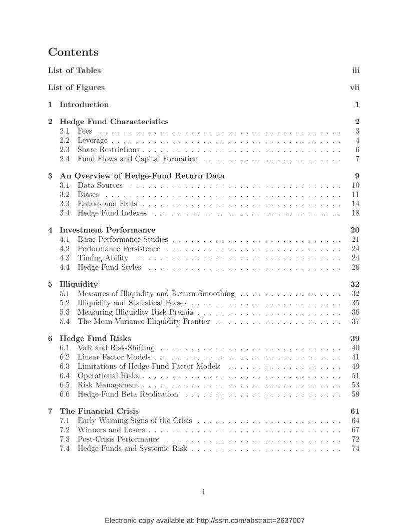
Contents

List of Tables iii

List of Figures vii

1 Introduction 1

2 Hedge Fund Characteristics 2

2.1 Fees . . . . . . . . . . . . . . . . . . . . . . . . . . . . . . . . . . . . . . . . 32.2 Leverage . . . . . . . . . . . . . . . . . . . . . . . . . . . . . . . . . . . . . . 42.3 Share Restrictions . . . . . . . . . . . . . . . . . . . . . . . . . . . . . . . . . 62.4 Fund Flows and Capital Formation . . . . . . . . . . . . . . . . . . . . . . . 7

3 An Overview of Hedge-Fund Return Data 9

3.1 Data Sources . . . . . . . . . . . . . . . . . . . . . . . . . . . . . . . . . . . 103.2 Biases . . . . . . . . . . . . . . . . . . . . . . . . . . . . . . . . . . . . . . . 113.3 Entries and Exits . . . . . . . . . . . . . . . . . . . . . . . . . . . . . . . . . 143.4 Hedge Fund Indexes . . . . . . . . . . . . . . . . . . . . . . . . . . . . . . . 18

4 Investment Performance 20

4.1 Basic Performance Studies . . . . . . . . . . . . . . . . . . . . . . . . . . . . 214.2 Performance Persistence . . . . . . . . . . . . . . . . . . . . . . . . . . . . . 244.3 Timing Ability . . . . . . . . . . . . . . . . . . . . . . . . . . . . . . . . . . 244.4 Hedge-Fund Styles . . . . . . . . . . . . . . . . . . . . . . . . . . . . . . . . 26

5 Illiquidity 32

5.1 Measures of Illiquidity and Return Smoothing . . . . . . . . . . . . . . . . . 325.2 Illiquidity and Statistical Biases . . . . . . . . . . . . . . . . . . . . . . . . . 355.3 Measuring Illiquidity Risk Premia . . . . . . . . . . . . . . . . . . . . . . . . 365.4 The Mean-Variance-Illiquidity Frontier . . . . . . . . . . . . . . . . . . . . . 37

6 Hedge Fund Risks 39

6.1 VaR and Risk-Shifting . . . . . . . . . . . . . . . . . . . . . . . . . . . . . . 406.2 Linear Factor Models . . . . . . . . . . . . . . . . . . . . . . . . . . . . . . . 416.3 Limitations of Hedge-Fund Factor Models . . . . . . . . . . . . . . . . . . . 496.4 Operational Risks . . . . . . . . . . . . . . . . . . . . . . . . . . . . . . . . . 516.5 Risk Management . . . . . . . . . . . . . . . . . . . . . . . . . . . . . . . . . 536.6 Hedge-Fund Beta Replication . . . . . . . . . . . . . . . . . . . . . . . . . . 59

7 The Financial Crisis 61

7.1 Early Warning Signs of the Crisis . . . . . . . . . . . . . . . . . . . . . . . . 647.2 Winners and Losers . . . . . . . . . . . . . . . . . . . . . . . . . . . . . . . . 677.3 Post-Crisis Performance . . . . . . . . . . . . . . . . . . . . . . . . . . . . . 727.4 Hedge Funds and Systemic Risk . . . . . . . . . . . . . . . . . . . . . . . . . 74

i

8 Implementation Issues for Hedge Fund Investing 78

8.1 The Limits of Mean-Variance Optimization . . . . . . . . . . . . . . . . . . . 798.2 Over-Diversification . . . . . . . . . . . . . . . . . . . . . . . . . . . . . . . . 798.3 Investment Implications . . . . . . . . . . . . . . . . . . . . . . . . . . . . . 818.4 An Integrated Hedge-Fund Investment Process . . . . . . . . . . . . . . . . . 868.5 The Adaptive Markets Hypothesis . . . . . . . . . . . . . . . . . . . . . . . . 96

9 Conclusion 104

A Appendix 105

A.1 Lipper TASS Fund Category Definitions . . . . . . . . . . . . . . . . . . . . 105A.2 Cleaning Lipper TASS Data . . . . . . . . . . . . . . . . . . . . . . . . . . . 106A.3 Glossary . . . . . . . . . . . . . . . . . . . . . . . . . . . . . . . . . . . . . . 107

References 110

ii

List of Tables

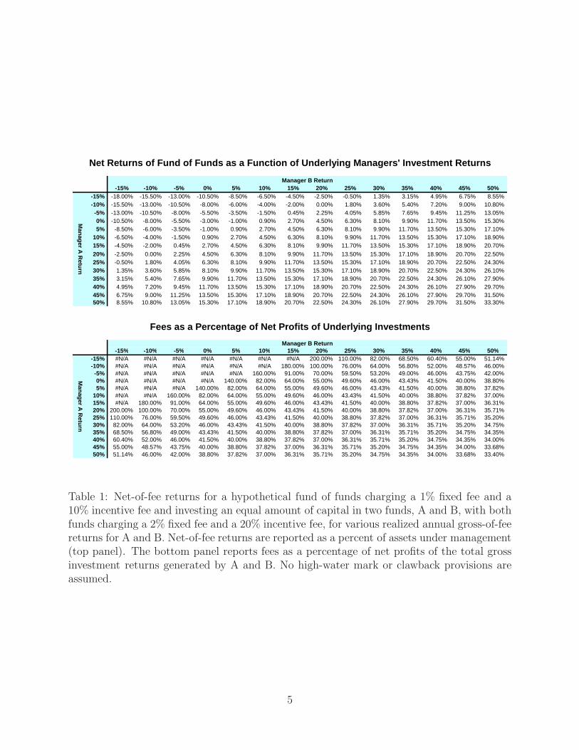
1 Net-of-fee returns for a hypothetical fund of funds charging a 1% fixed fee anda 10% incentive fee and investing an equal amount of capital in two funds, Aand B, with both funds charging a 2% fixed fee and a 20% incentive fee, forvarious realized annual gross-of-fee returns for A and B. Net-of-fee returns arereported as a percent of assets under management (top panel). The bottompanel reports fees as a percentage of net profits of the total gross investmentreturns generated by A and B. No high-water mark or clawback provisionsare assumed. . . . . . . . . . . . . . . . . . . . . . . . . . . . . . . . . . . . . 5

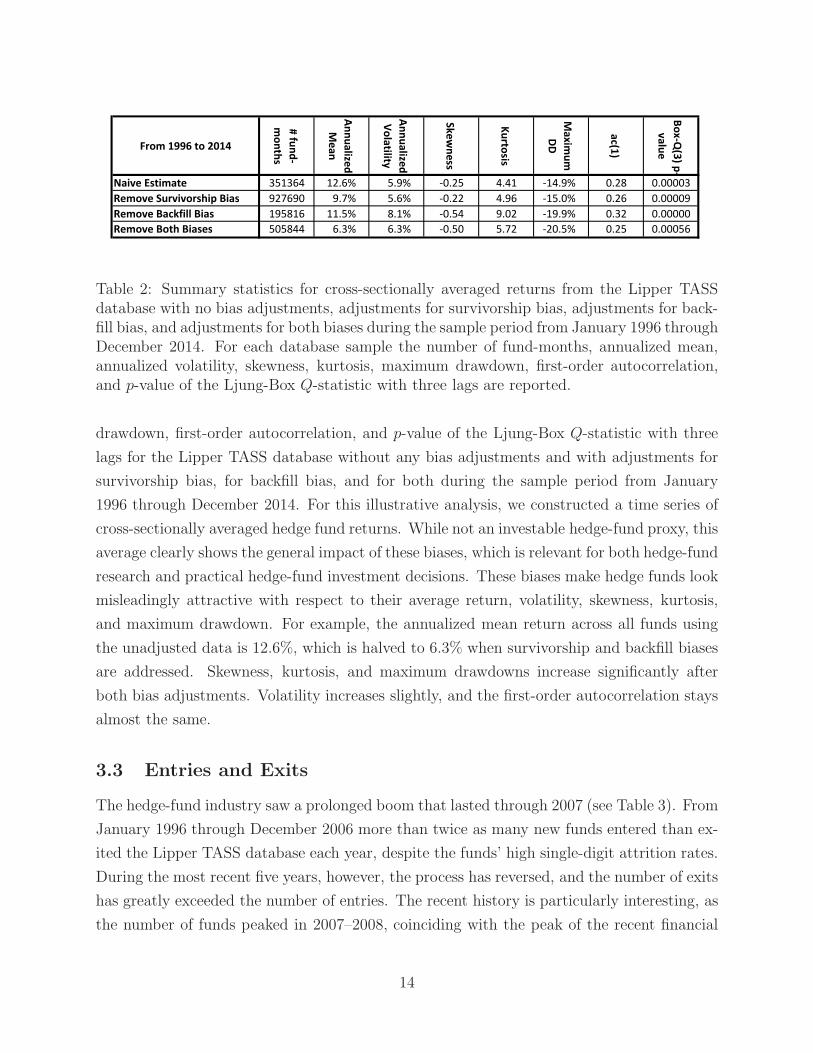
2 Summary statistics for cross-sectionally averaged returns from the LipperTASS database with no bias adjustments, adjustments for survivorship bias,adjustments for backfill bias, and adjustments for both biases during the sam-ple period from January 1996 through December 2014. For each databasesample the number of fund-months, annualized mean, annualized volatility,skewness, kurtosis, maximum drawdown, first-order autocorrelation, and p-value of the Ljung-Box Q-statistic with three lags are reported. . . . . . . . 14

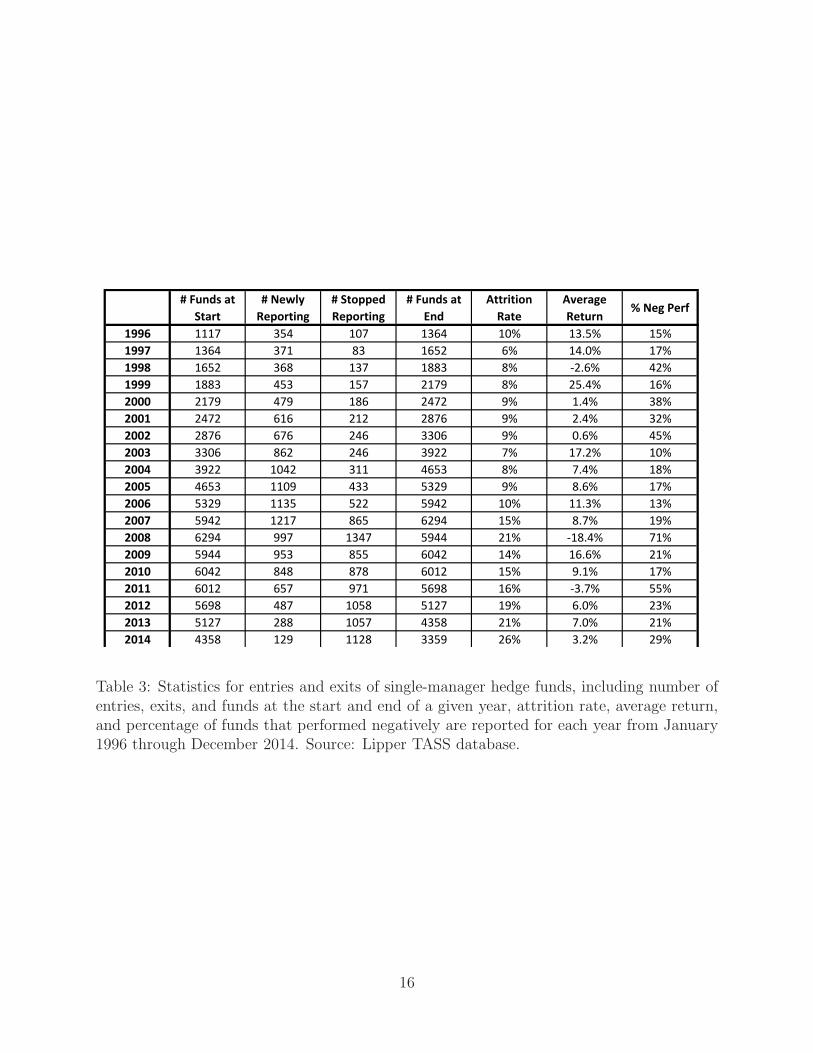
3 Statistics for entries and exits of single-manager hedge funds, including num-ber of entries, exits, and funds at the start and end of a given year, attritionrate, average return, and percentage of funds that performed negatively arereported for each year from January 1996 through December 2014. Source:Lipper TASS database. . . . . . . . . . . . . . . . . . . . . . . . . . . . . . . 16

4 Information about hedge-fund index providers, index family, and the avail-ability of total-industry and category indexes for commonly used monthly,daily, and replication hedge-fund indexes. . . . . . . . . . . . . . . . . . . . . 19

5 Monthly correlations of the average returns of funds in each hedge-fund stylecategory. Correlations for the 10 main Lipper TASS hedge fund categories,Funds of Funds, and All Single Manager Funds found in the Lipper TASSdatabase from January 1996 through December 2014 are reported. The AllSingle Manager Funds category includes the funds in all 10 main Lipper TASScategories and any other single-manager funds present in the database (rela-tively few) while excluding funds of funds. Correlations are color-coded withthe highest correlations in blue, intermediate correlations in yellow, and thelowest correlations in red. . . . . . . . . . . . . . . . . . . . . . . . . . . . . 26

6 Summary statistics for the returns of the average fund in each Lipper TASSstyle category and summary statistics for the corresponding CS/DJ Hedge-Fund Index. Number of fund months, annualized mean, annualized volatility,Sharpe ratio, Sortino ratio, skewness, kurtosis, maximum drawdown, corre-lation coefficient with the S&P 500, first-order autocorrelation, and p-valueof the Ljung-Box Q-statistic with three lags for the 10 main Lipper TASShedge fund categories, Funds of Funds, and All Single Manager Funds foundin the Lipper TASS database from January 1996 through December 2014 arereported. Sharpe and Sortino ratios are adjusted for the three-month U.S.Treasury Bill rate. The “All Single Manager Funds” category includes thefunds in all 10 main Lipper TASS categories and any other single-managerfunds present in the database (relatively few) while excluding funds of funds. 28

iii

7 Conditional exposures of average hedge fund category returns to the sevenFung and Hsieh (2001) factors. The exposures for the 10 main Lipper TASShedge fund categories, Funds of Funds, and All Single Manager Funds foundin the Lipper TASS database are based on a multivariate regression with aconstant term. Regression outputs that are significant with 95% confidenceare indicated by “*” and shown in color (orange for negative and blue forpositive). Monthly correlations between hedge fund returns and all sevenfactors are presented. This analysis spans January 1996 through December2014. . . . . . . . . . . . . . . . . . . . . . . . . . . . . . . . . . . . . . . . . 44

8 Conditional exposures of average hedge fund category returns to four in-vestable factors. The exposures for the 10 main Lipper TASS hedge fundcategories, Funds of Funds, and All Single Manager Funds found in the LipperTASS database are based on a multivariate regression with a constant term.Regression outputs that are significant with 95% confidence are indicated by“*” and shown in color (orange for negative and blue for positive). Monthlycorrelations between hedge fund returns and all four factors are presented.This analysis spans January 1996 through December 2014. . . . . . . . . . . 45

9 Out-of-sample analysis for the period 1998–2014. Comparison between thefour-factor investable model and the seven-factor Fung and Hsieh (2001)model. For each category, the better-performing model is marked in blue. . . 46

10 Conditional risk-adjusted exposures of average hedge fund category returns tothe seven Fung and Hsieh (2001) factors. The exposures for the 10 main LipperTASS hedge fund categories, Funds of Funds, and All Single Manager Fundsfound in the Lipper TASS database are based on a multivariate regression witha constant term. Regression outputs that are significant with 95% confidenceare indicated by “*” and shown in color (orange for negative and blue forpositive). Monthly correlations between hedge fund returns and all sevenfactors are presented. This analysis spans January 2006 through December2014. . . . . . . . . . . . . . . . . . . . . . . . . . . . . . . . . . . . . . . . . 47

11 Factor analysis based on the four-factor investable model over the period fromJanuary 2006 through December 2014. Factor loadings that are significantwith 95% confidence are indicated by “*” and shown in color (orange fornegative and blue for positive). . . . . . . . . . . . . . . . . . . . . . . . . . 48

12 Average annual returns of Convertible Arbitrage, Dedicated Short Bias, Emerg-ing Markets, Equity Market Neutral, Event Driven, Fixed Income Arbitrage,Global Macro, Long/Short Equity Hedge, Managed Futures, and Multi-Strategyfunds from January 2004 through December 2014. The highest average re-turns are color-coded in shades of blue, intermediate values are yellow, andthe worst values are red and orange. . . . . . . . . . . . . . . . . . . . . . . . 70

iv

13 Summary statistics for the returns of the average fund in each Lipper TASSstyle category from January 2004 through December 2014. Number of fundmonths, annualized mean, annualized volatility, Sharpe ratio, Sortino ratio,skewness, kurtosis, maximum drawdown, correlation coefficient with the S&P500, first-order autocorrelation, and p-value of the Ljung-Box Q-statistic withthree lags for the 10 main Lipper TASS hedge fund categories, Funds of Funds,and All Single Manager Funds found in the Lipper TASS database are re-ported. Sharpe and Sortino ratios are adjusted for the three-month U.S.Treasury Bill rate. The “All Single Manager Funds” category includes thefunds in all 10 main Lipper TASS categories and any other single-managerfunds present in the database (relatively few) while excluding funds of funds. 71

14 Summary statistics for the pre- and post-crisis returns of the average hedgefund in each Lipper TASS style category, including number of fund months,annualized mean, annualized volatility, Sharpe ratio, Sortino ratio, skewness,kurtosis, maximum drawdown, correlation coefficient with the S&P 500, first-order autocorrelation, and p-value of the Ljung-Box Q-statistic with threelags. The pre-crisis period is from January 1996 through December 2006 andthe post-crisis period is from January 2010 through December 2014. Sharpeand Sortino ratios are adjusted for the three-month U.S. Treasury Bill rate.The “All Single Manager Funds” category includes the funds in all 10 mainLipper TASS categories and any other single-manager funds present in thedatabase (relatively few) while excluding funds of funds. . . . . . . . . . . . 73

15 Results of Markowitz mean-variance optimization over the period January1996 through December 2014. The variably-colored columns show the op-timal portfolio weights and the adjacent blue columns show the optimizedportfolios expected arithmetic rate of return, volatility, and autocorrelation.Large long positions are colored green while large short positions are coloredred; intermediate positions are colored yellow. Each row corresponds to adifferent set of constraints on volatility, liquidity (using autocorrelation as anindicator), and shorting. . . . . . . . . . . . . . . . . . . . . . . . . . . . . . 80

16 Summary statistics for the stock, bond, and 60/40 stocks/bonds portfoliosfrom January 1996 through December 2014. The number of months, annual-ized mean, annualized volatility, Sharpe ratio, Sortino ratio, skewness, kurto-sis, maximum drawdown, correlation coefficient with the S&P 500, first-orderautocorrelation, and p-value of the Ljung-Box Q-statistic with three lags arecalculated for the S&P 500 Total Return Index (stock portfolio), BarclaysU.S. Aggregate Index (bond portfolio), and 60/40 stocks/bonds portfolio. . . 82

17 Summary statistics for the 60%/40%/0%, 57%/38%/5%, 54%/36%/10%, 48%/32%/20%,and 30%/20%/50% stock/bond/hedge fund portfolios from January 1996 throughDecember 2014. The number of months, annualized mean, annualized volatil-ity, Sharpe ratio, Sortino ratio, skewness, kurtosis, maximum drawdown, cor-relation coefficient with the S&P 500, first-order autocorrelation, and p-valueof the Ljung-Box Q-statistic with three lags are calculated for each portfolio. 84

v

18 Summary statistics for the 60%/40%/0% and 48%/32%/20% stock/bond/hedgefund portfolios from January 1996 through December 2014. The number ofmonths, annualized mean, annualized volatility, Sharpe ratio, Sortino ratio,skewness, kurtosis, maximum drawdown, correlation coefficient with the S&P500, first-order autocorrelation, and p-value of the Ljung-Box Q-statistic withthree lags are calculated for each portfolio. The 10 main Lipper TASS hedgefund categories, Funds of Funds, and All Single Manager Funds found in theLipper TASS database are considered in the hedge-fund allocation. . . . . . 85

vi

List of Figures

1 Autocorrelation and fat-tailed returns for funds in the Lipper TASS databaseand CS/DJ Hedge-Fund indexes. The location of each bubble reflects theskewness (x-axis) and kurtosis (y-axis) of a hedge-fund category. The sizeof each bubble reflects the corresponding category returns’ autocorrelation.Results are provided for each category based on the average returns of fundsin the Lipper TASS database and also based on the widely-used CS/DJ Hedge-Fund indexes. . . . . . . . . . . . . . . . . . . . . . . . . . . . . . . . . . . . 30

2 36-month rolling-window autocorrelation for (a) Convertible Arbitrage, EventDriven, and Fixed Income Arbitrage; (b) Emerging Market, Long/Short Eq-uity Hedge, and Equity Market Neutral; (c) Dedicated Short Bias, GlobalMacro, and Managed Futures; and (d) Fund of Hedge Funds and Multi-Strategy category returns from January 1996 through December 2014. . . . . 31

3 The return/volatility/autocorrelation surface for the optimal allocation amongcash, stocks, bonds, and hedge-fund-category indexes, using data from Jan-uary 1996 through December 2014. To help visualize the z-axis, colored bandshave been overlaid on the surface; where the required return can be achievedwith very low autocorrelation, the surface is colored blue. As the necessaryautocorrelation increases, the surface color becomes red, green, purple, cyan,and orange. . . . . . . . . . . . . . . . . . . . . . . . . . . . . . . . . . . . . 38

4 Time-varying exposures to the S&P 500 for Convertible Arbitrage and FixedIncome Arbitrage styles from January 2006 through December 2014. Trailing12-month S&P 500 betas from a univariate factor model are graphed. . . . . 50

5 Empirical distribution of the trailing 12-month returns of single-managerhedge funds from 1997 through 2014, where red and yellow indicate higherdensity and turquoise and blue indicate lower density. . . . . . . . . . . . . . 56

6 Average hedge-fund performance for individual hedge funds in three liquiditygroups from the Lipper TASS database: the most liquid (lowest autocorrela-tion), medium-liquid (medium autocorrelation), and the least liquid (highestautocorrelation). Returns are calculated yearly for each liquidity group fromJanuary 1996 through December 2014. . . . . . . . . . . . . . . . . . . . . . 68

7 First stage of a quantitative/qualitative capital allocation algorithm for alter-native investments, in which asset classes are defined and optimal asset-classweights are determined as a function of target expected returns and risk levels,and an estimated covariance matrix. . . . . . . . . . . . . . . . . . . . . . . 89

8 Second stage of a quantitative/qualitative capital allocation algorithm for al-ternative investments, in which capital is allocated to managers within anasset class according to a scoring procedure that incorporates qualitative aswell as quantitative information. . . . . . . . . . . . . . . . . . . . . . . . . . 90

9 Fund entries, exits, and average annual returns for single-manager funds in theCS/DJ database from 1996 through 2014 for two categories: (a) Fixed-IncomeArbitrage; and (b) Equity Market Neutral. . . . . . . . . . . . . . . . . . . . 100

vii

10 500-day rolling-window statistical significance (1−p-value) of the Ljung-BoxQ-statistic for autocorrelation in daily CRSP Value-Weighted Index returnsusing the first five autocorrelation coefficients, from August 31, 1927 throughDecember 31, 2014. The red line denotes 95% significance, hence all realiza-tions above this line are significant at the 5% level. . . . . . . . . . . . . . . 102

viii

1 Introduction

The growth of the hedge-fund industry over the past two decades has been nothing short

of miraculous. In 1990, hedge funds managed approximately $39 billion in assets, and de-

spite several industry-wide crises—including the Asian Contagion (1997), Long-Term Capital

Management (1998), the bursting of the Tech Bubble (2001–2002), the subprime mortgage

crisis (2006–2008), and the ongoing European debt crisis—current estimates put hedge-fund

assets at $2.5 trillion. This astonishing rate of growth is not accidental. It reflects a broad

and abiding demand for what hedge funds offer: higher risk-adjusted expected returns;

greater diversification across assets, markets, and styles; and fewer constraints on portfolio

managers who are incentivized to generate unique sources of excess expected returns, i.e.,

“alpha”.

However, along with these advantages, hedge funds also offer more complex risk expo-

sures that vary according to style and market circumstances— risks such as “tail events”,

illiquidity, and valuation uncertainty. Also, because hedge funds enjoy greater latitude in

their investment mandate and typically provide little transparency to their investors because

of the proprietary nature of their strategies, the possibility of fraud and operational risks

is of much greater concern to their investors. If typical hedge-fund investors are considered

“hot money”, there may be good reason.

These conflicting characteristics may explain why investors have a love/hate relationship

with alternative investments. According to HFR (2013), in 2013Q4 63% of funds of funds

experienced fund outflows; however, only 45% of single-fund manager funds did. This is

consistent with the general decline in the number of funds of funds, which is attributable to

their fees, competition from multi-strategy funds, and their general inability to avoid losses

during the recent financial crisis. Relative Value, Equity Hedge, and Event-Driven categories

each encompass about 27% of the total hedge fund assets under management. The rest

(about 19%) is invested with Global Macro funds. This situation changed dramatically from

1990Q4 when 40% was invested with Global Macro funds, and Event-Driven comprised only

10% of total hedge fund assets. About half (47%) of all hedge funds never reach their fifth

anniversary. However, 40% of funds survive for 7 years or longer.

It is now apparent that hedge funds are not simply a fad that will disappear. The industry

has matured considerably over the past two decades and now serves critical functions in

the global financial system such as liquidity provision, risk transfer, price discovery, credit,

and insurance. For all these reasons, a critical survey of the hedge-fund literature seems

worthwhile and is undertaken in this article. In addition to providing a review of recent

academic studies on hedge funds, we report updated empirical results on their performance

1

and risk characteristics. Given how quickly the industry changes, hedge-fund data from 10

years ago may no longer be representative of today’s reality, especially in the aftermath of

the Financial Crisis of 2007–2009.

In preparing our review, we considered four distinct perspectives on the hedge-fund indus-

try. The investor’s perspective is most concerned with the risk/reward profile that hedge-

fund strategies offer and how they compare to more traditional investment vehicles. The

manager’s perspective is focused on generating profitable trading strategies while managing

the risks of the investments as well as the business. The regulator’s perspective involves the

degree to which hedge-fund blowups may spill over to the rest of the financial system and

harm the real economy. And the academic’s perspective consists of the many implications of

hedge-fund profitability for the Efficient Markets Hypothesis, passive investing, linear factor

models, and the traditional quantitative investment paradigm. Rather than choosing just

one of these perspectives, we hope to broaden the usefulness of this survey by attempting to

cover all four to some degree.

We begin by summarizing the basic characteristics of hedge funds in Section 2, and

then review the various sources of hedge-fund data—a pre-requisite for any serious study of

the industry—in Section 3. We then provide an overview of basic investment performance

statistics for hedge funds in Section 4. One of the most important factors driving hedge-fund

performance is illiquidity, hence we focus squarely on this issue in Section 5. Of course, hedge

funds exhibit many sources of risk beyond illiquidity, and in Section 6 we explore these risks

and corresponding linear and nonlinear factor models to measure and manage such risks. No

survey of hedge funds would be complete without some discussion of how the industry fared

during and after the recent financial crisis, and we provide such a post-mortem in Section

7. Finally, in Section 8 we turn to some practical considerations for today’s hedge-fund

investors, and conclude in Section 9.

2 Hedge Fund Characteristics

Hedge funds generally have more complex structural and risk characteristics than mutual

funds and other traditional investment vehicles. In Sections 2.1–2.4 we highlight four of

the most important of these characteristics from an investor’s perspective: fees, leverage,

restrictions on entering and exiting a hedge fund, and the dynamic nature of assets under

management.

2

2.1 Fees

Most hedge funds charge annual fees consisting of two components: a fixed percentage of

assets under management (typically 1% to 2%) and an incentive fee that is a percentage

(typically 20%) of the fund’s annual net profits, which is often defined as the fund’s total

earnings above and beyond some minimum threshold such as the LIBOR return, and net of

previous cumulative losses (often called a “high-water mark”).1 The usual justification for

such a fee structure is that the fixed fee covers the basic operating expenses of the fund, and

the incentive fee aligns the interests of the manager with the investor in that the manager

is paid an incentive if and only if the manager has made money for the investor not only in

the current year but since inception.

Of course, the same logic should apply to portfolio managers of other types of investment

vehicles such as mutual funds, exchange-traded funds (ETFs), and pension funds, yet none of

them earn incentive fees. The more practical answer to why hedge funds charge an incentive

fee in addition to a fixed fee is “because they can”. In other words, hedge funds claim to

offer unique sources of investment return, i.e., alpha, and they are willing to share some of

this alpha with investors for a price. That price is the fee structure that hedge funds charge.

Is it justified?

Titman and Tiu (2011) argue that better-informed hedge funds have less exposure to

common-factor risks, and show that funds with less factor exposures—as measured by the R2

of a regression of their monthly returns on various factors—tend to have higher Sharpe ratios,

something investors will gladly pay for. As a result, funds in the lowest R2 quartile charge, on

average, 12 basis points more in management fees and 385 basis points more in incentive fees

compared to hedge funds in the highest R2 quartile. Goetzmann, Ingersoll, and Ross (2003)

conjecture that the option-like fees commanded by hedge funds exist because hedge-fund

strategies have limited capacity, hence good recent performance cannot be rewarded with

fees that scale linearly with assets under management. They estimate that the present value

of fees and other costs could be as high as 33% of the amount invested. However, Ibbotson,

Chen, and Zhu (2011) decompose their estimated pre-fee 1995–2008 average hedge fund

return of 11.13% into 3.43% of fees, 3.00% of alpha, and 4.70% of beta.

Feng, Getmansky, and Kapadia (2013) develop an algorithm to empirically estimate

monthly fees, fund flows, and gross asset values of individual hedge funds. They find that

management fees represent a major component in the dollar amount of total hedge fund fees

(62% equally-weighted and 54% value-weighted). Anson (2001) shows that incentive fees

1A high-water mark is a contractual provision that requires losses in any given year to be carried forwardfor purposes of incentive-fee computations, so that incentive fees are paid only on net profits, i.e., profits netof any previous cumulative losses.

3

resemble a call option at maturity, and that hedge-fund managers can increase the value

of this option by increasing the volatility of their assets. Aragon and Qian (2010) examine

the role of high-water mark provisions in hedge fund compensation contracts. The authors

suggest that compensation contracts in hedge funds help alleviate inefficiencies created by

asymmetric information.

Fees may be relevant to investors not only because of their direct impact on returns,

but also because they impact manager behavior. Using the Zurich hedge-fund database,

Kouwenberg and Ziemba (2007) find that hedge funds with incentive fees have significantly

lower mean returns (net of fees), while downside risk is positively related to the incentive-fee

level. Agarwal, Daniel, and Naik (2009) propose using the “delta” of the hedge fund manager

(defined as the expected dollar increase in the manager’s compensation for a 1% increase

in the fund’s net asset value), the hurdle rate, and the high-water mark provision to proxy

for managerial incentives. The authors find that hedge funds that have larger deltas and

high-water marks perform better.

Fees are especially relevant for funds of funds, as Brown, Goetzmann, and Liang (2004)

conclude. They find that individual funds dominate funds of funds in terms of net-of-fee

returns and Sharpe ratios, which they attribute to the double fees implicit in fund-of-funds

compensation structures. This consists of the fees charged by all the constituent funds as

well as a second layer of fees charged by the fund of funds, typically a 1% fixed fee and a 10%

incentive fee. Table 1 provides a simple illustration of this effect for a hypothetical fund of

funds charging 1% and 10% and investing an equal amount of its assets in two funds, A and

B, each charging 2% and 20%. If both of the underlying hedge-fund managers generate gross

returns of 20%, the net-of-fee return for the fund-of-funds investor is a reasonably attractive

11.70%, with fees comprising 41.50% of the total gross investment returns and the rest going

to the investor. However, if manager A earns a gross return of 20% and manager B loses

5%, the net-of-fee return for the fund-of-funds investor is only 2.25%; in this case, the vast

majority of the total gross investment return (70%) is paid to the individual managers and

the fund-of-funds manager as fees. More importantly, such a double layer of fees implies

certain incentives to take on higher-risk investments as well as high-Sharpe-ratio strategies

that can be leveraged at the fund of funds level so as to generate incentive fees on the

portfolio of hedge funds.

2.2 Leverage

Hedge funds often employ leverage in their strategies to boost returns. Leverage involves

borrowing capital—usually from banks or broker/dealers—which is used to increase a fund’s

4

-15% -10% -5% 0% 5% 10% 15% 20% 25% 30% 35% 40% 45% 50%-15% -18.00% -15.50% -13.00% -10.50% -8.50% -6.50% -4.50% -2.50% -0.50% 1.35% 3.15% 4.95% 6.75% 8.55% -10% -15.50% -13.00% -10.50% -8.00% -6.00% -4.00% -2.00% 0.00% 1.80% 3.60% 5.40% 7.20% 9.00% 10.80% -5% -13.00% -10.50% -8.00% -5.50% -3.50% -1.50% 0.45% 2.25% 4.05% 5.85% 7.65% 9.45% 11.25% 13.05% 0% -10.50% -8.00% -5.50% -3.00% -1.00% 0.90% 2.70% 4.50% 6.30% 8.10% 9.90% 11.70% 13.50% 15.30% 5% -8.50% -6.00% -3.50% -1.00% 0.90% 2.70% 4.50% 6.30% 8.10% 9.90% 11.70% 13.50% 15.30% 17.10%

10% -6.50% -4.00% -1.50% 0.90% 2.70% 4.50% 6.30% 8.10% 9.90% 11.70% 13.50% 15.30% 17.10% 18.90% 15% -4.50% -2.00% 0.45% 2.70% 4.50% 6.30% 8.10% 9.90% 11.70% 13.50% 15.30% 17.10% 18.90% 20.70%

20% -2.50% 0.00% 2.25% 4.50% 6.30% 8.10% 9.90% 11.70% 13.50% 15.30% 17.10% 18.90% 20.70% 22.50% 25% -0.50% 1.80% 4.05% 6.30% 8.10% 9.90% 11.70% 13.50% 15.30% 17.10% 18.90% 20.70% 22.50% 24.30% 30% 1.35% 3.60% 5.85% 8.10% 9.90% 11.70% 13.50% 15.30% 17.10% 18.90% 20.70% 22.50% 24.30% 26.10% 35% 3.15% 5.40% 7.65% 9.90% 11.70% 13.50% 15.30% 17.10% 18.90% 20.70% 22.50% 24.30% 26.10% 27.90% 40% 4.95% 7.20% 9.45% 11.70% 13.50% 15.30% 17.10% 18.90% 20.70% 22.50% 24.30% 26.10% 27.90% 29.70% 45% 6.75% 9.00% 11.25% 13.50% 15.30% 17.10% 18.90% 20.70% 22.50% 24.30% 26.10% 27.90% 29.70% 31.50% 50% 8.55% 10.80% 13.05% 15.30% 17.10% 18.90% 20.70% 22.50% 24.30% 26.10% 27.90% 29.70% 31.50% 33.30%

-15% -10% -5% 0% 5% 10% 15% 20% 25% 30% 35% 40% 45% 50%-15% #N/A #N/A #N/A #N/A #N/A #N/A #N/A 200.00% 110.00% 82.00% 68.50% 60.40% 55.00% 51.14% -10% #N/A #N/A #N/A #N/A #N/A #N/A 180.00% 100.00% 76.00% 64.00% 56.80% 52.00% 48.57% 46.00% -5% #N/A #N/A #N/A #N/A #N/A 160.00% 91.00% 70.00% 59.50% 53.20% 49.00% 46.00% 43.75% 42.00% 0% #N/A #N/A #N/A #N/A 140.00% 82.00% 64.00% 55.00% 49.60% 46.00% 43.43% 41.50% 40.00% 38.80% 5% #N/A #N/A #N/A 140.00% 82.00% 64.00% 55.00% 49.60% 46.00% 43.43% 41.50% 40.00% 38.80% 37.82%

10% #N/A #N/A 160.00% 82.00% 64.00% 55.00% 49.60% 46.00% 43.43% 41.50% 40.00% 38.80% 37.82% 37.00% 15% #N/A 180.00% 91.00% 64.00% 55.00% 49.60% 46.00% 43.43% 41.50% 40.00% 38.80% 37.82% 37.00% 36.31% 20% 200.00% 100.00% 70.00% 55.00% 49.60% 46.00% 43.43% 41.50% 40.00% 38.80% 37.82% 37.00% 36.31% 35.71% 25% 110.00% 76.00% 59.50% 49.60% 46.00% 43.43% 41.50% 40.00% 38.80% 37.82% 37.00% 36.31% 35.71% 35.20% 30% 82.00% 64.00% 53.20% 46.00% 43.43% 41.50% 40.00% 38.80% 37.82% 37.00% 36.31% 35.71% 35.20% 34.75% 35% 68.50% 56.80% 49.00% 43.43% 41.50% 40.00% 38.80% 37.82% 37.00% 36.31% 35.71% 35.20% 34.75% 34.35% 40% 60.40% 52.00% 46.00% 41.50% 40.00% 38.80% 37.82% 37.00% 36.31% 35.71% 35.20% 34.75% 34.35% 34.00% 45% 55.00% 48.57% 43.75% 40.00% 38.80% 37.82% 37.00% 36.31% 35.71% 35.20% 34.75% 34.35% 34.00% 33.68% 50% 51.14% 46.00% 42.00% 38.80% 37.82% 37.00% 36.31% 35.71% 35.20% 34.75% 34.35% 34.00% 33.68% 33.40%

Net Returns of Fund of Funds as a Function of Under lying Managers' Investment Returns

Manager B Return

Manager A

Return

Fees as a Percentage of Net Profits of Underlying I nvestments

Manager B Return

Manager A

Return

Table 1: Net-of-fee returns for a hypothetical fund of funds charging a 1% fixed fee and a10% incentive fee and investing an equal amount of capital in two funds, A and B, with bothfunds charging a 2% fixed fee and a 20% incentive fee, for various realized annual gross-of-feereturns for A and B. Net-of-fee returns are reported as a percent of assets under management(top panel). The bottom panel reports fees as a percentage of net profits of the total grossinvestment returns generated by A and B. No high-water mark or clawback provisions areassumed.

5

investment in its strategies, thereby magnifying its gains and losses.2 In particular, leverage

increases both the expected return and volatility of any strategy. Accordingly, it is most

relevant for strategies that have low volatility because they can afford to be leveraged without

generating unacceptable levels of risk. However, return volatility is not the only type of risk

that is relevant for leveraged investments—illiquidity risk often accompanies low-volatility

investments and we shall consider this in more detail in Section 5. The amount of leverage

varies considerably across hedge funds and over time, from none to a large multiple of assets

under management, and margin calls are quite common during financial crises, after which

many hedge funds are forced to shut down because of extreme losses stemming from excessive

leverage (see Section 7).

Several authors have identified key drivers in determining how hedge funds adjust their

leverage over time. Ang, Gorovyy, and van Inwegen (2011) find that economy-wide fac-

tors tend to predict changes in hedge-fund leverage better than fund-specific characteristics.

Decreases in funding costs and fund return volatilities, and increases in market values all

forecast increases in hedge fund leverage. The authors conclude that hedge fund leverage

decreased prior to the start of the financial crisis in 2007 and was at its lowest in early 2009

when the leverage of investment banks was the highest. In a related study, Cao, Chen, Liang,

and Lo (2013) show that hedge funds are able to adjust their portfolios’ market exposure as

aggregate market liquidity conditions change. Using a large sample of equity-oriented hedge

funds from 1994 through 2009, they find strong evidence of liquidity timing ability, and in

out-of-sample tests they find that top liquidity-timing funds outperform bottom liquidity-

timing funds by 4.0% to 5.5% annually on a risk-adjusted basis (see Section 4.3 for further

discussion).

2.3 Share Restrictions

The ability to invest or withdraw money from a hedge fund is often subject to various share

restrictions. For example, new investors have to undergo a subscription process before their

funds are invested in a hedge fund. Also, because of capacity constraints of a given strategy,

hedge fund managers might decide to close a fund to new investors. Restrictions are also

often imposed on fund withdrawals. For example, new investors (and new deposits) are often

subject to a one-year “lockup” period during which investors cannot withdraw their funds.

In addition, all withdrawals are subject to advance notice (typically 30 days but sometimes

2Leverage is typically measured by the ratio of the total gross investments, both long and short, to theassets under management. For example, a $100 million portfolio consisting of $100 million of long positionsand $100 million of short positions has a total gross investment of $200 million hence its leverage ratio is2-to-1.

6

as long as one year) and redemption periods (usually quarterly or annually). During periods

of financial distress, hedge-fund managers sometimes impose “gates”, temporary restrictions

on how much of an investor’s capital can be redeemed within a given period of time. Such

restrictions are meant to protect against “fire-sale” liquidations that can generate extreme

losses for the fund’s remaining investors.

Ang and Bollen (2010) model the investor’s decision to withdraw capital as a real option

and treat lockups and notice periods as exercise restrictions. They estimate that a two-

year lockup with a three-month notice period for redemptions is worth approximately 1% of

the investment capital of an investor with constant relative risk aversion utility and a risk

aversion coefficient of 3. They also find that a manager’s discretion to impose gates during

times of especially high illiquidity—as many managers did during the 12- to 18-month period

following the 2008 stock market decline—can cost investors much more.

Aragon (2007) studies the relation between hedge-fund returns and lockup restrictions,

and concludes that hedge funds with lockup restrictions have 4% to 7% per year higher

excess returns than those of non-lockup funds. Aragon, Liang, and Park (2013) find that

onshore hedge funds impose stronger share restrictions than offshore hedge funds, such as a

lockup provision, but hold more liquid assets. Aragon and Qian (2010) find that high-water

marks are commonly used by funds that restrict investor redemptions.

Among the hedge funds that imposed gates during the recent financial crisis, Aiken,

Clifford, and Ellis (2013) observe that the use of these restrictions was more common among

funds with lockup provisions. This suggests that the 4–7% in excess returns reflects illiquidity

risk from both lockups as well as discretionary liquidity restrictions such as gates. Ramadorai

(2012) documents that funds that are gated can be traded on secondary markets for hedge

funds, often at substantial discounts, but sometimes at premiums. This means that we

can measure the monetary impact of share restrictions on funds. Discounts and premiums

at which these shares are traded bear an intriguing resemblance to closed-end mutual-fund

discounts and premiums, and are related to measures of fund illiquidity and performance.

2.4 Fund Flows and Capital Formation

A number of studies have documented a positive empirical relationship between fund flows

and recent performance, suggesting that hedge-fund investors chase positive returns and

flee from negative returns (Goetzmann, Ingersoll and Ross (2003), Baquero and Verbeek

(2009), and Getmansky, Liang, Schwarz, and Wermers (2015)). However, the particular

relation between fund flows and investment performance is often nonlinear and depends on

a combination of factors including manager alpha, investor perceptions, market conditions,

7

fund restrictions (see Section 2.3), and other hedge-fund characteristics.

Aragon, Liang, and Park (2013) find that capital flows are less sensitive to past per-

formance in onshore funds compared to offshore funds due to regulation on advertising for

onshore hedge funds. Goetzmann, Ingersoll, and Ross (2003) conjecture that unwillingness

of successful funds to accept new money may be indicative of diminishing returns in the

industry as a whole as investments flow in. Aragon and Qian (2010) find that high-water

marks are associated with greater sensitivity of investor flows to past performance, but less

so following poor performance.

Baquero and Verbeek (2009) explore the flow-performance relationship by separating

inflows and outflows using a regime-switching model. They find a weak positive response

of fund inflows to past performance at quarterly horizons but a very pronounced positive

response of fund outflows to past performance. However, this pattern is reversed at an annual

horizon. Teo (2011) evaluates a group of liquid hedge funds and concludes that for this group,

funds with high net inflows subsequently outperform funds with low net inflows by 4.79%

per year after adjusting for risk. He defines liquid funds as those allowing monthly or less-

than-monthly redemptions. The return impact of fund flows is stronger when funds embrace

liquidity risk, when market liquidity is low, and when funding liquidity (as measured by the

Treasury-Eurodollar spread, aggregate hedge-fund flows, and prime broker stock returns) is

tight. Fung, Hsieh, Naik, and Ramadorai (2008) find that alpha-producing funds of funds

experience far greater and steadier capital inflows than non-alpha producers.

Getmansky, Liang, Schwarz, and Wermers (2015) study the effect of share restrictions on

the relation between a fund’s capital inflows/outflows and its performance, and document

a convex flow-performance relation in the absence of share restrictions (similar to mutual

funds), but a concave relation in the presence of restrictions. Further, they find that live

funds are subject to stricter restrictions than defunct funds.

Baquero and Verbeek (2014) find that the lengths of winning and losing streaks (the

number of subsequent quarters a fund performs above or below a given benchmark) sig-

nificantly impacts future fund flows. However, the authors conclude that such a simple

heuristic is sub-optimal and that investors would have performed better by simply using

recursive out-of-sample forecasts from basic linear regressions.

Agarwal, Aragon, and Shi (2014) concentrate on fund flows of funds of funds. They

find that funds of funds experiencing large outflows tend to liquidate holdings in funds with

relatively few redemptions (i.e., liquid funds), even when these funds perform well. The

authors conjecture that the best performing hedge funds are unlikely to accept capital from

funds of funds that are subject to greater liquidity mismatches because hedge funds are likely

to face significant redemption requests in the case of large outflows from funds of funds.

8

Baquero and Verbeek (2009) do not find evidence that hedge fund flows can predict future

returns, i.e., the “smart money” effect.

3 An Overview of Hedge-Fund Return Data

Hedge funds are under no obligation to report their monthly returns to any parties other than

their investors and the U.S. Securities and Exchange Commission (SEC).3 However, this data

is not publicly available. Because investment strategies are currently not patentable, hedge

funds protect their intellectual property—which includes their historical returns—through

trade secrecy. Some of the most successful hedge funds do not provide their returns to any

third party, hence we can only speculate as to their performance.

Offsetting this reluctance, however, is the need for most hedge funds to attract new capital

from investors. SEC Rule 502(c) of the Securities Act of 1933 bars hedge-fund advisers

from general advertising, including any form of communication published in newspapers or

magazines, or broadcast over television or radio. Therefore, many hedge-fund advisers choose

to self-report to commercial databases in order to market their funds and attract new clients.4

A cottage industry of hedge-fund data vendors has grown to accommodate this need, and

now many hedge funds share their return information with one or more of the companies

listed in Section 3.1 that maintain databases of historical hedge fund returns. Although such

data are not free, potential investors and academics can purchase access through monthly

or annual subscription fees. Much of what we know about hedge funds, and most of the

empirical research on this industry, depends upon such archival data.

Many researchers have pointed out that the voluntary reporting of these returns yields

selection biases (e.g., survivorship and back-fill bias) that can affect statistical inference in

various ways, and we consider their potential impact in Section 3.2. Although biases can

arise in any dataset, they are likely to be more severe when there is greater filtering of the

entries, either deliberately or through industry forces. In Section 3.3, we attempt to quantify

one aspect of this filtering by exploring the dynamics of hedge-fund entries and exits each

year. Any financial decision based on hedge-fund data should take these biases and dynamics

3On October 26, 2011, the SEC unanimously voted to adopt Rule 204(b)-1 (the “Rule”) under theInvestment Advisers Act of 1940, as amended (the “Advisers Act”), which implements Sections 404 and406 of the Dodd-Frank Act. The Rule requires certain SEC registered investment advisers to make periodicinformational filings on Form PF detailing certain information with respect to private funds that theymanage. Under the rule, as of 2012, all SEC-registered investment advisers that have at least $150 millionin regulatory “assets under management” in one or more private funds have to file Form PF. However, FormPF is currently not publicly disclosed.

4See Ackermann, McEnally, and Ravenscraft (1999), Aiken, Clifford, and Ellis (2013), and Agarwal, Fos,and Jiang (2014).

9

into account in some manner.

We conclude our survey of basic hedge-fund data by describing the properties of hedge-

fund indexes in Section 3.4. Despite the use of the term “index”, no hedge-fund index is

currently investable to the same extent as traditional indexes such as the S&P 500. Never-

theless, as indicators of broad industry performance, these indexes serve a useful purpose,

and their statistical characteristics highlight some interesting differences between alternative

and traditional investments.

3.1 Data Sources

Some of the most widely used hedge fund databases include Lipper TASS, Morningstar

Hedge/CISDM, Hedge Fund Research (HFR), Barclay Hedge, Albourne, Eurekahedge, eVest-

ment Alliance, HedgeFund.net, HedgeCo.net, Mercer, Russell Mellon, U.S. Offshore Funds

Directory, and Wilshire (Odyssey). The type of data provided for each hedge fund may

include: its net monthly returns; assets under management; style category; reporting cur-

rency; the names of the principals, fund managers, and brokers; share restrictions; audit

company information; geography and composition of investments; and other information.

When comparing hedge fund databases, some key considerations are the number of funds in

the database, whether a graveyard database is available, and how long ago the database was

established.

It can also be useful to compare the coverage of different databases: for example, do they

cover complementary portions of the hedge fund universe, or are they redundant? With

access to both the Lipper TASS and Morningstar Hedge/CISDM databases, we found that

many of the funds are redundant even within a single database. This duplication is due to the

fact that funds often have multiple legal entities employing the same investment strategy, but

in different jurisdictions to accommodate onshore vs. offshore investors. For both the Lipper

TASS and Morningstar Hedge/CISDM databases, roughly one-third of the funds within each

of the databases are redundant. We identified redundant funds by searching for similarly-

named funds with highly correlated returns. We then checked how many incremental unique

funds are present in Morningstar Hedge/CISDM relative to Lipper TASS and found that

roughly half the funds in the Morningstar Hedge/CISDM database are also present in the

Lipper TASS database.

Schneeweis, Kazemi, and Szado (2011) compare the Lipper TASS and Morningstar

Hedge/CISDM hedge fund databases further and find some differences in return and risk

between the two databases at the portfolio and average manager levels. However, these dif-

ferences are often relatively small. Liang (2000) compares hedge funds in the Lipper TASS

10

and HFR databases. He finds that for identical funds tracked by both databases, returns,

assets, fees, and investment style classifications can differ. He suggests that the Lipper

TASS database should be used for academic research because of its relative completeness

and accuracy. Much academic research does rely on the Lipper TASS database; however,

a combination of databases is also used by Ackermann, McEnally, and Ravenscraft (1999),

Fung and Hsieh (1997), Agarwal, Daniel, and Naik (2011), and others.

For this survey we use monthly returns data from the Lipper TASS database, subject to

minor cleaning to reduce the incidence of bad data, described in Appendix A.2.

3.2 Biases

When a hedge-fund manager reports its returns to any database, this is a purely voluntary

decision—managers are not required to disclose its returns to any data provider or regulator,

and are free to stop reporting at any time. Therefore, a number of biases may arise among

hedge-fund returns databases that are not present in other asset-pricing databases in which

all securities of a given type are included, e.g., the University of Chicago’s Center for Research

in Security Prices (CRSP) stock returns database.

First, given that the primary motivation for participating in a database is for market-

ing purposes, funds generally seem to begin contributing their returns to a database after

a period of outperformance. Because such funds are allowed to include prior returns upon

their entry into the database, this practice leads to “backfill bias” or “instant history bias”,

further boosting the average returns of funds in the database which are already inflated

from the selection bias associated with the decision to be listed. Fung and Hsieh (2000)

estimate a backfill bias of 1.4% per year for the Lipper TASS database from 1994 through

1998. Using the Managed Account Reports database (subsequently subsumed by Morn-

ingstar Hedge/CISDM) from January 1990 to August 1998, Edwards and Caglayan (2001)

estimate backfill bias of 1.2% per year.

Second, funds can choose to delist from the database at any time, and typically do so for

one of two reasons: (1) fund managers decide to close their funds to new investments because

they no longer have sufficient capacity; or (2) they shut down because of poor performance.

These two motivations impart considerably different biases on the data—collectively known

as “extinction bias”—the latter being more common and yielding a spurious favorable bias

on average investment returns.

Third, some databases do not include extinct funds. This introduces “survivorship bias”

and generally increases the average fund’s return since the vast majority of funds that leave

11

the database do so because they have underperformed and are shutting down.5 Survivorship

bias affects the estimated mean and volatility of hedge-fund returns as many authors have

pointed out.6 The estimated magnitude of this bias ranges from 0.16% (Ackermann, McE-

nally, and Ravenscraft (1999)) to 2% (Liang (2000), Amin and Kat (2003)) to 3% (Brown,

Goetzmann, and Ibbotson (1999)) for offshore hedge funds).

Aggarwal and Jorion (2010b) introduce the notion of “hidden survivorship bias”, which

they attribute to a merger between the Lipper TASS and Tremont databases: 60% of the

funds added to the Lipper TASS database between April 1999 and November 2001 are likely

to be survivors, i.e., funds that were alive as of March 31, 1999. This hidden survivorship bias

boosts average returns by more than 5% a year. The authors propose a sorting algorithm

to exclude these funds’ histories. Aggarwal and Jorion (2009 and 2010a) also find that both

the performance and risk of emerging hedge funds and managers are biased. Emerging funds

and managers have particularly strong financial incentives to create positive investment

performance and to take on greater risk. Liang (2003) finds that data quality is directly

related to auditing effectiveness—funds with more reputable auditors and more updated

auditing reveal less data inconsistency.

Aggarwal and Jorion (2009) document that typical hedge-fund volatilities tend to be

higher in the early years of the funds, but this result is entirely driven by the sample of

dead funds. Aggarwal and Jorion (2010a) find strong evidence of outperformance during

the first two to three years of existence. Joenvaara, Kosowski, and Tolonen (2014) show

that variations in database coverage with respect to defunct funds, small funds, fund char-

acteristics, assets under management, and backfill bias can lead to different performance

results. The authors recommend using an aggregate database to conduct fund performance

analysis, adjusting for the attrition rate and “filling in” missing observations of assets under

management rather than dropping such observations from the analysis.

Fourth, most funds report their investment results net of management fees which consist

of fixed and incentive fees (see Section 2.1). While the fixed fee affects the first moment

of the distribution of returns, the variable incentive fee can affect higher moments and

5However, survivorship bias is mitigated to some degree by the fact that some of the largest and mostsuccessful funds are also not included because they have no need to raise additional assets and prefer to keeptheir performance strictly confidential. Nevertheless, because there are considerably more underperformingfunds than outperforming ones, the net effect of survivorship bias is to impart an upward bias on averagereturns.

6See, for example, Brown, Goetzmann, Ibbotson, and Ross (1992), Schneeweis, Spurgin, and McCarthy(1996), Fung and Hsieh (1997, 2000), Hendricks, Patel, and Zeckhauser (1997), Ackermann, McEnally,and Ravenscraft (1999), Brown, Goetzmann, and Ibbotson (1999), Carpenter and Lynch (1999), Brown,Goetzmann, and Park (2001), Liang (2001), Baquero, Horst, and Verbeek (2005), Malkiel and Saha (2005),and Horst and Verbeek (2007).

12

induce nonlinearities and discontinuities in standard risk/reward relations such as linear

factor models (see Section 6.2). Furthermore, it is hard to reverse-engineer the gross returns

with precision because incentive fees may be different for each individual investor and subject

to additional considerations such as hurdle rates, high-water marks, and clawbacks. The

impact of these fees makes it harder to gauge the profitability of hedge funds’ strategies.

Fifth, many funds, especially larger and well-known funds that do not need any additional

advertisement, are more likely to refrain from reporting to commercial databases. This

“missing return bias” was first noted in Ackermann, McEnally, and Ravenscraft (1999).

Edelman, Fung, and Hsieh (2013) try to capture this bias by comparing non-reporting mega

hedge funds to large funds in the database. They collected information on mega funds from

two industry surveys, Hedge Fund 100 and the Billion Dollar Club, and find that both sets

of funds have similar behavior. However, some return differences emerge during large moves

in the credit market: mega funds apparently load up on the credit factor more than other

funds. The authors’ overall conclusion is that an index of reporting large firms is a reasonable

proxy for the performance of non-reporting mega firms.

Patton, Ramadorai, and Streatfield (2013) find that hedge fund returns change substan-

tially depending on the vintage of the data that is provided by commonly available databases.

The authors explore numerous reasons for this empirical fact and document systematic vari-

ation that suggests this is a product of the voluntary disclosure regime for hedge fund data.

Finally, Aragon and Nanda (2015) find that monthly returns are sometimes strategically

delayed in reporting to the Lipper TASS database. Specifically, they observe delays of three

weeks on average, but document longer delays when performance is worse, public market

news is better, and fund investors are restricted from redeeming their shares. Returns

also tend to be reported simultaneously in clusters. Strategic listing decisions and issues

related to misreporting to hedge fund databases have been further studied by Jorion and

Schwarz (2014a, 2014b), who find that hedge fund managers strategically list their small,

best performing funds in multiple databases immediately while delaying listing for other

funds.

In the remainder of this survey, we adjust all results for survivorship and backfill bi-

ases using the follow process. We address survivorship bias by including the Lipper TASS

Graveyard database in our analysis, and we address backfill bias by deleting any returns that

appear to have been backfilled. We identify and delete backfilled returns based primarily on

a list of fund-inclusion dates provided by Lipper TASS. We also have access to a number

of monthly database snapshots from previous years and, based on the date of a fund’s first

appearance in these snapshots, we are able to delete some additional backfilled returns.

Table 2 presents annualized mean, annualized volatility, skewness, kurtosis, maximum

13

From 1996 to 2014

# fu

nd

-

mo

nth

s

An

nu

alize

d

Me

an

An

nu

alize

d

Vo

latility

Sk

ew

ne

ss

Ku

rtosis

Ma

xim

um

DD

ac(1

)

Bo

x-Q

(3) p

-

va

lue

Naive Estimate 351364 12.6% 5.9% -0.25 4.41 -14.9% 0.28 0.00003

Remove Survivorship Bias 927690 9.7% 5.6% -0.22 4.96 -15.0% 0.26 0.00009

Remove Backfill Bias 195816 11.5% 8.1% -0.54 9.02 -19.9% 0.32 0.00000

Remove Both Biases 505844 6.3% 6.3% -0.50 5.72 -20.5% 0.25 0.00056

Table 2: Summary statistics for cross-sectionally averaged returns from the Lipper TASSdatabase with no bias adjustments, adjustments for survivorship bias, adjustments for back-fill bias, and adjustments for both biases during the sample period from January 1996 throughDecember 2014. For each database sample the number of fund-months, annualized mean,annualized volatility, skewness, kurtosis, maximum drawdown, first-order autocorrelation,and p-value of the Ljung-Box Q-statistic with three lags are reported.

drawdown, first-order autocorrelation, and p-value of the Ljung-Box Q-statistic with three

lags for the Lipper TASS database without any bias adjustments and with adjustments for

survivorship bias, for backfill bias, and for both during the sample period from January

1996 through December 2014. For this illustrative analysis, we constructed a time series of

cross-sectionally averaged hedge fund returns. While not an investable hedge-fund proxy, this

average clearly shows the general impact of these biases, which is relevant for both hedge-fund

research and practical hedge-fund investment decisions. These biases make hedge funds look

misleadingly attractive with respect to their average return, volatility, skewness, kurtosis,

and maximum drawdown. For example, the annualized mean return across all funds using

the unadjusted data is 12.6%, which is halved to 6.3% when survivorship and backfill biases

are addressed. Skewness, kurtosis, and maximum drawdowns increase significantly after

both bias adjustments. Volatility increases slightly, and the first-order autocorrelation stays

almost the same.

3.3 Entries and Exits

The hedge-fund industry saw a prolonged boom that lasted through 2007 (see Table 3). From

January 1996 through December 2006 more than twice as many new funds entered than ex-

ited the Lipper TASS database each year, despite the funds’ high single-digit attrition rates.

During the most recent five years, however, the process has reversed, and the number of exits

has greatly exceeded the number of entries. The recent history is particularly interesting, as

the number of funds peaked in 2007–2008, coinciding with the peak of the recent financial

14

crisis. In 2008, however, the attrition rate jumped to 21%, the average return was the lowest

of any year (−18.4%), and 71% of all hedge funds experience negative performance. In the

years following the crisis, rather than rebounding to pre-crisis levels, the number of hedge

funds reporting to the TASS database has declined markedly, particularly in the last part

of the sample: 2012, 2013, and 2014. In 2014, for example, the attrition rate rose to an

unprecedented 26%. This suggests that either the number of hedge funds is declining or that

fewer hedge funds are choosing to report their returns to the TASS commercial database.

These industry-wide statistics obscure interesting variations within the highly heteroge-

neous hedge-fund industry. For example, emerging-market funds saw a spike in fund exits

associated with the Asian and Russian crises: 10 exits in 1997 and 11 in 1999, but 30 exits in

1998. Fixed-income arbitrage funds, presumably investing in a manner similar to Long-Term

Capital Management (LTCM),7 saw a similar pattern: 4 exits in 1997 and 6 exits in 1999,

but 13 exits in 1998.

One final striking feature of the Lipper TASS database involves funds of funds: these

investment vehicles proliferated rapidly through 2007, with the number of funds growing by

more than 20% every year. By the end of 2007, there were 4,506 of them in the database,

and during this period (1996–2007) the attrition rate averaged 5%, lower than that of single-

manager funds. However, the fund formation rate in 2008–2014 was on average only 8% per

year, and the attrition rate leapt to 19% per year, implying significant decline in this sector.8

The survival rates of hedge funds have been estimated by a number of authors. Brown,

Goetzmann, and Park (2001) show that the probability of liquidation increases with increas-

ing risk, and that funds with negative returns for two consecutive years have a higher risk

of shutting down. Liang (2000) finds that the annual hedge-fund attrition rate is 8.3% for

the 1994–1998 sample period using Lipper TASS data, and Horst and Verbeek (2007) find a

slightly higher rate of 8.6% for the 1994–2000 sample period. Horst and Verbeek (2007) also

find that surviving funds outperform non-surviving funds by approximately 2.1% per year,

which is similar to the findings of Fung and Hsieh (2000, 2002) and Liang (2000), and that

investment style, size, and past performance are significant factors in explaining survival

rates. Many of these patterns are also documented by Liang (2000). In analyzing the life

cycle of hedge funds, Getmansky (2012) finds that the liquidation probabilities of individual

hedge funds depend on fund-specific characteristics such as past returns, asset flows, age,

and assets under management as well as category-specific variables such as competition and

favorable positioning within the industry. Further, Liang and Park (2010) demonstrate that

7Note: LTCM is not in the Lipper TASS database.8Results for formation and attrition rates for funds of funds are not reported but are available from the

authors upon request.

15

# Funds at

Start

# Newly

Reporting

# Stopped

Reporting

# Funds at

End

Attrition

Rate

Average

Return% Neg Perf

1996 1117 354 107 1364 10% 13.5% 15%

1997 1364 371 83 1652 6% 14.0% 17%

1998 1652 368 137 1883 8% -2.6% 42%

1999 1883 453 157 2179 8% 25.4% 16%

2000 2179 479 186 2472 9% 1.4% 38%

2001 2472 616 212 2876 9% 2.4% 32%

2002 2876 676 246 3306 9% 0.6% 45%

2003 3306 862 246 3922 7% 17.2% 10%

2004 3922 1042 311 4653 8% 7.4% 18%

2005 4653 1109 433 5329 9% 8.6% 17%

2006 5329 1135 522 5942 10% 11.3% 13%

2007 5942 1217 865 6294 15% 8.7% 19%

2008 6294 997 1347 5944 21% -18.4% 71%

2009 5944 953 855 6042 14% 16.6% 21%

2010 6042 848 878 6012 15% 9.1% 17%

2011 6012 657 971 5698 16% -3.7% 55%

2012 5698 487 1058 5127 19% 6.0% 23%

2013 5127 288 1057 4358 21% 7.0% 21%

2014 4358 129 1128 3359 26% 3.2% 29%

Table 3: Statistics for entries and exits of single-manager hedge funds, including number ofentries, exits, and funds at the start and end of a given year, attrition rate, average return,and percentage of funds that performed negatively are reported for each year from January1996 through December 2014. Source: Lipper TASS database.

16

traditional risk measures like standard deviation cannot easily predict fund attrition, while

downside risk measures, including fat tails, are more effective.

Brown, Goetzmann, and Park (2001) find that the half-life of typical Lipper TASS hedge

funds is 30 months, while Brooks and Kat (2002) estimate that approximately 30% of new

hedge funds do not make it past 36 months due to poor performance and Amin and Kat

(2003) find that 40% of their sample of hedge funds do not make it to the fifth year. Howell

(2001) observes that the probability of hedge funds failing in their first year is 7.4%, only to

increase to 20.3% in their second year. Poor-performing younger funds drop out of databases

at a faster rate than older funds (see Getmansky (2012) and Jen, Heasman, and Boyatt

(2001)), presumably because younger funds are more likely to take additional risks to obtain

good performance which they can use to attract new investors, whereas older funds that

have survived already have track records with which to attract and retain capital.

Ineichen (2001), Kramer (2001), Feffer and Kundro (2003), and Getmansky, Lo, and Mei

(2004) study the reasons for hedge-fund liquidations, and categorize funds as “liquidated”

due to failure or fraud, or because they are no longer reporting to the database, closed to new

investment, or have merged into another entity. Ineichen (2001) describes and expands on an

explanation for hedge-fund disasters first advanced in 2000 by Louis Bacon—founder of the

successful hedge fund Moore Capital Management—who proposes five early warning signs:

excess size, excess leverage, lack of transparency, funding mismatches, and hubris. Kramer

(2001) focuses on fraud, providing detailed accounts of six of history’s most egregious cases.

Feffer and Kundro (2003) conclude that “half of all failures could be attributed to operational

risk alone”, of which fraud is one example. Getmansky, Lo, and Mei (2004) document the

empirical properties of a sample of 1,765 funds in the TASS Hedge Fund database from 1977

to 2004 that are no longer active. They find that attrition rates differ significantly across

investment styles—from a low of 5.2% per year on average for convertible arbitrage funds to

a high of 14.4% for managed futures funds—and relate a number of factors to these attrition

rates, including past performance, volatility, and investment style. They also find differences

in illiquidity risk between active and liquidated funds, with active funds exhibiting smoother

returns which are associated with more illiquid investments. They attribute this difference

to three potential explanations: smoother returns are indicative of better risk control, which

leads to lower attrition rates; smoother returns have higher Sharpe ratios which are more

attractive to investors; and the illiquidity premium increases expected returns, making these

investments more attractive than more liquid counterparts.

Aragon and Qian (2010) find that funds with high-water marks in their fee structures

can reduce inefficient liquidation by raising after-fee returns following poor performance.

Studying funds of funds, Fung, Hsieh, Naik, and Ramadorai (2008) find that alpha-producing

17

funds are not as likely to liquidate as those that do not deliver alpha.

Finally, Liang and Park (2010) find that funds with larger downside risk have a higher

hazard rate, after controlling for style, performance, fund age, size, lockup, high-water mark,

and leverage. The authors show that the real failure rate of hedge funds is 3.1% compared

to the attrition rate of 8.7% on an annual basis using 1995–2004 data. This implies that

hedge fund liquidation does not necessarily mean failure in the hedge-fund industry.

3.4 Hedge Fund Indexes

Just as investors find it useful to have a data vendor calculate and disseminate equity indexes

such as the S&P 500, the Dow Jones Industrial Average, the Russell 2000, and the MSCI

World, hedge-fund investors find it useful to be able to see a measure of the average per-

formance of the hedge-fund industry. Accordingly, several firms calculate and disseminate

such aggregates. Because the industry is so heterogeneous, these firms generally also publish

category indexes. While some of these indexes are well over a decade old, a more recent

phenomenon is the emergence of daily hedge-fund indexes. Typically based on the returns

of a smaller number of hedge funds (relatively few hedge funds are willing to share daily

performance data), these indexes are less common.

Before turning to the properties of some commonly cited hedge-fund indexes in Section

4, it is important to qualify these results with the observation that such indexes are not

investable in the same way that popular equity and fixed-income indexes are investable. This

qualification is significant because many institutional investors such as pension funds base

their investment decisions on the properties of indexes. They have come to depend on indexes

because, as mostly passive investors, they concentrate on keeping costs to a minimum and

earning expected returns through buy-and-hold investments in assets that offer reasonable

long-term risk premia from “beta” or common risk exposures. Accordingly, such investors

focus more on asset-allocation decisions across asset classes, e.g., equities, fixed income, and

commodities, and within each asset class, the majority of the returns are generated through

low-cost passive vehicles that track the corresponding “benchmarks” to within basis points

of their monthly returns. Such benchmarks are almost always indexes such as the S&P 500

which have liquid investment vehicles like pooled funds and separately-managed accounts

that invest directly in the underlying securities, futures and swap contracts on such indexes,

ETFs, and more customized over-the-counter derivatives contracts. The combined effect of

these offerings is to allow large institutional investors to realize the stated performance of

indexes even when investing billions of dollars at a time.

The same cannot be said for any existing hedge-fund index. While some indexes include

18

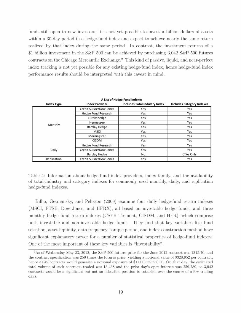
funds still open to new investors, it is not yet possible to invest a billion dollars of assets

within a 30-day period in a hedge-fund index and expect to achieve nearly the same return

realized by that index during the same period. In contrast, the investment returns of a

$1 billion investment in the S&P 500 can be achieved by purchasing 3,042 S&P 500 futures

contracts on the Chicago Mercantile Exchange.9 This kind of passive, liquid, and near-perfect

index tracking is not yet possible for any existing hedge-fund index, hence hedge-fund index

performance results should be interpreted with this caveat in mind.

Index Type Index Provider Includes Total Industry Index Includes Category Indexes

Credit Suisse/Dow Jones Yes Yes

Hedge Fund Research Yes Yes

Eurekahedge Yes Yes

Hennessee Yes Yes

Barclay Hedge Yes Yes

MSCI Yes Yes

Morningstar Yes Yes

CISDM Yes Yes

Hedge Fund Research Yes Yes

Credit Suisse/Dow Jones Yes Yes

Barclay Hedge No CTAs Only

Replication Credit Suisse/Dow Jones Yes Yes

Monthly

Daily

A List of Hedge Fund Indexes

Table 4: Information about hedge-fund index providers, index family, and the availabilityof total-industry and category indexes for commonly used monthly, daily, and replicationhedge-fund indexes.

Billio, Getmansky, and Pelizzon (2009) examine four daily hedge-fund return indexes

(MSCI, FTSE, Dow Jones, and HFRX), all based on investable hedge funds, and three

monthly hedge fund return indexes (CSFB Tremont, CISDM, and HFR), which comprise

both investable and non-investable hedge funds. They find that key variables like fund

selection, asset liquidity, data frequency, sample period, and index-construction method have

significant explanatory power for a number of statistical properties of hedge-fund indexes.

One of the most important of these key variables is “investability”.

9As of Wednesday May 23, 2012, the S&P 500 futures price for the June 2012 contract was 1315.70, andthe contract specification was 250 times the futures price, yielding a notional value of $328,952 per contract,hence 3,042 contracts would generate a notional exposure of $1,000,589,850.00. On that day, the estimatedtotal volume of such contracts traded was 13,438 and the prior day’s open interest was 259,289, so 3,042contracts would be a significant but not an infeasible position to establish over the course of a few tradingdays.

19

A new group of indexes is built around the idea of “factor replication”. These indexes

generally aim to answer the following question: if a portfolio of liquid instruments is formed to

match the performance of the investable liquid-beta portion of typical hedge funds’ portfolios,

what would its returns be? These indexes can be used in determining whether funds of funds

are delivering alpha or beta, or as the basis for hedge-fund beta replication products (see

Section 6.6). This group consists of two subgroups: daily replication indexes published by

data vendors who seem to have begun calculating them as an extension of their existing

index business, and indexes published by asset management firms whose motivation appears

to be the support of hedge-fund beta replication funds launched by the same firms. We

include only the former subgroup in our summary.

In Table 4 we report information about index providers, index families, and the avail-

ability of the total industry and category indexes for commonly used hedge-fund indexes.

Monthly indexes reflect the returns of hedge funds that report to databases at a monthly

frequency. Daily indexes reflect the returns of hedge funds that are willing to report their

returns daily. Replication indexes are daily indexes that show the hypothetical profit and

loss for a factor-model-based hedge-fund beta replication strategy. The Total Industry Index

represents the aggregate performance of the entire hedge-fund industry. A Category Index

is designed to represent the performance of funds within a specific category.

4 Investment Performance

Despite the heterogeneity and uniqueness of individual hedge funds, most hedge funds share

common characteristics with others that deploy similar strategies and/or invest in similar

financial markets and securities. Based on these commonalities, hedge funds may be clustered

into “styles” or “categories”. One popular categorization is that provided by the Lipper TASS

database, which contains 11 main groupings: Convertible Arbitrage, Dedicated Short Bias,

Emerging Markets, Equity Market Neutral, Event Driven, Fixed Income Arbitrage, Global

Macro, Long/Short Equity Hedge, Managed Futures, Multi-Strategy, and Fund of Funds

(see the Appendix for definitions of these categories). While these categories do provide a

useful nomenclature for interpreting the investment performance of hedge funds, it should

be emphasized that the heterogeneity within any single category is considerably greater than

that of traditional investment categories such as large-cap growth or small-cap value funds.

We will illustrate both the commonalities and the heterogeneity of hedge-fund styles through

the statistical properties of their investment returns.

We begin in Section 4.1 with a summary of the hedge-fund performance literature in

20

which the risks and rewards of hedge funds are linked to attributes such as managerial

incentive structures, managers’ ability to hedge, strategy distinctiveness, connections with

political lobbyists, education and career concerns, confidential holdings, delayed reporting,

managerial skills, and capacity constraints. While several of these links are intuitive, the

more important questions are whether or not they imply performance persistence (which

we consider in Section 4.2), and whether hedge-fund managers can actively change their

positions and leverage in response to changes in market conditions (which we consider in

Section 4.3)? In Section 4.4 we show that hedge funds are not all alike by comparing the

investment performance of funds across different style categories, and we also show that

hedge funds are not all unique by identifying a number of common factors among them that

may reduce their diversification properties. We explore the investment implications of these

empirical findings in Section 8.3.

4.1 Basic Performance Studies

The empirical properties of hedge-fund performance have been documented by many authors

using several of the databases cited in Section 3.10 Unlike the literature on mutual-fund

performance, a number of these studies document positive risk-adjusted returns in the hedge-

fund industry, i.e., positive alphas.11 In fact, using data from 1995 to 2009, Ibbotson, Chen,

and Zhu (2011) find that alphas were positive every year of the past decade, even during the

recent financial crisis. More specifically, using a sample of 4,750 stock swap mergers, cash

mergers, and cash tender offers from 1963 to 1998, Mitchell and Pulvino (2001) find that

risk-arbitrage strategies generated excess returns of 4% per year.

Fung, Hsieh, Naik, and Ramadorai (2008) investigate performance, risk, and capital for-

mation in the hedge-fund industry from 1995 to 2004, and over their 120-month sample, they

find that the average fund of funds delivered positive and statistically significant alpha only

in the 18-month sub-period between October 1998 and March 2000. Malkiel and Saha (2005)

report that, after adjusting for various hedge-fund database biases, hedge funds significantly

underperform their benchmarks on average, and our results confirm these findings. In a

sample of 7,000 hedge funds, Billio, Frattarolo, and Pelizzon (2014) find that alpha changes

10See, for example, Ackermann, McEnally, and Ravenscraft (1999), Liang (1999, 2001, 2003), Agarwaland Naik (2000b, 2000c), Fung and Hsieh (2000, 2001), Edwards and Caglayan (2001), Kao (2002), andKosowski, Naik, and Teo (2007). More detailed performance attribution and style analysis for hedge fundshas been considered by Fung and Hsieh (1997, 2002), Brown, Goetzmann, and Ibbotson (1999), Agarwal andNaik (2000b, 2000c), Brown, Goetzmann, and Park (2000, 2001), Liang (2001),Lochoff (2002), and Brownand Goetzmann (2003).

11See Brown, Goetzmann, and Ibbotson (1999), Ackermann, McEnally, and Ravenscraft (1999), Liang(1999), Agarwal and Naik (2000a,b,c), Fung and Hsieh (2004), Kosowski, Naik, and Teo (2007), and Fung,Hsieh, Naik, and Ramadorai (2008).

21

dramatically through time, across categories, and is related to the level of competition among

hedge funds.

Several studies link hedge-fund performance to various hedge-fund and strategy charac-

teristics such as managerial incentive structures, geography, career concerns, strategy capac-

ity, strategy distinctiveness, political connections, and even manager SAT scores. Agarwal,

Daniel, and Naik (2009) find that hedge funds with greater managerial incentives (proxied by

the delta of option-like incentive fee contracts), higher levels of managerial ownership, and

the inclusion of high-water mark provisions in the incentive contracts are associated with

superior performance. Getmansky (2012) documents a concave relationship between size

and performance for illiquid and capacity-constrained hedge funds, which connects strategy

capacity with fund performance. Ramadorai (2013) defines capacity constraints based on

past flows, fund size, and a novel variable—an indicator variable that indicates whether the

fund’s management company launched a new fund or a new share class. Consistent with

other results in the literature, he finds that capacity constraints lead to a reduction in future

returns.

Sun, Wang, and Zheng (2012) show that hedge-fund strategy distinctiveness is associ-

ated with higher performance, and Titman and Tiu (2011) find that managers’ ability to

hedge is directly related to hedge-fund performance. Gao and Huang (2014) conclude that

hedge-fund managers gain an informational advantage in securities trading through their

connections with political lobbyists. They identify politically sensitive companies as those

with high lobbying expenditures relative to their operating cash flows and find that polit-

ically connected hedge funds outperform non-connected funds by 1.6% to 2.5% per month

on their holdings of politically sensitive stocks as compared to their less politically sensitive

holdings. Teo (2009) shows that hedge funds with headquarters or a research office in their

investment region outperform those without it, suggesting that local funds possess an infor-

mational advantage. Liang and Park (2007) show that downside risk measures incorporating

higher return moments can effectively predict future fund performance. And Li, Zhang, and

Zhao (2011) conclude that education and career concerns can positively impact hedge fund

performance—managers from undergraduate institutions with higher average SAT scores

apparently have higher raw and risk-adjusted returns.

Hedge-fund performance has also been linked to macroeconomic factors. For example,

Avramov, Kosowski, Naik, and Teo (2011) show that conditioning on macroeconomic vari-

ables such as the Chicago Board Options Exchange Volatility Index (VIX) and default

spreads is important in detecting managerial skill, and this information can be exploited

in forming optimal portfolios of hedge funds. These results can be interpreted in at least two

ways: managerial alpha is, in fact, attributable to “exotic betas”, or hedge-fund managers

22

generate alpha when macro conditions are conducive. We shall have more to say about

factors driving hedge-fund returns in Section 6.

An important focus of research on hedge fund performance is managers’ ability to per-

form during periods of market distress. Gao, Gao, and Song (2014) show that hedge-fund

managers with better skills in exploiting the market’s ex ante disaster concerns deliver su-

perior returns. Jiang and Kelly (2012) find that hedge funds are exposed to downside “tail

risk” (the risk of rare events), so that a one-standard deviation positive shock to tail risk is

associated with a contemporaneous decline of 2.88% per year in the value of the aggregate

hedge-fund portfolio.

There is also a growing literature on the long-equity holdings of hedge funds retrieved

from 13F filings with the SEC.12 Brunnermeier and Nagel (2004) examine long stock holdings

of hedge funds during the time of the Technology Bubble in 2000 and find that hedge funds

reduced their exposure to technology stocks before prices collapsed and their technology

stock holdings outperformed characteristics-matched benchmarks. Griffin and Xu (2009)

show that hedge-fund managers are only marginally better than mutual-fund managers in

stock picking, and also find weak evidence of differential ability among hedge funds.

Agarwal, Jiang, Tang, and Yang (2013) study quarter-end equity holdings of hedge

funds that are disclosed with a delay through amendments to their 13F filings. Hedge-

fund managers delay reporting their positions due to concerns about private information

and price impact. Hedge funds managing large and concentrated portfolios, adopting non-

standard investment strategies with higher idiosyncratic risk, and holding stocks associated

with information-sensitive events such as mergers and acquisitions seek confidentiality more

frequently. The authors find that confidential holdings exhibit superior performance up to

twelve months, and take longer to build. Aragon, Hertzel, and Shi (2013) find that managers

seek confidential treatment of some of their 13F-reportable positions in order to hide confi-

dential information from the public. The hedge fund managers are also more likely to seek

confidential treatment of illiquid positions that are more susceptible to front-running. 13F

public filings thus are likely to attract informed hedge fund traders and investors. However,

there are some significant challenges in the detection of informed trading by hedge funds

because they pertain to a narrow scope of reportable securities, exclude short positions, and

are observable at a low (quarterly) frequency.

12Standard databases such as Thomson-Reuters Institutional Holdings systematically omit certain posi-tions that are 13F-reportable such as call- and put-option positions (Aragon and Martin (2012)), and con-fidentially held stock positions (Agarwal, Jiang, Tang, and Yang (2013), Aragon, Hertzel, and Shi (2013)),hence researchers should also check SEC filings directly.

23

4.2 Performance Persistence

The evidence regarding performance persistence is mixed. Agarwal and Naik (2000a) and

Chen (2007) find that monthly hedge-fund performance persists for short periods, but disap-

pears at an annual horizon. Using annual offshore hedge-fund data, Brown, Goetzmann, and

Ibbotson (1999) find no evidence of performance persistence. Edwards and Caglayan (2001)

use both parametric and non-parametric procedures to study persistence over one- and two-

year horizons and also find no persistence, though they do observe considerable variation

across style categories. Boyson (2008) does not find any performance persistence over short

and long intervals when funds are selected based purely on past performance, but when

manager tenure is taken into consideration, hedge funds do seem to exhibit performance

persistence over quarterly intervals.

However, Bares, Gibson, and Gyger (2003) do find short-term persistence, and Baquero,

Horst, and Verbeek (2005) find persistence in hedge funds at the quarterly frequency after

correcting for investment styles, but persistence is statistically insignificant annually. Kat

and Menexe (2003) find weak persistence in mean returns, but strong persistence in hedge

funds’ standard deviations and their correlation with the stock market. Fung, Hsieh, Naik,

and Ramadorai (2008) find that there is a greater chance for a fund to deliver alpha in the

subsequent two-year period if it has positive estimated alpha in the previous two-year period.

In particular, they show that the overall average transition probability for a positive-alpha

fund into the subsequent positive-alpha group is 28%, while the transition probability for

a no-alpha fund is only 14%. Moreover, the year-by-year alpha-transition probability for a

positive-alpha fund is always higher than that for a no-alpha fund, implying greater alpha

persistence among members of the positive-alpha group. Consistent with these findings,

Jagannathan, Malakhov, and Novikov (2010) document significant performance persistence

among superior hedge funds, while they find little evidence of persistence among inferior

funds.

Persistence in hedge fund performance challenges the no-persistence equilibrium result

of the Berk and Green (2004) model for mutual funds. Extending the model to deliver

persistence in a hedge fund setting may be an interesting direction for future research (e.g.,

Glode and Green (2011)).

4.3 Timing Ability

Among the entire population of professional investment managers, hedge funds should be

the most likely to display timing skills of some form given that they are less constrained and

more active. In fact, because of their broader investment mandates and greater flexibility to

24

exploit investment opportunities as they emerge, hedge funds can engage in several forms of

timing, e.g., market timing, volatility timing, and liquidity timing. The empirical evidence

generally seems to support this intuition.

Fung, Xu, and Yau (2002) examine global hedge-fund managers and conclude that they do

not show positive market timing ability, but have superior security-selection ability. Aragon

(2005) finds that funds of funds do not exhibit timing ability, but that market-timing ability

is positive for funds holding the most liquid portfolios and negative for funds holding the

most illiquid portfolios. However, Chen (2007) extends the timing measures in Treynor and

Mazuy (1966) and Henriksson and Merton (1981) and finds significant market-timing ability

for individual hedge funds and funds of funds in bond, currency, and equity markets. Chen

and Liang (2007) propose a new market-timing measure by relating fund returns to the

squared Sharpe ratio of the market portfolio. Using a sample of 221 market-timing funds

from January 1994 through June 2005, they find economically and statistically significant

evidence of return timing, volatility timing, and joint timing, both at the aggregate and

individual-fund levels.

Kazemi and Li (2009) consider the market- and volatility-timing ability of commodity

trading advisors (CTAs), and observe that CTAs display a negative relationship between

market-timing and security-selection ability. They also find that systematic CTAs are, in

general, better at market timing than discretionary CTAs. Cave, Hubner, and Sougne (2012)

identify “positive”, “mixed”, and “negative” market timers and study their performance dur-

ing the financial crisis of 2007–2009. Aragon and Martin (2012) study volatility timing ability

and selectivity skill revealed by the use of calls, puts, and equity positions by hedge-fund

investment advisers. They find that hedge funds successfully use derivatives to profit from

private information about stock fundamentals. For example, hedge funds greatly increased

their use of puts in the aftermath of the Technology Bubble, and there is a strong positive

(negative) relation between call (put) holdings and subsequent abnormal stock returns. Chen

(2011) finds that 71% of hedge funds trade derivatives. After controlling for fund strategies

and characteristics, derivatives users on average exhibit lower market, downside, and event

risk.

Cao, Chen, Liang, and Lo (2013) examine the liquidity timing ability for hedge funds,

and find strong evidence at both the strategy and individual-fund levels. Specifically, they

show that hedge-fund managers increase (decrease) their portfolios’ market exposure when

equity-market liquidity is high (low), and liquidity timing is most pronounced when market

liquidity is very low.

25

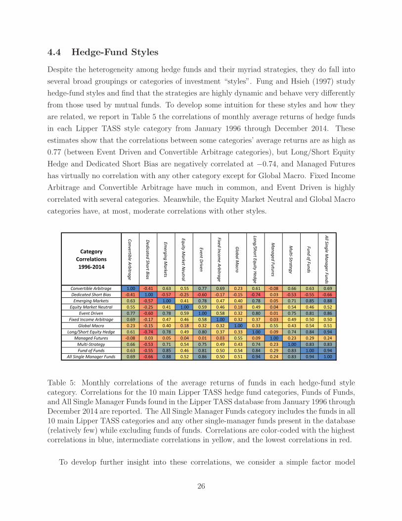
4.4 Hedge-Fund Styles

Despite the heterogeneity among hedge funds and their myriad strategies, they do fall into

several broad groupings or categories of investment “styles”. Fung and Hsieh (1997) study

hedge-fund styles and find that the strategies are highly dynamic and behave very differently

from those used by mutual funds. To develop some intuition for these styles and how they

are related, we report in Table 5 the correlations of monthly average returns of hedge funds

in each Lipper TASS style category from January 1996 through December 2014. These

estimates show that the correlations between some categories’ average returns are as high as

0.77 (between Event Driven and Convertible Arbitrage categories), but Long/Short Equity

Hedge and Dedicated Short Bias are negatively correlated at −0.74, and Managed Futures

has virtually no correlation with any other category except for Global Macro. Fixed Income

Arbitrage and Convertible Arbitrage have much in common, and Event Driven is highly

correlated with several categories. Meanwhile, the Equity Market Neutral and Global Macro

categories have, at most, moderate correlations with other styles.

Category

Correlations

1996-2014C

on

vertib

le A

rbitra

ge

De

dica

ted

Sh

ort B

ias

Em

erg

ing

Ma

rke

ts

Eq

uity M

ark

et N

eu

tral

Eve

nt D

riven

Fixe

d In

com

e A

rbitra

ge

Glo

ba

l Ma

cro

Lon

g/S

ho

rt Eq

uity H

ed

ge

Ma

na

ge

d F

utu

res

Mu

lti-Stra

teg

y

Fu

nd

of F

un

ds

All S

ing

le M

an

ag

er F

un

ds

Convertible Arbitrage 1.00 -0.41 0.63 0.55 0.77 0.69 0.23 0.61 -0.08 0.66 0.63 0.69

Dedicated Short Bias -0.41 1.00 -0.57 -0.25 -0.60 -0.17 -0.15 -0.74 0.03 -0.53 -0.55 -0.66

Emerging Markets 0.63 -0.57 1.00 0.41 0.78 0.47 0.40 0.78 0.05 0.71 0.85 0.88

Equity Market Neutral 0.55 -0.25 0.41 1.00 0.59 0.46 0.18 0.49 0.04 0.54 0.46 0.52

Event Driven 0.77 -0.60 0.78 0.59 1.00 0.58 0.32 0.80 0.01 0.75 0.81 0.86

Fixed Income Arbitrage 0.69 -0.17 0.47 0.46 0.58 1.00 0.32 0.37 0.03 0.49 0.50 0.50

Global Macro 0.23 -0.15 0.40 0.18 0.32 0.32 1.00 0.33 0.55 0.43 0.54 0.51

Long/Short Equity Hedge 0.61 -0.74 0.78 0.49 0.80 0.37 0.33 1.00 0.09 0.74 0.84 0.94

Managed Futures -0.08 0.03 0.05 0.04 0.01 0.03 0.55 0.09 1.00 0.23 0.29 0.24

Multi-Strategy 0.66 -0.53 0.71 0.54 0.75 0.49 0.43 0.74 0.23 1.00 0.83 0.83

Fund of Funds 0.63 -0.55 0.85 0.46 0.81 0.50 0.54 0.84 0.29 0.83 1.00 0.94

All Single Manager Funds 0.69 -0.66 0.88 0.52 0.86 0.50 0.51 0.94 0.24 0.83 0.94 1.00

Table 5: Monthly correlations of the average returns of funds in each hedge-fund stylecategory. Correlations for the 10 main Lipper TASS hedge fund categories, Funds of Funds,and All Single Manager Funds found in the Lipper TASS database from January 1996 throughDecember 2014 are reported. The All Single Manager Funds category includes the funds in all10 main Lipper TASS categories and any other single-manager funds present in the database(relatively few) while excluding funds of funds. Correlations are color-coded with the highestcorrelations in blue, intermediate correlations in yellow, and the lowest correlations in red.

To develop further insight into these correlations, we consider a simple factor model

26

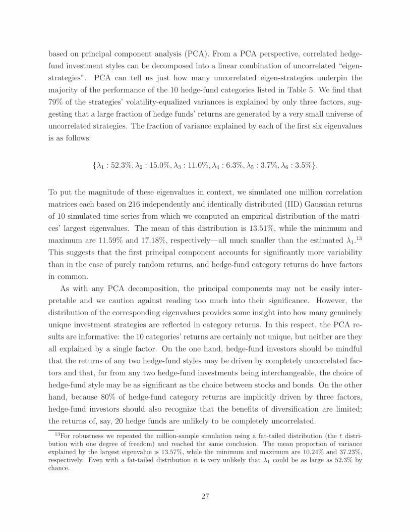
based on principal component analysis (PCA). From a PCA perspective, correlated hedge-

fund investment styles can be decomposed into a linear combination of uncorrelated “eigen-

strategies”. PCA can tell us just how many uncorrelated eigen-strategies underpin the

majority of the performance of the 10 hedge-fund categories listed in Table 5. We find that

79% of the strategies’ volatility-equalized variances is explained by only three factors, sug-

gesting that a large fraction of hedge funds’ returns are generated by a very small universe of

uncorrelated strategies. The fraction of variance explained by each of the first six eigenvalues

is as follows:

{λ1 : 52.3%, λ2 : 15.0%, λ3 : 11.0%, λ4 : 6.3%, λ5 : 3.7%, λ6 : 3.5%}.

To put the magnitude of these eigenvalues in context, we simulated one million correlation

matrices each based on 216 independently and identically distributed (IID) Gaussian returns

of 10 simulated time series from which we computed an empirical distribution of the matri-

ces’ largest eigenvalues. The mean of this distribution is 13.51%, while the minimum and

maximum are 11.59% and 17.18%, respectively—all much smaller than the estimated λ1.13

This suggests that the first principal component accounts for significantly more variability

than in the case of purely random returns, and hedge-fund category returns do have factors

in common.

As with any PCA decomposition, the principal components may not be easily inter-

pretable and we caution against reading too much into their significance. However, the

distribution of the corresponding eigenvalues provides some insight into how many genuinely

unique investment strategies are reflected in category returns. In this respect, the PCA re-

sults are informative: the 10 categories’ returns are certainly not unique, but neither are they

all explained by a single factor. On the one hand, hedge-fund investors should be mindful

that the returns of any two hedge-fund styles may be driven by completely uncorrelated fac-

tors and that, far from any two hedge-fund investments being interchangeable, the choice of

hedge-fund style may be as significant as the choice between stocks and bonds. On the other

hand, because 80% of hedge-fund category returns are implicitly driven by three factors,

hedge-fund investors should also recognize that the benefits of diversification are limited;

the returns of, say, 20 hedge funds are unlikely to be completely uncorrelated.

13For robustness we repeated the million-sample simulation using a fat-tailed distribution (the t distri-bution with one degree of freedom) and reached the same conclusion. The mean proportion of varianceexplained by the largest eigenvalue is 13.57%, while the minimum and maximum are 10.24% and 37.23%,respectively. Even with a fat-tailed distribution it is very unlikely that λ1 could be as large as 52.3% bychance.

27

A more intuitive illustration of the heterogeneity and commonality among hedge-fund

styles is presented in Table 6, in which a variety of summary statistics such as average return,

volatility, Sharpe ratio, and higher-order moments are reported for hedge-fund category

returns. The top panel reports the summary statistics for the average fund (averaged across

all available funds in the Lipper TASS database for each month), and the bottom panel

reports the same summary statistics for the Credit Suisse/Dow Jones (CS/DJ) Hedge-Fund

Category Index.

# fu

nd

-

mo

nth

s

An

nu

alize

d

Me

an

An

nu

alize

d

Vo

latility

Sh

arp

e

Ra

tio

So

rtino

Ra

tio

Sk

ew

ne

ss

Ku

rtosis

Ma

xim

um

DD

S&

P 5

00

Co

rrel.

ac(1

)

Bo

x-Q

(3) p

-

va

lue

Database Estimate Convertible Arbitrage 14231 5.4% 7.3% 0.38 0.51 -3.37 28.94 -34.4% 0.51 0.48 0.00

Database Estimate Dedicated Short Bias 2503 -1.1% 15.6% -0.23 -0.41 0.62 5.23 -47.3% -0.72 0.10 0.08

Database Estimate Emerging Markets 47054 6.8% 14.2% 0.29 0.42 -1.43 9.94 -49.3% 0.64 0.31 0.00

Database Estimate Equity Market Neutral 27459 4.7% 3.3% 0.61 0.99 -0.25 12.86 -14.6% 0.32 0.20 0.00

Database Estimate Event Driven 39227 6.8% 5.9% 0.70 1.05 -1.64 8.97 -24.8% 0.65 0.42 0.00

Database Estimate Fixed Income Arbitrage 18834 5.1% 4.4% 0.56 0.68 -4.35 32.93 -20.7% 0.29 0.37 0.00

Database Estimate Global Macro 32034 4.9% 5.2% 0.44 0.81 0.48 4.93 -14.2% 0.28 0.01 0.48

Database Estimate Long/Short Equity Hedge 178926 7.7% 9.0% 0.56 0.98 0.00 5.47 -24.7% 0.74 0.22 0.00

Database Estimate Managed Futures 46204 4.8% 9.4% 0.23 0.44 0.26 3.13 -16.3% -0.05 -0.02 0.29

Database Estimate Multi-Strategy 76233 5.8% 5.2% 0.62 0.93 -1.18 7.16 -21.5% 0.57 0.22 0.00

Database Estimate Fund of Funds 270369 3.8% 6.0% 0.20 0.31 -0.57 6.80 -21.9% 0.58 0.28 0.00

Database Estimate All Single Manager Funds 505844 6.3% 6.3% 0.58 0.97 -0.50 5.72 -20.5% 0.71 0.25 0.00

CS/Dow Jones Index Convertible Arbitrage 228 7.3% 6.8% 0.69 0.95 -2.75 20.03 -32.9% 0.37 0.55 0.00

CS/Dow Jones Index Dedicated Short Bias 228 -6.4% 16.7% -0.53 -0.95 0.78 4.65 -76.3% -0.77 0.08 0.53

CS/Dow Jones Index Emerging Markets 228 8.4% 13.1% 0.44 0.65 -1.28 10.74 -45.1% 0.60 0.26 0.00

CS/Dow Jones Index Equity Market Neutral 228 4.8% 10.2% 0.21 0.23 -11.88 165.26 -45.1% 0.31 0.07 0.06

CS/Dow Jones Index Event Driven 228 9.2% 6.3% 1.03 1.52 -2.25 13.60 -19.1% 0.63 0.36 0.00

CS/Dow Jones Index Fixed Income Arbitrage 228 5.3% 5.6% 0.48 0.58 -4.64 36.20 -29.0% 0.32 0.53 0.00

CS/Dow Jones Index Global Macro 228 10.9% 8.9% 0.92 1.60 -0.06 8.01 -26.8% 0.24 0.05 0.30

CS/Dow Jones Index Long/Short Equity Hedge 228 9.7% 9.6% 0.72 1.29 -0.03 6.63 -22.0% 0.67 0.18 0.04

CS/Dow Jones Index Managed Futures 228 6.1% 11.4% 0.30 0.57 0.06 2.69 -17.4% -0.05 0.03 0.21

CS/Dow Jones Index Multi-Strategy 228 8.4% 4.9% 1.16 1.77 -1.99 11.52 -24.7% 0.43 0.44 0.00

CS/Dow Jones Index All Single Manager Funds 228 8.6% 7.1% 0.82 1.44 -0.20 6.27 -19.7% 0.59 0.17 0.01

From 1996 to 2014

Table 6: Summary statistics for the returns of the average fund in each Lipper TASS stylecategory and summary statistics for the corresponding CS/DJ Hedge-Fund Index. Numberof fund months, annualized mean, annualized volatility, Sharpe ratio, Sortino ratio, skew-ness, kurtosis, maximum drawdown, correlation coefficient with the S&P 500, first-orderautocorrelation, and p-value of the Ljung-Box Q-statistic with three lags for the 10 mainLipper TASS hedge fund categories, Funds of Funds, and All Single Manager Funds found inthe Lipper TASS database from January 1996 through December 2014 are reported. Sharpeand Sortino ratios are adjusted for the three-month U.S. Treasury Bill rate. The “All SingleManager Funds” category includes the funds in all 10 main Lipper TASS categories and anyother single-manager funds present in the database (relatively few) while excluding funds offunds.

We observe new patterns of similarities and differences among hedge fund categories in

Table 6. During the period from January 1996 through December 2014, Dedicated Short

Bias underperformed all categories, which is not surprising given that equities performed

well during a significant portion of the sample period. Consistent with Agarwal and Kale

(2007) we find that Multi-Strategy hedge funds outperformed Funds of Funds. The average

28

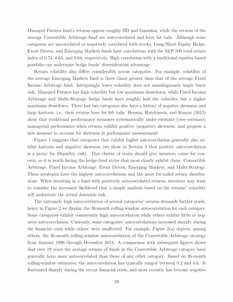
Managed Futures fund’s returns appear roughly IID and Gaussian, while the returns of the

average Convertible Arbitrage fund are autocorrelated and have fat tails. Although some

categories are uncorrelated or negatively correlated with stocks, Long/Short Equity Hedge,

Event Driven, and Emerging Markets funds have correlations with the S&P 500 total return

index of 0.74, 0.65, and 0.64, respectively. High correlation with a traditional equities-based

portfolio can undermine hedge funds’ diversification advantage.

Return volatility also differs considerably across categories. For example, volatility of

the average Emerging Markets fund is three times greater than that of the average Fixed

Income Arbitrage fund. Intriguingly, lower volatility does not unambiguously imply lower

risk: Managed Futures has high volatility but low maximum drawdown, while Fixed Income

Arbitrage and Multi-Strategy hedge funds have roughly half the volatility but a higher

maximum drawdown. These last two categories also have a history of negative skewness and

large kurtosis, i.e., their returns have fat left tails. Heuson, Hutchinson, and Kumar (2015)

show that traditional performance measures systematically under-estimate (over-estimate)

managerial performance when returns exhibit positive (negative) skewness, and propose a

new measure to account for skewness in performance measurement.

Figure 1 suggests that categories that exhibit higher autocorrelation generally also ex-

hibit kurtosis and negative skewness (we show in Section 5 that positive autocorrelation

is a proxy for illiquidity risk). This cluster of traits should give investors cause for con-

cern, so it is worth listing the hedge-fund styles that most clearly exhibit them: Convertible

Arbitrage, Fixed Income Arbitrage, Event Driven, Emerging Markets, and Multi-Strategy.

These strategies have the highest autocorrelations and the most fat-tailed return distribu-

tions. When investing in a fund with positively autocorrelated returns, investors may want

to consider the increased likelihood that a simple analysis based on the returns’ volatility

will understate the actual downside risk.

The extremely high autocorrelation of several categories’ returns demands further study,

hence in Figure 2 we display the 36-month rolling-window autocorrelation for each category.

Some categories exhibit consistently high autocorrelation while others exhibit little or neg-

ative autocorrelation. Curiously, some categories’ autocorrelations increased sharply during

the financial crisis while others’ were unaffected. For example, Figure 2(a) depicts, among

others, the 36-month rolling-window autocorrelation of the Convertible Arbitrage strategy

from January 1996 through December 2014. A comparison with subsequent figures shows

that over 19 years the average returns of funds in the Convertible Arbitrage category have

generally been more autocorrelated than those of any other category. Based on 36-month

rolling-window estimates, the autocorrelation has typically ranged between 0.2 and 0.6. It

fluctuated sharply during the recent financial crisis, and most recently has become negative

29

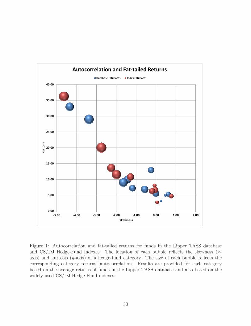
40.00

Autocorrelation and Fat-tailed Returns

Database Estimates Index Estimates

30.00

35.00

20.00

25.00

Ku

rto

sis

10.00

15.00

Ku

rto

sis

0.00

5.00

-5.00 -4.00 -3.00 -2.00 -1.00 0.00 1.00 2.00-5.00 -4.00 -3.00 -2.00 -1.00 0.00 1.00 2.00

Skewness

Figure 1: Autocorrelation and fat-tailed returns for funds in the Lipper TASS databaseand CS/DJ Hedge-Fund indexes. The location of each bubble reflects the skewness (x-axis) and kurtosis (y-axis) of a hedge-fund category. The size of each bubble reflects thecorresponding category returns’ autocorrelation. Results are provided for each categorybased on the average returns of funds in the Lipper TASS database and also based on thewidely-used CS/DJ Hedge-Fund indexes.

30

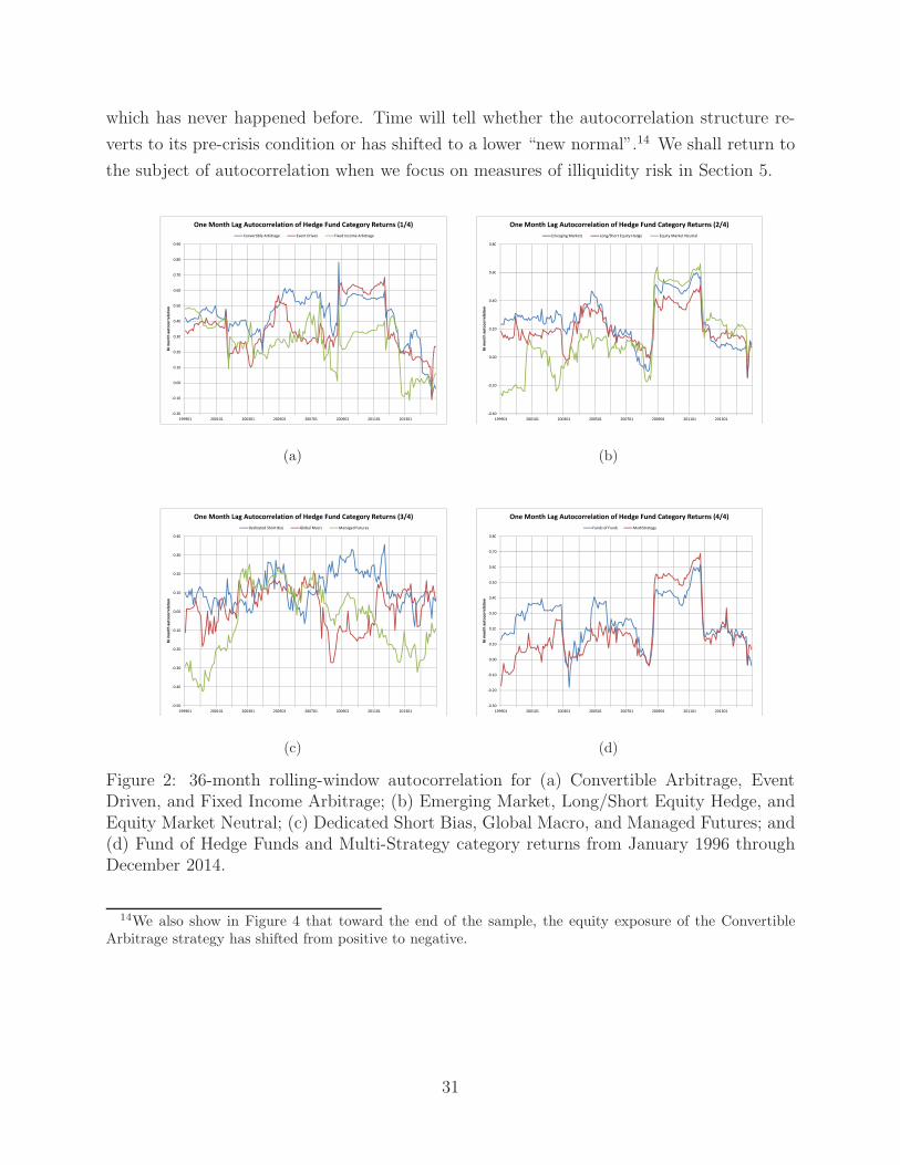
which has never happened before. Time will tell whether the autocorrelation structure re-

verts to its pre-crisis condition or has shifted to a lower “new normal”.14 We shall return to

the subject of autocorrelation when we focus on measures of illiquidity risk in Section 5.

0.30

0.40

0.50

0.60

0.70

0.80

0.90

36

mo

nth

au

toco

rre

lati

on

One Month Lag Autocorrelation of Hedge Fund Category Returns (1/4)

Convertible Arbitrage Event Driven Fixed Income Arbitrage

-0.20

-0.10

0.00

0.10

0.20

0.30

199901 200101 200301 200501 200701 200901 201101 201301

36

mo

nth

au

toco

rre

lati

on

(a)

0.80

One Month Lag Autocorrelation of Hedge Fund Category Returns (2/4)

Emerging Markets Long/Short Equity Hedge Equity Market Neutral

0.60

0.80

0.40

0.60

0.20

36

mo

nth

au

toco

rre

lati

on

0.00

36

mo

nth

au

toco

rre

lati

on

-0.20

-0.40

199901 200101 200301 200501 200701 200901 201101 201301

(b)

0.40

One Month Lag Autocorrelation of Hedge Fund Category Returns (3/4)

Dedicated Short Bias Global Macro Managed Futures

0.30

0.40

0.10

0.20

0.00

36

mo

nth

au

toco

rre

lati

on

-0.20

-0.10

36

mo

nth

au

toco

rre

lati

on

-0.40

-0.30

-0.50

-0.40

199901 200101 200301 200501 200701 200901 201101 201301

(c)

0.80

One Month Lag Autocorrelation of Hedge Fund Category Returns (4/4)

Funds of Funds MultiStrategy

0.60

0.70

0.80

0.40

0.50

0.60

0.20

0.30

0.40

36

mo

nth

au

toco

rre

lati

on

0.10

0.20

36

mo

nth

au

toco

rre

lati

on

-0.10

0.00

-0.30

-0.20

199901 200101 200301 200501 200701 200901 201101 201301

(d)

Figure 2: 36-month rolling-window autocorrelation for (a) Convertible Arbitrage, EventDriven, and Fixed Income Arbitrage; (b) Emerging Market, Long/Short Equity Hedge, andEquity Market Neutral; (c) Dedicated Short Bias, Global Macro, and Managed Futures; and(d) Fund of Hedge Funds and Multi-Strategy category returns from January 1996 throughDecember 2014.

14We also show in Figure 4 that toward the end of the sample, the equity exposure of the ConvertibleArbitrage strategy has shifted from positive to negative.

31

5 Illiquidity

Illiquidity is one of the most important characteristics of certain hedge fund investments

that has only recently begun to receive the attention it deserves. Not only is illiquidity at

the heart of most financial crises (see, for example, the discussion in Section 7), but it is

also central to how many financial investments generate their returns. Taking on illiquidity

risk is one of the most effective ways for long-horizon investors to build wealth, but it can

also be the downfall of investors who are unaware of their illiquidity exposure and attempt

to liquidate certain investments at the wrong time.

One of the biggest challenges to measuring illiquidity is the fact that there is currently

no single definition of liquidity. The reason is simple: liquidity is not a one-dimensional

characteristic, but has at least three distinct aspects to it. An asset is considered liquid if:

(1) it can be bought or sold quickly; (2) the amount that can be bought or sold is large; and

(3) buying or selling such large amounts will not adversely impact the market price. Certain

assets may have one or two of these properties, but only truly liquid assets will have all three.

For example, residential real estate can be sold quickly, but usually not without significant

price concessions, hence this asset would not be considered liquid. What makes liquidity even

harder to define is that these three characteristics are time- and context-dependent; what

is liquid today may be highly illiquid tomorrow. A clear illustration of just how dynamic

liquidity can be is the Quant Meltdown of August 2007, described in more detail in Section

7.1.

In Section 5.1, we review several measures of illiquidity that are specifically designed with

hedge funds in mind. We consider the impact of illiquidity on statistical measures of hedge-

fund performance such as volatilities, Sharpe ratios, and betas and how to correct for it in

5.2. Based on these and other measures of illiquidity, the magnitude of illiquidity risk premia

in hedge-fund returns can be quantified, which we describe in Section 5.3. And in Section

5.4, we show how to incorporate measures of illiquidity into the traditional mean-variance

portfolio optimization framework.

5.1 Measures of Illiquidity and Return Smoothing

The finance literature offers a number of theoretical and empirical measures of illiquidity

including percentage bid/offer spreads (Tinic (1972), Glosten and Milgrom (1985), Amihud

and Mendelson (1986)), price impact (Kraus and Stoll (1972), Kyle (1985), Hasbrouck and

Schwartz (1988), and Lillo, Farmer, and Mantegna (2003)), and volume-based statistics (Lo,

Mamaysky, and Wang (2004), Lo and Wang (2006), and Pastor and Stambaugh (2003)).

32

However, these measures all assume the existence of a centralized exchange in which price

discovery occurs regularly, that there exist designated market makers who post bids and

offers, and that trading volume can be measured. As a result, none of these measures

are applicable to investments in hedge funds, of which the vast majority are structured as

privately placed securities.

Lo (2001) and Getmansky, Lo, and Makarov (2004) propose an alternate measure of

illiquidity that depends only on asset returns, return autocorrelation, ρk:

ρk =Cov[Rt, Rt−k]

Var[Rt], k > 0 (1)

ρk =(T − k + 1)−1

∑T

t=k−1(Rt − µ)(Rt−k − µ)

(T − 1)−1∑T

t=1(Rt − µ)2, µ = T−1

T∑

t=1

Rt . (2)

In an efficient market, asset returns should be approximately serially uncorrelated, hence

ρk = 0 for all k > 0—past returns should contain very little information about future re-

turns, otherwise the information can be exploited via trading strategies that buy (shortsell)

securities with positive (negative) return forecasts. The very process of exploiting this infor-

mation will tend to reduce, if not eliminate entirely, any return autocorrelation. The only

two reasons such information cannot be exploited and, therefore, eliminated, are: (1) if the

autocorrelation is due to time-varying equilibrium expected returns; and (2) if the autocor-

relation cannot be exploited due to trading frictions, i.e., illiquidity. The first possibility

is less likely for shorter-horizon holding periods such as monthly or daily returns given the

definition of equilibrium expected returns, hence the second possibility is the more likely

explanation for significant return autocorrelation. In other words, returns may be autocor-

related because information about the underlying asset diffuses over time and investors with

early access to this information cannot exploit it because the asset cannot be traded quickly,

and/or cannot be traded in large size, and/or cannot be traded without moving the price

significantly.

Getmansky, Lo, and Makarov (2004) construct a simple econometric model to estimate

the degree of autocorrelation in hedge-fund returns by assuming that the true but unobserv-

able economic return, Rt, of a hedge fund in period t satisfies a linear single-factor model:

Rt = µ + βΛt + ǫt , E[Λt] = E[ǫt] = 0 , ǫt , Λt ∼ IID (3a)

Var[Rt] ≡ σ2 (3b)

33

whereas the reported return Rot is:

Rot = θ0 Rt + θ1Rt−1 + · · · + θk Rt−k (4)

θj ∈ [0, 1] , j = 0, . . . , k (5)

1 = θ0 + θ1 + · · · + θk (6)

which is a weighted average of the fund’s true returns over the most recent k+1 periods,

including the current period. True returns represent the flow of information that would

determine the equilibrium value of the fund’s securities in a frictionless market, and observed

returns represent the results that the fund reports each month. Using maximum likelihood

to estimate the smoothing parameters {θj}, Getmansky, Lo, and Makarov (2004) confirm

that funds with higher autocorrelation tend to be the more illiquid funds, e.g., emerging

market debt, fixed income arbitrage, etc.

More generally, Khandani and Lo (2011b) establish a link between illiquidity and positive

autocorrelation in asset returns among a sample of hedge funds, mutual funds, and various

equity portfolios. For hedge funds, this link can be confirmed by comparing the return auto-

correlations of funds with shorter vs. longer redemption-notice periods. They also document

significant positive return-autocorrelation in portfolios of securities that are generally con-

sidered less liquid, e.g., small-cap stocks, corporate bonds, mortgage-backed securities, and

emerging-market investments.

Getmansky, Lo, and Makarov (2004) and Bollen and Pool (2008) also observe that return

autocorrelation may be evidence of return smoothing, the unsavory practice of reporting only

part of the gains in the months when a fund has positive returns so as to partially offset

potential future losses, thereby reducing volatility and improving risk-adjusted performance

measures such as the Sharpe ratio (see Section 5.2). However, while large positive return

autocorrelations should raise concerns regarding the potential of deliberate return-smoothing

behavior, Getmansky, Lo, and Makarov (2004) emphasize that it is impossible to determine

whether a fund is intentionally smoothing returns just from its return autocorrelations.

Bollen and Pool (2009) and Jylha (2011) show that hedge funds often push otherwise

small negative returns above zero. Agarwal, Daniel, and Naik (2011) find evidence of manip-

ulating reported returns upward in the month of December. Cici, Kempf, and Puetz (2015)

use 13F filings to show that hedge-fund advisers strategically employ mismarking in stock

positions to smooth their reported returns and push otherwise small negative returns above

zero.

Aragon and Nanda (2015) link reporting delays to return smoothing, through report-

34

ing returns in “clusters”. Patton, Ramadorai, and Streatfield (2013) find that hedge fund

performance is lower among funds that have restated their return history to a database, es-

pecially among funds that show a high degree of monthly return autocorrelation. Ben-David,

Franzoni, Landier, and Moussawi (2013) provide evidence suggesting that some hedge funds

manipulate stock prices on critical reporting dates. They find that stocks in the top quartile

of hedge fund holdings exhibit abnormal returns of 0.30% on the last day of the quarter and

a reversal of 0.25% on the following day. A significant part of the return is earned during the

last minutes of trading. Kruttli, Patton, and Ramadorai (2014) use an aggregate version of

the liquidity measure of Getmansky, Lo, and Makarov (2004), estimated across a large set

of hedge funds, and find that the measure has the ability to predict a large range of asset

returns (commodities, currencies, bonds, and equities). The authors relate this finding to

the role of hedge funds in liquidity provision in capital markets.

5.2 Illiquidity and Statistical Biases

Illiquidity can lead to a number of biases in the statistical properties of hedge-fund returns.

For example, using a linear moving average time series model for illiquid hedge-fund returns,

Getmansky, Lo, and Makarov (2004) show that standard estimators of volatility are biased

downward, Sharpe ratios are biased upward, and the betas of regressions of hedge-fund

returns on lagged market factors are non-zero. The authors find that after correcting for

the effects of smoothed returns, some of the most successful types of funds tend to have

considerably less attractive performance characteristics. Lo (2001) provides the appropriate

correction term for computing volatilities and Sharpe ratios in these cases, and shows that

corrected annualized Sharpe ratios based on monthly data can differ from the standard

Sharpe ratio estimator by as much as 70%. Asness, Krail, and Liew (2001) show that in

some cases where hedge funds purport to be market neutral, i.e., funds with relatively small

market betas (market exposure) when only contemporaneous returns are used as regressors,

including both contemporaneous and lagged market returns as regressors and summing the

beta coefficients, yields significantly higher market exposure, implying a certain degree of

illiquidity.

These empirical properties may have potentially significant implications for assessing the

risks and expected returns of hedge-fund investments, including potential fraud detection.

35

5.3 Measuring Illiquidity Risk Premia

Suppose investors are given the choice between two assets that are identical in all respects

but one: while one asset can be traded around the clock, the other asset can only be traded

on the first Tuesday of each month. Most investors would choose the first (more liquid) asset.

But when enough investors do this, the supply of the first asset may dwindle, and its price

would rise relative to the second asset. At some point, investors will feel that the discount

on the second asset—which yields a higher expected return today, assuming that its future

expected payoff is unchanged—is sufficiently large to compensate them for the infrequency

with which it can be traded, leading them to buy the second asset. The investors buying the

second asset will obtain a higher expected return than investors in the first asset in exchange

for accepting the risk that at the moment they want to sell their asset, it may not be possible

to do so. This incremental return is called the “illiquidity premium”.

Unfortunately, paired with the illiquidity premium is the illiquidity penalty: the periods

when many owners want to sell are typically times during which few investors want to buy, so

the asset’s price may plummet beyond reason. In these circumstances it may be impossible

to sell at a price near what an owner considers fair.

Liang (1999) and Aragon (2007) study the relation between hedge fund returns and a

very specific form of illiquidity—lockup restrictions—and document a positive relationship

between lockups and fund performance. Aragon (2007) finds that hedge funds with lockups

have 4% to 7% per year higher excess returns than those of non-lockup funds (see Section 2.3

for further discussion of lockups and other share restrictions). Sadka (2010, 2012) shows that

liquidity risk is an important determinant of the cross-sectional differences in hedge fund re-

turns and concludes that hedge funds with significant liquidity risk subsequently outperform

low-liquidity-risk funds by an average of 6% annually. Consistent with Brunnermeier and

Pedersen (2009), Teo (2011) finds that hedge funds with strong incentives to raise capital,

low manager option deltas, and no manager capital co-invested are more likely to take on

excessive liquidity risk.

Using a sample of 2,927 hedge funds, 15,654 mutual funds, and 100 size- and book-

to-market-sorted portfolios of U.S. common stocks, Khandani and Lo (2011b) construct

autocorrelation-sorted long/short portfolios and conclude that illiquidity premia are gener-

ally positive and significant, ranging from 2.74% to 9.91% per year among the various hedge

funds and fixed-income mutual funds. They do not find evidence for this premium among

equity and asset-allocation mutual funds, or among the 100 U.S. equity portfolios. The time

variation in their aggregated illiquidity premium shows that while 1998 was a difficult year

for most funds with large illiquidity exposure, the following four years yielded significantly

36

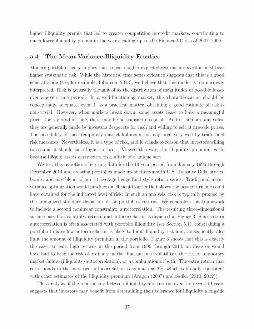
higher illiquidity premia that led to greater competition in credit markets, contributing to

much lower illiquidity premia in the years leading up to the Financial Crisis of 2007–2009.

5.4 The Mean-Variance-Illiquidity Frontier

Modern portfolio theory implies that, to earn higher expected returns, an investor must bear

higher systematic risk. While the historical time series evidence suggests that this is a good

general guide (see, for example, Ibbotson, 2013), we believe that this model is too narrowly

interpreted. Risk is generally thought of as the distribution of magnitudes of possible losses

over a given time period. In a well-functioning market, this characterization should be

conceptually adequate, even if, as a practical matter, obtaining a good estimate of risk is

non-trivial. However, when markets break down, some assets cease to have a meaningful

price—for a period of time, there may be no transactions at all. And if there are any sales,

they are generally made by investors desperate for cash and willing to sell at fire-sale prices.

The possibility of such temporary market failures is not captured very well by traditional

risk measures. Nevertheless, it is a type of risk, and it stands to reason that investors willing

to assume it should earn higher returns. Viewed this way, the illiquidity premium exists

because illiquid assets carry extra risk, albeit of a unique sort.

We test this hypothesis by using data for the 19-year period from January 1996 through

December 2014 and creating portfolios made up of three-month U.S. Treasury Bills, stocks,

bonds, and any blend of our 11 average hedge-fund-style return series. Traditional mean-

variance optimization would produce an efficient frontier that shows the best return one could

have obtained for the indicated level of risk. In such an analysis, risk is typically proxied by

the annualized standard deviation of the portfolio’s returns. We generalize this framework

to include a second nonlinear constraint: autocorrelation. The resulting three-dimensional

surface based on volatility, return, and autocorrelation is depicted in Figure 3. Since return

autocorrelation is often associated with portfolio illiquidity (see Section 5.1), constraining a

portfolio to have low autocorrelation is likely to limit illiquidity risk and, consequently, also

limit the amount of illiquidity premium in the portfolio. Figure 3 shows that this is exactly

the case: to earn high returns in the period from 1996 through 2014, an investor would

have had to bear the risk of ordinary market fluctuations (volatility), the risk of temporary

market failure (illiquidity/autocorrelation), or a combination of both. The extra return that

corresponds to the increased autocorrelation is as much as 2%, which is broadly consistent

with other estimates of the illiquidity premium (Aragon (2007) and Sadka (2010, 2012)).

This analysis of the relationship between illiquidity and returns over the recent 19 years

suggests that investors may benefit from determining their tolerance for illiquidity alongside

37

0.2

0.05

0.1

0.15

Re

qu

ire

d A

uto

corr

ela

tio

n

-0.05

0

0.05

Re

qu

ire

d A

uto

corr

ela

tio

n

0.06

0.065

0.07

0.075

0.08

-0.1

2%

5%

8%

11%

0.04

0.045 0.05

0.055

0.06

0.065

0.07

11%

14%

Minimum Required ReturnMaximum Permitted Volatility

Figure 3: The return/volatility/autocorrelation surface for the optimal allocation amongcash, stocks, bonds, and hedge-fund-category indexes, using data from January 1996 throughDecember 2014. To help visualize the z-axis, colored bands have been overlaid on the surface;where the required return can be achieved with very low autocorrelation, the surface iscolored blue. As the necessary autocorrelation increases, the surface color becomes red,green, purple, cyan, and orange.

38

their tolerance for traditional risk and choosing their asset allocation accordingly. Table 6

shows the striking differences in autocorrelation among hedge fund categories; it is possible

that the highly autocorrelated categories present investors with a greater opportunity to

earn the illiquidity premium while less autocorrelated categories present investors with more

protection against downside surprises due to market failures.

6 Hedge Fund Risks

What risks do hedge funds take and do they earn expected returns commensurate with those

risks? Understanding the answers to these two questions is crucial for any investor seeking

to determine whether a hedge fund investment would be a prudent addition to her portfolio.

The traditional investment framework of the Sharpe-Lintner Capital Asset Pricing Model

(CAPM) provides a natural starting point. Do hedge-fund expected returns exhibit any

alpha, i.e., do they exceed their risk-adjusted cost of capital where the risk adjustment is

with respect to their equity beta?

In many cases, the answer to this narrow question is yes, but there is a concern among

academics and hedge-fund investment professionals that a portion of this alpha may be

attributed to exposures to factors other than the stock market, e.g., other asset classes

such as commodities, currencies, and real estate. Moreover, many once-unique investment

strategies pioneered by the hedge-fund industry have become commoditized. For example,

the carry-trade, size-spread, and trend-following strategies are all so well-understood that

retail investors can now invest in them through ETFs and mutual funds that use mechanical

trading strategies.15 Exposures to all these well-understood drivers of returns may now

be thought of as “alternative” or “exotic” betas. Therefore, hedge-fund expected returns

are inextricably intertwined with the risk exposures associated with hedge-fund strategies.

Measuring and managing these exposures is the focus of this section.

In Section 6.1 we review how risk is measured and how hedge-fund managers adjust

their risk-taking in response to incentives. In Section 6.2 we discuss the use of linear factor

models, a common risk analysis tool that enables the user to estimate not only how much

risk is being taken, but also what kind of risk is being taken, even in the absence of portfolio

transparency. As useful as these models are, they have important limitations and in Section

6.3 we provide a specific example of how they can yield misleading results if used improperly.

In Section 6.4 we continue our focus on hedge fund risks, turning from market-based

risks to operational risks; in section Section 6.5 we describe how investors and hedge fund

15For a comprehensive guide to ETFs, see Hill, Nadig, and Hougan (2015).

39

managers manage the risks associated with hedge fund investing. In Section 6.6 we conclude

our discussion of hedge fund risks with the natural follow-on topic of hedge fund replication.16

As some aspects of hedge fund investing have become well-understood, investor demand has

grown for cheaper access to alternative betas. Hedge-fund replication strategies built to meet

this demand now invest billions of dollars around the world.

6.1 VaR and Risk-Shifting

Because of the heterogeneity and inherent nonlinearities of hedge-fund strategies, a natural

starting point for risk management in the hedge-fund industry is Value-at-Risk (VaR), a

concept that originated in the derivatives industry. Instead of adopting the traditional mean-

variance framework of the investment management industry, derivatives traders and their

risk managers focus on estimating the likelihood of extreme losses over a given investment

horizon. If the daily change in the value of a portfolio is given by the random variable Xt,

then the 5% one-day VaR of this portfolio is defined to be value K>0 such that

Prob(Xt ≤ −K) = 5% . (7)

By specifying a limit on K, investors and managers can control the amount of risk in their

portfolios. Of course, doing so requires the distribution of Xt which involves statistical

inference as well as considerable knowledge of the underlying strategies that generate Xt.

Jorion (2007) illustrates how VaR methods can be used to measure and control the

market risk of hedge funds. Gupta and Liang (2005) examine the risk characteristics and

capital adequacy through the VaR approach. They find that as of March 2003, 3.7% of

live funds and 10.9% of defunct funds were under-capitalized. Jorion (2008) develops meth-

ods to measure the forward-looking risk of portfolios exposed to corporate events such as

restructurings, bankruptcies, mergers, acquisitions, or other special situations. Using both

TASS and HFR databases, Bali, Gokcan, and Liang (2007) find that live funds with high

VaR outperform those with low VaR by 9% annually. On the other hand, the relationship

between downside risk and expected returns is negative for defunct funds. However, using

the TASS database Liang and Park (2007) describe shortcomings of VaR and find that other

left-tail risk measures such as Expected Shortfall and Tail Risk can be superior in explaining

the cross-sectional variation in hedge fund returns.

Brown, Goetzmann, and Park (2001) investigate risk-shifting in hedge funds, and find

16In the interest of full disclosure, two of the authors of this review—P. Lee and A. Lo—have commercialinterests in a hedge-fund beta replication mutual fund.

40

evidence of tournament behavior among funds. Specifically, funds that exhibit good perfor-

mance during the first half of the year tend to reduce the volatility of their portfolios during

the second half, and vice versa for funds that perform poorly during the first half of the

year. Agarwal, Daniel, and Naik (2002) also report this finding for hedge funds, using an

alternative method in high-water mark estimation. Hodder and Jackwerth (2007) analyze

the effect of incentive fees, high-water marks, and managerial ownership of shares on hedge

fund risk-taking. In a related paper, Panageas and Westerfield (2009) challenge the basic

intuition that convex compensation schemes—where managers are rewarded for gains but

not punished for losses—increase risk-taking. Convex payoffs are common in hedge fund

contracts, and the authors show that in an infinite-horizon setting, even a risk-neutral man-

ager will not take unbounded risks. As a result, the incentive to take greater risk depends

on the interaction between convexity and finite horizons, not just on convex compensation

structures.

Using the Zurich hedge fund universe, Kouwenberg and Ziemba (2007) test the relation

between risk taking and incentive fees. They find that loss averse managers increase the

risk of the fund’s investment strategy with higher incentive fees. However, risk taking is

greatly reduced if a substantial amount of the manager’s own money (at least 30%) is in the

fund. Aragon and Nanda (2012) find that when hedge funds are likely to be liquidated, and

therefore managers do not expect to operate the funds for many periods, high-water marks

are far less effective in moderating risk-shifting following poor performance. Goetzmann,

Ingersoll, and Ross (2003) provide a closed-form solution to the high-water mark contract

under certain conditions. This solution shows that managers have an incentive to take risks.

6.2 Linear Factor Models

A more refined approach to risk management for hedge funds is to approximate a fund’s

return Rpt by a linear factor model:

Rpt = αp + βp1F1t + · · · + βpKFKt + ǫpt (8)

where the factors {Fit} are observable explanatory variables such as stock and bond indexes

or the returns of well-defined algorithmic strategies such as trend-following, mean-reversion,

or carry-trade strategies. Such factor models are especially useful for answering questions

about the likely impact of various scenarios on a hedge fund’s returns, e.g., how will a specific

hedge fund’s return be affected if the stock market declines by 10%?; how sensitive is it to

interest-rate fluctuations?; does the hedge fund employ momentum strategies?

41

The unexplained components of (8) are attributable to three sources: alpha (the unique

investment skills of the hedge-fund manager), omitted factors, and idiosyncratic returns.

The portion of the returns explained by the factors is generally referred to as beta(s), which

comes from the traditional Sharpe-Lintner CAPM investment framework.

Linear factor models can provide insight into the intrinsic characteristics and risks of a

hedge fund’s investments and how they vary across time and circumstances. For example,

Titman and Tiu (2011) regress individual hedge fund returns on several risk factors and

show that hedge funds with low R2’s with respect to these factors tend to have higher

Sharpe ratios. On the other hand, Asness, Krail, and Liew (2001) use linear factor models

to show that certain hedge funds that claim to be market neutral are not, containing highly

significant lagged exposure to the S&P 500 which is a symptom of illiquidity (see Section 5).

The usefulness of linear factor models is determined largely by the choice of factors, and

many studies have contributed to our understanding of types of factors that are most relevant

for hedge-fund applications.17 As a result, many linear factor models have been proposed

for hedge funds, and the sheer number of published studies on this topic is a reflection of

the heterogeneity of the hedge-fund industry as well as the complexity and nonlinearity of

the returns that are being approximated by linear models.18 Several authors have suggested

using more easily interpretable factors such as fund characteristics and simple indexes.19

The sensitivity of a fund’s value to a broad-based gauge of asset-class returns in a well-

known category such as stocks is sometimes called “traditional beta”, while the sensitivities

of a fund’s returns to less-well-known factors such as the returns on lookback-straddles

or mechanical carry-trade strategies are often called “exotic betas” or “alternative betas”

(Roncalli and Teiletche (2008)). In recent years a number of ETFs and mutual funds have

launched with the aim of providing investors access to some of these alternative betas (see

Section 6.6).

These methods for selecting easily interpretable factors exhibit varying degrees of success

depending on the nature of the hedge-fund strategies to which they are applied, but they

are generally preferred to purely statistical approaches such as PCA, which Fung and Hsieh

(1997) use to extract factors from the covariance matrix of their sample of 409 hedge funds

17Examples of linear factor models for hedge funds include Fung and Hsieh (1997, 2002, 2004), Liang(1999, 2004), Agarwal and Naik (2004), Bondarenko (2004), Chan, Getmansky, Haas, and Lo (2004, 2006,2007), Bali, Brown, and Caglayan (2011, 2012), and Buraschi, Kosowski, and Trojani (2015).

18For example, Fung and Hsieh (2001), Mitchell and Pulvino (2001), and Agarwal and Naik (2004) haveempirically documented nonlinear relationships between hedge-fund and market returns, and Lo (1999)provides a simple analytical example of a nonlinear hedge-fund strategy consisting of shorting out-of-the-money put options on S&P 500 index futures.

19See Schneeweis and Spurgin (1998), Liang (1999), Edwards and Caglayan (2001), and Capocci andHubner (2004).

42

and CTAs.

To develop some intuition for linear factor models applied to hedge funds, consider Fung

and Hsieh’s (2001) seven-factor model consisting of bond-trend, currency-trend, commodity-

trend, equity-market, size-spread, bond-market, and credit-spread factors.20 The first three

factors are the returns of lookback straddles that capture the idea that trend-following funds

find profit opportunities in large market moves in several asset classes. The equity-market

factor is simply the return of the S&P 500 total return index, while the size-spread factor

is the outperformance of small caps relative to large caps (Russell 2000 vs. S&P 500). The

bond-market factor is the change in yield of the U.S. 10-year bond and is thus inversely

related to returns on an investment in the same. The credit-spread factor is the difference

between the changes in the yield on Baa-rated debt and the yield on U.S. Treasuries. Roughly

speaking, this factor is inversely related to the return on a strategy of buying high yield debt

while shorting U.S. Treasuries.

To illustrate how linear factor models might be used in practice, we regress our set of

average hedge fund category returns on the Fung and Hsieh (2001) seven factors over two

time periods: January 1996 through December 2014 (Table 7) and January 2006 through

December 2014 (Table 10).21 The results in Table 7 suggest that the equity-market, size-

spread, and credit-spread factors are linked to the returns of many hedge fund categories.

For example, the “All Single Manager Funds” row suggests that from 1996 through 2014

the average hedge fund portfolio included investments that behaved like stocks (especially

small cap stocks) and high yield debt. The results in Table 7 also suggest that some funds

behaved more idiosyncratically. For example, Managed Futures and Global Macro funds are

associated with investment strategies that rely on currency and commodity straddles, and

Equity Market Neutral funds are associated with a relative value (long small caps, short

large caps) strategy.

Although linear factor models like Fung and Hsieh’s (2001) are able to capture historical

relationships between hedge funds and risk factors, they may not be ideal for practical

purposes such as risk management. In particular, four of the seven factors in Fung and

Hsieh (2001) do not have liquid futures contracts associated with them (the three lookback

straddles and the credit spread); hence, if an investor wishes to reduce exposure to one of

these factors, it would be difficult to do so. Second, the large number of factors increases

the potential for overfitting and, therefore, implies less effective out-of-sample performance.

20The data for Fung and Hsieh’s (2001) seven factors is located at http://faculty.fuqua.duke.edu/

~dah7/DataLibrary/TF-FAC.xls.21We use bond data from the Federal Reserve and stock data from Bloomberg (SPTR Index and

RU30INTR Index).

43

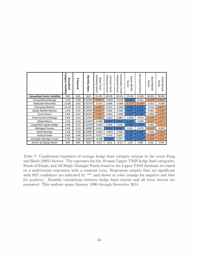
An

nu

alize

d

Ca

teg

ory

Vo

latility

R S

qu

are

d

Mo

nth

ly A

lph

a

Bo

nd

Tre

nd

Fo

llow

ing

Fa

ctor

Cu

rren

cy Tre

nd

Fo

llow

ing

Fa

ctor

Co

mm

od

ity Tre

nd

Fo

llow

ing

Fa

ctor

Eq

uity M

ark

et

Fa

ctor

Size

Sp

rea

d F

acto

r

Bo

nd

Ma

rke

t

Fa

ctor

Cre

dit S

pre

ad

Fa

ctor

Annualized Factor Volatility N/A N/A N/A 51.4% 63.4% 50.1% 15.4% 11.8% 92.6% 76.9%

Convertible Arbitrage 7.3% 0.58 0.332%* -0.014* -0.003 -0.010 0.114* 0.055 -0.020* -0.061*

Dedicated Short Bias 15.6% 0.62 0.557%* -0.022 0.000 -0.006 -0.722* -0.410* -0.013 -0.009

Emerging Markets 14.2% 0.52 0.181% -0.041* 0.015 -0.006 0.468* 0.210* -0.010 -0.047*

Equity Market Neutral 3.3% 0.24 0.333%* -0.012* 0.002 -0.002 0.037* 0.054* -0.001 -0.010*

Event Driven 5.9% 0.67 0.391%* -0.020* 0.003 -0.008 0.167* 0.120* -0.004 -0.029*

Fixed Income Arbitrage 4.4% 0.43 0.374%* -0.010* -0.007 0.000 0.009 0.019 -0.018* -0.039*

Global Macro 5.2% 0.24 0.310%* -0.008 0.024* 0.015* 0.100* 0.009 -0.015* -0.017*

Long/Short Equity Hedge 9.0% 0.72 0.322%* -0.003 0.009 0.003 0.388* 0.300* -0.002 -0.014*

Managed Futures 9.4% 0.23 0.389%* 0.016 0.033* 0.048* 0.051 0.070 -0.019* -0.003

Multi-Strategy 5.2% 0.43 0.339%* -0.003 -0.003 0.006 0.156* 0.100* -0.006 -0.016*

Fund of Funds 6.0% 0.46 0.147% -0.011 0.010 0.007 0.185* 0.113* -0.008* -0.022*

All Single Manager Funds 6.3% 0.66 0.304%* -0.008 0.010* 0.007 0.246* 0.161* -0.008* -0.022*

Correl. w/ Equity Factor N/A N/A N/A -0.23 -0.21 -0.17 1.00 0.08 0.22 -0.44

Table 7: Conditional exposures of average hedge fund category returns to the seven Fungand Hsieh (2001) factors. The exposures for the 10 main Lipper TASS hedge fund categories,Funds of Funds, and All Single Manager Funds found in the Lipper TASS database are basedon a multivariate regression with a constant term. Regression outputs that are significantwith 95% confidence are indicated by “*” and shown in color (orange for negative and bluefor positive). Monthly correlations between hedge fund returns and all seven factors arepresented. This analysis spans January 1996 through December 2014.

44

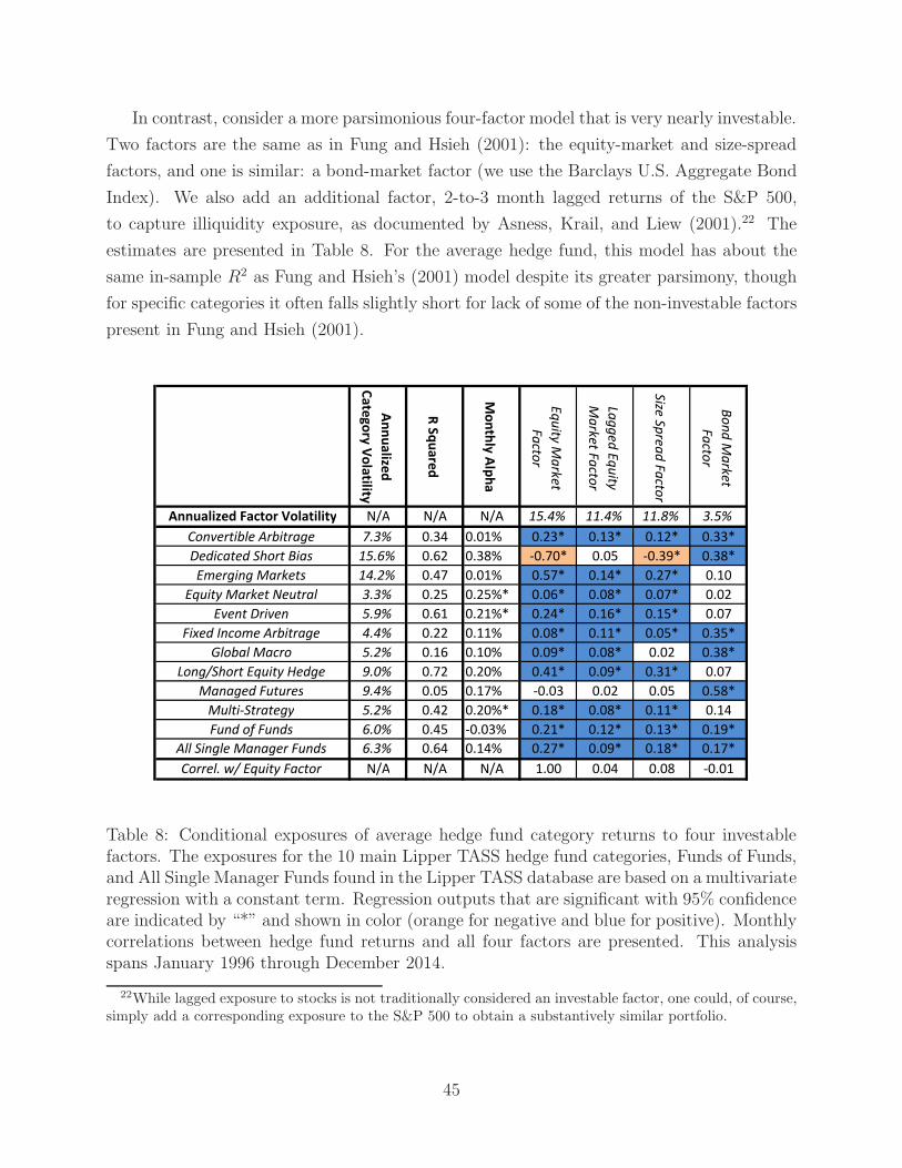
In contrast, consider a more parsimonious four-factor model that is very nearly investable.

Two factors are the same as in Fung and Hsieh (2001): the equity-market and size-spread

factors, and one is similar: a bond-market factor (we use the Barclays U.S. Aggregate Bond

Index). We also add an additional factor, 2-to-3 month lagged returns of the S&P 500,

to capture illiquidity exposure, as documented by Asness, Krail, and Liew (2001).22 The

estimates are presented in Table 8. For the average hedge fund, this model has about the

same in-sample R2 as Fung and Hsieh’s (2001) model despite its greater parsimony, though

for specific categories it often falls slightly short for lack of some of the non-investable factors

present in Fung and Hsieh (2001).

An

nu

alize

d

Ca

teg

ory

Vo

latility

R S

qu

are

d

Mo

nth

ly A

lph

a

Eq

uity M

ark

et

Fa

ctor

Lag

ge

d E

qu

ity

Ma

rke

t Fa

ctor

Size

Sp

rea

d F

acto

r

Bo

nd

Ma

rke

t

Fa

ctor

Annualized Factor Volatility N/A N/A N/A 15.4% 11.4% 11.8% 3.5%

Convertible Arbitrage 7.3% 0.34 0.01% 0.23* 0.13* 0.12* 0.33*

Dedicated Short Bias 15.6% 0.62 0.38% -0.70* 0.05 -0.39* 0.38*

Emerging Markets 14.2% 0.47 0.01% 0.57* 0.14* 0.27* 0.10

Equity Market Neutral 3.3% 0.25 0.25%* 0.06* 0.08* 0.07* 0.02

Event Driven 5.9% 0.61 0.21%* 0.24* 0.16* 0.15* 0.07

Fixed Income Arbitrage 4.4% 0.22 0.11% 0.08* 0.11* 0.05* 0.35*

Global Macro 5.2% 0.16 0.10% 0.09* 0.08* 0.02 0.38*

Long/Short Equity Hedge 9.0% 0.72 0.20% 0.41* 0.09* 0.31* 0.07

Managed Futures 9.4% 0.05 0.17% -0.03 0.02 0.05 0.58*

Multi-Strategy 5.2% 0.42 0.20%* 0.18* 0.08* 0.11* 0.14

Fund of Funds 6.0% 0.45 -0.03% 0.21* 0.12* 0.13* 0.19*

All Single Manager Funds 6.3% 0.64 0.14% 0.27* 0.09* 0.18* 0.17*

Correl. w/ Equity Factor N/A N/A N/A 1.00 0.04 0.08 -0.01

Table 8: Conditional exposures of average hedge fund category returns to four investablefactors. The exposures for the 10 main Lipper TASS hedge fund categories, Funds of Funds,and All Single Manager Funds found in the Lipper TASS database are based on a multivariateregression with a constant term. Regression outputs that are significant with 95% confidenceare indicated by “*” and shown in color (orange for negative and blue for positive). Monthlycorrelations between hedge fund returns and all four factors are presented. This analysisspans January 1996 through December 2014.

22While lagged exposure to stocks is not traditionally considered an investable factor, one could, of course,simply add a corresponding exposure to the S&P 500 to obtain a substantively similar portfolio.

45

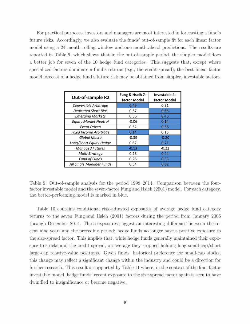
For practical purposes, investors and managers are most interested in forecasting a fund’s

future risks. Accordingly, we also evaluate the funds’ out-of-sample fit for each linear factor

model using a 24-month rolling window and one-month-ahead predictions. The results are

reported in Table 9, which shows that in the out-of-sample period, the simpler model does

a better job for seven of the 10 hedge fund categories. This suggests that, except where

specialized factors dominate a fund’s returns (e.g., the credit spread), the best linear factor

model forecast of a hedge fund’s future risk may be obtained from simpler, investable factors.

Out-of-sample R2Fung & Hseih 7-

factor Model

Investable 4-

factor Model

Convertible Arbitrage 0.49 0.31

Dedicated Short Bias 0.57 0.66

Emerging Markets 0.36 0.45

Equity Market Neutral -0.06 0.14

Event Driven 0.52 0.56

Fixed Income Arbitrage 0.14 0.13

Global Macro -0.39 -0.20

Long/Short Equity Hedge 0.62 0.71

Managed Futures -0.13 -0.22

Multi-Strategy 0.28 0.44

Fund of Funds 0.26 0.33

All Single Manager Funds 0.54 0.62

Table 9: Out-of-sample analysis for the period 1998–2014. Comparison between the four-factor investable model and the seven-factor Fung and Hsieh (2001) model. For each category,the better-performing model is marked in blue.

Table 10 contains conditional risk-adjusted exposures of average hedge fund category

returns to the seven Fung and Hsieh (2001) factors during the period from January 2006

through December 2014. These exposures suggest an interesting difference between the re-

cent nine years and the preceding period: hedge funds no longer have a positive exposure to

the size-spread factor. This implies that, while hedge funds generally maintained their expo-

sure to stocks and the credit spread, on average they stopped holding long small-cap/short

large-cap relative-value positions. Given funds’ historical preference for small-cap stocks,

this change may reflect a significant change within the industry and could be a direction for

further research. This result is supported by Table 11 where, in the context of the four-factor

investable model, hedge funds’ recent exposure to the size-spread factor again is seen to have

dwindled to insignificance or become negative.

46

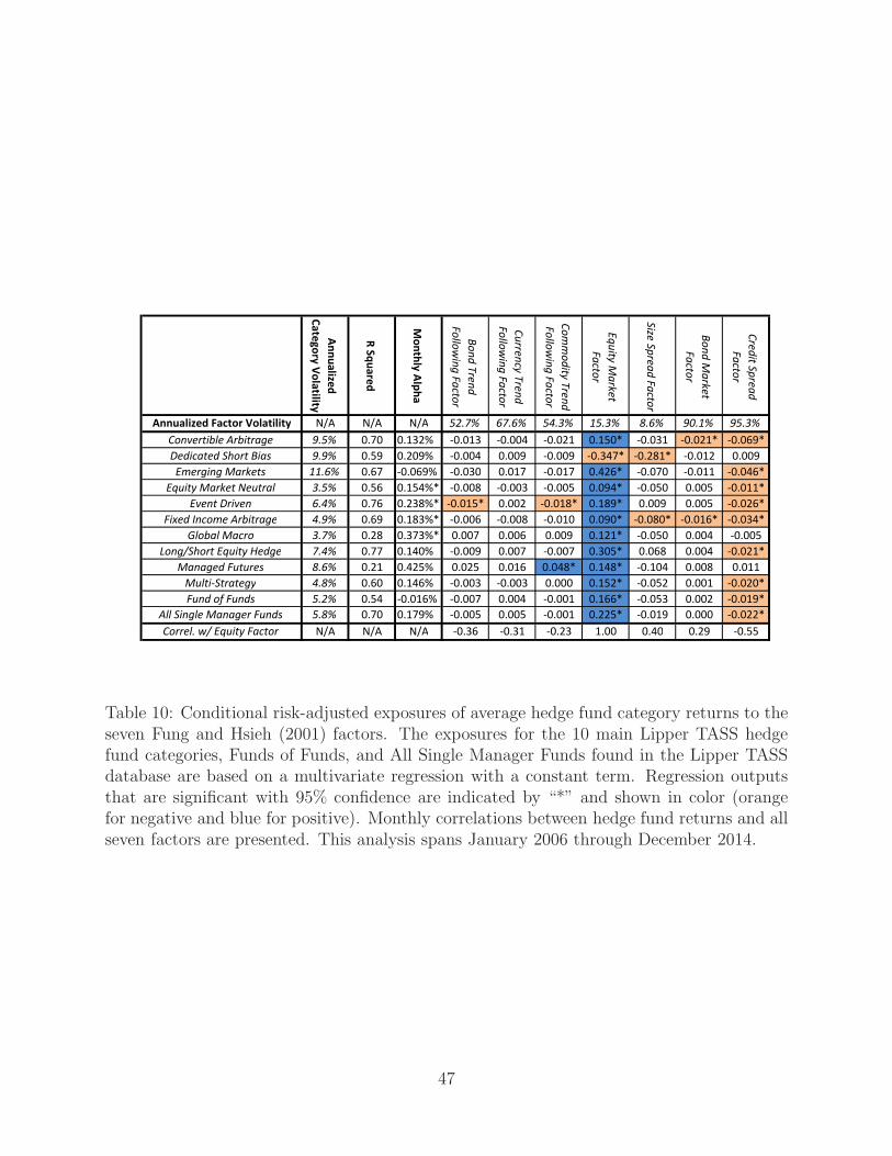
An

nu

alize

d

Ca

teg

ory

Vo

latility

R S

qu

are

d

Mo

nth

ly A

lph

a

Bo

nd

Tre

nd

Fo

llow

ing

Fa

ctor

Cu

rren

cy Tre

nd

Fo

llow

ing

Fa

ctor

Co

mm

od

ity Tre

nd

Fo

llow

ing

Fa

ctor

Eq

uity M

ark

et

Fa

ctor

Size

Sp

rea

d F

acto

r

Bo

nd

Ma

rke

t

Fa

ctor

Cre

dit S

pre

ad

Fa

ctor

Annualized Factor Volatility N/A N/A N/A 52.7% 67.6% 54.3% 15.3% 8.6% 90.1% 95.3%

Convertible Arbitrage 9.5% 0.70 0.132% -0.013 -0.004 -0.021 0.150* -0.031 -0.021* -0.069*

Dedicated Short Bias 9.9% 0.59 0.209% -0.004 0.009 -0.009 -0.347* -0.281* -0.012 0.009

Emerging Markets 11.6% 0.67 -0.069% -0.030 0.017 -0.017 0.426* -0.070 -0.011 -0.046*

Equity Market Neutral 3.5% 0.56 0.154%* -0.008 -0.003 -0.005 0.094* -0.050 0.005 -0.011*

Event Driven 6.4% 0.76 0.238%* -0.015* 0.002 -0.018* 0.189* 0.009 0.005 -0.026*

Fixed Income Arbitrage 4.9% 0.69 0.183%* -0.006 -0.008 -0.010 0.090* -0.080* -0.016* -0.034*

Global Macro 3.7% 0.28 0.373%* 0.007 0.006 0.009 0.121* -0.050 0.004 -0.005

Long/Short Equity Hedge 7.4% 0.77 0.140% -0.009 0.007 -0.007 0.305* 0.068 0.004 -0.021*

Managed Futures 8.6% 0.21 0.425% 0.025 0.016 0.048* 0.148* -0.104 0.008 0.011

Multi-Strategy 4.8% 0.60 0.146% -0.003 -0.003 0.000 0.152* -0.052 0.001 -0.020*

Fund of Funds 5.2% 0.54 -0.016% -0.007 0.004 -0.001 0.166* -0.053 0.002 -0.019*

All Single Manager Funds 5.8% 0.70 0.179% -0.005 0.005 -0.001 0.225* -0.019 0.000 -0.022*

Correl. w/ Equity Factor N/A N/A N/A -0.36 -0.31 -0.23 1.00 0.40 0.29 -0.55

Table 10: Conditional risk-adjusted exposures of average hedge fund category returns to theseven Fung and Hsieh (2001) factors. The exposures for the 10 main Lipper TASS hedgefund categories, Funds of Funds, and All Single Manager Funds found in the Lipper TASSdatabase are based on a multivariate regression with a constant term. Regression outputsthat are significant with 95% confidence are indicated by “*” and shown in color (orangefor negative and blue for positive). Monthly correlations between hedge fund returns and allseven factors are presented. This analysis spans January 2006 through December 2014.

47

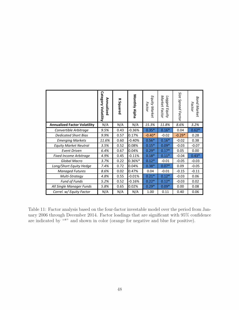
An

nu

alize

d

Ca

teg

ory

Vo

latility

R S

qu

are

d

Mo

nth

ly A

lph

a

Eq

uity M

ark

et

Fa

ctor

Lag

ge

d E

qu

ity

Ma

rke

t Fa

ctor

Size

Sp

rea

d F

acto

r

Bo

nd

Ma

rke

t

Fa

ctor

Annualized Factor Volatility N/A N/A N/A 15.3% 11.8% 8.6% 3.2%

Convertible Arbitrage 9.5% 0.43 -0.36% 0.35* 0.16* 0.04 0.62*

Dedicated Short Bias 9.9% 0.57 0.17% -0.40* -0.02 -0.29* 0.28

Emerging Markets 11.6% 0.60 -0.40% 0.56* 0.16* -0.02 0.38

Equity Market Neutral 3.5% 0.52 0.08% 0.15* 0.09* -0.03 -0.07

Event Driven 6.4% 0.67 0.04% 0.29* 0.17* 0.05 0.00

Fixed Income Arbitrage 4.9% 0.45 -0.11% 0.18* 0.11* -0.04 0.43*

Global Macro 3.7% 0.22 0.36%* 0.12* -0.01 -0.05 -0.03

Long/Short Equity Hedge 7.4% 0.72 0.04% 0.38* 0.07* 0.09 -0.05

Managed Futures 8.6% 0.02 0.47% 0.04 -0.01 -0.15 -0.11

Multi-Strategy 4.8% 0.55 -0.01% 0.21* 0.12* -0.03 0.06

Fund of Funds 5.2% 0.52 -0.16% 0.22* 0.12* -0.03 0.02

All Single Manager Funds 5.8% 0.65 0.02% 0.29* 0.09* 0.00 0.08

Correl. w/ Equity Factor N/A N/A N/A 1.00 0.11 0.40 0.06

Table 11: Factor analysis based on the four-factor investable model over the period from Jan-uary 2006 through December 2014. Factor loadings that are significant with 95% confidenceare indicated by “*” and shown in color (orange for negative and blue for positive).

48

6.3 Limitations of Hedge-Fund Factor Models

As useful as linear factor models are for capturing the risks and rewards of hedge-fund

returns, these models have their limitations and there are reasons to be cautious in their use:

(i) Correlation vs. causation: The fact that a combination of well-understood factors

may have similar patterns of gains and losses to a given hedge fund does not necessarily

mean that the hedge fund’s strategy is based on those factors. Correlation need not

imply causation, but could be the result of chance, overfitting, or some common latent

factor.

(ii) Approximate fit: A factor model usually explains only part of the hedge funds’

returns, and even that part is typically overfit because of a mismatch between the

explanatory factors and the true contents of the hedge fund portfolio.

(iii) Nonstationarity: Even if a factor model accurately explains a fund’s returns, the

risks associated with every hedge fund change over time, albeit often slowly. So a

factor model rarely predicts the future as well as it explains the past.

(iv) Non-investability: In general, a researcher cannot consider the returns of every

combination of well-understood factors to be an alternative to investing in the indicated

hedge fund, as the factors may not be investable. A combination of factors might not

be investable for many reasons. For example, one cannot invest $1 billion in the

Case-Shiller Atlanta housing index, even though using the index in a factor model

might provide insight into the intrinsic properties of the hedge fund’s portfolio. Even

simple factors like stock market indexes are not entirely investable (though they are

very nearly so) because accessing them incurs commissions, management fees, and/or

tracking error.

Several of these weaknesses are manifest in the following example, which involves two

categories of hedge funds that focus on relative value bets, often using illiquid fixed income

instruments: Fixed Income Arbitrage and Convertible Arbitrage. With a 12-month window,

we use a univariate factor model to estimate the exposure of each category to the S&P 500

index (see Figure 4). At first this is low, as one would expect in strategies like these. But

in the Fall of 2008, the estimated sensitivity of these funds’ returns to those of the S&P 500

spikes dramatically. A naıve interpretation of the results might be that the average fund

manager in both of these categories decided to buy a large quantity of equities. But it seems

unlikely that so many managers of low-volatility relative-value strategies would suddenly

49

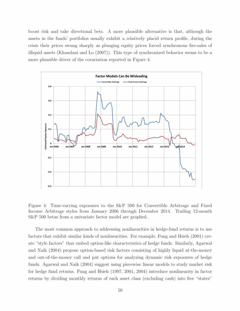
boost risk and take directional bets. A more plausible alternative is that, although the

assets in the funds’ portfolios usually exhibit a relatively placid return profile, during the

crisis their prices swung sharply as plunging equity prices forced synchronous fire-sales of

illiquid assets (Khandani and Lo (2007)). This type of synchronized behavior seems to be a

more plausible driver of the covariation reported in Figure 4.

0.8

Factor Models Can Be Misleading

Convertible Arbitrage Fixed Income Arbitrage

0.6

0.4

0.2

Est

ima

ted

Eq

uit

y E

xp

osu

re

0

Jan 2006 Jan 2007 Jan 2008 Jan 2009 Jan 2010 Jan 2011 Jan 2012 Jan 2013 Jan 2014

Est

ima

ted

Eq

uit

y E

xp

osu

re

-0.4

-0.2

-0.6

-0.4

Figure 4: Time-varying exposures to the S&P 500 for Convertible Arbitrage and FixedIncome Arbitrage styles from January 2006 through December 2014. Trailing 12-monthS&P 500 betas from a univariate factor model are graphed.

The most common approach to addressing nonlinearities in hedge-fund returns is to use

factors that exhibit similar kinds of nonlinearities. For example, Fung and Hsieh (2001) cre-

ate “style factors” that embed option-like characteristics of hedge funds. Similarly, Agarwal

and Naik (2004) propose option-based risk factors consisting of highly liquid at-the-money

and out-of-the-money call and put options for analyzing dynamic risk exposures of hedge

funds. Agarwal and Naik (2004) suggest using piecewise linear models to study market risk

for hedge fund returns. Fung and Hsieh (1997, 2001, 2004) introduce nonlinearity in factor

returns by dividing monthly returns of each asset class (excluding cash) into five “states”

50

to capture trading dynamics of hedge-fund styles. Billio, Getmansky, and Pelizzon (2012)

propose a regime-switching beta model to measure dynamic risk exposures of hedge funds

to various risk factors during different market volatility conditions. Bondarenko (2004) and

Buraschi, Kosowski and Trojani (2015) introduce and analyze variance and correlation risk

factors for hedge funds. Roncalli and Weisang (2010) apply advanced Bayesian filters’ algo-

rithms, known as particle filters, to capture nonlinearities documented in hedge fund returns

(see Section 6.6 for a more detailed discussion in the context of hedge-fund beta replication).

And Patton and Ramadorai (2013) introduce a new econometric methodology to capture

nonlinearities and time-series variation in hedge funds’ exposures to risk factors using high-

frequency data, and find that these exposures vary significantly across months. Diez de los

Rios and Garcia (2011) show that nonlinearities are important for some strategies, but not

for the entire hedge-fund industry. Cai and Liang (2012a,b) use rolling-window OLS and

Kalman filtering/smoothing to study non-linearities in hedge fund returns.

6.4 Operational Risks

Due to the complexities of proprietary trading, the lack of transparency, and the lack of

regulatory oversight, hedge funds are especially exposed to operational risk, defined by the

Basel Committee on Banking Supervision as “the risk of loss resulting from inadequate or

failed internal processes, people and systems, or from external events”. Feffer and Kundro

(2003) were perhaps the first to call attention to this important source of risk, noting that half

of all hedge-fund failures can be attributed to operational risk alone. They observe that “the

most common operational issues related to hedge fund losses have been misrepresentation of

fund investments, misappropriation of investor funds, unauthorized trading, and inadequate

resources” (Feffer and Kundro, 2003, p. 5). They report that only 6% of their sample

involved inadequate resources, whereas 41% involved misrepresentation of investments, 30%

involved misappropriation of funds, and 14% involved unauthorized trading.

Since then, a number of studies have focused on operational risk. For example, Gupta

and Kazemi (2007) study the failure of the $9 billion hedge fund Amaranth Advisors and

conclude that operational issues were a key factor in this fund’s demise. In a series of

papers, Brown, Goetzmann, Liang, and Schwarz (2008, 2009, and 2012) develop several

quantitative models for measuring operational risk in managed funds. Using a complete and

unique SEC ADV filing dataset, they find that operational risk (represented by past legal or

regulatory problems) is significantly related to the use of leverage, fund ownership structure,

and conflict-of-interest issues. Higher operational risk funds tend to have relatively low

leverage because of strict scrutiny from lenders, more concentrated ownership, and severe

51

conflict-of-interest problems. Through a canonical correlation analysis, they map the ADV

information to the regular fund information such as assets, returns, volatility, fees, leverage,

and share restrictions, which, in turn, they use to construct an omega-score model to predict

future fund performance and attrition. Consistent with the Basel definition, they find that

the higher the omega score, the lower the future performance and the higher the probability

of attrition.

Brown, Goetzmann, Liang, and Schwarz (2012) use finer information on the individual

funds to quantify operational risk. Based on 444 proprietary due diligence reports, they are

able to show that operational risk is directly related to inadequate or failed internal processes,

represented by internal pricing of the portfolio, lack of reliability on reputable auditors and

institutional quality signatures, and frequent misrepresentation of past problems or fund

characteristics. The quantitative model based on these variables sharply predicts future fund

performance and fund disappearance. However, the risk-flow analysis indicates that investors

either ignore the operational risk issues or are ignorant of them, which further validates the

importance of mandatory disclosure of fund information and information verification.

They also find that hedge funds that have experienced legal problems are less likely to use

independent pricing agents and are more likely to have switched pricing agents within the

past year, allowing these hedge funds greater pricing discretion. This discretion is a potential

concern because, as Cassar and Gerakos (2011) show, hedge funds with less verifiable pricing

sources and greater pricing discretion for their managers report smoother returns, resulting

in misleading volatility and Sharpe ratio estimates (see Section 5.1). Bollen and Pool (2012)

link the incidence of SEC lawsuits to suspicious patterns in reported returns, and find that

the discontinuity in a fund’s return distribution (some funds push returns above zero) is a

reliable predictor of subsequent charges of misreporting brought by the SEC.

Ozik and Sadka (2014) argue that hedge funds offer informational advantages to managers

over their clients through fund flows. They demonstrate that fund flows predict returns and

find evidence that managers front-run their clients using this information.

On a more positive note, Brown, Fraser, and Liang (2008) argue that due diligence is an

important source of alpha for diversified hedge fund portfolios. Effective due diligence can

eliminate or reduce problematic funds and avoid future losses resulting from operational risk.

However, due diligence is an expensive process; there is a significant competitive advantage

to sufficiently large funds of funds, which are able to absorb this fixed and necessary cost. In

contrast to hedge funds, the authors find significant economies of scale for funds of funds—the

larger the fund of funds, the better its performance.

52

6.5 Risk Management

The previous sections’ discussions highlight the fact that hedge funds have more complex and

dynamic risk exposures than traditional investments. Therefore, proper risk management

protocols are essential from both investors’ and managers’ perspectives. The old adage “a

good way to make money is not to lose it in the first place” is particularly relevant for hedge

funds given the active bets they make and the critical role that risk management plays in

generating their returns. Moreover, with reliable estimates of risk exposures from a linear

factor model, it is possible for investors to hedge certain risks that they wish to reduce, and

accentuate other risks that they are especially keen to take on.

This is the motivation for Healy and Lo’s (2009) proposal for hedge-fund investors to

use an overlay strategy consisting of futures contracts on major asset-class indexes such as

stocks, bonds, interest rates, currencies, and commodities so as to actively manage the factor

exposures of their hedge-fund investments (in the interest of full disclosure, two authors of

this survey—P. Lee and A. Lo—have commercial interests in an asset management company

engaged in these overlay strategies). By using these “beta-blockers” in concert with properly

estimated linear factor models, Healy and Lo (2009) argue that investors can reduce or

eliminate exposures that they do not wish to have, while increasing exposures they feel

are more rewarding, and this can be accomplished in a cost-effective manner thanks to

the liquidity and capital efficiency of futures contracts and markets. Black (2006) finds

that adding a small VIX position to an investment portfolio significantly reduces portfolio

volatility due to the negative correlation of VIX to the S&P 500 and most hedge-fund

styles. Even in cases where certain risks simply cannot be managed due to the nature of the

investment, e.g., illiquidity risk in a real estate portfolio, a clear understanding of the risks

will at least allow those exposed to them to prepare accordingly.

Beyond these overlay strategies, risk management is, of course, a well developed discipline

with a broad and deep literature that goes well beyond hedge funds and is impossible to

summarize in a single article, much less a section. However, Lo (2001) focuses on at least

three unique aspects of hedge-fund risk management that are worth reviewing here. The

first is the nonlinear nature of hedge-fund risk exposures, a feature that is not captured by

linear factor models unless specific accommodations are made in defining the factors. A case

in point is the relation between the trend-following strategies of CTAs and the S&P 500

index. A regression of the monthly returns of the CS/DJ Managed Futures Index on those

of the S&P 500 Total Return Index from January 1994 through December 2014 yields the

53

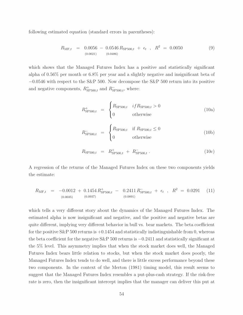
following estimated equation (standard errors in parentheses):

RMF,t = 0.0056(0.0021)

− 0.0546(0.0486)

RSP500,t + ǫt , R2 = 0.0050 (9)

which shows that the Managed Futures Index has a positive and statistically significant

alpha of 0.56% per month or 6.8% per year and a slightly negative and insignificant beta of

−0.0546 with respect to the S&P 500. Now decompose the S&P 500 return into its positive

and negative components, R+SP500,t and R−

SP500,t, where:

R+SP500,t =

RSP500,t ifRSP500,t > 0

0 otherwise(10a)

R−

SP500,t =

RSP500,t if RSP500,t ≤ 0

0 otherwise(10b)

RSP500,t = R+SP500,t + R−

SP500,t . (10c)

A regression of the returns of the Managed Futures Index on these two components yields

the estimate:

RMF,t = −0.0012

(0.0035)

+ 0.1454(0.0937)

R+SP500,t − 0.2411

(0.0891)

R−

SP500,t + ǫt , R2 = 0.0291 (11)

which tells a very different story about the dynamics of the Managed Futures Index. The

estimated alpha is now insignificant and negative, and the positive and negative betas are

quite different, implying very different behavior in bull vs. bear markets. The beta coefficient

for the positive S&P 500 returns is +0.1454 and statistically indistinguishable from 0, whereas

the beta coefficient for the negative S&P 500 returns is−0.2411 and statistically significant at

the 5% level. This asymmetry implies that when the stock market does well, the Managed

Futures Index bears little relation to stocks, but when the stock market does poorly, the

Managed Futures Index tends to do well, and there is little excess performance beyond these

two components. In the context of the Merton (1981) timing model, this result seems to

suggest that the Managed Futures Index resembles a put-plus-cash strategy. If the risk-free

rate is zero, then the insignificant intercept implies that the manager can deliver this put at

54

zero cost to investors.

Experienced investors in managed futures funds are familiar with this countercyclical pat-

tern of trend-followers, which Kaminski (2011) describes as “crisis alpha”. However, during

extended periods of positive equity-market performance, trend-followers may underperform

relative to their long-term average. For example, in 2012 the compound annual return of the

S&P 500 was 16.0% whereas the return of the Managed Futures Index was −2.9%. These pe-

riods of underperformance can cause inexperienced investors to panic and liquidate, largely

eliminating the diversification benefits of such countercyclical investments.

The second unique aspect of hedge-fund returns is tail risk. A classic example is liquidity

provision among strategies that sell more liquid assets and buy less liquid assets of similar

payoffs, a common feature of fixed-income arbitrage funds. Such strategies generate positive

cashflows most of the time since liquid assets are priced higher than their less liquid coun-

terparts, e.g., on-the-run vs. off-the-run U.S. Treasury securities with identical coupons, call

provisions, and other terms. During normal market conditions, these strategies yield very

steady returns—implying high Sharpe ratios—but during periods of market distress, they

can suffer tremendous losses in the face of “flights to safety”. This pattern of mostly positive

small returns punctuated by the occasional large loss characterizes a number of hedge-fund

strategies besides fixed-income arbitrage including equity market neutral strategies, convert-

ible bond arbitrage, high-frequency trading, and catastrophe reinsurance.

Seasoned hedge-fund investors are fully aware of this pattern and are able to withstand

periodic losses so as to capture the full benefits of these strategies. However, less experienced

investors may not be as well prepared, and if they respond by reducing or liquidating their

investments during periods of market distress, they will compound their losses and fail to

profit from the risk premia associated with tail risk exposures.

But perhaps the biggest concern with respect to such strategies is that standard risk

measures will not fully reflect their risks. Lo (2001) provides a simple illustration of a

hypothetical hedge-fund strategy consisting of selling out-of-the-money put options on the

S&P 500 index, which generates a very attractive risk/reward profile as long as the stock

market does not decline by more than the amount that the put option is out of the money.

Sharpe ratios do not reflect tail risk unless a significant loss has occurred within a given fund’s

track record, and when it has, the Sharpe ratio is likely to be misleadingly conservative.

This leads to the third unique aspect of hedge-fund returns which is their tendency

to become highly correlated during times of market distress. To develop intuition for this

aspect, consider the heat map of the empirical distribution of trailing 12-month returns of all

single-manager hedge funds in the Lipper TASS database from 1997 through 2014 in Figure

5. The downward plume of density during the Financial Crisis of 2007–2009 comes in stark

55

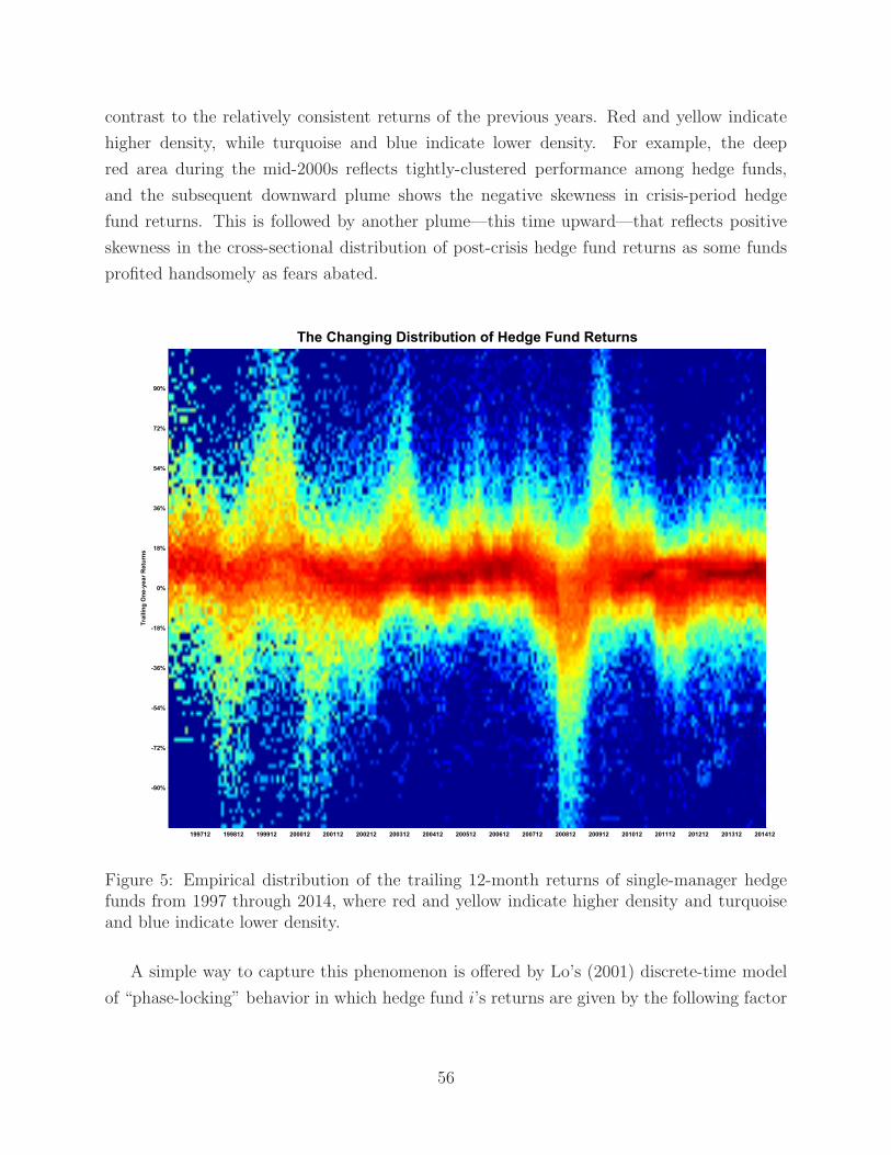
contrast to the relatively consistent returns of the previous years. Red and yellow indicate

higher density, while turquoise and blue indicate lower density. For example, the deep

red area during the mid-2000s reflects tightly-clustered performance among hedge funds,

and the subsequent downward plume shows the negative skewness in crisis-period hedge

fund returns. This is followed by another plume—this time upward—that reflects positive

skewness in the cross-sectional distribution of post-crisis hedge fund returns as some funds

profited handsomely as fears abated.

199712 199812 199912 200012 200112 200212 200312 200412 200512 200612 200712 200812 200912 201012 201112 201212 201312 201412

-90%

-72%

-54%

-36%

-18%

0%

18%

36%

54%

72%

90%

Tra

ilin

g O

ne

-ye

ar

Re

turn

s

The Changing Distribution of Hedge Fund Returns

Figure 5: Empirical distribution of the trailing 12-month returns of single-manager hedgefunds from 1997 through 2014, where red and yellow indicate higher density and turquoiseand blue indicate lower density.

A simple way to capture this phenomenon is offered by Lo’s (2001) discrete-time model

of “phase-locking” behavior in which hedge fund i’s returns are given by the following factor

56

model:

Rit = αi + βiΛt + ItZt + ǫit (12)

where Λt, It, Zt, and ǫit are mutually IID with the following moments:

E[Λt] = µλ , Var[Λt] = σ2λ

E[Zt] = 0 , Var[Zt] = σ2z

E[ǫit] = 0 , Var[ǫit] = σ2ǫi

(13)

and the phase-locking event indicator It is defined as:

It =

1 with probability p

0 with probability p0 = 1− p. (14)

According to (12), expected returns are driven by three components: the fund’s alpha, αi,

a “market” component, Λt, to which each fund has its own individual sensitivity, βi, and a

phase-locking component that is identical across all funds at all times, taking only one of

two possible values: 0 (with probability p) or Zt (with probability 1−p).

If we assume that p is small, say 0.001, then most of the time the expected returns of

fund i are determined by αi+βiΛt, but every once in a while an additional term, Zt, appears.

If the volatility, σz, of Zt is much larger than the volatilities of the market factor, Λt, and

the idiosyncratic risk, ǫit, then the common factor, Zt, will dominate the expected returns

of all stocks when It=1, i.e., phase-locking behavior is present.

Now consider the conditional correlation coefficient of two funds, i and j, defined as

the ratio of the conditional covariance divided by the square root of the product of the

conditional variances, conditioned on It=0:

Corr[Rit, Rjt | It = 0] =βiβjσ

2λ

√

β2i σ

2λ + σ2

ǫi

√

β2jσ

2λ + σ2

ǫj

≈ 0 for βi ≈ βj ≈ 0 (15a)

where we have assumed that βi ≈ βj ≈ 0 to capture the market-neutral characteristic that

many hedge-fund investors desire. Now consider the conditional correlation, conditioned on

57

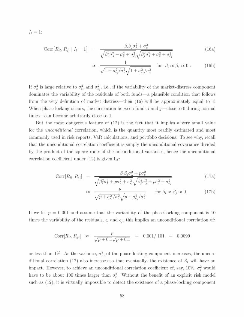
It = 1:

Corr[

Rit, Rjt | It = 1]

=βiβjσ

2λ + σ2

z√

β2i σ

2λ + σ2

z + σ2ǫi

√

β2jσ

2λ + σ2

z + σ2ǫj

(16a)

≈ 1√

1 + σ2ǫi/σ2

z

√

1 + σ2ǫj/σ2

z

for βi ≈ βj ≈ 0 . (16b)

If σ2z is large relative to σ2

ǫiand σ2

ǫj, i.e., if the variability of the market-distress component

dominates the variability of the residuals of both funds—a plausible condition that follows

from the very definition of market distress—then (16) will be approximately equal to 1!

When phase-locking occurs, the correlation between funds i and j—close to 0 during normal

times—can become arbitrarily close to 1.

But the most dangerous feature of (12) is the fact that it implies a very small value

for the unconditional correlation, which is the quantity most readily estimated and most

commonly used in risk reports, VaR calculations, and portfolio decisions. To see why, recall

that the unconditional correlation coefficient is simply the unconditional covariance divided

by the product of the square roots of the unconditional variances, hence the unconditional

correlation coefficient under (12) is given by:

Corr[Rit, Rjt] =βiβjσ

2λ + pσ2

z√

β2i σ

2λ + pσ2

z + σ2ǫi

√

β2jσ

2λ + pσ2

z + σ2ǫj

(17a)

≈ p√

p+ σ2ǫi/σ2

z

√

p+ σ2ǫj/σ2

z

for βi ≈ βj ≈ 0 . (17b)

If we let p = 0.001 and assume that the variability of the phase-locking component is 10

times the variability of the residuals, ǫi and ǫj , this implies an unconditional correlation of:

Corr[Rit, Rjt] ≈ p√p+ 0.1

√p+ 0.1

= 0.001/.101 = 0.0099

or less than 1%. As the variance, σ2z , of the phase-locking component increases, the uncon-

ditional correlation (17) also increases so that eventually, the existence of Zt will have an

impact. However, to achieve an unconditional correlation coefficient of, say, 10%, σ2z would

have to be about 100 times larger than σ2ǫ . Without the benefit of an explicit risk model

such as (12), it is virtually impossible to detect the existence of a phase-locking component

58

from standard correlation coefficients.

These considerations suggest that risk management for hedge funds cannot be approached

in the same manner as for traditional investments. Measuring and managing the risk expo-

sures of hedge funds require not only more sophisticated risk analytics, but also a deeper

understanding of the nature of the strategies being managed.

6.6 Hedge-Fund Beta Replication

Our discussion of factor modeling suggests that a portion of hedge funds’ returns may be

attributable to simple investments that do not require hedge funds’ high fees or expensive

trading infrastructure. In recent years the insights of a handful of researchers encouraged

asset managers to develop strategies that generate the “simple” portion of funds’ returns

while charging low fees and providing greater transparency and liquidity. Today billions of

dollars are managed in these strategies. In the interest of full disclosure, two of the authors

of this article—P. Lee and A. Lo—are affiliated with an asset management company offering

a hedge-fund beta replication mutual fund. While every effort has been undertaken to avoid

bias, readers should be aware of this potential conflict of interest and interpret the discussion

in this section accordingly.

Current replication methods fall into three categories: linear factor model replication,

replication of strategies, and replication of payoff functions or return distributions. In the

linear factor model approach, a linear factor model with investable factors is used to construct

a portfolio with the same betas—and corresponding risk premia—of the aggregate hedge-

fund industry or sector being replicated. Successful linear factor model replication depends

on the explanatory power of the factors and the timeliness of the beta estimates. In the

strategy replication approach, a manager employs a rules-based strategy that aims to make

the same sort of trades that a hedge fund would make and thereby generate similar returns.

One challenge this approach faces is that a fund that trades in a manner similar to a hedge

fund may effectively become a hedge fund itself, and not a replicator at all. Finally, the

distributional approach aims to replicate characteristics of the probability distribution of

hedge-fund returns. The challenge with this approach is that matching payoff distributions

can sometimes be more complex and costly than implementing the hedge-fund strategy itself.

Given the many linear factor models that have been estimated with hedge fund returns

(see Section 6.2), a natural starting point for hedge-fund beta replication is to use these

models to construct portfolios with alternative beta exposures. This is the approach proposed

by Hasanhodzic and Lo (2006, 2007), who constructed “linear clones” of individual hedge

funds in the Lipper TASS hedge fund database using six factors: the U.S. Dollar Index return,

59

the return on the Lehman Corporate AA intermediate Bond Index, the spread between the

Lehman BAA Corporate Bond Index and the Lehman Treasury Index, the S&P 500 total

returns, the Goldman Sachs Commodity Index total return, and the first-difference of the

end-of-month value of the VIX.

Based on these findings, they proposed using liquid futures contracts to construct repli-

cation portfolios. This proposal was subsequently implemented by the investment advisory

firm AlphaSimplex Group, LLC in 2008 using just over two dozen futures contracts; the

resulting strategy is currently the largest hedge-fund beta replication mutual fund (see Lee

and Lo (2014) for further discussion). However, Goldman Sachs was the first to market with

a hedge-fund beta replication mutual fund designed to track the Goldman Sachs Absolute

Return Tracker Index. Other large banks and some asset managers have followed suit with

their own versions of hedge-fund beta replication indexes or funds, including Barclays, Credit

Suisse, Deutsche Bank, Index IQ, Merrill Lynch, and Societe Generale.

Amenc, Martellini, Meyfredi, and Ziemann (2010) extend Hasanhodzic and Lo (2007)

by assessing the out-of-sample performance of various nonlinear and conditional hedge fund

replication models. They find that going beyond the linear case does not necessarily enhance

replication power, but selecting factors via economic analysis yields substantial improvement

in out-of-sample replication quality, irrespective of the underlying form of the factor model.

Overall, the authors confirm the findings in Hasanhodzic and Lo (2007) that the performance

of replicating strategies is systematically inferior to that of the actual hedge funds, but still

attractive enough to warrant consideration by investors seeking additional sources of risk

premia.

With respect to the replication of hedge-fund payoff distributions, Kat and Palaro (2005,

2006a,b) argue that sophisticated dynamic trading strategies involving liquid futures con-

tracts can replicate many of the statistical properties of hedge-fund returns. The authors

propose several models for the replication of return distribution. More generally, Bertsimas,

Kogan, and Lo (2001) have shown that securities with very general payoff functions (like

hedge funds, or complex derivatives) can be synthetically replicated to an arbitrary degree

of accuracy by dynamic trading strategies—called “epsilon-arbitrage” strategies—involving

more liquid instruments. Although these algorithmic strategies can replicate virtually any

payoff distribution, the complexity of the strategies make this form of replication less attrac-

tive to investors that do not have the necessary trading and risk management infrastructure.

A less complex approach to hedge-fund beta replication is to implement “plain vanilla”

versions of certain hedge-fund strategies, specifically those that can be fully described by me-

chanical trading rules. Examples include the currency carry-trade strategy, trend-following

60

managed futures, risk arbitrage, and a 130/30 long/short equity strategy.23 Investment

products based on these algorithms acknowledge that no manager alpha is contained in their

funds; instead, they seek to provide the corresponding risk premia associated with these

strategies at lower cost and with greater liquidity than their hedge-fund counterparts.

Kazemi, Li, and Tu (2008) develop a replication methodology suited for hedge fund

performance evaluation. The methodology develops two replicating portfolios such that the

distribution properties of the target are matched. The first portfolio delivers the statistical

properties at the lowest possible cost while the other is more expensive but delivers the same

properties as the target. Azlen (2011) combines a core holding of single managers and a

secondary holding of a blend of synthetic replication products to reduce costs and increase

liquidity.

Using Bayesian filters, Roncalli and Weisang (2010) propose solutions for a tracking

problem in hedge fund replication. They find that hedge fund trackers have smaller Sharpe

ratios than their respective indexes, even though they generally exhibit lower volatilities. The

trackers also exhibit a smaller maximum drawdown and kurtosis of the returns. Many illiquid

strategies (e.g., distressed securities), strategies with small betas (e.g., relative value), and

strategies based on stock picking (e.g., merger arbitrage and equity market neutral) present

low correlation with their respective trackers, and thus are hard to replicate. Interestingly,

for funds of funds the authors find that a replicating portfolio does not have a high correlation

with its respective index, but still exhibits similar performance.

Finally, Tuchschmid, Wallerstein, and Zaker (2010) survey 21 replication funds and in-

dexes from April 2008 to May 2009. They find that these replication products are sold at a

far lower fee level than hedge funds, and that many of them seem to live up to their promise

of low correlation with market indexes. All of them underperformed during the Financial

Crisis of 2007–2009, but so did hedge funds over this period. As a result, the authors con-

clude that, benchmarked against hedge-fund indexes, many replication products perform

well.

7 The Financial Crisis

No review of the hedge fund literature would be complete without some discussion of the

impact of the Financial Crisis of 2007–2009 on the hedge-fund industry as well as the in-

dustry’s role in the crisis, issues that are both nuanced and important from all stakeholders’

23A number of carry-trade and trend-following managed futures mutual funds and ETFs already exist.See Mitchell and Pulvino (2001) for a mechanical risk-arbitrage strategy, and Lo and Patel (2008) andHasanhodzic, Lo, and Patel (2009) for a mechanical 130/30 long/short equity strategy.

61

perspectives. If hedge funds are the “tip of the spear” in exploiting profitable opportunities

during good times, they are also the “canary in the coal mine” that suffers first during bad

times.

Figure 5 shows that the recent crisis has had an unprecedented effect on the industry.

While some funds were able to profit handsomely from these adverse market conditions,

about 70% of the funds in our sample experienced negative returns in 2008. Losses suffered

by funds invested in illiquid assets such as credit were particularly disproportionate to those

funds’ typical volatility levels. As the crisis began, reports of “10-sigma” or “20-sigma”

events were commonplace until a sort of ennui set in, and it became understood that mod-

els designed to characterize the behavior of asset prices during normal market conditions

had little relevance in a crisis so extreme that the need to survive trumped many financial

institutions’ normal profit-seeking behaviors.

In the face of heavy losses and investor redemptions, a record number of funds shut down,

and for the first time in the industry’s modern history the number of funds began to decline

(see Table 3). Moreover, these losses led many investors to re-evaluate the significance of

supposedly well-understood concepts such as diversification and absolute return strategies.

Hedge fund managers rushing to exit from crowded trades found that once-diversifying posi-

tions were now highly correlated, and many suffered acute losses. However, in a recent study,

Reca, Sias, and Turtle (2013) find that hedge fund trades are not very crowded, subject to

the limitations of 13F data. Managers whose portfolios survived the mayhem were often

more agile, more liquid, more tactical, and more contrarian, e.g., Managed Futures, Global

Macro, Dedicated Short Bias funds, and funds with less autocorrelated returns.

Although many hedge funds were unsuspecting victims of the Financial Crisis of 2007–

2009, several studies have considered the possibility that hedge funds played a significant

role in causing the crisis. Ever since the demise of LTCM in 1998, hedge funds have become

inextricably linked to systemic risk, though the links are still not yet well defined. A 2011

survey conducted by the Financial Crisis Inquiry Commission (FCIC) of more than 170 hedge

funds encompassing over $1.1 trillion in assets as of early 2010 found that hedge funds were

one of the largest purchasers of the riskiest equity tranches of collateralized debt obligation

(CDO) securities. More than half of the equity tranches were purchased by hedge funds

that simultaneously shorted other tranches, thus engaging in a correlation trade. However,

many hedge funds also used credit default swaps (CDSs) to take offsetting positions in

different tranches of the same CDO security. Therefore, hedge funds would profit if the

CDOs performed, but stood to earn even more if the entire market crashed (FCIC (2011)).

By being positioned to benefit from financial instability, hedge funds had an incentive to

increase systemic risk.

62

The crisis underscored the need for regulators to obtain greater transparency from hedge

funds so as to gauge the potential systemic risks posed by certain strategies such as the

correlation trade, to keep track of crowded trades (which could be vulnerable to runs such as

the August 2007 Quant Meltdown and the more opaque runs on mortgage-linked products),

to evaluate liquidity risks, etc. In 2012, the SEC began collecting confidential hedge-fund

data via Form PF. Regulators now have access to limited aggregate results about hedge-fund

positions, exposures, leverage, the use of derivatives, and different types of risks (SEC (2013)

and OFR (2013)).

Moreover, because hedge funds do lie outside the purview of banking supervision despite

the fact that they now engage in many of the same businesses as banks, they could pose

unique risks to financial stability that are more difficult to measure and manage in the current

regulatory framework. Although several industry leaders have argued that the hedge-fund

industry is simply not large enough to have an impact on financial stability, the experience

of LTCM—a hedge fund with only $4.7 billion in assets just prior to August 1998—seems

to suggest otherwise. But even if the hedge-fund industry played only a supporting role

in the most recent crisis, as the empirical evidence suggests, its unconstrained and dynamic

investment strategies can certainly facilitate both the build-up of systemic risk during periods

of market exuberance and the propagation of systemic shocks during periods of market

dislocation.

In fact, contributions to systemic risk may be an unavoidable consequence of the provision

of market liquidity and price discovery during normal market conditions. Although often

criticized as being part of the opaque “shadow banking system”, hedge funds also played a

critical role in supporting the economy when the official banking system ground to a halt

in 2007–2009. For example, of the eight investment funds created jointly by the private

sector and the U.S. Treasury as part of its Public-Private Investment Program (PPIP) to

purchase “troubled assets”, i.e., mortgage-backed securities, from banks so as to allow them

to start lending again, two were co-sponsored by hedge funds (Angelo, Gordon & Co. and

Oaktree),24 and many of the investors in all eight funds were hedge-fund investors. Hedge

funds and their investors are central to the financial ecosystem in providing much-needed

capital, particularly during times when typical investors are fleeing to safety.

Whether it is possible to keep the benefits that hedge funds offer while eliminating the

potential risks they pose is still an open question. But even if this is not possible, monitoring

the hedge-fund industry is essential for developing an accurate map of risk-taking activity

24Incidentally, these two funds earned the highest net internal rates of return for their investors amongthe eight: 26.3% for the Oaktree PPIP Fund, L.P. and 24.8% for the AG GECC PPIF Master Fund, L.P.from inception to end (U.S. Treasury, 2013).

63

in the economy, and may also yield early warning signs of impending financial distress. This

latter objective is the focus of Section 7.1 which contains a summary of the literature on

early indications of the Financial Crisis of 2007–2009 among a subset of hedge funds. We

then turn to a more systematic accounting of the hedge-fund winners and losers during the

crisis period in Section 7.2, and summarize the post-crisis performance of hedge funds in

Section 7.3. Finally, in Section 7.4 we review the subset of the burgeoning systemic risk

literature that involves the hedge-fund industry.

7.1 Early Warning Signs of the Crisis

Most of the public first became aware of the recent financial crisis during the fourth quarter of

2008 when Lehman Brothers filed for bankruptcy and the Reserve Primary Fund “broke the

buck”. However, well before 2008, early warning signs of the crisis emerged in three distinct

but interrelated sectors—U.S. residential real estate, banking, and hedge funds—and were

highlighted by several academics. In January 2005, Shiller (2005) published excerpts from

his new edition of Irrational Exuberance in Money Magazine in which he warned of an

asset bubble in the U.S. housing market. In August 2005, Rajan (2005) presented research

showing that recent financial innovations had increased risk in the banking sector. And at

an October 2004 conference organized by the National Bureau of Economic Research on

systemic risk, Chan, Getmansky, Haas, and Lo (2004) first presented their empirical findings

of an increased probability of a systemic shock in the hedge-fund industry due to significant

losses among large, leveraged, hedge funds investing in illiquid securities (see, also, their

published versions, Chan, Getmansky, Haas, and Lo (2006, 2007)).

Chan, Getmansky, Haas, and Lo (2004) based their inferences on several indirect mea-

sures including: asset-weighted return autocorrelations that pointed to greater reliance on

illiquid assets (see Section 5); regime-switching models that pointed to lower expected re-

turns, higher volatility, and, therefore, greater use of leverage; and increasing common-factor

exposures in individual hedge-fund returns, implying higher conditional correlations when

market indexes crash (see Section 6). In September 2005, the New York Times published a

story about this research and concluded that “The nightmare script . . . would be a series

of collapses of highly leveraged hedge funds that bring down the major banks or brokerage

firms that lend to them” (Gimein (2005)). Such an outcome seemed absurd at the time, but

the losses that brought down Bear Stearns—a company founded in 1923 with assets of $350

billion, over 13,500 employees, and record net revenues of $9.2 billion in 2006—began with

their two subprime mortgage hedge funds: the Bear Stearns High-Grade Structured Credit

Fund and the Bear Stearns High-Grade Structured Credit Enhanced Leveraged Fund.

64

With the benefit of hindsight, these three different warning signs, generated by three

very different sources, were manifestations of the very same forces at play in the economy.

Real estate prices were being driven to unprecedented levels by tremendous inflows of assets

from around the world via both the banking system and capital markets, thanks to financial

innovations such as securitization and the CDS. And because hedge funds are largely un-

constrained in their investment mandates and trading style, stress fractures in the financial

system are more likely to show up first in the hedge-fund industry. Their aggressive risk

appetite and incentive to generate absolute return cause them to be first to take advantage

of emerging investment opportunities, and also the first to take losses when crisis hits. In

fact, signs of credit problems were visible in the hedge-fund industry as early as May 2005

when convertible arbitrage funds suffered extraordinary losses in the aftermath of the down-

grading of General Motors and Ford corporate debt to “non-investment-grade” status by the

rating agencies. The two automakers had over $450 billion of debt outstanding, all of which

turned to junk bonds overnight.

These downgrades were emblematic of a broader deterioration of credit quality through-

out debt markets, wreaking havoc with highly leveraged financial institutions and many of

their counterparties. Like a flu pandemic in the age of international air travel, the credit cri-

sis spread quickly around the globe, occasionally erupting in unexpected venues. One of the

most unexpected venues was a little-known corner of the hedge-fund industry called equity

market neutral or “statistical arbitrage” funds. During the first four days of the second week

of August 2007, these highly quantitative equity trading funds all experienced significant

losses at the same time, for no apparent reason, and then on the last day of that week, they

experienced dramatic reversals. The press dubbed this episode the “Quant Meltdown of

August 2007” but offered no explanation for what had happened—hedge funds do not talk

to the press.

In attempt to piece together this puzzling sequence of events, Khandani and Lo (2007)

combined inferences from Lipper TASS hedge-fund data and simulations of a specific equity

market neutral trading strategy using historical stock returns from January 1995 through

September 2007 and reproduced the huge losses in August 2007. From these simulations,

they developed a hypothetical narrative to explain the Quant Meltdown: the losses were

initiated by the rapid “unwind” of one or more sizable quantitative equity market-neutral

portfolios, likely a forced liquidation stemming from a margin call or a desire to cut risk,

given the speed and price impact with which this unwind occurred. These initial losses

then put pressure on other equity market neutral funds which, by definition, are engaged in

65

similar strategies and, therefore, hold similar portfolios,25 causing further losses by triggering

stop/loss and deleveraging policies. This is one of the clearest examples of Brunnermeier’s

(2009) margin and deleveraging spirals.26 Adrian and Shin (2008, 2010) document a pro-

cyclical relationship between the leverage of U.S. investment banks and the sizes of their

balance sheets and explore the aggregate effects that such a relationship can have on asset

prices and the volatility risk premium. This empirical observation increases the likelihood

of Brunnermeier’s (2009) margin and deleveraging spiral. Allen and Carletti (2008) provide

a more detailed analysis of the role of liquidity in the financial crisis and consider the source

of the current “cash-in-the-market” pricing, i.e., market prices that are significantly below

what plausible fundamentals would suggest.

A significant rebound of these strategies occurred on August 10th, presumably in response

to an announced injection of capital into one of the hardest-hit funds, Goldman Sachs’s

Global Equity Opportunities Fund. But another factor that may have contributed to the

reversal on the 10th was the overnight liquidity injection by the major central banks into

short-term interbank lending markets in response to the so-called “run on repo” on August

9th (see Gorton and Metrick (2012)).

The research departments of the major investment banks also produced analyses, e.g.,

Goldman Sachs Asset Management (2007) and Rothman (2007a,b,c), citing coordinated

losses among portfolios constructed according to several well-known quant factors, and ar-

guing that simultaneous deleveraging and a lack of liquidity were responsible for these losses.

For example, the study by Rothman (2007a), which was first released on August 9, 2007,

reports the performance of a number of quant factors and attributes the simultaneous bad

performance to “a liquidity based deleveraging phenomena”. Goldman Sachs Asset Man-

agement (2007) provides additional evidence from foreign equity markets (Japan, U.K., and

Europe-ex-U.K.), indicating that the unwinds involved more than just U.S. securities. In

a follow-up study, Rothman (2007b) called attention to the perils of endogenous risk; in

referring to the breakdown of the risk models during that period, he concluded that: “By

and large, they understated the risks as they were not calibrated for quant managers/models

25In particular, Khandani and Lo (2011a) simulate simple equity market neutral strategies using five factorscommonly used in quantitative equity trading strategies—three value-factors similar to those in Lakonishok,Shleifer, and Vishny (1994), and two momentum factors as in Chan, Jegadeesh, and Lakonishok (1996)—andshow that funds began unwinding portfolios constructed with these factors as early as the beginning of July2007.

26Although Brunnermeier’s (2009) focus was on mortgage-related losses, his argument applies verbatim tothe Quant Meltdown. In both cases, the amplification mechanism is key: borrowers’ deteriorating balancesheets generate liquidity spirals from relatively small shocks, and once started, these spirals continue as lowerasset prices and higher volatility raise margin levels and lower available leverage.

66

becoming our own asset class, creating our own contagion”.27 And, most recently, Litter-

man (2013) provides a fascinating personal account of these events as he witnessed them

firsthand as a partner at Goldman Sachs during August 2007.28 His analysis of the Quant

Meltdown is both riveting and intellectually stimulating, and should be required viewing for

all hedge-fund managers, investors, and financial regulators.

In its conclusion, the Goldman Sachs Asset Management (2007) study suggests that

“. . .it is not clear that there were any obvious early warning signs. . . No one, however,

could possibly have forecasted the extent of deleveraging or the magnitude of last week’s

factor returns”. Using transactions data from July through September 2007, Khandani

and Lo (2011a) show that the dislocation was exacerbated by the withdrawal of market

making risk capital—possibly by high-frequency hedge funds—starting on August 8. This

highlights the endogenous nature of liquidity risk and the degree of interdependence among

market participants, or “species” in the terminology of Farmer and Lo (1999). The fact that

the ultimate origins of this dislocation were apparently outside the equity market neutral

sector—most likely in a completely unrelated set of markets and instruments—suggests that

the financial system is much more highly interconnected and tightly coupled than previously

recognized.

7.2 Winners and Losers

During periods of financial distress, hedge funds have often suffered larger losses than tradi-

tional risk-assessment methods have predicted. A number of authors have investigated this

curious phenomenon and have pointed to the potential impact of latent factors (see Section

6), with illiquidity being the most significant. The prices of illiquid assets often plummet

during market dislocations in response to forced liquidations that result in fire-sales, generat-

ing losses for all entities invested in illiquid assets. As can be seen in Figure 6, funds with the

highest autocorrelated returns—an indication of illiquidity (see Section 5.1)—underperform

during periods of market stress. More directly, Billio, Getmansky, and Pelizzon (2013) esti-

mate the latent factor present in hedge fund returns during the 1998 and 2007–2009 financial

crises, and find that this factor is connected to funding and asset liquidity. Cao, Liang, Lo,

and Petrasek (2014) conclude that hedge fund trading increases market efficiency in gen-

eral. However, during crises, hedge funds face leverage-induced margin calls and liquidity

squeezes hence their trading leads to greater price deviations from fundamentals during these

episodes. Therefore, the positive role of hedge funds in improving market efficiency critically

27See also Montier (2007).28See http://techtv.mit.edu/collections/mitsloanfinance/videos/25938-

s-donald-sussman-award-lecture-the-quant-liquidity-crunch-of-2007-an-unrecognized-crowded-trade

67

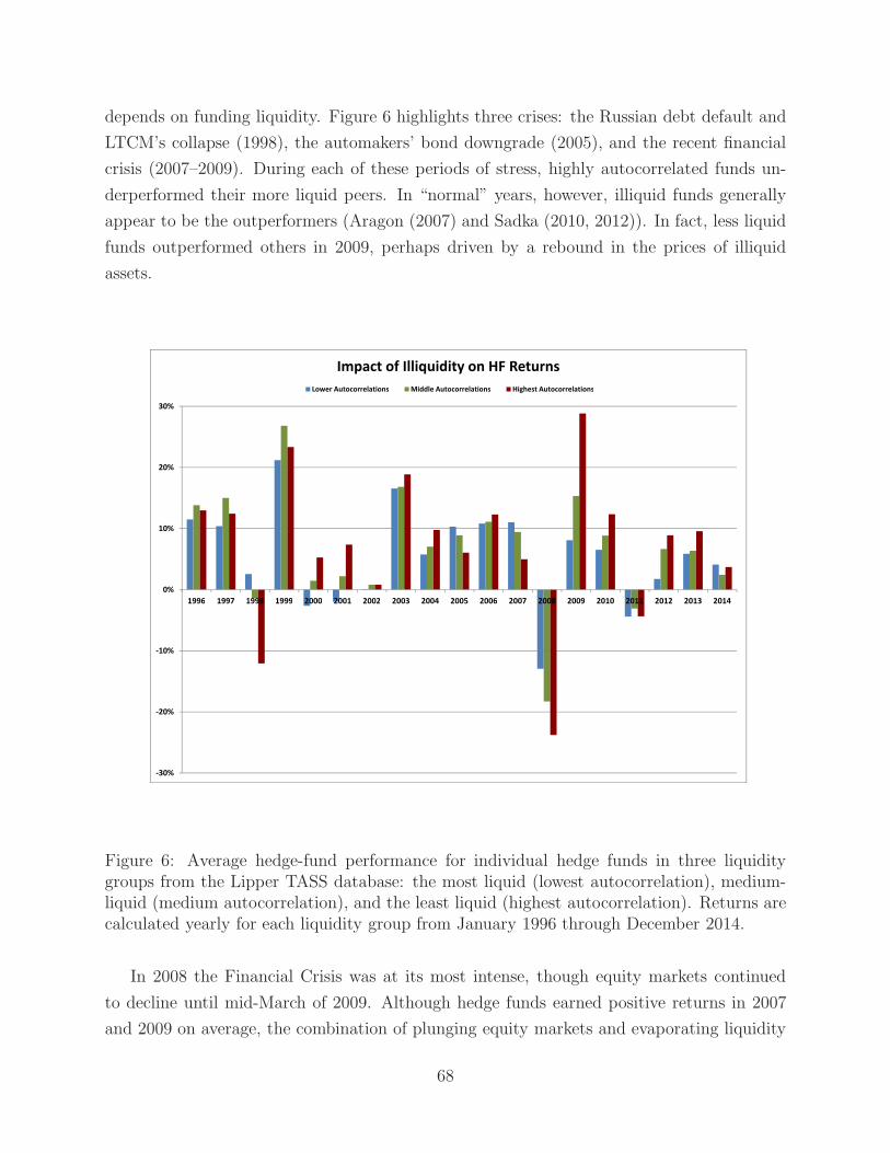
depends on funding liquidity. Figure 6 highlights three crises: the Russian debt default and

LTCM’s collapse (1998), the automakers’ bond downgrade (2005), and the recent financial

crisis (2007–2009). During each of these periods of stress, highly autocorrelated funds un-

derperformed their more liquid peers. In “normal” years, however, illiquid funds generally

appear to be the outperformers (Aragon (2007) and Sadka (2010, 2012)). In fact, less liquid

funds outperformed others in 2009, perhaps driven by a rebound in the prices of illiquid

assets.

30%

Impact of Illiquidity on HF Returns

Lower Autocorrelations Middle Autocorrelations Highest Autocorrelations

20%

30%

10%

20%

0%

10%

1996 1997 1998 1999 2000 2001 2002 2003 2004 2005 2006 2007 2008 2009 2010 2011 2012 2013 2014

-10%

1996 1997 1998 1999 2000 2001 2002 2003 2004 2005 2006 2007 2008 2009 2010 2011 2012 2013 2014

-20%

-30%

Figure 6: Average hedge-fund performance for individual hedge funds in three liquiditygroups from the Lipper TASS database: the most liquid (lowest autocorrelation), medium-liquid (medium autocorrelation), and the least liquid (highest autocorrelation). Returns arecalculated yearly for each liquidity group from January 1996 through December 2014.

In 2008 the Financial Crisis was at its most intense, though equity markets continued

to decline until mid-March of 2009. Although hedge funds earned positive returns in 2007

and 2009 on average, the combination of plunging equity markets and evaporating liquidity

68

in 2008 proved toxic and, in many cases fatal, leading to the industry’s worst-ever annual

return and the shutdown of over 2,000 hedge funds, as documented in Table 3. In 2008, the

attrition rate was 21%, the average hedge fund return was −18.4%, and the proportion of

hedge fund managers reporting negative returns for the year was 71%. Critics of the industry

asked why these absolute-return funds failed to generate positive returns, while supporters

noted that an investor would have fared far better in the average hedge fund than in, for

example, a stock index fund.

Lehman Brothers acted as one of the major prime brokers to the hedge-fund industry

prior to its bankruptcy on September 15, 2008. Aragon and Strahan (2012) study an example

of the propagation of illiquidity during the financial crisis: Lehman and the hedge funds that

used it as a prime broker. They document that the failure rate of Lehman’s hedge-fund clients

doubled after the bankruptcy, relative to funds with similar performance characteristics using

other brokers. The authors also show that stocks held by Lehman’s hedge-fund clients prior

to the bankruptcy experienced unexpectedly large declines in liquidity after the bankruptcy.

Ben-David, Franzoni, and Moussawi (2012) show that in 2008Q3–Q4, hedge funds sold about

29% of their aggregate portfolio. Redemptions and margin calls were the primary drivers

of the selloffs. In comparison, fund outflows and stock sales for mutual funds were not as

severe.

The remainder of 2009 was marked by the sharp appreciation of depressed asset prices

as governments flooded the markets with liquidity. 2010 saw a continued, albeit uneven,

recovery and the development of the European sovereign debt crisis. Hedge fund attrition,

though still in double digits, decreased to 15% in 2009 and 2010, and average hedge-fund

returns were positive in both years. Although hedge funds in most categories experienced

losses during 2008, those in three categories did not (see Table 12). As one would expect

in a declining equity market, Dedicated Short Bias produced handsome returns. Managed

Futures, an investment style that makes heavy use of trend-following, also performed well.

Indeed, one of the primary motivations for investing in managed futures funds is their per-

formance during and after crises, i.e., Kaminski’s (2011) crisis alpha. However, Global

Macro—the more-discretionary counterpart to Managed Futures that does not have as much

crisis alpha—finished the year roughly flat. Table 13 shows that funds belonging to these

three categories exhibited the lowest autocorrelation and lowest correlation with the S&P

500 during this period, which supports the narrative that the evaporation of liquidity and

the decline in the prices of equities or equity-like investments played an important role in

hedge funds’ losses.

69

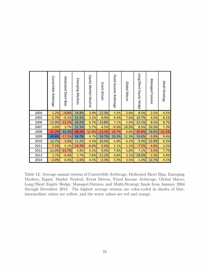
Co

nve

rtible

Arb

itrag

e

De

dica

ted

Sh

ort B

ias

Em

erg

ing

Ma

rke

ts

Eq

uity M

ark

et N

eu

tral

Eve

nt D

riven

Fixe

d In

com

e A

rbitra

ge

Glo

ba

l Ma

cro

Lon

g/S

ho

rt Eq

uity H

ed

ge

Ma

na

ge

d F

utu

res

Mu

lti-Stra

teg

y

2004 1.2% -9.8% 16.8% 3.9% 12.3% 5.5% 2.6% 8.5% 2.5% 4.5%

2005 -1.7% -0.2% 21.5% 5.2% 8.0% 4.3% 7.6% 10.7% 4.0% 8.1%

2006 11.9% -13.2% 23.2% 6.7% 13.8% 7.1% 5.0% 12.1% 8.5% 8.7%

2007 2.0% 3.7% 22.3% 5.7% 6.5% -0.3% 10.5% 8.5% 10.3% 7.3%

2008 -32.2% 31.2% -38.2% -12.9% -23.2% -18.7% 0.8% -20.8% 19.6% -21.1%

2009 43.8% -17.1% 34.7% 6.7% 24.7% 20.3% 11.3% 19.0% -5.9% 9.4%

2010 12.7% -3.0% 11.2% 4.3% 10.4% 5.0% 6.2% 9.4% 12.4% 6.3%

2011 -7.1% 5.1% -14.3% -0.6% -2.6% 5.1% 1.1% -7.5% -4.8% 2.2%

2012 11.0% -13.7% 5.8% 4.1% 9.4% 7.4% 5.8% 7.1% -3.4% 7.7%

2013 1.7% -0.4% 2.7% 7.6% 11.2% 4.6% 3.1% 14.5% -1.5% 5.8%

2014 -2.0% 6.0% -1.6% 4.5% -2.3% 3.3% 2.5% 1.3% 12.7% 4.1%

Table 12: Average annual returns of Convertible Arbitrage, Dedicated Short Bias, EmergingMarkets, Equity Market Neutral, Event Driven, Fixed Income Arbitrage, Global Macro,Long/Short Equity Hedge, Managed Futures, and Multi-Strategy funds from January 2004through December 2014. The highest average returns are color-coded in shades of blue,intermediate values are yellow, and the worst values are red and orange.

70

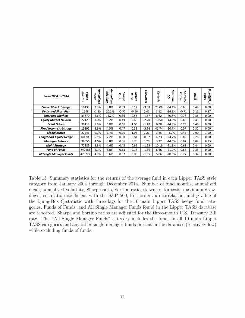
From 2004 to 2014

# fu

nd

-

mo

nth

s

An

nu

alize

d

Me

an

An

nu

alize

d

Vo

latility

Sh

arp

e

Ra

tio

So

rtino

Ra

tio

Sk

ew

ne

ss

Ku

rtosis

Ma

xim

um

DD

S&

P 5

00

Co

rrel.

ac(1

)

Bo

x-Q

(3) p

-

va

lue

Convertible Arbitrage 10133 2.3% 8.8% 0.09 0.12 -3.08 23.06 -34.4% 0.60 0.48 0.00

Dedicated Short Bias 1648 -1.8% 10.1% -0.32 -0.56 0.41 3.12 -34.1% -0.71 0.16 0.27

Emerging Markets 39670 5.6% 11.2% 0.36 0.55 -1.17 6.62 -40.6% 0.73 0.36 0.00

Equity Market Neutral 22129 3.0% 3.2% 0.49 0.66 -2.20 10.50 -14.6% 0.63 0.45 0.00

Event Driven 30113 5.5% 6.0% 0.66 1.00 -1.40 6.90 -24.8% 0.76 0.48 0.00

Fixed Income Arbitrage 15191 3.6% 4.5% 0.47 0.55 -5.16 41.74 -20.7% 0.57 0.32 0.00

Global Macro 27845 5.1% 3.7% 0.96 1.94 0.21 3.85 -4.7% 0.45 0.00 1.00

Long/Short Equity Hedge 144706 5.1% 7.2% 0.50 0.81 -0.82 4.23 -24.7% 0.82 0.26 0.00

Managed Futures 39056 4.6% 8.8% 0.36 0.70 0.28 3.22 -14.5% 0.07 0.02 0.33

Multi-Strategy 72889 3.5% 4.6% 0.45 0.62 -1.95 10.19 -21.5% 0.68 0.44 0.00

Fund of Funds 247483 2.1% 5.0% 0.13 0.18 -1.36 6.66 -21.9% 0.66 0.35 0.00

All Single Manager Funds 425222 4.7% 5.6% 0.57 0.89 -1.05 5.86 -20.5% 0.77 0.32 0.00

Table 13: Summary statistics for the returns of the average fund in each Lipper TASS stylecategory from January 2004 through December 2014. Number of fund months, annualizedmean, annualized volatility, Sharpe ratio, Sortino ratio, skewness, kurtosis, maximum draw-down, correlation coefficient with the S&P 500, first-order autocorrelation, and p-value ofthe Ljung-Box Q-statistic with three lags for the 10 main Lipper TASS hedge fund cate-gories, Funds of Funds, and All Single Manager Funds found in the Lipper TASS databaseare reported. Sharpe and Sortino ratios are adjusted for the three-month U.S. Treasury Billrate. The “All Single Manager Funds” category includes the funds in all 10 main LipperTASS categories and any other single-manager funds present in the database (relatively few)while excluding funds of funds.

71

7.3 Post-Crisis Performance

In the years following the financial crisis, some industry analysts have expressed disappoint-

ment with hedge funds in light of their underperformance relative to public equities. As a

result, investors’ ever-present interest in gauging manager alpha has a new and urgent form:

in the post-crisis era, have hedge funds lost their ability to generate attractive returns? Al-

though it is still too soon to answer this question with any degree of empirical accuracy,

some preliminary facts suggest a possible response.

In Table 14 we report summary statistics for the returns of the average hedge fund dur-

ing pre- and post-crisis periods, where the pre-crisis period is from January 1996 through

December 2006 and the post-crisis period is from January 2010 through December 2014. In

each period, we calculate the bias-adjusted average monthly returns for single-fund man-

agers in the Lipper TASS database, along with the other standard measures of investment

performance. The entries confirm the popular perception that the absolute returns of hedge

funds were higher on average during the pre-crisis period: 8.7% pre-crisis vs. 4.2% post-crisis.

Moreover, this inequality holds for every single category.

However, Table 14 also shows that, in the post-crisis period, the Sharpe ratios of hedge

funds have been as high as they were in the pre-crisis period or higher, suggesting that

managers are no less skilled at generating returns now than they were before the crisis.

Specifically, across all categories, the average Sharpe ratio is 0.72 in the pre-crisis period

and 1.00 in the post-crisis period. As a check, we calculated the Sharpe ratio of the CS/DJ

Hedge-Fund Index for the same periods, and again we found that the Sharpe ratio had, if

anything, increased: 0.97 in the pre-crisis period and 1.29 in the post-crisis period. This

result is hardly definitive, as the length of the post-crisis period is still rather short and many

authors have proposed more-elaborate measures of hedge fund skill. Nonetheless, it suggests

that any reports of the disappearance of hedge fund manager skill may be quite exaggerated.

This surprising result suggests a somewhat different narrative regarding the source of

hedge-fund underperformance. The most obvious explanation is the fact that the average

volatility of hedge funds’ returns was lower in the post-crisis period, damping absolute returns

even as risk-adjusted returns remained strong. We estimate that the annualized volatility

of the cross-sectionally averaged hedge fund returns in the Lipper TASS database dropped

from 6.5% to 4.2% between the two periods, and among the individual categories, only

Convertible Arbitrage funds have higher average volatilities in the post-crisis period. This

decline in volatility is likely due to lower amounts of leverage being deployed in the hedge-fund

industry for several reasons: a decrease in risk appetite among investors in the aftermath of

the financial crisis, more stringent capital requirements on the part of regulators, and fewer

72

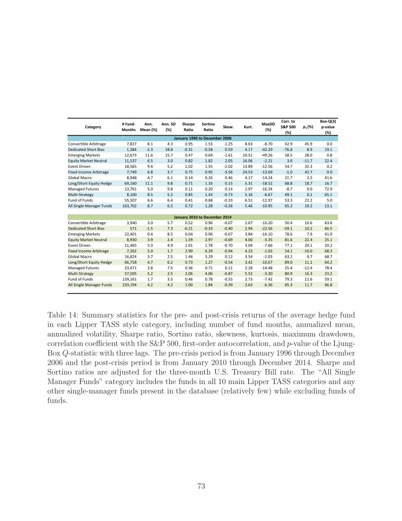
Category# Fund-

Months

Ann.

Mean (%)

Ann. SD

(%)

Sharpe

Ratio

Sortino

RatioSkew. Kurt.

MaxDD

(%)

Corr. to

S&P 500

(%)

ρ1 (%)

Box-Q(3)

p-value

(%)

Convertible Arbitrage 7,827 8.1 4.3 0.95 1.53 -1.25 8.63 -8.70 42.9 45.9 0.0

Dedicated Short Bias 1,384 -2.3 18.8 -0.31 -0.58 0.59 4.17 -42.29 -76.8 8.9 19.1

Emerging Markets 12,673 11.6 15.7 0.47 0.69 -1.61 10.51 -49.26 58.5 28.0 0.8

Equity Market Neutral 11,537 6.5 3.0 0.82 1.82 2.05 16.06 -2.21 3.0 -11.7 22.4

Event Driven 18,565 9.4 5.2 1.02 1.55 -2.02 13.89 -12.56 54.7 32.3 0.2

Fixed Income Arbitrage 7,749 6.8 3.7 0.75 0.95 -3.56 24.53 -13.69 -1.0 42.7 0.0

Global Macro 8,948 4.7 6.1 0.14 0.26 0.46 4.17 -14.24 21.7 2.5 41.6

Long/Short Equity Hedge 69,160 11.1 9.8 0.71 1.33 0.15 5.31 -18.52 68.8 18.7 16.7

Managed Futures 13,761 5.0 9.8 0.11 0.20 0.14 2.97 -16.34 -8.7 0.0 72.9

Multi-Strategy 8,100 8.5 5.2 0.85 1.43 -0.73 5.16 -6.67 49.1 0.1 65.1

Fund of Funds 55,507 6.6 6.4 0.41 0.68 -0.33 6.51 -12.97 53.3 22.2 5.0

All Single Manager Funds 163,702 8.7 6.5 0.72 1.28 -0.26 5.46 -10.95 65.2 19.2 13.1

Convertible Arbitrage 3,940 3.0 5.7 0.52 0.96 -0.07 2.67 -10.20 50.4 10.6 63.6

Dedicated Short Bias 571 -1.5 7.3 -0.21 -0.33 -0.40 2.94 -22.56 -59.1 10.2 66.5

January 1996 to December 2006

January 2010 to December 2014

Dedicated Short Bias 571 -1.5 7.3 -0.21 -0.33 -0.40 2.94 -22.56 -59.1 10.2 66.5

Emerging Markets 22,401 0.4 8.5 0.04 0.06 -0.67 3.84 -16.10 78.6 7.9 41.9

Equity Market Neutral 8,930 3.9 2.4 1.59 2.97 -0.69 4.00 -3.35 81.6 22.4 25.1

Event Driven 11,465 5.0 4.9 1.01 1.78 -0.70 3.04 -7.66 77.1 20.1 20.2

Fixed Income Arbitrage 7,202 5.0 1.7 2.90 6.29 -0.94 4.23 -1.03 54.1 -10.0 68.3

Global Macro 16,824 3.7 2.5 1.46 3.29 0.12 3.54 -2.03 63.2 9.7 68.7

Long/Short Equity Hedge 66,758 4.7 6.2 0.73 1.27 -0.54 3.42 -10.67 89.0 11.1 64.2

Managed Futures 23,471 2.8 7.5 0.36 0.71 0.11 2.28 -14.48 25.4 -12.4 78.4

Multi-Strategy 57,505 5.2 2.5 2.06 4.06 -0.87 5.52 -3.20 80.9 16.3 23.2

Fund of Funds 139,161 1.7 3.5 0.46 0.78 -0.55 2.73 -7.42 79.3 11.6 59.1

All Single Manager Funds 233,194 4.2 4.2 1.00 1.84 -0.39 3.63 -6.36 85.3 11.7 46.8

Table 14: Summary statistics for the pre- and post-crisis returns of the average hedge fundin each Lipper TASS style category, including number of fund months, annualized mean,annualized volatility, Sharpe ratio, Sortino ratio, skewness, kurtosis, maximum drawdown,correlation coefficient with the S&P 500, first-order autocorrelation, and p-value of the Ljung-BoxQ-statistic with three lags. The pre-crisis period is from January 1996 through December2006 and the post-crisis period is from January 2010 through December 2014. Sharpe andSortino ratios are adjusted for the three-month U.S. Treasury Bill rate. The “All SingleManager Funds” category includes the funds in all 10 main Lipper TASS categories and anyother single-manager funds present in the database (relatively few) while excluding funds offunds.

73

market opportunities due to central banking interventions that have changed traditional

risk/reward relations among assets.

This potential decrease in leverage is related to the second possible source of apparent

underperformance of post-crisis hedge funds: a lower risk-free rate. We estimate that the

average risk-free rate declined from 3.80% in the pre-crisis period to 0.07% in the post-crisis

period. If hedge funds earn a portion of their return from cash holdings, e.g., as collateral in

margin accounts, their post-crisis returns will definitely be affected by the low-interest-rate

policies of the world’s major central banks, irrespective of manager skill.

Third, hedge-fund database biases are much stronger for older data (see Section 3.2).

A researcher who naıvely averaged pre-crisis returns in the Lipper TASS database might

introduce an upward bias of 8.6%, whereas post-crisis average returns may only be subject

to a 1.9% bias. Unless these biases are corrected before averaging (as we do in this review

article), they will tend to exaggerate the difference between pre- and post-crisis hedge-fund

returns.

These three factors are sufficient to explain the entirety of the post-crisis underperfor-

mance of hedge funds. However, it is still too early to judge whether any or all of these

explanations are, in fact, correct. More data must be accumulated before we can come to a

definitive conclusion, and these hypotheses provide specific guidelines for the kinds of data

that need to be collected.

7.4 Hedge Funds and Systemic Risk

In the aftermath of the Financial Crisis of 2007–2009, the concept of “systemic risk” has

emerged as an important phenomenon that goes far beyond its original domain of macroe-

conomics and central banking policy. Although a review of the systemic risk literature is

beyond the scope of this article, the extent to which the hedge-fund industry can offer insights

into systemic risk is clearly within our purview.

A natural starting point for developing such insights is to first define and then measure

systemic risk—the adage that “one cannot manage what one does not measure” is particu-

larly relevant in this context. Remarkably, five years after one of the worst financial crises

since the Great Depression of 1929, we still do not have a consensus on the definition of

systemic risk, much less a standardized measure for it. In fact, the review article on sys-

temic risk measures published in this journal by Bisias, Flood, Lo, and Valavanis (2012) lists

31 distinct measures, not one of which is universally endorsed as the canonical measure of

systemic risk that should be regularly computed and released by the government. And even

after reviewing eight centuries of financial crises, Reinhart and Rogoff’s (2009) definitive

74

treatise offers no single barometer with which financial stability can be reliably gauged.

Billio, Getmansky, Lo, and Pelizzon (2012) define systemic risk as the risk of a “systemic

event”, which is any set of circumstances that threatens the stability of or public confidence

in the financial system. This is consistent with the “four L’s” of financial crisis—liquidity,

leverage, linkages, and losses—that appear repeatedly in various narratives of 2007–2009,

and all of these L’s touch the hedge-fund industry to some extent. Under this definition,

there is little doubt that LTCM’s decline in August and September of 1998 was a systemic

event, and that the private-sector bailout facilitated by the New York Fed was a reasonable, if

somewhat hastily arranged, response. However, in September 2006 when the much larger ($9

billion vs. $4.7 billion) hedge fund Amaranth Advisors shut down because of extreme trading

losses, there was no Fed-facilitated bail out and financial markets hardly noticed. Clearly this

event was not systemic, and the comparison with LTCM underscores the heterogeneity and

complexity of the hedge-fund industry, and the need for more refined analytics to determine

how hedge funds may or may not affect systemic risk.

In a series of papers, Chan, Getmansky, Haas, and Lo (2004, 2006, 2007) propose using the

hedge-fund industry like a geiger counter to construct measures of systemic risk. Employing

aggregate measures of volatility, illiquidity, and financial distress for hedge funds based on

statistical regime-switching models, autocorrelation, and linear factor exposures, they show

that periods of market dislocation can be predicted to some degree by certain trends in the

hedge-fund industry such as regime switches to lower-mean/higher-volatility returns, and

increases in illiquidity as measured by asset-weighted autocorrelations.29

More recently, Billio, Getmansky, Lo, and Pelizzon (2012) have proposed measures of

interconnectedness among four types of financial institutions that figured prominently in the

recent financial crisis: banks, broker/dealers, insurance companies, and hedge funds. Using

monthly returns for the top 25 institutions in each of these four categories, they estimate com-

mon factor exposures using PCA, and estimate pairwise connections using Granger-causality

tests. The former technique captures concentrated sources of risk and return across the four

sectors, and the latter is used to construct Granger-causality networks, directed graphs that

capture both the direction and statistical significance of pairwise relations among financial

institutions over time. By applying standard measures of connectivity from social network

analysis such as the eigenvector centrality parameter, they conclude that the banking and in-

surance sectors are particularly important sources of interconnectedness and, therefore, key

channels through which systemic events are propagated. Hedge funds are also important

nodes in this financial web, but they do not play as large a role in transmitting systemic

29Regime-switching models are commonly used in the broader financial economics literature, e.g., Bekaertand Harvey (1995), Ang and Bekaert (2002) and Guidolin and Timmermann (2008) among others.

75

shocks as banks.30 A distinct literature focusing on the reverse question—how does systemic

risk affect hedge funds?—has developed in parallel. Brunnermeier (2009) argues that hedge

funds could be affected by financial crises through many mechanisms: direct exposure, fund-

ing liquidity, market liquidity, loss and margin spirals, runs on hedge funds, and aversion to

Knightian uncertainty. Some of these mechanisms, like direct exposure and market liquidity,

can be captured by hedge fund exposures to market risk factors.

Billio, Getmansky, and Pelizzon (2013) find that liquidity, credit, equities, and equity-

market volatility are common risk factors during crises for various hedge-fund strategies.They

apply a novel methodology to identify the presence of a common latent risk-factor exposure

across all hedge-fund strategies, and find that this latent factor is related to asset and funding

liquidity. If the latent risk factor is omitted in risk modeling, the resulting effect of financial

crises on hedge fund risk is greatly underestimated. These results support the conclusions

of Boyson, Stahel, and Stulz (2010), who document significant contagion from lagged bank-

and broker-returns to hedge-fund returns.

Other factors such as funding liquidity, margin spirals, runs on hedge funds, and aversion

to Knightian uncertainty are hedge-fund-specific and affect the residual volatility of hedge

fund returns (Krishnamurthy (2010)). For example, Khandani and Lo (2007, 2011a) argue

that a forced liquidation of a given strategy should increase the strategy volatility through

the increase in the residual volatility of hedge fund returns. Billio, Getmansky, and Pelizzon

(2013) investigate residual volatility of hedge-fund strategies and show that the increase in

this volatility is common among all hedge-fund strategies they consider during the LTCM

crisis of 1998 and the Financial Crisis of 2007–2009.

Chan, Getmansky, Haas, and Lo (2004, 2006, 2007), Adrian (2007), and Khandani and

Lo (2007, 2011a) show that hedge funds’ risk profile during the LTCM crisis was drastically

different from other financial crises. Khandani and Lo (2007, 2011a) find an increased

correlation among hedge-fund styles in this period and conjecture that this can be due to

the increase in systematic linkages with market factors, liquidity, and credit proxies, e.g., the

Quant Meltdown of August 2007 (see Section 7.1). Boyson, Stahel, and Stulz (2010) study

potential explanations for the clustering of hedge funds’ worst returns and find that adverse

shocks to asset and funding liquidity as well as contagion may potentially explain this tail

risk.

Despite the fact that dislocation in the hedge-fund industry often presages broader fi-

30The role of hedge funds in financial crises has been documented in several studies, including Eichengreen,Mathieson, Chadha, Jansen, Kodres, and Sharma (1998), Brown, Goetzmann, and Park (2000), Fung, Hsieh,and Tsatsoronis (2000), Brunnermeier and Nagel (2004), and Chen and Liang (2007). Hedge fund failuresand liquidations, and their underlying causes, have also been studied, e.g., Getmansky, Lo, and Mei (2004)and Liang and Park (2010).

76

nancial crises, it is easy to miss or ignore these early warning signs. Although academic

studies raised the possibility of crisis as early as 2004 and 2005 (see Chan, Getmansky, Haas,

and Lo (2004), Rajan (2005), Shiller (2005), and Section 7.1), these were outliers with re-

spect to the financial industry’s perspective at the time. A sense for the magnitude of the

gulf between academia and industry can be obtained from the views of the Counterparty

Risk Management Policy Group II (CRMPG-II) (2005), a non-profit industry consortium

with the following mandate: “The primary purpose of CRMPG-II—building on the 1999

report of CRMPG-I—is to examine what additional steps should be taken by the private

sector to promote the efficiency, effectiveness and stability of the global financial system”.

The CRMPG-II was chaired by Gerald Corrigan, then a managing director at Goldman

Sachs, and the two vice chairs were Don Wilson, then Chief Risk Officer of JP Morgan,

and David Bushnell, then senior risk officer of Citigroup. The other members of the pol-

icy group included senior representatives from top financial institutions and their law firms:

Bear Stearns, Cleary Gottlieb Steen & Hamilton, Deutsche Bank, General Motors Asset

Management, HSBC, Lehman Brothers, Merrill Lynch, Morgan Stanley, TIAA-CREF, and

Tudor Investment Corporation. On July 25, 2005, this body of industry experts published

their report which began with the following summary assessment (CRMPG-II (2005, p. 1)):

In approaching its task, the Policy Group shared a broad consensus that the

already low statistical probabilities of the occurrence of truly systemic financial

shocks had further declined over time.

While this statement may seem naıve with the benefit of hindsight, it must be emphasized

that business was booming during this period, with many of the firms represented in the

CRMPG-II earning record profits that year and the year after. However, even in this context,

the CRMPG-II report contains some prescient warnings that the members both documented

and then dismissed with their blanket assessment. Recommendations 12, 21, and 22 of the

report called for industry-wide efforts to: (1) cope with serious “back-office” and potential

settlement problems in the CDS market; and (2) stop the practice whereby some market

participants “assign” their side of a trade to another institution without the consent of the

original counterparty to the trade.31 The first recommendation was for the largest institu-

tions to catch up on the one-year backlog in simply entering into their record-keeping and,

presumably, their risk-management systems, the terms of CDS contracts they had executed.

The second recommendation was to address the fact that a number of CDS contracts could

legally be reassigned to other counterparties without prior approval or notification, making

31See CRMPG-II (2005, p. iv).

77

it virtually impossible to determine the counterparty credit risk of such contracts.32 These

recommendations seem grossly inconsistent with the CRMPG-II’s conclusion that the risk

of a systemic shock had declined.

This example highlights the challenges that the financial industry faces in identifying

threats to financial stability; such threats are often forged in the crucible of highly prof-

itable, rapidly growing business lines. Unless corporate executives have perfect timing, it is

unrealistic to expect them to reduce risk as their businesses are expanding, nor will share-

holders support such behavior. While the concept of countercyclical capital buffers seems

sensible, it is virtually impossible for them to be self-imposed by the industry. Therefore,

macroprudential regulation can play a positive role in creating a more stable and robust

financial system.

8 Implementation Issues for Hedge Fund Investing

Having reviewed much of the academic hedge-fund literature in Sections 2–7, we now turn to

four implementation issues facing hedge-fund investors. In Section 8.1, we consider the po-

tential dangers of mindlessly applying traditional mean-variance portfolio analysis to hedge

fund returns. The multi-faceted nature of hedge-fund risk exposures, the smoothness of

certain hedge-fund returns due to illiquidity, and the nonstationarity of their return distri-

butions imply that standard mean-variance analysis can yield highly misleading portfolio

allocations, especially at the asset-class level.

A related problem is discussed in Section 8.2 involving the potential over-diversification

of hedge-fund portfolios, which can lead to lower expected returns and, surprisingly, greater

risks. The investment implications of adding hedge funds to a portfolio of traditional assets

are discussed in Section 8.3. Given the potential pitfalls in hedge-fund investing, the need

for a more systematic framework for making alternative investment decisions is clear and in

Section 8.4 we present such a framework.

From a broader perspective, investing in hedge funds seems at odds with much of the

academic investments literature which emphasizes passive risk premia and dismisses the

possibility of consistent sources of alpha. However, the popularity of hedge funds among large

institutional investors who also invest passively suggests a troubling contradiction between

theory and practice. In Section 8.5, we provide a review of the Adaptive Markets Hypothesis,

an alternative to the Efficient Markets Hypothesis that reconciles this contradiction in an

32Both of these problems were not isolated issues, but were so widespread that eventually Timothy Gei-thner, then president of the New York Fed, was motivated to intervene through moral suasion to get thefinancial industry to address these concerns.

78

intellectually satisfying manner.

8.1 The Limits of Mean-Variance Optimization

A common question facing investors, advisers, and institutional money managers is how

much should they allocate to hedge funds? Many turn to mathematical optimization tools

only to discover that their optimizer recommends a 200% allocation to hedge funds and

−100% allocation to other assets. Such results are usually disregarded, and rightly so. While

hedge funds may be desirable investments for some investors, biases in hedge fund reporting

artificially boost historical estimates of expected returns while autocorrelation due to illiquid

portfolios artificially dampens estimated variances and covariances. Furthermore, optimizers

may produce recommendations that are fine-tuned for a previous period but poorly suited

for the future, and the resulting portfolios may have unsuitable risk characteristics.

In Table 15 we show that a (nearly) unconstrained optimizer can produce a portfolio

that would have earned an amazing 40.4% per year between 1996 and 2014. However, the

investments required for such a portfolio are not even feasible: the optimizer calls for short

exposure to certain hedge fund categories. Nevertheless, mathematical optimizers can be

a useful guide for investors, calling attention to assets that have historically had desirable

average returns, low correlation, or other characteristics. It is usually helpful to constrain the

set of solutions from which the optimizer may choose, preemptively eliminating solutions that

are too risky, too illiquid, involve too much leverage, or are outside the feasible investment

universe. In Table 15 we show a number of mean-variance-optimized portfolio weights subject

to such constraints. Results toward the top of the table are generally more constrained and

are probably a better guide to the sorts of choices a prudent investor might have made during

the previous 19 years.

In addition to the traditional constraint on the portfolio’s standard deviation, we employ

a more novel constraint on portfolio autocorrelation in an effort to avoid portfolios that are

likely to be too illiquid. While some endowments may be able to tolerate an illiquid portfolio

because their investment horizon is presumably unbounded, individual investors often need

to access their assets sooner and may choose to be more cautious about illiquidity. See

Section 5.4 for further discussion about mean-variance-illiquidity optimization.

8.2 Over-Diversification

The proliferation of multi-strategy funds and funds of funds over the past two decades has

given investors an unprecedented amount of diversification within the hedge-fund industry

79

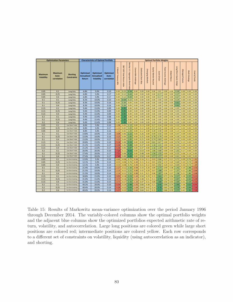
Maximum

Volatility

Maximum

Auto-

correlation

Shorting

Constraints

Optimized

Annualized

Return

Optimized

Annualized

Volatility

Optimized

Auto-

correlation

3 M

on

th T

rea

sury B

ills

S&

P 5

00

To

tal R

etu

rn In

de

x

Ba

rclay U

.S. A

gg

reg

ate

Bo

nd

Ind

ex

Co

nve

rtible

Arb

itrag

e

De

dica

ted

Sh

ort B

ias

Em

erg

ing

Ma

rke

ts

Eq

uity M

ark

et N

eu

tral

Eve

nt D

riven

Fixe

d In

com

e A

rbitra

ge

Glo

ba

l Ma

cro

Lon

g/S

ho

rt Eq

uity H

ed

ge

Ma

na

ge

d F

utu

res

Mu

lti-Stra

teg

y

Fu

nd

of F

un

ds

0.05 0.1 Long Only 6.8% 5.0% 0.10 0.00 0.15 0.54 0.00 0.00 0.00 0.00 0.01 0.00 0.00 0.30 0.00 0.00 0.00

0.05 0.25 Long Only 6.8% 5.0% 0.17 0.00 0.12 0.43 0.00 0.00 0.00 0.00 0.17 0.00 0.00 0.27 0.00 0.00 0.00

0.05 0.4 Long Only 6.8% 5.0% 0.17 0.00 0.12 0.43 0.00 0.00 0.00 0.00 0.17 0.00 0.00 0.27 0.00 0.00 0.00

0.1 0.1 Long Only 8.2% 10.0% 0.10 0.00 0.54 0.22 0.00 0.00 0.00 0.00 0.00 0.00 0.00 0.24 0.00 0.00 0.00

0.1 0.25 Long Only 8.3% 10.0% 0.16 0.00 0.34 0.05 0.00 0.00 0.00 0.00 0.00 0.00 0.00 0.62 0.00 0.00 0.00

0.1 0.4 Long Only 8.3% 10.0% 0.16 0.00 0.34 0.05 0.00 0.00 0.00 0.00 0.00 0.00 0.00 0.62 0.00 0.00 0.00

0.15 0.1 Long Only 9.4% 15.0% 0.09 0.00 0.95 0.00 0.00 0.00 0.00 0.00 0.00 0.00 0.00 0.05 0.00 0.00 0.00

0.15 0.25 Long Only 9.4% 15.0% 0.09 0.00 0.95 0.00 0.00 0.00 0.00 0.00 0.00 0.00 0.00 0.05 0.00 0.00 0.00

0.15 0.4 Long Only 9.4% 15.0% 0.09 0.00 0.95 0.00 0.00 0.00 0.00 0.00 0.00 0.00 0.00 0.05 0.00 0.00 0.00

0.2 0.1 Long Only 9.4% 15.4% 0.08 0.00 1.00 0.00 0.00 0.00 0.00 0.00 0.00 0.00 0.00 0.00 0.00 0.00 0.00

0.2 0.25 Long Only 9.4% 15.4% 0.08 0.00 1.00 0.00 0.00 0.00 0.00 0.00 0.00 0.00 0.00 0.00 0.00 0.00 0.00

0.2 0.4 Long Only 9.4% 15.4% 0.08 0.00 1.00 0.00 0.00 0.00 0.00 0.00 0.00 0.00 0.00 0.00 0.00 0.00 0.00

0.05 0.1 Can Short T-bills 8.6% 5.0% 0.10 -1.06 0.03 1.12 0.00 0.13 0.00 0.27 0.24 0.00 0.01 0.22 0.04 0.00 0.00

0.05 0.25 Can Short T-bills 8.8% 5.0% 0.17 -1.11 0.02 1.03 0.00 0.12 0.00 0.37 0.42 0.00 0.00 0.14 0.02 0.00 0.00

0.05 0.4 Can Short T-bills 8.8% 5.0% 0.16 -1.12 0.02 1.03 0.00 0.12 0.00 0.39 0.40 0.00 0.00 0.14 0.02 0.00 0.00

0.1 0.1 Can Short T-bills 14.8% 10.0% 0.10 -3.09 0.06 2.22 0.00 0.26 0.00 0.49 0.50 0.00 0.00 0.47 0.09 0.00 0.00

0.1 0.25 Can Short T-bills 15.0% 10.0% 0.16 -3.25 0.04 2.05 0.00 0.25 0.00 0.78 0.79 0.00 0.00 0.30 0.03 0.00 0.00

0.1 0.4 Can Short T-bills 15.0% 10.0% 0.17 -3.23 0.04 2.05 0.00 0.25 0.00 0.74 0.83 0.00 0.00 0.29 0.03 0.00 0.00

0.15 0.1 Can Short T-bills 20.8% 15.0% 0.10 -5.16 0.08 3.33 0.00 0.39 0.00 0.81 0.67 0.00 0.00 0.74 0.13 0.00 0.00

0.15 0.25 Can Short T-bills 21.2% 15.0% 0.17 -5.36 0.06 3.08 0.00 0.37 0.00 1.16 1.21 0.00 0.00 0.43 0.05 0.00 0.00

0.15 0.4 Can Short T-bills 21.2% 15.0% 0.17 -5.36 0.06 3.07 0.00 0.37 0.00 1.16 1.19 0.00 0.00 0.45 0.05 0.00 0.00

0.2 0.1 Can Short T-bills 26.9% 20.0% 0.10 -7.20 0.11 4.43 0.00 0.53 0.00 1.06 0.88 0.00 0.00 1.01 0.17 0.00 0.00

0.2 0.25 Can Short T-bills 27.4% 20.0% 0.17 -7.51 0.08 4.10 0.00 0.48 0.00 1.56 1.55 0.00 0.00 0.55 0.06 0.14 0.00

0.2 0.4 Can Short T-bills 27.4% 20.0% 0.17 -7.49 0.08 4.09 0.00 0.50 0.00 1.57 1.57 0.00 0.00 0.61 0.06 0.00 0.00

0.05 0.1 Can Short Anything 12.0% 5.0% 0.10 -0.60 -0.06 0.75 -0.46 0.16 0.11 0.03 0.86 0.25 0.21 0.72 0.09 0.76 -1.82

0.05 0.25 Can Short Anything 12.1% 5.0% 0.14 -0.55 -0.06 0.76 -0.40 0.15 0.12 0.01 0.92 0.19 0.20 0.69 0.10 0.74 -1.88

0.05 0.4 Can Short Anything 12.1% 5.0% 0.14 -0.54 -0.06 0.76 -0.40 0.15 0.12 0.01 0.92 0.20 0.21 0.69 0.10 0.73 -1.89

0.1 0.1 Can Short Anything 21.4% 10.0% 0.10 -2.27 -0.12 1.50 -0.96 0.33 0.20 0.09 1.77 0.49 0.38 1.42 0.19 1.48 -3.50

0.1 0.25 Can Short Anything 21.5% 10.0% 0.14 -2.15 -0.11 1.51 -0.80 0.32 0.20 0.07 1.88 0.35 0.37 1.37 0.21 1.46 -3.66

0.1 0.4 Can Short Anything 21.5% 10.0% 0.14 -2.14 -0.11 1.51 -0.80 0.31 0.21 0.06 1.87 0.36 0.37 1.36 0.21 1.46 -3.68

0.15 0.1 Can Short Anything 30.8% 15.0% 0.10 -3.91 -0.18 2.23 -1.43 0.50 0.29 0.15 2.61 0.71 0.56 2.17 0.28 2.25 -5.23

0.15 0.25 Can Short Anything 31.0% 15.0% 0.14 -3.71 -0.16 2.25 -1.21 0.48 0.31 0.11 2.79 0.50 0.53 2.07 0.31 2.22 -5.49

0.15 0.4 Can Short Anything 31.0% 15.0% 0.15 -3.71 -0.17 2.26 -1.20 0.47 0.31 0.09 2.80 0.54 0.55 2.05 0.31 2.19 -5.50

0.2 0.1 Can Short Anything 40.2% 20.0% 0.10 -5.54 -0.24 2.98 -1.92 0.66 0.38 0.21 3.45 0.94 0.74 2.90 0.36 3.02 -6.95

0.2 0.25 Can Short Anything 40.4% 20.0% 0.14 -5.26 -0.22 3.03 -1.64 0.64 0.42 0.14 3.70 0.65 0.69 2.79 0.40 2.94 -7.30

0.2 0.4 Can Short Anything 40.4% 20.0% 0.14 -5.27 -0.22 3.01 -1.62 0.64 0.41 0.15 3.71 0.66 0.70 2.77 0.41 2.95 -7.30

Optimization Parameters Characteristics of Optimal Portfolio Optimal Portfolio Weights

Table 15: Results of Markowitz mean-variance optimization over the period January 1996through December 2014. The variably-colored columns show the optimal portfolio weightsand the adjacent blue columns show the optimized portfolios expected arithmetic rate of re-turn, volatility, and autocorrelation. Large long positions are colored green while large shortpositions are colored red; intermediate positions are colored yellow. Each row correspondsto a different set of constraints on volatility, liquidity (using autocorrelation as an indicator),and shorting.

80

(Learned and Lhabitant (2003) and Amo, Harasty, and Hillion (2007)). However, the Fi-

nancial Crisis of 2007–2009 has called into question the view that hedge funds are really

“hedged”, and that diversification across hedge-fund styles is beneficial. Billio, Getmansky,

and Pelizzon (2013) find that the average correlation among hedge-fund strategies jumped

from 0.32 in August 2008 to 0.52 in September 2008, a 64% increase. At the same time,

the average returns of most hedge funds have declined significantly (see Section 7.3), leaving

investors wondering whether hedge-fund investing is still worthwhile.

Cumming, Dai, and Shawky (2012) show that on a risk-adjusted basis, hedge funds

that diversify across sectors and asset classes outperform other funds by an average of 1.6%

per year. However, diversification across styles is found to exhibit a significant negative

association with hedge fund returns. Nevertheless, for funds of funds, the authors find a

significant positive relation between performance and diversification across sectors, styles,

and geographies.

In documenting the performance of the hedge-fund industry from 1995 to 2004, Fung,

Hsieh, Naik, and Ramadorai (2008) find that, on average, funds of funds deliver alpha only

in the period between October 1998 and March 2000, although a subset of funds of funds do

seem to have consistent alpha.

Furthermore, Brown, Gregoriou, and Pascalau (2011) find that the variance-reducing

effects of diversification become insignificant once a fund of funds holds more than 20 un-

derlying hedge funds. Yet the majority of funds of funds are more diversified than this.

They find that over-diversification by funds of funds can increase left-tail risk exposure and

lower expected returns, especially when hedge fund returns are smoothed. This increase in

tail risk is accompanied by lower returns, which they attribute to the cost of necessary due

diligence, a drag on performance that increases with the number of underlying hedge funds

in portfolio.

8.3 Investment Implications

Reviewing the performance characteristics of hedge funds has provided ample evidence to

support the view that investors selecting their strategic asset allocations should not consider

hedge funds to be a monolithic category. The decision to allocate assets to a hedge fund

strategy should involve the consideration of a number of factors. First, of course, is a

strategy’s potential for contributing positive returns—determining this factor we leave solely

to the investor. But just as important is the investor’s consideration as to which hedge fund

risks she can best afford to add to her portfolio. Are occasional large losses acceptable?

Is an investment uncorrelated with equities preferable? What volatility is acceptable? Are

81

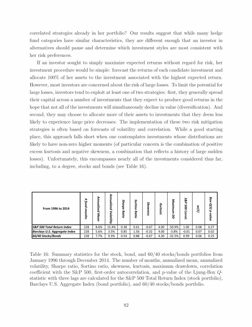
correlated strategies already in her portfolio? Our results suggest that while many hedge

fund categories have similar characteristics, they are different enough that an investor in

alternatives should pause and determine which investment styles are most consistent with

her risk preferences.

If an investor sought to simply maximize expected returns without regard for risk, her

investment procedure would be simple: forecast the returns of each candidate investment and

allocate 100% of her assets to the investment associated with the highest expected return.

However, most investors are concerned about the risk of large losses. To limit the potential for

large losses, investors tend to exploit at least one of two strategies: first, they generally spread

their capital across a number of investments that they expect to produce good returns in the

hope that not all of the investments will simultaneously decline in value (diversification). And

second, they may choose to allocate more of their assets to investments that they deem less

likely to experience large price decreases. The implementation of these two risk mitigation

strategies is often based on forecasts of volatility and correlation. While a good starting

place, this approach falls short when one contemplates investments whose distributions are

likely to have non-zero higher moments (of particular concern is the combination of positive

excess kurtosis and negative skewness, a combination that reflects a history of large sudden

losses). Unfortunately, this encompasses nearly all of the investments considered thus far,

including, to a degree, stocks and bonds (see Table 16).

From 1996 to 2014

# fu

nd

-mo

nth

s

An

nu

alize

d M

ea

n

An

nu

alize

d V

ola

tility

Sh

arp

e R

atio

So

rtino

Ra

tio

Sk

ew

ne

ss

Ku

rtosis

Ma

xim

um

DD

S&

P 5

00

Co

rrel.

ac(1

)

Bo

x-Q

(3) p

-va

lue

S&P 500 Total Return Index 228 8.6% 15.4% 0.38 0.61 -0.67 4.00 -50.9% 1.00 0.08 0.27

Barclays U.S. Aggregate Index 228 5.6% 3.5% 0.85 1.56 -0.32 4.00 -3.8% -0.01 0.07 0.02

60/40 Stocks/Bonds 228 7.7% 9.3% 0.54 0.88 -0.67 4.30 -32.5% 0.99 0.06 0.25

Table 16: Summary statistics for the stock, bond, and 60/40 stocks/bonds portfolios fromJanuary 1996 through December 2014. The number of months, annualized mean, annualizedvolatility, Sharpe ratio, Sortino ratio, skewness, kurtosis, maximum drawdown, correlationcoefficient with the S&P 500, first-order autocorrelation, and p-value of the Ljung-Box Q-statistic with three lags are calculated for the S&P 500 Total Return Index (stock portfolio),Barclays U.S. Aggregate Index (bond portfolio), and 60/40 stocks/bonds portfolio.

82

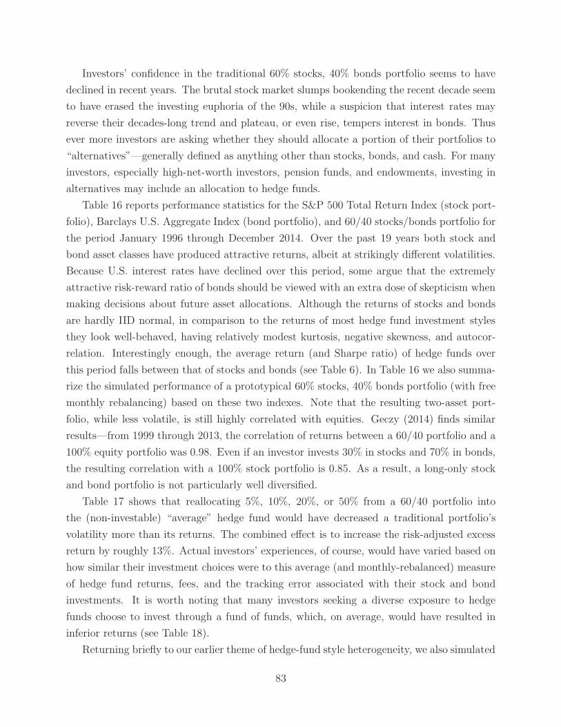
Investors’ confidence in the traditional 60% stocks, 40% bonds portfolio seems to have

declined in recent years. The brutal stock market slumps bookending the recent decade seem

to have erased the investing euphoria of the 90s, while a suspicion that interest rates may

reverse their decades-long trend and plateau, or even rise, tempers interest in bonds. Thus

ever more investors are asking whether they should allocate a portion of their portfolios to

“alternatives”—generally defined as anything other than stocks, bonds, and cash. For many

investors, especially high-net-worth investors, pension funds, and endowments, investing in

alternatives may include an allocation to hedge funds.

Table 16 reports performance statistics for the S&P 500 Total Return Index (stock port-

folio), Barclays U.S. Aggregate Index (bond portfolio), and 60/40 stocks/bonds portfolio for

the period January 1996 through December 2014. Over the past 19 years both stock and

bond asset classes have produced attractive returns, albeit at strikingly different volatilities.

Because U.S. interest rates have declined over this period, some argue that the extremely

attractive risk-reward ratio of bonds should be viewed with an extra dose of skepticism when

making decisions about future asset allocations. Although the returns of stocks and bonds

are hardly IID normal, in comparison to the returns of most hedge fund investment styles

they look well-behaved, having relatively modest kurtosis, negative skewness, and autocor-

relation. Interestingly enough, the average return (and Sharpe ratio) of hedge funds over

this period falls between that of stocks and bonds (see Table 6). In Table 16 we also summa-

rize the simulated performance of a prototypical 60% stocks, 40% bonds portfolio (with free

monthly rebalancing) based on these two indexes. Note that the resulting two-asset port-

folio, while less volatile, is still highly correlated with equities. Geczy (2014) finds similar

results—from 1999 through 2013, the correlation of returns between a 60/40 portfolio and a

100% equity portfolio was 0.98. Even if an investor invests 30% in stocks and 70% in bonds,

the resulting correlation with a 100% stock portfolio is 0.85. As a result, a long-only stock

and bond portfolio is not particularly well diversified.

Table 17 shows that reallocating 5%, 10%, 20%, or 50% from a 60/40 portfolio into

the (non-investable) “average” hedge fund would have decreased a traditional portfolio’s

volatility more than its returns. The combined effect is to increase the risk-adjusted excess

return by roughly 13%. Actual investors’ experiences, of course, would have varied based on

how similar their investment choices were to this average (and monthly-rebalanced) measure

of hedge fund returns, fees, and the tracking error associated with their stock and bond

investments. It is worth noting that many investors seeking a diverse exposure to hedge

funds choose to invest through a fund of funds, which, on average, would have resulted in

inferior returns (see Table 18).

Returning briefly to our earlier theme of hedge-fund style heterogeneity, we also simulated

83

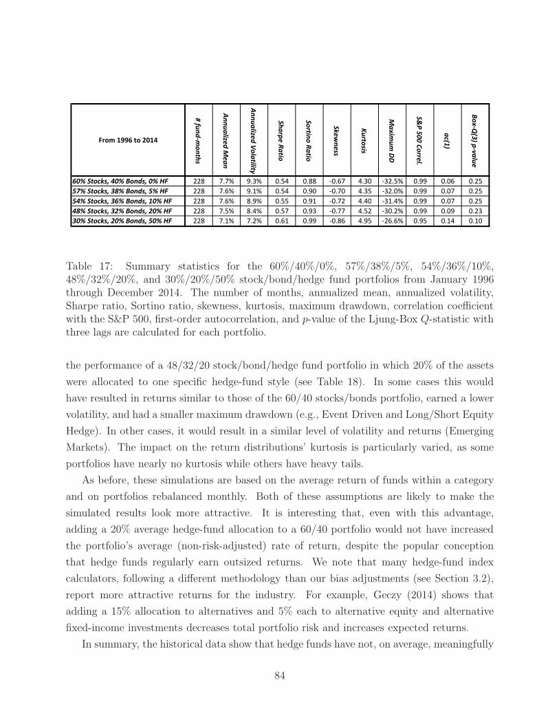
From 1996 to 2014

# fu

nd

-mo

nth

s

An

nu

alize

d M

ea

n

An

nu

alize

d V

ola

tility

Sh

arp

e R

atio

So

rtino

Ra

tio

Sk

ew

ne

ss

Ku

rtosis

Ma

xim

um

DD

S&

P 5

00

Co

rrel.

ac(1

)

Bo

x-Q

(3) p

-va

lue

60% Stocks, 40% Bonds, 0% HF 228 7.7% 9.3% 0.54 0.88 -0.67 4.30 -32.5% 0.99 0.06 0.25

57% Stocks, 38% Bonds, 5% HF 228 7.6% 9.1% 0.54 0.90 -0.70 4.35 -32.0% 0.99 0.07 0.25

54% Stocks, 36% Bonds, 10% HF 228 7.6% 8.9% 0.55 0.91 -0.72 4.40 -31.4% 0.99 0.07 0.25

48% Stocks, 32% Bonds, 20% HF 228 7.5% 8.4% 0.57 0.93 -0.77 4.52 -30.2% 0.99 0.09 0.23

30% Stocks, 20% Bonds, 50% HF 228 7.1% 7.2% 0.61 0.99 -0.86 4.95 -26.6% 0.95 0.14 0.10

Table 17: Summary statistics for the 60%/40%/0%, 57%/38%/5%, 54%/36%/10%,48%/32%/20%, and 30%/20%/50% stock/bond/hedge fund portfolios from January 1996through December 2014. The number of months, annualized mean, annualized volatility,Sharpe ratio, Sortino ratio, skewness, kurtosis, maximum drawdown, correlation coefficientwith the S&P 500, first-order autocorrelation, and p-value of the Ljung-Box Q-statistic withthree lags are calculated for each portfolio.

the performance of a 48/32/20 stock/bond/hedge fund portfolio in which 20% of the assets

were allocated to one specific hedge-fund style (see Table 18). In some cases this would

have resulted in returns similar to those of the 60/40 stocks/bonds portfolio, earned a lower

volatility, and had a smaller maximum drawdown (e.g., Event Driven and Long/Short Equity

Hedge). In other cases, it would result in a similar level of volatility and returns (Emerging

Markets). The impact on the return distributions’ kurtosis is particularly varied, as some

portfolios have nearly no kurtosis while others have heavy tails.

As before, these simulations are based on the average return of funds within a category

and on portfolios rebalanced monthly. Both of these assumptions are likely to make the

simulated results look more attractive. It is interesting that, even with this advantage,

adding a 20% average hedge-fund allocation to a 60/40 portfolio would not have increased

the portfolio’s average (non-risk-adjusted) rate of return, despite the popular conception

that hedge funds regularly earn outsized returns. We note that many hedge-fund index

calculators, following a different methodology than our bias adjustments (see Section 3.2),

report more attractive returns for the industry. For example, Geczy (2014) shows that

adding a 15% allocation to alternatives and 5% each to alternative equity and alternative

fixed-income investments decreases total portfolio risk and increases expected returns.

In summary, the historical data show that hedge funds have not, on average, meaningfully

84

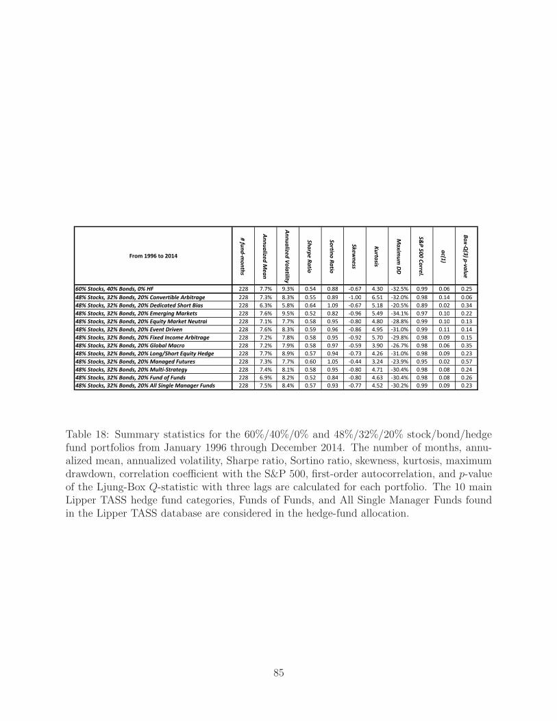
From 1996 to 2014

# fu

nd

-mo

nth

s

An

nu

alize

d M

ea

n

An

nu

alize

d V

ola

tility

Sh

arp

e R

atio

So

rtino

Ra

tio

Sk

ew

ne

ss

Ku

rtosis

Ma

xim

um

DD

S&

P 5

00

Co

rrel.

ac(1

)

Bo

x-Q

(3) p

-va

lue

60% Stocks, 40% Bonds, 0% HF 228 7.7% 9.3% 0.54 0.88 -0.67 4.30 -32.5% 0.99 0.06 0.25

48% Stocks, 32% Bonds, 20% Convertible Arbitrage 228 7.3% 8.3% 0.55 0.89 -1.00 6.51 -32.0% 0.98 0.14 0.06

48% Stocks, 32% Bonds, 20% Dedicated Short Bias 228 6.3% 5.8% 0.64 1.09 -0.67 5.18 -20.5% 0.89 0.02 0.34

48% Stocks, 32% Bonds, 20% Emerging Markets 228 7.6% 9.5% 0.52 0.82 -0.96 5.49 -34.1% 0.97 0.10 0.22

48% Stocks, 32% Bonds, 20% Equity Market Neutral 228 7.1% 7.7% 0.58 0.95 -0.80 4.80 -28.8% 0.99 0.10 0.13

48% Stocks, 32% Bonds, 20% Event Driven 228 7.6% 8.3% 0.59 0.96 -0.86 4.95 -31.0% 0.99 0.11 0.14

48% Stocks, 32% Bonds, 20% Fixed Income Arbitrage 228 7.2% 7.8% 0.58 0.95 -0.92 5.70 -29.8% 0.98 0.09 0.15

48% Stocks, 32% Bonds, 20% Global Macro 228 7.2% 7.9% 0.58 0.97 -0.59 3.90 -26.7% 0.98 0.06 0.35

48% Stocks, 32% Bonds, 20% Long/Short Equity Hedge 228 7.7% 8.9% 0.57 0.94 -0.73 4.26 -31.0% 0.98 0.09 0.23

48% Stocks, 32% Bonds, 20% Managed Futures 228 7.3% 7.7% 0.60 1.05 -0.44 3.24 -23.9% 0.95 0.02 0.57

48% Stocks, 32% Bonds, 20% Multi-Strategy 228 7.4% 8.1% 0.58 0.95 -0.80 4.71 -30.4% 0.98 0.08 0.24

48% Stocks, 32% Bonds, 20% Fund of Funds 228 6.9% 8.2% 0.52 0.84 -0.80 4.63 -30.4% 0.98 0.08 0.26

48% Stocks, 32% Bonds, 20% All Single Manager Funds 228 7.5% 8.4% 0.57 0.93 -0.77 4.52 -30.2% 0.99 0.09 0.23

Table 18: Summary statistics for the 60%/40%/0% and 48%/32%/20% stock/bond/hedgefund portfolios from January 1996 through December 2014. The number of months, annu-alized mean, annualized volatility, Sharpe ratio, Sortino ratio, skewness, kurtosis, maximumdrawdown, correlation coefficient with the S&P 500, first-order autocorrelation, and p-valueof the Ljung-Box Q-statistic with three lags are calculated for each portfolio. The 10 mainLipper TASS hedge fund categories, Funds of Funds, and All Single Manager Funds foundin the Lipper TASS database are considered in the hedge-fund allocation.

85

outperformed traditional portfolios of stocks and bonds after fees. On average, once returns

have been adjusted for various sampling biases (see Section 3.2), hedge funds do not routinely

generate double-digit returns. However, the ride for hedge-fund investors has generally been

smoother: as a group, hedge funds have exhibited lower volatility than traditional stock/bond

portfolios. In addition, there are a number of styles of hedge fund investing. While many

are correlated and have much in common, on the whole they are a heterogeneous lot: some

are as dissimilar as stocks and bonds. This is consistent with Brown and Goetzmann (2003)

who find that hedge funds are a reasonably heterogeneous group and present distinct styles.

Based on historical data, some styles of hedge fund investing result in higher volatility, and

some lower; some are correlated with equities, and some not; and some have a high propensity

to occasionally experience large losses, while others experience this to a lesser extent. Liang

(2004) studies asset allocation among hedge funds, funds of funds, and CTAs. He shows that

CTAs are a natural hedge for equity investments especially during market declines; CTAs

have relatively low correlations with hedge funds and funds of funds, and they have very

different characteristics from most hedge funds (see also Kaminski (2011)). We propose a

more systematic approach to alternative investing in the next section.

8.4 An Integrated Hedge-Fund Investment Process

Investing in hedge funds has changed considerably over the last two decades as the popu-

lation of investors has grown beyond family offices, foundations, endowments, and high net

worth investors to include more traditional institutional investors such as pension funds,

sovereign wealth funds, and investment consultants. This shift in the investor base has

brought new tools, policies, and procedures to the hedge-fund industry because today’s in-

stitutional investors require an unprecedented degree of transparency, accountability, and

repeatability, i.e., they require an investment process, not just the ability to select a port-

folio of hedge funds. Although in the past many institutional investors relied primarily on

the qualitative judgments that funds of funds managers offer, institutional investors today

often prefer a more systematic approach to making manager-selection decisions, as well as

broader asset-allocation decisions among various hedge-fund style categories.

Several systematic approaches have been proposed, largely led by practitioners from the

hedge-fund and funds of funds industry, and these approaches fall loosely into two groups:

top-down and bottom-up investment processes.

Goldman, Sachs & Co. and Financial Risk Management Ltd. (1999) develop a top-

down absolute-return framework emphasizing diversification across as well as within hedge-

fund strategies, with the primary constraint being the investor’s ability to monitor multiple

86

managers. Bein and Wander (2002) propose a top-down risk allocation framework that

allows investors to explicitly integrate active management decisions and hedge-fund risks into

a traditional overall asset allocation process. Chung, Rosenberg, and Tomeo (2004) provide

another top-down hedge-fund asset allocation process by dividing hedge-fund strategies into

two classes: convergent strategies that benefit from small temporary mispricings, which

are short volatility, and divergent strategies that exploit larger and longer-horizon market

inefficiencies, which are long volatility. Given that divergent strategies tend to be profitable

during periods of heightened volatility and economic uncertainty, the authors argue that

allocating assets to both types of strategies can improve expected returns and reduce risk.

Several studies propose a bottom-up approach to constructing hedge-fund portfolios.

Zask (2000) describes a method for hedge-fund valuation based on management fees, per-

formance fees, and discounted cash flows analysis. Stemme and Slattery (2002) outline the

practical considerations involved in selecting individual hedge funds, hiring a consultant, or

investing in a fund of funds, including costs, control, track record, and capacity issues. And

Clark and Winkelmann (2004) develop a framework where all hedge funds are analyzed based

on how much of the projected performance is due to market movements, due to manager

skill, and whether an investor is confident in the manager’s (or strategy’s) ability to continue

to deliver performance.

A hybrid approach proposed by Lo (2008) combines qualitative judgment with quantita-

tive methods, a particularly important feature for investing in complex, multi-faceted, and

highly heterogeneous assets such as hedge funds. This combination is achieved through a

two-stage investment process in which a top-down asset allocation decision to broad hedge-

fund categories is coupled with bottom-up manager-selection decisions within each category.

Although a two-stage investment process is generally sub-optimal relative to a single-stage

optimization, the complexities and qualitative aspects of hedge-fund investing make a two-

stage approach more robust and easier to implement. This investment process is based on a

set of six basic design principles:

• The target expected return for each strategy should be commensurate with the risks

of that strategy—higher-risk strategies should have higher target expected returns.

• The uses of funds should determine the target expected return, not the sources of

capital.

• In evaluating the risk/reward ratio for each strategy, return autocorrelation and illiq-

uidity exposure should be taken into account explicitly. In particular, the Sharpe ratios

of strategies with large positively serially correlated returns should be deflated (see Lo

87

(2001), Getmansky, Lo, and Makarov (2004), and Section 5 for details).

• Qualitative judgments about managers, strategies, and market conditions are valuable

inputs into the capital allocation process that no quantitative models can replace,

but those judgments should be integrated in a systematic and consistent fashion with

quantitative methods.

• Risk and performance attribution should be performed on a regular basis for and by

each manager, as well as for the entire portfolio.

• Risk limits and related guidelines for each manager should be consistent across time

and across managers, and should be communicated clearly to all managers on a regular

basis.

These design principles, coupled with insights from traditional portfolio management

theory and practice, imply a portfolio optimization component in which required or “target”

expected returns and variances are determined in advance by investor mandates and market

conditions, covariances are estimated via econometric methods and modified by qualitative

judgment, and then asset-class allocations are determined by minimizing variance subject

to an expected-return constraint. Within each asset class, manager-specific allocations are

determined by incorporating qualitative information into the investment process through a

scoring process. The seven components of this quantitative/qualitative investment process,

which we shall refer to as QQIP for convenience, are depicted in Figures 7 and 8 and given

by:

(i) Define asset classes by strategy.

(ii) Set target portfolio expected return, µo, and desired volatility, σo.

(iii) Set target expected returns and risks for asset classes.

(iv) Determine correlations via econometric analysis.

(v) Compute minimum-variance asset-class allocations subject to µo constraint.

(vi) Allocate capital to managers within each asset class.

(vii) Monitor performance and risk budgets, and re-optimize as needed.

Although Lo (2008) provides detailed discussions for each of these steps, he emphasizes

that this framework is meant to serve only as a starting point for designing a suitable

alternative investment process. Because of the heterogeneity of the hedge-fund industry and

the variability of investment objectives and constraints among investors, there is no single

investment process that fits all investors.

88

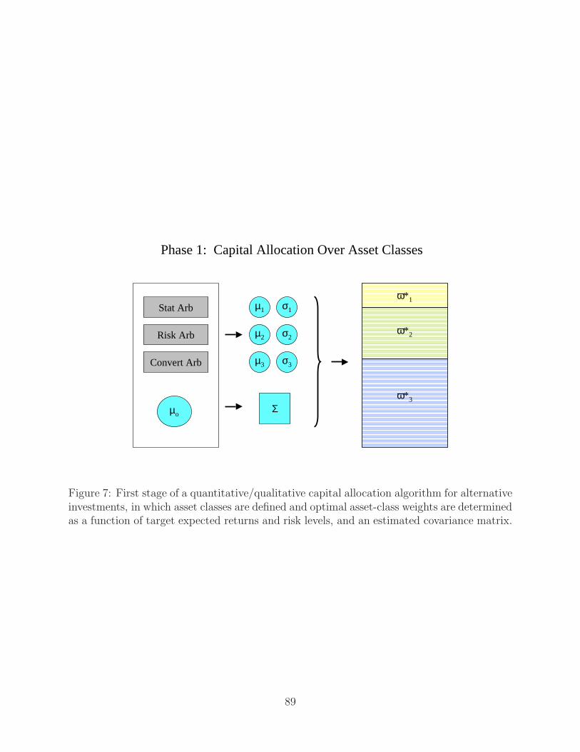
Stat Arb

Risk Arb

Convert Arb

µo

µ3

µ2

µ1 σ1

σ2

σ3

Σ

ω* 1

ω* 2

ω* 3

Phase 1: Capital Allocation Over Asset Classes

Figure 7: First stage of a quantitative/qualitative capital allocation algorithm for alternativeinvestments, in which asset classes are defined and optimal asset-class weights are determinedas a function of target expected returns and risk levels, and an estimated covariance matrix.

89

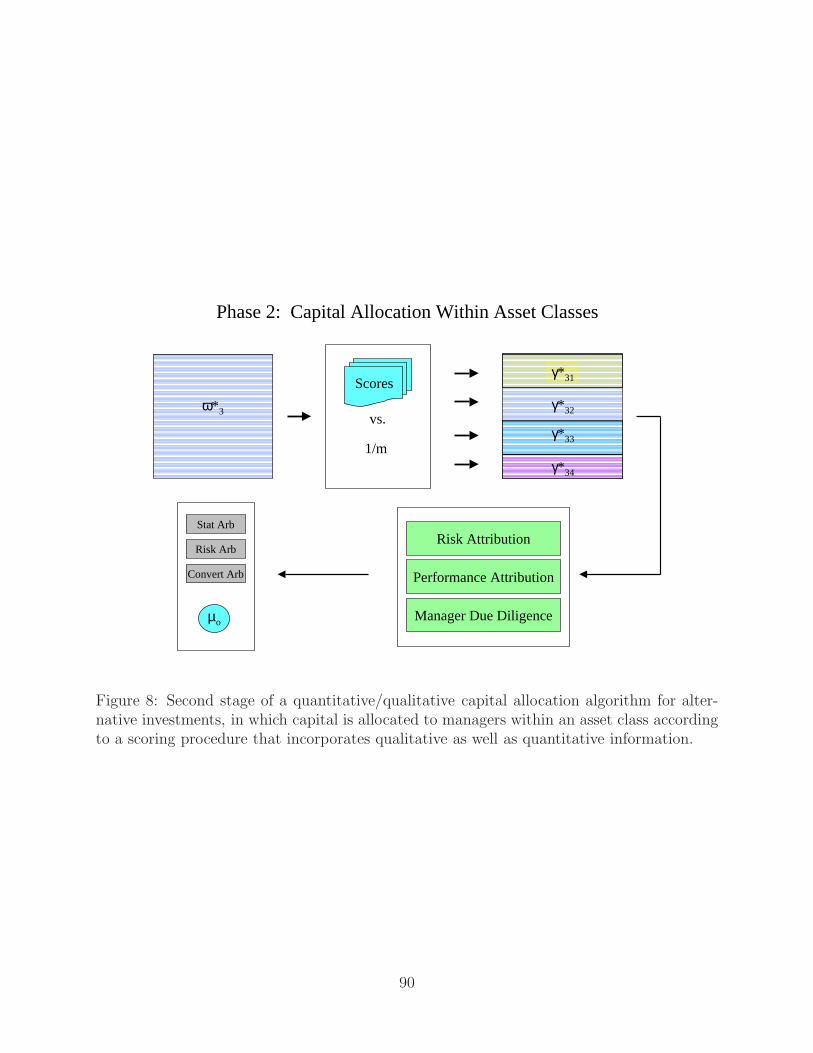
Phase 2: Capital Allocation Within Asset Classes

ω* 3

Scores

vs.

1/m

γ* 32

γ* 34

γ* 33

γ* 31

Risk Attribution

Performance Attribution

Manager Due Diligence

Stat Arb

Risk Arb

Convert Arb

µo

Figure 8: Second stage of a quantitative/qualitative capital allocation algorithm for alter-native investments, in which capital is allocated to managers within an asset class accordingto a scoring procedure that incorporates qualitative as well as quantitative information.

90

The first step in QQIP is to define the universe of all hedge funds into a smaller set of

categories where managers in each category pursue relatively homogeneous styles of investing.

An example of such categories is the Lipper TASS classification used throughout this survey

and described in the Appendix, but finer stratifications may be appropriate, depending on

the investment objectives of the investor and the size of the assets to be deployed.

The second step is to set a target expected return, desired level of risk, and acceptable

loss limits or maximum drawdown for the entire portfolio. While these parameters are, by

nature, rather ambiguous quantities when discussed among investment committee members

and investment officers, such discussions are invaluable in setting realistic expectations for

what a portfolio of hedge funds can offer.

Once these high-level parameters (or ranges of parameters) have been specified, the third

step is to do the same for the categories specified in the first step. This requires more

specialized knowledge of both the historical performance of individual categories of hedge

funds and how the categories are currently positioned. One way to develop target expected

returns and volatilities for hedge fund categories is to estimate linear factor models for

category indexes (see Section 6), and then to develop target expected returns and volatilities

for the factors. In many cases, it is easier to develop prospective intuition for the likely

behavior of factors such as liquidity, credit, the business cycle, and exchange ratios than for

hedge-fund category index returns.

Given the target expected returns and volatilities of the hedge-fund categories in the

investment universe, the next step in QQIP is to estimate the correlation matrix among

the index returns of the hedge-fund categories. This may seem straightforward from a

statistical perspective—use the standard estimator with historical data or a linear factor

model estimator that requires fewer estimated parameters (see Section 6.2). However, the

fact that correlations can change in response to market conditions makes this step more

challenging, requiring qualitative input to adjust the correlations to reflect current market

conditions that might not yet be reflected in historical time series estimators.33 In such

cases, qualitative adjustments to the correlation matrix of category-index returns may be

necessary, but it must be kept in mind that arbitrary changes to entries in a correlation matrix

could violate the positive semidefiniteness of the matrix. If such violations are ignored, the

outcome of a portfolio optimization using such a matrix could yield nonsensical results such

as negative variances. To avoid these pathologies, it is possible to compute the positive

semidefinite correlation matrix that is “closest” to the qualitatively adjusted correlation

33For example, during periods of macroeconomic stress, U.S. equities become more highly correlated withforeign currency movements, hence correlations between long/short equity managers and foreign currencytraders may be higher than historical estimates would imply if economic conditions deteriorate.

91

matrix using methods developed by Higham (2002) and Qi and Sun (2006).

Once the target expected returns, volatilities, and correlations among the hedge-fund

categories have been determined, the next step in QQIP is to construct an optimal portfolio.

There are several methods for doing so—see, for example, Brennan, Lo, and Nguyen (2015)—

but a natural starting point is to find the asset allocation over hedge-fund categories that

minimizes the portfolio variance subject to the target portfolio expected return constraint

specified in step 1. For most fund-of-fund and multi-manager applications, it is also necessary

to impose non-negativity constraints on the portfolio weights since it is typically impossible to

establish a “short” position in a manager. However, as long as the target expected returns are

realistic and the covariance matrix is well-behaved, (19) should yield non-negative portfolio

weights.34

Minω

12ω

′Σω subject to ω′µ ≥ µo and ω

′ι = 1 . (18)

The solution to (18) is given by (see Lo (2008)):

ω∗ = λΣ−1

µ + ξΣ−1ι (19)

where λ and ξ are constants defined in Lo (2008). As a consistency check, it is useful to

compute the volatility σ of the entire portfolio implied by ω∗:

σ =√ω∗′Σω∗ . (20)

If σ is higher than σo, this implies an inconsistency with the following set of objectives:

• target expected return (µo)

• desired risk level (σo)

• target expected returns and risks of asset classes (µi, σi)

and at least one of these three objectives must be modified to restore consistency. If the

total investment capital is K, the optimal dollar-allocation to each asset class is simply K∗

i

34If not, this may be a sign of model misspecification that can serve as a useful diagnostic for identifyingpotential problems with the portfolio construction process. Alternatively, recent innovations in structuredproducts do allow the synthetic shorting of certain hedge-fund strategies, in which case, more efficient fund-of-funds portfolios may be possible. However, given the complexities of over-the-counter derivatives on hedgefunds and the significant risks they can generate, the shorting hedge funds should be contemplated only bythe most sophisticated and well-capitalized investors.

92

where:

K∗

i = ω∗

i K (21)

Once the category asset allocations, {K∗

i }, have been determined, the next step is to

decide how to allocate each K∗

i across individual managers within each category i. Although

a similar mean-variance optimization may be performed at this stage, the target expected

returns, variances, and correlations among individual managers are much harder to estimate

precisely. Therefore, the impact of estimation error may outweigh the gains from optimiza-

tion methods at this level.

An alternative is to begin with identical allocations, K∗

i /mi, across all mi managers in

category i that satisfy certain minimum conditions, e.g., assets under management, years of

experience, track record, etc. Then for each manager, construct a score, Sik, by evaluating

the manager against the following criteria, perhaps using a numerical score from 1 to 5 for

each criterion:

• anticipated alpha

• anticipated risk

• anticipated capacity

• anticipated correlation with other managers and asset classes

• trading experience and past performance

• backtest performance attribution

• tracking error

• risk controls

• risk transparency

• alpha transparency

• operational risks

• social impact

• other qualitative characteristics

For example, a manager with a high anticipated alpha—as determined through the largely

qualitative manager-selection and due-diligence processes—would receive a score of 5, and

a manager with a low anticipated alpha would receive a score of 1. Similarly, a high-risk

manager (relative to the asset-class volatility, σi) would receive a score of 1 and a moderate-

risk manager would receive a score of 3. The sum of each of these ratings yields the manager’s

93

score, Sik. Then define the relative score, sik, as:

sik =Sik

Si1 + · · ·+ Simi

. (22)

These scores are given equal weighting in (22) but can easily be assigned unique weights to

over- or under-emphasize specific attributes. The manager’s allocation can then be defined

as:

γik = (1− δ)× 1

mi

+ δ × sik (23)

where δ is a parameter that determines the weight placed on the relative score (22) vs.

equal-weighting.

For a given set of manager allocations, γi≡ [ γi1 · · · γimi]′, in asset class i, the implied

expected return and volatility of the asset class are given by:

µi = γ′

iν i , σi =√

γ′

iΣiγi (24)

where νi is the vector of expected returns of each manager in asset class i (as determined ei-

ther by backtests or historical performance), and Σi is the covariance matrix of the managers

in asset class i. Before implementing the allocation γi, it is important to check whether the

implied expected return and risk of γ i given in (24) is consistent with the target expected

return and risk, µi and σi, for sector i. If not, then the allocations in γi may need to be

adjusted, or the target expected return and risk must be adjusted to reduce the discrepancy.

Given an allocation γ i, each manager’s dollar allocation is then:

K∗

ik = K∗

i × γik . (25)

These scores should be recomputed at least quarterly, and possibly more frequently as

changes in market conditions might dictate. Each manager should be given his/her score so

that the manager is aware of the link between performance (as determined by the many di-

mensions of the score) and capital allocation. Moreover, such scores can be used as a hurdle

for evaluating new managers, so that the process of manager selection is less arbitrary over

time and across individual fund analysts.

94

The last step in QQIP is to monitor the performance of each manager regularly to ensure

that risk budgets and investment mandates are being maintained, and that managers are

not straying from their stated styles. For example, if the target risk of asset class i is σi,

then the realized volatility, σi, of the asset class can be compared to σi to determine any

discrepancies that require further investigation, where:

σi ≡√

γ′

iΣiγi (26)

andΣi is the estimated covariance matrix of themi managers in asset class i. Those managers

that contribute more than proportionally to the asset-class volatility σi may be required to

accept lower capital allocations, and vice versa, other things equal. As performance varies

and as parameters change, the allocations across asset classes and across managers will

require periodic updating. Allocations should be recomputed monthly, although no action is

needed unless the updated allocations are significantly different from the current allocations.

The scope of QQIP can be broadened to include other alternative investments such as

venture capital, private equity, and impact investments. However, in such cases, a mean-

variance objective function is likely to be inadequate for capturing the investment charac-

teristics of these asset classes. In particular, both venture capital and private equity contain

significant illiquidity premia given the nature of those investments, and also involve longer

holding periods, hence the mean-variance-liquidity objective function described in Section

5.4 and depicted in Figure 3 may be more appropriate. For impact investments such as

environment-related technologies, socially responsible companies, and venture philanthropy,

additional metrics that measure impact must be incorporated into the objective function

along with risk and expected return. Once such metrics are constructed, the framework of

QQIP can be applied to the augmented objective function.

QQIP is considerably more intricate than the straightforward construction of a typical

long-only large-cap U.S. equity portfolio, but the intricacies are a manifestation of the greater

complexities of alternative investments, and the fact that qualitative judgment still plays a

significant role in this endeavor. Nevertheless, the industry is changing rapidly and the

hedge-fund investment process is becoming more systematic across all investors. Supporting

this trend are various innovations in academic research, new and improved hedge-fund data

sources, more sophisticated software applications for hedge-fund portfolio construction and

risk management, and professional organizations such as the Alternative Investment Man-

agement Association (AIMA), the Managed Funds Association (MFA), and the Chartered

Alternative Investment Analysts (CAIA) Association and CAIA certification. These inno-

95

vations parallel the shift in the mutual fund industry during the 1970s and 1980s toward

greater transparency, lower fees, and a more disciplined investment framework, all of which

has contributed to the growth and success of the entire industry.

8.5 The Adaptive Markets Hypothesis

One of the most enduring challenges to the very existence of the hedge-fund industry is the

Efficient Markets Hypothesis (EMH), the idea that market prices fully reflect all available

information. If the EMH holds, how can hedge funds earn “excess” expected returns over

time? The answer to this question is not just of academic interest—it has consequences for

how investors should allocate their capital across traditional and alternative assets, and how

they and regulators should respond to the rapid growth of the hedge-fund industry.

One possible answer is that the EMH is false and hedge funds routinely exploit the

departures from efficiency. However, this explanation does not account for the high failure

rate in the hedge-fund industry, the capacity constraints that the most successful funds face,

and the occasional periods of significant underperformance experienced by the entire industry

in comparison to passive buy-and-hold investments. By all accounts, it is very difficult to

produce excess risk-adjusted returns consistently and for large pools of assets.

The other extreme is that the EMH is true and hedge funds are simply taking on ad-

ditional sources of risk that have positive risk premia associated with them. There is some

empirical evidence for this view based on estimates of linear factor models for hedge fund

returns in which liquidity, credit, and volatility are statistically significant factors driving

industry returns (see Section 6). However, there are a number of inordinately successful man-

agers that earn positive risk-adjusted returns even after controlling for such factors, including

industry icons such as Warren Buffett, Paul Tudor Jones, Julian Robertson, David Shaw,

James Simons, George Soros, and others. It is difficult to dismiss all of these individuals as

statistical flukes.

The theoretical foundations of the hedge-fund industry can be found in the work of

Sandy Grossman, a successful hedge-fund manager in his own right. In Grossman (1976)

and Grossman and Stiglitz (1980), he and Nobel-prize-winning economist Joseph Stiglitz

argue convincingly that perfectly informationally efficient markets are an impossibility. If

markets are perfectly efficient, there is no profit to gathering information, in which case there

would be little reason to trade and markets would not exhibit the volume they currently do.

Alternatively, market efficiency is not a binary state but rather a continuum; the degree

of market inefficiency determines the effort investors will expend to gather and trade on

information. Therefore, a non-degenerate market equilibrium occurs only when there are

96

sufficient profit opportunities, i.e., inefficiencies, to compensate investors for the costs of

trading and information-gathering. The profits earned by these industrious investors are

not free lunches, but the “economic rents” that accrue to those willing to engage in such

activities.

Who are the providers of these rents? Black (1986) provides a compelling answer: “noise

traders”, individuals who trade for non-informational reasons such as liquidity needs, port-

folio rebalancing trades, or random misinformation.

More broadly, the conflict between the EMH and the hedge-fund industry can be rec-

onciled by acknowledging that, like any other industry, value-added is created through in-

novation and eventually commoditized and depleted through competition. For example,

the first mobile device that allowed users to exchange emails remotely—the Blackberry by

Research In Motion (RIM)—generated enormous shareholder value for its owners. The re-

turns that accrued to RIM’s original investors are unlikely to be explained by any set of risk

factors, especially since the mobile communications industry was just emerging, thanks in

no small part to the market that RIM created. Since then, this industry has matured and

several competitors to the Blackberry have captured significant market share, including the

Apple iPhone and other Android smartphones. The recent returns to RIM investors have

been disappointing, not because of changes in factor risk premia, but because competition

has reduced RIM’s customer base and RIM has not yet fully adapted to current market

conditions.

The dynamics of industrial organization and competition can easily explain the rise and

fall of corporations—the same principles apply to hedge-fund strategies and funds. The

waxing and waning and re-emergence of various hedge-fund styles are simply manifestations

of Schumpeter’s (1939) “creative destruction”, an observation that led Lo (2012) to call

the hedge-fund industry the “Galapagos Islands of the financial sector”.35 By appealing to

the principles of evolution—innovation, adaptation, competition, and natural selection—Lo

(2004, 2005, 2012, 2015) develops an alternative to the EMH which he calls the Adaptive

Markets Hypothesis (AMH). The AMH provides a natural and internally consistent recon-

ciliation of the apparent contradiction between the EMH and the existence and profitability

of hedge funds. From the AMH perspective, the EMH is not wrong; it is simply incomplete.

Prices reflect as much information as is available from the combination of environmental con-

ditions and the number and nature of “species” in the economy or, to use the appropriate

biological term, the market ecology. By species, Lo is referring to distinct groups of mar-

35Other evolutionary models of financial markets include: Blume and Easley (1992), Luo (1995, 1998,2001, 2003), Farmer and Lo (1999), Farmer (2002), Hirshleifer and Luo (2001), Kogan, Ross, Wang, andWesterfield (2006), and Brennan and Lo (2011).

97

ket participants, each behaving in a common manner. For example, pension funds may be

considered one species; mutual funds, another; broker/dealers, a third; and hedge-fund man-

agers, a fourth. If multiple species—or the members of a single highly populous species—are

competing for scarce resources within a single market, that market is likely to become highly

efficient, e.g., the market for S&P 500 futures contracts. If, on the other hand, a small num-

ber of species are competing for rather abundant resources in a given market, that market

is likely to be less efficient, e.g., the market for pre-Columbian artifacts. Market efficiency

is highly context-dependent and dynamic, in much the same way that animal populations

advance and decline as a function of the seasons, the number of predators and prey they

face, and their abilities to adapt to an ever-changing environment.

The profit opportunities in any given market are akin to the amount of food and water

in a particular local ecology—the more resources present, the less fierce the competition. As

competition increases, either because of dwindling food supplies or an increase in the animal

population, resources are depleted which, in turn, causes a population decline eventually, de-

creasing the level of competition and starting the cycle again. In some cases, cycles converge

to corner solutions, i.e., certain species become extinct, food sources are permanently ex-

hausted, or environmental conditions shift dramatically. By viewing economic profits as the

ultimate food source on which market participants depend for their survival, the dynamics of

market interactions and financial innovation can be readily derived. From this perspective,

the hedge-fund industry is the Galapagos Islands of the financial system—evolutionary dy-

namics can be seen by the naked eye through the waxing and waning of investment strategies

and the birth and death of hedge funds across the various categories. And in the same way

that an extinction event for one species can generate ripple effects that have devastating

consequences for many other species, extreme losses in the hedge-fund industry can serve as

early warning signs of far greater dislocation in the financial ecosystem (see Section 7.1).

Under the AMH, there is no contradiction between the competitiveness of the financial

industry and the possibility that market dislocation can occur and, as a result, certain

hedge funds can earn extraordinary profits. During the Fall of 1998, the desire for liquidity

and safety by a certain population of investors overwhelmed the population of hedge funds

attempting to arbitrage such preferences, causing those arbitrage relations to break down.

However, in the years prior to August 1998, fixed-income relative-value traders profited

handsomely from these activities, presumably at the expense of individuals with seemingly

“irrational” preferences. In fact, such preferences were shaped by a certain set of evolutionary

forces, and might be quite rational in other contexts.

Therefore, under the AMH, investment strategies undergo cycles of profitability and loss

in response to changing business conditions, the number of competitors entering and exiting

98

the industry, and the type and magnitude of profit opportunities available. As opportu-

nities shift, so too will the affected populations. For example, after 1998, the number of

fixed-income relative-value hedge funds declined dramatically—because of outright failures,

investor redemptions, and fewer startups in this sector—but many reappeared in subsequent

years as performance for this type of investment strategy improved, until the Financial Crisis

of 2007–2009.

Empirical support for the AMH as it applies to the hedge-fund industry can be found

in the dynamics of hedge-fund births and deaths, documented in Section 3.3. Hedge-fund

strategies and funds wax and wane in response to risk and reward, as Table 3 clearly shows.

A more specific illustration is contained in Figure 9, which depicts the entries, exits, and

average annual returns for funds in two particularly dynamic hedge-fund categories, fixed-

income arbitrage and equity market neutral. Figure 9a shows that the 1998 rout in fixed-

income arbitrage caused a slight increase in the number of funds exiting this category, but

its annual returns recovered quickly and the total number of fixed-income-arbitrage funds

continued to climb until the Financial Crisis of 2007–2009. However, even before the crisis

hit, as the average annual return of fixed-income arbitrage trended downward from 2001 to

2006, the number of exits climbed. Beginning in 2007, the widespread liquidity problems of

the crisis caused returns to drop precipitously, along with an unprecedented exodus of capital

and hedge funds from fixed-income arbitrage, after which returns improved once more.

Figure 9b offers a somewhat different narrative for equity market neutral hedge funds,

whose pre-crisis annual returns were more stable than those of fixed-income arbitrage. This

stability contributed to the popularity of this category, also known as “statistical arbitrage”,

which grew rapidly until its peak in 2007. However, the Quant Meltdown of August 2007

caught many investors and managers by surprise (see Section 7.1), and led to a large number

of hedge-fund exits and capital flight from this category post-crisis. Returns are recovering

and there are signs that this category is waxing again, however, the changing technological

and regulatory landscape of equity markets have greatly increased the complexity of the

environment in which equity market neutral hedge funds operate.

The AMH has a number of concrete implications for the hedge-fund industry. The first

implication is that contrary to the classical EMH, arbitrage opportunities do exist from time

to time in the AMH, as Grossman and Stiglitz (1980) have argued. From an evolutionary

perspective, the existence of active liquid financial markets implies that profit opportunities

must be present. As they are exploited, they disappear. But new opportunities are also

continually being created as certain species die out, as others are born, and as institutions

and business conditions change. Rather than the inexorable trend towards higher efficiency

predicted by the EMH, the AMH implies considerably more complex market dynamics, with

99

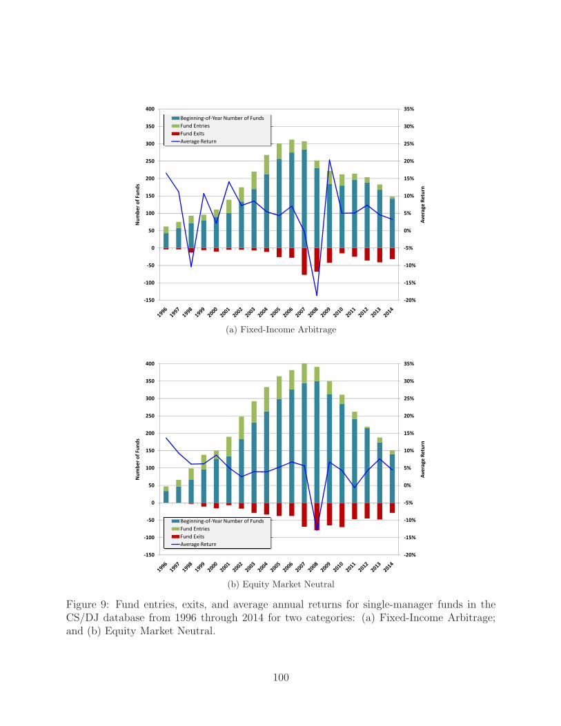
5%

10%

15%

20%

25%

30%

35%

100

150

200

250

300

350

400

Av

era

ge

Re

turn

Nu

mb

er

of

Fu

nd

s

Beginning-of-Year Number of Funds

Fund Entries

Fund Exits

Average Return

-20%

-15%

-10%

-5%

0%

-150

-100

-50

0

50

Av

era

ge

Re

turn

Nu

mb

er

of

Fu

nd

s

(a) Fixed-Income Arbitrage

5%

10%

15%

20%

25%

30%

35%

100

150

200

250

300

350

400

Av

era

ge

Re

turn

Nu

mb

er

of

Fu

nd

s

-20%

-15%

-10%

-5%

0%

-150

-100

-50

0

50

Av

era

ge

Re

turn

Nu

mb

er

of

Fu

nd

s

Beginning-of-Year Number of Funds

Fund Entries

Fund Exits

Average Return

(b) Equity Market Neutral

Figure 9: Fund entries, exits, and average annual returns for single-manager funds in theCS/DJ database from 1996 through 2014 for two categories: (a) Fixed-Income Arbitrage;and (b) Equity Market Neutral.

100

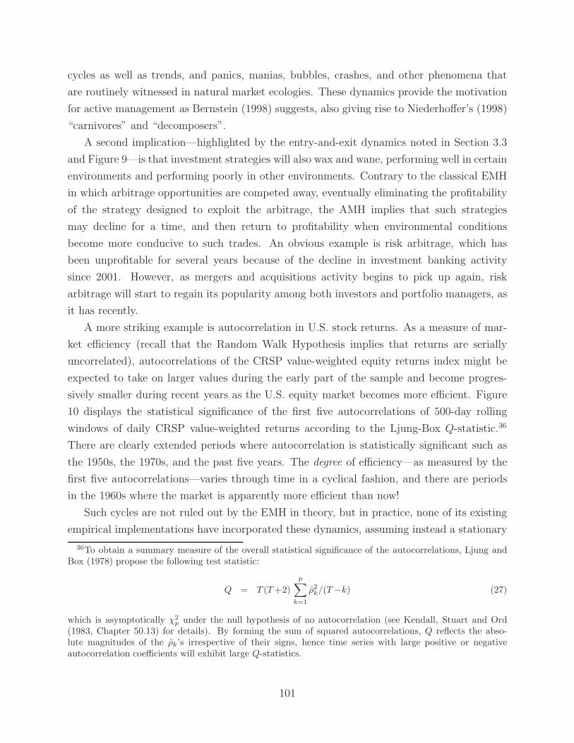
cycles as well as trends, and panics, manias, bubbles, crashes, and other phenomena that

are routinely witnessed in natural market ecologies. These dynamics provide the motivation

for active management as Bernstein (1998) suggests, also giving rise to Niederhoffer’s (1998)

“carnivores” and “decomposers”.

A second implication—highlighted by the entry-and-exit dynamics noted in Section 3.3

and Figure 9—is that investment strategies will also wax and wane, performing well in certain

environments and performing poorly in other environments. Contrary to the classical EMH

in which arbitrage opportunities are competed away, eventually eliminating the profitability

of the strategy designed to exploit the arbitrage, the AMH implies that such strategies

may decline for a time, and then return to profitability when environmental conditions

become more conducive to such trades. An obvious example is risk arbitrage, which has

been unprofitable for several years because of the decline in investment banking activity

since 2001. However, as mergers and acquisitions activity begins to pick up again, risk

arbitrage will start to regain its popularity among both investors and portfolio managers, as

it has recently.

A more striking example is autocorrelation in U.S. stock returns. As a measure of mar-

ket efficiency (recall that the Random Walk Hypothesis implies that returns are serially

uncorrelated), autocorrelations of the CRSP value-weighted equity returns index might be

expected to take on larger values during the early part of the sample and become progres-

sively smaller during recent years as the U.S. equity market becomes more efficient. Figure

10 displays the statistical significance of the first five autocorrelations of 500-day rolling

windows of daily CRSP value-weighted returns according to the Ljung-Box Q-statistic.36

There are clearly extended periods where autocorrelation is statistically significant such as

the 1950s, the 1970s, and the past five years. The degree of efficiency—as measured by the

first five autocorrelations—varies through time in a cyclical fashion, and there are periods

in the 1960s where the market is apparently more efficient than now!

Such cycles are not ruled out by the EMH in theory, but in practice, none of its existing

empirical implementations have incorporated these dynamics, assuming instead a stationary

36To obtain a summary measure of the overall statistical significance of the autocorrelations, Ljung andBox (1978) propose the following test statistic:

Q = T (T+2)

p∑

k=1

ρ2k/(T−k) (27)

which is asymptotically χ2p under the null hypothesis of no autocorrelation (see Kendall, Stuart and Ord

(1983, Chapter 50.13) for details). By forming the sum of squared autocorrelations, Q reflects the abso-lute magnitudes of the ρk’s irrespective of their signs, hence time series with large positive or negativeautocorrelation coefficients will exhibit large Q-statistics.

101

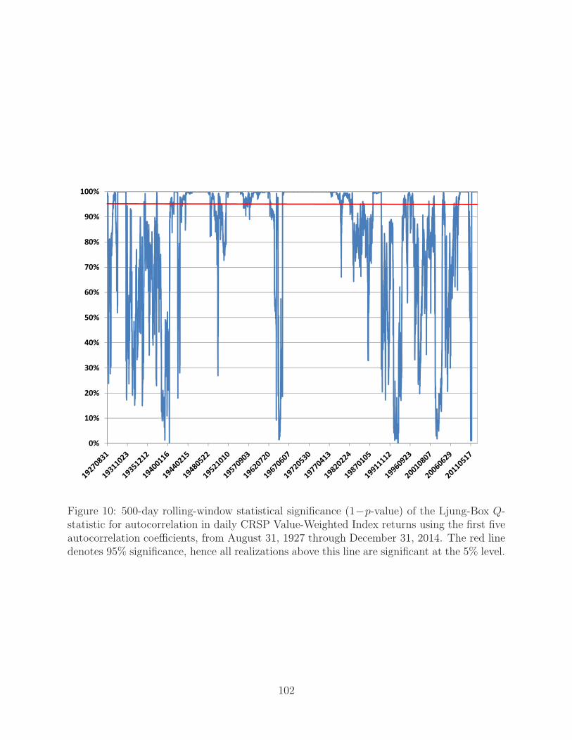
40%

50%

60%

70%

80%

90%

100%

0%

10%

20%

30%

Figure 10: 500-day rolling-window statistical significance (1−p-value) of the Ljung-Box Q-statistic for autocorrelation in daily CRSP Value-Weighted Index returns using the first fiveautocorrelation coefficients, from August 31, 1927 through December 31, 2014. The red linedenotes 95% significance, hence all realizations above this line are significant at the 5% level.

102

world in which markets are perpetually in equilibrium. This widening gulf between the

stationary EMH and obvious shifts in market conditions have no doubt contributed to the

recent spate of new investment offerings including risk-parity funds, tactical asset allocation

funds, and various active ETFs.

A third implication is that innovation is the key to survival. The classical EMH suggests

that certain levels of expected returns can be achieved simply by bearing a sufficient degree

of risk. The AMH implies that the risk/reward relation varies through time, and that

a better way of achieving a consistent level of expected returns is to adapt to changing

market conditions. By evolving a multiplicity of capabilities that are suited to a variety of

environmental conditions, investment managers are less likely to become extinct as a result

of rapid changes in business conditions. Consider the current theory of the demise of the

dinosaurs (Alvarez, 1997), and ask where the next financial asteroid might come from.

Finally, the AMH has a clear implication for all financial market participants: survival is

the only objective that matters in the long run. While profit maximization, utility maximiza-

tion, and general equilibrium are certainly relevant aspects of market ecology, the organizing

principle in determining the evolution of markets and financial technology is simply survival.

These evolutionary underpinnings are more than simple speculation in the context of the

hedge-fund industry. The extraordinary degree of competitiveness of global financial mar-

kets, the outsize rewards that accrue to the “fittest” managers, and the relatively low barriers

to entry and minimal fixed costs of setup suggest that Darwinian selection—“survival of the

richest”, to be precise—is at work in determining the typical profile of the successful hedge

fund. After all, unsuccessful managers are rather quickly eliminated from the population af-

ter suffering a certain level of losses, only to be replaced by many eager professionals hoping

to make their own name in this dynamic industry. In the same spirit in which the evolution-

ary biologist Theodosius Dobzhansky (1973) observed that “nothing in biology makes sense

except in the light of evolution”, none of the dynamics of the hedge-fund industry make

sense except in the light of adaptive markets.

103

9 Conclusion

Two dangerous myths about hedge funds can mislead investors, portfolios, regulators, and

policymakers into making inappropriate decisions. The first myth is that all hedge funds are

alike, implying that alternative investments comprise a homogeneous asset class that have

similar investment characteristics with returns that move in concert. The second myth is

that all hedge funds are unique, implying no commonalities and, therefore, no implications

for diversification or systemic risk. In this review article, we hope to have dispelled both

these myths by reviewing various aspects of the hedge-fund literature and their implications

for all stakeholders in this important and dynamic industry.

The freedom with which hedge funds are allowed to invest their capital gives them unique

breadth of coverage as an industry and unique depth of expertise at the individual fund level.

However, their unconstrained and varied investment strategies contain non-standard forms

of risk including phase-locking behavior, illiquidity, nonlinearities, and operational risks that

are poorly captured by conventional metrics. More sophisticated risk models are available,

but they require much greater training and experience.

The highly competitive nature of this industry implies rapid innovation and attrition,

which can greatly benefit the nimble and risk-tolerant investor, but which can be a source

of great stress and financial loss for the naive and inattentive investor. But considering the

suitability of the various risk dimensions associated with each hedge-fund investment style

along with the potential for generating attractive returns, investors can construct a sys-

tematic investment process that incorporates hedge-fund investments into more traditional

portfolios.

The adaptiveness of the hedge-fund industry also implies that hedge funds can serve as an

invaluable monitoring system for identifying trouble spots throughout the financial system.

The Financial Crisis of 2007–2009 left a significant mark on the industry, ending an era of

excessive optimism about hedge-fund returns and starting a new era in which the industry

is retrenching and re-emphasizing its core competencies under heavy investor scrutiny.

Because the hedge-fund industry will continue to evolve rapidly in response to new chal-

lenges and opportunities, continuous monitoring and research will be necessary for investors,

regulators, and hedge-fund managers to keep up with these changes, and we hope this survey

provides a useful perspective for this task.

104

A Appendix

A.1 Lipper TASS Fund Category Definitions

The following is a list of Lipper TASS category descriptions, that defines the criteria used

by Lipper TASS in assigning funds in their database to one of 11 possible categories:

Convertible Arbitrage This strategy is identified by hedge investing in the convertible securities of a

company. A typical investment is to be long the convertible bond and short the common stock of the

same company. Positions are designed to generate profits from the fixed income security as well as

the short sale of stock, while protecting principal from market moves.

Dedicated Short Bias Short biased managers take short positions in mostly equities and derivatives. The

short bias of a manager’s portfolio must be constantly greater than zero to be classified in this category.

Emerging Markets This strategy involves equity or fixed income investing in emerging markets around

the world. As many emerging markets do not allow short selling, nor offer viable futures or other

derivative products with which to hedge, emerging market investing often employs a long-only strategy.

Equity Market Neutral This investment strategy is designed to exploit equity and/or fixed income mar-

ket inefficiencies and usually involves being simultaneously long and short matched market portfolios

of the same size within a country. Market neutral portfolios are designed to be either beta or currency

neutral, or both.

Event Driven This strategy is defined as ’special situations’ investing designed to capture price movement

generated by a significant pending corporate event such as a merger, corporate restructuring, liquida-

tion, bankruptcy or reorganization. There are three popular sub-categories in event-driven strategies:

risk (merger) arbitrage, distressed/high yield securities, and Regulation D.

Risk Arbitrage - This strategy is identified by managers investing simultaneously in long and short

positions in both companies involved in a merger or acquisitions. Merger arbitrageurs are typically

long the stock of the company being acquired and short the stock of the acquirer. The principal risk

is deal risk, should the merger or acquisition fail to close.

Distressed Securities - Fund managers invest in the debt, equity or trade claims of companies in

financial distress and generally bankrupt. The securities of companies in need of legal action or

restructuring to revive financial stability typically trade at substantial discounts to par value and

thereby attract investments when managers perceive that a turn-around will materialize.

High Yield - Often called junk bonds, this strategy refers to investing in low-grade fixed-income

securities of companies that show significant upside potential. Managers generally buy and hold high

yield debt.

Regulation D - This strategy refers to investments in micro and small capitalization public companies

that are raising money in private capital markets. Investments usually take the form of a convertible

security with an exercise price that floats or is subject to a look-back provision that insulates the

investor from a decline in the price of the underlying stock.

105

Fixed Income Arbitrage Funds that attempt to limit volatility and generate profits from price anomalies

between related fixed income securities. Most managers trade globally with a goal of generating steady

returns with low volatility. This category includes interest rate swap arbitrage, United States and

non-United States government bond arbitrage, forward yield curve arbitrage and mortgage-backed

securities arbitrage. The mortgage-backed market is primarily United States-based and over-the-

counter.

Global Macro Global macro managers carry long and short positions in any of the world’s major capital

or derivative markets. These positions reflect their views on overall market direction as influenced

by major economic trends and or events. The portfolios of these funds can include stocks, bonds,

currencies, and commodities in the form of cash or derivatives instruments. Most funds invest globally

in both developed and emerging markets.

Long/Short Equity This directional strategy involves equity-oriented investing on both the long and short

sides of the market. The objective is not to be market neutral. Managers have the ability to shift from

value to growth, from small to medium to large capitalization stocks, and from a net long position

to a net short position. Managers may use futures and options to hedge. The focus may be regional,

such as long/short U.S. or European equity, or sector specific, such as long and short technology or

healthcare stocks. Long/short equity funds tend to build and hold portfolios that are substantially

more concentrated than those of traditional stock funds.

Managed Futures This strategy invests in listed financial and commodity futures markets and currency

markets around the world. The managers are usually referred to as Commodity Trading Advisors, or

CTAs. Trading disciplines are generally systematic or discretionary. Systematic traders tend to use

price and market specific information (often technical) to make trading decisions, while discretionary

managers use a judgmental approach.

Multi-Strategy This strategy describes hedge funds that use several strategies within the same pool of

assets. Hedge funds can use quantitative and fundamental techniques; strategies that are broadly

diversified or narrowly focused on specific sectors, have different levels of net exposure, leverage

employed, holding period, market capitalization, and valuation techniques.

Fund of Funds A ’Multi Manager’ fund will employ the services of two or more trading advisers or Hedge

Funds who will be allocated cash by the Trading Manager to trade on behalf of the fund.

A.2 Cleaning Lipper TASS Data

The objective is to detect likely data-entry errors and remove them so that they do not bias

the results. For example, if a return were too large by a factor of 100, this might introduce

an unwanted bias into the results. As a first step, we re-compute each monthly return based

on the reported net asset values (NAVs) to get a more-precise estimate of the rate of return.

When the NAV is missing, we simply use the reported rate of return. Then we reject the

following three types of suspicious data: monthly returns less than −100%, monthly returns

106

greater than 200%, and monthly returns that are exactly equal to the previous two months’

returns.

Except in the birth-death analysis, we restrict our attention to funds that report monthly.

Lipper TASS flags nearly all such funds, and in addition we systematically flag as non-

monthly any fund whose returns start and stop more than four times (a characteristic that

is inconsistent with steady monthly reporting).

A.3 Glossary

Accredited Investor Accredited (or qualified) investor is defined by Rule 501 of Regulation D under the

Securities Act of 1933. Generally it refers to individuals with net worth exceeding $1 million and

organizations with net worth exceeding $5 million.

Advance Notice Period Advance notice period is the number of days’ notice an investor must provide a

hedge fund in advance of the redemption period.

Alpha Alpha captures an active return on an investment. Alpha is measured as the return on an investment

less systematic contributions to the return.

Beta A beta measures systematic risk of a stock or portfolio with respect to the market as a whole. Beta

is the coefficient produced by a univariate regression.

Carried Interest Carried interest or carry, is a share of the profits of an investment or investment fund

that is paid to the investment manager in excess of the amount that the manager contributes to the

partnership.

Credit Risk Credit risk is an investor’s risk of loss arising from a borrower who does not make payments

as promised. Such an event is called a default during which both interest and principal may be lost.

Drawdown The drawdown is the measure of decline from a historical peak in the cumulative profit of a

financial trading strategy.

Feeder Fund A feeder fund is an investment fund which does almost all of its investments through a master

fund via a master-feeder relationship. The master fund oversees all portfolio investments and trading

activity. A feeder fund’s structure is commonly used by hedge funds to pool investment capital.

Funds of Funds A fund of funds (FOF) is an investment strategy of holding a portfolio of other investment

funds. A fund of funds can invest in funds managed by the same investment company or can invest

in external funds.

Gate Provision Gate provision is a restriction placed on a hedge fund limiting the amount of withdrawals

from the fund during a redemption period. This provision is agreed upfront between a hedge fund

manager and a limited partner. Gates are common when illiquid assets are involved. A hedge fund

manager has the right to implement the gate provision. The purpose of gates is to prevent a run on

the fund by limiting withdrawals. This run on the fund can be especially exacerbated when illiquid

securities are involved.

107

Hedge Fund A hedge fund is an investment fund that can undertake various investment strategies, is

typically open-ended, and is open only to particular types of investors specified by regulators. Hedge

fund typically employ a wide array of strategies, can short sell, and employ leverage. Hedge fund tend

to invest in various asset classes, implement high and low frequency trading, be long and short, invest

in assets and derivatives, and have fundamental and quantitative strategies.

High-Water Mark High-water mark is a loss carry-forward provision applied to the calculation of per-

formance fees of hedge funds. When a fund is subject to a high-water mark provision, it will earn

performance fees only on net profits, i.e., profits after losses in previous years have been recovered.

Hurdle Rate A hurdle, in the context of an incentive fee, is a level of return that the fund must beat before

it can charge an incentive fee. Hurdle rates are typically set as a percentage or are referenced to an

index. A typical index for this purpose might be LIBOR (or an equivalent) or an index reflecting the

underlying market in which the fund is investing.

Incentive Fee A performance fee that is charged by investment managers of hedge funds. The fee is

calculated as a percentage of the increase in the investment fund’s net asset value (NAV), which

represents the value of the fund’s investments. A typical performance fee charged by hedge funds is

20% of the increase in the NAV of the fund. Typically, hedge funds only charge a performance fee on

increases in NAV over the high water mark.

Institutional Investor An institutional investor is an organization that trades securities in large quantities

or dollar amounts. Banks, insurance companies, pension funds, hedge funds, investment advisers,

and mutual funds are examples of institutional investors. Institutional investors often qualify for

preferential treatment and lower commissions.

Lock-up Period Lock-up period is an initial time period during which an investor cannot remove money

from a hedge fund. All subsequent investments by an investor are often subject to the lockup period.

Management Fee A management fee is a periodic payment that is paid by fund investors for investment

and portfolio management services. In a hedge fund, the management fee is calculated as a percentage

of the fund’s NAV at the time when the fee becomes payable. Management fees range from 1% to 4%

per annum with 2% being the norm/mode.

Mark-to-market Accounting Mark-to-market or fair value accounting refers to accounting for the fair

value of an asset or liability based on the current market price of the asset or liability or for similar

assets and liabilities.

Margin Buying Margin buying is buying securities with cash borrowed from a broker, using other securities

or cash as collateral.

Master-Feeder Master-feeder structure allows asset managers to capture the efficiencies of larger pools

of assets while allowing for separate market niches of individual funds. Several small feeder funds

contribute to one master fund. To comply with distinct legal systems of different jurisdictions, an

offshore feeder and an onshore feeder contribute to the same master portfolio.

108

Net Asset Value Net asset value (NAV) of a hedge fund is calculated as the total value of the fund’s

portfolio (its assets) less its accrued liabilities (money owed to lending banks, fees owed to investment

managers and service providers, and other liabilities).

Open-ended Hedge funds are typically open-ended, meaning that the fund will periodically accept invest-

ments and allow investors to withdraw money from the fund. However, hedge fund managers can

choose to be closed to new investment.

Redemption Period Redemption period is the number of days an investor must wait before withdrawing

money. Most hedge funds have 45-65 day redemption periods.

Subscription Period Subscription period refers to the time period during which investors sign up and

commit capital to a hedge fund, before the actual closing of the purchase.

Two and Twenty Two and twenty refers to a typical hedge fund fee structure, where 2% of assets under

management is a fixed fee paid annually, and 20% of annual profits above some hurdle rate is the

incentive fee, also paid annually.

Volatility Volatility is captured by the standard deviation of the returns of a financial instrument.

109

References

Ackermann, C., McEnally, R., and D. Ravenscraft, 1999, “The Performance of Hedge Funds:Risk, Return, and Incentives”, Journal of Finance 54, 833–874.

Adrian, T., 2007, “Measuring Risk in the Hedge Fund Sector”, Current Issues in Economics

and Finance 13 (3).

Adrian, T., and H. Shin, 2008, “Liquidity, Monetary Policy, and Financial Cycles”, CurrentIssues in Economics and Finance 14, Federal Reserve Bank of New York.

Adrian, T. and H.S. Shin, 2010, “Liquidity and Leverage”, Journal of Financial Interme-

diation 19, 418–437.

Agarwal, V. and N. Y. Naik, 2000a, “Multi-Period Performance Persistence Analysis ofHedge Funds”, Journal of Financial and Quantitative Analysis 35, 327–342.

Agarwal, V. and N. Y. Naik, 2000b, “Generalized Style Analysis of Hedge Funds”, Journalof Asset Management 1, 93–109.

Agarwal, V. and N. Y. Naik, 2000c, “On Taking the Alternative Route: Risks, Rewards,and Performance Persistence of Hedge Funds”, Journal of Alternative Investments 2,6–23.

Agarwal, V., Daniel, N. D., and N. Y. Naik, 2002, “Determinants of Money-flow andRisk-taking Behavior in the Hedge Fund Industry”, Working Paper, Georgia StateUniversity.

Agarwal, V. and N. Y. Naik, 2004, “Risk and Portfolio Decisions Involving Hedge Funds”,Review of Financial Studies 17, 63–98.

Agarwal, V. and J.R. Kale, 2007, “On the Relative Performance of Multi-Strategy andFunds of Hedge Funds”, Journal of Investment Management 5 (3), 41–63.

Agarwal, V., Daniel, N. D., and N. Y. Naik, 2009, “Role of Managerial Incentives andDiscretion in Hedge Fund Performance”, Journal of Finance 64, 2221–2256.

Agarwal, V., Daniel, N. D., and N. Y. Naik, 2011, “Do Hedge Funds Manage Their ReportedReturns?”, Review of Financial Studies 24 (10), 3281–3320.

Agarwal, V., Jiang, W. Tang, Y., and B. Yang, 2013, “Uncovering Hedge Fund Skill FromThe Portfolio Holdings They Hide”, Journal of Finance 68 (2), 739–783.

Agarwal, V., Aragon, G. and Z. Shi, 2014, “Liquidity Spillovers in Hedge Funds: EvidenceFrom the Holdings of Funds of Hedge Funds”, Arizona State University Working Paper.

Agarwal, V., Fos, V. and W. Jiang, 2014, “What Happens “Before the Birth” and “Afterthe Death” of a Hedge Fund”, Bankers, Markets, & Investors 129, 17–25.

110

Aggarwal, R.K. and P. Jorion, 2009, “The Risks of Emerging Hedge Fund Managers”,Journal of Investing 100–107.

Aggarwal, R.K. and P. Jorion, 2010a, “The Performance of Emerging Hedge Fund Man-agers”, Journal of Financial Economics 96, 238–256.

Aggarwal, R.K. and P. Jorion, 2010b, “Hidden Survivorship in Hedge Fund Returns”,Financial Analysts Journal 55, 69–74.

Aiken, A.L., Clifford, C.P., and J. Ellis, 2013, “Out of the Dark: Hedge Fund reportingBiases and Commercial Databases”, Financial Analysts Journal 26 (1), 208-243.

Allen, F. and E. Carletti, 2008, “The Role of Liquidity in Financial Crises”, 2008 JacksonHole Symposium.

Alvarez, W., 1997, T. Rex and the Crater of Doom. Princeton, NJ: Princeton UniversityPress.

Amenc, N., Martellini, L., Meyfredi, J, and V. Ziemann, 2010, “Passive Hedge Fund Repli-cation - Beyond the Linear Case”, European Financial Management 16, 191–210.

Amihud, Y. and H. Mendelson, 1986, “Asset Pricing and the Bid-Asked Spread”, Journalof Financial Economics 17, 223–249.

Amin, G. and H. Kat, 2003, “Hedge Fund Performance 1990-2000: Do the “Money Ma-chines” Really Add Value?”, Journal of Financial and Quantitative Analysis 38 (2),251–274.

Amo, A., Harasty, H., and P. Hillion, 2007, “Diversification Benefits of Funds of HedgeFunds Identifying the Optimal Number of Hedge Funds”, Journal of Alternative In-

vestments 10, 10–21.

Ang, A. and G. Bekaert, 2002, “International Asset Allocation With Regime Shifts”, TheReview of Financial Studies 15, 4, 1137–1187.

Ang, A. and N.P.B. Bollen, 2010, “Locked Up by a Lockup: Valuing Liquidity as a RealOption”, Financial Management 39 (3), 1069–1095.

Ang, A. Gorovyy, S., and G.B. van Inwegen, 2011, “Hedge Fund Leverage”, Journal ofFinancial Economics 102, 102–126.

Anson, M.J.P., 2001, “Hedge Fund Incentive Fees and the ‘Free Option”’, Journal of Al-ternative Investments 4, 43–48.

Aragon, G., 2005, “Timing Multiple Markets: Theory and Evidence from Balanced MutualFunds”, Working Paper, Arizona State University.

Aragon, G., 2007, “Share Restrictions and Asset Pricing: Evidence from the Hedge FundIndustry”, Journal of Financial Economics 83, 33–58.

111

Aragon, G. and J. Qian, 2010, “High-water Marks and Hedge Fund Compensation”, Work-ing Paper, Arizona State University.

Aragon, G. and P.E. Strahan, 2012, “Hedge Funds as Liquidity Providers: Evidence Fromthe Lehman Bankruptcy”, Journal of Financial Economics 103, 570-587.

Aragon, G. and V. Nanda, 2012, “On Tournament Behavior in Hedge Funds: High-waterMarks, Fund Liquidation, and Managerial Stake”, Review of Financial Studies 25,937–974.

Aragon, G. and J.S. Martin, 2012, “A Unique View of Hedge Fund Derivatives Usage:Safeguard or Speculation”, Journal of Financial Economics 105, 436–456.

Aragon, G., Liang, B., and H. Park, 2013, “Onshore and Offshore Hedge Funds: Are TheyTwins?”, Management Science 60.1: 74-91.

Aragon, G., Hertzel, M., and Z. Shi, 2013, “Why Do Hedge Funds Avoid Disclosure? Evi-dence from Confidential 13F Filings”, Journal of Financial and Quantitative Analysis

48, 1499–1518.

Aragon, G. and V. Nanda, 2015, “Strategic Delays and Clustering in Hedge Fund ReportedReturns”, Journal of Financial and Quantitative Analysis Forthcoming.

Asness, C.S., Krail, R., and J.M. Liew, 2001, “Do Hedge Funds Hedge?”, Journal of Port-folio Management 28, 6–19.

Avramov, D, Kosowski, R., Naik, N., and M. Teo, 2011, “Hedge Funds, Managerial Skill,and Macroeconomic Variables”, Journal of Financial Economics 99, 672–692.

Azlen, M., 2011, “Hedge Funds Replication: A Blended Approach”, Working Paper, Fron-tier Capital Management LLP.

Bali, T. G., Gokcan, S., and B. Liang, 2007, “Value at Risk and the Cross-Section of HedgeFund Returns”, Journal of Banking and Finance 31, 827–856.

Bali, T. G., Brown, S. J., and M. O. Caglayan, 2011, “Do Hedge Funds’ Exposures to RiskFactors Predict Their Future Returns?”, Journal of Financial Economics 101, 36–68.

Bali, T. G. Brown, S. J., and M. O. Caglayan, 2012, “Systematic Risk and the Cross-Sectionof Hedge Fund Returns”, Journal of Financial Economics 106, 114–131.

Baquero, G., Horst, J.T, and M. Verbeek, 2005, “Survival, Look-Ahead Bias, and the Per-sistence in Hedge Fund Performance”, Journal of Financial and Quantitative Analysis

40, 493–517.

Baquero, G. and M. Verbeek, 2009, “A Portrait of Hedge Fund Investors: Flows, Perfor-mance and Smart Money”, Erasmus University Working Paper.

Baquero, G. and M. Verbeek, 2014, “Hedge Fund Flows and Performance Streaks: HowInvestors Weight Information”, Erasmus University Working Paper.

112

Bares, P., Gibson, R., and S. Gyger, 2003, “Performance in the Hedge Funds Industry: AnAnalysis of Short- and Long-term Persistence”, Journal of Alternative Investments,25–41.

Bein, D. and B. H. Wander, 2002, “How to Incorporate Hedge Funds and Active PortfolioManagement into an Asset Allocation Framework”, Journal of Wealth Management,Winter, 5(3), 14–19.

Bekaert, Geert, and Campbell R. Harvey, 1995, “Time-Varying World Market Integration”,The Journal of Finance 50, 2, 403–444.

Ben-David, I., Franzoni, F. and R. Moussawi, 2012, “Hedge Funds Stock Trading duringthe Financial Crisis of 2007-2009”, Review of Financial Studies 25, 1, 1–54. 403–444.

Ben-David, I., Franzoni, F., Landier, A. and R. Moussawi, 2013, “Do Hedge Funds Manip-ulate Stock Prices?”, Journal of Finance 68, 6, 2383–2434. 403–444.

Berk, J. and R. Green, 2004, “Mutual Fund Flows and Performance in Rational Markets”,Journal of Political Economy 112, 1269–1295.

Bernstein, P., 1998, Against the Gods: The Remarkable Story of Risk. John Wiley & Sons,Inc.

Bertsimas, D., Kogan, L. and A.W. Lo, 2001, “Hedging Derivative Securities and IncompleteMarkets: An Epsilon-Arbitrage Approach”, Operations Research 49, 372–397.

Billio, M., Getmansky, M., Lo, A. and L. Pelizzon, 2012, “Econometric Measures of Con-nectedness and Systemic Risk in the Finance and Insurance Sectors”, Journal of Fi-nancial Economics 104, 535–559.

Billio, M., Getmansky, M and L. Pelizzon, 2009, “Non-Parametric Analysis of Hedge FundReturns: New Insights from High Frequency Data”, Journal of Alternative Investments

12 (1), 21–38.

Billio, M., Getmansky, M. and L. Pelizzon, 2012, “Dynamic Risk Exposures in HedgeFunds”, Computational Statistics & Data Analysis 56, 3517–3532.

Billio, M., Getmansky, M. and L. Pelizzon, 2013, “Crises and Hedge Fund Risk”, UMassAmherst Working Paper.

Billio, M., Frattarolo, L. and L. Pelizzon, 2014, “A Time Varying Performance Evaluationof Hedge Fund Strategies Through Aggregation”, Bankers, Markets & Investors 129,38–56.

Bisias, D., Flood, M., Lo, A. and S. Valavanis, 2012, “A Survey of Systemic Risk Analytics”,Annual Review of Financial Economics 4, 255–296.

Black, F., 1986, “Noise”, Journal of Finance 41, 529–543.

Black, K., 2006, “Improving Hedge Fund Risk Exposures by Hedging Equity Market Volatil-ity or How the VIX Ate My Kurtosis”, The Journal of Trading Spring Issue, 6–15.

113

Blume, L. and D. Easley, 1992, “Evolution and Market Behavior”, Journal of Economic

Theory 58, 9–40.

Bollen, N. P. B. and V. K. Pool, 2008, “Conditional Return Smoothing in the Hedge FundIndustry”, Journal of Financial and Quantitative Analysis 43, 267–298.

Bollen, N. P. B. and V. K. Pool, 2009, “Do Hedge Fund Managers Misreport Returns?Evidence from the Pooled Distribution”, Journal of Finance 64, 2257–2288.

Bollen, N. P. B. and V. K. Pool, 2012, “Suspicious Patters in Hedge Fund Returns and theRisk of Fraud”, Review of Financial Studies 25 (9), 2673–2702.

Bondarenko, O., 2004, “Market Price of Variance Risk and Performance of Hedge Funds”,Working Paper, University of Illinois Chicago.

Boyson, N., 2008, “Do Hedge Funds Exhibit Performance Persistence? A New Approach”,Financial Analysts Journal 64 (6), 15–26.

Boyson, N., Stahel C., and R. Stulz, 2010, “Hedge Fund Contagion and Liquidity Shocks”,Journal of Finance 65 (5), 1789–1816.

Brennan, T. and A. Lo, 2011, “The Origin of Behavior”, Quarterly Journal of Finance 1,55–108.

Brennan, T., Lo, A. W., and T. Nguyen, 2015, “Portfolio Theory”, in N. Higham, ed., ThePrinceton Companion to Applied Mathematics: Princeton University Press. Princeton,NJ: Princeton University Press.

Brooks, C. and H. M. Kat, 2002, “The Statistical Properties of Hedge Fund Index Returnsand Their Implications for Investors”, Journal of Alternative Investments 5 (2), 26–44.

Brown, S.J., Goetzmann, W.N., Ibbotson, R.G., and S.A. Ross, 1992, “Survivorship Biasin Performance Studies”, Review of Financial Studies 5, 553–580.

Brown, S.J., Goetzmann, W.N., and R.G. Ibbotson, 1999, “Offshore Hedge Funds: Survivaland Performance 1989-1995”, Journal of Business 72 (1), 91–117.

Brown, S.J., Goetzmann, W.N., and J. Park, 2000, “Hedge Funds and the Asian CurrencyCrisis”, Journal of Portfolio Management 26 (4), 95–101.

Brown, S.J., Goetzmann, W.N., and J. Park, 2001, “Careers and Survival: Competitionand Risk in the Hedge Fund and CTA Industry”, Journal of Finance 56, 1869–1886.

Brown, S.J., and W.N. Goetzmann, 2003, “Hedge Funds with Style”, Journal of PortfolioManagement 29, 101–112.

Brown, S.J., Goetzmann, W.N., and B. Liang, 2004, “Fees on Fees in Funds of Funds”,Journal of Investment Management 2, 39–56.

114

Brown, S. J., Goetzmann, W. N., Liang, B. and C. Schwarz, 2008, “Mandatory Disclosureand Operational Risk: Evidence from Hedge Fund Registration”, Journal of Finance63, 2785–2815.

Brown, S.J., Fraser, T., and B. Liang, 2008, “Hedge Fund Due Diligence: A Source ofAlpha in a Hedge Fund Portfolio Strategy”, Journal of Investment Management 6 (4),23–33.

Brown, S. J., Goetzmann, W. N., Liang, B. and C. Schwarz, 2009, “Estimating OperationalRisk for Hedge Funds: The Omega Score”, Financial Analyst Journal 65, 43–53.

Brown, S. J., Goetzmann, W. N., Liang, B. and C. Schwarz, 2012, “Trust and Delegation”,Journal of Financial Economics 103 (2), 221–234.

Brown, S. J., Gregoriou, G., and R. Pascalau, 2011, “Diversification of Funds of HedgeFunds: Is it Possible to Overdersify?”, Review of Asset Pricing Studies 2 (1), 89–110.

Brunnermeier, M. and S. Nagel, 2004, “Hedge Funds and the Technology Bubble”, Journalof Finance 59, 2013–2040.

Brunnermeier, M. and L.H. Pedersen, 2009, “Market Liquidity and Funding Liquidity”,Review of Financial Studies 22, 2201–2238.

Brunnermeier, M., 2009, “Deciphering the Liquidity and Credit Crunch 2007-2008”, Journalof Economic Perspectives 23 (1), 77–100.

Buraschi, A., Kosowksi, R., and F. Trojani, 2015, “When There Is No Place to Hide:Correlation Risk and the Cross-Section of Hedge Funds Returns”, Review of Financial

Studies 27: 581-616.

Cai, L. and B. Liang, 2012a, “On the Dynamics of Hedge Fund Strategies”, Journal ofAlternative Investments 14, 51–68.

Cai, L. and B. Liang, 2012b, “Asset Allocation Dynamics in the Hedge Fund Industry”,Journal of Investment Management 10, 1–25.

Cao, C., Chen, Y., Liang, B., and A. Lo, 2013, “Can Hedge Funds Time Market Liquidity?”,Journal of Financial Economics 109 (2), 493–516.

Cao, C., Liang, B., Lo, A. and L. Petrasek, 2014, “Hedge Fund Owndership and StockMarket Efficiency”, University of Massachusetts Amherst Working Paper.

Capocci, D. and G. Hubner, 2004, “Analysis of Hedge Fund Performance”, Journal of

Empirical Finance 11, 55–89.

Carpenter, J. and A. Lynch, 1999, “Survivorship Bias and Attrition Effects in Measures ofPerformance Persistence”, Journal of Financial Economics 54, 337–374.

Cassar, G. and J. Gerakos, 2011, “Hedge Funds: Pricing Controls and the Smoothing ofSelf-reported Returns”, Review of Financial Studies 24, 1698–1734.

115

Cave, A., Hubner, G., and D. Sougne, 2012, “The Market Timing Skills of Hedge Fundsduring the Financial Crisis”, Managerial Finance 38, 4–26.

Chan, N., Getmansky, M., Haas, S., and A. Lo, 2004, “Systemic Risk and Hedge Funds”,presentation at NBER Conference on the Risks of Financial Institutions, October 22–23.

Chan, N., Getmansky, M., Haas, S., and A. Lo, 2006, “Do Hedge Funds Increase SystemicRisk?”, Federal Reserve Bank of Atlanta Economic Review Q4, 49–80.

Chan, N., Getmansky, M., Haas, S., and A. Lo, 2007, “Systemic Risk and Hedge Funds”,in M. Carey and R. Stulz, eds., The Risks of Financial Institutions and the Financial

Sector. Chicago, IL: University of Chicago Press.

Chan, L. K. C, Jegadeesh, N. and Lakonishok, J., 1996, “Momentum Strategies”, The

Journal of Finance 51, 1681–1713.

Chen, Y., 2007, “Timing Ability in the Focus Market of Hedge Funds”, Journal of Invest-ment Management 5, 66–98.

Chen, Y. and B. Liang, 2007, “Do Market Timing Hedge Funds Time the Market”, Journalof Financial and Quantitative Analysis 42, 827–856.

Chen, Y., 2011, “Derivatives Use and Risk Taking: Evidence from the Hedge Fund Indus-try”, Journal of Financial and Quantitative Analysis 46 (4), 1073–1106.

Chung, S., Rosenberg, M. and J. F. Tomeo, 2004, “Hedge Fund of Fund Allocations Usinga Convergent and Divergent Strategy Approach”, Journal of Alternative Investments

Summer, 7(1), 44–53.

Cici, G., Kempf, A., and A. Puetz, 2015, “Caught in the Act: How Hedge Funds ManipulateTheir Equity Positions”, Journal of Financial and Quantitative Analysis Forthcoming.

Clark, K. A. and K. D. Winkelmann, 2004, “Active Risk Budgeting in Action: Under-standing Hedge Fund Performance”, Journal of Alternative Investments, Winter, 7(3),35–46.

CRMPG-II (Counterparty Risk Management Policy Group II), 2005, Toward Greater Fi-

nancial Stability: A Private Sector Perspective. July 27. Accessed on July 26, 2015athttp://www.crmpolicygroup.org/crmpg2/.

Cumming, D., Dai, N., and H. Shawky, 2012, “Diversification in the Hedge Fund Industry”,Journal of Corporate Finance 18, 166–178.

Diez de los Rios, A. and Garcia, R., 2011, “Assessing and Valuing the Nonlinear Structureof Hedge Fund Returns”, Journal of Applied Econometrics 26 (2), 193–212.

Dobzhansky, T., 1973, “Nothing in Biology Makes Sense Except in the Light of Evolution”,American Biology Teacher 35, 125–129.

116

Edelman, D., Fung, W. and D. Hsieh, 2013, “Exploring Uncharted Territories of the HedgeFund Industry: Empirical Characteristics of Mega Hedge Fund Firms”, Journal of

Financial Economics 109, 734–748.

Edwards, F. R. and M. O. Caglayan, 2001, “Hedge Fund Performance and Manager Skill”,Journal of Futures Markets 21, 1003–1028.

Eichengreen, B., Mathieson, D, Sharma, S., Chadha, B., Kodres, L. and A. Jansen, 1998,“Hedge Funds and Financial Market Dynamics”, International Monetary Fund Occa-sional Paper No. 166. Washington, DC: International Monetary Fund.

Farmer, D., 2002, “Market Force, Ecology and Evolution”, Industrial and Corporate Change

11, 895–953.

Farmer, D. and A. Lo, 1999, “Frontiers of Finance: Evolution and Efficient Markets”,Proceedings of the National Academy of Sciences 96, 9991–9992.

FCIC (Financial Crisis Inquiry Commission), 2011, The Financial Crisis Inquiry Report.

Feffer, S. and C. Kundro, 2003, “Understanding and Mitigating Operational Risk in HedgeFund Investments”, Working Paper, The Capital Markets Company Ltd.

Feng, S., Getmansky, M., and N. Kapadia, 2013, “Flows: The “Invisible Hands” on HedgeFund Management”, Working Paper, University of Massachusetts, Amherst.

Fung, H., Xu, X.E., and J. Yau, 2002, “Global Hedge Funds: Risk, Return, and MarketTiming”, Financial Analysts Journal 19–30.

Fung, W. and D. A. Hsieh, 1997, “Empirical Characteristics of Dynamic Trading Strategies:The Case of Hedge Funds”, Review of Financial Studies 10, 275–302.

Fung, W. and D. A. Hsieh, 2000, “Performance Characteristics of Hedge Funds and CTAFunds: Natural Versus Spurious Biases”, Journal of Financial and Quantitative Anal-

ysis 35, 291–307.

Fung, W. and D. A. Hsieh, 2001, “The Risk in Hedge Fund Strategies: Theory and EvidenceFrom Trend Followers”, Review of Financial Studies 14, 313–341.

Fung, W. and D. A. Hsieh, 2002, “Asset-Based Style Factors for Hedge Funds”, FinancialAnalysts Journal 58 (5), 16–27.

Fung, W. and D. A. Hsieh, 2004, “Hedge Fund Benchmarks: A Risk-Based Approach”,Financial Analysts Journal 60, 65–80.

Fung, W. Hsieh, D.A., Naik, N., and T. Ramadorai, 2008, “Hedge Funds, Performance,Risk, and Capital Formation”, Journal of Finance 63, 1777–1803.

Gao, M. and J. Huang, 2014, “Capitalizing on Capitol Hill: Informed Trading by HedgeFund Managers”, AFA 2012 Chicago Meetings Paper.

117

Gao, G.P., Gao, P., and Z. Song, 2014, “Do Hedge Funds Exploit Rare Disaster Concerns?”,Cornell University Working Paper.

Getmansky, M., Lo, A.W., and S.X. Mei, 2004, “Sifting Through the Wreckage: Lessonsfrom Recent Hedge-Fund Liquidations”, Journal of Investment Management 2 (4),6–38.

Getmansky, M., Lo, A., and I. Makarov, 2004, “An Econometric Model of Serial Correlationand Illiquidity of Hedge Fund Returns”, Journal of Financial Economics 74, 529–610.

Getmansky, M., Liang, B., Schwarz, C., and R. Wermers, 2015, “Share Restrictions andInvestor Flows in the Hedge Fund Industry”, Working Paper, University of Mas-sachusetts, Amherst.

Getmansky, M., 2012, “The Life Cycle of Hedge Funds: Fund Flows, Size and Performance”,Quarterly Journal of Finance 2 (2), 1–53.

Geczy, C., 2014, “The New Diversification: Open Your Eyes to Alternatives”, The Journal

of Portfolio Management Special 40th Anniversary Issue, 146–155.

Gimein, M., 2005, “Is a Hedge Fund Shakeout Coming Soon? This Insider Thinks So”,New York Times, September 4.

Glode, V. and R. C. Green, 2011, “Information Spill-overs and Performance Persistence forHedge Funds”, Journal of Financial Economics 101, 1–17.

Glosten, L. and P. Milgrom, 1985, “Bid, Ask, and Transaction Prices in a Specialist Marketwith Heterogeneously Informed Traders”, Journal of Financial Economics 13, 71–100.

Goetzmann, W.N., Ingersoll, J.E., and S.A. Ross, 2003, “High-water Marks and HedgeFund Management Contracts”, Journal of Finance 58, 1685–1717.

Goldman Sachs & Co. and Financial Risk Management Ltd., 1999, “The Hedge Fund “In-dustry” and Absolute Return Funds”, The Journal of Alternative Investments Spring,1(4), 11–27.

Goldman Sachs Asset Management, 2007, “The Quant Liquidity Crunch”, Goldman SachsGlobal Quantitative Equity Group, August.

Gorton, G. and A. Metrick, 2012, “Securitized Banking and the Run on Repo”, Journal ofFinancial Economics 104, 425–451.

Griffin, J. and J. Xu, 2009, “How Smart are the Smart Guys? A Unique View From HedgeFund Stock Holdings”, Review of Financial Studies 22, 2331–2370.

Grossman, S., 1976, “On The Efficiency of Competitive Stock Markets Where Trades HaveDiverse Information”, Journal of Finance 31, 573–585.

Grossman, S. J. and J. E. Stiglitz, 1980, “On the Impossibility of Informationally EfficientMarkets”, American Economic Review 70 (3), 393–408.

118

Guidolin, M. and A. Timmermann, 2008, “International Asset Allocation under RegimeSwitching, Skew and Kurtosis Preferences”, Review of Financial Studies 21, 889–935.

Gupta, A. and B. Liang, 2005, “Do Hedge Funds Have Enough Capital? A Value at RiskApproach”, Journal of Financial Economics 77, 219–253.

Gupta, R. and H. Kazemi, 2007, “Factor Exposures and Hedge Fund Operational Risk:The Case of Amaranth”, Alternative Investment Quarterly 23.

Hasanhodzic, J. and A. Lo, 2006, “Attack of the Clones”, Alpha Magazine, June/July.

Hasanhodzic, J. and A. Lo, 2007, “Can Hedge-Fund Returns Be Replicated?: The LinearCase”, Journal of Investment Management 5, 5–45.

Hasanhodzic, J., Lo, A., and P. Patel, 2009, “The CS 130/30 Index: A Summary andPerformance Comparison”, Credit Suisse White Paper.

Hasbrouck, J. and R. Schwartz, 1988, “Liquidity and Execution Costs in Equity Markets”,Journal of Portfolio Management 14, 10–16.

Healy, A. and A. Lo, 2009, “Jumping the Gates: Using Beta-Overlay Strategies to HedgeLiquidity Constraints”, Journal of Investment Management 7(2009), 1–20.

Heuson, A., Hutchinson, M and A. Kumar, 2015, “Assessing Hedge Fund PerformanceWhen Fund Returns Are Skewed”, University of Miami Working Paper.

Hendricks, D., Patel, J., and R. Zeckhauser, 1997, “The J-Shape of Performance PersistenceGiven Survivorship Bias”, The Review of Economics and Statistics 79 (2), 161–166.

Henriksson, R. and R. Merton, 1981, “On Market Timing and Investment Performance:Statistical Procedures for Evaluating Forecasting Skills”, Journal of Business 54, 513–533.

HFR, 2013, Global Hedge Fund Industry Report. Chicago, IL: HFR.

Higham, N., 2002, “Computing the Nearest Correlation Matrix–A Problem from Finance”,IMA J. Numer. Anal. 22, 329–343.

Hill, J., Nadig, D. and M. Hougan, 2015, “A Comprehensive Guide to Exchange-TradedFunds (ETFs)”, CFA Institute Research Foundation.

Hirshleifer, D. and G. Luo, 2001, “On the Survival of Overconfident Traders in a Compet-itive Securities Market”, Journal of Financial Markets 4, 73–84.

Hodder, J. and J. Jackwerth, 2007, “Incentive Contracts and Hedge Fund Management”,Journal of Financial and Quantitative Analysis 42, 811–826.

Horst, J., and M. Verbeek, 2007, “Fund Liquidation, Self-Selection, and Look-Ahead Biasin the Hedge Fund Industry”, Review of Finance 4, 605–632.

119

Howell, M., 2001, “Fund Age and Performance”, The Journal of Alternative Investments 4(2), 57–60.

Ibbotson, R., Chen, P., and K. Zhu, 2011, “The ABCs of Hedge Funds: Alphas, Betas, andCosts”, Financial Analysts Journal 67, 15–25.

Ibbotson, R., 2013, Market Results for Stocks, Bonds, Bills, and Inflation 1926–2012.

Morningstar, Ibbotson SBBI 2013 Classic Yearbook.

Ineichen, A., 2001, “The Myth of Hedge Funds: Are Hedge Funds The Fireflies Ahead ofthe Storm?”, Journal of Global Financial Markets 2 (4), 34–46.

Jagannathan, R., Malakhov, A., and D. Novikov, 2010, “Do Hot Hands Exist Among HedgeFund Managers? An Empirical Evaluation”, Journal of Finance 65, 217–255.

Jen, P., Heasman, C. and K. Boyatt, 2001, “Alternative Asset Strategies: Early Perfor-mance in Hedge Fund Managers”, Lazard Asset Management.

Joenvaara, J., Kosowski, R., and P. Tolonen, 2014, “Hedge Fund Performance: What DoWe Know?”, Imperial College Working Paper.

Jiang, H. and B. Kelly, 2012, “Tail Risk and Hedge Fund Returns”, University of ChicagoWorking Paper.

Jorion, P., 2007, “Risk Management for Hedge Funds with Position Information”, Journalof Portfolio Management 34, 127–134.

Jorion, P., 2008, “Risk Management for Event-Driven Funds”, Financial Analysts Journal

64, 61–73.

Jorion, P. and C. Schwarz, 2014a, “The Strategic Listing Decisions of Hedge Funds”, Journalof Financial and Quantitative Analysis 49: 773–796.

Jorion, P. and C. Schwarz, 2014b, “Are Hedge Fund Managers Systematically Misreporting?Or Not?”, Journal of Financial Economics 111(2), 311–327.

Jylha, P., 2011, “Hedge Fund Return Misreporting: Incentives and Effects”, Working Paper,Aalto University.

Kaminski, K., 2011, In Search of Crisis Alpha: A Short Guide to Investing in Managed

Futures. Chicago, IL: Chicago Mercantile Exchange.

Kao, D., 2002, “Battle for Alphas: Hedge Funds versus Long-Only Portfolios”, FinancialAnalysts Journal 58 (2), 16–34.

Kat, H. and F. Menexe, 2003, “Persistence in Hedge Fund Performance: The True Valueof a Track Record”, Journal of Alternative Management 5, 66–72.

Kat, H. and H. Palaro, 2005, “Who Needs Hedge Funds? A Copula-Based Approach toHedge Fund Return Replication”. Working Paper, Cass Business School, City Univer-sity, London.

120

Kat, H. and H. Palaro, 2006a, “Replication and Evaluation of Fund of Hedge Funds Re-turns”. Working Paper, Cass Business School, City University, London.

Kat, H. and H. Palaro, 2006b, “Superstars or Average Joes?: A Replication-Based Perfor-mance Evaluation of 1917 Individual Hedge Funds”. Working Paper, Cass BusinessSchool, City University, London.

Kazemi, H., Li, Y., and F. Tu, 2008, “Replication and Benchmarking of Hedge Funds”,Journal of Alternative Management 11, 40–59.

Kazemi, H. and Y. Li, 2009, “Market Timing of CTAs: An Examination of Systematic andDiscretionary CTAs”, Journal of Futures Markets 29, 1067–1099.

Kendall, S. Stuart, A., and J. Ord, 1983, The Advanced Theory of Statistics Vol 3, 4th ed.,Griffin, High Wycombe, UK.

Khandani, A. and A. Lo, 2007, “What Happened to the Quants in August 2007”, Journalof Investment Management 5, 29–78.

Khandani, A. and A. Lo, 2011a, “What Happened to the Quants in August 2007? Evidencefrom Factors and Transactions Data”, Journal of Financial Markets 14, 1–46.

Khandani, A. and A. Lo, 2011b, “Illiquidity Premia in Asset Returns: An Empirical Anal-ysis of Hedge Funds, Mutual Funds, and U.S. Equity Portfolios”, Quarterly Journal of

Finance 2, 205–264.

Kogan, L., Ross, S., Wang, J. and M. Westerfield, 2006, “The Price Impact Survival andSurvival of Irrational Traders”, Journal of Finance 61, 195–229.

Kosowski, R., Naik, N., and M. Teo, 2007, “Do Hedge Funds Deliver Alpha? A Bayesianand Bootstrap Analysis”, Journal of Financial and Quantitative Analysis 84, 229–264.

Kouwenberg, R. and W. Ziemba, 2007, “Incentives and Risk Taking in Hedge Funds”,Journal of Banking and Finance 31, 3291–3310.

Kramer, D., 2001, “Hedge Fund Disasters: Avoiding the Next Catastrophe”, AlternativeInvestment Quarterly 1.

Kraus, A. and H. Stoll, 1972, “Price Impacts of Block Trading on the New York StockExchange”, Journal of Finance 27, 569–588.

Krishnamurthy, A., 2010, “Amplification Mechanisms in Liquidity Crises”, American Eco-

nomic Journal: Macroeconomics 2 (3), 1–30.

Kruttli, M., Patton, A. and T. Ramadorai, 2014, “The Impact of Hedge Funds on AssetMarkets”, Oxford University Working Paper.

Kyle, A., 1985, “Continuous Auctions and Insider Trading”, Econometrica 53, 1315–1335.

Lakonishok, J., Shleifer, A., and Vishny, R., 1994, “Contrarian Investment, Extrapolation,and Risk”, The Journal of Finance 49, 1541–1578.

121

Learned, M. and F. Lhabitant, 2003, “Hedge Fund Diversification: How Much is Enough?”,Journal of Alternative Investments 5 (3), 23–49.

Lee, P. and A. Lo, 2014, “Hedge Fund Beta Replication: A Five-Year Retrospective”,Journal of Investment Management 12, 5–18.

Li, H., Zhang, X, and R. Zhao, 2011, “Investing in Talents: Manager Characteristics andHedge Fund Performances”, Journal of Financial and Quantitative Analysis 46, 59–82.

Liang, B., 1999, “On the Performance of Hedge Funds”, Financial Analysts Journal 55,72–85.

Liang, B., 2000, “Hedge Fund: The Living and The Dead”, Journal of Financial and

Quantitative Analysis 35, 309–326.

Liang, B., 2001, “Hedge Fund Performance: 1990-1999”, Financial Analysts Journal 57,11–18.

Liang, B., 2003, “The Accuracy of Hedge Fund Returns”, Journal of Portfolio Management

29, 111–122.

Liang, B., 2004, “Alternative Investments: CTAs, Hedge Funds, and Funds of Funds”,Journal of Investment Management Forth Quarter 2, 76–93.

Liang, B. and H. Park, 2007, “Risk Measures for Hedge Funds: A Cross-Sectional Ap-proach”, European Financial Management, 333–370.

Liang, B. and H. Park, 2010, “Predicting Hedge Fund Failure: A Comparison of RiskMeasures”, Journal of Financial and Quantitative Analysis 45, 199–222.

Lillo, F., Farmer, D. and R. Mantegna, 2003, “Master Curve for Price-Impact Function”,Nature 421, 129–130.

Litterman, R., 2013, “The Quant Liquidity Crunch of 2007: An Unrecognized CrowdedTrade”, S. Donald Sussman Award Lecture, September 17, accessed January 4, 2014.http://18.9.60.50/videos/25938-s-donald-sussman-award-lecture-the-quant-liquidity-crunch-of-2007-an-unrecognized-crowded-trade

Ljung, G. and G. Box, 1978, “On a Measure of a Lack of Fit in Time Series Models”,Biometrika 65 (2), 297–303.

Lo, A., 1999, “The Three P’s of Total Risk Management”, Financial Analysts Journal 55,13–26.

Lo, A., 2001, “The Statistics of Sharpe Ratios”, Financial Analysts Journal 58 (4), 36–52.

Lo, A., 2004, “The Adaptive Markets Hypothesis: Market Efficiency from an EvolutionaryPerspective”, Journal of Portfolio Management 30, 15–29.

Lo, A., 2005, “Reconciling Efficient Markets with Behavioral Finance: The Adaptive Mar-kets Hypothesis”, Journal of Investment Consulting 7, 21–44.

122

Lo, A., 2008, Hedge Funds: An Analytic Perspective. Princeton, NJ: Princeton UniversityPress.

Lo, A., 2012, “Adaptive Markets and the New World Order, Financial Analysts Journal

68, 18–29.

Lo, A., 2015, The Adaptive Markets Hypothesis, Clarendon Lectures in Finance, forthcom-ing. Oxford, UK: Oxford University Press.

Lo, A., Mamaysky, H. and J. Wang, 2004, “Asset Prices and Trading Volume Under FixedTransaction Costs”, Journal of Political Economy 112, 1054–1090.

Lo, A. and J. Wang, 2006, ”Trading Volume: Implications of an Intertemporal CapitalAsset Pricing Model”, Journal of Finance 61, 2805–2840.

Lo, A. and P. Patel, 2008, ”130/30: The New Long-Only”, Journal of Portfolio Management

34, 12–38.

Lochoff, R., 2002, “Hedge Funds and Hope”, Journal of Portfolio Management 28 (4),92–99.

Luo, G., 1995, “Evolution and Market Competition”, Journal of Economic Theory 67,223–250.

Luo, G., 1998, “Market Efficiency and Natural Selection in a Commodity Futures Market”,Review of Financial Studies 11, 647–674.

Luo, G., 2001, “Natural Selection and Market Efficiency in a Futures Market with RandomShocks”, Journal of Futures Markets 21, 489–516.

Luo, G., 2003, “Evolution, Efficiency and Noise Traders in a One-Sided Auction Market”,Journal of Financial Markets 6, 163–197.

Malkiel, B. and A. Saha, 2005, “Hedge Funds: Risk and Return”, Financial Analysts

Journal 61, 80–88.

Markowitz, H., 1952, “Portfolio Selection”, Journal of Finance 7, 77–91.

Merton, R., 1981, “On Market Timing and Investment Performance. An Equilibrium The-ory of Value for Market Forecasts”, Journal of Business 54 (3), 363–406.

Mitchell, M. and T. Pulvino, 2001, “Characteristics of Risk in Risk Arbitrage”, Journal ofFinance 50, 549–572.

Montier, J., 2007, “The Myth of Exogenous Risk and the Recent Quant Problems”, Ac-cessed January 4, 2014.http://behaviouralinvesting.blogspot.com/2007/09/myth-of-exogenous-risk-and-recent-quant.html

Niederhoffer, V., 1998, The Education of a Speculator, New York: John Wiley & Sons.

123

OFR (Office of Financial Research), 2013, 2013 Annual Report. Washington, DC: Office ofFinancial Research.

Ozik, G. and R. Sadka, 2014, “Skin in the Game versus Skimming the Game: Governance,Share Restrictions, and Insider Flows”, Journal of Quantitative Analysis Forthcoming.

Pastor, L. and R. Stambaugh, 2003, “Liquidity Risk and Expected Stock Returns”, Journalof Political Economy, 642–685.

Panageas, S. and M. Westerfield, 2009, “High-Water Marks: High Risk Appetites? ConvexCompensation, Long Horizons, and Portfolio Choice”, Journal of Finance, 64 (1), 1–36.

Patton, A. and T. Ramadorai, 2013, “On the High-Frequency Dynamics of Hedge FundRisk Exposures”, Journal of Finance 68: 597–635.

Patton, A., Ramadorai, T., and M. Streatfield, 2013, “Change You Can Believe In? HedgeFund Data Revisions”, Journal of Finance Forthcoming.

Qi, H. and D. Sun, 2006, “A Quadratically Convergent Newton Method for Computing theNearest Correlation Matrix”, SIAM J. Matrix Anal. Appl. 28, 360–385.

Rajan, R., 2005, “Has Financial Development Made the World Riskier?”, in The Greenspan

Era: Lessons for the Future, A Symposium Sponsored by the Federal Reserve Bank of

Kansas City, August 25–27, Jackson Hole, WY.

Ramadorai, T., 2012, “The Secondary Market for Hedge Funds and the Closed Hedge FundPremium”, Journal of Finance 67: 479–512.

Ramadorai, T., 2013, “Capacity Constraints, Investor Information, and Hedge Fund Re-turns”, Journal of Financial Economics 107: 401–416.

Reca, B., Sias, R. and H. Turtle, 2013, “Hedge Fund Crowds and Mispricing”, Universityof Arizona Working Paper.

Reinhart, C. and K. Rogoff, 2009, This Time is Different: Eight Centuries of Financial

Folly. Princeton University Press.

Roncalli, T. and J. Teiletche, 2008, “An Alternative Approach to Alternative Beta”, Journalof Financial Transformation 24.

Roncalli, T. and G. Weisang, 2010, “Tracking Problems, Hedge Fund Replication, andAlternative Beta”, Journal of Financial Transformation 31.

Rothman, M., 2007a, “Turbulent Times in Quant Land”, U.S. Equity Quantitative Strate-gies, Lehman Brothers Research.

Rothman, M., 2007b, “View from QuantLand: Where Do We Go Now?” U.S. EquityQuantitative Strategies, Lehman Brothers Research.

Rothman, M., 2007c, “Rebalance of Large Cap Quant Portfolio”, U.S. Equity QuantitativeStrategies, Lehman Brothers Research.

124

Sadka, R., 2010, “Liquidity Risk and the Cross-section of Hedge-fund Returns”, Journal ofFinancial Economics 98, 54–71.

Sadka, R., 2012, “Hedge-fund Performance and Liquidity Risk”, Journal of Investment

Management 10, 60–72.

Schneeweis, T., Spurgin, R., and D. McCarthy, 1996, “Survivor Bias in CTA Performance”,Journal of Futures Markets 16 (7).

Schneeweis, T. and R. Spurgin, 1998, “Multi-Factor Analysis of Hedge Fund, ManagedFutures, and Mutual Fund Return and Risk Characteristics”, Journal of AlternativeInvestments 1, 1–24.

Schneeweis, T., Kazemi, H. and E. Szado, 2011, “Hedge Fund Database “Deconstruction”:Are Hedge Fund Databases Half Full or Half Empty?”, Journal of Alternative Invest-

ments 14, 65–88.

Schumpeter, J., 1939, Business Cycles: A Theoretical, Historical, And Statistical Analysis

of the Capitalist Process. New York: McGraw-Hill.

SEC (U.S. Securities and Exchange Commission), 2013, Annual Staff Report Relating tothe Use of Data Collected from Private Fund Systemic Risk Reports.

Shiller, R., 2005, “‘Irrational Exuberance’—Again”, CNN Money, January 25. AccessedJanuary 4, 2014.http://money.cnn.com/2005/01/13/real estate/realestate shiller1 0502/

Stemme, K. and P. Slattery, 2002, “Hedge Fund Investments: Do it Yourself or Hire aContractor?”, Journal of Alternative Investments, Special Issue, 1, 60–68.

Sun, Z., Wang, A., and L. Zheng, 2012, “The Road Less Traveled: Strategy Distinctivenessand Hedge Fund Performance”, Review of Financial Studies 25 (1), 96–143.

Teo, M., 2009, “The Geography of Hedge Funds”, Review of Financial Studies 22, 3531–3561.

Teo, M., 2011, “The Liquidity Risk of Liquid Hedge Funds”, Journal of Financial Eco-nomics 100 (1), 24–44.

Tinic, S., 1972, “The Economics of Liquidity Services”, Quarterly Journal of Economics

86, 79–93.

Titman, S. and C. Tiu, 2011, “Do the Best Hedge Funds Hedge”, Review of Financial

Studies 24, 123–168.

Treynor, J. and K. Mazuy, 1966, “Can Mutual Funds Outguess the Market”, Harvard

Business Review 44, 131–136.

Tuchschmid, N., Wallerstein, E. and S. Zaker, 2010, “How Do Hedge Fund Clones Managethe Real World?”, Journal of Alternative Investments 12, 37–50.

125

U.S. Treasury, 2013, “Legacy Securities Public-Private Investment Program Update—QuarterEnded September 30, 2013”, October 28, 2013.

Zask, E., 2000, “Hedge Funds: A Methodology for Hedge Fund Valuation”, Journal of

Alternative Investments, Winter, 3(3), 43–46.

126