Embed Size (px)
Citation preview
APPROVED: Robin Henson, Major Professor Prathiba Natesan, Co-Chair Kim Nimon, Committee Member Miriam Boesch, Committee Member Abbas Tashakkori, Chair of the Department of
Educational Psychology Jerry Thomas, Dean of the College of Education Costas Tsatsoulis, Interim Dean of the Toulouse
Graduate School
A PERFORMANCE EVALUATION OF CONFIDENCE INTERVALS
FOR ORDINAL COEFFICIENT ALPHA
Heather Jean Turner B.B.A, M.S.
Dissertation Prepared for the Degree of
DOCTOR OF PHILOSOPHY
UNIVERSITY OF NORTH TEXAS
May 2015

Turner, Heather Jean. A performance evaluation of confidence intervals for ordinal
coefficient alpha. Doctor of Philosophy (Educational Psychology), May 2015, 75 pp., 10 tables,
8 figures, references, 61 titles.
Ordinal coefficient alpha is a newly derived non-parametric reliability estimate. As with
any point estimate, ordinal coefficient alpha is merely an estimate of a population parameter and
tends to vary from sample to sample. Researchers report the confidence interval to provide
readers with the amount of precision obtained. Several methods with differing computational
approaches exist for confidence interval estimation for alpha, including the Fisher, Feldt, Bonner,
and Hakstian and Whalen (HW) techniques. Overall, coverage rates for the various methods
were unacceptably low with the Fisher method as the highest performer at 62%. Because of the
poor performance across all four confidence interval methods, a need exists to develop a method
which works well for ordinal coefficient alpha.

ii
Copyright 2015
by
Heather Jean Turner
iii
TABLE OF CONTENTS
Page
LIST OF TABLES ......................................................................................................................... iv LIST OF FIGURES ........................................................................................................................ v A PERFORMANCE EVALUATION OF CONFIDENCE INTERVALS FOR ORDINAL COEFFICIENT ALPHA ................................................................................................................. 1
Introduction ......................................................................................................................... 1
Purpose .................................................................................................................... 2
Internal Consistency as a Measure of Reliability ................................................... 3
Ordinal Coefficient Alpha ....................................................................................... 5
Confidence Intervals ............................................................................................... 7
Contemporary Literature Findings ........................................................................ 11
Evaluating Confidence Interval Performance ....................................................... 14
Methods............................................................................................................................. 17
Design Factors ...................................................................................................... 17
Data Analysis ........................................................................................................ 20
Results ............................................................................................................................... 21
Practical Computation Issues ................................................................................ 21
Analyses ................................................................................................................ 22
Discussion ......................................................................................................................... 37
Limitations ............................................................................................................ 40
Recommendations for Future Research ................................................................ 40 APPENDIX A HISTOGRAMS OF POPULATION RESPONSE DISTRIBUTIONS ............... 41 APPENDIX B TABLE OF NON-EXECUTABLE CONDITIONS ............................................ 44 APPENDIX C FULL FACTORIAL ANOVA RESULTS ........................................................... 46 APPENDIX D R CODE ............................................................................................................... 61 REFERENCE LIST ...................................................................................................................... 69
iv
LIST OF TABLES
Page
Table 1 Five-Point Likert Scale Thresholds ................................................................................ 19
Table 2 Seven-Point Likert Scale Thresholds .............................................................................. 19
Table 3 η2 by Confidence Interval Method for Captured Coverage Rates ................................. 23
Table 4 Noteworthy η2 for Higher Order Interaction Terms ...................................................... 23
Table 5 Mean Confidence Interval Width (SD) at Study Condition Level ................................. 26
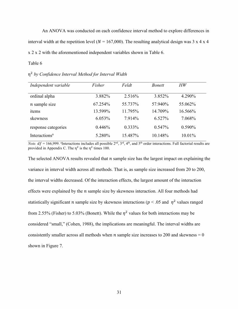
Table 6 η2 by Confidence Interval Method for Interval Width ................................................... 31
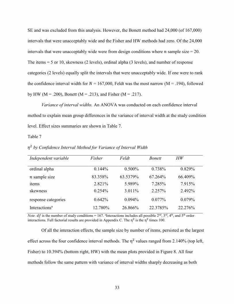
Table 7 η2 by Confidence Interval Method for Variance of Interval Width ............................... 33
Table 8 ANOVA Results for RMSE ............................................................................................ 35
Table 9 ANOVA Results for Bias of Ordinal Coefficient Alpha ................................................ 36
Table 10 Selected η2 Interaction Terms ...................................................................................... 37
v
LIST OF FIGURES
Page
Figure 1. Coverage rates by confidence interval method across 𝑁𝑁 = 167,000 replications. ........ 22
Figure 2. Two-way mean interaction plots of ordinal alpha by skewness effects for the dependent variable captured coverage rates. .................................................................................................. 24
Figure 3. Boxplot of 95% confidence interval widths for four estimation methods across 167 study conditions. ........................................................................................................................... 25
Figure 4. Mean confidence limits for ordinal alpha = .6. Dashed line references population parameter. Bottom marker is the mean lower limit and top marker is the mean upper limit. Middle marker is the mean sample ordinal coefficient alpha. ...................................................... 28
Figure 5. Mean confidence limits for ordinal alpha = .8. Dashed line references population parameter. Bottom marker is the mean lower limit and top marker is the mean upper limit. Middle marker is the mean sample ordinal coefficient alpha. ...................................................... 29
Figure 6. Mean confidence limits for ordinal alpha = .9. Dashed line references population parameter. Bottom marker is the mean lower limit and top marker is the mean upper limit. Middle marker is the mean sample ordinal coefficient alpha. ...................................................... 30
Figure 7. Two-way mean interaction plots of 𝑛𝑛 sample size by skewness interaction effects for the dependent variable interval width. .......................................................................................... 32
Figure 8. Two-way mean interaction plots of samples size by items interaction effects with the dependent variable variance of interval width. ............................................................................. 34
1
A PERFORMANCE EVALUATION OF CONFIDENCE INTERVALS FOR ORDINAL
COEFFICIENT ALPHA
Introduction
Reliability is an estimate of the consistency of results from a measurement (Crocker &
Algina, 2008; Cronbach, 1951) and an essential component to later establish construct validity of
a scale (Allen & Yen, 1979, 2002). Social scientists often measure attitudes and opinions with
ordinal, graded-response scales, or Likert-type ratings (e.g. 1 = strongly disagree, 5 = strongly
agree). The individual options on the scale are assumed to be discrete realizations of an
underlying continuously-scaled construct (Flora & Curran, 2004). Nevertheless, researchers
often use statistical methods that assume continuous distributions when reporting psychometric
information causing an empirical mismatch with the data analyzed (Gadermann, Guhn, &
Zumbo, 2012; Schmitt, 1996; Sijtsma, 2009; Streiner, 2003). Mismatching data to inappropriate
statistical analyses may lead researchers to incorrect conclusions (Duhachek & Iacobucci, 2004).
Likert-type data are often skewed and highly kurtotic in nature. Non-normality, which is
common with Likert-type data, may yield an underestimated reliability estimate when employing
sample coefficient alpha. This may mislead a researcher to reject information about true
population coefficient alpha (Duhachek & Iacobucci, 2004; Flora & Curran, 2004; Gadermann et
al., 2012; Maydeu-Olivares, Coffman, & Hartmann, 2007; Zumbo, Gadermann, & Zeisser,
2007). However, as the number of response categories increases to six or seven, sample
coefficient alpha is more accurately estimated (Duhachek & Iacobucci, 2004; Zumbo et al.,
2007). An ongoing debate still exists about the most appropriate measures of reliability when
ordinal measures are observed (Sijtsma, 2009; Zumbo et al., 2007). One strategy to overcome the
violation of normality is to use an alternative reliability estimate specifically for ordinal data
2
(Gadermann et al., 2012; Zumbo et al., 2007). Ordinal coefficient alpha uses a polychoric
correlation matrix, rather than the Pearson correlation matrix.
Although ordinal coefficient alpha may be more appropriate measure of reliability for
ordinal data, it still is just a point estimate. Researchers often report the confidence intervals to
quantify the amount of standard error around statistical point estimates. This is seen as an
essential interpretation and publishing practice because of the shift from the null hypothesis
statistical significance testing (NHSST) to confidence intervals and effect sizes (J Cohen, 1994;
Cumming, 2012; Cumming & Fidler, 2009; Finch, Cumming, & Thomason, 2001; Thompson,
2006a, 2006b; Wilkinson & APA Task Force on Statistical Inference, 1999). Confidence
intervals for coefficient alpha may be estimated using different approaches, including Feldt
(1965), Fisher (1950), Bonett (2002), and Hakstian and Whalen (1976). While a myriad of
studies have examined various confidence interval methods for coefficient alpha (Bonett, 2002;
Cui & Li, 2012; Duhachek & Iacobucci, 2004; Feldt, 1965; Fisher, 1950; Hakstian & Whalen,
1976; Maydeu-Olivares et al., 2007; Padilla, Divers, & Newton, 2012; van Zyl, Neudecker, &
Nel, 2000; K. Yuan & Bentler, 2002), no published studies currently examine confidence
intervals for ordinal coefficient alpha. Therefore, the purpose of this study is to evaluate the
performance of four confidence intervals methods for the ordinal coefficient alpha reliability
estimate.
Purpose
The objective of the article is two-fold. The primary objective is to compare differences
in coverage rates across four types of confidence interval methods. The second objective is to
examine the precision of ordinal coefficient alpha in terms of root mean square error (RMSE)
and bias. There are several known factors that affect confidence intervals for reliability estimates
3
including sample size, the number of items on an instrument, skewness of the responses, and
correlation amongst the items (Cui & Li, 2012; Duhachek & Iacobucci, 2004; Romano,
Kromrey, Owens, & Scott, 2011). The following research questions will guide this study:
a) How do the number of response categories, sample size, number of items, and skewness
impact the precision of coverage rates, interval width, and variance of interval width with
respect to varied population parameters of ordinal coefficient alpha?
b) How do the number of response categories, sample size, number of items, and skewness
impact the precision of ordinal coefficient alpha (RMSE, bias)?
The article is structured as follows: First, definitions of internal consistency, ordinal coefficient
alpha, and confidence intervals are provided. Next, the literature is discussed to provide the
rationale for the simulation design. Finally, the results are summarized to provide implications
for current research and recommendations for future research.
Internal Consistency as a Measure of Reliability
Random and systematic errors occur when measuring a person’s trait or ability and may
cause scores to be unreliable (Allen & Yen, 2002; Crocker & Algina, 2008). In classical test
theory, the observed score is expressed as
𝑋𝑋 = 𝑇𝑇 + 𝐸𝐸 (1)
where 𝑋𝑋 denotes the observed score, 𝑇𝑇 denotes the true score, and 𝐸𝐸 is the unique error of the
measurement. As error increases, either randomly or systematically, the scores become a less
accurate reflection of the true score, producing inconsistent results. Researchers often report a
measure of internal consistency of the scores (i.e. reliability), which is a pivotal yet often
misunderstood concept because reliability is not a psychometric property of the test (Cui & Li,
2012; Henson, 2001). Reliability, 𝜌𝜌𝑥𝑥𝑥𝑥, is formulaically expressed as
4
𝜌𝜌𝑥𝑥𝑥𝑥 = 𝜎𝜎𝑡𝑡𝑡𝑡𝑡𝑡𝑡𝑡2
𝜎𝜎𝑡𝑡𝑡𝑡𝑡𝑡𝑡𝑡𝑡𝑡2 (2)
where 𝜌𝜌𝑥𝑥𝑥𝑥 is the proportion of true score variance to total score variance.
A variety of reliability coefficients exist, including the test-retest (Crocker & Algina,
2008), split-half (Brown, 1910; Spearman, 1910), KR-20 and 21 (Kuder & Richardson, 1937),
alpha (Cronbach, 1951), and ordinal alpha coefficients (Zumbo et al., 2007). Depending on the
hypothesized source of measurement error, there are different procedures for estimating
reliability measures including single test administration, two test administrations, and multiple
raters techniques. Despite the different procedures, internal consistency estimates such as
coefficient alpha are frequently utilized in research because they only require a single test
administration (Cronbach & Shavelson, 2004; Henson, 2001; Streiner, 2003). Because of its
computational ease and convenience, coefficient alpha is the most commonly used metric (Cui &
Li, 2012; Henson, 2001; Padilla et al., 2012; Streiner, 2003).
Internal consistency estimates, such as coefficient alpha, quantify the degree of inter-item
relatedness (Cronbach, 1951). However, high levels of interrelatedness do not necessarily imply
unidimensionality, despite the conflicting counsel researchers have received (Duhachek &
Iacobucci, 2004; Gerbing & Anderson, 1988). The reliability of a composite score may be
estimated in a factor model as the ratio of item variances to total variances. The factor analytic
representation of classical test theory is expressed as
𝑋𝑋𝑖𝑖 = 𝑓𝑓𝑖𝑖𝜉𝜉 + 𝑢𝑢𝑖𝑖 𝑖𝑖 = 1,2, … ,𝑝𝑝, (3)
where 𝑋𝑋𝑖𝑖 denotes the observed scores on the 𝑖𝑖th item, 𝑓𝑓𝑖𝑖 denotes the factor loadings, 𝜉𝜉 is the true
score common factor, and 𝑢𝑢𝑖𝑖 is the uniqueness or random error up to 𝑝𝑝 number of items (Zumbo
et al., 2007). Novick and Lewis (1967) derived coefficient alpha as an unbiased estimate when
5
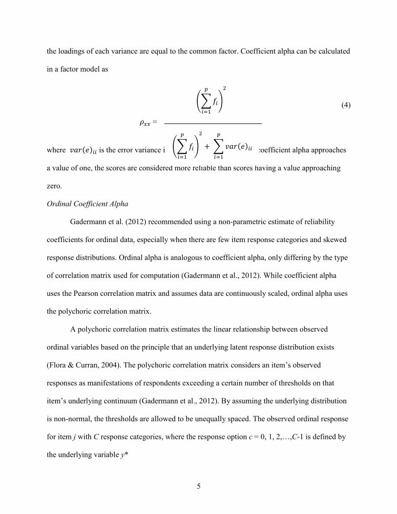
the loadings of each variance are equal to the common factor. Coefficient alpha can be calculated
in a factor model as
(4)
where 𝑣𝑣𝑣𝑣𝑣𝑣(𝑒𝑒)𝑖𝑖𝑖𝑖 is the error variance in a factor analytic model. As coefficient alpha approaches
a value of one, the scores are considered more reliable than scores having a value approaching
zero.
Ordinal Coefficient Alpha
Gadermann et al. (2012) recommended using a non-parametric estimate of reliability
coefficients for ordinal data, especially when there are few item response categories and skewed
response distributions. Ordinal alpha is analogous to coefficient alpha, only differing by the type
of correlation matrix used for computation (Gadermann et al., 2012). While coefficient alpha
uses the Pearson correlation matrix and assumes data are continuously scaled, ordinal alpha uses
the polychoric correlation matrix.
A polychoric correlation matrix estimates the linear relationship between observed
ordinal variables based on the principle that an underlying latent response distribution exists
(Flora & Curran, 2004). The polychoric correlation matrix considers an item’s observed
responses as manifestations of respondents exceeding a certain number of thresholds on that
item’s underlying continuum (Gadermann et al., 2012). By assuming the underlying distribution
is non-normal, the thresholds are allowed to be unequally spaced. The observed ordinal response
for item j with C response categories, where the response option c = 0, 1, 2,…,C-1 is defined by
the underlying variable y*
𝜌𝜌𝑥𝑥𝑥𝑥 =
��𝑓𝑓𝑖𝑖
𝑝𝑝
𝑖𝑖=1
�
2
��𝑓𝑓𝑖𝑖
𝑝𝑝
𝑖𝑖=1
�
2
+ �𝑣𝑣𝑣𝑣𝑣𝑣(𝑒𝑒)𝑖𝑖𝑖𝑖
𝑝𝑝
𝑖𝑖=1
6
yj = c, if 𝜏𝜏𝑐𝑐 < 𝜏𝜏𝑗𝑗∗ < 𝜏𝜏𝑐𝑐+1, (5)
where 𝜏𝜏𝑐𝑐, 𝜏𝜏𝑐𝑐+1are the thresholds on the underlying non-normal continuum and satisfy the
constraint
− ∞ = 𝜏𝜏0 < 𝜏𝜏1 < ⋯ < 𝜏𝜏𝑐𝑐−1 < 𝜏𝜏𝑐𝑐 = ∞. (6)
The polychoric correlation,Ф, is computed the same as Pearson product-moment correlation,
such that
Ф = 𝐶𝐶𝐶𝐶𝑣𝑣𝑣𝑣(𝑋𝑋1,𝑋𝑋2) = 𝐶𝐶𝐶𝐶𝐶𝐶 (𝑋𝑋1,𝑋𝑋2 )�𝑉𝑉𝑉𝑉𝑉𝑉(𝑋𝑋1)�𝑉𝑉𝑉𝑉𝑉𝑉(𝑋𝑋2)
(7)
where 𝑋𝑋1and 𝑋𝑋2 are latent response variables.
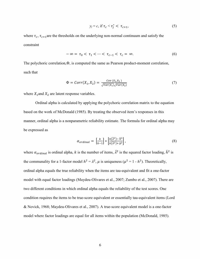
Ordinal alpha is calculated by applying the polychoric correlation matrix to the equation
based on the work of McDonald (1985). By treating the observed item’s responses in this
manner, ordinal alpha is a nonparametric reliability estimate. The formula for ordinal alpha may
be expressed as
𝛼𝛼𝐶𝐶𝑉𝑉𝑜𝑜𝑖𝑖𝑜𝑜𝑉𝑉𝑜𝑜 = � 𝑘𝑘𝑘𝑘−1
� ∗ �𝑘𝑘�𝜆𝜆�2�− ℎ�2
𝑘𝑘�𝜆𝜆�2�+ µ�2� , (8)
where 𝛼𝛼𝐶𝐶𝑉𝑉𝑜𝑜𝑖𝑖𝑜𝑜𝑉𝑉𝑜𝑜 is ordinal alpha, 𝑘𝑘 is the number of items, �̅�𝜆2 is the squared factor loading, ℎ�2 is
the communality for a 1-factor model ℎ2 = 𝜆𝜆2, 𝜇𝜇 is uniqueness (𝜇𝜇2 = 1 - ℎ2). Theoretically,
ordinal alpha equals the true reliability when the items are tau-equivalent and fit a one-factor
model with equal factor loadings (Maydeu-Olivares et al., 2007; Zumbo et al., 2007). There are
two different conditions in which ordinal alpha equals the reliability of the test scores. One
condition requires the items to be true-score equivalent or essentially tau-equivalent items (Lord
& Novick, 1968; Maydeu-Olivares et al., 2007). A true-score equivalent model is a one-factor
model where factor loadings are equal for all items within the population (McDonald, 1985).
7
When items conform to one-factor model, this implies that population covariances are equal, but
population variances are not necessarily equal for all items (Maydeu-Olivares et al., 2007).
The second condition is known as the parallel-items model which is considered a special
case of the true-score equivalent model. The unique variances of the error terms in the factor
model are assumed to be equal for all items yielding two parameters (Maydeu-Olivares et al.,
2007). The parameters include: (a) the covariance common to all possible pairs of items and (b)
variance of all items. This covariance structure is known as compound symmetry. Violations of
compound symmetry cause difficulties with respect to precision. Internal consistency may be
conceived as a theoretical estimate of reliability, with consideration to item homogeneity
(Henson, 2001). The more interrelated the items, then the magnitude of coefficient alpha
increases. In practice, meeting the parallel-items and compound symmetry conditions are often
untenable and cloud interpretations. Therefore, confidence intervals are essential to quantify the
precision obtained for the sample.
Confidence Intervals
According to Wilkinson and APA Task Force (1999), authors should report a reliability
coefficient even when the focus is not psychometric because it is a critical component to
interpreting observed effects (c.f. Henson, 2001). Cronbach and Shavelson (2004) suggested that
a reliability coefficient should be computed for the specific study, not relying on published
psychometrics, due to sampling and random errors. As with any point estimate, reliability
coefficients are estimates of population parameters and tend to vary from sample to sample. This
point is explicitly highlighted in reliability generalization studies that examine reliability
fluctuation across studies (Vacha-Haase, Henson, & Caruso, 2002; Vacha-Haase & Thompson,
8
2011). Therefore, estimating the standard error of reliability coefficients with confidence
intervals is critical.
A confidence interval provides information about the standard error of sample statistics
and estimated range of values that most likely capture the true parameter (Cumming, 2012;
Cumming & Finch, 2005). A confidence interval is interpreted as a relative frequency of how
many times the interval would actually capture the unknown parameter in repeated sampling
(Samaniego, 2010). Confidence intervals estimate the probability of a parameter value based
solely on observable data (Cumming, 2012; Samaniego & Reneau, 1994). The nominal width of
a confidence interval, often reported at the 90%, 95%, or 99% level, implies uncertainty and
provides information regarding the precision of a point estimate (Cumming & Fidler, 2009).
Confidence intervals may be calculated on most any statistic, including means, effect sizes
(Thompson, 2002, 2006a), and reliability coefficients (Cumming & Fidler, 2009; Fan &
Thompson, 2001; Romano et al., 2011). In order to compute a confidence interval and conduct
statistical inference, information about the standard error and sampling distribution of a statistic
are necessary.
The standard error is the standard deviation of the sampling distribution of a sample
statistic (Cummings, 2012), and standard error increases as sample size decreases. Ordinal alpha
is never free of error and the magnitude of error is approximated through its standard error. The
standard error is derived from the variance estimate to approximate a confidence interval of
plausible values surrounding the statistic based on its distributional properties. The larger the
standard error, the less reliable the scores obtained (Duhachek & Iacobucci, 2004). The standard
error for sample reliability coefficients is sensitive to sample size, the number of items, the level
of intercorrelation, and homogeneity of variance (Duhachek & Iacobucci, 2004).
9
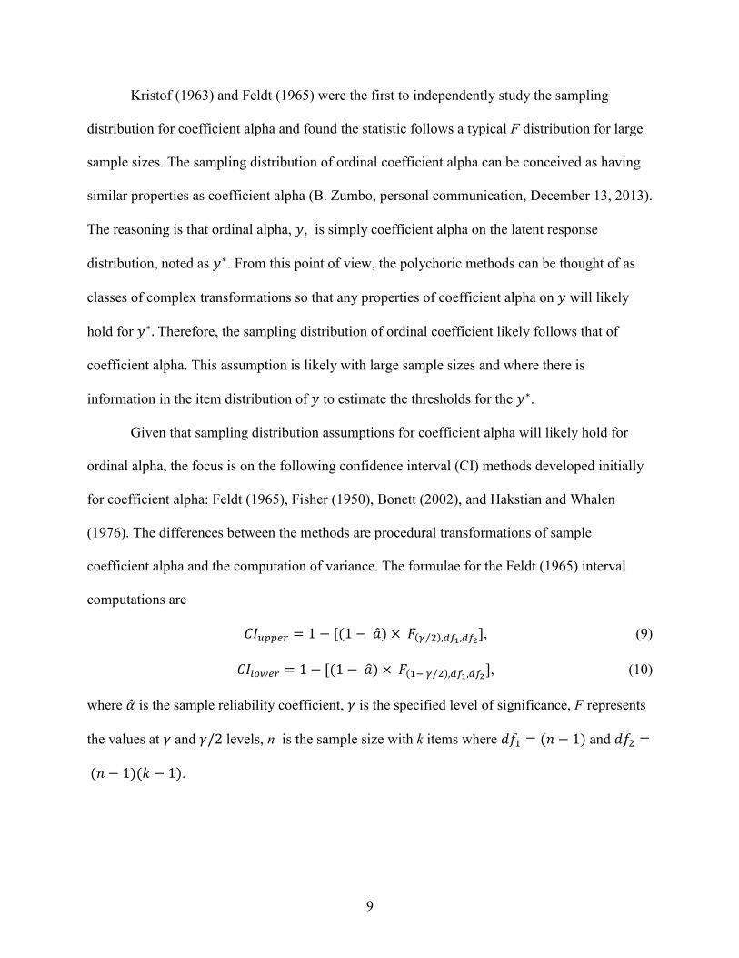
Kristof (1963) and Feldt (1965) were the first to independently study the sampling
distribution for coefficient alpha and found the statistic follows a typical F distribution for large
sample sizes. The sampling distribution of ordinal coefficient alpha can be conceived as having
similar properties as coefficient alpha (B. Zumbo, personal communication, December 13, 2013).
The reasoning is that ordinal alpha, 𝑦𝑦, is simply coefficient alpha on the latent response
distribution, noted as 𝑦𝑦∗. From this point of view, the polychoric methods can be thought of as
classes of complex transformations so that any properties of coefficient alpha on 𝑦𝑦 will likely
hold for 𝑦𝑦∗. Therefore, the sampling distribution of ordinal coefficient likely follows that of
coefficient alpha. This assumption is likely with large sample sizes and where there is
information in the item distribution of 𝑦𝑦 to estimate the thresholds for the 𝑦𝑦∗.
Given that sampling distribution assumptions for coefficient alpha will likely hold for
ordinal alpha, the focus is on the following confidence interval (CI) methods developed initially
for coefficient alpha: Feldt (1965), Fisher (1950), Bonett (2002), and Hakstian and Whalen
(1976). The differences between the methods are procedural transformations of sample
coefficient alpha and the computation of variance. The formulae for the Feldt (1965) interval
computations are
𝐶𝐶𝐶𝐶𝑢𝑢𝑝𝑝𝑝𝑝𝑢𝑢𝑉𝑉 = 1 − [(1 − 𝑣𝑣�) × 𝐹𝐹(𝛾𝛾 2⁄ ),𝑜𝑜𝑑𝑑1,𝑜𝑜𝑑𝑑2], (9)
𝐶𝐶𝐶𝐶𝑜𝑜𝐶𝐶𝑙𝑙𝑢𝑢𝑉𝑉 = 1 − [(1 − 𝑣𝑣�) × 𝐹𝐹(1− 𝛾𝛾 2⁄ ),𝑜𝑜𝑑𝑑1,𝑜𝑜𝑑𝑑2], (10)
where 𝛼𝛼� is the sample reliability coefficient, 𝛾𝛾 is the specified level of significance, F represents
the values at 𝛾𝛾 and 𝛾𝛾/2 levels, n is the sample size with k items where 𝑑𝑑𝑓𝑓1 = (𝑛𝑛 − 1) and 𝑑𝑑𝑓𝑓2 =
(𝑛𝑛 − 1)(𝑘𝑘 − 1).
10
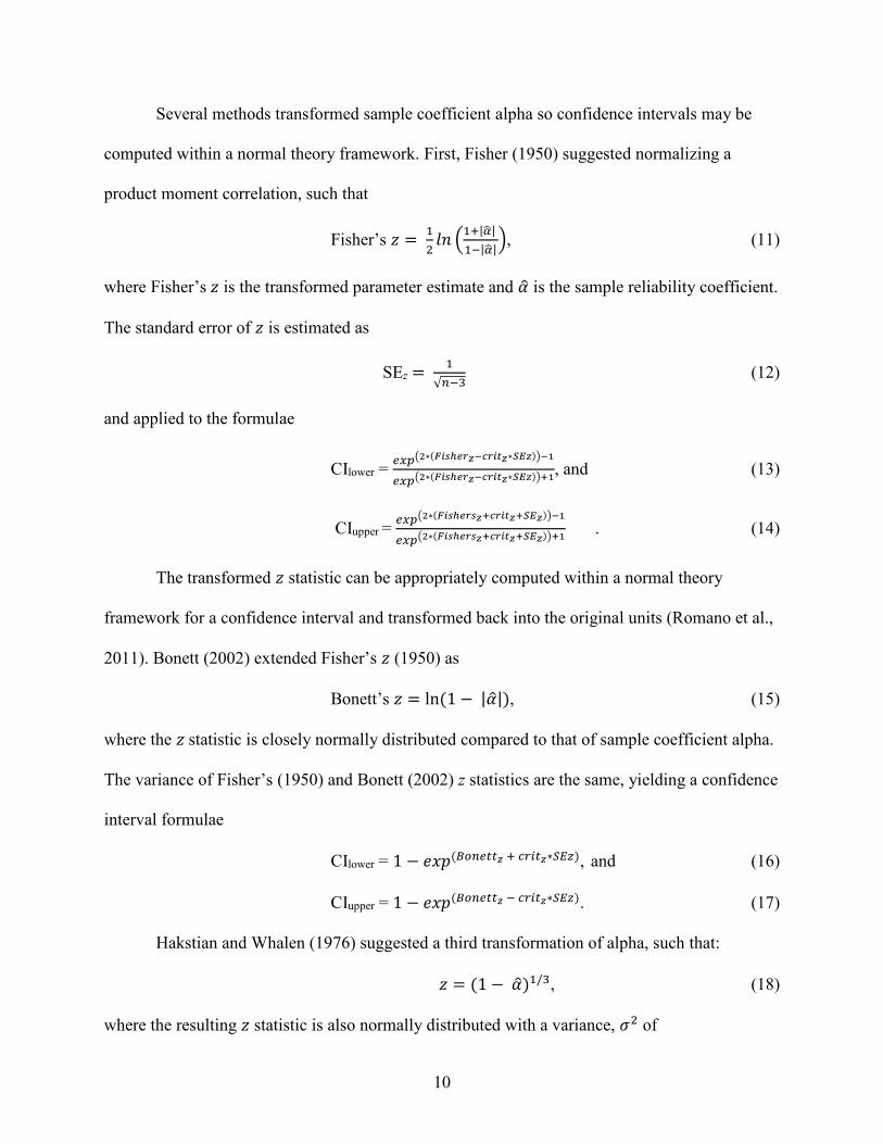
Several methods transformed sample coefficient alpha so confidence intervals may be
computed within a normal theory framework. First, Fisher (1950) suggested normalizing a
product moment correlation, such that
Fisher’s 𝑧𝑧 = 12𝑙𝑙𝑛𝑛 �1+|𝛼𝛼�|
1−|𝛼𝛼� |�, (11)
where Fisher’s 𝑧𝑧 is the transformed parameter estimate and 𝛼𝛼� is the sample reliability coefficient.
The standard error of 𝑧𝑧 is estimated as
SEz = 1√𝑜𝑜−3
(12)
and applied to the formulae
CIlower = 𝑢𝑢𝑥𝑥𝑝𝑝�2∗(𝐹𝐹𝐹𝐹𝐹𝐹ℎ𝑡𝑡𝑡𝑡𝑧𝑧−𝑐𝑐𝑡𝑡𝐹𝐹𝑡𝑡𝑧𝑧∗𝑆𝑆𝑆𝑆𝑧𝑧)�−1
𝑢𝑢𝑥𝑥𝑝𝑝�2∗(𝐹𝐹𝐹𝐹𝐹𝐹ℎ𝑡𝑡𝑡𝑡𝑧𝑧−𝑐𝑐𝑡𝑡𝐹𝐹𝑡𝑡𝑧𝑧∗𝑆𝑆𝑆𝑆𝑧𝑧)�+1, and (13)
CIupper = 𝑢𝑢𝑥𝑥𝑝𝑝�2∗(𝐹𝐹𝐹𝐹𝐹𝐹ℎ𝑡𝑡𝑡𝑡𝐹𝐹𝑧𝑧+𝑐𝑐𝑡𝑡𝐹𝐹𝑡𝑡𝑧𝑧+𝑆𝑆𝑆𝑆𝑧𝑧)�−1
𝑢𝑢𝑥𝑥𝑝𝑝�2∗(𝐹𝐹𝐹𝐹𝐹𝐹ℎ𝑡𝑡𝑡𝑡𝐹𝐹𝑧𝑧+𝑐𝑐𝑡𝑡𝐹𝐹𝑡𝑡𝑧𝑧+𝑆𝑆𝑆𝑆𝑧𝑧)�+1 . (14)
The transformed 𝑧𝑧 statistic can be appropriately computed within a normal theory
framework for a confidence interval and transformed back into the original units (Romano et al.,
2011). Bonett (2002) extended Fisher’s 𝑧𝑧 (1950) as
Bonett’s 𝑧𝑧 = ln (1 − |𝛼𝛼�|), (15)
where the 𝑧𝑧 statistic is closely normally distributed compared to that of sample coefficient alpha.
The variance of Fisher’s (1950) and Bonett (2002) z statistics are the same, yielding a confidence
interval formulae
CIlower = 1 − 𝑒𝑒𝑒𝑒𝑝𝑝(𝐵𝐵𝐶𝐶𝑜𝑜𝑢𝑢𝐵𝐵𝐵𝐵𝑧𝑧 + 𝑐𝑐𝑉𝑉𝑖𝑖𝐵𝐵𝑧𝑧∗𝑆𝑆𝑆𝑆𝑆𝑆), and (16)
CIupper = 1 − 𝑒𝑒𝑒𝑒𝑝𝑝(𝐵𝐵𝐶𝐶𝑜𝑜𝑢𝑢𝐵𝐵𝐵𝐵𝑧𝑧 − 𝑐𝑐𝑉𝑉𝑖𝑖𝐵𝐵𝑧𝑧∗𝑆𝑆𝑆𝑆𝑆𝑆). (17)
Hakstian and Whalen (1976) suggested a third transformation of alpha, such that:
𝑧𝑧 = (1 − 𝛼𝛼�)1/3, (18)
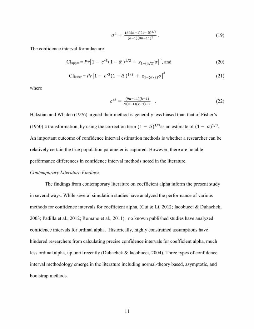
where the resulting 𝑧𝑧 statistic is also normally distributed with a variance, 𝜎𝜎2 of
11
𝜎𝜎2 = 18𝑘𝑘(𝑜𝑜−1)(1− 𝛼𝛼�)2/3
(𝑘𝑘−1)(9𝑜𝑜−11)2 . (19)
The confidence interval formulae are
CIupper = 𝑃𝑃𝑣𝑣�1 − 𝑐𝑐∗3(1 − 𝛼𝛼� )1 3⁄ − 𝑧𝑧1−(𝛼𝛼 2⁄ )𝜎𝜎�3, and (20)
CIlower = 𝑃𝑃𝑣𝑣�1 − 𝑐𝑐∗3(1 − 𝛼𝛼� )1 3⁄ + 𝑧𝑧1−(𝛼𝛼 2⁄ )𝜎𝜎�3 (21)
where
𝑐𝑐∗3 = (9𝑜𝑜−11)(𝑘𝑘−1)9(𝑜𝑜−1)(𝑘𝑘−1)−2
. (22)
Hakstian and Whalen (1976) argued their method is generally less biased than that of Fisher’s
(1950) 𝑧𝑧 transformation, by using the correction term (1 − 𝛼𝛼�)1/3as an estimate of (1 − 𝛼𝛼)1/3.
An important outcome of confidence interval estimation methods is whether a researcher can be
relatively certain the true population parameter is captured. However, there are notable
performance differences in confidence interval methods noted in the literature.
Contemporary Literature Findings
The findings from contemporary literature on coefficient alpha inform the present study
in several ways. While several simulation studies have analyzed the performance of various
methods for confidence intervals for coefficient alpha, (Cui & Li, 2012; Iacobucci & Duhachek,
2003; Padilla et al., 2012; Romano et al., 2011), no known published studies have analyzed
confidence intervals for ordinal alpha. Historically, highly constrained assumptions have
hindered researchers from calculating precise confidence intervals for coefficient alpha, much
less ordinal alpha, up until recently (Duhachek & Iacobucci, 2004). Three types of confidence
interval methodology emerge in the literature including normal-theory based, asymptotic, and
bootstrap methods.
12
Romano et al. (2011) evaluated which method performed the best with discrete and
ordinal response items. Romano et al. (2011) found negligible differences between eight
confidence interval methods, with respect to bias, coverage, and precision. The eight methods
examined included: (a) Maydeu-Oliveres et al. (2007) asymptotic distribution free (ADF), (b)
Bonett (2002), (c) Feldt (1965), (d) Fisher (1950), (e) Hakstian and Whalen (1976), (f) Duhachek
and Iacobucci (2004), (g) Koning and Franses asymptotic (2003), and (h) Koning and Franses
exact (2003) method. The findings suggest the ADF method was the least accurate for small
sample sizes, and little was gained from departing from the Fisher approach (Romano et al.,
2011). This finding is especially noteworthy because many other simulation studies suggested
that ADF method outperformed other normal theory approaches, and the Fisher approach was
extremely problematic (Duhachek & Iacobucci, 2004; Hakstian & Whalen, 1976; Maydeu-
Olivares et al., 2007). Romano et al. (2011) provided evidence that sophisticated confidence
interval methodology does not necessarily yield better performance.
The implication of the Romano et al. (2011) findings are significant because of the
advancements of ADF methods were considered a breakthrough. In 2000, van Zyl et al. derived
an asymptotic (i.e. large sample) distribution for sample coefficient alpha, only assuming a
multivariate normal distribution and positive definite matrix (Maydeu-Olivares, et al., 2007). The
findings from the van Zyl et al. (2000) ADF study are considered a noteworthy advancement
because the assumption of compound symmetry is not required. While van Zyl et al’s (2000)
intervals have been shown to yield the most narrow intervals they often do not capture the true
population coefficient (Cui & Li, 2012).
Duhachek and Iacobucci (2004) extended van Zyl et al. (2000) and presented statistics for
coefficient alpha’s standard error and computed an ADF-based confidence interval. Duhachek
13
and Iacobucci (2004) found ADF intervals repeatedly outperformed other normal theory based
intervals, including Feldt (1965) and Hakstian and Whalen (1976). The Duhachek and Iacobucci
(2004) finding was consistent across all study conditions, but their study was not generalizable to
Likert-type data. Maydeu-Olivares et al. (2007) extended the Duhachek and Iacobucci (2004
findings and derived an ADF confidence interval estimate for coefficient alpha. The Maydeu-
Olivares et al. (2007) findings stated the empirical coverage rate of the ADF intervals
outperforms that of normal theory intervals, regardless of observed skewness and kurtosis of
item distributions (Cui & Li, 2012; Romano et al., 2011). The implications from the Maydeu-
Olivares et al. (2007) findings are significant because researchers were no longer bound by
normality assumptions (i.e. normal theory) that were often violated when analyzing Likert-type
data.
Another study conducted by Cui and Li (2012) evaluated six parametric and non-
parametric confidence intervals for continuous, five-point Likert, and dichotomous data. A
particular noteworthy finding, consistent with Romano et al. (2011) finding, is the poor
performance of van Zyl et al’s (2000) ADF procedure for Likert-type data. Cui and Li (2012)
divided the methods into parametric methods techniques and non-parametric techniques. The
parametric methods include (a) Feldt (1965), (b) Hakstian and Whalen (1976), (c) ADF (van Zyl
et al., 2000), and non-parametric methods include (d) BSI; (Raykov, 1998), (e) BPI, (Raykov,
1998), and (f) BCaI, (Efron, 1987; Efron & Tibshirani, 1993). With regard to five-point Likert
data, the Feldt, Hakstian and Whalen, and BSI showed the best coverage performance and the
worst performers were the ADF van Zyl et al., BPI, and BCaI.
Padilla et al. (2012) also investigated effects of non-normality on the performance of
seven confidence intervals methods including: (a) Fisher, (b) Bonett, (c) normal theory, (d) ADF,
14
(e) normal theory bootstrap, (f) percentile bootstrap, and (g) bias-corrected and accelerated
bootstrap. The normal theory bootstrap method, by far, had the most acceptable coverage rate
under all conditions, followed by Bonett, and normal theory. The authors provided evidence
indicating the Fisher method yields unacceptably high variability, except under the condition of
at least 15 items (Padilla et al., 2012). As data became more non-normal, the coverage
probabilities decreased across all methods, a consistent finding across many simulation studies
(Cui & Li, 2012; Padilla et al., 2012).
According to Yuan and Bentler (2002), the normal theory confidence intervals were
found to be robust, even in the case of small sample sizes. Soon after, Yuan, Guarnaccia, and
Hayslip (2003) examined bootstrap and asymptotic confidence interval techniques with real data
using the Hopkins Symptom Checklist. Yuan et al. extended the results of van Zyl et al. (2000)
to more internal consistency coefficients beyond coefficient alpha, but pointed out that ADF
estimates are not optimal for small samples (Yuan et al., 2003).
These contemporary findings are informative to the present study for several reasons.
Despite significant advancements regarding the distributions of coefficient alpha, the seminal
works of Feldt (1965), Fisher (1950), and more recently Bonett (2002) often yield acceptable
confidence intervals, even when Likert-type data and smaller sample sizes are used. There seems
to be little gain from departing from more simple approaches to other sophisticated techniques
and the Fisher method was not as problematic as expected (Romano et al., 2011).
Evaluating Confidence Interval Performance
Confidence interval performance is assessed by two main areas: (a) coverage rates and
(b) precision of sample estimates.
15
Coverage rates. First, coverage rates are categorized by whether or not the interval
captures the true population parameter, the average width of the intervals, and variability of the
width of intervals (Zhang, Gutiérrez Rojas, & Cuervo, 2010). Jennings (1987) suggested a
successful coverage rate should have a value close to the nominal level, often set between 95%
and 99%. Coverage rates have been criticized as misleading, particularly when information about
the skewness of the sampling distribution is not provided or unknown (Jennings, 1987; Schall,
2012). Coverage rates should report the frequencies relative to whether the population parameter
was either captured, over-estimated, or under-estimated. For example, assume the population
parameter is .60. A sample ordinal alpha was .52 and the 95% CI [.45, .65]. The confidence
interval captured the population parameter of .60 because the value is between .45 and .65, but
under-estimated the population parameter if it was .80. The coverage rates are computed as
follows,
coverage rate = 𝐴𝐴 𝐵𝐵
× 100% (23) where 𝐴𝐴 is the frequency of intervals which captured, over-, or under-estimated the true
population parameter, and 𝐵𝐵 is the total frequency of intervals estimated. If 25 of 100 confidence
intervals captured the true population parameter, the captured coverage rate is 25%. Three
coverage rates categories provide information about the sampling distribution before the
confidence intervals is deemed biased. For example, an unbiased interval is equally likely to be
above or below the true value, in a normal sample distribution scenario. In skewed sampling
distributions, the equality related to the interval being above or below the true value is disrupted
(Jennings, 1986, 1987).
Interval widths. Zhang et al. (2010) suggested an analysis of interval widths, in addition
to coverage rates. The interval width is computed by subtracting the lower limit estimate from
the upper limit value estimate. For example, the width of a 95% CI [.45, .65] is
16
.20 = .65 - .45. (24) A mean interval width, μ, is computed as
𝜇𝜇 = ∑𝑥𝑥𝐹𝐹𝑁𝑁
(25) where 𝑒𝑒𝑖𝑖are the individual widths of each replication and 𝑁𝑁 is the number total number of widths
in population (i.e. total number of replications).
Variance of interval widths. The variance of interval widths are computed as
𝑉𝑉 = ∑(𝑥𝑥𝐹𝐹 −𝜇𝜇)2
𝑁𝑁 . (26)
where μ is the mean comparable to as a precision as narrow intervals, regardless of capturing the
true population parameter. A highly variable interval width indicates a poor precision for the
interval estimate method given certain study conditions.
Precision of point estimates. To analyze precision of ordinal alpha, bias and RMSE are of
computed. Bias is calculated by subtracting the true population parameter value from the sample
estimate. A bias value of zero indicates unbiased estimate of a parameter, a positive value
indicates an overestimation whereas, a negative value indicates an underestimation. RMSE is
computed as the standard deviation of the sample ordinal alpha values across valid replications
(N), aggregated to the study condition level as
= �∑(𝑥𝑥𝐹𝐹 −𝜇𝜇)2
𝑁𝑁 (27)
where μ is the mean sample ordinal coefficient alpha and 𝑒𝑒𝑖𝑖are the individual sample ordinal
coefficient alpha of each replication. To determine whether a confidence interval is unacceptably
wide, an empirical standard error (SE) of ordinal alpha is computed. The empirical SE is the
standard deviation of all computed sample ordinal alphas, at the repetition-level. The SE each
confidence interval method is compared to twice the empirical SE value to judge whether a
confidence interval is unacceptably wide.

17
Methods
This Monte Carlo study evaluated the performance of four confidence intervals methods
estimated around ordinal coefficient alpha. The program code is written using R (Version 3.0.2)
using the R Studio interface (Version 0.98.976). The code was executed in a Windows-based
environment (Version 8).
The following method was used to generate the population, by adapting the methods used
by Maydeu-Olivares et al. (2007) and Hakstian and Whalen (1976) through the use of the factor
analytic classical test theory model, assuming the parallel items model.
a) For a given condition, create a population of 1 million subjects by k number of
items, with 𝑝𝑝 ordinal alphas, c response categories, and 𝑠𝑠 skewness.
b) Generate an 𝑛𝑛 x 𝑘𝑘 items theoretical ability matrix 𝜽𝜽∗such that 𝜽𝜽∗~ 𝑵𝑵(𝟎𝟎,𝟏𝟏).
c) Generate an 𝑛𝑛 x 𝑘𝑘 random error matrix 𝑼𝑼 such that 𝑼𝑼 ~ 𝑴𝑴𝑴𝑴𝑵𝑵(𝟎𝟎,𝟎𝟎.𝝈𝝈) where σ =
�
0 . 5 … . 5… 0 … …… 0 . 5. 5 ⋯ . 5 0
� .
d) Calculate the 𝑛𝑛 x 𝑘𝑘 matrix 𝑿𝑿* such that 𝑒𝑒𝑖𝑖𝑘𝑘 = 𝑓𝑓1 ∗ 𝜃𝜃𝑖𝑖𝑘𝑘 + 𝑢𝑢𝑖𝑖𝑘𝑘 where 𝑓𝑓1 values
are factor loading values and provided later.
e) Categorize the scores in 𝑿𝑿* by applying rigid thresholds, 𝜏𝜏 (Muthén & Kaplan,
1985; Zumbo et al., 2007). The exact threshold values are provided in later tables.
Design Factors
Ordinal alphas (𝑣𝑣). Three ordinal alphas were specified at .6, .8, and .9 as used in
previous simulation studies (Cui & Li, 2012; Padilla et al., 2012; Romano et al., 2011; Zumbo et
al., 2007). Factor loadings values (f1) were based on Zumbo et al. (2007) with values of .311,
.471, and .625 for population ordinal coefficient alphas of .6, .8, and .9, respectively.
18
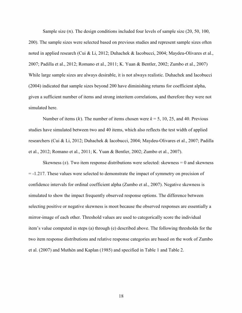
Sample size (𝑛𝑛). The design conditions included four levels of sample size (20, 50, 100,
200). The sample sizes were selected based on previous studies and represent sample sizes often
noted in applied research (Cui & Li, 2012; Duhachek & Iacobucci, 2004; Maydeu-Olivares et al.,
2007; Padilla et al., 2012; Romano et al., 2011; K. Yuan & Bentler, 2002; Zumbo et al., 2007)
While large sample sizes are always desirable, it is not always realistic. Duhachek and Iacobucci
(2004) indicated that sample sizes beyond 200 have diminishing returns for coefficient alpha,
given a sufficient number of items and strong interitem correlations, and therefore they were not
simulated here.
Number of items (𝑘𝑘). The number of items chosen were k = 5, 10, 25, and 40. Previous
studies have simulated between two and 40 items, which also reflects the test width of applied
researchers (Cui & Li, 2012; Duhachek & Iacobucci, 2004; Maydeu-Olivares et al., 2007; Padilla
et al., 2012; Romano et al., 2011; K. Yuan & Bentler, 2002; Zumbo et al., 2007).
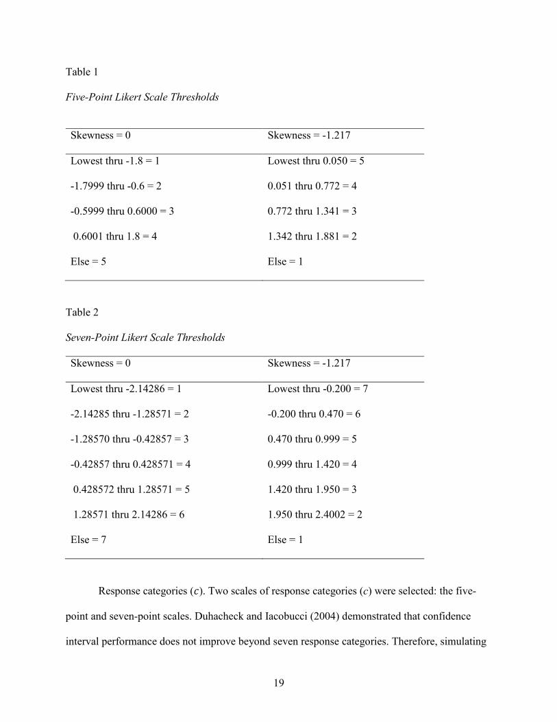
Skewness (𝑠𝑠). Two item response distributions were selected: skewness = 0 and skewness
= -1.217. These values were selected to demonstrate the impact of symmetry on precision of
confidence intervals for ordinal coefficient alpha (Zumbo et al., 2007). Negative skewness is
simulated to show the impact frequently observed response options. The difference between
selecting positive or negative skewness is moot because the observed responses are essentially a
mirror-image of each other. Threshold values are used to categorically score the individual
item’s value computed in steps (a) through (e) described above. The following thresholds for the
two item response distributions and relative response categories are based on the work of Zumbo
et al. (2007) and Muthѐn and Kaplan (1985) and specified in Table 1 and Table 2.
19
Table 1 Five-Point Likert Scale Thresholds
Skewness = 0 Skewness = -1.217
Lowest thru -1.8 = 1 Lowest thru 0.050 = 5
-1.7999 thru -0.6 = 2 0.051 thru 0.772 = 4
-0.5999 thru 0.6000 = 3 0.772 thru 1.341 = 3
0.6001 thru 1.8 = 4 1.342 thru 1.881 = 2
Else = 5 Else = 1
Table 2 Seven-Point Likert Scale Thresholds Skewness = 0 Skewness = -1.217
Lowest thru -2.14286 = 1 Lowest thru -0.200 = 7
-2.14285 thru -1.28571 = 2 -0.200 thru 0.470 = 6
-1.28570 thru -0.42857 = 3 0.470 thru 0.999 = 5
-0.42857 thru 0.428571 = 4 0.999 thru 1.420 = 4
0.428572 thru 1.28571 = 5 1.420 thru 1.950 = 3
1.28571 thru 2.14286 = 6 1.950 thru 2.4002 = 2
Else = 7 Else = 1
Response categories (𝑐𝑐). Two scales of response categories (c) were selected: the five-
point and seven-point scales. Duhacheck and Iacobucci (2004) demonstrated that confidence
interval performance does not improve beyond seven response categories. Therefore, simulating
20
more than seven response categories is not justifiable. Select population distributions are
provided in Appendix A.
The resulting design is a fully-crossed factorial design with 192 conditions 3(a) x 4(n) x 4
(k) x 2 (s) x 2 (c).
Data Analysis
Following the simulation, separate ANOVAs were conducted to examine mean group
differences. The independent variables included in this order are: (a) 𝑣𝑣 ordinal alpha (.6, .8, .9),
(b) 𝑛𝑛 sample size (20, 50, 100, 200), (c) 𝑘𝑘 number of items (5, 10, 25, 40), (d) s skewness level
(0, -1.217), and (e) 𝑐𝑐 number of response categories (5, 7) and the dependent variables were (a)
coverage rates, interval width, and variance of interval width and (b) RMSE and bias of ordinal
alpha for precision. ANOVAs were analyzed at the study condition level for coverage rates,
variance of interval width, and RMSE. Each study condition is represented as a mean value
containing 1,000 repetitions (e.g. mean confidence interval width). Repetition-level ANOVAs
were conducted for bias of ordinal alpha and interval width. Repetition-level values were
computed for every single repetition (e.g. bias of the sample ordinal alpha).
Homogeneity of variance was examined prior to the analysis and often revealed statistical
differences due to large sample sizes. Both main effects and all higher order interactions were
examined. Higher order interactions are discussed when noteworthy results appear. Estimated
marginal means (EMMs) are discussed with respect to precision and bias in the estimate of
ordinal coefficient alpha at the study condition level. To aid interpretation of the model, both 𝑝𝑝-
values and the effect size, 𝜂𝜂2, are used to select the independent variables which explain the most
variability in the dependent variables. The 𝜂𝜂2 is the ratio of variance of the effect (𝑆𝑆𝑆𝑆𝑢𝑢𝑑𝑑𝑑𝑑𝑢𝑢𝑐𝑐𝐵𝐵) to
total variance (𝑆𝑆𝑆𝑆𝐵𝐵𝐶𝐶𝐵𝐵𝑉𝑉𝑜𝑜).
21
Results
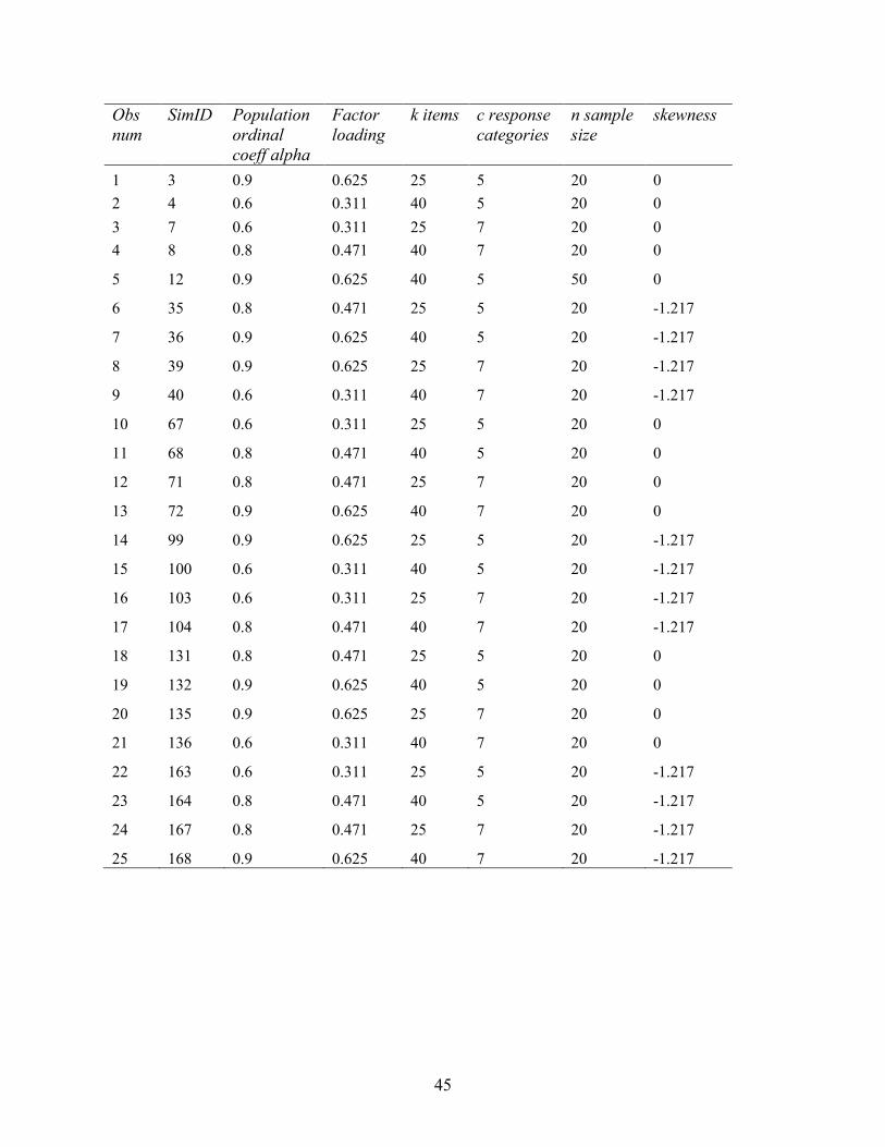
Practical Computation Issues
To minimize the standard error of the simulation, 1,000 samples were drawn for each
condition (Fan & SAS Institute, 2002; Wang & Thompson, 2007). Appendix A includes a list of
25 conditions (of the 192 conditions) that did not execute due to repeated crashing. The error
message stated a “non-positive definite matrix” was computed which caused computations to
stop. This error occurred when there was a large number of items (e.g. 25 or 40 items) with a
small sample size (e.g. 𝑛𝑛 = 20). The rigid thresholds set for the 5-point and 7-point Likert scales
removed important differences between the available response options (1, 2,…5 or 1, 2, ….7).
Ultimately, there simply was not enough sampling variability generated across each repetition
and the variables became constant (e.g. all responses were scored “3”). When no variability was
generated either across items or subjects, the covariance and standard deviation are essentially
zero. When this occurs, estimation stops because one cannot divide by zero to compute a
polychoric correlation. The issues related to the lack of variance generated seem to be an artifact
of restricted range with the ordinal data.
The resulting dataset contained 167,000 replications (167 workable conditions X 1000
samples each). The total time elapsed was approximately 691 computing hours. Between four
and eight conditions were executed simultaneously, yielding a real time elapsed of
approximately 12 days. Conditions containing 25 or 40 items took considerably longer to run
than 5 to 10 items due to computationally intensive pairwise polychoric correlation computations
necessary. The larger sample sizes drawn minimally impacted simulation execution time. The
various levels of skewness and number of response categories did not increase computation time.
22
The simulations were executed on a Dell Precision T3600 Intel (R) Xeon (R) CPU E5-1620 3.60
GHz Windows 8 machine. Data were analyzed in SPSS (version 22.0).
Analyses
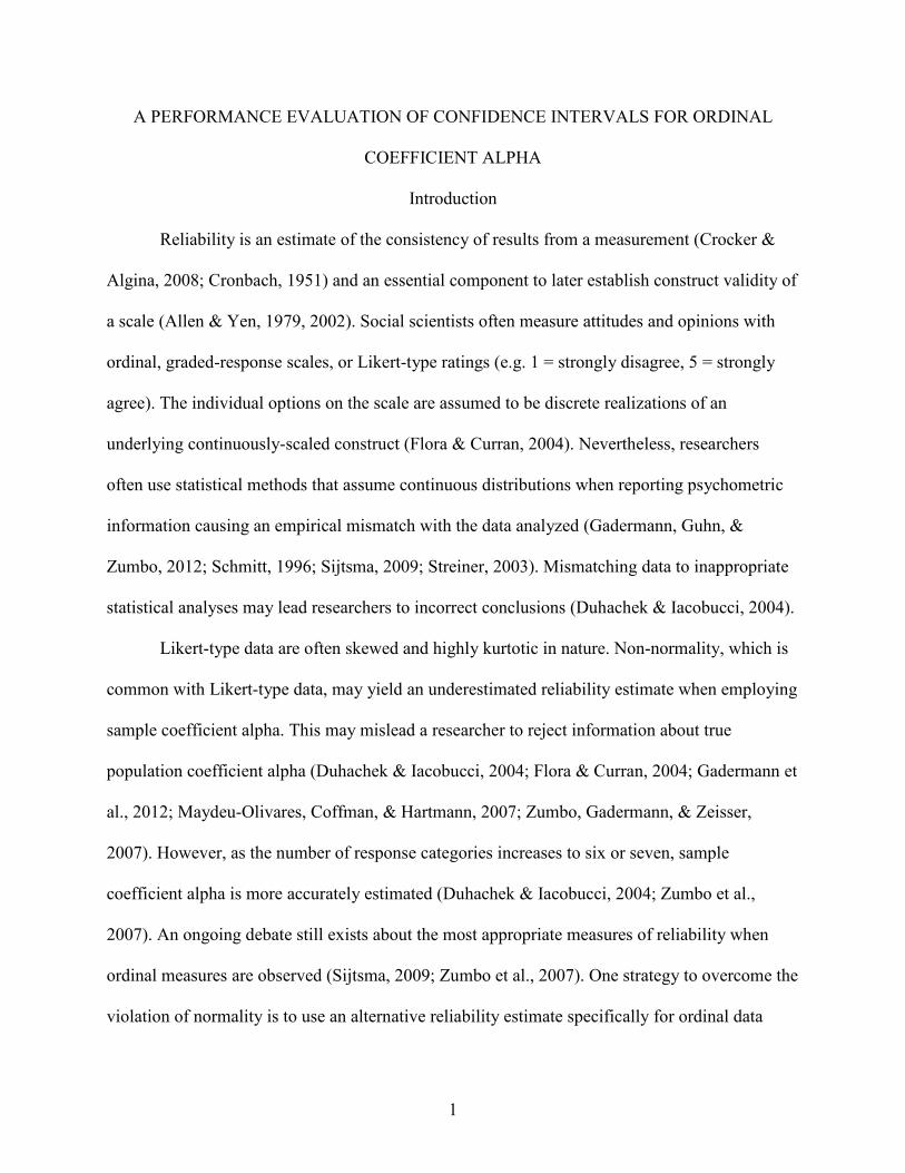
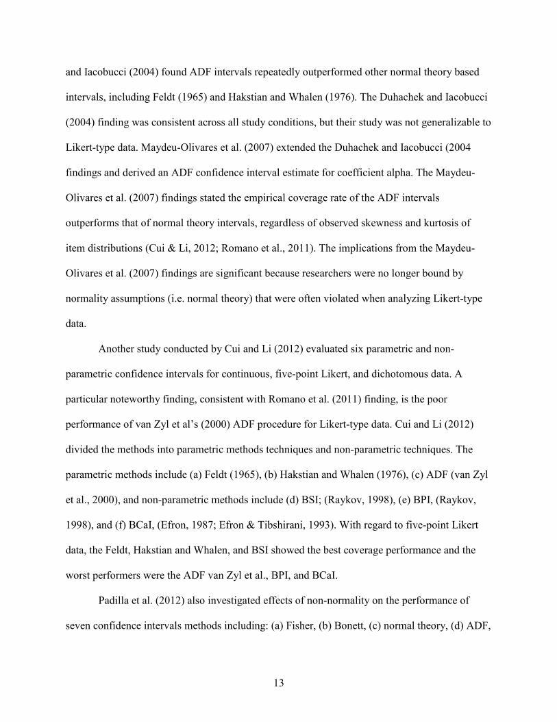
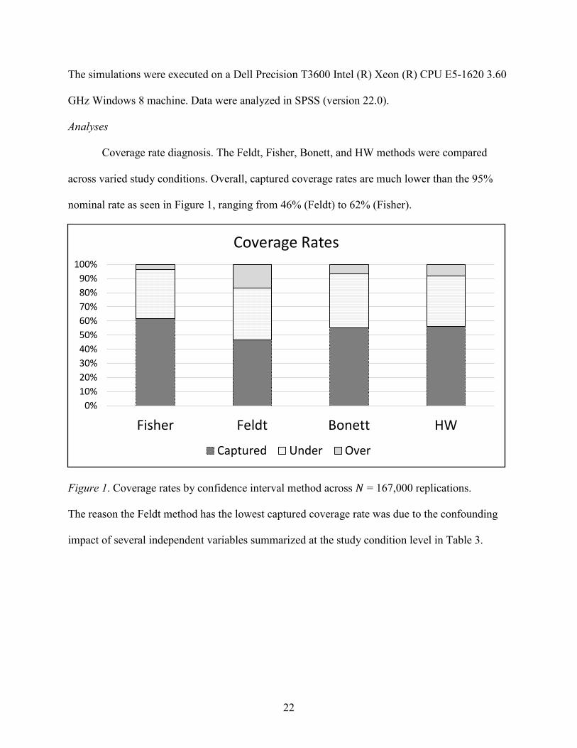
Coverage rate diagnosis. The Feldt, Fisher, Bonett, and HW methods were compared
across varied study conditions. Overall, captured coverage rates are much lower than the 95%
nominal rate as seen in Figure 1, ranging from 46% (Feldt) to 62% (Fisher).
Figure 1. Coverage rates by confidence interval method across 𝑁𝑁 = 167,000 replications. The reason the Feldt method has the lowest captured coverage rate was due to the confounding
impact of several independent variables summarized at the study condition level in Table 3.
0%10%20%30%40%50%60%70%80%90%
100%
Fisher Feldt Bonett HW
Coverage Rates
Captured Under Over
23
Table 3
𝜂𝜂2 by Confidence Interval Method for Captured Coverage Rates Independent variable Fisher Feldt Bonett HW
ordinal alpha 0.422% 0.252% 0.110% 0.381%
𝑛𝑛 sample size 4.122% 7.453% 4.692% 7.085% items 1.934% 2.722% 5.312% 6.116% skewness 62.915% 23.651% 55.108% 46.769%
response categories 2.157% 0.322% 0.997% 1.034%
Interactionsa 27.197% 64.968% 32.756% 37.590%
Note. Analyzed at study condition level where 𝑑𝑑𝑓𝑓 = 166. aInteractions includes all possible 2nd, 3rd, 4th, and 5th order interactions. Full factorial results are provided in Appendix C, Tables 12 to 15. 𝜂𝜂2 is the 𝜂𝜂2 times 100.
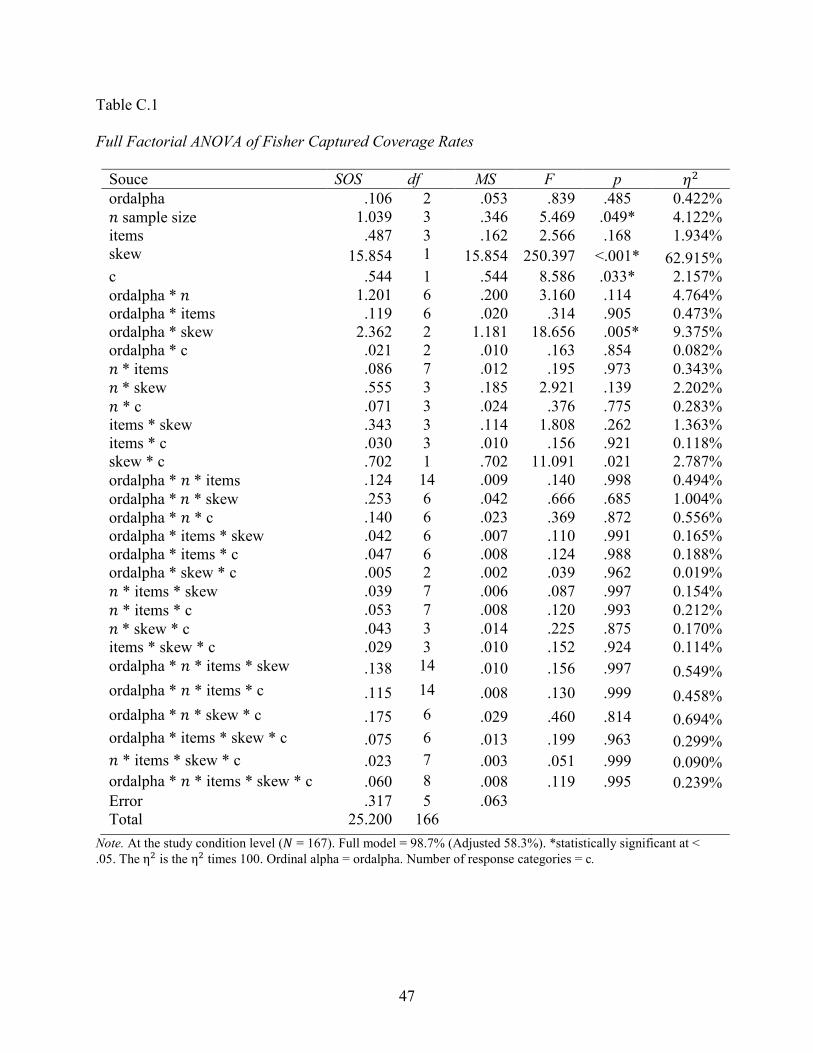
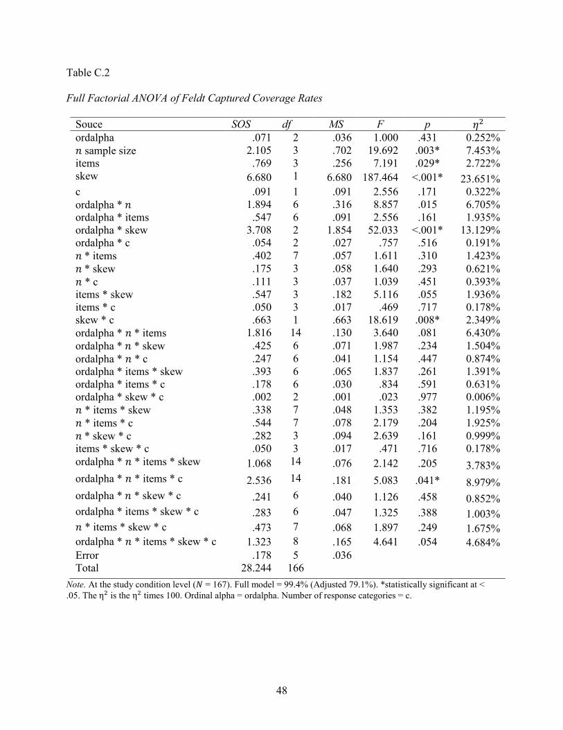
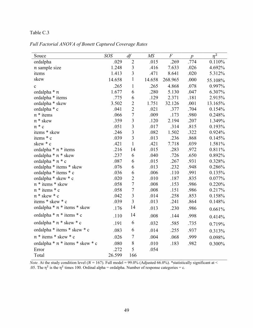
ANOVA results revealed variance in mean coverage rates was best explained by the main
effect of skewness levels (ranging from 23.651% to 62.915%) except for the Feldt method. The
sum of all the interaction effects have a dominating presence, especially for the Feldt method
where 𝜂𝜂2 = 64.968%. The Feldt method is the only method which did not transform ordinal
alpha and was impacted by several higher order interactions. The noteworthy interaction effects
across each method were selected for Table 4 below.
Table 4 Noteworthy 𝜂𝜂2 for Higher Order Interaction Terms
Independent variable Fisher Feldt Bonett HW
ordalpha * skew 9.375% 13.129% 13.165%
16.919%
ordalpha * 𝑛𝑛 sample size
4.764% 6.705% 6.307% 5.371%
ordalpha * 𝑛𝑛 sample size * items
0.494%
6.430% 0.811% 0.997%
ordalpha * 𝑛𝑛 sample size * items * 𝑐𝑐 0.458%
8.979% 0.414% 0.529%
Note. Analyzed at study conditions level where 𝑑𝑑𝑓𝑓 = 166. Values will not exactly sum to interaction values provided in Table 3 because only noteworthy terms are shown. Ordinal alpha = ordalpha. Number of response categories = c.
24
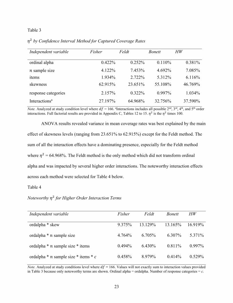
The reason the Feldt method has the lowest captured coverage rate was due to the
confounding impact of several independent variables summarized at the study condition level in
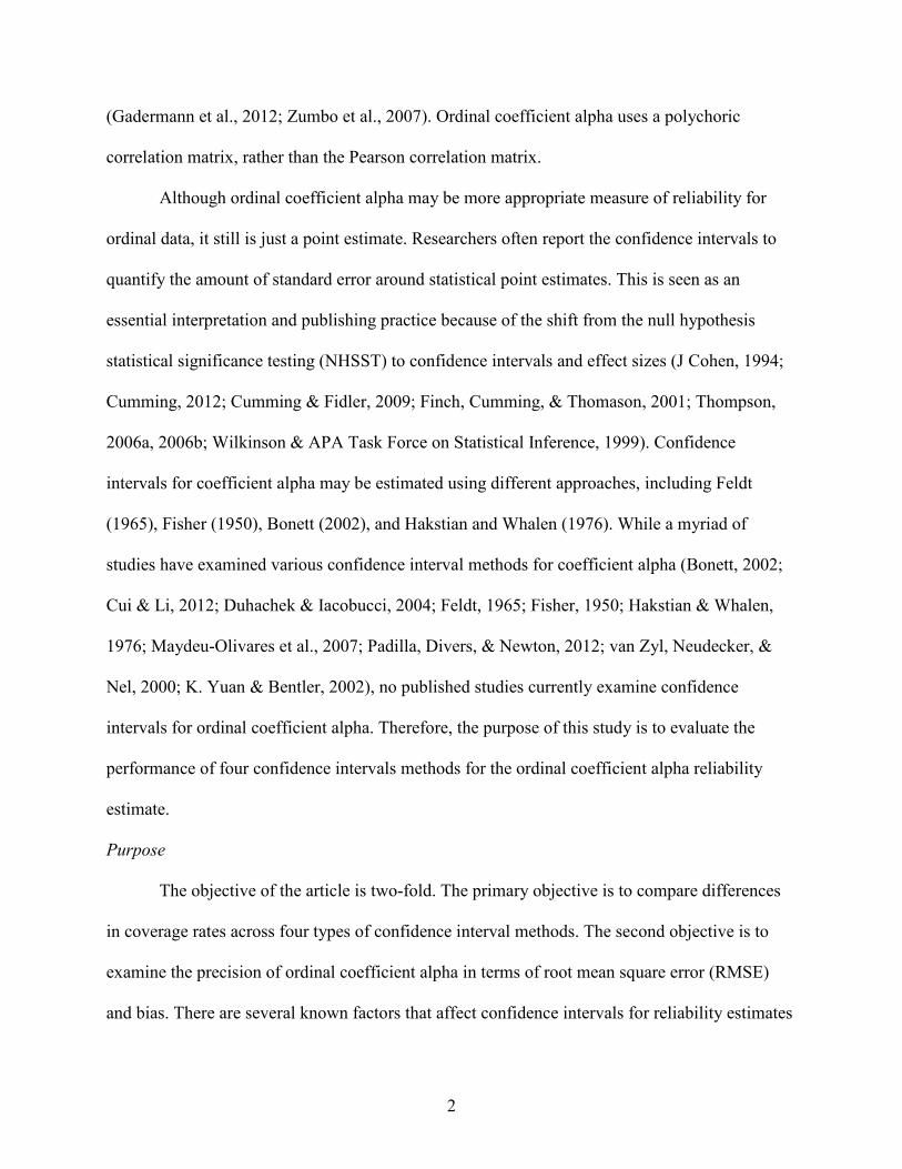
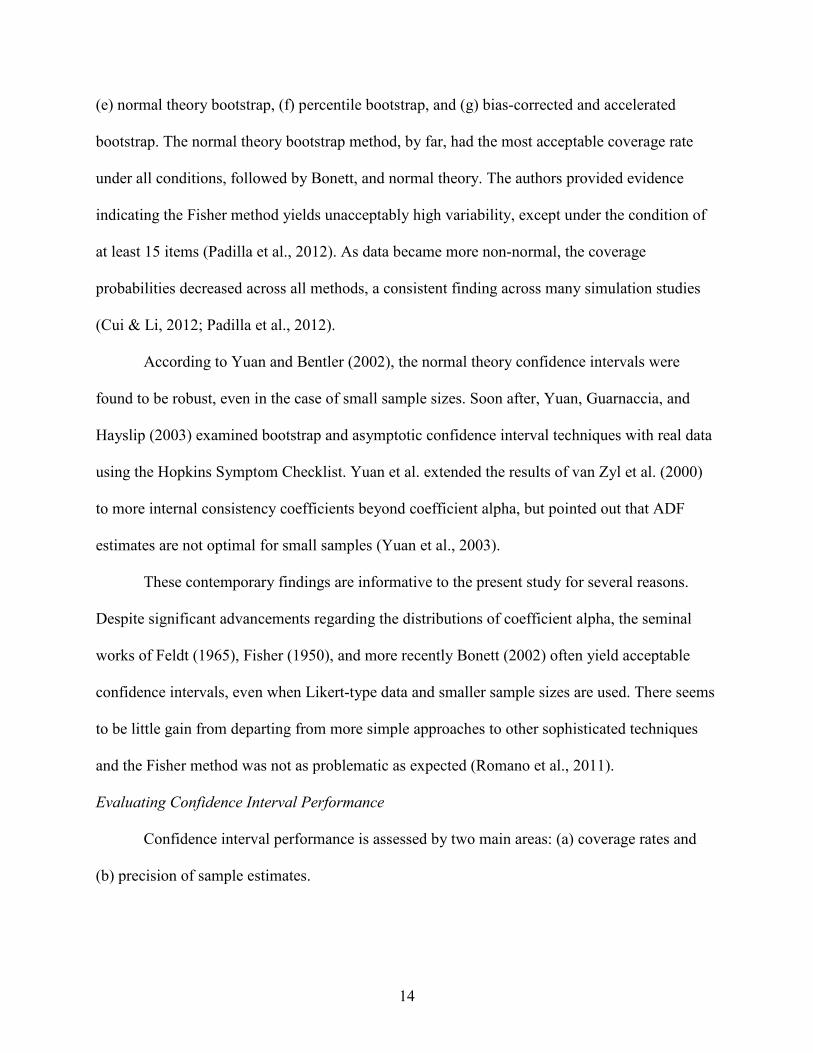
Table 3. The largest two-way interaction effect, ordinal alpha by skewness, is provided in Figure
2.
Figure 2. Two-way mean interaction plots of ordinal alpha by skewness effects for the dependent variable captured coverage rates.
As ordinal alpha increased from .6 to .9, the EMM’s of captured coverage rates increased when
skewness = -1.217 and decreased when skewness = 0. The pattern for the Feldt method (top
25
right) is much more linear compared to the Fisher, Bonett, and HW methods. The results reveal
that coverage rates increase due to the joint influence of ordinal alpha levels and skewness. In
addition, coverage rates are higher with skewed data rather than perfectly symmetrical data
except for the Feldt method, when ordinal alpha levels are .6.
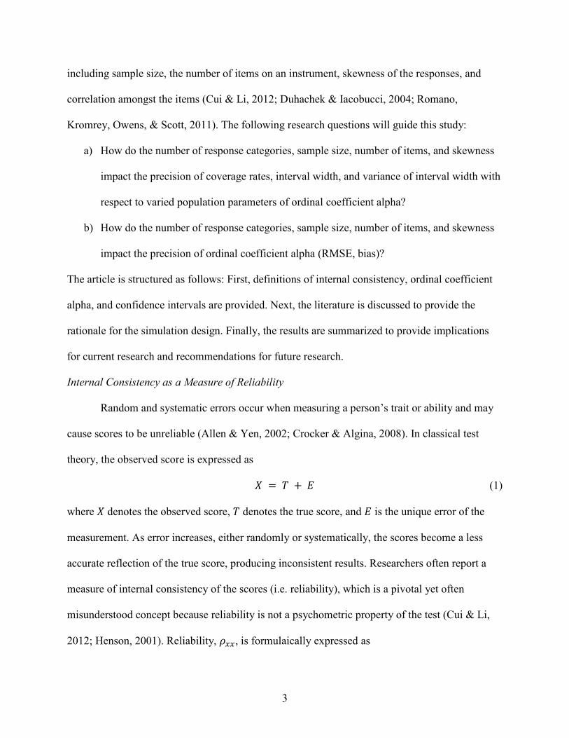
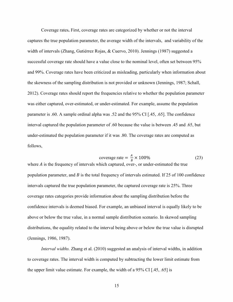
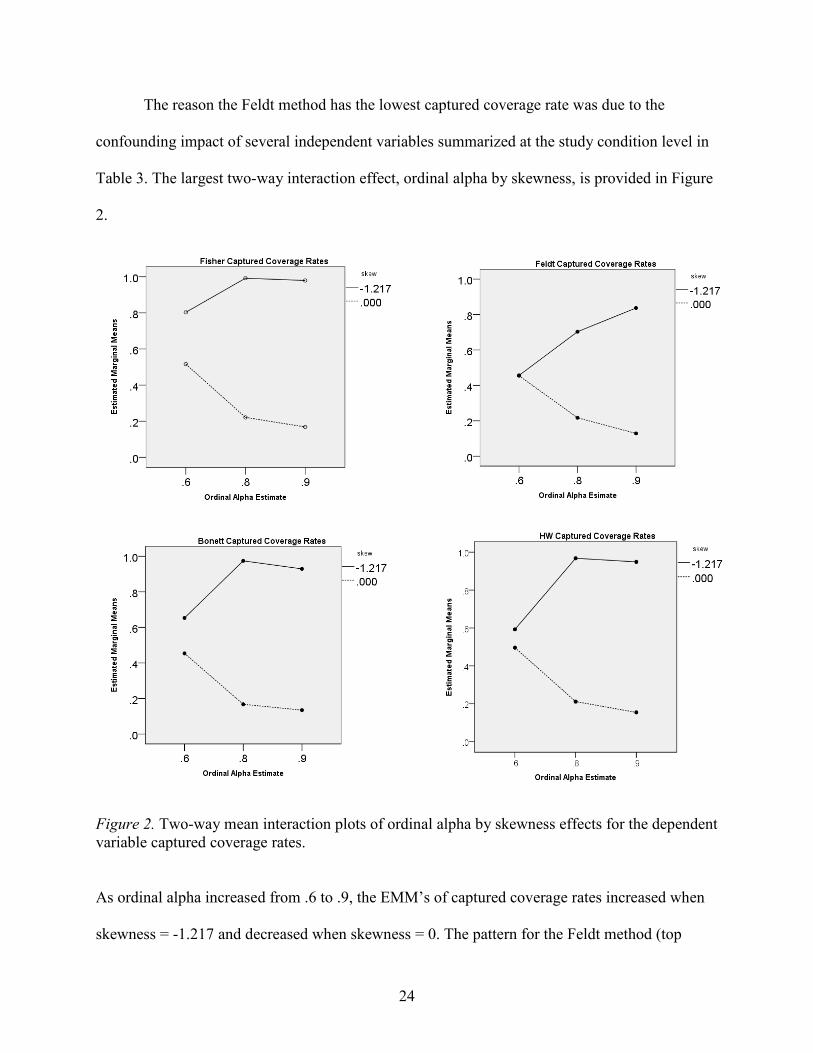
Interval widths. Next, the confidence interval widths were examined. The boxplot shown
in Figure 3 depicts the interquartile ranges of the 95% confidence interval width by the four
confidence interval methods. The Fisher confidence intervals consistently yielded the most
narrow intervals, while Bonett intervals tended to be the widest across all conditions.
Figure 3. Boxplot of 95% confidence interval widths for four estimation methods across 167 study conditions.
26
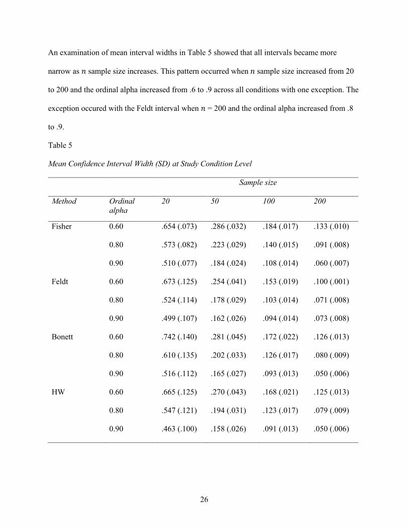
An examination of mean interval widths in Table 5 showed that all intervals became more
narrow as 𝑛𝑛 sample size increases. This pattern occurred when 𝑛𝑛 sample size increased from 20
to 200 and the ordinal alpha increased from .6 to .9 across all conditions with one exception. The
exception occured with the Feldt interval when 𝑛𝑛 = 200 and the ordinal alpha increased from .8
to .9.
Table 5 Mean Confidence Interval Width (SD) at Study Condition Level Sample size
Method Ordinal alpha
20 50 100 200
Fisher 0.60 .654 (.073) .286 (.032) .184 (.017) .133 (.010)
0.80 .573 (.082) .223 (.029) .140 (.015) .091 (.008)
0.90 .510 (.077) .184 (.024) .108 (.014) .060 (.007)
Feldt 0.60 .673 (.125) .254 (.041) .153 (.019) .100 (.001)
0.80 .524 (.114) .178 (.029) .103 (.014) .071 (.008)
0.90 .499 (.107) .162 (.026) .094 (.014) .073 (.008)
Bonett 0.60 .742 (.140) .281 (.045) .172 (.022) .126 (.013)
0.80 .610 (.135) .202 (.033) .126 (.017) .080 (.009)
0.90 .516 (.112) .165 (.027) .093 (.013) .050 (.006)
HW 0.60 .665 (.125) .270 (.043) .168 (.021) .125 (.013)
0.80 .547 (.121) .194 (.031) .123 (.017) .079 (.009)
0.90 .463 (.100) .158 (.026) .091 (.013) .050 (.006)
27
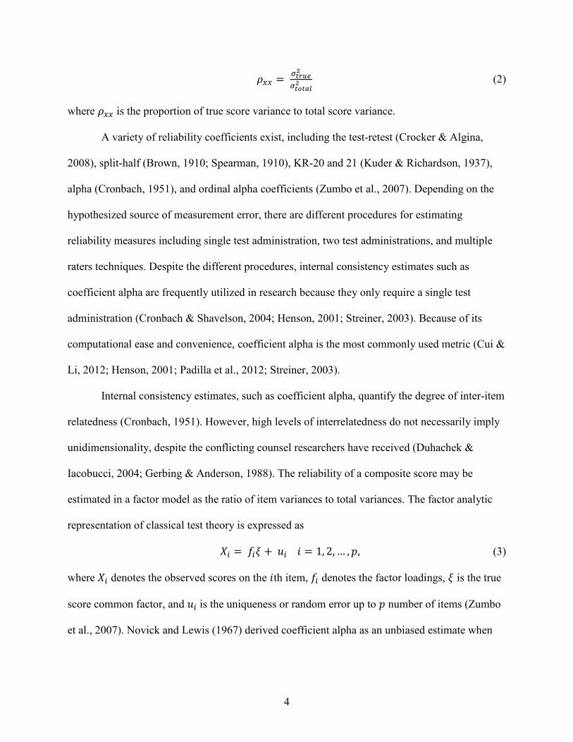
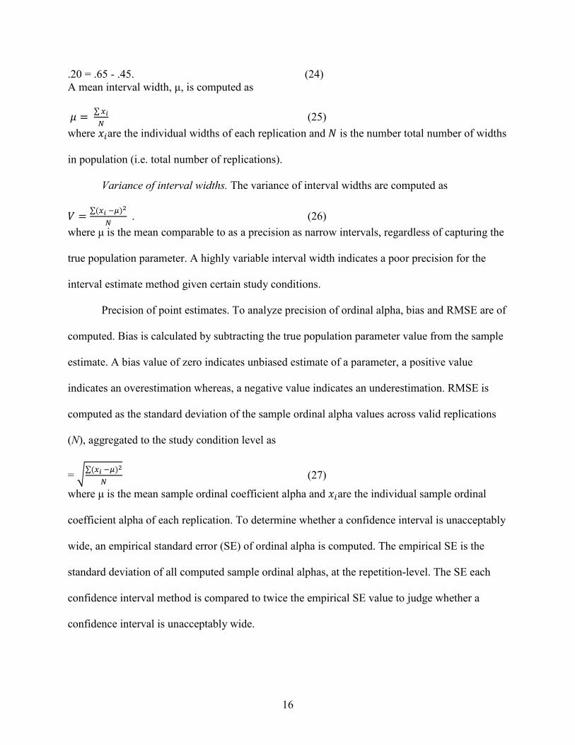
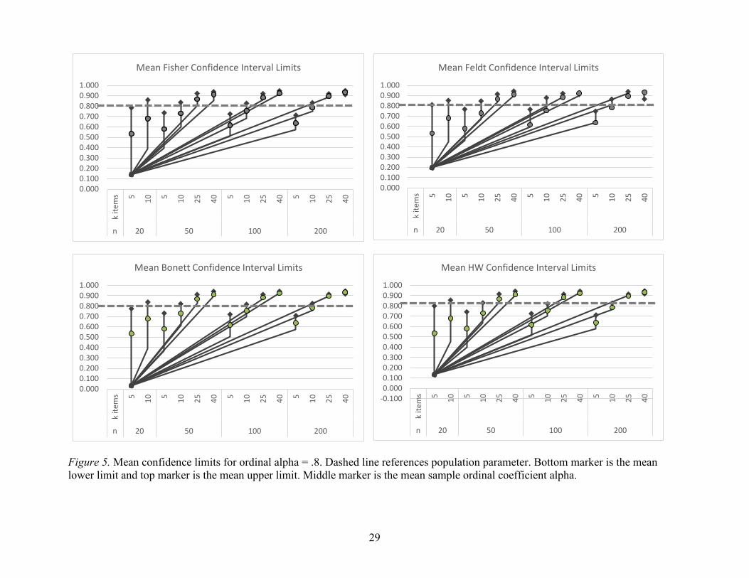
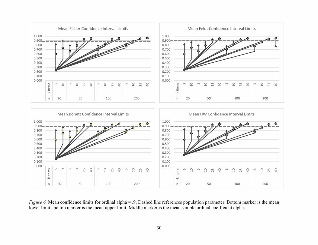
Additional graphical inspections shown in Figure 4 through Figure 6 portray mean upper
and lower limits by ordinal alpha levels for each confidence interval method. The confounding
impact of sample size and number of items for each confidence interval method follow the same
pattern. That is, as sample size and the number of items increased together, the intervals become
more narrow. The intervals became quite narrow when sample size = 200 and the number of
items = 40. There are no striking visual differences in Figures Figure 4 through Figure 6 in
confidence interval widths between the Fisher, Feldt, Bonett, and HW methods across various
levels of ordinal alpha.

28
Figure 4. Mean confidence limits for ordinal alpha = .6. Dashed line references population parameter. Bottom marker is the mean lower limit and top marker is the mean upper limit. Middle marker is the mean sample ordinal coefficient alpha.
0.0000.1000.2000.3000.4000.5000.6000.7000.8000.9001.000
k ite
ms 5 10 5 10 25 40 5 10 25 40 5 10 25 40
n 20 50 100 200
Mean Fisher Confidence Interval Limits
-0.1000.0000.1000.2000.3000.4000.5000.6000.7000.8000.9001.000
k ite
ms 5 10 5 10 25 40 5 10 25 40 5 10 25 40
n 20 50 100 200
Mean Feldt Confidence Interval Limits
-0.200-0.1000.0000.1000.2000.3000.4000.5000.6000.7000.8000.9001.000
k ite
ms 5 10 5 10 25 40 5 10 25 40 5 10 25 40
n 20 50 100 200
Mean Bonett Confidence Interval Limits
-0.1000.0000.1000.2000.3000.4000.5000.6000.7000.8000.9001.000
k ite
ms 5 10 5 10 25 40 5 10 25 40 5 10 25 40
n 20 50 100 200
Mean HW Confidence Interval Limits
29
Figure 5. Mean confidence limits for ordinal alpha = .8. Dashed line references population parameter. Bottom marker is the mean lower limit and top marker is the mean upper limit. Middle marker is the mean sample ordinal coefficient alpha.
0.0000.1000.2000.3000.4000.5000.6000.7000.8000.9001.000
k ite
ms 5 10 5 10 25 40 5 10 25 40 5 10 25 40
n 20 50 100 200
Mean Fisher Confidence Interval Limits
0.0000.1000.2000.3000.4000.5000.6000.7000.8000.9001.000
k ite
ms 5 10 5 10 25 40 5 10 25 40 5 10 25 40
n 20 50 100 200
Mean Feldt Confidence Interval Limits
0.0000.1000.2000.3000.4000.5000.6000.7000.8000.9001.000
k ite
ms 5 10 5 10 25 40 5 10 25 40 5 10 25 40
n 20 50 100 200
Mean Bonett Confidence Interval Limits
-0.1000.0000.1000.2000.3000.4000.5000.6000.7000.8000.9001.000
k ite
ms 5 10 5 10 25 40 5 10 25 40 5 10 25 40
n 20 50 100 200
Mean HW Confidence Interval Limits
30
Figure 6. Mean confidence limits for ordinal alpha = .9. Dashed line references population parameter. Bottom marker is the mean lower limit and top marker is the mean upper limit. Middle marker is the mean sample ordinal coefficient alpha.
0.0000.1000.2000.3000.4000.5000.6000.7000.8000.9001.000
k ite
ms 5 10 5 10 25 40 5 10 25 40 5 10 25 40
n 20 50 100 200
Mean Fisher Confidence Interval Limits
0.0000.1000.2000.3000.4000.5000.6000.7000.8000.9001.000
k ite
ms 5 10 5 10 25 40 5 10 25 40 5 10 25 40
n 20 50 100 200
Mean Feldt Confidence Interval Limits
0.0000.1000.2000.3000.4000.5000.6000.7000.8000.9001.000
k ite
ms 5 10 5 10 25 40 5 10 25 40 5 10 25 40
n 20 50 100 200
Mean Bonett Confidence Interval Limits
0.0000.1000.2000.3000.4000.5000.6000.7000.8000.9001.000
k ite
ms 5 10 5 10 25 40 5 10 25 40 5 10 25 40
n 20 50 100 200
Mean HW Confidence Interval Limits
31
An ANOVA was conducted on each confidence interval method to explore differences in
interval width at the repetition level (𝑁𝑁 = 167,000). The resulting analytical design was 3 x 4 x 4
x 2 x 2 with the aforementioned independent variables shown in Table 6.
Table 6 η2 by Confidence Interval Method for Interval Width Independent variable Fisher Feldt Bonett HW
ordinal alpha 3.882% 2.516% 3.852% 4.290%
𝑛𝑛 sample size 67.254% 55.737% 57.940% 55.062% items 13.599% 11.795% 14.709% 16.566% skewness 6.053% 7.914% 6.527% 7.068%
response categories 0.446% 0.333% 0.547% 0.590%
Interactionsa 5.280% 15.487% 10.148% 10.01%
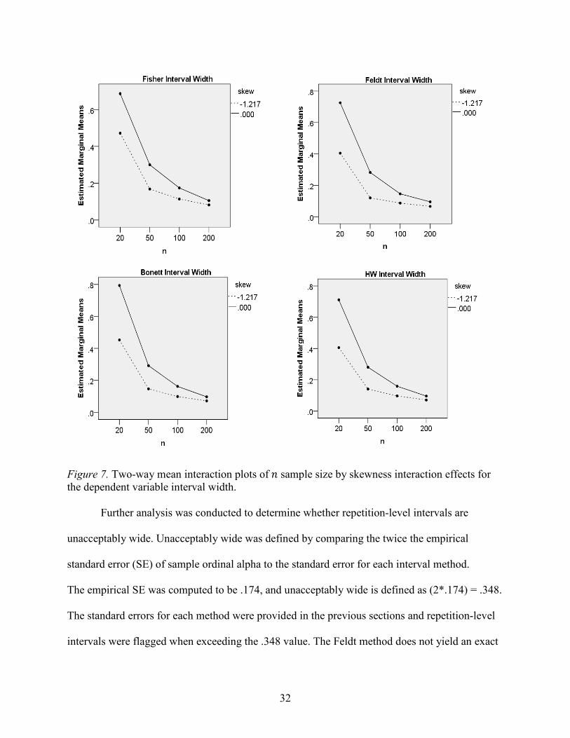
Note. 𝑑𝑑𝑓𝑓 = 166,999. aInteractions includes all possible 2nd, 3rd, 4th, and 5th order interactions. Full factorial results are provided in Appendix C. The η2 is the η2 times 100. The selected ANOVA results revealed that 𝑛𝑛 sample size has the largest impact on explaining the
variance in interval width across all methods. That is, as sample size increased from 20 to 200,
the interval widths decreased. Of the interaction effects, the largest amount of the interaction
effects were explained by the 𝑛𝑛 sample size by skewness interaction. All four methods had
statistically significant 𝑛𝑛 sample size by skewness interactions (𝑝𝑝 < .05 and 𝜂𝜂2 values ranged
from 2.55% (Fisher) to 5.03% (Bonett). While the 𝜂𝜂2 values for both interactions may be
considered “small,” (Cohen, 1988), the implications are meaningful. The interval widths are
consistently smaller across all methods when 𝑛𝑛 sample size increases to 200 and skewness = 0
shown in Figure 7.
32
Figure 7. Two-way mean interaction plots of 𝑛𝑛 sample size by skewness interaction effects for the dependent variable interval width.
Further analysis was conducted to determine whether repetition-level intervals are
unacceptably wide. Unacceptably wide was defined by comparing the twice the empirical
standard error (SE) of sample ordinal alpha to the standard error for each interval method.
The empirical SE was computed to be .174, and unacceptably wide is defined as (2*.174) = .348.
The standard errors for each method were provided in the previous sections and repetition-level
intervals were flagged when exceeding the .348 value. The Feldt method does not yield an exact
33
SE and was excluded from this analysis. However, the Bonett method had 24,000 (of 167,000)
intervals that were unacceptably wide and the Fisher and HW methods had zero. Of the 24,000
intervals that were unacceptably wide were from design conditions where 𝑛𝑛 sample size = 20.
The items = 5 or 10, skewness (2 levels), ordinal alpha (3 levels), and number of response
categories (2 levels) equally split the intervals that were unacceptably wide. If one were to rank
the confidence interval width for 𝑁𝑁 = 167,000, Feldt was the most narrow (M = .194), followed
by HW (M = .200), Bonett (M = .213), and Fisher (M = .217).
Variance of interval widths. An ANOVA was conducted on each confidence interval
method to explain mean group differences in the variance of interval width at the study condition
level. Effect sizes summaries are shown in Table 7.
Table 7 𝜂𝜂2 by Confidence Interval Method for Variance of Interval Width Independent variable Fisher Feldt Bonett HW
ordinal alpha 0.144% 0.500% 0.738% 0.829%
𝑛𝑛 sample size 83.358% 63.5379% 67.264% 66.409% items 2.821% 5.989% 7.285% 7.915% skewness 0.254% 3.011% 2.257% 2.492%
response categories 0.642% 0.094% 0.077% 0.079%
Interactionsa 12.780% 26.866% 22.3785% 22.276%
Note. 𝑑𝑑𝑓𝑓 is the number of study conditions = 167. aInteractions includes all possible 2nd, 3rd, 4th, and 5th order interactions. Full factorial results are provided in Appendix C. The η2 is the η2 times 100.
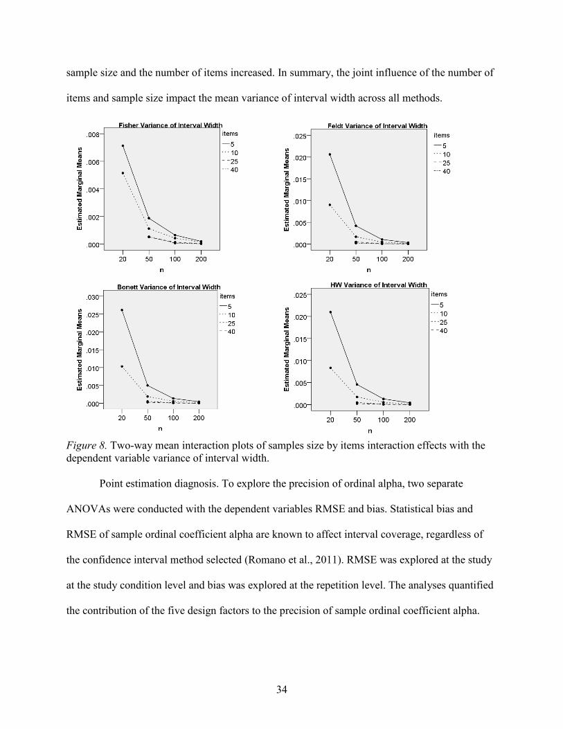
Of all the interaction effects, the sample size by number of items, persisted as the largest
effect across the four confidence interval methods. The η2 values ranged from 2.140% (top left,
Fisher) to 10.394% (bottom right, HW) with the mean plots provided in Figure 8. All four
methods follow the same pattern with variance of interval widths sharply decreasing as both
34
sample size and the number of items increased. In summary, the joint influence of the number of
items and sample size impact the mean variance of interval width across all methods.
Figure 8. Two-way mean interaction plots of samples size by items interaction effects with the dependent variable variance of interval width.
Point estimation diagnosis. To explore the precision of ordinal alpha, two separate
ANOVAs were conducted with the dependent variables RMSE and bias. Statistical bias and
RMSE of sample ordinal coefficient alpha are known to affect interval coverage, regardless of
the confidence interval method selected (Romano et al., 2011). RMSE was explored at the study
at the study condition level and bias was explored at the repetition level. The analyses quantified
the contribution of the five design factors to the precision of sample ordinal coefficient alpha.
35
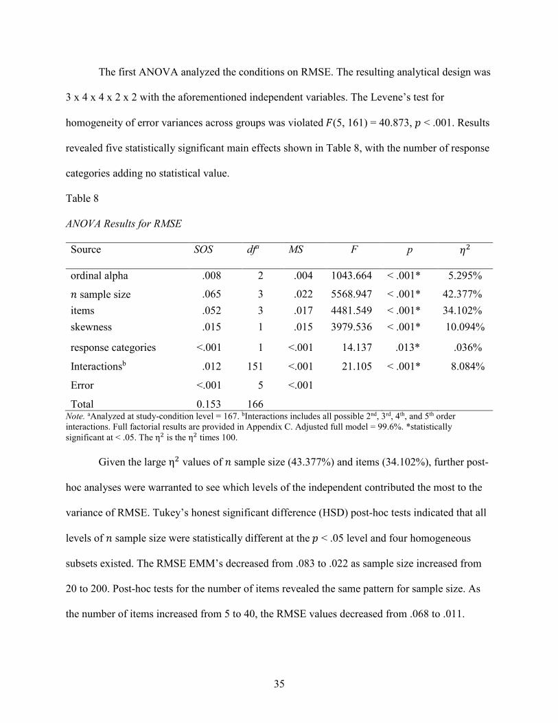
The first ANOVA analyzed the conditions on RMSE. The resulting analytical design was
3 x 4 x 4 x 2 x 2 with the aforementioned independent variables. The Levene’s test for
homogeneity of error variances across groups was violated 𝐹𝐹(5, 161) = 40.873, 𝑝𝑝 < .001. Results
revealed five statistically significant main effects shown in Table 8, with the number of response
categories adding no statistical value.
Table 8 ANOVA Results for RMSE Source SOS dfa MS F p 𝜂𝜂2
ordinal alpha .008 2 .004 1043.664 < .001* 5.295%
𝑛𝑛 sample size .065 3 .022 5568.947 < .001* 42.377% items .052 3 .017 4481.549 < .001* 34.102% skewness .015 1 .015 3979.536 < .001* 10.094%
response categories <.001 1 <.001 14.137 .013* .036%
Interactionsb .012 151 <.001 21.105 < .001* 8.084%
Error <.001 5 <.001
Total 0.153 166 Note. aAnalyzed at study-condition level = 167. bInteractions includes all possible 2nd, 3rd, 4th, and 5th order interactions. Full factorial results are provided in Appendix C. Adjusted full model = 99.6%. *statistically significant at < .05. The η2 is the η2 times 100.
Given the large η2 values of 𝑛𝑛 sample size (43.377%) and items (34.102%), further post-
hoc analyses were warranted to see which levels of the independent contributed the most to the
variance of RMSE. Tukey’s honest significant difference (HSD) post-hoc tests indicated that all
levels of 𝑛𝑛 sample size were statistically different at the 𝑝𝑝 < .05 level and four homogeneous
subsets existed. The RMSE EMM’s decreased from .083 to .022 as sample size increased from
20 to 200. Post-hoc tests for the number of items revealed the same pattern for sample size. As
the number of items increased from 5 to 40, the RMSE values decreased from .068 to .011.
36
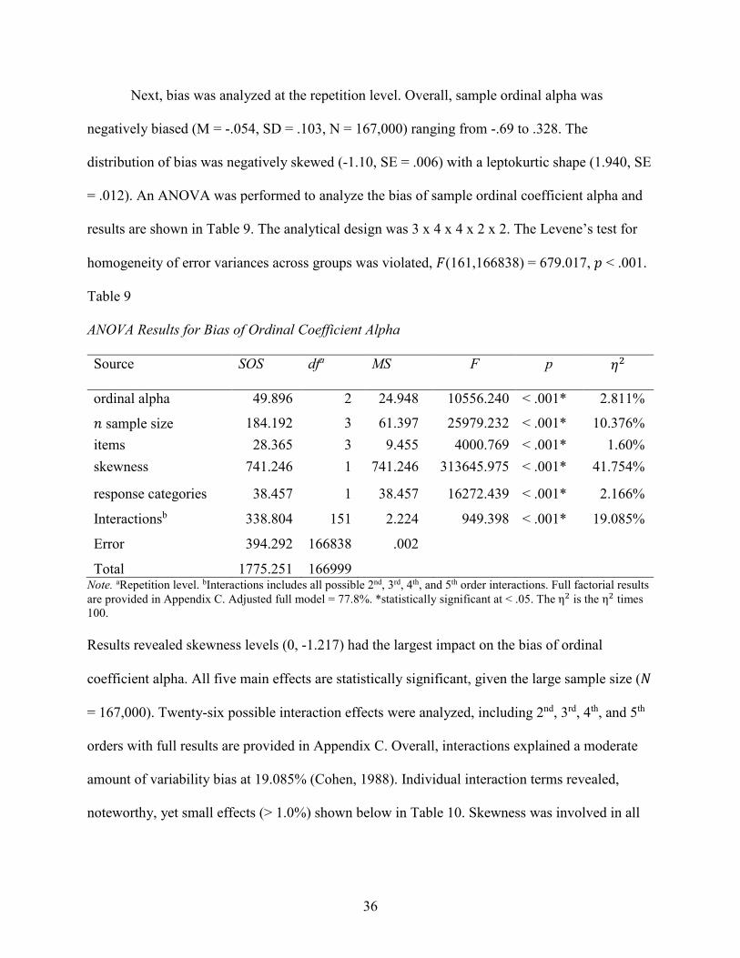
Next, bias was analyzed at the repetition level. Overall, sample ordinal alpha was
negatively biased (M = -.054, SD = .103, N = 167,000) ranging from -.69 to .328. The
distribution of bias was negatively skewed (-1.10, SE = .006) with a leptokurtic shape (1.940, SE
= .012). An ANOVA was performed to analyze the bias of sample ordinal coefficient alpha and
results are shown in Table 9. The analytical design was 3 x 4 x 4 x 2 x 2. The Levene’s test for
homogeneity of error variances across groups was violated, 𝐹𝐹(161,166838) = 679.017, 𝑝𝑝 < .001.
Table 9 ANOVA Results for Bias of Ordinal Coefficient Alpha Source SOS dfa MS F p 𝜂𝜂2
ordinal alpha 49.896 2 24.948 10556.240 < .001* 2.811%
𝑛𝑛 sample size 184.192 3 61.397 25979.232 < .001* 10.376% items 28.365 3 9.455 4000.769 < .001* 1.60% skewness 741.246 1 741.246 313645.975 < .001* 41.754%
response categories 38.457 1 38.457 16272.439 < .001* 2.166%
Interactionsb 338.804 151 2.224 949.398 < .001* 19.085%
Error 394.292 166838 .002
Total 1775.251 166999 Note. aRepetition level. bInteractions includes all possible 2nd, 3rd, 4th, and 5th order interactions. Full factorial results are provided in Appendix C. Adjusted full model = 77.8%. *statistically significant at < .05. The η2 is the η2 times 100. Results revealed skewness levels (0, -1.217) had the largest impact on the bias of ordinal
coefficient alpha. All five main effects are statistically significant, given the large sample size (𝑁𝑁
= 167,000). Twenty-six possible interaction effects were analyzed, including 2nd, 3rd, 4th, and 5th
orders with full results are provided in Appendix C. Overall, interactions explained a moderate
amount of variability bias at 19.085% (Cohen, 1988). Individual interaction terms revealed,
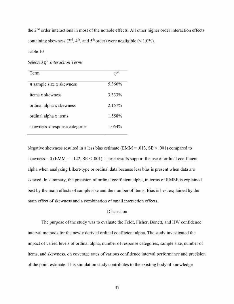
noteworthy, yet small effects (> 1.0%) shown below in Table 10. Skewness was involved in all
37
the 2nd order interactions in most of the notable effects. All other higher order interaction effects
containing skewness (3rd, 4th, and 5th order) were negligible (< 1.0%).
Table 10 Selected 𝜂𝜂2 Interaction Terms Term 𝜂𝜂2
𝑛𝑛 sample size x skewness 5.366%
items x skewness 3.333%
ordinal alpha x skewness 2.157%
ordinal alpha x items 1.558%
skewness x response categories 1.054%
Negative skewness resulted in a less bias estimate (EMM = .013, SE < .001) compared to
skewness = 0 (EMM = -.122, SE < .001). These results support the use of ordinal coefficient
alpha when analyzing Likert-type or ordinal data because less bias is present when data are
skewed. In summary, the precision of ordinal coefficient alpha, in terms of RMSE is explained
best by the main effects of sample size and the number of items. Bias is best explained by the
main effect of skewness and a combination of small interaction effects.
Discussion
The purpose of the study was to evaluate the Feldt, Fisher, Bonett, and HW confidence
interval methods for the newly derived ordinal coefficient alpha. The study investigated the
impact of varied levels of ordinal alpha, number of response categories, sample size, number of
items, and skewness, on coverage rates of various confidence interval performance and precision
of the point estimate. This simulation study contributes to the existing body of knowledge
38
because no known published studies have examined confidence intervals for ordinal alpha. This
study exploited problems in a manner that are untenable in applied settings (e.g. 167,000
replications). The findings about poor coverage rates are meaningful for everyone from the
mathematician to the applied researcher. Overall, great caution should be exercised with the
interpretation of confidence intervals for ordinal coefficient alpha and the sample ordinal
estimate itself.
Mean captured coverage rates were remarkably lower than expected. Coverage rates,
close to the nominal rate (95%) are deemed acceptable (Romano et al., 2011). The acceptable
criterion can more liberal (Romano et al., 2011), ranging between [.93, .97], but mean coverage
rates between 46% to 62% are low and unacceptable. The skewness main effect had the largest
impact in all the analyses with respect to captured coverage rates. The implications for a
researcher suggest taking an extremely cautious approach to the face validity of any confidence
interval method for the ordinal alpha. A researcher should not expect trustworthy results with
any of these confidence interval methods for ordinal alpha. However, all four confidence
intervals tended to follow the same coverage rate patterns across study conditions for the
captured-, over-, and under-estimated rates.
The study also investigated the impact of the aforementioned conditions on interval
widths and variance of interval widths. Confidence interval widths were statistically significantly
different across Feldt, Fisher, Bonett, and HW methods (𝑝𝑝 < .05). Confidence interval widths
became more narrow as ordinal alphas increased from .6 to .9. However, interval widths
dramatically decreased as sample size increased for all methods. There are small, but notable
differences observed with interval width between methods. The Feldt method was the only
method that did not use any transformation of sample ordinal coefficient alpha, and was
39
therefore, impacted differently than Fisher, Bonett, and HW. The Feldt interval width is
determined as a function of the degrees of freedom based on sample size and number of items
heavily impacted by higher order interactions. The Fisher, Bonett, and HW methods applied
logarithmic transformations of sample ordinal alpha and more easily explained by main effects
sample size and the number of items.
The main effects of sample size and number of items best explain the precision of ordinal
alpha, in terms of RMSE. The number of response categories was a useless predictor (𝜂𝜂2 =
0.036%). Interestingly, the number of response categories is a strong predictor of the parametric
counterpart, coefficient alpha, but not necessarily for ordinal coefficient alpha Zumbo et al.,
2007). EMMs of RMSE were statistically significantly different (𝑝𝑝 < .05) across all levels of
sample size (20, 50, 100 and 200) and items (5, 10, 25, and 40). The ordinal alpha and skewness
main effects were notable, but were much smaller in context with the sample size and number of
items effects. The practical implications suggest keeping an instrument, with Likert-type data,
between 10-25 items, while striving for samples sizes of at least 50 participants because RMSE
values are smaller.
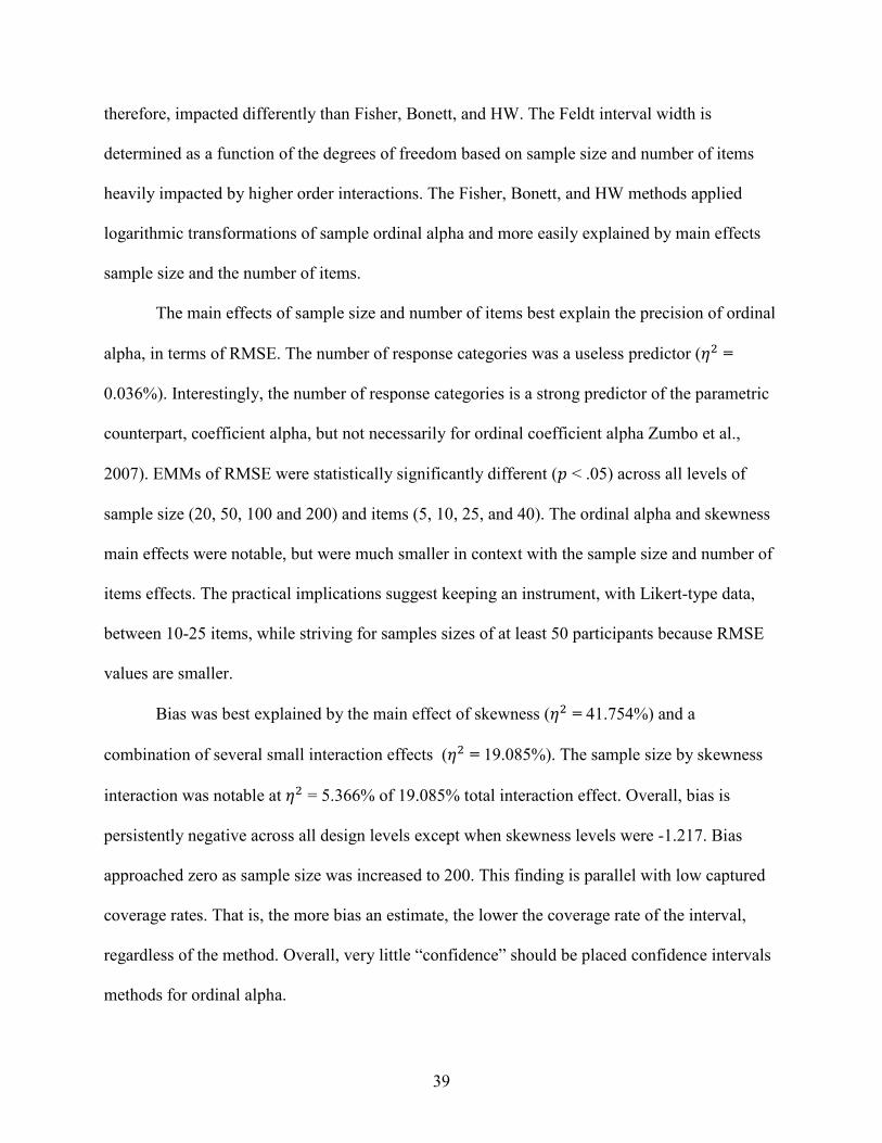
Bias was best explained by the main effect of skewness (𝜂𝜂2 = 41.754%) and a
combination of several small interaction effects (𝜂𝜂2 = 19.085%). The sample size by skewness
interaction was notable at 𝜂𝜂2 = 5.366% of 19.085% total interaction effect. Overall, bias is
persistently negative across all design levels except when skewness levels were -1.217. Bias
approached zero as sample size was increased to 200. This finding is parallel with low captured
coverage rates. That is, the more bias an estimate, the lower the coverage rate of the interval,
regardless of the method. Overall, very little “confidence” should be placed confidence intervals
methods for ordinal alpha.
40
Limitations
As with any simulation study, the results are limited to the conditions specified. The
conditions were based on previous research and reasonable justification to portray scenarios in
applied research. In order to explain variance of coverage rates, confidence interval width, and
interval width variance in a manner that was interpretable, methods were analyzed separately. An
emphasis was placed on 𝜂𝜂2values. Finally, bias was analyzed in its raw scale compared to an
absolute bias scale.
Recommendations for Future Research
There are a number of opportunities to extend the current research. First, a need exists to
develop a confidence interval method specifically for ordinal alpha which improves coverage
rates closer to the nominal rate. At present, the current methods are not adequate and do not
provide trustworthy results. The ADF-based and bootstrapped methods, may capture the true
population parameter better than the normal-theory based confidence intervals selected for this
type of study. In addition, the contiguous points between items = 10 and 25 may be explored to
determine the optimal point of precision of ordinal alpha for both RMSE and bias.

41
APPENDIX A
HISTOGRAMS OF POPULATION RESPONSE DISTRIBUTIONS
42
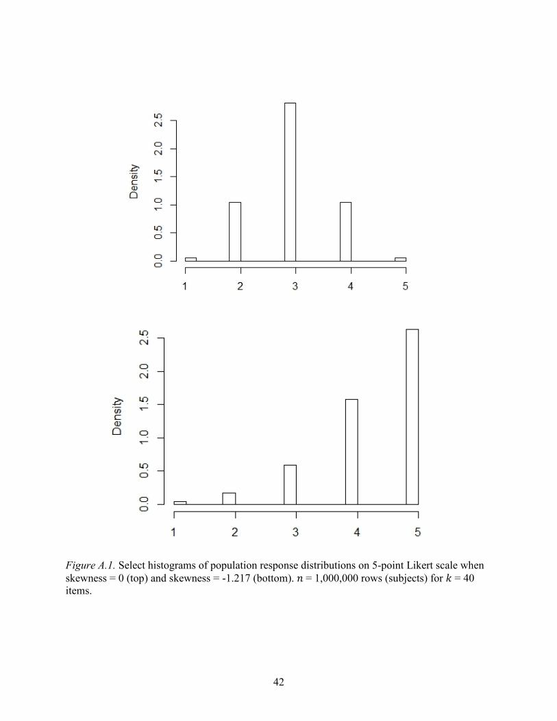
Figure A.1. Select histograms of population response distributions on 5-point Likert scale when skewness = 0 (top) and skewness = -1.217 (bottom). 𝑛𝑛 = 1,000,000 rows (subjects) for 𝑘𝑘 = 40 items.
43
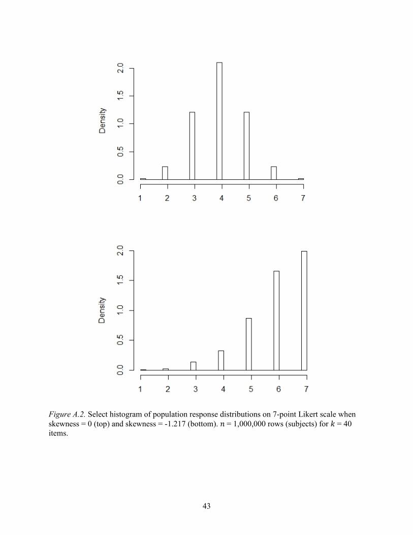
Figure A.2. Select histogram of population response distributions on 7-point Likert scale when skewness = 0 (top) and skewness = -1.217 (bottom). 𝑛𝑛 = 1,000,000 rows (subjects) for 𝑘𝑘 = 40 items.

44
APPENDIX B
TABLE OF NON-EXECUTABLE CONDITIONS
45
Obs num
SimID Population ordinal coeff alpha
Factor loading
k items c response categories
n sample size
skewness
1 3 0.9 0.625 25 5 20 0 2 4 0.6 0.311 40 5 20 0 3 7 0.6 0.311 25 7 20 0 4 8 0.8 0.471 40 7 20 0
5 12 0.9 0.625 40 5 50 0
6 35 0.8 0.471 25 5 20 -1.217
7 36 0.9 0.625 40 5 20 -1.217
8 39 0.9 0.625 25 7 20 -1.217
9 40 0.6 0.311 40 7 20 -1.217
10 67 0.6 0.311 25 5 20 0
11 68 0.8 0.471 40 5 20 0
12 71 0.8 0.471 25 7 20 0
13 72 0.9 0.625 40 7 20 0
14 99 0.9 0.625 25 5 20 -1.217
15 100 0.6 0.311 40 5 20 -1.217
16 103 0.6 0.311 25 7 20 -1.217
17 104 0.8 0.471 40 7 20 -1.217
18 131 0.8 0.471 25 5 20 0
19 132 0.9 0.625 40 5 20 0
20 135 0.9 0.625 25 7 20 0
21 136 0.6 0.311 40 7 20 0
22 163 0.6 0.311 25 5 20 -1.217
23 164 0.8 0.471 40 5 20 -1.217
24 167 0.8 0.471 25 7 20 -1.217
25 168 0.9 0.625 40 7 20 -1.217

46
APPENDIX C
FULL FACTORIAL ANOVA RESULTS
47
Table C.1
Full Factorial ANOVA of Fisher Captured Coverage Rates
Souce SOS df MS F p 𝜂𝜂2 ordalpha .106 2 .053 .839 .485 0.422% 𝑛𝑛 sample size 1.039 3 .346 5.469 .049* 4.122% items .487 3 .162 2.566 .168 1.934% skew 15.854 1 15.854 250.397 <.001* 62.915% c .544 1 .544 8.586 .033* 2.157% ordalpha * 𝑛𝑛 1.201 6 .200 3.160 .114 4.764% ordalpha * items .119 6 .020 .314 .905 0.473% ordalpha * skew 2.362 2 1.181 18.656 .005* 9.375% ordalpha * c .021 2 .010 .163 .854 0.082% 𝑛𝑛 * items .086 7 .012 .195 .973 0.343% 𝑛𝑛 * skew .555 3 .185 2.921 .139 2.202% 𝑛𝑛 * c .071 3 .024 .376 .775 0.283% items * skew .343 3 .114 1.808 .262 1.363% items * c .030 3 .010 .156 .921 0.118% skew * c .702 1 .702 11.091 .021 2.787% ordalpha * 𝑛𝑛 * items .124 14 .009 .140 .998 0.494% ordalpha * 𝑛𝑛 * skew .253 6 .042 .666 .685 1.004% ordalpha * 𝑛𝑛 * c .140 6 .023 .369 .872 0.556% ordalpha * items * skew .042 6 .007 .110 .991 0.165% ordalpha * items * c .047 6 .008 .124 .988 0.188% ordalpha * skew * c .005 2 .002 .039 .962 0.019% 𝑛𝑛 * items * skew .039 7 .006 .087 .997 0.154% 𝑛𝑛 * items * c .053 7 .008 .120 .993 0.212% 𝑛𝑛 * skew * c .043 3 .014 .225 .875 0.170% items * skew * c .029 3 .010 .152 .924 0.114% ordalpha * 𝑛𝑛 * items * skew .138 14 .010 .156 .997 0.549% ordalpha * 𝑛𝑛 * items * c .115 14 .008 .130 .999 0.458% ordalpha * 𝑛𝑛 * skew * c .175 6 .029 .460 .814 0.694% ordalpha * items * skew * c .075 6 .013 .199 .963 0.299% 𝑛𝑛 * items * skew * c .023 7 .003 .051 .999 0.090% ordalpha * 𝑛𝑛 * items * skew * c .060 8 .008 .119 .995 0.239% Error .317 5 .063 Total 25.200 166
Note. At the study condition level (𝑁𝑁 = 167). Full model = 98.7% (Adjusted 58.3%). *statistically significant at < .05. The η2 is the η2 times 100. Ordinal alpha = ordalpha. Number of response categories = c.
48
Table C.2
Full Factorial ANOVA of Feldt Captured Coverage Rates
Souce SOS df MS F p 𝜂𝜂2 ordalpha .071 2 .036 1.000 .431 0.252% 𝑛𝑛 sample size 2.105 3 .702 19.692 .003* 7.453% items .769 3 .256 7.191 .029* 2.722% skew 6.680 1 6.680 187.464 <.001* 23.651% c .091 1 .091 2.556 .171 0.322% ordalpha * 𝑛𝑛 1.894 6 .316 8.857 .015 6.705% ordalpha * items .547 6 .091 2.556 .161 1.935% ordalpha * skew 3.708 2 1.854 52.033 <.001* 13.129% ordalpha * c .054 2 .027 .757 .516 0.191% 𝑛𝑛 * items .402 7 .057 1.611 .310 1.423% 𝑛𝑛 * skew .175 3 .058 1.640 .293 0.621% 𝑛𝑛 * c .111 3 .037 1.039 .451 0.393% items * skew .547 3 .182 5.116 .055 1.936% items * c .050 3 .017 .469 .717 0.178% skew * c .663 1 .663 18.619 .008* 2.349% ordalpha * 𝑛𝑛 * items 1.816 14 .130 3.640 .081 6.430% ordalpha * 𝑛𝑛 * skew .425 6 .071 1.987 .234 1.504% ordalpha * 𝑛𝑛 * c .247 6 .041 1.154 .447 0.874% ordalpha * items * skew .393 6 .065 1.837 .261 1.391% ordalpha * items * c .178 6 .030 .834 .591 0.631% ordalpha * skew * c .002 2 .001 .023 .977 0.006% 𝑛𝑛 * items * skew .338 7 .048 1.353 .382 1.195% 𝑛𝑛 * items * c .544 7 .078 2.179 .204 1.925% 𝑛𝑛 * skew * c .282 3 .094 2.639 .161 0.999% items * skew * c .050 3 .017 .471 .716 0.178% ordalpha * 𝑛𝑛 * items * skew 1.068 14 .076 2.142 .205 3.783% ordalpha * 𝑛𝑛 * items * c 2.536 14 .181 5.083 .041* 8.979% ordalpha * 𝑛𝑛 * skew * c .241 6 .040 1.126 .458 0.852% ordalpha * items * skew * c .283 6 .047 1.325 .388 1.003% 𝑛𝑛 * items * skew * c .473 7 .068 1.897 .249 1.675% ordalpha * 𝑛𝑛 * items * skew * c 1.323 8 .165 4.641 .054 4.684% Error .178 5 .036 Total 28.244 166
Note. At the study condition level (𝑁𝑁 = 167). Full model = 99.4% (Adjusted 79.1%). *statistically significant at < .05. The η2 is the η2 times 100. Ordinal alpha = ordalpha. Number of response categories = c.
49
Table C.3
Full Factorial ANOVA of Bonett Captured Coverage Rates
Souce SOS df MS F p 𝜂𝜂2 ordalpha .029 2 .015 .269 .774 0.110% 𝑛𝑛 sample size 1.248 3 .416 7.633 .026 4.692% items 1.413 3 .471 8.641 .020 5.312% skew 14.658 1 14.658 268.965 .000 55.108% c .265 1 .265 4.868 .078 0.997% ordalpha * 𝑛𝑛 1.677 6 .280 5.130 .047 6.307% ordalpha * items .775 6 .129 2.371 .181 2.915% ordalpha * skew 3.502 2 1.751 32.126 .001 13.165% ordalpha * c .041 2 .021 .377 .704 0.154% 𝑛𝑛 * items .066 7 .009 .173 .980 0.248% 𝑛𝑛 * skew .359 3 .120 2.194 .207 1.349% 𝑛𝑛 * c .051 3 .017 .314 .815 0.193% items * skew .246 3 .082 1.502 .322 0.924% items * c .039 3 .013 .236 .868 0.145% skew * c .421 1 .421 7.718 .039 1.581% ordalpha * 𝑛𝑛 * items .216 14 .015 .283 .972 0.811% ordalpha * 𝑛𝑛 * skew .237 6 .040 .726 .650 0.892% ordalpha * 𝑛𝑛 * c .087 6 .015 .267 .931 0.328% ordalpha * items * skew .076 6 .013 .232 .948 0.286% ordalpha * items * c .036 6 .006 .110 .991 0.135% ordalpha * skew * c .020 2 .010 .187 .835 0.077% 𝑛𝑛 * items * skew .058 7 .008 .153 .986 0.220% 𝑛𝑛 * items * c .058 7 .008 .151 .986 0.217% 𝑛𝑛 * skew * c .042 3 .014 .258 .853 0.158% items * skew * c .039 3 .013 .241 .864 0.148% ordalpha * 𝑛𝑛 * items * skew .176 14 .013 .230 .986 0.661% ordalpha * 𝑛𝑛 * items * c .110 14 .008 .144 .998 0.414% ordalpha * 𝑛𝑛 * skew * c .191 6 .032 .585 .735 0.719% ordalpha * items * skew * c .083 6 .014 .255 .937 0.313% 𝑛𝑛 * items * skew * c .026 7 .004 .068 .999 0.098% ordalpha * 𝑛𝑛 * items * skew * c .080 8 .010 .183 .982 0.300% Error .272 5 .054 Total 26.599 166
Note. At the study condition level (𝑁𝑁 = 167). Full model = 99.0% (Adjusted 66.0%). *statistically significant at < .05. The η2 is the η2 times 100. Ordinal alpha = ordalpha. Number of response categories = c.

50
Table C.4
Full Factorial ANOVA of HW Captured Coverage Rates
Souce SOS df MS F p 𝜂𝜂2 ordalpha .100 2 .050 .929 .454 0.381% 𝑛𝑛 sample size 1.852 3 .617 11.521 .011 7.085% items 1.599 3 .533 9.945 .015 6.116% skew 12.228 1 12.228 228.157 .000 46.769% c .270 1 .270 5.045 .075 1.034% ordalpha * 𝑛𝑛 1.404 6 .234 4.367 .064 5.371% ordalpha * items .830 6 .138 2.580 .159 3.174% ordalpha * skew 4.423 2 2.212 41.269 .001 16.919% ordalpha * c .045 2 .022 .420 .678 0.172% 𝑛𝑛 * items .060 7 .009 .159 .984 0.228% 𝑛𝑛 * skew .410 3 .137 2.549 .169 1.568% 𝑛𝑛 * c .051 3 .017 .320 .811 0.197% items * skew .294 3 .098 1.830 .259 1.125% items * c .037 3 .012 .227 .874 0.1405 skew * c .525 1 .525 9.788 .026 2.006% ordalpha * 𝑛𝑛 * items .261 14 .019 .347 .946 0.997% ordalpha * 𝑛𝑛 * skew .353 6 .059 1.099 .469 1.351% ordalpha * 𝑛𝑛 * c .098 6 .016 .305 .910 0.375% ordalpha * items * skew .065 6 .011 .204 .961 0.251% ordalpha * items * c .044 6 .007 .136 .985 0.168% ordalpha * skew * c .006 2 .003 .059 .943 0.024% 𝑛𝑛 * items * skew .062 7 .009 .165 .982 0.237% 𝑛𝑛 * items * c .057 7 .008 .151 .986 0.216% 𝑛𝑛 * skew * c .040 3 .013 .247 .861 0.152% items * skew * c .037 3 .012 .227 .874 0.1405 ordalpha * 𝑛𝑛 * items * skew .194 14 .014 .259 .979 0.743% ordalpha * 𝑛𝑛 * items * c .138 14 .010 .184 .994 0.529% ordalpha * 𝑛𝑛 * skew * c .180 6 .030 .560 .750 0.689% ordalpha * items * skew * c .096 6 .016 .297 .914 0.366% 𝑛𝑛 * items * skew * c .021 7 .003 .056 .999 0.080% ordalpha * 𝑛𝑛 * items * skew * c .098 8 .012 .228 .968 0.374% Error .268 5 .054 Total 26.145 166
Note. At the study condition level (𝑁𝑁 = 167). Full model = 99.0% (Adjusted 66.0%). *statistically significant at < .05. The η2 is the η2 times 100. Ordinal alpha = ordalpha. Number of response categories = c.
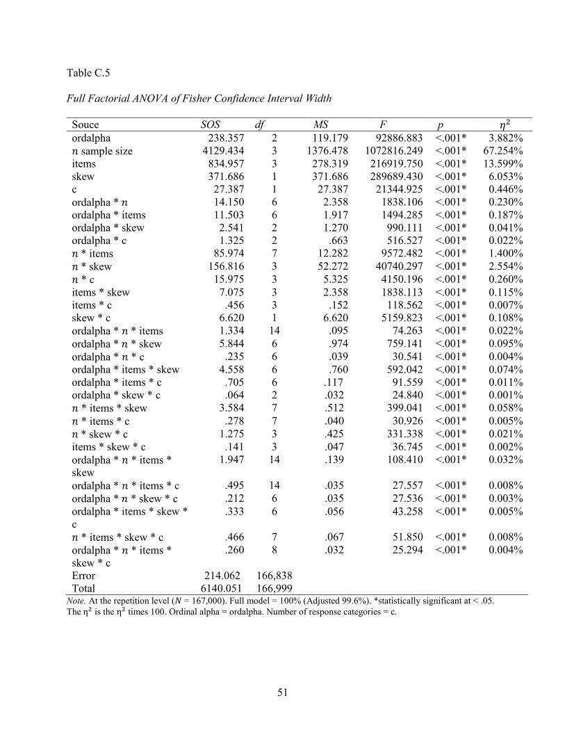
51
Table C.5
Full Factorial ANOVA of Fisher Confidence Interval Width
Souce SOS df MS F p 𝜂𝜂2 ordalpha 238.357 2 119.179 92886.883 <.001* 3.882% 𝑛𝑛 sample size 4129.434 3 1376.478 1072816.249 <.001* 67.254% items 834.957 3 278.319 216919.750 <.001* 13.599% skew 371.686 1 371.686 289689.430 <.001* 6.053% c 27.387 1 27.387 21344.925 <.001* 0.446% ordalpha * 𝑛𝑛 14.150 6 2.358 1838.106 <.001* 0.230% ordalpha * items 11.503 6 1.917 1494.285 <.001* 0.187% ordalpha * skew 2.541 2 1.270 990.111 <.001* 0.041% ordalpha * c 1.325 2 .663 516.527 <.001* 0.022% 𝑛𝑛 * items 85.974 7 12.282 9572.482 <.001* 1.400% 𝑛𝑛 * skew 156.816 3 52.272 40740.297 <.001* 2.554% 𝑛𝑛 * c 15.975 3 5.325 4150.196 <.001* 0.260% items * skew 7.075 3 2.358 1838.113 <.001* 0.115% items * c .456 3 .152 118.562 <.001* 0.007% skew * c 6.620 1 6.620 5159.823 <.001* 0.108% ordalpha * 𝑛𝑛 * items 1.334 14 .095 74.263 <.001* 0.022% ordalpha * 𝑛𝑛 * skew 5.844 6 .974 759.141 <.001* 0.095% ordalpha * 𝑛𝑛 * c .235 6 .039 30.541 <.001* 0.004% ordalpha * items * skew 4.558 6 .760 592.042 <.001* 0.074% ordalpha * items * c .705 6 .117 91.559 <.001* 0.011% ordalpha * skew * c .064 2 .032 24.840 <.001* 0.001% 𝑛𝑛 * items * skew 3.584 7 .512 399.041 <.001* 0.058% 𝑛𝑛 * items * c .278 7 .040 30.926 <.001* 0.005% 𝑛𝑛 * skew * c 1.275 3 .425 331.338 <.001* 0.021% items * skew * c .141 3 .047 36.745 <.001* 0.002% ordalpha * 𝑛𝑛 * items * skew
1.947 14 .139 108.410 <.001* 0.032%
ordalpha * 𝑛𝑛 * items * c .495 14 .035 27.557 <.001* 0.008% ordalpha * 𝑛𝑛 * skew * c .212 6 .035 27.536 <.001* 0.003% ordalpha * items * skew * c
.333 6 .056 43.258 <.001* 0.005%
𝑛𝑛 * items * skew * c .466 7 .067 51.850 <.001* 0.008% ordalpha * 𝑛𝑛 * items * skew * c
.260 8 .032 25.294 <.001* 0.004%
Error 214.062 166,838 Total 6140.051 166,999
Note. At the repetition level (𝑁𝑁 = 167,000). Full model = 100% (Adjusted 99.6%). *statistically significant at < .05. The η2 is the η2 times 100. Ordinal alpha = ordalpha. Number of response categories = c.

52
Table C.6
Full Factorial ANOVA of Feldt Confidence Interval Width
Souce SOS df MS F p 𝜂𝜂2 ordalpha 189.852 2 94.926 33763.786 <.001* 2.516% 𝑛𝑛 sample size 4205.846 3 1401.949 498653.330 <.001* 55.737% items 890.048 3 296.683 105525.834 <.001* 11.795% skew 597.240 1 597.240 212429.685 <.001* 7.915% c 25.137 1 25.137 8940.874 <.001* 0.333% ordalpha * 𝑛𝑛 65.298 6 10.883 3870.919 <.001* 0.865% ordalpha * items 21.409 6 3.568 1269.165 <.001* 0.284% ordalpha * skew 16.658 2 8.329 2962.544 <.001* 0.221% ordalpha * c 3.397 2 1.698 604.058 <.001* 0.045% 𝑛𝑛 * items 165.370 7 23.624 8402.827 <.001* 2.192% 𝑛𝑛 * skew 379.875 3 126.625 45038.693 <.001* 5.034% 𝑛𝑛 * c 54.274 3 18.091 6434.828 <.001* 0.719% items * skew 56.394 3 18.798 6686.209 <.001* 0.747% items * c 4.354 3 1.451 516.245 <.001* 0.058% skew * c 5.237 1 5.237 1862.657 <.001* 0.069% ordalpha * 𝑛𝑛 * items 18.189 14 1.299 462.119 <.001* 0.241% ordalpha * 𝑛𝑛 * skew 32.723 6 5.454 1939.856 <.001* 0.434% ordalpha * 𝑛𝑛 * c 22.894 6 3.816 1357.192 <.001* 0.303% ordalpha * items * skew
16.654 6 2.776 987.249 <.001* 0.221%
ordalpha * items * c 14.599 6 2.433 865.455 <.001* 0.193% ordalpha * skew * c 1.926 2 .963 342.495 <.001* 0.026% 𝑛𝑛 * items * skew 40.927 7 5.847 2079.573 <.001* 0.542% 𝑛𝑛 * items * c 40.089 7 5.727 2037.000 <.001* 0.531% 𝑛𝑛 * skew * c 15.005 3 5.002 1779.070 <.001* 0.199% items * skew * c 7.446 3 2.482 882.756 <.001* 0.099% ordalpha * 𝑛𝑛 * items * skew
56.617 14 4.044 1438.413 <.001* 0.750%
ordalpha * 𝑛𝑛 * items * c
48.446 14 3.460 1230.823 <.001* 0.642%
ordalpha * 𝑛𝑛 * skew * c
24.944 6 4.157 1478.696 <.001* 0.331%
ordalpha * items * skew * c
10.040 6 1.673 595.155 <.001* 0.133%
𝑛𝑛 * items * skew * c 12.401 7 1.772 630.140 <.001* 0.164% ordalpha * 𝑛𝑛 * items * skew * c
33.475 8 4.184 1488.320 <.001* 0.444%
Error 469.060 166,838 .003 Total 7545.823 166,999
Note. At the repetition level (𝑁𝑁 = 167,000). Full model = 93.8% (Adjusted 93.8%). *statistically significant at < .05. The η2 is the η2 times 100. Ordinal alpha = ordalpha. Number of response categories = c.
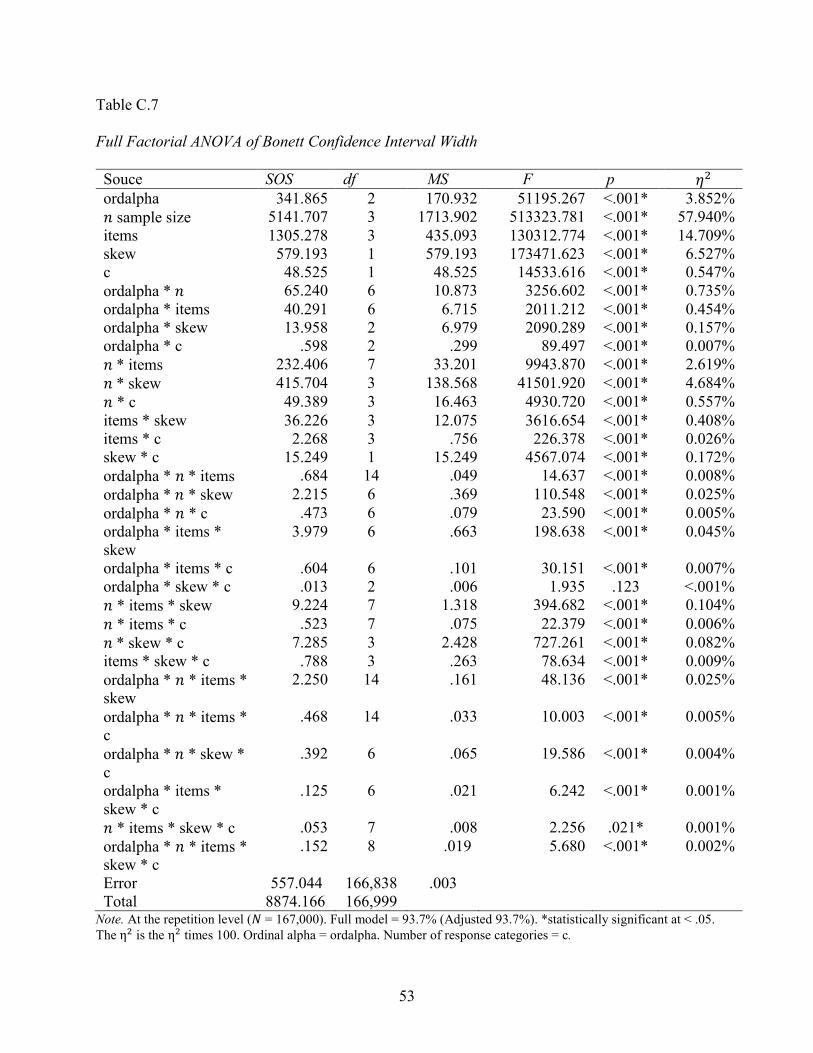
53
Table C.7
Full Factorial ANOVA of Bonett Confidence Interval Width
Souce SOS df MS F p 𝜂𝜂2 ordalpha 341.865 2 170.932 51195.267 <.001* 3.852% 𝑛𝑛 sample size 5141.707 3 1713.902 513323.781 <.001* 57.940% items 1305.278 3 435.093 130312.774 <.001* 14.709% skew 579.193 1 579.193 173471.623 <.001* 6.527% c 48.525 1 48.525 14533.616 <.001* 0.547% ordalpha * 𝑛𝑛 65.240 6 10.873 3256.602 <.001* 0.735% ordalpha * items 40.291 6 6.715 2011.212 <.001* 0.454% ordalpha * skew 13.958 2 6.979 2090.289 <.001* 0.157% ordalpha * c .598 2 .299 89.497 <.001* 0.007% 𝑛𝑛 * items 232.406 7 33.201 9943.870 <.001* 2.619% 𝑛𝑛 * skew 415.704 3 138.568 41501.920 <.001* 4.684% 𝑛𝑛 * c 49.389 3 16.463 4930.720 <.001* 0.557% items * skew 36.226 3 12.075 3616.654 <.001* 0.408% items * c 2.268 3 .756 226.378 <.001* 0.026% skew * c 15.249 1 15.249 4567.074 <.001* 0.172% ordalpha * 𝑛𝑛 * items .684 14 .049 14.637 <.001* 0.008% ordalpha * 𝑛𝑛 * skew 2.215 6 .369 110.548 <.001* 0.025% ordalpha * 𝑛𝑛 * c .473 6 .079 23.590 <.001* 0.005% ordalpha * items * skew
3.979 6 .663 198.638 <.001* 0.045%
ordalpha * items * c .604 6 .101 30.151 <.001* 0.007% ordalpha * skew * c .013 2 .006 1.935 .123 <.001% 𝑛𝑛 * items * skew 9.224 7 1.318 394.682 <.001* 0.104% 𝑛𝑛 * items * c .523 7 .075 22.379 <.001* 0.006% 𝑛𝑛 * skew * c 7.285 3 2.428 727.261 <.001* 0.082% items * skew * c .788 3 .263 78.634 <.001* 0.009% ordalpha * 𝑛𝑛 * items * skew
2.250 14 .161 48.136 <.001* 0.025%
ordalpha * 𝑛𝑛 * items * c
.468 14 .033 10.003 <.001* 0.005%
ordalpha * 𝑛𝑛 * skew * c
.392 6 .065 19.586 <.001* 0.004%
ordalpha * items * skew * c
.125 6 .021 6.242 <.001* 0.001%
𝑛𝑛 * items * skew * c .053 7 .008 2.256 .021* 0.001% ordalpha * 𝑛𝑛 * items * skew * c
.152 8 .019 5.680 <.001* 0.002%
Error 557.044 166,838 .003 Total 8874.166 166,999
Note. At the repetition level (𝑁𝑁 = 167,000). Full model = 93.7% (Adjusted 93.7%). *statistically significant at < .05. The η2 is the η2 times 100. Ordinal alpha = ordalpha. Number of response categories = c.
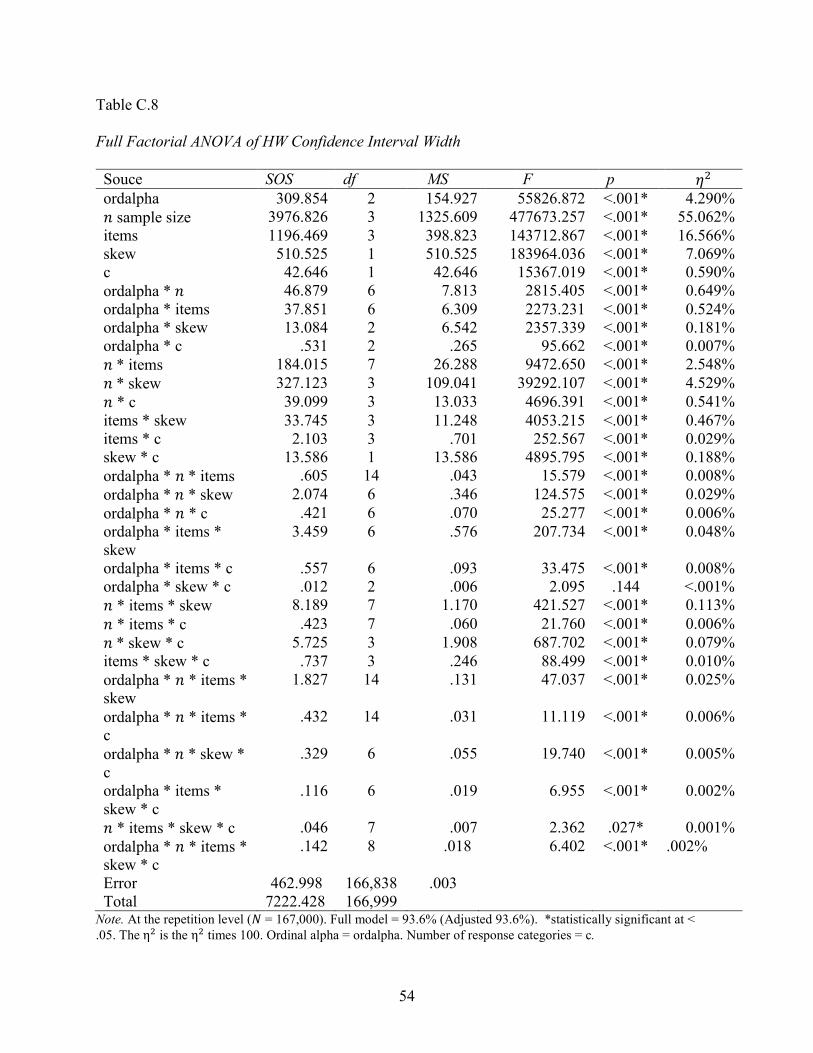
54
Table C.8
Full Factorial ANOVA of HW Confidence Interval Width
Souce SOS df MS F p 𝜂𝜂2 ordalpha 309.854 2 154.927 55826.872 <.001* 4.290% 𝑛𝑛 sample size 3976.826 3 1325.609 477673.257 <.001* 55.062% items 1196.469 3 398.823 143712.867 <.001* 16.566% skew 510.525 1 510.525 183964.036 <.001* 7.069% c 42.646 1 42.646 15367.019 <.001* 0.590% ordalpha * 𝑛𝑛 46.879 6 7.813 2815.405 <.001* 0.649% ordalpha * items 37.851 6 6.309 2273.231 <.001* 0.524% ordalpha * skew 13.084 2 6.542 2357.339 <.001* 0.181% ordalpha * c .531 2 .265 95.662 <.001* 0.007% 𝑛𝑛 * items 184.015 7 26.288 9472.650 <.001* 2.548% 𝑛𝑛 * skew 327.123 3 109.041 39292.107 <.001* 4.529% 𝑛𝑛 * c 39.099 3 13.033 4696.391 <.001* 0.541% items * skew 33.745 3 11.248 4053.215 <.001* 0.467% items * c 2.103 3 .701 252.567 <.001* 0.029% skew * c 13.586 1 13.586 4895.795 <.001* 0.188% ordalpha * 𝑛𝑛 * items .605 14 .043 15.579 <.001* 0.008% ordalpha * 𝑛𝑛 * skew 2.074 6 .346 124.575 <.001* 0.029% ordalpha * 𝑛𝑛 * c .421 6 .070 25.277 <.001* 0.006% ordalpha * items * skew
3.459 6 .576 207.734 <.001* 0.048%
ordalpha * items * c .557 6 .093 33.475 <.001* 0.008% ordalpha * skew * c .012 2 .006 2.095 .144 <.001% 𝑛𝑛 * items * skew 8.189 7 1.170 421.527 <.001* 0.113% 𝑛𝑛 * items * c .423 7 .060 21.760 <.001* 0.006% 𝑛𝑛 * skew * c 5.725 3 1.908 687.702 <.001* 0.079% items * skew * c .737 3 .246 88.499 <.001* 0.010% ordalpha * 𝑛𝑛 * items * skew
1.827 14 .131 47.037 <.001* 0.025%
ordalpha * 𝑛𝑛 * items * c
.432 14 .031 11.119 <.001* 0.006%
ordalpha * 𝑛𝑛 * skew * c
.329 6 .055 19.740 <.001* 0.005%
ordalpha * items * skew * c
.116 6 .019 6.955 <.001* 0.002%
𝑛𝑛 * items * skew * c .046 7 .007 2.362 .027* 0.001% ordalpha * 𝑛𝑛 * items * skew * c
.142 8 .018 6.402 <.001* .002%
Error 462.998 166,838 .003 Total 7222.428 166,999
Note. At the repetition level (𝑁𝑁 = 167,000). Full model = 93.6% (Adjusted 93.6%). *statistically significant at < .05. The η2 is the η2 times 100. Ordinal alpha = ordalpha. Number of response categories = c.
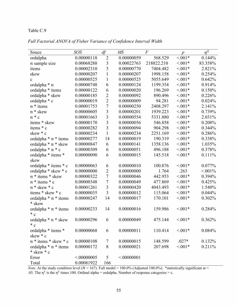
55
Table C.9
Full Factorial ANOVA of Fisher Variance of Confidence Interval Width
Souce SOS df MS F p 𝜂𝜂2 ordalpha 0.00000118 2 0.00000059 568.529 <.001* 0.144% 𝑛𝑛 sample size 0.00068288 3 0.00022763 218822.210 <.001* 83.358% items 0.00002310 3 0.00000770 7404.482 <.001* 2.821% skew 0.00000207 1 0.00000207 1998.158 <.001* 0.254% c 0.00000525 1 0.00000525 5055.649 <.001* 0.642% ordalpha * 𝑛𝑛 0.00000748 6 0.00000124 1199.354 <.001* 0.914% ordalpha * items 0.00000122 6 0.00000020 196.269 <.001* 0.150% ordalpha * skew 0.00000185 2 0.00000092 890.496 <.001* 0.226% ordalpha * c 0.00000019 2 0.00000009 94.281 <.001* 0.024% 𝑛𝑛 * items 0.00001753 7 0.00000250 2408.297 <.001* 2.141% 𝑛𝑛 * skew 0.00000605 3 0.00000201 1939.223 <.001* 0.739% 𝑛𝑛 * c 0.00001663 3 0.00000554 5331.880 <.001* 2.031% items * skew 0.00000170 3 0.00000056 546.858 <.001* 0.208% items * c 0.00000282 3 0.00000094 904.298 <.001* 0.344% skew * c 0.00000234 1 0.00000234 2251.169 <.001* 0.286% ordalpha * 𝑛𝑛 * items 0.00000277 14 0.00000019 190.319 <.001* 0.338% ordalpha * 𝑛𝑛 * skew 0.00000847 6 0.00000141 1358.136 <.001* 1.035% ordalpha * 𝑛𝑛 * c 0.00000309 6 0.00000051 496.188 <.001* 0.378% ordalpha * items * skew
0.00000090 6 0.00000015 145.518 <.001* 0.111%
ordalpha * items * c 0.00000063 6 0.00000010 100.876 <.001* 0.077% ordalpha * skew * c 0.00000000 2 0.00000000 1.764 .263 <.001% 𝑛𝑛 * items * skew 0.00000322 7 0.00000046 442.953 <.001* 0.394% 𝑛𝑛 * items * c 0.00000348 7 0.00000049 477.869 <.001* 0.425% 𝑛𝑛 * skew * c 0.00001261 3 0.00000420 4043.493 <.001* 1.540% items * skew * c 0.00000035 3 0.00000012 115.064 <.001* 0.044% ordalpha * 𝑛𝑛 * items * skew
0.00000247 14 0.00000017 170.101 <.001* 0.302%
ordalpha * 𝑛𝑛 * items * c
0.00000233 14 0.00000016 159.986 <.001* 0.284%
ordalpha * 𝑛𝑛 * skew * c
0.00000296 6 0.00000049 475.144 <.001* 0.362%
ordalpha * items * skew * c
0.00000068 6 0.00000011 110.414 <.001* 0.084%
𝑛𝑛 * items * skew * c 0.00000108 7 0.00000015 148.599 .027* 0.132% ordalpha * 𝑛𝑛 * items * skew * c
0.00000172 8 0.00000021 207.698 <.001* 0.211%
Error <.00000005 5 <.00000001 Total 0.00081922 166
Note. At the study condition level (𝑁𝑁 = 167). Full model = 100.0% (Adjusted 100.0%). *statistically significant at < .05. The η2 is the η2 times 100. Ordinal alpha = ordalpha. Number of response categories = c.
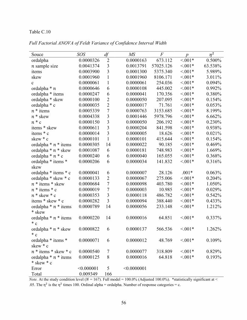
56
Table C.10
Full Factorial ANOVA of Feldt Variance of Confidence Interval Width
Souce SOS df MS F p 𝜂𝜂2 ordalpha 0.0000326 2 0.0000163 673.112 <.001* 0.500% 𝑛𝑛 sample size 0.0041374 3 0.0013791 57025.126 <.001* 63.538% items 0.0003900 3 0.0001300 5375.340 <.001* 5.989% skew 0.0001960 1 0.0001960 8106.171 <.001* 3.011% c 0.0000061 1 0.0000061 254.036 <.001* 0.094% ordalpha * 𝑛𝑛 0.0000646 6 0.0000108 445.002 <.001* 0.992% ordalpha * items 0.0000247 6 0.0000041 170.356 <.001* 0.380% ordalpha * skew 0.0000100 2 0.0000050 207.095 <.001* 0.154% ordalpha * c 0.0000035 2 0.0000017 71.761 <.001* 0.053% 𝑛𝑛 * items 0.0005339 7 0.0000763 3153.685 <.001* 8.199% 𝑛𝑛 * skew 0.0004338 3 0.0001446 5978.796 <.001* 6.662% 𝑛𝑛 * c 0.0000150 3 0.0000050 206.192 <.001* 0.230% items * skew 0.0000611 3 0.0000204 841.598 <.001* 0.938% items * c 0.0000014 3 0.0000005 18.626 <.001* 0.021% skew * c 0.0000101 1 0.0000101 415.644 <.001* 0.154% ordalpha * 𝑛𝑛 * items 0.0000305 14 0.0000022 90.185 <.001* 0.469% ordalpha * 𝑛𝑛 * skew 0.0001087 6 0.0000181 748.983 <.001* 1.669% ordalpha * 𝑛𝑛 * c 0.0000240 6 0.0000040 165.055 <.001* 0.368% ordalpha * items * skew
0.0000206 6 0.0000034 141.832 <.001* 0.316%
ordalpha * items * c 0.0000041 6 0.0000007 28.126 .001* 0.063% ordalpha * skew * c 0.0000133 2 0.0000067 275.006 <.001* 0.204% 𝑛𝑛 * items * skew 0.0000684 7 0.0000098 403.780 <.001* 1.050% 𝑛𝑛 * items * c 0.0000019 7 0.0000003 10.985 <.001* 0.029% 𝑛𝑛 * skew * c 0.0000353 3 0.0000118 486.782 <.001* 0.542% items * skew * c 0.0000282 3 0.0000094 388.440 <.001* 0.433% ordalpha * 𝑛𝑛 * items * skew
0.0000789 14 0.0000056 233.148 <.001* 1.212%
ordalpha * 𝑛𝑛 * items * c
0.0000220 14 0.0000016 64.851 <.001* 0.337%
ordalpha * 𝑛𝑛 * skew * c
0.0000822 6 0.0000137 566.536 <.001* 1.262%
ordalpha * items * skew * c
0.0000071 6 0.0000012 48.769 <.001* 0.109%
𝑛𝑛 * items * skew * c 0.0000540 7 0.0000077 318.809 <.001* 0.829% ordalpha * 𝑛𝑛 * items * skew * c
0.0000125 8 0.0000016 64.818 <.001* 0.193%
Error <0.000001 5 <0.0000001 Total 0.009349 166
Note. At the study condition level (𝑁𝑁 = 167). Full model = 100.0% (Adjusted 100.0%). *statistically significant at < .05. The η2 is the η2 times 100. Ordinal alpha = ordalpha. Number of response categories = c.
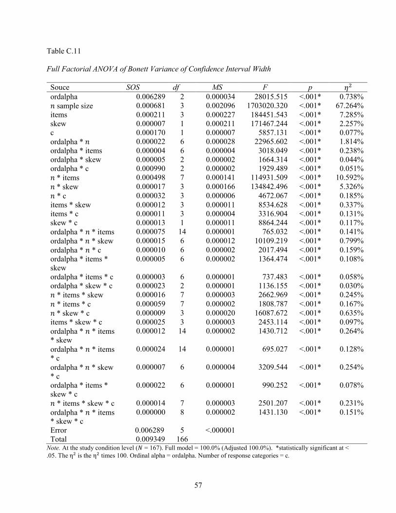
57
Table C.11
Full Factorial ANOVA of Bonett Variance of Confidence Interval Width
Souce SOS df MS F p 𝜂𝜂2 ordalpha 0.006289 2 0.000034 28015.515 <.001* 0.738% 𝑛𝑛 sample size 0.000681 3 0.002096 1703020.320 <.001* 67.264% items 0.000211 3 0.000227 184451.543 <.001* 7.285% skew 0.000007 1 0.000211 171467.244 <.001* 2.257% c 0.000170 1 0.000007 5857.131 <.001* 0.077% ordalpha * 𝑛𝑛 0.000022 6 0.000028 22965.602 <.001* 1.814% ordalpha * items 0.000004 6 0.000004 3018.049 <.001* 0.238% ordalpha * skew 0.000005 2 0.000002 1664.314 <.001* 0.044% ordalpha * c 0.000990 2 0.000002 1929.489 <.001* 0.051% 𝑛𝑛 * items 0.000498 7 0.000141 114931.509 <.001* 10.592% 𝑛𝑛 * skew 0.000017 3 0.000166 134842.496 <.001* 5.326% 𝑛𝑛 * c 0.000032 3 0.000006 4672.067 <.001* 0.185% items * skew 0.000012 3 0.000011 8534.628 <.001* 0.337% items * c 0.000011 3 0.000004 3316.904 <.001* 0.131% skew * c 0.000013 1 0.000011 8864.244 <.001* 0.117% ordalpha * 𝑛𝑛 * items 0.000075 14 0.000001 765.032 <.001* 0.141% ordalpha * 𝑛𝑛 * skew 0.000015 6 0.000012 10109.219 <.001* 0.799% ordalpha * 𝑛𝑛 * c 0.000010 6 0.000002 2017.494 <.001* 0.159% ordalpha * items * skew
0.000005 6 0.000002 1364.474 <.001* 0.108%
ordalpha * items * c 0.000003 6 0.000001 737.483 <.001* 0.058% ordalpha * skew * c 0.000023 2 0.000001 1136.155 <.001* 0.030% 𝑛𝑛 * items * skew 0.000016 7 0.000003 2662.969 <.001* 0.245% 𝑛𝑛 * items * c 0.000059 7 0.000002 1808.787 <.001* 0.167% 𝑛𝑛 * skew * c 0.000009 3 0.000020 16087.672 <.001* 0.635% items * skew * c 0.000025 3 0.000003 2453.114 <.001* 0.097% ordalpha * 𝑛𝑛 * items * skew
0.000012 14 0.000002 1430.712 <.001* 0.264%
ordalpha * 𝑛𝑛 * items * c
0.000024 14 0.000001 695.027 <.001* 0.128%
ordalpha * 𝑛𝑛 * skew * c
0.000007 6 0.000004 3209.544 <.001* 0.254%
ordalpha * items * skew * c
0.000022 6 0.000001 990.252 <.001* 0.078%
𝑛𝑛 * items * skew * c 0.000014 7 0.000003 2501.207 <.001* 0.231% ordalpha * 𝑛𝑛 * items * skew * c
0.000000 8 0.000002 1431.130 <.001* 0.151%
Error 0.006289 5 <.000001 Total 0.009349 166
Note. At the study condition level (𝑁𝑁 = 167). Full model = 100.0% (Adjusted 100.0%). *statistically significant at < .05. The η2 is the η2 times 100. Ordinal alpha = ordalpha. Number of response categories = c.
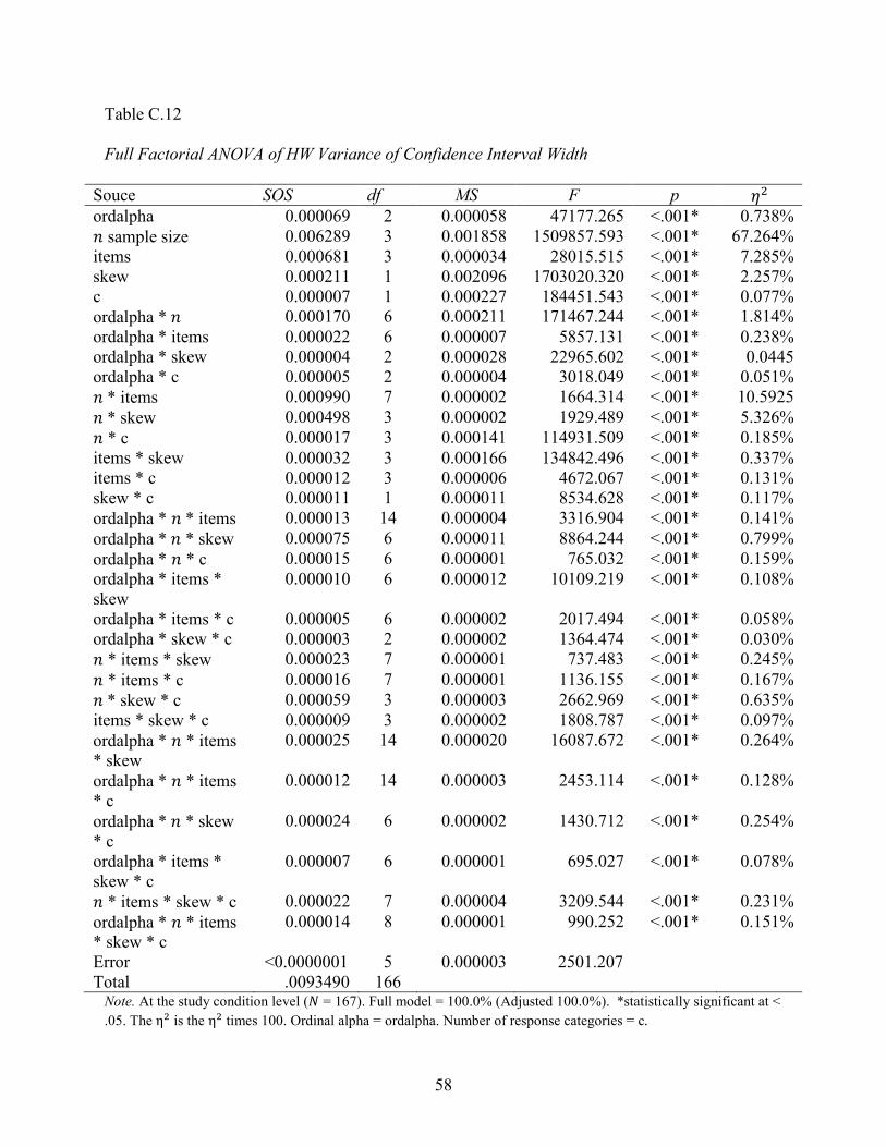
58
Table C.12
Full Factorial ANOVA of HW Variance of Confidence Interval Width
Souce SOS df MS F p 𝜂𝜂2 ordalpha 0.000069 2 0.000058 47177.265 <.001* 0.738% 𝑛𝑛 sample size 0.006289 3 0.001858 1509857.593 <.001* 67.264% items 0.000681 3 0.000034 28015.515 <.001* 7.285% skew 0.000211 1 0.002096 1703020.320 <.001* 2.257% c 0.000007 1 0.000227 184451.543 <.001* 0.077% ordalpha * 𝑛𝑛 0.000170 6 0.000211 171467.244 <.001* 1.814% ordalpha * items 0.000022 6 0.000007 5857.131 <.001* 0.238% ordalpha * skew 0.000004 2 0.000028 22965.602 <.001* 0.0445 ordalpha * c 0.000005 2 0.000004 3018.049 <.001* 0.051% 𝑛𝑛 * items 0.000990 7 0.000002 1664.314 <.001* 10.5925 𝑛𝑛 * skew 0.000498 3 0.000002 1929.489 <.001* 5.326% 𝑛𝑛 * c 0.000017 3 0.000141 114931.509 <.001* 0.185% items * skew 0.000032 3 0.000166 134842.496 <.001* 0.337% items * c 0.000012 3 0.000006 4672.067 <.001* 0.131% skew * c 0.000011 1 0.000011 8534.628 <.001* 0.117% ordalpha * 𝑛𝑛 * items 0.000013 14 0.000004 3316.904 <.001* 0.141% ordalpha * 𝑛𝑛 * skew 0.000075 6 0.000011 8864.244 <.001* 0.799% ordalpha * 𝑛𝑛 * c 0.000015 6 0.000001 765.032 <.001* 0.159% ordalpha * items * skew
0.000010 6 0.000012 10109.219 <.001* 0.108%
ordalpha * items * c 0.000005 6 0.000002 2017.494 <.001* 0.058% ordalpha * skew * c 0.000003 2 0.000002 1364.474 <.001* 0.030% 𝑛𝑛 * items * skew 0.000023 7 0.000001 737.483 <.001* 0.245% 𝑛𝑛 * items * c 0.000016 7 0.000001 1136.155 <.001* 0.167% 𝑛𝑛 * skew * c 0.000059 3 0.000003 2662.969 <.001* 0.635% items * skew * c 0.000009 3 0.000002 1808.787 <.001* 0.097% ordalpha * 𝑛𝑛 * items * skew
0.000025 14 0.000020 16087.672 <.001* 0.264%
ordalpha * 𝑛𝑛 * items * c
0.000012 14 0.000003 2453.114 <.001* 0.128%
ordalpha * 𝑛𝑛 * skew * c
0.000024 6 0.000002 1430.712 <.001* 0.254%
ordalpha * items * skew * c
0.000007 6 0.000001 695.027 <.001* 0.078%
𝑛𝑛 * items * skew * c 0.000022 7 0.000004 3209.544 <.001* 0.231% ordalpha * 𝑛𝑛 * items * skew * c
0.000014 8 0.000001 990.252 <.001* 0.151%
Error <0.0000001 5 0.000003 2501.207 Total .0093490 166
Note. At the study condition level (𝑁𝑁 = 167). Full model = 100.0% (Adjusted 100.0%). *statistically significant at < .05. The η2 is the η2 times 100. Ordinal alpha = ordalpha. Number of response categories = c.
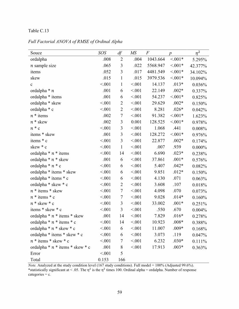
59
Table C.13
Full Factorial ANOVA of RMSE of Ordinal Alpha
Souce SOS df MS F p 𝜂𝜂2 ordalpha .008 2 .004 1043.664 <.001* 5.295% 𝑛𝑛 sample size .065 3 .022 5568.947 <.001* 42.377% items .052 3 .017 4481.549 <.001* 34.102% skew .015 1 .015 3979.536 <.001* 10.094% c <.001 1 <.001 14.137 .013* 0.036% ordalpha * 𝑛𝑛 .001 6 <.001 22.149 .002* 0.337% ordalpha * items .001 6 <.001 54.237 <.001* 0.825% ordalpha * skew <.001 2 <.001 29.629 .002* 0.150% ordalpha * c <.001 2 <.001 8.281 .026* 0.042% 𝑛𝑛 * items .002 7 <.001 91.382 <.001* 1.623% 𝑛𝑛 * skew .002 3 0.001 128.525 <.001* 0.978% 𝑛𝑛 * c <.001 3 <.001 1.068 .441 0.008% items * skew .001 3 <.001 128.272 <.001* 0.976% items * c <.001 3 <.001 22.877 .002* 0.174% skew * c <.001 1 <.001 .007 .939 0.000% ordalpha * 𝑛𝑛 * items <.001 14 <.001 6.690 .023* 0.238% ordalpha * 𝑛𝑛 * skew .001 6 <.001 37.861 .001* 0.576% ordalpha * 𝑛𝑛 * c <.001 6 <.001 5.407 .042* 0.082% ordalpha * items * skew <.001 6 <.001 9.851 .012* 0.150% ordalpha * items * c <.001 6 <.001 4.130 .071 0.063% ordalpha * skew * c <.001 2 <.001 3.608 .107 0.018% 𝑛𝑛 * items * skew <.001 7 <.001 4.098 .070 0.073% 𝑛𝑛 * items * c <.001 7 <.001 9.028 .014* 0.160% 𝑛𝑛 * skew * c <.001 3 <.001 33.002 .001* 0.251% items * skew * c <.001 3 <.001 .550 .670 0.004% ordalpha * 𝑛𝑛 * items * skew .001 14 <.001 7.829 .016* 0.278% ordalpha * 𝑛𝑛 * items * c <.001 14 <.001 10.923 .008* 0.388% ordalpha * 𝑛𝑛 * skew * c <.001 6 <.001 11.007 .009* 0.168% ordalpha * items * skew * c <.001 6 <.001 3.073 .119 0.047% 𝑛𝑛 * items * skew * c <.001 7 <.001 6.232 .030* 0.111% ordalpha * 𝑛𝑛 * items * skew * c .001 8 <.001 17.913 .003* 0.363% Error <.001 5 Total 0.153 166
Note. Analyzed at the study condition level (167 study conditions). Full model = 100% (Adjusted 99.6%). *statistically significant at < .05. The η2 is the η2 times 100. Ordinal alpha = ordalpha. Number of response categories = c.
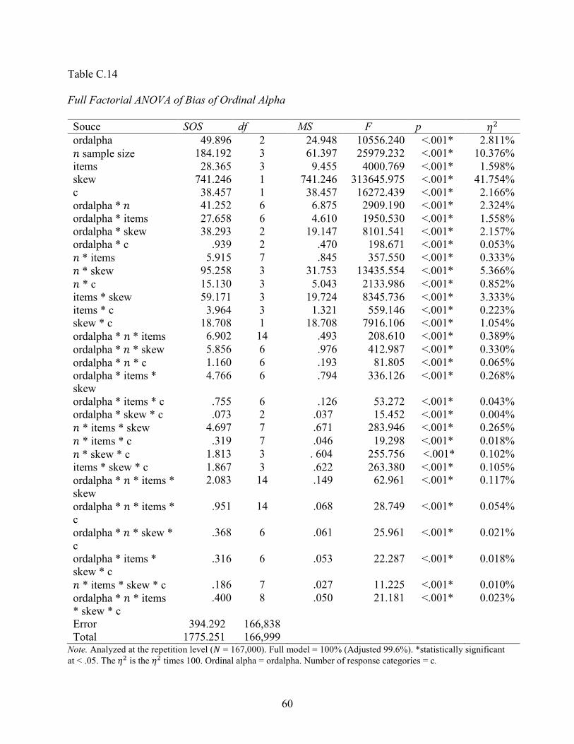
60
Table C.14
Full Factorial ANOVA of Bias of Ordinal Alpha
Souce SOS df MS F p 𝜂𝜂2 ordalpha 49.896 2 24.948 10556.240 <.001* 2.811% 𝑛𝑛 sample size 184.192 3 61.397 25979.232 <.001* 10.376% items 28.365 3 9.455 4000.769 <.001* 1.598% skew 741.246 1 741.246 313645.975 <.001* 41.754% c 38.457 1 38.457 16272.439 <.001* 2.166% ordalpha * 𝑛𝑛 41.252 6 6.875 2909.190 <.001* 2.324% ordalpha * items 27.658 6 4.610 1950.530 <.001* 1.558% ordalpha * skew 38.293 2 19.147 8101.541 <.001* 2.157% ordalpha * c .939 2 .470 198.671 <.001* 0.053% 𝑛𝑛 * items 5.915 7 .845 357.550 <.001* 0.333% 𝑛𝑛 * skew 95.258 3 31.753 13435.554 <.001* 5.366% 𝑛𝑛 * c 15.130 3 5.043 2133.986 <.001* 0.852% items * skew 59.171 3 19.724 8345.736 <.001* 3.333% items * c 3.964 3 1.321 559.146 <.001* 0.223% skew * c 18.708 1 18.708 7916.106 <.001* 1.054% ordalpha * 𝑛𝑛 * items 6.902 14 .493 208.610 <.001* 0.389% ordalpha * 𝑛𝑛 * skew 5.856 6 .976 412.987 <.001* 0.330% ordalpha * 𝑛𝑛 * c 1.160 6 .193 81.805 <.001* 0.065% ordalpha * items * skew
4.766 6 .794 336.126 <.001* 0.268%
ordalpha * items * c .755 6 .126 53.272 <.001* 0.043% ordalpha * skew * c .073 2 .037 15.452 <.001* 0.004% 𝑛𝑛 * items * skew 4.697 7 .671 283.946 <.001* 0.265% 𝑛𝑛 * items * c .319 7 .046 19.298 <.001* 0.018% 𝑛𝑛 * skew * c 1.813 3 . 604 255.756 <.001* 0.102% items * skew * c 1.867 3 .622 263.380 <.001* 0.105% ordalpha * 𝑛𝑛 * items * skew
2.083 14 .149 62.961 <.001* 0.117%
ordalpha * 𝑛𝑛 * items * c
.951 14 .068 28.749 <.001* 0.054%
ordalpha * 𝑛𝑛 * skew * c
.368 6 .061 25.961 <.001* 0.021%
ordalpha * items * skew * c
.316 6 .053 22.287 <.001* 0.018%
𝑛𝑛 * items * skew * c .186 7 .027 11.225 <.001* 0.010% ordalpha * 𝑛𝑛 * items * skew * c
.400 8 .050 21.181 <.001* 0.023%
Error 394.292 166,838 Total 1775.251 166,999
Note. Analyzed at the repetition level (𝑁𝑁 = 167,000). Full model = 100% (Adjusted 99.6%). *statistically significant at < .05. The 𝜂𝜂2 is the 𝜂𝜂2 times 100. Ordinal alpha = ordalpha. Number of response categories = c.

61
APPENDIX D
R CODE
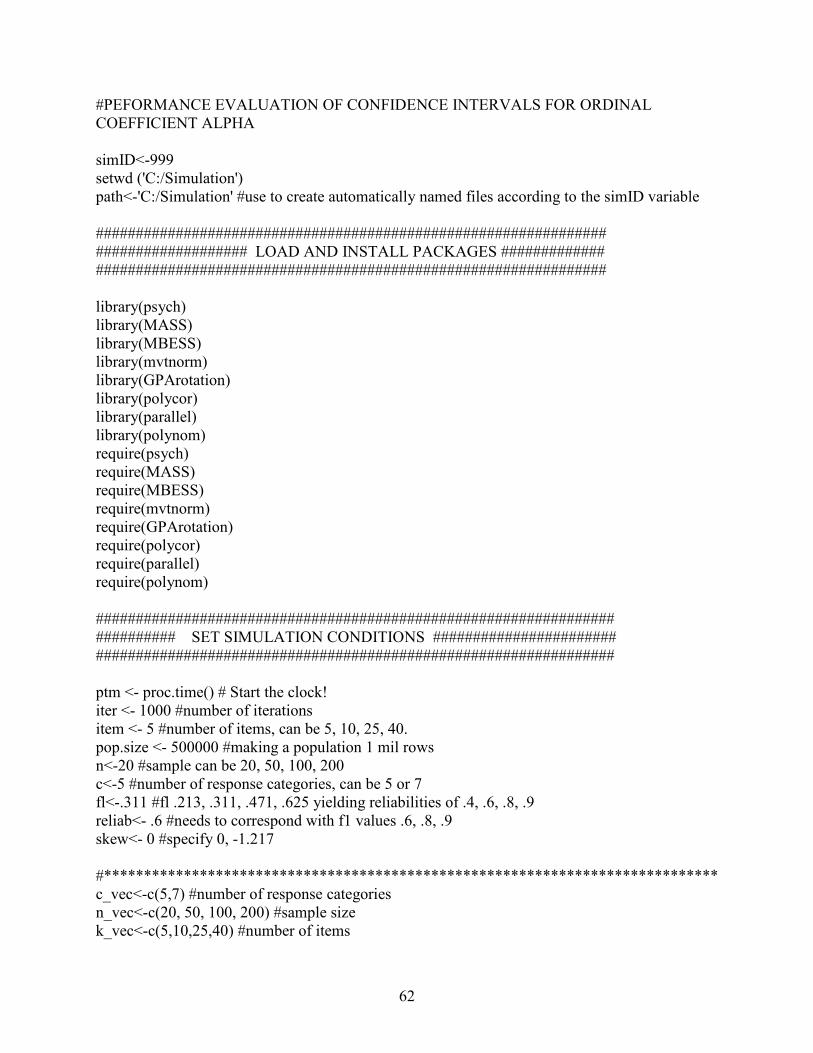
62
#PEFORMANCE EVALUATION OF CONFIDENCE INTERVALS FOR ORDINAL COEFFICIENT ALPHA simID<-999 setwd ('C:/Simulation') path<-'C:/Simulation' #use to create automatically named files according to the simID variable ################################################################ ################### LOAD AND INSTALL PACKAGES ############# ################################################################ library(psych) library(MASS) library(MBESS) library(mvtnorm) library(GPArotation) library(polycor) library(parallel) library(polynom) require(psych) require(MASS) require(MBESS) require(mvtnorm) require(GPArotation) require(polycor) require(parallel) require(polynom) ################################################################# ########## SET SIMULATION CONDITIONS ####################### ################################################################# ptm <- proc.time() # Start the clock! iter <- 1000 #number of iterations item <- 5 #number of items, can be 5, 10, 25, 40. pop.size <- 500000 #making a population 1 mil rows n<-20 #sample can be 20, 50, 100, 200 c<-5 #number of response categories, can be 5 or 7 fl<-.311 #fl .213, .311, .471, .625 yielding reliabilities of .4, .6, .8, .9 reliab<- .6 #needs to correspond with f1 values .6, .8, .9 skew<- 0 #specify 0, -1.217 #***************************************************************************** c_vec<-c(5,7) #number of response categories n_vec<-c(20, 50, 100, 200) #sample size k_vec<-c(5,10,25,40) #number of items
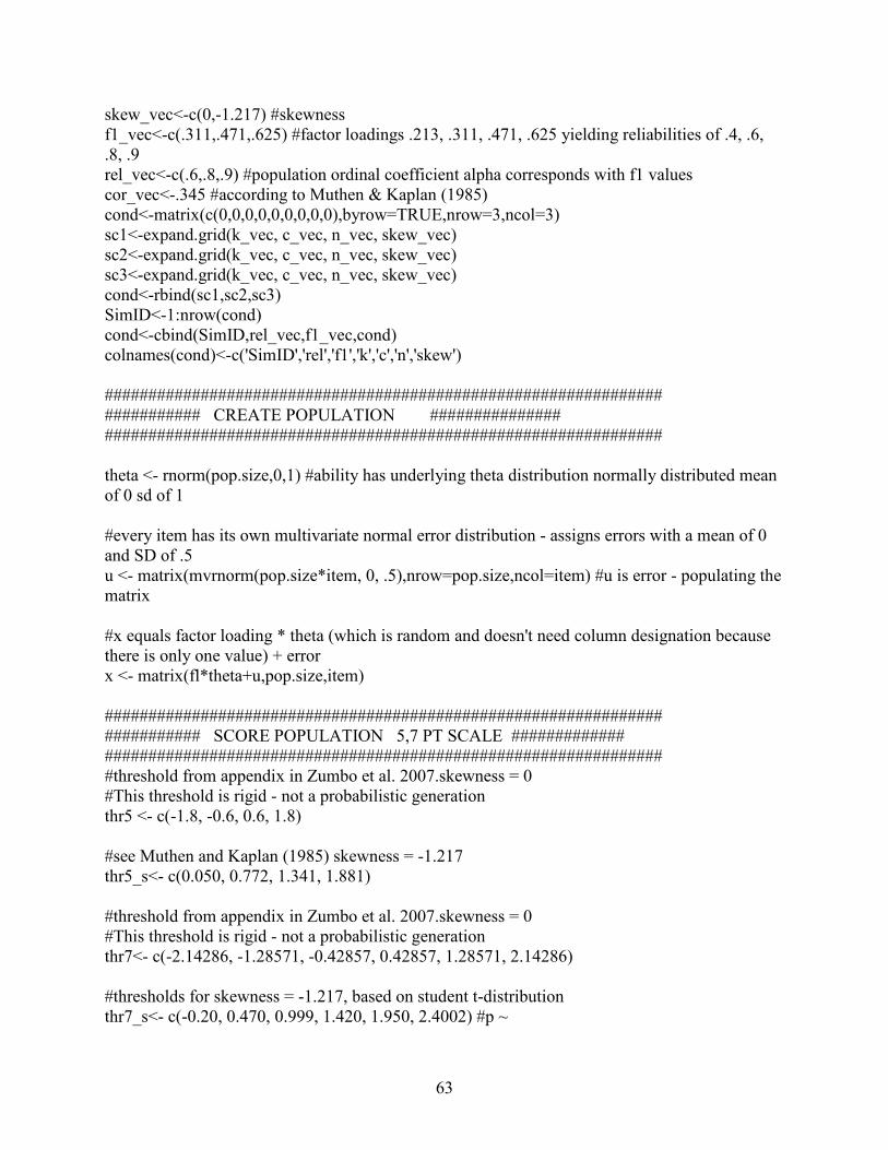
63
skew_vec<-c(0,-1.217) #skewness f1_vec<-c(.311,.471,.625) #factor loadings .213, .311, .471, .625 yielding reliabilities of .4, .6, .8, .9 rel_vec<-c(.6,.8,.9) #population ordinal coefficient alpha corresponds with f1 values cor_vec<-.345 #according to Muthen & Kaplan (1985) cond<-matrix(c(0,0,0,0,0,0,0,0,0),byrow=TRUE,nrow=3,ncol=3) sc1<-expand.grid(k_vec, c_vec, n_vec, skew_vec) sc2<-expand.grid(k_vec, c_vec, n_vec, skew_vec) sc3<-expand.grid(k_vec, c_vec, n_vec, skew_vec) cond<-rbind(sc1,sc2,sc3) SimID<-1:nrow(cond) cond<-cbind(SimID,rel_vec,f1_vec,cond) colnames(cond)<-c('SimID','rel','f1','k','c','n','skew') ################################################################ ########### CREATE POPULATION ############### ################################################################ theta <- rnorm(pop.size,0,1) #ability has underlying theta distribution normally distributed mean of 0 sd of 1 #every item has its own multivariate normal error distribution - assigns errors with a mean of 0 and SD of .5 u <- matrix(mvrnorm(pop.size*item, 0, .5),nrow=pop.size,ncol=item) #u is error - populating the matrix #x equals factor loading * theta (which is random and doesn't need column designation because there is only one value) + error x <- matrix(fl*theta+u,pop.size,item) ################################################################ ########### SCORE POPULATION 5,7 PT SCALE ############# ################################################################ #threshold from appendix in Zumbo et al. 2007.skewness = 0 #This threshold is rigid - not a probabilistic generation thr5 <- c(-1.8, -0.6, 0.6, 1.8) #see Muthen and Kaplan (1985) skewness = -1.217 thr5_s<- c(0.050, 0.772, 1.341, 1.881) #threshold from appendix in Zumbo et al. 2007.skewness = 0 #This threshold is rigid - not a probabilistic generation thr7<- c(-2.14286, -1.28571, -0.42857, 0.42857, 1.28571, 2.14286) #thresholds for skewness = -1.217, based on student t-distribution thr7_s<- c(-0.20, 0.470, 0.999, 1.420, 1.950, 2.4002) #p ~
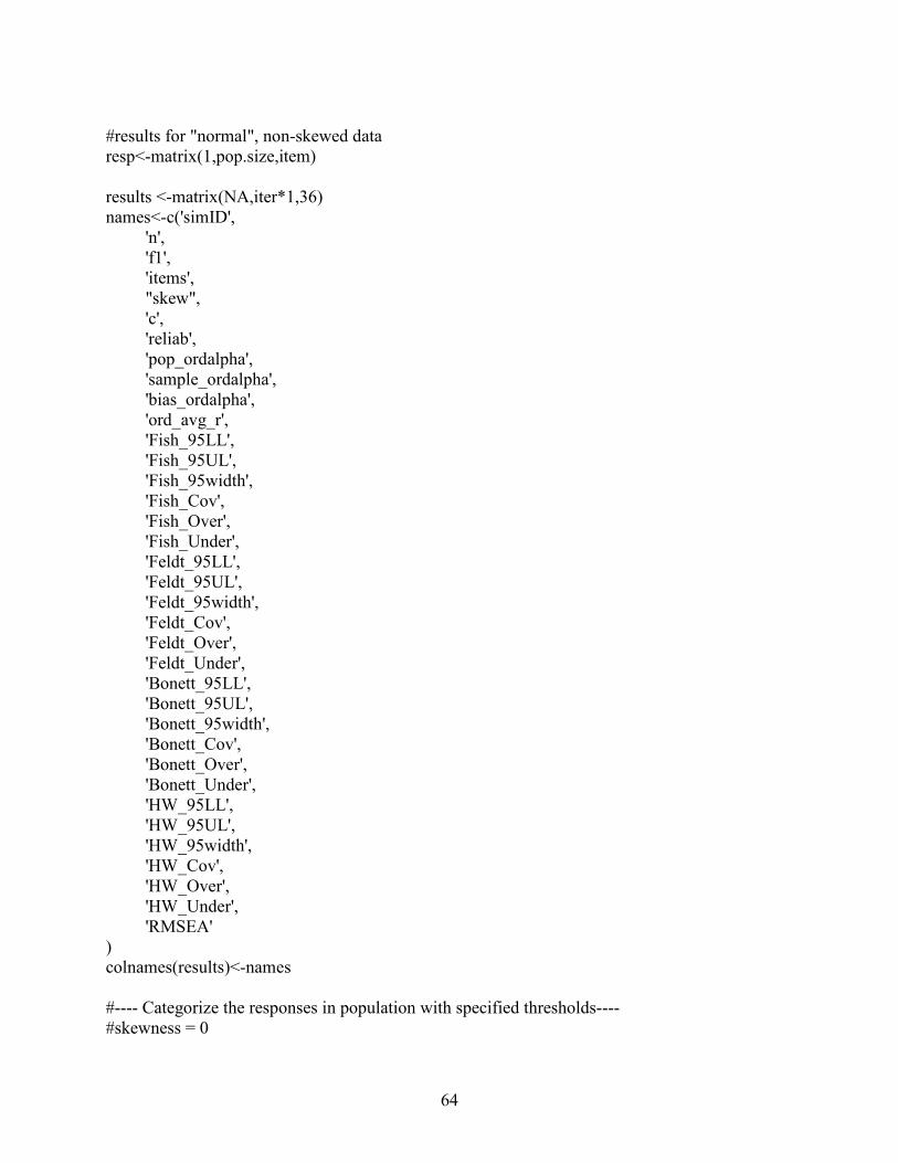
64
#results for "normal", non-skewed data resp<-matrix(1,pop.size,item) results <-matrix(NA,iter*1,36) names<-c('simID', 'n', 'f1', 'items', "skew", 'c', 'reliab', 'pop_ordalpha', 'sample_ordalpha', 'bias_ordalpha', 'ord_avg_r', 'Fish_95LL', 'Fish_95UL', 'Fish_95width', 'Fish_Cov', 'Fish_Over', 'Fish_Under', 'Feldt_95LL', 'Feldt_95UL', 'Feldt_95width', 'Feldt_Cov', 'Feldt_Over', 'Feldt_Under', 'Bonett_95LL', 'Bonett_95UL', 'Bonett_95width', 'Bonett_Cov', 'Bonett_Over', 'Bonett_Under', 'HW_95LL', 'HW_95UL', 'HW_95width', 'HW_Cov', 'HW_Over', 'HW_Under', 'RMSEA' ) colnames(results)<-names #---- Categorize the responses in population with specified thresholds---- #skewness = 0

65
if (c == 5 & skew == 0){ x1 <- findInterval(x, thr5) + 1 } #---- Categorize the responses in population with specified thresholds---- if (c == 5 & skew == -1.217) { x1 <- 5-findInterval(x, thr5_s) } #---- Categorize the responses in population with specified thresholds---- #skewness = 0 if (c == 7 & skew == 0){ x1 <- findInterval(x, thr7) + 1 } #skewness = -1.217 NOTICE reversed category order if (c == 7 & skew == -1.217) { x1 <- 7-findInterval(x, thr7_s) } x2 <- matrix(x1, nrow = nrow(x), byrow = FALSE) hist(x2, freq = F) describe(x2) ################################################################ ####### SAVE POPULATION DATA AND POLYCOR MAT ########### ################################################################ popcorr<- polychoric(x2,smooth=TRUE,global=TRUE, ML = FALSE, std.err=FALSE) popcorr<-as.data.frame(popcorr$rho) write.csv(file = paste(simID,"popcorr.csv",sep=""),popcorr,row.names=TRUE) #write file for population polychoric correlation matrix #write.csv(file = paste(simID,"popdata.csv",sep=""),x,row.names=TRUE) #save population data file popcorr2<-data.matrix(popcorr) ordalpha<-alpha(popcorr2) pop_ordalpha<-ordalpha$total$raw_alpha ################################################################ ########### ITERATE ############### ################################################################ for (d in 1:iter){ set.seed(3171+d) loop.sample <- x2[sample(1:pop.size, size=n, replace=F),] data1<-as.data.frame(loop.sample) descriptives<-describe(data1)
66
#fa<-fa(data1) #provides factor loadings, communalities, and uniquenessess for 1-factor solution #scree(data1) #scree plot to show one-factor models #mardia<-mardia(data1) #multivariate normality tests #This creates the polychoric correlation matrix, which is used to calculate ordinal alpha, and assigns it to "polymat" polymat<- polychoric(data1,smooth=TRUE,global=TRUE, ML = FALSE, std.err=FALSE) #This creates the Pearson correlation matrix, which is used for calculating coeffient alpha, and assigns it to "corrmat" corrmat<- cor(data1,y=NULL, use="complete.obs", method=c("pearson")) #This creates the Pearson method covariance matrix and assigns it to "covmat" covmat<- cov(data1, y=NULL, use="complete.obs", method=c("pearson")) #This is ordinal alpha, because we use the polychoric correlation matrix to compute it sample_ordalpha <- alpha(polymat$rho) #This uses Fan & Thompson (2001) formula for CL for reliability assuming F distribution #Feldt (1965) df1<-n-1 df2<-(n-1)*(item-1) Feldt.95LL<-1-((1-sample_ordalpha$total$raw_alpha)*qf(.025,df1,df2,lower.tail=F)) Feldt.95UL<-1-((1-sample_ordalpha$total$raw_alpha)*qf(.975,df1,df2,lower.tail=F)) #Feldt coverage flags if ((Feldt.95LL <= pop_ordalpha) & (Feldt.95UL >= pop_ordalpha)) Feldt_Cov <- 1 else Feldt_Cov <- 0 #coverage = 1 (true), 0 (false) if (Feldt.95UL <= pop_ordalpha) Feldt_Under <- 1 else Feldt_Under <- 0 #under estimated = 1 (true), 0 (false) if (Feldt.95LL >= pop_ordalpha) Feldt_Over <- 1 else Feldt_Over <- 0 #over estimated = 1 (true), 0 (false) critZ95<- -1*qnorm((1-.95)/2) #95% CI z stat #Based on Romano et al. (2011) #Bonett (2002) transBon_z <- log(1-abs(sample_ordalpha$total$raw_alpha)) if (sample_ordalpha$total$raw_alpha < 0) {transBon_z <= transBon_z * -1} Bon.var<-(2*item)/((item-1)*(n-2)) Bon.SE<-sqrt(Bon.var) Bonett.95LL<-1 - exp(transBon_z + critZ95*Bon.SE) Bonett.95UL<-1 - exp(transBon_z - critZ95*Bon.SE)
67
#Bonett coverage flags if ((Bonett.95LL <= pop_ordalpha) & (Bonett.95UL >= pop_ordalpha)) Bonett_Cov <- 1 else Bonett_Cov <- 0 #coverage = 1 (true), 0 (false) if (Bonett.95UL <= pop_ordalpha) Bonett_Under <- 1 else Bonett_Under <- 0 #under estimated = 1 (true), 0 (false) if (Bonett.95LL >= pop_ordalpha) Bonett_Over <- 1 else Bonett_Over <- 0 #over estimated = 1 (true), 0 (false) #Based on Romano et al. (2011) #Fisher z transformation (1950) transFish_z<-0.5*log((1+abs(sample_ordalpha$total$raw_alpha))/(1-abs(sample_ordalpha$total$raw_alpha))) if (sample_ordalpha$total$raw_alpha < 0) {transFish_z <= transFish_z * -1} Fish.SE_z <- sqrt(1/(n-3)) Fish.95LL<-(exp(2*(transFish_z - critZ95*Fish.SE_z))-1)/(exp(2*(transFish_z - critZ95*Fish.SE_z))+1) Fish.95UL<-(exp(2*(transFish_z + critZ95*Fish.SE_z))-1)/(exp(2*(transFish_z + critZ95*Fish.SE_z))+1) #Fisher coverage flags if ((Fish.95LL <= pop_ordalpha) & (Fish.95UL >= pop_ordalpha)) Fish_Cov <- 1 else Fish_Cov <- 0 #coverage = 1 (true), 0 (false) if (Fish.95UL <= pop_ordalpha) Fish_Under <- 1 else Fish_Under <- 0 #under estimated = 1 (true), 0 (false) if (Fish.95LL >= pop_ordalpha) Fish_Over <- 1 else Fish_Over <- 0 #over estimated = 1 (true), 0 (false) #Based on Romano et al. (2011) #Hakstian & Whalen (1976) transHW_z<-(1 - sample_ordalpha$total$raw_alpha)**(1/3) varHW_z <-18*item*(n - 1)*(1 - sample_ordalpha$total$raw_alpha)**(2/3)/((item - 1)*(9*n - 11)**2) SE_HW_z <-sqrt(varHW_z) cstar <- ((9*n - 11)*(item - 1))/(9*(n - 1)*(item - 1) - 2) HW.95LL<- 1 - cstar**3*((transHW_z + critZ95*SE_HW_z)**3) HW.95UL<- 1 - cstar**3*((transHW_z - critZ95*SE_HW_z)**3) #HW coverage flags if ((HW.95LL <= pop_ordalpha) & (HW.95UL >= pop_ordalpha)) HW_Cov <- 1 else HW_Cov <- 0 #coverage = 1 (true), 0 (false) if (HW.95UL <= pop_ordalpha) HW_Under <- 1 else HW_Under <- 0 #under estimated = 1 (true), 0 (false) if (HW.95LL >= pop_ordalpha) HW_Over <- 1 else HW_Over <- 0 #over estimated = 1 (true), 0 (false)
68
sample_ordinal<-sample_ordalpha$total #this shortens the number of items listed in the ordalpha "object" results[d,1]<-simID results[d,2]<-n results[d,3]<-fl results[d,4]<-item results[d,5]<-skew results[d,6]<-c results[d,7]<-reliab results[d,8]<-pop_ordalpha results[d,9]<-sample_ordinal$raw_alpha results[d,10]<-sample_ordinal$raw_alpha-pop_ordalpha results[d,11]<-sample_ordinal$average_r results[d,12]<-Fish.95LL results[d,13]<-Fish.95UL results[d,14]<-Fish.95UL - Fish.95LL results[d,15]<-Fish_Cov results[d,16]<-Fish_Over results[d,17]<-Fish_Under results[d,18]<-Feldt.95LL results[d,19]<-Feldt.95UL results[d,20]<-Feldt.95UL-Feldt.95LL results[d,21]<-Feldt_Cov results[d,22]<-Feldt_Over results[d,23]<-Feldt_Under results[d,24]<-Bonett.95LL results[d,25]<-Bonett.95UL results[d,26]<-Bonett.95UL-Bonett.95LL results[d,27]<-Bonett_Cov results[d,28]<-Bonett_Over results[d,29]<-Bonett_Under results[d,30]<-HW.95LL results[d,31]<-HW.95UL results[d,32]<-HW.95UL-HW.95LL results[d,33]<-HW_Cov results[d,34]<-HW_Over results[d,35]<-HW_Under results[d,36]<-fa$RMSEA[1] results<-as.data.frame(results) } #end of d loop proc.time() - ptm #EVERYTHING FROM HERE UP WORKS ITERATIVELY!!! write.csv(file = paste(simID,"outs.csv",sep=""),results,row.names=FALSE)
69
REFERENCE LIST
Allen, M. J., & Yen, W. M. (1979). Introduction to measurement theory. Monterey, CA:
Brooks/Cole.
Allen, M. J., & Yen, W. M. (2002). Classical true-score theory. Prospect Heights, IL: Waveland
Press.
American Psychological Association. (2010). Publication manual of the American Psychological
Association (6th ed.). Washington, DC: Author.
Bonett, D. G. (2002). Sample size requirements for testing and estimating coefficient alpha.
Journal of Educational and Behavioral Statistics, 27, 335-340. doi: 10.2307/3648121
Brown, W. (1910). Some experimental results in the correlation of mental abilities. British
Journal of Psychology, 3, 296-322.
Cohen, J. (1994). The earth is round (p<.05). American Psychologist, 49, 997-1003. doi:
10.1037/0003-066x.49.12.997
Cohen, J. (1988). Statistical power analysis for the behavioral sciences (2nd ed.). Hillsdale, NJ:
Erlbaum.
Crocker, L., & Algina, J. (2008). Introduction to classical & modern test theory. Mason, OH:
Cengage Learning.
Cronbach, L. J. (1951). Coefficient alpha and the internal structure of tests. Psychometrika, 16,
297-334.
Cronbach, L. J., & Shavelson, R. J. (2004). My current thoughts on coefficient alpha and
successor procedures. Educational and Psychological Measurement, 64, 391-418. doi:
10.1177/0013164404266386
70
Cui, Y., & Li, J. (2012). Evaluating the performance of different procedures for constructing
confidence intervals for coefficient alpha: A simulation study. British Journal of
Mathematical and Statistical Psychology, 65, 467-498. doi: 10.1111/j.2044-
8317.2012.02038.x
Cumming, G. (2012). Understanding the new statistics. New York: NY: Taylor & Francis
Group.
Cumming, G, & Fidler, F. (2009). Confidence intervals: Better answers to better questions.
Zeitschrift für Psychologie/Journal of Psychology, 217, 15-26. doi: 10.1027/0044-
3409.217.1.15
Cumming, G, & Finch, S. (2005). Inference by eye: Confidence intervals and how to read
pictures of data. American Psychologist, 60, 170-180. doi: 10.1037/0003-066X.60.2.170
Duhachek, A., & Iacobucci, D. (2004). Alpha's standard error (ASE): An accurate and precise
confidence interval estimate. Journal of Applied Psychology, 89, 792-808. doi:
10.1037/0021-9010.89.5.792
Efron, B. (1987). Better bootstrap confidence intervals. Journal of the American Statistical
Association, 82, 171-185. doi: 10.2307/2289144
Efron, B., & Tibshirani, R. J. (1993). An introduction to the bootstrap. New York: Chapman &
Hall.
Fan, X, & SAS Institute. (2002). SAS® for Monte Carlo studies : A guide for quantitative
reseachers. Cary, N.C.: SAS Institute.
Fan, X, & Thompson, B. (2001). Confidence intervals for effect sizes: Confidence intervals
about score reliability coefficients, please: An EPM guidelines editorial. Educational and
Psychological Measurement, 61, 517-531. doi: 10.1177/0013164401614001
71
Feldt, L. S. (1965). The approximate sampling distribution of Kuder-Richardson coefficient
twenty. Psychometrika, 30, 357-370.
Finch, S., Cumming, G., & Thomason, N. (2001). Colloquium on effect Sizes: The roles of
editors, textbook authors, and the publication manual: Reporting of statistical inference in
the Journal of Applied Psychology: Little evidence of reform. Educational and
Psychological Measurement, 61, 181-210. doi: 10.1177/0013164401612001
Fisher, R. A. (1950). Statistical methods for reseach workers. Edinburgh, UK: Oliver & Boyd.
Flora, D. B., & Curran, P. J. (2004). An empirical evaluation of alternative methods of
estimation for confirmatory factor analysis with ordinal data. Psychological Methods, 9,
466-491. doi: 10.1037/1082-989X.9.4.466
Gadermann, A. M., Guhn, M, & Zumbo, B. D. (2012). Estimating ordinal reliability for Likert-
type and ordinal item response data: A conceptual, empirical, and practical guide.
Practical Assessment, Reseach & Evaluation, 17(3). Available
online:http://pareonline.net/getvn.asp?v=17&n=3
Gerbing, D. W., & Anderson, J. C. (1988). An updated paradigm for scale development
incorporating unidieminsionality and its assessment. Journal of Marketing Reseach,
25(2), 186.
Hakstian, A. R., & Whalen, T. E. (1976). A k-sample significance test for independent alpha
coefficients. Psychometrika, 41, 219-231. doi: 10.1007/BF02291840
Henson, R. K. (2001). Understanding internal consistency reliability estimates: A conceptual
primer on coefficient alpha. Measurement and Evaluation in Counseling and
Development, October 177-189.
72
Iacobucci, D., & Duhachek, A. (2003). Advancing alpha: Measuring reliability with confidence.
Journal of Consumer Psychology, 13, 478-487. doi:
http://dx.doi.org/10.1207/S15327663JCP1304_14
Jennings, D. E. (1986). Judging inference adequacy in logistic regression. Journal of the
American Statistical Association, 81, 471-476. doi: 10.2307/2289237
Jennings, D. E. (1987). How do we judge confidence-interval adequacy? The American
Statistician, 41, 335-337. doi: 10.2307/2684768
Koning, A. J., & Franses, P. H. (2003). Confidence intervals for Cronbach’s coefficient alpha
values. ERIM Report Series Reference No. ERS-2003-041-MKT.
Kristof, W. (1963). The statistical theory of stepped-up reliability coefficients when a test has
been divided into several equivalent parts. Psychometrika, 28, 221-238. doi:
10.1007/BF02289571
Kuder, G. F., & Richardson, M. W. (1937). The theory of the estimation of test reliability.
Psychometrika, 2, 151-160.
Lehman, E. L. (1959). Testing statistical hypotheses. New York: J. Wiley & Sons, Inc.
Lord, F. M., & Novick, M. R. (1968). Statistical theories of mental test scores. Reading, MA:
Addison Wesley.
Maydeu-Olivares, A., Coffman, D. L., & Hartmann, W. M. (2007). Asymptotically distribution-
free (ADF) interval estimation of coefficient alpha. Psychological Methods, 12, 157-176.
doi: 10.1037/1082-989X.12.2.157
McDonald, R. P. (1985). Factor analysis and related methods. Hillsdale NJ: Erlbaum.
73
Muthén, B., & Kaplan, D. (1985). A comparison of some methodologies for the factor analysis
of non-normal Likert variables. British Journal of Mathematical and Statistical
Psychology, 38, 171-189.
Novick, M. R., & Lewis, M. R. (1967). Coefficient alpha and the reliability of composite
measurements. Psychometrika, 32, 1-13.
Padilla, M. A., Divers, J., & Newton, M. (2012). Coefficient alpha bootstrap confidence interval
under nonnormality. Applied Psychological Measurement, 36, 331-348. doi:
10.1177/0146621612445470
Raykov, T. (1998). A method for obtaining standard errors and confidence intervals of composite
reliability for congeneric items. Applied Psychological Measurement, 22, 369-374.
Romano, J. L. , Kromrey, J. D. , Owens, C. M. , & Scott, H. M. (2011). Confidence interval
methods for coefficient alpha on the basis of discrete, ordinal response items: Which one,
if any, is the best? Journal of Experimental Education, 79, 382-403. doi:
10.1080/00220973.2010.510859
Samaniego, F. J. (2010). A comparison of the Bayesian and frequentist approaches to estimation.
New York: Springer.
Samaniego, F. J., & Reneau, D. M. (1994). Toward a reconciliation of the Bayesian and
frequentist approaches to point estimation. Journal of the American Statistical
Association, 89, 947-957. doi: 10.2307/2290920
Schall, R. (2012). The empirical coverage of confidence intervals: Point estimates and
confidence intervals for confidence levels. Biometrical Journal, 54, 537-551. doi:
10.1002/bimj.201100134
74
Schmitt, N. (1996). Uses and abuses of coefficient alpha. Psychological Assessment, 8, 350-353.
doi: 10.1037/1040-3590.8.4.350
Sijtsma, K. (2009). On the use, the misuse, and the very limited usefulness of Cronbach’s alpha.
Psychometrika, 74, 107-120. doi: 10.1007/s11336-008-9101-0
Spearman, C. (1910). Correlation calculated from faulty data. British Journal of Psychology, 3,
271-295.
Streiner, D. L. (2003). Starting at the beginning: An introduction to coefficient alpha and internal
consistency. Journal of Personality Assessment, 80, 99-103.
Thompson, B. (2002). What future quantitative social science reseach could look like:
Confidence intervals for effect sizes. Educational Reseacher, 31, 25-32. doi:
10.2307/3594483
Thompson, B. (2006a). Foundations of behavioral statistics. New York, NY: The Guilford Press.
Thompson, B. (2006b). Reseach synthesis: Effect sizes. In J. L. Green, G. Camilli & P. B.
Elmore (Eds.), Handbook of complementary methods in education reseach (pp. 583-603).
New Jersey: Lawrence Erlbaum Associates.
Vacha-Haase, T., Henson, R. K., & Caruso, J. C. (2002). Reliability generalization: Moving
toward improved understanding and use of score reliability. Educational and
Psychological Measurement, 62, 562-569. doi: 10.1177/0013164402062004002
Vacha-Haase, T., & Thompson, B. (2011). Score reliability: A retrospective look back at 12
years of reliability generalization studies. Measurement and Evaluation in Counseling
and Development, 44, 159-168. doi: 10.1177/0748175611409845
75
van Zyl, J. M., Neudecker, H., & Nel, D. G. (2000). On the distribution of the maximum
likelihood estimator of Cronbach's alpha. Psychometrika, 65, 271-280. doi:
10.1007/BF02296146
Wang, Z., & Thompson, B. (2007). Is the Pearson r2 biased, and if so, what is the best correction
formula? Journal of Experimental Education, 75, 109-125. doi: 10.3200/JEXE.75.2.109-
125
Wilkinson, L , & APA Task Force on Statistical Inference. (1999). Statistical methods in
psychology journals: Guidelines and explanations. American Psychologist, 54, 594-604.
doi: 10.1037/0003-066X.54.8.594
Yuan, K.-H., Guarnaccia, C. A., & Hayslip, B. (2003). A study of the distribution of sample
coefficient alpha with the Hopkins symptom checklist: Bootstrap versus asymptotics.
Educational and Psychological Measurement, 63(1), 5-23.
Yuan, K., & Bentler, P. (2002). On robustness of the normal-theory based asymptotic
distributions of three reliability coefficient estimates. Psychometrika, 67, 251-259. doi:
10.1007/BF02294845
Zhang, H., Gutiérrez Rojas, H. A., & Cuervo, E. C. (2010). Confidence and credibility intervals
for the difference of two proportions. Revista Colombiana De Estadística, 1, 63-88.
Zumbo, B. D., Gadermann, A. M., & Zeisser, C. (2007). Ordinal versions of coefficients alpha
and theta for Likert rating scales. Journal of Modern Applied Statistical Methods 6, 21-
29.
(Kristof, 1963; K.-H. Yuan, Guarnaccia, & Hayslip, 2003) (Koning & Franses, 2003; Lehman, 1959) (American Psychological Association, 2010) (J. Cohen, 1988; Fisher, 1950) (Novick & Lewis, 1967) (J. Cohen, 1988; K.-H. Yuan et al., 2003)