Heath Lecture Ofdm

7/31/2019 Heath Lecture Ofdm

http://slidepdf.com/reader/full/heath-lecture-ofdm 1/26

Wireless OFDM SystemsWireless OFDM Systems

Lecture by Prof. Robert W. Heath Jr.

Telecommunications and Signal

Processing Research Center

The University of Texas at Austinhttp://wireless.ece.utexas.edu/





22 - 3

Wireless Digital Communication SystemWireless Digital Communication System

Message

Source

Encoder Pulseshape

exp(j2π f c t)

Modulator

Carrier frequency

Examples:

88.5-107.7MHz FM radio

Analog cellular 900MHz

Digital cellular 1.8GHz

Raised-cosine

pulseshaping filter

Transmitter



22 - 4

Wireless Digital Communication SystemWireless Digital Communication System

(continued)(continued)

Message

Sink

DemodulatorPulseshape

exp(-j2π f c t)

Decoder

hc(t)TX RX

noise

Propagation

Receiver

Remove carrier



22 - 5

Multipath PropagationMultipath Propagation –– Simple ModelSimple Model

• hc(t) =∑

k=0

K-1

ααααk δδδδ(t - ττττk )– αk : path gain (complex)

– τ0 = 0 normalize relative delay of first path

– ∆k = τk - τ0 difference in time-of-flight

| α| α| α| α0 |||| | α| α| α| α1 |||| | α| α| α| α2 ||||

∆∆∆∆1 ∆∆∆∆2

αααα0

αααα1

αααα2



22 - 6

Equivalent Propagation ChannelEquivalent Propagation Channel

heff (t) = gtr(t) ⊗ hc(t) ⊗ grx(t)

transmit filters receive filters

multipathchannel

convolution

• Effective channel at receiver

– Propagation channel

– TX / RX filters

• hc(t) typically random & changes with time

– Must estimate & re-estimate channel



22 - 7

Impact of Impact of MultipathMultipath: Delay Spread & ISI: Delay Spread & ISI

-6 -4 -2 0 2 4 6-0.2

0

0.2

0.4

0.6

0.8

1

t/Ts

2Ts 4Ts

Ts

-6 - 4 -2 0 2 4 6 8

-0.5

0

0.5

1

t/Ts

-6 - 4 -2 0 2 4 6 8

-0.2

0

0.2

0.4

0.6

0.8

t/Ts

Max delay spread = effective number of symbol periods occupied by channel

Requires equalization to remove resulting ISI



22 - 8

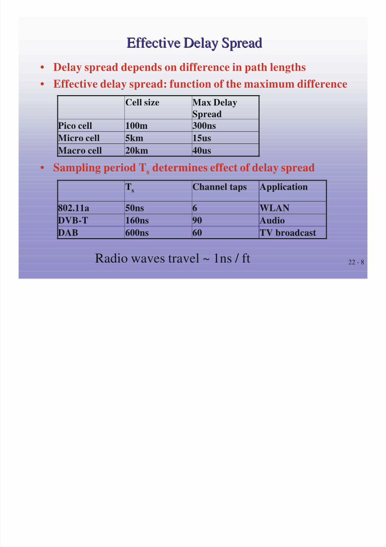
Effective Delay SpreadEffective Delay Spread

• Delay spread depends on difference in path lengths

• Effective delay spread: function of the maximum difference

• Sampling period Ts determines effect of delay spread

40us20kmMacro cell

15us5kmMicro cell

300ns100mPico cell

Max DelaySpread

Cell size

TV broadcast60600nsDAB

Audio90160nsDVB-TWLAN650ns802.11a

ApplicationChannel tapsTs

Radio waves travel ~ 1ns / ft



22 - 9

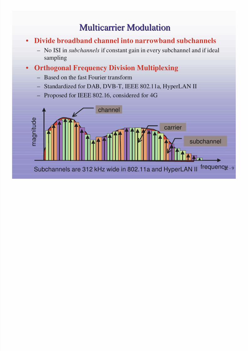
Multicarrier ModulationMulticarrier Modulation

• Divide broadband channel into narrowband subchannels

– No ISI in subchannels if constant gain in every subchannel and if ideal

sampling

• Orthogonal Frequency Division Multiplexing– Based on the fast Fourier transform

– Standardized for DAB, DVB-T, IEEE 802.11a, HyperLAN II

– Proposed for IEEE 802.16, considered for 4G

subchannel

frequency

m a g n i t u d e

carrier

channel

Subchannels are 312 kHz wide in 802.11a and HyperLAN II





22 - 11

P/S

QAMdemod

decoder

invert

channel=

frequency

domainequalizer

S/P

quadrature

amplitude

modulation(QAM)encoder

N -IFFT

add

cyclicprefix

P/S

D/A +

transmitfilter

N -FFT S/Premove

cyclicprefix

TRANSMITTER

RECEIVER

N subchannels 2N real samples

2N real samples N subchannels

Receivefilter

+A/D

multipath channel

An OFDM ModemAn OFDM Modem

Bits

00110



22 - 12

Frequency Domain EqualizationFrequency Domain Equalization

• For the k th carrier:

xk = Hk sk + vk

where Hk = n=0N-1 hk(nTs) exp(j2π k n / N)

• Frequency domain equalizer xk

Hk -1

ssk

• Noise enhancement factor

k

|Hk |2

|H-1k |

2

k

good

bad



22 - 13

DMT vs. OFDMDMT vs. OFDM

• DMT

– Channel changes very slowly ~ 1000s

– Subchannel gains known at transmitter

– Bitloading (sending more bits on good channels) increases throughput

• OFDM

– Channel may change quickly ~ 10ms

– Not enough time to convey gains to transmitter

– Forward error correction mitigates problems on bad channels

frequency

m a g n i t u d e

DMT: Send more data here

OFDM: Try to code so bad subchannels can be ignored



22 - 14

Coded OFDM (COFDM)Coded OFDM (COFDM)

• Error correction is necessary in OFDM systems

• Forward error correction (FEC)

– Adds redundancy to data stream

– Examples: convolutional codes, block codes

– Mitigates the effects of bad channels

– Reduces overall throughput according to the coding rate k/n

• Automatic repeat request (ARQ)– Adds error detecting ability to data stream

– Examples: 16-bit cyclic redundancy code

– Used to detect errors in an OFDM symbol

– Bad packets are retransmitted (hopefully the channel changes)

– Usually used with FEC

– Minus: Ineffective in broadcast systems



22 - 15

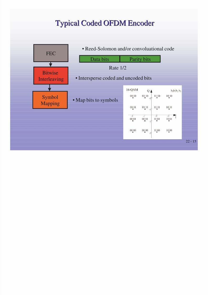
Typical Coded OFDM EncoderTypical Coded OFDM Encoder

FEC

Bitwise

Interleaving

Symbol

Mapping

• Reed-Solomon and/or convoluational code

• Intersperse coded and uncoded bits

Data bits Parity bits

Rate 1/2

• Map bits to symbols



22 - 16

Example: IEEE 802.11aExample: IEEE 802.11a

• IEEE 802.11 employs adaptive modulation– Code rate & modulation depends on distance from base station

– Overall data rate varies from 6Mbps to 54Mbps

Reference: IEEE Std 802.11a-1999



22 - 17

Typical COFDM DecoderTypical COFDM Decoder

Frequency-domain

equalization

Symbol

Demapping

Deinterleaving

Decoding

• Symbol demapping

– Produce soft estimate of each bit

– Improves decoding





22 - 19

Ideal Channel EstimationIdeal Channel Estimation

• Wireless channels change frequently ~ 10ms

• Require frequent channel estimation

• Many systems use pilot tones – known symbols

– Given sk , for k=k 1, k 2, k 3, … solve xk = l=0L hl e-j2π k l/N sk for hl

– Find Hk = l=0L hl e-j2π k l / N (significant computation)

• More pilot tones

– Better noise resiliance– Lower throughput (pilots are not informative)

frequency

m a g n i t u d e

Pilot tones



22 - 20

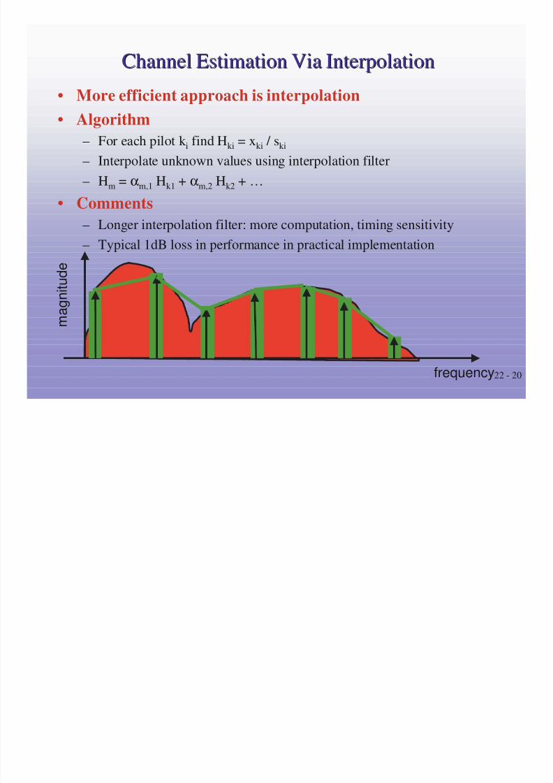
Channel Estimation Via InterpolationChannel Estimation Via Interpolation

• More efficient approach is interpolation

• Algorithm

– For each pilot k i find Hki = xki / ski

– Interpolate unknown values using interpolation filter

– Hm = αm,1 Hk1 + αm,2 Hk2 + …

• Comments

– Longer interpolation filter: more computation, timing sensitivity– Typical 1dB loss in performance in practical implementation

frequency

m a g n i t u d e



22 - 21

OFDM and Antenna DiversityOFDM and Antenna Diversity

• Wireless channels suffer from multipath fading

• Antenna diversity is a means of compensating for fading

• Example Transmit Delay Diversity

OFDM Modulator

Delay

h1(t)

h2(t)

• Equivalent channel is h(t) = h1(t) + h2(t-D)

• More channel taps = more diversity

• Choose D large enough



22 - 22

OFDM and MIMO SystemsOFDM and MIMO Systems

• Multiple-input multiple-output (MIMO) systems

– Use multiple transmit and multiple receive antennas

– Creates a matrix channel

• Equivalent system for kth tone

xk = Hk sk + vk

• Vector inputs & outputs! (more info see WSEL homepage)

OFDM Modulator

OFDM Modulator

Joint

DemodulatorH(t)



22 - 23

Why OFDM in Broadcast?Why OFDM in Broadcast?

• Enables Single Frequency Network (SFN)

– Multiple transmit antennas geographically separated

– Enables same radio/TV channel frequency throughout a country

– Creates artificially large delay spread – OFDM has no problems!

20km

0 5 10 15 20 25 30 35 400

0.1

0.2

0.3

0.4

0.5

0.6

0.7

0.8

0.9

1



22 - 24

Why OFDM for HighWhy OFDM for High--Speed Internet Access?Speed Internet Access?

• High-speed data transmission

– Large bandwidths -> high rate, many computations

– Small sampling periods -> delay spread becomes a serious impairment

– Requires much lower BER than voice systems

• OFDM pros

– Takes advantage of multipath through simple equalization

• OFDM cons– Synchronization requirements are much more strict

• Requires more complex algorithms for time / frequency synch

– Peak-to-average ratio

• PAR is approximately 10 log N (dB)

• Large signal peaks require higher power amplifiers

• Amplifier cost grows nonlinearly with required power



22 - 25

Case Study: IEEE 802.11a WLANCase Study: IEEE 802.11a WLAN

• System parameters

– FFT size: 64

– Number of tones used 52 (12 zero tones)

– Number of pilots 4 (data tones = 52-4 = 48 tones)

– Bandwidth: 20MHz

– Subcarrier spacing : ∆f = 20MHz / 64 = 312.5 kHz

– OFDM symbol duration: TFFT = 1/ ∆f = 3.2us

– Cyclic prefix duration: TGI = 0.8us

– Signal duration: Tsignal = TFFT + TGI

T FFT T GI

CP s y m b o l i



22 - 26

Case Study: IEEE 802.11a WLANCase Study: IEEE 802.11a WLAN

8005.725-5.825

2005.25 – 5.35

405.15 – 5.25

Maximum Output

Power

(6dBi antenna gain)

mW

Frequency band

(GHz)• Modulation: BPSK, QPSK, 16-QAM, 64-QAM

• Coding rate: 1 / 2, 2 / 3, 3 / 4

• FEC: K=7 (64 states) convolutional code

Documents

Heath Lecture Ofdm