HEAT TRANSFER LAB OBSERVATON - SVCET · 1 sri venkateswara college of engineering and technology (autonomous) r. v. s. nagar, chittoor-517127 department of mechanical engineering

1

SRI VENKATESWARA COLLEGE OF ENGINEERING AND

TECHNOLOGY

(AUTONOMOUS)

R. V. S. NAGAR, CHITTOOR-517127

DEPARTMENT OF MECHANICAL ENGINEERING

HEAT TRANSFER LAB

OBSERVATON

Name of the student: _____________________________

Roll Number: ______________ Branch: ______________

Name of the Laboratory: __________________________

Year & Sem: _______________ Academic Year: _______

2

SRI VENKATESWARA COLLEGE OF ENGINEERING & TECHNOLOGY

(AUTONOMOUS) R.V.S NAGAR, CHITTOOR-517 127

DEPARTMENT OF MECHANICAL ENGINEERING

HEAT TRANSFER LAB MANUAL

LIST OF EXPERIMENTS

1. Composite wall apparatus

2. Critical heat flux apparatus

33.. HHeeaatt ttrraannssffeerr iinn ddrroopp aanndd ffiillmm wwiissee ccoonnddeennssaattiioonn apparatus

44.. Emissivity measurement of radiating surfaces apparatus

55.. Heat transfer by forced convection apparatus

6. Heat pipe demonstration apparatus

7. Thermal conductivity of insulating powder apparatus

8. LLaaggggeedd ppiippee apparatus

9. Heat transfer by natural convection apparatus

10. Parallel flow/counter flow heat exchanger apparatus

11. Heat transfer from pin-fin apparatus

12. Stefan Boltzmann apparatus

13. Thermal conductivity of metal rod apparatus

14. Study of two phase flow apparatus

15. Experiment on Transient heat conduction apparatus

3

INDEX S.No: Date Name of the Experiment Page No: Signature of the

Faculty

1

2

3

4

5

6

7

8

9

10

11

12

13

14

15

4

Date:

Exp No:

COMPOSITE WALL APPARATUS

AIM:

To find out total thermal resistance and total thermal conductivity of

composite wall.

DESCRIPTION:

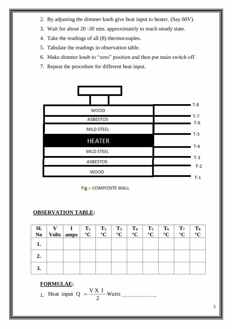
The apparatus consists of central heater sandwiched between the slabs of

MS, Asbestos and Wood, which forms composite structure. The whole structure is

well tightened make perfect contact between the slabs. A dimmer stat is provided

to vary heat input of heaters and it is measured by a digital volt meter and

ammeter. Thermocouples are embedded between interfaces of slabs. A digital

temperature indicator is provided to measure temperature at various points.

SPECIFICATION:

1. Slab assembly arranged symmetrically on both sides of the Heater.

2. Heater coil type of 250-Watt capacity.

3. Dimmer stat open type, 230V, 0-5 amp, single phase.

4. Volt meter range 0-270V

5. Ammeter range 0-20A

6. Digital temperature indicator range 0-8000 c

7. Thermocouple used: Teflon coated, Chromal - Alumal

8. Slab diameter of each =150 mm.

9. Thickness of mild steel = 10 mm.

10. Thickness of Asbestos = 6 mm.

11. Thickness of wood= 10 mm.

PROCEDURE:

1. Start the main switch.

5

2. By adjusting the dimmer knob give heat input to heater. (Say 60V).

3. Wait for about 20 -30 min. approximately to reach steady state.

4. Take the readings of all (8) thermocouples.

5. Tabulate the readings in observation table.

6. Make dimmer knob to “zero” position and then put main switch off.

7. Repeat the procedure for different heat input.

OBSERVATION TABLE:

Sl.

No

V

Volts

I

amps

T1

°C

T2

°C

T3

°C

T4

°C

T5

°C

T6

°C

T7

°C

T8

°C

1.

2.

3.

FORMULAE:

1. Watts2

I X V Qinput Heat ……………………………………....

6

2

T + T 81WoodT °C……………….

2

T + T T 72

Asbestos °C……………..

2

T + T T 63

steel Mild °C………………

2

T +T T 54

Heater °C ……………………..

2. Area of Slab

2

2

4m

dA

(Where “d” is diameter of slab= 300 mm)

3. Thermal Resistance of Slab ( R )

Q

T -T woodheaterR °C/W

4. Thermal Conductivity ( K )

km

WK

)T -A(T

x t Q

woodheater

(Where “t” is total thickness of slab=26mm)

PRECAUTIONS:

1. Keep the dimmer stat to zero before starting the experiment.

2. While removing plates do not disturb thermocouples.

3. Use the selector switch knob and dimmer knob gently.

RESULT:

1. Total thermal resistance of composite wall =……………………..

2. Total thermal conductivity of composite wall=……………………

7

Date:

Exp No:

CRITICAL HEAT FLUX APPARATUS

AIM:

To study the phenomenon of the boiling heat transfer and to plot the graph

of heat flux versus temperature difference.

APPARATUS:

It consists of a cylindrical glass container, the test heater and a heater coil

for initial heating of water in the container. This heater coil is directly connected to

the mains and the test heater is also connected to the mains via a Dimmer stat and

an ammeter is connected in series to the current while a voltmeter across it to read

the voltage.

The glass container is kept on the table. The test heater wire can be viewed

through a magnifying lens. Figure enclosed shows the set up.

SPECIFICATIONS:

1. Length of Nichrome wire L = 52 mm

2. Diameter of Nichrome wire D = 0.25 mm (33 gauge)

3. Distilled water quantity = 4 liters

4. Thermometer range : 0 – 100 0C

5. Heating coil capacity (bulk water heater ) : 2 kW

6. Dimmer stat

7. Ammeter

8. Voltmeter

8

THEORY:

When heat is added to a liquid surface from a submerged solid surface

which is at a temperature higher than the saturation temperature of the liquid, it is

usual that a part of the liquid to change phase. This change of phase is called

‘boiling’. If the liquid is not flowing and present in container, the type of boiling is

called as ‘pool boiling’. Pool boiling is also being of various types depending upon

the temperature difference between the surfaces of liquid. The different types of

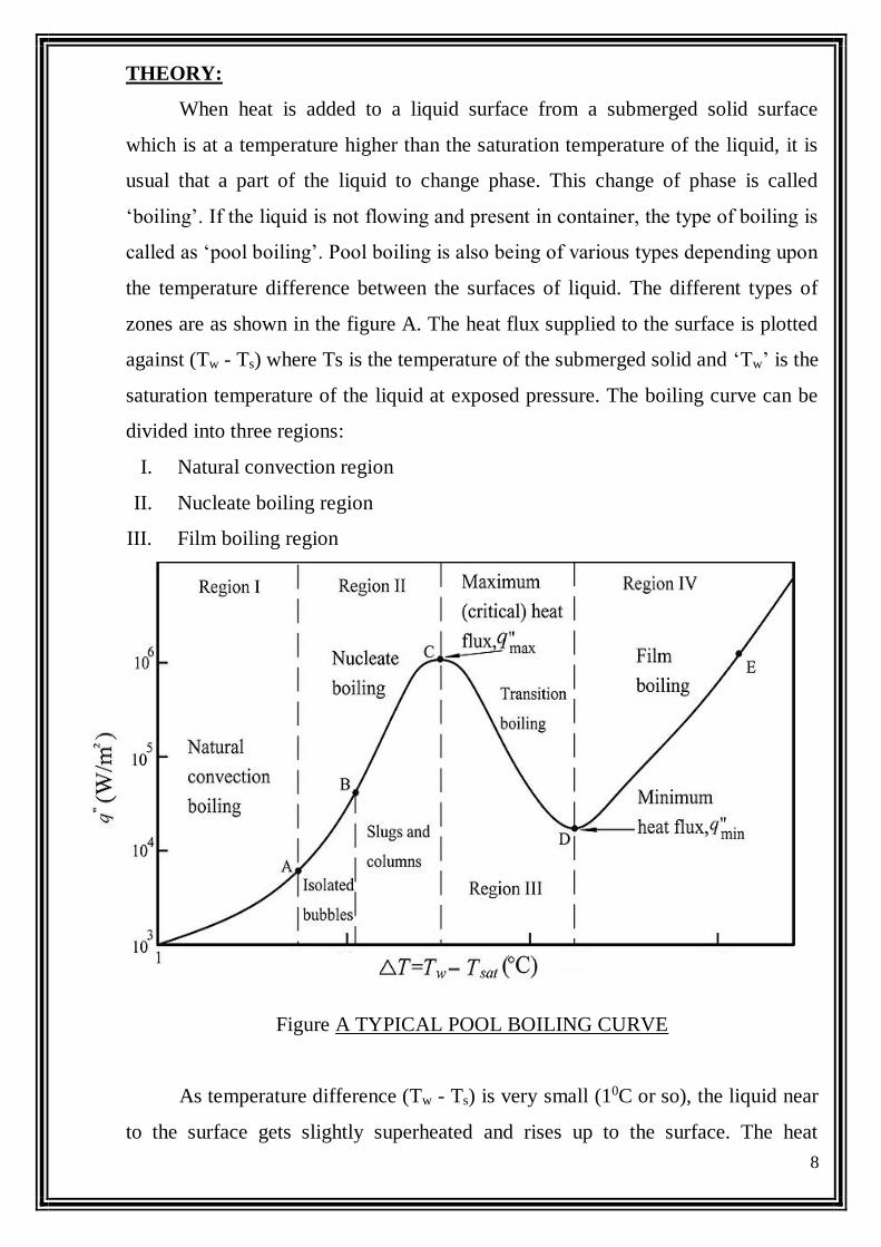
zones are as shown in the figure A. The heat flux supplied to the surface is plotted

against (Tw - Ts) where Ts is the temperature of the submerged solid and ‘Tw’ is the

saturation temperature of the liquid at exposed pressure. The boiling curve can be

divided into three regions:

I. Natural convection region

II. Nucleate boiling region

III. Film boiling region

Figure A TYPICAL POOL BOILING CURVE

As temperature difference (Tw - Ts) is very small (10C or so), the liquid near

to the surface gets slightly superheated and rises up to the surface. The heat

9

transfer from the heating surface to the liquid is similar to that by natural

convection and hence this region is called ‘natural convection region’.

When (Tw - Ts) becomes a few degrees, vapor bubble start forming at some

discrete locations of the heating surface and we enter into ‘Nucleate boiling

region’. Region II consists of two parts. In the first part, the bubbles formed are

very few in number and before reaching the top liquid surface, they get condensed.

In second part, the rate of bubble formation as well as the locations where they are

formed increases with increase in temperature difference. A stage is finally reached

when the rate of formation of bubbles is so high that they start coalesce and blanket

the surface with a vapor film. This is the beginning of region III since the vapor

has got very low thermal conductivity, the formation of vapor film on the heating

surface suddenly increases the temperature beyond the melting point of the

submerged surface and as such the end of ‘Nucleate boiling’ is important and its

limiting condition is known as critical heat flux point or burn out point.

The pool boiling phenomenon up to critical heat flux point can be visualized

and studied with the help of apparatus described above.

PROCEDURE:

1. Distilled water of about 5 liters is taken into the glass container.

2. The test heater (Nichrome wire) is connected across the studs and electrical

connections are made.

3. The heaters are kept in submerged position.

4. The bulk water is switched on and kept on, until the required bulk temperature

of water is obtained. (Say 400 C )

5. The bulk water heater coil is switched off and test heater coil is switched on.

6. The boiling phenomenon on wire is observed as power input to the test heater

coil is varied gradually.

7. The voltage is increased further and a point is reached when wire breaks

(melts) and at this point voltage and current are noted.

8. The experiment is repeated for different values of bulk temperature of water.

(Say 600 C, and 800 C).

10

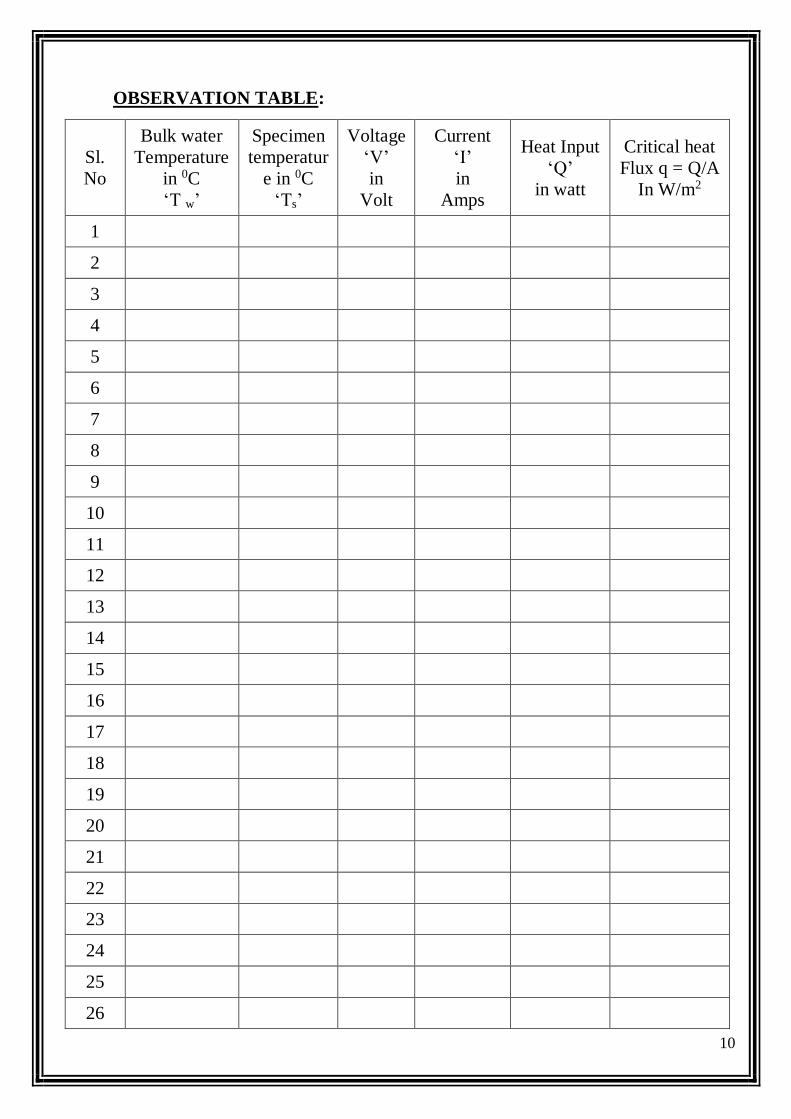
OBSERVATION TABLE:

Sl.

No

Bulk water

Temperature

in 0C

‘T w’

Specimen

temperatur

e in 0C

‘Ts’

Voltage

‘V’

in

Volt

Current

‘I’

in

Amps

Heat Input

‘Q’

in watt

Critical heat

Flux q = Q/A

In W/m2

1 2 3 4 5 6 7 8 9 10 11 12 13 14 15 16 17 18 19 20 21 22 23 24 25 26

11

MODEL CALCUALATIONS:

a. Area of Nichrome wire A = π x D x L =

b. Heater input Q = V x I =

c. Critical heat flux q = Q/A =

PRECAUTIONS:

1. All the switches and Dimmer stat knob should be operated gently.

2. When the experiment is over, bring the Dimmer stat to zero position.

3. Run the equipment once in a week for better performance.

4. Do not switch on heaters unless distilled water is present in the container.

RESULT:

The phenomenon of the boiling heat transfer is studied and plotted the graph

of the heat flux versus temperature difference and critical heat flux is calculated.

Critical heat flux q=-------------

12

Date:

Exp No:

HHEEAATT TTRRAANNSSFFEERR IINN DDRROOPP AANNDD FFIILLMM WWIISSEE CCOONNDDEENNSSAATTIIOONN

AIM:

To determine the experimental and theoretical heat transfer coefficient for

drop wise and film wise condensation.

INTRODUCTION:

Condensation of vapor is needed in many of the processes, like steam

condensers, refrigeration etc. When vapor comes in contact with surface having

temperature lower than saturation temperature, condensation occurs. When the

condensate formed wets the surface, a film is formed over surface and the

condensation is film wise condensation. When condensate does not wet the

surface, drops are formed over the surface and condensation is drop wise

condensation

APPARATUS:

The apparatus consists of two condensers, which are fitted inside a glass

cylinder, which is clamped between two flanges. Steam from steam generator

enters the cylinder through a separator. Water is circulated through the

condensers. One of the condensers is with natural surface finish to promote film

wise condensation and the other is chrome plated to create drop wise condensation.

Water flow is measured by a Rota meter. A digital temperature indicator measures

various temperatures. Steam pressure is measured by a pressure gauge. Thus heat

transfer coefficients in drop wise and film wise condensation cab be calculated.

SPECIFICATIONS:

Heater : Immersion type, capacity 2kW

Voltmeter : Digital type, Range 0-300v

Ammeter : Digital type, Range 0-20 amps

Dimmer stat : 0-240 V, 2 amps

Temperature Indicator : Digital type, 0-800°C

13

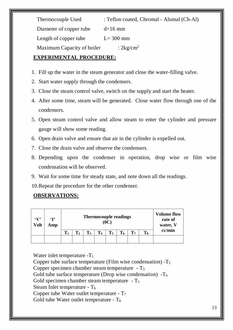
Thermocouple Used : Teflon coated, Chromal - Alumal (Ch-Al)

Diameter of copper tube d=16 mm

Length of copper tube L= 300 mm

Maximum Capacity of boiler : 2kg/cm2

EXPERIMENTAL PROCEDURE:

1. Fill up the water in the steam generator and close the water-filling valve.

2. Start water supply through the condensers.

3. Close the steam control valve, switch on the supply and start the heater.

4. After some time, steam will be generated. Close water flow through one of the

condensers.

5. Open steam control valve and allow steam to enter the cylinder and pressure

gauge will show some reading.

6. Open drain valve and ensure that air in the cylinder is expelled out.

7. Close the drain valve and observe the condensers.

8. Depending upon the condenser in operation, drop wise or film wise

condensation will be observed.

9. Wait for some time for steady state, and note down all the readings.

10. Repeat the procedure for the other condenser.

OBSERVATIONS:

Water inlet temperature -T1

Copper tube surface temperature (Film wise condensation) -T2

Copper specimen chamber steam temperature - T3

Gold tube surface temperature (Drop wise condensation) -T4

Gold specimen chamber steam temperature - T5

Steam Inlet temperature - T6

Copper tube Water outlet temperature - T7

Gold tube Water outlet temperature - T8

‘V’

Volt

‘I’

Amp

Thermocouple readings

(0C)

Volume flow

rate of

water, V

cc/min T1 T2 T3 T4 T5 T6 T7 T8

14

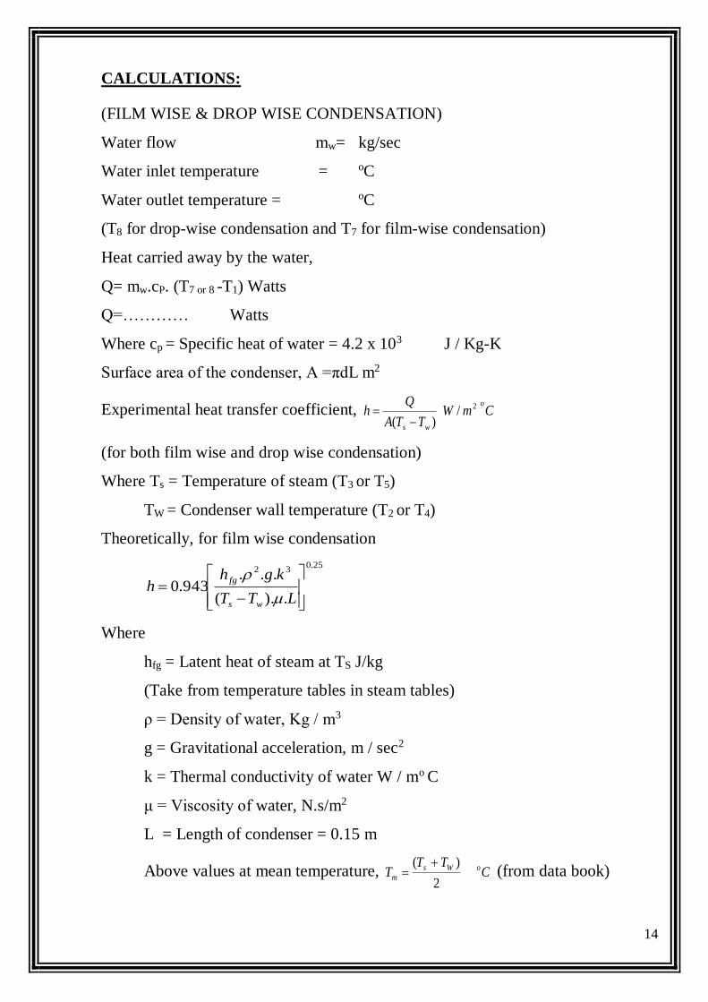
CALCULATIONS:

(FILM WISE & DROP WISE CONDENSATION)

Water flow mw= kg/sec

Water inlet temperature = oC

Water outlet temperature = oC

(T8 for drop-wise condensation and T7 for film-wise condensation)

Heat carried away by the water,

Q= mw.cP. (T7 or 8 -T1) Watts

Q=………… Watts

Where cp = Specific heat of water = 4.2 x 103 J / Kg-K

Surface area of the condenser, A =πdL m2

Experimental heat transfer coefficient, CmWTTA

Qh

o

ws

2/)(

(for both film wise and drop wise condensation)

Where Ts = Temperature of steam (T3 or T5)

TW = Condenser wall temperature (T2 or T4)

Theoretically, for film wise condensation

25.032

.).(

...943.0

LTT

kghh

ws

fg

Where

hfg = Latent heat of steam at TS J/kg

(Take from temperature tables in steam tables)

ρ = Density of water, Kg / m3

g = Gravitational acceleration, m / sec2

k = Thermal conductivity of water W / mo C

μ = Viscosity of water, N.s/m2

L = Length of condenser = 0.15 m

Above values at mean temperature, CTT

T oWs

m2

)( (from data book)

15

(For drop wise condensation, determine experimental heat transfer

coefficient only) In film wise condensation, film of water acts as barrier to heat

transfer whereas, in case of drop formation, there is no barrier to heat transfer,

Hence heat transfer coefficient in drop wise condensation is much greater than film

wise condensation, and is preferred for condensation. But practically, it is difficult

to prolong the drop wise condensation and after a period of condensation the

surface becomes wetted by the liquid. Hence slowly film wise condensation starts.

PRECAUTIONS:

1. Operate all the switches and controls gently

2. Never allow steam to enter the cylinder unless the water is flowing through

condenser.

3. Always ensure that the equipment is earthed properly before switching on the

supply.

RESULTS:

Thus we studied and compared the drop wise and film wise condensation.

1. Film wise condensation:

Experimental average heat transfer coefficient =

Theoretical average heat transfer coefficient =

2. Drop wise condensation:

Experimental average heat transfer coefficient =

Theoretical average heat transfer coefficient =

16

Date:

Exp No:

EMISSIVITY MEASUREMENT OF RADIATING SURFACES

AIM:

To determine the emissivity of given test plate surface.

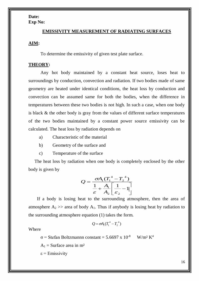
THEORY:

Any hot body maintained by a constant heat source, loses heat to

surroundings by conduction, convection and radiation. If two bodies made of same

geometry are heated under identical conditions, the heat loss by conduction and

convection can be assumed same for both the bodies, when the difference in

temperatures between these two bodies is not high. In such a case, when one body

is black & the other body is gray from the values of different surface temperatures

of the two bodies maintained by a constant power source emissivity can be

calculated. The heat loss by radiation depends on

a) Characteristic of the material

b) Geometry of the surface and

c) Temperature of the surface

The heat loss by radiation when one body is completely enclosed by the other

body is given by

111

)(

22

1

4

2

4

11

A

A

TTAQ

If a body is losing heat to the surrounding atmosphere, then the area of

atmosphere A2 >> area of body A1. Thus if anybody is losing heat by radiation to

the surrounding atmosphere equation (1) takes the form.

)(4

2

4

11 TTAQ

Where

σ = Stefan Boltzmannn constant = 5.6697 x 10-8 W/m² K4

A1 = Surface area in m²

ε = Emissivity

17

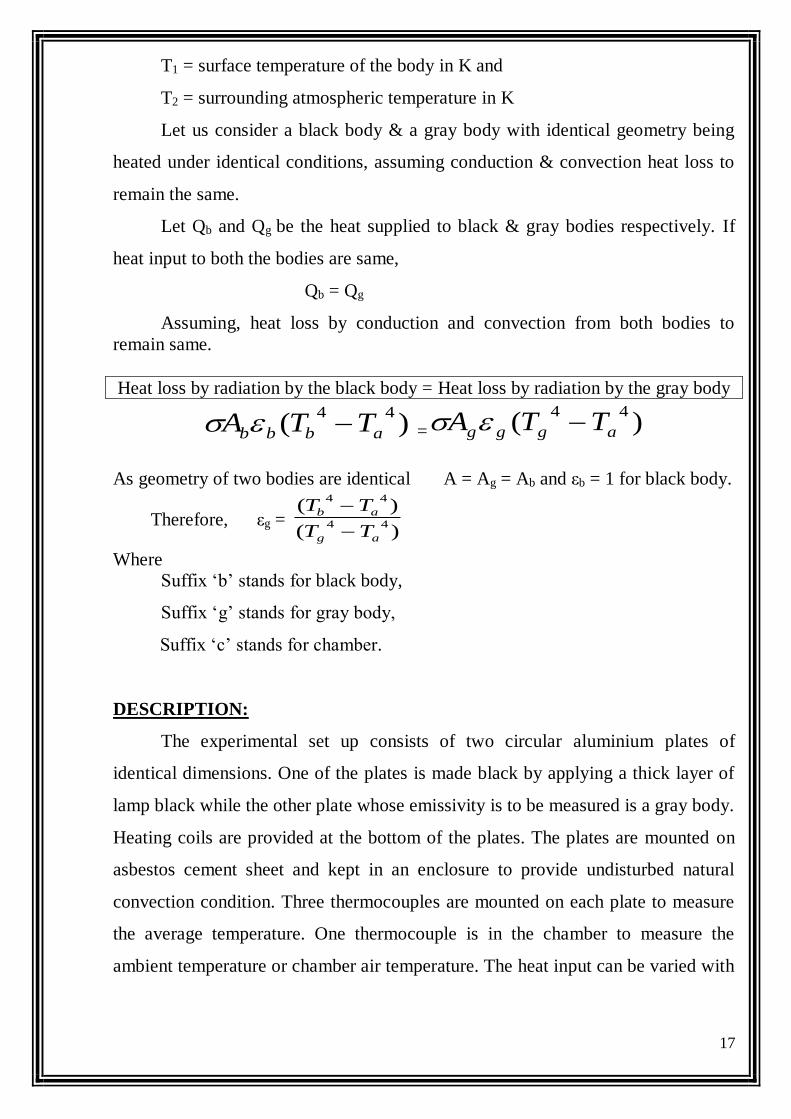
T1 = surface temperature of the body in K and

T2 = surrounding atmospheric temperature in K

Let us consider a black body & a gray body with identical geometry being

heated under identical conditions, assuming conduction & convection heat loss to

remain the same.

Let Qb and Qg be the heat supplied to black & gray bodies respectively. If

heat input to both the bodies are same,

Qb = Qg

Assuming, heat loss by conduction and convection from both bodies to

remain same.

Heat loss by radiation by the black body = Heat loss by radiation by the gray body

)(44

abbb TTA = )(44

aggg TTA

As geometry of two bodies are identical A = Ag = Ab and εb = 1 for black body.

Therefore, εg = )(

)(44

44

ag

ab

TT

TT

Where

Suffix ‘b’ stands for black body,

Suffix ‘g’ stands for gray body,

Suffix ‘c’ stands for chamber.

DESCRIPTION:

The experimental set up consists of two circular aluminium plates of

identical dimensions. One of the plates is made black by applying a thick layer of

lamp black while the other plate whose emissivity is to be measured is a gray body.

Heating coils are provided at the bottom of the plates. The plates are mounted on

asbestos cement sheet and kept in an enclosure to provide undisturbed natural

convection condition. Three thermocouples are mounted on each plate to measure

the average temperature. One thermocouple is in the chamber to measure the

ambient temperature or chamber air temperature. The heat input can be varied with

18

the help of variac for both the plates , that can be measured using digital volt and

ammeter.

SPECIFICATIONS:

Specimen material : Aluminum

Specimen Size : 150 mm, 10 mm thickness (gray & black body)

Voltmeter : Digital type, 0-300v

Ammeter : Digital type, 0-3 amps

Dimmer stat : 0-240 V, 2 amps

Temperature Indicator : Digital type, 0-300°C, K type

Thermocouple Used : 7 nos.

Heater : Sand witched type Nichrome heater, 400 W

PROCEDURE:

1. Switch on the electric mains.

2. Operate the dimmer stat very slowly and give same power input to both the

heater Say 60 V by using (or) operating cam switches provided panel.

3. When steady state is reached note down the temperatures T1 to T7 by rotating

the temperature selection switch gently.

4. Also note down the volt & ammeter reading

5. Repeat the experiment for different heat inputs.

OBSERVATION TABLE:

Sl.

No.

Heater input Temperature of black

surface °C

Temperature of gray

surface °C

Chamber

Temp

°C

V I T1 T2 T3 T5 T6 T7 T4

1.

2.

3.

19

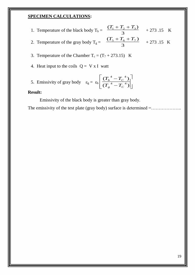
SPECIMEN CALCULATIONS:

1. Temperature of the black body Tb = 3

)( 321 TTT + 273 .15 K

2. Temperature of the gray body Tg = 3

)( 765 TTT + 273 .15 K

3. Temperature of the Chamber Tc = (T7 + 273.15) K

4. Heat input to the coils Q = V x I watt

5. Emissivity of gray body εg = εb

)(

)(44

44

Cg

Cb

TT

TT

Result:

Emissivity of the black body is greater than gray body.

The emissivity of the test plate (gray body) surface is determined =………………..

20

Date:

Exp No:

HEAT TRANSFER BY FORCED CONVECTION

AIM:

To determine the convective heat transfer coefficient and the rate of heat

transfer by forced convection for flow of air inside a horizontal pipe.

THEORY:

Convective heat transfer between a fluid and a solid surface takes place by

the movement of fluid particles relative to the surface. If the movement of fluid

particles is caused by means of external agency such as pump or blower that forces

fluid over the surface, then the process of heat transfer is called forced convection.

In convectional heat transfer, there are two flow regions namely laminar &

turbulent. The non-dimensional number called Reynolds number is used as the

criterion to determine change from laminar to turbulent flow. For smaller value of

Reynolds number viscous forces are dominant and the flow is laminar and for

larger value of Reynolds numbers the inertia forces become dominant and the flow

is turbulent. Dittus –Boelter correlation for fully developed turbulent flow in

circular pipes is,

Nu = 0.023 (Re) 0.8 (Pr) n (from data book)

Where

n = 0.4 for heating of fluid

n = 0.3 for cooling of fluid

Nusselt number= Nu = k

hd

Re = Reynolds Number =

Vd

Pr = Prandtl Number =k

CP

DESCRIPTION OF THE APPARATUS:

The apparatus consists of a blower to supply air. The air from the blower

passes through a flow passage, heater and then to the test section. Air flow is

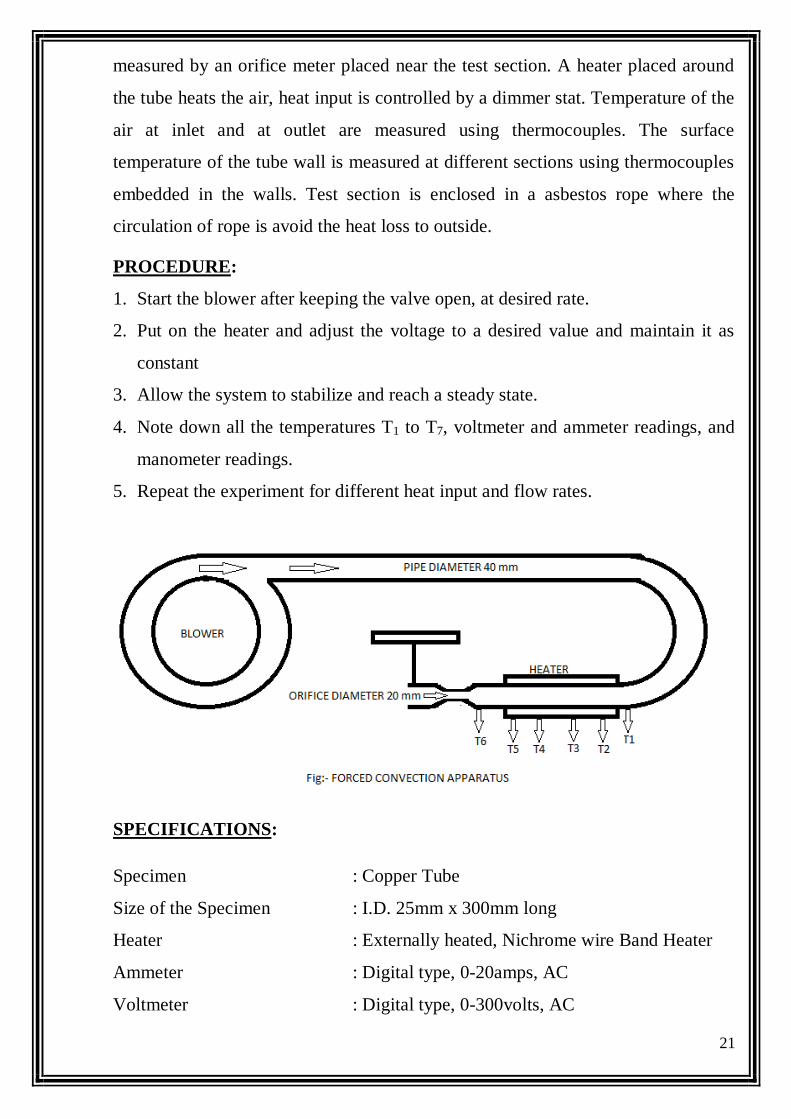
21

measured by an orifice meter placed near the test section. A heater placed around

the tube heats the air, heat input is controlled by a dimmer stat. Temperature of the

air at inlet and at outlet are measured using thermocouples. The surface

temperature of the tube wall is measured at different sections using thermocouples

embedded in the walls. Test section is enclosed in a asbestos rope where the

circulation of rope is avoid the heat loss to outside.

PROCEDURE:

1. Start the blower after keeping the valve open, at desired rate.

2. Put on the heater and adjust the voltage to a desired value and maintain it as

constant

3. Allow the system to stabilize and reach a steady state.

4. Note down all the temperatures T1 to T7, voltmeter and ammeter readings, and

manometer readings.

5. Repeat the experiment for different heat input and flow rates.

SPECIFICATIONS:

Specimen : Copper Tube

Size of the Specimen : I.D. 25mm x 300mm long

Heater : Externally heated, Nichrome wire Band Heater

Ammeter : Digital type, 0-20amps, AC

Voltmeter : Digital type, 0-300volts, AC

22

Dimmer stat for heating Coil : 0-230v, 2amps

Thermocouple Used : 7 nos.

Centrifugal Blower : Single Phase 230v, 50 hz, 3000rpm

Manometer : U-tube with water as working fluid

Orifice diameter, ‘d2’ : 20 mm

G. I pipe diameter, ‘d1’ : 40 mm

Coefficient of discharge : 0.62

Length of the tube : 500 mm

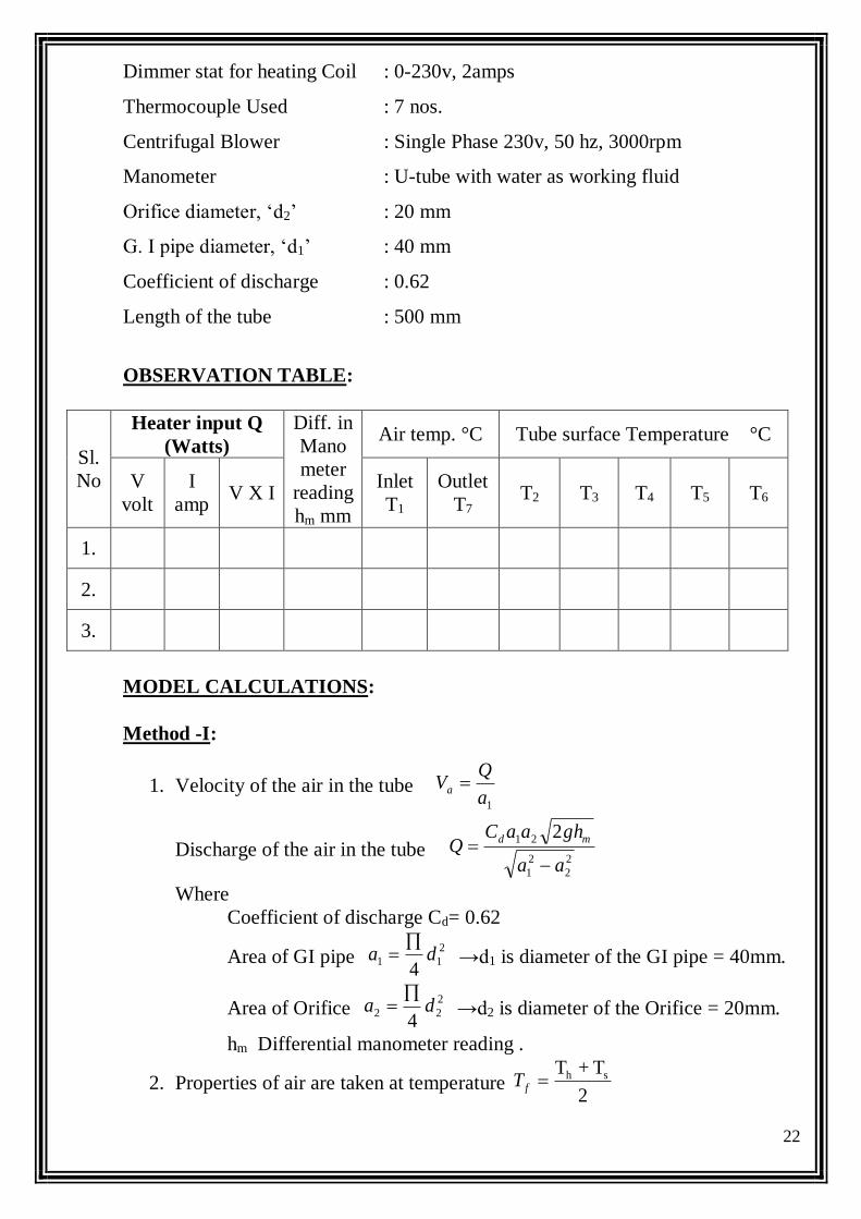
OBSERVATION TABLE:

Sl.

No

Heater input Q

(Watts)

Diff. in

Mano

meter

reading

hm mm

Air temp. °C Tube surface Temperature °C

V

volt

I

amp V X I

Inlet

T1

Outlet

T7 T2 T3 T4 T5 T6

1.

2.

3.

MODEL CALCULATIONS:

Method -I:

1. Velocity of the air in the tube 1a

QVa

Discharge of the air in the tube 2

2

2

1

21 2

aa

ghaaCQ

md

Where

Coefficient of discharge Cd= 0.62

Area of GI pipe 2

114

da

→d1 is diameter of the GI pipe = 40mm.

Area of Orifice 2

224

da

→d2 is diameter of the Orifice = 20mm.

hm Differential manometer reading .

2. Properties of air are taken at temperature 2

T+T shfT

23

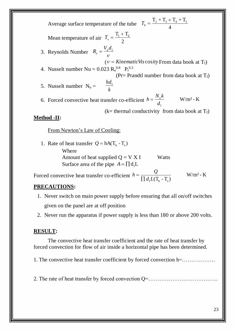
Average surface temperature of the tube 4

T+TT+T 5432 hT

Mean temperature of air 2

TT 61 sT

3. Reynolds Number

1dVR a

e

( ityisKinematicV cos From data book at Tf)

4. Nusselt number Nu = 0.023 Re0.8 Pr

0.3

(Pr= Prandtl number from data book at Tf)

5. Nusselt number Nu = k

hd1

6. Forced convective heat transfer co-efficient K- W/m² 1d

kNh u

(k= thermal conductivity from data book at Tf)

Method -II:

From Newton’s Law of Cooling:

1. Rate of heat transfer )T-hA(T shQ

Where

Amount of heat supplied Q = V X I Watts

Surface area of the pipe Ld1A

Forced convective heat transfer co-efficient K- W/m² )T-(T sh1Ld

Qh

PRECAUTIONS:

1. Never switch on main power supply before ensuring that all on/off switches

given on the panel are at off position

2. Never run the apparatus if power supply is less than 180 or above 200 volts.

RESULT:

The convective heat transfer coefficient and the rate of heat transfer by

forced convection for flow of air inside a horizontal pipe has been determined.

1. The convective heat transfer coefficient by forced convection h=………………

2. The rate of heat transfer by forced convection Q=………………………………..

24

Date:

Exp No:

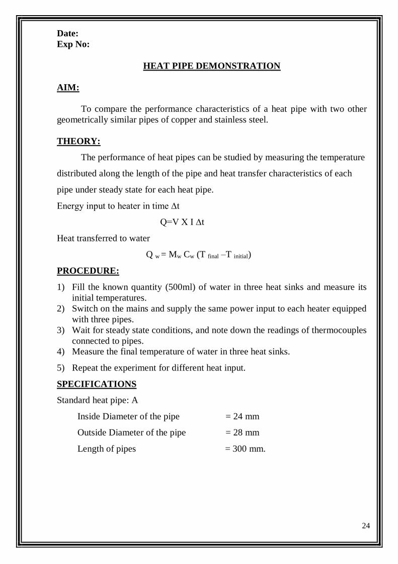
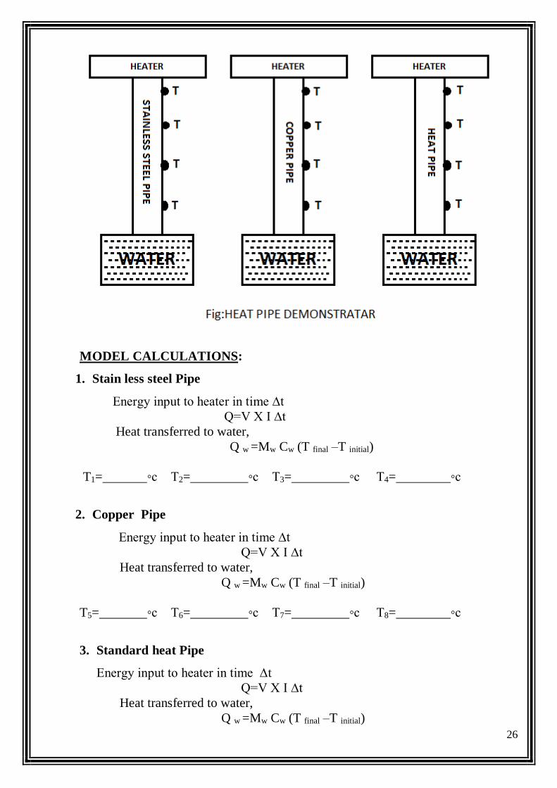
HEAT PIPE DEMONSTRATION

AIM:

To compare the performance characteristics of a heat pipe with two other

geometrically similar pipes of copper and stainless steel.

THEORY:

The performance of heat pipes can be studied by measuring the temperature

distributed along the length of the pipe and heat transfer characteristics of each

pipe under steady state for each heat pipe.

Energy input to heater in time ∆t

Q=V X I ∆t

Heat transferred to water

Q w = Mw Cw (T final –T initial)

PROCEDURE:

1) Fill the known quantity (500ml) of water in three heat sinks and measure its

initial temperatures.

2) Switch on the mains and supply the same power input to each heater equipped

with three pipes.

3) Wait for steady state conditions, and note down the readings of thermocouples

connected to pipes.

4) Measure the final temperature of water in three heat sinks.

5) Repeat the experiment for different heat input.

SPECIFICATIONS

Standard heat pipe: A

Inside Diameter of the pipe = 24 mm

Outside Diameter of the pipe = 28 mm

Length of pipes = 300 mm.

25

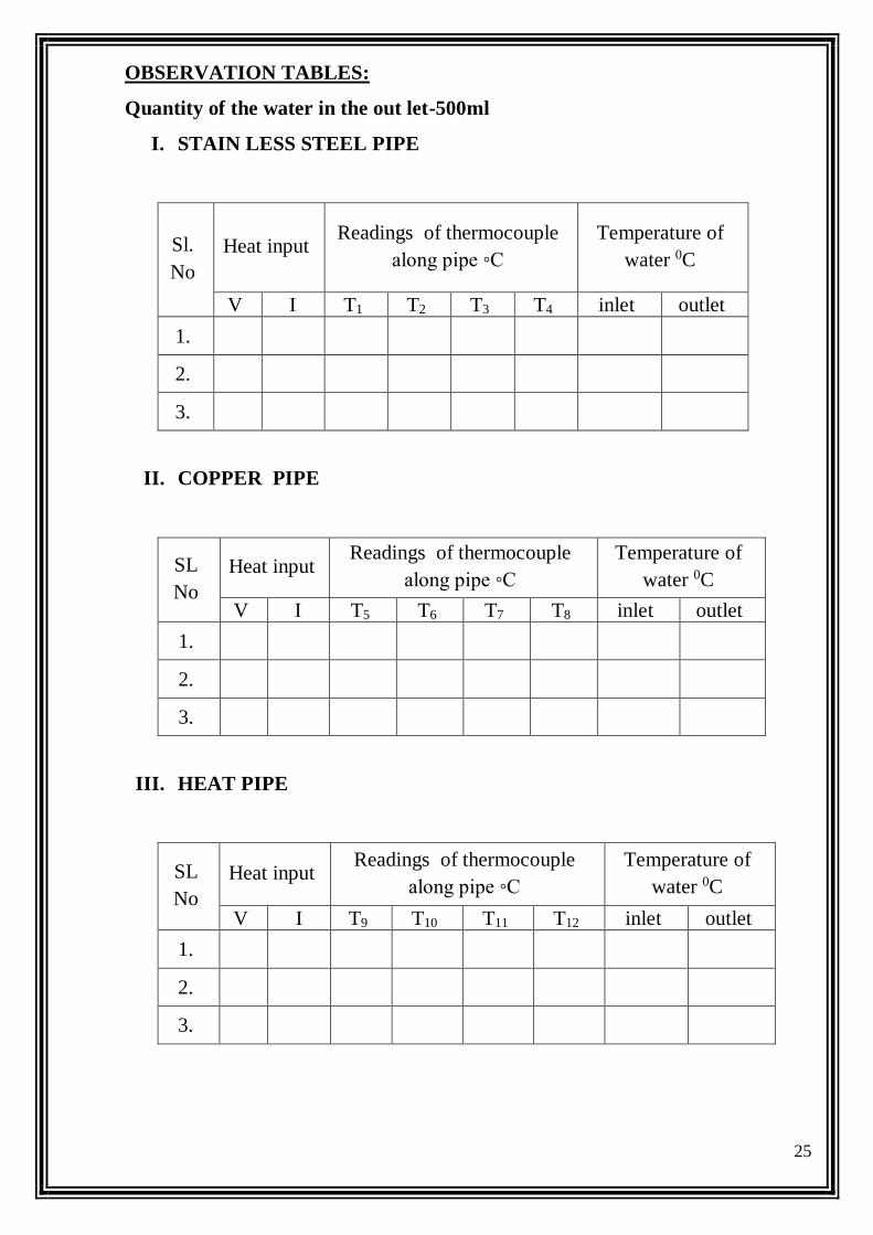
OBSERVATION TABLES:

Quantity of the water in the out let-500ml

I. STAIN LESS STEEL PIPE

Sl.

No

Heat input Readings of thermocouple

along pipe ◦C

Temperature of

water 0C

V I T1 T2 T3 T4 inlet outlet

1. 2. 3.

II. COPPER PIPE

SL

No


along pipe ◦C

Temperature of

water 0C


1. 2. 3.

III. HEAT PIPE

SL

No


along pipe ◦C

Temperature of

water 0C


1. 2. 3.

26

MODEL CALCULATIONS:

1. Stain less steel Pipe


Q=V X I ∆t

Heat transferred to water,

Q w =Mw Cw (T final –T initial)

T1= ◦c T2= ◦c T3= ◦c T4= ◦c

2. Copper Pipe


Q=V X I ∆t



T5= ◦c T6= ◦c T7= ◦c T8= ◦c

3. Standard heat Pipe


Q=V X I ∆t



27

T9= ◦c T10= ◦c T11= ◦c T12= ◦c

RESULT:

The performance characteristics of a heat pipe with two other geometrically

similar pipes of copper and stainless steel has been determined.

28

Date:

Exp No:

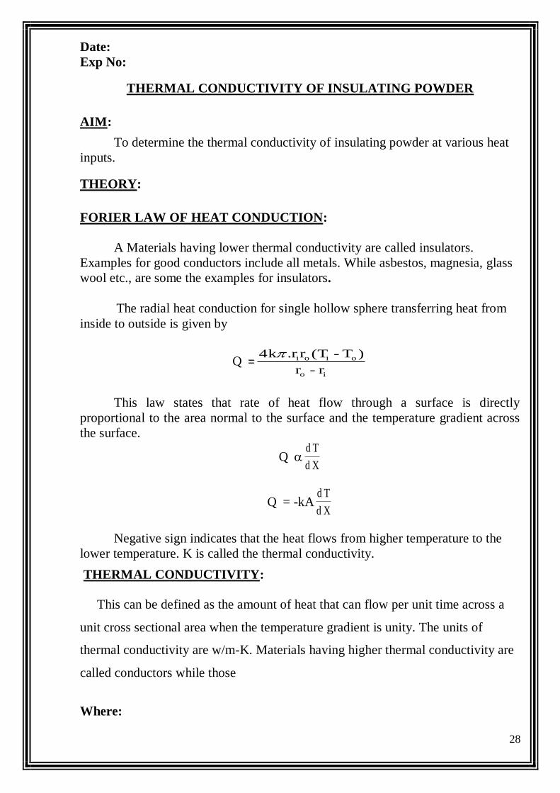
THERMAL CONDUCTIVITY OF INSULATING POWDER

AIM:

To determine the thermal conductivity of insulating powder at various heat

inputs.

THEORY:

FORIER LAW OF HEAT CONDUCTION:

A Materials having lower thermal conductivity are called insulators.

Examples for good conductors include all metals. While asbestos, magnesia, glass

wool etc., are some the examples for insulators.

The radial heat conduction for single hollow sphere transferring heat from

inside to outside is given by

Q ==io

oioi

r - r

)T-(Tr.r4k

This law states that rate of heat flow through a surface is directly

proportional to the area normal to the surface and the temperature gradient across

the surface.

Q X d

T d

Q = -kAX d

T d

Negative sign indicates that the heat flows from higher temperature to the

lower temperature. K is called the thermal conductivity.

THERMAL CONDUCTIVITY:

This can be defined as the amount of heat that can flow per unit time across a

unit cross sectional area when the temperature gradient is unity. The units of

thermal conductivity are w/m-K. Materials having higher thermal conductivity are

called conductors while those

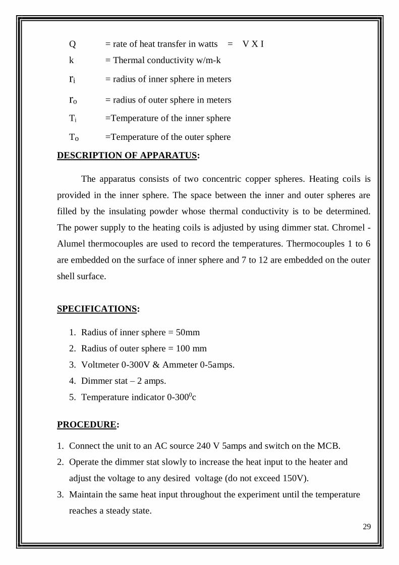
Where:

29

Q = rate of heat transfer in watts = V X I

k = Thermal conductivity w/m-k

ri = radius of inner sphere in meters

ro = radius of outer sphere in meters

Ti =Temperature of the inner sphere

To =Temperature of the outer sphere

DESCRIPTION OF APPARATUS:

The apparatus consists of two concentric copper spheres. Heating coils is

provided in the inner sphere. The space between the inner and outer spheres are

filled by the insulating powder whose thermal conductivity is to be determined.

The power supply to the heating coils is adjusted by using dimmer stat. Chromel -

Alumel thermocouples are used to record the temperatures. Thermocouples 1 to 6

are embedded on the surface of inner sphere and 7 to 12 are embedded on the outer

shell surface.

SPECIFICATIONS:

1. Radius of inner sphere = 50mm

2. Radius of outer sphere = 100 mm

3. Voltmeter 0-300V & Ammeter 0-5amps.

4. Dimmer stat – 2 amps.

5. Temperature indicator 0-3000c

PROCEDURE:

1. Connect the unit to an AC source 240 V 5amps and switch on the MCB.

2. Operate the dimmer stat slowly to increase the heat input to the heater and

adjust the voltage to any desired voltage (do not exceed 150V).

3. Maintain the same heat input throughout the experiment until the temperature

reaches a steady state.

30

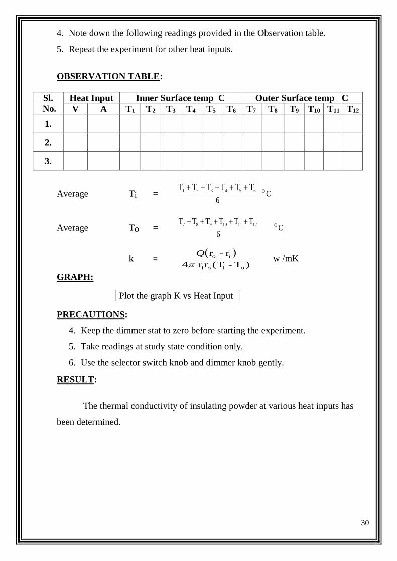
4. Note down the following readings provided in the Observation table.

5. Repeat the experiment for other heat inputs.

OBSERVATION TABLE:

Sl.

No.

Heat Input Inner Surface temp C Outer Surface temp C

V A T1 T2 T3 T4 T5 T6 T7 T8 T9 T10 T11 T12

1. 2. 3.

Average Ti = 6

TTTTTT 654321 CO

Average To = 6

TTTTTT 121110987 CO

kk ==

)T-(Trr 4

r - r

oioi

io

Q w /mK

GRAPH:

PRECAUTIONS:


5. Take readings at study state condition only.


RESULT:

The thermal conductivity of insulating powder at various heat inputs has

been determined.

Plot the graph K vs Heat Input

31

Date:

Exp No:

LLAAGGGGEEDD PPIIPPEE

AIM

To determine thermal conductivity of different insulating materials, Overall heat

transfer coefficient of lagged pipe and thermal resistance.

APPARATUS

The apparatus consists of three concentric pipes mounted on suitable stand.

The hollow space of the innermost pipe consists of the heater. Between first two

cylinders the insulating material with which lagging is to be done is filled

compactly. Between second and third cylinders, another material used for lagging

is filled. The third cylinder is concentric to other outer cylinder. The

thermocouples are attached to the surface of cylinders appropriately to measure the

temperatures. The input to the heater is varied through a dimmerstat .

SPECIFICATIONS:

Diameter of heater rod dH= 20 mm

Diameter of heater rod with asbestos lagging dA= 40mm

Diameter of heater rod with asbestos and saw dust lagging dS=80mm

Effective length of the cylinder l= 500mm.

PROCEDURE:

1. Switch on the unit and check if channels of temperature indicator showing

proper change temperature.

2. Switch on the heater using the regulator and keep the power input at some

particular value.

3. Allow the unit to stabilize for about 20 to 30 minutes

4. Now note down the ammeter reading, voltmeter reading, which gives the heat

input, temperatures 1,2,3 are the temperature of heater rod, 4,5,6 are the

32

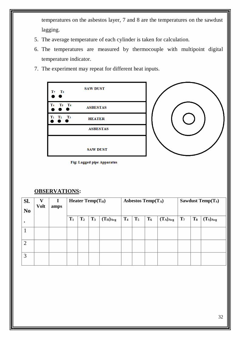
temperatures on the asbestos layer, 7 and 8 are the temperatures on the sawdust

lagging.

5. The average temperature of each cylinder is taken for calculation.

6. The temperatures are measured by thermocouple with multipoint digital

temperature indicator.

7. The experiment may repeat for different heat inputs.

OBSERVATIONS:

Sl.

No

.

V

Volt

I

amps

Heater Temp(TH) Asbestos Temp(TA) Sawdust Temp(TS)

T1 T2 T3 (TH)Avg T4 T5 T6 (TA)Avg T7 T8 (TS)Avg

1

2

3

33

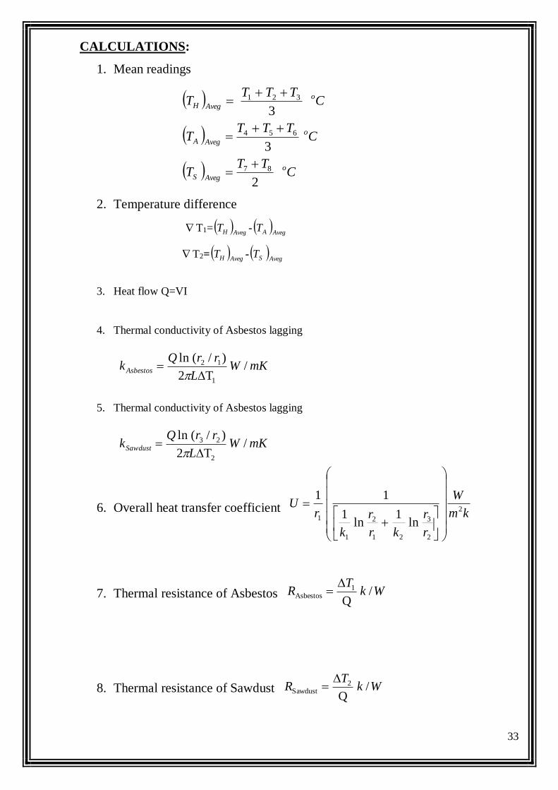
CALCULATIONS:

1. Mean readings

CTT

T

CTTT

T

CTTT

T

o

AvegS

o

AvegA

o

AvegH

2

3

3

87

654

321

2. Temperature difference

T1= AvegHT -

AvegAT

T2= AvegHT -

AvegST

3. Heat flow Q=VI

4. Thermal conductivity of Asbestos lagging

mKWL

rrQkAsbestos /

T2

)/(ln

1

12

5. Thermal conductivity of Asbestos lagging

mKWL

rrQkSawdust /

T2

)/(ln

2

23

6. Overall heat transfer coefficient km

W

r

r

kr

r

k

rU

2

2

3

21

2

1

1ln

1ln

1

11

7. Thermal resistance of Asbestos WkT

R /Q

1Asbestos

8. Thermal resistance of Sawdust WkT

R /Q

2Sawdust

34

PRECAUTIONS:

1) Keep dimmer stat to ZERO position before start.

2) Increase voltage gradually.

3) Keep the assembly undisturbed while testing.

4) While removing or changing the lagging materials do not disturb the

thermocouples.

5) Do not increase voltage above 150V

6) Operate selector switch of temperate indicator gently.

RESULTS: Thermal conductivity of different insulating materials, Overall heat

transfer coefficient of lagged pipe and thermal resistance has been determined.

1. Thermal conductivity of asbestos powder lagging Asbestosk =…………………

2. Thermal conductivity of sawdust lagging Sawdustk =……………………….

3. Overall heat transfer coefficient U=…………………………

4. Thermal resistance of Asbestos AsbestosR =……………………………

5. Thermal resistance of Sawdust SawdustR =………………………………..

35

Date:

Exp No:

HEAT TRANSFER BY NATURAL CONVECTION

AIM:

To find out heat transfer coefficient and heat transfer rate from vertical

cylinder in natural convection.

THEORY:

Natural convection heat transfer takes place by movement of fluid particles

on solid surface caused by density difference between the fluid particles on

account of difference in temperature. Hence there is no external agency facing

fluid over the surface. It has been observed that the fluid adjacent to the surface

gets heated, resulting in thermal expansion of the fluid and reduction in its density.

Subsequently a buoyancy force acts on the fluid causing it to flow up the surface.

Here the flow velocity is developed due to difference in temperature between fluid

particles.

The following empirical correlations may be used to find out the heat

transfer coefficient for vertical cylinder in natural convection.

4

1

Pr.53.0 GrNu for Gr.Pr<105

4

1

Pr.56.0 GrNu for 105<Gr.Pr<108

31


Where,

Nu = Nusselt number = k

hL

Gr = Grashof number = 2

3 )(

aS TTgL

Pr = Prandtl number =k

Cp

36

β = Coefficient of Volumetric expansion (or) temperature co-efficient of

thermal conductivity in K

1

For ideal gases β = fT

1

Where ‘Tf’ is the absolute film temperature at which the properties are taken.

SPECIFICATIONS:

Specimen : Stainless Steel tube,

Size of the Specimen : Outer diameter 45mm, 500mm length

Heater : Nichrome wire type heater along its length

Thermocouples used : 6nos.

Ammeter : Digital type, 0-2amps, AC

Voltmeter : Digital type, 0-300volts, AC

Dimmer stat for heating coil : 0-230 V, 2 amps, AC power

Enclosure with acrylic door : For visual display of test section (fixed)

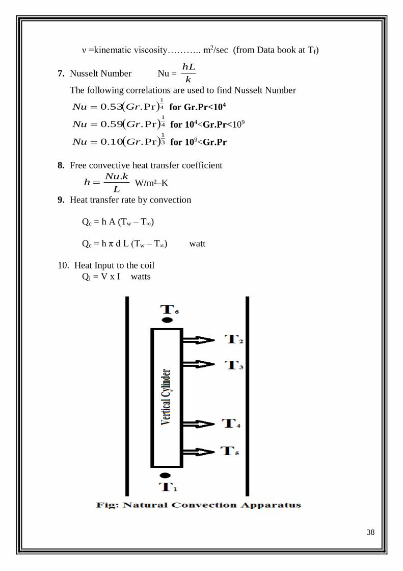
APPARATUS:

The apparatus consists of a stainless steel tube fitted in a rectangular duct in

a vertical position. The duct is open at the top and bottom and forms an enclosure

and serves the purpose of undisturbed surroundings. One side of the duct is made

of acrylic sheet for visualization. A heating element is kept in the vertical tube,

which heats the tube surface. The heat is lost from the tube to the surrounding air

by natural convection. Digital temperature indicator measures the temperature at

different points with the help of seven temperature sensors, including one for

measuring surrounding temperature. The heat input to the heater is measured by

Digital Ammeter and Digital Voltmeter and can be varied by a dimmer stat.

PROCEDURE:

1. Ensure that all ON/OFF switches given on the panel are at OFF position.

2. Ensure that variac knob is at zero position, provided on the panel.

3. Now switch on the main power supply (220 V AC, 50 Hz).

37

4. Switch on the panel with the help of mains ON/OFF switch given on the

panel.

5. Fix the power input to the heater with the help of variac, voltmeter and

ammeter provided.

6. Take thermocouple, voltmeter & ammeter readings when steady state is

reached.

7. When experiment is over, switch off heater first.

8. Adjust variac to zero position.

9. Switch off the panel with the help of Mains On/Off switch given on the panel.

10. Switch off power supply to panel.

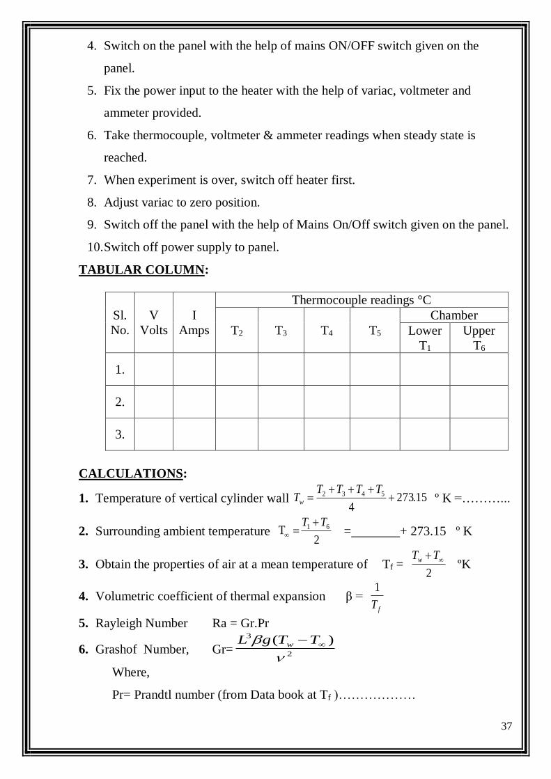
TABULAR COLUMN:

Sl.

No.

V

Volts

I

Amps

Thermocouple readings °C

T2 T3 T4 T5

Chamber

Lower

T1

Upper

T6

1.

2.

3.

CALCULATIONS:

1. Temperature of vertical cylinder wall 15.2734

5432

TTTT

Tw º K =………...

2. Surrounding ambient temperature 2

T 61 TT = + 273.15 º K

3. Obtain the properties of air at a mean temperature of Tf = 2

TTw ºK

4. Volumetric coefficient of thermal expansion β = fT

1

5. Rayleigh Number Ra = Gr.Pr

6. Grashof Number, Gr= 2

3 )(

TTgL w

Where,

Pr= Prandtl number (from Data book at Tf )………………

38

ν =kinematic viscosity……….. m2/sec (from Data book at Tf)

7. Nusselt Number Nu = k

hL

The following correlations are used to find Nusselt Number

4

1

Pr.53.0 GrNu for Gr.Pr<104

4

1


3

1

Pr.10.0 GrNu for 109<Gr.Pr

8. Free convective heat transfer coefficient

L

kNuh

. W/m²–K

9. Heat transfer rate by convection

Qc = h A (Tw – T∞)

Qc = h π d L (Tw – T∞) watt

10. Heat Input to the coil

Qi = V x I watts

39

PRECAUTIONS:

1. Never switch on the main power supply before ensuring that all on / off

switches give on the panel are at off position.

2. Never run the apparatus if power supply is less than 180 or above 200 Volts.

3. Make sure that convection should conduct in closed container.

4. Before switch on the main supply observer that the dimmer is in zero

position.

RESULT:

The convective heat transfer coefficient and heat transfer rate from vertical

cylinder in natural convection has been determined.

1. Convective heat transfer coefficient=…………………………..

2. Heat transfer rate=………………………………….

40

Date:

Exp No:

PARALLEL FLOW AND COUNTER FLOW HEAT EXCHANGER

AIM:

To determine LMTD, effectiveness and overall heat transfer coefficient for

parallel and counter flow heat exchanger

SPECIFICATIONS:

Length of heat exchanger L =2440 mm

Inner copper tube ID =12 mm

OD =15 mm

Outer GI tube ID =40 mm

Geyser capacity =1 Lt, 3 kW

THEORY:

Heat exchanger is a device in which heat is transferred from one fluid to

another. Common examples of heat exchangers are:

i. Condensers and boilers in steam plant

ii. Inter coolers and pre-heaters

iii. Automobile radiators

iv. Regenerators

CLASSIFICATION OF HEAT EXCHANGERS:

1. Based on the nature of heat exchange process:

i. Direct contact type – Here the heat transfer takes place by direct mixing

of hot and cold fluids

ii. Indirect contact heat exchangers – Here the two fluids are separated

through a metallic wall. ex. Regenerators, Recuperators etc

2. Based on the relative direction of fluid flow:

41

i. Parallel flow heat exchanger – Here both hot and cold fluids flow in the

same direction.

ii. Counter flow heat exchanger – Here hot and cold fluids flow in opposite

direction.

iii. Cross-flow heat exchangers – Here the two fluids cross one another.

LOGARITHMIC MEAN TEMPERATURE DIFFERENCE (LMTD):

This is defined as that temperature difference which, if constant, would give

the same rate of heat transfer as usually occurs under variable conditions of

temperature difference.

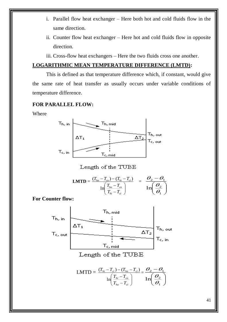
FOR PARALLEL FLOW:

Where

LMTD =

cihi

coho

cihicoho

TT

TT

TTTT

ln

)()( =

1

2

12

ln

For Counter flow:

LMTD =

ciho

cohi

cihocihi

TT

TT

TTTT

ln

)()(=

1

2

12

ln

42

Tho = Outlet temperature of hot fluid

Tco = Outlet temperature of cold fluid

Thi = Inlet temperature of hot fluid

Tci = Inlet temperature of cold fluid

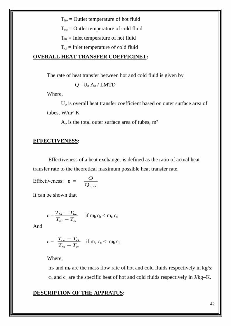
OVERALL HEAT TRANSFER COEFFICINET:

The rate of heat transfer between hot and cold fluid is given by

Q =Uo Ao / LMTD

Where,

Uo is overall heat transfer coefficient based on outer surface area of

tubes, W/m²-K

Ao is the total outer surface area of tubes, m²

EFFECTIVENESS:

Effectiveness of a heat exchanger is defined as the ratio of actual heat

transfer rate to the theoretical maximum possible heat transfer rate.

Effectiveness: ε = maxQ

Q

It can be shown that

ε =cihi

hohi

TT

TT

if mh ch < mc cc

And

ε = cihi

cico

TT

TT

if mc cc < mh ch

Where,

mh and mc are the mass flow rate of hot and cold fluids respectively in kg/s;

ch and cc are the specific heat of hot and cold fluids respectively in J/kg–K.

DESCRIPTION OF THE APPRATUS:

43

The apparatus consists of a concentric tube heat exchanger. The hot fluid

namely hot water is obtained from the Geyser (heater capacity 3 kW) & it flows

through the inner tube. The cold fluid i.e. cold water can be admitted at any one of

the ends enabling the heat exchanger to run as a parallel flow or as a counter flow

exchanger. Measuring jar used for measure flow rate of cold and hot water. This

can be adjusted by operating the different valves provided. Temperature of the

fluid can be measured using thermocouples with digital display indicator. The

outer tube is provided with insulation to minimize the heat loss to the

surroundings.

PROCEDURE:

1. First switch ON the unit panel

2. Start the flow of cold water through the annulus and run the exchanger as

counter flow or parallel flow.

3. Switch ON the geyser provided on the panel & allow to flow through the

inner tube by regulating the valve.

4. Adjust the flow rate of hot water and cold water by using rotameters & valves.

5. Keep the flow rate same till steady state conditions are reached.

6. Note down the temperatures on hot and cold water sides. Also note the flow

rate.

7. Repeat the experiment for different flow rates and for different temperatures.

The same method is followed for parallel flow also.

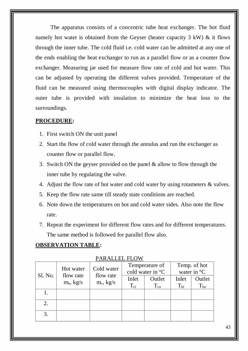
OBSERVATION TABLE:

PARALLEL FLOW

Sl. No.

Hot water

flow rate

mh, kg/s

Cold water

flow rate

mc, kg/s

Temperature of

cold water in °C

Temp. of hot

water in °C

Inlet

Tci

Outlet

Tco

Inlet

Thi

Outlet

Tho

1. 2. 3.

44

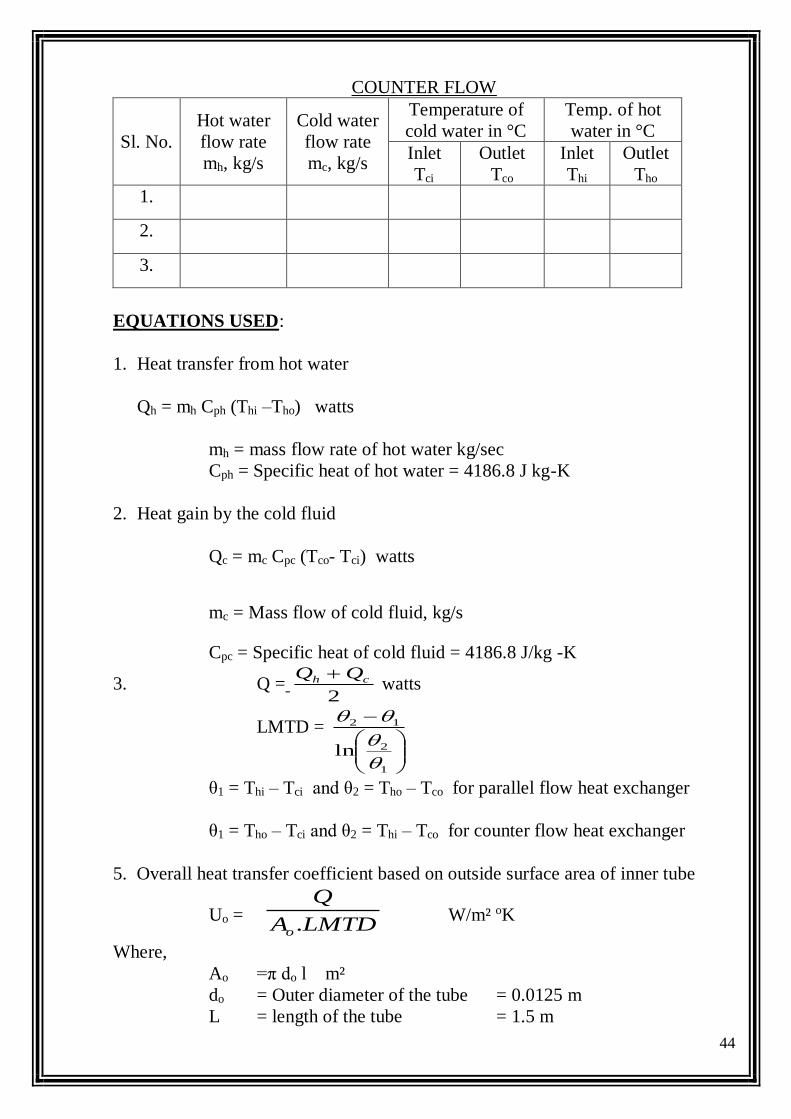
COUNTER FLOW

Sl. No.

Hot water

flow rate

mh, kg/s

Cold water

flow rate

mc, kg/s

Temperature of

cold water in °C

Temp. of hot

water in °C

Inlet

Tci

Outlet

Tco

Inlet

Thi

Outlet

Tho

1. 2. 3.

EQUATIONS USED:

1. Heat transfer from hot water

Qh = mh Cph (Thi –Tho) watts

mh = mass flow rate of hot water kg/sec

Cph = Specific heat of hot water = 4186.8 J kg-K

2. Heat gain by the cold fluid

Qc = mc Cpc (Tco- Tci) watts

mc = Mass flow of cold fluid, kg/s

Cpc = Specific heat of cold fluid = 4186.8 J/kg -K

3. Q = 2

ch QQ watts

LMTD =

1

2

12

ln

θ1 = Thi – Tci and θ2 = Tho – Tco for parallel flow heat exchanger

θ1 = Tho – Tci and θ2 = Thi – Tco for counter flow heat exchanger

5. Overall heat transfer coefficient based on outside surface area of inner tube

Uo = LMTDA

Q

o. W/m² oK

Where,

Ao =π do l m²

do = Outer diameter of the tube = 0.0125 m

L = length of the tube = 1.5 m

45

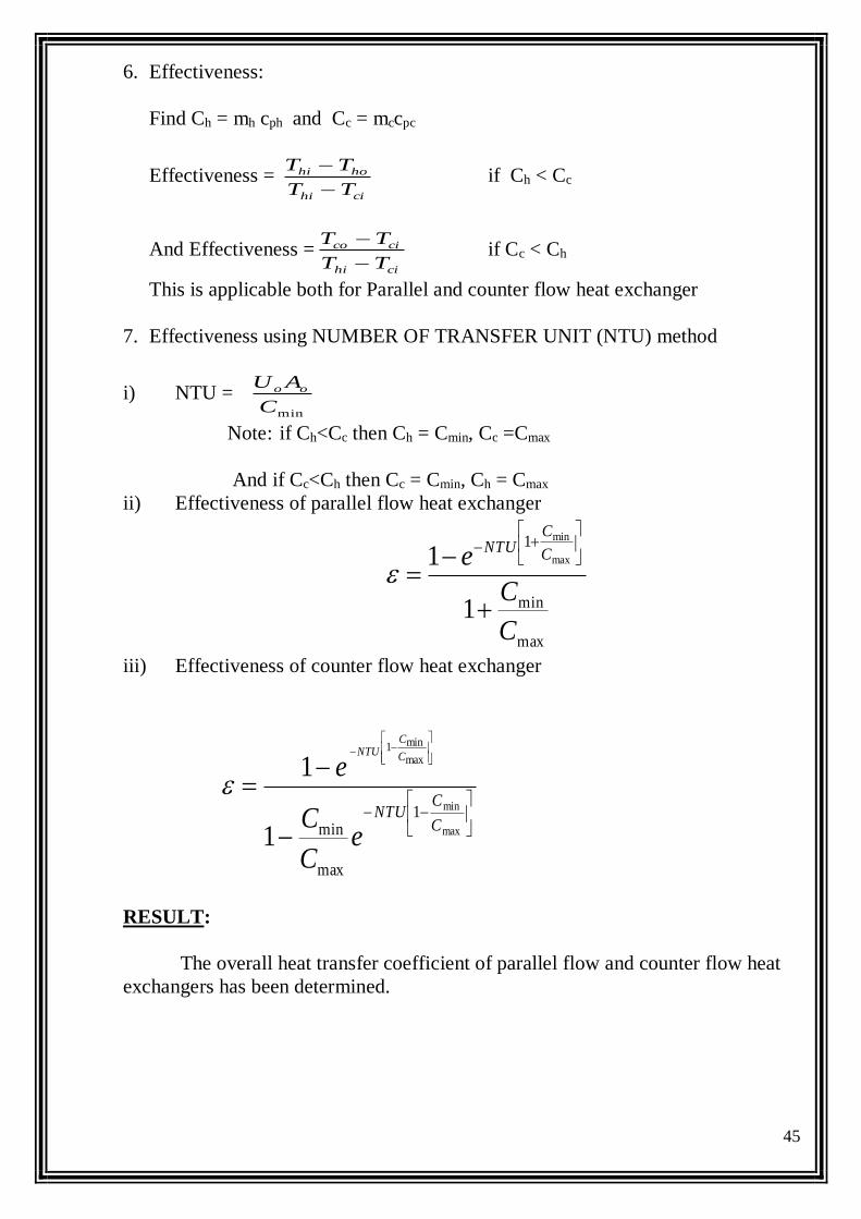
6. Effectiveness:

Find Ch = mh cph and Cc = mccpc

Effectiveness = cihi

hohi

TT

TT

if Ch < Cc

And Effectiveness =cihi

cico

TT

TT

if Cc < Ch

This is applicable both for Parallel and counter flow heat exchanger

7. Effectiveness using NUMBER OF TRANSFER UNIT (NTU) method

i) NTU = minC

AU oo

Note: if Ch<Cc then Ch = Cmin, Cc =Cmax

And if Cc<Ch then Cc = Cmin, Ch = Cmax

ii) Effectiveness of parallel flow heat exchanger

max

min

1

1

1 max

min

C

C

e C

CNTU

iii) Effectiveness of counter flow heat exchanger

max

min

max

min1

1

max

min1

1

C

CNTU

eC

C

eC

CNTU

RESULT:

The overall heat transfer coefficient of parallel flow and counter flow heat

exchangers has been determined.

46

Date:

Exp No:

HEAT TRANSFER FROM PIN-FIN APPARATUS

AIM:

To determine the temperature of a pin-fin for forced convection and to find

fin efficiency and effectiveness.

SPECIFICATIONS:

Length of the fin, ‘L’ = 145mm

Diameter of the fin, ‘df’ = 12mm

Diameter of the orifice, ‘do’ = 20 mm

Width of the duct, ‘W’ = 150 mm

Breadth of the duct, ‘B’ = 100 mm

Coefficient of discharge of the orifice, ‘Cd’ = 0.62

Density of manometric fluid (water) =1000 kg/m3

THEORY:

The heat transfer from a heated surface to the ambient surrounding is given

by the relation, q = h A T. In this relation hc is the convective heat transfer

coefficient, T is the temperature difference & A is the area of heat transfer. To

increase q, h may be increased or surface area may by increased. In some cases it is

not possible to increase the value of heat transfer coefficient & the temperature

difference T & thus the only alternative is to increase the surface area of heat

transfer. The surface area is increased by attaching extra material in the form of rod

(circular or rectangular) on the surface where we have to increase the heat transfer

rate. "This extra material attached is called the extended surface or fin."

The fins may be attached on a plane surface, and then they are called plane

surface fins. If the fins are attached on the cylindrical surface, they are called

circumferential fins. The cross section of the fin may be circular, rectangular,

triangular or parabolic.

47

Temperature distribution along the length of the fin:

mL

xLm

TT

TT

cosh

cosh

00

Where

T = Temperature at any distance x on the fin

T0 = Temperature at x = 0

T = Ambient temperature

L = Length of the fin

kA

Phm c

Where

h = convective heat transfer coefficient

P = Perimeter of the fin

A = area of the fin

K = Thermal conductivity of the fin

Rate of heat flow for end insulated condition:

mLPkAhQ c tanh0

Effectiveness of a fin is defined as the ratio of the heat transfer with fin to

the heat transfer from the surface without fins.

0

0 tanh

hA

mLhPkA

mLhA

Pktanh

The efficiency of a fin is defined as the ratio of the actual heat transferred by

the fin to the maximum heat transferred by the fin if the entire fin area were at base

temperature.

0

0 tanh

hPL

mLhPkAf

mL

mLf

tanh

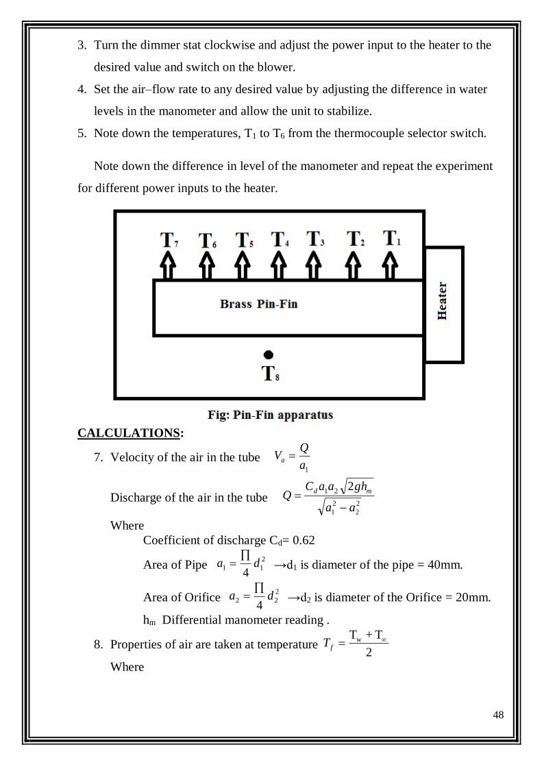
PROCEDURE:

1. Connect the equipment to electric power supply.

2. Keep the thermocouple selector switch to zero position.

48

3. Turn the dimmer stat clockwise and adjust the power input to the heater to the

desired value and switch on the blower.

4. Set the air–flow rate to any desired value by adjusting the difference in water

levels in the manometer and allow the unit to stabilize.

5. Note down the temperatures, T1 to T6 from the thermocouple selector switch.

Note down the difference in level of the manometer and repeat the experiment

for different power inputs to the heater.

CALCULATIONS:

7. Velocity of the air in the tube 1a

QVa

Discharge of the air in the tube 2

2

2

1

21 2

aa

ghaaCQ

md

Where

Coefficient of discharge Cd= 0.62

Area of Pipe 2

114

da

→d1 is diameter of the pipe = 40mm.

Area of Orifice 2

224

da

→d2 is diameter of the Orifice = 20mm.

hm Differential manometer reading .

8. Properties of air are taken at temperature 2

T+Tw fT

Where

49

Average surface temperature of the Pin-fin

7

T+TT+TT+TT 7654321 wavg TT

Ambient temperature of air in Duct T∞= T8

9. Reynolds Number

fa

D

dV .Re

( ityisKinematicV cos From data book at Tf)

(Pr= Prandtl number from data book at Tf)

10. Nusselt number Nu = 333.0PrRe

m

DC

For

ReD = 0.4 to 4.0 C = 0.989 m = 0.33

ReD = 4 to 40 C = 0.911 m = 0.385

ReD = 40 to 4000 C = 0.683 m = 0.466

ReD = 4000 to 40,000 C = 0.293 m = 0.618

ReD = 40,000 to 400,000 C = 0.27 m = 0.805

11. Nusselt number k

hdNu

f

12. Forced convective heat transfer co-efficient K- W/m² f

u

d

kNh

(k= thermal conductivity from data book at Tf)

13. Rate of heat transfer Qc = h A (Tw – T∞)

Qc = h π d L (Tw – T∞) watt

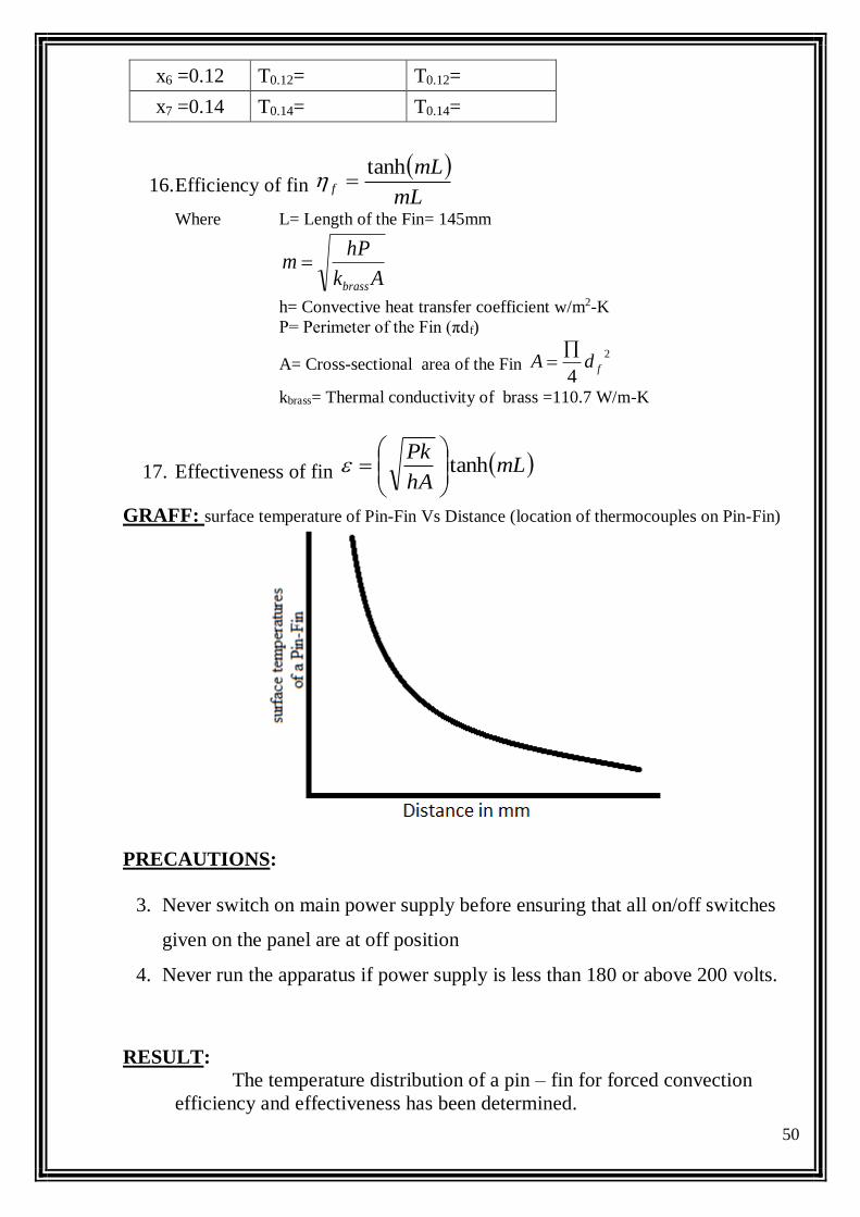
14. Temperature distribution is given by

mL

XLm

TT

TT

cosh

cosh

0

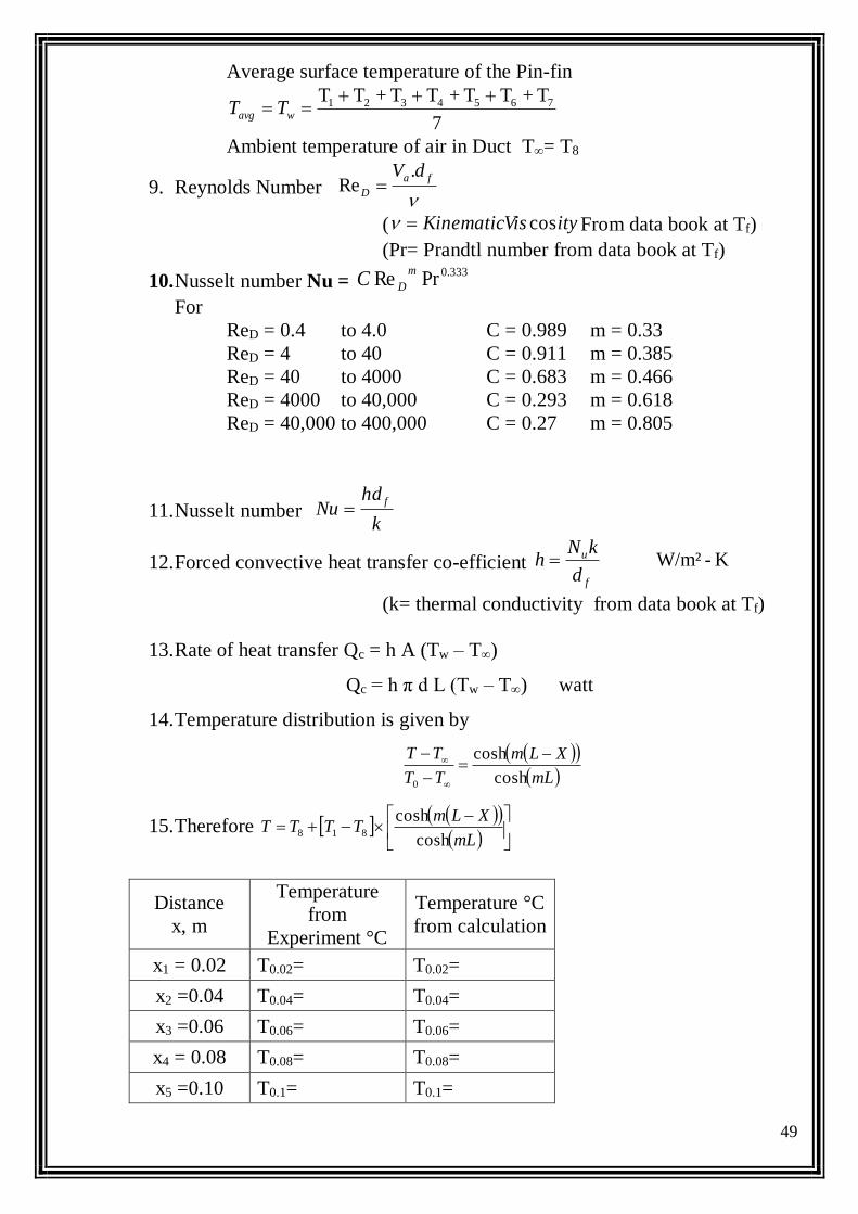
15. Therefore

mL

XLmTTTT

cosh

cosh818

Distance

x, m

Temperature

from

Experiment °C

Temperature °C

from calculation

x1 = 0.02 T0.02= T0.02=

x2 =0.04 T0.04= T0.04=

x3 =0.06 T0.06= T0.06=

x4 = 0.08 T0.08= T0.08=

x5 =0.10 T0.1= T0.1=

50

16. Efficiency of fin

mL

mLf

tanh

Where L= Length of the Fin= 145mm

Ak

hPm

brass

h= Convective heat transfer coefficient w/m2-K

P= Perimeter of the Fin (πdf)

A= Cross-sectional area of the Fin 2

4fdA

kbrass= Thermal conductivity of brass =110.7 W/m-K

17. Effectiveness of fin mLhA

Pktanh

GRAFF: surface temperature of Pin-Fin Vs Distance (location of thermocouples on Pin-Fin)

PRECAUTIONS:

3. Never switch on main power supply before ensuring that all on/off switches

given on the panel are at off position

4. Never run the apparatus if power supply is less than 180 or above 200 volts.

RESULT:

The temperature distribution of a pin – fin for forced convection

efficiency and effectiveness has been determined.

x6 =0.12 T0.12= T0.12=

x7 =0.14 T0.14= T0.14=

51

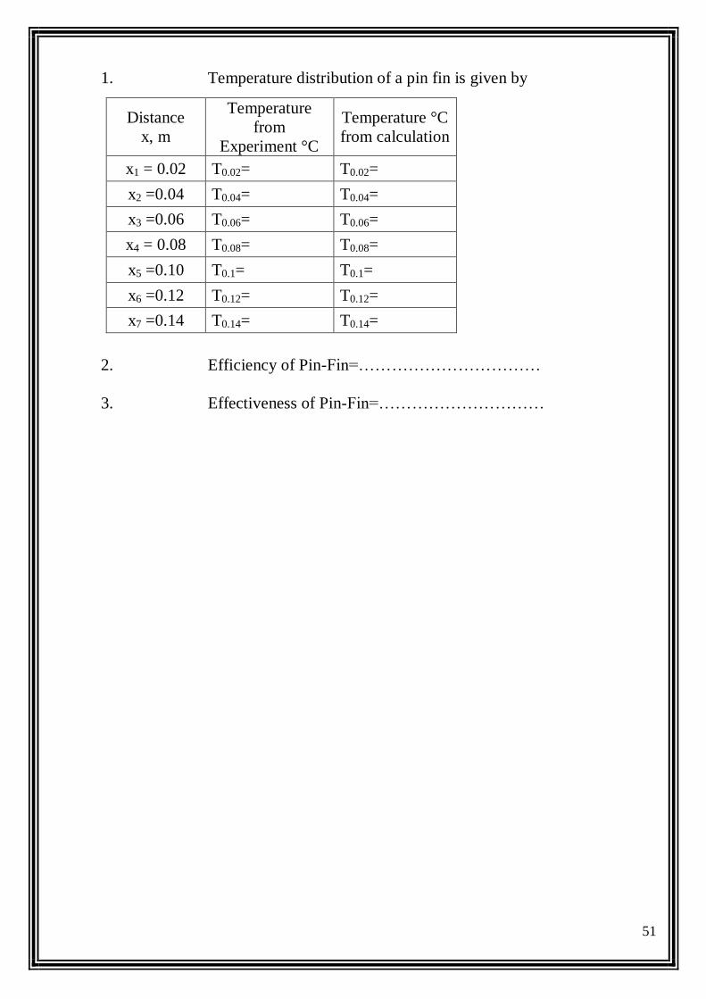
1. Temperature distribution of a pin fin is given by

2. Efficiency of Pin-Fin=……………………………

3. Effectiveness of Pin-Fin=…………………………

Distance

x, m

Temperature

from

Experiment °C

Temperature °C

from calculation

x1 = 0.02 T0.02= T0.02=

x2 =0.04 T0.04= T0.04=

x3 =0.06 T0.06= T0.06=

x4 = 0.08 T0.08= T0.08=

x5 =0.10 T0.1= T0.1=

x6 =0.12 T0.12= T0.12=

x7 =0.14 T0.14= T0.14=

52

Date:

Exp No:

STEFAN BOLTZMANN APPARATUS

AIM:

To determine the value of Stefan Boltzmann constant for radiation heat

transfer.

APPARATUS:

Hemisphere, Heater, Temperature indicator, Stopwatch.

THEORY:

Stefan Boltzmann law states that the total emissive power of a perfect black

body is proportional to fourth power of the absolute temperature of black body

surface.

Eb = σT4

Where

σ = Stefan Boltzmann constant = 5.6697 x 10-8 W/(m² K4)

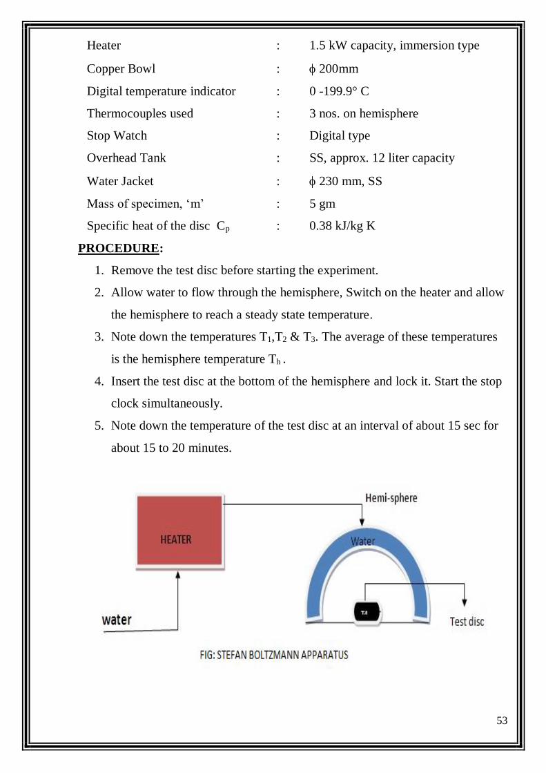
DESCRIPTION:

The apparatus consists of a flanged copper hemisphere fixed on a flat non-

conducting plate. A test disc made of copper is fixed to the plate. Thus the test disc

is completely enclosed by the hemisphere. The outer surface of the hemisphere is

enclosed in a vertical water jacket used to heat the hemisphere to a suitable

constant temperature. Three Cr-Al thermocouples are attached at three strategic

places on the surface of the hemisphere to obtain the temperatures. The disc is

mounted on an ebonite rod which is fitted in a hole drilled at the center of the base

plate. Another Cr-Al thermocouple is fixed to the disc to record its temperature.

Fill the water in the SS water container with immersion heater kept on top of the

panel.

SPECIFICATIONS:

Specimen material : Copper

Size of the disc : 20mm x 0.5mm thickness

Base Plate : 250mm x 12mm thickness (hylam)

53

Heater : 1.5 kW capacity, immersion type

Copper Bowl : 200mm

Digital temperature indicator : 0 -199.9° C

Thermocouples used : 3 nos. on hemisphere

Stop Watch : Digital type

Overhead Tank : SS, approx. 12 liter capacity

Water Jacket : 230 mm, SS

Mass of specimen, ‘m’ : 5 gm

Specific heat of the disc Cp : 0.38 kJ/kg K

PROCEDURE:

1. Remove the test disc before starting the experiment.

2. Allow water to flow through the hemisphere, Switch on the heater and allow

the hemisphere to reach a steady state temperature.

3. Note down the temperatures T1,T2 & T3. The average of these temperatures

is the hemisphere temperature Th .

4. Insert the test disc at the bottom of the hemisphere and lock it. Start the stop

clock simultaneously.

5. Note down the temperature of the test disc at an interval of about 15 sec for

about 15 to 20 minutes.

54

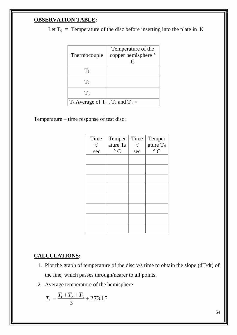
OBSERVATION TABLE:

Let Td = Temperature of the disc before inserting into the plate in K

Thermocouple

Temperature of the

copper hemisphere °

C

T1 T2 T3

Th Average of T1 , T2 and T3 =

Temperature – time response of test disc:

Time

‘t’

sec

Temper

ature Td

° C

Time

‘t’

sec

Temper

ature Td

° C

CALCULATIONS:

1. Plot the graph of temperature of the disc v/s time to obtain the slope (dT/dt) of

the line, which passes through/nearer to all points.

2. Average temperature of the hemisphere

15.2733

321

TTT

Th

55

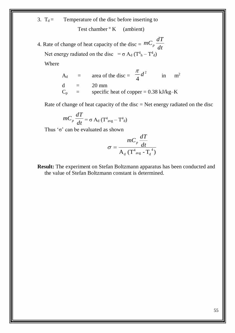
3. Td = Temperature of the disc before inserting to

Test chamber º K (ambient)

4. Rate of change of heat capacity of the disc = dt

dTmCp

Net energy radiated on the disc = σ Ad (T4

h – T4d)

Where

Ad = area of the disc = 2

4d

in m2

d = 20 mm

Cp = specific heat of copper = 0.38 kJ/kg–K

Rate of change of heat capacity of the disc = Net energy radiated on the disc

dt

dTmCp = σ Ad (T

4avg – T4

d)

Thus ‘σ’ can be evaluated as shown

)T - (T A

4

davg4

d

dt

dTmC p

Result: The experiment on Stefan Boltzmann apparatus has been conducted and

the value of Stefan Boltzmann constant is determined.

56

Date:

Exp No:

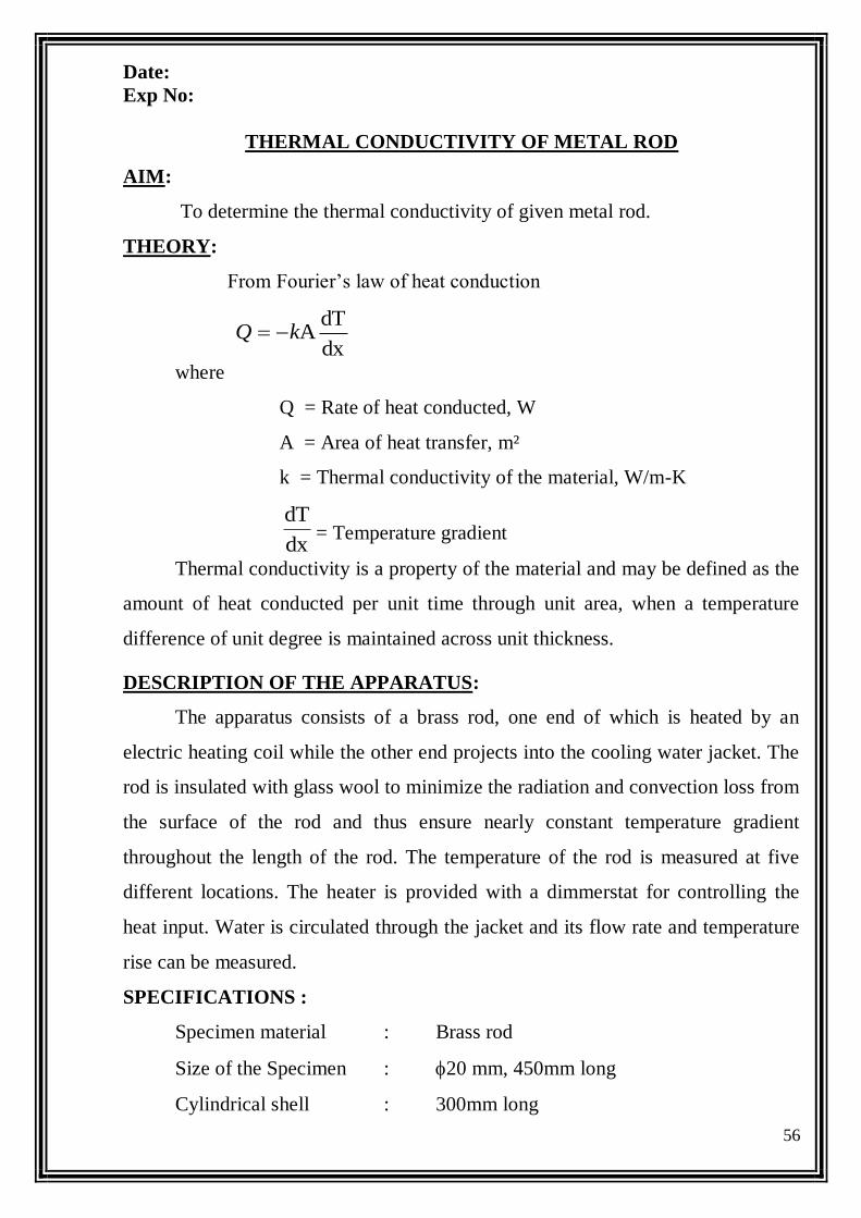
THERMAL CONDUCTIVITY OF METAL ROD

AIM:

To determine the thermal conductivity of given metal rod.

THEORY:

From Fourier’s law of heat conduction

dx

dTAkQ

where

Q = Rate of heat conducted, W

A = Area of heat transfer, m²

k = Thermal conductivity of the material, W/m-K

dx

dT= Temperature gradient

Thermal conductivity is a property of the material and may be defined as the

amount of heat conducted per unit time through unit area, when a temperature

difference of unit degree is maintained across unit thickness.

DESCRIPTION OF THE APPARATUS:

The apparatus consists of a brass rod, one end of which is heated by an

electric heating coil while the other end projects into the cooling water jacket. The

rod is insulated with glass wool to minimize the radiation and convection loss from

the surface of the rod and thus ensure nearly constant temperature gradient

throughout the length of the rod. The temperature of the rod is measured at five

different locations. The heater is provided with a dimmerstat for controlling the

heat input. Water is circulated through the jacket and its flow rate and temperature

rise can be measured.

SPECIFICATIONS :

Specimen material : Brass rod

Size of the Specimen : 20 mm, 450mm long

Cylindrical shell : 300mm long

57

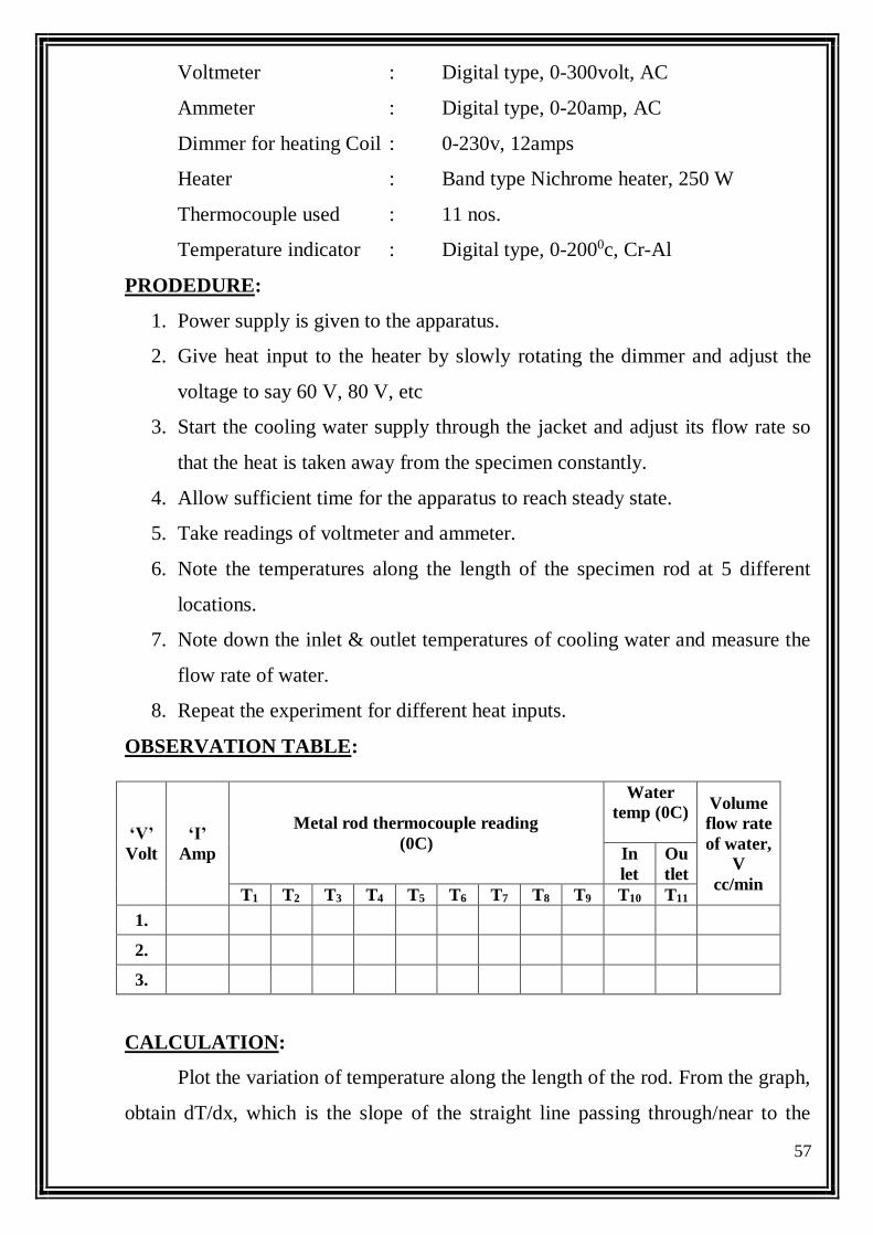
Voltmeter : Digital type, 0-300volt, AC

Ammeter : Digital type, 0-20amp, AC

Dimmer for heating Coil : 0-230v, 12amps

Heater : Band type Nichrome heater, 250 W

Thermocouple used : 11 nos.

Temperature indicator : Digital type, 0-2000c, Cr-Al

PRODEDURE:

1. Power supply is given to the apparatus.

2. Give heat input to the heater by slowly rotating the dimmer and adjust the

voltage to say 60 V, 80 V, etc

3. Start the cooling water supply through the jacket and adjust its flow rate so

that the heat is taken away from the specimen constantly.

4. Allow sufficient time for the apparatus to reach steady state.

5. Take readings of voltmeter and ammeter.

6. Note the temperatures along the length of the specimen rod at 5 different

locations.

7. Note down the inlet & outlet temperatures of cooling water and measure the

flow rate of water.

8. Repeat the experiment for different heat inputs.

OBSERVATION TABLE:

CALCULATION:

Plot the variation of temperature along the length of the rod. From the graph,

obtain dT/dx, which is the slope of the straight line passing through/near to the

‘V’

Volt

‘I’

Amp

Metal rod thermocouple reading

(0C)

Water

temp (0C)

Volume

flow rate

of water,

V

cc/min

In

let

Ou

tlet

T1 T2 T3 T4 T5 T6 T7 T8 T9 T10 T11

1.

2.

3.

58

points in the graph. Assuming no heat loss, heat conducted through the rod = heat

carried away by the cooling water

1011dx

dTA TTCmk pf

Where, ‘k’ = thermal conductivity of metal rod, (W/m-K)

‘A’ = Cross sectional area of metal rod = πd²/4 (m²)

‘d’ = diameter of the specimen = 20 mm

‘Cp’ = Specific heat of water = 4.187 kJ/kg-K

Thus, the thermal conductivity ‘k’ of metal rod can be evaluated.

dx

dTA

1011 TTCmk

pf

GRAPH:

PRECAUTIONS:




RESULT:

The thermal conductivity of given metal rod has been determined.

Plot the graph Distance vs Temperature.

59

Date:

Exp No:

TWO PHASE HEAT TRANSFER APPARATUS

AIM:

To Study the Two Phase heat transfer phenomena for pool boiling of water.

THEORY:

Two phase heat transfer is a mode of heat transfer that occurs because of

vaporization. Vaporization is a process in which a substance is changed from liquid

to vapour state. Pool boiling takes place when a liquid is confined in a container

and a heater is submerged in the liquid.

BOILING REGIMES:

Consider that the rate of heat convection, heat transfer for the system is

expressed analytically by the Newton’s equation:

Q= h A ∆t-------- (1)

Where ‘h’ is the heat transfer coefficient, ‘A’ is area involved in heat

transfer and ∆t is some well defined temperature difference, The difference

between the temperature of the solid and the mean temperature of fluid at the limit

of the thermal boundary layer, An analogous equation issued for boiling heat

transfer.

A

Q.

= h ∆t-------- (2)

Where q’’ = q/A is called the heat flux and h the boiling heat transfer coefficient.tw

is the wall superheat or surface temperature. ∆t which is defined as difference

between the wall temperature of the heating surface and saturation temperature of

the liquid ts.

∆t= tw - ts -------------------- (3)

DESCRIPTION:

The main apparatus is fitted on MS tube frame consisting of a glass column

with a sample holding sump with a heater and drain valve at the bottom and a

60

helical condenser, with water inlet and outlet , a safety valve, and a feed valve at

the top and the unit is made leak proof with necessary flange connections.

The panel consists of voltmeter, ammeter, temperature indicator, dimmer,

thermocouple selector switch, toggle switch for pump, Rotameter. Below the table

a water sump fitted with pump is provided to circulate water through the helical

condenser coil, a bypass is also provided for the pump to safety guard the motor.

PROCEDURE:

1. Fill the sample holding sump with sample of about 250ml (appox) through

the feed valve provided on top of the column (ensure that the drain valve

provided at the bottom is closed) and close the feed valve after filling.

2. Ensure that the dimmer is ‘OFF’, thermocouple selector switch at any

position; the pump toggle switch is ‘OFF’.

3. Connect the three pin plug top to 230V, 50, 5 amps power supply socket

with proper earthling.

4. Fill water into the water sump provided below the table.

5. Open the bypass valve fully and also open the Rota meter valve.

6. Switch ‘ON’ the toggle switch for pump.

7. Observe water falling into the sump through bypass.

8. Slowly turn the bypass valve clock wise and observe the Rota meter float to

rise.

9. Set the water flow rate to any desired value indicated by the Rota meter.

10. Turn the dimmer clockwise and set the power input to the heater at the

minimum possible limit by observing the volt and ammeter (V x I=W) and

note the readings.

11. Note down the temperatures indicated by the temperature indicator by

turning the thermocouple selector switch clockwise step by step.

12. Bring back the thermocouple selector switch to any position.

61

13. Increase the power input to the heater by lowest possible value (increasing

of the power output to the heater should be made at a known interval time)

record the readings.

14. Record the temperatures indicated at each step T1 & T2.

15. Repeat increasing of power input to the heater and recording the

temperatures at an interval of time till the sample start boiling.

16. Tabulate all the readings and calculate.

17. After the experiment is over turn the dimmer anticlockwise to ‘ZERO’

position. Also bring back thermocouple selector switch to any position allow

the water circulation pump to work for some time, switch ‘OFF’ the pump

switch, drain the sample by opening the drain valve and close the drain valve

after draining.

EXPERIMENT APPARATUS:

The apparatus consists of a vertical glass cylinder, in which liquid WATER

boils. Inside the glass cylinder a copper-condensing coil is placed. At the bottom of

the glass column a copper bowl heater electrically by a heating coil. Cooling water

is circulated through the condenser by means of pump. Water flow control is

achieved through valve V1 Rota meter gives an indication of water flow rate.

Thermocouple T1, measures the temperature in the heating pad a T2

measures the liquid and temperature. Voltmeter ‘V’ and Ammeter ‘A’ measure the

heater input voltage and current respectively.

THERMOCOUPLE DETAILS:

T1=Heater temperature

T2=Liquid temperature

T3=Vapour temperature

T4=Water inlet temperature to coil

T5=Water outlet temperature from coil

62

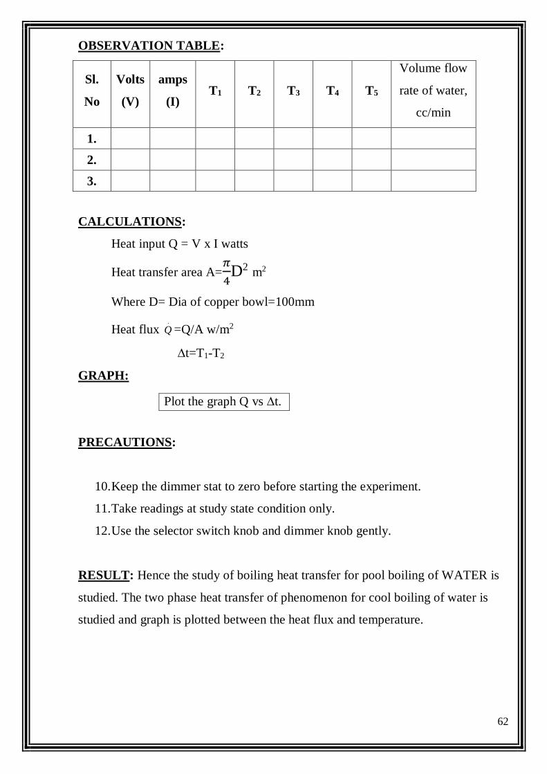
OBSERVATION TABLE:

Sl.

No

Volts

(V)

amps

(I) T1 T2 T3 T4 T5

Volume flow

rate of water,

cc/min

1.

2.

3.

CALCULATIONS:

Heat input Q = V x I watts

Heat transfer area A=𝜋

4D2 m2

Where D= Dia of copper bowl=100mm

Heat flux .

Q =Q/A w/m2

∆t=T1-T2

GRAPH:

PRECAUTIONS:




RESULT: Hence the study of boiling heat transfer for pool boiling of WATER is

studied. The two phase heat transfer of phenomenon for cool boiling of water is

studied and graph is plotted between the heat flux and temperature.

Plot the graph Q vs ∆t.

63

Date:

Exp No:

UNSTEADY STATE HEAT TRANSFER

AIM:

To obtain the specimen temperature at any interval of time by theoretical

methods and observe the heating and cooling curves of unsteady state.

INTRODUCTION:

Unsteady state designates a phenomenon which is time dependent.

Conduction of heat in unsteady state refers to transient conditions where in, heat

flow and temperature distribution at any point of system varies with time.

Transient conditions occur in heating or cooling of metal billets, cooling of IC

engine cylinder, brick and vulcanization of rubber.

DESCRIPTION:

Unsteady state heat transfer equipment has oil check which is at top of oil

heater. Thermocouple No.1is located inside the specimen No.2 thermocouple

measures the atmospheric temperature. No.3 thermocouple measures the oil

temperature.

Digital temperature indicator indicates respective temperatures of

thermocouples as we select it by selector switch. Heater ON/OFF toggle switch

and buzzer ON/OFF toggle switch is provided on the control panel.

SPECIFICATIONS:

1. D.C Buzzer : 10-30 volt

2. Oil Heater : 1 kW

3. Digital temperature indicator : 1200C0

4. Thermocouple : Al-Cr type

5. Specimens material : Copper

6. Fuse : 4 Amps.

EXPERIMENTATION:

Obtain the specimen temperature at any interval of time by practical and by

theoretical methods and observe the heating and cooling curves of unsteady state.

64

PROCEDURE:

1. Put ON the mains switch.

2. Fill the oil jar up to

th

4

3of its height.

3. Insert the thermocouple in jar having tag No.3.

4. Keep thermocouple No.2 near to the specimen inside the transparent

chamber.

5. Start the oil heater by putting heater’s toggle switch in downward direction.

6. Keep selector switch No.3 and observe oil temperature.

7. When the oil temperature reaches up to 950C insert specimen in oil jar. At

the same time note down the specimen temperature and start the stop watch.

8. Note down the specimen reading for every 30 sec. Check the oil temperature

by selecting No.3 on selector switch.

9. Take the readings of specimen temperature till it comes nearly too hot oil

temperature.

10. Now put the specimen inside the rectangular chamber. At the same timed

put OFF the heater.

11. Take the atmospheric temperature by selecting No.2 and specimen

temperature. Note the specimen temperature reading till it comes closer to

atmospheric temperature.

12. Put OFF the main switch.

OBSERVATIONS:

1. Specimen material : Copper

2. Thermal conductivity of copper, k=386 W/m0k.

3. Coefficient of thermal expansion a=17.7x10-6/0C

4. Specimen diameter, d=30mm

5. Specimen lengh, l=30mm

65

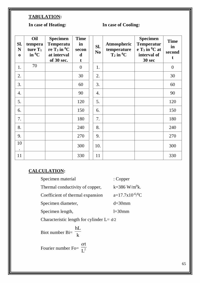
TABULATION:

In case of Heating: In case of Cooling:

Sl.

N

o

Oil

tempera

ture T1

in 0C

Specimen

Temperatu

re T3 in 0C

at interval

of 30 sec.

Time

in

secon

d

t

Sl.

No

Atmospheric

temperature

T2 in 0C

Specimen

Temperatur

e T3 in 0C at

interval of

30 sec

Time

in

second

t

1. 70 0 1. 0

2. 30 2. 30

3. 60 3. 60

4. 90 4. 90

5. 120 5. 120

6. 150 6. 150

7. 180 7. 180

8. 240 8. 240

9. 270 9. 270

10

.

300 10.

300

11 330 11 330

CALCULATION:

Specimen material : Copper

Thermal conductivity of copper, k=386 W/m0k.

Coefficient of thermal expansion a=17.7x10-6/0C

Specimen diameter, d=30mm

Specimen length, l=30mm

Characteristic length for cylinder L= d/2

Biot number Bi= k

hL

Fourier number Fo= 2L

t

66

Mean temperature = 2

TT minmax T

In case of cooling

Tmax=specimen temperature just after the hot oil both

Tmin= atmosperic temperature

In case of heating

Tmax=hot oil temperature

Tmin= specimen temperature before inserting into oil both

FoXBieT

.....

0 -T

T-T

Where

T= temperature of the specimen at time interval of ‘t’ sec

Ta= atmospheric temperature in 0C

Ts=specimen temperature

In case of cooling

Ta= atmospheric temperature

Ts= specimen temperature

In case of heating

Ta= Specimen temperature

Ts= hot oil temperature

Obtain the temperature at any desired interval of the time

Plot the graph of temperature difference V/S time for heating and cooling

PRECAUTIONS:


2. Operate the stop watch carefully.


RESULT:

The specimen temperature at an interval of time by practical and by

theoretical methods and observe the heating and cooling curves of unsteady state is

observed.

Documents

HEAT TRANSFER LAB OBSERVATON - SVCET · 1 sri venkateswara college of engineering and technology (autonomous) r. v. s. nagar, chittoor-517127 department of mechanical engineering