Embed Size (px)
Citation preview

Heat transfer in a pipe under conditions of transient turbulent ¯ow
J.D. Jackson a,*, O. B�uy�ukalaca b, S. He a
a School of Engineering, University of Manchester, Manchester, UKb Department of Mechanical Engineering, University of Cßukurova, Cßukurova, Turkey
Received 10 April 1998; accepted 21 October 1998
Abstract
This paper is concerned with the response of ¯uid temperature within a heated pipe to imposed excursions of ¯ow rate. Ex-
periments are reported in which measurements of wall temperature and local ¯uid temperature were made with fully developed
turbulent ¯ow of water in a uniformly heated tube during and after ramp-up excursions of ¯ow rate between steady initial and ®nal
values. The ¯uid temperature measurements were made using a traversable temperature probe incorporating a thermocouple ca-
pable of responding to turbulent ¯uctuations of temperature. Local values of mean temperature and RMS temperature ¯uctuation
were obtained by ensemble averaging the results from many tests in which the same ¯ow excursion was applied in a very repeatable
manner with ®xed values of inlet ¯uid temperature and heat ¯ux. Further measurements were made under conditions of steady ¯ow
rate at a number of values over the range covered in the transient ¯ow experiments. The results obtained in the experiments with
transient ¯ow show that there is a signi®cant delay in the variation of ensemble-averaged wall temperature and striking pertur-
bations in the variations of RMS ¯uctuation of wall temperature and local ¯uid temperature. These stem from the delayed response
of turbulence to the imposed excursions of ¯ow rate. They provide independent con®rmation of ideas concerning the modelling of
time scales for the production and di�usion of turbulence in pipe ¯ow which were developed by the present authors in the course of
earlier work. Ensemble-averaged local ¯uid temperature also varies in an unusual manner. Instead of falling monotonically with
increase of ¯ow rate, as might be expected, it starts to rise at some stage, reaches a peak value and then falls again. The release of
heat stored in the pipe wall contributes to this behaviour. Computational simulations of the present experiments were performed
using a spatially fully developed formulation of the equations for unsteady turbulent ¯ow and heat transfer in a boundary layer
utilising turbulence models of low Reynolds number, k±e type. Comparisons between predicted and measured variations of tem-
perature are presented in the paper. These show that the predictions di�er signi®cantly from model to model and that detailed
agreement with experiment is not obtained using any of the models. However, certain interesting features of the observed tem-
perature variations, such as a delay in the response of outer wall temperature and perturbations in local ¯uid temperature, are
present in the computed results. Ó 1999 Elsevier Science Inc. All rights reserved.
Keywords: Heat transfer; Flow rate excursions; Transient response; Turbulence models
1. Introduction
Heat transfer under conditions of transient turbulent ¯owin pipes is encountered in a variety of engineering applications.It is common practice in such applications to use a pseudo-steady state approach for the purpose of modelling systembehaviour. Energy conservation is applied on a one-dimen-sional basis using local values of wall temperature and ¯uidtemperature. Heat transfer is related to the di�erence betweenwall and ¯uid temperature using standard empirical equationswhich were developed for steady conditions. This approachfails to take account of in¯uences which the transient nature of
International Journal of Heat and Fluid Flow 20 (1999) 115±127
Notation
d pipe inside diameter (mm)r pipe inside radius (mm)t time (s)áT ñ ensemble averaged temperature (°C)T 0 root mean square temperature ¯uctuation (°C)Us friction velocity (m/s)Um mean velocity (m/s)y distance from the wall (mm)
Greekm kinematic viscosity (m2/s)s wall shear stress (N/m2)
Subscriptsf ¯uidw wall
* Corresponding author. E-mail: [email protected].
0142-727X/99/$ ± see front matter Ó 1999 Elsevier Science Inc. All rights reserved.
PII: S 0 1 4 2 - 7 2 7 X ( 9 8 ) 1 0 0 5 6 - 5
the ¯ow might have on turbulence and the di�usion of heat. Itslimitations were highlighted by results from the laser Doppleraneomometry study of turbulent ¯ow in a pipe during ramp-type excursions by He (1992). This showed that under suchconditions the turbulence di�ers signi®cantly from that insteady ¯ow. Time scales for the response of turbulence pro-duction and for the di�usion of turbulence from the near-wallregion of the ¯ow into the core ¯ow were established in thatstudy (see Jackson and He (1993)). Computational simulationsof the experiments using a variety of turbulence models weresubsequently reported (see Jackson and He (1995)).
A number of investigations of non-periodic transient ¯owshave been reported in the literature. Kataoka et al. (1975)examined the start-up response to a step input of ¯ow rate in apipe. Maruyama et al. (1976) studied turbulence structure intransient turbulent pipe ¯ow following a sudden change of¯ow rate. Transition from laminar ¯ow to turbulent ¯ow in apipe under conditions of transient ¯ow was examined byKurukawa and Morikawa (1986) and delayed transition inpipe ¯ow with constant acceleration starting from rest wasinvestigated by Lefebvre (1987). The e�ects of abrupt free-stream velocity changes on turbulent boundary layers wereinvestigated by Brereton et al. (1985).
Stimulated by the results of the investigation of He (1992),experiments were undertaken to study the response of thetemperature ®eld in a heated pipe to ramp-type excursions of¯ow rate. Experimental work by BuÈyuÈkalaca (1993) using apipe of similar dimensions was followed by computationalstudies (Jackson et al. (1994)). Previously, the problem oftransient turbulent ¯ow in heated pipes had received relativelylittle detailed attention. Koshkin et al. (1970) reported mea-surements made following step changes of electrical powerinput and with various types of ¯ow transient. Dreitser (1979)analysed experimental data for power and ¯ow transients inpipes to establish some limits for the applicability of quasi-stationary relations for calculating heat transfer. Later, Kali-nin and Dreitser (1985) proposed correlation equations forcalculating heat transfer coe�cient under the conditions ofimposed ¯ow transients. More recently, Gibson and Diakou-makos (1993) reported an experimental study of the ¯ow and
thermal ®elds in an oscillating turbulent boundary layer on aheated wall. This yielded values of time-averaged mean andturbulent velocity, time-averaged mean temperature and tur-bulent heat ¯ux.
In the present paper, the experimental results from the in-vestigation of BuÈyuÈkalaca (1993) are given detailed consider-ation and are compared with computational simulations.
2. Experimental arrangement
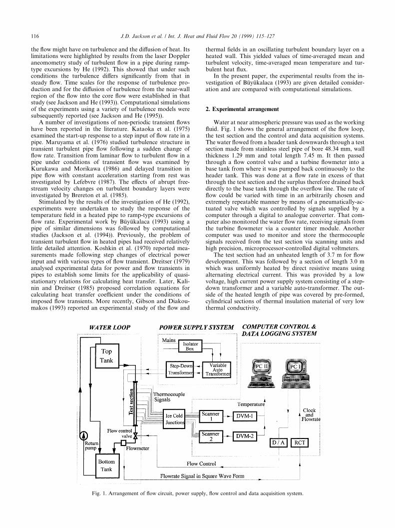
Water at near atmospheric pressure was used as the working¯uid. Fig. 1 shows the general arrangement of the ¯ow loop,the test section and the control and data acquisition systems.The water ¯owed from a header tank downwards through a testsection made from stainless steel pipe of bore 48.34 mm, wallthickness 1.29 mm and total length 7.45 m. It then passedthrough a ¯ow control valve and a turbine ¯owmeter into abase tank from where it was pumped back continuously to theheader tank. This was done at a ¯ow rate in excess of thatthrough the test section and the surplus therefore drained backdirectly to the base tank through the over¯ow line. The rate of¯ow could be varied with time in an arbitrarily chosen andextremely repeatable manner by means of a pneumatically-ac-tuated valve which was controlled by signals supplied by acomputer through a digital to analogue converter. That com-puter also monitored the water ¯ow rate, receiving signals fromthe turbine ¯owmeter via a counter timer module. Anothercomputer was used to monitor and store the thermocouplesignals received from the test section via scanning units andhigh precision, microprocessor-controlled digital voltmeters.
The test section had an unheated length of 3.7 m for ¯owdevelopment. This was followed by a section of length 3.0 mwhich was uniformly heated by direct resistive means usingalternating electrical current. This was provided by a lowvoltage, high current power supply system consisting of a step-down transformer and a variable auto-transformer. The out-side of the heated length of pipe was covered by pre-formed,cylindrical sections of thermal insulation material of very lowthermal conductivity.
Fig. 1. Arrangement of ¯ow circuit, power supply, ¯ow control and data acquisition system.
116 J.D. Jackson et al. / Int. J. Heat and Fluid Flow 20 (1999) 115±127
The temperature of the heated section of the stainless steel pipewas measured at seventeen axial locations along its length bychromel alumel thermocouples welded to the outside surface. Thewater temperature was measured at the test section inlet andoutlet by means of ®xed thermocouple probes mounted within the¯ow. Near the downstream end of the test section, 54.3 diametersfrom the start of heating and 131 diameters from entry to the testsection, local measurements of ¯uid temperature were made usinga traversable temperature probe incorporating a thermocouplecapable of responding to the turbulent ¯uctuations of tempera-ture in the water. This axial location was chosen with a view toensuring that fully developed hydrodynamic and thermal condi-tions were achieved there at the commencement of an imposedexcursion of ¯ow rate. It was su�ciently upstream of the outlet ofthe test section to be completely una�ected by end e�ects.
The electrical power input to the test section was main-tained at the same value in each of the experiments with thecurrent and voltage being recorded automatically by the dataacquisition system. Because the ¯ow circuit formed a closedloop, the heat supplied to the water had to be removed con-tinuously during the tests in order to keep its temperatureconstant at inlet to the test section. To do this, water waswithdrawn steadily from the base tank, pumped through acooling coil in a chilled bath and returned to the base tank.
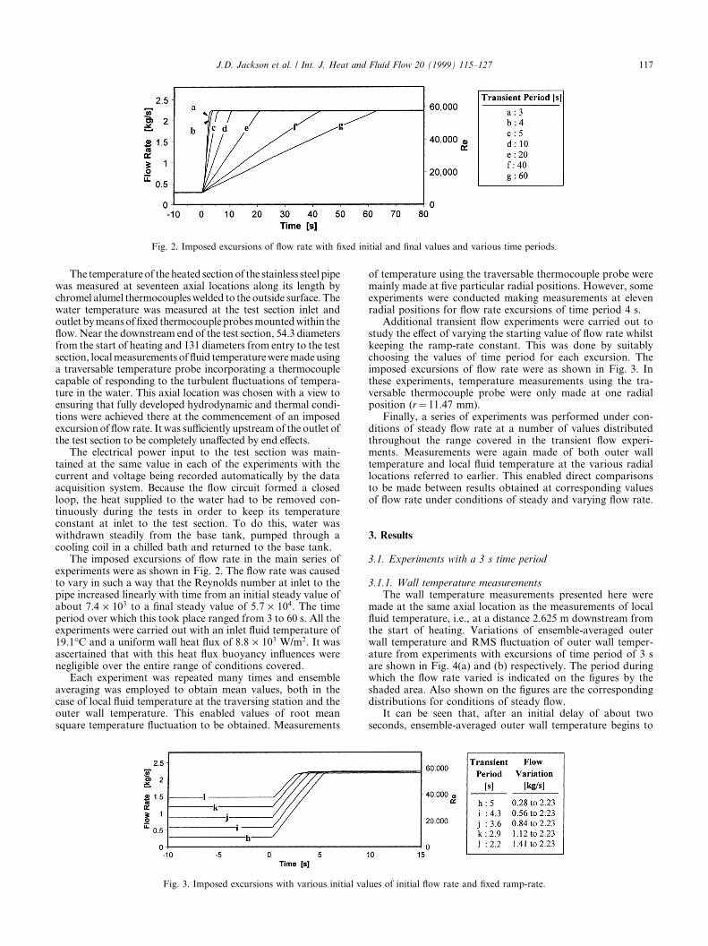
The imposed excursions of ¯ow rate in the main series ofexperiments were as shown in Fig. 2. The ¯ow rate was causedto vary in such a way that the Reynolds number at inlet to thepipe increased linearly with time from an initial steady value ofabout 7.4 ´ 103 to a ®nal steady value of 5.7 ´ 104. The timeperiod over which this took place ranged from 3 to 60 s. All theexperiments were carried out with an inlet ¯uid temperature of19.1°C and a uniform wall heat ¯ux of 8.8 ´ 103 W/m2. It wasascertained that with this heat ¯ux buoyancy in¯uences werenegligible over the entire range of conditions covered.
Each experiment was repeated many times and ensembleaveraging was employed to obtain mean values, both in thecase of local ¯uid temperature at the traversing station and theouter wall temperature. This enabled values of root meansquare temperature ¯uctuation to be obtained. Measurements
of temperature using the traversable thermocouple probe weremainly made at ®ve particular radial positions. However, someexperiments were conducted making measurements at elevenradial positions for ¯ow rate excursions of time period 4 s.
Additional transient ¯ow experiments were carried out tostudy the e�ect of varying the starting value of ¯ow rate whilstkeeping the ramp-rate constant. This was done by suitablychoosing the values of time period for each excursion. Theimposed excursions of ¯ow rate were as shown in Fig. 3. Inthese experiments, temperature measurements using the tra-versable thermocouple probe were only made at one radialposition (r� 11.47 mm).
Finally, a series of experiments was performed under con-ditions of steady ¯ow rate at a number of values distributedthroughout the range covered in the transient ¯ow experi-ments. Measurements were again made of both outer walltemperature and local ¯uid temperature at the various radiallocations referred to earlier. This enabled direct comparisonsto be made between results obtained at corresponding valuesof ¯ow rate under conditions of steady and varying ¯ow rate.
3. Results
3.1. Experiments with a 3 s time period
3.1.1. Wall temperature measurementsThe wall temperature measurements presented here were
made at the same axial location as the measurements of local¯uid temperature, i.e., at a distance 2.625 m downstream fromthe start of heating. Variations of ensemble-averaged outerwall temperature and RMS ¯uctuation of outer wall temper-ature from experiments with excursions of time period of 3 sare shown in Fig. 4(a) and (b) respectively. The period duringwhich the ¯ow rate varied is indicated on the ®gures by theshaded area. Also shown on the ®gures are the correspondingdistributions for conditions of steady ¯ow.
It can be seen that, after an initial delay of about twoseconds, ensemble-averaged outer wall temperature begins to
Fig. 2. Imposed excursions of ¯ow rate with ®xed initial and ®nal values and various time periods.
Fig. 3. Imposed excursions with various initial values of initial ¯ow rate and ®xed ramp-rate.
J.D. Jackson et al. / Int. J. Heat and Fluid Flow 20 (1999) 115±127 117

decrease and then falls monotonically with time, decaying to anew steady value about 9 s after the ¯ow rate excursion hasended.
In contrast, the response of RMS ¯uctuation of outer walltemperature is non-monotonic and involves three stages.During the ®rst stage, it decreases in a smooth manner forabout two seconds. Then it increases sharply for a fraction of asecond, peaking at a value above the initial one. Finally, itdecays in an exponential manner, reaching a steady valueabout 7 s after the ¯ow transient has ended.
3.1.2. Measurements of local ¯uid temperatureVariations of ensemble-averaged ¯uid temperature and
RMS temperature ¯uctuation at ®ve radial locations
(r� 22.67, 21.63, 19.01, 11.47 mm and on the centre line) areshown in Fig. 5(a) and (b), respectively. Again, the corre-sponding distributions for conditions of steady ¯ow are alsopresented.
As can be seen, ensemble-averaged local ¯uid temperatureresponds to the imposed excursion of ¯ow rate within a frac-tion of a second at all the radial positions considered. Theseresponses also involve three stages. Firstly the temperaturedecreases, slowly at ®rst but at a rate which increases with timein a smooth manner. Then there is a perturbation during whichit either increases and then peaks before decreasing again, or,at the near wall and at the mid-radius positions, simply de-creases for a short period at a relatively slower rate withoutpeaking. Finally, it decays in an exponential manner to a
Fig. 5. Variation with time of ensemble averaged mean and RMS ¯uid temperature ¯uctuation for a ¯ow rate excursion of time period 3 s (solid line:
transient experiment, dashed line: steady-state experiment).
Fig. 4. Variation with time of ensemble averaged mean and RMS wall temperature ¯uctuation for a ¯ow rate excursion of time period 3 s (solid line:
transient experiment, dashed line: steady-state experiment).
118 J.D. Jackson et al. / Int. J. Heat and Fluid Flow 20 (1999) 115±127
steady value. Some e�ect of the excursion of ¯ow rate can stillbe seen, up to 7 s after the excursion has ended, at all the radialpositions where measurements were made.
The pattern of behaviour in the case of RMS ¯uctuation of¯uid temperature is similar to that of ensemble-averaged ¯uidtemperature in that the variation is in three stages and per-turbations are seen. However, there are some detailed di�er-ences. The perturbations occur earlier than in the case ofensemble-averaged local temperature. Examination of the re-sponses at di�erent radial positions reveals that the time fromthe beginning of the ¯ow rate excursion to that at which aperturbation occurs increases systematically with distancefrom the wall.
In both Figs. 4 and 5 big di�erences can be seen betweenthe temperature responses for transient ¯ow and the corre-sponding distributions for steady ¯ow. The transient ¯ow re-sults lie well above the latter throughout the period of theimposed ¯ow transient and also for several seconds afterwards.
3.2. Experiments with 5, 20 and 60 s time periods
As can be seen from Figs. 6±11, the time taken for thetemperature ®eld to reach its new steady state becomes pro-gressively longer with increase in the time period of the ¯owrate excursion from 5 to 20 to 60 s. However, the generalpattern of behaviour found in the experiments is similar to that
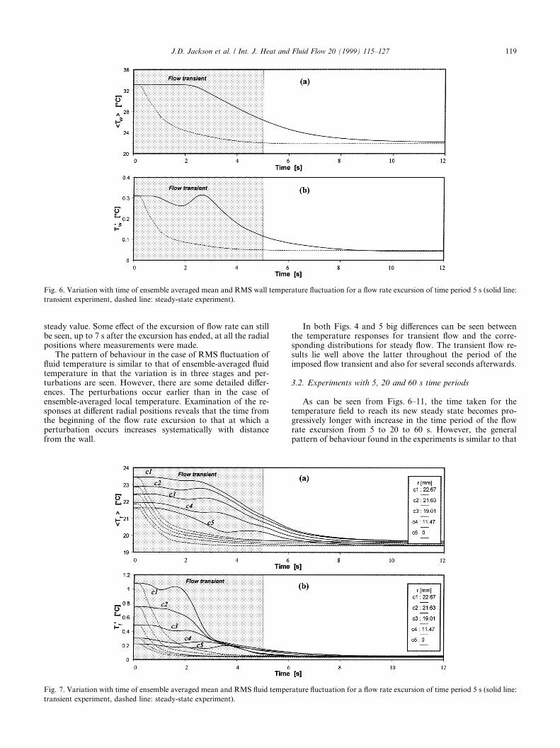
Fig. 6. Variation with time of ensemble averaged mean and RMS wall temperature ¯uctuation for a ¯ow rate excursion of time period 5 s (solid line:
transient experiment, dashed line: steady-state experiment).
Fig. 7. Variation with time of ensemble averaged mean and RMS ¯uid temperature ¯uctuation for a ¯ow rate excursion of time period 5 s (solid line:
transient experiment, dashed line: steady-state experiment).
J.D. Jackson et al. / Int. J. Heat and Fluid Flow 20 (1999) 115±127 119

for the excursion of 3 s time period. In each case there is adelay in the initial response of ensemble-averaged outer walltemperature, and a perturbation in the response of RMS¯uctuation of outer wall temperature. The time scales involvedare similar to those for the 3 s excursion but there is a tendencyfor them to increase slightly with increase of time period.
In the case of both ensemble-averaged local ¯uid temper-ature and RMS ¯uctuation of ¯uid temperature the responsesagain involve three stages and the time from the beginning ofthe ¯ow rate excursion to that at which a perturbation occursagain increases systematically with distance from the wall. Thetime at which a peak occurs on the perturbations increaseswith increase in the time period of the excursion.
The extent to which wall temperature and local ¯uid tem-perature continue to vary after the excursion has ended is smallfor a time period of 20 s and negligible for one of 60 s.However, even in these cases, di�erences between the transient¯ow responses and the distributions for conditions of steady¯ow are still clearly evident.
3.3. Experiments varying the starting ¯ow rate but keeping theramp-rate ®xed
In this series of experiments, as the starting ¯ow rate wasincreased the time period of the ¯ow rate excursion was ad-justed so as to keep the ramp-rate constant (see Fig. 3).
Fig. 8. Variation with time of ensemble averaged mean and RMS wall temperature ¯uctuation for a ¯ow rate excursion of time period 20 s (solid line:
transient experiment, dashed line: steady-state experiment).
Fig. 9. Variation with time of ensemble averaged mean and RMS ¯uid temperature ¯uctuation for a ¯ow rate excursion of time period 20 s (solid
line: transient experiment, dashed line: steady-state experiment).
120 J.D. Jackson et al. / Int. J. Heat and Fluid Flow 20 (1999) 115±127

Measurements of local ¯uid temperature were only made atone radial location, r� 11.47 mm.
Fig. 12(a) and (b), respectively, show the variation withtime of ensemble-averaged outer wall temperature and RMS¯uctuation of outer wall temperature for each of the values ofinitial ¯ow rate covered. From Fig. 12(a) it can be seen that aninitial delay in ensemble-averaged outer wall temperature isevident in all the cases but its value decreases markedly withincrease of initial ¯ow rate. Referring next to Fig. 12(b), per-turbations in RMS ¯uctuation of outer wall temperature canbe seen in all cases. However, they occur earlier with increaseof initial ¯ow rate and are of reduced magnitude.
Fig. 13(a) and (b), respectively, show the variation withtime of ensemble-averaged ¯uid temperature and RMS ¯uc-
tuation of ¯uid temperature at the radial location r� 11.47mm. It can be seen that perturbations are evident in both casesbut they become less pronounced with the increase of initial¯ow rate and eventually di�cult to discern.
4. Discussion
4.1. Factors which in¯uence the response of temperature toexcursions of ¯ow rate
In order to interpret the present results it is helpful to try toidentify the various ¯uid ¯ow and thermal phenomena whichmight a�ect the response of the temperature ®eld to imposed
Fig. 10. Variation with time of ensemble averaged mean and RMS wall temperature ¯uctuation for a ¯ow rate excursion of time period 60 s (solid
line: transient experiment, dashed line: steady-state experiment).
Fig. 11. Variation with time of ensemble averaged mean and RMS ¯uid temperature ¯uctuation for a ¯ow rate excursion of time period 60 s (solid
line: transient experiment, dashed line: steady-state experiment).
J.D. Jackson et al. / Int. J. Heat and Fluid Flow 20 (1999) 115±127 121

excursions of ¯ow rate in the case of turbulent ¯ow in a heatedpipe. One which is of particular importance in the presentstudy, is the response of turbulence. Jackson and He(1992, 1993) reported LDA measurements by He (1992) ofensemble-averaged mean velocity and turbulence duringtransient ¯ow in a unheated pipe where the pipe diameter,experimental conditions and imposed excursions of ¯ow ratewere similar to those in the present study. In the near-wallregion, the axial component of turbulence responded almostimmediately to the excursion of ¯ow rate but the radial andcircumferential components in that region exhibited a responsewhich was delayed by about 1 s. As a consequence, the re-sponses of turbulent shear stress and turbulent kinetic energywere also delayed. Further away from the wall all three com-ponents of turbulent velocity exhibited delays. These increasedin magnitude with distance from the wall, reaching values of
about 4 s at the centre of the pipe. In experiments where theinitial and ®nal ¯ow rates were kept constant as the time pe-riod of the excursion was varied, the delay at any given radialposition remained essentially unchanged. However, when theinitial ¯ow rate was increased, keeping the ramp-rate constant,the delays decreased.
In the case of a ramp-up excursion of ¯ow rate, the responseof turbulence begins with increased production of turbulence inthe ¯ow near to the wall. However, turbulent eddies are onlyproduced intermittently as local instabilities in the wall shear¯ow develop and lead to `bursts' of turbulence. Thus, during animposed excursion of ¯ow rate the turbulence ®eld respondsafter some delay, the magnitude of which is related to the tur-bulence bursting frequency. The time scale for such bursts isgiven by Cm/Us
2, in which Us is the friction velocity, m the ki-nematic viscosity of the ¯uid and C a constant of value 125
Fig. 13. Variation with time of ensemble averaged and RMS ¯uid temperature ¯uctuation.
Fig. 12. Variation with time of ensemble averaged and RMS wall temperature ¯uctuation.
122 J.D. Jackson et al. / Int. J. Heat and Fluid Flow 20 (1999) 115±127

(Blackwelder and Haritonidis, 1983). This expression wasfound to provide an estimate of the delay in the response ofturbulence in the near-wall region in good agreement with thatobserved in the experiments of He (1992), referred to earlier.
The response of turbulence in the near-wall region is fol-lowed by increased transmission of turbulent kinetic energytowards the centre of the pipe through the action of turbulentdi�usion. Thus, at any speci®ed location within the ¯ow, theresponse of turbulence exhibits a delay which is the sum of adelay in the response of turbulence production in the near-wallregion and one associated with the time needed for di�usion ofturbulence from the near-wall region to the location in ques-tion. The time scale for the latter process should depend uponthe distance y involved and the friction velocity Us. A satis-factory description of observed behaviour in the case of theexperiments of He (1992) was obtained by evaluating this usingthe ratio y/Us. In view of the fact that the hydrodynamicconditions in the present study are very similar to those in theinvestigation of He (1992), the turbulence ®eld should exhibit asimilar delayed response.
We next consider the thermal processes involved in thepresent study. The ¯uid temperature in a uniformly heatedpipe through which the ¯ow rate is increasing with time can becomputed from a simple energy balance, performed on a one-dimensional basis following the motion of the ¯uid. This ap-proach gives a volume weighted local mean value. Because theheating is uniform, the rise of temperature of the ¯uid as it¯ows through the tube is proportional to the time taken for itto travel from the start of heating to the location under con-sideration, i.e., the so called ``residence time''. In the case of aramp-up excursion of ¯ow rate, the residence time reduces asthe excursion proceeds and consequently ¯uid temperaturefalls. After an initial delay associated with the response of theturbulence ®eld, wall temperature also begins to fall. Energystored in the pipe wall is then released along with the energywhich is being steadily generated within it. Even in the case ofa pipe having a very thin wall, this additional rate of heat re-lease can in some circumstances be enough to modify the ¯uidtemperature by a signi®cant amount. The magnitude of thee�ect is directly related to the rate of change of wall temper-ature with time and this increases with reduction of the timeperiod of the imposed excursion.
4.2. Discussion of the present results
We now seek to relate the ideas presented in the previoussection to the present experiments, starting with those in whichthe imposed excursions of ¯ow rate had a time period of 3 s(Figs. 4 and 5). As remarked earlier, big di�erences are evi-dent, both during the period of the excursion of ¯ow rate andfor several seconds afterwards, between the temperature re-sponses for transient ¯ow and the corresponding distributionsof temperature for conditions of steady ¯ow. This is not sur-prising because the ¯uid residence time at the start of the ¯owrate excursion is about 16.5 s and this is large compared withthe time period of the excursion of ¯ow rate. Thus, even at theend of the excursion, the temperature of the ¯uid will onlyhave fallen by a relatively small amount. A particular featureof the transient ¯ow temperature responses is that they exhibitsigni®cant delays and striking perturbations. These stem fromthe delayed response of turbulence to the imposed excursionsof ¯ow rate.
4.2.1. Variation of wall temperatureWe begin by considering the initial delay of about 2 s in the
response of ensemble-averaged outer wall temperature which isevident in Fig. 4(a). For the conditions of the present experi-ments, the expression Cm/Us
2 yields a value of about 1.25 s for
the time scale involved in the delayed response of turbulenceproduction if the friction velocity at the start of the ¯ow rateexcursion is used in the calculation. Of course, it can be arguedthat because the ¯ow rate is increasing during the delay perioda somewhat higher value of Us might be more appropriate.However, it is not clear just how much higher it needs to be.Increasing Us would reduce the estimated delay.
Once additional turbulence production has occurred, sev-eral things follow as a consequence. A readjustment of tem-perature gradient through the action of molecular di�usionoccurs within a viscous sub-layer of reduced thickness. This isaccompanied by changes of temperature within the wall itselfas a result of unsteady conduction. Whilst these processes takeplace, turbulent energy is being transferred outwards acrossthe bu�er layer and the turbulent region through the action ofturbulent di�usion. As a result, the pipe wall and the ¯uid inthe outer region of the boundary layer become more e�ectively`thermally linked', so that heat can then be removed from thewall at an increased rate causing its temperature to fall.
The additional delay involved in the propagation of tem-perature disturbances through the ¯uid in the near-wall regioncannot be estimated precisely. However, it is possible to placean upper limit on its value by assuming that the layer of ¯uidinvolved is the viscous sub-layer as it was at the start of the¯ow rate excursion. An estimate of the additional delay wasmade on the above basis by BuÈyuÈkalaca (1993) using an ap-proximate solution of the equation for unsteady moleculardi�usion through such a layer. He obtained a value of 0.9 of asecond. The corresponding delay in the propagation of tem-perature disturbances through the pipe wall by unsteady con-duction was estimated to be 0.2 of a second, giving a combinedvalue of about 1.1 s. If we add this to the 1.25 s obtained earlierfor the delay in the response of turbulence production weobtain a total of 2.35 s as our estimate of the delay in the re-sponse of outer wall temperature. This is su�ciently close tothe observed delay of about 2 s to warrant the conclusion thatthe physical picture just presented of the processes involved issubstantially correct.
Turning next to RMS ¯uctuation of outer wall tempera-ture, we see from Fig. 4(b) that this responds almost imme-diately to the imposed excursion of ¯ow rate, falling slowly at®rst but at a rate which increases steadily. This is a conse-quence of the temperature of ¯uid in the near-wall regionfalling as a result of having experienced a reduced residencetime. The fall in RMS ¯uctuation of outer wall temperature isfollowed, just under 2 s into the excursion of ¯ow rate, by asudden increase for about half a second until a peak value isachieved 2.5 s into the excursion. The onset of this perturba-tion in RMS ¯uctuation of outer wall temperature can be as-sociated with the arrival of ¯uctuations of temperature at theoutside surface of the wall which have resulted from increased¯uctuations of temperature in the near-wall ¯uid following theresponse of turbulence there to the excursion of ¯ow rate.
It is of interest that even though the wall and the ¯uidadjacent to it both act as thermal ®lters, with the result thatsome of the applied temperature ¯uctuation is damped out, theincrease of temperature ¯uctuation in the near-wall region dueto the response of turbulence there is still easily detectable onthe outside of the wall.
The time from the beginning of the ¯ow rate excursion tothat at which a perturbation develops in outer wall RMStemperature ¯uctuation is just under 2 s, from which it can beinferred that the time actually taken for temperature distur-bances to be propagated across the viscous sub-layer andthrough the wall is about half that deduced earlier. If the es-timate of the initial delay in the response of ensemble-averagedouter wall temperature is revised taking account of this, veryclose agreement with observed behaviour is then obtained.
J.D. Jackson et al. / Int. J. Heat and Fluid Flow 20 (1999) 115±127 123
4.2.2. Variation of ¯uid temperatureWe next consider the responses of ensemble-averaged local
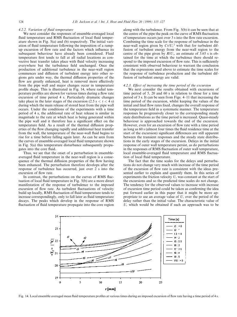
¯uid temperature and RMS ¯uctuation of local ¯uid temper-ature shown in Fig. 5(a) and (b) respectively. The initial vari-ation of ¯uid temperature following the imposition of a ramp-up excursion of ¯ow rate and the factors which in¯uence itssubsequent behaviour have already been considered. Fluidtemperature ®rst tends to fall at all radial locations as con-vective heat transfer takes place with ¯uid velocity increasingeverywhere but the turbulence ®eld unchanged. Once theproduction of additional turbulence in the near-wall regioncommences and di�usion of turbulent energy into other re-gions gets under way, the thermal di�usion properties of the¯ow are greatly enhanced, heat is removed more e�ectivelyfrom the pipe wall and major changes occur in temperaturepro®le shape. This is illustrated in Fig. 14, where radial tem-perature pro®les are shown for various times during a ¯ow rateexcursion of time period 4 s. Particularly dramatic changestake place in the later stages of the excursion (2.5 s < t < 4 s)during which the main release of stored heat from the pipe walloccurs. Under the conditions of the experiments with a timeperiod of 4 s, the additional rate of heat release is similar inmagnitude to the rate at which heat is being generated withinthe pipe wall and it therefore has a signi®cant e�ect on thetemperature ®eld. As a result of the thermal di�usion prop-erties of the ¯ow changing rapidly and additional heat transferfrom the wall, the temperature of the near-wall ¯uid begins torise for a time before falling again later. As can be seen fromthe curves of ensemble-averaged local ¯uid temperature shownin Fig. 5(a) this temperature disturbance subsequently propa-gates into the core ¯uid.
Thus, we see that the onset of a perturbation in ensemble-averaged ¯uid temperature in the near-wall region is a conse-quence of the thermal di�usion properties of the ¯ow havingbeen enhanced. The perturbation therefore develops after theresponse of turbulence has occurred, just over 2 s into theexcursion of ¯ow rate.
In contrast, the perturbations on the curves of RMS ¯uc-tuation of local ¯uid temperature in Fig. 5(b) are a more directmanifestation of the response of turbulence to the imposedexcursion of ¯ow rate. As turbulent ¯uctuations of velocitybuild up locally, RMS ¯uctuation of ¯uid temperature tends toincrease correspondingly, only to fall later as ¯uid temperaturedecays. The peaks which develop in the response of RMS¯uctuation of ¯uid temperature propagate into the core region
along with the turbulence. From Fig. 5(b) it can be seen that atthe centre of the pipe the peak on the curve of RMS ¯uctuationof temperature occurs just over 3 s into the ¯ow rate excursion.Combining the time scale for the response of turbulence in thenear-wall region given by Cm/Us
2 with that for turbulent dif-fusion of turbulent energy from the near-wall region to thecentre of the pipe given by R/Us, an estimate of 3.65 s is ob-tained for the time at which the turbulence there should re-spond to the imposed excursion of ¯ow rate. This is su�cientlyconsistent with observed behaviour to warrant the conclusionthat the expressions used above to estimate the time scales forthe response of turbulence production and the turbulent dif-fusion of turbulent energy are valid.
4.2.3. E�ect of increasing the time period of the excursionWe next consider the results obtained with excursions of
time period of 5, 20 and 60 s in relation to those for a timeperiod of 3 s. It can be seen from Figs. 4±11 that increasing thetime period of the excursion, whilst keeping the values of theinitial and ®nal ¯ow rates ®xed, changes the overall response ofthe temperature ®eld in a systematic manner. The temperatureresponses lie progressively closer to the corresponding steadystate distributions as the time period is increased. Quasi-steadybehaviour is approached towards the end of the excursion.However, even for an excursion of ¯ow rate with a time periodas long as 60 s (almost four times the ¯uid residence time at thestart of the excursion) signi®cant di�erences are still apparentbetween the transient responses and the steady state distribu-tions in the early stages of the excursion. Delays in the initialresponse of outer wall temperature persist, as do perturbationsin the responses of RMS ¯uctuation of outer wall temperature,local ensemble-averaged ¯uid temperature and RMS ¯uctua-tion of local ¯uid temperature.
The fact that the time scales for the delays and perturba-tions do not change very much with increase of the time periodof the excursion of ¯ow rate is consistent with the ideas pre-sented earlier to explain and quantify them. In this series ofexperiments the friction velocity Us was constant at the start ofthe excursions and so the predicted time scales do not change.The tendency for the observed values to increase with increaseof excursion time period could be taken as con®rming the ideaput forward earlier in this paper that it might be more ap-propriate to use an average value of Us over the period of thedelay rather than the initial value. The characteristic value ofUs which would be obtained if such an approach was to be
Fig. 14. Local ensemble averaged mean ¯uid temperature pro®les at various times during an imposed excursion of ¯ow rate having a time period of 4 s.
124 J.D. Jackson et al. / Int. J. Heat and Fluid Flow 20 (1999) 115±127

adopted would reduce. Thus, the time scales predicted for theresponse of turbulence production and the di�usion of tur-bulent energy would increase. However, it must be said thatthe observed increases of time scale are slight and the ideas justpresented to explain them are rather speculative.
4.2.4. E�ect of increasing the ¯ow rate at the start of theexcursion
Finally, we examine the results of the series of experimentsin which the ¯ow rate at the start of the excursion was in-creased keeping the ramp-rate ®xed.
We again begin by considering the delay in the response ofensemble-averaged outer wall temperature. This reduces as the¯ow rate at the start of the excursion is increased. We haveseen earlier that the delay is a consequence of the delay in theresponse of turbulence and delays associated with the propa-gation of temperature disturbances across the viscous sub-layer and through the pipe wall. With increase of initial ¯owrate, the value of Us at the start of the excursion increases, thethickness of the viscous sub-layer reduces and turbulence in thenear-wall region responds more rapidly. These e�ects combineto cause the delay in the response of outer wall temperature toreduce. The value of Us at the start of the excursions in thisseries of experiments increases in a manner which is approxi-mately proportional to the initial ¯ow rate. If the simple ap-proach to modelling the problem presented earlier in this paperis used to predict the delays in these experiments, the observedtrends are well captured.
Perturbations in the variation of ensemble-averaged ¯uidtemperature and RMS ¯uctuation of ¯uid temperature developearlier as the starting ¯ow rate is increased. This is because thetime scales for production of turbulence and di�usion of tur-bulence into the core are both reduced. The variations ofturbulence and temperature become progressively smaller withincrease of initial ¯ow rate and therefore the temperatureperturbations are reduced in magnitude. Clearly, uncertaintiesin the experimental data become increasingly important undersuch conditions and ultimately limit the conclusions which canbe drawn from the results.
5. Computational simulations
5.1. Modelling approach
The interpretation of the experimental results reported herehas been greatly assisted by some associated computationalwork (see Jackson et al., 1994). In that study the present ex-periments were simulated by solving the unsteady forms of theequations for turbulent boundary layer ¯ow and heat transferin conjunction with the transport equations for turbulent ki-netic energy and dissipation rate. Several well known low-
Reynolds number k-e turbulence models were used. The con-stants and functions in the turbulence models were as speci®edby the authors who originally developed them. TurbulentPrandtl number was assigned the ®xed value 0.9 in order torelate turbulent conductivity to turbulent viscosity. Transientheat conduction within the tube wall was taken account of bysolving the equation for unsteady heat conduction in that re-gion simultaneously with the equations for ¯uid ¯ow, energytransfer in the ¯ow ®eld.
5.2. Computational results
5.2.1. Predictions of wall temperatureIn Fig. 15, curves showing the computed variations of outer
wall temperature obtained using three well known turbulencemodels, are presented for an excursion of time period of 5 salong with the experimental curve. The models used were thoseof Launder and Sharma (1974), Lam and Bremhorst (1981)and Shih and Hsu (1991). It can be seen that the results ob-tained using the three models di�er even for conditions ofsteady ¯ow. For the condition prior to the ¯ow transient, theSH model gives a wall temperature of 32.8°C, which is close tothe experimental value of 33.1°C. The corresponding predic-tions using the LS and LB models are about 5° and 3° higher,respectively. Corresponding discrepancies are evident for thesteady condition achieved after the ¯ow transient has ended.They are an inevitable consequence of the fact that when themodels were originally developed they were `tuned' by thevarious authors in di�erent ways. As pointed out earlier, noattempt has been made to adjust them to ®t our experiments.
It can be seen from Fig. 15 that in terms of reproducing theobserved response of outer wall temperature to the imposedexcursion of ¯ow rate (including the initial delay), the LSmodel performs best, even though for steady conditions itexhibits the biggest discrepancy. It predicts a 2 s initial delay,which is very close to that observed experimentally. The LBmodel gives an initial delay of just over 1 s and the SH modelpredicts very little delay. The subsequent decay of outer walltemperature with time predicted by each of the models issimilar.
5.2.2. Predictions of local ¯uid temperatureComputed variations of local ¯uid temperature obtained
using the three models are shown in Fig. 16(a)±(c) along withthe corresponding experimental curves. It can be seen that, tosome extent, each of the simulations predicts a pattern of ¯uidtemperature variation similar to that found in the experiments.Perturbations having a local minimum and maximum, devel-oping at times which depend on radial position, are evident ineach case. However, the predicted behaviour varies in detailfrom model to model and signi®cant discrepancies exist be-tween the experiments and computed results. All the models
Fig. 15. Variation with time of predicted wall temperature for a ¯ow rate excursion of time period 5 s (solid lines: simulations, broken line: ex-
periment).
J.D. Jackson et al. / Int. J. Heat and Fluid Flow 20 (1999) 115±127 125

tend to predict time scales for perturbations which are some-what shorter than those observed. As an example, consider thepredictions of the variation of temperature at the centre of thepipe. In the measurements shown, a peak occurs there after 4.5s. However, as can be seen from Fig. 16, the correspondingvalue given by the LS model is about 4 s whereas the LB andSH models give values of about 3.5 s. The predicted responsesobtained using the SH model are generally less satisfactorythan those yielded by the other two models. As can be seenfrom Fig. 16(c), the temperature at radial positions c2 and c3
increases continually in the case of the SH model until it peaks.This is not so in the case of the other predictions, nor is it so inthe experiment. Taking all aspects of the behaviour into con-sideration, it is felt that the LS model gives the best overallsimulation of the experiments in spite of it not being well tunedfor steady conditions. However, its performance was onlymarginally better than that of the LB model.
A useful outcome of the computational study was that thesimulations provided information which was not availablefrom the experimental study concerning the response of thetemperature ®eld within the wall itself.
6. Conclusions
There are very clear di�erences between the temperaturesmeasured in the transient ¯ow experiments and the valuesmeasured under conditions of steady ¯ow for corresponding
¯ow rates. Even for the longest ¯ow rate excursion considered,the wall and ¯uid temperatures for conditions of transient ¯owlie well above the corresponding steady state values for muchof the period of the excursion. For the shorter time periodsquasi-steady thermal conditions are never approached. Mostof the decay of temperature occurs after the ¯ow rate excursionhas ended.
Wall temperature exhibits a delayed response to imposedexcursions of ¯ow rate. This can be attributed to a delayedresponse in the production of turbulence followed by delaysassociated with the propagation of temperature disturbancesthrough the near-wall ¯uid and the pipe wall.
The responses of RMS ¯uctuation of outer wall tempera-ture exhibit perturbations having peaks which occur shortlyafter the ensemble-averaged outer wall temperature begins torespond. These are directly related to the response of turbu-lence in the near-wall region to the imposed excursions of ¯owrate.
Local ensemble-averaged ¯uid temperature and RMS¯uctuation of ¯uid temperature both start to respond to theimposition of a ¯ow transient within a fraction of a second atall radial positions. However, they also exhibit perturbationsin their variation. The response of local ¯uid temperature canbe explained in terms of a redistribution of temperature, fol-lowing a delayed response of the turbulence ®eld. This is ac-companied by release of heat stored in the pipe wall.
Peaks on the curves of RMS ¯uctuation of local ¯uidtemperature provide evidence concerning the response of tur-
Fig. 16. Variation with time of predicted local ¯uid temperature for a ¯ow rate excursion of time period 5 s (solid lines: simulations, broken lines:
experiment).
126 J.D. Jackson et al. / Int. J. Heat and Fluid Flow 20 (1999) 115±127

bulence in pipe ¯ow to ramp-type excursions of ¯ow ratewhich substantiates that from earlier work.
Simple ideas presented in the paper concerning the pro-duction and di�usion of turbulence in pipe ¯ow have enabledsatisfactory estimates to be made of delays in the response ofwall temperature to the excursions of ¯ow rate. Furthermore,they have also yielded time scales which match observed be-haviour in terms of the onset and propagation of ¯uid tem-perature perturbations within the ¯ow.
Computational simulations of the present experiments,using a fully developed ¯ow formulation of the unsteady formof the governing equations incorporating three di�erent lowReynolds number k-e turbulence models produced resultswhich display some of the interesting features of the experi-mental results, such as delays in the response of wall temper-ature and perturbations in ¯uid temperature variation.However, the predicted results di�er signi®cantly from modelto model and there are clear discrepancies between the com-puted and measured variations of temperature.
References
Blackwelder, R.F., Haritonidis, J.H., 1983. Scaling of the bursting
frequency in turbulent boundary layers. J. Fluid Mech. 132, 87±
103.
Brereton, G.J., Reynolds, W.C., Carr, L.W. 1985. Unsteady turbulent
boundary layer. Some e�ects of abrupt free-stream velocity
changes. Proceedings of 5th Symposium on Turbulent Shear
Flows, USA, pp. 18.1±18.5.
B�uy�ukalaca, O., 1993. Studies of convective heat transfer to water in
steady and unsteady pipe ¯ow. Ph.D. Thesis, University of
Manchester.
Dreitser, G.A., 1979. Limits of applicability of quasi-stationary values
of heat transfer coe�cient in calculating real non-steady thermal
processes. J. Engrg. Physics 36, 540±544.
Gibson, M.M., Diakoumakos, E., 1993. Oscillating turbulent boun-
dary layer on a heated wall. Proceedings of Ninth Symposium on
Turbulent Shear Flows, Kyoto, Japan.
He, S., 1992. On transient turbulent pipe ¯ow. Ph.D. Thesis,
University of Manchester.
Jackson, J.D., He, S., 1992. Experimental investigation of transient
turbulent pipe-¯ow. Symposium on Laser Anemometry, Depart-
ment of Engineering, University of Swansea.
Jackson, J.D., He, S., 1993. Turbulence propagation in transient
turbulent shear ¯ows. In: So, R.M.C., Speziale, C.G., Launder,
B.E. (Ed.), Proceedings of the International Conference on Near-
Wall Turbulent Flows, Arizona State University, Tempe, Elsevier,
Amsterdam.
Jackson, J.D., He, S., 1995. Simulations of transient turbulent ¯ow
using various two-equation low-Reynolds number turbulence
models. Proceedings of 10th Symposium on Turbulent Shear
Flows, The Pensylvania State University, USA.
Jackson, J.D., He, S., B�uy�ukalaca, O., 1994. Numerical study of
turbulent forced convection in a vertical pipe with unsteady ¯ow.
In: Wrobel, L.C., Brebbia, C.A., Nowak, A.J. (Eds.), Proceedings
of the Third International Conference on Advanced Computation-
al Methods in Heat Transfer, Computational Mechanics Publica-
tions, Southampton, UK.
Kalinin, E.K., Dreitser, G.A., 1985. Unsteady convective heat transfer
for turbulent ¯ow of gases and liquids in tubes. Int. J. Heat Mass
Transfer 28, 361±369.
Kataoka, K., Kawabata, T., Miki, M., 1975. The start-up response of
pipe ¯ow to a step change in ¯ow rate. J. Chem. Eng. Japan 8, 266±
271.
Koshkin, V.K., Kalinin, E.K., Dreitser, G.A., Galitseisky, B.M.,
Izosimov, V.G., 1970. Experimental study of nonsteady convective
heat transfer in tubes. Int. J. Heat Mass Transfer 13, 1271±1281.
Kurukawa, J., Morikawa, M., 1986. Accelerated and decelerated ¯ows
in a circular pipe. Bull. JSME 29, 758±765.
Lam, C.K.G., Bremhorst, K., 1981. A modi®ed form of the k-e model
for predicting wall turbulence. ASME Transactions, Journal of
Fluids Engineering 103, 456±460.
Launder, B.E., Sharma, B.I., 1974. Application of the energy-dissipa-
tion model of turbulence to the calculations of ¯ow near a spinning
disc. Letters, Heat and Mass Transfer 1, 131±138.
Lefebvre, P.J., 1987. Characterization of accelerating pipe ¯ow. Ph.D.
Thesis, University of Rhode Island.
Maruyama, T., Kuribayashi, T., Mizushina, T., 1976. The structure of
the turbulence in transient pipe ¯ows. J. Chem. Eng. Japan 9, 431±
439.
Shih, T.H., Hsu, A.T., 1991. An improved k-e model for near-wall
turbulence. AIAA Paper, AIAA-91-0611.
J.D. Jackson et al. / Int. J. Heat and Fluid Flow 20 (1999) 115±127 127