Embed Size (px)
Citation preview
The University of Reading
School of Mathematical and Physical Sciences
Heat Transfer in a Buried Pipe
Martin Conway
August 2010
-------------------------------------------------------------------------
This dissertation is a joint MSc in the Departments of Mathematics & Meteorology and is
submitted in partial fulfilment of the requirements for the degree of Master of Science

DECLARATION:
I confirm that this is my own work, and the use of all material from other sources has
been properly and fully acknowledged.
Signed ...........................................................
ACKNOWLEDGEMENTS:
I would like to thank my supervisors Dr. Stepher Langdon and Prof. Mike Baines for
their help and advice during the course of this dissertation. I would also like to thank the
NERC for their financial support.
Abstract
In this dissertation, we are considering the heat transfer from a pipe buried underground. This
is a classic heat diffusion problem which has many applications in the oil and gas industry as well as
other agricultural and domestic uses. The simplified problem under consideration in this dissertation
concerns an underground pipe with circular cross-section buried in soil which we assume has constant
thermal properties. Heat diffuses with a given flux rate across the boundary of the pipe, and at
a different flux rate at ground level. We are interested in the temperature distribution below the
ground surface, exterior to the pipe when the temperature is in a steady state. Since there is no time
dependency, we are effectively solving Laplace’s Equation in two dimensions on an exterior domain
with Neumann boundary conditions given on the pipe boundary and at the ground surface.
The aim of this dissertation is to derive an accurate numerical solution using Boundary Element
Methods. There are several methods we could deploy to solve this equation, depending on the
boundary conditions, but we will demonstrate why this method is highly suitable for this particular
problem. There will be numerous examples given to demonstrate that an accurate solution has been
achieved and we will also highlight techniques which enhance accuracy often for very little extra
computational cost. The examples given may not necessarily accurately reflect real world physical
situations - rather the aim is to be able to benchmark numerical solutions versus analytic solutions
where possible so that we can prove the method to be robust.
In Section 1 we introduce the problem and give some background material, then in Section 2 we
formulate the Boundary Integral Equation using Green’s Second Identity. In Section 3, we introduce
the numerical methods and techniques we will use when solving the Boundary Integral Equation and
in Section 4, we give numerical examples to support the theory. In Section 5, we look at the situation
where the pipe is only partially buried underground. This requires some adaptation of the previous
theory which we will outline. Some further examples are provided to illustrate the robustness of
adapted method.
i
Contents
1 Introduction 1
1.1 Background . . . . . . . . . . . . . . . . . . . . . . . . . . . . . . . . . . . . . . . . . . . . 11.2 Governing equation . . . . . . . . . . . . . . . . . . . . . . . . . . . . . . . . . . . . . . . . 21.3 Boundary Conditions . . . . . . . . . . . . . . . . . . . . . . . . . . . . . . . . . . . . . . . 31.4 Methods of Solution . . . . . . . . . . . . . . . . . . . . . . . . . . . . . . . . . . . . . . . 4
1.4.1 Analytic solution using polar coordinates (r, θ) . . . . . . . . . . . . . . . . . . . . 41.4.2 Finite Difference and Finite Element Methods . . . . . . . . . . . . . . . . . . . . . 51.4.3 Conformal mapping . . . . . . . . . . . . . . . . . . . . . . . . . . . . . . . . . . . 61.4.4 Bipolar coordinates . . . . . . . . . . . . . . . . . . . . . . . . . . . . . . . . . . . . 61.4.5 Boundary Element Methods . . . . . . . . . . . . . . . . . . . . . . . . . . . . . . . 7
2 Formulating the Boundary Integral Equation 8
2.1 Background . . . . . . . . . . . . . . . . . . . . . . . . . . . . . . . . . . . . . . . . . . . . 82.2 Assumptions . . . . . . . . . . . . . . . . . . . . . . . . . . . . . . . . . . . . . . . . . . . 92.3 Formulation of BIE . . . . . . . . . . . . . . . . . . . . . . . . . . . . . . . . . . . . . . . . 102.4 Theorems . . . . . . . . . . . . . . . . . . . . . . . . . . . . . . . . . . . . . . . . . . . . . 112.5 The Boundary Integral Equation . . . . . . . . . . . . . . . . . . . . . . . . . . . . . . . . 15
2.5.1 Operator Notation . . . . . . . . . . . . . . . . . . . . . . . . . . . . . . . . . . . . 152.5.2 Operators on the Boundary . . . . . . . . . . . . . . . . . . . . . . . . . . . . . . . 16
3 Numerical Methods for solving Boundary Integral Equations 17
3.1 Background . . . . . . . . . . . . . . . . . . . . . . . . . . . . . . . . . . . . . . . . . . . . 173.2 Quadrature . . . . . . . . . . . . . . . . . . . . . . . . . . . . . . . . . . . . . . . . . . . . 17
3.2.1 Definition . . . . . . . . . . . . . . . . . . . . . . . . . . . . . . . . . . . . . . . . . 173.2.2 Gauss-Legendre Quadrature . . . . . . . . . . . . . . . . . . . . . . . . . . . . . . . 183.2.3 Calculation of abscissas and weights . . . . . . . . . . . . . . . . . . . . . . . . . . 193.2.4 Gaussian quadrature over infinite ranges . . . . . . . . . . . . . . . . . . . . . . . . 193.2.5 Gaussian quadrature across a singularity . . . . . . . . . . . . . . . . . . . . . . . . 20
3.3 Discretisation Methods . . . . . . . . . . . . . . . . . . . . . . . . . . . . . . . . . . . . . . 223.3.1 Nystrom’s Method . . . . . . . . . . . . . . . . . . . . . . . . . . . . . . . . . . . . 223.3.2 Collocation Method . . . . . . . . . . . . . . . . . . . . . . . . . . . . . . . . . . . 23
3.4 Basis functions . . . . . . . . . . . . . . . . . . . . . . . . . . . . . . . . . . . . . . . . . . 243.5 Singular Kernels . . . . . . . . . . . . . . . . . . . . . . . . . . . . . . . . . . . . . . . . . 253.6 Numerical integration over an infinite range . . . . . . . . . . . . . . . . . . . . . . . . . . 283.7 Error Analysis . . . . . . . . . . . . . . . . . . . . . . . . . . . . . . . . . . . . . . . . . . 29
3.7.1 Trapezium Rule . . . . . . . . . . . . . . . . . . . . . . . . . . . . . . . . . . . . . 303.7.2 Trapezium Rule on Periodic Functions . . . . . . . . . . . . . . . . . . . . . . . . . 31
4 Numerical Examples for a buried pipe 33
4.1 Exterior Neumann problem on an unbounded domain . . . . . . . . . . . . . . . . . . . . 334.1.1 Analytic Solution . . . . . . . . . . . . . . . . . . . . . . . . . . . . . . . . . . . . . 334.1.2 Numerical Solution . . . . . . . . . . . . . . . . . . . . . . . . . . . . . . . . . . . . 34
ii
4.1.3 Global Error Observations . . . . . . . . . . . . . . . . . . . . . . . . . . . . . . . . 354.1.4 L2 norm error . . . . . . . . . . . . . . . . . . . . . . . . . . . . . . . . . . . . . . . 38
4.2 Exterior Neumann problem on a semi-infinite domain . . . . . . . . . . . . . . . . . . . . 394.2.1 Numerical Solution . . . . . . . . . . . . . . . . . . . . . . . . . . . . . . . . . . . . 394.2.2 Global Error Observations . . . . . . . . . . . . . . . . . . . . . . . . . . . . . . . . 404.2.3 L2 norm error . . . . . . . . . . . . . . . . . . . . . . . . . . . . . . . . . . . . . . . 41
4.3 Exterior Neumann problem on semi-infinite region with non-zero c . . . . . . . . . . . . . 424.3.1 Numerical Solutions . . . . . . . . . . . . . . . . . . . . . . . . . . . . . . . . . . . 424.3.2 Global Error Observations . . . . . . . . . . . . . . . . . . . . . . . . . . . . . . . . 454.3.3 L2 norm error . . . . . . . . . . . . . . . . . . . . . . . . . . . . . . . . . . . . . . . 45
4.4 Successive Examples as pipe approaches ground level . . . . . . . . . . . . . . . . . . . . . 46
5 Partially Buried Pipe 49
5.1 Background . . . . . . . . . . . . . . . . . . . . . . . . . . . . . . . . . . . . . . . . . . . . 495.2 Formulating the BIE . . . . . . . . . . . . . . . . . . . . . . . . . . . . . . . . . . . . . . . 50
5.2.1 Numerical integration using mollifiers . . . . . . . . . . . . . . . . . . . . . . . . . 505.2.2 Numerical integration using grading . . . . . . . . . . . . . . . . . . . . . . . . . . 52
5.3 Examples with partially buried pipe . . . . . . . . . . . . . . . . . . . . . . . . . . . . . . 535.3.1 Benchmark example - half buried pipe . . . . . . . . . . . . . . . . . . . . . . . . . 535.3.2 Successive examples as pipe emerges above ground . . . . . . . . . . . . . . . . . . 54
6 Conclusions 57
iii
1 Introduction
1.1 Background
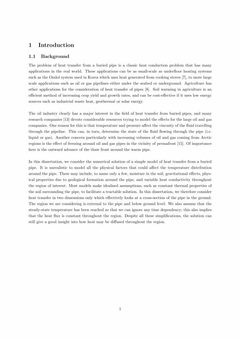
The problem of heat transfer from a buried pipe is a classic heat conduction problem that has manyapplications in the real world. These applications can be as small-scale as underfloor heating systemssuch as the Ondol system used in Korea which uses heat generated from cooking stoves [7], to more largescale applications such as oil or gas pipelines either under the seabed or underground. Agriculture hasother applications for the consideration of heat transfer of pipes [8]. Soil warming in agriculture is anefficient method of increasing crop yield and growth rates, and can be cost-effective if it uses low energysources such as industrial waste heat, geothermal or solar energy.
The oil industry clearly has a major interest in the field of heat transfer from buried pipes, and manyresearch companies [13] devote considerable resources trying to model the effects for the large oil and gascompanies. One reason for this is that temperature and pressure affect the viscosity of the fluid travellingthrough the pipeline. This can, in turn, determine the state of the fluid flowing through the pipe (i.e.liquid or gas). Another concern particularly with increasing volumes of oil and gas coming from Arcticregions is the effect of freezing around oil and gas pipes in the vicinity of permafrost [15]. Of importancehere is the outward advance of the thaw front around the warm pipe.
In this dissertation, we consider the numerical solution of a simple model of heat transfer from a buriedpipe. It is unrealistic to model all the physical factors that could affect the temperature distributionaround the pipe. These may include, to name only a few, moisture in the soil, gravitational effects, phys-ical properties due to geological formation around the pipe, and variable heat conductivity throughoutthe region of interest. Most models make idealised assumptions, such as constant thermal properties ofthe soil surrounding the pipe, to facilitate a tractable solution. In this dissertation, we therefore considerheat transfer in two dimensions only which effectively looks at a cross-section of the pipe in the ground.The region we are considering is external to the pipe and below ground level. We also assume that thesteady-state temperature has been reached so that we can ignore any time dependency; this also impliesthat the heat flux is constant throughout the region. Despite all these simplifications, the solution canstill give a good insight into how heat may be diffused throughout the region.
1
Figure 1: Schematic of the physical situation
1.2 Governing equation
The starting point for our model is derived from Fourier’s Law [21] which specifies that heat transfer isgoverned by the equation:
q = −κ∇u (1)
where:
q ≡ heat flux vector per unit length
κ ≡ heat conductivity of the soil
u ≡ temperature throughout the region.
If our system is in steady-state, then Conservation of Energy [21] implies that, in the absence of heatsinks or sources, the heat flux throughout the region must satisfy:
∇ · q = 0. (2)
In one dimension, this would imply that heat flux must be constant at all points; in more than onedimension, it implies that heat flux entering a control region must equal heat flux leaving the sameregion. If we assume that all thermal properties are constant, then κ is constant and (2) reduces toLaplace’s Equation:
∇2u = 0.
2
The simplest scenario for which we can solve this problem analytically is to assume that:
• the pipe is buried deep underground
• the temperature depends only on the distance from the centre of the pipe, O
• the region exterior to the pipe is unbounded.
Under these assumptions, we could now transform Laplace’s equation into polar coordinates (r, θ), centredat O, which would yield the solution:
u(r) = A ln r +B
where A and B are constants; these can be determined if we know u(r) and∂u
∂ron the boundary of the
pipe r = a, where a is the radius of the pipe. This solution blows up as r → ∞ so is only of limitedinterest in estimating the temperature distribution near the pipe. When the boundary at ground level isintroduced, it becomes clear we cannot parametrise the solution by r alone. The purpose of highlightingthis solution is that it provides the basis for the Fundamental Solution of Laplace’s Equation which wewill discuss later in this dissertation (see §2.1).
1.3 Boundary Conditions
In this problem, we have two boundaries of interest which will determine the solution u; the pipe boundaryand the ground surface/mudline. There has been much research on modelling the heat transfer associatedwith buried pipes with constant wall temperatures [7]. A widely used concept here is the conduction shapefactor, S, which for a buried pipe takes the form:
S =2π
cosh−1(Ya
)where a is the pipe radius, and Y is the distance of the pipe centre from the ground.This formulation leads to some unphysical heat transfer properties at the surface when both pipe andsurface boundary temperatures are constant. This approach gives better results when the heat flux isgiven on the ground surface - a more detailed account is given in the paper by Bau and Sadhal [4].
Rather than prescribing the temperature on these boundaries, we are assuming that the heat flux, q
will be known, and hence∂u
∂ncan be prescribed on each boundary. On the pipe boundary, we set
∂u
∂n= f
and on the ground surface we set∂u
∂n= g, where f, g are known functions. On the pipe boundary, in
terms of polar coordinates (r, θ), r is fixed so f will depend only on θ; in terms of Cartesian coordinates(x, y), g will depend on x alone since y is fixed so will depend on both r and θ. This type of problem,
where we seek a solution u in a region outside a closed domain (i.e. the pipe) and∂u
∂nis given on the
boundary, is known as an exterior Neumann problem.
As we get further away from the heat source of the pipe, we wish the solution to tend towards anambient temperature. The ambient temperature at the ground surface, T0, is easy to measure, but as wego further underground it is realistic to expect the temperature to increase. Again this is an idealisedcondition since in some shallow underground caves the temperature would be much cooler than at the
3
surface due to lack of sunlight and moisture considerations. However, in some deep mines (4 km un-derground) in South Africa for example, temperatures have been known to climb to around 55◦C, wellabove ambient ground temperatures [19]. As a simplification we assume u → cy + T0 as we get furtheraway from the pipe, where c is a negative constant, |y| is the depth below the centre of the pipe, O. Amore mathematically rigorous analysis of this asymptotic behaviour will be given in §2.4.
1.4 Methods of Solution
First, we summarise the exterior Neumann problem we wish to solve:
∇2u = 0 in D (3a)
∂u
∂n= f on Γa (3b)
∂u
∂n= g on Γ1 (3c)
u→ cy + T0 as |x| → ∞, y → −∞ (3d)
where D is the region exterior to the pipe, Γa is the pipe boundary, and Γ1 is the ground surface boundary(for a fuller description see §2.1 and Figure 3).
There are several ways we could go about trying to solve (3). We now describe some of the optionsavailable highlighting strengths and weaknesses of each approach, with some illustrative examples whereappropriate. At this point we will not be applying full mathematical rigour to any results; this will bedone later in §2.4.
1.4.1 Analytic solution using polar coordinates (r, θ)
Generally it is not possible to solve this problem analytically for a general boundary condition at groundlevel. There are two scenarios where it is possible to have an analytic solution (depending on the na-ture of the boundary conditions f, g). This is very useful because this gives us a benchmark solutionfor our numerical model, and gives us an indication of how accurate our solution will be in other scenarios.
The first scenario is when the pipe is buried deep underground and the heat flux at ground level is0. Thus we can set g = 0. We also assume for now that c = 0, T0 = 0 for simplicity. Problem (3) nowreduces to:
∇2u = 0 in D
∂u
∂n(a, θ) = f(θ) on Γa. (4)
In summary, this becomes an eigenvalue problem such that there are an infinite number of solutions,
un =1r
(An cosnθ +Bn sinnθ)
u =∞∑0
un (5)
4
where we have used the fact that un must not blow up as r →∞ and un is 2π-periodic. Furthermore,
An =a2
π
∫ 2π
0
f(θ) cosnθdθ
Bn =a2
π
∫ 2π
0
f(θ) sinnθdθ. (6)
Thus for a simple closed-form solution, we could for example choose f to be sin θ or cos θ which wouldleave u with one term only. A solution as an infinite sum could be reduced down to a simpler integralform but this would still require numerical methods to solve and would not be that useful as a benchmark.
The second scenario where we may be able to obtain an analytic solution is when the pipe is exactlyhalf-buried. In this case, our boundary conditions apply along the constant lines r = a, θ = π, θ = 2π.Our ability to produce a simple analytical expression depends on the boundary conditions. For example,using the following boundary conditions:
f(θ) = sin 2θ
g(x) =a3
x3
would yield the closed-form solution, u =a3 sin 2θ
2r2, where a is the radius of the pipe. Again, this solution
would provide useful benchmarking for our numerical solution.
1.4.2 Finite Difference and Finite Element Methods
The finite differerence (FD) method is often used as a brute force method to solve many Partial DifferentialEquations (PDEs) as it is often easy to set up and understand [9, pp. 167–187]. A two dimensionalregular mesh (N×M grid points) is constructed on the region in which we are looking for a solution, usingCartesian coordinates in this case. At each mesh point (xi, yj), we use the discretised version of Laplace’sEquation:
(ui−1,j + ui+1,j + ui,j−1 + ui,j+1 − 4ui,j)∆x∆y
= 0
where ui,j ≈ u(xi, yj),∆x = xi+1−xi,∆y = yj+1− yj for a uniform mesh. For a Neumann problem, thisrequires us to solve a system of equations [N×M]×[N×M], so for 10 x, y nodes each, the linear system tobe solved would be 100×100. We can immediately see several problems with this method:
• Since this is an external Neumann problem, the mesh would need to cover a large truncated regionmeaning either a large number of points leading to long compute time, or a coarse discretisationwhich would imply a significant error. It would also be difficult to check in the model whether theambient temperature had been reached as |x|, |y| → ∞.
• The pipe boundary is circular which does not lend itself well to a square mesh. We may need toresort to a more sophisticated finite element approach.
• The error in general would be O(∆x2) which may be unacceptably large.
5
• Although the matrix above would be sparse (many of the elements would be zero), storing suchlarge data structures could have an adverse effect on computational speeds.
Hence for problem (3), we do not expect the Finite Difference Method to provide an acceptably quickand accurate solution.
1.4.3 Conformal mapping
This technique maps the physical region onto a rectangular domain by using a complex transformation[7]:
w = ln
(z − i
√h2 − a2
z + i√h2 − a2
).
The transformed boundaries now form the boundary of a rectangle in the complex domain which may beeasier to handle using separation of variables, although the boundary conditions are different and maybe more difficult to handle. For most problems, however, numerical methods may still be involved so thisdoes not necessarily help us solve the problem.
For a much more detailed discussion, refer to [7].
1.4.4 Bipolar coordinates
There are two standard definitions for bipolar coordinate systems:
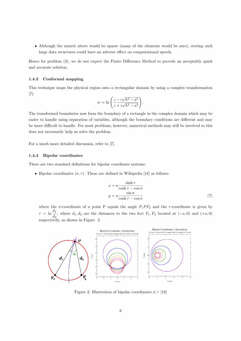
• Bipolar coordinates (σ, τ). These are defined in Wikipedia [18] as follows:
x = asinh τ
cosh τ − cosσ
y = asinσ
cosh τ − cosσ(7)
where the σ-coordinate of a point P equals the angle F1PF2 and the τ -coordinate is given by
τ = lnd1
d2, where d1, d2 are the distances to the two foci F1, F2 located at (−a, 0) and (+a, 0)
respectively, as shown in Figure 2.
Figure 2: Illustration of bipolar coordinates σ, τ [18]
6
In (σ, τ) coordinates, ∇2 =1a2
(cosh τ − coshσ)2(∂2
∂τ2+
∂2
∂σ2).
• Two-centre bipolar coordinates (r1, r2) [20]. For a given point p = (x, y), then r1 is the distancebetween p and the point (−a, 0) and r2 is the distance between p and the point (+a, 0).
r1 =√
(x+ a)2 + y2
r2 =√
(x− a)2 + y2.
Simple rearrangement yields the transformation to Cartesian coordinates from bipolars (r1, r2):
x =r21 − r2
2
4a
y = ± 14a
√16a2r2
1 − (r21 − r2
2 + 4a2)2. (8)
Whilst either of these coordinate systems may be of use solving problem (3), we have not focussedon this method of solution in this dissertation. Elsewhere, analytic solutions have been obtainedthrough this method (see [13],[14]).
1.4.5 Boundary Element Methods
This approach works when the PDE we are looking to solve has a simple Fundamental Solution associatedwith it. In the case of Laplace’s Equation, the Fundamental Solution at a point p = (xp, yp) is:
G(x, y|xp, yp) =1
4πln[(x− xp)2 + (y − yp)2
]. (9)
G is defined everywhere in R2 apart from at (xp, yp) where it is singular. As we will see later in §2, wecan now transform the PDE (3) into a Boundary Integral Equation (BIE) which we can solve numericallyon the boundary of the pipe.
With this approach, there is no need to mesh the semi-infinite domain; we only need to discretise the pipeboundary. In fact we have reduced the dimensionality of the problem from two dimensions to one, as wediscretise θ only. When the boundary is smooth as is the case here, we will get rapid convergence as weshall demonstrate in §4. On the downside, we do have to invert dense matrices with this approach, butthey tend to be relatively small since we can use a small number of sample points for rapid convergence.
Given the advantages of this approach, we shall now use this method to obtain a solution for (3). Thereare a couple of different ways this can be done via the Direct Method (which solves for u directly) or theIndirect Method (which solves for a density function which then generates solutions for u). Both thesemethods are summarised succinctly in [17, 290-297]. We shall use the Direct Method because in thiscase it has the advantage of immediately yielding the boundary temperature, which we will then use tocompute solutions very close to (but not on) the boundary.
7
2 Formulating the Boundary Integral Equation
2.1 Background
Given the complicated nature of the different domains and boundaries we need to consider, it is helpfulto define these in detail for later reference (see Figure 3).
• Let the origin of our Cartesian (x, y) plane, O, be at the centre of the oil pipe.
• Let Da be the interior of circular pipe radius a, with boundary Γa.
• Let the large bounded domain Dbox be defined by the interior of the region enclosed by the linesy = Y, x = −R, y = −R, x = +R.
• Let the boundary of Dbox be Γ1,Γ2,Γ3,Γ4 as shown in the diagram below, where Γ1 coincides withthe line y = Y , Γ2 coincides with the line x = −R, Γ3 coincides with the line y = −R, and Γ4
coincides with the line x = +R.
• Define point p ∈ Dbox/Da and let Dε be a small circular domain, centre p, radius ε and boundaryΓε.
• Let D = Dbox/(Da ∪Dε) with boundary Γ = Γa ∪ Γε ∪ Γ1 ∪ Γ2 ∪ Γ3 ∪ Γ4.
• Let G be the Fundamental Solution to Laplace’s Equation, G(p,q) =ln |p− q|
2πor in Cartesian
terms G(xp, yp|xq, yq) =ln |(xp − xq)2 − (yp − yq)2|
4π.
• Let u be the temperature exterior to the pipe, therefore in steady state, u is harmonic on D subject
to the boundary conditions∂u
∂n= f on Γa and
∂u
∂n= g on Γ1. The functions f, g are assumed to
be continuously infinitely differentiable i.e f, g ∈ C∞.
8
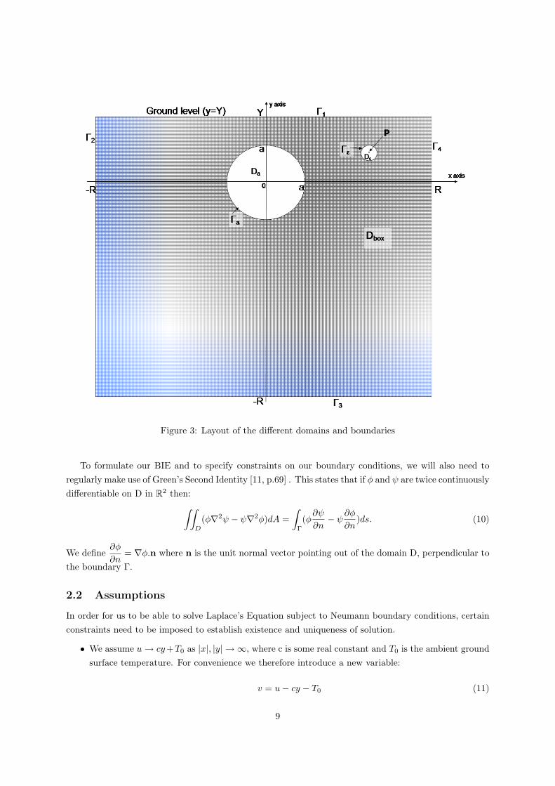
Figure 3: Layout of the different domains and boundaries
To formulate our BIE and to specify constraints on our boundary conditions, we will also need toregularly make use of Green’s Second Identity [11, p.69] . This states that if φ and ψ are twice continuouslydifferentiable on D in R2 then:∫∫
D
(φ∇2ψ − ψ∇2φ)dA =∫
Γ
(φ∂ψ
∂n− ψ∂φ
∂n)ds. (10)
We define∂φ
∂n= ∇φ.n where n is the unit normal vector pointing out of the domain D, perpendicular to
the boundary Γ.
2.2 Assumptions
In order for us to be able to solve Laplace’s Equation subject to Neumann boundary conditions, certainconstraints need to be imposed to establish existence and uniqueness of solution.
• We assume u→ cy+T0 as |x|, |y| → ∞, where c is some real constant and T0 is the ambient groundsurface temperature. For convenience we therefore introduce a new variable:
v = u− cy − T0 (11)
9
so that v → 0 as |x|, |y| → ∞. v is still harmonic on D and∂v
∂n=
∂u
∂n− cny where ny is the y
component of the outward normal vector to the boundary.
• In order that the solution v does not blow up as |R| → ∞, we need to stipulate that for some realα > 0:
∂v
∂x= O(|x|−(1+α)) as |x| → ∞
∂v
∂y= O(|y|−(1+α)) as y → −∞ (12)
v → 0 as |x|, |y| → ∞, (which immediately follows from our first assumption).
We will see later in §2.4 that this together with compatability (see below) is sufficient to guaranteeexistence of a unique solution to (3).
• For any harmonic function v in D, substituting φ = v and ψ = 1 into (10), we get:∫Γ
∂v
∂nds = 0. (13)
Rewriting boundary conditions for v as f = f + c sin θ on Γa and g = g − c on Γ1, then as R→∞the integrals over Γ2,Γ3,Γ4 disappear and the above condition (13) reduces to:∫
Γa
fds+∫
Γ1
gds = 0. (14)
This is known as the compatability condition.
Since f = f − c sin θ and g = g + c, it follows that we require:∫Γa
fds+∫
Γ1
gds = 0
as all integrals involving the constant c sum to 0.
2.3 Formulation of BIE
To formulate our BIE using the Direct Method, we could make use of (10) by substituting φ = v andψ = G. Since v and G are harmonic on D, this would give us:∫
Γ
(v∂G
∂n−G∂v
∂n)ds = 0 in D. (15)
Taking each element of Γ in turn, we can see that (15) incorporates values of v on Γa,Γ1,Γε since∂G
∂n6= 0
on these boundaries. The integrals over Γ2,Γ3,Γ4 all disappear as R → ∞ because of our assumptions
for v,∂v
∂non these boundaries. Solving for v over two distinct boundaries would be cumbersome and also
difficult to get an accurate solution since x ∈ (−∞,∞) on Γ1. Therefore we introduce a modified Green’s
10
function G using method of images such that∂G
∂n= 0 on Γ1.
The modified Green’s function G is defined by:
G(xp, yp|xq, yq) = G(xp, yp|xq, yq) +G(xp, yp|xq, yq′ ), where yq′ = 2Y − yq. (16)
On Γ1:∂G
∂n=∂G
∂yq=∂G(xp, yp|xq, yq)
∂yq
∣∣∣∣yq=Y
−∂G(xp, yp|xq, yq′ )
∂yq′
∣∣∣∣∣yq′=Y
= 0. (17)
G now has two singularities both of which are outside the domain D. Therefore within D, G is stillharmonic and so we can still use Green’s Second Identity to formulate our BIE.
Using our modified Green’s function we can now state that for p ∈ D:
∫Γ
(v(q)
∂G(p,q)∂nq
− G(p,q)∂v(q)∂nq
)dsq = 0. (18)
which will only incorporate values of v on Γa and Γε since∂G
∂n= 0 on Γ1. We set out below each element
of the above integral and will prove each result in turn.
2.4 Theorems
Theorem 1. If p ∈ D and q ∈ Γa, and G is as defined in (16), then for any f ∈ C, v satisfies:
∫Γa
[v(q)
∂G(p,q)∂nq
− G(p,q)∂v(q)∂nq
]dsq = −a
∫ 2π
0
[v(θ)
(∂G(p,q)∂xq
cos θ +∂G(p,q)∂yq
sin θ
)+ G(p,q)f(θ)
]dθ
(19)where q = (xq, yq) = (a cos θ, a sin θ).
Furthermore, if p∗ ∈ Γa,
∫Γa
[v(q)
∂G
∂nq(p∗,q)− G(p∗,q)
∂v
∂nq(q)
]dsq = −
∫ 2π
0
v(θ)[
14π
+ a∂G
∂xq(p′,q) cos θ + a
∂G
∂yq(p′,q) sin θ
]dθ
−∫ 2π
0
af(θ)[
14π
ln(
4a2 sin2 (θ∗ − θ)2
)+G(p
′,q)]dθ
(20)
where p∗ = (a cos θ∗, a sin θ∗),p′
= (a cos θ∗, 2Y − a sin θ∗).
Proof. On the left hand side (LHS) of (19),∂G
∂nqis defined to be ∇G.nq where nq is unit normal vector
to boundary.In this case, the outward direction is towards the centre of the pipe as this out of the domain D.
11
Since Γa describes a circle, nq = (− cos θ,− sin θ). Therefore∂G
∂nq= − ∂G
∂xqcos θ − ∂G
∂yqsin θ.
In this case, dsq describes small changes in arc length, therefore dsq = adθ.
Finally we can substitute∂v
∂nq= f on Γa, leading to equation (19).
To prove equation (20), first observe that for p ∈ Γa:
∂G
∂xq(p∗,q) =
(xq − xp)2π[(xq − xp)2 + (yq − yp)2]
∂G
∂yq(p∗,q) =
(yq − yp)2π[(xq − xp)2 + (yq − yp)2]
and substitute in the trigonometric expressions for xp, xq, yp, yq.
This yields:
∂G
∂nq(p∗,q) =
−a(cos θ − cos θ∗) cos θ − a(sin θ − sin θ∗) sin θ2πa2[(cos θ − cos θ∗)2 + (sin θ − sin θ∗)2]
= − (1− cos(θ − θ∗))2πa[2− 2 cos(θ − θ∗)]
= − 14πa
. (21)
We also observe that for the reflected Green’s function:
G(xp, yp|xq, 2Y − yq) = G(xp, 2Y − yp|xq, yq) (22)
∂G
∂nq(xp, yp|xq, 2Y − yq) =
∂G
∂nq(xp, 2Y − yp|xq, yq). (23)
Hence∂G
∂nq(p∗,q) =
∂G
∂nq(p∗,q) +
∂G
∂nq(p′,q). (24)
Using expressions (21) and (24), the first term on the LHS of equation (20) becomes:
−∫ 2π
0
v(θ)[
14π
+ a∂G
∂xq(p′,q) cos θ + a
∂G
∂yq(p′,q) sin θ
]dθ. (25)
Now looking at the second term on the LHS of equation (20), we again observe that:
G(p∗,q) = G(p∗,q) +G(p′,q). (26)
12
Furthermore,
G(p∗,q) =1
4πln[a2(cos θ − cos θ∗)2 + a2(sin θ − sin θ∗)2
]=
14π
ln[a2(2− 2 cos(θ − θ∗))
]=
14π
ln[4a2 sin2 (θ − θ∗)
2
]. (27)
Substituting (26) and (27) into (20), we obtain the following for the second term on the LHS:
−∫ 2π
0
af(θ)[
14π
ln(
4a2 sin2 (θ∗ − θ)2
)+G(p
′,q)]dθ. (28)
Hence our proof is complete for the case where p∗ ∈ Γa.
Theorem 2. If p,q, G and Γε are as defined in §2.1–§2.3, then v satisfies:
limε→0
∫Γε
[v(q)
∂G(p,q)∂nq
− G(p,q)∂v(q)∂nq
]dsq =
−v(p) if p ∈ D/Γa
−v(p)2
if p ∈ Γa.(29)
Proof. For p ∈ D,Γε describes a circle, so p = (xp, yp),q = (xp + ε cos θ, yp + ε sin θ) and dsq = εdθ.Hence,
G =1
4π(2 ln ε+ ln(ε2 + 2βε sin θ + β2)) where β = 2(Y − yq) > 0 (30)
by substituting above values of xp, yp, xq, yq into (16).As ε → 0, it can be seen immediately that the second term in the integral (29) is O(ε ln ε). Using
L’Hopital’s Rule on limε→0
ln εε−1
, it can easily be shown that this limit is 0. Therefore we only need toconsider the first term.
If q ∈ Γε,∂G
∂nq= −∂G
∂ε= − 1
2πε− ε+ β sin θ
2π(ε2 + 2βε sin θ + β2)(31)
by differentiating (30) with respect to ε, which gives us:
limε→0
∫Γε
v(q)∂G(p,q)∂nq
dsq = − limε→0
∫ 2π
0
v(q)[1
2π+
ε(ε+ β sin θ)2π(ε2 + 2βε sin θ + β2)
]dθ
= −v(p). (32)
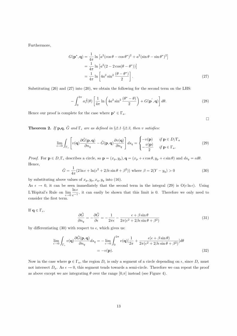
Now in the case where p ∈ Γa, the region Dε is only a segment of a circle depending on ε, since Dε mustnot intersect Da. As ε→ 0, this segment tends towards a semi-circle. Therefore we can repeat the proofas above except we are integrating θ over the range [0,π] instead (see Figure 4).
13
Figure 4: Showing load point p in D, and on Γa
It follows immediately that:
limε→0
∫Γε
v(q)∂G(p,q)∂nq
dsq = − limε→0
∫ π
0
v(q)[1
2π+
ε(ε+ β sin θ)2π(ε2 + 2βε sin θ + β2)
]dθ
= −v(p)2
. (33)
Theorem 3. If p,q, G and Γ1 are as defined in §2.1–§2.3, then for any g ∈ C, v satisfies:
limR→∞
∫Γ1
[v(q)∂G(p,q)∂nq
− G(p,q)∂v(q)∂nq
]dsq = −2∫ ∞−∞
G(p,q)|yq=Y g(xq)dxq. (34)
Proof. By definition, on Γ1, yq = Y,∂G
∂nq= 0,
∂v
∂nq= g, and G
∣∣∣yq=Y
= 2 G|yq=Y .
Finally dsq = dxq since yq is constant, hence our result.
Theorem 4. If p,q, G and Γ2,Γ3,Γ4 are as defined in §2.1–§2.3, then v satisfies:
limR→∞
∫Γi
[v(q)
∂G(p,q)∂nq
− G(p,q)∂v(q)∂nq
]dsq = 0 for i = 2, 3, 4. (35)
Proof. First consider the boundary Γ4 where xq = +R.
Since∂v
∂nq=
∂v
∂xq= O(|xq|−(1+α)) as |xq| → ∞, by definition there exist x0,M ∈ R such that
∂v
∂xq≤
Mx−(1+α)q for all xq ≥ x0.
14
Also since v → 0 as |x| → ∞, there exists x1 ∈ R such that for any ε > 0, |v| ≤ ε for all x ≥ x1.Therefore for R ≥ max(x0, x1) we can rewrite LHS of (35) as:∣∣∣∣∣∣∫ R
−R(v∂G
∂xq)
∣∣∣∣∣xq=R
− (G∂v
∂xq)∣∣∣∣xq=R
dyq
∣∣∣∣∣∣ ≤∫ R
−R
∣∣∣∣∣v(R, yq)∂G
∂xq(xp, yp|R, yq)
∣∣∣∣∣ dyq +∫ R
−R
∣∣∣∣G(xp, yp|R, yq)∂v
∂xq(R, yq)
∣∣∣∣ dyq≤ ε
∫ R
−R
∣∣∣∣∣ ∂G∂xq (xp, yp|R, yq)
∣∣∣∣∣ dyq +MR−(1+α)
∫ R
−R
∣∣∣G(xp, yp|R, yq)∣∣∣ dyq
=ε
2π
∫ R
−R
∣∣∣∣ (R− xp)(R− xp)2 + (yp − yq)2
∣∣∣∣ dyq+MR−(1+α)
4π
∫ R
−R
∣∣ln[(R− xp)2 + (yq − yp)2]∣∣ dyq
≤ ε
2π
∣∣∣∣ 2R(R− xp)
∣∣∣∣+MR−(1+α)
4π.2R ln(8R2)
=ε
π(1− xpR )
+(ln 8 + 2 lnR)MR−α
2π. (36)
As R → ∞ and ε → 0, the first term clearly tends to 0. To prove that limR→∞
lnRRα
= 0 use L’Hopital’s
Rule giving limR→∞
lnRRα
=1
αRα= 0.
Hence we have proved that:
limR→∞
∫Γ4
(v(q)
∂G(p,q)∂nq
− G(p,q)∂v(q)∂nq
)dsq = 0. (37)
It follows trivially that the same result holds for Γ2 where we effectively make the substitution x′
= −x.
We can use the same proof for Γ3 since we are replacating it using∂v
∂yqas yq → −∞ instead of
∂v
∂xqas
|xq| → ∞. Although the range of integration [-R,Y] is different, this does not affect the end result.
We have now proved (35) and are in a position to formulate the BIE to solve this problem.
2.5 The Boundary Integral Equation
2.5.1 Operator Notation
In general, when analysing BIEs, it is convenient to use operator notation to represent integral operatorsas it is a more compact and convenient notation. It can also be useful when applying rigorous functionalanalysis techniques to prove existence, uniqueness and to perform error analysis. From a conceptualbasis, it is also simple to understand that if the BIE is solved on a particular boundary, we can apply the
15
same operators (referencing any point in the domain) using those boundary values to solve the equationfor that point in the domain.
In this example, we have the following operator representation:
v(p)− (Av)(p) = (Bf)(p) + (Cg)(p) for p ∈ D (38)
v(p∗)2− (Av)(p∗) = (Bf)(p∗) + (Cg)(p∗) for p∗ ∈ Γa (39)
where:
Az(p) =∫
Γa
z(q)∂G
∂nq(p,q)dsq
Bz(p) = −∫
Γa
G(p,q)z(q)dsq
Cz(p) = −∫
Γ1
G(p,q)z(q)dsq.
2.5.2 Operators on the Boundary
In order to obtain a solution v at any point p ∈ D, we first need to solve (39) which is a BIE of theSecond Kind. Whilst we would use the above definitions of our operators in (38) for a general pointp ∈ D, it is important that we make use of the expressions derived in §2.4 when using the operators in(39). Using these expressions has a significant impact on accuracy and speed when solving the BIE.
The expressions for each operator when p∗ ∈ Γa are as follows:
Az(p∗) = −∫ 2π
0
z(θ)[
14π
+ a∂G
∂xq(p′,q) cos θ + a
∂G
∂yq(p′,q) sin θ
]dθ (40)
Bz(p∗) = −∫ 2π
0
az(θ)[
14π
ln(4a2 sin2 θ∗ − θ
2) +G(p
′,q)]dθ (41)
Cz(p∗) = −2∫ ∞−∞
G(p∗,q)|yq=Y z(xq)dxq. (42)
Since the operators B and C do not act on v in our BIE (39) it is convenient to define a function h suchthat:
h(p∗) = Bf(p∗) + Cg(p∗). (43)
The BIE then becomes:v(p∗)
2− (Av)(p∗) = h(p∗) for p∗ ∈ Γa. (44)
Having solved for v on the boundary we can then use (38) to determine v at any point p ∈ D.
16
3 Numerical Methods for solving Boundary Integral Equations
3.1 Background
In the previous section, we formulated the BIE which we need to solve on Γa. In general, this equationcannot be solved analytically, so we need to develop some numerical techniques to provide the solution.The goal here is to approximate the continuous operators using discrete operators on v so that a linearsystem of equations on v can then be solved using matrix inversion.
There are several techniques for discretising the BIE; the ones we will look at in this dissertation areknown as Nystrom’s Method and the Collocation Method. Although Galerkin’s Method is popularamongst mathematicians due to some of its elegant analytical properties, we will not be discussing itfurther.
Accuracy in our numerical integration techniques is also critical as this will allow us to use fewer samplepoints and hence decrease calculation times. Therefore we will be examining different numerical inte-gration rules (known as quadrature), namely the trapezium rule and Gauss-Legendre quadrature, with aview to how precision can be optimised whilst not impacting calculation speeds too adversely.
Finally we will look at some simple examples where the analytic solution is known so we can com-pare accuracy for the various methods and present some numerical results. This will include exampleswhere the pipe is buried deep underground, and a sequence of results as the pipe approaches ground level.
3.2 Quadrature
Throughout the following discussion, there are numerous references to the term quadrature and the rulesused to perform numerical integration. Therefore it would be helpful to set out some definitions here tomake the subsequent material clearer.
3.2.1 Definition
A quadrature rule is a numerical approximation for a definite integral, I =∫ b
a
f(x)dx. In general, an
N-point quadrature rule would approximate the integral as:
I ≈N∑i=1
wif(xi)
where wi are called the weights and xi are called the abscissas.As a simple example, the trapezium rule would approximate the integral as follows:
I ≈ (b− a)2
(f(a) + f(b))
and would therefore be termed a 2-point quadrature rule. Here we have specified the abscissas x1 =a, x2 = b and solved for the weights w1, w2 to ensure that I is exact when f is any polynomial of order 1since this gives us two equations in two unknowns.
17
If the range of integration is subdivided into N equal partitions [xi, xi+1] where i = 1, . . . , N , we getthe composite version of the trapezium rule:
N∑n=1
∫ xn
xn−1
f(x)dx ≈N∑n=1
(b− a)2N
(f(xn−1) + f(xn)) =(b− a)
2N
[f(x0) + f(xN ) + 2
N−1∑n=1
f(xn)
]. (45)
We will see later in §3.7.2 that when the composite trapezium rule is used for smooth periodic func-tions, we get rapid convergence.
More generally, for an N-point quadrature rule, we can specify N abscissas x1, . . . , xN and calculatethe weights w1, . . . , wN accordingly by making sure I is exact when f is any polynomial of order (N-1).
3.2.2 Gauss-Legendre Quadrature
In the above, the abscissas are specified and the weights can be calculated. Gaussian quadrature aims toimprove the accuracy by solving simultaneously for both the abscissas and the weights, thereby guaran-teeing I is exact for all polynomials of order (2N-1). One of the most popular Gaussian quadrature rulesis the Gaussian-Legendre formula, of which we will make widespread use [16, pp. 136–145].
This formula works well when the definite integral is over a finite range [a,b] and the function, f ∈ C∞.If there is a singularity in the range, then the quadrature rule can be enhanced to minimise the effect ofthe singularity and we will examine this later on.
It is customary to use a normalised integration range [-1,1] to calculate the abscissas and weights. Theycan then be used for any definite integral of any smooth function g. If we can calculate {wi}, {xi} suchthat: ∫ 1
−1
f(x)dx ≈N∑i=1
wif(xi), for any f ∈ C∞
then∫ b
a
g(x)dx ≈ (b− a)2
N∑i=1
wig
(b− a
2xi +
b+ a
2
)(46)
by making the substitution, x =b− a
2x′+b+ a
2.
It can be shown that the abscissas are the N roots of the Legendre polynomials:
PN (x) =1
2NN !dN
dxN(x2 − 1)N
where P0(x) = 1, P1(x) = x, P2(x) = 12 (3x2 − 1), ....
18
The weights are then defined as:
wi =2(1− x2
i )N2[PN−1(xi)]2
.
The proof of these results is outside the scope of this document (see [16, pp. 136–145]). However,we will refer to this proof to obtain some properties of the Legendre polynomials needed to calculate theabscissas and weights for any number N.
3.2.3 Calculation of abscissas and weights
The relevant properties we will make use of are:
PN (xi) = 0 for i = 1, 2, ..., N
PN (x) =(2N − 1)
NxPN−1(x)− (N − 1)
NPN−2(x) for all x ∈ R, N ≥ 2 (47)
P′
N (x) =NPN−1(x)−NxPN (x)
(1− x2)for all x ∈ R, N ≥ 1.
Using a judicious starting value for x0i , we will use the recurrence relation in (47) to generate a value
for PN (x0i ). This value should converge to 0 for xi to be a root. Therefore we iterate xi by using the
Newton-Raphson method, thereby giving a new start value:
x1i = x0
i −PN (x0
i )P′N (x0
i ).
We continue iterating xji in this fashion until PN (xji ) converges towards a given tolerance� 1. Once thishas been achieved, we can then calculate the weight wi.
The judicious initial guess for xi can be achieved by using the formula [1, p.787]:
xi = − cos(4i+ 3)π4N + 2
which ensures that there are no repeated roots and that xi converges to a real root in [-1,1].
We can also save time during the calculation by observing that PN (−x) = (−1)NPN (x) and hence if
xi is a root of PN (x) then so is −xi. Therefore, for an even number N, we only have to calculateN
2roots
and then set xi = −xN+1−i and wi = wN+1−i for allN
2< i ≤ N .
3.2.4 Gaussian quadrature over infinite ranges
As stated previously, Gauss-Legendre is intended for definite integrals over finite ranges with no singu-larities. In our problem, however, we need to integrate over Γ1 in which xq ∈ [−∞,∞]. We could employa different Gaussian quadrature rule such as Gauss-Hermite, but this really needs the integrand f toexhibit exponential decay as x → ±∞ for good convergence. There is also the possibility that we need
19
to split the integral into two semi-infinite ranges to isolate any singularities which would require us touse Gauss-Laguerre quadrature instead. A simpler solution is to transform the infinite (or semi-infinite)range to a finite one by using the substitution:
x = tan(π
2λ).
Therefore, the integral is now transformed from:∫ ∞−∞
f(x)dx→ π
2
∫ 1
−1
f(
tan(π
2λ))
sec2(π
2λ)dλ.
It can be seen here that we require f to be O(x−(2+p)) as x → ∞ (for some p > 0) to ensure goodconvergence, since sec2
(π2λ)
blows up as λ → ±1. However, this is less onerous than exponential decayand we will explain later how to improve accuracy when the location of a singularity is known. Thisintegral can now be approximated using the standard Gauss-Legendre abscissas and weights.
3.2.5 Gaussian quadrature across a singularity
Using standard Gaussian quadrature where f or its derivatives are singular within the bounds of inte-gration can lead to significant errors being introduced. Sometimes it is possible to make a substitutionto get rid of the singularity.
For example, ∫ b
a
f(x)√xdx→
∫ √b√a
f(y2)y
2ydy
by making the substitution, x = y2.
Another technique is to subtract out the singularity by setting f(x) = f1(x) + f2(x) where f1 is rel-atively smooth and can be numerically integrated more accurately, and f2 contains the singularity butcan be integrated analytically.
For example, ∫ 1
0
sin√xdx =
∫ 1
0
(sin√x− x 1
2 +x
32
6
)dx+
∫ 1
0
x12 − x
32
6dx.
The first part of the integral now has first and second derivatives that vanishes at x = 0, so can thereforebe integrated more accurately. The second part integrates analytically.
Where these two techniques do not help, then we need to refine our Gaussian quadrature to obtainmore accuracy. For our problem we shall use a graded one-dimensional mesh.
Suppose the integral is given by:
I =∫ 1
0
f(x)dx
20
where the singularity is at 0. We then split the integrals into (N+1) ranges such that:
I =∫ σN
0
f(x)dx+∫ σN−1
σNf(x)dx+
∫ σN−2
σN−1f(x)dx+ ...+
∫ 1
σ
f(x)dx
where 0 < σ < 1. Each of the (N+1) integrals is then approximated numerically using Gauss-Legendrequadrature using N abscissas and weights. The number of calculations is then of order N2. When usinggrading in this way it is usual to use a number of weights close to the square root of that used withoutgrading so as to improve accuracy without impairing calculation time.
More generally when integrating over x ∈ [a, b] with a singularity at a,
I =∫ a+(b−a)σN
a
f(x)dx+∫ a+(b−a)σN−1
a+(b−a)σNf(x)dx+
∫ a+(b−a)σN−2
a+(b−a)σN−1f(x)dx+ ...+
∫ b
a+(b−a)σ
f(x)dx.
Similarly, when integrating over x ∈ [a, b] with a singularity at b,
I =∫ b
b+(a−b)σNf(x)dx+
∫ a+(b−a)σN
b+(a−b)σN−1f(x)dx+
∫ b+(a−b)σN−1
b+(a−b)σN−2f(x)dx+ ...+
∫ b+(a−b)σ
a
f(x)dx.
Clearly we don’t want σ to be too close to 1 otherwise our weighting of the singularity will still producesignificant errors. If σ is too close to 0, we will not really have graded the mesh sufficiently since thefinal integral will dominate. To find the approximate optimal value of σ to be used, we illustrate with anexample in Table 1.
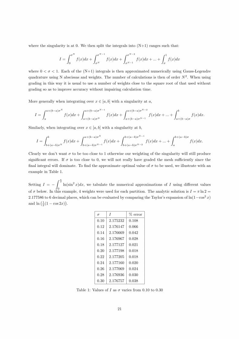
Setting I = −∫ π
2
0
ln(sin2 x)dx, we tabulate the numerical approximations of I using different values
of σ below. In this example, 4 weights were used for each partition. The analytic solution is I = π ln 2 =2.177586 to 6 decimal places, which can be evaluated by comparing the Taylor’s expansion of ln(1−cos2 x)and ln
(12 (1− cos 2x)
).
σ I % error
0.10 2.175232 0.1080.12 2.176147 0.0660.14 2.176669 0.0420.16 2.176967 0.0280.18 2.177127 0.0210.20 2.177198 0.0180.22 2.177205 0.0180.24 2.177160 0.0200.26 2.177069 0.0240.28 2.176936 0.0300.30 2.176757 0.038
Table 1: Values of I as σ varies from 0.10 to 0.30
21
This suggests that the optimal value for σ in this scenario would be around 0.20. In practice, whenmore weights are used an optimal σ of 0.15 is commonly used [12], and this is the value we have used inour examples later on. As a further comparison, when we use 16 weights with no grading, I = 2.170295which gives an error of 0.335%.
3.3 Discretisation Methods
3.3.1 Nystrom’s Method
Perhaps the simplest discretisation method to understand is Nystrom’s Method [2, pp. 100–103] whichgives a quick and efficient way to discretise BIEs of the Second Kind, using the quadrature rule of ourchoice to approximate the integral.
In general, suppose we have a BIE such as:
v(p)−Av(p) = h(p)
where A =∫
Γ
K(p,q)v(q)dsq and K is a continuous kernel.
We can use a quadrature rule on the operator A such that:
(Av)(p) ≈N∑j=1
wjK(p,qj)v(qj)
Now suppose that our approximation for v using N node points is vN , then we can define vN as follows:
vN (p)−N∑j=1
wjK(p,qj)vN (qj) = h(p) (48)
At each node point, pi where i = 1, . . . , N :
vN (pi)−N∑j=1
wjK(pi,qj)vN (qj) = h(pi) (49)
which is a linear system for vN of order N which can be solved by matrix inversion.
For other points p ∈ D, we can then write:
vN (p) =N∑j=1
wjK(p,qj)vN (qj) + h(p) (50)
Equation (50) is known as Nystrom’s interpolation formula and is the key to maintaining the accuracy ofthe solution. This method works well when the kernel K is continuous everywhere and does not containsingularities. In the problem we are looking at however, the kernel of the operator A is the derivative ofthe Green’s function which will become singular for any point p approaching the boundary Γa. In this
22
instance, to gain greater accuracy we would need to use more points, either by using a larger numberof sample points which would be relatively expensive computationally, or by interpolating our solutionaround the boundary across a larger number of points.
For this reason in our search for greater accuracy close to the pipe boundary, we prefer to use theCollocation Method instead.
3.3.2 Collocation Method
For the collocation method, we first define a finite N-dimensional space of candidate solutions {φi}Ni=1.The solution for any point p ∈ D ∪ Γa ∪ Γ1 can then be expressed as:
v(p) ≈N∑j=1
cjφj(p) (51)
and we substitute this into our BIE (44).
Therefore,
N∑j=1
cjφj(p)
2−A
N∑j=1
cjφj(p) ≈ h(p)
N∑j=1
cjφj(p)
2−
N∑j=1
cjAφj(p) ≈ h(p), since A is a linear operator
N∑j=1
cj
(φj(p)
2−Aφj(p)
)≈ h(p). (52)
We then chose N collocation points, {pi}Ni=1, on the boundary Γa where this equation holds exactly. Asthere are N collocation points {pi} and N unknown coefficients {cj}, this gives us a system of N linearequations in {cj} which can be solved using matrix inversion.
The matrix representation becomes:
Mc = h
c = M−1h (53)
where:
• M is N×N matrix with elements Mij =(φj(pi)
2−Aφj(pi)
)• c is N×1 vector with elements {cj}
• h is N×1 vector with elements h(pi).
23
3.4 Basis functions
The next step in implementing the numerical method is to choose suitable basis functions that we canuse in (51). This often depends on factors such as nature of boundary conditions, accuracy required, easeof implementation, speed of computation. Common basis functions include:
• Piecewise constant e.g.
φj(x) =
1 if x ∈ Xj
0 if x /∈ Xj .(54)
Alternative definitions for Xj are [xj−1, xj ], [xj , xj+1] or for regularly spaced nodes [xj −∆x2, xj +
∆x2
].
• Piecewise linear e.g.
φj(x) =
x− xj−1
xj − xj−1if x ∈ [xj−1, xj ]
xj+1 − xxj+1 − xj
if x ∈ [xj , xj+1]
0 otherwise.
(55)
• Piecewise polynomial e.g. Lagrange polynomial basis
φN1 (x) =(x− x0)(x− x2)(x− x3)....(x− xN )
(x1 − x0)(x1 − x2)(x1 − x3)....(x1 − xN )
φNj (x) =(x− x0)(x− x1)....(x− xj−1)(x− xj+1)....(x− xN )
(xj − x0)(xj − x1)....(xj − xj−1)(xj − xj+1)....(xj − xN ).
Hence φNj (xk) = δjk. (56)
• Trigonometric basis e.g. Lagrange basis functions where 2N points are evenly spaced around acircular boundary [11, p. 182]
φNj (x) =1
2N
[1 + cosN(x− xj) + 2
N−1∑n=1
cosn(x− xj)
]. (57)
Lemma 1. The basis function given in (57) has the property that φNj (xk) = δjk.
Proof. Consider the case where j = k, then trivially φNj (xj) =1
2N
[1 + 1 + 2
N−1∑n=1
1
]= 1.
For j 6= k, first observe that:
cosN(xk − xj) = cos(N(k − j)2πN
) = cos 2π(k − j) = 1.
24
Next consider the geometric series:
N−1∑n=1
ein(xk−xj) =(
1− ei(k−j)2π
1− ei(k−j)2π
N
)− 1
= −1. (58)
Therefore,1
2N
[1 + cosN(xk − xj) + 2
N−1∑n=1
cosn(xk − xj)
]= 0 for j 6= k.
Hence, φNj (xk) = δjk.
If we express v in terms of basis functions {φj}Mj=1 as defined in (57) so that v(θ) ≈M∑j=1
φj(θ)v(θj)
where M = 2N is an even number, then:
Av ≈∫
Γa
∂G
∂n(θ)
M∑j=1
φj(θ)v(θj)dθ (59)
≈M∑j=1
v(θj)(∫
Γa
∂G
∂n(θ)φj(θ)dθ
)(60)
If we now use the composite trapezium rule as described in (45) to numerically integrate, we get thefollowing expression:
Av ≈M∑j=1
v(θj)∂G
∂n(θj)∆θ (61)
where ∆θ =2πM
.
This result shows that if our quadrature rule is the composite trapezium rule, and the collocation pointsare the same as the sample points, then Nystrom’s Method and the Collocation Method are in fact equiv-alent.
We shall see in the §3.7.2 that because∂G
∂n(θ), φj(θ) and every derivative of these functions are all
2π-periodic, then the substitution
∫Γa
∂G
∂n(θ)φj(θ)dθ =
M∑j=1
∂G
∂n(θj)∆θ
has arbitrarily small error for sufficiently large M.
3.5 Singular Kernels
When calculating Bf , a problem arises since G has a singularity on Γa. Therefore if we were simplyto apply the composite Trapezium Rule to numerically integrate we may generate significant errors.However, since the singular kernel in this case is logarithmic, we express f in terms of the Lagrangian
25
trigonometric basis functions {Lj}, defined below, to resolve this problem. We can then integrate theresulting interpolation by parts to give us a much more accurate estimate of the integral.
Express Lj(θ) as a sum of cos terms [11, p.182]:
Lj(θ) =1
2N
(1 + cosN(θ − θj) + 2
N−1∑k=1
cos k(θ − θj)
).
Let f(θ) =2N−1∑j=0
f(θj)Lj(θ) so that Bf(θ) =2N−1∑j=0
f(θj)BLj(θ).
The problem arises in trying to calculate
wj(θ∗) =∫ 2π
0
Lj(θ) ln[4a2 sin2 (θ∗ − θ)
2
]dθ. (62)
The integral (62) is a linear sum of integrals where the integrands are all 2π-periodic. Without loss ofgenerality, we can therefore integrate each one over a shifted interval:∫ 2π+θ∗
θ∗cos k(θ − θj) ln
[4 sin2 (θ∗ − θ)
2
]dθ =
∫ 2π
0
cos k(θ − [θj − θ∗]) ln(
4 sin2 θ
2
)dθ.
We now need to prove the following result outlined in [11, p.146], but expanded here for clarity.
Theorem 5.
Ik =∫ 2π
0
ln(
4 sin2 θ
2
)eikθdθ =
0 k = 0
− 2π|k| |k| ≥ 1
(63)
Proof. When k = 0, we observe that:
I0 =∫ 2π
0
ln(
4 sin2 θ
2
)dθ
=∫ π
0
ln(
4 sin2 θ
2
)dθ +
∫ 2π
π
ln(
4 sin2 θ
2
)dθ
=∫ π
0
ln(
4 sin2 θ
2
)dθ +
∫ π
0
ln(
4 sin2 φ+ π
2
)dφ
=∫ π
0
ln(
4 sin2 θ
2
)dθ +
∫ π
0
ln(
4 cos2 φ
2
)dφ
(64)
making the substitution θ = φ+ π. Similarly,∫ 2π
0
ln(
4 cos2 θ
2
)dθ =
∫ π
0
ln(
4 cos2 θ
2
)dθ +
∫ π
0
ln(
4 sin2 φ
2
)dφ
(65)
implying that I0 =∫ 2π
0
ln(
4 sin2 θ
2
)dθ =
∫ 2π
0
ln(
4 cos2 θ
2
)dθ.
26
Therefore,
2I0 =∫ 2π
0
ln(
4 sin2 θ
2
)+∫ 2π
0
ln(
4 cos2 θ
2
)dθ
=∫ 2π
0
ln(
16 sin2 θ
2cos2 θ
2
)dθ
=∫ 2π
0
ln(4 sin2 θ
)dθ
=12
∫ 4π
0
ln(
4 sin2 θ
2
)dθ
= I0. (66)
Hence I0 = 0.
For the case where k ≥ 1, we need to make use of the geometric sum:
1 + eikθ + 2k−1∑j=1
eijθ = 1 + eikθ + 2(eikθ − 1eiθ − 1
− 1)
= (eikθ − 1){
1 +2
eiθ − 1
}= i(1− eikθ) cot
θ
2. (67)
Now if we integrate both sides of (67) over [0,2π], we get:
2π = i
∫ 2π
0
cotθ
2dθ − i
∫ 2π
0
eikθ cotθ
2dθ. (68)
Using the two identities: ∫ π2
0
cot θdθ =∫ π
2
0
tan θdθ∫ π
π2
cot θdθ = −∫ π
2
0
tan θdθ
we can easily show that i∫ 2π
0
cotθ
2dθ = 0.
Therefore (68) now gives us: ∫ 2π
0
eikθ cotθ
2dθ = 2πi.
27
Comparing real and imaginary parts, this yields:∫ 2π
0
cos kθ cotθ
2dθ = 0∫ 2π
0
sin kθ cotθ
2dθ = 2π. (69)
If we integrate the real part of (63) by parts we obtain:
∫ 2π
0
ln(
4 sin2 θ
2
)cos kθdθ =
[ln(
4 sin2 θ
2
)sin kθk
]2π
0
− 1k
∫ 2π
0
4 sin θ2 cos θ2 sin kθ4 sin2 θ
2
dθ
= 0− 1k
∫ 2π
0
sin kθ cotθ
2dθ
= −2πk
(70)
using the result (69).
Since Ik is real, then it follows that I−k = Ik. Hence for integer values of k ≤ −1, the value of our
integral is−2π|k|
, and our proof is complete.
Substituting this into (62) we now get:
wj(θ∗) =∫ 2π
0
Lj(θ + θ∗) ln[4a2 sin2 θ
2
]dθ
=1
2N
∫ 2π
0
[ln a2 + ln
(4 sin2 θ
2
)][1 + cosN(θ − θj + θ∗) + 2
N−1∑k=1
cos k(θ − θj + θ∗)
]dθ
=2πN
(ln a−
[N−1∑k=1
1k
cos k(θj − θ∗) +1
2NcosN(θj − θ∗)
])(71)
by noting that: ∫ 2π
0
ln(
4 sin2 θ
2
)cos k(θ − θj + θ∗)dθ = Re(eik(θ∗−θj)Ik)
= −2πk
cos k(θj − θ∗). (72)
Therefore if operator B = BS +BNS , where BS is singular and BNS is non-singular, then:
(Bf)(θ∗) = (BNS f)(θ∗) +2N−1∑j=0
wj(θ∗)f(θj).
3.6 Numerical integration over an infinite range
When we numerically integrate operator C, we need to integrate across the real line (−∞,∞). Thisintegral has no dependency on the integral over the pipe boundary so we can independently choose theoptimal way to integrate over Γ1. The most obvious way is to use the trapezium rule but this produces
28
poor convergence rates of O(h2) where h = R/N with R arbitrarily large.
As explained in §3.2, an improvement to this approach would be to use Gaussian quadrature, whichfor a smooth kernel would be extremely accurate for relatively few points (N ≈ 32) - Gauss-Hermitewould probably give rapid convergence here. However, the kernel becomes singular as the load pointapproaches the line y = Y , which is a problem when we want to solve for all points in the domain D.Gauss-Hermite quadrature also performs best when the integrand decays exponentially as |x| → ∞ whichmay not be the case in this problem.
An alternative approach is to make a substitution in the integral to give us finite limits so we canthen use Gauss-Legendre quadrature. For example, we can choose x = tan(φ). Thus the range for φ is(−π2 ,
π2 ). This substitution effectively gives us a large ∆x as x approaches ±∞ where we know the solu-
tion decays to 0, and a much smaller ∆x near x = 0 where we need a much more granular discretisation.There are some limitations to using this quadrature which we have stated previously, but in the exampleswe have used this produces the best convergence.
The equation for operator C now becomes:
Cz(p∗) = −2∫ π
2
−π2G(p∗,q(φ))|yq=Y z(φ) sec2 φdφ. (73)
This kernel is not singular for p∗ ∈ Γa if Y > a. However, we still have the problem of near singularityfor those points p ∈ D as p approaches Γ1. An improvement is achieved by splitting the integral intotwo domains (-∞, xp) and (xp,∞), and using the substitutions x = xp − tanφ on the first domain, anduse x = xp + tanφ on the second domain. This ensures that the point of singularity (i.e. x = xp) is theupper boundary on the first integral and the lower boundary on the second integral.
We can then use Gauss-Legendre quadrature as described above on both integrals with grading if neces-sary. The operator C is then transformed to:
Cz(p∗) = − 12π
∫ π2
0
ln[tan2(θ) + (Y − yp)2
][z(xp + tanφ) + z(xp − tanφ)] sec2 φdφ (74)
Given that we have a finite range, we generally use Gauss-Legendre integration with 64 points or withgrading we use 8 points on 8 graded domains. This approach shows distinctly better convergence when p
approaches the line y = Y over other traditional approximations such as trapezium rule with x = tanφsubstitution.
3.7 Error Analysis
We now examine the error for these composite rules to see what order of magnitude we should expectfor a given discretisation. This will then give us some basis on which rule to choose for our numericalintegration given other considerations such as speed and memory constraints.
29
3.7.1 Trapezium Rule
We expand the derivation given in Kress for clarity [11, p.198].
Theorem 6. Let the remainder R(f) be defined as:
R(f) =∫ b
a
f(x)dx− h[f(x0)
2+ f(x1) + ....+ f(xN−1) +
f(xN )2
]. (75)
Then |R(f)| ≤ h2
12(b− a)
∥∥∥f ′′∥∥∥∞
.
Proof. Define K(x) for each partition of the interval [a,b].
K(x) =
12 (x− x0)(x− x1) x0 ≤ x ≤ x1
....
12 (x− xj−1)(x− xj) xj−1 ≤ x ≤ xj....
12 (x− xN−1)(x− xN ) xN−1 ≤ x ≤ xN
(76)
We integrate by parts twice to obtain:
∫ xj
xj−1
K(x)f′′(x)dx =
[y(y − h)
2f′(y + xj−1)
]h0
−∫ h
0
(y − h
2)f′(y + xj−1)
= 0−[(y − h
2)f(y + xj−1)
]h0
+∫ h
0
f(y + xj−1)dy
= −h2
[f(xj−1) + f(xj)] +∫ h
0
f(y + xj−1)dy
=∫ xj
xj−1
f(x)dx− h
2[f(xj−1) + f(xj)] . (77)
Summing over j = 1, . . . , N we get:
|R(f)| ≤N∑j=1
∫ xj
xj−1
∣∣∣K(x)f′′(x)∣∣∣ dx
≤∥∥∥f ′′∥∥∥
∞
N∑j=1
∫ h
0
|y(y − h)2
|dy
=∥∥∥f ′′∥∥∥
∞
N∑j=1
[hy2
4− y3
6
]h0
=∥∥∥f ′′∥∥∥
∞
Nh3
12
=h2
12(b− a)
∥∥∥f ′′∥∥∥∞. (78)
30

3.7.2 Trapezium Rule on Periodic Functions
In the problem we are looking at, we know that our integrand is 2π-periodic around the pipe boundary.Therefore we can use a special feature of the trapezium rule which improves our accuracy from O(h2)considerably [10].The most convenient way to analyse the periodicity is to look at the discrete Fourier transform of theintegrand f .
f(x) =1
2π
∞∑m=−∞
cmeimx
where
cm =∫ 2π
0
f(x)e−imxdx.
Define the exact integral I =∫ 2π
0
f(x)dx. It follows immediately that I = c0.
Also define the numerical integral :
IN =N∑n=1
f(n∆x)∆x
=N∑n=1
(∞∑
m=−∞
12πcme
imn∆x)∆x
=∞∑
m=−∞cm(
N∑n=1
e2πimnN )
1N.
(79)
ButN∑n=1
e2πimnN = 0 unless m is an integer multiple of N. So we can simplify the above to:
IN =∞∑
k=−∞
ckN .
Therefore the error in the trapezium rule is:
E = |I − IN |
=
∣∣∣∣∣c0 −∞∑
k=−∞
ckN
∣∣∣∣∣=
∣∣∣∣∣∞∑k=1
(ckN + c−kN )
∣∣∣∣∣=
∣∣∣∣∣∞∑k=1
2∫ 2π
0
f(x) cos(kNx)dx
∣∣∣∣∣ . (80)
Thus we can see that the error in our trapezium rule approximation is dependent on the discrete Fouriertransform of f . In fact there exists N such that the error in the trapezium rule approximation is arbi-
31
trarily small, since standard Fourier analysis tells us that the coefficients cm are of order O( 1mp+1 ) for a
p-times differentiable function. However, for a function f whose derivatives are all periodic, there mayexist values of N where the error is significant.
For example, f(x) = cos5 x, has a discrete Fourier transform:
f(x) =1
2π
5∑m=−5
cmeimx
where c±5 =π
16, c±3 =
5π16, c±1 =
5π8, cm = 0 otherwise. Since c0 = 0 the exact value of the integral
should be 0. From (80) we can see that if we use N = 1, 3, 5 we will get errors 2π, 5π8 ,
π8 respectively and
zero error for other values of N. Thus predicting a value for N which will give an arbitrarily small errorfor a general function f , is difficult to do analytically and will in all likelihood involve some trial and error.
Alternatively, by using repeated integration by parts on (80), we get the result that:∫ 2π
0
f(x) cos(kNx)dx =1
(kN)2
[f′(2π)− f
′(0)]− 1
(kN)4
[f′′′
(2π)− f′′′
(0)]
+ ....
+(−1)p−1
(kN)2p
[f2p−1(2π)− f2p−1(0)
]+ ....
This result is formalised in the Euler Maclaurin Summation Formula [5]. This states that if f ∈
C2p+2[0, 2π] for p ≥ 1, and IN is the trapezoidal rule approximation to∫ 2π
0
f(x)dx with N uniform
subintervals, then:
EN = IN − I
=p∑
m=1
(2πN
)2mB2m
(2m)![f2m−1(2π)− f2m−1(0)
]+ 2π
(2πN
)2p+2B2p+2
(2p+ 2)!f2p+2(ξ). (81)
where 0 ≤ ξ ≤ 2π and Bn is the nth Bernoulli number. This suggests that if f is (2p+2)-times differ-entiable, and all derivatives are periodic then the error is of order O(1/N2p+2) i.e. if f ∈ C∞ then theerror is exponentially small with respect to N .
32
4 Numerical Examples for a buried pipe
4.1 Exterior Neumann problem on an unbounded domain
4.1.1 Analytic Solution
In order to test our methodology outlined above, and to examine the accuracy of our numerical imple-mentation, it is usual to benchmark using a simple example where the anaytical result is known. Sincewe know with 100% confidence the true result we can therefore draw conclusions from our numericalapproach.
The first example we will look at is solving Laplace’s equation with Neumann boundary conditionson an unbounded exterior domain, where the boundary is the rim of the pipe of unit radius. In physicalterms, this means that the pipe is deep underground (we set Y = 100,000) and we set a = 1, c = 0, g = 0.
In order to satisfy the compatability condition, from (14), we must ensure that∫
Γa
f = 0. Choosing
f =x√
x2 + y2in Cartesian terms, satisfies this condition and makes the problem solvable analytically.
We have also stipulated earlier that v → 0 as |x|, |y| → ∞.If we now transform this problem into polar coordinates (r, θ) then:
r2vrr + rvr + vθθ = 0
∂v
∂r(a, θ) = − cos θ
limr→∞
v(r, θ) = 0. (82)
Using separation of variables v(r, θ) = R(r)Θ(θ), we obtain:
r2R′′
+ rR′
R= λ
Θ′′
Θ= −λ (83)
where λ is a real constant.Since v is 2π periodic, so is Θ, and therefore λ must be a positive constant to give a solution of the
form A cos√λθ +B sin
√λθ. Moreover to satisfy periodicity, λ = n2 where n is an integer.
To solve for R in the form Crm +Dr−m, we must first solve the resulting characteristic equation:
m(m− 1) +m− n2 = 0
m = ±n. (84)
Given (82), m cannot be positive since the solution would blow up as r → ∞. This gives us a generalsolution of:
v(r, θ) = r−n(An cosnθ +Bn sinnθ), where n is a positive integer. (85)
Applying boundary conditions from (82), we finally we obtain the solution:
v(r, θ) =a2 cos θ
r. (86)
33
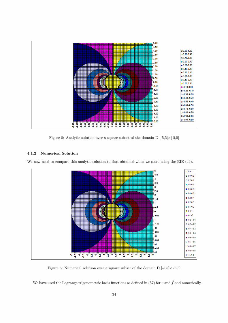
Figure 5: Analytic solution over a square subset of the domain D [-5,5]×[-5,5]
4.1.2 Numerical Solution
We now need to compare this analytic solution to that obtained when we solve using the BIE (44).
Figure 6: Numerical solution over a square subset of the domain D [-5,5]×[-5,5]
We have used the Lagrange trigonometric basis functions as defined in (57) for v and f and numerically
34
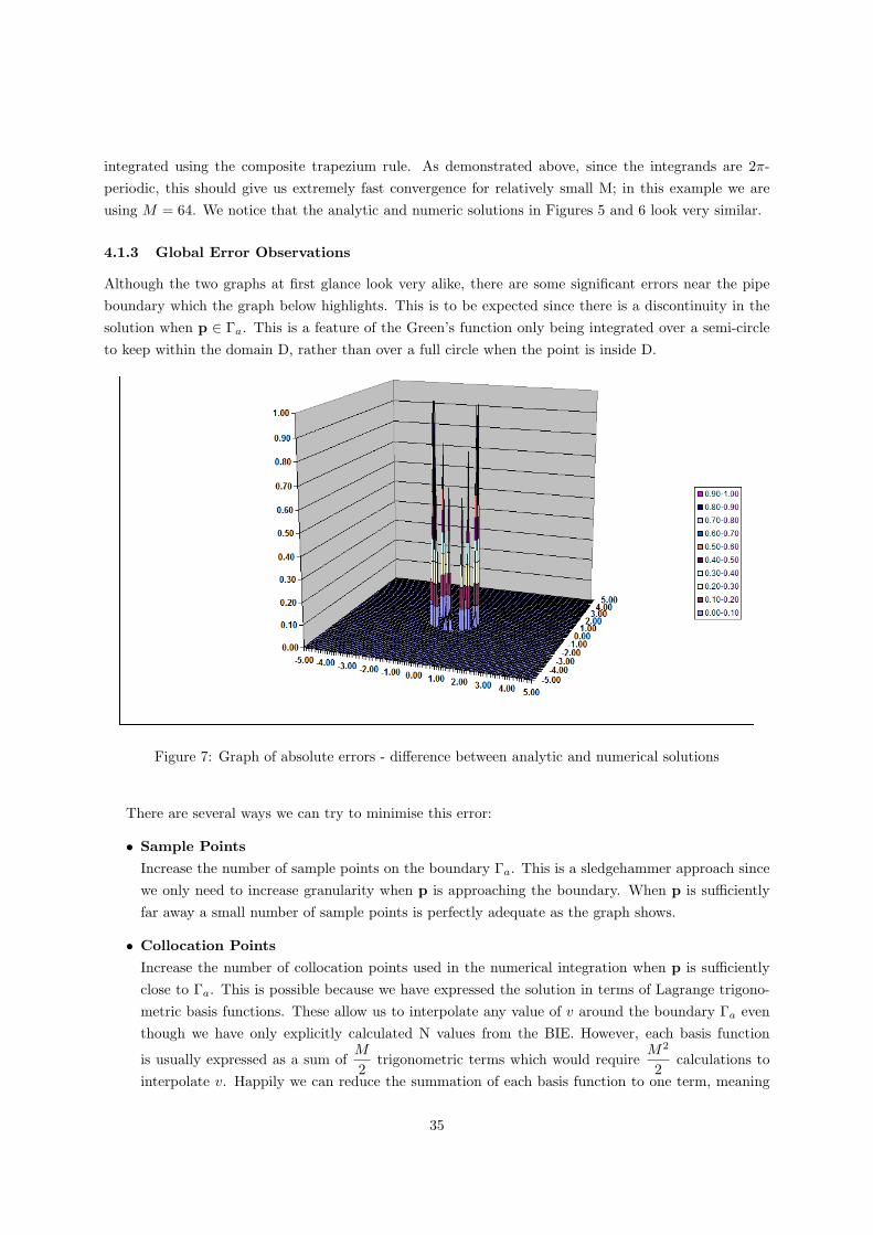
integrated using the composite trapezium rule. As demonstrated above, since the integrands are 2π-periodic, this should give us extremely fast convergence for relatively small M; in this example we areusing M = 64. We notice that the analytic and numeric solutions in Figures 5 and 6 look very similar.
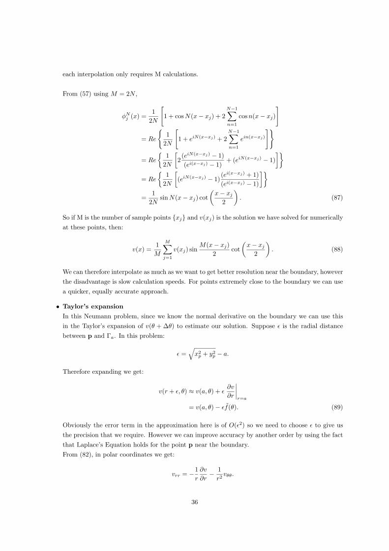
4.1.3 Global Error Observations
Although the two graphs at first glance look very alike, there are some significant errors near the pipeboundary which the graph below highlights. This is to be expected since there is a discontinuity in thesolution when p ∈ Γa. This is a feature of the Green’s function only being integrated over a semi-circleto keep within the domain D, rather than over a full circle when the point is inside D.
Figure 7: Graph of absolute errors - difference between analytic and numerical solutions
There are several ways we can try to minimise this error:
• Sample Points
Increase the number of sample points on the boundary Γa. This is a sledgehammer approach sincewe only need to increase granularity when p is approaching the boundary. When p is sufficientlyfar away a small number of sample points is perfectly adequate as the graph shows.
• Collocation Points
Increase the number of collocation points used in the numerical integration when p is sufficientlyclose to Γa. This is possible because we have expressed the solution in terms of Lagrange trigono-metric basis functions. These allow us to interpolate any value of v around the boundary Γa eventhough we have only explicitly calculated N values from the BIE. However, each basis function
is usually expressed as a sum ofM
2trigonometric terms which would require
M2
2calculations to
interpolate v. Happily we can reduce the summation of each basis function to one term, meaning
35
each interpolation only requires M calculations.
From (57) using M = 2N ,
φNj (x) =1
2N
[1 + cosN(x− xj) + 2
N−1∑n=1
cosn(x− xj)
]
= Re
{1
2N
[1 + eiN(x−xj) + 2
N−1∑n=1
ein(x−xj)
]}
= Re
{1
2N
[2
(eiN(x−xj) − 1)(ei(x−xj) − 1)
+ (eiN(x−xj) − 1)]}
= Re
{1
2N
[(eiN(x−xj) − 1)
(ei(x−xj) + 1)(ei(x−xj) − 1)
]}=
12N
sinN(x− xj) cot(x− xj
2
). (87)
So if M is the number of sample points {xj} and v(xj) is the solution we have solved for numericallyat these points, then:
v(x) =1M
M∑j=1
v(xj) sinM(x− xj)
2cot(x− xj
2
). (88)
We can therefore interpolate as much as we want to get better resolution near the boundary, howeverthe disadvantage is slow calculation speeds. For points extremely close to the boundary we can usea quicker, equally accurate approach.
• Taylor’s expansion
In this Neumann problem, since we know the normal derivative on the boundary we can use thisin the Taylor’s expansion of v(θ + ∆θ) to estimate our solution. Suppose ε is the radial distancebetween p and Γa. In this problem:
ε =√x2p + y2
p − a.
Therefore expanding we get:
v(r + ε, θ) ≈ v(a, θ) + ε∂v
∂r
∣∣∣∣r=a
= v(a, θ)− εf(θ). (89)
Obviously the error term in the approximation here is of O(ε2) so we need to choose ε to give usthe precision that we require. However we can improve accuracy by another order by using the factthat Laplace’s Equation holds for the point p near the boundary.From (82), in polar coordinates we get:
vrr = −1r
∂v
∂r− 1r2vθθ.
36
We can therefore estimate vrr at r = a by using boundary data and estimating vθθ with the threepoint approximation,
vθθ =v(θ + ∆θ) + v(θ −∆θ)− 2v(θ)
∆θ2
where ∆θ can be arbitrarily small and the values of v found by Lagrangian interpolation. This nowgives us:
vrr|r=a =1af(θ)− v(a, θ + ∆θ) + v(a, θ −∆θ)− 2v(a, θ)
a2∆θ2.
Our new estimate for v becomes:
v(r, θ) = v(a, θ)− εf(θ) +ε2
2
(1af(θ)− v(a, θ + ∆θ) + v(a, θ −∆θ)− 2v(a, θ)
a2∆θ2
).
The error in the approximation is now O(ε3).
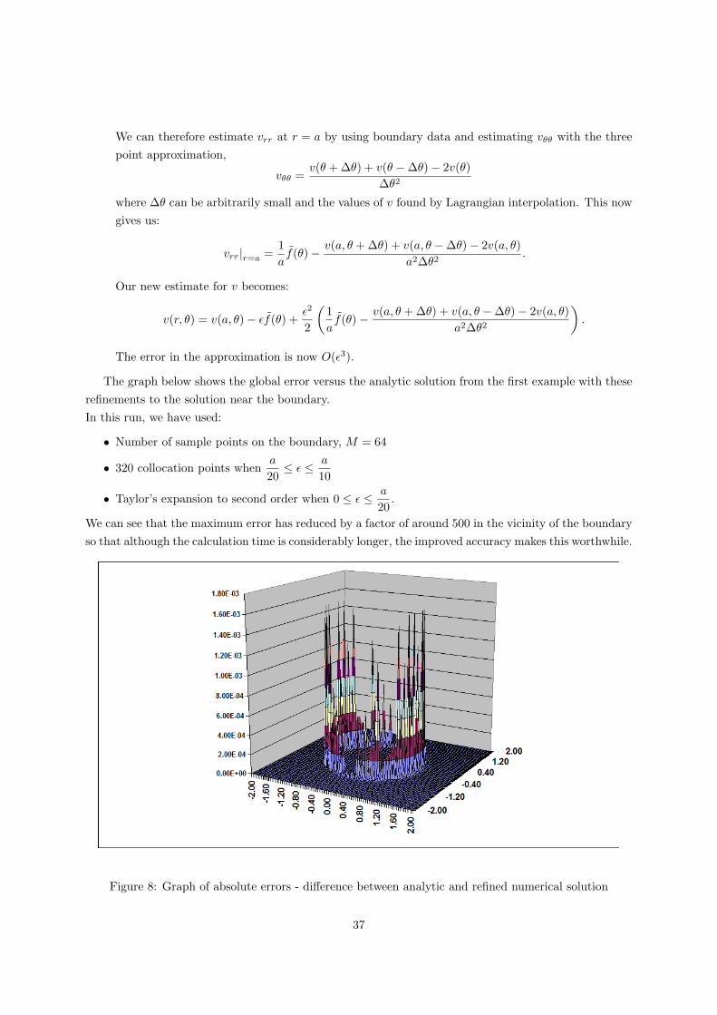
The graph below shows the global error versus the analytic solution from the first example with theserefinements to the solution near the boundary.In this run, we have used:
• Number of sample points on the boundary, M = 64
• 320 collocation points whena
20≤ ε ≤ a
10
• Taylor’s expansion to second order when 0 ≤ ε ≤ a
20.
We can see that the maximum error has reduced by a factor of around 500 in the vicinity of the boundaryso that although the calculation time is considerably longer, the improved accuracy makes this worthwhile.
Figure 8: Graph of absolute errors - difference between analytic and refined numerical solution
37
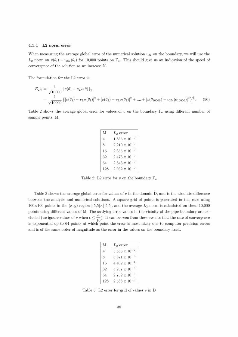
4.1.4 L2 norm error
When measuring the average global error of the numerical solution vM on the boundary, we will use theL2 norm on v(θi) − v2N (θi) for 10,000 points on Γa. This should give us an indication of the speed ofconvergence of the solution as we increase N.
The formulation for the L2 error is:
E2N =1√
10000‖v(θ)− v2N (θ)‖2
=1√
10000
{[v(θ1)− v2N (θ1)]2 + [v(θ2)− v2N (θ2)]2 + ....+ [v(θ10000)− v2N (θ10000)]2
} 12 . (90)
Table 2 shows the average global error for values of v on the boundary Γa using different number ofsample points, M.
M L2 error
4 1.836 x 10⁻⁹
8 2.210 x 10⁻⁹
16 2.355 x 10⁻⁹
32 2.473 x 10⁻⁹
64 2.643 x 10⁻⁹
128 2.932 x 10⁻⁹
Table 2: L2 error for v on the boundary Γa
Table 3 shows the average global error for values of v in the domain D, and is the absolute differencebetween the analytic and numerical solutions. A square grid of points is generated in this case using100×100 points in the (x, y)-region [-5,5]×[-5,5], and the average L2 norm is calculated on these 10,000points using different values of M. The outlying error values in the vicinity of the pipe boundary are ex-cluded (we ignore values of v when ε ≤ a
10). It can be seen from these results that the rate of convergence
is exponential up to 64 points at which point the error is most likely due to computer precision errorsand is of the same order of magnitude as the error in the values on the boundary itself.
M L2 error
4 3.553 x 10⁻²
8 5.671 x 10⁻³
16 4.402 x 10⁻⁴
32 5.257 x 10⁻⁶
64 2.752 x 10⁻⁹
128 2.588 x 10⁻⁹
Table 3: L2 error for grid of values v in D
38
4.2 Exterior Neumann problem on a semi-infinite domain
In example §4.1, as the pipe was deep underground, we ignored the boundary condition at ground levelsince this had negligible effect on the solution. In this example we still want to compare our numericalresults with the analytic solution, so we set Y = 2 and set the boundary values on the line y = Y to be:
v =a2 cos θ(x, Y )
r(x, Y ).
We can easily re-express this in Cartesian terms so that:
v(x, Y ) =a2x
(x2 + Y 2)∂v
∂y
∣∣∣∣y=Y
=−2a2xY
(x2 + Y 2)2. (91)
We do not expect discontinuous solutions on the boundary y = Y , since integrating both the Green’sfunction at the load point and at the reflected point ensure there is no jump discontinuity when p ∈ Γ1.We should also note that this is a well-posed problem since the compatability condition is satisfied. Infact, g is an odd function so will always integrate to 0 over the real line.
This example will therefore test that our formulation for all operators A,B and C is correct and giveconfidence that we can solve any exterior problem with good accuracy (away from the vicinity of the pipeboundary).
4.2.1 Numerical Solution
The following graph is a surface plot of the solution v in the box [-2,2]×[-2,2] so that the upper boundaryis ground level. Note that the plot looks extremely similar to the previous example which is as wewould expect given the contrived boundary condition at y=Y. We will also initially run this without therefinements around the boundary to see if we get similar results.
39
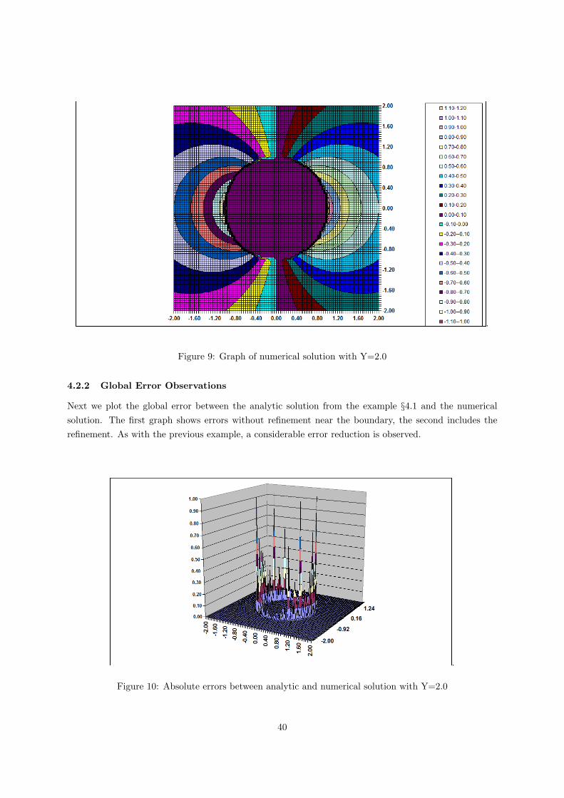
.
Figure 9: Graph of numerical solution with Y=2.0
4.2.2 Global Error Observations
Next we plot the global error between the analytic solution from the example §4.1 and the numericalsolution. The first graph shows errors without refinement near the boundary, the second includes therefinement. As with the previous example, a considerable error reduction is observed.
.
Figure 10: Absolute errors between analytic and numerical solution with Y=2.0
40
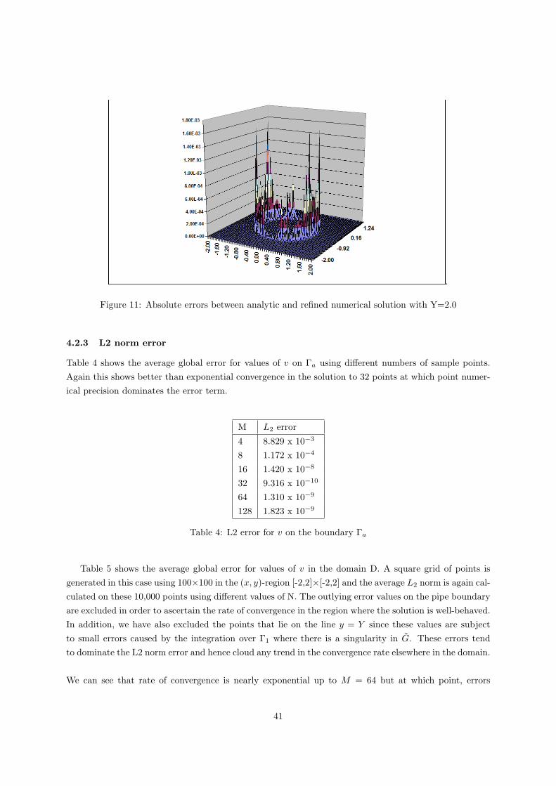
.
Figure 11: Absolute errors between analytic and refined numerical solution with Y=2.0
4.2.3 L2 norm error
Table 4 shows the average global error for values of v on Γa using different numbers of sample points.Again this shows better than exponential convergence in the solution to 32 points at which point numer-ical precision dominates the error term.
M L2 error
4 8.829 x 10⁻³
8 1.172 x 10⁻⁴
16 1.420 x 10⁻⁸
32 9.316 x 10⁻¹⁰
64 1.310 x 10⁻⁹
128 1.823 x 10⁻⁹
Table 4: L2 error for v on the boundary Γa
Table 5 shows the average global error for values of v in the domain D. A square grid of points isgenerated in this case using 100×100 in the (x, y)-region [-2,2]×[-2,2] and the average L2 norm is again cal-culated on these 10,000 points using different values of N. The outlying error values on the pipe boundaryare excluded in order to ascertain the rate of convergence in the region where the solution is well-behaved.In addition, we have also excluded the points that lie on the line y = Y since these values are subjectto small errors caused by the integration over Γ1 where there is a singularity in G. These errors tendto dominate the L2 norm error and hence cloud any trend in the convergence rate elsewhere in the domain.
We can see that rate of convergence is nearly exponential up to M = 64 but at which point, errors
41
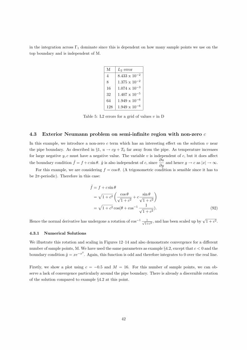
in the integration across Γ1 dominate since this is dependent on how many sample points we use on thetop boundary and is independent of M.
M L2 error
4 8.433 x 10⁻²
8 1.375 x 10⁻²
16 1.074 x 10⁻³
32 1.407 x 10⁻⁵
64 1.949 x 10⁻⁶
128 1.949 x 10⁻⁶
Table 5: L2 errors for a grid of values v in D
4.3 Exterior Neumann problem on semi-infinite region with non-zero c
In this example, we introduce a non-zero c term which has an interesting effect on the solution v nearthe pipe boundary. As described in §1, u → cy + T0 far away from the pipe. As temperature increasesfor large negative y, c must have a negative value. The variable v is independent of c, but it does affect
the boundary condition f = f + c sin θ. g is also independent of c, since∂u
∂yand hence g → c as |x| → ∞.
For this example, we are considering f = cos θ. (A trigonometric condition is sensible since it has tobe 2π-periodic). Therefore in this case:
f = f + c sin θ
=√
1 + c2(
cos θ√1 + c2
+ csin θ√1 + c2
)=√
1 + c2 cos(θ + cos−1 1√1 + c2
). (92)
Hence the normal derivative has undergone a rotation of cos−1 1√1+c2
, and has been scaled up by√
1 + c2.
4.3.1 Numerical Solutions
We illustrate this rotation and scaling in Figures 12–14 and also demonstrate convergence for a differentnumber of sample points, M. We have used the same parameters as example §4.2, except that c < 0 and theboundary condition g = xe−x
2. Again, this function is odd and therefore integrates to 0 over the real line.
Firstly, we show a plot using c = −0.5 and M = 16. For this number of sample points, we can ob-serve a lack of convergence particularly around the pipe boundary. There is already a discernible rotationof the solution compared to example §4.2 at this point.
42
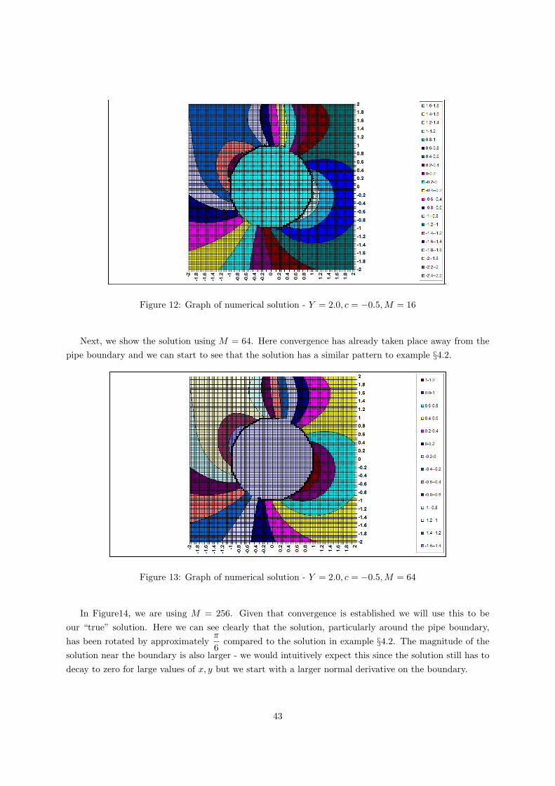
.
Figure 12: Graph of numerical solution - Y = 2.0, c = −0.5,M = 16
Next, we show the solution using M = 64. Here convergence has already taken place away from thepipe boundary and we can start to see that the solution has a similar pattern to example §4.2.
Figure 13: Graph of numerical solution - Y = 2.0, c = −0.5,M = 64
In Figure14, we are using M = 256. Given that convergence is established we will use this to beour “true” solution. Here we can see clearly that the solution, particularly around the pipe boundary,has been rotated by approximately
π
6compared to the solution in example §4.2. The magnitude of the
solution near the boundary is also larger - we would intuitively expect this since the solution still has todecay to zero for large values of x, y but we start with a larger normal derivative on the boundary.
43
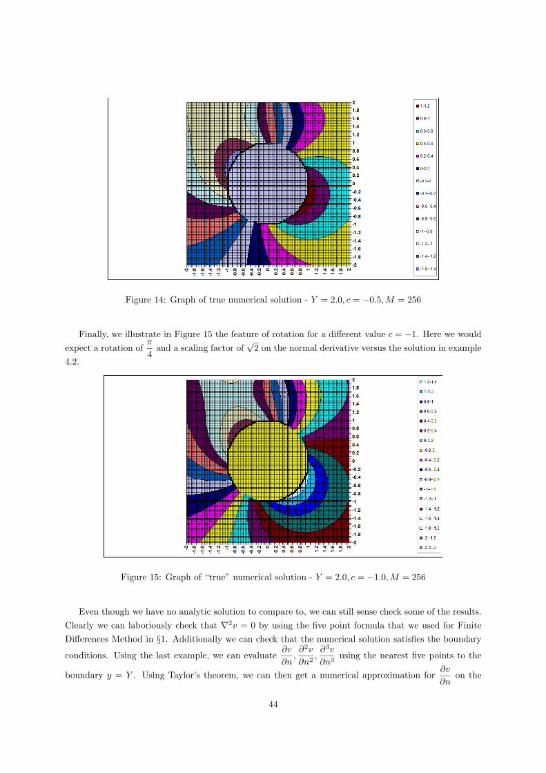
Figure 14: Graph of true numerical solution - Y = 2.0, c = −0.5,M = 256
Finally, we illustrate in Figure 15 the feature of rotation for a different value c = −1. Here we wouldexpect a rotation of
π
4and a scaling factor of
√2 on the normal derivative versus the solution in example
4.2.
Figure 15: Graph of “true” numerical solution - Y = 2.0, c = −1.0,M = 256
Even though we have no analytic solution to compare to, we can still sense check some of the results.Clearly we can laboriously check that ∇2v = 0 by using the five point formula that we used for FiniteDifferences Method in §1. Additionally we can check that the numerical solution satisfies the boundary
conditions. Using the last example, we can evaluate∂v
∂n,∂2v
∂n2,∂3v
∂n3using the nearest five points to the
boundary y = Y . Using Taylor’s theorem, we can then get a numerical approximation for∂v
∂non the
44
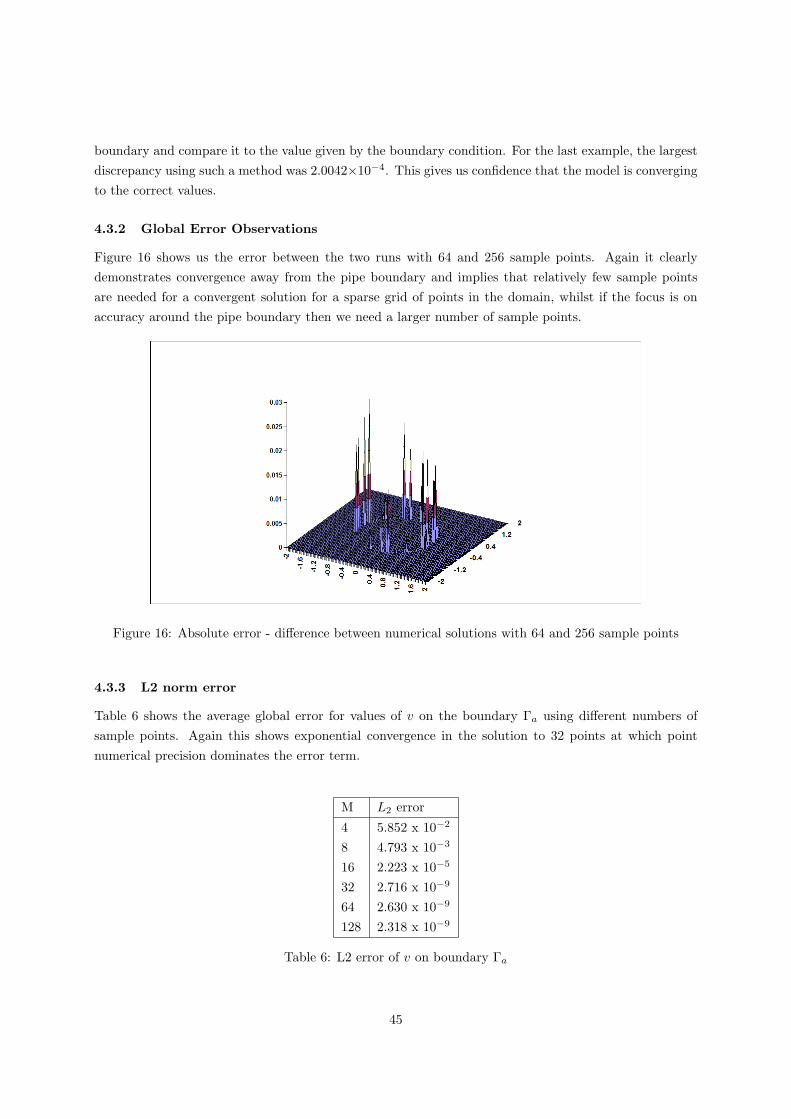
boundary and compare it to the value given by the boundary condition. For the last example, the largestdiscrepancy using such a method was 2.0042×10⁻⁴. This gives us confidence that the model is convergingto the correct values.
4.3.2 Global Error Observations
Figure 16 shows us the error between the two runs with 64 and 256 sample points. Again it clearlydemonstrates convergence away from the pipe boundary and implies that relatively few sample pointsare needed for a convergent solution for a sparse grid of points in the domain, whilst if the focus is onaccuracy around the pipe boundary then we need a larger number of sample points.
Figure 16: Absolute error - difference between numerical solutions with 64 and 256 sample points
4.3.3 L2 norm error
Table 6 shows the average global error for values of v on the boundary Γa using different numbers ofsample points. Again this shows exponential convergence in the solution to 32 points at which pointnumerical precision dominates the error term.
M L2 error
4 5.852 x 10⁻²
8 4.793 x 10⁻³
16 2.223 x 10⁻⁵
32 2.716 x 10⁻⁹
64 2.630 x 10⁻⁹
128 2.318 x 10⁻⁹
Table 6: L2 error of v on boundary Γa
45
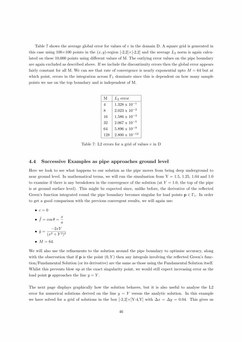
Table 7 shows the average global error for values of v in the domain D. A square grid is generated inthis case using 100×100 points in the (x, y)-region [-2,2]×[-2,2] and the average L2 norm is again calcu-lated on these 10,000 points using different values of M. The outlying error values on the pipe boundaryare again excluded as described above. If we include the discontinuity errors then the global error appearsfairly constant for all M. We can see that rate of convergence is nearly exponential upto M = 64 but atwhich point, errors in the integration across Γ1 dominate since this is dependent on how many samplepoints we use on the top boundary and is independent of M.
M L2 error
4 1.328 x 10⁻¹
8 2.023 x 10⁻²
16 1.586 x 10⁻³
32 2.067 x 10⁻⁵
64 5.896 x 10⁻⁹
128 2.800 x 10⁻¹²
Table 7: L2 errors for a grid of values v in D
4.4 Successive Examples as pipe approaches ground level
Here we look to see what happens to our solution as the pipe moves from being deep underground tonear ground level. In mathematical terms, we will run the simuluation from Y = 1.5, 1.25, 1.04 and 1.0to examine if there is any breakdown in the convergence of the solution (at Y = 1.0, the top of the pipeis at ground surface level). This might be expected since, unlike before, the derivative of the reflectedGreen’s function integrated round the pipe boundary becomes singular for load points p ∈ Γ1. In orderto get a good comparison with the previous convergent results, we will again use:
• c = 0
• f = cos θ =x
a
• g =−2xY
(x2 + Y 2)2
• M = 64.
We will also use the refinements to the solution around the pipe boundary to optimise accuracy, alongwith the observation that if p is the point (0, Y ) then any integrals involving the reflected Green’s func-tion/Fundamental Solution (or its derivative) are the same as those using the Fundamental Solution itself.Whilst this prevents blow up at the exact singularity point, we would still expect increasing error as theload point p approaches the line y = Y .
The next page displays graphically how the solution behaves, but it is also useful to analyse the L2error for numerical solutions derived on the line y = Y versus the analytic solution. In this examplewe have solved for a grid of solutions in the box [-2,2]×[Y-4,Y] with ∆x = ∆y = 0.04. This gives us
46
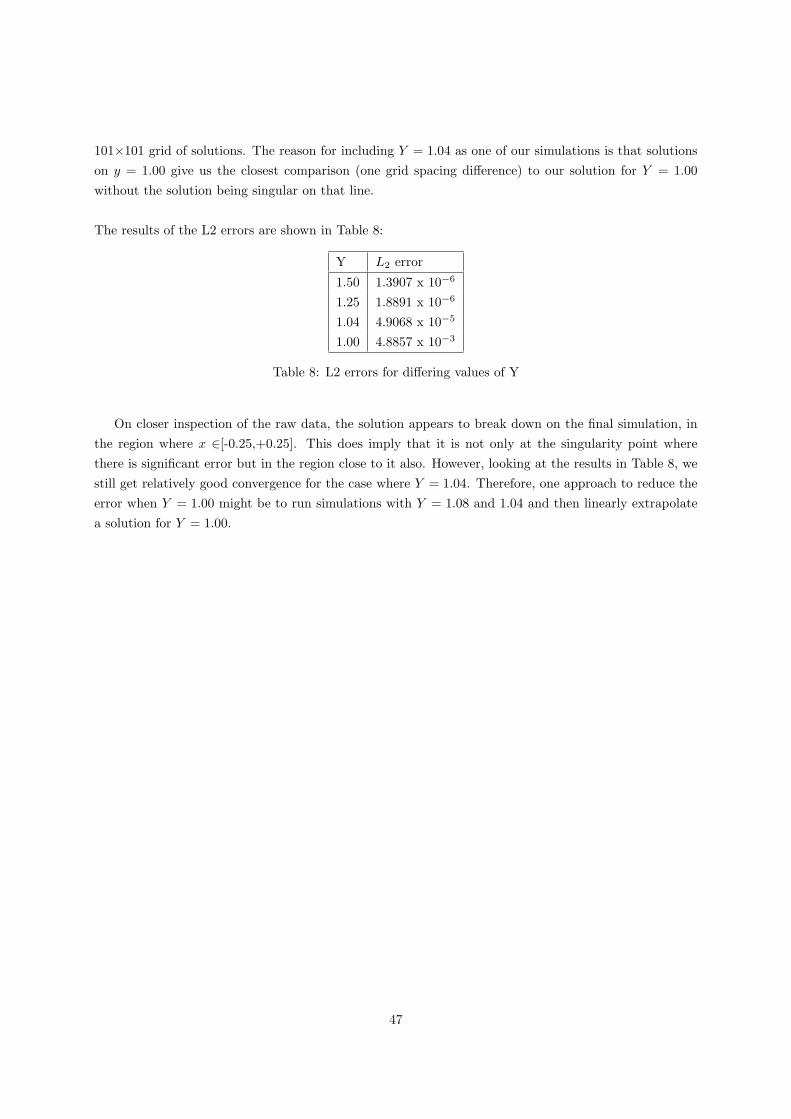
101×101 grid of solutions. The reason for including Y = 1.04 as one of our simulations is that solutionson y = 1.00 give us the closest comparison (one grid spacing difference) to our solution for Y = 1.00without the solution being singular on that line.
The results of the L2 errors are shown in Table 8:
Y L2 error
1.50 1.3907 x 10⁻⁶
1.25 1.8891 x 10⁻⁶
1.04 4.9068 x 10⁻⁵
1.00 4.8857 x 10⁻³
Table 8: L2 errors for differing values of Y
On closer inspection of the raw data, the solution appears to break down on the final simulation, inthe region where x ∈[-0.25,+0.25]. This does imply that it is not only at the singularity point wherethere is significant error but in the region close to it also. However, looking at the results in Table 8, westill get relatively good convergence for the case where Y = 1.04. Therefore, one approach to reduce theerror when Y = 1.00 might be to run simulations with Y = 1.08 and 1.04 and then linearly extrapolatea solution for Y = 1.00.
47
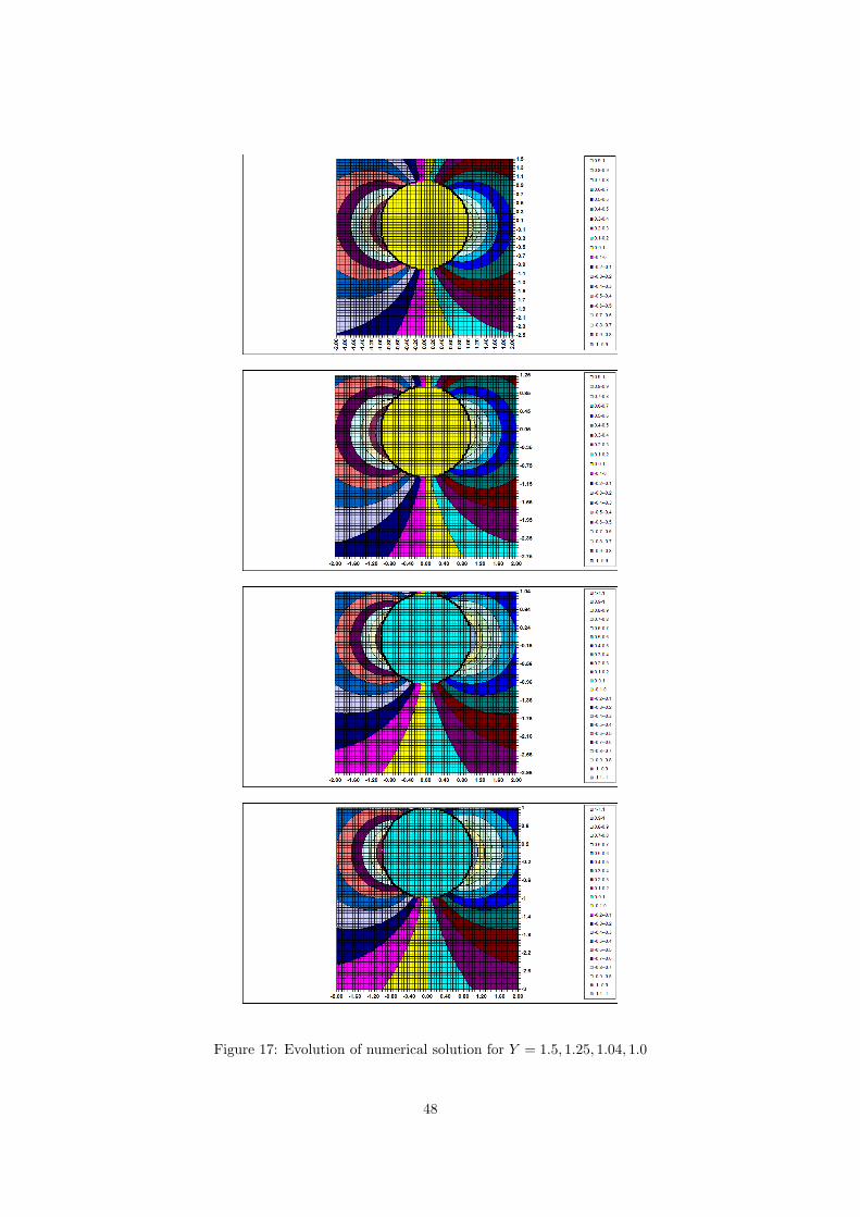
Figure 17: Evolution of numerical solution for Y = 1.5, 1.25, 1.04, 1.0
48
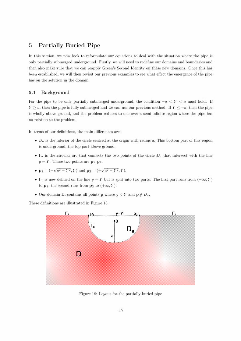
5 Partially Buried Pipe
In this section, we now look to reformulate our equations to deal with the situation where the pipe isonly partially submerged underground. Firstly, we will need to redefine our domains and boundaries andthen also make sure that we can reapply Green’s Second Identity on these new domains. Once this hasbeen established, we will then revisit our previous examples to see what effect the emergence of the pipehas on the solution in the domain.
5.1 Background
For the pipe to be only partially submerged underground, the condition −a < Y < a must hold. IfY ≥ a, then the pipe is fully submerged and we can use our previous method. If Y ≤ −a, then the pipeis wholly above ground, and the problem reduces to one over a semi-infinite region where the pipe hasno relation to the problem.
In terms of our definitions, the main differences are:
• Da is the interior of the circle centred at the origin with radius a. This bottom part of this regionis underground, the top part above ground.
• Γa is the circular arc that connects the two points of the circle Da that intersect with the liney = Y . These two points are p1,p2.
• p1 = (−√a2 − Y 2, Y ) and p2 = (+
√a2 − Y 2, Y ).
• Γ1 is now defined on the line y = Y but is split into two parts. The first part runs from (−∞, Y )to p1, the second runs from p2 to (+∞, Y ).
• Our domain D, contains all points p where y < Y and p /∈ Da.
These definitions are illustrated in Figure 18.
Figure 18: Layout for the partially buried pipe
49
5.2 Formulating the BIE
For the existence of a convergent solution we still need to stipulate that:
• v → 0 as x→ ±∞.
• ∂v
∂nmust be O(x−1−α) for some α > 0.
• The compatability condition (14) must still hold for f and g.
• We are still solving for v over Γa, and using this boundary solution to solve for all points in thedomain D.
There immediately appears to be a problem in defining the normal derivative∂v
∂nat points p1 and p2,
since at this intersection point the boundary has a discontinuous derivative. Given that there is also adiscontinuity in the solution at the pipe boundary we may have to consider how we discretise the problemas we approach both Γa and Γ1.
Using the new definitions, we can apply Green’s Identity as before on the domain D.
For p ∈ D:
v(p) =∫
Γa
(∂G
∂nq(p,q)v(q)− G(p,q)f(q)
)dsq −
∫Γ1
G(p,q)g(q)dsq. (93)
For p∗ ∈ Γa:
v(p∗)2−∫
Γa
∂G
∂nq(p∗,q)v(q) = −
∫Γa
G(p∗,q)f(q)dsq −∫
Γ1
G(p∗,q)g(q)dsq. (94)
Thus to solve (94), we must integrate round Γa from points p1 to p2, and similarly for Γ1 we mustuse quadrature along the line y = Y , omitting the interval [−
√a2 − Y 2,+
√a2 − Y 2].
5.2.1 Numerical integration using mollifiers
Turning our attention initially to the right hand side (RHS) of (94), numerically this is equivalent tointegrating around the whole pipe boundary and along the whole real line, and setting the functions f , gto zero where the range of integration needs to be omitted. The only extra stipulation for the compositetrapezium rule to work is that the function f ∈ C∞, so that the discontinuities across points p1 and p2
are smoothed out. Since we are using Gaussian quadrature to integrate across the real line, this conditionneed not apply to g.
Let the modified function be f∗, so that f∗(θ) = f(θ)η(θ). We choose η(θ) in such a way that:
• f∗ = f for all collocation points on the pipe boundary where yq ≤ Y
50
• f∗ = 0 for all collocation points where yq > Y .
We also need to ensure that η ∈ C∞, and that all derivatives of f∗ and f are equal at points p1,p2. Thisis equivalent to stipulating that all derivatives of η are zero at points p1,p2.
In obtaining our function η we can borrow an idea from Probability theory which makes use of theCumulative Normal Distribution Function, N(x), where:
N(x) =∫ x
−∞
1√2πe−
12 z
2dz.
We see immediately that N(−∞) = 0 and N(∞) = 1.The derivatives of N are:
N′(x) =
1√2πe−
12x
2
N′′(x) =
−x√2πe−
12x
2
N′′′
(x) =x2 − 1√
2πe−
12x
2(95)
and so on, so that Nm(x) = P (x)e−12x
2, where P(x) is an (m− 1)th order polynomial; this ensures that
as x→ ±∞, Nm(x)→ 0.
If θ1 and θ2 correspond to the points p1,p2, and ∆θ is some arbitrarily small interval, we need toconstruct η such that:
η(θ1) = 1
η(θ1 + ∆θ) = 0
η(θ2 −∆θ) = 0
η(θ2) = 1. (96)
One function that satisfies these conditions is:
η(θ) =
1 θ ≤ θ1
N[tan
(π2 −
π∆θ (θ − θ1)
)]θ1 ≤ θ ≤ θ1 + ∆θ
0 θ1 + ∆θ ≤ θ ≤ θ2 −∆θ
N[tan
(π2 + π
∆θ (θ − θ2))]
θ2 −∆θ ≤ θ ≤ θ2
1 θ ≥ θ2.
This function can be termed a mollifying function as it smoothes out the discontinuities at θ1, θ2.Making the substitution x = tan
(π2− π
∆θ(θ − θ1)
)and using results from (95), we can quickly see using
the chain rule that all derivatives ηm(θ) are zero at the points θ1 and θ1 + ∆θ. We can make a similarsubstitution to get the same result at θ2 −∆θ and θ2. This ensures that η(θ) is infinitely differentiablearound the pipe boundary and so we can now apply the composite trapezium rule.
51
Tests show that this approximation does give reasonable accuracy for N = 64. However as N is in-creased the approximation oscillates around the convergent value. This is probably because the Fourierseries required to fit the function requires many terms given the discontinuity, and as we observed beforeN must be greater than the order of the Fourier series to obtain super-algebraic convergence.
5.2.2 Numerical integration using grading
• Operators A,B
Another more obvious approach is to integrate around the circle from θ1 to θ2 using Gaussianquadrature with grading. When we were integrating round a full circle we were able to isolate thesingularity using the properties of the Lagrangian basis functions. However, we now know that forp∗ ∈ Γa there will be a singularity in the integrand.
Supposing this singularity occurs when θ = θ∗, then we should perform Gaussian quadrature withgrading from θ1 to θ∗ and also from θ∗ to θ2. Using 8 points for each graded domain should ensurebetter convergence than for 64 points with no grading.
• Operator C
When integrating operator C, we may also need to refine our methodology since if we simply
make ˜g(x) = 0 in the range [x1, x2] = [a cos θ1, a cos θ2], then∂g
∂xbecomes infinite across the dis-
continuity which will effect convergence of the integral. An alternative approach follows.
Suppose p ∈ D is sufficiently far away from Γ1. Therefore the kernel of operator C will notbe singular. We only need to split the integral into two parts:
(Cg)(p) =∫ −x2
−∞G(xq)g(xq)dxq +
∫ ∞x2
G(xq)g(xq)dxq =∫ ∞x2
(G(xq)g(xq) + G(−xq)g(−xq)
)dxq.
(97)
As the integrand is not singular, this can be integrated without grading using 64 points and thetan2 φ substitution.
Now suppose p∗ ∈ Γa given by (xp, Y ). The integral will certainly be singular at x = xp. This time
52
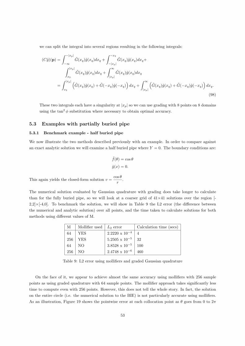
we can split the integral into several regions resulting in the following integrals:
(Cg)(p) =∫ −|xp|−∞
G(xq)g(xq)dxq +∫ −x2
−|xp|G(xq)g(xq)dxq+∫ |xp|
x2
G(xq)g(xq)dxq +∫ ∞|xp|
G(xq)g(xq)dxq
=∫ |xp|x2
(G(xq)g(xq) + G(−xq)g(−xq)
)dxq +
∫ ∞|xp|
(G(xq)g(xq) + G(−xq)g(−xq)
)dxq.
(98)
These two integrals each have a singularity at |xp| so we can use grading with 8 points on 8 domainsusing the tan2 φ substitution where necessary to obtain optimal accuracy.
5.3 Examples with partially buried pipe
5.3.1 Benchmark example - half buried pipe
We now illustrate the two methods described previously with an example. In order to compare againstan exact analytic solution we will examine a half buried pipe where Y = 0. The boundary conditions are:
f(θ) = cos θ
g(x) = 0.
This again yields the closed-form solution v =cos θr
.
The numerical solution evaluated by Gaussian quadrature with grading does take longer to calculatethan for the fully buried pipe, so we will look at a coarser grid of 41×41 solutions over the region [-2,2]×[-4,0]. To benchmark the solution, we will show in Table 9 the L2 error (the difference betweenthe numerical and analytic solution) over all points, and the time taken to calculate solutions for bothmethods using different values of M.
M Mollifier used L2 error Calculation time (secs)
64 YES 2.2220 x 10⁻⁴ 4256 YES 5.2505 x 10⁻⁵ 3264 NO 3.8528 x 10⁻⁵ 100256 NO 2.4748 x 10⁻⁶ 460
Table 9: L2 error using mollifiers and graded Gaussian quadrature
On the face of it, we appear to achieve almost the same accuracy using mollifiers with 256 samplepoints as using graded quadrature with 64 sample points. The mollifier approach takes significantly lesstime to compute even with 256 points. However, this does not tell the whole story. In fact, the solutionon the entire circle (i.e. the numerical solution to the BIE) is not particularly accurate using mollifiers.As an illustration, Figure 19 shows the pointwise error at each collocation point as θ goes from 0 to 2π
53
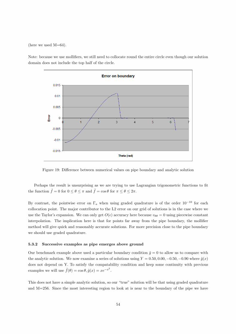
(here we used M=64).
Note: because we use mollifiers, we still need to collocate round the entire circle even though our solutiondomain does not include the top half of the circle.
Figure 19: Difference between numerical values on pipe boundary and analytic solution
Perhaps the result is unsurprising as we are trying to use Lagrangian trigonometric functions to fitthe function f = 0 for 0 ≤ θ ≤ π and f = cos θ for π ≤ θ ≤ 2π.
By contrast, the pointwise error on Γa when using graded quadrature is of the order 10−10 for eachcollocation point. The major contributor to the L2 error on our grid of solutions is in the case where weuse the Taylor’s expansion. We can only get O(ε) accuracy here because vθθ = 0 using piecewise constantinterpolation. The implication here is that for points far away from the pipe boundary, the mollifiermethod will give quick and reasonably accurate solutions. For more precision close to the pipe boundarywe should use graded quadrature.
5.3.2 Successive examples as pipe emerges above ground
Our benchmark example above used a particular boundary condition g = 0 to allow us to compare withthe analytic solution. We now examine a series of solutions using Y = 0.50, 0.00,−0.50,−0.90 where g(x)does not depend on Y. To satisfy the compatability condition and keep some continuity with previousexamples we will use f(θ) = cos θ, g(x) = xe−x
2.
This does not have a simple analytic solution, so our “true” solution will be that using graded quadratureand M=256. Since the most interesting region to look at is near to the boundary of the pipe we have
54
solved for a grid 41×41 points in the region [-1,1]×[Y-2,Y]. For each value of Y = 0.50, 0.00,−0.50,−0.90,we run the simulation using M = 64 with graded quadrature. For the case Y = 0, we compute the L2error against the “true” solution (i.e. with M = 256) which turns out to be 2.9439 × 10⁻⁵. This givesus confidence that our solutions using M = 64 will be sufficiently accurate using other values of Y. Thereason for using M = 64 is the time saving it gives us (100 secs per run rather than 460 secs).
The results of the simulations are shown in Figure 20. We can see immediately that away from thepipe boundary, we have a convergent solution; close to the boundary it is harder to discern due to thecoarseness of the grid whether the solution has converged sufficiently. Drilling down into the raw data, wecan see that the numerical solution does indeed satisfy Laplace’s Equation and the boundary conditionsto within an acceptable tolerance which suggests that the method is robust and convergent.
55
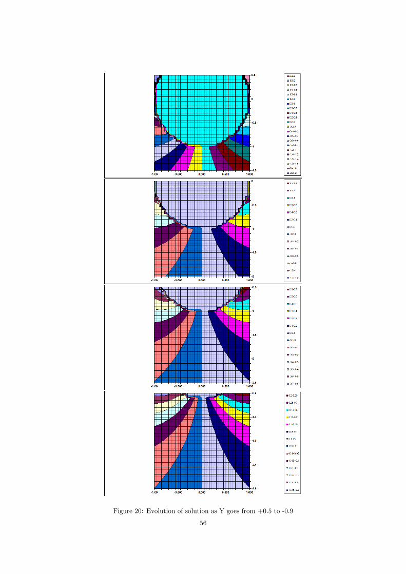
Figure 20: Evolution of solution as Y goes from +0.5 to -0.9
56
6 Conclusions
In this dissertation, we have demonstrated that the BEM is a very powerful technique to solve Laplace’sEquation, particularly in the situation where we have an infinite or semi-infinite exterior domain andNeumann boundary conditions. By comparing our solutions to known analytic solutions with certainboundary conditions we have been able to show that away from the boundary, the numerical solution us-ing BEM converges rapidly with a relatively small number of sample points. We have also illustrated twonumerical methods, Nystrom’s Method and the collocation method, where a linear system of equationscan easily be solved to give us our solution. In the case of the collocation method, we have highlighted theuse of Lagrangian trigonometric basis functions, which lend themselves very well to circular boundaries.Not only is the interpolation of solutions on the boundary smooth, but so are all their derivatives whichmeans that for 2π-periodic boundary functions, we can use the composite trapezium rule to numericallyintegrate and expect rapid (super-algebraic) convergence. These basis functions can also be of use whenconfronted with some singular integrals (e.g. logarithmic kernels), since we can evaluate these analyticallyin certain cases.
Whilst we can use these techniques to get very accurate solutions on the boundary itself, when weapproach the pipe boundary, we find that the solution converges slowly. Therefore we have developedsome alternative approaches. One simple approach is to increase the number of collocation points as weapproach the boundary. When we are extremely close to the boundary, we can use a Taylor’s expansionto get a good approximation, since we know that our solution on the boundary is accurate. We also knowthe first derivative of the solution since that is our Neumann condition, and we can derive an approximatesecond derivative from Laplace’s Equation. Both these techniques improve accuracy considerably and wedemonstrate this in §4.
Our original aim was to develop a model that could also handle a partially buried pipe. This requiresdifferent treatment to the entirely buried pipe because our boundary is not a full circle any more and thusmany of the elegant properties of the Lagrangian basis functions do not necessarily hold. We examine twodifferent approaches to try and circumvent these issues. The first approach is to evaluate the integralsover the buried part of the pipe, by integrating over the full circle and setting the boundary function to0 where the pipe is above ground. To maintain infinite differentiability we need to use mollifying func-tions. The second approach uses a more obvious method where we use piecewise constant basis functionsand Gauss-Legendre quadrature to numerically integrate over the part of the circle that is underground.Where there are singularities, we have numerically integrated using grading to minimise its effect. Bothapproaches are outlined in §5. Finally we run some simulations as the pipe emerges from the ground todemonstrate that the numerical method behaves as expected and does not “blow up”.
We have not attempted to run any real physical simulations on this model, but have demonstrated thatthe model we have implemented converges well to known analytic solutions and to simulations with largenumber of sample points and therefore should be fit for purpose when used in an industrial environment.
57
References
[1] M. Abramowitz and I. Stegun: Handbook of Mathematical Functions, Dover (2006)
[2] K. Atkinson: Numerical Solutions of Integral Equations of the Second Kind, Cambridge UniversityPress (1997)
[3] H. Bau: Cognitive Heat Losses from pipe buried in semi-infinite porous medium, International Journalof Heat and Mass Transfer, Vol 27, Issue 11, pp 2047-2056 (1984)
[4] H. Bau and S. Sadhal: Heat Losses from Fluid Flowing in a Buried Pipe, International Journal ofHeat and Mass Transfer, Vol 25, Issue 11, pp 1621-1629 (1982)
[5] W. Briggs and Van Emden Henson: The DFT - an owner’s manual for the discrete Fourier Trans-form,SIAM (1995)
[6] O. Bruno, C. Geuzaine, J. Monro, F. Reitich: Prescribed error tolerances within fixed computationaltimes for scattering problems of arbitrarily high frequency, The Royal Society, pp 629-645 (1984)
[7] M. Chung, P. Jung and R. Rangel: Semi-analytical solution for heat transfer from a buried pipewith convection on the exposed surface, International Journal of Heat and Mass Transfer, Vol 42, pp3771-3786 (1999)
[8] A. Dayan, A. Merbaum and I. Segal: Temporary Distributions around Buried Pipe Networks, Inter-national Journal of Heat and Mass Transfer, Vol 27, Issue 3, pp 409-417 (1984)
[9] P. DuChateau, D. Zachmann: Schaum’s Outline of Partial Differential Equations (1986)
[10] S. Johnson: Notes on the convergence of Trapezoidal Rule Quadrature,http://math.mit.edu/stevenj/trapezoidal.pdf (2010)
[11] R. Kress: Linear Integral Equations - Second Edition, Springer-Verlag (1999)
[12] S. Langdon: Pers. Comm. (2010)
[13] C. Ovuworie: Partially Buried Pipe Heat Transfer Presentation (2008)
[14] C. Ovuworie: Steady-State Heat Transfer Models For Fully And Partially Buried Pipelines, Societyof Petroleum Engineers (SPE) paper 131137-MS, 2010 (doi 10.2118/131137-MS)
[15] A. Sadegh, L. Jiji and S. Weinbaum: Boundary integral equation technique with application tofreezing around a buried pipe, International Journal of Heat and Mass Transfer, Vol 30, Issue 2, pp223-232 (1987)
[16] F. Scheid: Schaum’s Outline of Theory and Problems of Numerical Analysis, Second Edition (1989)
[17] I. Sloan: Error Analysis of boundary integral methods, Acta Numerica, pp 287-339 (1991)
[18] Web page: http://en.wikipedia.org/wiki/Bipolar coordinates
[19] Web page: http://en.wikipedia.org/wiki/TauTona Mine
58

[20] Web page: http://en.wikipedia.org/wiki/Two-center bipolar coordinates
[21] Web page: http://www4.ncsu.edu/ rsmith/MA573 F09/Heat Equation.pdf
59


![Design of Buried PVC Pipe[2]](https://img.pdfslide.us/doc/110x75/55cf98e2550346d0339a3cfd/design-of-buried-pvc-pipe2.jpg)