Embed Size (px)
Citation preview
NIST Technical Note 1895shy
Heat Pump Test Apparatus for the
Evaluation of Low Global Warming
Potential Refrigerants
Harrison Skye
httpdxdoiorg106028NISTTN1895
NIST Technical Note 1895
Heat Pump Test Apparatus for the
Evaluation of Low Global Warming
Potential Refrigerants
Harrison Skye Engineering Laboratory
Energy and Environment Division
This publication is available free of charge from httpdxdoiorg106028NISTTN1895
November 2015
US Department of Commerce Penny Pritzker Secretary
National Institute of Standards and Technology
Willie E May Under Secretary of Commerce for Standards and Technology and Director
Certain commercial entities equipment or materials may be identified in this
document in order to describe an experimental procedure or concept adequately
Such identification is not intended to imply recommendation or endorsement by the
National Institute of Standards and Technology nor is it intended to imply that the
entities materials or equipment are necessarily the best available for the purpose
National Institute of Standards and Technology Technical Note 1895
Natl Inst Stand Technol Tech Note 1895 48 pages (November 2015)
httpdxdoiorg106028NISTTN1895
CODEN NTNOEF
AbstractshyInternational efforts to reduce human-induced global warming include restrictions on the
use of chemicals with a high global warming potential (GWP) The heating ventilation air-
conditioning and refrigeration (HVACampR) industry subsequently faces a phasedown of many
commonly used hydrofluorocarbon (HFC) refrigerants that have a relatively high GWP A new
family of refrigerants known as hydrofluoroolefins (HFOs) including their mixtures with HFCs
show promise as replacements The overall GWP impact of refrigerant use includes both the
direct GWP related to inadvertent release of the fluid into the atmosphere as well as an indirect
GWP caused by emissions from the power source used to energize the associated HVACampR
equipment In nearly all HVACampR applications the indirect emissions far outweigh the direct
emissions so the efficiency of candidate replacements must be carefully quantified to guide the
selection of fluids that actually achieve a reduction in the overall GWP
A 34 kW (1 ton) heat pump test apparatus has been constructed and instrumented for
measuring the cycle performance of low-GWP refrigerants the description of that apparatus is
the focus of this report Details are described for the system components instrumentation data
reduction and uncertainty analysis Results from baseline experiments with R134a were used to
test and verify the apparatus and data reduction procedure The data will be used to provide a
relative comparison between the low-GWP refrigerants as quantified by metrics including
coefficient of performance and volumetric capacity
Future tests with low-GWP refrigerants will be compared with those from baseline
refrigerants R134a and R410A Additionally the test data will be used to verify a new NIST
heat pump modeling tool CYCLE_D-HX which captures both thermodynamic and heat transfer
processes in HVACampR equipment Refrigerants refrigerant mixtures and cycle configurations
that are difficult andor time consuming to test can be rapidly explored using the verified model
iishy
AcknowledgementsshyThis apparatus was constructed by John Wamsley based on the initial design by David
Yashar Dr Yashar also helped create the outline of the report which was valuable for keeping
the presentation of information organized and complete I would like to acknowledge Vance
Payne for his help in determining the operating procedures and target operating parameters
Patrick Goenner refined the instrumentation and collected early sets of data while visiting as a
guest researcher from Germany I would also like to thank Piotr Domanski and Riccardo
Brignoli for reviewing data sets and working on the CYCLE_D-HX model Thanks to Mark
Kedzierski for thoughtful insight into the calibration and uncertainty analysis for the test rig
Tara Fortin of the NIST Applied Chemicals and Materials Division performed differential
scanning calorimeter measurements of the heat transfer fluid specific heat these data were
critical for achieving an acceptable energy balance Finally I would like to thank the reviewers
for their helpful suggestions including Piotr Domanski and Amanda Pertzborn at NIST and
Steve Brown at The Catholic University of America
iiishy
Table of ContentsshyAbstract iishy
Acknowledgements iiishy
Table of Contents ivshy
List of Figures vishy
List of Tables viishy
Nomenclature viiishy
1 Introduction 1shy
2 Test Apparatus 3shy
21 Components 3shy
22 Instrumentation 11shy
23 Operation 15shy
231 Test Rig Control Parameters 15shy
232 Test Rig Operating Parameters 15shy
2321shy Operating Parameters 1 amp 2 Evaporator and Condenser Saturation Temperature 15shy
2322shy Operating Parameters 3 4 amp 5 Capacity and Heat Flux 17shy
2323shy Operating Parameters 6 amp 7 HTF-side Thermal Resistance Ratio 18shy
2324shy Operating Parameters 8 amp 9 Subcool and Superheat 18shy
2325 Operating Parameter 10 LLSL-HX included or bypassed 19shy
3 Data Analysis 20shy
31 Thermodynamic States 20shy
32 Thermodynamic Performance 20shy
321 Capacity 20shy
322 Compressor Power 21shy
323 Coefficient of Performance 22shy
324 Volumetric Capacity 22shy
325 Compressor Efficiency 22shy
326 Superheat and Subcooling 23shy
327 LLSL-HX Effectiveness 23shy
4 Validation and Baseline Tests with R134a 25shy
5 Conclusions and Future Work 28shy
6 References 29shy
iv
Appendix A Uncertainty Analysis 31shy
A1 Symbols Used in Uncertainty Analysis 31shy
A2 General Remarks 32shy
A3 Thermocouples with CJC Compensation 32shy
A4 Thermocouples with Ice-Water Bath Compensation 33shy
A5 Thermopiles in Heat Transfer Fluid 34shy
A6 Evaporator Heat Transfer Fluid Specific Heat 36shy
A7 Condenser Heat Transfer Fluid Specific Heat 37shy
A8 Evaporator and Condenser Insulation Conductance 37shy
A9 Uncertainty Analysis Software 39shy
A10 Moving Window and Steady State Uncertainty 40shy
A11 Uncertainty Results Summary 41shy
A111 Uncertainty Results Summary Cooling 41shy
A112 Uncertainty Results Summary Heating 43shy
Appendix B Instrumentation Schematic with DAQ Number Convention 46shy
Appendix C Microfin Tube Surface Area 48shy
v
List of FiguresshyFigure 2-1 Schematic of MBBHP test apparatus 5
Figure 2-2 Pictures of MBBHP apparatus 6
Figure 2-3 Pictures of MBBHP compressor (a) without and (b) with safety cage 7
Figure 2-4 Schematic showing the tube numbering convention in the (a) condenser and (b)shyevaporator 8
Figure 2-5 Schematics of annular heat exchanger including (a) refrigerant tube lengths (b)shycross section of annular heat exchanger (c) detail cross-section of microfin tube and (d) helix angle of microfins 9
Figure 2-6 Capacity and heat flux for baseline R134a tests for (a) evaporator and (b)shycondenser 18
Figure 3-1 Temperature profile in (a) evaporator showing superheat and (b) condenser showing subcooling 23
Figure 4-1 Energy imbalance in the evaporator and condenser 25
Figure 4-2 Heat pump cycle pressures on the (a) high pressure side and (b) low pressureshyside 26
Figure 4-3 Performance metrics including (a) compressor power and (b) mass flow and massshyflux 26
Figure 4-4 Performance metrics including (a) COP (b) capacity (c) volumetric capacity and (d) compressor isentropic and volumetric efficiency 27
Figure 4-5 Flow regime map for microfin tube (a) evaporation and (b) condensation 28
Figure A-1 Temperature calibration for CJC compensated thermocouples where (a) data areshy
Figure A-4 Contours of thermopile (a) uncertainty and (b) relative contribution to
Figure A-8 Uncertainty in temperature due to fluctuations at steady state for (a) evaporatorshy
divided by each of the 5 calibrations and (b) all data are combined 33
Figure A-2 Ice-water bath referenced thermocouple calibration data 34
Figure A-3 Thermopile calibration data 35
uncertainty 36
Figure A-5 Specific heat measurements for evaporator HTF 37
Figure A-6 Specific heat of condenser HTF (water) 37
Figure A-7 Insulation conductance for evaporator and condenser 39
outlet and (b) evaporator inlet 41
vishy
List of TablesshyTable 2-1 Components for MBBHP rig 10
Table 2-2 Refrigerant microfin tube specifications 11
Table 2-3 List of MBBHP instruments (SI units) 13
Table 2-4 List of MBBHP instruments (I-P units) 14
Table 2-5 List of the Control Parameters and Operating Parameters 15
Table 2-6 Evaporator and condenser fluid temperatures for standard rating tests 17
Table 3-1 Measurements and equations used to define the thermodynamic states 20
Table A-1 Condenser amp evaporator thermopile polynomial coefficients 35
Table A-2 Evaporator HTF specific heat polynomial coefficients 37
Table A-3 Uncertainty of refrigerant-side evaporator cooling capacity 42
Table A-4 Uncertainty of HTF-side evaporator cooling capacity 42
Table A-5 Uncertainty of cooling COP 43
Table A-6 Uncertainty of refrigerant-side condenser heating capacity 44
Table A-7 Uncertainty of HTF-side condenser heating capacity 44
Table A-8 Uncertainty of heating COP 45
viishy
NomenclatureshySymbol Units Definition
A m2 Area
Atotal m2 Total combined heat transfer area from evaporator and condenser
COPheat -- Coefficient of Performance - Heating
COPcool -- Coefficient of Performance - Cooling
Cp kJ kg -1 K-1 Specific heat
do mm Microfin tube outer diameter
di mm Microfin tube inner diameter
Dcomp m3 Compressor displacement
h kJ kg -1 Specific enthalpy
L m Tube length
mɺ kgs -1 Mass flow rate
N Hz Compressor frequency
Nf -- Number of microfins on inner circumference of refrigerant tube
NT -- Number of heat exchanger tubes
P kPa Pressure
∆P kPa Pressure difference
R K kW -1 Thermal resistance
Rtotal K kW -1 Total resistance in heat exchanger including both fluids and tube wall
Qɺ kW Energy transfer
Qɺ kW Energy transfer in LLSL-HX on the vapor side LLSL v
Qɺ kW Maximum possible energy transfer in LLSL-HX
LLSL max
T degC Temperature
∆T K Temperature difference
tb mm Microfin tube bottom wall thickness
sf mm Spacing between microfins
s kJ kg -1 K-1 Specific entropy
SC K Condenser subcooling
SH K Evaporator superheat
UA W K -1 Thermal conductance
v m3 kg-1 Specific volume
VCC kJ m -3 Volumetric Cooling Capacity
VHC kJ m -3 Volumetric Heating Capacity
Wɺ comp kW Compressor power computed using enthalpy change of refrigerant
Wɺ kW Compressor power computed using torque and speed of driveshaft shaft
x -- Vapor quality (mass of vapor divided by total mass of fluid)
viiishy
c
Greek
Symbol Units Definition
α deg Microfin helix angle about tube axis
β deg Microfin angle
εLLSL -- Effectiveness of the liquid-line suction-line heat exchanger
ηs -- Compressor isentropic efficiency
ηv -- Compressor volumetric efficiency
ρair kgm -3 Density of air
τ N m Compressor shaft torque
Subscript Definition
active Active refrigerant heat exchanger tubesshy
air Airshy
amb Ambient air surrounding test apparatusshy
avg Averageshy
Condenser
e Evaporator
HTF Heat Transfer Fluid
in Inlet
ins Insulation
inactive Inactive refrigerant heat exchanger tubes
out Outlet
ref Refrigerant
1 to 11 Refrigerant thermodynamic states as defined in Figure 2-1
ix
Abbreviation Definition
AHRI Air-Conditioning Heating and Refrigeration Institute
ANSI American National Standards Institute
CFC Chlorofluorocarbon
COP Coefficient of Performance (W of capacity per W of electric input)
CYCLE_D-HX A NIST heat pump cycle simulation model currently under development
The simulation captures both thermodynamic and transport processes in the
cycle
DAQ Data Acquisition
DOE Department of Energy (United States)
EER Energy Efficiency Ratio (Btu of capacity per W of electric input)
EOS Equation of State
GWP Global Warming Potential
HFC Hydrofluorocarbon
HFO Hydrofluoroolefin
HTF Heat Transfer Fluid
HVACampR Heating Ventilation Air-Conditioning and Refrigeration
LLSL-HX Liquid-Line Suction-Line Heat Exchanger
MBBHP Mini Breadboard Heat Pump
NIST National Institute of Standards and Technology (United States)
PID Proportional Integral Derivative controller
RPM Revolutions per Minute (compressor shaft)
x
1 IntroductionshyConcerns about the environmental impacts of global warming (ie global climate change)
are driving an effort to limit anthropogenic sources of atmospheric pollutants that trap longwave
radiation emitted from the earthrsquos surface The chlorinated- and fluorinated-hydrocarbon
working fluids (ie refrigerants) employed by the heating ventilation air-conditioning and
refrigeration (HVACampR) industry exhibit a particularly large global warming potential (GWP)
with 100-year GWP values hundreds to thousands of times larger than an equivalent mass of
carbon dioxide (Solomon et al 2007 p 212) In the European Union the F-gas regulation (EU
2014) mandates a phase-down of hydrofluorocarbons (HFCs) with high GWP to 21 of the
average levels from years 2009 through 2012 by 2030 The current North American proposal
would amend the Montreal Protocol to limit HFC consumption to have a weighted GWP of 15
of average levels from years 2011 through 2013 by 2036 (EPA 2015)
Major efforts are underway to identify alternative refrigerants with a lower GWP Chemical
manufacturers are proposing halogenated olefins (eg hydrofluoroolefins or HFOs) which offer
substantially lower GWP due to short atmospheric lifetimes For some HFOs the lower GWP
comes at the cost of an increase in flammability The Air-Conditioning Heating and
Refrigeration Institute (AHRI) is leading a collaborative effort to evaluate the drop-in and soft-
optimized performance of low-GWP alternatives largely consisting of HFOs and HFOHFC
blends (AHRI 2015) The National Institute of Standards and Technology (NIST) investigated
the maximum thermodynamic potential expected for working fluids by optimizing the
parameters governing the Equations of State (EOS) (Domanski et al 2014) In a companion
NIST study a coarse filter criteria was developed (based on the atomic elements GWP toxicity
flammability critical temperature and stability) to sift through the 100 million chemicals
currently listed in the public-domain PubChem database for possible low-GWP refrigerant
candidates 1234 of which were identified (Kazakov et al 2012) The candidate list was further
refined to 62 by limiting the critical temperature to the range 300 K to 400 K which is typical for
fluids in HVACampR equipment (McLinden et al 2014)
The remaining 62 candidates and their mixtures must be evaluated using more stringent
criteria that consider detailed performance in HVACampR equipment In particular the criteria
must include the cycle efficiency of the fluid since the carbon dioxide emissions from the power
source (ie ldquoindirect emissionsrdquo) far outweighs the direct GWP impact (ie the GWP from the
release of the fluid into the atmosphere) of the working fluid in nearly all HVACampR equipment
A cycle modeling tool CYCLE_D-HX is being developed at NIST to evaluate the efficiency of
low-GWP refrigerants and refrigerant mixtures The model expands upon the thermodynamic
considerations from CYCLE_D (Brown et al 2011) by including transport phenomena In this
way appropriate penalties can be applied to refrigerants whose thermodynamic properties are
favorable but exhibit poor performance in HVACampR systems because of large pressure drops or
poor heat transfer The consideration of transport processes represents a lesson learned from the
previous effort to find replacements for chlorofluorocarbon (CFC) fluids that were found to
cause stratospheric ozone destruction R410A the dominant replacement for the CFC R22 was
initially considered to be a significantly inferior replacement based on thermodynamic properties
alone However later practice showed that the lower pressure drop (due to high operating
pressure) and superior heat transfer of R410A could be exploited with optimized heat exchangers
to yield performance competitive with R22 Including transport processes also allows for the
1
optimization of mass flux the number of parallel heat exchanger tube circuits are adjusted to
balance performance enhancementdegradation of increased heat transferpressure drop with
higher mass flux The more sophisticated capabilities of the new model will allow for more
accurate identification of optimal low-GWP fluids using computational methods
A heat pump test apparatus has been constructed for the purpose of generating cycle
performance data to compare low-GWP refrigerants and to tune and verify the new NIST model
that test apparatus is the focus of this report The apparatus is highly configurable which allows
the system to operate with a wide variety of working fluids as if tailored to each one
Specifically the apparatus features a variable-speed compressor variable-area heat exchangers
and a manually adjusted throttle valve These adjustable components allow for operation at ɺconstant capacity per total combined evaporator and condenser conductance (Q UA ) across total
all test fluids a condition required for equitable comparison of refrigerants (as well as fixed heat
transfer fluid inletoutlet temperatures) (McLinden et al 1987) In practice it is difficult to hold ɺQ UA constant because the conductance depends on the refrigerant side heat transfer total
coefficient which changes for each fluid and operating condition Rather a fixed capacity per
total heat exchanger area ( Qɺ A ) is used as a close approximation For example with a fixed total
heat exchanger area Qɺ A is held constant from R134a (low volumetric capacity) to R410A total
(high volumetric capacity) by decreasing the compressor speed If adjustment of compressor
speed is insufficient to maintain constant Qɺ A between refrigerants the heat exchanger area total
can be adjusted as well The adjustability and relatively small capacity of 17 kW to 35 kW (05
ton to 1 ton) provide the etymology for the apparatus name the Mini Breadboard Heat Pump
(MBBHP) Measurements of cycle performance with legacy high-GWP HFCs and novel low-
GWP fluids in the MBBHP will provide a rich data set to test the predictive capability of the new
NIST model This report describes the construction and operation of the test apparatus the data analysis
used to quantify performance an uncertainty analysis of the performance metrics and baseline
and validation results using refrigerant R134a
2
2 Test Apparatusshy
21 Components
The test apparatus shown in Figure 2-1 through Figure 2-3 was designed to emulate
refrigerant-side operating conditions of typical HVACampR equipment (Figure B-1 and Figure B-
2 in Appendix B show the instrument numbering convention used in the raw data files) The rig
design is partially based on one used in a previous NIST effort to investigate alternatives to
CFCs (Pannock et al 1991) The refrigerant circuit includes a variable-speed compressor
powered by an electric motor and inverter where the speed controls coolingheating capacity
The evaporator and condenser shown in detail in Figure 2-4 and Figure 2-5 (a) and (b) are
single-circuit (ie there are no parallel tube branches) annular heat exchangers where the
refrigerant is on the inner tube and the liquid heat transfer fluid (HTF) is in the annular space
As shown in Figure 2-5(c) the refrigerant tube is smooth on the outside and enhanced with rifled
microfins on the inside The size of the heat exchangers can be adjusted by changing the number
of active refrigerant tubes the valves on the side of the heat exchanger allow for up to 10 (in
increments of 2) of the 20 refrigerant tubes to be bypassed (this section of the rig is referred to as
the ldquobypass valve headerrdquo) When operating these bypass valves care is taken to avoid trapping
subcooled liquid in a closed section a section completely filled with subcooled liquid will
experience a catastrophic increase in pressure if the temperature rises enough to vaporize the
refrigerant A liquid-line suction-line heat exchanger (LLSL-HX) can be included or bypassed
as needed Each of three heat exchangers (evaporator condenser and LLSL-HX) are arranged in
counterflow configuration Two sizes of manually controlled Vernier-handled needle valves are
used to throttle the refrigerant and can be used individually or in tandem the needle valve sizes
were selected using a correlation for short tubes (Kim et al 2005) A filter-dryer is used to
control contaminants and an oil separator is used to ensure proper oil return to the compressor
and to minimize oil circulation in the heat exchangers The system refrigerant charge is adjusted
using two Shrader access valves where refrigerant is removed from or added to the
liquidsuction line valves respectively Two 40 W heaters preheat the compressor before startup
to avoid foam in the oil (the heaters are turned off after the discharge temperature has warmed to
about 60 degC) A safety cage was constructed around the compressor because during cooling tests
with high pressure fluids such as R410A the compressor will be operated slightly above the
manufacturerrsquos specified maximum pressure of 2600 kPa (363 psig) Finally a series of sight
glasses provide visual confirmation of fully subcooled liquid exiting the condenser vapor only
(ie no liquid) entering the compressor suction port proper oil level in the compressor and
proper oil return from the oil separator Detailed component specifications are listed in Table
2-1 The microfin tube parameters are shown in Figure 2-5 and Table 2-2 and Appendix C
shows how the microfin surface area was calculated
The HTF circuits include a water heaterchiller to respectively control the evaporator and
condenser HTF inlet temperatures where the heaterchiller contains a pump for circulating the
fluid The evaporator HTF is a potassium formate and water solution with freeze protection
to -40 degC (-40 degF) whereas water is used for the HTF in the condenser Flow control provided
by three valves in each HTF circuit allows for a wide range of flowrates two in-line valves are
used where the largersmaller (gateneedle) valve provides grossfine flow adjustment and the
third valve bypasses the heater (or chiller) for flow and pressure control Air bubbles in the
condenser HTF circuit are controlled by drawing from the bottom of the vented chiller reservoir
3
tank The evaporator HTF circuit is pressurized with an expansion tank so air bubbles can be
removed by venting trapped air from local high spots using Shrader valves Experience
operating the test apparatus has shown that the vented reservoir tank (in the chiller) is a superior
solution for minimizing air bubbles The temperature of the fluid delivered to the heat
exchangers is regulated using proportional-integral-derivative (PID) controllers
4
Figure 2-1 Schematic of MBBHP test apparatus
5
Figure 2-2 Pictures of MBBHP apparatus
6shy
(a) (b)shy
Figure 2-3 Pictures of MBBHP compressor (a) without and (b) with safety cageshy
7shy
(a)shy (b)
Figure 2-4shy Schematic showing the tube numbering convention in the (a) condenser
and (b) evaporator
8shy
(a)shy
(b)shy (c) (d)
Figure 2-5shy Schematics of annular heat exchanger including (a) refrigerant tube
lengths (b) cross section of annular heat exchanger (c) detail cross-
section of microfin tube and (d) helix angle of microfins
9shy
Table 2-1 Components for MBBHP rig
Component Characteristics
Chiller Cooling capacity 2500 W (07 ton)
Compressor Type
Cylinders
Speed
Displacement rate
Displacement
Max pressure
Reciprocating
2
83 Hz to 667 Hz
(500 RPM to 4000 RPM)
131 m3h-1 to 1081 m3h-1
7165 cm3
2604 kPa (363 psia)
Electric motor Maximum power 373 kW (5 hp)
Expansion tank (HTF) Size 19 liter (5 gallon)
Filter (HTF) Filter size 50 microm
Filter-dryer (refrig) Line size 95 mm (0375 in)
Inverter Voltage
Maximum power
230 VAC 3-phase
373 kW (5 hp)
Heater Heating capacity 10 kW (28 ton)
Heat exchanger
(evaporatorcondenser)
Number of tubes
Tube active length
Return bend length
Outer tube ID
Outer tube OD
Outer tube material
Inner tube
10 to 20 increments of 2
560 mm (22 in)
83 mm (325 in)
254 mm (1 in)
268 mm (1125 in)
Copper
See Table 2-2
Liquid-line suction-line heat
exchanger (LLSL-HX)
Nominal capacity
Shell OD
Type
370 W (05 hp)
51 mm (2 in)
Corrugated (liquid side)
Needle valves (refrig) Valve 1
Orifice
Flow coeff (Cv)
Valve 1
142 mm (0056 in)
003
Valve 2
Orifice
Flow coeff (Cv)
Valve 2
325 mm (0128 in)
016
Needle valves (HTF) Orifice
Flow coeff (Cv)
64 mm (025 in)
073
Oil separator Diameter
Height
Capacity
102 mm (4 in)
356 mm (14 in)
10 to 17 kW (3 to 5 ton)
Pressure relief valve Cracking pressure 800 psig
Note valve orifice sizes and flow coefficients (Cv) can vary between 0 and the listed
maximum values
10
Table 2-2 Refrigerant microfin tube specifications
Parameter Symbol Value Uncertainty
Inside diameter di 846 mm (0333 in) Unknown
Outside diameter do 952 mm (0375 in) plusmn0050 mm (plusmn0002 in)
Bottom wall thickness tb 033 mm (0013 in) plusmn0025 mm (plusmn0001 in)
Fin height e 020 mm (0008 in) plusmn0025 mm (plusmn0001 in)
Spacing between fins sf 022 mm (0009 in) Unknown
Number of fins Nf 60 --
Fin angle β 60deg Unknown
Helix angle α 18deg 2deg
Internal surface area AiL 00424 m (167 in)
per unit tube length
Material Copper
22 Instrumentation
Refrigerant-side instrumentation is selected to capture the key thermodynamic state points in
the cycle Specifications for the instruments (including instrument uncertainty) in both the
refrigerant and HTF circuits are listed in Table 2-3 (Table 2-4 shows I-P units) The pressure
transducers and in-stream thermocouple probes are numbered in Figure 2-1 according to the
eleven states computed in Section 31 the thermodynamic state number convention is also
consistent with that used in the new CYCLE_D-HX model The thermocouple probes are
referenced to a cold junction in an ice-water bath Differential pressure transducers quantify the
pressure drop in the condenser evaporator and suction line The location of the heat exchanger
pressure taps has been selected at the bottom of the bypass valve header where the pressure is
equal to that of the refrigerant leaving the heat exchanger regardless of how many tubes are
bypassed A coriolis flowmeter measures the refrigerant mass flow and density and provides
confirmation of fully subcooled liquid in the liquid line (a two-phase mixture will exhibit large
oscillations in measured flowrate) The compressor shaft power is captured by the in-line torque
meter and tachometer
On the HTF fluid side energy transfers are measured in the evaporator and condenser to
provide verification of the refrigerant-side calculations The mass flow and temperature
difference in the heat exchangers are measured with coriolis meters and thermopiles (in
thermowells) which are combined with the fluid heat capacity to compute energy transfer
Thermocouples inserted into the thermowells with the thermopiles provide the measure of
absolute temperature required for applying the thermopile calibration Additionally the
thermocouples provide verification of the thermopile temperature difference measurement
Figure 2-1 and Figure 2-4 also show the tube-surface-mounted thermocouples used to
measure both refrigerant and HTF temperature profiles in the evaporator and condenser As
shown in Section 326 these temperature profiles are useful for determining refrigerant tube
11
number where the phase transitions (superheat subcooling two-phase) occur The refrigerant-
and HTF-side sensors are mounted on the return bends of each innerouter tube respectively
The instruments are scanned once per minute by the data acquisition (DAQ) system and
when steady state is achieved the measurements are calculated as the average of a moving
window of 30 readings (ie the average over the last 30 minutes) The measurements inevitably
fluctuate during steady state which contributes to the uncertainty of the measurement This
ldquosteady staterdquo uncertainty has been quantified for a nominal test condition and is listed in Table
2-3 The total measurement uncertainty (last column of Table 2-3) is found by adding the
instrument error and the steady state error in quadrature A detailed discussion of the selection
of the steady state moving window size and computation of steady state uncertainty is shown in
Appendix A10
12
Table 2-3 List of MBBHP instruments (SI units)
Instrument Range
Instrument
Uncertainty1
Steady State
Uncertainty1
Total
Uncertainty12
Coriolis meter (HTF) Mass flow
(0 to 756) gs -1
Mass flow 3
plusmn01 rdg
Mass flow
plusmn023 gs -1
Mass flow
plusmn026 gs -1
Density
(0 to 3) g cm-3
Density
plusmn0001 gcm-3
Density
plusmn00001 gcm-3
Density
plusmn0001 gcm-3
Coriolis meter (refrigerant) Mass flow Mass flow 4 Mass flow Mass flow
(0 to 60)5 gs -1 plusmn01 rdg plusmn001 gs-1 plusmn0016 gs -1
Density Density Density Density
(0 to 3) g cm-3 plusmn00005 gcm-3 plusmn00001 gcm-3 plusmn00005 gcm-3
Data acquisition system (-10 to 10) V plusmn1 microV -- plusmn1 microV
Press transducer (diff) ndash condenser (0 to 172) kPa plusmn07 kPa plusmn08 kPa plusmn13 kPa
Press transducer (diff) ndash evaporator (0 to 345) kPa plusmn01 kPa plusmn08 kPa plusmn08 kPa
Press transducer (diff) ndash suction (0 to 69) kPa plusmn001 kPa plusmn03 kPa plusmn03 kPa
Press transducer (high press) (0 to 3447) kPa plusmn34 kPa plusmn07 kPa plusmn35 kPa
Press transducer (low press) (0 to 1724) kPa plusmn34 kPa plusmn07 kPa plusmn35 kPa
Tachometer (017 to 1667) Hz plusmn00167 Hz plusmn0005 Hz plusmn00173 Hz
(10 to 99 999) RPM plusmn1 RPM plusmn03 RPM plusmn104 RPM
Thermocouple (in-stream probe ice ref) (-10 to 100) degC plusmn008 degC plusmn006 degC plusmn009 degC
Thermocouple (surface-mount CJC) (-10 to 60) degC plusmn06 degC plusmn004 degC plusmn06 degC
Thermopile5 (1 to 10) K plusmn0015 K plusmn0013 K plusmn00153 K
Thermopile voltage (-10 to 10) V plusmn1 microV plusmn65 microV plusmn7 microV
Torque meter (0 to 40) N m plusmn033 Nm plusmn0005 Nm 033 Nm
1 95 confidence interval (k = 2)shy2 rdg values have been applied to nominal valuesshy3 Maximum of 01 and (zsflowrate)100 where zs is zero stability = 00491 g s -1 shy4 Maximum of 01 and (zsflowrate)100 where zs is zero stability = 00075 g s -1 shy5 For temperature differences in 1 K to 10 K range Outside range uncertainty is higher See Appendix A5 for moreshydetail
13
Table 2-4 List of MBBHP instruments (I-P units)
Instrument Range
Instrument
Uncertainty1
Steady State
Uncertainty1
Total
Uncertainty12
Coriolis meter (HTF) Mass flow
(0 to 100) lb min-1
Mass flow 3
plusmn01 rdg
Mass flow
plusmn003 lb min-1
Mass flow
plusmn0035 lb min-1
Density
(0 to 187) lb ft-3
Density
plusmn0062 lb ft-3
Density
plusmn0006 lb ft-3
Density
plusmn0062 lb ft-3
Coriolis meter (refrigerant) Mass flow Mass flow 4 Mass flow Mass flow
(0 to 799) lb min-1 plusmn01 rdg plusmn00015 lb min-1 plusmn0002 lb min-1
Density Density Density Density
(0 to 187) lb ft-3 plusmn0062 lb ft-3 plusmn0006 lb ft-3 plusmn0062 lb ft-3
Data acquisition system (-10 to 10) V plusmn1 microV -- plusmn1 microV
Press transducer (diff) ndash condenser (0 to 25) psi plusmn01 psi plusmn01 psi plusmn018 psi
Press transducer (diff) ndash evaporator (0 to 50) psi plusmn0015 psi plusmn01 psi plusmn01 psi
Press transducer (diff) ndash suction (0 to 10) psi plusmn00015 psi plusmn004 psi plusmn004 psi
Press transducer (high press) (0 to 500) psia plusmn05 psi plusmn01 psi plusmn051 psi
Press transducer (low press) (0 to 250) psia plusmn05 psi plusmn01 psi plusmn051 psi
Tachometer (017 to 1667) Hz plusmn00167 Hz plusmn0005 Hz plusmn00173 Hz
(10 to 99 999) RPM plusmn1 RPM plusmn03 RPM plusmn104 RPM
Thermocouple (in-stream probe ice ref) (14 to 212) degF plusmn015 degF plusmn011 degF plusmn018 degF
Thermocouple (surface-mount CJC) (14 to 140) degF plusmn11 degF plusmn008 degF plusmn11 degF
Thermopile5 (18 to 18) degF plusmn0027 degF plusmn0023 degF plusmn004 degF
Torque meter (0 to 350) in lb plusmn29 in lb plusmn0045 in lb plusmn29 in lb
1 95 confidence interval (k = 2) 2 rdg values have been applied to nominal values 3 Maximum of 01 and (zsflowrate)100 where zs is zero stability = 00065 lb min-1
4 Maximum of 01 and (zsflowrate)100 where zs is zero stability = 0001 lb min-1
5 For temperature differences in 18 degF to 18 degF range Outside range uncertainty is higher See Appendix A5 for more
detail
14
23 Operation
231 Test Rig Control Parameters
There are ten Control Parameters (ie settings of adjustable components) listed in Table 2-5
that the MBBHP operator sets to achieve a desired set of Operating Parameters Each Control
Parameter primarily governs one or two Operating Parameters the correspondence is shown in
the table
Table 2-5 List of the Control Parameters and Operating Parameters
Operating Parameter Operating Parameter Values Control Parameter
1 Evaporator saturation temperature See Table 2-6 Heater setpoint (HTF inlet temp)
2 Condenser saturation temperature See Table 2-6 Chiller setpoint (HTF inlet temp)
3 Capacityheat flux 1760 W to 3520 W Compressor speed
(05 ton to 1 ton)
4 Evaporator heat flux 2000 W m-2 to 12 000 W m-2 Number of evaporator tubes
(600 Btu h-1 ft-2 to 3800 Btu h-1 ft-2)
5 Condenser heat flux 2000 W m-2 to 12 000 W m-2 Number of condenser tubes
(600 Btu h-1 ft-2 to 3800 Btu h-1 ft-2)
6 Condenser HTF-side resistance 50 to 70 of overall resistance Condenser HTF flowrate
7 Evaporator HTF-side resistance 70 to 85 of overall resistance Evaporator HTF flowrate
8 Subcool Superheat le 2 tubes1 le 1 tube2 Refrigerant needle valve setting
9 Subcool Superheat le 2 tubes1 le 1 tube2 Refrigerant charge
10 LLSL-HX includedbypassed Includedbypassed LLSL-HX valves
1achieved with subcooling of 2 K to 3 K (18 degF to 36 degF) 2achieved with superheat of 3 K to 6 K (54 degF to 108 degF)
232 Test Rig Operating Parameters
This section describes each of the target Operating Parameters and how they are set using
the Control Parameters Note that the headings for Sections 2321 through 2325 include the
Operating Parameters numbers (1 to 10) as listed in Table 2-5
2321 Operating Parameters 1 amp 2 Evaporator and Condenser Saturation Temperature
The US Department of Energy (DOE) requires heat pumps and air conditioners to be rated
at conditions prescribed in the ANSIAHRI 210240-2008 (AHRI 2008) standard The standard
specifies temperatures of the HTF (air in the standard) entering the evaporator and condenser A
somewhat different but derivative method is employed here the HTF inlet temperatures are set
to achieve refrigerant saturation temperatures expected under ANSIAHRI Cooling A Cooling B
and Heating H1 Rating Tests for the baseline refrigerant R134a
The target saturation temperatures are computed first for the Cooling A test where the
assumed Coefficient of Performance (COPcool) is 44 (energy efficiency ratio EER is 15) The
15
ANSIAHRI standard is not prescriptive about airflow so typical values per unit evaporator ɺcapacity are used for the evaporator (Vɺ Qevap ) 0189 m3 s-1 kW-1 (400 ft3 min-1 ton-1) and air evap
ɺfor the condenser (Vɺ Qevap ) 0378 m3 s-1 kW-1 (800 ft3 min-1 ton-1) Inlet air temperatures air cond
(Tairin) prescribed by the ANSIAHRI standard are listed in Table 2-6 the temperature change
across the evaporator and condenser (∆Tairevap ∆Taircond) is 126 K and 97 K (228 degF and 175
degF) respectively as computed using an energy balance on the airstream where the condenser
energy is larger by an amount that reflects the compressor power (in the COP term)
ɺ )minus1 1ɺ= V (21) ∆Tair evap ( air evap Qevap ρ Cair p air
minus 1 1ɺ Qɺ evap )
1
1+ (22) ∆T = Vair cond ( air cond COP ρ C cool air p air
where the variables represent
Cpair = specific heat of air at constant pressure
ɺV Qɺ evap = condenser airflow per unit evaporator capacity air cond
ɺV Qɺ evap = evaporator airflow per unit evaporator capacity air evap
ρair = density of air
The air outlet temperatures (Tairout) are then computed by respectively subtracting or adding the
∆Tairevap ∆Taircond from the Tairin values
The average temperature difference between the refrigerant and the air (∆Tairref) for
Cooling A is specified as 10 K and 33 K (18 degF and 6 degF) in the evaporator and condenser
respectively based on experience and measurements at NIST for air-source heat pumps with comparable COPs Table 2-6 shows the average air (Tairavg) and average refrigerant saturation
temperatures (Trefavg) computed using this method The Cooling B refrigerant saturation
temperatures are computed using the same ∆Tair and ∆Tairref In heating the heat exchangers
operating as the evaporatorcondenser swap so the values of ∆Tair and ∆Tairref for the evaporator
(in cooling) are used for the condenser and vice versa The resulting refrigerant saturation
temperatures are nominally aligned with values observed in heat pump measurements at NIST
The HTF inlet temperatures (THTFin) are adjusted to achieve the target refrigeration saturation
temperature at a compressor speed of 30 Hz (1800 RPM) with R134a and then held constant for
all other speeds The corresponding HTF outlet temperatures (THTFout) are defined as
T = T + ∆ T (21) HTF e in HTF e out e
T = T + ∆ T (22) HTF c in HTF c out c
where ∆Te and ∆Tc are the HTF temperature differences across the evaporatorcondenser
measured by the thermopiles The THTFout values differ for each speed Table 2-6 shows the
values at 30 Hz (1800 RPM) as a nominal example As discussed in Section 1 a completely fair
comparison of refrigerants requires the same HTF inlet and outlet temperatures (McLinden et al
1987) However it is only possible to match either the evaporator or condenser (but not both)
THTFout by adjusting the heat pump capacity (via compressor speed) the other THTFout will be an
16
uncontrolled value which will vary somewhat from the R134a value depending on the COP of
each fluid (note the HTF mass flow rate is fixed as described in Section 2323 so it cannot be
adjusted to control the other THTFout) Tests with future refrigerants will be carried out with an
evaporator or condenser THTFout equal to the measurements for R134a in cooling or heating
respectively and the other THTFout will vary for each fluid
Table 2-6 Evaporator and condenser fluid temperatures for standard rating tests
Rating Test
Tairin
degC
(degF)
∆Tair
K
(degF)
Tairout
degC
(degF)
Tairavg
degC
(degF)
∆Tairref
K
(degF)
Trefavg
degC
(degF)
THTFin
degC
(degF)
THTFout 1
degC
(degF)
HTFmɺ kg s-1
lb min-1
Cooling A 350 97 447 399 33 432 339 391 0098
(950) (175) (1125) (1038) (60) (1098) (930) (1024) (13)
Condenser Cooling B 278 97 375 326 33 360 249 309 0098
(820) (175) (995) (908) (60) (968) (767) (876) (13)
Heating H1 211 126 338 274 100 374 320 363 0098
(700) (228) (928) (814) (180) (994) (895) (973) (13)
Cooling A 267
(800)
126
(228)
140
(573)
203
(686)
100
(180)
103
(506)
202
(685)
154
(597)
0131
(173)
Evaporator Cooling B
Heating H1
267
(800)
126
(228)
140
(573)
203
(686)
100
(180)
103
(506)
199
(678)
142
(576)
0131
(173)
83 97 -14 35 33 01 103 65 0131
(470) (175) (295) (383) (60) (323) (505) (437) (173)
1 Values for R134a at a compressor speed of 30 Hz (1800 RPM)
2322 Operating Parameters 3 4 amp 5 Capacity and Heat Flux
Baseline capacities were established for R134a at speeds of 233 Hz to 367 Hz (1400 RPM to
2200 RPM) in 33 Hz (200 RPM) increments for each Rating Test Tests with subsequent
refrigerants will be carried out with compressor speeds that match the capacities from the ɺbaseline tests this ensures the refrigerants are tested at the same Q A The target refrigerant-total
side heat flux range was 2 kW m-2 to 12 kW m-2 (600 Btu h-1 ft-2 to 3800 Btu h-1 ft-2) to coincide
with values from typical HVACampR equipment The average heat flux in the evaporator and
condenser was controlled by setting the number of active tubes to 10 and 12 respectively
Figure 2-6 summarizes the capacity for the baseline tests where the evaporator capacity varies
from 12 kW to 21 kW (034 ton to 060 ton) and condenser capacity ranges from 16 kW to 28
kW (045 ton to 080 ton) The heat flux in the evaporator varies from 5 kW m-2 to 9 kW m-2
(1600 Btu h-1 ft-2 to 2900 Btu h-1 ft-2) and in the condenser from 5 kW m-2 to 10 kW m-2 (1700
Btu h-1 ft-2 to 3200 Btu h-1 ft-2) meeting the target heat flux range
17shy
heat transfer area = 0237 m
14
16
20
70
77
84
91
22 94 28
20 25 30 35 40
Cooling B
Cooling A
Heating H1
Evaporator
2
f luid = R134a
tubes = 10
98
20 25 30 35 40
Cooling B
Cooling A
Heating H1
Condenser
heat transfer area = 0285 m2
f luid = R134a
tubes = 12
26 85
Avera
ge
heat
flu
x
[kW
m2]
Cap
acit
y
[kW
]
Avera
ge h
eat
flu
x
[Wm
2]
Cap
acit
y
[kW
] 24
22
20
18shy 76
68
18 60
16
12 51
Compressor frequency [Hz] Compressor frequency [Hz]
(a) (b)
Figure 2-6shy Capacity and heat flux for baseline R134a tests for (a) evaporator and (b)
condenser
2323 Operating Parameters 6 amp 7 HTF-side Thermal Resistance Ratio
In typical air-to-air heat pumps the air-side convection provides the majority of the
resistance to heat transfer Evaporation heat transfer coefficients are generally larger than those
for condensation so the HTF-side resistance ratio (RHTFRtotal) is selected in the range of 50 to
70 for the condenser and 70 to 85 in the evaporator The CYCLE_D-HX model reports
heat exchanger thermal resistances for both the evaporator and condenser when given
measurements of HTF inout temperatures capacity compressor efficiency and heat exchanger
geometry pressure drop and log-mean temperature difference These resistances include the
heat exchanger total conductance (UA) (the total resistance Rtotal is the inverse of UA) the heat
transfer-side resistance (RHTF) in the evaporatorcondenser and the refrigerant-side thermal
resistance (Rref) in the evaporatorcondenser Note that the tube wall thermal resistance is
neglected
The MBBHP was operated under varied HTF flowrates ( mɺ HTF ) and the resulting data were
processed using the CYCLE_D-HX model to determine RHTFRtotal for each flowrate The
evaporator and condenser HTF flowrates used for the tests are 0131 kgs-1 and 0098 kgs-1 (173
lb min-1 and 13 lb min-1) as shown in Table 2-6 which yield RHTFRtotal of 80 and 60 for the
baseline Cooling A test with R134a at 30 Hz (1800 RPM) The flowrates are kept constant for
all other speeds test conditions and refrigerants Maintaining a constant flowrate is important
for verifying the CYCLE_D-HX model the model evaluates the HTF-side thermal resistance for
a reference data set and then holds this resistance constant as other operating parameters
refrigerants and tube circuit configurations are computationally explored
2324 Operating Parameters 8 amp 9 Subcool and Superheat
The number of evaporator tubes containing superheated-vapor and condenser tubes with
subcooled-liquid are controlled to one and two respectively It is important to limit the number
of tubes in superheat and subcooling for comparison with the CYCLE_D-HX model because the
18shy
56
63
model does not consider the pressure drop or area required for heat transfer in these sections
rather it only accounts for transport phenomena in the two-phase section (Note that the
superheat and subcooling are included as an input to the model to determine the thermodynamic
states at the heat exchanger outlets) The superheat and subcooling are also limited because of
performance considerations the single phase fluid exhibits a lower heat transfer coefficient
compared to a two-phase fluid The superheat is bound at the low end by the need to prevent
liquid from entering the compressor The lower limit for subcooling is governed by a
requirement of fully subcooled liquid entering the expansion valve vapor bubbles entering the
expansion valve cause oscillations in the flow that make it difficult to achieve steady state In
general a superheat range of 3 K to 6 K and a subcooling range of 2 K to 3 K satisfies this
Operating Parameter requirement
Closing the refrigerant needle valve increases the superheat and the subcooling whereas
adding refrigerant increases the subcooling and reduces the superheat The combination of these
two controls allows for independent regulation of superheat and subcooling
2325 Operating Parameter 10 LLSL-HX included or bypassed
The LLSL-HX heat exchanger is included or bypassed using the six valves shown in Figure
2-1 When the LLSL-HX is bypassed only one (rather than both) of the valves that stops flow
through the heat exchanger is closed this prevents the possibility of trapping subcooled liquid
between the valves (and presenting the same pressure hazard discussed in Section 21
19shy
3 Data Analysisshy
31 Thermodynamic States
The thermodynamic states numbered 1 through 11 in Figure 2-1 are fixed with two intensive
properties defined by the measurements and equations presented in Table 3-1 Thermodynamic
property data for R134a are computed using the Engineering Equation Solver (EES) software
(Klein 2015) the software uses the equation of state developed by Tilner-Roth et al (1994) for
R134a Note that property data for mixtures and for fluids not directly available in EES will be
computed using the NIST REFPROP database (Lemmon et al 2013)
Table 3-1 Measurements and equations used to define the thermodynamic states
State Description Measurement Equations
1 Compressor inlet LLSL-HX vapor outlet T1 P1 = P11 ndash ∆Ps
2 Compressor cylinder before compression T2 = T1 P2 = P1
3 Compressor outlet T3 P3 = P4
4 Condenser inlet T4 P4 = P7 + ∆Pc
5 Condenser saturated vapor P5 = P4 x5 = 1
6 Condenser saturated liquid P6 = P7 x6 = 0
7 Condenser outlet LLSL-HX liquid inlet T7 P7
8 Expansion valve inlet LLSL-HX liquid outlet T8 P8 = P7
9 Evaporator inlet Expansion valve outlet P9 h9 = h8
10 Evaporator saturated vapor P10 = P11 x10 = 1
11 Evaporator outlet LLSL-HX vapor inlet T11 P11 = P9 ndash ∆Pe
T = temperature P = pressure h = enthalpy x = thermodynamic quality
32 Thermodynamic Performance
Given the fixed state points identified in Table 3-1 (and all associated intensive properties)
the key thermodynamic performance metrics are calculated according to the equations in
Sections 321 through 327 Nominal values and uncertainties of the metrics are shown in
Section 4 and Appendix A respectively
321 Capacity
The evaporator and condenser capacities are computed on the refrigerantHTF-sides
according to
ɺQ = mɺ (h minus h ) (31) ref 4c ref 7
ɺQ = mɺ (h minus h ) (32) ref 9e ref 11
Qɺ = mɺ C ∆T minus Qɺ (33) c HTF HTF c c ins c p HTF c
20shy
ɺQɺ = mɺ C ∆T minus Q (34) p HTF e e HTF HTF e e ins e
where the variables represent
mɺ ref = mass flow of refrigerant
mɺ HTF e mɺ HTF c = mass flow of HTF in evaporatorcondenser
C C = specific heats (average) of HTF in evaporatorcondenser pHTFe pHTFc
ɺQins e Qɺ = insulation heat leak in evaporatorcondenser ins c
∆Te ∆Tc = temperature change of HTF in evaporatorcondenser
The insulation heat leak is a non-trivial 30 W to 50 W and therefore must be accounted for in the
heat exchanger capacity The heat leak is debited from the HTF-side capacity because the HTF
is the annulus and therefore thermally interacts with the surrounding ambient air The heat
exchangers are divided into active and inactive sections (ie tubes where the HTF flows but the
refrigerant does and does not respectively) to compute the heat leak according to
NT NT e active e inactive ɺQ = UA (T minusT ) + (T minusT ) (35) ins e HTF e active avg HTF e inactive avg ins e amb e amb e NT NT e total e total
NT NT c active c inactive
Qɺ = UA ins c (THTF c active avg minusTamb c ) + (T minusTamb c ) (36) ins c HTF c inactive avg NT NT c total c total
where
UAinse UAinsc = insulation conductance for evaporatorcondenser
NTetotal NTetotal = number of tubes in evaporatorcondenser total (20)
NTeactive NTcactive = number of active tubes in evaporatorcondenser
NTeinactive NTeinactive = number of inactive tubes in evaporatorcondenser
THTFeactiveavg THTFcactiveavg = avg HTF temp in the active evaporatorcondenser tubes
THTFeinactiveavg THTFcinactiveavg = avg HTF temp in the inactive evaporatorcondenser tubes
Tambe Tambc = temp of ambient air surrounding evaporatorcondenser
The HTF temperatures are taken from the surface-mounted thermocouples and the ambient air
temperature is taken from a thermocouple near each of the heat exchangers The heat exchangers
are split into activeinactive sections because the slope of the HTF temperature profile is
different in each section the heat transfer is only governed by the average temperature difference
if the slopes (and specific heats) are constant throughout the section The UAinse and UAinsc
values for all 20 tubes are 548 W K-1 plusmn031 W K-1 and 652 W K-1 plusmn041 WK-1 (104 Btu h-1 degF-1
plusmn059 Btu h-1 degF-1 and 124 Btu h-1 degF-1 plusmn078 Btu h-1 degF-1) The method used to compute the
conductance values and their uncertainties is described in Appendix A8
322 Compressor Power
The compressor power is computed using the change in enthalpy across the compressor
21shy
ɺW = ɺ h comp mref ( 3 minus h1 ) (37)
The shaft power is computed for comparison with the compressor power
ɺW = 2πτ N (38) shaft
where the variables represent
N = compressor shaft speed
τ = compressor shaft torque
323 Coefficient of Performance
The cooling and heating COP are computed using the refrigerant-side capacity and the
compressor power applied to the refrigerant
ɺCOP = Qɺ Wcomp (39) cool e ref
ɺ= QCOPheat ɺ
Wcomp (310) c ref
324 Volumetric Capacity
The volumetric cooling and heating capacity (VCC and VHC) are
(mɺ ref v ) (311) VCC = Qɺ
e ref 1
ɺ ( mɺ ref v ) (312) VHC = Q
c ref 1
where
v1 = compressor suction specific volume
325 Compressor Efficiency
The compressor isentropic efficiency is calculated asshy
h ( P s ) minus h3 1 1η s = (313) h minus
3 h
1
where
h(P3s1) = compressor discharge enthalpy under isentropic compression
The volumetric efficiency is quantified by the refrigerant displacement normalized by the
compressor swept volume displacement
mɺ vref 1η v = (314) D N comp
where
22shy
Dcomp = compressor displacement (listed in Table 2-1)
326 Superheat and Subcooling
The evaporator superheat is
SH = T minusT ( P x = 1) (315) 11 11
and the condenser subcooling is
SC = T (P7 x = 0) minusT7shy (316)
where
T(P11 x = 1) = saturated vapor temperature at the evaporator exit pressureshy
T(P7 x = 0) = saturated liquid temperature at the condenser exit pressureshy
The number of refrigerant tubes containing superheatedsubcooled fluid in the
evaporatorcondenser is controlled to one and two respectively during experimental tests
Visual inspection of the temperature profile such as the one shown in Figure 3-1 is used to
determine the locations of the various phase transitions The tube number on the x-axis reflects
the convention established in Figure 2-5
(a)shy (b)
Figure 3-1shy Temperature profile in (a) evaporator showing superheat and (b)
condenser showing subcooling
The location 21 is the exit of the 20th tube
327 LLSL-HX Effectiveness
The LLSL-HX effectiveness is computed as the ratio of the heat transferred on the vapor
23shy
side ( Qɺ ) to the maximum possible heat transfer LLSL v
ɺQ C (T minus T )LLSL v 111 11 p avg 1ε = = (317) ɺLLSL
Q MIN( C C ) (T minus T )LLSL max p avg 111 78 7p avg 11
where
Cpavg111 = average specific heats of the refrigerant on the vapor sideshyCpavg78 = average specific heats of the refrigerant on the liquid sideshy
The heat transfer on the vapor side rather than liquid side is chosen for the numerator because
the larger temperature difference exhibited on the vapor side (due to lower specific heat) results
in a smaller uncertainty in the effectiveness
24shy
4 Validation and Baseline Tests with R134ashyAn initial set of tests were carried out with R134a to provide verification of the
instrumentation and show the nominal uncertainties of the measurements One of the most
important validations is to show an energy balance between the refrigerant and the HTF in the ɺ ɺheat exchangers The energy imbalance defined as Qɺ
ref (Qref minus Q
HTF ) for the initial tests is
shown in Figure 4-1 the imbalance is generally around 1 to 15 or better in both the
evaporator and condenser The imbalance falls well within its uncertainty at the 95
confidence interval indicating that the estimation of the uncertainty in HTF capacity (3 ) is
likely too conservative note that the HTF capacity accounts for more than 90 of the relative
uncertainty in the imbalance metric
Figure 4-1 Energy imbalance in the evaporator and condenser
The performance of R134a in the MBBHP as described by the metrics defined in Section
32 are presented in Figure 4-2 through Figure 4-4 Figure 4-2 (a) and (b) show nominal
pressure profiles on the lowhigh pressure sides of the cycle where the error bars represent
measurement uncertainty listed in Table 2-3 The compressor power measured both by the shaft
power and change of enthalpy of the working fluid are shown in Figure 4-3(a) where the
conversion from mechanical to fluid power is about 65 efficient The error bars represent the
uncertainty calculated by propagating measurement uncertainty through Eqs (37) and (38)
The mass flow ranges from 8 gs-1 to 13 gs-1 (11 lb min-1 to 17 lb min-1) Figure 4-4 shows the
COP ranges from 24 to 4 and the capacity ranges from 16 kW to 21 kW (045 ton to 060 ton)
The figure shows the uncertainties of the COP and capacity where the computation and
tabulation of uncertainty is described further in Appendix A10 and A11 The volumetric
capacity ranges from 2100 kJ m-3 to 2800 kJ m-3 (56 Btu ft-3 to 75 Btu ft-3) and the compressor
isentropic and volumetric efficiencies are nominally 046 and 055 uncertainties in all three of
these metrics are shown in the figures and are computed using a similar method as the
capacityCOP but the computation is not discussed in detail in this report
Figure 4-3 (b) also shows the mass flux which is used to determine the two-phase flow
regimes indicated in Figure 4-5 The refrigerant generally entered the annular flow regime in the
evaporator and condenser though for some tests with low mass flux the refrigerant never left the
stratified-wavy regime
25shy
1100
1150
1200 450 C
om
pre
sso
r p
ow
er
[kW
]shy
Pre
ssu
re [
kP
a]
evaporator tubes = 10
condenser tubes = 12
f luid = R134a
LLSL-HX = no
condenser outlet (P7)
rating test = cooling A
condenser inlet (P4)
Pre
ssu
re [
kP
a]
20 25 30 35 40
Compressor frequency [Hz]
evaporator tubes = 10
condenser tubes = 12
f luid = R134a
LLSL-HX = no
evaporator outlet (P11)
compressor suction (P1)
rating test = cooling A
evaporator inlet (P9)
400
350
1050 300
20 25 30 35 40
Compressor frequency [Hz]
(a)shy (b)
Figure 4-2shy Heat pump cycle pressures on the (a) low pressure side and (b) highshypressure sideshy
0013 12
20 25 30 35 40
Compressor frequency [Hz]
evaporator tubes = 10
condenser tubes = 12
f luid = R134a
LLSL-HX = no
cooling A
cooling B
heating H1
pow er to w orking f luid (Wcomp)
shaft pow er (Wshaf t)
Mass
flo
w [
kg
s]
20 25 30 35 40
evaporator tubes = 10
condenser tubes = 12
f luid = R134a
LLSL-HX = no
cooling A
cooling B
heating H1
0012
Mass
flu
x [
kg
s-m
2]
200 09 0011
180 001
06
0009
0008 03
Compressor frequency [Hz]
(a)shy (b)
Figure 4-3shy Performance metrics including (a) compressor power and (b) mass flow and
mass flux
26shy
140
160
220
Vo
lum
etr
ic c
ap
acit
y [
kJm
3]
CO
P
Vo
lum
etr
ic e
ffic
ien
cy
(η
v)
(a) (b)
20 25 30 35 40 2
25
3
35
4
45
Compressor frequency [Hz]
evaporator tubes = 10
condenser tubes = 12
cooling A
cooling B
heating H1
f luid = R134a
LLSL-HX = no
20 25 30 35 40 15
16
17
18
19
2
21
Compressor frequency [Hz] C
ap
acit
y [
kW
]
cooling A
cooling B
heating H1
evaporator tubes = 10
condenser tubes = 12
fluid = R134a
LLSL-HX = no
2800 07 07
evaporator tubes = 10
condenser tubes = 12
fluid = R134a
LLSL-HX = no
cooling A
cooling B
heating H1
20 25 30 35 40 04
05
06
03
04
05
06
evaporator tubes = 10
condenser tubes = 12
fluid = R134a
LLSL-HX = no
cooling A
cooling B
heating H1
cooling B
cooling A
heating H1
2600
2400
2200
Isen
tro
pic
eff
icie
ncy
( η
s)
20 2000
25 30
Compressor frequency
35
[Hz]
40
Compressor frequency [Hz]
(c) (d)
Figure 4-4 Performance metrics including (a) COP (b) capacity (c) volumetric
capacity and (d) compressor isentropic and volumetric efficiency
27shy
50
Flow boiling with microfin tubeshy Flow condensing with microfin tube 350 350
300 300
S
heat flux 70 kWm2
=
= A
I
SG
S+SW
D
Tsat = 8 C
fluid = R134a
flow range during tests
M
SW
=
Tsat 43 C
fluid = R134a
heat flux 77 kWm2
flow range during tests
A
I
SG
S SW+
SW
0
50
S
Mass F
lux [
kg
s-m
2]
250
200
150
100
Mass F
lux [
kg
s-m
2]
250
200
150
100
0 0shy 02 04 06 08 1 0 02 04 06 08 1
Vapor quality Vapor quality A = Annular D = Dryout I = Intermittant M = Mist A = Annular D = Dryout I = Intermittant M = Mist
S = Stratified SG = Slug SW = Stratified-Wavy S = Stratified SG = Slug SW = Stratified-Wavy
(a)13shy (b)23
Figure 4-5shy Flow regime map for microfin tube (a) evaporation and (b) condensation
1 Flow boiling regime map from (Wojtan et al 2005)shy2 Flow condensation regime map from (Hajal et al 2003)shy3 Boundary between IntermittentAnnular regimes from (Thome 2007) using equation 1261 with a coefficientshy
of 0678 for helical microfins
5 Conclusions and Future Work
This report shows that the test apparatus is capable of measuring the performance of
low-GWP refrigerants with high fidelity including less than 05 uncertainty in both capacity
and COP The energy balance closure on the evaporator and condenser was better than 15
and will be continually tracked to ensure continued high quality data are collected
Future tests will include a second baseline refrigerant R410A followed by a series of
comparative tests with low-GWP refrigerants and refrigerant mixtures The HTF flowrates will
remain fixed from the R134a baseline tests so that the CYCLE_D-HX simulations of the test
data can be carried out for all test data based on a single reference data set After the model
results are verified the model will be used to identify additional candidate refrigerants to test in
the MBBHP test apparatus
28shy
6 ReferencesshyAHRI (2008) 2008 Standard for Performance Rating of Unitary Air-Conditioning amp Air-
Source Heat Pump Equipment Air-Conditioning Heating and Refrigeration Institute
Arlington VA United States Retrieved from wwwahrinetorg
AHRI (2015) Participants Handbook AHRI Low-GWP Alternative Refrigerants Evaluation
Program (Low-GWP AREP) Arlington VA United States Air-Conditioning Heating
and Refrigeration Institute Retrieved from
httpwwwahrinetorgsite514ResourcesResearchAHRI-Low-GWP-Alternative-
Refrigerants-Evaluation
Brown J S Domanski P A amp Lemmon E (2011) Standard Reference Database 49
CYCLE_D NIST Vapor Compression Cycle Design Program Version 50 Retrieved
from httpwwwnistgovsrdnist49cfm
Domanski P A Brown S J Heo J Wojtusiak J amp McLinden M O (2014) A
thermodynamic analysis of refrigerants Performance limits of the vapor compression
cycle International Journal of Refrigeration 38 71-79
doi101016jijrefrig201309036
EPA (2015) 2015 North American Amendment Proposal to Address HFCs under the Montreal
Protocol Retrieved from httpwwwepagovozoneintpolmpagreementhtml and
httpwwwepagovozoneintpolHFC_Amendment_2015_Summarypdf
EU (2014 April 16) Regulation (EU) No 5172014 of the European Parliament and of the
Council of 16 April 2014 on fluorinated greenhouse gases and repealing Regulation (EC)
No 8422006 Journal of the European Union Retrieved from httpeur-
lexeuropaeulegal-contentENTXTuri=uriservOJL_201415001019501ENG
Fortin T J (2015) Personal communication
Hajal J E Thome J R amp Cavallini A (2003) Condensation in horizontal tubes part 1 two-
phase flow pattern map International Journal of Heat and Mass Transfer 3349-3363
doi101016S0017-9310(03)00139-X
Harr L Gallagher J S amp Kell G S (1984) NBSNRC Steam Tables Hemisphere Publishing
Co
Kazakov A McLinden M O amp Frenkel M (2012) Computational Design of New
Refrigerant Fluids Based on Environmental Safety and Thermodynamic Characteristics
Industrial amp Engineering Chemistry Research 51 12537-12548 doi101021ie3016126
Kim Y Payne V Choi J amp Domanski P A (2005) Mass flow rate of R-410A through short
tubes working near the critical point International Journal of Refrigeration 28 547-553 doi101016jijrefrig200410007
Klein S A (2015) Engineering Equation Solver v 9908 Retrieved from
httpwwwfchartcomees
Lemmon E W Huber M L amp McLinden M O (2013) NIST Standard Reference Database
23 Reference Fluid Thermodynamic and Transport Properties (REFPROP) Version 91
29shy
National Institute of Standards and Technology Retrieved fromshyhttpwwwnistgovsrdnist23cfmshy
McLinden M O amp Radermacher R (1987) Methods for Comparing the Performance of Pure
and Mixed Refrigerants in the Vapour Compression Cycle International Journal of
Refrigeration 10(6) 318-325 doi1010160140-7007(87)90117-4
McLinden M O Kazakov A Heo J Brown J S amp Domanski P A (2014) A
thermodynamic analysis of refrigerants Possibilities and tradeoffs for Low-GWP
refrigerants International Journal of Refrigeration 38 80-92
doi101016jijrefrig201309032
Pannock J amp Didion D A (1991) The Performance of Chlorine-Free Binary Zeotropic
Refrigerant Mixtures in a Heat Pump NISTIR 4748 Internal Report National Institute of
Standards and Technology US Department of Commerce Gaithersburg Retrieved from
httpfirenistgovbfrlpubsbuild91art002html
Solomon S Qin D Manning M Chen Z Marquis M Averyt K B Miller H L
(2007) Contribution of Working Group I to the Fourth Assessment Report of the
Intergovernmental Panel on Climate Change New York NY USA Cambridge
University Press Retrieved July 29 2015 from
httpwwwipccchpublications_and_datapublications_ipcc_fourth_assessment_report_
wg1_report_the_physical_science_basishtm
Taylor B N amp Kuyatt C E (1994) Guidelines for Evaluating and Expressing the Uncertainty
of NIST Measurement Results National Institute of Standards and Technology Technical
Note 1297
Thome J R (Updated in 2007) Wolverine Heat Transfer Engineering Data book III Germany
Weiland-Werke AG Retrieved from httpwwwwlvcomheat-transfer-databook
Tilner-Roth R amp Baehr H D (1994) An International Standard Formulation for the
Thermodynamic Properties of 1112-Tetrafluoroethane (HFC-134a) for Temperatures
from 170 K to 455 K and Pressures up to 70 MPa J Phys Chem Ref Data 23(5)
Wojtan L Ursenbacher T amp Thome J R (2005) Investigation of flow boiling in horizontal
tubes Part ImdashA new diabatic two-phase flow pattern map International Journal of Heat
and Mass Transfer 2955-2969 doi101016jijheatmasstransfer200412012
30shy
Appendix A Uncertainty Analysisshy
A1 Symbols Used in Uncertainty Analysisshy
Symbol Units Definition
k -- Expanded uncertainty coverage factor
n -- Number of data points
Qɺ kW Energy transfer
SUAinse W K -1 Standard deviation of evaporator insulation conductance
SX -- Standard deviation of measured quantity ldquoXrdquo
T degC Temperature
T1 degC Temperature at cold end of thermopile
Tcal degC Temperature of RTD used for calibrations
TTCcal degC Calibrated thermocouple measurement
TTCCJC degC Thermocouple measurement with Cold Junction Compensation
∆Tlm K Log-mean temperature difference
∆TTCcal K Thermocouple calibration temperature difference
∆TTP K Temperature difference of thermopile
UA W K -1 Thermal conductance
UA ins e U W K-1 Uncertainty of average of evaporator insulation conductance
UTC degC Total instrument uncertainty of thermocouple
UTCcal degC Thermocouple instrument uncertainty from calibrating device uncertainty
UTCfit degC Instrument uncertainty of thermocouple due to fit of calibration regression
UX -- Uncertainty of measured quantity ldquoXrdquo
X U -- Uncertainty of average of measured quantity ldquoXrdquo
UY Uncertainty of calculated quantity ldquoYrdquo
V V Voltage
V1 V Thermopile voltage of cold end of thermopile (referenced to ice-point)
VCC kJ m -3 Volumetric Cooling Capacity
VHC kJ m -3 Volumetric Heating Capacity
VTC V Thermocouple voltage
∆VTP V Thermopile voltage
X -- Measured quantity
Y -- Calculated quantity
31shy
Subscript Definition
amb Ambient airshyc Condensershye EvaporatorshyHTF Heat Transfer Fluidshyin Inletshyins Insulationshyout Outletshy1 to 11 Refrigerant thermodynamic states as defined by Figure 2-1shy
Abbreviation Definition
COP Coefficient of Performance (W capacity per W of input power)shyCJC Cold Junction Compensation (for thermocouples)shyDAQ Data AcquisitionshyDSC Differential Scanning Calorimeter (used to measure fluid specific heat)shyEES Engineering Equation Solver (software used to reduce data)shyHTF Heat Transfer FluidshyMBBHP Mini Breadboard Heat PumpshyRPM Revolutions per Minute (compressor shaft)shyRTD Resistance Temperature Detectorshy
A2 General Remarks
The uncertainty analyses for key performance metrics are presented in this section All
uncertainties are estimated based on instrument uncertainties computed at a 95 confidence
interval
A3 Thermocouples with CJC Compensation
The surface-mounted thermocouples as well as the thermocouples measuring the air
temperature near the evaporatorcondenser are compensated at the DAQ using a thermistor-
based Cold Junction Compensation (CJC) A calibration (∆Tcal) is applied to the resulting
temperature reading (TTCCJC) to compute the calibrated temperature (TTCcal) according to
T = T + ∆ T (A1) TC cal TC cal TC CJC
where the calibration is fit to a 2nd order polynomial (the order of this curve fit and others
presented in Appendix A were selected based on t-test of polynomial coefficients)
= T minus a T + a T 2∆T cal T = a0 + 1 TC CJC 2 TC CJC (A2)
TC cal TC CJC
The polynomial coefficients (a0 a1 a2) are fit using the least square error method and Tcal is the
temperature measured by the calibrating instrument (two calibrated RTDs read by a precision
digital thermometer expanded uncertainty of plusmn002 degC) The thermocouples were calibrated over
a temperature range of -10 degC to 60 degC and this calibration was repeated five times over the
32shy
course of two weeks Figure A-1 (a) shows the calibration data and polynomial curve fits for a
representative thermocouple Each calibration shows a significant offset from the others this is
likely a manifestation of the repeatability error of the CJC which has an overall uncertainty of
plusmn05 degC Figure A-1 (b) shows the aggregation of the five data sets and the resulting curve fit
and 95 confidence interval (plusmn06 degC) The uncertainty of the calibrated RTDs is more than an
order of magnitude smaller than the curve fit confidence interval and is therefore neglected The
CJC thermocouple instrument uncertainty listed in Table 2-3 is therefore plusmn06 degC
05 05
Tem
pera
ture
cali
bra
tio
n( ∆
Tc
al)
[K]
Tem
pera
ture
cali
bra
tio
n( ∆
Tc
al)
[K]
0
-05
-1 ddaattaa
ccuurrvvee ffiitt
9955 ccoonnffiiddeennccee iinntteerrvvaall
0
-05 ccaalliibbrraattiioonn 11
ccaalliibbrraattiioonn 22
ccaalliibbrraattiioonn 33
ccaalliibbrraattiioonn 44
-1 ccaalliibbrraattiioonn 55
ccuurrvvee ffiittss
-15 -15 -10 0 10 20 30 40 50 60 -10 0 10 20 30 40 50 60
Temperature (TTCCJC) [degC] Temperature (TTCCJC) [degC]
(a) (b)
Figure A-1 Temperature calibration for CJC compensated thermocouples where
(a) data are divided by each of the 5 calibrations and (b) all data are
combined
A4 Thermocouples with Ice-Water Bath Compensation
A lower level of uncertainty is achieved for the in-stream probe thermocouples which
measure the refrigerant temperatures at key thermodynamic states by utilizing an ice-water bath
reference junction The ice-water bath consists of a vacuum insulated Dewar filled with crushed
ice and water the reference junction is submerged in the bath inside of a water-filled test tube
Using the ice-water bath removes the large uncertainty associated with the electronic CJC on the
DAQ system The thermocouples were calibrated against the RTDs (same ones used to calibrate
thermocouples with CJC) where the resulting data and curve fit are shown for a representative
thermocouple in Figure A-2 The data were fit to 5th order polynomials according to
5
T aV i (A3) =sum iTC cal TC
i=0
where VTC is the thermocouple voltage The resulting instrument uncertainty (plusmn008 degC) listed in
Table 2-3 is the combination of the curve fit standard error (UTCfit k = 2) and the calibrating
RTD error (UTcal)
2 2 2 2 U = plusmn U +U = plusmn 0079 + 002 = plusmn008 degC (A4)TC TC fit T cal
33
Tem
pera
ture
[degC
]
80
ddaattaa
ccuurrvvee ffiitt60
40
20
0
-20 -00005 0 00005 0001 00015 0002 00025
Voltage [V]
Figure A-2 Ice-water bath referenced thermocouple calibration data
A5 Thermopiles in Heat Transfer Fluid
The 13-junction thermopiles were calibrated by immersing one end in an ice-water bath
(inside a water-filled test tube) and the other end in a temperature controlled bath The
temperature in the controlled bath was measured using the two calibrated RTDs A thermopile
voltage-temperature dataset was generated and fit to a 4th order polynomial Figure A-3 shows
the calibration data and the curve fit and Table A-1 shows the polynomial coefficients The
calibration data are fit to the equation
N =4 i
T = sum aTP i V (A5) i=0
The temperature difference for a thermopile is computed according to
∆T = ( V T V + ∆ ) minusT (A6)TP 1 TP 1
where ∆VTP is the measured thermopile voltage and T1 is the temperature measured at the cold
end of the thermopile by a CJC-corrected thermocouple Eq (A5) is substituted into Eq (A6)
to calculate the thermopile temperature difference
N =4
∆TTP = sum aTP i (V1 +∆VTP ) minusT1 (A7) i=0
where V1 (cold-end voltage) is computed by numerically solving Eq (A5) where T is set to (T1)
N =4 i V1 = root T1 minussum aTPi V1 = 0 (A8)
i=0
The thermopile uncertainties are computed with respect to the curve fit voltage
measurement and temperature measurement at the cold end of the thermopile (characterized
respectively by the coefficient uncertainties in Table A-1 the thermopile voltage uncertainty in
Table 2-3 and the CJC corrected thermocouple in Table 2-3) The EES (Klein 2015) software
34
is used to numerically compute the partial derivatives and subsequent thermopile uncertainties
Figure A-4(a) shows the contours of uncertainty in the temperature difference measured by the
evaporatorcondenser HTF thermopiles
Figure A-4(b) shows the contours of relative contribution to uncertainty in the thermopile
measurement Each of the uncertainty sources is dominant in different regions
bull voltage measurement dominant at low temperature differences (less than 1 K)
bull curve fit error dominant at high cold end temperatures (greater than 50 degC)
bull cold end temperature dominant at moderate cold end temperatures -5 degC to 20 degC and temperature differences 25 K to 20 K
As noted in this discussion the thermopile uncertainty is a complex function of the curve fit
voltage measurement and cold end temperature measurement For the temperature difference
range expected for this application 1 K to 10 K (18 degF to 18 degF) the upper bound of uncertainty
is about 0015 K (0027 degF) for simplicity this is the value listed in Table 2-3 Note that the
contribution to the uncertainty by the calibrating instrument (two calibrated RTDs) is negligible
here as the error in slope (which is the error that propagates into the thermopile temperature
difference) is less than 0000248 K per K of temperature difference (eg 000248 K for a 10 K
temperature difference)
Table A-1 Condenser amp evaporator60
thermopile polynomial coefficients 50
Uncertainty
Coeff Value (k=2) 95 40
Tem
pera
ture
[degC
]
aTPe0 39243 E-02 plusmn41 E-04 30
aTPe1 20243 E+03 plusmn12 E-01 20
aTPe2 -55466 E+03 plusmn22 E+01 TTPP11
10 TTPP22 aTPe3 39023 E+04 plusmn13 E+03 TTPP11 ((ffiitt))
TTPP22 ((ffiitt)) aTPe4 -26229 E+05 plusmn22 E+04
0
-10
38494 E-02 plusmn53 E-04 -001 0 001 002 003 004 aTPc0
Voltage [V]shy aTPc1 20241 E+03 plusmn15 E-01
Figure A-3 Thermopile calibration data aTPc2 -55190 E+03 plusmn28 E+01
aTPc3 38551 E+04 plusmn16 E+03
aTPc4 -25440 E+05 plusmn29 E+04
35
-5
0
10
20 contours of thermopile uncertainty [K] contours of contribution to uncertainty []
20
balance is T1004
0035
Tem
pera
ture
dif
fere
nce
(∆
TT
P)
[K]
15 003
0025
002
0015
001 0001 5
0002 0005
0004 0003
Tem
pera
ture
dif
fere
nce (∆
TT
P)
[K]
15
10
curve fit
80 60
40 20
5 voltage (∆VTP)
20 40
0 60
80
0 10 20 30 40 50
Temperature at cold end (T1) [degC]
60 -5
0 10 20 30 40 50
Temperature at cold end (T1) [degC]
60
(a) (b)
Figure A-4 Contours of thermopile (a) uncertainty and (b) relative contribution to
uncertainty
A6 Evaporator Heat Transfer Fluid Specific Heat
The evaporator HTF is a potassium formate and water heat transfer fluid that is freeze
protected to -40 degC The manufacturerrsquos specific heat data were found to have error of at least
10 so a sample of the fluid was analyzed in a Differential Scanning Calorimeter (DSC) by the
NIST-Boulder Applied Chemicals and Materials Division The temperature dependent specific
heat and the 2nd order curve fit to the data are shown in Figure A-5 the curve fit coefficients and
their uncertainties are listed in Table A-2 Figure A-5 also shows the manufacturerrsquos reported
specific heat data for comparison The exact uncertainty of the DSC measurement was not
available at the time of writing but was estimated to be about 2 to 3 of reading based on the
experience of the DSC operator (Fortin 2015) An uncertainty of 3 of reading is therefore
assigned as a conservative estimate Both the curve fit and DSC calibration uncertainties are
included in the calculation of overall uncertainties
36shy
DSC measurements
curve fit
3 Table A-2 Evaporator HTF specific
heat polynomial coefficients
29 Uncertainty
DSC measurements
curve fit
manufacturers data
-10 0 10 20 30
Sp
ecif
ic h
eat
(Cp)
[Jg
-K]
Coeff Value (k=2) 95
28 aCpe0 25643 E+00 plusmn16 E-03
aCpe1 11015 E-03 plusmn21 E-04
27 aCpe2 17422 E-05 plusmn95 E-06
26
25
Temperature [degC]
Figure A-5 Specific heat measurements for
evaporator HTF
A7 Condenser Heat Transfer Fluid Specific Heat
The condenser HTF is water the specific heat data are computed in EES using the data from
(Harr et al 1984) and are shown in Figure A-6 A conservative estimate of plusmn3 is used for the
uncertainty in the specific heat
423
0 20 40 60 80 100
Sp
ecif
ic h
eat
(Cp)
[kJk
g-K
]
422
421
42
419
418
Temperature [degC]
Figure A-6 Specific heat of condenser HTF (water)
A8 Evaporator and Condenser Insulation Conductance
The total evaporator and condenser insulation conductances (UAinse and UAinsc) for thermal
interaction with the ambient air were measured during an initial test where the HTFs were
circulated at various flow rates through the apparatus at an elevated temperature while the
refrigerant tubes were under vacuum The temperature change of the HTF across the heat
37shy
exchanger was assumed to be entirely attributed to insulation heat leak and therefore an
effective insulation conductance could be computed The resulting UAinse and UAinsc values for
all 20 tubes are shown in Figure A-7 Average values of conductances for the evaporator and
condenser were calculated as 548 W K-1 plusmn031 W K-1 and 652 W K-1 plusmn041 W K-1
(104 Btu h-1 degF-1 plusmn059 Btu h-1 degF-1 and 124 Btu h-1 degF-1 plusmn078 Btu h-1 degF-1) respectively where the
uncertainty accounts for both instrumentation error and test variance The evaporator insulation
conductance for these tests is computed according to
ɺQins e mɺ HTF e C (THTF in e minusT )p HTF e HTF out e
UA = = (A9) ins e ∆T T minusT minus T minusT e ( HTF in e amb e ) ( HTF out )lm HTF e amb e
(T minusT ) amb e HTF in e ln (T
minusT
amb e ) HTF out e
where the variables represent
Cp HTF e = evaporator HTF specific heat
mɺ HTF e = evaporator HTF mass flow
Qɺ = evaporator insulation heat leak ins e
Tambe = ambient air temperature surrounding evaporator
THTFine = evaporator HTF inlet temperature
THTFoute = evaporator HTF outlet temperature
∆TlmHTFe = evaporator log-mean temperature difference
and the uncertainty of the average value is calculated according to
U = k S n (A10) UA ins e UA ins e
where the variables represent
k = expanded uncertainty coverage factor (k = 2) for 95 confidence interval
SUAinse = standard deviation of conductances
n = number of conductance data points
The condenser conductance is computed using the same method with the corresponding
measurements from that heat exchanger
38shy
4
5
6
7
8
Insu
lati
on
co
nd
ucta
nce (
UA
ins)
[WK
]
UAinscond
UAinsev ap
average for evaporator
average for condenser
0 005 01 015
Mass flow [kgs]
Figure A-7 Insulation conductance for evaporator and condenser
A9 Uncertainty Analysis Software
The uncertainty analyses on each of the performance metrics shown in Figure 4-1 through
Figure 4-4 were calculated using the uncertainty propagation capability in EES The software
numerically computes the performance metric uncertainty by evaluating the partial derivatives
with respect to each relevant measurement and applying the specified measurement uncertainty
Assuming the measurements are independent and uncorrelated the uncertainty of a quantity is
computed according to (Taylor amp Kuyatt 1994)
partY 2 2
UY = sum U X (A11) i partXi
i
where the variables represent
Y = calculated quantity
Uy = uncertainty of calculated quantity
Xi = measurement
UXi = uncertainty of measurement
39shy
A10 Moving Window and Steady State Uncertainty
A moving window average was used to compute the measurements at steady state during the
tests In order to determine a proper window size the variation of measurement steady state
uncertainty with window size was examined The steady state uncertainty is defined as the
expanded standard uncertainty for the average reading within the window
S X (A12) U = k X
n
where
k = coverage factor (k = 2) for 95 confidence interval
n = number of samples in the window
Sx = standard deviation of measurement
X = average value of measurement
The data for analysis were generated by holding the MBBHP at a nominal steady operating
condition and recording the measurements at 1-minute intervals (same as collection rate for all
performance testing) for an extended time (3 hours) Figure A-8 shows the fluctuation of steady
state uncertainty for the evaporator inlet and outlet temperatures (T9 and T11) The figure
highlights two characteristic trends observed for all of the instruments both of which suggest the
need for a large moving window (1) the steady state uncertainty decreases as the window size
increases and (2) the steady state uncertainty is highly oscillatory for small windows (the
oscillations are undesirable because short-term fluctuations can have a disproportionate impact
on the averaged result) A 30 sample moving window was selected to achieve low uncertainty
while allowing for collection of data in a timely manner
Figure A-8 shows that the measurement steady state uncertainty is not constant in time (it
would be constant if the fluctuations at steady state were purely random) but rather exhibits
drifting and periodic movements This is possibly due to hunting by the PID controllers
regulating HTF fluid temperatures changes in air temperature in the lab space or some other
uncontrolled andor uncharacterized phenomena These non-random fluctuations are accounted
for by using the maximum steady state uncertainty value observed during the extended steady
state test For example Figure A-8(a) shows the maximum steady state uncertainty for the
evaporator outlet (T9) is plusmn006 degC this value and values for all other sensors are listed in Table
2-3 The data in the moving window are only recorded when steady state uncertainties are below
these established thresholds The total uncertainty (plusmn009 degC) also shown in Table 2-3 is
subsequently computed by adding the instrument uncertainty (plusmn008 degC) and steady state
uncertainty (plusmn006 degC) in quadrature
Note that different sensors of the same type exhibit different levels of fluctuation as a
conservative estimate the largest uncertainty of any one is applied to all of them For example
Figure A-8(b) shows the fluctuations of steady state uncertainty for the evaporator inlet
temperature (T9) are much smaller than for the evaporator outlet (T11) In fact the evaporator
outlet temperature (T11) shows the most fluctuation of all the ice-water bath compensated
thermocouple probes therefore its value (plusmn006 degC) is used in Table 2-3 to represent them all
40shy
05 05
01 01
Ts
[C]
001 001
Ute
ad
y
0002
(a)
Time elapsed [s]
0002
(b)
Time elapsed [s]
Figure A-8shy Uncertainty in temperature due to fluctuations at steady state for (a)
evaporator outlet and (b) evaporator inlet
A11 Uncertainty Results Summary
The detailed instrument uncertainty analysis for performance metrics including the
refrigerantHTF-side capacities and the COPs are tabulated in Appendices A111 (cooling) and
A112 (heating) The tables show the performance metric and its total uncertainty (including
both instrument and steady state contributions) as well as the measurements that contribute to
the uncertainty The measurement values uncertainties partial derivatives (of performance
metric with respect to the measurement) and relative errors (contribution to the overall error in
the performance metric) are also shown where the measurements are listed in order of
decreasing relative error Uncertainties for other performance metrics (eg VCCVHC ηisen)
were analyzed using similar techniques but are not shown in detail in this report Note that
Appendices A111 and A112 show sample calculations for a single nominal operating
condition whereas the uncertainty values presented in the Section 4 figures are computed for
each test run
The uncertainty in cooling performance metrics are shown for a nominal operating point for
R134a during a Cooling A test with a compressor speed of about 30 Hz (1800 RPM) Similarly
the uncertainty in heating performance metrics are shown for R134a during a Heating H1 test
with a compressor speed of about 30 Hz (1800 RPM)
A111 Uncertainty Results Summary Cooling
Table A-3 shows that the dominant sources of instrument uncertainty for the refrigerant-side
capacity are refrigerant mass flow (66 ) expansion valve inlet temperature (17 ) evaporator
exit pressure (8 ) and evaporator exit temperature (7 ) Table A-4 shows the dominant
source of instrument uncertainty for the HTF-side capacity is the HTF specific heat (97
estimate for instrument used to measure fluid properties) Table A-5 shows the dominant
sources of instrument uncertainty for cooling COP are evaporator inlet pressure (39 )
compressor discharge temperature (25 ) and compressor suction temperature (18 )
8000 12000 16000 20000
UT
ste
ad
y [
C]
increasing
time window
10 min
30 min 60 min
05 min
maximum (006 degC)
8000 12000 16000 20000
increasing
time window
10 min
30 min 60 min
05 min
41shy
Table A-3 Uncertainty of refrigerant-side evaporator cooling capacity
Total Partial Relative
Parameter Symbol Value Uncertainty Derivative Error
Refrigerant-side evaporator capacity eref Qɺ 1692 kW plusmn00035 kW
(020) -- --
Refrigerant mass flow refmɺ 1100 g s-1 plusmn0024 g s-1 1538 E-01 66
Refrigerant temp at expansion valve inlet T8 3816 C plusmn009 degC -1634 E-02 17
Refrigerant press at evaporator inlet P9 412 kPa plusmn35 kPa -2817 E-04 8
Refrigerant temp at evaporator exit T11 1209 C plusmn009 degC 1009 E-02 7
Refrigerant press at condenser exit P7 1104 kPa plusmn35 kPa 2103 E-06 0
Refrigerant evaporator differential press ∆Pe 4392 kPa plusmn08 kPa 2817 E-04 0
Table A-4 Uncertainty of HTF-side evaporator cooling capacity
Total Partial Relative
Parameter Symbol Value Uncertainty Derivative Error
plusmn005 kW HTF-side evaporator capacity Qɺ 1672 kW -- --eHTF (30)
Evaporator HTF capacity cp HTF e 259 J g-1 K-1 plusmn3 of cp 6369 E-01 97 calibration uncertainty HTF e
Temperature of ambient air
surrounding evaporator Tambe 230 degC plusmn06 degC 5474 E-03 1
HTF mass flow HTF e mɺ 1312 g s-1 plusmn026 g s-1 1257 E-02 1
Evaporator HTF thermopile voltage ∆VTPe 2512 mV plusmn0007 mV 6537 E-01 1
Evaporator HTF thermopile aTPe0 39243 E-02 plusmn41 E-04 4047 E-03 0
polynomial coefficients aTPe1 20243 E+03 plusmn12 E-01 8832 E-04 0
aTPe2 -55466 E+03 plusmn22 E+01 1559 E-05 0
aTPe3 39023 E+04 plusmn13 E+03 2106 E-07 0
aTPe4 -26229 E+05 plusmn22 E+04 2554 E-09 0
Evaporator HTF capacity aCpe0 25643 E+00 plusmn16 E-03 6369 E-01 0
polynomial coefficients aCpe1 11015 E-03 plusmn21 E-04 1135 E+01 0
aCpe2 17422 E-05 plusmn95 E-06 2024 E+02 0
Temperature at cold end of
evaporator HTF thermopile THTFeout 1542 degC plusmn06 degC -2963 E-03 0
Evaporator insulation conductance UAinse 5474 W K-1 plusmn03052 W K-1 4175 E-03 0
42shy
Table A-5 Uncertainty of cooling COP
Total Partial Relative
Parameter Symbol Value Uncertainty Derivative Error
Cooling COP coolCOP 2844
plusmn001
(035 ) -- --
Refrigerant press at evaporator inlet P9 412 kPa plusmn35 kPa -1232 E-02 39
Refrigerant temp at compressor discharge T3 8197 degC plusmn009 degC 5571 E-02 25
Refrigerant temp at compressor suction T1 1273 degC plusmn009 degC 4788 E-02 18
Refrigerant press at condenser exit P7 1104 kPa plusmn35 kPa 5144 E-03 7
Refrigerant temp at expansion valve inlet T8 3816 degC plusmn009 degC -2746 E-02 6
Refrigerant temp at evaporator exit T11 1209 degC plusmn009 degC 1696 E-02 2
Refrigerant evaporator diff press ∆Pe 4392 kPa plusmn08 kPa 7432 E-04 2
Refrigerant condenser diff press ∆Pc 3234 kPa plusmn13 kPa 4731 E-04 1
Refrigerant suction line diff press ∆Ps 1422 kPa plusmn03 kPa 1314 E-03 0
Refrigerant mass flow refmɺ 1100 g s-1 plusmn0016 g s-1 2209 E-04 0
A112 Uncertainty Results Summary Heating
Table A-6 shows the dominant sources of instrument uncertainty for the refrigerant-side
capacity are refrigerant mass flow (85 ) condenser exit temperature (9 ) and condenser inlet
temperature (5 ) Table A-7 shows the dominant source of instrument uncertainty for the HTF-
side capacity is the HTF specific heat (97 estimate for instrument used to measure specific
heat of water in the reference) Table A-8 shows the dominant sources of instrument uncertainty
for cooling COP are evaporator inlet pressure (32 ) compressor discharge temperature (31 )
and compressor suction temperature (22 )
43shy
Table A-6 Uncertainty of refrigerant-side condenser heating capacityshy
Total Partial Relative
Parameter Symbol Value Uncertainty Derivative Error
Refrigerant-side condenser capacity c refQɺ 1873 kW plusmn0004 kW
(02) -- --
Refrigerant mass flow refmɺ 906 g s-1 plusmn0016 g s-1 2067 E-01 85
Refrigerant temp at condenser exit T7 3739 degC plusmn009 degC -1343 E-02 9
Refrigerant temp at condenser inlet T4 7722 degC plusmn009 degC 9443 E-03 5
Refrigerant press at condenser exit P7 9928 kPa plusmn35 kPa -1296 E-04 1
Refrigerant condenser differential press ∆Pc 272 kPa plusmn13 kPa -9028 E-04 0
Table A-7 Uncertainty of HTF-side condenser heating capacity
Total Partial Relative
Parameter Symbol Value Uncertainty Derivative Error
plusmn0054 kW HTF-side condenser capacity Qɺ 1852 kW -- --cHTF (29)
Condenser HTF capacity calibration cp HTF c 4183 J g-1 K-1 plusmn3 of cp 4262 E-01 97 uncertainty HTF c
Condenser insulation conductance UAinsc 6521 W K-1 plusmn04071 W K-1 1056 E-02 1
HTF mass flow HTF c mɺ 9881 g s-1 plusmn023 g s-1 1804 E-02 1
Condenser HTF thermopile voltage ∆VTPc 2318 mV plusmn0007 mV 7652 E-01 1
Condenser HTF thermopile aTPc0 38494 E-02 plusmn53 E-04 4057 E-03 0
polynomial coefficients aTPc1 20241 E+03 plusmn15 E-01 1025 E-03 0
aTPc2 -55190 E+03 plusmn28 E+01 3481 E-05 0
aTPc3 38551 E+04 plusmn16 E+03 9078 E-07 0
aTPc4 -25440 E+05 plusmn29 E+04 2309 E-08 0
Temperature of ambient air
surrounding condenser Tambc 243 degC plusmn06 degC -6521 E-03 0
Temperature at cold end of
condenser HTF thermopile THTFcin 3196 degC plusmn06 degC -4093 E-03 0
44shy
Table A-8 Uncertainty of heating COP
Total Partial Relative
Parameter Symbol Value Uncertainty Derivative Error
Heating COP heatCOP 3431
plusmn001
(028 ) -- --
Refrigerant press at evaporator inlet P9 3148 kPa plusmn35 kPa -1520 E-03 32
Refrigerant temp at compressor discharge T3 8073 degC plusmn009 degC -5933 E-02 31
Refrigerant temp at compressor suction T1 354 degC plusmn009 degC 5000 E-02 22
Refrigerant temp at condenser inlet T7 3739 degC plusmn009 degC -2461 E-02 6
Refrigerant press at condenser exit P7 9928 kPa plusmn35 kPa 5532 E-04 5
Refrigerant temp at condenser inlet T4 7722 degC plusmn009 degC 1731 E-02 3
Refrigerant condenser differential press ∆Pc 272 kPa plusmn13 kPa 5509 E-04 1
Refrigerant suction line diff press ∆Ps 1269 kPa plusmn03 kPa 1520 E-03 0
Refrigerant evaporator diff press ∆Pe 3999 kPa plusmn08 kPa 1520 E-03 0
Refrigerant mass flow refmɺ 906 g s-1 plusmn0016 g s-1 2187 E-04 0
45shy
Appendix B Instrumentation with DAQ Number ConventionshyThe instrument numbering scheme shown in Figure 2-1 and Figure 2-5 is based on the
thermodynamic states 1 to 11 However the raw data files recorded by the DAQ system use a
different numbering scheme shown in Figure B-1 and Figure B-2
(a)shy (b)
Figure B-1shy Schematic of (a) condenser and (b) evaporator showing the instrument
numbering convention used in the DAQ system
46shy
Figure B-2 Schematic of MBBHP test apparatus including instrument numbering convention used in the DAQ system
47
Appendix C Microfin Tube Surface AreashyThe microfinned surface area (per tube length) is estimated according to
Ai s f 2e
= N f + (C1) L
cosα cosα cos (β 2)
where the variables represent
e = fin height
Nf = number of fins
sf = fin spacing
α = fin helix angle
β = fin angle
and AiL is computed as 00424 m (167 in) The fin parameters are shown in Figure 2-5 and
Table 2-2
48shy
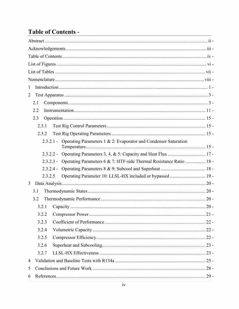
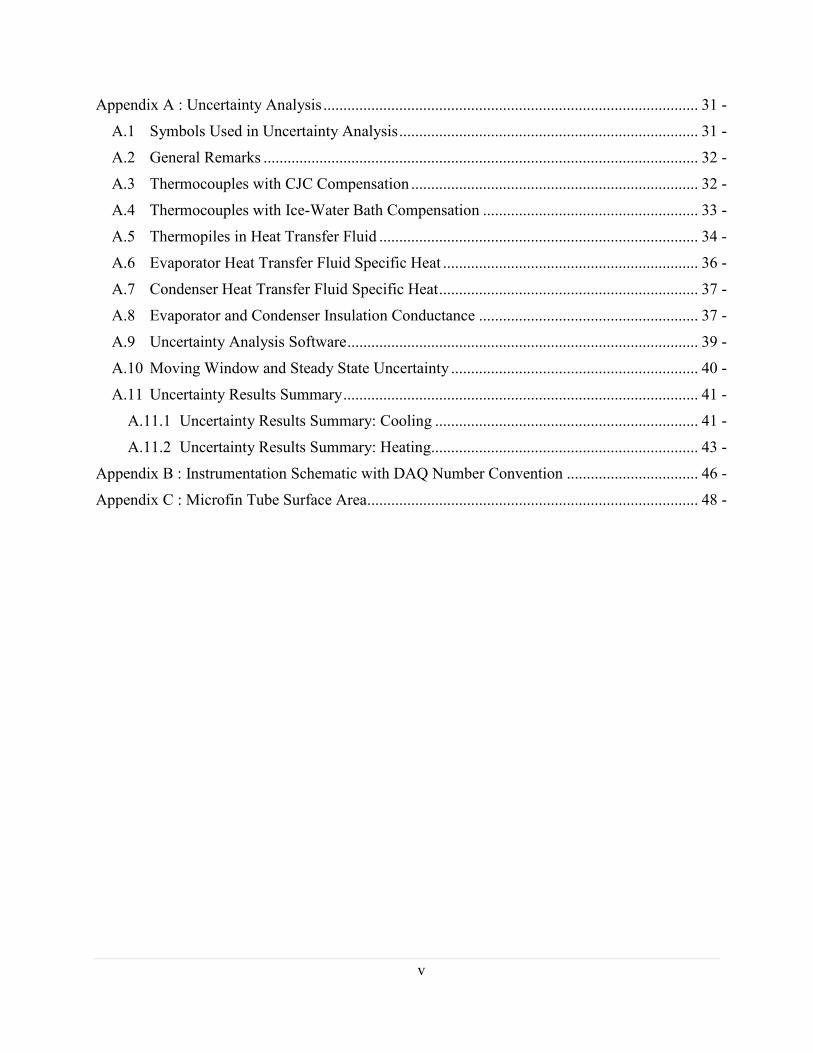
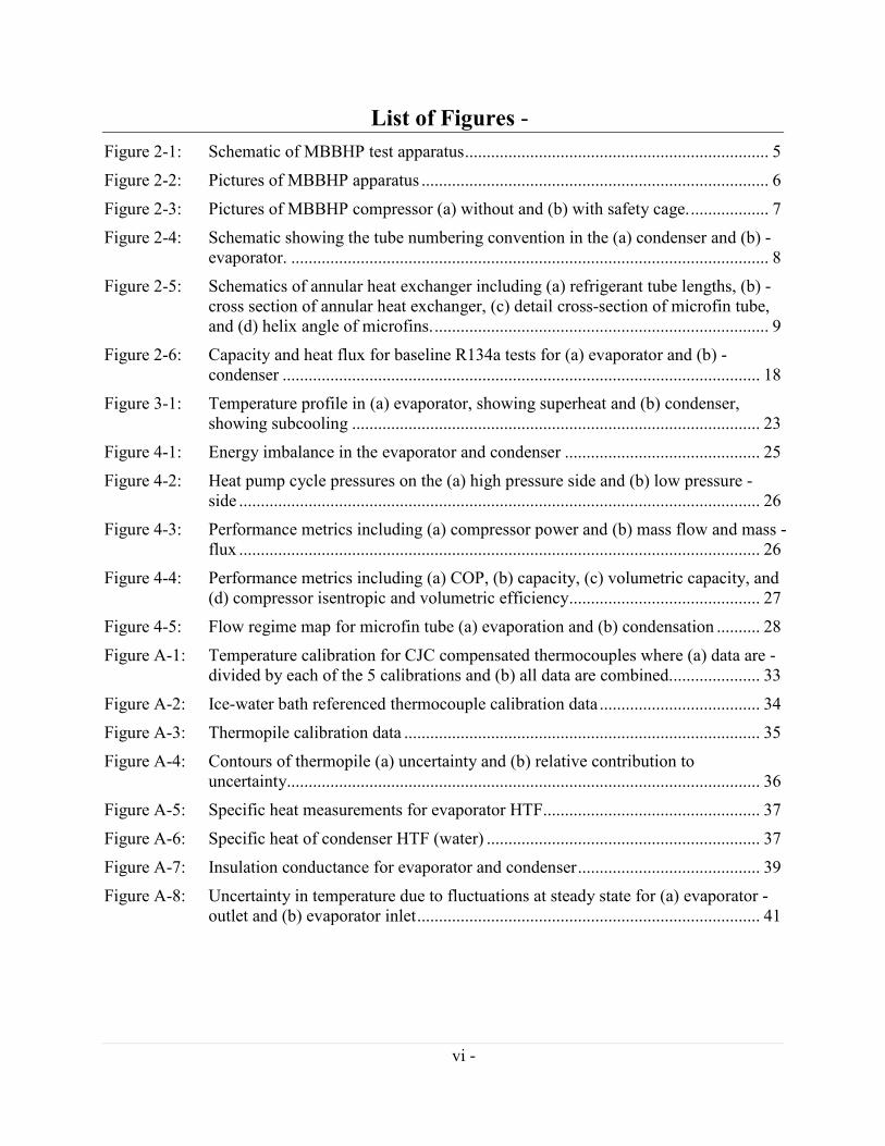
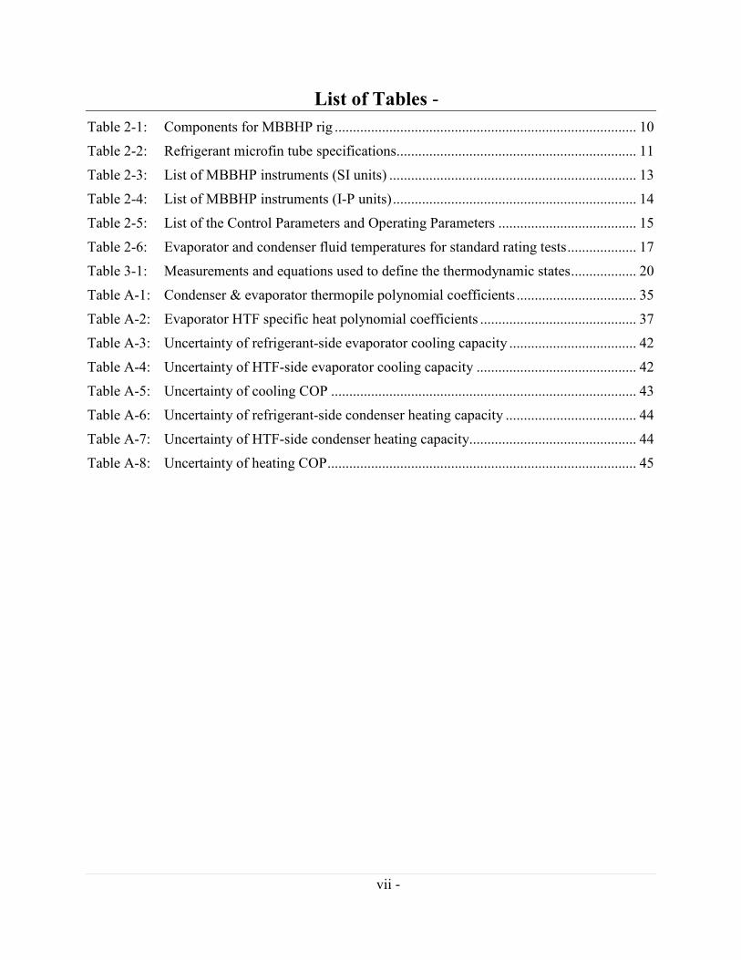
Abbreviation Definition
AHRI Air-Conditioning Heating and Refrigeration Institute
ANSI American National Standards Institute
CFC Chlorofluorocarbon
COP Coefficient of Performance (W of capacity per W of electric input)
CYCLE_D-HX A NIST heat pump cycle simulation model currently under development
The simulation captures both thermodynamic and transport processes in the
cycle
DAQ Data Acquisition
DOE Department of Energy (United States)
EER Energy Efficiency Ratio (Btu of capacity per W of electric input)
EOS Equation of State
GWP Global Warming Potential
HFC Hydrofluorocarbon
HFO Hydrofluoroolefin
HTF Heat Transfer Fluid
HVACampR Heating Ventilation Air-Conditioning and Refrigeration
LLSL-HX Liquid-Line Suction-Line Heat Exchanger
MBBHP Mini Breadboard Heat Pump
NIST National Institute of Standards and Technology (United States)
PID Proportional Integral Derivative controller
RPM Revolutions per Minute (compressor shaft)
x
1 IntroductionshyConcerns about the environmental impacts of global warming (ie global climate change)
are driving an effort to limit anthropogenic sources of atmospheric pollutants that trap longwave
radiation emitted from the earthrsquos surface The chlorinated- and fluorinated-hydrocarbon
working fluids (ie refrigerants) employed by the heating ventilation air-conditioning and
refrigeration (HVACampR) industry exhibit a particularly large global warming potential (GWP)
with 100-year GWP values hundreds to thousands of times larger than an equivalent mass of
carbon dioxide (Solomon et al 2007 p 212) In the European Union the F-gas regulation (EU
2014) mandates a phase-down of hydrofluorocarbons (HFCs) with high GWP to 21 of the
average levels from years 2009 through 2012 by 2030 The current North American proposal
would amend the Montreal Protocol to limit HFC consumption to have a weighted GWP of 15
of average levels from years 2011 through 2013 by 2036 (EPA 2015)
Major efforts are underway to identify alternative refrigerants with a lower GWP Chemical
manufacturers are proposing halogenated olefins (eg hydrofluoroolefins or HFOs) which offer
substantially lower GWP due to short atmospheric lifetimes For some HFOs the lower GWP
comes at the cost of an increase in flammability The Air-Conditioning Heating and
Refrigeration Institute (AHRI) is leading a collaborative effort to evaluate the drop-in and soft-
optimized performance of low-GWP alternatives largely consisting of HFOs and HFOHFC
blends (AHRI 2015) The National Institute of Standards and Technology (NIST) investigated
the maximum thermodynamic potential expected for working fluids by optimizing the
parameters governing the Equations of State (EOS) (Domanski et al 2014) In a companion
NIST study a coarse filter criteria was developed (based on the atomic elements GWP toxicity
flammability critical temperature and stability) to sift through the 100 million chemicals
currently listed in the public-domain PubChem database for possible low-GWP refrigerant
candidates 1234 of which were identified (Kazakov et al 2012) The candidate list was further
refined to 62 by limiting the critical temperature to the range 300 K to 400 K which is typical for
fluids in HVACampR equipment (McLinden et al 2014)
The remaining 62 candidates and their mixtures must be evaluated using more stringent
criteria that consider detailed performance in HVACampR equipment In particular the criteria
must include the cycle efficiency of the fluid since the carbon dioxide emissions from the power
source (ie ldquoindirect emissionsrdquo) far outweighs the direct GWP impact (ie the GWP from the
release of the fluid into the atmosphere) of the working fluid in nearly all HVACampR equipment
A cycle modeling tool CYCLE_D-HX is being developed at NIST to evaluate the efficiency of
low-GWP refrigerants and refrigerant mixtures The model expands upon the thermodynamic
considerations from CYCLE_D (Brown et al 2011) by including transport phenomena In this
way appropriate penalties can be applied to refrigerants whose thermodynamic properties are
favorable but exhibit poor performance in HVACampR systems because of large pressure drops or
poor heat transfer The consideration of transport processes represents a lesson learned from the
previous effort to find replacements for chlorofluorocarbon (CFC) fluids that were found to
cause stratospheric ozone destruction R410A the dominant replacement for the CFC R22 was
initially considered to be a significantly inferior replacement based on thermodynamic properties
alone However later practice showed that the lower pressure drop (due to high operating
pressure) and superior heat transfer of R410A could be exploited with optimized heat exchangers
to yield performance competitive with R22 Including transport processes also allows for the
1
optimization of mass flux the number of parallel heat exchanger tube circuits are adjusted to
balance performance enhancementdegradation of increased heat transferpressure drop with
higher mass flux The more sophisticated capabilities of the new model will allow for more
accurate identification of optimal low-GWP fluids using computational methods
A heat pump test apparatus has been constructed for the purpose of generating cycle
performance data to compare low-GWP refrigerants and to tune and verify the new NIST model
that test apparatus is the focus of this report The apparatus is highly configurable which allows
the system to operate with a wide variety of working fluids as if tailored to each one
Specifically the apparatus features a variable-speed compressor variable-area heat exchangers
and a manually adjusted throttle valve These adjustable components allow for operation at ɺconstant capacity per total combined evaporator and condenser conductance (Q UA ) across total
all test fluids a condition required for equitable comparison of refrigerants (as well as fixed heat
transfer fluid inletoutlet temperatures) (McLinden et al 1987) In practice it is difficult to hold ɺQ UA constant because the conductance depends on the refrigerant side heat transfer total
coefficient which changes for each fluid and operating condition Rather a fixed capacity per
total heat exchanger area ( Qɺ A ) is used as a close approximation For example with a fixed total
heat exchanger area Qɺ A is held constant from R134a (low volumetric capacity) to R410A total
(high volumetric capacity) by decreasing the compressor speed If adjustment of compressor
speed is insufficient to maintain constant Qɺ A between refrigerants the heat exchanger area total
can be adjusted as well The adjustability and relatively small capacity of 17 kW to 35 kW (05
ton to 1 ton) provide the etymology for the apparatus name the Mini Breadboard Heat Pump
(MBBHP) Measurements of cycle performance with legacy high-GWP HFCs and novel low-
GWP fluids in the MBBHP will provide a rich data set to test the predictive capability of the new
NIST model This report describes the construction and operation of the test apparatus the data analysis
used to quantify performance an uncertainty analysis of the performance metrics and baseline
and validation results using refrigerant R134a
2
2 Test Apparatusshy
21 Components
The test apparatus shown in Figure 2-1 through Figure 2-3 was designed to emulate
refrigerant-side operating conditions of typical HVACampR equipment (Figure B-1 and Figure B-
2 in Appendix B show the instrument numbering convention used in the raw data files) The rig
design is partially based on one used in a previous NIST effort to investigate alternatives to
CFCs (Pannock et al 1991) The refrigerant circuit includes a variable-speed compressor
powered by an electric motor and inverter where the speed controls coolingheating capacity
The evaporator and condenser shown in detail in Figure 2-4 and Figure 2-5 (a) and (b) are
single-circuit (ie there are no parallel tube branches) annular heat exchangers where the
refrigerant is on the inner tube and the liquid heat transfer fluid (HTF) is in the annular space
As shown in Figure 2-5(c) the refrigerant tube is smooth on the outside and enhanced with rifled
microfins on the inside The size of the heat exchangers can be adjusted by changing the number
of active refrigerant tubes the valves on the side of the heat exchanger allow for up to 10 (in
increments of 2) of the 20 refrigerant tubes to be bypassed (this section of the rig is referred to as
the ldquobypass valve headerrdquo) When operating these bypass valves care is taken to avoid trapping
subcooled liquid in a closed section a section completely filled with subcooled liquid will
experience a catastrophic increase in pressure if the temperature rises enough to vaporize the
refrigerant A liquid-line suction-line heat exchanger (LLSL-HX) can be included or bypassed
as needed Each of three heat exchangers (evaporator condenser and LLSL-HX) are arranged in
counterflow configuration Two sizes of manually controlled Vernier-handled needle valves are
used to throttle the refrigerant and can be used individually or in tandem the needle valve sizes
were selected using a correlation for short tubes (Kim et al 2005) A filter-dryer is used to
control contaminants and an oil separator is used to ensure proper oil return to the compressor
and to minimize oil circulation in the heat exchangers The system refrigerant charge is adjusted
using two Shrader access valves where refrigerant is removed from or added to the
liquidsuction line valves respectively Two 40 W heaters preheat the compressor before startup
to avoid foam in the oil (the heaters are turned off after the discharge temperature has warmed to
about 60 degC) A safety cage was constructed around the compressor because during cooling tests
with high pressure fluids such as R410A the compressor will be operated slightly above the
manufacturerrsquos specified maximum pressure of 2600 kPa (363 psig) Finally a series of sight
glasses provide visual confirmation of fully subcooled liquid exiting the condenser vapor only
(ie no liquid) entering the compressor suction port proper oil level in the compressor and
proper oil return from the oil separator Detailed component specifications are listed in Table
2-1 The microfin tube parameters are shown in Figure 2-5 and Table 2-2 and Appendix C
shows how the microfin surface area was calculated
The HTF circuits include a water heaterchiller to respectively control the evaporator and
condenser HTF inlet temperatures where the heaterchiller contains a pump for circulating the
fluid The evaporator HTF is a potassium formate and water solution with freeze protection
to -40 degC (-40 degF) whereas water is used for the HTF in the condenser Flow control provided
by three valves in each HTF circuit allows for a wide range of flowrates two in-line valves are
used where the largersmaller (gateneedle) valve provides grossfine flow adjustment and the
third valve bypasses the heater (or chiller) for flow and pressure control Air bubbles in the
condenser HTF circuit are controlled by drawing from the bottom of the vented chiller reservoir
3
tank The evaporator HTF circuit is pressurized with an expansion tank so air bubbles can be
removed by venting trapped air from local high spots using Shrader valves Experience
operating the test apparatus has shown that the vented reservoir tank (in the chiller) is a superior
solution for minimizing air bubbles The temperature of the fluid delivered to the heat
exchangers is regulated using proportional-integral-derivative (PID) controllers
4
Figure 2-1 Schematic of MBBHP test apparatus
5
Figure 2-2 Pictures of MBBHP apparatus
6shy
(a) (b)shy
Figure 2-3 Pictures of MBBHP compressor (a) without and (b) with safety cageshy
7shy
(a)shy (b)
Figure 2-4shy Schematic showing the tube numbering convention in the (a) condenser
and (b) evaporator
8shy
(a)shy
(b)shy (c) (d)
Figure 2-5shy Schematics of annular heat exchanger including (a) refrigerant tube
lengths (b) cross section of annular heat exchanger (c) detail cross-
section of microfin tube and (d) helix angle of microfins
9shy
Table 2-1 Components for MBBHP rig
Component Characteristics
Chiller Cooling capacity 2500 W (07 ton)
Compressor Type
Cylinders
Speed
Displacement rate
Displacement
Max pressure
Reciprocating
2
83 Hz to 667 Hz
(500 RPM to 4000 RPM)
131 m3h-1 to 1081 m3h-1
7165 cm3
2604 kPa (363 psia)
Electric motor Maximum power 373 kW (5 hp)
Expansion tank (HTF) Size 19 liter (5 gallon)
Filter (HTF) Filter size 50 microm
Filter-dryer (refrig) Line size 95 mm (0375 in)
Inverter Voltage
Maximum power
230 VAC 3-phase
373 kW (5 hp)
Heater Heating capacity 10 kW (28 ton)
Heat exchanger
(evaporatorcondenser)
Number of tubes
Tube active length
Return bend length
Outer tube ID
Outer tube OD
Outer tube material
Inner tube
10 to 20 increments of 2
560 mm (22 in)
83 mm (325 in)
254 mm (1 in)
268 mm (1125 in)
Copper
See Table 2-2
Liquid-line suction-line heat
exchanger (LLSL-HX)
Nominal capacity
Shell OD
Type
370 W (05 hp)
51 mm (2 in)
Corrugated (liquid side)
Needle valves (refrig) Valve 1
Orifice
Flow coeff (Cv)
Valve 1
142 mm (0056 in)
003
Valve 2
Orifice
Flow coeff (Cv)
Valve 2
325 mm (0128 in)
016
Needle valves (HTF) Orifice
Flow coeff (Cv)
64 mm (025 in)
073
Oil separator Diameter
Height
Capacity
102 mm (4 in)
356 mm (14 in)
10 to 17 kW (3 to 5 ton)
Pressure relief valve Cracking pressure 800 psig
Note valve orifice sizes and flow coefficients (Cv) can vary between 0 and the listed
maximum values
10
Table 2-2 Refrigerant microfin tube specifications
Parameter Symbol Value Uncertainty
Inside diameter di 846 mm (0333 in) Unknown
Outside diameter do 952 mm (0375 in) plusmn0050 mm (plusmn0002 in)
Bottom wall thickness tb 033 mm (0013 in) plusmn0025 mm (plusmn0001 in)
Fin height e 020 mm (0008 in) plusmn0025 mm (plusmn0001 in)
Spacing between fins sf 022 mm (0009 in) Unknown
Number of fins Nf 60 --
Fin angle β 60deg Unknown
Helix angle α 18deg 2deg
Internal surface area AiL 00424 m (167 in)
per unit tube length
Material Copper
22 Instrumentation
Refrigerant-side instrumentation is selected to capture the key thermodynamic state points in
the cycle Specifications for the instruments (including instrument uncertainty) in both the
refrigerant and HTF circuits are listed in Table 2-3 (Table 2-4 shows I-P units) The pressure
transducers and in-stream thermocouple probes are numbered in Figure 2-1 according to the
eleven states computed in Section 31 the thermodynamic state number convention is also
consistent with that used in the new CYCLE_D-HX model The thermocouple probes are
referenced to a cold junction in an ice-water bath Differential pressure transducers quantify the
pressure drop in the condenser evaporator and suction line The location of the heat exchanger
pressure taps has been selected at the bottom of the bypass valve header where the pressure is
equal to that of the refrigerant leaving the heat exchanger regardless of how many tubes are
bypassed A coriolis flowmeter measures the refrigerant mass flow and density and provides
confirmation of fully subcooled liquid in the liquid line (a two-phase mixture will exhibit large
oscillations in measured flowrate) The compressor shaft power is captured by the in-line torque
meter and tachometer
On the HTF fluid side energy transfers are measured in the evaporator and condenser to
provide verification of the refrigerant-side calculations The mass flow and temperature
difference in the heat exchangers are measured with coriolis meters and thermopiles (in
thermowells) which are combined with the fluid heat capacity to compute energy transfer
Thermocouples inserted into the thermowells with the thermopiles provide the measure of
absolute temperature required for applying the thermopile calibration Additionally the
thermocouples provide verification of the thermopile temperature difference measurement
Figure 2-1 and Figure 2-4 also show the tube-surface-mounted thermocouples used to
measure both refrigerant and HTF temperature profiles in the evaporator and condenser As
shown in Section 326 these temperature profiles are useful for determining refrigerant tube
11
number where the phase transitions (superheat subcooling two-phase) occur The refrigerant-
and HTF-side sensors are mounted on the return bends of each innerouter tube respectively
The instruments are scanned once per minute by the data acquisition (DAQ) system and
when steady state is achieved the measurements are calculated as the average of a moving
window of 30 readings (ie the average over the last 30 minutes) The measurements inevitably
fluctuate during steady state which contributes to the uncertainty of the measurement This
ldquosteady staterdquo uncertainty has been quantified for a nominal test condition and is listed in Table
2-3 The total measurement uncertainty (last column of Table 2-3) is found by adding the
instrument error and the steady state error in quadrature A detailed discussion of the selection
of the steady state moving window size and computation of steady state uncertainty is shown in
Appendix A10
12
Table 2-3 List of MBBHP instruments (SI units)
Instrument Range
Instrument
Uncertainty1
Steady State
Uncertainty1
Total
Uncertainty12
Coriolis meter (HTF) Mass flow
(0 to 756) gs -1
Mass flow 3
plusmn01 rdg
Mass flow
plusmn023 gs -1
Mass flow
plusmn026 gs -1
Density
(0 to 3) g cm-3
Density
plusmn0001 gcm-3
Density
plusmn00001 gcm-3
Density
plusmn0001 gcm-3
Coriolis meter (refrigerant) Mass flow Mass flow 4 Mass flow Mass flow
(0 to 60)5 gs -1 plusmn01 rdg plusmn001 gs-1 plusmn0016 gs -1
Density Density Density Density
(0 to 3) g cm-3 plusmn00005 gcm-3 plusmn00001 gcm-3 plusmn00005 gcm-3
Data acquisition system (-10 to 10) V plusmn1 microV -- plusmn1 microV
Press transducer (diff) ndash condenser (0 to 172) kPa plusmn07 kPa plusmn08 kPa plusmn13 kPa
Press transducer (diff) ndash evaporator (0 to 345) kPa plusmn01 kPa plusmn08 kPa plusmn08 kPa
Press transducer (diff) ndash suction (0 to 69) kPa plusmn001 kPa plusmn03 kPa plusmn03 kPa
Press transducer (high press) (0 to 3447) kPa plusmn34 kPa plusmn07 kPa plusmn35 kPa
Press transducer (low press) (0 to 1724) kPa plusmn34 kPa plusmn07 kPa plusmn35 kPa
Tachometer (017 to 1667) Hz plusmn00167 Hz plusmn0005 Hz plusmn00173 Hz
(10 to 99 999) RPM plusmn1 RPM plusmn03 RPM plusmn104 RPM
Thermocouple (in-stream probe ice ref) (-10 to 100) degC plusmn008 degC plusmn006 degC plusmn009 degC
Thermocouple (surface-mount CJC) (-10 to 60) degC plusmn06 degC plusmn004 degC plusmn06 degC
Thermopile5 (1 to 10) K plusmn0015 K plusmn0013 K plusmn00153 K
Thermopile voltage (-10 to 10) V plusmn1 microV plusmn65 microV plusmn7 microV
Torque meter (0 to 40) N m plusmn033 Nm plusmn0005 Nm 033 Nm
1 95 confidence interval (k = 2)shy2 rdg values have been applied to nominal valuesshy3 Maximum of 01 and (zsflowrate)100 where zs is zero stability = 00491 g s -1 shy4 Maximum of 01 and (zsflowrate)100 where zs is zero stability = 00075 g s -1 shy5 For temperature differences in 1 K to 10 K range Outside range uncertainty is higher See Appendix A5 for moreshydetail
13
Table 2-4 List of MBBHP instruments (I-P units)
Instrument Range
Instrument
Uncertainty1
Steady State
Uncertainty1
Total
Uncertainty12
Coriolis meter (HTF) Mass flow
(0 to 100) lb min-1
Mass flow 3
plusmn01 rdg
Mass flow
plusmn003 lb min-1
Mass flow
plusmn0035 lb min-1
Density
(0 to 187) lb ft-3
Density
plusmn0062 lb ft-3
Density
plusmn0006 lb ft-3
Density
plusmn0062 lb ft-3
Coriolis meter (refrigerant) Mass flow Mass flow 4 Mass flow Mass flow
(0 to 799) lb min-1 plusmn01 rdg plusmn00015 lb min-1 plusmn0002 lb min-1
Density Density Density Density
(0 to 187) lb ft-3 plusmn0062 lb ft-3 plusmn0006 lb ft-3 plusmn0062 lb ft-3
Data acquisition system (-10 to 10) V plusmn1 microV -- plusmn1 microV
Press transducer (diff) ndash condenser (0 to 25) psi plusmn01 psi plusmn01 psi plusmn018 psi
Press transducer (diff) ndash evaporator (0 to 50) psi plusmn0015 psi plusmn01 psi plusmn01 psi
Press transducer (diff) ndash suction (0 to 10) psi plusmn00015 psi plusmn004 psi plusmn004 psi
Press transducer (high press) (0 to 500) psia plusmn05 psi plusmn01 psi plusmn051 psi
Press transducer (low press) (0 to 250) psia plusmn05 psi plusmn01 psi plusmn051 psi
Tachometer (017 to 1667) Hz plusmn00167 Hz plusmn0005 Hz plusmn00173 Hz
(10 to 99 999) RPM plusmn1 RPM plusmn03 RPM plusmn104 RPM
Thermocouple (in-stream probe ice ref) (14 to 212) degF plusmn015 degF plusmn011 degF plusmn018 degF
Thermocouple (surface-mount CJC) (14 to 140) degF plusmn11 degF plusmn008 degF plusmn11 degF
Thermopile5 (18 to 18) degF plusmn0027 degF plusmn0023 degF plusmn004 degF
Torque meter (0 to 350) in lb plusmn29 in lb plusmn0045 in lb plusmn29 in lb
1 95 confidence interval (k = 2) 2 rdg values have been applied to nominal values 3 Maximum of 01 and (zsflowrate)100 where zs is zero stability = 00065 lb min-1
4 Maximum of 01 and (zsflowrate)100 where zs is zero stability = 0001 lb min-1
5 For temperature differences in 18 degF to 18 degF range Outside range uncertainty is higher See Appendix A5 for more
detail
14
23 Operation
231 Test Rig Control Parameters
There are ten Control Parameters (ie settings of adjustable components) listed in Table 2-5
that the MBBHP operator sets to achieve a desired set of Operating Parameters Each Control
Parameter primarily governs one or two Operating Parameters the correspondence is shown in
the table
Table 2-5 List of the Control Parameters and Operating Parameters
Operating Parameter Operating Parameter Values Control Parameter
1 Evaporator saturation temperature See Table 2-6 Heater setpoint (HTF inlet temp)
2 Condenser saturation temperature See Table 2-6 Chiller setpoint (HTF inlet temp)
3 Capacityheat flux 1760 W to 3520 W Compressor speed
(05 ton to 1 ton)
4 Evaporator heat flux 2000 W m-2 to 12 000 W m-2 Number of evaporator tubes
(600 Btu h-1 ft-2 to 3800 Btu h-1 ft-2)
5 Condenser heat flux 2000 W m-2 to 12 000 W m-2 Number of condenser tubes
(600 Btu h-1 ft-2 to 3800 Btu h-1 ft-2)
6 Condenser HTF-side resistance 50 to 70 of overall resistance Condenser HTF flowrate
7 Evaporator HTF-side resistance 70 to 85 of overall resistance Evaporator HTF flowrate
8 Subcool Superheat le 2 tubes1 le 1 tube2 Refrigerant needle valve setting
9 Subcool Superheat le 2 tubes1 le 1 tube2 Refrigerant charge
10 LLSL-HX includedbypassed Includedbypassed LLSL-HX valves
1achieved with subcooling of 2 K to 3 K (18 degF to 36 degF) 2achieved with superheat of 3 K to 6 K (54 degF to 108 degF)
232 Test Rig Operating Parameters
This section describes each of the target Operating Parameters and how they are set using
the Control Parameters Note that the headings for Sections 2321 through 2325 include the
Operating Parameters numbers (1 to 10) as listed in Table 2-5
2321 Operating Parameters 1 amp 2 Evaporator and Condenser Saturation Temperature
The US Department of Energy (DOE) requires heat pumps and air conditioners to be rated
at conditions prescribed in the ANSIAHRI 210240-2008 (AHRI 2008) standard The standard
specifies temperatures of the HTF (air in the standard) entering the evaporator and condenser A
somewhat different but derivative method is employed here the HTF inlet temperatures are set
to achieve refrigerant saturation temperatures expected under ANSIAHRI Cooling A Cooling B
and Heating H1 Rating Tests for the baseline refrigerant R134a
The target saturation temperatures are computed first for the Cooling A test where the
assumed Coefficient of Performance (COPcool) is 44 (energy efficiency ratio EER is 15) The
15
ANSIAHRI standard is not prescriptive about airflow so typical values per unit evaporator ɺcapacity are used for the evaporator (Vɺ Qevap ) 0189 m3 s-1 kW-1 (400 ft3 min-1 ton-1) and air evap
ɺfor the condenser (Vɺ Qevap ) 0378 m3 s-1 kW-1 (800 ft3 min-1 ton-1) Inlet air temperatures air cond
(Tairin) prescribed by the ANSIAHRI standard are listed in Table 2-6 the temperature change
across the evaporator and condenser (∆Tairevap ∆Taircond) is 126 K and 97 K (228 degF and 175
degF) respectively as computed using an energy balance on the airstream where the condenser
energy is larger by an amount that reflects the compressor power (in the COP term)
ɺ )minus1 1ɺ= V (21) ∆Tair evap ( air evap Qevap ρ Cair p air
minus 1 1ɺ Qɺ evap )
1
1+ (22) ∆T = Vair cond ( air cond COP ρ C cool air p air
where the variables represent
Cpair = specific heat of air at constant pressure
ɺV Qɺ evap = condenser airflow per unit evaporator capacity air cond
ɺV Qɺ evap = evaporator airflow per unit evaporator capacity air evap
ρair = density of air
The air outlet temperatures (Tairout) are then computed by respectively subtracting or adding the
∆Tairevap ∆Taircond from the Tairin values
The average temperature difference between the refrigerant and the air (∆Tairref) for
Cooling A is specified as 10 K and 33 K (18 degF and 6 degF) in the evaporator and condenser
respectively based on experience and measurements at NIST for air-source heat pumps with comparable COPs Table 2-6 shows the average air (Tairavg) and average refrigerant saturation
temperatures (Trefavg) computed using this method The Cooling B refrigerant saturation
temperatures are computed using the same ∆Tair and ∆Tairref In heating the heat exchangers
operating as the evaporatorcondenser swap so the values of ∆Tair and ∆Tairref for the evaporator
(in cooling) are used for the condenser and vice versa The resulting refrigerant saturation
temperatures are nominally aligned with values observed in heat pump measurements at NIST
The HTF inlet temperatures (THTFin) are adjusted to achieve the target refrigeration saturation
temperature at a compressor speed of 30 Hz (1800 RPM) with R134a and then held constant for
all other speeds The corresponding HTF outlet temperatures (THTFout) are defined as
T = T + ∆ T (21) HTF e in HTF e out e
T = T + ∆ T (22) HTF c in HTF c out c
where ∆Te and ∆Tc are the HTF temperature differences across the evaporatorcondenser
measured by the thermopiles The THTFout values differ for each speed Table 2-6 shows the
values at 30 Hz (1800 RPM) as a nominal example As discussed in Section 1 a completely fair
comparison of refrigerants requires the same HTF inlet and outlet temperatures (McLinden et al
1987) However it is only possible to match either the evaporator or condenser (but not both)
THTFout by adjusting the heat pump capacity (via compressor speed) the other THTFout will be an
16
uncontrolled value which will vary somewhat from the R134a value depending on the COP of
each fluid (note the HTF mass flow rate is fixed as described in Section 2323 so it cannot be
adjusted to control the other THTFout) Tests with future refrigerants will be carried out with an
evaporator or condenser THTFout equal to the measurements for R134a in cooling or heating
respectively and the other THTFout will vary for each fluid
Table 2-6 Evaporator and condenser fluid temperatures for standard rating tests
Rating Test
Tairin
degC
(degF)
∆Tair
K
(degF)
Tairout
degC
(degF)
Tairavg
degC
(degF)
∆Tairref
K
(degF)
Trefavg
degC
(degF)
THTFin
degC
(degF)
THTFout 1
degC
(degF)
HTFmɺ kg s-1
lb min-1
Cooling A 350 97 447 399 33 432 339 391 0098
(950) (175) (1125) (1038) (60) (1098) (930) (1024) (13)
Condenser Cooling B 278 97 375 326 33 360 249 309 0098
(820) (175) (995) (908) (60) (968) (767) (876) (13)
Heating H1 211 126 338 274 100 374 320 363 0098
(700) (228) (928) (814) (180) (994) (895) (973) (13)
Cooling A 267
(800)
126
(228)
140
(573)
203
(686)
100
(180)
103
(506)
202
(685)
154
(597)
0131
(173)
Evaporator Cooling B
Heating H1
267
(800)
126
(228)
140
(573)
203
(686)
100
(180)
103
(506)
199
(678)
142
(576)
0131
(173)
83 97 -14 35 33 01 103 65 0131
(470) (175) (295) (383) (60) (323) (505) (437) (173)
1 Values for R134a at a compressor speed of 30 Hz (1800 RPM)
2322 Operating Parameters 3 4 amp 5 Capacity and Heat Flux
Baseline capacities were established for R134a at speeds of 233 Hz to 367 Hz (1400 RPM to
2200 RPM) in 33 Hz (200 RPM) increments for each Rating Test Tests with subsequent
refrigerants will be carried out with compressor speeds that match the capacities from the ɺbaseline tests this ensures the refrigerants are tested at the same Q A The target refrigerant-total
side heat flux range was 2 kW m-2 to 12 kW m-2 (600 Btu h-1 ft-2 to 3800 Btu h-1 ft-2) to coincide
with values from typical HVACampR equipment The average heat flux in the evaporator and
condenser was controlled by setting the number of active tubes to 10 and 12 respectively
Figure 2-6 summarizes the capacity for the baseline tests where the evaporator capacity varies
from 12 kW to 21 kW (034 ton to 060 ton) and condenser capacity ranges from 16 kW to 28
kW (045 ton to 080 ton) The heat flux in the evaporator varies from 5 kW m-2 to 9 kW m-2
(1600 Btu h-1 ft-2 to 2900 Btu h-1 ft-2) and in the condenser from 5 kW m-2 to 10 kW m-2 (1700
Btu h-1 ft-2 to 3200 Btu h-1 ft-2) meeting the target heat flux range
17shy
heat transfer area = 0237 m
14
16
20
70
77
84
91
22 94 28
20 25 30 35 40
Cooling B
Cooling A
Heating H1
Evaporator
2
f luid = R134a
tubes = 10
98
20 25 30 35 40
Cooling B
Cooling A
Heating H1
Condenser
heat transfer area = 0285 m2
f luid = R134a
tubes = 12
26 85
Avera
ge
heat
flu
x
[kW
m2]
Cap
acit
y
[kW
]
Avera
ge h
eat
flu
x
[Wm
2]
Cap
acit
y
[kW
] 24
22
20
18shy 76
68
18 60
16
12 51
Compressor frequency [Hz] Compressor frequency [Hz]
(a) (b)
Figure 2-6shy Capacity and heat flux for baseline R134a tests for (a) evaporator and (b)
condenser
2323 Operating Parameters 6 amp 7 HTF-side Thermal Resistance Ratio
In typical air-to-air heat pumps the air-side convection provides the majority of the
resistance to heat transfer Evaporation heat transfer coefficients are generally larger than those
for condensation so the HTF-side resistance ratio (RHTFRtotal) is selected in the range of 50 to
70 for the condenser and 70 to 85 in the evaporator The CYCLE_D-HX model reports
heat exchanger thermal resistances for both the evaporator and condenser when given
measurements of HTF inout temperatures capacity compressor efficiency and heat exchanger
geometry pressure drop and log-mean temperature difference These resistances include the
heat exchanger total conductance (UA) (the total resistance Rtotal is the inverse of UA) the heat
transfer-side resistance (RHTF) in the evaporatorcondenser and the refrigerant-side thermal
resistance (Rref) in the evaporatorcondenser Note that the tube wall thermal resistance is
neglected
The MBBHP was operated under varied HTF flowrates ( mɺ HTF ) and the resulting data were
processed using the CYCLE_D-HX model to determine RHTFRtotal for each flowrate The
evaporator and condenser HTF flowrates used for the tests are 0131 kgs-1 and 0098 kgs-1 (173
lb min-1 and 13 lb min-1) as shown in Table 2-6 which yield RHTFRtotal of 80 and 60 for the
baseline Cooling A test with R134a at 30 Hz (1800 RPM) The flowrates are kept constant for
all other speeds test conditions and refrigerants Maintaining a constant flowrate is important
for verifying the CYCLE_D-HX model the model evaluates the HTF-side thermal resistance for
a reference data set and then holds this resistance constant as other operating parameters
refrigerants and tube circuit configurations are computationally explored
2324 Operating Parameters 8 amp 9 Subcool and Superheat
The number of evaporator tubes containing superheated-vapor and condenser tubes with
subcooled-liquid are controlled to one and two respectively It is important to limit the number
of tubes in superheat and subcooling for comparison with the CYCLE_D-HX model because the
18shy
56
63
model does not consider the pressure drop or area required for heat transfer in these sections
rather it only accounts for transport phenomena in the two-phase section (Note that the
superheat and subcooling are included as an input to the model to determine the thermodynamic
states at the heat exchanger outlets) The superheat and subcooling are also limited because of
performance considerations the single phase fluid exhibits a lower heat transfer coefficient
compared to a two-phase fluid The superheat is bound at the low end by the need to prevent
liquid from entering the compressor The lower limit for subcooling is governed by a
requirement of fully subcooled liquid entering the expansion valve vapor bubbles entering the
expansion valve cause oscillations in the flow that make it difficult to achieve steady state In
general a superheat range of 3 K to 6 K and a subcooling range of 2 K to 3 K satisfies this
Operating Parameter requirement
Closing the refrigerant needle valve increases the superheat and the subcooling whereas
adding refrigerant increases the subcooling and reduces the superheat The combination of these
two controls allows for independent regulation of superheat and subcooling
2325 Operating Parameter 10 LLSL-HX included or bypassed
The LLSL-HX heat exchanger is included or bypassed using the six valves shown in Figure
2-1 When the LLSL-HX is bypassed only one (rather than both) of the valves that stops flow
through the heat exchanger is closed this prevents the possibility of trapping subcooled liquid
between the valves (and presenting the same pressure hazard discussed in Section 21
19shy
3 Data Analysisshy
31 Thermodynamic States
The thermodynamic states numbered 1 through 11 in Figure 2-1 are fixed with two intensive
properties defined by the measurements and equations presented in Table 3-1 Thermodynamic
property data for R134a are computed using the Engineering Equation Solver (EES) software
(Klein 2015) the software uses the equation of state developed by Tilner-Roth et al (1994) for
R134a Note that property data for mixtures and for fluids not directly available in EES will be
computed using the NIST REFPROP database (Lemmon et al 2013)
Table 3-1 Measurements and equations used to define the thermodynamic states
State Description Measurement Equations
1 Compressor inlet LLSL-HX vapor outlet T1 P1 = P11 ndash ∆Ps
2 Compressor cylinder before compression T2 = T1 P2 = P1
3 Compressor outlet T3 P3 = P4
4 Condenser inlet T4 P4 = P7 + ∆Pc
5 Condenser saturated vapor P5 = P4 x5 = 1
6 Condenser saturated liquid P6 = P7 x6 = 0
7 Condenser outlet LLSL-HX liquid inlet T7 P7
8 Expansion valve inlet LLSL-HX liquid outlet T8 P8 = P7
9 Evaporator inlet Expansion valve outlet P9 h9 = h8
10 Evaporator saturated vapor P10 = P11 x10 = 1
11 Evaporator outlet LLSL-HX vapor inlet T11 P11 = P9 ndash ∆Pe
T = temperature P = pressure h = enthalpy x = thermodynamic quality
32 Thermodynamic Performance
Given the fixed state points identified in Table 3-1 (and all associated intensive properties)
the key thermodynamic performance metrics are calculated according to the equations in
Sections 321 through 327 Nominal values and uncertainties of the metrics are shown in
Section 4 and Appendix A respectively
321 Capacity
The evaporator and condenser capacities are computed on the refrigerantHTF-sides
according to
ɺQ = mɺ (h minus h ) (31) ref 4c ref 7
ɺQ = mɺ (h minus h ) (32) ref 9e ref 11
Qɺ = mɺ C ∆T minus Qɺ (33) c HTF HTF c c ins c p HTF c
20shy
ɺQɺ = mɺ C ∆T minus Q (34) p HTF e e HTF HTF e e ins e
where the variables represent
mɺ ref = mass flow of refrigerant
mɺ HTF e mɺ HTF c = mass flow of HTF in evaporatorcondenser
C C = specific heats (average) of HTF in evaporatorcondenser pHTFe pHTFc
ɺQins e Qɺ = insulation heat leak in evaporatorcondenser ins c
∆Te ∆Tc = temperature change of HTF in evaporatorcondenser
The insulation heat leak is a non-trivial 30 W to 50 W and therefore must be accounted for in the
heat exchanger capacity The heat leak is debited from the HTF-side capacity because the HTF
is the annulus and therefore thermally interacts with the surrounding ambient air The heat
exchangers are divided into active and inactive sections (ie tubes where the HTF flows but the
refrigerant does and does not respectively) to compute the heat leak according to
NT NT e active e inactive ɺQ = UA (T minusT ) + (T minusT ) (35) ins e HTF e active avg HTF e inactive avg ins e amb e amb e NT NT e total e total
NT NT c active c inactive
Qɺ = UA ins c (THTF c active avg minusTamb c ) + (T minusTamb c ) (36) ins c HTF c inactive avg NT NT c total c total
where
UAinse UAinsc = insulation conductance for evaporatorcondenser
NTetotal NTetotal = number of tubes in evaporatorcondenser total (20)
NTeactive NTcactive = number of active tubes in evaporatorcondenser
NTeinactive NTeinactive = number of inactive tubes in evaporatorcondenser
THTFeactiveavg THTFcactiveavg = avg HTF temp in the active evaporatorcondenser tubes
THTFeinactiveavg THTFcinactiveavg = avg HTF temp in the inactive evaporatorcondenser tubes
Tambe Tambc = temp of ambient air surrounding evaporatorcondenser
The HTF temperatures are taken from the surface-mounted thermocouples and the ambient air
temperature is taken from a thermocouple near each of the heat exchangers The heat exchangers
are split into activeinactive sections because the slope of the HTF temperature profile is
different in each section the heat transfer is only governed by the average temperature difference
if the slopes (and specific heats) are constant throughout the section The UAinse and UAinsc
values for all 20 tubes are 548 W K-1 plusmn031 W K-1 and 652 W K-1 plusmn041 WK-1 (104 Btu h-1 degF-1
plusmn059 Btu h-1 degF-1 and 124 Btu h-1 degF-1 plusmn078 Btu h-1 degF-1) The method used to compute the
conductance values and their uncertainties is described in Appendix A8
322 Compressor Power
The compressor power is computed using the change in enthalpy across the compressor
21shy
ɺW = ɺ h comp mref ( 3 minus h1 ) (37)
The shaft power is computed for comparison with the compressor power
ɺW = 2πτ N (38) shaft
where the variables represent
N = compressor shaft speed
τ = compressor shaft torque
323 Coefficient of Performance
The cooling and heating COP are computed using the refrigerant-side capacity and the
compressor power applied to the refrigerant
ɺCOP = Qɺ Wcomp (39) cool e ref
ɺ= QCOPheat ɺ
Wcomp (310) c ref
324 Volumetric Capacity
The volumetric cooling and heating capacity (VCC and VHC) are
(mɺ ref v ) (311) VCC = Qɺ
e ref 1
ɺ ( mɺ ref v ) (312) VHC = Q
c ref 1
where
v1 = compressor suction specific volume
325 Compressor Efficiency
The compressor isentropic efficiency is calculated asshy
h ( P s ) minus h3 1 1η s = (313) h minus
3 h
1
where
h(P3s1) = compressor discharge enthalpy under isentropic compression
The volumetric efficiency is quantified by the refrigerant displacement normalized by the
compressor swept volume displacement
mɺ vref 1η v = (314) D N comp
where
22shy
Dcomp = compressor displacement (listed in Table 2-1)
326 Superheat and Subcooling
The evaporator superheat is
SH = T minusT ( P x = 1) (315) 11 11
and the condenser subcooling is
SC = T (P7 x = 0) minusT7shy (316)
where
T(P11 x = 1) = saturated vapor temperature at the evaporator exit pressureshy
T(P7 x = 0) = saturated liquid temperature at the condenser exit pressureshy
The number of refrigerant tubes containing superheatedsubcooled fluid in the
evaporatorcondenser is controlled to one and two respectively during experimental tests
Visual inspection of the temperature profile such as the one shown in Figure 3-1 is used to
determine the locations of the various phase transitions The tube number on the x-axis reflects
the convention established in Figure 2-5
(a)shy (b)
Figure 3-1shy Temperature profile in (a) evaporator showing superheat and (b)
condenser showing subcooling
The location 21 is the exit of the 20th tube
327 LLSL-HX Effectiveness
The LLSL-HX effectiveness is computed as the ratio of the heat transferred on the vapor
23shy
side ( Qɺ ) to the maximum possible heat transfer LLSL v
ɺQ C (T minus T )LLSL v 111 11 p avg 1ε = = (317) ɺLLSL
Q MIN( C C ) (T minus T )LLSL max p avg 111 78 7p avg 11
where
Cpavg111 = average specific heats of the refrigerant on the vapor sideshyCpavg78 = average specific heats of the refrigerant on the liquid sideshy
The heat transfer on the vapor side rather than liquid side is chosen for the numerator because
the larger temperature difference exhibited on the vapor side (due to lower specific heat) results
in a smaller uncertainty in the effectiveness
24shy
4 Validation and Baseline Tests with R134ashyAn initial set of tests were carried out with R134a to provide verification of the
instrumentation and show the nominal uncertainties of the measurements One of the most
important validations is to show an energy balance between the refrigerant and the HTF in the ɺ ɺheat exchangers The energy imbalance defined as Qɺ
ref (Qref minus Q
HTF ) for the initial tests is
shown in Figure 4-1 the imbalance is generally around 1 to 15 or better in both the
evaporator and condenser The imbalance falls well within its uncertainty at the 95
confidence interval indicating that the estimation of the uncertainty in HTF capacity (3 ) is
likely too conservative note that the HTF capacity accounts for more than 90 of the relative
uncertainty in the imbalance metric
Figure 4-1 Energy imbalance in the evaporator and condenser
The performance of R134a in the MBBHP as described by the metrics defined in Section
32 are presented in Figure 4-2 through Figure 4-4 Figure 4-2 (a) and (b) show nominal
pressure profiles on the lowhigh pressure sides of the cycle where the error bars represent
measurement uncertainty listed in Table 2-3 The compressor power measured both by the shaft
power and change of enthalpy of the working fluid are shown in Figure 4-3(a) where the
conversion from mechanical to fluid power is about 65 efficient The error bars represent the
uncertainty calculated by propagating measurement uncertainty through Eqs (37) and (38)
The mass flow ranges from 8 gs-1 to 13 gs-1 (11 lb min-1 to 17 lb min-1) Figure 4-4 shows the
COP ranges from 24 to 4 and the capacity ranges from 16 kW to 21 kW (045 ton to 060 ton)
The figure shows the uncertainties of the COP and capacity where the computation and
tabulation of uncertainty is described further in Appendix A10 and A11 The volumetric
capacity ranges from 2100 kJ m-3 to 2800 kJ m-3 (56 Btu ft-3 to 75 Btu ft-3) and the compressor
isentropic and volumetric efficiencies are nominally 046 and 055 uncertainties in all three of
these metrics are shown in the figures and are computed using a similar method as the
capacityCOP but the computation is not discussed in detail in this report
Figure 4-3 (b) also shows the mass flux which is used to determine the two-phase flow
regimes indicated in Figure 4-5 The refrigerant generally entered the annular flow regime in the
evaporator and condenser though for some tests with low mass flux the refrigerant never left the
stratified-wavy regime
25shy
1100
1150
1200 450 C
om
pre
sso
r p
ow
er
[kW
]shy
Pre
ssu
re [
kP
a]
evaporator tubes = 10
condenser tubes = 12
f luid = R134a
LLSL-HX = no
condenser outlet (P7)
rating test = cooling A
condenser inlet (P4)
Pre
ssu
re [
kP
a]
20 25 30 35 40
Compressor frequency [Hz]
evaporator tubes = 10
condenser tubes = 12
f luid = R134a
LLSL-HX = no
evaporator outlet (P11)
compressor suction (P1)
rating test = cooling A
evaporator inlet (P9)
400
350
1050 300
20 25 30 35 40
Compressor frequency [Hz]
(a)shy (b)
Figure 4-2shy Heat pump cycle pressures on the (a) low pressure side and (b) highshypressure sideshy
0013 12
20 25 30 35 40
Compressor frequency [Hz]
evaporator tubes = 10
condenser tubes = 12
f luid = R134a
LLSL-HX = no
cooling A
cooling B
heating H1
pow er to w orking f luid (Wcomp)
shaft pow er (Wshaf t)
Mass
flo
w [
kg
s]
20 25 30 35 40
evaporator tubes = 10
condenser tubes = 12
f luid = R134a
LLSL-HX = no
cooling A
cooling B
heating H1
0012
Mass
flu
x [
kg
s-m
2]
200 09 0011
180 001
06
0009
0008 03
Compressor frequency [Hz]
(a)shy (b)
Figure 4-3shy Performance metrics including (a) compressor power and (b) mass flow and
mass flux
26shy
140
160
220
Vo
lum
etr
ic c
ap
acit
y [
kJm
3]
CO
P
Vo
lum
etr
ic e
ffic
ien
cy
(η
v)
(a) (b)
20 25 30 35 40 2
25
3
35
4
45
Compressor frequency [Hz]
evaporator tubes = 10
condenser tubes = 12
cooling A
cooling B
heating H1
f luid = R134a
LLSL-HX = no
20 25 30 35 40 15
16
17
18
19
2
21
Compressor frequency [Hz] C
ap
acit
y [
kW
]
cooling A
cooling B
heating H1
evaporator tubes = 10
condenser tubes = 12
fluid = R134a
LLSL-HX = no
2800 07 07
evaporator tubes = 10
condenser tubes = 12
fluid = R134a
LLSL-HX = no
cooling A
cooling B
heating H1
20 25 30 35 40 04
05
06
03
04
05
06
evaporator tubes = 10
condenser tubes = 12
fluid = R134a
LLSL-HX = no
cooling A
cooling B
heating H1
cooling B
cooling A
heating H1
2600
2400
2200
Isen
tro
pic
eff
icie
ncy
( η
s)
20 2000
25 30
Compressor frequency
35
[Hz]
40
Compressor frequency [Hz]
(c) (d)
Figure 4-4 Performance metrics including (a) COP (b) capacity (c) volumetric
capacity and (d) compressor isentropic and volumetric efficiency
27shy
50
Flow boiling with microfin tubeshy Flow condensing with microfin tube 350 350
300 300
S
heat flux 70 kWm2
=
= A
I
SG
S+SW
D
Tsat = 8 C
fluid = R134a
flow range during tests
M
SW
=
Tsat 43 C
fluid = R134a
heat flux 77 kWm2
flow range during tests
A
I
SG
S SW+
SW
0
50
S
Mass F
lux [
kg
s-m
2]
250
200
150
100
Mass F
lux [
kg
s-m
2]
250
200
150
100
0 0shy 02 04 06 08 1 0 02 04 06 08 1
Vapor quality Vapor quality A = Annular D = Dryout I = Intermittant M = Mist A = Annular D = Dryout I = Intermittant M = Mist
S = Stratified SG = Slug SW = Stratified-Wavy S = Stratified SG = Slug SW = Stratified-Wavy
(a)13shy (b)23
Figure 4-5shy Flow regime map for microfin tube (a) evaporation and (b) condensation
1 Flow boiling regime map from (Wojtan et al 2005)shy2 Flow condensation regime map from (Hajal et al 2003)shy3 Boundary between IntermittentAnnular regimes from (Thome 2007) using equation 1261 with a coefficientshy
of 0678 for helical microfins
5 Conclusions and Future Work
This report shows that the test apparatus is capable of measuring the performance of
low-GWP refrigerants with high fidelity including less than 05 uncertainty in both capacity
and COP The energy balance closure on the evaporator and condenser was better than 15
and will be continually tracked to ensure continued high quality data are collected
Future tests will include a second baseline refrigerant R410A followed by a series of
comparative tests with low-GWP refrigerants and refrigerant mixtures The HTF flowrates will
remain fixed from the R134a baseline tests so that the CYCLE_D-HX simulations of the test
data can be carried out for all test data based on a single reference data set After the model
results are verified the model will be used to identify additional candidate refrigerants to test in
the MBBHP test apparatus
28shy
6 ReferencesshyAHRI (2008) 2008 Standard for Performance Rating of Unitary Air-Conditioning amp Air-
Source Heat Pump Equipment Air-Conditioning Heating and Refrigeration Institute
Arlington VA United States Retrieved from wwwahrinetorg
AHRI (2015) Participants Handbook AHRI Low-GWP Alternative Refrigerants Evaluation
Program (Low-GWP AREP) Arlington VA United States Air-Conditioning Heating
and Refrigeration Institute Retrieved from
httpwwwahrinetorgsite514ResourcesResearchAHRI-Low-GWP-Alternative-
Refrigerants-Evaluation
Brown J S Domanski P A amp Lemmon E (2011) Standard Reference Database 49
CYCLE_D NIST Vapor Compression Cycle Design Program Version 50 Retrieved
from httpwwwnistgovsrdnist49cfm
Domanski P A Brown S J Heo J Wojtusiak J amp McLinden M O (2014) A
thermodynamic analysis of refrigerants Performance limits of the vapor compression
cycle International Journal of Refrigeration 38 71-79
doi101016jijrefrig201309036
EPA (2015) 2015 North American Amendment Proposal to Address HFCs under the Montreal
Protocol Retrieved from httpwwwepagovozoneintpolmpagreementhtml and
httpwwwepagovozoneintpolHFC_Amendment_2015_Summarypdf
EU (2014 April 16) Regulation (EU) No 5172014 of the European Parliament and of the
Council of 16 April 2014 on fluorinated greenhouse gases and repealing Regulation (EC)
No 8422006 Journal of the European Union Retrieved from httpeur-
lexeuropaeulegal-contentENTXTuri=uriservOJL_201415001019501ENG
Fortin T J (2015) Personal communication
Hajal J E Thome J R amp Cavallini A (2003) Condensation in horizontal tubes part 1 two-
phase flow pattern map International Journal of Heat and Mass Transfer 3349-3363
doi101016S0017-9310(03)00139-X
Harr L Gallagher J S amp Kell G S (1984) NBSNRC Steam Tables Hemisphere Publishing
Co
Kazakov A McLinden M O amp Frenkel M (2012) Computational Design of New
Refrigerant Fluids Based on Environmental Safety and Thermodynamic Characteristics
Industrial amp Engineering Chemistry Research 51 12537-12548 doi101021ie3016126
Kim Y Payne V Choi J amp Domanski P A (2005) Mass flow rate of R-410A through short
tubes working near the critical point International Journal of Refrigeration 28 547-553 doi101016jijrefrig200410007
Klein S A (2015) Engineering Equation Solver v 9908 Retrieved from
httpwwwfchartcomees
Lemmon E W Huber M L amp McLinden M O (2013) NIST Standard Reference Database
23 Reference Fluid Thermodynamic and Transport Properties (REFPROP) Version 91
29shy
National Institute of Standards and Technology Retrieved fromshyhttpwwwnistgovsrdnist23cfmshy
McLinden M O amp Radermacher R (1987) Methods for Comparing the Performance of Pure
and Mixed Refrigerants in the Vapour Compression Cycle International Journal of
Refrigeration 10(6) 318-325 doi1010160140-7007(87)90117-4
McLinden M O Kazakov A Heo J Brown J S amp Domanski P A (2014) A
thermodynamic analysis of refrigerants Possibilities and tradeoffs for Low-GWP
refrigerants International Journal of Refrigeration 38 80-92
doi101016jijrefrig201309032
Pannock J amp Didion D A (1991) The Performance of Chlorine-Free Binary Zeotropic
Refrigerant Mixtures in a Heat Pump NISTIR 4748 Internal Report National Institute of
Standards and Technology US Department of Commerce Gaithersburg Retrieved from
httpfirenistgovbfrlpubsbuild91art002html
Solomon S Qin D Manning M Chen Z Marquis M Averyt K B Miller H L
(2007) Contribution of Working Group I to the Fourth Assessment Report of the
Intergovernmental Panel on Climate Change New York NY USA Cambridge
University Press Retrieved July 29 2015 from
httpwwwipccchpublications_and_datapublications_ipcc_fourth_assessment_report_
wg1_report_the_physical_science_basishtm
Taylor B N amp Kuyatt C E (1994) Guidelines for Evaluating and Expressing the Uncertainty
of NIST Measurement Results National Institute of Standards and Technology Technical
Note 1297
Thome J R (Updated in 2007) Wolverine Heat Transfer Engineering Data book III Germany
Weiland-Werke AG Retrieved from httpwwwwlvcomheat-transfer-databook
Tilner-Roth R amp Baehr H D (1994) An International Standard Formulation for the
Thermodynamic Properties of 1112-Tetrafluoroethane (HFC-134a) for Temperatures
from 170 K to 455 K and Pressures up to 70 MPa J Phys Chem Ref Data 23(5)
Wojtan L Ursenbacher T amp Thome J R (2005) Investigation of flow boiling in horizontal
tubes Part ImdashA new diabatic two-phase flow pattern map International Journal of Heat
and Mass Transfer 2955-2969 doi101016jijheatmasstransfer200412012
30shy
Appendix A Uncertainty Analysisshy
A1 Symbols Used in Uncertainty Analysisshy
Symbol Units Definition
k -- Expanded uncertainty coverage factor
n -- Number of data points
Qɺ kW Energy transfer
SUAinse W K -1 Standard deviation of evaporator insulation conductance
SX -- Standard deviation of measured quantity ldquoXrdquo
T degC Temperature
T1 degC Temperature at cold end of thermopile
Tcal degC Temperature of RTD used for calibrations
TTCcal degC Calibrated thermocouple measurement
TTCCJC degC Thermocouple measurement with Cold Junction Compensation
∆Tlm K Log-mean temperature difference
∆TTCcal K Thermocouple calibration temperature difference
∆TTP K Temperature difference of thermopile
UA W K -1 Thermal conductance
UA ins e U W K-1 Uncertainty of average of evaporator insulation conductance
UTC degC Total instrument uncertainty of thermocouple
UTCcal degC Thermocouple instrument uncertainty from calibrating device uncertainty
UTCfit degC Instrument uncertainty of thermocouple due to fit of calibration regression
UX -- Uncertainty of measured quantity ldquoXrdquo
X U -- Uncertainty of average of measured quantity ldquoXrdquo
UY Uncertainty of calculated quantity ldquoYrdquo
V V Voltage
V1 V Thermopile voltage of cold end of thermopile (referenced to ice-point)
VCC kJ m -3 Volumetric Cooling Capacity
VHC kJ m -3 Volumetric Heating Capacity
VTC V Thermocouple voltage
∆VTP V Thermopile voltage
X -- Measured quantity
Y -- Calculated quantity
31shy
Subscript Definition
amb Ambient airshyc Condensershye EvaporatorshyHTF Heat Transfer Fluidshyin Inletshyins Insulationshyout Outletshy1 to 11 Refrigerant thermodynamic states as defined by Figure 2-1shy
Abbreviation Definition
COP Coefficient of Performance (W capacity per W of input power)shyCJC Cold Junction Compensation (for thermocouples)shyDAQ Data AcquisitionshyDSC Differential Scanning Calorimeter (used to measure fluid specific heat)shyEES Engineering Equation Solver (software used to reduce data)shyHTF Heat Transfer FluidshyMBBHP Mini Breadboard Heat PumpshyRPM Revolutions per Minute (compressor shaft)shyRTD Resistance Temperature Detectorshy
A2 General Remarks
The uncertainty analyses for key performance metrics are presented in this section All
uncertainties are estimated based on instrument uncertainties computed at a 95 confidence
interval
A3 Thermocouples with CJC Compensation
The surface-mounted thermocouples as well as the thermocouples measuring the air
temperature near the evaporatorcondenser are compensated at the DAQ using a thermistor-
based Cold Junction Compensation (CJC) A calibration (∆Tcal) is applied to the resulting
temperature reading (TTCCJC) to compute the calibrated temperature (TTCcal) according to
T = T + ∆ T (A1) TC cal TC cal TC CJC
where the calibration is fit to a 2nd order polynomial (the order of this curve fit and others
presented in Appendix A were selected based on t-test of polynomial coefficients)
= T minus a T + a T 2∆T cal T = a0 + 1 TC CJC 2 TC CJC (A2)
TC cal TC CJC
The polynomial coefficients (a0 a1 a2) are fit using the least square error method and Tcal is the
temperature measured by the calibrating instrument (two calibrated RTDs read by a precision
digital thermometer expanded uncertainty of plusmn002 degC) The thermocouples were calibrated over
a temperature range of -10 degC to 60 degC and this calibration was repeated five times over the
32shy
course of two weeks Figure A-1 (a) shows the calibration data and polynomial curve fits for a
representative thermocouple Each calibration shows a significant offset from the others this is
likely a manifestation of the repeatability error of the CJC which has an overall uncertainty of
plusmn05 degC Figure A-1 (b) shows the aggregation of the five data sets and the resulting curve fit
and 95 confidence interval (plusmn06 degC) The uncertainty of the calibrated RTDs is more than an
order of magnitude smaller than the curve fit confidence interval and is therefore neglected The
CJC thermocouple instrument uncertainty listed in Table 2-3 is therefore plusmn06 degC
05 05
Tem
pera
ture
cali
bra
tio
n( ∆
Tc
al)
[K]
Tem
pera
ture
cali
bra
tio
n( ∆
Tc
al)
[K]
0
-05
-1 ddaattaa
ccuurrvvee ffiitt
9955 ccoonnffiiddeennccee iinntteerrvvaall
0
-05 ccaalliibbrraattiioonn 11
ccaalliibbrraattiioonn 22
ccaalliibbrraattiioonn 33
ccaalliibbrraattiioonn 44
-1 ccaalliibbrraattiioonn 55
ccuurrvvee ffiittss
-15 -15 -10 0 10 20 30 40 50 60 -10 0 10 20 30 40 50 60
Temperature (TTCCJC) [degC] Temperature (TTCCJC) [degC]
(a) (b)
Figure A-1 Temperature calibration for CJC compensated thermocouples where
(a) data are divided by each of the 5 calibrations and (b) all data are
combined
A4 Thermocouples with Ice-Water Bath Compensation
A lower level of uncertainty is achieved for the in-stream probe thermocouples which
measure the refrigerant temperatures at key thermodynamic states by utilizing an ice-water bath
reference junction The ice-water bath consists of a vacuum insulated Dewar filled with crushed
ice and water the reference junction is submerged in the bath inside of a water-filled test tube
Using the ice-water bath removes the large uncertainty associated with the electronic CJC on the
DAQ system The thermocouples were calibrated against the RTDs (same ones used to calibrate
thermocouples with CJC) where the resulting data and curve fit are shown for a representative
thermocouple in Figure A-2 The data were fit to 5th order polynomials according to
5
T aV i (A3) =sum iTC cal TC
i=0
where VTC is the thermocouple voltage The resulting instrument uncertainty (plusmn008 degC) listed in
Table 2-3 is the combination of the curve fit standard error (UTCfit k = 2) and the calibrating
RTD error (UTcal)
2 2 2 2 U = plusmn U +U = plusmn 0079 + 002 = plusmn008 degC (A4)TC TC fit T cal
33
Tem
pera
ture
[degC
]
80
ddaattaa
ccuurrvvee ffiitt60
40
20
0
-20 -00005 0 00005 0001 00015 0002 00025
Voltage [V]
Figure A-2 Ice-water bath referenced thermocouple calibration data
A5 Thermopiles in Heat Transfer Fluid
The 13-junction thermopiles were calibrated by immersing one end in an ice-water bath
(inside a water-filled test tube) and the other end in a temperature controlled bath The
temperature in the controlled bath was measured using the two calibrated RTDs A thermopile
voltage-temperature dataset was generated and fit to a 4th order polynomial Figure A-3 shows
the calibration data and the curve fit and Table A-1 shows the polynomial coefficients The
calibration data are fit to the equation
N =4 i
T = sum aTP i V (A5) i=0
The temperature difference for a thermopile is computed according to
∆T = ( V T V + ∆ ) minusT (A6)TP 1 TP 1
where ∆VTP is the measured thermopile voltage and T1 is the temperature measured at the cold
end of the thermopile by a CJC-corrected thermocouple Eq (A5) is substituted into Eq (A6)
to calculate the thermopile temperature difference
N =4
∆TTP = sum aTP i (V1 +∆VTP ) minusT1 (A7) i=0
where V1 (cold-end voltage) is computed by numerically solving Eq (A5) where T is set to (T1)
N =4 i V1 = root T1 minussum aTPi V1 = 0 (A8)
i=0
The thermopile uncertainties are computed with respect to the curve fit voltage
measurement and temperature measurement at the cold end of the thermopile (characterized
respectively by the coefficient uncertainties in Table A-1 the thermopile voltage uncertainty in
Table 2-3 and the CJC corrected thermocouple in Table 2-3) The EES (Klein 2015) software
34
is used to numerically compute the partial derivatives and subsequent thermopile uncertainties
Figure A-4(a) shows the contours of uncertainty in the temperature difference measured by the
evaporatorcondenser HTF thermopiles
Figure A-4(b) shows the contours of relative contribution to uncertainty in the thermopile
measurement Each of the uncertainty sources is dominant in different regions
bull voltage measurement dominant at low temperature differences (less than 1 K)
bull curve fit error dominant at high cold end temperatures (greater than 50 degC)
bull cold end temperature dominant at moderate cold end temperatures -5 degC to 20 degC and temperature differences 25 K to 20 K
As noted in this discussion the thermopile uncertainty is a complex function of the curve fit
voltage measurement and cold end temperature measurement For the temperature difference
range expected for this application 1 K to 10 K (18 degF to 18 degF) the upper bound of uncertainty
is about 0015 K (0027 degF) for simplicity this is the value listed in Table 2-3 Note that the
contribution to the uncertainty by the calibrating instrument (two calibrated RTDs) is negligible
here as the error in slope (which is the error that propagates into the thermopile temperature
difference) is less than 0000248 K per K of temperature difference (eg 000248 K for a 10 K
temperature difference)
Table A-1 Condenser amp evaporator60
thermopile polynomial coefficients 50
Uncertainty
Coeff Value (k=2) 95 40
Tem
pera
ture
[degC
]
aTPe0 39243 E-02 plusmn41 E-04 30
aTPe1 20243 E+03 plusmn12 E-01 20
aTPe2 -55466 E+03 plusmn22 E+01 TTPP11
10 TTPP22 aTPe3 39023 E+04 plusmn13 E+03 TTPP11 ((ffiitt))
TTPP22 ((ffiitt)) aTPe4 -26229 E+05 plusmn22 E+04
0
-10
38494 E-02 plusmn53 E-04 -001 0 001 002 003 004 aTPc0
Voltage [V]shy aTPc1 20241 E+03 plusmn15 E-01
Figure A-3 Thermopile calibration data aTPc2 -55190 E+03 plusmn28 E+01
aTPc3 38551 E+04 plusmn16 E+03
aTPc4 -25440 E+05 plusmn29 E+04
35
-5
0
10
20 contours of thermopile uncertainty [K] contours of contribution to uncertainty []
20
balance is T1004
0035
Tem
pera
ture
dif
fere
nce
(∆
TT
P)
[K]
15 003
0025
002
0015
001 0001 5
0002 0005
0004 0003
Tem
pera
ture
dif
fere
nce (∆
TT
P)
[K]
15
10
curve fit
80 60
40 20
5 voltage (∆VTP)
20 40
0 60
80
0 10 20 30 40 50
Temperature at cold end (T1) [degC]
60 -5
0 10 20 30 40 50
Temperature at cold end (T1) [degC]
60
(a) (b)
Figure A-4 Contours of thermopile (a) uncertainty and (b) relative contribution to
uncertainty
A6 Evaporator Heat Transfer Fluid Specific Heat
The evaporator HTF is a potassium formate and water heat transfer fluid that is freeze
protected to -40 degC The manufacturerrsquos specific heat data were found to have error of at least
10 so a sample of the fluid was analyzed in a Differential Scanning Calorimeter (DSC) by the
NIST-Boulder Applied Chemicals and Materials Division The temperature dependent specific
heat and the 2nd order curve fit to the data are shown in Figure A-5 the curve fit coefficients and
their uncertainties are listed in Table A-2 Figure A-5 also shows the manufacturerrsquos reported
specific heat data for comparison The exact uncertainty of the DSC measurement was not
available at the time of writing but was estimated to be about 2 to 3 of reading based on the
experience of the DSC operator (Fortin 2015) An uncertainty of 3 of reading is therefore
assigned as a conservative estimate Both the curve fit and DSC calibration uncertainties are
included in the calculation of overall uncertainties
36shy
DSC measurements
curve fit
3 Table A-2 Evaporator HTF specific
heat polynomial coefficients
29 Uncertainty
DSC measurements
curve fit
manufacturers data
-10 0 10 20 30
Sp
ecif
ic h
eat
(Cp)
[Jg
-K]
Coeff Value (k=2) 95
28 aCpe0 25643 E+00 plusmn16 E-03
aCpe1 11015 E-03 plusmn21 E-04
27 aCpe2 17422 E-05 plusmn95 E-06
26
25
Temperature [degC]
Figure A-5 Specific heat measurements for
evaporator HTF
A7 Condenser Heat Transfer Fluid Specific Heat
The condenser HTF is water the specific heat data are computed in EES using the data from
(Harr et al 1984) and are shown in Figure A-6 A conservative estimate of plusmn3 is used for the
uncertainty in the specific heat
423
0 20 40 60 80 100
Sp
ecif
ic h
eat
(Cp)
[kJk
g-K
]
422
421
42
419
418
Temperature [degC]
Figure A-6 Specific heat of condenser HTF (water)
A8 Evaporator and Condenser Insulation Conductance
The total evaporator and condenser insulation conductances (UAinse and UAinsc) for thermal
interaction with the ambient air were measured during an initial test where the HTFs were
circulated at various flow rates through the apparatus at an elevated temperature while the
refrigerant tubes were under vacuum The temperature change of the HTF across the heat
37shy
exchanger was assumed to be entirely attributed to insulation heat leak and therefore an
effective insulation conductance could be computed The resulting UAinse and UAinsc values for
all 20 tubes are shown in Figure A-7 Average values of conductances for the evaporator and
condenser were calculated as 548 W K-1 plusmn031 W K-1 and 652 W K-1 plusmn041 W K-1
(104 Btu h-1 degF-1 plusmn059 Btu h-1 degF-1 and 124 Btu h-1 degF-1 plusmn078 Btu h-1 degF-1) respectively where the
uncertainty accounts for both instrumentation error and test variance The evaporator insulation
conductance for these tests is computed according to
ɺQins e mɺ HTF e C (THTF in e minusT )p HTF e HTF out e
UA = = (A9) ins e ∆T T minusT minus T minusT e ( HTF in e amb e ) ( HTF out )lm HTF e amb e
(T minusT ) amb e HTF in e ln (T
minusT
amb e ) HTF out e
where the variables represent
Cp HTF e = evaporator HTF specific heat
mɺ HTF e = evaporator HTF mass flow
Qɺ = evaporator insulation heat leak ins e
Tambe = ambient air temperature surrounding evaporator
THTFine = evaporator HTF inlet temperature
THTFoute = evaporator HTF outlet temperature
∆TlmHTFe = evaporator log-mean temperature difference
and the uncertainty of the average value is calculated according to
U = k S n (A10) UA ins e UA ins e
where the variables represent
k = expanded uncertainty coverage factor (k = 2) for 95 confidence interval
SUAinse = standard deviation of conductances
n = number of conductance data points
The condenser conductance is computed using the same method with the corresponding
measurements from that heat exchanger
38shy
4
5
6
7
8
Insu
lati
on
co
nd
ucta
nce (
UA
ins)
[WK
]
UAinscond
UAinsev ap
average for evaporator
average for condenser
0 005 01 015
Mass flow [kgs]
Figure A-7 Insulation conductance for evaporator and condenser
A9 Uncertainty Analysis Software
The uncertainty analyses on each of the performance metrics shown in Figure 4-1 through
Figure 4-4 were calculated using the uncertainty propagation capability in EES The software
numerically computes the performance metric uncertainty by evaluating the partial derivatives
with respect to each relevant measurement and applying the specified measurement uncertainty
Assuming the measurements are independent and uncorrelated the uncertainty of a quantity is
computed according to (Taylor amp Kuyatt 1994)
partY 2 2
UY = sum U X (A11) i partXi
i
where the variables represent
Y = calculated quantity
Uy = uncertainty of calculated quantity
Xi = measurement
UXi = uncertainty of measurement
39shy
A10 Moving Window and Steady State Uncertainty
A moving window average was used to compute the measurements at steady state during the
tests In order to determine a proper window size the variation of measurement steady state
uncertainty with window size was examined The steady state uncertainty is defined as the
expanded standard uncertainty for the average reading within the window
S X (A12) U = k X
n
where
k = coverage factor (k = 2) for 95 confidence interval
n = number of samples in the window
Sx = standard deviation of measurement
X = average value of measurement
The data for analysis were generated by holding the MBBHP at a nominal steady operating
condition and recording the measurements at 1-minute intervals (same as collection rate for all
performance testing) for an extended time (3 hours) Figure A-8 shows the fluctuation of steady
state uncertainty for the evaporator inlet and outlet temperatures (T9 and T11) The figure
highlights two characteristic trends observed for all of the instruments both of which suggest the
need for a large moving window (1) the steady state uncertainty decreases as the window size
increases and (2) the steady state uncertainty is highly oscillatory for small windows (the
oscillations are undesirable because short-term fluctuations can have a disproportionate impact
on the averaged result) A 30 sample moving window was selected to achieve low uncertainty
while allowing for collection of data in a timely manner
Figure A-8 shows that the measurement steady state uncertainty is not constant in time (it
would be constant if the fluctuations at steady state were purely random) but rather exhibits
drifting and periodic movements This is possibly due to hunting by the PID controllers
regulating HTF fluid temperatures changes in air temperature in the lab space or some other
uncontrolled andor uncharacterized phenomena These non-random fluctuations are accounted
for by using the maximum steady state uncertainty value observed during the extended steady
state test For example Figure A-8(a) shows the maximum steady state uncertainty for the
evaporator outlet (T9) is plusmn006 degC this value and values for all other sensors are listed in Table
2-3 The data in the moving window are only recorded when steady state uncertainties are below
these established thresholds The total uncertainty (plusmn009 degC) also shown in Table 2-3 is
subsequently computed by adding the instrument uncertainty (plusmn008 degC) and steady state
uncertainty (plusmn006 degC) in quadrature
Note that different sensors of the same type exhibit different levels of fluctuation as a
conservative estimate the largest uncertainty of any one is applied to all of them For example
Figure A-8(b) shows the fluctuations of steady state uncertainty for the evaporator inlet
temperature (T9) are much smaller than for the evaporator outlet (T11) In fact the evaporator
outlet temperature (T11) shows the most fluctuation of all the ice-water bath compensated
thermocouple probes therefore its value (plusmn006 degC) is used in Table 2-3 to represent them all
40shy
05 05
01 01
Ts
[C]
001 001
Ute
ad
y
0002
(a)
Time elapsed [s]
0002
(b)
Time elapsed [s]
Figure A-8shy Uncertainty in temperature due to fluctuations at steady state for (a)
evaporator outlet and (b) evaporator inlet
A11 Uncertainty Results Summary
The detailed instrument uncertainty analysis for performance metrics including the
refrigerantHTF-side capacities and the COPs are tabulated in Appendices A111 (cooling) and
A112 (heating) The tables show the performance metric and its total uncertainty (including
both instrument and steady state contributions) as well as the measurements that contribute to
the uncertainty The measurement values uncertainties partial derivatives (of performance
metric with respect to the measurement) and relative errors (contribution to the overall error in
the performance metric) are also shown where the measurements are listed in order of
decreasing relative error Uncertainties for other performance metrics (eg VCCVHC ηisen)
were analyzed using similar techniques but are not shown in detail in this report Note that
Appendices A111 and A112 show sample calculations for a single nominal operating
condition whereas the uncertainty values presented in the Section 4 figures are computed for
each test run
The uncertainty in cooling performance metrics are shown for a nominal operating point for
R134a during a Cooling A test with a compressor speed of about 30 Hz (1800 RPM) Similarly
the uncertainty in heating performance metrics are shown for R134a during a Heating H1 test
with a compressor speed of about 30 Hz (1800 RPM)
A111 Uncertainty Results Summary Cooling
Table A-3 shows that the dominant sources of instrument uncertainty for the refrigerant-side
capacity are refrigerant mass flow (66 ) expansion valve inlet temperature (17 ) evaporator
exit pressure (8 ) and evaporator exit temperature (7 ) Table A-4 shows the dominant
source of instrument uncertainty for the HTF-side capacity is the HTF specific heat (97
estimate for instrument used to measure fluid properties) Table A-5 shows the dominant
sources of instrument uncertainty for cooling COP are evaporator inlet pressure (39 )
compressor discharge temperature (25 ) and compressor suction temperature (18 )
8000 12000 16000 20000
UT
ste
ad
y [
C]
increasing
time window
10 min
30 min 60 min
05 min
maximum (006 degC)
8000 12000 16000 20000
increasing
time window
10 min
30 min 60 min
05 min
41shy
Table A-3 Uncertainty of refrigerant-side evaporator cooling capacity
Total Partial Relative
Parameter Symbol Value Uncertainty Derivative Error
Refrigerant-side evaporator capacity eref Qɺ 1692 kW plusmn00035 kW
(020) -- --
Refrigerant mass flow refmɺ 1100 g s-1 plusmn0024 g s-1 1538 E-01 66
Refrigerant temp at expansion valve inlet T8 3816 C plusmn009 degC -1634 E-02 17
Refrigerant press at evaporator inlet P9 412 kPa plusmn35 kPa -2817 E-04 8
Refrigerant temp at evaporator exit T11 1209 C plusmn009 degC 1009 E-02 7
Refrigerant press at condenser exit P7 1104 kPa plusmn35 kPa 2103 E-06 0
Refrigerant evaporator differential press ∆Pe 4392 kPa plusmn08 kPa 2817 E-04 0
Table A-4 Uncertainty of HTF-side evaporator cooling capacity
Total Partial Relative
Parameter Symbol Value Uncertainty Derivative Error
plusmn005 kW HTF-side evaporator capacity Qɺ 1672 kW -- --eHTF (30)
Evaporator HTF capacity cp HTF e 259 J g-1 K-1 plusmn3 of cp 6369 E-01 97 calibration uncertainty HTF e
Temperature of ambient air
surrounding evaporator Tambe 230 degC plusmn06 degC 5474 E-03 1
HTF mass flow HTF e mɺ 1312 g s-1 plusmn026 g s-1 1257 E-02 1
Evaporator HTF thermopile voltage ∆VTPe 2512 mV plusmn0007 mV 6537 E-01 1
Evaporator HTF thermopile aTPe0 39243 E-02 plusmn41 E-04 4047 E-03 0
polynomial coefficients aTPe1 20243 E+03 plusmn12 E-01 8832 E-04 0
aTPe2 -55466 E+03 plusmn22 E+01 1559 E-05 0
aTPe3 39023 E+04 plusmn13 E+03 2106 E-07 0
aTPe4 -26229 E+05 plusmn22 E+04 2554 E-09 0
Evaporator HTF capacity aCpe0 25643 E+00 plusmn16 E-03 6369 E-01 0
polynomial coefficients aCpe1 11015 E-03 plusmn21 E-04 1135 E+01 0
aCpe2 17422 E-05 plusmn95 E-06 2024 E+02 0
Temperature at cold end of
evaporator HTF thermopile THTFeout 1542 degC plusmn06 degC -2963 E-03 0
Evaporator insulation conductance UAinse 5474 W K-1 plusmn03052 W K-1 4175 E-03 0
42shy
Table A-5 Uncertainty of cooling COP
Total Partial Relative
Parameter Symbol Value Uncertainty Derivative Error
Cooling COP coolCOP 2844
plusmn001
(035 ) -- --
Refrigerant press at evaporator inlet P9 412 kPa plusmn35 kPa -1232 E-02 39
Refrigerant temp at compressor discharge T3 8197 degC plusmn009 degC 5571 E-02 25
Refrigerant temp at compressor suction T1 1273 degC plusmn009 degC 4788 E-02 18
Refrigerant press at condenser exit P7 1104 kPa plusmn35 kPa 5144 E-03 7
Refrigerant temp at expansion valve inlet T8 3816 degC plusmn009 degC -2746 E-02 6
Refrigerant temp at evaporator exit T11 1209 degC plusmn009 degC 1696 E-02 2
Refrigerant evaporator diff press ∆Pe 4392 kPa plusmn08 kPa 7432 E-04 2
Refrigerant condenser diff press ∆Pc 3234 kPa plusmn13 kPa 4731 E-04 1
Refrigerant suction line diff press ∆Ps 1422 kPa plusmn03 kPa 1314 E-03 0
Refrigerant mass flow refmɺ 1100 g s-1 plusmn0016 g s-1 2209 E-04 0
A112 Uncertainty Results Summary Heating
Table A-6 shows the dominant sources of instrument uncertainty for the refrigerant-side
capacity are refrigerant mass flow (85 ) condenser exit temperature (9 ) and condenser inlet
temperature (5 ) Table A-7 shows the dominant source of instrument uncertainty for the HTF-
side capacity is the HTF specific heat (97 estimate for instrument used to measure specific
heat of water in the reference) Table A-8 shows the dominant sources of instrument uncertainty
for cooling COP are evaporator inlet pressure (32 ) compressor discharge temperature (31 )
and compressor suction temperature (22 )
43shy
Table A-6 Uncertainty of refrigerant-side condenser heating capacityshy
Total Partial Relative
Parameter Symbol Value Uncertainty Derivative Error
Refrigerant-side condenser capacity c refQɺ 1873 kW plusmn0004 kW
(02) -- --
Refrigerant mass flow refmɺ 906 g s-1 plusmn0016 g s-1 2067 E-01 85
Refrigerant temp at condenser exit T7 3739 degC plusmn009 degC -1343 E-02 9
Refrigerant temp at condenser inlet T4 7722 degC plusmn009 degC 9443 E-03 5
Refrigerant press at condenser exit P7 9928 kPa plusmn35 kPa -1296 E-04 1
Refrigerant condenser differential press ∆Pc 272 kPa plusmn13 kPa -9028 E-04 0
Table A-7 Uncertainty of HTF-side condenser heating capacity
Total Partial Relative
Parameter Symbol Value Uncertainty Derivative Error
plusmn0054 kW HTF-side condenser capacity Qɺ 1852 kW -- --cHTF (29)
Condenser HTF capacity calibration cp HTF c 4183 J g-1 K-1 plusmn3 of cp 4262 E-01 97 uncertainty HTF c
Condenser insulation conductance UAinsc 6521 W K-1 plusmn04071 W K-1 1056 E-02 1
HTF mass flow HTF c mɺ 9881 g s-1 plusmn023 g s-1 1804 E-02 1
Condenser HTF thermopile voltage ∆VTPc 2318 mV plusmn0007 mV 7652 E-01 1
Condenser HTF thermopile aTPc0 38494 E-02 plusmn53 E-04 4057 E-03 0
polynomial coefficients aTPc1 20241 E+03 plusmn15 E-01 1025 E-03 0
aTPc2 -55190 E+03 plusmn28 E+01 3481 E-05 0
aTPc3 38551 E+04 plusmn16 E+03 9078 E-07 0
aTPc4 -25440 E+05 plusmn29 E+04 2309 E-08 0
Temperature of ambient air
surrounding condenser Tambc 243 degC plusmn06 degC -6521 E-03 0
Temperature at cold end of
condenser HTF thermopile THTFcin 3196 degC plusmn06 degC -4093 E-03 0
44shy
Table A-8 Uncertainty of heating COP
Total Partial Relative
Parameter Symbol Value Uncertainty Derivative Error
Heating COP heatCOP 3431
plusmn001
(028 ) -- --
Refrigerant press at evaporator inlet P9 3148 kPa plusmn35 kPa -1520 E-03 32
Refrigerant temp at compressor discharge T3 8073 degC plusmn009 degC -5933 E-02 31
Refrigerant temp at compressor suction T1 354 degC plusmn009 degC 5000 E-02 22
Refrigerant temp at condenser inlet T7 3739 degC plusmn009 degC -2461 E-02 6
Refrigerant press at condenser exit P7 9928 kPa plusmn35 kPa 5532 E-04 5
Refrigerant temp at condenser inlet T4 7722 degC plusmn009 degC 1731 E-02 3
Refrigerant condenser differential press ∆Pc 272 kPa plusmn13 kPa 5509 E-04 1
Refrigerant suction line diff press ∆Ps 1269 kPa plusmn03 kPa 1520 E-03 0
Refrigerant evaporator diff press ∆Pe 3999 kPa plusmn08 kPa 1520 E-03 0
Refrigerant mass flow refmɺ 906 g s-1 plusmn0016 g s-1 2187 E-04 0
45shy
Appendix B Instrumentation with DAQ Number ConventionshyThe instrument numbering scheme shown in Figure 2-1 and Figure 2-5 is based on the
thermodynamic states 1 to 11 However the raw data files recorded by the DAQ system use a
different numbering scheme shown in Figure B-1 and Figure B-2
(a)shy (b)
Figure B-1shy Schematic of (a) condenser and (b) evaporator showing the instrument
numbering convention used in the DAQ system
46shy
Figure B-2 Schematic of MBBHP test apparatus including instrument numbering convention used in the DAQ system
47
Appendix C Microfin Tube Surface AreashyThe microfinned surface area (per tube length) is estimated according to
Ai s f 2e
= N f + (C1) L
cosα cosα cos (β 2)
where the variables represent
e = fin height
Nf = number of fins
sf = fin spacing
α = fin helix angle
β = fin angle
and AiL is computed as 00424 m (167 in) The fin parameters are shown in Figure 2-5 and
Table 2-2
48shy
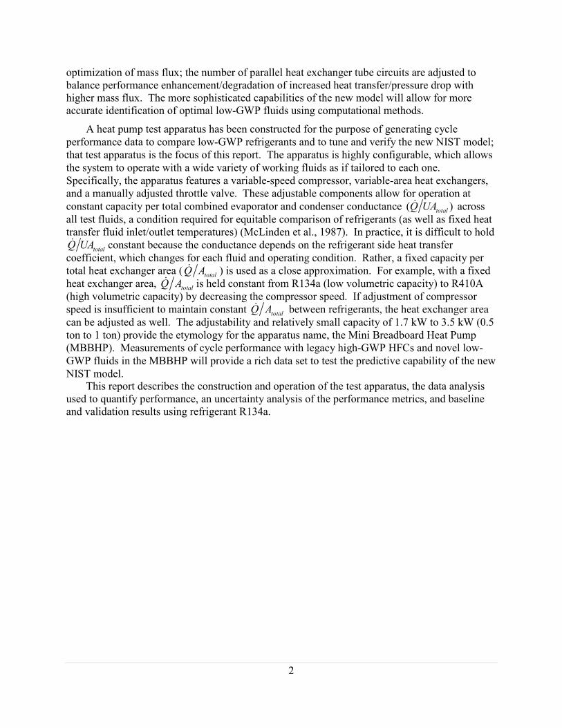
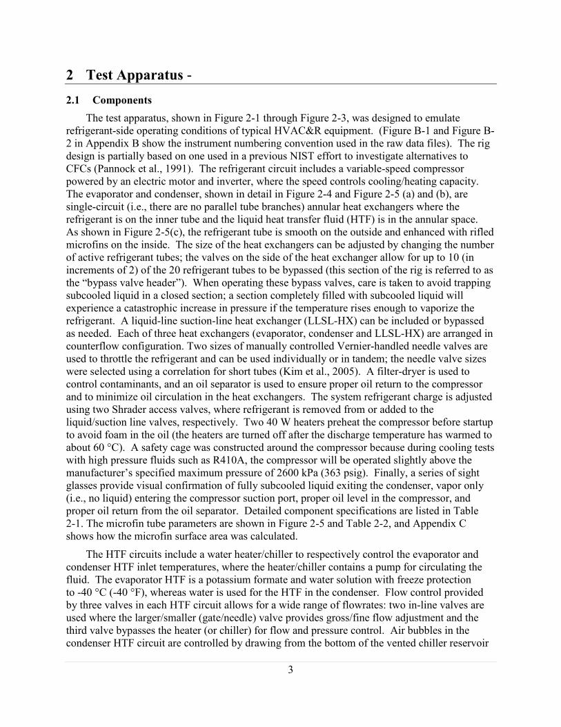
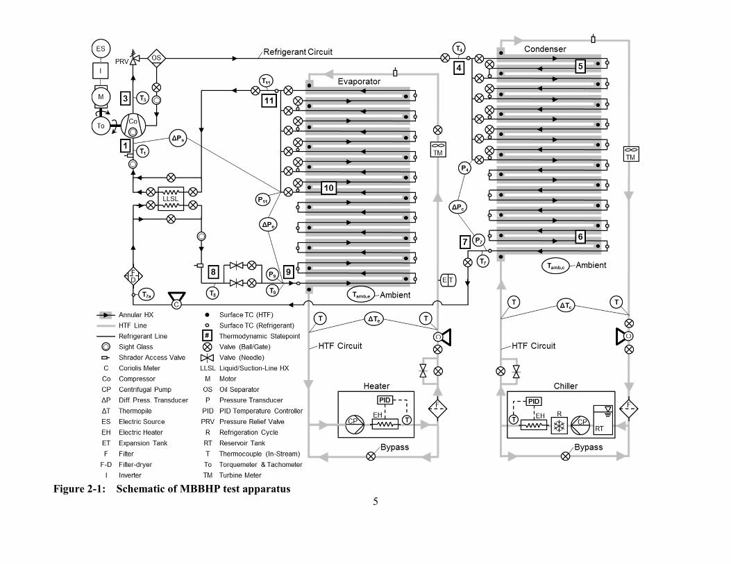
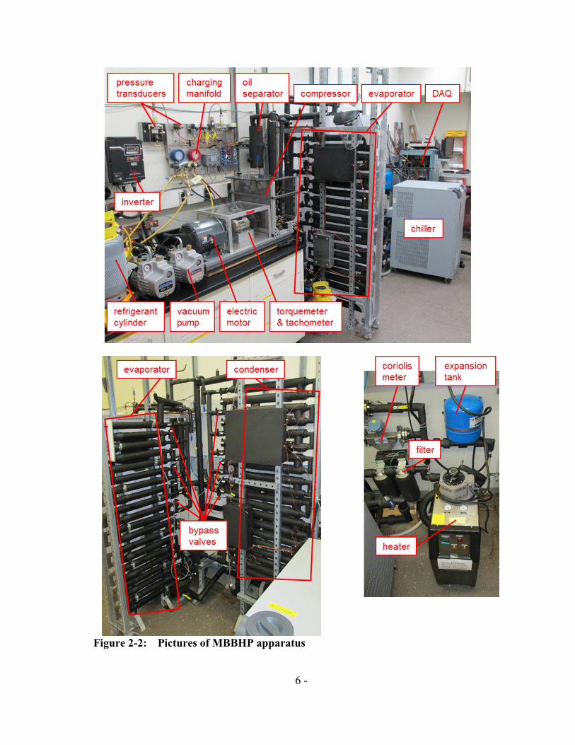
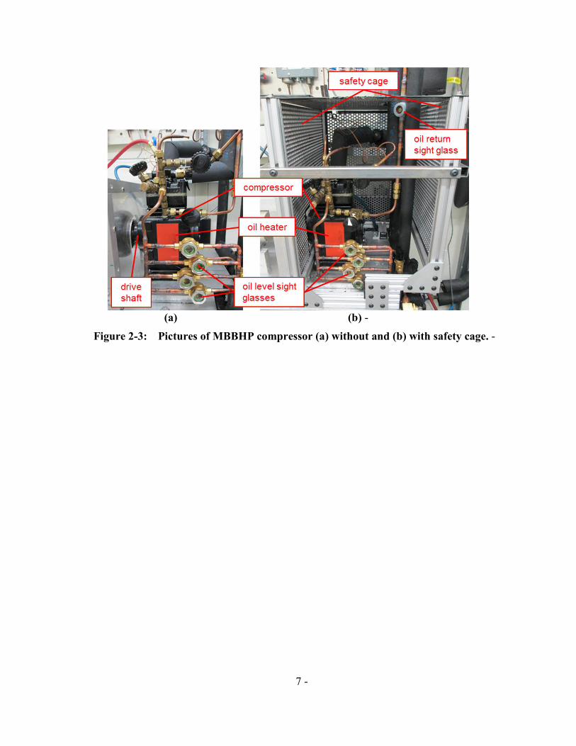
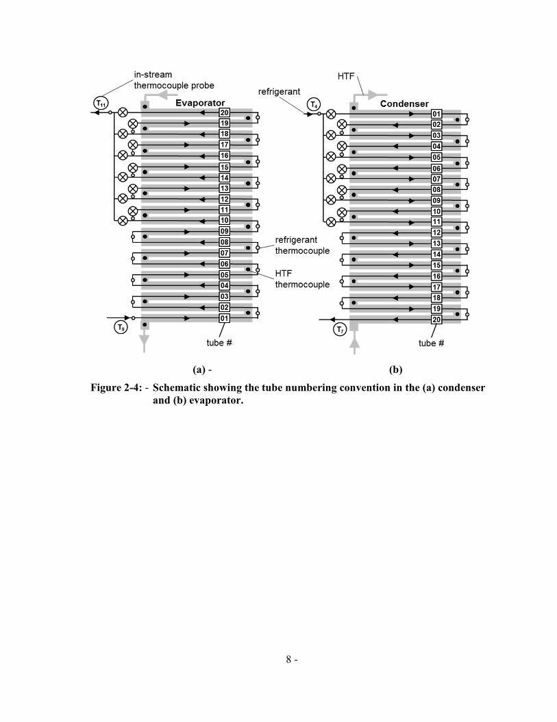
(a)shy (b)
Figure 2-4shy Schematic showing the tube numbering convention in the (a) condenser
and (b) evaporator
8shy
(a)shy
(b)shy (c) (d)
Figure 2-5shy Schematics of annular heat exchanger including (a) refrigerant tube
lengths (b) cross section of annular heat exchanger (c) detail cross-
section of microfin tube and (d) helix angle of microfins
9shy
Table 2-1 Components for MBBHP rig
Component Characteristics
Chiller Cooling capacity 2500 W (07 ton)
Compressor Type
Cylinders
Speed
Displacement rate
Displacement
Max pressure
Reciprocating
2
83 Hz to 667 Hz
(500 RPM to 4000 RPM)
131 m3h-1 to 1081 m3h-1
7165 cm3
2604 kPa (363 psia)
Electric motor Maximum power 373 kW (5 hp)
Expansion tank (HTF) Size 19 liter (5 gallon)
Filter (HTF) Filter size 50 microm
Filter-dryer (refrig) Line size 95 mm (0375 in)
Inverter Voltage
Maximum power
230 VAC 3-phase
373 kW (5 hp)
Heater Heating capacity 10 kW (28 ton)
Heat exchanger
(evaporatorcondenser)
Number of tubes
Tube active length
Return bend length
Outer tube ID
Outer tube OD
Outer tube material
Inner tube
10 to 20 increments of 2
560 mm (22 in)
83 mm (325 in)
254 mm (1 in)
268 mm (1125 in)
Copper
See Table 2-2
Liquid-line suction-line heat
exchanger (LLSL-HX)
Nominal capacity
Shell OD
Type
370 W (05 hp)
51 mm (2 in)
Corrugated (liquid side)
Needle valves (refrig) Valve 1
Orifice
Flow coeff (Cv)
Valve 1
142 mm (0056 in)
003
Valve 2
Orifice
Flow coeff (Cv)
Valve 2
325 mm (0128 in)
016
Needle valves (HTF) Orifice
Flow coeff (Cv)
64 mm (025 in)
073
Oil separator Diameter
Height
Capacity
102 mm (4 in)
356 mm (14 in)
10 to 17 kW (3 to 5 ton)
Pressure relief valve Cracking pressure 800 psig
Note valve orifice sizes and flow coefficients (Cv) can vary between 0 and the listed
maximum values
10
Table 2-2 Refrigerant microfin tube specifications
Parameter Symbol Value Uncertainty
Inside diameter di 846 mm (0333 in) Unknown
Outside diameter do 952 mm (0375 in) plusmn0050 mm (plusmn0002 in)
Bottom wall thickness tb 033 mm (0013 in) plusmn0025 mm (plusmn0001 in)
Fin height e 020 mm (0008 in) plusmn0025 mm (plusmn0001 in)
Spacing between fins sf 022 mm (0009 in) Unknown
Number of fins Nf 60 --
Fin angle β 60deg Unknown
Helix angle α 18deg 2deg
Internal surface area AiL 00424 m (167 in)
per unit tube length
Material Copper
22 Instrumentation
Refrigerant-side instrumentation is selected to capture the key thermodynamic state points in
the cycle Specifications for the instruments (including instrument uncertainty) in both the
refrigerant and HTF circuits are listed in Table 2-3 (Table 2-4 shows I-P units) The pressure
transducers and in-stream thermocouple probes are numbered in Figure 2-1 according to the
eleven states computed in Section 31 the thermodynamic state number convention is also
consistent with that used in the new CYCLE_D-HX model The thermocouple probes are
referenced to a cold junction in an ice-water bath Differential pressure transducers quantify the
pressure drop in the condenser evaporator and suction line The location of the heat exchanger
pressure taps has been selected at the bottom of the bypass valve header where the pressure is
equal to that of the refrigerant leaving the heat exchanger regardless of how many tubes are
bypassed A coriolis flowmeter measures the refrigerant mass flow and density and provides
confirmation of fully subcooled liquid in the liquid line (a two-phase mixture will exhibit large
oscillations in measured flowrate) The compressor shaft power is captured by the in-line torque
meter and tachometer
On the HTF fluid side energy transfers are measured in the evaporator and condenser to
provide verification of the refrigerant-side calculations The mass flow and temperature
difference in the heat exchangers are measured with coriolis meters and thermopiles (in
thermowells) which are combined with the fluid heat capacity to compute energy transfer
Thermocouples inserted into the thermowells with the thermopiles provide the measure of
absolute temperature required for applying the thermopile calibration Additionally the
thermocouples provide verification of the thermopile temperature difference measurement
Figure 2-1 and Figure 2-4 also show the tube-surface-mounted thermocouples used to
measure both refrigerant and HTF temperature profiles in the evaporator and condenser As
shown in Section 326 these temperature profiles are useful for determining refrigerant tube
11
number where the phase transitions (superheat subcooling two-phase) occur The refrigerant-
and HTF-side sensors are mounted on the return bends of each innerouter tube respectively
The instruments are scanned once per minute by the data acquisition (DAQ) system and
when steady state is achieved the measurements are calculated as the average of a moving
window of 30 readings (ie the average over the last 30 minutes) The measurements inevitably
fluctuate during steady state which contributes to the uncertainty of the measurement This
ldquosteady staterdquo uncertainty has been quantified for a nominal test condition and is listed in Table
2-3 The total measurement uncertainty (last column of Table 2-3) is found by adding the
instrument error and the steady state error in quadrature A detailed discussion of the selection
of the steady state moving window size and computation of steady state uncertainty is shown in
Appendix A10
12
Table 2-3 List of MBBHP instruments (SI units)
Instrument Range
Instrument
Uncertainty1
Steady State
Uncertainty1
Total
Uncertainty12
Coriolis meter (HTF) Mass flow
(0 to 756) gs -1
Mass flow 3
plusmn01 rdg
Mass flow
plusmn023 gs -1
Mass flow
plusmn026 gs -1
Density
(0 to 3) g cm-3
Density
plusmn0001 gcm-3
Density
plusmn00001 gcm-3
Density
plusmn0001 gcm-3
Coriolis meter (refrigerant) Mass flow Mass flow 4 Mass flow Mass flow
(0 to 60)5 gs -1 plusmn01 rdg plusmn001 gs-1 plusmn0016 gs -1
Density Density Density Density
(0 to 3) g cm-3 plusmn00005 gcm-3 plusmn00001 gcm-3 plusmn00005 gcm-3
Data acquisition system (-10 to 10) V plusmn1 microV -- plusmn1 microV
Press transducer (diff) ndash condenser (0 to 172) kPa plusmn07 kPa plusmn08 kPa plusmn13 kPa
Press transducer (diff) ndash evaporator (0 to 345) kPa plusmn01 kPa plusmn08 kPa plusmn08 kPa
Press transducer (diff) ndash suction (0 to 69) kPa plusmn001 kPa plusmn03 kPa plusmn03 kPa
Press transducer (high press) (0 to 3447) kPa plusmn34 kPa plusmn07 kPa plusmn35 kPa
Press transducer (low press) (0 to 1724) kPa plusmn34 kPa plusmn07 kPa plusmn35 kPa
Tachometer (017 to 1667) Hz plusmn00167 Hz plusmn0005 Hz plusmn00173 Hz
(10 to 99 999) RPM plusmn1 RPM plusmn03 RPM plusmn104 RPM
Thermocouple (in-stream probe ice ref) (-10 to 100) degC plusmn008 degC plusmn006 degC plusmn009 degC
Thermocouple (surface-mount CJC) (-10 to 60) degC plusmn06 degC plusmn004 degC plusmn06 degC
Thermopile5 (1 to 10) K plusmn0015 K plusmn0013 K plusmn00153 K
Thermopile voltage (-10 to 10) V plusmn1 microV plusmn65 microV plusmn7 microV
Torque meter (0 to 40) N m plusmn033 Nm plusmn0005 Nm 033 Nm
1 95 confidence interval (k = 2)shy2 rdg values have been applied to nominal valuesshy3 Maximum of 01 and (zsflowrate)100 where zs is zero stability = 00491 g s -1 shy4 Maximum of 01 and (zsflowrate)100 where zs is zero stability = 00075 g s -1 shy5 For temperature differences in 1 K to 10 K range Outside range uncertainty is higher See Appendix A5 for moreshydetail
13
Table 2-4 List of MBBHP instruments (I-P units)
Instrument Range
Instrument
Uncertainty1
Steady State
Uncertainty1
Total
Uncertainty12
Coriolis meter (HTF) Mass flow
(0 to 100) lb min-1
Mass flow 3
plusmn01 rdg
Mass flow
plusmn003 lb min-1
Mass flow
plusmn0035 lb min-1
Density
(0 to 187) lb ft-3
Density
plusmn0062 lb ft-3
Density
plusmn0006 lb ft-3
Density
plusmn0062 lb ft-3
Coriolis meter (refrigerant) Mass flow Mass flow 4 Mass flow Mass flow
(0 to 799) lb min-1 plusmn01 rdg plusmn00015 lb min-1 plusmn0002 lb min-1
Density Density Density Density
(0 to 187) lb ft-3 plusmn0062 lb ft-3 plusmn0006 lb ft-3 plusmn0062 lb ft-3
Data acquisition system (-10 to 10) V plusmn1 microV -- plusmn1 microV
Press transducer (diff) ndash condenser (0 to 25) psi plusmn01 psi plusmn01 psi plusmn018 psi
Press transducer (diff) ndash evaporator (0 to 50) psi plusmn0015 psi plusmn01 psi plusmn01 psi
Press transducer (diff) ndash suction (0 to 10) psi plusmn00015 psi plusmn004 psi plusmn004 psi
Press transducer (high press) (0 to 500) psia plusmn05 psi plusmn01 psi plusmn051 psi
Press transducer (low press) (0 to 250) psia plusmn05 psi plusmn01 psi plusmn051 psi
Tachometer (017 to 1667) Hz plusmn00167 Hz plusmn0005 Hz plusmn00173 Hz
(10 to 99 999) RPM plusmn1 RPM plusmn03 RPM plusmn104 RPM
Thermocouple (in-stream probe ice ref) (14 to 212) degF plusmn015 degF plusmn011 degF plusmn018 degF
Thermocouple (surface-mount CJC) (14 to 140) degF plusmn11 degF plusmn008 degF plusmn11 degF
Thermopile5 (18 to 18) degF plusmn0027 degF plusmn0023 degF plusmn004 degF
Torque meter (0 to 350) in lb plusmn29 in lb plusmn0045 in lb plusmn29 in lb
1 95 confidence interval (k = 2) 2 rdg values have been applied to nominal values 3 Maximum of 01 and (zsflowrate)100 where zs is zero stability = 00065 lb min-1
4 Maximum of 01 and (zsflowrate)100 where zs is zero stability = 0001 lb min-1
5 For temperature differences in 18 degF to 18 degF range Outside range uncertainty is higher See Appendix A5 for more
detail
14
23 Operation
231 Test Rig Control Parameters
There are ten Control Parameters (ie settings of adjustable components) listed in Table 2-5
that the MBBHP operator sets to achieve a desired set of Operating Parameters Each Control
Parameter primarily governs one or two Operating Parameters the correspondence is shown in
the table
Table 2-5 List of the Control Parameters and Operating Parameters
Operating Parameter Operating Parameter Values Control Parameter
1 Evaporator saturation temperature See Table 2-6 Heater setpoint (HTF inlet temp)
2 Condenser saturation temperature See Table 2-6 Chiller setpoint (HTF inlet temp)
3 Capacityheat flux 1760 W to 3520 W Compressor speed
(05 ton to 1 ton)
4 Evaporator heat flux 2000 W m-2 to 12 000 W m-2 Number of evaporator tubes
(600 Btu h-1 ft-2 to 3800 Btu h-1 ft-2)
5 Condenser heat flux 2000 W m-2 to 12 000 W m-2 Number of condenser tubes
(600 Btu h-1 ft-2 to 3800 Btu h-1 ft-2)
6 Condenser HTF-side resistance 50 to 70 of overall resistance Condenser HTF flowrate
7 Evaporator HTF-side resistance 70 to 85 of overall resistance Evaporator HTF flowrate
8 Subcool Superheat le 2 tubes1 le 1 tube2 Refrigerant needle valve setting
9 Subcool Superheat le 2 tubes1 le 1 tube2 Refrigerant charge
10 LLSL-HX includedbypassed Includedbypassed LLSL-HX valves
1achieved with subcooling of 2 K to 3 K (18 degF to 36 degF) 2achieved with superheat of 3 K to 6 K (54 degF to 108 degF)
232 Test Rig Operating Parameters
This section describes each of the target Operating Parameters and how they are set using
the Control Parameters Note that the headings for Sections 2321 through 2325 include the
Operating Parameters numbers (1 to 10) as listed in Table 2-5
2321 Operating Parameters 1 amp 2 Evaporator and Condenser Saturation Temperature
The US Department of Energy (DOE) requires heat pumps and air conditioners to be rated
at conditions prescribed in the ANSIAHRI 210240-2008 (AHRI 2008) standard The standard
specifies temperatures of the HTF (air in the standard) entering the evaporator and condenser A
somewhat different but derivative method is employed here the HTF inlet temperatures are set
to achieve refrigerant saturation temperatures expected under ANSIAHRI Cooling A Cooling B
and Heating H1 Rating Tests for the baseline refrigerant R134a
The target saturation temperatures are computed first for the Cooling A test where the
assumed Coefficient of Performance (COPcool) is 44 (energy efficiency ratio EER is 15) The
15
ANSIAHRI standard is not prescriptive about airflow so typical values per unit evaporator ɺcapacity are used for the evaporator (Vɺ Qevap ) 0189 m3 s-1 kW-1 (400 ft3 min-1 ton-1) and air evap
ɺfor the condenser (Vɺ Qevap ) 0378 m3 s-1 kW-1 (800 ft3 min-1 ton-1) Inlet air temperatures air cond
(Tairin) prescribed by the ANSIAHRI standard are listed in Table 2-6 the temperature change
across the evaporator and condenser (∆Tairevap ∆Taircond) is 126 K and 97 K (228 degF and 175
degF) respectively as computed using an energy balance on the airstream where the condenser
energy is larger by an amount that reflects the compressor power (in the COP term)
ɺ )minus1 1ɺ= V (21) ∆Tair evap ( air evap Qevap ρ Cair p air
minus 1 1ɺ Qɺ evap )
1
1+ (22) ∆T = Vair cond ( air cond COP ρ C cool air p air
where the variables represent
Cpair = specific heat of air at constant pressure
ɺV Qɺ evap = condenser airflow per unit evaporator capacity air cond
ɺV Qɺ evap = evaporator airflow per unit evaporator capacity air evap
ρair = density of air
The air outlet temperatures (Tairout) are then computed by respectively subtracting or adding the
∆Tairevap ∆Taircond from the Tairin values
The average temperature difference between the refrigerant and the air (∆Tairref) for
Cooling A is specified as 10 K and 33 K (18 degF and 6 degF) in the evaporator and condenser
respectively based on experience and measurements at NIST for air-source heat pumps with comparable COPs Table 2-6 shows the average air (Tairavg) and average refrigerant saturation
temperatures (Trefavg) computed using this method The Cooling B refrigerant saturation
temperatures are computed using the same ∆Tair and ∆Tairref In heating the heat exchangers
operating as the evaporatorcondenser swap so the values of ∆Tair and ∆Tairref for the evaporator
(in cooling) are used for the condenser and vice versa The resulting refrigerant saturation
temperatures are nominally aligned with values observed in heat pump measurements at NIST
The HTF inlet temperatures (THTFin) are adjusted to achieve the target refrigeration saturation
temperature at a compressor speed of 30 Hz (1800 RPM) with R134a and then held constant for
all other speeds The corresponding HTF outlet temperatures (THTFout) are defined as
T = T + ∆ T (21) HTF e in HTF e out e
T = T + ∆ T (22) HTF c in HTF c out c
where ∆Te and ∆Tc are the HTF temperature differences across the evaporatorcondenser
measured by the thermopiles The THTFout values differ for each speed Table 2-6 shows the
values at 30 Hz (1800 RPM) as a nominal example As discussed in Section 1 a completely fair
comparison of refrigerants requires the same HTF inlet and outlet temperatures (McLinden et al
1987) However it is only possible to match either the evaporator or condenser (but not both)
THTFout by adjusting the heat pump capacity (via compressor speed) the other THTFout will be an
16
uncontrolled value which will vary somewhat from the R134a value depending on the COP of
each fluid (note the HTF mass flow rate is fixed as described in Section 2323 so it cannot be
adjusted to control the other THTFout) Tests with future refrigerants will be carried out with an
evaporator or condenser THTFout equal to the measurements for R134a in cooling or heating
respectively and the other THTFout will vary for each fluid
Table 2-6 Evaporator and condenser fluid temperatures for standard rating tests
Rating Test
Tairin
degC
(degF)
∆Tair
K
(degF)
Tairout
degC
(degF)
Tairavg
degC
(degF)
∆Tairref
K
(degF)
Trefavg
degC
(degF)
THTFin
degC
(degF)
THTFout 1
degC
(degF)
HTFmɺ kg s-1
lb min-1
Cooling A 350 97 447 399 33 432 339 391 0098
(950) (175) (1125) (1038) (60) (1098) (930) (1024) (13)
Condenser Cooling B 278 97 375 326 33 360 249 309 0098
(820) (175) (995) (908) (60) (968) (767) (876) (13)
Heating H1 211 126 338 274 100 374 320 363 0098
(700) (228) (928) (814) (180) (994) (895) (973) (13)
Cooling A 267
(800)
126
(228)
140
(573)
203
(686)
100
(180)
103
(506)
202
(685)
154
(597)
0131
(173)
Evaporator Cooling B
Heating H1
267
(800)
126
(228)
140
(573)
203
(686)
100
(180)
103
(506)
199
(678)
142
(576)
0131
(173)
83 97 -14 35 33 01 103 65 0131
(470) (175) (295) (383) (60) (323) (505) (437) (173)
1 Values for R134a at a compressor speed of 30 Hz (1800 RPM)
2322 Operating Parameters 3 4 amp 5 Capacity and Heat Flux
Baseline capacities were established for R134a at speeds of 233 Hz to 367 Hz (1400 RPM to
2200 RPM) in 33 Hz (200 RPM) increments for each Rating Test Tests with subsequent
refrigerants will be carried out with compressor speeds that match the capacities from the ɺbaseline tests this ensures the refrigerants are tested at the same Q A The target refrigerant-total
side heat flux range was 2 kW m-2 to 12 kW m-2 (600 Btu h-1 ft-2 to 3800 Btu h-1 ft-2) to coincide
with values from typical HVACampR equipment The average heat flux in the evaporator and
condenser was controlled by setting the number of active tubes to 10 and 12 respectively
Figure 2-6 summarizes the capacity for the baseline tests where the evaporator capacity varies
from 12 kW to 21 kW (034 ton to 060 ton) and condenser capacity ranges from 16 kW to 28
kW (045 ton to 080 ton) The heat flux in the evaporator varies from 5 kW m-2 to 9 kW m-2
(1600 Btu h-1 ft-2 to 2900 Btu h-1 ft-2) and in the condenser from 5 kW m-2 to 10 kW m-2 (1700
Btu h-1 ft-2 to 3200 Btu h-1 ft-2) meeting the target heat flux range
17shy
heat transfer area = 0237 m
14
16
20
70
77
84
91
22 94 28
20 25 30 35 40
Cooling B
Cooling A
Heating H1
Evaporator
2
f luid = R134a
tubes = 10
98
20 25 30 35 40
Cooling B
Cooling A
Heating H1
Condenser
heat transfer area = 0285 m2
f luid = R134a
tubes = 12
26 85
Avera
ge
heat
flu
x
[kW
m2]
Cap
acit
y
[kW
]
Avera
ge h
eat
flu
x
[Wm
2]
Cap
acit
y
[kW
] 24
22
20
18shy 76
68
18 60
16
12 51
Compressor frequency [Hz] Compressor frequency [Hz]
(a) (b)
Figure 2-6shy Capacity and heat flux for baseline R134a tests for (a) evaporator and (b)
condenser
2323 Operating Parameters 6 amp 7 HTF-side Thermal Resistance Ratio
In typical air-to-air heat pumps the air-side convection provides the majority of the
resistance to heat transfer Evaporation heat transfer coefficients are generally larger than those
for condensation so the HTF-side resistance ratio (RHTFRtotal) is selected in the range of 50 to
70 for the condenser and 70 to 85 in the evaporator The CYCLE_D-HX model reports
heat exchanger thermal resistances for both the evaporator and condenser when given
measurements of HTF inout temperatures capacity compressor efficiency and heat exchanger
geometry pressure drop and log-mean temperature difference These resistances include the
heat exchanger total conductance (UA) (the total resistance Rtotal is the inverse of UA) the heat
transfer-side resistance (RHTF) in the evaporatorcondenser and the refrigerant-side thermal
resistance (Rref) in the evaporatorcondenser Note that the tube wall thermal resistance is
neglected
The MBBHP was operated under varied HTF flowrates ( mɺ HTF ) and the resulting data were
processed using the CYCLE_D-HX model to determine RHTFRtotal for each flowrate The
evaporator and condenser HTF flowrates used for the tests are 0131 kgs-1 and 0098 kgs-1 (173
lb min-1 and 13 lb min-1) as shown in Table 2-6 which yield RHTFRtotal of 80 and 60 for the
baseline Cooling A test with R134a at 30 Hz (1800 RPM) The flowrates are kept constant for
all other speeds test conditions and refrigerants Maintaining a constant flowrate is important
for verifying the CYCLE_D-HX model the model evaluates the HTF-side thermal resistance for
a reference data set and then holds this resistance constant as other operating parameters
refrigerants and tube circuit configurations are computationally explored
2324 Operating Parameters 8 amp 9 Subcool and Superheat
The number of evaporator tubes containing superheated-vapor and condenser tubes with
subcooled-liquid are controlled to one and two respectively It is important to limit the number
of tubes in superheat and subcooling for comparison with the CYCLE_D-HX model because the
18shy
56
63
model does not consider the pressure drop or area required for heat transfer in these sections
rather it only accounts for transport phenomena in the two-phase section (Note that the
superheat and subcooling are included as an input to the model to determine the thermodynamic
states at the heat exchanger outlets) The superheat and subcooling are also limited because of
performance considerations the single phase fluid exhibits a lower heat transfer coefficient
compared to a two-phase fluid The superheat is bound at the low end by the need to prevent
liquid from entering the compressor The lower limit for subcooling is governed by a
requirement of fully subcooled liquid entering the expansion valve vapor bubbles entering the
expansion valve cause oscillations in the flow that make it difficult to achieve steady state In
general a superheat range of 3 K to 6 K and a subcooling range of 2 K to 3 K satisfies this
Operating Parameter requirement
Closing the refrigerant needle valve increases the superheat and the subcooling whereas
adding refrigerant increases the subcooling and reduces the superheat The combination of these
two controls allows for independent regulation of superheat and subcooling
2325 Operating Parameter 10 LLSL-HX included or bypassed
The LLSL-HX heat exchanger is included or bypassed using the six valves shown in Figure
2-1 When the LLSL-HX is bypassed only one (rather than both) of the valves that stops flow
through the heat exchanger is closed this prevents the possibility of trapping subcooled liquid
between the valves (and presenting the same pressure hazard discussed in Section 21
19shy
3 Data Analysisshy
31 Thermodynamic States
The thermodynamic states numbered 1 through 11 in Figure 2-1 are fixed with two intensive
properties defined by the measurements and equations presented in Table 3-1 Thermodynamic
property data for R134a are computed using the Engineering Equation Solver (EES) software
(Klein 2015) the software uses the equation of state developed by Tilner-Roth et al (1994) for
R134a Note that property data for mixtures and for fluids not directly available in EES will be
computed using the NIST REFPROP database (Lemmon et al 2013)
Table 3-1 Measurements and equations used to define the thermodynamic states
State Description Measurement Equations
1 Compressor inlet LLSL-HX vapor outlet T1 P1 = P11 ndash ∆Ps
2 Compressor cylinder before compression T2 = T1 P2 = P1
3 Compressor outlet T3 P3 = P4
4 Condenser inlet T4 P4 = P7 + ∆Pc
5 Condenser saturated vapor P5 = P4 x5 = 1
6 Condenser saturated liquid P6 = P7 x6 = 0
7 Condenser outlet LLSL-HX liquid inlet T7 P7
8 Expansion valve inlet LLSL-HX liquid outlet T8 P8 = P7
9 Evaporator inlet Expansion valve outlet P9 h9 = h8
10 Evaporator saturated vapor P10 = P11 x10 = 1
11 Evaporator outlet LLSL-HX vapor inlet T11 P11 = P9 ndash ∆Pe
T = temperature P = pressure h = enthalpy x = thermodynamic quality
32 Thermodynamic Performance
Given the fixed state points identified in Table 3-1 (and all associated intensive properties)
the key thermodynamic performance metrics are calculated according to the equations in
Sections 321 through 327 Nominal values and uncertainties of the metrics are shown in
Section 4 and Appendix A respectively
321 Capacity
The evaporator and condenser capacities are computed on the refrigerantHTF-sides
according to
ɺQ = mɺ (h minus h ) (31) ref 4c ref 7
ɺQ = mɺ (h minus h ) (32) ref 9e ref 11
Qɺ = mɺ C ∆T minus Qɺ (33) c HTF HTF c c ins c p HTF c
20shy
ɺQɺ = mɺ C ∆T minus Q (34) p HTF e e HTF HTF e e ins e
where the variables represent
mɺ ref = mass flow of refrigerant
mɺ HTF e mɺ HTF c = mass flow of HTF in evaporatorcondenser
C C = specific heats (average) of HTF in evaporatorcondenser pHTFe pHTFc
ɺQins e Qɺ = insulation heat leak in evaporatorcondenser ins c
∆Te ∆Tc = temperature change of HTF in evaporatorcondenser
The insulation heat leak is a non-trivial 30 W to 50 W and therefore must be accounted for in the
heat exchanger capacity The heat leak is debited from the HTF-side capacity because the HTF
is the annulus and therefore thermally interacts with the surrounding ambient air The heat
exchangers are divided into active and inactive sections (ie tubes where the HTF flows but the
refrigerant does and does not respectively) to compute the heat leak according to
NT NT e active e inactive ɺQ = UA (T minusT ) + (T minusT ) (35) ins e HTF e active avg HTF e inactive avg ins e amb e amb e NT NT e total e total
NT NT c active c inactive
Qɺ = UA ins c (THTF c active avg minusTamb c ) + (T minusTamb c ) (36) ins c HTF c inactive avg NT NT c total c total
where
UAinse UAinsc = insulation conductance for evaporatorcondenser
NTetotal NTetotal = number of tubes in evaporatorcondenser total (20)
NTeactive NTcactive = number of active tubes in evaporatorcondenser
NTeinactive NTeinactive = number of inactive tubes in evaporatorcondenser
THTFeactiveavg THTFcactiveavg = avg HTF temp in the active evaporatorcondenser tubes
THTFeinactiveavg THTFcinactiveavg = avg HTF temp in the inactive evaporatorcondenser tubes
Tambe Tambc = temp of ambient air surrounding evaporatorcondenser
The HTF temperatures are taken from the surface-mounted thermocouples and the ambient air
temperature is taken from a thermocouple near each of the heat exchangers The heat exchangers
are split into activeinactive sections because the slope of the HTF temperature profile is
different in each section the heat transfer is only governed by the average temperature difference
if the slopes (and specific heats) are constant throughout the section The UAinse and UAinsc
values for all 20 tubes are 548 W K-1 plusmn031 W K-1 and 652 W K-1 plusmn041 WK-1 (104 Btu h-1 degF-1
plusmn059 Btu h-1 degF-1 and 124 Btu h-1 degF-1 plusmn078 Btu h-1 degF-1) The method used to compute the
conductance values and their uncertainties is described in Appendix A8
322 Compressor Power
The compressor power is computed using the change in enthalpy across the compressor
21shy
ɺW = ɺ h comp mref ( 3 minus h1 ) (37)
The shaft power is computed for comparison with the compressor power
ɺW = 2πτ N (38) shaft
where the variables represent
N = compressor shaft speed
τ = compressor shaft torque
323 Coefficient of Performance
The cooling and heating COP are computed using the refrigerant-side capacity and the
compressor power applied to the refrigerant
ɺCOP = Qɺ Wcomp (39) cool e ref
ɺ= QCOPheat ɺ
Wcomp (310) c ref
324 Volumetric Capacity
The volumetric cooling and heating capacity (VCC and VHC) are
(mɺ ref v ) (311) VCC = Qɺ
e ref 1
ɺ ( mɺ ref v ) (312) VHC = Q
c ref 1
where
v1 = compressor suction specific volume
325 Compressor Efficiency
The compressor isentropic efficiency is calculated asshy
h ( P s ) minus h3 1 1η s = (313) h minus
3 h
1
where
h(P3s1) = compressor discharge enthalpy under isentropic compression
The volumetric efficiency is quantified by the refrigerant displacement normalized by the
compressor swept volume displacement
mɺ vref 1η v = (314) D N comp
where
22shy
Dcomp = compressor displacement (listed in Table 2-1)
326 Superheat and Subcooling
The evaporator superheat is
SH = T minusT ( P x = 1) (315) 11 11
and the condenser subcooling is
SC = T (P7 x = 0) minusT7shy (316)
where
T(P11 x = 1) = saturated vapor temperature at the evaporator exit pressureshy
T(P7 x = 0) = saturated liquid temperature at the condenser exit pressureshy
The number of refrigerant tubes containing superheatedsubcooled fluid in the
evaporatorcondenser is controlled to one and two respectively during experimental tests
Visual inspection of the temperature profile such as the one shown in Figure 3-1 is used to
determine the locations of the various phase transitions The tube number on the x-axis reflects
the convention established in Figure 2-5
(a)shy (b)
Figure 3-1shy Temperature profile in (a) evaporator showing superheat and (b)
condenser showing subcooling
The location 21 is the exit of the 20th tube
327 LLSL-HX Effectiveness
The LLSL-HX effectiveness is computed as the ratio of the heat transferred on the vapor
23shy
side ( Qɺ ) to the maximum possible heat transfer LLSL v
ɺQ C (T minus T )LLSL v 111 11 p avg 1ε = = (317) ɺLLSL
Q MIN( C C ) (T minus T )LLSL max p avg 111 78 7p avg 11
where
Cpavg111 = average specific heats of the refrigerant on the vapor sideshyCpavg78 = average specific heats of the refrigerant on the liquid sideshy
The heat transfer on the vapor side rather than liquid side is chosen for the numerator because
the larger temperature difference exhibited on the vapor side (due to lower specific heat) results
in a smaller uncertainty in the effectiveness
24shy
4 Validation and Baseline Tests with R134ashyAn initial set of tests were carried out with R134a to provide verification of the
instrumentation and show the nominal uncertainties of the measurements One of the most
important validations is to show an energy balance between the refrigerant and the HTF in the ɺ ɺheat exchangers The energy imbalance defined as Qɺ
ref (Qref minus Q
HTF ) for the initial tests is
shown in Figure 4-1 the imbalance is generally around 1 to 15 or better in both the
evaporator and condenser The imbalance falls well within its uncertainty at the 95
confidence interval indicating that the estimation of the uncertainty in HTF capacity (3 ) is
likely too conservative note that the HTF capacity accounts for more than 90 of the relative
uncertainty in the imbalance metric
Figure 4-1 Energy imbalance in the evaporator and condenser
The performance of R134a in the MBBHP as described by the metrics defined in Section
32 are presented in Figure 4-2 through Figure 4-4 Figure 4-2 (a) and (b) show nominal
pressure profiles on the lowhigh pressure sides of the cycle where the error bars represent
measurement uncertainty listed in Table 2-3 The compressor power measured both by the shaft
power and change of enthalpy of the working fluid are shown in Figure 4-3(a) where the
conversion from mechanical to fluid power is about 65 efficient The error bars represent the
uncertainty calculated by propagating measurement uncertainty through Eqs (37) and (38)
The mass flow ranges from 8 gs-1 to 13 gs-1 (11 lb min-1 to 17 lb min-1) Figure 4-4 shows the
COP ranges from 24 to 4 and the capacity ranges from 16 kW to 21 kW (045 ton to 060 ton)
The figure shows the uncertainties of the COP and capacity where the computation and
tabulation of uncertainty is described further in Appendix A10 and A11 The volumetric
capacity ranges from 2100 kJ m-3 to 2800 kJ m-3 (56 Btu ft-3 to 75 Btu ft-3) and the compressor
isentropic and volumetric efficiencies are nominally 046 and 055 uncertainties in all three of
these metrics are shown in the figures and are computed using a similar method as the
capacityCOP but the computation is not discussed in detail in this report
Figure 4-3 (b) also shows the mass flux which is used to determine the two-phase flow
regimes indicated in Figure 4-5 The refrigerant generally entered the annular flow regime in the
evaporator and condenser though for some tests with low mass flux the refrigerant never left the
stratified-wavy regime
25shy
1100
1150
1200 450 C
om
pre
sso
r p
ow
er
[kW
]shy
Pre
ssu
re [
kP
a]
evaporator tubes = 10
condenser tubes = 12
f luid = R134a
LLSL-HX = no
condenser outlet (P7)
rating test = cooling A
condenser inlet (P4)
Pre
ssu
re [
kP
a]
20 25 30 35 40
Compressor frequency [Hz]
evaporator tubes = 10
condenser tubes = 12
f luid = R134a
LLSL-HX = no
evaporator outlet (P11)
compressor suction (P1)
rating test = cooling A
evaporator inlet (P9)
400
350
1050 300
20 25 30 35 40
Compressor frequency [Hz]
(a)shy (b)
Figure 4-2shy Heat pump cycle pressures on the (a) low pressure side and (b) highshypressure sideshy
0013 12
20 25 30 35 40
Compressor frequency [Hz]
evaporator tubes = 10
condenser tubes = 12
f luid = R134a
LLSL-HX = no
cooling A
cooling B
heating H1
pow er to w orking f luid (Wcomp)
shaft pow er (Wshaf t)
Mass
flo
w [
kg
s]
20 25 30 35 40
evaporator tubes = 10
condenser tubes = 12
f luid = R134a
LLSL-HX = no
cooling A
cooling B
heating H1
0012
Mass
flu
x [
kg
s-m
2]
200 09 0011
180 001
06
0009
0008 03
Compressor frequency [Hz]
(a)shy (b)
Figure 4-3shy Performance metrics including (a) compressor power and (b) mass flow and
mass flux
26shy
140
160
220
Vo
lum
etr
ic c
ap
acit
y [
kJm
3]
CO
P
Vo
lum
etr
ic e
ffic
ien
cy
(η
v)
(a) (b)
20 25 30 35 40 2
25
3
35
4
45
Compressor frequency [Hz]
evaporator tubes = 10
condenser tubes = 12
cooling A
cooling B
heating H1
f luid = R134a
LLSL-HX = no
20 25 30 35 40 15
16
17
18
19
2
21
Compressor frequency [Hz] C
ap
acit
y [
kW
]
cooling A
cooling B
heating H1
evaporator tubes = 10
condenser tubes = 12
fluid = R134a
LLSL-HX = no
2800 07 07
evaporator tubes = 10
condenser tubes = 12
fluid = R134a
LLSL-HX = no
cooling A
cooling B
heating H1
20 25 30 35 40 04
05
06
03
04
05
06
evaporator tubes = 10
condenser tubes = 12
fluid = R134a
LLSL-HX = no
cooling A
cooling B
heating H1
cooling B
cooling A
heating H1
2600
2400
2200
Isen
tro
pic
eff
icie
ncy
( η
s)
20 2000
25 30
Compressor frequency
35
[Hz]
40
Compressor frequency [Hz]
(c) (d)
Figure 4-4 Performance metrics including (a) COP (b) capacity (c) volumetric
capacity and (d) compressor isentropic and volumetric efficiency
27shy
50
Flow boiling with microfin tubeshy Flow condensing with microfin tube 350 350
300 300
S
heat flux 70 kWm2
=
= A
I
SG
S+SW
D
Tsat = 8 C
fluid = R134a
flow range during tests
M
SW
=
Tsat 43 C
fluid = R134a
heat flux 77 kWm2
flow range during tests
A
I
SG
S SW+
SW
0
50
S
Mass F
lux [
kg
s-m
2]
250
200
150
100
Mass F
lux [
kg
s-m
2]
250
200
150
100
0 0shy 02 04 06 08 1 0 02 04 06 08 1
Vapor quality Vapor quality A = Annular D = Dryout I = Intermittant M = Mist A = Annular D = Dryout I = Intermittant M = Mist
S = Stratified SG = Slug SW = Stratified-Wavy S = Stratified SG = Slug SW = Stratified-Wavy
(a)13shy (b)23
Figure 4-5shy Flow regime map for microfin tube (a) evaporation and (b) condensation
1 Flow boiling regime map from (Wojtan et al 2005)shy2 Flow condensation regime map from (Hajal et al 2003)shy3 Boundary between IntermittentAnnular regimes from (Thome 2007) using equation 1261 with a coefficientshy
of 0678 for helical microfins
5 Conclusions and Future Work
This report shows that the test apparatus is capable of measuring the performance of
low-GWP refrigerants with high fidelity including less than 05 uncertainty in both capacity
and COP The energy balance closure on the evaporator and condenser was better than 15
and will be continually tracked to ensure continued high quality data are collected
Future tests will include a second baseline refrigerant R410A followed by a series of
comparative tests with low-GWP refrigerants and refrigerant mixtures The HTF flowrates will
remain fixed from the R134a baseline tests so that the CYCLE_D-HX simulations of the test
data can be carried out for all test data based on a single reference data set After the model
results are verified the model will be used to identify additional candidate refrigerants to test in
the MBBHP test apparatus
28shy
6 ReferencesshyAHRI (2008) 2008 Standard for Performance Rating of Unitary Air-Conditioning amp Air-
Source Heat Pump Equipment Air-Conditioning Heating and Refrigeration Institute
Arlington VA United States Retrieved from wwwahrinetorg
AHRI (2015) Participants Handbook AHRI Low-GWP Alternative Refrigerants Evaluation
Program (Low-GWP AREP) Arlington VA United States Air-Conditioning Heating
and Refrigeration Institute Retrieved from
httpwwwahrinetorgsite514ResourcesResearchAHRI-Low-GWP-Alternative-
Refrigerants-Evaluation
Brown J S Domanski P A amp Lemmon E (2011) Standard Reference Database 49
CYCLE_D NIST Vapor Compression Cycle Design Program Version 50 Retrieved
from httpwwwnistgovsrdnist49cfm
Domanski P A Brown S J Heo J Wojtusiak J amp McLinden M O (2014) A
thermodynamic analysis of refrigerants Performance limits of the vapor compression
cycle International Journal of Refrigeration 38 71-79
doi101016jijrefrig201309036
EPA (2015) 2015 North American Amendment Proposal to Address HFCs under the Montreal
Protocol Retrieved from httpwwwepagovozoneintpolmpagreementhtml and
httpwwwepagovozoneintpolHFC_Amendment_2015_Summarypdf
EU (2014 April 16) Regulation (EU) No 5172014 of the European Parliament and of the
Council of 16 April 2014 on fluorinated greenhouse gases and repealing Regulation (EC)
No 8422006 Journal of the European Union Retrieved from httpeur-
lexeuropaeulegal-contentENTXTuri=uriservOJL_201415001019501ENG
Fortin T J (2015) Personal communication
Hajal J E Thome J R amp Cavallini A (2003) Condensation in horizontal tubes part 1 two-
phase flow pattern map International Journal of Heat and Mass Transfer 3349-3363
doi101016S0017-9310(03)00139-X
Harr L Gallagher J S amp Kell G S (1984) NBSNRC Steam Tables Hemisphere Publishing
Co
Kazakov A McLinden M O amp Frenkel M (2012) Computational Design of New
Refrigerant Fluids Based on Environmental Safety and Thermodynamic Characteristics
Industrial amp Engineering Chemistry Research 51 12537-12548 doi101021ie3016126
Kim Y Payne V Choi J amp Domanski P A (2005) Mass flow rate of R-410A through short
tubes working near the critical point International Journal of Refrigeration 28 547-553 doi101016jijrefrig200410007
Klein S A (2015) Engineering Equation Solver v 9908 Retrieved from
httpwwwfchartcomees
Lemmon E W Huber M L amp McLinden M O (2013) NIST Standard Reference Database
23 Reference Fluid Thermodynamic and Transport Properties (REFPROP) Version 91
29shy
National Institute of Standards and Technology Retrieved fromshyhttpwwwnistgovsrdnist23cfmshy
McLinden M O amp Radermacher R (1987) Methods for Comparing the Performance of Pure
and Mixed Refrigerants in the Vapour Compression Cycle International Journal of
Refrigeration 10(6) 318-325 doi1010160140-7007(87)90117-4
McLinden M O Kazakov A Heo J Brown J S amp Domanski P A (2014) A
thermodynamic analysis of refrigerants Possibilities and tradeoffs for Low-GWP
refrigerants International Journal of Refrigeration 38 80-92
doi101016jijrefrig201309032
Pannock J amp Didion D A (1991) The Performance of Chlorine-Free Binary Zeotropic
Refrigerant Mixtures in a Heat Pump NISTIR 4748 Internal Report National Institute of
Standards and Technology US Department of Commerce Gaithersburg Retrieved from
httpfirenistgovbfrlpubsbuild91art002html
Solomon S Qin D Manning M Chen Z Marquis M Averyt K B Miller H L
(2007) Contribution of Working Group I to the Fourth Assessment Report of the
Intergovernmental Panel on Climate Change New York NY USA Cambridge
University Press Retrieved July 29 2015 from
httpwwwipccchpublications_and_datapublications_ipcc_fourth_assessment_report_
wg1_report_the_physical_science_basishtm
Taylor B N amp Kuyatt C E (1994) Guidelines for Evaluating and Expressing the Uncertainty
of NIST Measurement Results National Institute of Standards and Technology Technical
Note 1297
Thome J R (Updated in 2007) Wolverine Heat Transfer Engineering Data book III Germany
Weiland-Werke AG Retrieved from httpwwwwlvcomheat-transfer-databook
Tilner-Roth R amp Baehr H D (1994) An International Standard Formulation for the
Thermodynamic Properties of 1112-Tetrafluoroethane (HFC-134a) for Temperatures
from 170 K to 455 K and Pressures up to 70 MPa J Phys Chem Ref Data 23(5)
Wojtan L Ursenbacher T amp Thome J R (2005) Investigation of flow boiling in horizontal
tubes Part ImdashA new diabatic two-phase flow pattern map International Journal of Heat
and Mass Transfer 2955-2969 doi101016jijheatmasstransfer200412012
30shy
Appendix A Uncertainty Analysisshy
A1 Symbols Used in Uncertainty Analysisshy
Symbol Units Definition
k -- Expanded uncertainty coverage factor
n -- Number of data points
Qɺ kW Energy transfer
SUAinse W K -1 Standard deviation of evaporator insulation conductance
SX -- Standard deviation of measured quantity ldquoXrdquo
T degC Temperature
T1 degC Temperature at cold end of thermopile
Tcal degC Temperature of RTD used for calibrations
TTCcal degC Calibrated thermocouple measurement
TTCCJC degC Thermocouple measurement with Cold Junction Compensation
∆Tlm K Log-mean temperature difference
∆TTCcal K Thermocouple calibration temperature difference
∆TTP K Temperature difference of thermopile
UA W K -1 Thermal conductance
UA ins e U W K-1 Uncertainty of average of evaporator insulation conductance
UTC degC Total instrument uncertainty of thermocouple
UTCcal degC Thermocouple instrument uncertainty from calibrating device uncertainty
UTCfit degC Instrument uncertainty of thermocouple due to fit of calibration regression
UX -- Uncertainty of measured quantity ldquoXrdquo
X U -- Uncertainty of average of measured quantity ldquoXrdquo
UY Uncertainty of calculated quantity ldquoYrdquo
V V Voltage
V1 V Thermopile voltage of cold end of thermopile (referenced to ice-point)
VCC kJ m -3 Volumetric Cooling Capacity
VHC kJ m -3 Volumetric Heating Capacity
VTC V Thermocouple voltage
∆VTP V Thermopile voltage
X -- Measured quantity
Y -- Calculated quantity
31shy
Subscript Definition
amb Ambient airshyc Condensershye EvaporatorshyHTF Heat Transfer Fluidshyin Inletshyins Insulationshyout Outletshy1 to 11 Refrigerant thermodynamic states as defined by Figure 2-1shy
Abbreviation Definition
COP Coefficient of Performance (W capacity per W of input power)shyCJC Cold Junction Compensation (for thermocouples)shyDAQ Data AcquisitionshyDSC Differential Scanning Calorimeter (used to measure fluid specific heat)shyEES Engineering Equation Solver (software used to reduce data)shyHTF Heat Transfer FluidshyMBBHP Mini Breadboard Heat PumpshyRPM Revolutions per Minute (compressor shaft)shyRTD Resistance Temperature Detectorshy
A2 General Remarks
The uncertainty analyses for key performance metrics are presented in this section All
uncertainties are estimated based on instrument uncertainties computed at a 95 confidence
interval
A3 Thermocouples with CJC Compensation
The surface-mounted thermocouples as well as the thermocouples measuring the air
temperature near the evaporatorcondenser are compensated at the DAQ using a thermistor-
based Cold Junction Compensation (CJC) A calibration (∆Tcal) is applied to the resulting
temperature reading (TTCCJC) to compute the calibrated temperature (TTCcal) according to
T = T + ∆ T (A1) TC cal TC cal TC CJC
where the calibration is fit to a 2nd order polynomial (the order of this curve fit and others
presented in Appendix A were selected based on t-test of polynomial coefficients)
= T minus a T + a T 2∆T cal T = a0 + 1 TC CJC 2 TC CJC (A2)
TC cal TC CJC
The polynomial coefficients (a0 a1 a2) are fit using the least square error method and Tcal is the
temperature measured by the calibrating instrument (two calibrated RTDs read by a precision
digital thermometer expanded uncertainty of plusmn002 degC) The thermocouples were calibrated over
a temperature range of -10 degC to 60 degC and this calibration was repeated five times over the
32shy
course of two weeks Figure A-1 (a) shows the calibration data and polynomial curve fits for a
representative thermocouple Each calibration shows a significant offset from the others this is
likely a manifestation of the repeatability error of the CJC which has an overall uncertainty of
plusmn05 degC Figure A-1 (b) shows the aggregation of the five data sets and the resulting curve fit
and 95 confidence interval (plusmn06 degC) The uncertainty of the calibrated RTDs is more than an
order of magnitude smaller than the curve fit confidence interval and is therefore neglected The
CJC thermocouple instrument uncertainty listed in Table 2-3 is therefore plusmn06 degC
05 05
Tem
pera
ture
cali
bra
tio
n( ∆
Tc
al)
[K]
Tem
pera
ture
cali
bra
tio
n( ∆
Tc
al)
[K]
0
-05
-1 ddaattaa
ccuurrvvee ffiitt
9955 ccoonnffiiddeennccee iinntteerrvvaall
0
-05 ccaalliibbrraattiioonn 11
ccaalliibbrraattiioonn 22
ccaalliibbrraattiioonn 33
ccaalliibbrraattiioonn 44
-1 ccaalliibbrraattiioonn 55
ccuurrvvee ffiittss
-15 -15 -10 0 10 20 30 40 50 60 -10 0 10 20 30 40 50 60
Temperature (TTCCJC) [degC] Temperature (TTCCJC) [degC]
(a) (b)
Figure A-1 Temperature calibration for CJC compensated thermocouples where
(a) data are divided by each of the 5 calibrations and (b) all data are
combined
A4 Thermocouples with Ice-Water Bath Compensation
A lower level of uncertainty is achieved for the in-stream probe thermocouples which
measure the refrigerant temperatures at key thermodynamic states by utilizing an ice-water bath
reference junction The ice-water bath consists of a vacuum insulated Dewar filled with crushed
ice and water the reference junction is submerged in the bath inside of a water-filled test tube
Using the ice-water bath removes the large uncertainty associated with the electronic CJC on the
DAQ system The thermocouples were calibrated against the RTDs (same ones used to calibrate
thermocouples with CJC) where the resulting data and curve fit are shown for a representative
thermocouple in Figure A-2 The data were fit to 5th order polynomials according to
5
T aV i (A3) =sum iTC cal TC
i=0
where VTC is the thermocouple voltage The resulting instrument uncertainty (plusmn008 degC) listed in
Table 2-3 is the combination of the curve fit standard error (UTCfit k = 2) and the calibrating
RTD error (UTcal)
2 2 2 2 U = plusmn U +U = plusmn 0079 + 002 = plusmn008 degC (A4)TC TC fit T cal
33
Tem
pera
ture
[degC
]
80
ddaattaa
ccuurrvvee ffiitt60
40
20
0
-20 -00005 0 00005 0001 00015 0002 00025
Voltage [V]
Figure A-2 Ice-water bath referenced thermocouple calibration data
A5 Thermopiles in Heat Transfer Fluid
The 13-junction thermopiles were calibrated by immersing one end in an ice-water bath
(inside a water-filled test tube) and the other end in a temperature controlled bath The
temperature in the controlled bath was measured using the two calibrated RTDs A thermopile
voltage-temperature dataset was generated and fit to a 4th order polynomial Figure A-3 shows
the calibration data and the curve fit and Table A-1 shows the polynomial coefficients The
calibration data are fit to the equation
N =4 i
T = sum aTP i V (A5) i=0
The temperature difference for a thermopile is computed according to
∆T = ( V T V + ∆ ) minusT (A6)TP 1 TP 1
where ∆VTP is the measured thermopile voltage and T1 is the temperature measured at the cold
end of the thermopile by a CJC-corrected thermocouple Eq (A5) is substituted into Eq (A6)
to calculate the thermopile temperature difference
N =4
∆TTP = sum aTP i (V1 +∆VTP ) minusT1 (A7) i=0
where V1 (cold-end voltage) is computed by numerically solving Eq (A5) where T is set to (T1)
N =4 i V1 = root T1 minussum aTPi V1 = 0 (A8)
i=0
The thermopile uncertainties are computed with respect to the curve fit voltage
measurement and temperature measurement at the cold end of the thermopile (characterized
respectively by the coefficient uncertainties in Table A-1 the thermopile voltage uncertainty in
Table 2-3 and the CJC corrected thermocouple in Table 2-3) The EES (Klein 2015) software
34
is used to numerically compute the partial derivatives and subsequent thermopile uncertainties
Figure A-4(a) shows the contours of uncertainty in the temperature difference measured by the
evaporatorcondenser HTF thermopiles
Figure A-4(b) shows the contours of relative contribution to uncertainty in the thermopile
measurement Each of the uncertainty sources is dominant in different regions
bull voltage measurement dominant at low temperature differences (less than 1 K)
bull curve fit error dominant at high cold end temperatures (greater than 50 degC)
bull cold end temperature dominant at moderate cold end temperatures -5 degC to 20 degC and temperature differences 25 K to 20 K
As noted in this discussion the thermopile uncertainty is a complex function of the curve fit
voltage measurement and cold end temperature measurement For the temperature difference
range expected for this application 1 K to 10 K (18 degF to 18 degF) the upper bound of uncertainty
is about 0015 K (0027 degF) for simplicity this is the value listed in Table 2-3 Note that the
contribution to the uncertainty by the calibrating instrument (two calibrated RTDs) is negligible
here as the error in slope (which is the error that propagates into the thermopile temperature
difference) is less than 0000248 K per K of temperature difference (eg 000248 K for a 10 K
temperature difference)
Table A-1 Condenser amp evaporator60
thermopile polynomial coefficients 50
Uncertainty
Coeff Value (k=2) 95 40
Tem
pera
ture
[degC
]
aTPe0 39243 E-02 plusmn41 E-04 30
aTPe1 20243 E+03 plusmn12 E-01 20
aTPe2 -55466 E+03 plusmn22 E+01 TTPP11
10 TTPP22 aTPe3 39023 E+04 plusmn13 E+03 TTPP11 ((ffiitt))
TTPP22 ((ffiitt)) aTPe4 -26229 E+05 plusmn22 E+04
0
-10
38494 E-02 plusmn53 E-04 -001 0 001 002 003 004 aTPc0
Voltage [V]shy aTPc1 20241 E+03 plusmn15 E-01
Figure A-3 Thermopile calibration data aTPc2 -55190 E+03 plusmn28 E+01
aTPc3 38551 E+04 plusmn16 E+03
aTPc4 -25440 E+05 plusmn29 E+04
35
-5
0
10
20 contours of thermopile uncertainty [K] contours of contribution to uncertainty []
20
balance is T1004
0035
Tem
pera
ture
dif
fere
nce
(∆
TT
P)
[K]
15 003
0025
002
0015
001 0001 5
0002 0005
0004 0003
Tem
pera
ture
dif
fere
nce (∆
TT
P)
[K]
15
10
curve fit
80 60
40 20
5 voltage (∆VTP)
20 40
0 60
80
0 10 20 30 40 50
Temperature at cold end (T1) [degC]
60 -5
0 10 20 30 40 50
Temperature at cold end (T1) [degC]
60
(a) (b)
Figure A-4 Contours of thermopile (a) uncertainty and (b) relative contribution to
uncertainty
A6 Evaporator Heat Transfer Fluid Specific Heat
The evaporator HTF is a potassium formate and water heat transfer fluid that is freeze
protected to -40 degC The manufacturerrsquos specific heat data were found to have error of at least
10 so a sample of the fluid was analyzed in a Differential Scanning Calorimeter (DSC) by the
NIST-Boulder Applied Chemicals and Materials Division The temperature dependent specific
heat and the 2nd order curve fit to the data are shown in Figure A-5 the curve fit coefficients and
their uncertainties are listed in Table A-2 Figure A-5 also shows the manufacturerrsquos reported
specific heat data for comparison The exact uncertainty of the DSC measurement was not
available at the time of writing but was estimated to be about 2 to 3 of reading based on the
experience of the DSC operator (Fortin 2015) An uncertainty of 3 of reading is therefore
assigned as a conservative estimate Both the curve fit and DSC calibration uncertainties are
included in the calculation of overall uncertainties
36shy
DSC measurements
curve fit
3 Table A-2 Evaporator HTF specific
heat polynomial coefficients
29 Uncertainty
DSC measurements
curve fit
manufacturers data
-10 0 10 20 30
Sp
ecif
ic h
eat
(Cp)
[Jg
-K]
Coeff Value (k=2) 95
28 aCpe0 25643 E+00 plusmn16 E-03
aCpe1 11015 E-03 plusmn21 E-04
27 aCpe2 17422 E-05 plusmn95 E-06
26
25
Temperature [degC]
Figure A-5 Specific heat measurements for
evaporator HTF
A7 Condenser Heat Transfer Fluid Specific Heat
The condenser HTF is water the specific heat data are computed in EES using the data from
(Harr et al 1984) and are shown in Figure A-6 A conservative estimate of plusmn3 is used for the
uncertainty in the specific heat
423
0 20 40 60 80 100
Sp
ecif
ic h
eat
(Cp)
[kJk
g-K
]
422
421
42
419
418
Temperature [degC]
Figure A-6 Specific heat of condenser HTF (water)
A8 Evaporator and Condenser Insulation Conductance
The total evaporator and condenser insulation conductances (UAinse and UAinsc) for thermal
interaction with the ambient air were measured during an initial test where the HTFs were
circulated at various flow rates through the apparatus at an elevated temperature while the
refrigerant tubes were under vacuum The temperature change of the HTF across the heat
37shy
exchanger was assumed to be entirely attributed to insulation heat leak and therefore an
effective insulation conductance could be computed The resulting UAinse and UAinsc values for
all 20 tubes are shown in Figure A-7 Average values of conductances for the evaporator and
condenser were calculated as 548 W K-1 plusmn031 W K-1 and 652 W K-1 plusmn041 W K-1
(104 Btu h-1 degF-1 plusmn059 Btu h-1 degF-1 and 124 Btu h-1 degF-1 plusmn078 Btu h-1 degF-1) respectively where the
uncertainty accounts for both instrumentation error and test variance The evaporator insulation
conductance for these tests is computed according to
ɺQins e mɺ HTF e C (THTF in e minusT )p HTF e HTF out e
UA = = (A9) ins e ∆T T minusT minus T minusT e ( HTF in e amb e ) ( HTF out )lm HTF e amb e
(T minusT ) amb e HTF in e ln (T
minusT
amb e ) HTF out e
where the variables represent
Cp HTF e = evaporator HTF specific heat
mɺ HTF e = evaporator HTF mass flow
Qɺ = evaporator insulation heat leak ins e
Tambe = ambient air temperature surrounding evaporator
THTFine = evaporator HTF inlet temperature
THTFoute = evaporator HTF outlet temperature
∆TlmHTFe = evaporator log-mean temperature difference
and the uncertainty of the average value is calculated according to
U = k S n (A10) UA ins e UA ins e
where the variables represent
k = expanded uncertainty coverage factor (k = 2) for 95 confidence interval
SUAinse = standard deviation of conductances
n = number of conductance data points
The condenser conductance is computed using the same method with the corresponding
measurements from that heat exchanger
38shy
4
5
6
7
8
Insu
lati
on
co
nd
ucta
nce (
UA
ins)
[WK
]
UAinscond
UAinsev ap
average for evaporator
average for condenser
0 005 01 015
Mass flow [kgs]
Figure A-7 Insulation conductance for evaporator and condenser
A9 Uncertainty Analysis Software
The uncertainty analyses on each of the performance metrics shown in Figure 4-1 through
Figure 4-4 were calculated using the uncertainty propagation capability in EES The software
numerically computes the performance metric uncertainty by evaluating the partial derivatives
with respect to each relevant measurement and applying the specified measurement uncertainty
Assuming the measurements are independent and uncorrelated the uncertainty of a quantity is
computed according to (Taylor amp Kuyatt 1994)
partY 2 2
UY = sum U X (A11) i partXi
i
where the variables represent
Y = calculated quantity
Uy = uncertainty of calculated quantity
Xi = measurement
UXi = uncertainty of measurement
39shy
A10 Moving Window and Steady State Uncertainty
A moving window average was used to compute the measurements at steady state during the
tests In order to determine a proper window size the variation of measurement steady state
uncertainty with window size was examined The steady state uncertainty is defined as the
expanded standard uncertainty for the average reading within the window
S X (A12) U = k X
n
where
k = coverage factor (k = 2) for 95 confidence interval
n = number of samples in the window
Sx = standard deviation of measurement
X = average value of measurement
The data for analysis were generated by holding the MBBHP at a nominal steady operating
condition and recording the measurements at 1-minute intervals (same as collection rate for all
performance testing) for an extended time (3 hours) Figure A-8 shows the fluctuation of steady
state uncertainty for the evaporator inlet and outlet temperatures (T9 and T11) The figure
highlights two characteristic trends observed for all of the instruments both of which suggest the
need for a large moving window (1) the steady state uncertainty decreases as the window size
increases and (2) the steady state uncertainty is highly oscillatory for small windows (the
oscillations are undesirable because short-term fluctuations can have a disproportionate impact
on the averaged result) A 30 sample moving window was selected to achieve low uncertainty
while allowing for collection of data in a timely manner
Figure A-8 shows that the measurement steady state uncertainty is not constant in time (it
would be constant if the fluctuations at steady state were purely random) but rather exhibits
drifting and periodic movements This is possibly due to hunting by the PID controllers
regulating HTF fluid temperatures changes in air temperature in the lab space or some other
uncontrolled andor uncharacterized phenomena These non-random fluctuations are accounted
for by using the maximum steady state uncertainty value observed during the extended steady
state test For example Figure A-8(a) shows the maximum steady state uncertainty for the
evaporator outlet (T9) is plusmn006 degC this value and values for all other sensors are listed in Table
2-3 The data in the moving window are only recorded when steady state uncertainties are below
these established thresholds The total uncertainty (plusmn009 degC) also shown in Table 2-3 is
subsequently computed by adding the instrument uncertainty (plusmn008 degC) and steady state
uncertainty (plusmn006 degC) in quadrature
Note that different sensors of the same type exhibit different levels of fluctuation as a
conservative estimate the largest uncertainty of any one is applied to all of them For example
Figure A-8(b) shows the fluctuations of steady state uncertainty for the evaporator inlet
temperature (T9) are much smaller than for the evaporator outlet (T11) In fact the evaporator
outlet temperature (T11) shows the most fluctuation of all the ice-water bath compensated
thermocouple probes therefore its value (plusmn006 degC) is used in Table 2-3 to represent them all
40shy
05 05
01 01
Ts
[C]
001 001
Ute
ad
y
0002
(a)
Time elapsed [s]
0002
(b)
Time elapsed [s]
Figure A-8shy Uncertainty in temperature due to fluctuations at steady state for (a)
evaporator outlet and (b) evaporator inlet
A11 Uncertainty Results Summary
The detailed instrument uncertainty analysis for performance metrics including the
refrigerantHTF-side capacities and the COPs are tabulated in Appendices A111 (cooling) and
A112 (heating) The tables show the performance metric and its total uncertainty (including
both instrument and steady state contributions) as well as the measurements that contribute to
the uncertainty The measurement values uncertainties partial derivatives (of performance
metric with respect to the measurement) and relative errors (contribution to the overall error in
the performance metric) are also shown where the measurements are listed in order of
decreasing relative error Uncertainties for other performance metrics (eg VCCVHC ηisen)
were analyzed using similar techniques but are not shown in detail in this report Note that
Appendices A111 and A112 show sample calculations for a single nominal operating
condition whereas the uncertainty values presented in the Section 4 figures are computed for
each test run
The uncertainty in cooling performance metrics are shown for a nominal operating point for
R134a during a Cooling A test with a compressor speed of about 30 Hz (1800 RPM) Similarly
the uncertainty in heating performance metrics are shown for R134a during a Heating H1 test
with a compressor speed of about 30 Hz (1800 RPM)
A111 Uncertainty Results Summary Cooling
Table A-3 shows that the dominant sources of instrument uncertainty for the refrigerant-side
capacity are refrigerant mass flow (66 ) expansion valve inlet temperature (17 ) evaporator
exit pressure (8 ) and evaporator exit temperature (7 ) Table A-4 shows the dominant
source of instrument uncertainty for the HTF-side capacity is the HTF specific heat (97
estimate for instrument used to measure fluid properties) Table A-5 shows the dominant
sources of instrument uncertainty for cooling COP are evaporator inlet pressure (39 )
compressor discharge temperature (25 ) and compressor suction temperature (18 )
8000 12000 16000 20000
UT
ste
ad
y [
C]
increasing
time window
10 min
30 min 60 min
05 min
maximum (006 degC)
8000 12000 16000 20000
increasing
time window
10 min
30 min 60 min
05 min
41shy
Table A-3 Uncertainty of refrigerant-side evaporator cooling capacity
Total Partial Relative
Parameter Symbol Value Uncertainty Derivative Error
Refrigerant-side evaporator capacity eref Qɺ 1692 kW plusmn00035 kW
(020) -- --
Refrigerant mass flow refmɺ 1100 g s-1 plusmn0024 g s-1 1538 E-01 66
Refrigerant temp at expansion valve inlet T8 3816 C plusmn009 degC -1634 E-02 17
Refrigerant press at evaporator inlet P9 412 kPa plusmn35 kPa -2817 E-04 8
Refrigerant temp at evaporator exit T11 1209 C plusmn009 degC 1009 E-02 7
Refrigerant press at condenser exit P7 1104 kPa plusmn35 kPa 2103 E-06 0
Refrigerant evaporator differential press ∆Pe 4392 kPa plusmn08 kPa 2817 E-04 0
Table A-4 Uncertainty of HTF-side evaporator cooling capacity
Total Partial Relative
Parameter Symbol Value Uncertainty Derivative Error
plusmn005 kW HTF-side evaporator capacity Qɺ 1672 kW -- --eHTF (30)
Evaporator HTF capacity cp HTF e 259 J g-1 K-1 plusmn3 of cp 6369 E-01 97 calibration uncertainty HTF e
Temperature of ambient air
surrounding evaporator Tambe 230 degC plusmn06 degC 5474 E-03 1
HTF mass flow HTF e mɺ 1312 g s-1 plusmn026 g s-1 1257 E-02 1
Evaporator HTF thermopile voltage ∆VTPe 2512 mV plusmn0007 mV 6537 E-01 1
Evaporator HTF thermopile aTPe0 39243 E-02 plusmn41 E-04 4047 E-03 0
polynomial coefficients aTPe1 20243 E+03 plusmn12 E-01 8832 E-04 0
aTPe2 -55466 E+03 plusmn22 E+01 1559 E-05 0
aTPe3 39023 E+04 plusmn13 E+03 2106 E-07 0
aTPe4 -26229 E+05 plusmn22 E+04 2554 E-09 0
Evaporator HTF capacity aCpe0 25643 E+00 plusmn16 E-03 6369 E-01 0
polynomial coefficients aCpe1 11015 E-03 plusmn21 E-04 1135 E+01 0
aCpe2 17422 E-05 plusmn95 E-06 2024 E+02 0
Temperature at cold end of
evaporator HTF thermopile THTFeout 1542 degC plusmn06 degC -2963 E-03 0
Evaporator insulation conductance UAinse 5474 W K-1 plusmn03052 W K-1 4175 E-03 0
42shy
Table A-5 Uncertainty of cooling COP
Total Partial Relative
Parameter Symbol Value Uncertainty Derivative Error
Cooling COP coolCOP 2844
plusmn001
(035 ) -- --
Refrigerant press at evaporator inlet P9 412 kPa plusmn35 kPa -1232 E-02 39
Refrigerant temp at compressor discharge T3 8197 degC plusmn009 degC 5571 E-02 25
Refrigerant temp at compressor suction T1 1273 degC plusmn009 degC 4788 E-02 18
Refrigerant press at condenser exit P7 1104 kPa plusmn35 kPa 5144 E-03 7
Refrigerant temp at expansion valve inlet T8 3816 degC plusmn009 degC -2746 E-02 6
Refrigerant temp at evaporator exit T11 1209 degC plusmn009 degC 1696 E-02 2
Refrigerant evaporator diff press ∆Pe 4392 kPa plusmn08 kPa 7432 E-04 2
Refrigerant condenser diff press ∆Pc 3234 kPa plusmn13 kPa 4731 E-04 1
Refrigerant suction line diff press ∆Ps 1422 kPa plusmn03 kPa 1314 E-03 0
Refrigerant mass flow refmɺ 1100 g s-1 plusmn0016 g s-1 2209 E-04 0
A112 Uncertainty Results Summary Heating
Table A-6 shows the dominant sources of instrument uncertainty for the refrigerant-side
capacity are refrigerant mass flow (85 ) condenser exit temperature (9 ) and condenser inlet
temperature (5 ) Table A-7 shows the dominant source of instrument uncertainty for the HTF-
side capacity is the HTF specific heat (97 estimate for instrument used to measure specific
heat of water in the reference) Table A-8 shows the dominant sources of instrument uncertainty
for cooling COP are evaporator inlet pressure (32 ) compressor discharge temperature (31 )
and compressor suction temperature (22 )
43shy
Table A-6 Uncertainty of refrigerant-side condenser heating capacityshy
Total Partial Relative
Parameter Symbol Value Uncertainty Derivative Error
Refrigerant-side condenser capacity c refQɺ 1873 kW plusmn0004 kW
(02) -- --
Refrigerant mass flow refmɺ 906 g s-1 plusmn0016 g s-1 2067 E-01 85
Refrigerant temp at condenser exit T7 3739 degC plusmn009 degC -1343 E-02 9
Refrigerant temp at condenser inlet T4 7722 degC plusmn009 degC 9443 E-03 5
Refrigerant press at condenser exit P7 9928 kPa plusmn35 kPa -1296 E-04 1
Refrigerant condenser differential press ∆Pc 272 kPa plusmn13 kPa -9028 E-04 0
Table A-7 Uncertainty of HTF-side condenser heating capacity
Total Partial Relative
Parameter Symbol Value Uncertainty Derivative Error
plusmn0054 kW HTF-side condenser capacity Qɺ 1852 kW -- --cHTF (29)
Condenser HTF capacity calibration cp HTF c 4183 J g-1 K-1 plusmn3 of cp 4262 E-01 97 uncertainty HTF c
Condenser insulation conductance UAinsc 6521 W K-1 plusmn04071 W K-1 1056 E-02 1
HTF mass flow HTF c mɺ 9881 g s-1 plusmn023 g s-1 1804 E-02 1
Condenser HTF thermopile voltage ∆VTPc 2318 mV plusmn0007 mV 7652 E-01 1
Condenser HTF thermopile aTPc0 38494 E-02 plusmn53 E-04 4057 E-03 0
polynomial coefficients aTPc1 20241 E+03 plusmn15 E-01 1025 E-03 0
aTPc2 -55190 E+03 plusmn28 E+01 3481 E-05 0
aTPc3 38551 E+04 plusmn16 E+03 9078 E-07 0
aTPc4 -25440 E+05 plusmn29 E+04 2309 E-08 0
Temperature of ambient air
surrounding condenser Tambc 243 degC plusmn06 degC -6521 E-03 0
Temperature at cold end of
condenser HTF thermopile THTFcin 3196 degC plusmn06 degC -4093 E-03 0
44shy
Table A-8 Uncertainty of heating COP
Total Partial Relative
Parameter Symbol Value Uncertainty Derivative Error
Heating COP heatCOP 3431
plusmn001
(028 ) -- --
Refrigerant press at evaporator inlet P9 3148 kPa plusmn35 kPa -1520 E-03 32
Refrigerant temp at compressor discharge T3 8073 degC plusmn009 degC -5933 E-02 31
Refrigerant temp at compressor suction T1 354 degC plusmn009 degC 5000 E-02 22
Refrigerant temp at condenser inlet T7 3739 degC plusmn009 degC -2461 E-02 6
Refrigerant press at condenser exit P7 9928 kPa plusmn35 kPa 5532 E-04 5
Refrigerant temp at condenser inlet T4 7722 degC plusmn009 degC 1731 E-02 3
Refrigerant condenser differential press ∆Pc 272 kPa plusmn13 kPa 5509 E-04 1
Refrigerant suction line diff press ∆Ps 1269 kPa plusmn03 kPa 1520 E-03 0
Refrigerant evaporator diff press ∆Pe 3999 kPa plusmn08 kPa 1520 E-03 0
Refrigerant mass flow refmɺ 906 g s-1 plusmn0016 g s-1 2187 E-04 0
45shy
Appendix B Instrumentation with DAQ Number ConventionshyThe instrument numbering scheme shown in Figure 2-1 and Figure 2-5 is based on the
thermodynamic states 1 to 11 However the raw data files recorded by the DAQ system use a
different numbering scheme shown in Figure B-1 and Figure B-2
(a)shy (b)
Figure B-1shy Schematic of (a) condenser and (b) evaporator showing the instrument
numbering convention used in the DAQ system
46shy
Figure B-2 Schematic of MBBHP test apparatus including instrument numbering convention used in the DAQ system
47
Appendix C Microfin Tube Surface AreashyThe microfinned surface area (per tube length) is estimated according to
Ai s f 2e
= N f + (C1) L
cosα cosα cos (β 2)
where the variables represent
e = fin height
Nf = number of fins
sf = fin spacing
α = fin helix angle
β = fin angle
and AiL is computed as 00424 m (167 in) The fin parameters are shown in Figure 2-5 and
Table 2-2
48shy
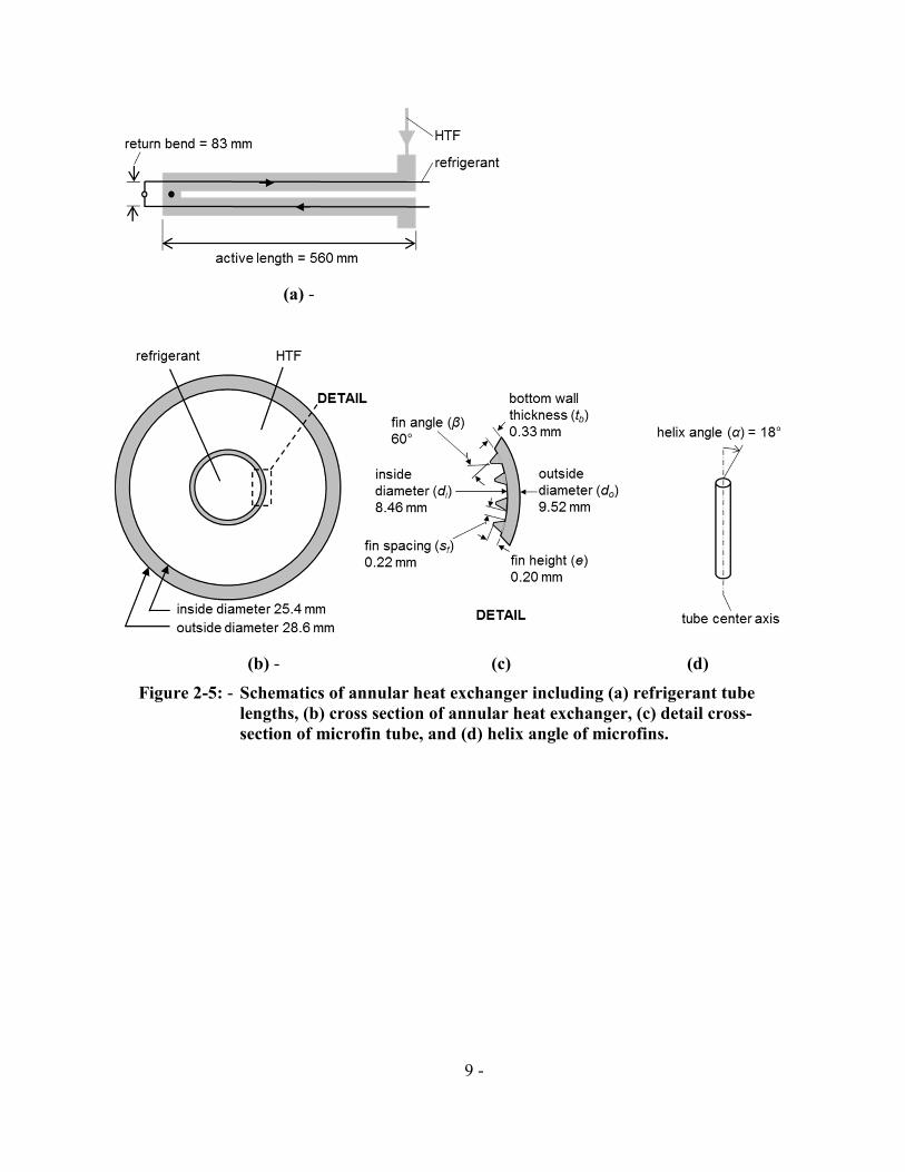
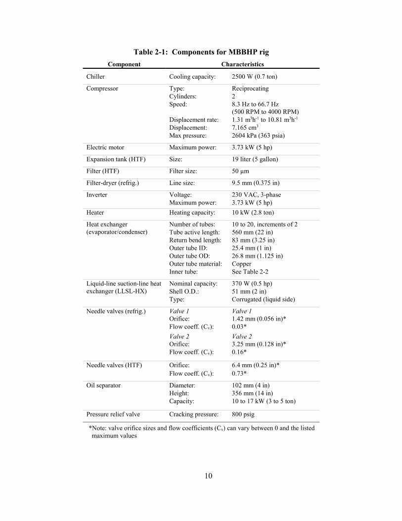
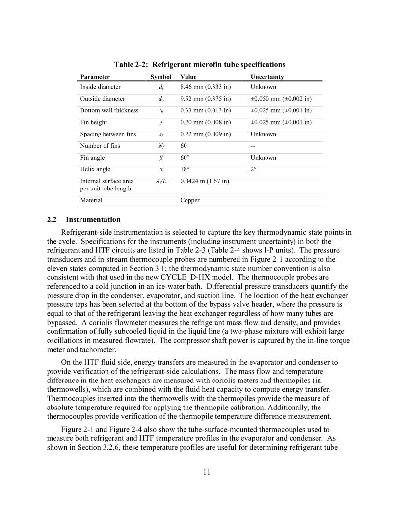
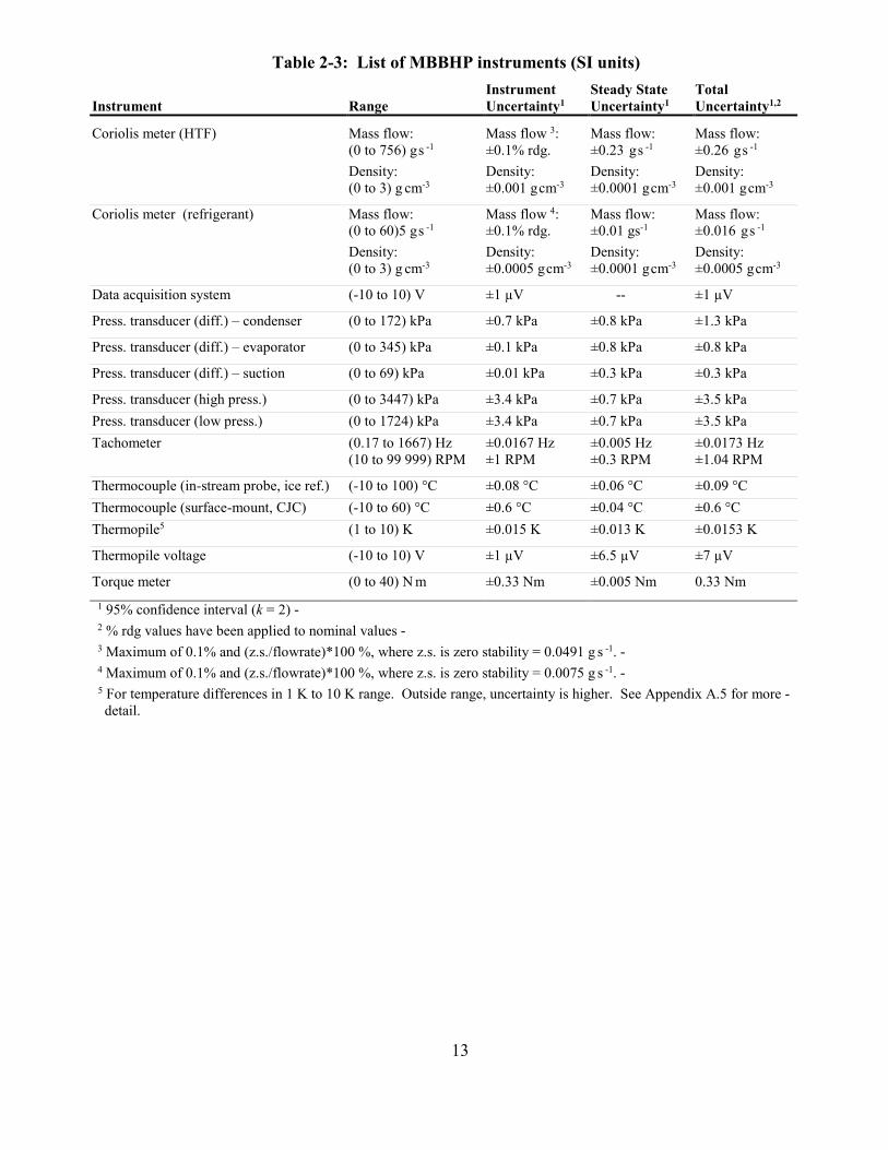
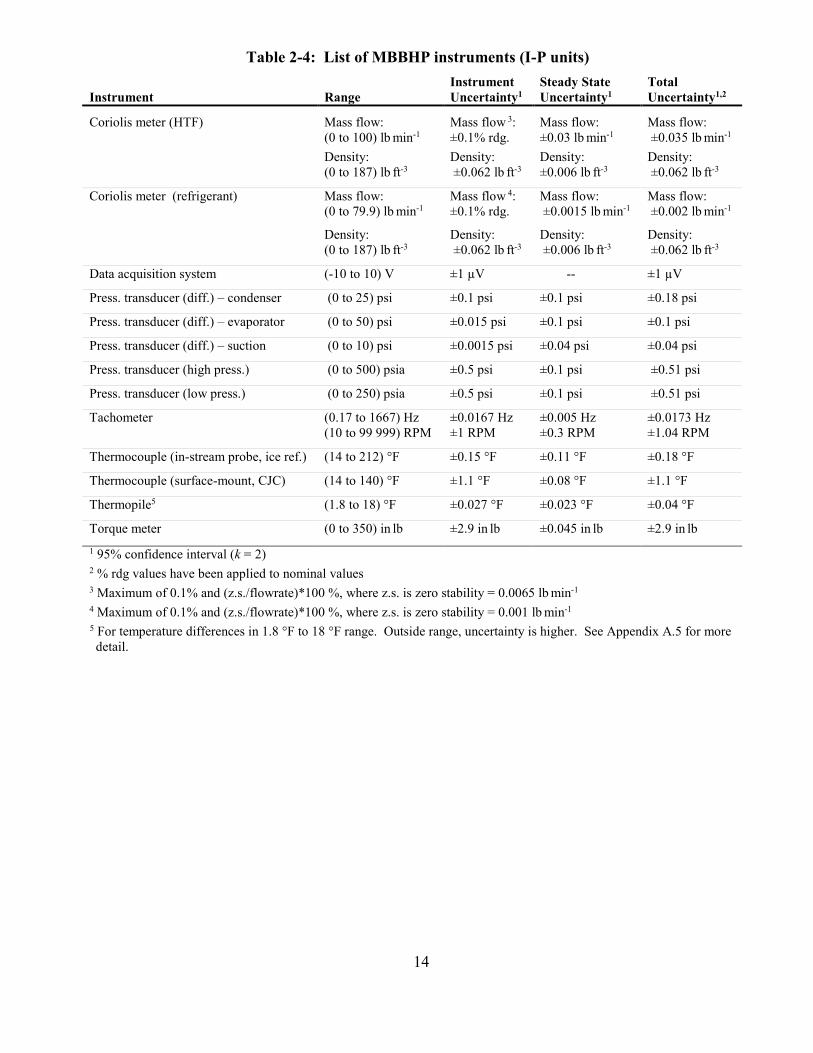
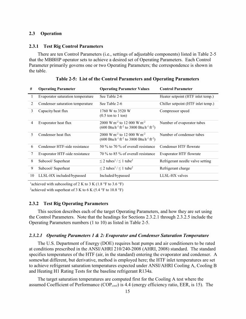
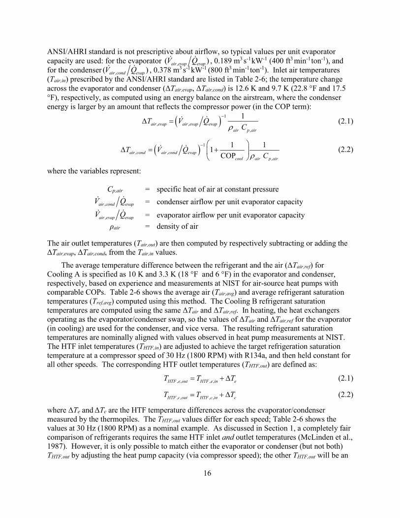
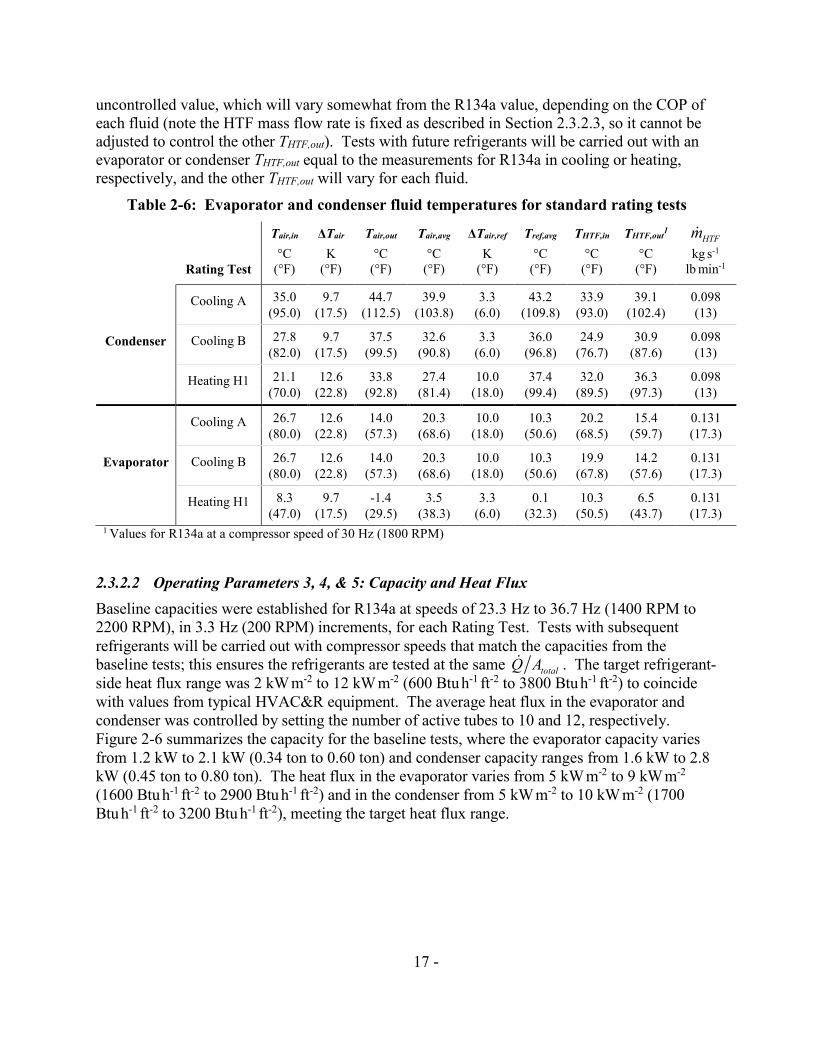
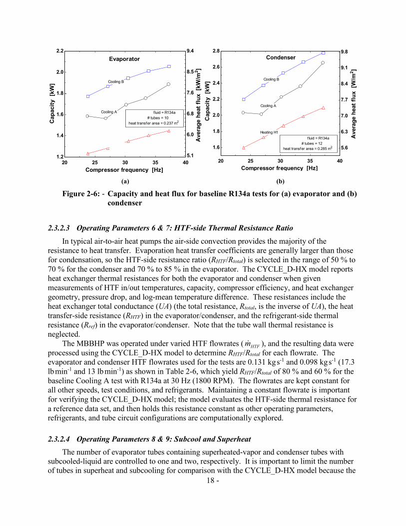
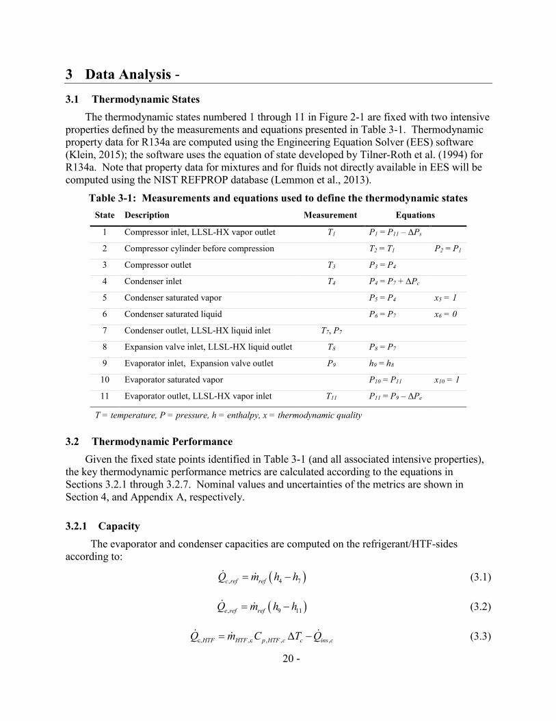
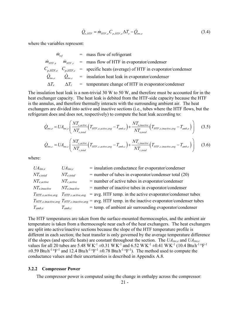
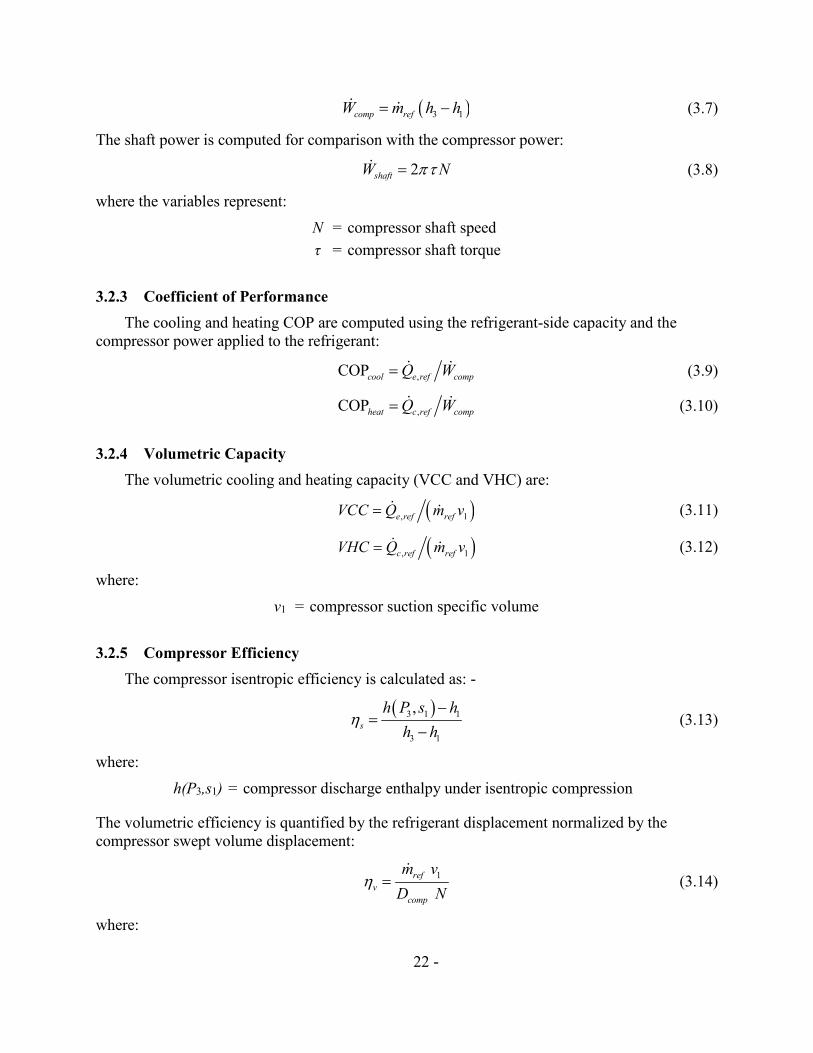
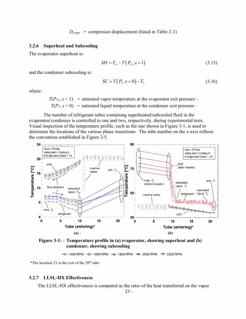
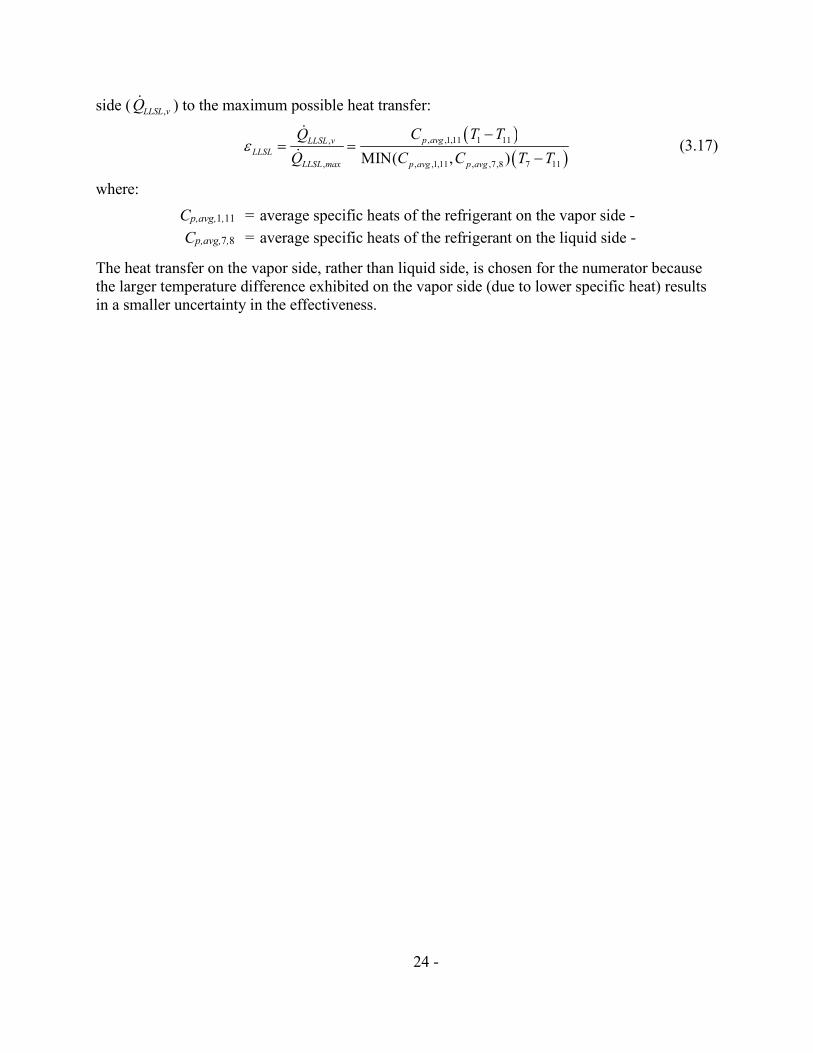
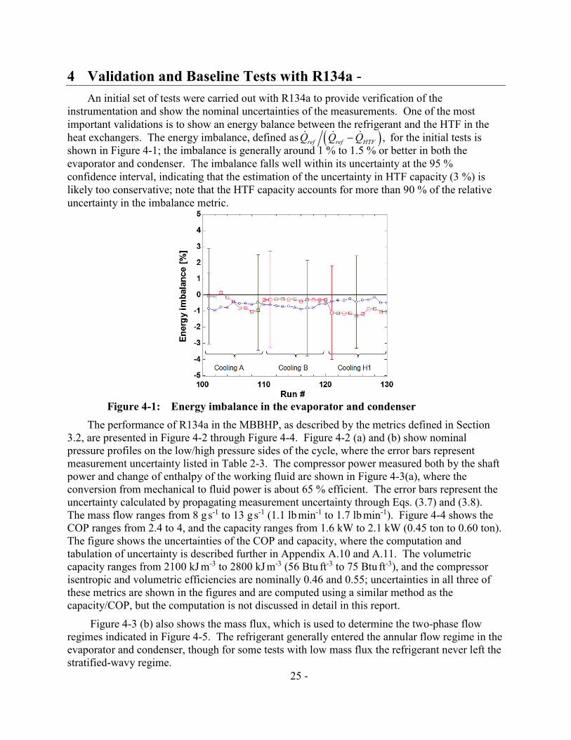
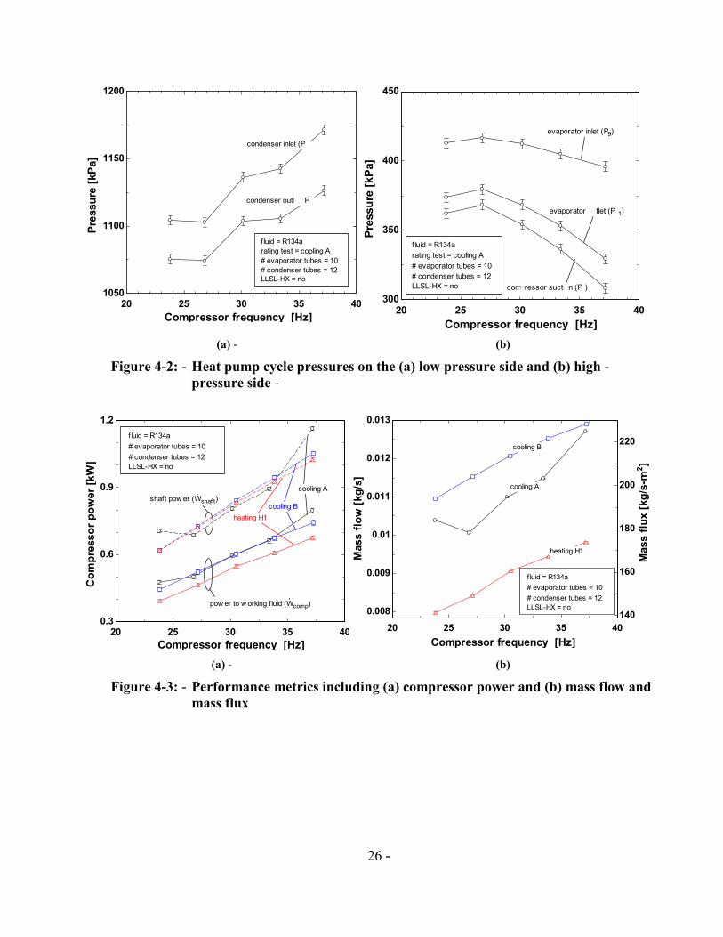
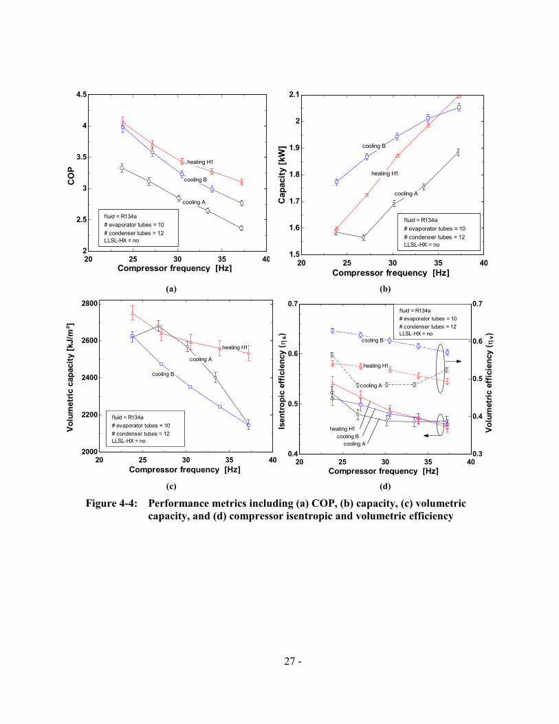
Vo
lum
etr
ic c
ap
acit
y [
kJm
3]
CO
P
Vo
lum
etr
ic e
ffic
ien
cy
(η
v)
(a) (b)
20 25 30 35 40 2
25
3
35
4
45
Compressor frequency [Hz]
evaporator tubes = 10
condenser tubes = 12
cooling A
cooling B
heating H1
f luid = R134a
LLSL-HX = no
20 25 30 35 40 15
16
17
18
19
2
21
Compressor frequency [Hz] C
ap
acit
y [
kW
]
cooling A
cooling B
heating H1
evaporator tubes = 10
condenser tubes = 12
fluid = R134a
LLSL-HX = no
2800 07 07
evaporator tubes = 10
condenser tubes = 12
fluid = R134a
LLSL-HX = no
cooling A
cooling B
heating H1
20 25 30 35 40 04
05
06
03
04
05
06
evaporator tubes = 10
condenser tubes = 12
fluid = R134a
LLSL-HX = no
cooling A
cooling B
heating H1
cooling B
cooling A
heating H1
2600
2400
2200
Isen
tro
pic
eff
icie
ncy
( η
s)
20 2000
25 30
Compressor frequency
35
[Hz]
40
Compressor frequency [Hz]
(c) (d)
Figure 4-4 Performance metrics including (a) COP (b) capacity (c) volumetric
capacity and (d) compressor isentropic and volumetric efficiency
27shy
50
Flow boiling with microfin tubeshy Flow condensing with microfin tube 350 350
300 300
S
heat flux 70 kWm2
=
= A
I
SG
S+SW
D
Tsat = 8 C
fluid = R134a
flow range during tests
M
SW
=
Tsat 43 C
fluid = R134a
heat flux 77 kWm2
flow range during tests
A
I
SG
S SW+
SW
0
50
S
Mass F
lux [
kg
s-m
2]
250
200
150
100
Mass F
lux [
kg
s-m
2]
250
200
150
100
0 0shy 02 04 06 08 1 0 02 04 06 08 1
Vapor quality Vapor quality A = Annular D = Dryout I = Intermittant M = Mist A = Annular D = Dryout I = Intermittant M = Mist
S = Stratified SG = Slug SW = Stratified-Wavy S = Stratified SG = Slug SW = Stratified-Wavy
(a)13shy (b)23
Figure 4-5shy Flow regime map for microfin tube (a) evaporation and (b) condensation
1 Flow boiling regime map from (Wojtan et al 2005)shy2 Flow condensation regime map from (Hajal et al 2003)shy3 Boundary between IntermittentAnnular regimes from (Thome 2007) using equation 1261 with a coefficientshy
of 0678 for helical microfins
5 Conclusions and Future Work
This report shows that the test apparatus is capable of measuring the performance of
low-GWP refrigerants with high fidelity including less than 05 uncertainty in both capacity
and COP The energy balance closure on the evaporator and condenser was better than 15
and will be continually tracked to ensure continued high quality data are collected
Future tests will include a second baseline refrigerant R410A followed by a series of
comparative tests with low-GWP refrigerants and refrigerant mixtures The HTF flowrates will
remain fixed from the R134a baseline tests so that the CYCLE_D-HX simulations of the test
data can be carried out for all test data based on a single reference data set After the model
results are verified the model will be used to identify additional candidate refrigerants to test in
the MBBHP test apparatus
28shy
6 ReferencesshyAHRI (2008) 2008 Standard for Performance Rating of Unitary Air-Conditioning amp Air-
Source Heat Pump Equipment Air-Conditioning Heating and Refrigeration Institute
Arlington VA United States Retrieved from wwwahrinetorg
AHRI (2015) Participants Handbook AHRI Low-GWP Alternative Refrigerants Evaluation
Program (Low-GWP AREP) Arlington VA United States Air-Conditioning Heating
and Refrigeration Institute Retrieved from
httpwwwahrinetorgsite514ResourcesResearchAHRI-Low-GWP-Alternative-
Refrigerants-Evaluation
Brown J S Domanski P A amp Lemmon E (2011) Standard Reference Database 49
CYCLE_D NIST Vapor Compression Cycle Design Program Version 50 Retrieved
from httpwwwnistgovsrdnist49cfm
Domanski P A Brown S J Heo J Wojtusiak J amp McLinden M O (2014) A
thermodynamic analysis of refrigerants Performance limits of the vapor compression
cycle International Journal of Refrigeration 38 71-79
doi101016jijrefrig201309036
EPA (2015) 2015 North American Amendment Proposal to Address HFCs under the Montreal
Protocol Retrieved from httpwwwepagovozoneintpolmpagreementhtml and
httpwwwepagovozoneintpolHFC_Amendment_2015_Summarypdf
EU (2014 April 16) Regulation (EU) No 5172014 of the European Parliament and of the
Council of 16 April 2014 on fluorinated greenhouse gases and repealing Regulation (EC)
No 8422006 Journal of the European Union Retrieved from httpeur-
lexeuropaeulegal-contentENTXTuri=uriservOJL_201415001019501ENG
Fortin T J (2015) Personal communication
Hajal J E Thome J R amp Cavallini A (2003) Condensation in horizontal tubes part 1 two-
phase flow pattern map International Journal of Heat and Mass Transfer 3349-3363
doi101016S0017-9310(03)00139-X
Harr L Gallagher J S amp Kell G S (1984) NBSNRC Steam Tables Hemisphere Publishing
Co
Kazakov A McLinden M O amp Frenkel M (2012) Computational Design of New
Refrigerant Fluids Based on Environmental Safety and Thermodynamic Characteristics
Industrial amp Engineering Chemistry Research 51 12537-12548 doi101021ie3016126
Kim Y Payne V Choi J amp Domanski P A (2005) Mass flow rate of R-410A through short
tubes working near the critical point International Journal of Refrigeration 28 547-553 doi101016jijrefrig200410007
Klein S A (2015) Engineering Equation Solver v 9908 Retrieved from
httpwwwfchartcomees
Lemmon E W Huber M L amp McLinden M O (2013) NIST Standard Reference Database
23 Reference Fluid Thermodynamic and Transport Properties (REFPROP) Version 91
29shy
National Institute of Standards and Technology Retrieved fromshyhttpwwwnistgovsrdnist23cfmshy
McLinden M O amp Radermacher R (1987) Methods for Comparing the Performance of Pure
and Mixed Refrigerants in the Vapour Compression Cycle International Journal of
Refrigeration 10(6) 318-325 doi1010160140-7007(87)90117-4
McLinden M O Kazakov A Heo J Brown J S amp Domanski P A (2014) A
thermodynamic analysis of refrigerants Possibilities and tradeoffs for Low-GWP
refrigerants International Journal of Refrigeration 38 80-92
doi101016jijrefrig201309032
Pannock J amp Didion D A (1991) The Performance of Chlorine-Free Binary Zeotropic
Refrigerant Mixtures in a Heat Pump NISTIR 4748 Internal Report National Institute of
Standards and Technology US Department of Commerce Gaithersburg Retrieved from
httpfirenistgovbfrlpubsbuild91art002html
Solomon S Qin D Manning M Chen Z Marquis M Averyt K B Miller H L
(2007) Contribution of Working Group I to the Fourth Assessment Report of the
Intergovernmental Panel on Climate Change New York NY USA Cambridge
University Press Retrieved July 29 2015 from
httpwwwipccchpublications_and_datapublications_ipcc_fourth_assessment_report_
wg1_report_the_physical_science_basishtm
Taylor B N amp Kuyatt C E (1994) Guidelines for Evaluating and Expressing the Uncertainty
of NIST Measurement Results National Institute of Standards and Technology Technical
Note 1297
Thome J R (Updated in 2007) Wolverine Heat Transfer Engineering Data book III Germany
Weiland-Werke AG Retrieved from httpwwwwlvcomheat-transfer-databook
Tilner-Roth R amp Baehr H D (1994) An International Standard Formulation for the
Thermodynamic Properties of 1112-Tetrafluoroethane (HFC-134a) for Temperatures
from 170 K to 455 K and Pressures up to 70 MPa J Phys Chem Ref Data 23(5)
Wojtan L Ursenbacher T amp Thome J R (2005) Investigation of flow boiling in horizontal
tubes Part ImdashA new diabatic two-phase flow pattern map International Journal of Heat
and Mass Transfer 2955-2969 doi101016jijheatmasstransfer200412012
30shy
Appendix A Uncertainty Analysisshy
A1 Symbols Used in Uncertainty Analysisshy
Symbol Units Definition
k -- Expanded uncertainty coverage factor
n -- Number of data points
Qɺ kW Energy transfer
SUAinse W K -1 Standard deviation of evaporator insulation conductance
SX -- Standard deviation of measured quantity ldquoXrdquo
T degC Temperature
T1 degC Temperature at cold end of thermopile
Tcal degC Temperature of RTD used for calibrations
TTCcal degC Calibrated thermocouple measurement
TTCCJC degC Thermocouple measurement with Cold Junction Compensation
∆Tlm K Log-mean temperature difference
∆TTCcal K Thermocouple calibration temperature difference
∆TTP K Temperature difference of thermopile
UA W K -1 Thermal conductance
UA ins e U W K-1 Uncertainty of average of evaporator insulation conductance
UTC degC Total instrument uncertainty of thermocouple
UTCcal degC Thermocouple instrument uncertainty from calibrating device uncertainty
UTCfit degC Instrument uncertainty of thermocouple due to fit of calibration regression
UX -- Uncertainty of measured quantity ldquoXrdquo
X U -- Uncertainty of average of measured quantity ldquoXrdquo
UY Uncertainty of calculated quantity ldquoYrdquo
V V Voltage
V1 V Thermopile voltage of cold end of thermopile (referenced to ice-point)
VCC kJ m -3 Volumetric Cooling Capacity
VHC kJ m -3 Volumetric Heating Capacity
VTC V Thermocouple voltage
∆VTP V Thermopile voltage
X -- Measured quantity
Y -- Calculated quantity
31shy
Subscript Definition
amb Ambient airshyc Condensershye EvaporatorshyHTF Heat Transfer Fluidshyin Inletshyins Insulationshyout Outletshy1 to 11 Refrigerant thermodynamic states as defined by Figure 2-1shy
Abbreviation Definition
COP Coefficient of Performance (W capacity per W of input power)shyCJC Cold Junction Compensation (for thermocouples)shyDAQ Data AcquisitionshyDSC Differential Scanning Calorimeter (used to measure fluid specific heat)shyEES Engineering Equation Solver (software used to reduce data)shyHTF Heat Transfer FluidshyMBBHP Mini Breadboard Heat PumpshyRPM Revolutions per Minute (compressor shaft)shyRTD Resistance Temperature Detectorshy
A2 General Remarks
The uncertainty analyses for key performance metrics are presented in this section All
uncertainties are estimated based on instrument uncertainties computed at a 95 confidence
interval
A3 Thermocouples with CJC Compensation
The surface-mounted thermocouples as well as the thermocouples measuring the air
temperature near the evaporatorcondenser are compensated at the DAQ using a thermistor-
based Cold Junction Compensation (CJC) A calibration (∆Tcal) is applied to the resulting
temperature reading (TTCCJC) to compute the calibrated temperature (TTCcal) according to
T = T + ∆ T (A1) TC cal TC cal TC CJC
where the calibration is fit to a 2nd order polynomial (the order of this curve fit and others
presented in Appendix A were selected based on t-test of polynomial coefficients)
= T minus a T + a T 2∆T cal T = a0 + 1 TC CJC 2 TC CJC (A2)
TC cal TC CJC
The polynomial coefficients (a0 a1 a2) are fit using the least square error method and Tcal is the
temperature measured by the calibrating instrument (two calibrated RTDs read by a precision
digital thermometer expanded uncertainty of plusmn002 degC) The thermocouples were calibrated over
a temperature range of -10 degC to 60 degC and this calibration was repeated five times over the
32shy
course of two weeks Figure A-1 (a) shows the calibration data and polynomial curve fits for a
representative thermocouple Each calibration shows a significant offset from the others this is
likely a manifestation of the repeatability error of the CJC which has an overall uncertainty of
plusmn05 degC Figure A-1 (b) shows the aggregation of the five data sets and the resulting curve fit
and 95 confidence interval (plusmn06 degC) The uncertainty of the calibrated RTDs is more than an
order of magnitude smaller than the curve fit confidence interval and is therefore neglected The
CJC thermocouple instrument uncertainty listed in Table 2-3 is therefore plusmn06 degC
05 05
Tem
pera
ture
cali
bra
tio
n( ∆
Tc
al)
[K]
Tem
pera
ture
cali
bra
tio
n( ∆
Tc
al)
[K]
0
-05
-1 ddaattaa
ccuurrvvee ffiitt
9955 ccoonnffiiddeennccee iinntteerrvvaall
0
-05 ccaalliibbrraattiioonn 11
ccaalliibbrraattiioonn 22
ccaalliibbrraattiioonn 33
ccaalliibbrraattiioonn 44
-1 ccaalliibbrraattiioonn 55
ccuurrvvee ffiittss
-15 -15 -10 0 10 20 30 40 50 60 -10 0 10 20 30 40 50 60
Temperature (TTCCJC) [degC] Temperature (TTCCJC) [degC]
(a) (b)
Figure A-1 Temperature calibration for CJC compensated thermocouples where
(a) data are divided by each of the 5 calibrations and (b) all data are
combined
A4 Thermocouples with Ice-Water Bath Compensation
A lower level of uncertainty is achieved for the in-stream probe thermocouples which
measure the refrigerant temperatures at key thermodynamic states by utilizing an ice-water bath
reference junction The ice-water bath consists of a vacuum insulated Dewar filled with crushed
ice and water the reference junction is submerged in the bath inside of a water-filled test tube
Using the ice-water bath removes the large uncertainty associated with the electronic CJC on the
DAQ system The thermocouples were calibrated against the RTDs (same ones used to calibrate
thermocouples with CJC) where the resulting data and curve fit are shown for a representative
thermocouple in Figure A-2 The data were fit to 5th order polynomials according to
5
T aV i (A3) =sum iTC cal TC
i=0
where VTC is the thermocouple voltage The resulting instrument uncertainty (plusmn008 degC) listed in
Table 2-3 is the combination of the curve fit standard error (UTCfit k = 2) and the calibrating
RTD error (UTcal)
2 2 2 2 U = plusmn U +U = plusmn 0079 + 002 = plusmn008 degC (A4)TC TC fit T cal
33
Tem
pera
ture
[degC
]
80
ddaattaa
ccuurrvvee ffiitt60
40
20
0
-20 -00005 0 00005 0001 00015 0002 00025
Voltage [V]
Figure A-2 Ice-water bath referenced thermocouple calibration data
A5 Thermopiles in Heat Transfer Fluid
The 13-junction thermopiles were calibrated by immersing one end in an ice-water bath
(inside a water-filled test tube) and the other end in a temperature controlled bath The
temperature in the controlled bath was measured using the two calibrated RTDs A thermopile
voltage-temperature dataset was generated and fit to a 4th order polynomial Figure A-3 shows
the calibration data and the curve fit and Table A-1 shows the polynomial coefficients The
calibration data are fit to the equation
N =4 i
T = sum aTP i V (A5) i=0
The temperature difference for a thermopile is computed according to
∆T = ( V T V + ∆ ) minusT (A6)TP 1 TP 1
where ∆VTP is the measured thermopile voltage and T1 is the temperature measured at the cold
end of the thermopile by a CJC-corrected thermocouple Eq (A5) is substituted into Eq (A6)
to calculate the thermopile temperature difference
N =4
∆TTP = sum aTP i (V1 +∆VTP ) minusT1 (A7) i=0
where V1 (cold-end voltage) is computed by numerically solving Eq (A5) where T is set to (T1)
N =4 i V1 = root T1 minussum aTPi V1 = 0 (A8)
i=0
The thermopile uncertainties are computed with respect to the curve fit voltage
measurement and temperature measurement at the cold end of the thermopile (characterized
respectively by the coefficient uncertainties in Table A-1 the thermopile voltage uncertainty in
Table 2-3 and the CJC corrected thermocouple in Table 2-3) The EES (Klein 2015) software
34
is used to numerically compute the partial derivatives and subsequent thermopile uncertainties
Figure A-4(a) shows the contours of uncertainty in the temperature difference measured by the
evaporatorcondenser HTF thermopiles
Figure A-4(b) shows the contours of relative contribution to uncertainty in the thermopile
measurement Each of the uncertainty sources is dominant in different regions
bull voltage measurement dominant at low temperature differences (less than 1 K)
bull curve fit error dominant at high cold end temperatures (greater than 50 degC)
bull cold end temperature dominant at moderate cold end temperatures -5 degC to 20 degC and temperature differences 25 K to 20 K
As noted in this discussion the thermopile uncertainty is a complex function of the curve fit
voltage measurement and cold end temperature measurement For the temperature difference
range expected for this application 1 K to 10 K (18 degF to 18 degF) the upper bound of uncertainty
is about 0015 K (0027 degF) for simplicity this is the value listed in Table 2-3 Note that the
contribution to the uncertainty by the calibrating instrument (two calibrated RTDs) is negligible
here as the error in slope (which is the error that propagates into the thermopile temperature
difference) is less than 0000248 K per K of temperature difference (eg 000248 K for a 10 K
temperature difference)
Table A-1 Condenser amp evaporator60
thermopile polynomial coefficients 50
Uncertainty
Coeff Value (k=2) 95 40
Tem
pera
ture
[degC
]
aTPe0 39243 E-02 plusmn41 E-04 30
aTPe1 20243 E+03 plusmn12 E-01 20
aTPe2 -55466 E+03 plusmn22 E+01 TTPP11
10 TTPP22 aTPe3 39023 E+04 plusmn13 E+03 TTPP11 ((ffiitt))
TTPP22 ((ffiitt)) aTPe4 -26229 E+05 plusmn22 E+04
0
-10
38494 E-02 plusmn53 E-04 -001 0 001 002 003 004 aTPc0
Voltage [V]shy aTPc1 20241 E+03 plusmn15 E-01
Figure A-3 Thermopile calibration data aTPc2 -55190 E+03 plusmn28 E+01
aTPc3 38551 E+04 plusmn16 E+03
aTPc4 -25440 E+05 plusmn29 E+04
35
-5
0
10
20 contours of thermopile uncertainty [K] contours of contribution to uncertainty []
20
balance is T1004
0035
Tem
pera
ture
dif
fere
nce
(∆
TT
P)
[K]
15 003
0025
002
0015
001 0001 5
0002 0005
0004 0003
Tem
pera
ture
dif
fere
nce (∆
TT
P)
[K]
15
10
curve fit
80 60
40 20
5 voltage (∆VTP)
20 40
0 60
80
0 10 20 30 40 50
Temperature at cold end (T1) [degC]
60 -5
0 10 20 30 40 50
Temperature at cold end (T1) [degC]
60
(a) (b)
Figure A-4 Contours of thermopile (a) uncertainty and (b) relative contribution to
uncertainty
A6 Evaporator Heat Transfer Fluid Specific Heat
The evaporator HTF is a potassium formate and water heat transfer fluid that is freeze
protected to -40 degC The manufacturerrsquos specific heat data were found to have error of at least
10 so a sample of the fluid was analyzed in a Differential Scanning Calorimeter (DSC) by the
NIST-Boulder Applied Chemicals and Materials Division The temperature dependent specific
heat and the 2nd order curve fit to the data are shown in Figure A-5 the curve fit coefficients and
their uncertainties are listed in Table A-2 Figure A-5 also shows the manufacturerrsquos reported
specific heat data for comparison The exact uncertainty of the DSC measurement was not
available at the time of writing but was estimated to be about 2 to 3 of reading based on the
experience of the DSC operator (Fortin 2015) An uncertainty of 3 of reading is therefore
assigned as a conservative estimate Both the curve fit and DSC calibration uncertainties are
included in the calculation of overall uncertainties
36shy
DSC measurements
curve fit
3 Table A-2 Evaporator HTF specific
heat polynomial coefficients
29 Uncertainty
DSC measurements
curve fit
manufacturers data
-10 0 10 20 30
Sp
ecif
ic h
eat
(Cp)
[Jg
-K]
Coeff Value (k=2) 95
28 aCpe0 25643 E+00 plusmn16 E-03
aCpe1 11015 E-03 plusmn21 E-04
27 aCpe2 17422 E-05 plusmn95 E-06
26
25
Temperature [degC]
Figure A-5 Specific heat measurements for
evaporator HTF
A7 Condenser Heat Transfer Fluid Specific Heat
The condenser HTF is water the specific heat data are computed in EES using the data from
(Harr et al 1984) and are shown in Figure A-6 A conservative estimate of plusmn3 is used for the
uncertainty in the specific heat
423
0 20 40 60 80 100
Sp
ecif
ic h
eat
(Cp)
[kJk
g-K
]
422
421
42
419
418
Temperature [degC]
Figure A-6 Specific heat of condenser HTF (water)
A8 Evaporator and Condenser Insulation Conductance
The total evaporator and condenser insulation conductances (UAinse and UAinsc) for thermal
interaction with the ambient air were measured during an initial test where the HTFs were
circulated at various flow rates through the apparatus at an elevated temperature while the
refrigerant tubes were under vacuum The temperature change of the HTF across the heat
37shy
exchanger was assumed to be entirely attributed to insulation heat leak and therefore an
effective insulation conductance could be computed The resulting UAinse and UAinsc values for
all 20 tubes are shown in Figure A-7 Average values of conductances for the evaporator and
condenser were calculated as 548 W K-1 plusmn031 W K-1 and 652 W K-1 plusmn041 W K-1
(104 Btu h-1 degF-1 plusmn059 Btu h-1 degF-1 and 124 Btu h-1 degF-1 plusmn078 Btu h-1 degF-1) respectively where the
uncertainty accounts for both instrumentation error and test variance The evaporator insulation
conductance for these tests is computed according to
ɺQins e mɺ HTF e C (THTF in e minusT )p HTF e HTF out e
UA = = (A9) ins e ∆T T minusT minus T minusT e ( HTF in e amb e ) ( HTF out )lm HTF e amb e
(T minusT ) amb e HTF in e ln (T
minusT
amb e ) HTF out e
where the variables represent
Cp HTF e = evaporator HTF specific heat
mɺ HTF e = evaporator HTF mass flow
Qɺ = evaporator insulation heat leak ins e
Tambe = ambient air temperature surrounding evaporator
THTFine = evaporator HTF inlet temperature
THTFoute = evaporator HTF outlet temperature
∆TlmHTFe = evaporator log-mean temperature difference
and the uncertainty of the average value is calculated according to
U = k S n (A10) UA ins e UA ins e
where the variables represent
k = expanded uncertainty coverage factor (k = 2) for 95 confidence interval
SUAinse = standard deviation of conductances
n = number of conductance data points
The condenser conductance is computed using the same method with the corresponding
measurements from that heat exchanger
38shy
4
5
6
7
8
Insu
lati
on
co
nd
ucta
nce (
UA
ins)
[WK
]
UAinscond
UAinsev ap
average for evaporator
average for condenser
0 005 01 015
Mass flow [kgs]
Figure A-7 Insulation conductance for evaporator and condenser
A9 Uncertainty Analysis Software
The uncertainty analyses on each of the performance metrics shown in Figure 4-1 through
Figure 4-4 were calculated using the uncertainty propagation capability in EES The software
numerically computes the performance metric uncertainty by evaluating the partial derivatives
with respect to each relevant measurement and applying the specified measurement uncertainty
Assuming the measurements are independent and uncorrelated the uncertainty of a quantity is
computed according to (Taylor amp Kuyatt 1994)
partY 2 2
UY = sum U X (A11) i partXi
i
where the variables represent
Y = calculated quantity
Uy = uncertainty of calculated quantity
Xi = measurement
UXi = uncertainty of measurement
39shy
A10 Moving Window and Steady State Uncertainty
A moving window average was used to compute the measurements at steady state during the
tests In order to determine a proper window size the variation of measurement steady state
uncertainty with window size was examined The steady state uncertainty is defined as the
expanded standard uncertainty for the average reading within the window
S X (A12) U = k X
n
where
k = coverage factor (k = 2) for 95 confidence interval
n = number of samples in the window
Sx = standard deviation of measurement
X = average value of measurement
The data for analysis were generated by holding the MBBHP at a nominal steady operating
condition and recording the measurements at 1-minute intervals (same as collection rate for all
performance testing) for an extended time (3 hours) Figure A-8 shows the fluctuation of steady
state uncertainty for the evaporator inlet and outlet temperatures (T9 and T11) The figure
highlights two characteristic trends observed for all of the instruments both of which suggest the
need for a large moving window (1) the steady state uncertainty decreases as the window size
increases and (2) the steady state uncertainty is highly oscillatory for small windows (the
oscillations are undesirable because short-term fluctuations can have a disproportionate impact
on the averaged result) A 30 sample moving window was selected to achieve low uncertainty
while allowing for collection of data in a timely manner
Figure A-8 shows that the measurement steady state uncertainty is not constant in time (it
would be constant if the fluctuations at steady state were purely random) but rather exhibits
drifting and periodic movements This is possibly due to hunting by the PID controllers
regulating HTF fluid temperatures changes in air temperature in the lab space or some other
uncontrolled andor uncharacterized phenomena These non-random fluctuations are accounted
for by using the maximum steady state uncertainty value observed during the extended steady
state test For example Figure A-8(a) shows the maximum steady state uncertainty for the
evaporator outlet (T9) is plusmn006 degC this value and values for all other sensors are listed in Table
2-3 The data in the moving window are only recorded when steady state uncertainties are below
these established thresholds The total uncertainty (plusmn009 degC) also shown in Table 2-3 is
subsequently computed by adding the instrument uncertainty (plusmn008 degC) and steady state
uncertainty (plusmn006 degC) in quadrature
Note that different sensors of the same type exhibit different levels of fluctuation as a
conservative estimate the largest uncertainty of any one is applied to all of them For example
Figure A-8(b) shows the fluctuations of steady state uncertainty for the evaporator inlet
temperature (T9) are much smaller than for the evaporator outlet (T11) In fact the evaporator
outlet temperature (T11) shows the most fluctuation of all the ice-water bath compensated
thermocouple probes therefore its value (plusmn006 degC) is used in Table 2-3 to represent them all
40shy
05 05
01 01
Ts
[C]
001 001
Ute
ad
y
0002
(a)
Time elapsed [s]
0002
(b)
Time elapsed [s]
Figure A-8shy Uncertainty in temperature due to fluctuations at steady state for (a)
evaporator outlet and (b) evaporator inlet
A11 Uncertainty Results Summary
The detailed instrument uncertainty analysis for performance metrics including the
refrigerantHTF-side capacities and the COPs are tabulated in Appendices A111 (cooling) and
A112 (heating) The tables show the performance metric and its total uncertainty (including
both instrument and steady state contributions) as well as the measurements that contribute to
the uncertainty The measurement values uncertainties partial derivatives (of performance
metric with respect to the measurement) and relative errors (contribution to the overall error in
the performance metric) are also shown where the measurements are listed in order of
decreasing relative error Uncertainties for other performance metrics (eg VCCVHC ηisen)
were analyzed using similar techniques but are not shown in detail in this report Note that
Appendices A111 and A112 show sample calculations for a single nominal operating
condition whereas the uncertainty values presented in the Section 4 figures are computed for
each test run
The uncertainty in cooling performance metrics are shown for a nominal operating point for
R134a during a Cooling A test with a compressor speed of about 30 Hz (1800 RPM) Similarly
the uncertainty in heating performance metrics are shown for R134a during a Heating H1 test
with a compressor speed of about 30 Hz (1800 RPM)
A111 Uncertainty Results Summary Cooling
Table A-3 shows that the dominant sources of instrument uncertainty for the refrigerant-side
capacity are refrigerant mass flow (66 ) expansion valve inlet temperature (17 ) evaporator
exit pressure (8 ) and evaporator exit temperature (7 ) Table A-4 shows the dominant
source of instrument uncertainty for the HTF-side capacity is the HTF specific heat (97
estimate for instrument used to measure fluid properties) Table A-5 shows the dominant
sources of instrument uncertainty for cooling COP are evaporator inlet pressure (39 )
compressor discharge temperature (25 ) and compressor suction temperature (18 )
8000 12000 16000 20000
UT
ste
ad
y [
C]
increasing
time window
10 min
30 min 60 min
05 min
maximum (006 degC)
8000 12000 16000 20000
increasing
time window
10 min
30 min 60 min
05 min
41shy
Table A-3 Uncertainty of refrigerant-side evaporator cooling capacity
Total Partial Relative
Parameter Symbol Value Uncertainty Derivative Error
Refrigerant-side evaporator capacity eref Qɺ 1692 kW plusmn00035 kW
(020) -- --
Refrigerant mass flow refmɺ 1100 g s-1 plusmn0024 g s-1 1538 E-01 66
Refrigerant temp at expansion valve inlet T8 3816 C plusmn009 degC -1634 E-02 17
Refrigerant press at evaporator inlet P9 412 kPa plusmn35 kPa -2817 E-04 8
Refrigerant temp at evaporator exit T11 1209 C plusmn009 degC 1009 E-02 7
Refrigerant press at condenser exit P7 1104 kPa plusmn35 kPa 2103 E-06 0
Refrigerant evaporator differential press ∆Pe 4392 kPa plusmn08 kPa 2817 E-04 0
Table A-4 Uncertainty of HTF-side evaporator cooling capacity
Total Partial Relative
Parameter Symbol Value Uncertainty Derivative Error
plusmn005 kW HTF-side evaporator capacity Qɺ 1672 kW -- --eHTF (30)
Evaporator HTF capacity cp HTF e 259 J g-1 K-1 plusmn3 of cp 6369 E-01 97 calibration uncertainty HTF e
Temperature of ambient air
surrounding evaporator Tambe 230 degC plusmn06 degC 5474 E-03 1
HTF mass flow HTF e mɺ 1312 g s-1 plusmn026 g s-1 1257 E-02 1
Evaporator HTF thermopile voltage ∆VTPe 2512 mV plusmn0007 mV 6537 E-01 1
Evaporator HTF thermopile aTPe0 39243 E-02 plusmn41 E-04 4047 E-03 0
polynomial coefficients aTPe1 20243 E+03 plusmn12 E-01 8832 E-04 0
aTPe2 -55466 E+03 plusmn22 E+01 1559 E-05 0
aTPe3 39023 E+04 plusmn13 E+03 2106 E-07 0
aTPe4 -26229 E+05 plusmn22 E+04 2554 E-09 0
Evaporator HTF capacity aCpe0 25643 E+00 plusmn16 E-03 6369 E-01 0
polynomial coefficients aCpe1 11015 E-03 plusmn21 E-04 1135 E+01 0
aCpe2 17422 E-05 plusmn95 E-06 2024 E+02 0
Temperature at cold end of
evaporator HTF thermopile THTFeout 1542 degC plusmn06 degC -2963 E-03 0
Evaporator insulation conductance UAinse 5474 W K-1 plusmn03052 W K-1 4175 E-03 0
42shy
Table A-5 Uncertainty of cooling COP
Total Partial Relative
Parameter Symbol Value Uncertainty Derivative Error
Cooling COP coolCOP 2844
plusmn001
(035 ) -- --
Refrigerant press at evaporator inlet P9 412 kPa plusmn35 kPa -1232 E-02 39
Refrigerant temp at compressor discharge T3 8197 degC plusmn009 degC 5571 E-02 25
Refrigerant temp at compressor suction T1 1273 degC plusmn009 degC 4788 E-02 18
Refrigerant press at condenser exit P7 1104 kPa plusmn35 kPa 5144 E-03 7
Refrigerant temp at expansion valve inlet T8 3816 degC plusmn009 degC -2746 E-02 6
Refrigerant temp at evaporator exit T11 1209 degC plusmn009 degC 1696 E-02 2
Refrigerant evaporator diff press ∆Pe 4392 kPa plusmn08 kPa 7432 E-04 2
Refrigerant condenser diff press ∆Pc 3234 kPa plusmn13 kPa 4731 E-04 1
Refrigerant suction line diff press ∆Ps 1422 kPa plusmn03 kPa 1314 E-03 0
Refrigerant mass flow refmɺ 1100 g s-1 plusmn0016 g s-1 2209 E-04 0
A112 Uncertainty Results Summary Heating
Table A-6 shows the dominant sources of instrument uncertainty for the refrigerant-side
capacity are refrigerant mass flow (85 ) condenser exit temperature (9 ) and condenser inlet
temperature (5 ) Table A-7 shows the dominant source of instrument uncertainty for the HTF-
side capacity is the HTF specific heat (97 estimate for instrument used to measure specific
heat of water in the reference) Table A-8 shows the dominant sources of instrument uncertainty
for cooling COP are evaporator inlet pressure (32 ) compressor discharge temperature (31 )
and compressor suction temperature (22 )
43shy
Table A-6 Uncertainty of refrigerant-side condenser heating capacityshy
Total Partial Relative
Parameter Symbol Value Uncertainty Derivative Error
Refrigerant-side condenser capacity c refQɺ 1873 kW plusmn0004 kW
(02) -- --
Refrigerant mass flow refmɺ 906 g s-1 plusmn0016 g s-1 2067 E-01 85
Refrigerant temp at condenser exit T7 3739 degC plusmn009 degC -1343 E-02 9
Refrigerant temp at condenser inlet T4 7722 degC plusmn009 degC 9443 E-03 5
Refrigerant press at condenser exit P7 9928 kPa plusmn35 kPa -1296 E-04 1
Refrigerant condenser differential press ∆Pc 272 kPa plusmn13 kPa -9028 E-04 0
Table A-7 Uncertainty of HTF-side condenser heating capacity
Total Partial Relative
Parameter Symbol Value Uncertainty Derivative Error
plusmn0054 kW HTF-side condenser capacity Qɺ 1852 kW -- --cHTF (29)
Condenser HTF capacity calibration cp HTF c 4183 J g-1 K-1 plusmn3 of cp 4262 E-01 97 uncertainty HTF c
Condenser insulation conductance UAinsc 6521 W K-1 plusmn04071 W K-1 1056 E-02 1
HTF mass flow HTF c mɺ 9881 g s-1 plusmn023 g s-1 1804 E-02 1
Condenser HTF thermopile voltage ∆VTPc 2318 mV plusmn0007 mV 7652 E-01 1
Condenser HTF thermopile aTPc0 38494 E-02 plusmn53 E-04 4057 E-03 0
polynomial coefficients aTPc1 20241 E+03 plusmn15 E-01 1025 E-03 0
aTPc2 -55190 E+03 plusmn28 E+01 3481 E-05 0
aTPc3 38551 E+04 plusmn16 E+03 9078 E-07 0
aTPc4 -25440 E+05 plusmn29 E+04 2309 E-08 0
Temperature of ambient air
surrounding condenser Tambc 243 degC plusmn06 degC -6521 E-03 0
Temperature at cold end of
condenser HTF thermopile THTFcin 3196 degC plusmn06 degC -4093 E-03 0
44shy
Table A-8 Uncertainty of heating COP
Total Partial Relative
Parameter Symbol Value Uncertainty Derivative Error
Heating COP heatCOP 3431
plusmn001
(028 ) -- --
Refrigerant press at evaporator inlet P9 3148 kPa plusmn35 kPa -1520 E-03 32
Refrigerant temp at compressor discharge T3 8073 degC plusmn009 degC -5933 E-02 31
Refrigerant temp at compressor suction T1 354 degC plusmn009 degC 5000 E-02 22
Refrigerant temp at condenser inlet T7 3739 degC plusmn009 degC -2461 E-02 6
Refrigerant press at condenser exit P7 9928 kPa plusmn35 kPa 5532 E-04 5
Refrigerant temp at condenser inlet T4 7722 degC plusmn009 degC 1731 E-02 3
Refrigerant condenser differential press ∆Pc 272 kPa plusmn13 kPa 5509 E-04 1
Refrigerant suction line diff press ∆Ps 1269 kPa plusmn03 kPa 1520 E-03 0
Refrigerant evaporator diff press ∆Pe 3999 kPa plusmn08 kPa 1520 E-03 0
Refrigerant mass flow refmɺ 906 g s-1 plusmn0016 g s-1 2187 E-04 0
45shy
Appendix B Instrumentation with DAQ Number ConventionshyThe instrument numbering scheme shown in Figure 2-1 and Figure 2-5 is based on the
thermodynamic states 1 to 11 However the raw data files recorded by the DAQ system use a
different numbering scheme shown in Figure B-1 and Figure B-2
(a)shy (b)
Figure B-1shy Schematic of (a) condenser and (b) evaporator showing the instrument
numbering convention used in the DAQ system
46shy
Figure B-2 Schematic of MBBHP test apparatus including instrument numbering convention used in the DAQ system
47
Appendix C Microfin Tube Surface AreashyThe microfinned surface area (per tube length) is estimated according to
Ai s f 2e
= N f + (C1) L
cosα cosα cos (β 2)
where the variables represent
e = fin height
Nf = number of fins
sf = fin spacing
α = fin helix angle
β = fin angle
and AiL is computed as 00424 m (167 in) The fin parameters are shown in Figure 2-5 and
Table 2-2
48shy
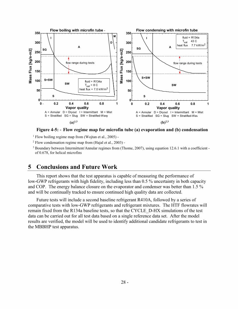
50
Flow boiling with microfin tubeshy Flow condensing with microfin tube 350 350
300 300
S
heat flux 70 kWm2
=
= A
I
SG
S+SW
D
Tsat = 8 C
fluid = R134a
flow range during tests
M
SW
=
Tsat 43 C
fluid = R134a
heat flux 77 kWm2
flow range during tests
A
I
SG
S SW+
SW
0
50
S
Mass F
lux [
kg
s-m
2]
250
200
150
100
Mass F
lux [
kg
s-m
2]
250
200
150
100
0 0shy 02 04 06 08 1 0 02 04 06 08 1
Vapor quality Vapor quality A = Annular D = Dryout I = Intermittant M = Mist A = Annular D = Dryout I = Intermittant M = Mist
S = Stratified SG = Slug SW = Stratified-Wavy S = Stratified SG = Slug SW = Stratified-Wavy
(a)13shy (b)23
Figure 4-5shy Flow regime map for microfin tube (a) evaporation and (b) condensation
1 Flow boiling regime map from (Wojtan et al 2005)shy2 Flow condensation regime map from (Hajal et al 2003)shy3 Boundary between IntermittentAnnular regimes from (Thome 2007) using equation 1261 with a coefficientshy
of 0678 for helical microfins
5 Conclusions and Future Work
This report shows that the test apparatus is capable of measuring the performance of
low-GWP refrigerants with high fidelity including less than 05 uncertainty in both capacity
and COP The energy balance closure on the evaporator and condenser was better than 15
and will be continually tracked to ensure continued high quality data are collected
Future tests will include a second baseline refrigerant R410A followed by a series of
comparative tests with low-GWP refrigerants and refrigerant mixtures The HTF flowrates will
remain fixed from the R134a baseline tests so that the CYCLE_D-HX simulations of the test
data can be carried out for all test data based on a single reference data set After the model
results are verified the model will be used to identify additional candidate refrigerants to test in
the MBBHP test apparatus
28shy
6 ReferencesshyAHRI (2008) 2008 Standard for Performance Rating of Unitary Air-Conditioning amp Air-
Source Heat Pump Equipment Air-Conditioning Heating and Refrigeration Institute
Arlington VA United States Retrieved from wwwahrinetorg
AHRI (2015) Participants Handbook AHRI Low-GWP Alternative Refrigerants Evaluation
Program (Low-GWP AREP) Arlington VA United States Air-Conditioning Heating
and Refrigeration Institute Retrieved from
httpwwwahrinetorgsite514ResourcesResearchAHRI-Low-GWP-Alternative-
Refrigerants-Evaluation
Brown J S Domanski P A amp Lemmon E (2011) Standard Reference Database 49
CYCLE_D NIST Vapor Compression Cycle Design Program Version 50 Retrieved
from httpwwwnistgovsrdnist49cfm
Domanski P A Brown S J Heo J Wojtusiak J amp McLinden M O (2014) A
thermodynamic analysis of refrigerants Performance limits of the vapor compression
cycle International Journal of Refrigeration 38 71-79
doi101016jijrefrig201309036
EPA (2015) 2015 North American Amendment Proposal to Address HFCs under the Montreal
Protocol Retrieved from httpwwwepagovozoneintpolmpagreementhtml and
httpwwwepagovozoneintpolHFC_Amendment_2015_Summarypdf
EU (2014 April 16) Regulation (EU) No 5172014 of the European Parliament and of the
Council of 16 April 2014 on fluorinated greenhouse gases and repealing Regulation (EC)
No 8422006 Journal of the European Union Retrieved from httpeur-
lexeuropaeulegal-contentENTXTuri=uriservOJL_201415001019501ENG
Fortin T J (2015) Personal communication
Hajal J E Thome J R amp Cavallini A (2003) Condensation in horizontal tubes part 1 two-
phase flow pattern map International Journal of Heat and Mass Transfer 3349-3363
doi101016S0017-9310(03)00139-X
Harr L Gallagher J S amp Kell G S (1984) NBSNRC Steam Tables Hemisphere Publishing
Co
Kazakov A McLinden M O amp Frenkel M (2012) Computational Design of New
Refrigerant Fluids Based on Environmental Safety and Thermodynamic Characteristics
Industrial amp Engineering Chemistry Research 51 12537-12548 doi101021ie3016126
Kim Y Payne V Choi J amp Domanski P A (2005) Mass flow rate of R-410A through short
tubes working near the critical point International Journal of Refrigeration 28 547-553 doi101016jijrefrig200410007
Klein S A (2015) Engineering Equation Solver v 9908 Retrieved from
httpwwwfchartcomees
Lemmon E W Huber M L amp McLinden M O (2013) NIST Standard Reference Database
23 Reference Fluid Thermodynamic and Transport Properties (REFPROP) Version 91
29shy
National Institute of Standards and Technology Retrieved fromshyhttpwwwnistgovsrdnist23cfmshy
McLinden M O amp Radermacher R (1987) Methods for Comparing the Performance of Pure
and Mixed Refrigerants in the Vapour Compression Cycle International Journal of
Refrigeration 10(6) 318-325 doi1010160140-7007(87)90117-4
McLinden M O Kazakov A Heo J Brown J S amp Domanski P A (2014) A
thermodynamic analysis of refrigerants Possibilities and tradeoffs for Low-GWP
refrigerants International Journal of Refrigeration 38 80-92
doi101016jijrefrig201309032
Pannock J amp Didion D A (1991) The Performance of Chlorine-Free Binary Zeotropic
Refrigerant Mixtures in a Heat Pump NISTIR 4748 Internal Report National Institute of
Standards and Technology US Department of Commerce Gaithersburg Retrieved from
httpfirenistgovbfrlpubsbuild91art002html
Solomon S Qin D Manning M Chen Z Marquis M Averyt K B Miller H L
(2007) Contribution of Working Group I to the Fourth Assessment Report of the
Intergovernmental Panel on Climate Change New York NY USA Cambridge
University Press Retrieved July 29 2015 from
httpwwwipccchpublications_and_datapublications_ipcc_fourth_assessment_report_
wg1_report_the_physical_science_basishtm
Taylor B N amp Kuyatt C E (1994) Guidelines for Evaluating and Expressing the Uncertainty
of NIST Measurement Results National Institute of Standards and Technology Technical
Note 1297
Thome J R (Updated in 2007) Wolverine Heat Transfer Engineering Data book III Germany
Weiland-Werke AG Retrieved from httpwwwwlvcomheat-transfer-databook
Tilner-Roth R amp Baehr H D (1994) An International Standard Formulation for the
Thermodynamic Properties of 1112-Tetrafluoroethane (HFC-134a) for Temperatures
from 170 K to 455 K and Pressures up to 70 MPa J Phys Chem Ref Data 23(5)
Wojtan L Ursenbacher T amp Thome J R (2005) Investigation of flow boiling in horizontal
tubes Part ImdashA new diabatic two-phase flow pattern map International Journal of Heat
and Mass Transfer 2955-2969 doi101016jijheatmasstransfer200412012
30shy
Appendix A Uncertainty Analysisshy
A1 Symbols Used in Uncertainty Analysisshy
Symbol Units Definition
k -- Expanded uncertainty coverage factor
n -- Number of data points
Qɺ kW Energy transfer
SUAinse W K -1 Standard deviation of evaporator insulation conductance
SX -- Standard deviation of measured quantity ldquoXrdquo
T degC Temperature
T1 degC Temperature at cold end of thermopile
Tcal degC Temperature of RTD used for calibrations
TTCcal degC Calibrated thermocouple measurement
TTCCJC degC Thermocouple measurement with Cold Junction Compensation
∆Tlm K Log-mean temperature difference
∆TTCcal K Thermocouple calibration temperature difference
∆TTP K Temperature difference of thermopile
UA W K -1 Thermal conductance
UA ins e U W K-1 Uncertainty of average of evaporator insulation conductance
UTC degC Total instrument uncertainty of thermocouple
UTCcal degC Thermocouple instrument uncertainty from calibrating device uncertainty
UTCfit degC Instrument uncertainty of thermocouple due to fit of calibration regression
UX -- Uncertainty of measured quantity ldquoXrdquo
X U -- Uncertainty of average of measured quantity ldquoXrdquo
UY Uncertainty of calculated quantity ldquoYrdquo
V V Voltage
V1 V Thermopile voltage of cold end of thermopile (referenced to ice-point)
VCC kJ m -3 Volumetric Cooling Capacity
VHC kJ m -3 Volumetric Heating Capacity
VTC V Thermocouple voltage
∆VTP V Thermopile voltage
X -- Measured quantity
Y -- Calculated quantity
31shy
Subscript Definition
amb Ambient airshyc Condensershye EvaporatorshyHTF Heat Transfer Fluidshyin Inletshyins Insulationshyout Outletshy1 to 11 Refrigerant thermodynamic states as defined by Figure 2-1shy
Abbreviation Definition
COP Coefficient of Performance (W capacity per W of input power)shyCJC Cold Junction Compensation (for thermocouples)shyDAQ Data AcquisitionshyDSC Differential Scanning Calorimeter (used to measure fluid specific heat)shyEES Engineering Equation Solver (software used to reduce data)shyHTF Heat Transfer FluidshyMBBHP Mini Breadboard Heat PumpshyRPM Revolutions per Minute (compressor shaft)shyRTD Resistance Temperature Detectorshy
A2 General Remarks
The uncertainty analyses for key performance metrics are presented in this section All
uncertainties are estimated based on instrument uncertainties computed at a 95 confidence
interval
A3 Thermocouples with CJC Compensation
The surface-mounted thermocouples as well as the thermocouples measuring the air
temperature near the evaporatorcondenser are compensated at the DAQ using a thermistor-
based Cold Junction Compensation (CJC) A calibration (∆Tcal) is applied to the resulting
temperature reading (TTCCJC) to compute the calibrated temperature (TTCcal) according to
T = T + ∆ T (A1) TC cal TC cal TC CJC
where the calibration is fit to a 2nd order polynomial (the order of this curve fit and others
presented in Appendix A were selected based on t-test of polynomial coefficients)
= T minus a T + a T 2∆T cal T = a0 + 1 TC CJC 2 TC CJC (A2)
TC cal TC CJC
The polynomial coefficients (a0 a1 a2) are fit using the least square error method and Tcal is the
temperature measured by the calibrating instrument (two calibrated RTDs read by a precision
digital thermometer expanded uncertainty of plusmn002 degC) The thermocouples were calibrated over
a temperature range of -10 degC to 60 degC and this calibration was repeated five times over the
32shy
course of two weeks Figure A-1 (a) shows the calibration data and polynomial curve fits for a
representative thermocouple Each calibration shows a significant offset from the others this is
likely a manifestation of the repeatability error of the CJC which has an overall uncertainty of
plusmn05 degC Figure A-1 (b) shows the aggregation of the five data sets and the resulting curve fit
and 95 confidence interval (plusmn06 degC) The uncertainty of the calibrated RTDs is more than an
order of magnitude smaller than the curve fit confidence interval and is therefore neglected The
CJC thermocouple instrument uncertainty listed in Table 2-3 is therefore plusmn06 degC
05 05
Tem
pera
ture
cali
bra
tio
n( ∆
Tc
al)
[K]
Tem
pera
ture
cali
bra
tio
n( ∆
Tc
al)
[K]
0
-05
-1 ddaattaa
ccuurrvvee ffiitt
9955 ccoonnffiiddeennccee iinntteerrvvaall
0
-05 ccaalliibbrraattiioonn 11
ccaalliibbrraattiioonn 22
ccaalliibbrraattiioonn 33
ccaalliibbrraattiioonn 44
-1 ccaalliibbrraattiioonn 55
ccuurrvvee ffiittss
-15 -15 -10 0 10 20 30 40 50 60 -10 0 10 20 30 40 50 60
Temperature (TTCCJC) [degC] Temperature (TTCCJC) [degC]
(a) (b)
Figure A-1 Temperature calibration for CJC compensated thermocouples where
(a) data are divided by each of the 5 calibrations and (b) all data are
combined
A4 Thermocouples with Ice-Water Bath Compensation
A lower level of uncertainty is achieved for the in-stream probe thermocouples which
measure the refrigerant temperatures at key thermodynamic states by utilizing an ice-water bath
reference junction The ice-water bath consists of a vacuum insulated Dewar filled with crushed
ice and water the reference junction is submerged in the bath inside of a water-filled test tube
Using the ice-water bath removes the large uncertainty associated with the electronic CJC on the
DAQ system The thermocouples were calibrated against the RTDs (same ones used to calibrate
thermocouples with CJC) where the resulting data and curve fit are shown for a representative
thermocouple in Figure A-2 The data were fit to 5th order polynomials according to
5
T aV i (A3) =sum iTC cal TC
i=0
where VTC is the thermocouple voltage The resulting instrument uncertainty (plusmn008 degC) listed in
Table 2-3 is the combination of the curve fit standard error (UTCfit k = 2) and the calibrating
RTD error (UTcal)
2 2 2 2 U = plusmn U +U = plusmn 0079 + 002 = plusmn008 degC (A4)TC TC fit T cal
33
Tem
pera
ture
[degC
]
80
ddaattaa
ccuurrvvee ffiitt60
40
20
0
-20 -00005 0 00005 0001 00015 0002 00025
Voltage [V]
Figure A-2 Ice-water bath referenced thermocouple calibration data
A5 Thermopiles in Heat Transfer Fluid
The 13-junction thermopiles were calibrated by immersing one end in an ice-water bath
(inside a water-filled test tube) and the other end in a temperature controlled bath The
temperature in the controlled bath was measured using the two calibrated RTDs A thermopile
voltage-temperature dataset was generated and fit to a 4th order polynomial Figure A-3 shows
the calibration data and the curve fit and Table A-1 shows the polynomial coefficients The
calibration data are fit to the equation
N =4 i
T = sum aTP i V (A5) i=0
The temperature difference for a thermopile is computed according to
∆T = ( V T V + ∆ ) minusT (A6)TP 1 TP 1
where ∆VTP is the measured thermopile voltage and T1 is the temperature measured at the cold
end of the thermopile by a CJC-corrected thermocouple Eq (A5) is substituted into Eq (A6)
to calculate the thermopile temperature difference
N =4
∆TTP = sum aTP i (V1 +∆VTP ) minusT1 (A7) i=0
where V1 (cold-end voltage) is computed by numerically solving Eq (A5) where T is set to (T1)
N =4 i V1 = root T1 minussum aTPi V1 = 0 (A8)
i=0
The thermopile uncertainties are computed with respect to the curve fit voltage
measurement and temperature measurement at the cold end of the thermopile (characterized
respectively by the coefficient uncertainties in Table A-1 the thermopile voltage uncertainty in
Table 2-3 and the CJC corrected thermocouple in Table 2-3) The EES (Klein 2015) software
34
is used to numerically compute the partial derivatives and subsequent thermopile uncertainties
Figure A-4(a) shows the contours of uncertainty in the temperature difference measured by the
evaporatorcondenser HTF thermopiles
Figure A-4(b) shows the contours of relative contribution to uncertainty in the thermopile
measurement Each of the uncertainty sources is dominant in different regions
bull voltage measurement dominant at low temperature differences (less than 1 K)
bull curve fit error dominant at high cold end temperatures (greater than 50 degC)
bull cold end temperature dominant at moderate cold end temperatures -5 degC to 20 degC and temperature differences 25 K to 20 K
As noted in this discussion the thermopile uncertainty is a complex function of the curve fit
voltage measurement and cold end temperature measurement For the temperature difference
range expected for this application 1 K to 10 K (18 degF to 18 degF) the upper bound of uncertainty
is about 0015 K (0027 degF) for simplicity this is the value listed in Table 2-3 Note that the
contribution to the uncertainty by the calibrating instrument (two calibrated RTDs) is negligible
here as the error in slope (which is the error that propagates into the thermopile temperature
difference) is less than 0000248 K per K of temperature difference (eg 000248 K for a 10 K
temperature difference)
Table A-1 Condenser amp evaporator60
thermopile polynomial coefficients 50
Uncertainty
Coeff Value (k=2) 95 40
Tem
pera
ture
[degC
]
aTPe0 39243 E-02 plusmn41 E-04 30
aTPe1 20243 E+03 plusmn12 E-01 20
aTPe2 -55466 E+03 plusmn22 E+01 TTPP11
10 TTPP22 aTPe3 39023 E+04 plusmn13 E+03 TTPP11 ((ffiitt))
TTPP22 ((ffiitt)) aTPe4 -26229 E+05 plusmn22 E+04
0
-10
38494 E-02 plusmn53 E-04 -001 0 001 002 003 004 aTPc0
Voltage [V]shy aTPc1 20241 E+03 plusmn15 E-01
Figure A-3 Thermopile calibration data aTPc2 -55190 E+03 plusmn28 E+01
aTPc3 38551 E+04 plusmn16 E+03
aTPc4 -25440 E+05 plusmn29 E+04
35
-5
0
10
20 contours of thermopile uncertainty [K] contours of contribution to uncertainty []
20
balance is T1004
0035
Tem
pera
ture
dif
fere
nce
(∆
TT
P)
[K]
15 003
0025
002
0015
001 0001 5
0002 0005
0004 0003
Tem
pera
ture
dif
fere
nce (∆
TT
P)
[K]
15
10
curve fit
80 60
40 20
5 voltage (∆VTP)
20 40
0 60
80
0 10 20 30 40 50
Temperature at cold end (T1) [degC]
60 -5
0 10 20 30 40 50
Temperature at cold end (T1) [degC]
60
(a) (b)
Figure A-4 Contours of thermopile (a) uncertainty and (b) relative contribution to
uncertainty
A6 Evaporator Heat Transfer Fluid Specific Heat
The evaporator HTF is a potassium formate and water heat transfer fluid that is freeze
protected to -40 degC The manufacturerrsquos specific heat data were found to have error of at least
10 so a sample of the fluid was analyzed in a Differential Scanning Calorimeter (DSC) by the
NIST-Boulder Applied Chemicals and Materials Division The temperature dependent specific
heat and the 2nd order curve fit to the data are shown in Figure A-5 the curve fit coefficients and
their uncertainties are listed in Table A-2 Figure A-5 also shows the manufacturerrsquos reported
specific heat data for comparison The exact uncertainty of the DSC measurement was not
available at the time of writing but was estimated to be about 2 to 3 of reading based on the
experience of the DSC operator (Fortin 2015) An uncertainty of 3 of reading is therefore
assigned as a conservative estimate Both the curve fit and DSC calibration uncertainties are
included in the calculation of overall uncertainties
36shy
DSC measurements
curve fit
3 Table A-2 Evaporator HTF specific
heat polynomial coefficients
29 Uncertainty
DSC measurements
curve fit
manufacturers data
-10 0 10 20 30
Sp
ecif
ic h
eat
(Cp)
[Jg
-K]
Coeff Value (k=2) 95
28 aCpe0 25643 E+00 plusmn16 E-03
aCpe1 11015 E-03 plusmn21 E-04
27 aCpe2 17422 E-05 plusmn95 E-06
26
25
Temperature [degC]
Figure A-5 Specific heat measurements for
evaporator HTF
A7 Condenser Heat Transfer Fluid Specific Heat
The condenser HTF is water the specific heat data are computed in EES using the data from
(Harr et al 1984) and are shown in Figure A-6 A conservative estimate of plusmn3 is used for the
uncertainty in the specific heat
423
0 20 40 60 80 100
Sp
ecif
ic h
eat
(Cp)
[kJk
g-K
]
422
421
42
419
418
Temperature [degC]
Figure A-6 Specific heat of condenser HTF (water)
A8 Evaporator and Condenser Insulation Conductance
The total evaporator and condenser insulation conductances (UAinse and UAinsc) for thermal
interaction with the ambient air were measured during an initial test where the HTFs were
circulated at various flow rates through the apparatus at an elevated temperature while the
refrigerant tubes were under vacuum The temperature change of the HTF across the heat
37shy
exchanger was assumed to be entirely attributed to insulation heat leak and therefore an
effective insulation conductance could be computed The resulting UAinse and UAinsc values for
all 20 tubes are shown in Figure A-7 Average values of conductances for the evaporator and
condenser were calculated as 548 W K-1 plusmn031 W K-1 and 652 W K-1 plusmn041 W K-1
(104 Btu h-1 degF-1 plusmn059 Btu h-1 degF-1 and 124 Btu h-1 degF-1 plusmn078 Btu h-1 degF-1) respectively where the
uncertainty accounts for both instrumentation error and test variance The evaporator insulation
conductance for these tests is computed according to
ɺQins e mɺ HTF e C (THTF in e minusT )p HTF e HTF out e
UA = = (A9) ins e ∆T T minusT minus T minusT e ( HTF in e amb e ) ( HTF out )lm HTF e amb e
(T minusT ) amb e HTF in e ln (T
minusT
amb e ) HTF out e
where the variables represent
Cp HTF e = evaporator HTF specific heat
mɺ HTF e = evaporator HTF mass flow
Qɺ = evaporator insulation heat leak ins e
Tambe = ambient air temperature surrounding evaporator
THTFine = evaporator HTF inlet temperature
THTFoute = evaporator HTF outlet temperature
∆TlmHTFe = evaporator log-mean temperature difference
and the uncertainty of the average value is calculated according to
U = k S n (A10) UA ins e UA ins e
where the variables represent
k = expanded uncertainty coverage factor (k = 2) for 95 confidence interval
SUAinse = standard deviation of conductances
n = number of conductance data points
The condenser conductance is computed using the same method with the corresponding
measurements from that heat exchanger
38shy
4
5
6
7
8
Insu
lati
on
co
nd
ucta
nce (
UA
ins)
[WK
]
UAinscond
UAinsev ap
average for evaporator
average for condenser
0 005 01 015
Mass flow [kgs]
Figure A-7 Insulation conductance for evaporator and condenser
A9 Uncertainty Analysis Software
The uncertainty analyses on each of the performance metrics shown in Figure 4-1 through
Figure 4-4 were calculated using the uncertainty propagation capability in EES The software
numerically computes the performance metric uncertainty by evaluating the partial derivatives
with respect to each relevant measurement and applying the specified measurement uncertainty
Assuming the measurements are independent and uncorrelated the uncertainty of a quantity is
computed according to (Taylor amp Kuyatt 1994)
partY 2 2
UY = sum U X (A11) i partXi
i
where the variables represent
Y = calculated quantity
Uy = uncertainty of calculated quantity
Xi = measurement
UXi = uncertainty of measurement
39shy
A10 Moving Window and Steady State Uncertainty
A moving window average was used to compute the measurements at steady state during the
tests In order to determine a proper window size the variation of measurement steady state
uncertainty with window size was examined The steady state uncertainty is defined as the
expanded standard uncertainty for the average reading within the window
S X (A12) U = k X
n
where
k = coverage factor (k = 2) for 95 confidence interval
n = number of samples in the window
Sx = standard deviation of measurement
X = average value of measurement
The data for analysis were generated by holding the MBBHP at a nominal steady operating
condition and recording the measurements at 1-minute intervals (same as collection rate for all
performance testing) for an extended time (3 hours) Figure A-8 shows the fluctuation of steady
state uncertainty for the evaporator inlet and outlet temperatures (T9 and T11) The figure
highlights two characteristic trends observed for all of the instruments both of which suggest the
need for a large moving window (1) the steady state uncertainty decreases as the window size
increases and (2) the steady state uncertainty is highly oscillatory for small windows (the
oscillations are undesirable because short-term fluctuations can have a disproportionate impact
on the averaged result) A 30 sample moving window was selected to achieve low uncertainty
while allowing for collection of data in a timely manner
Figure A-8 shows that the measurement steady state uncertainty is not constant in time (it
would be constant if the fluctuations at steady state were purely random) but rather exhibits
drifting and periodic movements This is possibly due to hunting by the PID controllers
regulating HTF fluid temperatures changes in air temperature in the lab space or some other
uncontrolled andor uncharacterized phenomena These non-random fluctuations are accounted
for by using the maximum steady state uncertainty value observed during the extended steady
state test For example Figure A-8(a) shows the maximum steady state uncertainty for the
evaporator outlet (T9) is plusmn006 degC this value and values for all other sensors are listed in Table
2-3 The data in the moving window are only recorded when steady state uncertainties are below
these established thresholds The total uncertainty (plusmn009 degC) also shown in Table 2-3 is
subsequently computed by adding the instrument uncertainty (plusmn008 degC) and steady state
uncertainty (plusmn006 degC) in quadrature
Note that different sensors of the same type exhibit different levels of fluctuation as a
conservative estimate the largest uncertainty of any one is applied to all of them For example
Figure A-8(b) shows the fluctuations of steady state uncertainty for the evaporator inlet
temperature (T9) are much smaller than for the evaporator outlet (T11) In fact the evaporator
outlet temperature (T11) shows the most fluctuation of all the ice-water bath compensated
thermocouple probes therefore its value (plusmn006 degC) is used in Table 2-3 to represent them all
40shy
05 05
01 01
Ts
[C]
001 001
Ute
ad
y
0002
(a)
Time elapsed [s]
0002
(b)
Time elapsed [s]
Figure A-8shy Uncertainty in temperature due to fluctuations at steady state for (a)
evaporator outlet and (b) evaporator inlet
A11 Uncertainty Results Summary
The detailed instrument uncertainty analysis for performance metrics including the
refrigerantHTF-side capacities and the COPs are tabulated in Appendices A111 (cooling) and
A112 (heating) The tables show the performance metric and its total uncertainty (including
both instrument and steady state contributions) as well as the measurements that contribute to
the uncertainty The measurement values uncertainties partial derivatives (of performance
metric with respect to the measurement) and relative errors (contribution to the overall error in
the performance metric) are also shown where the measurements are listed in order of
decreasing relative error Uncertainties for other performance metrics (eg VCCVHC ηisen)
were analyzed using similar techniques but are not shown in detail in this report Note that
Appendices A111 and A112 show sample calculations for a single nominal operating
condition whereas the uncertainty values presented in the Section 4 figures are computed for
each test run
The uncertainty in cooling performance metrics are shown for a nominal operating point for
R134a during a Cooling A test with a compressor speed of about 30 Hz (1800 RPM) Similarly
the uncertainty in heating performance metrics are shown for R134a during a Heating H1 test
with a compressor speed of about 30 Hz (1800 RPM)
A111 Uncertainty Results Summary Cooling
Table A-3 shows that the dominant sources of instrument uncertainty for the refrigerant-side
capacity are refrigerant mass flow (66 ) expansion valve inlet temperature (17 ) evaporator
exit pressure (8 ) and evaporator exit temperature (7 ) Table A-4 shows the dominant
source of instrument uncertainty for the HTF-side capacity is the HTF specific heat (97
estimate for instrument used to measure fluid properties) Table A-5 shows the dominant
sources of instrument uncertainty for cooling COP are evaporator inlet pressure (39 )
compressor discharge temperature (25 ) and compressor suction temperature (18 )
8000 12000 16000 20000
UT
ste
ad
y [
C]
increasing
time window
10 min
30 min 60 min
05 min
maximum (006 degC)
8000 12000 16000 20000
increasing
time window
10 min
30 min 60 min
05 min
41shy
Table A-3 Uncertainty of refrigerant-side evaporator cooling capacity
Total Partial Relative
Parameter Symbol Value Uncertainty Derivative Error
Refrigerant-side evaporator capacity eref Qɺ 1692 kW plusmn00035 kW
(020) -- --
Refrigerant mass flow refmɺ 1100 g s-1 plusmn0024 g s-1 1538 E-01 66
Refrigerant temp at expansion valve inlet T8 3816 C plusmn009 degC -1634 E-02 17
Refrigerant press at evaporator inlet P9 412 kPa plusmn35 kPa -2817 E-04 8
Refrigerant temp at evaporator exit T11 1209 C plusmn009 degC 1009 E-02 7
Refrigerant press at condenser exit P7 1104 kPa plusmn35 kPa 2103 E-06 0
Refrigerant evaporator differential press ∆Pe 4392 kPa plusmn08 kPa 2817 E-04 0
Table A-4 Uncertainty of HTF-side evaporator cooling capacity
Total Partial Relative
Parameter Symbol Value Uncertainty Derivative Error
plusmn005 kW HTF-side evaporator capacity Qɺ 1672 kW -- --eHTF (30)
Evaporator HTF capacity cp HTF e 259 J g-1 K-1 plusmn3 of cp 6369 E-01 97 calibration uncertainty HTF e
Temperature of ambient air
surrounding evaporator Tambe 230 degC plusmn06 degC 5474 E-03 1
HTF mass flow HTF e mɺ 1312 g s-1 plusmn026 g s-1 1257 E-02 1
Evaporator HTF thermopile voltage ∆VTPe 2512 mV plusmn0007 mV 6537 E-01 1
Evaporator HTF thermopile aTPe0 39243 E-02 plusmn41 E-04 4047 E-03 0
polynomial coefficients aTPe1 20243 E+03 plusmn12 E-01 8832 E-04 0
aTPe2 -55466 E+03 plusmn22 E+01 1559 E-05 0
aTPe3 39023 E+04 plusmn13 E+03 2106 E-07 0
aTPe4 -26229 E+05 plusmn22 E+04 2554 E-09 0
Evaporator HTF capacity aCpe0 25643 E+00 plusmn16 E-03 6369 E-01 0
polynomial coefficients aCpe1 11015 E-03 plusmn21 E-04 1135 E+01 0
aCpe2 17422 E-05 plusmn95 E-06 2024 E+02 0
Temperature at cold end of
evaporator HTF thermopile THTFeout 1542 degC plusmn06 degC -2963 E-03 0
Evaporator insulation conductance UAinse 5474 W K-1 plusmn03052 W K-1 4175 E-03 0
42shy
Table A-5 Uncertainty of cooling COP
Total Partial Relative
Parameter Symbol Value Uncertainty Derivative Error
Cooling COP coolCOP 2844
plusmn001
(035 ) -- --
Refrigerant press at evaporator inlet P9 412 kPa plusmn35 kPa -1232 E-02 39
Refrigerant temp at compressor discharge T3 8197 degC plusmn009 degC 5571 E-02 25
Refrigerant temp at compressor suction T1 1273 degC plusmn009 degC 4788 E-02 18
Refrigerant press at condenser exit P7 1104 kPa plusmn35 kPa 5144 E-03 7
Refrigerant temp at expansion valve inlet T8 3816 degC plusmn009 degC -2746 E-02 6
Refrigerant temp at evaporator exit T11 1209 degC plusmn009 degC 1696 E-02 2
Refrigerant evaporator diff press ∆Pe 4392 kPa plusmn08 kPa 7432 E-04 2
Refrigerant condenser diff press ∆Pc 3234 kPa plusmn13 kPa 4731 E-04 1
Refrigerant suction line diff press ∆Ps 1422 kPa plusmn03 kPa 1314 E-03 0
Refrigerant mass flow refmɺ 1100 g s-1 plusmn0016 g s-1 2209 E-04 0
A112 Uncertainty Results Summary Heating
Table A-6 shows the dominant sources of instrument uncertainty for the refrigerant-side
capacity are refrigerant mass flow (85 ) condenser exit temperature (9 ) and condenser inlet
temperature (5 ) Table A-7 shows the dominant source of instrument uncertainty for the HTF-
side capacity is the HTF specific heat (97 estimate for instrument used to measure specific
heat of water in the reference) Table A-8 shows the dominant sources of instrument uncertainty
for cooling COP are evaporator inlet pressure (32 ) compressor discharge temperature (31 )
and compressor suction temperature (22 )
43shy
Table A-6 Uncertainty of refrigerant-side condenser heating capacityshy
Total Partial Relative
Parameter Symbol Value Uncertainty Derivative Error
Refrigerant-side condenser capacity c refQɺ 1873 kW plusmn0004 kW
(02) -- --
Refrigerant mass flow refmɺ 906 g s-1 plusmn0016 g s-1 2067 E-01 85
Refrigerant temp at condenser exit T7 3739 degC plusmn009 degC -1343 E-02 9
Refrigerant temp at condenser inlet T4 7722 degC plusmn009 degC 9443 E-03 5
Refrigerant press at condenser exit P7 9928 kPa plusmn35 kPa -1296 E-04 1
Refrigerant condenser differential press ∆Pc 272 kPa plusmn13 kPa -9028 E-04 0
Table A-7 Uncertainty of HTF-side condenser heating capacity
Total Partial Relative
Parameter Symbol Value Uncertainty Derivative Error
plusmn0054 kW HTF-side condenser capacity Qɺ 1852 kW -- --cHTF (29)
Condenser HTF capacity calibration cp HTF c 4183 J g-1 K-1 plusmn3 of cp 4262 E-01 97 uncertainty HTF c
Condenser insulation conductance UAinsc 6521 W K-1 plusmn04071 W K-1 1056 E-02 1
HTF mass flow HTF c mɺ 9881 g s-1 plusmn023 g s-1 1804 E-02 1
Condenser HTF thermopile voltage ∆VTPc 2318 mV plusmn0007 mV 7652 E-01 1
Condenser HTF thermopile aTPc0 38494 E-02 plusmn53 E-04 4057 E-03 0
polynomial coefficients aTPc1 20241 E+03 plusmn15 E-01 1025 E-03 0
aTPc2 -55190 E+03 plusmn28 E+01 3481 E-05 0
aTPc3 38551 E+04 plusmn16 E+03 9078 E-07 0
aTPc4 -25440 E+05 plusmn29 E+04 2309 E-08 0
Temperature of ambient air
surrounding condenser Tambc 243 degC plusmn06 degC -6521 E-03 0
Temperature at cold end of
condenser HTF thermopile THTFcin 3196 degC plusmn06 degC -4093 E-03 0
44shy
Table A-8 Uncertainty of heating COP
Total Partial Relative
Parameter Symbol Value Uncertainty Derivative Error
Heating COP heatCOP 3431
plusmn001
(028 ) -- --
Refrigerant press at evaporator inlet P9 3148 kPa plusmn35 kPa -1520 E-03 32
Refrigerant temp at compressor discharge T3 8073 degC plusmn009 degC -5933 E-02 31
Refrigerant temp at compressor suction T1 354 degC plusmn009 degC 5000 E-02 22
Refrigerant temp at condenser inlet T7 3739 degC plusmn009 degC -2461 E-02 6
Refrigerant press at condenser exit P7 9928 kPa plusmn35 kPa 5532 E-04 5
Refrigerant temp at condenser inlet T4 7722 degC plusmn009 degC 1731 E-02 3
Refrigerant condenser differential press ∆Pc 272 kPa plusmn13 kPa 5509 E-04 1
Refrigerant suction line diff press ∆Ps 1269 kPa plusmn03 kPa 1520 E-03 0
Refrigerant evaporator diff press ∆Pe 3999 kPa plusmn08 kPa 1520 E-03 0
Refrigerant mass flow refmɺ 906 g s-1 plusmn0016 g s-1 2187 E-04 0
45shy
Appendix B Instrumentation with DAQ Number ConventionshyThe instrument numbering scheme shown in Figure 2-1 and Figure 2-5 is based on the
thermodynamic states 1 to 11 However the raw data files recorded by the DAQ system use a
different numbering scheme shown in Figure B-1 and Figure B-2
(a)shy (b)
Figure B-1shy Schematic of (a) condenser and (b) evaporator showing the instrument
numbering convention used in the DAQ system
46shy
Figure B-2 Schematic of MBBHP test apparatus including instrument numbering convention used in the DAQ system
47
Appendix C Microfin Tube Surface AreashyThe microfinned surface area (per tube length) is estimated according to
Ai s f 2e
= N f + (C1) L
cosα cosα cos (β 2)
where the variables represent
e = fin height
Nf = number of fins
sf = fin spacing
α = fin helix angle
β = fin angle
and AiL is computed as 00424 m (167 in) The fin parameters are shown in Figure 2-5 and
Table 2-2
48shy
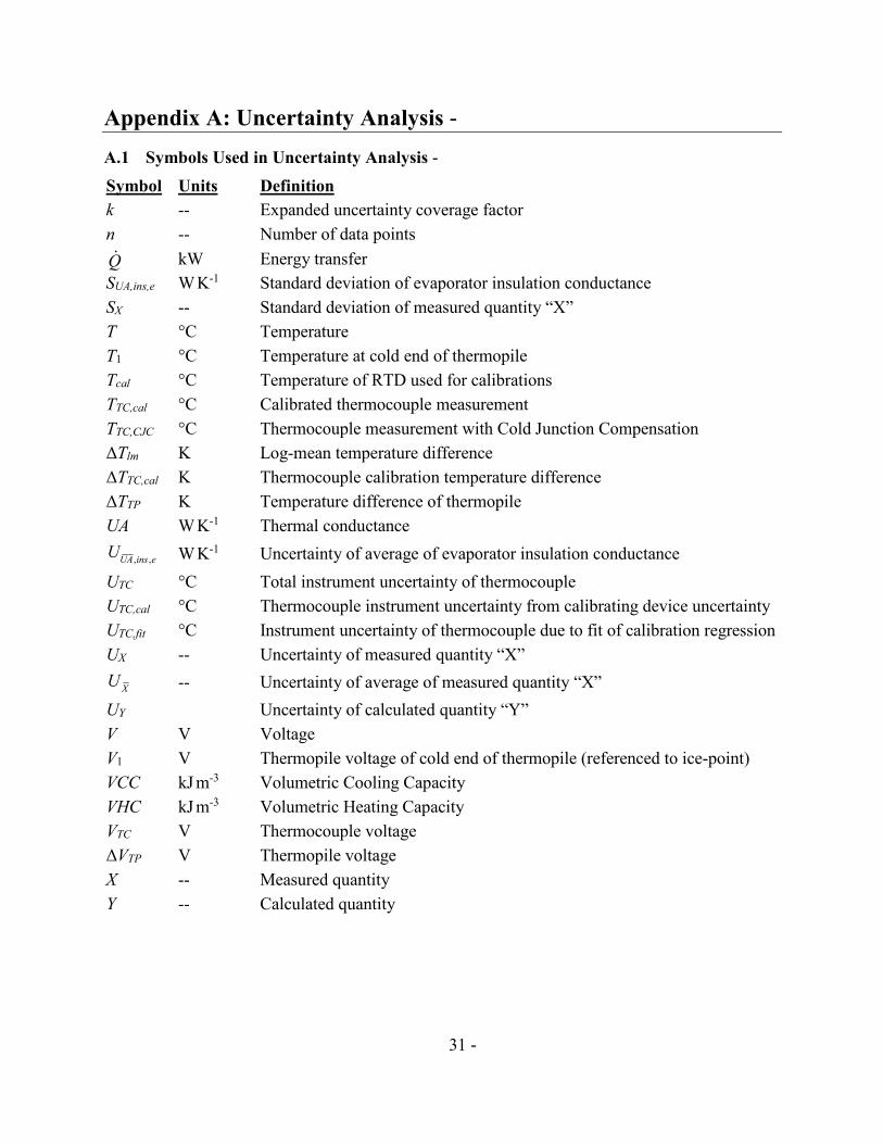
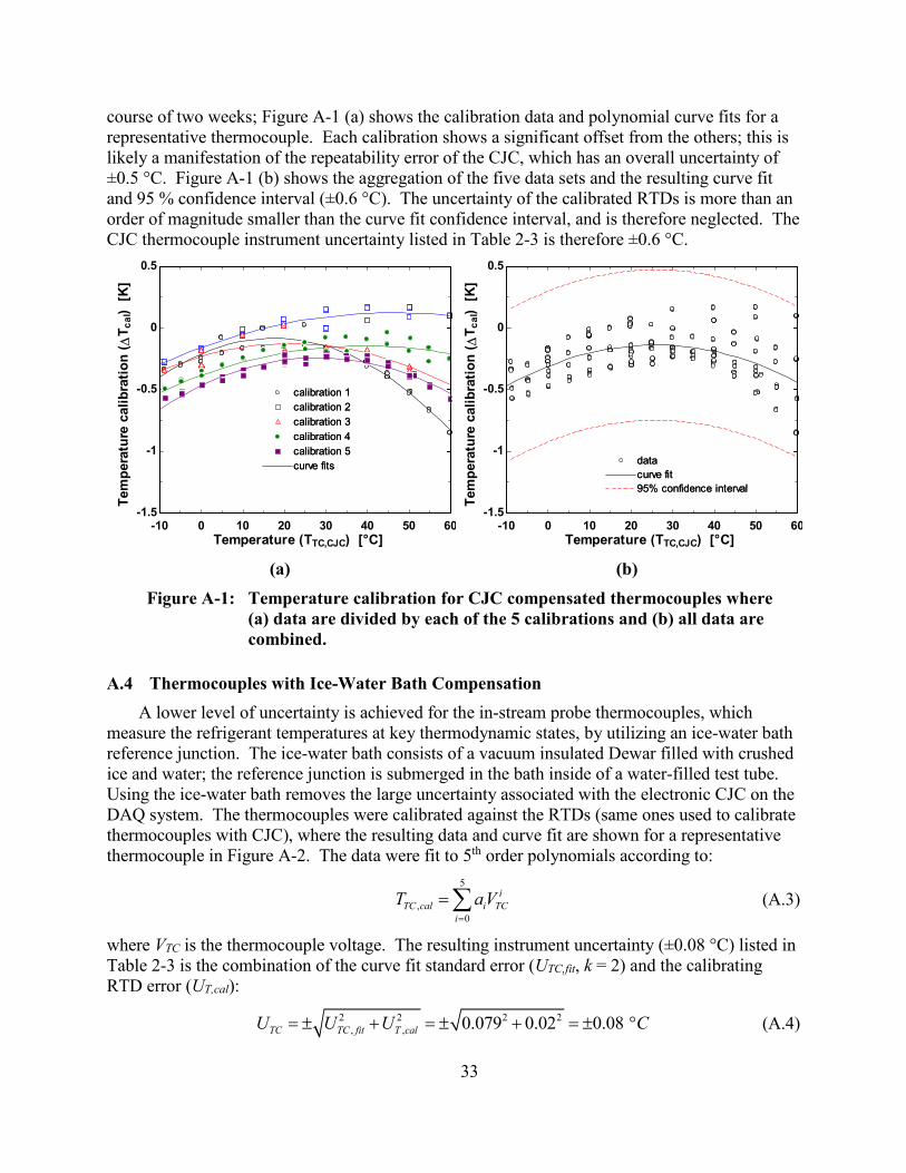
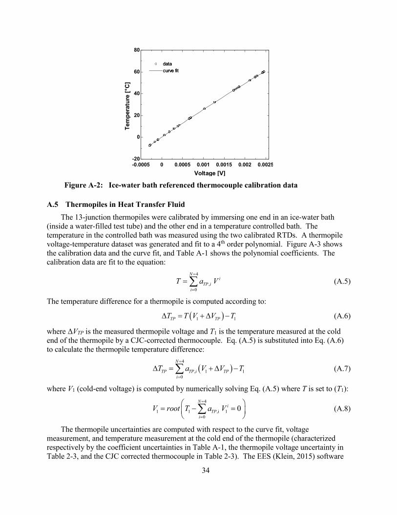
Tem
pera
ture
[degC
]
80
ddaattaa
ccuurrvvee ffiitt60
40
20
0
-20 -00005 0 00005 0001 00015 0002 00025
Voltage [V]
Figure A-2 Ice-water bath referenced thermocouple calibration data
A5 Thermopiles in Heat Transfer Fluid
The 13-junction thermopiles were calibrated by immersing one end in an ice-water bath
(inside a water-filled test tube) and the other end in a temperature controlled bath The
temperature in the controlled bath was measured using the two calibrated RTDs A thermopile
voltage-temperature dataset was generated and fit to a 4th order polynomial Figure A-3 shows
the calibration data and the curve fit and Table A-1 shows the polynomial coefficients The
calibration data are fit to the equation
N =4 i
T = sum aTP i V (A5) i=0
The temperature difference for a thermopile is computed according to
∆T = ( V T V + ∆ ) minusT (A6)TP 1 TP 1
where ∆VTP is the measured thermopile voltage and T1 is the temperature measured at the cold
end of the thermopile by a CJC-corrected thermocouple Eq (A5) is substituted into Eq (A6)
to calculate the thermopile temperature difference
N =4
∆TTP = sum aTP i (V1 +∆VTP ) minusT1 (A7) i=0
where V1 (cold-end voltage) is computed by numerically solving Eq (A5) where T is set to (T1)
N =4 i V1 = root T1 minussum aTPi V1 = 0 (A8)
i=0
The thermopile uncertainties are computed with respect to the curve fit voltage
measurement and temperature measurement at the cold end of the thermopile (characterized
respectively by the coefficient uncertainties in Table A-1 the thermopile voltage uncertainty in
Table 2-3 and the CJC corrected thermocouple in Table 2-3) The EES (Klein 2015) software
34
is used to numerically compute the partial derivatives and subsequent thermopile uncertainties
Figure A-4(a) shows the contours of uncertainty in the temperature difference measured by the
evaporatorcondenser HTF thermopiles
Figure A-4(b) shows the contours of relative contribution to uncertainty in the thermopile
measurement Each of the uncertainty sources is dominant in different regions
bull voltage measurement dominant at low temperature differences (less than 1 K)
bull curve fit error dominant at high cold end temperatures (greater than 50 degC)
bull cold end temperature dominant at moderate cold end temperatures -5 degC to 20 degC and temperature differences 25 K to 20 K
As noted in this discussion the thermopile uncertainty is a complex function of the curve fit
voltage measurement and cold end temperature measurement For the temperature difference
range expected for this application 1 K to 10 K (18 degF to 18 degF) the upper bound of uncertainty
is about 0015 K (0027 degF) for simplicity this is the value listed in Table 2-3 Note that the
contribution to the uncertainty by the calibrating instrument (two calibrated RTDs) is negligible
here as the error in slope (which is the error that propagates into the thermopile temperature
difference) is less than 0000248 K per K of temperature difference (eg 000248 K for a 10 K
temperature difference)
Table A-1 Condenser amp evaporator60
thermopile polynomial coefficients 50
Uncertainty
Coeff Value (k=2) 95 40
Tem
pera
ture
[degC
]
aTPe0 39243 E-02 plusmn41 E-04 30
aTPe1 20243 E+03 plusmn12 E-01 20
aTPe2 -55466 E+03 plusmn22 E+01 TTPP11
10 TTPP22 aTPe3 39023 E+04 plusmn13 E+03 TTPP11 ((ffiitt))
TTPP22 ((ffiitt)) aTPe4 -26229 E+05 plusmn22 E+04
0
-10
38494 E-02 plusmn53 E-04 -001 0 001 002 003 004 aTPc0
Voltage [V]shy aTPc1 20241 E+03 plusmn15 E-01
Figure A-3 Thermopile calibration data aTPc2 -55190 E+03 plusmn28 E+01
aTPc3 38551 E+04 plusmn16 E+03
aTPc4 -25440 E+05 plusmn29 E+04
35
-5
0
10
20 contours of thermopile uncertainty [K] contours of contribution to uncertainty []
20
balance is T1004
0035
Tem
pera
ture
dif
fere
nce
(∆
TT
P)
[K]
15 003
0025
002
0015
001 0001 5
0002 0005
0004 0003
Tem
pera
ture
dif
fere
nce (∆
TT
P)
[K]
15
10
curve fit
80 60
40 20
5 voltage (∆VTP)
20 40
0 60
80
0 10 20 30 40 50
Temperature at cold end (T1) [degC]
60 -5
0 10 20 30 40 50
Temperature at cold end (T1) [degC]
60
(a) (b)
Figure A-4 Contours of thermopile (a) uncertainty and (b) relative contribution to
uncertainty
A6 Evaporator Heat Transfer Fluid Specific Heat
The evaporator HTF is a potassium formate and water heat transfer fluid that is freeze
protected to -40 degC The manufacturerrsquos specific heat data were found to have error of at least
10 so a sample of the fluid was analyzed in a Differential Scanning Calorimeter (DSC) by the
NIST-Boulder Applied Chemicals and Materials Division The temperature dependent specific
heat and the 2nd order curve fit to the data are shown in Figure A-5 the curve fit coefficients and
their uncertainties are listed in Table A-2 Figure A-5 also shows the manufacturerrsquos reported
specific heat data for comparison The exact uncertainty of the DSC measurement was not
available at the time of writing but was estimated to be about 2 to 3 of reading based on the
experience of the DSC operator (Fortin 2015) An uncertainty of 3 of reading is therefore
assigned as a conservative estimate Both the curve fit and DSC calibration uncertainties are
included in the calculation of overall uncertainties
36shy
DSC measurements
curve fit
3 Table A-2 Evaporator HTF specific
heat polynomial coefficients
29 Uncertainty
DSC measurements
curve fit
manufacturers data
-10 0 10 20 30
Sp
ecif
ic h
eat
(Cp)
[Jg
-K]
Coeff Value (k=2) 95
28 aCpe0 25643 E+00 plusmn16 E-03
aCpe1 11015 E-03 plusmn21 E-04
27 aCpe2 17422 E-05 plusmn95 E-06
26
25
Temperature [degC]
Figure A-5 Specific heat measurements for
evaporator HTF
A7 Condenser Heat Transfer Fluid Specific Heat
The condenser HTF is water the specific heat data are computed in EES using the data from
(Harr et al 1984) and are shown in Figure A-6 A conservative estimate of plusmn3 is used for the
uncertainty in the specific heat
423
0 20 40 60 80 100
Sp
ecif
ic h
eat
(Cp)
[kJk
g-K
]
422
421
42
419
418
Temperature [degC]
Figure A-6 Specific heat of condenser HTF (water)
A8 Evaporator and Condenser Insulation Conductance
The total evaporator and condenser insulation conductances (UAinse and UAinsc) for thermal
interaction with the ambient air were measured during an initial test where the HTFs were
circulated at various flow rates through the apparatus at an elevated temperature while the
refrigerant tubes were under vacuum The temperature change of the HTF across the heat
37shy
exchanger was assumed to be entirely attributed to insulation heat leak and therefore an
effective insulation conductance could be computed The resulting UAinse and UAinsc values for
all 20 tubes are shown in Figure A-7 Average values of conductances for the evaporator and
condenser were calculated as 548 W K-1 plusmn031 W K-1 and 652 W K-1 plusmn041 W K-1
(104 Btu h-1 degF-1 plusmn059 Btu h-1 degF-1 and 124 Btu h-1 degF-1 plusmn078 Btu h-1 degF-1) respectively where the
uncertainty accounts for both instrumentation error and test variance The evaporator insulation
conductance for these tests is computed according to
ɺQins e mɺ HTF e C (THTF in e minusT )p HTF e HTF out e
UA = = (A9) ins e ∆T T minusT minus T minusT e ( HTF in e amb e ) ( HTF out )lm HTF e amb e
(T minusT ) amb e HTF in e ln (T
minusT
amb e ) HTF out e
where the variables represent
Cp HTF e = evaporator HTF specific heat
mɺ HTF e = evaporator HTF mass flow
Qɺ = evaporator insulation heat leak ins e
Tambe = ambient air temperature surrounding evaporator
THTFine = evaporator HTF inlet temperature
THTFoute = evaporator HTF outlet temperature
∆TlmHTFe = evaporator log-mean temperature difference
and the uncertainty of the average value is calculated according to
U = k S n (A10) UA ins e UA ins e
where the variables represent
k = expanded uncertainty coverage factor (k = 2) for 95 confidence interval
SUAinse = standard deviation of conductances
n = number of conductance data points
The condenser conductance is computed using the same method with the corresponding
measurements from that heat exchanger
38shy
4
5
6
7
8
Insu
lati
on
co
nd
ucta
nce (
UA
ins)
[WK
]
UAinscond
UAinsev ap
average for evaporator
average for condenser
0 005 01 015
Mass flow [kgs]
Figure A-7 Insulation conductance for evaporator and condenser
A9 Uncertainty Analysis Software
The uncertainty analyses on each of the performance metrics shown in Figure 4-1 through
Figure 4-4 were calculated using the uncertainty propagation capability in EES The software
numerically computes the performance metric uncertainty by evaluating the partial derivatives
with respect to each relevant measurement and applying the specified measurement uncertainty
Assuming the measurements are independent and uncorrelated the uncertainty of a quantity is
computed according to (Taylor amp Kuyatt 1994)
partY 2 2
UY = sum U X (A11) i partXi
i
where the variables represent
Y = calculated quantity
Uy = uncertainty of calculated quantity
Xi = measurement
UXi = uncertainty of measurement
39shy
A10 Moving Window and Steady State Uncertainty
A moving window average was used to compute the measurements at steady state during the
tests In order to determine a proper window size the variation of measurement steady state
uncertainty with window size was examined The steady state uncertainty is defined as the
expanded standard uncertainty for the average reading within the window
S X (A12) U = k X
n
where
k = coverage factor (k = 2) for 95 confidence interval
n = number of samples in the window
Sx = standard deviation of measurement
X = average value of measurement
The data for analysis were generated by holding the MBBHP at a nominal steady operating
condition and recording the measurements at 1-minute intervals (same as collection rate for all
performance testing) for an extended time (3 hours) Figure A-8 shows the fluctuation of steady
state uncertainty for the evaporator inlet and outlet temperatures (T9 and T11) The figure
highlights two characteristic trends observed for all of the instruments both of which suggest the
need for a large moving window (1) the steady state uncertainty decreases as the window size
increases and (2) the steady state uncertainty is highly oscillatory for small windows (the
oscillations are undesirable because short-term fluctuations can have a disproportionate impact
on the averaged result) A 30 sample moving window was selected to achieve low uncertainty
while allowing for collection of data in a timely manner
Figure A-8 shows that the measurement steady state uncertainty is not constant in time (it
would be constant if the fluctuations at steady state were purely random) but rather exhibits
drifting and periodic movements This is possibly due to hunting by the PID controllers
regulating HTF fluid temperatures changes in air temperature in the lab space or some other
uncontrolled andor uncharacterized phenomena These non-random fluctuations are accounted
for by using the maximum steady state uncertainty value observed during the extended steady
state test For example Figure A-8(a) shows the maximum steady state uncertainty for the
evaporator outlet (T9) is plusmn006 degC this value and values for all other sensors are listed in Table
2-3 The data in the moving window are only recorded when steady state uncertainties are below
these established thresholds The total uncertainty (plusmn009 degC) also shown in Table 2-3 is
subsequently computed by adding the instrument uncertainty (plusmn008 degC) and steady state
uncertainty (plusmn006 degC) in quadrature
Note that different sensors of the same type exhibit different levels of fluctuation as a
conservative estimate the largest uncertainty of any one is applied to all of them For example
Figure A-8(b) shows the fluctuations of steady state uncertainty for the evaporator inlet
temperature (T9) are much smaller than for the evaporator outlet (T11) In fact the evaporator
outlet temperature (T11) shows the most fluctuation of all the ice-water bath compensated
thermocouple probes therefore its value (plusmn006 degC) is used in Table 2-3 to represent them all
40shy
05 05
01 01
Ts
[C]
001 001
Ute
ad
y
0002
(a)
Time elapsed [s]
0002
(b)
Time elapsed [s]
Figure A-8shy Uncertainty in temperature due to fluctuations at steady state for (a)
evaporator outlet and (b) evaporator inlet
A11 Uncertainty Results Summary
The detailed instrument uncertainty analysis for performance metrics including the
refrigerantHTF-side capacities and the COPs are tabulated in Appendices A111 (cooling) and
A112 (heating) The tables show the performance metric and its total uncertainty (including
both instrument and steady state contributions) as well as the measurements that contribute to
the uncertainty The measurement values uncertainties partial derivatives (of performance
metric with respect to the measurement) and relative errors (contribution to the overall error in
the performance metric) are also shown where the measurements are listed in order of
decreasing relative error Uncertainties for other performance metrics (eg VCCVHC ηisen)
were analyzed using similar techniques but are not shown in detail in this report Note that
Appendices A111 and A112 show sample calculations for a single nominal operating
condition whereas the uncertainty values presented in the Section 4 figures are computed for
each test run
The uncertainty in cooling performance metrics are shown for a nominal operating point for
R134a during a Cooling A test with a compressor speed of about 30 Hz (1800 RPM) Similarly
the uncertainty in heating performance metrics are shown for R134a during a Heating H1 test
with a compressor speed of about 30 Hz (1800 RPM)
A111 Uncertainty Results Summary Cooling
Table A-3 shows that the dominant sources of instrument uncertainty for the refrigerant-side
capacity are refrigerant mass flow (66 ) expansion valve inlet temperature (17 ) evaporator
exit pressure (8 ) and evaporator exit temperature (7 ) Table A-4 shows the dominant
source of instrument uncertainty for the HTF-side capacity is the HTF specific heat (97
estimate for instrument used to measure fluid properties) Table A-5 shows the dominant
sources of instrument uncertainty for cooling COP are evaporator inlet pressure (39 )
compressor discharge temperature (25 ) and compressor suction temperature (18 )
8000 12000 16000 20000
UT
ste
ad
y [
C]
increasing
time window
10 min
30 min 60 min
05 min
maximum (006 degC)
8000 12000 16000 20000
increasing
time window
10 min
30 min 60 min
05 min
41shy
Table A-3 Uncertainty of refrigerant-side evaporator cooling capacity
Total Partial Relative
Parameter Symbol Value Uncertainty Derivative Error
Refrigerant-side evaporator capacity eref Qɺ 1692 kW plusmn00035 kW
(020) -- --
Refrigerant mass flow refmɺ 1100 g s-1 plusmn0024 g s-1 1538 E-01 66
Refrigerant temp at expansion valve inlet T8 3816 C plusmn009 degC -1634 E-02 17
Refrigerant press at evaporator inlet P9 412 kPa plusmn35 kPa -2817 E-04 8
Refrigerant temp at evaporator exit T11 1209 C plusmn009 degC 1009 E-02 7
Refrigerant press at condenser exit P7 1104 kPa plusmn35 kPa 2103 E-06 0
Refrigerant evaporator differential press ∆Pe 4392 kPa plusmn08 kPa 2817 E-04 0
Table A-4 Uncertainty of HTF-side evaporator cooling capacity
Total Partial Relative
Parameter Symbol Value Uncertainty Derivative Error
plusmn005 kW HTF-side evaporator capacity Qɺ 1672 kW -- --eHTF (30)
Evaporator HTF capacity cp HTF e 259 J g-1 K-1 plusmn3 of cp 6369 E-01 97 calibration uncertainty HTF e
Temperature of ambient air
surrounding evaporator Tambe 230 degC plusmn06 degC 5474 E-03 1
HTF mass flow HTF e mɺ 1312 g s-1 plusmn026 g s-1 1257 E-02 1
Evaporator HTF thermopile voltage ∆VTPe 2512 mV plusmn0007 mV 6537 E-01 1
Evaporator HTF thermopile aTPe0 39243 E-02 plusmn41 E-04 4047 E-03 0
polynomial coefficients aTPe1 20243 E+03 plusmn12 E-01 8832 E-04 0
aTPe2 -55466 E+03 plusmn22 E+01 1559 E-05 0
aTPe3 39023 E+04 plusmn13 E+03 2106 E-07 0
aTPe4 -26229 E+05 plusmn22 E+04 2554 E-09 0
Evaporator HTF capacity aCpe0 25643 E+00 plusmn16 E-03 6369 E-01 0
polynomial coefficients aCpe1 11015 E-03 plusmn21 E-04 1135 E+01 0
aCpe2 17422 E-05 plusmn95 E-06 2024 E+02 0
Temperature at cold end of
evaporator HTF thermopile THTFeout 1542 degC plusmn06 degC -2963 E-03 0
Evaporator insulation conductance UAinse 5474 W K-1 plusmn03052 W K-1 4175 E-03 0
42shy
Table A-5 Uncertainty of cooling COP
Total Partial Relative
Parameter Symbol Value Uncertainty Derivative Error
Cooling COP coolCOP 2844
plusmn001
(035 ) -- --
Refrigerant press at evaporator inlet P9 412 kPa plusmn35 kPa -1232 E-02 39
Refrigerant temp at compressor discharge T3 8197 degC plusmn009 degC 5571 E-02 25
Refrigerant temp at compressor suction T1 1273 degC plusmn009 degC 4788 E-02 18
Refrigerant press at condenser exit P7 1104 kPa plusmn35 kPa 5144 E-03 7
Refrigerant temp at expansion valve inlet T8 3816 degC plusmn009 degC -2746 E-02 6
Refrigerant temp at evaporator exit T11 1209 degC plusmn009 degC 1696 E-02 2
Refrigerant evaporator diff press ∆Pe 4392 kPa plusmn08 kPa 7432 E-04 2
Refrigerant condenser diff press ∆Pc 3234 kPa plusmn13 kPa 4731 E-04 1
Refrigerant suction line diff press ∆Ps 1422 kPa plusmn03 kPa 1314 E-03 0
Refrigerant mass flow refmɺ 1100 g s-1 plusmn0016 g s-1 2209 E-04 0
A112 Uncertainty Results Summary Heating
Table A-6 shows the dominant sources of instrument uncertainty for the refrigerant-side
capacity are refrigerant mass flow (85 ) condenser exit temperature (9 ) and condenser inlet
temperature (5 ) Table A-7 shows the dominant source of instrument uncertainty for the HTF-
side capacity is the HTF specific heat (97 estimate for instrument used to measure specific
heat of water in the reference) Table A-8 shows the dominant sources of instrument uncertainty
for cooling COP are evaporator inlet pressure (32 ) compressor discharge temperature (31 )
and compressor suction temperature (22 )
43shy
Table A-6 Uncertainty of refrigerant-side condenser heating capacityshy
Total Partial Relative
Parameter Symbol Value Uncertainty Derivative Error
Refrigerant-side condenser capacity c refQɺ 1873 kW plusmn0004 kW
(02) -- --
Refrigerant mass flow refmɺ 906 g s-1 plusmn0016 g s-1 2067 E-01 85
Refrigerant temp at condenser exit T7 3739 degC plusmn009 degC -1343 E-02 9
Refrigerant temp at condenser inlet T4 7722 degC plusmn009 degC 9443 E-03 5
Refrigerant press at condenser exit P7 9928 kPa plusmn35 kPa -1296 E-04 1
Refrigerant condenser differential press ∆Pc 272 kPa plusmn13 kPa -9028 E-04 0
Table A-7 Uncertainty of HTF-side condenser heating capacity
Total Partial Relative
Parameter Symbol Value Uncertainty Derivative Error
plusmn0054 kW HTF-side condenser capacity Qɺ 1852 kW -- --cHTF (29)
Condenser HTF capacity calibration cp HTF c 4183 J g-1 K-1 plusmn3 of cp 4262 E-01 97 uncertainty HTF c
Condenser insulation conductance UAinsc 6521 W K-1 plusmn04071 W K-1 1056 E-02 1
HTF mass flow HTF c mɺ 9881 g s-1 plusmn023 g s-1 1804 E-02 1
Condenser HTF thermopile voltage ∆VTPc 2318 mV plusmn0007 mV 7652 E-01 1
Condenser HTF thermopile aTPc0 38494 E-02 plusmn53 E-04 4057 E-03 0
polynomial coefficients aTPc1 20241 E+03 plusmn15 E-01 1025 E-03 0
aTPc2 -55190 E+03 plusmn28 E+01 3481 E-05 0
aTPc3 38551 E+04 plusmn16 E+03 9078 E-07 0
aTPc4 -25440 E+05 plusmn29 E+04 2309 E-08 0
Temperature of ambient air
surrounding condenser Tambc 243 degC plusmn06 degC -6521 E-03 0
Temperature at cold end of
condenser HTF thermopile THTFcin 3196 degC plusmn06 degC -4093 E-03 0
44shy
Table A-8 Uncertainty of heating COP
Total Partial Relative
Parameter Symbol Value Uncertainty Derivative Error
Heating COP heatCOP 3431
plusmn001
(028 ) -- --
Refrigerant press at evaporator inlet P9 3148 kPa plusmn35 kPa -1520 E-03 32
Refrigerant temp at compressor discharge T3 8073 degC plusmn009 degC -5933 E-02 31
Refrigerant temp at compressor suction T1 354 degC plusmn009 degC 5000 E-02 22
Refrigerant temp at condenser inlet T7 3739 degC plusmn009 degC -2461 E-02 6
Refrigerant press at condenser exit P7 9928 kPa plusmn35 kPa 5532 E-04 5
Refrigerant temp at condenser inlet T4 7722 degC plusmn009 degC 1731 E-02 3
Refrigerant condenser differential press ∆Pc 272 kPa plusmn13 kPa 5509 E-04 1
Refrigerant suction line diff press ∆Ps 1269 kPa plusmn03 kPa 1520 E-03 0
Refrigerant evaporator diff press ∆Pe 3999 kPa plusmn08 kPa 1520 E-03 0
Refrigerant mass flow refmɺ 906 g s-1 plusmn0016 g s-1 2187 E-04 0
45shy
Appendix B Instrumentation with DAQ Number ConventionshyThe instrument numbering scheme shown in Figure 2-1 and Figure 2-5 is based on the
thermodynamic states 1 to 11 However the raw data files recorded by the DAQ system use a
different numbering scheme shown in Figure B-1 and Figure B-2
(a)shy (b)
Figure B-1shy Schematic of (a) condenser and (b) evaporator showing the instrument
numbering convention used in the DAQ system
46shy
Figure B-2 Schematic of MBBHP test apparatus including instrument numbering convention used in the DAQ system
47
Appendix C Microfin Tube Surface AreashyThe microfinned surface area (per tube length) is estimated according to
Ai s f 2e
= N f + (C1) L
cosα cosα cos (β 2)
where the variables represent
e = fin height
Nf = number of fins
sf = fin spacing
α = fin helix angle
β = fin angle
and AiL is computed as 00424 m (167 in) The fin parameters are shown in Figure 2-5 and
Table 2-2
48shy
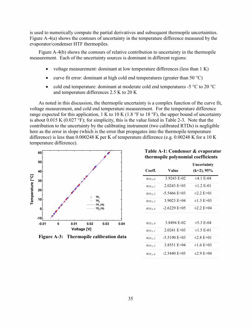
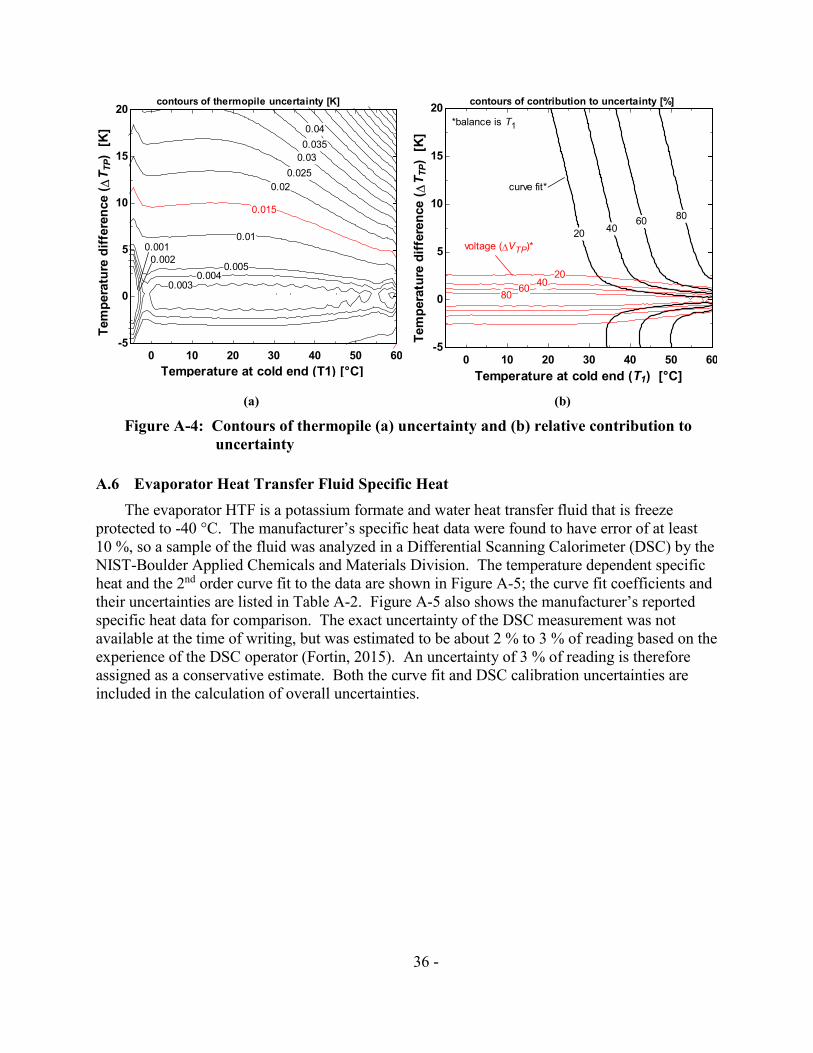
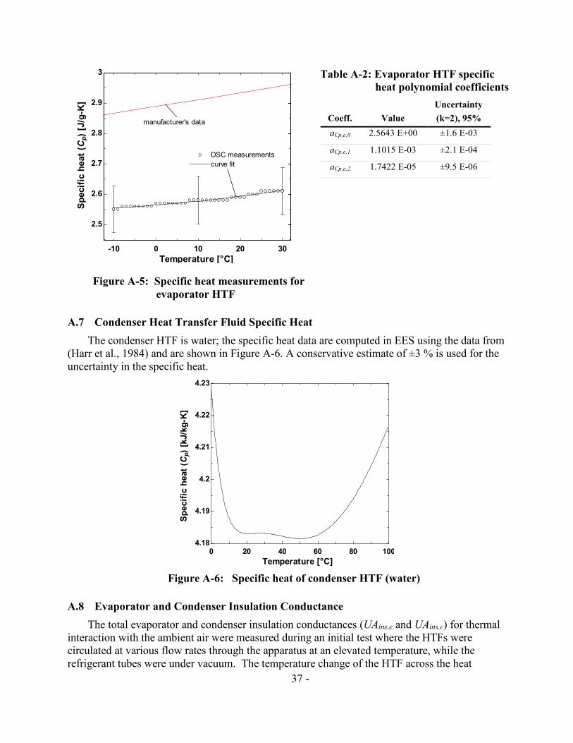
DSC measurements
curve fit
3 Table A-2 Evaporator HTF specific
heat polynomial coefficients
29 Uncertainty
DSC measurements
curve fit
manufacturers data
-10 0 10 20 30
Sp
ecif
ic h
eat
(Cp)
[Jg
-K]
Coeff Value (k=2) 95
28 aCpe0 25643 E+00 plusmn16 E-03
aCpe1 11015 E-03 plusmn21 E-04
27 aCpe2 17422 E-05 plusmn95 E-06
26
25
Temperature [degC]
Figure A-5 Specific heat measurements for
evaporator HTF
A7 Condenser Heat Transfer Fluid Specific Heat
The condenser HTF is water the specific heat data are computed in EES using the data from
(Harr et al 1984) and are shown in Figure A-6 A conservative estimate of plusmn3 is used for the
uncertainty in the specific heat
423
0 20 40 60 80 100
Sp
ecif
ic h
eat
(Cp)
[kJk
g-K
]
422
421
42
419
418
Temperature [degC]
Figure A-6 Specific heat of condenser HTF (water)
A8 Evaporator and Condenser Insulation Conductance
The total evaporator and condenser insulation conductances (UAinse and UAinsc) for thermal
interaction with the ambient air were measured during an initial test where the HTFs were
circulated at various flow rates through the apparatus at an elevated temperature while the
refrigerant tubes were under vacuum The temperature change of the HTF across the heat
37shy
exchanger was assumed to be entirely attributed to insulation heat leak and therefore an
effective insulation conductance could be computed The resulting UAinse and UAinsc values for
all 20 tubes are shown in Figure A-7 Average values of conductances for the evaporator and
condenser were calculated as 548 W K-1 plusmn031 W K-1 and 652 W K-1 plusmn041 W K-1
(104 Btu h-1 degF-1 plusmn059 Btu h-1 degF-1 and 124 Btu h-1 degF-1 plusmn078 Btu h-1 degF-1) respectively where the
uncertainty accounts for both instrumentation error and test variance The evaporator insulation
conductance for these tests is computed according to
ɺQins e mɺ HTF e C (THTF in e minusT )p HTF e HTF out e
UA = = (A9) ins e ∆T T minusT minus T minusT e ( HTF in e amb e ) ( HTF out )lm HTF e amb e
(T minusT ) amb e HTF in e ln (T
minusT
amb e ) HTF out e
where the variables represent
Cp HTF e = evaporator HTF specific heat
mɺ HTF e = evaporator HTF mass flow
Qɺ = evaporator insulation heat leak ins e
Tambe = ambient air temperature surrounding evaporator
THTFine = evaporator HTF inlet temperature
THTFoute = evaporator HTF outlet temperature
∆TlmHTFe = evaporator log-mean temperature difference
and the uncertainty of the average value is calculated according to
U = k S n (A10) UA ins e UA ins e
where the variables represent
k = expanded uncertainty coverage factor (k = 2) for 95 confidence interval
SUAinse = standard deviation of conductances
n = number of conductance data points
The condenser conductance is computed using the same method with the corresponding
measurements from that heat exchanger
38shy
4
5
6
7
8
Insu
lati
on
co
nd
ucta
nce (
UA
ins)
[WK
]
UAinscond
UAinsev ap
average for evaporator
average for condenser
0 005 01 015
Mass flow [kgs]
Figure A-7 Insulation conductance for evaporator and condenser
A9 Uncertainty Analysis Software
The uncertainty analyses on each of the performance metrics shown in Figure 4-1 through
Figure 4-4 were calculated using the uncertainty propagation capability in EES The software
numerically computes the performance metric uncertainty by evaluating the partial derivatives
with respect to each relevant measurement and applying the specified measurement uncertainty
Assuming the measurements are independent and uncorrelated the uncertainty of a quantity is
computed according to (Taylor amp Kuyatt 1994)
partY 2 2
UY = sum U X (A11) i partXi
i
where the variables represent
Y = calculated quantity
Uy = uncertainty of calculated quantity
Xi = measurement
UXi = uncertainty of measurement
39shy
A10 Moving Window and Steady State Uncertainty
A moving window average was used to compute the measurements at steady state during the
tests In order to determine a proper window size the variation of measurement steady state
uncertainty with window size was examined The steady state uncertainty is defined as the
expanded standard uncertainty for the average reading within the window
S X (A12) U = k X
n
where
k = coverage factor (k = 2) for 95 confidence interval
n = number of samples in the window
Sx = standard deviation of measurement
X = average value of measurement
The data for analysis were generated by holding the MBBHP at a nominal steady operating
condition and recording the measurements at 1-minute intervals (same as collection rate for all
performance testing) for an extended time (3 hours) Figure A-8 shows the fluctuation of steady
state uncertainty for the evaporator inlet and outlet temperatures (T9 and T11) The figure
highlights two characteristic trends observed for all of the instruments both of which suggest the
need for a large moving window (1) the steady state uncertainty decreases as the window size
increases and (2) the steady state uncertainty is highly oscillatory for small windows (the
oscillations are undesirable because short-term fluctuations can have a disproportionate impact
on the averaged result) A 30 sample moving window was selected to achieve low uncertainty
while allowing for collection of data in a timely manner
Figure A-8 shows that the measurement steady state uncertainty is not constant in time (it
would be constant if the fluctuations at steady state were purely random) but rather exhibits
drifting and periodic movements This is possibly due to hunting by the PID controllers
regulating HTF fluid temperatures changes in air temperature in the lab space or some other
uncontrolled andor uncharacterized phenomena These non-random fluctuations are accounted
for by using the maximum steady state uncertainty value observed during the extended steady
state test For example Figure A-8(a) shows the maximum steady state uncertainty for the
evaporator outlet (T9) is plusmn006 degC this value and values for all other sensors are listed in Table
2-3 The data in the moving window are only recorded when steady state uncertainties are below
these established thresholds The total uncertainty (plusmn009 degC) also shown in Table 2-3 is
subsequently computed by adding the instrument uncertainty (plusmn008 degC) and steady state
uncertainty (plusmn006 degC) in quadrature
Note that different sensors of the same type exhibit different levels of fluctuation as a
conservative estimate the largest uncertainty of any one is applied to all of them For example
Figure A-8(b) shows the fluctuations of steady state uncertainty for the evaporator inlet
temperature (T9) are much smaller than for the evaporator outlet (T11) In fact the evaporator
outlet temperature (T11) shows the most fluctuation of all the ice-water bath compensated
thermocouple probes therefore its value (plusmn006 degC) is used in Table 2-3 to represent them all
40shy
05 05
01 01
Ts
[C]
001 001
Ute
ad
y
0002
(a)
Time elapsed [s]
0002
(b)
Time elapsed [s]
Figure A-8shy Uncertainty in temperature due to fluctuations at steady state for (a)
evaporator outlet and (b) evaporator inlet
A11 Uncertainty Results Summary
The detailed instrument uncertainty analysis for performance metrics including the
refrigerantHTF-side capacities and the COPs are tabulated in Appendices A111 (cooling) and
A112 (heating) The tables show the performance metric and its total uncertainty (including
both instrument and steady state contributions) as well as the measurements that contribute to
the uncertainty The measurement values uncertainties partial derivatives (of performance
metric with respect to the measurement) and relative errors (contribution to the overall error in
the performance metric) are also shown where the measurements are listed in order of
decreasing relative error Uncertainties for other performance metrics (eg VCCVHC ηisen)
were analyzed using similar techniques but are not shown in detail in this report Note that
Appendices A111 and A112 show sample calculations for a single nominal operating
condition whereas the uncertainty values presented in the Section 4 figures are computed for
each test run
The uncertainty in cooling performance metrics are shown for a nominal operating point for
R134a during a Cooling A test with a compressor speed of about 30 Hz (1800 RPM) Similarly
the uncertainty in heating performance metrics are shown for R134a during a Heating H1 test
with a compressor speed of about 30 Hz (1800 RPM)
A111 Uncertainty Results Summary Cooling
Table A-3 shows that the dominant sources of instrument uncertainty for the refrigerant-side
capacity are refrigerant mass flow (66 ) expansion valve inlet temperature (17 ) evaporator
exit pressure (8 ) and evaporator exit temperature (7 ) Table A-4 shows the dominant
source of instrument uncertainty for the HTF-side capacity is the HTF specific heat (97
estimate for instrument used to measure fluid properties) Table A-5 shows the dominant
sources of instrument uncertainty for cooling COP are evaporator inlet pressure (39 )
compressor discharge temperature (25 ) and compressor suction temperature (18 )
8000 12000 16000 20000
UT
ste
ad
y [
C]
increasing
time window
10 min
30 min 60 min
05 min
maximum (006 degC)
8000 12000 16000 20000
increasing
time window
10 min
30 min 60 min
05 min
41shy
Table A-3 Uncertainty of refrigerant-side evaporator cooling capacity
Total Partial Relative
Parameter Symbol Value Uncertainty Derivative Error
Refrigerant-side evaporator capacity eref Qɺ 1692 kW plusmn00035 kW
(020) -- --
Refrigerant mass flow refmɺ 1100 g s-1 plusmn0024 g s-1 1538 E-01 66
Refrigerant temp at expansion valve inlet T8 3816 C plusmn009 degC -1634 E-02 17
Refrigerant press at evaporator inlet P9 412 kPa plusmn35 kPa -2817 E-04 8
Refrigerant temp at evaporator exit T11 1209 C plusmn009 degC 1009 E-02 7
Refrigerant press at condenser exit P7 1104 kPa plusmn35 kPa 2103 E-06 0
Refrigerant evaporator differential press ∆Pe 4392 kPa plusmn08 kPa 2817 E-04 0
Table A-4 Uncertainty of HTF-side evaporator cooling capacity
Total Partial Relative
Parameter Symbol Value Uncertainty Derivative Error
plusmn005 kW HTF-side evaporator capacity Qɺ 1672 kW -- --eHTF (30)
Evaporator HTF capacity cp HTF e 259 J g-1 K-1 plusmn3 of cp 6369 E-01 97 calibration uncertainty HTF e
Temperature of ambient air
surrounding evaporator Tambe 230 degC plusmn06 degC 5474 E-03 1
HTF mass flow HTF e mɺ 1312 g s-1 plusmn026 g s-1 1257 E-02 1
Evaporator HTF thermopile voltage ∆VTPe 2512 mV plusmn0007 mV 6537 E-01 1
Evaporator HTF thermopile aTPe0 39243 E-02 plusmn41 E-04 4047 E-03 0
polynomial coefficients aTPe1 20243 E+03 plusmn12 E-01 8832 E-04 0
aTPe2 -55466 E+03 plusmn22 E+01 1559 E-05 0
aTPe3 39023 E+04 plusmn13 E+03 2106 E-07 0
aTPe4 -26229 E+05 plusmn22 E+04 2554 E-09 0
Evaporator HTF capacity aCpe0 25643 E+00 plusmn16 E-03 6369 E-01 0
polynomial coefficients aCpe1 11015 E-03 plusmn21 E-04 1135 E+01 0
aCpe2 17422 E-05 plusmn95 E-06 2024 E+02 0
Temperature at cold end of
evaporator HTF thermopile THTFeout 1542 degC plusmn06 degC -2963 E-03 0
Evaporator insulation conductance UAinse 5474 W K-1 plusmn03052 W K-1 4175 E-03 0
42shy
Table A-5 Uncertainty of cooling COP
Total Partial Relative
Parameter Symbol Value Uncertainty Derivative Error
Cooling COP coolCOP 2844
plusmn001
(035 ) -- --
Refrigerant press at evaporator inlet P9 412 kPa plusmn35 kPa -1232 E-02 39
Refrigerant temp at compressor discharge T3 8197 degC plusmn009 degC 5571 E-02 25
Refrigerant temp at compressor suction T1 1273 degC plusmn009 degC 4788 E-02 18
Refrigerant press at condenser exit P7 1104 kPa plusmn35 kPa 5144 E-03 7
Refrigerant temp at expansion valve inlet T8 3816 degC plusmn009 degC -2746 E-02 6
Refrigerant temp at evaporator exit T11 1209 degC plusmn009 degC 1696 E-02 2
Refrigerant evaporator diff press ∆Pe 4392 kPa plusmn08 kPa 7432 E-04 2
Refrigerant condenser diff press ∆Pc 3234 kPa plusmn13 kPa 4731 E-04 1
Refrigerant suction line diff press ∆Ps 1422 kPa plusmn03 kPa 1314 E-03 0
Refrigerant mass flow refmɺ 1100 g s-1 plusmn0016 g s-1 2209 E-04 0
A112 Uncertainty Results Summary Heating
Table A-6 shows the dominant sources of instrument uncertainty for the refrigerant-side
capacity are refrigerant mass flow (85 ) condenser exit temperature (9 ) and condenser inlet
temperature (5 ) Table A-7 shows the dominant source of instrument uncertainty for the HTF-
side capacity is the HTF specific heat (97 estimate for instrument used to measure specific
heat of water in the reference) Table A-8 shows the dominant sources of instrument uncertainty
for cooling COP are evaporator inlet pressure (32 ) compressor discharge temperature (31 )
and compressor suction temperature (22 )
43shy
Table A-6 Uncertainty of refrigerant-side condenser heating capacityshy
Total Partial Relative
Parameter Symbol Value Uncertainty Derivative Error
Refrigerant-side condenser capacity c refQɺ 1873 kW plusmn0004 kW
(02) -- --
Refrigerant mass flow refmɺ 906 g s-1 plusmn0016 g s-1 2067 E-01 85
Refrigerant temp at condenser exit T7 3739 degC plusmn009 degC -1343 E-02 9
Refrigerant temp at condenser inlet T4 7722 degC plusmn009 degC 9443 E-03 5
Refrigerant press at condenser exit P7 9928 kPa plusmn35 kPa -1296 E-04 1
Refrigerant condenser differential press ∆Pc 272 kPa plusmn13 kPa -9028 E-04 0
Table A-7 Uncertainty of HTF-side condenser heating capacity
Total Partial Relative
Parameter Symbol Value Uncertainty Derivative Error
plusmn0054 kW HTF-side condenser capacity Qɺ 1852 kW -- --cHTF (29)
Condenser HTF capacity calibration cp HTF c 4183 J g-1 K-1 plusmn3 of cp 4262 E-01 97 uncertainty HTF c
Condenser insulation conductance UAinsc 6521 W K-1 plusmn04071 W K-1 1056 E-02 1
HTF mass flow HTF c mɺ 9881 g s-1 plusmn023 g s-1 1804 E-02 1
Condenser HTF thermopile voltage ∆VTPc 2318 mV plusmn0007 mV 7652 E-01 1
Condenser HTF thermopile aTPc0 38494 E-02 plusmn53 E-04 4057 E-03 0
polynomial coefficients aTPc1 20241 E+03 plusmn15 E-01 1025 E-03 0
aTPc2 -55190 E+03 plusmn28 E+01 3481 E-05 0
aTPc3 38551 E+04 plusmn16 E+03 9078 E-07 0
aTPc4 -25440 E+05 plusmn29 E+04 2309 E-08 0
Temperature of ambient air
surrounding condenser Tambc 243 degC plusmn06 degC -6521 E-03 0
Temperature at cold end of
condenser HTF thermopile THTFcin 3196 degC plusmn06 degC -4093 E-03 0
44shy
Table A-8 Uncertainty of heating COP
Total Partial Relative
Parameter Symbol Value Uncertainty Derivative Error
Heating COP heatCOP 3431
plusmn001
(028 ) -- --
Refrigerant press at evaporator inlet P9 3148 kPa plusmn35 kPa -1520 E-03 32
Refrigerant temp at compressor discharge T3 8073 degC plusmn009 degC -5933 E-02 31
Refrigerant temp at compressor suction T1 354 degC plusmn009 degC 5000 E-02 22
Refrigerant temp at condenser inlet T7 3739 degC plusmn009 degC -2461 E-02 6
Refrigerant press at condenser exit P7 9928 kPa plusmn35 kPa 5532 E-04 5
Refrigerant temp at condenser inlet T4 7722 degC plusmn009 degC 1731 E-02 3
Refrigerant condenser differential press ∆Pc 272 kPa plusmn13 kPa 5509 E-04 1
Refrigerant suction line diff press ∆Ps 1269 kPa plusmn03 kPa 1520 E-03 0
Refrigerant evaporator diff press ∆Pe 3999 kPa plusmn08 kPa 1520 E-03 0
Refrigerant mass flow refmɺ 906 g s-1 plusmn0016 g s-1 2187 E-04 0
45shy
Appendix B Instrumentation with DAQ Number ConventionshyThe instrument numbering scheme shown in Figure 2-1 and Figure 2-5 is based on the
thermodynamic states 1 to 11 However the raw data files recorded by the DAQ system use a
different numbering scheme shown in Figure B-1 and Figure B-2
(a)shy (b)
Figure B-1shy Schematic of (a) condenser and (b) evaporator showing the instrument
numbering convention used in the DAQ system
46shy
Figure B-2 Schematic of MBBHP test apparatus including instrument numbering convention used in the DAQ system
47
Appendix C Microfin Tube Surface AreashyThe microfinned surface area (per tube length) is estimated according to
Ai s f 2e
= N f + (C1) L
cosα cosα cos (β 2)
where the variables represent
e = fin height
Nf = number of fins
sf = fin spacing
α = fin helix angle
β = fin angle
and AiL is computed as 00424 m (167 in) The fin parameters are shown in Figure 2-5 and
Table 2-2
48shy
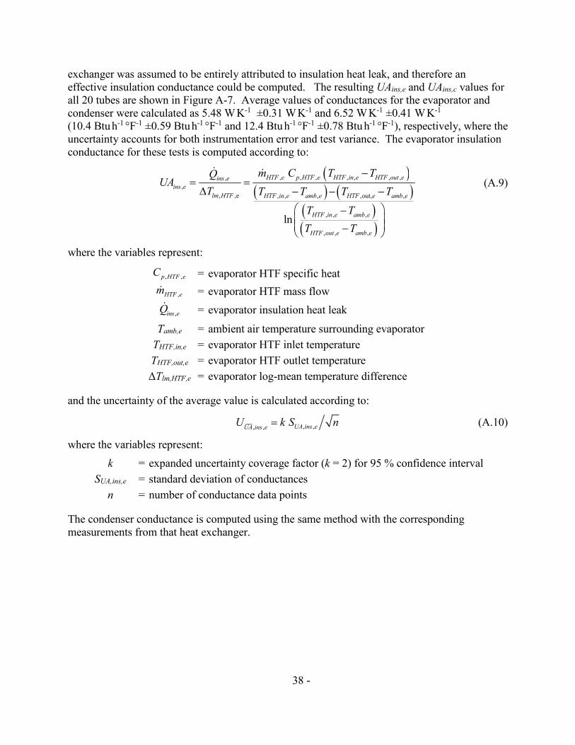
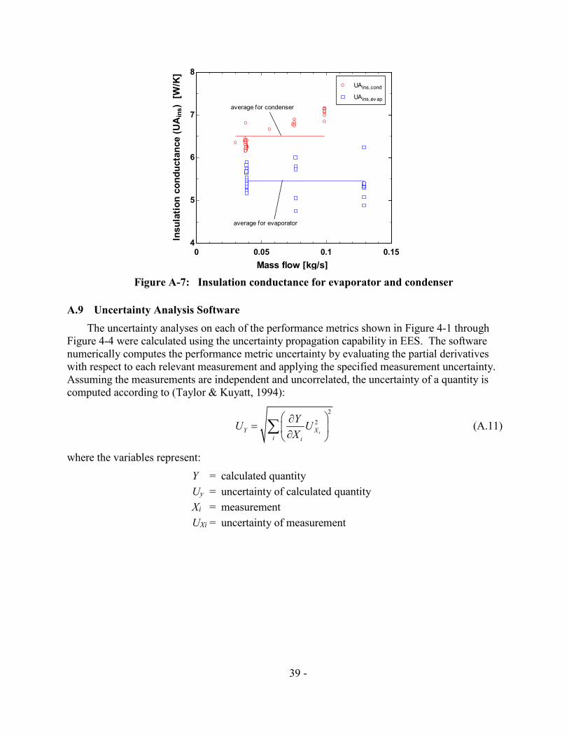
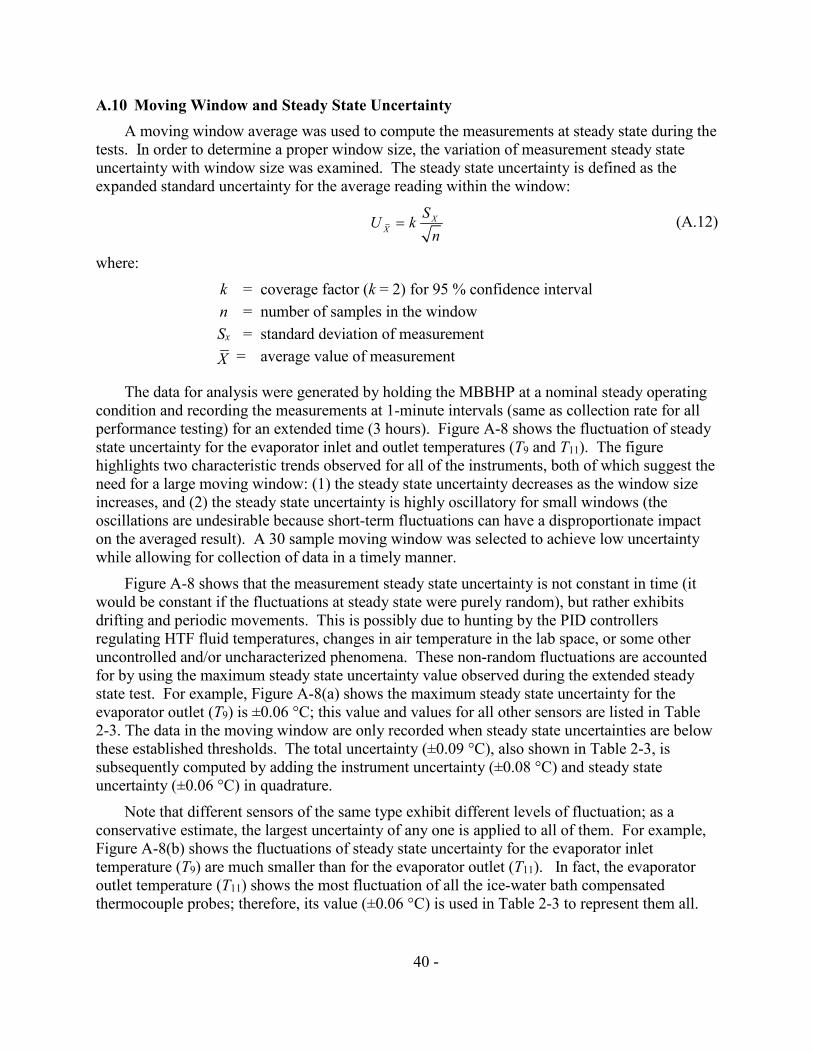
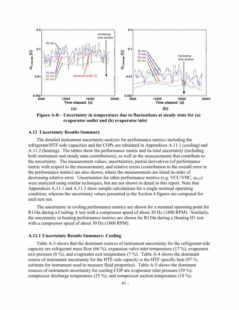
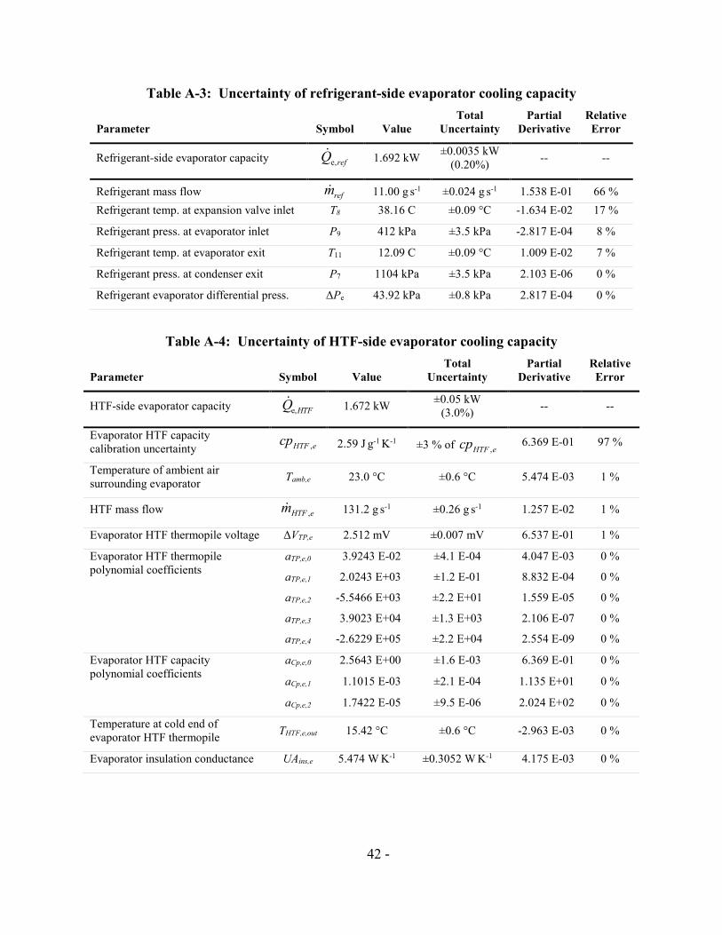
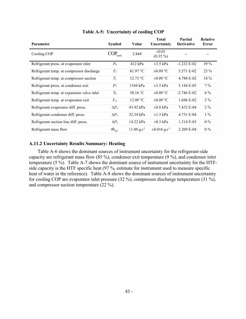
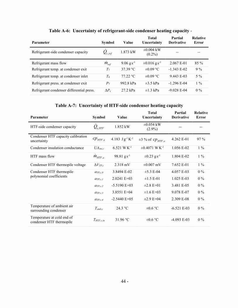
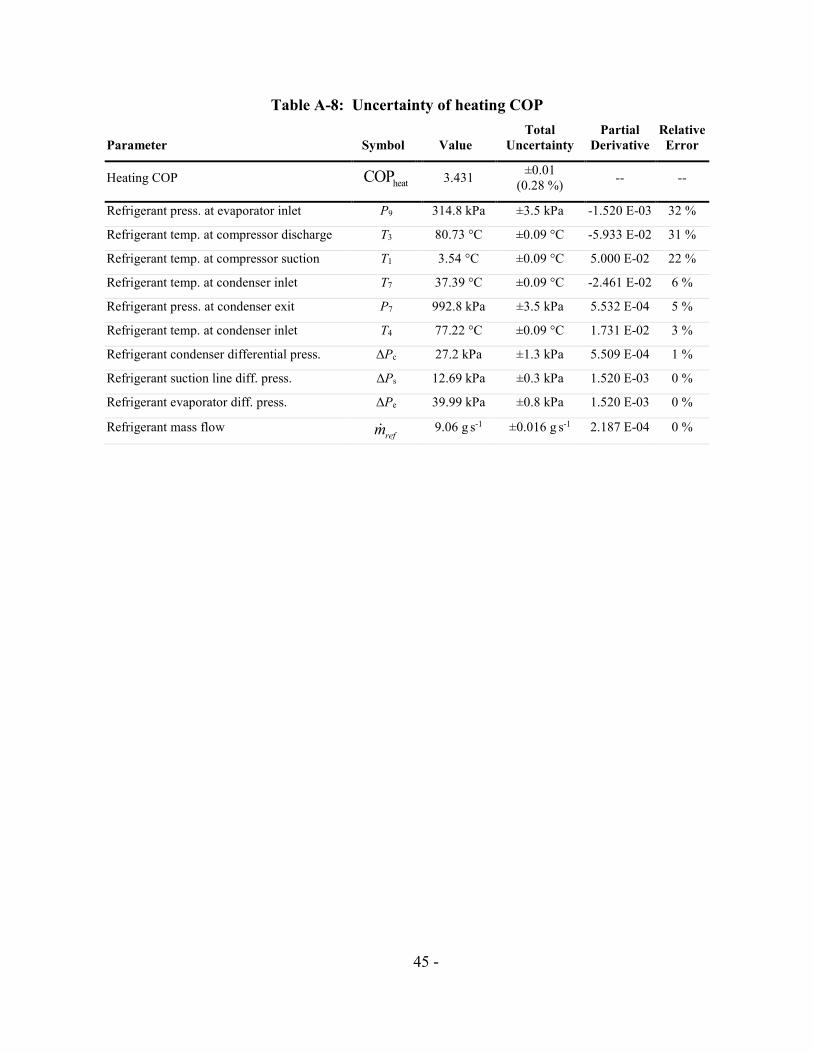
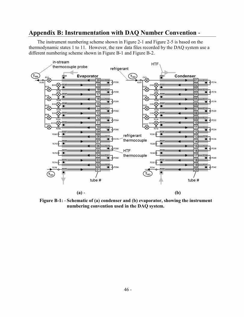
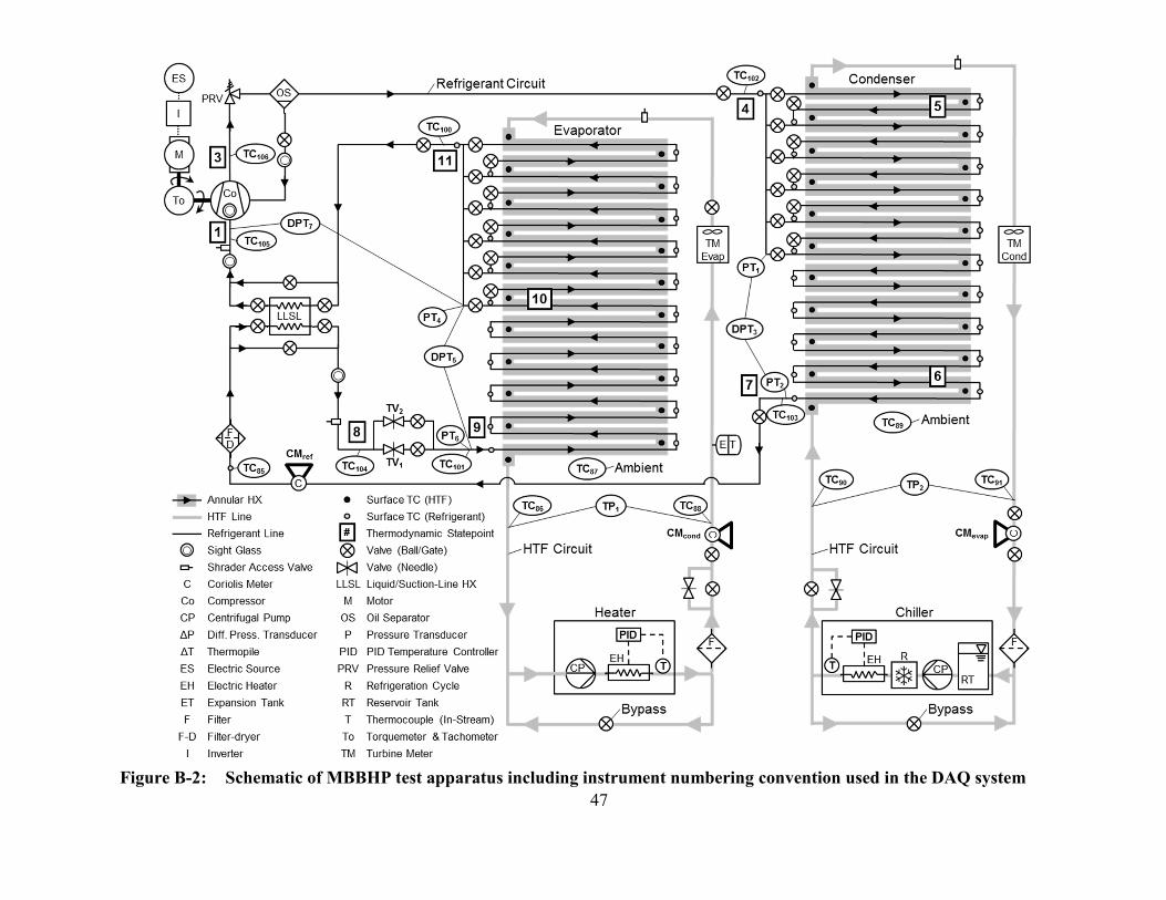
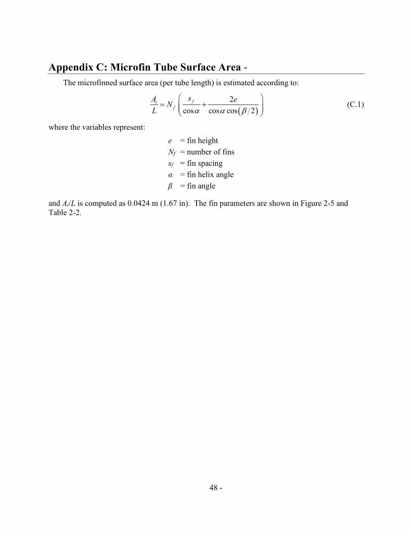