Embed Size (px)
Citation preview

Heat exchanger network retrofit through heat transfer enhancement
A thesis submitted to the University of Manchester for the degree of Doctor of Philosophy
in the Faculty of Engineering and Physical Sciences
2012
Yufei Wang
School of Chemical Engineering and Analytical Science

1
LIST OF CONTENTS
LIST OF CONTENTS................................................................................... 1
LIST OF FIGURES....................................................................................... 5
LIST OF TABLES......................................................................................... 8
ABSTRACT ................................................................................................ 10
DECLEARATION ....................................................................................... 11
COPYRIGHT STATEMENT ....................................................................... 12
ACKNOWLEDGMENT ............................................................................... 13
Chapter 1 Introduction................................................................................ 14
1.1 Research background ................................................................... 14
1.1.1 Background of heat exchanger network retrofit................... 14
1.1.1 Background of heat transfer enhancement ....................... 15
1.2 Motivation and objectives of this work........................................... 16
1.2 Outline of the thesis ...................................................................... 19
Chapter 2 Literature review ...................................................................... 21
2.1 Retrofit of heat exchanger networks.............................................. 21
2.1.1 Pinch design methods for heat exchanger network retrofit . 21
2.1.2 Mathematical programming techniques .............................. 23
2.1.3 Network pinch approach ..................................................... 25
2.1.4 Stochastic approaches for retrofit ....................................... 27
2.2 Heat transfer enhancement techniques ........................................ 28
2.2.1 Tube side heat transfer enhancement ................................ 28
2.2.2 Shell side heat transfer enhancement................................. 30
2.3 Heat exchanger network retrofit considering heat transfer
enhancement ...................................................................................... 31
2.4 Consideration of pressure drop in existing heat exchanger networks
............................................................................................................ 33
2.5 Heat exchanger network retrofit considering fouling ..................... 34
2.6 Summary....................................................................................... 37
Chapter 3 Heuristic methodology for heat exchanger network retrofit with
heat transfer enhancement ........................................................................ 39
3.1 Introduction ................................................................................... 39

2
3.2 Heuristic rules for heat exchanger network retrofit with heat transfer
enhancement ...................................................................................... 40
3.2.1 Rule 1: Network structure analysis...................................... 42
3.2.2 Rule 2: Sensitivity table....................................................... 46
3.2.3 Rule 3: Checking the pinching match.................................. 54
3.2.4 Enhancing candidates simultaneously ................................ 56
3.2.5 Rule 4: Enhancing pinching match...................................... 57
3.3 Case study .................................................................................... 60
3.3.1 An existing preheat train for a crude oil distillation column.. 60
3.3.2 Summary of the case study................................................. 67
3.4 Conclusion .................................................................................... 71
Nomenclature...................................................................................... 72
Chapter 4 Heat exchanger network retrofit optimization considering heat
transfer enhancement ................................................................................ 74
4.1 Introduction ................................................................................... 74
4.2 Simulated annealing...................................................................... 75
4.2.1 Simulated annealing parameters................................................ 77
4.3 General modeling framework ........................................................ 81
4.3.1 Steady state heat exchangers specified in terms of heat load
..................................................................................................... 82
4.3.2 Steady state heat exchangers specified in terms of heat
transfer area................................................................................. 85
4.3.3 Stream splitter and mixer .................................................... 86
4.3.4 Overall heat transfer coefficient .......................................... 88
4.3.5 Heat transfer enhancement................................................. 89
4.3.6 Temperature-dependent thermal properties of process
streams ........................................................................................ 92
4.3.7 Steady state heat exchanger network model ...................... 94
4.4 Duty based optimization retrofit design method with heat transfer
enhancement ...................................................................................... 95
4.4.1 Objective function ............................................................... 96
4.4.2 Simulated annealing moves ................................................ 97
4.4.3 Constraints in duty based optimization.............................. 101

3
4.4.4 Consideration of streams with temperature-dependent
thermal properties ...................................................................... 104
4.4.5 Recovering network feasibility........................................... 106
4.5 Area based optimization retrofit design method with heat transfer
enhancement .................................................................................... 108
4.5.1 SA moves in area based optimization............................... 109
4.5.2 Constraints in area based optimization ............................. 110
4.6 Case studies ............................................................................... 114
4.6.1 Case study 4.1: An existing preheat train retrofit design... 114
4.6.2 Case study 4.2: Retrofit design of a well-established heat
exchanger network..................................................................... 122
4.7 Conclusion .................................................................................. 126
Nomenclature.................................................................................... 128
Chapter 5 Applying heat transfer enhancement in heat exchanger network
considering fouling ................................................................................... 130
5.1 Introduction ................................................................................. 130
5.2 Consideration of fouling in heat exchanger network retrofit ........ 131
5.2.1 Background on fouling of heat exchangers ....................... 131
5.2.2 Fouling in refinery crude oil preheat trains ........................ 132
5.2.3 The performance of heat transfer enhancement under fouling
consideration.............................................................................. 133
5.2.4 Models of fouling............................................................... 135
5.2.5 Fouling model of tube with enhancement.......................... 137
5.3 Opportunities to reduce fouling in heat exchanger networks....... 139
5.3.1 Reducing fouling by applying heat transfer enhancement. 139
5.3.2 Reducing fouling by modifying network structure.............. 141
5.4 Sensitivity to fouling .................................................................... 144
5.5 Optimization of heat exchanger network considering heat transfer
enhancement and fouling.................................................................. 149
5.5.1 Non-steady state simulation of heat exchanger networks . 149
5.5.2 Objective function ............................................................. 152
5.6 Case Study.................................................................................. 153
5.6.1 Case study: An existing preheat train for a crude oil
distillation column....................................................................... 153
4
5.6.2 Case study: An existing preheat train for a simple crude oil
preheat train............................................................................... 155
5.7 Conclusion .................................................................................. 162
Nomenclature.................................................................................... 163
Chapter 6 Pressure drop consideration in heat exchanger network retrofit
with heat transfer enhancement ............................................................... 165
6.1 Introduction ................................................................................. 165
6.2 Detailed heat exchanger models................................................. 165
6.2.1 Tube side models.............................................................. 165
6.2.2 Shell side models.............................................................. 169
6.3 Pressure drop models accounting for enhancement ................... 173
6.4 Methods to reduce pressure drop ............................................... 175
6.4.1 Modifying the number of tube passes ............................... 175
6.4.2 Modifying the shell arrangement ....................................... 178
6.4.3 Reducing pressure drop by using heat transfer enhancement
................................................................................................... 183
6.4.4 Other ways to reduce pressure drop................................. 185
6.5 Case study .................................................................................. 186
4.7 Conclusion .................................................................................. 195
Nomenclature.................................................................................... 196
Chapter 7 Conclusions and future work ................................................... 199
7.1 Conclusions................................................................................. 199
7.1.1 Heuristic methodology for applying heat transfer
enhancement in heat exchanger network retrofit ....................... 199
7.1.2 Simulated annealing based optimization for retrofit with heat
transfer enhancement ................................................................ 200
7.1.3 The performance of heat transfer enhancement in a network
considering pressure drop and fouling ....................................... 202
7.2 Future Work ................................................................................ 203
Reference................................................................................................. 205
Words: 48901

5
LIST OF FIGURES
Figure 2.1 Procedure of network pinch approach ............................... 26
Figure 3.1 Procedure of the proposed heuristic retrofit approach ....... 41
Figure 3.2 Example of a path .............................................................. 43
Figure 3.3 Example network for heuristic methodology....................... 43
Figure 3.4 Path through more than 2 streams..................................... 45
Figure 3.5 Example network for sensitivity table ................................. 47
Figure 3.6 Sensitivity graph for the sensitivity table example.............. 48
Figure 3.7 Sensitivity graph of exchanger 2 ........................................ 49
Figure 3.8 Sensitivity graph of exchanger 3 ........................................ 49
Figure 3.9 Maximum heat recovery when CPh is smaller................... 51
Figure 3.10 Maximum heat recovery when CPc is smaller .................. 52
Figure 3.11 Performance of heat transfer enhancement under different
∆Tmin ............................................................................................ 53
Figure 3.12 A sequence of heat exchangers....................................... 54
Figure 3.13 Influence of downstream exchangers after enhancement 54
Figure 3.14 Example network for heuristic methodology rule 3........... 55
Figure 3.15 Illustration of heat duty reduction in pinching match ........ 56
Figure 3.16 Illustration of enhancing pinching match .......................... 57
Figure 3.17 Existing preheat train network......................................... 63
Figure 3.18 Sensitivity graphs of exchangers 24, 26, 27, 28 and 29 in
the case study.............................................................................. 64
Figure 3.19 Sensitivity graphs of exchangers 4 and 23 in the case study
..................................................................................................... 64
Figure 3.20 Heat exchanger network with enhanced heat exchangers
..................................................................................................... 67
Figure 3.21 Energy saving with different enhancement augmentation
levels............................................................................................ 69
Figure 3.22 Contributions of different heat transfer enhancement levels
to the overall heat transfer coefficient .......................................... 71
Figure 4.1 Flowchart for SA algorithm................................................. 76
Figure 4.2 An example of a heat exchanger ...................................... 82

6
Figure 4.3 Stream with only splitter ..................................................... 87
Figure 4.4 Stream with both splitter and mixer.................................... 87
Figure 4.5 Variables of the stream splitting model ............................. 88
Figure 4.6 Single segment stream ..................................................... 93
Figure 4.7 Multi-segment stream........................................................ 93
Figure 4.8 Node-based heat exchanger network structure
representation .............................................................................. 95
Figure 4.9 The detailed moves of our SA optimization........................ 98
Figure 4.10 SA moves in area based optimization............................ 110
Figure 4.11 Temperature approach violation in duty based optimization
................................................................................................... 111
Figure 4.12 An example network for enthalpy balance constraint..... 112
Figure 4.13 Energy saving results of each strategy .......................... 118
Figure 4.14 Pay-back period results of each strategy ...................... 118
Figure 4.15 Crude oil preheat train with enhanced exchangers
highlighted.................................................................................. 120
Figure 4.16 Network structure of case study 4.2............................... 123
Figure 5.1 Fouling in plain tube and tube fitted with hiTRAN [36] ..... 134
Figure 4.2 Threshold film temperature as a function of flow shear
stress ......................................................................................... 135
Figure 5.3 Vertical and criss-crossed heat transfer .......................... 142
Figure 5.4 Example for different heat transfer patterns .................... 143
Figure 5.5 Sensitivity to fouling in a heat exchanger......................... 146
Figure 5.6 An example of sensitivity to fouling and enhancement..... 147
Figure 5.7 Using sensitivity table in fouling consideration ................. 148
Figure 5.8 Flowchart for heat exchanger network dynamic simulation
................................................................................................... 151
Figure 5.9 Heat exchanger structure of case 5.6.2 ........................... 156
Figure 5.10 Network structure of retrofit design with only topology
modification................................................................................ 160
Figure 5.11 Network structure of retrofit design with both topology
modification and heat transfer enhancement ............................. 160
Figure 6.1 Three types of shell arrangement .................................... 178

7
Figure 6.2 Two options for stream flow when the shells in series
arrangement is changed to the shells in parallel arrangement... 179
Figure 6.3 Temperature change after stream split ............................ 180
Figure 6.4 Total pressure drop of a stream....................................... 186
Figure 6.5 Crude oil preheat train with consideration of pressure drop
................................................................................................... 188

8
LIST OF TABLES
Table 3.1 Heat exchanger data........................................................... 61
Table 3.2 Stream data......................................................................... 62
Table 3.3 Heat transfer data of candidate exchangers........................ 65
Table 3.4 Heat transfer data of enhanced candidate exchangers....... 65
Table 3.5 Heat exchanger data after enhancement ............................ 66
Table 3.6 Comparison of different retrofit designs............................... 67
Table 3.7 Energy saving with different enhancement augmentation
levels............................................................................................ 69
Table 3.8 Contributions of different heat transfer enhancement levels to
the overall heat transfer coefficient .............................................. 70
Table 4.1 SA move probability in Case study 4.1.............................. 116
Table 4.2 Energy cost and retrofit investment of different retrofit
strategies ................................................................................... 117
Table 4.3 Comparison of SA optimization and heuristic methodology
results ........................................................................................ 121
Table 4.4 Comparison between duty based and area base optimization
................................................................................................... 121
Table 4.5 Stream data of case study 4.2........................................... 122
Table 4.6 Exchanger data of case study 4.2 ..................................... 122
Table 4.7 Topology constraints in case study 4.2 ............................ 124
Table 4.8 Results of the three retrofit strategies in case study 4.2.... 124
Table 4.9 Modified exchangers in case study 4.2 ............................. 125
Table 4.10 Enhanced exchanger data of strategy 1 in case study 4.2
................................................................................................... 126
Table 5.1 Initial fouling rate of exchangers in case 5.6.1 .................. 154
Table 5.2 Key exchangers in the network with and without fouling ... 154
Table 5.3 Exchanger data of case 5.6.2............................................ 156
Table 5.4 Stream data of case 5.6.2 ................................................. 156
Table 5.5 Fouling rates computed using different correlated parameters
at a wall temperature of 530 K ................................................... 157

9
Table 5.6 Fouling rates computed using different correlated parameters
at a Re of 20000 ........................................................................ 158
Table 5.7 Exchangers prone to fouling in case 5.6.2 ........................ 158
Table 5.8 Results of different retrofit designs.................................... 158
Table 5.9 Total costs for two network structures under different retrofit
considerations............................................................................ 161
Table 5.10 Fouling rates for two network structures under different
retrofit considerations................................................................. 161
Table 6.1 Values of x and y for different baffle arrangements........... 183
Table 6.2 Values of A and B for different baffle arrangements.......... 184
Table 6.3 Physical properties of streams .......................................... 188
Table 6.4 Detailed data of enhanced exchangers ............................. 189
Table 6.5 Pressure drop and heat transfer coefficients in enhanced
exchangers in the existing network ............................................ 189
Table 6.6 Pressure drop and heat transfer coefficients in enhanced
exchangers in retrofit design ...................................................... 190
Table 6.7 The performance of exchanger 20 with pressure drop
consideration.............................................................................. 191
Table 6.8 The performance of exchanger 24 with pressure drop
consideration.............................................................................. 192
Table 6.9 The performance of exchanger 26 with pressure drop
consideration.............................................................................. 193
Table 6.10 The performance of exchanger 28 with pressure drop
consideration.............................................................................. 193
Table 6.11 Exchanger modification selections .................................. 194
Table 6.12 Overall performances of designs for the case study ....... 194

10
ABSTRACT
Heat exchanger network retrofit plays an important role in energy saving in process industry. Many design methods for the retrofit of heat exchanger networks have been proposed during the last three decades. Conventional retrofit methods rely heavily on topology modifications which often results in a long retrofit duration and high initial costs. Moreover, the addition of extra surface area to the heat exchanger can prove difficult due to topology, safety and downtime constraints. These problems can be avoided through the use of heat transfer enhancement in heat exchanger network retrofit. This thesis develops a heuristic methodology and an optimization methodology to consider heat transfer enhancement in heat exchanger network retrofit. The heuristic methodology is to identify the most appropriate heat exchangers requiring heat transfer enhancements in the heat exchanger network. From analysis in the heuristic roles, some great physical insights are presented. The optimisation method is based on simulated annealing. It has been developed to find the appropriate heat exchangers to be enhanced and to calculate the level of enhancement required. The new methodology allows several possible retrofit strategies using different retrofit methods be determined. Comparison of these retrofit strategies demonstrates that retrofit modification duration and pay-back time are reduced significantly when only heat transfer enhancement is utilised. Heat transfer enhancement may increase pressure drop in a heat exchanger. The fouling performance in a heat exchanger will also be affected when heat transfer enhancement is used. Therefore, the implications of pressure drop and fouling are assessed in the proposed methodology predicated on heat transfer enhancement. Methods to reduce pressure drop and mitigate fouling are developed to promote the application of heat transfer enhancement in heat exchanger network retrofit. In optimization methodology considering fouling, the dynamic nature of fouling is simulated by using temperature intervals. It can predict fouling performance when heat transfer enhancement is considered in the network. Some models for both heat exchanger and heat transfer enhancement are used to predict the pressure drop performance in heat exchanger network retrofit. Reducing pressure by modifying heat exchanger structure is proposed in this thesis. From case study, the pressure drop increased by heat transfer enhancement can be eliminated by modifying heat exchanger structure.

11
DECLEARATION
No portion of the work referred to in this thesis has been submitted in
support of an application for another degree or qualification of this or any
other university or other institution of learning.
Yufei Wang

12
COPYRIGHT STATEMENT
1. The author of this thesis (including any appendices and/or schedules to
this thesis) owns any copyright in it (the “Copyright”) and s/he has given
The University of Manchester the right to use such Copyright for any
administrative, promotional, educational and/or teaching purposes.
2. Copies of this thesis, either in full or in extracts, may be made only in
accordance with the regulations of the John Rylands University Library
of Manchester. Details of these regulations may be obtained from the
Librarian. This page must form part of any such copies made.
3. The ownership of any patents, designs, trade marks and any and all
other intellectual property rights except for the Copyright (the
“Intellectual Property Rights”) and any reproductions of copyright works,
for example graphs and tables (“Reproductions”), which may be
described in this thesis, may not be owned by the author and may be
owned by third parties. Such Intellectual Property Rights and
Reproductions cannot and must not be made available for use without
the prior written permission of the owner(s) of the relevant Intellectual
Property Rights and/or Reproductions.
4. Further information on the conditions under which disclosure, publication
and exploitation of this thesis, the Copyright and any Intellectual
Property Rights and/or Reproductions described in it may take place is
available from the Head of School of Chemical Engineering and
Analytical Science and the Dean of the Faculty of Life Sciences, for
Faculty of Life Sciences’ candidates.

13
ACKNOWLEDGMENT
I would like to express my sincere gratitude to my supervisor, Prof. Robin
Smith, for his patience, guidance and support through the period of this
work. Although he is always so busy, he helped me whenever I needed.
Special thanks to Centre for Process Integration for giving me such a great
opportunity to study at the University of Manchester with the friendly staffs
and students. I wish to thank all staffs and students of Centre for Process
Integration for their help and support whenever I need. Special thanks to
Steve Doyle for his support in the programming part of my research. I thank
Xuesong for the help in both living and study, especially in the first year
when I know nothing about Manchester. I thank Kok-siew, Zixin, Nan, Li and
Luyi for always having nice chats in office, and luckily, in Chinese.
I would give my great appreciation to those friends and roommates (Zhe,
you know you are the most important one, and Qingqing, thanks for giving
me the motivation to finish this thesis by promising me to run naked if I
finish thesis first) that make every minute of my life in Manchester full of joy.
Many thanks to Renmin University and Beijing Normal University, for
sending me some Meizi.
I am very thankful to my parents who have always been supporting and
encouraging me, to overcome the difficulties encountered these years.
Without you, I will never achieve this.

14
Chapter 1 Introduction
1.1 Research background
1.1.1 Background of heat exchanger network retrofit
The retrofit of heat exchanger networks plays an important role in energy
saving today. A plant may need to be retrofitted several times in order to
increase energy efficiency or to accommodate increase in throughput in its
life time. Compared with retrofit of reactors and separators, retrofit of heat
exchanger networks is normally much easier to implement to improve
energy saving. Compared with grassroots design, retrofit design is
constrained by the existing network. Therefore, it is desired to modify the
network as little as possible to achieve the retrofit target. There are many
ways to improve energy saving in a retrofit design. For example, changes in
the use of utility, topology modifications, installing of additional area,
repiping of streams and reassignment of matches. Retrofit can be classified
into three categories according to the objective, as described below.
1. Debottlenecking projects
Sometimes it is necessary for a chemical plant to increase its production
throughput in order to meet greater market demand. In this situation,
reactors and separators should be investigated first to see if they have the
extra capacity to deal with the increase in throughput. The capability of the
heat exchanger network should then be analyzed. Normally after increasing
throughput, there are some bottlenecks within the network that cannot
accommodate the new duty requirement. Accordingly, retrofit of the network
is necessary in order to cope with the increased throughput, preferably with
minimum financial investment.

15
2. Energy conservation projects
Improving energy efficiency in an existing heat exchanger network is always
a worthwhile goal to pursue because it can help to cut the operation cost in
chemical production which consumes large amounts of energy. The most
common way is to reduce utility consumption. Normally, a high level of
energy saving will require a high level of investment in the retrofit project.
3. Process modification projects
Changeover of feed or product is quite common in refinery industries.
Because of the changes in feed or product physical properties, the
operation conditions will be changed. To adjust a plant to new operation
conditions, the retrofit of its heat exchanger network might be required.
1.1.1 Background of heat transfer enhancement
In recent years, practical heat transfer enhancement techniques have been
developed and Polley et al [1] first mentioned the combination of heat
transfer enhancement and process integration. The use of heat transfer
enhancement in process integration can bring many benefits. First, an
enhanced exchanger has a higher heat transfer coefficient to exchange the
same duty under a smaller heat transfer area requirement. Second, with the
same heat transfer area, the enhanced exchanger can have a higher heat
duty. Third, the use of heat transfer enhancement can reduce the pressure
drop in some situations. This is because heat exchange can be achieved
with a higher overall film heat transfer coefficient under a smaller velocity
and enhancement of an exchanger may reduce the number of shells of the
exchanger.
The aforementioned points suggest that using heat transfer enhancement
can bring practical advantages. A smaller heat transfer area means that
less space is required to install the heat exchanger. The enhanced

16
exchanger can exchange heat under a smaller temperature difference,
which means more effective heat integration may be achieved.
1.2 Motivation and objectives of this work
Most retrofit designs require changes in heat exchanger duties. Additional
heat transfer areas are normally used to accommodate the increased heat
transfer driving force requirements. In practice, the implementation of
additional heat transfer area may be difficult due to the constraints of
topology, safety and maintenance. Besides, the capital cost associated with
the related pipe work and civil work is high and the negative financial impact
of production losses due to plant shut down during lengthy periods of retrofit
is also a concern.
According to the features of heat transfer enhancement, in a retrofit design,
heat transfer enhancement can take the place of expensive modifications of
physical area. The implementation of heat transfer enhancement is a
relatively simple task which involves little civil work and can be completed in
a normal shut down period. Therefore, production losses can be kept to a
minimum level.
In many current heat exchanger network retrofit methodologies, the final
retrofit design often involves too many topology modifications. This will
invariably make the retrofit process complex and expensive. If both topology
modification and additional area are not considered in retrofit, the retrofit
process can be extremely simple and will only require a very small financial
investment.
Although several relevant articles have been published over the years [1-3],
the research on this topic is still in its infancy. For example, no exact
methods have been presented to guide the placement of heat transfer
enhancement in a network and optimize the augmentation level of
enhancement.

17
While considerable efforts have been invested in the field of heat exchanger
network retrofit design, the issue of how to combine these methods with
heat transfer enhancement techniques remains unresolved. Until now, the
most common way to analyze a heat exchanger network retrofit problem is
via mathematical programming. But the programming methodology is
limited by the size and complexity of the retrofit problem. Another way is to
use the well established pinch analysis approach to locate the cross-pinch
match and reconnect the network following the grassroots design derived
from pinch analysis. However, this methodology often leads to too many
network modifications. Interestingly, the method of network pinch analysis
can determine the thermodynamic bottleneck of a network topology. This
methodology provides promising structure changes to overcome the
bottleneck but it suffers from drawbacks such as the practical difficulties
associated with the implementation of additional area and topology
modifications.
It is clear that the current suite of methodologies for heat exchanger network
retrofit needs further development. This thesis reports on research efforts
conducted to develop novel retrofit methodologies based on the technique
of heat transfer enhancement. The specific objectives of the research are as
follows:
1) Development of a methodology predicated on heat transfer
enhancement for use in heat exchanger network retrofit.
In most methodologies developed for heat exchanger network retrofit, heat
transfer enhancement is only used as a complementary tool to reduce the
amount of additional area and hence lower the retrofit investment. As a
result, the strengths of heat transfer enhancement are not fully exploited.
Only when the options of additional area and topology modifications are not
considered in a retrofit, can the advantages of heat transfer enhancement
be appreciated. Therefore, it is of great interest to develop a retrofit
methodology based solely on heat transfer enhancement. In such a

18
methodology, because no topology modification is considered, the main
issues to consider include the selection of which exchangers to be
enhanced and the augmentation of each enhancement. Moreover, the
physical insights gained from selecting exchangers to be enhanced will help
promote a deeper understanding of applying heat transfer enhancement in
retrofit design.
2) Optimization of heat exchanger network retrofit considering heat transfer
enhancement
To determine the augmentation level of heat transfer enhancement, an
optimization should be carried out. A trade-off between the cost of heat
transfer enhancement and the energy cost should be made. Moreover,
some constraints that exist in heat exchanger networks such as the stream
enthalpy balance and minimum approach temperature should be accounted
for in the optimization process. Although it is desired to use only heat
transfer enhancement in retrofit because it can lead to a simple and low
cost design, sometimes such approach cannot achieve the retrofit
objectives. In this situation, it is of interest to explore how a heat exchanger
network retrofit considering heat transfer enhancement performs when the
options of topology modification and additional area are also included in the
optimization process.
3) Application of heat transfer enhancement considering pressure drop and
fouling.
High pressure drop and fear of fouling problems are the main reasons that
hinder the use of heat transfer enhancement in industrial retrofit projects.
Therefore, the implications of pressure drop and fouling must be assessed
in the proposed methodology predicated on heat transfer enhancement.
Methods to reduce pressure drop and mitigate fouling need to be developed
to promote the application of heat transfer enhancement in heat exchanger
network retrofit.

19
1.2 Outline of the thesis
Chapter 2 reviews previous studies on heat exchanger network retrofit,
some existing heat transfer enhancement techniques and heat exchanger
network retrofit designs under different considerations.
Chapter 3 introduces a new heuristic methodology predicated on heat
transfer enhancement. A procedure based on sensitivity tables [4] and the
network pinch approach [5] is proposed for screening the best heat
exchanger candidates for enhancement. The physical insights of the
selection procedure are analyzed in this chapter.
Chapter 4 describes a new optimization approach that considers heat
transfer enhancement in heat exchanger network retrofit. Simulated
annealing is used as the optimization algorithm. Several retrofit strategies
are used to evaluate the performance of heat transfer enhancement.
Chapter 5 explores the impact of fouling on the optimization approach
considering heat transfer enhancement. Only crude oil fouling is considered
in this chapter. Modelling results for both exchangers and enhanced
exchangers show that fouling mainly depends on the velocity of fluid and
wall temperature. Some methods for decreasing wall temperature to reduce
fouling are presented. The performance of heat transfer enhancement
under fouling conditions is analyzed.
Chapter 6 presents a retrofit methodology considering both heat transfer
enhancement and pressure drop. Pressure drop can be reduced by
changing the heat exchanger structure at the expense of heat transfer
coefficients. However, the heat transfer enhancement can be used to
compensate for the reduction in heat transfer and can even give a higher
heat transfer coefficient when heat exchanger structure modification is
considered.

20
Chapter 7 provides a summary of the main results and suggests some key
areas for future research.

21
Chapter 2 Literature review
2.1 Retrofit of heat exchanger networks
The need to retrofit an existing heat exchanger network may arise from a
desire to reduce its utility consumption, to increase the throughput, to deal
with modification of the feed to the process, or to cope with modification to
the product specification. All of these objectives might require heat duties
within the network to be changed.
The heat exchanger network retrofit problem has been subject to intensive
research over the years. The most common methods are the pinch analysis
based approach and mathematical programming.
2.1.1 Pinch design methods for heat exchanger network retrofit
Tjoe and Linnhoff [6] first proposed a systematic methodology for heat
exchanger network retrofit based on the Pinch approach. The methodology
includes two steps. In the first step, the retrofit target is set by applying the
concept of area efficiency. In the second step, some heuristic rules are used
to modify the existing network. Area efficiency is a concept that is defined
as the ratio between the target area for the level of heat recovery reached in
the existing heat exchanger network and the existing area installed. Based
on the assumption of constant area efficiency, the trade-off between energy
recovery and heat transfer area for the retrofit design is optimized. By doing
this, the optimal △Tmin can be determined to initialise the retrofit design. In
the second step, similar to the grassroots design, the whole network is
divided into two parts: above the process pinch and below the process
pinch. Heuristic rules are used to relocate heat exchangers that transfer
heat across the pinch or add new heat exchangers to the network.
22
Shokoya [7] proposed the so-called area matrix method using a linear
model to determine retrofit targets. The area matrix represents the
distribution of the area between each pair of hot and cold streams in the
existing network. A target matrix is generated by assuming vertical heat
transfer between the hot and the cold composite curves. After that, a
deviation area matrix is defined as the difference between the target area
matrix and the existing area matrix. Then the target area matrix with the
maximum compatibility with the existing area matrix is found by minimising
the sum of the squares of the elements in the deviation area matrix. The
consideration of area distribution enables the additional area target to be
more realistic than that obtained by the area efficiency methods of Tjoe and
Linnhoff [6]. The design procedure used also involves decomposition of the
design problem at the process pinch and the correction of the cross pinch
matches. This procedure is guided by the deviation area matrix as well as
the pinch design rules.
Carlsson et al. [8] introduced the cost matrix method for heat exchanger
network retrofit. In their work, besides cost of heat transfer area, other costs
such as physical piping distance between pair of streams, auxiliary
equipment, pumping cost are also considered. Based on the Pinch
approach, this method decomposes the design problem at the pinch
location. The cost matrix is applied separately to the above pinch and below
pinch subsystems. Each time a modification is selected, the cost matrix is
updated. Unlike the Pinch approach, this method does not have a targeting
stage. Because no targeting is performed, several networks need to be
evaluated for different △Tmin. Based on the cost matrix and a set of rules,
matches are selected until the level of heat recovery defined by △Tmin is
reached.
Because the Pinch approach is a well-developed methodology, Pinch based
retrofit design is widely used in practical retrofit situations. It can give the
designer a target, and perform well in large scale processes. However, it
has a number of fundamental problems:

23
1. The retrofit design is likely to entail a large number of modifications to
the existing network, which will induce a too high retrofit investment.
2. Existing equipment is only reused in an ad hoc way.
3. Constraints associated with the existing network are not readily included.
4. Although it provides a good user interaction, it requires expert users.
The most important problem can be summed up as follows: the network is
treated as a grassroots design rather than accepting the features that
already exist.
2.1.2 Mathematical programming techniques
Mathematical programming methods convert the heat exchanger network
problem into an optimization task by formulating the retrofit problem as a
mathematical model. The two most important issues in mathematical
methods are to find an efficient and reasonably sized representation of the
problems and efficient optimization techniques to solve the problems. The
optimization objective is to identify the lowest cost design from many
possible solutions embedded in a superstructure. The mathematical models
used in the optimization can be classified on the basis of presence or
absence of non-linear and discrete variables as linear programming (LP),
non-linear programming (NP), mixed integer linear programming (MILP) or
mixed integer non-linear programming (MINLP).
Yee and Grossmann [9, 10] developed an MILP assignment-transhipment
model for structural retrofit of heat exchanger networks based on the
transhipment model proposed by Papoulias and Grossmann [11]. This
model minimises the number of structural modifications required to reach a
given level of heat recovery in an existing heat exchanger network. This is
carried out by first minimising the number of new heat exchangers required
and then minimising the number of heat exchangers reassigned to different
matches. The assignment-transhipment model has been further developed.

24
The new model includes two stages: pre-screening and optimization stages.
The pre-screening stage is used to determine the optimal heat recovery
level and assess the economic feasibility of the retrofit design. Only the
number of new units required to achieve the optimum investment is carried
forward to the optimization stage. In the optimization stage, a design
method using a superstructure that includes all the possible structural
scenarios is proposed, and it is formulated in an optimisation framework as
an MINLP model.
Ciric and Floudas [12] proposed another two-stage approach for the retrofit
of heat exchanger networks. The two stages are match selection stage and
optimization stage. In the match selection stage, an MILP model is used to
identify promising structural modifications. In this stage, decisions regarding
selecting matches, reassigning exchangers, purchasing new exchangers
and repiping streams are made. The objective of the MILP model is to
minimise the costs of additional area, new heat exchangers and repiping.
The result of this stage is then used in the next stage to generate a
superstructure containing all possible network configurations. The optimal
heat exchanger network retrofit design is found by optimizing the
superstructure by using an NLP model. Later, they presented a single stage
MINLP model in which the transhipment model and the generalised match
network hyper-structure [13] are used to model the heat flow and the
network structure. This new approach can avoid the limitations from the
decomposition step.
Sorsak and Kravanja [14] proposed an MINLP optimisation model for heat
exchanger network retrofit, in which the selection of different exchanger
types, such as double pipe exchangers (DP), shell and tube exchangers
(ST), and plate and frame exchangers (PF), can be made simultaneously.
Since their extended model considers different types of exchangers, the
feasibility of heat transfer throughout the heat exchanger network is strongly
dependent on the choice of exchanger types, which limits the extent of heat
recovery. For example, in counter-flow heat exchangers, the outlet
temperature of the cold stream can be higher than other flow pattern, due to

25
geometry-characteristics of the exchangers. When multiple tube passes are
used for ST exchangers, the flow arrangement combines the counter and
co-current flows, and consequently the feasibility of heat transfer is limited
by those flow patterns in the exchangers. To overcome this problem,
additional constraints are specified for ST exchangers in their model.
Mathematical programming methods enable the heat exchanger retrofit
design procedure to be automated. However, mathematical programming
approaches cannot guarantee global optimality in their solutions due to the
non-convexities in the objective function and constraints of NLP and MINLP
models. Moreover, mathematical programming impedes user interaction, is
sensitive to initial points and exerts heavy demand on computer resources.
Mathematical programming could be a poor choice when the problem size
is large and rigorous exchanger models are to be used.
2.1.3 Network pinch approach
Network pinch approach is a heat exchanger network retrofit method
proposed by Asante and Zhu [5]. It combines the advantages of pinch
analysis and mathematical programming. It evolves the network from the
existing structure in order to identify the most critical changes to the network
structure. The approach has two stages: diagnosis stage and optimization
stage. In the diagnosis stage, the potential modifications to the existing
configuration of heat exchanger network are suggested according to pinch
technology; then each candidate modification is optimized for maximum
heat recovery by varying heat loads of each exchanger unit. In the
optimization stage, designers can select the modification they prefer, and
then further cost optimization is carried out on the selected heat exchanger
network with a modified topology. The procedure of network pinch is
illustrated in Figure 2.1.

26
Figure 2.1 Procedure of network pinch approach
The difference between the network pinch and the process pinch is that the
former is a characteristic of both the process streams and the heat
exchanger network topology, whilst the latter is a characteristic of the
process streams only. Consequently, changes of the topology of a heat
exchanger network will affect the network pinch, but leave the process pinch
unchanged.
Although the network pinch approach is a sequential approach, it exploits
possible topology modifications in a systematic way and at the same time
provides access to the design procedure. These characteristics make the
network pinch approach a promising retrofit method, especially in industry.
However, generating the design with minimum cost cannot be guaranteed
since the selection of the potential modifications is not based on costs but
on energy demands.
Smith et al. [15] further improved the network pinch approach by accounting
for the fact that stream thermal properties are temperature-dependent.
Moreover, the two-level pinch approach is developed for the optimization of
Original Network
Diagnosis Stage Determine topology modifications
Optimization Stage Minimise total cost
Retrofit Network Design
Independent of area
(MILP)
For a given topology
(NLP)

27
all continuous variables in order to make sure that the bottleneck is the
network topology rather than heat transfer areas. In their methodology, they
combine structural changes and capital-energy optimization into a single
step in order not to miss cost effective designs.
2.1.4 Stochastic approaches for retrofit
Nielsen et al. [16] present a framework for the design and retrofit of heat
exchanger networks. The methodology includes detailed modelling of
diverse types of heat exchangers, non-constant heat capacities and heat
transfer coefficients, as well as considerations of pressure drop and
flexibility. The framework uses Simulated Annealing (SA) as optimization
tool to carry out the design task, with a formulation similar to that presented
by Dolan and co-workers [17].
In the work of Athier et al. [18], two loops are included. The SA algorithm is
used to select a heat exchanger network configuration in the outer loop, and
an NLP formulation is used to optimize the continuous variables such as
heat loads and split ratios for a fixed heat exchanger network structure in
the inner loop. This approach was applied to several literature examples
successfully. However, the computational time required is considerably high
compared with other approaches.
Rodriguez [19] presented an optimization-based approach for mitigation of
fouling in heat exchanger networks. Although the main aim of this work is to
minimize fouling aspects when designing HENs, the approach can also be
applied to steady state design and retrofit. In the approach, the SA
algorithm was employed as the optimization algorithm. Both structural
options, such as re-piping, re-sequencing of existing exchangers, and
continuous variables, such as stream split fractions and exchanger duties,
were considered without simplification of cost models and objective
functions.

28
Compared with deterministic mathematical programming, stochastic
methods have more chance to find global optimum for non-linear problems
with mixed integer and continuous variables, due to the random nature of
the optimization methods. However, stochastic methods are normally time
consuming.
2.2 Heat transfer enhancement techniques
Heat transfer enhancement is a technique that can improve heat transfer
performance. In recent years, practical heat transfer enhancement
techniques have been developed and many papers are devoted to this area
[20]. Heat transfer enhancement can be classified into passive, which
requires no direct application of external power, and active, which requires
external power. Different enhancement techniques have different impacts
on the film coefficients, pressure drop and fouling.
2.2.1 Tube side heat transfer enhancement
García et al. [21] have classified the tube-side enhancement techniques
according to two different criteria. First, additional devices, which are
incorporated into a plain round tube, e.g. twisted tapes and wire coils.
Second, non-plain round tube techniques such as surface modification of a
plain tube, e.g. corrugated and dimpled tubes; or manufacturing of special
tube geometries, e.g. internally finned tubes.
Twisted tapes are swirl-flow devices that create rotating or secondary flow
along the tube length. They consist of a thin strip of twisted metal with
usually the same width as the tube inner diameter. These types of inserts
are often used in retrofit of existing shell-and-tube heat exchangers to
upgrade their heat duties. Several authors have conducted research on the
thermal and hydraulic performance of twisted tapes in single-phase, boiling
and condensation forced convection. Abu-Khader [22] stated that generally
twisted tapes are more effective in the laminar region than the turbulent
29
region because of larger heat transfer enhancement ratio at lower fluid
velocities. Many studies [23-25] have been done to simulate the twisted
tapes in order to clarify the mechanism, especially the effect of swirl flow.
From these works, it can be concluded that twisted tapes are able to
provide a high level of enhancement, especially within the laminar region.
Nevertheless, the pressure drop penalty is very high and independent of Re.
If the pressure drop is of no concern, then twisted tapes should be preferred
in both laminar and turbulent regions. The high increase in pressure drop
often restricts the industrial applications of twisted tapes.
Wire coils are tube inserts that act as roughness elements. They induce a
swirl effect and hasten the transition from laminar to turbulent flow. Wire
coils are usually used in oil cooling devices, pre-heaters or fire boilers.
García et al. [21] highlighted the advantages that these inserts present in
relation to other enhancement techniques: low cost, easy installation and
removal, preservation of original tube mechanical strength, and possibility of
installation in an existing heat exchanger. Early stage research on wire coils
was conducted by Kumar and Judd [26] and Sethumadhavan and Raja Rao
[27]. They developed empirical correlations to assess the performance of
these types of inserts in turbulent flow. Many ensuing works [28-30] have
been done to predict the performance of wire coils. From these studies, it
can be concluded that wire coils provide more enhancement under laminar
flow conditions with the benefit of a small pressure drop penalty. In turbulent
conditions the level of enhancement was still considerable, although the
pressure drop increase was relatively high.
Internally finned tubes are one of the most widely used methods for passive
heat transfer enhancement [31]. Many geometric configurations for fins
were proposed in the literature. Carnavos [32] first proposed the
correlations to predict the heat transfer coefficient and pressure drop for
internally finned tubes in turbulent flow. Ravigururajan and Bergles [33]
proposed what is considered the most general and accurate method for
predicting heat transfer coefficient and pressure drop inside internally ribbed
tubes. In the experimental research of Jensen and Vlakancic [34], empirical

30
correlations that describe the heat transfer coefficient and pressure drop
performance of internally finned tubes in turbulent flow were developed.
Based on the results reported in the heat transfer literature, it is possible to
conclude that micro-fins are not beneficial when used under laminar flow
conditions, but in turbulent flow they are able to provide a medium-high level
of enhancement of the overall heat transfer of a heat exchanger, affecting
not only the tube-side heat transfer coefficient, but also the overall heat
transfer area.
hiTRAN Matrix turbulator is an effective heat transfer enhancement
technique. From the literature [35], it is reported that the technique is
particularly effective at enhancing heat transfer efficiency in a plain tube
design operating at low Reynolds Numbers (laminar to transitional flow). For
fully turbulent flow, increase in heat transfer is still possible. However the
application is only effective if there is sufficient pressure drop. For hiTRAN
Matrix turbulator, more attention [36-38] has been paid on the fouling
consideration of hiTRAN. From these studies, it is evident that hiTRAN can
reduce the fouling by different mechanisms, especially in chemical reaction,
crystallization, and particulate fouling.
2.2.2 Shell side heat transfer enhancement
Over the last few decades, various shell-side heat transfer enhancement
technologies have been developed and used in industry. The most
commonly used baffle technology is the segmental baffle. The conventional
segmental baffle improves the heat transfer in the heat exchanger shell side.
However, it also induces significant penalties such as high shell-side
pressure drop, low shell-side mass flow velocity, fouling and vibration.
Helical baffles have been developed to reduce the number of dead spots
created by the segmental baffles [39]. From the studies of helical baffles
[40-42], it is clear that their benefits include improved heat transfer
coefficient, low pressure drop increasing, low possibility of flow-induced

31
vibration, and reduced fouling with a trivial increase in pumping. Helical
baffles are classified into continuous and non-continuous baffles [39]. They
offer better levels of augmentation at smaller helix angles and helical
pitches. The compact structure of non-continuous helical baffles can offer
superior augmentation levels with a trivial increase in pressure drop
compared to continuous baffles.
External fin is another widely used heat transfer enhancement technique for
shell side. The fin not only increases the film coefficient with added
turbulence but also increases the heat transfer area. From literature results
[43], it is known that extended surface finned tubes provide two to four times
as much heat transfer area on the outside as the corresponding bare tube,
and this area ratio helps to offset a lower outside heat transfer coefficient.
Some recent papers have presented some useful data for the performance
of finned tubes [44-46]. From these results, it can be seen that finned tubes
can enhance the heat transfer quite significantly, however, with a
substantial increase in associated pressure drop levels.
2.3 Heat exchanger network retrofit considering heat transfer enhancement
Heat transfer enhancements are very attractive options for heat exchanger
network retrofit. They are used to avoid implementation of additional area,
which can lead to significant cost savings. When heat transfer enhancement
is considered capital costs are usually low for no piping or civil work is
required. Moreover, heat transfer enhancement can be done during normal
maintenance periods, so that the production losses during retrofit period can
be avoided. However, heat transfer enhancement and heat exchanger
network retrofit are normally researched separately, and studies that
combine both aspects are very rare in the literature.
Polley et al. [1] first mentioned the possibilities of applying heat transfer
enhancement in heat exchanger network retrofit. In their work, they

32
analyzed the potential benefit of using heat transfer enhancement in retrofit,
and the aspects of fouling and pressure drop are considered. A correlation
of pressure drop in the enhanced exchanger has been proposed. Different
enhancement devices are compared in their work. However, only a
targeting methodology based on ‘area efficiency’ was proposed. Area
efficiency is a concept that is defined as the ratio between the target area
for the level of heat recovery reached in the existing heat exchanger
network and the existing area installed. No novel ways for applying heat
transfer enhancement in retrofit can be found in the study.
Nie and Zhu [47] proposed a retrofit methodology considering heat transfer
enhancement and pressure drop. This work was mainly focused on the
pressure drop aspects, and heat transfer enhancement was only used to cut
down the retrofit investment. Although it is easy to implement heat transfer
enhancement, this feature was not considered in the methodology.
Moreover, it is difficult to use the methodology to solve large scale problems.
Zhu et al. [3] developed an approach to retrofit heat exchanger networks
considering heat transfer enhancement based on the network pinch
approach. The methodology has two stages: targeting stage and selecting
stage. In the targeting stage, the network pinch approach is applied to
determine the heat exchanger candidates for enhancement and the
augmentation level of enhancement. Then, the most suitable heat transfer
enhancement technique is selected for each candidate using a pressure
drop criterion. However, this method only considers enhancement when
additional area requirements are determined using network pinch analysis.
Pan [48] has recently proposed an MILP optimization to address the
systematic implementation of heat transfer enhancement in retrofit without
allowing topology modifications. In this work, the exact value of log mean
temperature difference and correlation factor FT and multiple tube passes
are considered in the optimization process. This methodology allows heat
transfer enhancement to be optimized, and considers the simple

33
implementation nature of heat transfer enhancement. However, this study is
limited to small-scale design problems.
2.4 Consideration of pressure drop in existing heat exchanger networks
In current retrofit design methodologies, pressure drop is seldom
considered. However, the allowable pressure drops may not be satisfied for
the retrofitted network. As shown in section 2.2, most heat transfer
enhancement techniques will induce a significant increase in pressure drop.
Consequently, pressure drop should be considered in heat exchanger
network retrofit, especially when heat transfer enhancement is considered.
Polley et al. [49] first developed a targeting procedure by considering
pressure drop. In their work, a relation between pressure drop (△P), heat
transfer coefficients (h) and the heat transfer area (A) is established in the
form shown in equation 2.1. A significant advancement reported in their
work is that the allowable pressure drop for each stream is specified rather
than the heat transfer coefficients. Then the heat transfer coefficients for
streams are calculated iteratively to minimise the total area. This targeting
procedure is based on the pinch approach, and the design problem is
decomposed into two parts defined by the above and below pinch positions.
The network is corrected by using heuristic rules from the pinch method.
This methodology considers the allowable pressure drop as specification for
the first time. However, it cannot avoid the disadvantages of Pinch based
retrofit methodologies.
m
KAhP =∆ (2.1)
Nie and Zhu [47] proposed a retrofit methodology considering heat transfer
enhancement and pressure drop. This methodology has two stages. In the
first stage, unit-based optimization is used to find the exchangers requiring
additional area. In the second stage, a combined model optimization is

34
used to determine the duty of heat exchangers, heat transfer enhancement
and shell arrangement simultaneously. This methodology is based on
allowable pressure drop. However, some good retrofit opportunities may be
missed when it is constrained by allowable pressure drop, and total cost of
the network tends to be sub-optimum. Moreover, it cannot solve large scale
problems.
Silva et al. [50] proposed a methodology to consider pressure drop in heat
exchanger network retrofit. In this work, the area matrix procedure and
pressure drop consideration are combined. The area distribution and
pressure drop are considered simultaneously in the targeting stage of this
methodology, and then a non-linear optimization is used to minimize the
additional area. Allowable pressure drop is used as constraints in the
optimization stage. However, this methodology also suffers from the same
drawback associated with the methodology proposed by Nie and Zhu [47].
Panjeshahi et al. [51] proposed a debottleneck methodology considering
pressure drop. The new methodology enables the designer to study pump
and/or compressor replacement whilst at the same time optimizing the
additional area and operating cost of the network. In their work, the
allowable pressure drop is flexible rather than fixed, which permits the
methodology to overcome the drawback of other methodologies with fixed
pressure drop.
2.5 Heat exchanger network retrofit considering fouling
One of the most common ways to deal with fouling is to remove fouling
deposit from heat exchangers. By cleaning the fouling deposit from heat
exchangers, the exchangers can restore their thermal and hydraulic
performances. The cleaning process may be achieved in a normal shut
down period when the fouling is not severe. However, sometimes the
fouling deposits so quickly that it must be removed between two normal
shut down periods. In this case, cleaning scheduling of heat exchangers

35
needs to be worked out to avoid too much energy and product loss when
the fouled heat exchangers are taken out of service for cleaning.
Epstein [52] presented a graphical method to predict the optimum cycle of
evaporators with scale formation. This method can be also used to
determine the optimal length of the operating cycle of heat exchangers
suffering from fouling, when the conditions of the heating or cooling medium
are kept constant. Casado [53] presented his work that deals with fouling in
crude oil preheat train. His model can be also extended to other cases with
appropriate modifications. In his work, an optimization based on fouling cost
is presented to find the optimum operation time between cleaning actions
for heat exchangers prone to fouling. However, the thrust of this work is to
optimize the cleaning scheduling for individual heat exchangers, not for the
whole heat exchanger network. It is well known that complex interactions
exist between heat exchangers in a network, and so the global optimum can
only be found when the network is considered as a whole.
To determine cleaning scheduling for a whole heat exchanger network,
Smaïli et al. [54] presented a model for heat exchanger networks prone to
fouling. In their work, they collected the heat transfer data and fouling data
from an operating sugar refinery reheat train. From these data, an MINLP
model was formulated. In this model, operation time is divided into some
equal periods of length. Then these periods are further subdivided into a
cleaning interval and a subsequent processing interval. In the subsequent
processing interval, cleaning is not allowed. This model is solved by using
the Outer Approximation with NLP sub-problem method. The non-convexity
problem is solved by using a set of different initial points.
Georgiadis et al. [55] studied the cleaning process in heat exchanger
networks with rapid fouling. In the proposed model, a trade off between the
total number and timings of cleaning operations and the utility cost is made.
The time horizon is also divided into several time intervals to simulate the
dynamic nature of fouling and binary variables are used to represent the
cleaning status of each exchanger in each period. In this work, arithmetic

36
mean temperature difference is used rather than logarithmic mean
temperature difference to convert the MINLP model to an MILP model. In
Georgiadis et al.’s later work [56], they simplified the problem of scheduling
by using a much shorter period rather than the whole time horizon. A new
concept of wrap-around is defined whereby the cleaning task extending
beyond the end of the period is assumed to wrap around to the beginning of
the same period. In another word, they used the repeated short time period
to embody the whole time horizon. By using the new concept of wrap-
around, the number of variables in the model is reduced significantly.
Another methodology to mitigate fouling in heat exchanger networks is to
optimize the operation conditions. With the development of fouling threshold
model [57-59], it is found that fouling may be completely avoided by
changing the operating conditions of heat exchangers. This model is very
attractive as a large amount of money for removing fouling can be saved.
Wilson et al. [60] considered the fouling threshold model in crude oil preheat
trains. In this work, they applied the model to heat exchanger design, retrofit
and individual design of heat exchangers. A useful graphical tool named
temperature field plot is presented which allows unsuitable candidate
designs to be excluded at an early stage, before detailed optimization is
considered. However, optimization of heat exchanger network designs is
not reported.
Yeap [59, 61] studied both pressure drop and fouling problems in heat
exchanger network retrofit. A modified temperature field plot is presented to
include both thermal and hydraulic effects in network analysis. By using the
modified temperature field plot, potential retrofits can be checked against
the plot in order to filter out less robust designs. However, optimization is
also not reported in this work.
Rodriguez and Smith [19, 62] presented a method for mitigating fouling in
existing heat exchanger networks. In their work, they not only optimized
cleaning scheduling of heat exchangers, but also optimized operation

37
conditions to mitigate fouling according to a fouling threshold model. The
problem comprises continuous variables, representing the setting of
operation variables, and binary variables, representing the cleaning
schedule. Because the equations representing the relationship between the
variables are highly nonlinear, simulated anneal optimization algorithm is
used. By combining optimization of operation conditions and optimization of
cleaning scheduling, this methodology can exploit most fouling mitigation
opportunities. But it is noted that only fouling model for crude oil fouling is
considered in this methodology, this method can be used in other fouling
mechanism by applying different fouling models.
2.6 Summary
Although heat transfer enhancement techniques and heat exchanger
network retrofit have been well developed in last few decades, the
combination of retrofit and enhancement is still in its infant.
For retrofit methodology, Pinch approach based methodologies often
involve too many modifications and require expert user, and mathematic
programming is difficult in solving large scale problem. Among those retrofit
methodologies, network pinch approach can identify the structure bottleneck
to provide key structure modifications in network and a good user
interaction, and stochastic optimization algorithm based retrofit methodology
can solve large scale problem with a relatively long computing time.
For heat transfer enhancement techniques, twisted tape, coiled wire,
internal fin and hiTRAN are very common in tube side, and helical baffle
and external fin are very common in shell side. For tube side, all foresaid
enhancement techniques increase both heat transfer enhancement and
pressure drop in heat exchanger with different level. For shell side, external
fin increases both heat transfer enhancement and pressure drop and the
performance of helical baffle is different in various literatures.

38
When fouling is considered, cleaning process, anti-fouling medium, and
operation condition optimization can be considered. Among these ways to
deal with fouling, optimizing operation condition can be easily combined
with heat exchanger network retrofit optimization. Moreover, from fouling
threshold model, by optimizing operation condition, fouling may be
completely avoided, which will reduce operation cost significantly.

39
Chapter 3 Heuristic methodology for heat exchanger network retrofit with heat transfer enhancement
3.1 Introduction
In the conventional methodology, energy saving improvement of retrofit
design is normally achieved through topology modifications and increases in
exchanger area. However, in practice, the associated pipe works and civil
engineering of topology modifications are expensive and the
implementation of additional area is difficult. Moreover, increasing heat
transfer area by replacing tube bundles or by new shells is also expensive.
Therefore, cost effective network retrofit design remains an ongoing
problem.
As mentioned in chapter 1, heat transfer enhancement can improve heat
transfer coefficients in heat transfer equipment. In design, it can be used to
reduce the size of exchangers, and in retrofit, it can be used as additional
area to accommodate additional heat duty requirements. Implementing heat
transfer enhancement is relatively simple compared with deploying
additional area. Especially on the tube side, tube inserts are extremely easy
to install. It means that the process of installing heat transfer enhancement
can be achieved in a normal shut down period with a low investment.
Therefore, applying heat transfer enhancement can avoid the
disadvantages of using additional area. However, if topology modifications
are included in retrofit design, the retrofit will be difficult due to the
complexity of topology modification. So, a retrofit design without topology
modifications is desirable.
Most of the previous work focused on how to modify topology to improve
energy performance. Without any topology modifications, the major problem
of applying heat transfer enhancement is to find the most beneficial place of
applying heat transfer enhancement.

40
In this chapter, heat exchanger retrofit problems are considered from the
viewpoint of reducing the use of utilities and number of heat exchangers to
be enhanced. As there is a large number of potential exchanger
enhancement options in a typical heat exchanger network, estimating the
efficiency for all these options is not straightforward. Moreover, safety and
operability play an important role in the decision for retrofitting. These
factors are qualitative in nature, and although they cannot be expressed
explicitly, they must be traded off against other design requirements. To
solve complex and large-scale problems, solution strategies for solving
optimisation problems can benefit by considering heuristic rules. In this
section, a heuristic methodology is proposed for heat exchanger network
retrofit to identify the exchangers to be enhanced.
3.2 Heuristic rules for heat exchanger network retrofit with heat transfer enhancement
Heat exchanger networks are complex systems which include intricate
interactions among the network components (process exchangers, utility
exchangers, stream splitters and mixers). A single change of one
component in the network may affect the performance of many others. Also
because of the complexity of heat exchanger networks, the resulting
passive changes are difficult to predict. In this heuristic methodology, each
rule has its physical insight and the associated passive changes are
considered by using sensitivity tables.
Before using our heuristic methodology, Pinch approach can be used to
identify the energy target. Although Pinch approach normally involves too
many modification and can only provide an energy target without
considering cost. But it can clearly provide an energy saving potential based
only on the stream data. It is a good habit for user to use Pinch approach to
check the energy saving potential of network before further exploration of
energy saving.

41
Figure 3.1 shows the flowchart of the heuristic methodology. The whole
procedure includes 4 main rules. The first rule is network structure analysis,
which is based on the structure of the network. From the physical insight of
the network, some potential candidate exchangers are chosen for the next
step.
The second rule is the key step of the whole procedure, which is sensitivity
tables. In this step, the candidate exchangers can be chosen according to
the results of sensitivity tables.
Figure 3.1 Procedure of the proposed heuristic retrofit approach
The third rule is to check the network pinch. The network pinch is the
structure bottleneck of a network, and the match located in the network
Network structure analysis
Sensitivity table
Check pinching match and enhance the best candidate
Any other good candidate?
Yes
No
Still need improvement?
Enhance pinching match
Results
No
Yes

42
pinch is called the pinching match. The performance of candidate
exchangers can be affected by the pinching match. After checking the
network pinch, the best candidate exchanger can be found.
The fourth rule is enhancement of the pinching match. The pinching match
can be released by being enhanced. In other words, the candidate
exchangers constrained by the pinching match can be enhanced to improve
energy savings.
After implementing these rules, the candidate exchangers can be found.
3.2.1 Rule 1: Network structure analysis
Candidates are those exchangers which may increase heat recovery in a
heat exchanger network after heat transfer enhancements are implemented.
Because it is desired to retrofit the network without any topology
modifications, changing the duty of candidate exchangers is the main way
to reduce utility consumption.
The path concept has been proposed many years ago in order to explore
for a controlled reduction in the number of units [63, 64]. A path is a
connection through streams and exchangers between hot utility and cold
utility. Figure 3.2 shows the simplest form of a path (path C-3-H). In this
figure, C is the cold utility and H is hot utility.
An important feature of a path is that heat loads can be shifted along the
path from one unit to another. Heat load is subtracted from a heater, added
to an exchanger, subtracted from the next exchanger in the path, and so on
until heat load is finally subtracted from a cooler. For example, in Figure 3.2,
heat load is subtracted from heater H, added to heat exchanger 3 and
finally subtracted from cooler C. Stream enthalpy balance and target
temperature is maintained and exchangers’ operation conditions (heat load,
heat transfer driving force) are changed.

43
Figure 3.2 Example of a path
Figure 3.3 Example network for heuristic methodology
H1
H2
H3
H4
C2
C3
LP
HP
CW
1
9
9
1
5
2
2
4
8
8
7
7
3
3
10
10
Process to process heat exchangers: Utility heat exchangers:
C1 4 5
6
6
11
11
H1
H2
1 2
C1
C2 2
3 C
1
3 H
H Hot Stream: C Cold Stream: Heat exchanger:
Path:
+duty -duty
-duty

44
However, shifting duty through paths is not that simple in retrofit. In retrofit,
the area of each exchanger is fixed, and changing the duty of a specified
exchanger cannot be achieved unless the operating conditions of that
exchanger are changed. Only the duties of utility exchangers are assumed
to be flexible to meet the target temperature of each stream. This means
when shifting duty is considered along a path, the exchangers with an
increased duty require more heat transfer driving force, and the exchangers
with a decreased duty require a stream bypass. So with consideration of
heat transfer enhancement, the simplest way we can do with a path in
retrofit is to subtract heat from a heater, add heat to the enhanced
exchanger, and then subtract heat from a cooler. Some of the other
exchangers in the path will have a slight passive change due to the change
of heat transfer driving force. The passive change of these exchangers will
be discussed in sections 3.2.2 and 3.2.3. The point of the path concept is
that only if an exchanger is on a utility path, it can be modified without
changing the streams’ target temperature.
Figure 3.3 is used to illustrate the whole procedure of our heuristic
methodology. First of all, we pick the exchangers on a utility path as
candidates. As shown in Figure 3.3, every exchanger except exchanger 3 is
on a utility path. Generally, after checking the utility path, there are still
many candidate exchangers left.
From the feature of path in retrofit, it can be calculated that not only the
candidate should be on a utility path, but it should also connect two streams
both with utility exchangers on them. Because in a path, it is assumed that
the duty of utility exchangers can be changed and the duty of enhanced
exchangers can be changed due to the change in heat transfer coefficient, if
heat is shifted duty along a path through more than 2 streams, more
enhancements are required to shift heat among streams. An example is
used to illustrate this assertion. We assume that the utility exchanger 10
does not exist in Figure 3.3. The new network is shown in Figure 3.4. In this
figure, a path (7-1-4-5-11) through more than 2 streams is highlighted. It is

45
assumed that a certain heat load is subtracted from hot utility heater 7,
added to exchanger 1, subtracted from exchanger 4, then added to
exchanger 5, and at last subtracted from cold utility exchanger 11. For
process exchangers 1, 4 and 5, heat transfer enhancement or additional
area should be applied to exchangers 1 and 5 to accommodate the
increased heat load, and bypass should be applied to exchanger 4 to
account for the reduction in heat load. In this case, two exchangers require
enhancement and one exchanger requires bypass, which is not as
economic as enhancing one exchanger directly that connects two streams
with utility exchangers.
Figure 3.4 Path through more than 2 streams
In most processes, more than one hot utility or cold utility are used, which is
called multiple utilities. Also there are often price differentials between them.
To further reduce the number of candidate exchangers, a key utility can be
selected. A key exchanger is selected by the user, which is usually the most
H1
H2
H3
H4
C2
C3
LP
HP
CW
1
9
9
1
5
2
2
4
8
8
7
7
3
3
10
10
Process to process heat exchangers: Utility heat exchangers:
C1 4 5
6
6
11
11

46
expensive one. The exchangers that are not directly connected with the
stream with key utility exchangers can be eliminated from the list of
candidates.
In the example shown in Figure 3.3, there are two kinds of hot utility and
one kind of cold utility. Among these utilities, high-pressure steam is the
most expensive one, so it is selected as our key utility in the network. From
the structure of the network, it can be seen that exchanger 7 is the only
exchanger using high-pressure utility and it is located in stream C3.
Therefore, all exchangers that are not connected with stream C3 are
eliminated. After network structure analysis, the candidate exchangers
selected for consideration in the next step are exchangers 1 and 2.
The first step, in brief, is to find the exchangers which connect one stream
with key utility exchanger and one stream with any utility exchanger.
3.2.2 Rule 2: Sensitivity table
A sensitivity table was proposed by Kotjabasakis and Linnhoff [4] to
enhance the flexibility of heat exchanger networks. It can identify the
passive response of a network when design changes are made. Sensitivity
tables are based on the well-known heat transfer equation (Equation 3.1).
To construct a sensitivity table, the only data needed is base case stream
data and network structure. The passive response of the network can be
determined and then used to identify design changes that can bring benefits.
A sensitivity table can provide simple insight into network behaviour and is
suitable for analysing large and complex networks.
LMTUAQ ∆= (3.1)
An example is used to demonstrate how sensitivity tables work. The
example network structure is shown in Figure 3.5. The existing network is to
be retrofitted to allow an alternative mode of operation. In the alternative
mode, supply temperature of stream H1 decreases from 300°C to 270°C.

47
Also, it is undesirable for target temperatures to alter from their base case
values.
In the alternative mode, without any retrofit, the target temperature of
stream C1 will change from 180°C to 174.6°C, which is undesirable. Target
temperature of the other streams can be maintained by the use of utility
exchangers. Because there is no utility exchanger on stream C1, under the
alternative mode, the energy that transfers through exchangers 3 and 4 only
is not enough to accommodate the energy requirement of stream C1.
Normally, to maintain the target temperature of stream C1, additional area
would be added to exchanger 3 or 4 to increase the heat load in order to
heat up stream C1 from 174.6°C to its original target temperature of 180°C.
Figure 3.5 Example network for sensitivity table
A sensitivity table is constructed to see if there is a better way. Figure 3.6
plots the results of the sensitivity table. The Y axis in Figure 3.6 indicates
the change in target temperature of stream C1 and the X axis denotes the
change of UA of each exchanger (the figure is generated by SPRINT[65], in
figure X axis is area, from equation 3.1, change in area can be understood
as change in UA) . From the figure, it can be seen that the best way to
maintain the target temperature is to decrease the duty of exchanger 1.
Going back to the network, decreasing the duty of exchanger 1 can
H1
H2
C1
C2
HU
CU
1 5
5
1
3
3
2
7
7
2
10
Process to process heat exchangers: Utility heat exchangers:
4
4
10

48
increase the temperature difference of exchanger 3, suggesting that an
increase in heat transfer driving force can be achieved in order to exchange
more heat through exchanger 3 to maintain the target temperature.
After step 1, many exchangers do not need to be considered as
enhancement candidates. The redundant exchangers can be compared
with each other through the results of sensitivity table.
Figure 3.6 Sensitivity graph for the sensitivity table example
In the heuristic methodology, the inlet temperature of the utility exchanger is
set to be the response parameter in sensitivity table. And the UA value of
candidates is considered as variables. When the UA values of candidate
exchangers are changed, the corresponding response of the inlet
temperature of the utility exchanger can be known. From the increased level
of inlet temperature and augmentation level of UA, the best candidate can
be obtained.
In the example in Figure 3.3, after the first step, only exchangers 2 and 3
are selected. Figures 3.7 and 3.8 show the sensitivity table results of
exchangers 2 and 3. From the results, it can be seen that exchanger 2 is a
better candidate compared with exchanger 3, because with the increase in
the UA value of exchanger 2, the inlet temperature of utility exchanger 7

49
increases significantly. And with the decrease in the UA value of exchanger
3, the inlet temperature of utility exchanger 7 increases slightly.
Figure 3.7 Sensitivity graph of exchanger 2
Figure 3.8 Sensitivity graph of exchanger 3
The sensitivity table is a key step of the whole procedure. It can help us to
identify which exchanger is the one with most energy saving potential.
Because the sensitivity table considers both the effect of loops [63, 64] and

50
the passive response of the network, the result of the sensitivity graph is
reliable. Loop is a concept same with path, the exchangers in the same
loop can shift duty with each others. After this step, some of the most
promising candidates are selected for consideration in the next step.
The sensitivity graph is generated by simple software (SPRINT[65]), before
moving on to the next step of the heuristic methodology, some physical
insights arising from sensitivity table are analyzed in some detail. To explain
what kind of exchangers can have a high sensitivity in a sensitivity table, we
begin with the following well-known heat transfer equations:
)( ,, outhinhh TTCPQ −= (3.2)
)( ,, incoutcc TTCPQ −= (3.3)
where Q is the heat duty of an exchanger, CPh and CPc are heat capacity
flow rate of the hot and cold stream, respectively. Th,in and Th,out are inlet and
outlet temperatures of the hot stream, and Tc,in and Tc,out are inlet and outlet
temperatures of the cold stream. After enhancement, CPh, CPc, Th,in and
Tc,in remain unchanged, and only Th,out and Tc,out are changed. Therefore, the
improvement of heat duty before and after enhancement can be expressed
as:
)()()( ,,,,,,
e
outhouthhouthinhh
e
outhinhh TTCPTTCPTTCPQ −=−−−=∆ (3.4)
)()()( ,,,,,, outc
e
outccincoutccinc
e
outcc TTCPTTCPTTCPQ −=−−−=∆ (3.5)
where Tec,out and Te
h,out are outlet temperatures of cold and hot stream after
enhancement. From equations (3.4) and (3.5), it can be deduced that
)()( min chh CPCPTCPQ ≤∆∆=∆ (3.6)
)()( min chc CPCPTCPQ ≥∆∆=∆ (3.7)
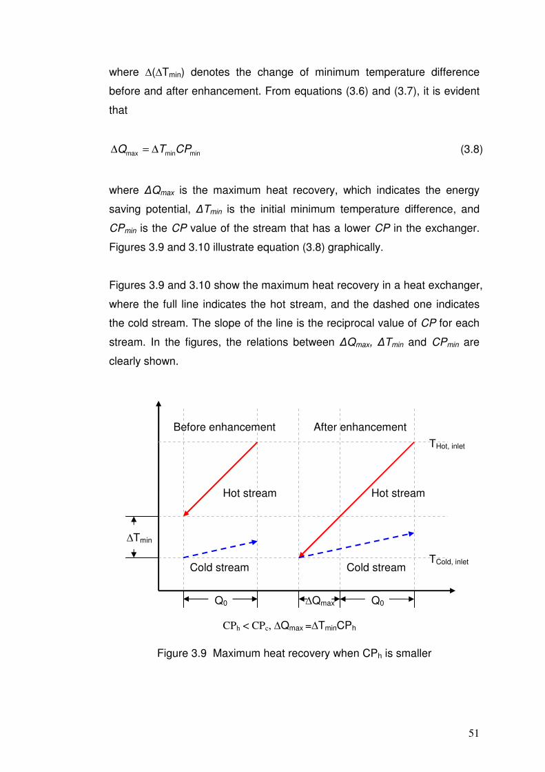
51
where ∆(∆Tmin) denotes the change of minimum temperature difference
before and after enhancement. From equations (3.6) and (3.7), it is evident
that
minminmax CPTQ ∆=∆ (3.8)
where ∆Qmax is the maximum heat recovery, which indicates the energy
saving potential, ∆Tmin is the initial minimum temperature difference, and
CPmin is the CP value of the stream that has a lower CP in the exchanger.
Figures 3.9 and 3.10 illustrate equation (3.8) graphically.
Figures 3.9 and 3.10 show the maximum heat recovery in a heat exchanger,
where the full line indicates the hot stream, and the dashed one indicates
the cold stream. The slope of the line is the reciprocal value of CP for each
stream. In the figures, the relations between ∆Qmax, ∆Tmin and CPmin are
clearly shown.
Figure 3.9 Maximum heat recovery when CPh is smaller
Before enhancement After enhancement
∆Tmin
Q0 Q0 ∆Qmax
Hot stream Hot stream
Cold stream Cold stream
CPh < CPc, ∆Qmax =∆TminCPh
THot, inlet
TCold, inlet
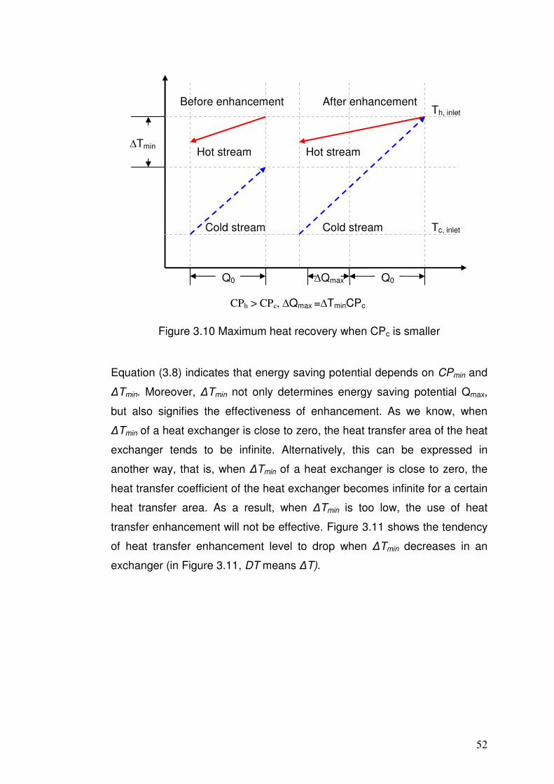
52
Figure 3.10 Maximum heat recovery when CPc is smaller
Equation (3.8) indicates that energy saving potential depends on CPmin and
∆Tmin. Moreover, ∆Tmin not only determines energy saving potential Qmax,
but also signifies the effectiveness of enhancement. As we know, when
∆Tmin of a heat exchanger is close to zero, the heat transfer area of the heat
exchanger tends to be infinite. Alternatively, this can be expressed in
another way, that is, when ∆Tmin of a heat exchanger is close to zero, the
heat transfer coefficient of the heat exchanger becomes infinite for a certain
heat transfer area. As a result, when ∆Tmin is too low, the use of heat
transfer enhancement will not be effective. Figure 3.11 shows the tendency
of heat transfer enhancement level to drop when ∆Tmin decreases in an
exchanger (in Figure 3.11, DT means ∆T).
Before enhancement After enhancement
∆Tmin
Q0 Q0 ∆Qmax
Hot stream Hot stream
Cold stream Cold stream
CPh > CPc, ∆Qmax =∆TminCPc
Th, inlet
Tc, inlet

53
DT-UA-1
0
20
40
60
80
100
120
0 1 2 3 4 5 6 7 8
UA'/UA
DT
lm DT-UA
Figure 3.11 Performance of heat transfer enhancement under different ∆Tmin
Another factor that can affect the results of a sensitivity table is the location
of the exchanger in the network. As mentioned in 3.2.1, when a design is
made, all the exchangers downstream of the changed exchanger will be
affected and send out passive responses. The sensitivity table is able to
consider such responses. As shown in Figure 3.12, when heat exchanger 4
is enhanced, its cold outlet temperature increases, causing the cold inlet
temperature of exchanger 3 to increase as well. As a result, the heat
transfer driving force is reduced, resulting in a reduction in the heat load of
exchanger 3. The same process will also take place in exchangers 1 and 2.
After each influence, the ensuing influence will decline a little. Figure 3.13
shows the influence of downstream exchangers after enhancement. From
the bottom sketch of Figure 3.13, it can be seen that when exchanger 1 is
enhanced, no downstream exchanger is affected, and the hot utility is
reduced considerably. In contrast, when exchanger 2 is enhanced, as
shown in the top sketch of Figure 3.13, downstream exchanger 1 is affected.
Although the duty of exchanger 1 is reduced, the hot utility reduction is not
as large as that in the case of enhancing exchanger 1. Therefore, those
exchangers that are close to utility exchangers can have a higher sensitivity.

54
Figure 3.12 A sequence of heat exchangers
Figure 3.13 Influence of downstream exchangers after enhancement
In brief, the exchangers with large CPmin and ∆Tmin, and are close to a utility
exchanger will exhibit high sensitivity.
3.2.3 Rule 3: Checking the pinching match
The third rule of the heuristic methodology is checking of the pinching match.
From the network pinch concept presented by Asante and Zhu [5, 66], as
reviewed in Chapter 2, the pinching match is the bottleneck of a heat
recovery network. The pinching match always has a low △Tmin, because
Ex1
Ex2 Ex3
Ex4
Heater
Ex1
Ex2 Ex3
Ex4
Heater
Hot stream Hot stream after enhancement Cold stream
T
T
Q
Q
4 1 2 3 H

55
when the heat recovery is increased in a heat exchanger network, the
△Tmin of pinching match unavoidably tends towards a limiting value. If the
pinching match appears in the downstream of a candidate, that candidate
cannot be the best candidate.
Figure 3.14 Example network for heuristic methodology rule 3
For example, in the network shown in Figure 3.14, candidate exchanger 1 is
constrained by its downstream pinching match exchanger 4. Because the
△Tmin of a pinching match is too small, a slight change in inlet temperature
of pinching match can cause a significant reduction in heat transfer driving
force, so that the heat duty of pinching match will decrease significantly.
This means the enhancement does not bring much benefit to the overall
heat recovery. As shown in Figure 3.15, after enhancement, the total
amount of heat recovery of exchanger 1 and exchanger 4 does not change
much.
H1
H2
H3
H4
C2
C3
LP
HP
CW
1
9
9
1
5
2
2
4
8
8
7
7
3
3
10
10
Candidate: Pinching match:
C1 4 5
6
6
11
11

56
Figure 3.15 Illustration of heat duty reduction in pinching match
In this step, heat exchangers constrained by a pinching match are
eliminated from the list of good candidates. The best candidate can then be
selected from the results of sensitivity tables.
3.2.4 Enhancing candidates simultaneously
Enhancing only one exchanger usually cannot make a big improvement on
energy saving performance. The whole procedure provides a methodology
to select candidates. Normally, more than one good candidate can be found
in a network. So after enhancing the best candidate, there may be
opportunities for enhancing some other candidates to improve the energy
savings.
After enhancing the first candidate, the duty and temperature difference of
all its downstream exchangers will change. Some good candidates may no
longer be good enough. Even for those very good candidates, there is no
guarantee that they are still good enough. For example, two exchangers
connect the same streams and both of them are good candidates, once one
is enhanced, the other one normally becomes a not so good candidate due
to the tight heat transfer driving force. So we need to apply sensitivity tables
again to find the next best candidate.
Enhance Ex.1
Tem
pera
ture
Tem
pera
ture
Duty Duty
Ex.1 Ex.1
Ex.4 Ex.4

57
3.2.5 Rule 4: Enhancing pinching match
Sometimes, no good candidate can be found after applying sensitivity tables
or all the good candidates have been enhanced, but an opportunity for
saving more energy is still looked for. In such cases the enhancement of
pinching match can be considered. From the procedure of finding
candidates, when the sensitivity graphs are constructed, the good
candidates can be found. However, some of the good candidates are
constrained by the pinching match, which means that these candidates do
not offer large potential due to the significant loss in heat transfer driving
force in pinching match.
However, there is still benefit to apply heat transfer enhancement to
compensate the loss in heat transfer driving force in the pinching match. As
shown in Figure 3.16, after enhancement of both the pinching match and
candidate, some improvement of energy recovery can be achieved.
Because the pinching match and candidate are from the same hot stream,
their CP values are the same. So from equation (3.8), the improvement of
energy savings depends on the value of △(△Tmin). Therefore, the pinching
match is the controlling exchanger because it has a smaller △Tmin.
Figure 3.16 Illustration of enhancing pinching match
Enhance both exchangers
Tem
pera
ture
Tem
pera
ture
Duty Duty
Ex.1 Ex.1
Ex.4 Ex.4

58
In the methodology, the controlling pinching match should be considered
first followed by the candidate. After calculating the energy saving potential
released by enhancing the pinching match, the augmentation level of the
candidate can be determined. As mentioned, heat transfer enhancement is
used to compensate the loss of heat transfer driving force in the pinching
match. So we can assume that all the heat transfer driving force
improvement due to heat transfer enhancement is used to compensate the
heat transfer driving force loss caused by increased hot inlet temperature.
This means that the duty of pinching match does not change after
enhancement. If the duty of the pinching match remains constant, after
enhancement, only the hot inlet and outlet temperatures would be changed.
From equation (3.1), it can be deduced that
AU
QT
eLM =∆ (3.9)
And
c
h
chLM
T
T
TTT
∆
∆
∆−∆=∆
ln (3.10)
where
outcinhh TTT ,, −=∆ (3.11)
incouthc TTT ,, −=∆ (3.12)
In Equations (3.9) and (3.10), Q, Ue, A, Tc,in and Tc,out are known. From
Equation (3.2), the relation between Th,in and Th,out can be determined. Then
Th,in and Th,out can be calculated.
From Figure 3.15, for the candidate exchanger, the hot outlet temperature is
the hot inlet temperature of the pinching match. After computing the values

59
of the hot inlet and hot outlet temperatures, the value of Q and the cold
outlet temperature can be calculated from Equations (3.2) and (3.3). Finally
the value of U after enhancement can be calculated from Equation (3.1).
The candidate constrained by the pinching match is not recommended for
enhancement previously due to the small △(△Tmin) of the pinching match
and inefficiency of applying two enhancements. However, in some
situations, enhancement of both pinching match and candidate can bring
quite a large improvement on energy savings. From Equation (3.1), the
improvement of heat recovery equals the product of △(△Tmin) and CP of
the hot stream. It can bring great benefit if the CP of the hot stream is very
large. It is difficult to decide whether the performance of enhancing the
pinching match is better than that of enhancing the good candidates at this
stage unless some accurate calculations including investment are made.
However, enhancing the pinching match provides a way to release energy
from the pinching match in order to gain benefit. In practice, very good
candidates are normally constrained by pinching matches.
In this situation, the pinching match is the controlling exchanger but not the
candidate, and so only the results of sensitivity tables for candidate are
needed. This is because heat is released from the pinching match and
recovered by the candidate. Based on reasoning of high sensitivity,
because the △(△Tmin) term is constrained, the quantity of heat recovery
mainly depends on the CP value, which is the same for both pinching match
and the candidate. The heat recovery depends on the position of the
candidate but not the position of the pinching match. So, candidates
constrained by the pinching match are in accordance with the results of
sensitivity tables.
It should be noted that the pinching match normally has a very small
temperature difference, and after enhancement of the pinching match, the
temperature difference will become even smaller. So the enhancement
needs to be checked by detailed consideration of the individual heat

60
exchanger layout to make sure that it is feasible to have such a small
temperature difference in the individual heat exchanger.
3.3 Case study
3.3.1 An existing preheat train for a crude oil distillation column
The case is modified from a real commercial case. In this case study, the
purpose is to reduce operating cost by using heat transfer enhancement.
The candidates to be enhanced are to be found by using the heuristic
methodology. The base case data are shown in Tables 3.1 and 3.2, in
which the former shows exchanger data and the latter lists stream data. The
network structure is shown in Figure 3.17. In exchanger data, U value is
from practical data and it includes fouling resistance.
From Table 3.2, it can be noted that stream data are divided into several
segments. This approach is used to overcome the assumption of constant
thermal properties with temperature in heat exchanger networks. The
related simulation methodology is presented by Chen [67]. Temperature-
dependent thermal properties are considered in this work based on Chen’s
work. The detailed methodology is discussed in Chapter 4.
Because the network is a crude oil preheat train, Figure 3.17 shows only
one hot utility exchanger 30 (furnace) in the network. In addition, cold utility
is cooling water, which is much cheaper than hot utility. Therefore, in this
network the objective is to reduce the energy consumption of utility
exchanger 30. In other words, we seek to increase the cold inlet
temperature of exchanger 30 (furnace).
According to the heuristic methodology, the first step is heat exchanger
network analysis. The network structure indicates that exchangers
connected with stream C3 should first be selected. These are exchangers 4,
22, 23, 24, 26, 27, 28 and 29. Next, we need to check if these exchangers
are on a utility path and connect two streams with utility exchangers. Once

61
all the exchangers are in accordance with the rule, they are selected for
consideration in the next step.
Table 3.1 Heat exchanger data
U Area ∆TLM Duty
Exchanger (kW/m2·K) (m2) (°C) (kW) 1 0.14 167.6 48.2 1132 2 0.47 90.4 143.6 6087 3 0.637 89.9 73.0 4117 4 0.19 153.0 75.2 2128 5 0.57 97.4 101.0 5626 6 0.20 653.1 45.7 6090 7 0.35 13.3 43.3 204 8 0.41 23.4 56.7 548 9 0.41 47.3 35.5 693 10 0.10 282.8 90.4 2532 11 0.37 55.5 65.7 1360 12 0.084 225.4 46.8 889 13 0.063 380.8 89.6 2143 14 0.27 81.2 86.9 1920 15 0.35 31.3 90.1 993 16 0.67 113.1 110.5 8408 17 0.13 191.1 122.2 2989 18 0.19 188.9 40.0 1421 19 0.20 97.9 84.5 1655 20 0.32 1338.4 24.3 10450 21 0.053 220.2 20.1 233 22 0.075 768.5 23.1 1335 23 0.14 390.9 35.6 1992 24 0.22 1003.3 46 10100 25 0.35 63.1 210.1 4667 26 0.17 1308.0 16.7 3718 27 0.20 223.5 42.1 1834 28 0.21 1003.3 44.1 9333 29 0.13 227.1 88.1 2522 30 0.57 139.5 819 65240 31 0.57 458.6 90.1 23600 32 0.80 45.8 114.1 4190

62
Table 3.2 Stream data
Stream Supply
Temperature[℃] Target
Temperature[℃] Duty [kW] CP[kW/℃]
C1 33.5 53.1 6052.5 308.5 53.1 68.4 4900.1 320.5 68.4 83.8 5089.9 329.2 83.8 95.5 3953.6 337.6
C2 91.4 106.6 5167.4 340.6 106.6 132.9 9225.9 350.8 132.9 136.8 1421.2 364.4 136.8 157.2 7689.1 375.6
C3 151.0 158.2 2607.3 360.1 158.2 185.5 10100.0 370.9 185.5 207.9 8695.3 388.2 207.9 214.8 2736.6 393.8 214.8 237.9 9333.3 404.7 237.9 249.9 4970.1 413.8 249.9 351.9 59757.1 585.9
H1 335.4 147.2 2988.8 15.9 147.2 110.0 492.8 13.2 110.0 69.4 500.1 12.3
H2 253.2 193.8 11287.0 190.2 193.8 116.0 13456.0 173.0
H3 293.7 276.6 2107.7 123.8 276.6 204.4 8407.4 116.4 204.4 180.5 2583.7 108.2 180.5 130.0 5113.9 101.1
H4 212.4 156.0 5626.3 99.8 H5 212.6 157.2 1335.2 24.1
157.2 117.2 888.9 22.2 117.2 61.6 1131.6 20.4
H6 174.4 76.6 4116.5 42.1 76.6 62.2 547.6 37.9 62.2 43.3 692.5 36.7
H7 134.5 74.2 23600.0 391.4 H8 364.2 287.7 2522.3 33.0
287.7 226.6 1833.9 30.0 226.6 147.2 2143.4 27.0 147.2 65.5 1919.8 23.5
H9 290.3 264.8 4666.6 183.1 264.8 238.4 4666.6 176.4 238.4 210.9 4666.6 169.5
H10 284.2 270.0 392.9 27.7 270.0 236.1 909.5 26.8
236.1 179.4 1421.2 25.1 179.4 65.5 2478.7 21.8
H11 240.0 166.6 1992.4 27.1 166.6 129.4 921.3 24.8 129.4 103.8 599.3 23.4 103.8 57.7 1011.3 21.9
H12 178.7 110.0 4872.8 70.9 110.0 69.3 2810.1 69.0
Hot utility 1500.0 800.0 65234.4 93.2 Cooling water 10.0 15.0 48238.5 9647.7

63
After implementing the first step, sensitivity tables are constructed to check
the energy saving potential of each candidate. Figures 3.18 and 3.19 show
the results of sensitivity graphs. It is evident that exchangers 24, 26 and 28
are good candidates. Although exchangers 4, 27 and 29 can increase the
inlet temperature of utility exchanger 30, the increases are not significant.
Exchanger 23 is a poor candidate because it hardly changes the inlet
temperature of utility exchanger 30 when its UA value increases. So the
best candidate is one of exchangers 24, 26 and 28. To find the best
candidate, step 3 is carried out.
C1
C2
C3
H1
H2
H3
H4
H5
H6
H7
H8
H9
H1
0
H1
1
H1
2
HU
CU
1
1
3
3
2
2
30
30
29
29
21
21
28
28
27
27
26
26
24
24
20
20
4
4
18
18
17
17
16
16
23
23
13
13
22
22
12
12
6
6
25
25
32
32
19
19
15
15
14
14
7
7
11
11
10
10
8
8
9
9
31
31
Figure 3.17 Existing preheat train network
Applying rule 3, it is found that exchanger 20 is a pinching match, which is
the network structure bottleneck. The network structure shows that pinching
match 20 is in the downstream of exchanger 24, which is one of the good
candidates. This means exchanger 24 is constrained by the pinching match
exchanger 20. So exchanger 24 is not the best candidate. After checking
the network pinch, exchanger 28 is the best candidate because it is not
constrained by a pinching match. Exchanger 28 should thus be enhanced
first.

64
Figure 3.18 Sensitivity graphs of exchangers 24, 26, 27, 28 and 29 in the case study
Figure 3.19
Figure 3.19 Sensitivity graphs of exchangers 4 and 23 in the case study
After implementing rule 3, a sensitivity graph is applied again to find the
next best candidate. The results of the sensitivity graph suggest that

65
exchanger 26 is the next best candidate after the enhancement of
exchanger 28. Accordingly, exchanger 26 is next in line for enhancement.
After the enhancement of both exchangers 26 and 28, there is no good
candidate left according to the results of sensitivity graph. Rule 4 is now
applied to check whether further energy savings can be made. The results
of previous steps reveal that exchanger 24 is a good candidate that is
constrained by a pinching match, i.e. exchanger 20. So, according to rule 4,
both exchanger 24 and exchanger 20 are to be enhanced.
Estimating the enhancement performances of the four exchangers requires
their detailed heat transfer data, and these are shown in Table 3.3 (data is
assumed).
Table 3.3 Heat transfer data of candidate exchangers
hs
(W/m2·K)
ht
(W/m2·K)
Rfs
(m2·K/W)
Rft
(m2·K/W)
U
(W/m2·K)
Ex. 20 975 822 0.00006 0.00036 321.4
Ex. 24 1117 824 0.0012 0.00072 219.1
Ex. 26 753 961 0.00221 0.0008 169.8
Ex. 28 979 894 0.00117 0.00088 211.1
Table 3.4 Heat transfer data of enhanced candidate exchangers
hs
(W/m2·K)
ht
(W/m2·K)
Rfs
(m2·K/W)
Rft
(m2·K/W)
U
(W/m2·K)
Ex. 20 975 1684 0.00006 0.00036 428.5
Ex. 24 1117 2778 0.0012 0.00072 286.0
Ex. 26 753 1954 0.00221 0.0008 191.3
Ex. 28 979 3827 0.00117 0.00088 272.8
According to the heuristic methodology, exchangers 20, 24, 26 and 28 are
selected for enhancement, which are highlighted in Figure 3.20. Their
detailed heat transfer data after enhancement are shown in Table 3.4. The

66
new design achieves 2.2 MW of heat duty reduction in exchanger 30,
leading to 3.4% of overall energy savings. The detailed heat exchanger
data after enhancement are shown in Table 3.5. It should be emphasised
that this saving has been obtained without any additional topology
modification of the network.
Table 3.5 Heat exchanger data after enhancement
U Area ∆TLM Duty Exchanger (kW/m2·K) (m2) (°C) (kW) 1 0.14 167.6 48.2 1131 2 0.47 90.4 125.9 5337 3 0.63 89.9 73.0 4117 4 0.19 153.0 75.1 2127 5 0.57 97.4 101.0 5626 6 0.20 653.1 45.6 6074 7 0.35 110.6 5.2 204 8 0.41 23.4 55.8 539 9 0.41 47.3 36.9 721 10 0.10 282.8 90.4 2532 11 0.37 55.5 65.6 1359 12 0.084 225.4 46.9 890 13 0.063 380.8 85.7 2050 14 0.27 81.2 92.3 2038 15 0.35 31.3 90.5 997 16 0.67 113.1 105.6 8041 17 0.13 191.1 122.2 2989 18 0.19 188.9 40.5 1439 19 0.2.0 97.9 85.0 1665 20 0.48 1338.4 15.7 10080 21 0.053 220.2 21.8 253 22 0.075 768.5 23.1 1335 23 0.14 390.9 35.6 1992 24 0.31 1003.3 38.4 11800 25 0.35 63.1 197.7 4391 26 0.24 1308.0 15.6 4845 27 0.20 223.5 43.5 1897 28 0.27 1003.3 35.2 9637 29 0.13 227.1 83.0 2376 30 (furnace) 0.57 139.5 790.9 63000 31 0.57 458.6 90.1 23600 32 0.80 45.8 76.8 2820

67
C1
C2
C3
H1
H2
H3
H4
H5
H6
H7
H8
H9
H1
0
H1
1
H1
2
HU
CU
1
1
3
3
2
2
30
30
29
29
21
21
28
28
27
27
26
26
24
24
20
20
4
4
18
18
17
17
16
16
23
23
13
13
22
22
12
12
6
6
25
25
32
32
19
19
15
15
14
14
7
7
11
11
10
10
8
8
9
9
31
31
Figure 3.20 Heat exchanger network with enhanced heat exchangers
3.3.2 Summary of the case study
Table 3.6 compares different retrofit designs made by our heuristic
methodology. The first one is the design derived from the detailed heuristic
process described in the preceding section. In the second design, only
candidate exchangers 24, 26 and 28 have been enhanced, leaving out the
constrained pinching match. The third design includes one additional
candidate, i.e. exchanger 29, but the results of sensitivity graphs reveal that
this exchanger is not a very strong candidate compared with exchangers 24,
26 and 28.
Table 3.6 Comparison of different retrofit designs
Retrofit design number
Enhanced exchangers Energy saving (kW)
1 Exchangers 20, 24, 26, 28 2240 2 Exchangers 24, 26, 28 1327 3 Exchangers 20, 24, 26, 28, 29 2654
Comparing the results of retrofit designs 1 and 2 in Table 3.6 indicates that
enhancing the pinching match (exchanger 20) can promote the performance

68
of exchanger 24 significantly. This observation is in accordance with our
heuristic rule 4. Retrofit design 3 suggests that enhancing exchanger 29
brings an additional heat recovery improvement of 414 kW over that of
retrofit design 1. This extra benefit is rather modest. The results of
sensitivity tables are thus reliable and instructive.
Note that exchangers 24, 26 and 28 are all with large duty. The hot streams
in exchangers 24, 26 and 28 are all with large CP values. Table 3.2 shows
that exchanger 24 is on H2, exchanger 28 is on H3, and exchanger 26 is on
H9. The CP values of these three streams are larger than 100 kW/℃, and
the others are mostly smaller than 100 kW/℃. The three exchangers 24, 26
and 28 are quite close to utility exchanger 30. So the results are in good
agreement with the analysis obtained from rule 2.
It is worth mentioning that the retrofit design derived from the heuristic
methodology does not involve any topology modifications and additional
area. As a result, the retrofit investment is lower, the retrofit duration is
shorter and the retrofit process is much simpler.
Table 3.7 shows the energy saving with different enhancement
augmentation levels, and Figure 3.21 plots the results of Table 3.7 and
gives an illustration of energy saving trend with increasing augmentation
level. It can be seen from Figure 3.21 that the rate of energy saving
diminishes slightly with increasing augmentation level. From Equation (3.1),
we know that the duty of an exchanger increases with increasing U value.
Furthermore, Equations (3.2) and (3.3) show that an increase in duty will
cause the hot side outlet temperature Th,out to become lower and the cold
side outlet temperature Tc,out higher. This means the temperature difference
between hot and cold streams becomes smaller. When the temperature
difference between hot and cold streams becomes very small, △TLM will
decrease significantly, compensating most of the increase in the U value in
equation (3.1). Consequently, there is no obvious increase in duty with
increasing U value. It is thus important to select an appropriate

69
augmentation level of overall heat transfer coefficients in order to make the
best use of enhancement. However, the proposed heuristic methodology
does not address the question of selecting the best augmentation level.
Table 3.7 Energy saving with different enhancement augmentation levels
Augmentation level Energy saving (MW) 20% 1.74 30% 2.44 40% 3.10 50% 3.72
Figure 3.21 Energy saving with different enhancement augmentation levels
As a first approximation, the overall heat transfer coefficient U can be
expressed as a function of the tube side film coefficient ht and shell side film
coefficient hs.
st hhU
111+= (3.13)
Equation (3.13) is a simple expression for calculating U value, which will be
discussed in detailed in section 4.3.4. This equation indicates that the value
of U is less than either of the two coefficients. If the two values are very
different, the value of U tends to be closer to the smaller one. The side with
the smaller heat transfer coefficient is called the controlling side. Adding

70
enhancement to the controlling side is more effective. However, when
different heat transfer enhancement augmentation levels are added to one
side, the relative contributions to the overall heat transfer coefficient are
different.
An example is shown in Table 3.8 and Figure 3.22. It can be seen that with
increasing enhancement augmentation level in the tube side, the increase
in the overall heat transfer coefficient levels dose not increase as mush as
enhancement augmentation level. The reason is that some part of
enhancement is not added to the controlling side. In the example, when the
level of increase in ht is 50%, after enhancement ht is no longer the
controlling side. Even if after enhancement, the enhanced side is still the
controlling side, the efficiency of enhancement will still decrease with
increasing enhancement augmentation level. This is due to the fact that the
more deviation between ht and hs, the more efficient the enhancement.
Given that the enhancement will eliminate the difference between ht and hs,
it follows that the larger enhancement level eliminates more deviation. As a
result, the larger enhancement becomes less efficient. Therefore, it is
important to adopt an appropriate augmentation level of tube or shell side
film heat transfer coefficient in order to make the enhancement more
economic. However, as with the question of choosing a suitable overall heat
transfer enhancement augmentation level, the proposed heuristic
methodology does not address the question of selecting an appropriate
augmentation level of tube or shell side film heat transfer coefficient.
Table 3.8 Contributions of different heat transfer enhancement levels to the overall heat transfer coefficient
Increase in ht
(%)
ht (W/m2·K) hs (W/m2·K) U (W/m2·K) Increase in U
(%)
0 0.8 1 0.44 0
20 0.96 1 0.49 11.4
50 1.2 1 0.55 25
100 1.6 1 0.62 40.1

71
Figure 3.22 Contributions of different heat transfer enhancement levels to the overall heat transfer coefficient
Further optimization is needed in order to tackle the problem of finding the
best augmentation level of enhancement.
3.4 Conclusion
A practical heuristic methodology is presented in this chapter for
implementing heat transfer enhancement in heat exchanger network retrofit.
The heuristic methodology has 4 rules. The first rule is based on the path
concept [63, 64]. Its basic tenet is that an exchanger has potential to
recover more heat without network structure modifications after retrofit.
Paths ensure that the target temperature of streams do not change when
exchangers on the path change. The second rule is based on sensitivity
tables [4], which is a reliable tool to estimate energy saving potential of heat
exchangers. However, it ignores some structure and practical problems,
such as stream target temperature change mentioned in rule 1 and network
structure bottleneck mentioned in rule 3. Rule 3 is based on network pinch
approach [5]. By using rule 3, the influence of network structure bottleneck
can be considered in the heuristic methodology. In rule 4, the network pinch
is further analyzed, and it is found that enhancing a pinching match can
release the energy saving potential of candidate exchangers that are
constrained by the pinching match.

72
The proposed heuristic methodology is able to provide some great physical
insights into heat exchanger network retrofit. For example, the results of
sensitivity tables reveal that the exchangers with significant heat recovery
potential normally have large duty, are on the streams with large CP and
are close to a utility exchanger. The network pinch is the bottleneck of a
heat exchanger network. It cannot be eliminated without network structure
modification. The analysis based on rule 3 demonstrates that the heat
transfer driving force in a pinching match will change significantly when the
candidate exchanger located upstream of the pinching match changes.
Heat transfer enhancement can be used to compensate the significant loss
of heat transfer driving force in a changed pinching match and give more
energy saving space to a candidate constrained by the pinching match.
The proposed heuristic methodology can be easily implemented in practice
to find the best candidate in a network for enhancement. Compared with
mathematic programming, the heuristic methodology is appealing because
it is able to handle large scale problems.
However, the nature of heuristic methodology limits its ability to determine
the optimal augmentation level of each enhancement. The results of the
case study show that an increase in the augmentation level will cause both
heat transfer coefficients and cost to increase, but it is not possible to
determine the optimal investment level. To overcome this deficiency of the
heuristic methodology, an optimization procedure is required. The
optimization problem is addressed in Chapter 4.
Nomenclature
A Total heat exchanger area (m2)
CP Heat capacity flow rate of a stream (kW/℃)
CPmin Heat capacity flow rate of the stream that has a lower Heat
capacity flow rate in the exchanger (kW/℃)
h Film heat transfer coefficient (kW/℃·m2)

73
Q Heat duty of a heat exchanger (kW)
Rf Heat transfer resistance of fouling (m2·K/W)
T Temperature of a node (℃)
U Overall heat transfer coefficients of a heat exchanger
(kW/℃·m2)
∆Qmax The maximum heat recovery of a match (kW)
△TLM Log mean temperature difference of a heat exchanger (℃)
△Tmin Minimum temperature difference of a heat exchanger (℃)
Subscripts and superscripts
c Cold side of a heat exchanger
e Exchangers with enhancement
h Hot side of a heat exchanger
in Inlet of one stream in a heat exchanger
out Outlet of one stream in a heat exchanger
s Shell side
t Tube side

74
Chapter 4 Heat exchanger network retrofit optimization considering heat transfer enhancement
4.1 Introduction
Chapter 3 provides a heuristic methodology to find exchangers to be
enhanced and gives physical insights into the retrofit design considering
heat transfer enhancement. However, the augmentation level of each
enhancement cannot be determined through the heuristic methodology. It is
desired to optimize the augmentation level with a trade-off between costs of
enhancement devices and reduction of utility cost.
Retrofit design of heat exchanger networks has been researched for many
years. As mentioned in Chapter 2, many of the previous optimization
approaches fail to solve large-scale problems. Also most of the prior work
does not consider the application of heat transfer enhancement.
The conventional heat exchanger network retrofit approaches often rely
upon duty based calculations. In duty based calculations, the exchanger
model is simple and additional area can be calculated directly from the
increased duty. Moreover, it is easy to maintain the target temperature of
streams by using duty based calculations. However, the practical aspects of
the retrofit process cannot be described, because duty based calculations
cannot predict the passive change of the network when retrofit designs are
made. On the other hand, area based calculations can describe the
practical aspects of retrofit and predict well the passive change of the
network, but the model of an area based exchanger is more complex than
that of a duty based model.
In this chapter, a retrofit optimization model considering heat transfer
enhancement well be presented. Simulated annealing is used as the
optimization algorithm due to its ability to escape from local optima. Both
duty based calculations and area based calculations are considered in this

75
chapter. The application of this new optimization approach is illustrated with
two case studies.
4.2 Simulated annealing
Simulated annealing (SA) is a widely used optimization algorithm derived
from the Metropolis algorithm [68]. SA is a stochastic optimization
methodology, using random changes to search the solution space and can
avoid being trapped in local optima.
SA is inspired by the metallurgic process of metal annealing. In the
annealing process, metal is melted at a very high temperature and then
slowly cooled down. In the beginning, the metal atoms are distributed
randomly and the system is in high disorder. With the cooling of the metal,
the system becomes more ordered with decreasing energy. If the cooling
procedure is long enough, the metal will freeze into a stable minimum
energy crystal. If the cooling procedure is not long enough or the initial
metal temperature is not high enough, the metal will form a glassy structure
with higher energy.
Kirkpatrick and co-workers [69] proposed a mathematical optimization
application of annealing procedure. Figure 4.1 shows a typical SA algorithm.
In SA, a control parameter called annealing temperature, which is
analogous to the annealing temperature in annealing process, is used to
guide the optimization. In the beginning of the optimization, the annealing
temperature is set to a high value. With the progress of optimization, the
annealing temperature is reduced. The process of SA optimization starts
with an initial trial solution, which normally comes from approximate
calculation or heuristic methodology. Then a random change called a move
is executed to generate a new trial. The solution of a new trial is calculated
through the objective function and is compared with the solution of current
trial. If the new solution is better than the previous one, the new solution is
accepted. Otherwise, the new solution has a small probability to be

76
accepted according to some acceptance criterion, for example, according to
Boltzmann factor, to avoid local optima. This process is repeated a number
of times, and is terminated when the annealing temperature condition is met.
Figure 4.1 Flowchart for SA algorithm
Compared with conventional gradient based optimization algorithms, SA
can avoid being trapped at local optima by accepting not only moves that
improve the objective function (downhill moves) but also moves that weaken
it (uphill moves). So for an infinite scheduling time, a global optimal solution
can be guaranteed by SA, and a very good solution close to the global
optimum can be obtained in a long enough time. SA optimization is not
Get initial trial solution
Set initial annealing temperature
Repeat
LM times
Generate a new trial solution by
making a random move
Evaluate objective function
Acceptance
criterion
Accept move Reject move
Yes No
Reduce annealing temperature
Termination
criterion
No
Yes
Finish

77
based on the gradient of objective function, and so the problem of
discontinuities can be easily dealt with. However, the computing time
depends on the problem size and is normally longer than conventional
optimization algorithms.
4.2.1 Simulated annealing parameters
•Acceptance criterion
As previously mentioned, an acceptance criterion is used to decide whether
a new trial solution is acceptable or not. If the new trial solution is better, it
will be accepted. If the new trial solution is not better, it may be accepted
according to some acceptance criterion. A good acceptance criterion allows
enough uphill moves to be accepted to avoid trapping into a local minimum.
Kirkpatrick et al. [69] use the Metropolis [68] acceptance criterion in their SA
optimization algorithm. In our work, the same acceptance criterion is used.
Equation (4.1) shows the Metropolis [68] acceptance criterion. In the
equation, p indicates the probability of uphill move being accepted, ∆f
denotes the change in objective function and Ta is the annealing
temperature. In a heat exchanger retrofit design, the objective is to establish
a cost-effective network. The optimization starts with the initial network
structure, and a new network is generated after each move. The downhill
moves that make cost smaller are accepted. Uphill moves that make cost
larger will be judged by equation (4.1).
>∆∆−
≤∆
=
)0()/exp(
)0(1
fifTf
fif
p
a
(4.1)

78
•Initial annealing temperature
The initial annealing temperature affects the cooling schedule of SA
optimization. A too high initial annealing temperature will increase
calculation time significantly. On the other hand, a not high enough initial
annealing temperature will lead to insufficient uphill moves so that the
solution has a higher probability of being trapped in local optima.
The optimal value for initial annealing temperature depends on the scale of
the problem. Some studies have been done to estimate a good value of
initial annealing temperature. Van Laarhoven and Aarts [70] suggested that
a certain initial probability of accepting uphill moves can be obtained when
the initial annealing temperature is set. Equation (4.2) shows the estimation
of initial annealing temperature Ta0.
00 ln p
fTa
+∆−= (4.2)
where +∆f is the average increment of the objective function for uphill
moves. +∆f is calculated through a test run in which all the uphill moves are
accepted and the average increase in the objective function is computed. p0
is the desired initial acceptance probability, which is normally around 0.8.
•Cooling schedule
The cooling schedule also affects the calculation time of the SA optimization
and the ability of SA to avoid local optima. The cooling schedule must be
slow enough to allow sufficient uphill moves. But a too slow cooling
schedule will increase the computation time.
In this work, the cooling schedule proposed by Van Laarhoven and Aarts
[70] is used, which is shown in Equation (4.3). In this equation, θ is a
cooling parameter that controls the speed of cooling. θ assumes a value

79
between 0 and 1, and is normally around 0.5. σ(Ta) indicates the standard
deviation of the objective function of all the trial solutions generated at the
temperature Ta. This factor controls the speed of cooling, when the
deviation of objective function is large. For example, in the beginning of the
SA optimization, the cooling speed is low. When the deviation of objective
function becomes small, this factor in the cooling schedule equation has the
effect of accelerating the cooling.
1
)(3
)1ln(11
−
++=+
Ta
TaTaTa
σ
θ (4.3)
•Markov chain length
A Markov chain is a random sequence of events occurring in a system in
which the probability of occurrence of future events depends only on its
present state, and it is not influenced by events occurred in the past [71].
The same as the other SA parameters already discussed, the value of
Markov chain should be specified so that a balance between quality of the
solution and computing time can be obtained. Only when an infinite Markov
chain is used, the global optimum can be guaranteed [72]. There are two
loops in the SA optimization, the inner loop is the Markov loop and the outer
loop is the annealing temperature loop. It may be seen from Equation (4.1)
that the possibility of accepting uphill moves depends on the annealing
temperature. The Markov chain length determines the number of moves at
each annealing temperature level. In other words, the Markov chain length
determines the number of trial solutions under the same level of possibility
of accepting uphill moves.
The length of the Markov chain determined by some methodologies [73, 74]
often tends to be very long in many problems, which means an excessively
long computing time. In this work, the Markov criteria are defined as [19]:

80
1. The number of new configurations generated reaches Markov chain
length (LM)
2. The number of accepted configurations reaches half of Markov chain
length (1/2 LM)
By using these criteria, the actual Markov chain length becomes dynamic.
When the SA process is at a high annealing temperature, since almost
every move is accepted, the second criterion is met first. When the
annealing temperature reduces to a low level, the number of accepted
moves becomes low. At this time, the first criterion is met first. In this way,
the optimization algorithm spends more time searching for a solution at low
annealing temperature than at high annealing temperature. Therefore, with
these criteria, the algorithm can search for a good optimum within a
relatively short computing time.
•Termination criterion
Several criteria for stopping the optimization are shown as follows. The
algorithm will stop whenever one of these criteria is met.
1. The annealing temperature reaches the lower boundary, Taf.
2. No moves are accepted consecutively for a given number of annealing
temperature loops (typically ten).
3. After a certain number of overall annealing temperature loops have been
completed. In the present work, the maximum number of annealing
temperature loops is taken as 25000.
It is observed in the present work that the first criterion is usually reached
and the third criterion is hardly reached in SA runs [67].

81
4.3 General modeling framework
Heat exchanger networks contain not only heat exchangers, but also stream
splitters and mixers, and sometimes unit operations. Unit operations are
devices designed to alter either the temperature or heat content of a stream.
Changes in operatingn conditions of any single component of a network can
affect the performance of the whole network. These passive changes of a
network are difficult to predict when the network is large. If these passive
changes of a network are not considered, some retrofit designs may
become unacceptable due to large deviations of process conditions, for
example, target temperature. These passive changes depend on the
topology of the network and also operation conditions of the individual heat
exchanger. In this work, the performance of heat exchangers with heat
transfer enhancement is considered as well as the passive changes caused
by those enhancement devices.
An effective model must account for each individual component in the heat
exchanger network and the interactions between these components. This
section presents the models used in this work. Firstly, models of
components in heat exchanger networks such as heat exchangers and
stream splitters are presented. Secondly, the thermal performance of
enhancement devices is discussed. Thirdly, the temperature-dependent
thermal properties of process streams and the representation of heat
exchanger networks are presented. The modelling of heat exchanger
networks is implemented in SPRINT (v2.3).
Only shell-and-tube heat exchangers are considered in the heat exchanger
network model, which are the most common type of heat exchangers used
in industrial applications so far. Different configurations of shell-and-tube
heat exchangers are considered in this work, such as multiple tube passes
heat exchangers and heat exchangers with multiple shells in series or
parallel. The flow rate of process streams is assumed constant in the model.

82
Simulating the performance of a heat exchanger requires calculation of the
outlet temperatures of both streams given their inlet conditions, physical
properties and the characteristics of the equipment. Depending on the
information available for the heat exchanger, two different cases are
considered:
1. The heat load of the exchanger is known, and the heat transfer area
needs to be calculated. (duty-based calculation)
2. The exchanger area is known but its heat load is unknown. (area-
based calculation)
The first case is used in the heat exchanger network design. In design
problems, the objective is to estimate the size of exchangers to
accommodate a specified duty. In most retrofit design problems, the first
case is preferred because the duty-based model is much easier to be
calculated than the area-based model. Area-based calculation is only
applied in a few publications, and normally it is used as a tool to check the
passive response of an existing network.
4.3.1 Steady state heat exchangers specified in terms of heat load
Figure 4.2 An example of a heat exchanger
Figure 4.2 depicts a countercurrent heat exchanger. Th,in and Th,out are hot
inlet and outlet temperature and Tc,in and Tc,out are cold inlet and outlet
CPh
CPc
Th,out Th,in
Tc,in Tc,out
83
temperature. CPh and CPc are heat capacity flow rate of hot and cold
stream, respectively.
The outlet temperature of both hot and cold streams in duty-based model
can be calculated directly from Equations (4.4) and (4.5).
hinhouth CPQTT /,, −= (4.4)
cincoutc CPQTT /,, += (4.5)
Once the outlet temperatures of both hot and cold sides are known, the
required heat transfer area can be calculated from the following well-known
design equation:
LMTU
QA
∆⋅= (4.6)
where [75]:
−
−
−−−=∆
incouth
outcinh
incouthoutcinh
LM
TT
TT
TTTTT
,,
,,
,,,,
ln
)()( (4.7)
Many flow arrangements other than the 1-1 design (1 shell pass – 1 tube
pass) exist, the most common of which is the 1-2 design (1 shell pass – 2
tube passes). However, the 1-2 design will exhibit a part countercurrent and
part cocurrent flow pattern, and the effective temperature difference for heat
exchange is reduced compared with a pure countercurrent heat exchanger.
The correction factor FT is used to quantify this reduction of effective
temperature difference, as shown in Equation (4.8).
LMT TUAFQ ∆= (4.8)

84
FT can be calculated through two dimensionless factors P and R. For the 1-
2 design, FT is calculated as follows [76]:
incoutc
outhinh
h
c
TT
TT
CP
CPR
,,
,,
−
−== (4.9)
incinh
incoutc
TT
TTP
,,
,,
−
−= (4.10)
For R≠1,
( ) ( )( )
+++−
+−+−−
−
−⋅+
=
112
112ln1
11
ln1
2
2
2
RRP
RRPR
RP
PR
FT (4.11)
For R=1
( )( )
+−
−−
−
⋅
=
222
222ln
12
P
P
P
P
FT (4.12)
When FT is too small, the heat transfer area becomes very inefficient and
this situation must be avoided. This situation can be resolved by using a
number of 1-2 heat exchangers in series. In such arrangement, the value of
FT for each shell is the same, which is also equal to the value of FT across
the whole arrangement. Also, all values of P for each shell pass are equal,
but they are not equal to the value of P across all shells. Equations (4.13)
and (4.14) are used to calculate the value of P1-2 for a single 1-2 shell. In
these equations NSH is the number of shells.
For R≠1,

85
RP
RP
P
RP
P
SH
SH
N
N
−
−
−
−
−
−
=− 1
1
21
11
11
1
(4.13)
For R=1
SHSH NPNP
PP
+−=−21 (4.14)
4.3.2 Steady state heat exchangers specified in terms of heat transfer area
Again Figure 4.2 is used to illustrate the exchanger model specified in terms
of heat transfer area.
From heat balance equations:
)( ,, outhinhh TTCPQ −= (4.15)
)( ,, incoutcc TTCPQ −= (4.16)
and the design equation
)( LMTUAQ ∆= (4.17)
We can transform these equations into:
0)1()1()1( ,,, =−+−+− inhincouth TRRTBTRB (4.18)
0)1()1()1( ,,, =−+−+− incinhoutc BRTRRTBTRBR (4.19)
where

86
h
c
CP
CPR =
( )( )[ ]1/exp −= RCPUAB c
From these equations, it can be seen that Equations (4.18) and (4.19) are
linear with respect to temperatures but they are non-linear with respect to
heat capacity and (UA).
If (UA), CPh, CPc and two out of the four temperatures (Th,in, Th,out, Tc,in, Tc,out)
are known, it is then possible to calculate the other two temperatures
without iteration.
4.3.3 Stream splitter and mixer
Stream splitting is often used in heat exchanger networks. Stream splitters
allow better use of heat transfer driving force so that the network requires
less heat transfer area. Moreover, without stream splitting, heat exchangers
are in series, the inlet temperature of each exchanger on the stream
reduces one by one, so that at the end of the stream, the minimum
approach temperature in exchangers may be violated due to a low inlet
temperature. But with stream splitting, exchangers can be in parallel, and all
inlet temperatures of the exchangers on the stream are the same. In this
situation, stream with splitting allows more heat to be exchanged.
In networks, streams can be split into several branches, and in our heat
exchanger network model, these branches will be remixed later in the
network. The reason why these branches must be remixed is that in the
Pinch approach, every stream must have only one supply temperature and
only one target temperature. As shown in Figures 4.3 and 4.4, a stream
without a mixer has two target temperatures and a stream with a mixer has
only one target temperature. The model is developed step by step based
on the Pinch approach. According to the Pinch approach, a mixer in our
model is guaranteed to associate with a stream splitter. The splitter-mixer is

87
considered in the model as a whole unit. Any number of heat exchangers
can be located between the splitter and the mixer.
Figure 4.3 Stream with only splitter
Figure 4.4 Stream with both splitter and mixer
Figure 4.5 illustrates a simple stream splitter and an associated mixer. The
splitter divides a stream into several branches. The mass and energy
balances at the splitting point are as follows:
CPSFCP n ×=1 (4.20)
Sinn TT =, (4.21)
where SFn is the flow splitting fraction of branch n, CP is the heat capacity
flow rate of the main stream, CPn is the heat capacity flow rate of branch n,
and Tn,in is the inlet temperature of branch n.
Ts TT
splitter mixer
Ts
TT1
TT2
splitter

88
Figure 4.5 Variables of the stream splitting model
The stream temperature after a mixer can be calculated by carrying out
energy balances at mixing point.
∑=
×=NBR
n
outnnT TSPT1
, (4.22)
where TT is the temperature after the mixer, Tn,out is the outlet temperature
of branch n and NBR is the total number of branches.
4.3.4 Overall heat transfer coefficient
The overall heat transfer coefficient (U) is defined as follows:
fsft
wfsft
RRhhhU
++++=1111
(4.23)
where hft and hfs are the film transfer coefficients for tube and shell side in
an exchanger, respectively, Rft and Rfs are the fouling resistance for the hot
and cold side in an exchanger, respectively. hw is the heat transfer
coefficient for the tube wall.
In order to calculate the overall heat transfer coefficient from Equation
(4.23), all the film transfer coefficients and fouling resistances must be
Ts TT
splitter mixer
T1,out
T2,out
CP1
CP2
CP
CPn
Tn,out
T2,in
T1,in
Tn,in

89
based on the same surface area, which is normally the external area of the
tubes. The heat transfer coefficient and fouling resistance inside the tubes
must be corrected by multiplying the ratio of the internal to external tube
diameter. Equation (4.23) has been simplified as it ignores this ratio. The
ratio is frequently very close to one, thus it can be omitted without incurring
significant errors.
Under steady-state conditions, Equation (4.23) can be re-written in a simple
expression, as shown in Equation (4.24). The overall heat transfer
coefficient U can be represented as a function of the tube side heat transfer
coefficient ht and shell side heat transfer coefficient hs. The resistance (1/hw)
to the flow of heat across the metallic wall of tubes of the exchanger is small
compared with the other resistances found in the heat exchanger, so
normally it is ignored. The fouling resistances are included in ht and hs
because under steady state conditions they do not change with time.
st hhU
111+= (4.24)
4.3.5 Heat transfer enhancement
From Equation (4.24), it can be seen that the value of U is less than either
of the two coefficients. If the two values are very different, the value of U
tends to be closer to the smaller one. The side with the smaller heat transfer
coefficient is called the controlling side. We define hs/ht as control ratio rh,
when rh > 1, the tube side has a bigger heat transfer resistance. Then the
enhancement technique should be applied to the tube side in order to
achieve more effective improvement. On the other hand, if rh < 1, the
enhancement technique should be applied to the shell side. However, if the
heat transfer coefficients on both sides are similar then the enhancement
may be added to both sides.
Heat transfer enhancement can be added to the tube side, the shell side, or

90
both the tube and shell sides of one exchanger with an increasing ratio of
heat transfer coefficients. After enhancement, the value of U can be
expressed as:
set
e hhU
111+= (Tube-side enhancement) (4.25)
est
e hhU
111+= (Shell-side enhancement) (4.26)
es
et
e hhU
111+= (Both side enhancement) (4.27)
where het and he
s are, respectively, the heat transfer coefficients of the tube
and shell side after enhancement and Ue is the overall heat transfer
coefficient after enhancement.
To measure the improvement of heat transfer in the tube side or the shell
side, or both, we use the following enhancement ratios:
t
e
te
th
hr =
(4.28)
s
e
se
sh
hr =
(4.29)
where ret and re
s are the enhancement ratio of the tube side and the shell
side, respectively.
Then we can define the corresponding enhancement ratios of the overall
heat transfer coefficient:
h
he
t
et
e r
rr
rU
U
+
+×=
11
(for tube-side enhancement) (4.30)
h
he
s
es
e r
rr
rU
U
/11/11
+
+×=
(for shell-side enhancement) (4.31)

91
For a retrofit problem, additional area may be added to accommodate the
increased heat load. If heat transfer enhancement is considered, the
existing heat transfer area can exchange larger heat duty, and additional
area using plain tubes can be eliminated or reduced. From these
considerations, we can have:
existinge
existing AUAAU ×=∆+× )( (4.32)
where △A is additional area. Combining Equations (4.30), (4.31) and (4.32),
we have
h
he
t
etexisting
existing
r
rr
rAA
A
+
+×=
∆+ 11
(for tube-side enhancement)
(4.33)
h
he
s
esexisting
existing
r
rr
rAA
A
/11/11
+
+×=
∆+
(for shell-side enhancement) (4.34)
If we define Aexisting/(Aexisting + △A) as area ratio αA, for a given αA, the
enhancement ratio can be calculated from the equations below:
1)1( −+==
hA
h
t
ete
tr
r
h
hr
α
(for tube-side enhancement) (4.35)
1)/11(/1
−+==
hA
h
s
ese
sr
r
h
hr
α (for shell-side enhancement)
(4.36)
From these two equations, the heat transfer enhancement augmentation
level can be easily calculated through additional area requirement. However,
the enhancement ratios ret and re
s are not infinitely large, and so they must
be limited by the maximum argumentation level of current heat transfer
enhancement techniques (defined as ret,max and re
s,max). When αA is very
small (i.e. additional area requirement is large), we have:

92
h
h
e
t
e
texisting
existing
r
rr
rAA
A
+
+×<
∆+=
1
1 max,
max,
α (for tube-side enhancement)
(4.37)
h
h
e
s
e
sexisting
existing
r
rr
rAA
A
/11
/11 max,
max, +
+×<
∆+=α
(for shell-side enhancement) (4.38)
In this situation, additional area cannot be completely eliminated by using
heat transfer enhancement. A combination of additional area and heat
transfer enhancement should be considered. We can first calculate the
value of the overall heat transfer coefficient Uemax under the maximum value
of heat transfer enhancement:
s
e
tt
e hrhU
111
max,max
+⋅
=
(for tube-side enhancement) (4.39)
e
sst
e rhhU max,max
111
⋅+=
(for shell-side enhancement) (4.40)
And then, we have:
)()( max eexistinge
pexisting AAUAAU ∆+=∆+ (4.41)
where △Ap and △Ae are additional area under plain and enhanced
conditions, respectively. △Ae can be calculated from Equation (4.41). The
difference between △Ap and △Ae is the reduction in additional area due to
the use of heat transfer enhancement.
4.3.6 Temperature-dependent thermal properties of process streams
In conventional design, stream physical properties are considered as
temperature-independent, which means streams are treated as a single
segment stream. For example, Figure 4.6 indicates a single segment
stream. This assumption may not incur significant error when stream

93
physical properties do not change significantly with temperature. However in
practice, many streams are highly dependent on temperature, and so for
these streams, single segment stream is no longer suitable. Multi-segment
formulations proposed by Chen [67] are employed in our work to describe
temperature-dependent streams. As shown in Figure 4.7, one segment is
broken up into several segments to indicate the change in physical
properties with temperature. Non-linear behavior is modeled as a set of
piecewise segments, each representing the stream over a range of
temperature.
Figure 4.6 Single segment stream
Figure 4.7 Multi-segment stream
For each segment, segment supply temperature (SST), segment target
temperature (STT), heat capacity flow rate (CP) or enthalpy change (DH)
and film heat transfer coefficients (HTC) are needed to define the segment.
Note that only one of the two parameters CP and DH is independently
specified:
T
(°C)
Enthalpy (kW)
T
(°C)
Enthalpy (kW)

94
)( SSTSTT
DHCP
−= (4.42)
Chen’s multi-segment stream model [67] is very useful in heat exchanger
network retrofit design. The data of multi-segment stream can be directly
regressed from exchangers in the existing heat exchanger network. By
using the multi-segment stream model, the data in the model are more
realistic from the practical viewpoint.
4.3.7 Steady state heat exchanger network model
A heat exchanger network model is not a simple composition of the various
models mentioned in previous sections. It is structurally complex and each
of the components in the network has a connection with the other
components. When one component in the network is changed, the others
will be affected. So it is important to represent this connection in the heat
exchanger network model.
The node-based representation of heat exchanger networks proposed by
Rodriguez [19] is used in this work to represent the network structure. In his
work, the connections between components are represented by unique
nodes. Each of these unique nodes is associated with a temperature,
which means a new node will only be defined if its temperature is different.
For example, a heat exchanger has four nodes associated with it: hot side
inlet node, hot side outlet node, cold side inlet node and cold side outlet
node. Because the supply temperature and target temperature are fixed in
the model, so the temperature of the first node in a stream is always the
supply temperature and the temperature of the last node in a stream is
always the target temperature. When there is no exchanger on the stream,
the supply temperature is equal to the target temperature, which means
only one node is on this stream. An example of nodes is shown in Figure
4.8. In this example, exchanger 1 has 4 nodes associated with it: node 1,
node 8, node 4 and node 15. In these nodes, node 1 and node 4 are the

95
supply temperature of stream 1 and stream 4, and node 15 is the target
temperature of stream 4.
Figure 4.8 Node-based heat exchanger network structure representation
4.4 Duty based optimization retrofit design method with heat transfer enhancement
As noted previously, simulated annealing (SA) is a widely used stochastic
optimization algorithm. It was first proposed by Kirkpatrick et al. [69] to solve
combinational problems. Since then, it has been applied in the synthesis
and optimization of heat exchanger networks [17, 73, 77]. Some main
features of SA are described below:
1. The simulation and optimization of a problem are decoupled. The
problem is treated as a black box in the algorithm, so detailed
information of network is not needed in the optimization algorithm, and
only the value of objective function is required by the optimizer. This
feature is beneficial for solving large scale problems.
2. Continuous and discrete variables can be optimized simultaneously in
S1
S2
Steam
S3
S4
S5
CW
3
2
1
3
2 4
4
5
5
1
N: 1
N: 2
N: 3
N: 4
N: 5
N: 7
N: 8
N: 10
N: 11
N: 16
N: 9
N: 12
N: 13 N: 14
N: 15
N: 6 N: 17
N: 18

96
SA optimization. Different from the descent method, the search for
optima is based on random search of the objective function, so the
discontinuous and non-differentiable problems can be handled easily.
3. Because it is a stochastic optimization algorithm, the search is
independent of the starting point.
Heat exchanger networks are complex systems which include intricate
interactions between each of the components (process exchangers, utility
exchangers, stream splitters and mixers). A single change of one
component in a network may affect the performance of several others.
Because of the complexity of heat exchanger networks, such changes are
difficult to predict. Moreover, the optimization of a heat exchanger network
needs to consider structure change and operation parameters at the same
time, and this makes the problem non-differentiable. SA is therefore used in
this work, as it avoids local optima and can be used under non-differentiable
conditions.
As a stochastic optimization algorithm, SA does not require large amount of
information about the problem being solved. The problem is treated as a
black box in which trial solutions are the input and the value of the objective
function is returned as the output. Simulation models and optimization
algorithms are decoupled in our SA methodology which means any
modifications to the objective function do not require development of a new
optimization algorithm or a new simulation model.
4.4.1 Objective function
The normal objective in heat exchanger network retrofit design is to
establish a cost-effective network. Both annual operating cost and retrofit
investment are accounted for in the objective function. Normally, retrofit
investment includes the cost of increasing the surface area, the cost of
structure modifications, and the cost of adding new exchangers. In this work,

97
the cost of heat transfer enhancement is added to the objective function.
The objective function is shown below:
Objective function = Min (annualized capital cost + annual utility cost)
(4.43)
Capital cost = (area cost + structure modification cost + enhancement cost)
(4.44)
4.4.2 Simulated annealing moves
Simulated annealing moves are very important issues in SA optimization.
They determine the search space of the optimal solution in the optimization.
If the moves are not properly defined, the optimal solution may not be
included in the search space with the result that the optimization algorithm
will only find sub-optimal solutions. Each move generates a network with a
small random difference from the current network. Each annealing move
has a probability to be executed. The probability of each move can be
different according to its influence on the performance of the network.
However, the assignment of probabilities to moves is highly problem
specific.
Rodriguez [19] developed an optimization approach based on SA
optimization to solve fouling mitigation problems in heat exchanger
networks. In his approach, the heat exchanger network is represented by
unique nodes on each stream. Linear equation-based models are solved
simultaneously to calculate the node temperature. Simulated annealing
moves, such as heat duty moves and splitter flow fraction moves are
considered in the optimization. Chen [67] further developed the optimization
approach proposed by Rodriguez. In that approach, a new model of heat
exchanger networks is developed considering temperature-dependent
thermal properties. More simulated annealing moves such as re-pipe moves,
re-sequence moves, ‘add/remove new exchangers’ moves and ‘add/remove

98
new splitters’ moves are considered. In our methodology, the approaches
proposed by Rodriguez [19] and Chen [67] are further extended to consider
the application of heat transfer enhancement by the addition of ‘heat
transfer coefficients’ moves and ‘add or remove heat transfer enhancement’
moves, as shown in Figure 4.9.
Moves
Continuous moves Structural moves
Splitter flow fraction move
HTC move
Repipe a HX
Resequence a HX
Add/remove a splitter
Add/remove a HX
Heat duty move
Add/remove HTE
Figure 4.9 The detailed moves of our SA optimization
In Figure 4.9, HTE is short for heat transfer enhancement, HX is short for
heat exchanger, and HTC is short for heat transfer coefficient.
The ‘add a heat exchanger move’ is to add a new heat exchanger in a
random place in the network. The thermodynamic feasibility is considered
here. Only those moves in a feasible place are accepted in optimization.
The ‘delete a heat exchanger move’ is to delete a new heat exchanger. In
retrofit, existing exchangers are not considered for deletion, and the
purpose of this move is related to new exchangers to be added by the ‘add
a heat exchanger move’.
The ‘re-pipe heat exchanger move’ is to select a random exchanger and
reconnect either its hot or cold side to a different stream randomly chosen.
The ‘re-sequence a heat exchanger move’ is to relocate randomly the

99
selected side of a random heat exchanger to a different position in the same
stream. Re-sequence is a special case of re-pipe. The temperature
difference feasibility constraint is considered in both moves.
The ‘split a stream move’ randomly chooses two heat exchangers located in
series in a stream and splits them into two parallel branches, relocating
each exchanger into a branch. The ‘change a split fraction move’ is to
change the split fraction of those parallel branches.
The ‘add a heat transfer enhancement move’ is to randomly enhance a side
of a randomly selected heat exchanger. Similar to the function of the ‘delete
a heat exchanger move’, the ‘delete a heat transfer enhancement move’ is
to delete an added heat transfer enhancement and to avoid too many
enhancements. The ‘heat transfer coefficients move’ is to randomly change
the enhancement augmentation level of an enhanced exchanger to find the
best augmentation level. These two moves are connected with each other,
when a random enhancement level is added to an exchanger, the binary
variable of enhancement change from 0 to 1. When the enhancement is
deleted, the heat transfer coefficient is set to original value.
The purpose of optimization is to increase cost efficiency by reducing
energy consumption. When a duty change is made, the additional heat
exchanger area is calculated. So a duty move actually means an additional
area move, because the duty change is what we expect to happen, and the
change in area after calculation is the result for the duty change. Topology
modification moves are needed to combine with the duty moves because
the duty of an exchanger after re-pipe or re-sequence needs to be
optimized. This means that when topology modifications are involved in
optimization, adding additional area is also involved.
The optimization search space is enlarged by considering more simulated
annealing moves. However, this does not mean that it is necessary to run
all the simulated annealing moves every time. By selecting different
simulated annealing moves, the optimization search space can be designed

100
to meet a specified problem. The purpose of the optimization is to identify
the optimal value under different search space specifications. As mentioned
earlier, topology modifications and the implementation of additional physical
area are difficult and expensive, so the aim of our work is to obtain the
results of retrofit by using only heat transfer enhancement. In our approach,
we only run the ‘heat transfer coefficients’ moves and ‘add or remove heat
transfer enhancement’ moves. When other retrofit options are desirable, the
relevant simulated annealing moves are used.
In our SA optimization, heat transfer enhancement will randomly be
removed from an enhanced exchanger. It is important to identify the key
exchangers to be enhanced, so that the situation of too many
implementations of heat transfer enhancement is avoided. In the
optimization, the maximum number of exchangers to be enhanced can
therefore be set by users to avoid too many modifications. However, when
the maximum number of enhancements is reached, a new enhancement
cannot be added even if it is a superior one. Moreover, it is not always
possible to remove an enhancement move because the enhancement
normally improves the cost performance of the network. Therefore, an
additional move has been included within the ‘add enhancement move’
which removes an enhancement and enhances another exchanger
simultaneously in order to avoid such situation. When the maximum number
of heat transfer enhancements is reached, the ‘add enhancement move’ is
switched to that additional move. However, the ‘delete enhancement move’
cannot be completely substituted by this additional move. Because when
the maximum number of enhancements is set to a large number, the ‘delete
enhancement move’ is needed to protect the network from uneconomic
enhancement.
According to the published data on enhancement devices [1], each device
has a limit on the value of augmentation ratio. These limits are used to
define the maximum values of het and he
s. The minimum values of het and
hes are the original values of ht and hs. SA optimization will randomly change
the value of the enhanced exchangers between the maximum value and the
101
minimum value. After enhancement, the heat duty can be calculated as
follows:
LM
ee TAUQ ∆= (4.43)
The objective function is to minimize the total cost of the network. When a
simulated annealing move is made, the new network will be accepted if the
total cost reduces. On the other hand, if the total cost increases, the new
solution may be accepted if it meets a specified acceptance criterion. After a
numbers of moves, the optimal network can be found. The SA optimization
algorithm is implemented in SPRINT (v2.5) [65] software.
As indicated previously, without topology modifications, the retrofit becomes
a simple and low cost task, but the energy saving is usually relatively small.
Therefore, in those situations where a large reduction of energy saving is
required, retrofit using only heat transfer enhancement may not produce
sufficient improvements. In these cases, topology modification or additional
area should be considered. In different situations, different simulated
annealing moves and retrofit strategies may be used. When limited heat
transfer driving force is the main reason of low energy efficiency, additional
area should be considered in the first place. If a structural bottleneck is the
main reason for low energy efficiency, then a topology modification should
be considered in the first place. Heat transfer enhancement can be
combined with topology modifications or additional area in order to reduce
the cost of the retrofit and make the retrofit design more effective. In SA
optimization, moves such as duty move, re-pipe, re-sequence, and adding a
new exchanger should then be considered.
4.4.3 Constraints in duty based optimization
In the duty based heat exchanger network design, it is important to make
sure that the temperatures of hot and cold streams do not crossover. This
means that temperature approaches between hot and cold streams must be
102
greater than zero. In practice, because heat transfer under the condition of
a very small temperature difference is difficult to be achieved within a
normal shell and tube exchanger, a specified temperature approach is used.
Any design that violates the specified minimum temperature approach is
identified as infeasible.
In addition, the stream enthalpy balances must be met in the design. The
stream enthalpy balance is the second constraint. In SA, after each move,
one variable is changed in the network and sometimes the stream enthalpy
balance cannot be maintained. Then the network becomes infeasible
because the target temperature is changed.
It is very likely that the heat exchanger network becomes infeasible due to
the violation of one or both of the two constraints mentioned above. As the
purpose of the optimization is to design a feasible cost-effective heat
exchanger network, the way of dealing with constraints is of great
importance and it will significantly influence the performance of the
optimization algorithm.
Some approaches have been proposed to manage constraints in stochastic
optimization methodology [78]. Because the trial solution is based on
random moves and the constraints are not considered in the generation of a
trial solution, both feasible and infeasible solutions are generated. It is very
common to add a penalty in the objective function with constraint violations
so that when an infeasible solution is generated, the solution will be
penalised by increasing the value of the objective function.
The most common formulation of the penalty function method is to
transform a constrained problem into an unconstrained one. The form of
unconstrained problem is shown below:
Minimize ∑∑=
+=
++=n
j
r
jjm
rm
i
ii xgxhxfxF11
))(,0max()()()( γγ (4.44)

103
where F(x) is the unconstrained objective function and f(x) is the original
constrained objective function, hi(x) are equality constraints, gj(x) are
inequality constraints, γ are weighting factors and r is a parameter with a
value 1 or 2.
Setting the magnitude of weighting factors γ needs careful deliberations. A
too small weighting factor cannot guarantee the final solution satisfying the
constraints. A too large weighting factor on the other hand may stop the
optimization in the early stage because the optimization fails to move away
from a particular feasible region when the feasible regions of the problem
are not continuous. There are two kinds of weighting factor depending on
the definition method. They are known as static and dynamic weighting
factors. The static penalty approach is relatively simple, e.g. weighting
factors are predefined and fixed during the optimization. Dynamic weighting
factors, in contrast, evolve with a predefined schedule. It is suggested that,
in the early stage of optimization, the weighting factor is set to a small value
and it is allowed to increase with time [79]. However, such a predefined
schedule is not easy to implement. It requires fine-tuning for optimal
performance.
Another approach to deal with constraints is to reject the trial solution that
violates a constraint. It performs like a penalty function with infinite weight
factors. This approach is very simple to use and very easy to implement in
the optimization process. However, it has several drawbacks [78]. First of all,
for some heavily constrained problems, it may be difficult to find feasible
solutions. Secondly, it wastes a significant amount of time to evaluate
unfeasible solutions that will be discarded. For disjointed problems, it is not
possible to move from one feasible region to another so that some
promising regions in the search space cannot be explored.
A third approach to deal with constraints is based on the application of
repair algorithms to restore feasibility of any trial solution that incurs
constraint violations. The repair algorithms overcome the shortcomings of
104
the approach that uses penalty function, and smoothen exploration of the
search space. However, implementing the approach is time consuming and
problem specific. In this work, both the minimum temperature approach and
the enthalpy balance constraints are employed, which are used in the works
of Rodrigues [19] and Chen [67].
Topology modification and heat transfer enhancement are considered in our
optimization. In practical heat exchanger network retrofit, the maximum
number of topology modifications (repiping, resequencing) is constrained in
order to keep the modification duration short and retain features of the
existing heat exchanger network. The maximum number of heat transfer
enhancements is constrained to keep them to a small number so that the
most promising candidate exchanger can be identified. Forbidden matches
between pairs of streams is another constraint in our optimization. To deal
with all these network topology constraints, annealing moves generating a
new configuration are controlled so that the undesired features are not
generated at all. For instance, if the maximum number of enhancements is
reached, the annealing move which adds heat transfer enhancement is
excluded from the list of moves by setting the particular add heat transfer
enhancement move probability to zero.
4.4.4 Consideration of streams with temperature-dependent thermal properties
In this work, streams with temperature-dependent thermal properties are
considered. Based on the work of Chen [67], multi-segmented data are
implemented in formulating the varying heat capacities of streams. From the
exchanger model, the CP value in Equations (4.4) and (4.5) depends on the
inlet condition of a heat exchanger, in other words, the outlet condition of
the upstream heat exchanger. To make the multi-segmented data feasible
in optimization, first a correlation is needed to associate the node
temperature (Tk) with heat load (Ql) of the heat exchanger and supply
temperature (TSm) of the stream on which the node k is located.
105
When heat capacity flow rates (CP) are constant with temperature, we have:
m
kmk
CP
DHTST += (4.45)
where:
k is the node associated with the temperature
m is the stream on which the node is located
DHk is the accumulated enthalpy change from the start of stream (TSm) to
the specified node k. DHk is equal to the sum of duty of all heat exchangers
located on stream m between the start point and the specified point k. It is
given by:
∑=
=NHX
l lm
lklk
ff
QyDH
1 (4.46)
where:
ykl = 1 or 0, it indicates whether exchanger l is on the section of stream m
between the start point of stream m and node k.
fflm represents the flow ratio of the branch to the main stream m on which
the exchanger unit l is located.
Equation (4.45) can be re-written as follows:
kmmk DHBAT ++= (4.47)
where,
mm TSA = , m
mCP
B1
=
From Equation (4.47), it can be seen that temperature can be correlated as
a function of the enthalpy change for multi-segmented streams. According

106
to the work of Chen [67], a polynomial correlation can be used to associate
the temperature and the accumulated enthalpy change from the supply
temperature, as shown in Equation (4.48).
mkmkmkmkmk EDHDDHCDHBDHAT +×+×+×+×= 234
(4.48)
This polynomial correlation is flexible, simple and in the simulation of the
heat exchanger network, no formulation between the temperature and
thermal properties are required since the stream data with varying thermal
properties are input as multiple linear segments. However, a polynomial
correlation is not a suitable choice when there is phase change in the
temperature range of interest. If a stream with phase change needs to be
considered, a separate stream is needed where there is a phase change,
rather than making a segment.
4.4.5 Recovering network feasibility
Each time an annealing move is made, it is likely that the heat exchanger
network becomes infeasible due to the violation of the minimum
temperature approach and stream enthalpy balance constraints. In the
optimization, after each move, the constraints are checked for any violation
in the new network. If there are violations, the heat loads of the exchangers
in the network are adjusted to recover the feasibility of the network.
For a given heat exchanger i, the minimum temperature approach
constraints are formulated as follows:
min,,,, TTT outciinhi ∆≥− (4.49)
min,,,, TTT inciouthi ∆≥− (4.50)
where △Tmin is the allowed minimum temperature approach.

107
For a given hot stream m and a given cold stream n, the stream enthalpy
balance constraints are formulated as follows:
)( mmm
HXSmi
mi TTTSCPQm
−=∑∈
(4.51)
)( nnn
HXSni
ni TTTSCPQn
−=∑∈
(4.52)
where HXSm and HXSn are sets of the heat exchangers located on hot
stream m and cold stream n. mi and ni are exchangers on stream m and
stream n.
By combining Equations (4.46) and (4.48),:
m
NHX
l lm
lklm
NHX
l lm
lklm
NHX
l lm
lklm
NHX
l lm
lklmk E
ff
QyD
ff
QyC
ff
QyB
ff
QyAT +×+×+×+×= ∑∑∑∑
==== 1
2
11
34
1
)()()(
(4.53)
By using Equation (4.53), the node temperature Tk can be calculated. By
combining Equations (4.49) to (4.52), the infeasibility of network becomes:
Infeasibility=
∑ ∑∑= ∈=
=−−+∆−−∆−−NSR
m
mmm
HXSmi
miinclouthloutclinhl
NHX
l
TTTSCPQTTTTTTm1
2min,,,,min,,,,
1
0))(()0,,min(
(4.54)
where NHX is the total number of heat exchangers and NSR is the total
number of streams.
Then node temperature is substituted into Equation (4.54), the problem of
recovering the network feasibility is transformed to solving a non-linear
model
NHXQQQf ⋅⋅⋅,,( 21 ) =0 (4.55)

108
Equation (4.55) is a non-linear least square problem. The Levenberg-
Marquardt algorithm [80] is employed in this work to recover the network
feasibility by solving Equation (4.55).
The above feasibility solver, as used by Chen [67], works well most of the
time. But only the heat loads of exchangers are distributed in the network in
the feasibility solver, the network configuration and stream split fractions are
not changed. When the proposed structure and stream split fraction are
infeasible, the optimization results are infeasible no matter how the heat
loads are varied. In those failed cases, hot and cold utilities are adjusted to
keep the enthalpy balance of streams. For the still violated minimum
temperature approach constraints after implementing the feasibility solver,
an infinite penalty is imposed on the objective function of the optimization in
order to reject the infeasible design.
4.5 Area based optimization retrofit design method with heat transfer enhancement
As mentioned in Introduction, duty based calculation has its advantages
over area based calculations. The model is simple, the calculation is direct,
and the enthalpy balance is easy to be maintained. Most optimization in
heat exchanger network retrofit design is duty based. However, because the
duties of heat exchangers are specified in duty based calculation, the
passive changes after retrofit design are represented as change in area,
which is not practical. For example, the duty of an exchanger is increased in
a retrofit design, and its area will also increase to match the increased duty.
After this change, the cold outlet temperature increases, consequently the
heat transfer driving force will decrease in the next heat exchanger in the
cold stream. Because exchangers are duty specified, to maintain the duty,
the area will increase. Because the passive change is captured by the area
parameter, after optimization, many exchangers will require additional area.

109
Although some of these exchangers only require a small amount of
additional area, it is still not practical.
For area based calculations, all the exchangers are specified in terms of
area. Contrary to calculation in the duty based approach, the passive
change in retrofit design in area based calculation is captured by the duty
parameter. So in the area based calculation, the duty of many exchangers
will change after retrofit, which is more realistic. The area based calculation
can avoid the need for additional area in heat exchanger network retrofit
design.
Area based optimization uses almost the same optimization framework as in
duty based optimization. The objective function is also to minimize the total
cost that includes annual operation cost and annualized retrofit investment.
The main difference between area based calculation and duty based
calculation is that the models of heat exchangers are different. In the duty
based method, all the heat exchangers are specified in duty. In area based
calculation, the process to process heat exchanger models are specified in
area and utility heat exchangers are specified in duty. Specifying utility heat
exchangers in duty is to maintain the target temperature of streams.
4.5.1 SA moves in area based optimization
The duty based calculation approach cannot avoid the need for additional
area, and in our work, it is desired to make a retrofit design with only heat
transfer enhancement to simplify the retrofit process. So area based
calculation is used to overcome the drawback of duty based calculation.
When only heat transfer enhancement is considered in this simple retrofit
design, all the other moves such as additional area and topology
modification moves are not executed. The SA moves executed in area
based optimization are shown in Figure 4.10.
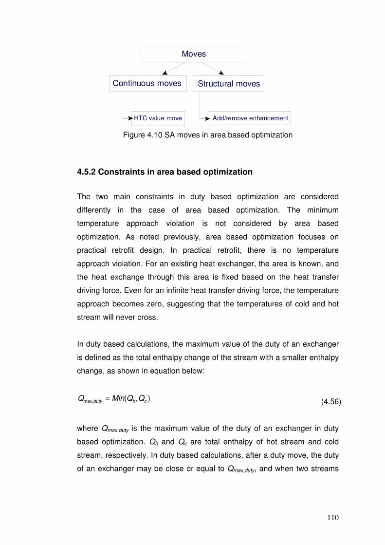
110
Moves
Continuous moves Structural moves
Add/remove enhancementHTC value move
Figure 4.10 SA moves in area based optimization
4.5.2 Constraints in area based optimization
The two main constraints in duty based optimization are considered
differently in the case of area based optimization. The minimum
temperature approach violation is not considered by area based
optimization. As noted previously, area based optimization focuses on
practical retrofit design. In practical retrofit, there is no temperature
approach violation. For an existing heat exchanger, the area is known, and
the heat exchange through this area is fixed based on the heat transfer
driving force. Even for an infinite heat transfer driving force, the temperature
approach becomes zero, suggesting that the temperatures of cold and hot
stream will never cross.
In duty based calculations, the maximum value of the duty of an exchanger
is defined as the total enthalpy change of the stream with a smaller enthalpy
change, as shown in equation below:
),(max, chduty QQMinQ = (4.56)
where Qmax,duty is the maximum value of the duty of an exchanger in duty
based optimization. Qh and Qc are total enthalpy of hot stream and cold
stream, respectively. In duty based calculations, after a duty move, the duty
of an exchanger may be close or equal to Qmax,duty, and when two streams

111
cross, like the situation shown in Figure 4.11, a heat transfer from low
temperature to high temperature would occur, violating heat transfer laws.
Figure 4.11 Temperature approach violation in duty based optimization
For two streams that are not crossed, the maximum value of the duty of an
exchanger in area based optimization can be also described with Equation
(4.45). However, for two streams that are crossed, as shown in Figure 4.11,
point C is the crossover point of the two streams. For the area based
method, the maximum value of duty is:
),( ,,max, CcCharea QQMinQ = (4.57)
where
)( ,, CinhhCh TTCPQ −⋅= (CPH<CPC) (4.58)
)( ,, outhChCh TTCPQ −⋅= (CPH>CPC) (4.59)
)( ,, CoutccCc TTCPQ −⋅= (CPH<CPC) (4.60)
)( ,, incCcCc TTCPQ −⋅= (CPH>CPC) (4.61)
where TC is the temperature at point C.
Qmax in area based Qmax in duty based
T
Q
C

112
Because the value of duty is calculated from the heat transfer driving force,
the value calculated from these equations are equal to the maximum value
of duty when the heat transfer driving force is infinite.
Figure 4.12 An example network for enthalpy balance constraint
The other main constraint in duty based optimization is enthalpy balance. In
area optimization, it is desired to achieve enthalpy balance, but it cannot be
completely balanced. A heat exchanger network is shown in Figure 4.12 to
illustrate the enthalpy balance constraint in both duty based and area based
optimizations. In duty based optimization, when the duty of heat exchanger
4 is changed, the duties of all the process to process heat exchangers are
not changed. The duties of utility heat exchangers 9 and 11 are changed to
maintain the target temperatures. Moreover, feasibility solver is employed
to distribute heat load around the network to maintain the target
temperatures of streams.
H1
H2
H3
H4
C2
C3
HP
CW
1
8
8
1
5
2
2
4
7
7
3
3
9
9
Process to process heat exchangers: Utility heat exchangers:
C1 4 5
6
6
10
10
11
11

113
In area based calculations, after the change of duty in heat exchanger 4,
the downstream heat exchanger 5 will be affected. The area based
calculation method requires the duty of heat exchanger 5 be changed to
meet the change in duty. Exchanger 6 will also be affected because of the
duty change in exchanger 5. After this change, the duties of utility
exchangers 9 and 11 are changed to maintain the target temperatures of
streams H4 and C1. However, since there is no utility heat exchanger on
stream C2, the target temperature of stream C2 will change due to the duty
change in exchanger 6.
It is possible to change the area of exchanger 6 to maintain the original duty.
However, when the network is a large one and the change of operation
condition is not restricted to just one exchanger, many exchangers as
exchanger 6 will require additional area. As a result, the area based
calculation becomes meaningless. In area based optimization, a feasibility
solver cannot be employed because area is specified and duty cannot be
distributed around the network anymore. If area is distributed around the
network, the area based optimization approach cannot avoid the need for
additional area.
Failure to maintain the target temperature is one of the reasons that area
based calculation is not widely used. After area based retrofit optimization,
occasionally some streams without utility heat exchangers cannot maintain
their target temperatures. A penalty function can be added to limit significant
change in target temperature, but the weighting factor needs to be selected
very carefully. Because the stream enthalpy balance constraint will be
definitely violated in optimization, and if the weighting factor is too large, the
optimization will miss some potential energy saving options, especially
those exchangers within a long utility path.
In the area based optimization, such a change in target temperature is
unavoidable, but despite this undesirable effect, the area based calculation
is still meaningful. As mentioned previously, it describes practical retrofit
process and can avoid the need for additional area, which is very important

114
when only heat transfer enhancement is considered. The change in target
temperature is incurred by passive response in the network. As mentioned
in Chapter 3, the passive response is normally not large (unless passive
response happens in the pinching match), and so the change in target
temperature is also not large. Moreover, only heat transfer enhancement
moves are considered in the optimization and the number of enhancements
is also constrained, so that the number of changes that can result in passive
response is small. The penalty function can also control the enthalpy
balance. So in the work, the influence of change in target temperature can
be controlled within a small range.
4.6 Case studies
4.6.1 Case study 4.1: An existing preheat train retrofit design
This case study is the same as the case analyzed in Chapter 3, so that the
results can be compared with the heuristic methodology and those of SA
optimization presented here. The existing heat exchanger network is
studied using SA optimization with different moves. Five heat exchanger
network retrofit considerations are made for comparison with each other.
These are:
1. Retrofit strategy with only heat transfer enhancement. For this retrofit
design, in optimization, only the ‘add/remove enhancement’ moves
and ‘heat transfer coefficients’ moves are allowed. The purpose of
this retrofit design is to reduce retrofit investment as much as
possible to get a short payback period, and to see which exchangers
are enhanced.
2. Retrofit strategy with only additional area. For this retrofit design, in
optimization, only the duty moves are allowed. This strategy is to
trade-off energy savings and the cost of additional area. If the main
reason of energy inefficiency is low heat transfer driving force, this
strategy can result in large energy savings.

115
3. Retrofit strategy with both enhancement and additional area. For this
retrofit design, in optimization, the duty moves, ‘add/remove
enhancement’ moves and ‘heat transfer coefficients’ moves are
allowed. In a similar way to strategy 2, this strategy is intended to
exploit the energy saving potential constrained by low heat transfer
driving force. The main purpose of this strategy is to compare cost
efficiency with strategy 2.
4. Retrofit strategy with topology modifications. For this retrofit design,
in optimization, the duty moves, ‘add/remove new exchanger’ moves,
re-pipe moves, and re-sequence moves are considered. In cases
where the main reason for energy inefficiency is a structural
bottleneck, this retrofit design can be very beneficial.
5. Retrofit strategy with both topology modifications and enhancement.
In the optimization, the enhancement moves, duty moves,
‘add/remove enhancement’ moves and ‘heat transfer coefficients’
moves are all considered. The cost efficiency of this strategy is
compared with that of strategy 4.
In this case, the initial utility cost is assumed to be £20.5 M/y. The cost
estimation of enhancement has rarely been reported in the literature, and
the only one that can be found is as follows [47] :
existingACost ×= 40 (4.62)
where b = £40 m-2.
It should be noted that this cost estimation is for a specified heat transfer
enhancement device, so the cost is only related to the existing area.
However, if we use this equation in our optimization, the augmentation level
cannot be traded-off with cost. Accordingly, the equation is modified to the
following form:
1000)(40 ×++×= e
h
e
sexisting rrACost (4.63)

116
By using Equation (4.63), the optimization can make trade-off between the
augmentation level and cost. Both Equations (4.62) and (4.63) are not very
accurate for estimating the cost of heat transfer enhancement. However,
Equation (4.63) will not incur a large deviation in optimization and is
accurate enough to be used in the optimization.
In this case study, the maximum number of enhanced exchangers is set at
5 while the maximum number of new exchangers added is set at 3. The
maximum number of enhancements and new exchangers are chosen
according to user experience or through screening tools or heuristic
methodologies [81].
The detailed probability of each move in different retrofit strategies is shown
in Table 4.1
Table 4.1 SA move probability in Case study 4.1
Move probability
SA move Duty based strategy Area based
1 2 3 4 5 --
Add new exchanger 0 0 0 0.1 0.1 0
Delete new exchanger 0 0 0 0.05 0.05 0
Re-pipe 0 0 0 0.15 0.1 0
Re-sequence 0 0 0 0.15 0.1 0
Heat duty move 0 1 0.5 0.45 0.3 0
Add enhancement 0.3 0 0.15 0 0.1 0.3
Delete enhancement 0.2 0 0.1 0 0.05 0.2
Modify enhancement level 0.5 0 0.25 0 0.2 0.5

117
Table 4.2 Energy cost and retrofit investment of different retrofit strategies
Retrofit
strategy
Utility cost
(million£/y)
Utility cost
saving
(million£/y)
Additional
area (m2)
Investment
(million£)
Payback
period
(year)
1 19.4 1.1 104.4 0.37 0.34
2 18.4 2.1 1492.0 3.03 1.44
3 18.3 2.2 497.8 1.35 0.61
4 17.3 3.2 1713.0 3.61 1.13
5 17.3 3.2 871.9 2.08 0.65
Table 4.2 shows the results of different retrofit strategies (1 – strategy with
only enhancement; 2 – strategy with only additional area; 3 – strategy with
both enhancement and additional area; 4 – strategy with topology
modification; 5 – strategy with both topology modification and enhancement).
From the results, it can be seen that the investment of those designs with
enhancement are lower than those without enhancement. The retrofit
design with only enhancement (retrofit strategy 1) can reduce£1.1 million/y
utility costs, which accounts for 5.4% of the total utility cost. Although the
energy saving is not as large as the other designs, the investment required
for the design with only enhancement is much lower than those of the
others. Because of the simple implementation of enhancement, the whole
retrofit can be achieved in a short time with a low investment. It should be
noted that the cost of civil and pipe work and the loss in product during
retrofit are not considered in optimization. The economic benefit of retrofit
with only enhancement will be more impressive if these cost factors are
accounted for in all retrofit strategies.
From Table 4.2, it also can be seen that the retrofit design with both
topology modification and enhancement (retrofit strategy 5) can achieve a
large reduction in energy consumption (£3.2 million/y) with a relatively low
investment. Compared with the design using enhancement only, the design
with both topology modification and enhancement cannot be implemented
in a short time due to the required civil and pipe work. The design with both

118
topology modification and enhancement is an attractive option when a large
energy saving is required. Figures 4.13 and 4.14 compare the energy
saving and payback period for each strategy.
Energy Saving
0
2
4
6
8
10
12
Strategy 1 Strategy 2 Strategy 3 Strategy 4 Strategy 5
En
erg
y s
av
ing
(MW
)
Figure 4.13 Energy saving results of each strategy
Pay-back time
0
0.2
0.4
0.6
0.8
1
1.2
1.4
1.6
Strategy 1 Strategy 2 Strategy 3 Strategy 4 Strategy 5
Ye
ar
Figure 4.14 Pay-back period results of each strategy
The results in Figure 4.13 show that the energy saving obtained from the
strategy with enhancement only (retrofit strategy 1) is lower than that from

119
the strategy with additional area (retrofit strategy 2). The reason for this is
that the number of enhancements is constrained, and so is the maximum
enhancement augmentation ratio. The strategy with additional area involves
a larger number of modified exchangers and the maximum value of the
additional area is very large. In the strategy with both enhancement and
additional area (retrofit strategy 3), some exchangers require both
enhancement and additional area. This is because the enhancement costs
are lower but the augmentation level is not large enough to accommodate
the duty improvement due to the maximum augmentation ratio constraints.
This demonstrates why a strategy using additional area can lead to more
energy saving than a strategy using enhancement only. As mentioned
previously, topology modification moves need to be combined with the duty
moves because the duties of the exchangers after re-piping or re-
sequencing need to be optimized. In this work, the energy saving of the
strategy with topology modification (retrofit strategy 4) is larger than that of
the strategy with additional area (retrofit strategy 2). When the network
structure is close to optimal, the energy saving of the strategy with topology
modification and strategy with additional area will be very close. Analysis
shows that the strategy with enhancement only can be very attractive in a
well-established network, when both additional area and topology
modification cannot make a large improvement in energy saving. In Figure
4.14, it is seen that the pay back time of retrofit strategy is very short, as
expected. Because heat transfer enhancement can reduce retrofit
investment, the pay back time of strategies 3 and 5 are also attractive.
The enhanced exchangers in the retrofit design with enhancement only are
highlighted with a bold line in Figure 4.15. From the figure, it can be seen
that exchangers 4, 20, 24, 26 and 28 are enhanced. Of these five
exchangers, exchangers 4, 24, 26 and 28 are on the same stream with
utility exchanger 30. The four exchangers all have a large duty. From
Equation (4.8), it can be seen that with a ratio of increasing overall heat
transfer coefficient U, the duty increases by the same ratio. Therefore, for a
larger duty, a greater energy improvement can be achieved.

120
C1
C2
C3
H1
H2
H3
H4
H5
H6
H7
H8
H9
H10
H11
H12
HU
CU
1
1
3
3
2
2
30
30
29
29
21
21
28
28
27
27
26
26
24
24
20
20
4
4
18
18
17
17
16
16
23
23
13
13
22
22
12
12
6
6
25
25
32
32
19
19
15
15
14
14
7
7
11
11
10
10
8
8
9
9
31
31
Figure 4.15 Crude oil preheat train with enhanced exchangers highlighted
Exchanger 20 is a pinching match, which is the structure bottleneck of the
network [66]. Normally, the pinching match is an exchanger with a small
temperature difference, and a small change of inlet temperature will
influence the heat transfer driving force significantly. Pinching match 20 is
downstream of exchanger 24. If exchanger 24 is enhanced, the hot inlet
temperature of exchanger 20 will decrease. The duty of exchanger 20 will
decrease dramatically due to the low heat transfer driving force. Therefore,
heat transfer enhancement must be added to exchanger 20 to compensate
for the loss of heat transfer driving force if exchanger 24 is enhanced.
A comparison between the SA optimization methodology of this chapter and
the heuristic methodology reported in Chapter 3 is shown in Table 4.3. The
heuristic methodology was employed to find the candidate exchangers to be
enhanced and the physical insights of exchangers to be enhanced have
been analyzed in some detail in Chapter 3. Table 4.3 indicates that the
results of the SA optimization are broadly similar to the results of the
heuristic methodology.

121
Table 4.3 Comparison of SA optimization and heuristic methodology results
Methodology Enhanced exchangers
Heuristic Best candidates: Exchangers 26, 28
Good candidates: Exchangers 4, 27, 29
Good candidates with pinching match: Exchangers
20, 24
SA optimization Exchangers 4, 20, 24, 26, 28
The area based optimization has also been applied to the case study, and
the results are compared with those of the duty based optimization in Table
4.4.
Table 4.4 Comparison between duty based and area base optimization
Methodology Energy saving
(million£/year)
Additional area
(m2)
Enhanced
exchangers
Duty Based 1.1 104.4 4,20,24,26,28
Area Based 1.0 0 20,24,26,28,29
Table 4.4 shows that the area based optimization can eliminate the need for
additional area effectively. The enhanced exchangers are in accordance
with the results of both the duty based optimization and the heuristic
methodology. Because the duty based optimization allows additional area to
be added, its energy saving is slightly higher than that of the area based
optimization.
The computing time for duty based calculation is 1 hour and for area based
calculation is 2 hours. The CPU of the computer used to optimize is E7400
@ 2.80 GHz. From the results, it can be seen that the computing time is
much longer than conventional mathematical programming because of its
stochastic nature. Also the area based calculation is longer because the
area based exchanger model is more complex.
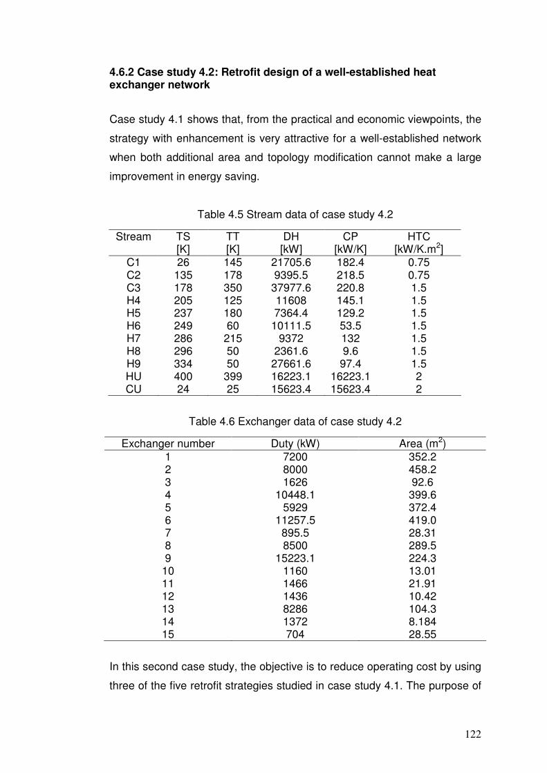
122
4.6.2 Case study 4.2: Retrofit design of a well-established heat exchanger network
Case study 4.1 shows that, from the practical and economic viewpoints, the
strategy with enhancement is very attractive for a well-established network
when both additional area and topology modification cannot make a large
improvement in energy saving.
Table 4.5 Stream data of case study 4.2
Stream TS TT DH CP HTC [K] [K] [kW] [kW/K] [kW/K.m2]
C1 26 145 21705.6 182.4 0.75 C2 135 178 9395.5 218.5 0.75 C3 178 350 37977.6 220.8 1.5 H4 205 125 11608 145.1 1.5 H5 237 180 7364.4 129.2 1.5 H6 249 60 10111.5 53.5 1.5 H7 286 215 9372 132 1.5 H8 296 50 2361.6 9.6 1.5 H9 334 50 27661.6 97.4 1.5 HU 400 399 16223.1 16223.1 2 CU 24 25 15623.4 15623.4 2
Table 4.6 Exchanger data of case study 4.2
Exchanger number Duty (kW) Area (m2) 1 7200 352.2 2 8000 458.2 3 1626 92.6 4 10448.1 399.6 5 5929 372.4 6 11257.5 419.0 7 895.5 28.31 8 8500 289.5 9 15223.1 224.3
10 1160 13.01 11 1466 21.91 12 1436 10.42 13 8286 104.3 14 1372 8.184 15 704 28.55
In this second case study, the objective is to reduce operating cost by using
three of the five retrofit strategies studied in case study 4.1. The purpose of
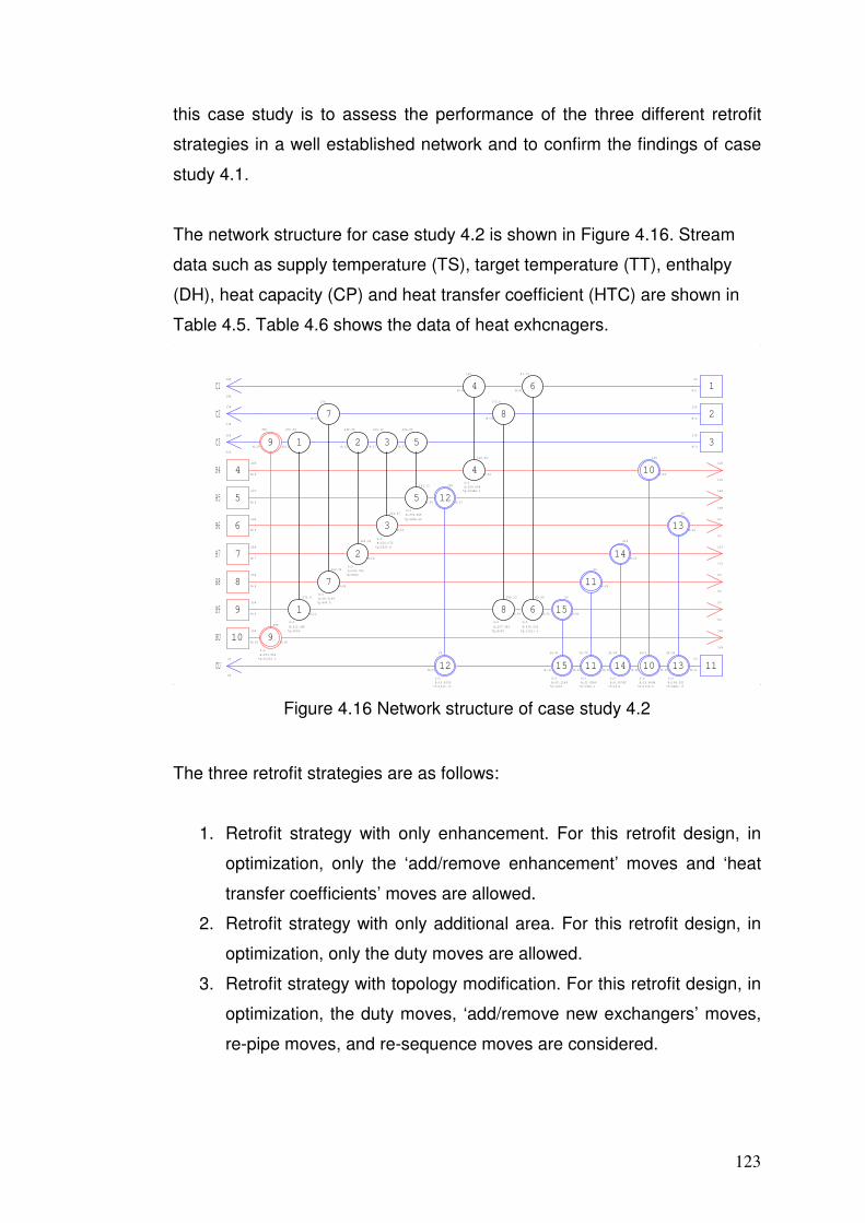
123
this case study is to assess the performance of the three different retrofit
strategies in a well established network and to confirm the findings of case
study 4.1.
The network structure for case study 4.2 is shown in Figure 4.16. Stream
data such as supply temperature (TS), target temperature (TT), enthalpy
(DH), heat capacity (CP) and heat transfer coefficient (HTC) are shown in
Table 4.5. Table 4.6 shows the data of heat exhcnagers.
1N:1
26145
145
2N:2
135178
178
3N:3
178350
350
4N:4
205 125
125
5N:5
237 180
180
6N:6
249 60
60
7N:7
286 215
215
8N:8
296 50
50
9N:9
334 50
50
10N:10
400 399
399
11N:11
2425
25
4
4
N:32
N:33
132.99
145
*Q:10448.1
A:399.604
S:0
10
10
N:26
N:20
125
24.6
*Q:1159.9
A:12.9644
S:0
5
5
N:36
N:37
191.11
204.85
*Q:5928.69
A:372.406
S:0
12
12
N:27
N:24
180
25
*Q:1435.71
A:10.4335
S:0
3
3
N:16
N:17
214.87
213.12
*Q:1825.8
A:120.072
S:0
13
13
N:22
N:29
60
24.53
*Q:8285.73
A:104.301
S:0
2
2
N:14
N:15
225.39
249.35
*Q:8000
A:478.706
S:0
14
14
N:23
N:25
215
24.69
*Q:1372
A:8.18742
S:0
7
7
N:38
N:39
202.72
178
*Q:895.5
A:28.3104
S:0
11
11
N:28
N:21
50
24.79
*Q:1466.1
A:21.8568
S:0
1
1
N:12
N:13
272.4
276.53
*Q:6000
A:212.346
S:0
8
8
N:34
N:35
185.13
173.9
*Q:8500
A:237.393
S:0
6
6
N:30
N:31
69.55
87.72
*Q:11257.5
A:336.525
S:0
15
15
N:40
N:41
50
24.91
*Q:1904
A:65.3184
S:0
9
9
N:18
N:19
399
350
*Q:16223.1
A:233.962
S:0
C1
C2
C3
H4
H5
H6
H7
H8
H9
HU
CU
Figure 4.16 Network structure of case study 4.2
The three retrofit strategies are as follows:
1. Retrofit strategy with only enhancement. For this retrofit design, in
optimization, only the ‘add/remove enhancement’ moves and ‘heat
transfer coefficients’ moves are allowed.
2. Retrofit strategy with only additional area. For this retrofit design, in
optimization, only the duty moves are allowed.
3. Retrofit strategy with topology modification. For this retrofit design, in
optimization, the duty moves, ‘add/remove new exchangers’ moves,
re-pipe moves, and re-sequence moves are considered.
124
In this case study, the minimum temperature difference is set at 10°C, and
the topology constraints are shown in Table 4.7.
Table 4.7 Topology constraints in case study 4.2
Topology
constraint
Number of
enhancements
Number
of re-pipe
Number of
re-sequence
Number of new
exchangers
Maximum
number
3 3 3 2
The results of the three heat exchanger network retrofit strategies are
shown in Table 4.8. The utility cost of existing heat exchanger network
before retrofit is 834273 GBP/year.
Table 4.8 Results of the three retrofit strategies in case study 4.2
Retrofit
strategy
Utility cost
(GBP/y)
Reduction in utility
cost (GBP/y)
Investment
(GBP)
Payback
(year)
1 806376 27897 19330.1 0.69
2 808693 25580 31514.5 1.23
3 808298 25975 32285.8 1.24
The results in Table 4.8 indicates that the energy saving of all three retrofit
strategies is almost the same. The reasons for this finding are discussed
below.
1. Given that the existing network is well-established, although the heat
transfer driving force is small, the minimum temperature differences in
exchangers that can affect utility consumption significantly are close to
the global minimum temperature difference, which is 10°C. Compared
with case study 4.1, the constraints of maximum augmentation level
cannot be reached in case study 4.2. As a result, using heat transfer
enhancement only can lead to the same impact as in the case of using
additional area.

125
2. In a well-established network, most of its heat exchangers follow the
rules of Pinch Approach. Although the results of Pinch analysis indicate
that there is still a little across pinch heat transfer, the energy saving
improvement is low. Because of the relatively high retrofit investment,
the structure modification is not economic.
3. The small difference between the utility reduction costs of retrofit
strategies 2 and 3 is mainly due to the stochastic nature of SA
optimization.
The results in Table 4.8 confirm that the heat transfer enhancement option
is very attractive for a well-established heat exchanger network retrofit. The
retrofit design with only heat transfer enhancement achieves a level of
energy saving that is very similar to those of the retrofit design with topology
modification and the retrofit design with additional area, but it requires much
lower investment compared to the other two designs. So the payback period
is again impressive.
Table 4.9 shows the exchangers with additional area in strategies 2 and 3
and the exchangers with heat transfer enhancement in strategy 1.
Table 4.9 Modified exchangers in case study 4.2
Retrofit strategy Modified exchangers
1 1, 2, 5
2 1, 2
3 1, 2
Table 4.9 indicates that three exchangers are modified in strategy 1 but only
two are modified in strategies 2 and 3. The difference may be attributed to
the differences in capital cost. Because the energy saving improvement in
exchanger 5 is small (shown in Table 4.10), with the trade-off between
energy cost and capital cost, the heat transfer enhancement feature of
strategy 1 can make a profit while the additional area feature of strategies 2
and 3 cannot.

126
Table 4.10 Enhanced exchanger data of strategy 1 in case study 4.2
Exchanger number Increase in Q (kW) Increase in U
(kW/K.m2)
1 256 0.38
2 1365 0.38
5 49 0.11
In Table 4.10, the reason why the increase in the duty of exchanger 1 is
relatively low is that exchanger 1 is located downstream of exchanger 2,
and the increased duty of exchanger 2 will reduce the heat transfer driving
force in exchanger 1.
4.7 Conclusion
Heat transfer enhancement is a very attractive option for heat exchanger
network retrofit. This chapter proposes a new methodology for heat
exchanger network retrofit optimization considering heat transfer
enhancement. The objective of this new methodology is to find the
appropriate heat exchangers to be enhanced and calculate the
augmentation level of enhancement with and without topology modifications.
When heat transfer enhancement is applied, the retrofit process becomes
simpler and requires lower investment. Simulated annealing is used as the
optimization algorithm, which can avoid local optima in large-scale retrofit
problems. To include heat transfer enhancement in the optimization process,
simulated annealing moves considering heat transfer enhancement are
added. The optimization can automatically search for which exchangers are
to be enhanced, and optimize the augmentation level of each enhancement.
Area based optimization is used to describe the practical retrofit and
passive changes of a network, which cannot be accounted for in duty based
calculation. Moreover, area based optimization can avoid the need for
additional area, and this can be very attractive when only enhancement is
considered in retrofit design. Although area based calculation will induce

127
stream enthalpy imbalance, it can be restricted to a small number by
constraints.
In case study 4.1, the investment required for retrofit with enhancement only
is very low (0.37 million GBP), and the retrofit scheme provides a very short
payback period (0.34 years) and short modification duration. The results
show that the exchangers that have a large duty requirement and are close
to the utility exchanger have great energy saving potential when only heat
transfer enhancement is applied. The new methodology can provide several
low investment retrofit options featuring enhancement, which can be used in
different situations. The strategy with enhancement only is suitable for use
when the original network is close to optimal, or short modification duration
is desired. The strategy with both enhancement and additional area is
suitable when low heat transfer driving force is the main reason of energy
inefficiency, and enhancement is used to reduce retrofit investment. The
strategy with both enhancement and topology modification is suitable when
a structural bottleneck is the main reason of energy inefficiency, and
enhancement is also used to reduce retrofit investment. Area based
calculations are also considered in this case study. The results show that it
can eliminate the need for additional area. The results of the area based
calculation are in accordance with those of the duty based calculation as
well as those of the heuristic methodology reported in Chapter 3.
In case study 4.2, a well-established exchanger network is optimized by
using three different retrofit strategies. The results prove that the heat
transfer enhancement option is very attractive in well-established heat
exchanger network retrofit. The retrofit design with only heat transfer
enhancement achieves energy saving s similar to that of the retrofit design
with topology modification or the retrofit design with additional area.
However, it requires a lower investment and gives a shorter payback time.
In contrast to conventional retrofit methodologies, the new methodology
considers the application of heat transfer enhancement in considerable
detail. This methodology uses the features of heat transfer enhancement

128
and the simulated annealing optimization algorithm to relate retrofit design
to different practical retrofit situations.
Nomenclature
A Total heat exchanger area (m2)
Aexisting Existing area of a heat exchanger in a retrofit project (m2)
B A parameter used in area based exchanger model
CP Heat capacity flow rate of a stream (kW/℃)
DH enthalpy change (kW)
FT Log mean temperature difference correction factor
fflm flow ratio of the branch to the main stream m on which the
exchanger unit l is located
+∆f Average increment of the objective function for uphill moves in
simulated annealing algorithm
h Heat transfer coefficient (kW/℃·m2)
hf Film heat transfer coefficient (kW/℃·m2)
hw heat transfer coefficient for tube wall (kW/℃·m2)
LM Markov chain length in simulated annealing algorithm
P Thermal effectiveness of a heat exchanger
p0 desired initial acceptance probability in simulated annealing
algorithm
NSH Number of shells in a heat exchanger
NBR total number of branches
Q Heat duty of a heat exchanger (kW)
R Ratio of the heat capacity flow rates of hot and cold stream
r Parameter used in penalty function
re enhancement ratio
rh Ratio of the shell side and tube side heat transfer coefficient
SFn the flow splitting fraction of branch n
T Temperature of a node (℃)
Ta Annealing temperature in simulated annealing algorithm (℃)
TS Supply temperature of a stream (℃)

129
TT Target temperature of a stream (℃)
U Overall heat transfer coefficients of a heat exchanger
(kW/℃·m2)
△A Additional area (m2)
△f Difference in the objective function values of two different
solutions in simulated annealing algorithm
△TLM Log mean temperature difference of a heat exchanger (℃)
△Tmin Minimum temperature difference of a heat exchanger (℃)
ykl indicates whether exchanger l is on the section of stream m
between the start point of stream m and node k
αA Area ratio
γ weight factor used in penalty function
θ A cooling parameter that controls the speed of cooling in
simulated annealing algorithm
σ(Ta)
Standard deviation of the objective function of all the trial
solutions generated at the temperature Ta in simulated
annealing algorithm
Subscripts and superscripts
c Cold side of a heat exchanger
e Exchanger under enhancement condition
h Hot side of a heat exchanger
in Inlet of one stream in a heat exchanger
max Maximum value
out Outlet of one stream in a heat exchanger
p Exchanger under plain tube condition
s Shell side
t Tube side
0 Initial value
130
Chapter 5 Applying heat transfer enhancement in
heat exchanger network considering fouling
5.1 Introduction
Heat exchanger network retrofit methodologies have been well developed
over the last three decades. Recent work considered other important issues
for practical heat exchanger network retrofit, such as operability, control,
flexibility, safety and pressure drop. However, little work has been done in
the area of examining the effect of fouling on heat exchanger network
retrofit.
Fouling is an important issue that can affect the operation of a heat
exchanger network in practice. It will decrease the heat transfer in a heat
exchanger, resulting in a reduction in the heat recovery. Moreover, it can
increase the pressure drop across the affected equipment. These problems
incurred by fouling can cause an increase in utility consumption, loss in
production and requirement of more pumping capacity. Concerns regarding
fouling are probably the main reason that heat transfer enhancement is not
widely used in the process industry. Therefore, if heat transfer enhancement
is considered in heat exchanger network retrofit, the fouling aspect must be
addressed in order to make sure that meaningful results are obtained.
In this chapter, the SA optimization methodology presented in Chapter 4 is
further developed to consider the fouling aspect. The physical insights into
the fouling deposition process are presented. These physical insights of
fouling will lead to a deeper understanding of the interactions between the
network topology and fouling deposition.

131
5.2 Consideration of fouling in heat exchanger network retrofit
5.2.1 Background on fouling of heat exchangers
Fouling of heat transfer equipment is a very costly problem. It is difficult to
estimate the cost of fouling accurately, but its implications may be
summarized as follows:
1. To account for the decrease of heat duty in heat exchangers with time,
normally oversized heat exchangers are selected in the design stage to
compensate the reduction in the overall heat transfer coefficients when
fouling happens.
2. Fouling reduces the efficiency of a network to transfer heat, so more
external utility needs to be used to meet the energy demands of a
process.
3. The cleaning cost of fouling. When fouling is severe, it is necessary to
clean the deposition to restore the network’s original performance.
Many types of fouling may occur in heat exchangers. They can be classified
according to the mechanism that gives rise to deposition. Fouling is
generally the result of several simultaneous mechanisms, but for a
particular process, normally there is a dominant type of fouling. A commonly
accepted classification groups fouling in six main categories: particulate,
crystallization, chemical reaction, corrosion, biological and freezing
fouling[82, 83].
Every type of fouling has its own property, and has different condition to
occur. In our work, only one type of fouling is considered, which is fouling in
crude oil heating. This type of fouling is of great practical interest because
the refinery crude oil preheat train is an important example of heat
exchanger networks whose operation is significantly affected by fouling.

132
Because there are many types of fouling, numerous variables can affect the
fouling deposition process. For example, temperature, flow velocity, fluid
composition, heat flux, construction materials and condition of the surface
can exert great influence on the fouling process. The dominant variables
affecting fouling in the crude oil preheat train will be discussed later in detail.
Given the impact of fouling deposition on the economics and operation of a
heat exchanger network, effective mitigation strategies are required. There
are a number of fouling mitigation strategies used in practice. The most
frequently used methods include the use of chemical additives, control of
feedstock, use of robust heat transfer equipment and cleaning of fouling
units. Among these methods, the use of antifouling additives is cost-
effective in recirculation water systems but cannot be used in applications
that cannot tolerate contamination [84]. Control of feedstock is very useful in
the crude oil preheat train system [85-87]. Robust heat exchangers are
mostly the heat exchangers with heat transfer enhancement, which will be
discussed later. Cleaning of fouled equipment is the most common way to
remove deposition when fouling occurs, but the exchangers to be cleaned
need to be taken out of service sometimes.
5.2.2 Fouling in refinery crude oil preheat trains
Furnaces of a crude distillation unit are the main energy consuming units in
refineries. Almost half of the overall operational cost of the refineries is due
to the energy losses resulting from fouling formation in the preheat
exchangers [88]. In our work, only fouling in crude oil heating is considered.
In a crude oil preheat train, crude oil is fed from storage tanks at ambient
temperature. Then the crude oil is first heated up to around 110-150°C in
the heat exchanger network before entering the desalter. In the desalter,
salts and particulate matter contained in the crude oil are removed.
Normally a 10°C temperature drop will happen in the desalter. After leaving
133
the desalter, the crude oil is further heated up to 230-300°C before entering
the furnaces. The inlet temperature of furnace is a parameter normally used
to measure the effectiveness of the preheat train. In the furnace, the oil is
heated to a final temperature which is about 350-390°C. The crude oil from
the furnace is fed to the distillation unit.
Crude oil preheat trains suffer from fouling. In a crude oil preheat train,
fouling is more severe on the crude oil side of heat exchangers, although
fouling may also happen in the other places, especially for the heavy
product streams such as reduced crude oil or heavy gas oil [58, 89]. The
mechanism of fouling in a crude oil preheat train varies in different parts of
the train. The most severe fouling in a crude oil preheat train is at the very
hot end, where fouling is due to chemical reactions [60, 82]. The two most
important factors that affect fouling in a crude oil preheat train are
exchanger wall temperature and the rate of shear experienced by the fluid
at the heat transfer service as it flows through the exchanger [90].
Fouling occurs in the furnace as well, but the impact of fouling in the furnace
is not as large as that in the preheat train. Because the heat transfer driving
force in the furnace is very high, its reduction due to fouling is not significant
enough to negatively affect heat transfer in the furnace [82].
5.2.3 The performance of heat transfer enhancement under fouling consideration
In shell sides, the conventional segment baffle is largely responsible for
fouling [91]. Helical baffles can be used to control the fouling in shell sides.
In heat exchangers with helical baffle, the quadrant shaped baffle plates are
arranged at an angle to the tube axis in a sequential pattern, creating a
helical flow path through the tube bundle. Helical baffle gives a uniform flow
velocity through the tube bundle. A higher velocity can be achieved with the
same pressure drop in conventional shell so that the shear stress will be
increased. These features of helical baffle can effectively reduce the fouling

134
rate in shell sides.
In tube sides, the fouling performance of wire coil inserts and wire mesh
inserts is studied by Pahlavanzadeh et al [92]. In their work, the fouling
resistance can be reduced by using wire coil tube inserts, the average
fouling resistance is decreased by 34%. However for mesh inserts, the
fouling resistance cannot be reduced, and sometimes it even increases
fouling. The fouling performance of scraped wall insert is reported by Polley
et al [93], which can be used in the exchangers positioned before the
desalter to reduce fouling.
Figure 5.1 Fouling in plain tube and tube fitted with hiTRAN [36]
hiTRAN wire matrix insert is a widely used tube insert. Its performance has
been well studied [36-38]. hiTRAN wire matrix inserts work by continually
mixing fluid from the tube wall into the bulk flow and vice versa. This
disrupts the laminar boundary layer that dominates in low Reynolds number
flows, removing this inhibitor to heat transfer and resulting in significantly
higher heat transfer coefficients on the tube side. The fouling performance
of hiTRAN has been studied by Crittenden et al [36], and the results are
shown in Figure 5.1. The figure shows that hiTRAN can reduce fouling
significantly. The study of Ritchie et al [37] indicates that hiTRAN is effective

135
against all fouling mechanisms, including chemical reaction, crystallization,
and particulate fouling.
5.2.4 Models of fouling
Fouling threshold models can be used to predict the fouling in crude oil
preheat train, which was proposed by Ebert and Panchal [58]. In the model,
the average (linear) fouling rate under given conditions is a result of two
competing terms, namely, a deposition term and a mitigation term. The
equation is shown below:
Fouling rate = (deposition term) - (deposition removal term)
W
f
f
RT
E
dt
dRγτα β −
−= )exp(Re (5.1)
where α, β, γ are parameters determined by regression, τw is the shear
stress at the tube wall, Tf is the crude film temperature (average of the local
bulk crude and local wall temperatures), and E is the activation energy.
0 0.2 0.4 0.6 0.8 1 1.2 1.4
380
345
365
Shear stress (Pa)
Fouling
No Fouling
Figure 4.2 Threshold film temperature as a function of flow shear stress
The threshold temperature, above which fouling is expected to occur, can
be calculated for a given shear stress by setting Equation (5.1) to zero. The

136
relationship between threshold temperature and shear stress is shown in
Figure 5.2. For film temperature and shear stress to the right and below the
threshold line, fouling can be ignored. For conditions above the threshold
line, fouling is expected to occur, and it becomes more severe as the
conditions move away from the threshold line.
The threshold model of Ebert and Panchal was improved by Polley et al [57].
Their model uses tube wall temperature instead of film temperature in the
fouling formation, shown below:
8.033.08.0 Re)exp(PrRe γα −−
= −−
W
f
RT
E
dt
dR (5.2)
Polley et al correlated the model with the fouling data reported by Kundsen
et al [94]. The model performs well in predicting accurately fouling threshold
constitutions and initial fouling rates. The differences between the two
models are as follows. First, in the threshold model of Polley et al, the
exponent of Reynolds number is a fixed number. Next, the film temperature
in Ebert and Panchal’s model is replaced by wall temperature. Finally, in the
threshold model of Polley et al, wall shear stress in the removal term is
replaced by Reynolds number.
Yeap et al [59] introduced more modifications to the threshold model. Their
model is shown below:
8.0
32
31
31
23
34
32
32
)/exp(1v
TRETfv
Tvf
dt
dR
WW
Wf ⋅−⋅⋅⋅⋅⋅⋅⋅+
⋅⋅⋅⋅⋅=
−−
−
γµρβ
µρα (5.3)
The physical properties of the fluid are evaluated at the film temperature.
The model exhibits two temperature dependences, i.e. the Arrhenius term
and the fluid properties, and three velocity dependencies. For large values
of the constant β, the model reduces to the form of Polley et al’s model.

137
Fouling threshold models can identify a set of operating conditions to see if
fouling is going to happen. It can be also used to predict the initial fouling
rate under certain conditions. These models can be only used to describe
crude oil flowing through tubes. In our work, only fouling in crude oil heating
is considered, and so the threshold models are relevant and applicable to
our situations. Models for predicting other types of fouling will not be
discussed here.
5.2.5 Fouling model of tube with enhancement
Although some research has been conducted to observe the fouling
performance of tube with different enhancement devices, useful fouling
models are rare in the literature. Yang and Crittenden [38] proposed a
modified version of the model of Yeap et al for hiTRAN, as shown below:
w
WW
sf
TRETfv
Tvf
dt
dRγτ
µρβ
µρα−
⋅⋅⋅⋅⋅⋅⋅+
⋅⋅⋅⋅⋅=
−−
−
)/exp(1 3/23/13/123
3/43/23/2
(5.4)
where
E = 52.1 (kJ/mol)
α = 7.93×10⁻¹⁰ (kg2/3K1/3m5/3(kW-1)s-1/3h-1)
β = 1.80×10⁻⁵ (m13/3kg2/3s8/3K-2/3)
γ = 1.60×10⁻⁵ (m6/5Ks4/5K-2/3(kW)-1h-1)
In this model, several modifications have been made. First, the fouling
removal term is amended to include shear stress rather than average fluid
flow velocity. Secondly, equivalent velocity is introduced to replace average
linear velocity. Equivalent velocity is defined as the velocity in a bare tube
that gives the same wall shear stress in a tube of the same internal
diameter fitted with inserts and operating at a different average fluid velocity.
Yang and Crittenden [38] state that the model of Polley et al is difficult to
use directly in the case of tube with inserts. If simplicity is desired, the
138
model of Polley et al may be used by replacing Re in the model with the
equivalent Re obtained from CFD simulation. An equivalent Re is defined as
the Re in a bare tube that gives the same wall shear stress in a tube of the
same internal diameter fitted with inserts and operating at a different
average fluid velocity. For the crude oil tested (Maya crude oil), the
correlation generated with the help of CFD simulation is as follows:
3945.0Re8526.1Re 0 −=e (5.5)
Re is calculated as if there is no inserts in the tube within the range of 8000
– 30000. This may be applicable to other types of crude oil provided the
viscosity is similar. The model of Polley et al can then be used for the
prediction of fouling rate in a tube with or without inserts, even though the
model fitting is not as good as l that of the model of Yeap et al.
For the Maya crude oil tested, the model parameters obtained by curve
fitting are as follows:
E = 46.2 (kJ/mol)
α = 58950 (m2kW-1h-1)
γ = 5.7×10⁻¹⁰ (m2kW-1h-1)
µ = 0.0011 (P·s) at 250℃
ρ = 760 (kg/m3)
With this set of parameters, fouling rates of both bare tube and tube with
inserts can be correlated using the model of Polley et al.
In this work, hiTRAN is used as the enhancement device. The modified
model of Polley et al is used in optimization for predicting the fouling
performance of hiTRAN. Although the modified model of Polley et al is not
as accurate as the modified model of Yeap et al, the parameters of the
former such as Re and Pr are easier to determine compared with those of
the latter such as the parameters f and wτ . The modified model of Polley et

139
al is used to predict the fouling of tube with enhancement as well as bare
tube.
5.3 Opportunities to reduce fouling in heat exchanger networks
As mentioned in section 5.2.2, the most important factors that affect fouling
in a crude oil preheat train are exchanger wall temperature and the rate of
shear experienced by the fluid as it flows through the exchanger. The
opportunities of reducing fouling by changing wall temperature and shear
stress are discussed in this section.
5.3.1 Reducing fouling by applying heat transfer enhancement
In a crude oil preheat train, the temperature of the heat transfer surface has
a great impact on fouling rate, especially at the hot end of the preheat train.
In a preheat train, the high wall temperature tends to accelerate the
deposition. Consequently, the wall temperature should be kept low to
reduce fouling.
The surface temperature of a heat exchanger is a function of the heat
transfer coefficients and bulk temperature of the hot and cold streams. The
relevant equations are shown below:
+
⋅
⋅+
⋅
⋅
−−=
1ln2
,
I
O
W
OO
II
OO
IOOOW
d
dhd
hd
hd
TTTT
λ
(5.6)
+
⋅
⋅+
⋅
⋅
−+=
1ln2
,
I
O
W
II
OO
II
IOIIW
d
dhd
hd
hd
TTTT
λ
(5.7)

140
where the subscripts I and O refer to the inside and outside of tube,
respectively, TW is wall temperature, d is the diameter, and λ is thermal
conductivity of tube wall, and h is heat transfer coefficient. It is noted that
thin wall assumption is not made in equation (5.6) and (5.7), because a tiny
wall temperature difference may affect fouling rate significantly.
When hot stream flows through outside of tube and cold stream flows
through inside of tube, Equations (5.6) and (5.7) become:
+
⋅
⋅+
⋅
⋅
−−=
1ln2
,
I
O
W
hO
cI
hO
chhOW
d
dhd
hd
hd
TTTT
λ
(5.8)
+
⋅
⋅+
⋅
⋅
−+=
1ln2
,
I
O
W
hI
hO
cI
chcIW
d
dhd
hd
hd
TTTT
λ
(5.9)
In Equations (5.8) and (5.9), (Th – Tc) is larger than zero. Therefore, for
Equation 5.8, when the term
+
⋅
⋅+
⋅
⋅1ln
2 I
O
W
hO
cI
hO
d
dhd
hd
hd
λ becomes smaller,
the wall temperature becomes smaller. For Equation 5.9, when the term
+
⋅
⋅+
⋅
⋅1ln
2 I
O
W
hI
hO
cI
d
dhd
hd
hd
λ becomes larger, the wall temperature becomes
smaller. It can be deduced that increasing hc or decreasing hh reduces wall
temperature. When the cold stream flows through outside of tube and hot
stream flows through inside of tube, the same conclusion is reached: an
increase in hc or a decrease in hh reduces wall temperature.
As a result, in a heat exchanger, wall temperature can be reduced by
increasing cold side heat transfer coefficient or decreasing hot side heat
transfer coefficient or a combination of both changes. In a crude oil preheat
train, a decrease in wall temperature means a reduction in fouling rate.

141
According to the previously mentioned threshold models, fouling may be
completely eliminated when wall temperature is reduced.
Heat transfer enhancement can increase heat transfer coefficient in a heat
exchanger. It can be used to increase cold side heat transfer coefficient in
order to decrease wall temperature. For a typical crude oil preheat train,
crude oil is a cold stream and normally flows through tube side of an
exchanger. Therefore, the tube side heat transfer enhancement can be
applied to increase heat transfer coefficient and reduce fouling rate. This
option should be implemented when heat transfer enhancement is applied
to a crude oil preheat train.
However, if the tube side is the hot side, tube inserts can promote fouling
considering wall temperature. Because tube inserts such as hiTRAN or wire
coil have the ability to reduce fouling rate, their impact on fouling needs to
be assessed carefully.
5.3.2 Reducing fouling by modifying network structure
The wall temperatures of exchangers are not only affected by the heat
transfer coefficients of both cold and hot sides, but also affected by the
temperatures of hot and cold streams. By selecting different matches, the
temperature of match can be different.
In heat exchanger network design, based on the stream matches that
appear in the composite curves [76, 95], the heat flow pattern in a heat
exchanger network is classified as either vertical heat transfer or criss-
crossed heat transfer. Vertical heat transfer corresponds to overall counter-
current heat exchange between the hot and cold streams. In composite
curves, the stream matches in vertical heat transfer appear vertically
aligned, as shown in Figure 5.3.

142
Enthalpy
Enthalpy
Vertical heat transfer Criss-crossed heat transfer
Highest walltemperature
Higher walltemperature
Lower walltemperature
Figure 5.3 Vertical and criss-crossed heat transfer
The advantage of vertical heat transfer is that it makes good use of overall
temperature difference between hot and cold streams. For vertical heat
transfer, the area requirement of a heat exchanger network is close to the
minimum when the heat transfer coefficients do not differ significantly
throughout the network [96]. Strictly speaking, vertical heat transfer results
in the absolute minimum area requirement only when the film transfer
coefficients of all streams are almost identical.
Vertical heat transfer network is normally desired in heat exchanger network
design. However, if the fouling aspect is considered in network design, the
vertical heat transfer may not be that beneficial. In vertical heat transfer, the
cold streams at progressively higher temperature are matched with
increasingly hotter hot streams, which result in a wall temperature profile
that continuously increases from the cold to the hot end of the network. In
other words, the hottest spot in the cold stream exchanges heat with the
hottest spot in the hot stream. As a result, at the hot end of a heat
exchanger network, the wall temperature will reach its maximum value. This
hottest spot is very likely to have severe fouling deposition.
Criss-crossed heat transfer requires more heat transfer area because it
cannot make good use of overall temperature difference between hot and
cold streams. This means for a heat exchanger network with criss-crossed
heat transfer design, the capital cost is high. However, Figure 5.3 shows
that in design with criss-crossed heat transfer, the hottest spot in hot stream

143
does not exchange heat with the hottest spot in cold stream. The
temperature in the hottest place is thus lower.
An example is used to illustrate the designs with vertical heat transfer and
criss-crossed heat transfer. The example heat exchanger networks are
shown in Figure 5.4. The left hand side network features vertical heat
transfer. In this case, the cold stream exchanges heat with the hot stream at
a relatively low temperature at first, and then exchanges heat with the hot
stream at a relatively high temperature. The highest wall temperature in the
design with vertical heat transfer is 325°C. The right hand side network
depicts the criss-crossed heat transfer design. In this design, the cold
stream exchanges heat with the hot stream at a relatively high temperature
at first and then exchanges heat with the hot stream at a relatively low
temperature. In the criss-crossed design, the highest wall temperature is
290°C, which is much lower than that in the vertical heat transfer design. If
fouling is considered, it is likely that the exchanger at the hot end of the
vertical heat transfer design will suffer severe fouling deposition.
H1
H2
H1
E1
E2
370C 300C
250C 300C
130C 280C
3500kW 4000kW
210C
H1
H2
H1
E1
E2
370C 300C
250C 300C
130C 280C
4000kW 3500kW
200C
Vertical heat transfer Criss-crossed heat transfer
Highest wall temperature: 325EC Highest wall temperature: 290EC
Figure 5.4 Example for different heat transfer patterns
The purpose to change heat transfer pattern from vertical to criss-crossed is
to decrease the wall temperature of the hottest place in the network, where
fouling is most like to occur. However, more heat transfer area is required.
It should be noted that it is difficult to say which heat transfer pattern is
better without making a trade-off between heat transfer area cost and
fouling related cost. An optimization must be conducted so that the network

144
structure can be investigated when fouling is considered. Another issue to
keep in mind is that reducing fouling rate by decreasing wall temperature is
analyzed based on a crude oil fouling model which does not account for all
possible fouling mechanisms.
When heat transfer enhancement is considered in heat exchanger network
retrofit optimization, the need for additional area can be replaced by heat
transfer enhancement, which will incur a lower capital cost. Therefore, in
optimization considering fouling and heat transfer enhancement, the criss-
crossed heat transfer pattern may be more promising owing to the low
capital cost induced by heat transfer enhancement.
5.4 Sensitivity to fouling
Fouling can reduce the thermal performance of heat transfer systems. It can
result in a reduction of the system’s ability to recover heat so that the
operation cost will increase. The way in which fouling affects the
performance of these systems depends on numerous factors, including the
nature and severity of the deposition process, specific characteristics of the
heat transfer equipment, operation conditions, etc. Fryer [97] studied how
the configuration of a heat exchanger network affects the way in which
fouling deposition reduces the network capability to recover heat. Under
similar fouling conditions, he observed that the heat recovery in some
network designs is less sensitive to fouling deposition than in other designs.
In order to explain the differences in the sensitivity to fouling found in
different heat exchanger network designs, Fryer has derived the following
mathematical expressions to estimate the change in the heat duty of a heat
exchanger as a function of the variation of its input parameters:
incTinhTU TaTaUaQ ,, ⋅−⋅+⋅= δδδ (5.10)
where

145
( )incinh
ch
chU TT
CPCPK
CPCPKa ,,
2
1
11−
−
−= (5.11)
ch
T
CPCPK
Ka
11
−
−= (5.12)
−=
ch CPCp
UAK
11exp (5.13)
Equations (5.11) and (5.12) can be simplified when the heat capacity flows
of hot and cold streams are equal. When CPh=CPc=CP:
( )2,,
1CP
AU
TTa incinh
U⋅+
−= (5.14)
CPAU
AUaT ⋅+
⋅=
1 (5.15)
The expressions can be further simplified by removing UA, using the well-
known heat exchanger design equation (Q=U*A* △ TLM). The resulting
equations are now expressed in terms of temperature and heat duty:
incinh
outcinhincouth
UTT
TTTTa
,,
,,,, ))((
−
−−= (5.16)
incinh
TTT
Qa
,, −= (5.17)

146
The main influence induced by fouling deposition is a reduction in the
overall heat transfer coefficient. Equation (5.10) indicates that for a small
value of aU, the amount of heat recovery by a heat exchanger is less
affected by changes in the overall heat transfer coefficient. Equation (5.16)
shows that a small value of approach temperature in a heat exchanger will
make aU small. Therefore, it can be concluded that the exchangers with
small temperature driving forces will exhibit low sensitivity to fouling.
Before enhancement After enhancement
Min, initial
Q0 Q0
Q improvement
Hot stream Hot stream
Cold stream Cold stream
Q improvement =( ÎTmin, initial - ÎTmin , new )CP hot
ÎTmin, new
Clean condition Fouled condition
ÎTmin, init ial
Q0 Q0
Qreduction
Hot stream Hot stream
Cold stream Cold stream
Qreduction =( ÎTmin, new - ÎTmin, initial)CP hot
ÎTmin, new ÎT
Figure 5.5 Sensitivity to fouling in a heat exchanger
Because the main influence induced by heat transfer enhancement is an
increase in the overall heat transfer coefficient, the reduction in the overall
heat transfer coefficient in fouling can be considered as an inverse process
of applying heat transfer enhancement. We have analyzed the sensitivity to
heat transfer enhancement of an exchanger in Chapter 3, and from
Equation (3.8) and Figures 3.9 and 3.10, it can be seen that the sensitivity
of heat transfer enhancement in a heat exchanger is influenced by
temperature driving forces. Figure 5.5 compares the sensitivity to fouling
and enhancement in a heat exchanger.
As analyzed in Chapter 3, the sensitivity to heat transfer enhancement is
also dependent on the location in a heat exchanger network due to the
passive response in downstream heat exchangers. An example is shown in
Figure 5.6, in which the original heat exchanger network is shown in Figure
5.6A, the heat exchanger network with enhancement in Figure 5.6B, and

147
the heat exchanger network with fouling in Figure 5.6C. When enhancement
is added to heat exchanger 2, the duty of heat exchanger 2 will increase.
Due to the passive response, the duty of exchanger 1 decreases. When
fouling is present in heat exchanger 2, the duty of the heat exchanger will
reduce. Due to the passive response again, the duty of exchanger 1 will
increase. This example clearly shows that all downstream exchangers will
counteract a part of the influence of both fouling and enhancement.
H2
C1
C
C
H
1
1
2
2
275 EC 123 EC
225 EC 100 EC
225 EC
100 EC 1348kW
1152kW
800kW
552kW
198kW
H1
A. Clean condition without enhancement
H2
C1
C
C
H
1
1
2
2
275 EC 123 EC
225 EC 100 EC
225 EC
100 EC 1323kW
1262kW
715kW
577kW
88kW
H1
B. Clean condition with enhancement
H2
C1
C
C
H
1
1
2
2
275 EC 123 EC
225 EC 100 EC
225 EC
100 EC 1381kW
1004kW 915kW
519kW
346kW
H1
C. Fouled condition without enhancement
Figure 5.6 An example of sensitivity to fouling and enhancement

148
Equation (5.10) proposed by Fryer [24], suggests that the passive response
is related to values of aT. Equation (5.15) indicates that an exchanger with a
large heat duty or/and small difference between its hot inlet temperature
and cold inlet temperature will result in a large value of aT. Therefore, if the
downstream exchanger of a fouled heat exchanger has a low temperature
driving force or/and large heat duty, the sensitivity of the network to fouling
is low.
It is known that fouling will decrease the U value while heat transfer
enhancement will increase the U value. According to Fryer’s equations, it is
clear that when U is changed, the sensitivity will vary with aU. So a heat
exchanger with a large aU will be sensitive to both fouling and heat transfer
enhancement. The sensitivity graph introduced in Chapter 3 is used here
again to illustrate this point, as shown in Figure 5.7. In the sensitivity graph,
the sensitivity of one exchanger to both fouling and enhancement can be
seen. Figure 5.6 shows that the exchanger that is sensitive to fouling is also
sensitive to heat transfer enhancement.
Figure 5.7 Using sensitivity table in fouling consideration

149
In summary, sections 5.25 and 5.31 show that heat transfer enhancement
can reduce fouling. The discussion on sensitivity to fouling and
enhancement clarifies that applying heat transfer enhancement to an
exchanger sensitive to fouling will reduce the fouling rate.
5.5 Optimization of heat exchanger network considering heat transfer enhancement and fouling
The simulated annealing algorithm described in Chapter 4 is used here to
optimize heat exchanger networks considering fouling. Including the fouling
aspect in the optimization is complex due to the dynamic nature of the
fouling process. A non-steady state simulation of heat exchanger networks
is thus required. The objective function will need to be modified to
incorporate the dynamic nature of fouling. The constraints however remain
essentially unchanged and are similar to those used in the area based
optimization presented in Chapter 4. The same SA moves are used in this
optimization.
5.5.1 Non-steady state simulation of heat exchanger networks
The effects of fouling on the thermal and hydraulic performance of heat
exchanger networks are not instantaneous. The formation of deposits on
heat transfer surfaces causes a progressive decline in the effectiveness of
heat transfer in the affected equipment. The time required for fouling
deposits to build up ranges from a few hours to several years, depending on
the severity of the fouling process.
Fouling affects the energy and mass flow patterns across a network.
Operating variables such as stream temperature, pressure drop, flow rate,
exchanger thermal duty and so on, are all affected by fouling deposition.
Due to the transient nature of the fouling process, changes in these
variables are also time dependant. In order to study effectively the
performance of a heat exchanger network affected by fouling, the dynamic

150
nature of this process must be modeled. For this, a non-steady-state model
for heat exchanger networks is developed.
The aim of the dynamic model is to be able to predict the performance of a
heat exchanger network under fouling conditions over a given time horizon.
In our non-steady-state heat exchanger network simulation, the time horizon
is divided into a number of time intervals of equal length, as defined below:
T
F
N
tt =∆ (5.18)
where tF (year) is the time horizon of study, NT is the number of time
intervals and △t is the duration of each time interval.
In each time interval, all operation conditions of the network are assumed
constant. The network is then simulated by solving the steady-state model
for each time interval. The dynamic nature of fouling is modeled by using
the fouling resistance as a link between different time interval simulations.
The relationship between the fouling resistances of a heat exchanger in two
consecutive time intervals is shown below:
tRfRfRf ttt ∆⋅+=++ '11 (5.19)
where Rft+1 and Rft are the fouling resistance in time interval t+1 and t,
respectively. tRf ' is the average fouling rate in time interval t.
A flowchart of the dynamic simulation procedure is shown in Figure 5.8. The
procedure starts by initializing the fouling resistances of each heat
exchanger in the network. Initial fouling resistance is defined as zero,
meaning that the analysis is started with clean conditions. The network is
then simulated for the first time interval, assuming steady-state conditions.
After that, fouling rates are computed and fouling resistances for the next
time interval are calculated according to Equation (5.19). The loop is

151
repeated for the remaining time intervals, but using the updated values of
fouling resistance calculated from Equation (5.19).
Figure 5.8 Flowchart for heat exchanger network dynamic simulation
In non-steady-state simulation considering fouling, area-based calculations
should be used. This is because in duty based calculation, the model would
predict a constant duty regardless of the amount of fouling deposited.
Therefore, in order to take this into consideration, the specification of each
heat exchanger is checked before the network is dynamically simulated. If
any process to process heat exchanger is specified in terms of duty, the
corresponding heat transfer area of the exchanger is computed by using
Equation (4.6) and all the exchangers are re-specified in terms of area.
Regarding the length of each time interval, there is a trade-off between the
accuracy of the dynamic simulation and computation time. The shorter the
time interval, the higher the accuracy of simulation.
Initial Rf0 = 0
Repeat for t=1 to NT
Simulate in steady state
Calculate tRf '
Calculate Rft+1
End

152
5.5.2 Objective function
In Chapter 4, the objective function for heat exchanger network retrofit is
defined in Equations (4.43) and (4.44). The objective is to minimize the total
annual cost (TAC), which is the sum of annualized capital cost (ACC) and
annual utility cost (AUC). When fouling is considered, the model becomes
dynamic. The objective function needs to be modified accordingly. The total
annual cost for retrofit design considering fouling is given by Equation (5.20).
ACCAUCTAC += (5.20)
where
−+
+=
1)1()1(
y
y
r
ryCCACC (5.21)
T
N
t
t
N
AUC
AUC
T
∑== 1
)( (5.22)
CC= Capital Cost
y = loan period in years
r = annual interest rate
The capital cost is a one-time investment, while the utility cost and the
fouling penalties are recurring expenses. In order to express capital cost on
a time basis, it is assumed that the capital is borrowed at a fixed rate of
interest over a fixed period [76]. The annualized capital cost is calculated
with Equation (5.21).
The economic penalties caused by fouling include several components,
such as extra utility consumption, loss of production, extra pumping power,
maintenance cost, etc. The evaluation of all the cost contributions is
complicated since it requires the simultaneous evaluation of multiple related
aspects. Therefore, in this work, only extra utility consumption is considered

153
as economic penalty caused by fouling. As the severity of fouling increases,
the extra utility cost in the time interval will also increase. Equation (5.22)
indicates that the annual utility cost depends on the sum of utility cost of all
time intervals, and so the annual cost will increase with increasing fouling.
Since some components of the total costs of fouling are not taken into
account in our work, the economic penalties caused by fouling will be
underestimated. In many cases, the fraction of the cost of fouling associated
with the energy penalties is high enough to guide the optimization toward
heat exchanger retrofit design with low fouling [19].
5.6 Case Study
5.6.1 Case study: An existing preheat train for a crude oil distillation column
This case is based on the same crude oil preheat train case analyzed in
Chapters 3 and 4 The case study is extended here to include the aspect of
fouling.
It should be noted that only fouling at the hot end of the crude oil preheat
train is considered. The dominant fouling mechanism is chemical reaction
fouling. The model used here is the threshold model of Polley et al [57]. The
fouling model of the enhanced exchanger is the modified version of the
threshold model of Polley et al proposed by Yang and Crittenden [38]. Only
tube side heat transfer enhancement is considered in this case study due to
the lack of shell side enhancement fouling model. The correlated
parameters used in the modified threshold model of Polley et al are shown
below.
E = 46.2 (kJ/mol)
α = 58950 (m2kW-1h-1)
γ = 5.7×10⁻¹⁰ (m2kW-1h-1)

154
By using the modified threshold model of Polley et al, exchangers 29, 28
and 27 are identified to exhibit a tendency to foul, as shown in Table 5.1.
(Table 5.2 shows exchangers 20, 24, 26, 28, 29 with fouling)
Table 5.1 Initial fouling rate of exchangers in case 5.6.1
Exchanger number Initial fouling rate (m2·K·kW-1·h-1)
4 6.7×10⁻⁵
22 5.1×10⁻⁵
23 7.1×10⁻⁵
24 1.3×10⁻⁴
26 2.9×10⁻⁴
27 2.4×10⁻⁴
28 3.1×10⁻⁴
29 6.5×10⁻⁴
In this case, the number of heat transfer enhancements is the same as that
used in Chapter 4, which is five. The maximum augmentation level of
enhancement is also the same as that used in Chapter 4, which is three.
Optimizations are carried out to assess the enhanced exchangers and the
energy saving performance of the network with and without fouling. The
results are shown in Table 5.2.
Table 5.2 Key exchangers in the network with and without fouling
With fouling Without fouling
Enhanced exchanger 20, 24, 26, 28,
29
4, 20, 24, 26, 28
Initial energy cost (MGBP/y) 21.8 20.5
Energy cost after enhancement (MGBP/y) 19.9 19.4
The results in Table 5.2 show that because of fouling, the initial energy
costs of the network are different. The fouling decreases heat transfer so
that the energy consumption increases. A larger energy cost is observed in
the network with fouling. It is also noted that the enhanced exchangers in

155
the network with and without considering fouling are different. This is
because the reduction in heat transfer due to fouling in exchanger 29 is
much more severe than that in exchanger 4. Without mitigating the impact
of fouling, the performance of exchanger 29 will drop significantly. It is
known that heat transfer enhancement devices can reduce fouling. So when
fouling is considered, exchanger 29 is much preferred to be enhanced to
promote heat transfer and mitigate fouling. The results in Table 5.2 also
suggest that the energy saving by enhancement in the network considering
fouling is larger than that in the network without considering fouling. This is
because heat transfer enhancement in the fouling case not only increases
heat transfer but also reduces fouling. By contrast, heat transfer
enhancement in the non-fouling case is only used to increase heat transfer.
5.6.2 Case study: An existing preheat train for a simple crude oil preheat train
It is known that fouling exerts a great impact on the performance of a heat
exchanger network. Heat transfer enhancement has the ability to mitigate
the impact of fouling, as discussed in the preceding case study. In this
second case study, a simple crude oil preheat train is analyzed to assess
the performance of the heat exchanger network and the enhanced heat
exchanger network under fouling considerations.
As is assumed in case 5.6.1, only fouling at the hot end of the crude oil
preheat train is considered. The threshold model (i.e. model of Polley et al
[57]) and the fouling model of enhanced exchanger (i.e. modified model of
Polley et al proposed by Yang and Crittenden [38]) used here have already
been mentioned in case 5.6.1.
In this case study, the objective is to reduce energy cost. The heat
exchanger data, stream data and network structure are shown in Table 5.3,
Table 5.4 and Figure 5.9, respectively.

156
Table 5.3 Exchanger data of case 5.6.2
Exchanger Duty (kW) Area (m2) U (kW/K·m2) Ret Prt 1 4838 372.4 0.5 21000 14.5 2 4223 122.6 0.5 21000 14.5 3 2948 181.9 0.5 21000 14.5 4 2369 65.4 0.5 20000 10 5 1223 67.2 0.5 20000 10 6 5804 218.1 0.5 20000 10 7 5207 121.1 0.5 20000 10 8 2838 112.9 0.5 20000 10 9 9267 208.3 0.5 20000 10 10 885 8.9 0.5 20000 10 11 3509 56.6 0.5 20000 10
Table 5.4 Stream data of case 5.6.2
Stream TS TT DH CP [C] [C] [kW] [kW/K] C1 26 145 21705.6 182.4 C2 135 178 9395.5 218.5 C3 178 350 37977.6 220.8 H1 170 120 6460 129.2 H2 205 125 11608 145.1 H3 237 180 7364.4 129.2 H4 249 60 10111.5 53.5 H5 286 215 9372 132 H6 296 50 2361.6 9.6 H7 334 160 16947.6 97.4 CW 20 21 16115.4 16115.4 STEAM 400 399 23306.6 23306.6
1N:1
26145
145
2N:2
135178
178
3N:3
178350
350
4N:4
170 120
120
5N:5
205 125
125
6N:6
237 180
180
7N:7
249 60
60
8N:8
286 215
215
9N:9
296 50
50
10N:10
310 160
160
11N:11
2021
21
12N:12
400 399
399
8
8
N:27
N:28
148.03
116.46
Q:2838
*A:112.902
S:0
13
13
N:37
N:38
120
21
*Q:3622
A:64.3583
S:0
5
5
N:21
N:22
196.57
167.16
Q:1223
*A:67.1872
S:0
9
9
N:29
N:30
132.71
100.9
Q:9267
*A:208.281
S:0
14
14
N:39
N:40
125
20.78
*Q:1118
A:20.6909
S:0
7
7
N:25
N:26
196.7
145
Q:5206.6
*A:121.099
S:0
15
15
N:41
N:42
180
20.71
*Q:2157.8
A:25.7532
S:0
3
3
N:17
N:18
193.9
191.35
Q:2948
*A:181.919
S:0
11
11
N:33
N:34
128.31
45.24
Q:3509
*A:56.5768
S:0
16
16
N:43
N:44
60
20.57
*Q:3654.5
A:107.3
S:0
2
2
N:15
N:16
254.01
210.48
Q:4223
*A:122.603
S:0
4
4
N:19
N:20
236.06
178
Q:2368.5
*A:65.4301
S:0
17
17
N:45
N:46
215
20.35
*Q:2780.5
A:27.1141
S:0
10
10
N:31
N:32
203.81
50.09
Q:885
*A:8.89182
S:0
18
18
N:47
N:48
50
20.17
*Q:1476.6
A:34.8589
S:0
1
1
N:13
N:14
233
244.44
Q:7500
*A:372.42
S:0
6
6
N:23
N:24
173.41
161.56
Q:5804
*A:218.093
S:0
19
19
N:49
N:50
160
20.08
*Q:1306
A:17.8217
S:0
12
12
N:35
N:36
399
350
*Q:23306.6
A:503.125
S:0
C1
C2
C3
H1
H2
H3
H4
H5
H6
H7
WS
STEAM
Figure 5.9 Heat exchanger structure of case 5.6.2

157
In Table 5.3, Ret and Prt are Reynolds number and Prandtl number in tube
side in each exchanger, respectively. In Table 5.4, TS, TT and DH denote
stream supply temperature, stream target temperature and stream enthalpy,
respectively. In this case, only fouling in stream C3 is considered. The time
period is divided into 10 time intervals.
The correlated parameters used in the modified Polley’s model for this case
are different from those used for case 5.6.1. The parameter values, taken
from Rodriguez and Smith [62], are listed below.
E = 46.2 (kJ/mol)
α = 2.4×10⁷ (m2kW-1h-1)
γ = 3.6×10⁻⁵ (m2kW-1h-1)
Comparisons between this set of correlated parameters and those used in
case 5.6.1 are shown in Tables 5.5 and 5.6. In Table 5.5, the wall
temperature is fixed at 530 K while in Table 5.6 the Reynolds number is
fixed at 20000. The two tables indicate that the fouling rates calculated
using the correlated parameters for case 5.6.2 are higher. Moreover, the
threshold condition is easier to reach using the correlated parameters for
case 5.6.2. Different correlations have been regressed from practical fouling
data of different crude oils. It is thus not surprising that different correlations
will yield different fouling rates and threshold conditions.
Table 5.5 Fouling rates computed using different correlated parameters at a wall temperature of 530 K
Reynolds
Number
Fouling rate with correlated
parameters for case 5.6.1
(m2·K/kW·h)
Fouling rate with correlated
parameters for case 5.6.2
(m2·K/kW·h)
10000 4.22×10⁻⁴ 5.45×10⁻³
14000 3.22×10⁻⁴ 3.23×10⁻³
18000 2.63×10⁻⁴ 1.73×10⁻³
22000 2.23×10⁻⁴ 5.90×10⁻⁴
26000 1.95×10⁻⁴ 0

158
Table 5.6 Fouling rates computed using different correlated parameters at a Re of 20000
Wall
temperature
(K)
Fouling rate with correlated
parameters for case 5.6.1
(m2·K/kW·h)
Fouling rate with correlated
parameters for case 5.6.2
(m2·K/kW·h)
510 1.95×10⁻⁴ 0
520 1.97×10⁻⁴ 3.76×10⁻⁴
530 2.41×10⁻⁴ 1.13×10⁻³
540 2.93×10⁻⁴ 2.01×10⁻³
550 3.54×10⁻⁴ 3,05×10⁻³
According to Equation (5.2) and the correlated parameters for case 5.6.2,
the exchangers prone to fouling can be identified, which are shown in Table
5.7.
Table 5.7 Exchangers prone to fouling in case 5.6.2
Exchanger Initial fouling rate (m2·K/kW·h)
Exchanger 1 1.52×10⁻³
Exchanger 2 0
Exchanger 3 0
Table 5.8 Results of different retrofit designs
Retrofit design Cost (£/year)
Initial 9.33×10⁶
With only additional area 8.16×10⁶
With only enhancement 5.95×10⁶
With topology modification 7.57×10⁶
With topology modification and enhancement 5.06×10⁶
Several retrofit designs are evaluated, as shown in Table 5.8. When fouling
is considered, the results show that using heat transfer enhancement is
more cost effective. Compared with the design with additional area, the

159
design with enhancement is cheaper, and more importantly, it can reduce
fouling. As for the design with topology modification, the reduction in the
total cost is dramatic after applying heat transfer enhancement.
The structure of the network after topology modification is shown in Figures
5.10 and 5.11. Figure 5.10 shows the network structure of the retrofit design
with only topology modification while Figure 5.11 shows the network
structure of the retrofit design with both topology modification and heat
transfer enhancement. It is evident that the optimal network structures for
the two retrofit strategies are quite different. In Comparing Figures 5.10 and
5.11 indicates that the positions of exchangers 1 and 2 are swapped. The
stream data in Table 5.4 show that exchanger 1 has a higher hot side
temperature. The network structure in Figure 5.10 is a criss-crossed heat
transfer network. As mentioned in section 5.3.2, this kind of structure can
reduce the temperature in the hottest place so that the fouling in the hottest
place can be reduced. The network structure in Figure 5.11 by contrast is
the vertical heat transfer type, which can make good use of the heat transfer
driving force. Because heat transfer enhancement can reduce fouling, and it
is more economic than reducing fouling by using the criss-crossed heat
transfer network, the vertical heat transfer network with enhanced
exchangers depicted in Figure 5.11 is the optimal network structure when
fouling is considered.

160
1N:1
26145.09
145
2N:2
135177.34
178
3N:3
178350
350
4N:4
170 120
120
5N:5
205 125
125
6N:6
237 180
180
7N:7
249 60
60
8N:8
286 215
215
9N:9
296 50
50
10N:10
334 160
160
11N:11
2021
21
12N:12
400 399
399
8
8
N:25
N:26
160.56
145.09
Q:1220.24
*A:103.826
S:0
13
13
N:45
N:34
120
21
*Q:5239.76
A:88.5496
S:0
5
5
N:20
N:21
205
162.07
Q:0
*A:0
S:0
9
9
N:27
N:28
125.05
138.4
Q:11600.2
*A:399.717
S:0
14
14
N:35
N:36
125
20.6
*Q:7.798
A:0.149343
S:0
7
7
N:24
N:48
202.82
212.73
Q:4416.51
*A:546.866
S:0
15
15
N:37
N:38
180
20.6
*Q:2947.89
A:34.5436
S:0
3
3
N:17
N:18
188.21
192.73
Q:3252.5
*A:241.088
S:0
11
11
N:30
N:31
60.17
63.55
Q:6849.65
*A:195.932
S:0
16
16
N:39
N:40
60
20.37
*Q:9.3471
A:0.470668
S:0
2
2
N:15
N:16
270.19
269.74
Q:2087.54
*A:308.076
S:0
4
4
N:46
N:19
244.91
177.34
Q:3336.87
*A:25.3526
S:0
17
17
N:47
N:41
215
20.37
*Q:3947.59
A:37.7061
S:0
10
10
N:50
N:29
82.25
74.8
Q:2051.98
*A:50.0704
S:0
18
18
N:49
N:42
50
20.06
*Q:309.619
A:14.0325
S:0
1
1
N:13
N:14
226.2
260.29
Q:10499.6
*A:197.496
S:0
6
6
N:22
N:23
165.48
162.07
Q:5914.57
*A:261.491
S:0
19
19
N:43
N:44
160
20.04
*Q:533.465
A:7.4767
S:0
12
12
N:32
N:33
399
350
*Q:17721.5
A:0.2E+1
S:0
C1
C2
C3
H1
H2
H3
H4
H5
H6
H7
WS
STEAM
Figure 5.10 Network structure of retrofit design with only topology modification
1N:1
26145.09
145
2N:2
135178
178
3N:3
178350
350
4N:4
170 119.99
120
5N:5
205 125.05
125
6N:6
237 180.05
180
7N:7
249 60.17
60
8N:8
286 214.97
215
9N:9
296 50.21
50
10N:10
334 160.02
160
11N:11
2021
21
12N:12
400 399
399
8
8
N:25
N:26
160.56
145.09
*Q:1220.24
A:103.826
S:0
13
13
N:45
N:34
119.99
21
*Q:5240.91
A:88.5626
S:0
5
5
N:20
N:21
205
173.3
*Q:0
A:0
S:0
9
9
N:27
N:28
125.05
138.4
*Q:11600.2
A:399.717
S:0
14
14
N:35
N:36
125.05
20.57
*Q:0
A:0
S:0
7
7
N:24
N:48
202.82
212.73
*Q:4416.51
A:546.866
S:0
15
15
N:37
N:38
180.05
20.57
*Q:2940.83
A:34.4489
S:0
3
3
N:17
N:18
188.21
192.73
*Q:3252.5
A:241.088
S:0
11
11
N:30
N:31
60.17
63.55
*Q:6849.65
A:195.932
S:0
16
16
N:39
N:40
60.17
20.33
*Q:0
A:0
S:0
2
2
N:15
N:16
245.48
236.96
*Q:5348.52
A:265.113
S:0
4
4
N:46
N:19
237.69
178
*Q:1027.8
A:31.1801
S:0
17
17
N:47
N:41
214.97
20.33
*Q:3000
A:29.138
S:0
10
10
N:50
N:29
82.25
74.8
*Q:2051.98
A:50.0704
S:0
18
18
N:49
N:42
50.21
20.09
*Q:307.582
A:13.904
S:0
1
1
N:13
N:14
253.76
272.35
*Q:7814.96
A:452.988
S:0
6
6
N:22
N:23
167.85
173.3
*Q:8367.88
A:314.869
S:0
19
19
N:43
N:44
160.02
20.06
*Q:762.726
A:10.603
S:0
12
12
N:32
N:33
399
350
*Q:17144.5
A:415.753
S:0
C1
C2
C3
H1
H2
H3
H4
H5
H6
H7
WS
STEAM
Figure 5.11 Network structure of retrofit design with both topology modification and heat transfer enhancement
Another optimization is conducted to obtain the network structure after
topology modification without considering fouling. The network structure
after optimization is the same as the structure shown in Figure 5.11. The
total costs for both network structures shown in Figures 5.10 and 5.11 under

161
different retrofit considerations are shown in Table 5.9, and the fouling rates
are shown in Table 5.10.
Table 5.9 Total costs for two network structures under different retrofit considerations
Retrofit Consideration Structure in Figure 5.10 Structure in Figure 5.11
No fouling £6.24 M/year £5.34 M/year
With fouling £7.57 M/year £8.01 M/year
With fouling and enhancement £5.56 M/year £5.07 M/year
When fouling is considered in network retrofit design, the optimal network
structure may become criss-crossed. From results in Table 5.10, the fouling
rates of both structures show that the criss-crossed structure can reduce the
fouling rate in the hottest place (Ex.2) significantly and the vertical structure
has a very high fouling rate in the hottest place (Ex.1). It is noted that in
criss-crossed structure, there are two exchangers that suffer from fouling,
and in vertical structure, there is only one exchanger. This is because that
criss-crossed heat transfer reduces the temperature in the hottest place in
the network but increases the temperature in some other places. From the
results shown in Table 5.9, after applying heat transfer enhancement,
fouling in both the vertical and criss-crossed pattern is eliminated, so the
network with a vertical heat transfer pattern is again better because of the
better use of temperature driving force. From the results, it can be
calculated that both heat transfer enhancement and network structure can
affect the network performance and fouling rate significantly.
Table 5.10 Fouling rates for two network structures under different retrofit considerations
Exchanger Structure in Figure 5.10 Structure in Figure 5.11
Without enhancement Ex. 1 4.94×10⁻⁴ m2·K/kW·h 2.51 ×10⁻³ m2·K/kW·h
Ex.2 1.01×10⁻³ m2·K/kW·h 0 m2·K/kW·h
With enhancement Ex.1 0 m2·K/kW·h 0 m2·K/kW·h
Ex.2 0 m2·K/kW·h 0 m2·K/kW·h

162
5.7 Conclusion
The challenge posed by fouling concerns is the main reason that heat
transfer enhancement is not widely used in industries. However, some
studies have shown that heat transfer enhancement can reduce fouling [37,
38]. Moreover, fouling can be reduced through changing the network
structure. In this chapter, the fouling aspect of crude oil heat exchanger
networks is studied. The most important variables that affect crude oil
fouling are wall temperature and shear stress. In threshold models, shear
stress is represented by the Reynolds number. This chapter considers heat
exchanger network retrofit under fouling conditions. Optimization studies are
conducted to determine the most economic network by considering heat
transfer enhancement coupled with the phenomenon of fouling. The
dynamic nature of fouling is simulated by using temperature intervals. The
period between regular shut down is divided into several time segments,
and heat transfer coefficient is recalculated in each segment considering
fouling. The total cost is the sum of the individual cost in each segment.
In case study 5.6.1, the results show that when fouling is considered, the
best candidate to be enhanced may be changed. The enhancement tends
to be added to exchangers prone to fouling due to the fact that it can reduce
fouling. Compared with those exchangers free of fouling, enhancing
exchangers prone to fouling not only enhance the heat transfer in
exchanger but only reduce fouling, so that the operation cost can be
significantly reduced.
In case study 5.6.2, different correlated parameters are used in the
threshold model of Polley et al to compute fouling rates. Different correlated
parameters are regressed from different crude oils. The results show that
different crude oils can affect the threshold condition significantly. By
considering topology modification in heat exchanger networks, the criss-
crossed heat transfer structure may be used when fouling is very sensitive

163
to temperature. When fouling is not very sensitive to fouling or fouling is
eliminated by heat transfer enhancement, structure with vertical heat
transfer pattern may be used. The reason is that structure with criss-
crossed heat transfer pattern has ability to reduce fouling rate in the hottest
place in the network with an expense of heat transfer. When the fouling is
sensitivity to temperature, it is economic to decrease fouling with a
reduction in heat transfer. Compared with using criss-crossed heat transfer
pattern to reduce fouling, enhancement performs much better because it not
only reduces fouling but also enhances heat transfer.
Nomenclature
A Total heat exchanger area (m2)
aT, aU Parameter used in Fryer’s model
ACC annualized capital cost (£/year)
AUC annual utility cost (£/year)
CP Heat capacity flow rate of a stream (kW/℃)
d Tube diameter (m)
E Activation energy (kJ/mol) f Finning friction factor used in Yeap’ fouling threshold model
h Heat transfer coefficient (kW/℃·m2)
Pr Prandtl Number
NT Number of time intervals
Q Heat duty of a heat exchanger (kW)
R Gas Constant (J/mol·K)
Rf Heat transfer resistance of fouling (m2·K/W)
Re Reynolds Number
r annual interest rate
T Temperature (℃)
Tf Crude film temperature (℃)
TW Tube wall Temperature (℃)
TAC Total annual cost (£/year)

164
tF Time horizon of study (year)
U Overall heat transfer coefficients of a heat exchanger
(kW/℃·m2)
v Mean flow velocity (m/s)
y Loan period in years
△TLM Log mean temperature difference of a heat exchanger (℃)
α parameters determined by regression in fouling threshold model
(m2/kW·h)
β parameters determined by regression in fouling threshold model
γ parameters determined by regression in fouling threshold model
(m2/kW·h)
τw shear stress at the tube wall (N/m2)
ρ Fluid density (kg/m3)
µ Dynamic viscosity (kg/m·s)
λW thermal conductivity of tube wall (W/m·K)
Subscripts and superscripts
c Cold side of a heat exchanger
e Exchanger under enhancement condition
h Hot side of a heat exchanger
I Inside of the tube
O Outside of the tube

165
Chapter 6 Pressure drop consideration in heat exchanger network retrofit with heat transfer enhancement
6.1 Introduction
Pressure drop is an important issue in heat exchanger network retrofit. The
implementation of additional area, new heat exchangers and heat transfer
enhancement in retrofit will increase the pressure drop. If the increasing
pressure drop exceeds the maximum allowable pressure drop of a current
pump/compressor, a new pump/compressor needs to be purchased.
However, in retrofit, it might not be justifiable to purchase a new pump,
which may be very expensive. The pressure drop induced by enhancement
devices is normally very high, and so pressure drop is a very important
constraint in heat exchanger network retrofit, especially when heat transfer
enhancement is considered.
In retrofit, additional area can be implemented by inserting tubes into an
existing unit, by adding new shells in series or in parallel and combination of
the three. In this work, heat transfer enhancement is used in lieu of
providing additional area. All these methods to increase the heat transfer
driving force will impact on pressure drops differently. It is thus necessary to
consider pressure drop in heat exchanger network retrofit.
6.2 Detailed heat exchanger models
6.2.1 Tube side models
Since shell-and-tube heat exchangers are the most widely used in the
process industries, only this type of exchangers is considered in this chapter.
To predict heat exchanger performances, it is necessary to calculate the
overall heat transfer coefficient, as well as pressure drop for both fluids in

166
the tube and shell sides. Characterizing fluid behaviour in the tube side is
relatively straightforward, and well-known correlations, such as the Colburn
correlation [98], Dittus-Boelter correlation [98] and plain tube pressure drop
estimation method [99, 100] are sufficiently accurate for tube-side
calculations.
Heat transfer coefficient:
To calculate the tube-side heat transfer coefficient (hi), parameters such as
the velocity (vi), Reynolds number (Rei), and Prandtl number (Pri) of tube
side need to be obtained first, as shown in Equations 6.1 to 6.3, where im
is the mass flowrate of tube-side fluid; np is the number of tube passes; nt is
the number of tubes; Di is tube inner diameter. For tube-side fluid properties,
L is tube length, specific heat capacity (Cpi), viscosity (µi), fluid density (ρi),
and thermal conductivity (ki) are evaluated at average bulk fluid temperature,
and these values are assumed to be known.
( )( )4/
/2ii
tpi
iD
nnmv
πρ= (6.1)
iiiii vD µρ /Re = (6.2)
iiPii kC /Pr µ= (6.3)
Equations (6.4)-(6.6) are the correlations of the tube-side Nusselt number
(Nui) based on the Dittus-Boelter correlation [98],
=cooling for Pr0.023Re
heating for PrRe023.03.00.8
i
4.08.0
i
iiiNu 410Re ≥i (6.4)
( ) ( ) ]/1[Pr125Re116.0 3/23/13/2 LDNu iiii +−= 410Re2100 << i (6.5)
( )[ ] 31/PrRe86.1 LDNu iiii = 2100Re ≤i (6.6)
Once Nui is known, the tube-side heat transfer coefficient hi can be
calculated:

167
( ) iiii NuDkh ×= / (6.7)
Pressure drop:
Tube-side pressure drop has three major elements; pressure drop due to
fluid friction in straight sections of tube △Pfi, pressure drop due to tube
entrance, exit and return losses △Pr, and pressure drop in nozzles △Pni.
The pressure drop due to friction loss △Pfi is based on the Darcy friction
factor ( fi ) [99].
2585.0Re4137.0 −= iif 3000Re ≥i (6.8)
iif Re/64= 3000Re <i (6.9)
ic
iiip
fiDg
vLfnP
2
2ρ=∆ (6.10)
where gc is a unit conversion factor which is equal to 1.0 kg·m/(N·s2).
Equations (6.11)-(6.13) present the pressure drop related to the tube
entrance, exit and return losses (△Pr) [99].
flow turbulent for 5.12 −= pr nα (6.11)
flow laminar for 5.125.3 −= pr nα (6.12)
c
iirr
g
vP
25.0 ρα=∆ (6.13)
To estimate the pressure drop in nozzles △Pni, inlet and outlet nozzles
should be considered separately, as shown in Equations (6.14)-(6.21) [99].

168
( )4/2,
,inletnii
i
inletniD
mv
πρ= (6.14)
i
iinletniinletni
inletni
vD
µ
ρ,,,Re = (6.15)
c
inletniiS
inletnig
vNP
2,
,
375.0 ρ=∆ for turbulent flow (6.16)
c
inletniiS
inletnig
vNP
2,
,
75.0 ρ=∆ for laminar flow (6.17)
where vni,inlet is the velocity of inlet nozzle in tube side, Dni,inlet is the inner
diameter of inlet nozzle on the tube side, NS is the number of shell passes,
and △Pni,inlet is the pressure drop of the inlet nozzle on the tube side.
( )4/2,
,outletnii
i
outletniD
mv
πρ= (6.18)
i
ioutletnioutletni
outletni
vD
µ
ρ,,,Re = (6.19)
c
outletniiS
outletnig
vNP
2,
,
375.0 ρ=∆ for turbulent flow (6.20)
c
outletniiS
outletnig
vNP
2,
,
75.0 ρ=∆ for laminar flow (6.21)
where vni,outlet is the velocity of outlet nozzle in tube side, Dni,outlet is the inner
diameter of outlet nozzle in tube side, and △Pni,outlet is the pressure drop of
outlet nozzle in tube side.
The pressure drop in nozzles (△Pni) is given by:
outletniinletnini PPP ,, ∆+∆=∆ (6.22)
Based on Equations (6.10), (6.13) and (6.22), the overall tube-side pressure
drop (△Pi) is given by:

169
nirfii PPPP ∆+∆+∆=∆ (6.23)
6.2.2 Shell side models
The methods commonly used for calculating both shell-side heat transfer
coefficient and pressure drop include the Bell-Delaware method [101], the
developed Delaware method [102], the Chart method [103], the simple
Delaware method [104], the simplified Tinker method [105] and the Wills-
Johnston method [106]. However, due to the complex flow patterns in shell
side, the aforementioned methods often result in significantly different
pressure drops and heat transfer coefficients.
Heat transfer coefficient:
Shell-side heat transfer coefficient can be considered as the heat transfer
coefficient outside the tube bundles. When baffles are employed in the tube
bundles, the heat transfer coefficient is higher than the coefficient for
undisturbed flow conditions along the axis of tube without baffles. Baffles
can increase turbulence on the shell side so that it can provide a higher
heat transfer coefficient. Normally in shell and tube heat exchangers, baffles
are employed. So only heat transfer coefficients on the shell side with
baffles are discussed in this work.
Mcadams [107] suggested the following correlation for calculating heat
transfer coefficients on the shell side:
=
w
b
o
op
o
oo
o
oo
k
CGD
k
Dh
µ
µµ
µ
3/155.0
36.0 (6.24)
for 63 101Re102 ×<=<×o
ooo
DG
µ
where

170
ho = shell side heat transfer coefficient, W/m2*K
Do = equivalent diameter on the shell side, m
Go = shell side mass velocity, kg/m2*s
Cp = specific heat at constant pressure, J/kg*K
ko = thermal conductivity of shell side fluid, W/m*K
µ0 = dynamic viscosity of shell side fluid, mPa/s
µb = viscosity evaluated at the bulk mean temperature, mPa/s
µw = viscosity evaluated at the wall temperature, mPa/s
The equivalent diameter on the shell side Do can be calculated from
Equation (6.25).
perimeterwetted
areaflowfreeDo
−×=
4 (6.25)
For example, the Do of the square-pitch and triangular-pitch can be
calculated as follows:
( )o
oTo
d
dPD
π
π 4/4 22 −×= Square pitch (6.26)
2/
843
422
o
oT
od
dP
Dπ
π
−×
= Triangular pitch (6.27)
where PT is pitch size and do is tube outside diameter.
The shell side mass velocity Go can be calculated from the equation below:
o
oA
mG
�= (6.28)
where m� (kg/s) is shell side mass flow rate and Ao (m2) is defined as the
bundle crossflow area at the hypothetical tube row possessing the

171
maximum flow area corresponding to the center of the shell. The following
equation can be used for calculating Ao:
T
oo
P
CBDA = (6.29)
where C (m) is the clearance between adjacent tubes and B (m) is the baffle
spacing.
Pressure drop:
The shell side pressure drop is composed of three distinct parts [108]:
pressure drop in pure cross flow, △Pco; pressure drop in the baffle windows,
△Pwo; and pressure drop in the end zones, △Peo.
△Pco (kPa) is the pressure drop in cross flow between baffle tips. It is based
on △Pbi, the ideal tube bank pressure drop in one baffle compartment of
central baffle spacing Lbc. The number of cross passes is (Nb-1), and the
ideal △Pbi is corrected for both bypass and leakage effects:
( ) lbbbico RRNPP ⋅⋅−∆=∆ 1 (6.30)
where
Nb = number of baffles
Rb = bypass correction factor
Rl = leakage correction factor
△Pwo (kPa) is the pressure drop in all the baffles windows crossed. The
Bell-Delaware method [101] gives two different correlations for turbulent
and laminar flow, respectively. The correlations are shown below:

172
( ) ( ) ( ) l
o
wtcwbwo R
mNNP
+=∆
−32
102
6.02ρ
� Re>100 (6.31)
( )( )
( ) 32
2)10(
2226 −
+
+
−=∆ l
o
w
w
T
oT
tcw
o
owbwo R
m
D
P
dP
NmNP
ρρ
η ��
Re<100
(6.32)
where
Ntcw = number of tube rows crossed between baffle tips of one baffle
compartment
ρo = shell side fluid density, kg/m3
Dw = hydraulic diameter of baffle window, mm
µo = shell side fluid viscosity, mPa/s
wm� = shell side flow mass velocity, kg/m2*s, which can be calculated as
follows:
610×=wm
sw
SS
Mm
�
� (6.33)
where
Sm = cross-flow area near shell centerline, mm2
Sw = net cross-flow area through one baffle window, mm2
sM� = shell side fluid mass flow rate, kg/s
△Peo is the cross flow pressure drop in the end zones, the first and the last
baffle compartment. The correlation for △Peo is
( ) sb
tcc
tcwbieo RR
N
NPP
+∆=∆ 1 (6.34)
where
Ntcc = number of tube rows crossed between baffle tips of one baffle
compartment

173
Rs = baffle end zones correction factor for pressure drop
Then the shell side total pressure drop is
eowocoo pppp ∆+∆+∆=∆ (6.35)
Industrial streams are often in the turbulent flow regime, and so in our
methodology, we assume here that all streams are in turbulent flow.
6.3 Pressure drop models accounting for enhancement
Although many correlations to calculate heat transfer coefficient and
pressure drop in enhanced tube and shell passes have been proposed,
they cannot be used directly in this work. For different heat transfer
enhancement techniques, different variables are used to predict the thermal
and hydraulic performance of enhancement. For example, in the correlation
for coiled wire tube insert, the helical pitch, the wire diameter and the helix
angle are required, and in the correlation for twisted tapes, geometric
features such as twist pitch, tape thickness and tape width are needed.
Tube side:
To be useful in design the performance data for enhanced devices must be
correlated into a useful form. Polley et al [1] employed literature data for
coiled wire and twisted tape inserts to correlate the pressure drop using
equations in the following form:
1
1
b
i
ei
i
ei
h
ha
P
P
=
∆
∆ (6.36)
where a and b are two correlation factors.

174
Nie and Zhu [47] further improved the correlation proposed by Polley et al
[1]. The improved correlation can calculate pressure drop more conveniently.
The equation is shown below:
2)1(1 2b
i
ei
i
ei
h
ha
P
P−+=
∆
∆ (6.37)
In this equation, when i
ei
h
h=1, the enhancement is not used and the
pressure drop is equal to the pressure drop for plain tubes. When i
ei
h
h>1,
enhancement is used and the pressure drop is calculated according to
Equation (6.37).
Nie and Zhu [47] presented another correlation for calculating pressure drop
of coiled wire:
66.0)1(383.11 −+=∆
∆
i
ei
i
ei
h
h
P
P (6.38)
Shell side:
Heat transfer coefficients and friction factors of external fins were
determined by Delorenzo and Anderson [109]. Their data were plotted by
Kern and Kraus [104]. Serth [99] and converted the plot to the following
correlations:
3/1618.279145.0 )Re109.4Re0263.0( −×+=e
Hj (for 24 fins) (6.39)
3/1618.279145.0 )Re109.4Re0116.0( −×+=eHj (for 36 fins) (6.40)
[ ]6806.0Reln7434.1Re)(ln08172.0exp576 2 −−=eof (Re>400) (6.41)
where jH is heat transfer factor based on Nusselt number.

175
Based on the correlation of heat transfer coefficients and friction factors for
external fins and plain tube, the correlation for calculating pressure drop of
external fin can be constructed in the form of Polley’s expression [1]:
62.0)(42.1o
eo
o
eo
h
h
P
P=
∆
∆ (6.42)
Although both Equations 6.38 and 6.42 are not very accurate for detailed
heat exchanger design, the number of variables required for calculating the
pressure drop after enhancement is rather small in these correlations. The
ratio of pressure drop can be calculated when the augmentation level of
enhancement is known. In retrofit design, pressure drop for plain tubes can
be calculated from the equations given in section 6.2 or can be directly
obtained from actual plant data.
6.4 Methods to reduce pressure drop
There are many ways to reduce pressure drop in a heat exchanger network.
Some methods may involve detailed exchanger structural modifications;
some may require a change of the network structure. All these methods will
involve a trade-off between pressure drop related cost and some other
costs, such as energy cost and capital cost. Some of these methods are
discussed in some detail in the following sections.
6.4.1 Modifying the number of tube passes
As has been discussed previously, heat transfer enhancement techniques
in tube side such as twisted tapes, wire coils and internal fins increase both
heat transfer coefficients and pressure drop. The increase of tube-side
pressure drop is thus a major concern when using heat transfer
enhancement techniques. Zhu et al. [3] mentioned that pressure drop
reduction could be one of the advantages of tube-side heat transfer
enhancement techniques if higher heat transfer coefficients can be obtained
176
for smaller fluid velocities. Therefore, heat exchanger geometry
modifications can be considered to reduce flow velocity and compensate for
the increased pressure drop induced by the enhancement devices. One of
the proposed modifications is to reduce the number of tube passes, which
reduces tube-side flow velocity.
A heat exchanger tube pass represents each traverse of the tube-side fluid
from one end of the exchanger to the other. Generally, a number of tube
passes are used to increase tube side fluid velocity and the heat transfer
coefficient. The most common numbers of tube passes used for shell-and-
tube heat exchangers are one, two, four, six and eight. In most cases, for
pipework reasons, the tube side fluid enters and exits at the same end,
making it necessary to have an even number of tube passes.
The relation between number of tube passes and velocity is given by
Equation (6.1). From Equations (6.2), (6.4) and (6.7), the correlation
between number of tube passes and heat transfer coefficient can be
deduced:
8.0
0,0,
=
p
p
i
i
N
N
h
h (6.43)
Similarly, the correlation between pressure drop and tube passes can be
deduced from Equations (6.1), (6.2), (6.8) and (6.10):
7415.2
0,0,
=
∆
∆
p
p
i
i
N
N
P
P (6.44)
As mentioned in Chapter 4, a design of multiple tube passes exhibits a mix
of countercurrent and cocurrent flow patterns, and the effective temperature
difference for heat exchange is reduced compared with a pure
countercurrent heat exchanger. So a correction factor FT is introduced to
quantify this reduction of effective temperature difference. In this situation,

177
Equation 4.8 may be used to calculate heat duty affected by FT. When the
number of tube passes is reduced in retrofit, FT will eventually assume a
value of one when the number of tube passes is reduced to one. This will
lead to an increase in heat transfer. Bowman et al [75] show that the FT
value for a design of 1-Np (Np≥3) is slightly less than that for the 1-2 design,
and even for a design of infinite tube passes, the FT value is generally only
1 to 2 percent less than that for the 1-2 exchanger. So if a multiple tube
passes design is reduced to a design of smaller number of tube passes, the
change in FT is negligible and can thus be ignored.
The modification of tube passes is relatively simple, only the partition plates
and nozzles may need to be modified. The heads of heat exchangers are
fitted with flat metal plates, known as partition plates, which divide the head
into separate compartments. They are usually welded to the head barrel
and also to adjacent tube-sheet or cover, as appropriate, if either is welded
to the barrel [110]. In order to reduce tube passes, a certain number of
partition plates should be removed from the heat exchanger heads. The
different cases are presented as follows:
• For heat exchangers with an even (or odd) number of tube passes
reduced to a smaller number of even (or odd) tube passes, the
number of partition plates to be removed should equal the difference
between the original and new number of tube passes. The remaining
partition plates should be relocated within its original head. No
changes in the tube-side nozzles are required.
• For heat exchangers with an even number of tube passes reduced to
an odd number of tube passes, or vice versa, the number of partition
plates to be removed should equal the difference between the
original and new number of tube passes. The remaining partition
plates should be relocated within its original head. One of the tube-
side nozzles has to be relocated to the opposite side of the heat
exchanger.

178
6.4.2 Modifying the shell arrangement
When pressure drop is considered in heat exchanger network retrofit,
different shell arrangements can affect the magnitude of heat transfer and
pressure drop. There are three common types of shell arrangement: parallel,
series and mixed arrangement, as illustrated in Figure 6.1.
Shells in series Shells in parallel Shells in mixedarrangement
Figure 6.1 Three types of shell arrangement
The three types of shell arrangement have different features. For shells in
series, the full flow going through both shells, so both the heat transfer
coefficient and the pressure drop of each shell will be relatively high. For
shells in parallel, the flow going through each shell is lower, so both the heat
transfer coefficient and the pressure drop of each shell is relatively low. For
shells in mixed arrangement, each shell has intermediate heat transfer
coefficients and pressure drops compared to the first two cases.
When heat transfer enhancement is considered in retrofit, pressure drop
can be reduced by changing shells arranged in series to shells in parallel.
The concomitant reduction in the value of heat transfer coefficients is
compensated by heat transfer enhancement. When the shells in series
arrangement is modified to the shells in parallel arrangement, two options
for stream flow can be considered. As shown in Figure 6.2, one is to split
the tube side stream while the other is to split the shell side stream.

179
t1 t1t1
t1
t2
t1
t2
t1
t2
T1
T1 T1
T2
T2
T2
T2
Split tube-side stream Split shell-side stream
Figure 6.2 Two options for stream flow when the shells in series arrangement is changed to the shells in parallel arrangement
It is clear that after a stream is split, the CP value of the split streams will
change. The inlet and outlet temperatures of the split streams are different,
as shown in Figure 6.3. In the figure, it is assumed that the split ratio is 50%.
The slope of the line denotes the CP value of the stream. It should be noted
that splitting the stream with a smaller CP value (the hot stream in Figure
6.3b) will give a very small temperature difference between the hot and cold
streams in one shell and a large temperature difference in the other shell.
Sometimes the temperature difference in the shell with a small temperature
difference may even approach zero. In the shell with a very small
temperature difference, the heat transfer driving force is very small. Splitting
the stream with a large CP value (cold stream in Figure 6.3c) will also give a
small temperature difference between the hot and cold streams in one shell
and a large temperature difference in the other shell. However, the
minimum temperature difference in the shell with a small temperature
difference is much higher than that in the case of splitting the stream with a
small CP. So it is better to split the stream with a larger CP value when the
shell arrangement is modified from series to parallel.

180
(a) Temperature change before stream splitting
(b) Temperature change after splitting hot stream
(c) Temperature change after splitting cold stream
Figure 6.3 Temperature change after stream split
The values of heat transfer coefficients and pressure drop will also change
when a stream split is made. The changes in heat transfer coefficients and
pressure drop can be correlated with the split ratio r, as described below.
For the tube side pressure drop:
Q (kW)
T (°C)
Tc,out
Tc,in
Q (kW)
T (°C)
Th,in
Th,out
Q (kW)
T (°C)

181
7415.2
0,
=
∆
∆
oi
i
r
r
P
P (6.45)
For the shell side pressure drop:
2
0,
=
∆
∆
oo
o
r
r
P
P (6.46)
where r0 and r are the split ratio for the existing stream and new branches. If
the existing shell is on the main stream, then r0 = 1.
For the tube side heat transfer coefficient:
8.0
0,
=
oi
i
r
r
h
h (6.47)
For the shell side heat transfer coefficient:
6.0
0,
=
oo
o
r
r
h
h (6.48)
As discussed in Chapter 4, the overall heat transfer coefficient U is a
function of film coefficients for tube side hi and shell side ho. U will be closer
to the smaller of the two film coefficients. So when hi and ho are very
different from each other, the stream with the larger film coefficient should
be split to prevent a large reduction in the U value. If hi and ho are similar,
the shell side stream may be split. Equations (4.46) and (4.47) indicate that
the shell side has a smaller reduction in its heat transfer coefficient after
splitting.

182
If shells with multiple tube passes are used in a heat exchanger, the heat
transfer equation becomes Q=UA△TLMFT. After stream splitting, the CP
value of the branch streams will change, causing the FT value to change
also. The change in FT should be accounted for after modifying the shell
arrangement.
The correction factor FT can be calculated through two dimensionless
factors P and R. The equations for calculating FT are given by Equations
(4.9)-(4.14). The factor P is a function of the temperatures of a heat
exchanger and the factor R is a function of the CP value of both the hot and
cold streams. So changing the shell arrangement will change the values of
both R and P. Equations (4.9)-(4.14) show that the expressions for
calculating FT for a single shell and for shells in series are different.
As mentioned in Chapter 4, when FT is too small, the heat transfer area
becomes very inefficient and this situation must be avoided. Using a
number of 1-2 heat exchangers in series can solve this problem. When the
shells in series arrangement are modified to the shells in parallel layout, the
resulting effect on FT should be noted. Such a modification should not be
made if it can reduce the value of FT significantly.
Different shell arrangements affect pressure drop in different ways. For the
shells in series layout, the total pressure drop (△P) is:
21 PPP ∆+∆=∆ (6.49)
where △P1 and △P2 are pressure drop for two individual shells.
For the shells in parallel arrangement, the total pressure drop (△P) is:
),( 21 PPMaxP ∆∆=∆ (6.50)

183
When two shells are arranged in parallel, the pressure drop across each of
the two shells should be the same or similar according to Equation 6.50. If
the pressure drops are very different, control valves will have to be installed
to lower the difference, which will waste the available head.
6.4.3 Reducing pressure drop by using heat transfer enhancement
Although most of the heat transfer enhancement techniques will induce a
higher pressure drop, there are some enhancement techniques that can
reduce pressure drop. For example, helical baffles actually have a better
performance in decreasing pressure drop rather than increasing heat
transfer coefficient [111]. In some cases, helical baffles even decrease heat
transfer coefficients. However, in most cases, helical baffle can reduce
pressure drop significantly. Therefore, helical baffles are useful for reducing
the shell side pressure drop.
Zhang et al [112, 113] presented a correlation to predict the friction factor
for the shell side of a heat exchanger, based on the shell side fluid
Reynolds number. The correlation and its associated constants are given
below:
y
oo xf Re= (6.51)
where the constants x and y change with the type of baffle used.
Table 6.1 Values of x and y for different baffle arrangements
Baffle Type x y
Segmental Baffles 25.1 - 0.692
Helical Baffles with β = 20 ⁰ 11 - 0.715
Helical Baffles with β = 30 ⁰ 13.5 - 0.774
Helical Baffles with β = 40 ⁰ 34.7 - 0.806
Helical Baffles with β = 50 ⁰ 47.9 - 0.849

184
Zhang et al [113] also introduced new correlations for predicting shell side
heat transfer coefficients. According to their work, the enhanced shell side
heat transfer coefficient depends on the value of the associated Nusselt
number (Nu).
The enhanced shell side heat transfer coefficient (h0) is therefore calculated
as
Nudkh oso )/(= (6.52)
The Nusselt number is determined from the equation below:
3/1PrRe o
B
oo ANu = (6.53)
where A and B are constants. The values of A and B, as presented by
Zhang et al [113], depend on the helical angle (β) of the baffle (see Table
6.2).
Table 6.2 Values of A and B for different baffle arrangements
Baffle Type A B
Segmental Baffles 0.706 0.474
Helical Baffles with β = 20 ⁰ 0.275 0.542
Helical Baffles with β = 30 ⁰ 0.365 0.516
Helical Baffles with β = 40 ⁰ 0.455 0.488
Helical Baffles with β = 50 ⁰ 0.326 0.512

185
From the data presented by Zhang et al [113], helical baffles cannot
improve heat transfer, and so the correlation for pressure drop and heat
transfer coefficients should be expressed as follows:
b
o
eo
o
eo
P
Pa
h
h
∆
∆= (6.54)
By using Equation 6.54, the reduction in heat transfer coefficients can be
estimated according to the reduction in the pressure drop. The data in
Tables 6.1 and 6.2 are used to derive a correlation, which is shown below:
For β=40°
123.0
623.0−
∆
∆=
o
eo
o
eo
P
P
h
h (6.55)
Although helical baffle decreases heat transfer coefficients, it is still effective
in reducing the shell side pressure drop.
6.4.4 Other ways to reduce pressure drop
The work of Nie and Zhu [47] describes some other ways to reduce
pressure drop in retrofit, such as exploiting the streams with spare pump
capacity, releasing pressure drop from the existing units, modifying the
existing pumps, and exploiting heat transfer driving force from the utility
streams.
1. Exploiting the streams with spare pump capacity is to shift pressure drop
from a constrained stream to a non-constrained stream by shifting duty
between exchangers on the two streams. In this way the pressure drop
constraint for the constrained stream is satisfied.

186
Figure 6.4 Total pressure drop of a stream
2. Releasing pressure drop from existing units is to shift pressure drop from
one unit to another in the same stream. The pressure drop for a stream
can be taken as the sum of individual pressure drops. As shown in
Figure 6.4, the total pressure drop for the stream is △P =
△P1+△P2+max(△P3,△P4)+△P5. For example, the structure of
exchanger 5 may be modified to yield a lower pressure drop, and then
the heat transfer coefficients of heat exchanger 1 can be increased with
a penalty of an increase in pressure drop. This method is to distribute
pressure drop within exchangers in the same stream to achieve a better
energy performance.
3. Modifying the existing pumps is to improve pump capacity so that the
allowable pressure drop for a stream can be increased. However, this
will incur pump modification costs and the extent of pump modification is
limited.
4. Exploiting heat transfer driving force from a utility is to use the utility with
higher quality or with higher film heat transfer coefficient to increase the
heat transfer driving force rather than using additional area. The
pressure drop induced by installing additional area can thus be
eliminated.
All these methods can be used to reduce pressure drop but they will also
induce additional cost or impair some other performance such as heat
transfer in the network. So a trade-off between reduction in pressure drop
and additional cost is needed.
6.5 Case study
E1
△P1 △P2
△P3
△P4 △P5
E2 E4 E5
E3

187
The same crude oil preheat train example analyzed in previous chapters is
studied in this chapter. Figure 6.5 presents the optimized retrofit design of
the crude oil preheat train considering only enhancement reported in
Chapter 4. In this case study, the retrofit objective is still to reduce the hot
utility consumption. Moreover, the pressure drop aspect is considered. It is
assumed that the crude oil stream C3 and hot stream H2 are the streams
that the spare pump capacities are low. As shown in Figure 6.5, the key
streams C3 and H2 and the enhanced exchangers are highlighted in bold
lines. Because some of the enhanced exchangers are connected with
streams C3 and H2, it is very likely that the increased pressure drops of
streams C3 and H2 are larger than the maximum allowable pressure drop.
So some ways to reduce the pressure drop must be considered.
The detailed physical properties of all streams related to the enhanced
exchangers are shown in Table 6.3. Because the stream physical properties
change with temperature, the properties of the same stream are different in
each exchanger. In Case study 4.1, exchangers 4, 20, 24, 26 and 28 are
enhanced when only heat transfer enhancement is considered. The
increased pressure drops in these five exchangers are considered. In this
case, the maximum augmentation ratio of enhancement is three, and this
means the maximum value of enhanced heat transfer coefficient is three
times the initial value. The detailed data of enhanced exchangers are
shown in Table 6.4.

188
Figure 6.5 Crude oil preheat train with consideration of pressure drop
Table 6.3 Physical properties of streams
Ex. Stream Specific heat CP (J/kg·K)
Thermal conductivity k (W/m·K)
Viscosity µ (Pa·s)
Density ρ (kg/m3)
Flow rate m (kg/s)
H10 520 0.08 2×10⁻³ 500 50 4 C3 2343 0.087 1.2×10⁻³ 766 153.7 H2 1689 0.3 0.6×10⁻³ 700 102.5 20 C2 2368 0.083 0.8×10⁻³ 760 153.7 H2 1856 0.28 0.6×10⁻³ 700 102.5 24 C3 2444 0.085 1.2×10⁻³ 766 153.7 H3 1230 0.1 1.1×10⁻³ 600 100 26 C3 2526 0.078 1.2×10⁻³ 766 153.7 H9 1664 0.135 0.7×10⁻³ 733 110.0 28 C3 2609 0.074 1.2×10⁻³ 766 153.7
The crude oil is on the tube side flow in all heat exchangers. Therefore,
based on the data in Tables 6.3 and 6.4 and the equations in section 6.2,
the pressure drop for the exchangers on the key streams can be calculated.
The results are shown in Table 6.5.

189
Table 6.4 Detailed data of enhanced exchangers
Ex.4 Ex.20 Ex.24 Ex.26 Ex.28
Tube side Cold Cold Cold Cold Cold Tube pitch PT (m) 0.0275 0.03125 0.03125 0.03125 0.03125 Number of tubes nt 774 2400 2310 3000 1602 Number of tube passes np 1 4 2 4 2 Tube length L (m) 2.5 7 5.6 5.55 8 Tube pattern (tube layout angle) 90° 90° 90° 90° 90° Tube inner diameter Di (m) 0.02 0.02 0.02 0.02 0.02 Tube outer diameter D0 (m) 0.025 0.025 0.025 0.025 0.025 Shell inner diameter Ds (m) 0.5 1.37 1.5 1.5 1.5 Number of baffles nb 8 22 16 16 16 Baffle spacing B (m) 0.3 0.49 0.49 0.49 0.49 Inlet baffle spacing Bin (m) 0.4 0.57 0.57 0.57 0.57 Outlet baffle spacing Bout (m) 0.4 0.57 0.57 0.57 0.57 Baffle cut Bc 40% 20% 20% 20% 20% Inner diameter of tube-side inlet nozzle Di,inlet (m)
0.3 0.336 0.336 0.336 0.336
Inner diameter of tube-side outlet nozzle Di,outlet (m)
0.3 0.336 0.336 0.336 0.336
Inner diameter of shell-side inlet nozzle D0,inlet (m) 0.3 0.255 0.255 0.255 0.255
Inner diameter of shell-side outlet nozzle D0,outlet (m)
0.3 0.255 0.255 0.255 0.255
Shell-bundle diametric clearance Lsb (m)
0.035 0.035 0.035 0.035 0.035
Shell number (series×parallel) 1×1 2×1 2×1 1×1 4×1
Table 6.5 Pressure drop and heat transfer coefficients in enhanced exchangers in the existing network
Ex. Side Film coefficients h (W/m2·K)
Pressure drop △P (kPa)
Overall heat transfer coefficient U (kW/m2·K)
Area (m2)
Tube 469.2 1.57 4 Shell 306.1 9.8
0.185 152
Tube 558.3 24.87 20 Shell 756.3 5.8
0.321 1318
Tube 319.6 3.2 24 Shell 708.2 4.0
0.219 1015
Tube 455.9 13.5 26 Shell 269.7 5.0
0.169 1307
Tube 420.9 7.43 28 Shell 422.3 4.47
0.211 1006
After enhancement, the heat transfer coefficients are increased. The
pressure drops of the exchangers are also increased. The pressure drop is
calculated from Equations (6.38) and (6.42) based on the augmentation
level of each enhancement. The results are shown in Table 6.6.

190
Table 6.6 Pressure drop and heat transfer coefficients in enhanced exchangers in retrofit design
Ex. Side Stream h (W/m2·K) △P (kPa)
U (kW/m2·K) Shell number and arrangement
Tube C3 680.2 2.85 1 shell 4 Shell H10 526.1 19.47
0.297
Tube C2 1175 61.6 2 shells in series 20 Shell H2 941.2 9.43
0.523
Tube C3 700 8.16 2 shells in series 24 Shell H2 708.2 4.0
0.352
Tube C3 709.8 26.2 1 shell 26 Shell H3 514 10.6
0.298
Tube C3 780.9 16.7 4 shells in series 28 Shell H9 690.3 8.61
0.366
The key streams constrained by pressure drop are streams C3 and H2.
Table 6.6 shows that, after applying enhancement to the heat exchanger
network, the increased pressure drops for streams C3 and H2 are 28.2 kPa
and 3.63 kPa, respectively. Because it is undesirable to increase the
pressure drop of the two streams, detailed modifications of the enhanced
heat exchangers are needed, as discussed below.
Exchanger 4: Only stream C3 is constrained by pressure drop, and so only
tube side pressure drop should be considered. Since there is only one shell
pass and one tube pass in exchanger 4, it is not possible to lower the
pressure drop by reducing the number of tube passes or changing the shell
arrangement. Therefore, the structure of the exchanger will not be changed,
and the increased pressure drop induced by enhancement in exchanger 4
can be relieved by changing the other exchangers on stream C3.
Exchanger 20: Only stream H2 is constrained by pressure drop, and so the
shell side pressure drop is considered. There are two ways to counter the
increase in the shell side pressure drop. One is to change the shell
arrangement to parallel, and the other is to use a helical baffle shell in
exchanger 20. From Equations 6.46, 6.48 and 6.50, the pressure drop
reduction and heat transfer coefficient reductions after changing the shell
arrangement are calculated, which are shown in Table 6.7 (based on the
previous retrofit design). By using Equation 6.55, the new pressure drop
and heat transfer coefficient after using helical baffle are calculated, which

191
are shown in Table 6.7 (the original augmentation level column). After the
modification, it is seen that the heat transfer coefficient is even smaller than
that in the original design. Using this modification, no improvement is made
in energy saving. So the heat transfer enhancement augmentation level is
further increased to compensate the reduction in structure modification. The
results are shown in Table 6.7 (the new augmentation level column). It can
be seen that the heat transfer coefficient increases without a corresponding
increase in the pressure drop when exchanger structure modification is
considered under the new augmentation level. Moreover, changing the shell
arrangement gives better results than using helical baffles.
Table 6.7 The performance of exchanger 20 with pressure drop consideration
Original augmentation level New augmentation level
ho (W/m2·K) △P (kPa) ho (W/m2·K) △P (kPa)
Retrofit design 941.2 26.2 1441.2 12.3
Changing shell arrangement 621 2.36 950.8 3.07
Helical baffle 552 5.8 818.7 5.8
Original design 756.3 5.8 756.3 5.8
Exchanger 24: Both streams H2 and C3 are constrained by pressure drop,
and so both the tube side and shell side pressure drops should be
considered. However, the results in Tables 6.5 and 6.6 indicate that the
shell side of exchanger 24 is not enhanced, and so only the tube side
pressure drop is considered. There are two ways to reduce the tube side
pressure drop. One is to reduce the number of tube passes and the other is
to change the shell arrangement. For the case of reducing the number of
tube passes, Equations 6.43 and 6.44 are used to calculate the pressure
drop and heat transfer coefficients. The results are shown in Table 6.8.
Two points concerning the results of exchanger 24 require discussion. The
first is that the performance of the two modification methods is the same.
This is because both methods are based on the principle of reducing the
flow velocity of stream. Reducing the number of tube passes from two to

192
one and rearranging the layout of two shells from series to parallel both
reduce the stream velocity to half of its initial value. The second is that the
heat transfer coefficient (574.3 W/m2·K) with exchanger structure
modifications under the new augmentation level is smaller than that (700
W/m2·K) in the retrofit design under the original augmentation level. This is
because the augmentation level reaches its maximum value. So for heat
exchanger 24, the heat transfer performance will be slightly lower than the
design without considering pressure drop. Reducing the number of tube
passes is relatively simple compared with changing the shell arrangement.
Accordingly, reducing the number of tube pass should be considered first,
even though both methods lead to similar results.
Table 6.8 The performance of exchanger 24 with pressure drop consideration
Original augmentation level New augmentation level
hi (W/m2·K) △Pi (kPa) hi (W/m2·K) △Pi (kPa)
Retrofit design 700 8.16 1000 10.5
Changing shell arrangement 402 1.22 574.3 1.56
Reducing tube passes 402 1.22 574.3 1.56
Original design 319.6 3.2 319.6 3.2
Exchanger 26: Stream C3 is constrained by pressure drop, and so the tube
side pressure drop is considered. Given that there is only one shell in
exchanger 26, reducing the number of tube passes is the only viable option
in this case. Because exchanger 4 has four tube passes, three different
scenarios of tube pass reduction are possible, as shown in Table 6.9. The
design of one tube pass reduction cannot reduce the pressure drop much
while the case of three tube pass reduction cannot improve heat transfer.
Moreover, an even number of tube passes is necessary in most situations,
and so two tube pass reduction is the most suitable design for exchanger 26.

193
Table 6.9 The performance of exchanger 26 with pressure drop consideration
Original augmentation level New augmentation level
hi (W/m2·K) △Pi (kPa) hi (W/m2·K) △Pi (kPa)
Retrofit design 709.2 26.2 1240 40.2
One tube pass reduction 234.1 0.59 985.1 18.3
Two tube pass reduction 407.7 3.9 712.2 6.01
Three tube pass reduction 563.9 11.9 409.0 0.99
Original design 455.9 13.5 455.9 13.5
Table 6.10 The performance of exchanger 28 with pressure drop consideration
Original augmentation level New augmentation level
hi (W/m2·K) △Pi (kPa) hi (W/m2·K) △Pi (kPa)
Retrofit design 780.9 16.7 1200 22.9
Changing shell arrangement
to 1×4
257.6 0.37 395.9 0.51
Reducing tube passes
(or changing shell
arrangement to 2x2)
448.5 2.5 689.2 3.4
Original design 420.9 7.43 319.6 3.2
Exchanger 28: Stream C3 is constrained by pressure drop, and so the tube
side pressure drop is considered. Given that there are four shells in
exchanger 28, two different shell arrangements may be considered: the 4×1
(series × parallel) layout can be changed to the 2×2 and 1×4 designs. Other
possible designs such as the design of three exchangers on one branch
and the remaining exchanger on the other branch are not considered
because they would result in pump capacity wastage according to Equation
6.50. Reducing the number of tube passes should also be considered. The
results for exchanger 24 suggest that the case of reducing the number of
tube passes from two to one should be similar to the design of changing the
shell arrangement from 4×1 to 2×2. The results obtained for the cases
described above are shown in Table 6.10. It is clear that changing the shell
arrangement from 4×1 to 1×4 cannot improve heat transfer. Reducing the
number of tube passes appears to be a good design for exchanger 28.

194
The final selections of preferred design for each exchanger are shown in
Table 6.11.
Table 6.11 Exchanger modification selections
Exchanger Modification
4 None
20 Changing shell rearrangement
24 Reducing number of tube passes
26 Reducing number of tube passes
28 Reducing number of tube passes
According to the results in Tables 6.7-6.11, the total pressure drop and
energy saving for designs with and without consideration of pressure drop
reduction are summarized in Table 6.12. The design considering exchanger
structure modifications can completely eliminate the increase in pressure
drop induced by heat transfer enhancement. Also, when heat exchanger
structure modifications are considered, most of the reduction in heat
transfer is compensated by applying heat transfer enhancement with a
larger augmentation level.
Table 6.12 Overall performances of designs for the case study
Design Energy
improvement (MW)
Increase in△P in
C3 (kPa)
Increase in △P in
H2 (kPa)
Design considering
pressure drop
3.25 -11.85 -2.7
Design with only
enhancement
3.53 50.7 6.5
Some useful observations gleaned from the case study are described below.
To reduce the shell side pressure drop, changing the shell arrangement and
using helical baffle are two effective techniques. To reduce the tube side
pressure drop, changing the shell arrangement is also applicable, and so is
reducing the number of tube passes. By considering exchanger structure

195
modification and heat transfer enhancement, the heat transfer process can
be improved in the network without any significant increase in the pressure
drop.
4.7 Conclusion
Heat transfer enhancement is a very attractive option for heat exchanger
network retrofit. However, it will cause the pressure drop to increase when it
is applied. This chapter presents an overview of the commonly used models
for calculating pressure drop in both shell and tube sides. Some simple
models are used to calculate the pressure drop after heat transfer
enhancement is applied. Several methods are proposed to tackle the
problem of increased pressure drop and the relevant models are described.
The objective of this chapter is to explore practical ways to increase heat
transfer in heat exchanger network retrofit with heat transfer enhancement
without any significant increase in pressure drop. Any increase in pressure
drop is undesirable because it can be prohibitively expensive to install a
new pump in a retrofit design. When both heat transfer enhancement and
exchanger structure modifications are considered, the retrofit process is
mostly confined to some simple individual heat exchangers, and no major
modification of the network structure is necessary. Therefore, the retrofit
process is simple to implement and requires a lower investment.
The case study is based on the same crude oil preheat train example
analyzed in the last several chapters. It is shown that several exchanger
structure modification methods are effective in tackling the problem of
increased pressure drop induced by heat transfer enhancement. Among
those exchanger structure modification methodologies, changing the shell
arrangement and using helical baffle are effective in mitigating increases in
the shell side pressure drop. Changing the shell arrangement and reducing
the number of tube passes can be used to reduce the tube side pressure
drop. The results of the case study show that applying the exchanger
structure modification methods can eliminate the increase in pressure drop

196
induced by heat transfer enhancement. However, the heat transfer
performance is affected. A small drop is observed in energy saving
compared with the design without exchanger structure modifications. The
final retrofit design is thus still very attractive from the viewpoint of energy
saving.
Nomenclature
A Total heat exchanger area (m2)
Ao bundle crossflow area at the hypothetical tube row possessing
the maximum flow area corresponding to the center of the shell
(m2)
B Baffle spacing (m)
C clearance between adjacent tubes (m)
CP Heat capacity flow rate of a stream (kW/℃)
Cp Specific heat capacity (J/kg·K)
Di tube inner diameter (m)
Dni,inlet Inner diameter of inlet nozzle in tube side (m)
Dni,outlet Inner diameter of outlet nozzle in tube side (m)
Do equivalent diameter on the shell side (m)
Dw hydraulic diameter of baffle window (mm)
di Tube diameter (m)
FT Log mean temperature difference correction factor
f Darcy friction factor
GO Shell side mass velocity (kg/m2·s)
h Heat transfer coefficient (kW/℃·m2)
jH Heat transfer factor based on Nusselt number
k Thermal conductivity (W/m·K)
L Tube length (m)
Pr Prandtl Number
PT Pitch size (m)

197
sM� Shell side fluid mass flow rate (kg/s)
im Mass flow rate of tube-side fluid (kg/s)
wm� Shell side flow mass velocity (kg/m2·s)
NS Number of shell passes
Ntcc number of tube rows crossed between baffle tips of one baffle
compartment
Ntcw number of tube rows crossed between baffle tips of one baffle
compartment
Nu Nusselt number
np Number of tube passes
nt Number of tubes
Q Heat duty of a heat exchanger (kW)
Re Reynolds Number
Rb bypass correction factor
Rl leakage correction factor
Rs baffle end zones correction factor for pressure drop
r Split ratio
Sm Cross-flow area near shell centerline (mm2)
Sw Net cross-flow area through one baffle window (mm2)
v Mean flow velocity (m/s)
vni,outlet velocity of outlet nozzle in tube side (m/s)
△P Pressure drop (Pa)
△Pbi ideal tube bank pressure drop in one baffle compartment of
central baffle spacing (Pa)
△Pco pressure drop in pure cross flow (Pa)
△Peo pressure drop in the end zones (Pa)
△Pfi Pressure drop due to fluid friction in straight sections of tube
(Pa)
△Pni Pressure drop in nozzles (Pa)
△Pr Pressure drop due to tube entrance, exit and return losses (Pa)
△Pni,inlet pressure drop of inlet nozzle in tube side (Pa)

198
△Pni,outlet pressure drop of outlet nozzle in tube side (Pa)
△Pwo pressure drop in the baffle windows (Pa)
ρ Fluid density (kg/m3)
µ Dynamic viscosity (kg/m·s)
µb Viscosity evaluated at the bulk mean temperature (mPa/s)
µw Viscosity evaluated at the wall temperature (mPa/s)
Subscripts and superscripts
e Exchanger under enhancement condition
i Tube side
o Shell side
0 Initial value

199
Chapter 7 Conclusions and future work
7.1 Conclusions
In this thesis, the features of heat transfer enhancement and heat
exchanger network retrofit have been presented. Based on these features,
two heat exchanger network retrofit design methodologies have been
proposed for the application of heat transfer enhancement in retrofit design.
Heat transfer enhancement will, however, induce higher pressure drop and
fouling when it is implemented in retrofit design. The proposed retrofit
methodologies are further extended to alleviate the negative impacts of
increased pressure drop and fouling.
The main contributions of the work presented in this thesis are summarized
below.
7.1.1 Heuristic methodology for applying heat transfer enhancement in heat exchanger network retrofit
By analyzing the features of heat transfer enhancement and heat
exchanger network retrofit design, it is noted that if the retrofit excludes
other options such as topology modifications and additional area and is
based solely on heat transfer enhancement, the retrofit design can be very
simple and cost effective. To apply heat transfer enhancement in such a
retrofit design, it is most desirable to know which exchangers are good
candidates to be enhanced. To achieve this goal of identifying exchanger
candidates for enhancement, a novel heuristic methodology is proposed.
It is known that heat exchanger networks are complex systems which
include intricate interactions between each of the components (process
exchangers, utility exchangers, stream splitters and mixers). A single
change of one component in a network may affect the performance of

200
several others. This is referred to as passive change. In the heuristic
methodology, sensitivity tables are used to predict energy saving potential
of the candidates under passive change conditions.
Although topology modifications are not considered in the heuristic
methodology, the issue of topology bottleneck needs to be addressed
because it is the most sensitive part of a network. The network pinch
approach is used to locate the topology bottleneck, and the heuristic rules
are employed to guide the retrofit design.
By using sensitivity tables and the network pinch approach, the proposed
heuristic methodology can find the best candidate exchanger in a given
network with consideration of topology bottleneck and passive change of
the network. Following the heuristic procedures, all good candidates can be
found and enhanced simultaneously.
Based on both the results of the heuristic methodology and sensitivity table,
some useful physical insights have been found for those exchangers with
high sensitivity in sensitivity tables. It is shown that the CP value, the duty of
candidate exchangers and the position of candidate exchangers all exert an
impact on the results of sensitivity tables. The results indicate that the
exchangers with significant heat recovery potential normally have a large
duty, are found on the streams with large CP, and are close to utility
exchangers.
The proposed heuristic methodology exploits energy saving potential from
exchangers that are short of heat transfer driving force and does not
consider modifying an unreasonable topology. Because of the nature of the
heuristic methodology, it can be applied in large scale problems easily.
7.1.2 Simulated annealing based optimization for retrofit with heat transfer enhancement
An automatic optimization methodology for heat exchanger network retrofit
considering heat transfer enhancement is proposed in this thesis. Two

201
different models are used in this methodology: duty based and area based
models. In this methodology, simulated annealing (SA) is selected as the
optimization algorithm to take advantage of its ability to escape from local
optima. By executing different SA moves, different network modifications
can be selected. In duty based calculations, the SA moves examined
include structural moves such as re-pipe, re-sequence, add/delete heat
transfer enhancement, add/delete splitter/mixer and add/delete new
exchangers and operation variable moves such as duty move, splitter ratio
move, and enhancement augmentation ratio move. Different retrofit
strategies can be formulated by executing different combinations of the SA
moves. In area based calculations, only heat transfer enhancement related
moves are implemented.
In duty based calculations, to keep the retrofit process simple, only heat
transfer enhancement is considered in optimization by executing the
add/delete heat transfer enhancement move and the enhancement
augmentation ratio move. The results suggest that the investment required
for retrofit with enhancement only is very low compared with other retrofit
strategies. Although the energy saving is not as large as other designs, the
payback period is very short. When topology modifications and additional
area are considered in the retrofit, enhancement can be also included to cut
down the investment cost. However, the retrofit becomes complicated due
to difficulties in implementing additional area and topology modifications. It
is found that in a well-established network, using heat transfer enhancement
in retrofit is much more productive than using additional area and topology
modifications.
In area based calculations, only heat transfer enhancement is considered.
Different from duty based calculations, area based calculations can predict
the passive response of a network when design changes are made, and
can avoid unwanted additional area. However, area based calculation
cannot completely meet the target temperatures of streams if the streams
have no utility exchangers on them. The duty based calculations can be
understood as finding the energy target with additional area and incurring

202
new heat exchanger cost penalty. By contrast, the area based calculations
can be understood as determining the network performance of a design
change. Area based calculations are seldom used in heat exchanger
network retrofit, but are suitable for determining the network performance
after using several heat transfer enhancements.
The results of both duty based calculations and area based calculations are
in accordance with those of the heuristic methodology.
7.1.3 The performance of heat transfer enhancement in a network considering pressure drop and fouling
Perceived increase in fouling and high pressure drop are the two main
reasons responsible for the limited use of heat transfer enhancement
techniques in industrial retrofit projects.
Interestingly, heat transfer enhancement devices can actually reduce fouling.
In addition, changing the network heat transfer pattern from vertical heat
transfer to criss-crossed heat transfer can also reduce fouling. It is known
that wall temperature and shear stress can affect crude oil fouling
significantly. A higher heat transfer coefficient in the cold side can reduce
wall temperature so that the fouling can be mitigated. Therefore, tube
inserts can be very attractive for reducing fouling in a crude oil preheat train
because crude oil (the cold stream) normally passes through tube sides.
Sensitivity analysis indicates that exchangers that are sensitive to fouling
are also sensitive to heat transfer enhancement. Therefore, enhancing such
exchangers can both reduce fouling and improve heat transfer at the most
sensitive place of a network.
In heat exchanger network retrofit considering fouling, several time intervals
are used to embody the dynamic nature of fouling. When fouling is
considered in network optimization, the results can be very different from
those without considering fouling. The energy saving potential of
203
exchangers will be different due to the influence of fouling, and heat transfer
enhancement tends to be added to exchangers prone to fouling because it
can reduce fouling. Moreover, fouling and heat transfer enhancement also
have impacts on the optimal network structure. In a network without
considering fouling, vertical heat transfer tends to be used; in a network
considering fouling, criss-crossed heat transfer tends to be used; and in a
network considering both fouling and heat transfer enhancement, vertical
heat transfer again tends to be used because fouling can be mitigated by
heat transfer enhancement devices.
When pressure drop considerations are included in heat exchanger network
retrofit with heat transfer enhancement, it is found that most heat transfer
enhancement techniques will cause a notable increase in pressure drop. To
overcome this drawback, some heat exchanger structure modifications may
be used. It is known that reducing the stream velocity in a heat exchanger
will reduce pressure drop but the heat transfer performance will also be
reduced. There are several ways to reduce stream velocity in heat
exchangers, and in this thesis, reducing the number of tube passes and
changing the shell arrangement have been evaluated. The results show that,
by using various heat exchanger structure modifications, the enhanced heat
exchangers can have a higher heat transfer coefficient without a
corresponding increase in the pressure drop.
7.2 Future Work
The following issues merit further research.
1. Simulated annealing is a stochastic optimization algorithm that can
require large calculation times. The calculation time of some simulation
cases reported in this thesis is found to be rather long. This is especially
obvious when all moves are considered in the optimization of a heat
exchanger network as all the variables need to be randomly changed
over a large number of times. When fouling is not considered in
204
optimization, each trial only requires network simulation once, but when
fouling is considered, each trial requires network simulation many times
for each time interval. More work is needed to optimize the simulation
procedure, for example, by reducing unnecessary trials or removing
minor variables.
2. Pressure drop considerations have not been included in network retrofit
optimizations reported in this thesis. A promising area to explore is
development of an exchanger superstructure of shell arrangement and
tube passes for use in optimization. Also, it is noted that when detailed
exchanger structure modification techniques are used to reduce
pressure drop, the change of stream velocity in exchangers will have an
impact on the fouling rate. Pressure drop and fouling have been studied
as separate subjects in this thesis. The interaction between fouling and
pressure drop merits further study.
3. Only crude oil fouling has been considered in this work. More versatile
fouling models accounting for different fouling mechanisms should be
considered in future studies. Given that temperature and Reynolds
number exert different impacts on different fouling mechanisms,
interesting results that are different from those reported here may be
obtained.
4. Fouling in the shell side has not been considered in this work. Shell side
fouling is more complicated than tube side fouling. More work is needed
to formulate and test models for shell side fouling with and without heat
transfer enhancement.
5. The optimization framework and models presented in this work can be
further extended to integrate with other systems such as separation
systems, water systems or utility systems.

205
Reference
1. Polley, G.T., C.M. Reyes Athie, and M. Gough, Use of Heat Transfer Enhancement in Process Integration. Heat Recovery Systems and CHP, 1992. 12(3): p. 191-202.
2. Nie, X. and X. Zhu, Heat Exchanger Network Retrofit Considering Pressure Drop and Heat-transfer Enhancement. AIChE Journal, 1999. 45(6): p. 1239-1254.
3. Zhu, X.X., M. Zanfir, and J. Klemes, Heat Transfer Enhancement for Heat Exchanger Network Retrofit. Heat Transfer Engineering, 2000. 21(2): p. 7-18.
4. Kotjabasakis, E. and B. Linnhoff, Sensitivity Tables for the Design of Flexible Processes (1)-How Much Contingency in Heat Exchanger Networks is Cost-Effective. Chemical Engineering Research and Design, 1986. 64(a): p. 197-211.
5. Asante, N.D.K. and X.X. Zhu, An Automated and Interactive Approach for Heat Exchanger Network Retrofit. Chemical Engineering Research and Design, 1997. 75(3): p. 349-360.
6. Tjoe, T. and B. Linnhoff, Using Pinch Technology for Process Retrofit. Chemical engineering(New York, NY), 1986. 93(8): p. 47-60.
7. Shokoya, C.G., Retrofit of Heat Exchanger Networks for Debottelenecking and Energy Saving, in Department of Chemical Engineering. 1992, University of Manchester Institute of Science and Technology: Manchester.
8. Carlsson, A., P.A. Franck, and T. Berntsson, Design Better Heat Exchanger Network Retrofits. Journal Name: Chemical Engineering Progress; (United States); Journal Volume: 89:3, 1993: p. Medium: X; Size: Pages: 87-96.
9. Yee, T.F. and I.E. Grossmann, Simultaneous Optimization Models for Heat Integration--II. Heat Exchanger Network Synthesis. Computers & Chemical Engineering, 1990. 14(10): p. 1165-1184.
10. Yee, T.F. and I.E. Grossmann, A Screening and Optimization Approach for the Retrofit of Heat-exchanger Networks. Industrial & Engineering Chemistry Research, 1991. 30(1): p. 146-162.
11. Papoulias, S.A. and I.E. Grossmann, A Structural Optimization Approach in Process Synthesis—II: Heat Recovery Networks. Computers & Chemical Engineering, 1983. 7(6): p. 707-721.
12. Ciric, A.R. and C.A. Floudas, A Retrofit Approach for Heat Exchanger Networks. Computers & Chemical Engineering, 1989. 13(6): p. 703-715.
13. Floudas, C.A. and A.R. Ciric, Strategies for Overcoming Uncertainties in Heat Exchanger Network Synthesis. Computers & Chemical Engineering, 1989. 13(10): p. 1133-1152.
14. Soršak, A. and Z. Kravanja, MINLP Retrofit of Heat Exchanger Networks Comprising Different Exchanger Types. Computers & Chemical Engineering, 2004. 28(1–2): p. 235-251.

206
15. Smith, R., M. Jobson, and L. Chen, Recent Development in the Retrofit of Heat Exchanger Networks. Applied Thermal Engineering, 2010. 30(16): p. 2281-2289.
16. Nielsen, J.S., M. Weel Hansen, and S. bay Joergensen, Heat Exchanger Network Modelling Framework for Optimal Design and Retrofitting. Computers & Chemical Engineering, 1996. 20, Supplement 1(0): p. S249-S254.
17. Dolan, W.B., P.T. Cummings, and M.D. LeVan, Process Optimization Via Simulated Annealing: Application to Network Design. AIChE Journal, 1989. 35(5): p. 725-736.
18. Athier, G., et al., A Mixed Method for Retrofiting Heat Exchanger Networks. Computers & Chemical Engineering, 1998. 22, Supplement 1(0): p. S505-S511.
19. Rodriguez, C.A., Fouling Mitigation Strategies for Heat Exchanger Networks. 2005, PhD Thesis, University of Manchester.
20. Bergles, A.E., The Implications and Challenges of Enhanced Heat Transfer for the Chemical Process Industries. Chemical Engineering Research and Design, 2001. 79(4): p. 437-444.
21. Garcia, A., P.G. Vicente, and A. Viedma, Experimental Study of Heat Transfer Enhancement with Wire Coil Inserts in Laminar-transition-turbulent Regimes at Different Prandtl Numbers. International Journal of Heat and Mass Transfer, 2005. 48(21-22): p. 4640-4651.
22. Abu-Khader, M., Further understanding of twisted tape effects as tube insert for heat transfer enhancement. Heat and Mass Transfer, 2006. 43(2): p. 123-134.
23. Kazuhisa, Y., et al., Numerical Simulation on Heat Transfer Enhancement in Twisted-Tape-Inserted Tubes. Journal of Enhanced heat trasnfer, 2004. 11(4): p. 379-390.
24. Sarma, P.K., et al., A Combined Approach to Predict Friction Coefficients and Convective Heat Transfer Characteristics in A Tube with Twisted Tape Inserts for a Wide Range of Re and Pr. International Journal of Thermal Sciences, 2005. 44(4): p. 393-398.
25. Date, A.W., Numerical Prediction of Laminar Flow and Heat Transfer in a Tube with Twisted-tape Insert: Effects of Property Variations and Buoyancy. 2000. 7(4): p. 217-229.
26. Kumar, P. and R.L. Judd, Heat Transfer with Coiled Wire Turbulence Promoters. The Canadian Journal of Chemical Engineering, 1970. 48(4): p. 378-383.
27. Sethumadhavan, R. and M. Raja Rao, Turbulent Flow Heat Transfer and Fluid Friction in Helical-wire-coil-inserted Tubes. International Journal of Heat and Mass Transfer, 1983. 26(12): p. 1833-1845.
28. Shoji, Y., K. Sato, and D.R. Oliver, Heat Transfer Enhancement in Round Tube Using Wire Coil: Influence of Length and Segmentation. Heat Transfer—Asian Research, 2003. 32(2): p. 99-107.
29. Uttarwar, S.B. and M.R. Rao, Augmentation of Laminar Flow Heat Transfer in Tubes by Means of Wire Coil Inserts. Journal of Heat Transfer, 1985. 107(4): p. 930-935.
30. Inaba, H., Ozaki, K., & Kanakoa, S., A Fundamental Study of Heat-Transfer Enhancement and Flow-Drag Reduction in Tubes by Means of Wire Coil Insert. Trans Jpn Soc Mech Eng, 1994. 60: p. 240-247.

207
31. Bergles, A.E., Augmentation of Heat Transfer, in Heat Exchanger Design Handbook. 1983, Hemisphere Publishing Corporation.
32. Carnavos, T.C., Heat Transfer Performance of Internally Finned Tubes in Turbulent Flow. Heat Transfer Engineering, 1980. 1(4): p. 32-37.
33. Ravigururajan, T.S. and A.E. Bergles, Development and Verification of General Correlations for Pressure Drop and Heat Transfer in Single-Phase Turbulent Flow in Enhanced Tubes. Experimental Thermal and Fluid Science, 1996. 13(1): p. 55-70.
34. Jensen, M.K. and A. Vlakancic, Technical Note Experimental investigation of turbulent heat transfer and fluid flow in internally finned tubes. International Journal of Heat and Mass Transfer, 1999. 42(7): p. 1343-1351.
35. Brahim, S.S.a.F., Intensification of Thermal and Fluiddynamic Performance of Thermosiphon Reboilers, in 4th European Thermal Sciences Conference. 2004: Birmingham/UK.
36. Crittenden, B.D., Kolaczkowski, S.t., and TakemotoT., Use of In-tube Inserts to Reduce Fouling From Crude Oils. AIChE Journal, 1993. 89(295): p. 300-307.
37. Ritchie , J.M.D., P. and Simmons, M. J. H. , hiTRAN® Wire Matrix Inserts in Fouling Applications. Heat Transfer Engineering, 2009. 30(10-11): p. 876-884.
38. Yang, M. and B. Crittenden, Fouling Thresholds in Bare Tubes and Tubes Fitted with Inserts. Applied Energy, 2012. 89(1): p. 67-73.
39. Wang, Q., et al., Shell-side heat transfer enhancement for shell-and-tube heat exchangers by helical baffles. Chemical Engineering Transactions, 2010. 21: p. 217-222.
40. Gupta, B.B., et al., A Helical Baffle for Cross-flow Microfiltration. Journal of Membrane Science, 1995. 102(0): p. 31-42.
41. Kral, D., et al., Helical Baffles in Shell-and-Tube Heat Exchangers, Part I: Experimental Verification. Heat Transfer Engineering, 1996. 17(1): p. 93-101.
42. StehlÍK, P., et al., Comparison of Correction Factors for Shell-and-Tube Heat Exchangers with Segmental or Helical Baffles. Heat Transfer Engineering, 1994. 15(1): p. 55-65.
43. Mukherjee, R., Effectively design shell-and-tube heat exchangers. Chemical Engineering Progress, 1998. 94(2): p. Medium: X; Size: pp. 21-37.
44. Ganapathy, V., Design and evaluate finned tube bundles. Hydrocarbon Processing, 1996. 75(9): p. Medium: X; Size: pp. 103-111.
45. Hashizume, K., Heat Transfer and Pressure Drop Characteristics of Finned Tubes in Cross Flow. Heat Transfer Engineering, 1981. 3(2): p. 15-20.
46. Lei, Y.-G., et al., Effects of Baffle Inclination Angle on Flow and Heat Transfer of a Heat Exchanger with Helical Baffles. Chemical Engineering and Processing: Process Intensification, 2008. 47(12): p. 2336-2345.

208
47. Nie, X.R. and X.X. Zhu, Heat Exchanger Network Retrofit Considering Pressure Drop and Heat-transfer Enhancement. AIChE Journal, 1999. 45(6): p. 1239-1254.
48. Pan, M., BULATOV, I., SMITH, R. & KIM, J. K. , Improving Energy Recovery in Heat Exchanger Network with Intensified Tube-side Heat Transfer. Chemical Engineering Transactions, 2011. 25: p. 375-380.
49. Polley, G.T., Panjeh Shahi, M.H. and Jegede, F.O., Pressure Drop Considerations in the Retrofit of Heat Exchanger Networks. Chemical engineering research & design, 1990. 68: p. 211-220.
50. Silva, M.L. and R.J. Zemp, Retrofit of Pressure Drop Constrained Heat Exchanger Networks. Applied Thermal Engineering, 2000. 20(15–16): p. 1469-1480.
51. Panjeshahi, M.H. and N. Tahouni, Pressure Drop Optimisation in Debottlenecking of Heat Exchanger Networks. Energy, 2008. 33(6): p. 942-951.
52. Epstein, N., Optimum Evaporator Cycles with Scale Formation. The Canadian Journal of Chemical Engineering, 1979. 57(5): p. 659-661.
53. Casado, E., Model Optimizes Exchanger Cleaning. Journal Name: Hydrocarbon Processing; (USA); Journal Volume: 69, 1990: p. Medium: X; Size: Pages: 71-76.
54. Smaïli, F., et al., Optimization of Scheduling of Cleaning in Heat Exchanger Networks Subject to Fouling: Sugar Industry Case Study. Food and Bioproducts Processing, 1999. 77(2): p. 159-164.
55. Georgiadis, M.C., L.G. Papageorgiou, and S. Macchietto, Optimal Cleaning Policies in Heat Exchanger Networks under Rapid Fouling. Industrial & Engineering Chemistry Research, 2000. 39(2): p. 441-454.
56. Georgiadis, M.C. and L.G. Papageorgiou, Optimal Energy and Cleaning Management in Heat Exchanger Networks Under Fouling. Chemical Engineering Research and Design, 2000. 78(2): p. 168-179.
57. Polley, G.T., et al., Evaluation of Laboratory Crude Oil Threshold Fouling Data for Application to Refinery Pre-heat Trains. Applied Thermal Engineering, 2002. 22(7): p. 777-788.
58. Ebert, W. and C.B. Panchal, Analysis of Exxon crude-oil-slip stream coking data, in Fouling mitigation of industrial heat exchangers. 1995: San Luis Ebispo, CA p. Medium: ED.
59. Yeap, B.L., et al., Mitigation of Crude Oil Refinery Heat Exchanger Fouling Through Retrofits Based on Thermo-Hydraulic Fouling Models. Chemical Engineering Research and Design, 2004. 82(1): p. 53-71.
60. I. Wilson, G.T.P.S.J.P.D., Mitigation of Crude Oil Preheat Train Fouling by Design. Heat Transfer Engineering, 2002. 23(1): p. 24-37.
61. Yeap, B.L., et al., Retrofitting Crude Oil Refinery Heat Exchanger Networks to Minimize Fouling While Maximizing Heat Recovery. Heat Transfer Engineering, 2005. 26(1): p. 23-34.
62. Rodriguez, C. and R. Smith, Optimization of Operating Conditions for Mitigating Fouling in Heat Exchanger Networks. Chemical Engineering Research and Design, 2007. 85(6): p. 839-851.

209
63. Linnhoff, B. and E. Hindmarsh, The Pinch Design Method for Heat Exchanger Networks. Chemical Engineering Science, 1983. 38(5): p. 745-763.
64. Varbanov, P.S. and J. Klemes, Rules for Paths Construction for HENs Debottlenecking. Applied Thermal Engineering, 2000. 20(15-16): p. 1409-1420.
65. Sprint. 2011, Centre for Process Integration: Manchester. 66. Asante, N.D.K. and X.X. Zhu, An automated approach for heat
exchanger network retrofit featuring minimal topology modifications. Computers & Chemical Engineering, 1996. 20(Supplement 1): p. S7-S12.
67. Chen, L., Heat-Integrated Crude Oil Distillation System Design, in Centre for Process Integration. 2008, PhD Thesis, University of Manchester: Manchester.
68. N. Metropolis, A.W.R., M. N. Rosenbluthand A. H. Teller, Equation of State Calculations by Fast Computing Machines. The journal of chemical physics, 1953. 21(6).
69. Kirkpatrick, S., C.D. Gelatt, and M.P. Vecchi, Optimization by Simulated Annealing. Science, 1983. 220(4598): p. 671-680.
70. P.J.M. Laarhoven, E.H.L.A., Simulated annealing: Theory and applications. 1987: D. Reidel.
71. Tijms, H.C., Front Matter, in A First Course in Stochastic Models. 2004, John Wiley & Sons, Ltd. p. i-ix.
72. Trosset, M., What is Simulated Annealing? Optimization and Engineering, 2001. 2(2): p. 201-213.
73. Athier, G., et al., Synthesis of Heat Exchanger Network by Simulated Annealing and NLP Procedures. AIChE Journal, 1997. 43(11): p. 3007-3020.
74. Pirlot, M., General Local Search Methods. European Journal of Operational Research, 1996. 92(3): p. 493-511.
75. Bowman RA, M.A.a.N.W., Mean Temperature differences in Design. Trans ASME, 1940. 62: p. 283.
76. Smith, R., Chemical Process Design and Integration. 2005, Chichester: John Wiley & Sons, Ltd.
77. Dolan, W.B., P.T. Cummings, and M.D. Le Van, Algorithmic Efficiency of Simulated Annealing for Heat Exchanger Network Design. Computers & Chemical Engineering, 1990. 14(10): p. 1039-1050.
78. Michalewicz, Z., Genetic Algorithms + Data Structures = Evolution Programs. second ed. 1994, Berlin: Springer-Velag. 340.
79. Wang, Global Optimisation for Constrained Nonlinear Programming. 2001, University of Illinois. p. 220.
80. Gill, P.E., W. Murray, J. Siam, Numer. Anal., 1978. 15(5): p. 977-992. 81. Wang, Y., et al., Application of Intensified Heat Transfer for the
Retrofit of Heat Exchanger Network. Applied Energy, 2012. 89(1): p. 45-59.
82. ESDU, Fouling of Heat Exchanger Surfaces: General Principles. 1989, London, UK: ESDU International.
83. Bott, T.R., Fouling Notebook. 1990, Warwickshire: Institution of Chemical Engineering.

210
84. Company, N.C., The Nalco Water Handbook. second ed. 1988, New York: McGraw-Hill Book Company.
85. Stark, J.L. and S. Asomaning, Crude Oil Blending Effects on Asphaltene Stability in Refinery Fouling. Petroleum Science and Technology, 2003. 21(3-4): p. 569-579.
86. Wiehe, I.A. and R.J. Kennedy, The Oil Compatibility Model and Crude Oil Incompatibility. Energy & Fuels, 1999. 14(1): p. 56-59.
87. Wiehe, I.A., R.J. Kennedy, and G. Dickakian, Fouling of Nearly Incompatible Oils. Energy & Fuels, 2001. 15(5): p. 1057-1058.
88. Saleh, Z.S., R. Sheikholeslami, and A.P. Watkinson, Fouling Characteristics of a Light Australian Crude Oil. Heat Transfer Engineering, 2005. 26(1): p. 15-22.
89. Crittenden B. D., K., S.T., Downey I.L., Fouling of Crude Oil Preheat Exchangers. Transactions of the instituition of chemical engineers: Part A, 1992. 70A: p. 547-557.
90. Petitjean , E., Aquino, B. and Polley, G.T., Obser Vations on the Use of Tube Inserts to Suppress Fouling in Heat Exchangers. Process technologies/Equipment, 2007: p. 47-51.
91. Bashir I. Master, K.S.C.a.V.P., Fouling Mitigation Using Helixchanger Heat exchanger. Heat Exchanger Fouling and Cleaning: Fundamentals and Applications, 2003. RP1: p. 317-322.
92. Pahlavanzadeh, H., M.R. Jafari Nasr, and S.H. Mozaffari, Experimental Study of Thermo-hydraulic and Fouling Performance of Enhanced Heat Exchangers. International Communications in Heat and Mass Transfer, 2007. 34(7): p. 907-916.
93. Polley, G.T., Pogh, S.J., and King, D.C., Emerging Heat Exchanger Technologies for the Mitigation of Fouling in Crude Oil Pre-heat Trains, in The industrial energy technology conference. 2002: Houston.
94. Knudsen, J.G., Dahcheng, L., and Ebert W.A., The Determination of the Threshold Fouling Curve for a Crude Oil, in Understanding Heat Exchanger Fouling and Its Mitigation. 1997, Begell House: Castelvecchio Pascoli, Italy.
95. Linnhoff, B., Townsend,D.W., Boland,D., Hewitt,G.F., Thomas,B.E.A., Guy,A.R., and Marsland,R.H., A User Guide on Process Integration for the Efficient Use of Energy. Revised first ed. 1994, Rugby, UK: Institution of Chemical Engineers.
96. Linnhoff, B. and S. Ahmad, Cost Optimum Heat Exchanger Networks—1. Minimum Energy and Capital Using Simple Models for Capital Cost. Computers & Chemical Engineering, 1990. 14(7): p. 729-750.
97. Fryer, P.J., The Fouling of Heat Exchanger Networks, in NATO Advanced Study on Advances in Fouling Science and Technology. 1987, Kluwer Academic: Alvor, Portugal.
98. Bhatti, M.S., Shah R.K., Turbulent and Transition Convective Heat Transfer in Ducts. 1987, Wiley: New York.
99. Serth, R.W., Design of Shell-and-tube Heat Exchangers, in Handbook of Process Heat Transfer Principles and Applications. 2007, Elsevier Ltd.

211
100. Kakac, S., Liu, H., Heat Exchangers Selection, Rating, and Thermal Design. 2002, New York: CRC Press LLC.
101. Taborek, J., Shell-and-tube Heat Exchangers, in Heat Exchanger Design Handbook. 1988, Hemisphere Publishing Corp: New York.
102. Gnielinski , A., Zukauskas, A., Skrinska, A., Banks of Plain and Finned Tubes, in Heat Exchanger Design Handbook. 1988, Hemisphere Publishing Corp: New York.
103. Ayub, Z., A New Chart Method for Evaluating Single-Phase Shell Side Heat Transfer Coefficient in a Single Segmental Shell and Tube Heat Exchanger. Applied Thermal Engineering, 2005. 25: p. 2412-2420.
104. Kern, D.Q., Kraus, A.D., Extended Surface Heat Transfer. 1972, New York: McGraw-Hill.
105. Ltd, E., Baffled shell-and-tube heat exchangers; flow distribution, pressure drop and heat transfer coefficient on the shell side. 1984, London: ESDU International Ltd.
106. Wills, M., Johnston, D., New and Accurate Hand Calculation Method for Shell-side Pressure Drop and Flow Distribution, in Proc. 22nd National Heat Transfer Conference, American Society of Mechanical Engineers. 1984. p. 67-79.
107. Fraas, A.P., Heat Exchanger Design. 1989, New York: John Wiley & Sons.
108. Hewitt, G.F., Hemisphere Handbook of Heat Exchanger Design. 1990, New York: Hemisphere Pub. Corp.
109. Delorenzo, B.a.E.D.A., Heat Transfer and Pressure Drop of Liquids in Double-pipe Fin-tube exchangers. Trans. ASME, 1945. 67(697-702).
110. Saunders, E., Features Relating to Thermal Design, in Heat Exchanger Design Handbook. 1983, Hemispher Publishing Corporation.
111. Elsiedig, A., Heat Exchanger Network Retrofit Using Shell-Side Heat Trasnfer Enhancement. 2011, Univeristy of Manchester: Manchester.
112. Zhang, J.-F., Y.-L. He, and W.-Q. Tao, 3D Numerical Simulation on Shell-and-tube Heat Exchangers with Middle-overlapped Helical Baffles and Continuous Baffles – Part II: Simulation Results of Periodic Model and Comparison Between Continuous and Noncontinuous Helical Baffles. International Journal of Heat and Mass Transfer, 2009. 52(23–24): p. 5381-5389.
113. Zhang, J.-F., et al., Experimental Performance Comparison of Shell-side Heat Transfer for Shell-and-tube Heat Exchangers with Middle-overlapped Helical Baffles and Segmental Baffles. Chemical Engineering Science, 2009. 64(8): p. 1643-1653.