Embed Size (px)
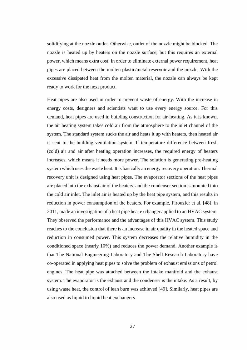
Citation preview

HEAT DISSIPATION FROM ELECTRONIC PACKAGES WITH THE HELP OF
HEAT PIPE NETWORK AND ITS APPLICATION TO ROTARY PLATFORMS
A THESIS SUBMITTED TO
THE GRADUATE SCHOOL OF NATURAL AND APPLIED SCIENCES
OF
MIDDLE EAST TECHNICAL UNIVERSITY
BY
ANIL ÇALIŞKAN
IN PARTIAL FULFILLMENT OF THE REQUIREMENTS
FOR
THE DEGREE OF MASTER OF SCIENCE
IN
MECHANICAL ENGINEERING
SEPTEMBER 2015

ii
iii
Approval of the thesis:
HEAT DISSIPATION FROM ELECTRONIC PACKAGES WITH THE HELP
OF HEAT PIPE NETWORK AND ITS APPLICATION TO ROTARY
PLATFORMS
submitted by ANIL ÇALIŞKAN in partial fulfillment of the requirements for the
degree of Master of Science in Mechanical Engineering Department, Middle East
Technical University by,
Prof. Dr. Gülbin Dural Ünver
Dean, Graduate School of Natural and Applied Sciences
Prof. Dr. R.Tuna Balkan
Head of Department, Mechanical Engineering Dept.
Assoc. Prof. Dr. İlker Tarı
Supervisor, Mechanical Engineering Dept., METU
Examining Committee Members:
Assoc. Prof. Dr. Cemil Yamalı
Mechanical Eng. Dept., METU
Assoc. Prof. Dr. İlker Tarı
Mechanical Eng. Dept., METU
Assoc. Prof. Dr. Derek K. Baker
Mechanical Eng. Dept., METU
Assoc. Prof. Dr. Tuba Okutucu Özyurt
Mechanical Eng. Dept., METU
Assoc. Prof. Dr. Cemil Koçar
Nuclear Eng. Dept., Hacettepe University
Date: 11.09.2015

iv
I hereby declare that all information in this document has been obtained and
presented in accordance with academic rules and ethical conduct. I also declare
that, as required by these rules and conduct, I have fully cited and referenced all
material and results that are not original to this work.
Name, Last name: Anıl ÇALIŞKAN
Signature:
v
ABSTRACT
HEAT DISSIPATION FROM ELECTRONIC PACKAGES ON ROTARY
PLATFORMS WITH THE HELP OF HEAT PIPE NETWORKS
Çalışkan, Anıl
M.S., Department of Mechanical Engineering
Supervisor: Assoc. Prof. Dr. İlker Tarı
September 2015, 144 pages
An electronics package on a rotary platform including two components with 600 W,
one component with 350 W and one small component with 70 W heat dissipation rates
(1620 W total heat load) is numerically and experimentally investigated under steady
state conditions. In order to avoid rotary joints and to reduce the costs of design,
maintenance and production, the thermal management solution for the heat dissipation
is entirely placed on the rotary platform. The thermal management solution includes
heat sinks attached to the vertical side surfaces of the platform and heat pipes
connected to heat sinks. The heat dissipating components are connected to the heat
sinks with heat pipes. The heat sinks are cooled by forced convection with high power
fan assemblies. Two different fin configurations are considered. One of them is a pin
fin design and the other one is a plate fin covered with duct design. The thermal
management systems are numerically modeled and then one of the numerical models
is validated with a set of experiments. The validated model is used for the optimization
of the system and as a demonstration of feasibility of the heat pipes. The optimization
parameters are the heat pipe locations, their connections to the heat sinks and
geometrical properties of the heat sinks. The optimization criteria are to maintain
nearly uniform temperature distributions on the heat sinks and to keep critical

vi
components below their thermal shut-down points. The constraints are the lengths of
the standard heat pipes and the limited options to bend the heat pipes due to their fragile
structures. The success of the system is that it can keep the hot spot temperatures below
the allowed maximum temperature of 120 oC even for the case of 50 °C ambient air
temperature. The limitation of 120 oC working temperature comes from the thermal
shut-down limits of the components in the electronics package.
Keywords: Electronics cooling, Forced convection, Rotary platforms, Heat sinks,
Heat pipes, CFD

vii
ÖZ
ISI BORUSU AĞLARI YARDIMIYLA ELEKTRONİK PAKETLERDEN ISI
ATIMI VE BUNUN DÖNER TABLALARA UYGULANMASI
Çalışkan, Anıl
Yüksek Lisans, Makina Mühendisliği Bölümü
Tez Yöneticisi: Doç. Dr. İlker Tarı
Eylül 2015, 144 sayfa
Döner platform üzerinde bulunan, 600 W’lık 2 adet, 350 W’lık 1 adet ve küçük bir 70
W’lık ısı atım kapasitesine sahip olan bileşenlerden oluşan (toplamda 1620 W’lık ısı
atımı) bir elektronik paket sabit koşullar altında sayısal ve deneysel olarak
incelenmiştir. Döner (hareketli) bağlantılardan kaçınmak ve tasarım, bakım, üretim
maliyetini azaltmak için, ısı atımı için kullanılan termal yönetim çözümü tamamen
döner platform üzerine yerleştirilmiştir. Termal yönetim çözümü platformun yanal
yüzeyine tutturulmuş soğutucuları ve bunlara bağlı ısıl boruları içerir. Elektronik paket
içerisindeki ısı atımı yapan bileşenler soğutuculara ısıl borularla bağlıdır. Soğutucular
yüksek güçlü fanlar yardımıyla zorlamalı ısı taşınımı ile soğutulmuştur. Bu kapsamda
iki farklı soğutucu tasarımı üzerinde durulmuştur. Bunlardan biri pin soğutucu tipi,
diğeri ise düz plaka soğutucu tipi tasarımıdır. Oluşturulan bu termal yönetim sistemleri
sayısal olarak modellenmiş ve seçilen örnek sayısal model deney çalışması ile
doğrulanmıştır. Doğrulanmış model, ısıl boruların güvenilirliğinin ispatlanmasında ve
sistemin en uygun duruma getirilmesinde kullanılmıştır. En uygun duruma getirme
değişkenleri ise ısıl boruların yerleri, boruların soğutuculara olan bağlantıları ve
soğutucu blokların geometrik yapılarıdır. En uygun durum ölçütü ise soğutucular
üzerinde eş ısıl dağılımlarının oluşturulması ve önemli yüzeylerin ısıl-kapanma sınırı

viii
altında kalmasıdır. Standart ısıl boruların uzunluğu ve kırılgan yapıları nedeniyle
boruları bükmede sınırlı seçenek olması kısıtlamalara neden olmuştur. Sistem başarısı
ise 50 oC çevresel sıcaklıkta, sıcak bölge sıcaklığını izin verilen azami 120 oC altında
tutabilmesidir. 120 oC sınırı elektronik paket içerisinde bulunan bileşenlerin, ısıl-
kapanma sınırından gelmektedir.
Anahtar Kelimeler: Elektronik soğutma, Zorlamalı ısı taşınımı, Döner platformlar,
Soğutucular, Isı boruları, CFD, Bilgisayar Destekli Akışkanlar Mekaniği

ix
To my family

x
ACKNOWLEDGEMENTS
The author would like to express his sincere appreciation to his supervisor Assoc. Prof.
Dr. İlker TARI for his continuous guidance, support, encouragement, inspiration and
patience throughout the progress of this study. Besides, the author is very grateful to
find a chance of being a master student of his supervisor. The committee members of
thesis are appreciated for their valuable comments and suggestions on the contents of
this study.
This study is a project, which is supported by ASELSAN Inc. and Republic of Turkey
Ministry of Science, Industry and Technology as SAN-TEZ project 0233.STZ.2013.
The author would like to thank both ASELSAN Inc. and Republic of Turkey Ministry
of Science, Industry and Technology for financial support. In addition to this,
ASELSAN Inc. is thanked due to providing manufacturing and testing background.
The author is thankful to his colleagues Mehmet YENER, Hakan BORAN, Murat
PARLAK and Çağrı BALIKÇI for valuable contribution about applications of
electronic cooling and heat pipe. Apart from appreciations to all, the author is grateful
to find working together with Çağrı BALIKÇI in SANTEZ project and this study.
The author would to declare his graces about Suna KIYAK, who always supports
during the study and helps during writing period of the thesis.
Finally, for their understanding, endless patience and encouragement throughout his
study, his sincere thanks go to his parents, Recai ÇALIŞKAN and Aysel ÇALIŞKAN,
and his sister, Sırma ÇALIŞKAN.
xi
TABLE OF CONTENTS
ABSTRACT ................................................................................................................. v
ÖZ .............................................................................................................................. vii
ACKNOWLEDGEMENTS ......................................................................................... x
TABLE OF CONTENTS ............................................................................................ xi
LIST OF TABLES .................................................................................................... xiv
LIST OF FIGURES ................................................................................................... xv
LIST OF ABBREVIATIONS ................................................................................... xix
CHAPTERS ................................................................................................................. 1
1. INTRODUCTION ................................................................................................... 1
1.1 Motivation of the Study ............................................................................... 1
1.2 Electronic Cooling Techniques .................................................................... 3
1.2.1 Conduction and Thermal Interface Materials ........................................ 5
1.2.2 Convection Cooling ............................................................................... 7
1.2.2.1 Air Cooling ..................................................................................... 8
1.2.2.2 Liquid Cooling .............................................................................. 10
1.2.2.2.1 Single Phase Liquid Cooling .................................................... 12
1.2.2.2.2 Liquid Cooling with Micro-channels and Mini-channels ........ 12
1.2.2.2.3 Two Phase Liquid Cooling ....................................................... 13
1.2.2.2.4 Spray Cooling ........................................................................... 14
1.2.2.2.5 Jet Impingement ....................................................................... 14
1.2.3 Thermo-electric Cooling (TEC) ........................................................... 15
1.2.4 Heat Pipe .............................................................................................. 15
1.3 Summary of Cooling Techniques ............................................................ 16
1.4 Objective of Study...................................................................................... 17
2. THEORY AND LITERATURE SURVEY ........................................................... 21
2.1 Historical Development of Heat Pipe ........................................................ 21
2.2 Applications and Advantages of Heat Pipes .............................................. 24
2.3 Working Principles of Heat Pipes ................................................................. 29
xii
2.4 Wick Structures of Heat Pipes ................................................................... 31
2.5 Limitations of Heat Pipes ........................................................................... 32
2.5.1 Viscous Limit ....................................................................................... 34
2.5.2 Sonic Limit ........................................................................................... 34
2.5.3 Entrainment / Flooding Limit ............................................................... 35
2.5.4 Capillary Limit ..................................................................................... 36
2.5.5 Boiling Limit ........................................................................................ 37
2.6 Heat Pipe Arrangement and Operations ..................................................... 38
2.6.1 Horizontal Orientation .......................................................................... 39
2.6.2 Gravity Aided ....................................................................................... 39
2.6.3 Gravity Against .................................................................................... 40
2.7 Heat Pipe – Heat Sink Performance [57] ................................................... 40
3. PRELIMINARY DESIGNS AND NUMERICAL ANALYSIS ........................... 43
3.1 Military Rotary Platforms .......................................................................... 43
3.2 Used Software ........................................................................................... 45
3.3 Selection of Heat Pipe ................................................................................ 49
3.3.1 How to Select a Heat Pipe? .................................................................. 49
3.3.2 The Construction Material of Heat Pipe .............................................. 51
3.3.3 Wick Structure of Heat Pipe ................................................................. 53
3.4 CAD Design of the Whole Structure .......................................................... 54
3.5 Preliminary Numerical Analyses ............................................................... 56
3.5.1 Procedures of Numerical Analyses ...................................................... 57
3.5.2 Results and Discussions of Numerical Analyses ................................. 61
4. EXPRIMENTAL PROCEDURES AND RESULTS ............................................. 73
4.1 Manufacturing of Experimental Setup ....................................................... 73
4.2 Preparation of Experiment Setup ............................................................... 79
4.3 Results of Experiment ................................................................................ 85
4.3.1 Results Collected From Data Acquisition System and Discussions .... 86
4.3.2 Results Collected From Thermal Camera and Discussions ................. 91
4.4 Uncertainty Analysis .................................................................................. 96
5. OPTIMIZATION ................................................................................................... 99
5.1 Corrected Analysis of Pin Fin Heat Sink Configuration ............................ 99

xiii
5.2 Optimization of Plate Fin Heat Sink Configuration ................................. 104
5.2.1 Procedures of ‘What If’ Analysis ....................................................... 105
5.2.2 Results and Discussions of ‘What If’ Analyses ................................. 107
6. RESULTS AND DISCUSSION .......................................................................... 113
7. CONCLUSION .................................................................................................... 121
REFERENCES ......................................................................................................... 123
APPENDICES ......................................................................................................... 129
A. Design Items ........................................................................................................ 129
B. Equipments of Experiment .................................................................................. 135
C. Optimization Graphs ........................................................................................... 141
D. Results of Corrected Experiment ........................................................................ 143
xiv
LIST OF TABLES
TABLES
Table 1.1 Thermal Conductivities of Some Common Materials ................................. 5
Table1.2 Cooling Techniques and Respective Heat Fluxes and Heat Transfer
Coefficients (Glassman, 2005) [20] ........................................................................... 17
Table 2.1 Heat transport limits of heat pipe [53] ....................................................... 33
Table 3.1 Typical Operating Characteristics of Heat Pipes [68] ............................... 52
Table 3.2 Dimensions of Computational Domain ..................................................... 58
Table 3.3 Heat Source of the System ........................................................................ 59
Table 3.4 Mesh Independence Study: the change of Heater 1 average surface
temperature with the number of cells in the model at 50 oC ambient temperature .... 62
Table 4.1 Dimensions and quantities of used heat pipes ........................................... 75
Table 4.2 Specifications and dimensions of heaters .................................................. 79
Table 4.3 Used devices during the experiment .......................................................... 84
Table 4.4 Calibration parameters of thermal camera ................................................ 91
Table 4.5 Results of experimental runs ..................................................................... 96
Table 4.6 Average percentage uncertainty of temperatures of all heaters ................. 97
Table 5.1 Change in the average surface temperature distribution on the surface of
heaters 1.1 and 1.2 with changed geometrical design variables ............................... 107
Table 6.1 Comparison between numerical % relative temperature difference and
experimental % relative temperature difference ...................................................... 114
Table 6.2 Comparison between corrected numerical % relative temperature difference
and corrected experimental % relative temperature difference after re-production of
fins ............................................................................................................................ 118
Table A.1 Product ingredient information of Artic Silver 5 .................................... 130
Table A.2 Technical features of EBM Papst 8214 JH3 ........................................... 132
Table A.3 Technical data for Laird T-flex 640 ....................................................... 133
Table B.1 Properties of Agilent HP 34970A data logger ........................................ 135
Table B.2 Flir E60 infrared camera specifications .................................................. 140

xv
LIST OF FIGURES
FIGURES
Figure 1.1 (a) Babbage’s mechanical computer [1] (b) ENIAC, first fully functional
digital computer [1] (c) IBM ACORN, first personal computer [1] (d) APPLE
MacBook Air, one of the thinnest ultra-books [2] ....................................................... 2
Figure 1.2 Heat transfer coefficient attainable with natural convection, single-phase
liquid forced convection and boiling for different coolants [5] ................................... 4
Figure 1.3 The Section of Thermacore’s K-Core [7] .................................................. 6
Figure 1.4 The illustration of gap between two solid and temperature drop due to
imperfect contact .......................................................................................................... 7
Figure 1.5 Example of a product cooled by natural convection [8] ............................ 9
Figure 1.6 Schematic of liquid cooling system ......................................................... 11
Figure 1.7 Scheme of two phase liquid cooling system design [13] ......................... 13
Figure 1.8 Layers of TECs (Peltier Cooler) [16] ...................................................... 15
Figure 1.9 Examples of Rotary Platforms (a) ASELSAN Naval System [31] and (b)
ASELSAN Automatic Weapons System [32] ............................................................ 18
Figure 2.1 Gaugler’s patent drawing [34] ................................................................. 22
Figure 2.2 Temperature gradient of satellite with/without heat pipes [47] ............... 26
Figure 2.3 Heat pipe application in Alaska pipeline with permafrost ground [51] ... 28
Figure 2.4 Internal design of Apple MacBook Pro [52] ........................................... 29
Figure 2.5 The working operation of heat pipe [53] ................................................. 30
Figure 2.6 Usage Limitations of Heat Pipe, Axial Flux vs Temperature [54] .......... 32
Figure 2.7 The Resistance Network of Heat Pipe ..................................................... 40
Figure 3.1 SPINNER High-quality hybrid rotary joints are mainly used in military
radar systems, fire control systems, rotating vehicle-mounted camera systems and in
mobile battlefield communication systems [62] ........................................................ 45
Figure 3.2 Diameter effects on heat pipe performance. Heat pipe is water copper
groove type and at vertical orientation (gravity assist) [68] ...................................... 50
xvi
Figure 3.3 Enertron’s actual test results of heat pipe with different wick structure at
horizontal (gravity against) orientation [68] .............................................................. 53
Figure 3.4 Enertron’s actual test results of heat pipe with different wick structure at
vertical (gravity assist) orientation [68] ..................................................................... 54
Figure 3.5 CAD model of Pin Fin Configuration, which will be used in experiment
.................................................................................................................................... 55
Figure 3.6 Sample CAD model of Rectangular Channel Type Configuration ......... 55
Figure 3.7 Flow Chart of Preliminary Procedures ................................................... 56
Figure 3.8 Temperature Distributions on Heaters (50 oC ambient, pin fin
configuration) ............................................................................................................. 64
Figure 3.9 The Cut-View of Platform, with mesh and temperature distribution ...... 65
Figure 3.10 Temperature Distributions on Heaters (25oC ambient, pin fin
configuration) ............................................................................................................. 66
Figure 3.11 Iteration Numbers vs Iterations for Pin Fin Configuration @ 25 oC ..... 67
Figure 3.12 Temperature Distributions on Heaters (50 oC ambient, rectangular plate
fin with duct structured) ............................................................................................. 68
Figure 3.13 Temperature Distributions on Heaters (25oC ambient, rectangular plate
fin with duct structured) ............................................................................................. 69
Figure 3.14 Temperature Distribution on Right Fin (8 heat Pipes Connected) ........ 70
Figure 3.15 Temperature Distribution on Left Fin (9 heat Pipes Connected) ........... 70
Figure 3.16 Exhaust Air Temperature Distribution on Right Fin (8 heat Pipes
Connected) ................................................................................................................. 71
Figure 3.17 Exhaust Air Temperature Distribution on Left Fin (9 heat Pipes
Connected) ................................................................................................................. 71
Figure 4.1 Cross-section of sintered wick heat pipe ................................................. 74
Figure 4.2 Manufactured dummy rotary platform ..................................................... 74
Figure 4.3 Filler material is applied to mounting holes ............................................ 76
Figure 4.4 Heat pipes are mounted into mounting holes of pin fin ........................... 77
Figure 4.5 Condenser module ................................................................................... 77
Figure 4.6 The final mounting of heat pipes ............................................................. 78
Figure 4.7 Heaters (a) Heater 2 (350W) (b) Heater 1(600W) (c) Heater 3 (70W) ... 79
Figure 4.8 Sample view of thermocouple’s location ................................................. 81
xvii
Figure 4.9 Heater mounting with gap filler ‘Laird Tflex 600’ .................................. 82
Figure 4.10 Experimental setup with dummy platform ............................................ 82
Figure 4.11 Illustration of labeled heaters ................................................................. 86
Figure 4.12 Average surface temperature of Heater 1.1 ........................................... 87
Figure 4.13 Average surface temperature of Heater 1.2 ........................................... 87
Figure 4.14 Average surface temperature of Heater 2 .............................................. 88
Figure 4.15 Average surface temperature of Heater 3 .............................................. 89
Figure 4.16 Illustration of Thermocouple couples’ place on heat pipe ..................... 89
Figure 4.17 Temperature Distributions of Longest Heat Pipe .................................. 90
Figure 4.18 Temperature distributions on all heaters ................................................ 92
Figure 4.19 Average temperature distributions on heaters ....................................... 93
Figure 4.20 Temperatures on pin fin heat sink.......................................................... 94
Figure 4.21 Temperatures of connections on pin fin heat sink ................................. 94
Figure 4.22 Axial temperature distribution on selected heat pipe............................. 95
Figure 4.23 Bending effect on the performance of heat pipe .................................... 95
Figure 5.1 Mesh refinement of FloEFD and Cut View of Mesh Distribution from the
Back Side of Platform .............................................................................................. 101
Figure 5.2 Final Temperature Distributions on Heaters .......................................... 101
Figure 5.3 Temperature Distributions on Pin Fins (Left Side of Platform) ............ 102
Figure 5.4 Temperature Distributions on Pin Fins (Right Side of Platform) .......... 103
Figure 5.5 The view of isothermal temperature distributions on heaters at experimental
stage.......................................................................................................................... 104
Figure 5.6 Average Surface Temperature Distributions of Heaters (Rectangular Plate
Fin with Duct Structured with 5 mm Thickness and 3 mm Spacing) ...................... 109
Figure 5.7 Average Surface Temperature Distribution on Right Fin (8 heat pipes are
connected) ................................................................................................................ 110
Figure 5.8 Average Surface Temperature Distribution on Right Fin (8 heat pipes are
connected) ................................................................................................................ 111
Figure 6.1 Average surface temperature of Heater 1.2 after manufacturing
improvement ............................................................................................................ 116
Figure 6.2 Observation for dry-out phenomena ...................................................... 117
Figure A.1 Specification and dimensions Alpha Novatech S20100 series ............. 129
xviii
Figure A.2 Artic Silver 5 ......................................................................................... 130
Figure A.3 View of EBM Papst 8214 JH3 and its nominal data ............................. 131
Figure A.4 Fan curve of EBM Papst 8214 JH3 ....................................................... 131
Figure B.1 Agilent HP 34970A data logger ............................................................ 135
Figure B.2 Agilent 6032A system power supply 0-60V /0-50A, 1000W ............... 136
Figure B.3 Agilent 6692A DC power supply 0-60V /0-110A ................................ 137
Figure B.4 HP 6573A System DC Power Supply 0-35V /0-60A ........................... 138
Figure B.5 Agilent E3634A DC Power Supply 0-25V, 7A / 0-50V, 4A ................ 139
Figure C.1 Result of optimization for 3 mm fin thickness vs variable spacing ...... 141
Figure C.2 Result of optimization for 4 mm fin thickness vs variable spacing ...... 141
Figure C.3 Result of optimization for 5mm fin thickness vs variable spacing ....... 142
Figure C.4 Result of optimization for 6 mm fin thickness vs variable spacing ...... 142
Figure D.1 Result of corrected experiment for heater 1.1 ....................................... 143
Figure D.2 Result of corrected experiment for heater 1.2 ....................................... 143
Figure D.3 Result of corrected experiment for heater 2 .......................................... 144
Figure D.4 Result of corrected experiment for heater 3 .......................................... 144

xix
LIST OF ABBREVIATIONS
Abbreviations
APG Annealed Pyrolytic Carbon
CAD Computer Aided Drawing
CFD Computational Fluid Dynamics
FVM Finite Volume Method
HVAC Heating, Venting and Cooling
LRU Line Replaceable Unit
LTCC Low Temperature Co-firing Ceramic
TEC Thermo-Electronic Cooling
TWT Travelling Wave Tube
PA Power Amplifier
PCB Printed Circuit Board
RF Radio Frequency
SIMPLE Semi-Implement Method for Pressure-Linked Equations
Nomenclature
A Area (mm2 or m2)
Ablock Heat Input Area of Evaporator Block (mm2 or m2)
Afin Total Surface Area of Fin(mm2 or m2)
As Surface Area (mm2 or m2)
Av Surface Area of Vapor Section (mm2 or m2)
xx
Cp Specific Heat of Air (kJ/(kg.K))
Dh Hydraulic Diameter (mm)
DHP Diameter of Heat Pipe (mm)
DVS Diameter of Heat Pipe Vapor Space (mm)
δ Enthalpy of Vaporization (J)
ε Turbulent Dissipations
ΔPcap Pressure Drop due to Capillary Limit
ΔPg Pressure Drop due to Gravitational Effect
ΔTair Temperature Difference of Cooling Air Flow
ΔTblock Temperature Difference of Evaporator Block
ΔTconv Temperature Difference due to Convection
ΔTfin Temperature Difference of Fin
ΔTHP Temperature Difference of Heat Pipe
ΔTinter Temperature Difference of Evaporator Block / Heat Pipe
Interface
ΔTtotal Total Temperature Changes
g Acceleration of Gravity (m/s2)
Gr Groshof Number
h Convection Coefficient (W/(m2.K))
hf Convection Coefficient of Fluid (W/(m2.K))
I Turbulence Intensity (%)
ηfin Fin Efficiency
k Turbulent Kinetic Energy
k Thermal Conductivity (W/(m.K))
kblock Thermal Conductivity of Evaporator Block (W/(m.K))
kfin Thermal Conductivity of Fin (W/(m.K))

xxi
L Length (mm or m)
LCond Length of Condenser Section (mm)
LEff Effective Length of Heat Pipe (mm)
Lfineff Effective Fin Length (mm)
Levap Length of Evaporator Section (mm)
ls Turbulent Length (mm)
mfin Fin Factor for Uniform Cross-sectional Area
µv Dynamic Viscosity of Vapor Phase (Pa.s)
Q Heat Load to be Dissipated (W)
θ Angle Between a Heat Pipe and Horizontal Plane
qent Heat Transfer Rate for Avoiding Entrainment Limit
qsonic Heat Transfer Rate for Avoiding Sonic Limit
qvis Maximum Axial Heat Transfer Rate Reaching Viscous Limit
Pr Prandtl Number
Pv Vapor Pressure (Pa)
Rair Thermal Resistance of Cooling Air Flow (oC/W or K/W)
Raxial Thermal Resistance Along Heat Pipe (oC/W or K/W)
Rblock Thermal Resistance of Evaporator Block (oC/W or K/W)
Rcond Thermal Resistance of Conduction Heat Pipe and Its Contact
(oC/W or K/W)
Rcondenser Thermal Resistance of Heat Pipe Condenser (oC/W or K/W)
Revaporator Thermal Resistance of Heat Pipe Evaporator (oC/W or K/W)
Rfin Thermal Resistance of fin (oC/W or K/W)
RHP Thermal Resistance of Heat Pipe (oC/W or K/W)
Rinter Thermal Resistance of Evaporator Block / Heat Pipe Interface
(oC/W or K/W)
Rs-a Thermal Resistance of Heat Sink to Ambient (oC/W or K/W)
xxii
Rwall Thermal Resistance of Heat Pipe’s Wall (oC/W or K/W)
Re Reynold Number
rσ Effective Radius of Wick (mm)
ρ Density (g/cm3)
ρv Density of Vapor Phase (g/cm3)
σ Surface Tension for Working Liquid (N/mm)
t Thickness (mm)
tblock Thickness of Evaporator Block (mm)
tfin Thickness of Fin (mm)
T∞ Ambient Temperature (oC or K)
v Velocity (m/s)
x Characteristic Dimension of Wick Structure
Subscripts
a Air
cap Capillary Limit
cond Conduction
conv Convection
eff Effective
ent Entrainment Limit
evap Evaporator
fluid Fluid
g Gravitational
HP Heat Pipe
inter Interface

xxiii
liq Liquid
surr Surrounding
surf Surface
v Vapor
vis Viscous Limit
VS Vapor Space

xxiv

1
CHAPTER 1
INTRODUCTION
The main topic of this thesis is the application of forced convection cooling to
electronics on rotary platforms which is a very common application for the defense
electronics industry. In this chapter, a general overview of the topic will be covered
together with the motivation and the objectives of the study.
1.1 Motivation of the Study
The defense electronics industry has been continuously developing following the
trends in other high technology areas. One of the biggest trends is miniaturization. This
trend can be traced back to the introduction of electronics and computers to our lives.
Computers are probably the best illustration of how fast the technology has been
evolving. At the beginning of the information age, conceptual design of the first
computer created by Charles Babbage in 1822 (see Fig. 1.1a), was totally mechanical,
and it might have only mechanical problems, which means there were no other
complicated problems. In 1936, Konrad Zuse made the first electro-mechanical
computer, and it was the first step where the complicated problems started. In 1946,
ENIAC (see Fig. 1.1b) was the first digital computer, which occupied about 1,800
square feet area (approximately 167 m2) and used about 18,000 vacuum tubes,
weighing almost 50 tons, which means a very large room was required for that
computer that can make only thousands of calculations in a second [1]. In the middle
of 1950s, the first personal computers (see Fig. 1.1c) were introduced with more
compact designs after a significant decrease in their dimensions. The reduction in size
requires smaller components and the improvements in computing capability requires
more power, combination of both leading to more heat dissipation per unit area.

2
Recently, as a consequence of the mobility trend in electronic devices, there are many
small and micro devices produced with high power consumptions requiring dissipation
of very high heat fluxes (e.g. Fig. 1.1d).
(a) (b)
(c) (d)
Miniaturization of electronics is achieved with the miniaturization of the microchips
made out of semiconductor materials. These materials are very sensitive to working
temperatures. If they are not properly cooled, they may malfunction or may get
permanently damaged due to high heat fluxes. If ‘Moore’s Law’, which was suggested
by Gordon Moore of INTEL Corporation in 1965 [3], continues to hold, more powerful
semiconductor devices will continue to be placed in smaller and smaller areas, year
Figure 1.1 (a) Babbage’s mechanical computer [1] (b) ENIAC, first fully functional
digital computer [1] (c) IBM ACORN, first personal computer [1] (d) APPLE
MacBook Air, one of the thinnest ultra-books [2]

3
after year, causing the heat transfer problems we encounter with to get more and more
challenging in the future.
Dissipation of waste heat is a problem in every area such as electronic devices, an
engine of a car, air-conditioner system. In electronic devices, it is even a bigger
problem due to miniaturization and the temperature sensitivity of the semiconductors.
Semiconductor microcircuits should be maintained below their maximum allowable
temperature limit during their operation. At steady state, waste heat should be
continuously dissipated to keep the device at a certain temperature. In military
electronics, ambient temperatures may be much higher than the ones dealt with in
consumer electronics making heat dissipation more difficult due to lower temperature
differences through which high heat fluxes should be dissipated. In our case, since we
dissipate the heat from military electronics on a rotary platform, heat transfer problem
gets more difficult and more complicated, further. Creating a solution for this
challenging problem is the motivation of this study.
1.2 Electronic Cooling Techniques
Heat transfer can be defined as thermal energy transfer from a hot reservoir (source)
to a cold reservoir (sink). Heat transfer occurs in three different modes, namely
conduction, convection and radiation. Generally, in electronic system design,
conduction is used for basic design and for spreading heat on the base material;
convection and radiation are used for eliminating or removing dissipated heat from the
system to the surroundings. The thermal resistance in convection mechanism is higher
than conduction and radiation resistances thus cooling behavior of the packaged
system is mostly determined by convection [4].
High power military electronic devices mostly use forced convection with air or liquid
flow. However less power dissipating military products use natural convection which
is simpler and more reliable. In military device design, conduction performance is
improved by using proper materials such as aluminum and copper due to their high
thermal conductivity. Radiation is only considered in harsh environmental conditions
e.g. in oceans and deserts. In a suitable environment, radiation can support the system

4
by cooling it. On the other hand, solar load is a big problem in ocean and desert
environments, which may make the system a heat sink for the high temperature
surroundings. The radiation mechanism may start to heat up the system.
Figure 1.2 shows a comparison of various cooling techniques as a function of the
attainable heat transfer in terms of the heat transfer coefficient. To accommodate a
heat flux of 100 W/cm2 at a temperature difference of 50 K requires an effective heat
transfer coefficient (including a possible area enlargement factor) of 20,000 W/m2K
[5].
Figure 1.2 Heat transfer coefficient attainable with natural convection, single-phase
liquid forced convection and boiling for different coolants [5]
Although liquid forced convection may lead to better cooling performance, designers
cannot use it easily due to design limitations such as size, cost and reliability. In
contrast, all standard cooling techniques have physical limitations in terms of heat
transfer capacity. These techniques are limited by the thermal conductivity of air for
convection and the thermal conductivity of copper (the best pure material with the
highest thermal conductivity) for conduction. To eliminate or to reduce the effects of
these limitations, engineers developed many techniques. Some of these techniques are
summarized below.
5
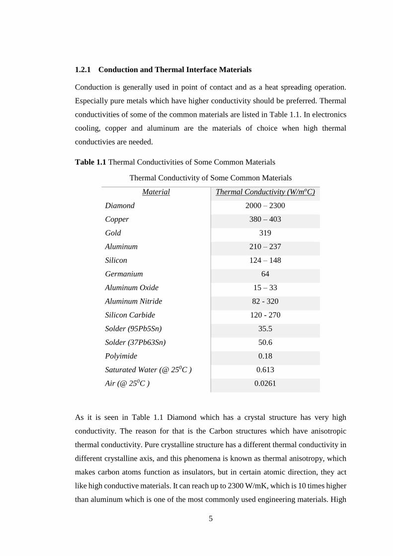
1.2.1 Conduction and Thermal Interface Materials
Conduction is generally used in point of contact and as a heat spreading operation.
Especially pure metals which have higher conductivity should be preferred. Thermal
conductivities of some of the common materials are listed in Table 1.1. In electronics
cooling, copper and aluminum are the materials of choice when high thermal
conductivies are needed.
Table 1.1 Thermal Conductivities of Some Common Materials
Thermal Conductivity of Some Common Materials
Material Thermal Conductivity (W/moC)
Diamond 2000 – 2300
Copper 380 – 403
Gold 319
Aluminum 210 – 237
Silicon 124 – 148
Germanium 64
Aluminum Oxide 15 – 33
Aluminum Nitride 82 - 320
Silicon Carbide 120 - 270
Solder (95Pb5Sn) 35.5
Solder (37Pb63Sn) 50.6
Polyimide 0.18
Saturated Water (@ 250C ) 0.613
Air (@ 250C ) 0.0261
As it is seen in Table 1.1 Diamond which has a crystal structure has very high
conductivity. The reason for that is the Carbon structures which have anisotropic
thermal conductivity. Pure crystalline structure has a different thermal conductivity in
different crystalline axis, and this phenomena is known as thermal anisotropy, which
makes carbon atoms function as insulators, but in certain atomic direction, they act
like high conductive materials. It can reach up to 2300 W/mK, which is 10 times higher
than aluminum which is one of the most commonly used engineering materials. High
6
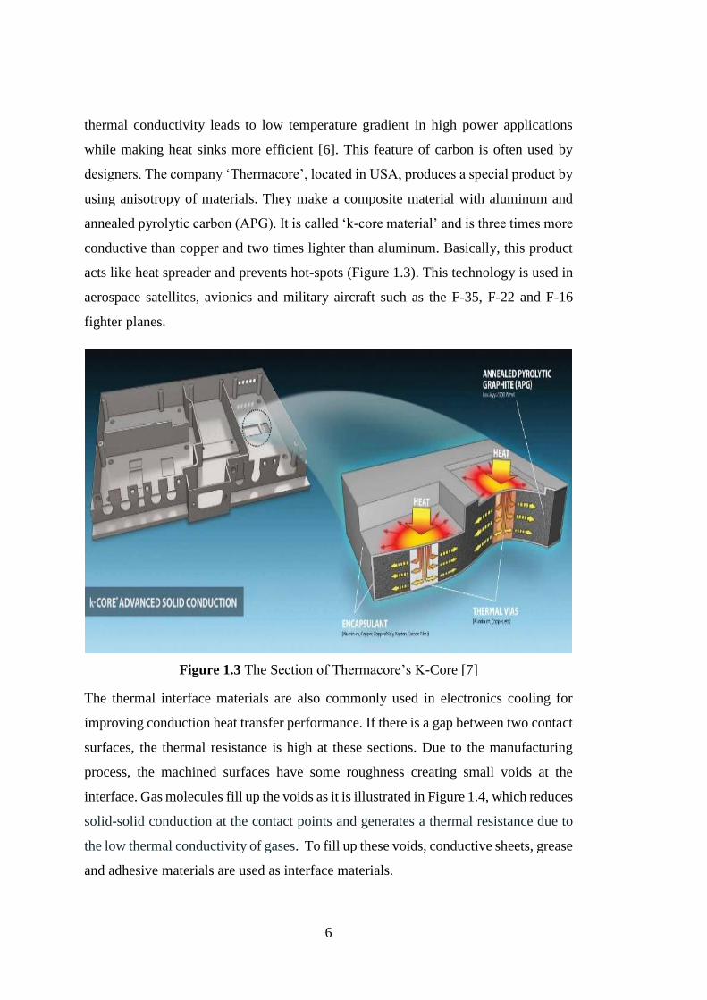
thermal conductivity leads to low temperature gradient in high power applications
while making heat sinks more efficient [6]. This feature of carbon is often used by
designers. The company ‘Thermacore’, located in USA, produces a special product by
using anisotropy of materials. They make a composite material with aluminum and
annealed pyrolytic carbon (APG). It is called ‘k-core material’ and is three times more
conductive than copper and two times lighter than aluminum. Basically, this product
acts like heat spreader and prevents hot-spots (Figure 1.3). This technology is used in
aerospace satellites, avionics and military aircraft such as the F-35, F-22 and F-16
fighter planes.
Figure 1.3 The Section of Thermacore’s K-Core [7]
The thermal interface materials are also commonly used in electronics cooling for
improving conduction heat transfer performance. If there is a gap between two contact
surfaces, the thermal resistance is high at these sections. Due to the manufacturing
process, the machined surfaces have some roughness creating small voids at the
interface. Gas molecules fill up the voids as it is illustrated in Figure 1.4, which reduces
solid-solid conduction at the contact points and generates a thermal resistance due to
the low thermal conductivity of gases. To fill up these voids, conductive sheets, grease
and adhesive materials are used as interface materials.

7
Figure 1.4 The illustration of gap between two solid and temperature drop due to
imperfect contact
1.2.2 Convection Cooling
Heat transfer between a solid and an adjacent moving fluid such as liquid or gas is
known as convection heat transfer. The main requirement is the fluid, and there must
also be a temperature gradient as the driving force. Increase in the temperature gradient
results in an increase in the performance of the heat transfer.
𝑄𝑐𝑜𝑛𝑣 = ℎ𝑓𝐴𝑠𝑢𝑟𝑓∆𝑇 (1.2)
∆𝑇 = 𝑇𝑠𝑢𝑟𝑓 − 𝑇∞ (1.3)
The governing equation for convective heat transfer is given in Equation 1.2, which is
known as Newton’s law of cooling. Convection heat transfer depends on the type of
fluid (Prandtl number of the fluid), flow conditions (Reynolds number of the flow),
fluid interaction area and the temperature difference between the surface and the
ambient (Eq. 1.3). Engineers design the cooling system according to these parameters.
They can increase the interaction areas by using specific geometries and increase the
heat transfer coefficient by choosing the proper fluid or conditioning the fluid. Two
main types of cooling relying on convection are explained below.
8
1.2.2.1 Air Cooling
There are two different air cooling methods: by natural convection and by forced
convection. In military electronics, less power consuming devices use natural
convection for its low cost and high reliability. For high power consuming devices,
forced convection is often used.
Natural convection system guarantees the long term reliability and reduction in cost;
however, it is restricted to low heat dissipation values. It is also a type of passive
cooling because there is no need for any external power. In the military products with
low heat dissipating units such as walkie-talkies, low power control computers, rugged
ATR chassis etc. and in the commercial marketing products such as radios, TVs,
smartphones etc., natural convection is used. The main goal in natural convection
design is to maximize the convection area. This is done by using properly designed fin
structures because other parameters of air cannot be controlled in natural convection.
The heat transfer coefficient for natural convection is given with;
ℎ𝑐𝑜𝑛𝑣 ∝𝑘𝑓𝑙𝑢𝑖𝑑
𝐿(Pr 𝐺𝑟)𝑛 (1.4)
Where kfluid is the thermal conductivity of fluid, L is the length of the surface which is
controlled by design engineers, Pr is the Prandtl Number and Gr is the Grashof
Number. Pr and kfluid are the material properties. Gr is the ratio of buoyant and viscous
forces and depends on the surface geometry, fluid properties and the temperature
difference between the surface and the fluid. The chosen geometry, fin structure, must
support the buoyancy effect of the air. (Figure 1.5). Geometry plays an important role
in natural convection systems.
9
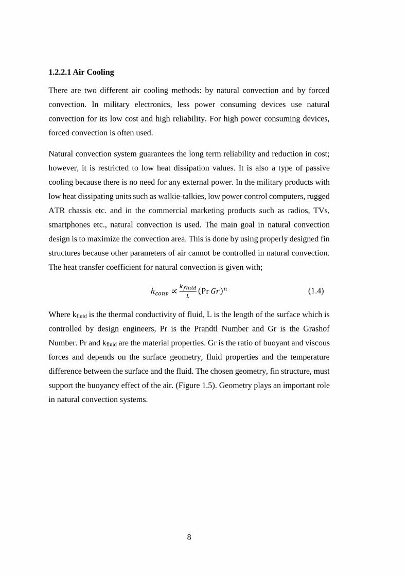
Figure 1.5 Example of a product cooled by natural convection [8]
The biggest obstacle in natural convection is localized hot spots because natural
convection has limited heat carrying capacity. Maximum heat flux obtained with
natural convection in electronic devices is just 0.05 W/cm2 [9]. This result
demonstrates that the thermal resistance for natural convection is too high due to the
low conductivity of air (the fluid).
In forced convection, fluid motion is facilitated by an external power source, which
makes forced convection an active method. There is need for an external power to
drive fans or pumps. Unlike air natural cooling systems, air is driven through the heat
transfer section by using fans. Engineers generally choose air as cooling fluid because
air is available everywhere and has no additional cost. Using standard fans, the
maximum heat transfer coefficient can be reached to 150 W/m2K with acceptable noise
levels, which refers to 1 W/cm2 for a 60 K temperature difference. Special fans with
heat sink assemblies can reach to the maximum flux of 50 W/cm2, which is a factor of
10 times higher than the values expected 15 years ago [5]. Being an active component,
fans can reduce reliability slightly. The weakness of forced convention air cooled
systems is the decrease in reliability and the increase in noise levels due to fans.
Instead of common fans, piezo fans are used as a new trend, nowadays. Piezoelectric
fans are low power, small, relatively low noise, solid-state devices that recently
emerged as viable thermal management solutions for a variety of portable electronics
applications including laptop computers and cellular phones. Piezoelectric fans utilize
piezo-ceramic patches bonded onto thin, low frequency flexible blades to drive the fan
at its resonance frequency. The resonating low frequency blade creates a streaming
10
airflow directed at electronic components [5]. A group at Purdue reports that piezo-
electric fans are more efficient than natural convection heat transfer up to a 100% [10].
1.2.2.2 Liquid Cooling
Liquid cooling is a successful technique in electronics cooling, but it has some
disadvantages such as high cost and significant decrease in reliability. Engineers may
prefer a liquid as the cooling fluid instead of air or a gas because heat transfer
coefficients for liquids are higher than that for gases. In liquid cooling, engineers must
identify the hot-spots and create a liquid interface between cooling liquid and the hot-
spot region. Water is the most commonly used coolant for cooling high power
electronics.
The design stage of a liquid cooling system is complicated. The type of cooling,
coolant fluid, power requirement, interface between environment and other additional
requirements such as chiller, reservoir, and drainage are the main parameters that
define the size of the system. Due to the complexity and the existence of many
connected parts, the system setup cost drastically increases, and system reliability
decreases because of leakages and power losses of the supporting system.
In a liquid cooling system (see Figure 1.6), heat is added to the system from the hot-
spots, and it is eliminated from the system at the heat exchanger. Liquid cooling system
requires a heat exchanger and fans, pumps for moving the liquid, a filter to prevent
clogging, a reservoir tank to collect the coolant liquid and a cold plate to create an
interface between the hot spot and the working fluid.
There are two main types of liquid cooling: direct and indirect liquid cooling. In the
direct cooling method, coolant is in direct contact with the electronics, which reduces
the thermal resistance. In the indirect cooling method, liquid does not have any contact
with the electronics; under such condition, liquid moves inside a special path (e.g. a
serpentine) and some section of it contacts the heat affected region, which leads to an
increase in thermal resistance.

11
Figure 1.6 Schematic of liquid cooling system
The type of liquid and the selection of it are the most important steps of liquid cooling.
Existence of liquid can create leakage risk. If there is a leakage, contact with
electronics may cause short circuits and unrepairable damages that may occur if an
electrically conductive liquid is used. The most frequently used liquids such as water,
alcohol, glycol etc. are electrically conductive, but they have high heat cooling
capacity. Because of all these, in order to provide adequate reliability for military
products, engineers need to pay much more attention. The typical operating
temperature under 0 oC for military devices is between -20 oC and -40 oC according to
military quality control test procedures. At that point, water cannot be used anymore
due to the fact that freezing point of water is 0 oC. To overcome this situation, a liquid
mixture such as glycol and water is used. On the other hand, pumping power need
considerably increases for glycol based liquids due to high viscosity values at low
temperatures [11].
Liquid cooling can be named differently according to applications. There are several
liquid cooling techniques some of which will be explained below. Main idea of the
whole technique is using the advantage of liquid’s high heat carrying capacity.

12
1.2.2.2.1 Single Phase Liquid Cooling
In single phase liquid cooling, coolant always remains in liquid phase, which means
there is no phase change. First, the coolant contacts with the heat affected zone, and
the temperature of the coolant is changed without phase change. Then, heated liquid is
cooled by the heat exchanger. This cycle goes on in the same way. The weakness of
this system is requirement of the design space that is the dimension of the system. The
heat exchanger may be larger than expected.
1.2.2.2.2 Liquid Cooling with Micro-channels and Mini-channels
The term ‘micro channel’ is applied to channels having hydraulic diameters of ten to
several hundred micrometers while ‘mini channel’ refers to diameters on the order of
one to few millimeters. In many practical cases, the low flow rate within micro-
channels produces laminar flow resulting in a heat transfer coefficient inversely
proportional to the hydraulic diameter. In other words, the smaller the channel, the
higher the heat transfer coefficient. Unfortunately, the pressure drop increases with the
inverse of the second power of the channel size, keeping the mass flow constant and
limiting ongoing miniaturization in practice [5].
Liquid cooling with mini and micro –channels is a very effective technique, but the
production of these channels is another problem for cooling systems. The production
cost is high, and it needs special manufacturing techniques. Engineers should take into
consideration whether it is worth spending time and money or not. In Mudawar [11],
a high heat flux thermal management scheme was demonstrated with heat fluxes
ranging between 1000 W/cm2 and 100000 W/cm2. Besides, in 2005, Georgia Tech also
announced a novel fabricating technique for liquid channel cooling onto the back of
high performance integrated circuits, which was done by embedded fluidic channels
into PCB [12]. The German company, IMST, has been working on producing an LTCC
with micro-channels to upgrade a compact phased array radar. This trend is still being
investigated by other researchers and institutions. This technology will be used in the
future for super computers and military detecting systems for weapons.
13
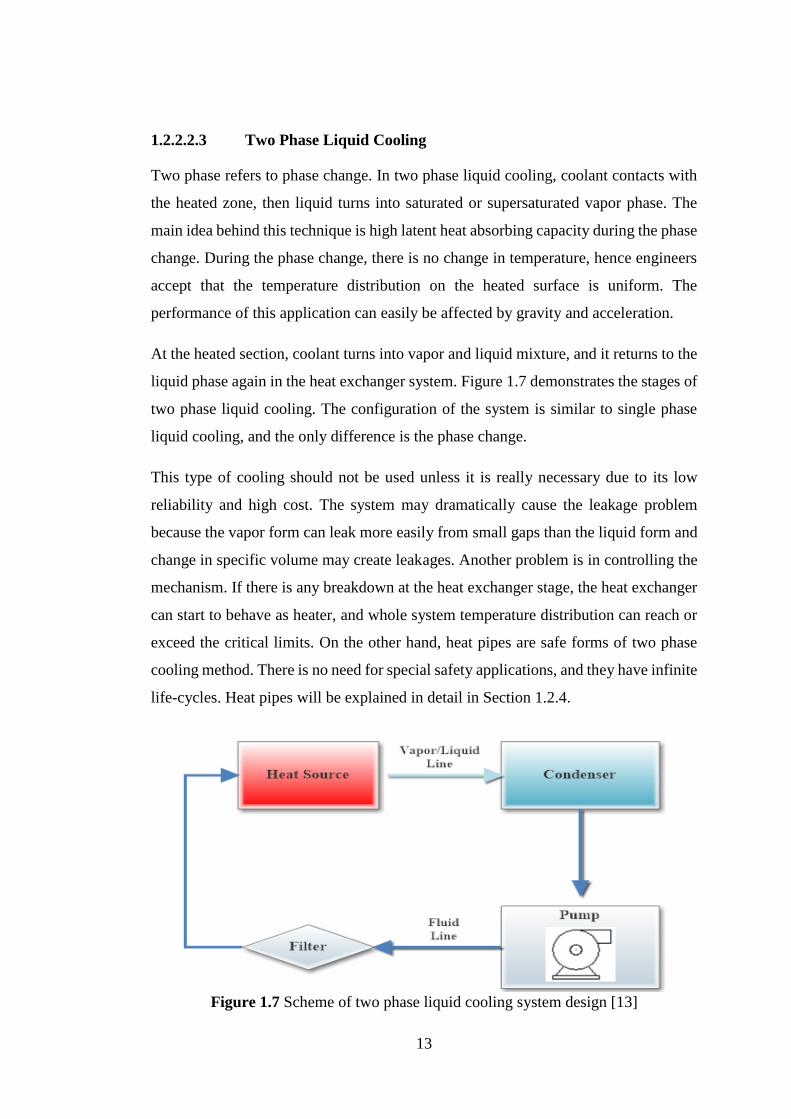
1.2.2.2.3 Two Phase Liquid Cooling
Two phase refers to phase change. In two phase liquid cooling, coolant contacts with
the heated zone, then liquid turns into saturated or supersaturated vapor phase. The
main idea behind this technique is high latent heat absorbing capacity during the phase
change. During the phase change, there is no change in temperature, hence engineers
accept that the temperature distribution on the heated surface is uniform. The
performance of this application can easily be affected by gravity and acceleration.
At the heated section, coolant turns into vapor and liquid mixture, and it returns to the
liquid phase again in the heat exchanger system. Figure 1.7 demonstrates the stages of
two phase liquid cooling. The configuration of the system is similar to single phase
liquid cooling, and the only difference is the phase change.
This type of cooling should not be used unless it is really necessary due to its low
reliability and high cost. The system may dramatically cause the leakage problem
because the vapor form can leak more easily from small gaps than the liquid form and
change in specific volume may create leakages. Another problem is in controlling the
mechanism. If there is any breakdown at the heat exchanger stage, the heat exchanger
can start to behave as heater, and whole system temperature distribution can reach or
exceed the critical limits. On the other hand, heat pipes are safe forms of two phase
cooling method. There is no need for special safety applications, and they have infinite
life-cycles. Heat pipes will be explained in detail in Section 1.2.4.
Figure 1.7 Scheme of two phase liquid cooling system design [13]
14
1.2.2.2.4 Spray Cooling
Spray cooling method is a new trend. Coolant liquid is directly sprayed to hot
electronic component such as chips or ICs. It is a direct cooling method because the
coolant directly contacts with heated zone. It can be single and two phase type. Spray
cooling with two phase condition is more applicable for high heat fluxes. The coolant
is sprayed by a nozzle which is also known as atomizer. The nozzle creates fine liquid
droplets. When these droplets hit the heated surface, they suddenly vaporize and this
absorbs excessive amount of heat.
The coolant here is generally different from the liquids used in other liquid cooling
applications. Due to risk of short circuits, these liquids are generally dielectric
(electrically non-conductive) type such as FC-72, FC-84 etc.
Important components of spray cooling are nozzle and pump because of the
requirement of high pressure for producing droplets. The nozzle design and its position
are very important factors affecting the performance. Balıkçı, (2013), studied the types
of coolants and positions of the nozzle [14]. In a related study, Öksüz [15] made an
investigation about characterization of the spray cooling for electronic devices. They
tried to solve the problems on a prototype of an ASELSAN Inc. product which was a
rugged chassis design using spray cooling.
1.2.2.2.5 Jet Impingement
The idea behind jet impingement is similar to spray cooling. The main difference
between spray cooling and jet impingement is the velocity of sprayed liquid. In jet
impingement, heated zone is directly cooled by high velocity liquid from a nozzle
whose position is normal to the surface. Due to high speed fluid contact, there can be
metal abrasion and corrosion on the cold surface. Hence, this method is not used for
long-life electronic devices.

15
1.2.3 Thermo-electric Cooling (TEC)
Thermoelectric cooling uses Peltier effect to create a heat flux between two different
types of materials. A thermoelectric is a small electronic heat pump without any
moving parts. It can cool the application surface up to sub-ambient temperature. The
cooler operates with direct current. According to the direction of current, it can be used
as a cooler or a heater. Such an instrument is also called a Peltier device, Peltier heat
pump, solid state refrigerator, or thermoelectric cooler (TEC). The advantage of it is
that there are no moving parts, so it operates silently. The disadvantage of the system
is that efficiency of TECs is less than that of other techniques, and TECs can resist low
heat fluxes. The structural layers of a TEC are illustrated in Figure 1.8.
Figure 1.8 Layers of TECs (Peltier Cooler) [16]
1.2.4 Heat Pipe
Heat pipes provide passive and indirect cooling. For this reason, their reliability is very
high, and their product life is infinite. Heat pipes cannot be used as coolers by
themselves, but they can enrich the performance of conduction and convection.
Working principle of heat pipes comes from two phase cooling mechanism. Heat pipes
are sealed and vacuum pumped vessels that are partially filled with a liquid. The
internal walls of heat pipes are lined with a porous medium (the wick) that acts as a
16
passive capillary pump. When heat is applied to one side of a heat pipe, the liquid starts
evaporating. A pressure gradient exists causing the vapor to flow to the cooler regions.
The vapor condenses at the cooler regions, and the condensate is transported back by
the wick structure, thereby closing the loop [5].
Heat pipes are also known as super conductive materials. Their directional thermal
conductivity is almost 200 times higher than pure copper [17]. The effective thermal
conductivity of a heat pipe can reach to values from 50000 W/mK to 200000 W/mK
[18]. Heat pipes are used in specific areas such as cooling of a computer CPU, nuclear
plants, special studies in aerospace applications, petroleum piping structures and waste
heat recovery.
Chapter 2 includes a section with some specific information about heat pipes, their
limitations and their applications.
1.3 Summary of Cooling Techniques
In Section 1.2, different types of electronics cooling methods are covered in general,
emphasizing the advantages and disadvantages of the cooling system. In addition to
summarized techniques, there are several novel and recent methods for cooling. For
example, phase change materials, thermionic and thermotunneling cooling,
electrohydrodynamic and electrowetting cooling, immersion cooling and magnetic
cooling are the popular research topics in the 21st century. Yan et al. [19] made a review
comparing the performance of different cooling techniques, and they tabulated the
results given in Table 1.2.
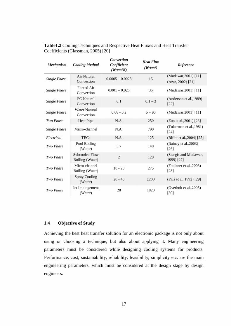
17
Table1.2 Cooling Techniques and Respective Heat Fluxes and Heat Transfer
Coefficients (Glassman, 2005) [20]
Mechanism Cooling Method
Convection
Coefficient
(W/cm2K)
Heat Flux
(W/cm2) Reference
Single Phase Air Natural
Convection 0.0005 – 0.0025 15
(Mudawar,2001) [11]
(Azar, 2002) [21]
Single Phase Forced Air
Convection 0.001 – 0.025 35 (Mudawar,2001) [11]
Single Phase FC Natural
Convection 0.1 0.1 – 3
(Anderson et al.,1989)
[22]
Single Phase Water Natural
Convection 0.08 - 0.2 5 – 90 (Mudawar,2001) [11]
Two Phase Heat Pipe N.A. 250 (Zuo et al.,2001) [23]
Single Phase Micro-channel N.A. 790 (Tukerman et al.,1981)
[24]
Electrical TECs N.A. 125 (Riffat et al.,2004) [25]
Two Phase Pool Boiling
(Water) 3.7 140
(Rainey et al.,2003)
[26]
Two Phase Subcooled Flow
Boiling (Water) 2 129
(Sturgis and Mudawar,
1999) [27]
Two Phase Micro-channel
Boiling (Water) 10 - 20 275
(Faulkner et al.,2003)
[28]
Two Phase Spray Cooling
(Water) 20 - 40 1200 (Pais et al.,1992) [29]
Two Phase Jet Impingement
(Water) 28 1820
(Overholt et al.,2005)
[30]
1.4 Objective of Study
Achieving the best heat transfer solution for an electronic package is not only about
using or choosing a technique, but also about applying it. Many engineering
parameters must be considered while designing cooling systems for products.
Performance, cost, sustainability, reliability, feasibility, simplicity etc. are the main
engineering parameters, which must be considered at the design stage by design
engineers.

18
As indicated in Section 1.2, there are many techniques with many parameters and some
limitations to select as an appropriate cooling for a designed system. Combination of
these techniques generally gives the best results.
Aim of this study is to design a combined cooling system for the military electronic
devices on rotary platforms. The major concerns for the design are performance,
simplicity and cost. To achieve in all of these, heat pipes and forced convection
techniques are combined.
Rotary platforms in land and naval military systems can carry weapons, active and
passive antennas, radar system and telecommunication system as illustrated in Figure
1.9. These platforms rotate 360 degree around the z-axis. Due to rotation, there must
be special components which must provide electrical, mechanical and fluidic
connections. This part is called ‘slip ring’. Slip ring is an electromechanical device that
allows transmission of power, electrical signals and mechanical interface from the
stationary part of the system to the rotating structure.
(a) (b)
A slip ring with only an electrical interface has a price between 10,000 and 60,000
dollars. A slip ring with both electrical and fluidic connections cost more than hundred
thousand dollars. Besides being expensive, these parts also reduce the reliability of the
whole system. Slip ring can carry control signals, power connection, RF (radio
frequency) for radar applications and fluidic connections for liquid cooling. For the
Figure 1.9 Examples of Rotary Platforms (a) ASELSAN Naval System [31] and (b)
ASELSAN Automatic Weapons System [32]
Figure 1.2 : Examples of Rotary Platforms (a) AMDR Raytheon Dual-Band Radar
[34], (b) ASELSAN Naval System [35] (c) ASELSAN Automatic Weapons System
[36]
Figure 1.3 : Examples of Rotary Platforms (a) AMDR Raytheon Dual-Band Radar
[34], (b) ASELSAN Naval System [35] (c) ASELSAN Automatic Weapons System
[36]
Figure 1.4 : Examples of Rotary Platforms (a) AMDR Raytheon Dual-Band Radar
[34], (b) ASELSAN Naval System [35] (c) ASELSAN Automatic Weapons System

19
high speed rotation ranges, there might be leakage problems, which may cause whole
system failure.
In order to overcome the difficulties associated with slip-rings, in this study, long
bended heat pipes are used together with forced convection. Heat pipes are connected
to heat sinks with different shapes and sizes of fins. At the first stage of the study, a
preliminary design and numerical analyses of the preliminary design are done. Then,
these results are validated with experiments. Finally, there is a design optimization in
light of the information coming from the numerical analyses.

20

21
CHAPTER 2
THEORY AND LITERATURE SURVEY
In this chapter, the theories of heat pipes and forced convection are presented. First,
the heat pipe is explained in detail. Then, the theory section continues with forced
convection and its parameters. Finally, there is a review of the related literature.
2.1 Historical Development of Heat Pipe
The heat pipe is a simple passive cooling device, operating principle of which
combines the theories of thermal conductivity and two-phase heat transfer between
two solid interfaces. This combination makes the heat transfer problem in heat pipes
complex. It is a passive device because there is no need to provide any power from
outside. There is one driving force that is the temperature gradient between solid
interfaces at its ends.
The initial appearance of heat pipes was in 1800s with Perkins tube which is a heat
transfer device operating like a two-phase thermosyphon. A.M. Perkins and J. Perkins
focused on single or two phase heat transfer phenomena from a furnace to a boiler.
This device was produced in order to make rapid superheated steam [33].
The first occurrence of a heat pipe product was in 1942 by Richard S. Gaugler. It was
patented by General Motors Corp (Patent no: US 2350348 A). It was the first passive
device which was based on two phase heat transfer with capability of transfer of large
heat loads with minimum temperature drop [33] [34]. It was the proof of the adiabatic
assumption of heat pipes.
22
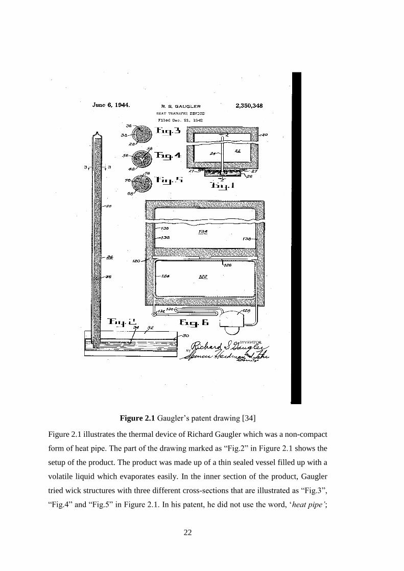
Figure 2.1 Gaugler’s patent drawing [34]
Figure 2.1 illustrates the thermal device of Richard Gaugler which was a non-compact
form of heat pipe. The part of the drawing marked as “Fig.2” in Figure 2.1 shows the
setup of the product. The product was made up of a thin sealed vessel filled up with a
volatile liquid which evaporates easily. In the inner section of the product, Gaugler
tried wick structures with three different cross-sections that are illustrated as “Fig.3”,
“Fig.4” and “Fig.5” in Figure 2.1. In his patent, he did not use the word, ‘heat pipe’;
23
the product was called ‘heat transfer device’; and it was declared as a refrigeration
unit [34].
In 1960s, space applications became popular, and NASA started to finance thermal
management applications for space. In 1964, Grovers et al. [35] from Los Alamos
National Laboratory announced a study about a heat transfer device, and this device
was named ‘heat pipe’. In addition, this study was patented, which was filed on behalf
of the United States Atomic Energy Commission. The word of ‘heat pipe’ was new,
but the idea behind it was the same as Gaugler’s idea. The difference from Gaugler’s
is that they studied the temperature ranges (operational conditions) and upgraded the
mathematical modelling.
After appearance of heat pipes, scientists and researchers began to investigate working
conditions and heat pipe behavior in space. In 1967, an experiment which was the first
flight of a heat pipe to space was done. The experimental setup consisted of an
electrical heater at one side of the heat pipe, a compact heat pipe which was a water /
stainless steel heat pipe and a telemetric data collector. It was launched into earth orbit
from Cape Kennedy on an Atlas-Agena Vehicle [36]. After the success in 1967, the
first use of heat pipes in a space thermal control application was on GEOS-B satellite,
launched from Vandenburg Air Force Base. The heat pipe in the satellite was
manufactured from aluminum 6061-T6 as a vessel material and freon-11 was used as
the working fluid [37]. The main goal of using the heat pipe was obtaining isothermal
surfaces on satellite’s panels.
The first commercial company producing heat pipes was RCA which was supported
by U.S. Government. They used glass, copper, nickel, stainless steel, molybdenum and
TZM molybdenum as vessel materials in their heat pipes. In addition to these, they
used water, cesium, sodium, lithium and bismuth as working fluids. Maximum
operating temperature of 1650 oC was achieved [38] [39] [40].
Apart from the developments in USA, there were also several investigations about heat
pipes, elsewhere. In mid 1960s, The Harwell Comp. made an investigation about using
heat pipes in a nuclear application in Ispra, Italy [41]. In Japan, (1968), Kisha Seizo
Kaisha Company started a program about using heat pipes in refrigeration engines and

24
air conditioners [42]. During 1969, the companies from Europe, British Aircraft Corp.
(BAC) and Royal Aircraft Establishment, made investigations in using heat pipes in
aviation systems [43]. The avionic researches proved how heat pipe was used in
electronic cooling. The first electronic cooling application was done by Calimbas and
Hultt of the Philco-Ford Corp., which was mainly about high-power airborne travelling
wave tube (TWT) [44].
Today’s technologies are more complex than the ones in 1960s or 1970s due to
increased power consumption and decreased dimensions. Engineers do not want to
consume extra power for thermal management, hence the trend of using passive
techniques is increasing rapidly. That is, heat pipe is becoming a new trend in the area
of cooling.
2.2 Applications and Advantages of Heat Pipes
Applications of heat pipes are very widespread. Heat pipes can be seen in military
devices, in household appliances, in computers especially in tablets and laptops, in air
conditioning systems and in molding industry etc. The reasons behind why heat pipes
are commonly preferred are that heat pipes are compact in size, and their use in
electronics cooling increases system reliability and reduces the initial cost. Another
reason may be their long life-cycle. Many producers give infinite life for their
products. This is an advantage for satellite and military device applications because
maintenance risk must be minimum in these areas. However, for a long service life it
is important to choose the proper vessel material and to identify the working fluid
which is compatible with that vessel material.
As it is emphasized above, for heat pipe use in electronics cooling, the initial cost is
low, and the reliability is high because there is no excessive use of forced convection
products. For high power dissipating electronic systems generally liquid cooling is
used. Liquid can be selected as oil, water or special chemical mixtures according to
working conditions. In addition to this, these systems require liquid guide channels in
the product and large heat exchangers, which all increase the initial cost. Designers try
to eliminate these obstacles by applying passive cooling techniques. To employ heat

25
pipes for industrial applications, it is desirable to know thermal performance of the
heat pipe under various operating conditions, a priori. Thermal performance of a heat
pipe depends on various radial and axial thermal resistances at the evaporator,
condenser and inner sections of the heat pipe [45]. Hence, for the heat pipe
applications, design engineers must focus on the evaporator and condenser designs.
Consequently, use of heat pipes requires detailed focus on the design.
An important point about heat pipe use is that it is not a complete solution to the
thermal management problem by itself. It is merely a part of heat transfer
enhancement. This enhancement comes from the properties of heat pipes. Heat pipes
can be used for spatial separation of the heat source and the heat sink. They are also
utilized in temperature flattening, heat flux transformation, and temperature control.
In electronics applications, some components generate a hot spot and cause high heat
dissipations. However, in some cases these components are surrounded by other
components which have different temperature sensitivity levels. As it is shown in
above scenario, if the designer cannot remove heat from the hot spot region, a heat
pipe can be used as a separator of heat source and heat sink. Heat is captured rapidly
and transferred to the remote heat sink through high effective thermal conductivity of
the heat pipe. Another application is temperature flatting in which the heat pipe
function as a heat spreader. The main aim of thermal design is to generate an iso-
thermal base which requires to minimize the temperature gradients. In addition to this,
temperature flatting is the idea behind the use of heat pipes in space applications. The
third application is flux transformation which is generally used for reactor technology
and casting applications. The last one is temperature control which is more
complicated than other applications. It requires a variable conductivity heat pipe and
used in spacecraft design [46].
In 1960s, NASA started to investigate use of heat pipes in space applications. Today,
NASA uses heat pipes as heat spreaders in satellite design. The outer surface of a
satellite, facing the sun, has very high temperature values, however inner surface, in
the shadow, has an extremely low temperature. Hence, there is a large temperature
gradient between the surfaces. These two surfaces are connected with heat pipes,
which makes hot section function as a source and cold section as a sink. When the
26
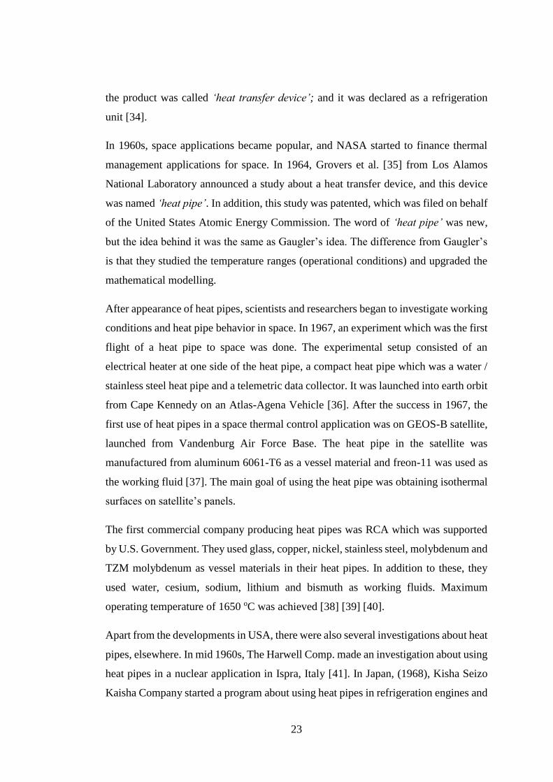
system reaches to the steady condition, the temperature gradient is minimized. Dornier
Company [47] demonstrated the difference between with /without heat pipe designs
for a satellite as given in Figure 2.2. As it is seen, heat pipes can eliminate ∆T = ~100
oC.
Figure 2.2 Temperature gradient of satellite with/without heat pipes [47]
Another application area is die casting and injection molding. For the die-cast process,
during the solidification, dies are generally cooled by water. However, this causes
thermal shock for the product, and there can be some defects such as cracks, splitting,
draws etc. As an alternative solution, the die is produced from high thermal
conductivity materials and heat pipes are attached to certain points of the die. Other
ends of the heat pipes are connected to a liquid channel. When the casting is finished,
channel is filled up with water. Die starts to cool down rapidly thanks to super
conductivity of heat pipes. In this method, even though there is no direct contact with
liquid, die is cooled in a short time, and there is no thermal shock. Using heat pipes in
injection molding is the reverse process of casting. At the end of the each manufactured
product process, injection nozzle starts to cool down. Nevertheless, before the next
molding is started, nozzle must be heated in order to prevent plastic or metal from
27
solidifying at the nozzle outlet. Otherwise, outlet of the nozzle might be blocked. The
nozzle is heated up by heaters on the nozzle surface, but this requires an external
power, which means extra cost. In order to eliminate external power requirement, heat
pipes are placed between the molten plastic/metal reservoir and the nozzle. With the
excessive dissipated heat from the molten material, the nozzle can always be kept
ready to work for the next product.
Heat pipes are also used in order to prevent waste of energy. With the increase in
energy costs, designers and scientists want to use every energy source. For this
demand, heat pipes are used in building construction for air-heating. As it is known,
the air heating system takes cold air from the atmosphere to the inlet channel of the
system. The standard system sucks the air and heats it up with heaters, then heated air
is sent to the building ventilation system. If temperature difference between fresh
(cold) air and air after heating operation increases, the required energy of heaters
increases, which means it needs more power. The solution is generating pre-heating
system which uses the waste heat. It is basically an energy recovery operation. Thermal
recovery unit is designed using heat pipes. The evaporator sections of the heat pipes
are placed into the exhaust air of the heaters, and the condenser section is mounted into
the cold air inlet. The inlet air is heated up by the heat pipe system, and this results in
reduction in power consumption of the heaters. For example, Firouzfer et al. [48], in
2011, made an investigation of a heat pipe heat exchanger applied to an HVAC system.
They observed the performance and the advantages of this HVAC system. This study
reaches to the conclusion that there is an increase in air quality in the heated space and
reduction in consumed power. This system decreases the relative humidity in the
conditioned space (nearly 10%) and reduces the power demand. Another example is
that The National Engineering Laboratory and The Shell Research Laboratory have
co-operated in applying heat pipes to solve the problem of exhaust emissions of petrol
engines. The heat pipe was attached between the intake manifold and the exhaust
system. The evaporator is the exhaust and the condenser is the intake. As a result, by
using waste heat, the control of lean burn was achieved [49]. Similarly, heat pipes are
also used as liquid to liquid heat exchangers.
28
The most striking example comes from Alaska pipe line, the surrounding, low
temperature, is used as the condenser and the transported fluid section is the
evaporator[50]. In Alaska, ground has a permafrost layer. The permafrost layer is the
layer occurring below 0 oC at which soil and salt water mixture freezes, and it creates
a non-porous ice rock under the surface layer. When pipeline penetrates the ground,
heat spreading from the fluid melts this structure, which results in the collapse of the
pipeline. In order to eliminate this obstacle, excessive heat dissipation of the fluid is
transferred to the atmosphere by using heat pipes. As it is seen in Figure 2.3, the heat
pipes used are long and they are used in order to prevent the permafrost layer from
melting. 100000 heat pipes are used and their dimensions range in diameter between
5 cm and 7.5 cm, in length between 9 m to 18 m.
Figure 2.3 Heat pipe application in Alaska pipeline with permafrost ground [51]
The most common example of heat pipe application is electronic cooling. In
notebooks, the heat pipe is attached on CPU, and its condenser may be located in
different sections inside the notebook. For example, Apple MacBook Pro with retina
display is the last example for CPU cooling. As it is illustrated in Figure 2.4, the heat
pipe is connected to CPU, and its ends are connected to specially designed slim fans.

29
With all these, the thickness of the notebook is only 18 mm. Also it can be easily seen
that heat pipe’s middle sections are used as evaporators and the ends are condensers.
Figure 2.4 Internal design of Apple MacBook Pro [52]
To sum up, applications of heat pipes are widespread. They can be seen in buildings,
HVAC systems, space and avionic applications and electronic devices. Heat pipes are
preferred for their low cost, infinite life-cycle and high reliability.
2.3 Working Principles of Heat Pipes
Historically, metallic heat sinks are very useful in thermal management of electronic
devices. Nevertheless new generation electronic devices have large amounts of heat
dissipation, hence metallic heat sinks, which are combined with natural or forced
convection are not sufficient against excessive heat dissipation rates. Other limitations
are the weight and the required physical volume (size). Due to these limitations, the
trend of application of heat pipes is rising.
Heat pipes provide passive and indirect cooling. Because of this, their reliability is
very high and their product life is infinite. Working principle of heat pipes comes from
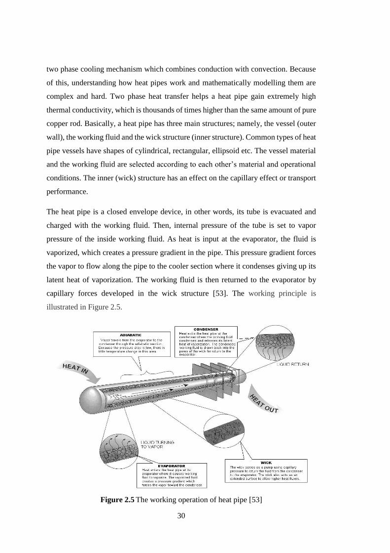
30
two phase cooling mechanism which combines conduction with convection. Because
of this, understanding how heat pipes work and mathematically modelling them are
complex and hard. Two phase heat transfer helps a heat pipe gain extremely high
thermal conductivity, which is thousands of times higher than the same amount of pure
copper rod. Basically, a heat pipe has three main structures; namely, the vessel (outer
wall), the working fluid and the wick structure (inner structure). Common types of heat
pipe vessels have shapes of cylindrical, rectangular, ellipsoid etc. The vessel material
and the working fluid are selected according to each other’s material and operational
conditions. The inner (wick) structure has an effect on the capillary effect or transport
performance.
The heat pipe is a closed envelope device, in other words, its tube is evacuated and
charged with the working fluid. Then, internal pressure of the tube is set to vapor
pressure of the inside working fluid. As heat is input at the evaporator, the fluid is
vaporized, which creates a pressure gradient in the pipe. This pressure gradient forces
the vapor to flow along the pipe to the cooler section where it condenses giving up its
latent heat of vaporization. The working fluid is then returned to the evaporator by
capillary forces developed in the wick structure [53]. The working principle is
illustrated in Figure 2.5.
Figure 2.5 The working operation of heat pipe [53]

31
There are many factors affecting the performance and design of heat pipes. These are
length, diameter, bending effect, compatibility of vessel and working fluid, operating
temperature range, mounting orientation, power limitation, thermal resistance and
connections of ends. During heat pipes are manufactured or designed, all factors
should be taken into consideration.
Consequently, heat pipes are designed for a large range of working conditions from
cryogenic temperatures (< -243 oC) to elevated temperatures (> 1500 oC) by selecting
proper vessels and working fluids. In heat pipe operations, there is no external power
to drive the mechanism. If there is a ‘heat-in’ section and a temperature difference
between two ends, the mechanism will operate itself. Heat and the temperature
difference are driving forces for heat pipe operations.
2.4 Wick Structures of Heat Pipes
Identifying the inner structures of heat pipes is the most critical point in the design of
a cooling system supported with heat pipes. The wick type of a heat pipe directly
affects performance of the heat pipe. Essentially, wick structures affect capillary
pressure inside the heat pipe, which has importance when working against gravity. The
most commonly used wick structures are sintered powders, grooves, screens and felts.
The sintered type wick has more advantages than the others in terms of
manufacturability, cost and performance. In addition to these, it is the simplest one.
The most critical advantage of the sintered type is operational orientation. It can be
easily used in the against gravity application by placing the condenser section above
the level of the evaporator or the heat source. On the other hand, the groove and the
screen mesh heat pipes have very limited capillary forces to support the continuous
cycle. These types are not suitable for the against gravity application; however,
especially the groove type is the most frequently used in space applications due to its
minimum irregularity in non-gravitational space. The felt type is not very common
because it is produced from knitted metal wire mesh, so it has some composite types.
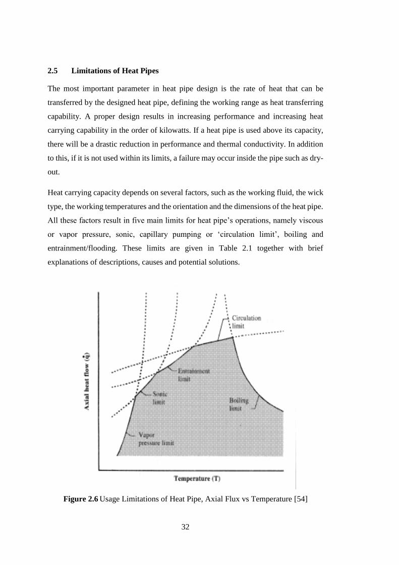
32
2.5 Limitations of Heat Pipes
The most important parameter in heat pipe design is the rate of heat that can be
transferred by the designed heat pipe, defining the working range as heat transferring
capability. A proper design results in increasing performance and increasing heat
carrying capability in the order of kilowatts. If a heat pipe is used above its capacity,
there will be a drastic reduction in performance and thermal conductivity. In addition
to this, if it is not used within its limits, a failure may occur inside the pipe such as dry-
out.
Heat carrying capacity depends on several factors, such as the working fluid, the wick
type, the working temperatures and the orientation and the dimensions of the heat pipe.
All these factors result in five main limits for heat pipe’s operations, namely viscous
or vapor pressure, sonic, capillary pumping or ‘circulation limit’, boiling and
entrainment/flooding. These limits are given in Table 2.1 together with brief
explanations of descriptions, causes and potential solutions.
Figure 2.6 Usage Limitations of Heat Pipe, Axial Flux vs Temperature [54]
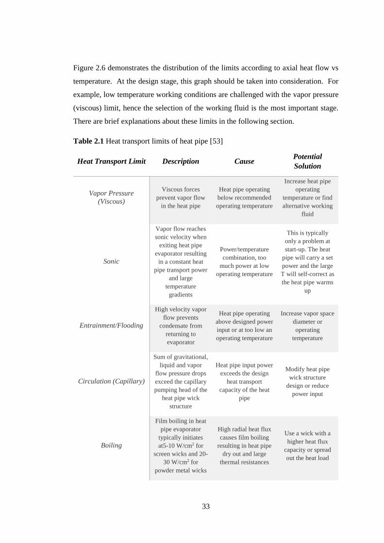
33
Figure 2.6 demonstrates the distribution of the limits according to axial heat flow vs
temperature. At the design stage, this graph should be taken into consideration. For
example, low temperature working conditions are challenged with the vapor pressure
(viscous) limit, hence the selection of the working fluid is the most important stage.
There are brief explanations about these limits in the following section.
Table 2.1 Heat transport limits of heat pipe [53]
Heat Transport Limit Description Cause Potential
Solution
Vapor Pressure
(Viscous)
Viscous forces
prevent vapor flow
in the heat pipe
Heat pipe operating
below recommended
operating temperature
Increase heat pipe
operating
temperature or find
alternative working
fluid
Sonic
Vapor flow reaches
sonic velocity when
exiting heat pipe
evaporator resulting
in a constant heat
pipe transport power
and large
temperature
gradients
Power/temperature
combination, too
much power at low
operating temperature
This is typically
only a problem at
start-up. The heat
pipe will carry a set
power and the large
T will self-correct as
the heat pipe warms
up
Entrainment/Flooding
High velocity vapor
flow prevents
condensate from
returning to
evaporator
Heat pipe operating
above designed power
input or at too low an
operating temperature
Increase vapor space
diameter or
operating
temperature
Circulation (Capillary)
Sum of gravitational,
liquid and vapor
flow pressure drops
exceed the capillary
pumping head of the
heat pipe wick
structure
Heat pipe input power
exceeds the design
heat transport
capacity of the heat
pipe
Modify heat pipe
wick structure
design or reduce
power input
Boiling
Film boiling in heat
pipe evaporator
typically initiates
at5-10 W/cm2 for
screen wicks and 20-
30 W/cm2 for
powder metal wicks
High radial heat flux
causes film boiling
resulting in heat pipe
dry out and large
thermal resistances
Use a wick with a
higher heat flux
capacity or spread
out the heat load

34
2.5.1 Viscous Limit
This limit is also known as the vapor pressure limit. At the start-up range of the heat
pipe, which is the low temperature range, vapor pressure difference between the
evaporator and the condenser of the heat pipe can be too small. This results in an
increase in the viscous force of the working fluid, which means the viscous force
within the vapor region can be larger than the pressure gradient at the working
temperature. Occurrence of the viscous region prevents the vapor flow inside the tube
and vapor stays stagnated [55]. This limitation is a big problem for cryogenic heat
pipes, heat pipes with a long condenser and operating temperatures below the freezing
point of working fluid.
Busse (1973) made an experimental study and created a mathematical model. The
mathematical relation giving the maximum axial heat transfer rate reaching viscous
limit [56] is
𝑞𝑎𝑝𝑝 < 𝑞𝑣𝑖𝑠 =
𝐴𝑣. 𝑟02. 𝛿. 𝜌𝑣 . 𝑃𝑣
16. 𝜇𝑣. 𝐿𝑒𝑓𝑓 (2.1)
where Pv and 𝜌v are respectively vapor pressure and density at the evaporator end of
heat pipe. ‘δ' is the enthalpy of vaporization, Av is area of the vapor section and µv is
the dynamic viscosity of the vapor phase. Finally, Leff is the effective length of the heat
pipe, which can be calculated from
𝐿𝑒𝑓𝑓 =
1
2𝑙𝑐𝑜𝑛𝑑𝑒𝑛𝑠𝑒𝑟 + 𝑙𝑎𝑑𝑖𝑎𝑏𝑎𝑡𝑖𝑐 +
1
2𝑙𝑒𝑣𝑎𝑝𝑟𝑎𝑡𝑜𝑟 (2.2)
The solution for eliminating this limit is changing the working fluid or increasing the
operational temperature.
2.5.2 Sonic Limit
In a heat pipe of constant vapor space diameter, vapor flow accelerates and decelerates
because of vapor addition in the evaporator and vapor removal in the condenser. The
changes in vapor flow also change the pressures along the heat pipe. As more heat is
applied to the heat pipe, vapor velocities generally increase. A choked flow condition
35
will eventually arise, where the flow becomes sonic. At this point, vapor velocities
cannot increase and a maximum heat transport limitation is achieved. The heat flux
that results in choked flow is considered as the sonic limit [57]. The recommended
heat transfer rate for avoiding sonic limit is given with
𝑞𝑎𝑝𝑝 < 𝑞𝑠𝑜𝑛𝑖𝑐 = 0.474𝐴𝑣. 𝛿. (𝜌𝑣. 𝑃𝑣)1/2 (2.3)
On the other hand, a high vapor velocity also results in quick response of the heat pipe.
2.5.3 Entrainment / Flooding Limit
Vapor velocity increases with temperature and may be sufficiently high to produce
shear force effects on the liquid return flow from condenser to evaporator, which cause
entrainment of the liquid by vapor. Restraining force of liquid surface tension is a
major parameter in determining the entrainment limit [54]. The existing vapor blocks
the motion of liquid to evaporator section, in other words condensed flow cannot reach
evaporator section. This situation concludes in ‘dry-out’ phenomena. The
corresponding heat transfer rate causes this procedure, called entrainment limit. This
limit is calculated using Formula 2.4.
𝑞𝑒𝑛𝑡 = 𝐴𝑣. 𝛿. √
𝜌𝑣 . 𝜎
𝑥 (2.4)
Where ‘σ’ is surface tension of working liquid and ‘x’ is characteristic dimension of
wick structure.
𝑥 = 2𝑟𝜎 (2.5)
Where ‘rσ’ is effective radius of pure structure.
Flooding limits are valid for gravity aided operations due to the existence of excess
liquid. The wick structure is saturated and the excess fluid results in a “puddle” flow
on the surface of wick structure. The flooding limit, likewise the entrainment, happens
when high vapor velocities preclude the fluid that is flowing on the surface of wick to
return to evaporator. The shear force of vapor prevents the condensed fluid from
reaching to evaporator and leads to a flooding condition in the condenser section [57].
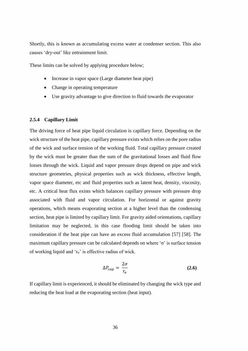
36
Shortly, this is known as accumulating excess water at condenser section. This also
causes ‘dry-out’ like entrainment limit.
These limits can be solved by applying procedure below;
Increase in vapor space (Large diameter heat pipe)
Change in operating temperature
Use gravity advantage to give direction to fluid towards the evaporator
2.5.4 Capillary Limit
The driving force of heat pipe liquid circulation is capillary force. Depending on the
wick structure of the heat pipe, capillary pressure exists which relies on the pore radius
of the wick and surface tension of the working fluid. Total capillary pressure created
by the wick must be greater than the sum of the gravitational losses and fluid flow
losses through the wick. Liquid and vapor pressure drops depend on pipe and wick
structure geometries, physical properties such as wick thickness, effective length,
vapor space diameter, etc and fluid properties such as latent heat, density, viscosity,
etc. A critical heat flux exists which balances capillary pressure with pressure drop
associated with fluid and vapor circulation. For horizontal or against gravity
operations, which means evaporating section at a higher level than the condensing
section, heat pipe is limited by capillary limit. For gravity aided orientations, capillary
limitation may be neglected, in this case flooding limit should be taken into
consideration if the heat pipe can have an excess fluid accumulation [57] [58]. The
maximum capillary pressure can be calculated depends on where ‘σ’ is surface tension
of working liquid and ‘rσ’ is effective radius of wick.
∆𝑃𝑐𝑎𝑝 =
2𝜎
𝑟𝜎 (2.6)
If capillary limit is experienced, it should be eliminated by changing the wick type and
reducing the heat load at the evaporating section (heat input).

37
2.5.5 Boiling Limit
If excessive heat load is applied to the evaporating section of the heat pipe, the liquid
inside the pipe can produce bubbles in the evaporator wick. Formation of vapor
bubbles in the wick is undesirable because they can cause hot spots and obstruct the
circulation of the liquid. In other words, it is defined as a drastic decrease in thermal
conductivity. With the increase of heat flux, more bubbles come out. At a certain heat
flux limit, bubble formation completely blocks the liquid flow, at that point fluid flow
stops and heat is only transferred on the wall of the heat pipe. In this case, the heat
pipe does not function as a super conductor, and its conductivity becomes equal to that
of the wall material. Hence, this limitation is associated to a radial heat flux, which
means heat is applied to the perimeter of the heat pipe or outer shell. The boiling limit
generally occurs at high temperature working conditions [54] [57] [59].
By increasing the heat flux at the evaporator, the critical point is reached when the
temperature difference exceeds the degree of superheating sustainable in relation to
nucleate boiling conditions. When most of the liquid transforms into vapor, the first
dry out occurs. ‘Dry-out’ exists due to an unbalanced ratio between vapor and liquid.
If high heat flux is still applied, the evaporator section loses all fluid itself, and this
phenomena is known as ‘burn-out’. When ‘burn-out’ occurs, heat pipe starts to act like
a metal rod.
Boiling limits can be prevented by using a wick with a higher heat flux capacity or
spreading out the heat load. Among the type of wicks, the sintered wick is the best way
of dealing with boiling limits. This type has significantly more area inside the pipe,
hence it can deal with high fluxes. The basic understanding of whether dry-out occurs
or not is done by taking temperature measurements on the heat pipe wall between the
end of the evaporator and the top of the condenser. If the temperature differences are
large then the adiabatic assumption is not correct, and the dry-out exists.
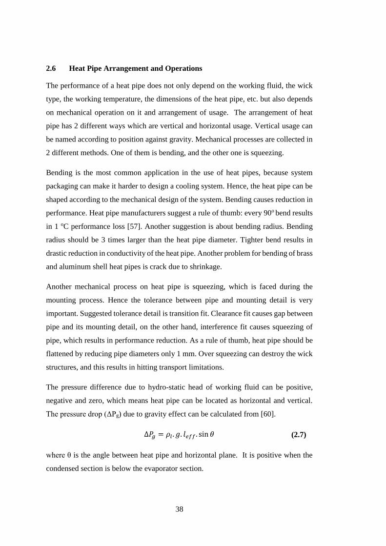
38
2.6 Heat Pipe Arrangement and Operations
The performance of a heat pipe does not only depend on the working fluid, the wick
type, the working temperature, the dimensions of the heat pipe, etc. but also depends
on mechanical operation on it and arrangement of usage. The arrangement of heat
pipe has 2 different ways which are vertical and horizontal usage. Vertical usage can
be named according to position against gravity. Mechanical processes are collected in
2 different methods. One of them is bending, and the other one is squeezing.
Bending is the most common application in the use of heat pipes, because system
packaging can make it harder to design a cooling system. Hence, the heat pipe can be
shaped according to the mechanical design of the system. Bending causes reduction in
performance. Heat pipe manufacturers suggest a rule of thumb: every 90o bend results
in 1 oC performance loss [57]. Another suggestion is about bending radius. Bending
radius should be 3 times larger than the heat pipe diameter. Tighter bend results in
drastic reduction in conductivity of the heat pipe. Another problem for bending of brass
and aluminum shell heat pipes is crack due to shrinkage.
Another mechanical process on heat pipe is squeezing, which is faced during the
mounting process. Hence the tolerance between pipe and mounting detail is very
important. Suggested tolerance detail is transition fit. Clearance fit causes gap between
pipe and its mounting detail, on the other hand, interference fit causes squeezing of
pipe, which results in performance reduction. As a rule of thumb, heat pipe should be
flattened by reducing pipe diameters only 1 mm. Over squeezing can destroy the wick
structures, and this results in hitting transport limitations.
The pressure difference due to hydro-static head of working fluid can be positive,
negative and zero, which means heat pipe can be located as horizontal and vertical.
The pressure drop (ΔPg) due to gravity effect can be calculated from [60].
∆𝑃𝑔 = 𝜌𝑙 . 𝑔. 𝑙𝑒𝑓𝑓. sin 𝜃 (2.7)
where θ is the angle between heat pipe and horizontal plane. It is positive when the
condensed section is below the evaporator section.
39
The working orientations will be summarized in the following three subsections.
Detailed information about working orientation will be in Chapter 3, as a part of the
heat pipe selection guide.
2.6.1 Horizontal Orientation
The horizontal orientation of a heat pipe is the most common one, especially in
notebooks. In this orientation, the performance of the heat pipe is limited by capillary
limit. This limit depends on heat pipe dimensions such as diameter and length. Larger
diameter can carry more heat load; in contrast, a longer heat pipe carries less heat load.
Besides, gravity effect and wick type directly affect the capillary limit. For horizontal
orientation, gravity effect can be ignored, hence designer should accordingly select the
wick type [57].
The heat pipe length which affects capillary limit is not the full length of the pipe. It
must be the effective length, which is given with Equation 2.2.
Grooved wick type is good for horizontal applications because this kind of heat pipes
has large pore radius with a high permeability, which do not cause drastic pressure
drop. By contrast, powder (sintered) wick has small radii and relatively low
permeability. Hence, sintered wicks are limited by pressure drop in horizontal
operation [53].
2.6.2 Gravity Aided
In gravity aided orientation, evaporator section is located below the condenser section,
hence the angle between horizontal plane in Equation 2.7 is negative. Gravity aided or
gravity assist configuration is the best configuration for heat pipe applications. Gravity
helps to return condensed fluid to evaporator section. Flooding and boiling limits are
the critical transport limits for gravity aided orientation [57].

40
2.6.3 Gravity Against
In gravity against orientation, evaporator section is located above the condenser
section, hence the angle measured from the horizontal plane in Equation 2.7 is positive.
Gravity against configuration is a problematic configuration for heat pipe applications.
The main limitation is capillary limit, similar to the horizontal configuration [57].
Gravity can be ignored for horizontal placement, in contrast for gravity against
placement gravity effect should be taken into consideration. To eliminate the
disadvantages of this orientation, the dimensions of heat pipe must be carefully
selected. As the elevation between evaporator section and condenser section increases,
the performance of heat pipe decreases proportionally.
2.7 Heat Pipe – Heat Sink Performance [57]
Up to this section, theory of heat pipe and its performance have been summarized. This
section is related to cooling performance of the cooling system. A cooling system with
heat pipes has 3 main sections. It starts with evaporator base (heat in), continues with
heat pipe (heat carrying) and ends with condenser section (heat dissipation). Resistance
network is given in Figure 2.7. This network is placed between evaporator and
condenser.
Figure 2.7 The Resistance Network of Heat Pipe
Each resistance can be found to calculate an associated temperature change. The
calculation starts with the block section. The governing equation comes from Fourier’s
Law of conduction, in order to calculate Rblock.
∆𝑇𝑏𝑙𝑜𝑐𝑘 =
𝑄. 𝑡𝑏𝑙𝑜𝑐𝑘
𝑘𝑏𝑙𝑜𝑐𝑘. 𝐴𝑏𝑙𝑜𝑐𝑘 (2.8)
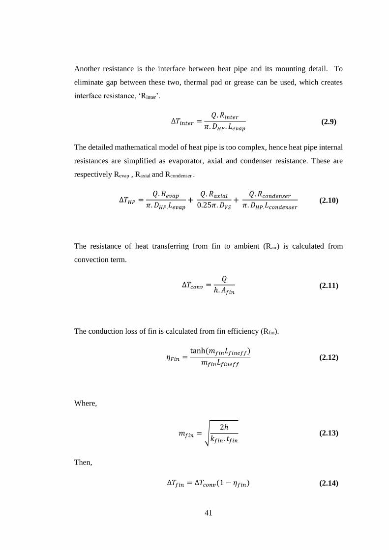
41
Another resistance is the interface between heat pipe and its mounting detail. To
eliminate gap between these two, thermal pad or grease can be used, which creates
interface resistance, ‘Rinter’.
∆𝑇𝑖𝑛𝑡𝑒𝑟 =
𝑄. 𝑅𝑖𝑛𝑡𝑒𝑟
𝜋. 𝐷𝐻𝑃. 𝐿𝑒𝑣𝑎𝑝 (2.9)
The detailed mathematical model of heat pipe is too complex, hence heat pipe internal
resistances are simplified as evaporator, axial and condenser resistance. These are
respectively Revap , Raxial and Rcondenser .
∆𝑇𝐻𝑃 =
𝑄. 𝑅𝑒𝑣𝑎𝑝
𝜋. 𝐷𝐻𝑃.𝐿𝑒𝑣𝑎𝑝+
𝑄. 𝑅𝑎𝑥𝑖𝑎𝑙
0.25𝜋. 𝐷𝑉𝑆+
𝑄. 𝑅𝑐𝑜𝑛𝑑𝑒𝑛𝑠𝑒𝑟
𝜋. 𝐷𝐻𝑃.𝐿𝑐𝑜𝑛𝑑𝑒𝑛𝑠𝑒𝑟 (2.10)
The resistance of heat transferring from fin to ambient (Rair) is calculated from
convection term.
∆𝑇𝑐𝑜𝑛𝑣 =
𝑄
ℎ. 𝐴𝑓𝑖𝑛 (2.11)
The conduction loss of fin is calculated from fin efficiency (Rfin).
𝜂𝐹𝑖𝑛 =
tanh(𝑚𝑓𝑖𝑛𝐿𝑓𝑖𝑛𝑒𝑓𝑓)
𝑚𝑓𝑖𝑛𝐿𝑓𝑖𝑛𝑒𝑓𝑓 (2.12)
Where,
𝑚𝑓𝑖𝑛 = √2ℎ
𝑘𝑓𝑖𝑛. 𝑡𝑓𝑖𝑛 (2.13)
Then,
∆𝑇𝑓𝑖𝑛 = ∆𝑇𝑐𝑜𝑛𝑣(1 − 𝜂𝑓𝑖𝑛) (2.14)

42
The change in air temperature is calculated from bulk air properties,
∆𝑇𝑎𝑖𝑟 =
𝑄
𝑚. 𝐶𝑝 (2.15)
The overall performance of heat sink is calculated with summation of all temperature
changes.
∆𝑇𝑇𝑜𝑡𝑎𝑙 = ∆𝑇𝑏𝑙𝑜𝑐𝑘 + ∆𝑇𝑖𝑛𝑡𝑒𝑟 + ∆𝑇𝐻𝑃 + ∆𝑇𝑐𝑜𝑛𝑣 + ∆𝑇𝑓𝑖𝑛 + ∆𝑇𝑎𝑖𝑟 (2.16)
The thermal resistance of the sink to surrounding is calculated with.
𝑅𝑠−𝑎 =
∆𝑇𝑇𝑜𝑡𝑎𝑙
𝑄 (2.17)
If calculation above is followed, designers can estimate the performance of heat sink
with heat pipe system.
43
CHAPTER 3
PRELIMINARY DESIGNS AND NUMERICAL ANALYSIS
This chapter includes the starting point of the conceptual design. First, preliminary
design is defined according to four main parameters. These are the system
requirements, reliability, environment conditions and the configuration cost. Then, a
numerical investigation is done in order to make corrections and optimization in the
preliminary design.
The preliminary design consists of two different designs. Main differences between
the designs are the type of cooling surface (rectangular plate fins versus pin fins). The
type of cooling surface is also determined by the operating conditions. Numerical
analyses are done for both designs, but the numerical model is validated only for the
pin fin configuration using the results from the conducted experiments.
Chapter 3 includes the details about the purpose of using rotary platforms, explanations
about the software used (PTC Creo and FloEFD), heat pipe selection, and CAD
designs with numerical calculation.
3.1 Military Rotary Platforms
Military product design is done based on environmental conditions (cold, hot, rain, salt
fog, high pressure etc.), operating conditions (land, naval, and air), minimum
dimensions and ergonomics. Some devices are out of action (stagnant) such as
detectors, walkie-talkies, mission computers, LRUs etc. which have simple designs
due to not having moving parts. However, radars, antennas, weapon systems, target
detecting systems etc. can move in x-, y- and z- directions and rotate around an axis;
this movability makes design procedure difficult due to movements.
44
Military systems often require special designs such as rotary platforms, launching
systems and lifting systems to perform their missions successfully. Vehicles with
rotating turrets and rotating carriers are obvious examples of critical rotating platforms.
The systems with rotating components are generally used in radar applications, target
detection and destruction systems and unmanned vehicles. All types of rotating
platforms require power, signal exchange and a cooling fluid with the stationary
vehicle hull. The turret to hull interface must often transmit electrical power, as well
as safety interlocks, digital data, video data, other signals (RF, control etc.) and coolant
of the system. These functional requirements must be satisfied in a mechanical
package that meets battlefield environmental requirements [66]. To transmit all
required things from the stationary section to the rotary section, slip rings are generally
used. As it is defined previously, slip ring is an electromechanical device that allows
the transmission of power, electrical signals and mechanical interface from a stationary
part of the system to a rotating structure. The slip ring is a high-tech device,
nevertheless its reliability is very low because of its complexity.
A traditional rotary slip with fluid interface assemblies contains discrete precious
metal rings for each electrical circuit and corresponding sliding wipers (or brushes) to
conduct power and signals from rotating rings to a stationary member [61]. In the
middle of some slip rings, there is a circular gap which supplies the fluid passing
channel during rotation. This channel is specially designed, and it is a sealed section
of slip rings against leakage and break down. A sample of military rotary joint is given
in Figure 3.1 with electrical and fluidic interfaces.
Rotary joints with only an electrical interface cost between 10,000 and 60,000 dollars
in military applications. However, rotary joints with electrical and fluidic connections
cost more than hundred thousand dollars in military applications. These high prices
come from the military standards. Despite military standards, there is always a
malfunction possibility due to complexity. The most critical problem is the leakage of
coolant, which causes permanent and inevitable results. However, military designs
must be reliable and long lasting under harsh conditions. Military product designers
generally suggest that slip ring must not be used if it is not really necessary.

45
Figure 3.1 SPINNER High-quality hybrid rotary joints are mainly used in military
radar systems, fire control systems, rotating vehicle-mounted camera systems and in
mobile battlefield communication systems [62]
3.2 Used Software
In this study, two different commercial software packages are used, which are PTC
Creo 2.0 Educational License and FloEFD with Electronic Cooling. PTC Creo 2.0 is
a parametric CAD program and FloEFD is a commercial CFD program, which works
with CAD integrated and has its own solver.
PTC Creo 2.0 is a Computer Aided Drawing (CAD) program. This program is used
for creating 3-D models for the parametric study. ASELSAN rotary platforms are
simplified for the experimental setup and for the numerical investigations by using
PTC Creo 2.0. The first design procedure is to create a 3-D CAD model by simplifying
the real design. Then, model’s parameters are identified. Finally, these parameters are
identified for later use in parametric optimization according to identified sections
which affect the results of experiments and numerical simulations.
FloEFD is a CFD program which is highly focused on heat transfer and flow problems.
Many companies including the leaders of defense and automotive industries use
FloEFD for analysis of heat transfer and fluid flow problems in their designs because
of its reliable results and reduction in solution time of analyses. FloEFD has a

46
capability of solving both external and internal fluid flows, steady-state and time-
dependent fluid flows, compressible gas and incompressible fluid flows, free, forced
and mixed convection problems, HVAC operations, fluid flows with boundary layers,
including wall roughness effects, laminar and turbulent fluid flows, radiation heat
transfer, electronic cooling applications such as heat pipes and joule heating, flows of
non-Newtonian liquids, flows of compressible liquids, real gases, two phase flows
etc.[63].
In this study, FloEFD with electronic cooling module is used. Electronic cooling
module provides additional capabilities for analysis by specialists who support
electronic cooling applications. FloEFD Electronic Cooling Module contains joule
heating effect, PCB generator, electronic materials such as components, fans, single-
and multi-stage thermo-electric coolers, interface materials, etc. and compact modules
such as heat pipe module and two resistor module. FloEFD is working with CAD
integration, which means that it takes geometrical data from a CAD program directly,
hence it is suitable for parametric analysis. Another advantage of FloEFD is that it has
its own mesh generator inside the software. The auto-mesh generator creates structural
Cartesian mesh, which is the only mesh type inside it.
CFD software packages numerically calculate flow behavior, temperature and pressure
data for designers. For reliable results, there must be selected methodologies and
algorithms behind all calculations and approaches. Behind the solver of FloEFD, Finite
Volume Method (FVM) is used for solving the governing equations. FVM is a method
for representing and evaluating partial differential equations in the form of algebraic
equations. The values are calculated at discrete places on a meshed geometry. The
unknowns in the discretized equations for calculation are obtained by Semi-Implicit
Method for Pressure –Linked Equations (SIMPLE). SIMPLE depends on guesses and
corrections. First, the point is guessed, then the result is corrected. Procedures behind
SIMPLE algorithm are listed below [64]:
Estimation of pressure field
By predicting the pressure field, velocities in x, y , and z- direction are
calculated from the momentum equations
47
After initial guess calculation, pressure is corrected by correction equation.
Then, velocities are again calculated with new ‘corrected’ pressure value
Temperature value is found by correct pressure and velocity components
with solving of energy equation.
If convergence of temperature does not occur, new estimation must be
done, which means all steps are given above must be repeated
If convergence occurs, stop the calculations.
FloEFD has only one turbulence model, which is k-ε turbulence model. k-ε turbulence
model is reliable enough for thermo-fluid problems. This turbulence model is also
known as ‘two equations model’ which means it includes two extra transport equations
to reflect turbulence properties of the fluid. The first transported variable is turbulent
kinetic energy ‘k’ and the second one is turbulent dissipation ‘ε’, which defines the
scale of turbulence [65]. There is an important notice that k-ε turbulence model should
not be used in a large adverse pressure gradient, hence this model is not suitable for a
compressor inlet [66]. Mathematical model of k-ε turbulence model is obtaining by
given below equations. The general equations for turbulent kinetic energy ‘k’ and
turbulent dissipation ‘ε’ respectively are [67]
𝜕𝑘
𝜕𝑡+ 𝑈. ∇𝑘 = ∇. 𝐷𝑘∇𝑘 + 𝑃𝑟𝑜𝑑𝑢𝑐𝑡𝑖𝑜𝑛 − 𝐷𝑖𝑠𝑠𝑖𝑝𝑎𝑡𝑖𝑜𝑛 (3.1)
𝜕휀
𝜕𝑡+ 𝑈. ∇휀 = ∇. 𝐷𝜀∇𝜀 + 𝑃𝑟𝑜𝑑𝑢𝑐𝑡𝑖𝑜𝑛 − 𝐷𝑖𝑠𝑠𝑖𝑝𝑎𝑡𝑖𝑜𝑛 (3.2)
If above equations are solved, these two main equations are (given in index form)
obtained.
𝜌
𝜕𝑘
𝜕𝑡+ 𝜌𝑈𝑗
𝜕𝑘
𝜕𝑥𝑗=
𝜕
𝜕𝑥𝑗((𝜇 +
𝜇𝑡
𝜎𝑘)
𝜕𝑘
𝜕𝑥𝑗) + 𝜏𝑖𝑗
𝜕𝑈𝑖
𝜕𝑥𝑗− 𝜌휀 (3.3)

48
𝜌
𝜕휀
𝜕𝑡+ 𝜌𝑈𝑗
𝜕휀
𝜕𝑥𝑗=
𝜕
𝜕𝑥𝑗((𝜇 +
𝜇𝑡
𝜎𝜀)
𝜕휀
𝜕𝑥𝑗) + 𝐶𝜀1
휀
𝑘𝜏𝑖𝑗
𝜕𝑈𝑖
𝜕𝑥𝑗− 𝐶𝜀2𝜌
휀2
𝑘 (3.4)
where 𝜇𝑡 is eddy viscosity,
𝜇𝑡 =
𝜌𝐶𝜇𝑘2
휀 (3.5)
and all constants are given below. These constants are calculated by a semi-empirical
procedure and optimization procedure.
𝐶𝜀1 = 1.44 𝐶𝜀2 = 1.92 𝐶𝜇 = 0.09
𝜎𝑘 = 1.0 𝜎𝜀 = 1.3
Actually, there is no certain answer to the question of which turbulence model must
be chosen and how reliable it is. As a rule of thumb, the k-ε turbulence model should
not be used in large pressure gradient problem.
As it is indicated above, FVM requires calculation nodes, hence computational domain
must be divide into small control volumes. FloEFD prepares these small volumes with
its mesh generator. It uses structured Cartesian mesh. With the changes of geometry
or domain, mesh is automatically updated. Another feature of the mesh is solution
adaptive mesh refinement. Mesh numbers and dimensions can be automatically or
manually refined according to convergence criteria or user’s demand, which also
reduces meshing and solving time. Therefore, mesh mechanism of FloEFD is easier
than the most of other similar software. Level of mesh which refers to the cell number
of mesh and the level of mesh refinement can be done by user and the rest of the work
is done automatically by FloEFD. If mesh refinement is active during the study, the
total cell number of the mesh can change during the calculation.
In FloEFD, there are three different mesh types; namely, these are fluid cell, solid cell,
and partial cell. Fluid cell is the mesh at fluid regions, similarly solid mesh is the mesh
at solid regions. Partial mesh is used for solid and fluid interface regions. The sum of
the fluid, solid and partial cells numbers gives the total mesh for analyses.
49
FloEFD with electronic cooling is a good choice for modeling and analyzing the
cooling system of an electronic package when design process and solving time for
analysis is taken into consideration.
3.3 Selection of Heat Pipe
Heat pipes are generally used when conventional cooling methods are insufficient. At
that point, selection of heat pipes considering their working range, the fluid inside
them, diameter and shape, inside structures etc. becomes very important and critical.
However, this is not an easily manageable task that is why designers must follow some
procedures. Manufacturers of heat pipes are the best consultants for the designers.
Thermacore, Enertron Inc. and Advanced Cooling Technologies (ACT) are the most
popular heat pipe manufactures. The selection steps of heat pipes are explained in
detail below.
3.3.1 How to Select a Heat Pipe?
The procedure is quite complicated and grueling; however; if the steps below are
applied, selection will be simplified. The heat pipe selection guide or Enertron [68] is
used as a reference.
1) Identify the operational parameter
Geometry and heat load capacity of the heat source.
To determine heat sink structure and locations. It gives the shape of
distance and orientation from the heat sink to heat source.
To create expected temperature profile for ambient, heat source and heat
sink
To investigate environmental conditions in order to create temperature
gradient and to protect from corrosion.
2) Select heat pipe’s material, fluid inside it and wick structure inside it. (The best
way at that point is to consult manufacturers.)
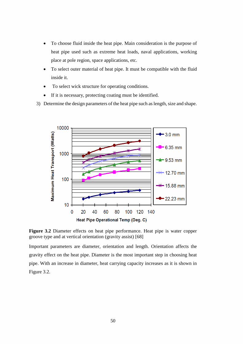
50
To choose fluid inside the heat pipe. Main consideration is the purpose of
heat pipe used such as extreme heat loads, naval applications, working
place at pole region, space applications, etc.
To select outer material of heat pipe. It must be compatible with the fluid
inside it.
To select wick structure for operating conditions.
If it is necessary, protecting coating must be identified.
3) Determine the design parameters of the heat pipe such as length, size and shape.
Figure 3.2 Diameter effects on heat pipe performance. Heat pipe is water copper
groove type and at vertical orientation (gravity assist) [68]
Important parameters are diameter, orientation and length. Orientation affects the
gravity effect on the heat pipe. Diameter is the most important step in choosing heat
pipe. With an increase in diameter, heat carrying capacity increases as it is shown in
Figure 3.2.
51
3.3.2 The Construction Material of Heat Pipe
The working fluid is functional in a certain temperature range due to changes at
different temperatures. In addition to this, working fluid needs to be compatible with
the shell of heat pipe to prevent corrosion and chemical reaction. If chemical reaction
or corrosion occurs, non-condensable gases appear, which decreases the performance
of the heat pipe. Hence, corrosion effect and compatibility of the vessel material must
be considered. Some examples for the compatibility between the fluid and the vessel
material are given in Table 3.1.
The most commonly used heat pipe type is water as a working fluid and copper as a
vessel. It is generally used in electronic cooling applications within the range of 5 oC
to 230 oC. Due to working range, liquid nitrogen and liquid ammonia heat pipes are
used in special areas such as cryogenic applications, space applications, etc. Liquid
ammonia with aluminum vessel heat pipe is very common popularity in space
applications due to lightweight of aluminum.
Functionality of a heat pipe is restricted by the freezing point of the working fluid.
Under the freezing point, heat pipe’s sealed joints can be damaged, and flow inside
can have discontinuity, which directly affects the performance of the heat pipe.

52
Table 3.1 Typical Operating Characteristics of Heat Pipes [68]
Temperature
Range (oC) Working Fluid
Vessel
Material
Measured Axial
Heat Flux at
Certain
Temperature
(kW/cm2)
Measured
Surface Heat
Flux at Certain
Temperature
(W/cm2)
-200 to -80 Liq. Nitrogen Stainless
Steel 0.067 @-163 oC 1.01 @-163 oC
-70 to +60 Liq. Ammonia
Nickel,
Aluminum,
Stainless
Steel
0.295 oC 2.95 oC
-45 to +120 Methanol
Nickel,
Copper,
Stainless
Steel
0.45 @100 oC 75.5 @100 oC
+5 to +230 Water Copper,
Nickel 0.67 @200 oC 146 @170 oC
+190 to +550 Mercury(0.02%)
Magnesium(0.001%)
Stainless
Steel 25.1 @360 oC 181 @750 oC
+400 to +800 Potassium
Nickel,
Stainless
Steel
5.6 @750 oC 181 @750 oC
+500 to +900 Sodium
Nickel,
Stainless
Steel
9.3 @850 oC 224 @850 oC
+900 to
+1500 Lithium
Niobim (1%),
Zirconium 2.0 @1250 oC 207 @1250 oC
+1500 to
+2000 Silver
Tantalum
(5%),
Tungsten
4.1 oC 413 oC
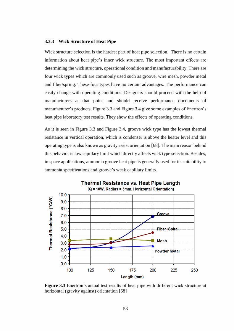
53
3.3.3 Wick Structure of Heat Pipe
Wick structure selection is the hardest part of heat pipe selection. There is no certain
information about heat pipe’s inner wick structure. The most important effects are
determining the wick structure, operational condition and manufacturability. There are
four wick types which are commonly used such as groove, wire mesh, powder metal
and fiber/spring. These four types have no certain advantages. The performance can
easily change with operating conditions. Designers should proceed with the help of
manufacturers at that point and should receive performance documents of
manufacturer’s products. Figure 3.3 and Figure 3.4 give some examples of Enertron’s
heat pipe laboratory test results. They show the effects of operating conditions.
As it is seen in Figure 3.3 and Figure 3.4, groove wick type has the lowest thermal
resistance in vertical operation, which is condenser is above the heater level and this
operating type is also known as gravity assist orientation [68]. The main reason behind
this behavior is low capillary limit which directly affects wick type selection. Besides,
in space applications, ammonia groove heat pipe is generally used for its suitability to
ammonia specifications and groove’s weak capillary limits.
Figure 3.3 Enertron’s actual test results of heat pipe with different wick structure at
horizontal (gravity against) orientation [68]

54
Figure 3.4 Enertron’s actual test results of heat pipe with different wick structure at
vertical (gravity assist) orientation [68]
3.4 CAD Design of the Whole Structure
This study is inspired from ASELSAN’s radar project. Radar systems are usually
placed on rotating platforms. These platforms generally rotate around the z-axis.
Rotating platforms in ASELSAN are used in radars, tracking and weapon carrying
applications. Generated platform is designed based on a real system. Dimensions are
close enough to implement the gathered information from this study to real
applications.
Most of the rotating platforms generally are ‘U- shape’. There is a planar base for
connection to rotating base, and it has support walls on two sides. Rotating platforms
do not carry only the main system, but they also carry controller sections, RF units for
radar applications, power amplifiers, power controller etc. Hence at the first step of
design stage, platforms should be designed for satisfying the requirements.
In this study, one of the mass produced ASELSAN rotary platforms is simplified to
implement a cooling method for it. Experimental platform is generated by PTC Creo
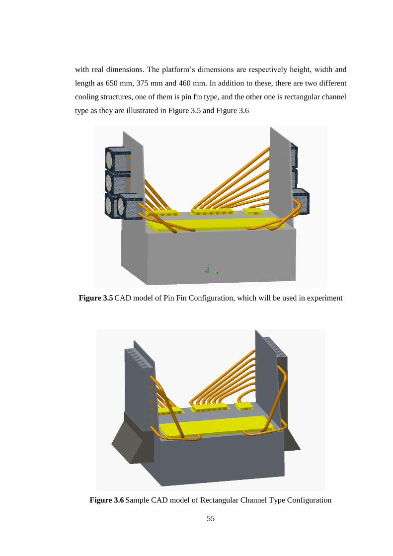
55
with real dimensions. The platform’s dimensions are respectively height, width and
length as 650 mm, 375 mm and 460 mm. In addition to these, there are two different
cooling structures, one of them is pin fin type, and the other one is rectangular channel
type as they are illustrated in Figure 3.5 and Figure 3.6
Figure 3.5 CAD model of Pin Fin Configuration, which will be used in experiment
Figure 3.6 Sample CAD model of Rectangular Channel Type Configuration
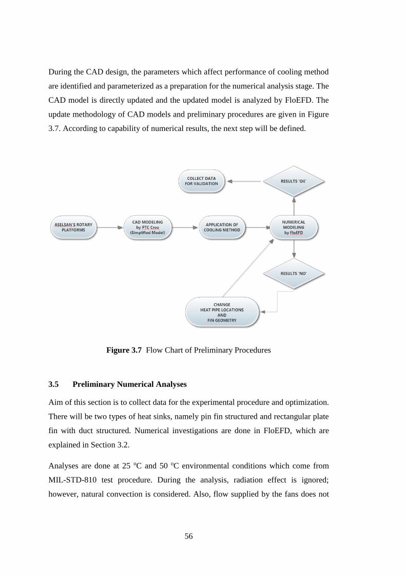
56
During the CAD design, the parameters which affect performance of cooling method
are identified and parameterized as a preparation for the numerical analysis stage. The
CAD model is directly updated and the updated model is analyzed by FloEFD. The
update methodology of CAD models and preliminary procedures are given in Figure
3.7. According to capability of numerical results, the next step will be defined.
Figure 3.7 Flow Chart of Preliminary Procedures
3.5 Preliminary Numerical Analyses
Aim of this section is to collect data for the experimental procedure and optimization.
There will be two types of heat sinks, namely pin fin structured and rectangular plate
fin with duct structured. Numerical investigations are done in FloEFD, which are
explained in Section 3.2.
Analyses are done at 25 oC and 50 oC environmental conditions which come from
MIL-STD-810 test procedure. During the analysis, radiation effect is ignored;
however, natural convection is considered. Also, flow supplied by the fans does not
57
have a constant flow rate, for each condition flow rate is directly obtained from the fan
performance curve (see Figure A.4 in Appendix A).
These runs will be used for making comparisons with the experiments and improving
the design. Numerical analysis procedure will be explained in detail in following
headlines.
3.5.1 Procedures of Numerical Analyses
The first step of starting numerical runs is 3-D CAD design of the system which will
be manufactured to be used in the experiments. Numerical runs are done under 1atm
pressure and 25 oC and 50 oC environmental conditions. During the analyses, inputs
of the runs such as turbulence parameters, environmental properties, boundary
conditions etc. always remain the same. All geometrical upgrades are done in CAD,
then the numerical model is re-generated.
The next step of numerical runs is configuration analysis. FloEFD needs some settings,
in other words, beginning input. These are flow type such as internal or external flow,
modes of heat transfer considered during the run such as conduction, convection or
radiation, types or materials and fluids, flow type such as laminar, turbulent or mixed
flow, turbulence parameters and initial state in terms of temperature, pressure, velocity
etc. After all these settings are done, boundary conditions and tools are defined.
In this study, flow type is set to external flow. For all cases of analyses, radiation is
ignored. Conduction in solids and natural convection in fluids are considered. In
addition to these, flow is considered as laminar first and then as turbulent. As it is
mentioned before, FloEFD only uses k-ε turbulence model, hence solver needs only
the parameters of k-ε model. There are two different setup configurations about
turbulence parameter. One of them is turbulence intensity (%) and turbulence length
(m) configuration, which is selected in this study. Another one is turbulent energy
(J/kg) and turbulent dissipation (W/kg) combination. Turbulence parameters in terms
of turbulence length and turbulence intensity are calculated from the following
equations [69].
58
Turbulence length (ls);
𝑙𝑠 = 0.07𝐷ℎ (3.6)
Turbulence intensity (I);
𝐼 = 0.16𝑅𝑒𝐷ℎ−1/8
(3.7)
where Re is the Reynolds Number which is the ratio of inertial forces to viscous forces
defined as
𝑅𝑒 =
𝜌𝜗𝐷ℎ
𝜇
(3.8)
In Equations 3.6, 3.7 and 3.8, Dh is the hydraulic diameter.
After the calculations, the turbulence intensity of 5.4% and the turbulence length of
0.525 mm are defined as initial values. As the fluid, air is chosen at 25 oC and 50 oC
depending on the case. During the analyses, solver needs thermodynamic properties,
hence initial temperature and pressure are defined. Temperature is changing with
analyzed conditions (25 oC or 50 oC) and pressure is always constant at 1 atm.
After all of the definitions above the configuration step is completed. Then the
computational domain and boundary conditions must be defined. First step here is to
define the calculation domain; in other words, calculation envelope. The dimensions
of the envelope are given in Table 3.2.
Table 3.2 Dimensions of Computational Domain
Dimensions of the Computational Domain
x axis 0.5 m
-x axis -0.5 m
y axis 0.75 m
-y axis -0.15 m
z axis 0.65 m
-z axis -0.65 m
59
The material definitions are made. All solid parts are defined as Aluminum 5052.
Except the outer shells of fans that are defined as insulators, because they are plastic
materials. Al 5052 is chosen for its accessibility and economy. Generally, in military
applications Al 6061 and Al 6063 are used; however, they are expensive and hard to
obtain. In terms of thermal conductivity of these materials, the differences are quite
large, and it affects the performance of system and experiments. Al 5052 has the
conductivity of 138 W/mK, Al 6061 has the conductivity of 180 W/mK and Al 6063
has the conductivity of 218 W/mK at room temperature, 25 oC. The selection of Al
5052 for the mock-up guarantees the performance of the final product that will be
made out of Al 6061 or Al 6063.
Then, the boundary conditions are defined. The heaters representing the electronic
chips are defined as constant heat sources, which are classified as surface heat sources.
Powers of the sources are given in Table 3.3. These sources simulate the real TWT
and PA modules of the radar electronics.
Table 3.3 Heat Source of the System
Source Quantity Dimension
(mm)
Power
(W)
Heat Flux
(W/cm2)
Heater 1 2 50 x 126 x 10 600 10
Heater 2 1 152 x 400 x 10 350 0.58
Heater 3 1 68 x 54 x 10 70 1.91
Next step is to create heat pipes. In FloEFD, there is an electronic cooling module, and
this module has some special components for electronics cooling. Heat pipe is one of
them. In literature, there are some mathematical models for heat pipes; however, these
may not work with all systems. Hence, heat pipes are commonly modeled as super
conductive rods in axial direction. Radial direction conductivity is ignored. During the
analyses, requirements for creating heat pipes are identifying condenser and
evaporator sections as heat in / out sections and guessing effective thermal resistance
of the heat pipe. The first assumption for the effective thermal resistance value is 0.25
oC/W or K/W. This is only a prediction, and corrected values are defined after the
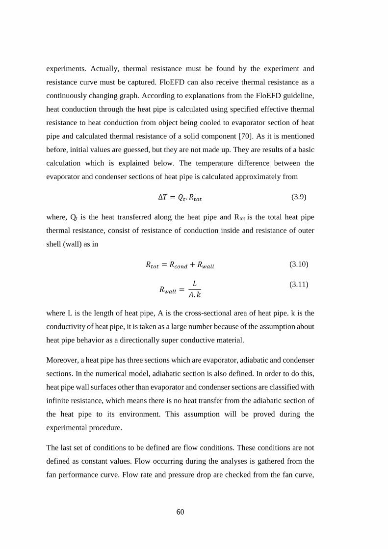
60
experiments. Actually, thermal resistance must be found by the experiment and
resistance curve must be captured. FloEFD can also receive thermal resistance as a
continuously changing graph. According to explanations from the FloEFD guideline,
heat conduction through the heat pipe is calculated using specified effective thermal
resistance to heat conduction from object being cooled to evaporator section of heat
pipe and calculated thermal resistance of a solid component [70]. As it is mentioned
before, initial values are guessed, but they are not made up. They are results of a basic
calculation which is explained below. The temperature difference between the
evaporator and condenser sections of heat pipe is calculated approximately from
∆𝑇 = 𝑄𝑡. 𝑅𝑡𝑜𝑡 (3.9)
where, Qt is the heat transferred along the heat pipe and Rtot is the total heat pipe
thermal resistance, consist of resistance of conduction inside and resistance of outer
shell (wall) as in
𝑅𝑡𝑜𝑡 = 𝑅𝑐𝑜𝑛𝑑 + 𝑅𝑤𝑎𝑙𝑙 (3.10)
𝑅𝑤𝑎𝑙𝑙 =
𝐿
𝐴. 𝑘
(3.11)
where L is the length of heat pipe, A is the cross-sectional area of heat pipe. k is the
conductivity of heat pipe, it is taken as a large number because of the assumption about
heat pipe behavior as a directionally super conductive material.
Moreover, a heat pipe has three sections which are evaporator, adiabatic and condenser
sections. In the numerical model, adiabatic section is also defined. In order to do this,
heat pipe wall surfaces other than evaporator and condenser sections are classified with
infinite resistance, which means there is no heat transfer from the adiabatic section of
the heat pipe to its environment. This assumption will be proved during the
experimental procedure.
The last set of conditions to be defined are flow conditions. These conditions are not
defined as constant values. Flow occurring during the analyses is gathered from the
fan performance curve. Flow rate and pressure drop are checked from the fan curve,

61
which is supplied from the manufacturer. The fan that is used is Ebm Papst 8214JH3,
and its specifications are given in Appendix A.
During the analyses, mesh is automatically generated and refinement levels are always
active. The mesh independence is also studied, which will be given in Section 3.5.2.
There, different cell numbers of mesh are tried then, optimum mesh number and level
is selected.
A summary of preliminary procedures can be given as
Real rotary platform is simplified in PTC Creo.
Two types of cooling techniques are modelled.
All models are parameterized in CAD to prepare CAD models for FloEFD.
Working conditions are identified from MIL-STD-810.
Numerical modeling is done in FloEFD.
Heat loads, boundary conditions and some assumptions are defined.
Optimum mesh is obtained.
Results are collected. The results which are above the thermal shut-down
range are ignored and the designs leading to these results are eliminated for
being inadequate.
If a result is above thermal shut-down point, heat pipe locations and
geometry of fins are changed.
For the experimental procedure, hot spots are identified. The measurements
in experiments will be taken from these hot spot points.
3.5.2 Results and Discussions of Numerical Analyses
Configurations of analyses are summarized in previous sections. This section covers
the results of preliminary analyses and their discussions. Some of these results will be
validated in the experiment which is in Chapter 4. Finally, gathered knowledge will be
used for correcting the model and optimizing the rectangular plate fin model in Chapter
5. The investigations will be started with the pin fin configuration because this system
is also used in the experiments.

62
The first numerical study is for mesh convergence in pin fin configurations. During
this process, FloEFD’s performance and the numerical model parameters and the mesh
are optimized. As it is known, duration of numerical analyses directly depend on the
performances of the solver and the computer, complexity of numerical modelling,
quantities of inputs and outputs etc. Hence, the first step is identifying optimum
solution condition for analyses, which is directly affected by mesh or cell numbers.
For the mesh convergence study, one goal is defined, which is the surface temperature
of Heater 1. The reasons for the selection of Heater 1 are listed below;
It simulates the critical component.
It has a higher importance in the electronic system.
It has the highest heat dissipation with 600 W and the highest heat flux with
10 W/cm2.
Table 3.4 Mesh Independence Study: the change of Heater 1 average surface
temperature with the number of cells in the model at 50 oC ambient temperature
Number of
Total Mesh
Cells
Number of
Solid Mesh
Cells
Number of
Fluid Mesh
Cells
Number of
Partial
Mesh Cells
Average
Temperature
on Surface of
Heater 1 (oC)
Duration
(hour)
173546 12468 64252 96826 102.54 1.66
307384 19968 89152 198264 102.05 2.42
421751 20567 99782 301402 102.76 3.86
682101 39535 150252 492314 102.61 5.29
734660 43724 178562 512284 102.70 6.18
896478 59570 231977 604711 102.60 6.94
1200778 63642 312516 824614 102.62 9.13
1572110 84656 486158 1001296 102.59 11.34
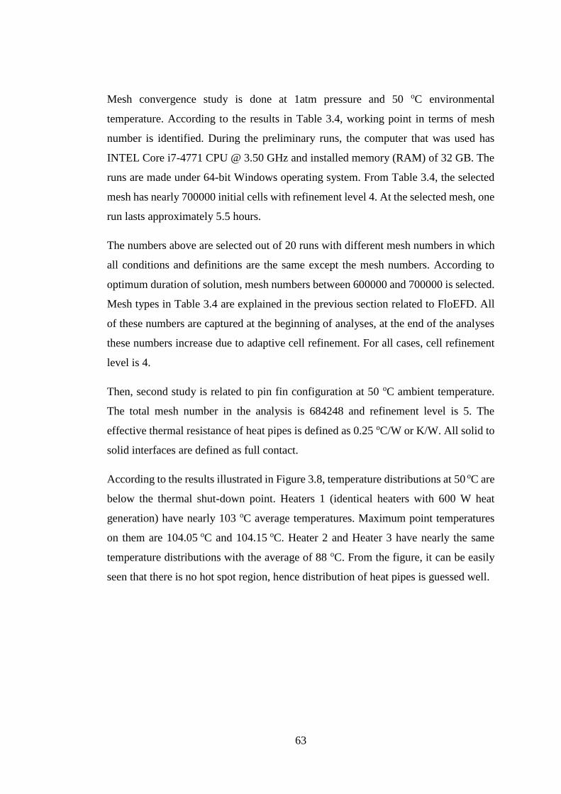
63
Mesh convergence study is done at 1atm pressure and 50 oC environmental
temperature. According to the results in Table 3.4, working point in terms of mesh
number is identified. During the preliminary runs, the computer that was used has
INTEL Core i7-4771 CPU @ 3.50 GHz and installed memory (RAM) of 32 GB. The
runs are made under 64-bit Windows operating system. From Table 3.4, the selected
mesh has nearly 700000 initial cells with refinement level 4. At the selected mesh, one
run lasts approximately 5.5 hours.
The numbers above are selected out of 20 runs with different mesh numbers in which
all conditions and definitions are the same except the mesh numbers. According to
optimum duration of solution, mesh numbers between 600000 and 700000 is selected.
Mesh types in Table 3.4 are explained in the previous section related to FloEFD. All
of these numbers are captured at the beginning of analyses, at the end of the analyses
these numbers increase due to adaptive cell refinement. For all cases, cell refinement
level is 4.
Then, second study is related to pin fin configuration at 50 oC ambient temperature.
The total mesh number in the analysis is 684248 and refinement level is 5. The
effective thermal resistance of heat pipes is defined as 0.25 oC/W or K/W. All solid to
solid interfaces are defined as full contact.
According to the results illustrated in Figure 3.8, temperature distributions at 50 oC are
below the thermal shut-down point. Heaters 1 (identical heaters with 600 W heat
generation) have nearly 103 oC average temperatures. Maximum point temperatures
on them are 104.05 oC and 104.15 oC. Heater 2 and Heater 3 have nearly the same
temperature distributions with the average of 88 oC. From the figure, it can be easily
seen that there is no hot spot region, hence distribution of heat pipes is guessed well.
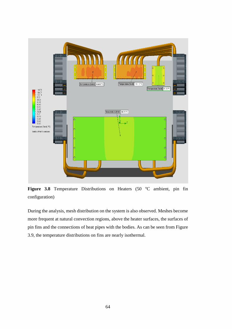
64
Figure 3.8 Temperature Distributions on Heaters (50 oC ambient, pin fin
configuration)
During the analysis, mesh distribution on the system is also observed. Meshes become
more frequent at natural convection regions, above the heater surfaces, the surfaces of
pin fins and the connections of heat pipes with the bodies. As can be seen from Figure
3.9, the temperature distributions on fins are nearly isothermal.
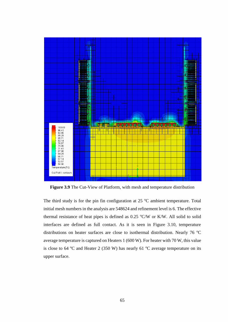
65
Figure 3.9 The Cut-View of Platform, with mesh and temperature distribution
The third study is for the pin fin configuration at 25 oC ambient temperature. Total
initial mesh numbers in the analysis are 548624 and refinement level is 6. The effective
thermal resistance of heat pipes is defined as 0.25 oC/W or K/W. All solid to solid
interfaces are defined as full contact. As it is seen in Figure 3.10, temperature
distributions on heater surfaces are close to isothermal distribution. Nearly 76 oC
average temperature is captured on Heaters 1 (600 W). For heater with 70 W, this value
is close to 64 oC and Heater 2 (350 W) has nearly 61 oC average temperature on its
upper surface.
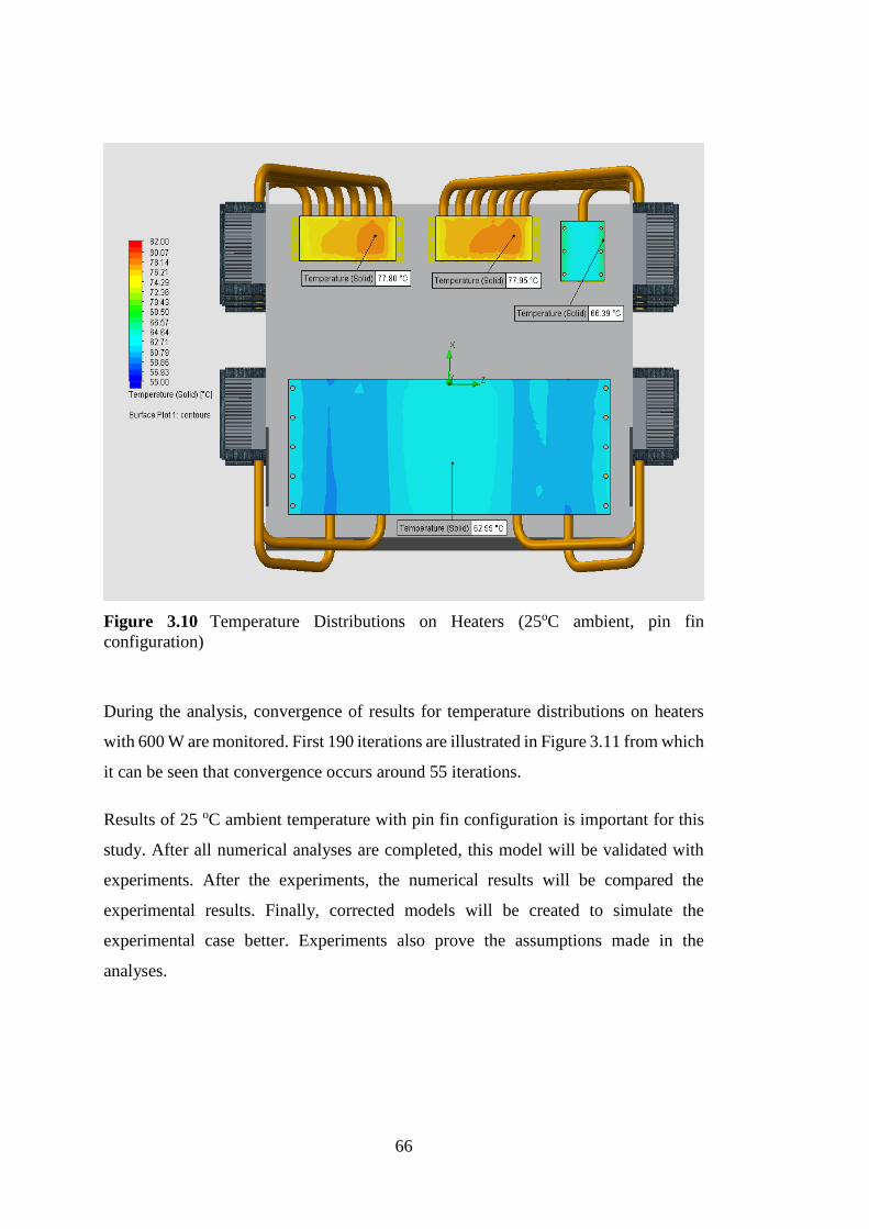
66
Figure 3.10 Temperature Distributions on Heaters (25oC ambient, pin fin
configuration)
During the analysis, convergence of results for temperature distributions on heaters
with 600 W are monitored. First 190 iterations are illustrated in Figure 3.11 from which
it can be seen that convergence occurs around 55 iterations.
Results of 25 oC ambient temperature with pin fin configuration is important for this
study. After all numerical analyses are completed, this model will be validated with
experiments. After the experiments, the numerical results will be compared the
experimental results. Finally, corrected models will be created to simulate the
experimental case better. Experiments also prove the assumptions made in the
analyses.
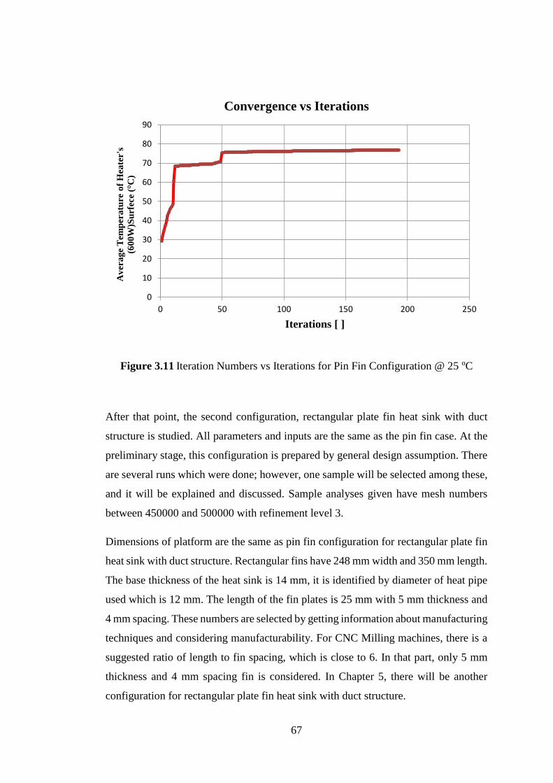
67
Figure 3.11 Iteration Numbers vs Iterations for Pin Fin Configuration @ 25 oC
After that point, the second configuration, rectangular plate fin heat sink with duct
structure is studied. All parameters and inputs are the same as the pin fin case. At the
preliminary stage, this configuration is prepared by general design assumption. There
are several runs which were done; however, one sample will be selected among these,
and it will be explained and discussed. Sample analyses given have mesh numbers
between 450000 and 500000 with refinement level 3.
Dimensions of platform are the same as pin fin configuration for rectangular plate fin
heat sink with duct structure. Rectangular fins have 248 mm width and 350 mm length.
The base thickness of the heat sink is 14 mm, it is identified by diameter of heat pipe
used which is 12 mm. The length of the fin plates is 25 mm with 5 mm thickness and
4 mm spacing. These numbers are selected by getting information about manufacturing
techniques and considering manufacturability. For CNC Milling machines, there is a
suggested ratio of length to fin spacing, which is close to 6. In that part, only 5 mm
thickness and 4 mm spacing fin is considered. In Chapter 5, there will be another
configuration for rectangular plate fin heat sink with duct structure.
0
10
20
30
40
50
60
70
80
90
0 50 100 150 200 250
Av
era
ge
Tem
per
atu
re o
f H
eate
r's
(60
0W
)Su
rfec
e (°
C)
Iterations [ ]
Convergence vs Iterations

68
Figure 3.12 is given for basic illustration of temperature distributions for this
configuration at 50 oC ambient. The maximum temperature occurs at the surface of
heaters with 600 W, which is nearly 122 oC. This number is in critical range for real
product form of heaters. These devices make thermal shut-down at 120 oC base
temperature distribution. This system is cooled by 6 fans, each duct has 3 fans inside.
Figure 3.12 Temperature Distributions on Heaters (50 oC ambient, rectangular plate
fin with duct structured)
Same study is also done for 25 oC ambient temperature. This configuration will be
optimized in Chapter 5. The used plate fin heat sinks are the same as the ones in the
analysis above. Moreover, there are some observations related to flow on fin plates
and temperature distribution on fins, located on two sides. Figure 3.13 gives the
temperature distributions on heater surfaces, the heaters with 600 W have temperatures
close to 95 oC. Heater 2 and 3 have average temperatures of 74 oC and 78 oC,
respectively. Figure 3.14 and Figure 3.15 demonstrate temperature distributions on
heat sinks, average solid temperatures. When these figures are examined, heat pipes

69
locations can be easily identified from temperature distributions. In order to gather
close to isothermal surfaces on fins; heat pipe locations are studied. Locations of heat
pipes are adjusted iteratively. Suggested method is to keep more powerful heat pipe
close to air flow. Another suggestion about placement of pipes is that, pipes must be
embedded to the base of the heat sink because heat pipes transfer heat by conduction
at evaporator and condenser sections. Average temperature on fins is approximately
58 oC. Finally, air flow temperature is considered. The heat sink at the left side, which
has 9 heat pipe connections exhausts the air at a temperature 3 oC hotter than the other
heat sink. Another observation can be made from Figures 3.14-3.17 is the mesh density
on heat sinks. When the figures are examined in detail, there are some additional
divided cells seen around the connections of fluid flow and the fins. These are the
refined cells occurring during the calculation, which is an advantage of the adaptive
mesh mechanism of FloEFD.
Figure 3.13 Temperature Distributions on Heaters (25oC ambient, rectangular plate
fin with duct structured)
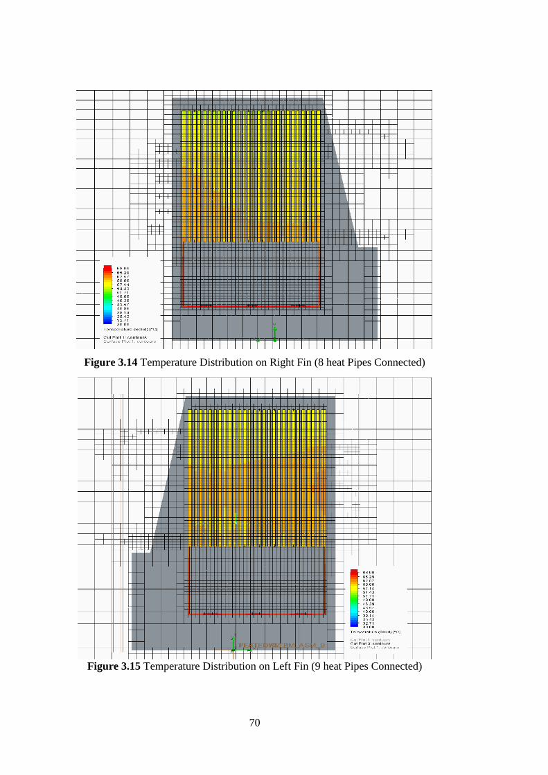
70
Figure 3.14 Temperature Distribution on Right Fin (8 heat Pipes Connected)
Figure 3.15 Temperature Distribution on Left Fin (9 heat Pipes Connected)

71
Figure 3.16 Exhaust Air Temperature Distribution on Right Fin (8 heat Pipes
Connected)
Figure 3.17 Exhaust Air Temperature Distribution on Left Fin (9 heat Pipes
Connected)
72
Finally, these runs are done in order to gather a general idea about the usage of heat
pipes. Collected results will be validated experimentally for the pin fin heat sink case.
This validation will prove the performance of heat pipe and show the real characteristic
of system such as thermal and contact resistances. In this case, effective thermal
resistance for all heat pipes is defined as 0.25 oC/W or K/W. This number will be
checked by experiments and re-calculated. The next chapter covers the experimental
procedures and comparisons of experimental and numerical analyses. After that, plate
fin heat sink optimization in terms of thickness and spacing will be done in Chapter 5.
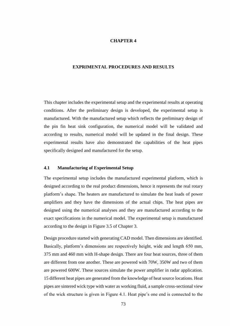
73
CHAPTER 4
EXPRIMENTAL PROCEDURES AND RESULTS
This chapter includes the experimental setup and the experimental results at operating
conditions. After the preliminary design is developed, the experimental setup is
manufactured. With the manufactured setup which reflects the preliminary design of
the pin fin heat sink configuration, the numerical model will be validated and
according to results, numerical model will be updated in the final design. These
experimental results have also demonstrated the capabilities of the heat pipes
specifically designed and manufactured for the setup.
4.1 Manufacturing of Experimental Setup
The experimental setup includes the manufactured experimental platform, which is
designed according to the real product dimensions, hence it represents the real rotary
platform’s shape. The heaters are manufactured to simulate the heat loads of power
amplifiers and they have the dimensions of the actual chips. The heat pipes are
designed using the numerical analyses and they are manufactured according to the
exact specifications in the numerical model. The experimental setup is manufactured
according to the design in Figure 3.5 of Chapter 3.
Design procedure started with generating CAD model. Then dimensions are identified.
Basically, platform’s dimensions are respectively height, wide and length 650 mm,
375 mm and 460 mm with H-shape design. There are four heat sources, three of them
are different from one another. These are powered with 70W, 350W and two of them
are powered 600W. These sources simulate the power amplifier in radar application.
15 different heat pipes are generated from the knowledge of heat source locations. Heat
pipes are sintered wick type with water as working fluid, a sample cross-sectional view
of the wick structure is given in Figure 4.1. Heat pipe’s one end is connected to the

74
designed condenser cold plate and the other end is attached to the pin fin heat sink
assembly.
Preparation of the experimental setup will be explained step by step. In addition to the
platform, the measurement devices and techniques will also be explained.
Figure 4.1 Cross-section of sintered wick heat pipe
First step is the manufacturing of the dummy platform. Real dimensions are used in
order to manufacture the dummy rotary platform with dimensions 650 mm x 375 mm
x 460 mm. Platform is produced from an Aluminum 5000 series sheet with 5 mm
thickness. The assembled platform is illustrated in Figure 4.2.
Figure 4.2 Manufactured dummy rotary platform
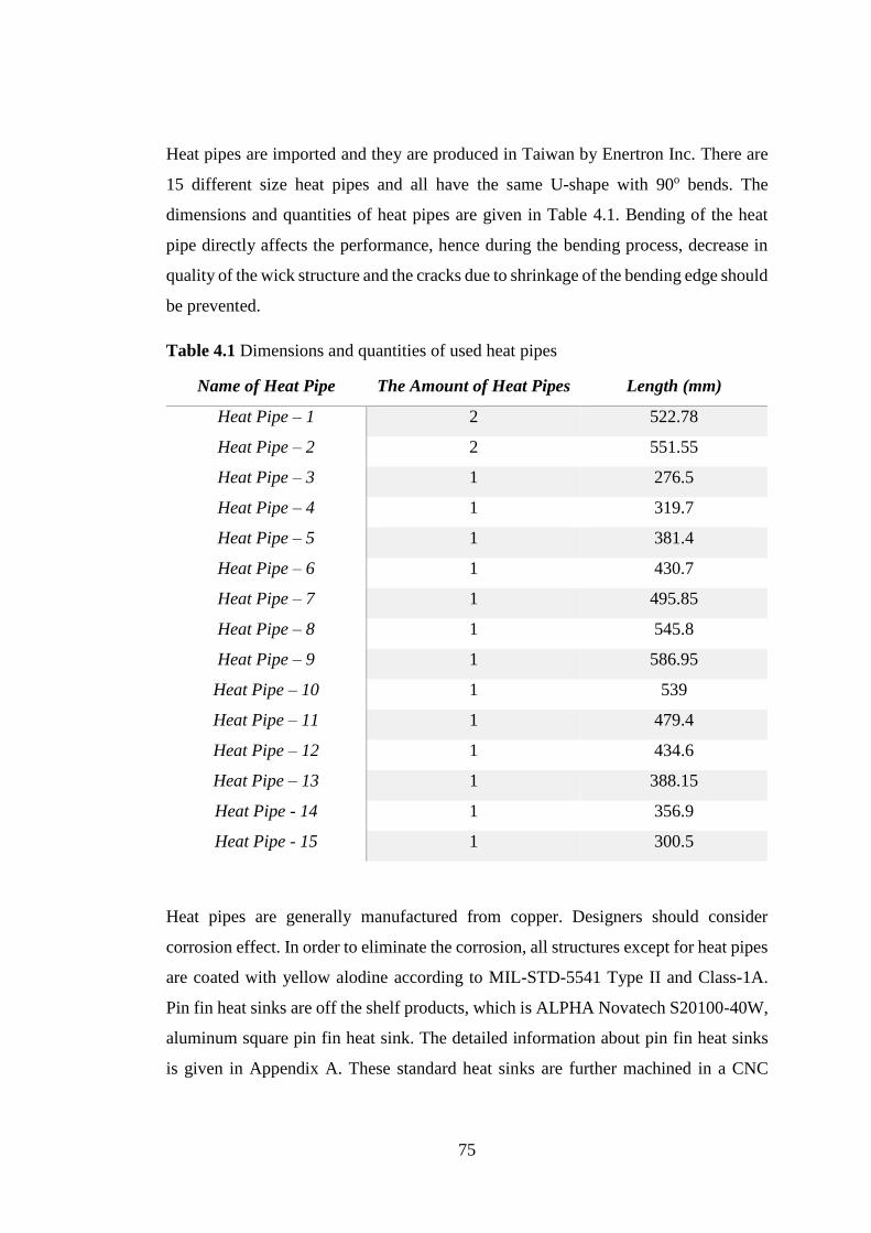
75
Heat pipes are imported and they are produced in Taiwan by Enertron Inc. There are
15 different size heat pipes and all have the same U-shape with 90o bends. The
dimensions and quantities of heat pipes are given in Table 4.1. Bending of the heat
pipe directly affects the performance, hence during the bending process, decrease in
quality of the wick structure and the cracks due to shrinkage of the bending edge should
be prevented.
Table 4.1 Dimensions and quantities of used heat pipes
Name of Heat Pipe The Amount of Heat Pipes Length (mm)
Heat Pipe – 1 2 522.78
Heat Pipe – 2 2 551.55
Heat Pipe – 3 1 276.5
Heat Pipe – 4 1 319.7
Heat Pipe – 5 1 381.4
Heat Pipe – 6 1 430.7
Heat Pipe – 7 1 495.85
Heat Pipe – 8 1 545.8
Heat Pipe – 9 1 586.95
Heat Pipe – 10 1 539
Heat Pipe – 11 1 479.4
Heat Pipe – 12 1 434.6
Heat Pipe – 13 1 388.15
Heat Pipe - 14 1 356.9
Heat Pipe - 15 1 300.5
Heat pipes are generally manufactured from copper. Designers should consider
corrosion effect. In order to eliminate the corrosion, all structures except for heat pipes
are coated with yellow alodine according to MIL-STD-5541 Type II and Class-1A.
Pin fin heat sinks are off the shelf products, which is ALPHA Novatech S20100-40W,
aluminum square pin fin heat sink. The detailed information about pin fin heat sinks
is given in Appendix A. These standard heat sinks are further machined in a CNC

76
milling machine. Assembly connection holes and heat pipe connection locations are
prepared.
The heat pipes that are used have 12 mm diameter with different lengths, as shown in
Table 4.1. Hence the machined heat sinks have 12 mm diameter assembly holes for
heat pipes with close-fit tolerances. The gap between the heat pipe and its connection
location is the most important design criteria in manufacturing process due to the
resulting thermal resistance caused by the clearance gap. To eliminate a high thermal
contact resistance, an interface material is used for filling the clearance between the
heat pipe and its hole. As a filler material, Artic Silver 5 is used, which is high density
polysynthetic silver thermal compound (Appendix A). This filler material is spread in
the form of a thin layer, as illustrated in Figure 4.3. Then, heat pipe is attached to the
interface hole. During the assembly steps, this filler also behaves like lubricant for heat
pipe’s fitting. The fitted heat pipe is shown in Figure 4.4.
Figure 4.3 Filler material is applied to mounting holes
During the design steps, accessibility and maintenance procedures are also considered.
Hence, the condenser section is designed as a cooling module. This part includes the
pin fin heat sink, the fan and its holder, the mounting back plate, and the heat pipes.

77
The final form of the module is shown in Figure 4.5. All assemblies are readied to
easily connect them to the platform. The main idea behind this is to decrease the
replacement time and the maintenance duration.
Figure 4.4 Heat pipes are mounted into mounting holes of pin fin
Figure 4.5 Condenser module

78
The selected fan is EbmPapst 8214 JH4, whose specifications are given in Appendix
A. Ebm 8214JH4 is very close to military standards and it is a high speed fan. There
is only one negative side, which is noise at maximum speed. During the experiment,
fans are driven with external DC power supply. This fan is produced from plastic
material, hence it is only 0.2 kilograms. It is very important for the overall system
weight.
Finally, cooling module is screwed the side walls of platform. This configuration is
appropriate for desert environment. Because there is no suction or exhaust to the
normal of the ground. If there is blow or suction, the critical damage may occur due to
sand particles. The evaporator ends of the heat pipes are attached to heater base plates.
These plates are produced from the same material with the platforms and they used for
the connection between heat pipes and power sources. Fans can be under operation
independent from the cooling module, which means it can be easily replaced.
However, the cooling module and platform’s heater base must be attached at the same
time. The final mounting of the heat pipes is given in Figure 4.6.
Figure 4.6 The final mounting of heat pipes
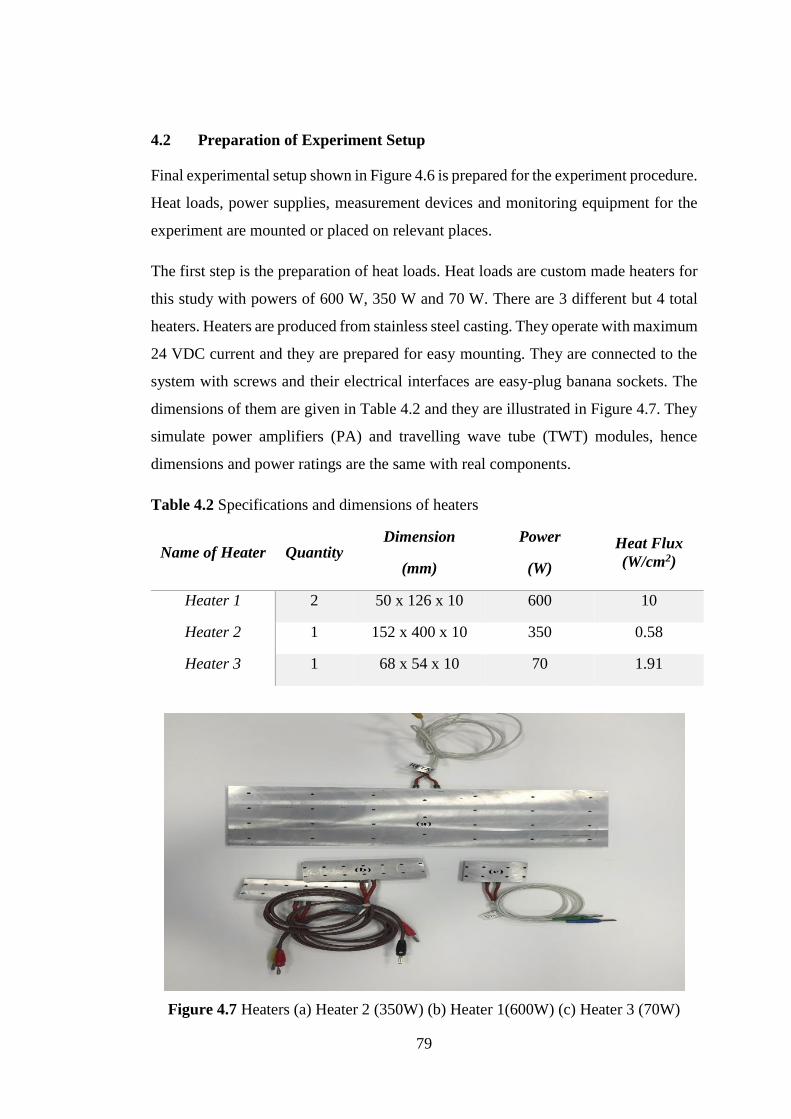
79
4.2 Preparation of Experiment Setup
Final experimental setup shown in Figure 4.6 is prepared for the experiment procedure.
Heat loads, power supplies, measurement devices and monitoring equipment for the
experiment are mounted or placed on relevant places.
The first step is the preparation of heat loads. Heat loads are custom made heaters for
this study with powers of 600 W, 350 W and 70 W. There are 3 different but 4 total
heaters. Heaters are produced from stainless steel casting. They operate with maximum
24 VDC current and they are prepared for easy mounting. They are connected to the
system with screws and their electrical interfaces are easy-plug banana sockets. The
dimensions of them are given in Table 4.2 and they are illustrated in Figure 4.7. They
simulate power amplifiers (PA) and travelling wave tube (TWT) modules, hence
dimensions and power ratings are the same with real components.
Table 4.2 Specifications and dimensions of heaters
Name of Heater Quantity Dimension
(mm)
Power
(W)
Heat Flux
(W/cm2)
Heater 1 2 50 x 126 x 10 600 10
Heater 2 1 152 x 400 x 10 350 0.58
Heater 3 1 68 x 54 x 10 70 1.91
Figure 4.7 Heaters (a) Heater 2 (350W) (b) Heater 1(600W) (c) Heater 3 (70W)

80
The second step is preparation of the data logging system for the test setup. The main
parts of this system are the data logger, the multiplexers for data-logger, the
thermocouples and the computer. The thermocouples are used for receiving
temperature data as electrical input, hence they are used as thermal sensor. During the
experiment, ‘Type-J’ thermocouples are used. ‘Type-J’ is nickel alloy thermocouple
and it has iron–constantan couple. ‘Type-J’ thermocouples have a restricted
measurement range (-40 oC to 750 oC) compared to other types, however they have
higher sensitivity than the other types with 50 µV/oC. Upper limit 750 oC comes from
iron’s properties. Thermocouples generate a voltage difference due to temperature
change, hence receiving data must be converted. This conversion can be done with a
calibration based on ‘Type-J voltage to temperature transformation catalogue’.
However, during the experiment they are calibrated automatically by the data logger.
Thermocouples are prepared at ASELSAN Thermal Laboratory. 2 m length
thermocouple wires are cut. Then, the junction weld is done by thermocouple welder
‘Omega TL-WELD’, this device is listed in Table 4.3. After the thermocouples are
finalized, they are connected to their measurement points by pieces of thermally
conductive 3MTM Aluminum adhesive foil tape. All thermocouples are numbered as
illustrated in Figure 4.8. In total, twenty nine thermocouples are placed and 3 of them
are connected to the platform body to monitor the platform wall temperatures. These
thermocouples are placed according to identified hot spot points from the numerical
simulation results at the preliminary stage.

81
Figure 4.8 Sample view of thermocouple’s location
In order to process the data coming from thermocouples, Agilent 34970A Data Logger
device is used. These thermocouples are connected to the data logger with two Agilent
34903A 20-Channels Switch Unit Multiplexer Boards. A single board has twenty
channels, which means twenty inputs can be collected by one multiplexer. A computer
is used for screening the data coming from the data logger and collecting the data with
certain time intervals. All measurement devices are tabulated and explained in Table
4.3.
The third and final step of the setup is mounting the heaters to the upper-side of heat
pipe’s heat collecting plates. The heaters are not installed directly. Because of the
manufacturing tolerances and presence of thermocouples on the surface, there might
be gaps between the heaters and the heat collecting plates. Existence of a gap can cause
to thermal contact resistance and it can obstruct the conduction between heaters and
their sitting place. To eliminate this obstacle, a thermal interface material is used. The
used material is Laird Tflex 640. It is boron nitride filled silicone elastomer with
3W/mK thermal conductivity. It is also adhesive, so it can easily be applied, which is
shown in Figure 4.9. It is elastic material, hence it can be compressed by mounting
load due to screws.
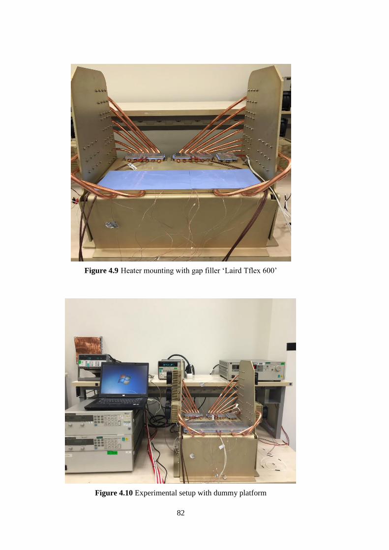
82
Figure 4.9 Heater mounting with gap filler ‘Laird Tflex 600’
Figure 4.10 Experimental setup with dummy platform

83
Another data collection approach used is thermal imaging. The system is monitored
with a FLIR E60 thermal camera. Detailed specifications of the camera are given in
Appendix B. Before capturing images, the thermal camera must be calibrated. The
thermal camera is calibrated with a 3M matt black tape, which has (ε = 0.95)
emissivity. It is seen attached to the wall on the right side of the equipment in Figure
4.10. The calibration is done manually, by holding the camera at a 0.5 meter distance.
While preparing the setup, four different AC to DC power supplies are used. Three of
them run the heaters and one of them runs the fans. Fans are powered with Agilent
6032A System Power Supply 0-60V /0-50A, 1000W. EbmPapst 8214 JH4 works with
24VDC and 1.65A, hence eight fans require 317 Watt. Heaters are controlled with
three different power supplies. Heater 1 (2 pieces) is controlled by Agilent 6692A DC
Power Supply 0-60V /0-110A. Heater 2 is controlled by HP 6573A System DC Power
Supply 0-35V /0-60A. Heater 3 is controlled by Agilent E3634A DC Power Supply 0-
25V, 7A / 0-50V, 4A. All supplies are tabulated in Table 4.3 and their specifications
are given in Appendix B. Due to the risk of electricity because the required current is
too high for running heaters, all power supplies are grounded with a ground terminal,
a copper sheet, which is seen on the left, in Figure 4.10.
The experimental setup is prepared as shown in Figure 4.10 and the experiment is done
at ASELSAN Thermal Laboratory. As it is mentioned above, the validation of the
numerical model will be at 25 oC environmental temperature. Hence first limitation is
to obtain the same environmental condition in the real case. Before starting the
experiment, the laboratory’s temperature is set to 25 oC by the air-conditioner system
in one day.
To conclude, the steps of the experimental procedure are given below.
Numerical results are interpreted.
From the numerical runs and specifications of the modules, hot spots and
the points that thermocouples are attached are identified.
The manufactured platform is mounted.
Cooling modules (heat pipes + heat sink + fan) are attached to the platform.
Mounting holes are filled with thermal grease.

84
Gap filler is spread on mounting plates.
Under the filler material, thermocouples are attached to certain points
defined from numerical runs and technical documents of modules.
Heaters are mounted on cold plates.
System is prepared as shown in Figure 4.10.
Room temperature is stabilized by air-conditioning system by 2 hours.
Measurements are captured from thermocouples and thermal camera.
Measurements are stopped when system reaches steady conditions.
Results should be compared with numerical runs.
Table 4.3 Used devices during the experiment
PRODUCT PURPOSE OF USE
NAME IMAGE
Omega TL-WELD
Arc weld for
thermocouples
Agilent 34970A Data
Logger
Collecting data
Agilent 34903A 20-
Channels Switch Unit
Multiplying Data
Logger’s channels

85
Agilent 6032A
System Power Supply
0-60V /0-50A, 1000W
Feeding fans
Agilent 6692A DC
Power Supply 0-60V
/0-110A
Feeding heater 1
HP 6573A System DC
Power Supply 0-35V
/0-60A
Feeding heater 2
Agilent E3634A DC
Power Supply 0-25V,
7A / 0-50V, 4A
Feeding heater 3
4.3 Results of Experiment
Results are obtained in nearly 25 oC laboratory environment. As it is mentioned in the
previous part, the laboratory’s temperature is set to 25 oC by air-conditioner system in
one day before start to experiment.
Measurements taken from setup are results of the worst case scenario. As it is
explained before, heaters simulate real TWT and PA modules and they only work in
extreme case of TWT and PA modules’ working conditions, which means the full
power case is studied.
Table 4.3 (cont’d)

86
Results are divided in to two sections, one of them is thermocouple data and the other
one is thermal imaging data. In this part, results and their explanations are covered, in
addition to this the summarized discussions are in Chapter 6.
4.3.1 Results Collected From Data Acquisition System and Discussions
These results are collected by the data logger from thermocouples. They are calibrated
and controlled by Agilent 34970A Data Logger. The idea behind the thermocouple use
is obtaining the temperatures of the heaters. Hot spot temperatures on the heaters are
important because the investigated devices make thermal shut-down above 120 oC
temperature. All heaters’ average base temperatures are given in the following pages.
In Figure 4.11, heaters are labeled in order to show which graph belongs to which
heater.
Figure 4.11 Illustration of labeled heaters

87
Figure 4.12 Average surface temperature of Heater 1.1
From Figure 4.12, the average surface temperature of Heater 1.1’s base plane is nearly
82.75 oC. Heater 1.1 reaches steady state conditions in approximately 1000 seconds.
The highest point temperature on the surface is 86.27 oC.
Figure 4.13 Average surface temperature of Heater 1.2
20
25
30
35
40
45
50
55
60
65
70
75
80
85
90
0 2000 4000 6000 8000 10000 12000
Aver
age
Tem
per
ature
(0
C)
Time (s)
Average SurfaceTemperature of Heater 1.1
20253035404550556065707580859095
100
0 2000 4000 6000 8000 10000 12000
Aver
age
Tem
per
ature
(0
C)
Time (s)
Average SurfaceTemperature of Heater 1.2
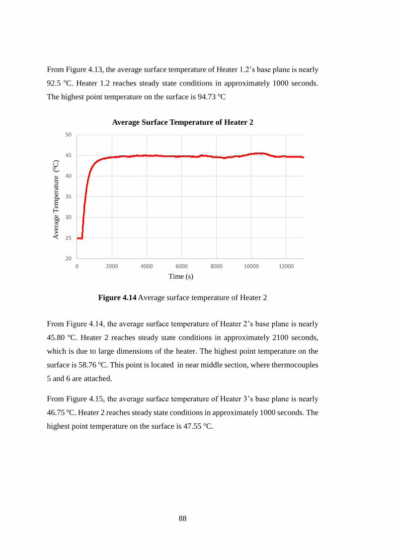
88
From Figure 4.13, the average surface temperature of Heater 1.2’s base plane is nearly
92.5 oC. Heater 1.2 reaches steady state conditions in approximately 1000 seconds.
The highest point temperature on the surface is 94.73 oC
Figure 4.14 Average surface temperature of Heater 2
From Figure 4.14, the average surface temperature of Heater 2’s base plane is nearly
45.80 oC. Heater 2 reaches steady state conditions in approximately 2100 seconds,
which is due to large dimensions of the heater. The highest point temperature on the
surface is 58.76 oC. This point is located in near middle section, where thermocouples
5 and 6 are attached.
From Figure 4.15, the average surface temperature of Heater 3’s base plane is nearly
46.75 oC. Heater 2 reaches steady state conditions in approximately 1000 seconds. The
highest point temperature on the surface is 47.55 oC.
20
25
30
35
40
45
50
0 2000 4000 6000 8000 10000 12000
Aver
age
Tem
per
atu
re (0
C)
Time (s)
Average Surface Temperature of Heater 2
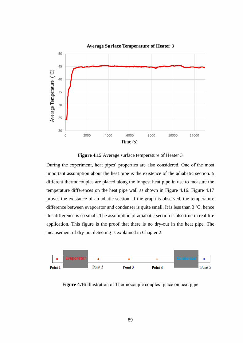
89
Figure 4.15 Average surface temperature of Heater 3
During the experiment, heat pipes’ properties are also considered. One of the most
important assumption about the heat pipe is the existence of the adiabatic section. 5
different thermocouples are placed along the longest heat pipe in use to measure the
temperature differences on the heat pipe wall as shown in Figure 4.16. Figure 4.17
proves the existance of an adiatic section. If the graph is observed, the temperature
difference between evaporator and condenser is quite small. It is less than 3 oC, hence
this difference is so small. The assumption of adiabatic section is also true in real life
application. This figure is the proof that there is no dry-out in the heat pipe. The
meausement of dry-out detecting is explained in Chapter 2.
Figure 4.16 Illustration of Thermocouple couples’ place on heat pipe
20
25
30
35
40
45
50
0 2000 4000 6000 8000 10000 12000
Aver
age
Tem
per
ature
(0
C)
Time (s)
Average Surface Temperature of Heater 3
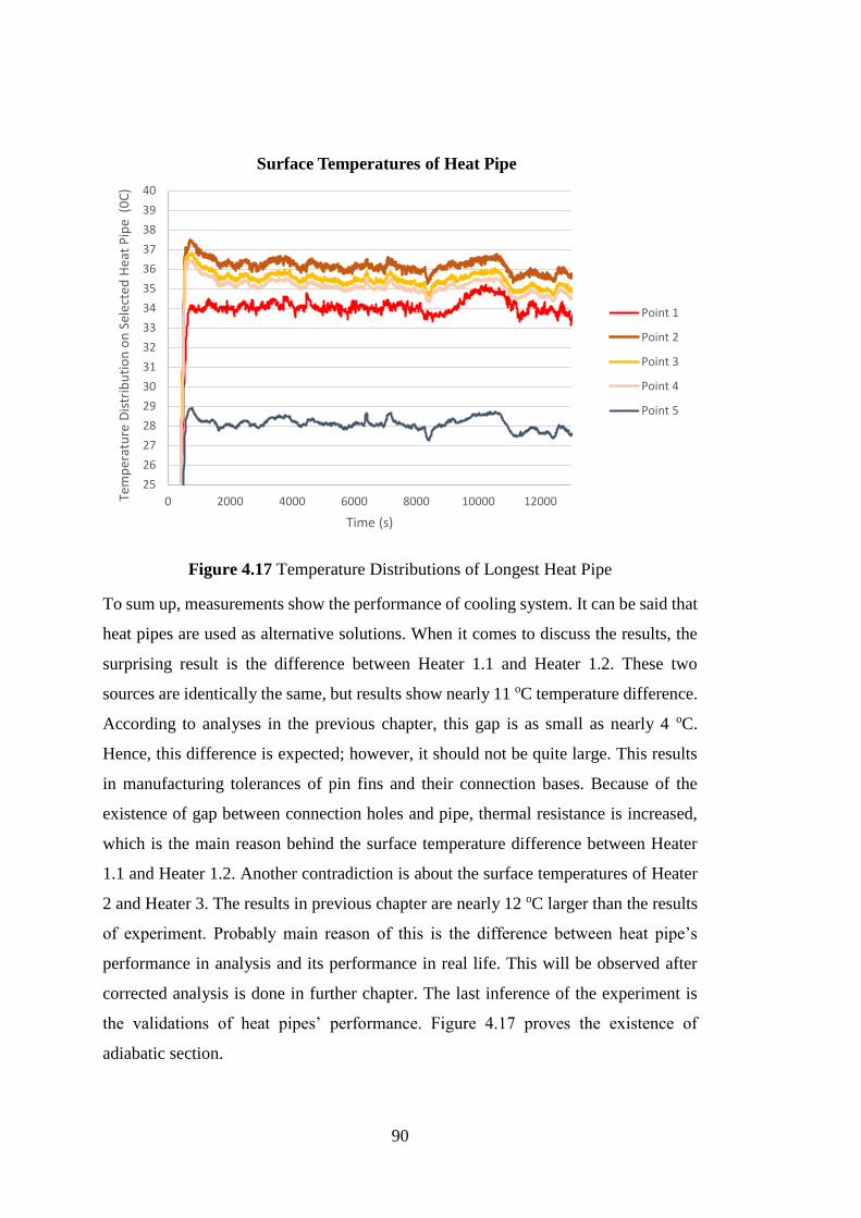
90
Figure 4.17 Temperature Distributions of Longest Heat Pipe
To sum up, measurements show the performance of cooling system. It can be said that
heat pipes are used as alternative solutions. When it comes to discuss the results, the
surprising result is the difference between Heater 1.1 and Heater 1.2. These two
sources are identically the same, but results show nearly 11 oC temperature difference.
According to analyses in the previous chapter, this gap is as small as nearly 4 oC.
Hence, this difference is expected; however, it should not be quite large. This results
in manufacturing tolerances of pin fins and their connection bases. Because of the
existence of gap between connection holes and pipe, thermal resistance is increased,
which is the main reason behind the surface temperature difference between Heater
1.1 and Heater 1.2. Another contradiction is about the surface temperatures of Heater
2 and Heater 3. The results in previous chapter are nearly 12 oC larger than the results
of experiment. Probably main reason of this is the difference between heat pipe’s
performance in analysis and its performance in real life. This will be observed after
corrected analysis is done in further chapter. The last inference of the experiment is
the validations of heat pipes’ performance. Figure 4.17 proves the existence of
adiabatic section.
25
26
27
28
29
30
31
32
33
34
35
36
37
38
39
40
0 2000 4000 6000 8000 10000 12000Tem
per
atu
re D
istr
ibu
tio
n o
n S
elec
ted
Hea
t P
ipe
(0
C)
Time (s)
Surface Temperatures of Heat Pipe
Point 1
Point 2
Point 3
Point 4
Point 5
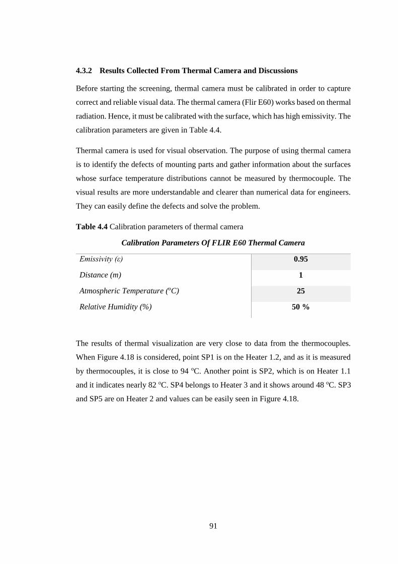
91
4.3.2 Results Collected From Thermal Camera and Discussions
Before starting the screening, thermal camera must be calibrated in order to capture
correct and reliable visual data. The thermal camera (Flir E60) works based on thermal
radiation. Hence, it must be calibrated with the surface, which has high emissivity. The
calibration parameters are given in Table 4.4.
Thermal camera is used for visual observation. The purpose of using thermal camera
is to identify the defects of mounting parts and gather information about the surfaces
whose surface temperature distributions cannot be measured by thermocouple. The
visual results are more understandable and clearer than numerical data for engineers.
They can easily define the defects and solve the problem.
Table 4.4 Calibration parameters of thermal camera
Calibration Parameters Of FLIR E60 Thermal Camera
Emissivity (ε) 0.95
Distance (m) 1
Atmospheric Temperature (oC) 25
Relative Humidity (%) 50 %
The results of thermal visualization are very close to data from the thermocouples.
When Figure 4.18 is considered, point SP1 is on the Heater 1.2, and as it is measured
by thermocouples, it is close to 94 oC. Another point is SP2, which is on Heater 1.1
and it indicates nearly 82 oC. SP4 belongs to Heater 3 and it shows around 48 oC. SP3
and SP5 are on Heater 2 and values can be easily seen in Figure 4.18.
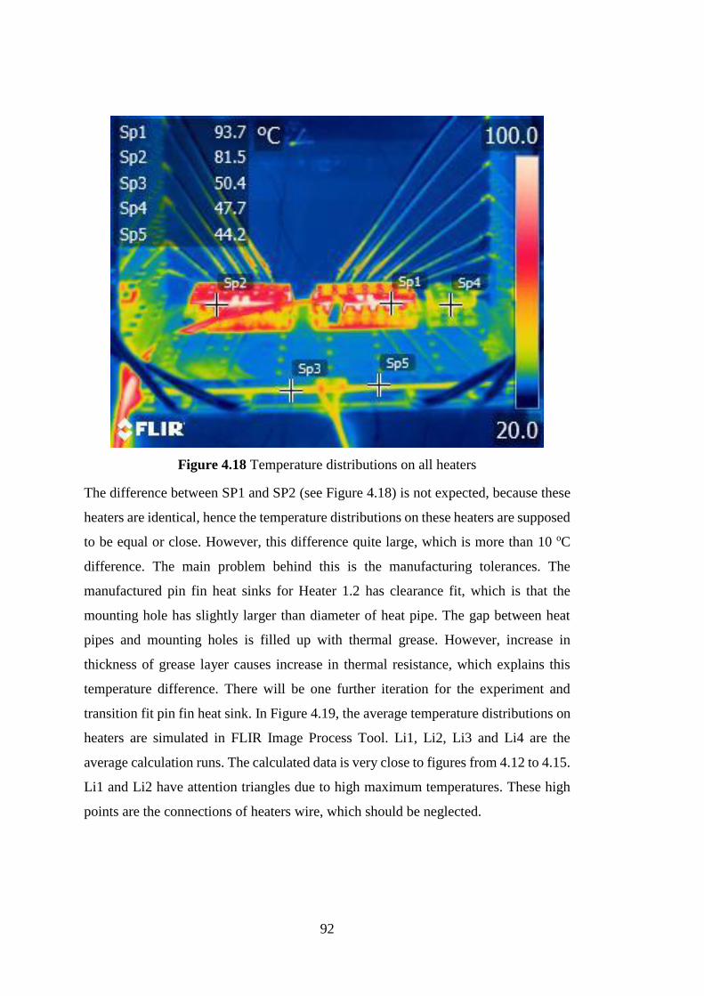
92
Figure 4.18 Temperature distributions on all heaters
The difference between SP1 and SP2 (see Figure 4.18) is not expected, because these
heaters are identical, hence the temperature distributions on these heaters are supposed
to be equal or close. However, this difference quite large, which is more than 10 oC
difference. The main problem behind this is the manufacturing tolerances. The
manufactured pin fin heat sinks for Heater 1.2 has clearance fit, which is that the
mounting hole has slightly larger than diameter of heat pipe. The gap between heat
pipes and mounting holes is filled up with thermal grease. However, increase in
thickness of grease layer causes increase in thermal resistance, which explains this
temperature difference. There will be one further iteration for the experiment and
transition fit pin fin heat sink. In Figure 4.19, the average temperature distributions on
heaters are simulated in FLIR Image Process Tool. Li1, Li2, Li3 and Li4 are the
average calculation runs. The calculated data is very close to figures from 4.12 to 4.15.
Li1 and Li2 have attention triangles due to high maximum temperatures. These high
points are the connections of heaters wire, which should be neglected.

93
Figure 4.19 Average temperature distributions on heaters
Figure 4.20 and 4.21 illustrate temperature on pin fin heat sink and heat pipe
connections. The shown heat sink is attached to Heaters 1.1. From Figure 4.20; SP1
indicates the connections of basal plate and pin fin heat sink. The temperature for this
connection is measured nearly 35 oC. SP2 shows temperature of fin’s pin and SP3 is
for air inside the fin. When the figure is observed, it can be seen that there is nearly
isothermal distribution on pin fin heat sinks. The important issue for the thermal
visualization is reflection. The thermal camera works based on radiation, hence it also
measures reflection and shows like mirror image (see Figure 4.20 and 4.21). Figure
4.21 illustrates heat pipe’s connections and average temperature distribution along the
connection of basal plate and heat sink. The average temperature around connection
of heat sink and its basal plate is close to 32 oC. At it is demonstrated, the temperature
around heat pipe rises up to more than 35 oC. This is due to thermal resistance around
the pipe. The existence of thermal grease around the pipe directly affects the
performance in terms of thermal resistance. The most critical point about that is the
thickness of the grease layer. The suggested layer thickness is less than 0.01 inch
(0.254 mm), which is equal to 0.3 mm. To eliminate this, manufacturing details must
be evaluated.
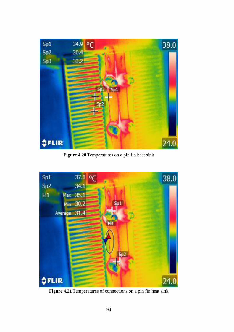
94
Figure 4.20 Temperatures on a pin fin heat sink
Figure 4.21 Temperatures of connections on a pin fin heat sink

95
Figure 4.22 Axial temperature distribution on selected heat pipe
Performance of the longest heat pipe is measured and it is also shown in Figure 4.17.
The visual proof ‘Figure 4.22’ has the equal number with Figure 4.17. From the
illustration, it is easily seen that the temperature difference along the pipe is so small.
Figure 4.23 Bending effect on the performance of heat pipe
96
The last comment is related to bending effect. In Figure 4.23, bend regions are quite
hotter than other areas. Bend increases the thermal resistance of heat pipe’s inner
section. From the general knowledge of heat transfer theory, if resistance increases,
temperature around the resistance region also increases. The more the bend increases,
the less the performance of heat pipe will be as it is mentioned in theory section. As a
rule of thumb, every 90o bends causes 1 oC performance loss.
After the experimental validation, numerical analysis will be updated. In the previous
chapter ‘Preliminary Design’, thermal resistances are not identified in analyses,
however these thermal resistances will be taken into consideration in the following
section, corrected numerical model.
4.4 Uncertainty Analysis
For calculation of uncertainty of the system measurement, three sets of data are
captured experimentally. The results of these three experiments are shown in Table
4.5.
Table 4.5 Results of experimental runs
Number of Run Heater 1.1 (oC) Heater 1.2 (oC) Heater 2 (oC) Heater 3 (oC)
1 76.92 86.28 47.23 51.46
2 77.85 85.64 45.15 52.32
3 77.32 85.84 46.26 51.84
Uncertainty can be calculated with equation below.
𝑈𝑗 = |
𝑀𝑖+1,𝑗 − 𝑀𝑖,𝑗
𝑀𝑖,𝑗 | 𝑥100 (4.1)

97
Then, average relative percentage uncertainty is found by,
𝑈 ̅ = ∑
𝑈𝑗
𝑛
𝑛
𝐽=1
(4.2)
By using formula 4.1 and 4.2, Table 4.6 is calculated, which is average percentage
uncertainty of all heaters.
Table 4.6 Average percentage uncertainty of temperatures of all heaters
U1.1 U1.2 U2 U3
0.95 % 0.49 % 3.43 % 1.29 %
From the data sheets of thermocouples and thermal camera, the measurement errors
are respectively 0.75 % and 2 %.

98
99
CHAPTER 5
OPTIMIZATION
This chapter deals with the corrected numerical model and optimization procedures of
design. In this section, pin fin heat sink configuration will be analyzed by corrected
parameters taken from initial analyses and experiment. Then, with the information
gathered about the heat pipes performance, plated fin heat sink design will be upgraded
and optimized. Optimization is done by FloEFD ‘What if’ analyses.
In ‘What if’ analyses, optimized section in CAD model must be identified and
parametrized. Then, FloEFD automatically solves problem for all conditions. Finally,
it can be easily seen which point displays the best performance.
5.1 Corrected Analysis of Pin Fin Heat Sink Configuration
After initial analyses and experiment, problematic points are round out. Numerical
modelling is created again. Thermal resistances are added and heat pipe’s connection
and internal resistances are recalculated.
In initial runs, all heat pipes have same internal resistance; however, experiment
showed that this assumption is only used in the beginning. For real life situations,
different length heat pipe has different effective thermal resistance. Hence, all effective
thermal resistances are recalculated by looking at the results of experiment. At the
beginning of analyses, they are defined as 0.25 0C/W or 0.25 K/W. This value is
updated to 0.084 0C/W or K/W for heat pipes connected to Heater 1.1 (600 W) and
Heater 1.2 (600 W), 0.015 0C/W or K/W for heat pipes connected to Heater 2 (350 W)
and 0.002 0C/W or K/W for heat pipes connected to Heater 3 (70 W).
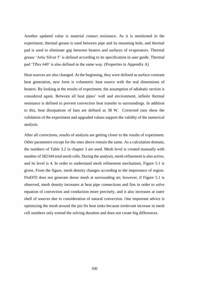
100
Another updated value is material contact resistance. As it is mentioned in the
experiment, thermal grease is used between pipe and its mounting hole, and thermal
pad is used to eliminate gap between heaters and surfaces of evaporators. Thermal
grease ‘Artic Silver 5’ is defined according to its specification in user guide. Thermal
pad ‘Tflex 640’ is also defined in the same way. (Properties in Appendix A)
Heat sources are also changed. At the beginning, they were defined as surface constant
heat generation, new form is volumetric heat source with the real dimensions of
heaters. By looking at the results of experiment, the assumption of adiabatic section is
considered again. Between all heat pipes’ wall and environment, infinite thermal
resistance is defined to prevent convection heat transfer to surroundings. In addition
to this, heat dissipations of fans are defined as 38 W. Corrected runs show the
validation of the experiment and upgraded values support the validity of the numerical
analysis.
After all corrections, results of analysis are getting closer to the results of experiment.
Other parameters except for the ones above remain the same. As a calculation domain,
the numbers of Table 3.2 in chapter 3 are used. Mesh level is created manually with
number of 582344 total mesh cells. During the analysis, mesh refinement is also active,
and its level is 4. In order to understand mesh refinement mechanism, Figure 5.1 is
given. From the figure, mesh density changes according to the importance of region.
FloEFD does not generate dense mesh at surrounding air; however, if Figure 5.1 is
observed, mesh density increases at heat pipe connections and fins in order to solve
equation of convection and conduction more precisely, and it also increases at outer
shell of sources due to consideration of natural convection. One important advice is
optimizing the mesh around the pin fin heat sinks because irrelevant increase in mesh
cell numbers only extend the solving duration and does not create big differences.

101
Figure 5.1 Mesh refinement of FloEFD and Cut View of Mesh Distribution from the
Back Side of Platform
Figure 5.2 Final Temperature Distributions on Heaters
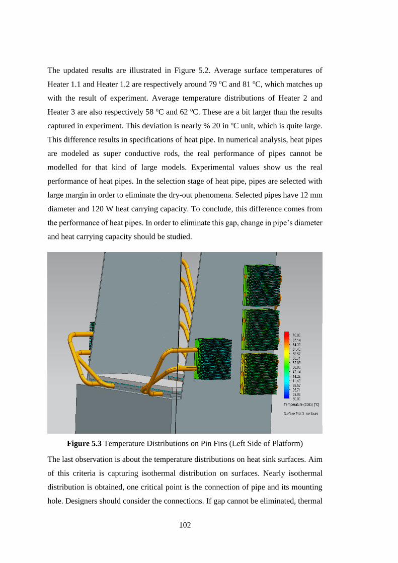
102
The updated results are illustrated in Figure 5.2. Average surface temperatures of
Heater 1.1 and Heater 1.2 are respectively around 79 oC and 81 oC, which matches up
with the result of experiment. Average temperature distributions of Heater 2 and
Heater 3 are also respectively 58 oC and 62 oC. These are a bit larger than the results
captured in experiment. This deviation is nearly % 20 in oC unit, which is quite large.
This difference results in specifications of heat pipe. In numerical analysis, heat pipes
are modeled as super conductive rods, the real performance of pipes cannot be
modelled for that kind of large models. Experimental values show us the real
performance of heat pipes. In the selection stage of heat pipe, pipes are selected with
large margin in order to eliminate the dry-out phenomena. Selected pipes have 12 mm
diameter and 120 W heat carrying capacity. To conclude, this difference comes from
the performance of heat pipes. In order to eliminate this gap, change in pipe’s diameter
and heat carrying capacity should be studied.
Figure 5.3 Temperature Distributions on Pin Fins (Left Side of Platform)
The last observation is about the temperature distributions on heat sink surfaces. Aim
of this criteria is capturing isothermal distribution on surfaces. Nearly isothermal
distribution is obtained, one critical point is the connection of pipe and its mounting
hole. Designers should consider the connections. If gap cannot be eliminated, thermal

103
resistance occurs high and the performance of system directly decreases. Figure 5.3
shows the left side of platform and Figure 5.4 illustrates the right side of platform.
Figure 5.4 Temperature Distributions on Pin Fins (Right Side of Platform)
From the figures above, nearly isothermal distribution is captured, which is obtained
through proper decision of pipes’ locations and proper selection of heat sink geometry.
The temperature distributions on fins are between 45 oC and 53 oC. Disproportionate
regions are locations of fan’s rotor, and in Figure 5.4 pin fin with 3 heat pipes
connections. Rotor problem cannot be solved because it comes from the nature of fan.
However, if these three pipes’ connection are separated, the problem will be solved.
In this case, there will be a spacing problem for the design of platform.
In order to compare the results of corrected numerical runs and experiment, Figure 5.5
should be examined. If Figure 5.2 and 5.5 are compared, it can be easily seen that
isothermal surfaces are very close to each other. In corrected runs, hot spots on Heater
1.1 and 1.2 are respectively 79.86 oC and 83.14 oC. In Figure 5.5, these points have
respectively hot spots at 81.25 oC and 85.34 oC. These results are also proof of
coinciding with the results of corrected numerical runs and experiment.
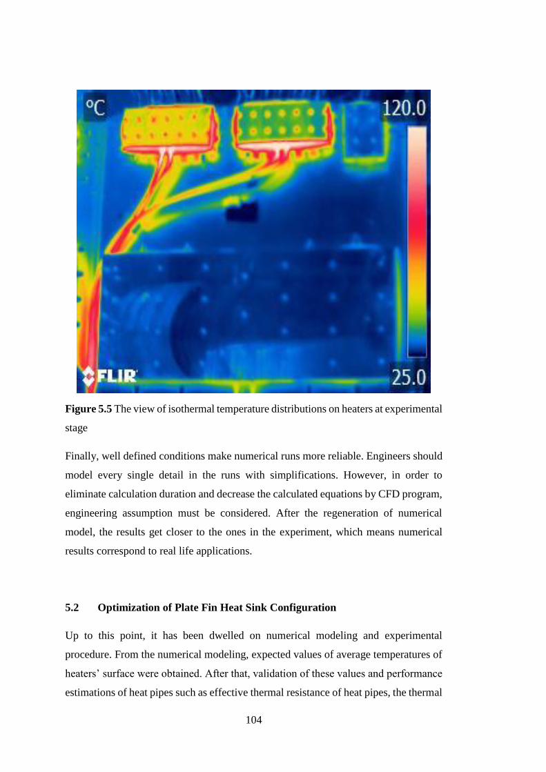
104
Figure 5.5 The view of isothermal temperature distributions on heaters at experimental
stage
Finally, well defined conditions make numerical runs more reliable. Engineers should
model every single detail in the runs with simplifications. However, in order to
eliminate calculation duration and decrease the calculated equations by CFD program,
engineering assumption must be considered. After the regeneration of numerical
model, the results get closer to the ones in the experiment, which means numerical
results correspond to real life applications.
5.2 Optimization of Plate Fin Heat Sink Configuration
Up to this point, it has been dwelled on numerical modeling and experimental
procedure. From the numerical modeling, expected values of average temperatures of
heaters’ surface were obtained. After that, validation of these values and performance
estimations of heat pipes such as effective thermal resistance of heat pipes, the thermal
105
resistance between the heat pipe and its connections were obtained from the
experimental procedure. Also, pin fin heat sink configuration was validated, and with
the help of the information gathered, corrected numerical model is created as it is
explained in part 5.1. Consequently, corrected model helps the numerical model to
match up with the real life conditions. However, the second configuration which is the
rectangular plate fin heat sink with duct structured model has not been validated yet
under the real life conditions. The second model will be optimized according to surface
temperatures of heaters. Changing optimization parameters are fin thickness and the
spacing between two fins.
A mechanical design optimization is a challenge in which certain design parameters
needed to be determined to achieve the best measurable performance (i.e. objective
function) under given constraints. Hence, the selection is done by the best average
temperatures distributions on the surfaces of heaters. The set of design variables is
composed of fin thickness and spacing between two fins. The main constrain during
the optimization step is getting hot spot temperature below thermal shut-down
(critical) point. This optimization procedure is done by ‘What If ? Analysis ’ module
of FloEFD.
One of the most powerful features of FloEFD is the ease with which engineers can
conduct “what-if?” analyses. FloEFD makes it simple to clone/ modify your models
and analyze design variations. The process is very simple. First step is creating base
model in 3D with parametric modelling. Then, the setup of a numerical analysis should
be generated. . After that multiple variations of analyzed design should be created by
modifying the solid model without having to reapply boundary conditions, material
properties etc. When the analysis is complete, FloEFD makes it easy to compare the
results among the many options to choose best possible design automatically [71].
5.2.1 Procedures of ‘What If’ Analysis
The starting point of the ‘What If’ analysis is creating parametric CAD, which is
generated by PTC Creo. Geometrical properties and dimensions are the same as
preliminary section.

106
After the modelling is finished, numerical setup must be created in FloEFD. All
procedures are the same as procedures explained in Chapter 3 (3.5.1 Procedures of
Numerical Analyses). Numerical runs are done at 25 oC environment temperature and
1 atm pressure. The numbers of fans are increased to 8, there are 4 fans inside each
ducts. Another difference from the preliminary conditions is effective thermal
resistance of a heat pipe, which was identified as 0.25 oC/W or K/W. The new value
is selected as 0.05 oC/W or K/W. This value is assumed by the results of experiment
as an average of thermal effective resistance of a heat pipe.
Rectangular fin heat sink has 248 mm width and 350 mm length. The base thickness
of fin is 14 mm, it is identified by diameter of heat pipe used which is 12 mm. The
placements of heat pipes and fin connection are obtained in preliminary stage. There
are two identically powered sources, hence placement is done with nearly symmetry
condition. Two pipes which are connected to 350 W heater are mounting to top and
bottom side of fin. They are placed in a 40 mm distance from horizontal edges of fin
(top edge and bottom edge). All other heat pipes are attached to every 40 mm after the
first heat pipe. Length of fin plate is 25 mm with variable thickness and spacing. The
thickness of fin changes from 3 mm to 6 mm. In addition to this, considered spacing
values are 2, 2.5, 3, 3.5, 4, 5 and 6 mm.
During the analyses, total mesh number is also simplified. All analyses are done with
278642 total mesh cells. This value is lower than the values in Chapter 3. Because
‘What If’ analysis solves the problem one by one, and then it compares the results.
During this procedure, twenty-eight different analyses are considered in one setup. In
other words, FloEFD has done 28 different analyses with consecutive calculations. In
order to minimize the solution time, the number of total mesh cells is lowered. During
the process, HP Z820 Workstation is used. This computer is configured with Intel
Xeon Processor E5-2640 v2 2.0 GHz 8 cores CPU and installed memory (RAM) with
64 GB. Each run lasts approximately 100 minutes.
Finally, the average surface temperatures distributions on Heater 1.1 and Heater 1.2 is
defined as constrain functions of the optimization steps. All calculations stop when
these two constrains are achieved. During the calculation, approximately 420 iterations
are done.
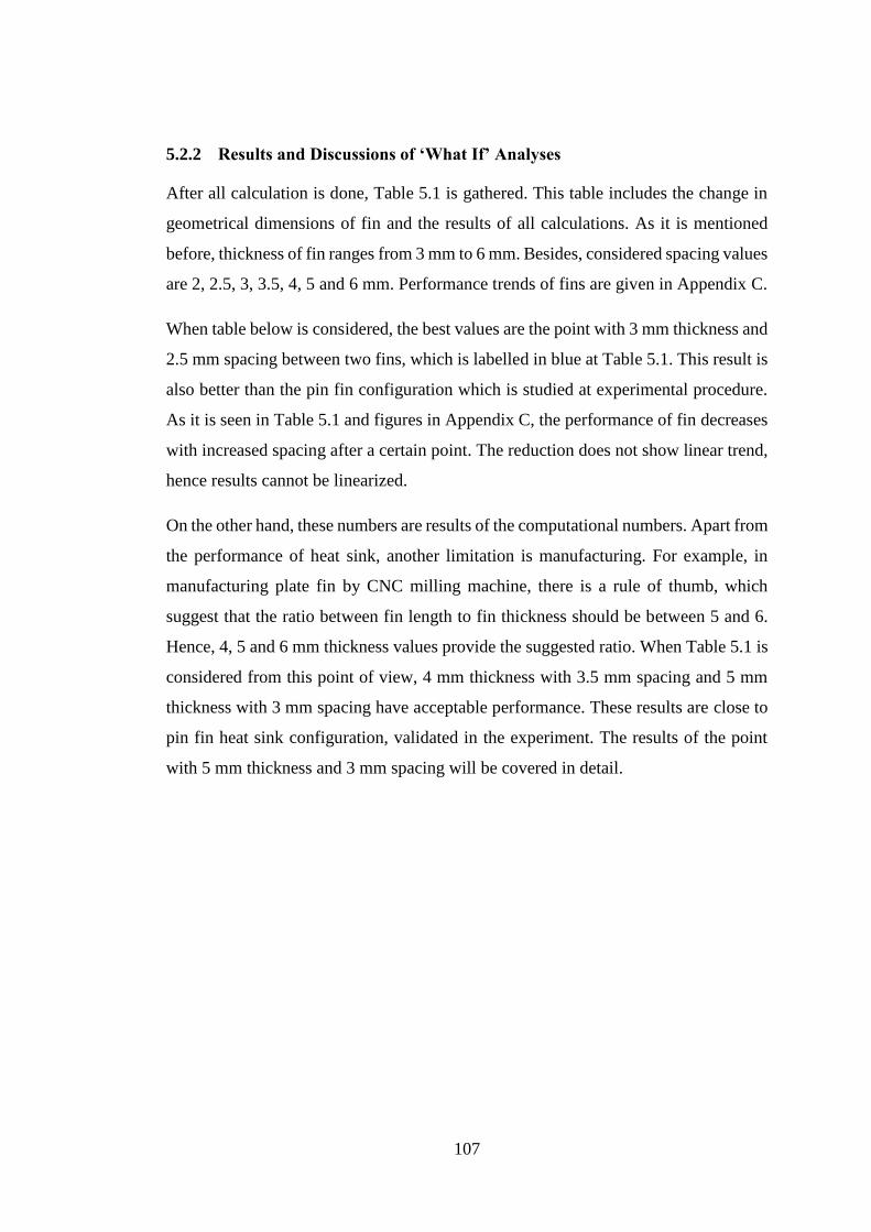
107
5.2.2 Results and Discussions of ‘What If’ Analyses
After all calculation is done, Table 5.1 is gathered. This table includes the change in
geometrical dimensions of fin and the results of all calculations. As it is mentioned
before, thickness of fin ranges from 3 mm to 6 mm. Besides, considered spacing values
are 2, 2.5, 3, 3.5, 4, 5 and 6 mm. Performance trends of fins are given in Appendix C.
When table below is considered, the best values are the point with 3 mm thickness and
2.5 mm spacing between two fins, which is labelled in blue at Table 5.1. This result is
also better than the pin fin configuration which is studied at experimental procedure.
As it is seen in Table 5.1 and figures in Appendix C, the performance of fin decreases
with increased spacing after a certain point. The reduction does not show linear trend,
hence results cannot be linearized.
On the other hand, these numbers are results of the computational numbers. Apart from
the performance of heat sink, another limitation is manufacturing. For example, in
manufacturing plate fin by CNC milling machine, there is a rule of thumb, which
suggest that the ratio between fin length to fin thickness should be between 5 and 6.
Hence, 4, 5 and 6 mm thickness values provide the suggested ratio. When Table 5.1 is
considered from this point of view, 4 mm thickness with 3.5 mm spacing and 5 mm
thickness with 3 mm spacing have acceptable performance. These results are close to
pin fin heat sink configuration, validated in the experiment. The results of the point
with 5 mm thickness and 3 mm spacing will be covered in detail.
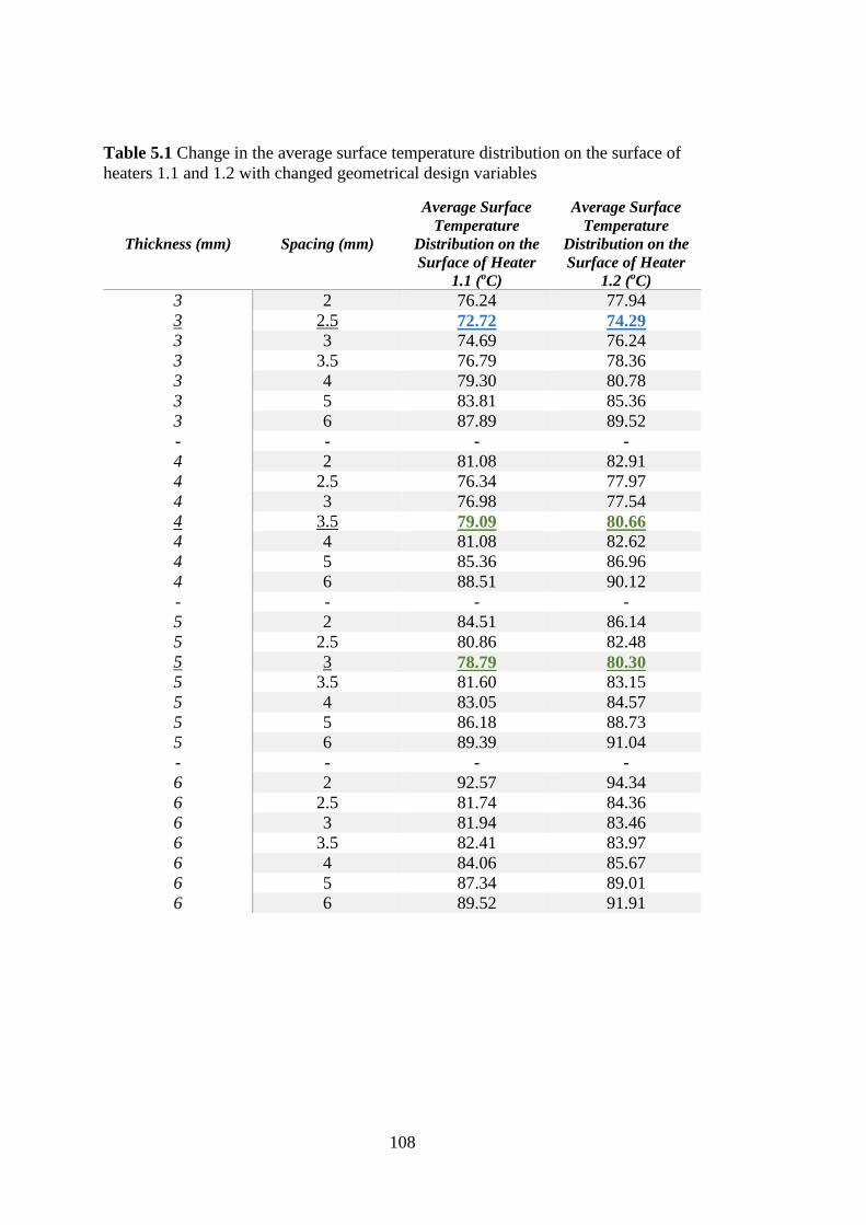
108
Table 5.1 Change in the average surface temperature distribution on the surface of
heaters 1.1 and 1.2 with changed geometrical design variables
Thickness (mm) Spacing (mm)
Average Surface
Temperature
Distribution on the
Surface of Heater
1.1 (oC)
Average Surface
Temperature
Distribution on the
Surface of Heater
1.2 (oC)
3 2 76.24 77.94
3 2.5 72.72 74.29
3 3 74.69 76.24
3 3.5 76.79 78.36
3 4 79.30 80.78
3 5 83.81 85.36
3 6 87.89 89.52
- - - -
4 2 81.08 82.91
4 2.5 76.34 77.97
4 3 76.98 77.54
4 3.5 79.09 80.66
4 4 81.08 82.62
4 5 85.36 86.96
4 6 88.51 90.12
- - - -
5 2 84.51 86.14
5 2.5 80.86 82.48
5 3 78.79 80.30
5 3.5 81.60 83.15
5 4 83.05 84.57
5 5 86.18 88.73
5 6 89.39 91.04
- - - -
6 2 92.57 94.34
6 2.5 81.74 84.36
6 3 81.94 83.46
6 3.5 82.41 83.97
6 4 84.06 85.67
6 5 87.34 89.01
6 6 89.52 91.91
109
Figure 5.6 Average Surface Temperature Distributions of Heaters (Rectangular Plate
Fin with Duct Structured with 5 mm Thickness and 3 mm Spacing)
The average surface temperatures on heaters are given in Figure 5.6.Heater 1.1 and
Heater 1.2 have average nearly 80 oC temperature distribution. Other heaters surface
temperatures are also easily seen in figure above. When the values are considered,
these values are very close to the values at pin fin configuration.
In addition to temperature distributions on the heater surfaces, the temperature
distributions on plate fin heat sinks are considered. As it is mentioned before, the major
aim is to create nearly isothermal distributions on heat sinks. The average temperature
distributions on the surfaces of heat sinks are very close to 57 oC (see Figure 5.7 and
Figure 5.8). When these figures are examined, the first connecting points of heat pipes
and heat sinks are observable. These points have higher temperatures than other
surfaces.

110
Figure 5.7Average Surface Temperature Distribution on Right Fin (8 heat pipes are
connected)
To conclude, design is upgraded by optimization. The performance of plate fin heat
sink is enhanced according to initial design at preliminary part. During the ‘what if’
analyses, some of contact resistances and resistance due to interface materials are
ignored. Because these materials are known for this design and these identifications
extend the calculation time. However, when these materials are identified to numerical
analyses, the results will slightly increase.
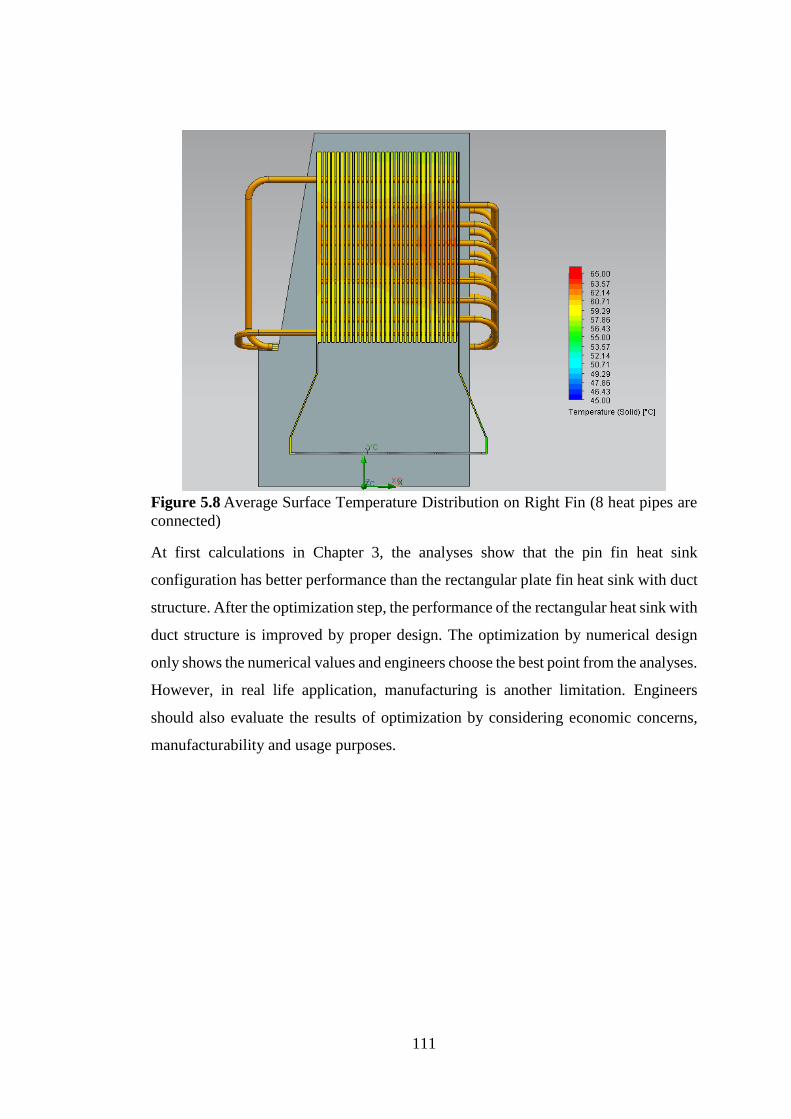
111
Figure 5.8 Average Surface Temperature Distribution on Right Fin (8 heat pipes are
connected)
At first calculations in Chapter 3, the analyses show that the pin fin heat sink
configuration has better performance than the rectangular plate fin heat sink with duct
structure. After the optimization step, the performance of the rectangular heat sink with
duct structure is improved by proper design. The optimization by numerical design
only shows the numerical values and engineers choose the best point from the analyses.
However, in real life application, manufacturing is another limitation. Engineers
should also evaluate the results of optimization by considering economic concerns,
manufacturability and usage purposes.

112
113
CHAPTER 6
RESULTS AND DISCUSSION
This part summarizes all the results and discussions in the study. This study has been
created after 2 years of study about heat pipes. This study is supported by ASELSAN
and Republic of Turkey Ministry of Science, Industry and Technology.
The first step of study started with preliminary conceptual design. By evaluating the
operational conditions of military rotary platforms, two different configurations were
designed. One of them is pin fin heat sink configuration and another one is the
rectangular plate fin heat sink with duct structure configuration. These models are
illustrated in Figure 3.5 and Figure 3.6. Numerical runs are done at 25 oC and 50 oC
environmental temperature with 1 atm constant pressure. For pin fin case; the critical
component has average surface temperature with 78 oC at 25 oC environment and it is
105 oC at 50 oC environment. For the rectangular plate fin heat sink configuration,
these values are respectively 93 oC and 121 oC. However, pin fin heat sink
configuration has 8 fan for every 8 pin fins and rectangular plate fin heat sink
configuration has 6 fan for 2 ducts. Each duct includes 3 fans.
In the experimental setup, the heat dissipating components are connected to the pin fin
heat sinks with 17 heat pipes of 12 mm diameter, which is shown in Figure 4.6. During
the experiment, whole system reaches steady-state conditions approximately in 2000
seconds. However, the experimental procedure is completed in 2 hours. During the
experiment, no dangerous conditions, such as fire, component malfunction have been
observed. Therefore, experiment is successfully completed. Experiment are done at 25
oC conditioned environment temperature. The figures from 4.12 to 4.16 show the
average temperature distributions on the surfaces of heaters. With respectively, Heater
1.1, Heater 1.2, Heater 2 and Heater 3 have average surface temperature with. 82.75
oC, 92.5 oC, 45.8 oC and 46.75 oC. Some of these values are different from the results

114
obtained in preliminary stages. In order to find the percentage relative temperature
difference in the results of numerical study and the experimental study, Equation 6.1
below is used.
% 𝑅𝑒𝑙𝑎𝑡𝑖𝑣𝑒 𝑇𝑒𝑚𝑝𝑒𝑟𝑎𝑡𝑢𝑟𝑒 𝐷𝑖𝑓𝑓𝑒𝑟𝑒𝑛𝑐𝑒 = |∆𝑇
∆𝑇𝑚𝑎𝑥 | 𝑥100 (6.1)
where;
∆𝑇 = 𝑇𝑚𝑒𝑎𝑠𝑢𝑟𝑒𝑑 − 𝑇𝑎𝑚𝑏 (6.2)
∆𝑇𝑚𝑎𝑥 = 𝑇𝑐𝑟𝑖𝑡𝑖𝑐𝑎𝑙 − 𝑇𝑎𝑚𝑏 (6.3)
where Tcritical is the thermal shot-down point for TWT and PA modules. It is mentioned
before as 120 oC. In order to provide consistent validation, the difference between
percent relative temperature difference for numerical value and percent relative
temperature difference for experimental value should be as small as obtained. The
percent relative temperature difference values are given in Table 6.1.
Table 6.1 Comparison between numerical % relative temperature difference and
experimental % relative temperature difference
Heaters
% Relative Temperature
Difference for Numerical
Value
% Relative Temperature
Difference for
Experimental Value
Heater 1.1 57.06 60.79
Heater 1.2 59.32 71.05
Heater 2 34.73 21.89
Heater 3 38.94 22.89
If Table 6.1 is considered, it can be easily seen that there is a quite large difference for
heaters 1.2, 2 and 3. These values are evaluated after the preliminary run is obtained
by experimental results. The most critical point is the difference between Heater 1.1
and Heater 1.2, because it is not normal. These two sources are identically same and
the numerical values for these two sources are also close to each other. This results in
manufacturing defect. In the first run of experiment, some of the mounting tolerances
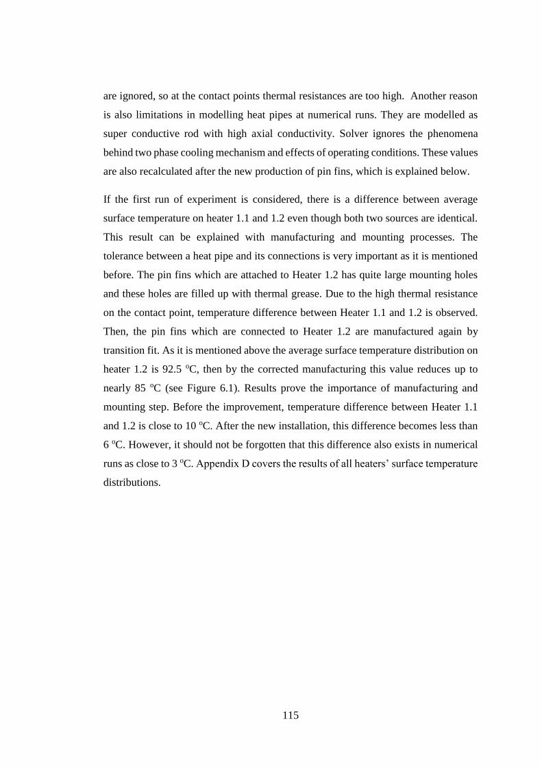
115
are ignored, so at the contact points thermal resistances are too high. Another reason
is also limitations in modelling heat pipes at numerical runs. They are modelled as
super conductive rod with high axial conductivity. Solver ignores the phenomena
behind two phase cooling mechanism and effects of operating conditions. These values
are also recalculated after the new production of pin fins, which is explained below.
If the first run of experiment is considered, there is a difference between average
surface temperature on heater 1.1 and 1.2 even though both two sources are identical.
This result can be explained with manufacturing and mounting processes. The
tolerance between a heat pipe and its connections is very important as it is mentioned
before. The pin fins which are attached to Heater 1.2 has quite large mounting holes
and these holes are filled up with thermal grease. Due to the high thermal resistance
on the contact point, temperature difference between Heater 1.1 and 1.2 is observed.
Then, the pin fins which are connected to Heater 1.2 are manufactured again by
transition fit. As it is mentioned above the average surface temperature distribution on
heater 1.2 is 92.5 oC, then by the corrected manufacturing this value reduces up to
nearly 85 oC (see Figure 6.1). Results prove the importance of manufacturing and
mounting step. Before the improvement, temperature difference between Heater 1.1
and 1.2 is close to 10 oC. After the new installation, this difference becomes less than
6 oC. However, it should not be forgotten that this difference also exists in numerical
runs as close to 3 oC. Appendix D covers the results of all heaters’ surface temperature
distributions.
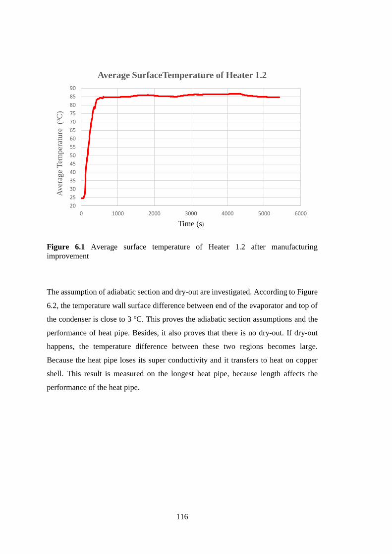
116
Figure 6.1 Average surface temperature of Heater 1.2 after manufacturing
improvement
The assumption of adiabatic section and dry-out are investigated. According to Figure
6.2, the temperature wall surface difference between end of the evaporator and top of
the condenser is close to 3 oC. This proves the adiabatic section assumptions and the
performance of heat pipe. Besides, it also proves that there is no dry-out. If dry-out
happens, the temperature difference between these two regions becomes large.
Because the heat pipe loses its super conductivity and it transfers to heat on copper
shell. This result is measured on the longest heat pipe, because length affects the
performance of the heat pipe.
20
25
30
35
40
45
50
55
60
65
70
75
80
85
90
0 1000 2000 3000 4000 5000 6000
Aver
age
Tem
per
ature
(o
C)
Time (s)
Average SurfaceTemperature of Heater 1.2
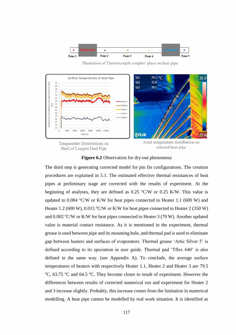
117
Figure 6.2 Observation for dry-out phenomena
The third step is generating corrected model for pin fin configurations. The creation
procedures are explained in 5.1. The estimated effective thermal resistances of heat
pipes at preliminary stage are corrected with the results of experiment. At the
beginning of analyses, they are defined as 0.25 oC/W or 0.25 K/W. This value is
updated to 0.084 oC/W or K/W for heat pipes connected to Heater 1.1 (600 W) and
Heater 1.2 (600 W), 0.015 oC/W or K/W for heat pipes connected to Heater 2 (350 W)
and 0.002 oC/W or K/W for heat pipes connected to Heater 3 (70 W). Another updated
value is material contact resistance. As it is mentioned in the experiment, thermal
grease is used between pipe and its mounting hole, and thermal pad is used to eliminate
gap between heaters and surfaces of evaporators. Thermal grease ‘Artic Silver 5’ is
defined according to its speciation in user guide. Thermal pad ‘Tflex 640’ is also
defined in the same way. (see Appendix A). To conclude, the average surface
temperatures of heaters with respectively Heater 1.1, Heater 2 and Heater 3 are 79.5
oC, 63.75 oC and 64.5 oC. They become closer to result of experiment. However the
differences between results of corrected numerical run and experiment for Heater 2
and 3 increase slightly. Probably, this increase comes from the limitation in numerical
modelling. A heat pipe cannot be modelled by real work situation. It is identified as

118
super conductive rod. Hence, FloEFD gives the results with super conductive
constrain. However, as it is explained in Chapter 3, pipe diameter is selected as large
as 12 mm in order to prevent dry-out or other limitation. From the data taken from
manufacturer, a heat pipe with 12 mm, which is used in experiment, has heat carrying
capacity with 120 Watt. Hence, the heat pipes, connected to Heater 2 and Heater 3,
have very large safety margin. These results in unpredicted increase in performance.
This parameters cannot be modelled with commercial CFD programs.
After the corrected experiment and corrected numerical run, the percent relative
temperature difference for experiment and numerical run are recalculated. New values
are tabulated in Table 6.2. If values are observed, all numerical result values get closer
to the new experiment values. The difference for heater 1.2 decreases. Results
demonstrate that tolerances in manufacturing and mounting are very important.
However, for heater 2 and 3, reason is different. These values are better than the
numerical ones. This is because, numerical solver cannot model the advantages and
disadvantages of orientation and heat pipe geometry such as effects of diameter,
effective length, operating position according to gravity, operating limits etc.
Table 6.2 Comparison between corrected numerical % relative temperature difference
and corrected experimental % relative temperature difference after re-production of
fins
Heaters
% Relative Temperature
Difference for Corrected
Numerical Value
% Relative Temperature
Difference for Corrected
Experimental Value
Heater 1.1 57.86 56.34
Heater 1.2 60.43 63.62
Heater 2 40.73 22.04
Heater 3 40.71 29.82
By optimization, the performance of the rectangular plate fin heat sink configuration
is increased. The maximum performance is achieved the point that has 25 mm fin
length, 3mm thickness and 2.5 mm spacing between two fins. The results of the
optimization also shows that the performance of rectangular plate fin with 5 mm
119
thickness, 3 mm spacing and 4 mm thickness, 3.5 mm spacing is nearly equal to the
tested pin fin configuration. All optimization trends are given in Appendix C.
The last comparison is the total heat transfer area for both configurations. A pin fin
heat sink has 163980.43 mm2 heat transfer surface area. 8pin fins are used, hence total
heat transfer area on the surface of pin fin heat sinks is 1311843.4 mm2 (~1.32 x 10⁻⁶
m2).On the other hand, a plate fin heat sink has 583800 mm2 heat transfer surface area.
There are 2 plate fin heat sinks attached both left and right side of platform, hence total
heat transfer area is 1167600 mm2 (~1.17 x 10⁻⁶ m2). To conclude, instead of using
plate pin, using pin fin has an advantage of total heat transfer area with ease of getting
good tolerances for small pieces in manufacturing process.
As a result of several simulations with various heat pipe arrangements and two
different heat sink types and experiment of pin fin configuration, the following
observations are made:
The thermal management solution with pin fin heat sinks is more effective and
easier than the solution with plate fins. If the pin fins are also optimized, the
results will be better than plated fin.
To dissipate high heat loads with heat pipes, heat pipes with large diameters
are needed. The heat sink bases should be thicker to accommodate theses
thicker heat pipes. In this case, small pin fin heat sinks are better than long
parallel plate finned heat sinks. By small pieces, tolerances in manufacturing
process can easily be obtained.
In case of large plate fin heat sinks, smaller number of heat sinks may be
enough but arrangement of heat pipes becomes more important.
The connection between the ends of heat pipes and sources / sinks is very
important. The gap or thermal interfaces material creates thermal resistance.
Hence the performance of cooling system decreases with increasing thermal
resistance.
The operational position of a heat pipe is important. The suggested position is
gravity added orientation.

120
Bending is another design limitation. Bending diameter should be 3 times
larger than diameter of a heat pipe. If it is less than suggested value, there might
be cracks and shrinkage on the heat pipe’s wall material.
In addition to these conclusions, it is observed that the optimization of customized heat
sinks can be done with the aforementioned criteria, in the optimization, not only
lengths of the heat pipes but also where they are connected to both heat distribution
plates of the heat generating components and to the heat sinks.

121
CHAPTER 7
CONCLUSION
Electronics cooling with heat pipes which is the major topic of this study can be used
instead of liquid cooling. Heat pipes are used as heat transfer enhancement products.
The results of the present study show increase in reliability, and reduction in the cost
of design and manufacturing by eliminating leakage problems of liquid cooling. In
addition to the application investigated in this study, there are many other examples of
the use of heat pipes in various areas. Heat pipe use is convenient and easy especially
in military applications, and especially for cooling of electronic devices sensitive to
operating environment.
In the present study, numerical analyses, experiments and optimizations show which
points are critical in application of heat pipes for electronics cooling. From the results
of this study and the conducted literature survey, it is deduced that the following points
should be taken into consideration:
Materials and types of heat pipes
Heat pipe dimensions and geometrical features (diameter, length, angle of
bends)
The orientation and location of a heat pipe in the system
The connection interfaces of the heat pipe at both ends: the heat sink at the
condenser section and the cooling plate at the evaporator section.
The tolerances in the production of condenser and evaporator section parts,
interfaces and connectors.
To conclude, this study covers the alternative method of cooling to liquid cooling for
military rotary platforms. The sample dummy rotary platforms are generated in CAD.
There are two types of configurations: the one with pin fin heat sinks and the other one
122
with two rectangular plate fin heat sinks. These two configurations are designed
according to where they will be used e.g. in land systems at deserts or on vehicles and
in naval systems. The best average temperature values on critical components are
nearly 79 oC with the pin fin heat sink configuration at 25 oC environment. This result
is also verified with an experiment. By the optimization of the rectangular plate fin
heat sink design, the performance of the cooling system is improved. The best
performance is obtained with the fins having 3 mm thickness and 2.5 mm spacing. The
average temperature value for this configuration is very close to 73 oC in a 25 oC
environment.
In the following studies in the future, the performance of heat pipes should be
investigated while the platform is rotating. As a result of this, the effects of rotation
and Coriolis force on the heat pipe performance may be investigated. Moreover, this
study only deals with a single pin fin configuration. The next study may cover the
optimization of pin fin heat sinks.

123
REFERENCES
[1] When was the first computer invented? (n.d.). Retrieved June 14, 2015, from
http://www.computerhope.com/issues/ch000984.htm
[2] Don’t hold your breath for a Retina MacBook Air this week. (n.d.). Retrieved
June 15,2015, from http://www.slashgear.comretina-macbook-air- tipped-for-
2014-26322258
[3] Moore, G.E. (1965). Cramming more components onto integrated circuits.
Electronics, 38
[4] Ellison, G.N. (2011). Thermal Computations for Electronics. CRC Press
[5] Lasance, C., & Simons, R. (2005, November 1). Advances In High-
Performance Cooling For Electronics. Retrieved July 5, 2015, from
http://www.electronics-cooling.com/2005/11/advances-in-high-performance-
cooling-for-electronics/
[6] Laird Technologies. Thermoelectric - Structure and Function, 2010.
[7] Thermacore Inc. (2013). k-Core [Brochure]. Lancaster, USA.
[8] Streacom's FC10 and Nano150: Building a Fanless Ivy Bridge HTPC. (n.d.).
Retrieved June 24, 2015, from
http://www.anandtech.com/show/6523/streacoms-fc10-and-nano150-
building-a-fanless-ivy-bridge-htpc/2
[9] Wits., W.W. (2008). Integrated Cooling Concepts for Printed Circuit Boards.
PhD thesis, University of Twente.
[10] Açikalin, T., Wait, S., Garimella, S., & Raman, A. (2004). Experimental
Investigation of the Thermal Performance of Piezoelectric Fans. Heat
Transfer Engineering, 25, pp. 4-14.
[11] Mudawar, I. (2001). Assessment of high-heat-flux thermal management
schemes. IEEE Transactions on Components and Packaging
Technologies, 24, pp. 122-141.
[12] Liquid cooling technique uses microfluidic channels integrated onto the backs
of chips. (2005, June 21). Retrieved July 5, 2015, from
http://www.gtresearchnews.gatech.edu/newsrelease/cooling.htm
[13] Aselsan AS. (2013). DK-0000-0100 Isıl Tasarım Rehberi. Ankara, Türkiye.
124
[14] Balıkçı, Ç. (2013). Experimental study of spray cooling of electronics over
high heat fluxed surface. MSc thesis, Middle East Technical University
[15] Öksüz, S. (2014). Characterization of spray cooling for electronics device. MSc
thesis, Middle East Technical University
[16] Delta logo fan and thermal management. (n.d.). Retrieved June 19, 2015,
from http://www.delta-fan.com/subcategory.aspx?id=116
[17] Noie, S. (2005). Heat transfer characteristics of a two-phase closed
thermosyphon. Applied Thermal Engineering, 25, pp. 495-506.
[18] Thyrum, G., (2006). Critical Aspects of Modeling Heat Pipe Assisted Heat
Sinks. Thermacore Inc.
[19] Yan, Z., Zhao, R., Duan, F., Wong, T.N., Toh, K.C., Choo, K.F., Chan, P.K.,
& Chua, Y.S. (2011). Spray Cooling, Two Phase Flow, Phase Change and
Numerical Modeling. Dr. Amimul Ahsan (Ed.), ISBN: 978-953- 307-584-6.
InTech. Available from: http://www.intechopen.com/books/twophase-
flow-phase-change-andnumerical-modeling/spray-cooling
[20] Glassman, B.S. (2015). Spay cooling for land, sea, air and space based
applications, a fluid management system for multiple nozzle spray
cooing and a guide to high heat flux heater design. MSc thesis, University
of Central Florida.
[21] Azar, K. (2002). Advanced cooling concepts and their challenges.
[22] Anderson, T.M., & Mudawar, I. (1989). Microelectronic cooling by enhanced
pool boiling of a dielectric fluorocarbon liquid. Journal of Heat Transfer,
111, pp. 752- 759, 1989.
[23] Zuo, Z.J., North, M.T., & Wert K.L. (2001). High heat flux heat pipe
mechanism for cooling of electronics. IEEE transactions on Components and
Packaging Technologies, 24, pp. 220–225.
[24] Tuckerman, D.B., & Pease, R.F.W. (1981). High-performance heat sink for
vlsi. IEEE Electron Device Letters, 2, pp.126–129.
[25] Riffat, S.B., & Ma X. (2004). Improving the coefficient of performance of
thermoelectric cooling systems: a review. International Journal of Energy
Research, 28, pp. 753–768.
[26] Rainey, K.N., You, S.M., & Lee, S. (2003). Effect of pressure, subcooling, and
dissolved gas on pool boiling heat transfer from microporous square pin-
finned surfaces in fc-72. International Journal of Heat Transfer, 46, pp. 23–
25.
125
[27] Sturgis, J.C., & Mudawar, I. (1999). Critical heat flux in a long, rectangular
channel subjected to one sided heating - ii. Analysis of critical heat flux data.
International Journal of Heat Mass and Transfer, 42, pp. 1849–1862.
[28] Faulkner, D., Khotan, M., & Shekarriz, R. (2003). Practical design of a 1000
w/cm2 cooling system. 19th IEEE SEMI-THERM Symposium, pp. 223–230.
[29] Pais, M.R., Chow, L.C., & Mahefkey, E.T. (1992). Surface roughness and its
effect on the heat transfer mechanism in spray cooling. Journal of Heat
Transfer, 114, pp. 211–219.
[30] Overholt, M.R., McCandless, A., Kelly, K.W., Becnel, C.J., & Motakef, S.
(2005). Micro-jet arrays for cooling of electronic equipment. 3rd
International Conference on Microchannels and Minichannels
[31] ASELSAN Naval Platform Radar ESM System. (n.d.). Retrieved June 26,
2015, from http://www.aselsan.com.tr/en-us/capabilities/electronic-
warfare-systems/electronik- support-and-electronic-attack-systems/aselsan-
naval-platform-radar-esm-system
[32] 25 mm STOP Uzaktan Komutalı Stabilize Top Sistemi. (n.d.). Retrieved June
26, 2015, from http://www.aselsan.com.tr/tr-tr/cozumlerimiz/silah-
sistemleri/uzaktan-komutali-atis-sistemleri/25-mm-stop-uzaktan-komutali-
stabilize -top-sistemi
[33] Peterson, G. (1994). Introduction. In An Introduction to Heat Pipe Modeling,
Testing, and Applications. pp. 2-4. A Wiley-Interscience Publication.
[34] Gaugler, R.S., (1944). Heat Transfer Device. U.S. Patent 2350348 A
[35] Grover, G.M., Cotter, T.P., & Erikson, G.F. (1964). Structures of Very High
Thermal Conductivity. Journal of Applied Physics, Vol. 35, pp. 1190-1191.
[36] Deverall,J.E., & Kemme, (1970). J.E. Satellite heat pipe. USAEC Report LA-
3278, Contract W-7405-eng-36. Los Alamos Scientific Laboratory, University
of California
[37] Anand, D.K. (1968). Heat pipe application to a gravity gradient satellite.
Proc.of ASME Annual Aviation and Space Conf., pp.634-658.
[38] Leefer, B.I. (1966). Nuclear Thermionic energy converter. 20th Annual Power
Source Conf., pp. 172-175.
[39] Judge, J.F. (1969). RCA test thermal energy pipe. Missiles and Rockets., 18,
pp. 36-38.

126
[40] Dunn, P., & Reay, D. (1976). Historical Development. In Heat pipes: P.
Dunn and D.A. Reay. 1st ed. Oxford: Pergamon Press., pp. 10
[41] Bainton, K.F. (1965). Experimental heat pipes. AERE-M1610, Harwell, Berks.
Atomic Energy Research Establishment. Appl. Physics Div.
[42] Nozu,S. et al. (1969). Studies related to the heat pipe. Trans. Soc. Mech. Engrs.,
Japan, 35 (2), pp. 392-401.
[43] Savage, C.J. (1969). Heat pipes and vapor chambers for satellite thermal
balance. RAE TR-63125, Royal Aircraft Establishment
[44] Calimbas, A.T., & Hulett, R.H. (1969). An avionic heat pipe. ASME Paper 69-
HT-16 New York, American Society of Mechanical Engineers
[45] Kumar, V., Gangacharyulu, D., & Tathgir, R. (n.d.). Heat Transfer Studies of
a Heat Pipe. Heat Transfer Engineering, pp. 954-965.
[46] Dunn, P., & Reay, D. (1976). Applications of the Heat Pipe. In Heat Pipes
(1 st ed., pp. 232-233). Pergamon Press.
[47] Dunn, P., & Reay, D. (1976). ‘Fig.7.1 Satellite Isothermalisation’, Applications
of the Heat Pipe. In Heat Pipes (1 st ed., pp. 233). Pergamon Press.
[48] Firouzfer, E., Soltanieh, M., Noie, S., & Saidi, M. (2011). Application of heat
pipe heat exchangers in heating, ventilation and air conditioning (HVAC)
systems. Scientific Research and Essays, 6(9), pp. 1900-1908.
[49] Dunn, P., & Reay, D. (1976). Applications of the Heat Pipe. In Heat Pipes
(1 st ed., pp. 256-258). Pergamon Press.
[50] Korn, F. (2008). Heat pipes and its application. 2008 MVK 160 Heat and
Mass Transport, Project Report.
[51] Heat pipes in vertical supports maintain a frozen bulb around portions of the
Trans-Alaska Pipeline that are at risk of thawing. (n.d.).
[52] The best design. For the best performance. (n.d.). Retrieved August 5, 2015,
from http://www.apple.com/macbook-pro/design-retina/
[53] Scott, D., & Garner, P. (1996, September 1). Heat Pipes for Electronics
Cooling Applications. Retrieved March 11, 2014, from
http://www.electronics-cooling.com/1996/09/heat-pipes-for-electronics-
cooling-applications/
[54] Heat Pipes. (n.d.). Retrieved August 9, 2015, from
http://www.thermopedia.com/content/835/
127
[55] Peterson, G. (1994). 'Chapter 4' Other Operating Limits. In An Introduction to
Heat Pipe Modeling, Testing, and Applications. p. 77. A Wiley-Interscience
Publication.
[56] Peterson, G. (1994). 'Chapter 4' Other Operating Limits. In An Introduction to
Heat Pipe Modeling, Testing, and Applications. p. 78. A Wiley-Interscience
Publication.
[57] DeHoff, R., & Grubb, K. (n.d.). Heat pipe application guidelines.
Thermacore, Inc.
[58] Peterson, G. (1994). 'Chapter 3' Capillary Limitation in Heat Pipes and
Thermosyphons. In An Introduction to Heat Pipe Modeling, Testing, and
Aplications. pp. 44-74. A Wiley-Interscience Publication.
[59] Peterson, G. (1994). 'Chapter 4' Other Operating Limits. In An Introduction to
Heat Pipe Modeling, Testing, and Applications. pp. 97-99. A Wiley-
Interscience Publication.
[60] Dunn, P., & Reay, D. (1976). 'Chapter 4' Theory of the Heat Pipe. In HEAT
PIPES (1 st ed., pp. 52-54). Pergamon Press.
[61] Dorsey, G. (2005). High-Speed Data Transmission and Rotary Platforms: Slip
Rings, Fiber Optic Rotary Joints, and Multiplexers. MOOG Component
Group, (24).
[62] SPINNER High-Frequency Rotary Joints. (n.d.). Retrieved April 16, 2015,
from http://www.militarysystems-tech.com/military-gallery/spinner-
gmbh/spinner-high-frequency-rotary-joints
[63] FloEFD for Creo. (n.d.). Retrieved April 15, 2014, from
http://www.mentor.com/products/mechanical/floefd/floefd-creo/
[64] Versteeg H.K., Malalasekera W., An Introduction to Computational Fluid
Dynamics, The Finite Volume Method, Pearson Education Limited, 1995.
[65] K-epsilon models. (n.d.). Retrieved September 6, 2015, from http://www.cfd-
online.com/Wiki/K-epsilon_models
[66] Wilcox, David C. (1998). Turbulence Modeling for CFD. Second edition.
Anaheim: DCW Industries, pp. 174.
[67] Celik, I. (1999). Introductory Turbulence Modeling - Lecture Notes. West
Virginia University Mechanical & Aerospace Engineering Dept.
[68] Enertron Inc. (2001). Heat pipe selection guide. Enertron Inc.

128
[69] FloEFD User Manual for V.14.0, Mentor Graphics Corporation
[70] FloEFD for Creo 13.0 Technical Reference, Mentor Graphics Corporation,
2013-12-07.
[71] FloEFD Electronic Cooling Module Data sheet. (n.d.). Retrieved May 19,
2015, from http://s3.mentor.com/public_documents/datasheet/products/
mechanical/products/floefd-electronics-cooling-module.pdf

129
APPENDIX A
Design Items
ALPHA Novatech S20100 Series
Figure A.1 Specification and dimensions Alpha Novatech S20100 series

130
ARTIC SILVER® 5 (99.9% Silver)
Table A.1 Product ingredient information of
Artic Silver 5
SPECIFICATIONS
Average Particle Size: <0.49 micron <0.000020 inch
Extended Temperature Limits: Peak: –50°C to >180°C
Long-Term: –50°C to 130°C
Performance:
3 to 12 degrees centigrade lower CPU full load core temperatures than standard
thermal compounds or thermal pads when measured with a calibrated thermal diode
imbedded in the CPU core.
Coverage Area:
A 3.5 gram syringe contains enough compound to cover at least 15 to 25 small CPU
cores, or 6 to 10 large CPU cores, or 2 to 5 heat plates. At a layer 0.003" thick, the
3.5 gram syringe will cover approximately 16 square inches.
Product Ingredient Information
Silver (Metallic)
Boron Nitride
Zinc Oxide
Aluminum Oxide
Ester Oil Blend
Figure A.2 Artic Silver 5

131
EBM Papst 8214 JH3 - DC Axial Fan
Nominal Data
Fan Curve
Figure A.4 Fan curve of EBM Papst 8214 JH3
Figure A.3 View of EBM Papst 8214 JH3 and its nominal data

132
Technical Features
Table A.2 Technical features of EBM Papst 8214 JH3
General description Free air power consumption, these values may
be considerably higher at the operating point
Housing material Fiberglass-reinforced plastic (PBT)
Impeller material Fiberglass-reinforced plastic (PA)
Mass 0.200 kg
Dimensions 80 x 80 x 38 mm
Direction of air flow Air exhaust over bars
Direction of rotation Left, looking at rotor
Bearing Ball bearings
Connection line Single strands AWG 22, TR 64, bared and tin-
plated
Motor protection Protected against reverse polarity and locking
Option Speed signal
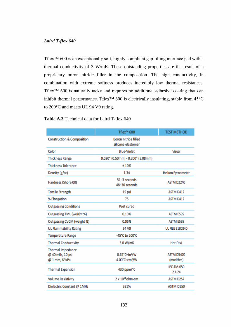
133
Laird T-flex 640
Tflex™ 600 is an exceptionally soft, highly compliant gap filling interface pad with a
thermal conductivity of 3 W/mK. These outstanding properties are the result of a
proprietary boron nitride filler in the composition. The high conductivity, in
combination with extreme softness produces incredibly low thermal resistances.
Tflex™ 600 is naturally tacky and requires no additional adhesive coating that can
inhibit thermal performance. Tflex™ 600 is electrically insulating, stable from 45°C
to 200°C and meets UL 94 V0 rating.
Table A.3 Technical data for Laird T-flex 640

134

135
APPENDIX B
Equipments of Experiment
Data Logger
Technical Features
Table B.1 Properties of Agilent HP 34970A data logger
Figure B.1 Agilent HP 34970A data logger

136
Power Supplies
Agilent 6032A System Power Supply 0-60V /0-50A, 1000W
Figure B.2 Agilent 6032A system power supply 0-60V /0-50A, 1000W
Technical Features
Output ratings
Voltage: 0 to 60 V
Current: 0 to 50 A
Programming accuracy at 25°C ±5°C
Voltage: 0.035%, +40 mV
Current: 0.2%, +85 mA
Ripple & noise 20 Hz to 20 MHz
Voltage rms: 8 mV
Voltage Peak-to-Peak: 40 mV
Current rms: 25 mA
Read-back accuracy at 25°C ±5°C
Voltage: 0.08%, +20 mV
Current: 0.36%, +35 mA

137
Agilent 6692A DC Power Supply 0-60V /0-110A
Figure B.3 Agilent 6692A DC power supply 0-60V /0-110A
Technical Features
Output Ratings
Voltage: 0 to 60 V
Output current : 0 to 110 A
Programming Accuracy (at 25 ±5°C)
Voltage: 0.04% + 60 mV
Current: 0. 1% + 65 mA
Ripple & Noise (20 Hz to 20 MHz)
Voltage: rms: 2.5 mV
Voltage: Peak-to-peak: 25 mV

138
HP 6573A System DC Power Supply 0-35V /0-60A
Figure B.4 HP 6573A System DC Power Supply 0-35V /0-60A
Technical Features
Output Ratings at 40°C
Output voltage: 0 to 35 V
Output current: 0 to 60 A
Programming Accuracy at 25°C ±5°C
Voltage: 0.04% + 35 mV
Current: 0.1% + 40 mA
Ripple & Noise (20 Hz to 20 MHz)
Voltage rms: 800 µV
Peak-to-Peak: 9 mV
Current rms: 40 mA
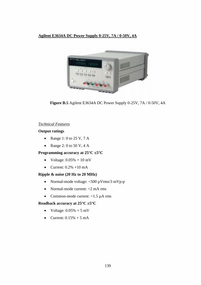
139
Agilent E3634A DC Power Supply 0-25V, 7A / 0-50V, 4A
Figure B.5 Agilent E3634A DC Power Supply 0-25V, 7A / 0-50V, 4A
Technical Features
Output ratings
Range 1: 0 to 25 V, 7 A
Range 2: 0 to 50 V, 4 A
Programming accuracy at 25°C ±5°C
Voltage: 0.05% + 10 mV
Current: 0.2% +10 mA
Ripple & noise (20 Hz to 20 MHz)
Normal-mode voltage: <500 µVrms/3 mVp-p
Normal-mode current: <2 mA rms
Common-mode current: <1.5 µA rms
Readback accuracy at 25°C ±5°C
Voltage: 0.05% + 5 mV
Current: 0.15% + 5 mA
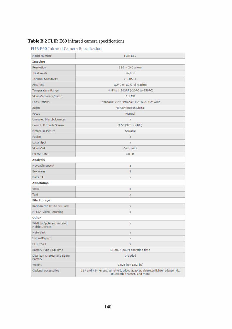
140
Table B.2 FLIR E60 infrared camera specifications

141
APPENDIX C
Optimization Graphs
Figure C.1 Result of optimization for 3 mm fin thickness vs variable spacing
Figure C.2 Result of optimization for 4 mm fin thickness vs variable spacing

142
Figure C.3 Result of optimization for 5 mm fin thickness vs variable spacing
Figure C.4 Result of optimization for 6 mm fin thickness vs variable spacing

143
APPENDIX D
Results of Corrected Experiment
Figure D.1 Result of corrected experiment for heater 1.1
Figure D.2 Result of corrected experiment for heater 1.2
202530354045505560657075808590
0 1000 2000 3000 4000 5000 6000 7000
Aver
age
Tem
per
ature
(o
C)
Time (s)
Average Surface Temperature of Heater 1.1 (oC)
202530354045505560657075808590
0 1000 2000 3000 4000 5000 6000Aver
age
Tem
per
ature
(o
C)
Time (s)
Average SurfaceTemperature of Heater 1.2 (oC)
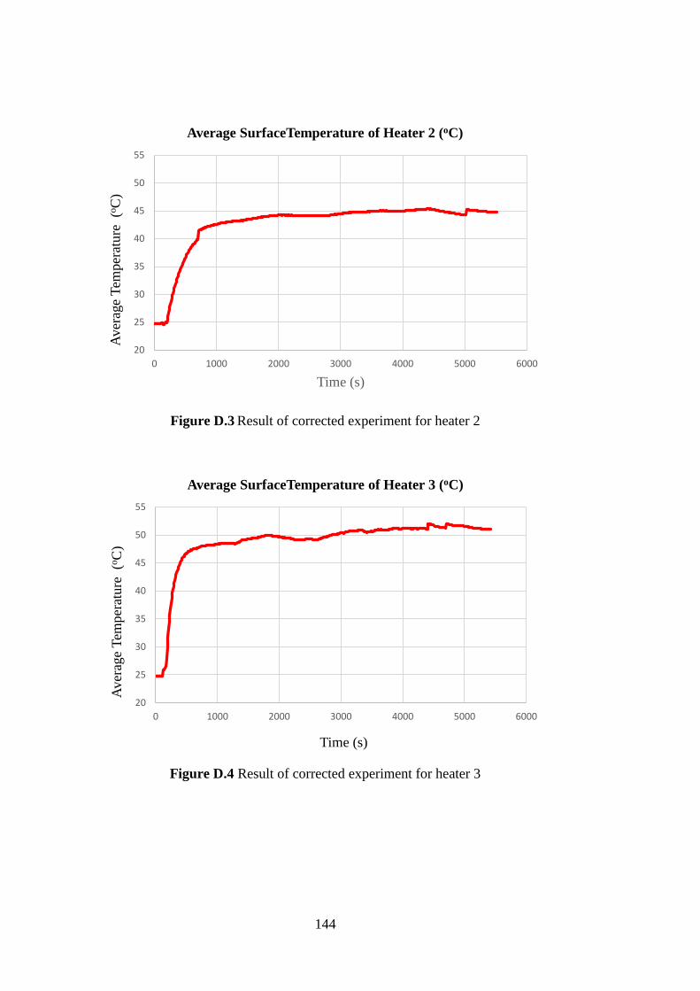
144
Figure D.3 Result of corrected experiment for heater 2
Figure D.4 Result of corrected experiment for heater 3
20
25
30
35
40
45
50
55
0 1000 2000 3000 4000 5000 6000
Aver
age
Tem
per
atu
re
(oC
)
Time (s)
Average SurfaceTemperature of Heater 2 (oC)
20
25
30
35
40
45
50
55
0 1000 2000 3000 4000 5000 6000
Av
erag
e T
emper
ature
(o
C)
Time (s)
Average SurfaceTemperature of Heater 3 (oC)


![Investigation of Heat Sink Efficiency for Electronic ...2013/01/26 · of heat sink, (mm) Number of fins Natural convection, Power dissipation [W], 60 ºC rise heat sink to ambient](https://img.pdfslide.us/doc/110x75/5f0eacc47e708231d44061ee/investigation-of-heat-sink-efficiency-for-electronic-20130126-of-heat-sink.jpg)