Healthy Business? Managerial Education and Management in Healthcare

Nicholas Bloom Renata Lemos

Raffaella Sadun John Van Reenen

Working Paper 18-025

Working Paper 18-025

Copyright © 2017 by Nicholas Bloom, Raffaella Sadun, Renata Lemos, and John Van Reenen

Working papers are in draft form. This working paper is distributed for purposes of comment and discussion only. It may not be reproduced without permission of the copyright holder. Copies of working papers are available from the author.

Healthy Business? Managerial Education and Management in Healthcare

Nicholas Bloom Stanford University

Renata Lemos World Bank

Raffaella Sadun Harvard Business School

John Van Reenen Massachusetts Institute of Technology

1

Healthy Business?

Managerial Education and Management in Healthcare

Nicholas Bloom

Stanford University, SIEPR, NBER

Raffaella Sadun

Harvard University

Renata Lemos*

World Bank, CEP-LSE

John Van Reenen

MIT, CEP-LSE

September 17th 2017

Abstract We investigate the link between hospital performance and managerial education by

collecting a large database of management practices and skills in hospitals across nine countries.

We find that hospitals that are closer to universities offering both medical education and business

education have higher management quality, more MBA trained managers and lower mortality

rates. This is true compared to the distance to universities that offer only business or medical

education (or neither). We argue that supplying joint MBA-healthcare courses may be a channel

through which universities increase medical business skills and raise clinical performance.

Keywords: Management, hospitals, mortality, education

JEL Classification: M1, I1

Acknowledgments: We would like to thank the European Research Council and Economic and

Social Research Centre for financial support through the Centre for Economic Performance. We

are grateful to Daniela Scur for ongoing discussion and feedback on the paper. Dennis Layton,

Stephen Dorgan and John Dowdy were invaluable partners in this project although we have

received no financial support from McKinsey (or any other company). We thank Jonathan

Haskel, Carol Propper and participants in seminars at the AEA, RES and MIT for helpful

comments. An earlier version of this paper was entitled: “Does Management Matter in

Healthcare?”

* Corresponding author: Renata Lemos. rlemos@worldbank.org

2

1. INTRODUCTION

Across the world, healthcare systems are under severe pressure due to aging populations, the

rising costs of medical technologies, tight public budgets and increasing expectations. Given the

evidence of enormous variations in efficiency levels across different hospitals and healthcare

systems, these pressures could be mitigated by improving hospital productivity. For example,

high-spending areas in the U.S. incur costs that are 50% higher than low-spending ones (Fisher

et al., 2003, in the “Dartmouth Atlas”).1 Some commentators focus on technologies (such as

Information and Communication Technologies) as a key reason for such differences, but others

have focused on divergent preferences and human capital among medical professionals (Phelps

and Mooney, 1993; Eisenberg, 2002; Sirovich et al., 2008). One aspect of the latter are

management practices such as checklists (e.g. Gawande, 2009). In this paper we seek to measure

management practices across hospitals in the US and eight other countries using a survey tool

originally applied by Bloom and Van Reenen (2007) for the manufacturing sector. The

underlying concepts of the survey tool are very general and provide a metric to measure the

adoption of best practices over operations, monitoring, targets and people management in

hospitals.

We document considerable variation in management practices both between and within

countries. Hospitals with high management scores have high levels of clinical performance, as

proxied by outcomes such as survival rates from emergency heart attacks (acute myocardial

infarction or AMI). These hospitals also tend to have a higher proportion of managers with

greater levels of business skills as measured by whether they have attained MBA-type degrees.

To further investigate the importance of the supply of managerial human capital on managerial

and clinical outcomes we draw on data from the World Higher Education Database (WHED)

providing the location of all universities in our chosen countries (see Valero and Van Reenen,

2016). We calculate geographical closeness measures (the driving times from a hospital to the

nearest university) by geo-coding the location of all hospitals and universities in our sample. We

show that hospitals that are closer to universities offering both medical and business courses

1 Annual Medicare spending per capita ranges from $6,264 to $15,571 across geographic areas (Skinner et al, 2011),

yet health outcomes do not positively co-vary with these spending differentials (e.g. Baicker and Chandra, 2004;

Chandra, Staiger, Skinner, 2010).

3

within their premises have significantly better clinical outcomes and management practices than

those located further away. This relationship holds even after conditioning on a wide range of

location-specific characteristics such as income, population density and climate. In contrast, the

distance to universities with only a business school, only a medical school, or neither—as in a

pure liberal arts college offering only arts, humanities, or religious courses—has no significant

relationship with management quality, suggesting that the results are not entirely driven by

unobserved heterogeneity in location characteristics correlated with educational institutions.

Proximity to schools offering bundles of medical and managerial courses is positively associated

with the fraction of managers with formal business education (MBA-type courses) in hospitals,

consistent with the idea that the courses increase the supply of employees with these combined

skills. We do not have an instrument for the location of universities, and cannot therefore

demonstrate the causality links behind these correlations. Nevertheless, these results are

suggestive of a strong—and so far unexplored—relationship between managerial education and

hospital performance.

Our paper relates to several literatures. First, the paper is related to the literature documenting the

presence of wide productivity differences across hospitals. Chandra et al (2013) estimate a large

heterogeneity in hospital “Total Factor Productivity” across U.S. hospitals of an order of

magnitude similar to the magnitude documented in manufacturing and retail. We contribute to

this literature by suggesting that management education may be a possible factor driving the

productivity dispersion via its effect on management practices. Second, our paper contributes to

the literature on the importance of human capital (especially managerial human capital) for

organizational performance. Examples of this work would include Bertrand and Schoar (2003)

for CEOs, Moretti (2004) for ordinary workers, and Gennaioli et al (2013) at the regional and

national levels. More specifically Doyle, Ewer and Wagner (2010) examine the causal

importance of physician human capital on patient outcomes. Finally, this paper is related to the

work on measuring management practices across firms, sectors and countries—for example,

Osterman (1994), Huselid (1995), Ichniowski, Shaw and Prenushi, (1997), Black and Lynch

(2001) and Bloom et al (2016).

4

The structure of the paper is as follows. In section 2 we provide an overview of the methodology

used to collect the hospital management data, the health outcomes data, the skills data as well as

other data used in the analysis. Section 3 describes the basic summary statistics emerging from

the data and section 4 presents the results. Section 5 concludes. The online Appendices give

much more detail on the data (A), additional results (B), sampling frame (C) and case studies of

management practices in individual hospitals (D).

2. DATA

2.1. Collecting Measures of Management Practices across Countries:

To measure hospital management practices and the share of managers with a MBA-type degree,

we adapt the World Management Survey (Bloom and Van Reenen 2007, Bloom et al 2014)

methodology to healthcare. This is based on the work of international consultants and the

healthcare management literature. The evaluation tool scores a set of 20 basic management

practices on a grid from one (“worst practice”) to five (“best practice”) in four broad areas:

operations (4 questions), monitoring, (5 questions), targets (5 questions) and human resource

management (6 questions). Our management index is the average of all 20 questions. To

compute our main management measure used in our regression analysis, we z-score the average

of the z-scores of the 20 management questions. The full list of dimensions can be found in

Appendix Table A1. To measure manager business and management skills, we asked “What

percentage of managers have an MBA?”, considering management-related courses that are at

least 6-months long.

We used a variety of procedures to persuade hospital employees to participate in the survey.

First, we encouraged our interviewers to be persistent running on average two hour-long

interviews a day. Second, we never asked hospital managers about the hospital’s overall

performance during the interview (these were obtained from external administrative sources).

Third, we sent informational letters, and, if necessary, copies of country endorsements letters

(e.g. UK Health Department).

5

Following these procedures helped us obtain an overall high response rate in terms of interviews

completed. The overall response rate was 34%, which is similar to the response rates for our

manufacturing and school surveys. The country-specific response rates ranged from 66%, 53%

and 49% of eligible hospitals in Sweden, Germany, and Brazil, to 21% of eligible hospitals in the

US. In contrast, the overall explicit refusal rate was 11% and generally low across all countries

surveyed, ranging from no refusals in hospitals in Sweden to 22% of all eligible hospitals in

Germany. In terms of selection bias, we compare our sample of hospitals for which we secured

an interview with the sample of eligible hospitals in each country against size, ownership and

location. Looking at the overall pattern of results, we obtain few significant coefficients with

marginal effects small in magnitude. In our country-specific analysis, the results show that

hospitals with certain location characteristics are more likely to respond in India, public hospitals

are more likely to be interviewed in the US, and larger hospitals are more likely to be

interviewed in Germany and in Italy. We further construct sampling weights and observe that our

main unweighted results hold even when using this alternative sample weighting scheme. We

describe our selection analysis as well as the sampling frame sources and response rates in more

detail in Appendix C.

To elicit candid responses, we took several steps. First, our interviewers received extensive

training in advance on hospital management. Second, we also employed a double-blind

technique. Interviewers are not told in advance about the hospital’s performance – they only had

the hospital’s name and telephone number – and respondents are not told in advance their

answers are scored. Third, we told respondents we were interviewing them about their hospital

management, asking open-ended questions like “Tell me how you track performance?” and “If I

walked through your ward what performance data might I see?”. The combined responses to

these types of questions are scored against a grid. For example, these two questions help to score

question 6, performance monitoring, which goes from 1, which is defined as “Measures tracked

do not indicate directly if overall objectives are being met. Tracking is an ad-hoc process

(certain processes aren’t tracked at all)”, to 5 defined as “Performance is continuously tracked

and communicated, both formally and informally, to all staff using a range of visual management

tools.” Interviewers kept asking questions until they could score each dimension.

6

Other steps to guarantee data quality included: (i) each interviewer conducted on average 39

interviews in order to generate consistent interpretation of responses. They received one week of

intensive initial training and four hours of weekly on-going training;2 (ii) 70% of interviews had

another interviewer silently listening and scoring the responses, which they discussed with the

lead interviewer after the end of the interview. This provided cross-training, consistency and

quality assurance. (iii) We collected a series of ‘noise controls’, such as interviewee and

interviewer characteristics. We include these controls in the regressions to reduce potential

response bias.

The data was collected for Canada, France, Italy, Germany, Sweden, U.S and U.K. (in 2009);

India (2012); and Brazil (2013). For the U.K. we combine two waves of the survey (2006 and

2009).3 The choice of countries was driven by funding availability, the availability of hospital

sampling frames, and research and policy interest. In every country the sampling frame for the

management survey was randomly drawn from administrative register data and included all

hospitals that (i) have an Orthopedics or Cardiology Department, (ii) provide acute care, (iii)

have overnight beds. Interviewers were each given a random list of hospitals from a sampling

frame representative of the population of hospitals with these characteristics in the country. We

interviewed the director of nursing, medical superintendent, nurse manager or administrator of

the specialty, that is, the clinical service lead at the top of the specialty who is still involved in its

management on a daily basis. We describe the country sampling frames, their sources, and

eligibility criteria in Appendices A and C. In most countries, we find that some hospitals are part

of larger networks. Therefore, in our analysis we cluster standard errors by hospital network to

take into account potential similarities across these hospitals, and multiple observations across

years for the UK sample.

2.2. Collecting Hospital Health Outcomes

Given the absence of publicly comparable measures of hospital-level performance across

countries, we collected country-specific measures of AMI (acute myocardial infarction,

commonly called heart attacks) death rates. AMI is a common emergency condition, recorded

2 See, for example, the video of the training for our 2009 wave http://worldmanagementsurvey.org/?page_id=187 3 The 2006 U.K. data has been used in Bloom et al (2015).

7

accurately and believed to be strongly influenced by the organization of hospital care (Kessler

and McClellan 2000), and used as a standard measure of clinical quality. We tried to create a

consistent measure across countries, although there are inevitably some differences in

construction so we include country dummies in almost all of our specifications.4 We observe

substantial differences in spread of this measure across countries—the country specific

coefficient of variation is 0.51 for Brazil, 0.52 for Canada, 0.21 for Sweden, 0.10 for the U.S.

and 0.34 (2006) and 0.15 (2009) for the U.K.

2.3. Classifying differences across universities

In the WHED we can distinguish whether universities offer courses in Business (Management,

Administration, Entrepreneurship, Marketing, Advertising courses), Medical (Clinical courses),

and Humanities (Arts, Language, Religion courses) and a range of other “divisions” (see Feng,

2015; Valero and Van Reenen, 2015). We geocode the location of each school using their

published addresses and compute drive-times between hospitals and universities of different

types using GoogleMaps. The computation of travel times is restricted to hospitals and

universities in the same county (see Appendix A for a more detailed explanation).

2.4. Collecting Location Characteristics Information

Using the geographic coordinates of hospitals in our sample, we also collected a range of other

location characteristics. At the regional level, we use the variables provided in Gennaioli et al

(2013).5 For data at the grid level, we construct a dataset based on the G-Econ Project in Yale

that estimates geographical measures for each grid cell which represents 1 degree in latitude by 1

degree longitude. Table B1 presents descriptive statistics for the sets of location characteristics

used in this analysis.

4 For Brazil we compute a simple risk-adjusted measure by taking the unweighted average across rates for

myocardial infarction specified as acute or with a stated duration of 4 weeks or less from onset for each rage-gender-

age cell for each hospital for the years of 2012 and 2013. For Canada, we use risk-adjusted rate for acute myocardial

infarction mortality for the years 2004-2005, 2005-2006 and 2006-2007. For Sweden, we use 28-day case fatality

rate from myocardial infarction from 2005 to 2007. For the US, we use the risk-adjusted 30-day death (mortality)

rates from heart attack from July 2005 to June 2008. For the UK we use 30 day risk adjusted mortality rates

purchased from the company “Dr Foster”, the leading provider of NHS clinical data. (See Appendix A for more

information and sources). For each hospital, we consider three years of data (the survey year plus two years

preceding, or the closest years to the survey with available data) to smooth over possible large annual fluctuations. 5 The regional data from Gennaioli et al (2013) consists of NUTS1, NUTS2, State or Provincial level, depending on

the country.

8

3. DESCRIPTIVE STATISTICS

3.1 Basic Descriptives

Table 1 shows the management scores across hospitals (which is the simple average of the

questions ranging between 1 and 5) and Figure 1 shows the differences across countries. The US

has the highest management score (3.0), closely followed by the UK, Sweden, and Germany (all

around 2.7) with Canada, Italy, and France slightly lower (at around 2.5). The emerging

economies of Brazil (2.2) and India (1.9) have the lowest scores.6 The rankings do not change

substantially (except for Sweden) when we include controls for hospital characteristics and

interview noise. Country fixed effects are significant (p-value on the F-test of joint significance

is 0.00) and account for 32% of the variance in the hospital-level management scores, which is a

greater fraction than for manufacturing firms, where the figure is 25% for the same set of

countries.7

Figure 2 shows the distribution of management scores within each country compared to the

smoothed (kernel) fit of the US distribution. Across OECD countries, lower average country-

level management scores are associated with an increasing dispersion towards the left tail of the

distribution. Hospitals with very weak management practices (score of 2 or below) have almost

no monitoring, very weak targets (e.g. only an annual hospital-level target) and extremely weak

incentives (e.g. tenure based promotion, no financial or non-financial incentives and no effective

action taken over underperforming nurses or doctors). While the fraction of hospitals with very

weak management practices in OECD countries is small (from 5% in the US to 18% in France),

this fraction rises to 45% in Brazil and 68% in India. At the other end of the distribution, the

fraction of hospitals scoring with some reasonable performance monitoring, a mix of targets and

performance-based promotion, rewards and steps taken to address persistent underperformance

(score 3 or above) ranges from 50% in the US to 3% in India.

6 In the Appendix, we provide examples of management practices in the average hospital in the US (at the top of the

ranking) and in India (at the bottom of the ranking). 7 Table C2 presents hospital characteristics across countries. Although there are many differences in cross country

means (e.g. the median French hospital has 730 beds compared to 45 in Canada). However, within all countries non-

responders were not significantly different from participating hospitals. Characteristics are different because the

healthcare systems differ and our sample reflects this.

9

3.2 AMI Mortality Rates and Management

As an external validation of our management measure across countries, we investigate whether

management is related clinical outcomes. Table 2 shows that management practices are

significantly negatively correlated with AMI mortality rates.8 In column (1) the management

coefficient suggests that a one standard deviation increase in a hospital’s management score is

associated with a fall of -0.188 standard deviations in AMI deaths rates, and this relationship

holds even after controlling for a wide variety of factors. Column (2) includes a measure of size

(hospital beds), ownership dummies (for-profits; non-for-profit and government owned), other

hospital characteristics (local competition and skills) and statistical noise controls. Column (3)

includes regional geographic controls (income per capita, education, population density, climate,

ethnicity, etc.). Column (4) includes regional dummies, and column (5) uses more disaggregated

geographical controls. Although the coefficient on management varies between columns (from -

0.188 to -0.223), it is significant at the 1% level throughout.

Table 2 is consistent with findings from other work. For example, Bloom et al (2015) use

English hospitals from 2006 and also find a positive link between management and positive

performance such as survival rates from general surgery, lower staff turnover, lower waiting

lists, shorter lengths of stay and lower infection rates.9 Chandra et al (2016) look at the

management scores and risk-adjusted AMI survival rates in US hospitals and also report a

positive relationship.

3.3. Management and Management Education

We explore the correlation between management scores and management education in Table 3.

First, column (1) shows that country dummies and basic interviewer, department and interview

controls can account for about half of the overall variation in management scores. Column (2)

shows that the management score is positively and significantly correlated with the share of

managers in the hospital who have received managerial education. The coefficient implies that a

100% increase in the managerial skills variable (that is an average hospital that moves from

8 Note that we can only do this for a sub-set of hospitals (478 from the total of 1960 observations), as AMI data is

not available for all hospitals. 9 These are only correlations so may not be causal. The results do indicate that hospitals like Virginia Mason,

ThedaCare and Intermountain that are famous for adopting these types of management practices typically have

better outcomes than others.

10

having 26% to 52% of managers with a MBA-type course) is associated with .88 of standard

deviation increase in the management score.

To evaluate whether the correlation of management scores with managerial skills is due to basic

structural differences across hospitals, we control for hospital size (number of beds) in column

(4) and ownership (dummies for private-for profit and private-not for profit status) in column

(5).10 Larger hospitals tend to have higher management scores, whereas government run

hospitals tend to have lower management scores. While the inclusion of these controls reduces

the coefficient on the management skills variable by 29%, the variable remains positive and

significant. Another possible explanation is that the correlation we observe is due to competition

levels. For example, Bloom, Propper, Seiler, and Van Reenen (2015) show causal evidence of

the impact of higher competition on improved managerial quality in English hospitals. To

account for this, we add a measure of competition in column (5).11 In column (6) we add the

share of managers with a clinical degree to explore whether hospitals perform better when they

are run by managers with a clinical background (Goodall 2011). Finally, in column (7) we add

geographic controls at the regional level to test for whether the relationship found is simply

being driven by differences in location. Management skills remain correlated with management

across all these specifications.

3.4. Summary

Overall, the data show: a) a positive correlation between clinical outcomes and management

practices; and b) a positive correlation between management practices and management

education.

4. MAIN RESULTS

In this section we explore the relationship between the proximity of a university offering both

management and clinical education and three hospital-level variables of interest: (i) AMI

10 See, for example, evidence of firm basic structures as possible explanations for the variation in management

quality in Bloom, Sadun, and Van Reenen (2016). 11 Our measure of competition is collected during the survey itself by asking the interviewee ‘How many other

hospitals with the same specialty are within a 30-minute drive from your hospital?’

11

mortality rates, (ii) management practices, and (iii) the fraction of managers with an MBA-type

qualification.

4.1 AMI Mortality Rates

The average driving time between hospitals and universities is 37 minutes with a median of 19

minutes. Column (1) of Table 4 regresses AMI death rates on driving hours to the nearest

university and includes country dummies and general controls. Column (2) includes hospital

characteristics (size, ownership and competition) and column (3) adds regional controls.

Although there is a positive coefficient on distance from a university, it is statistically

insignificant.

Next, we explore whether distance to universities offering both business and medical/clinical

courses (henceforth, “joint M-B school”) is correlated with clinical performance. We calculate

driving distances from each hospital to the nearest joint M-B school, which is 67 minutes on

average. While we include a range of geographic characteristics in our specification (such as

income, education, population and temperature) there could still be unobserved heterogeneity

specific to university locations confounding the relationship between hospital performance and

the distance to universities. Therefore, in addition to including joint M-B school we also include

driving distance to universities specializing solely on arts, humanities or religious courses

(“stand-alone HUM”) and therefore not offering clinical/medical or business-type courses (and

expect to find no significant relationship between these universities and hospital performance).

To validate the use of this type of school as a placebo, Figure 3 shows that the nearest stand-

alone HUM school and joint M-B school are similar in proximity to the hospitals in our sample:

82% of hospitals have a driving time difference of two hours or less between these two types of

universities. We also observe that the means of a range of location characteristics of the nearest

joint M-B school and stand-alone HUM school are not statistically significant (in Table B2).12

Finally, we also include universities that do not offer medical, business or humanities (“no M, B,

HUM”).

12 The only measures that are statistically significant are latitude and longitude.

12

In column (4) of Table 3 we show that there is a statistically significant and positive relationship

between distance only to the nearest joint M-B school and AMI mortality rates—an additional

hour of driving to a joint M-B school increases AMI mortality rates by 0.393 of a standard

deviation. Reassuringly, we do not observe a significant relationship between hospital

performance and the other university types.

The significance of the joint M-B school in the AMI regressions may be due to other nearby

universities that do not have medical/clinical or business courses, but offer other types of

quantitative courses (such as engineering, etc.). To investigate this issue, we calculate distances

to other schools such as (i) the nearest university offering business courses but no

medical/clinical courses (“B school, no M”), (ii) the nearest university offering medical/clinical

courses but not business courses (“M school, no B”), and (iii) the nearest university offering

other courses but no business nor medical courses (“nearest school, no M nor B”). Figure 4

shows that the distributions are similar across all types of schools. In column (5) of Table 3, we

include variables measuring driving distances to all four types of schools. The distance to joint

M-B schools has explanatory power over and above distances to other school types, and has a

coefficient similar to the previous column in terms of magnitude. Since none of these other

school types are individually or jointly significant we drop them in column (6) which is our

preferred specification.

Could the coefficient on our main variable of interest be due to a failure to control for finer

geographical characteristics? Column (7) of Table 3 includes regional dummies, grid level

geographical controls in the most general specification of column (5) and show that the

coefficient on distance to a joint M-B school is if anything even larger.

Since we do not need the management survey for the results in Table 3, we can in principle

estimate this on a larger sample. We focused on the US where information on AMI is available

for close to the hospital population13 and re-ran a similar specification to column (5) of Table 3.

Although we only have one country, the coefficient on distance remains positive and (weakly)

13 We use a sample of hospitals in the US for which AMI measures are reported in 2009, our year of reference for

the OECD countries. We approximate the sample used in the US to the cross-country sample used in this paper by

excluding sole community providers and hospitals operated by the Catholic Church.

13

significant. Because we have a larger number of hospitals within networks in the US-only

sample we can also estimate a specification with network fixed effects in column (9). This

exploits within network variation in AMI mortality rates and distance to schools, thus controlling

for possible network-level confounders (the sample is smaller as we require at least two hospitals

in the chain for which performance data was available).14 These results confirm that distance to

joint M-B schools is associated with AMI mortality rates, while the distance to other types of

schools is not.15

4.2 Management Practices

Table 5 explores the relationship between distance to universities and management practices -

the specifications are the same as the first seven columns of Table 3 with a different dependent

variable. There is a negative correlation between distance to the nearest university and

management quality, but it is insignificant in column (3) which controls for regional

characteristics. As with Table 3 columns (4) and (5) show that it is only joint M-B schools that

has explanatory power over and above distances to other school types. The results in our

preferred specification in column (6) suggest that every additional hour of driving to a joint M-B

school is associated with a decrease in hospital management quality of 0.145 of a standard

deviation. 16

4.3 Business education

What could be the reason for this relationship between distance and better hospital outcomes (in

terms of AMI survival rates and management practices)? One obvious mechanism is that there is

a greater supply of workers with managerial skills when a hospital is close to a joint M-B school.

14 This is analogous to a manufacturing context where one could use plant-specific variation within a firm (i.e. firm

fixed effects with plant level data). 15 We also repeat the specification in column (8) but add HRR fixed effects to check if our results are robust to

market characteristics and find similar results. Using a larger UK sample, we explore another dimension of hospital

performance: the average probability of staff intending to leave in the next year as a measure of worker job

satisfaction for the U.K. reported by the NHS staff surveys and used on Bloom et al (2015). Reassuringly, we find

similar patterns to those described in Table 3, indicating a significant positive correlation between distant to the

nearest joint M-B school and the likelihood of the average employee wanting to leave the hospital. 16 In Table B3 we check whether this relationship is driven by joint M-B school quality characteristics such as age

and ranking. While we observe that these measures are to some extent significantly correlated to hospital

management quality (but not to AMI mortality rates) when included in the analysis, our results show that adding

these measures do not result in substantial changes to the magnitude and significant of our distance to joint M-B

coefficient of interest.

14

In Figure 6 we investigate the relationship between the share of managers with an MBA type

degree and the hospital’s closeness to a joint M-B school (left hand side).17 There is a clear

downwards slope – being closer to these types of schools is associated with a higher fraction of

managers with MBAs. By contrast, the right hand side panel of Figure 6, shows that there is no

relationship between the share of MBAs and the distance to stand-alone HUM schools. We

formalize Figure 6 in Table 6 which uses the same specifications as Table 5 except has the share

of managers with MBA-type course as the dependent variable. Consistent with the two earlier

tables, closeness to a joint M-B school (but not other types of school) is associated with

significantly more hospital managers with business education.

We bring these ideas together by instrumenting the share of MBA with the distance to a joint M-

B school embodying the idea that proximity increases the managerial skill supply which in turn

benefits hospital performance. If the only way that university proximity matters is through skill

supply this should identify the causal impact of managerial education on hospital performance.

With the important caveats that the exclusion restriction may not be valid (as universities could

in principle affect hospitals through other routes than the supply of human capital) and the

instrument is not strong, we observe that results are consistent with a large causal effect. These

results are detailed in Table B4 and described in the Appendix.

5. CONCLUSIONS

We have collected data on management practices in 2,000 hospitals in nine countries. We

document a large variation of these management practices within each country and find that our

index of “better management” is positively associated with improved clinical outcomes such as

survival rates from AMI.

We show evidence that a hospital’s proximity to a university which supplies joint business and

clinical education is associated with a higher management practice score (and better clinical

outcomes). Proximity to universities that do not have medical schools or do not have business

schools does not statistically matter for hospital management scores, suggesting that the bundle

17 All variables in Figure 6 are orthogonalized off geographical controls through a first stage regression.

15

of managerial and clinical skills has an impact on hospital management quality. We find that

hospitals which are closer to the combined clinical and business schools also have a higher

fraction of managers with MBAs which is consistent with this interpretation.

Our work suggests that management matters for hospital performance and that the supply of

managerial human capital may be a way of improving hospital productivity. Given the enormous

pressure health systems are under, this may be a complementary way of dealing with health

demands in addition to the usual recipe of greater medical inputs.

The correlations we describe are only suggestive as we do not have panel data or experimental

evidence to track out causal impacts. Such evidence from either randomized control trials or

natural experiments is an obvious next step in this agenda.

16

REFERENCES

Arrow, Kenneth (1963) “Uncertainty and the Welfare Economics of medical care” American

Economic Review, 53(5) 141-149.

Baicker, Katherine and Amitabh Chandra (2004) “Medicare Spending, the Physician Workforce,

and the Quality of Healthcare Received by Medicare Beneficiaries.” Health Affairs,

April, 184-197.

Bertrand, Marianne, and Antoinette Schoar (2003) “Managing with Style: The Effect of

Managers on Firm Policies.” Quarterly Journal of Economics, 118 (4): 1169-1208.

Black, Sandra and Lisa Lynch (2001) “How to Compete: The Impact of Workplace Practices and

Information Technology on Productivity”, Review of Economics and Statistics, 83(3),

434–445.

Bloom, Nicholas and John Van Reenen (2007) “Measuring and Explaining Management

practices across firms and nations”, Quarterly Journal of Economics, 122, No. 4: 1351–

1408.

Bloom, Nicholas, Stephen Dorgan, Rebecca Homkes, Dennis Layton and Raffaella Sadun (2010)

“Management in Healthcare: Why Good Practice Really Matters” Report

http://cep.lse.ac.uk/textonly/_new/research/productivity/management/PDF/Management_

in_Healthcare_Report.pdf

Bloom, Nicholas, Renata Lemos, Raffaella Sadun, Daniela Scur, John Van Reenen (2014) "The

New Empirical Economics of Management". Journal of the European Economic

Association, 12, No. 4 (August 2014): 835–876.

Bloom, Nicholas, Carol Propper, Stephan Seiler and John Van Reenen (2015) “The Impact of

Competition on Management Quality: Evidence from Public Hospitals” Review of

Economic Studies 82: 457-489.

Bloom, Nicholas, Raffaella Sadun and John Van Reenen (2016) “Management as a

Technology”, CEP Discussion Paper 1433.

Cacace, Mirella, Stefanie Ettelt, Laura Brereton, Janice S. Pedersen and Ellen Nolte (2011)

“How health systems make available information on service providers: Experience in

seven countries.” Mimeo, RAND Corporation.

17

Capelli, Peter and David Neumark, 2001. ‘Do ‘High-Performance’ Work Practices Improve

Establishment-Level Outcomes?’, Industrial and Labor Relations Review, 54(4), 737-

775.

Chandra, Amitabh and Douglas O. Staiger (2007) “Productivity Spillovers in Healthcare:

Evidence from the Treatment of Heart Attacks.” Journal of Political Economy 115, 103-

140.

Chandra, Amitabh, Douglas O. Staiger, Skinner Jonathan (2010) Saving Money and Lives, in

The Healthcare Imperative: Lowering Costs and Improving Outcomes. Institute of

Medicine. http://www.ncbi.nlm.nih.gov/books/NBK53920/

Cutler, David (2010) “Where are the Healthcare Entrepreneurs?” Issues in Science and

Technology. (1): 49-56.

Doyle, Joe, Todd Wagner and Steven Ewer (2010) “Returns to Physician Human Capital:

Evidence from Patients Randomized to Physician Teams” Journal of Health

Economics 29(6) 866-882.

Eisenberg, John M. 2002. “Physician Utilization: The State of Research about Physicians’

Practice Patterns.” Medical Care. 40(11): 1016-1035.

Fisher, Elliott S., David Wennberg, Theresa Stukel, Daniel Gottlieb, F.L. Lucas, and Etoile L.

Pinder (2003) “The Implications of Regional Variations in Medicare Spending. Part 1:

The Content, Quality and Accessibility of Care” Annals of Internal Medicine 138(4):

273-287.

Gawande, Atul (2009) The Checklist Manifesto, New York: Henry Holt.

Gennailoi, Nicola, Rafael La Porta, Florencio Lopez-de-Silvanes and Andrei Shleifer (2013)

“Human Capital and Regional Development” Quarterly Journal of Economics 128(1)

105-164.

Goodall, Amanda (2011) “Physician-leaders and hospital performance: Is there an

association?” Social Science and Medicine, 73(4), 535-539.

Huselid, Mark, 1995. ‘The Impact of Human Resource Management Practices on Turnover,

Productivity and Corporate Financial Performance’, Academy of Management Journal,

38, 635-672.

18

Ichniowski, Casey, Katheryn Shaw and Prennushi, Giovanni. (1997) “The effects of human

resource management practices on productivity: A study of steel finishing lines” The

American Economic Review, 87(3), 291–313.

Jamison. D. T. and Martin Sandbu, (2001), “WHO Rankings of Health System Performance”,

Science, 293: 5535, 1595-1596.

Kessler, Daniel P., and Mark B. McClellan (2000) “Is Hospital Competition Socially Wasteful?”

Quarterly Journal of Economics 115: 577–615.

McConnell K, Lindrooth RC, Wholey DR, Maddox TM and Bloom N. (2013) “Management

Practices and the Quality of Care in Cardiac Units” JAMA Intern Med.; 173(8):684-692.

Moretti, Enrico (2004) Workers’ Education, Spillovers and Productivity: Evidence from Plant-

Level Production Functions, American Economic Review, 94(3).

Osterman, Paul (1994) “How common is workplace transformation and who adopts it?”

Industrial and Labor Relations Review, 47(2), 173–188.

Paris, V., M. Devaux and L. Wei (2010), "Health Systems Institutional Characteristics: A Survey

of 29 OECD Countries", OECD Health Working Papers, No. 50, OECD Publishing.

Phelps, Charles and Cathleen Mooney (1993) “Variations in Medical Practice Use: Causes and

Consequences” In Competitive Approaches to Health Care Reform, ed. Arnould, Richard,

Robert Rich and William White. Washington DC: The Urban Institute Press.

Sirovich, Brenda, Gallagher, Patricia M., Wennberg, David E., and Elliott S. Fisher. (2008)

“Discretionary Decision Making by Primary Care Physicians and the Cost of U.S. Health

Care.” Health Affairs. 27(3): 813-823.

Valero, Anna and John Van Reenen (2016) “The Economic Impact of Universities: Evidence

from Across the Globe” NBER Discussion Paper 22501.

World Health Organization. The world health report 2000 — Health systems: improving

performance. Geneva: World Health Organization; 2000.

19

ONLINE APPENDICES (NOT INTENDED FOR PUBLICATION)

APPENDIX A: DATA

A1. Management Survey Data

Table A1 lists the 20 management practices questions asked during the survey.

A2. Hospital-Level Performance Data

We use hospital performance data for five countries surveyed, for which data was publicly available. Below is a

description of our hospital performance dataset for each country.

Brazil: We used the rate for myocardial infarction specified as acute or with a stated duration of 4 weeks (28

days) or less from onset (ICD-10, I21) for years 2012 and 2013. We create a simple risk-adjusted measure by

taking the unweighted average across rates for each rage-gender-age cell for each hospital. The raw data was

extracted from Datasus Tabnet (http://tabnet.datasus.gov.br).

Canada: We take the average of the risk-adjusted rate for acute myocardial infarction mortality for the years

2004-2005, 2005-2006 and 2006-2007 for the provinces British Columbia and Ontario. The data was extracted

from hospital reports provided by the Fraser Institute (www.fraserinstitute.org).

Sweden: We use 28-day case fatality rate from myocardial infarction for hospitalized patients for the years of

2004 to 2006 computed and published by the Swedish Association of Local Authorities and Regions (SALAR)

and the Swedish National Board of Health and Welfare (NBHW) in the report "Quality and Efficiency in Swedish

Health Care – Regional Comparisons 2008".

United States: We use the 30-day death (mortality) rates from heart attack from July 2005 to June 2008 (2009 for

the specifications in Table 2, columns 8 and 9) computed and published by Hospital Compare.

United Kingdom: We use 30-day risk adjusted AMI mortality data purchased from “Dr Foster” relative to 2006

(matched with the 2006 survey wave) and 2009 (matched with the 2009 survey wave).

A3. University Data

The University data comes from the World Higher Education Database (WHED) which has the location, foundation

date and list of “divisions” (subjects) of all research universities in our chosen countries (see Feng, 2015; Valero and

Van Reenen, 2016). Divisions are classified into Business (Management, Administration, Entrepreneurship,

Marketing, Advertising courses), Medical (Clinical courses), and Humanities (Arts, Language, Religion courses).

Table A2 shows the number of unique schools in each country used in this analysis.

A4. Distance Information

We geo-code the location of hospitals and universities using addresses available, cross referencing four sources of

coordinates (Geopostcodes datasets purchased, Google geo-coding of address, geo-coding of institution name and

manual searches on search engines) and converging to a final dataset. We compute travel times using Google API

(travel times are not a function of time of day, that it, running the Google distance API at 11pm on a Sunday vs 9am

on a Monday yields the same result). Computation of distance is restricted to hospitals and universities in the same

county.

A5. Location Information

The source data on population density comes from CIESIN and is presented as average density within population

grids identified by the coordinates of the grid’s centroid. Population density is computed using ArGIS. We spatially

join hospital coordinates with centroid coordinates and (1) take the population density of the closest centroid (2)

20

compute the average population density of all centroids within 100km (3) compute the inverse distance weighted

population density of all centroids within 100km. Results are robust to using any one of these three measures.

Computation of distance is restricted to hospitals and universities in the same county.

APPENDIX B: ADDITIONAL RESULTS

Table B1 presents descriptive statistics on the range of regional- and grid-level location characteristics used in the

analysis.

Table B2 presents the Difference in means of grid-level location characteristics of the nearest joint M-B and stand-

alone HUM schools to each hospital in our dataset.

Table B3 explores whether the relationship between hospital performance (as measured by clinical or managerial

quality) and distance to joint M-B school are being driven by school quality characteristics. We show our results are

robust to controlling for the age of the university or the ranking of the university in global league tables.

In Table B4 we bring the results of Tables 2, 3 and 4 together. Columns (1) through (3) use AMI mortality rates as

the dependent variable and regress this on the share of managers with an MBA type degree. We instrument share of

MBA with the distance to a joint M-B school embodying the idea that proximity increases the managerial skill

supply which in turn benefits hospital performance. If the only way that university proximity matters is through this

school supply this should identify the causal impact of managerial education on hospital performance. The negative

and significant effect in column (1) is consistent with a large causal effect. However, an important caveat is that the

exclusion restriction may not be valid. For example, if proximity enabled a hospital to receive other beneficial inputs

(executive education and consultancy that are not reflected in MBA share) this would violate the exclusion

restriction. Columns (4) through (6) of Table 6 repeat the specifications of the first three columns, but use

management practices as the dependent variable instead of AMI death rates. In column (7) and (8) we add distance

to stand-alone HUM schools as a control and as an instrument, respectively, while maintaining distance to joint M-B

as an instrument. There is a positive and significant coefficient on MBA share across all five columns. In column (9)

we perform a placebo test by removing distance to joint M-B schools and using solely distance to stand-alone HUM

schools as an instrument. As expected, the MBA share coefficient is no longer significant and turns negative.

Another caveat to these results is that the instruments are not strong. The F-statistics shown in the lower rows are

about 8 in the simplest specifications, but are much lower when we control for other covariates, especially

geographical controls in columns (3) and (6). The second stage coefficients also become much more imprecise in

these columns which is consistent with the weak instruments problem.

APPENDIX C: SAMPLING FRAME

C1. The Sampling Frame and Eligibility to Participate in the Management Survey

In every country the sampling frame for the management survey included all hospitals that (i) have an Orthopaedics

or Cardiology Department, (ii) provide acute care, (iii) have overnight beds. The source of this sampling frame by

country is shown in Table C1. Interviewers were each given a randomly selected list of hospitals from the sampling

frame. This should therefore be representative of the population of hospitals in the country. At hospitals, we either

interviewed the director of nursing, medical superintendent/nurse manager/administrator of specialty, that is, the

clinical service lead at the top of the speciality who is still involved in its management on a daily basis. The clinical

service leads also had to be in the post for at least one year at the time of the interview.

Table C2 shows the number of healthcare facilities in each country, the number of eligible hospitals randomly drawn

the sampling frame, and hospital characteristics from these eligible hospitals. For the countries where information is

21

available, the sample in Canada, France and the UK present the largest percentage of hospitals which are funded and

managed by government authorities (all above 60% with Canada reaching 99%), while the samples in Brazil and the

US have the lowest percentage (39% and 28%, respectively).

The median hospital size in the sample in France as measured by the number of hospital beds is by far the largest

(730) while the median hospital in the sample in Italy, Germany, the UK and Sweden are of similar size (between

195 and 269 beds). The US and Canada samples present the smallest sized hospitals.

C2. The Survey Response Rates

Table C3 shows the survey response rates by country. The top table represents all hospitals in the randomly selected

list of hospitals given to the interviewers as described above. The bottom table represents all hospitals eligible for

the interview. The eligibility criteria were confirmed by the interviewer during the process of contacting and

scheduling the interview. As the type of healthcare facilities included in the lists sourced in each country varied

substantially, interviewers spent significant time on the phone screening out ineligible hospitals. For example,

interviewers identified 78% of hospitals to be ineligible for the survey in Brazil while in France this number is down

to 16%. This is one of the main reasons for a lower average of hospital interviews conducted per day in comparison

to the average for our manufacturing interviews (2.8 per day).

In terms of interviews completed, we managed to obtain a response rate ranging from 66%, 53% and 49% of eligible

hospitals in Sweden, Germany, and Brazil, to 21% of eligible hospitals in the US. In contrast, the explicit refusal

rate was generally low across all countries surveyed, ranging from no refusals in hospitals in Sweden to 22% of all

eligible hospitals in Germany. The high response rate in general was due to greater persistence in following up non-

respondents in order to meet the target numbers we were aiming for and to the fact that most hospital managers

interviewed in these countries responded with a scheduled time and date soon after the first or second contact with

the interviewer.

“Scheduling in progress” indicates hospitals which have been contacted by an interviewer and which have not

refused to be interviewed (for example they may schedule an interview but cancel or postpone it or simply take more

time to respond). The high share of “scheduling in progress” schools was due to the need for interviewers to keep a

stock of between 100 to 300 hospitals to cycle though when trying to arrange interviews. Since interviewers only ran

an average of 1.1 interviews a day the majority of their time was spent trying to contact hospitals managers to

schedule future interviews.

The ratio of successful interviews to rejections (ignoring “scheduling in progress”) is above 1 in every country.

Hence, managers typically agreed to the survey proposition when interviewers were able to connect with them.

C3. Selection Analysis

Panel A of Table C4 analyses the probability of being interviewed. Within each country, we compare the responding

hospitals with those eligible hospitals in the sampling frame - including “interviews refused” and “scheduling in

progress” but removing “hospital not eligible” for the survey - against three types of selection bias: location

characteristics (income per capita, population size, population average years of education, share of population with a

high school degree, share of population with a college degree, average temperature, inverse distance to coast, oil

production per capital), size (number of hospital beds), ownership (whether the hospital is owned and managed by

government authorities).

Looking at the overall pattern of results, there are very few significant coefficients. The results from the pooled

sample show that only the coefficients for temperature and inverse distance to coast are significant (this is driven by

a few countries as opposed to being an overall trend). One noticeable exception is India where the results show that

hospitals with certain location characteristics are more likely to respond (hospitals in areas less populated, lower

share of population with high school, farther away to the coast, and with a larger number of ethnic groups).

Information on whether the hospital is owned and managed by government authorities and the number of hospital

22

beds is not available for all countries, nonetheless we check for any potential selection bias in the countries for

which we have this information. The results show that public hospitals are more likely to be interviewed, although

this is only significant in the US, and larger hospitals are more likely to be interviewed in Germany (significant at

the 1% level) and in Italy (significant at the 10% level).

To address selection concerns, we used the pooled regression in Column 1 of Table C4 (where data are available for

all countries) to construct sampling weights. We then plot our cross-country ranking using the estimated weights.

We found that the rankings across countries for the unweighted scores in Figure 1 were very robust when using this

alternative sample weighting scheme. Figure C1 below gives the equivalent of Figure 1 using the weights from

Table C4.

APPENDIX D: EXAMPLES OF HOSPITAL MANAGEMENT PRACTICE

United States

A typical US hospital has a set layout of patient flow which has been thought through and streamlined to be as

efficient as possible. If the hospital is spread over a set of floors, it has a dedicated patient elevator to avoid delays in

transporting patients. Diagnostic rooms, operation theatres and pharmacies are fairly close to each other by design,

though there is not much discussion to improve this pathway anymore. There is a certain level of standardization of

clinical processes across the hospital, with a set of "care models" or checklists which are to be followed by

physicians and nurses. The compliance with these is checked infrequently and through an audit once per quarter or

year.

For improvements to the hospital, suggestions are only followed up on if someone mentions it. The hospital has

some informal processes to collect staff feedback via suggestion boxes or an open-door policy for managers. With

respect to their staff, a hospital has fixed sets of staff, which are competent in their specific areas. Staff are not found

performing duties for which they are over-qualified for. Ward nurses are flexible, but there is no cross-ward

movement.

In terms of key performance indicators, a hospital mainly tracks patient satisfaction reports and some other

government indicators. The directors review the reports monthly, and clinical leaders are responsible for sharing this

data with lower level staff. While there is a process, there are no proactive visual cues in the wards or hallways. For

reviewing this data, the managers have a monthly meeting that all staff, care technicians and administration staff are

involved. Metrics regarding different aspects of the hospital management are reviewed, and while there is some

follow up plans drawn up, no clear responsible person, expectations or deadlines are assigned.

For overall targets, there is broad range of targets that include several different aspects, from clinical to operational

and financial. But these are seen as an overall mission rather than day-to-day goals. As a consequence, targets are

not well understood and shared at the lower level of the hospital. Generally, they are set by the regional government

and are not coherently shared with the various levels within the hospital. They usually have short-term and long-

term components, with at least a 3-year plan that is loosely linked to the short-term targets. These targets are

challenging but not pushy for most departments. Hospital meets 70-80% of its targets. Not all departments have the

same difficulty of targets (for instance, surgery gets easier targets than cardiology), and while nurses are held

accountable for budget targets, doctors are not held responsible.

There are yearly appraisal conversations with staff. These try to detect development necessities or possibilities for

the staff, but there is no bonus system. Rewards are sometimes given in form of flowers or a voucher to a movie

theatre. For poor performers, this evaluation system triggers a training system when under-performance is identified.

23

If the person does not get “fixed” after training, a disciplinary process starts. However, the process can last years

and, if the person is eventually fired, the likelihood that he or she will be reinstated in the post is very high because

of pressures from the unions and the infinite bureaucratic procedures.

India

The typical hospital in India is spread over a set of floors, with diagnostic centers and the emergency room on the

ground floor, the Operation Theatres and post-op rooms on the first floor. General wards would usually be in the

floors above the OT, though there are usually a set of "deluxe" rooms in the same floor of the OT for higher-paying

patients. There is one elevator, which is shared, and a ramp in case the elevator fails. There is a general push for

standardization and a willingness to develop protocols to seek accreditation, though this is not fully implemented

yet. There is usually a basic lab certification, and an ISO certificate for very basic processes (i.e. are the basic

procedures and infrastructure to carry out the operations of the hospital?). Checklists are not used. There is a patient

history file, but processes are not thoroughly documented. Monitoring of these processes are done by ad-hoc peer-

checking and not through a set procedure.

Nurses are trained in a particular department and then rotated every six months. They are cross-trained, and any staff

movement is coordinated by the matron. There is no documentation of skills, and only the matron would know who

could be allocated where based on her experience.

Performance is generally not tracked, apart from patient satisfaction surveys. The average hospital will sometimes

track infection rates and occupancy rates, but not in a systematic manner and nothing beyond this. Whatever is

tracked, is normally done on a monthly basis. Managers have monthly meetings to review the state of the hospital,

but there is not much data to review. Conversations revolve around issues that happened in the month, any problems

that arose, and they record the minutes of the meeting which are shared only with the attendees. The heads of

department are then expected to share the information with other staff, though this is not checked or followed up on.

Overall hospital targets are very vague and not quantitative, such as "we would like to improve our specialty" or "we

aim to get more equipment." There are no financial or operational targets. Since there are no targets, there is not a

general concept of short-term or long-term targets, interconnection or difficulty of targets.

There is a yearly appraisal system, mostly done by observation of work, and it is not well defined in terms of

quantifiable parameters. For instance, there is not a specific attendance rate that is expected or measured. The

evaluation is based on more qualitative perceptions, such as "does the person do their job well" (without a clear

measure of what "well" means). There is an increment to salary if the appraisal goes "well," but bonuses are not

based on performance. Promotions are based on tenure first, and then, among the set of most senior people,

performance is taken into account. There are no opportunities for professional development beyond sending people

to courses and conferences, which are not frequent (once per year at most). Poor performers are dealt with through a

3-step process of verbal warning, written warning followed by termination. This usually takes at most one month,

and if the problem is not fixed their employment is terminated.

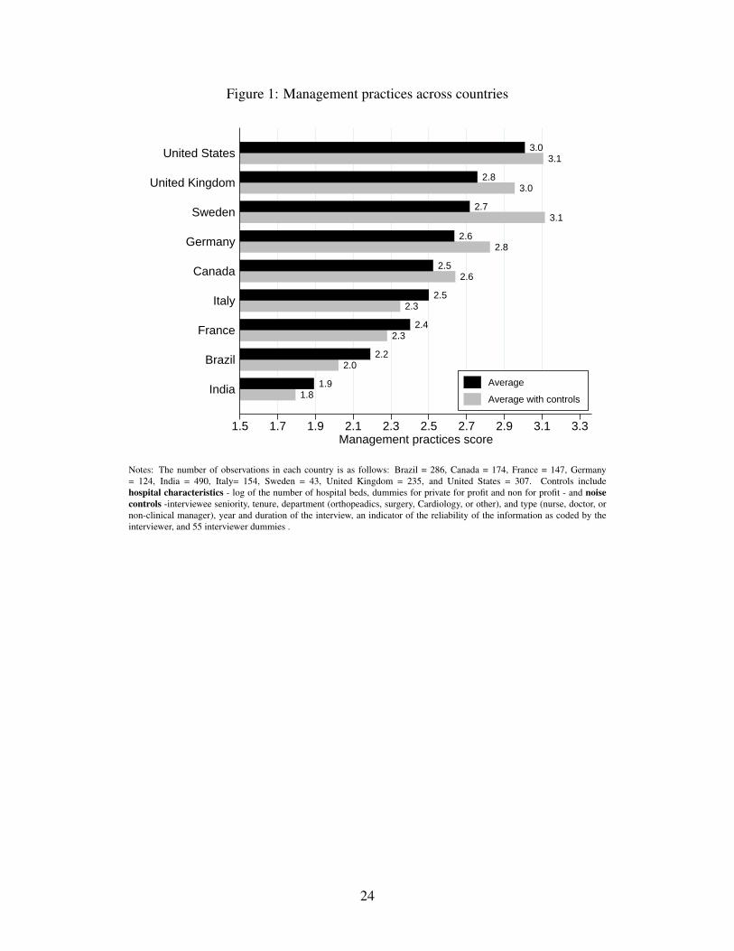
Figure 1: Management practices across countries

1.81.9

2.02.2

2.32.4

2.32.5

2.62.5

2.82.6

3.12.7

3.02.8

3.13.0

1.5 1.7 1.9 2.1 2.3 2.5 2.7 2.9 3.1 3.3Management practices score

India

Brazil

France

Italy

Canada

Germany

Sweden

United Kingdom

United States

Average

Average with controls

Notes: The number of observations in each country is as follows: Brazil = 286, Canada = 174, France = 147, Germany= 124, India = 490, Italy= 154, Sweden = 43, United Kingdom = 235, and United States = 307. Controls includehospital characteristics - log of the number of hospital beds, dummies for private for profit and non for profit - and noisecontrols -interviewee seniority, tenure, department (orthopeadics, surgery, Cardiology, or other), and type (nurse, doctor, ornon-clinical manager), year and duration of the interview, an indicator of the reliability of the information as coded by theinterviewer, and 55 interviewer dummies .

24

Figure 2: Management practices within countries

0.5

11.

52

0.5

11.

52

0.5

11.

52

1 2 3 4 5 1 2 3 4 5 1 2 3 4 5

1 US 2 UK 3 Sweden

4 Germany 5 Canada 6 Italy

7 France 8 Brazil 9 India

Management practices scoreGraphs by Country

Notes: The number of observations in each country is as follows: Brazil = 286, Canada = 174, France = 147, Germany =124, India = 490, Italy= 154, Sweden = 43, United Kingdom = 235, and United States = 307 .

25

Figure 3: Driving time difference between placebo and IV

Less than 2−hourdifference for 82%

of hospitals0

200

400

600

800

1000

# of

hos

pita

ls

−8 −7 −6 −5 −4 −3 −2 −1 0 1 2 3 4 5 6 7 8Driving time difference in hours between stand−alone HUM and joint M−B schools

Additional time tojoint M−B schools

Additional time tostand−alone HUM

Notes: 1,960 observations. Driving time difference capped at 8 hours.

26

Figure 4: Driving hours between hospital location and nearest school

0.5

1D

ensi

ty

0 1 2 3 4 5 6 7 8

Joint M−B school

0.5

1D

ensi

ty

0 1 2 3 4 5 6 7 8

B school, no M

0.5

1D

ensi

ty

0 1 2 3 4 5 6 7 8

M school, no B

0.5

1D

ensi

ty

0 1 2 3 4 5 6 7 8

No M−B school

Driving hours from hospital to nearest school (15min bins)

Notes: 1,960 observations. Joint M-B school offers both business and medical courses. B school, no M offers business butno medical courses. M school, no B offers medical but no business courses. No M-B school offers neither types of courses.Figure excludes hospitals with driving hours longer than 8 hours for presentation purposes (Number excluded: Top-left panel= 13, Top-right panel = 20, Bottom-left panel = 25, Bottom-right panel = 17) .

27

Figure 5: Share of hospital managers with a MBA-type course

01

23

4D

ensi

ty

0 .2 .4 .6 .8 1Share of managers with MBA−type courses (.10 bins)

Notes: 1,960 observations.

28

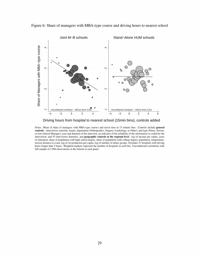
Figure 6: Share of managers with MBA-type course and driving hours to nearest school

Unconditional correlation: −.085 (p−level: 0.00).1.2

.3.4

−4 −2 0 2 4

Joint M−B schools

Unconditional correlation: −.028 (p−level: 0.21).1.2

.3.4

−4 −2 0 2 4 6

Stand−Alone HUM schoolsS

hare

of M

anag

ers

with

MB

A−

type

cou

rse

Driving hours from hospital to nearest school (15min bins), controls added

Notes: Mean of share of managers with MBA-type courses and travel time in 15 minute bins. Controls include generalcontrols - interviewee seniority, tenure, department (Orthopeadics, Surgery, Cardiology, or Other), and type (Nurse, Doctor,or non-clinical Manager), year and duration of the interview, an indicator of the reliability of the information as coded by theinterviewer, and 55 interviewer dummies, and geographic controls at the regional level - log of income per capita, yearsof education, share of population with high school degree, share of population with college degree, population, temperature,inverse distance to coast, log of oil production per capita, log of number of ethnic groups. Excludes 31 hospitals with drivinghours longer than 5 hours. Weighted markers represent the number of hospitals in each bin. Unconditional correlation withfull-sample of 1,960 observations at the bottom or each panel.

29

Table 1: Descriptive statistics

mean p50 sd min max count

Management Quality and PerformanceManagement 2.42 2.40 (0.65) 1.0 4.3 1960

Measures of Managerial SkillsShare of managers with MBA-type course 0.26 0.15 (0.29) 0.0 1.0 1960

Hospital CharacteristicsHospital beds 270.39 133.00 (365.40) 6.0 4000.0 1959# of competitors: 0 0.14 0.00 (0.35) 0.0 1.0 1955# of competitors: 1 to 5 0.61 1.00 (0.49) 0.0 1.0 1955# of competitors: more than 5 0.24 0.00 (0.43) 0.0 1.0 1955Dummy public 0.51 1.00 (0.50) 0.0 1.0 1960Dummy private for profit 0.30 0.00 (0.46) 0.0 1.0 1960Dummy private not for profit 0.19 0.00 (0.39) 0.0 1.0 1960

Distances to UniversitiesDriving hrs, nearest joint M-B schools 1.16 0.65 (1.84) 0.0 41.8 1960Driving distance (km) to nearest joint M-B schools 80.28 36.59 (135.39) 0.0 2842.4 1960Driving hrs, nearest B school, no M 1.46 0.86 (2.16) 0.0 44.4 1960Driving hrs, nearest M school, no B 1.47 0.89 (2.19) 0.0 44.4 1960Driving hrs, nearest school, no M or B 1.24 0.71 (2.06) 0.0 44.4 1960Driving hrs, nearest stand-alone humanities school 1.86 1.14 (2.42) 0.0 44.4 1960Driving hrs, nearest university in general 0.62 0.32 (1.47) 0.0 41.8 1960

30

Table 2: Hospital management is strongly correlated with health outcomes

(1) (2) (3) (4) (5)Dependent variable: Z(AMI) Z(AMI) Z(AMI) Z(AMI) Z(AMI)

Z(Mgmt) -0.188*** -0.223*** -0.203*** -0.204*** -0.203***(0.055) (0.067) (0.065) (0.071) (0.066)

Ln(Hospital beds) -0.041 -0.035 -0.093 -0.047(0.081) (0.084) (0.090) (0.082)

Dummy private for profit -0.129 -0.089 0.000 -0.027(0.209) (0.213) (0.272) (0.214)

Dummy private not for profit -0.340** -0.256* -0.224 -0.199(0.147) (0.140) (0.145) (0.143)

General controls Y Y Y YHospital characteristics Y Y Y YGeographic controls - Regional level Y YGeographic controls - Grid level Y

Observations 478 478 478 478 478No of clusters 397 397 397 397 397Fixed effects country country country region countryR-squared 0.02 0.17 0.20 0.34 0.19

Notes: * p < 0.1, ** p < 0.05, *** p < 0.01. All columns estimated by OLS. Standard errors clustered by hospital network inparentheses. Dependent variable Z(AMI) refers to a pooled measure of country-specific acute myocardial infarction mortalityrates (measures are standardized by country and year of survey). General controls include interviewee seniority, tenure, depart-ment (orthopeadics, surgery, Cardiology, or other), and type (nurse, doctor, or non-clinical manager), year and duration of theinterview, an indicator of the reliability of the information as coded by the interviewer, and 55 interviewer dummies. Hospitalcharacteristics include number of competitors constructed from the response to the survey question on number of competitors,and is coded as zero for none (16% of responses), 1 for “less than 5" (59% of responses), and 2 for “5 or more" (25% of re-sponses), and log of share of managers with a clinical degrees. Geographic controls - Regional level include log of incomeper capita, years of education, share of population with high school degree, share of population with college degree, population,temperature, inverse distance to coast, log of oil production per capita, log of number of ethnic groups. Geographic controls -Grid level include log of gross product per capita, 2005 USD at market exchange rates, log of gross product per capita, 2005USD at pp exchange rates, 2005, distance to major navigable river, distance to ice-free ocean, average precipitation, averagetemperature, and elevation. Whenever one of these two sets of geographic controls are added, hospital latitude, hospital longi-tude and population density within 100km radius is also added.

31

Table 3: Is management education driving hospital management?

Main Specification Robustness

(1) (2) (3) (4) (5) (6) (7) (8) (9)Dependent variable: Z(Mgmt) Z(Mgmt) Z(Mgmt) Z(Mgmt) Z(Mgmt) Z(Mgmt) Z(Mgmt) Z(Mgmt) Z(Mgmt)

Ln(% of managers with MBA-type course) 0.878*** 0.676*** 0.629*** 0.625*** 0.630*** 0.613*** 0.597*** 0.611***(0.086) (0.085) (0.085) (0.085) (0.084) (0.084) (0.084) (0.089)

Ln(Hospital beds) 0.180*** 0.198*** 0.193*** 0.192*** 0.186*** 0.183*** 0.177***(0.017) (0.017) (0.017) (0.017) (0.017) (0.017) (0.019)

Dummy private for profit 0.283*** 0.269*** 0.271*** 0.277*** 0.258*** 0.223***(0.056) (0.056) (0.056) (0.055) (0.056) (0.059)

Dummy private not for profit 0.263*** 0.256*** 0.260*** 0.233*** 0.237*** 0.174***(0.050) (0.050) (0.050) (0.052) (0.051) (0.055)

Number of Competitors 0.049* 0.052* 0.030 0.030 0.034(0.026) (0.026) (0.028) (0.028) (0.030)

Ln(% of managers with clinical degree) 0.189** 0.165* 0.169* 0.220**(0.092) (0.091) (0.091) (0.096)

Hospital latitude 0.002 -0.003 -0.010(0.005) (0.004) (0.014)

Hospital longitude 0.003 0.005*** -0.004(0.002) (0.002) (0.007)

Ln(Population density within 100km radius) 0.029* 0.032** 0.045**(0.018) (0.016) (0.023)

General controls Y Y Y Y Y Y Y Y YGeographic controls - Regional level YGeographic controls - Grid level Y Y

Observations 1960 1960 1960 1960 1960 1960 1960 1960 1960No of clusters 1869 1869 1869 1869 1869 1869 1869 1869 1869Fixed effects country country country country country country country country regionR-squared 0.55 0.58 0.60 0.61 0.61 0.62 0.63 0.63 0.67

Notes: * p < 0.1, ** p < 0.05, *** p < 0.01. All columns estimated by OLS. Standard errors clustered by hospital network in parentheses. Dependent variable Z(Mgmt) refers to the hospital’sz-score of management (the z-score of the average z-scores of the 20 management questions). General controls include interviewee seniority, tenure, department (orthopeadics, surgery, Cardiol-ogy, or other), and type (nurse, doctor, or non-clinical manager), year and duration of the interview, an indicator of the reliability of the information as coded by the interviewer, and 55 interviewerdummies. Geographic controls - Regional level include log of income per capita, years of education, share of population with high school degree, share of population with college degree, pop-ulation, temperature, inverse distance to coast, log of oil production per capita, log of number of ethnic groups. Geographic controls - Grid level include log of gross product per capita, 2005USD at market exchange rates, log of gross product per capita, 2005 USD at pp exchange rates, 2005, distance to major navigable river, distance to ice-free ocean, average precipitation, averagetemperature, and elevation. Whenever one of these two sets of geographic controls are added, hospital latitude, hospital longitude and population density within 100km radius is also added.

32

Table 4: Hospital health outcomes and distance to nearest schools

Main Specification Robustness Robustness - US

(1) (2) (3) (4) (5) (6) (7) (8) (9)Dependent variable: Z(AMI) Z(AMI) Z(AMI) Z(AMI) Z(AMI) Z(AMI) Z(AMI) Z(AMI) Z(AMI)

Ln(Driving hrs, nearest school)iiiiiiiiiiiiiiiiiiiiiiiiiii 0.226 0.035 0.038(0.208) (0.232) (0.234)

Ln(Driving hrs, nearest joint M-B schools) 0.393** 0.358** 0.344** 0.482** 0.210* 0.284*(0.160) (0.163) (0.154) (0.214) (0.111) (0.164)

Ln(Driving hrs, nearest school, no M, B, HUM) 0.072(0.159)

Ln(Driving hrs, nearest stand-alone HUM) -0.196(0.173)

Ln(Driving hrs, nearest B school, no M) 0.066 -0.026 -0.023 0.097(0.156) (0.215) (0.105) (0.184)

Ln(Driving hrs, nearest M school, no B) 0.075 -0.035 0.090 -0.018(0.162) (0.176) (0.093) (0.146)

Ln(Driving hrs, nearest school, no M or B) -0.180 -0.003 -0.065 -0.088(0.194) (0.219) (0.085) (0.159)

General controls Y Y Y Y Y Y YHospital characteristics Y Y Y Y Y Y Y YGeographic controls - Regional level Y Y Y Y Y YGeographic controls - Grid level Y

Observations 478 478 478 478 478 478 478 2034 1175No of clusters 397 397 397 397 397 397 397 1071 212Fixed effects country country country country country country region networkTest of Equality: Joint M-B = HUM 0.03Test of Equality: Joint M-B = B, no M 0.20 0.12 0.14 0.47Test of Equality: Joint M-B = M, no B 0.28 0.10 0.41 0.16Test of Joint Sig.: HUM, no M-B-HUM 0.47Test of Joint Sig.: B, M, No B-M 0.72 1.00 0.72 0.90R-squared 0.12 0.15 0.19 0.20 0.20 0.20 0.37 0.09 0.36

Notes: * p < 0.1, ** p < 0.05, *** p < 0.01. All columns estimated by OLS. Standard errors clustered by hospital network in parentheses. Dependent variable Z(AMI) refers to a pooledmeasure of country-specific acute myocardial infarction mortality rates (measures are standardized by country and year of survey). General controls include interviewee seniority, tenure,department (orthopeadics, surgery, cardiology, or other), and type (nurse, doctor, or non-clinical manager), year and duration of the interview, an indicator of the reliability of the infor-mation as coded by the interviewer, and 55 interviewer dummies. Hospital characteristics include log of the number of hospital beds, dummies for private for profit and non for profit,and number of competitors constructed from the response to the survey question on number of competitors, and is coded as zero for none (16% of responses), 1 for “less than 5" (59% ofresponses), and 2 for “5 or more" (25% of responses). Geographic controls - Regional level include log of income per capita, years of education, share of population with high schooldegree, share of population with college degree, population, temperature, inverse distance to coast, log of oil production per capita, log of number of ethnic groups. Geographic controls- Grid level include log of gross product per capita, 2005 USD at market exchange rates, log of gross product per capita, 2005 USD at pp exchange rates, 2005, distance to major naviga-ble river, distance to ice-free ocean, average precipitation, average temperature, and elevation. Whenever one of these two sets of geographic controls are added, hospital latitude, hospitallongitude and population density within 100km radius is also added.

33

Table 5: Hospital management and distance to nearest schools

Main Specification Robustness

(1) (2) (3) (4) (5) (6) (7)Dependent variable: Z(Mgmt) Z(Mgmt) Z(Mgmt) Z(Mgmt) Z(Mgmt) Z(Mgmt) Z(Mgmt)

Ln(Driving hrs, nearest school)iiiiiiiiiiiiiiiiiiiiiiiiiii -0.339*** -0.139*** -0.080(0.046) (0.045) (0.049)

Ln(Driving hrs, nearest joint M-B schools) -0.112** -0.107** -0.145*** -0.128**(0.044) (0.044) (0.038) (0.051)

Ln(Driving hrs, nearest school, no M, B, HUM) -0.054(0.042)

Ln(Driving hrs, nearest stand-alone HUM) -0.019(0.039)

Ln(Driving hrs, nearest B school, no M) 0.001 -0.002(0.041) (0.049)

Ln(Driving hrs, nearest M school, no B) -0.034 -0.010(0.043) (0.049)

Ln(Driving hrs, nearest school, no M or B) -0.053 -0.072(0.045) (0.052)

General controls Y Y Y Y Y Y YHospital characteristics Y Y Y Y Y YGeographic controls - Regional level Y Y Y YGeographic controls - Grid level Y

Observations 1960 1960 1960 1960 1960 1960 1960No of clusters 1869 1869 1869 1869 1869 1869 1869Fixed effects country country country country country country regionTest of Equality: Joint M-B = HUM 0.16Test of Equality: Joint M-B = B, no M 0.09 0.09Test of Equality: Joint M-B = M, no B 0.25 0.11Test of Joint Sig.: HUM, no M-B-HUM 0.28Test of Joint Sig.: B, M, No B-M 0.39 0.52R-squared 0.56 0.60 0.61 0.61 0.61 0.61 0.66

Notes: * p < 0.1, ** p < 0.05, *** p < 0.01. All columns estimated by OLS. Standard errors clustered by hospital network in parentheses. Dependent variable Z(Mgmt)refers to the hospital’s z-score of management (the z-score of the average z-scores of the 20 management questions).General controls include interviewee seniority, tenure,department (orthopeadics, surgery, cardiology, or other), and type (nurse, doctor, or non-clinical manager), year and duration of the interview, an indicator of the reliabilityof the information as coded by the interviewer, and 55 interviewer dummies. Hospital characteristics include log of the number of hospital beds, dummies for private forprofit and non for profit, and number of competitors constructed from the response to the survey question on number of competitors, and is coded as zero for none (16% ofresponses), 1 for “less than 5" (59% of responses), and 2 for “5 or more" (25% of responses). Geographic controls - Regional level include log of income per capita, yearsof education, share of population with high school degree, share of population with college degree, population, temperature, inverse distance to coast, log of oil productionper capita, log of number of ethnic groups. Geographic controls - Grid level include log of gross product per capita, 2005 USD at market exchange rates, log of gross prod-uct per capita, 2005 USD at pp exchange rates, 2005, distance to major navigable river, distance to ice-free ocean, average precipitation, average temperature, and elevation.Whenever one of these two sets of geographic controls are added, hospital latitude, hospital longitude and population density within 100km radius is also added.

34

Table 6: Share of MBA-type education and distance to schools

Main Specification Robustness

(1) (2) (3) (4) (5) (6) (7)Dependent variable: Ln(MBA) Ln(MBA) Ln(MBA) Ln(MBA) Ln(MBA) Ln(MBA) Ln(MBA)

Ln(Driving hrs, nearest school)iiiiiiiiiiiiiiiiiiiiiiiiiii -0.063*** -0.023 -0.004(0.016) (0.017) (0.016)

Ln(Driving hrs, nearest joint M-B schools) -0.028* -0.030** -0.023* -0.031*(0.014) (0.015) (0.013) (0.017)

Ln(Driving hrs, nearest school, no M, B, HUM) -0.002(0.013)

Ln(Driving hrs, nearest stand-alone HUM) 0.014(0.011)

Ln(Driving hrs, nearest B school, no M) 0.016 0.014(0.013) (0.016)

Ln(Driving hrs, nearest M school, no B) -0.019 -0.033**(0.012) (0.015)

Ln(Driving hrs, nearest school, no M or B) 0.016 0.008(0.013) (0.016)

General controls Y Y Y Y Y Y YHospital characteristics Y Y Y Y Y YGeographic controls - Regional level Y Y Y YGeographic controls - Grid level Y

Observations 1960 1960 1960 1960 1960 1960 1960No of clusters 1869 1869 1869 1869 1869 1869 1869Fixed effects country country country country country country regionTest of Equality: Joint M-B = HUM 0.04Test of Equality: Joint M-B = B, no M 0.03 0.07Test of Equality: Joint M-B = M, no B 0.62 0.91Test of Joint Sig.: HUM, no M-B-HUM 0.48Test of Joint Sig.: B, M, No B-M 0.19 0.17R-squared 0.23 0.27 0.28 0.29 0.29 0.28 0.37

Notes: * p < 0.1, ** p < 0.05, *** p < 0.01. All columns estimated by OLS. Standard errors clustered by hospital network in parentheses. Dependent variable Ln(MBA) refersto the log of the share of hospital managers with a MBA-type course. General controls include interviewee seniority, tenure, department (orthopeadics, surgery, cardiology, orother), and type (nurse, doctor, or non-clinical manager), year and duration of the interview, an indicator of the reliability of the information as coded by the interviewer, and 55interviewer dummies. Hospital characteristics include log of the number of hospital beds, dummies for private for profit and non for profit, and number of competitors con-structed from the response to the survey question on number of competitors, and is coded as zero for none (16% of responses), 1 for “less than 5" (59% of responses), and 2 for“5 or more" (25% of responses). Geographic controls - Regional level include log of income per capita, years of education, share of population with high school degree, shareof population with college degree, population, temperature, inverse distance to coast, log of oil production per capita, log of number of ethnic groups. Geographic controls -Grid level include log of gross product per capita, 2005 USD at market exchange rates, log of gross product per capita, 2005 USD at pp exchange rates, 2005, distance to majornavigable river, distance to ice-free ocean, average precipitation, average temperature, and elevation. Whenever one of these two sets of geographic controls are added, hospitallatitude, hospital longitude and population density within 100km radius is also added.

35

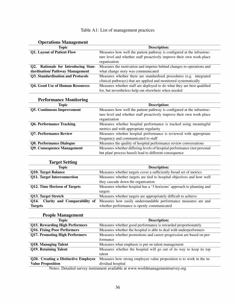
Table A1: List of management practices

Operations ManagementTopic Description:

Q1. Layout of Patient Flow Measures how well the patient pathway is configured at the infrastruc-ture level and whether staff proactively improve their own work-placeorganization

Q2. Rationale for Introducing Stan-dardisation/ Pathway Management

Measures the motivation and impetus behind changes to operations andwhat change story was communicated

Q3. Standardisation and Protocols Measures whether there are standardised procedures (e.g. integratedclinical pathways) that are applied and monitored systematically

Q4. Good Use of Human Resources Measures whether staff are deployed to do what they are best qualifiedfor, but nevertheless help out elsewhere when needed

Performance MonitoringTopic Description:

Q5. Continuous Improvement Measures how well the patient pathway is configured at the infrastruc-ture level and whether staff proactively improve their own work-placeorganization

Q6. Performance Tracking Measures whether hospital performance is tracked using meaningfulmetrics and with appropriate regularity

Q7. Performance Review Measures whether hospital performance is reviewed with appropriatefrequency and communicated to staff

Q8. Performance Dialogue Measures the quality of hospital performance review conversationsQ9. Consequence Management Measures whether differing levels of hospital performance (not personal

but plan/ process based) lead to different consequence

Target SettingTopic Description:

Q10. Target Balance Measures whether targets cover a sufficiently broad set of metricsQ11. Target Interconnection Measures whether targets are tied to hospital objectives and how well

they cascade down the organisationQ12. Time Horizon of Targets Measures whether hospital has a ‘3 horizons’ approach to planning and

targetsQ13. Target Stretch Measures whether targets are appropriately difficult to achieveQ14. Clarity and Comparability ofTargets

Measures how easily understandable performance measures are andwhether performance is openly communicated

People ManagementTopic Description:

Q15. Rewarding High Performers Measures whether good performance is rewarded proportionatelyQ16. Fixing Poor Performers Measures whether the hospital is able to deal with underperformersQ17. Promoting High Performers Measures whether promotions and career progression are based on per-

formanceQ18. Managing Talent Measures what emphasis is put on talent managementQ19. Retaining Talent Measures whether the hospital will go out of its way to keep its top

talentQ20. Creating a Distinctive EmployeeValue Proposition

Measures how strong employee value proposition is to work in the in-dividual hospital

Notes: Detailed survey instrument available at www.worldmanagementsurvey.org

36

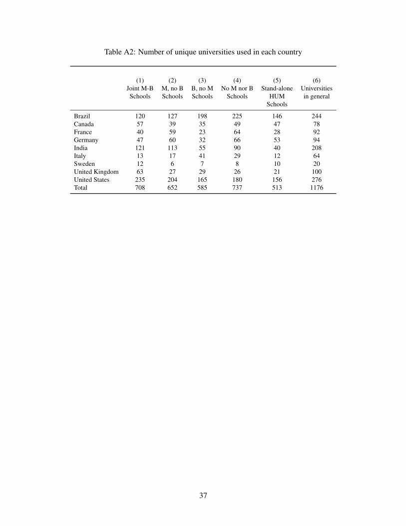
Table A2: Number of unique universities used in each country

(1)Joint M-BSchools

(2)M, no BSchools

(3)B, no MSchools

(4)No M nor B

Schools

(5)Stand-alone

HUMSchools

(6)Universitiesin general

Brazil 120 127 198 225 146 244Canada 57 39 35 49 47 78France 40 59 23 64 28 92Germany 47 60 32 66 53 94India 121 113 55 90 40 208Italy 13 17 41 29 12 64Sweden 12 6 7 8 10 20United Kingdom 63 27 29 26 21 100United States 235 204 165 180 156 276Total 708 652 585 737 513 1176

37

Table B1: Descriptive statistics

mean p50 sd min max count

Geographic CharacteristicsHospital latitude 30.39 40.79 (24.40) -32.0 68.4 1960Hospital longitude -8.48 -0.17 (63.16) -157.8 94.9 1960Population density within 100km radius 956.46 450.01 (1552.22) 0.2 12667.0 1960

Geographic Characteristics - Regional levelLn(Income per capita), regional 9.58 10.23 (1.13) 6.6 11.0 1960Years of education, regional 7.51 9.53 (10.55) -99.0 12.8 1960Share of pop with high school degree, regional 0.31 0.29 (0.20) 0.0 0.7 1960Share of pop with college degree, regional 0.18 0.16 (0.12) 0.0 0.5 1960Population, regional 16.14 16.03 (1.38) 10.3 19.0 1960Temperature, regional 14.89 12.38 (8.62) -12.2 28.3 1960Inverse distance to coast, regional 0.84 0.87 (0.14) 0.5 1.0 1960Ln(Oil production per capita), regional 0.09 0.00 (0.32) 0.0 4.2 1960Ln(# of ethnic groups), regional 1.10 1.10 (0.80) 0.0 3.0 1960

Geographic Characteristics - Grid levelGross prod. p.c, 2005 USD at market xrt, 2005 1.87 2.26 (1.52) 0.0 8.0 1957Gross prod. p.c, 2005 USD at ppp xrt, 2005 2.11 2.52 (1.50) 0.0 9.4 1957Distance to major navigable river (km) 879422.83 537973.40 (833327.76) 2821.7 4030517.0 1958Distance to ice-free ocean (km) 314802.57 154694.60 (371156.10) 312.1 1804279.0 1958Average precipitation 1101.90 1009.80 (422.77) 92.1 3495.1 1960Average temperature 15.05 12.73 (8.16) -9.2 28.9 1899Elevation 401.15 280.70 (437.14) 1.8 4731.4 1960

38

Table B2: Difference in means of location characteristics of the nearest joint M-B and stand-alone HUM schools to each hospital

HumanitiesSchoolsMean

Medicine & BusinessSchoolsMean

Diff inmeans T Stat

HumanitiesSchools

N

Medicine & BusinessSchools

NPopulation density within 100km radius 978.18 1105.39 127.20 1.34 534 725Latitude 25.55 30.06 4.51** 2.95 534 726Longitude -41.18 -30.27 10.91** 3.25 534 726Gross product per capita, 2005 USD at market exchange rates, 2005 2.21 2.21 -0.01 -0.08 532 724Gross product per capita, 2005 USD at market exchange rates, 1990 1.75 1.73 -0.02 -0.32 532 724Gross product per capita, 2005 USD at ppp exchange rates, 2005 2.46 2.40 -0.05 -0.61 532 724Gross product per capita, 2005 USD at ppp exchange rates, 1990 1.95 1.88 -0.07 -1.01 532 724Distance to major navigable river (km) 683143.98 756754.61 73610.62 1.92 534 724Distance to ice-free ocean (km) 383102.62 375410.09 -7692.54 -0.34 534 724Average precipitation 1198.19 1159.67 -38.52 -1.37 534 726Average temperature 13.52 12.36 -1.16 -1.40 534 726Elevation 473.68 437.22 -36.46 -1.21 534 726

39

Table B3: Is the performance-distance to university relationship being driven by university characteristics?

(1) (2) (3) (4) (5) (6) (7) (8)Dependent variable: Z(Mgmt) Z(Mgmt) Z(Mgmt) Z(Mgmt) Z(AMI) Z(AMI) Z(AMI) Z(AMI)Ln(D-hrs to joint M-B) -0.189*** -0.142*** -0.143*** -0.141*** 0.376** 0.334** 0.352** 0.342**

(0.035) (0.038) (0.038) (0.038) (0.157) (0.155) (0.155) (0.157)Log(Age of joint M-B) 0.048*** 0.042** 0.068 0.045

(0.017) (0.020) (0.085) (0.090)Global QS Rank Dummy for joint M-B 0.080* 0.033 0.160 0.131

(0.044) (0.051) (0.170) (0.180)General controls Y Y Y Y Y Y Y YHospital characteristics Y Y Y Y Y Y Y YGeographic controls - Regional level Y Y Y Y Y YObservations 1960 1960 1960 1960 478 478 478 478No of clusters 1869 1869 1869 1869 397 397 397 397R-squared 0.61 0.62 0.61 0.62 0.16 0.20 0.20 0.20

Notes: * p < 0.1, ** p < 0.05, *** p < 0.01. Standard errors clustered by hospital network in parentheses. Dependent variable Z(AMI) refers to a pooled measure ofcountry-specific acute myocardial infarction mortality rates (measures are standardized by country and year of survey. Dependent variable Z(Mgmt) refers to the hospital’sz-score of management (the z-score of the average z-scores of the 20 management questions). Age of joint M-B refers to the age of the university hosting both businessand medical schools in the year the hospital survey was conducted in each country. Global QS Rank Dummy equals to 1 if the university hosting both business andmedical schools was mentioned in the Quacquarelli Symonds World University Ranking in 2011. General controls are 55 interviewer dummies, the seniority and tenureof the manager who responded, the duration of the interview, and an indicator of the reliability of the information as coded by the interviewer, interviewee type (nurse,doctor or non clinical manager). Hospital characteristics refers to the log of the number of hospital beds, dummies for private for profit and non for profit, and numberof competitors (hospitals within a 30-minute drive). Geographic controls - Regional level include log of income per capita, years of education, share of population withhigh school degree, share of population with college degree, population, temperature, inverse distance to coast, log of oil production per capita, log of number of ethnicgroups. Hospital latitude, hospital longitude and population density within 100km radius is also added.

40

Table B4: The effects of MBA-trained managers on hospital management

2nd Stage in Top Panel, 1st Stage in Bottom Panel Placebo Robustness

(1) (2) (3) (4) (5) (6) (7) (8) (9) (10)Dependent variable: Z(AMI) Z(AMI) Z(AMI) Z(Mgmt) Z(Mgmt) Z(Mgmt) Z(Mgmt) Z(Mgmt) Z(Mgmt) Z(Mgmt)

Endogenous Variable: xxxxxxxxxxLn(% of managers with MBA-type course) -6.082*** -8.052* -13.833 5.050*** 5.090*** 6.346* 4.548** 3.775* -17.076 4.707**

(2.355) (4.759) (14.491) (1.020) (1.827) (3.600) (2.313) (1.984) (42.620) (1.957)

x(1)xxx x(1)xxx x(1)xxx x(1)xxx x(1)xxx x(1)xxx x(1)xxx x(1)xxx x(1)xxx x(1)xxx

Ln(Driving hrs, nearest joint M-B schools) -0.074*** -0.047* -0.025 -0.062*** -0.037*** -0.023* -0.029** -0.029** -0.035**(0.026) (0.028) (0.029) (0.012) (0.013) (0.013) (0.014) (0.014) (0.014)

Ln(Driving hrs, nearest stand-alone HUM) 0.013 0.013 0.004(0.011) (0.011) (0.011)

General controls Y Y Y Y Y Y Y Y Y YHospital characteristics Y Y Y Y Y Y Y YGeographic controls - Regional level Y Y Y Y YGeographic controls - Grid level Y

Observations 478 478 478 1960 1960 1960 1960 1960 1960 1960No of clusters 397 397 397 1869 1869 1869 1869 1869 1869 1869Fixed effects country country country country country country country country country regionFirst stage F-stat 7.90 2.82 0.72 24.90 8.42 3.14 4.39 2.33 0.17 6.09Placebo added as control instrument instrument

Notes: * p < 0.1, ** p < 0.05, *** p < 0.01. Standard errors clustered by hospital network in parentheses. Dependent variable Z(AMI) refers to a pooled measure of country-specific acute myocardial infarctionmortality rates (measures are standardized by country and year of survey). Dependent variable Z(Mgmt) refers to the hospital’s z-score of management (the z-score of the average z-scores of the 20 manage-ment questions). General controls are 55 interviewer dummies, the seniority and tenure of the manager who responded, the duration of the interview, and an indicator of the reliability of the information ascoded by the interviewer, interviewee type (nurse, doctor or non clinical manager). Geographic controls - Regional level include log of income per capita, years of education, share of population with highschool degree, share of population with college degree, population, temperature, inverse distance to coast, log of oil production per capita, log of number of ethnic groups. Geographic controls - Grid levelinclude log of gross product per capita, 2005 USD at market exchange rates, log of gross product per capita, 2005 USD at pp exchange rates, 2005, distance to major navigable river, distance to ice-free ocean,average precipitation, average temperature, and elevation. Whenever one of these two sets of geographic controls are added, hospital latitude, hospital longitude and population density within 100km radius isalso added. Other hospital drivers refers to the log of the number of hospital beds, dummies for private for profit and non for profit, and number of competitors (hospitals within a 30-minute drive).

41

Figure C1: Management practices across countries corrected for sampling response rates

1.9

2.2

2.4

2.5

2.5

2.6

2.7

2.8

3.0

1.5 1.7 1.9 2.1 2.3 2.5 2.7 2.9 3.1 3.3Management practices score

India

Brazil

France

Italy

Canada

Germany

Sweden

United Kingdom

United States

Notes: Average management score using sample weights constructed from the sample selection model in Column 1 of TableC4. The number of observations in each country is as follows: Brazil = 286, Canada = 174, France = 147, Germany = 124,India = 490, Italy= 154, Sweden = 43, United Kingdom = 235, and United States = 307. .

42

Table C1: Sampling frame sources

Country SourceBrazil National Registry of Health Facilities (Cadastro nacional de estabelecimentos de saúde).Canada Scott’s Directories (https://secure.scottsdirectories.com/)India The hospital sampling frame was constructed using several online sources.

• National Accreditation Board for Hospitals and Healthcare Providers (NABH)(http://www.nabh.co/main/hospitals/accredited.asp)

• Medicards.in (https://www.medicards.in/)

• Hospital Khoj (http://www.hospitalkhoj.com/general.htm)

• Cite HR (http://www.citehr.com/110771-all-india-hospitals-adresses-contact-nos.html)

• Hospitals in India (http://www.hospitalsinindia.org/)

The process used to construct the sampling frame was the following. First, we extracted hospitalnames, contact info and all other info available from these five sources. This yielded a total of 15,431entries. Second, we appended all lists and remove duplicate entries and ineligible hospitals using(i) exact match with hospital name and (ii) exact match with state and city, (iii) and dropping hos-pitals containing the following words in the name (acupuncture, advanced glaucoma, plastic, ENTresearch foundation, neuro, mental, maternity, maternity, cosmetic, child care, ENT, communicablediseases, bone and joint, day care, clinic of integrated medicine, diabetes, integrated organ transplant,reproductive, poly clinic, polyclinic, community hospital, surgical clinic, physiotheraphy, nursing, di-gestive, diabetic, leprosy, scanning, laproscopic, micro surgery). This yielded a total of 7,191 entries.This number is in agreement with statistics from the Ministry of Health reporting that 7,008 rural andurban hospitals exist in India (http://cbhidghs.nic.in/hia2005/8.01.htm)

Italy Ministry of Health (Ministero della Sanita’)France Federation Hospitaliere de FranceGermany Hospital directory acquired separately for each stateSweden Sveriges Kommuner och Landsting (Swedish Association of Local Authorities and Regions)US American Hospital AssociationUK National Health Service and Private Healthcare UK

43

Table C2: Sampling frame characteristics

BR CA DE FR IN IT SE UK US

Healthcare facilities (N) 5861 902 1559 3926 3831 1572 153 1219 6388Eligible hospitals in random sample (N) 591 527 553 292 1309 376 85 483 1526Public hospitals in eligible random sample (%) 39 99 86 61 28Beds in eligible random sample (median) 45 238 730 269 197 195 110

Notes: BR=Brazil, CA=Canada, DE=Germany, FR=France, IN=India, IT=Italy, SE=Sweden, UK=United Kingdom, US=United States. Sam-pling frame is the total number of hospitals eligible for the survey drawn from a random sample of hospitals from the universe of healthcarefacilities in the country. Public Hospitals refers to the percentage of hospitals which are funded and managed by government authorities. Thisinformation is not available for Germany, India, Italy, and Sweden. Beds is the median number of beds in the hospital. This information is notavailable for Brazil and India.

44

Table C3: Survey response rates

All Hospitals in Random SampleBR CA DE FR IN IT SE UK US

Interviews completed (%) 10.73 24.61 19.4 44.96 12.87 30.18 41.18 20.18 16.7Scheduling in progress (%) 9.58 45.4 44.48 31.7 14.36 34.36 21.32 30.6 57.78Interviews refused (%) 1.63 4.53 18.66 7.49 6.94 3.82 0 2.77 4.18Hospital not eligible (%) 78.06 25.46 17.46 15.85 65.83 31.64 37.5 46.45 21.34Sample, all (N) 2694 707 670 347 3831 550 136 902 1940

Eligible Hospitals in Random SampleBR CA DE FR IN IT SE UK US

Interviews completed (%) 48.9 33.02 23.51 53.42 37.66 44.15 65.88 37.68 21.23Scheduling in progress (%) 43.65 60.91 53.89 37.67 42.02 50.27 34.12 57.14 73.46Interviews refused (%) 7.45 6.07 22.6 8.9 20.32 5.59 0 5.18 5.31Sample, eligible (N) 591 527 553 292 1309 376 85 483 1526

Interviews completed (N) 289 174 130 156 493 166 56 182 324

Notes: BR=Brazil, CA=Canada, DE=Germany, FR=France, IN=India, IT=Italy, SE=Sweden, UK=United Kingdom, US=UnitedStates. 1) Interviews completed reports all the hospitals contacted for which a management interview was completed. 2) Schedul-ing in progress reports all the hospitals contacted with no interview run or manager refusing to be interviewed. 3) Interviewsrefused reports all hospitals contacted in which the manager refused to take part in the interview. 4) No longer eligible reportsall hospitals contacted which do not have an Orthopeadics or Cardiology Department, do not provide acute care, and do not haveovernight beds. It also included organizations out-of business or for which no phone number was found. Sample, all is the totalnumber of hospitals that were randomly selected and contacted from the complete sampling frame. Sample, eligible is the totalnumber of hospitals that were randomly selected, contacted from the complete sampling frame, and eligible for the survey.

45

Table C4: Selection analysis

(1) (2) (3) (4) (5) (6) (7) (8) (9) (10)Dependent variable: Interview Interview Interview Interview Interview Interview Interview Interview Interview InterviewLn(Income per capita) -0.022 0.410 0.318 -1.000 -1.715 -0.134 0.697 1.361 2.482 -0.813*

(0.090) (0.589) (0.611) (0.714) (1.406) (0.197) (0.627) (2.589) (1.600) (0.448)Population 0.035 0.066 -0.026 0.378*** 0.468 -0.171** 0.170 -2.187 -0.420 0.100*

(0.023) (0.073) (0.101) (0.144) (0.306) (0.084) (0.169) (5.514) (0.302) (0.055)Years of education -0.042 -0.006 0.062 0.121 0.363 0.080 0.039 5.131 -0.391 0.185

(0.048) (0.365) (0.407) (0.232) (0.347) (0.119) (1.559) (12.106) (0.424) (0.212)Share of pop with high school degree 0.239 -4.474 -3.390 -6.654 0.725 -7.106** -5.292 102.795 20.042* 0.031

(0.733) (9.182) (8.408) (4.444) (3.684) (2.855) (20.402) (124.026) (10.569) (1.640)Temperature -0.025*** -0.050 -0.003 -0.280 0.140 -0.047 -0.166 1.274 0.074 -0.025*

(0.008) (0.054) (0.041) (0.224) (0.108) (0.036) (0.104) (2.855) (0.178) (0.013)Inverse distance to coast -0.287* -0.396 1.315 0.849 -0.788 -1.152*** 13.259** 33.055 -1.692 0.029

(0.166) (0.908) (0.992) (1.513) (1.940) (0.422) (5.825) (22.453) (7.519) (0.318)Ln(# of ethnic groups) 0.012 0.008 0.106 -0.185 0.056 0.203* 0.007 2.130 0.296 0.033

(0.033) (0.107) (0.237) (0.166) (0.240) (0.120) (0.227) (4.048) (0.377) (0.062)Public Hospital 0.059 -0.654 0.186 0.054 0.789***

(0.114) (0.473) (0.220) (0.208) (0.082)Ln(# of Hospital Beds) 0.032 0.185*** 0.133* -0.019 0.080 -0.027

(0.052) (0.069) (0.070) (0.148) (0.068) (0.036)Observations 5742 591 526 553 292 1288 375 85 448 1434Sample ALL BR CA DE FR IN IT SW UK US

Notes: Estimate by Probit ML (marginal effects reported with robust standard errors in parentheses). The dependent variable Interview equals to 1 if hospital has been interviewed. BR=Brazil, CA=Canada,DE=Germany, FR=France, IN=India, IT=Italy, SE=Sweden, UK=United Kingdom, US=United States.

46