Health Savings Accounts, Plan Choice, and Health Care ...thew.web.unc.edu › files › 2013 › 09 › cardon.pdf · Cope, Roger Feldman, Carol Rapaport, Greg Scandlen, and from

Health Savings Accounts, Plan Choice, and Health Care

Utilization: Simulating the Effects of HSA Introduction in

Individual and Group Markets

James H. Cardon and Mark H. Showalter∗

Department of EconomicsBrigham Young University

Provo, UT 84602

November 14, 2011

Abstract

Many policies and proposals for health care reform involve complex insurance products. Forexample, the Modernization of Medicare Act (2003) included two innovations: 1) health savingsaccounts, but only if accompanied with high-deductible health insurance policies; and 2) Medi-care Part D coverage for prescription pharmaceutical products with an associated donut-hole.Future proposals are also likely to involve complex insurance products interacting in complicatedways with the tax system. Current methods for evaluating and predicting the implications ofsuch policies tends to treat insurance as a homogeneous, stand-alone product. It is likely thatprediction and evaluation can be substantially improved by accounting for important complex-ities.

Our research introduces a straightforward methodology to evaluate a variety of complexinsurance products. Specifically, we evaluate the implications of introducing Health SavingsAccounts coupled with high-deductible policies. A novel aspect of our approach is a calibrationof underlying preference parameters that allow us to simulate how consumers will value productslike high-deductible insurance and HSAs. We focus on three groups of particular policy interest:1) the currently uninsured who do not have access to group coverage, 2) the currently uninsuredwho have access to group coverage, but choose to be uninsured, 3) the currently insured in groupcoverage.

Preliminary draft: Please do not cite or quote without permission. Comments wel-come.

∗[email protected] and [email protected]. The authors gratefully acknowledge funding through from the RobertWood Johnson Foundation, through Academy Health. We appreciate very constructive comments from Lisa Clemens-Cope, Roger Feldman, Carol Rapaport, Greg Scandlen, and from participants at several conferences.

1 Introduction

In December of 2003, Congress passed the Modernization of Medicare Act which had as a primary

goal the addition of a prescription drug benefit to the Medicare program. But the legislation also

included a provision establishing health savings accounts (HSAs). Such accounts, when coupled

with a catastrophic high deductible health insurance policy (CHP), allow individuals to avoid

income and payroll taxes for qualified medical expenditures.

There have been a number of proposals to make HSAs and high-deductible health insurance

policies more affordable and attractive for the currently uninsured. For example, current proposals

include the following: 1) create an income tax deduction for the premium on a HSA-qualified

insurance policy, 2) create an income tax credit for HSA-qualified policies purchased outside the

employment-based group market, and 3) increase the allowable annual HSA contribution amount.

(State of the Union Address, January 31, 2006). The first two proposals would lower the cost of

insurance by extending the tax subsidy to those not purchasing insurance through employers; and

the third proposal was later signed into law.

While these proposals would likely lower the cost for HSA-qualified insurance, it is unclear

whether such proposals would actually decrease the number of uninsured. The tax-based policies

noted above are designed to eliminate the tax advantage currently available to employment-based

insurance. But employment-based insurance pools also economize on underwriting costs and help

to reduce the potential for adverse selection. Some analysts have argued that eliminating that

differential could adversely affect the employment-based market, causing firms to offer less attractive

policies to employees, resulting in lower take-up rates, or to drop coverage altogether (Moon et al.,

1996; Zabinski et al., 1999; Glied and Remler, 2005; Hoffman and Tolbert, 2006). The net effect

could be a weakening of these pools and an increase in the number of uninsured.

We will explore the impact of HSAs and the various tax proposals on the uninsured population,

including the effect of how adopting the tax deduction and credit policies for non-group insurance

would affect the employment-based group market. The foundation for our work is a recently devel-

oped simulation model based on utility-maximizing, representative agents (Cardon and Showalter,

2007). From our previous work, it is apparent that the form of the HSA contract, which depends

2

both on Federal regulations and employer choices, is important in determining whether the intro-

duction of HSAs undermines traditional insurance pools and differentially affects individuals based

on their health status. These issues will have important implications for determining the ultimate

impact of these proposals on the uninsured population.

The main advantage of our framework over previous simulation models is the ability to determine

consumers’ valuation of products for which little or no data exists-e.g. HSA contributions and high-

deductible insurance. This is accomplished through empirical calibration of parameters of consumer

preferences and the risks associated with uncertain medical expenditures. Given these estimates

we are better able to extrapolate to new products or policies.

To illustrate, consider the problem of assessing the impact of various HSA-linked proposals. It

is critical to have an estimate of consumers’ price elasticity of high-deductible policies. But there

are no generally accepted estimates of this elasticity due to the paucity of data on such policies.

Thus previous work has been forced to use elasticity estimates based on more traditional insurance;

but it is not clear these elasticities will be similar. Our methodology can adjust for such differences

because it is based on consumers’ underlying risk preferences.

We focus on three consumer groups of particular policy interest: 1) the currently uninsured who

do not have access to group coverage, 2) the currently uninsured who have access to group coverage,

but choose to be uninsured, 3) the currently insured in group coverage. For each group, we the

Medical Expenditure Panel Survey to assess representative values for demographic variables such

as income, age-specific health expenditures, and tax rates. For each group, we will then calibrate

our model to match the observable characteristics. Then we model a variety of policy changes and

assess the value of each change to consumers and their likelihood of changing from the status quo.

2 Related Simulation Approaches

Several methods have been used to estimate the impact of various health policy proposals. Glied

et al. (2002) provide a useful summary of the literature, which we follow in this section.

3

The Elasticity Approach

This is the most widely used method. It typically uses individual-level data, and in highly simplified

terms it can be described as having three steps: 1) estimate the impact of a policy change on

prices and income for individuals; 2) compute the change in demand, given the Step (1) change,

using elasticity estimates for insurance demand (or other behavioral responses); 3) aggregate across

individuals, with the appropriate weighting, to get national estimates.

The Discrete Choice Approach

This method uses a binary choice regression framework where the dependent variable is 1 if a person

has insurance, and 0 otherwise. Observable characteristics of the individual (age, income, gender,

employment status, etc) and a measure of insurance price are used as explanatory variables. This

methodology is similar to the elasticity approach, except that the elasticity estimate is embodied

in the regression parameters and the functional form of the specification. The procedure is roughly

as follows: 1) estimate the initial regression model which will specify the elasticity; 2) estimate the

impact of the policy change on prices and incomes for individuals; 3) estimate the change in the

probability of being insured using the data from Step (2) in the regression model of Step (1); 4)

aggregate across individuals to get national estimates.1

The Matrix Approach

This method uses grouping of individuals, applies group-specific take-up elasticities, and then

aggregates to get national estimates. The estimation steps include: 1) estimate the impact of the

policy change on average prices and incomes for each group; 2) compute the change in demand

for each group, using group-specific take-up elasticities; 3) aggregate across groups to get national

estimates.

1An interesting recent example of this approach is Feldman et al. (2005) which estimates a conditional logit modelof HSA takeup rates for employees in three large firms. They use the estimated model to simulate take-up rates inthe group and non-group markets. Health Reimbursement Arrangements (HRA) are used as a proxy for HSA choicesince HSAs were not an option for the employees in their data. Their simulations predict a 9 percent HSA take-uprate in the non-group market, but a very low take-up rate in the group market. A refundable tax-credit for HSAs ispredicted to double the HSA take-up rate while lowering the number of uninsured by 8 percent.

4

The Reservation Price Approach

This category uses indirect approaches to measure how utility changes with a given policy option.

The measured change in utility is then used to estimate behavioral responses. The two primary

methodologies are Zabinski et al. (1999) and Pauly and Herring (2002). Zabinski et al. (1999) use

a linear approximation to the change in utility, combined with income and price changes from a

given policy, to estimate whether a given individual will switch from a ‘standard’ insurance policy

to high-deductible insurance policy coupled with a medical savings account. Pauly and Herring

use a revealed preference argument to estimate how individuals would respond to a tax credit for

health insurance. Both of these indirect approaches are tailored to answer specific questions and

are not easily comparable to the first three general approaches.

Discussion

Remler et al. (2002) works through an example that shows that the first three methods give roughly

the same results if the underlying data and elasticity estimates are the same. One important feature

of the first three methods is that there is little scope for variation in insurance policies; to a first

approximation, an individual is treated as having insurance or not; there is generally no attempt

to account for variation in policy generosity and how consumers might value policy generosity.

Policy generosity is now at the center of the public debate. “Consumer directed health care”

focuses on the advantages of high-deductible policies over more traditional insurance. But the

framework and data used for currently available simulations are ill-suited for analyzing the impact

of such policies. The estimation shortcomings are even more acute when trying to account for

tax-subsidized financial accounts like health savings accounts, health reimbursement accounts, and

flexible spending accounts. These accounts are explicitly designed to work in conjunction with

insurance policies, but no data exist to allow researchers to understand how consumers view the

tradeoff between money in a tax-preferred account and the generosity of insurance.

Of the reservation price approaches, it is not clear how the Pauly/Herring approach could

handle policy innovations like health savings accounts, since the accounts, which are critical part of

overall coverage, are not part of traditional plans. The Zabinski et al. (1999) article is an explicit

5

attempt to measure the impact of HSAs, but the linear approximation approach embodies strong

assumptions about the value of HSAs accounts which seem to overstate their attractiveness..2

In the next section we outline a framework for evaluating the impact of recent policy innovations

such as health savings accounts and high-deductible policies. Our framework is explicitly based on

a utility maximization assumption and this allows us to explore how consumers would react to new

policy choices for which no data exists. The calibration of the model is done using observable data

so the utility parameters have an empirical foundation, but they allow much greater flexibility in

simulating policy options than is possible using current methods.

Our approach can be thought of as a combination of existing methodologies: We group con-

sumers into identifiable demographic categories based on observable characteristics (e.g. income,

age, employment status, etc) like the Matrix Approach. Each group is then modeled with a rep-

resentative agent who maximizes utility, similar to the Reservation Price Approach, except we use

a specific form of utility rather than an approximation to a change in utility. Within each demo-

graphic category, we then use a discrete choice framework to model the selection between being

insured and uninsured, accounting for utility gain or loss given a particular policy proposal.

3 Approach and Methodology

We begin by describing our utility-maximizing framework which will be applied to each demographic

group. Our model accounts for the uncertainty inherent in making choices about insurance, and is

dynamic: choices made in one period affect outcomes and utility in later periods.

Preferences

Utility in each period is derived from the consumption of a composite consumption good, C, and

Health. Health is determined by a random health state θ and “health services,” X. θ denotes

the random health status which determines the relative value of health expenditures. The utility

function is a modest generalization of a standard constant elasticity of substitution utility function.

2Their model predicts that even without the tax advantage, most consumers would choose to have a high-deductiblepolicy and a health savings account.

6

For a single period it is

U(C,H) =Cλ − 1

λ+ γ

(X − θ)λ − 1

λ,

where health H = X − θ. The structure on utility implies that optimal X will not be less than θ.

Note that the higher the value of θ, the higher will be marginal utility of health services in that

period. Were this a single-good model, 1− λ would also be the coefficient of relative risk aversion.

With two goods, however, the interpretation of 1 − λ is not precisely the same; but we will treat

it as an approximate measure of risk aversion when interpreting parameters. The parameter γ

accounts for the relative value of health compared to C.

Dynamic Optimization Problem

For tractability we assume there are two periods denoted by subscript t: in period 1, a consumer

knows her health status for that period, but health status in period 2, θ2, is unknown. An insurance

policy for period 2 consists of a coinsurance rate, α2, and a deductible, D2. In period 1, the consumer

chooses the following:

1. How much of good X to consume in period 1 (X1).

2. How much to withdraw from the HSA balance available in period 1 to pay for period 1 health

services (W1).

3. How much of period 2 income to allocate to the HSA in period 2 (Z2).

The HSA balance in period 2, M2, is determined by current contributions, Z2, and the return on

unused balance from the previous period according to the equation M2 = Z2 + (M1 −W1)(1 + r),

where r is the interest rate on HSA balances. The insurance policy will be associated with a

premium, P2, which includes a loading factor. Withdrawals, W2, are limited by the account balance

and by out-of-pocket costs, O(X2), defined below. Given these choices, the consumer in period 2

then chooses optimal health expenditures for period 2, X2, and the withdrawal W2 conditional on

the realized health state, θ2. C2 is determined by the budget constraint.

7

The objective function in period 1 problem is given by

EU =Cλ1 − 1

λ+ γ

(X1 − θ1)λ − 1

λ+ βE

[Cλ2 − 1

λ+ γ

(X2 − θ2)λ − 1

λ

](1)

with constraints

M2 = Z2 + (M1 −W1)(1 + r) (2)

C1 = (Y1 − P1 − T1)−O(X1) +W1 (3)

C2 = (Y2 − P2 − Z2 − T2)−O(X2) +W2 (4)

0 ≤ Wt ≤Mt (5)

Wt ≤ O(Xt) (6)

O(Xt) =

Xt: Xt < Dt

Dt + αt(Xt −Dt): Xt ≥ Dt

(7)

The values θ1, M1, Z1, P1, D1, α1 are known and given as of time 1. β is the one period discount

rate, and Tt is the total tax, which is a function of the marginal tax rate, τ3. Think about solving

this by backward induction. In period 2 there is no HSA contribution (Z3 = 0), because we consider

a 2-period model. Instead, after θ2 is revealed the consumer chooses X2 and the optimal withdrawal

W2 to maximize

Cλ2 − 1

λ+ γ

(X2 − θ2)λ − 1

λ

subject to (2) and (4)-(7). Moving back to the first period, prior to observing θ2, the consumer

chooses X1, W1, and Z2 subject to (2)-(7) and assuming optimal period 2 choices. Note that

maximizing (1) assumes optimal choices for health expenditures as well as optimal usage of the

HSA account for HSA policies in both periods. Traditional insurance (and no insurance) are

special cases of this model and that optimal behavior for these cases can be computed using the

same method. The optimized value of (1) is EU∗.

The use of tax-preferred accounts like HSAs is intuitively a multi-period problem. Indeed, some

observers have noted that HSAs could act as a useful retirement savings vehicle (Furman, 2006).

3We use an algorithm based on NBER’s TaxSim model to compute taxable income, total taxes, and marginal taxrates.

8

We approximate a long-horizon dynamic model by allowing conversion of unused HSA balances to

consumption after paying taxes plus a penalty, similar to the treatment of early IRA withdrawals.

The justification comes from the theoretical framework found in Cardon and Showalter (2007): in an

infinite horizon model, the expected marginal utility per dollar (accounting for taxes) will generally

be equalized across Xt, Ct, and the discounted value of Mt+1, because the marginal dollar could be

spent on any of those commodities. We therefore set the model to allow the representative agent

to consume as C2 any unused HSA balance in the second period at a rate of $1 of HSA convertible

to $ (1 − τ)(1 − Penalty) of C2. We simulate the model using Penalty = .055. We obtain this

by assuming that unused balances earn interest at interest rate r = .05 and are discounted using

β = 0.9, yielding (1−Penalty) = β(1+r) = 0.945. We label this “recovery” factor π. Setting π = 0

turns the account into a use-it-or-lose-it FSA4.

Deductibles will induce a kink into the usual linear budget constraint; a positive HSA balance

will create a second kink. These non-linearities create a serious challenge for optimization. Consider

the kinked budget sets for HSAs in two cases below. The case of a low HSA balance, whereM2 ≤ D2,

is shown in Figure 1. Slopes and the intercept depend on the Penalty, where (1 − Penalty) = π.

For the first segment between the vertical intercept and point a, the slope is −(1 − τ)π. At point

a the account is exhausted, and the slope changes to −1 up to point b. At point b the deductible

is reached and therefore the slope beyond b is −α2. For a very healthy person (low θ2), health care

consumption is zero, and C2 = Y2−P2−(1−π)Z2−T2. If the penalty is zero, or if π = 1, then there

is no penalty for the unused balance, and consumption would be as if Z2 = 0. For higher values

of θ2, indifference curves flatten and the optimal bundle will move down the budget constraint.

Optimal behavior with convex preferences implies a concentration at a, since many values of the

health state will imply consumption at the kink.

4The resulting consumption expenditures, C2, will be too high relative to what we would find with an infinitehorizon model (because the agent allocates to C2 what would have been allocated to M3), but expected utility, healthexpenditures, and HSA balances should be a better approximation than not allowing any conversion.

9

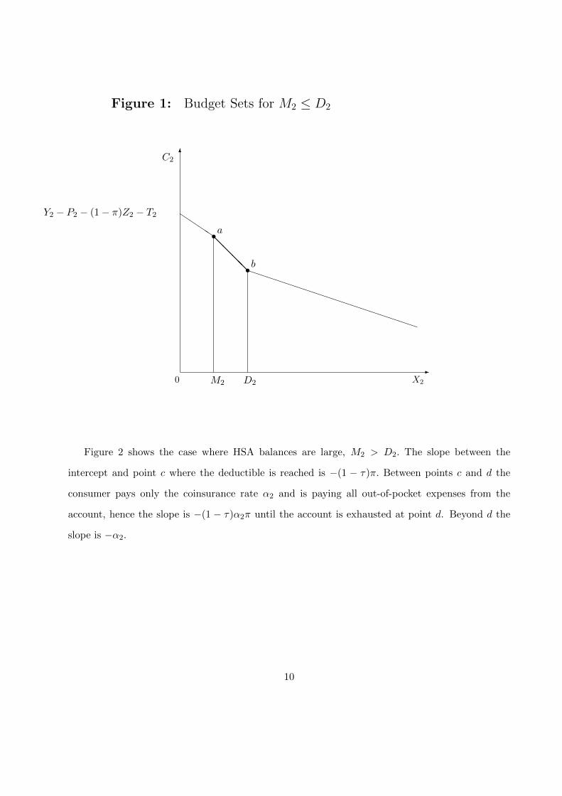
Figure 1: Budget Sets for M2 ≤ D2

0-

X2

6C2

@@@@

s

M2

s

D2

QQQQ

PPPPPPPPPPPPPPPPPP

a

b

Y2 − P2 − (1− π)Z2 − T2

Figure 2 shows the case where HSA balances are large, M2 > D2. The slope between the

intercept and point c where the deductible is reached is −(1 − τ)π. Between points c and d the

consumer pays only the coinsurance rate α2 and is paying all out-of-pocket expenses from the

account, hence the slope is −(1 − τ)α2π until the account is exhausted at point d. Beyond d the

slope is −α2.

10

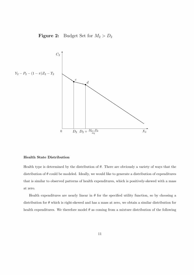
Figure 2: Budget Set for M2 > D2

0-

X2

6C2

XXXXs

D2

s

D2 + M2−D2α2

QQQQ

QQQ

QQQ

QQQ

QQQ

QQ

QQQQ

cd

Y2 − P2 − (1− π)Z2 − T2

Health State Distribution

Health type is determined by the distribution of θ. There are obviously a variety of ways that the

distribution of θ could be modeled. Ideally, we would like to generate a distribution of expenditures

that is similar to observed patterns of health expenditures, which is positively-skewed with a mass

at zero.

Health expenditures are nearly linear in θ for the specified utility function, so by choosing a

distribution for θ which is right-skewed and has a mass at zero, we obtain a similar distribution for

health expenditures. We therefore model θ as coming from a mixture distribution of the following

11

form:

θ = 0 with probability p

= Θ with probability 1− p

where Θ is lognormal random variable with mean µ and variance σ2.

Simulation Model

Due to the complexity of the problem, closed-form analytic solutions are not possible and we there-

fore proceed by developing a computer simulation model. One complication that arises in the

simulation of equation (1) is the specification of the insurance contract. We assume the insurance

contract arises out of a competitive process with proportional loading so that the premium for an

insurance contract with deductible D and coinsurance rate α is proportional to an actuarially fair

contract. But this premium will depend upon the expected expenditures in period 2, which are

endogenous. We overcome this difficulty by using the following algorithm to compute a rational

expectations equilibrium: 1) Choose a 2nd period insurance contract (α2, D2) and premium, P2.

2) Maximize expected utility subject to that particular insurance contract. 3) If expected insured

outlays exceed the premium, re-estimate with a higher premium; if the premium exceeds the ex-

pected outlays, re-estimate with a lower premium. Steps (1)-(3) are repeated until convergence of

the premium. For group insurance, the pooled premium depends on the expected expenditures of

consumers in the group, and the algorithm is modified accordingly to reflect group composition.

4 Setup and Calibration

Since the simulation model is programmed to determine optimal behavior for individual households,

we simulate behavior for households of different types broken down by age, family size, income,

and educational attainment. For each “cell” of similar households we use data on health care

utilization from the Medical Expenditure Panel Survey (MEPS) to obtain estimates of the unknown

parameters of the utility function (λ and γ) and the distribution of health states (µ and σ2)in the

12

following way. We observe the sample mean and variance of expenditures for each cell, and we have

estimates of the population price and income elasticities of health expenditures from the RAND

Health Insurance Experiment. We obtain method of moments estimators for the 4 parameters by

matching these sample moments with theoretical moments (which are functions of the parameters

to be estimated) implied by the period utility function U(C,H) above.5 Using this method we can

match the mean and variance of expenditures (measured in $1,000s) as well as price and income

sensitivity in a simple, flexible way. To estimate p = Pr(θ = 0) we simply use the frequency of zero

expenditures for each cell. We will use estimates available from the literature on time preference

to set β = 0.9.6

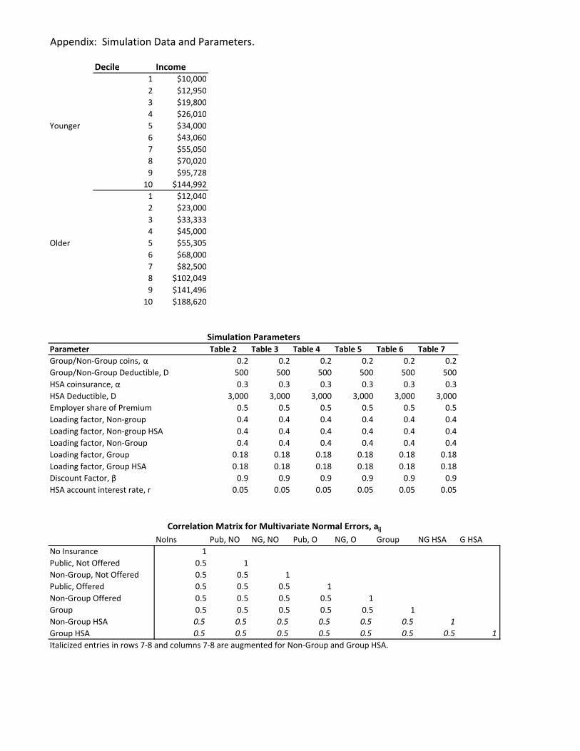
In the current version of the model we use 300 cells: 10 income deciles, an age indicator for

whether the head of household is Younger (age≤ 40) or Older (age> 40), indicators for 5 family

size groups, and indicators for 3 levels of education (No Degree, High School Degree, and College

Degree). Table 1 shows theoretical and sample moments and the resulting estimates. We compute

different values of the risk and preference parameters for 10 age/income cells.

Simulation

Each cell is characterized by a set of parameters for utility and risk, and a set of insurance options.

For those not offered group insurance, the choice set is

{No insurance, Public Insurance, Non-group Private,}

while for those offered it is

{No insurance, Public Insurance, Non-group Private, Group Insurance}

The characteristics (price, cost-sharing, etc.) of these options will vary across cells according to

employer choices (such as the decision to offer insurance and how much of the premium to pay)

and public insurance eligibility.

5The demand function for health expenditures is X∗ = Y+KθK+α

This implies that the E(X∗) = Y+KE(θ)K+α

and

V ar(X∗) = ( KK+α

)2V ar(θ). Price and income elasticities are the standard definitions evaluated at the mean of θ.See Table 1. Elasticities could, in principle, vary across cells, but in this version they were set at εp = −0.15 andεY = 0.2 for all cells. With more data it would be feasible to estimate distinct (µ, σ2, λ, γ) for each cell.

6Typical estimates range from 0.80 to 0.95.

13

Taking estimated (calibrated) parameters as given, we run the simulation model for cell i and

option j, which yields a simulated utility, δ∗ij . This represents the component of expected utility

that can be explained by the simulation model. We repeat this for cells i = 1, ..., I and for the range

of options j = 0, ..., Ji in the choice set for cell i, including option 0, which is no insurance of any

type. To account for unobserved factors, including behavioral factors and other heterogeneity, we

include option-specific random taste shocks, aij . If this were a conventional discrete choice model,

the variance of the shocks would need to be normalized and the coefficients of the model scaled to

be in the same units. Here the scaling of the δ∗ij from the simulation model are in the (arbitrary)

units of the utility function. We assume that expected utility V ∗ij is a function of δ∗ij , option- and

cell-specific dummy variables ∆ij and the random taste shocks:

V ∗ij = EU∗ij + aij = βjδ∗ij + ξ′ij∆ij + aij , for i = 1, ..., N and j = 0, ..., Ji. (8)

The scale parameter βj , which we allow to vary across options, adjusts the scale of δ∗ij so that it is

in the same units as the (normalized) taste shocks. We then estimate the unknown parameters of

(8) using a multinomial discrete choice model. Inclusion of a rich set of dummy variables (including

those for income deciles, family size, and education) enables us to account for cell and option specific

factors that the simulation model has not captured. We are then able to match observed market

shares.

Finally, having simulated the market shares Pij as the probability that consumer i chooses

option j from data, we add the HSA option to the choice set, simulate V ∗i,HSA for each cell, and

recompute the probabilities. Comparison of these probabilities with the initial set allows us to

predict the effects of HSA introduction.

Distributional Assumptions

If we assume the option-specific shocks aij are independent (over both i and j) and identically

distributed Type 1 extreme-value random variables then model (2) is the conditional logit. The

14

probability that individual i chooses option j is :

Pij =eV∗ij

Ji∑k=0

eV∗ik

. (9)

The advantage of the conditional logit model is the simple, closed form of the probabilities (9) and

the straightforward way to add new options to the choice set. If cell i initially has Ji options but a

new option Ji + 1 with utility V ∗i,Ji+1 is added, then the new probabilities are easily computed as

P′ij =

eV∗ij

Ji+1∑k=0

eV∗ik

. (10)

However, as is well known, the relative probability–or relative market shares–of any two options is

independent of the addition of the new option, since the ratio reduces to

P ′ijP ′ik

=eV∗ij

eV∗ik

for any j and k. If options j and k are in the original choice set, independence of irrelevant alterna-

tives (IIA) implies that their relative probabilities will remain unchanged regardless of the nature

of the new option. This is a consequence of assuming that the taste shocks aij are independent.

Multinomial Probit Alternative

A more flexible alternative is the multinomial probit allowing for correlation of errors across options.

This will reduce the influence of distributional assumptions on substitution patterns. Given the set

of δ∗ij , we estimate (8) assuming ai = (ai0, ai2, ..., a1,Ji) ∼ N(0,Σ) on observed market shares to get

estimates of the scale parameters (βj), dummy variable coefficients, the baseline market shares Pij ,

and the covariance matrix Σ. We then augment the covariance matrix to form Σ̂A using plausible

values for correlations between the original options and the new HSA options. We then use Monte

Carlo simulation to estimate the new probabilities, P ′ij .

The simplest way to do this is as follows. For each cell i take a draw εit from the multivariate

15

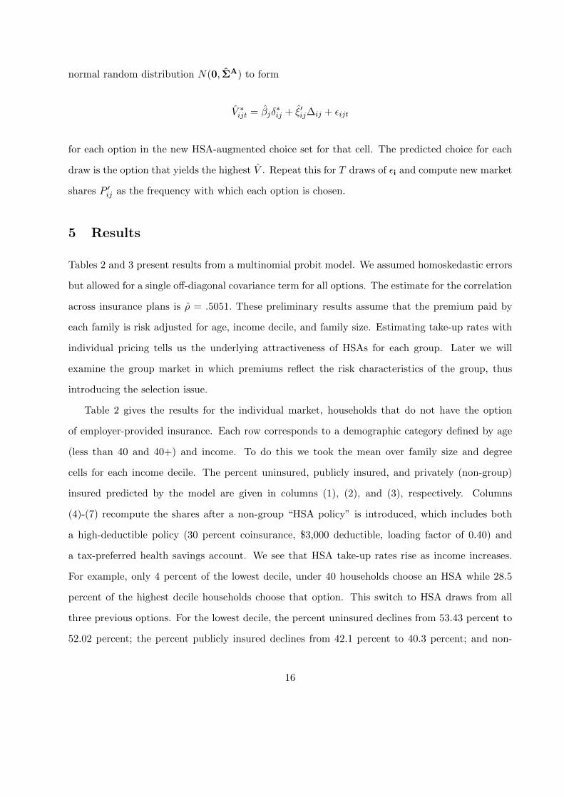
normal random distribution N(0, Σ̂A) to form

V̂ ∗ijt = β̂jδ∗ij + ξ̂′ij∆ij + εijt

for each option in the new HSA-augmented choice set for that cell. The predicted choice for each

draw is the option that yields the highest V̂ . Repeat this for T draws of εi and compute new market

shares P ′ij as the frequency with which each option is chosen.

5 Results

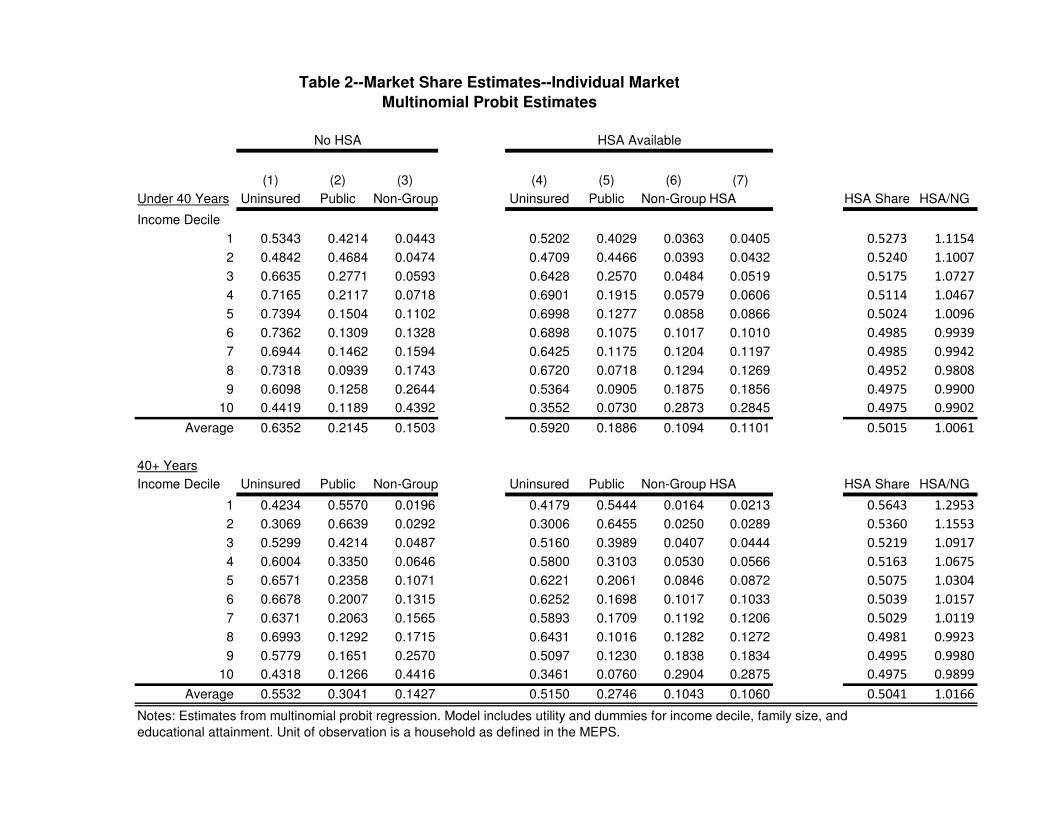
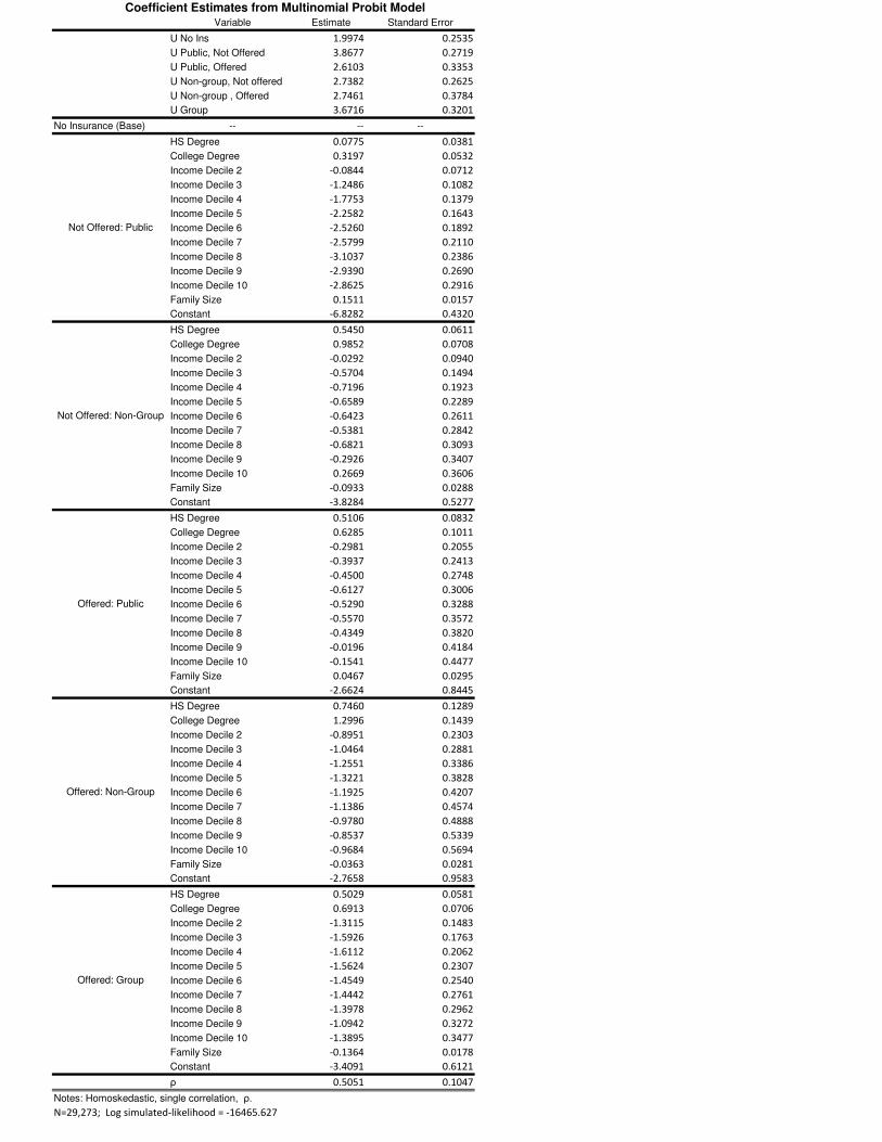
Tables 2 and 3 present results from a multinomial probit model. We assumed homoskedastic errors

but allowed for a single off-diagonal covariance term for all options. The estimate for the correlation

across insurance plans is ρ̂ = .5051. These preliminary results assume that the premium paid by

each family is risk adjusted for age, income decile, and family size. Estimating take-up rates with

individual pricing tells us the underlying attractiveness of HSAs for each group. Later we will

examine the group market in which premiums reflect the risk characteristics of the group, thus

introducing the selection issue.

Table 2 gives the results for the individual market, households that do not have the option

of employer-provided insurance. Each row corresponds to a demographic category defined by age

(less than 40 and 40+) and income. To do this we took the mean over family size and degree

cells for each income decile. The percent uninsured, publicly insured, and privately (non-group)

insured predicted by the model are given in columns (1), (2), and (3), respectively. Columns

(4)-(7) recompute the shares after a non-group “HSA policy” is introduced, which includes both

a high-deductible policy (30 percent coinsurance, $3,000 deductible, loading factor of 0.40) and

a tax-preferred health savings account. We see that HSA take-up rates rise as income increases.

For example, only 4 percent of the lowest decile, under 40 households choose an HSA while 28.5

percent of the highest decile households choose that option. This switch to HSA draws from all

three previous options. For the lowest decile, the percent uninsured declines from 53.43 percent to

52.02 percent; the percent publicly insured declines from 42.1 percent to 40.3 percent; and non-

16

group insurance falls from 4.4 percent to 3.6 percent. Older households display similar patterns:

HSA take-up rises with income, drawing from all three original categories. Note also that for

lower income households HSAs have higher predicted take-up rates than the non-group plan. The

difference shrinks as incomes rise, and higher income deciles prefer the traditional plans. This is

shown the the last two columns. HSA Share is the the fraction of privately-insured choosing HSA;

HSA/NG is the ratio of HSA to non-group take-up rates. Only 7.68 percent of younger households

in decile 1 choose private insurance, but 52.73 percent of those choose HSA. This measure of HSA

attractiveness starts high and falls for both younger and older households. This means that while

the HSA take-up rates increase with income, the relative attractiveness of HSAs decreases with

income. It seems that HSAs are an inferior good in the individual market.

Table 3 gives the results for households who have the option of employer-provided insurance.

These estimates are a preliminary exercise, since the each premium is adjusted for observable

individual characteristics. The differences between these estimates and those in Table 2 are the

employer subsidy (assumed to be 50 percent), the implicit tax subsidy, and the lower loading

factor for the group market (18 percent instead of 40 percent). These households are modeled as

having four options: no insurance, public insurance, non-group insurance, and group insurance.

The simulation here adds a group HSA policy.7 HSA take-up rates rise with income, but the

attractiveness of HSAs relative to all private insurance declines with income, as HSA share falls for

both younger and older households. For higher deciles Group and HSA take-up rates are roughly

equal. Note that for Table 2 HSA Share starts high and falls, while for Table 3 HSA Share starts

low and rises; both end up at just under 50 percent for both cases.

These preliminary results are suggestive that HSAs are attractive even to lower income house-

holds and have the potential to decrease the ranks of the uninsured. For example, in the individual

market, HSA take-up rates for lowest five deciles are higher than non-group plans when both are

available. Overall, the percentage uninsured declines from 59.4 percent to 55.5 for households not

eligible for group insurance, and from 10.76 percent to 6.72 percent for those who are.

7We also experimented with adding a non-group HSA, but the percentages were so small that it made littledifference.

17

6 Group Market Policy Simulations and Extensions

The above simulation results assume that insurance options are individually priced. This gives us

a way to measure the attractiveness of such insurance. For the group market, however, insurance

premia reflect the risk characteristics of the group, and there is potential for adverse selection. In

particular, there is potential for HSA introduction to initiate a death spiral which drives out the

traditional group plan. We now change the simulation strategy to reflect this.

We construct a firm’s insurance pool by taking a sampling of households with different char-

acteristics. We will continue to include no insurance and public insurance as options. We use the

above framework as follows. Consumers evaluate each option by computing its expected utility

Vij = β̂jδ∗i1 + ξ̂′ij∆ij + aij

where the hats denote that we are using estimates from the multinomial probit model above. The

difference between the results above that those in this section is that here the δ∗’s depend on

household characteristics and on the pooled premium. By integrating as above over draws of the

error terms, we can compute initial market shares.

Next we add an HSA to the pool and let consumers move to their preferred plans. As premiums

adjust, consumers update their optimal choices, and premiums adjust further. When this process

converges we observe the new market shares and compare Group and HSA premiums in the new

equilibrium with the original Group premium. We repeat the process for a variety of parameters,

such as the composition of the firms (older, richer, etc.) and employer generosity. Note that the

dummy variable coefficients ξ̂ij estimated above are assumed to be equal for the Group policy and

the newly-added HSA, so the difference in market shares is driven by the differences in δ∗ alone.

6.1 First Stage Insurance Choice Results

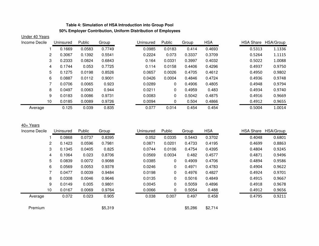
The first set of results are found in Table 4. For these estimates we assume an employer is subsidizing

insurance at a proportional rate of 50 percent. It is well known that proportional employer subsidy

is better than a fixed dollar subsidy in avoiding potential adverse selection. Note also that since

18

we aggregate medical expenditures the plans are identical in what medical conditions are covered8.

For Table 4 we use the actual frequency counts from the MEPS data to weight each cell.

With a pooled premium, HSA take-up rates are higher than those in Table 3 for Younger

households and slightly higher for Older households. Compared with Table 3, Group take-up rates

are lower for younger households and higher for older households. HSA take-up rates rise with

income, but HSA Share falls from 53.13 percent to 49.12 percent for the younger households and

rises from 40.48 percent to the same 49.12 percent for the older households. Note that for a group

plan all households pay the same premium. This means that younger, lower income households

are paying a premium based on the average risk in the pool. Both types of insurance are likely

to be unfairly priced for these households, and they are therefore more likely to prefer the lower-

coverage HSA. As income and risk rise, the higher-coverage plan becomes more attractive. For

older households it seems that the rise in relative shares is due in part to more aggressive use of

the savings account as income and marginal tax rates rise. In fact, as we show in the next section,

the lowest deciles have little incentive to contribute funds to the account. This would explain the

jump in HSA take-ip after the first decile for older households. This same pattern holds for Tables

5 and 6 as well.

The original premium for the Group policy is $5,319. After HSA introduction, the Group

premium falls to $5,286 and the HSA premium is $2,714. That is, the average makeup of the

Group pool is not very different after HSAs are introduced, but what selection there is slightly

advantageous. HSAs are a low cost alternative that do not offer first dollar coverage except through

the account, which is self-funded. After the deductible is reached, however, the plans are similar.

HSAs offer higher risk up to that point in exchange for a lower premium. Variation in take-up rates

across cells reflects differences in the way households evaluate this tradeoff. Expected utilities are

similar for many groups, so market shares are as well.

The makeup of the insurance pool should affect the potential for adverse selection. Table 5

shows results from a firm with a higher-risk pool made up of Older workers and only the lowest 4

income deciles of the Younger. As expected with a higher percentage of higher-risk, higher income

8See (Cutler and Zeckhauser, 1998)

19

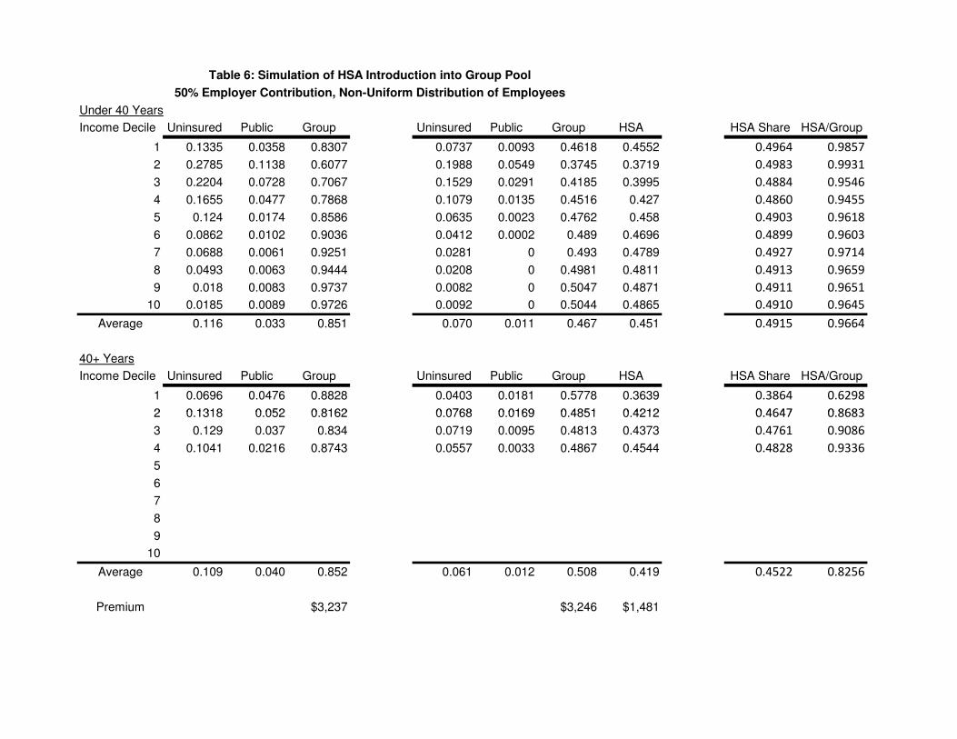
households, the pooled Group premium rises to $6,087 without the HSA option. When HSAs are

offered, the HSA premium is $3,193, but the Group premium falls to $6,014.

Table 6 constructs a lower-risk firm made up of Younger workers and the lowest four income

deciles of the Older workers. The Group premium rises from $3,237 to $3,246 when HSAs are

offered, indicating a small amount of adverse selection. The HSA premium is $1,481. Lower

premiums compared with the uniform pool in Table 4 leads to overall higher insurance take-up,

and HSAs lose much of their advantage.

Overall, we see that lower income households find HSAs attractive and that there appears to

be no meaningful adverse selection, at least for the plan characteristics chosen for the estimation.

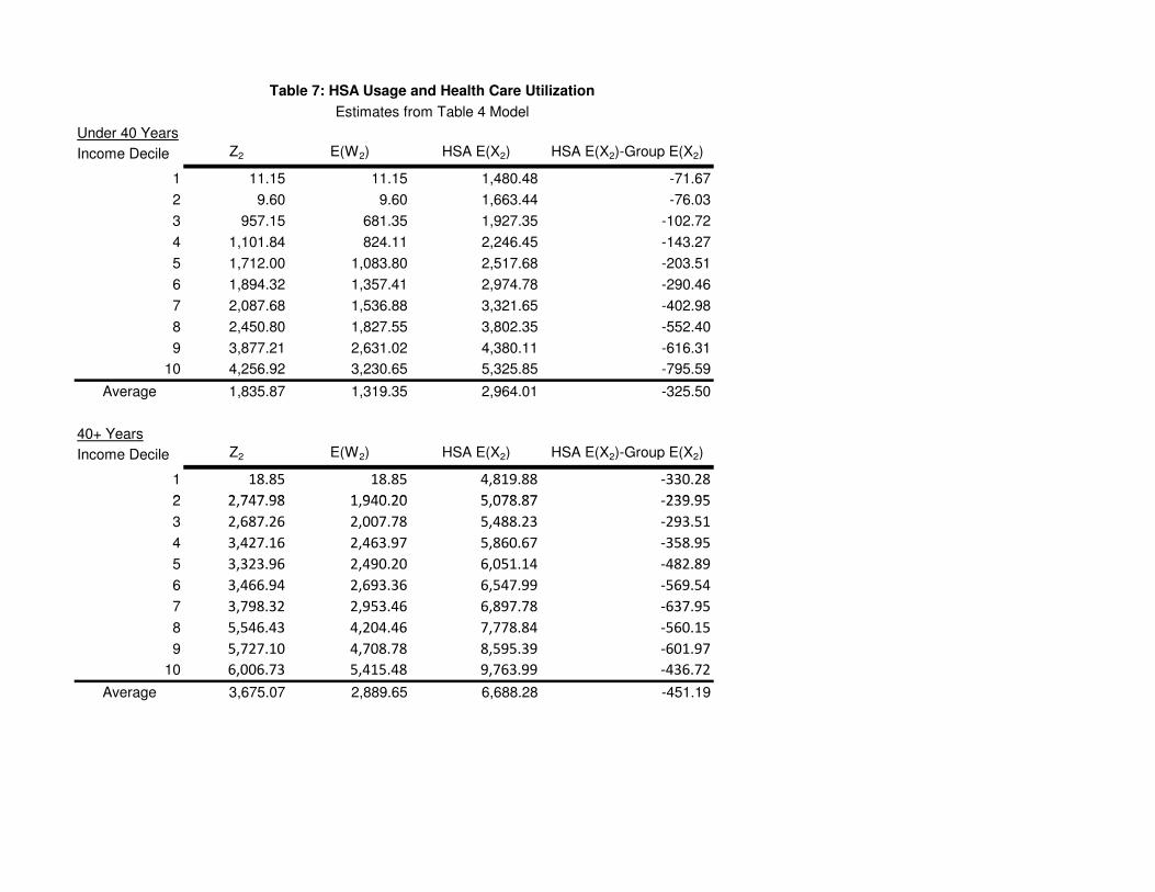
6.2 Second Stage HSA Balances and Health Care Utilization

Next we turn attention to HSA account contributions, balances, and withdrawals as well as health

care utilization. Looking closely at HSA contributions, Z2, we see that while lower income house-

holds do find HSAs attractive, they do not find it optimal to make use of the accounts. This is

because for low income households the tax code does not provide any incentive to do so. Their

marginal tax rates are low and their total taxes are, for the lowest deciles, negative when we account

for the EITC. Further, we find that EITC phase-out rules lead to increasing marginal tax rates

as we increase income, at least for the lowest deciles. For younger households, Z2 increases from

essentially zero to $4, 257. The different risk parameters of the older households lead to a similar

if more abrupt pattern of increase, topping out at $6, 007.

We also present expectations of period 2 withdrawals W2 and total health care expenditures

for HSA, X2, in the second and third columns. Recall that unused balances are not rolled over as

in an infinite horizon model but are converted to current consumption after paying taxes and a

penalty. This means that E(W2) is often substantially lower than Z2. We interpret the difference

as the expected rollover in an infinite horizon model. The ratio of average withdrawals to average

contributions is 71.8 percent for the younger and 78.6 percent for older households. We conjecture

that E(W2) is close to what would be the steady state contribution level in a longer-horizon model.

Expected expenditures rise with income, age, and family size. Households contribute more

20

than half of their expected expenditures to their accounts. The ratio of average contributions to

average expected expenditures is 61.9 percent for the younger and 54.9 percent for older households.

The last column gives an expected difference of expenditures with a HSA and with a traditional

group plan. Expected utilization is lower with HSAs for all deciles and for both younger and older

households. Note that the increase is monotonic for the younger group but is not for the older group.

For the younger group, the decline represents 9.90 percent reduction relative to group expenditures

for the younger group and a 6.3 percent reduction for older households. The theoretical effect

of HSA enrollment on total health care expenditures is not obvious. A higher deductible will

reduce utilization, but this is softened somewhat by the tax-preferred account. The overall effect

will depend on the level of account balances actually chosen. If a household mistakenly chose an

excessively-high contribution level, the incentive to spend today on health care increases either

because (as in our model) unused balances can only be consumed after paying taxes and a penalty

or (in general) usage of unused balances must wait until a future period. The simulation, which

computes optimal HSA contributions and balances, provides support for the claim that HSAs will

significantly reduce the level of health care utilization.

6.3 Discussion

In the preceding results we find evidence of both adverse and favorable selection into HSA plans,

though in no case was the effect large. Why do we fail to find the death spiral in these preliminary

results? There are a number of possible explanations, some of which are related to modeling

assumptions. HSAs are modeled as being similar to the traditional Group coverage alternative. We

believe the HSA characteristics chosen are fairly typical. However, it may be that selection would

be more pronounced for firms with high-coverage traditional plans. Another concern is that HSAs

might also be setup with more exclusions for specific medical conditions. Since we have not tried

to disaggregate medical expenditures into categories, we cannot address this in the current version

of the paper. On the other hand, such exclusions are often a feature of traditional plans and have

little to do with HSAs in particular.

Second, we have used a proportional employer subsidy instead of a fixed-dollar subsidy. Since

21

HSA premia are so much lower, adverse selection in firms with fixed dollar subsidies would likely

be more severe. For example, using the numbers in Table 4 we observe that the Group premium is

$4,600 and and the HSA premium is $2,200. Proportional 50 percent subsidies cut these to $2,300

and $1,100, so that the Group plan is about twice the price of the HSA. If, instead, the employer

offered a $1,500 fixed subsidy, the employee costs (ignoring taxes) would be $3,100 and $700, and

adverse selection would likely increase.

As seen above, the specifics of the pool composition do affect the equilibrium. Even if a typical

firm experiences limited adverse selection that does not imply all firms are safe. In addition, the

variation in risk from age, income decile, family size cells may not be sufficient to tease out significant

selection effects. We can address this by adding additional demographics. Alternatively, we could

introduce true asymmetric information by assuming that each cell is composed of a mixture of

healthy and sick households. With group premiums, all heterogeneity is treated as asymmetric

information, even though the household risk types are in fact observable. The mixture distribution

would allow us to vary the amount variation in risk types within cells.

Finally, the conventional wisdom about HSAs and FSAs is sometimes wrong. For example,

Cardon (2009) shows that Flexible Spending Accounts can strengthen insurance pools. It is tempt-

ing to notice a high deductible and a lower premium and conclude that HSAs are simply a low

coverage alternative. However, both the theoretical model and simulation results suggest that the

reality is more complex. The ability to self-insure through the saving account reduces the effect of

the deductible. Risk types matter, of course, but it is also true that income and tax effects seem to

be important. The complexities of HSA plans (dynamics, corner solutions, kinks, etc.) make these

plans more difficult to evaluate.

7 Conclusion

This work is very preliminary, but we believe it is promising. The approach we have taken highlights

subtle economic effects that can easily be missed in alternative models. Our results suggest that

properly-designed HSAs are potentially a useful option for many households, and carry the potential

to reduce (modestly) the ranks of the uninsured. Perhaps surprisingly, we find little evidence

22

of adverse selection. More work is needed to identify potential cases where selection may be

problematic. Plan design is important, as usual.

Although our primary purpose is to estimate the effect of various proposals on the number

of uninsured, our framework is sufficiently flexible to handle a variety of simulation tasks. For

example, our framework estimates health expenditures jointly with insurance choice. It would also

be possible to estimate standard economic welfare effects, quantifying the gains and losses to various

policies measured in terms of consumer surplus. Additional micro-level simulations concerning firm

choice of optimal policies for various demographic compositions of employees are also feasible within

this framework.

23

References

Cardon, James H. and Igal Hendel (1999). “Asymmetric Information in Health Markets: Evidencefrom the National Medical Expenditure Survey. RAND Journal of Economics. Vol. 32, No.3, Autumn, 2001, pp.408-427.

Cardon, James H. and Mark H. Showalter (2001). An Examination of Flexible Spending Accounts.Journal Of Health Economics. Vol. 20, No. 6 (2001), pp. 935-954.

Cardon, James H. and Mark H. Showalter (2003). “Flexible Spending Accounts as Insurance.”The Journal of Risk and Insurance. Vol.70, No. 1, 43-51.

Cardon, James H. and Mark H. Showalter (2007). “Insurance Choice and Tax-Preferred HealthSavings Accounts Journal of Health Economics.” Journal of Health Economics. Vol. 26, No.2 (2007),pp. 373-399.

Cardon, James H. (2009). “Flexible Spending Accounts and Adverse Selection.” Forthcoming inThe Journal of Risk and Insurance.

Cutler, David M., and Richard J. Zeckhauser. (1998) “Adverse Selection in Health Insurance”.Forum for Health Economics & Policy: Frontiers in Health Policy Research. Vol. 1, Article2. 1998.

Furman, Jason. (2006) ”Expansion inf HSA Tax Breaks is Larger–and more Problematic–ThanPreviouly Understood.” Center on Budget and Policy Priorities. Revised February 7, 2006.URL: http://www.globalaging.org/health/us/2006/BudgetHSA.pdf.

Glied, Sherry A. and Dahlia K. Remler (2005).“The Effect of Health Savings Accounts on HealthInsurance Coverage.” Commonwealth Fund Publication #811, 2005.

Glied, Sherry, Dahlia K. Remler and Joshua Graff Zivin (2002). “Inside the Sausage Factory:Improving Estimates of the Effects of Health Insurance Expansion Proposals.” The MilbankQuarterly. Vol. 80, No. 4, 2002, pp.603-636.

Economic Report of the President, Chapter 10, “Health Care and Insurance.” Council of EconomicAdvisers, February 2004.

Feldman, R., Parente, S.T., Abraham, J., Christianson, J., Taylor, R. (2005). “Health SavingsAccounts: Early Estimates of National Take-up from the 2003 Medicare Modernization Actand Future Policy Proposals. November 18, 2005. Health Affairs.

Hamilton, Barton H. and James Marton (2006). “Employee Choice of Flexible Spending AccountParticipation and Health Plan,” University of Kentucky working paper, February.

Nevo, Aviv (2000). “A Practitioners Guide to Estimation of Random Coefficients Logit Modelsof Demand, Journal of Economics & Management Strategy, 9(4), 513-548, 2000.

Moon, M. L. Nichols, and S. Wall (1996). “Medical Savings Accounts: A Policy Analysis.” UrbanInstitute: http://www.urban.org/pubs/hinsure/msa.htm.

24

Pauly, M. and B. Herring (2000). “An efficient employer strategy for dealing with adverse selectionin multiple-plan offerings: an MSA example.” Journal of Health Economics, Vol. 19 (4) pp.513-528.

Pauly, M. and B. Herring (2002). Cutting Taxes For Insuring: Options and Effects of Tax Creditsfor Health Insurance. Washington DC.: AEI Press.

Petrin, Amil (2002). “Quantifying the Benefits of New Products: The Case of the Minivan.”Journal of Political Economy. Vol. 110, No. 4, 2002, pp. 705-729.

Remler, Dahlia K., Joshua Graff Zivin, and Sherry A. Glied. (2002) “Modeling Health InsuranceExpansions: Effects of Alternative Approaches.” NBER Working paper 9130.http://www.nber.org/papers/w1930.

Zabinski, D., T. Selden, J. Moeller, and J. Banthin (1999), “Medical Savings Accounts: Microsim-ulation Results From a Model With Adverse Selection,” Journal of Health Economics, Vol.18, pp. 195-218.

25

Table 1: Method of Moments Estimation

Theoretical Moments

E(X∗) = Y+KE(θ)K+α

V ar(X∗) = ( KK+α)2V ar(θ)

εp =α((αE(θ)−I) dK

dα−(I+KE(θ)))

(K+α)(I+KE(θ))

εI = IK+KE(θ)

Sample Moments

RAND HIE Estimates

ε̂Rp -0.15

ε̂RI 0.2

Age< 40Family Size X S p̂

1 2.6478 7.7729 0.37982 4.4176 8.7298 0.05353 5.3495 8.3094 0.03174 6.5910 12.1283 0.0312> 4 6.8319 10.9560 0.0241

Age ≥ 40Family Size X S p̂

1 7.8235 14.9325 0.15782 10.4103 15.9165 0.03583 9.1954 15.9990 0.03464 8.5338 12.5475 0.0216> 4 8.6598 16.5576 0.0248

EstimatesAge < 40

Family Size µ̂ σ̂ λ̂ γ̂

1 2.1530 7.7931 0.0005 -0.33862 3.6007 8.7676 0.0010 -0.34223 4.3657 8.3531 0.0013 -0.34424 5.3878 12.2070 0.0017 -0.3468> 4 5.5866 11.0298 0.0018 -0.3473

Age ≥ 401 6.3849 15.0113 0.0013 -0.34422 8.5163 16.0287 0.0019 -0.34803 7.5140 16.0985 0.0016 -0.34624 6.9691 12.6199 0.0015 -0.3452> 4 7.0729 16.6545 0.0015 -0.3454

Notes: X∗ = Y+KθK+α , where Y is income and K = ( γα)1−λ.

θ ∼ Lognormal(µ, σ2)ε̂Rp and ε̂RI are estimates from the RAND Health Insurance Experiment.

U(C,H) = Cλ−1λ + γ (X−θ)λ−1

λ

26

(1) (2) (3) (4) (5) (6) (7)

Under 40 Years Uninsured Public Non-Group Uninsured Public Non-Group HSA HSA Share HSA/NG

Income Decile

1 0.5343 0.4214 0.0443 0.5202 0.4029 0.0363 0.0405 0.5273 1.1154

2 0.4842 0.4684 0.0474 0.4709 0.4466 0.0393 0.0432 0.5240 1.1007

3 0.6635 0.2771 0.0593 0.6428 0.2570 0.0484 0.0519 0.5175 1.0727

4 0.7165 0.2117 0.0718 0.6901 0.1915 0.0579 0.0606 0.5114 1.0467

5 0.7394 0.1504 0.1102 0.6998 0.1277 0.0858 0.0866 0.5024 1.0096

6 0.7362 0.1309 0.1328 0.6898 0.1075 0.1017 0.1010 0.4985 0.9939

7 0.6944 0.1462 0.1594 0.6425 0.1175 0.1204 0.1197 0.4985 0.9942

8 0.7318 0.0939 0.1743 0.6720 0.0718 0.1294 0.1269 0.4952 0.9808

9 0.6098 0.1258 0.2644 0.5364 0.0905 0.1875 0.1856 0.4975 0.9900

10 0.4419 0.1189 0.4392 0.3552 0.0730 0.2873 0.2845 0.4975 0.9902

Average 0.6352 0.2145 0.1503 0.5920 0.1886 0.1094 0.1101 0.5015 1.0061

Table 2--Market Share Estimates--Individual Market

Multinomial Probit Estimates

No HSA HSA Available

40+ Years

Income Decile Uninsured Public Non-Group Uninsured Public Non-Group HSA HSA Share HSA/NG

1 0.4234 0.5570 0.0196 0.4179 0.5444 0.0164 0.0213 0.5643 1.2953

2 0.3069 0.6639 0.0292 0.3006 0.6455 0.0250 0.0289 0.5360 1.1553

3 0.5299 0.4214 0.0487 0.5160 0.3989 0.0407 0.0444 0.5219 1.0917

4 0.6004 0.3350 0.0646 0.5800 0.3103 0.0530 0.0566 0.5163 1.0675

5 0.6571 0.2358 0.1071 0.6221 0.2061 0.0846 0.0872 0.5075 1.0304

6 0.6678 0.2007 0.1315 0.6252 0.1698 0.1017 0.1033 0.5039 1.0157

7 0.6371 0.2063 0.1565 0.5893 0.1709 0.1192 0.1206 0.5029 1.0119

8 0.6993 0.1292 0.1715 0.6431 0.1016 0.1282 0.1272 0.4981 0.9923

9 0.5779 0.1651 0.2570 0.5097 0.1230 0.1838 0.1834 0.4995 0.9980

10 0.4318 0.1266 0.4416 0.3461 0.0760 0.2904 0.2875 0.4975 0.9899

Average 0.5532 0.3041 0.1427 0.5150 0.2746 0.1043 0.1060 0.5041 1.0166

Notes: Estimates from multinomial probit regression. Model includes utility and dummies for income decile, family size, and

educational attainment. Unit of observation is a household as defined in the MEPS.

(1) (2) (3) (4) (5) (6) (7) (8) (9)

Under 40 Years Uninsured Public Non-Group Group Uninsured Public Non-Group Group Group HSA HSA Share HSA/Group

Income Decile

1 0.1190 0.0667 0.0294 0.7849 0.0785 0.0337 0.0114 0.5045 0.3719 0.4190 0.7373

2 0.2800 0.1408 0.0324 0.5468 0.2186 0.0878 0.0157 0.3727 0.3051 0.4501 0.8187

3 0.2406 0.0936 0.0325 0.6333 0.1736 0.0476 0.0139 0.4033 0.3616 0.4728 0.8967

4 0.1982 0.0637 0.0180 0.7201 0.1321 0.0270 0.0064 0.4331 0.4014 0.4810 0.9268

5 0.1525 0.0291 0.0116 0.8068 0.0924 0.0093 0.0035 0.4609 0.4339 0.4849 0.9415

6 0.1093 0.0211 0.0107 0.8588 0.0605 0.0059 0.0029 0.4768 0.4538 0.4876 0.9517

7 0.0863 0.0145 0.0099 0.8893 0.0448 0.0035 0.0024 0.4839 0.4654 0.4903 0.9619

8 0.0641 0.0133 0.0113 0.9113 0.0312 0.0030 0.0027 0.4893 0.4738 0.4919 0.9683

9 0.0305 0.0140 0.0053 0.9503 0.0127 0.0029 0.0010 0.4987 0.4847 0.4929 0.972010 0.0315 0.0147 0.0070 0.9469 0.0133 0.0031 0.0014 0.4974 0.4848 0.4936 0.9746

Average 0.1312 0.0472 0.0168 0.8048 0.0858 0.0224 0.0061 0.4620 0.4236 0.4783 0.9169

40+ Years

No HSA HSA Available

Table 3—Market Share Estimates—Group Market

Multinomial Probit Estimates

40+ Years Income Decile Uninsured Public Non-Group Group Uninsured Public Non-Group Group Group HSA HSA Share HSA/Group

1 0.0851 0.0708 0.0172 0.8269 0.0537 0.0332 0.0068 0.5481 0.3582 0.3952 0.6534

2 0.1588 0.0765 0.0217 0.7430 0.1049 0.0334 0.0082 0.4618 0.3916 0.4589 0.8481

3 0.1529 0.0576 0.0225 0.7670 0.0968 0.0221 0.0079 0.4567 0.4165 0.4770 0.9121

4 0.1233 0.0368 0.0114 0.8285 0.0717 0.0117 0.0034 0.4719 0.4412 0.4832 0.9349

5 0.0995 0.0175 0.0076 0.8754 0.0534 0.0044 0.0020 0.4828 0.4575 0.4866 0.9476

6 0.0721 0.0132 0.0071 0.9075 0.0359 0.0029 0.0016 0.4898 0.4698 0.4896 0.9592

7 0.0597 0.0095 0.0069 0.9239 0.0284 0.0019 0.0015 0.4933 0.4749 0.4905 0.9628

8 0.0467 0.0095 0.0083 0.9356 0.0211 0.0019 0.0017 0.4956 0.4797 0.4919 0.9681

9 0.0215 0.0101 0.0040 0.9644 0.0083 0.0019 0.0006 0.5013 0.4879 0.4932 0.973310 0.0271 0.0114 0.0052 0.9563 0.0109 0.0022 0.0009 0.4990 0.4869 0.4939 0.9758

Average 0.0847 0.0313 0.0112 0.8728 0.0485 0.0116 0.0035 0.4900 0.4464 0.4767 0.9110

Notes: Estimates from multinomial probit regression. Model includes utility and dummies for income decile, family size, and educational

attainment. Unit of observation is a household as defined in the MEPS.

Under 40 Years

Income Decile Uninsured Public Group Uninsured Public Group HSA HSA Share HSA/Group

1 0.1669 0.0583 0.7749 0.0985 0.0183 0.414 0.4693 0.5313 1.1336

2 0.3067 0.1392 0.5541 0.2224 0.073 0.3337 0.3709 0.5264 1.1115

3 0.2333 0.0824 0.6843 0.164 0.0331 0.3997 0.4032 0.5022 1.0088

4 0.1744 0.053 0.7725 0.114 0.0158 0.4406 0.4296 0.4937 0.9750

5 0.1275 0.0198 0.8526 0.0657 0.0026 0.4705 0.4612 0.4950 0.9802

6 0.0887 0.0112 0.9001 0.0426 0.0004 0.4846 0.4724 0.4936 0.9748

7 0.0706 0.0065 0.923 0.0289 0 0.4906 0.4805 0.4948 0.9794

8 0.0497 0.0063 0.944 0.0211 0 0.4959 0.483 0.4934 0.9740

9 0.0183 0.0086 0.9731 0.0083 0 0.5042 0.4875 0.4916 0.9669

10 0.0185 0.0089 0.9726 0.0094 0 0.504 0.4866 0.4912 0.9655

Average 0.125 0.039 0.835 0.077 0.014 0.454 0.454 0.5004 1.0014

40+ Years


1 0.0868 0.0737 0.8395 0.052 0.0335 0.5443 0.3702 0.4048 0.6801

2 0.1423 0.0596 0.7981 0.0871 0.0201 0.4733 0.4195 0.4699 0.8863

3 0.1345 0.0405 0.825 0.0744 0.0106 0.4754 0.4395 0.4804 0.9245

4 0.1064 0.023 0.8706 0.0569 0.0034 0.482 0.4577 0.4871 0.9496

5 0.0839 0.0072 0.9088 0.0385 0 0.4909 0.4706 0.4894 0.9586

6 0.0569 0.0053 0.9378 0.0246 0 0.4971 0.4783 0.4904 0.9622

7 0.0477 0.0039 0.9484 0.0198 0 0.4976 0.4827 0.4924 0.9701

8 0.0308 0.0046 0.9646 0.0135 0 0.5016 0.4849 0.4915 0.9667

9 0.0149 0.005 0.9801 0.0045 0 0.5059 0.4896 0.4918 0.9678

10 0.0167 0.0069 0.9764 0.0066 0 0.5054 0.488 0.4912 0.9656

Average 0.072 0.023 0.905 0.038 0.007 0.497 0.458 0.4795 0.9211

Premium $5,319 $5,286 $2,714

Table 4: Simulation of HSA Introduction into Group Pool

50% Employer Contribution, Uniform Distribution of Employees

Under 40 Years


1 0.1799 0.0701 0.75 0.1057 0.0242 0.3926 0.4775 0.5488 1.2163

2 0.3191 0.1521 0.5287 0.2315 0.0782 0.3195 0.3708 0.5372 1.1606

3 0.2386 0.0869 0.6746 0.1675 0.0356 0.3919 0.4049 0.5082 1.0332

4 0.1783 0.0557 0.766 0.1166 0.0166 0.4367 0.4301 0.4962 0.9849

5

6

7

8

9

10

Average 0.229 0.091 0.680 0.155 0.039 0.385 0.421 0.5221 1.0926

40+ Years


1 0.0944 0.0886 0.817 0.0565 0.0422 0.5281 0.3732 0.4141 0.7067

2 0.1454 0.0634 0.7912 0.0892 0.0224 0.4669 0.4215 0.4744 0.9028

3 0.1357 0.0425 0.8218 0.0769 0.0111 0.4728 0.4392 0.4816 0.9289

4 0.1077 0.0237 0.8687 0.0571 0.0034 0.4809 0.4585 0.4881 0.9534

5 0.0844 0.0075 0.9081 0.0386 0 0.4898 0.4716 0.4905 0.9628

6 0.0575 0.0053 0.9371 0.0249 0 0.4962 0.479 0.4912 0.9653

7 0.0481 0.004 0.9479 0.0199 0 0.4971 0.4829 0.4928 0.9714

8 0.0309 0.0046 0.9645 0.0135 0 0.5014 0.4851 0.4917 0.9675

9 0.0149 0.005 0.9801 0.0045 0 0.5059 0.4896 0.4918 0.9678

10 0.0167 0.0069 0.9764 0.0066 0 0.5054 0.488 0.4912 0.9656

Average 0.074 0.025 0.901 0.039 0.008 0.494 0.459 0.4813 0.9280

Premium $6,087 $6,014 $3,193


50% Employer Contribution, Non-Uniform Distribution of Employees

Under 40 Years


1 0.1335 0.0358 0.8307 0.0737 0.0093 0.4618 0.4552 0.4964 0.9857

2 0.2785 0.1138 0.6077 0.1988 0.0549 0.3745 0.3719 0.4983 0.9931

3 0.2204 0.0728 0.7067 0.1529 0.0291 0.4185 0.3995 0.4884 0.9546

4 0.1655 0.0477 0.7868 0.1079 0.0135 0.4516 0.427 0.4860 0.9455

5 0.124 0.0174 0.8586 0.0635 0.0023 0.4762 0.458 0.4903 0.9618

6 0.0862 0.0102 0.9036 0.0412 0.0002 0.489 0.4696 0.4899 0.9603

7 0.0688 0.0061 0.9251 0.0281 0 0.493 0.4789 0.4927 0.9714

8 0.0493 0.0063 0.9444 0.0208 0 0.4981 0.4811 0.4913 0.9659

9 0.018 0.0083 0.9737 0.0082 0 0.5047 0.4871 0.4911 0.9651

10 0.0185 0.0089 0.9726 0.0092 0 0.5044 0.4865 0.4910 0.9645

Average 0.116 0.033 0.851 0.070 0.011 0.467 0.451 0.4915 0.9664

40+ Years


1 0.0696 0.0476 0.8828 0.0403 0.0181 0.5778 0.3639 0.3864 0.6298

2 0.1318 0.052 0.8162 0.0768 0.0169 0.4851 0.4212 0.4647 0.8683


50% Employer Contribution, Non-Uniform Distribution of Employees

2 0.1318 0.052 0.8162 0.0768 0.0169 0.4851 0.4212 0.4647 0.8683

3 0.129 0.037 0.834 0.0719 0.0095 0.4813 0.4373 0.4761 0.9086

4 0.1041 0.0216 0.8743 0.0557 0.0033 0.4867 0.4544 0.4828 0.9336

5

6

7

8

9

10

Average 0.109 0.040 0.852 0.061 0.012 0.508 0.419 0.4522 0.8256

Premium $3,237 $3,246 $1,481

Under 40 Years

Income Decile Z2 E(W2) HSA E(X2) HSA E(X2)-Group E(X2)

1 11.15 11.15 1,480.48 -71.67

2 9.60 9.60 1,663.44 -76.03

3 957.15 681.35 1,927.35 -102.72

4 1,101.84 824.11 2,246.45 -143.27

5 1,712.00 1,083.80 2,517.68 -203.51

6 1,894.32 1,357.41 2,974.78 -290.46

7 2,087.68 1,536.88 3,321.65 -402.98

8 2,450.80 1,827.55 3,802.35 -552.40

9 3,877.21 2,631.02 4,380.11 -616.31

10 4,256.92 3,230.65 5,325.85 -795.59

Average 1,835.87 1,319.35 2,964.01 -325.50

40+ Years

Income Decile Z2 E(W2) HSA E(X2) HSA E(X2)-Group E(X2)

1 18.85 18.85 4,819.88 -330.28

2 2,747.98 1,940.20 5,078.87 -239.95

Table 7: HSA Usage and Health Care Utilization

Estimates from Table 4 Model

2 2,747.98 1,940.20 5,078.87 -239.95

3 2,687.26 2,007.78 5,488.23 -293.51

4 3,427.16 2,463.97 5,860.67 -358.95

5 3,323.96 2,490.20 6,051.14 -482.89

6 3,466.94 2,693.36 6,547.99 -569.54

7 3,798.32 2,953.46 6,897.78 -637.95

8 5,546.43 4,204.46 7,778.84 -560.15

9 5,727.10 4,708.78 8,595.39 -601.97

10 6,006.73 5,415.48 9,763.99 -436.72

Average 3,675.07 2,889.65 6,688.28 -451.19

Appendix: Simulation Data and Parameters.

Decile Income

1 $10,000

2 $12,950

3 $19,800

4 $26,010

Younger 5 $34,000

6 $43,060

7 $55,050

8 $70,020

9 $95,728

10 $144,992

1 $12,040

2 $23,000

3 $33,333

4 $45,000

Older 5 $55,305

6 $68,000

7 $82,500

8 $102,049

9 $141,496

10 $188,620

Table 2 Table 3 Table 4 Table 5 Table 6 Table 7

0.2 0.2 0.2 0.2 0.2 0.2

500 500 500 500 500 500

0.3 0.3 0.3 0.3 0.3 0.3

3,000 3,000 3,000 3,000 3,000 3,000

Employer share of Premium 0.5 0.5 0.5 0.5 0.5 0.5

0.4 0.4 0.4 0.4 0.4 0.4

0.4 0.4 0.4 0.4 0.4 0.4

0.4 0.4 0.4 0.4 0.4 0.4

0.18 0.18 0.18 0.18 0.18 0.18

0.18 0.18 0.18 0.18 0.18 0.18

0.9 0.9 0.9 0.9 0.9 0.9

0.05 0.05 0.05 0.05 0.05 0.05

NoIns Pub, NO NG, NO Pub, O NG, O Group NG HSA G HSA

1

0.5 1

0.5 0.5 1

0.5 0.5 0.5 1

0.5 0.5 0.5 0.5 1

0.5 0.5 0.5 0.5 0.5 1

0.5 0.5 0.5 0.5 0.5 0.5 1

0.5 0.5 0.5 0.5 0.5 0.5 0.5 1

Italicized entries in rows 7-8 and columns 7-8 are augmented for Non-Group and Group HSA.

Non-Group Offered

Group

Non-Group HSA

Group HSA

HSA coinsurance, α

HSA Deductible, D

Simulation Parameters

Parameter

No Insurance

Public, Not Offered

Non-Group, Not Offered

Public, Offered

Correlation Matrix for Multivariate Normal Errors, aij

Group/Non-Group coins, α

Group/Non-Group Deductible, D

Loading factor, Non-group

Loading factor, Non-group HSA

Loading factor, Non-Group

Loading factor, Group

Loading factor, Group HSA

Discount Factor, β

HSA account interest rate, r

Variable Estimate Standard Error

U No Ins 1.9974 0.2535

U Public, Not Offered 3.8677 0.2719

U Public, Offered 2.6103 0.3353

U Non-group, Not offered 2.7382 0.2625

U Non-group , Offered 2.7461 0.3784

U Group 3.6716 0.3201

No Insurance (Base) -- -- --

HS Degree 0.0775 0.0381

College Degree 0.3197 0.0532

Income Decile 2 -0.0844 0.0712








Income Decile 10 -2.8625 0.2916

Family Size 0.1511 0.0157

Constant -6.8282 0.4320

HS Degree 0.5450 0.0611










Income Decile 10 0.2669 0.3606

Family Size -0.0933 0.0288

Constant -3.8284 0.5277

HS Degree 0.5106 0.0832










Income Decile 10 -0.1541 0.4477

Family Size 0.0467 0.0295

Constant -2.6624 0.8445

HS Degree 0.7460 0.1289










Income Decile 10 -0.9684 0.5694

Family Size -0.0363 0.0281

Constant -2.7658 0.9583

HS Degree 0.5029 0.0581










Income Decile 10 -1.3895 0.3477

Family Size -0.1364 0.0178

Constant -3.4091 0.6121

ρ 0.5051 0.1047

Notes: Homoskedastic, single correlation, ρ.

N=29,273; Log simulated-likelihood = -16465.627

Coefficient Estimates from Multinomial Probit Model

Not Offered: Public

Not Offered: Non-Group

Offered: Public

Offered: Non-Group

Offered: Group

Documents

Health Savings Accounts, Plan Choice, and Health Care ...thew.web.unc.edu › files › 2013 › 09 › cardon.pdf · Cope, Roger Feldman, Carol Rapaport, Greg Scandlen, and from