Working Paper No. 2016-14

November 17, 2016

Health and Health Inequality during the Great Recession: Evidence from the

PSID

by

Huixia Wang, Chenggang Wang, and Timothy J. Halliday

UNIVERSITY OF HAWAI‘ I AT MANOA2424 MAILE WAY, ROOM 540 • HONOLULU, HAWAI‘ I 96822

WWW.UHERO.HAWAII .EDU

WORKING PAPERS ARE PRELIMINARY MATERIALS CIRCULATED TO STIMULATE DISCUSSION AND CRITICAL COMMENT. THE VIEWS EXPRESSED ARE THOSE OF

THE INDIVIDUAL AUTHORS.

1

Health and Health Inequality during the Great Recession: Evidence from the PSID

Huixia Wang Hunan University, School of Economy and Trade

Chenggang Wang

University of Hawaii at Manoa, Department of Economics

Timothy J. Halliday+ University of Hawaii at Manoa, Department of Economics

University of Hawaii Economic Research Organization IZA

First Version: July 6, 2016

Last Update: November 17, 2016

Abstract We employ granular information on local macroeconomic conditions from the Panel Study of Income Dynamics to estimate the impact of the Great Recession on health and health-related behaviors. Among working-aged adults, a one percentage point increase in the county-level unemployment rate resulted in a 2.4-3.2% increase in chronic drinking, a 1.8-1.9% decrease in mental health status, and a 7.8-8.9% increase in reports of poor health. Notably, there was heterogeneity in the impact of the recession across socioeconomic groups. Particularly, obesity and overweight rates increased for blacks and high school educated people, while there is weak evidence that they decreased for whites and the college educated. Along some dimensions, the Great Recession may have widened some socioeconomic health disparities in the United States. Keywords: Great Recession, Health Behaviors, Health Outcomes, Obesity, Inequality

                                                            + Corresponding author. Address: 2424 Maile Way; 533 Saunders Hall; Honolulu, HI 96822. E-mail: halliday@hawaii.edu

2

I. Introduction

Recessions are a major source of systematic risk to households. Because they affect large groups

of people at once, they are very difficult to insure. Moreover, due to moral hazard problems,

public insurance schemes like unemployment insurance only provide limited recourse to the

unemployed. As a consequence, recessions can have serious, adverse impacts on household and

individual welfare.

One of the more commonly studied of these potential impacts is the effect of recessions on

human health. Early work on the topic indicated that poor macroeconomic conditions raised

mortality rates substantially (e.g. Brenner 1979). However, seminal work by Ruhm (2000)

pointed out severe methodological shortcomings in this earlier work and he showed that, once

these issues are corrected, mortality rates tend to decline during recessions so that mortality rates

are actually pro-cyclical in the aggregate data.1 Improved health-related behaviors due to relaxed

time constraints and tightened budget constraints was cited as a mechanism driving these results

by Ruhm (2000, 2005), although subsequent work by Stevens, et al. (2015) suggested that higher

rates of vehicular accidents and poor nursing home staffing during robust economic times were

the primary mechanisms. Notably, more recent work by Ruhm (2015) has shown that mortality

rates for many causes of death did not decline during the Great Recession and that mortality due

to accidental poisoning actually increased. Importantly, all of these studies utilize aggregate

state-level mortality and unemployment rates and so their unit of analysis is a state/time

observation.

On the other hand, studies that are based on individual-level data tend to show that health and

health-related behaviors worsen during recessions. For example, Gerdtham and Johannesson

(2003, 2005) use micro-data and show that mortality risks increase during recessions for

working-aged men. Similar evidence over the period 1984-1993 is provided for the United

States by Halliday (2014) who used the Panel Study of Income Dynamics (PSID). In a similar

vein to these studies, Jensen and Richter (2003) showed that pensioners who were adversely                                                             1 This result has been replicated in other countries such as Canada (Ariizumi and Schirle 2012), France (Buchmueller, et al. 2007), OECD countries (Gerdtham and Ruhm 2006), Spain (Tapia Granados 2005), Germany (Neumayer 2004), and Mexico (Gonzalez and Quast 2011).

3

affected by a large-scale macroeconomic crisis in Russia in 1996 were 5% more likely to die

within two years of the crisis. Related, Charles and DeCicca (2008) use the National Health

Interview Survey (NHIS) and MSA-level unemployment rates to show that increases in the

unemployment rate were accompanied by worse mental health and increases in obesity. Hence,

while the macro-based studies tend to be somewhat conflicted, the micro-based studies indicate

that the uninsured risks posed by recessions have real, adverse impacts on human health.

In this study, we investigate the impact of the Great Recession of 2007-2009 on health and

health-related behaviors using the PSID. This is an important episode to study since this

recession was the deepest and longest recession during the post-war period. In fact, Farber

(2015) estimates that, over this period, one in six workers lost their job at least once. From

trough to peak, the unemployment rate increased from 4.6 to 9.3 percent which is the largest

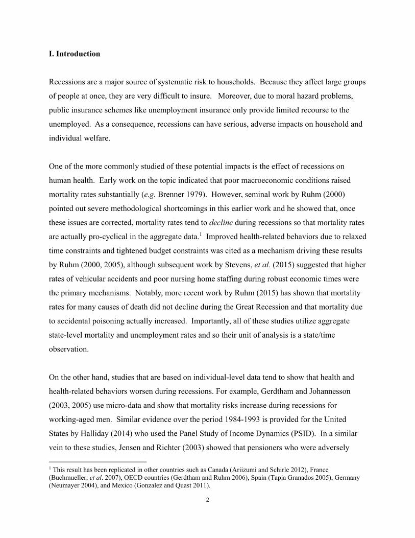
increase during the post-war period. To illustrate, we present Figure 1 which shows the

unemployment rate during this period. This figure clearly indicates that the recession of 2007-

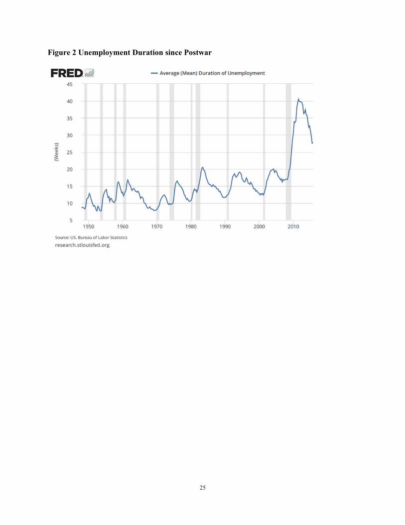
2009 was the most severe. In addition, as shown in Figure 2, unemployment duration during the

most recent recession was also, by far, the longest of any recession since World War II peaking at

just over 40 weeks.

This paper is most similar to Tekin, et al. (2013) who also study the health impact of the Great

Recession using the Behavioral Risk Factor Surveillance System. By-and-large and in contrast

to this study, they find little effect of the Great Recession on health. We suspect that our ability

to measure local macroeconomic conditions at a more granular level is the reason for this

discrepancy.

There are also some other studies that have investigated the impact of the Great Recession on

inputs to health, particularly, illicit drug use. For example, Carpenter, et al. (2016) look at the

impact of the business cycle over the period 2002-2013 on illicit drug use in the United States

and find that there is strong evidence that economic downturns lead to increases in the use of

prescription pain relievers. This result is consistent with findings in Ruhm (2015) who showed

that mortality due to accidental poisoning in the United States increased during the Great

Recession. Related to this, Bassols, et al. (2016) showed that the Great Recession increased legal

4

and illegal drug use in Spain. Finally, Asgeirsdottir, et al. (2012) showed that the 2008

economic crisis in Iceland reduced consumption of health compromising goods.2

We contribute to this literature in the following ways. First, we make important methodological

contributions to the Tekin, et al. (2013). Second, we show that, on the whole, the Great

Recession adversely impacted health. Third, we provide a nuanced portrait of how the Great

Recession impacted the health of different socioeconomic groups and show that its effects were

more pronounced among more disadvantaged groups.

We build on previous work by using county-specific unemployment rates as opposed to state-

specific unemployment rates. Doing so, we find larger and more significant results for similar

outcomes. Our explanation for this is that state-specific unemployment rates are error-ridden

proxies for county-specific unemployment rates and so the estimates in the Tekin, et al. (2013)

study suffer from attenuation biases. In addition, we use the PSID’s geocode file which allows

us to include county-specific fixed effects which control for a rich set of confounding variables at

a more granular level. So, not only do we employ more precise measures of prevailing economic

conditions, but we also can adjust for a wide range of county-specific confounding variables.

Importantly, this is the first study that looks at the impact of the Great Recession on individual

health using county-level information on macroeconomic conditions.3

In addition to the methodological contributions that we make, we also provide new and

important results concerning the health impact of the Great Recession on different

socioeconomic groups. In particular, we document that the Great Recession had more adverse

                                                            2 Although, with respect to this finding, it is possible for a recession to reduce consumption of a normal good such as alcohol, while also increasing problematic binge drinking. 3 In this sense, our study is also related to Charles and DeCicca (2008) who employ MSA-specific fixed effects and individual-level data from the NHIS. However, there are important differences between our study and theirs. First, their study does not consider the Great Recession and as indicated by Ruhm (2015), this most recent recession may have impacted human health in considerably different ways than previous recessions. Second, because we use a panel, we are also able to employ individual fixed effects in robustness checks. Third, they limit their study to the 58 largest MSA’s in the United States, whereas we use a sample that is more representative of the United States. Finally, while we do replicate their key findings that mental health and obesity worsen during recessions, we also provide evidence that drinking and smoking behaviors were affected by the Great Recession, albeit in complicated ways.  

5

consequences on health-related behaviors for blacks and less educated people than it had on

whites and more educated people which is a result that is also new to the literature. Obesity,

smoking, and drinking all increased for blacks. In contrast, the effects of the recession on

drinking were smaller for whites. Moreover, there is weak evidence that the recession actually

reduced obesity and smoking prevalence for whites. In a similar vein, we show that the Great

Recession had larger adverse effects on drinking, obesity, and mental health for less educated

people.

Interestingly, the fact that the recession appeared to reduce obesity rates for more privileged

groups but increased them for the less privileged is consistent with recent findings by Coleman

and Dave (2013). Specifically, they show that recessions increase physical exertion for people

who are more likely to be employed in white collar professions but decrease it for people who

more likely to be employed in blue collar professions. Consequently, another impact of the

Great Recession was that, along many dimensions, it widened socioeconomic disparities in

health-related behaviors.

The balance of this paper is organized as follows. In the next section, we discuss some avenues

through which the macro-economy can affect health. After that, we discuss our data. After that,

we describe our empirical methods. We then present our findings. Finally, we conclude.

II. Mechanisms

Theoretically, the impact of recessions on health and health-related behavior is ambiguous with

some effects promoting health (salubrious effects) and others adversely impacting health

(deleterious effects). This is clearly borne out in the empirical evidence as discussed above. On

the whole, the salubrious effects of recessions will happen via time investment in health and

reduced consumption of vices provided that they are normal goods. On the other hand, the

deleterious effects of recessions will happen through increased consumption of vices if they are

inferior goods or reduced physical exertion at work if work is physically strenuous.

Salubrious Effects

6

These effects have been discussed by many including Ruhm (2000). Essentially, recessions will

reduce the opportunity cost of time and reduce incomes. As a consequence, time investment in

health will increase and consumption of vices that are also normal goods will decline. Ruhm

(2005) does provide evidence for both of these channels. Evidence for reduced consumption of

alcohol and other potentially harmful goods is also provided by Asgeirsdottir, et al. (2012) and

Cotti, et al. (2015).

Deleterious Effects

Recessions may damage health via two channels. First, if some vices are inferior goods, then

consumption of them will increase. Moreover, even for some goods such as alcohol which is a

normal good (e.g. Cotti, et al. (2015)), problematic use such as binge drinking may increase

during recessions if it is used as a coping mechanism (e.g. Dee (2001), Davalos, et al. (2012)). A

similar argument can be made for obesity since idle time can be used for eating more and food

can also provide comfort during stressful times. Second, if people have physically strenuous

occupations, then job loss could be associated with less physical exertion.

The net effects of recessions on health-related behaviors, theoretically, could vary based on a

person’s economic status. So, why would some groups experience positive impacts while others

experience negative impacts? First, as pointed out by Coleman and Dave (2013), people of

lower economic status are more likely to be engaged in physically strenuous occupations and this

suggests that recessions could be associated with increased obesity for these groups. Second,

people for whom the effects of recessions are more temporary have a greater incentive to invest

in their own health during the economic lull since, within the context of a model in the spirit of

Grossman (1972), this will pay off in the future in the form of more productive time. On the

other hand, people who are more severely and permanently impacted by recessions will be less

likely to be employed in the future and so they have less incentive to preserve their health. As a

consequence, these people have a greater incentive to take part in harmful (albeit temporarily

pleasurable) behaviors to cope with the effects of the recession. To the extent that the effect of

the recession is more severe for people with less economic status, we would then expect the

7

impact of the recession to be more harmful to their health.

III. Data

We utilize data from the PSID which is a national longitudinal study that collects individual-

specific information on health, demographic, and socioeconomic outcomes that is run by the

University of Michigan. The PSID began in 1968 with interviews of about 5000 families and has

continued to interview their descendants since then. To obtain county-specific information, we

use the county identifier file from the PSID.4 We utilize the 2003, 2005, 2007, 2009, 2011 and

2013 waves. We employ these waves because the 2007 and 2009 waves contain the recession

and we have two waves prior to the recession (2003 and 2005) and two waves after the recession

(2011 and 2013). Because only heads of household and their spouses were asked the health-

related questions in the survey, we limit our sample to them. We employ county-level

unemployment rates from the Local Area Unemployment Statistics (LAUS) of the Bureau of

Labor Statistics (BLS) which were then merged into the PSID for each year using PSID’s

geocode file.

For most of the estimations, we restrict the sample to people with strong labor force attachments

which we define to be people between ages 25 and 55. Sample sizes by year for the 25-55

sample are reported in Table A1. In addition, we further restrict this sample by dropping retired

and disabled people, students, and housewives. We also present some estimations for people age

65 or older. The idea for using this sample is that this sub-sample has weaker labor force

attachments and so if the impact of the recession on health is operating through the labor market

then we should see attenuated effects in this population. Because the goal of this exercise is to

see if the recession impacted people with weak labor force attachments, we included the retired,

disabled, students (to the extent that there are full-time students older than 65), and housewives.

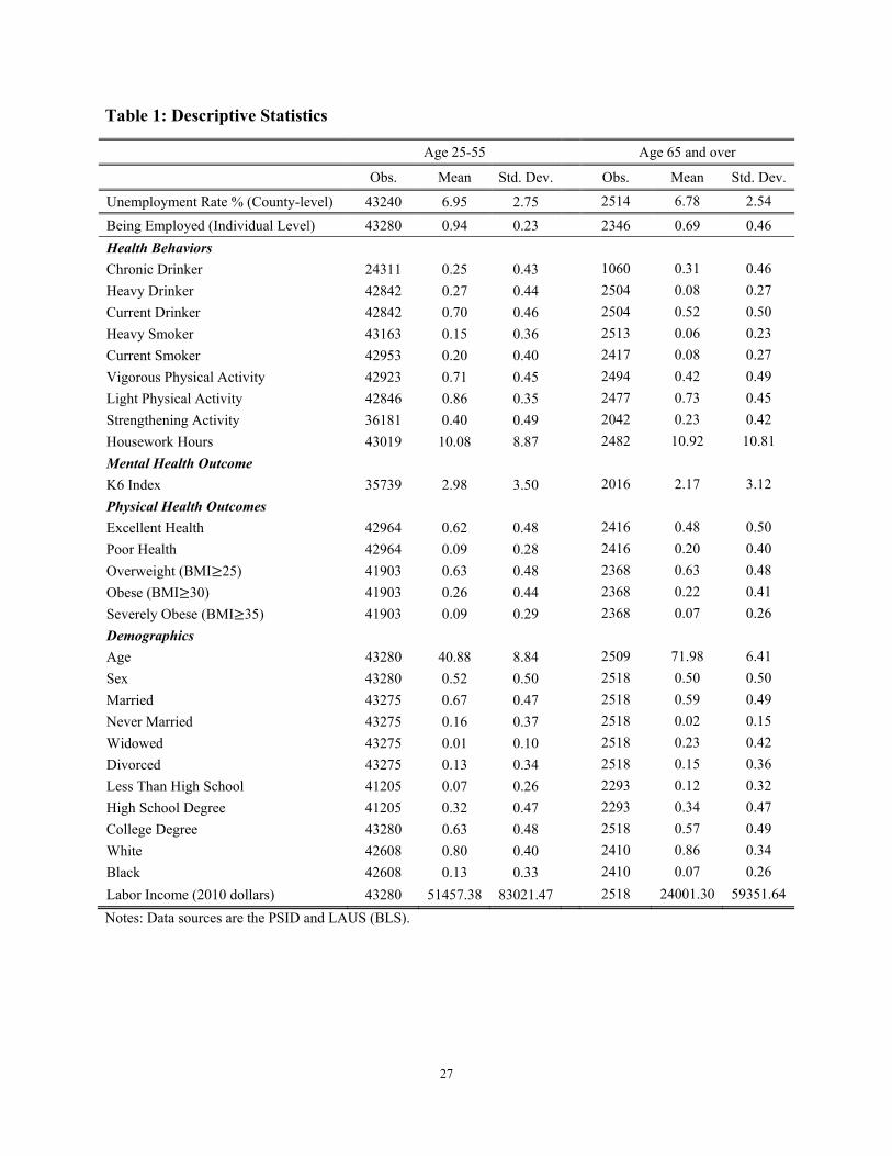
Descriptive statistics for our sample are reported in Table 1. The data can be broadly categorized

under the following rubrics: health-related behaviors, health outcomes (physical and mental), and

                                                            4 See http://simba.isr.umich.edu/restricted/ProcessReq.aspx for details.

8

demographics. The demographic variables are fairly self-explanatory and are listed in the

bottom portion of the table. The health variables require a bit more explanation which we

provide in the next two subsections. With a few exceptions, the outcomes that we use closely

follow Tekin, et al. (2013).

The county-level unemployment rate was obtained from the LAUS of the Bureau of Labor

Statistics (BLS). We collected 3,218 county unemployment rates from every other year between

the years of 2003 to 2013 which corresponds to the years of our PSID sample. In our sample, the

average county-level unemployment rate was 6.95 percent with a standard deviation of 2.75

percent indicating that there is substantial variation in county-level unemployment rates in our

data. Moreover, a regression of the county-level unemployment rate onto county fixed effects

has an R2 of 47.22% indicating that over half of the variation of the county-level unemployment

rate is within counties which is critical for our research design.

Health-related Behaviors

The PSID includes numerous questions about alcohol and smoking consumption. Specifically,

respondents were asked how often they drank and individuals who reported drinking several

times a week or everyday were categorized as a “chronic drinker.” The PSID survey also asked

respondents about the typical number of drinks consumed per day. Following standard

guidelines, we define men who drink three to four drinks or more per day and women who

consume one to two drinks or more per day as “heavy drinkers.”5 A “current drinker” is defined

as an individual who reported having had a drink in the last year. Similarly, we define a “current

smoker” as someone who has ever smoked during the last year. Since the definition of light or

heavy smoker varies widely, we define a “heavy smoker” as individuals who smoke six or more

cigarettes per day.6 Note that we are well aware that the definition of current drinking includes

many behaviors that people would not consider problematic. However, given the penchant for                                                             5 According to the definition from the Centers for Disease Control and Prevention, heavy drinking is defined as consumption of 15 or more drinks per week for men and consumption of 8 or more drinks per week for women. See http://www.cdc.gov/alcohol/faqs.htm#heavyDrinking. 6 Husten (2009) documents that the definition of light smoking ranged from "smoking 1-39 cigarettes per week" to "smoke 10-20 cigarettes per day."

9

under-reporting socially undesirable behaviors, these questions may measure problematic

behaviors that are not measured by either the heavy or chronic drinking variables.

In addition, we consider physical activity. The PSID provides information about vigorous

physical activity (which includes activities such as heavy housework, aerobics, running,

swimming, and bicycling), light physical activity (which includes activities such as walking,

dancing, gardening, golfing, and bowling), and strengthening activities (which includes activities

that are specifically designed to strengthen muscles such as lifting weights). Each of these three

variables is binary and is set to unity if the respondent reported any of these types of activities.

Finally, we use weekly hours of housework as an additional measure of physical activity.

Health Outcomes

We use the K6 Non-specific Psychological Distress scale which was also used by Charles and

DeCicca (2008). Recent work by Tekin, et al. (2013) also looks at mental health as an outcome,

although they use a different depression index. This K6 distress scale includes six questions

designed to measure different markers of psychological distress including reports of feelings of

effortlessness, hopelessness, restlessness, sadness, and worthlessness during the past 30 days.

The K6 distress scale is a weighted sum of these six outcomes. Kessler, et al. (2003) has shown

that the K6 scale is at least as effective as a number of other depression scales in predicting

serious mental health problems.

The physical health outcomes that we employ include variables based on self-reported health

status (SRHS) and body mass index (BMI). SRHS is a categorical variable that takes on integer

values between one and five where one is excellent and five is poor. We transform the SRHS

variable into two binary indicator variables for excellent (SRHS equal to one or two) and poor

(SRHS equal to four or five) health. The BMI variable is transformed into three dummy

variables for being overweight (BMI 25), obese (BMI 30), and severely obese (BMI 35).

IV. Methodology

10

To estimate the effect of the Great Recession on health outcomes and health-related behaviors,

we employ a linear regression model. If we let i denote the individual, c the county, s the state,

and y the year, the basic estimation model is:

∗ . (1)

The dependent variable, , is a health outcome or behavior. The county-specific

unemployment rate in a given year is . The vector, , contains individual-specific control

variables including age, gender, race, marriage status, education, and labor income. We also

include county and year dummies which are denoted by and . Finally, we include state-

specific time trends which are denoted by ∗ . We estimate two different specifications of

equation (1) both with and without the state-specific trends which has the advantage of

controlling for potentially confounding within state trends but the disadvantage of eliminating

potentially meaningful exogenous variation in the county-level unemployment rates. Finally, we

employ the weights provided by the PSID when estimating these models.

We compute the standard errors using two-way clustering by year and county. When we cluster

by county, this accounts for any potential serial correlation within counties or individuals. When

we cluster by year, this accounts for spatial correlations within a year. Note that this is a very

conservative approach to computing the standard errors.

An important feature of this research design is that we employ county and not state-specific

unemployment rates. Within states, there can be considerable variation in local economic

conditions, particularly, in larger states. As such, using county-specific unemployment rates does

a better job of capturing the macroeconomic circumstances that an individual is facing. In this

sense, the state-specific unemployment rates can be viewed as error-ridden proxies for the

county-specific rates.

In addition to doing a comprehensive job of measuring local macroeconomic conditions, our

study also does a comprehensive job of controlling for heterogeneity across local labor markets.

Importantly, Tekin, et al. (2013) and Ruhm (2005), which also closely align with our own study,

11

only control for state fixed effects which only accounts for the state-level and time-invariant

confounders. Clearly, the use of state fixed effects may be too coarse since potential confounders

such as education and health infrastructure, culture, demographic composition, and weather may

vary at a finer geographical level. For example, Asians are about one third of the population in

San Francisco whereas they are only 0.4% of the population of Sierra County in California.

Another example is that within states, particularly in the South, some counties are “dry” which

means that alcohol cannot be purchased within them. Given that many of our outcomes relate to

alcohol consumption, this is another important potential county-specific confound. Simple

inclusion of state fixed effects would not account for these within state confounders.

We also adopt a more comprehensive approach to addressing heterogeneity by including

individual fixed effects which subsume the county fixed effects. This approach has the

advantage of controlling for a greater amount of unobserved confounding variables than the

county fixed effects. However, it comes with the cost of wasting important exogenous variation

in the data as has been argued by Deaton (1997) and Angrist and Pischke (2008). It is also less

efficient. As such, we view the results with the individual fixed effects as a robustness check for

our core results and we primarily focus on the results with the county fixed effects for most of

the paper.

V. Results

Core Results

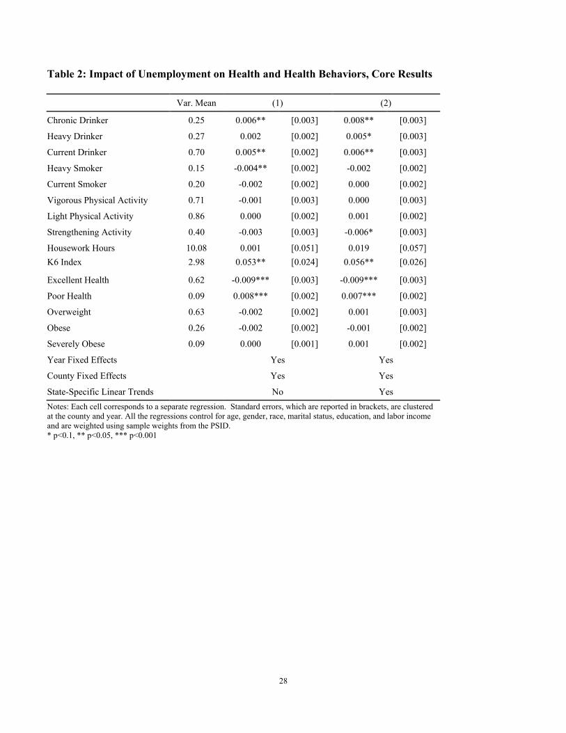
Our core estimation results are reported in Table 2. In the first column, we include county and

year fixed effects. In the second column, we further include state-specific trends. Each cell

corresponds to a separate estimate of our parameter of interest, , and each row corresponds to

a separate outcome.

First, we see strong evidence that increases in the unemployment rate during this period

increased drinking and, particularly, problematic drinking. In the first column, we see that

increases in unemployment are positively associated with increased prevalence of drinking and

chronic drinking. In the second column, we see that it is associated with increases in all three

12

types of drinking behavior. Particularly, a one percentage point (PP) increase in the

unemployment rate is associated with a 0.6-0.8 PP increase in chronic drinking and a 0.5-0.6 PP

increase in current drinking. This constitutes a 2.4-3.2% increase in the prevalence of chronic

drinking and a 0.71-0.86% increase in current drinking.

Next, we do not see strong evidence that increases in the unemployment rate impact smoking

behaviors or reports of physical activities. We do see evidence that heavy smoking decreased in

both specifications, but only the estimate from the specification without the state specific trends

is significant. However, there is no evidence that the recession impacted reports of currently

being a smoker. Finally, we look at four different measurements of physical activity (vigorous

physical activity, light physical activity, strengthening activity, and housework hours) using our

two different specifications and we see only one estimate for strengthening activity that is

negative and significant at the 10% level. On the whole, there is little to no evidence that the

recession impacted physical activities or smoking.

Next, we do see some evidence that there was a deterioration of mental health outcomes because

of the recession. Consistent with Tefft (2011), when we look at the K6 index, we see strong

evidence that the recession led to worsened mental health outcomes using both specifications.

The estimates indicate that a one PP increase in the unemployment rate resulted in an increase in

the K6 index of 1.8-1.9%. This apparent deterioration in mental health is consistent with the

observed increase in drinking that we just saw which may have been a way of coping with the

stress induced by the recession.

In addition, the recession did have strong effects on self-reported health status using both

specifications. We see that a one PP increase in the unemployment rate is associated with a 0.9

PP decrease in self-reports of excellent health and a 0.7-0.8 PP increase in self-reports of poor

health. This constitutes a 1.5% increase in the probability of reporting good health and a 7.8-

8.9% increase in the probability of reporting poor health. This result is consistent with Halliday

(forthcoming) who showed that fluctuations in earnings have causal impacts on self-rated health.

Finally, there is no evidence that the recession impacted obesity in this table. None of our three

13

measures of obesity and overweight were impacted. However, it is important to note that this

could mask important variation across demographic subgroups as we will see.

In Table 3, we estimate the same models that we estimated in the previous table for the sub-

sample that is 65 or older. This population is, by-and-large, retired and so has weak labor force

attachments. Looking at the results from our preferred specification in the second column, we

see that none of the estimates are significant at the 5 or 1% levels and only the estimate of the

coefficient on severe obesity is significant at the 10% level. In the first column where we

exclude the state-specific time trends, we see that the coefficient estimates on vigorous physical

and strengthening activities are positive and significant but only at the 10% level and this result

is not robust to the inclusion of the state-specific trends. On a similar note, there is evidence in

the first column that the recession improved self-rated health but, once again, this finding is not

robust to the inclusion of state-specific time trends. On the whole, the results in this table do not

indicate that the Great Recession had systematic, negative effects on an elderly population with

weak labor force attachments. This seems to indicate that the effects of the recession on health

ran primarily through the labor market.

Next, in Table 4, we conduct a series of robustness checks. The table contains four sets of

estimations. The first two sets include individual fixed effects both with and without state-

specific trends. The second two are estimates of county fixed effects models using a sub-sample

of people who did not change counties while in the sample, again, both with and without state-

specific trends. These two exercises address a concern discussed in Halliday (2007) in which

healthier people migrate in response to recessions. So, if the estimate indicates that the recession

is adversely impacting health, then the bias stemming from selective out-migration would make

it appear as if the recession is worse for human health than it actually is. On the other hand, the

reverse is true if the estimates indicate that some aspect of health or health behavior improves

during recessions. Note that, while these exercises do address this concern, they also place much

heavier demands on the data which, most likely, will result in higher standard errors and, hence,

reduced power.

The results in Table 4, on the whole, buttress the results in Table 2. First, we still see strong

14

evidence that problematic drinking increased during the recession when looking at the estimates

using the non-mover sample and we see similar (albeit somewhat weaker) evidence when

employing individual fixed effects in the first two columns. Interestingly, the results in this table

suggest that smoking and obesity actually decreased during the recession. Particularly, a one PP

increase in the unemployment rate reduced the prevalence of heavy smoking by between 0.3 and

0.5 PP and obesity by 0.5 PP. Note that we did not see significant effects on smoking or obesity

in Table 2. This is consistent with our discussion of the selection bias induced by migration in

the previous section. Healthier people leave depressed areas which will create a positive bias in

the smoking and obesity estimates in Table 2. Finally, we also see negative effects of the

recession on SRHS and the K6 index, although the effects on the K6 index are not significant in

the individual fixed effects specifications.

Results by Demographic Group

We begin this sub-section by estimating equation (1) using a dummy variable for currently being

employed for our sample of 25-55 year olds. We estimate the model by race (black and white),

gender, and education (people with 12 or fewer years of schooling and people with college

degrees).7 The point of this exercise is to obtain an idea of which groups were most impacted by

the recession and to compare this to the health impacts of the recession by demographic sub-

groups. Not surprisingly, all six of our estimations delivered coefficient estimates on the county-

level unemployment rate that were significant at 1% level.

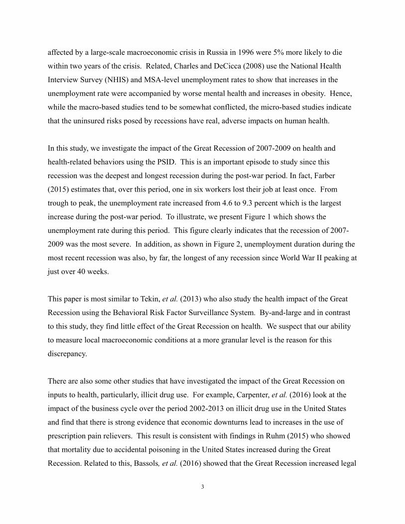
The point-estimates are reported in Figure 3. We see that a one PP increase in the unemployment

rate reduced the probability of being employed in the PSID by 0.6 PP for whites and 0.9 PP for

blacks. Similarly, we see that the corresponding marginal effects for men and women are 0.6 and

0.8 and the estimates by education are 0.6 and 0.7 for the college and high school educated. The

overall pattern is that, while the recession had a broad impact, women and more disadvantaged

socio-economic groups were the most impacted by it.

In Table 5, we report our estimation results of both specifications from Table 2 separated by race.

                                                            7 We estimated the more parsimonious specification that excluded the state-specific time trends.

15

First, looking at the drinking outcomes, we see that the recession had much stronger effects on

the drinking behavior of black people than on white people. For example, when we included

state-specific trends in the second and fourth columns, we see that a one PP increase in the

unemployment rate is associated with a 0.9 PP increase in chronic drinking for whites and a 2.2

PP increase for blacks. In the same specifications, the probability of being a current drinker

increased by 0.5 PP for whites and 1.8 PP for blacks. We also see that a one PP increase in the

unemployment rate resulted in a 1.1-1.7 PP increase in the prevalence of heavy drinking for

blacks but had no effects on whites. Similarly, we see that blacks report a 1.1-1.3 PP increase in

the probability of being a current smoker in response to a one PP increase in the unemployment

rate. Interestingly, there is weak evidence that whites smoked less in response to the recession;

in the first column, we see that the probability of being a heavy or a current smoker decreased by

0.4-0.6 PP. As before, we see no evidence, at the 5 or 1% level, that the recession impacted any

of our physical activity measures. Turning to the mental health outcomes, we see that the

recession had large effects on whites but no effects on blacks. In a similar vein, while there is

some evidence that blacks reported worse self-rated health in column three, the bulk of the

effects on SRHS appears to have been for the white sub-population. Specifically, we see that a

one PP increase in the unemployment rate is associated with a 0.9 PP decrease in the probability

of reporting excellent health and a 0.7-0.8 PP increase in the probability of reporting poor health

for whites.

Finally, as with smoking, we see an interesting contrast in how the recession impacted obesity

rates by race. Looking at whites in the first column, there is evidence that the rate of obesity and

severe obesity declined by 0.5 and 0.3 PP, respectively. However, this result is not robust to the

inclusion of state-specific trends. In contrast, all three measures of obesity increased in response

to increases in the unemployment rate for blacks. This is true in both specifications from

columns three and four. These effects vary in a narrow band between 1.1 and 1.5 PP.

In Table 6, we present estimates by gender. First, the recession impacted drinking for both men

and women, although in different ways. For men, the bulk of the impact was on moderate

drinking. Indeed, we see that there is weak evidence that chronic drinking increased by 0.5-0.8

PP and stronger evidence that current drinking increased by 0.7 PP for men. In contrast, for

16

women, the probabilities of being a current or heavy drinker were unaffected, but the probability

of being a chronic drinker increased by 0.8 PP and this estimate is significant at the 95% level in

both specifications. Next, there is little evidence that the recession impacted smoking or physical

activity for either gender. There is some evidence that the recession impacted mental health

outcomes, but looking at the point-estimates of the coefficient on the K6 index, we do not see

any discernible gender differences as the point-estimates are all similar. In the same spirit, we

see that fluctuations in the unemployment rate impacted SRHS for both genders, but the effects

were larger for women. Specifically, we see that a one PP increase in the unemployment rate is

associated with a 0.7-1.0 PP increase in the probability of reporting being in poor health for

women and 0.4-0.5 PP for men. Similarly, we see a decrease in the likelihood of excellent health

of 0.9 PP for women and 0.7 PP for men. Finally, we see no evidence that the recession

impacted obesity rates for men, but we do see some evidence that the recession reduced obesity

rates for women as the probability of being obese declined by between 0.7-0.8 PP for women.

Finally, we investigate differential impacts of the Great Recession by education levels in Table 7.

We estimate the models separately for people with college degrees and people with at most a

high school degree. First, we see that the bulk of the effects of the recession on drinking

occurred for the least educated. We see no effects for people with college degrees but we see

that there was a 0.6-0.8 PP increase in the probability of being a current drinker and a 0.6-1.0 PP

increase in the probability of being a chronic drinker for people with at most a high school

degree. As before, we see little to no evidence that the recession impacted either smoking or

physical activity for either educational group. Next, we see that the bulk of the effects of the

recession on mental health outcomes occurred for the least educated as evidenced by the

estimates of the coefficient on the K6 index; the point estimates in the third and fourth columns

for the high school educated group are 0.064 and 0.53, respectively, whereas they are 0.018 and

0.040 in the first two columns for the college-educated group. A similar pattern exists for SRHS.

We see no effects for the college-educated, but we do see a 1.0-1.2 PP reduction in reports of

excellent health and a 0.7-0.8 PP increase in reports of poor health for the least educated.

Finally, and similar to our results broken down by race, we see that the recession reduced the

probability of being overweight for the college educated by 1.1 PP in the first specification but

increased the likelihood of being overweight for people with at most a high school degree by 0.6

17

PP in both specifications.

These results underscore some of the distributional impacts of the Great Recession in ways that

have not hitherto been articulated in the literature. For many important health outcomes, the

recession appears to have exacerbated health disparities between blacks and whites and across

educational groups. By race, we saw that the recession had larger impacts on drinking, smoking,

and obesity rates for blacks than for whites. Moreover, there is some evidence that the recession

actually resulted in lower obesity rates for whites and women. However, the recession impacted

subjective health measures (i.e. the K6 index and the SRHS measures) more for whites than

blacks. In addition, the results by educational group indicate that there were larger effects on

drinking, mental health, SRHS, and obesity for the least educated. The results for subjective

health outcomes by race notwithstanding, these results are consistent with Figure 3 and our

theoretical discussion in Section II in that blacks and high school educated people were most

impacted by the recessions and these groups drank more and experienced a greater deterioration

in their health status in response to the exigencies posed by the Great Recession.

Results with State Unemployment Rates

Finally, we re-estimate the regression models from Table 2 except that now we use state

unemployment rates in lieu of county unemployment rates. The basic idea here is that the state

unemployment rate is a crude proxy for the county-level unemployment rate. For example and

as discussed earlier many states have considerable heterogeneity within them in economic

conditions. This is particularly true of larger states. As such, we view the state-level

unemployment rate as an error-ridden proxy for the county-level unemployment rate. Given this,

one would expect that using state-level unemployment rates in lieu of county-level rates should

dampen the impact of the unemployment rate on our outcomes if the measurement error results

in the standard attenuation bias.

We report the results in Table 8. On the whole, the estimates in this table are substantially more

muted than those in Table 2 which is consistent with the measurement error story. The only

results that are statistically significant in both specifications are the estimate for poor health and

18

overweight (which was not present in Table 2). There are not consistently significant (i.e. in both

specifications) effects for the K6 index, excellent health, current drinking, and chronic drinking

as there were in Table 2.

These findings are consistent with the notion that the state-specific unemployment rates do not

measure the macroeconomic circumstances of a given individual as well as the county-specific

rates. This would then induce measurement error that ostensibly would lead to muted estimates

of the effects of recessions on health vis-à-vis those in Table 2. This may be the reason that we

uncover larger effects of recessions on health than do Tekin, et al. (2013).

VI. Conclusions

In this paper, we showed that, overall, the Great Recession resulted in worse health outcomes.

We built on previous work by employing more granular information on local macroeconomic

conditions by using the geocode file from the Panel Study of Income Dynamics. For a

population of working-aged adults, we showed that a one percentage point increase in the

county-level unemployment rate resulted in a 2.4-3.2% increase in chronic drinking, a 1.8-1.9%

increase in the K6 depression index, and a 7.8-8.9% increase in the probability of reporting poor

health. Importantly, however, these effects mask that there was considerable heterogeneity in the

recession’s effects across socioeconomic groups.

As discussed above, it is well documented that aggregate mortality rates are pro-cyclical (e.g.

Ruhm 2000, Stevens, et al. 2015). Ruhm (2000) suggested that one of the mechanisms behind

this counter-intuitive finding was that health-related behaviors improved during recessions since

relaxed time constraints would enable more time spent exercising and tightened budget

constraints would result in less money spent on vices such as alcohol and cigarettes. Indeed,

Ruhm (2005) provided evidence that tobacco consumption decreases and physical activity

increases during economic lulls in the BRFSS over the period 1987-2000, although Tekin, et al.

(2013) show that this relationship has severely weakened or become zero over the period 2005-

2011 in the BRFSS. Our results, on the whole, are not consistent with these findings in that we

19

find that SRHS, mental health, and problematic drinking behavior all worsen during recessions

for people of prime working age, although some of our findings indicate that some health-related

behaviors may have improved for whites and the college-educated. It is also important to note

that more recent work by Ruhm (2015) has shown that mortality rates have not been pro-cyclical

since the early 2000’s. In this sense, since we look at the period 2003-2013, our work need not

be viewed as being at loggerheads with Ruhm (2000).

While this work may seem to be at odds with many of the studies that rely on aggregate data

(e.g. state-level mortality rates) discussed above, the results are consistent with studies on the

impact of recessions on mortality that use micro-data. For example, Gerdtham and Johannesson

(2003, 2005) use individual-level Swedish administrative data and find that mortality risk

increases during economic downturns for working-aged men. Similarly, Halliday (2014) uses

the PSID and finds that a one PP increase in the unemployment rate results in a 6% increase in

one-year mortality risk at baseline also for working aged men.

Our findings on the effects of the Great Recession on obesity are also consistent with other

findings in the literature. For example, and similar to our own findings, Charles and DeCicca

(2008) find the obesity tends to increase during recessions for men with low ex ante employment

probabilities and for black men. Evidence for a mechanism underlying this finding is provided

by Coleman and Dave (2013) who show that, while exercise hours increase during recessions,

for less educated individuals, this does not compensate for total loss in physical exertion due to

the loss of physically demanding jobs.

Related to this, an important conclusion of our work is that different socioeconomic groups

responded to the Great Recession in very different ways. As already discussed, the Great

Recession increased obesity rates for black and high school educated people but there is weak

evidence that it decreased obesity rates for white and college educated people. Similar results

also obtain for smoking by race; whites smoked less in response to the recession, whereas blacks

smoked more. Finally, the recession adversely impacted the drinking behaviors of black and

white people and of less educated and more educated people; however, the magnitudes were

much larger for black and less educated people. In this sense, the Great Recession appears to

20

have exacerbated many socio-economic health disparities in the United States.

21

References Angrist, Joshua D., and Jörn-Steffen Pischke. Mostly harmless econometrics: An empiricist's companion. Princeton university press, 2008. Ariizumi, Hideki, and Tammy Schirle. "Are recessions really good for your health? Evidence from Canada." Social Science & Medicine 74, no. 8 (2012): 1224-1231. Asgeirsdottir, Tinna Laufey, Hope Corman, Kelly Noonan, Þórhildur Ólafsdóttir, and Nancy E. Reichman. Are recessions good for your health behaviors? Impacts of the economic crisis in Iceland. No. w18233. National Bureau of Economic Research, 2012. Bassols, Nicolau Martin, and Judit Vall Castelló. "Effects of the Great Recession on drugs consumption in Spain." Economics & Human Biology 22 (2016): 103-116. Brenner, M. Harvey. "Mortality and the national economy: A review, and the experience of England and Wales, 1936-76." The Lancet 314, no. 8142 (1979): 568-573. Buchmueller, Thomas C., Michel Grignon, Florence Jusot, and Marc Perronnin. Unemployment and mortality in France, 1982-2002. Centre for Health Economics and Policy Analysis, McMaster University, 2007. Carpenter, Christopher S., Chandler B. McClellan, and Daniel I. Rees. Economic Conditions, Illicit Drug Use, and Substance Use Disorders in the United States. No. w22051. National Bureau of Economic Research, 2016. Charles, Kerwin Kofi, and Philip DeCicca. "Local labor market fluctuations and health: is there a connection and for whom?." Journal of Health Economics 27, no. 6 (2008): 1532-1550. Coleman, Gregory, and Dhaval Dave. "Exercise, physical activity, and exertion over the business cycle." Social Science & Medicine 93 (2013): 11-20. Cotti, Chad, Richard A. Dunn, and Nathan Tefft. "The Great Recession and Consumer Demand for Alcohol: A Dynamic Panel-Data Analysis of US Households." American Journal of Health Economics (2015). Dávalos, María E., Hai Fang, and Michael T. French. "Easing the pain of an economic downturn: macroeconomic conditions and excessive alcohol consumption." Health economics 21, no. 11 (2012): 1318-1335. Deaton, Angus. The analysis of household surveys: a microeconometric approach to development policy. World Bank Publications, 1997. Dee, Thomas S. "Alcohol abuse and economic conditions: evidence from repeated cross‐sections of individual‐level data." Health economics 10, no. 3 (2001): 257-270.

22

Farber, Henry S. Job loss in the Great Recession and its aftermath: US evidence from the displaced workers survey. No. w21216. National Bureau of Economic Research, 2015. Gerdtham, Ulf-G., and Magnus Johannesson. "A note on the effect of unemployment on mortality." Journal of health economics 22, no. 3 (2003): 505-518. Gerdtham, Ulf-G., and Magnus Johannesson. "Business cycles and mortality: results from Swedish microdata." Social science & medicine 60, no. 1 (2005): 205-218. Gerdtham, Ulf-G., and Christopher J. Ruhm. "Deaths rise in good economic times: evidence from the OECD." Economics & Human Biology 4, no. 3 (2006): 298-316. Gonzalez, Fidel, and Troy Quast. "Macroeconomic changes and mortality in Mexico." Empirical Economics 40, no. 2 (2011): 305-319. Granados, José A. Tapia. "Recessions and mortality in Spain, 1980–1997." European Journal of Population/Revue européenne de Démographie 21, no. 4 (2005): 393-422. Grossman, Michael. "On the concept of health capital and the demand for health." Journal of Political economy 80, no. 2 (1972): 223-255. Halliday, Timothy J. "Business cycles, migration and health." Social Science & Medicine 64, no. 7 (2007): 1420-1424. Halliday, Timothy J. "Unemployment and Mortality: Evidence from the PSID." Social Science & Medicine 113 (2014): 15-22. Halliday, Timothy J. “Earnings Growth and Movements in Self-Reported Health,” forthcoming Review of Income and Wealth. Husten, Corinne G. "How should we define light or intermittent smoking? Does it matter?." Nicotine & Tobacco Research 11, no. 2 (2009): 111-121. Jensen, Robert T., and Kaspar Richter. "The health implications of social security failure: evidence from the Russian pension crisis." Journal of Public Economics 88, no. 1 (2004): 209-236. Kessler, Ronald C., Gavin Andrews, Lisa J. Colpe, Eva Hiripi, Daniel K. Mroczek, S-LT Normand, Ellen E. Walters, and Alan M. Zaslavsky. "Short screening scales to monitor population prevalences and trends in non-specific psychological distress." Psychological medicine 32, no. 06 (2002): 959-976. Neumayer, Eric. "Recessions lower (some) mortality rates: evidence from Germany." Social Science & Medicine 58, no. 6 (2004): 1037-1047.

23

Ruhm, C. J. “Are Recessions Good for Your Health?” The Quarterly journal of economics, 115, no. 2 (2000): 617-650 Ruhm, Christopher J. "Healthy living in hard times." Journal of Health Economics 24, no. 2 (2005): 341-363. Ruhm, Christopher J. "Recessions, healthy no more?." Journal of Health Economics 42 (2015): 17-28. Stevens, Ann H., Douglas L. Miller, Marianne E. Page, and Mateusz Filipski. "The best of times, the worst of times: Understanding pro-cyclical mortality." American Economic Journal: Economic Policy 7, no. 4 (2015): 279-311. Tefft, Nathan. "Insights on unemployment, unemployment insurance, and mental health." Journal of Health Economics 30, no. 2 (2011): 258-264. Tekin, Erdal, Chandler McClellan, and Karen Jean Minyard. Health and health behaviors during the worst of times: evidence from the Great Recession. No. w19234. National Bureau of Economic Research, 2013.

24

Figure 1 Total Unemployment Rate in Each Recession since Postwar

25

Figure 2 Unemployment Duration since Postwar

   

26

Figure 3: Impacts of Great Recession by Demographic Group

Note: Each bar corresponds to the impact of a one percentage point increase in the county-level unemployment rate on the probability of currently being employed in the PSID in percentage points.

White Men College

Black

Women

High School

‐1.1

‐0.9

‐0.7

‐0.5

‐0.3

‐0.1

Race Gender Education

27

Table 1: Descriptive Statistics

Age 25-55 Age 65 and over

Obs. Mean Std. Dev. Obs. Mean Std. Dev. Unemployment Rate % (County-level) 43240 6.95 2.75 2514 6.78 2.54 Being Employed (Individual Level) 43280 0.94 0.23 2346 0.69 0.46 Health Behaviors Chronic Drinker 24311 0.25 0.43 1060 0.31 0.46 Heavy Drinker 42842 0.27 0.44 2504 0.08 0.27 Current Drinker 42842 0.70 0.46 2504 0.52 0.50 Heavy Smoker 43163 0.15 0.36 2513 0.06 0.23 Current Smoker 42953 0.20 0.40 2417 0.08 0.27 Vigorous Physical Activity 42923 0.71 0.45 2494 0.42 0.49 Light Physical Activity 42846 0.86 0.35 2477 0.73 0.45 Strengthening Activity 36181 0.40 0.49 2042 0.23 0.42 Housework Hours 43019 10.08 8.87 2482 10.92 10.81 Mental Health Outcome K6 Index 35739 2.98 3.50 2016 2.17 3.12 Physical Health Outcomes Excellent Health 42964 0.62 0.48 2416 0.48 0.50 Poor Health 42964 0.09 0.28 2416 0.20 0.40 Overweight (BMI 25) 41903 0.63 0.48 2368 0.63 0.48 Obese (BMI 30) 41903 0.26 0.44 2368 0.22 0.41 Severely Obese (BMI 35) 41903 0.09 0.29 2368 0.07 0.26 Demographics Age 43280 40.88 8.84 2509 71.98 6.41 Sex 43280 0.52 0.50 2518 0.50 0.50 Married 43275 0.67 0.47 2518 0.59 0.49 Never Married 43275 0.16 0.37 2518 0.02 0.15 Widowed 43275 0.01 0.10 2518 0.23 0.42 Divorced 43275 0.13 0.34 2518 0.15 0.36 Less Than High School 41205 0.07 0.26 2293 0.12 0.32 High School Degree 41205 0.32 0.47 2293 0.34 0.47 College Degree 43280 0.63 0.48 2518 0.57 0.49 White 42608 0.80 0.40 2410 0.86 0.34 Black 42608 0.13 0.33 2410 0.07 0.26 Labor Income (2010 dollars) 43280 51457.38 83021.47 2518 24001.30 59351.64 Notes: Data sources are the PSID and LAUS (BLS).    

28

Table 2: Impact of Unemployment on Health and Health Behaviors, Core Results Var. Mean (1) (2)

Chronic Drinker 0.25 0.006** [0.003] 0.008** [0.003]

Heavy Drinker 0.27 0.002 [0.002] 0.005* [0.003]

Current Drinker 0.70 0.005** [0.002] 0.006** [0.003]

Heavy Smoker 0.15 -0.004** [0.002] -0.002 [0.002]

Current Smoker 0.20 -0.002 [0.002] 0.000 [0.002]

Vigorous Physical Activity 0.71 -0.001 [0.003] 0.000 [0.003]

Light Physical Activity 0.86 0.000 [0.002] 0.001 [0.002]

Strengthening Activity 0.40 -0.003 [0.003] -0.006* [0.003]

Housework Hours 10.08 0.001 [0.051] 0.019 [0.057] K6 Index 2.98 0.053** [0.024] 0.056** [0.026]

Excellent Health 0.62 -0.009*** [0.003] -0.009*** [0.003]

Poor Health 0.09 0.008*** [0.002] 0.007*** [0.002]

Overweight 0.63 -0.002 [0.002] 0.001 [0.003]

Obese 0.26 -0.002 [0.002] -0.001 [0.002]

Severely Obese 0.09 0.000 [0.001] 0.001 [0.002]

Year Fixed Effects Yes Yes

County Fixed Effects Yes Yes

State-Specific Linear Trends No Yes Notes: Each cell corresponds to a separate regression. Standard errors, which are reported in brackets, are clustered at the county and year. All the regressions control for age, gender, race, marital status, education, and labor income and are weighted using sample weights from the PSID. * p<0.1, ** p<0.05, *** p<0.001

 

   

29

Table 3: Impact of Unemployment on Health and Health Behaviors, Ages 65 + Var. Mean (1) (2)

Chronic Drinker 0.31 0.003 [0.016] 0.000 [0.019]

Heavy Drinker 0.08 0.009 [0.007] 0.007 [0.007]

Current Drinker 0.52 0.017 [0.011] 0.016 [0.013]

Heavy Smoker 0.06 0.001 [0.005] 0.005 [0.006]

Current Smoker 0.08 0.003 [0.006] 0.006 [0.007]

Vigorous Physical Activity 0.42 0.024* [0.013] 0.021 [0.015]

Light Physical Activity 0.73 0.013 [0.012] 0.014 [0.013]

Strengthening Activity 0.23 0.020* [0.011] 0.017 [0.013]

Housework Hours 10.92 -0.134 [0.246] -0.311 [0.290]

K6 Scale 2.17 0.052 [0.095] 0.038 [0.103]

Excellent Health 0.48 0.025** [0.012] 0.015 [0.014]

Poor Health 0.20 -0.019** [0.008] -0.008 [0.009]

Overweight 0.63 -0.013 [0.009] -0.002 [0.011]

Obese 0.22 0.002 [0.009] -0.002 [0.010]

Severely Obese 0.07 0.01 [0.007] 0.015* [0.008]

Year Fixed Effects Yes Yes

County Fixed Effects Yes Yes

State-Specific Linear Trends No Yes Notes: Per Table 2.

 

30

Table 4: Robustness Checks

Outcome Whole Sample (Individual FE)

Non-mover (County FE)

Chronic Drinker 0.006 [0.004] 0.007* [0.004] 0.006* [0.003] 0.007* [0.004] Heavy Drinker 0.004 [0.003] 0.005 [0.003] 0.003 [0.003] 0.006** [0.003] Current Drinker 0.002 [0.003] 0.003 [0.003] 0.003 [0.002] 0.006** [0.003] Heavy Smoker -0.003* [0.002] -0.002 [0.002] -0.005*** [0.002] -0.004** [0.002] Current Smoker -0.002 [0.002] -0.001 [0.002] -0.004** [0.002] -0.002 [0.002] Vigorous Physical Activity 0.004 [0.003] 0.004 [0.004] 0.000 [0.003] 0.002 [0.003] Light Physical Activity -0.001 [0.003] 0.001 [0.003] -0.001 [0.003] 0.002 [0.003] Strengthening Activity 0.000 [0.003] -0.002 [0.004] 0.001 [0.003] 0.000 [0.003] Housework Hours -0.057 [0.058] -0.043 [0.061] -0.01 [0.057] -0.009 [0.064] K6 Scale 0.028 [0.028] 0.029 [0.030] 0.044* [0.026] 0.056* [0.029] Excellent Health -0.006* [0.003] -0.008** [0.004] -0.009*** [0.003] -0.010*** [0.004] Poor Health 0.007*** [0.002] 0.008*** [0.002] 0.007*** [0.002] 0.007*** [0.002] Overweight 0.001 [0.002] 0.003 [0.002] -0.001 [0.002] 0.001 [0.003] Obese -0.003 [0.002] -0.002 [0.002] -0.005** [0.002] -0.005* [0.003] Severely Obese 0.000 [0.002] 0.001 [0.002] -0.003 [0.002] -0.002 [0.002] Year Fixed Effects Yes Yes Yes Yes Type of Fixed Effects Individual Individual County County State-specific Linear Trends No Yes No Yes Notes: Per Table 2.

31

Table 5: Impacts by Race

Outcome White Black

Chronic Drinker 0.007** [0.003] 0.009** [0.004] 0.012 [0.008] 0.022** [0.009]

Heavy Drinker 0.000 [0.003] 0.001 [0.003] 0.011* [0.006] 0.017*** [0.006]

Current Drinker 0.004 [0.002] 0.005* [0.003] 0.012 [0.007] 0.018** [0.007]

Heavy Smoker -0.006*** [0.002] -0.003 [0.002] 0.006 [0.005] 0.007 [0.006]

Current Smoker -0.004* [0.002] -0.001 [0.002] 0.011** [0.005] 0.013** [0.006]

Vigorous Physical Activity 0.001 [0.003] 0.002 [0.003] 0.004 [0.007] 0.005 [0.007]

Light Physical Activity 0.001 [0.002] 0.002 [0.003] -0.004 [0.006] -0.005 [0.007]

Strengthening Activity -0.004 [0.003] -0.007* [0.004] 0.004 [0.007] 0.002 [0.007]

Housework Hours -0.047 [0.051] -0.001 [0.057] 0.086 [0.112] -0.054 [0.113] K6 Index 0.060** [0.025] 0.068** [0.028] -0.048 [0.075] -0.028 [0.080]

Excellent Health -0.009*** [0.003] -0.009** [0.004] -0.015* [0.008] -0.010 [0.008]

Poor Health 0.008*** [0.002] 0.007*** [0.002] 0.002 [0.005] -0.001 [0.006]

Overweight -0.003 [0.003] 0.000 [0.003] 0.014** [0.005] 0.013** [0.006]

Obese -0.005** [0.002] -0.003 [0.003] 0.013** [0.006] 0.011* [0.007]

Severely Obese -0.003** [0.002] -0.001 [0.002] 0.015*** [0.005] 0.013** [0.005]

Year Fixed Effects Yes Yes Yes Yes

County Fixed Effects Yes Yes Yes Yes

State-Specific Linear Trends No Yes No Yes

Notes: Per Table 2.

   

32

Table 6: Impacts by Gender Outcome Male Female

Chronic Drinker 0.005 [0.004] 0.008* [0.005] 0.008** [0.004] 0.008** [0.004]

Heavy Drinker 0.005 [0.003] 0.006 [0.004] 0.001 [0.003] 0.005 [0.004]

Current Drinker 0.007** [0.003] 0.007** [0.003] 0.001 [0.003] 0.004 [0.004]

Heavy Smoker -0.004** [0.002] -0.002 [0.002] -0.003 [0.002] -0.002 [0.003]

Current Smoker -0.002 [0.002] 0.000 [0.003] -0.001 [0.003] 0.000 [0.003]

Vigorous Physical Activity 0.000 [0.003] 0.003 [0.004] -0.002 [0.004] -0.003 [0.004]

Light Physical Activity 0.001 [0.003] 0.004 [0.003] -0.002 [0.003] 0.000 [0.003]

Strengthening Activity -0.001 [0.004] -0.005 [0.004] -0.004 [0.004] -0.005 [0.005]

Housework Hours 0.047 [0.058] 0.039 [0.065] -0.035 [0.073] 0.002 [0.078] K6 Index 0.057** [0.029] 0.048 [0.031] 0.043 [0.031] 0.051 [0.034]

Excellent Health -0.007** [0.004] -0.007* [0.004] -0.009** [0.004] -0.009* [0.004]

Poor Health 0.004* [0.002] 0.005** [0.002] 0.010*** [0.003] 0.007** [0.003]

Overweight -0.001 [0.003] 0.000 [0.003] -0.002 [0.003] 0.002 [0.004]

Obese 0.001 [0.003] 0.003 [0.003] -0.008** [0.003] -0.007** [0.004]

Severely Obese -0.001 [0.002] 0.001 [0.002] 0.000 [0.002] 0.000 [0.002]

Year Fixed Effects Yes Yes Yes Yes

County Fixed Effects Yes Yes Yes Yes

State-Specific Linear Trends No Yes No Yes

Notes: Per Table 2.

   

33

Table 7: Impacts by Education Outcome College High School

Chronic Drinker 0.008 [0.005] 0.004 [0.006] 0.006 [0.004] 0.010** [0.004]

Heavy Drinker -0.002 [0.004] -0.001 [0.005] 0.002 [0.003] 0.006 [0.004]

Current Drinker 0.001 [0.004] 0.000 [0.004] 0.006* [0.003] 0.008** [0.003]

Heavy Smoker -0.003 [0.002] -0.003 [0.002] -0.003 [0.002] -0.001 [0.003]

Current Smoker -0.003 [0.002] -0.004 [0.003] -0.001 [0.003] 0.001 [0.003]

Vigorous Physical Activity -0.001 [0.005] -0.004 [0.006] -0.001 [0.004] 0.002 [0.004]

Light Physical Activity -0.007** [0.003] -0.005 [0.004] 0.002 [0.003] 0.004 [0.003]

Strengthening Activity -0.004 [0.006] -0.009 [0.006] -0.003 [0.004] -0.004 [0.004]

Housework Hours -0.124 [0.079] -0.056 [0.086] 0.033 [0.066] 0.01 [0.073] K6 Index 0.018 [0.037] 0.04 [0.040] 0.064** [0.030] 0.053 [0.033]

Excellent Health -0.003 [0.005] 0.000 [0.005] -0.010*** [0.004] -0.012*** [0.004]

Poor Health 0.003 [0.002] 0.002 [0.003] 0.008*** [0.002] 0.007*** [0.003]

Overweight -0.011** [0.004] -0.002 [0.005] 0.006* [0.003] 0.006* [0.003]

Obese -0.002 [0.003] 0.000 [0.004] -0.003 [0.003] -0.002 [0.003]

Severely Obese -0.003 [0.002] -0.002 [0.003] 0.002 [0.002] 0.003 [0.002]

Year Fixed Effects Yes Yes Yes Yes

County Fixed Effects Yes Yes Yes Yes

State-Specific Linear Trends No Yes No Yes

Notes: Per Table 2.

    

34

Table 8: Results Using State Unemployment Rates Var. Mean (1) (2)

Chronic Drinker 0.25 0.004 [0.003] 0.007** [0.003]

Heavy Drinker 0.27 0.002 [0.003] 0.006* [0.003]

Current Drinker 0.70 0.003 [0.002] 0.005* [0.002]

Heavy Smoker 0.15 -0.002 [0.002] -0.001 [0.002]

Current Smoker 0.20 -0.001 [0.002] 0.000 [0.002]

Vigorous Physical Activity 0.71 0.001 [0.003] 0.004 [0.003]

Light Physical Activity 0.86 -0.002 [0.002] 0.002 [0.003]

Strengthening Activity 0.40 -0.001 [0.003] 0.002 [0.003]

Housework Hours 10.08 -0.036 [0.056] -0.02 [0.055] K6 Index 2.98 0.031 [0.030] 0.049 [0.039]

Excellent Health 0.62 -0.007** [0.003] -0.006 [0.003]

Poor Health 0.09 0.010*** [0.002] 0.009*** [0.002]

Overweight 0.63 -0.007*** [0.002] -0.005** [0.003]

Obese 0.26 -0.001 [0.002] 0.001 [0.002]

Severely Obese 0.09 0.000 [0.002] 0.000 [0.002]

Year Fixed Effects Yes Yes

State Fixed Effects Yes Yes

State-Specific Linear Trends No Yes

Notes: Per Table 2.    

35

Table A1: Sample Sizes by Year, Ages 25-55

Year Sample size2003 7166 2005 7168 2007 7210 2009 7405 2011 7253 2013 7336