Embed Size (px)
Citation preview
School of Engineering and Information Technology
Department Electrical Engineering, Energy and Physics
Bachelor of Engineering Honours (H1264)
Majors: Electrical Power Engineering & Instrumentation and Control Engineering
Demand Response Implementation Into Residential
Sector
Headline text Verdana Bold 20pt

Cindy Van Heerden-2016
ACADEMIC SUPERVISOR ENDORSEMENT
I am satisfied with the progress of this thesis project and that the attached report is
an accurate reflection of the work undertaken.
Signed
Date

DECLARATION
This thesis is presented for the Bachelor of Engineering Honours degree of Murdoch
University, and submitted in January 2016. I declare that this thesis is my own work
and all sources of information used in this thesis have been fully acknowledged.
Name: Cindy Van Heerden
Signature: ____________________
Date: 29-Jan-2016

COPYRIGHT STATEMENT
iv | P a g e
iii. ABSTRACT
In the current financial climate, focus on energy saving within the home has
intensified by the desire to reduce costs. Western Australian residential electricity
prices are expected to increase in 2016 and 2017. Between 2015 and 2017 the cost of
supplying electricity is predicted to increase annually by 7% (Australian Energy
Market Commission 2014, 57 -63). Fossil fuel savings, lowering average carbon
emissions, as well as a permanent fall in electricity prices, are all significant
incentives for the residential sector to look at different methods to reduce its power
consumption.
In Australia, the residential sector contributes about 25% of the total energy
consumption but can incorporate up to 45% of Peak Demand. Pricing techniques and
enabling technologies offer various possibilities for lowering Peak Demand by
encouraging consumers to participate actively in power Demand Response. Our
power networks are designed to meet Peak Demand to avoid equipment failure and
service disruptions; this provides excellent opportunities for energy savings.
Reducing Peak Demand will benefit consumers and suppliers by reducing power
system costs. Suitable Pricing techniques can be applied in the residential sector,
which could lead to consumer savings on electricity bills.
v | P a g e
Due to its complexity, the introduction and integration of pricing schemes into the
different Energy Markets entails a comprehensive approach, including consideration
of the functional energy performance, economic and environmental aspects, from
conceptual design through to design realization. This report defines some enabling
technologies such as smart meters, appliances, and tools which provide an
opportunity for consumers to respond at short notice to a variety of signals. For
example electricity price, by changing their energy consumption.
The pricing techniques are divided into several basic pricing schemes and the
effectiveness of each programme in Demand Response implementation into the
household sector will be explored. The pricing tariffs are systematically examined,
and proper cost analysis is performed to determine the practicality of
implementation. Existing pricing schemes and pilot studies, smart appliances and
meters, in-home displays and smart energy measuring devices are first introduced to
estimate the suitability of the introduction of pricing schemes into the residential
sector.
Multiple scenarios with comparable pricing tariffs is recommended for a
comprehensive evaluation of Demand Response implementation in the residential
area and the selection of the optimal pricing technique. The proposed general pricing
schemes are also applied to solving a real problem. Namely, the introduction of
pricing schemes in two typical residential households in the suburbs of Thornlie and

vi | P a g e
Ferndale in Perth, Western Australia to verify consumer shift in energy consumption
behaviour.

vii | P a g e
iv. ACKNOWLEDGEMENTS
Foremost, I wish to express my sincere gratitude to my advisors Dr Gareth Lee and
Dr Sujeewa Hettiwatte for their continuous support of my undergraduate honours
study and research. Dr Hettiwatte was a tremendous help in the planning and
development of the project. I am disappointed that Dr Hettiwatte couldn’t remain at
Murdoch University for the whole duration of the project, but I do wish him all the
best in his new position and future endeavours. Dr Lee proved to be invaluable in
providing direction with his insight and practical advice to guide the project to its
completion.
I am very grateful and indebted to Dr GM Shafiullah and Mr MD Moktadir Rahman
(Ph.D. student) for their guidance and support. They encouraged me to push harder
and go the extra mile. I thank you both for the time end effort you have put aside for
my project.
I would like to acknowledge Geoff McCarron-Benson and Michael O'Connell from
Power Tracker for partaking in numerous requests and discussions on the
functionality of their equipment, which helped me improve my knowledge and
understanding of the captured measurement data.
Last but not least, I would like to thank my husband, family and friends for their
support and encouragement throughout my years of study. Your understanding

viii | P a g e
about my absenteeism at many important gatherings and functions is much
appreciated.
ix | P a g e
TABLE OF CONTENTS
Academic Supervisor endorsement ...................................................................................................... iv
Declaration ............................................................................................................................................. v
Copyright Statement ............................................................................................................................. vi
............................................................................................................................................................... vi
iii. Abstract...................................................................................................................................... iv
iv. Acknowledgements ...................................................................................................................... vii
Table of Contents .................................................................................................................................. ix
1 list of figures ................................................................................................................................... xi
2 list of tables ................................................................................................................................... xii
1 Introduction .................................................................................................................................... 1
2 Time or Price Based Demand Response Programs........................................................................ 4
2.1 Background ............................................................................................................................. 4
2.2 pricing Schemes ...................................................................................................................... 5
2.3 Pilot Studies ............................................................................................................................ 9
2.4 Synergy Residential Pricing Schemes................................................................................... 11
2.4.1 The Home Plan (A1) tariff: ........................................................................................... 12
2.4.2 Smart Home (SM1) tariff: ............................................................................................. 12
2.4.3 Power Shift (PS1) tariff: ................................................................................................ 12
2.4.4 Smart Power (SP1) tariff: ............................................................................................. 13
3 Smart Devices & Enabling Technologies ...................................................................................... 14
3.1 Background ........................................................................................................................... 14
3.2 Smart Appliances .................................................................................................................. 14
3.4 In-home displays (IHD) ......................................................................................................... 16
3.5 Smart energy measuring devices ......................................................................................... 17
4 Data Collection ............................................................................................................................. 18
4.1 Tools ...................................................................................................................................... 18
4.2 Case study 1 .......................................................................................................................... 22
4.2.1 Domestic household profile ......................................................................................... 22
4.2.2 Appliances measured ................................................................................................... 23
4.2.3 Results ........................................................................................................................... 23
4.2.3.1 Air conditioner characteristics ..................................................................................... 25
x | P a g e
4.2.3.2 Oven characteristics ..................................................................................................... 26
4.2.3.3 Refrigerator characteristics .......................................................................................... 27
4.2.3.4 Washing Machine characteristics ................................................................................ 28
4.2.3.5 Kettle Characteristics ................................................................................................... 29
4.2.3.6 Dishwasher Characteristics .......................................................................................... 30
4.2.3.7 Television characteristics ............................................................................................. 31
4.2.3.8 Vacuum Cleaner characteristics ................................................................................... 32
4.2.3.9 Room 1 bedside lights Characteristics ......................................................................... 32
4.2.3.10 Room 2 bedside lights Characteristics ..................................................................... 32
4.2.3.11 Room 3 bedside lights Characteristics ..................................................................... 33
4.2.4 Cost Analysis ................................................................................................................. 34
4.3 Case Study 2 .......................................................................................................................... 38
4.3.1 Domestic household profile ......................................................................................... 38
4.3.2 Appliances measured ................................................................................................... 38
4.3.3 Results ........................................................................................................................... 39
4.3.3.1 Hair Dryer characteristics ............................................................................................. 39
4.3.3.2 Toaster characteristics ................................................................................................. 41
4.3.3.3 Laptop computer and charger characteristics ............................................................. 41
4.3.3.4 Portable fridge characteristics ..................................................................................... 43
4.3.4 Cost Analysis ................................................................................................................. 44
4.4 Data Collection issues .......................................................................................................... 48
5 Conclusion .................................................................................................................................... 50
6 Future Work .................................................................................................................................. 52
7 References .................................................................................................................................... 53
8 Appendix ....................................................................................................................................... 56
8.1 Synergy Tariffs & Bills ........................................................................................................... 56
8.2 Case Study 1 Results ............................................................................................................. 59
8.3 Case Study 2 Results ............................................................................................................. 80
9 Acronym Glossary ......................................................................................................................... 90
xi | P a g e
1 LIST OF FIGURES Figure 1 The SG6200NXL Smart Energy Gateway (POWER TRACKER PTY LTD, 2011 – 2015, Products) ........... 19
Figure 2 The SG3010-T3 Smart Clamp (POWER TRACKER PTY LTD, 2011 – 2015, Products) ............................ 20
Figure 3 The SG3010-T1 Smart Appliance (POWER TRACKER PTY LTD, 2011 – 2015, Products) ...................... 21
Figure 4 Case Study 1 load profile for 21 November 2015 .............................................................................. 24
Figure 5 The air conditioner’s power demand for the 21st of Nov 2015 ......................................................... 25
Figure 6 Oven Power Demand for the 21st Nov 2015 ..................................................................................... 26
Figure 7 Characteristics of a refrigerator ........................................................................................................ 27
Figure 8 Washing Machine Power Demand for the 21st of Nov 2015 ............................................................. 28
Figure 9 Kettle power load for the 21st of Nov 2015 ...................................................................................... 29
Figure 10 The dishwasher power demand for the 21st of Nov 2015 ............................................................... 30
Figure 11 Power demand of the TV for the 21st of Nov 2015 ......................................................................... 31
Figure 12 Room 2 bedside lamp drawing stand-by power on the 21st Nov 2015 ........................................... 33
Figure 13 Case Study 1’s weekly energy consumption ................................................................................... 34
Figure 14 The pie chart comparison of energy consumption for different appliances in case study 1 ............ 35
Figure 16 Power demand for hair dryer on 6 Nov 2015 .................................................................................. 40
Figure 17 The toaster's power demand for the 6th Nov 2015 ........................................................................ 41
Figure 18 The laptop & charger’s power demand .......................................................................................... 42
Figure 19 The portable refrigerator's power demand .................................................................................... 43
Figure 20 Case Study 2’s weekly energy consumption ................................................................................... 44
Figure 21 The energy consumption comparison for different appliances in case study 2 ............................... 45
Figure 22 Refrigerator's Duty Cycle ................................................................................................................ 59
Figure 23 A closer look at the AC's duty cycle ................................................................................................ 62
Figure 24 The air conditioner stand-by power demand .................................................................................. 63
Figure 25 Stand- by power demand of the washing machine ......................................................................... 64
Figure 26 The power demand for the dishwasher on the 22nd Nov 2015 ...................................................... 65
Figure 27 The dishwasher in operation mode ................................................................................................ 65
Figure 28 The TV's power demand for the 24th of Nov 2015 .......................................................................... 66
Figure 29 Vacuum cleaner's power demand for the 24th of Nov 2015 ........................................................... 67
Figure 30 Room 1 bedside light’s power demand- 24 Nov 2015 ..................................................................... 68
Figure 31 Room 2 beside lamp power demand – 25 Nov 2015 ....................................................................... 69
Figure 32 Graphical illustration for the definition of Riemann Sums for calculating energy from power curves
.............................................................................................................................................................. 70
Figure 33 Stand-by power demand for the hair dryer .................................................................................... 81
Figure 34 Laptop charger stand-by power demand ........................................................................................ 81
xii | P a g e
2 LIST OF TABLES Table 1 Cost analysis of four different scenarios with three comparative tariffs for Case Study 1 37
Table 2 Cost analysis of four different scenarios with two comparative tariffs for Case Study 2 47
Table 3 Synergy Home Plan (A1) tariff (Synergy 2015) 56
Table 4 Synergy Smart Home Plan (SM1) tariff (Synergy 2015) 57
Table 5 Synergy Power Shift Plan (PS1) tariff (Synergy 2015) 57
Table 6 Rate comparison between current SM1 tariff and last year’s SP1 tariff 58
Table 7 Peak values of a refrigerator’s duty cycle 60
Table 8 Averaged values of the peak cycles of a refrigerator’s duty cycle 60
Table 9 Minimum values of the refrigerator's duty cyle 61
Table 10 Averaged minimum values of the refrigerator's duty cycle 61
Table 11 Appliance energy consumption compared 71
Table 12 Synergy Home Plan Cost Analysis 71
Table 13 Synergy Smart Home Plan Cost Analysis 72
Table 14 Synergy Power Shift Plan Cost Analysis 73
Table 15 Synergy Home plan plus excluding stand-by power consumption 74
Table 16 Synergy Smart Home plan plus excluding stand-by power consumption 75
Table 17 Synergy Power Shift Plan Cost Analysis 75
Table 18 Synergy Home plan with optimal changed consumer behaviour 76
Table 19 Synergy Smart Home plan with optimal changed consumer behaviour 76
Table 20 Synergy Power Shift plan with optimal changed consumer behaviour 77
Table 21 Synergy Home plan with optimal changed consumer behaviour and excluding stand-by power 78
Table 22 Synergy Smart Home plan with optimal changed consumer behaviour and excluding stand-by
power 78
Table 23 Synergy Power Shift plan with optimal changed consumer behaviour and excluding stand-by power
79
Table 24 Appliance energy consumption compared 82
Table 25 Synergy Home Plan Cost Analysis 84
Table 26 Cost analysis with Smart Power tariff 85
Table 27 Synergy Home plan plus excluding stand-by power consumption 86
Table 28 Synergy Smart Home plan plus excluding stand-by power consumption 86
Table 29 Synergy Smart Power plan with optimal changed consumer behaviour 87
Table 30 Synergy Smart Power plan with optimal changed consumer behaviour and excluding stand-by
power 88

1 | P a g e
1 INTRODUCTION
Electricity prices are always on the increase due to aging infrastructures, increase in
population and new technologies, just to name a few uncontrollable causes. The
residential sector, which accounts for about 25% of total energy consumption, can
make up to 45% of Peak Demand in Australia. An essential aspect of Australian
energy consumption patterns is the rapid growth of Peak Demand relative to average
demand. In the time between 2005 and 2011, the peak demand significantly
increased at a rate of about 1.8% annually compared to only a percentile growth of
0.5 for total energy (Australian Energy Market Commission 2012, 26 -27).
Our power networks need to meet peak demands to avoid equipment failure and
service disruptions. It would require investment in the expansion of power
generation, transmission and distribution capacity to meet the increase in peak
demand.
If consumer consumption can be reduced during peak periods, it could result in
substantial savings on total power generation and distribution costs (Australian
Energy Market Commission 2012, 26 -27). Currently, the majority of the consumer
sector is on flat tariffs, with no incentives or information provided to them to
encourage any change in their consumption behaviour.
2 | P a g e
Demand Response techniques may assist in curbing electricity price hikes and avoid
network expansion costs. Demand Response techniques can be actions such as peak
demand shifting, changing consumer behaviour, appliance energy efficiency and
installation of renewables. The increase in renewable energies has proven to reduce
total energy demand but has not had a significant impact on peak demand. This study
will explore some pricing techniques the electricity retailer can employ to encourage
consumers to shift peak loads or reduce it all together.
Some trials that have been successful in shifting demand with pricing techniques,
such as Real Time Pricing (RTP), Time of Use Pricing (TOU) and Critical Peak Pricing
(CPP), will be investigated in this report. Financial incentives, enabling technologies
and education programs on benefits and impacts are other methods that can be used
to encourage participation in Demand Response (Faruqui, Hledik and Tsoukalis
2009, 1-15). This study will research the different strategies employed in Demand
Response pricing techniques to establish which techniques will prove to be
successful within the Western Australian market. The validity and limitations of the
various techniques will be established based on the Australian consumer traits and
needs.
Innovative use of information technology could permit users to access their power
usage and other informative data. Some pilot studies indicate that if customers are
provided with direct feedback on their power consumption, it induces a change in
their consumption behaviour. The studies will be examined more in-depth within the
report.
3 | P a g e
This study will also explore available tools such as smart meters, In-House Displays
and smart appliances, that will enable residential consumers to partake in Demand
Response. The smart devices allow the consumer to make a conscious decision of
changing their electrical consumption behaviour. It has been proven that In-House
displays together with dynamic pricing schemes lead to increased demand response.
(Faruqui, Sergici and Sharif 2009, 1-10) This study will try to develop a more
strategic and organised approach to enhance consumer knowledge by looking at
preconceptions and energy usage within the consumer sector. If customers are
provided with the right tools and information, they will be encouraged to shift their
behaviour due to an increased awareness of efficient energy consumption.

4 | P a g e
2 TIME OR PRICE BASED DEMAND
RESPONSE PROGRAMS
Pricing schemes such as time or price-based demand response programs are
employed to guide consumer behaviour in their electricity usage to match power
generation. These systems are valuable in balancing energy, especially during peak
times. Time-based electricity price programs such as Time of Use Pricing (TOU) or
Real Time Pricing (RTP) encourages consumers to voluntarily adjust their
consumption behaviour.
2.1 BACKGROUND
Focus has been placed on increasing demand response in the energy market. One
way is to involve the customer in the wholesale fluctuation of electricity expenses.
This could be achieved by introducing dynamic (RTP) or variable time pricing (TOU)
to the consumer.
On average, TOU programs have led to a mean reduction of 4% in peak usage, while
CPP programs can reduce peak usage by 17%. CPP programs supported with
enabling technologies reduce peak usage by 36% (Faruqui and Sergici 2010).
5 | P a g e
2.2 PRICING SCHEMES
2.2.1 REAL TIME PRICING (RTP)
RTP is the simplest form of dynamic pricing where electricity prices are adjusted
according to fluctuations in the wholesale cost of electricity on an hourly or sub-
hourly basis. Consumers are made aware of the tariffs on a day-ahead or hour-ahead
basis (Ahmad, Hledik and Tsoukalis 2009, 1-15). A drop in electricity price, will cause
consumers to increase their demand. This results in increased aggregate demand and
higher generation costs which are then reflected in a increased electricity price. The
change in off-peak consumption may not equal the change in peak use, but an overall
usage decrease may be observed resulting in overall energy savings for the day
(Widergren, Marinovici, Berliner and Graves 2012). RTP could be combined with
other programs to avoid increased aggregate peak demand.
However, if certain consumption activities cannot be interrupted once started, it
could mean that consumers will receive higher electricity bills with RTP.
Interruptible activities, on the other hand, may introduce fluctuations in the system,
which potentially could be dangerous and hard to control (Rostami, Mehdi and
Safaee 2012).
To avoid having some consumers being concerned about the high volatility of the
electricity price, part of their bill could be fixed for a baseline consumption level, and
then usage above that level could be billed according to the RTP.
6 | P a g e
An important aspect of the design of an RTP program is the time interval between
announcing the price to the consumer and the actual consumption. A long time lag
would result in a less precise reflection of wholesale cost, which then may require a
balancing of the power system. A shorter time lag would give a truer reflection of
what is happening in the electricity market but would make it harder for the
consumer to plan their consumption (Steen, Tuan and Bertling 2012).
RTP with 5-minute pricing signals alongside automated energy management systems
have the potential to optimize the consumer’s use and reduce peak loads. RTP
programs hold benefits not only in peak shaving but also increases the system’s
flexibility to respond to a generator outage and local distribution system capacity
limiting circumstances (Widergren, Marinovici, Berliner and Graves 2012). The
demand shifting due to RTP could also support the increase of renewable energy
sources available.
7 | P a g e
2.2.2 TIME OF USE RATES (TOU)
TOU rates are more generally employed and can be viewed as an RTP with the
wholesale cost of electricity production being adjusted over an extended time
interval. The average day is divided into two or more time periods to reflect
variations in power generation costs. Consumers will be charged higher tariffs
during peak load periods and reduced fares for off-peak periods. TOU rates are not
dynamic rates and are an inadequate reflection of the wholesale cost. Around 14% of
the wholesale price difference would be exhibited in the TOU rates as opposed to
RTP rates. TOU rates might thus not capture the total peak demand in the power
system (Steen, Tuan and Bertling 2012). It also limits the support for the integration
of the ever increasing but fluctuating renewable energy sources.
TOU rates are easy to implement, and they remove uncertainty, for customers have
the security of knowing what the rates would be for each period and can plan their
energy consumption accordingly. Studies have shown (Ahmad, Hledik and Tsoukalis
2009, 1-15) that TOU pricing is efficient, and customers do respond to pricing
techniques, which results in shifting demand. The demand response varies from
modest to substantial and is due to variation in tariffs and enabling technologies.
TOU rates prompt a decrease in peak demand ranging from 3 to 6 %. However, this
impact is significantly enhanced when combined with enabling technologies
(Faruqui, Ahmad and Sergici 2010, 193-225).
8 | P a g e
Energy management systems allow consumers to optimise energy usage by
comparing costs with the different load plans and make decisions accordingly. Thus,
TOU rates lead to customers saving energy and reducing their electricity bills.
However, it has been shown that optimizing individual consumption may result in a
shift of the aggregate demand to form an even steeper and higher peak in the off-
peak period. Tiered pricing provides the need to delay consumption but not to
reduce it in total (Matteo, Schuelke-Leech and Rizzoni 2014, 546-553).
Due to the evolution of the electrical system more sophisticated techno-economic
solutions would be required to address peak shifting and anxieties about market
volatility caused by price-based demand response programs. This will be
investigated in more depth in this research project.
2.2.3 CRITICAL PEAK PRICING (CPP) WITH TIME OF USE RATE (TOU)
This is a time-varying rate structure, where during a few hours of the year, critical
rates are charged. These periods can be referred to as Super Peak times. It is
intended to reflect the electricity wholesale cost during desperate times such as
extreme weather conditions or significant events. Customers will be charged higher
rates during peak periods and lower rates during off-peak periods compared to
standard flat tariffs. This CPP with TOU rate will provide a more accurate
representation of the market wholesale cost of electricity generation.

9 | P a g e
This pricing scheme will provide the consumer with the opportunity to save on
electricity bills by lowering their Peak Demand (Ahmad, Hledik and Tsoukalis 2009,
1-15).
2.3 PILOT STUDIES
California State-wide Pricing Pilot (SPP)-
The object of the pilot concluded by Ahmad, Hledik and Tsoukalis (2009, 1-15), was
to investigate any changes in consumer consumption behaviour if their flat tariff
electricity plans were changed to a time of use (TOU) structure. Over 2500
residential and small businesses participated in the study which spanned more than
two years. The principal outcome of the study was Peak Demand reductions of
between 1 and 9 % produced by the time-varying rate structure.
Perth Solar City –Western Autralia (PSC)
The Perth Solar City 2012 pilot programme was conducted between 2009- 2012 and
over 16000 residential customers took part in the study. The programme was a five-
part programme: the Smart Grid Trial; the Air Conditioning Trial; the In-Home
Display trial; the Time-of-Use Trial and the Solar Photovoltaic Saturation Trial.
The Smart Grid Trial: Over 9000 smart meters were installed in residential areas. It
was shown that providing households with the smart meters contributed to lowering
Peak Demand and increased network efficiencies.
10 | P a g e
The In-Home Display (IHD) trial: Families were given an IHD, which provided real-
time power usage statistics, facilitated by smart meters. This test resulted in a 1.5%
reduction in total electricity consumption and 5% reduction of Peak Demand.
The Time-of-Use Trial: Used the variable time pricing structure called Power Shift
(PS1). See sections 2.4.3 and Appendix 9.1.3 for a breakdown of the tariff. The
households had the ability to inspect their energy consumption in real-time on the
IHD, which was enabled by the smart meter, and could make informed decisions
about their behaviour. The trial proved that the pricing scheme caused about 9%
reduction in Peak periods, but when combined with an IHD this figure increased to
about 13%.
Canada/Ontario – Hydro One time-of-use pilot:
Hydro One time-of-use pilot (Faruqui, Ahmad, Sergici, and Sharif 2010, 1598-608)
was conducted in 2007 over five months during the summer period. The aim of the
trial was to examine the effects of TOU pricing schemes with real-time feedback. Four
different scenarios were tested:
• 153 customers were placed on TOU rates and provided with IHDs,
• 177 customers were placed on TOU rates alone but rewarded with $50 at the
end of the trial
• 81 customers were just provided with an IHD with no pricing structure changes
or financial incentives
• 75 customers were the control group with no incentives, IHD or TOU rates
11 | P a g e
The trial demonstrated that by just providing families with real-time power usage
facilitated by IHD, total energy consumption was lowered by 6.7%. The group with a
IHD and subject to TOU reduced their consumption by 7.6%. The group placed only
on a TOU structure lowered their usage by 3.3%. This programme revealed that TOU
rates and IHD are very effective tools for conserving electricity. Furthermore, IHDs
perform better in regard to energy conservation than TOU prices. The study found
that the combination of TOU and IHDs shifted 5.5 percent of load from on-peak to
mid-peak and off-peak hours.
2.4 SYNERGY RESIDENTIAL PRICING SCHEMES
Synergy is Western Australia’s electricity supplier-retailer within the South West
Interconnected System (SWIS). Synergy offers five types of tariffs that residential
consumers can choose from. Four of these plans will be applied to verify what cost
effects the different pricing techniques will have on this particular load profile. The
four tariffs are:
1. Home Plan (A1) Plan (2016)
2. Smart Home (SM1) tariff (2016)
3. Power Shift (PS1) Plan (2009-2012)
4. Smart Power (SP1) tariff (2015)

12 | P a g e
2.4.1 The Home Plan (A1) tariff:
The consumer is charged a flat rate for their electricity consumption regardless of the
time of day they use electricity or how much they use. See Appendix 9.1.1 for a
detailed breakdown of the tariff.
2.4.2 Smart Home (SM1) tariff:
The Smart Home tariff is a variable rate or a TOU pricing scheme. This tariff has four
different time periods, namely Peak, Off-peak, Weekday shoulder and Weekend
shoulder periods. However, the weekday and weekend shoulder periods are
currently charged at the same rate. During the peak period, electricity consumption
is charged at the highest rate, while the three other periods are charged at lower
rates compared to the Home Plan (A1) tariff. To be able to select this tariff, a smart
meter or TOU meter is required to record the amount of energy and what time of day
the energy was consumed. See Appendix 9.1.2 for a detailed breakdown of the Smart
Home tariff.
2.4.3 Power Shift (PS1) tariff:
This tariff is also a TOU pricing scheme but is divided up into three time periods
namely peak, off-peak and super-peak periods. The Peak period times are different
for weekend and weekdays. The Super peak weekdays charge is a CPP, which tries to
account for unusual occurrences when exceptionally high peak demand is expected.
13 | P a g e
See Appendix 9.1.3 for a detailed breakdown of the Power Shift tariff. This pricing
scheme was also employed in the Perth Solar City trial.
2.4.4 Smart Power (SP1) tariff:
The Smart Power tariff was a variable rate or a TOU pricing scheme offered by
Synergy in 2015. This tariff had four different time periods namely Peak, Off-peak,
Weekday shoulder and Weekend shoulder periods. The Smart Power tariff was very
similar to Synergy’s Smart Home tariff. The difference is that the SP1 tariff charged
higher rates for the weekday shoulder time of day but less for the weekend shoulder
time of day than the SM1 tariff. The peak period was also more expensive that the
current SM1 tariff. During the peak period, electricity consumption also was charged
at a higher rate and the three other periods were charged at a lower rate compared
to the Home Plan (A1) tariff. To be able to select this tariff a smart meter or TOU
meter was required to record the amount of energy and what time of day the energy
was consumed. See Appendix 9.1.4 for a detailed breakdown of the Smart Power
tariff.

14 | P a g e
3 SMART DEVICES & ENABLING
TECHNOLOGIES
3.1 BACKGROUND
Results of studies conducted revealed that pricing techniques are successful in
reducing peak demand. However, pricing schemes enabled by smart technologies
amplify the reductions significantly.
3.2 SMART APPLIANCES
Over the last few decades, improvements and advancement in technologies have
meant that smart technologies can be incorporated into standard household
appliances. Devices can be controlled and managed remotely. It is hard to come by a
washing machine these days that does not have a simple timer. The consumer can
take control of their Peak time consumption by changing the time of use for
appliances such as the washing machine or dishwasher simply by setting a timer or
managing it from afar.

15 | P a g e
3.3 SMART METERS
Placing a high-performance Power Quality meter on the main incomer to a facility
allows for real-time energy monitoring. A smart meter is a more advanced meter that
records total energy consumption and is capable of capturing usage in half hour
intervals. The meter is capable of two-way communication and meter readings are
automatically sent daily to Western Power.
Western Power had planned to use Smart meters to create a Smart Grid by
integrating data and communication to the existing infrastructure. These smart
technologies will make the grid more flexible and adaptable to changes in the power
system. These meters are no longer being installed; see the Perth Solar City (PSC)
trial.
Western Power is currently installing only Bi-directional meters. Bi-directional
meters measure a customer’s energy consumption and energy generation. Anyone
who has installed a system which generates energy into Western Power’s grid must
have a bi-directional meter fitted.

16 | P a g e
Models
EM1000: standard electronic accumulation meter; single phase (<100 A);
programmable for all time & TOU metering/tariffs; bi-directional; capable of storing
interval data
EM3330: standard electronic accumulation meter; 3phase installation (<125 A);
programmable for all time & TOU metering/tariffs; bi-directional; capable of storing
interval data – This meter is only available for commercial and residential customers
which are heavy energy users due to higher cost of capturing and administering data
to customers (special data team involved in issuing data)
U3300: latest standard electronic accumulation meter; 3 phase (<125A);
programmable for TOU metering; bi-directional
3.4 IN-HOME DISPLAYS (IHD)
In-Home Displays, which are easy to install and use, provide the user with
information on their energy consumptions and cost. Useful information which can be
displayed to the household includes:
• The present rate of use (dollars or kWh)
• The amount of power used yesterday (dollars)
• The amount of energy used last month (dollars)
• The amount of electricity/cost so far in the current month
• Cost projections for the month
• Current date and time
17 | P a g e
• The current energy usage period: the IHD changes colour to reflect different
periods: blue for off-peak hours, green for on-peak hours, flashes red a couple
of hours in advance of a critical peak event, and turned solid red for critical
peak hours.
• The particular device/appliance in use and its typical energy usage
3.5 SMART ENERGY MEASURING DEVICES
One of the reasons why so few people economise on their power consumption is that
they simply are not aware of how much energy their appliances can consume. Smart
energy measuring devices are valuable tools for observing and decreasing electricity
consumption within a household. The smart tools provide useful and real-time
feedback on power consumption and other informative data. With advances in
technologies, there are many models with different functionalities that are available
on the market. The key to choosing between these models is to evaluate all the
energy options and then select the best-integrated technologies that provide the
consumer with the greatest end solution.
See Section 4.1 for the smart measuring devices used in real-time data capturing for a
typical residential household.
18 | P a g e
4 DATA COLLECTION
Residential load profiles can be used to form some knowledge about consumer
consumption patterns. To investigate the success of demand response
implementation in the residential sector, access to real load data from ordinary
households was required. This was made possible by Murdoch University providing
smart energy measuring devices manufactured and designed by Power Tracker Pty
Ltd (Power Tracker Pty Ltd 2011-2015).
4.1 TOOLS
Power Tracker’s wireless smart devices are very durable and easy to install. The
devices can be monitored and controlled online or via Power Tracker’s free mobile
phone app. Power Tracker wireless products could be integrated with other smart
devices. The web platform provides home energy information such as:
• Real-time energy consumption monitoring
• Daily, weekly, monthly and yearly historical information
• Comprehensible charts and graphs
• Cost predictions
19 | P a g e
The devices can be used to monitor solar system performance, control appliances
remotely and provide power surge protection.
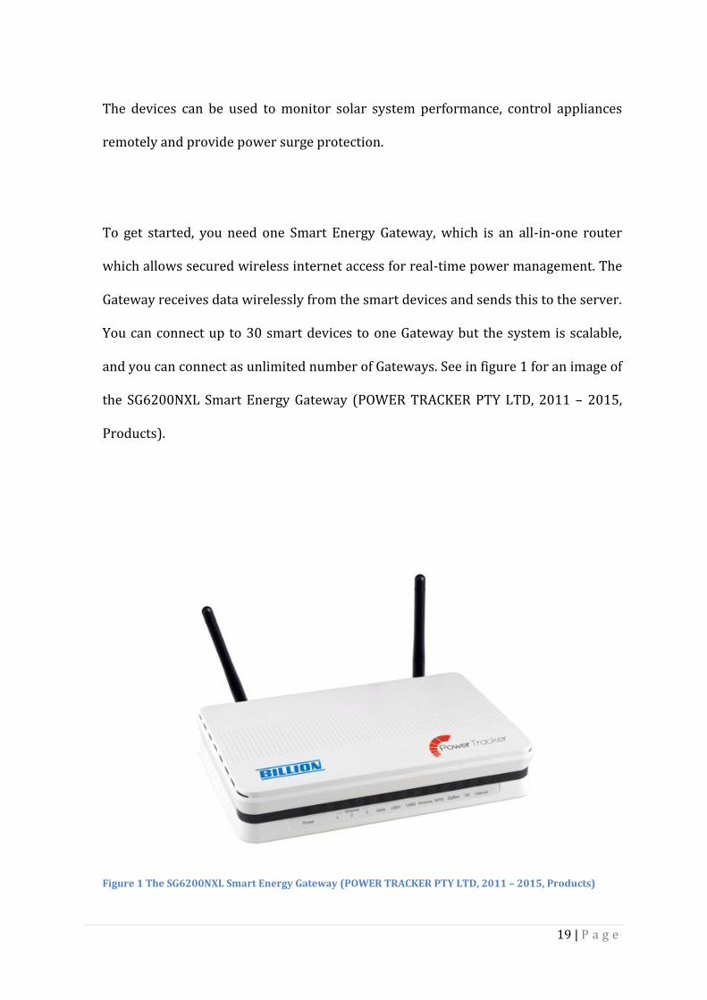
To get started, you need one Smart Energy Gateway, which is an all-in-one router
which allows secured wireless internet access for real-time power management. The
Gateway receives data wirelessly from the smart devices and sends this to the server.
You can connect up to 30 smart devices to one Gateway but the system is scalable,
and you can connect as unlimited number of Gateways. See in figure 1 for an image of
the SG6200NXL Smart Energy Gateway (POWER TRACKER PTY LTD, 2011 – 2015,
Products).
Figure 1 The SG6200NXL Smart Energy Gateway (POWER TRACKER PTY LTD, 2011 – 2015, Products)

20 | P a g e
The Smart Clamp can monitor an entire premise including hard-wired appliances
such as an air conditioner, solar system or lighting. The clamp is installed into the
distribution board to the house. The device can measure electricity in both directions
to determine if a house is consuming or exporting electricity. See figure 2 for a
picture of the SG3010-T3 Smart Clamp.
Figure 2 The SG3010-T3 Smart Clamp (POWER TRACKER PTY LTD, 2011 – 2015, Products)

21 | P a g e
The Smart Appliance can be used to control and measure the power consumption of
individual appliances. These devices provide not only the ability to turn devices on
and off remotely but they also provide power surge protection. It is simply an
extension of the appliance you require to control and measure. See figure 3 for an
image of the SG3010-T1 Smart Appliance.
Figure 3 The SG3010-T1 Smart Appliance (POWER TRACKER PTY LTD, 2011 – 2015, Products)
The data captured by the smart devices were power demand [W] with sampling
interval times of approximately sixty seconds. The data is exported to Microsoft Excel
spreadsheets. The area under the power vs. time graph gives the total energy
consumption of an appliance over the course of a day. See Appendix 9.2.9 for the
calculation of energy consumption from a power curve.

22 | P a g e
4.2 CASE STUDY 1
Power Tracker smart measuring devices were installed in a private house in the
suburb of Ferndale in Perth.
4.2.1 DOMESTIC HOUSEHOLD PROFILE
The Ferndale house is a small three bedroom, one bathroom villa. Power
consumption data was collected over a seven-day period from 20 November to 26
November 2015. Monthly, quarterly and annual usage and cost estimations were
calculated from consumption data collected over this seven-day period. The
household is on the standard Synergy Home Plan (A1).
The weather during that week ranged from mid twenty degrees Celsius to mid thirty
degree Celsius. Sunday the 22nd of November was the hottest day recorded over the
seven-day period when the temperature reached 35.3 degrees Celsius (Elders, 2016).
The weather was atypical to the summer month of November and the load profile
should reflect a typical domestic summer load profile. Seasonal variations in
electricity demand needs to be considered since typically, demand is higher in winter
than in summer.
Five people occupied the premises.
23 | P a g e
4.2.2 APPLIANCES MEASURED
One Gateway (SG6200NXL), three clamps (SG3010-T3) and ten smart devices
(SG3010-T1) were fitted. The three clamps were separately wired into the
distribution board of the house by an electrician. One clamp monitored the main
incomer, the second clamp monitored the air conditioner and the third clamp
monitored the oven.
The smart appliances were connected to the following appliances:
Refrigerator
Washing Machine
Kettle
Dishwasher
Television
Vacuum cleaner
Bedroom 1 bedside lamps (2 lights bulbs)
Bedroom 2 bedside lamp (1 light bulbs)
Bedroom 3 bedside lamp (1 light bulb)
4.2.3 RESULTS
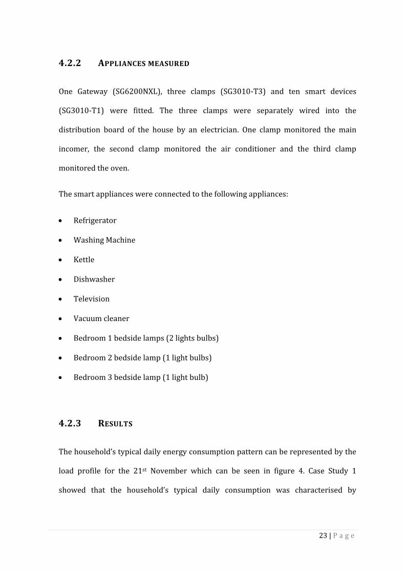
The household’s typical daily energy consumption pattern can be represented by the
load profile for the 21st November which can be seen in figure 4. Case Study 1
showed that the household’s typical daily consumption was characterised by
24 | P a g e
morning cyclic patterns then afternoon peaks followed by similar cyclic patterns as
in the morning and then late night peaks again.
Figure 4 Case Study 1 load profile for 21 November 2015
The morning recurring pattern is caused by the cyclic behaviour of the refrigerator’s
compressor switching on and off; this will be discussed in detail in section 4.2.3.3
below.
The afternoon peaks were caused by using the air conditioner, oven and kettle. Each
appliance’s effect will be discussed in more detail in sections 4.2.3.1, 4.2.3.2 and
4.2.3.5 respectively.
25 | P a g e
The evening peaks can be explained by the functioning of the refrigerator, washing
machine and kettle. This will be discussed in detail in sections 4.2.3.3, 4.2.3.4 and
4.2.3.2 respectively.
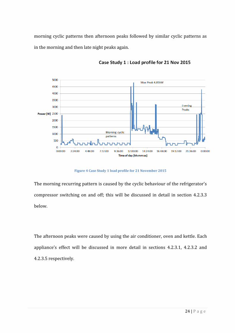
4.2.3.1 AIR CONDITIONER CHARACTERISTICS
The air conditioner (AC) was turned on at 11:45 am on the 21st of November 2015
and remained on for four hours twenty-eight minutes and eighteen seconds. The
power demand of the AC for this day can be viewed in figure 5.
Figure 5 The air conditioner’s power demand for the 21st of Nov 2015
The AC is rated to have a power capacity of 6.2kW and an input power demand of
1.72kW. It is estimated from the power measurements taken that the AC consumes
47.8kWh of energy a month of which 4.44kWh is for stand-by energy. The AC has an
average stand-by power demand of 7.56W and contributes 9.3% of the total monthly
26 | P a g e
AC energy used. The duty cycle of an AC is influenced by factors such as household
activity and extreme weather changes. The duty cycle and stand-by power loads can
be viewed more in detail in Appendix 9.2.2.
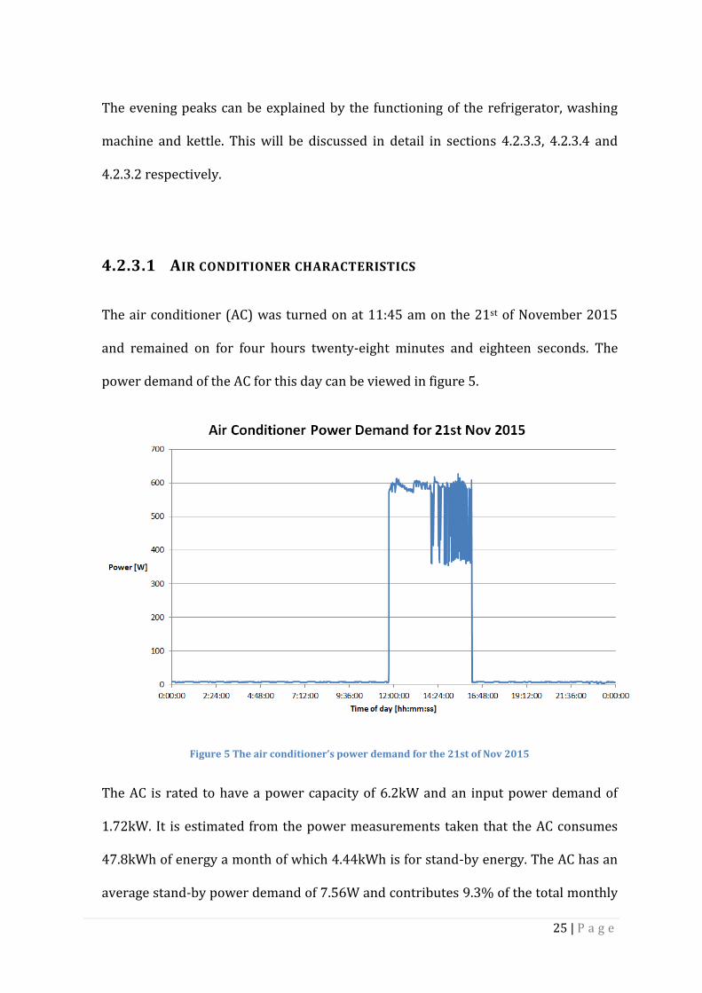
4.2.3.2 OVEN CHARACTERISTICS
On the 21st of November, the oven was used for about fourteen minutes and twelve
seconds at 11:36 am. The power demand of the oven for this day can be viewed in
figure 6.
Figure 6 Oven Power Demand for the 21st Nov 2015
The monthly energy consumption estimated from the power measurements is
3.54kWh.
27 | P a g e
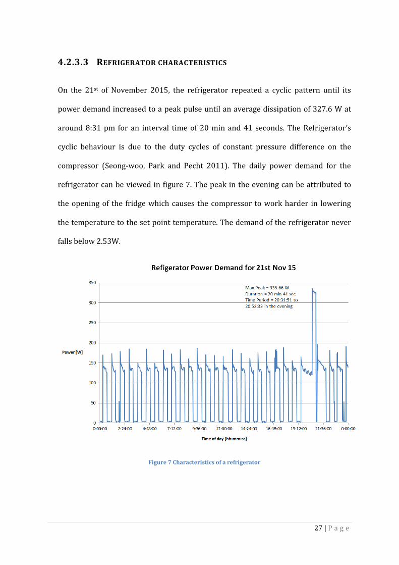
4.2.3.3 REFRIGERATOR CHARACTERISTICS
On the 21st of November 2015, the refrigerator repeated a cyclic pattern until its
power demand increased to a peak pulse until an average dissipation of 327.6 W at
around 8:31 pm for an interval time of 20 min and 41 seconds. The Refrigerator’s
cyclic behaviour is due to the duty cycles of constant pressure difference on the
compressor (Seong-woo, Park and Pecht 2011). The daily power demand for the
refrigerator can be viewed in figure 7. The peak in the evening can be attributed to
the opening of the fridge which causes the compressor to work harder in lowering
the temperature to the set point temperature. The demand of the refrigerator never
falls below 2.53W.
Figure 7 Characteristics of a refrigerator

28 | P a g e
The compressor for this particular refrigerator turns ON for an average of 19 minutes
and 28 seconds and switches OFF for an average 27 minutes and 21 seconds. The
examination of the compressor’s duty cycle can be seen in Appendix 9.2.
From the power measurements taken, the refrigerator is estimated to consume 62.7
kWh of energy per month, which equates to about 752.4kWh of energy over a year.
The refrigerator’s energy rating is 916kWh/year. The disparity indicates that the
actual energy use and running costs will depend on how the appliance is used.
4.2.3.4 WASHING MACHINE CHARACTERISTICS
On the 21st of November 2015, the washing machine was in stand-by mode until it
was used at 10:31 pm for an operation cycle of around 1 hour 27 minutes. See figure
8 for the daily power load for the washing machine.
Figure 8 Washing Machine Power Demand for the 21st of Nov 2015
29 | P a g e
The average stand-by power demand for the washing machine is 0.58 W. The
washing machine consumes an estimated 4.54kWh of energy a month, of which
0.39kWh is for stand-by energy. The stand-by energy works out to be 8.5% of the
total monthly energy used.
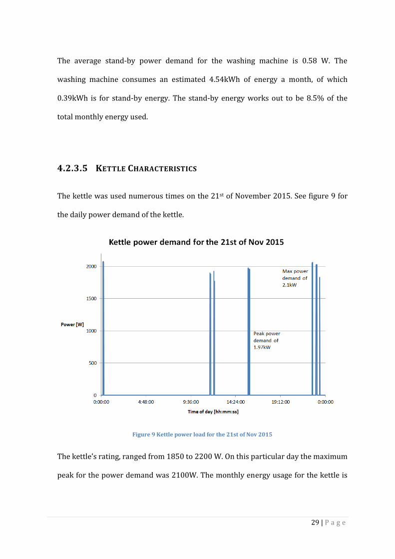
4.2.3.5 KETTLE CHARACTERISTICS
The kettle was used numerous times on the 21st of November 2015. See figure 9 for
the daily power demand of the kettle.
Figure 9 Kettle power load for the 21st of Nov 2015
The kettle’s rating, ranged from 1850 to 2200 W. On this particular day the maximum
peak for the power demand was 2100W. The monthly energy usage for the kettle is

30 | P a g e
estimated to be 15.6kWh. It takes an average of 4 min to boil the kettle. The power
demand is very high for very short time intervals.
4.2.3.6 DISHWASHER CHARACTERISTICS
The dishwasher was not used on the 21st of November 2015 but consumed stand-by
energy. The power demand for the day can be viewed below in figure 10.
Figure 10 The dishwasher power demand for the 21st of Nov 2015
The dishwasher was only used three times during this week. The average stand-by
power demand is 1.6W. The monthly stand-by energy calculates to 1.1kWh, which is
7.4% of the total energy consumption of 14.9kWh. The expected total annual energy
consumption is thus calculated to be 179.1kWh and is half of the rated annual energy
consumption of 400kWh. Once again it proves that the actual energy use of an
31 | P a g e
appliance depends on individual consumer behaviour. The operation of the
dishwasher is investigated in depth in Appendix 9.2.4
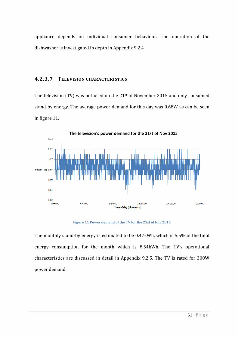
4.2.3.7 TELEVISION CHARACTERISTICS
The television (TV) was not used on the 21st of November 2015 and only consumed
stand-by energy. The average power demand for this day was 0.68W as can be seen
in figure 11.
Figure 11 Power demand of the TV for the 21st of Nov 2015
The monthly stand-by energy is estimated to be 0.47kWh, which is 5.5% of the total
energy consumption for the month which is 8.54kWh. The TV’s operational
characteristics are discussed in detail in Appendix 9.2.5. The TV is rated for 300W
power demand.
32 | P a g e
4.2.3.8 VACUUM CLEANER CHARACTERISTICS
There was no consumption for the vacuum cleaner on the 21st of November 2015.
The vacuum cleaner was only used three times during the week. The vacuum cleaner
is rated at 1600 to 1800 W. For consumption patterns based on this week’s power
measurements, it is estimated that the monthly energy consumption should be
2.27kWh. A closer inspection of the operation of the vacuum cleaner is available in
Appendix 9.2.7.
4.2.3.9 ROOM 1 BEDSIDE LIGHTS CHARACTERISTICS
The bedside lamps were only used three nights during the week when monitoring
took place. There were two bedside lamps and both were investigated with the one
smart appliance. No energy consumption was recorded for the 21st of Nov 2015. The
total energy consumption was calculated to be 0.51Wh based on the consumption
patterns observed during the seven-day observation.
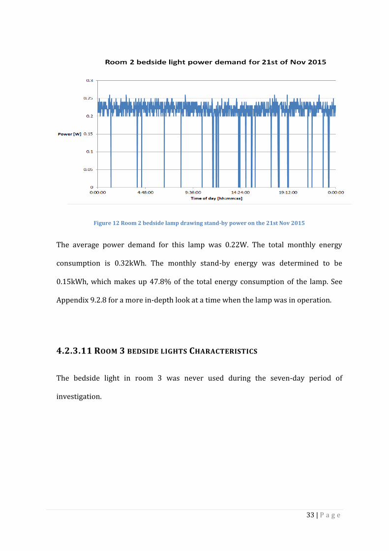
4.2.3.10 ROOM 2 BEDSIDE LIGHTS CHARACTERISTICS
There is only one bedside lamp in room 2 with a light bulb rated at 25W. The bedside
light in room 2 was not used on the 21st of November 2015 and was only used three
nights of the week. However, on this day, the bedside lamp did draw stand-by energy
as seen below in figure 12.
33 | P a g e
Figure 12 Room 2 bedside lamp drawing stand-by power on the 21st Nov 2015
The average power demand for this lamp was 0.22W. The total monthly energy
consumption is 0.32kWh. The monthly stand-by energy was determined to be
0.15kWh, which makes up 47.8% of the total energy consumption of the lamp. See
Appendix 9.2.8 for a more in-depth look at a time when the lamp was in operation.
4.2.3.11 ROOM 3 BEDSIDE LIGHTS CHARACTERISTICS
The bedside light in room 3 was never used during the seven-day period of
investigation.
34 | P a g e
4.2.4 COST ANALYSIS
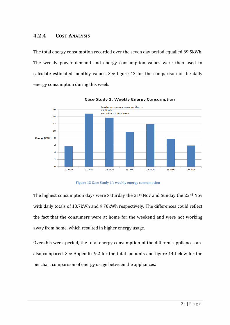
The total energy consumption recorded over the seven day period equalled 69.5kWh.
The weekly power demand and energy consumption values were then used to
calculate estimated monthly values. See figure 13 for the comparison of the daily
energy consumption during this week.
Figure 13 Case Study 1’s weekly energy consumption
The highest consumption days were Saturday the 21st Nov and Sunday the 22nd Nov
with daily totals of 13.7kWh and 9.70kWh respectively. The differences could reflect
the fact that the consumers were at home for the weekend and were not working
away from home, which resulted in higher energy usage.
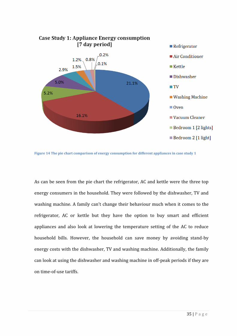
Over this week period, the total energy consumption of the different appliances are
also compared. See Appendix 9.2 for the total amounts and figure 14 below for the
pie chart comparison of energy usage between the appliances.
35 | P a g e
Figure 14 The pie chart comparison of energy consumption for different appliances in case study 1
As can be seen from the pie chart the refrigerator, AC and kettle were the three top
energy consumers in the household. They were followed by the dishwasher, TV and
washing machine. A family can’t change their behaviour much when it comes to the
refrigerator, AC or kettle but they have the option to buy smart and efficient
appliances and also look at lowering the temperature setting of the AC to reduce
household bills. However, the household can save money by avoiding stand-by
energy costs with the dishwasher, TV and washing machine. Additionally, the family
can look at using the dishwasher and washing machine in off-peak periods if they are
on time-of-use tariffs.
36 | P a g e
To investigate whether avoiding stand-by energy and changing consumer behaviour
will lead to savings for a residential household, a more detailed cost analysis was
done using real-time data accumulated with different Synergy residential pricing
schemes. The family in case study 1 is on the Synergy Home Plan (A1) tariff. The
Synergy bill was received for the supply period 10 November 2015 to 11 January
2016 (63 days). The total units used were 940 which resulted in a total payable
amount of $272.20. See Appendix 9.1.4 for the bill.
The percentage error between estimated monthly energy consumption and the real-
time consumption equalled 4.98%. See Appendix 9.2.10.1 for the calculation of the
percentage error.
Cost analyse were then done for four different scenarios by comparing three
different Synergy tariffs: the Home Plan, the Smart Home Plan and the Power Shift
Plan. The first scenario just compared the cost differences between the plans. See
Appendix 9.1.1 for the different Synergy tariff costs and Appendix 9.2.10.1 for the
unit totals and cost calculations. Options 1, 5 and 9 in Table 1 are the results of the
cost comparisons between the different plans.
Secondly, the costs of the various programmes were compared when stand-by
energy was omitted. See option 2, 6 and 10 for the association cost in the table below.
The unit totals and cost calculations can be viewed in Appendix 9.2.10.2
37 | P a g e
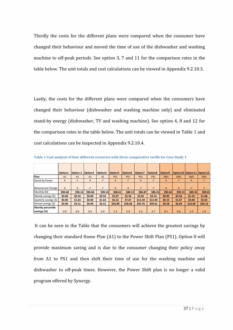
Thirdly the costs for the different plans were compared when the consumer have
changed their behaviour and moved the time of use of the dishwasher and washing
machine to off-peak periods. See option 3, 7 and 11 for the comparison rates in the
table below. The unit totals and cost calculations can be viewed in Appendix 9.2.10.3.
Lastly, the costs for the different plans were compared when the consumers have
changed their behaviour (dishwasher and washing machine only) and eliminated
stand-by energy (dishwasher, TV and washing machine). See option 4, 8 and 12 for
the comparison rates in the table below. The unit totals can be viewed in Table 1 and
cost calculations can be inspected in Appendix 9.2.10.4.
Table 1 Cost analysis of four different scenarios with three comparative tariffs for Case Study 1
It can be seen in the Table that the consumers will achieve the greatest savings by
changing their standard Home Plan (A1) to the Power Shift Plan (PS1). Option 8 will
provide maximum saving and is due to the consumer changing their policy away
from A1 to PS1 and then shift their time of use for the washing machine and
dishwasher to off-peak times. However, the Power Shift plan is no longer a valid
program offered by Synergy.
Option1 Option 2 Option3 Option4 Option5 Option6 Option7 Option8 Option9 Option10 Option11 Option12
Plan A1 A1 A1 A1 PS1 PS1 PS1 PS1 SM1 SM1 SM1 SM1
Stand-by Power
Behavioural Change
Monthly Bill $90.68 $90.14 $90.68 $90.14 $88.61 $88.13 $86.87 $86.55 $90.64 $90.13 $89.35 $89.01
Montly savings [$] $0.00 $0.54 $0.00 $0.54 $2.07 $2.56 $3.81 $4.13 $0.05 $0.56 $1.33 $1.68
Quaterly savings [$] $0.00 $1.63 $0.00 $1.63 $6.22 $7.67 $11.44 $12.40 $0.15 $1.67 $4.00 $5.03
Annual savings [$] $0.00 $6.51 $0.00 $6.51 $24.89 $30.68 $45.76 $49.61 $0.58 $6.69 $16.00 $20.12
Montly percentile
savings [%] 0.0 0.6 0.0 0.6 2.3 2.9 4.3 4.7 0.1 0.6 1.5 1.9
38 | P a g e
4.3 CASE STUDY 2
Power Tracker smart measuring devices were also installed in a private house in the
suburb of Thornlie in Perth.
4.3.1 DOMESTIC HOUSEHOLD PROFILE
The Thornlie dwelling is a four bedroom two bathroom house. Power consumption
data was collected during the period 3 November to 9 November 2015.
The weather during that week ranged from mid twenty degrees Celsius to thirty
degree Celsius. On Tuesday the 9th of November, the hottest day was recorded, when
the temperature reached a maximum of 30.9 degrees Celsius (Elders, 2016).
Five people occupied the premises.
4.3.2 APPLIANCES MEASURED
With Case Study 2, no data could be collected for the main incomer, air conditioner
and electric hot water system. The total household consumption could not be
recorded which meant that an exact daily load profile could not be obtained.
However, it is known that the air conditioner was not used during the observation
time interval but it would have still have drawn stand-by power.
39 | P a g e
One Gateway (SG6200NXL) and ten smart appliances (SG3010-T1) were fitted. The
smart devices were connected to the following machines:
Refrigerator
Washing Machine
Kettle
Television
Microwave Oven
Oven
Hair Dryer
Toaster
Laptop charger
Portable Fridge
4.3.3 RESULTS
Case Study 2’s appliance characteristics for the oven, refrigerator, washing machine,
kettle, television are very similar to that of Case Study 1’s features and won’t be
revisited. See sections 4.2.3.2 to 4.2.3.5 and 4.2.3.7 previously.
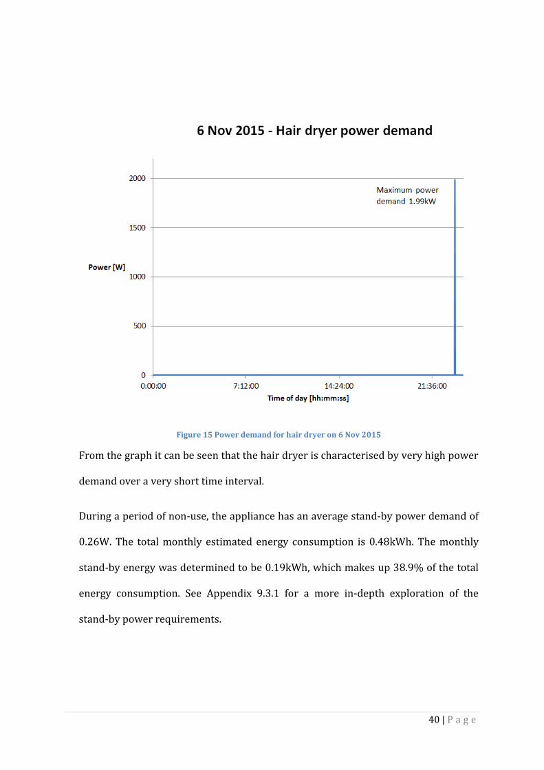
4.3.3.1 HAIR DRYER CHARACTERISTICS
On the 6th of November 2015, the hair dryer was in stand-by mode until it was used
at 11:22 pm and was in operation for around 1 minute. See figure 16 for the daily
load for the hair dryer.
40 | P a g e
Figure 15 Power demand for hair dryer on 6 Nov 2015
From the graph it can be seen that the hair dryer is characterised by very high power
demand over a very short time interval.
During a period of non-use, the appliance has an average stand-by power demand of
0.26W. The total monthly estimated energy consumption is 0.48kWh. The monthly
stand-by energy was determined to be 0.19kWh, which makes up 38.9% of the total
energy consumption. See Appendix 9.3.1 for a more in-depth exploration of the
stand-by power requirements.
41 | P a g e
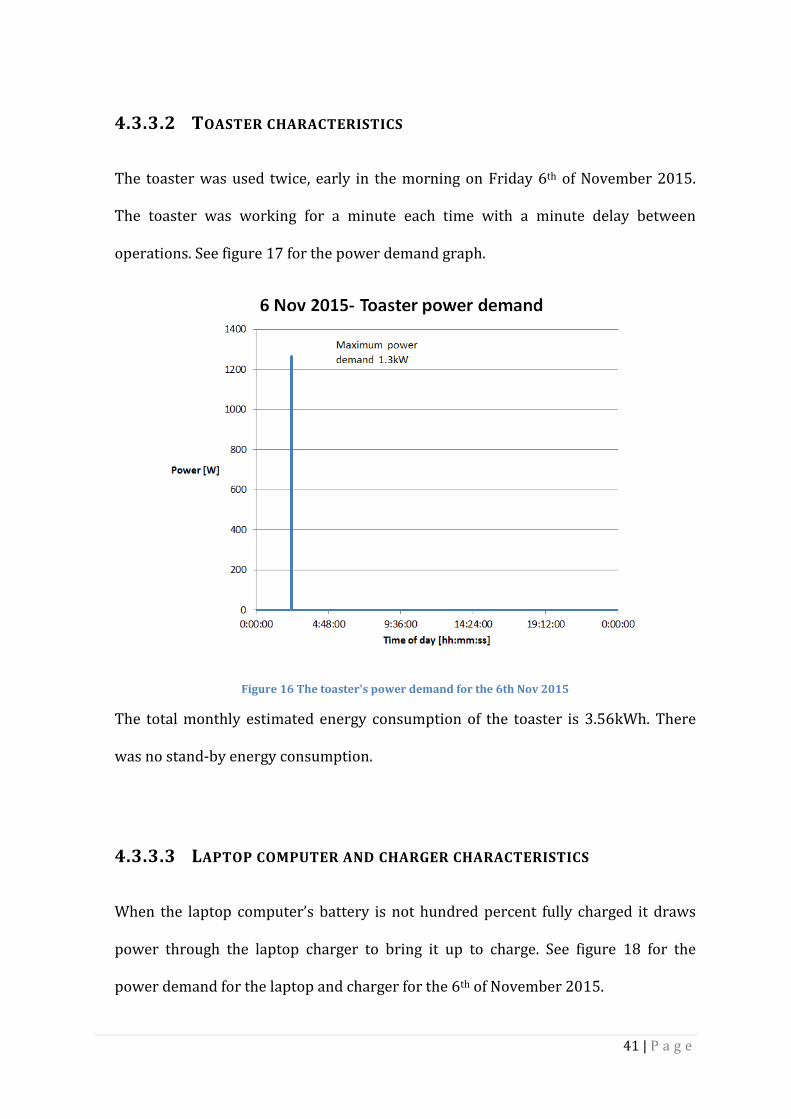
4.3.3.2 TOASTER CHARACTERISTICS
The toaster was used twice, early in the morning on Friday 6th of November 2015.
The toaster was working for a minute each time with a minute delay between
operations. See figure 17 for the power demand graph.
Figure 16 The toaster's power demand for the 6th Nov 2015
The total monthly estimated energy consumption of the toaster is 3.56kWh. There
was no stand-by energy consumption.
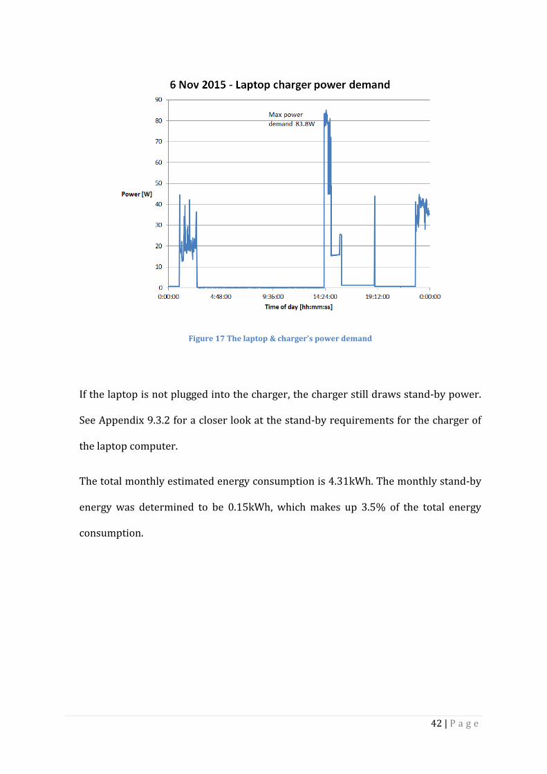
4.3.3.3 LAPTOP COMPUTER AND CHARGER CHARACTERISTICS
When the laptop computer’s battery is not hundred percent fully charged it draws
power through the laptop charger to bring it up to charge. See figure 18 for the
power demand for the laptop and charger for the 6th of November 2015.
42 | P a g e
Figure 17 The laptop & charger’s power demand
If the laptop is not plugged into the charger, the charger still draws stand-by power.
See Appendix 9.3.2 for a closer look at the stand-by requirements for the charger of
the laptop computer.
The total monthly estimated energy consumption is 4.31kWh. The monthly stand-by
energy was determined to be 0.15kWh, which makes up 3.5% of the total energy
consumption.

43 | P a g e
4.3.3.4 PORTABLE FRIDGE CHARACTERISTICS
A portable refrigerator was used as additional freezer space for the household. See
figure 19 for the power demand requirements for the portable refrigerator.
Figure 18 The portable refrigerator's power demand
The compressor for this portable refrigerator turns ON for an average of 3 minutes
and 32 seconds and switches OFF for an average 10 minutes and 57 seconds. The
refrigerator’s demand never falls below 4.67W. From the power measurements
taken, the refrigerator is estimated to consume 11.9kWh of energy per month which
equates to about 143.0kWh of energy over a year.
44 | P a g e
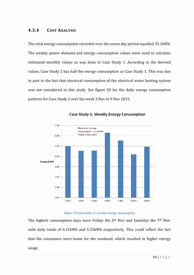
4.3.4 COST ANALYSIS
The total energy consumption recorded over the seven day period equalled 35.1kWh.
The weekly power demand and energy consumption values were used to calculate
estimated monthly values as was done in Case Study 1. According to the derived
values, Case Study 2 has half the energy consumption as Case Study 1. This was due
in part to the fact that electrical consumption of the electrical water heating system
was not considered in this study. See figure 20 for the daily energy consumption
patterns for Case Study 2 over the week 3 Nov to 9 Nov 2015.
Figure 19 Case Study 2’s weekly energy consumption
The highest consumption days were Friday the 6th Nov and Saturday the 7th Nov,
with daily totals of 6.31kWh and 5.53kWh respectively. This could reflect the fact
that the consumers were home for the weekend, which resulted in higher energy
usage.

45 | P a g e
Over this week period, the total energy consumption of the different appliances were
also compared. See Appendix for the total amounts and figure 22 for the pie chart
comparison of energy usage between the appliances.
Figure 20 The energy consumption comparison for different appliances in case study 2
As can be seen from the pie chart, the refrigerator, television and kettle were the
three top energy users in the household. They were followed by the portable
refrigerator, washing machine and the laptop computer and charger. A household
can’t change its behaviour much when it comes to the refrigerator, kettle or a laptop
computer and charger. This household could look at purchasing a smart and efficient
refrigerator with a larger capacity for storage to avoid utilising the portable
refrigerator. The family can also save money by avoiding stand-by energy costs
associated with the hair dryer, television, microwave oven, oven, laptop charger and
washing machine. Additionally, the household can look at using the dishwasher and
washing machine in off-peak periods if they are on time-of-use tariffs.

46 | P a g e
To investigate whether avoiding stand-by energy and changing consumer behaviour
will lead to savings for a residential household, a cost analysis was done using real-
time data accumulated with different Synergy residential pricing schemes. The family
in Case Study 2 was on the Synergy Home Plan (A1) tariff but changed to the time of
use (TOU) Smart Power (SP1) tariff on the 29th October. A meter reading was taken
on the 29th of October and then again on the 12th of November. The family moved out
of the house on the 11th of November. The hot water system, oven and air conditioner
system should have been the only appliances drawing power after the 11th.
The Synergy bill was received for the supply period 16 September 2015 to 12
November 2015 (58 days). The total units used were 1085 of which 277 units were
consumed during the last 15 days when operating under the TOU tariff. The total
payable amount was $376.20 of which $82.23 were under the TOU tariff. See
Attachment 1 for the Synergy bill. Cost analysis for Case Study 2, conduct cost
analysis, using the Synergy rates as seen on the bill for the Home Plan (A1) and Smart
Power (SP1) using.
Cost analysis was then done on four different scenarios by comparing two different
Synergy tariffs; the Home Plan and the Smart Power Plan. The first scenario just
compared the cost differences between the plans. See Appendix 9.1.4 for the Synergy
Smart Power tariff costs and Appendix 9.3.2.1 for the unit totals and cost calculations.
Options 1 and 5 in Table 2 are the results of the cost comparisons between the
different plans.
47 | P a g e
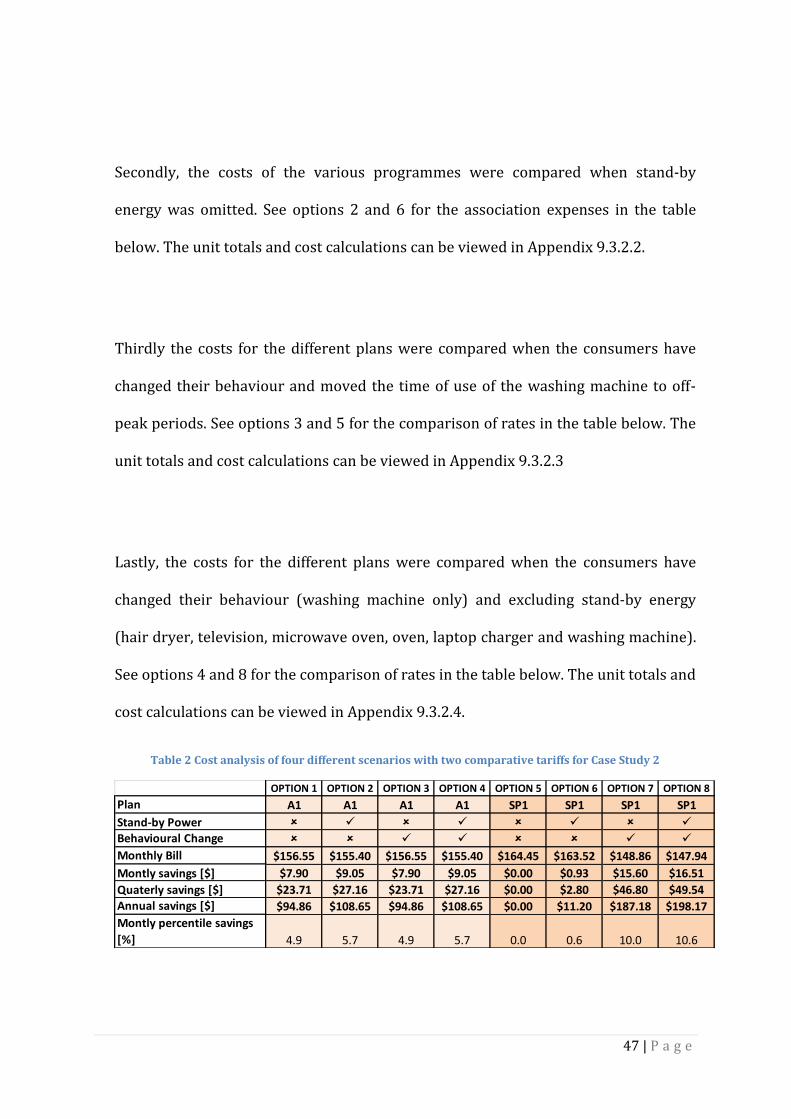
Secondly, the costs of the various programmes were compared when stand-by
energy was omitted. See options 2 and 6 for the association expenses in the table
below. The unit totals and cost calculations can be viewed in Appendix 9.3.2.2.
Thirdly the costs for the different plans were compared when the consumers have
changed their behaviour and moved the time of use of the washing machine to off-
peak periods. See options 3 and 5 for the comparison of rates in the table below. The
unit totals and cost calculations can be viewed in Appendix 9.3.2.3
Lastly, the costs for the different plans were compared when the consumers have
changed their behaviour (washing machine only) and excluding stand-by energy
(hair dryer, television, microwave oven, oven, laptop charger and washing machine).
See options 4 and 8 for the comparison of rates in the table below. The unit totals and
cost calculations can be viewed in Appendix 9.3.2.4.
Table 2 Cost analysis of four different scenarios with two comparative tariffs for Case Study 2
OPTION 1 OPTION 2 OPTION 3 OPTION 4 OPTION 5 OPTION 6 OPTION 7 OPTION 8
Plan A1 A1 A1 A1 SP1 SP1 SP1 SP1
Stand-by Power
Behavioural Change
Monthly Bill $156.55 $155.40 $156.55 $155.40 $164.45 $163.52 $148.86 $147.94
Montly savings [$] $7.90 $9.05 $7.90 $9.05 $0.00 $0.93 $15.60 $16.51
Quaterly savings [$] $23.71 $27.16 $23.71 $27.16 $0.00 $2.80 $46.80 $49.54Annual savings [$] $94.86 $108.65 $94.86 $108.65 $0.00 $11.20 $187.18 $198.17
Montly percentile savings
[%] 4.9 5.7 4.9 5.7 0.0 0.6 10.0 10.6

48 | P a g e
It can be seen from the table that the consumer has paid more for their energy bill. If
they had remained on the standard A1 plan, they would have saved $23.71 on their
Synergy bill. The consumer would have achieved the greatest savings on the Smart
Power programme (SP1) if they changed the time of use for the washing machine
plus switching off appliances which draw power when not in operation. Note, the
Smart Power Plan (SM1) is no longer a valid plan offered by Synergy.
4.4 DATA COLLECTION ISSUES
Several issues arose while collecting data. With Case study 1, the first problem was
that no data was recorded for the microwave due to the device not syncing with the
Gateway. The smart appliance was connected to the microwave but had to be
installed at the back of the built-in fridge in order to reach the power socket. This
could have affected the connectivity of the device to the Gateway.
The second difficulty was that the electrician installed the clamps monitoring the air
conditioner (AC) and the main incomer upside down in the distribution board. This
resulted in negative results/ measurements being documented. However, the issue
was promptly resolved by the Power Tracker IT department who fixed the problem
remotely, circumventing the need for the electrician to attend the site again.
49 | P a g e
The Power Tracker smart devices sample the active and apparent power every
minute. Fluctuations within the sample points might be missed. This is not normally
a problem and will have no effect if the device is stable.
PERIOD data can be downloaded in big data blocks but it has already been processed.
PERIOD data is first broken into 10 minute blocks and then averaged. Those averages
are then combined to create the hourly and daily data. It is desirable that the average
of the ten minute blocks to be as close to the real average as possible, the grouping of
data provides this. The average power is delivered to the customer in hourly periods.
RAW data is sampled minute-by-minute. If it is preferred to see any peaks in power
usage, RAW data needs to be retrieved and not PERIOD data. The issue is that this
provides vast amounts of data and big data blocks can’t be downloaded without some
data corruption. Small data blocks need to be selected, which means it is fairly time
consuming to download the entire required big data block.

50 | P a g e
5 CONCLUSION
The TOU pricing schemes are designed for energy to cost more during peak periods
to encourage the consumer to change their consumption behaviour and use
electricity during cheaper off-peak periods. This will lead either to peak load
reductions or shifting the peak load to a different time periods where the peaks can
be managed to a higher degree. Also, TOU pricing schemes compared to fixed rates
are intended to be a cheaper option if a consumer makes the effort to restructure
their consumption behaviour. It is a clear incentive for consumers to change their
tariff option to a more dynamic option such as a TOU rate.
Consumers will be more likely to select an alternative to fixed tariffs if enabling
technologies are employed. The customer can allow a smart device and/or smart grid
to calculate the optimal consumption pattern which will result in the lowest cost.
IHDs as well as TOU rates contributed to both energy savings and demand response
effects. However, the results suggested that IHD usage has a stronger impact on
energy conservation (impact of 4.3–6.7 percent) than on demand response (1.8
percent).
51 | P a g e
Together with enabling technologies, personalized newsletters and internet/email
communications could encourage and educate consumers further about energy
conservation.
The demand response results from pilot trials and Case Study 1 and 2 indicate that
pricing techniques could implement demand response in the residential sector.
However, differences in success rates with the different rate structures are
dependent on the use of enabling technologies. Results from experiments reveal that
customers do respond to price. However, the magnitude of demand response induced
by dynamic pricing rates varies from modest to substantial. These variations are
likely due to the variations in rates that have been observed in the experiments and
also due to the difference in enabling technologies. Additional changes may also come
from differences in experimental design, demography and other factors that are
difficult to control.
52 | P a g e
6 FUTURE WORK
Future work can focus on broadening the scope of pricing schemes. It can investigate
the effect of combining some of the pricing techniques mentioned in this report, but it
could also look at other methods not investigated in this study. For example, there
are block schemes where customers are rewarded for low energy consumption and
charged large amounts for heavy usage.
Electric hot water systems and lighting contribute significantly to the overall energy
consumption of a household. It might be instructive to do a real-time study looking at
these systems.

53 | P a g e
7 REFERENCES
Australian Energy Market Commission, 2012, Final Report on “2014 Residential
Electricity Price Trends”, 57 -63. [Online]. Available:
http://www.aemc.gov.au/Media/docs/Final-report-1b158644-c634-48bf-bb3a-
e3f204beda30-0.pdf [Accessed: Jan. 9, 2015].
Australian Energy Market Commission, 2014, Final Report on “Power of choice
review- giving consumers options in the way they use electricity”, 26 -27. [Online].
Available: http://www.aemc.gov.au/getattachment/ae5d0665-7300-4a0d-b3b2-
bd42d82cf737/2014-Residential-Electricity-Price-Trends-report.aspx [Accessed:
Jan. 26, 2015].
D. Steen, L. Tuan, and L. Bertling. 2012. Priced-Based Demand-Side Management for
reducing peak demand in electrical Distribution Systems-with examples from
Gothenburg.
Elders, 2016. Weather Home: Perth 3 Month History- November 2015. [Online].
Available:
http://www.eldersweather.com.au/dailysummary.jsp?lt=site&lc=9225&dt=2.
[Accessed: Jan. 20, 2015].

54 | P a g e
Faruqui, Ahmad, Sanem Sergici, and Ahmed Sharif. 2010. The impact of informational
feedback on energy consumption—A survey of the experimental evidence. Energy 35
(4): 1598-608.
Faruqui, Ahmad, and Sanem Sergici. 2010. Household response to dynamic pricing of
electricity: A survey of 15 experiments. Journal of Regulatory Economics 38 (2): 193-
225. (Faruqui and Sergici 2010)
Faruqui, Ahmad, Ryan Hledik, and John Tsoukalis. 2009. The power of dynamic
pricing. The Electricity Journal 22 (3): 42-56.
Mohammadzadeh Rostami, M., and J. Safaee. 2012. Demand response management in
restructured systems.
Muratori, Matteo, Beth-Anne Schuelke-Leech, and Giorgio Rizzoni. 2014. Role of
residential demand response in modern electricity markets. Renewable and
Sustainable Energy Reviews 33 : 546-553
Perth Solar City - Annual Report - 2012. [Online]. Available:
http://perthsolarcity.com.au/resources/Perth_Solar_City_Annual_Report_2012_low_
res.pdf [Accessed: Jan. 20, 2015].
55 | P a g e
POWER TRACKER PTY LTD, 2011 – 2015. Power Tracker Products. [Online].
Available: https://powertracker.com.au/products. [Accessed: Jan. 20, 2015].
Synergy. 2015. Prices & fees. List of tariffs. [Online]. Available:
http://www.synergy.net.au/at_home/list_of_tariffs_res.xhtml. [Accessed: Jan. 25,
2015].
Widergren, S., C. Marinovici, T. Berliner, and A. Graves. 2012. Real-time pricing
demand response in operations.
Woo, Seong-woo, Jungwan Park, and Michael Pecht. 2011. Reliability design and case
study of refrigerator parts subjected to repetitive loads under consumer usage
conditions. Engineering Failure Analysis 18 (7): 1818-30.
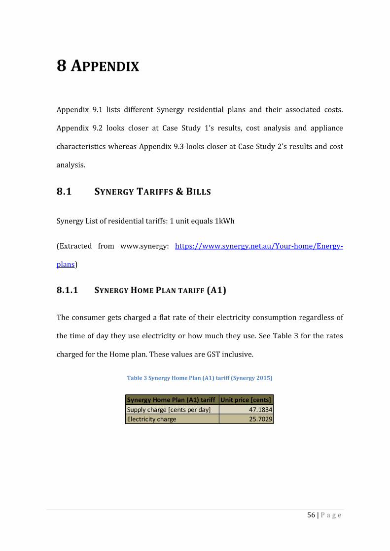
56 | P a g e
8 APPENDIX
Appendix 9.1 lists different Synergy residential plans and their associated costs.
Appendix 9.2 looks closer at Case Study 1’s results, cost analysis and appliance
characteristics whereas Appendix 9.3 looks closer at Case Study 2’s results and cost
analysis.
8.1 SYNERGY TARIFFS & BILLS
Synergy List of residential tariffs: 1 unit equals 1kWh
(Extracted from www.synergy: https://www.synergy.net.au/Your-home/Energy-
plans)
8.1.1 SYNERGY HOME PLAN TARIFF (A1)
The consumer gets charged a flat rate of their electricity consumption regardless of
the time of day they use electricity or how much they use. See Table 3 for the rates
charged for the Home plan. These values are GST inclusive.
Table 3 Synergy Home Plan (A1) tariff (Synergy 2015)
Synergy Home Plan (A1) tariff Unit price [cents]
Supply charge [cents per day] 47.1834
Electricity charge 25.7029
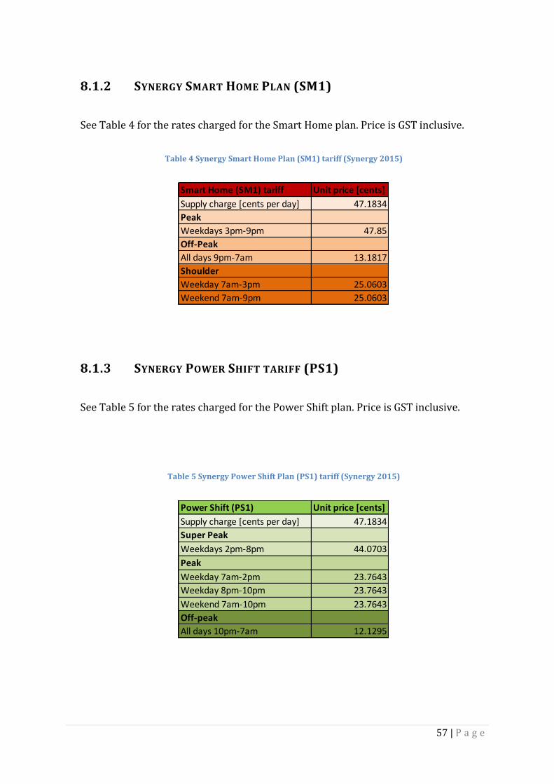
57 | P a g e
8.1.2 SYNERGY SMART HOME PLAN (SM1)
See Table 4 for the rates charged for the Smart Home plan. Price is GST inclusive.
Table 4 Synergy Smart Home Plan (SM1) tariff (Synergy 2015)
8.1.3 SYNERGY POWER SHIFT TARIFF (PS1)
See Table 5 for the rates charged for the Power Shift plan. Price is GST inclusive.
Table 5 Synergy Power Shift Plan (PS1) tariff (Synergy 2015)
Smart Home (SM1) tariff Unit price [cents]
Supply charge [cents per day] 47.1834
Peak
Weekdays 3pm-9pm 47.85
Off-Peak
All days 9pm-7am 13.1817
Shoulder
Weekday 7am-3pm 25.0603
Weekend 7am-9pm 25.0603
Power Shift (PS1) Unit price [cents]
Supply charge [cents per day] 47.1834
Super Peak
Weekdays 2pm-8pm 44.0703
Peak
Weekday 7am-2pm 23.7643
Weekday 8pm-10pm 23.7643
Weekend 7am-10pm 23.7643
Off-peak
All days 10pm-7am 12.1295
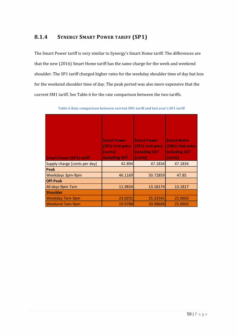
58 | P a g e
8.1.4 SYNERGY SMART POWER TARIFF (SP1)
The Smart Power tariff is very similar to Synergy’s Smart Home tariff. The differences are
that the new (2016) Smart Home tariff has the same charge for the week and weekend
shoulder. The SP1 tariff charged higher rates for the weekday shoulder time of day but less
for the weekend shoulder time of day. The peak period was also more expensive that the
current SM1 tariff. See Table 6 for the rate comparison between the two tariffs.
Table 6 Rate comparison between current SM1 tariff and last year’s SP1 tariff
Smart Power (SP1) tariff
Smart Power
(SP1) Unit price
[cents]
excluding GST
Smart Power
(SP1) Unit price
including GST
[cents]
Smart Home
(SM1) Unit price
including GST
[cents]
Supply charge [cents per day] 42.894 47.1834 47.1834
Peak
Weekdays 3pm-9pm 46.1169 50.72859 47.85
Off-Peak
All days 9pm-7am 11.9834 13.18174 13.1817
Shoulder
Weekday 7am-3pm 23.0231 25.32541 25.0603
Weekend 7am-9pm 19.0788 20.98668 25.0603
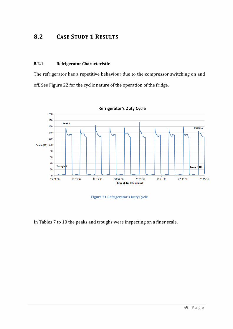
59 | P a g e
8.2 CASE STUDY 1 RESULTS
8.2.1 Refrigerator Characteristic
The refrigerator has a repetitive behaviour due to the compressor switching on and
off. See Figure 22 for the cyclic nature of the operation of the fridge.
Figure 21 Refrigerator's Duty Cycle
In Tables 7 to 10 the peaks and troughs were inspecting on a finer scale.
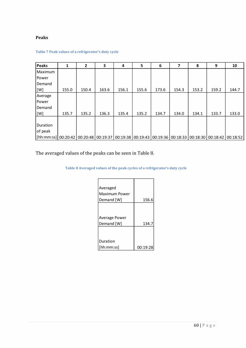
60 | P a g e
Peaks
Table 7 Peak values of a refrigerator’s duty cycle
The averaged values of the peaks can be seen in Table 8.
Table 8 Averaged values of the peak cycles of a refrigerator’s duty cycle
Peaks 1 2 3 4 5 6 7 8 9 10
Maximum
Power
Demand
[W] 155.0 150.4 163.6 156.1 155.6 173.6 154.3 153.2 159.2 144.7
Average
Power
Demand
[W] 135.7 135.2 136.3 135.4 135.2 134.7 134.0 134.1 133.7 133.0
Duration
of peak
[hh:mm:ss] 00:20:42 00:20:48 00:19:37 00:19:38 00:19:43 00:19:36 00:18:33 00:18:30 00:18:42 00:18:52
Averaged
Maximum Power
Demand [W] 156.6
Average Power
Demand [W] 134.7
Duration
[hh:mm:ss] 00:19:28
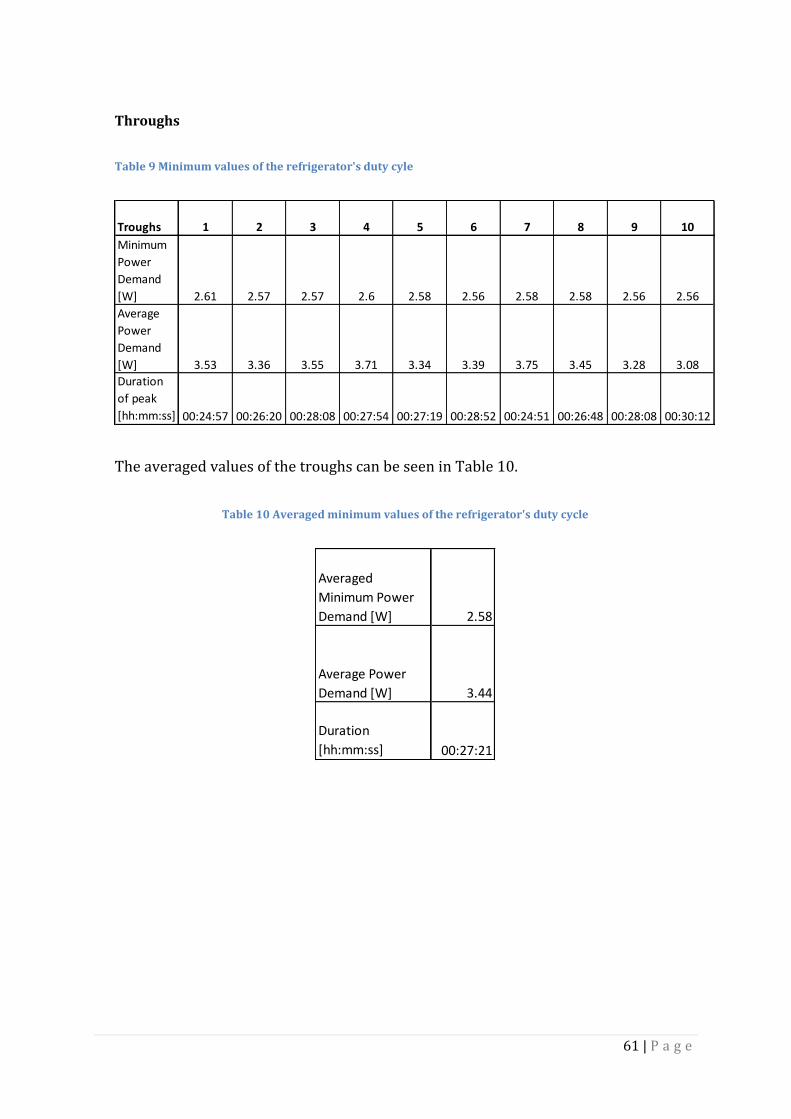
61 | P a g e
Throughs
Table 9 Minimum values of the refrigerator's duty cyle
The averaged values of the troughs can be seen in Table 10.
Table 10 Averaged minimum values of the refrigerator's duty cycle
Troughs 1 2 3 4 5 6 7 8 9 10
Minimum
Power
Demand
[W] 2.61 2.57 2.57 2.6 2.58 2.56 2.58 2.58 2.56 2.56
Average
Power
Demand
[W] 3.53 3.36 3.55 3.71 3.34 3.39 3.75 3.45 3.28 3.08
Duration
of peak
[hh:mm:ss] 00:24:57 00:26:20 00:28:08 00:27:54 00:27:19 00:28:52 00:24:51 00:26:48 00:28:08 00:30:12
Averaged
Minimum Power
Demand [W] 2.58
Average Power
Demand [W] 3.44
Duration
[hh:mm:ss] 00:27:21
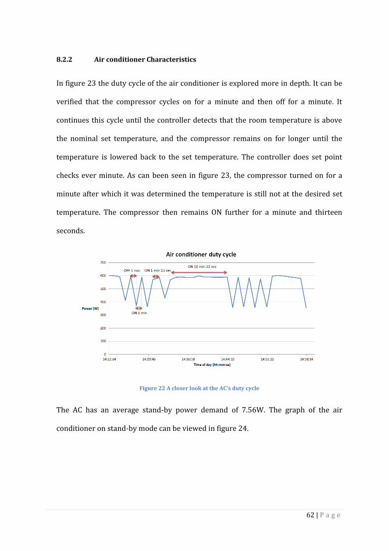
62 | P a g e
8.2.2 Air conditioner Characteristics
In figure 23 the duty cycle of the air conditioner is explored more in depth. It can be
verified that the compressor cycles on for a minute and then off for a minute. It
continues this cycle until the controller detects that the room temperature is above
the nominal set temperature, and the compressor remains on for longer until the
temperature is lowered back to the set temperature. The controller does set point
checks ever minute. As can been seen in figure 23, the compressor turned on for a
minute after which it was determined the temperature is still not at the desired set
temperature. The compressor then remains ON further for a minute and thirteen
seconds.
Figure 22 A closer look at the AC's duty cycle
The AC has an average stand-by power demand of 7.56W. The graph of the air
conditioner on stand-by mode can be viewed in figure 24.
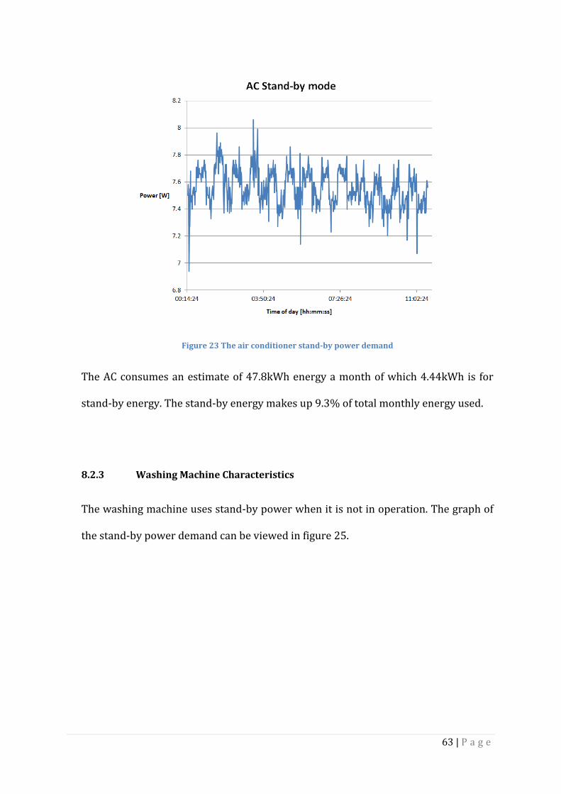
63 | P a g e
Figure 23 The air conditioner stand-by power demand
The AC consumes an estimate of 47.8kWh energy a month of which 4.44kWh is for
stand-by energy. The stand-by energy makes up 9.3% of total monthly energy used.
8.2.3 Washing Machine Characteristics
The washing machine uses stand-by power when it is not in operation. The graph of
the stand-by power demand can be viewed in figure 25.
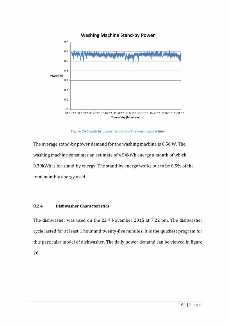
64 | P a g e
Figure 24 Stand- by power demand of the washing machine
The average stand-by power demand for the washing machine is 0.58 W. The
washing machine consumes an estimate of 4.54kWh energy a month of which
0.39kWh is for stand-by energy. The stand-by energy works out to be 8.5% of the
total monthly energy used.
8.2.4 Dishwasher Characteristics
The dishwasher was used on the 22nd November 2015 at 7:22 pm. The dishwasher
cycle lasted for at least 1 hour and twenty-five minutes. It is the quickest program for
this particular model of dishwasher. The daily power demand can be viewed in figure
26.
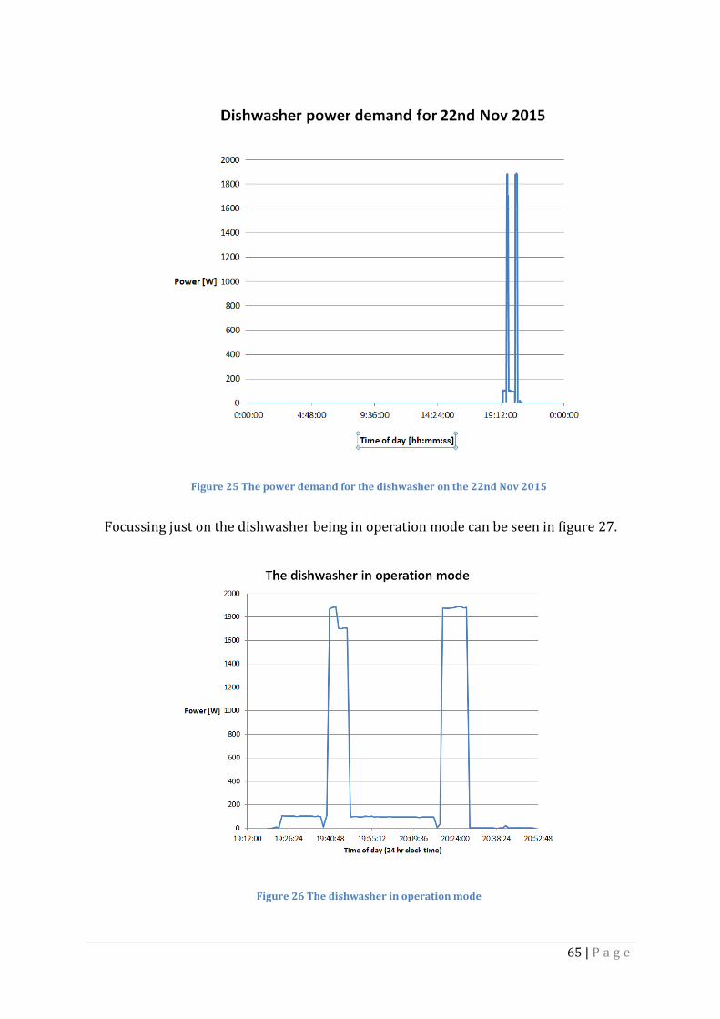
65 | P a g e
Figure 25 The power demand for the dishwasher on the 22nd Nov 2015
Focussing just on the dishwasher being in operation mode can be seen in figure 27.
Figure 26 The dishwasher in operation mode
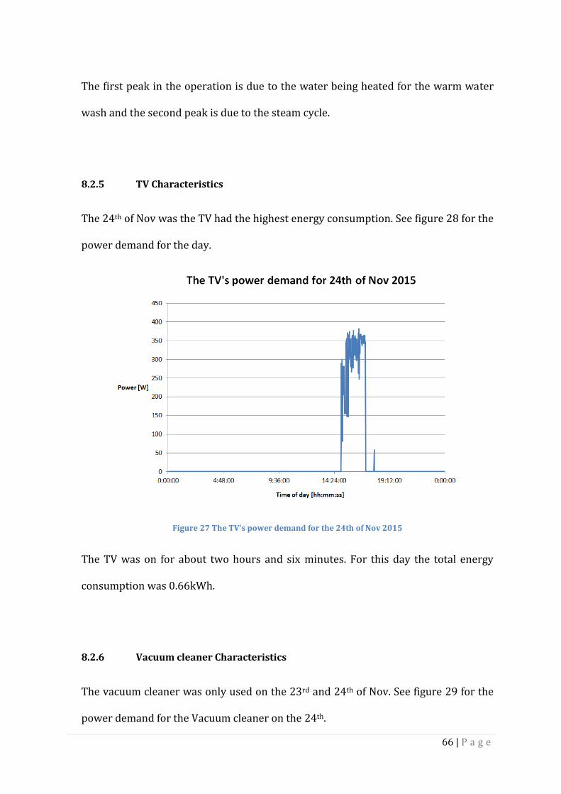
66 | P a g e
The first peak in the operation is due to the water being heated for the warm water
wash and the second peak is due to the steam cycle.
8.2.5 TV Characteristics
The 24th of Nov was the TV had the highest energy consumption. See figure 28 for the
power demand for the day.
Figure 27 The TV's power demand for the 24th of Nov 2015
The TV was on for about two hours and six minutes. For this day the total energy
consumption was 0.66kWh.
8.2.6 Vacuum cleaner Characteristics
The vacuum cleaner was only used on the 23rd and 24th of Nov. See figure 29 for the
power demand for the Vacuum cleaner on the 24th.
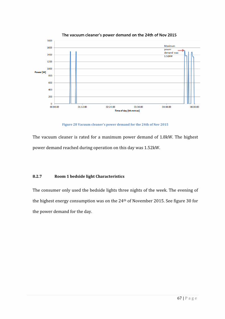
67 | P a g e
Figure 28 Vacuum cleaner's power demand for the 24th of Nov 2015
The vacuum cleaner is rated for a maximum power demand of 1.8kW. The highest
power demand reached during operation on this day was 1.52kW.
8.2.7 Room 1 bedside light Characteristics
The consumer only used the bedside lights three nights of the week. The evening of
the highest energy consumption was on the 24th of November 2015. See figure 30 for
the power demand for the day.
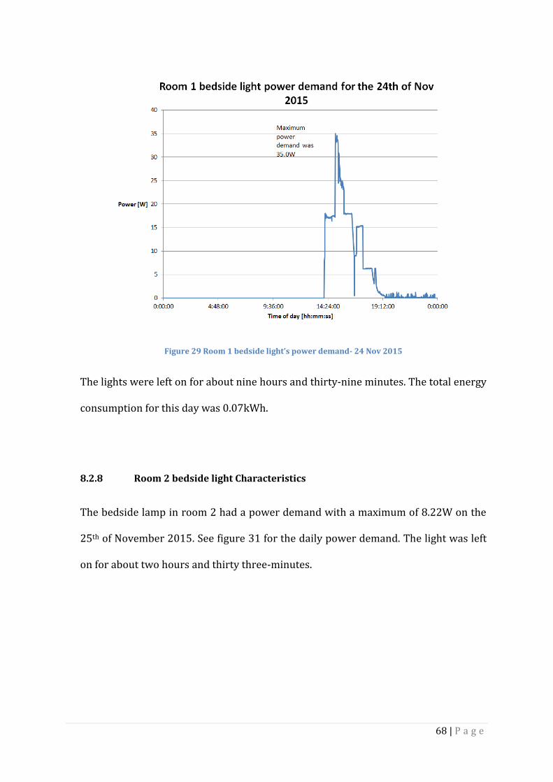
68 | P a g e
Figure 29 Room 1 bedside light’s power demand- 24 Nov 2015
The lights were left on for about nine hours and thirty-nine minutes. The total energy
consumption for this day was 0.07kWh.
8.2.8 Room 2 bedside light Characteristics
The bedside lamp in room 2 had a power demand with a maximum of 8.22W on the
25th of November 2015. See figure 31 for the daily power demand. The light was left
on for about two hours and thirty three-minutes.

69 | P a g e
Figure 30 Room 2 beside lamp power demand – 25 Nov 2015
The daily energy consumption was 0.03kWh.
8.2.9 Energy derived from power curves
The data captured by the smart devices were power demand [W] with sample times
being about sixty seconds. The data was exported to Microsoft Excel spreadsheets.
The area under the power vs. time graph needed to be calculated to determine the
total energy consumption of an appliance over the course of a day. The area under a
curve can be approximated by adding up the areas of geometrical rectangles. Excel
code was written to use the rectangular Riemann sums method to find the area under
the curve. Since the sample times were uneven, a good approximation was found by
finding the midway points between the sample points and adding them to form the
width of the rectangles. See figure 32 for the graph to illustrate how the energy
calculations were performed.
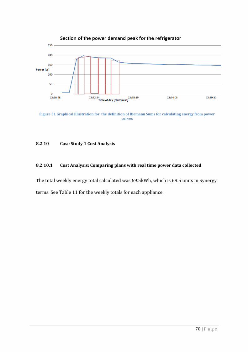
70 | P a g e
Figure 31 Graphical illustration for the definition of Riemann Sums for calculating energy from power curves
8.2.10 Case Study 1 Cost Analysis
8.2.10.1 Cost Analysis: Comparing plans with real time power data collected
The total weekly energy total calculated was 69.5kWh, which is 69.5 units in Synergy
terms. See Table 11 for the weekly totals for each appliance.
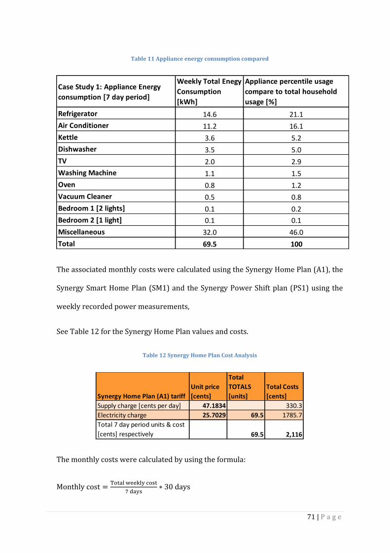
71 | P a g e
Table 11 Appliance energy consumption compared
The associated monthly costs were calculated using the Synergy Home Plan (A1), the
Synergy Smart Home Plan (SM1) and the Synergy Power Shift plan (PS1) using the
weekly recorded power measurements,
See Table 12 for the Synergy Home Plan values and costs.
Table 12 Synergy Home Plan Cost Analysis
The monthly costs were calculated by using the formula:
Case Study 1: Appliance Energy
consumption [7 day period]
Weekly Total Enegy
Consumption
[kWh]
Appliance percentile usage
compare to total household
usage [%]
Refrigerator 14.6 21.1
Air Conditioner 11.2 16.1
Kettle 3.6 5.2
Dishwasher 3.5 5.0
TV 2.0 2.9
Washing Machine 1.1 1.5
Oven 0.8 1.2
Vacuum Cleaner 0.5 0.8
Bedroom 1 [2 lights] 0.1 0.2
Bedroom 2 [1 light] 0.1 0.1
Miscellaneous 32.0 46.0
Total 69.5 100
Synergy Home Plan (A1) tariff
Unit price
[cents]
Total
TOTALS
[units]
Total Costs
[cents]
Supply charge [cents per day] 47.1834 330.3
Electricity charge 25.7029 69.5 1785.7
Total 7 day period units & cost
[cents] respectively 69.5 2,116

72 | P a g e
It equates to a monthly cost of $90.68
See Table 13 for the Synergy Home Plan values and costs.
Table 13 Synergy Smart Home Plan Cost Analysis
It equates to a monthly cost of $90.64
See Table 14 for the Synergy Power Shift Plan values and costs.
Smart Home (SM1) tariff
Unit price
[cents]
Total
TOTALS
[units]
Total Costs
[cents]
Supply charge [cents per day] 47.1834 330.3
Peak
Weekdays 3pm-9pm 47.85 13.2 632.2
Off-Peak
All days 9pm-7am 13.1817 21.7 285.9
Shoulder
Weekday 7am-3pm 25.0603 12.3 307.6
Weekend 7am-9pm 25.0603 22.3 558.9
Total 7 day period units & cost
[cents] respectively 69.5 2,115
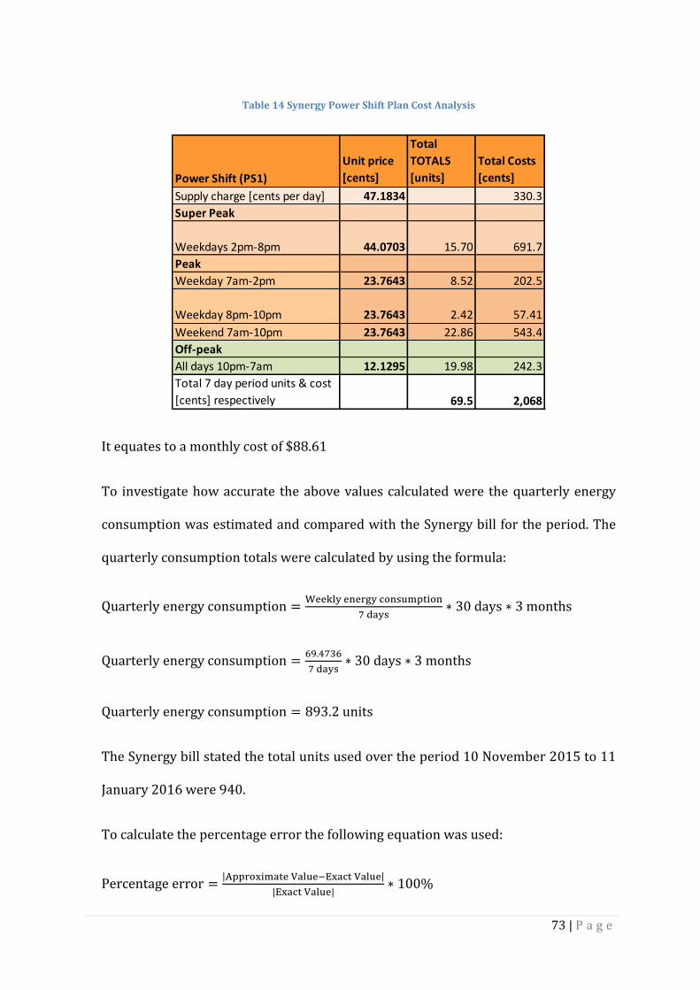
73 | P a g e
Table 14 Synergy Power Shift Plan Cost Analysis
It equates to a monthly cost of $88.61
To investigate how accurate the above values calculated were the quarterly energy
consumption was estimated and compared with the Synergy bill for the period. The
quarterly consumption totals were calculated by using the formula:
The Synergy bill stated the total units used over the period 10 November 2015 to 11
January 2016 were 940.
To calculate the percentage error the following equation was used:
| |
| |
Power Shift (PS1)
Unit price
[cents]
Total
TOTALS
[units]
Total Costs
[cents]
Supply charge [cents per day] 47.1834 330.3
Super Peak
Weekdays 2pm-8pm 44.0703 15.70 691.7
Peak
Weekday 7am-2pm 23.7643 8.52 202.5
Weekday 8pm-10pm 23.7643 2.42 57.41
Weekend 7am-10pm 23.7643 22.86 543.4
Off-peak
All days 10pm-7am 12.1295 19.98 242.3
Total 7 day period units & cost
[cents] respectively 69.5 2,068
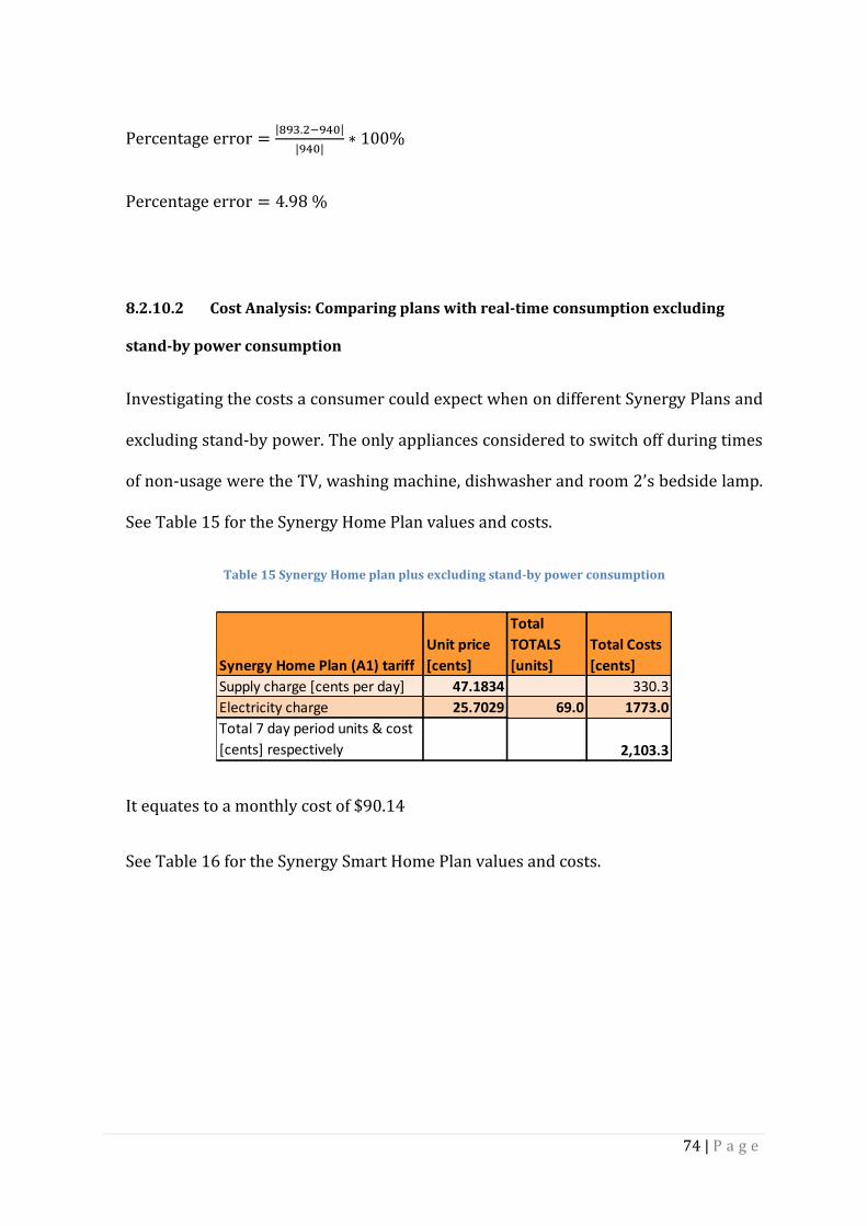
74 | P a g e
| |
| |
8.2.10.2 Cost Analysis: Comparing plans with real-time consumption excluding
stand-by power consumption
Investigating the costs a consumer could expect when on different Synergy Plans and
excluding stand-by power. The only appliances considered to switch off during times
of non-usage were the TV, washing machine, dishwasher and room 2’s bedside lamp.
See Table 15 for the Synergy Home Plan values and costs.
Table 15 Synergy Home plan plus excluding stand-by power consumption
It equates to a monthly cost of $90.14
See Table 16 for the Synergy Smart Home Plan values and costs.
Synergy Home Plan (A1) tariff
Unit price
[cents]
Total
TOTALS
[units]
Total Costs
[cents]
Supply charge [cents per day] 47.1834 330.3
Electricity charge 25.7029 69.0 1773.0
Total 7 day period units & cost
[cents] respectively 2,103.3

75 | P a g e
Table 16 Synergy Smart Home plan plus excluding stand-by power consumption
It equates to a monthly cost of $90.13
See Table 17 for the Synergy Power Shift Plan values and costs.
Table 17 Synergy Power Shift Plan Cost Analysis
It equates to a monthly cost of $88.13
Smart Home (SM1) tariff
Unit price
[cents]
Total
TOTALS
[units]
Total Costs
[cents]
Supply charge [cents per day] 47.1834 330.3
Peak
Weekdays 3pm-9pm 47.85 13.1 628.1
Off-Peak
All days 9pm-7am 13.1817 21.5 283.1
Shoulder
Weekday 7am-3pm 25.0603 12.2 304.7
Weekend 7am-9pm 25.0603 22.2 556.8
Total 7 day period units & cost
[cents] respectively 68.98 2,103.0
Power Shift (PS1)
Unit price
[cents]
Total
TOTALS
[units]
Total Costs
[cents]
Supply charge [cents per day] 47.1834 330.3
Super Peak
Weekdays 2pm-8pm 44.0703 15.61 688.0
Peak
Weekday 7am-2pm 23.7643 8.42 200.0
Weekday 8pm-10pm 23.7643 2.39 56.69
Weekend 7am-10pm 23.7643 22.78 541.3
Off-peak
All days 10pm-7am 12.1295 19.79 240.1
Total 7 day period units & cost
[cents] respectively 69.5 2,056

76 | P a g e
8.2.10.3 Cost Analysis: Comparing plans with real time consumption and changing
consumer behaviour
Investigating the costs a consumer could expect when on different Synergy Plans and
changing consumer behaviour. The only changes in consumer patterns considered
were shifting the time of use for the washing machine and dishwasher to off-peak
periods. See table 18 for the Synergy Home Plan values and costs.
Table 18 Synergy Home plan with optimal changed consumer behaviour
This equates to a monthly cost of $90.68
See Table 19 for the Synergy Smart Home Plan values and costs.
Table 19 Synergy Smart Home plan with optimal changed consumer behaviour
Synergy Home Plan (A1) tariff
Unit price
[cents]
Total
TOTALS
[units]
Total
Costs
[cents]
Supply charge [cents per day] 47.1834 330.3
Electricity charge 25.7029 69.5 1785.7
Total 7 day period units & cost
[cents] respectively 2,116.0
Smart Home (SM1) tariff
Unit price
[cents]
Total
TOTALS
[units]
Total
Costs
[cents]
Supply charge [cents per day] 47.1834 330.3
Peak
Weekdays 3pm-9pm 47.85 12.8 612.8
Off-Peak
All days 9pm-7am 13.1817 23.4 308.8
Shoulder
Weekday 7am-3pm 25.0603 11.6 290.1
Weekend 7am-9pm 25.0603 21.7 542.9
Total 7 day period units & cost
[cents] respectively 69.47 2,084.9
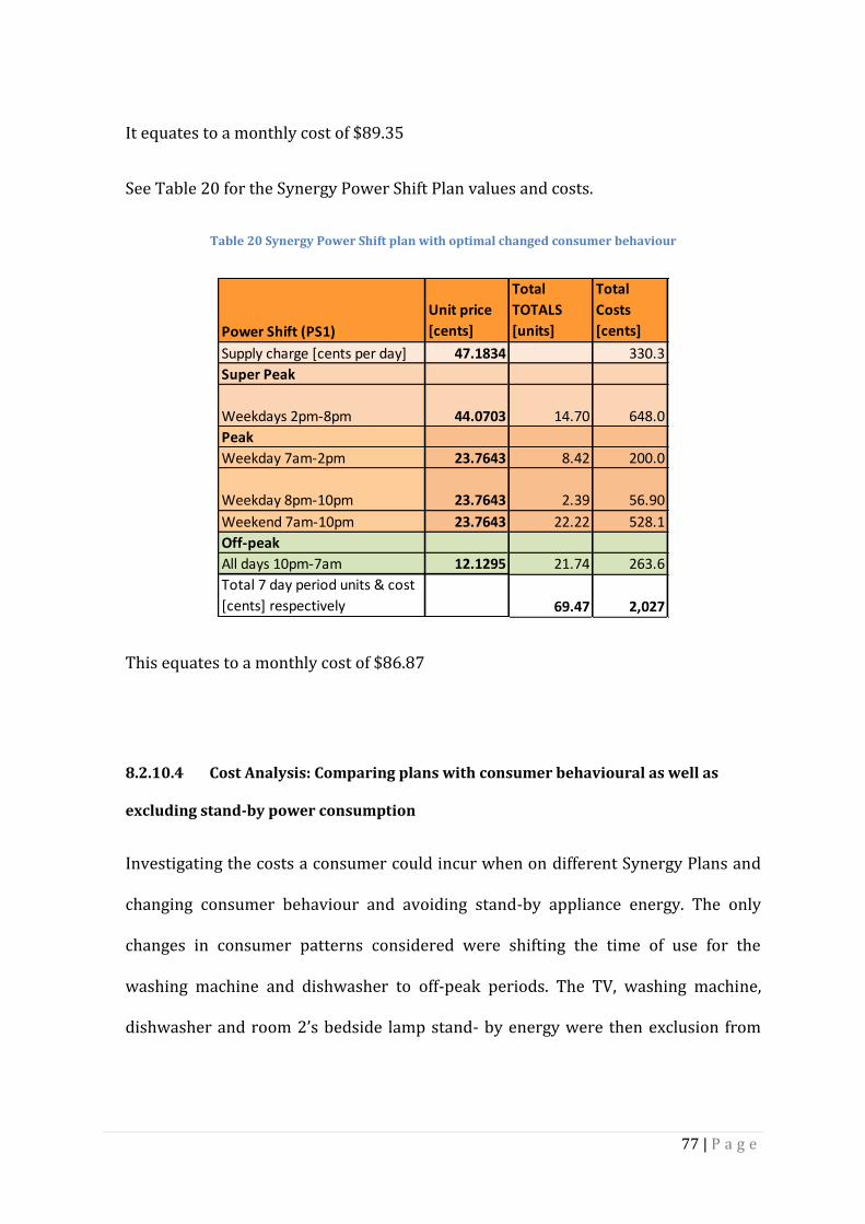
77 | P a g e
It equates to a monthly cost of $89.35
See Table 20 for the Synergy Power Shift Plan values and costs.
Table 20 Synergy Power Shift plan with optimal changed consumer behaviour
This equates to a monthly cost of $86.87
8.2.10.4 Cost Analysis: Comparing plans with consumer behavioural as well as
excluding stand-by power consumption
Investigating the costs a consumer could incur when on different Synergy Plans and
changing consumer behaviour and avoiding stand-by appliance energy. The only
changes in consumer patterns considered were shifting the time of use for the
washing machine and dishwasher to off-peak periods. The TV, washing machine,
dishwasher and room 2’s bedside lamp stand- by energy were then exclusion from
Power Shift (PS1)
Unit price
[cents]
Total
TOTALS
[units]
Total
Costs
[cents]
Supply charge [cents per day] 47.1834 330.3
Super Peak
Weekdays 2pm-8pm 44.0703 14.70 648.0
Peak
Weekday 7am-2pm 23.7643 8.42 200.0
Weekday 8pm-10pm 23.7643 2.39 56.90
Weekend 7am-10pm 23.7643 22.22 528.1
Off-peak
All days 10pm-7am 12.1295 21.74 263.6
Total 7 day period units & cost
[cents] respectively 69.47 2,027
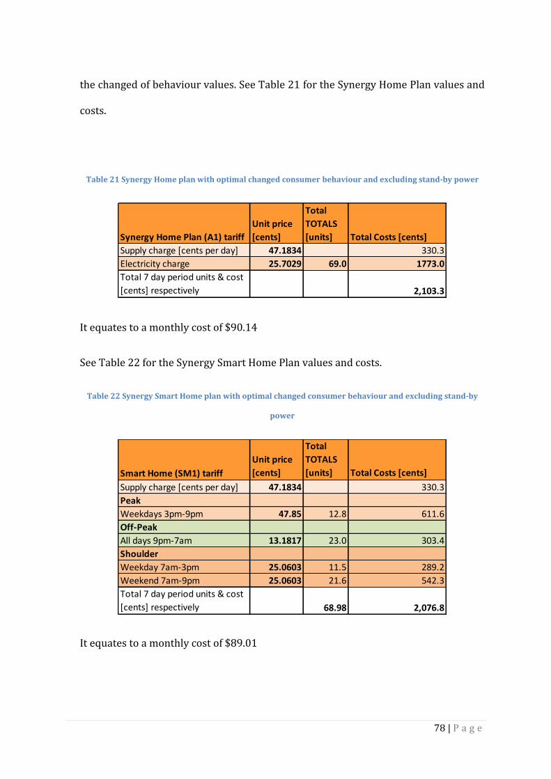
78 | P a g e
the changed of behaviour values. See Table 21 for the Synergy Home Plan values and
costs.
Table 21 Synergy Home plan with optimal changed consumer behaviour and excluding stand-by power
It equates to a monthly cost of $90.14
See Table 22 for the Synergy Smart Home Plan values and costs.
Table 22 Synergy Smart Home plan with optimal changed consumer behaviour and excluding stand-by
power
It equates to a monthly cost of $89.01
Synergy Home Plan (A1) tariff
Unit price
[cents]
Total
TOTALS
[units] Total Costs [cents]
Supply charge [cents per day] 47.1834 330.3
Electricity charge 25.7029 69.0 1773.0
Total 7 day period units & cost
[cents] respectively 2,103.3
Smart Home (SM1) tariff
Unit price
[cents]
Total
TOTALS
[units] Total Costs [cents]
Supply charge [cents per day] 47.1834 330.3
Peak
Weekdays 3pm-9pm 47.85 12.8 611.6
Off-Peak
All days 9pm-7am 13.1817 23.0 303.4
Shoulder
Weekday 7am-3pm 25.0603 11.5 289.2
Weekend 7am-9pm 25.0603 21.6 542.3
Total 7 day period units & cost
[cents] respectively 68.98 2,076.8
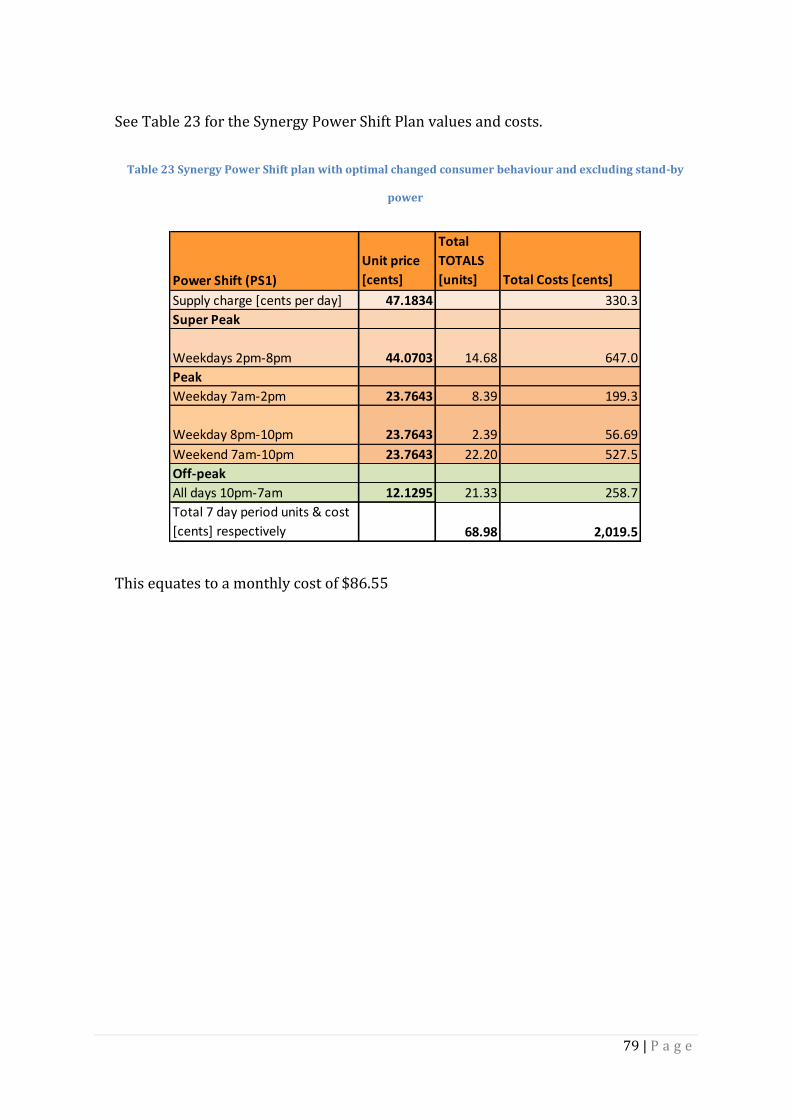
79 | P a g e
See Table 23 for the Synergy Power Shift Plan values and costs.
Table 23 Synergy Power Shift plan with optimal changed consumer behaviour and excluding stand-by
power
This equates to a monthly cost of $86.55
Power Shift (PS1)
Unit price
[cents]
Total
TOTALS
[units] Total Costs [cents]
Supply charge [cents per day] 47.1834 330.3
Super Peak
Weekdays 2pm-8pm 44.0703 14.68 647.0
Peak
Weekday 7am-2pm 23.7643 8.39 199.3
Weekday 8pm-10pm 23.7643 2.39 56.69
Weekend 7am-10pm 23.7643 22.20 527.5
Off-peak
All days 10pm-7am 12.1295 21.33 258.7
Total 7 day period units & cost
[cents] respectively 68.98 2,019.5

80 | P a g e
8.3 CASE STUDY 2 RESULTS
With Case Study 2 no data could be collected for the main incomer, air conditioner
and electric hot water system. The total household consumption could thus not have
been monitored, and an exact daily load profile could not be compiled. However, it is
known that the air conditioner was not used during the observation time interval but
would have still had drawn stand-by power.
8.3.1 Appliance Characteristics
8.3.1.1 Hair Dryer Characteristics
The hair dryer uses stand-by power when it is not in operation. The graph of the
stand-by power demand can be viewed in figure 33.
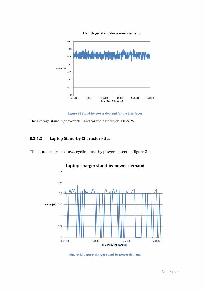
81 | P a g e
Figure 32 Stand-by power demand for the hair dryer
The average stand-by power demand for the hair dryer is 0.26 W.
8.3.1.2 Laptop Stand-by Characteristics
The laptop charger draws cyclic stand-by power as seen in figure 34.
Figure 33 Laptop charger stand-by power demand

82 | P a g e
As seen in the figure, the laptop charger draws power which spikes to predominately
maximums of 0.22 W but then the power demand drops back to 0W demand.
8.3.2 Case Study 1 Cost Analysis
8.3.2.1 Cost Analysis: Comparing plans with real time power data collected
The total weekly energy total calculated was 35.1kWh. See Table 24 for the weekly
totals for each appliance.
Table 24 Appliance energy consumption compared
The last 15 days under the TOU tariff the Synergy bill received by the household
indicated for the total energy consumption was 277 units. To investigate how
accurate the above values calculated were the quarterly energy consumption was
Case Study 2: Appliance Energy
consumption [7 day period]
Weekly Total Enegy
Consumption
[kWh]
Appliance percentile usage
compare to total household
usage [%]
Refrigerator 19.9 56.7
TV 4.7 13.5
Kettle 3.2 9.2
Portable Fridge 2.8 7.9
Washing Machine 1.1 3.1
Laptop charger 1.0 2.9
Toaster 0.8 2.4
Microwave Oven 0.7 2.1
Oven 0.7 1.9
Hair Dryer 0.1 0.3
Total 35.1 100

83 | P a g e
estimated and compared with the Synergy bill for the period. The monthly
consumption totals were calculated by using the formula:
The Synergy bill stated the total units used over the period 29 November 2015 to 12
December 2015 were 277. It calculates be around 554 units of energy consumption
over a month period. It is quite a significant difference. It needs to be noted again that
the water system, air conditioner and other appliances were not measured which
could have significantly added to the total consumption of the house. The real total
energy consumption of 277 units for 15 days will be used in the cost analysis of
changes in consumer behaviour calculated just by measurements taken from the
appliances mentioned in section 4.3.2 above.
Thus using the weekly recorded power measurements the monthly associated costs
was calculated using the Synergy Home Plan (A1) and the Synergy Smart Power Plan
(SP1).
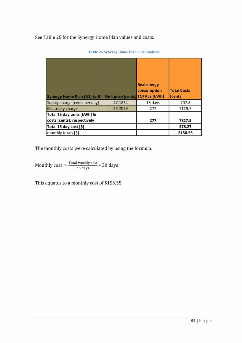
84 | P a g e
See Table 25 for the Synergy Home Plan values and costs.
Table 25 Synergy Home Plan Cost Analysis
The monthly costs were calculated by using the formula:
This equates to a monthly cost of $156.55
Synergy Home Plan (A1) tariff Unit price [cents]
Real energy
consumption
TOTALS [kWh]
Total Costs
[cents]
Supply charge [cents per day] 47.1834 15 days 707.8
Electricity charge 25.7029 277 7119.7
Total 15 day units [kWh] &
costs [cents], respectively 277 7827.5
Total 15 day cost [$] $78.27
monthly totals [$] $156.55

85 | P a g e
See Table 26 for the Synergy Smart Power Plan (SP1) values and costs.
Table 26 Cost analysis with Smart Power tariff
It equates to a monthly cost of $164.45
8.3.2.2 Cost Analysis: Comparing plans with real-time consumption
excluding stand-by power consumption
Investigating the costs a consumer could expect when on different Synergy Plans and
excluding stand-by power. The appliances considered to switch off during times of
non-usage were the TV, washing machine, oven, microwave oven, laptop charger and
the hair dryer. See Table 27 for the Synergy Home Plan values and costs.
Smart Power (SP1) tariff
Smart Power
(SP1) Unit price
[cents]
excluding GST
Smart Power
(SP1) Unit price
including GST
[cents]
Real energy
consumption
TOTALS
[kWh]
Total
Costs
[cents]
Supply charge [cents per day] 42.894 47.1834 15 days 707.8
Peak
Weekdays 3pm-9pm 46.1169 50.72859 64 3246.6
Off-Peak
All days 9pm-7am 11.9834 13.18174 72 949.1
Shoulder
Weekday 7am-3pm 23.0231 25.32541 83 2102.0
Weekend 7am-9pm 19.0788 20.98668 58 1217.2
Total 15 day units [kWh] &
costs [cents], respectively 277 8222.7
Total 15 day cost [$] $75.45 $82.23
monthly totals [$] $164.45
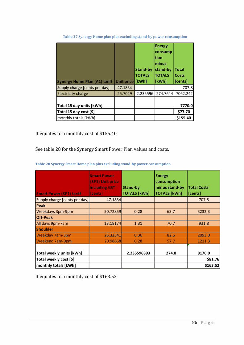
86 | P a g e
Table 27 Synergy Home plan plus excluding stand-by power consumption
It equates to a monthly cost of $155.40
See table 28 for the Synergy Smart Power Plan values and costs.
Table 28 Synergy Smart Home plan plus excluding stand-by power consumption
It equates to a monthly cost of $163.52
Synergy Home Plan (A1) tariff Unit price [cents]
Stand-by
TOTALS
[kWh]
Energy
consump
tion
minus
stand-by
TOTALS
[kWh]
Total
Costs
[cents]
Supply charge [cents per day] 47.1834 707.8
Electricity charge 25.7029 2.235596 274.7644 7062.242
Total 15 day units [kWh] 7770.0
Total 15 day cost [$] $77.70
monthly totals [kWh] $155.40
Smart Power (SP1) tariff
Smart Power
(SP1) Unit price
including GST
[cents]
Stand-by
TOTALS [kWh]
Energy
consumption
minus stand-by
TOTALS [kWh]
Total Costs
[cents]
Supply charge [cents per day] 47.1834 707.8
Peak
Weekdays 3pm-9pm 50.72859 0.28 63.7 3232.3
Off-Peak
All days 9pm-7am 13.18174 1.31 70.7 931.8
Shoulder
Weekday 7am-3pm 25.32541 0.36 82.6 2093.0
Weekend 7am-9pm 20.98668 0.28 57.7 1211.3
Total weekly units [kWh] 2.235596393 274.8 8176.0
Total weekly cost [$] $81.76
monthly totals [kWh] $163.52
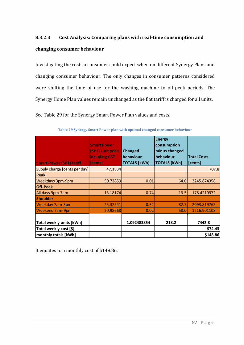
87 | P a g e
8.3.2.3 Cost Analysis: Comparing plans with real-time consumption and
changing consumer behaviour
Investigating the costs a consumer could expect when on different Synergy Plans and
changing consumer behaviour. The only changes in consumer patterns considered
were shifting the time of use for the washing machine to off-peak periods. The
Synergy Home Plan values remain unchanged as the flat tariff is charged for all units.
See Table 29 for the Synergy Smart Power Plan values and costs.
Table 29 Synergy Smart Power plan with optimal changed consumer behaviour
It equates to a monthly cost of $148.86.
Smart Power (SP1) tariff
Smart Power
(SP1) Unit price
including GST
[cents]
Changed
behaviour
TOTALS [kWh]
Energy
consumption
minus changed
behaviour
TOTALS [kWh]
Total Costs
[cents]
Supply charge [cents per day] 47.1834 707.8
Peak
Weekdays 3pm-9pm 50.72859 0.01 64.0 3245.874358
Off-Peak
All days 9pm-7am 13.18174 0.74 13.5 178.4219972
Shoulder
Weekday 7am-3pm 25.32541 0.32 82.7 2093.819765
Weekend 7am-9pm 20.98668 0.02 58.0 1216.901108
Total weekly units [kWh] 1.092483854 218.2 7442.8
Total weekly cost [$] $74.43
monthly totals [kWh] $148.86
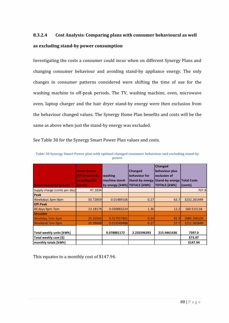
88 | P a g e
8.3.2.4 Cost Analysis: Comparing plans with consumer behavioural as well
as excluding stand-by power consumption
Investigating the costs a consumer could incur when on different Synergy Plans and
changing consumer behaviour and avoiding stand-by appliance energy. The only
changes in consumer patterns considered were shifting the time of use for the
washing machine to off-peak periods. The TV, washing machine, oven, microwave
oven, laptop charger and the hair dryer stand-by energy were then exclusion from
the behaviour changed values. The Synergy Home Plan benefits and costs will be the
same as above when just the stand-by energy was excluded.
See Table 30 for the Synergy Smart Power Plan values and costs.
Table 30 Synergy Smart Power plan with optimal changed consumer behaviour and excluding stand-by power
This equates to a monthly cost of $147.94.
Smart Power (SP1) tariff
Smart Power
(SP1) Unit price
including GST
[cents]
washing
machine stand-
by energy [kWh]
Changed
behaviour for
Stand-by energy
TOTALS [kWh]
Changed
behaviour plus
exclusion of
Stand-by energy
TOTALS [kWh]
Total Costs
[cents]
Supply charge [cents per day] 47.1834 707.8
Peak
Weekdays 3pm-9pm 50.72859 0.01489106 0.27 63.7 3232.261449
Off-Peak
All days 9pm-7am 13.18174 0.030883224 1.36 12.2 160.515118
Shoulder
Weekday 7am-3pm 25.32541 0.017557401 0.34 82.3 2085.206109
Weekend 7am-9pm 20.98668 0.015549488 0.27 57.7 1211.262649
Total weekly units [kWh] 0.078881172 2.235596393 215.9461436 7397.0
Total weekly cost [$] $73.97
monthly totals [kWh] $147.94

89 | P a g e
8.4 CASE STUDY 1& 2 SYNERGY BILLS
Case study 1 is on the Synergy Home Plan(A1) tariff. The Synergy bill was for the
supply period 10 November 2015 to 11 January 2016 (63 days). The total units used
were 940 which resulted in a total payable amount of $272.20.
See Attachment 1 for the Synergy bill.

90 | P a g e
9 ACRONYM GLOSSARY
AC – Air Conditioner
ACT - Air-Conditioner Trial
CT - Current Transformer
DM - Direct Marketing
DR - Demand Response
DRED - Demand Response Enabling Device
HAN - Home Area Network
HW - High Voltage
IHD - In Home Display
kW - Kilowatt
kWh - Kilowatt Hour
KPIs - Key Performance Indicators
LV - Low Voltage
MW - Megawatt
MWh - Megawatt Hour
NMI - National Meter Identifier
NMS - Network Management System

91 | P a g e
PQ - Power Quality
PV - Photovoltaic
RF - Radio Frequency
SWIS - South West Interconnected System
TOU - Time of Use
TV - Television
V - Volts
W - Watt