introduction•my interpretation of “data analysis techniques” is here “doing a

data analysis”

• follow the steps from the beginning (data taking) to the end (the result)

65

‣ the luminosity

‣ the trigger, from the point of view of the analysis

‣ the reconstruction and detector response

‣ the simulation

‣ differential cross-section measurement: a di-jet correction

‣ searches: the H > WW > lvlv

‣ multivariate techniques

thanks to the following people, for interesting discussions, for liberally “borrowing” slides, or both: D. Benedetti, C. Bernet, T. Camporesi, G. Cowan, K. Cranmer, K. Ellis, S. Gennai , A. Ghezzi, A. Hoecker, R. Van Kooten, M. Nguyen, M. Paganoni, M. Pelliccioni, E. Rizvi, R. Rossin ...

the pile-up

66

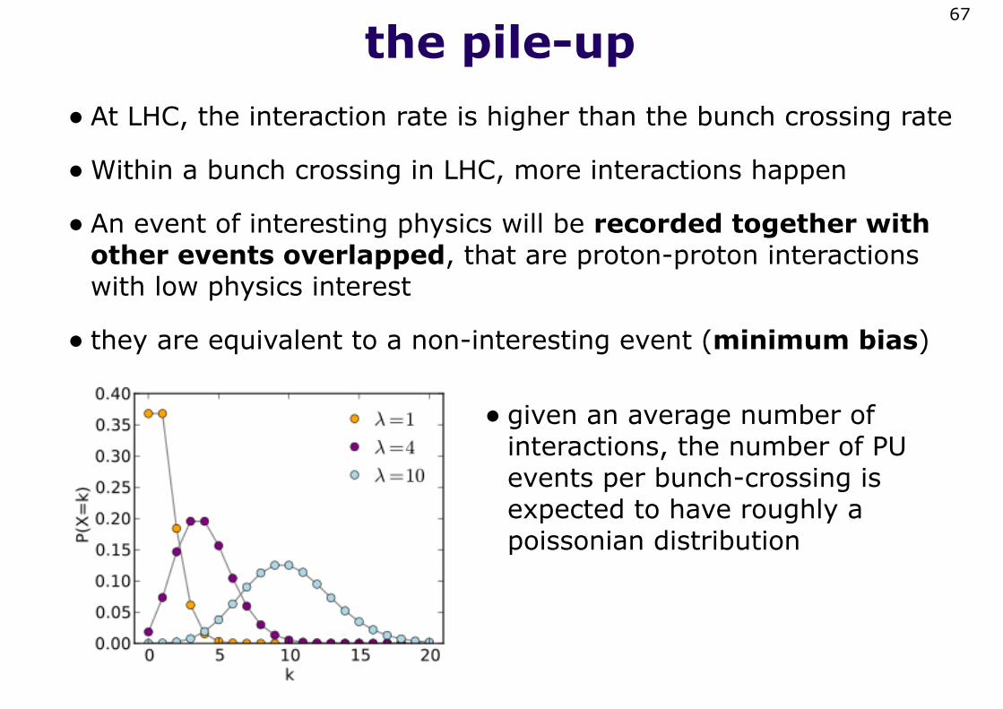
the pile-up• At LHC, the interaction rate is higher than the bunch crossing rate

•Within a bunch crossing in LHC, more interactions happen

• An event of interesting physics will be recorded together with other events overlapped, that are proton-proton interactions with low physics interest

• they are equivalent to a non-interesting event (minimum bias)

67

• given an average number of interactions, the number of PU events per bunch-crossing is expected to have roughly a poissonian distribution

•multiply the luminosity (per bunch) by the minimum bias cross-section (71.3 mb) gets the expected rate per bunch:

• divide by the revolution frequency of a bunch to get the number of PU events:

• calculate average distributions over longer periods, weighting by the luminosities

measure the pile-up68

effects of pile-up

• fill in the detector with deposits:

• jet reconstruction algorithms incorporate pile-up deposits

• lepton isolation cones are filled in with pile-up deposits

• new jets might appear in the event

•more hits in the tracker appear

• the trigger is affected

•MET resolution worsens

• ....

69

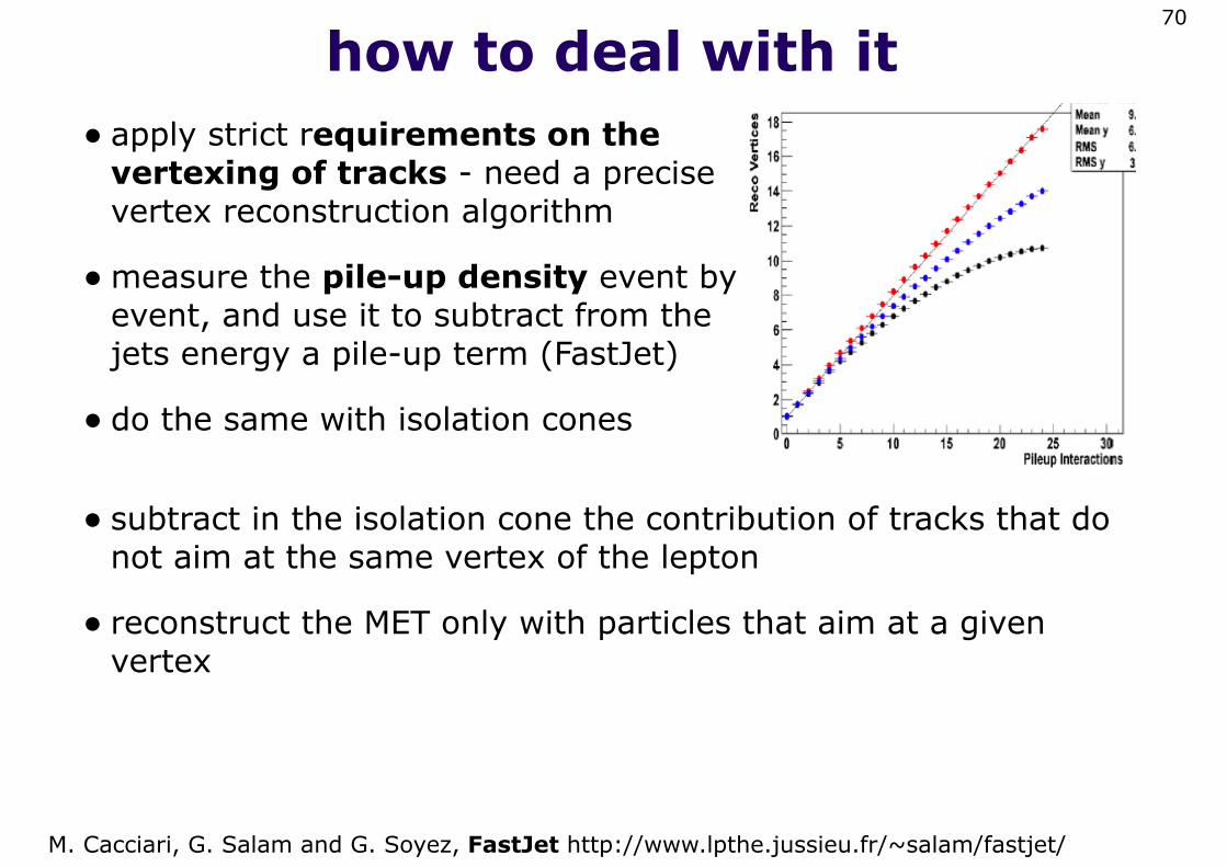
how to deal with it• apply strict requirements on the

vertexing of tracks - need a precise vertex reconstruction algorithm

•measure the pile-up density event by event, and use it to subtract from the jets energy a pile-up term (FastJet)

• do the same with isolation cones

70

• subtract in the isolation cone the contribution of tracks that do not aim at the same vertex of the lepton

• reconstruct the MET only with particles that aim at a given vertex

M. Cacciari, G. Salam and G. Soyez, FastJet http://www.lpthe.jussieu.fr/~salam/fastjet/

H > WW > lvlv

71

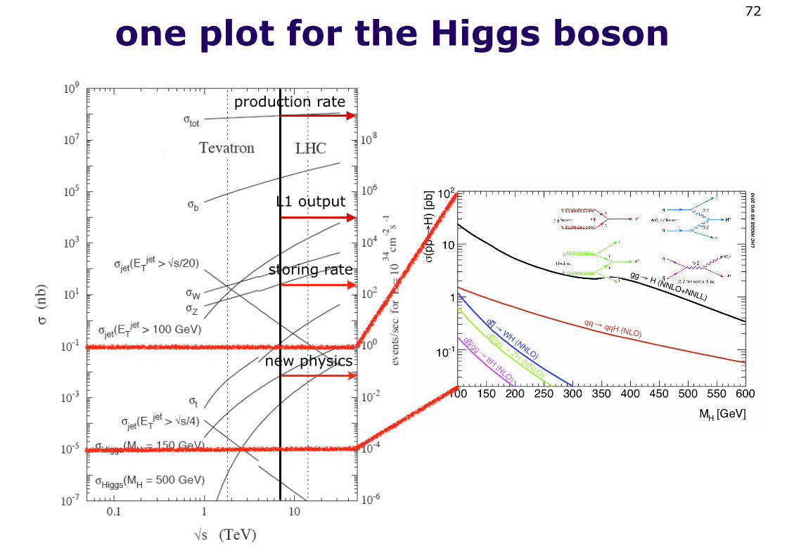
one plot for the Higgs boson72

production rate

L1 output

storing rate

new physics

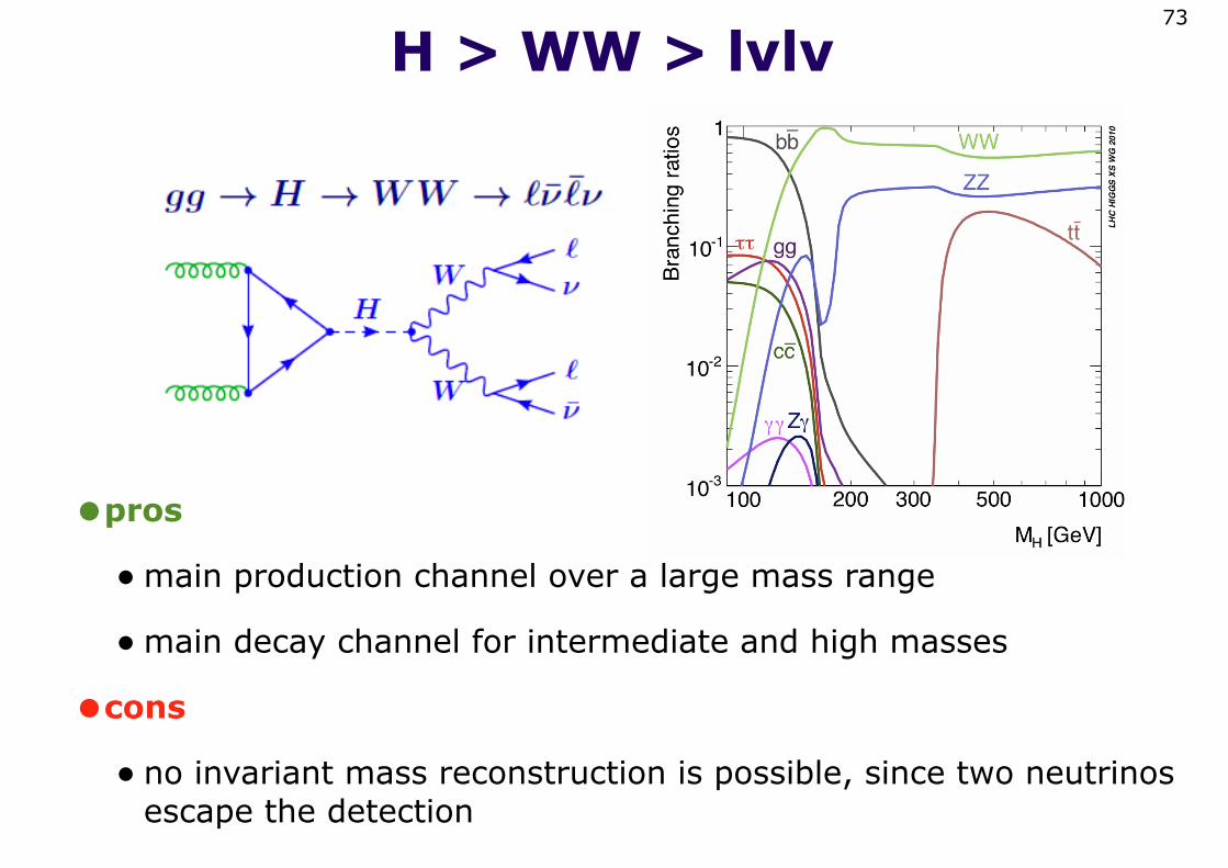
H > WW > lvlv

•pros

•main production channel over a large mass range

•main decay channel for intermediate and high masses

•cons

• no invariant mass reconstruction is possible, since two neutrinos escape the detection

73

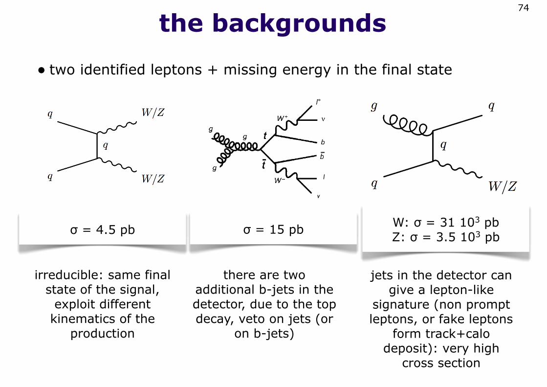
the backgrounds

• two identified leptons + missing energy in the final state

74

irreducible: same final state of the signal,

exploit different kinematics of the

production

there are two additional b-jets in the detector, due to the top decay, veto on jets (or

on b-jets)

jets in the detector can give a lepton-like

signature (non prompt leptons, or fake leptons

form track+calo deposit): very high

cross section

W: σ = 31 103 pbZ: σ = 3.5 103 pbσ = 15 pb

l

v

σ = 4.5 pb

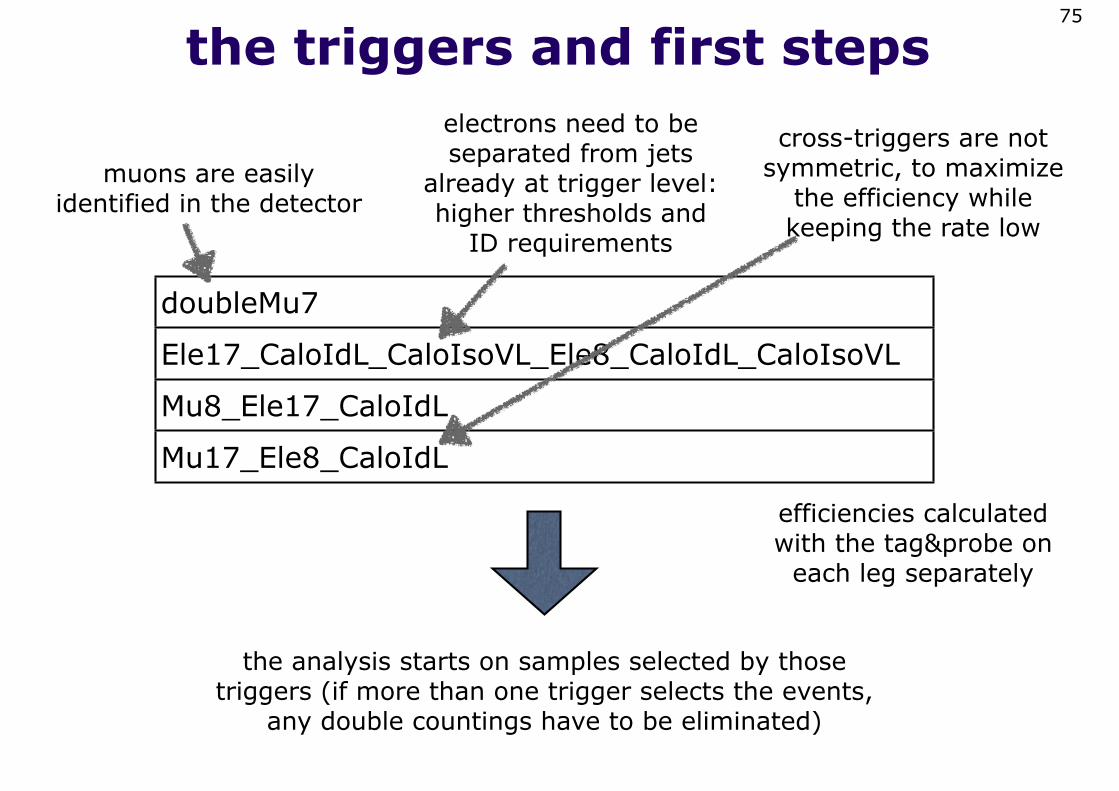
the triggers and first steps75

doubleMu7

Ele17_CaloIdL_CaloIsoVL_Ele8_CaloIdL_CaloIsoVL

Mu8_Ele17_CaloIdL

Mu17_Ele8_CaloIdL

muons are easily identified in the detector

electrons need to be separated from jets

already at trigger level: higher thresholds and

ID requirements

cross-triggers are not symmetric, to maximize

the efficiency while keeping the rate low

the analysis starts on samples selected by those triggers (if more than one trigger selects the events,

any double countings have to be eliminated)

efficiencies calculated with the tag&probe on

each leg separately

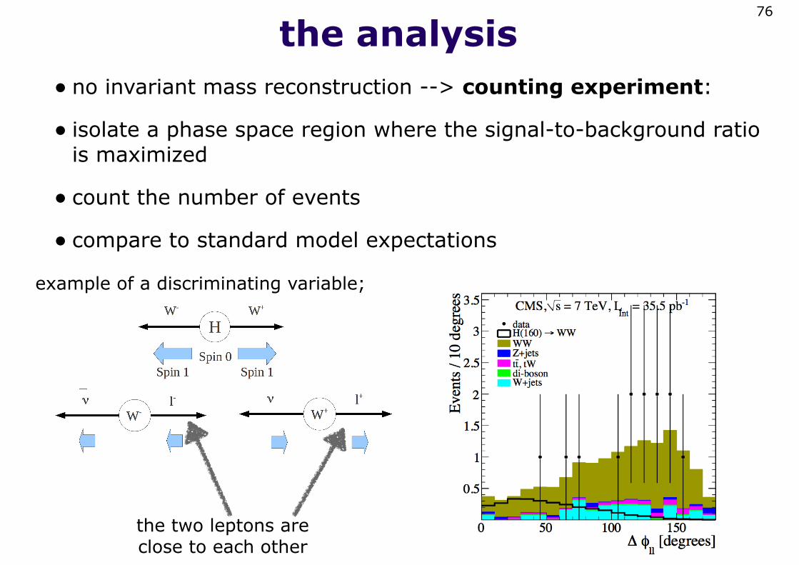
the analysis• no invariant mass reconstruction --> counting experiment:

• isolate a phase space region where the signal-to-background ratio is maximized

• count the number of events

• compare to standard model expectations

76

the two leptons are close to each other

example of a discriminating variable;

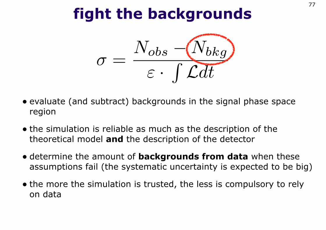
fight the backgrounds

• evaluate (and subtract) backgrounds in the signal phase space region

• the simulation is reliable as much as the description of the theoretical model and the description of the detector

• determine the amount of backgrounds from data when these assumptions fail (the systematic uncertainty is expected to be big)

• the more the simulation is trusted, the less is compulsory to rely on data

77

σ =Nobs −Nbkg

ε ·�Ldt

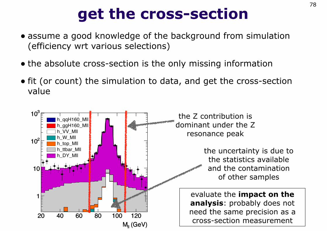
get the cross-section• assume a good knowledge of the background from simulation

(efficiency wrt various selections)

• the absolute cross-section is the only missing information

• fit (or count) the simulation to data, and get the cross-section value

78

the Z contribution is dominant under the Z

resonance peak

(GeV)llM20 40 60 80 100 120

1

10

210

310

(GeV)llM20 40 60 80 100 120

1

10

210

310h_qqH160_Mllh_ggH160_Mllh_VV_Mllh_W_Mllh_top_Mllh_ttbar_Mllh_DY_Mll

the uncertainty is due to the statistics available and the contamination

of other samples

evaluate the impact on the analysis: probably does not need the same precision as a cross-section measurement

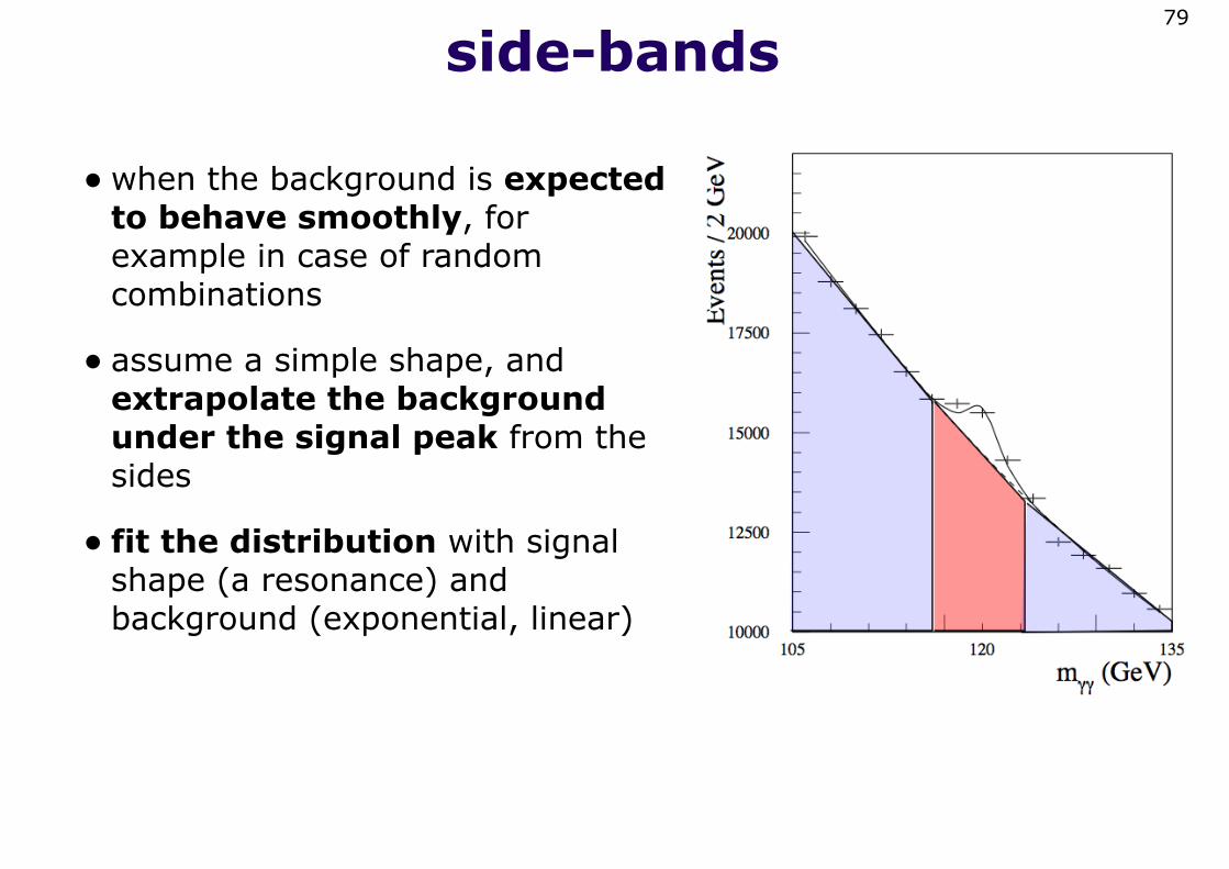
side-bands

•when the background is expected to behave smoothly, for example in case of random combinations

• assume a simple shape, and extrapolate the background under the signal peak from the sides

• fit the distribution with signal shape (a resonance) and background (exponential, linear)

79

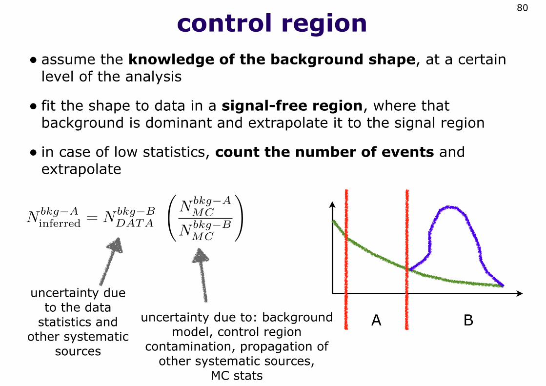
control region• assume the knowledge of the background shape, at a certain

level of the analysis

• fit the shape to data in a signal-free region, where that background is dominant and extrapolate it to the signal region

• in case of low statistics, count the number of events and extrapolate

80

N bkg−Ainferred = N bkg−B

DATA

�N bkg−A

MC

N bkg−BMC

�

uncertainty due to the data

statistics and other systematic

sources

uncertainty due to: background model, control region

contamination, propagation of other systematic sources,

MC stats

A B

ABCD method•measure also the shape from data, to perform the extrapolation

from a control region to a signal region

• assume the bkg pdf to be factorized:

• the correlation check done with simulation is a less stringent requirement than the good description of the shape

• in case of low statistics, count the number of events and extrapolate

81

f bkg(x, y) = f bkgx (x) · f bkg

y (y)

N bkgA = N bkg

B · NbkgC

N bkgD

uncertainty due to the data

statistics and other systematic

sources

uncertainty due to: control region contamination, propagation of other systematic sources

C

A B

D

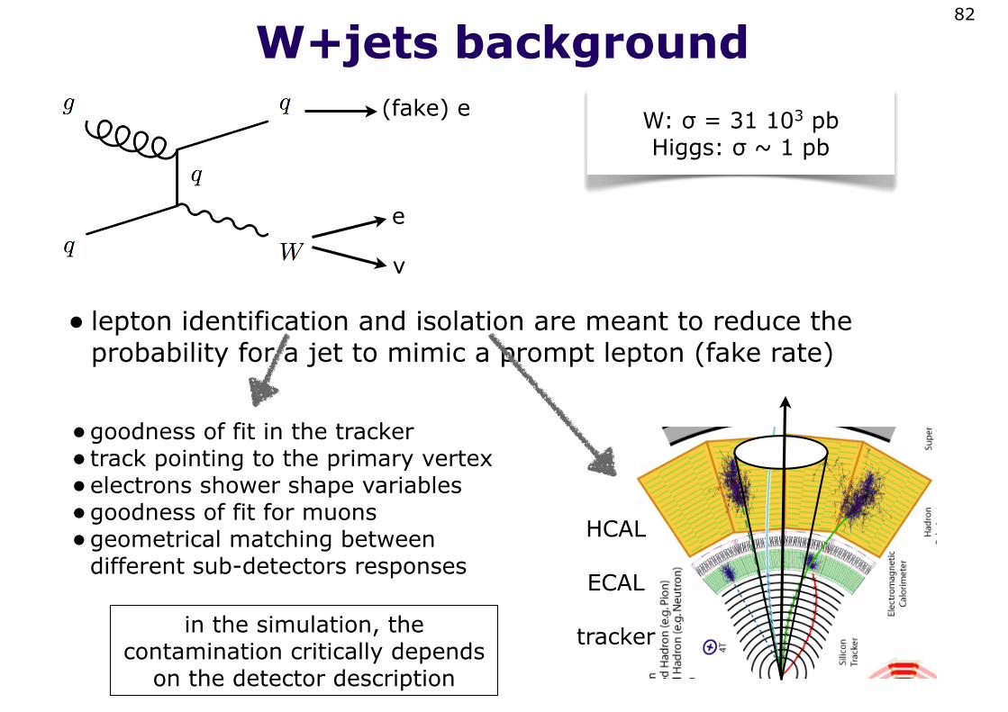
W+jets background

• lepton identification and isolation are meant to reduce the probability for a jet to mimic a prompt lepton (fake rate)

82

W: σ = 31 103 pbHiggs: σ ~ 1 pb

e

v

(fake) e

HCAL

ECAL

tracker

•goodness of fit in the tracker• track pointing to the primary vertex•electrons shower shape variables•goodness of fit for muons•geometrical matching between

different sub-detectors responses

in the simulation, the contamination critically depends

on the detector description

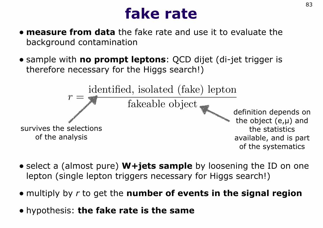
fake rate•measure from data the fake rate and use it to evaluate the

background contamination

• sample with no prompt leptons: QCD dijet (di-jet trigger is therefore necessary for the Higgs search!)

83

r =identified, isolated (fake) lepton

fakeable objectdefinition depends on the object (e,µ) and

the statistics available, and is part of the systematics

survives the selections of the analysis

• select a (almost pure) W+jets sample by loosening the ID on one lepton (single lepton triggers necessary for Higgs search!)

•multiply by r to get the number of events in the signal region

• hypothesis: the fake rate is the same

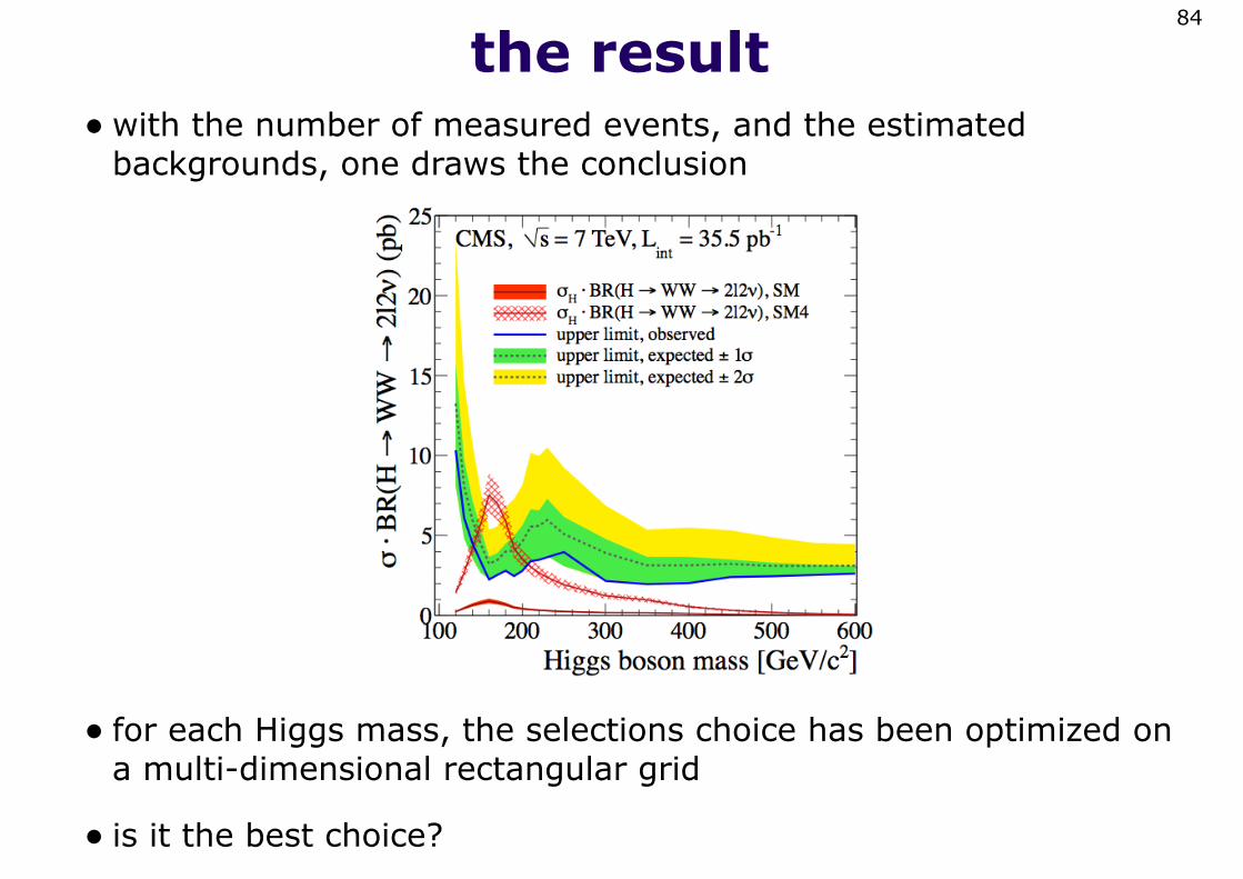
the result•with the number of measured events, and the estimated

backgrounds, one draws the conclusion

84

• for each Higgs mass, the selections choice has been optimized on a multi-dimensional rectangular grid

• is it the best choice?

multi variate techniques

85

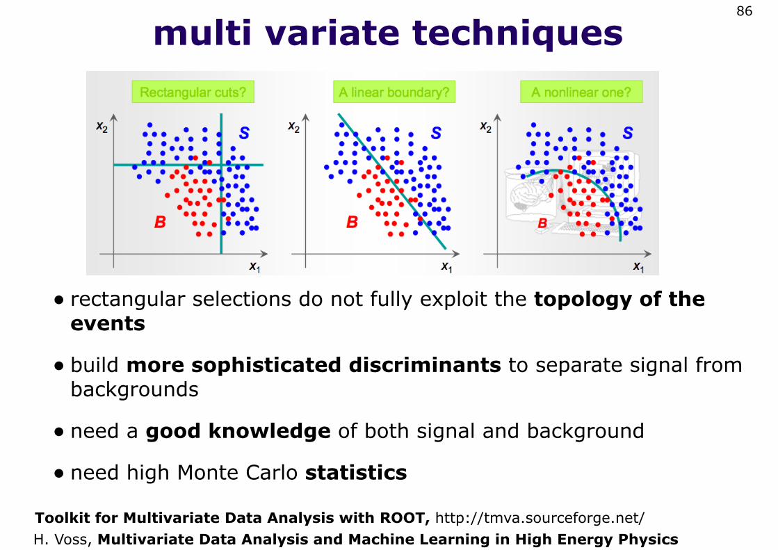
multi variate techniques

• rectangular selections do not fully exploit the topology of the events

• build more sophisticated discriminants to separate signal from backgrounds

• need a good knowledge of both signal and background

• need high Monte Carlo statistics

86

H. Voss, Multivariate Data Analysis and Machine Learning in High Energy PhysicsToolkit for Multivariate Data Analysis with ROOT, http://tmva.sourceforge.net/

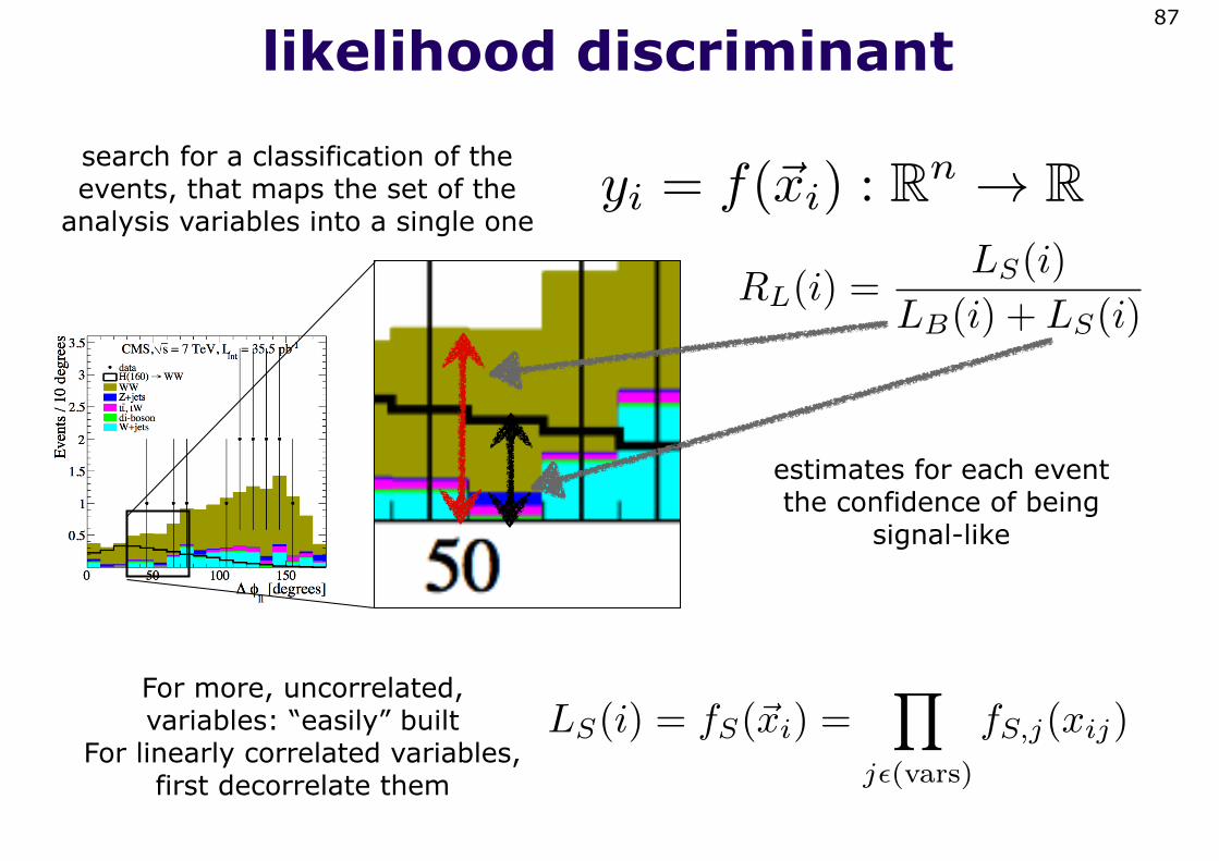
likelihood discriminant87

LS(i) = fS(�xi) =�

j�(vars)

fS,j(xij)

estimates for each event the confidence of being

signal-like

yi = f(�xi) : Rn → Rsearch for a classification of the events, that maps the set of the

analysis variables into a single one

RL(i) =LS(i)

LB(i) + LS(i)

For more, uncorrelated, variables: “easily” built

For linearly correlated variables, first decorrelate them

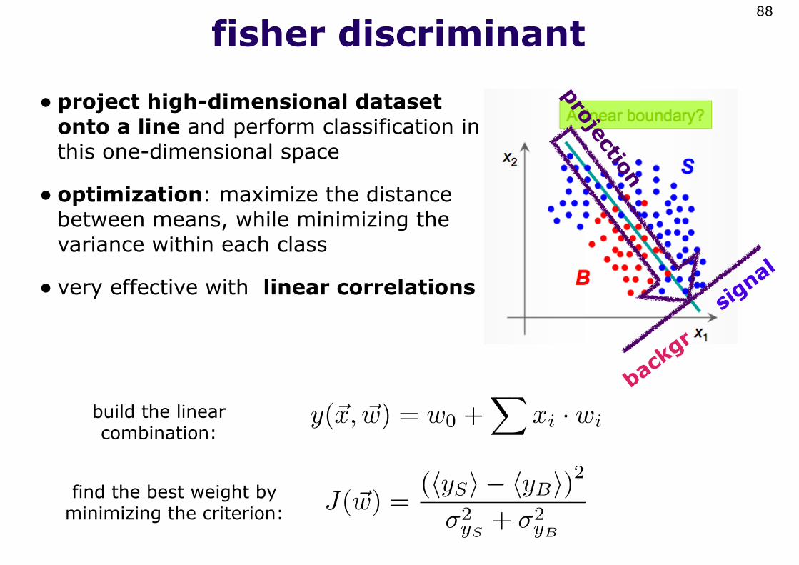
fisher discriminant

• project high-dimensional dataset onto a line and perform classification in this one-dimensional space

• optimization: maximize the distance between means, while minimizing the variance within each class

• very effective with linear correlations

88

J(�w) =(�yS� − �yB�)2

σ2yS

+ σ2yB

signal

backgr

projection

build the linear combination:

y(�x, �w) = w0 +�

xi · wi

find the best weight by minimizing the criterion:

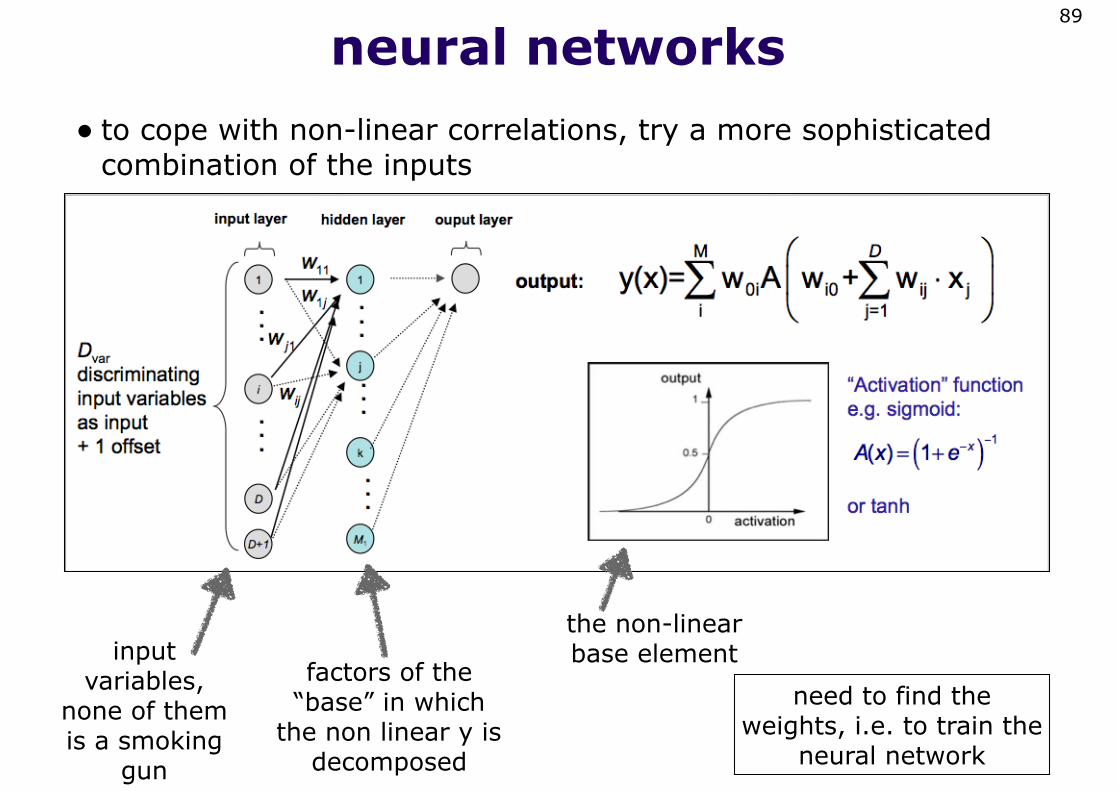
neural networks• to cope with non-linear correlations, try a more sophisticated

combination of the inputs

89

input variables,

none of them is a smoking

gun

factors of the “base” in which

the non linear y is decomposed

the non-linear base element

need to find the weights, i.e. to train the

neural network

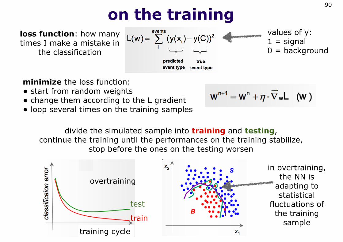
on the training90

loss function: how many times I make a mistake in

the classification

values of y:1 = signal0 = background

minimize the loss function: • start from random weights• change them according to the L gradient• loop several times on the training samples

divide the simulated sample into training and testing, continue the training until the performances on the training stabilize,

stop before the ones on the testing worsen

in overtraining, the NN is

adapting to statistical

fluctuations of the training

sampletraining cycle

overtraining

test

train

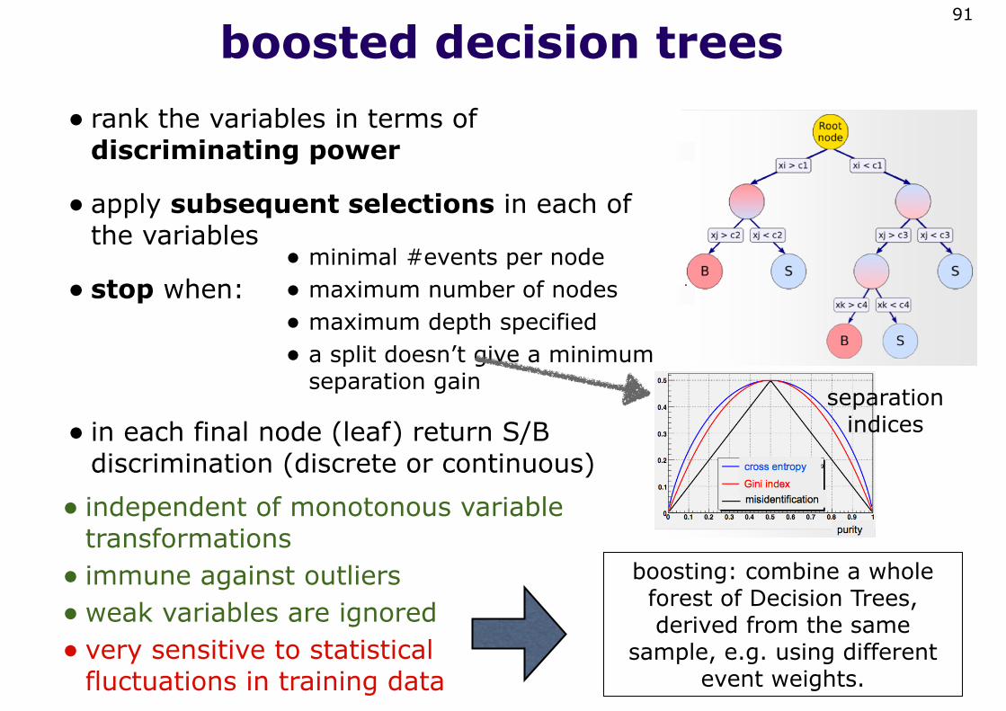
boosted decision trees• rank the variables in terms of

discriminating power

• apply subsequent selections in each of the variables

• stop when:

91

• minimal #events per node• maximum number of nodes• maximum depth specified• a split doesn’t give a minimum

separation gain

• in each final node (leaf) return S/B discrimination (discrete or continuous)

• independent of monotonous variable transformations• immune against outliers•weak variables are ignored• very sensitive to statistical

fluctuations in training data

boosting: combine a whole forest of Decision Trees, derived from the same

sample, e.g. using different event weights.

separation indices

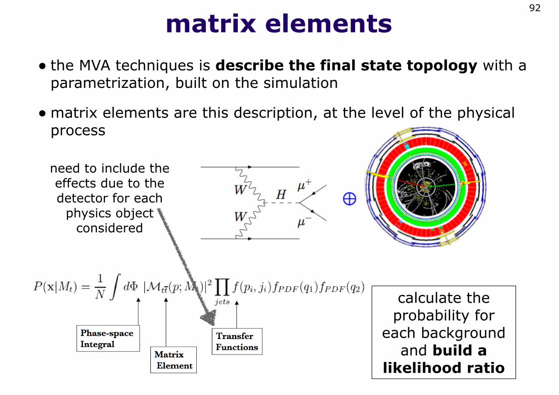
matrix elements• the MVA techniques is describe the final state topology with a

parametrization, built on the simulation

•matrix elements are this description, at the level of the physical process

92

need to include the effects due to the detector for each

physics object considered

calculate the probability for

each background and build a

likelihood ratio

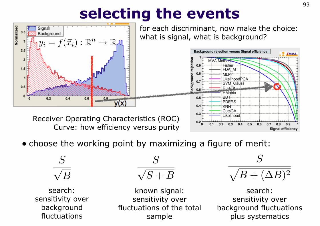
selecting the events93

Receiver Operating Characteristics (ROC) Curve: how efficiency versus purity

for each discriminant, now make the choice: what is signal, what is background?

yi = f(�xi) : Rn → R

• choose the working point by maximizing a figure of merit:

S√B

S√S +B

S�B + (∆B)2

search: sensitivity over

background fluctuations

known signal: sensitivity over

fluctuations of the total sample

search: sensitivity over

background fluctuations plus systematics

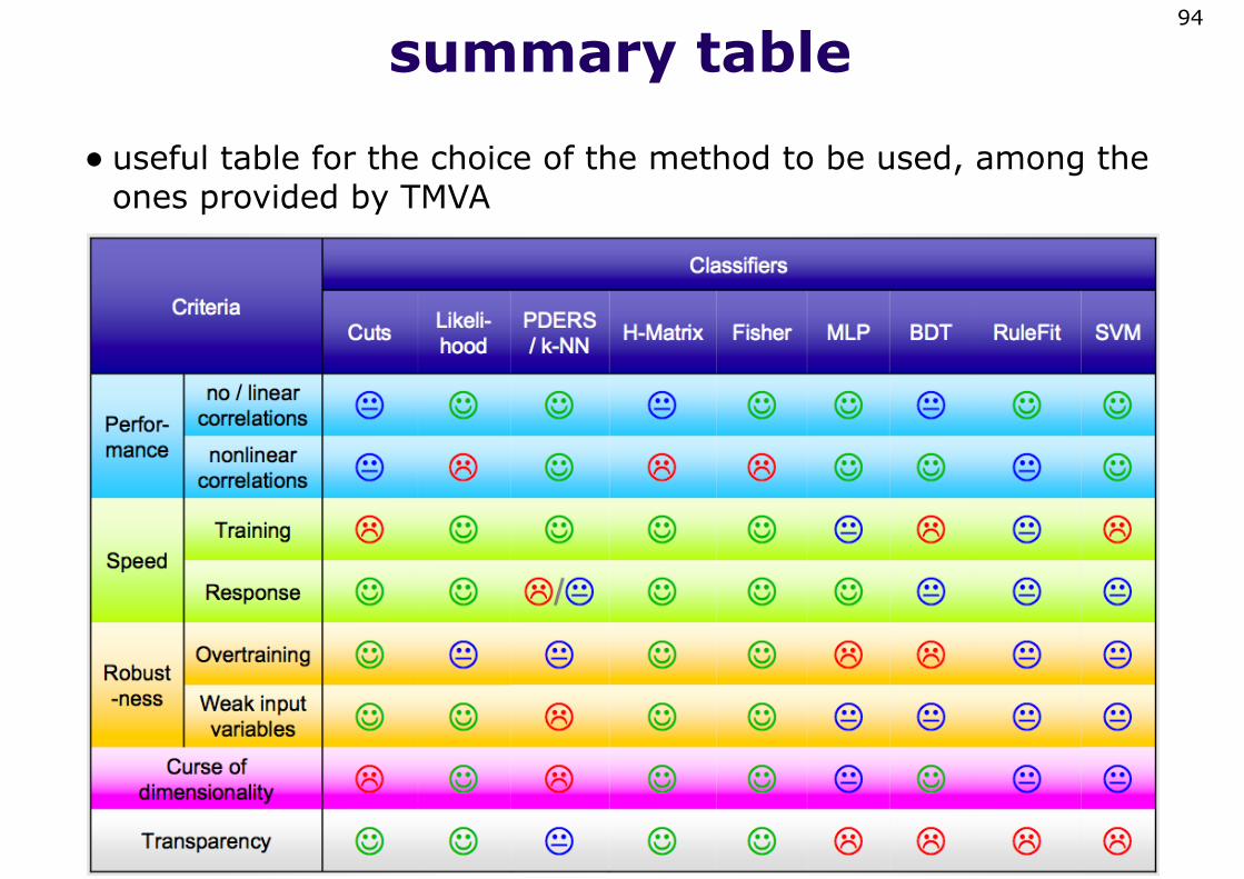
summary table

• useful table for the choice of the method to be used, among the ones provided by TMVA

94

what about systematics?• in terms of training, a systematic effect yields a sub-optimal

discriminant

• in terms of results, a systematic in the model reflects in the the efficiency and purity estimates, and in the event counts

• compare data to MC for the y(x) variable

• train the discriminator on different models

• try and understand effects by training on reduced sets of variables

95

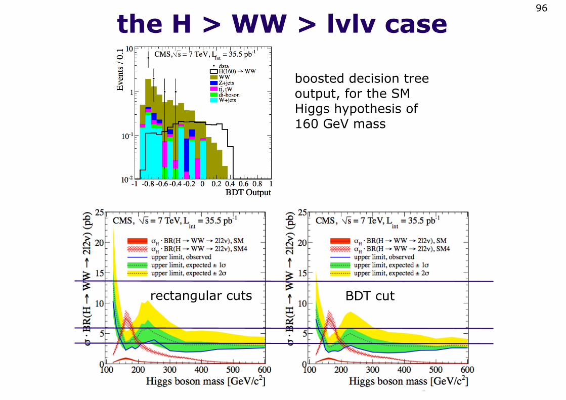
the H > WW > lvlv case96

boosted decision tree output, for the SM Higgs hypothesis of 160 GeV mass

rectangular cuts BDT cut

in conclusion

• data are arriving... when the going gets tough, the toughs get going, ... and have fun!

97

‣ the luminosity

‣ the trigger, from the point of view of the analysis

‣ the reconstruction and detector response

‣ the simulation

‣ differential cross-section measurement: a di-jet correction

‣ searches: the H > WW > lvlv

‣ multivariate techniques