This article was downloaded by: [Central Michigan University]On: 10 October 2014, At: 11:46Publisher: Taylor & FrancisInforma Ltd Registered in England and Wales Registered Number: 1072954 Registered office: Mortimer House,37-41 Mortimer Street, London W1T 3JH, UK

Communications in Statistics - Theory and MethodsPublication details, including instructions for authors and subscription information:http://www.tandfonline.com/loi/lsta20

HAZARD RATE ESTIMATION FOR CENSORED DATA BYWAVELET METHODSLinyuan Li aa Department of Statistics and Probability , Michigan State University , East Lansing, MI,48824, U.S.A.Published online: 19 Aug 2006.

To cite this article: Linyuan Li (2002) HAZARD RATE ESTIMATION FOR CENSORED DATA BY WAVELET METHODS, Communicationsin Statistics - Theory and Methods, 31:6, 943-960, DOI: 10.1081/STA-120004191

To link to this article: http://dx.doi.org/10.1081/STA-120004191

PLEASE SCROLL DOWN FOR ARTICLE

Taylor & Francis makes every effort to ensure the accuracy of all the information (the “Content”) containedin the publications on our platform. However, Taylor & Francis, our agents, and our licensors make norepresentations or warranties whatsoever as to the accuracy, completeness, or suitability for any purpose of theContent. Any opinions and views expressed in this publication are the opinions and views of the authors, andare not the views of or endorsed by Taylor & Francis. The accuracy of the Content should not be relied upon andshould be independently verified with primary sources of information. Taylor and Francis shall not be liable forany losses, actions, claims, proceedings, demands, costs, expenses, damages, and other liabilities whatsoeveror howsoever caused arising directly or indirectly in connection with, in relation to or arising out of the use ofthe Content.

This article may be used for research, teaching, and private study purposes. Any substantial or systematicreproduction, redistribution, reselling, loan, sub-licensing, systematic supply, or distribution in anyform to anyone is expressly forbidden. Terms & Conditions of access and use can be found at http://www.tandfonline.com/page/terms-and-conditions

CENSORED DATA ANALYSIS

HAZARD RATE ESTIMATION

FOR CENSORED DATA BY

WAVELET METHODS

Linyuan Li

Department of Statistics and Probability,Michigan State University, East Lansing, MI 48824

E-mail: lilinyua@stt.msu.edu

ABSTRACT

We study the estimation of a hazard rate function based oncensored data by non-linear wavelet method. We provide anasymptotic formula for the mean integrated squared error(MISE) of nonlinear wavelet-based hazard rate estimatorsunder randomly censored data. We show this MISE formula,when the underlying hazard rate function and censoring dis-tribution function are only piecewise smooth, has the sameexpansion as analogous kernel estimators, a feature not avail-able for the kernel estimators. In addition, we establish anasymptotic normality of the nonlinear wavelet estimator.

Key Words: Hazard rate estimator; Censored data; Meanintegrated square error; Non-linear wavelet estimator;Asymptotic normality

943

Copyright & 2002 by Marcel Dekker, Inc. www.dekker.com

COMMUN. STATIST.—THEORY METH., 31(6), 943–960 (2002)

Dow

nloa

ded

by [

Cen

tral

Mic

higa

n U

nive

rsity

] at

11:

46 1

0 O

ctob

er 2

014

1. INTRODUCTION

In medical research, industrial life-testing and the other studies, data onthe time to the occurrence of a particular event, such as the death of a patient,the failure of an electric equipment, the recurrence of a particular conditionand so on, are generically refered as survival data. These observations of theoccurrence of the events (called survival times) are often incomplete due tothe occurrence of another event (called censoring event), for example,patient withdraw alive during the study, termination of the experimentalstudy, patient died from the other causes than those under study and so on.So only part of the observations are real survival time. Formally, let X1,X2, . . . ,Xn be i.i.d. nonnegative survival times with a common distributionfunction F and density function f. Also let Y1,Y2, . . . ,Yn be another i.i.d.nonnegative censoring times with a common distribution function G.Assume that survival times and censoring times are independent. In thesetting of survival analysis with random censorship, one observes the bivari-ate sample ðZ1, �1Þ, ðZ2, �2Þ, . . . , ðZn, �nÞ, where Zi ¼ minðXi,YiÞ ¼ Xi ^ Yi

and �i ¼ IðXi � YiÞ, i ¼ 1, 2, . . . , n with IðAÞ denoting the indicator functionon the set A. One interesting question in survival analysis is to estimate thehazard rate function

�ðxÞ ¼ lim�!0þ

Pðx � X < xþ �jX xÞ

�¼

f ðxÞ

1 FðxÞ, x 2 ð0,1Þ:

There is an extensive inferential procedures available on estimating �ðxÞfrom censored data in literature, see e.g., the survey paper[14] and thereview paper [12]. References [16] and [10] studied a kernel estimation ofdensity and hazard rate under random censorship and provided MeanSquare Error (MSE) and asymptotic normality of hazard rate estimator.

Recently, the mathematical theory of wavelets and their applicationsin statistics have become a well-known technique for non-parametric curveestimation: See e.g., Refs. [3–6,11] For a systematic discussion of waveletsand their applications in statistics, see recent monograph.[8] The majoradvantage of the wavelet method is its adaptation to erratic behaviour of thedensity and local adaptation to the degree of smoothness of the unknowndensity. These wavelet estimators typically achieve the optimal convergencerates over exceptionally large function spaces. They do an excellent job oftaking care of discontinuities in the target function, and in consequence theyenjoy very good convergence rate even if smoothness conditions are imposedonly in a piecewise sense.

The objective of the present paper is to provide a non-linear wavelet-based hazard rate estimator for randomly censored data, its asymptotic

944 LI

Dow

nloa

ded

by [

Cen

tral

Mic

higa

n U

nive

rsity

] at

11:

46 1

0 O

ctob

er 2

014

formula for the mean integrated square error (MISE) and its asymptoticnormality.We show thisMISE formula, when the underlying survival densityfunction and censoring distribution function are only piecewise smooth, hasthe analogous expansion for the kernel estimators. This is no surprise, sinceRef. [7] and [13] have presented similar results with the complete data set in theestimation of density and hazard rate functions. More recently, Ref. [9] pres-ented an analogous result in the estimation of density function under randomcensorship. Ref. [2] describe a wavelet method for the estimation of densityand hazard rate functions from randomly right-censored data under bothsurvival and censoring densities are continuous, taking advantage of fastcomputing speed of wavelet methods. Ref. [17] provided hazard rate estima-tion by non-linear wavelet methods in the left truncation and right censoringmodel. They applied counting process techniques and obtained analogousexpansion, but needed further truncation. They provided a wavelet-basedestimator for hazard rate function over bounded interval ½�, �� which is chosensuch that the size of risk population satisfies some additional conditions.

In the next section, we give the elements of wavelet transform andprovide nonlinear wavelet-based hazard rate estimators. The main resultsare described in Section 3, while their proofs appear in Section 4.

2. NOTATIONS AND ESTIMATORS

This section contain some facts about wavelets that will be used in thesequel. Let �ðxÞ and ðxÞ be father and mother wavelets, having theproperties: � and are bounded and compactly supported.

R�2 ¼R

2¼ 1, k �

Ryk ð yÞ dy ¼ 0 for 0 � k � r 1 and r ¼ r!� 6¼ 0, here

� ¼ ðr!Þ1Ryr ð yÞ dy. Let

�jðxÞ ¼ p1=2�ðpx jÞ, ijðxÞ ¼ p1=2i ðpix jÞ, x 2 R

for arbitrary p > 0, 1 < j <1 and pi ¼ p2i, i 0. ThenZ�j1�j2 ¼ �j1j2 ,

Z i1j1 i2j2 ¼ �i1i2�j1j2 ,

Z�j1 ij2 ¼ 0,

where �ij denotes the Kronecker delta, i.e., �ij ¼ 1, if i ¼ j; 0, otherwise.Furthermore, an arbitrary square-integrable function f may be expandedin wavelet transform series:

f ðxÞ ¼X1j¼1

bj�jðxÞ þX1i¼0

X1j¼1

bij ijðxÞ, bj ¼

Zf�j , bij ¼

Zf ij:

For the more on wavelets, see Ref. [3].

HAZARD RATE ESTIMATION BY WAVELETS 945

Dow

nloa

ded

by [

Cen

tral

Mic

higa

n U

nive

rsity

] at

11:

46 1

0 O

ctob

er 2

014

In our random censorship model, we observe Zi ¼ minðXi,YiÞ, and�i ¼ IðXi � YiÞ, i ¼ 1, 2, . . . , n. Let T < �H be fixed and �1ðxÞ ¼�ðxÞIðx � TÞ, where �H ¼ inffx : HðxÞ ¼ 1g � 1 is the least upper boundfor the support of H, the distribution function of Z1. Since, in general,hazard rate function �ðxÞ is not square integrable, we here estimate �1ðxÞ,i.e., hazard rate function for x 2 ð0,T �. The wavelet expansion of �1ðxÞ is

�1ðxÞ ¼X1j¼1

bj�jðxÞ þX1i¼0

X1j¼1

bij ijðxÞ, bj ¼

Z�1�j , bij ¼

Z�1 ij:

ð2:1Þ

We propose a nonlinear wavelet estimator of �1ðxÞ:

��1ðxÞ ¼X1j¼1

bbj�jðxÞ þXq1i¼0

X1j¼1

bbijIðjbbijj > �Þ ijðxÞ, ð2:2Þ

where the wavelet coefficients bbj and bbij are defined as follows:

bbj ¼

Z�jðxÞIðx � TÞ

dFFnðxÞ

1 FFnðxÞ¼1

n

Xnk¼1

�kIðZk � TÞ�jðZkÞ

½1 FFnðZkÞ�½1 GGnðZkÞ�,

bbij ¼

Z ijðxÞIðx � TÞ

dFFnðxÞ

1 FFnðxÞ¼1

n

Xnk¼1

�kIðZk � TÞ ijðZkÞ

½1 FFnðZkÞ�½1 GGnðZkÞ�,

ð2:3Þ

where FFn and GGn are the Kaplan-Meier estimators of distribution function Fand G, respectively:

FFnðxÞ ¼ 1Ynk¼1

1�ðkÞ

n kþ 1

� �IðZðkÞ�xÞ

,

GGnðxÞ ¼ 1Ynk¼1

11 �ðkÞn kþ 1

� �IðZðkÞ�xÞ

:

Here ZðkÞ is the k-th ordered Z-value, �ðkÞ is the concomitant of the i-th orderZ statistic, that is, �ðkÞ ¼ �j, if ZðkÞ ¼ Zj. �k=nð1 GGnðZkÞÞ is the jump ofthe Kaplan-Meier estimator FnFn at Zk, � > 0 is a ‘‘threshold’’ and q 1 isanother smoothing parameter.

946 LI

Dow

nloa

ded

by [

Cen

tral

Mic

higa

n U

nive

rsity

] at

11:

46 1

0 O

ctob

er 2

014

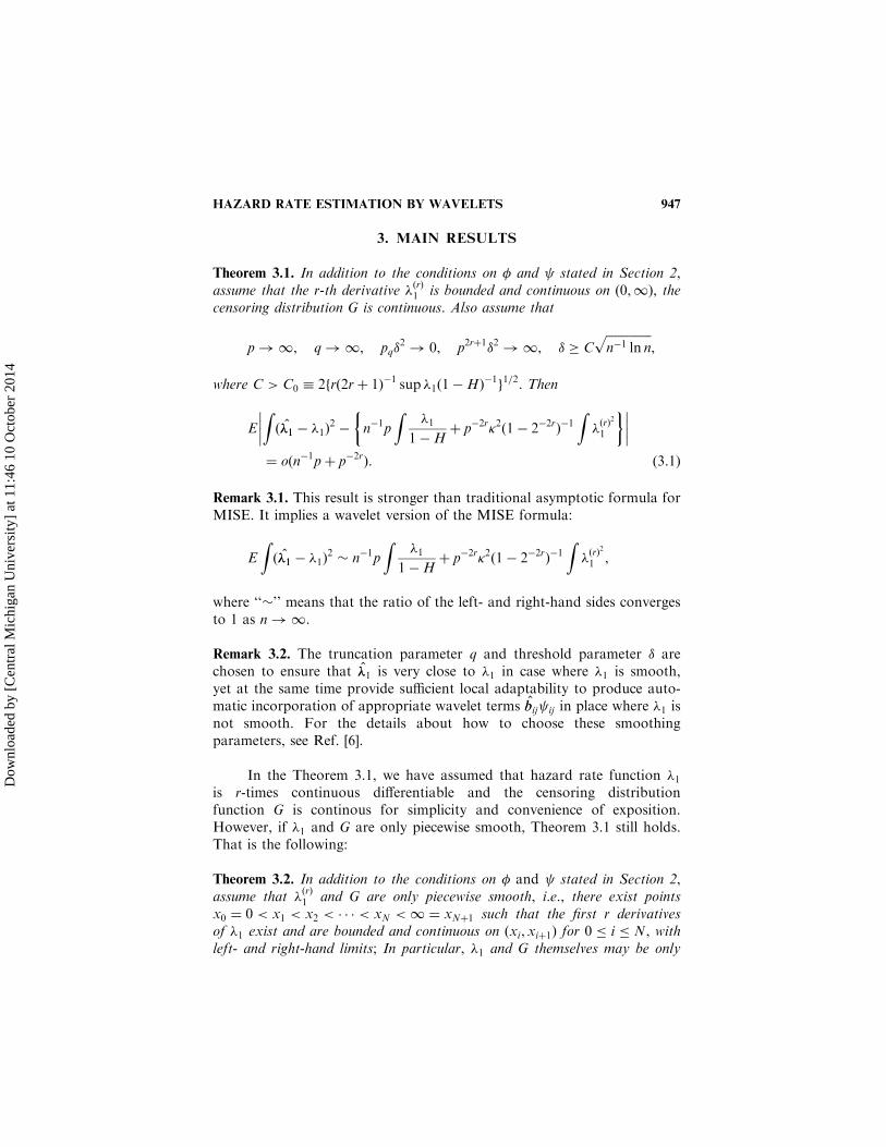
3. MAIN RESULTS

Theorem 3.1. In addition to the conditions on � and stated in Section 2,assume that the r-th derivative �ðrÞ1 is bounded and continuous on ð0,1Þ, thecensoring distribution G is continuous. Also assume that

p ! 1, q ! 1, pq�2! 0, p2rþ1�2 ! 1, � C

ffiffiffiffiffiffiffiffiffiffiffiffiffiffiffin1 ln n

p,

where C > C0 � 2frð2rþ 1Þ1 sup �1ð1HÞ1g1=2. Then

E

Zð�1�1 �1Þ

2 n1p

Z�1

1Hþ p2r�2ð1 22rÞ1

Z�ðrÞ

2

1

��������

¼ oðn1pþ p2rÞ: ð3:1Þ

Remark 3.1. This result is stronger than traditional asymptotic formula forMISE. It implies a wavelet version of the MISE formula:

E

Zð�1�1 �1Þ

2� n1p

Z�1

1Hþ p2r�2ð1 22rÞ1

Z�ðrÞ

2

1 ,

where ‘‘�’’ means that the ratio of the left- and right-hand sides convergesto 1 as n ! 1.

Remark 3.2. The truncation parameter q and threshold parameter � arechosen to ensure that ��1 is very close to �1 in case where �1 is smooth,yet at the same time provide sufficient local adaptability to produce auto-matic incorporation of appropriate wavelet terms bbij ij in place where �1 isnot smooth. For the details about how to choose these smoothingparameters, see Ref. [6].

In the Theorem 3.1, we have assumed that hazard rate function �1is r-times continuous differentiable and the censoring distributionfunction G is continous for simplicity and convenience of exposition.However, if �1 and G are only piecewise smooth, Theorem 3.1 still holds.That is the following:

Theorem 3.2. In addition to the conditions on � and stated in Section 2,assume that �ðrÞ1 and G are only piecewise smooth, i.e., there exist pointsx0 ¼ 0 < x1 < x2 < � � � < xN <1 ¼ xNþ1 such that the first r derivativesof �1 exist and are bounded and continuous on ðxi, xiþ1Þ for 0 � i � N, withleft- and right-hand limits; In particular, �1 and G themselves may be only

HAZARD RATE ESTIMATION BY WAVELETS 947

Dow

nloa

ded

by [

Cen

tral

Mic

higa

n U

nive

rsity

] at

11:

46 1

0 O

ctob

er 2

014

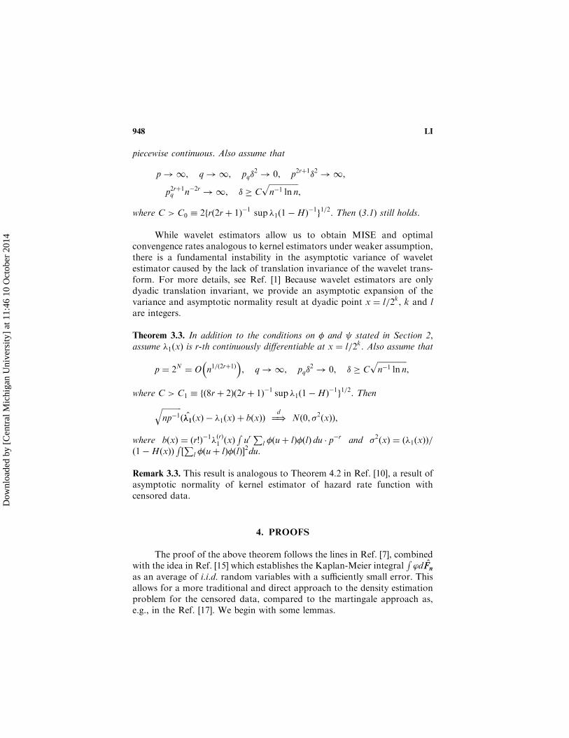
piecewise continuous. Also assume that

p ! 1, q ! 1, pq�2! 0, p2rþ1�2 ! 1,

p2rþ1q n2r ! 1, � Cffiffiffiffiffiffiffiffiffiffiffiffiffiffiffin1 ln n

p,

where C > C0 � 2frð2rþ 1Þ1 sup �1ð1HÞ1g1=2. Then (3.1) still holds.

While wavelet estimators allow us to obtain MISE and optimalconvengence rates analogous to kernel estimators under weaker assumption,there is a fundamental instability in the asymptotic variance of waveletestimator caused by the lack of translation invariance of the wavelet trans-form. For more details, see Ref. [1] Because wavelet estimators are onlydyadic translation invariant, we provide an asymptotic expansion of thevariance and asymptotic normality result at dyadic point x ¼ l=2k, k and lare integers.

Theorem 3.3. In addition to the conditions on � and stated in Section 2,assume �1ðxÞ is r-th continuously differentiable at x ¼ l=2k. Also assume that

p ¼ 2N ¼ O n1=ð2rþ1Þ�

, q ! 1, pq�2! 0, � C

ffiffiffiffiffiffiffiffiffiffiffiffiffiffiffin1 ln n

p,

where C > C1 � fð8rþ 2Þð2rþ 1Þ1 sup �1ð1HÞ1g1=2. Then

ffiffiffiffiffiffiffiffiffiffinp1

qð�1�1ðxÞ �1ðxÞ þ bðxÞÞ ¼)

dNð0, �2ðxÞÞ,

where bðxÞ ¼ ðr!Þ1�ðrÞ1 ðxÞRurP

l �ðuþ lÞ�ðlÞ du � pr and �2ðxÞ ¼ ð�1ðxÞÞ=ð1HðxÞÞ

R½P

l �ðuþ lÞ�ðlÞ�2du:

Remark 3.3. This result is analogous to Theorem 4.2 in Ref. [10], a result ofasymptotic normality of kernel estimator of hazard rate function withcensored data.

4. PROOFS

The proof of the above theorem follows the lines in Ref. [7], combinedwith the idea in Ref. [15] which establishes the Kaplan-Meier integral

R’dFnFn

as an average of i.i.d. random variables with a sufficiently small error. Thisallows for a more traditional and direct approach to the density estimationproblem for the censored data, compared to the martingale approach as,e.g., in the Ref. [17]. We begin with some lemmas.

948 LI

Dow

nloa

ded

by [

Cen

tral

Mic

higa

n U

nive

rsity

] at

11:

46 1

0 O

ctob

er 2

014

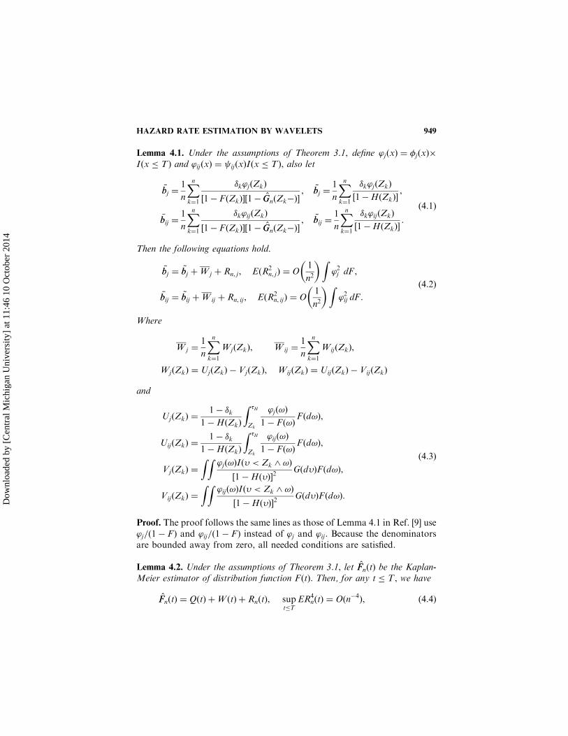
Lemma 4.1. Under the assumptions of Theorem 3.1, define ’jðxÞ ¼ �jðxÞ�Iðx � TÞ and ’ijðxÞ ¼ ijðxÞIðx � TÞ, also let

�bbj ¼1

n

Xnk¼1

�k’jðZkÞ

½1 FðZkÞ�½1 GGnðZkÞ�, ~bbj ¼

1

n

Xnk¼1

�k’jðZkÞ

½1HðZkÞ�,

�bbij ¼1

n

Xnk¼1

�k’ijðZkÞ

½1 FðZkÞ�½1 GGnðZkÞ�, ~bbij ¼

1

n

Xnk¼1

�k’ijðZkÞ

½1HðZkÞ�:

ð4:1Þ

Then the following equations hold.

�bbj ¼ ~bbj þWj þ Rn, j, EðR2n, jÞ ¼ O

1

n2

� �Z’2j dF ,

�bbij ¼ ~bbij þWij þ Rn, ij, EðR2n, ijÞ ¼ O

1

n2

� �Z’2ij dF :

ð4:2Þ

Where

Wj ¼1

n

Xnk¼1

WjðZkÞ, Wij ¼1

n

Xnk¼1

WijðZkÞ,

WjðZkÞ ¼ UjðZkÞ VjðZkÞ, WijðZkÞ ¼ UijðZkÞ VijðZkÞ

and

UjðZkÞ ¼1 �k

1HðZkÞ

Z �H

Zk

’jð!Þ

1 Fð!ÞFðd!Þ,

UijðZkÞ ¼1 �k

1HðZkÞ

Z �H

Zk

’ijð!Þ

1 Fð!ÞFðd!Þ,

VjðZkÞ ¼

Z Z’jð!ÞIð� < Zk ^ !Þ

½1Hð�Þ�2Gðd�ÞFðd!Þ,

VijðZkÞ ¼

Z Z’ijð!ÞIð� < Zk ^ !Þ

½1Hð�Þ�2Gðd�ÞFðd!Þ:

ð4:3Þ

Proof. The proof follows the same lines as those of Lemma 4.1 in Ref. [9] use’j=ð1 FÞ and ’ij=ð1 FÞ instead of ’j and ’ij. Because the denominatorsare bounded away from zero, all needed conditions are satisfied.

Lemma 4.2. Under the assumptions of Theorem 3.1, let FFnðtÞ be the Kaplan-Meier estimator of distribution function FðtÞ. Then, for any t � T , we have

FFnðtÞ ¼ QðtÞ þWðtÞ þ RnðtÞ, supt�T

ER4nðtÞ ¼ Oðn4Þ, ð4:4Þ

HAZARD RATE ESTIMATION BY WAVELETS 949

Dow

nloa

ded

by [

Cen

tral

Mic

higa

n U

nive

rsity

] at

11:

46 1

0 O

ctob

er 2

014

where

QðtÞ ¼1

n

Xnk¼1

QðZk, tÞ, WðtÞ ¼1

n

Xnk¼1

WðZk, tÞ

QðZk, tÞ ¼�kIðZk � tÞ

1 GðZkÞ, WðZk, tÞ ¼ UðZk, tÞ VðZk, tÞ

ð4:5Þ

and

UðZk, tÞ ¼1 �k

1HðZkÞ

ZIðZk < ! � tÞFðd!Þ,

VðZk, tÞ ¼

Z ZIð! � tÞIð� < Zk ^ !Þ

½1Hð�Þ�½1 Gð�Þ�Gðd�ÞFðd!Þ:

ð4:6Þ

Proof. From a result in p.434 of Ref. [15] and details of the proof of themain theorem of Ref. [15], we have the (4.4), an approximation of theKaplan-Meier estimator when ’ðxÞ ¼ Iðx � tÞ. The rest of proof is comple-tely analogous to that of Lemma 4.1 of Ref. [9]. Here we only consider thespecific integrand ’ðxÞ, instead of ’ijðxÞ there. Also we consider the fourthmoment of RnðtÞ, instead of second moment there. However, follow thedetails of the proof of Lemma 4.1 of Ref. [9], it is not hard to seeER4

nðtÞ ¼ Oðn4ÞR’4ðxÞ dF . Thus we have supt�T ER4

nðtÞ ¼ Oðn4Þ, whichproves the lemma.

Remark 4.1. In the lemma, we have shown supt�T ER4nðtÞ ¼ Oðn4Þ, which

will be needed in the following lemma. In fact, follows the same lines, we canshow that, for any integer k 1, supt�T ER2k

n ðtÞ ¼ Oðn2kÞ. Thus, from theHolder’s inequality, we have, for any � 1, supt�T EjR�nðtÞj ¼ Oðn�Þ,which is analogous to Lemma 2.1 in Ref. [10], where they showsupt�T EjR�nðtÞj ¼ Oð½ln n=n��Þ. Because of the technical reason, they definedestimator FFn slightly different from here. In addtion, by theorem 1.1 ofRef. [15], under F and G are only piecewise continous case, Lemma 4.2still holds, which will be used in proving Theorem 3.2.

Lemma 4.3. Under the assumptions of Theorem 3.1, we have

EXj

ðbbj �bbjÞ2¼ oðn1pÞ:

Proof. In view of (2.3) and (4.1), we have

bbj �bbj ¼1

n

Xnk¼1

�k’jðZkÞ

1 FðZkÞ

FFnðZkÞ FðZkÞ

½1 FFnðZkÞ�½1 GGnðZkÞ�:

950 LI

Dow

nloa

ded

by [

Cen

tral

Mic

higa

n U

nive

rsity

] at

11:

46 1

0 O

ctob

er 2

014

Notice ½1 FFnðZkÞ�½1 GGnðZkÞ� ¼ ðnþ 1RankZkÞ=n ¼ ðnP

l 6¼k �

IðZl � ZkÞÞ=n and apply Lemma 4.2, FðZkÞ ¼ FðZkÞ when F is continu-ous, we have

bbj �bbj ¼1

n

Xnk¼1

AjðZkÞBðZkÞPðZkÞ þ1

n

Xnk¼1

AjðZkÞBðZkÞWðZkÞ

þ1

n

Xnk¼1

AjðZkÞBðZkÞRnðZkÞ

¼ I1j þ I2j þ I3j, (say),

where

AjðZkÞ :¼�k’jðZkÞ

1 FðZkÞ, BðZkÞ :¼

n

nP

l 6¼k IðZl � ZkÞ,

PðZkÞ :¼ QðZkÞ FðZkÞ,

QðZkÞ,WðZkÞ and RnðZkÞ are defined as in (4.5) and (4.6). Conditionally onfZ1 ¼ z1g, f�1 ¼ d1g, through direct caculation, we have

EP4ðz1Þ ¼ Oðn2Þ uniformly in d1 and t � T : ð4:7Þ

Conditionally on fZ1 ¼ z1g, f�1 ¼ d1g, Bðz1Þ ¼ n=ðn VÞ, where V ¼Pnl¼2 IðZl � z1Þ is a binomial random variable with parameter n 1 and

p :¼ Hðz1Þ. Thus, through direct calculation, we have

EB4ðz1Þ ¼ Oð1Þ uniformly in d1 and z1 � T : ð4:8Þ

Now,

I21j ¼1

n2

Xnk¼1

A2j ðZkÞB

2ðZkÞP

2ðZkÞ

þ1

n2

Xnk¼1

Xnl¼1, 6¼k

AjðZkÞBðZkÞPðZkÞAjðZlÞBðZlÞPðZlÞ

¼ I21jð1Þ þ I21jð2Þ, ðsayÞ:

The first term

EI21jð1Þ ¼1

nE½A2

j ðZ1ÞB2ðZ1ÞP

2ðZ1Þ�

¼ O

�1

n

�EhA2

j ðZ1ÞE1=2

ðB4ðZ1ÞjZ1, �1ÞE

1=2ðP4

ðZ1ÞjZ1, �1Þi

¼ O

�1

n2

�EA2

j ðZ1Þ ¼ O

�1

n2

�Z’2j dF , ð4:9Þ

HAZARD RATE ESTIMATION BY WAVELETS 951

Dow

nloa

ded

by [

Cen

tral

Mic

higa

n U

nive

rsity

] at

11:

46 1

0 O

ctob

er 2

014

hence

EXj

I21jð1Þ ¼ oðn1pÞ byXj

p1Z’2j dF <1: ð4:10Þ

The second term

EI21jð2Þ ¼ O1

n2

� �Xnk¼1

Xnl¼1, 6¼k

EhjAjðZkÞjjAjðZlÞj

�EðjBðZkÞjjBðZlÞjjPðZkÞjjPðZlÞj

���Zk,Zl , �k, �lÞi:

Conditionally on fZk ¼ zkg, f�k ¼ dkg, fZl ¼ zlg and f�l ¼ dlg, applyCauchy-Schwarz inequality, we have

EðjBðzkÞjjBðzlÞjjPðzkÞjjPðzlÞjÞ � EB4ðzkÞEB

4ðzlÞEP

4ðzkÞEP

4ðzlÞ

� �1=4:

Through direct calculation as that in (4.7) and (4.8), we have

EI21jð2Þ ¼ O1

n3

� �Xnk¼1

Xnl¼1, 6¼k

EjAjðZkÞjjAjðZlÞj ¼ O1

n

� � Zj’jj dF

� �2

,

ð4:11Þ

hence

EXj

I21jð2Þ ¼ O

�1

n

�Xj

�Zj’jj dF

�2

¼ O

�1

n

�¼ oðn1pÞ ð4:12Þ

byP

jðRj’jj dFÞ

2 <1 and p ! 1. This, together with (4.10), we haveEP

j I21j ¼ oðn1pÞ. Applying the previous same lines to I2j, we can

show EP

j I22j ¼ oðn1pÞ too.

In order to prove the lemma, it suffices to show EP

j I23j ¼ oðn1pÞ.

Apply moment inequality to I3j, we have EI23j � E½A2j ðZ1ÞB

2ðZ1ÞR

2nðZ1Þ�:

Conditionally on fZ1 ¼ z1g, f�1 ¼ d1g, apply Cauchy-Schwarz inequality,we have E½B2

ðz1ÞR2nðz1Þ� � ½EB4

ðz1ÞER4nðz1Þ�

1=2¼ Oð1=n2Þ by (4.8) and

Lemma 4.2. Thus

EXj

I23j¼O1

n2

� �Xj

Z’2j dF¼O

p

n2

� �Xj

p1Z’2j dF¼oðn1pÞ: ð4:13Þ

Lemma 4.4. Under the assumptions of Theorem 3.1, we have

s1 � EXj

ðbbj bjÞ2 n1p

Z�1

1H

���������� ¼ oðn1pÞ:

952 LI

Dow

nloa

ded

by [

Cen

tral

Mic

higa

n U

nive

rsity

] at

11:

46 1

0 O

ctob

er 2

014

Proof. In view of (4.2) andP

jðbbj bjÞ2¼

Pjð�bbj bjÞ

2þP

jðbbj �bbjÞ

2þ

2P

jð�bbj bjÞðbbj �bbjÞ, we have

s1 � EXj

ð ~bbj bjÞ2 n1p

Z�1

1H

����������þ E

Xj

W2j þ E

Xj

R2n, j

þ 2EXj

j ~bbj bjjjRn, jj þ 2EXj

j ~bbj bjjjWjj þ 2EXj

jRn, jjjWjj

þ EXj

ðbbj �bbjÞ2þ 2E

Xj

j �bbj bjjjbbj �bbjj

¼ I1 þ I2 þ I3 þ I4 þ I5 þ I6 þ I7 þ I8, (say):

Notice that

nEð ~bbj bjÞ2¼

Z�2j ðxÞ

�1ðxÞ

1HðxÞdx b2j ,

we have

Xj

Eð ~bbj bjÞ2¼

p

n

Z�2ð yÞ

Xj

p1�1ðð yþ jÞ=pÞ

1Hðð yþ jÞ=pÞdy

1

n

Xj

b2j ,

sinceR�2 ¼ 1,

Pj p

1�1ððyþ jÞ=pÞ=ð1Hððyþ jÞ=pÞÞ !R�1=ð1HÞ,P

j b2j ¼ Oð

R�21Þ, then E

Pjð~bbj bjÞ

2¼ n1p

R�1=ð1HÞþ oðn1pÞ. Because

the denominator appearing in ~bbj is bounded away from below. Thus theymay be handled along the same lines as those in p.922 of Ref. [7] to showthat Varf

Pjð~bbj bjÞ

2g ¼ oðn2p2Þ. So we obtain I1 ¼ oðn1pÞ. By Lemma

4.1, I2 ¼ n1P

j EW2j ðZ1Þ � 2n1

PjðEU

2j ðZ1Þ þ EV2

j ðZ1ÞÞ: By direct calcu-lation, notice all denominators are bounded away from below, we have

EU2j ðZ1Þ ¼ EV2

j ðZ1Þ ¼ O p1Z�2ðuÞ�21

uþ j

p

� �du

� �:

Thus, I2 ¼ Oðn1ÞR�2ðuÞ

Pj p

1�21ððuþ jÞ=pÞdu ¼ oðn1pÞ byP

j p1�21�

ððuþ jÞ=pÞ !R�21 <1 and p ! 1. By Lemma 4.1 or (4.2), we have

I3 ¼ oðn1pÞ. From Lemma 4.3, I7 ¼ oðn1pÞ: Applying Cauchy-Schwarzinequality to the rest of the terms, we complete the proof.

Lemma 4.5. Under the assumptions of Theorem 3.1, we have

s2 �Xq1i¼0

Xj

Enðbbij bijÞ

2Iðjbbijj > �Þo¼ oðn2r=ð2rþ1ÞÞ:

HAZARD RATE ESTIMATION BY WAVELETS 953

Dow

nloa

ded

by [

Cen

tral

Mic

higa

n U

nive

rsity

] at

11:

46 1

0 O

ctob

er 2

014

Proof. Let � and � denote positive numbers satisfying �þ � ¼ 1, we have

s2 � 2Xq1i¼0

Xj

Efðbbij �bbijÞ2Iðjbbijj> �Þgþ 2

Xq1i¼0

Xj

Efð �bbij bijÞ2Iðjbbijj> �Þg

� 2Xq1i¼0

Xj

Efðbbij �bbijÞ2gþ 2

Xq1i¼0

Xj

Efð �bbij bijÞ2Iðj �bbijj>��Þg

þ 2Xq1i¼0

Xj

Efð �bbij bijÞ2Iðjbbij �bbijj>��Þg

¼ 2ðs21þ s22þ s23Þ, (say):

Applying the analogous argument as (4.9), (4.11) and (4.13) in Lemma 4.3 tos21, we can show

s21 ¼ O1

n2

� �Xq1i¼0

Xj

Z’2ij dF þO

1

n

� �Xq1i¼0

Xj

Zj’ijj dF

� �2

¼ O1

n2

� �Xq1i¼0

piXj

p1i

Z’2ij dF þO

1

n

� �Xq1i¼0

Xj

Zj’ijj dF

� �2

¼ Opq

n2

� �þO

ln n

n

� �¼ oðn2r=ð2rþ1ÞÞ:

The third equality follows fromP

j p1i

R’2ij dF <1,

PjðRj’ijj� dFÞ2 <1

and q ¼ Oðln nÞ, while the last equality follows from n1pq ! 0. Apply thesame lines as those of Lemma 4.3 in Ref. [9] to s22, use �bbij instead of bbij inthat paper, we can show s22 ¼ oðn2r=ð2rþ1ÞÞ:Now letA ¼ fj �bbij bijj > �g, then

s23 ¼Xq1i¼0

Xj

Efð �bbij bijÞ2Iðjbbij �bbijj> ��ÞIðAÞg

þXq1i¼0

Xj

Efð �bbij bijÞ2Iðjbbij �bbijj> ��ÞIðA

cÞg

�Xq1i¼0

Xj

Efð �bbij bijÞ2Iðj �bbij bijj> �Þg þ

Xq1i¼0

Xj

�2Pðjbbij �bbijj> ��Þ

�Xq1i¼0

Xj

Efð �bbij bijÞ2Iðj �bbij bijj> �Þg þ

Xq1i¼0

Xj

�2Eðbbij �bbijÞ2

¼ s23ð1Þ þ s23ð2Þ, (say),

954 LI

Dow

nloa

ded

by [

Cen

tral

Mic

higa

n U

nive

rsity

] at

11:

46 1

0 O

ctob

er 2

014

where s23ð1Þ is analogous to s22 in,[9] which is oðn2r=ð2rþ1ÞÞ. While s23ð2Þis Oðs21Þ, which is oðn2r=ð2rþ1ÞÞ too. Together with s21 and s22, we provethe lemma.

Lemma 4.6. Under the assumptions of Theorem 3.1, we have

s3 � EXq1i¼0

Xj

b2ijIðjbbijj � �Þ p2r�2ð1 22rÞ1Z�ðrÞ

2

1

���������� ¼ oðp2rÞ:

Proof. The proof follows the same lines as that of Lemma 4.4 in Ref. [9].

Lemma 4.7. Under the assumptions of Theorem 3.1, we have

s4 �X1i¼q

Xj

b2ij ¼ oðp2rÞ:

Proof. The proof follows from the Step 3 of Theorem 2.1 of Ref. [6].

We are now in the position to give the proof of the Theorems 3.1 and 3.2.

Proof of the Theorem 3.1. Observe that

E

Zð�1�1 �1Þ

2 n1p

Z�1

1Hþ p2r�2ð1 22rÞ1

Z�ðrÞ

2

1

��������

� s1 þ s2 þ s3 þ s4,

combining Lemmas 4.4–4.7, we come to the proof of Theorem 3.1.

Proof of the Theorem 3.2. The basic ideas of the proof are similar to those inthe proof of Theorem 3.2 in Ref. [9]. We omit the proof.

In the sequel we prove the Theorem 3.3. This will involve the followingtwo lemmas.

Lemma 4.8. Under the assumptions of Theorem 3.3, we have

ffiffiffiffiffiffiffiffiffiffinp1

q �Xj

ð ~bbj bjÞ�jðxÞ

�¼)d

Nð0, �2ðxÞÞ,

where

�2ðxÞ ¼�1ðxÞ

1HðxÞ

Z hXl

�ðuþ lÞ�ðlÞi2

du:

HAZARD RATE ESTIMATION BY WAVELETS 955

Dow

nloa

ded

by [

Cen

tral

Mic

higa

n U

nive

rsity

] at

11:

46 1

0 O

ctob

er 2

014

Proof. In view of (4.1),

ffiffiffiffiffiffiffiffiffiffinp1

q �Xj

ð ~bbj bjÞ�jðxÞ

�¼

Xnk¼1

� ffiffiffip

n

r�kIðZk � TÞKðpZk, pxÞ

1HðZkÞ

ffiffiffip

n

r �Z�1ðtÞKðpt, pxÞ dt

��:¼

Xnk¼1

Vn, k,

where Kðt, xÞ ¼P

j �ðt jÞ�ðx jÞ. For our wavelets in Section 2, the kernelKðt, xÞ satisfies the moment condition (See Theorem 8.3 of Ref. [8] p.95), i.e.,Rðt xÞkKðt, xÞ dt ¼ �0k, for k ¼ 0, 1, . . . , r 1. Notice ðZk, �kÞ are i.i.d. for

k ¼ 1, 2, . . . , n and EVn, k ¼ 0.

EV2n, k ¼

p

n

Z�1ðtÞ

1HðtÞK2

ðpt, pxÞ dtp

n

�Z�1ðtÞKðpt, pxÞ dt

�2

¼1

n

Z�1ðxþ u=pÞ

1Hðxþ u=pÞ

�Xj

�ðuþ px jÞ�ðpx jÞ

�2du

1

np

�Z�1ðxþ u=pÞ

Xj

�ðuþ px jÞ�ðpx jÞdu

�2

¼1

n

Z�1ðxÞ

1HðxÞ

�Xl

�ðuþ lÞ�ðlÞ

�2duþOðn1p1Þ:

The second equality follows by change of variable, while the third equalityby p ¼ 2N , x ¼ l=2k, N ! 1 and Taylor expansion. Thus

Pnk¼1 EV

2n, k ¼

�2ðxÞ þOðp1Þ ! �2ðxÞ. In addition, Kðt, xÞ is uniformly bounded, we havejVn, kj � c

ffiffiffiffiffiffiffiffiffiffin1p

p! 0, c is a constant. So for all � > 0, limn!1

Pnk¼1�

EðjVn, kj2; jVn, kj > �Þ ¼ 0. Thus by Lindeberge-Feller theorem, the lemma

follows.

Lemma 4.9. Under the assumptions of Theorem 3.3, let

J6 �Xq1i¼0

Xj

bbij ijðxÞIðjbbijj > �Þ, then EJ26 ¼ oðn1pÞ:

Proof. In view of (4.2), write bbij as following

bbij ¼ ~bbij þ ðbbij �bbijÞ þWij þ Rn, ij : ð4:14Þ

956 LI

Dow

nloa

ded

by [

Cen

tral

Mic

higa

n U

nive

rsity

] at

11:

46 1

0 O

ctob

er 2

014

Then

J6¼Xq1i¼0

Xj

~bbij ijðxÞIðjbbijj>�ÞþXq1i¼0

Xj

ðbbij �bbijÞ ijðxÞIðjbbijj>�Þ

þXq1i¼0

Xj

Wij ijðxÞIðjbbijj>�ÞþXq1i¼0

Xj

Rn, ij ijðxÞIðjbbijj>�Þ

¼ I1þ I2þ I3þ I4, (say): ð4:15Þ

Because of the compact support of ðxÞ, for each i, there are only finitej terms of ijðxÞ are non-zero. So

EI22 ¼ OðqÞXq1i¼0

Xj

Eðbbij �bbijÞ2 2

ijðxÞ

¼ OðqÞXq1i¼0

Xj

�1

n2

Z’2ij dF þ

1

n

�Zj’ijj dF

�2�pi

¼ OðqÞ

�pq

n2þq

n

�¼ oðn1pÞ,

the second equality follows from the argument similar to (4.9), (4.11) and(4.13) in Lemma 4.3, while the last equality by pqn

1! 0 and q ¼ Oðln nÞ.

Similarly, we can show EI23 ¼ EI24 ¼ oðn1pÞ too.As to the first term of J6,

I1¼Xq1i¼0

Xj

ð ~bbijbijÞ ijðxÞIðjbbijj>�ÞþXq1i¼0

Xj

bij ijðxÞIðjbbijj>�Þ ¼ I11þI12:

Let � and � are positive numbers such that �þ � ¼ 1, so

jI11j �Xq1i¼0

Xj

j ~bbij bijjj ijðxÞjIðjbijj > ��Þ

þXq1i¼0

Xj

j ~bbij bijjj ijðxÞjIðjbbij bijj > ��Þ:

Because �1ðxÞ is r-times continuously differentiable at x, so jbijj � cpðrþ1=2Þi ,

or b2ij � c2pð2rþ1Þi , c is a constant (see Ref. [7], p.917). Notice �2 ¼ Oðln n=nÞ,

pi ¼ p2i, p ¼ Oðn1=ð2rþ1ÞÞ, thus Iðjbijj > �Þ ¼ 0 for large n, hence the firstterm of I11 actually is zero. In view of (4.14), the leading term to

HAZARD RATE ESTIMATION BY WAVELETS 957

Dow

nloa

ded

by [

Cen

tral

Mic

higa

n U

nive

rsity

] at

11:

46 1

0 O

ctob

er 2

014

approximate bbij is ~bbij. Apply the similar argument as in (4.15) to I11, all therest of the terms are in smaller order, we have

EI211 ¼ OðqÞXq1i¼0

Xj

Eð ~bbij bijÞ2 2

ijðxÞIðj ~bbij bijj > ��Þ

¼ OðqÞXq1i¼0

Xj

E1=að ~bbij bijÞ

2a 2ijðxÞP

1=b�j ~bbij bijj > ��

¼ OðqÞXq1i¼0

Xj

pinpin

d¼ OðqÞp2qn

d1, where d >4rþ 1

2rþ 1

¼ oðn2r=ð2rþ1ÞÞ ¼ oðn1pÞ:

The second equality follows by Holder’s inequality, while the third equalityby Rosenthal’s and Bernstein’s inequality and let a ! 1, b ! 1 (see thedetails in Ref. [7], p.917–918). The fifth equality follows by n1pq ! 0.Apply the same argument to I12, using b2ij � c2p

ð2rþ1Þi , we can show that

EI212 ¼ oðn1pÞ too, which proves the lemma.Now we give the proof of the Theorem 3.3.

Proof of Theorem 3.3. In view of (2.2), by analogous equality of (4.14) to bbjand the defination of J6 in Lemma 4.9, we have

��1ðxÞ�1ðxÞbðxÞ¼Xj

ðbbjbjÞ�jðxÞþ

�Xj

bj�jðxÞ�1ðxÞbðxÞ

�þJ6

¼Xj

ð ~bbjbjÞ�jðxÞþXj

ðbbj �bbjÞ�jðxÞ

þXj

Wj�jðxÞþXj

Rn, j�jðxÞ

þ

�Xj

bj�jðxÞ�1ðxÞbðxÞ

�þJ6

¼J1þJ2þJ3þJ4þJ5þJ6, (say):

By Lemma 4.8,ffiffiffiffiffiffiffiffiffiffinp1

pJ1¼)

dNð0, �2ðxÞÞ. By Lemma 4.9, we haveffiffiffiffiffiffiffiffiffiffi

np1p

J6!p

0. J2, J3 and J4 are analogous to I2, I3 and I4 in Lemma 4.9,so apply the same argument, we can show EJ22 ¼ EJ23 ¼ EJ24 ¼ oðn1pÞ.Thus

ffiffiffiffiffiffiffiffiffiffinp1

pJ2!

p0, same as J3 and J4. Hence, in order to prove the the-

orem, it suffices to prove J5 ¼ oð prÞ. Apply the same argument as in

958 LI

Dow

nloa

ded

by [

Cen

tral

Mic

higa

n U

nive

rsity

] at

11:

46 1

0 O

ctob

er 2

014

Lemma 4.8, using the moment condition of Kðt, xÞ, it is easy to see

J5 ¼

Z½�1ðtÞ �1ðxÞ�pKðpt, pxÞ dt bðxÞ

¼

Z½�1ðxþ u=pÞ �1ðxÞ�Kðpxþ u, pxÞ du bðxÞ

¼

Z Xr

k¼1

�ðkÞ1 ðxÞ

k!

uk

pkKðpxþ u, pxÞ duþ oðpr

Þ bðxÞ

¼�ðrÞ1 ðxÞ

r!

ZurXl

�ðuþ lÞ�ðlÞ du pr bðxÞ þ oðpr

Þ ¼ oðprÞ,

the last equality follows from the moment condition of Kðt,xÞ, which provesthe theorem.

ACKNOWLEDGMENT

Research is partly supported by the NSF Grant DMS 0071619, theauthor thanks his advisor Professor Hira Koul for his constant guidanceand insightful suggestion.

REFERENCES

1. Antoniadis, A.; Gregoire, G.; McKeague, I.W. Wavelet Methods forCurve Estimation. J. Amer. Statist. Assoc. 1994, 89, 1340–1353.

2. Antoniadis, A.; Gregoire, G.; Nason, G. Density and Hazard RateEstimation for Right-Censored Data by Using Wavelet Methods. J.R. Statist. Soc. B 1999, 61, 63–84.

3. Daubechies, I. Ten Lectures on Wavelets; SIAM: Philadelphia, 1992.4. Donoho, D.L.; Johnstone, I.M.; Kerkyacharian, G.; Picard, D. Wavelet

Shrinkage: Asymptopia? (with discussion). J. Roy. Statist. Soc. Ser. B1995, 57, 301–369.

5. Donoho, D.L.; Johnstone, I.M.; Kerkyacharian, G.; Picard, D. DensityEstimation by Wavelet Thresholding. Ann. Statist. 1996, 24, 508–539.

6. Hall, P.; Patil, P. On the Choice of Smoothing Parameter, Thresholdand Truncation in Nonparametric Regression by Nonlinear WaveletMethods. Research Report SMS-72–93. Center for Mathematics andStatistics, Australian National University: Canberra, 1993.

HAZARD RATE ESTIMATION BY WAVELETS 959

Dow

nloa

ded

by [

Cen

tral

Mic

higa

n U

nive

rsity

] at

11:

46 1

0 O

ctob

er 2

014

7. Hall, P.; Patil, P. Formulae for Mean Integated Squared Error ofNon-Linear Wavelet-Based Density Estimators. Ann. Statist. 1995,23, 905-928.

8. Hardle, W.; Kerkyacharian, G.; Picard, D.; Tsybakov, A. Wavelets,Approximation and Statistical Applications. Lecture Notes in Statistics,1998; 129.

9. Li, L. Nonlinear Wavelet-Based Density Estimatiors Under RandomCensorship. accept to Journal of Statistical Planning and Inference.

10. Lo, S.H.; Mack, Y.P.; Wang, J.L. Density and Hazard RateEstimation for Censored Data via Strong Representation of theKaplan-Meier Estimator. Probab. Theory and Related Fields 1989,80, 461–473.

11. Meyer, Y. Ondelettes et Operateurs, Hermann, Paris, 1990.12. Padgett, W.J.; McNichols, D.T. Nonparametric Density Estimation

from Censored Data. Comm. Statist. Theory and Methods 1984, 13,1581–1611.

13. Patil, P. Nonparametric Hazard Rate Estimation by OrthogonalWavelet Methods. Journal of Statistical Planning and Inference 1997,60, 153–168.

14. Singpurwalla, N.D.; Wong, M.Y. Estimation of the Failure Rate,A Survey of the Nonparametric Methods. Part I: Non BayesianMethods. Comm. Statist. Theory and Methods 1983, 12, 559–588.

15. Stute, W. The Central Limit Theorem Under Random Censorship.Ann. Statist. 1995, 23, 422–439.

16. Tanner, M.A.; Wong, W.H. The Estimation of the Hazard Functionfrom Randomly Censored Data by the Kernel Method. Ann. Statist.1983, 11, 989–993.

17. Wu, S.; Wells, M. Estimating Hazard Rate with Truncated andCensored Data by Wavelet Methods, 1999 preprint.

960 LI

Dow

nloa

ded

by [

Cen

tral

Mic

higa

n U

nive

rsity

] at

11:

46 1

0 O

ctob

er 2

014