HaskellNotes for ProfessionalsHaskell

Notes for Professionals

GoalKicker.comFree Programming Books

DisclaimerThis is an unocial free book created for educational purposes and is

not aliated with ocial Haskell group(s) or company(s).All trademarks and registered trademarks are

the property of their respective owners

200+ pagesof professional hints and tricks

ContentsAbout 1 ...................................................................................................................................................................................

Chapter 1: Getting started with Haskell Language 2 ..................................................................................... Section 1.1: Getting started 2 ............................................................................................................................................ Section 1.2: Hello, World! 4 ............................................................................................................................................... Section 1.3: Factorial 6 ...................................................................................................................................................... Section 1.4: Fibonacci, Using Lazy Evaluation 6 ............................................................................................................ Section 1.5: Primes 7 ......................................................................................................................................................... Section 1.6: Declaring Values 8 ........................................................................................................................................

Chapter 2: Overloaded Literals 10 ........................................................................................................................... Section 2.1: Strings 10 ....................................................................................................................................................... Section 2.2: Floating Numeral 10 .................................................................................................................................... Section 2.3: Integer Numeral 11 ...................................................................................................................................... Section 2.4: List Literals 11 ..............................................................................................................................................

Chapter 3: Foldable 13 ................................................................................................................................................... Section 3.1: Definition of Foldable 13 .............................................................................................................................. Section 3.2: An instance of Foldable for a binary tree 13 ............................................................................................ Section 3.3: Counting the elements of a Foldable structure 14 ................................................................................... Section 3.4: Folding a structure in reverse 14 ............................................................................................................... Section 3.5: Flattening a Foldable structure into a list 15 ............................................................................................ Section 3.6: Performing a side-eect for each element of a Foldable structure 15 ................................................. Section 3.7: Flattening a Foldable structure into a Monoid 16 .................................................................................... Section 3.8: Checking if a Foldable structure is empty 16 ...........................................................................................

Chapter 4: Traversable 18 ........................................................................................................................................... Section 4.1: Definition of Traversable 18 ........................................................................................................................ Section 4.2: Traversing a structure in reverse 18 ......................................................................................................... Section 4.3: An instance of Traversable for a binary tree 19 ...................................................................................... Section 4.4: Traversable structures as shapes with contents 20 ................................................................................ Section 4.5: Instantiating Functor and Foldable for a Traversable structure 20 ....................................................... Section 4.6: Transforming a Traversable structure with the aid of an accumulating parameter 21 ...................... Section 4.7: Transposing a list of lists 22 .......................................................................................................................

Chapter 5: Lens 24 ............................................................................................................................................................ Section 5.1: Lenses for records 24 ................................................................................................................................... Section 5.2: Manipulating tuples with Lens 24 ............................................................................................................... Section 5.3: Lens and Prism 25 ........................................................................................................................................ Section 5.4: Stateful Lenses 25 ........................................................................................................................................ Section 5.5: Lenses compose 26 ..................................................................................................................................... Section 5.6: Writing a lens without Template Haskell 26 ............................................................................................. Section 5.7: Fields with makeFields 27 ........................................................................................................................... Section 5.8: Classy Lenses 29 .......................................................................................................................................... Section 5.9: Traversals 29 ................................................................................................................................................

Chapter 6: QuickCheck 30 ............................................................................................................................................. Section 6.1: Declaring a property 30 ............................................................................................................................... Section 6.2: Randomly generating data for custom types 30 ..................................................................................... Section 6.3: Using implication (==>) to check properties with preconditions 30 ........................................................ Section 6.4: Checking a single property 30 ................................................................................................................... Section 6.5: Checking all the properties in a file 31 ...................................................................................................... Section 6.6: Limiting the size of test data 31 .................................................................................................................

Chapter 7: Common GHC Language Extensions 33 ......................................................................................... Section 7.1: RankNTypes 33 ............................................................................................................................................. Section 7.2: OverloadedStrings 33 .................................................................................................................................. Section 7.3: BinaryLiterals 34 .......................................................................................................................................... Section 7.4: ExistentialQuantification 34 ........................................................................................................................ Section 7.5: LambdaCase 35 ........................................................................................................................................... Section 7.6: FunctionalDependencies 36 ........................................................................................................................ Section 7.7: FlexibleInstances 36 ..................................................................................................................................... Section 7.8: GADTs 37 ...................................................................................................................................................... Section 7.9: TupleSections 37 .......................................................................................................................................... Section 7.10: OverloadedLists 38 ..................................................................................................................................... Section 7.11: MultiParamTypeClasses 38 ........................................................................................................................ Section 7.12: UnicodeSyntax 39 ....................................................................................................................................... Section 7.13: PatternSynonyms 39 .................................................................................................................................. Section 7.14: ScopedTypeVariables 40 ........................................................................................................................... Section 7.15: RecordWildCards 41 ...................................................................................................................................

Chapter 8: Free Monads 42 .......................................................................................................................................... Section 8.1: Free monads split monadic computations into data structures and interpreters 42 ........................... Section 8.2: The Freer monad 43 .................................................................................................................................... Section 8.3: How do foldFree and iterM work? 44 ........................................................................................................ Section 8.4: Free Monads are like fixed points 45 .........................................................................................................

Chapter 9: Type Classes 46 .......................................................................................................................................... Section 9.1: Eq 46 .............................................................................................................................................................. Section 9.2: Monoid 46 ..................................................................................................................................................... Section 9.3: Ord 47 ........................................................................................................................................................... Section 9.4: Num 47 .......................................................................................................................................................... Section 9.5: Maybe and the Functor Class 49 ............................................................................................................... Section 9.6: Type class inheritance: Ord type class 49 .................................................................................................

Chapter 10: IO 51 ............................................................................................................................................................... Section 10.1: Getting the 'a' "out of" 'IO a' 51 .................................................................................................................. Section 10.2: IO defines your program's `main` action 51 ............................................................................................ Section 10.3: Checking for end-of-file conditions 52 ..................................................................................................... Section 10.4: Reading all contents of standard input into a string 52 ........................................................................ Section 10.5: Role and Purpose of IO 53 ........................................................................................................................ Section 10.6: Writing to stdout 55 .................................................................................................................................... Section 10.7: Reading words from an entire file 56 ....................................................................................................... Section 10.8: Reading a line from standard input 56 .................................................................................................... Section 10.9: Reading from `stdin` 57 .............................................................................................................................. Section 10.10: Parsing and constructing an object from standard input 57 ............................................................... Section 10.11: Reading from file handles 58 ...................................................................................................................

Chapter 11: Record Syntax 59 ..................................................................................................................................... Section 11.1: Basic Syntax 59 ............................................................................................................................................ Section 11.2: Defining a data type with field labels 60 .................................................................................................. Section 11.3: RecordWildCards 60 ................................................................................................................................... Section 11.4: Copying Records while Changing Field Values 61 ................................................................................... Section 11.5: Records with newtype 61 ...........................................................................................................................

Chapter 12: Partial Application 63 ............................................................................................................................ Section 12.1: Sections 63 ................................................................................................................................................... Section 12.2: Partially Applied Adding Function 63 ....................................................................................................... Section 12.3: Returning a Partially Applied Function 64 ...............................................................................................

Chapter 13: Monoid 65 ..................................................................................................................................................... Section 13.1: An instance of Monoid for lists 65 .............................................................................................................. Section 13.2: Collapsing a list of Monoids into a single value 65 ................................................................................. Section 13.3: Numeric Monoids 65 ................................................................................................................................... Section 13.4: An instance of Monoid for () 66 ................................................................................................................

Chapter 14: Category Theory 67 .............................................................................................................................. Section 14.1: Category theory as a system for organizing abstraction 67 ................................................................. Section 14.2: Haskell types as a category 67 ................................................................................................................ Section 14.3: Definition of a Category 69 ....................................................................................................................... Section 14.4: Coproduct of types in Hask 70 ................................................................................................................. Section 14.5: Product of types in Hask 71 ...................................................................................................................... Section 14.6: Haskell Applicative in terms of Category Theory 72 ..............................................................................

Chapter 15: Lists 73 .......................................................................................................................................................... Section 15.1: List basics 73 ................................................................................................................................................ Section 15.2: Processing lists 73 ...................................................................................................................................... Section 15.3: Ranges 74 .................................................................................................................................................... Section 15.4: List Literals 75 ............................................................................................................................................. Section 15.5: List Concatenation 75 ................................................................................................................................ Section 15.6: Accessing elements in lists 75 ................................................................................................................... Section 15.7: Basic Functions on Lists 75 ........................................................................................................................ Section 15.8: Transforming with `map` 76 ...................................................................................................................... Section 15.9: Filtering with `filter` 76 ................................................................................................................................ Section 15.10: foldr 77 ....................................................................................................................................................... Section 15.11: Zipping and Unzipping Lists 77 ................................................................................................................. Section 15.12: foldl 78 ........................................................................................................................................................

Chapter 16: Sorting Algorithms 79 ............................................................................................................................ Section 16.1: Insertion Sort 79 ........................................................................................................................................... Section 16.2: Permutation Sort 79 ................................................................................................................................... Section 16.3: Merge Sort 79 .............................................................................................................................................. Section 16.4: Quicksort 80 ................................................................................................................................................ Section 16.5: Bubble sort 80 ............................................................................................................................................. Section 16.6: Selection sort 80 .........................................................................................................................................

Chapter 17: Type Families 81 ...................................................................................................................................... Section 17.1: Datatype Families 81 .................................................................................................................................. Section 17.2: Type Synonym Families 81 ....................................................................................................................... Section 17.3: Injectivity 83 .................................................................................................................................................

Chapter 18: Monads 84 ................................................................................................................................................... Section 18.1: Definition of Monad 84 ............................................................................................................................... Section 18.2: No general way to extract value from a monadic computation 84 ..................................................... Section 18.3: Monad as a Subclass of Applicative 85 .................................................................................................... Section 18.4: The Maybe monad 85 ................................................................................................................................ Section 18.5: IO monad 87 ............................................................................................................................................... Section 18.6: List Monad 88 .............................................................................................................................................. Section 18.7: do-notation 88 ............................................................................................................................................

Chapter 19: Stack 90 ........................................................................................................................................................ Section 19.1: Profiling with Stack 90 ................................................................................................................................. Section 19.2: Structure 90 ................................................................................................................................................. Section 19.3: Build and Run a Stack Project 90 .............................................................................................................. Section 19.4: Viewing dependencies 90 ..........................................................................................................................

Section 19.5: Stack install 91 ............................................................................................................................................ Section 19.6: Installing Stack 91 ....................................................................................................................................... Section 19.7: Creating a simple project 91 ..................................................................................................................... Section 19.8: Stackage Packages and changing the LTS (resolver) version 91 ........................................................

Chapter 20: Generalized Algebraic Data Types 93 ......................................................................................... Section 20.1: Basic Usage 93 ...........................................................................................................................................

Chapter 21: Recursion Schemes 94 .......................................................................................................................... Section 21.1: Fixed points 94 ............................................................................................................................................. Section 21.2: Primitive recursion 94 ................................................................................................................................. Section 21.3: Primitive corecursion 95 ............................................................................................................................. Section 21.4: Folding up a structure one layer at a time 95 ......................................................................................... Section 21.5: Unfolding a structure one layer at a time 95 .......................................................................................... Section 21.6: Unfolding and then folding, fused 95 .......................................................................................................

Chapter 22: Data.Text 97 .............................................................................................................................................. Section 22.1: Text Literals 97 ............................................................................................................................................ Section 22.2: Checking if a Text is a substring of another Text 97 ............................................................................. Section 22.3: Stripping whitespace 97 ............................................................................................................................ Section 22.4: Indexing Text 98 ......................................................................................................................................... Section 22.5: Splitting Text Values 98 ............................................................................................................................. Section 22.6: Encoding and Decoding Text 99 ..............................................................................................................

Chapter 23: Using GHCi 100 .......................................................................................................................................... Section 23.1: Breakpoints with GHCi 100 ........................................................................................................................ Section 23.2: Quitting GHCi 100 ...................................................................................................................................... Section 23.3: Reloading a already loaded file 101 ........................................................................................................ Section 23.4: Starting GHCi 101 ...................................................................................................................................... Section 23.5: Changing the GHCi default prompt 101 .................................................................................................. Section 23.6: The GHCi configuration file 101 ............................................................................................................... Section 23.7: Loading a file 102 ...................................................................................................................................... Section 23.8: Multi-line statements 102 ..........................................................................................................................

Chapter 24: Strictness 103 ........................................................................................................................................... Section 24.1: Bang Patterns 103 ...................................................................................................................................... Section 24.2: Lazy patterns 103 ...................................................................................................................................... Section 24.3: Normal forms 104 ...................................................................................................................................... Section 24.4: Strict fields 105 ...........................................................................................................................................

Chapter 25: Syntax in Functions 106 ....................................................................................................................... Section 25.1: Pattern Matching 106 ................................................................................................................................. Section 25.2: Using where and guards 106 ................................................................................................................... Section 25.3: Guards 107 .................................................................................................................................................

Chapter 26: Functor 108 ................................................................................................................................................. Section 26.1: Class Definition of Functor and Laws 108 ............................................................................................... Section 26.2: Replacing all elements of a Functor with a single value 108 ................................................................ Section 26.3: Common instances of Functor 108 .......................................................................................................... Section 26.4: Deriving Functor 110 ................................................................................................................................. Section 26.5: Polynomial functors 111 ........................................................................................................................... Section 26.6: Functors in Category Theory 112 ............................................................................................................

Chapter 27: Testing with Tasty 114 ......................................................................................................................... Section 27.1: SmallCheck, QuickCheck and HUnit 114 ..................................................................................................

Chapter 28: Creating Custom Data Types 115 .................................................................................................. Section 28.1: Creating a data type with value constructor parameters 115 ..............................................................

Section 28.2: Creating a data type with type parameters 115 ................................................................................... Section 28.3: Creating a simple data type 115 ............................................................................................................. Section 28.4: Custom data type with record parameters 116 .....................................................................................

Chapter 29: Reactive-banana 117 ............................................................................................................................ Section 29.1: Injecting external events into the library 117 .......................................................................................... Section 29.2: Event type 117 ........................................................................................................................................... Section 29.3: Actuating EventNetworks 117 .................................................................................................................. Section 29.4: Behavior type 118 .....................................................................................................................................

Chapter 30: Optimization 119 ..................................................................................................................................... Section 30.1: Compiling your Program for Profiling 119 .............................................................................................. Section 30.2: Cost Centers 119 ........................................................................................................................................

Chapter 31: Concurrency 121 ....................................................................................................................................... Section 31.1: Spawning Threads with `forkIO` 121 .......................................................................................................... Section 31.2: Communicating between Threads with `MVar` 121 ................................................................................ Section 31.3: Atomic Blocks with Software Transactional Memory 122 .....................................................................

Chapter 32: Function composition 124 ................................................................................................................... Section 32.1: Right-to-left composition 124 ................................................................................................................... Section 32.2: Composition with binary function 124 ..................................................................................................... Section 32.3: Left-to-right composition 124 ...................................................................................................................

Chapter 33: Databases 125 .......................................................................................................................................... Section 33.1: Postgres 125 ................................................................................................................................................

Chapter 34: Data.Aeson - JSON in Haskell 126 ................................................................................................. Section 34.1: Smart Encoding and Decoding using Generics 126 ................................................................................ Section 34.2: A quick way to generate a Data.Aeson.Value 126 ................................................................................. Section 34.3: Optional Fields 127 ....................................................................................................................................

Chapter 35: Higher-order functions 128 ................................................................................................................ Section 35.1: Basics of Higher Order Functions 128 ...................................................................................................... Section 35.2: Lambda Expressions 128 .......................................................................................................................... Section 35.3: Currying 129 ...............................................................................................................................................

Chapter 36: Containers - Data.Map 130 ................................................................................................................ Section 36.1: Importing the Module 130 .......................................................................................................................... Section 36.2: Monoid instance 130 ................................................................................................................................. Section 36.3: Constructing 130 ........................................................................................................................................ Section 36.4: Checking If Empty 130 .............................................................................................................................. Section 36.5: Finding Values 130 ..................................................................................................................................... Section 36.6: Inserting Elements 131 .............................................................................................................................. Section 36.7: Deleting Elements 131 ...............................................................................................................................

Chapter 37: Fixity declarations 132 .......................................................................................................................... Section 37.1: Associativity 132 ......................................................................................................................................... Section 37.2: Binding precedence 132 ........................................................................................................................... Section 37.3: Example declarations 133 .........................................................................................................................

Chapter 38: Web Development 134 ......................................................................................................................... Section 38.1: Servant 134 ................................................................................................................................................. Section 38.2: Yesod 135 ...................................................................................................................................................

Chapter 39: Vectors 136 ................................................................................................................................................. Section 39.1: The Data.Vector Module 136 ..................................................................................................................... Section 39.2: Filtering a Vector 136 ................................................................................................................................ Section 39.3: Mapping (`map`) and Reducing (`fold`) a Vector 136 ............................................................................ Section 39.4: Working on Multiple Vectors 136 .............................................................................................................

Chapter 40: Cabal 137 .................................................................................................................................................... Section 40.1: Working with sandboxes 137 .................................................................................................................... Section 40.2: Install packages 137 .................................................................................................................................

Chapter 41: Type algebra 138 .................................................................................................................................... Section 41.1: Addition and multiplication 138 ................................................................................................................. Section 41.2: Functions 139 .............................................................................................................................................. Section 41.3: Natural numbers in type algebra 139 ...................................................................................................... Section 41.4: Recursive types 140 ................................................................................................................................... Section 41.5: Derivatives 141 ...........................................................................................................................................

Chapter 42: Arrows 142 ................................................................................................................................................. Section 42.1: Function compositions with multiple channels 142 ................................................................................

Chapter 43: Typed holes 143 ...................................................................................................................................... Section 43.1: Syntax of typed holes 143 ......................................................................................................................... Section 43.2: Semantics of typed holes 143 .................................................................................................................. Section 43.3: Using typed holes to define a class instance 143 ..................................................................................

Chapter 44: Rewrite rules (GHC) 146 ...................................................................................................................... Section 44.1: Using rewrite rules on overloaded functions 146 ...................................................................................

Chapter 45: Date and Time 147 ................................................................................................................................ Section 45.1: Finding Today's Date 147 .......................................................................................................................... Section 45.2: Adding, Subtracting and Comparing Days 147 ......................................................................................

Chapter 46: List Comprehensions 148 .................................................................................................................... Section 46.1: Basic List Comprehensions 148 ................................................................................................................ Section 46.2: Do Notation 148 ......................................................................................................................................... Section 46.3: Patterns in Generator Expressions 148 ................................................................................................... Section 46.4: Guards 149 ................................................................................................................................................. Section 46.5: Parallel Comprehensions 149 ................................................................................................................... Section 46.6: Local Bindings 149 ..................................................................................................................................... Section 46.7: Nested Generators 150 .............................................................................................................................

Chapter 47: Streaming IO 151 .................................................................................................................................... Section 47.1: Streaming IO 151 ........................................................................................................................................

Chapter 48: Google Protocol Buers 152 ............................................................................................................ Section 48.1: Creating, building and using a simple .proto file 152 .............................................................................

Chapter 49: Template Haskell & QuasiQuotes 154 ......................................................................................... Section 49.1: Syntax of Template Haskell and Quasiquotes 154 ................................................................................. Section 49.2: The Q type 155 .......................................................................................................................................... Section 49.3: An n-arity curry 156 ..................................................................................................................................

Chapter 50: Phantom types 158 ................................................................................................................................ Section 50.1: Use Case for Phantom Types: Currencies 158 ........................................................................................

Chapter 51: Modules 159 ................................................................................................................................................ Section 51.1: Defining Your Own Module 159 ................................................................................................................. Section 51.2: Exporting Constructors 159 ....................................................................................................................... Section 51.3: Importing Specific Members of a Module 159 ......................................................................................... Section 51.4: Hiding Imports 160 ..................................................................................................................................... Section 51.5: Qualifying Imports 160 .............................................................................................................................. Section 51.6: Hierarchical module names 160 ...............................................................................................................

Chapter 52: Tuples (Pairs, Triples, ...) 162 ............................................................................................................. Section 52.1: Extract tuple components 162 .................................................................................................................. Section 52.2: Strictness of matching a tuple 162 ..........................................................................................................

Section 52.3: Construct tuple values 162 ....................................................................................................................... Section 52.4: Write tuple types 163 ................................................................................................................................ Section 52.5: Pattern Match on Tuples 163 ................................................................................................................... Section 52.6: Apply a binary function to a tuple (uncurrying) 164 ............................................................................. Section 52.7: Apply a tuple function to two arguments (currying) 164 ...................................................................... Section 52.8: Swap pair components 164 ......................................................................................................................

Chapter 53: Graphics with Gloss 165 ....................................................................................................................... Section 53.1: Installing Gloss 165 ..................................................................................................................................... Section 53.2: Getting something on the screen 165 .....................................................................................................

Chapter 54: State Monad 167 ..................................................................................................................................... Section 54.1: Numbering the nodes of a tree with a counter 167 ................................................................................

Chapter 55: Pipes 169 ...................................................................................................................................................... Section 55.1: Producers 169 ............................................................................................................................................. Section 55.2: Connecting Pipes 169 ................................................................................................................................ Section 55.3: Pipes 169 ..................................................................................................................................................... Section 55.4: Running Pipes with runEect 169 ............................................................................................................ Section 55.5: Consumers 170 .......................................................................................................................................... Section 55.6: The Proxy monad transformer 170 ......................................................................................................... Section 55.7: Combining Pipes and Network communication 170 ..............................................................................

Chapter 56: Infix operators 173 ................................................................................................................................. Section 56.1: Prelude 173 ................................................................................................................................................. Section 56.2: Finding information about infix operators 174 ....................................................................................... Section 56.3: Custom operators 174 ...............................................................................................................................

Chapter 57: Parallelism 176 ......................................................................................................................................... Section 57.1: The Eval Monad 176 ................................................................................................................................... Section 57.2: rpar 176 ...................................................................................................................................................... Section 57.3: rseq 177 ......................................................................................................................................................

Chapter 58: Parsing HTML with taggy-lens and lens 178 ............................................................................. Section 58.1: Filtering elements from the tree 178 ........................................................................................................ Section 58.2: Extract the text contents from a div with a particular id 178 ...............................................................

Chapter 59: Foreign Function Interface 180 ........................................................................................................ Section 59.1: Calling C from Haskell 180 ........................................................................................................................ Section 59.2: Passing Haskell functions as callbacks to C code 180 ..........................................................................

Chapter 60: Gtk3 182 ....................................................................................................................................................... Section 60.1: Hello World in Gtk 182 ...............................................................................................................................

Chapter 61: Monad Transformers 183 .................................................................................................................... Section 61.1: A monadic counter 183 ...............................................................................................................................

Chapter 62: Bifunctor 186 ............................................................................................................................................. Section 62.1: Definition of Bifunctor 186 ......................................................................................................................... Section 62.2: Common instances of Bifunctor 186 ....................................................................................................... Section 62.3: first and second 186 ..................................................................................................................................

Chapter 63: Proxies 188 .................................................................................................................................................. Section 63.1: Using Proxy 188 .......................................................................................................................................... Section 63.2: The "polymorphic proxy" idiom 188 ........................................................................................................ Section 63.3: Proxy is like () 188 ......................................................................................................................................

Chapter 64: Applicative Functor 190 ....................................................................................................................... Section 64.1: Alternative definition 190 ........................................................................................................................... Section 64.2: Common instances of Applicative 190 ....................................................................................................

Chapter 65: Common monads as free monads 193 ........................................................................................ Section 65.1: Free Empty ~~ Identity 193 ........................................................................................................................ Section 65.2: Free Identity ~~ (Nat,) ~~ Writer Nat 193 ................................................................................................. Section 65.3: Free Maybe ~~ MaybeT (Writer Nat) 193 ................................................................................................ Section 65.4: Free (Writer w) ~~ Writer [w] 194 ............................................................................................................. Section 65.5: Free (Const c) ~~ Either c 194 ................................................................................................................... Section 65.6: Free (Reader x) ~~ Reader (Stream x) 195 .............................................................................................

Chapter 66: Common functors as the base of cofree comonads 196 ................................................... Section 66.1: Cofree Empty ~~ Empty 196 ...................................................................................................................... Section 66.2: Cofree (Const c) ~~ Writer c 196 .............................................................................................................. Section 66.3: Cofree Identity ~~ Stream 196 .................................................................................................................. Section 66.4: Cofree Maybe ~~ NonEmpty 196 ............................................................................................................. Section 66.5: Cofree (Writer w) ~~ WriterT w Stream 197 ............................................................................................ Section 66.6: Cofree (Either e) ~~ NonEmptyT (Writer e) 197 ...................................................................................... Section 66.7: Cofree (Reader x) ~~ Moore x 198 ...........................................................................................................

Chapter 67: Arithmetic 199 ........................................................................................................................................... Section 67.1: Basic examples 201 .................................................................................................................................... Section 67.2: `Could not deduce (Fractional Int) ...` 201 ................................................................................................ Section 67.3: Function examples 201 ..............................................................................................................................

Chapter 68: Role 203 ....................................................................................................................................................... Section 68.1: Nominal Role 203 ....................................................................................................................................... Section 68.2: Representational Role 203 ....................................................................................................................... Section 68.3: Phantom Role 203 .....................................................................................................................................

Chapter 69: Arbitrary-rank polymorphism with RankNTypes 204 .......................................................... Section 69.1: RankNTypes 204 ........................................................................................................................................

Chapter 70: GHCJS 205 .................................................................................................................................................. Section 70.1: Running "Hello World!" with Node.js 205 ..................................................................................................

Chapter 71: XML 206 ......................................................................................................................................................... Section 71.1: Encoding a record using the `xml` library 206 ..........................................................................................

Chapter 72: Reader / ReaderT 207 ......................................................................................................................... Section 72.1: Simple demonstration 207 .........................................................................................................................

Chapter 73: Function call syntax 208 ...................................................................................................................... Section 73.1: Partial application - Part 1 208 .................................................................................................................. Section 73.2: Partial application - Part 2 208 ................................................................................................................. Section 73.3: Parentheses in a basic function call 208 ................................................................................................. Section 73.4: Parentheses in embedded function calls 209 .........................................................................................

Chapter 74: Logging 210 ............................................................................................................................................... Section 74.1: Logging with hslogger 210 ........................................................................................................................

Chapter 75: Attoparsec 211 ......................................................................................................................................... Section 75.1: Combinators 211 ........................................................................................................................................ Section 75.2: Bitmap - Parsing Binary Data 211 ...........................................................................................................

Chapter 76: zipWithM 213 .............................................................................................................................................. Section 76.1: Calculatings sales prices 213 ....................................................................................................................

Chapter 77: Profunctor 214 .......................................................................................................................................... Section 77.1: (->) Profunctor 214 .....................................................................................................................................

Chapter 78: Type Application 215 ............................................................................................................................. Section 78.1: Avoiding type annotations 215 ................................................................................................................. Section 78.2: Type applications in other languages 215 ..............................................................................................

Section 78.3: Order of parameters 216 .......................................................................................................................... Section 78.4: Interaction with ambiguous types 216 ....................................................................................................

Credits 218 ............................................................................................................................................................................

You may also like 220 ......................................................................................................................................................

GoalKicker.com – Haskell Notes for Professionals 1

About

Please feel free to share this PDF with anyone for free,latest version of this book can be downloaded from:

https://goalkicker.com/HaskellBook

This Haskell Notes for Professionals book is compiled from Stack OverflowDocumentation, the content is written by the beautiful people at Stack Overflow.Text content is released under Creative Commons BY-SA, see credits at the end

of this book whom contributed to the various chapters. Images may be copyrightof their respective owners unless otherwise specified

This is an unofficial free book created for educational purposes and is notaffiliated with official Haskell group(s) or company(s) nor Stack Overflow. Alltrademarks and registered trademarks are the property of their respective

company owners

The information presented in this book is not guaranteed to be correct noraccurate, use at your own risk

Please send feedback and corrections to web@petercv.com

GoalKicker.com – Haskell Notes for Professionals 2

Chapter 1: Getting started with HaskellLanguage

Version Release DateHaskell 2010 2012-07-10

Haskell 98 2002-12-01

Section 1.1: Getting startedOnline REPL

The easiest way to get started writing Haskell is probably by going to the Haskell website or Try Haskell and use theonline REPL (read-eval-print-loop) on the home page. The online REPL supports most basic functionality and evensome IO. There is also a basic tutorial available which can be started by typing the command help. An ideal tool tostart learning the basics of Haskell and try out some stuff.

GHC(i)

For programmers that are ready to engage a little bit more, there is GHCi, an interactive environment that comeswith the Glorious/Glasgow Haskell Compiler. The GHC can be installed separately, but that is only a compiler. In orderto be able to install new libraries, tools like Cabal and Stack must be installed as well. If you are running a Unix-likeoperating system, the easiest installation is to install Stack using:

curl -sSL https://get.haskellstack.org/ | sh

This installs GHC isolated from the rest of your system, so it is easy to remove. All commands must be preceded bystack though. Another simple approach is to install a Haskell Platform. The platform exists in two flavours:

The minimal distribution contains only GHC (to compile) and Cabal/Stack (to install and build packages)1.The full distribution additionally contains tools for project development, profiling and coverage analysis. Also2.an additional set of widely-used packages is included.

These platforms can be installed by downloading an installer and following the instructions or by using yourdistribution's package manager (note that this version is not guaranteed to be up-to-date):

Ubuntu, Debian, Mint:

sudo apt-get install haskell-platform

Fedora:

sudo dnf install haskell-platform

Redhat:

sudo yum install haskell-platform

Arch Linux:

sudo pacman -S ghc cabal-install haskell-haddock-api \ haskell-haddock-library happy alex

GoalKicker.com – Haskell Notes for Professionals 3

Gentoo:

sudo layman -a haskellsudo emerge haskell-platform

OSX with Homebrew:

brew cask install haskell-platform

OSX with MacPorts:

sudo port install haskell-platform

Once installed, it should be possible to start GHCi by invoking the ghci command anywhere in the terminal. If theinstallation went well, the console should look something like

me@notebook:~$ ghciGHCi, version 6.12.1: http://www.haskell.org/ghc/ :? for helpPrelude>

possibly with some more information on what libraries have been loaded before the Prelude>. Now, the consolehas become a Haskell REPL and you can execute Haskell code as with the online REPL. In order to quit thisinteractive environment, one can type :qor :quit. For more information on what commands are available in GHCi,type :? as indicated in the starting screen.

Because writing the same things again and again on a single line is not always that practically, it might be a goodidea to write the Haskell code in files. These files normally have .hs for an extension and can be loaded into theREPL by using :l or :load.

As mentioned earlier, GHCi is a part of the GHC, which is actually a compiler. This compiler can be used to transforma .hs file with Haskell code into a running program. Because a .hs file can contain a lot of functions, a main functionmust be defined in the file. This will be the starting point for the program. The file test.hs can be compiled with thecommand

ghc test.hs

this will create object files and an executable if there were no errors and the main function was defined correctly.

More advanced tools

It has already been mentioned earlier as package manager, but stack can be a useful tool for Haskell1.development in completely different ways. Once installed, it is capable of

installing (multiple versions of) GHCproject creation and scaffoldingdependency managementbuilding and testing projectsbenchmarking

IHaskell is a haskell kernel for IPython and allows to combine (runnable) code with markdown and2.mathematical notation.

GoalKicker.com – Haskell Notes for Professionals 4

Section 1.2: Hello, World!A basic "Hello, World!" program in Haskell can be expressed concisely in just one or two lines:

main :: IO ()main = putStrLn "Hello, World!"

The first line is an optional type annotation, indicating that main is a value of type IO (), representing an I/O actionwhich "computes" a value of type () (read "unit"; the empty tuple conveying no information) besides performingsome side effects on the outside world (here, printing a string at the terminal). This type annotation is usuallyomitted for main because it is its only possible type.

Put this into a helloworld.hs file and compile it using a Haskell compiler, such as GHC:

ghc helloworld.hs

Executing the compiled file will result in the output "Hello, World!" being printed to the screen:

./helloworldHello, World!

Alternatively, runhaskell or runghc make it possible to run the program in interpreted mode without having tocompile it:

runhaskell helloworld.hs

The interactive REPL can also be used instead of compiling. It comes shipped with most Haskell environments, suchas ghci which comes with the GHC compiler:

ghci> putStrLn "Hello World!"Hello, World!ghci>

Alternatively, load scripts into ghci from a file using load (or :l):

ghci> :load helloworld

:reload (or :r) reloads everything in ghci:

Prelude> :l helloworld.hs[1 of 1] Compiling Main ( helloworld.hs, interpreted )

<some time later after some edits>

*Main> :rOk, modules loaded: Main.

Explanation:

This first line is a type signature, declaring the type of main:

main :: IO ()

Values of type IO () describe actions which can interact with the outside world.

GoalKicker.com – Haskell Notes for Professionals 5

Because Haskell has a fully-fledged Hindley-Milner type system which allows for automatic type inference, typesignatures are technically optional: if you simply omit the main :: IO (), the compiler will be able to infer the typeon its own by analyzing the definition of main. However, it is very much considered bad style not to write typesignatures for top-level definitions. The reasons include:

Type signatures in Haskell are a very helpful piece of documentation because the type system is soexpressive that you often can see what sort of thing a function is good for simply by looking at its type. This“documentation” can be conveniently accessed with tools like GHCi. And unlike normal documentation, thecompiler's type checker will make sure it actually matches the function definition!

Type signatures keep bugs local. If you make a mistake in a definition without providing its type signature, thecompiler may not immediately report an error but instead simply infer a nonsensical type for it, with which itactually typechecks. You may then get a cryptic error message when using that value. With a signature, thecompiler is very good at spotting bugs right where they happen.

This second line does the actual work:

main = putStrLn "Hello, World!"

If you come from an imperative language, it may be helpful to note that this definition can also be written as:

main = do { putStrLn "Hello, World!" ; return () }

Or equivalently (Haskell has layout-based parsing; but beware mixing tabs and spaces inconsistently which willconfuse this mechanism):

main = do putStrLn "Hello, World!" return ()

Each line in a do block represents some monadic (here, I/O) computation, so that the whole do block represents theoverall action comprised of these sub-steps by combining them in a manner specific to the given monad (for I/Othis means just executing them one after another).

The do syntax is itself a syntactic sugar for monads, like IO here, and return is a no-op action producing itsargument without performing any side effects or additional computations which might be part of a particularmonad definition.

The above is the same as defining main = putStrLn "Hello, World!", because the value putStrLn "Hello,World!" already has the type IO (). Viewed as a “statement”, putStrLn "Hello, World!" can be seen as acomplete program, and you simply define main to refer to this program.

You can look up the signature of putStrLn online:

putStrLn :: String -> IO ()-- thus,putStrLn (v :: String) :: IO ()

putStrLn is a function that takes a string as its argument and outputs an I/O-action (i.e. a value representing aprogram that the runtime can execute). The runtime always executes the action named main, so we simply need todefine it as equal to putStrLn "Hello, World!".

GoalKicker.com – Haskell Notes for Professionals 6

Section 1.3: FactorialThe factorial function is a Haskell "Hello World!" (and for functional programming generally) in the sense that itsuccinctly demonstrates basic principles of the language.

Variation 1fac :: (Integral a) => a -> afac n = product [1..n]

Live demo

Integral is the class of integral number types. Examples include Int and Integer.(Integral a) => places a constraint on the type a to be in said classfac :: a -> a says that fac is a function that takes an a and returns an aproduct is a function that accumulates all numbers in a list by multiplying them together.[1..n] is special notation which desugars to enumFromTo 1 n, and is the range of numbers 1 ≤ x ≤ n.

Variation 2fac :: (Integral a) => a -> afac 0 = 1fac n = n * fac (n - 1)

Live demo

This variation uses pattern matching to split the function definition into separate cases. The first definition isinvoked if the argument is 0 (sometimes called the stop condition) and the second definition otherwise (the order ofdefinitions is significant). It also exemplifies recursion as fac refers to itself.

It is worth noting that, due to rewrite rules, both versions of fac will compile to identical machine code when usingGHC with optimizations activated. So, in terms of efficiency, the two would be equivalent.

Section 1.4: Fibonacci, Using Lazy EvaluationLazy evaluation means Haskell will evaluate only list items whose values are needed.

The basic recursive definition is:

f (0) <- 0f (1) <- 1f (n) <- f (n-1) + f (n-2)

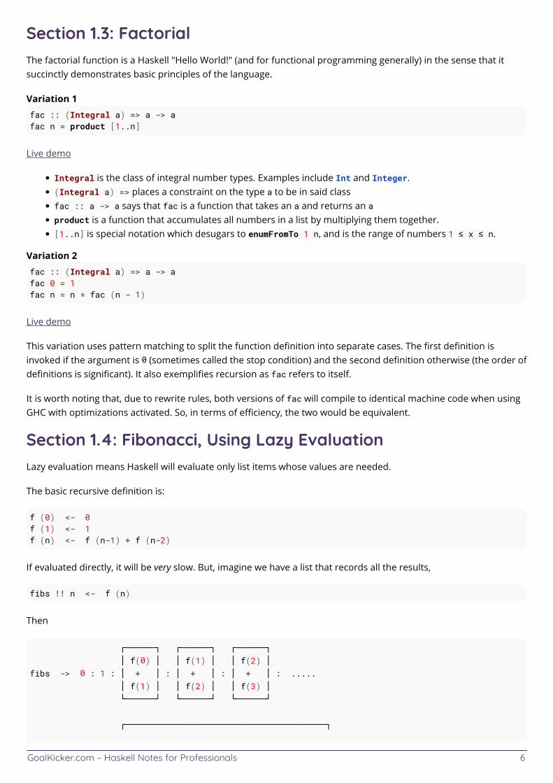
If evaluated directly, it will be very slow. But, imagine we have a list that records all the results,

fibs !! n <- f (n)

Then

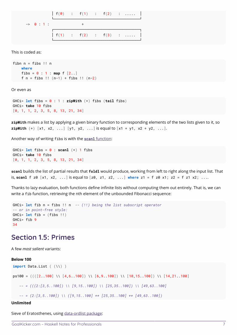
┌──────┐ ┌──────┐ ┌──────┐ │ f(0) │ │ f(1) │ │ f(2) │fibs -> 0 : 1 : │ + │ : │ + │ : │ + │ : ..... │ f(1) │ │ f(2) │ │ f(3) │ └──────┘ └──────┘ └──────┘

┌────────────────────────────────────────┐

GoalKicker.com – Haskell Notes for Professionals 7

│ f(0) : f(1) : f(2) : ..... │ └────────────────────────────────────────┘ -> 0 : 1 : + ┌────────────────────────────────────────┐ │ f(1) : f(2) : f(3) : ..... │ └────────────────────────────────────────┘

This is coded as:

fibn n = fibs !! n where fibs = 0 : 1 : map f [2..] f n = fibs !! (n-1) + fibs !! (n-2)

Or even as

GHCi> let fibs = 0 : 1 : zipWith (+) fibs (tail fibs)GHCi> take 10 fibs[0, 1, 1, 2, 3, 5, 8, 13, 21, 34]

zipWith makes a list by applying a given binary function to corresponding elements of the two lists given to it, sozipWith (+) [x1, x2, ...] [y1, y2, ...] is equal to [x1 + y1, x2 + y2, ...].

Another way of writing fibs is with the scanl function:

GHCi> let fibs = 0 : scanl (+) 1 fibsGHCi> take 10 fibs[0, 1, 1, 2, 3, 5, 8, 13, 21, 34]

scanl builds the list of partial results that foldl would produce, working from left to right along the input list. Thatis, scanl f z0 [x1, x2, ...] is equal to [z0, z1, z2, ...] where z1 = f z0 x1; z2 = f z1 x2; ....

Thanks to lazy evaluation, both functions define infinite lists without computing them out entirely. That is, we canwrite a fib function, retrieving the nth element of the unbounded Fibonacci sequence:

GHCi> let fib n = fibs !! n -- (!!) being the list subscript operator-- or in point-free style:GHCi> let fib = (fibs !!)GHCi> fib 934

Section 1.5: PrimesA few most salient variants:

Below 100import Data.List ( (\\) )

ps100 = ((([2..100] \\ [4,6..100]) \\ [6,9..100]) \\ [10,15..100]) \\ [14,21..100]

-- = (((2:[3,5..100]) \\ [9,15..100]) \\ [25,35..100]) \\ [49,63..100]

-- = (2:[3,5..100]) \\ ([9,15..100] ++ [25,35..100] ++ [49,63..100])

Unlimited

Sieve of Eratosthenes, using data-ordlist package:

GoalKicker.com – Haskell Notes for Professionals 8

import qualified Data.List.Ordered

ps = 2 : _Y ((3:) . minus [5,7..] . unionAll . map (\p -> [p*p, p*p+2*p..]))

_Y g = g (_Y g) -- = g (g (_Y g)) = g (g (g (g (...)))) = g . g . g . g . ...

Traditional

(a sub-optimal trial division sieve)

ps = sieve [2..] where sieve (x:xs) = [x] ++ sieve [y | y <- xs, rem y x > 0]

-- = map head ( iterate (\(x:xs) -> filter ((> 0).(`rem` x)) xs) [2..] )

Optimal trial divisionps = 2 : [n | n <- [3..], all ((> 0).rem n) $ takeWhile ((<= n).(^2)) ps]

-- = 2 : [n | n <- [3..], foldr (\p r-> p*p > n || (rem n p > 0 && r)) True ps]

Transitional

From trial division to sieve of Eratosthenes:

[n | n <- [2..], []==[i | i <- [2..n-1], j <- [0,i..n], j==n]]

The Shortest CodenubBy (((>1).).gcd) [2..] -- i.e., nubBy (\a b -> gcd a b > 1) [2..]

nubBy is also from Data.List, like (\\).

Section 1.6: Declaring ValuesWe can declare a series of expressions in the REPL like this:

Prelude> let x = 5Prelude> let y = 2 * 5 + xPrelude> let result = y * 10Prelude> x5Prelude> y15Prelude> result150

To declare the same values in a file we write the following:

-- demo.hs

module Demo where-- We declare the name of our module so-- it can be imported by name in a project.

x = 5

y = 2 * 5 + x

result = y * 10

GoalKicker.com – Haskell Notes for Professionals 9

Module names are capitalized, unlike variable names.

GoalKicker.com – Haskell Notes for Professionals 10

Chapter 2: Overloaded LiteralsSection 2.1: StringsThe type of the literal

Without any extensions, the type of a string literal – i.e., something between double quotes – is just a string, aka listof characters:

Prelude> :t "foo""foo" :: [Char]

However, when the OverloadedStrings extension is enabled, string literals become polymorphic, similar to numberliterals:

Prelude> :set -XOverloadedStringsPrelude> :t "foo""foo" :: Data.String.IsString t => t

This allows us to define values of string-like types without the need for any explicit conversions. In essence, theOverloadedStrings extension just wraps every string literal in the generic fromString conversion function, so if thecontext demands e.g. the more efficient Text instead of String, you don't need to worry about that yourself.

Using string literals{-# LANGUAGE OverloadedStrings #-}

import Data.Text (Text, pack)import Data.ByteString (ByteString, pack)

withString :: StringwithString = "Hello String"

-- The following two examples are only allowed with OverloadedStrings

withText :: TextwithText = "Hello Text" -- instead of: withText = Data.Text.pack "Hello Text"

withBS :: ByteStringwithBS = "Hello ByteString" -- instead of: withBS = Data.ByteString.pack "Hello ByteString"

Notice how we were able to construct values of Text and ByteString in the same way we construct ordinary String(or [Char]) Values, rather than using each types pack function to encode the string explicitly.

For more information on the OverloadedStrings language extension, see the extension documentation.

Section 2.2: Floating NumeralThe type of the literalPrelude> :t 1.01.0 :: Fractional a => a

Choosing a concrete type with annotations

You can specify the type with a type annotation. The only requirement is that the type must have a Fractional

GoalKicker.com – Haskell Notes for Professionals 11

instance.

Prelude> 1.0 :: Double1.0it :: DoublePrelude> 1.0 :: Data.Ratio.Ratio Int1 % 1it :: GHC.Real.Ratio Int

if not the compiler will complain

Prelude> 1.0 :: Int<interactive>: No instance for (Fractional Int) arising from the literal `1.0' In the expression: 1.0 :: Int In an equation for `it': it = 1.0 :: Int

Section 2.3: Integer NumeralThe type of the literalPrelude> :t 11 :: Num a => a

choosing a concrete type with annotations

You can specify the type as long as the target type is Num with an annotation:

Prelude> 1 :: Int1it :: IntPrelude> 1 :: Double1.0it :: DoublePrelude> 1 :: Word1it :: Word

if not the compiler will complain

Prelude> 1 :: String

<interactive>: No instance for (Num String) arising from the literal `1' In the expression: 1 :: String In an equation for `it': it = 1 :: String

Section 2.4: List LiteralsGHC's OverloadedLists extension allows you to construct list-like data structures with the list literal syntax.

This allows you to Data.Map like this:

> :set -XOverloadedLists> import qualified Data.Map as M> M.lookup "foo" [("foo", 1), ("bar", 2)]Just 1

GoalKicker.com – Haskell Notes for Professionals 12

Instead of this (note the use of the extra M.fromList):

> import Data.Map as M> M.lookup "foo" (M.fromList [("foo", 1), ("bar", 2)])Just 1

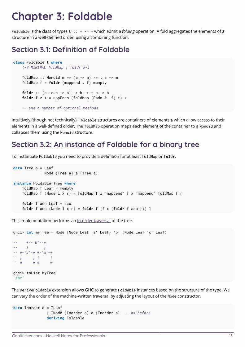
GoalKicker.com – Haskell Notes for Professionals 13

Chapter 3: FoldableFoldable is the class of types t :: * -> * which admit a folding operation. A fold aggregates the elements of astructure in a well-defined order, using a combining function.

Section 3.1: Definition of Foldableclass Foldable t where {-# MINIMAL foldMap | foldr #-}

foldMap :: Monoid m => (a -> m) -> t a -> m foldMap f = foldr (mappend . f) mempty

foldr :: (a -> b -> b) -> b -> t a -> b foldr f z t = appEndo (foldMap (Endo #. f) t) z

-- and a number of optional methods

Intuitively (though not technically), Foldable structures are containers of elements a which allow access to theirelements in a well-defined order. The foldMap operation maps each element of the container to a Monoid andcollapses them using the Monoid structure.

Section 3.2: An instance of Foldable for a binary treeTo instantiate Foldable you need to provide a definition for at least foldMap or foldr.

data Tree a = Leaf | Node (Tree a) a (Tree a)

instance Foldable Tree where foldMap f Leaf = mempty foldMap f (Node l x r) = foldMap f l `mappend` f x `mappend` foldMap f r foldr f acc Leaf = acc foldr f acc (Node l x r) = foldr f (f x (foldr f acc r)) l

This implementation performs an in-order traversal of the tree.

ghci> let myTree = Node (Node Leaf 'a' Leaf) 'b' (Node Leaf 'c' Leaf)

-- +--'b'--+-- | |-- +-'a'-+ +-'c'-+-- | | | |-- * * * *

ghci> toList myTree"abc"

The DeriveFoldable extension allows GHC to generate Foldable instances based on the structure of the type. Wecan vary the order of the machine-written traversal by adjusting the layout of the Node constructor.

data Inorder a = ILeaf | INode (Inorder a) a (Inorder a) -- as before deriving Foldable

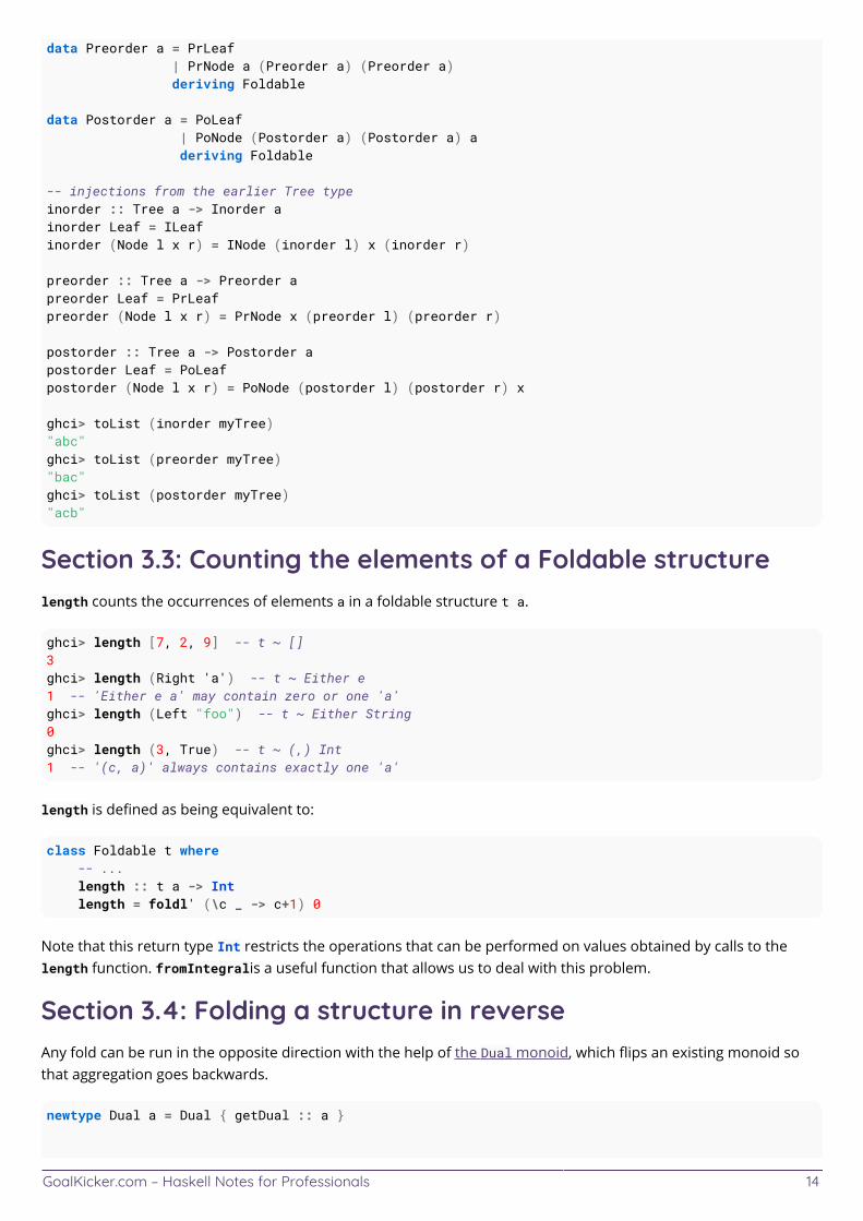
GoalKicker.com – Haskell Notes for Professionals 14

data Preorder a = PrLeaf | PrNode a (Preorder a) (Preorder a) deriving Foldable

data Postorder a = PoLeaf | PoNode (Postorder a) (Postorder a) a deriving Foldable

-- injections from the earlier Tree typeinorder :: Tree a -> Inorder ainorder Leaf = ILeafinorder (Node l x r) = INode (inorder l) x (inorder r)

preorder :: Tree a -> Preorder apreorder Leaf = PrLeafpreorder (Node l x r) = PrNode x (preorder l) (preorder r)

postorder :: Tree a -> Postorder apostorder Leaf = PoLeafpostorder (Node l x r) = PoNode (postorder l) (postorder r) x

ghci> toList (inorder myTree)"abc"ghci> toList (preorder myTree)"bac"ghci> toList (postorder myTree)"acb"

Section 3.3: Counting the elements of a Foldable structurelength counts the occurrences of elements a in a foldable structure t a.

ghci> length [7, 2, 9] -- t ~ []3ghci> length (Right 'a') -- t ~ Either e1 -- 'Either e a' may contain zero or one 'a'ghci> length (Left "foo") -- t ~ Either String0ghci> length (3, True) -- t ~ (,) Int1 -- '(c, a)' always contains exactly one 'a'

length is defined as being equivalent to:

class Foldable t where -- ... length :: t a -> Int length = foldl' (\c _ -> c+1) 0

Note that this return type Int restricts the operations that can be performed on values obtained by calls to thelength function. fromIntegralis a useful function that allows us to deal with this problem.

Section 3.4: Folding a structure in reverseAny fold can be run in the opposite direction with the help of the Dual monoid, which flips an existing monoid sothat aggregation goes backwards.

newtype Dual a = Dual { getDual :: a }

GoalKicker.com – Haskell Notes for Professionals 15

instance Monoid m => Monoid (Dual m) where mempty = Dual mempty (Dual x) `mappend` (Dual y) = Dual (y `mappend` x)

When the underlying monoid of a foldMap call is flipped with Dual, the fold runs backwards; the following Reversetype is defined in Data.Functor.Reverse:

newtype Reverse t a = Reverse { getReverse :: t a }

instance Foldable t => Foldable (Reverse t) where foldMap f = getDual . foldMap (Dual . f) . getReverse

We can use this machinery to write a terse reverse for lists:

reverse :: [a] -> [a]reverse = toList . Reverse

Section 3.5: Flattening a Foldable structure into a listtoList flattens a Foldable structure t a into a list of as.

ghci> toList [7, 2, 9] -- t ~ [][7, 2, 9]ghci> toList (Right 'a') -- t ~ Either e"a"ghci> toList (Left "foo") -- t ~ Either String[]ghci> toList (3, True) -- t ~ (,) Int[True]

toList is defined as being equivalent to:

class Foldable t where -- ... toList :: t a -> [a] toList = foldr (:) []

Section 3.6: Performing a side-eect for each element of aFoldable structuretraverse_ executes an Applicative action for every element in a Foldable structure. It ignores the action's result,keeping only the side-effects. (For a version which doesn't discard results, use Traversable.)

-- using the Writer applicative functor (and the Sum monoid)ghci> runWriter $ traverse_ (\x -> tell (Sum x)) [1,2,3]((),Sum {getSum = 6})-- using the IO applicative functorghci> traverse_ putStrLn (Right "traversing")traversingghci> traverse_ putStrLn (Left False)-- nothing printed

for_ is traverse_ with the arguments flipped. It resembles a foreach loop in an imperative language.

ghci> let greetings = ["Hello", "Bonjour", "Hola"]ghci> :{

GoalKicker.com – Haskell Notes for Professionals 16

ghci| for_ greetings $ \greeting -> doghci| print (greeting ++ " Stack Overflow!")ghci| :}"Hello Stack Overflow!""Bonjour Stack Overflow!""Hola Stack Overflow!"

sequenceA_ collapses a Foldable full of Applicative actions into a single action, ignoring the result.

ghci> let actions = [putStrLn "one", putStLn "two"]ghci> sequenceA_ actionsonetwo

traverse_ is defined as being equivalent to:

traverse_ :: (Foldable t, Applicative f) => (a -> f b) -> t a -> f ()traverse_ f = foldr (\x action -> f x *> action) (pure ())

sequenceA_ is defined as:

sequenceA_ :: (Foldable t, Applicative f) -> t (f a) -> f ()sequenceA_ = traverse_ id

Moreover, when the Foldable is also a Functor, traverse_ and sequenceA_ have the following relationship:

traverse_ f = sequenceA_ . fmap f

Section 3.7: Flattening a Foldable structure into a MonoidfoldMap maps each element of the Foldable structure to a Monoid, and then combines them into a single value.

foldMap and foldr can be defined in terms of one another, which means that instances of Foldable need only givea definition for one of them.

class Foldable t where foldMap :: Monoid m => (a -> m) -> t a -> m foldMap f = foldr (mappend . f) mempty

Example usage with the Product monoid:

product :: (Num n, Foldable t) => t n -> nproduct = getProduct . foldMap Product

Section 3.8: Checking if a Foldable structure is emptynull returns True if there are no elements a in a foldable structure t a, and False if there is one or more.Structures for which null is True have a length of 0.

ghci> null []Trueghci> null [14, 29]Falseghci> null NothingTrueghci> null (Right 'a')

GoalKicker.com – Haskell Notes for Professionals 17

Falseghci> null ('x', 3)False

null is defined as being equivalent to:

class Foldable t where -- ... null :: t a -> Bool null = foldr (\_ _ -> False) True

GoalKicker.com – Haskell Notes for Professionals 18

Chapter 4: TraversableThe Traversable class generalises the function formerly known as mapM :: Monad m => (a -> m b) -> [a] -> m[b] to work with Applicative effects over structures other than lists.

Section 4.1: Definition of Traversableclass (Functor t, Foldable t) => Traversable t where {-# MINIMAL traverse | sequenceA #-} traverse :: Applicative f => (a -> f b) -> t a -> f (t b) traverse f = sequenceA . fmap f sequenceA :: Applicative f => t (f a) -> f (t a) sequenceA = traverse id mapM :: Monad m => (a -> m b) -> t a -> m (t b) mapM = traverse sequence :: Monad m => t (m a) -> m (t a) sequence = sequenceA

Traversable structures t are finitary containers of elements a which can be operated on with an effectful "visitor"operation. The visitor function f :: a -> f b performs a side-effect on each element of the structure andtraverse composes those side-effects using Applicative. Another way of looking at it is that sequenceA saysTraversable structures commute with Applicatives.

Section 4.2: Traversing a structure in reverseA traversal can be run in the opposite direction with the help of the Backwards applicative functor, which flips anexisting applicative so that composed effects take place in reversed order.

newtype Backwards f a = Backwards { forwards :: f a }

instance Applicative f => Applicative (Backwards f) where pure = Backwards . pure Backwards ff <*> Backwards fx = Backwards ((\x f -> f x) <$> fx <*> ff)

Backwards can be put to use in a "reversed traverse". When the underlying applicative of a traverse call is flippedwith Backwards, the resulting effect happens in reverse order.

newtype Reverse t a = Reverse { getReverse :: t a }

instance Traversable t => Traversable (Reverse t) where traverse f = fmap Reverse . forwards . traverse (Backwards . f) . getReverse

ghci> traverse print (Reverse "abc")'c''b''a'

The Reverse newtype is found under Data.Functor.Reverse.

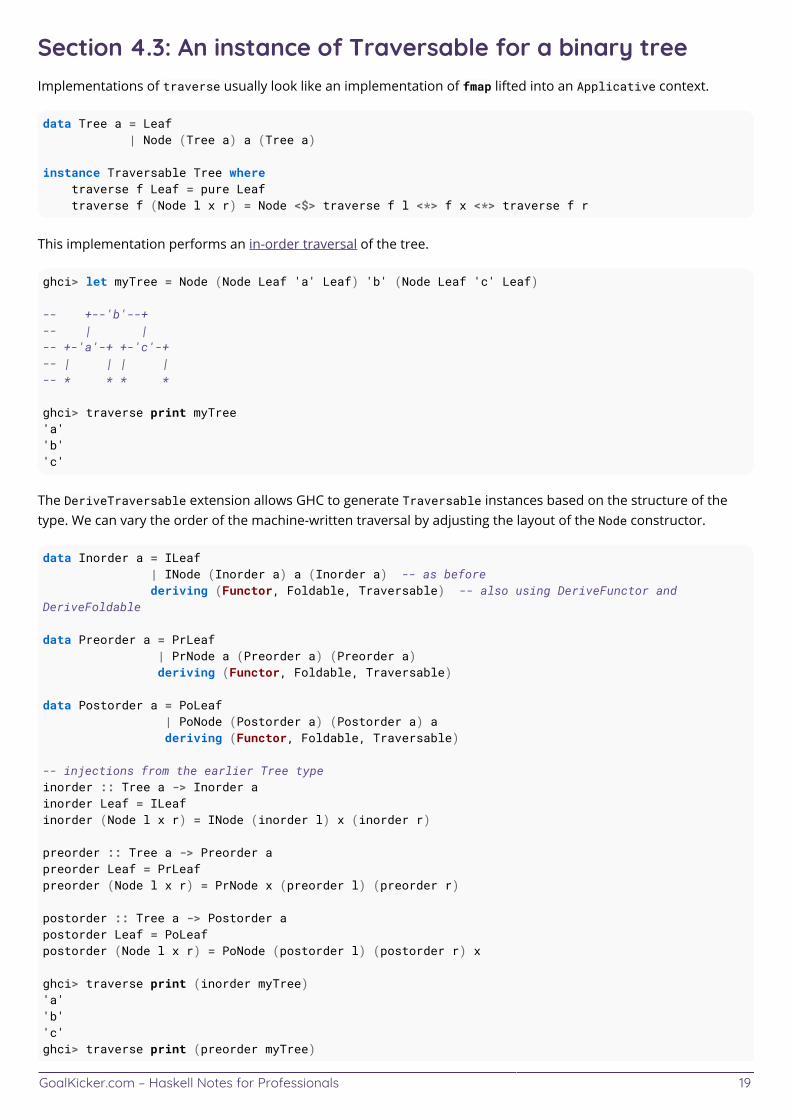
GoalKicker.com – Haskell Notes for Professionals 19

Section 4.3: An instance of Traversable for a binary treeImplementations of traverse usually look like an implementation of fmap lifted into an Applicative context.

data Tree a = Leaf | Node (Tree a) a (Tree a)

instance Traversable Tree where traverse f Leaf = pure Leaf traverse f (Node l x r) = Node <$> traverse f l <*> f x <*> traverse f r

This implementation performs an in-order traversal of the tree.

ghci> let myTree = Node (Node Leaf 'a' Leaf) 'b' (Node Leaf 'c' Leaf)

-- +--'b'--+-- | |-- +-'a'-+ +-'c'-+-- | | | |-- * * * *

ghci> traverse print myTree'a''b''c'

The DeriveTraversable extension allows GHC to generate Traversable instances based on the structure of thetype. We can vary the order of the machine-written traversal by adjusting the layout of the Node constructor.

data Inorder a = ILeaf | INode (Inorder a) a (Inorder a) -- as before deriving (Functor, Foldable, Traversable) -- also using DeriveFunctor andDeriveFoldable

data Preorder a = PrLeaf | PrNode a (Preorder a) (Preorder a) deriving (Functor, Foldable, Traversable)

data Postorder a = PoLeaf | PoNode (Postorder a) (Postorder a) a deriving (Functor, Foldable, Traversable)

-- injections from the earlier Tree typeinorder :: Tree a -> Inorder ainorder Leaf = ILeafinorder (Node l x r) = INode (inorder l) x (inorder r)

preorder :: Tree a -> Preorder apreorder Leaf = PrLeafpreorder (Node l x r) = PrNode x (preorder l) (preorder r)

postorder :: Tree a -> Postorder apostorder Leaf = PoLeafpostorder (Node l x r) = PoNode (postorder l) (postorder r) x

ghci> traverse print (inorder myTree)'a''b''c'ghci> traverse print (preorder myTree)

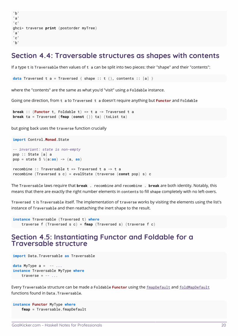
GoalKicker.com – Haskell Notes for Professionals 20

'b''a''c'ghci> traverse print (postorder myTree)'a''c''b'

Section 4.4: Traversable structures as shapes with contentsIf a type t is Traversable then values of t a can be split into two pieces: their "shape" and their "contents":

data Traversed t a = Traversed { shape :: t (), contents :: [a] }

where the "contents" are the same as what you'd "visit" using a Foldable instance.

Going one direction, from t a to Traversed t a doesn't require anything but Functor and Foldable

break :: (Functor t, Foldable t) => t a -> Traversed t abreak ta = Traversed (fmap (const ()) ta) (toList ta)

but going back uses the traverse function crucially

import Control.Monad.State

-- invariant: state is non-emptypop :: State [a] apop = state $ \(a:as) -> (a, as)

recombine :: Traversable t => Traversed t a -> t arecombine (Traversed s c) = evalState (traverse (const pop) s) c

The Traversable laws require that break . recombine and recombine . break are both identity. Notably, thismeans that there are exactly the right number elements in contents to fill shape completely with no left-overs.

Traversed t is Traversable itself. The implementation of traverse works by visiting the elements using the list'sinstance of Traversable and then reattaching the inert shape to the result.

instance Traversable (Traversed t) where traverse f (Traversed s c) = fmap (Traversed s) (traverse f c)

Section 4.5: Instantiating Functor and Foldable for aTraversable structureimport Data.Traversable as Traversable

data MyType a = -- ...instance Traversable MyType where traverse = -- ...

Every Traversable structure can be made a Foldable Functor using the fmapDefault and foldMapDefaultfunctions found in Data.Traversable.

instance Functor MyType where fmap = Traversable.fmapDefault

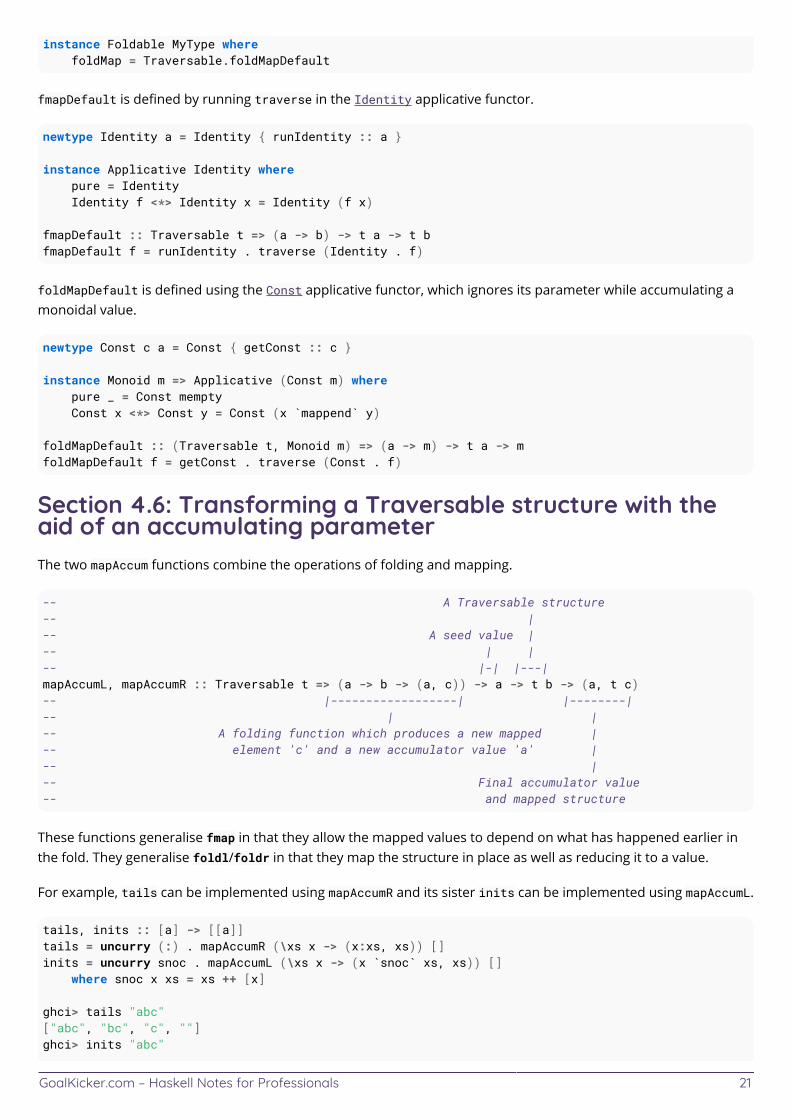
GoalKicker.com – Haskell Notes for Professionals 21

instance Foldable MyType where foldMap = Traversable.foldMapDefault

fmapDefault is defined by running traverse in the Identity applicative functor.

newtype Identity a = Identity { runIdentity :: a }

instance Applicative Identity where pure = Identity Identity f <*> Identity x = Identity (f x)

fmapDefault :: Traversable t => (a -> b) -> t a -> t bfmapDefault f = runIdentity . traverse (Identity . f)

foldMapDefault is defined using the Const applicative functor, which ignores its parameter while accumulating amonoidal value.

newtype Const c a = Const { getConst :: c }

instance Monoid m => Applicative (Const m) where pure _ = Const mempty Const x <*> Const y = Const (x `mappend` y)

foldMapDefault :: (Traversable t, Monoid m) => (a -> m) -> t a -> mfoldMapDefault f = getConst . traverse (Const . f)

Section 4.6: Transforming a Traversable structure with theaid of an accumulating parameterThe two mapAccum functions combine the operations of folding and mapping.

-- A Traversable structure-- |-- A seed value |-- | |-- |-| |---|mapAccumL, mapAccumR :: Traversable t => (a -> b -> (a, c)) -> a -> t b -> (a, t c)-- |------------------| |--------|-- | |-- A folding function which produces a new mapped |-- element 'c' and a new accumulator value 'a' |-- |-- Final accumulator value-- and mapped structure

These functions generalise fmap in that they allow the mapped values to depend on what has happened earlier inthe fold. They generalise foldl/foldr in that they map the structure in place as well as reducing it to a value.

For example, tails can be implemented using mapAccumR and its sister inits can be implemented using mapAccumL.

tails, inits :: [a] -> [[a]]tails = uncurry (:) . mapAccumR (\xs x -> (x:xs, xs)) []inits = uncurry snoc . mapAccumL (\xs x -> (x `snoc` xs, xs)) [] where snoc x xs = xs ++ [x]

ghci> tails "abc"["abc", "bc", "c", ""]ghci> inits "abc"

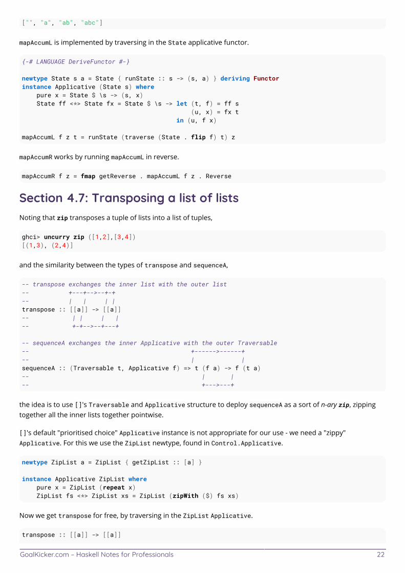
GoalKicker.com – Haskell Notes for Professionals 22

["", "a", "ab", "abc"]

mapAccumL is implemented by traversing in the State applicative functor.

{-# LANGUAGE DeriveFunctor #-}

newtype State s a = State { runState :: s -> (s, a) } deriving Functorinstance Applicative (State s) where pure x = State $ \s -> (s, x) State ff <*> State fx = State $ \s -> let (t, f) = ff s (u, x) = fx t in (u, f x)

mapAccumL f z t = runState (traverse (State . flip f) t) z

mapAccumR works by running mapAccumL in reverse.

mapAccumR f z = fmap getReverse . mapAccumL f z . Reverse

Section 4.7: Transposing a list of listsNoting that zip transposes a tuple of lists into a list of tuples,

ghci> uncurry zip ([1,2],[3,4])[(1,3), (2,4)]

and the similarity between the types of transpose and sequenceA,

-- transpose exchanges the inner list with the outer list-- +---+-->--+-+-- | | | |transpose :: [[a]] -> [[a]]-- | | | |-- +-+-->--+---+

-- sequenceA exchanges the inner Applicative with the outer Traversable-- +------>------+-- | |sequenceA :: (Traversable t, Applicative f) => t (f a) -> f (t a)-- | |-- +--->---+

the idea is to use []'s Traversable and Applicative structure to deploy sequenceA as a sort of n-ary zip, zippingtogether all the inner lists together pointwise.

[]'s default "prioritised choice" Applicative instance is not appropriate for our use - we need a "zippy"Applicative. For this we use the ZipList newtype, found in Control.Applicative.

newtype ZipList a = ZipList { getZipList :: [a] }

instance Applicative ZipList where pure x = ZipList (repeat x) ZipList fs <*> ZipList xs = ZipList (zipWith ($) fs xs)

Now we get transpose for free, by traversing in the ZipList Applicative.

transpose :: [[a]] -> [[a]]

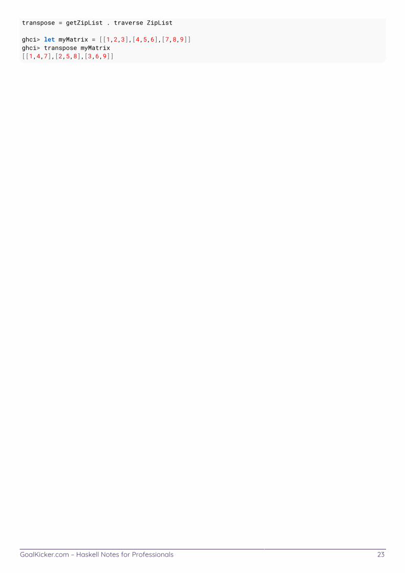
GoalKicker.com – Haskell Notes for Professionals 23

transpose = getZipList . traverse ZipList

ghci> let myMatrix = [[1,2,3],[4,5,6],[7,8,9]]ghci> transpose myMatrix[[1,4,7],[2,5,8],[3,6,9]]

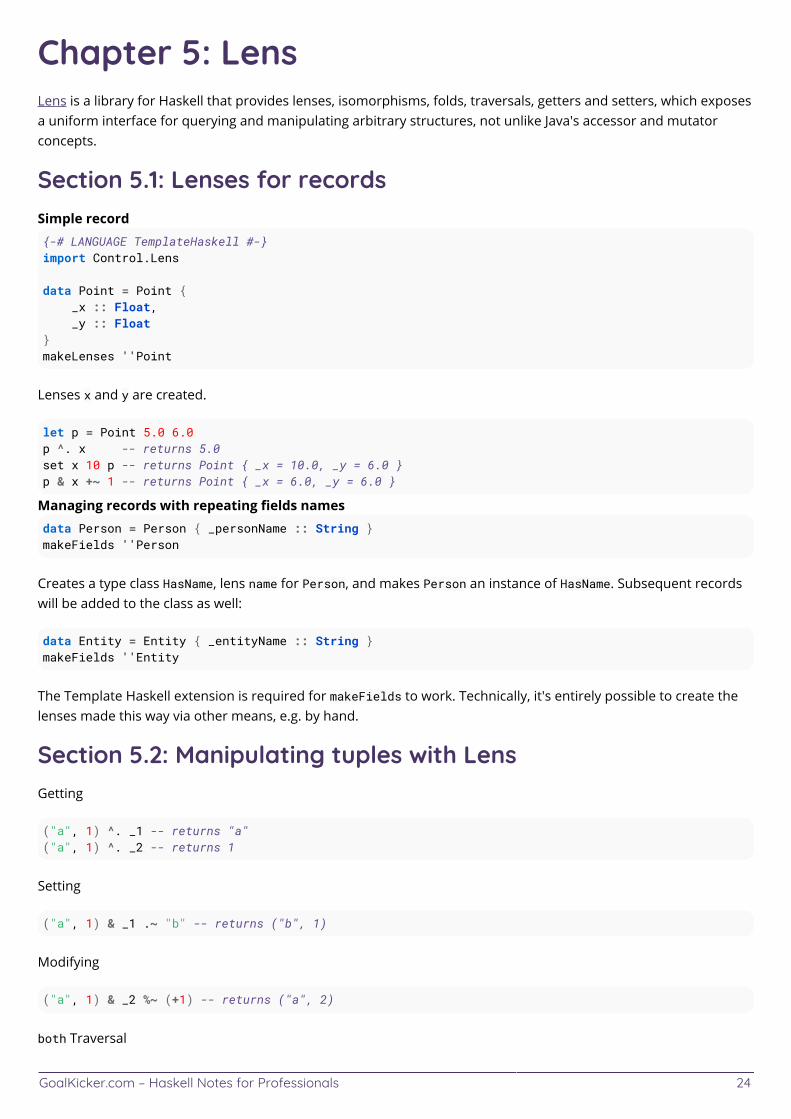
GoalKicker.com – Haskell Notes for Professionals 24

Chapter 5: LensLens is a library for Haskell that provides lenses, isomorphisms, folds, traversals, getters and setters, which exposesa uniform interface for querying and manipulating arbitrary structures, not unlike Java's accessor and mutatorconcepts.

Section 5.1: Lenses for recordsSimple record{-# LANGUAGE TemplateHaskell #-}import Control.Lens

data Point = Point { _x :: Float, _y :: Float}makeLenses ''Point

Lenses x and y are created.

let p = Point 5.0 6.0p ^. x -- returns 5.0set x 10 p -- returns Point { _x = 10.0, _y = 6.0 }p & x +~ 1 -- returns Point { _x = 6.0, _y = 6.0 }

Managing records with repeating fields namesdata Person = Person { _personName :: String }makeFields ''Person

Creates a type class HasName, lens name for Person, and makes Person an instance of HasName. Subsequent recordswill be added to the class as well:

data Entity = Entity { _entityName :: String }makeFields ''Entity

The Template Haskell extension is required for makeFields to work. Technically, it's entirely possible to create thelenses made this way via other means, e.g. by hand.

Section 5.2: Manipulating tuples with LensGetting

("a", 1) ^. _1 -- returns "a"("a", 1) ^. _2 -- returns 1

Setting

("a", 1) & _1 .~ "b" -- returns ("b", 1)

Modifying

("a", 1) & _2 %~ (+1) -- returns ("a", 2)

both Traversal

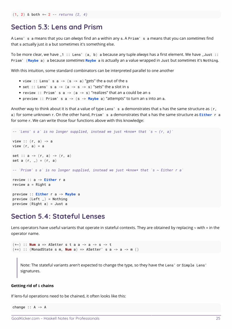
GoalKicker.com – Haskell Notes for Professionals 25

(1, 2) & both *~ 2 -- returns (2, 4)

Section 5.3: Lens and PrismA Lens' s a means that you can always find an a within any s. A Prism' s a means that you can sometimes findthat s actually just is a but sometimes it's something else.

To be more clear, we have _1 :: Lens' (a, b) a because any tuple always has a first element. We have _Just ::Prism' (Maybe a) a because sometimes Maybe a is actually an a value wrapped in Just but sometimes it's Nothing.

With this intuition, some standard combinators can be interpreted parallel to one another

view :: Lens' s a -> (s -> a) "gets" the a out of the sset :: Lens' s a -> (a -> s -> s) "sets" the a slot in sreview :: Prism' s a -> (a -> s) "realizes" that an a could be an spreview :: Prism' s a -> (s -> Maybe a) "attempts" to turn an s into an a.

Another way to think about it is that a value of type Lens' s a demonstrates that s has the same structure as (r,a) for some unknown r. On the other hand, Prism' s a demonstrates that s has the same structure as Either r afor some r. We can write those four functions above with this knowledge:

-- `Lens' s a` is no longer supplied, instead we just *know* that `s ~ (r, a)`

view :: (r, a) -> aview (r, a) = a

set :: a -> (r, a) -> (r, a)set a (r, _) = (r, a)

-- `Prism' s a` is no longer supplied, instead we just *know* that `s ~ Either r a`

review :: a -> Either r areview a = Right a

preview :: Either r a -> Maybe apreview (Left _) = Nothingpreview (Right a) = Just a

Section 5.4: Stateful LensesLens operators have useful variants that operate in stateful contexts. They are obtained by replacing ~ with = in theoperator name.

(+~) :: Num a => ASetter s t a a -> a -> s -> t(+=) :: (MonadState s m, Num a) => ASetter' s a -> a -> m ()

Note: The stateful variants aren't expected to change the type, so they have the Lens' or Simple Lens'signatures.

Getting rid of & chains

If lens-ful operations need to be chained, it often looks like this:

change :: A -> A

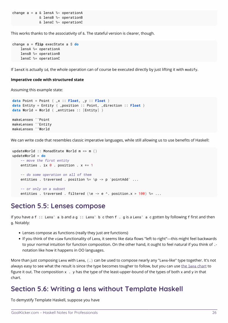
GoalKicker.com – Haskell Notes for Professionals 26

change a = a & lensA %~ operationA & lensB %~ operationB & lensC %~ operationC

This works thanks to the associativity of &. The stateful version is clearer, though.

change a = flip execState a $ do lensA %= operationA lensB %= operationB lensC %= operationC

If lensX is actually id, the whole operation can of course be executed directly by just lifting it with modify.

Imperative code with structured state

Assuming this example state:

data Point = Point { _x :: Float, _y :: Float }data Entity = Entity { _position :: Point, _direction :: Float }data World = World { _entities :: [Entity] }

makeLenses ''PointmakeLenses ''EntitymakeLenses ''World

We can write code that resembles classic imperative languages, while still allowing us to use benefits of Haskell:

updateWorld :: MonadState World m => m ()updateWorld = do -- move the first entity entities . ix 0 . position . x += 1

-- do some operation on all of them entities . traversed . position %= \p -> p `pointAdd` ...

-- or only on a subset entities . traversed . filtered (\e -> e ^. position.x > 100) %= ...

Section 5.5: Lenses composeIf you have a f :: Lens' a b and a g :: Lens' b c then f . g is a Lens' a c gotten by following f first and theng. Notably:

Lenses compose as functions (really they just are functions)If you think of the view functionality of Lens, it seems like data flows "left to right"—this might feel backwardsto your normal intuition for function composition. On the other hand, it ought to feel natural if you think of .-notation like how it happens in OO languages.

More than just composing Lens with Lens, (.) can be used to compose nearly any "Lens-like" type together. It's notalways easy to see what the result is since the type becomes tougher to follow, but you can use the lens chart tofigure it out. The composition x . y has the type of the least-upper-bound of the types of both x and y in thatchart.

Section 5.6: Writing a lens without Template HaskellTo demystify Template Haskell, suppose you have

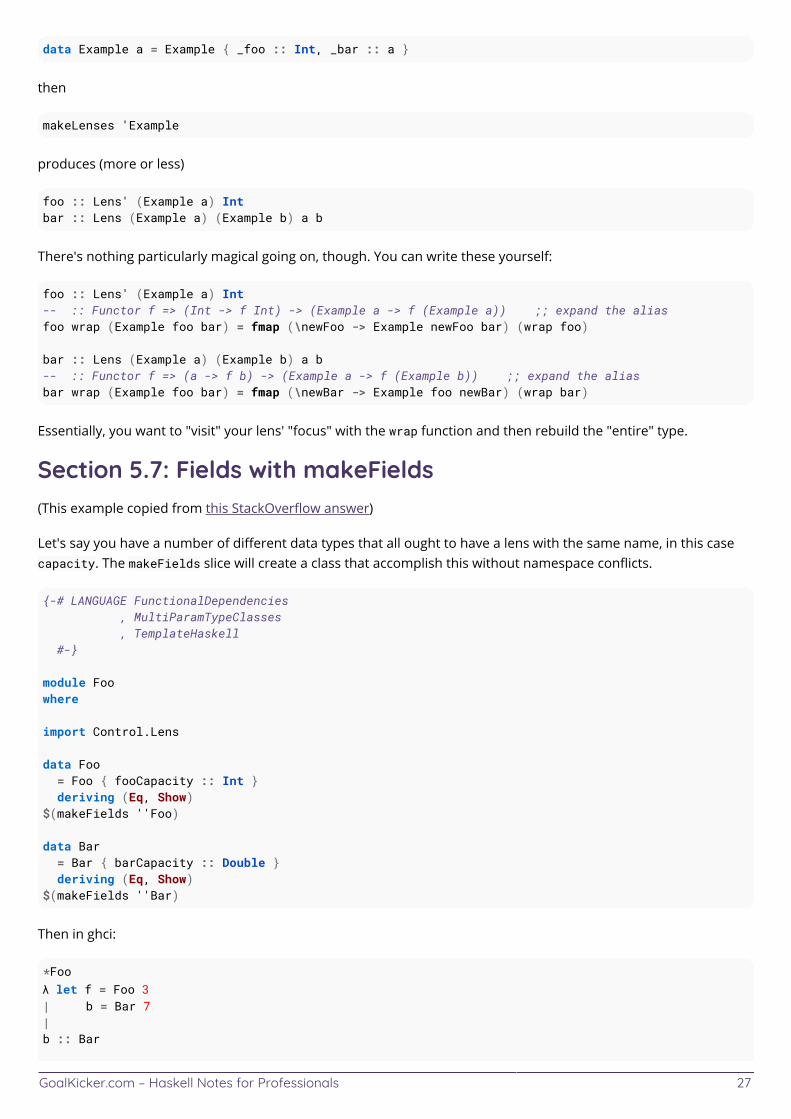
GoalKicker.com – Haskell Notes for Professionals 27

data Example a = Example { _foo :: Int, _bar :: a }

then

makeLenses 'Example

produces (more or less)

foo :: Lens' (Example a) Intbar :: Lens (Example a) (Example b) a b

There's nothing particularly magical going on, though. You can write these yourself:

foo :: Lens' (Example a) Int-- :: Functor f => (Int -> f Int) -> (Example a -> f (Example a)) ;; expand the aliasfoo wrap (Example foo bar) = fmap (\newFoo -> Example newFoo bar) (wrap foo)

bar :: Lens (Example a) (Example b) a b-- :: Functor f => (a -> f b) -> (Example a -> f (Example b)) ;; expand the aliasbar wrap (Example foo bar) = fmap (\newBar -> Example foo newBar) (wrap bar)

Essentially, you want to "visit" your lens' "focus" with the wrap function and then rebuild the "entire" type.

Section 5.7: Fields with makeFields(This example copied from this StackOverflow answer)

Let's say you have a number of different data types that all ought to have a lens with the same name, in this casecapacity. The makeFields slice will create a class that accomplish this without namespace conflicts.

{-# LANGUAGE FunctionalDependencies , MultiParamTypeClasses , TemplateHaskell #-}

module Foowhere

import Control.Lens

data Foo = Foo { fooCapacity :: Int } deriving (Eq, Show)$(makeFields ''Foo)

data Bar = Bar { barCapacity :: Double } deriving (Eq, Show)$(makeFields ''Bar)

Then in ghci:

*Fooλ let f = Foo 3| b = Bar 7|b :: Bar

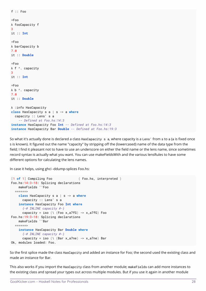
GoalKicker.com – Haskell Notes for Professionals 28

f :: Foo

*Fooλ fooCapacity f3it :: Int

*Fooλ barCapacity b7.0it :: Double

*Fooλ f ^. capacity3it :: Int

*Fooλ b ^. capacity7.0it :: Double

λ :info HasCapacityclass HasCapacity s a | s -> a where capacity :: Lens' s a -- Defined at Foo.hs:14:3instance HasCapacity Foo Int -- Defined at Foo.hs:14:3instance HasCapacity Bar Double -- Defined at Foo.hs:19:3

So what it's actually done is declared a class HasCapacity s a, where capacity is a Lens' from s to a (a is fixed onces is known). It figured out the name "capacity" by stripping off the (lowercased) name of the data type from thefield; I find it pleasant not to have to use an underscore on either the field name or the lens name, since sometimesrecord syntax is actually what you want. You can use makeFieldsWith and the various lensRules to have somedifferent options for calculating the lens names.

In case it helps, using ghci -ddump-splices Foo.hs:

[1 of 1] Compiling Foo ( Foo.hs, interpreted )Foo.hs:14:3-18: Splicing declarations makeFields ''Foo ======> class HasCapacity s a | s -> a where capacity :: Lens' s a instance HasCapacity Foo Int where {-# INLINE capacity #-} capacity = iso (\ (Foo x_a7fG) -> x_a7fG) FooFoo.hs:19:3-18: Splicing declarations makeFields ''Bar ======> instance HasCapacity Bar Double where {-# INLINE capacity #-} capacity = iso (\ (Bar x_a7ne) -> x_a7ne) BarOk, modules loaded: Foo.

So the first splice made the class HasCapcity and added an instance for Foo; the second used the existing class andmade an instance for Bar.

This also works if you import the HasCapcity class from another module; makeFields can add more instances tothe existing class and spread your types out across multiple modules. But if you use it again in another module

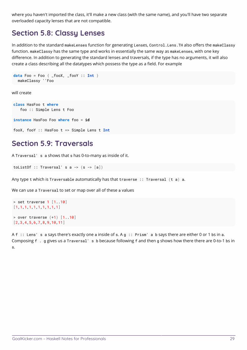
GoalKicker.com – Haskell Notes for Professionals 29

where you haven't imported the class, it'll make a new class (with the same name), and you'll have two separateoverloaded capacity lenses that are not compatible.

Section 5.8: Classy LensesIn addition to the standard makeLenses function for generating Lenses, Control.Lens.TH also offers the makeClassyfunction. makeClassy has the same type and works in essentially the same way as makeLenses, with one keydifference. In addition to generating the standard lenses and traversals, if the type has no arguments, it will alsocreate a class describing all the datatypes which possess the type as a field. For example

data Foo = Foo { _fooX, _fooY :: Int } makeClassy ''Foo

will create

class HasFoo t where foo :: Simple Lens t Foo

instance HasFoo Foo where foo = id

fooX, fooY :: HasFoo t => Simple Lens t Int

Section 5.9: TraversalsA Traversal' s a shows that s has 0-to-many as inside of it.

toListOf :: Traversal' s a -> (s -> [a])

Any type t which is Traversable automatically has that traverse :: Traversal (t a) a.

We can use a Traversal to set or map over all of these a values

> set traverse 1 [1..10][1,1,1,1,1,1,1,1,1,1]

> over traverse (+1) [1..10][2,3,4,5,6,7,8,9,10,11]

A f :: Lens' s a says there's exactly one a inside of s. A g :: Prism' a b says there are either 0 or 1 bs in a.Composing f . g gives us a Traversal' s b because following f and then g shows how there there are 0-to-1 bs ins.

GoalKicker.com – Haskell Notes for Professionals 30

Chapter 6: QuickCheckSection 6.1: Declaring a propertyAt its simplest, a property is a function which returns a Bool.

prop_reverseDoesNotChangeLength xs = length (reverse xs) == length xs

A property declares a high-level invariant of a program. The QuickCheck test runner will evaluate the function with100 random inputs and check that the result is always True.

By convention, functions that are properties have names which start with prop_.

Section 6.2: Randomly generating data for custom typesThe Arbitrary class is for types that can be randomly generated by QuickCheck.

The minimal implementation of Arbitrary is the arbitrary method, which runs in the Gen monad to produce arandom value.

Here is an instance of Arbitrary for the following datatype of non-empty lists.

import Test.QuickCheck.Arbitrary (Arbitrary(..))import Test.QuickCheck.Gen (oneof)import Control.Applicative ((<$>), (<*>))

data NonEmpty a = End a | Cons a (NonEmpty a)

instance Arbitrary a => Arbitrary (NonEmpty a) where arbitrary = oneof [ -- randomly select one of the cases from the list End <$> arbitrary, -- call a's instance of Arbitrary Cons <$> arbitrary <*> -- call a's instance of Arbitrary arbitrary -- recursively call NonEmpty's instance of Arbitrary ]

Section 6.3: Using implication (==>) to check properties withpreconditionsprop_evenNumberPlusOneIsOdd :: Integer -> Propertyprop_evenNumberPlusOneIsOdd x = even x ==> odd (x + 1)

If you want to check that a property holds given that a precondition holds, you can use the

==>

operator. Note that if it's very unlikely for arbitrary inputs to match the precondition, QuickCheck can give up early.

prop_overlySpecific x y = x == 0 ==> x * y == 0

ghci> quickCheck prop_overlySpecific*** Gave up! Passed only 31 tests.

Section 6.4: Checking a single propertyThe quickCheck function tests a property on 100 random inputs.

GoalKicker.com – Haskell Notes for Professionals 31

ghci> quickCheck prop_reverseDoesNotChangeLength+++ OK, passed 100 tests.

If a property fails for some input, quickCheck prints out a counterexample.

prop_reverseIsAlwaysEmpty xs = reverse xs == [] -- plainly not true for all xs

ghci> quickCheck prop_reverseIsAlwaysEmpty*** Failed! Falsifiable (after 2 tests): [()]

Section 6.5: Checking all the properties in a filequickCheckAll is a Template Haskell helper which finds all the definitions in the current file whose name beginswith prop_ and tests them.

{-# LANGUAGE TemplateHaskell #-}

import Test.QuickCheck (quickCheckAll)import Data.List (sort)

idempotent :: Eq a => (a -> a) -> a -> Boolidempotent f x = f (f x) == f x

prop_sortIdempotent = idempotent sort

-- does not begin with prop_, will not be picked up by the test runnersortDoesNotChangeLength xs = length (sort xs) == length xs

return []main = $quickCheckAll

Note that the return [] line is required. It makes definitions textually above that line visible to Template Haskell.

$ runhaskell QuickCheckAllExample.hs=== prop_sortIdempotent from tree.hs:7 ===+++ OK, passed 100 tests.

Section 6.6: Limiting the size of test dataIt can be difficult to test functions with poor asymptotic complexity using quickcheck as the random inputs are notusually size bounded. By adding an upper bound on the size of the input we can still test these expensive functions.

import Data.List(permutations)import Test.QuickCheck

longRunningFunction :: [a] -> IntlongRunningFunction xs = length (permutations xs)

factorial :: Integral a => a -> afactorial n = product [1..n]

prop_numberOfPermutations xs = longRunningFunction xs == factorial (length xs)

ghci> quickCheckWith (stdArgs { maxSize = 10}) prop_numberOfPermutations

GoalKicker.com – Haskell Notes for Professionals 32

By using quickCheckWith with a modified version of stdArgs we can limit the size of the inputs to be at most 10. Inthis case, as we are generating lists, this means we generate lists of up to size 10. Our permutations functiondoesn't take too long to run for these short lists but we can still be reasonably confident that our definition iscorrect.

GoalKicker.com – Haskell Notes for Professionals 33

Chapter 7: Common GHC LanguageExtensionsSection 7.1: RankNTypesImagine the following situation:

foo :: Show a => (a -> String) -> String -> Int -> IO ()foo show' string int = do putStrLn (show' string) putStrLn (show' int)

Here, we want to pass in a function that converts a value into a String, apply that function to both a stringparameter and and int parameter and print them both. In my mind, there is no reason this should fail! We have afunction that works on both types of the parameters we're passing in.

Unfortunately, this won't type check! GHC infers the a type based off of its first occurrence in the function body.That is, as soon as we hit:

putStrLn (show' string)

GHC will infer that show' :: String -> String, since string is a String. It will proceed to blow up while trying toshow' int.

RankNTypes lets you instead write the type signature as follows, quantifying over all functions that satisfy the show'type:

foo :: (forall a. Show a => (a -> String)) -> String -> Int -> IO ()

This is rank 2 polymorphism: We are asserting that the show' function must work for all as within our function, andthe previous implementation now works.

The RankNTypes extension allows arbitrary nesting of forall ... blocks in type signatures. In other words, it allowsrank N polymorphism.

Section 7.2: OverloadedStringsNormally, string literals in Haskell have a type of String (which is a type alias for [Char]). While this isn't a problemfor smaller, educational programs, real-world applications often require more efficient storage such as Text orByteString.

OverloadedStrings simply changes the type of literals to

"test" :: Data.String.IsString a => a

Allowing them to be directly passed to functions expecting such a type. Many libraries implement this interface fortheir string-like types including Data.Text and Data.ByteString which both provide certain time and spaceadvantages over [Char].

There are also some unique uses of OverloadedStrings like those from the Postgresql-simple library which allowsSQL queries to be written in double quotes like a normal string, but provides protections against improperconcatenation, a notorious source of SQL injection attacks.

GoalKicker.com – Haskell Notes for Professionals 34

To create a instance of the IsString class you need to impliment the fromString function. Example†:

data Foo = A | B | Other String deriving Show

instance IsString Foo where fromString "A" = A fromString "B" = B fromString xs = Other xs

tests :: [ Foo ]tests = [ "A", "B", "Testing" ]

† This example courtesy of Lyndon Maydwell (sordina on GitHub) found here.

Section 7.3: BinaryLiteralsStandard Haskell allows you to write integer literals in decimal (without any prefix), hexadecimal (preceded by 0x or0X), and octal (preceded by 0o or 0O). The BinaryLiterals extension adds the option of binary (preceded by 0b or0B).

0b1111 == 15 -- evaluates to: True

Section 7.4: ExistentialQuantificationThis is a type system extension that allows types that are existentially quantified, or, in other words, have typevariables that only get instantiated at runtime†.

A value of existential type is similar to an abstract-base-class reference in OO languages: you don't know the exacttype in contains, but you can constrain the class of types.

data S = forall a. Show a => S a

or equivalently, with GADT syntax:

{-# LANGUAGE GADTs #-}data S where S :: Show a => a -> S

Existential types open the door to things like almost-heterogenous containers: as said above, there can actually bevarious types in an S value, but all of them can be shown, hence you can also do

instance Show S where show (S a) = show a -- we rely on (Show a) from the above

Now we can create a collection of such objects:

ss = [S 5, S "test", S 3.0]

Which also allows us to use the polymorphic behaviour:

mapM_ print ss

Existentials can be very powerful, but note that they are actually not necessary very often in Haskell. In the example

GoalKicker.com – Haskell Notes for Professionals 35

above, all you can actually do with the Show instance is show (duh!) the values, i.e. create a string representation.The entire S type therefore contains exactly as much information as the string you get when showing it. Therefore,it is usually better to simply store that string right away, especially since Haskell is lazy and therefore the string willat first only be an unevaluated thunk anyway.

On the other hand, existentials cause some unique problems. For instance, the way the type information is “hidden”in an existential. If you pattern-match on an S value, you will have the contained type in scope (more precisely, itsShow instance), but this information can never escape its scope, which therefore becomes a bit of a “secret society”:the compiler doesn't let anything escape the scope except values whose type is already known from the outside.This can lead to strange errors like Couldn't match type ‘a0’ with ‘()’ ‘a0’ is untouchable.

†Contrast this with ordinary parametric polymorphism, which is generally resolved at compile time (allowing fulltype erasure).

Existential types are different from Rank-N types – these extensions are, roughly speaking, dual to each other: toactually use values of an existential type, you need a (possibly constrained-) polymorphic function, like show in theexample. A polymorphic function is universally quantified, i.e. it works for any type in a given class, whereasexistential quantification means it works for some particular type which is a priori unknown. If you have apolymorphic function, that's sufficient, however to pass polymorphic functions as such as arguments, you need {-#LANGUAGE Rank2Types #-}:

genShowSs :: (∀ x . Show x => x -> String) -> [S] -> [String]genShowSs f = map (\(S a) -> f a)

Section 7.5: LambdaCaseA syntactic extension that lets you write \case in place of \arg -> case arg of.

Consider the following function definition:

dayOfTheWeek :: Int -> StringdayOfTheWeek 0 = "Sunday"dayOfTheWeek 1 = "Monday"dayOfTheWeek 2 = "Tuesday"dayOfTheWeek 3 = "Wednesday"dayOfTheWeek 4 = "Thursday"dayOfTheWeek 5 = "Friday"dayOfTheWeek 6 = "Saturday"

If you want to avoid repeating the function name, you might write something like:

dayOfTheWeek :: Int -> StringdayOfTheWeek i = case i of 0 -> "Sunday" 1 -> "Monday" 2 -> "Tuesday" 3 -> "Wednesday" 4 -> "Thursday" 5 -> "Friday" 6 -> "Saturday"

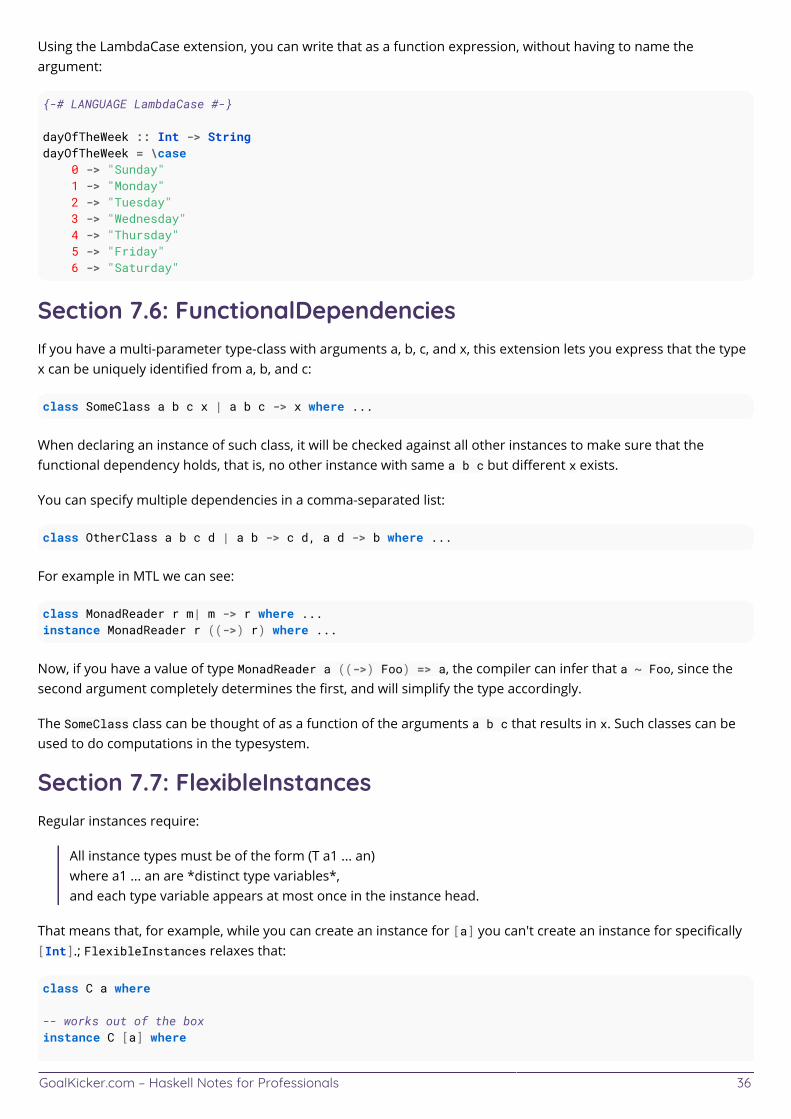
GoalKicker.com – Haskell Notes for Professionals 36

Using the LambdaCase extension, you can write that as a function expression, without having to name theargument:

{-# LANGUAGE LambdaCase #-}

dayOfTheWeek :: Int -> StringdayOfTheWeek = \case 0 -> "Sunday" 1 -> "Monday" 2 -> "Tuesday" 3 -> "Wednesday" 4 -> "Thursday" 5 -> "Friday" 6 -> "Saturday"

Section 7.6: FunctionalDependenciesIf you have a multi-parameter type-class with arguments a, b, c, and x, this extension lets you express that the typex can be uniquely identified from a, b, and c:

class SomeClass a b c x | a b c -> x where ...

When declaring an instance of such class, it will be checked against all other instances to make sure that thefunctional dependency holds, that is, no other instance with same a b c but different x exists.

You can specify multiple dependencies in a comma-separated list:

class OtherClass a b c d | a b -> c d, a d -> b where ...

For example in MTL we can see:

class MonadReader r m| m -> r where ...instance MonadReader r ((->) r) where ...

Now, if you have a value of type MonadReader a ((->) Foo) => a, the compiler can infer that a ~ Foo, since thesecond argument completely determines the first, and will simplify the type accordingly.

The SomeClass class can be thought of as a function of the arguments a b c that results in x. Such classes can beused to do computations in the typesystem.

Section 7.7: FlexibleInstancesRegular instances require:

All instance types must be of the form (T a1 ... an)where a1 ... an are *distinct type variables*,and each type variable appears at most once in the instance head.

That means that, for example, while you can create an instance for [a] you can't create an instance for specifically[Int].; FlexibleInstances relaxes that:

class C a where

-- works out of the boxinstance C [a] where

GoalKicker.com – Haskell Notes for Professionals 37

-- requires FlexibleInstancesinstance C [Int] where

Section 7.8: GADTsConventional algebraic datatypes are parametric in their type variables. For example, if we define an ADT like

data Expr a = IntLit Int | BoolLit Bool | If (Expr Bool) (Expr a) (Expr a)

with the hope that this will statically rule out non-well-typed conditionals, this will not behave as expected since thetype of IntLit :: Int -> Expr a is universially quantified: for any choice of a, it produces a value of type Expr a.In particular, for a ~ Bool, we have IntLit :: Int -> Expr Bool, allowing us to construct something like If(IntLit 1) e1 e2 which is what the type of the If constructor was trying to rule out.

Generalised Algebraic Data Types allows us to control the resulting type of a data constructor so that they are notmerely parametric. We can rewrite our Expr type as a GADT like this:

data Expr a where IntLit :: Int -> Expr Int BoolLit :: Bool -> Expr Bool If :: Expr Bool -> Expr a -> Expr a -> Expr a

Here, the type of the constructor IntLit is Int -> Expr Int, and so IntLit 1 :: Expr Bool will not typecheck.

Pattern matching on a GADT value causes refinement of the type of the term returned. For example, it is possible towrite an evaluator for Expr a like this:

crazyEval :: Expr a -> acrazyEval (IntLit x) = -- Here we can use `(+)` because x :: Int x + 1crazyEval (BoolLit b) = -- Here we can use `not` because b :: Bool not bcrazyEval (If b thn els) = -- Because b :: Expr Bool, we can use `crazyEval b :: Bool`. -- Also, because thn :: Expr a and els :: Expr a, we can pass either to -- the recursive call to `crazyEval` and get an a back crazyEval $ if crazyEval b then thn else els

Note that we are able to use (+) in the above definitions because when e.g. IntLit x is pattern matched, we alsolearn that a ~ Int (and likewise for not and if_then_else_ when a ~ Bool).

Section 7.9: TupleSectionsA syntactic extension that allows applying the tuple constructor (which is an operator) in a section way:

(a,b) == (,) a b

-- With TupleSections(a,b) == (,) a b == (a,) b == (,b) a

N-tuples

It also works for tuples with arity greater than two

GoalKicker.com – Haskell Notes for Professionals 38

(,2,) 1 3 == (1,2,3)

Mapping

This can be useful in other places where sections are used:

map (,"tag") [1,2,3] == [(1,"tag"), (2, "tag"), (3, "tag")]

The above example without this extension would look like this:

map (\a -> (a, "tag")) [1,2,3]

Section 7.10: OverloadedListsadded in GHC 7.8.

OverloadedLists, similar to OverloadedStrings, allows list literals to be desugared as follows:

[] -- fromListN 0 [][x] -- fromListN 1 (x : [])[x .. ] -- fromList (enumFrom x)

This comes handy when dealing with types such as Set, Vector and Maps.

['0' .. '9'] :: Set Char[1 .. 10] :: Vector Int[("default",0), (k1,v1)] :: Map String Int['a' .. 'z'] :: Text

IsList class in GHC.Exts is intended to be used with this extension.

IsList is equipped with one type function, Item, and three functions, fromList :: [Item l] -> l, toList :: l-> [Item l] and fromListN :: Int -> [Item l] -> l where fromListN is optional. Typical implementations are:

instance IsList [a] where type Item [a] = a fromList = id toList = id

instance (Ord a) => IsList (Set a) where type Item (Set a) = a fromList = Set.fromList toList = Set.toList

Examples taken from OverloadedLists – GHC.

Section 7.11: MultiParamTypeClassesIt's a very common extension that allows type classes with multiple type parameters. You can think of MPTC as arelation between types.

{-# LANGUAGE MultiParamTypeClasses #-}

class Convertable a b where convert :: a -> b

instance Convertable Int Float where

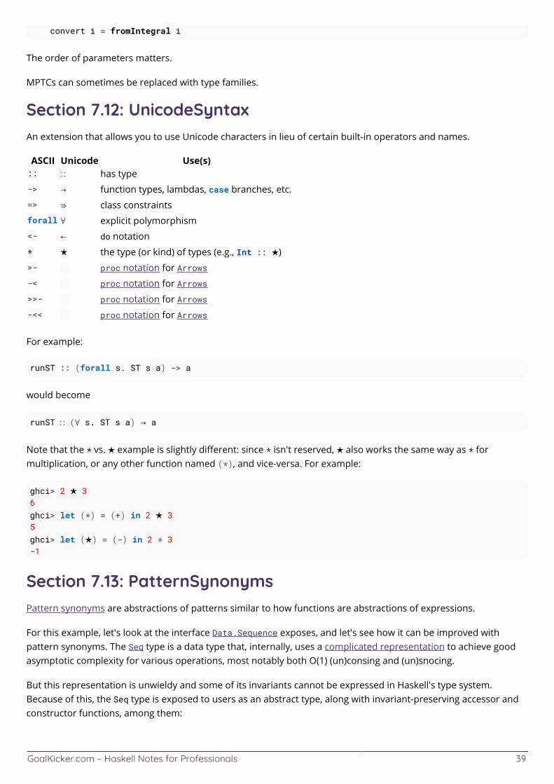
GoalKicker.com – Haskell Notes for Professionals 39

convert i = fromIntegral i

The order of parameters matters.

MPTCs can sometimes be replaced with type families.

Section 7.12: UnicodeSyntaxAn extension that allows you to use Unicode characters in lieu of certain built-in operators and names.

ASCII Unicode Use(s):: ∷ has type-> → function types, lambdas, case branches, etc.=> ⇒ class constraintsforall ∀ explicit polymorphism<- ← do notation* ★ the type (or kind) of types (e.g., Int :: ★)>- � proc notation for Arrows-< � proc notation for Arrows>>- � proc notation for Arrows-<< � proc notation for Arrows

For example:

runST :: (forall s. ST s a) -> a

would become

runST ∷ (∀ s. ST s a) → a

Note that the * vs. ★ example is slightly different: since * isn't reserved, ★ also works the same way as * formultiplication, or any other function named (*), and vice-versa. For example:

ghci> 2 ★ 36ghci> let (*) = (+) in 2 ★ 35ghci> let (★) = (-) in 2 * 3-1

Section 7.13: PatternSynonymsPattern synonyms are abstractions of patterns similar to how functions are abstractions of expressions.

For this example, let's look at the interface Data.Sequence exposes, and let's see how it can be improved withpattern synonyms. The Seq type is a data type that, internally, uses a complicated representation to achieve goodasymptotic complexity for various operations, most notably both O(1) (un)consing and (un)snocing.

But this representation is unwieldy and some of its invariants cannot be expressed in Haskell's type system.Because of this, the Seq type is exposed to users as an abstract type, along with invariant-preserving accessor andconstructor functions, among them:

GoalKicker.com – Haskell Notes for Professionals 40

empty :: Seq a

(<|) :: a -> Seq a -> Seq adata ViewL a = EmptyL | a :< (Seq a)viewl :: Seq a -> ViewL a

(|>) :: Seq a -> a -> Seq adata ViewR a = EmptyR | (Seq a) :> aviewr :: Seq a -> ViewR a

But using this interface can be a bit cumbersome:

uncons :: Seq a -> Maybe (a, Seq a)uncons xs = case viewl xs of x :< xs' -> Just (x, xs') EmptyL -> Nothing

We can use view patterns to clean it up somewhat:

{-# LANGUAGE ViewPatterns #-}

uncons :: Seq a -> Maybe (a, Seq a)uncons (viewl -> x :< xs) = Just (x, xs)uncons _ = Nothing

Using the PatternSynonyms language extension, we can give an even nicer interface by allowing pattern matchingto pretend that we have a cons- or a snoc-list:

{-# LANGUAGE PatternSynonyms #-}import Data.Sequence (Seq)import qualified Data.Sequence as Seq

pattern Empty :: Seq apattern Empty <- (Seq.viewl -> Seq.EmptyL)

pattern (:<) :: a -> Seq a -> Seq apattern x :< xs <- (Seq.viewl -> x Seq.:< xs)

pattern (:>) :: Seq a -> a -> Seq apattern xs :> x <- (Seq.viewr -> xs Seq.:> x)

This allows us to write uncons in a very natural style:

uncons :: Seq a -> Maybe (a, Seq a)uncons (x :< xs) = Just (x, xs)uncons _ = Nothing

Section 7.14: ScopedTypeVariablesScopedTypeVariables let you refer to universally quantified types inside of a declaration. To be more explicit:

import Data.Monoid

foo :: forall a b c. (Monoid b, Monoid c) => (a, b, c) -> (b, c) -> (a, b, c)foo (a, b, c) (b', c') = (a :: a, b'', c'') where (b'', c'') = (b <> b', c <> c') :: (b, c)

GoalKicker.com – Haskell Notes for Professionals 41

The important thing is that we can use a, b and c to instruct the compiler in subexpressions of the declaration (thetuple in the where clause and the first a in the final result). In practice, ScopedTypeVariables assist in writingcomplex functions as a sum of parts, allowing the programmer to add type signatures to intermediate values thatdon't have concrete types.

Section 7.15: RecordWildCardsSee RecordWildCards

GoalKicker.com – Haskell Notes for Professionals 42

Chapter 8: Free MonadsSection 8.1: Free monads split monadic computations intodata structures and interpretersFor instance, a computation involving commands to read and write from the prompt:

First we describe the "commands" of our computation as a Functor data type

{-# LANGUAGE DeriveFunctor #-}

data TeletypeF next = PrintLine String next | ReadLine (String -> next) deriving Functor

Then we use Free to create the "Free Monad over TeletypeF" and build some basic operations.

import Control.Monad.Free (Free, liftF, iterM)

type Teletype = Free TeletypeF

printLine :: String -> Teletype ()printLine str = liftF (PrintLine str ())

readLine :: Teletype StringreadLine = liftF (ReadLine id)

Since Free f is a Monad whenever f is a Functor, we can use the standard Monad combinators (including donotation) to build Teletype computations.

import Control.Monad -- we can use the standard combinators

echo :: Teletype ()echo = readLine >>= printLine

mockingbird :: Teletype amockingbird = forever echo

Finally, we write an "interpreter" turning Teletype a values into something we know how to work with like IO a

interpretTeletype :: Teletype a -> IO ainterpretTeletype = foldFree run where run :: TeletypeF a -> IO a run (PrintLine str x) = putStrLn *> return x run (ReadLine f) = fmap f getLine

Which we can use to "run" the Teletype a computation in IO

> interpretTeletype mockingbirdhellohellogoodbyegoodbyethis will go on foreverthis will go on forever

GoalKicker.com – Haskell Notes for Professionals 43

Section 8.2: The Freer monadThere's an alternative formulation of the free monad called the Freer (or Prompt, or Operational) monad. The Freermonad doesn't require a Functor instance for its underlying instruction set, and it has a more recognisably list-likestructure than the standard free monad.

The Freer monad represents programs as a sequence of atomic instructions belonging to the instruction set i :: *-> *. Each instruction uses its parameter to declare its return type. For example, the set of base instructions for theState monad are as follows:

data StateI s a where Get :: StateI s s -- the Get instruction returns a value of type 's' Put :: s -> StateI s () -- the Put instruction contains an 's' as an argument and returns ()

Sequencing these instructions takes place with the :>>= constructor. :>>= takes a single instruction returning an aand prepends it to the rest of the program, piping its return value into the continuation. In other words, given aninstruction returning an a, and a function to turn an a into a program returning a b, :>>= will produce a programreturning a b.

data Freer i a where Return :: a -> Freer i a (:>>=) :: i a -> (a -> Freer i b) -> Freer i b

Note that a is existentially quantified in the :>>= constructor. The only way for an interpreter to learn what a is is bypattern matching on the GADT i.

Aside: The co-Yoneda lemma tells us that Freer is isomorphic to Free. Recall the definition of theCoYoneda functor:

data CoYoneda i b where CoYoneda :: i a -> (a -> b) -> CoYoneda i b

Freer i is equivalent to Free (CoYoneda i). If you take Free's constructors and set f ~ CoYoneda i, youget:

Pure :: a -> Free (CoYoneda i) aFree :: CoYoneda i (Free (CoYoneda i) b) -> Free (CoYonda i) b ~ i a -> (a -> Free (CoYoneda i) b) -> Free (CoYoneda i) b

from which we can recover Freer i's constructors by just setting Freer i ~ Free (CoYoneda i).

Because CoYoneda i is a Functor for any i, Freer is a Monad for any i, even if i isn't a Functor.

instance Monad (Freer i) where return = Return Return x >>= f = f x (i :>>= g) >>= f = i :>>= fmap (>>= f) g -- using `(->) r`'s instance of Functor, so fmap = (.)

Interpreters can be built for Freer by mapping instructions to some handler monad.

foldFreer :: Monad m => (forall x. i x -> m x) -> Freer i a -> m afoldFreer eta (Return x) = return xfoldFreer eta (i :>>= f) = eta i >>= (foldFreer eta . f)

GoalKicker.com – Haskell Notes for Professionals 44

For example, we can interpret the Freer (StateI s) monad using the regular State s monad as a handler:

runFreerState :: Freer (StateI s) a -> s -> (a, s)runFreerState = State.runState . foldFreer toState where toState :: StateI s a -> State s a toState Get = State.get toState (Put x) = State.put x

Section 8.3: How do foldFree and iterM work?There are some functions to help tear down Free computations by interpreting them into another monad m: iterM:: (Functor f, Monad m) => (f (m a) -> m a) -> (Free f a -> m a) and foldFree :: Monad m => (forallx. f x -> m x) -> (Free f a -> m a). What are they doing?

First let's see what it would take to tear down an interpret a Teletype a function into IO manually. We can see Freef a as being defined

data Free f a = Pure a | Free (f (Free f a))

The Pure case is easy:

interpretTeletype :: Teletype a -> IO ainterpretTeletype (Pure x) = return xinterpretTeletype (Free teletypeF) = _

Now, how to interpret a Teletype computation that was built with the Free constructor? We'd like to arrive at avalue of type IO a by examining teletypeF :: TeletypeF (Teletype a). To start with, we'll write a function runIO:: TeletypeF a -> IO a which maps a single layer of the free monad to an IO action:

runIO :: TeletypeF a -> IO arunIO (PrintLine msg x) = putStrLn msg *> return xrunIO (ReadLine k) = fmap k getLine

Now we can use runIO to fill in the rest of interpretTeletype. Recall that teletypeF :: TeletypeF (Teletype a)is a layer of the TeletypeF functor which contains the rest of the Free computation. We'll use runIO to interpret theoutermost layer (so we have runIO teletypeF :: IO (Teletype a)) and then use the IO monad's >>= combinatorto interpret the returned Teletype a.

interpretTeletype :: Teletype a -> IO ainterpretTeletype (Pure x) = return xinterpretTeletype (Free teletypeF) = runIO teletypeF >>= interpretTeletype

The definition of foldFree is just that of interpretTeletype, except that the runIO function has been factored out.As a result, foldFree works independently of any particular base functor and of any target monad.

foldFree :: Monad m => (forall x. f x -> m x) -> Free f a -> m afoldFree eta (Pure x) = return xfoldFree eta (Free fa) = eta fa >>= foldFree eta

foldFree has a rank-2 type: eta is a natural transformation. We could have given foldFree a type of Monad m => (f(Free f a) -> m (Free f a)) -> Free f a -> m a, but that gives eta the liberty of inspecting the Freecomputation inside the f layer. Giving foldFree this more restrictive type ensures that eta can only process a singlelayer at a time.

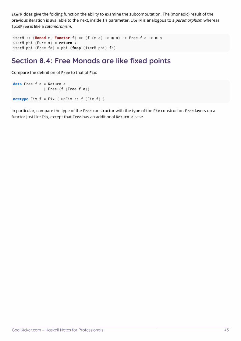
GoalKicker.com – Haskell Notes for Professionals 45

iterM does give the folding function the ability to examine the subcomputation. The (monadic) result of theprevious iteration is available to the next, inside f's parameter. iterM is analogous to a paramorphism whereasfoldFree is like a catamorphism.

iterM :: (Monad m, Functor f) => (f (m a) -> m a) -> Free f a -> m aiterM phi (Pure x) = return xiterM phi (Free fa) = phi (fmap (iterM phi) fa)

Section 8.4: Free Monads are like fixed pointsCompare the definition of Free to that of Fix:

data Free f a = Return a | Free (f (Free f a))

newtype Fix f = Fix { unFix :: f (Fix f) }

In particular, compare the type of the Free constructor with the type of the Fix constructor. Free layers up afunctor just like Fix, except that Free has an additional Return a case.

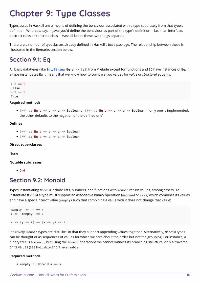
GoalKicker.com – Haskell Notes for Professionals 46

Chapter 9: Type ClassesTypeclasses in Haskell are a means of defining the behaviour associated with a type separately from that type'sdefinition. Whereas, say, in Java, you'd define the behaviour as part of the type's definition -- i.e. in an interface,abstract class or concrete class -- Haskell keeps these two things separate.

There are a number of typeclasses already defined in Haskell's base package. The relationship between these isillustrated in the Remarks section below.

Section 9.1: EqAll basic datatypes (like Int, String, Eq a => [a]) from Prelude except for functions and IO have instances of Eq. Ifa type instantiates Eq it means that we know how to compare two values for value or structural equality.

> 3 == 2False> 3 == 3True

Required methods

(==) :: Eq a => a -> a -> Boolean or (/=) :: Eq a => a -> a -> Boolean (if only one is implemented,the other defaults to the negation of the defined one)

Defines

(==) :: Eq a => a -> a -> Boolean

(/=) :: Eq a => a -> a -> Boolean

Direct superclasses

None

Notable subclasses

Ord

Section 9.2: MonoidTypes instantiating Monoid include lists, numbers, and functions with Monoid return values, among others. Toinstantiate Monoid a type must support an associative binary operation (mappend or (<>)) which combines its values,and have a special "zero" value (mempty) such that combining a value with it does not change that value:

mempty <> x == xx <> mempty == x

x <> (y <> z) == (x <> y) <> z

Intuitively, Monoid types are "list-like" in that they support appending values together. Alternatively, Monoid typescan be thought of as sequences of values for which we care about the order but not the grouping. For instance, abinary tree is a Monoid, but using the Monoid operations we cannot witness its branching structure, only a traversalof its values (see Foldable and Traversable).

Required methods

mempty :: Monoid m => m

GoalKicker.com – Haskell Notes for Professionals 47

mappend :: Monoid m => m -> m -> m

Direct superclasses

None

Section 9.3: OrdTypes instantiating Ord include, e.g., Int, String, and [a] (for types a where there's an Ord a instance). If a typeinstantiates Ord it means that we know a “natural” ordering of values of that type. Note, there are often manypossible choices of the “natural” ordering of a type and Ord forces us to favor one.

Ord provides the standard (<=), (<), (>), (>=) operators but interestingly defines them all using a custom algebraicdata type

data Ordering = LT | EQ | GT

compare :: Ord a => a -> a -> Ordering

Required methods

compare :: Ord a => a -> a -> Ordering or (<=) :: Ord a => a -> a -> Boolean (the standard’sdefault compare method uses (<=) in its implementation)

Defines

compare :: Ord a => a -> a -> Ordering

(<=) :: Ord a => a -> a -> Boolean

(<) :: Ord a => a -> a -> Boolean

(>=) :: Ord a => a -> a -> Boolean

(>) :: Ord a => a -> a -> Boolean

min :: Ord a => a -> a -> a

max :: Ord a => a -> a -> a

Direct superclasses

Eq

Section 9.4: NumThe most general class for number types, more precisely for rings, i.e. numbers that can be added and subtractedand multiplied in the usual sense, but not necessarily divided.

This class contains both integral types (Int, Integer, Word32 etc.) and fractional types (Double, Rational, alsocomplex numbers etc.). In case of finite types, the semantics are generally understood as modular arithmetic, i.e.with over- and underflow†.

Note that the rules for the numerical classes are much less strictly obeyed than the monad or monoid laws, orthose for equality comparison. In particular, floating-point numbers generally obey laws only in a approximatesense.

The methods

fromInteger :: Num a => Integer -> a. convert an integer to the general number type (wrapping aroundthe range, if necessary). Haskell number literals can be understood as a monomorphic Integer literal withthe general conversion around it, so you can use the literal 5 in both an Int context and a Complex Double

GoalKicker.com – Haskell Notes for Professionals 48

setting.

(+) :: Num a => a -> a -> a. Standard addition, generally understood as associative and commutative,i.e.,

a + (b + c) ≡ (a + b) + c a + b ≡ b + a

(-) :: Num a => a -> a -> a. Subtraction, which is the inverse of addition:

(a - b) + b ≡ (a + b) - b ≡ a

(*) :: Num a => a -> a -> a. Multiplication, an associative operation that's distributive over addition:

a * (b * c) ≡ (a * b) * c a * (b + c) ≡ a * b + a * c

for the most common instances, multiplication is also commutative, but this is definitely not a requirement.

negate :: Num a => a -> a. The full name of the unary negation operator. -1 is syntactic sugar for negate1.

-a ≡ negate a ≡ 0 - a

abs :: Num a => a -> a. The absolute-value function always gives a non-negative result of the samemagnitude

abs (-a) ≡ abs a abs (abs a) ≡ abs a

abs a ≡ 0 should only happen if a ≡ 0.

For real types it's clear what non-negative means: you always have abs a >= 0. Complex etc. types don'thave a well-defined ordering, however the result of abs should always lie in the real subset‡ (i.e. give anumber that could also be written as a single number literal without negation).

signum :: Num a => a -> a. The sign function, according to the name, yields only -1 or 1, depending on thesign of the argument. Actually, that's only true for nonzero real numbers; in general signum is betterunderstood as the normalising function:

abs (signum a) ≡ 1 -- unless a≡0 signum a * abs a ≡ a -- This is required to be true for all Num instances

Note that section 6.4.4 of the Haskell 2010 Report explicitly requires this last equality to hold for any valid Numinstance.

Some libraries, notably linear and hmatrix, have a much laxer understanding of what the Num class is for: they treatit just as a way to overload the arithmetic operators. While this is pretty straightforward for + and -, it alreadybecomes troublesome with * and more so with the other methods. For instance, should * mean matrix multiplicationor element-wise multiplication?

GoalKicker.com – Haskell Notes for Professionals 49

It is arguably a bad idea to define such non-number instances; please consider dedicated classes such asVectorSpace.

† In particular, the “negatives” of unsigned types are wrapped around to large positive, e.g. (-4 :: Word32) ==4294967292.

‡ This is widely not fulfilled: vector types do not have a real subset. The controversial Num-instances for such typesgenerally define abs and signum element-wise, which mathematically speaking doesn't really make sense.

Section 9.5: Maybe and the Functor ClassIn Haskell, data types can have arguments just like functions. Take the Maybe type for example.

Maybe is a very useful type which allows us to represent the idea of failure, or the possiblity thereof. In other words,if there is a possibility that a computation will fail, we use the Maybe type there. Maybe acts kind of like a wrapper forother types, giving them additional functionality.

Its actual declaration is fairly simple.

Maybe a = Just a | Nothing

What this tells is that a Maybe comes in two forms, a Just, which represents success, and a Nothing, whichrepresents failure. Just takes one argument which determines the type of the Maybe, and Nothing takes none. Forexample, the value Just "foo" will have type Maybe String, which is a string type wrapped with the additionalMaybe functionality. The value Nothing has type Maybe a where a can be any type.

This idea of wrapping types to give them additional functionality is a very useful one, and is applicable to more thanjust Maybe. Other examples include the Either, IO and list types, each providing different functionality. However,there are some actions and abilities which are common to all of these wrapper types. The most notable of these isthe ability to modify the encapsulated value.

It is common to think of these kinds of types as boxes which can have values placed in them. Different boxes holddifferent values and do different things, but none are useful without being able to access the contents within.

To encapsulate this idea, Haskell comes with a standard typeclass, named Functor. It is defined as follows.

class Functor f where fmap :: (a -> b) -> f a -> f b

As can be seen, the class has a single function, fmap, of two arguments. The first argument is a function from onetype, a, to another, b. The second argument is a functor (wrapper type) containing a value of type a. It returns afunctor (wrapper type) containing a value of type b.

In simple terms, fmap takes a function and applies to the value inside of a functor. It is the only function necessaryfor a type to be a member of the Functor class, but it is extremely useful. Functions operating on functors that havemore specific applications can be found in the Applicative and Monad typeclasses.

Section 9.6: Type class inheritance: Ord type classHaskell supports a notion of class extension. For example, the class Ord inherits all of the operations in Eq, but inaddition has a compare function that returns an Ordering between values. Ord may also contain the common ordercomparison operators, as well as a min method and a max method.

The => notation has the same meaning as it does in a function signature and requires type a to implement Eq, in

GoalKicker.com – Haskell Notes for Professionals 50

order to implement Ord.

data Ordering = EQ | LT | GT

class Eq a => Ord a where compare :: Ord a => a -> a -> Ordering (<) :: Ord a => a -> a -> Bool (<=) :: Ord a => a -> a -> Bool (>) :: Ord a => a -> a -> Bool (>=) :: Ord a => a -> a -> Bool min :: Ord a => a -> a -> a max :: Ord a => a -> a -> a

All of the methods following compare can be derived from it in a number of ways:

x < y = compare x y == LTx <= y = x < y || x == y -- Note the use of (==) inherited from Eqx > y = not (x <= y)x >= y = not (x < y)

min x y = case compare x y of EQ -> x LT -> x GT -> y

max x y = case compare x y of EQ -> x LT -> y GT -> x

Type classes that themselves extend Ord must implement at least either the compare method or the (<=) methodthemselves, which builds up the directed inheritance lattice.

GoalKicker.com – Haskell Notes for Professionals 51

Chapter 10: IOSection 10.1: Getting the 'a' "out of" 'IO a'A common question is "I have a value of IO a, but I want to do something to that a value: how do I get access to it?"How can one operate on data that comes from the outside world (for example, incrementing a number typed bythe user)?

The point is that if you use a pure function on data obtained impurely, then the result is still impure. It depends onwhat the user did! A value of type IO a stands for a "side-effecting computation resulting in a value of type a" whichcan only be run by (a) composing it into main and (b) compiling and executing your program. For that reason, thereis no way within pure Haskell world to "get the a out".

Instead, we want to build a new computation, a new IO value, which makes use of the a value at runtime. This isanother way of composing IO values and so again we can use do-notation:

-- assumingmyComputation :: IO Int

getMessage :: Int -> StringgetMessage int = "My computation resulted in: " ++ show int newComputation :: IO ()newComputation = do int <- myComputation -- we "bind" the result of myComputation to a name, 'int' putStrLn $ getMessage int -- 'int' holds a value of type Int

Here we're using a pure function (getMessage) to turn an Int into a String, but we're using do notation to make itbe applied to the result of an IO computation myComputation when (after) that computation runs. The result is abigger IO computation, newComputation. This technique of using pure functions in an impure context is called lifting.

Section 10.2: IO defines your program's `main` actionTo make a Haskell program executable you must provide a file with a main function of type IO ()

main :: IO ()main = putStrLn "Hello world!"

When Haskell is compiled it examines the IO data here and turns it into a executable. When we run this program itwill print Hello world!.

If you have values of type IO a other than main they won't do anything.

other :: IO ()other = putStrLn "I won't get printed"

main :: IO ()main = putStrLn "Hello world!"

Compiling this program and running it will have the same effect as the last example. The code in other is ignored.

In order to make the code in other have runtime effects you have to compose it into main. No IO values noteventually composed into main will have any runtime effect. To compose two IO values sequentially you can use do-notation:

GoalKicker.com – Haskell Notes for Professionals 52

other :: IO ()other = putStrLn "I will get printed... but only at the point where I'm composed into main"

main :: IO ()main = do putStrLn "Hello world!" other

When you compile and run this program it outputs

Hello world!I will get printed... but only at the point where I'm composed into main

Note that the order of operations is described by how other was composed into main and not the definition order.

Section 10.3: Checking for end-of-file conditionsA bit counter-intuitive to the way most other languages' standard I/O libraries do it, Haskell's isEOF does notrequire you to perform a read operation before checking for an EOF condition; the runtime will do it for you.

import System.IO( isEOF )

eofTest :: Int -> IO ()eofTest line = do end <- isEOF if end then putStrLn $ "End-of-file reached at line " ++ show line ++ "." else do getLine eofTest $ line + 1

main :: IO ()main = eofTest 1

Input:

Line #1.Line #2.Line #3.

Output:

End-of-file reached at line 4.

Section 10.4: Reading all contents of standard input into astringmain = do input <- getContents putStr input

Input:

GoalKicker.com – Haskell Notes for Professionals 53

This is an example sentence.And this one is, too!

Output:

This is an example sentence.And this one is, too!

Note: This program will actually print parts of the output before all of the input has been fully read in. This meansthat, if, for example, you use getContents over a 50MiB file, Haskell's lazy evaluation and garbage collector willensure that only the parts of the file that are currently needed (read: indispensable for further execution) will beloaded into memory. Thus, the 50MiB file won't be loaded into memory at once.

Section 10.5: Role and Purpose of IOHaskell is a pure language, meaning that expressions cannot have side effects. A side effect is anything that theexpression or function does other than produce a value, for example, modify a global counter or print to standardoutput.

In Haskell, side-effectful computations (specifically, those which can have an effect on the real world) are modelledusing IO. Strictly speaking, IO is a type constructor, taking a type and producing a type. For example, IO Int is thetype of an I/O computation producing an Int value. The IO type is abstract, and the interface provided for IOensures that certain illegal values (that is, functions with non-sensical types) cannot exist, by ensuring that all built-in functions which perform IO have a return type enclosed in IO.

When a Haskell program is run, the computation represented by the Haskell value named main, whose type can beIO x for any type x, is executed.

Manipulating IO values

There are many functions in the standard library providing typical IO actions that a general purpose programminglanguage should perform, such as reading and writing to file handles. General IO actions are created and combinedprimarily with two functions:

(>>=) :: IO a -> (a -> IO b) -> IO b

This function (typically called bind) takes an IO action and a function which returns an IO action, and produces theIO action which is the result of applying the function to the value produced by the first IO action.

return :: a -> IO a

This function takes any value (i.e., a pure value) and returns the IO computation which does no IO and produces thegiven value. In other words, it is a no-op I/O action.

There are additional general functions which are often used, but all can be written in terms of the two above. Forexample, (>>) :: IO a -> IO b -> IO b is similar to (>>=) but the result of the first action is ignored.

A simple program greeting the user using these functions:

main :: IO () main = putStrLn "What is your name?" >>

GoalKicker.com – Haskell Notes for Professionals 54

getLine >>= \name -> putStrLn ("Hello " ++ name ++ "!")

This program also uses putStrLn :: String -> IO () and getLine :: IO String.

Note: the types of certain functions above are actually more general than those types given (namely >>=, >> andreturn).

IO semantics

The IO type in Haskell has very similar semantics to that of imperative programming languages. For example, whenone writes s1 ; s2 in an imperative language to indicate executing statement s1, then statement s2, one can writes1 >> s2 to model the same thing in Haskell.

However, the semantics of IO diverge slightly of what would be expected coming from an imperative background.The return function does not interrupt control flow - it has no effect on the program if another IO action is run insequence. For example, return () >> putStrLn "boom" correctly prints "boom" to standard output.

The formal semantics of IO can given in terms of simple equalities involving the functions in the previous section:

return x >>= f ≡ f x, ∀ f x y >>= return ≡ return y, ∀ y (m >>= f) >>= g ≡ m >>= (\x -> (f x >>= g)), ∀ m f g

These laws are typically referred to as left identity, right identity, and composition, respectively. They can be statedmore naturally in terms of the function

(>=>) :: (a -> IO b) -> (b -> IO c) -> a -> IO c (f >=> g) x = (f x) >>= g

as follows:

return >=> f ≡ f, ∀ f f >=> return ≡ f, ∀ f (f >=> g) >=> h ≡ f >=> (g >=> h), ∀ f g h

Lazy IO

Functions performing I/O computations are typically strict, meaning that all preceding actions in a sequence ofactions must be completed before the next action is begun. Typically this is useful and expected behaviour -putStrLn "X" >> putStrLn "Y" should print "XY". However, certain library functions perform I/O lazily, meaningthat the I/O actions required to produce the value are only performed when the value is actually consumed.Examples of such functions are getContents and readFile. Lazy I/O can drastically reduce the performance of aHaskell program, so when using library functions, care should be taken to note which functions are lazy.

IO and do notation

Haskell provides a simpler method of combining different IO values into larger IO values. This special syntax isknown as do notation* and is simply syntactic sugar for usages of the >>=, >> and return functions.

The program in the previous section can be written in two different ways using do notation, the first being layout-sensitive and the second being layout insensitive:

main = do

GoalKicker.com – Haskell Notes for Professionals 55

putStrLn "What is your name?" name <- getLine putStrLn ("Hello " ++ name ++ "!")

main = do { putStrLn "What is your name?" ; name <- getLine ; putStrLn ("Hello " ++ name ++ "!") }

All three programs are exactly equivalent.

*Note that do notation is also applicable to a broader class of type constructors called monads.

Section 10.6: Writing to stdoutPer the Haskell 2010 Language Specification the following are standard IO functions available in Prelude, so noimports are required to use them.

putChar :: Char -> IO () - writes a char to stdoutPrelude> putChar 'a'aPrelude> -- Note, no new line

putStr :: String -> IO () - writes a String to stdoutPrelude> putStr "This is a string!"This is a string!Prelude> -- Note, no new line

putStrLn :: String -> IO () - writes a String to stdout and adds a new linePrelude> putStrLn "Hi there, this is another String!"Hi there, this is another String!

print :: Show a => a -> IO () - writes a an instance of Show to stdoutPrelude> print "hi""hi"Prelude> print 11Prelude> print 'a''a'Prelude> print (Just 'a') -- Maybe is an instance of the `Show` type classJust 'a'Prelude> print NothingNothing

Recall that you can instantiate Show for your own types using deriving:

-- In ex.hsdata Person = Person { name :: String } deriving Showmain = print (Person "Alex") -- Person is an instance of `Show`, thanks to `deriving`

Loading & running in GHCi:

Prelude> :load ex.hs[1 of 1] Compiling ex ( ex.hs, interpreted )Ok, modules loaded: ex.*Main> main -- from ex.hsPerson {name = "Alex"}*Main>

GoalKicker.com – Haskell Notes for Professionals 56

Section 10.7: Reading words from an entire fileIn Haskell, it often makes sense not to bother with file handles at all, but simply read or write an entire file straightfrom disk to memory†, and do all the partitioning/processing of the text with the pure string data structure. Thisavoids mixing IO and program logic, which can greatly help avoiding bugs.

-- | The interesting part of the program, which actually processes data-- but doesn't do any IO!reverseWords :: String -> [String]reverseWords = reverse . words

-- | A simple wrapper that only fetches the data from disk, lets-- 'reverseWords' do its job, and puts the result to stdout.main :: IO ()main = do content <- readFile "loremipsum.txt" mapM_ putStrLn $ reverseWords content

If loremipsum.txt contains

Lorem ipsum dolor sit amet,consectetur adipiscing elit

then the program will output

elitadipiscingconsecteturamet,sitdoloripsumLorem

Here, mapM_ went through the list of all words in the file, and printed each of them to a separate line with putStrLn.

†If you think this is wasteful on memory, you have a point. Actually, Haskell's laziness can often avoid that the entirefile needs to reside in memory simultaneously... but beware, this kind of lazy IO causes its own set of problems. Forperformance-critical applications, it often makes sense to enforce the entire file to be read at once, strictly; you cando this with the Data.Text version of readFile.

Section 10.8: Reading a line from standard inputmain = do line <- getLine putStrLn line

Input:

This is an example.

Output:

This is an example.

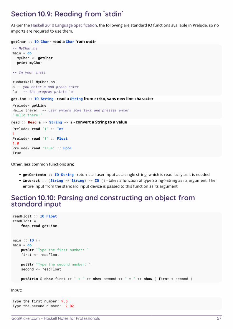
GoalKicker.com – Haskell Notes for Professionals 57

Section 10.9: Reading from `stdin`As-per the Haskell 2010 Language Specification, the following are standard IO functions available in Prelude, so noimports are required to use them.

getChar :: IO Char - read a Char from stdin-- MyChar.hsmain = do myChar <- getChar print myChar

-- In your shell

runhaskell MyChar.hsa -- you enter a and press enter'a' -- the program prints 'a'

getLine :: IO String - read a String from stdin, sans new line characterPrelude> getLineHello there! -- user enters some text and presses enter"Hello there!"

read :: Read a => String -> a - convert a String to a valuePrelude> read "1" :: Int1Prelude> read "1" :: Float1.0Prelude> read "True" :: BoolTrue

Other, less common functions are:

getContents :: IO String - returns all user input as a single string, which is read lazily as it is neededinteract :: (String -> String) -> IO () - takes a function of type String->String as its argument. Theentire input from the standard input device is passed to this function as its argument

Section 10.10: Parsing and constructing an object fromstandard inputreadFloat :: IO FloatreadFloat = fmap read getLine

main :: IO ()main = do putStr "Type the first number: " first <- readFloat

putStr "Type the second number: " second <- readFloat

putStrLn $ show first ++ " + " ++ show second ++ " = " ++ show ( first + second )

Input:

Type the first number: 9.5Type the second number: -2.02

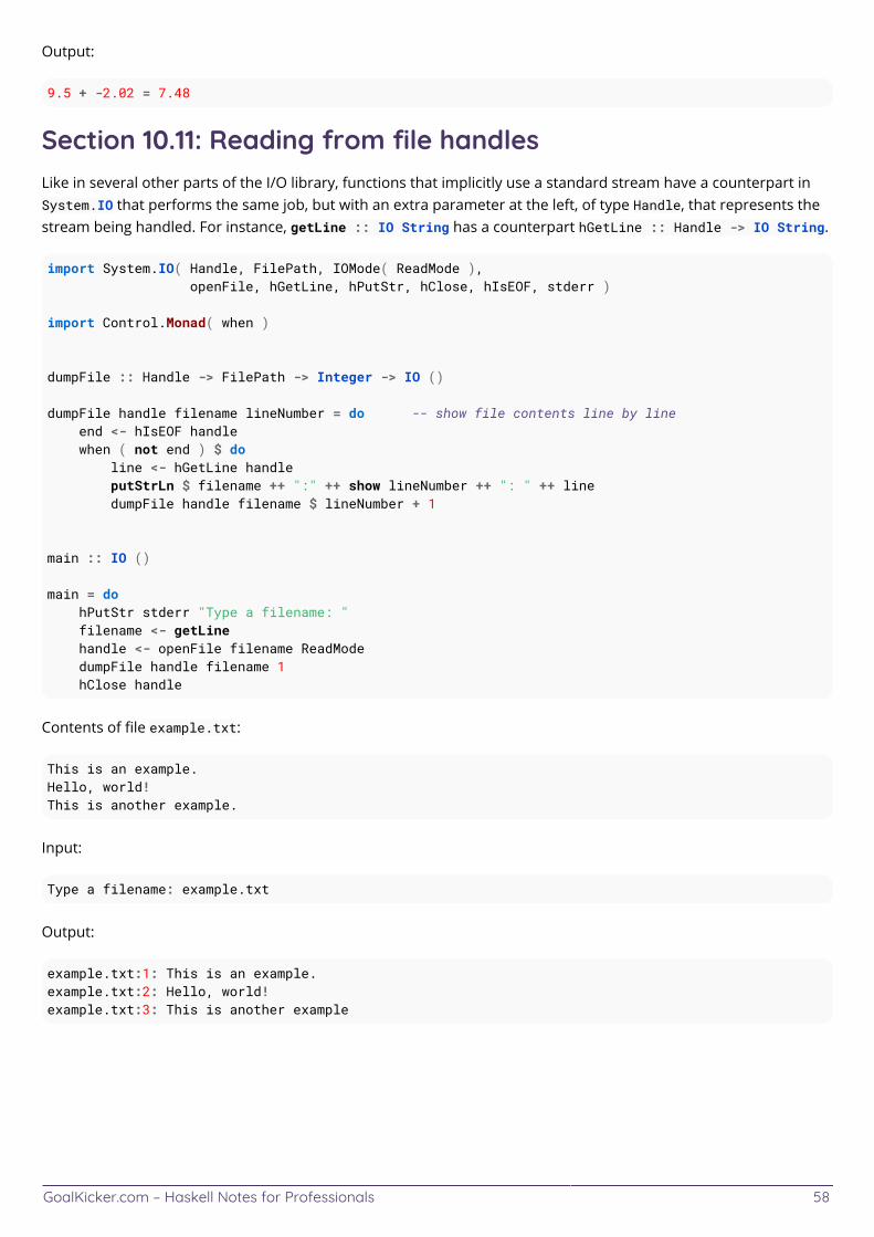
GoalKicker.com – Haskell Notes for Professionals 58

Output:

9.5 + -2.02 = 7.48

Section 10.11: Reading from file handlesLike in several other parts of the I/O library, functions that implicitly use a standard stream have a counterpart inSystem.IO that performs the same job, but with an extra parameter at the left, of type Handle, that represents thestream being handled. For instance, getLine :: IO String has a counterpart hGetLine :: Handle -> IO String.

import System.IO( Handle, FilePath, IOMode( ReadMode ), openFile, hGetLine, hPutStr, hClose, hIsEOF, stderr )

import Control.Monad( when )

dumpFile :: Handle -> FilePath -> Integer -> IO ()

dumpFile handle filename lineNumber = do -- show file contents line by line end <- hIsEOF handle when ( not end ) $ do line <- hGetLine handle putStrLn $ filename ++ ":" ++ show lineNumber ++ ": " ++ line dumpFile handle filename $ lineNumber + 1

main :: IO ()

main = do hPutStr stderr "Type a filename: " filename <- getLine handle <- openFile filename ReadMode dumpFile handle filename 1 hClose handle

Contents of file example.txt:

This is an example.Hello, world!This is another example.

Input:

Type a filename: example.txt

Output:

example.txt:1: This is an example.example.txt:2: Hello, world!example.txt:3: This is another example

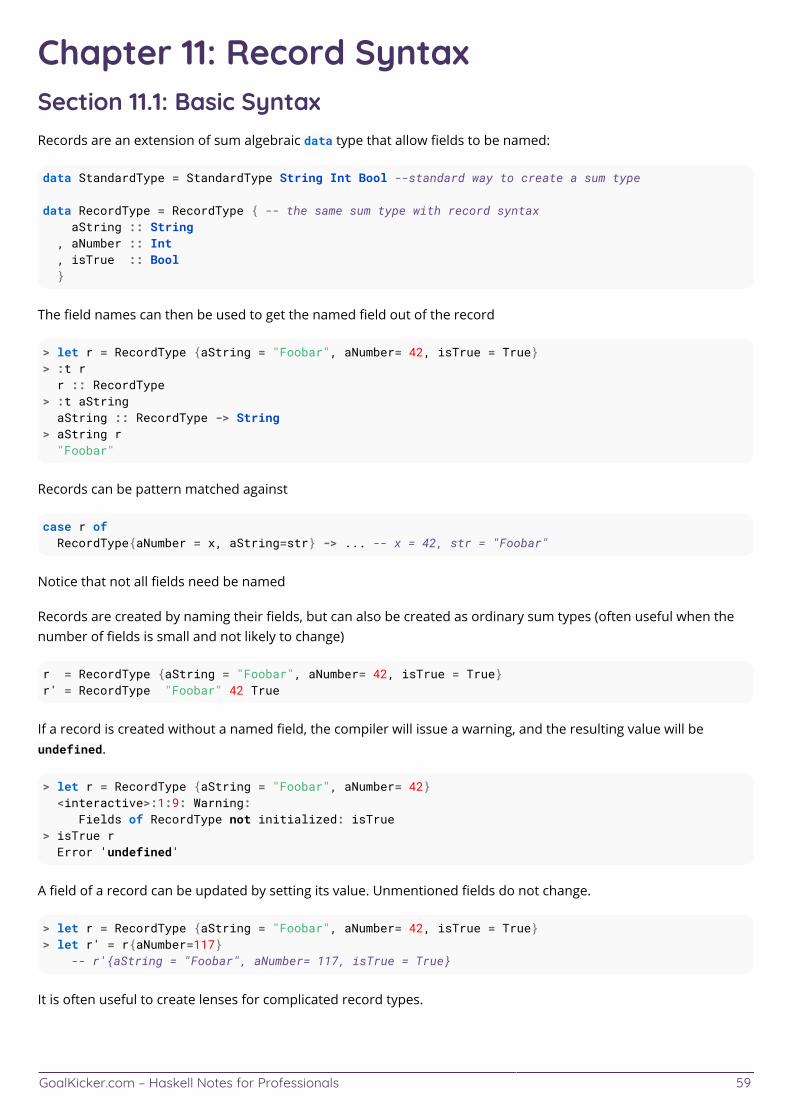
GoalKicker.com – Haskell Notes for Professionals 59

Chapter 11: Record SyntaxSection 11.1: Basic SyntaxRecords are an extension of sum algebraic data type that allow fields to be named:

data StandardType = StandardType String Int Bool --standard way to create a sum type

data RecordType = RecordType { -- the same sum type with record syntax aString :: String , aNumber :: Int , isTrue :: Bool }

The field names can then be used to get the named field out of the record

> let r = RecordType {aString = "Foobar", aNumber= 42, isTrue = True}> :t r r :: RecordType> :t aString aString :: RecordType -> String> aString r "Foobar"

Records can be pattern matched against

case r of RecordType{aNumber = x, aString=str} -> ... -- x = 42, str = "Foobar"

Notice that not all fields need be named

Records are created by naming their fields, but can also be created as ordinary sum types (often useful when thenumber of fields is small and not likely to change)

r = RecordType {aString = "Foobar", aNumber= 42, isTrue = True}r' = RecordType "Foobar" 42 True

If a record is created without a named field, the compiler will issue a warning, and the resulting value will beundefined.

> let r = RecordType {aString = "Foobar", aNumber= 42} <interactive>:1:9: Warning: Fields of RecordType not initialized: isTrue> isTrue r Error 'undefined'

A field of a record can be updated by setting its value. Unmentioned fields do not change.

> let r = RecordType {aString = "Foobar", aNumber= 42, isTrue = True}> let r' = r{aNumber=117} -- r'{aString = "Foobar", aNumber= 117, isTrue = True}

It is often useful to create lenses for complicated record types.

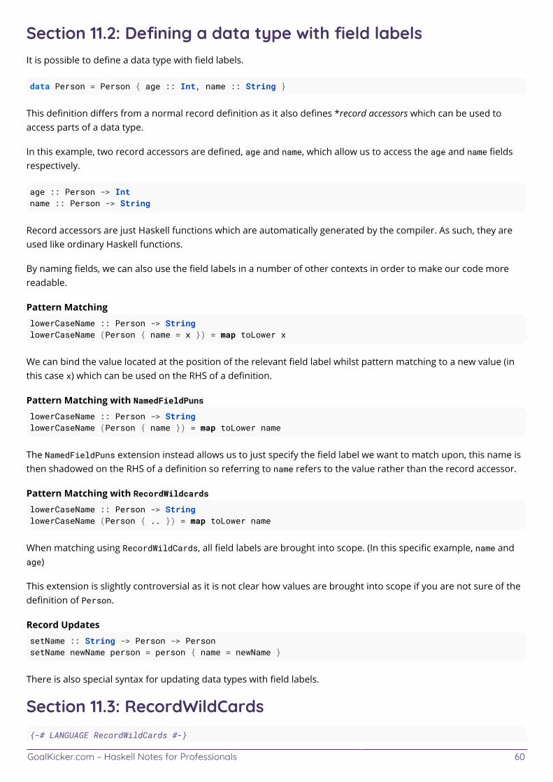
GoalKicker.com – Haskell Notes for Professionals 60

Section 11.2: Defining a data type with field labelsIt is possible to define a data type with field labels.

data Person = Person { age :: Int, name :: String }

This definition differs from a normal record definition as it also defines *record accessors which can be used toaccess parts of a data type.

In this example, two record accessors are defined, age and name, which allow us to access the age and name fieldsrespectively.

age :: Person -> Intname :: Person -> String

Record accessors are just Haskell functions which are automatically generated by the compiler. As such, they areused like ordinary Haskell functions.

By naming fields, we can also use the field labels in a number of other contexts in order to make our code morereadable.

Pattern MatchinglowerCaseName :: Person -> StringlowerCaseName (Person { name = x }) = map toLower x

We can bind the value located at the position of the relevant field label whilst pattern matching to a new value (inthis case x) which can be used on the RHS of a definition.

Pattern Matching with NamedFieldPunslowerCaseName :: Person -> StringlowerCaseName (Person { name }) = map toLower name

The NamedFieldPuns extension instead allows us to just specify the field label we want to match upon, this name isthen shadowed on the RHS of a definition so referring to name refers to the value rather than the record accessor.

Pattern Matching with RecordWildcardslowerCaseName :: Person -> StringlowerCaseName (Person { .. }) = map toLower name

When matching using RecordWildCards, all field labels are brought into scope. (In this specific example, name andage)

This extension is slightly controversial as it is not clear how values are brought into scope if you are not sure of thedefinition of Person.

Record UpdatessetName :: String -> Person -> PersonsetName newName person = person { name = newName }

There is also special syntax for updating data types with field labels.

Section 11.3: RecordWildCards{-# LANGUAGE RecordWildCards #-}

GoalKicker.com – Haskell Notes for Professionals 61

data Client = Client { firstName :: String , lastName :: String , clientID :: String } deriving (Show)

printClientName :: Client -> IO ()printClientName Client{..} = do putStrLn firstName putStrLn lastName putStrLn clientID

The pattern Client{..} brings in scope all the fields of the constructor Client, and is equivalent to the pattern

Client{ firstName = firstName, lastName = lastName, clientID = clientID }

It can also be combined with other field matchers like so:

Client { firstName = "Joe", .. }

This is equivalent to

Client{ firstName = "Joe", lastName = lastName, clientID = clientID }

Section 11.4: Copying Records while Changing Field ValuesSuppose you have this type:

data Person = Person { name :: String, age:: Int } deriving (Show, Eq)

and two values:

alex = Person { name = "Alex", age = 21 }jenny = Person { name = "Jenny", age = 36 }

a new value of type Person can be created by copying from alex, specifying which values to change:

anotherAlex = alex { age = 31 }

The values of alex and anotherAlex will now be:

Person {name = "Alex", age = 21}

Person {name = "Alex", age = 31}

Section 11.5: Records with newtypeRecord syntax can be used with newtype with the restriction that there is exactly one constructor with exactly onefield. The benefit here is the automatic creation of a function to unwrap the newtype. These fields are often namedstarting with run for monads, get for monoids, and un for other types.

newtype State s a = State { runState :: s -> (s, a) }

newtype Product a = Product { getProduct :: a }

newtype Fancy = Fancy { unfancy :: String }

GoalKicker.com – Haskell Notes for Professionals 62

-- a fancy string that wants to avoid concatenation with ordinary strings

It is important to note that the record syntax is typically never used to form values and the field name is usedstrictly for unwrapping

getProduct $ mconcat [Product 7, Product 9, Product 12]-- > 756

GoalKicker.com – Haskell Notes for Professionals 63

Chapter 12: Partial ApplicationSection 12.1: SectionsSectioning is a concise way to partially apply arguments to infix operators.

For example, if we want to write a function which adds "ing" to the end of a word we can use a section to succinctlydefine a function.

> (++ "ing") "laugh""laughing"

Notice how we have partially applied the second argument. Normally, we can only partially apply the arguments inthe specified order.

We can also use left sectioning to partially apply the first argument.

> ("re" ++) "do""redo"

We could equivalently write this using normal prefix partial application:

> ((++) "re") "do""redo"

A Note on Subtraction

Beginners often incorrectly section negation.

> map (-1) [1,2,3]***error: Could not deduce...

This does not work as -1 is parsed as the literal -1 rather than the sectioned operator - applied to 1. The subtractfunction exists to circumvent this issue.

> map (subtract 1) [1,2,3][0,1,2]

Section 12.2: Partially Applied Adding FunctionWe can use partial application to "lock" the first argument. After applying one argument we are left with a functionwhich expects one more argument before returning the result.

(+) :: Int -> Int -> Int

addOne :: Int -> IntaddOne = (+) 1

We can then use addOne in order to add one to an Int.

> addOne 56> map addOne [1,2,3][2,3,4]

GoalKicker.com – Haskell Notes for Professionals 64

Section 12.3: Returning a Partially Applied FunctionReturning partially applied functions is one technique to write concise code.

add :: Int -> Int -> Intadd x = (+x)

add 5 2

In this example (+x) is a partially applied function. Notice that the second parameter to the add function does notneed to be specified in the function definition.

The result of calling add 5 2 is seven.

GoalKicker.com – Haskell Notes for Professionals 65

Chapter 13: MonoidSection 13.1: An instance of Monoid for listsinstance Monoid [a] where mempty = [] mappend = (++)

Checking the Monoid laws for this instance:

mempty `mappend` x = x <-> [] ++ xs = xs -- prepending an empty list is a no-op

x `mappend` mempty = x <-> xs ++ [] = xs -- appending an empty list is a no-op

x `mappend` (y `mappend` z) = (x `mappend` y) `mappend` z <->xs ++ (ys ++ zs) = (xs ++ ys) ++ zs -- appending lists is associative

Section 13.2: Collapsing a list of Monoids into a single valuemconcat :: [a] -> a is another method of the Monoid typeclass:

ghci> mconcat [Sum 1, Sum 2, Sum 3]Sum {getSum = 6}ghci> mconcat ["concat", "enate"]"concatenate"

Its default definition is mconcat = foldr mappend mempty.

Section 13.3: Numeric MonoidsNumbers are monoidal in two ways: addition with 0 as the unit, and multiplication with 1 as the unit. Both areequally valid and useful in different circumstances. So rather than choose a preferred instance for numbers, thereare two newtypes, Sum and Product to tag them for the different functionality.

newtype Sum n = Sum { getSum :: n }

instance Num n => Monoid (Sum n) where mempty = Sum 0 Sum x `mappend` Sum y = Sum (x + y)

newtype Product n = Product { getProduct :: n }

instance Num n => Monoid (Product n) where mempty = Product 1 Product x `mappend` Product y = Product (x * y)

This effectively allows for the developer to choose which functionality to use by wrapping the value in theappropriate newtype.

Sum 3 <> Sum 5 == Sum 8Product 3 <> Product 5 == Product 15

GoalKicker.com – Haskell Notes for Professionals 66

Section 13.4: An instance of Monoid for ()() is a Monoid. Since there is only one value of type (), there's only one thing mempty and mappend could do:

instance Monoid () where mempty = () () `mappend` () = ()

GoalKicker.com – Haskell Notes for Professionals 67

Chapter 14: Category TheorySection 14.1: Category theory as a system for organizingabstractionCategory theory is a modern mathematical theory and a branch of abstract algebra focused on the nature ofconnectedness and relation. It is useful for giving solid foundations and common language to many highly reusableprogramming abstractions. Haskell uses Category theory as inspiration for some of the core typeclasses available inboth the standard library and several popular third-party libraries.

An example

The Functor typeclass says that if a type F instantiates Functor (for which we write Functor F) then we have ageneric operation

fmap :: (a -> b) -> (F a -> F b)

which lets us "map" over F. The standard (but imperfect) intuition is that F a is a container full of values of type aand fmap lets us apply a transformation to each of these contained elements. An example is Maybe

instance Functor Maybe where fmap f Nothing = Nothing -- if there are no values contained, do nothing fmap f (Just a) = Just (f a) -- else, apply our transformation

Given this intuition, a common question is "why not call Functor something obvious like Mappable?".

A hint of Category Theory

The reason is that Functor fits into a set of common structures in Category theory and therefore by calling Functor"Functor" we can see how it connects to this deeper body of knowledge.

In particular, Category Theory is highly concerned with the idea of arrows from one place to another. In Haskell, themost important set of arrows are the function arrows a -> b. A common thing to study in Category Theory is howone set of arrows relates to another set. In particular, for any type constructor F, the set of arrows of the shape F a-> F b are also interesting.

So a Functor is any F such that there is a connection between normal Haskell arrows a -> b and the F-specificarrows F a -> F b. The connection is defined by fmap and we also recognize a few laws which must hold

forall (x :: F a) . fmap id x == x

forall (f :: a -> b) (g :: b -> c) . fmap g . fmap f = fmap (g . f)

All of these laws arise naturally from the Category Theoretic interpretation of Functor and would not be asobviously necessary if we only thought of Functor as relating to "mapping over elements".

Section 14.2: Haskell types as a categoryDefinition of the category

The Haskell types along with functions between types form (almost†) a category. We have an identity morphism(function) (id :: a -> a) for every object (type) a; and composition of morphisms ((.) :: (b -> c) -> (a -> b)-> a -> c), which obey category laws:

GoalKicker.com – Haskell Notes for Professionals 68

f . id = f = id . fh . (g . f) = (h . g) . f

We usually call this category Hask.

Isomorphisms

In category theory, we have an isomorphism when we have a morphism which has an inverse, in other words, thereis a morphism which can be composed with it in order to create the identity. In Hask this amounts to have a pair ofmorphisms f,g such that:

f . g == id == g . f

If we find a pair of such morphisms between two types, we call them isomorphic to one another.

An example of two isomorphic types would be ((),a) and a for some a. We can construct the two morphisms:

f :: ((),a) -> af ((),x) = x

g :: a -> ((),a)g x = ((),x)

And we can check that f . g == id == g . f.

Functors

A functor, in category theory, goes from a category to another, mapping objects and morphisms. We are workingonly on one category, the category Hask of Haskell types, so we are going to see only functors from Hask to Hask,those functors, whose origin and destination category are the same, are called endofunctors. Our endofunctorswill be the polymorphic types taking a type and returning another:

F :: * -> *

To obey the categorical functor laws (preserve identities and composition) is equivalent to obey the Haskell functorlaws:

fmap (f . g) = (fmap f) . (fmap g)fmap id = id

So, we have, for example, that [], Maybe or (-> r) are functors in Hask.

Monads

A monad in category theory is a monoid on the category of endofunctors. This category has endofunctors asobjects F :: * -> * and natural transformations (transformations between them forall a . F a -> G a) asmorphisms.

A monoid object can be defined on a monoidal category, and is a type having two morphisms:

zero :: () -> Mmappend :: (M,M) -> M

We can translate this roughly to the category of Hask endofunctors as:

GoalKicker.com – Haskell Notes for Professionals 69

return :: a -> m ajoin :: m (m a) -> m a

And, to obey the monad laws is equivalent to obey the categorical monoid object laws.

†In fact, the class of all types along with the class of functions between types do not strictly form a category inHaskell, due to the existance of undefined. Typically this is remedied by simply defining the objects of the Haskcategory as types without bottom values, which excludes non-terminating functions and infinite values (codata). Fora detailed discussion of this topic, see here.

Section 14.3: Definition of a CategoryA category C consists of:

A collection of objects called Obj(C) ;

A collection (called Hom(C)) of morphisms between those objects. If a and b are in Obj(C), then a morphism fin Hom(C) is typically denoted f : a -> b, and the collection of all morphism between a and b is denotedhom(a,b) ;

A special morphism called the identity morphism - for every a : Obj(C) there exists a morphism id : a ->a ;

A composition operator (.), taking two morphisms f : a -> b, g : b -> c and producing a morphism a ->c

which obey the following laws:

For all f : a -> x, g : x -> b, then id . f = f and g . id = g

For all f : a -> b, g : b -> c and h : c -> d, then h . (g . f) = (h . g) . f

In other words, composition with the identity morphism (on either the left or right) does not change the othermorphism, and composition is associative.

In Haskell, the Category is defined as a typeclass in Control.Category:

-- | A class for categories.-- id and (.) must form a monoid.class Category cat where -- | the identity morphism id :: cat a a

-- | morphism composition (.) :: cat b c -> cat a b -> cat a c

In this case, cat :: k -> k -> * objectifies the morphism relation - there exists a morphism cat a b if and only ifcat a b is inhabited (i.e. has a value). a, b and c are all in Obj(C). Obj(C) itself is represented by the kind k - forexample, when k ~ *, as is typically the case, objects are types.

The canonical example of a Category in Haskell is the function category:

instance Category (->) where id = Prelude.id (.) = Prelude..

GoalKicker.com – Haskell Notes for Professionals 70

Another common example is the Category of Kleisli arrows for a Monad:

newtype Kleisli m a b = Kleisli (a -> m b)

class Monad m => Category (Kleisli m) where id = Kleisli return Kleisli f . Kleisli g = Kleisli (f >=> g)

Section 14.4: Coproduct of types in HaskIntuition

The categorical product of two types A and B should contain the minimal information necessary to contain insidean instance of type A or type B. We can see now that the intuitive coproduct of two types should be Either a b.Other candidates, such as Either a (b,Bool), would contain a part of unnecessary information, and they wouldn'tbe minimal.

The formal definition is derived from the categorical definition of coproduct.

Categorical coproducts

A categorical coproduct is the dual notion of a categorical product. It is obtained directly by reversing all the arrowsin the definition of the product. The coproduct of two objects X,Y is another object Z with two inclusions: i_1: X → Zand i_2: Y → Z; such that any other two morphisms from X and Y to another object decompose uniquely throughthose inclusions. In other words, if there are two morphisms f₁ : X → W and f₂ : Y → W, exists a unique morphism g :Z → W such that g ○ i₁ = f₁ and g ○ i₂ = f₂

Coproducts in Hask

The translation into the Hask category is similar to the translation of the product:

-- if there are two functionsf1 :: A -> Wf2 :: B -> W-- and we have a coproduct with two inclusionsi1 :: A -> Zi2 :: B -> Z-- we can construct a unique functiong :: Z -> W-- such that the other two functions decompose using gg . i1 == f1g . i2 == f2

The coproduct type of two types A and B in Hask is Either a b or any other type isomorphic to it:

-- Coproduct-- The two inclusions are Left and Rightdata Either a b = Left a | Right b

-- If we have those functions, we can decompose them through the coproductdecompose :: (A -> W) -> (B -> W) -> (Either A B -> W)decompose f1 f2 (Left x) = f1 xdecompose f1 f2 (Right y) = f2 y

GoalKicker.com – Haskell Notes for Professionals 71

Section 14.5: Product of types in HaskCategorical products

In category theory, the product of two objects X, Y is another object Z with two projections: π₁ : Z → X and π₂ : Z → Y;such that any other two morphisms from another object decompose uniquely through those projections. In otherwords, if there exist f₁ : W → X and f₂ : W → Y, exists a unique morphism g : W → Z such that π₁ ○ g = f₁ and π₂ ○ g =f₂.

Products in Hask

This translates into the Hask category of Haskell types as follows, Z is product of A, B when:

-- if there are two functionsf1 :: W -> Af2 :: W -> B-- we can construct a unique functiong :: W -> Z-- and we have two projectionsp1 :: Z -> Ap2 :: Z -> B-- such that the other two functions decompose using gp1 . g == f1p2 . g == f2

The product type of two types A, B, which follows the law stated above, is the tuple of the two types (A,B), andthe two projections are fst and snd. We can check that it follows the above rule, if we have two functions f1 :: W-> A and f2 :: W -> B we can decompose them uniquely as follow:

decompose :: (W -> A) -> (W -> B) -> (W -> (A,B))decompose f1 f2 = (\x -> (f1 x, f2 x))

And we can check that the decomposition is correct:

fst . (decompose f1 f2) = f1snd . (decompose f1 f2) = f2

Uniqueness up to isomorphism

The choice of (A,B) as the product of A and B is not unique. Another logical and equivalent choice would have been:

data Pair a b = Pair a b

Moreover, we could have also chosen (B,A) as the product, or even (B,A,()), and we could find a decompositionfunction like the above also following the rules:

decompose2 :: (W -> A) -> (W -> B) -> (W -> (B,A,()))decompose2 f1 f2 = (\x -> (f2 x, f1 x, ()))

This is because the product is not unique but unique up to isomorphism. Every two products of A and B do not haveto be equal, but they should be isomorphic. As an example, the two different products we have just defined, (A,B)and (B,A,()), are isomorphic:

iso1 :: (A,B) -> (B,A,())iso1 (x,y) = (y,x,())

GoalKicker.com – Haskell Notes for Professionals 72

iso2 :: (B,A,()) -> (A,B)iso2 (y,x,()) = (x,y)

Uniqueness of the decomposition

It is important to remark that also the decomposition function must be unique. There are types which follow all therules required to be product, but the decomposition is not unique. As an example, we can try to use (A,(B,Bool))with projections fst fst . snd as a product of A and B:

decompose3 :: (W -> A) -> (W -> B) -> (W -> (A,(B,Bool)))decompose3 f1 f2 = (\x -> (f1 x, (f2 x, True)))

We can check that it does work:

fst . (decompose3 f1 f2) = f1 x(fst . snd) . (decompose3 f1 f2) = f2 x

But the problem here is that we could have written another decomposition, namely:

decompose3' :: (W -> A) -> (W -> B) -> (W -> (A,(B,Bool)))decompose3' f1 f2 = (\x -> (f1 x, (f2 x, False)))

And, as the decomposition is not unique, (A,(B,Bool)) is not the product of A and B in Hask

Section 14.6: Haskell Applicative in terms of Category TheoryA Haskell's Functor allows one to map any type a (an object of Hask) to a type F a and also map a function a -> b(a morphism of Hask) to a function with type F a -> F b. This corresponds to a Category Theory definition in asense that functor preserves basic category structure.

A monoidal category is a category that has some additional structure:

A tensor product (see Product of types in Hask)A tensor unit (unit object)

Taking a pair as our product, this definition can be translated to Haskell in the following way:

class Functor f => Monoidal f where mcat :: f a -> f b -> f (a,b) munit :: f ()

The Applicative class is equivalent to this Monoidal one and thus can be implemented in terms of it:

instance Monoidal f => Applicative f where pure x = fmap (const x) munit f <*> fa = (\(f, a) -> f a) <$> (mcat f fa)

GoalKicker.com – Haskell Notes for Professionals 73

Chapter 15: ListsSection 15.1: List basicsThe type constructor for lists in the Haskell Prelude is []. The type declaration for a list holding values of type Int iswritten as follows:

xs :: [Int] -- or equivalently, but less conveniently,xs :: [] Int

Lists in Haskell are homogeneous sequences, which is to say that all elements must be of the same type. Unliketuples, list type is not affected by length:

[1,2,3] :: [Int][1,2,3,4] :: [Int]

Lists are constructed using two constructors:

[] constructs an empty list.

(:), pronounced "cons", prepends elements to a list. Consing x (a value of type a) onto xs (a list of values ofthe same type a) creates a new list, whose head (the first element) is x, and tail (the rest of the elements) isxs.

We can define simple lists as follows:

ys :: [a]ys = []

xs :: [Int]xs = 12 : (99 : (37 : [])) -- or = 12 : 99 : 37 : [] -- ((:) is right-associative)-- or = [12, 99, 37] -- (syntactic sugar for lists)

Note that (++), which can be used to build lists is defined recursively in terms of (:) and [].

Section 15.2: Processing listsTo process lists, we can simply pattern match on the constructors of the list type:

listSum :: [Int] -> IntlistSum [] = 0listSum (x:xs) = x + listSum xs

We can match more values by specifying a more elaborate pattern:

sumTwoPer :: [Int] -> IntsumTwoPer [] = 0sumTwoPer (x1:x2:xs) = x1 + x2 + sumTwoPer xssumTwoPer (x:xs) = x + sumTwoPer xs

Note that in the above example, we had to provide a more exhaustive pattern match to handle cases where an oddlength list is given as an argument.

GoalKicker.com – Haskell Notes for Professionals 74

The Haskell Prelude defines many built-ins for handling lists, like map, filter, etc.. Where possible, you should usethese instead of writing your own recursive functions.

Section 15.3: RangesCreating a list from 1 to 10 is simple using range notation:

[1..10] -- [1,2,3,4,5,6,7,8,9,10]

To specify a step, add a comma and the next element after the start element:

[1,3..10] -- [1,3,5,7,9]

Note that Haskell always takes the step as the arithmetic difference between terms, and that you cannot specifymore than the first two elements and the upper bound:

[1,3,5..10] -- error[1,3,9..20] -- error

To generate a range in descending order, always specify the negative step:

[5..1] -- []

[5,4..1] -- [5,4,3,2,1]

Because Haskell is non-strict, the elements of the list are evaluated only if they are needed, which allows us to useinfinite lists. [1..] is an infinite list starting from 1. This list can be bound to a variable or passed as a functionargument:

take 5 [1..] -- returns [1,2,3,4,5] even though [1..] is infinite

Be careful when using ranges with floating-point values, because it accepts spill-overs up to half-delta, to fend offrounding issues:

[1.0,1.5..2.4] -- [1.0,1.5,2.0,2.5] , though 2.5 > 2.4

[1.0,1.1..1.2] -- [1.0,1.1,1.2000000000000002] , though 1.2000000000000002 > 1.2

Ranges work not just with numbers but with any type that implements Enum typeclass. Given some enumerablevariables a, b, c, the range syntax is equivalent to calling these Enum methods:

[a..] == enumFrom a[a..c] == enumFromTo a c[a,b..] == enumFromThen a b[a,b..c] == enumFromThenTo a b c

For example, with Bool it's

[False ..] -- [False,True]

Notice the space after False, to prevent this to be parsed as a module name qualification (i.e. False.. would beparsed as . from a module False).

GoalKicker.com – Haskell Notes for Professionals 75

Section 15.4: List LiteralsemptyList = []

singletonList = [0] -- = 0 : []

listOfNums = [1, 2, 3] -- = 1 : 2 : [3]

listOfStrings = ["A", "B", "C"]

Section 15.5: List ConcatenationlistA = [1, 2, 3]

listB = [4, 5, 6]

listAThenB = listA ++ listB -- [1, 2, 3, 4, 5, 6]

(++) xs [] = xs(++) [] ys = ys(++) (x:xs) ys = x : (xs ++ ys)

Section 15.6: Accessing elements in listsAccess the nth element of a list (zero-based):

list = [1 .. 10]

firstElement = list !! 0 -- 1

Note that !! is a partial function, so certain inputs produce errors:

list !! (-1) -- *** Exception: Prelude.!!: negative index

list !! 1000 -- *** Exception: Prelude.!!: index too large

There's also Data.List.genericIndex, an overloaded version of !!, which accepts any Integral value as the index.

import Data.List (genericIndex)

list `genericIndex` 4 -- 5

When implemented as singly-linked lists, these operations take O(n) time. If you frequently access elements byindex, it's probably better to use Data.Vector (from the vector package) or other data structures.

Section 15.7: Basic Functions on Listshead [1..10] -- 1

last [1..20] -- 20

tail [1..5] -- [2, 3, 4, 5]

init [1..5] -- [1, 2, 3, 4]

length [1 .. 10] -- 10

GoalKicker.com – Haskell Notes for Professionals 76

reverse [1 .. 10] -- [10, 9 .. 1]

take 5 [1, 2 .. ] -- [1, 2, 3, 4, 5]

drop 5 [1 .. 10] -- [6, 7, 8, 9, 10]

concat [[1,2], [], [4]] -- [1,2,4]

Section 15.8: Transforming with `map`Often we wish to convert, or transform the contents of a collection (a list, or something traversable). In Haskell weuse map:

-- Simple add 1 map (+ 1) [1,2,3] [2,3,4] map odd [1,2,3] [True,False,True] data Gender = Male | Female deriving Show data Person = Person String Gender Int deriving Show

-- Extract just the age from a list of people map (\(Person n g a) -> a) [(Person "Alex" Male 31),(Person "Ellie" Female 29)] [31,29]

Section 15.9: Filtering with `filter`Given a list:

li = [1,2,3,4,5]

we can filter a list with a predicate using filter :: (a -> Bool) -> [a] -> [a]:

filter (== 1) li -- [1] filter (even) li -- [2,4] filter (odd) li -- [1,3,5] -- Something slightly more complicated comfy i = notTooLarge && isEven where notTooLarge = (i + 1) < 5 isEven = even i filter comfy li -- [2]

Of course it's not just about numbers:

data Gender = Male | Female deriving Show data Person = Person String Gender Int deriving Show onlyLadies :: [Person] -> Person onlyLadies x = filter isFemale x where isFemale (Person _ Female _) = True

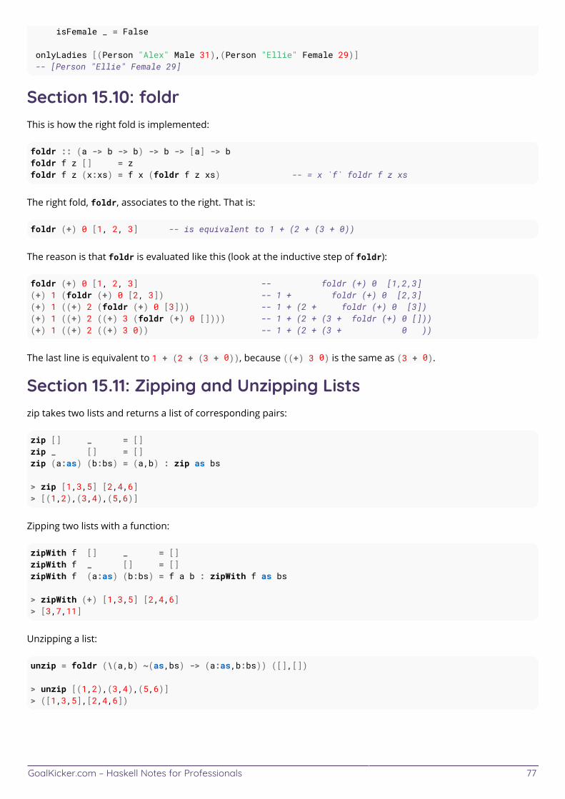
GoalKicker.com – Haskell Notes for Professionals 77

isFemale _ = False onlyLadies [(Person "Alex" Male 31),(Person "Ellie" Female 29)] -- [Person "Ellie" Female 29]

Section 15.10: foldrThis is how the right fold is implemented:

foldr :: (a -> b -> b) -> b -> [a] -> bfoldr f z [] = zfoldr f z (x:xs) = f x (foldr f z xs) -- = x `f` foldr f z xs

The right fold, foldr, associates to the right. That is:

foldr (+) 0 [1, 2, 3] -- is equivalent to 1 + (2 + (3 + 0))

The reason is that foldr is evaluated like this (look at the inductive step of foldr):

foldr (+) 0 [1, 2, 3] -- foldr (+) 0 [1,2,3](+) 1 (foldr (+) 0 [2, 3]) -- 1 + foldr (+) 0 [2,3](+) 1 ((+) 2 (foldr (+) 0 [3])) -- 1 + (2 + foldr (+) 0 [3])(+) 1 ((+) 2 ((+) 3 (foldr (+) 0 []))) -- 1 + (2 + (3 + foldr (+) 0 []))(+) 1 ((+) 2 ((+) 3 0)) -- 1 + (2 + (3 + 0 ))

The last line is equivalent to 1 + (2 + (3 + 0)), because ((+) 3 0) is the same as (3 + 0).

Section 15.11: Zipping and Unzipping Listszip takes two lists and returns a list of corresponding pairs:

zip [] _ = []zip _ [] = []zip (a:as) (b:bs) = (a,b) : zip as bs

> zip [1,3,5] [2,4,6]> [(1,2),(3,4),(5,6)]

Zipping two lists with a function:

zipWith f [] _ = []zipWith f _ [] = []zipWith f (a:as) (b:bs) = f a b : zipWith f as bs

> zipWith (+) [1,3,5] [2,4,6]> [3,7,11]

Unzipping a list:

unzip = foldr (\(a,b) ~(as,bs) -> (a:as,b:bs)) ([],[])

> unzip [(1,2),(3,4),(5,6)]> ([1,3,5],[2,4,6])

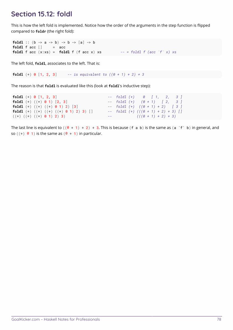
GoalKicker.com – Haskell Notes for Professionals 78

Section 15.12: foldlThis is how the left fold is implemented. Notice how the order of the arguments in the step function is flippedcompared to foldr (the right fold):

foldl :: (b -> a -> b) -> b -> [a] -> bfoldl f acc [] = accfoldl f acc (x:xs) = foldl f (f acc x) xs -- = foldl f (acc `f` x) xs

The left fold, foldl, associates to the left. That is:

foldl (+) 0 [1, 2, 3] -- is equivalent to ((0 + 1) + 2) + 3

The reason is that foldl is evaluated like this (look at foldl's inductive step):

foldl (+) 0 [1, 2, 3] -- foldl (+) 0 [ 1, 2, 3 ]foldl (+) ((+) 0 1) [2, 3] -- foldl (+) (0 + 1) [ 2, 3 ]foldl (+) ((+) ((+) 0 1) 2) [3] -- foldl (+) ((0 + 1) + 2) [ 3 ]foldl (+) ((+) ((+) ((+) 0 1) 2) 3) [] -- foldl (+) (((0 + 1) + 2) + 3) []((+) ((+) ((+) 0 1) 2) 3) -- (((0 + 1) + 2) + 3)

The last line is equivalent to ((0 + 1) + 2) + 3. This is because (f a b) is the same as (a `f` b) in general, andso ((+) 0 1) is the same as (0 + 1) in particular.

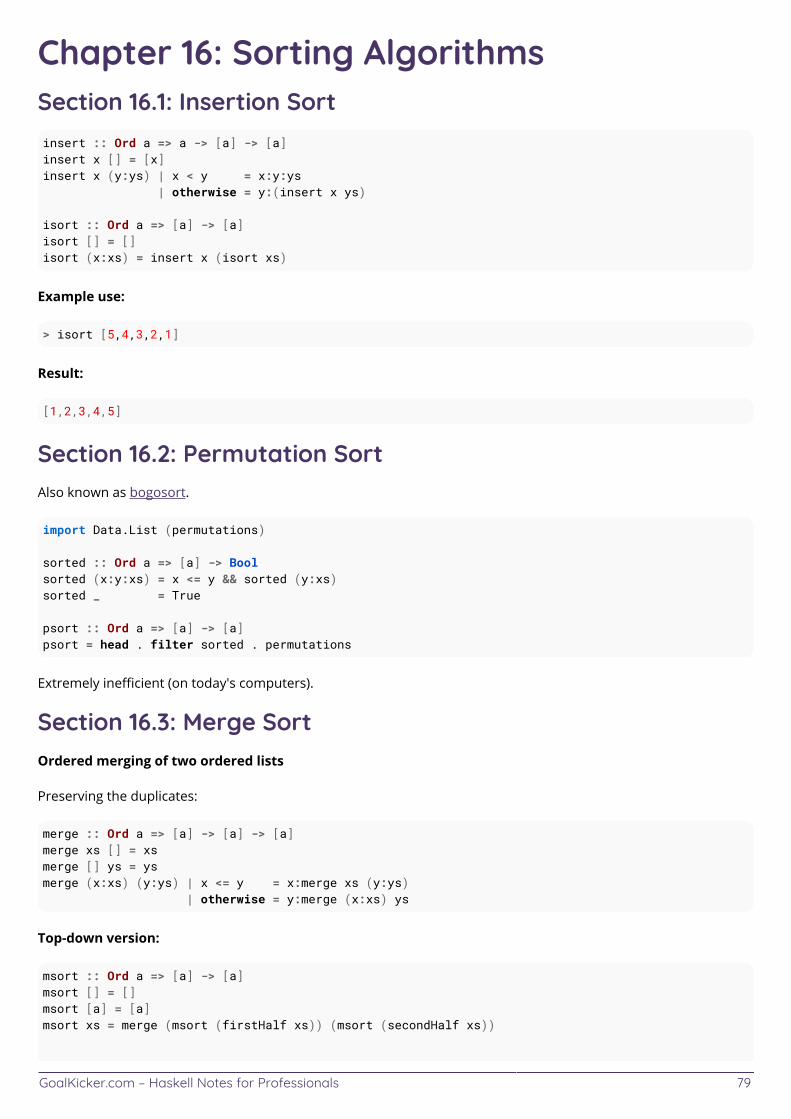
GoalKicker.com – Haskell Notes for Professionals 79

Chapter 16: Sorting AlgorithmsSection 16.1: Insertion Sortinsert :: Ord a => a -> [a] -> [a]insert x [] = [x]insert x (y:ys) | x < y = x:y:ys | otherwise = y:(insert x ys)

isort :: Ord a => [a] -> [a]isort [] = []isort (x:xs) = insert x (isort xs)

Example use:

> isort [5,4,3,2,1]

Result:

[1,2,3,4,5]

Section 16.2: Permutation SortAlso known as bogosort.

import Data.List (permutations)

sorted :: Ord a => [a] -> Boolsorted (x:y:xs) = x <= y && sorted (y:xs)sorted _ = True

psort :: Ord a => [a] -> [a]psort = head . filter sorted . permutations

Extremely inefficient (on today's computers).

Section 16.3: Merge SortOrdered merging of two ordered lists

Preserving the duplicates:

merge :: Ord a => [a] -> [a] -> [a]merge xs [] = xsmerge [] ys = ysmerge (x:xs) (y:ys) | x <= y = x:merge xs (y:ys) | otherwise = y:merge (x:xs) ys

Top-down version:

msort :: Ord a => [a] -> [a]msort [] = []msort [a] = [a]msort xs = merge (msort (firstHalf xs)) (msort (secondHalf xs))

GoalKicker.com – Haskell Notes for Professionals 80

firstHalf xs = let { n = length xs } in take (div n 2) xssecondHalf xs = let { n = length xs } in drop (div n 2) xs

It is defined this way for clarity, not for efficiency.

Example use:

> msort [3,1,4,5,2]

Result:

[1,2,3,4,5]

Bottom-up version:

msort [] = []msort xs = go [[x] | x <- xs] where go [a] = a go xs = go (pairs xs) pairs (a:b:t) = merge a b : pairs t pairs t = t

Section 16.4: Quicksortqsort :: (Ord a) => [a] -> [a]qsort [] = []qsort (x:xs) = qsort [a | a <- xs, a < x] ++ [x] ++ qsort [b | b <- xs, b >= x]

Section 16.5: Bubble sortbsort :: Ord a => [a] -> [a]bsort s = case bsort' s of t | t == s -> t | otherwise -> bsort t where bsort' (x:x2:xs) | x > x2 = x2:(bsort' (x:xs)) | otherwise = x:(bsort' (x2:xs)) bsort' s = s

Section 16.6: Selection sortSelection sort selects the minimum element, repeatedly, until the list is empty.

import Data.List (minimum, delete)

ssort :: Ord t => [t] -> [t]ssort [] = []ssort xs = let { x = minimum xs } in x : ssort (delete x xs)

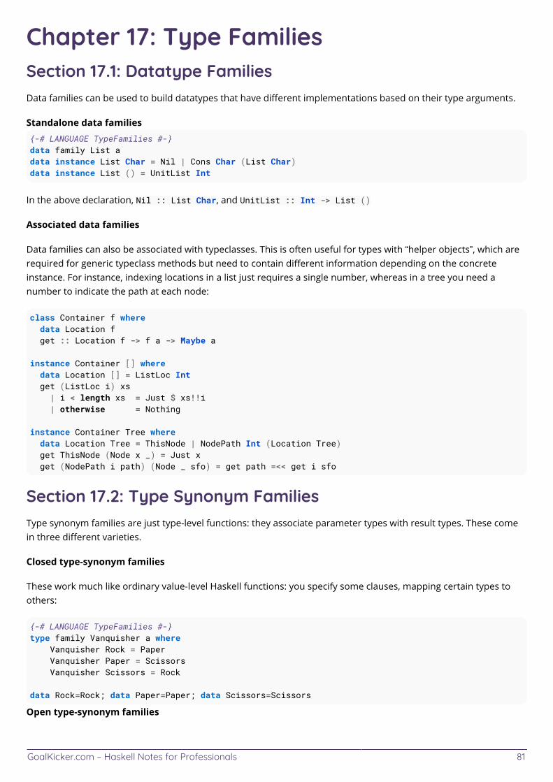
GoalKicker.com – Haskell Notes for Professionals 81

Chapter 17: Type FamiliesSection 17.1: Datatype FamiliesData families can be used to build datatypes that have different implementations based on their type arguments.

Standalone data families{-# LANGUAGE TypeFamilies #-}data family List adata instance List Char = Nil | Cons Char (List Char)data instance List () = UnitList Int

In the above declaration, Nil :: List Char, and UnitList :: Int -> List ()

Associated data families

Data families can also be associated with typeclasses. This is often useful for types with “helper objects”, which arerequired for generic typeclass methods but need to contain different information depending on the concreteinstance. For instance, indexing locations in a list just requires a single number, whereas in a tree you need anumber to indicate the path at each node:

class Container f where data Location f get :: Location f -> f a -> Maybe a

instance Container [] where data Location [] = ListLoc Int get (ListLoc i) xs | i < length xs = Just $ xs!!i | otherwise = Nothing

instance Container Tree where data Location Tree = ThisNode | NodePath Int (Location Tree) get ThisNode (Node x _) = Just x get (NodePath i path) (Node _ sfo) = get path =<< get i sfo

Section 17.2: Type Synonym FamiliesType synonym families are just type-level functions: they associate parameter types with result types. These comein three different varieties.

Closed type-synonym families

These work much like ordinary value-level Haskell functions: you specify some clauses, mapping certain types toothers:

{-# LANGUAGE TypeFamilies #-}type family Vanquisher a where Vanquisher Rock = Paper Vanquisher Paper = Scissors Vanquisher Scissors = Rock

data Rock=Rock; data Paper=Paper; data Scissors=Scissors

Open type-synonym families

GoalKicker.com – Haskell Notes for Professionals 82

These work more like typeclass instances: anybody can add more clauses in other modules.

type family DoubledSize w

type instance DoubledSize Word16 = Word32type instance DoubledSize Word32 = Word64-- Other instances might appear in other modules, but two instances cannot overlap-- in a way that would produce different results.

Class-associated type synonyms

An open type family can also be combined with an actual class. This is usually done when, like with associated datafamilies, some class method needs additional helper objects, and these helper objects can be different for differentinstances but may possibly also shared. A good example is VectorSpace class:

class VectorSpace v where type Scalar v :: * (*^) :: Scalar v -> v -> v

instance VectorSpace Double where type Scalar Double = Double μ *^ n = μ * n

instance VectorSpace (Double,Double) where type Scalar (Double,Double) = Double μ *^ (n,m) = (μ*n, μ*m) instance VectorSpace (Complex Double) where type Scalar (Complex Double) = Complex Double μ *^ n = μ*n

Note how in the first two instances, the implementation of Scalar is the same. This would not be possible with anassociated data family: data families are injective, type-synonym families aren't.

While non-injectivity opens up some possibilities like the above, it also makes type inference more difficult. Forinstance, the following will not typecheck:

class Foo a where type Bar a :: * bar :: a -> Bar ainstance Foo Int where type Bar Int = String bar = showinstance Foo Double where type Bar Double = Bool bar = (>0)

main = putStrLn (bar 1)

In this case, the compiler can't know what instance to use, because the argument to bar is itself just a polymorphicNum literal. And the type function Bar can't be resolved in “inverse direction”, precisely because it's not injective† andhence not invertible (there could be more than one type with Bar a = String).

†With only these two instances, it is actually injective, but the compiler can't know somebody won't add moreinstances later on and thereby break the behaviour.

GoalKicker.com – Haskell Notes for Professionals 83

Section 17.3: InjectivityType Families are not necessarily injective. Therefore, we cannot infer the parameter from an application. Forexample, in servant, given a type Server a we cannot infer the type a. To solve this problem, we can use Proxy. Forexample, in servant, the serve function has type ... Proxy a -> Server a -> .... We can infer a from Proxy abecause Proxy is defined by data which is injective.

GoalKicker.com – Haskell Notes for Professionals 84

Chapter 18: MonadsA monad is a data type of composable actions. Monad is the class of type constructors whose values represent suchactions. Perhaps IO is the most recognizable one: a value of IO a is a "recipe for retrieving an a value from the realworld".

We say a type constructor m (such as [] or Maybe) forms a monad if there is an instance Monad m satisfying certainlaws about composition of actions. We can then reason about m a as an "action whose result has type a".

Section 18.1: Definition of Monadclass Monad m where return :: a -> m a (>>=) :: m a -> (a -> m b) -> m b

The most important function for dealing with monads is the bind operator >>=:

(>>=) :: m a -> (a -> m b) -> m b

Think of m a as "an action with an a result".Think of a -> m b as “an action (depending on an a parameter) with a b result.”.

>>= sequences two actions together by piping the result from the first action to the second.

The other function defined by Monad is:

return :: a -> m a

Its name is unfortunate: this return has nothing to do with the return keyword found in imperative programminglanguages.

return x is the trivial action yielding x as its result. (It is trivial in the following sense:)

return x >>= f ≡ f x -- “left identity” monad law x >>= return ≡ x -- “right identity” monad law

Section 18.2: No general way to extract value from a monadiccomputationYou can wrap values into actions and pipe the result of one computation into another:

return :: Monad m => a -> m a(>>=) :: Monad m => m a -> (a -> m b) -> m b

However, the definition of a Monad doesn’t guarantee the existence of a function of type Monad m => m a -> a.

That means there is, in general, no way to extract a value from a computation (i.e. “unwrap” it). This is the casefor many instances:

extract :: Maybe a -> aextract (Just x) = x -- Sure, this works, but...extract Nothing = undefined -- We can’t extract a value from failure.

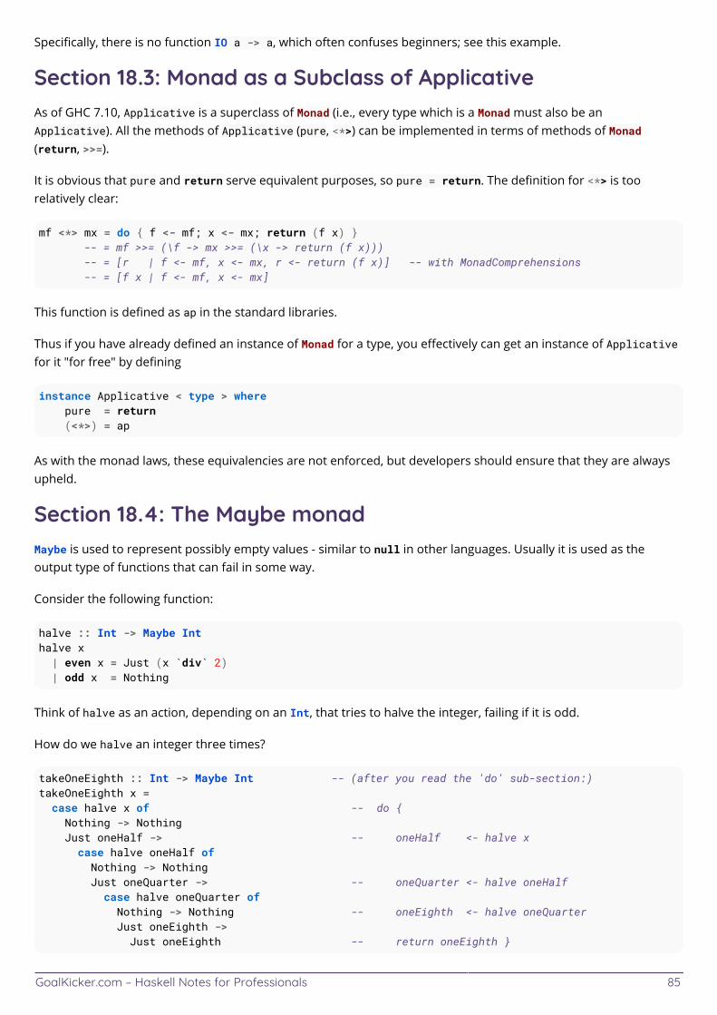
GoalKicker.com – Haskell Notes for Professionals 85

Specifically, there is no function IO a -> a, which often confuses beginners; see this example.

Section 18.3: Monad as a Subclass of ApplicativeAs of GHC 7.10, Applicative is a superclass of Monad (i.e., every type which is a Monad must also be anApplicative). All the methods of Applicative (pure, <*>) can be implemented in terms of methods of Monad(return, >>=).

It is obvious that pure and return serve equivalent purposes, so pure = return. The definition for <*> is toorelatively clear:

mf <*> mx = do { f <- mf; x <- mx; return (f x) } -- = mf >>= (\f -> mx >>= (\x -> return (f x))) -- = [r | f <- mf, x <- mx, r <- return (f x)] -- with MonadComprehensions -- = [f x | f <- mf, x <- mx]

This function is defined as ap in the standard libraries.

Thus if you have already defined an instance of Monad for a type, you effectively can get an instance of Applicativefor it "for free" by defining

instance Applicative < type > where pure = return (<*>) = ap

As with the monad laws, these equivalencies are not enforced, but developers should ensure that they are alwaysupheld.

Section 18.4: The Maybe monadMaybe is used to represent possibly empty values - similar to null in other languages. Usually it is used as theoutput type of functions that can fail in some way.

Consider the following function:

halve :: Int -> Maybe Inthalve x | even x = Just (x `div` 2) | odd x = Nothing

Think of halve as an action, depending on an Int, that tries to halve the integer, failing if it is odd.

How do we halve an integer three times?

takeOneEighth :: Int -> Maybe Int -- (after you read the 'do' sub-section:)takeOneEighth x = case halve x of -- do { Nothing -> Nothing Just oneHalf -> -- oneHalf <- halve x case halve oneHalf of Nothing -> Nothing Just oneQuarter -> -- oneQuarter <- halve oneHalf case halve oneQuarter of Nothing -> Nothing -- oneEighth <- halve oneQuarter Just oneEighth -> Just oneEighth -- return oneEighth }

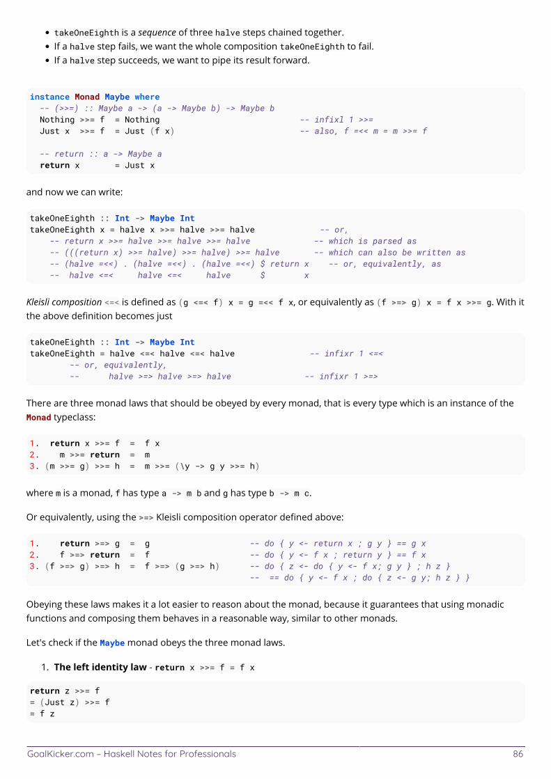
GoalKicker.com – Haskell Notes for Professionals 86

takeOneEighth is a sequence of three halve steps chained together.If a halve step fails, we want the whole composition takeOneEighth to fail.If a halve step succeeds, we want to pipe its result forward.

instance Monad Maybe where -- (>>=) :: Maybe a -> (a -> Maybe b) -> Maybe b Nothing >>= f = Nothing -- infixl 1 >>= Just x >>= f = Just (f x) -- also, f =<< m = m >>= f -- return :: a -> Maybe a return x = Just x

and now we can write:

takeOneEighth :: Int -> Maybe InttakeOneEighth x = halve x >>= halve >>= halve -- or, -- return x >>= halve >>= halve >>= halve -- which is parsed as -- (((return x) >>= halve) >>= halve) >>= halve -- which can also be written as -- (halve =<<) . (halve =<<) . (halve =<<) $ return x -- or, equivalently, as -- halve <=< halve <=< halve $ x

Kleisli composition <=< is defined as (g <=< f) x = g =<< f x, or equivalently as (f >=> g) x = f x >>= g. With itthe above definition becomes just

takeOneEighth :: Int -> Maybe InttakeOneEighth = halve <=< halve <=< halve -- infixr 1 <=< -- or, equivalently, -- halve >=> halve >=> halve -- infixr 1 >=>

There are three monad laws that should be obeyed by every monad, that is every type which is an instance of theMonad typeclass:

1. return x >>= f = f x2. m >>= return = m3. (m >>= g) >>= h = m >>= (\y -> g y >>= h)

where m is a monad, f has type a -> m b and g has type b -> m c.

Or equivalently, using the >=> Kleisli composition operator defined above:

1. return >=> g = g -- do { y <- return x ; g y } == g x2. f >=> return = f -- do { y <- f x ; return y } == f x3. (f >=> g) >=> h = f >=> (g >=> h) -- do { z <- do { y <- f x; g y } ; h z } -- == do { y <- f x ; do { z <- g y; h z } }

Obeying these laws makes it a lot easier to reason about the monad, because it guarantees that using monadicfunctions and composing them behaves in a reasonable way, similar to other monads.

Let's check if the Maybe monad obeys the three monad laws.

The left identity law - return x >>= f = f x1.

return z >>= f= (Just z) >>= f= f z

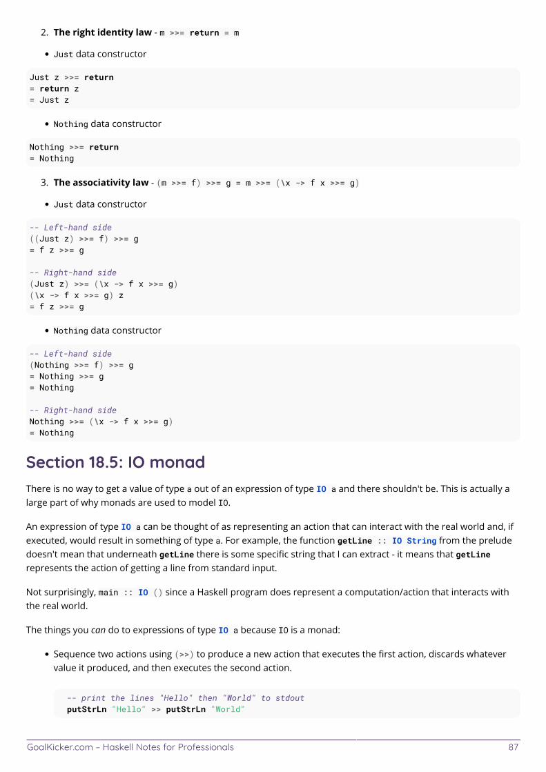
GoalKicker.com – Haskell Notes for Professionals 87

The right identity law - m >>= return = m2.

Just data constructor

Just z >>= return= return z= Just z

Nothing data constructor

Nothing >>= return= Nothing

The associativity law - (m >>= f) >>= g = m >>= (\x -> f x >>= g)3.

Just data constructor

-- Left-hand side((Just z) >>= f) >>= g= f z >>= g

-- Right-hand side(Just z) >>= (\x -> f x >>= g)(\x -> f x >>= g) z= f z >>= g

Nothing data constructor

-- Left-hand side(Nothing >>= f) >>= g= Nothing >>= g= Nothing

-- Right-hand sideNothing >>= (\x -> f x >>= g)= Nothing

Section 18.5: IO monadThere is no way to get a value of type a out of an expression of type IO a and there shouldn't be. This is actually alarge part of why monads are used to model IO.

An expression of type IO a can be thought of as representing an action that can interact with the real world and, ifexecuted, would result in something of type a. For example, the function getLine :: IO String from the preludedoesn't mean that underneath getLine there is some specific string that I can extract - it means that getLinerepresents the action of getting a line from standard input.

Not surprisingly, main :: IO () since a Haskell program does represent a computation/action that interacts withthe real world.

The things you can do to expressions of type IO a because IO is a monad:

Sequence two actions using (>>) to produce a new action that executes the first action, discards whatevervalue it produced, and then executes the second action.

-- print the lines "Hello" then "World" to stdout putStrLn "Hello" >> putStrLn "World"

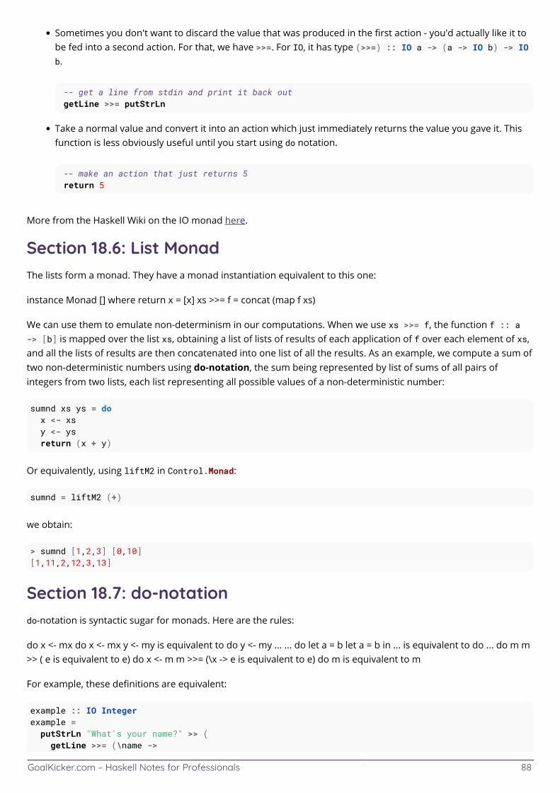
GoalKicker.com – Haskell Notes for Professionals 88

Sometimes you don't want to discard the value that was produced in the first action - you'd actually like it tobe fed into a second action. For that, we have >>=. For IO, it has type (>>=) :: IO a -> (a -> IO b) -> IOb.

-- get a line from stdin and print it back out getLine >>= putStrLn

Take a normal value and convert it into an action which just immediately returns the value you gave it. Thisfunction is less obviously useful until you start using do notation.

-- make an action that just returns 5 return 5

More from the Haskell Wiki on the IO monad here.

Section 18.6: List MonadThe lists form a monad. They have a monad instantiation equivalent to this one:

instance Monad [] where return x = [x] xs >>= f = concat (map f xs)

We can use them to emulate non-determinism in our computations. When we use xs >>= f, the function f :: a-> [b] is mapped over the list xs, obtaining a list of lists of results of each application of f over each element of xs,and all the lists of results are then concatenated into one list of all the results. As an example, we compute a sum oftwo non-deterministic numbers using do-notation, the sum being represented by list of sums of all pairs ofintegers from two lists, each list representing all possible values of a non-deterministic number:

sumnd xs ys = do x <- xs y <- ys return (x + y)

Or equivalently, using liftM2 in Control.Monad:

sumnd = liftM2 (+)

we obtain:

> sumnd [1,2,3] [0,10][1,11,2,12,3,13]

Section 18.7: do-notationdo-notation is syntactic sugar for monads. Here are the rules:

do x <- mx do x <- mx y <- my is equivalent to do y <- my ... ... do let a = b let a = b in ... is equivalent to do ... do m m>> ( e is equivalent to e) do x <- m m >>= (\x -> e is equivalent to e) do m is equivalent to m

For example, these definitions are equivalent:

example :: IO Integerexample = putStrLn "What's your name?" >> ( getLine >>= (\name ->

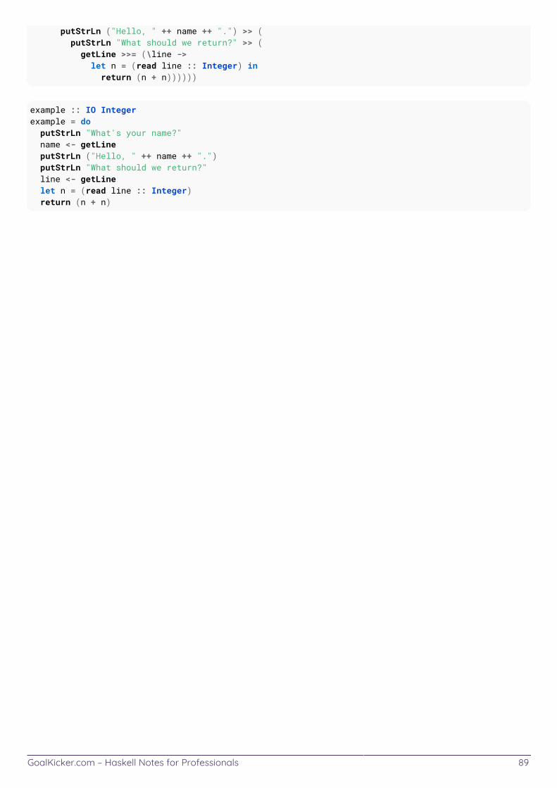
GoalKicker.com – Haskell Notes for Professionals 89

putStrLn ("Hello, " ++ name ++ ".") >> ( putStrLn "What should we return?" >> ( getLine >>= (\line -> let n = (read line :: Integer) in return (n + n))))))

example :: IO Integerexample = do putStrLn "What's your name?" name <- getLine putStrLn ("Hello, " ++ name ++ ".") putStrLn "What should we return?" line <- getLine let n = (read line :: Integer) return (n + n)

GoalKicker.com – Haskell Notes for Professionals 90

Chapter 19: StackSection 19.1: Profiling with StackConfigure profiling for a project via stack. First build the project with the --profile flag:

stack build --profile

GHC flags are not required in the cabal file for this to work (like -prof). stack will automatically turn on profiling forboth the library and executables in the project. The next time an executable runs in the project, the usual +RTS flagscan be used:

stack exec -- my-bin +RTS -p

Section 19.2: StructureFile structure

A simple project has the following files included in it:

➜ helloworld lsLICENSE Setup.hs helloworld.cabal src stack.yaml

In the folder src there is a file named Main.hs. This is the "starting point" of the helloworld project. By defaultMain.hs contains a simple "Hello, World!" program.

Main.hs

module Main where

main :: IO ()main = do putStrLn "hello world"

Running the program

Make sure you are in the directory helloworld and run:

stack build # Compile the programstack exec helloworld # Run the program# prints "hello world"

Section 19.3: Build and Run a Stack ProjectIn this example our project name is "helloworld" which was created with stack new helloworld simple

First we have to build the project with stack build and then we can run it with

stack exec helloworld-exe

Section 19.4: Viewing dependenciesTo find out what packages your project directly depends on, you can simply use this command:

GoalKicker.com – Haskell Notes for Professionals 91

stack list-dependencies

This way you can find out what version of your dependencies where actually pulled down by stack.

Haskell projects frequently find themselves pulling in a lot of libraries indirectly, and sometimes these externaldependencies cause problems that you need to track down. If you find yourself with a rogue external dependencythat you'd like to identify, you can grep through the entire dependency graph and identify which of yourdependencies is ultimately pulling in the undesired package:

stack dot --external | grep template-haskell

stack dot prints out a dependency graph in text form that can be searched. It can also be viewed:

stack dot --external | dot -Tpng -o my-project.png

You can also set the depth of the dependency graph if you want:

stack dot --external --depth 3 | dot -Tpng -o my-project.png

Section 19.5: Stack installBy running the command

stack install

Stack will copy a executable file to the folder

/Users/<yourusername>/.local/bin/

Section 19.6: Installing StackMac OSX

Using Homebrew:

brew install haskell-stack

Section 19.7: Creating a simple projectTo create a project called helloworld run:

stack new helloworld simple

This will create a directory called helloworld with the files necessary for a Stack project.

Section 19.8: Stackage Packages and changing the LTS(resolver) versionStackage is a repository for Haskell packages. We can add these packages to a stack project.

Adding lens to a project.

In a stack project, there is a file called stack.yaml. In stack.yaml there is a segment that looks like:

GoalKicker.com – Haskell Notes for Professionals 92

resolver: lts-6.8

Stackage keeps a list of packages for every revision of lts. In our case we want the list of packages for lts-6.8 Tofind these packages visit:

https://www.stackage.org/lts-6.8 # if a different version is used, change 6.8 to the correctresolver number.

Looking through the packages, there is a Lens-4.13.

We can now add the language package by modifying the section of helloworld.cabal:

build-depends: base >= 4.7 && < 5

to:

build-depends: base >= 4.7 && 5, lens == 4.13

Obviously, if we want to change a newer LTS (after it's released), we just change the resolver number, eg.:

resolver: lts-6.9

With the next stack build Stack will use the LTS 6.9 version and hence download some new dependencies.

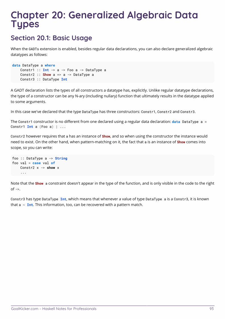
GoalKicker.com – Haskell Notes for Professionals 93

Chapter 20: Generalized Algebraic DataTypesSection 20.1: Basic UsageWhen the GADTs extension is enabled, besides regular data declarations, you can also declare generalized algebraicdatatypes as follows:

data DataType a where Constr1 :: Int -> a -> Foo a -> DataType a Constr2 :: Show a => a -> DataType a Constr3 :: DataType Int

A GADT declaration lists the types of all constructors a datatype has, explicitly. Unlike regular datatype declarations,the type of a constructor can be any N-ary (including nullary) function that ultimately results in the datatype appliedto some arguments.

In this case we've declared that the type DataType has three constructors: Constr1, Constr2 and Constr3.

The Constr1 constructor is no different from one declared using a regular data declaration: data DataType a =Constr1 Int a (Foo a) | ...

Constr2 however requires that a has an instance of Show, and so when using the constructor the instance wouldneed to exist. On the other hand, when pattern-matching on it, the fact that a is an instance of Show comes intoscope, so you can write:

foo :: DataType a -> Stringfoo val = case val of Constr2 x -> show x ...

Note that the Show a constraint doesn't appear in the type of the function, and is only visible in the code to the rightof ->.

Constr3 has type DataType Int, which means that whenever a value of type DataType a is a Constr3, it is knownthat a ~ Int. This information, too, can be recovered with a pattern match.

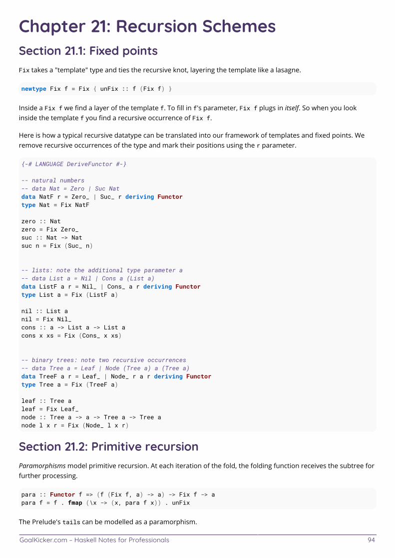
GoalKicker.com – Haskell Notes for Professionals 94

Chapter 21: Recursion SchemesSection 21.1: Fixed pointsFix takes a "template" type and ties the recursive knot, layering the template like a lasagne.

newtype Fix f = Fix { unFix :: f (Fix f) }

Inside a Fix f we find a layer of the template f. To fill in f's parameter, Fix f plugs in itself. So when you lookinside the template f you find a recursive occurrence of Fix f.

Here is how a typical recursive datatype can be translated into our framework of templates and fixed points. Weremove recursive occurrences of the type and mark their positions using the r parameter.

{-# LANGUAGE DeriveFunctor #-}

-- natural numbers-- data Nat = Zero | Suc Natdata NatF r = Zero_ | Suc_ r deriving Functortype Nat = Fix NatF

zero :: Natzero = Fix Zero_suc :: Nat -> Natsuc n = Fix (Suc_ n)

-- lists: note the additional type parameter a-- data List a = Nil | Cons a (List a)data ListF a r = Nil_ | Cons_ a r deriving Functortype List a = Fix (ListF a)

nil :: List anil = Fix Nil_cons :: a -> List a -> List acons x xs = Fix (Cons_ x xs)

-- binary trees: note two recursive occurrences-- data Tree a = Leaf | Node (Tree a) a (Tree a)data TreeF a r = Leaf_ | Node_ r a r deriving Functortype Tree a = Fix (TreeF a)

leaf :: Tree aleaf = Fix Leaf_node :: Tree a -> a -> Tree a -> Tree anode l x r = Fix (Node_ l x r)

Section 21.2: Primitive recursionParamorphisms model primitive recursion. At each iteration of the fold, the folding function receives the subtree forfurther processing.

para :: Functor f => (f (Fix f, a) -> a) -> Fix f -> apara f = f . fmap (\x -> (x, para f x)) . unFix

The Prelude's tails can be modelled as a paramorphism.

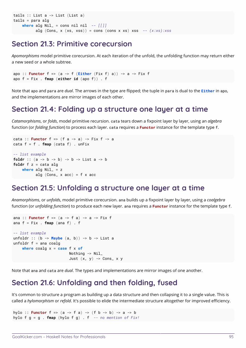
GoalKicker.com – Haskell Notes for Professionals 95

tails :: List a -> List (List a)tails = para alg where alg Nil_ = cons nil nil -- [[]] alg (Cons_ x (xs, xss)) = cons (cons x xs) xss -- (x:xs):xss

Section 21.3: Primitive corecursionApomorphisms model primitive corecursion. At each iteration of the unfold, the unfolding function may return eithera new seed or a whole subtree.

apo :: Functor f => (a -> f (Either (Fix f) a)) -> a -> Fix fapo f = Fix . fmap (either id (apo f)) . f

Note that apo and para are dual. The arrows in the type are flipped; the tuple in para is dual to the Either in apo,and the implementations are mirror images of each other.

Section 21.4: Folding up a structure one layer at a timeCatamorphisms, or folds, model primitive recursion. cata tears down a fixpoint layer by layer, using an algebrafunction (or folding function) to process each layer. cata requires a Functor instance for the template type f.

cata :: Functor f => (f a -> a) -> Fix f -> acata f = f . fmap (cata f) . unFix

-- list examplefoldr :: (a -> b -> b) -> b -> List a -> bfoldr f z = cata alg where alg Nil_ = z alg (Cons_ x acc) = f x acc

Section 21.5: Unfolding a structure one layer at a timeAnamorphisms, or unfolds, model primitive corecursion. ana builds up a fixpoint layer by layer, using a coalgebrafunction (or unfolding function) to produce each new layer. ana requires a Functor instance for the template type f.

ana :: Functor f => (a -> f a) -> a -> Fix fana f = Fix . fmap (ana f) . f

-- list exampleunfoldr :: (b -> Maybe (a, b)) -> b -> List aunfoldr f = ana coalg where coalg x = case f x of Nothing -> Nil_ Just (x, y) -> Cons_ x y

Note that ana and cata are dual. The types and implementations are mirror images of one another.

Section 21.6: Unfolding and then folding, fusedIt's common to structure a program as building up a data structure and then collapsing it to a single value. This iscalled a hylomorphism or refold. It's possible to elide the intermediate structure altogether for improved efficiency.

hylo :: Functor f => (a -> f a) -> (f b -> b) -> a -> bhylo f g = g . fmap (hylo f g) . f -- no mention of Fix!

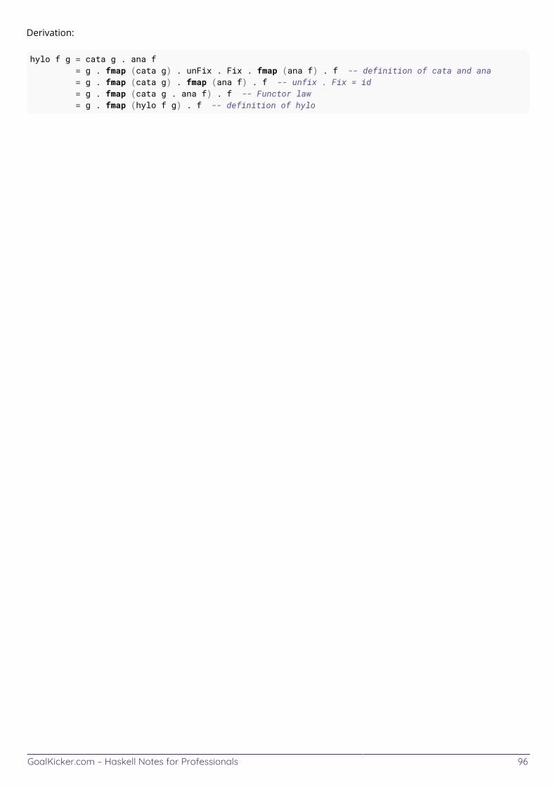
GoalKicker.com – Haskell Notes for Professionals 96

Derivation:

hylo f g = cata g . ana f = g . fmap (cata g) . unFix . Fix . fmap (ana f) . f -- definition of cata and ana = g . fmap (cata g) . fmap (ana f) . f -- unfix . Fix = id = g . fmap (cata g . ana f) . f -- Functor law = g . fmap (hylo f g) . f -- definition of hylo

GoalKicker.com – Haskell Notes for Professionals 97

Chapter 22: Data.TextSection 22.1: Text LiteralsThe OverloadedStrings language extension allows the use of normal string literals to stand for Text values.

{-# LANGUAGE OverloadedStrings #-}

import qualified Data.Text as T

myText :: T.TextmyText = "overloaded"

Section 22.2: Checking if a Text is a substring of another Textghci> :set -XOverloadedStringsghci> import Data.Text as T

isInfixOf :: Text -> Text -> Bool checks whether a Text is contained anywhere within another Text.

ghci> "rum" `T.isInfixOf` "crumble"True

isPrefixOf :: Text -> Text -> Bool checks whether a Text appears at the beginning of another Text.

ghci> "crumb" `T.isPrefixOf` "crumble"True

isSuffixOf :: Text -> Text -> Bool checks whether a Text appears at the end of another Text.

ghci> "rumble" `T.isSuffixOf` "crumble"True

Section 22.3: Stripping whitespace{-# LANGUAGE OverloadedStrings #-}

import qualified Data.Text as T

myText :: T.TextmyText = "\n\r\t leading and trailing whitespace \t\r\n"

strip removes whitespace from the start and end of a Text value.

ghci> T.strip myText"leading and trailing whitespace"

stripStart removes whitespace only from the start.

ghci> T.stripStart myText"leading and trailing whitespace \t\r\n"

stripEnd removes whitespace only from the end.

GoalKicker.com – Haskell Notes for Professionals 98

ghci> T.stripEnd myText"\n\r\t leading and trailing whitespace"

filter can be used to remove whitespace, or other characters, from the middle.

ghci> T.filter /=' ' "spaces in the middle of a text string""spacesinthemiddleofatextstring"

Section 22.4: Indexing Text{-# LANGUAGE OverloadedStrings #-}

import qualified Data.Text as T

myText :: T.Text

myText = "mississippi"

Characters at specific indices can be returned by the index function.

ghci> T.index myText 2's'

The findIndex function takes a function of type (Char -> Bool) and Text and returns the index of the firstoccurrence of a given string or Nothing if it doesn't occur.

ghci> T.findIndex ('s'==) myTextJust 2ghci> T.findIndex ('c'==) myTextNothing

The count function returns the number of times a query Text occurs within another Text.

ghci> count ("miss"::T.Text) myText1

Section 22.5: Splitting Text Values{-# LANGUAGE OverloadedStrings #-}

import qualified Data.Text as T

myText :: T.TextmyText = "mississippi"

splitOn breaks a Text up into a list of Texts on occurrences of a substring.

ghci> T.splitOn "ss" myText["mi","i","ippi"]

splitOn is the inverse of intercalate.

ghci> intercalate "ss" (splitOn "ss" "mississippi")"mississippi"

GoalKicker.com – Haskell Notes for Professionals 99

split breaks a Text value into chunks on characters that satisfy a Boolean predicate.

ghci> T.split (== 'i') myText["m","ss","ss","pp",""]

Section 22.6: Encoding and Decoding TextEncoding and decoding functions for a variety of Unicode encodings can be found in the Data.Text.Encodingmodule.

ghci> import Data.Text.Encodingghci> decodeUtf8 (encodeUtf8 "my text")"my text"

Note that decodeUtf8 will throw an exception on invalid input. If you want to handle invalid UTF-8 yourself, usedecodeUtf8With.

ghci> decodeUtf8With (\errorDescription input -> Nothing) messyOutsideData

GoalKicker.com – Haskell Notes for Professionals 100

Chapter 23: Using GHCiSection 23.1: Breakpoints with GHCiGHCi supports imperative-style breakpoints out of the box with interpreted code (code that's been :loaded).

With the following program:

-- mySum.hsdoSum n = do putStrLn ("Counting to " ++ (show n)) let v = sum [1..n] putStrLn ("sum to " ++ (show n) ++ " = " ++ (show v))

loaded into GHCi:

Prelude> :load mySum.hs[1 of 1] Compiling Main ( mySum.hs, interpreted )Ok, modules loaded: Main.*Main>

We can now set breakpoints using line numbers:

*Main> :break 2Breakpoint 0 activated at mySum.hs:2:3-39

and GHCi will stop at the relevant line when we run the function:

*Main> doSum 12Stopped at mySum.hs:2:3-39_result :: IO () = _n :: Integer = 12[mySum.hs:2:3-39] *Main>

It might be confusing where we are in the program, so we can use :list to clarify:

[mySum.hs:2:3-39] *Main> :list1 doSum n = do2 putStrLn ("Counting to " ++ (show n)) -- GHCi will emphasise this line, as that's where we'vestopped3 let v = sum [1..n]

We can print variables, and continue execution too:

[mySum.hs:2:3-39] *Main> n12:continueCounting to 12sum to 12 = 78*Main>

Section 23.2: Quitting GHCiYou can quit GHCi simply with :q or :quit

GoalKicker.com – Haskell Notes for Professionals 101

ghci> :qLeaving GHCi.

ghci> :quitLeaving GHCi.

Alternatively, the shortcut CTRL + D ( Cmd + D for OSX) has the same effect as :q.

Section 23.3: Reloading a already loaded fileIf you have loaded a file into GHCi (e.g. using :l filename.hs) and you have changed the file in an editor outside ofGHCi you must reload the file with :r or :reload in order to make use of the changes, hence you don't need to typeagain the filename.

ghci> :rOK, modules loaded: Main.

ghci> :reloadOK, modules loaded: Main.

Section 23.4: Starting GHCiType ghci at a shell prompt to start GHCI.

$ ghciGHCi, version 8.0.1: http://www.haskell.org/ghc/ :? for helpPrelude>

Section 23.5: Changing the GHCi default promptBy default, GHCI's prompt shows all the modules you have loaded into your interactive session. If you have manymodules loaded this can get long:

Prelude Data.List Control.Monad> -- etc

The :set prompt command changes the prompt for this interactive session.

Prelude Data.List Control.Monad> :set prompt "foo> "foo>

To change the prompt permanently, add :set prompt "foo> " to the GHCi config file.

Section 23.6: The GHCi configuration fileGHCi uses a configuration file in ~/.ghci. A configuration file consists of a sequence of commands which GHCi willexecute on startup.

$ echo ":set prompt \"foo> \"" > ~/.ghci$ ghciGHCi, version 8.0.1: http://www.haskell.org/ghc/ :? for helpLoaded GHCi configuration from ~/.ghcifoo>

GoalKicker.com – Haskell Notes for Professionals 102

Section 23.7: Loading a fileThe :l or :load command type-checks and loads a file.

$ echo "f = putStrLn \"example\"" > example.hs$ ghciGHCi, version 8.0.1: http://www.haskell.org/ghc/ :? for helpghci> :l example.hs[1 of 1] Compiling Main ( example.hs, interpreted )Ok, modules loaded: Main.ghci> fexample

Section 23.8: Multi-line statementsThe :{ instruction begins multi-line mode and :} ends it. In multi-line mode GHCi will interpret newlines assemicolons, not as the end of an instruction.

ghci> :{ghci| myFoldr f z [] = zghci| myFoldr f z (y:ys) = f y (myFoldr f z ys)ghci| :}ghci> :t myFoldrmyFoldr :: (a -> b -> b) -> b -> [a] -> b

GoalKicker.com – Haskell Notes for Professionals 103

Chapter 24: StrictnessSection 24.1: Bang PatternsPatterns annotated with a bang (!) are evaluated strictly instead of lazily.

foo (!x, y) !z = [x, y, z]

In this example, x and z will both be evaluated to weak head normal form before returning the list. It's equivalentto:

foo (x, y) z = x `seq` z `seq` [x, y, z]

Bang patterns are enabled using the Haskell 2010 BangPatterns language extension.

Section 24.2: Lazy patternsLazy, or irrefutable, patterns (denoted with the syntax ~pat) are patterns that always match, without even looking atthe matched value. This means lazy patterns will match even bottom values. However, subsequent uses of variablesbound in sub-patterns of an irrefutable pattern will force the pattern matching to occur, evaluating to bottomunless the match succeeds.

The following function is lazy in its argument:

f1 :: Either e Int -> Intf1 ~(Right 1) = 42

and so we get

λ» f1 (Right 1)42λ» f1 (Right 2)42λ» f1 (Left "foo")42λ» f1 (error "oops!")42λ» f1 "oops!"*** type mismatch ***

The following function is written with a lazy pattern but is in fact using the pattern's variable which forces thematch, so will fail for Left arguments:

f2 :: Either e Int -> Intf2 ~(Right x) = x + 1

λ» f2 (Right 1)2λ» f2 (Right 2)3λ» f2 (Right (error "oops!"))*** Exception: oops!λ» f2 (Left "foo")*** Exception: lazypat.hs:5:1-21: Irrefutable pattern failed for pattern (Right x)

GoalKicker.com – Haskell Notes for Professionals 104

λ» f2 (error "oops!")*** Exception: oops!

let bindings are lazy, behave as irrefutable patterns:

act1 :: IO ()act1 = do ss <- readLn let [s1, s2] = ss :: [String] putStrLn "Done"

act2 :: IO ()act2 = do ss <- readLn let [s1, s2] = ss putStrLn s1

Here act1 works on inputs that parse to any list of strings, whereas in act2 the putStrLn s1 needs the value of s1which forces the pattern matching for [s1, s2], so it works only for lists of exactly two strings:

λ» act1> ["foo"]Doneλ» act2> ["foo"]*** readIO: no parse ***

Section 24.3: Normal formsThis example provides a brief overview - for a more in-depth explanation of normal forms and examples, see thisquestion.

Reduced normal form

The reduced normal form (or just normal form, when the context is clear) of an expression is the result ofevaluating all reducible subexpressions in the given expression. Due to the non-strict semantics of Haskell (typicallycalled laziness), a subexpression is not reducible if it is under a binder (i.e. a lambda abstraction - \x -> ..). Thenormal form of an expression has the property that if it exists, it is unique.

In other words, it does not matter (in terms of denotational semantics) in which order you reduce subexpressions.However, the key to writing performant Haskell programs is often ensuring that the right expression is evaluated atthe right time, i.e, the understanding the operational semantics.

An expression whose normal form is itself is said to be in normal form.

Some expressions, e.g. let x = 1:x in x, have no normal form, but are still productive. The example expressionstill has a value, if one admits infinite values, which here is the list [1,1, ...]. Other expressions, such as let y =1+y in y, have no value, or their value is undefined.

Weak head normal form

The RNF corresponds to fully evaluating an expression - likewise, the weak head normal form (WHNF) correspondsto evaluating to the head of the expression. The head of an expression e is fully evaluated if e is an application Cone1 e2 .. en and Con is a constructor; or an abstraction \x -> e1; or a partial application f e1 e2 .. en, wherepartial application means f takes more than n arguments (or equivalently, the type of e is a function type). In anycase, the subexpressions e1..en can be evaluated or unevaluated for the expression to be in WHNF - they can even

GoalKicker.com – Haskell Notes for Professionals 105

be undefined.

The evaluation semantics of Haskell can be described in terms of the WHNF - to evaluate an expression e, firstevaluate it to WHNF, then recursively evaluate all of its subexpressions from left to right.

The primitive seq function is used to evaluate an expression to WHNF. seq x y is denotationally equal to y (thevalue of seq x y is precisely y); furthermore x is evaluated to WHNF when y is evaluated to WHNF. An expressioncan also be evaluated to WHNF with a bang pattern (enabled by the -XBangPatterns extension), whose syntax is asfollows:

f !x y = ...

In which x will be evaluated to WHNF when f is evaluated, while y is not (necessarily) evaluated. A bang pattern canalso appear in a constructor, e.g.

data X = Con A !B C .. N

in which case the constructor Con is said to be strict in the B field, which means the B field is evaluated to WHNFwhen the constructor is applied to sufficient (here, two) arguments.

Section 24.4: Strict fieldsIn a data declaration, prefixing a type with a bang (!) makes the field a strict field. When the data constructor isapplied, those fields will be evaluated to weak head normal form, so the data in the fields is guaranteed to alwaysbe in weak head normal form.

Strict fields can be used in both record and non-record types:

data User = User { identifier :: !Int , firstName :: !Text , lastName :: !Text }

data T = MkT !Int !Int

GoalKicker.com – Haskell Notes for Professionals 106

Chapter 25: Syntax in FunctionsSection 25.1: Pattern MatchingHaskell supports pattern matching expressions in both function definition and through case statements.

A case statement is much like a switch in other languages, except it supports all of Haskell's types.

Let's start simple:

longName :: String -> StringlongName name = case name of "Alex" -> "Alexander" "Jenny" -> "Jennifer" _ -> "Unknown" -- the "default" case, if you like

Or, we could define our function like an equation which would be pattern matching, just without using a casestatement:

longName "Alex" = "Alexander"longName "Jenny" = "Jennifer"longName _ = "Unknown"

A more common example is with the Maybe type:

data Person = Person { name :: String, petName :: (Maybe String) }

hasPet :: Person -> BoolhasPet (Person _ Nothing) = FalsehasPet _ = True -- Maybe can only take `Just a` or `Nothing`, so this wildcard suffices

Pattern matching can also be used on lists:

isEmptyList :: [a] -> BoolisEmptyList [] = TrueisEmptyList _ = False

addFirstTwoItems :: [Int] -> [Int]addFirstTwoItems [] = []addFirstTwoItems (x:[]) = [x]addFirstTwoItems (x:y:ys) = (x + y) : ys

Actually, Pattern Matching can be used on any constructor for any type class. E.g. the constructor for lists is : andfor tuples ,

Section 25.2: Using where and guardsGiven this function:

annualSalaryCalc :: (RealFloat a) => a -> a -> StringannualSalaryCalc hourlyRate weekHoursOfWork | hourlyRate * (weekHoursOfWork * 52) <= 40000 = "Poor child, try to get another job" | hourlyRate * (weekHoursOfWork * 52) <= 120000 = "Money, Money, Money!" | hourlyRate * (weekHoursOfWork * 52) <= 200000 = "Ri¢hie Ri¢h" | otherwise = "Hello Elon Musk!"

GoalKicker.com – Haskell Notes for Professionals 107

We can use where to avoid the repetition and make our code more readable. See the alternative function below,using where:

annualSalaryCalc' :: (RealFloat a) => a -> a -> StringannualSalaryCalc' hourlyRate weekHoursOfWork | annualSalary <= smallSalary = "Poor child, try to get another job" | annualSalary <= mediumSalary = "Money, Money, Money!" | annualSalary <= highSalary = "Ri¢hie Ri¢h" | otherwise = "Hello Elon Musk!" where annualSalary = hourlyRate * (weekHoursOfWork * 52) (smallSalary, mediumSalary, highSalary) = (40000, 120000, 200000)

As observed, we used the where in the end of the function body eliminating the repetition of the calculation(hourlyRate * (weekHoursOfWork * 52)) and we also used where to organize the salary range.

The naming of common sub-expressions can also be achieved with let expressions, but only the where syntaxmakes it possible for guards to refer to those named sub-expressions.

Section 25.3: GuardsA function can be defined using guards, which can be thought of classifying behaviour according to input.

Take the following function definition:

absolute :: Int -> Int -- definition restricted to Ints for simplicityabsolute n = if (n < 0) then (-n) else n

We can rearrange it using guards:

absolute :: Int -> Intabsolute n | n < 0 = -n | otherwise = n

In this context otherwise is a meaningful alias for True, so it should always be the last guard.

GoalKicker.com – Haskell Notes for Professionals 108

Chapter 26: FunctorFunctor is the class of types f :: * -> * which can be covariantly mapped over. Mapping a function over a datastructure applies the function to all the elements of the structure without changing the structure itself.

Section 26.1: Class Definition of Functor and Lawsclass Functor f where fmap :: (a -> b) -> f a -> f b

One way of looking at it is that fmap lifts a function of values into a function of values in a context f.

A correct instance of Functor should satisfy the functor laws, though these are not enforced by the compiler:

fmap id = id -- identityfmap f . fmap g = fmap (f . g) -- composition

There's a commonly-used infix alias for fmap called <$>.

infixl 4 <$>(<$>) :: Functor f => (a -> b) -> f a -> f b(<$>) = fmap

Section 26.2: Replacing all elements of a Functor with a singlevalueThe Data.Functor module contains two combinators, <$ and $>, which ignore all of the values contained in afunctor, replacing them all with a single constant value.

infixl 4 <$, $>

<$ :: Functor f => a -> f b -> f a(<$) = fmap . const

$> :: Functor f => f a -> b -> f b($>) = flip (<$)

void ignores the return value of a computation.

void :: Functor f => f a -> f ()void = (() <$)

Section 26.3: Common instances of FunctorMaybe

Maybe is a Functor containing a possibly-absent value:

instance Functor Maybe where fmap f Nothing = Nothing fmap f (Just x) = Just (f x)

Maybe's instance of Functor applies a function to a value wrapped in a Just. If the computation has previously failed(so the Maybe value is a Nothing), then there's no value to apply the function to, so fmap is a no-op.

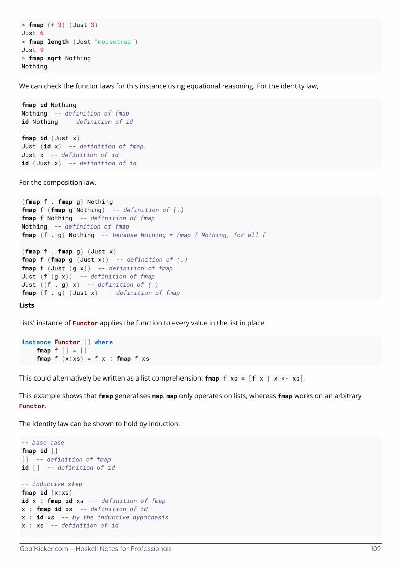
GoalKicker.com – Haskell Notes for Professionals 109

> fmap (+ 3) (Just 3)Just 6> fmap length (Just "mousetrap")Just 9> fmap sqrt NothingNothing

We can check the functor laws for this instance using equational reasoning. For the identity law,

fmap id NothingNothing -- definition of fmapid Nothing -- definition of id

fmap id (Just x)Just (id x) -- definition of fmapJust x -- definition of idid (Just x) -- definition of id

For the composition law,

(fmap f . fmap g) Nothingfmap f (fmap g Nothing) -- definition of (.)fmap f Nothing -- definition of fmapNothing -- definition of fmapfmap (f . g) Nothing -- because Nothing = fmap f Nothing, for all f

(fmap f . fmap g) (Just x)fmap f (fmap g (Just x)) -- definition of (.)fmap f (Just (g x)) -- definition of fmapJust (f (g x)) -- definition of fmapJust ((f . g) x) -- definition of (.)fmap (f . g) (Just x) -- definition of fmap

Lists

Lists' instance of Functor applies the function to every value in the list in place.

instance Functor [] where fmap f [] = [] fmap f (x:xs) = f x : fmap f xs

This could alternatively be written as a list comprehension: fmap f xs = [f x | x <- xs].

This example shows that fmap generalises map. map only operates on lists, whereas fmap works on an arbitraryFunctor.

The identity law can be shown to hold by induction:

-- base casefmap id [][] -- definition of fmapid [] -- definition of id

-- inductive stepfmap id (x:xs)id x : fmap id xs -- definition of fmapx : fmap id xs -- definition of idx : id xs -- by the inductive hypothesisx : xs -- definition of id

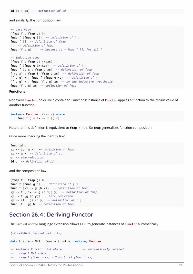
GoalKicker.com – Haskell Notes for Professionals 110

id (x : xs) -- definition of id

and similarly, the composition law:

-- base case(fmap f . fmap g) []fmap f (fmap g []) -- definition of (.)fmap f [] -- definition of fmap[] -- definition of fmapfmap (f . g) [] -- because [] = fmap f [], for all f

-- inductive step(fmap f . fmap g) (x:xs)fmap f (fmap g (x:xs)) -- definition of (.)fmap f (g x : fmap g xs) -- definition of fmapf (g x) : fmap f (fmap g xs) -- definition of fmap(f . g) x : fmap f (fmap g xs) -- definition of (.)(f . g) x : fmap (f . g) xs -- by the inductive hypothesisfmap (f . g) xs -- definition of fmap

Functions

Not every Functor looks like a container. Functions' instance of Functor applies a function to the return value ofanother function.

instance Functor ((->) r) where fmap f g = \x -> f (g x)

Note that this definition is equivalent to fmap = (.). So fmap generalises function composition.

Once more checking the identity law:

fmap id g\x -> id (g x) -- definition of fmap\x -> g x -- definition of idg -- eta-reductionid g -- definition of id

and the composition law:

(fmap f . fmap g) hfmap f (fmap g h) -- definition of (.)fmap f (\x -> g (h x)) -- definition of fmap\y -> f ((\x -> g (h x)) y) -- definition of fmap\y -> f (g (h y)) -- beta-reduction\y -> (f . g) (h y) -- definition of (.)fmap (f . g) h -- definition of fmap

Section 26.4: Deriving FunctorThe DeriveFunctor language extension allows GHC to generate instances of Functor automatically.

{-# LANGUAGE DeriveFunctor #-}

data List a = Nil | Cons a (List a) deriving Functor

-- instance Functor List where -- automatically defined-- fmap f Nil = Nil-- fmap f (Cons x xs) = Cons (f x) (fmap f xs)

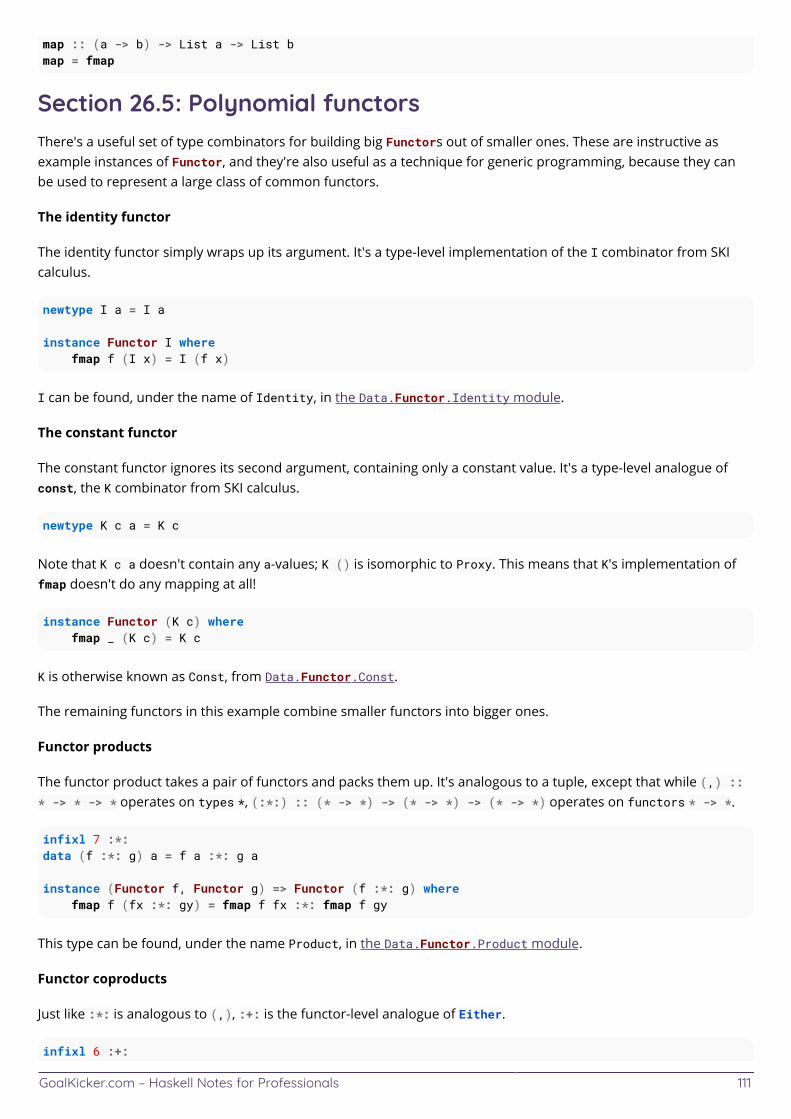
GoalKicker.com – Haskell Notes for Professionals 111

map :: (a -> b) -> List a -> List bmap = fmap

Section 26.5: Polynomial functorsThere's a useful set of type combinators for building big Functors out of smaller ones. These are instructive asexample instances of Functor, and they're also useful as a technique for generic programming, because they canbe used to represent a large class of common functors.

The identity functor

The identity functor simply wraps up its argument. It's a type-level implementation of the I combinator from SKIcalculus.

newtype I a = I a

instance Functor I where fmap f (I x) = I (f x)

I can be found, under the name of Identity, in the Data.Functor.Identity module.

The constant functor

The constant functor ignores its second argument, containing only a constant value. It's a type-level analogue ofconst, the K combinator from SKI calculus.

newtype K c a = K c

Note that K c a doesn't contain any a-values; K () is isomorphic to Proxy. This means that K's implementation offmap doesn't do any mapping at all!

instance Functor (K c) where fmap _ (K c) = K c

K is otherwise known as Const, from Data.Functor.Const.

The remaining functors in this example combine smaller functors into bigger ones.

Functor products

The functor product takes a pair of functors and packs them up. It's analogous to a tuple, except that while (,) ::* -> * -> * operates on types *, (:*:) :: (* -> *) -> (* -> *) -> (* -> *) operates on functors * -> *.

infixl 7 :*:data (f :*: g) a = f a :*: g a

instance (Functor f, Functor g) => Functor (f :*: g) where fmap f (fx :*: gy) = fmap f fx :*: fmap f gy

This type can be found, under the name Product, in the Data.Functor.Product module.

Functor coproducts

Just like :*: is analogous to (,), :+: is the functor-level analogue of Either.

infixl 6 :+:

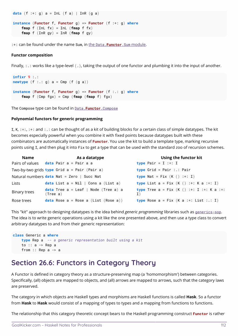
GoalKicker.com – Haskell Notes for Professionals 112

data (f :+: g) a = InL (f a) | InR (g a)

instance (Functor f, Functor g) => Functor (f :+: g) where fmap f (InL fx) = InL (fmap f fx) fmap f (InR gy) = InR (fmap f gy)

:+: can be found under the name Sum, in the Data.Functor.Sum module.

Functor composition

Finally, :.: works like a type-level (.), taking the output of one functor and plumbing it into the input of another.

infixr 9 :.:newtype (f :.: g) a = Cmp (f (g a))

instance (Functor f, Functor g) => Functor (f :.: g) where fmap f (Cmp fgx) = Cmp (fmap (fmap f) fgx)

The Compose type can be found in Data.Functor.Compose

Polynomial functors for generic programming

I, K, :*:, :+: and :.: can be thought of as a kit of building blocks for a certain class of simple datatypes. The kitbecomes especially powerful when you combine it with fixed points because datatypes built with thesecombinators are automatically instances of Functor. You use the kit to build a template type, marking recursivepoints using I, and then plug it into Fix to get a type that can be used with the standard zoo of recursion schemes.

Name As a datatype Using the functor kitPairs of values data Pair a = Pair a a type Pair = I :*: I

Two-by-two grids type Grid a = Pair (Pair a) type Grid = Pair :.: Pair

Natural numbers data Nat = Zero | Succ Nat type Nat = Fix (K () :+: I)

Lists data List a = Nil | Cons a (List a) type List a = Fix (K () :+: K a :*: I)

Binary trees data Tree a = Leaf | Node (Tree a) a(Tree a)

type Tree a = Fix (K () :+: I :*: K a :*:I)

Rose trees data Rose a = Rose a (List (Rose a)) type Rose a = Fix (K a :*: List :.: I)

This "kit" approach to designing datatypes is the idea behind generic programming libraries such as generics-sop.The idea is to write generic operations using a kit like the one presented above, and then use a type class to convertarbitrary datatypes to and from their generic representation:

class Generic a where type Rep a -- a generic representation built using a kit to :: a -> Rep a from :: Rep a -> a

Section 26.6: Functors in Category TheoryA Functor is defined in category theory as a structure-preserving map (a 'homomorphism') between categories.Specifically, (all) objects are mapped to objects, and (all) arrows are mapped to arrows, such that the category lawsare preserved.

The category in which objects are Haskell types and morphisms are Haskell functions is called Hask. So a functorfrom Hask to Hask would consist of a mapping of types to types and a mapping from functions to functions.

The relationship that this category theoretic concept bears to the Haskell programming construct Functor is rather

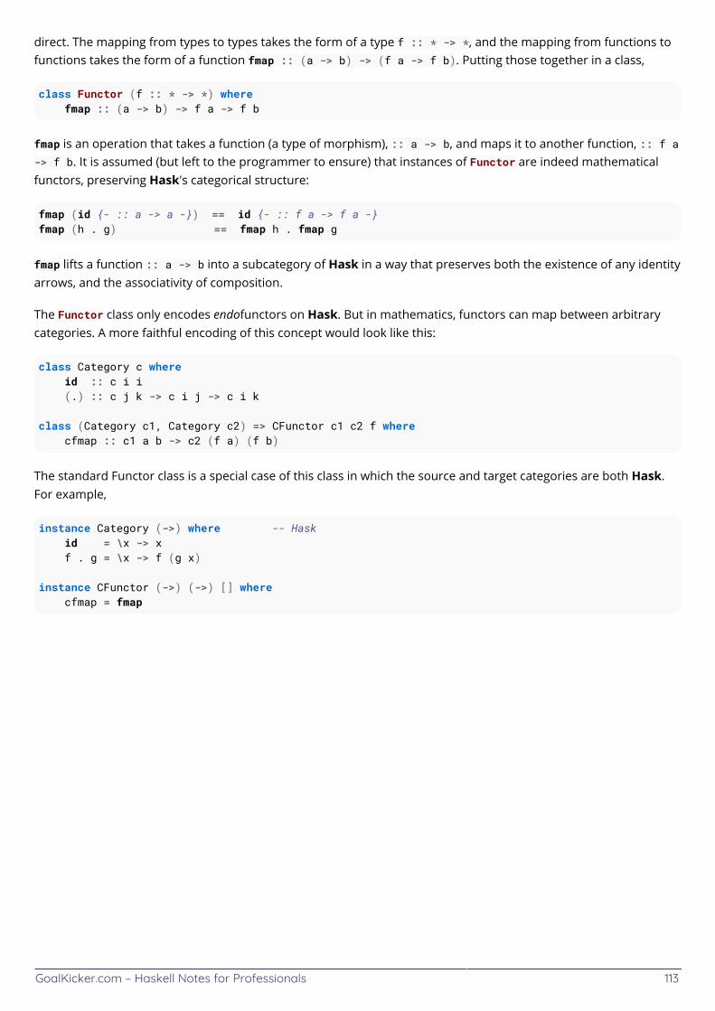
GoalKicker.com – Haskell Notes for Professionals 113

direct. The mapping from types to types takes the form of a type f :: * -> *, and the mapping from functions tofunctions takes the form of a function fmap :: (a -> b) -> (f a -> f b). Putting those together in a class,

class Functor (f :: * -> *) where fmap :: (a -> b) -> f a -> f b

fmap is an operation that takes a function (a type of morphism), :: a -> b, and maps it to another function, :: f a-> f b. It is assumed (but left to the programmer to ensure) that instances of Functor are indeed mathematicalfunctors, preserving Hask's categorical structure:

fmap (id {- :: a -> a -}) == id {- :: f a -> f a -}fmap (h . g) == fmap h . fmap g

fmap lifts a function :: a -> b into a subcategory of Hask in a way that preserves both the existence of any identityarrows, and the associativity of composition.

The Functor class only encodes endofunctors on Hask. But in mathematics, functors can map between arbitrarycategories. A more faithful encoding of this concept would look like this:

class Category c where id :: c i i (.) :: c j k -> c i j -> c i k

class (Category c1, Category c2) => CFunctor c1 c2 f where cfmap :: c1 a b -> c2 (f a) (f b)

The standard Functor class is a special case of this class in which the source and target categories are both Hask.For example,

instance Category (->) where -- Hask id = \x -> x f . g = \x -> f (g x)

instance CFunctor (->) (->) [] where cfmap = fmap

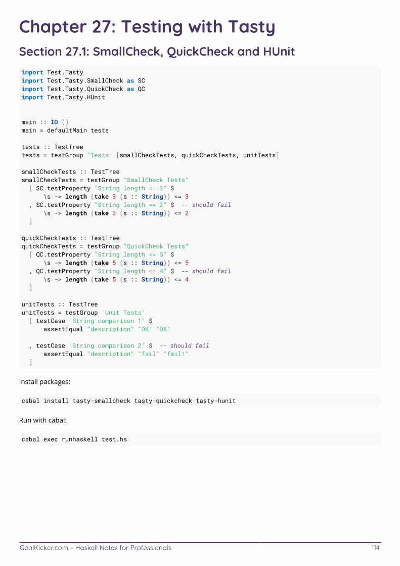
GoalKicker.com – Haskell Notes for Professionals 114

Chapter 27: Testing with TastySection 27.1: SmallCheck, QuickCheck and HUnitimport Test.Tastyimport Test.Tasty.SmallCheck as SCimport Test.Tasty.QuickCheck as QCimport Test.Tasty.HUnit

main :: IO ()main = defaultMain tests

tests :: TestTreetests = testGroup "Tests" [smallCheckTests, quickCheckTests, unitTests]

smallCheckTests :: TestTreesmallCheckTests = testGroup "SmallCheck Tests" [ SC.testProperty "String length <= 3" $ \s -> length (take 3 (s :: String)) <= 3 , SC.testProperty "String length <= 2" $ -- should fail \s -> length (take 3 (s :: String)) <= 2 ]

quickCheckTests :: TestTreequickCheckTests = testGroup "QuickCheck Tests" [ QC.testProperty "String length <= 5" $ \s -> length (take 5 (s :: String)) <= 5 , QC.testProperty "String length <= 4" $ -- should fail \s -> length (take 5 (s :: String)) <= 4 ]

unitTests :: TestTreeunitTests = testGroup "Unit Tests" [ testCase "String comparison 1" $ assertEqual "description" "OK" "OK"

, testCase "String comparison 2" $ -- should fail assertEqual "description" "fail" "fail!" ]

Install packages:

cabal install tasty-smallcheck tasty-quickcheck tasty-hunit

Run with cabal:

cabal exec runhaskell test.hs

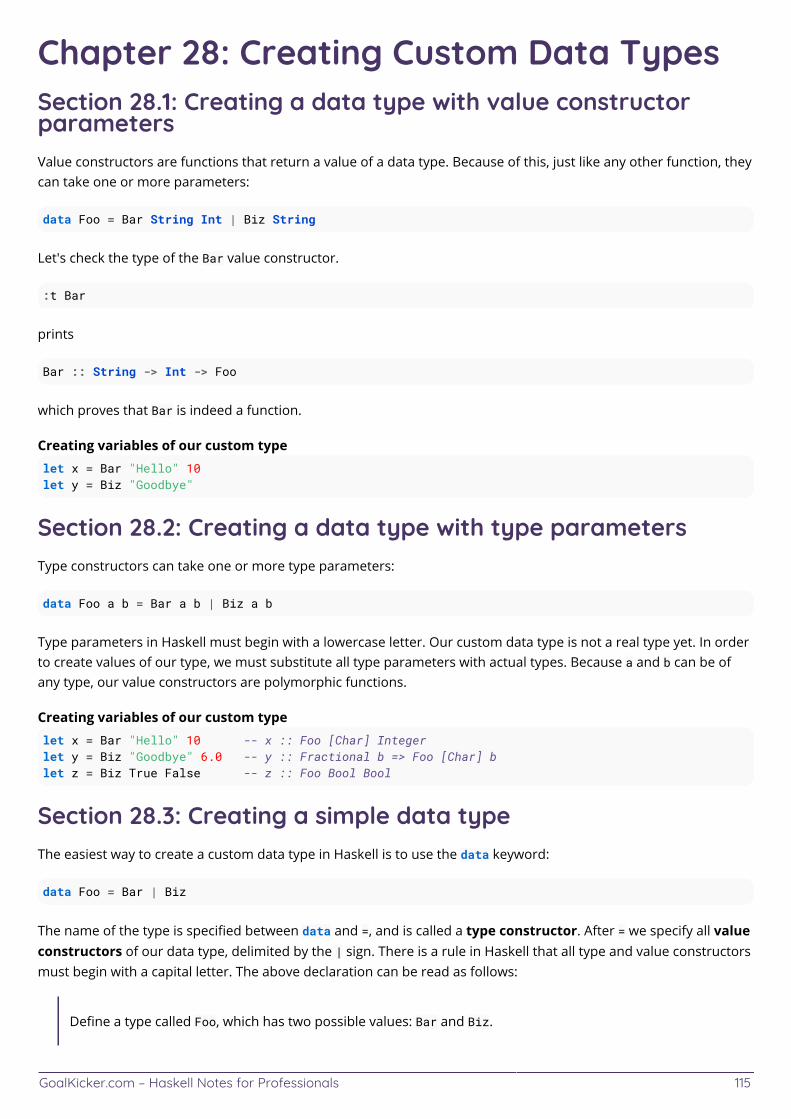
GoalKicker.com – Haskell Notes for Professionals 115

Chapter 28: Creating Custom Data TypesSection 28.1: Creating a data type with value constructorparametersValue constructors are functions that return a value of a data type. Because of this, just like any other function, theycan take one or more parameters:

data Foo = Bar String Int | Biz String

Let's check the type of the Bar value constructor.

:t Bar

prints

Bar :: String -> Int -> Foo

which proves that Bar is indeed a function.

Creating variables of our custom typelet x = Bar "Hello" 10let y = Biz "Goodbye"

Section 28.2: Creating a data type with type parametersType constructors can take one or more type parameters:

data Foo a b = Bar a b | Biz a b

Type parameters in Haskell must begin with a lowercase letter. Our custom data type is not a real type yet. In orderto create values of our type, we must substitute all type parameters with actual types. Because a and b can be ofany type, our value constructors are polymorphic functions.

Creating variables of our custom typelet x = Bar "Hello" 10 -- x :: Foo [Char] Integerlet y = Biz "Goodbye" 6.0 -- y :: Fractional b => Foo [Char] blet z = Biz True False -- z :: Foo Bool Bool

Section 28.3: Creating a simple data typeThe easiest way to create a custom data type in Haskell is to use the data keyword:

data Foo = Bar | Biz

The name of the type is specified between data and =, and is called a type constructor. After = we specify all valueconstructors of our data type, delimited by the | sign. There is a rule in Haskell that all type and value constructorsmust begin with a capital letter. The above declaration can be read as follows:

Define a type called Foo, which has two possible values: Bar and Biz.

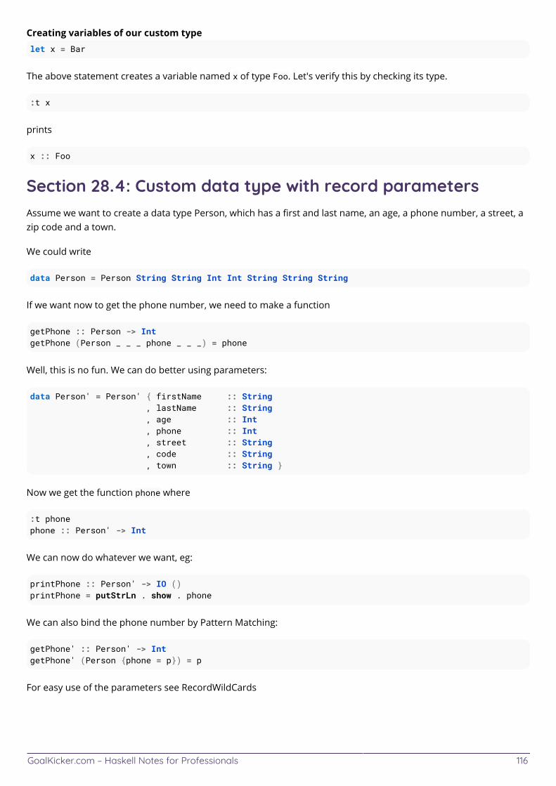
GoalKicker.com – Haskell Notes for Professionals 116

Creating variables of our custom typelet x = Bar

The above statement creates a variable named x of type Foo. Let's verify this by checking its type.

:t x

prints

x :: Foo

Section 28.4: Custom data type with record parametersAssume we want to create a data type Person, which has a first and last name, an age, a phone number, a street, azip code and a town.

We could write

data Person = Person String String Int Int String String String

If we want now to get the phone number, we need to make a function

getPhone :: Person -> IntgetPhone (Person _ _ _ phone _ _ _) = phone

Well, this is no fun. We can do better using parameters:

data Person' = Person' { firstName :: String , lastName :: String , age :: Int , phone :: Int , street :: String , code :: String , town :: String }

Now we get the function phone where

:t phonephone :: Person' -> Int

We can now do whatever we want, eg:

printPhone :: Person' -> IO ()printPhone = putStrLn . show . phone

We can also bind the phone number by Pattern Matching:

getPhone' :: Person' -> IntgetPhone' (Person {phone = p}) = p

For easy use of the parameters see RecordWildCards

GoalKicker.com – Haskell Notes for Professionals 117

Chapter 29: Reactive-bananaSection 29.1: Injecting external events into the libraryThis example is not tied to any concrete GUI toolkit, like reactive-banana-wx does, for instance. Instead it showshow to inject arbitrary IO actions into FRP machinery.

The Control.Event.Handler module provides an addHandler function which creates a pair of AddHandler a and a-> IO () values. The former is used by reactive-banana itself to obtain an Event a value, while the latter is a plainfunction that is used to trigger the corresponding event.

import Data.Char (toUpper) import Control.Event.Handler import Reactive.Banana main = do (inputHandler,inputFire) <- newAddHandler

In our case the a parameter of the handler is of type String, but the code that lets compiler infer that will bewritten later.

Now we define the EventNetwork that describes our FRP-driven system. This is done using compile function:

main = do (inputHandler, inputFire) <- newAddHandler compile $ do inputEvent <- fromAddHandler inputHandler

The fromAddHandler function transforms AddHandler a value into a Event a, which is covered in the next example.

Finally, we launch our "event loop", that would fire events on user input:

main = do (inputHandler, inputFire) <- newAddHandler compile $ do ... forever $ do input <- getLine inputFire input

Section 29.2: Event typeIn reactive-banana the Event type represents a stream of some events in time. An Event is similar to an analogimpulse signal in the sense that it is not continuous in time. As a result, Event is an instance of the Functortypeclass only. You can't combine two Events together because they may fire at different times. You can dosomething with an Event's [current] value and react to it with some IO action.

Transformations on Events value are done using fmap:

main = do (inputHandler, inputFire) <- newAddHandler compile $ do inputEvent <- fromAddHandler inputHandler --turn all characters in the signal to upper case let inputEvent' = fmap (map toUpper) inputEvent

Reacting to an Event is done the same way. First you fmap it with an action of type a -> IO () and then pass it toreactimate function:

main = do (inputHandler, inputFire) <- newAddHandler compile $ do inputEvent <- fromAddHandler inputHandler --turn all characters in the signal to upper case let inputEvent' = fmap (map toUpper) inputEvent letinputEventReaction = fmap putStrLn inputEvent' -- this has type `Event (IO ()) reactimate inputEventReaction

Now whenever inputFire "something" is called, "SOMETHING" would be printed.

Section 29.3: Actuating EventNetworksEventNetworks returned by compile must be actuated before reactimated events have an effect.

main = do (inputHandler, inputFire) <- newAddHandler

GoalKicker.com – Haskell Notes for Professionals 118

eventNetwork <- compile $ do inputEvent <- fromAddHandler inputHandler let inputEventReaction = fmap putStrLn inputEvent reactimate inputEventReaction

inputFire "This will NOT be printed to the console!" actuate eventNetwork inputFire "This WILL be printed to the console!"

Section 29.4: Behavior typeTo represent continious signals, reactive-banana features Behavior a type. Unlike Event, a Behavior is anApplicative, which lets you combine n Behaviors using an n-ary pure function (using <$> and <*>).

To obtain a Behavior a from the Event a there is accumE function:

main = do (inputHandler, inputFire) <- newAddHandler compile $ do ... inputBehavior <- accumE "" $ fmap (\oldValue newValue -> newValue) inputEvent

accumE takes Behavior's initial value and an Event, containing a function that would set it to the new value.

As with Events, you can use fmap to work with current Behaviors value, but you can also combine them with (<*>).

main = do (inputHandler, inputFire) <- newAddHandler compile $ do ... inputBehavior <- accumE "" $ fmap (\oldValue newValue -> newValue) inputEvent inputBehavior' <- accumE "" $ fmap (\oldValue newValue -> newValue) inputEvent let constantTrueBehavior = (==) <$> inputBehavior <*> inputBehavior'

To react on Behavior changes there is a changes function:

main = do (inputHandler, inputFire) <- newAddHandler compile $ do ... inputBehavior <- accumE "" $ fmap (\oldValue newValue -> newValue) inputEvent inputBehavior' <- accumE "" $ fmap (\oldValue newValue -> newValue) inputEvent let constantTrueBehavior = (==) <$> inputBehavior <*> inputBehavior' inputChanged <- changes inputBehavior

The only thing that should be noted is that changes return Event (Future a) instead of Event a. Because of this,reactimate' should be used instead of reactimate. The rationale behind this can be obtained from thedocumentation.

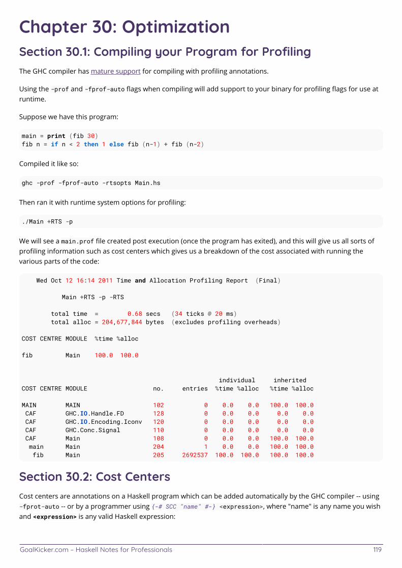
GoalKicker.com – Haskell Notes for Professionals 119

Chapter 30: OptimizationSection 30.1: Compiling your Program for ProfilingThe GHC compiler has mature support for compiling with profiling annotations.

Using the -prof and -fprof-auto flags when compiling will add support to your binary for profiling flags for use atruntime.

Suppose we have this program:

main = print (fib 30)fib n = if n < 2 then 1 else fib (n-1) + fib (n-2)

Compiled it like so:

ghc -prof -fprof-auto -rtsopts Main.hs

Then ran it with runtime system options for profiling:

./Main +RTS -p

We will see a main.prof file created post execution (once the program has exited), and this will give us all sorts ofprofiling information such as cost centers which gives us a breakdown of the cost associated with running thevarious parts of the code:

Wed Oct 12 16:14 2011 Time and Allocation Profiling Report (Final)

Main +RTS -p -RTS

total time = 0.68 secs (34 ticks @ 20 ms) total alloc = 204,677,844 bytes (excludes profiling overheads)

COST CENTRE MODULE %time %alloc

fib Main 100.0 100.0

individual inheritedCOST CENTRE MODULE no. entries %time %alloc %time %alloc

MAIN MAIN 102 0 0.0 0.0 100.0 100.0 CAF GHC.IO.Handle.FD 128 0 0.0 0.0 0.0 0.0 CAF GHC.IO.Encoding.Iconv 120 0 0.0 0.0 0.0 0.0 CAF GHC.Conc.Signal 110 0 0.0 0.0 0.0 0.0 CAF Main 108 0 0.0 0.0 100.0 100.0 main Main 204 1 0.0 0.0 100.0 100.0 fib Main 205 2692537 100.0 100.0 100.0 100.0

Section 30.2: Cost CentersCost centers are annotations on a Haskell program which can be added automatically by the GHC compiler -- using-fprot-auto -- or by a programmer using {-# SCC "name" #-} <expression>, where "name" is any name you wishand <expression> is any valid Haskell expression:

GoalKicker.com – Haskell Notes for Professionals 120

-- Main.hsmain :: IO ()main = do let l = [1..9999999] print $ {-# SCC "print_list" #-} (length l)

Compiling with -fprof and running with +RTS -p e.g. ghc -prof -rtsopts Main.hs && ./Main.hs +RTS -p wouldproduce Main.prof once the program's exited.

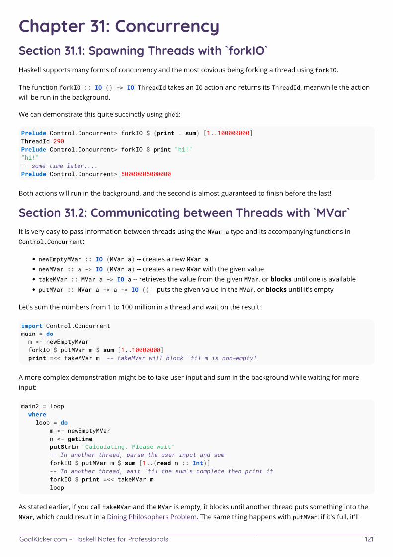
GoalKicker.com – Haskell Notes for Professionals 121

Chapter 31: ConcurrencySection 31.1: Spawning Threads with `forkIO`Haskell supports many forms of concurrency and the most obvious being forking a thread using forkIO.

The function forkIO :: IO () -> IO ThreadId takes an IO action and returns its ThreadId, meanwhile the actionwill be run in the background.

We can demonstrate this quite succinctly using ghci:

Prelude Control.Concurrent> forkIO $ (print . sum) [1..100000000]ThreadId 290Prelude Control.Concurrent> forkIO $ print "hi!""hi!"-- some time later....Prelude Control.Concurrent> 50000005000000

Both actions will run in the background, and the second is almost guaranteed to finish before the last!

Section 31.2: Communicating between Threads with `MVar`It is very easy to pass information between threads using the MVar a type and its accompanying functions inControl.Concurrent:

newEmptyMVar :: IO (MVar a) -- creates a new MVar anewMVar :: a -> IO (MVar a) -- creates a new MVar with the given valuetakeMVar :: MVar a -> IO a -- retrieves the value from the given MVar, or blocks until one is availableputMVar :: MVar a -> a -> IO () -- puts the given value in the MVar, or blocks until it's empty

Let's sum the numbers from 1 to 100 million in a thread and wait on the result:

import Control.Concurrentmain = do m <- newEmptyMVar forkIO $ putMVar m $ sum [1..10000000] print =<< takeMVar m -- takeMVar will block 'til m is non-empty!

A more complex demonstration might be to take user input and sum in the background while waiting for moreinput:

main2 = loop where loop = do m <- newEmptyMVar n <- getLine putStrLn "Calculating. Please wait" -- In another thread, parse the user input and sum forkIO $ putMVar m $ sum [1..(read n :: Int)] -- In another thread, wait 'til the sum's complete then print it forkIO $ print =<< takeMVar m loop

As stated earlier, if you call takeMVar and the MVar is empty, it blocks until another thread puts something into theMVar, which could result in a Dining Philosophers Problem. The same thing happens with putMVar: if it's full, it'll

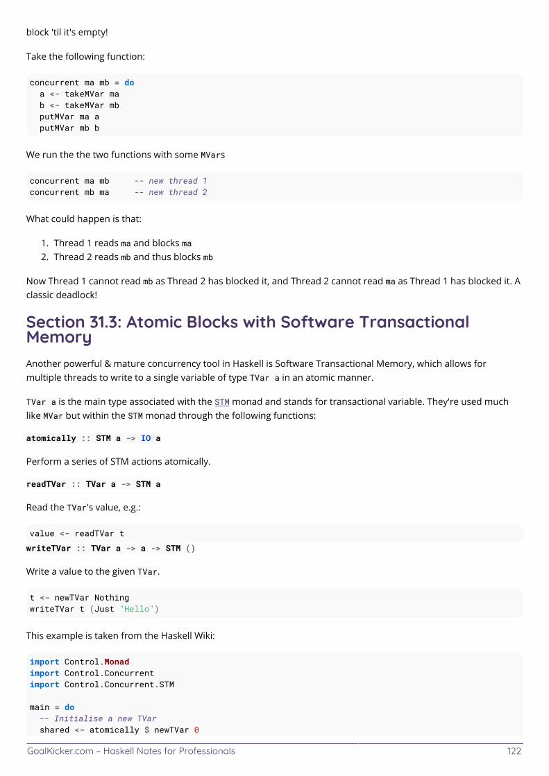
GoalKicker.com – Haskell Notes for Professionals 122

block 'til it's empty!

Take the following function:

concurrent ma mb = do a <- takeMVar ma b <- takeMVar mb putMVar ma a putMVar mb b

We run the the two functions with some MVars

concurrent ma mb -- new thread 1concurrent mb ma -- new thread 2

What could happen is that:

Thread 1 reads ma and blocks ma1.Thread 2 reads mb and thus blocks mb2.

Now Thread 1 cannot read mb as Thread 2 has blocked it, and Thread 2 cannot read ma as Thread 1 has blocked it. Aclassic deadlock!

Section 31.3: Atomic Blocks with Software TransactionalMemoryAnother powerful & mature concurrency tool in Haskell is Software Transactional Memory, which allows formultiple threads to write to a single variable of type TVar a in an atomic manner.

TVar a is the main type associated with the STM monad and stands for transactional variable. They're used muchlike MVar but within the STM monad through the following functions:

atomically :: STM a -> IO a

Perform a series of STM actions atomically.

readTVar :: TVar a -> STM a

Read the TVar's value, e.g.:

value <- readTVar t

writeTVar :: TVar a -> a -> STM ()

Write a value to the given TVar.

t <- newTVar NothingwriteTVar t (Just "Hello")

This example is taken from the Haskell Wiki:

import Control.Monadimport Control.Concurrentimport Control.Concurrent.STM main = do -- Initialise a new TVar shared <- atomically $ newTVar 0

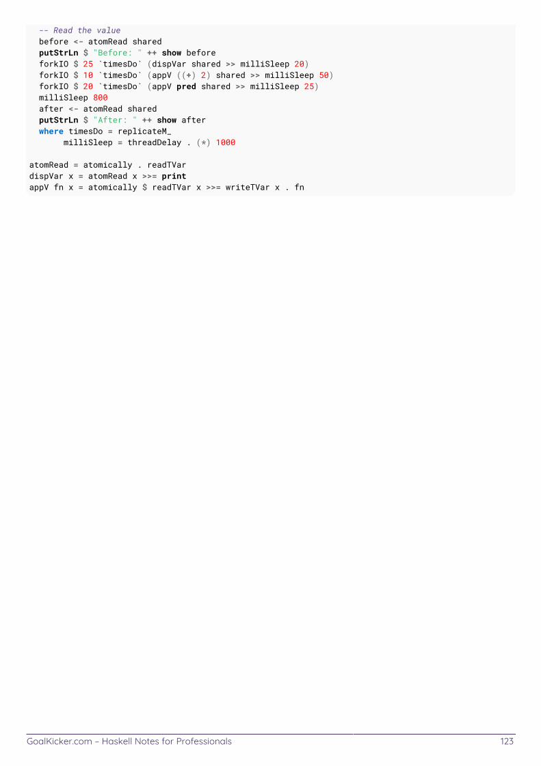
GoalKicker.com – Haskell Notes for Professionals 123

-- Read the value before <- atomRead shared putStrLn $ "Before: " ++ show before forkIO $ 25 `timesDo` (dispVar shared >> milliSleep 20) forkIO $ 10 `timesDo` (appV ((+) 2) shared >> milliSleep 50) forkIO $ 20 `timesDo` (appV pred shared >> milliSleep 25) milliSleep 800 after <- atomRead shared putStrLn $ "After: " ++ show after where timesDo = replicateM_ milliSleep = threadDelay . (*) 1000

atomRead = atomically . readTVardispVar x = atomRead x >>= printappV fn x = atomically $ readTVar x >>= writeTVar x . fn

GoalKicker.com – Haskell Notes for Professionals 124

Chapter 32: Function compositionSection 32.1: Right-to-left composition(.) lets us compose two functions, feeding output of one as an input to the other:

(f . g) x = f (g x)

For example, if we want to square the successor of an input number, we can write

((^2) . succ) 1 -- 4

There is also (<<<) which is an alias to (.). So,

(+ 1) <<< sqrt $ 25 -- 6

Section 32.2: Composition with binary functionThe regular composition works for unary functions. In the case of binary, we can define

(f .: g) x y = f (g x y) -- which is also = f ((g x) y) = (f . g x) y -- by definition of (.) = (f .) (g x) y = ((f .) . g) x y

Thus, (f .: g) = ((f .) . g) by eta-contraction, and furthermore,

(.:) f g = ((f .) . g) = (.) (f .) g = (.) ((.) f) g = ((.) . (.)) f g

so (.:) = ((.) . (.)), a semi-famous definition.

Examples:

(map (+1) .: filter) even [1..5] -- [3,5](length .: filter) even [1..5] -- 2

Section 32.3: Left-to-right compositionControl.Category defines (>>>), which, when specialized to functions, is

-- (>>>) :: Category cat => cat a b -> cat b c -> cat a c -- (>>>) :: (->) a b -> (->) b c -> (->) a c-- (>>>) :: (a -> b) -> (b -> c) -> (a -> c)( f >>> g ) x = g (f x)

Example:

sqrt >>> (+ 1) $ 25 -- 6.0

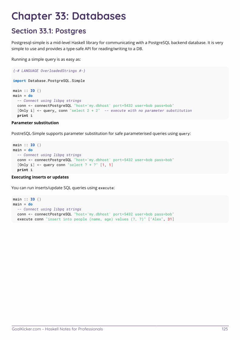
GoalKicker.com – Haskell Notes for Professionals 125

Chapter 33: DatabasesSection 33.1: PostgresPostgresql-simple is a mid-level Haskell library for communicating with a PostgreSQL backend database. It is verysimple to use and provides a type-safe API for reading/writing to a DB.

Running a simple query is as easy as:

{-# LANGUAGE OverloadedStrings #-}

import Database.PostgreSQL.Simple

main :: IO ()main = do -- Connect using libpq strings conn <- connectPostgreSQL "host='my.dbhost' port=5432 user=bob pass=bob" [Only i] <- query_ conn "select 2 + 2" -- execute with no parameter substitution print i

Parameter substitution

PostreSQL-Simple supports parameter substitution for safe parameterised queries using query:

main :: IO ()main = do -- Connect using libpq strings conn <- connectPostgreSQL "host='my.dbhost' port=5432 user=bob pass=bob" [Only i] <- query conn "select ? + ?" [1, 1] print i

Executing inserts or updates

You can run inserts/update SQL queries using execute:

main :: IO ()main = do -- Connect using libpq strings conn <- connectPostgreSQL "host='my.dbhost' port=5432 user=bob pass=bob" execute conn "insert into people (name, age) values (?, ?)" ["Alex", 31]

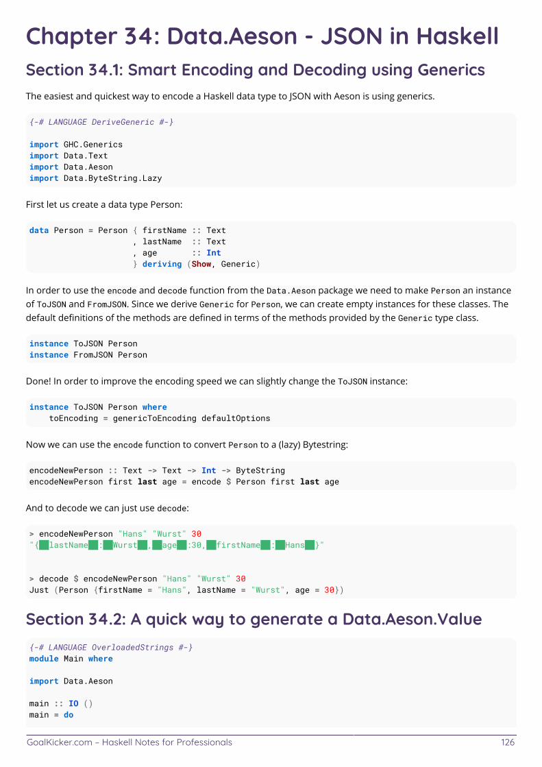
GoalKicker.com – Haskell Notes for Professionals 126

Chapter 34: Data.Aeson - JSON in HaskellSection 34.1: Smart Encoding and Decoding using GenericsThe easiest and quickest way to encode a Haskell data type to JSON with Aeson is using generics.

{-# LANGUAGE DeriveGeneric #-}

import GHC.Genericsimport Data.Textimport Data.Aesonimport Data.ByteString.Lazy

First let us create a data type Person:

data Person = Person { firstName :: Text , lastName :: Text , age :: Int } deriving (Show, Generic)

In order to use the encode and decode function from the Data.Aeson package we need to make Person an instanceof ToJSON and FromJSON. Since we derive Generic for Person, we can create empty instances for these classes. Thedefault definitions of the methods are defined in terms of the methods provided by the Generic type class.

instance ToJSON Personinstance FromJSON Person

Done! In order to improve the encoding speed we can slightly change the ToJSON instance:

instance ToJSON Person where toEncoding = genericToEncoding defaultOptions

Now we can use the encode function to convert Person to a (lazy) Bytestring:

encodeNewPerson :: Text -> Text -> Int -> ByteStringencodeNewPerson first last age = encode $ Person first last age

And to decode we can just use decode:

> encodeNewPerson "Hans" "Wurst" 30"{\"lastName\":\"Wurst\",\"age\":30,\"firstName\":\"Hans\"}"

> decode $ encodeNewPerson "Hans" "Wurst" 30Just (Person {firstName = "Hans", lastName = "Wurst", age = 30})

Section 34.2: A quick way to generate a Data.Aeson.Value{-# LANGUAGE OverloadedStrings #-}module Main where

import Data.Aeson

main :: IO ()main = do

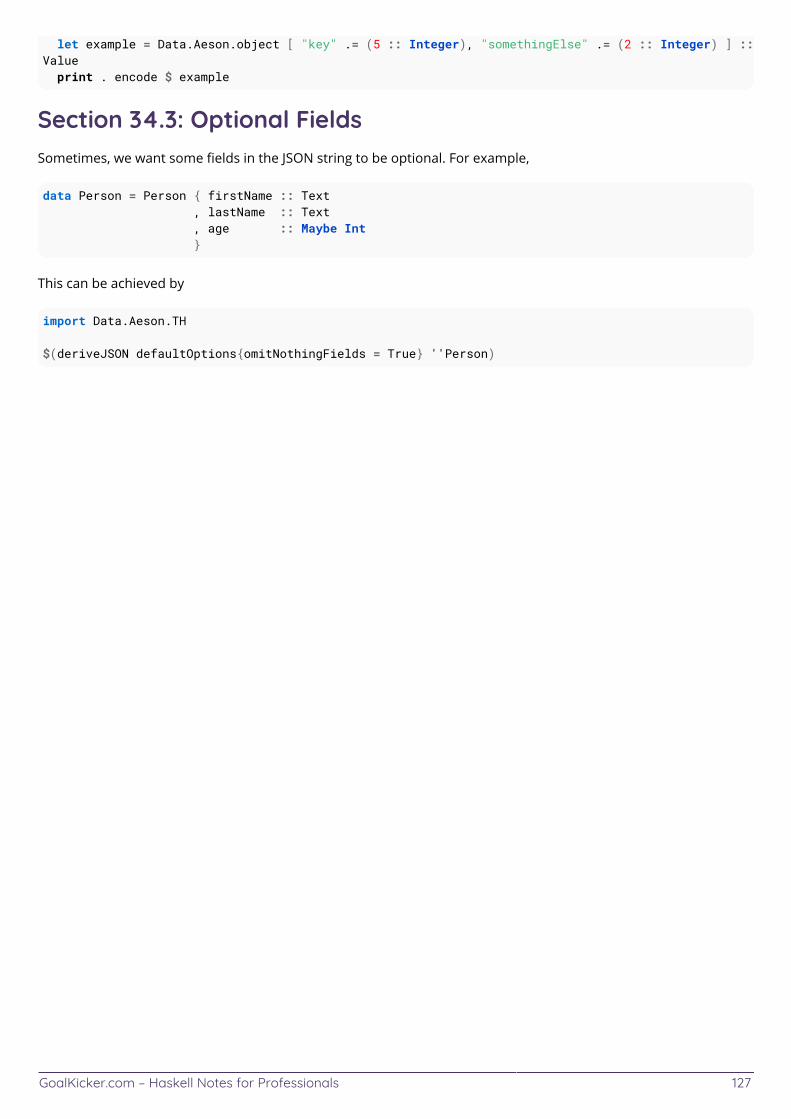
GoalKicker.com – Haskell Notes for Professionals 127

let example = Data.Aeson.object [ "key" .= (5 :: Integer), "somethingElse" .= (2 :: Integer) ] ::Value print . encode $ example

Section 34.3: Optional FieldsSometimes, we want some fields in the JSON string to be optional. For example,

data Person = Person { firstName :: Text , lastName :: Text , age :: Maybe Int }

This can be achieved by

import Data.Aeson.TH

$(deriveJSON defaultOptions{omitNothingFields = True} ''Person)

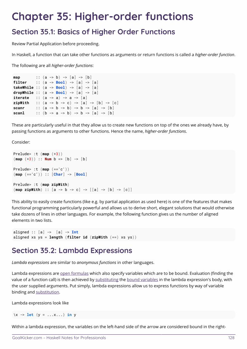
GoalKicker.com – Haskell Notes for Professionals 128

Chapter 35: Higher-order functionsSection 35.1: Basics of Higher Order FunctionsReview Partial Application before proceeding.

In Haskell, a function that can take other functions as arguments or return functions is called a higher-order function.

The following are all higher-order functions:

map :: (a -> b) -> [a] -> [b]filter :: (a -> Bool) -> [a] -> [a]takeWhile :: (a -> Bool) -> [a] -> [a]dropWhile :: (a -> Bool) -> [a] -> [a]iterate :: (a -> a) -> a -> [a]zipWith :: (a -> b -> c) -> [a] -> [b] -> [c]scanr :: (a -> b -> b) -> b -> [a] -> [b]scanl :: (b -> a -> b) -> b -> [a] -> [b]

These are particularly useful in that they allow us to create new functions on top of the ones we already have, bypassing functions as arguments to other functions. Hence the name, higher-order functions.

Consider:

Prelude> :t (map (+3))(map (+3)) :: Num b => [b] -> [b]

Prelude> :t (map (=='c'))(map (=='c')) :: [Char] -> [Bool]

Prelude> :t (map zipWith)(map zipWith) :: [a -> b -> c] -> [[a] -> [b] -> [c]]

This ability to easily create functions (like e.g. by partial application as used here) is one of the features that makesfunctional programming particularly powerful and allows us to derive short, elegant solutions that would otherwisetake dozens of lines in other languages. For example, the following function gives us the number of alignedelements in two lists.

aligned :: [a] -> [a] -> Intaligned xs ys = length (filter id (zipWith (==) xs ys))

Section 35.2: Lambda ExpressionsLambda expressions are similar to anonymous functions in other languages.

Lambda expressions are open formulas which also specify variables which are to be bound. Evaluation (finding thevalue of a function call) is then achieved by substituting the bound variables in the lambda expression's body, withthe user supplied arguments. Put simply, lambda expressions allow us to express functions by way of variablebinding and substitution.

Lambda expressions look like

\x -> let {y = ...x...} in y

Within a lambda expression, the variables on the left-hand side of the arrow are considered bound in the right-

GoalKicker.com – Haskell Notes for Professionals 129

hand side, i.e. the function's body.

Consider the mathematical function

f(x) = x^2

As a Haskell definition it is

f x = x^2

f = \x -> x^2

which means that the function f is equivalent to the lambda expression \x -> x^2.

Consider the parameter of the higher-order function map, that is a function of type a -> b. In case it is used onlyonce in a call to map and nowhere else in the program, it is convenient to specify it as a lambda expression insteadof naming such a throwaway function. Written as a lambda expression,

\x -> let {y = ...x...} in y

x holds a value of type a, ...x... is a Haskell expression that refers to the variable x, and y holds a value of type b.So, for example, we could write the following

map (\x -> x + 3)

map (\(x,y) -> x * y)

map (\xs -> 'c':xs) ["apples", "oranges", "mangos"]

map (\f -> zipWith f [1..5] [1..5]) [(+), (*), (-)]

Section 35.3: CurryingIn Haskell, all functions are considered curried: that is, all functions in Haskell take just one argument.

Let's take the function div:

div :: Int -> Int -> Int

If we call this function with 6 and 2 we unsurprisingly get 3:

Prelude> div 6 2 3

However, this doesn't quite behave in the way we might think. First div 6 is evaluated and returns a function oftype Int -> Int. This resulting function is then applied to the value 2 which yields 3.

When we look at the type signature of a function, we can shift our thinking from "takes two arguments of type Int"to "takes one Int and returns a function that takes an Int". This is reaffirmed if we consider that arrows in the typenotation associate to the right, so div can in fact be read thus:

div :: Int -> (Int -> Int)

In general, most programmers can ignore this behaviour at least while they're learning the language. From atheoretical point of view, "formal proofs are easier when all functions are treated uniformly (one argument in, oneresult out)."

GoalKicker.com – Haskell Notes for Professionals 130

Chapter 36: Containers - Data.MapSection 36.1: Importing the ModuleThe Data.Map module in the containers package provides a Map structure that has both strict and lazyimplementations.

When using Data.Map, one usually imports it qualified to avoid clashes with functions already defined in Prelude:

import qualified Data.Map as Map

So we'd then prepend Map function calls with Map., e.g.

Map.empty -- give me an empty Map

Section 36.2: Monoid instanceMap k v provides a Monoid instance with the following semantics:

mempty is the empty Map, i.e. the same as Map.emptym1 <> m2 is the left-biased union of m1 and m2, i.e. if any key is present both in m1 and m2, then the value fromm1 is picked for m1 <> m2. This operation is also available outside the Monoid instance as Map.union.

Section 36.3: ConstructingWe can create a Map from a list of tuples like this:

Map.fromList [("Alex", 31), ("Bob", 22)]

A Map can also be constructed with a single value:

> Map.singleton "Alex" 31 fromList [("Alex",31)]

There is also the empty function.

empty :: Map k a

Data.Map also supports typical set operations such as union, difference and intersection.

Section 36.4: Checking If EmptyWe use the null function to check if a given Map is empty:

> Map.null $ Map.fromList [("Alex", 31), ("Bob", 22)] False > Map.null $ Map.empty True

Section 36.5: Finding ValuesThere are many querying operations on maps.

member :: Ord k => k -> Map k a -> Bool yields True if the key of type k is in Map k a:

> Map.member "Alex" $ Map.singleton "Alex" 31 True > Map.member "Jenny" $ Map.empty False

notMember is similar:

GoalKicker.com – Haskell Notes for Professionals 131

> Map.notMember "Alex" $ Map.singleton "Alex" 31 False > Map.notMember "Jenny" $ Map.empty True

You can also use findWithDefault :: Ord k => a -> k -> Map k a -> a to yield a default value if the key isn'tpresent:

Map.findWithDefault 'x' 1 (fromList [(5,'a'), (3,'b')]) == 'x' Map.findWithDefault 'x' 5 (fromList [(5,'a'), (3,'b')]) == 'a'

Section 36.6: Inserting ElementsInserting elements is simple:

> let m = Map.singleton "Alex" 31 fromList [("Alex",31)] > Map.insert "Bob" 99 m fromList [("Alex",31),("Bob",99)]

Section 36.7: Deleting Elements> let m = Map.fromList [("Alex", 31), ("Bob", 99)] fromList [("Alex",31),("Bob",99)] > Map.delete "Bob" m fromList[("Alex",31)]

GoalKicker.com – Haskell Notes for Professionals 132

Chapter 37: Fixity declarationsDeclaration component Meaninginfixr the operator is right-associativeinfixl the operator is left-associativeinfix the operator is non-associative

optional digit binding precedence of the operator (range 0...9, default 9)op1, ... , opn operators

Section 37.1: Associativityinfixl vs infixr vs infix describe on which sides the parens will be grouped. For example, consider the followingfixity declarations (in base)

infixl 6 -infixr 5 :infix 4 ==

The infixl tells us that - has left associativity, which means that 1 - 2 - 3 - 4 gets parsed as

((1 - 2) - 3) - 4

The infixr tells us that : has right associativity, which means that 1 : 2 : 3 : [] gets parsed as

1 : (2 : (3 : []))

The infix tells us that == cannot be used without us including parenthesis, which means that True == False ==True is a syntax error. On the other hand, True == (False == True) or (True == False) == True are fine.

Operators without an explicit fixity declaration are infixl 9.

Section 37.2: Binding precedenceThe number that follows the associativity information describes in what order the operators are applied. It mustalways be between 0 and 9 inclusive. This is commonly referred to as how tightly the operator binds. For example,consider the following fixity declarations (in base)

infixl 6 +infixl 7 *

Since * has a higher binding precedence than + we read 1 * 2 + 3 as

(1 * 2) + 3

In short, the higher the number, the closer the operator will "pull" the parens on either side of it.

Remarks

Function application always binds higher than operators, so f x `op` g y must be interpreted as (f x)op(gy) no matter what the operator `op` and its fixity declaration are.

If the binding precedence is omitted in a fixity declaration (for example we have infixl *!?) the default is 9.

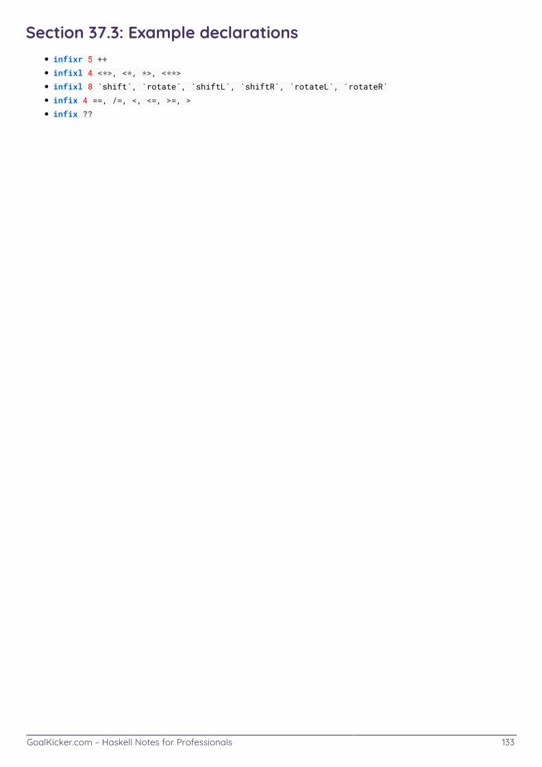
GoalKicker.com – Haskell Notes for Professionals 133

Section 37.3: Example declarationsinfixr 5 ++

infixl 4 <*>, <*, *>, <**>

infixl 8 `shift`, `rotate`, `shiftL`, `shiftR`, `rotateL`, `rotateR`

infix 4 ==, /=, <, <=, >=, >

infix ??

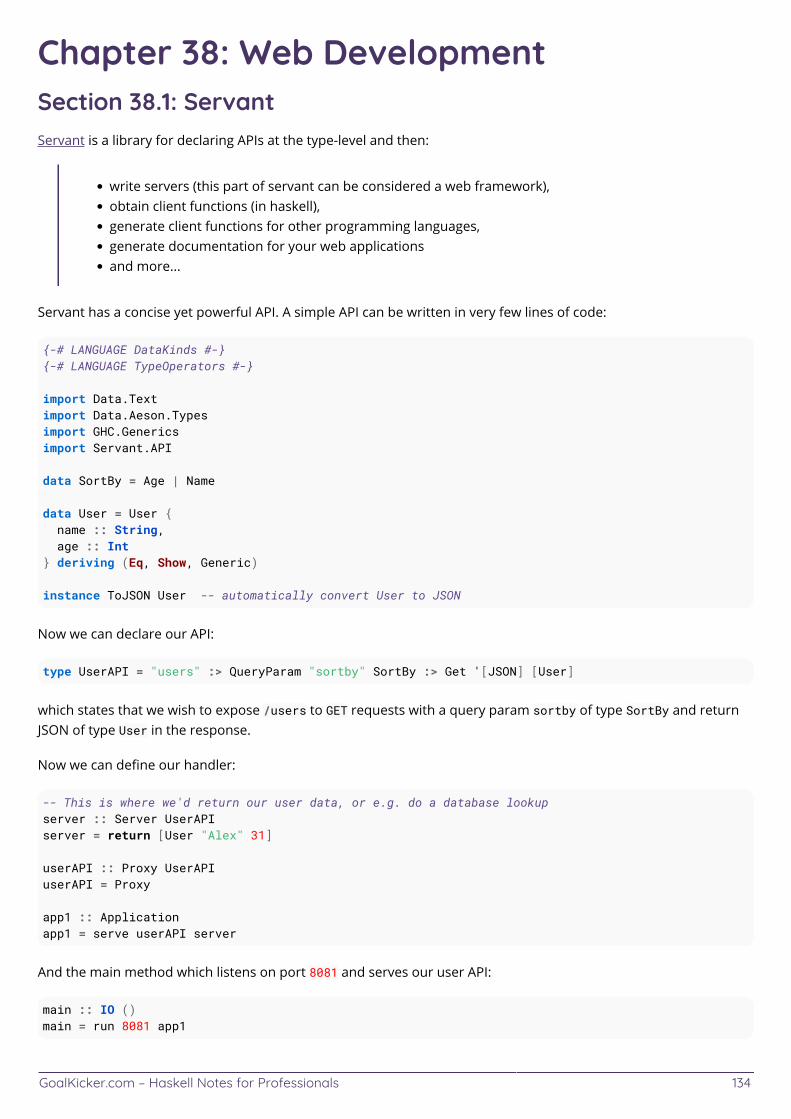
GoalKicker.com – Haskell Notes for Professionals 134

Chapter 38: Web DevelopmentSection 38.1: ServantServant is a library for declaring APIs at the type-level and then:

write servers (this part of servant can be considered a web framework),obtain client functions (in haskell),generate client functions for other programming languages,generate documentation for your web applicationsand more...

Servant has a concise yet powerful API. A simple API can be written in very few lines of code:

{-# LANGUAGE DataKinds #-}{-# LANGUAGE TypeOperators #-}

import Data.Textimport Data.Aeson.Typesimport GHC.Genericsimport Servant.API

data SortBy = Age | Name

data User = User { name :: String, age :: Int} deriving (Eq, Show, Generic)

instance ToJSON User -- automatically convert User to JSON

Now we can declare our API:

type UserAPI = "users" :> QueryParam "sortby" SortBy :> Get '[JSON] [User]

which states that we wish to expose /users to GET requests with a query param sortby of type SortBy and returnJSON of type User in the response.

Now we can define our handler:

-- This is where we'd return our user data, or e.g. do a database lookupserver :: Server UserAPIserver = return [User "Alex" 31]

userAPI :: Proxy UserAPIuserAPI = Proxy

app1 :: Applicationapp1 = serve userAPI server

And the main method which listens on port 8081 and serves our user API:

main :: IO ()main = run 8081 app1

GoalKicker.com – Haskell Notes for Professionals 135

Note, Stack has a template for generating basic APIs in Servant, which is useful for getting up and running veryquick.

Section 38.2: YesodYesod project can be created with stack new using following templates:

yesod-minimal. Simplest Yesod scaffold possible.yesod-mongo. Uses MongoDB as DB engine.yesod-mysql. Uses MySQL as DB engine.yesod-postgres. Uses PostgreSQL as DB engine.yesod-postgres-fay. Uses PostgreSQL as DB engine. Uses Fay language for front-end.yesod-simple. Recommended template to use, if you don't need database.yesod-sqlite. Uses SQlite as DB engine.

yesod-bin package provides yesod executable, which can be used to run development server. Note that you alsocan run your application directly, so yesod tool is optional.

Application.hs contains code that dispatches requests between handlers. It also sets up database and loggingsettings, if you used them.

Foundation.hs defines App type, that can be seen as an environment for all handlers. Being in HandlerT monad,you can get this value using getYesod function.

Import.hs is a module that just re-exports commonly used stuff.

Model.hs contains Template Haskell that generates code and data types used for DB interaction. Present only if youare using DB.

config/models is where you define your DB schema. Used by Model.hs.

config/routes defines URI's of the Web application. For each HTTP method of the route, you'd need to create ahandler named {method}{RouteR}.

static/ directory contains site's static resources. These get compiled into binary by Settings/StaticFiles.hsmodule.

templates/ directory contains Shakespeare templates that are used when serving requests.

Finally, Handler/ directory contains modules that define handlers for routes.

Each handler is a HandlerT monad action based on IO. You can inspect request parameters, its body and otherinformation, make queries to the DB with runDB, perform arbitrary IO and return various types of content to theuser. To serve HTML, defaultLayout function is used that allows neat composition of shakespearian templates.

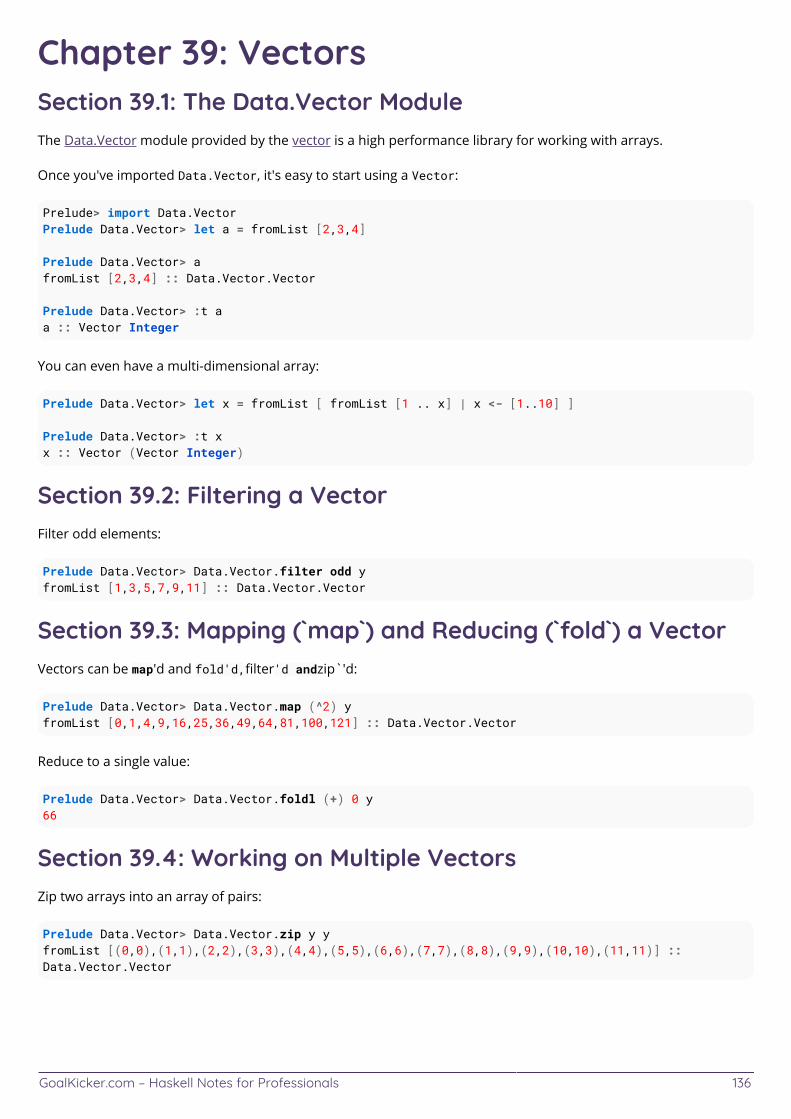
GoalKicker.com – Haskell Notes for Professionals 136

Chapter 39: VectorsSection 39.1: The Data.Vector ModuleThe Data.Vector module provided by the vector is a high performance library for working with arrays.

Once you've imported Data.Vector, it's easy to start using a Vector:

Prelude> import Data.VectorPrelude Data.Vector> let a = fromList [2,3,4] Prelude Data.Vector> afromList [2,3,4] :: Data.Vector.Vector Prelude Data.Vector> :t aa :: Vector Integer

You can even have a multi-dimensional array:

Prelude Data.Vector> let x = fromList [ fromList [1 .. x] | x <- [1..10] ] Prelude Data.Vector> :t xx :: Vector (Vector Integer)

Section 39.2: Filtering a VectorFilter odd elements:

Prelude Data.Vector> Data.Vector.filter odd yfromList [1,3,5,7,9,11] :: Data.Vector.Vector

Section 39.3: Mapping (`map`) and Reducing (`fold`) a VectorVectors can be map'd and fold'd,filter'd andzip`'d:

Prelude Data.Vector> Data.Vector.map (^2) yfromList [0,1,4,9,16,25,36,49,64,81,100,121] :: Data.Vector.Vector

Reduce to a single value:

Prelude Data.Vector> Data.Vector.foldl (+) 0 y66

Section 39.4: Working on Multiple VectorsZip two arrays into an array of pairs:

Prelude Data.Vector> Data.Vector.zip y yfromList [(0,0),(1,1),(2,2),(3,3),(4,4),(5,5),(6,6),(7,7),(8,8),(9,9),(10,10),(11,11)] ::Data.Vector.Vector

GoalKicker.com – Haskell Notes for Professionals 137

Chapter 40: CabalSection 40.1: Working with sandboxesA Haskell project can either use the system wide packages or use a sandbox. A sandbox is an isolated packagedatabase and can prevent dependency conflicts, e. g. if multiple Haskell projects use different versions of apackage.

To initialize a sandbox for a Haskell package go to its directory and run:

cabal sandbox init

Now packages can be installed by simply running cabal install.

Listing packages in a sandbox:

cabal sandbox hc-pkg list

Deleting a sandbox:

cabal sandbox delete

Add local dependency:

cabal sandbox add-source /path/to/dependency

Section 40.2: Install packagesTo install a new package, e.g. aeson:

cabal install aeson

GoalKicker.com – Haskell Notes for Professionals 138

Chapter 41: Type algebraSection 41.1: Addition and multiplicationThe addition and multiplication have equivalents in this type algebra. They correspond to the tagged unions andproduct types.

data Sum a b = A a | B bdata Prod a b = Prod a b

We can see how the number of inhabitants of every type corresponds to the operations of the algebra.

Equivalently, we can use Either and (,) as type constructors for the addition and the multiplication. They areisomorphic to our previously defined types:

type Sum' a b = Either a btype Prod' a b = (a,b)

The expected results of addition and multiplication are followed by the type algebra up to isomorphism. Forexample, we can see an isomorphism between 1 + 2, 2 + 1 and 3; as 1 + 2 = 3 = 2 + 1.

data Color = Red | Green | Blue

f :: Sum () Bool -> Colorf (Left ()) = Redf (Right True) = Greenf (Right False) = Blue

g :: Color -> Sum () Boolg Red = Left ()g Green = Right Trueg Blue = Right False

f' :: Sum Bool () -> Colorf' (Right ()) = Redf' (Left True) = Greenf' (Left False) = Blue

g' :: Color -> Sum Bool ()g' Red = Right ()g' Green = Left Trueg' Blue = Left False

Rules of addition and multiplication

The common rules of commutativity, associativity and distributivity are valid because there are trivial isomorphismsbetween the following types:

-- CommutativitySum a b <=> Sum b aProd a b <=> Prod b a-- AssociativitySum (Sum a b) c <=> Sum a (Sum b c)Prod (Prod a b) c <=> Prod a (Prod b c)-- DistributivityProd a (Sum b c) <=> Sum (Prod a b) (Prod a c)

GoalKicker.com – Haskell Notes for Professionals 139

Section 41.2: FunctionsFunctions can be seen as exponentials in our algebra. As we can see, if we take a type a with n instances and a typeb with m instances, the type a -> b will have m to the power of n instances.

As an example, Bool -> Bool is isomorphic to (Bool,Bool), as 2*2 = 2².

iso1 :: (Bool -> Bool) -> (Bool,Bool)iso1 f = (f True,f False)

iso2 :: (Bool,Bool) -> (Bool -> Bool)iso2 (x,y) = (\p -> if p then x else y)

Section 41.3: Natural numbers in type algebraWe can draw a connection between the Haskell types and the natural numbers. This connection can be madeassigning to every type the number of inhabitants it has.

Finite union types

For finite types, it suffices to see that we can assign a natural type to every number, based in the number ofconstructors. For example:

type Color = Red | Yellow | Green

would be 3. And the Bool type would be 2.

type Bool = True | False

Uniqueness up to isomorphism

We have seen that multiple types would correspond to a single number, but in this case, they would be isomorphic.This is to say that there would be a pair of morphisms f and g, whose composition would be the identity,connecting the two types.

f :: a -> bg :: b -> a

f . g == id == g . f

In this case, we would say that the types are isomorphic. We will consider two types equal in our algebra as long asthey are isomorphic.

For example, two different representations of the number two are trivally isomorphic:

type Bit = I | Otype Bool = True | False

bitValue :: Bit -> BoolbitValue I = TruebitValue O = False

booleanBit :: Bool -> BitbooleanBit True = IbooleanBit False = O

GoalKicker.com – Haskell Notes for Professionals 140

Because we can see bitValue . booleanBit == id == booleanBit . bitValue

One and Zero

The representation of the number 1 is obviously a type with only one constructor. In Haskell, this type is canonicallythe type (), called Unit. Every other type with only one constructor is isomorphic to ().

And our representation of 0 will be a type without constructors. This is the Void type in Haskell, as defined inData.Void. This would be equivalent to a unhabited type, wihtout data constructors:

data Void

Section 41.4: Recursive typesLists

Lists can be defined as:

data List a = Nil | Cons a (List a)

If we translate this into our type algebra, we get

List(a) = 1 + a * List(a)

But we can now substitute List(a) again in this expression multiple times, in order to get:

List(a) = 1 + a + a*a + a*a*a + a*a*a*a + ...

This makes sense if we see a list as a type that can contain only one value, as in []; or every value of type a, as in[x]; or two values of type a, as in [x,y]; and so on. The theoretical definition of List that we should get from therewould be:

-- Not working Haskell code!data List a = Nil | One a | Two a a | Three a a a ...

Trees

We can do the same thing with binary trees, for example. If we define them as:

data Tree a = Empty | Node a (Tree a) (Tree a)

We get the expression:

Tree(a) = 1 + a * Tree(a) * Tree(a)

And if we make the same substitutions again and again, we would obtain the following sequence:

GoalKicker.com – Haskell Notes for Professionals 141

Tree(a) = 1 + a + 2 (a*a) + 5 (a*a*a) + 14 (a*a*a*a) + ...

The coefficients we get here correspond to the Catalan numbers sequence, and the n-th catalan number isprecisely the number of possible binary trees with n nodes.

Section 41.5: DerivativesThe derivative of a type is the type of its type of one-hole contexts. This is the type that we would get if we make atype variable disappear in every possible point and sum the results.

As an example, we can take the triple type (a,a,a), and derive it, obtaining

data OneHoleContextsOfTriple = (a,a,()) | (a,(),a) | ((),a,a)

This is coherent with our usual definition of derivation, as:

d/da (a*a*a) = 3*a*a

More on this topic can be read on this article.

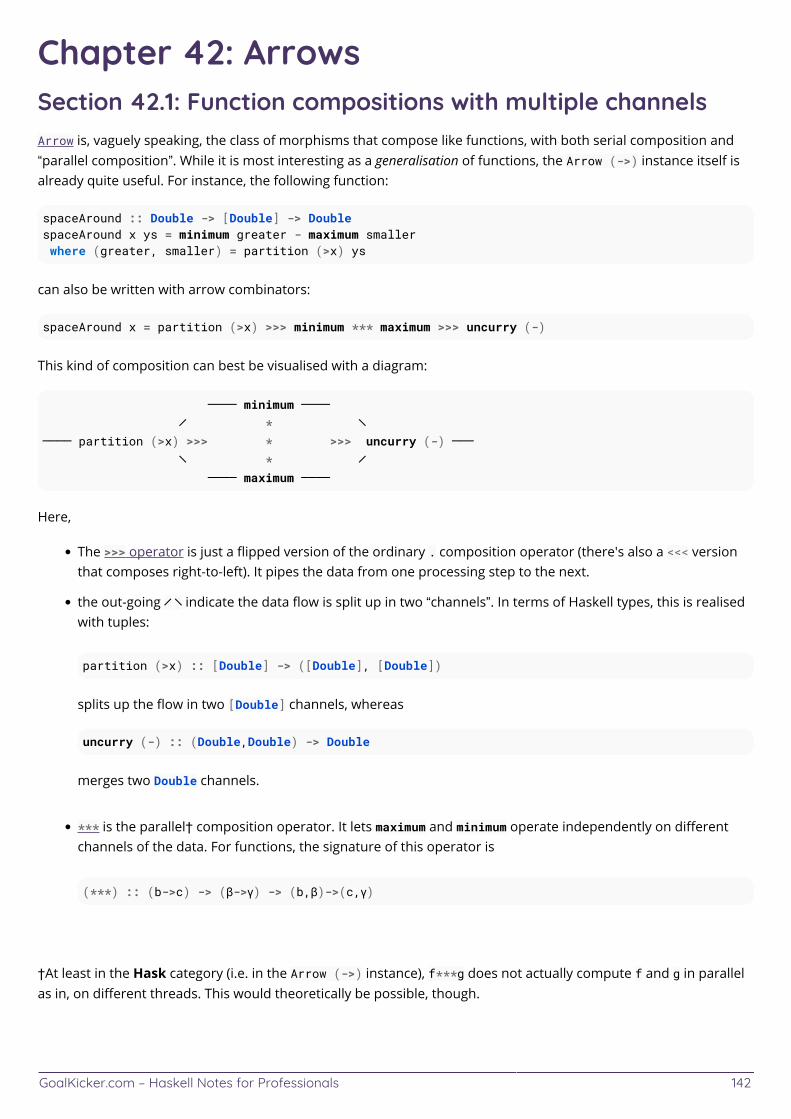
GoalKicker.com – Haskell Notes for Professionals 142

Chapter 42: ArrowsSection 42.1: Function compositions with multiple channelsArrow is, vaguely speaking, the class of morphisms that compose like functions, with both serial composition and“parallel composition”. While it is most interesting as a generalisation of functions, the Arrow (->) instance itself isalready quite useful. For instance, the following function:

spaceAround :: Double -> [Double] -> DoublespaceAround x ys = minimum greater - maximum smaller where (greater, smaller) = partition (>x) ys

can also be written with arrow combinators:

spaceAround x = partition (>x) >>> minimum *** maximum >>> uncurry (-)

This kind of composition can best be visualised with a diagram:

──── minimum ──── ╱ * ╲──── partition (>x) >>> * >>> uncurry (-) ─── ╲ * ╱ ──── maximum ────

Here,

The >>> operator is just a flipped version of the ordinary . composition operator (there's also a <<< versionthat composes right-to-left). It pipes the data from one processing step to the next.

the out-going ╱ ╲ indicate the data flow is split up in two “channels”. In terms of Haskell types, this is realisedwith tuples:

partition (>x) :: [Double] -> ([Double], [Double])

splits up the flow in two [Double] channels, whereas

uncurry (-) :: (Double,Double) -> Double

merges two Double channels.

*** is the parallel† composition operator. It lets maximum and minimum operate independently on differentchannels of the data. For functions, the signature of this operator is

(***) :: (b->c) -> (β->γ) -> (b,β)->(c,γ)

†At least in the Hask category (i.e. in the Arrow (->) instance), f***g does not actually compute f and g in parallelas in, on different threads. This would theoretically be possible, though.

GoalKicker.com – Haskell Notes for Professionals 143

Chapter 43: Typed holesSection 43.1: Syntax of typed holesA typed hole is a single underscore (_) or a valid Haskell identifier which is not in scope, in an expression context.Before the existance of typed holes, both of these things would trigger an error, so the new syntax does notinterfere with any old syntax.

Controlling behaviour of typed holes

The default behaviour of typed holes is to produce a compile-time error when encountering a typed hole. However,there are several flags to fine-tune their behaviour. These flags are summarized as follows (GHC trac):

By default GHC has typed holes enabled and produces a compile error when it encounters a typed hole.

When -fdefer-type-errors or -fdefer-typed-holes is enabled, hole errors are converted to warningsand result in runtime errors when evaluated.

The warning flag -fwarn-typed-holes is on by default. Without -fdefer-type-errors or -fdefer-typed-holes this flag is a no-op, since typed holes are an error under these conditions. If either of the defer flagsare enabled (converting typed hole errors into warnings) the -fno-warn-typed-holes flag disables thewarnings. This means compilation silently succeeds and evaluating a hole will produce a runtime error.

Section 43.2: Semantics of typed holesThe value of a type hole can simply said to be undefined, although a typed hole triggers a compile-time error, so itis not strictly necessary to assign it a value. However, a typed hole (when they are enabled) produces a compile timeerror (or warning with deferred type errors) which states the name of the typed hole, its inferred most general type,and the types of any local bindings. For example:

Prelude> \x -> _var + length (drop 1 x)

<interactive>:19:7: Warning: Found hole `_var' with type: Int Relevant bindings include x :: [a] (bound at <interactive>:19:2) it :: [a] -> Int (bound at <interactive>:19:1) In the first argument of `(+)', namely `_var' In the expression: _var + length (drop 1 x) In the expression: \ x -> _var + length (drop 1 x)

Note that in the case of typed holes in expressions entered into the GHCi repl (as above), the type of the expressionentered also reported, as it (here of type [a] -> Int).

Section 43.3: Using typed holes to define a class instanceTyped holes can make it easier to define functions, through an interactive process.

Say you want to define a class instance Foo Bar (for your custom Bar type, in order to use it with some polymorphiclibrary function that requires a Foo instance). You would now traditionally look up the documentation of Foo, figureout which methods you need to define, scrutinise their types etc. – but with typed holes, you can actually skip that!

GoalKicker.com – Haskell Notes for Professionals 144

First just define a dummy instance:

instance Foo Bar where

The compiler will now complain

Bar.hs:13:10: Warning:No explicit implementation for ‘foom’ and ‘quun’In the instance declaration for ‘Foo Bar’

Ok, so we need to define foom for Bar. But what is that even supposed to be? Again we're too lazy to look in thedocumentation, and just ask the compiler:

instance Foo Bar where foom = _

Here we've used a typed hole as a simple “documentation query”. The compiler outputs

Bar.hs:14:10: Found hole ‘_’ with type: Bar -> Gronk Bar Relevant bindings include foom :: Bar -> Gronk Bar (bound at Foo.hs:4:28) In the expression: _ In an equation for ‘foom’: foom = _ In the instance declaration for ‘Foo Bar’

Note how the compiler has already filled the class type variable with the concrete type Bar that we want toinstantiate it for. This can make the signature a lot easier to understand than the polymorphic one found in theclass documentation, especially if you're dealing with a more complicated method of e.g. a multi-parameter typeclass.

But what the hell is Gronk? At this point, it is probably a good idea to ask Hayoo. However we may still get awaywithout that: as a blind guess, we assume that this is not only a type constructor but also the single valueconstructor, i.e. it can be used as a function that will somehow produce a Gronk a value. So we try

instance Foo Bar where foom bar = _ Gronk

If we're lucky, Gronk is actually a value, and the compiler will now say

Found hole ‘_’ with type: (Int -> [(Int, b0)] -> Gronk b0) -> Gronk Bar Where: ‘b0’ is an ambiguous type variable

Ok, that's ugly – at first just note that Gronk has two arguments, so we can refine our attempt:

instance Foo Bar where foom bar = Gronk _ _

And this now is pretty clear:

Found hole ‘_’ with type: [(Int, Bar)] Relevant bindings include bar :: Bar (bound at Bar.hs:14:29)

GoalKicker.com – Haskell Notes for Professionals 145

foom :: Bar -> Gronk Bar (bound at Foo.hs:15:24) In the second argument of ‘Gronk’, namely ‘_’ In the expression: Gronk _ _ In an equation for ‘foom’: foom bar = Gronk _ _

You can now further progress by e.g. deconstructing the bar value (the components will then show up, with types,in the Relevant bindings section). Often, it is at some point completely obvious what the correct definition will be,because you you see all avaliable arguments and the types fit together like a jigsaw puzzle. Or alternatively, youmay see that the definition is impossible and why.

All of this works best in an editor with interactive compilation, e.g. Emacs with haskell-mode. You can then usetyped holes much like mouse-over value queries in an IDE for an interpreted dynamic imperative language, butwithout all the limitations.

GoalKicker.com – Haskell Notes for Professionals 146

Chapter 44: Rewrite rules (GHC)Section 44.1: Using rewrite rules on overloaded functionsIn this question, @Viclib asked about using rewrite rules to exploit typeclass laws to eliminate some overloadedfunction calls:

Mind the following class:

class ListIsomorphic l where toList :: l a -> [a] fromList :: [a] -> l a

I also demand that toList . fromList == id. How do I write rewrite rules to tell GHC to make thatsubstitution?

This is a somewhat tricky use case for GHC's rewrite rules mechanism, because overloaded functions are rewritteninto their specific instance methods by rules that are implicitly created behind the scenes by GHC (so something likefromList :: Seq a -> [a] would be rewritten into Seq$fromList etc.).

However, by first rewriting toList and fromList into non-inlined non-typeclass methods, we can protect them frompremature rewriting, and preserve them until the rule for the composition can fire:

{-# RULES "protect toList" toList = toList'; "protect fromList" fromList = fromList'; "fromList/toList" forall x . fromList' (toList' x) = x; #-}

{-# NOINLINE [0] fromList' #-}fromList' :: (ListIsomorphic l) => [a] -> l afromList' = fromList

{-# NOINLINE [0] toList' #-}toList' :: (ListIsomorphic l) => l a -> [a]toList' = toList

GoalKicker.com – Haskell Notes for Professionals 147

Chapter 45: Date and TimeSection 45.1: Finding Today's DateCurrent date and time can be found with getCurrentTime:

import Data.Time

print =<< getCurrentTime-- 2016-08-02 12:05:08.937169 UTC

Alternatively, just the date is returned by fromGregorian:

fromGregorian 1984 11 17 -- yields a Day

Section 45.2: Adding, Subtracting and Comparing DaysGiven a Day, we can perform simple arithmetic and comparisons, such as adding:

import Data.Time

addDays 1 (fromGregorian 2000 1 1)-- 2000-01-02addDays 1 (fromGregorian 2000 12 31)-- 2001-01-01

Subtract:

addDays (-1) (fromGregorian 2000 1 1)-- 1999-12-31

addDays (-1) (fromGregorian 0 1 1)-- -0001-12-31-- wat

and even find the difference:

diffDays (fromGregorian 2000 12 31) (fromGregorian 2000 1 1)365

note that the order matters:

diffDays (fromGregorian 2000 1 1) (fromGregorian 2000 12 31)-365

GoalKicker.com – Haskell Notes for Professionals 148

Chapter 46: List ComprehensionsSection 46.1: Basic List ComprehensionsHaskell has list comprehensions, which are a lot like set comprehensions in math and similar implementations inimperative languages such as Python and JavaScript. At their most basic, list comprehensions take the followingform.

[ x | x <- someList ]

For example

[ x | x <- [1..4] ] -- [1,2,3,4]

Functions can be directly applied to x as well:

[ f x | x <- someList ]

This is equivalent to:

map f someList

Example:

[ x+1 | x <- [1..4]] -- [2,3,4,5]

Section 46.2: Do NotationAny list comprehension can be correspondingly coded with list monad's do notation.

[f x | x <- xs] f <$> xs do { x <- xs ; return (f x) }

[f x | f <- fs, x <- xs] fs <*> xs do { f <- fs ; x <- xs ; return (f x) }

[y | x <- xs, y <- f x] f =<< xs do { x <- xs ; y <- f x ; return y }

The guards can be handled using Control.Monad.guard:

[x | x <- xs, even x] do { x <- xs ; guard (even x) ; return x }

Section 46.3: Patterns in Generator ExpressionsHowever, x in the generator expression is not just variable, but can be any pattern. In cases of pattern mismatchthe generated element is skipped over, and processing of the list continues with the next element, thus acting like afilter:

[x | Just x <- [Just 1, Nothing, Just 3]] -- [1, 3]

A generator with a variable x in its pattern creates new scope containing all the expressions on its right, where x isdefined to be the generated element.

This means that guards can be coded as

GoalKicker.com – Haskell Notes for Professionals 149

[ x | x <- [1..4], even x] ==[ x | x <- [1..4], () <- [() | even x]] ==[ x | x <- [1..4], () <- if even x then [()] else []]

Section 46.4: GuardsAnother feature of list comprehensions is guards, which also act as filters. Guards are Boolean expressions andappear on the right side of the bar in a list comprehension.

Their most basic use is

[x | p x] === if p x then [x] else []

Any variable used in a guard must appear on its left in the comprehension, or otherwise be in scope. So,

[ f x | x <- list, pred1 x y, pred2 x] -- `y` must be defined in outer scope

which is equivalent to

map f (filter pred2 (filter (\x -> pred1 x y) list)) -- or,

-- ($ list) (filter (`pred1` y) >>> filter pred2 >>> map f)

-- list >>= (\x-> [x | pred1 x y]) >>= (\x-> [x | pred2 x]) >>= (\x -> [f x])

(the >>= operator is infixl 1, i.e. it associates (is parenthesized) to the left). Examples:

[ x | x <- [1..4], even x] -- [2,4]

[ x^2 + 1 | x <- [1..100], even x ] -- map (\x -> x^2 + 1) (filter even [1..100])

Section 46.5: Parallel ComprehensionsWith Parallel List Comprehensions language extension,

[(x,y) | x <- xs | y <- ys]

is equivalent to

zip xs ys

Example:

[(x,y) | x <- [1,2,3] | y <- [10,20]]

-- [(1,10),(2,20)]

Section 46.6: Local BindingsList comprehensions can introduce local bindings for variables to hold some interim values:

[(x,y) | x <- [1..4], let y=x*x+1, even y] -- [(1,2),(3,10)]

Same effect can be achieved with a trick,

GoalKicker.com – Haskell Notes for Professionals 150

[(x,y) | x <- [1..4], y <- [x*x+1], even y] -- [(1,2),(3,10)]

The let in list comprehensions is recursive, as usual. But generator bindings are not, which enables shadowing:

[x | x <- [1..4], x <- [x*x+1], even x] -- [2,10]

Section 46.7: Nested GeneratorsList comprehensions can also draw elements from multiple lists, in which case the result will be the list of everypossible combination of the two elements, as if the two lists were processed in the nested fashion. For example,

[ (a,b) | a <- [1,2,3], b <- ['a','b'] ]

-- [(1,'a'), (1,'b'), (2,'a'), (2,'b'), (3,'a'), (3,'b')]

GoalKicker.com – Haskell Notes for Professionals 151

Chapter 47: Streaming IOSection 47.1: Streaming IOio-streams is Stream-based library that focuses on the Stream abstraction but for IO. It exposes two types:

InputStream: a read-only smart handle

OutputStream: a write-only smart handle

We can create a stream with makeInputStream :: IO (Maybe a) -> IO (InputStream a). Reading from a streamis performed using read :: InputStream a -> IO (Maybe a), where Nothing denotes an EOF:

import Control.Monad (forever)import qualified System.IO.Streams as Simport System.Random (randomRIO)

main :: IO ()main = do is <- S.makeInputStream $ randomInt -- create an InputStream forever $ printStream =<< S.read is -- forever read from that stream return ()

randomInt :: IO (Maybe Int)randomInt = do r <- randomRIO (1, 100) return $ Just r

printStream :: Maybe Int -> IO ()printStream Nothing = print "Nada!"printStream (Just a) = putStrLn $ show a

GoalKicker.com – Haskell Notes for Professionals 152

Chapter 48: Google Protocol BuersSection 48.1: Creating, building and using a simple .proto fileLet us first create a simple .proto file person.proto

package Protocol;

message Person { required string firstName = 1; required string lastName = 2; optional int32 age = 3;}

After saving we can now create the Haskell files which we can use in our project by running

$HOME/.local/bin/hprotoc --proto_path=. --haskell_out=. person.proto

We should get an output similar to this:

Loading filepath: "/<path-to-project>/person.proto"All proto files loadedHaskell name mangling doneRecursive modules resolved./Protocol/Person.hs./Protocol.hsProcessing complete, have a nice day.

hprotoc will create a new folder Protocol in the current directory with Person.hs which we can simply import intoour haskell project:

import Protocol (Person)

As a next step, if using Stack add

protocol-buffers , protocol-buffers-descriptor

to build-depends: and

Protocol

to exposed-modules in your .cabal file.

If we get now a incoming message from a stream, the message will have the type ByteString.

In order to transform the ByteString (which obviously should contain encoded "Person" data) into our Haskell datatype, we need to call the function messageGet which we import by

import Text.ProtocolBuffers (messageGet)

which enables to create a value of type Person using:

transformRawPerson :: ByteString -> Maybe PersontransformRawPerson raw = case messageGet raw of

GoalKicker.com – Haskell Notes for Professionals 153

Left _ -> Nothing Right (person, _) -> Just person

GoalKicker.com – Haskell Notes for Professionals 154

Chapter 49: Template Haskell &QuasiQuotesSection 49.1: Syntax of Template Haskell and QuasiquotesTemplate Haskell is enabled by the -XTemplateHaskell GHC extension. This extension enables all the syntacticfeatures further detailed in this section. The full details on Template Haskell are given by the user guide.

Splices

A splice is a new syntactic entity enabled by Template Haskell, written as $(...), where (...) is someexpression.

There must not be a space between $ and the first character of the expression; and Template Haskelloverrides the parsing of the $ operator - e.g. f$g is normally parsed as ($) f g whereas with TemplateHaskell enabled, it is parsed as a splice.

When a splice appears at the top level, the $ may be omitted. In this case, the spliced expression is the entireline.

A splice represents code which is run at compile time to produce a Haskell AST, and that AST is compiled asHaskell code and inserted into the program

Splices can appear in place of: expressions, patterns, types, and top-level declarations. The type of the splicedexpression, in each case respectively, is Q Exp, Q Pat, Q Type, Q [Decl]. Note that declaration splices mayonly appear at the top level, whereas the others may be inside other expressions, patterns, or types,respectively.

Expression quotations (note: not a QuasiQuotation)

An expression quotation is a new syntactic entity written as one of:

[e|..|] or [|..|] - .. is an expression and the quotation has type Q Exp;[p|..|] - .. is a pattern and the quotation has type Q Pat;[t|..|] - .. is a type and the quotation has type Q Type;[d|..|] - .. is a list of declarations and the quotation has type Q [Dec].

An expression quotation takes a compile time program and produces the AST represented by that program.

The use of a value in a quotation (e.g. \x -> [| x |]) without a splice corresponds to syntactic sugar for \x-> [| $(lift x) |], where lift :: Lift t => t -> Q Exp comes from the class

class Lift t where lift :: t -> Q Exp default lift :: Data t => t -> Q Exp Typed splices and quotations

Typed splices are similair to previously mentioned (untyped) splices, and are written as $$(..) where (..) isan expression.

If e has type Q (TExp a) then $$e has type a.

Typed quotations take the form [||..||] where .. is an expression of type a; the resulting quotation hastype Q (TExp a).

Typed expression can be converted to untyped ones: unType :: TExp a -> Exp.

QuasiQuotes

GoalKicker.com – Haskell Notes for Professionals 155

QuasiQuotes generalize expression quotations - previously, the parser used by the expression quotation isone of a fixed set (e,p,t,d), but QuasiQuotes allow a custom parser to be defined and used to produce codeat compile time. Quasi-quotations can appear in all the same contexts as regular quotations.

A quasi-quotation is written as [iden|...|], where iden is an identifier of typeLanguage.Haskell.TH.Quote.QuasiQuoter.

A QuasiQuoter is simply composed of four parsers, one for each of the different contexts in which quotationscan appear:

data QuasiQuoter = QuasiQuoter { quoteExp :: String -> Q Exp, quotePat :: String -> Q Pat, quoteType :: String -> QType, quoteDec :: String -> Q [Dec] } Names

Haskell identifiers are represented by the type Language.Haskell.TH.Syntax.Name. Names form the leavesof abstract syntax trees representing Haskell programs in Template Haskell.

An identifier which is currently in scope may be turned into a name with either: 'e or 'T. In the first case, e isinterpreted in the expression scope, while in the second case T is in the type scope (recalling that types andvalue constructors may share the name without amiguity in Haskell).

Section 49.2: The Q typeThe Q :: * -> * type constructor defined in Language.Haskell.TH.Syntax is an abstract type representingcomputations which have access to the compile-time environment of the module in which the computation is run.The Q type also handles variable substituion, called name capture by TH (and discussed here.) All splices have type QX for some X.

The compile-time environment includes:

in-scope identifiers and information about said identifiers,types of functionstypes and source data types of constructorsfull specification of type declarations (classes, type families)

the location in the source code (line, column, module, package) where the splice occursfixities of functions (GHC 7.10)enabled GHC extensions (GHC 8.0)

The Q type also has the ability to generate fresh names, with the function newName :: String -> Q Name. Note thatthe name is not bound anywhere implicitly, so the user must bind it themselves, and so making sure the resultinguse of the name is well-scoped is the responsibility of the user.

Q has instances for Functor,Monad,Applicative and this is the main interface for manipulating Q values, along withthe combinators provided in Language.Haskell.TH.Lib, which define a helper function for every constructor of theTH ast of the form:

LitE :: Lit -> ExplitE :: Lit -> ExpQ

AppE :: Exp -> Exp -> ExpappE :: ExpQ -> ExpQ -> ExpQ

Note that ExpQ, TypeQ, DecsQ and PatQ are synonyms for the AST types which are typically stored inside the Q type.

The TH library provides a function runQ :: Quasi m => Q a -> m a, and there is an instance Quasi IO, so it would

GoalKicker.com – Haskell Notes for Professionals 156

seem that the Q type is just a fancy IO. However, the use of runQ :: Q a -> IO a produces an IO action which doesnot have access to any compile-time environment - this is only available in the actual Q type. Such IO actions will failat runtime if trying to access said environment.

Section 49.3: An n-arity curryThe familiar

curry :: ((a,b) -> c) -> a -> b -> ccurry = \f a b -> f (a,b)

function can be generalized to tuples of arbitrary arity, for example:

curry3 :: ((a, b, c) -> d) -> a -> b -> c -> dcurry4 :: ((a, b, c, d) -> e) -> a -> b -> c -> d -> e

However, writing such functions for tuples of arity 2 to (e.g.) 20 by hand would be tedious (and ignoring the fact thatthe presence of 20 tuples in your program almost certainly signal design issues which should be fixed with records).

We can use Template Haskell to produce such curryN functions for arbitrary n:

{-# LANGUAGE TemplateHaskell #-}import Control.Monad (replicateM)import Language.Haskell.TH (ExpQ, newName, Exp(..), Pat(..))import Numeric.Natural (Natural)

curryN :: Natural -> Q Exp

The curryN function takes a natural number, and produces the curry function of that arity, as a Haskell AST.

curryN n = do f <- newName "f" xs <- replicateM (fromIntegral n) (newName "x")

First we produces fresh type variables for each of the arguments of the function - one for the input function, andone for each of the arguments to said function.

let args = map VarP (f:xs)

The expression args represents the pattern f x1 x2 .. xn. Note that a pattern is separate syntactic entity - wecould take this same pattern and place it in a lambda, or a function binding, or even the LHS of a let binding (whichwould be an error).

ntup = TupE (map VarE xs)

The function must build the argument tuple from the sequence of arguments, which is what we've done here. Notethe distinction between pattern variables (VarP) and expression variables (VarE).

return $ LamE args (AppE (VarE f) ntup)

Finally, the value which we produce is the AST \f x1 x2 .. xn -> f (x1, x2, .. , xn).

We could have also written this function using quotations and 'lifted' constructors:

...

GoalKicker.com – Haskell Notes for Professionals 157

import Language.Haskell.TH.Lib

curryN' :: Natural -> ExpQcurryN' n = do f <- newName "f" xs <- replicateM (fromIntegral n) (newName "x") lamE (map varP (f:xs)) [| $(varE f) $(tupE (map varE xs)) |]

Note that quotations must be syntactically valid, so [| \ $(map varP (f:xs)) -> .. |] is invalid, because there isno way in regular Haskell to declare a 'list' of patterns - the above is interpreted as \ var -> .. and the splicedexpression is expected to have type PatQ, i.e. a single pattern, not a list of patterns.

Finally, we can load this TH function in GHCi:

>:set -XTemplateHaskell>:t $(curryN 5)$(curryN 5) :: ((t1, t2, t3, t4, t5) -> t) -> t1 -> t2 -> t3 -> t4 -> t5 -> t>$(curryN 5) (\(a,b,c,d,e) -> a+b+c+d+e) 1 2 3 4 515

This example is adapted primarily from here.

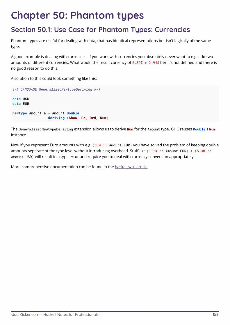
GoalKicker.com – Haskell Notes for Professionals 158

Chapter 50: Phantom typesSection 50.1: Use Case for Phantom Types: CurrenciesPhantom types are useful for dealing with data, that has identical representations but isn't logically of the sametype.

A good example is dealing with currencies. If you work with currencies you absolutely never want to e.g. add twoamounts of different currencies. What would the result currency of 5.32€ + 2.94$ be? It's not defined and there isno good reason to do this.

A solution to this could look something like this:

{-# LANGUAGE GeneralizedNewtypeDeriving #-}

data USDdata EUR

newtype Amount a = Amount Double deriving (Show, Eq, Ord, Num)

The GeneralisedNewtypeDeriving extension allows us to derive Num for the Amount type. GHC reuses Double's Numinstance.

Now if you represent Euro amounts with e.g. (5.0 :: Amount EUR) you have solved the problem of keeping doubleamounts separate at the type level without introducing overhead. Stuff like (1.13 :: Amount EUR) + (5.30 ::Amount USD) will result in a type error and require you to deal with currency conversion appropriately.

More comprehensive documentation can be found in the haskell wiki article

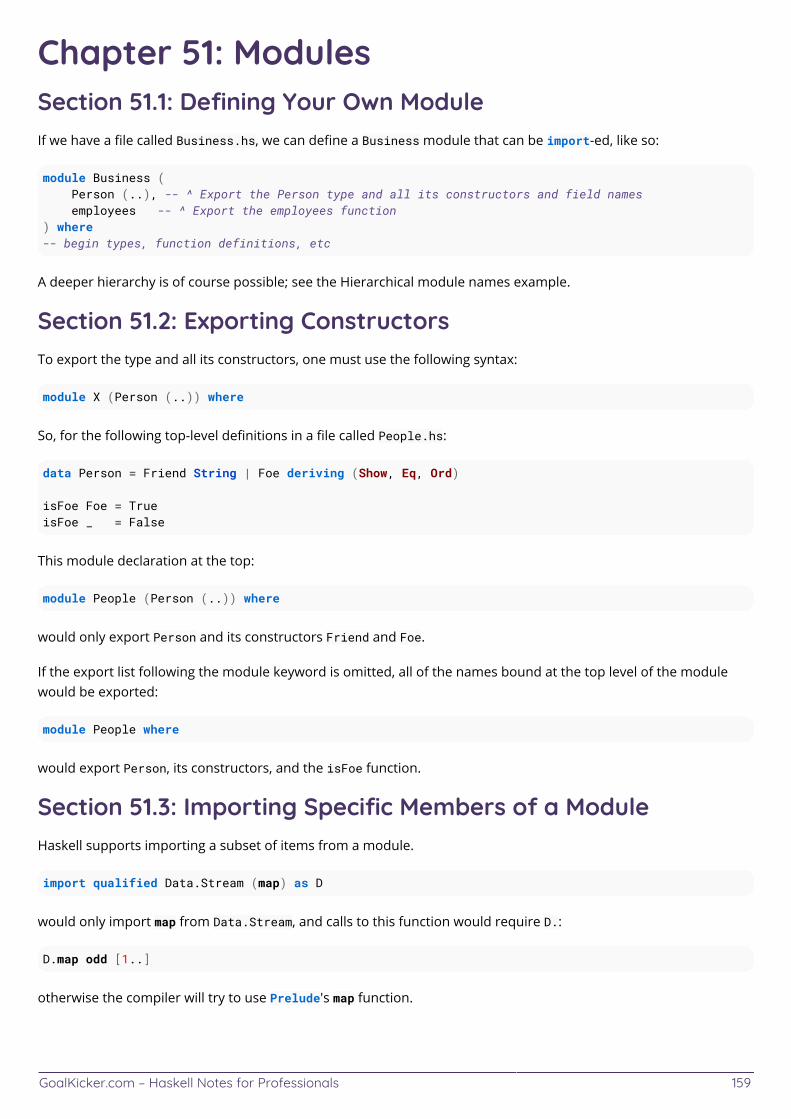
GoalKicker.com – Haskell Notes for Professionals 159

Chapter 51: ModulesSection 51.1: Defining Your Own ModuleIf we have a file called Business.hs, we can define a Business module that can be import-ed, like so:

module Business ( Person (..), -- ^ Export the Person type and all its constructors and field names employees -- ^ Export the employees function) where-- begin types, function definitions, etc

A deeper hierarchy is of course possible; see the Hierarchical module names example.

Section 51.2: Exporting ConstructorsTo export the type and all its constructors, one must use the following syntax:

module X (Person (..)) where

So, for the following top-level definitions in a file called People.hs:

data Person = Friend String | Foe deriving (Show, Eq, Ord)

isFoe Foe = TrueisFoe _ = False

This module declaration at the top:

module People (Person (..)) where

would only export Person and its constructors Friend and Foe.

If the export list following the module keyword is omitted, all of the names bound at the top level of the modulewould be exported:

module People where

would export Person, its constructors, and the isFoe function.

Section 51.3: Importing Specific Members of a ModuleHaskell supports importing a subset of items from a module.

import qualified Data.Stream (map) as D

would only import map from Data.Stream, and calls to this function would require D.:

D.map odd [1..]

otherwise the compiler will try to use Prelude's map function.

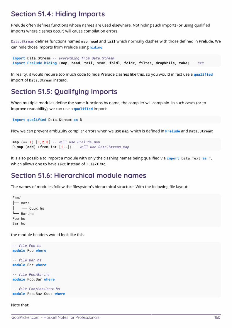
GoalKicker.com – Haskell Notes for Professionals 160

Section 51.4: Hiding ImportsPrelude often defines functions whose names are used elsewhere. Not hiding such imports (or using qualifiedimports where clashes occur) will cause compilation errors.

Data.Stream defines functions named map, head and tail which normally clashes with those defined in Prelude. Wecan hide those imports from Prelude using hiding:

import Data.Stream -- everything from Data.Streamimport Prelude hiding (map, head, tail, scan, foldl, foldr, filter, dropWhile, take) -- etc

In reality, it would require too much code to hide Prelude clashes like this, so you would in fact use a qualifiedimport of Data.Stream instead.

Section 51.5: Qualifying ImportsWhen multiple modules define the same functions by name, the compiler will complain. In such cases (or toimprove readability), we can use a qualified import:

import qualified Data.Stream as D

Now we can prevent ambiguity compiler errors when we use map, which is defined in Prelude and Data.Stream:

map (== 1) [1,2,3] -- will use Prelude.mapD.map (odd) (fromList [1..]) -- will use Data.Stream.map

It is also possible to import a module with only the clashing names being qualified via import Data.Text as T,which allows one to have Text instead of T.Text etc.

Section 51.6: Hierarchical module namesThe names of modules follow the filesystem's hierarchical structure. With the following file layout:

Foo/├── Baz/│ └── Quux.hs└── Bar.hsFoo.hsBar.hs

the module headers would look like this:

-- file Foo.hsmodule Foo where

-- file Bar.hsmodule Bar where

-- file Foo/Bar.hsmodule Foo.Bar where

-- file Foo/Baz/Quux.hsmodule Foo.Baz.Quux where

Note that:

GoalKicker.com – Haskell Notes for Professionals 161

the module name is based on the path of the file declaring the moduleFolders may share a name with a module, which gives a naturally hierarchical naming structure to modules

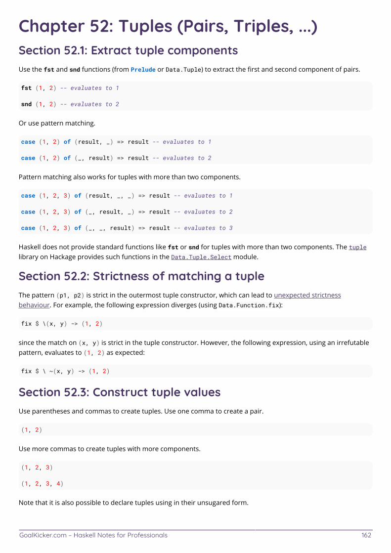
GoalKicker.com – Haskell Notes for Professionals 162

Chapter 52: Tuples (Pairs, Triples, ...)Section 52.1: Extract tuple componentsUse the fst and snd functions (from Prelude or Data.Tuple) to extract the first and second component of pairs.

fst (1, 2) -- evaluates to 1

snd (1, 2) -- evaluates to 2

Or use pattern matching.

case (1, 2) of (result, _) => result -- evaluates to 1

case (1, 2) of (_, result) => result -- evaluates to 2

Pattern matching also works for tuples with more than two components.

case (1, 2, 3) of (result, _, _) => result -- evaluates to 1

case (1, 2, 3) of (_, result, _) => result -- evaluates to 2

case (1, 2, 3) of (_, _, result) => result -- evaluates to 3

Haskell does not provide standard functions like fst or snd for tuples with more than two components. The tuplelibrary on Hackage provides such functions in the Data.Tuple.Select module.

Section 52.2: Strictness of matching a tupleThe pattern (p1, p2) is strict in the outermost tuple constructor, which can lead to unexpected strictnessbehaviour. For example, the following expression diverges (using Data.Function.fix):

fix $ \(x, y) -> (1, 2)

since the match on (x, y) is strict in the tuple constructor. However, the following expression, using an irrefutablepattern, evaluates to (1, 2) as expected:

fix $ \ ~(x, y) -> (1, 2)

Section 52.3: Construct tuple valuesUse parentheses and commas to create tuples. Use one comma to create a pair.

(1, 2)

Use more commas to create tuples with more components.

(1, 2, 3)

(1, 2, 3, 4)

Note that it is also possible to declare tuples using in their unsugared form.

GoalKicker.com – Haskell Notes for Professionals 163

(,) 1 2 -- equivalent to (1,2)(,,) 1 2 3 -- equivalent to (1,2,3)

Tuples can contain values of different types.

("answer", 42, '?')

Tuples can contain complex values such as lists or more tuples.

([1, 2, 3], "hello", ('A', 65))

(1, (2, (3, 4), 5), 6)

Section 52.4: Write tuple typesUse parentheses and commas to write tuple types. Use one comma to write a pair type.

(Int, Int)

Use more commas to write tuple types with more components.

(Int, Int, Int)

(Int, Int, Int, Int)

Tuples can contain values of different types.

(String, Int, Char)

Tuples can contain complex values such as lists or more tuples.

([Int], String, (Char, Int))

(Int, (Int, (Int, Int), Int), Int)

Section 52.5: Pattern Match on TuplesPattern matching on tuples uses the tuple constructors. To match a pair for example, we'd use the (,) constructor:

myFunction1 (a, b) = ...

We use more commas to match tuples with more components:

myFunction2 (a, b, c) = ...

myFunction3 (a, b, c, d) = ...

Tuple patterns can contain complex patterns such as list patterns or more tuple patterns.

myFunction4 ([a, b, c], d, e) = ...

myFunction5 (a, (b, (c, d), e), f) = ...

GoalKicker.com – Haskell Notes for Professionals 164

Section 52.6: Apply a binary function to a tuple (uncurrying)Use the uncurry function (from Prelude or Data.Tuple) to convert a binary function to a function on tuples.

uncurry (+) (1, 2) -- computes 3

uncurry map (negate, [1, 2, 3]) -- computes [-1, -2, -3]

uncurry uncurry ((+), (1, 2)) -- computes 3

map (uncurry (+)) [(1, 2), (3, 4), (5, 6)] -- computes [3, 7, 11]

uncurry (curry f) -- computes the same as f

Section 52.7: Apply a tuple function to two arguments(currying)Use the curry function (from Prelude or Data.Tuple) to convert a function that takes tuples to a function that takestwo arguments.

curry fst 1 2 -- computes 1

curry snd 1 2 -- computes 2

curry (uncurry f) -- computes the same as f

import Data.Tuple (swap)curry swap 1 2 -- computes (2, 1)

Section 52.8: Swap pair componentsUse swap (from Data.Tuple) to swap the components of a pair.

import Data.Tuple (swap)swap (1, 2) -- evaluates to (2, 1)

Or use pattern matching.

case (1, 2) of (x, y) => (y, x) -- evaluates to (2, 1)

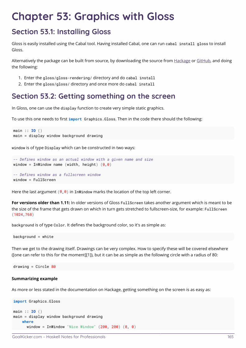
GoalKicker.com – Haskell Notes for Professionals 165

Chapter 53: Graphics with GlossSection 53.1: Installing GlossGloss is easily installed using the Cabal tool. Having installed Cabal, one can run cabal install gloss to installGloss.

Alternatively the package can be built from source, by downloading the source from Hackage or GitHub, and doingthe following:

Enter the gloss/gloss-rendering/ directory and do cabal install1.Enter the gloss/gloss/ directory and once more do cabal install2.

Section 53.2: Getting something on the screenIn Gloss, one can use the display function to create very simple static graphics.

To use this one needs to first import Graphics.Gloss. Then in the code there should the following:

main :: IO ()main = display window background drawing

window is of type Display which can be constructed in two ways:

-- Defines window as an actual window with a given name and sizewindow = InWindow name (width, height) (0,0)

-- Defines window as a fullscreen windowwindow = FullScreen

Here the last argument (0,0) in InWindow marks the location of the top left corner.

For versions older than 1.11: In older versions of Gloss FullScreen takes another argument which is meant to bethe size of the frame that gets drawn on which in turn gets stretched to fullscreen-size, for example: FullScreen(1024,768)

background is of type Color. It defines the background color, so it's as simple as:

background = white

Then we get to the drawing itself. Drawings can be very complex. How to specify these will be covered elsewhere([one can refer to this for the moment][1]), but it can be as simple as the following circle with a radius of 80:

drawing = Circle 80

Summarizing example

As more or less stated in the documentation on Hackage, getting something on the screen is as easy as:

import Graphics.Gloss

main :: IO ()main = display window background drawing where window = InWindow "Nice Window" (200, 200) (0, 0)

GoalKicker.com – Haskell Notes for Professionals 166

background = white drawing = Circle 80

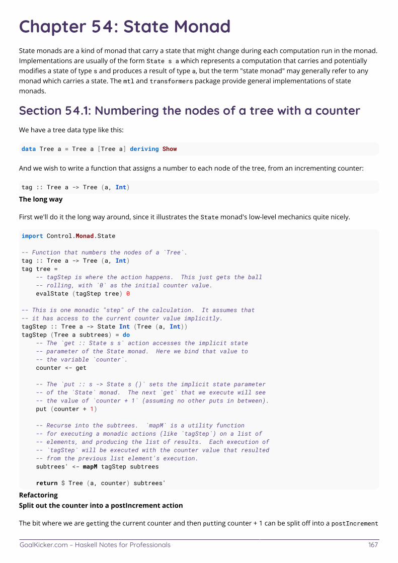
GoalKicker.com – Haskell Notes for Professionals 167

Chapter 54: State MonadState monads are a kind of monad that carry a state that might change during each computation run in the monad.Implementations are usually of the form State s a which represents a computation that carries and potentiallymodifies a state of type s and produces a result of type a, but the term "state monad" may generally refer to anymonad which carries a state. The mtl and transformers package provide general implementations of statemonads.

Section 54.1: Numbering the nodes of a tree with a counterWe have a tree data type like this:

data Tree a = Tree a [Tree a] deriving Show

And we wish to write a function that assigns a number to each node of the tree, from an incrementing counter:

tag :: Tree a -> Tree (a, Int)

The long way

First we'll do it the long way around, since it illustrates the State monad's low-level mechanics quite nicely.

import Control.Monad.State

-- Function that numbers the nodes of a `Tree`.tag :: Tree a -> Tree (a, Int)tag tree = -- tagStep is where the action happens. This just gets the ball -- rolling, with `0` as the initial counter value. evalState (tagStep tree) 0

-- This is one monadic "step" of the calculation. It assumes that-- it has access to the current counter value implicitly.tagStep :: Tree a -> State Int (Tree (a, Int))tagStep (Tree a subtrees) = do -- The `get :: State s s` action accesses the implicit state -- parameter of the State monad. Here we bind that value to -- the variable `counter`. counter <- get

-- The `put :: s -> State s ()` sets the implicit state parameter -- of the `State` monad. The next `get` that we execute will see -- the value of `counter + 1` (assuming no other puts in between). put (counter + 1)

-- Recurse into the subtrees. `mapM` is a utility function -- for executing a monadic actions (like `tagStep`) on a list of -- elements, and producing the list of results. Each execution of -- `tagStep` will be executed with the counter value that resulted -- from the previous list element's execution. subtrees' <- mapM tagStep subtrees

return $ Tree (a, counter) subtrees'

RefactoringSplit out the counter into a postIncrement action

The bit where we are getting the current counter and then putting counter + 1 can be split off into a postIncrement

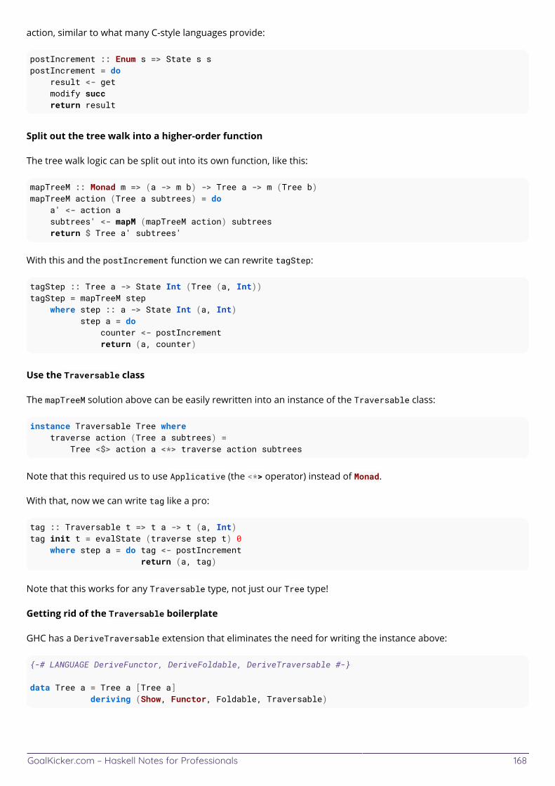
GoalKicker.com – Haskell Notes for Professionals 168

action, similar to what many C-style languages provide:

postIncrement :: Enum s => State s spostIncrement = do result <- get modify succ return result

Split out the tree walk into a higher-order function

The tree walk logic can be split out into its own function, like this:

mapTreeM :: Monad m => (a -> m b) -> Tree a -> m (Tree b)mapTreeM action (Tree a subtrees) = do a' <- action a subtrees' <- mapM (mapTreeM action) subtrees return $ Tree a' subtrees'

With this and the postIncrement function we can rewrite tagStep:

tagStep :: Tree a -> State Int (Tree (a, Int))tagStep = mapTreeM step where step :: a -> State Int (a, Int) step a = do counter <- postIncrement return (a, counter)

Use the Traversable class

The mapTreeM solution above can be easily rewritten into an instance of the Traversable class:

instance Traversable Tree where traverse action (Tree a subtrees) = Tree <$> action a <*> traverse action subtrees

Note that this required us to use Applicative (the <*> operator) instead of Monad.

With that, now we can write tag like a pro:

tag :: Traversable t => t a -> t (a, Int)tag init t = evalState (traverse step t) 0 where step a = do tag <- postIncrement return (a, tag)

Note that this works for any Traversable type, not just our Tree type!

Getting rid of the Traversable boilerplate

GHC has a DeriveTraversable extension that eliminates the need for writing the instance above:

{-# LANGUAGE DeriveFunctor, DeriveFoldable, DeriveTraversable #-}

data Tree a = Tree a [Tree a] deriving (Show, Functor, Foldable, Traversable)

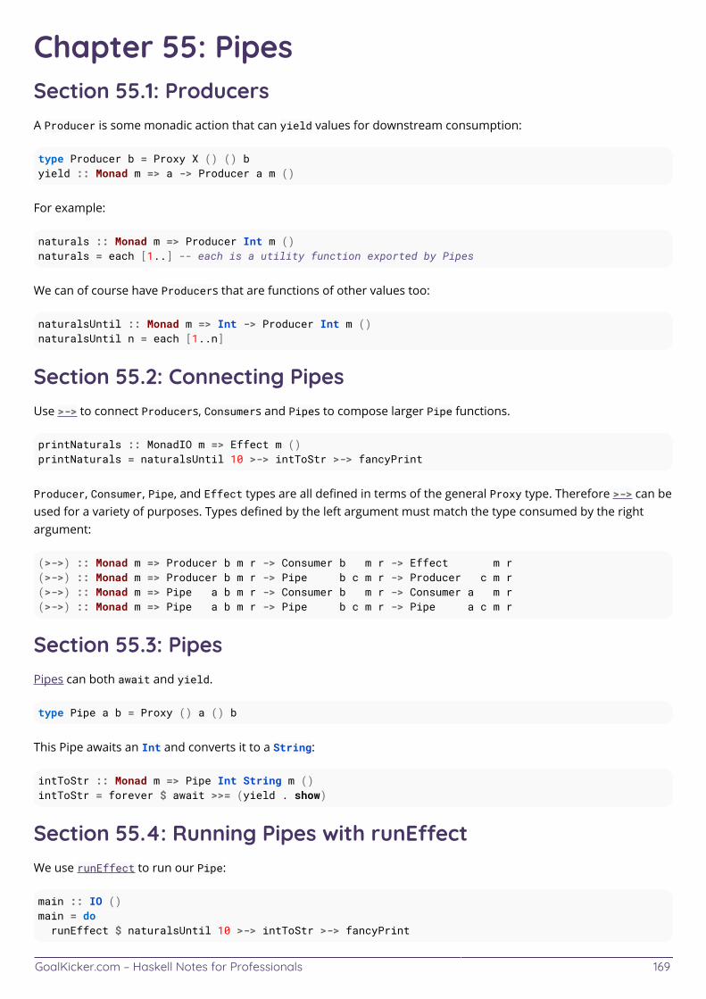
GoalKicker.com – Haskell Notes for Professionals 169

Chapter 55: PipesSection 55.1: ProducersA Producer is some monadic action that can yield values for downstream consumption:

type Producer b = Proxy X () () byield :: Monad m => a -> Producer a m ()

For example:

naturals :: Monad m => Producer Int m ()naturals = each [1..] -- each is a utility function exported by Pipes

We can of course have Producers that are functions of other values too:

naturalsUntil :: Monad m => Int -> Producer Int m ()naturalsUntil n = each [1..n]

Section 55.2: Connecting PipesUse >-> to connect Producers, Consumers and Pipes to compose larger Pipe functions.

printNaturals :: MonadIO m => Effect m ()printNaturals = naturalsUntil 10 >-> intToStr >-> fancyPrint

Producer, Consumer, Pipe, and Effect types are all defined in terms of the general Proxy type. Therefore >-> can beused for a variety of purposes. Types defined by the left argument must match the type consumed by the rightargument:

(>->) :: Monad m => Producer b m r -> Consumer b m r -> Effect m r(>->) :: Monad m => Producer b m r -> Pipe b c m r -> Producer c m r(>->) :: Monad m => Pipe a b m r -> Consumer b m r -> Consumer a m r(>->) :: Monad m => Pipe a b m r -> Pipe b c m r -> Pipe a c m r

Section 55.3: PipesPipes can both await and yield.

type Pipe a b = Proxy () a () b

This Pipe awaits an Int and converts it to a String:

intToStr :: Monad m => Pipe Int String m ()intToStr = forever $ await >>= (yield . show)

Section 55.4: Running Pipes with runEectWe use runEffect to run our Pipe:

main :: IO ()main = do runEffect $ naturalsUntil 10 >-> intToStr >-> fancyPrint

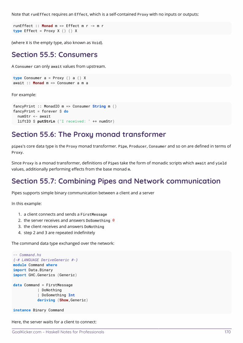
GoalKicker.com – Haskell Notes for Professionals 170

Note that runEffect requires an Effect, which is a self-contained Proxy with no inputs or outputs:

runEffect :: Monad m => Effect m r -> m rtype Effect = Proxy X () () X

(where X is the empty type, also known as Void).

Section 55.5: ConsumersA Consumer can only await values from upstream.

type Consumer a = Proxy () a () Xawait :: Monad m => Consumer a m a

For example:

fancyPrint :: MonadIO m => Consumer String m ()fancyPrint = forever $ do numStr <- await liftIO $ putStrLn ("I received: " ++ numStr)

Section 55.6: The Proxy monad transformerpipes's core data type is the Proxy monad transformer. Pipe, Producer, Consumer and so on are defined in terms ofProxy.

Since Proxy is a monad transformer, definitions of Pipes take the form of monadic scripts which await and yieldvalues, additionally performing effects from the base monad m.

Section 55.7: Combining Pipes and Network communicationPipes supports simple binary communication between a client and a server

In this example:

a client connects and sends a FirstMessage1.the server receives and answers DoSomething 02.the client receives and answers DoNothing3.step 2 and 3 are repeated indefinitely4.

The command data type exchanged over the network:

-- Command.hs{-# LANGUAGE DeriveGeneric #-}module Command whereimport Data.Binaryimport GHC.Generics (Generic)

data Command = FirstMessage | DoNothing | DoSomething Int deriving (Show,Generic)

instance Binary Command

Here, the server waits for a client to connect:

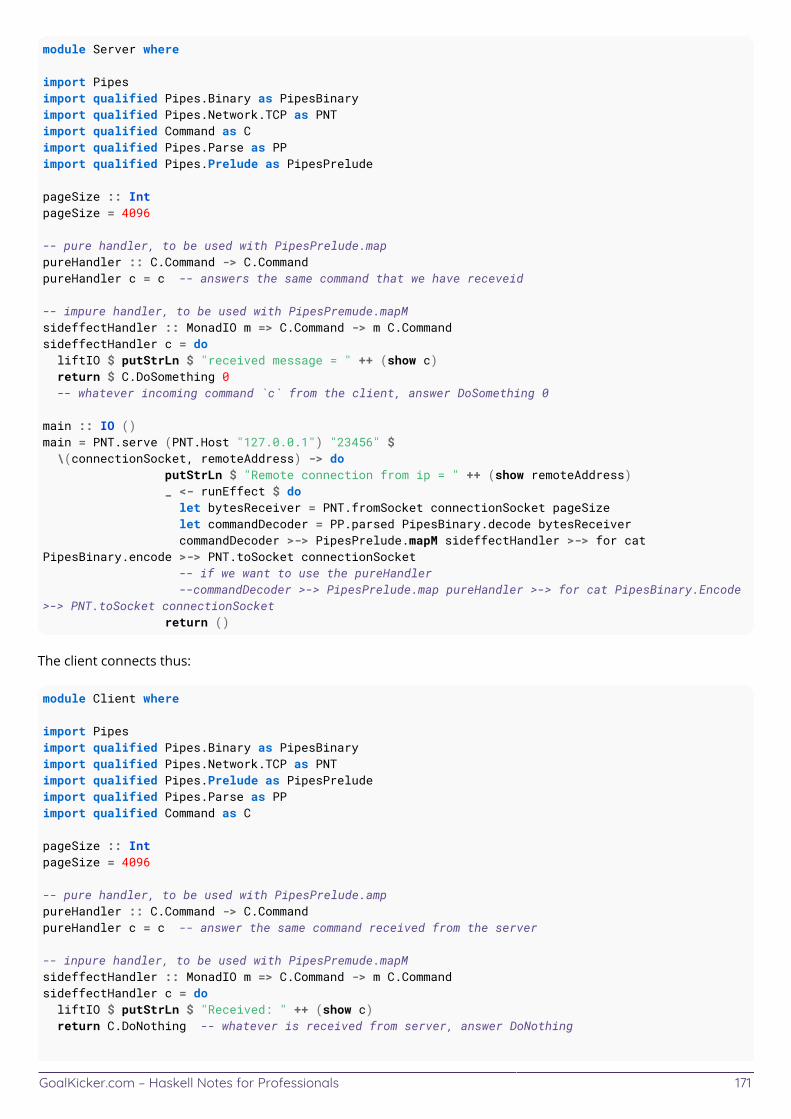
GoalKicker.com – Haskell Notes for Professionals 171

module Server where

import Pipesimport qualified Pipes.Binary as PipesBinaryimport qualified Pipes.Network.TCP as PNTimport qualified Command as Cimport qualified Pipes.Parse as PPimport qualified Pipes.Prelude as PipesPrelude

pageSize :: IntpageSize = 4096

-- pure handler, to be used with PipesPrelude.mappureHandler :: C.Command -> C.CommandpureHandler c = c -- answers the same command that we have receveid

-- impure handler, to be used with PipesPremude.mapMsideffectHandler :: MonadIO m => C.Command -> m C.CommandsideffectHandler c = do liftIO $ putStrLn $ "received message = " ++ (show c) return $ C.DoSomething 0 -- whatever incoming command `c` from the client, answer DoSomething 0

main :: IO ()main = PNT.serve (PNT.Host "127.0.0.1") "23456" $ \(connectionSocket, remoteAddress) -> do putStrLn $ "Remote connection from ip = " ++ (show remoteAddress) _ <- runEffect $ do let bytesReceiver = PNT.fromSocket connectionSocket pageSize let commandDecoder = PP.parsed PipesBinary.decode bytesReceiver commandDecoder >-> PipesPrelude.mapM sideffectHandler >-> for catPipesBinary.encode >-> PNT.toSocket connectionSocket -- if we want to use the pureHandler --commandDecoder >-> PipesPrelude.map pureHandler >-> for cat PipesBinary.Encode>-> PNT.toSocket connectionSocket return ()

The client connects thus:

module Client where

import Pipesimport qualified Pipes.Binary as PipesBinaryimport qualified Pipes.Network.TCP as PNTimport qualified Pipes.Prelude as PipesPreludeimport qualified Pipes.Parse as PPimport qualified Command as C

pageSize :: IntpageSize = 4096

-- pure handler, to be used with PipesPrelude.amppureHandler :: C.Command -> C.CommandpureHandler c = c -- answer the same command received from the server

-- inpure handler, to be used with PipesPremude.mapMsideffectHandler :: MonadIO m => C.Command -> m C.CommandsideffectHandler c = do liftIO $ putStrLn $ "Received: " ++ (show c) return C.DoNothing -- whatever is received from server, answer DoNothing

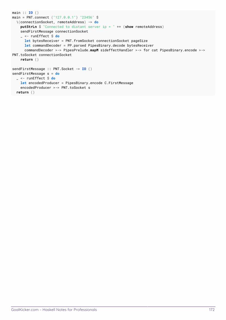
GoalKicker.com – Haskell Notes for Professionals 172

main :: IO ()main = PNT.connect ("127.0.0.1") "23456" $ \(connectionSocket, remoteAddress) -> do putStrLn $ "Connected to distant server ip = " ++ (show remoteAddress) sendFirstMessage connectionSocket _ <- runEffect $ do let bytesReceiver = PNT.fromSocket connectionSocket pageSize let commandDecoder = PP.parsed PipesBinary.decode bytesReceiver commandDecoder >-> PipesPrelude.mapM sideffectHandler >-> for cat PipesBinary.encode >->PNT.toSocket connectionSocket return ()

sendFirstMessage :: PNT.Socket -> IO ()sendFirstMessage s = do _ <- runEffect $ do let encodedProducer = PipesBinary.encode C.FirstMessage encodedProducer >-> PNT.toSocket s return ()

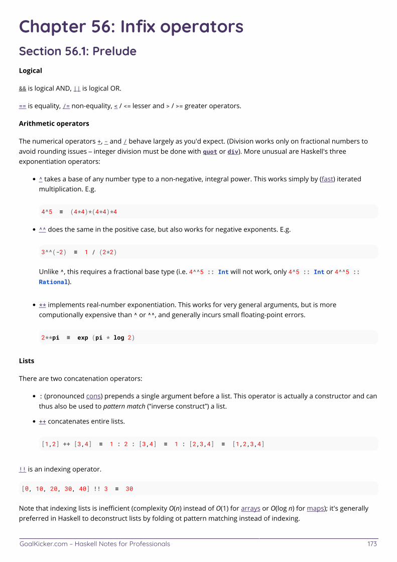
GoalKicker.com – Haskell Notes for Professionals 173

Chapter 56: Infix operatorsSection 56.1: PreludeLogical

&& is logical AND, || is logical OR.

== is equality, /= non-equality, < / <= lesser and > / >= greater operators.

Arithmetic operators

The numerical operators +, - and / behave largely as you'd expect. (Division works only on fractional numbers toavoid rounding issues – integer division must be done with quot or div). More unusual are Haskell's threeexponentiation operators:

^ takes a base of any number type to a non-negative, integral power. This works simply by (fast) iteratedmultiplication. E.g.

4^5 ≡ (4*4)*(4*4)*4

^^ does the same in the positive case, but also works for negative exponents. E.g.

3^^(-2) ≡ 1 / (2*2)

Unlike ^, this requires a fractional base type (i.e. 4^^5 :: Int will not work, only 4^5 :: Int or 4^^5 ::Rational).

** implements real-number exponentiation. This works for very general arguments, but is morecomputionally expensive than ^ or ^^, and generally incurs small floating-point errors.

2**pi ≡ exp (pi * log 2)

Lists

There are two concatenation operators:

: (pronounced cons) prepends a single argument before a list. This operator is actually a constructor and canthus also be used to pattern match (“inverse construct”) a list.

++ concatenates entire lists.

[1,2] ++ [3,4] ≡ 1 : 2 : [3,4] ≡ 1 : [2,3,4] ≡ [1,2,3,4]

!! is an indexing operator.

[0, 10, 20, 30, 40] !! 3 ≡ 30

Note that indexing lists is inefficient (complexity O(n) instead of O(1) for arrays or O(log n) for maps); it's generallypreferred in Haskell to deconstruct lists by folding ot pattern matching instead of indexing.

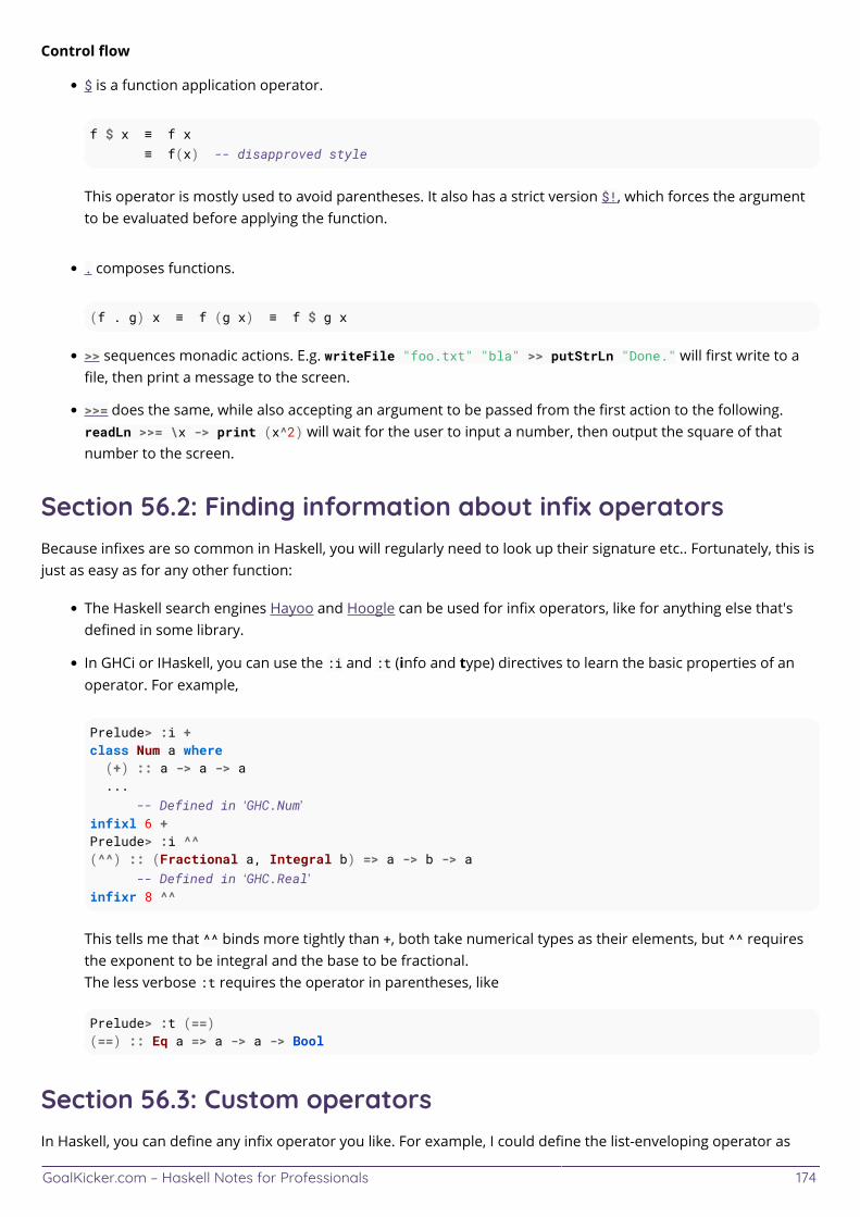
GoalKicker.com – Haskell Notes for Professionals 174

Control flow

$ is a function application operator.

f $ x ≡ f x ≡ f(x) -- disapproved style

This operator is mostly used to avoid parentheses. It also has a strict version $!, which forces the argumentto be evaluated before applying the function.

. composes functions.

(f . g) x ≡ f (g x) ≡ f $ g x

>> sequences monadic actions. E.g. writeFile "foo.txt" "bla" >> putStrLn "Done." will first write to afile, then print a message to the screen.

>>= does the same, while also accepting an argument to be passed from the first action to the following.readLn >>= \x -> print (x^2) will wait for the user to input a number, then output the square of thatnumber to the screen.

Section 56.2: Finding information about infix operatorsBecause infixes are so common in Haskell, you will regularly need to look up their signature etc.. Fortunately, this isjust as easy as for any other function:

The Haskell search engines Hayoo and Hoogle can be used for infix operators, like for anything else that'sdefined in some library.

In GHCi or IHaskell, you can use the :i and :t (info and type) directives to learn the basic properties of anoperator. For example,

Prelude> :i +class Num a where (+) :: a -> a -> a ... -- Defined in ‘GHC.Num’infixl 6 +Prelude> :i ^^(^^) :: (Fractional a, Integral b) => a -> b -> a -- Defined in ‘GHC.Real’infixr 8 ^^

This tells me that ^^ binds more tightly than +, both take numerical types as their elements, but ^^ requiresthe exponent to be integral and the base to be fractional.The less verbose :t requires the operator in parentheses, like

Prelude> :t (==)(==) :: Eq a => a -> a -> Bool

Section 56.3: Custom operatorsIn Haskell, you can define any infix operator you like. For example, I could define the list-enveloping operator as

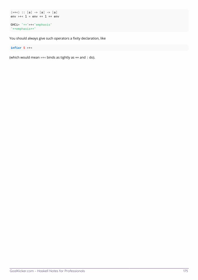
GoalKicker.com – Haskell Notes for Professionals 175

(>+<) :: [a] -> [a] -> [a]env >+< l = env ++ l ++ env

GHCi> "**">+<"emphasis""**emphasis**"

You should always give such operators a fixity declaration, like

infixr 5 >+<

(which would mean >+< binds as tightly as ++ and : do).

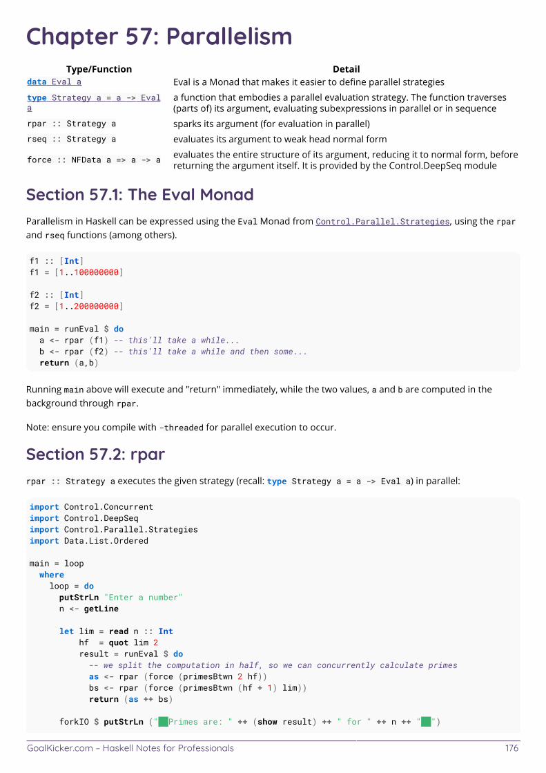
GoalKicker.com – Haskell Notes for Professionals 176

Chapter 57: ParallelismType/Function Detail

data Eval a Eval is a Monad that makes it easier to define parallel strategies

type Strategy a = a -> Evala

a function that embodies a parallel evaluation strategy. The function traverses(parts of) its argument, evaluating subexpressions in parallel or in sequence

rpar :: Strategy a sparks its argument (for evaluation in parallel)rseq :: Strategy a evaluates its argument to weak head normal form

force :: NFData a => a -> a evaluates the entire structure of its argument, reducing it to normal form, beforereturning the argument itself. It is provided by the Control.DeepSeq module

Section 57.1: The Eval MonadParallelism in Haskell can be expressed using the Eval Monad from Control.Parallel.Strategies, using the rparand rseq functions (among others).

f1 :: [Int]f1 = [1..100000000]

f2 :: [Int]f2 = [1..200000000]

main = runEval $ do a <- rpar (f1) -- this'll take a while... b <- rpar (f2) -- this'll take a while and then some... return (a,b)

Running main above will execute and "return" immediately, while the two values, a and b are computed in thebackground through rpar.

Note: ensure you compile with -threaded for parallel execution to occur.

Section 57.2: rparrpar :: Strategy a executes the given strategy (recall: type Strategy a = a -> Eval a) in parallel:

import Control.Concurrentimport Control.DeepSeqimport Control.Parallel.Strategiesimport Data.List.Ordered

main = loop where loop = do putStrLn "Enter a number" n <- getLine

let lim = read n :: Int hf = quot lim 2 result = runEval $ do -- we split the computation in half, so we can concurrently calculate primes as <- rpar (force (primesBtwn 2 hf)) bs <- rpar (force (primesBtwn (hf + 1) lim)) return (as ++ bs)

forkIO $ putStrLn ("\nPrimes are: " ++ (show result) ++ " for " ++ n ++ "\n")

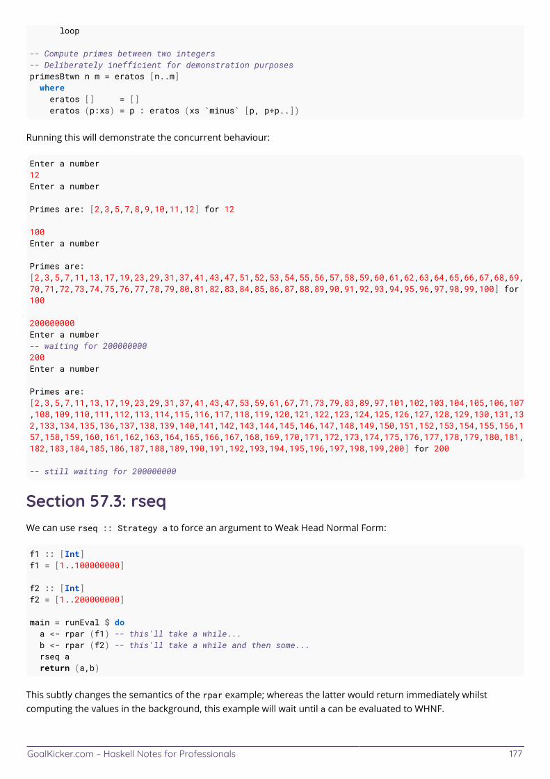
GoalKicker.com – Haskell Notes for Professionals 177

loop

-- Compute primes between two integers-- Deliberately inefficient for demonstration purposesprimesBtwn n m = eratos [n..m] where eratos [] = [] eratos (p:xs) = p : eratos (xs `minus` [p, p+p..])

Running this will demonstrate the concurrent behaviour:

Enter a number12Enter a number

Primes are: [2,3,5,7,8,9,10,11,12] for 12

100Enter a number

Primes are:[2,3,5,7,11,13,17,19,23,29,31,37,41,43,47,51,52,53,54,55,56,57,58,59,60,61,62,63,64,65,66,67,68,69,70,71,72,73,74,75,76,77,78,79,80,81,82,83,84,85,86,87,88,89,90,91,92,93,94,95,96,97,98,99,100] for100

200000000Enter a number-- waiting for 200000000 200Enter a number

Primes are:[2,3,5,7,11,13,17,19,23,29,31,37,41,43,47,53,59,61,67,71,73,79,83,89,97,101,102,103,104,105,106,107,108,109,110,111,112,113,114,115,116,117,118,119,120,121,122,123,124,125,126,127,128,129,130,131,132,133,134,135,136,137,138,139,140,141,142,143,144,145,146,147,148,149,150,151,152,153,154,155,156,157,158,159,160,161,162,163,164,165,166,167,168,169,170,171,172,173,174,175,176,177,178,179,180,181,182,183,184,185,186,187,188,189,190,191,192,193,194,195,196,197,198,199,200] for 200

-- still waiting for 200000000

Section 57.3: rseqWe can use rseq :: Strategy a to force an argument to Weak Head Normal Form:

f1 :: [Int]f1 = [1..100000000]

f2 :: [Int]f2 = [1..200000000]

main = runEval $ do a <- rpar (f1) -- this'll take a while... b <- rpar (f2) -- this'll take a while and then some... rseq a return (a,b)

This subtly changes the semantics of the rpar example; whereas the latter would return immediately whilstcomputing the values in the background, this example will wait until a can be evaluated to WHNF.

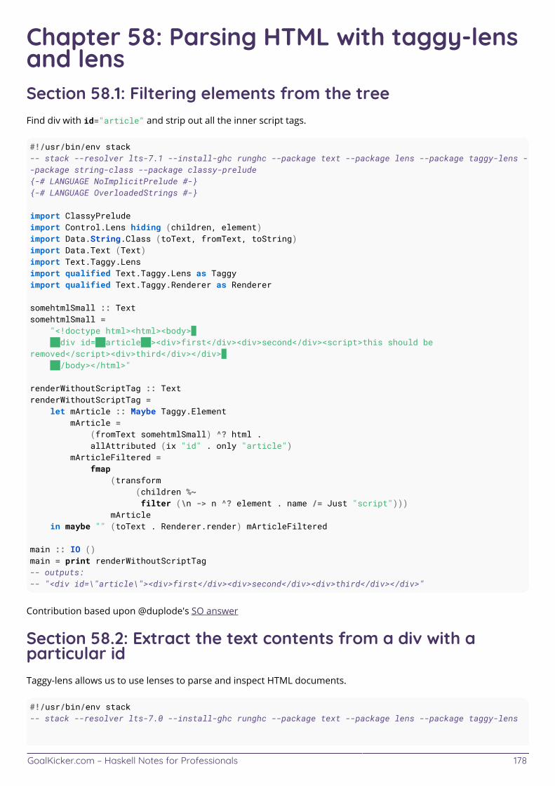
GoalKicker.com – Haskell Notes for Professionals 178

Chapter 58: Parsing HTML with taggy-lensand lensSection 58.1: Filtering elements from the treeFind div with id="article" and strip out all the inner script tags.

#!/usr/bin/env stack-- stack --resolver lts-7.1 --install-ghc runghc --package text --package lens --package taggy-lens --package string-class --package classy-prelude{-# LANGUAGE NoImplicitPrelude #-}{-# LANGUAGE OverloadedStrings #-}

import ClassyPreludeimport Control.Lens hiding (children, element)import Data.String.Class (toText, fromText, toString)import Data.Text (Text)import Text.Taggy.Lensimport qualified Text.Taggy.Lens as Taggyimport qualified Text.Taggy.Renderer as Renderer

somehtmlSmall :: TextsomehtmlSmall = "<!doctype html><html><body>\ \<div id=\"article\"><div>first</div><div>second</div><script>this should beremoved</script><div>third</div></div>\ \</body></html>"

renderWithoutScriptTag :: TextrenderWithoutScriptTag = let mArticle :: Maybe Taggy.Element mArticle = (fromText somehtmlSmall) ^? html . allAttributed (ix "id" . only "article") mArticleFiltered = fmap (transform (children %~ filter (\n -> n ^? element . name /= Just "script"))) mArticle in maybe "" (toText . Renderer.render) mArticleFiltered

main :: IO ()main = print renderWithoutScriptTag-- outputs:-- "<div id=\"article\"><div>first</div><div>second</div><div>third</div></div>"

Contribution based upon @duplode's SO answer

Section 58.2: Extract the text contents from a div with aparticular idTaggy-lens allows us to use lenses to parse and inspect HTML documents.

#!/usr/bin/env stack-- stack --resolver lts-7.0 --install-ghc runghc --package text --package lens --package taggy-lens

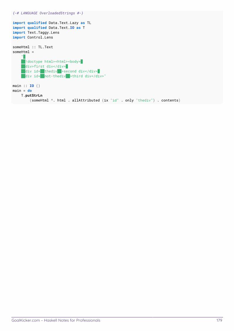
GoalKicker.com – Haskell Notes for Professionals 179

{-# LANGUAGE OverloadedStrings #-}

import qualified Data.Text.Lazy as TLimport qualified Data.Text.IO as Timport Text.Taggy.Lensimport Control.Lens

someHtml :: TL.TextsomeHtml = "\ \<!doctype html><html><body>\ \<div>first div</div>\ \<div id=\"thediv\">second div</div>\ \<div id=\"not-thediv\">third div</div>"

main :: IO ()main = do T.putStrLn (someHtml ^. html . allAttributed (ix "id" . only "thediv") . contents)

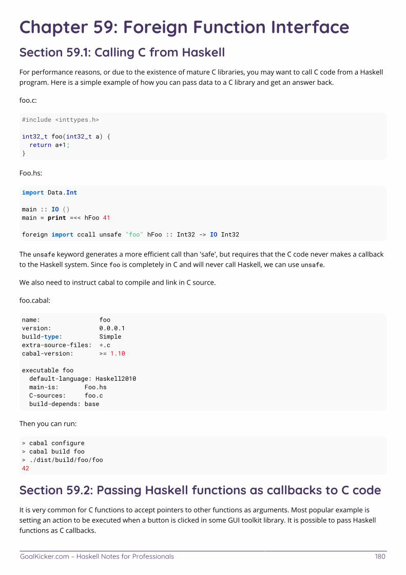
GoalKicker.com – Haskell Notes for Professionals 180

Chapter 59: Foreign Function InterfaceSection 59.1: Calling C from HaskellFor performance reasons, or due to the existence of mature C libraries, you may want to call C code from a Haskellprogram. Here is a simple example of how you can pass data to a C library and get an answer back.

foo.c:

#include <inttypes.h>

int32_t foo(int32_t a) { return a+1;}

Foo.hs:

import Data.Int

main :: IO ()main = print =<< hFoo 41

foreign import ccall unsafe "foo" hFoo :: Int32 -> IO Int32

The unsafe keyword generates a more efficient call than 'safe', but requires that the C code never makes a callbackto the Haskell system. Since foo is completely in C and will never call Haskell, we can use unsafe.

We also need to instruct cabal to compile and link in C source.

foo.cabal:

name: fooversion: 0.0.0.1build-type: Simpleextra-source-files: *.ccabal-version: >= 1.10

executable foo default-language: Haskell2010 main-is: Foo.hs C-sources: foo.c build-depends: base

Then you can run:

> cabal configure> cabal build foo> ./dist/build/foo/foo42

Section 59.2: Passing Haskell functions as callbacks to C codeIt is very common for C functions to accept pointers to other functions as arguments. Most popular example issetting an action to be executed when a button is clicked in some GUI toolkit library. It is possible to pass Haskellfunctions as C callbacks.

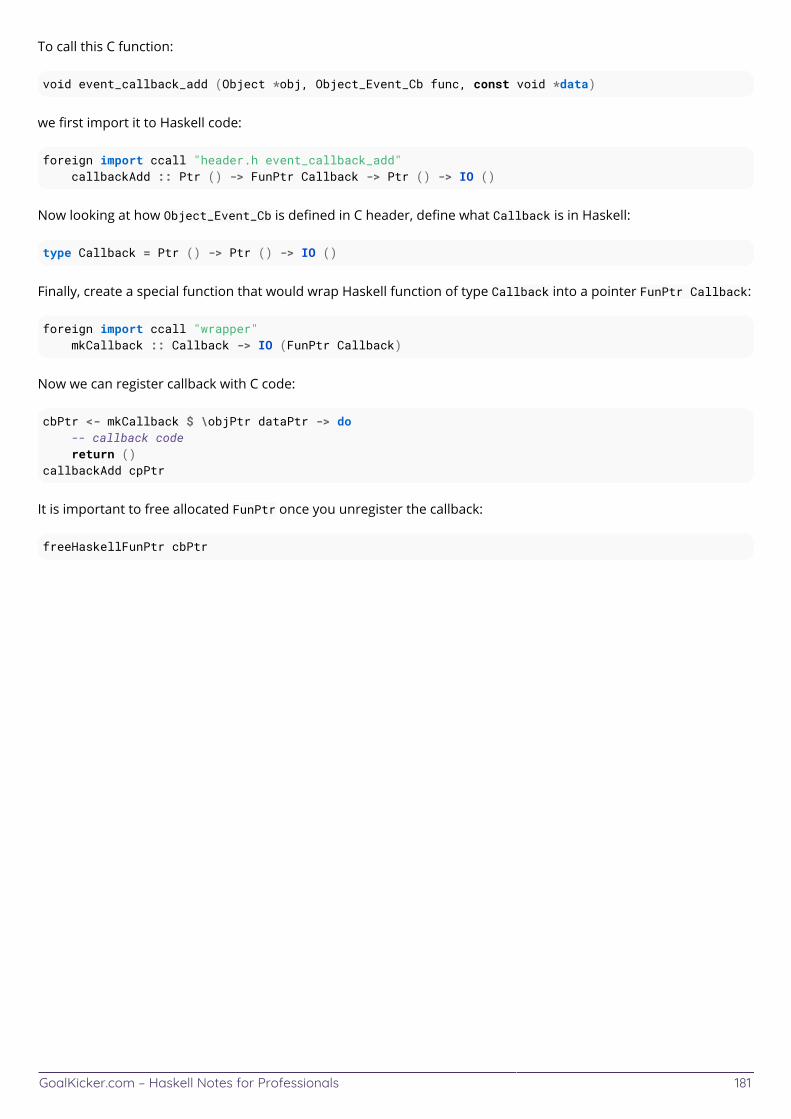
GoalKicker.com – Haskell Notes for Professionals 181

To call this C function:

void event_callback_add (Object *obj, Object_Event_Cb func, const void *data)

we first import it to Haskell code:

foreign import ccall "header.h event_callback_add" callbackAdd :: Ptr () -> FunPtr Callback -> Ptr () -> IO ()

Now looking at how Object_Event_Cb is defined in C header, define what Callback is in Haskell:

type Callback = Ptr () -> Ptr () -> IO ()

Finally, create a special function that would wrap Haskell function of type Callback into a pointer FunPtr Callback:

foreign import ccall "wrapper" mkCallback :: Callback -> IO (FunPtr Callback)

Now we can register callback with C code:

cbPtr <- mkCallback $ \objPtr dataPtr -> do -- callback code return ()callbackAdd cpPtr

It is important to free allocated FunPtr once you unregister the callback:

freeHaskellFunPtr cbPtr

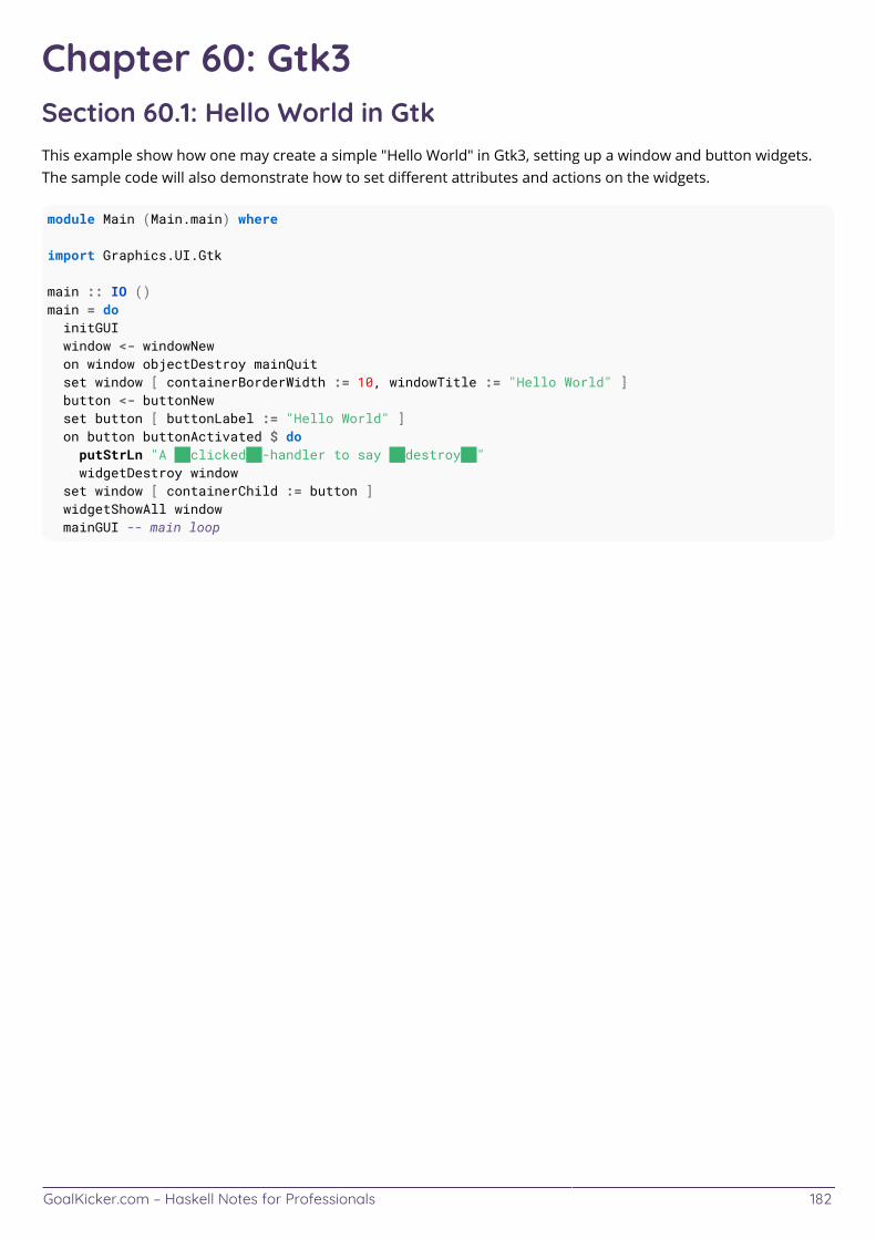
GoalKicker.com – Haskell Notes for Professionals 182

Chapter 60: Gtk3Section 60.1: Hello World in GtkThis example show how one may create a simple "Hello World" in Gtk3, setting up a window and button widgets.The sample code will also demonstrate how to set different attributes and actions on the widgets.

module Main (Main.main) where

import Graphics.UI.Gtk

main :: IO ()main = do initGUI window <- windowNew on window objectDestroy mainQuit set window [ containerBorderWidth := 10, windowTitle := "Hello World" ] button <- buttonNew set button [ buttonLabel := "Hello World" ] on button buttonActivated $ do putStrLn "A \"clicked\"-handler to say \"destroy\"" widgetDestroy window set window [ containerChild := button ] widgetShowAll window mainGUI -- main loop

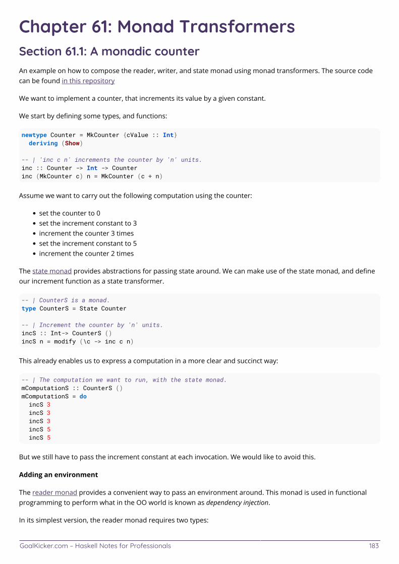
GoalKicker.com – Haskell Notes for Professionals 183

Chapter 61: Monad TransformersSection 61.1: A monadic counterAn example on how to compose the reader, writer, and state monad using monad transformers. The source codecan be found in this repository

We want to implement a counter, that increments its value by a given constant.

We start by defining some types, and functions:

newtype Counter = MkCounter {cValue :: Int} deriving (Show)

-- | 'inc c n' increments the counter by 'n' units.inc :: Counter -> Int -> Counterinc (MkCounter c) n = MkCounter (c + n)

Assume we want to carry out the following computation using the counter:

set the counter to 0set the increment constant to 3increment the counter 3 timesset the increment constant to 5increment the counter 2 times

The state monad provides abstractions for passing state around. We can make use of the state monad, and defineour increment function as a state transformer.

-- | CounterS is a monad.type CounterS = State Counter

-- | Increment the counter by 'n' units.incS :: Int-> CounterS ()incS n = modify (\c -> inc c n)

This already enables us to express a computation in a more clear and succinct way:

-- | The computation we want to run, with the state monad.mComputationS :: CounterS ()mComputationS = do incS 3 incS 3 incS 3 incS 5 incS 5

But we still have to pass the increment constant at each invocation. We would like to avoid this.

Adding an environment

The reader monad provides a convenient way to pass an environment around. This monad is used in functionalprogramming to perform what in the OO world is known as dependency injection.

In its simplest version, the reader monad requires two types:

GoalKicker.com – Haskell Notes for Professionals 184

the type of the value being read (i.e. our environment, r below),

the value returned by the reader monad (a below).

Reader r a

However, we need to make use of the state monad as well. Thus, we need to use the ReaderT transformer:

newtype ReaderT r m a :: * -> (* -> *) -> * -> *

Using ReaderT, we can define our counter with environment and state as follows:

type CounterRS = ReaderT Int CounterS

We define an incR function that takes the increment constant from the environment (using ask), and to define ourincrement function in terms of our CounterS monad we make use of the lift function (which belongs to themonad transformer class).

-- | Increment the counter by the amount of units specified by the environment.incR :: CounterRS ()incR = ask >>= lift . incS

Using the reader monad we can define our computation as follows:

-- | The computation we want to run, using reader and state monads.mComputationRS :: CounterRS ()mComputationRS = do local (const 3) $ do incR incR incR local (const 5) $ do incR incR

The requirements changed: we need logging!

Now assume that we want to add logging to our computation, so that we can see the evolution of our counter intime.

We also have a monad to perform this task, the writer monad. As with the reader monad, since we are composingthem, we need to make use of the reader monad transformer:

newtype WriterT w m a :: * -> (* -> *) -> * -> *

Here w represents the type of the output to accumulate (which has to be a monoid, which allow us to accumulatethis value), m is the inner monad, and a the type of the computation.

We can then define our counter with logging, environment, and state as follows:

type CounterWRS = WriterT [Int] CounterRS

And making use of lift we can define the version of the increment function which logs the value of the counterafter each increment:

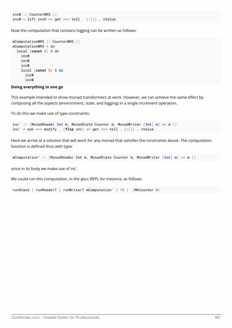
GoalKicker.com – Haskell Notes for Professionals 185

incW :: CounterWRS ()incW = lift incR >> get >>= tell . (:[]) . cValue

Now the computation that contains logging can be written as follows:

mComputationWRS :: CounterWRS ()mComputationWRS = do local (const 3) $ do incW incW incW local (const 5) $ do incW incW

Doing everything in one go

This example intended to show monad transformers at work. However, we can achieve the same effect bycomposing all the aspects (environment, state, and logging) in a single increment operation.

To do this we make use of type-constraints:

inc' :: (MonadReader Int m, MonadState Counter m, MonadWriter [Int] m) => m ()inc' = ask >>= modify . (flip inc) >> get >>= tell . (:[]) . cValue

Here we arrive at a solution that will work for any monad that satisfies the constraints above. The computationfunction is defined thus with type:

mComputation' :: (MonadReader Int m, MonadState Counter m, MonadWriter [Int] m) => m ()

since in its body we make use of inc'.

We could run this computation, in the ghci REPL for instance, as follows:

runState ( runReaderT ( runWriterT mComputation' ) 15 ) (MkCounter 0)

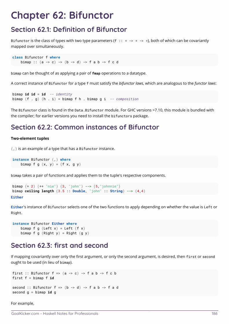
GoalKicker.com – Haskell Notes for Professionals 186

Chapter 62: BifunctorSection 62.1: Definition of BifunctorBifunctor is the class of types with two type parameters (f :: * -> * -> *), both of which can be covariantlymapped over simultaneously.

class Bifunctor f where bimap :: (a -> c) -> (b -> d) -> f a b -> f c d

bimap can be thought of as applying a pair of fmap operations to a datatype.

A correct instance of Bifunctor for a type f must satisfy the bifunctor laws, which are analogous to the functor laws:

bimap id id = id -- identitybimap (f . g) (h . i) = bimap f h . bimap g i -- composition

The Bifunctor class is found in the Data.Bifunctor module. For GHC versions >7.10, this module is bundled withthe compiler; for earlier versions you need to install the bifunctors package.

Section 62.2: Common instances of BifunctorTwo-element tuples

(,) is an example of a type that has a Bifunctor instance.

instance Bifunctor (,) where bimap f g (x, y) = (f x, g y)

bimap takes a pair of functions and applies them to the tuple's respective components.

bimap (+ 2) (++ "nie") (3, "john") --> (5,"johnnie")bimap ceiling length (3.5 :: Double, "john" :: String) --> (4,4)

Either

Either's instance of Bifunctor selects one of the two functions to apply depending on whether the value is Left orRight.

instance Bifunctor Either where bimap f g (Left x) = Left (f x) bimap f g (Right y) = Right (g y)

Section 62.3: first and secondIf mapping covariantly over only the first argument, or only the second argument, is desired, then first or secondought to be used (in lieu of bimap).

first :: Bifunctor f => (a -> c) -> f a b -> f c bfirst f = bimap f id

second :: Bifunctor f => (b -> d) -> f a b -> f a dsecond g = bimap id g

For example,

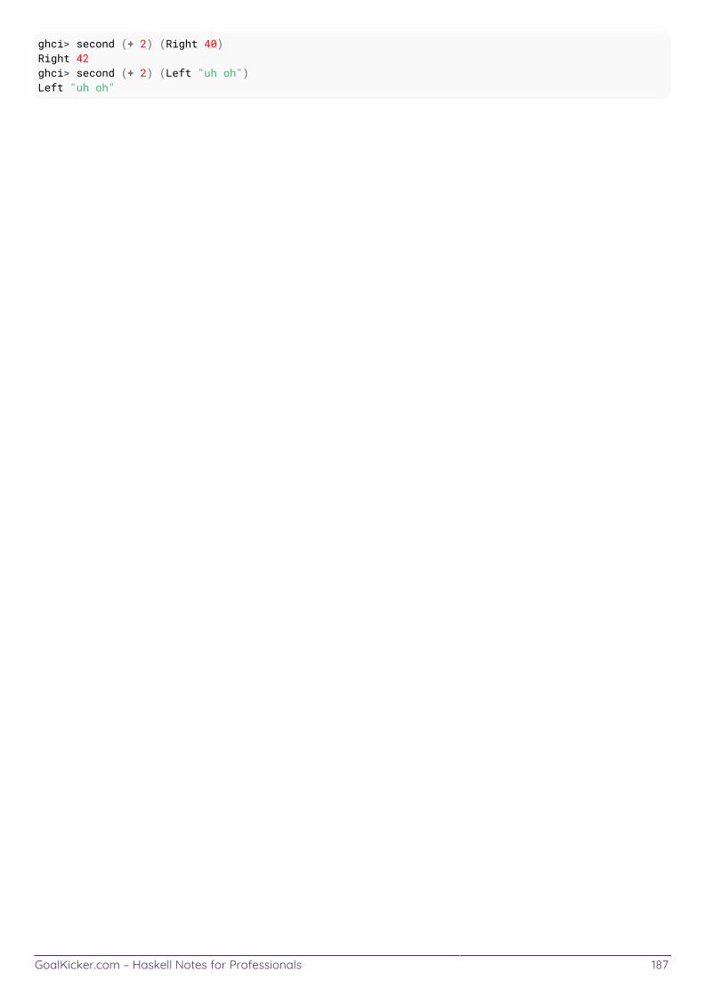
GoalKicker.com – Haskell Notes for Professionals 187

ghci> second (+ 2) (Right 40)Right 42ghci> second (+ 2) (Left "uh oh")Left "uh oh"

GoalKicker.com – Haskell Notes for Professionals 188

Chapter 63: ProxiesSection 63.1: Using ProxyThe Proxy :: k -> * type, found in Data.Proxy, is used when you need to give the compiler some typeinformation - eg, to pick a type class instance - which is nonetheless irrelevant at runtime.

{-# LANGUAGE PolyKinds #-}

data Proxy a = Proxy

Functions which use a Proxy typically use ScopedTypeVariables to pick a type class instance based on the a type.

For example, the classic example of an ambiguous function,

showread :: String -> Stringshowread = show . read

which results in a type error because the elaborator doesn't know which instance of Show or Read to use, can beresolved using Proxy:

{-# LANGUAGE ScopedTypeVariables #-}

import Data.Proxy

showread :: forall a. (Show a, Read a) => Proxy a -> String -> Stringshowread _ = (show :: a -> String) . read

When calling a function with Proxy, you need to use a type annotation to declare which a you meant.

ghci> showread (Proxy :: Proxy Int) "3""3"ghci> showread (Proxy :: Proxy Bool) "'m'" -- attempt to parse a char literal as a Bool"*** Exception: Prelude.read: no parse

Section 63.2: The "polymorphic proxy" idiomSince Proxy contains no runtime information, there is never a need to pattern-match on the Proxy constructor. So acommon idiom is to abstract over the Proxy datatype using a type variable.

showread :: forall proxy a. (Show a, Read a) => proxy a -> String -> Stringshowread _ = (show :: a -> String) . read

Now, if you happen to have an f a in scope for some f, you don't need to write out Proxy :: Proxy a when callingf.

ghci> let chars = "foo" -- chars :: [Char]ghci> showread chars "'a'""'a'"

Section 63.3: Proxy is like ()Since Proxy contains no runtime information, you can always write a natural transformation f a -> Proxy a forany f.

GoalKicker.com – Haskell Notes for Professionals 189

proxy :: f a -> Proxy aproxy _ = Proxy

This is just like how any given value can always be erased to ():

unit :: a -> ()unit _ = ()

Technically, Proxy is the terminal object in the category of functors, just like () is the terminal object in the categoryof values.

GoalKicker.com – Haskell Notes for Professionals 190

Chapter 64: Applicative FunctorApplicative is the class of types f :: * -> * which allows lifted function application over a structure where thefunction is also embedded in that structure.

Section 64.1: Alternative definitionSince every Applicative Functor is a Functor, fmap can always be used on it; thus the essence of Applicative is thepairing of carried contents, as well as the ability to create it:

class Functor f => PairingFunctor f where funit :: f () -- create a context, carrying nothing of import fpair :: (f a,f b) -> f (a,b) -- collapse a pair of contexts into a pair-carrying context

This class is isomorphic to Applicative.

pure a = const a <$> funit = a <$ funit

fa <*> fb = (\(a,b) -> a b) <$> fpair (fa, fb) = uncurry ($) <$> fpair (fa, fb)

Conversely,

funit = pure ()

fpair (fa, fb) = (,) <$> fa <*> fb

Section 64.2: Common instances of ApplicativeMaybe

Maybe is an applicative functor containing a possibly-absent value.

instance Applicative Maybe where pure = Just Just f <*> Just x = Just $ f x _ <*> _ = Nothing

pure lifts the given value into Maybe by applying Just to it. The (<*>) function applies a function wrapped in a Maybeto a value in a Maybe. If both the function and the value are present (constructed with Just), the function is appliedto the value and the wrapped result is returned. If either is missing, the computation can't proceed and Nothing isreturned instead.

Lists

One way for lists to fit the type signature <*> :: [a -> b] -> [a] -> [b] is to take the two lists' Cartesianproduct, pairing up each element of the first list with each element of the second one:

fs <*> xs = [f x | f <- fs, x <- xs] -- = do { f <- fs; x <- xs; return (f x) }

pure x = [x]

This is usually interpreted as emulating nondeterminism, with a list of values standing for a nondeterministic value

GoalKicker.com – Haskell Notes for Professionals 191

whose possible values range over that list; so a combination of two nondeterministic values ranges over all possiblecombinations of the values in the two lists:

ghci> [(+1),(+2)] <*> [3,30,300][4,31,301,5,32,302]

Infinite streams and zip-lists

There's a class of Applicatives which "zip" their two inputs together. One simple example is that of infinitestreams:

data Stream a = Stream { headS :: a, tailS :: Stream a }

Stream's Applicative instance applies a stream of functions to a stream of arguments point-wise, pairing up thevalues in the two streams by position. pure returns a constant stream – an infinite list of a single fixed value:

instance Applicative Stream where pure x = let s = Stream x s in s Stream f fs <*> Stream x xs = Stream (f x) (fs <*> xs)

Lists too admit a "zippy" Applicative instance, for which there exists the ZipList newtype:

newtype ZipList a = ZipList { getZipList :: [a] }

instance Applicative ZipList where ZipList xs <*> ZipList ys = ZipList $ zipWith ($) xs ys

Since zip trims its result according to the shortest input, the only implementation of pure that satisfies theApplicative laws is one which returns an infinite list:

pure a = ZipList (repeat a) -- ZipList (fix (a:)) = ZipList [a,a,a,a,...

For example:

ghci> getZipList $ ZipList [(+1),(+2)] <*> ZipList [3,30,300][4,32]

The two possibilities remind us of the outer and the inner product, similar to multiplying a 1-column (n x 1) matrixwith a 1-row (1 x m) one in the first case, getting the n x m matrix as a result (but flattened); or multiplying a 1-rowand a 1-column matrices (but without the summing up) in the second case.

Functions

When specialised to functions (->) r, the type signatures of pure and <*> match those of the K and S combinators,respectively:

pure :: a -> (r -> a)<*> :: (r -> (a -> b)) -> (r -> a) -> (r -> b)

pure must be const, and <*> takes a pair of functions and applies them each to a fixed argument, applying the tworesults:

instance Applicative ((->) r) where pure = const f <*> g = \x -> f x (g x)

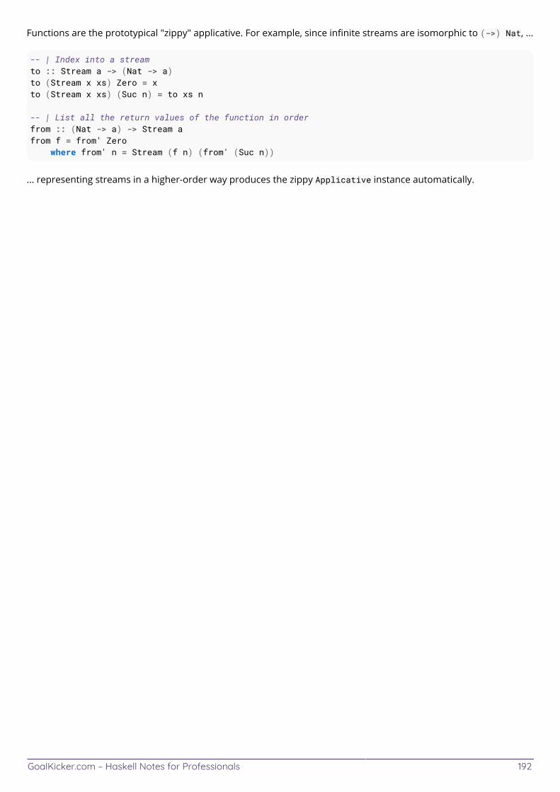
GoalKicker.com – Haskell Notes for Professionals 192

Functions are the prototypical "zippy" applicative. For example, since infinite streams are isomorphic to (->) Nat, ...

-- | Index into a streamto :: Stream a -> (Nat -> a)to (Stream x xs) Zero = xto (Stream x xs) (Suc n) = to xs n

-- | List all the return values of the function in orderfrom :: (Nat -> a) -> Stream afrom f = from' Zero where from' n = Stream (f n) (from' (Suc n))

... representing streams in a higher-order way produces the zippy Applicative instance automatically.

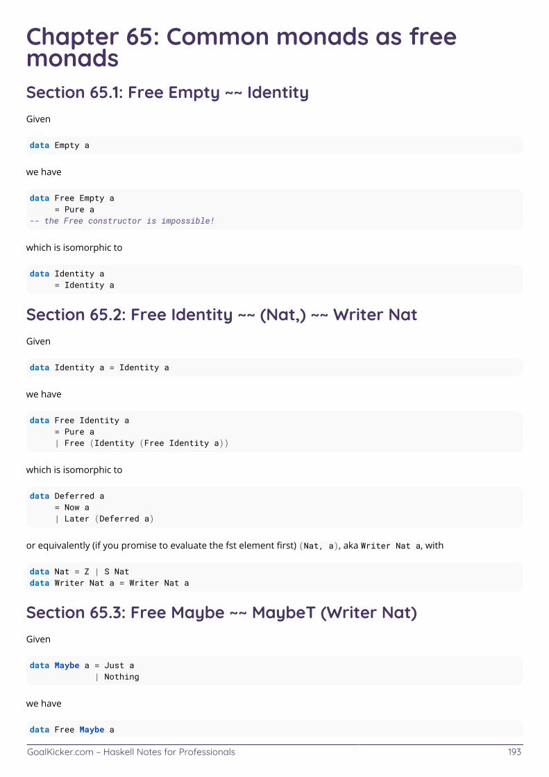
GoalKicker.com – Haskell Notes for Professionals 193

Chapter 65: Common monads as freemonadsSection 65.1: Free Empty ~~ IdentityGiven

data Empty a

we have

data Free Empty a = Pure a-- the Free constructor is impossible!

which is isomorphic to

data Identity a = Identity a

Section 65.2: Free Identity ~~ (Nat,) ~~ Writer NatGiven

data Identity a = Identity a

we have

data Free Identity a = Pure a | Free (Identity (Free Identity a))

which is isomorphic to

data Deferred a = Now a | Later (Deferred a)

or equivalently (if you promise to evaluate the fst element first) (Nat, a), aka Writer Nat a, with

data Nat = Z | S Natdata Writer Nat a = Writer Nat a

Section 65.3: Free Maybe ~~ MaybeT (Writer Nat)Given

data Maybe a = Just a | Nothing

we have

data Free Maybe a

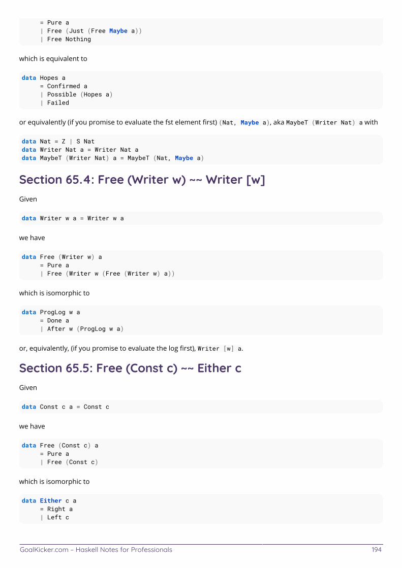
GoalKicker.com – Haskell Notes for Professionals 194

= Pure a | Free (Just (Free Maybe a)) | Free Nothing

which is equivalent to

data Hopes a = Confirmed a | Possible (Hopes a) | Failed

or equivalently (if you promise to evaluate the fst element first) (Nat, Maybe a), aka MaybeT (Writer Nat) a with

data Nat = Z | S Natdata Writer Nat a = Writer Nat adata MaybeT (Writer Nat) a = MaybeT (Nat, Maybe a)

Section 65.4: Free (Writer w) ~~ Writer [w]Given

data Writer w a = Writer w a

we have

data Free (Writer w) a = Pure a | Free (Writer w (Free (Writer w) a))

which is isomorphic to

data ProgLog w a = Done a | After w (ProgLog w a)

or, equivalently, (if you promise to evaluate the log first), Writer [w] a.

Section 65.5: Free (Const c) ~~ Either cGiven

data Const c a = Const c

we have

data Free (Const c) a = Pure a | Free (Const c)

which is isomorphic to

data Either c a = Right a | Left c

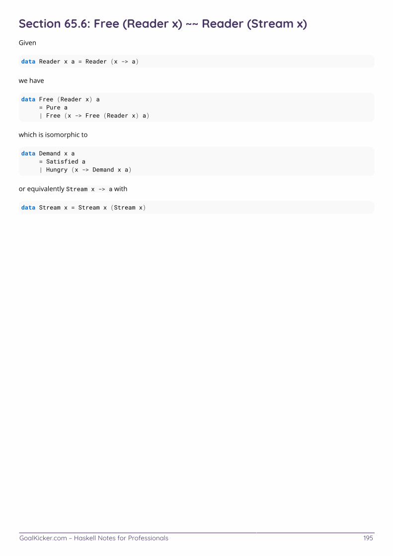
GoalKicker.com – Haskell Notes for Professionals 195

Section 65.6: Free (Reader x) ~~ Reader (Stream x)Given

data Reader x a = Reader (x -> a)

we have

data Free (Reader x) a = Pure a | Free (x -> Free (Reader x) a)

which is isomorphic to

data Demand x a = Satisfied a | Hungry (x -> Demand x a)

or equivalently Stream x -> a with

data Stream x = Stream x (Stream x)

GoalKicker.com – Haskell Notes for Professionals 196

Chapter 66: Common functors as the baseof cofree comonadsSection 66.1: Cofree Empty ~~ EmptyGiven

data Empty a

we have

data Cofree Empty a -- = a :< ... not possible!

Section 66.2: Cofree (Const c) ~~ Writer cGiven

data Const c a = Const c

we have

data Cofree (Const c) a = a :< Const c

which is isomorphic to

data Writer c a = Writer c a

Section 66.3: Cofree Identity ~~ StreamGiven

data Identity a = Identity a

we have

data Cofree Identity a = a :< Identity (Cofree Identity a)

which is isomorphic to

data Stream a = Stream a (Stream a)

Section 66.4: Cofree Maybe ~~ NonEmptyGiven

data Maybe a = Just a | Nothing

we have

GoalKicker.com – Haskell Notes for Professionals 197

data Cofree Maybe a = a :< Just (Cofree Maybe a) | a :< Nothing

which is isomorphic to

data NonEmpty a = NECons a (NonEmpty a) | NESingle a

Section 66.5: Cofree (Writer w) ~~ WriterT w StreamGiven

data Writer w a = Writer w a

we have

data Cofree (Writer w) a = a :< (w, Cofree (Writer w) a)

which is equivalent to

data Stream (w,a) = Stream (w,a) (Stream (w,a))

which can properly be written as WriterT w Stream with

data WriterT w m a = WriterT (m (w,a))

Section 66.6: Cofree (Either e) ~~ NonEmptyT (Writer e)Given

data Either e a = Left e | Right a

we have

data Cofree (Either e) a = a :< Left e | a :< Right (Cofree (Either e) a)

which is isomorphic to

data Hospitable e a = Sorry_AllIHaveIsThis_Here'sWhy a e | EatThis a (Hospitable e a)

or, if you promise to only evaluate the log after the complete result, NonEmptyT (Writer e) a with

data NonEmptyT (Writer e) a = NonEmptyT (e,a,[a])

GoalKicker.com – Haskell Notes for Professionals 198

Section 66.7: Cofree (Reader x) ~~ Moore xGiven

data Reader x a = Reader (x -> a)

we have

data Cofree (Reader x) a = a :< (x -> Cofree (Reader x) a)

which is isomorphic to

data Plant x a = Plant a (x -> Plant x a)

aka Moore machine.

GoalKicker.com – Haskell Notes for Professionals 199

Chapter 67: ArithmeticThe numeric typeclass hierarchy

Num sits at the root of the numeric typeclass hierarchy. Its characteristic operations and some common instancesare shown below (the ones loaded by default with Prelude plus those of Data.Complex):

λ> :i Numclass Num a where (+) :: a -> a -> a (-) :: a -> a -> a (*) :: a -> a -> a negate :: a -> a abs :: a -> a signum :: a -> a fromInteger :: Integer -> a {-# MINIMAL (+), (*), abs, signum, fromInteger, (negate | (-)) #-} -- Defined in ‘GHC.Num’instance RealFloat a => Num (Complex a) -- Defined in ‘Data.Complex’instance Num Word -- Defined in ‘GHC.Num’instance Num Integer -- Defined in ‘GHC.Num’instance Num Int -- Defined in ‘GHC.Num’instance Num Float -- Defined in ‘GHC.Float’instance Num Double -- Defined in ‘GHC.Float’

We have already seen the Fractional class, which requires Num and introduces the notions of "division" (/) andreciprocal of a number:

λ> :i Fractionalclass Num a => Fractional a where (/) :: a -> a -> a recip :: a -> a fromRational :: Rational -> a {-# MINIMAL fromRational, (recip | (/)) #-} -- Defined in ‘GHC.Real’instance RealFloat a => Fractional (Complex a) -- Defined in ‘Data.Complex’instance Fractional Float -- Defined in ‘GHC.Float’instance Fractional Double -- Defined in ‘GHC.Float’

The Real class models .. the real numbers. It requires Num and Ord, therefore it models an ordered numerical field.As a counterexample, Complex numbers are not an ordered field (i.e. they do not possess a natural orderingrelationship):

λ> :i Realclass (Num a, Ord a) => Real a where toRational :: a -> Rational {-# MINIMAL toRational #-} -- Defined in ‘GHC.Real’instance Real Word -- Defined in ‘GHC.Real’instance Real Integer -- Defined in ‘GHC.Real’instance Real Int -- Defined in ‘GHC.Real’instance Real Float -- Defined in ‘GHC.Float’instance Real Double -- Defined in ‘GHC.Float’

RealFrac represents numbers that may be rounded

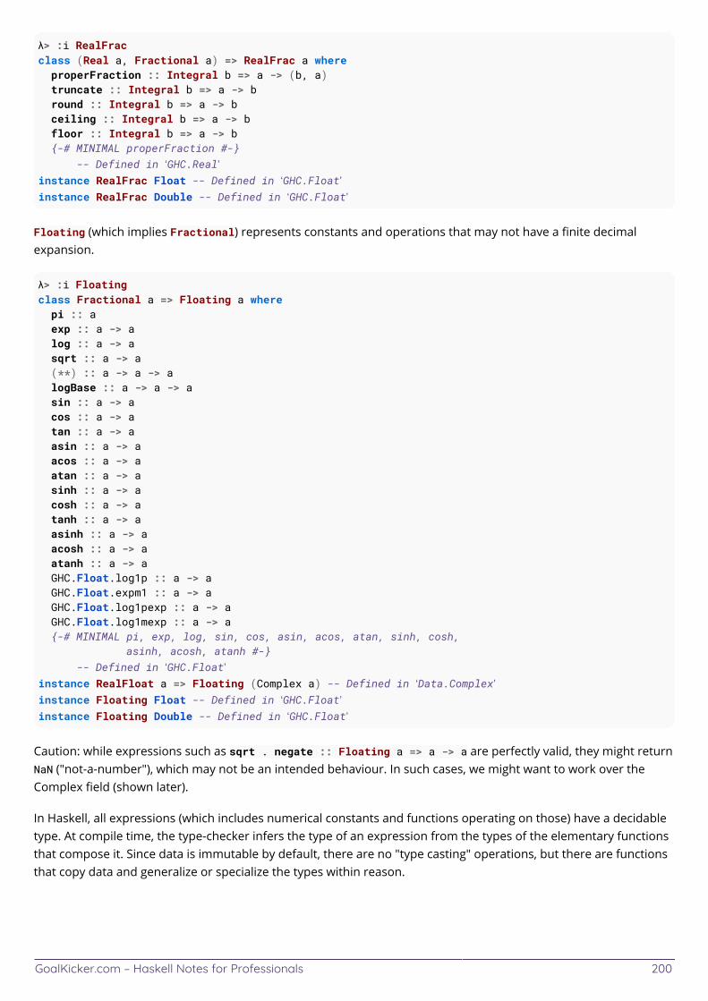
GoalKicker.com – Haskell Notes for Professionals 200

λ> :i RealFracclass (Real a, Fractional a) => RealFrac a where properFraction :: Integral b => a -> (b, a) truncate :: Integral b => a -> b round :: Integral b => a -> b ceiling :: Integral b => a -> b floor :: Integral b => a -> b {-# MINIMAL properFraction #-} -- Defined in ‘GHC.Real’instance RealFrac Float -- Defined in ‘GHC.Float’instance RealFrac Double -- Defined in ‘GHC.Float’

Floating (which implies Fractional) represents constants and operations that may not have a finite decimalexpansion.

λ> :i Floatingclass Fractional a => Floating a where pi :: a exp :: a -> a log :: a -> a sqrt :: a -> a (**) :: a -> a -> a logBase :: a -> a -> a sin :: a -> a cos :: a -> a tan :: a -> a asin :: a -> a acos :: a -> a atan :: a -> a sinh :: a -> a cosh :: a -> a tanh :: a -> a asinh :: a -> a acosh :: a -> a atanh :: a -> a GHC.Float.log1p :: a -> a GHC.Float.expm1 :: a -> a GHC.Float.log1pexp :: a -> a GHC.Float.log1mexp :: a -> a {-# MINIMAL pi, exp, log, sin, cos, asin, acos, atan, sinh, cosh, asinh, acosh, atanh #-} -- Defined in ‘GHC.Float’instance RealFloat a => Floating (Complex a) -- Defined in ‘Data.Complex’instance Floating Float -- Defined in ‘GHC.Float’instance Floating Double -- Defined in ‘GHC.Float’

Caution: while expressions such as sqrt . negate :: Floating a => a -> a are perfectly valid, they might returnNaN ("not-a-number"), which may not be an intended behaviour. In such cases, we might want to work over theComplex field (shown later).

In Haskell, all expressions (which includes numerical constants and functions operating on those) have a decidabletype. At compile time, the type-checker infers the type of an expression from the types of the elementary functionsthat compose it. Since data is immutable by default, there are no "type casting" operations, but there are functionsthat copy data and generalize or specialize the types within reason.

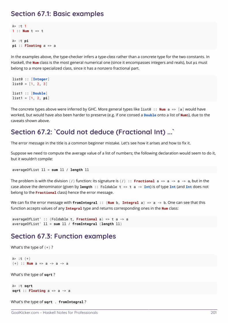
GoalKicker.com – Haskell Notes for Professionals 201

Section 67.1: Basic examplesλ> :t 11 :: Num t => t

λ> :t pipi :: Floating a => a

In the examples above, the type-checker infers a type-class rather than a concrete type for the two constants. InHaskell, the Num class is the most general numerical one (since it encompasses integers and reals), but pi mustbelong to a more specialized class, since it has a nonzero fractional part.

list0 :: [Integer]list0 = [1, 2, 3]

list1 :: [Double]list1 = [1, 2, pi]

The concrete types above were inferred by GHC. More general types like list0 :: Num a => [a] would haveworked, but would have also been harder to preserve (e.g. if one consed a Double onto a list of Nums), due to thecaveats shown above.

Section 67.2: `Could not deduce (Fractional Int) ...`The error message in the title is a common beginner mistake. Let's see how it arises and how to fix it.

Suppose we need to compute the average value of a list of numbers; the following declaration would seem to do it,but it wouldn't compile:

averageOfList ll = sum ll / length ll

The problem is with the division (/) function: its signature is (/) :: Fractional a => a -> a -> a, but in thecase above the denominator (given by length :: Foldable t => t a -> Int) is of type Int (and Int does notbelong to the Fractional class) hence the error message.

We can fix the error message with fromIntegral :: (Num b, Integral a) => a -> b. One can see that thisfunction accepts values of any Integral type and returns corresponding ones in the Num class:

averageOfList' :: (Foldable t, Fractional a) => t a -> aaverageOfList' ll = sum ll / fromIntegral (length ll)

Section 67.3: Function examplesWhat's the type of (+) ?

λ> :t (+)(+) :: Num a => a -> a -> a

What's the type of sqrt ?

λ> :t sqrtsqrt :: Floating a => a -> a

What's the type of sqrt . fromIntegral ?

GoalKicker.com – Haskell Notes for Professionals 202

sqrt . fromIntegral :: (Integral a, Floating c) => a -> c

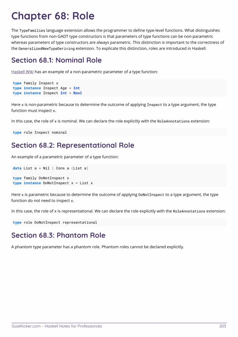
GoalKicker.com – Haskell Notes for Professionals 203

Chapter 68: RoleThe TypeFamilies language extension allows the programmer to define type-level functions. What distinguishestype functions from non-GADT type constructors is that parameters of type functions can be non-parametricwhereas parameters of type constructors are always parametric. This distinction is important to the correctness ofthe GeneralizedNewTypeDeriving extension. To explicate this distinction, roles are introduced in Haskell.

Section 68.1: Nominal RoleHaskell Wiki has an example of a non-parametric parameter of a type function:

type family Inspect xtype instance Inspect Age = Int type instance Inspect Int = Bool

Here x is non-parametric because to determine the outcome of applying Inspect to a type argument, the typefunction must inspect x.

In this case, the role of x is nominal. We can declare the role explicitly with the RoleAnnotations extension:

type role Inspect nominal

Section 68.2: Representational RoleAn example of a parametric parameter of a type function:

data List a = Nil | Cons a (List a)

type family DoNotInspect xtype instance DoNotInspect x = List x

Here x is parametric because to determine the outcome of applying DoNotInspect to a type argument, the typefunction do not need to inspect x.

In this case, the role of x is representational. We can declare the role explicitly with the RoleAnnotations extension:

type role DoNotInspect representational

Section 68.3: Phantom RoleA phantom type parameter has a phantom role. Phantom roles cannot be declared explicitly.

GoalKicker.com – Haskell Notes for Professionals 204

Chapter 69: Arbitrary-rank polymorphismwith RankNTypesGHC’s type system supports arbitrary-rank explicit universal quantification in types through the use of theRank2Types and RankNTypes language extensions.

Section 69.1: RankNTypesStackOverflow forces me to have one example. If this topic is approved, we should move this example here.

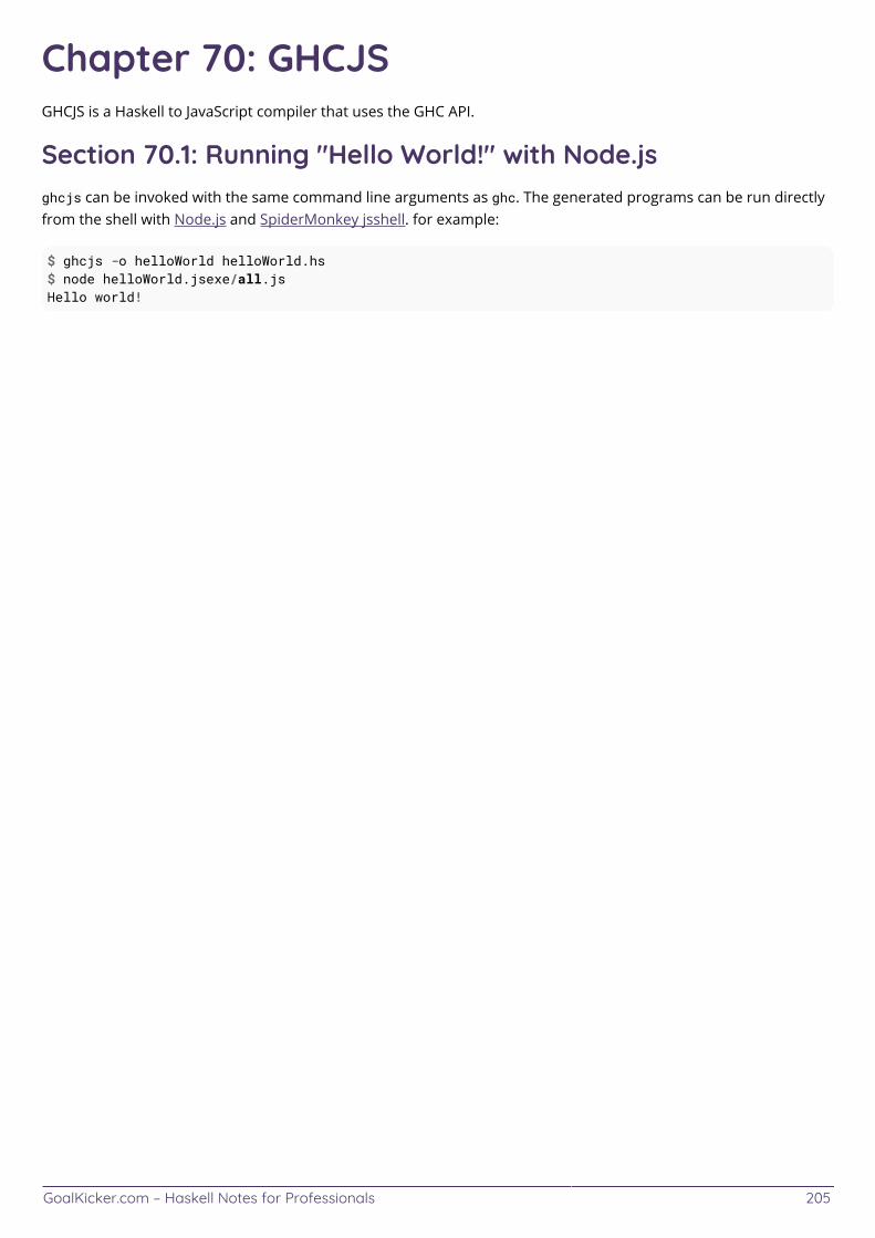
GoalKicker.com – Haskell Notes for Professionals 205

Chapter 70: GHCJSGHCJS is a Haskell to JavaScript compiler that uses the GHC API.

Section 70.1: Running "Hello World!" with Node.jsghcjs can be invoked with the same command line arguments as ghc. The generated programs can be run directlyfrom the shell with Node.js and SpiderMonkey jsshell. for example:

$ ghcjs -o helloWorld helloWorld.hs$ node helloWorld.jsexe/all.jsHello world!

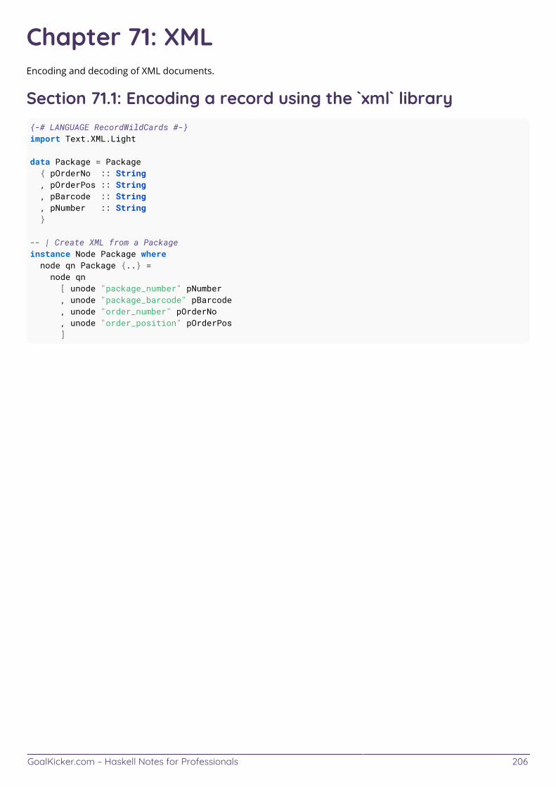
GoalKicker.com – Haskell Notes for Professionals 206

Chapter 71: XMLEncoding and decoding of XML documents.

Section 71.1: Encoding a record using the `xml` library{-# LANGUAGE RecordWildCards #-}import Text.XML.Light

data Package = Package { pOrderNo :: String , pOrderPos :: String , pBarcode :: String , pNumber :: String }

-- | Create XML from a Packageinstance Node Package where node qn Package {..} = node qn [ unode "package_number" pNumber , unode "package_barcode" pBarcode , unode "order_number" pOrderNo , unode "order_position" pOrderPos ]

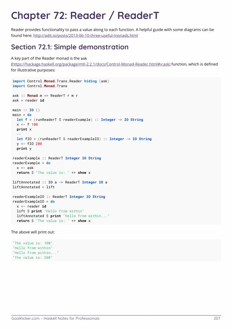
GoalKicker.com – Haskell Notes for Professionals 207

Chapter 72: Reader / ReaderTReader provides functionality to pass a value along to each function. A helpful guide with some diagrams can befound here: http://adit.io/posts/2013-06-10-three-useful-monads.html

Section 72.1: Simple demonstrationA key part of the Reader monad is the ask(https://hackage.haskell.org/package/mtl-2.2.1/docs/Control-Monad-Reader.html#v:ask) function, which is definedfor illustrative purposes:

import Control.Monad.Trans.Reader hiding (ask)import Control.Monad.Trans

ask :: Monad m => ReaderT r m rask = reader id

main :: IO ()main = do let f = (runReaderT $ readerExample) :: Integer -> IO String x <- f 100 print x -- let fIO = (runReaderT $ readerExampleIO) :: Integer -> IO String y <- fIO 200 print y

readerExample :: ReaderT Integer IO StringreaderExample = do x <- ask return $ "The value is: " ++ show x

liftAnnotated :: IO a -> ReaderT Integer IO aliftAnnotated = lift

readerExampleIO :: ReaderT Integer IO StringreaderExampleIO = do x <- reader id lift $ print "Hello from within" liftAnnotated $ print "Hello from within..." return $ "The value is: " ++ show x

The above will print out:

"The value is: 100""Hello from within""Hello from within...""The value is: 200"

GoalKicker.com – Haskell Notes for Professionals 208

Chapter 73: Function call syntaxHaskell's function call syntax, explained with comparisons to C-style languages where applicable. This is aimed atpeople who are coming to Haskell from a background in C-style languages.

Section 73.1: Partial application - Part 1In Haskell, functions can be partially applied; we can think of all functions as taking a single argument, andreturning a modified function for which that argument is constant. To illustrate this, we can bracket functions asfollows:

(((plus) 1) 2)

Here, the function (plus) is applied to 1 yielding the function ((plus) 1), which is applied to 2, yielding thefunction (((plus) 1) 2). Because plus 1 2 is a function which takes no arguments, you can consider it a plainvalue; however in Haskell, there is little distinction between functions and values.

To go into more detail, the function plus is a function that adds its arguments.The function plus 1 is a function that adds 1 to its argument.The function plus 1 2 is a function that adds 1 to 2, which is always the value 3.

Section 73.2: Partial application - Part 2As another example, we have the function map, which takes a function and a list of values, and applies the functionto each value of the list:

map :: (a -> b) -> [a] -> [b]

Let's say we want to increment each value in a list. You may decide to define your own function, which adds one toits argument, and map that function over your list

addOne x = plus 1 xmap addOne [1,2,3]

but if you have another look at addOne's definition, with parentheses added for emphasis:

(addOne) x = ((plus) 1) x

The function addOne, when applied to any value x, is the same as the partially applied function plus 1 applied to x.This means the functions addOne and plus 1 are identical, and we can avoid defining a new function by justreplacing addOne with plus 1, remembering to use parentheses to isolate plus 1 as a subexpression:

map (plus 1) [1,2,3]

Section 73.3: Parentheses in a basic function callFor a C-style function call, e.g.

plus(a, b); // Parentheses surrounding only the arguments, comma separated

Then the equivalent Haskell code will be

GoalKicker.com – Haskell Notes for Professionals 209

(plus a b) -- Parentheses surrounding the function and the arguments, no commas

In Haskell, parentheses are not explicitly required for function application, and are only used to disambiguateexpressions, like in mathematics; so in cases where the brackets surround all the text in the expression, theparentheses are actually not needed, and the following is also equivalent:

plus a b -- no parentheses are needed here!

It is important to remember that while in C-style languages, the function

Section 73.4: Parentheses in embedded function callsIn the previous example, we didn't end up needing the parentheses, because they did not affect the meaning of thestatement. However, they are often necessary in more complex expression, like the one below.In C:

plus(a, take(b, c));

In Haskell this becomes:

(plus a (take b c))-- or equivalently, omitting the outermost parenthesesplus a (take b c)

Note, that this is not equivalent to:

plus a take b c -- Not what we want!

One might think that because the compiler knows that take is a function, it would be able to know that you want toapply it to the arguments b and c, and pass its result to plus.However, in Haskell, functions often take other functions as arguments, and little actual distinction is madebetween functions and other values; and so the compiler cannot assume your intention simply because take is afunction.

And so, the last example is analogous to the following C function call:

plus(a, take, b, c); // Not what we want!

GoalKicker.com – Haskell Notes for Professionals 210

Chapter 74: LoggingLogging in Haskell is achieved usually through functions in the IO monad, and so is limited to non-pure functions or"IO actions".

There are several ways to log information in a Haskell program: from putStrLn (or print), to libraries such ashslogger or through Debug.Trace.

Section 74.1: Logging with hsloggerThe hslogger module provides a similar API to Python's logging framework, and supports hierarchically namedloggers, levels and redirection to handles outside of stdout and stderr.

By default, all messages of level WARNING and above are sent to stderr and all other log levels are ignored.

import System.Log.Logger (Priority (DEBUG), debugM, infoM, setLevel, updateGlobalLogger, warningM)

main = do debugM "MyProgram.main" "This won't be seen" infoM "MyProgram.main" "This won't be seen either" warningM "MyProgram.main" "This will be seen"

We can set the level of a logger by its name using updateGlobalLogger:

updateGlobalLogger "MyProgram.main" (setLevel DEBUG)

debugM "MyProgram.main" "This will now be seen"

Each Logger has a name, and they are arranged hierarchically, so MyProgram is a parent of MyParent.Module.

GoalKicker.com – Haskell Notes for Professionals 211

Chapter 75: AttoparsecType Detail

Parser i a The core type for representing a parser. i is the string type, e.g. ByteString.

IResult i r The result of a parse, with Fail i [String] String, Partial (i -> IResult i r) and Done i r asconstructors.

Attoparsec is a parsing combinator library that is "aimed particularly at dealing efficiently with network protocolsand complicated text/binary file formats".

Attoparsec offers not only speed and efficiency, but backtracking and incremental input.

Its API closely mirrors that of another parser combinator library, Parsec.

There are submodules for compatibility with ByteString, Text and Char8. Use of the OverloadedStrings languageextension is recommended.

Section 75.1: CombinatorsParsing input is best achieved through larger parser functions that are composed of smaller, single purpose ones.

Let's say we wished to parse the following text which represents working hours:

Monday: 0800 1600.

We could split these into two "tokens": the day name -- "Monday" -- and a time portion "0800" to "1600".

To parse a day name, we could write the following:

data Day = Day String day :: Parser Day day = do name <- takeWhile1 (/= ':') skipMany1 (char ':') skipSpace return $Day name

To parse the time portion we could write:

data TimePortion = TimePortion String String time = do start <- takeWhile1 isDigit skipSpace end <- takeWhile1isDigit return $ TimePortion start end

Now we have two parsers for our individual parts of the text, we can combine these in a "larger" parser to read anentire day's working hours:

data WorkPeriod = WorkPeriod Day TimePortion work = do d <- day t <- time return $ WorkPeriod d t

and then run the parser:

parseOnly work "Monday: 0800 1600"

Section 75.2: Bitmap - Parsing Binary DataAttoparsec makes parsing binary data trivial. Assuming these definitions:

import Data.Attoparsec.ByteString (Parser, eitherResult, parse, take)import Data.Binary.Get (getWord32le, runGet)import Data.ByteString (ByteString, readFile)

GoalKicker.com – Haskell Notes for Professionals 212

import Data.ByteString.Char8 (unpack)import Data.ByteString.Lazy (fromStrict)import Prelude hiding (readFile, take)

-- The DIB section from a bitmap headerdata DIB = BM | BA | CI | CP | IC | PT deriving (Show, Read)

type Reserved = ByteString

-- The entire bitmap headerdata Header = Header DIB Int Reserved Reserved Int deriving (Show)

We can parse the header from a bitmap file easily. Here, we have 4 parser functions that represent the headersection from a bitmap file:

Firstly, the DIB section can be read by taking the first 2 bytes

dibP :: Parser DIBdibP = read . unpack <$> take 2

Similarly, the size of the bitmap, the reserved sections and the pixel offset can be read easily too:

sizeP :: Parser IntsizeP = fromIntegral . runGet getWord32le . fromStrict <$> take 4

reservedP :: Parser ReservedreservedP = take 2

addressP :: Parser IntaddressP = fromIntegral . runGet getWord32le . fromStrict <$> take 4

which can then be combined into a larger parser function for the entire header:

bitmapHeader :: Parser HeaderbitmapHeader = do dib <- dibP sz <- sizeP reservedP reservedP offset <- addressP return $ Header dib sz "" "" offset

GoalKicker.com – Haskell Notes for Professionals 213

Chapter 76: zipWithMzipWithM is to zipWith as mapM is to map: it lets you combine two lists using a monadic function.

From the module Control.Monad

Section 76.1: Calculatings sales pricesSuppose you want to see if a certain set of sales prices makes sense for a store.

The items originally cost $5, so you don't want to accept the sale if the sales price is less for any of them, but you dowant to know what the new price is otherwise.

Calculating one price is easy: you calculate the sales price, and return Nothing if you don't get a profit:

calculateOne :: Double -> Double -> Maybe DoublecalculateOne price percent = let newPrice = price*(percent/100) in if newPrice < 5 then Nothing else Just newPrice

To calculate it for the entire sale, zipWithM makes it really simple:

calculateAllPrices :: [Double] -> [Double] -> Maybe [Double]calculateAllPrices prices percents = zipWithM calculateOne prices percents

This will return Nothing if any of the sales prices are below $5.

GoalKicker.com – Haskell Notes for Professionals 214

Chapter 77: ProfunctorProfunctor is a typeclass provided by the profunctors package in Data.Profunctor.

See the "Remarks" section for a full explanation.

Section 77.1: (->) Profunctor(->) is a simple example of a profunctor: the left argument is the input to a function, and the right argument is thesame as the reader functor instance.

instance Profunctor (->) where lmap f g = g . f rmap f g = g . g

GoalKicker.com – Haskell Notes for Professionals 215

Chapter 78: Type ApplicationTypeApplications are an alternative to type annotations when the compiler struggles to infer types for a givenexpression.

This series of examples will explain the purpose of the TypeApplications extension and how to use it

Don't forget to enable the extension by placing {-# LANGUAGE TypeApplications #-} at the top of your source file.

Section 78.1: Avoiding type annotationsWe use type annotations to avoid ambiguity. Type applications can be used for the same purpose. For example

x :: Num a => ax = 5

main :: IO ()main = print x

This code has an ambiguity error. We know that a has a Num instance, and in order to print it we know it needs aShow instance. This could work if a was, for example, an Int, so to fix the error we can add a type annotation

main = print (x :: Int)

Another solution using type applications would look like this

main = print @Int x

To understand what this means we need to look at the type signature of print.

print :: Show a => a -> IO ()

The function takes one parameter of type a, but another way to look at it is that it actually takes two parameters.The first one is a type parameter, the second one is a value whose type is the first parameter.

The main difference between value parameters and the type parameters is that the latter ones are implicitlyprovided to functions when we call them. Who provides them? The type inference algorithm! WhatTypeApplications let us do is give those type parameters explicitly. This is especially useful when the typeinference can't determine the correct type.

So to break down the above example

print :: Show a => a -> IO ()print @Int :: Int -> IO ()print @Int x :: IO ()

Section 78.2: Type applications in other languagesIf you're familiar with languages like Java, C# or C++ and the concept of generics/templates then this comparisonmight be useful for you.

Say we have a generic function in C#

GoalKicker.com – Haskell Notes for Professionals 216

public static T DoNothing<T>(T in) { return in; }

To call this function with a float we can do DoNothing(5.0f) or if we want to be explicit we can sayDoNothing<float>(5.0f). That part inside of the angle brackets is the type application.

In Haskell it's the same, except that the type parameters are not only implicit at call sites but also at definition sites.

doNothing :: a -> adoNothing x = x

This can also be made explicit using either ScopedTypeVariables, Rank2Types or RankNTypes extensions like this.

doNothing :: forall a. a -> adoNothing x = x

Then at the call site we can again either write doNothing 5.0 or doNothing @Float 5.0

Section 78.3: Order of parametersThe problem with type arguments being implicit becomes obvious once we have more than one. Which order dothey come in?

const :: a -> b -> a

Does writing const @Int mean a is equal to Int, or is it b? In case we explicitly state the type parameters using aforall like const :: forall a b. a -> b -> a then the order is as written: a, then b.

If we don't, then the order of variables is from left to right. The first variable to be mentioned is the first typeparameter, the second is the second type parameter and so on.

What if we want to specify the second type variable, but not the first? We can use a wildcard for the first variablelike this

const @_ @Int

The type of this expression is

const @_ @Int :: a -> Int -> a

Section 78.4: Interaction with ambiguous typesSay you're introducing a class of types that have a size in bytes.

class SizeOf a where sizeOf :: a -> Int

The problem is that the size should be constant for every value of that type. We don't actually want the sizeOffunction to depend on a, but only on it's type.

Without type applications, the best solution we had was the Proxy type defined like this

data Proxy a = Proxy

The purpose of this type is to carry type information, but no value information. Then our class could look like this

GoalKicker.com – Haskell Notes for Professionals 217

class SizeOf a where sizeOf :: Proxy a -> Int

Now you might be wondering, why not drop the first argument altogether? The type of our function would then justbe sizeOf :: Int or, to be more precise because it is a method of a class, sizeOf :: SizeOf a => Int or to beeven more explicit sizeOf :: forall a. SizeOf a => Int.

The problem is type inference. If I write sizeOf somewhere, the inference algorithm only knows that I expect anInt. It has no idea what type I want to substitute for a. Because of this, the definition gets rejected by the compilerunless you have the {-# LANGUAGE AllowAmbiguousTypes #-} extension enabled. In that case the definitioncompiles,it just can't be used anywhere without an ambiguity error.

Luckily, the introduction of type applications saves the day! Now we can write sizeOf @Int, explicitly saying that a isInt. Type applications allow us to provide a type parameter, even if it doesn't appear in the actual parameters of thefunction!

GoalKicker.com – Haskell Notes for Professionals 218

CreditsThank you greatly to all the people from Stack Overflow Documentation who helped provide this content,

more changes can be sent to web@petercv.com for new content to be published or updated

3442 Chapter 10Adam Wagner Chapter 2Alec Chapters 18 and 37alejosocorro Chapter 1Amitay Stern Chapter 1Antal Spector Chapter 7arjanen Chapter 9arrowd Chapters 14, 29, 38 and 59arseniiv Chapters 1, 12, 21 and 32Bartek Banachewicz Chapters 5 and 7baxbaxwalanuksiwe Chapter 1Benjamin Hodgson Chapters 3, 4, 6, 8, 10, 13, 15, 18, 21, 22, 23, 24, 26, 50, 51, 55, 62, 63 and 64Benjamin Kovach Chapters 1, 7, 14 and 24Billy Brown Chapter 9bleakgadfly Chapters 59 and 60Brian Min Chapter 16Burkhard Chapter 1Cactus Chapters 3, 7, 8, 9, 11, 24, 36, 44 and 52carpemb Chapter 19Carsten Chapter 2Chris Stryczynski Chapters 34 and 72Christof Schramm Chapter 50CiscoIPPhone Chapter 12crockeea Chapter 59Dair Chapter 19Damian Nadales Chapter 61Daniel Jour Chapter 1David Grayson Chapter 10Delapouite Chapter 25dkasak Chapter 22Doruk Chapter 35dsign Chapter 5erisco Chapters 1 and 15fgb Chapter 18Firas Moalla Chapter 15Gallifreyan Chapters 1 and 15gdziadkiewicz Chapters 1, 6 and 9Itbot Chapter 36J Atkin Chapter 1J. Abrahamson Chapters 3, 4, 5, 8, 9, 10 and 14James Chapters 23 and 25Janos Potecki Chapters 7, 11, 15, 19, 23, 25, 28, 31, 34 and 48jkeuhlen Chapter 22John F. Miller Chapters 5, 7 and 11Jules Chapter 1K48 Chapter 7Kapol Chapters 18 and 28

GoalKicker.com – Haskell Notes for Professionals 219

Kostiantyn Rybnikov Chapter 58Kwarrtz Chapters 1, 5, 9, 18 and 46leftaroundabout Chapters 1, 2, 7, 9, 10, 17, 42, 43, 56, 65 and 66liminalisht Chapters 26 and 62Luis Casillas Chapter 54Luka Horvat Chapter 78Lynn Chapters 15 and 18Mads Buch Chapter 7Mario Román Chapters 14, 18 and 41mathk Chapter 26Matthew Pickering Chapters 5, 6, 11, 12 and 34Matthew Walton Chapter 15mb21 Chapter 1Mikkel Chapters 70 and 71Mirzhan Irkegulov Chapter 15mkovacs Chapter 7mniip Chapters 7, 17 and 20mnoronha Chapters 1, 3, 15, 22, 26, 46, 52, 56 and 64Mr Tsjolder Chapter 1ocharles Chapters 1 and 69ocramz Chapter 67pdexter Chapter 2pouya Chapter 1Sebastian Graf Chapter 1Shoe Chapter 16Stephane Rolland Chapter 55Steve Trout Chapter 6tlo Chapters 27 and 40Toxaris Chapter 52Undreren Chapter 29unhammer Chapter 22user239558 Chapter 1user2407038 Chapters 10, 14, 15, 24, 43 and 49Vektorweg Chapter 16

Will Ness Chapters 1, 10, 12, 13, 15, 16, 18, 24, 25, 26, 32, 35, 36, 37, 43, 45, 46, 51 and64

Wysaard Chapter 53xuh Chapters 17, 34 and 68Yosh Chapters 7 and 15zbw Chapters 1, 76 and 77zeronone Chapter 9Zoey Hewll Chapter 73

λlεx Chapters 1, 7, 9, 10, 11, 15, 18, 23, 25, 26, 30, 31, 33, 35, 36, 38, 39, 45, 47, 48,51, 55, 57, 58, 64, 74 and 75

You may also like