Embed Size (px)
Citation preview
Outline Basics Collision resolution Universal hashing Efficiency
Hashing to Store Symbol TablesBasics Collision resolution Universal hashing
Lecturer: Georgy Gimel’farb
COMPSCI 220 Algorithms and Data Structures
1 / 41
Outline Basics Collision resolution Universal hashing Efficiency
1 Hash tables: basics
2 Hash tables: collision resolution
3 Universal hashing
4 Search efficiency of hash tables
2 / 41
Outline Basics Collision resolution Universal hashing Efficiency
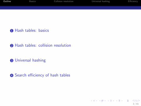
World Airports
Textbook, Table 3.1 of airports ordered by symbolic codes:
Key, k Associated value, v
Code City Country Place
AKL Auckland New ZealandDCA Washington USA District ColumbiaFRA Frankfurt a.M. Germany Rheinland-PfalzGLA Glasgow UK ScotlandHKG Hong Kong ChinaLAX Los Angeles USA CaliforniaORY Paris-Orly FranceSDF Louisville USA Kentucky
Array implementation: works well, provided the number of possiblesearch keys is sufficiently small (here, 263 = 17, 576 codes).
3 / 41
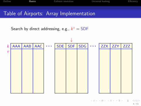
Outline Basics Collision resolution Universal hashing Efficiency
Table of Airports: Array Implementation
Search by direct addressing, e.g., k◦ = SDF
kv
AAA AAB AAC . . .↓
SDE SDF SDG . . . ZZX ZZY ZZZ
4 / 41
Outline Basics Collision resolution Universal hashing Efficiency
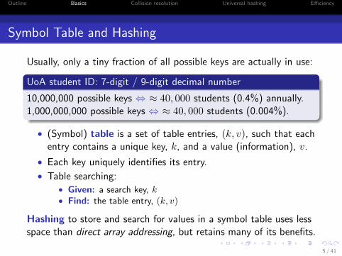
Symbol Table and Hashing
Usually, only a tiny fraction of all possible keys are actually in use:
UoA student ID: 7-digit / 9-digit decimal number
10,000,000 possible keys ⇔ ≈ 40, 000 students (0.4%) annually.1,000,000,000 possible keys ⇔ ≈ 40, 000 students (0.004%).
• (Symbol) table is a set of table entries, (k, v), such that eachentry contains a unique key, k, and a value (information), v.
• Each key uniquely identifies its entry.
• Table searching:• Given: a search key, k• Find: the table entry, (k, v)
Hashing to store and search for values in a symbol table uses lessspace than direct array addressing, but retains many of its benefits.
5 / 41
Outline Basics Collision resolution Universal hashing Efficiency
Symbol Table and Hashing
Hashing stores values and searches for them in:
• Linear, O(n), worst-case time and
• Extremely fast, O(1), average-case time.
Once the entry (k, v) of a symbol table is found:
• its value v, may be updated, or
• it may be retrieved, or
• the entire entry, (k, v), may be removed from the table.
If no entry with key k exists in the table:
• A new entry with k as its key may be inserted to the table.
6 / 41
Outline Basics Collision resolution Universal hashing Efficiency
Basic Features of Hashing
Hashing computes an integer hash code, for each object.
• The computation implements a hash function, h(k).
• It maps objects (e.g., keys k) to indices of a given linear array,called the hash table.
• The function must always return a valid array index.
An object with a key k has to be stored at the location h(k).
• Hash codes must be computed quickly.
• Hashing a key to an index depends only on the key to hash.
• It is independent of all other keys in the table.
7 / 41
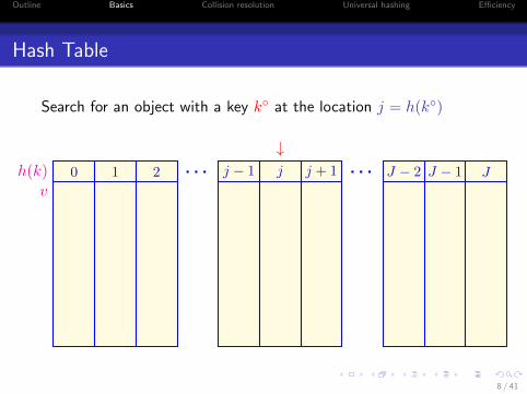
Outline Basics Collision resolution Universal hashing Efficiency
Hash Table
Search for an object with a key k◦ at the location j = h(k◦)
h(k)
v0 1 2 . . .
↓j − 1 j j + 1 . . . J − 2 J − 1 J
8 / 41
Outline Basics Collision resolution Universal hashing Efficiency
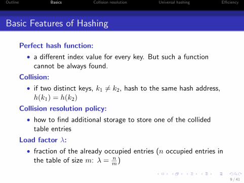
Basic Features of Hashing
Perfect hash function:
• a different index value for every key. But such a functioncannot be always found.
Collision:
• if two distinct keys, k1 6= k2, hash to the same hash address,h(k1) = h(k2)
Collision resolution policy:
• how to find additional storage to store one of the collidedtable entries
Load factor λ:
• fraction of the already occupied entries (n occupied entries inthe table of size m: λ = n
m)
9 / 41
Outline Basics Collision resolution Universal hashing Efficiency
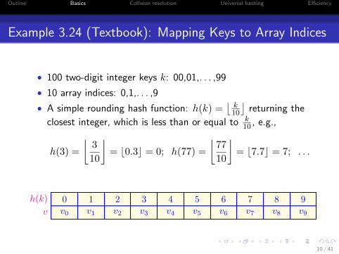
Example 3.24 (Textbook): Mapping Keys to Array Indices
• 100 two-digit integer keys k: 00,01,. . . ,99
• 10 array indices: 0,1,. . . ,9
• A simple rounding hash function: h(k) =⌊k10
⌋returning the
closest integer, which is less than or equal to k10 , e.g.,
h(3) =
⌊3
10
⌋= b0.3c = 0; h(77) =
⌊77
10
⌋= b7.7c = 7; . . .
h(k)
v
0v0
1v1
2v2
3v3
4v4
5v5
6v6
7v7
8v8
9v9
10 / 41
Outline Basics Collision resolution Universal hashing Efficiency
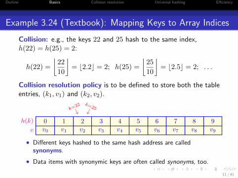
Example 3.24 (Textbook): Mapping Keys to Array Indices
Collision: e.g., the keys 22 and 25 hash to the same index,h(22) = h(25) = 2:
h(22) =
⌊22
10
⌋= b2.2c = 2; h(25) =
⌊25
10
⌋= b2.5c = 2; . . .
Collision resolution policy is to be defined to store both the tableentries, (k1, v1) and (k2, v2).
h(k)
v
k=22
↓k=25↓
0v0
1v1
2v2
3v3
4v4
5v5
6v6
7v7
8v8
9v9
• Different keys hashed to the same hash address are calledsynonyms.
• Data items with synonymic keys are often called synonyms, too.
11 / 41
Outline Basics Collision resolution Universal hashing Efficiency
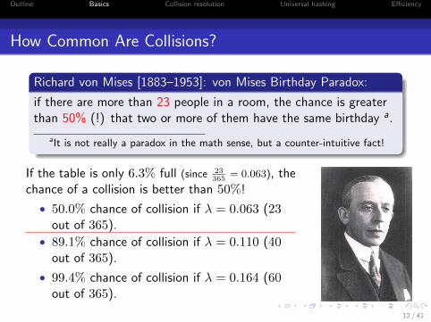
How Common Are Collisions?
Richard von Mises [1883–1953]: von Mises Birthday Paradox:
if there are more than 23 people in a room, the chance is greaterthan 50% (!) that two or more of them have the same birthday a.
aIt is not really a paradox in the math sense, but a counter-intuitive fact!
If the table is only 6.3% full (since 23365
= 0.063), thechance of a collision is better than 50%!
• 50.0% chance of collision if λ = 0.063 (23out of 365).
• 89.1% chance of collision if λ = 0.110 (40out of 365).
• 99.4% chance of collision if λ = 0.164 (60out of 365).
12 / 41
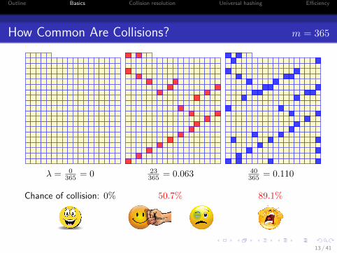
Outline Basics Collision resolution Universal hashing Efficiency
How Common Are Collisions? m = 365
λ = 0365 = 0
Chance of collision: 0%
23365 = 0.063
50.7%
40365 = 0.110
89.1%
13 / 41
Outline Basics Collision resolution Universal hashing Efficiency
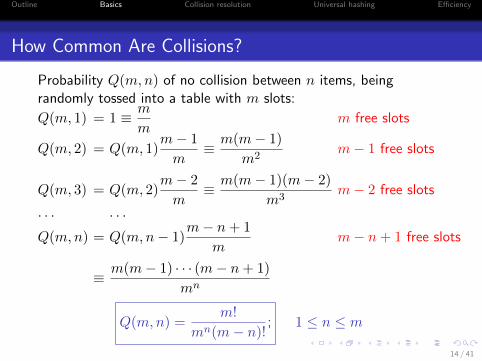
How Common Are Collisions?
Probability Q(m,n) of no collision between n items, beingrandomly tossed into a table with m slots:
Q(m, 1) = 1 ≡ m
mm free slots
Q(m, 2) = Q(m, 1)m− 1
m≡ m(m− 1)
m2m− 1 free slots
Q(m, 3) = Q(m, 2)m− 2
m≡ m(m− 1)(m− 2)
m3m− 2 free slots
. . . . . .
Q(m,n) = Q(m,n− 1)m− n+ 1
mm− n+ 1 free slots
≡ m(m− 1) · · · (m− n+ 1)
mn
Q(m,n) =m!
mn(m− n)!; 1 ≤ n ≤ m
14 / 41
Outline Basics Collision resolution Universal hashing Efficiency
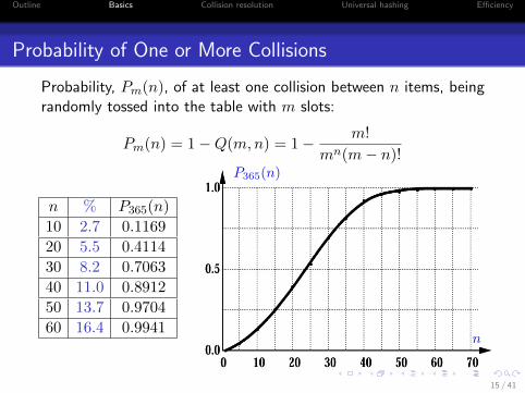
Probability of One or More Collisions
Probability, Pm(n), of at least one collision between n items, beingrandomly tossed into the table with m slots:
Pm(n) = 1−Q(m,n) = 1− m!
mn(m− n)!
n % P365(n)
10 2.7 0.1169
20 5.5 0.4114
30 8.2 0.7063
40 11.0 0.8912
50 13.7 0.9704
60 16.4 0.9941
P365(n)
n
15 / 41
Outline Basics Collision resolution Universal hashing Efficiency
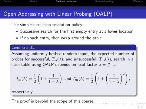
Open Addressing with Linear Probing (OALP)
The simplest collision resolution policy:
• Successive search for the first empty entry at a lower location
• If no such entry, then wrap around the table
Lemma 3.31:
Assuming uniformly hashed random input, the expected number ofprobes for successful, Tss(λ), and unsuccessful, Tus(λ), search in ahash table using OALP depends on load factor λ = n
m as
Tss(λ) =1
2
(1 +
1
1− λ
)and Tus(λ) =
1
2
(1 +
(1
1− λ
)2),
respectively.
The proof is beyond the scope of this course.16 / 41
Outline Basics Collision resolution Universal hashing Efficiency
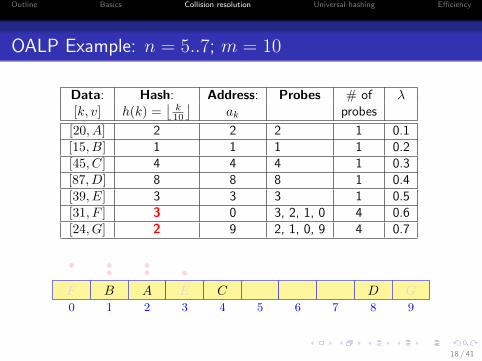
OALP Example: n = 5..7; m = 10
17 / 41
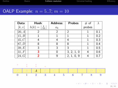
Outline Basics Collision resolution Universal hashing Efficiency
OALP Example: n = 5..7; m = 10
Data: Hash: Address: Probes # of λ[k, v] h(k) =
⌊k10
⌋ak probes
[20, A] 2 2 2 1 0.1[15, B] 1 1 1 1 0.2[45, C] 4 4 4 1 0.3[87, D] 8 8 8 1 0.4[39, E] 3 3 3 1 0.5[31, F ] 3 0 3, 2, 1, 0 4 0.6[24, G] 2 9 2, 1, 0, 9 4 0.7
0 1 2 3 4 5 6 7 8 9
AB C DE
•••F
•••
G
18 / 41
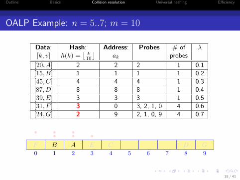
Outline Basics Collision resolution Universal hashing Efficiency
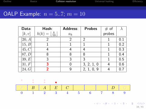
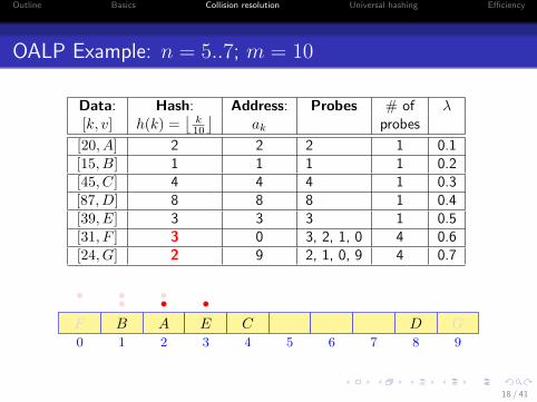
OALP Example: n = 5..7; m = 10
Data: Hash: Address: Probes # of λ[k, v] h(k) =
⌊k10
⌋ak probes
[20, A] 2 2 2 1 0.1[15, B] 1 1 1 1 0.2[45, C] 4 4 4 1 0.3[87, D] 8 8 8 1 0.4[39, E] 3 3 3 1 0.5[31, F ] 3 0 3, 2, 1, 0 4 0.6[24, G] 2 9 2, 1, 0, 9 4 0.7
0 1 2 3 4 5 6 7 8 9
AB C DE
•••F
•••
G
18 / 41
Outline Basics Collision resolution Universal hashing Efficiency
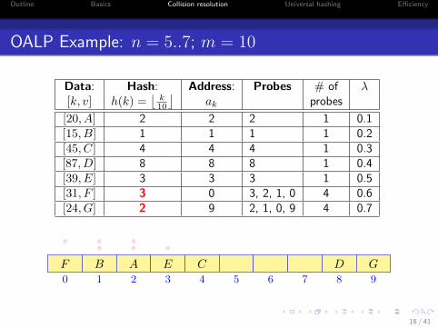
OALP Example: n = 5..7; m = 10
Data: Hash: Address: Probes # of λ[k, v] h(k) =
⌊k10
⌋ak probes
[20, A] 2 2 2 1 0.1[15, B] 1 1 1 1 0.2[45, C] 4 4 4 1 0.3[87, D] 8 8 8 1 0.4[39, E] 3 3 3 1 0.5[31, F ] 3 0 3, 2, 1, 0 4 0.6[24, G] 2 9 2, 1, 0, 9 4 0.7
0 1 2 3 4 5 6 7 8 9
AB C DE
•••F
•••
G
18 / 41

Outline Basics Collision resolution Universal hashing Efficiency
OALP Example: n = 5..7; m = 10
Data: Hash: Address: Probes # of λ[k, v] h(k) =
⌊k10
⌋ak probes
[20, A] 2 2 2 1 0.1[15, B] 1 1 1 1 0.2[45, C] 4 4 4 1 0.3[87, D] 8 8 8 1 0.4[39, E] 3 3 3 1 0.5[31, F ] 3 0 3, 2, 1, 0 4 0.6[24, G] 2 9 2, 1, 0, 9 4 0.7
0 1 2 3 4 5 6 7 8 9
AB C DE
•••F
•••
G
18 / 41
Outline Basics Collision resolution Universal hashing Efficiency
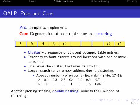
OALP: Pros and Cons
Pro: Simple to implement.
Con: Degeneration of hash tables due to clustering.
F B A E C D G
• Cluster – a sequence of adjacent occupied table entries.• Tendency to form clusters around locations with one or more
collisions.• The larger the cluster, the faster its growth.• Longer search for an empty address due to clustering:
• Average number ν of probes for Example in Slides 17–18:λ 0.1 0.2 0.3 0.4 0.5 0.6 0.7
ν 1 1 1 1 1 1.5 1.86
Another probing scheme, double hashing, reduces the likeihood ofclustering.
19 / 41
Outline Basics Collision resolution Universal hashing Efficiency
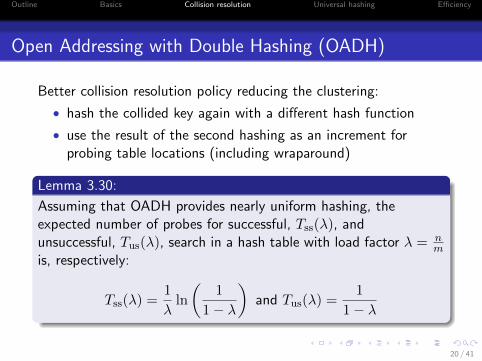
Open Addressing with Double Hashing (OADH)
Better collision resolution policy reducing the clustering:
• hash the collided key again with a different hash function
• use the result of the second hashing as an increment forprobing table locations (including wraparound)
Lemma 3.30:
Assuming that OADH provides nearly uniform hashing, theexpected number of probes for successful, Tss(λ), andunsuccessful, Tus(λ), search in a hash table with load factor λ = n
mis, respectively:
Tss(λ) =1
λln
(1
1− λ
)and Tus(λ) =
1
1− λ
20 / 41
Outline Basics Collision resolution Universal hashing Efficiency
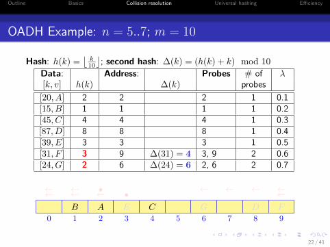
OADH Example: n = 5..7; m = 10
21 / 41

Outline Basics Collision resolution Universal hashing Efficiency
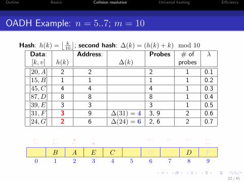
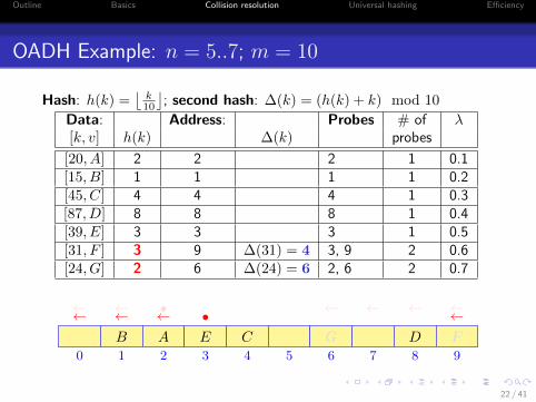
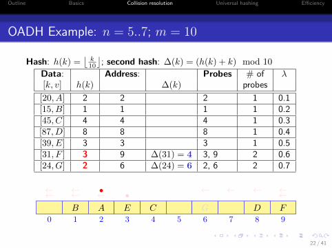
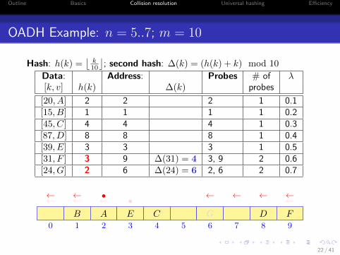
OADH Example: n = 5..7; m = 10
Hash: h(k) =⌊
k10
⌋; second hash: ∆(k) = (h(k) + k) mod 10
Data: Address: Probes # of λ[k, v] h(k) ∆(k) probes
[20, A] 2 2 2 1 0.1[15, B] 1 1 1 1 0.2[45, C] 4 4 4 1 0.3[87, D] 8 8 8 1 0.4[39, E] 3 3 3 1 0.5[31, F ] 3 9 ∆(31) = 4 3, 9 2 0.6[24, G] 2 6 ∆(24) = 6 2, 6 2 0.7
0 1 2 3 4 5 6 7 8 9
AB C DE
• ←←←←F
•←← ←←←←
G
22 / 41

Outline Basics Collision resolution Universal hashing Efficiency
OADH Example: n = 5..7; m = 10
Hash: h(k) =⌊
k10
⌋; second hash: ∆(k) = (h(k) + k) mod 10
Data: Address: Probes # of λ[k, v] h(k) ∆(k) probes
[20, A] 2 2 2 1 0.1[15, B] 1 1 1 1 0.2[45, C] 4 4 4 1 0.3[87, D] 8 8 8 1 0.4[39, E] 3 3 3 1 0.5[31, F ] 3 9 ∆(31) = 4 3, 9 2 0.6[24, G] 2 6 ∆(24) = 6 2, 6 2 0.7
0 1 2 3 4 5 6 7 8 9
AB C DE
• ←←←←F
•←← ←←←←
G
22 / 41
Outline Basics Collision resolution Universal hashing Efficiency
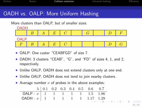
OADH vs. OALP: More Uniform Hashing
More clusters than OALP, but of smaller sizes:
F B A E C D G
OALP
B A E C G D F
OADH
• OALP: One custer “CEABFGD” of size 7.
• OADH: 3 clusters “CEAB”, “G”, and “FD” of sizes 4, 1, and 2,respectively.
• Unlike OALP, OADH does not extend clusters only at one end.
• Unlike OALP, OADH does not tend to join nearby clusters.
• Average number ν of probes in the above examples:
λ 0.1 0.2 0.3 0.4 0.5 0.6 0.7OALP : ν 1 1 1 1 1 1.5 1.86
OADH : ν 1 1 1 1 1 1.17 1.29
23 / 41
Outline Basics Collision resolution Universal hashing Efficiency
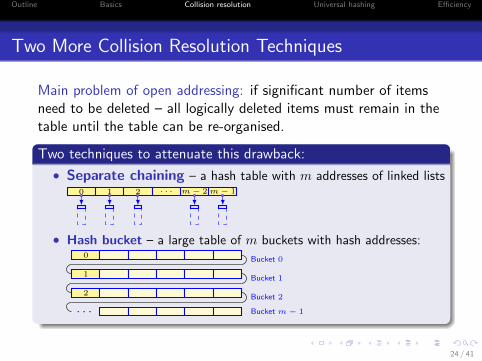
Two More Collision Resolution Techniques
Main problem of open addressing: if significant number of itemsneed to be deleted – all logically deleted items must remain in thetable until the table can be re-organised.
Two techniques to attenuate this drawback:
• Separate chaining – a hash table with m addresses of linked lists0 1 2 . . . m − 2 m − 1
• Hash bucket – a large table of m buckets with hash addresses:0 Bucket 0
1 Bucket 1
2 Bucket 2
. . . Bucket m − 1
24 / 41
Outline Basics Collision resolution Universal hashing Efficiency
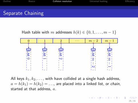
Separate Chaining
Hash table with m addresses h(k) ∈ {0, 1, . . . ,m− 1}
0 1 2 . . . m− 2 m− 1
List
0
List
1
List
2
List
m−
2
List
m−
1
All keys k1, k2, . . . , with have collided at a single hash address,a = h(k1) = h(k2) = . . ., are placed into a linked list, or chain,started at that address, a.
25 / 41
Outline Basics Collision resolution Universal hashing Efficiency
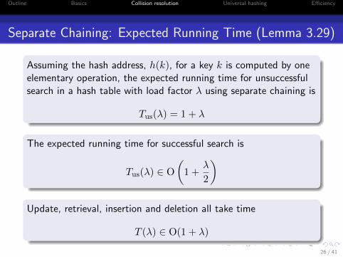
Separate Chaining: Expected Running Time (Lemma 3.29)
Assuming the hash address, h(k), for a key k is computed by oneelementary operation, the expected running time for unsuccessfulsearch in a hash table with load factor λ using separate chaining is
Tus(λ) = 1 + λ
The expected running time for successful search is
Tus(λ) ∈ O
(1 +
λ
2
)
Update, retrieval, insertion and deletion all take time
T (λ) ∈ O(1 + λ)
26 / 41
Outline Basics Collision resolution Universal hashing Efficiency
Separate Chaining: Expected Running Time
Proof.
• The average running time to unsuccessfully search for the keyat that address is equal to the average length of theassociated chain, λ = n
m .
• Thus in total Tus(λ) = 1 + λ = 1 + nm .
• The average value of Tss(λ) (in accord with Lemma 3.3)equals one plus the average of the times for the unsuccessfulsearches undertaken while building the table.
• In this case, it is one plus the average of 0 + 1 + 2 + . . .+ λ,i.e., 1 + λ
2 .
• Since update, retrieval and deletion from a linked list takeconstant time, Tss(λ) is in O
(1 + λ
2
).
27 / 41
Outline Basics Collision resolution Universal hashing Efficiency
Hash Bucket
0Bucket 0
1Bucket 1
2Bucket 2
. . . Bucket m− 1
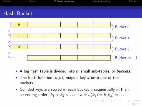
• A big hash table is divided into m small sub-tables, or buckets.
• The hush function, h(k), maps a key k onto one of thebuckets.
• Collided keys are stored in each bucket a sequentially in theirascending order: k1 < k2 < . . . if a = h(k1) = h(k2) = . . ..
28 / 41
Outline Basics Collision resolution Universal hashing Efficiency
Implementation of Hashing: Resizing
Resizing a hash table for open addressing to keep λ < 0.75:
• Doubling the table size when λ ≥ 0.75.
• Readdressing all the elements with a new hash function.
• Average insertion time: Θ(1) (as now λ� 1).
• Time for m insertions – of order m.
• Total time to grow a table from 1 to m = 2k elements:1 + 2 + . . .+ 2k−1 = 2k − 1 = m− 1 .
Thus, the average insertion time with resizing is still Θ(1).
29 / 41
Outline Basics Collision resolution Universal hashing Efficiency
Implementation of Hashing: Deletion
Deletion of a table entry: simple for separate chaining (SC), butdifficult for open addressing (OA) tables.
Because an emptied place in an OA table invalidates the search forsubsequent keys, make the table valid as follows:
• Mark the deleted entries empty for insertion, but non-emptyfor key search.
• If too many such marked entries, really delete them and resizethe table.
The deletion time O(1) for both SC and OA hash tables.
30 / 41
Outline Basics Collision resolution Universal hashing Efficiency
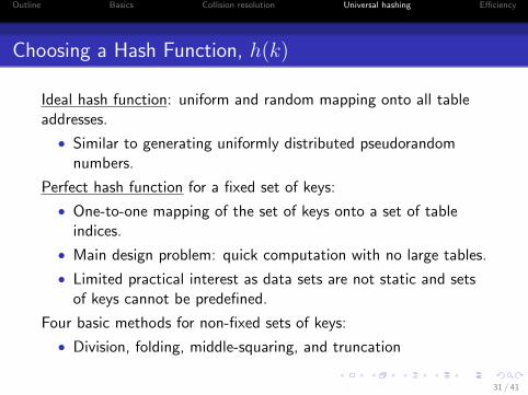
Choosing a Hash Function, h(k)
Ideal hash function: uniform and random mapping onto all tableaddresses.
• Similar to generating uniformly distributed pseudorandomnumbers.
Perfect hash function for a fixed set of keys:
• One-to-one mapping of the set of keys onto a set of tableindices.
• Main design problem: quick computation with no large tables.
• Limited practical interest as data sets are not static and setsof keys cannot be predefined.
Four basic methods for non-fixed sets of keys:
• Division, folding, middle-squaring, and truncation
31 / 41
Outline Basics Collision resolution Universal hashing Efficiency
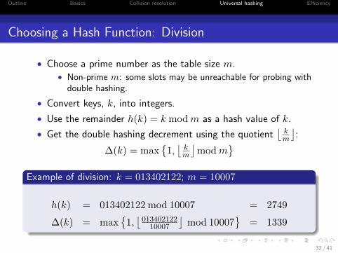
Choosing a Hash Function: Division
• Choose a prime number as the table size m.• Non-prime m: some slots may be unreachable for probing with
double hashing.
• Convert keys, k, into integers.
• Use the remainder h(k) = k modm as a hash value of k.
• Get the double hashing decrement using the quotient⌊km
⌋:
∆(k) = max{
1,⌊km
⌋modm
}Example of division: k = 013402122; m = 10007
h(k) = 013402122 mod 10007 = 2749
∆(k) = max{
1,⌊013402122
10007
⌋mod 10007
}= 1339
32 / 41
Outline Basics Collision resolution Universal hashing Efficiency
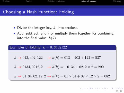
Choosing a Hash Function: Folding
• Divide the integer key, k, into sections.
• Add, subtract, and / or multiply them together for combininginto the final value, h(k)
Examples of folding: k = 013402122
k → 013, 402, 122 → h(k) = 013 + 402 + 122 = 537
k → 0134, 0212, 2 → h(k) = −0134 + 0212× 2 = 290
k → 01, 34, 02, 12, 2 → h(k) = 01× 34 + 02× 12× 2 = 082
33 / 41
Outline Basics Collision resolution Universal hashing Efficiency
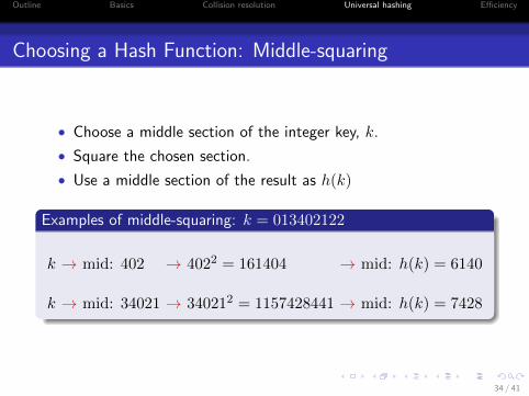
Choosing a Hash Function: Middle-squaring
• Choose a middle section of the integer key, k.
• Square the chosen section.
• Use a middle section of the result as h(k)
Examples of middle-squaring: k = 013402122
k → mid: 402 → 4022 = 161404 → mid: h(k) = 6140
k → mid: 34021 → 340212 = 1157428441 → mid: h(k) = 7428
34 / 41
Outline Basics Collision resolution Universal hashing Efficiency
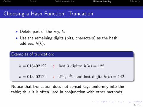
Choosing a Hash Function: Truncation
• Delete part of the key, k.
• Use the remaining digits (bits, characters) as the hashaddress, h(k).
Examples of truncation:
k = 013402122 → last 3 digits: h(k) = 122
k = 013402122 → 2nd, 4th, and last digit: h(k) = 142
Notice that truncation does not spread keys uniformly into thetable; thus it is often used in conjunction with other methods.
35 / 41
Outline Basics Collision resolution Universal hashing Efficiency
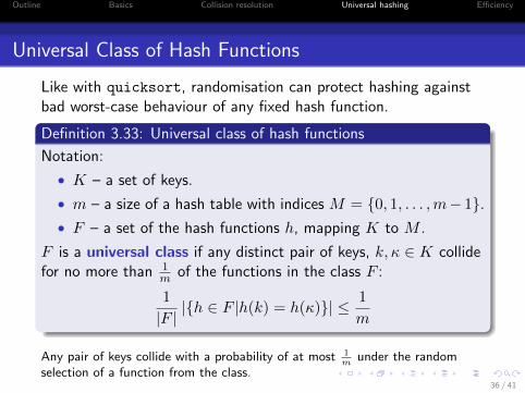
Universal Class of Hash Functions
Like with quicksort, randomisation can protect hashing againstbad worst-case behaviour of any fixed hash function.
Definition 3.33: Universal class of hash functions
Notation:
• K – a set of keys.
• m – a size of a hash table with indices M = {0, 1, . . . ,m− 1}.• F – a set of the hash functions h, mapping K to M .
F is a universal class if any distinct pair of keys, k, κ ∈ K collidefor no more than 1
m of the functions in the class F :
1
|F ||{h ∈ F |h(k) = h(κ)}| ≤ 1
m
Any pair of keys collide with a probability of at most 1m
under the randomselection of a function from the class.
36 / 41
Outline Basics Collision resolution Universal hashing Efficiency
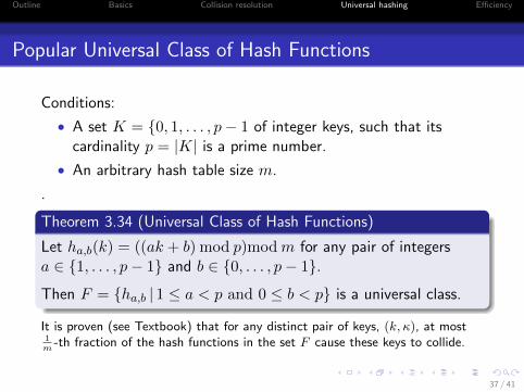
Popular Universal Class of Hash Functions
Conditions:
• A set K = {0, 1, . . . , p− 1 of integer keys, such that itscardinality p = |K| is a prime number.
• An arbitrary hash table size m.
.
Theorem 3.34 (Universal Class of Hash Functions)
Let ha,b(k) = ((ak + b) mod p)modm for any pair of integersa ∈ {1, . . . , p− 1} and b ∈ {0, . . . , p− 1}.
Then F = {ha,b | 1 ≤ a < p and 0 ≤ b < p} is a universal class.
It is proven (see Textbook) that for any distinct pair of keys, (k, κ), at most1m-th fraction of the hash functions in the set F cause these keys to collide.
37 / 41
Outline Basics Collision resolution Universal hashing Efficiency
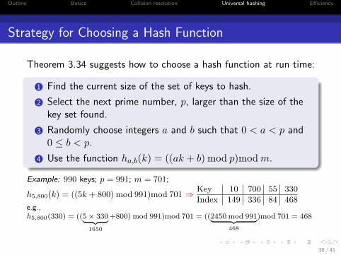
Strategy for Choosing a Hash Function
Theorem 3.34 suggests how to choose a hash function at run time:
1 Find the current size of the set of keys to hash.
2 Select the next prime number, p, larger than the size of thekey set found.
3 Randomly choose integers a and b such that 0 < a < p and0 ≤ b < p.
4 Use the function ha,b(k) = ((ak + b) mod p)modm.
Example: 990 keys; p = 991; m = 701;
h5,800(k) = ((5k + 800) mod 991)mod 701 ⇒ Key 10 700 55 330
Index 149 336 84 468e.g.,h5,800(330) = ((5× 330︸ ︷︷ ︸
1650
+800) mod 991)mod 701 = ((2450 mod 991︸ ︷︷ ︸468
)mod 701 = 468
38 / 41
Outline Basics Collision resolution Universal hashing Efficiency
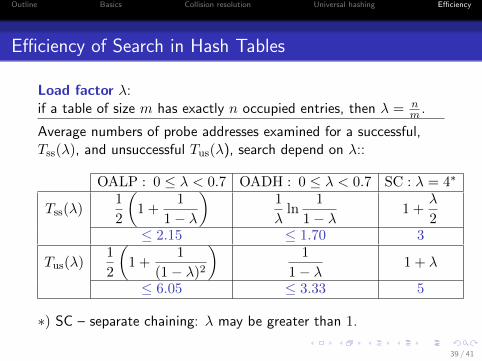
Efficiency of Search in Hash Tables
Load factor λ:if a table of size m has exactly n occupied entries, then λ = n
m .
Average numbers of probe addresses examined for a successful,Tss(λ), and unsuccessful Tus(λ), search depend on λ::
OALP : 0 ≤ λ < 0.7 OADH : 0 ≤ λ < 0.7 SC : λ = 4∗
Tss(λ)1
2
(1 +
1
1− λ
)1
λln
1
1− λ1 +
λ
2≤ 2.15 ≤ 1.70 3
Tus(λ)1
2
(1 +
1
(1− λ)2
)1
1− λ1 + λ
≤ 6.05 ≤ 3.33 5
∗) SC – separate chaining: λ may be greater than 1.
39 / 41
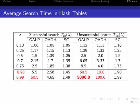
Outline Basics Collision resolution Universal hashing Efficiency
Average Search Time in Hash Tables
λ Successful search Tss(λ) Unsuccessful search Tus(λ)OALP OADH SC OALP OADH SC
0.10 1.06 1.05 1.05 1.12 1.11 1.100.25 1.17 1.15 1.13 1.39 1.33 1.250.5 1.5 1.39 1.25 2.5 2.0 1.50.7 2.15 1.7 1.35 6.05 3.33 1.7
0.75 2.5 1.85 1.38 8.5 4.0 1.75
0.90 5.5 2.56 1.45 50.5 10.0 1.900.99 50.5 4.65 1.49 5000.0 100.0 1.99
40 / 41
Outline Basics Collision resolution Universal hashing Efficiency
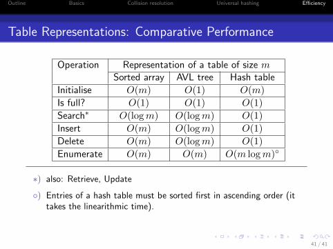
Table Representations: Comparative Performance
Operation Representation of a table of size mSorted array AVL tree Hash table
Initialise O(m) O(1) O(m)
Is full? O(1) O(1) O(1)
Search∗ O(logm) O(logm) O(1)
Insert O(m) O(logm) O(1)
Delete O(m) O(logm) O(1)
Enumerate O(m) O(m) O(m logm)◦
∗) also: Retrieve, Update
◦) Entries of a hash table must be sorted first in ascending order (ittakes the linearithmic time).
41 / 41