Embed Size (px)
Citation preview

Has Technology Increased Yield Risk?
Evidence From the Crop Insurance
Biotech Endorsement ∗
Barry K. Goodwin
and Nicholas E. Piggott
Revised: November 28, 2018
Abstract
The conventional wisdom that technological advances in seed breeding and geneticmodification of corn traits has lowered yield risk has recently been challenged by re-search that argues that the converse is true. The implications of this research have beenapplied to models of climate change and have led to the conclusion that these tech-nological advances have actually increased agronomic risk, such that climate change isasserted to raise important concerns regarding the stability and viability of corn yieldsin the future. The argument is based upon assertions that corn yields have becomemore sensitive to weather stresses. We use corn yields and data from the US federalcrop insurance program to evaluate these claims. An examination of yield responsesto droughts in 1988 and 2012 suggests more robust yields in the latter period, in spiteof very comparable weather stresses. We also use side-by-side data collected under theBiotech Endorsement (BE) between 2008 and 2011. We find that risk, as measured bythe rate of indemnities paid per units insured, was significantly lower for crops insuredunder the BE. We also find that the difference in risk tends to be greater when growingconditions are less favorable.
Key Words: Yield Risk, Biotechnology, Corn Yields
JEL Codes: Q16, O47, C23
∗ Goodwin is William Neal Reynolds Distinguished Professor in the Department of Agricultural andResource Economics and Graduate Alumni Distinguished Professor in the Department of Economics at NorthCarolina State University. Piggott is Professor in the Department of Agricultural and Resource Economicsat North Carolina State University. Direct correspondence to Goodwin at Box 8109, North Carolina StateUniversity, Raleigh, NC, 27695, E-mail: barry [email protected].

Has Technology Increased Yield Risk?
Evidence From the Crop Insurance
Biotech Endorsement
Abstract
The conventional wisdom that technological advances in seed breeding and genetic modifica-
tion of corn traits has lowered yield risk has recently been challenged by research that argues
that the converse is true. The implications of this research have been applied to models of
climate change and have led to the conclusion that these technological advances have actually
increased agronomic risk, such that climate change is asserted to raise important concerns
regarding the stability and viability of corn yields in the future. The argument is based
upon assertions that corn yields have become more sensitive to weather stresses. We use
corn yields and data from the US federal crop insurance program to evaluate these claims.
An examination of yield responses to droughts in 1988 and 2012 suggests more robust yields
in the latter period, in spite of very comparable weather stresses. We also use side-by-side
data collected under the Biotech Endorsement (BE) between 2008 and 2011. We find that
risk, as measured by the rate of indemnities paid per units insured, was significantly lower
for crops insured under the BE. We also find that the difference in risk tends to be greater
when growing conditions are less favorable.
Key Words: Yield Risk, Biotechnology, Corn Yields
JEL Codes: Q16, O47, C23

Has Technology Increased Yield Risk?
Evidence From the Crop Insurance
Biotech Endorsement
Introduction
The US agricultural sector has realized a long and steady pattern of technological advances
that have increased corn yields. In recent years, these advances have included improved seed
breeding methods as well as genetic modification of corn plant traits. There is no doubt that
average corn yields, however or wherever measured, have significantly trended upward over
time. Malcolm, Aillery, and Weinberg (2009) measure the recent average annual increase
in corn yields to be about 2-3.5% per year. The National Corn Growers Association has
asserted that corn yields will reach 300 bushels per acre by 2030—a target that will require
substantially greater yield increases in the future.
Recent research has argued that, along with these increases in mean yields, corn has
become more sensitive to environmental stresses induced by high temperatures and limited
moisture. The literature here is voluminous though much of it is based upon a single data
set drawn from historical crop insurance records. This research is almost entirely unanimous
in concluding that the risks of crop yields are likely to increase in response to changes in
climate variables associated with heat and moisture stresses. A non-exhaustive list of relevant
papers include work by D’Agostino and Schlenker (2016), Liu et al. (2016), Roberts et al.
(2013), Rosenzweig et al. (2014), Schlenker and Roberts (2009), Tack et al. (2015), Urban
et al. (2015), Welch et al. (2010), Lusk, Tack, and Hendricks (2018), and Tack, Coble,
and Barnett (2018). Though individual empirical approaches and conclusions differ, most
research has found that, although biotechnology has tended to increase average yields, yield
risk has increased or, at best, has not been influenced by technological advances. Studies that
have concentrated on the negative effects of increases in warming on corn yield risk include
1
Attavanich and McCarl (2014), Ray et al. (2015), and Urban et al. (2012, 2015). An
important exception to these conclusions exists in a recent paper by Chavas, Shi, and Lauer
(2014), who found that experimental corn production data revealed that the interaction of
genetical modification and management practices reduced exposure to downside yield risk.1
Perhaps the most prominent research findings suggesting increased corn yield risk are
found in a series of papers by David Lobell and his collaborators.2 The conclusions of
this line of research are largely summarized in Lobell et al. (2014). Using these unit-
level yield records, Lobell et al. (2014) concluded that technological advances have led to
increased planting density of corn and as a result, corn yields have become more sensitive to
environmental stresses. Similar research by Schlenker and Roberts (2009) concluded that this
increased sensitivity implies that average corn yields in current growing regions is predicted
to decrease by 30-46% under the most optimistic climate change scenarios and by 63-82%
under the most rapidly warming climate change modeling. Along with an increase in planting
density, current technologies have led to a general decrease in chemical and fertilizer inputs.
These changes could also contribute to lower yields and increased yield risk in response to
climate changes in the future.
It is indeed true that corn planting density has risen significantly over the last 30 years.
Figure 1 illustrates state-average planting density (plants per acre) for corn in Iowa between
1963 and 2018. In 1963, Iowa corn growers were planting 13,600 seeds per acre. By 2018,
this density had risen to 31,150 seeds per acre. It is certainly true that a denser stand of corn
will result in more competition among plants for the available moisture and soil nutrients.
Further, insect pressures may increase in more densely planted corn. Based on experimental
data collected from 10 site-years of research trials done in Western Iowa, the Iowa State
1Their study, based upon university experimental yield data for 2000 and 2005, focused on corn-after-corncrop rotation management practices in the Northern Corn Belt. They found that the negative yield impactsof corn planted after corn were much smaller for biotech corn hybrids.
2Many of these studies use a single data set collected from randomly-sampled, unit-level crop insurancerecords for Iowa, Illinois, and Indiana. The data are from confidential crop insurance records that span the1995-2012 period and that have since been made unavailable for follow-up research. An non-exhaustive listincludes Roberts et al. (2017), Urban, Sheffield, and Lobell (2015), Seifert, Roberts, and Lobell (2017), andLobell et al. (2014).
2

University Extension Service (Wright and Licht (2018)) state that “the recommended plant
populations for Iowa are around 34,000-37,000 plants per acre, and these plant populations
would not need to be changed if row spacing was reduced.” Figure 1 includes this recom-
mended density range, which is considerably above the 31,150 average reported by the USDA
for 2018. Thus, the evidence does not appear to be consistent with research that asserts a
causal relationship between current corn plant densities and increased yield risk.3 Chavas,
Shi, and Lauer (2014) also found that a higher density of corn plants contributed to a higher
yield.
The research by Schlenker and Roberts (2009) established important nonlinearities and
thresholds in corn plant responses to temperature and precipitation. Specifically, they find
that corn has a current threshold of 29o centigrade, beyond which corn yields decrease
sharply. The also find important nonlinear yield responses to precipitation, with an optimal
level of about 25.0 inches of rain for maximum yields. Tack, Coble, and Barnett (2018) found
that climate-driven changes consistent with a 1 Co increase in temperature would trigger
increases in corn yield risk that are expected to increase crop insurance coverage premium
rates by 22% relative to current levels. This rate increase rises to 57% with a 2 Co warming
scenario. Tack, Coble, and Barnett (2018) are careful to note that their estimated marginal
effects of warming temperatures are conditional on current technology, production, and crop
insurance enrollments—factors often neglected in the existing literature.
Tolhurst and Ker (2015) find that the dispersion of yields is increasing and the coeffi-
cient of variation of yields is decreasing over time. Li and Ker (2013) find that changes in
average yields and the variance of yields due to climate change imply increases in expected
crop insurance payouts and actuarially fair premium rates in the Agricorp (Ontario) crop
insurance program. Roberts, Schenkler, and Eyer (2012) find that heat, precipitation, and
3This is not to say that corn yields do not eventually decrease as planting density is increased. Woli etal. (2014) summarize yield data collected from 33 site-years in Iowa from 2006 to 2009 and find that cornyields begin to decrease as seeding density exceeds 38,850 seeds per acre.
3

vapor pressure deficits may have important negative influences on corn yields that again
imply diminishing yields in response to climate change in the future.
As Li and Ker (2013) note, changes in technology and any resultant increases in the
sensitivity of yields to weather have important implications for crop insurance programs. The
US federal crop insurance program currently insures in excess of $40 billion in corn liability on
over 78 million acres. The subsidized crop insurance program has become the cornerstone of
US agricultural programs, accounting for the largest share of spending (excluding nutritional
assistance programs) in the 2014 Farm Bill.
The Risk Management Agency (RMA) of the USDA approved a pilot program that
offered a significant premium discount on certain types of biotech corn. The program was
introduced in 2008 as the Biotech Yield Endorsement (BYE) and was initially restricted to
the stacked trait varieties offered by Monsanto in Iowa, Illinois, Indiana, and Minnesota. In
2009, Dupont/Pioneer and Syngenta gained approval for their stacked trait corn hybrids to
also be included in the program, which became known as the Biotech Endorsement (BE). The
program was extended in 2009 to include Colorado, Kansas, Michigan, Missouri, Nebraska,
Ohio, South Dakota, and Wisconsin. The RMA was persuaded that these stacked trait
corn hybrids intrinsically had less risk in that they were less sensitive to the very factors
that climate change researchers had argued were making corn yields more risky. The pilot
endorsement program was eliminated in 2012 under the contention that nearly all corn was
of the biotech varieties. The RMA undertook significant rate decreases in important corn
growing areas as the BE was terminated under the assertion that biotech corn was less risky
and had become ubiquitous in the Corn Belt.4
4For example, in the BE pilot states, the yield protection premium rate for corn on optional units at 65%coverage fell from 6.6% in 2010 to 5.7% in 2012.
4

How Do We Measure Yield Risk?
A first fundamental question involves how one measures the risks associated with crop yields.
A number of empirical hurdles complicate this seemingly basic question. A simple fact, and
one that is indisputable in the empirical literature, is that the technology that is being
modeled in this body of research is itself non-stationary and endogenous to variables that
include weather as well as government policies and changing market conditions. Nearly all
existing research uses yield data collected over time, often over periods as long as 50 years.
Attempts to adequately represent these changes typically include linear or nonlinear trends.
More sophisticated approaches include models that allow parametric yield distributions to
vary over time (see, for example, Zhu, Ghosh, and Goodwin (2011) and Tolhurst and Ker
(2015)). However, any parametric specification of these changes in technology is likely to
be fragile and subject to considerable specification biases. This is not to say that existing
research has neglected technological change, but rather that the corn of 1990 is simply not
comparable to the corn of 2018, much less the corn expected to exist in 2050.
A related concern pertains to exactly how one chooses to represent “risk” in an envi-
ronment where the second and higher moments of the yield distribution are likely to be
simultaneously evolving. It is non-debatable that average yields are increasing. However,
arguments based upon a characterization of yield risk using only variance changes are likely
to be deficient. Likewise, changes in the coefficient of variation or other related statistics
are also likely to have issues with interpretation. In this paper, we argue that one straight-
forward approach to measuring yield risk is to consider the simple cost of providing a given
level of protection against yield shortfalls in an insurance context. Annan and Schlenker
(2015) concluded that insured corn and soybeans are significantly more sensitive to extreme
heat than uninsured crops and that widespread expansions in insurance coverage of these
crops may have important implications for incentives to adapt to climate change. Chen and
Chang (2005) and Di Falco, et al. (2014) found that crop insurance may be an instrument
useful to stabilize farm revenues under climate changes. The recent papers of Tack, Coble,
5
and Barnett (2018) and Li and Ker (2013) are, to our knowledge, the only existing studies
to explicitly consider the costs of crop insurance protection.
The issue of “adaptation” is also a point of contention in how one defines technological
change. Lobell (2014) argues that many existing studies confound adaptation to climate
changes with many other potential changes in agricultural management and technology that
he maintains may improve crop productivity but should not be considered as an adaptation
to climate change. Indeed, responses to the aforementioned changes in policies and market
conditions should perhaps not be confounded with changes in technology that represent
adaptation. From our perspective, these distinctions may be interesting from an academic
perspective but are not likely to be meaningful in addressing the basic issues associated with
changes in the technology associated with corn production. We remain agnostic as to how
one chooses to characterize changes in yield risk and maintain that such distinctions are
largely irrelevant to many of the fundamental issues of interest.
A related point that is often noted in the empirical literature addressing biotechnology
and its impacts on yields is that genetic modification is but one of the many changes that have
occurred to agronomic technologies over time. It is often noted that significant improvements
in seed breeding practices and improved germplasm have had similar or even greater effects on
corn yields than have the innovations specific to the genetic modification of corn traits. Other
relevant changes might include differences in farmer abilities, education, improved machinery
and other capital assets, and changes in the productivity of non-seed inputs. Again, we find
these distinctions to be important in framing certain aspects of the yield risk issue, but
irrelevant to our basic question of interest—how has the adoption of biotechnology, along
with the other concomitant changes in agronomic practices and other inputs, affected yield
risk? In our analysis, which is largely based upon empirical comparisons of side-by-side (at
least at a county level) production technologies, we are largely uninterested in distinguishing
the precise role that genetic modification may play in affecting corn yield risk and rather
focus on the central question of whether the adopters of biotechnology have significantly
6

different yield risk than do similarly-situated non-adopters. In a cross-section, it is difficult
if not impossible to distinguish adoption of genetically-modified hybrids from other related
factors that may be associated with such adoption. This limitation is not unique to our
modeling approach. The entire body of literature reviewed above would also have difficulties
in separating the impacts of technological change into its individual components. Further,
such a decomposition of change into its individual components is not likely to be either
relevant or informative in the popular simulations of yield risks 50 years into the future.
From our perspective, one really is not concerned with the question of whether changes are
attributable to one factor or another, but rather how the factors collectively will impact
yields in the future.
The Biotech Crop Insurance Endorsement
The Biotech Endorsement (BE) was introduced in 2008. The endorsement was the result of
a private product submission made by Monsanto to the Risk Management Agency (RMA).
The endorsement proposed an actuarially-accurate discount on the yield protection portion
of crop insurance premiums that would reflect an asserted reduction in yield risk associated
with certain stacked trait corn hybrids. The proposed endorsement was submitted to the
RMA in 2007 and subsequently underwent a rigorous review process by RMA staff and by
outside expert reviewers. To qualify for the premium discount, growers had to plant at least
75% of the insured acreage in an individual unit to Monsanto branded hybrids (YieldGard
VT-Triple and/or YieldGard-Plus). The discount was applied at the unit level and a grower
could elect to insure a portion of their overall acreage under the endorsement.
The BE project was motivated by anecdotal observations made by growers and Monsanto
sales staff in Illinois in 2005. Illinois experienced a somewhat localized drought in 2005 that
ranked among the three worst droughts the state had experienced in over 100 years. The
2005 drought was not as widespread as the 1988 and 2012 droughts and thus did not garner
7

the widespread attention that accompanied the severe droughts in those years. Figure 2
presents Palmer Z Drought Index values across the calendar year for a single National Oceanic
and Atmospheric Administration (NOAA) climate division (Division 2, corresponding to
Northeast Illinois counties). The figure demonstrates the fact that the growing conditions
in this region of the Corn Belt were of a comparable severity to those experienced in the
landmark drought years of 1988 and 2012.
In the midst of the 2005 harvest, growers and seed marketing agents observed that the
stacked hybrids suffered much less of a yield loss because of the drought. This difference
was largely attributed to the healthier and more robust root ball that was provided by the
below-ground root-worm protection provided by the stacked hybrids. Figure 3 illustrates a
comparison of the root balls for conventional (non-biotech) corn and SmartStax, a Monsanto
biotech hybrid. The conventional wisdom advocated by agronomic specialists maintained
that the substantial difference in root balls made the biotech corn significantly less sensitive
to drought conditions. The argument also suggested that the difference in yields may be
negligible in years and areas with sufficient moisture and lower heat stress. However, under
conditions of heat and moisture stress, the larger root ball resulted in greater yields and
thus less yield stress. The implication for yield risk, however measured, was that the biotech
hybrids resulted in significantly less yield risk relative to conventional hybrids (as well as
biotech hybrids having only herbicide tolerance).
The analysis of yields, based upon proprietary commercial field trials data, utilized data
from 1,637 individual fields (with multiple replications per field) in the initial four-state
pilot region comprised of Illinois, Iowa, Indiana, and Minnesota. The data and analysis,
which remain confidential, were supplied to the RMA along with actuarial algorithms that
measured the relevant rate discounts. The submission contained Figure 4, which illustrated
the empirical differences between conventional and biotech corn yield distributions.
The BE was expanded to include stacked hybrids from Syngenta and Dupont/Pioneer in
2009. The pilot area was also expanded to include Colorado, Kansas, Michigan, Missouri,
8

Nebraska, Ohio, South Dakota, and Wisconsin, yielding a 12-state pilot region for the years of
2009-2011. The pilot program was terminated in 2011 and, as noted above, widespread rate
adjustments were made to reflect the fact that adoption of the biotech hybrids had increased
to the extent that most corn being planted would likely qualify for the BE discount. The
BE program resulted in over $532 million in total premium savings, which was derived from
a lower premium subsidy ($318 million) as well as lower producer-paid premiums ($214
million). The program was not popular with the insurance companies, adjustors, and agents
tasked with administering the endorsement. At the same time that total premiums were
being reduced, resulting in less compensation for agents and lower underwriting gains for
insurance companies, the companies were tasked with conducting a monitoring program
that required genetic testing of sampled leaves to validate that the corn insured under the
endorsement was an approved hybrid.5
Empirical Analysis
A Comparison of 1988 and 2012 Corn Yields
An initial assessment of the impact of biotechnology on corn yields can be garnered from a
consideration of how yields responded during the 1988 and 2012 droughts. In a newspaper
article written in the midst of the 2012 drought, Pitt (2012) noted that new corn technology
helped to limit corn losses in such a drought. Pitt goes on to quote Secretary of Agriculture
Thomas Vilsack, who stated “it is important to point out that improved seed technology
and improved efficiencies on the farm have made it a little bit easier for some producers
to get through a very, very difficult weather stretch.” These statements, which reflect the
conventional wisdom of Corn Belt corn growers, are in stark contrast to the assertions of
the body of research arguing that biotech corn varieties are likely to be more sensitive to
5The industry complaint can best be summarized as “more work for less money.” An interesting anecdoteis that noncompliance was found to be very rare. The limited number of cases that were revealed typicallycorresponded to growers planting a biotech hybrid that was not on the list of qualifying seed.
9

drought. Of course, growers did not have access to genetically-modified corn in 1988, though
by 2012, 91% of the corn planted in Iowa was of a genetically-engineered variety.6
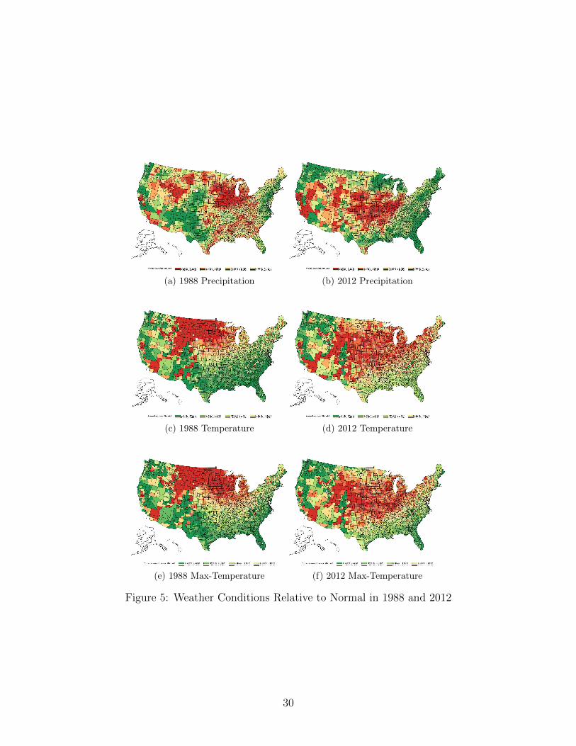
A first question relates to how the 1988 and 2012 droughts compared to one-another.
Figure 5 presents climate variable statistics for every county in the contiguous US. Three
weather variables were collected—the May to July averages of the ratios of realized pre-
cipitation over normal precipitation, average temperatures over normal temperatures, and
the maximum temperatures relative to the normal maximum temperatures. Each of these
weather variables has been found to be relevant to corn yield risk in the existing literature.
Panels (a), (c), and (e) present the variables for 1988 while panels (b), (d), and (f) present
the equivalent statistics for 2012. The figures demonstrate the fact that the weather condi-
tions, at least as measured by these three variables, were similar in 1988 and 2012. Figure
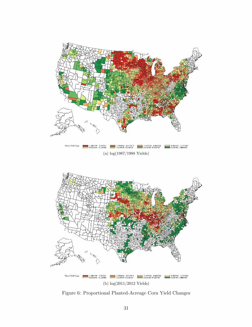
6 presents proportional corn yield changes from 1987 to 1988 and 2011 to 2012. The figure
demonstrates that yield losses appear to have been significantly lower in the later period.
Finally, we focus on relative yield changes in the 12 BE states in 1988 and 2012. Panel (a)
of Figure 7 presents a plot of yield changes in each county in the two drought years, along
with a 45o line. Observations that fall above the line represent a lower yield decline (or
greater yield increase). Although there is considerable variability in the diagram, a majority
of the points fall above the line, reflecting less yield loss in 2012. Panel (b) of 7 presents
relative yield changes in 1988 and 2012 along with the July Palmer-Z Drought Index, an
important indicator of drought stress. The figure illustrates two important points. First,
average drought conditions in July in the 12 BE states were worse in 2012 than in 1988. This
is evidenced by the mean values of Palmer’s Z, which were actually lower in 2012 than in
1988. Second, yield changes in 2012 were less severe in response to the drought than was the
case in 1988. Although the average yield changes are similar, most of the 2012 yield changes
fall above those observed in 1988. In all, a simple consideration of yield changes between
6Adoption statistics for genetically-engineered corn were collected from unpublished data furnished bythe Economic Research Service of the USDA.
10

1987-1988 and 2011-2012 illustrates a more robust response to the drought conditions in the
latter period.
The USDA reports adoption of genetically-engineered (GE) corn at the state level. GE
corn is summarized by four categories of genetic traits—Bt insect resistance, herbicide tol-
erance, stacked traits, and an aggregation of all GE hybrids. Of course, none of these GE
varieties were available in 1988. A very simple consideration of the extent to which GE adop-
tion may have been associated with improved yield performance in the presence of severe
drought conditions can be revealed by a simple regression of the yield changes on state-level
BE adoption. Such a regression is naturally limited by the aggregate nature of the adop-
tion statistics. Table 1 presents the results of regressions of yield changes on aggregate BE
adoption. Of course, many other omitted factors would be suspected to have influenced
county-level yield changes. However, in every case, a significant positive impact of adoption
on yield changes is noted in the regression results.
Evidence From the BE Endorsement
A richer evaluation of the impacts of biotech corn adoption on yield performance can be
drawn from county-level data comparing crop insurance performance on those crop insurance
units that qualified for the BE to units that did not qualify. Experience data from the BE
were obtained via a Freedom of Information Act request from the RMA. The data were
supplied at a county-level of aggregation, with the experience data being decomposed into
coverage level (50-85%), practice type (irrigated and non-irrigated), insurance plan (revenue
and yield protection), and unit structure (optional, basic, and enterprise units). These data
were matched to overall crop insurance experience data at the year, county, coverage level,
practice, insurance plan, and unit structure and used to derive experience data for the non-
BE units. The primary objective is to empirically evaluate crop insurance losses, expressed
in terms of the loss-cost ratio (the ratio of indemnity payments to total liability) and the loss-
ratio (the ratio of indemnity payments to total premium collected). Two testable hypotheses
11

emerge from this collection of data. First, yield risk, as represented in the loss-cost ratio
(LCR), should be lower on those units that were insured under the endorsement and received
the premium discount. Second, if the premium rate adjustments were accurate, one would
expect the loss-ratios (LRs) to be equivalent across units insured under the endorsement and
those not subject to the endorsement discount. In addition, the experience data permit an
evaluation of a central argument inherent in the conventional wisdom regarding biotech corn
performance—that the benefits of biotech corn hybrids tend to be greater in areas and years
that have less favorable growing conditions.
This comparison is subject to a number of caveats. First, it is likely that a substantial
share of the non-qualifying units were also planted to biotech corn hybrids. This may have
arisen from limited adoption (i.e., below the 75% acreage requirement) or from biotech
hybrids that were not included on the list of qualifying varieties. Likewise, many growers and
agents may have simply chosen not to apply for the endorsement because of the additional
administrative burden associated with the certification and validation process.7 The threat
of being found in noncompliance, which carried the penalty of being declared ineligible for
any indemnity payments, may also have served as a disincentive to participation.
The comparisons are also subject to the limitations associated with the aggregation
of experience data to the county level and across different insurance plans and causes of
loss. Unobserved heterogeneity within a county may complicate direct comparisons of BE
experience to units without the endorsement. Ideally, one would be able to match experience
data at the farm/policy level on those policies that had a mix of qualifying and non-qualifying
insurance units. However, data confidentiality limitations prohibit such a comparison. The
data permit a sort of side-by-side comparison, but only within a county. One may also
quibble with the obvious fact that farmers taking the BE endorsement may be intrinsically
different from those that declined the coverage. As we have noted, we are less interested in
the specific reasons why experience differs but rather with the simple question of whether it
7To qualify, growers had to furnish seed sales receipts that substantiated their claimed plantings.
12
differs at all. It could certainly be true that biotech adopters are in some way different from
non-adopters (e.g., more efficient, better informed, superior equipment, etc.). However, this
is not germane to the fundamental question of whether adoption of biotech corn, along with
the concomitant production characteristics of adopters, reduces yield risk.
The analysis is also limited by the fact that most of the experience data are drawn
from revenue-protection policies. Such policies cover yield risks but also provide protection
against revenue losses triggered by declines in price between planting and harvest. We
control for this limitation by including the county-level proportion of indemnity payments
made for price declines. Specifically, we collected cause of loss data from unpublished RMA
summary of business data and calculated the proportion of indemnities that loss adjustors
attributed to a decline in crop price. This limitation is somewhat tempered by the fact that
BE and non-BE policies for a given year and county are likely to be subject to identical price
declines. Price-based losses may influence the magnitude of indemnity differences, but not
the direction.
Table 2 presents summary statistics of the relevant variables. The table demonstrates the
differences in LCR and LR and also the difference in premium rates, which averaged 8.94% for
the BE units and 10.57% for the non-BE units. Several variables are only observable at the
state-level of aggregation. These include crop conditions (Poor Condition), crop progress
(Emerged and Silking), and trait adoption (Stacked). The poor crop condition variable
represents the percentage of the corn crop that is rated as fair, poor, or very poor at the
next to final week of the season. The crop progress variables represent the proportion of corn
emerged as of week 20 (mid-May) and silking as of week 30 (late-July). Late emergence and
silking may expose corn to greater heat and drought stress during the summer months. We
include the average APH yield and the historical average (2000-2007) LCR, both of which
reflect general differences in long-term growing conditions and risk in specific counties. We
expect the biotech advantage to be greater as APH falls and LCR rises. The proportion of
losses attributed to price declines averaged about 6.7%, though this was very year-specific,
13
ranging from 34% in 2008 to less than 3% in other years. In the BE endorsement states,
adoption of stacked trait hybrids averaged about 51%. It is notable that only about 26% of
the liability and 25% of insured acreage were covered under the endorsement.
The aforementioned caveats associated with this aggregation are applicable here. The
experience data were evaluated at two levels of aggregation. The first aggregates all ex-
perience data to the year, county, and coverage-level. A finer level of aggregation allows
data to be considered at the unit and practice type level. We present results for both levels
of aggregation. The finer disaggregation to the unit and practice type can be complicated
by the manner in which indemnity data are recorded by adjustors and summarized by the
RMA. Due to the occasional occurrence of mixed practices and the assignment of losses to
individual units, it is possible to observe negative indemnity payments at the unit/practice
level. These anomalies are less common once the data are aggregated across unit and practice
types. Data for catastrophic coverage policies were dropped from the analysis.8
Our initial evaluation of crop insurance risk differences across BE and non-BE policies
included a simple comparison of means and conditional means for the loss-cost ratios (LCR)
and loss ratios (LR). Table 3 presents summary statistics for liability-weighted (for the LCR
and premium rate) and premium-weighted (for the LR) values of the LCR and LR.9 Several
observations are apparent in the results. First, the LCR is, on average, about 2.7% lower
for the BE policies. The endorsement resulted in about a 2% difference in premium rates,
with the BE units having a mean rate of about 8.9% and the non-BE units having rates of
about 10.6%, suggesting an overall premium discount of about 20% under the endorsement.
Average loss ratios tended to be about 23% lower on the BE units, implying that the 2%
premium rate difference was conservative and understated the actual difference in risk. The
averages are decomposed by coverage level, year, state, practice, unit structure, and insurance
8Catastrophic, or CAT coverage, is a minimal level of coverage (50% yield and 55% price) that is providedto growers premium-free, save a modest fixed administrative fee. Very few producers take such coverage inthe BE pilot area and such policies are not typically representative of overall conditions in these states.
9The weighted means are derived from the sum of the numerator variable over the sum of the denominatorvariable in each ratio.
14
plan. In every case, the weighted mean LCRs are lower for the BE units. In the case of
loss-ratios, the only case in which BE units realized higher loss ratios occurs for Kansas.
The LCR differences are the smallest for 2008, likely reflecting the fact that a significant
proportion of indemnities in that year were due to price declines. In 2010 and 2011, the
differences were much larger. Participation was greater at higher coverage levels, with the
mode of the distribution of participation occurring at 75%. Participation in the BE was the
highest in the four original pilot states of Iowa, Illinois, Indiana, and Minnesota, which is
not surprising in that an additional year of experience exists for these states. As would be
expected, the risk reducing benefits of biotechnology appear to be much smaller for irrigated
units, though such units only accounted for about 10% of the participation and were likely
to be concentrated in Colorado, Kansas, and Nebraska. The LCR differences are lower
for enterprise units, which would be expected in light of the lower overall risk provided by
diversification across individual units. The experience is heavily skewed in favor of revenue
protection, which is a characteristic of the overall corn crop insurance program.
An alternative consideration of the differences in conditional means can be provided
through a comparison of average differences calculated at the individual county-year level.
In this case, we can also consider a standard paired t-test of the differences in LCR and LR
values. This ignores differences in size and scale across counties. Table 4 presents the average
values as well as t-tests of the differences. In nearly every case, the LCR and LR differences
are statistically significant. Exceptions include the LCR and LR at the 55% coverage level,
the LR in 2008, the LCR and LR for Colorado and Kansas, the LR for Nebraska, and for
units insured under the yield protection plan. In every case, these specific categories have
relatively little experience, which may make distinguishing the significance of the differences
more difficult.
Overall, the results again confirm important differences in the relative risk associated with
units insured under the BE endorsement. Premium rates are substantially lower for units on
the endorsement, reflecting the premium rate discounts provided under the BE. However, in
15
nearly every case, the loss ratios for the BE policies are significantly lower, suggesting that
the discounts may not have been large enough to accurately reflect risk differences.
Richer inferences may be possible with a comparison of the factors associated with the
differences in loss cost and loss ratios. That is, a regression of such differences provides a
multivariate decomposition of conditional means. A fundamental objective of this analysis is
to consider whether the differences in risk, as reflected in insurance indemnity payments, is
related to environmental and insurance-related parameters. In particular, we are interested in
determining whether factors associated with greater stress or unfavorable growing conditions
tend to suggest a larger biotech advantage. To this end, we considered two different sets
of regressions applied to the different levels of unit aggregation. Table 5 presents results
for the units aggregated to the county, coverage level, and year levels. We present both
heteroscedasticity-consistent standard errors and standard errors that allow for clustering
within counties. Any observation having no indemnities for both BE and non-BE policies
was dropped from the analysis in that such observations provide no relevant information
about risk differences.10 We first consider a simple regression of the LCR and LR differences
between BE and non-BE insurance units on an state-aggregate measure of the end-of-season
crop condition. We expect states and years with poorer conditions to exhibit a greater
biotech advantage. This is confirmed by the regression results. When a greater proportion
of the corn crop is rated as being of poor condition, the LCR and LR differences are higher.
We next consider a more detailed regression that includes a variety of environmental and
conditioning variables. Table 5 presents regression results and summary statistics for both
LCR and LR differences. Indicators of the early progress of the corn crop, as reflected in
the percentages of the crop that is emerged in mid-May and that were silking in late-July,
have statistically significant effects on the differences in implied risk. The end-of-season
crop condition indicator remains statistically significant for the LCR equation, even after
conditioning for these two important early season crop progress indicators. A poor crop
10This resulted in about 19% of the observations being omitted from this portion of the analysis.
16
condition does not significantly affect the LR in the more detailed regression. As would
be expected, a greater adoption of biotech hybrids with stacked traits (those hybrids that
qualified for the endorsement) is associated with a greater biotech advantage, as reflected in
lower LCR and LR ratios.
As a greater proportion of indemnity payments that is associated with price declines, the
biotech advantage reflected in LCR and LR differences is smaller. Again, this is consistent
with expectations in that the technology offers no protection against price-based losses.
The regressions include two variables intended to represent the intrinsic quality and risk of
growing conditions across the geography of the BE pilot. We include the long-run (2000-
2007) historical loss-cost ratio averages and the implied APH yields, which were determined
by the accumulated yield histories in each county. In both cases, poorer growing conditions,
as reflected in a lower APH yield and a higher historical LCR, increase the risk advantages
implied by units insured under the BE endorsement.
Finally, we consider how the advantage differs across coverage levels. In that higher
coverage levels tend to have higher risk and thus higher LCR values, one would expect
coverage level to increase the difference in LCR. However, the opposite result occurs in
the the differences appear to be lower at higher coverage levels. This is also true for the
LR regression. This may reflect unobservable differences in growers that tend to purchase
higher levels of coverage. Alternatively, this may reflect a significant shift that began in 2008
toward enterprise units at higher coverage levels. This shift occurred in response to policy
changes that increased the subsidy on enterprise units. Many growers chose to shift coverage
to enterprise units at a higher coverage level. The acreage-weighted average coverage level
for corn increased from about 70% in 2008 to 73.6% in 2011 while the acreage enrolled in
enterprise units went from 8.2% in 2008 to 45.9% in 2011.
Table 6 present results obtained from an analogous analysis of the experience data at a
less aggregated level. In particular, the data are broken down by unit structure and practice
type. This finer disaggregation expanded the sample from 8,842 observations to 17,918 while
17

permitting differences in practice and unit type to be distinguished. The results are very
similar to those obtained for the more aggregated data. The LCR differences do not appear
to differ for enterprise units or coverage level in this case. Irrigated practice units appear to
exhibit a larger difference in the LCR but have no apparent impact on the LR differences.
In contrast to the LCR results, the LR differences appear to be greater for enterprise units
but smaller at higher coverage levels.
The results largely confirm prior expectations that crop insurance units insured under
the BE endorsement realized a lower degree of risk than similarly situated units (in the
same county at the same coverage level) that were not insured under the endorsement. The
differences in risk are robust across a number of different comparisons and are consistent with
a conventional wisdom often expressed during the 2012 drought that technological advances
in corn seed and production practices resulted in a lower degree of yield risk.
Concluding Remarks
In all, the results offer several implications relevant to the debate over the impacts of biotech-
nology on crop yield risk. The implications are, of course, tempered by a number of caveats
regarding the nature of the available data. First, anecdotal evidence gleaned from the 1988
and 2012 droughts demonstrates that, although the drought conditions were comparable,
the impacts on corn yields were substantially less in the latter period, which was associated
with the adoption of biotech corn hybrids. Second, crop insurance risks, as reflected in re-
alized loss cost ratios and loss ratios, appear to be significantly smaller for those units that
were insured under the BE endorsement. This difference is consistent across a wide variety
of conditioning factors, including year, state, coverage level, unit type, insurance plan, and
practice.
It is certainly possible that the differences that are revealed may reflect other unobserved
factors that are associated with the adoption of biotech corn hybrids. However, as we
18

have emphatically noted, our results should not be tied specifically to the mere adoption
of a particular type of seed but rather to the bundle of seed, environmental, and producer
characteristics that are associated with such adoption. We believe this distinction is likely
to be the most relevant to the central question underlying this large body of research—is
adoption of biotech corn associated with differences in yield risk? We also confirm that the
yield advantages imparted to biotech corn appear to be larger under conditions of greater
stress and less desirable production conditions. Poorer conditions of corn at the end of the
growing season are associated with greater yield advantages.
We believe that these findings contribute to the growing body of research addressing the
relationship between technological advances in agriculture and their relationship to yield
risk. We make no assertions as to how crop yields will respond to changes in climatic
conditions many years into the future as we believe such assertions are fundamentally flawed
by the inability to adequately project what future agronomic technologies will be. Put
differently, the confidence intervals associated with such long projections and based upon
empirical analyses conducted on yield data from 25-50 years ago are likely to be so wide as
to be uninformative. That is not to discredit any such projections, which are certainly of
interest to the climate change debate, but rather to limit the implications of our own analysis.
Future research has many unexplored dimensions of the issue to explore, including the ex-post
specification of technological change, the tenuous linkages between specific climate variables
and yield risk, the intra-seasonal timing of yield stresses, and potential issues related to
resistance.
19
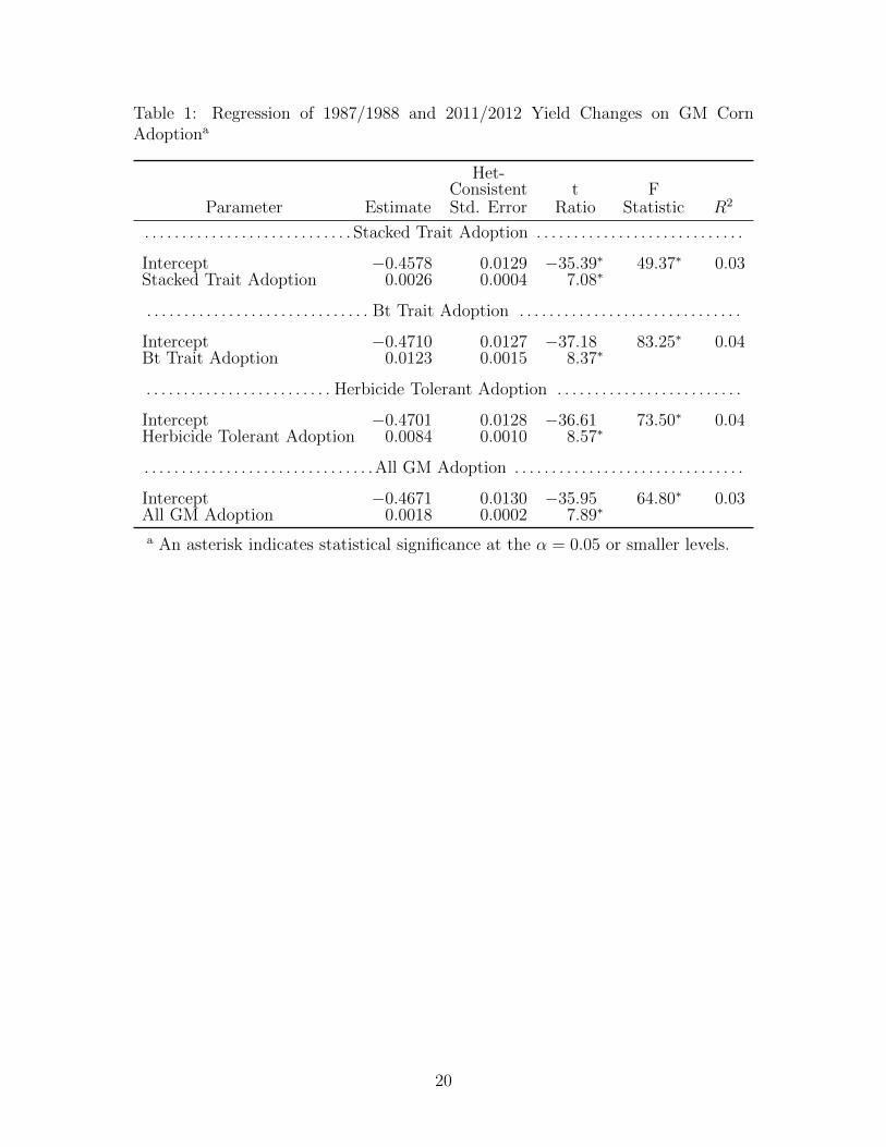
Table 1: Regression of 1987/1988 and 2011/2012 Yield Changes on GM CornAdoptiona
Het-Consistent t F
Parameter Estimate Std. Error Ratio Statistic R2
. . . . . . . . . . . . . . . . . . . . . . . . . . . . Stacked Trait Adoption . . . . . . . . . . . . . . . . . . . . . . . . . . . .
Intercept −0.4578 0.0129 −35.39∗ 49.37∗ 0.03Stacked Trait Adoption 0.0026 0.0004 7.08∗
. . . . . . . . . . . . . . . . . . . . . . . . . . . . . . Bt Trait Adoption . . . . . . . . . . . . . . . . . . . . . . . . . . . . . .
Intercept −0.4710 0.0127 −37.18 83.25∗ 0.04Bt Trait Adoption 0.0123 0.0015 8.37∗
. . . . . . . . . . . . . . . . . . . . . . . . . Herbicide Tolerant Adoption . . . . . . . . . . . . . . . . . . . . . . . . .
Intercept −0.4701 0.0128 −36.61 73.50∗ 0.04Herbicide Tolerant Adoption 0.0084 0.0010 8.57∗
. . . . . . . . . . . . . . . . . . . . . . . . . . . . . . .All GM Adoption . . . . . . . . . . . . . . . . . . . . . . . . . . . . . . .
Intercept −0.4671 0.0130 −35.95 64.80∗ 0.03All GM Adoption 0.0018 0.0002 7.89∗
a An asterisk indicates statistical significance at the α = 0.05 or smaller levels.
20

Table 2: Summary Statistics
Aggregated Coverage Level By Unit and Practice
Std. Std.Variable Mean Dev. Mean Dev.
Coverage Level 0.7403 0.0748 0.7471 0.0681BE Liability 2,805,761 4,980,505 1,248,938 2,748,301Non-BE Liability 8,032,964 11,502,464 3,700,757 6,130,394BE Premium 202,076 337,992 91,179 183,992Non-BE Premium 732,139 1,016,921 342,360 560,770BE Acres 4,589 7,489 2,026 4,042Non-BE Acres 13,999 17,972 6,436 9,610BE Indemnities 69,016 192,687 33,875 114,217Non-BE Indemnities 422,312 1,047,585 208,417 601,358APH Yield 145.06 23.34 147.11 26.45BE LR 0.4890 1.0872 0.5296 1.2703Non-BE LR 0.6597 1.1148 0.6940 1.1921BE LCR 0.0446 0.1078 0.0473 0.1156Non-BE LCR 0.0744 0.1347 0.0796 0.1436BE Premium Rate 0.0894 0.0455 0.0920 0.0463Non-BE Premium Rate 0.1057 0.0513 0.1086 0.0534Poor Condition 35.8445 12.0742 35.8267 11.8498Stacked 50.5390 8.4375 51.2335 8.1853Price-Based Loss 0.0676 0.1591 0.0712 0.1630Emerged 42.2821 26.9730 42.4277 27.0430Silking 73.0503 22.4624 73.3773 22.1752Historical LCR 0.0647 0.0752 0.0592 0.0674Enterprise — — 0.2697 0.4438Irrigated — — 0.0769 0.2664
21

Table 3: Summary Statistics: Weighted Conditional Means for LCRand LR Differencesa
LCR LR RateCategory N Difference Difference Difference
Aggregate Sample
All 36, 969 0.0274 0.2313 0.0191
By Coverage Level
0.50 942 0.0213 0.1818 0.02240.55 182 0.0542 0.4836 0.01380.60 757 0.0456 0.1490 0.04720.65 5, 459 0.0406 0.2425 0.01730.70 8, 786 0.0560 0.2318 0.02540.75 9, 700 0.0562 0.2832 0.02270.80 7, 068 0.0468 0.2114 0.01820.85 4, 075 0.0443 0.1236 0.0110
By Year
2008 5, 924 0.0134 0.0327 0.01292009 11, 206 0.0153 0.1046 0.02512010 10, 666 0.0283 0.2333 0.02322011 9, 173 0.0233 0.2095 0.0190
By State
Colorado 159 0.0089 0.0030 0.0259Illinois 6, 864 0.0172 0.1339 0.0163Indiana 4, 505 0.0425 0.3339 0.0230Iowa 8, 050 0.0257 0.2530 0.0142Kansas 1, 216 0.0011 −0.0699 0.0183Michigan 875 0.0203 0.1760 0.0068Minnesota 5, 138 0.0290 0.2567 0.0198Missouri 459 0.0328 0.2261 0.0036Nebraska 4, 429 0.0056 0.0227 0.0141Ohio 1, 983 0.0255 0.2419 0.0099South Dakota 2, 137 0.0977 0.6057 0.0360Wisconsin 1, 154 0.0161 0.1162 0.0178
By Practice
IRR 3, 549 0.0060 0.0179 0.0115NON-IRR 33, 420 0.0292 0.2481 0.0198
By Unit Structure
BU 14, 783 0.0246 0.2265 0.0149EU 9, 275 0.0211 0.2062 0.0163OU 12, 911 0.0272 0.1906 0.0181
By Plan
RP 30, 211 0.0284 0.2348 0.0199YP 6, 758 0.0072 0.0753 0.0107
a Weighted means calculated as ratios of conditional sums of in-demnities, liabilities, and premiums.
22

Table 4: Summary Statistics: Unweighted Conditional Means for LCR and LRDifferencesa
LCR t LR t Rate tCategory Difference Statistic Difference Statistic Difference Statistic
Aggregate Sample
All 0.0209 29.42∗ 0.0970 11.79∗ 0.0144 96.82∗
By Coverage Level
0.50 0.0198 4.47∗ 0.2915 2.72∗ 0.0144 11.73∗
0.55 0.0934 1.92 0.0934 0.83 0.0144 3.99∗
0.60 0.0195 5.26∗ 0.2296 2.63∗ 0.0193 10.52∗
0.65 0.0867 10.93∗ 0.0867 3.35∗ 0.0144 38.21∗
0.70 0.0870 13.44∗ 0.0870 5.26∗ 0.0154 51.96∗
0.75 0.0906 17.04∗ 0.0906 6.61∗ 0.0150 53.33∗
0.80 0.0941 12.95∗ 0.0941 6.67∗ 0.0131 44.83∗
0.85 0.0803 8.86∗ 0.0803 4.20∗ 0.0124 26.26∗
By Year
2008 0.0091 6.70∗ −0.0394 −1.62 0.0104 48.09∗
2009 0.0127 11.28∗ 0.0512 4.00∗ 0.0160 50.39∗
2010 0.0287 18.10∗ 0.1410 8.17∗ 0.0162 58.31∗
2011 0.0285 19.98∗ 0.1793 12.54∗ 0.0130 45.23∗
By State
Colorado 0.0040 0.43 0.0115 0.17 0.0208 9.60∗
Illinois 0.0208 14.23∗ 0.1024 4.35∗ 0.0147 39.15∗
Indiana 0.0273 13.20∗ 0.1560 8.04∗ 0.0173 40.24∗
Iowa 0.0070 5.86∗ −0.0499 −2.38∗ 0.0117 85.23∗
Kansas 0.0042 1.04 −0.0053 −0.15 0.0129∗ 9.32∗
Michigan 0.0313 4.94∗ 0.1667 2.81∗ 0.0144 13.76∗
Minnesota 0.0149 10.66∗ 0.1176 6.98∗ 0.0139 41.08∗
Missouri 0.0510 5.28∗ 0.1782 2.54∗ 0.0203 11.40∗
Nebraska 0.0050 2.93∗ 0.0032 0.15 0.0111 28.52∗
Ohio 0.0334 10.82∗ 0.2603 10.14∗ 0.0133 28.36∗
South Dakota 0.1043 18.01∗ 0.5601 15.83∗ 0.0262 28.84∗
Wisconsin 0.0154 4.86∗ 0.0841 3.52∗ 0.0147 11.87∗
By Practice
IRR 0.0183 6.13∗ 0.0827 2.45∗ 0.0121 34.21∗
NON-IRR 0.0212 29.58∗ 0.0985 11.83∗ 0.0147 91.35∗
By Unit Structure
BU 0.0212 18.56∗ 0.0843 5.89∗ 0.0150 62.96∗
EU 0.0225 15.47∗ 0.1724 11.96∗ 0.0100 42.48∗
OU 0.0195 16.80∗ 0.0582 4.38∗ 0.0169 61.11∗
By Plan
RP 0.0235 28.17∗ 0.1151 14.87∗ 0.0150 85.20∗
YP 0.0114 8.95∗ 0.0309 1.20 0.0124 47.80∗
a Average of conditional means at the state, county, and year level. Asterisks indicatestatistical significance at the α = 0.05 or smaller level.
23

Table 5: Loss-Cost and Loss Ratio Difference Regressions (Coverage Level/County/YearAggregation)a
Het-Consistent t Clustered t
Parameter Estimate Std. Error Ratio Std. Error Ratio
Loss Cost Regressions
Intercept 0.01749 0.00467 3.75∗∗ 0.00596 2.94∗∗
Poor Condition 0.00035 0.00013 2.70∗∗ 0.00015 2.29∗∗
. . . . . . . . . . . . . . . . . . . . . . . . . . . . . . . . . . . . . . . . . . . . . . . . . . . . . . . . . . . . . . . . . . . . . . . . . . . . . . . . . . . . . . . . .N 8,956F-Statistic 9.83∗∗
R2 0.0011
Intercept 0.06394 0.02282 2.80∗∗ 0.02636 2.43∗∗
Emerged −0.00025 0.00008 −3.14∗∗ 0.00009 −2.84∗∗
Silking 0.00030 0.00009 3.27∗∗ 0.00011 2.87∗∗
Poor Condition 0.00032 0.00014 2.27∗∗ 0.00016 2.04∗∗
Stacked Trait Adoption 0.00145 0.00019 7.59∗∗ 0.00027 5.44∗∗
Price-Based Loss −0.01486 0.00518 −2.87∗∗ 0.00602 −2.47∗∗
APH Yield −0.00064 0.00013 −4.98∗∗ 0.00015 −4.38∗∗
Historical LCR 0.20862 0.05482 3.81∗∗ 0.06940 3.01∗∗
Coverage Level −0.06740 0.02457 −2.74∗∗ 0.02613 −2.58∗∗
. . . . . . . . . . . . . . . . . . . . . . . . . . . . . . . . . . . . . . . . . . . . . . . . . . . . . . . . . . . . . . . . . . . . . . . . . . . . . . . . . . . . . . . . .N 8,842F-Statistic 67.83∗∗
R2 0.0579
Loss Ratio Regressions
Intercept 0.06638 0.04153 1.60 0.04650 1.43Poor Condition 0.00286 0.00121 2.37∗∗ 0.00131 2.19∗∗
. . . . . . . . . . . . . . . . . . . . . . . . . . . . . . . . . . . . . . . . . . . . . . . . . . . . . . . . . . . . . . . . . . . . . . . . . . . . . . . . . . . . . . . . .N 8,956F-Statistic 7.53∗∗
R2 0.0008
Intercept 0.73615 0.25871 2.85∗∗ 0.27502 2.68∗∗
Emerged −0.00273 0.00079 −3.44∗∗ 0.00085 −3.20∗∗
Silking 0.00357 0.00095 3.74∗∗ 0.00104 3.42∗∗
Poor Condition 0.00209 0.00133 1.58 0.00142 1.47Stacked Trait Adoption 0.00782 0.00143 5.47∗∗ 0.00177 4.41∗∗
Price-Based Loss −0.25548 0.06060 −4.22∗∗ 0.06445 −3.96∗∗
APH Yield −0.00259 0.00111 −2.33∗∗ 0.00119 −2.17∗∗
Historical LCR 0.79254 0.36394 2.18∗∗ 0.41722 1.90∗
Coverage Level −1.13343 0.36248 −3.13∗∗ 0.37011 −3.06∗∗
. . . . . . . . . . . . . . . . . . . . . . . . . . . . . . . . . . . . . . . . . . . . . . . . . . . . . . . . . . . . . . . . . . . . . . . . . . . . . . . . . . . . . . . . .N 8,842F-Statistic 22.73∗∗
R2 0.0202
a Single and double asterisks indicate statistical significance at the α = 0.10 and α = 0.05or smaller levels, respectively.
24
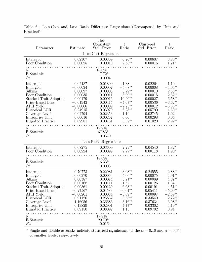
Table 6: Loss-Cost and Loss Ratio Difference Regressions (Decomposed by Unit andPractice)a
Het-Consistent t Clustered t
Parameter Estimate Std. Error Ratio Std. Error Ratio
Loss Cost Regressions
Intercept 0.02307 0.00369 6.26∗∗ 0.00607 3.80∗∗
Poor Condition 0.00025 0.00010 2.58∗∗ 0.00015 1.71∗
. . . . . . . . . . . . . . . . . . . . . . . . . . . . . . . . . . . . . . . . . . . . . . . . . . . . . . . . . . . . . . . . . . . . . . . . . . . . . . . . . . . . . . . . .N 18,098F-Statistic 7.72∗∗
R2 0.0004
Intercept 0.02487 0.01800 1.38 0.02264 1.10Emerged −0.00034 0.00007 −5.08∗∗ 0.00008 −4.04∗∗
Silking 0.00027 0.00008 3.29∗∗ 0.00010 2.55∗∗
Poor Condition 0.00035 0.00011 3.09∗∗ 0.00015 2.32∗∗
Stacked Trait Adoption 0.00179 0.00016 10.90∗∗ 0.00027 6.58∗∗
Price-Based Loss −0.01942 0.00415 −4.67∗∗ 0.00536 −3.62∗∗
APH Yield −0.00066 0.00009 −7.23∗∗ 0.00012 −5.55∗∗
Historical LCR 0.24915 0.03970 6.28∗∗ 0.05790 4.30∗∗
Coverage Level −0.02794 0.02353 −1.19 0.02745 −1.02Enterprise Unit 0.00016 0.00267 0.06 0.00298 0.05Irrigated Practice 0.02981 0.00781 3.82∗∗ 0.01020 2.92∗∗
. . . . . . . . . . . . . . . . . . . . . . . . . . . . . . . . . . . . . . . . . . . . . . . . . . . . . . . . . . . . . . . . . . . . . . . . . . . . . . . . . . . . . . . . .N 17,918F-Statistic 67.83∗∗
R2 0.0579
Loss Ratio Regressions
Intercept 0.08275 0.03609 2.29∗∗ 0.04540 1.82∗
Poor Condition 0.00224 0.00099 2.27∗∗ 0.00118 1.90∗
. . . . . . . . . . . . . . . . . . . . . . . . . . . . . . . . . . . . . . . . . . . . . . . . . . . . . . . . . . . . . . . . . . . . . . . . . . . . . . . . . . . . . . . . .N 18,098F-Statistic 6.33∗∗
R2 0.0003
Intercept 0.70773 0.22981 3.08∗∗ 0.24555 2.88∗∗
Emerged −0.00370 0.00066 −5.60∗∗ 0.00075 −4.91∗∗
Silking 0.00387 0.00074 5.21∗∗ 0.00089 4.37∗∗
Poor Condition 0.00168 0.00111 1.52 0.00126 1.34Stacked Trait Adoption 0.00861 0.00129 6.68∗∗ 0.00191 4.51∗∗
Price-Based Loss −0.27567 0.04583 −6.01∗∗ 0.05411 −5.09∗∗
APH Yield −0.00261 0.00084 −3.09∗∗ 0.00097 −2.69∗∗
Historical LCR 0.91126 0.25837 3.53∗∗ 0.33549 2.72∗∗
Coverage Level −1.16056 0.36683 −3.16∗∗ 0.37634 −3.08∗∗
Enterprise Unit 0.13829 0.02901 4.77∗∗ 0.03302 4.19∗∗
Irrigated Practice 0.09150 0.08092 1.13 0.09702 0.94. . . . . . . . . . . . . . . . . . . . . . . . . . . . . . . . . . . . . . . . . . . . . . . . . . . . . . . . . . . . . . . . . . . . . . . . . . . . . . . . . . . . . . . . .N 17,918F-Statistic 29.79∗∗
R2 0.0164
a Single and double asterisks indicate statistical significance at the α = 0.10 and α = 0.05or smaller levels, respectively.
25

Figure 1: USDA-NASS Average Corn Planting Density in Iowa with ISU Extension Recom-mended Range
26

Figure 2: Palmer’s Z Drought Index: Northeast Illinois
27

Figure 3: A Comparison of Corn Root Balls for Conventional Corn (left) and SmartStaxCorn (right). (Source: Mycogen Seeds, Agronomy Bulletin 116, “Which Trait Package isRight for You?” August 9, 2015.)
28

Figure 4: Left-tail Differences in Yield Distributions for Conventional (NT) and Biotech(BT) corn. (Source: Biotech Yield Endorsement Submission and Review Materials.)
29
(a) 1988 Precipitation (b) 2012 Precipitation
(c) 1988 Temperature (d) 2012 Temperature
(e) 1988 Max-Temperature (f) 2012 Max-Temperature
Figure 5: Weather Conditions Relative to Normal in 1988 and 2012
30
(a) log(1987/1988 Yields)
(b) log(2011/2012 Yields)
Figure 6: Proportional Planted-Acreage Corn Yield Changes
31

(a) 1987/1988 and 2011/2012 Corn Yield Changes
(b) Yield Changes and the Palmer Z Drought Index
Figure 7: Yield Changes and Drought Conditions in 1988 and 2012
32

References
Annan, F., Schlenker, W., 2015. Federal crop insurance and the disincentive to adapt to
extreme heat. Am. Econ. Rev. 105 (5), 262-266.
Attavanich, W., McCarl, B.A., 2014. How is CO2 affecting yields and technological progress?
A statistical analysis. Climatic Change. 124 (4), 747-762.
Chavas, J.P., Shi, G. and Lauer, J., 2014. The effects of gm technology on maize yield.
Crop Sci. 54:1331-1335.
Chen, C., Chang, C., 2005. The impact of weather on crop yield distribution in Taiwan:
Some new evidence from panel data models and implications for crop insurance. Agr.
Econ. 33, 503-511.
DAgostino, A.L., Schlenker, W., 2016. Recent weather fluctuations and agricultural yields:
Implications for climate change. Agr. Econ. 47, 159-171.
Di Falco, S., Adinolfi, F., Bozzola, M., Capitanio, F., 2014. Crop insurance as a strategy
for adapting to climate change. J. Agr. Econ. 65 (2), 485-504.
Li, S., Ker, A. P., 2013. An Assessment of the Canadian Federal-Provincial Crop Produc-
tion Insurance Program under Future Climate Change Scenarios in Ontario. Paper
presented at the 2013 AAEA Annual Meeting, August 4-6, 2013, Washington, D.C.
Lobell, D.B., 2014. Climate change adaptation in crop production: Beware of illusions.
Global Food Security. 3: 72-76
Lobell, D.B., Hammer, G.L., McLean, G., Messina, C., Roberts, M.J., Schlenker, W., 2013.
The critical role of extreme heat for maize production in the United States. Nat. Clim.
Change. 3, 497-501.
33

Lobell, D.B., Roberts, M.J., Schlenker, W., Braun, N., Little, B.B., Rejesus, R.M. and
Hammer, G.L., 2014. Greater sensitivity to drought accompanies maize yield increase
in the U.S. Midwest. Science, 344(6183): 516-519.
Lobell, D.B., Schlenker, W., Costa-Roberts J., 2011. Climate trends and global crop pro-
duction since 1980. Science. 333(6042), 616-620.
Malcolm, S., Aillery, M., Weinberg, M., 2009. Ethanol and a changing agricultural land-
scape. Washington, DC: Economic Research Service Economic Research Report No.
(ERR-86), March 2009.
Jayson L. Lusk, J. L., Tack,J., Hendricks, N.P. 2018. Heterogeneous Yield Impacts from
Adoption of Genetically Engineered Corn and the Importance of Controlling for Weather.
NBER Working Paper No. 23519, July 23, 2018.
Pitt, D., 2012. Crop technology helps limit corn losses in drought. The Waterloo (Iowa)
Courier, July 11, 2012.
Ray D.K., Gerber, J.S., MacDonald, G.K., West, P.C., 2015. Climate variation explains a
third of global crop yield variability. Nat. Commun. 6, 5989.
Roberts, M.J., Schlenker, W., Eyer, J., 2013. Agronomic weather measures in econometric
models of crop yield with implications for climate change. Am. J. Agr. Econ. 95 (2),
236-243.
Roberts, M. J., Braun, N. O., Sinclair, T. R., Lobell, D. B., Schlenker, W., 2017. Comparing
and crop models and statistical models with some implications for climate change.
Environmental Research Letters, 12(9), 095010.
Rosenzweig, C, Elliott, J., Deryng, D., Ruane, A.C., Muller, C., Arneth, A., Boote, K.J.,
Folberth, C., Glotter, M., Khabarov, N., Neumann, K., Piontek, F., Pugh, T.A.M.,
Schmid, E., Stehfest, E., Yang, H., Jones, J.W., 2014. Assessing agricultural risks of
34

climate change in the 21st century in a global gridded crop model intercomparison.
Proc. Natl. Acad. Sci. 111(9), 3268-3273.
Seifert, C.A., Roberts, M.J., Lobell, D. B., 2017. Continuous Corn and Soybean Yield
Penalties across Hundreds of Thousands of Fields. Agron. J. 109:541-548.
Schlenker W., Roberts, M.J., 2009. Nonlinear temperature effects indicate severe damages
to US crop yields under climate change. Proc. Natl. Acad. Sci. 106(37), 15,594-
615,598.
Tack, J., Coble, K., and Barnett, B., 2018. Warming temperatures will likely induce higher
premium rates and government outlays for the U.S. crop insurance program. Agr.
Econ. 49, 635-47.
Tack, J., Barkley, A., Nalley, L.L., 2015. Effect of warming temperatures on US wheat
yields. Proc. Natl. Acad. Sci. 112(22), 6931-6936.
Tolhurst, T. N., Ker, A. P., 2015. On Technological Change in Crop Yields. American
Journal of Agricultural Economics, Volume 97(1):137-158.
Urban, D.W., Sheffield, J., Lobell, D.B., 2015. The impacts of future climate and carbon
dioxide changes on the average and variability of US maize yields under two emission
scenarios. Environ. Res. Lett. 10(04), 1-9.
Urban, D., Roberts, M.J., Schlenker, W., Lobell, D.B., 2012. Projected temperature
changes indicate significant increase in interannual variability of US maize yields. Cli-
matic Change. 112(2), 525-533.
Weitzman, M.L., 2011. Fat-tailed uncertainty in the economics of catastrophic climate
change. Rev. Env. Econ. Policy. 5 (2), 275-292.
35

Welch, J.R., Vincent, J.R., Auffhammer, M., Moya, P.F., Dobermann, A., Dawe, D., 2010.
Rice yields in tropical/subtropical Asia exhibit large but opposing sensitivities to min-
imum and maximum temperatures. Proc. Natl. Acad. Sci. 7(33), 14,562-14,567.
Woli, K.P., Burras, C.L. Abendroth, L.J., Elmore, R.W., 2014. Optimizing corn seeding
rates using a fields corn suitability rating. Agronomy J., 106:1523-32.
Wright, E., Licht, M., 2018. Corn row spacing considerations. Iowa State Univeristy, March
12, 2018, https://crops.extension.iastate.edu/cropnews/2018/03/corn-row-spacing-considerations.
Zhu,Y., Goodwin, B.K., Ghosh, S.K., 2011. Modeling yield risk under technological change:
dynamic yield distributions and the US crop insurance program. J. Agr. Res. Econ.
36(1):192-210.
36