Policy Research Working Paper 5103

Has India’s Economic Growth Become More Pro-Poor in the Wake

of Economic Reforms?Gaurav Datt

Martin Ravallion

The World BankDevelopment Research GroupDirector’s OfficeOctober 2009

WPS5103P

ublic

Dis

clos

ure

Aut

horiz

edP

ublic

Dis

clos

ure

Aut

horiz

edP

ublic

Dis

clos

ure

Aut

horiz

edP

ublic

Dis

clos

ure

Aut

horiz

edP

ublic

Dis

clos

ure

Aut

horiz

edP

ublic

Dis

clos

ure

Aut

horiz

edP

ublic

Dis

clos

ure

Aut

horiz

edP

ublic

Dis

clos

ure

Aut

horiz

ed

Produced by the Research Support Team

Abstract

The Policy Research Working Paper Series disseminates the findings of work in progress to encourage the exchange of ideas about development issues. An objective of the series is to get the findings out quickly, even if the presentations are less than fully polished. The papers carry the names of the authors and should be cited accordingly. The findings, interpretations, and conclusions expressed in this paper are entirely those of the authors. They do not necessarily represent the views of the International Bank for Reconstruction and Development/World Bank and its affiliated organizations, or those of the Executive Directors of the World Bank or the governments they represent.

Policy Research Working Paper 5103

The extent to which India’s poor have benefited from the country’s economic growth has long been debated. This paper revisits the issues using a new series of consumption-based poverty measures spanning 50 years, and including a 15-year period after economic reforms began in earnest in the early 1990s. Growth has tended to reduce poverty, including in the post-reform period. There is no robust evidence that the responsiveness of poverty to growth has increased, or decreased, since the reforms began, although there are signs of rising

This paper—a product of the Director’s Office, Development Research Group—is part of a larger effort in the department to monitor and explain progress against poverty in developing countries. Policy Research Working Papers are also posted on the Web at http://econ.worldbank.org. The author may be contacted at mravallion@worldbank.org.

inequality. The impact of growth is higher for poverty measures that reflect distribution below the poverty line, and it is higher using growth rates calculated from household surveys than national accounts. The urban-rural pattern of growth matters to the pace of poverty reduction. However, in marked contrast to the pre-reform period, the post-reform process of urban economic growth has brought significant gains to the rural poor as well as the urban poor.

Has India’s Economic Growth Become More Pro-Poor

in the Wake of Economic Reforms?

Gaurav Datt and Martin Ravallion1

World Bank

1 The authors are grateful to Ann Harrison, Rinku Murgai and Abhijit Sen for helpful comments and to Dandan Zhang for excellent research assistance. These are the views of the authors, and should not be attributed to the World Bank.

2

1. Introduction

India's post-independence planners in the 1950s must surely have expected better

performance from the new country's economic strategy. Poverty has always figured prominently

in assessments of India’s economic performance. On average, slightly more than one person in

two lived below the poverty line in India during the 1950s and ‘60s. By 1990 the proportion had

fallen, but was still slightly more than one person in three; Figure 1 gives our estimates of the

poverty rate for the date of each available survey as well as an estimate of the mean poverty rate

by year.2 There was no trend increase, or decrease, in consumption inequality over the period up

to about 1990 (Bruno et al., 1998). So the (proximate) reason why poverty did not fall more

rapidly was low rates of economic growth; GDP per capita grew at an annual rate of barely 1%

in the 1960s and 1970s, though picking up to 3% in the 1980s.

There has been much hope that India’s economic reforms starting in the early 1990s

would bring more rapid poverty reduction. There has certainly been an acceleration of growth,

with GDP per capita growing at 4-5% since 1991. However, we also know from past research

that the sectoral pattern of India’s growth matters to its impact on poverty. The green revolution

appears to have stimulated pro-poor rural growth.3 In past work, we found that both the urban

and rural poor gained from growth within the rural sector, but that urban growth had adverse

distributional effects within urban areas and no discernable impact on rural poverty (Ravallion

and Datt, 1996). The disappointing outcomes for the poor from non-farm growth have also been

traced back to India’s antecedent socio-economic inequalities in access to schooling.4 However,

while past research pointed to the importance of rural economic growth to poverty reduction in

India, the post-reform process of economic growth has not favored the rural sector. A number of

observers have pointed to both geographic and sectoral divergence in India’s post-reform growth

process.5 We have argued elsewhere that this has meant that much of the non-farm economic

2 The estimates use the data and methods described later; the estimates of the conditional mean by year (the bold line in Figure 1) are locally-weighted regression estimates. The mean (and median) poverty rate up to 1970 was 53% with a standard deviation of 6.3% 3 Datt and Ravallion (1998) found that farm productivity growth reduced rural poverty. Earlier support for this view includes Ahluwalia (1978, 1985), van de Walle (1985), Bhattacharya et al. (1991) and Bell and Rich (1994). Dissenting views include Saith (1981) and Gaiha (1995). 4 Ravallion and Datt (2002) found a strong interaction effect between the initial level of human development at state level and the non-farm growth rate in determining poverty reduction at state level. 5 Bhattacharya and Sakthivel (2004), Jha (2000), Datt and Ravallion (2002) and Purfield (2006).

3

growth bypassed the sectors and states where it would have had the most impact on poverty

based on a model calibrated to largely pre-reform data (Datt and Ravallion, 2002). By this view,

the composition of the higher growth would mean that it by-passed many of India’s poor.

Against this view, it can be conjectured that India’s growth process has changed—

implying a new set of parameters in the relationship between growth and poverty reduction.

Ravallion and Datt (1996) studied a period in which the development strategy emphasized rapid

development of the capital goods sector in a largely closed economy.6 The strategy assumed that

the capital stock and industrial structure could be manipulated exogenously through central

planning, even in a largely market-based economy. The strategy was also founded on “trade

pessimism”—the beliefs, grounded in the experiences of colonialism, that India could never

compete in global markets until its domestic capital stock had been greatly expanded, coupled

with a distrust of foreign (Western) countries as a source of essential goods. These assumptions

were questioned in both academic and policy circles at the time, and with greater veracity as the

years passed, in the light of the evidently poor economic performance.7 The success of China’s

pro-market reforms starting in 1978 also fueled doubts in the 1980s about India’s economic

strategy. The policy debate raged for many years, but it was not until a balance of payments

crisis that reforms started in earnest, in the early 1990s. (As is evident in Figure 1, the

macroeconomic difficulties appear to have also stalled progress against poverty.) Trade

liberalization was combined with efforts to support higher productivity in the private sector.8

Supporters argued that these reforms would allow India to better exploit its comparative

advantage in labor-intensive goods and services, and that this would directly benefit the poor; by

this view, the reforms would “..favour the poor by beginning to remove the pervasive bias that

exists against the employment of unskilled labour” (Joshi and Little, 1996, p.221). The hope was

that the post-reform urban economy would be more effective in reducing both urban and rural

poverty.

6 On the history of thought on development strategies and their implications for poverty, with specific reference to India, see Lipton and Ravallion (1995). 7 Some observers in India at the time had questioned these assumptions, raising concerns about labor absorption (given high population growth) and (hence) poverty reduction; in particular see Vakil and Brahmanand (1956). Chakravarty (1987) provides an insightful account of the history of thought on India’s (pre-reform) development strategy. For a broader analysis of industrial policy in developing countries, emphasizing the endogeneity of industrial structure to factor endowments, see Lin (2009).

4

However, there are also reasons to question whether the new policy environment would

succeed in putting India on a new path of rapid poverty reduction. The greater openness to

external trade came with sufficient productivity growth to assure a higher growth rate of national

output.9 But it appears that new inequality-increasing forces also emerged, and a number of

observers have reported evidence of rising consumption inequality since the early 1990s.10 This

may well reflect the antecedent inequalities in other “non-income” dimensions, particularly in

human capital, which can mean that the poorest are largely left behind; these inequalities were

far greater in India around 1990 than China around 1980.11

Some observers have also questioned whether the post-reform growth process has

fulfilled the expectations of reform advocates that it would increase aggregate demand for

unskilled labor and (hence) help reduce poverty. The fastest growing sectors of India’s economy

have tended to be more intensive in capital and skilled labor, notably the booming business-

services sector. And the share of employment in agriculture has fallen much less than (say)

China. This pattern of growth is hardly what the “comparative-advantage” arguments of reform

advocates in the 1980s predicted as the outcome of India becoming a far more open economy.12

However, it is also important to note that the non-farm sectors that are relatively intensive in

unskilled labor—trade, construction and the informal manufacturing sector—fared better in the

post-1991 period than earlier (Kotwal et al., 2009).13 The non-farm sector’s aggregate demand

8 On India’s reform agenda since the early 1990s see Ahluwalia (2002) and Panagariya (2008). 9 See the interesting discussion in Eswaran and Kotwal (1994, Chapter 7) who argue that domestic productivity growth is key to the outcomes for poor people from trade openness in India. Here the sequencing of reforms was important, and India’s reformers wisely emphasized domestic reforms (such as industrial de-licensing) prior to external reforms (Bhagwatti, 1993). 10 Evidence of rising inequality in India since 1991 is reported in Ravallion (2000), Deaton and Drèze (2002) and Sen and Hiamnshu (2004b). 11 See the discussion in Drèze and Sen (1995) on the constraints stemming from India’s poor human development attainments at the outset of its current reform period, and the contrast with China. Also see Chaudhuri and Ravallion (2006) on the distinction between “good” and “bad” inequalities in both China and India, and the discussion of inequality of opportunity in World Bank (2005). 12 Few people in the 1980s would have predicted that technological changes in the 1990s, combined with the required human skills, would entail that India developed a comparative advantage in sectors such as business services. 13 The formal (“organized”) manufacturing sector has not seen rising employment after trade liberalization (Sen, 2009), although this is a moot point given that 80% of manufacturing employment is in the informal sector (Kotwal et al., 2009).

5

for unskilled labor appears to have increased after the reforms, even though the most dynamic

sectors have been intensive in skilled labor.

Motivated by these observations, this paper addresses the following questions: Have

India’s higher growth rates since the early 1990s delivered a higher pace of progress against

absolute poverty? Have we seen any change in the responsiveness of poverty to growth in the

post-reform period? Has the poverty impact of the urban-rural composition of growth changed?

In particular, is there any sign that the post-reform urban economic growth process has been

more pro-poor than the pre-reform process?

The following section outlines the concepts and methods used in this study. Section 3

describes our data set, which updates that we constructed for Ravallion and Datt (1996) (with

some improvements in the estimation methods, as described below). Section 4 then presents our

results and discusses their implications. Section 5 concludes.

2. Concepts and methods

There are two ways in which economic growth can be considered “pro-poor.” 14 By the

first, which we label Definition 1, “pro-poor growth” is growth that reduces an agreed measure

of poverty, and the extent of poverty reduction is then the sole metric of “pro-poorness.”

Definition 2 says instead that “pro-poor growth” is growth that disproportionately benefits the

poor when judged relative to the rate of growth; by this view the pro-poorness of growth is

measured by the elasticity of the agreed poverty measure with respect to economic growth.

We use three poverty measures for implementing both definitions: The head-count index

(H) is given by the percentage of the population who live in households with a consumption per

capita less than the poverty line. The poverty gap index (PG) is the mean distance below the

poverty line expressed as a proportion of that line, where the mean is formed over the entire

population, counting the non-poor as having zero poverty gap; this can be interpreted as a

measure of the depth of poverty. The squared poverty gap index (SPG), introduced by Foster et

al. (1984), is the mean of the squared proportionate poverty gaps. Unlike PG, SPG is sensitive to

distribution amongst the poor, in that it satisfies the transfer axiom for poverty measurement

14 For an overview of the various approaches to defining “pro-poor growth” see Ravallion (2004).

6

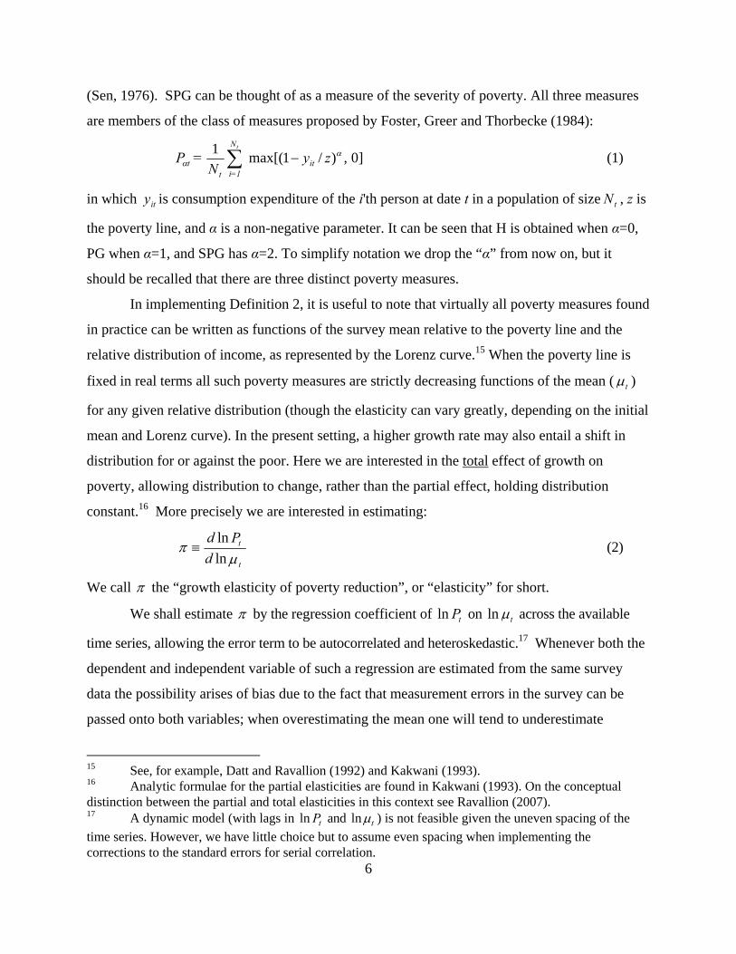
(Sen, 1976). SPG can be thought of as a measure of the severity of poverty. All three measures

are members of the class of measures proposed by Foster, Greer and Thorbecke (1984):

]0,)/1max[(1

zy N

= P it

N

1=itt

t

(1)

in which ity is consumption expenditure of the i'th person at date t in a population of size tN , z is

the poverty line, and α is a non-negative parameter. It can be seen that H is obtained when α=0,

PG when α=1, and SPG has α=2. To simplify notation we drop the “α” from now on, but it

should be recalled that there are three distinct poverty measures.

In implementing Definition 2, it is useful to note that virtually all poverty measures found

in practice can be written as functions of the survey mean relative to the poverty line and the

relative distribution of income, as represented by the Lorenz curve.15 When the poverty line is

fixed in real terms all such poverty measures are strictly decreasing functions of the mean ( t )

for any given relative distribution (though the elasticity can vary greatly, depending on the initial

mean and Lorenz curve). In the present setting, a higher growth rate may also entail a shift in

distribution for or against the poor. Here we are interested in the total effect of growth on

poverty, allowing distribution to change, rather than the partial effect, holding distribution

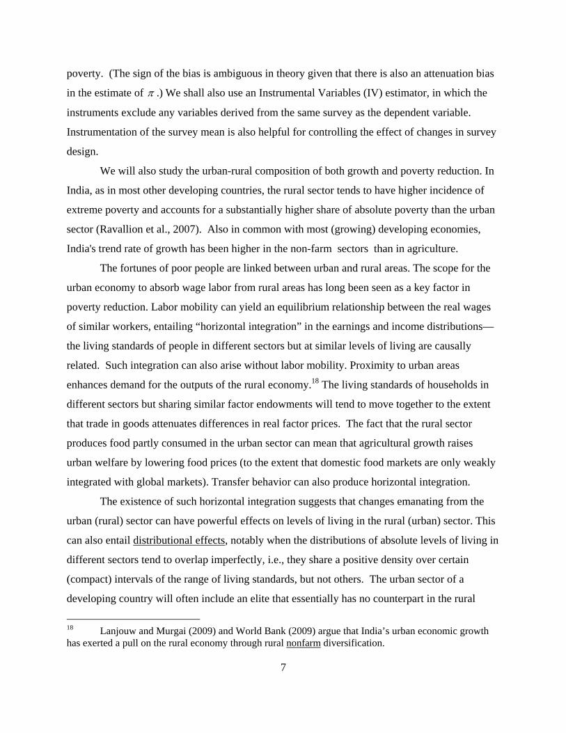
constant.16 More precisely we are interested in estimating:

d

Pd

t

t

ln

ln (2)

We call the “growth elasticity of poverty reduction”, or “elasticity” for short.

We shall estimate by the regression coefficient of tPln on tln across the available

time series, allowing the error term to be autocorrelated and heteroskedastic.17 Whenever both the

dependent and independent variable of such a regression are estimated from the same survey

data the possibility arises of bias due to the fact that measurement errors in the survey can be

passed onto both variables; when overestimating the mean one will tend to underestimate

15 See, for example, Datt and Ravallion (1992) and Kakwani (1993). 16 Analytic formulae for the partial elasticities are found in Kakwani (1993). On the conceptual distinction between the partial and total elasticities in this context see Ravallion (2007). 17 A dynamic model (with lags in tPln and tln ) is not feasible given the uneven spacing of the

time series. However, we have little choice but to assume even spacing when implementing the corrections to the standard errors for serial correlation.

7

poverty. (The sign of the bias is ambiguous in theory given that there is also an attenuation bias

in the estimate of .) We shall also use an Instrumental Variables (IV) estimator, in which the

instruments exclude any variables derived from the same survey as the dependent variable.

Instrumentation of the survey mean is also helpful for controlling the effect of changes in survey

design.

We will also study the urban-rural composition of both growth and poverty reduction. In

India, as in most other developing countries, the rural sector tends to have higher incidence of

extreme poverty and accounts for a substantially higher share of absolute poverty than the urban

sector (Ravallion et al., 2007). Also in common with most (growing) developing economies,

India's trend rate of growth has been higher in the non-farm sectors than in agriculture.

The fortunes of poor people are linked between urban and rural areas. The scope for the

urban economy to absorb wage labor from rural areas has long been seen as a key factor in

poverty reduction. Labor mobility can yield an equilibrium relationship between the real wages

of similar workers, entailing “horizontal integration” in the earnings and income distributions—

the living standards of people in different sectors but at similar levels of living are causally

related. Such integration can also arise without labor mobility. Proximity to urban areas

enhances demand for the outputs of the rural economy.18 The living standards of households in

different sectors but sharing similar factor endowments will tend to move together to the extent

that trade in goods attenuates differences in real factor prices. The fact that the rural sector

produces food partly consumed in the urban sector can mean that agricultural growth raises

urban welfare by lowering food prices (to the extent that domestic food markets are only weakly

integrated with global markets). Transfer behavior can also produce horizontal integration.

The existence of such horizontal integration suggests that changes emanating from the

urban (rural) sector can have powerful effects on levels of living in the rural (urban) sector. This

can also entail distributional effects, notably when the distributions of absolute levels of living in

different sectors tend to overlap imperfectly, i.e., they share a positive density over certain

(compact) intervals of the range of living standards, but not others. The urban sector of a

developing country will often include an elite that essentially has no counterpart in the rural

18 Lanjouw and Murgai (2009) and World Bank (2009) argue that India’s urban economic growth has exerted a pull on the rural economy through rural nonfarm diversification.

8

sector. When combined with shared poverty in the overlapping interval of the distribution, this

can have strong implications for how an increase in incomes in one sector will spill over to affect

both average levels of living, and inequalities within the other sector.

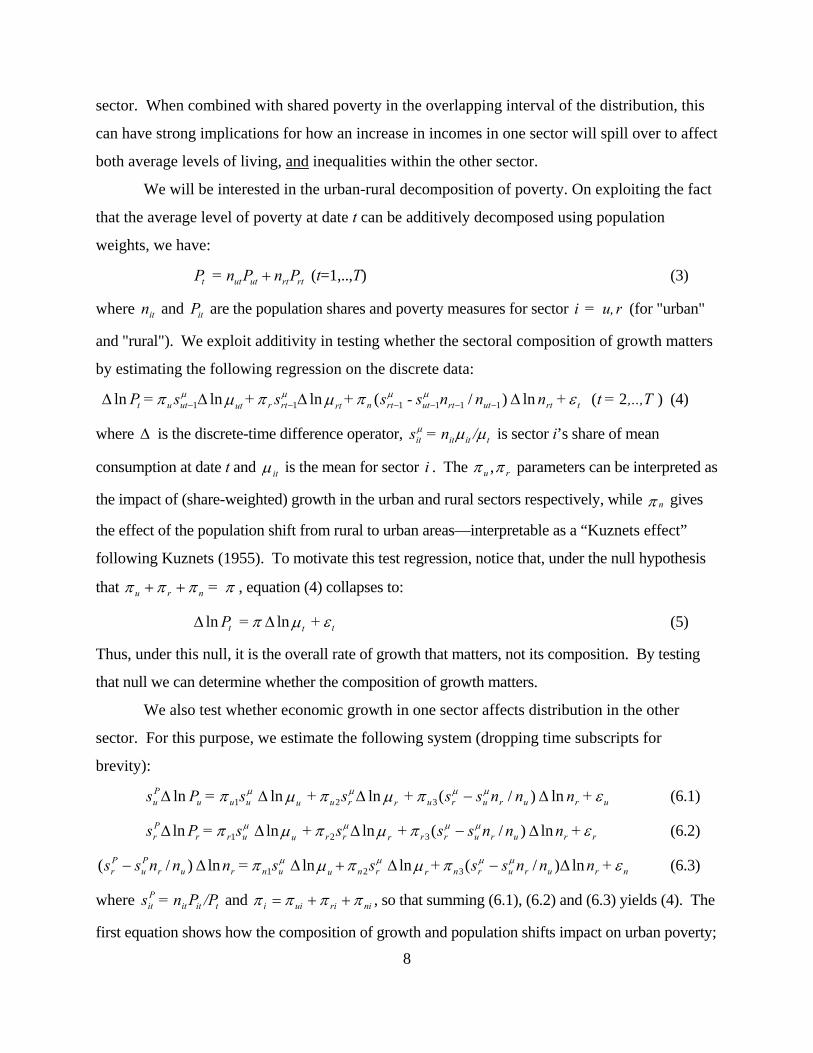
We will be interested in the urban-rural decomposition of poverty. On exploiting the fact

that the average level of poverty at date t can be additively decomposed using population

weights, we have:

rtrtututt PnPn= P (t=1,..,T) (3)

where itn and itP are the population shares and poverty measures for sector r u, =i (for "urban"

and "rural"). We exploit additivity in testing whether the sectoral composition of growth matters

by estimating the following regression on the discrete data:

)2(ln)/(lnlnln 111111 T,..,=t + n nn s- s + s + s = P trtutrtutrtnrtrtrututut (4)

where is the discrete-time difference operator, tititit /n= s is sector i’s share of mean

consumption at date t and it is the mean for sector i . The ru , parameters can be interpreted as

the impact of (share-weighted) growth in the urban and rural sectors respectively, while n gives

the effect of the population shift from rural to urban areas—interpretable as a “Kuznets effect”

following Kuznets (1955). To motivate this test regression, notice that, under the null hypothesis

that =nru , equation (4) collapses to:

ttt + = P lnln (5)

Thus, under this null, it is the overall rate of growth that matters, not its composition. By testing

that null we can determine whether the composition of growth matters.

We also test whether economic growth in one sector affects distribution in the other

sector. For this purpose, we estimate the following system (dropping time subscripts for

brevity):

ururururruuuuuPu + n nnss+ s + s= Ps ln)/(lnlnln 321 (6.1)

rrururrrrruurrPr + n nnss+ s + s= Ps ln)/(lnlnln 321 (6.2)

nrururnrrnuunrurPu

Pr +nnnss+ s s =n nnss ln)/(lnlnln)/( 321 (6.3)

where tititPit /PPn= s and niriuii , so that summing (6.1), (6.2) and (6.3) yields (4). The

first equation shows how the composition of growth and population shifts impact on urban poverty;

9

the second shows how they impact on rural poverty. The third equation gives the impact on the

population shift component of Plog . We estimate (6.1) and (6.2).19

3. Data

In addressing the questions posed in the Introduction, it is clearly desirable to have a

reasonable long time series of household surveys; a short series can be deceptive for inferring a

trend.20 Amongst developing countries, India has the longest series of national household

surveys suitable for tracking living conditions of the poor. At the time of writing, we can

assemble distributional data on household consumption in India from 47 surveys spanning 1951-

2006, though some of the earliest surveys had smaller sample sizes and covered shorter periods.

However, the surveys are large enough to be considered representative at the urban and rural

levels as well as nationally, and they appear to be reasonably comparable over time since the

basic survey instruments and methods have changed rather little (though we note, and address,

some comparability problems). India thus provides rich time series evidence for testing and

quantifying the relationship between living standards of the poor and macroeconomic

aggregates.

The period of analysis in Ravallion and Datt (1996) ended only two years after India’s

process of economic reform had started. This paper updates Ravallion and Datt (1996) by

incorporating an extra 14 rounds of the National Sample Surveys (NSS). The data are not, of

course, ideal. Imperfect matching between the survey periods and the annual accounting periods

used in the national accounts makes it harder to detect the true effect of aggregate growth on

poverty. There are also long-standing concerns about the rising gap between aggregate

household consumption as measured from the NSS and the “private consumption” component of

domestic absorption in the national accounts (NAS). New problems also emerge in the post-1991

period, including changes in survey design that we address later.

Notwithstanding these issues, we believe there is now sufficient data for the “post-

reform” period to revisit the question of whether India’s higher growth rates have delivered the

19 Equation (6.3) need not be estimated separately since the parameters can be inferred from the estimates of (6.1) and (6.2) and (4) using the adding-up restriction. 20 For example, the first survey (1992) available in the post-reform period indicated a substantial increase in poverty and this fuelled much debate about the wisdom of reforms. We questioned this inference at the time arguing that the 1992 survey was deceptive about trends (Datt and Ravallion, 1997).

10

promise of a higher rate of progress against poverty. Attribution to reforms per se is clearly

problematic. However, revisiting our earlier findings with these new data offers at least a clue as

to whether the reform process has accelerated, or decelerated, India’s progress against poverty.

We also use these data revisit the results on the urban-rural composition of growth from

Ravallion and Datt (1996) in the light of the extra 15 years of data for the post-reform period.

For the purpose of this study, we have derived a new and consistent time series of

poverty measures for rural and urban India over the period 1951 to 2006. This is based on

consumption distributions from 47 household surveys conducted by the National Sample Survey

Organization (NSSO); beginning with the 3rd round for August to November 1951, we use

distributions up to the 62nd round for 2005/06. This series significantly improves upon the most

widely-used time series on poverty measures in India to date.21 The pre-1991 data also differ in

some respects to the data set we constructed in Ravallion and Datt (1996), as noted below.

Some of the early NSS rounds (in particular rounds 4 to 12) had survey periods that were

considerably shorter than a year. We opted to aggregate some of these rounds to broadly

conform to a year-long survey period. The estimates for rounds 4 and 5, 6 and 7, 9 and 10, and

rounds 11 and 12 were thus pair-wise aggregated using the number of survey months covered by

the round as weights. For instance, the headcount index for combined rounds 6 (for May-

September 1953) and 7 (for October 1953-March 1954) is 5/11-th of the headcount index for

round 6 plus 6/11-th of the headcount index for round 7. Thus, with these combined rounds, for

the full period from 1951 to 2006 our data set has 43 observations.

Following now well-established practice for India and elsewhere, a household's standard

of living is measured by real consumption expenditure per person. The underlying NSS data do

not include incomes, though it can be argued that current consumption is a better indicator of

living standards than current income. Nonetheless, there are various "non-income" dimensions

of well-being that this measure cannot hope to capture, and we say nothing here about how

responsive these other dimensions may be to growth.

While the NSS surveys are highly comparable over time by international standards, there

is a comparability problem in the rounds since the early 1990s. While most of the surveys have

21 Prior to Ravallion and Datt (1996), past work on poverty and growth in India had relied on poverty measures presented in Ahluwalia (1978) giving estimates of poverty measures for rural areas only for 12 rounds spanning 1956-57 to 1973-74. This was extended to add one round (1977-78) in Ahluwalia (1985).

11

used a uniform recall period of 30 days for all consumption items, seven of the survey rounds

over this period have used instead a mixed-recall period (MRP), with shorter (one week) recall

for some items (for food in the 55th round) and longer (one year) for others (mainly non-food

items).22 On a preliminary investigation of the data we found that the use of a mixed recall

period reduced the log of the headcount index at a given level of mean consumption by about 0.2

and the effect is (highly) significant.23 All our regressions include a control for MRP survey

rounds.

We use the NSSO’s urban-rural classification.24 Over such a long period, some rural

areas would have become urban areas. To the extent that rural (non-farm) economic growth may

help create such re-classifications, as successful villages evolve into towns, this process may

produce a downward bias in our estimates of the (absolute) elasticities of rural poverty to rural

economic growth. The impact on the urban elasticities could go either way, depending on the

circumstances of new urban areas relative to the old ones. We have little choice but to use the

NSSO's classification, given that the unit record data are unavailable for the full period covered

by this exercise. But nor is it clear what the best corrective would be with access to that data.

Figure 2 gives the urban share of total consumption in the NSS data, which has risen

steadily since about 1960. The increase clearly predates the reform period, but the share has

increased appreciably since the 1980s.

The poverty line is based on the line defined by the Planning Commission (1979), and

endorsed by Planning Commission (1993). This is based on a nutritional norm of 2,400 calories

per person per day in rural areas and 2,100 calories for urban areas. The poverty lines for rural

and urban sectors were defined as the level of average per capita total expenditure at which these

caloric norms were typically attained. The rural poverty line was thus determined at a per capita

monthly expenditure of Rs. 49, and the urban at Rs. 57 at 1973-74 prices.

22 Mixed reference periods have been used for rounds 55, 56, 57, 58, 59, 60 and 62. 23 Regressing the change in the log of the headcount index across 42 rounds on the change in the log of the survey mean and the change in a dummy variable for MRP rounds, the latter had a regression coefficient of -0.20 with a t-ratio of 16.7. Similarly, MRP rounds tended to yield significantly lower inequality (as measured by the Gini index) in both rural and urban areas. 24 The NSS has followed the Census definition of urban areas which is based on a number of criteria including a population greater than 5000, a density not less than 400 persons per sq. km. and three-fourths of the male workers engaged in non-agricultural pursuits.

12

For the urban sector after August 1968, the all-India Consumer Price Index for Industrial

Workers (CPIIW) is used as the deflator. For the earlier period, the Labour Bureau's Consumer

Price Index for the Working Class is used, which is an earlier incarnation of the CPIIW albeit

with a smaller coverage of urban centers (27 against 50). The rural cost of living index series

was constructed in three parts. For the period since September 1964, the rural cost of living

index is the all-India Consumer Price Index for Agricultural Laborers (CPIAL) published by the

Labour Bureau. For the period September 1956 to August 1964 (for which an all-India CPIAL

does not exist), a monthly series of the all-India CPIAL was constructed as a weighted average

of the state-level CPIALs, using the same state-level weights as those used in the all-India

CPIAL published since September 1964. For the initial period August 1951 to August 1956,

forecasts were obtained from a dynamic model of the CPIAL as a function of the CPIIW and the

Wholesale Price Index (see Datt, 1997, for details).

Our CPIAL series also dealt with a problem to do with the fact that the Labour Bureau

used the same price of firewood in its published series since 1960-61. Firewood is typically a

common property resource for agricultural laborers, but it is also a market good, and so the

Labour Bureau's practice is questionable. Our CPIAL series corrects this by replacing the

firewood sub-series in the CPIAL by one based on mean rural firewood prices (only available

from 1970) and a series assuming that firewood prices increased at the same rate as all other

items in the Fuel and Light category (prior to 1970). This correction to the CPIAL series is

made for the period up to the 51st round for July 1994-June 1995 when the Labor Bureau re-

based the series using a revised weighting diagram. The final CPIIW and CPIAL indices are

averages of monthly indices corresponding to the exact survey period of each of the NSSO's

rounds.

Our price indices also take account of an issue that has recently been raised in

discussions of how the measurement of price trends influences the estimation of poverty in India

(Deaton, 2007). It has been argued that the overall weight of food in the CPIAL is too large such

that a rise (fall) in the relative price of food results is an overestimation (underestimation) of the

rate of inflation. Potentially, the same problem also arises for the CPIIW. Hence, to deal with

this issue we reweight the food and non-food components of the CPIAL (and CPIIW) for any

round by the predicted food and the non-food shares for the rural (and urban) poor in the

13

preceding round, starting with round 15 for July 1959-June 1960 (and using the predicted food

share for the poor from round 14 for July 1958-June 1959).25 The reweighted indices for

successive rounds are then combined to form chain price indices which give our preferred

measures of inflation in rural and urban areas corresponding to the evolving food and non-food

budget shares of the poor.

The population numbers are from the censuses and assume a constant growth rate

between censuses. They are also centered at the mid-points of the NSSO’s survey periods. The

trend increase in the urban population share was 0.24 percentage points per year in the period

1951 to 2005-6 (with a robust standard error of 0.04). In the 40 years after 1950, the urban

sector’s population share rose from 17% to 26%, and by 2005 it rose to 29%.

We use private final consumption expenditure and net domestic product from the NAS.

To mesh the NAS data with the poverty data from the NSSO, we have linearly interpolated the

annual national accounts data to the mid-point of the survey period for different rounds. We

follow Ravallion and Datt (1996) in only using both NAS and NSS data in the same regressions

for the period 1958 onwards, given the poor mapping between NSS rounds and NAS annual data

prior to 1958 in view of the shorter survey periods of the early rounds.

While our use of household surveys, such as the NSS, in measuring poverty is standard

practice, it has been questioned by some observers. Bhalla (2002), in particular, has argued that

the NSS underestimates consumption levels, leading to an overestimation of the level of poverty

in India and underestimation of the pace of poverty reduction. The main reason given is the large

and rising gap between the measure of aggregate household consumption implied by the NSS

and the estimate of private consumption that can be derived from India’s national accounts

(NAS). The gap is unusually large for India. The NSS data suggest a consumption aggregate that

is only about half of the household consumption component of the NAS.

Figure 3 plots consumption per person from the NSS (urban and rural) and the private

consumption component of the national accounts, also per person, and mapped into NSS rounds.

25 Predicted food shares are derived from grouped data on budget shares, using a regression for the previous round of food budget shares as a cubic function of the cumulative proportion of the population ranked by per capita monthly total expenditure. Food shares for the poor for the current round were then predicted at the estimated headcount index for the previous round. In the case of MRP survey rounds, the regression for the most recent round with a uniform recall period was used.

14

From the point of view of the present discussion, it is notable that the NSS series does not reflect

fully the gains in mean consumption indicated by the NAS from the early 1990s onwards. Upon

regressing consumption growth from the NSS on that from the NAS, with controls for changes in

whether the round used MRP and changes in the log ratio of rural price index to the National

Accounts deflator, the overall elasticity of the NSS mean consumption to NAS consumption is

0.48 (t=4.03). The elasticity is significantly less than unity. The elasticity is also lower in the

post-1991 period, declining to 0.45 (t=3.29) from 0.57 (4.47) in the pre-1991 period. However,

one cannot reject the null hypothesis that the elasticities for the two sub-periods are the same.

To investigate further the source of divergence between NAS and NSS consumption in the two

sub-periods, we also regressed the difference between NAS and NSS mean consumption growth

rates on dummy variables for pre-1991 and post-1991 sub-periods, and on pre- and post-1991 per

capita net domestic product (NDP) growth rates. (All regressions include controls for change in

dummy variable for an MRP round as well as change in the log ratio of rural price index to the

NA deflator.) These tests confirmed that the divergence in the NAS and NSS mean consumption

growth rates has been greater in the post-1991 period, although the difference between the two

sub-periods is not statistically significant. We also found that the divergence between NAS and

NSS mean consumption growth rates tends to be higher the higher the per capita NDP growth

rate, and this association between NAS-NSS divergence and per capita income growth is

somewhat stronger in the post-1991 period.

We do not know what role NSS survey methods have played in this divergence from

NAS consumption. By international standards, the NSSO’s methods appear to have changed

rather little over many decades. That is probably good news for comparability reasons, although

it does raise questions about whether their methods are in accord with international best practice.

This is something that should be reviewed in the future, in the light of international experience.

However, it is notable that the MRP rounds of the NSS have helped close the gap between the

NAS and NSS consumption aggregates. Regressing the log difference of the NSS mean on the

log difference of NAS consumption and the change in the dummy variable for MRP rounds, the

latter variable has a coefficient of 0.055 (t=4.14). This suggests that NSS design may account for

at least some of the discrepancy between the two data sources.

15

However, it is also important to note that the gap between the consumption aggregates

from these two sources does not imply that the NSS overestimates poverty. Some of the gap is

due to errors in NAS consumption, which is determined residually in India, after subtracting

other components of domestic absorption from output at the commodity level. There are also

differences in the definition of consumption, and there are things included in NAS consumption

that should not be in a measure of household living standards.26 Some degree of under-reporting

of consumption by respondents, or selective compliance with the NSS’s randomized

assignments, is inevitable. However, it is expected that this is more of a problem for estimating

consumption by the rich than the poor.27 While we cannot rule out the possibility that such

problems lead us to overestimate poverty in India—and an external review of the procedures

used by the NSS, in the light of international best practice, is called for in our view—it is hard to

justify the practice used by some analysts of replacing the mean from the NSS by consumption

per capita from the NAS, while assuming that inequality is correctly measured by the NSS.

For the for the same reason that the consumption aggregates from the NSS are diverging

from the private consumption component of domestic absorption as estimated by the NAS, one

cannot rule out the possibility that the increase in inequality in India is being underestimated by

the NSS. That depends on why we are seeing the divergence between NSS and NAS aggregates;

if it stems from a failure of the surveys to fully capture the rising consumptions of the rich then it

is not clear that there will be much bias in the poverty measures based on the surveys.28

4. Results

We begin with an overview of the trends in the variables of interest, both for the 50 year

period and the periods before and after 1991. We then present the estimated growth elasticities of

poverty reduction, also looking separately at urban and rural areas and their interaction.

Trends over time

26 For further discussion of the differences between the two data sources see Sundaram and Tendulkar (2001), Ravallion (2000, 2003), Sen (2005) and Deaton (2005). 27 There is evidence from other sources consistent with that expectation; see Banerjee and Piketty (2006) on income under-reporting by India’s rich. 28 For a more complete discussion of this issue see Korinek et al. (2006).

16

There cannot be any doubt that growth has picked up in the post-reform period. The trend

rate of growth in India’s NDP per capita in the period 1958-1991 was 1.63% (with a robust

standard error of 0.06%) while it was and 4.28% (0.18%) in the period 1992-2006 (Table 1).29

Similarly, the rate of growth of private consumption per capita from the national accounts also

increased 1.21% per annum in the first period to 3.13% in the second. The acceleration in the

survey-based per capita consumption growth—though less than that in mean income or

consumption from the national accounts—is also significant, from 0.68% per annum in the pre-

1991 period to 1.33% in the post-1991 period. Looking at the composition of output by sectors,

the highest growth rates in the period after 1991 has been in the tertiary sector (primarily

services and trade), followed closely by the secondary (manufacturing) sector, while agriculture

has continued to lag. Compared to the pre-reform period, the sector that gained the most was

services, while agricultural growth rates showed little or no improvement (Chaudhuri and

Ravallion, 2006).The main long-run structural shift in India’s economy has been out of

agriculture into services, and this continued after 1991.

Turning to the poverty measures, Figure 6 gives the headcount index and squared poverty

gap for both urban and rural sectors. There was neither a trend increase nor decrease in rural

poverty until about 1970, when a trend decrease emerged; sustained, though uneven, progress

against poverty had clearly emerged in India prior to the economic reforms starting in the early

1990s. Co-movement is strong between the urban and rural measures and there is a clear

indication of a declining absolute difference between the poverty measures for urban and rural

areas after about 1970.30 Indeed, the urban SPG overtakes the rural index by the end of the

period. In common with other developing countries (Ravallion et al., 2007) poverty has been

urbanizing over time, with a rising share of the poor living in urban areas. In the early 1950s,

only about 15% of India’s poor lived in urban areas, but this had risen to about 28% in 2005-6.

However, given that more than 70% of the population is still in rural areas, the rural sector

29 These are based on regressions of log NDP per capita on time. Here and elsewhere we follow Boyce (1986) in estimating the two growth rates as parameters of a single regression, constrained to assure that the predicted values were equal in 1992 (to avoid an implausible discontinuity). 30 The regression coefficient of rural H minus urban H on time after 1970 is -0.231% points per year (t-ratio=-4.617); for SPG it is -0.062 (t=-9.545).

17

accounts for the bulk of national poverty at the end of the period—72% of the total number of

poor, 68% of the aggregate poverty gap and 65% of the aggregate squared poverty gap.

Table 1 also gives the growth rates of the poverty measures. Over the 50-year period, the

exponential trend—the regression coefficient of the log poverty measure on time—was 1.3% per

annum for H, rising to 2.2% and 3.0% for PG and SPG respectively. For the period prior to 1991,

the trends were 1.1%, 2.1% and 2.8% for H, PG and SPG, while the corresponding post-reform

trends were 2.4%, 3.4% and 4.2%. So we find higher exponential trends in poverty reduction the

post-reform period. However, the difference between the pre- and post-1991 trends can only be

considered statistically significant for the headcount index and then only at about the 8% level.

Alternatively one might prefer to define the trend in the level of the poverty measure or

mean consumption/income rather than its log. This again confirms the same finding of an

acceleration of growth (in mean income and consumption) in the post-1991 period, but yields no

evidence of a parallel acceleration in poverty reduction; see bottom panel of Table 1.

Growth and poverty trends in urban and rural areas reveal a pattern that is similar to the

national level. While the (survey-based) mean consumption growth rates are higher (nearly

twice as high) in the post-1991 period than pre-1991 in both rural and urban areas, only the

acceleration in urban growth is statistically significant (Table 2). There are some indications of

a faster poverty decline post-1991, more notably in rural areas, but the increase is often not

statistically significant. For instance, there is no significant acceleration in the trend decline in

PG or SPG in either rural or urban areas. Only for the headcount index is the increase in the

trend rate of poverty decline significant—at the 10% level in rural areas, and at the 3% level in

urban areas.

Given that an important link in the argument for reform is that it would make India’s

growth more labor intensive, it is of interest to see what has happened to employment growth.

The first large survey of employment by the NSSO after 1991 (for 1999-00) suggested a slight

slow-down in the rate of growth of employment, although the latest available NSSO for 2004-05

suggests that the employment growth rate in the period 1993-94 to 2004-05 has been virtually

the same as the preceding 10 years (Panagariya, 2008, p.146). These comparisons are clouded

somewhat by the fact that a large share of employment is in the informal sector, for which

18

reliable measurement is more difficult, and that the reforms themselves may well induce output

and employment to shift to the informal sector.

A part of the reason why the faster post-reform growth has not yielded comparably

higher rates of poverty reduction is that this higher overall growth has been accompanied by a

rise in inequality. As in any developing country, the gap between urban and rural living

standards is an important dimension of overall inequality. The urban mean has risen over time

relative to the rural mean. The trend rate of growth in mean consumption based on the NSS since

1958 has been 0.87% per annum (standard error of 0.10%) for urban areas versus 0.65%

(standard error of 0.14%) for rural areas.31 Figure 4 plots the ratio of urban mean consumption to

the rural mean over time, which rose from 1.15 around 1960 to 1.30 around 2000. Fitting a linear

trend to the post-1958 series in Figure 4 implies that the ratio increases by 0.03 per 10 years, and

this is significant at the 1% level (t=4.01; n=37). So inequality increased between urban and rural

areas.

What has happened to inequality within urban and rural areas separately? The Gini

indices calculated from the relevant NSS rounds, but without an adjustment for the difference

between the uniform versus mixed recall period, suggest that inequality within rural areas has

tended to decline while that within urban areas declined up to about 1980 with a tendency to

increase thereafter (Figure 5). However, this is no longer true once we control for the mixed

reference periods of the several NSS rounds since the 1990s, which have a dampening effect on

measured inequality; as can be seen in Figure 5, which also gives the predicted values when we

control for the differences between surveys in their recall periods. We find evidence of an

increase in inequality within both rural and urban areas after 1991, with a clear rising trend

emerging in the post-1991 period (upon controlling for the influence of mixed reference period

in several of the post-1991 rounds), which replaced a flat inequality level in urban areas and a

declining trend in rural areas during the earlier (pre-1991) period (see Table 2 and Figure 5).

Growth elasticities of poverty reduction

Table 3 gives our estimates of the elasticities of all three poverty measures with respect

to: (i) consumption per person from the NSS; (ii) consumption per person as estimated by the

31 The rural mean was rising relative to the urban mean during most of the 1950s (Figure 1). We exclude this period from the calculation since it is so unusual.

19

NAS and population census; and (iii) Net Domestic Product (NDP; "income" for short) per

person, also from the NAS and census. In all cases, the elasticities are estimated by regressing

the log poverty measure on the log mean consumption or income. We also give an "adjusted"

estimate in which a control variable was added for the first difference of the log of the ratio of

the consumer price index for agricultural laborers to the national income deflator (i.e., the

difference in the rate of inflation implied by the two deflators). This was included to allow for

possible bias in estimating the growth elasticity due to the difference in the deflator used for the

national accounts data and that used for the poverty lines.

For 1958-2006 as a whole, the national poverty measures responded significantly to all

three measures. This also holds when we use lagged survey means and national accounts and

price data as instruments for the current survey mean, in an attempt to reduce the potential for

spurious correlation due to common survey measurement errors. The (absolute) elasticities are

higher if one uses the NSS estimate of mean consumption, rather than the national accounts

estimate. The elasticities are lowest for per capita income. This may be due to inter-temporal

consumption smoothing, which may make poverty (in terms of consumption) less responsive in

the short-term to income growth than to consumption growth. Imperfect matching of the time

periods between the NSS and the NAS could also be playing a role in attenuating the elasticities

using NAS growth rates. But probably the most important reason for lower (absolute)

elasticities with respect to NAS consumption or income has to do with the increasing divergence

between NSS and NAS growth rates of mean consumption or income. Note that:

Cd

d

d

Pd

Cd

Pd

ln

ln.

ln

ln

ln

ln

(7)

An elasticity of w.r.t. C (NAS consumption per capita) of around 0.5 (Section 3) would yield

a poverty elasticity w.r.t. that is about double that w.r.t. C—roughly in accord with Table 3.

When we split the period into two at 1991, we find an appreciably higher (absolute)

elasticity of the headcount index with respect to the survey mean in the post-1991 period; the

difference in the estimated elasticities (1.58 and 2.07 respectively for the two periods) is

statistically significant.32 However, for the poverty gap measures, the difference in the

32 See Table 3. These results are based on regressions of log poverty measures on log survey mean interacted with dummy variables for pre- and post-1991 periods, and a dummy variable for MRP surveys.

20

elasticities for the two periods is much smaller (2.63 and 2.94 respectively) and is not

statistically significant. Finally, for the squared poverty gap measure, the elasticities are the

same for the two periods (about 3.48). The pattern is similar when we use our IVE method to

control for correlated measurement errors, however the difference between the two periods is

narrower, and for the squared poverty gap measure the post-91 elasticity of 3.28 is in fact lower

that the pre-91 elasticity of 3.52. The vanishing difference in post- and pre-91 elasticities for the

higher-order measures of poverty is consistent with the increase in inequality during the latter

period.

As a check on the internal consistence of our estimates, the estimated elasticities of

poverty measures with respect to survey mean can be multiplied with the trend growth rates of

survey mean to yield an estimate of the trend rates of decline in poverty measures. Table 4

reports the results of this calculation, which indicate that the trends in poverty measures

estimated by using the elasticities track the actual trends in poverty measures reasonably well.

In contrast to the growth rates based on the survey means, we find that both NAS-based

growth rates indicate lower (absolute) elasticities in the post-1991 period, although the

difference between the two periods is generally not statistically significant; the exceptions to this

pattern are for the “unadjusted” elasticities of PG and SPG which are significantly lower in the

post-reform period. It is nevertheless notable how much difference there is in the elasticity

based on the NSS consumption growth rates versus the NAS rates for the post-1991 period. The

much lower NAS elasticities are reflective of the much faster NAS-based growth relative to that

based on the NSS. Since the NAS-NSS growth divergence is more pronounced post-91, for the

PG and SPG measures it even yields lower (absolute) elasticities for this period relative to the

pre-91 period.

We also estimated the semi-elasticities, from the regression of tP on tln . We found that

the poverty impact of growth in the survey mean is lower in the post-91 period. The estimated

semi-elasticities for the post-1991 period were -0.73 (t=-45.8) for H, -0.34 (t=-32.3) for PG, and -

0.17 (t=-25.3) for SPG as compared with -0.63 (t=-15.7), -0.20 (t=-9.82) and -0.08 (t=-7.24)

respectively in the pre-91 period.

The regressions also incorporate a kink at NSS round 47 (July-December 1991) such that there is no discontinuity in the predicted values of log poverty measures between the pre- and post-1991 periods.

21

To summarize: the responsiveness of poverty to growth when measured from the surveys

has generally remained the same across the pre- and post-reform periods, while there are signs that

the responsiveness to growth measured through the national accounts has declined during the post-

reform period. This seems to be largely the product of the faster post-reform growth not being

fully reflected in the surveys, and the increase in inequalities during the post-reform period.

Urban-rural composition of consumption growth

Table 5 summarizes the results in testing the poverty impact of the urban-rural

composition of consumption growth. Table 6 gives the test statistics on whether the urban-rural

composition of growth matters and whether the population shift effect is significant. These

results on the relative effects of urban-rural growth are presented for national poverty measures

as well as separately for urban and rural areas.

For the pre-1991 period, the hypothesis that it is only the overall rate of growth that

matters for poverty reduction is strongly rejected (Table 6). The weaker hypothesis of uniform

poverty effects of urban and rural growth is also strongly rejected. This echoes the results from

Ravallion and Datt (1996). Thus, we confirm our earlier finding that the growth effects on

poverty for pre-1991 are largely attributable to rural consumption growth, with virtually no

contribution from urban growth and a only limited contribution from the Kuznets process.

However, there is a significant structural shift between the pre-91 and post-91 periods.

The hypothesis of similar growth effects during the two-periods is rejected (at the 8% level of

significance or better; see Table 5). In the post-1991 period, the rural growth rate remains

significant for poverty reduction (with the possible exception of the squared poverty gap

measure) though the growth effects are smaller in absolute terms. Unlike the pre-1991 period,

rural growth does not appear to be the prime driver of national poverty reduction. The most

notable change is that the (share-weighted) urban growth variable is now highly significant. We

can also mostly reject the null that only the overall growth rate matters for poverty reduction in

the post-1991 period (Table 6), although the evidence for a Kuznetz effect during this period is

weaker and only limited to the headcount index of poverty.

The emergence of a significant effect of urban growth on national poverty is the most

striking feature of the post-reform economic growth in India. Table 7 reports the elasticities of

national H, PG, and SPG measures with respect to urban and rural growth. The contrast between

22

the pre-1991 and post-1991 periods is compelling. While pre-1991 urban growth did not seem to

matter for national poverty reduction, after 1991 not only did a significant urban growth effect

emerge, but the urban growth elasticities of all three national poverty measures were higher (in

absolute terms) than the corresponding elasticities with respect to rural growth.

The urban-rural decomposition of the rate of poverty reduction reveals something about

the source of the evident structural break between the pre- and post-reform periods. The

hypothesis of no structural change is rejected for measures of depth and severity of poverty in

urban areas, but only for the headcount index in rural areas. However, for rural PG and SPG too,

the hypothesis of similar effects of urban growth for the two sub-periods is rejected.

For the pre-1991 phase, we find that urban growth reduced urban poverty (Table 5), but

so too did rural growth, which had a significant impact on poverty in both sectors for all three

poverty measures. Indeed, for SPG, the (absolute) elasticity of urban poverty to rural growth

(0.77) is virtually the same as it is to urban growth (0.78); see Table 7. The effect of urban

growth, which for this period is confined to urban poverty, appears to be too small to be detected

in the national average poverty measures in the pre-1991 period.

The data for the post-1991 period look very different. Now we find that the urban-

economic growth not only reduced urban poverty (as it did before), but had a positive feedback

effects on rural poverty, especially the rural headcount index. Indeed, the estimated elasticities

of rural poverty measures with respect to urban growth are even higher than those with respect to

rural growth. On the other hand, rural economic growth remains important to rural poverty

reduction (in particular for the incidence and depth of rural poverty), but its spillover effect to

the urban poor has become considerably weaker in the post-1991 period for H and PG, though it

remains strong for SPG, suggestive of a continuing (positive) distributional effect in urban areas

of rural economic expansion (Table 7).

Figure 7 shows the estimated impact of urban economic growth in both the pre-1991 and

post-1991 periods. For each period, the figure plots the change in log national headcount index

that remains unexplained by rural growth against the change in log urban mean consumption. We

see that there was no significant poverty-reducing effect of growth in mean urban consumption

in the pre-1991 period, but a significant impact emerges after 1991.

23

It can be seen from Tables 3-7 that our qualitative results are generally robust to the

choice of poverty measure. Similarly to Ravallion and Datt (1996), the growth elasticities tend

to be highest (in absolute value) for SPG and higher for PG than H. As we show in the 1996

paper, the higher growth elasticity of PG than H implies that the depth of poverty (as measured by

the mean poverty gap relative to the poverty line) is also reduced by growth. Similarly, the even

higher elasticity of SPG implies that inequality amongst the poor (as measured by the coefficient

of variation) is reduced by growth. Thus the impacts of growth within and between sectors are

not confined to households in a neighborhood of the poverty line.

There are two notable exceptions to this pattern. The first is found in the pre-1991 data

for urban areas, where we find a slightly lower elasticity for SPG than PG in the effects of urban

growth on urban poverty (Table 7). This is suggestive of underlying adverse distributional

effects amongst the poor in the urban economic growth process of the pre-reform period. The

second exception is in the impacts of rural economic growth on rural poverty in the post-1991

period, for which we find a lower elasticity for SPG than PG in the post-1991 period (Table 7). It

appears that an adverse distributional effect amongst the rural poor has emerged in the rural

growth process of the pre-reform period.

Compared to our earlier findings, the most striking new result is the evidence that the

urban economic growth process since 1991 has been appreciably more effective in reducing rural

(and national) poverty. Since the regressions for rural poverty include rural mean consumption,

the urban growth effect can be interpreted as a distributional effect. Evidence in support of such

a distributional effect is provided by the following regression of changes in the rural log Gini

index (G) of inequality on the (share-weighted) urban and rural growth rates:33

ttrtrttrtrtt

ututtututtrt

MRPsdsd

sdsdG

ˆ08.0ln48.1ln)1(20.0

ln64.3ln)1(54.1ln

)67.1(1

91

)50.2(1

91

)13.1(

191

)68.1(1

91

)75.1(

R2=0.32; n=41

It can be seen that, unlike the pre-1991 period, higher growth rates of mean urban consumption

since 1991 have reduced inequality within rural areas (significant at the 10% level). Rural

consumption growth on the other hand has had the opposite effect.

33 We included the population shift effects (as in equation 6.2), but these were insignificant and are not reported. The share-weighted urban and rural growth terms are instrumented as in Table 5.

24

5. Conclusions

We have studied a new time series of survey-based poverty measures for urban and rural

India spanning 50 years, including 15 years after economic reforms started in earnest in the early

1990s. While progress against poverty has been highly uneven over time, we find a long-run

trend decline in all three of the poverty measures we have used. Exponential (proportionate)

trends are higher for the poverty gap and squared poverty gap indices than the headcount index,

reflecting gains to those living well below the poverty line. Both urban and rural poverty

measures have shown a trend decline; rural poverty measures have historically been higher than

for urban areas, though the urban and rural poverty measures have been converging over time,

and in recent years the squared poverty gap index for urban India has started to exceed that for

rural India.

Progress against poverty has been maintained in the post-reform period. Indeed, we find a

higher proportionate rate of progress against poverty after 1991, although the difference in trend

rates of change between the two periods is only statistically significant for the headcount index.

The linear trend—the annual percentage point reduction in the poverty measures—has remained

about the same in the post-reform period. We also find that the responsiveness of poverty to

growth in the survey mean—the growth elasticity of poverty reduction—has generally remained

the same between the two periods; only for the headcount index do we find a significant increase

in the absolute growth elasticity in the post-reform period. When we use growth as measured in

the national accounts there are signs that the post-reform growth process has become less pro-

poor in the sense of attaining a lower proportionate rate of poverty reduction from a given rate of

growth. Overall, while the higher rate of growth in the post-reform period has come with a

higher proportionate rate of progress against poverty, we do not see in these data a robust case

for saying that the growth elasticity of poverty reduction has risen since the reforms began.

Recognizing that the fortunes of the poor in each of the urban and rural sectors are linked

in various ways—through trade, migration, and transfers—we have also revisited our earlier

(pre-reform) findings on the relative importance of growth in the two sectors to poverty

reduction in both sectors and nationally. Like our 1996 study, we find that that the pattern of

growth matters for poverty reduction. But we find that the post-reform period has seen a striking

change in the relative importance of urban versus rural economic growth. Our 1996 study found

25

that urban economic growth helped reduce urban poverty but brought little or no overall benefit

to the rural poor; in fact, the main driving force for overall poverty reduction was rural economic

growth. We confirm this finding for the data up to 1991, but the picture looks different after

1991. As before, urban growth reduced urban poverty, and rural growth reduced rural poverty.

But we find much stronger evidence of a feedback effect from urban economic growth to rural

poverty reduction than we had found in the pre-1991 data.

The relatively weak performance of India’s agricultural sector and the widening

disparities between urban and rural living standards remain important concerns, including for

India’s poor. However, it is encouraging that rising overall living standards in India’s urban

areas in the post-reform period appear to have had significant distributional effects favoring the

country’s rural poor. While the attribution to the reforms is hardly conclusive—since we can

have no comparison group, to observe India after 1991 but without the reforms—these findings

are consistent with the view that India’s efforts to create a more open and productive market

economy have come with a reversal in the historical pattern of weak feedback effects of urban

economic growth on rural living standards.

This may be a surprising conclusion given that the most dynamic sectors of India’s post-

reform economy have been more intensive in skilled than unskilled labor. However, the more

relevant observation is that the non-farm sectors that use unskilled labor more intensively—

notably trade, construction and the “unorganized” manufacturing sectors—have seen higher

employment growth in the post-reform period. It is a plausible conjecture that this is the main

reason why we have found stronger spillover effect on the rural distribution of urban economic

growth since 1991.

This encouraging finding comes with a warning, however. While the rural poor have

benefited more from urban economic growth in the post-reform economy, it can be expected that

the reverse also holds: India’s rural poor will be more vulnerable in the future to urban-based

economic shocks.

26

References

Ahluwalia, Montek S. 1978. “Rural Poverty and Agricultural Performance in India,” Journal of

Development Studies, 14: 298-323.

__________________. 1985. “Rural Poverty, Agricultural Production, and Prices: A

Reexamination.” In Mellor, J.W., and G.M. Desai (eds), Agricultural Change and Rural

Poverty. Baltimore: Johns Hopkins University Press.

__________________. 2002. “Economic Reforms in India: A Decade of Gradualism,” Journal

of Economic Perspectives 16(2): 67-88.

Banerjee, Abhijit and Thomas Piketty. 2003. “Top Indian Incomes: 1956–2000,” World Bank

Economic Review 19(1):1-20.

Bell, Clive, and R. Rich. 1994. “Rural Poverty and Agricultural Performance in

Post-Independence India,” Oxford Bulletin of Economics and Statistics, 56(2): 111-133.

Bhagwati, Jagdish. 1993. India in Transition. Oxford: Clarendon Paperbacks.

Bhalla, Surjit. 2002. Imagine There’s No Country: Poverty, Inequality and Growth in the

Era of Globalization, Institute for International Economics, Washington DC.

Bhattacharya, B., and S. Sakthivel,.2004. “Regional Growth and Disparity in India: Comparison

of Pre- and Post Reform Decades,” Economic and Political Weekly 39(10) (March 6):

1071-77.

Bhattacharya, N., D. Coondoo, P. Maiti, and R. Mukherjee. 1991. Poverty, Inequality and Prices

in Rural India. Sage Publications, New Delhi.

Boyce, James K. 1986. “Kinked Exponential Models for Growth Rate Estimation,” Oxford

Bulletin of Economics and Statistics 48(4): 385-391.

Bruno, Michael, Martin Ravallion and Lyn Squire. 1998. “Equity and Growth in Developing

Countries: Old and New Perspectives on the Policy Issues”, in Income Distribution and

High-Quality Growth (edited by Vito Tanzi and Ke-young Chu), Cambridge, Mass:

MIT Press.

Chakravarty, Sukhamoy. 1987. Development Planning: The Indian Experience. Delhi: Oxford

University Press.

Chaudhuri, Shubham and Martin Ravallion. 2006. “Partially Awakened Giants: Uneven Growth

in China and India” in Dancing with Giants: China, India, and the Global Economy

27

(edited by L. Alan Winters and Shahid Yusuf), Washington DC: World Bank.

Datt, Gaurav. 1997. “Poverty in India 1951-1994: Trends and Decompositions”, International

Food Policy Research Institute, Washington D.C.

Datt, Gaurav and Martin Ravallion. 1992. “Growth and Redistribution Components of Changes

in Poverty: A Decomposition with Application to Brazil and India,” Journal of

Development Economics, 38: 275-295.

__________ and _______________.1997. “Macroeconomic Crises and Poverty Monitoring: A

Case Study for India,” Review of Development Economics 1(2): 135-152.

__________ and _______________.1998. “Farm Productivity and Rural Poverty in India,”

Journal of Development Studies 34: 62-85.

__________ and _______________. 2002. “Has India’s Post-Reform Economic Growth Left

the Poor Behind,” Journal of Economic Perspectives 16(3): 89-108.

Deaton, Angus. 2005. “Measuring Poverty in a Growing World (or Measuring Growth in a Poor

World),” Review of Economics and Statistics 87: 353-378.

____________. 2007. “Price Trends in India and their Implications for Measuring Poverty,”

Princeton University, mimeo.

Deaton, Angus and Jean Drèze. 2002. “Poverty and Inequality in India: A Re-Examination,”

Economic and Political Weekly, September 7: 3729-3748.

Drèze, Jean and Amartya Sen. 1995. India: Economic Development and Social Opportunity.

Delhi: Oxford University Press.

Eswaran, Mukesh and Ashok Kotwal. 1994. Why Poverty Persists in India, Delhi: Oxford

University Press.

Foster, James, J. Greer, and Erik Thorbecke. 1984. “A Class of Decomposable Poverty

Measures,” Econometrica 52: 761-765.

Gaiha, Raghav, 1995, “Does Agricultural Growth Matter to Poverty Alleviation?,”

Development and Change 26: 285-304.

Jha, Raghbendra. 2000. “Growth, Inequality and Poverty in India. Spatial and Temporal

Characteristics,” Economic and Political Weekly 35 (March 11): 921-28.

Joshi, Vijay and Ian Little. 1996. India’s Economic Reforms 1991-2001. Oxford: Clarendon

Press.

28

Kakwani, Nanak. 1993. “Poverty and Economic Growth with Application to Côte D'Ivoire,”

Review of Income and Wealth 39: 121-139.

Korinek, Anton, Johan Mistiaen and Martin Ravallion. 2006. “Survey Nonresponse and

the Distribution of Income.” Journal of Economic Inequality 4(2): 33–55.

Kotwal, Askok, Bharat Ramaswami and Wilma Wadhwa. 2009. “Economic Liberalization and

India Economic Growth: What’s the Evidence?”, mimeo, University of British Columbia,

Vancouver.

Kuznets, Simon. 1955. “Economic Growth and Income Inequality.” American Economic Review

45:1-28.

Lanjouw, Peter and Rinku Murgai. 2009. “Poverty Decline, Agricultural Wages and Nonfarm

Employment in Rural India, 1983-2004,” Agricultural Economics 40(2): 243-264.

Lin, Justin Yifu. 2009. Economic Development and Transition: Thought, Strategy, and Viability,

Cambridge: Cambridge University Press.

Lipton, Michael and Martin Ravallion. 1995. “Poverty and Policy.” In Jere Behrman and T.N.

Srinivasan (eds) Handbook of Development Economics Volume 3 Amsterdam: North-

Holland.

Minhas, B.S. 1988. “Validation of Large Scale Sample Survey Data: Case of NSS Estimates of

Household Consumption Expenditure,” Sankhya 50 (Series B, Pt. 3, Supplement): 1-63.

Panagariya, Arvind. 2008. India: The Emerging Giant. Oxford: Oxford University Press.

Planning Commission. 1979. Report of the Task Force on Projections of Minimum Needs and

Effective Consumption. Government of India. New Delhi.

__________________. 1993. Report of the Expert Group on Estimation of Proportion and

Number of Poor. Government of India. New Delhi.

Purfield, Catriona. 2006. “Mind the Gap: Is Economic Growth in India Leaving Some States

Behind?” IMF Working Paper 06/103, International Monetary Fund.

Ravallion, Martin. 2000. “Should Poverty Measures be Anchored to the National Accounts?”

Economic and Political Weekly, 34(35&36), August 26: 3245-3252.

_____________. 2003. “Measuring Aggregate Economic Welfare in Developing Countries:

How Well do National Accounts and Surveys Agree?,” Review of Economics and

Statistics 85: 645–652.

29

_____________. 2004. “Pro-Poor Growth: A Primer,” Policy Research Working Paper 3242,

World Bank, Washington DC.

_____________. 2007. “Inequality is Bad for the Poor,” in Inequality and Poverty

Re-Examined, edited by John Micklewright and Steven Jenkins, Oxford: Oxford

University Press.

______________. 2009. “A Comparative Perspective on Poverty Reduction in Brazil, China

and India,” Policy Research Working Paper 5080, World Bank, Washington DC.

Ravallion, Martin, Shaohua Chen and Prem Sangraula. 2007. “New Evidence on the

Urbanization of Global Poverty,” Population and Development Review 33(4): 667-702.

Ravallion, Martin and Gaurav Datt. 1996. “How Important to India's Poor is the Sectoral

Composition of Economic Growth?”, World Bank Economic Review 10: 1-26.

_______________and __________. 2002. “Why Has Economic Growth Been More

Pro-Poor in Some States of India than Others?”, Journal of Development Economics, 68:

381-400.

Saith, Ashwani. 1981. “Production, Prices and Poverty in Rural India, Journal of Development

Studies 19: 196-214.

Sen, Amartya. 1976. “Poverty: an Ordinal Approach to Measurement.” Econometrica 46: 437-

446.

Sen, Abhiit. 2005. “Estimates of Consumer Expenditure and its Distribution. Statistical Priorities

after the NSS 55th Round,” in Angus Deaton and Valerie Kozel (eds) The Great Indian

Poverty Debate, Delhi: Macmillan Press.

Sen, Abhiit and Hiamnshu. 2004a. “Poverty and Inequality in India 1,” Economic and Political

Weekly, 39 (September 18): 4247–4263.

_________and ________. 2004b. “Poverty and Inequality in India 2: Widening Disparities

During the 1990s,” Economic and Political Weekly, 39 (September 25): 4361–4375.

Sen, Kunal. 2009. “International Trade and Manufacturing Employment: Is India Following the

Footsteps of Asia or Africa?,” Review of Development Economics 13(4): 765-777.

Sundaram, K., and Suresh D. Tendulkar. 2001. “NAS-NSS Estimates of Private Consumption for

Poverty Estimation: A Disaggregated Comparison for 1993-94,” Economic and Political

Weekly, (January 13): 119-129.

30

Vakil, C.N., and P.R. Brahmanand. 1956. Planning for an Expanding Economy. Bombay: Vora

and Co.

van de Walle, Dominique.1985. “Population Growth and Poverty: Another Look at the Indian

Time Series Data,” Journal of Development Studies 21: 429-439.

World Bank. 2009. Perspectives on Poverty in India: Stylized Facts from Survey Data, World

Bank, Washington DC, forthcoming.

31

Table 1: Trend growth rates in national poverty measures, mean consumption and income: 1958-2006 Whole period

1958-2006 Pre-1991 Post-1991 Ho: pre-91 trend =

post-91 trend F(1, 33) (Prob.)

Exponential trends Mean consumption/income: Mean consumption from NSS 0.76

(5.75) 0.68

(4.27) 1.33

(5.39) 3.40

(0.07) Mean private consumption from national accounts

1.64 (17.43)

1.21 (23.68)

3.13 (22.85)

118.89 (0.00)

Mean net domestic product 2.22 (18.19)

1.63 (25.69)

4.28 (23.71)

132.65 (0.00)

Poverty measures: Headcount index -1.29

(-6.69) -1.14

(-4.84) -2.36

(-4.51) 3.25

(0.08) Poverty gap index -2.23

(-8.08) -2.06

(-6.06) -3.42

(-4.56) 2.02

(0.16) Squared poverty gap index -2.98

(-8.64) -2.80

(-6.58) -4.23

(-4.59) 1.47

(0.23)

Linear trends Mean consumption/income: Mean consumption from NSS 0.17

(6.04) 0.15

(4.45) 0.34

(5.87) 6.25

(0.02) Mean private consumption from national accounts

159.1 (11.74)

97.1 (16.70)

377.7 (18.46)

127.92 (0.00)

Mean net domestic product

252.6 (10.67)

140.9 (16.33)

645.7 (17.77)

139.54 (0.00)

Poverty measures: Headcount index -0.56

(-6.23) -0.53

(-4.67) -0.77

(-3.86) 0.78

(0.38) Poverty gap index -0.27

(-6.97) -0.27

(-5.52) -0.26

(-3.58) 0.01

(0.94) Squared poverty gap index -0.14

(-6.91) -0.14

(-5.66) -0.11

(-3.33) 0.48

(0.49) Source and notes: Authors’ calculations. These are “least-squares growth trends” based on regressions of poverty measures or mean consumption/income on time. Robust (heteroskedasticity and autocorrelation consistent) t-statistics are in parentheses except for the final column, which gives the prob. iIn parentheses. For estimating exponential trends, logs of poverty measures or mean consumption/income are used, while their levels are used for estimating linear trends. In the levels case, poverty measures are in percentages, mean consumption from NSS surveys is constant rural prices of NSS round 14 (July 1958-June 1959), mean private consumption per capita from national accounts and NDP per capita are at constant 1999-2000 prices. The trends regressions for poverty measures and mean NSS consumption also control for mixed reference period rounds of the NSS. The growth rates for pre- and post-1991 sub-periods were estimated as parameters of a single regression, constrained to assure that the predicted values were equal in 1992.

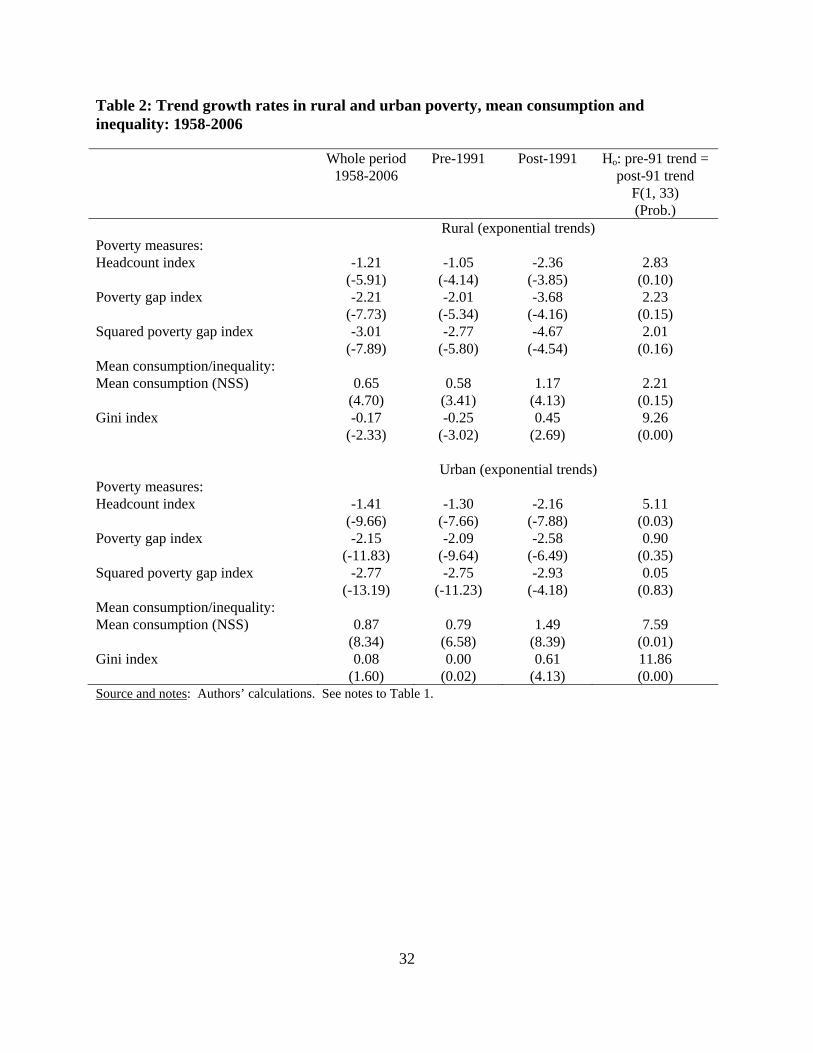
32

Table 2: Trend growth rates in rural and urban poverty, mean consumption and inequality: 1958-2006 Whole period

1958-2006 Pre-1991 Post-1991 Ho: pre-91 trend =

post-91 trend F(1, 33) (Prob.)

Rural (exponential trends) Poverty measures: Headcount index -1.21

(-5.91) -1.05

(-4.14) -2.36

(-3.85) 2.83

(0.10) Poverty gap index -2.21

(-7.73) -2.01

(-5.34) -3.68

(-4.16) 2.23

(0.15) Squared poverty gap index -3.01

(-7.89) -2.77

(-5.80) -4.67

(-4.54) 2.01

(0.16) Mean consumption/inequality: Mean consumption (NSS) 0.65

(4.70) 0.58

(3.41) 1.17

(4.13) 2.21

(0.15) Gini index -0.17

(-2.33) -0.25

(-3.02) 0.45

(2.69) 9.26

(0.00)

Urban (exponential trends) Poverty measures: Headcount index -1.41

(-9.66) -1.30

(-7.66) -2.16

(-7.88) 5.11

(0.03) Poverty gap index -2.15

(-11.83) -2.09

(-9.64) -2.58

(-6.49) 0.90

(0.35) Squared poverty gap index -2.77

(-13.19) -2.75

(-11.23) -2.93

(-4.18) 0.05

(0.83) Mean consumption/inequality: Mean consumption (NSS) 0.87

(8.34) 0.79

(6.58) 1.49

(8.39) 7.59

(0.01) Gini index 0.08

(1.60) 0.00

(0.02) 0.61

(4.13) 11.86 (0.00)

Source and notes: Authors’ calculations. See notes to Table 1.

33

Table 3: Elasticities of national poverty measures to economic growth in India: 1958-2006 Elasticity of poverty measure with respect to:

Mean consumption from

NSS

Mean private consumption from national accounts

Mean net domestic product

OLS IVE Unadjusted Adjusted Unadjusted Adjusted

Headcount index

Whole period

-1.62 (-26.0)

-1.60 (-61.4)

-0.90 (-9.57)

-0.50 (-9.76)

-0.65 (-9.20)

-0.35 (-9.27)

Up to 1991 -1.58 (-27.8)

-1.57 (-75.2)

-0.98 (-6.77)

-0.51 (-7.35)

-0.73 (-6.07)

-0.36 (-6.35)

After 1991 -2.07 (-21.4)

-2.07 (-22.9)

-0.70 (-5.10)

-0.62 (-2.99)

-0.49 (-4.13)

-0.42 (-2.70)

Ho: pre-91 elasticity = post-91elasticity

F(1,34 or 32) (Prob.)

16.08 (0.00)

24.91 (0.00)

1.50 (0.23)

0.25 (0.62)

1.43 (0.24)

0.12 (0.73)

Poverty gap index

Whole period

-2.66 (-

21.8)

-2.68 (-35.5)

-1.53 (-10.6)

-0.95 (-11.5)

-1.11 (-10.3)

-0.68 (-11.5)

Up to 1991 -2.63 (-20.3)

-2.66 (-33.5)

-1.75 (-8.74)

-1.09 (-10.6)

-1.31 (-7.97)

-0.80 (-9.88)

After 1991 -2.94 (-12.2)

-2.78 (-11.5)

-0.97 (-4.94)

-0.80 (-2.43)

-0.69 (-4.17)

-0.56 (-2.24)

Ho: pre-91 elasticity = post-91elasticity

F(1,34 or 32) (Prob.)

1.10 (0.30)

0.19 (0.66)

5.96 (0.02)

0.67 (0.42)

5.21 (0.03)

0.67 (0.42)

Squared poverty gap index

Whole period

-3.48 (-

19.7)

-3.48 (-31.8)

-2.03 (-10.7)

-1.31 (-10.7)

-1.48 (-10.5)

-0.94 (-10.9)

Up to 1991 -3.48 (-18.0)

-3.52 (-26.3)

-2.37 (-9.63)

-1.58 (-10.6)

-1.79 (-8.86)

-1.16 (-10.3)

After 1991 -3.49 (-8.20)

-3.28 (-7.73)

-1.17 (-4.74)

-0.95 (-2.20)

-0.84 (-4.17)

-0.69 (-2.10)

Ho: pre-91elasticity = post-91elasticity

F(1,34 or 32) Prob.)

0.00 (0.99)

0.26 (0.61)

9.51 (0.00)

1.78 (0.19)

8.36 (0.01)

1.56 (0.22)

Source and notes: Authors’ calculations. Based on regressions of log poverty measures against log consumption or net product per person using 37 surveys spanning 1958-2006. All regressions include a control for surveys that used a mixed-recall period (by adding a dummy variable for such surveys). The “adjusted” estimates control for the difference in the rates of inflation implied by the rural consumer price index and the national income deflator (Ravallion and Datt, 1996). The instrumental variables for the survey mean regressions included lagged survey means (split urban and rural), current and lagged mean consumption from the national accounts, current and lagged rural and urban consumer price indices, current and lagged rural population shares, interval between mid-points of survey periods and a time trend. The t-ratios in parentheses are based on heteroskedastcity and autocorrelation-

34

consistent standard errors. The regressions also incorporate a kink at NSS round 47 (July-December 1991) such that there is no discontinuity in the predicted values of log poverty measures between the pre- and post-1991 periods.

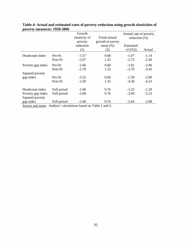
35

Table 4: Actual and estimated rates of poverty reduction using growth elasticities of poverty measures: 1958-2006

Growth

elasticity of poverty

reduction (1)

Trend annual growth in survey

mean (%) (2)

Annual rate of poverty reduction (%)

Estimated =(1)*(2) Actual

Headcount index Pre-91 -1.57 0.68 -1.07 -1.14 Post-91 -2.07 1.33 -2.75 -2.36

Poverty gap index Pre-91 -2.66 0.68 -1.81 -2.06 Post-91 -2.78 1.33 -3.70 -3.42

Squared poverty gap index Pre-91 -3.52 0.68 -2.39 -2.80

Post-91 -3.28 1.33 -4.36 -4.23 Headcount index Full period -1.60 0.76 -1.22 -1.29 Poverty gap index Full period -2.68 0.76 -2.04 -2.23 Squared poverty gap index Full period -3.48 0.76 -2.64 -2.98 Source and notes: Authors’ calculations based on Table 1 and 3.

36

Table 5: Impacts on poverty of the urban-rural composition of growth: 1951-2006 Poverty measure

Period

National poverty Urban poverty Rural poverty

Coeff. t-ratio Coeff. t-ratio Coeff. t-ratio

Headcount index

Up to 1991 Urban growth -0.38 -1.03 -0.64 -11.42 0.46 1.47 Rural growth -1.45 -21.79 -0.08 -4.16 -1.38 -34.32

After 1991 Urban growth -3.73 -2.40 -0.94 -3.47 -2.96 -2.07 Rural growth -0.98 -3.88 -0.03 -0.25 -1.01 -5.18

Ho: Pre-91 coefficient = Post-91 coefficient

F(2,34) (prob.)

2.78 (0.08)

0.52 (0.60)

3.44 (0.04)

Ho: All Pre-91 coeffs. = Post-91 coeffs.

F(3,34) (prob.)

2.16 (0.11)

0.97 (0.42)

2.96 (0.05)

Poverty gap index

Up to 1991 Urban growth 0.21 0.27 -0.67 -4.54 0.90 1.16 Rural growth -2.19 -26.32 -0.14 -4.04 -2.06 -16.82

After 1991 Urban growth -8.19 -2.79 -2.24 -3.84 -5.31 -1.88 Rural growth -1.59 -3.72 0.00 0.03 -1.59 -3.27

Ho: Pre-91 coefficient = Post-91 coefficient

F(2,34) (prob.)

4.12 (0.02)

3.25 (0.05)

2.13 (0.13)

Ho: All Pre-91 coeffs. = Post-91 coeffs.

F(3,34) (prob.)

2.79 (0.06)

4.50 (0.01)

1.47 (0.24)

Squared poverty gap index

Up to 1991 Urban growth 0.47 0.44 -0.58 -3.55 1.51 1.48 Rural growth -2.69 -15.27 -0.17 -4.13 -2.54 -11.80

After 1991 Urban growth -11.64 -2.33 -3.95 -4.77 -7.45 -1.70 Rural growth -1.66 -1.54 -0.33 -1.27 -1.19 -1.35

Ho: Pre-91 coefficient = Post-91 coefficient

F(2,34) (prob.)

2.73 (0.08)

11.03 (0.00)

2.33 (0.11)

Ho: All Pre-91 coeffs. = Post-91 coeffs.

F(3,34) (prob.)

1.86 (0.15)

7.42 (0.00)

1.56 (0.22)

Source and notes: Authors’ calculations. These are the coefficients in the regressions in equations (5) and (6) rather than elasticities. All regressions include a control for surveys that used a mixed-recall period (by adding the change between surveys in a dummy variable for such surveys). The regressions are estimated using a 2-stage GMM estimator. The instruments for the urban and rural growth variables included lagged survey means (split urban and rural), current and lagged mean consumption from the national accounts, current and lagged rural and urban consumer price indices, current and lagged rural population shares, interval between mid-points of survey periods and a time trend. The t-ratios are based on heteroskedastcity and autocorrelation-consistent standard errors.

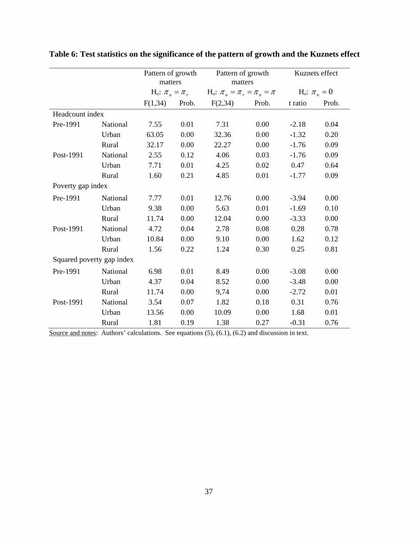
37

Table 6: Test statistics on the significance of the pattern of growth and the Kuznets effect Pattern of growth

matters Ho: ru

Pattern of growth matters

Ho: nru  

Kuznets effect

Ho: 0n

F(1,34) Prob. F(2,34) Prob. t ratio Prob.

Headcount index Pre-1991 National 7.55 0.01 7.31 0.00 -2.18 0.04 Urban 63.05 0.00 32.36 0.00 -1.32 0.20 Rural 32.17 0.00 22.27 0.00 -1.76 0.09 Post-1991 National 2.55 0.12 4.06 0.03 -1.76 0.09 Urban 7.71 0.01 4.25 0.02 0.47 0.64

Rural 1.60 0.21 4.85 0.01 -1.77 0.09 Poverty gap index

Pre-1991 National 7.77 0.01 12.76 0.00 -3.94 0.00 Urban 9.38 0.00 5.63 0.01 -1.69 0.10 Rural 11.74 0.00 12.04 0.00 -3.33 0.00 Post-1991 National 4.72 0.04 2.78 0.08 0.28 0.78 Urban 10.84 0.00 9.10 0.00 1.62 0.12

Rural 1.56 0.22 1.24 0.30 0.25 0.81 Squared poverty gap index

Pre-1991 National 6.98 0.01 8.49 0.00 -3.08 0.00 Urban 4.37 0.04 8.52 0.00 -3.48 0.00 Rural 11.74 0.00 9,74 0.00 -2.72 0.01 Post-1991 National 3.54 0.07 1.82 0.18 0.31 0.76 Urban 13.56 0.00 10.09 0.00 1.68 0.01

Rural 1.81 0.19 1.38 0.27 -0.31 0.76 Source and notes: Authors’ calculations. See equations (5), (6.1), (6.2) and discussion in text.

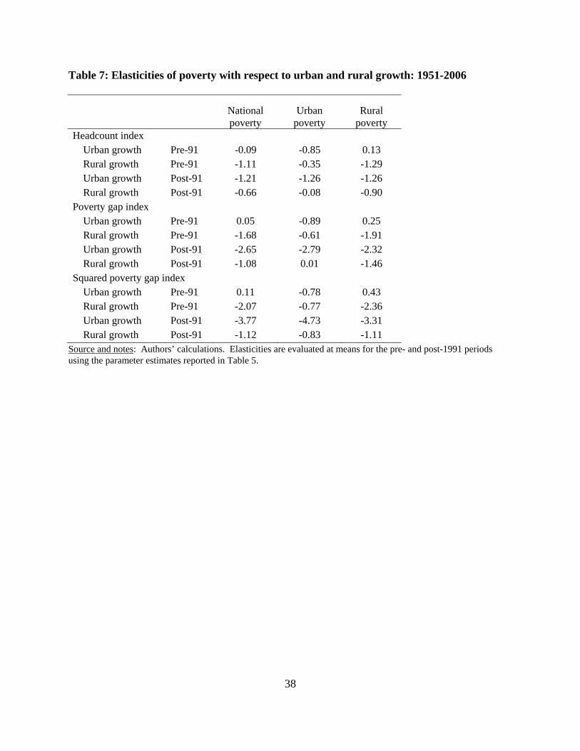
38

Table 7: Elasticities of poverty with respect to urban and rural growth: 1951-2006

     National poverty

Urban poverty

Rural poverty

Headcount index Urban growth Pre-91 -0.09 -0.85 0.13 Rural growth Pre-91 -1.11 -0.35 -1.29 Urban growth Post-91 -1.21 -1.26 -1.26 Rural growth Post-91 -0.66 -0.08 -0.90

Poverty gap index Urban growth Pre-91 0.05 -0.89 0.25 Rural growth Pre-91 -1.68 -0.61 -1.91 Urban growth Post-91 -2.65 -2.79 -2.32 Rural growth Post-91 -1.08 0.01 -1.46

Squared poverty gap index Urban growth Pre-91 0.11 -0.78 0.43 Rural growth Pre-91 -2.07 -0.77 -2.36 Urban growth Post-91 -3.77 -4.73 -3.31 Rural growth Post-91 -1.12 -0.83 -1.11

Source and notes: Authors’ calculations. Elasticities are evaluated at means for the pre- and post-1991 periods using the parameter estimates reported in Table 5.

39

Figure 1: Headcount index of poverty for India 1951-2006

0

10

20

30

40

50

60

70

1950 1960 1970 1980 1990 2000 2010

Na

tion

al h

ea

dco

un

t in

de

x (%

be

low

po

vert

y lin

e)

Source: Author’s estimates using the data and methods described in section 3. Figure 2: Urban share of total consumption, 1951-2006 (%)

Source and notes: Authors’ calculations.

40

Figure 3: Average consumption in India, 1951-2006

Source and notes: Authors’ calculations. Mean consumption refers to per capita monthly consumption in Rs. at constant 1958-9 (Round 14) prices. Figure 4: Ratio of urban mean consumption to rural mean consumption, India 1951-2006

Note: Fitted values are a 4th degree polynomial

41

Figure 5: Trends in urban and rural inequality, 1951-2006, controlling for changes in survey reference periods

Urban Gini

Rural Gini

25

30

35

40

Gin

i in

dex

(%)

1960 1970 1980 1990 2000 2010Year

Source and notes: Authors’ calculations. The lines show predicted Gini indices after controlling for the effect of MRP rounds (as distinct from predicted values without controls).

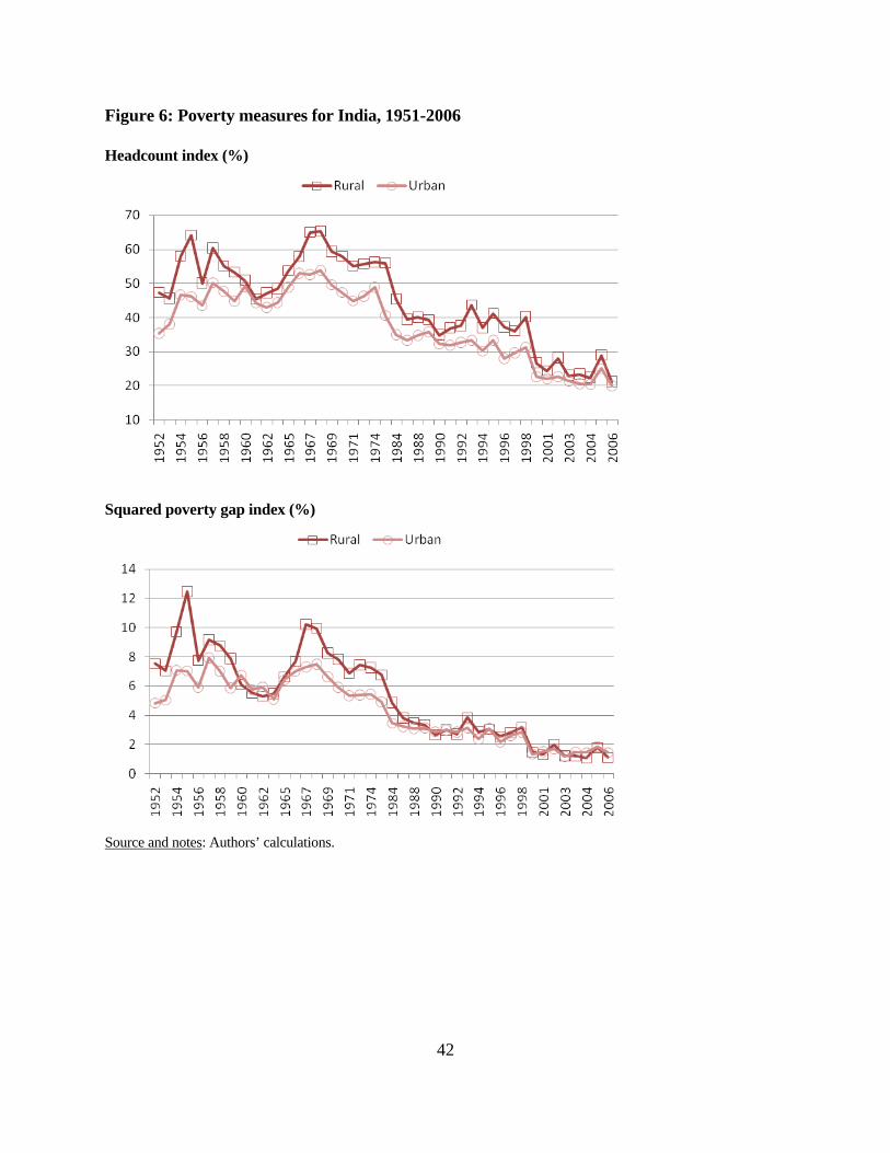
42

Figure 6: Poverty measures for India, 1951-2006 Headcount index (%)

Squared poverty gap index (%)

Source and notes: Authors’ calculations.

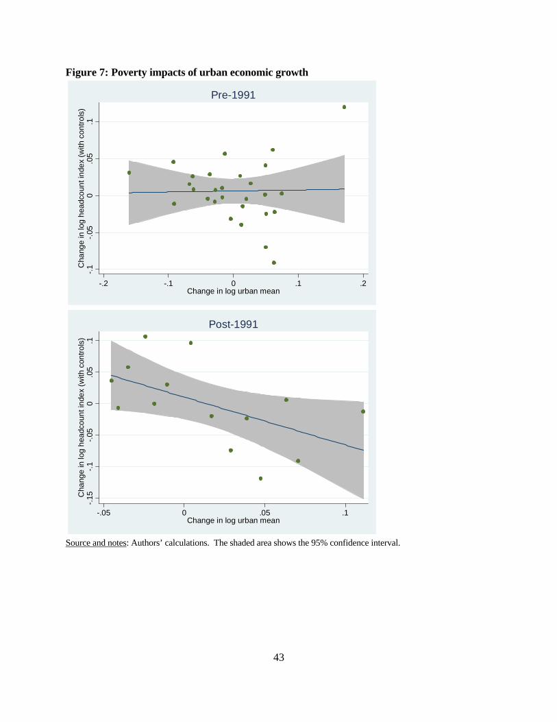
43

Figure 7: Poverty impacts of urban economic growth

-.1

-.05

0.0

5.1

Cha

nge

in lo

g h

eadc

oun

t in

dex

(with

con

tro

ls)

-.2 -.1 0 .1 .2Change in log urban mean

Pre-1991-.

15-.

1-.

050

.05

.1C

hang

e in

log

hea

dco

unt i

nde

x (w

ith c

ontr

ols

)

-.05 0 .05 .1Change in log urban mean

Post-1991

Source and notes: Authors’ calculations. The shaded area shows the 95% confidence interval.