Embed Size (px)
Citation preview

Has India emerged? Business cycle facts from atransitioning economy
Chetan Ghate, Radhika Pandey, Ila Patnaik
Working Paper 2011-88
April 2011
National Institute of Public Finance and PolicyNew Delhi
http://www.nipfp.org.in
Has India Emerged ? Business Cycle Stylized Factsfrom a Transitioning Economy
Chetan Ghate∗ Radhika Pandey† Ila Patnaik‡§
April 15, 2011
Abstract
This paper presents a comprehensive set of stylised facts for business cycles inIndia from 1950 - 2009. We find that the nature of the business cycle has changeddramatically after India’s liberalisation reforms in 1991. In particular, after the themid 1990s, the properties of India’s business cycle has moved closer in key respects toselect advanced countries. This is consistent with India’s structural transformationfrom a pre-dominantly agricultural and planned developing economy to a more mar-ket based industrial-income economy. We also identify in what respects the behaviourof the Indian business cycle is different from that of other advanced economies, andcloser to that of other less developed economies. This is the first exercise of thiskind to generate an exhaustive set of stylised facts for India using both annual andquarterly data.
JEL Classification: E10, E32Keywords: Macroeconomics, Real Business Cycles, Emerging Market DSGE Models, Volatil-ity and Growth.
∗Email:[email protected]†Email:[email protected]‡Email:[email protected]§This paper was written under the aegis of the SPF Financial and Monetary Policy Reform Project at
the National Institute for Public Finance and Policy, New Delhi. We are grateful to Abhijit Banerjee forcomments. We also thank participants at the ‘Business Cycle Facts and DSGE Model for India’ workshopat NIPFP, the Eighth meeting of the NIPFP-DEA Research Program, and Workshop 5 of the Center forInternational Macroeconomic Studies (Surrey University) for useful comments.
1
Contents
1 Introduction 3
2 Stylised Facts from Emerging Economies 5
3 India in Transition 8
4 The Dataset 11
5 Statistical Methodology 12
6 Indian Business Cycle Stylised Facts in the Pre and Post Reform Period 13
7 Robustness Checks 167.1 Stylised Facts with Quarterly Data . . . . . . . . . . . . . . . . . . . . . . 167.2 An Alternative Detrending Method . . . . . . . . . . . . . . . . . . . . . . 197.3 Redefining the Sample Period . . . . . . . . . . . . . . . . . . . . . . . . . 20
8 Conclusion 21
A Data Definition and Sources 26
2
1 Introduction
This paper describes the changing nature of the Indian business cycle from 1950 - 2009.Our focus is to compare India’s business cycle in the pre 1991 economy, with the post 1991Indian economy, after the large scale liberalization reforms of 1991. Our main finding is thatafter the liberalisation of the Indian economy in 1991, the properties of the Indian businesscycle look closer to that of advanced industrialized economies in several key respects. Thispaper - to the best of our knowledge - is the first such exercise to comprehensively documentchanges in the properties of the Indian business cycle in the pre and post reform period.
A large literature documents business cycle stylised facts both in advanced industrialeconomies (Kydland and Prescott, 1990; Backus and Kehoe, 1992; Stock and Watson, 1999;King and Rebelo, 1999) as well as developing and emerging market economies (Agenoret al., 2000; Rand and Tarp, 2002; Male, 2010). Agenor et al. (2000) present a compar-ison of the business cycle properties of developed and developing economies based on aquarterly dataset from first quarter of 1978 to the fourth quarter of 1995. The Index ofindustrial production (IIP) is taken as a proxy for aggregate business activity. Cyclicalcomponents of variables are derived using both the Hodrick-Prescott and Baxter-King fil-ters. A main finding of the paper is that developing economies are characterized by higheroutput volatility compared to developed economies. Similarly, Rand and Tarp (2002) re-port business cycle stylised facts for 15 developing economies based on an annual datasetfrom 1970-1997. gdp is taken as a proxy for aggregate business activity. These authorsfind that output volatility in developing economies is 15-20% higher than that of developedcountries. They also find that consumption is more volatile than output for developingeconomies (with South Africa and India as exceptions). Volatility in investment is foundto be similar to developed economies. However, they do not find any consistent evidenceof counter-cyclical government expenditure in their sample of developing economies.1
Other papers in the literature - such as Neumeyer and Perri (2005) - also provide a com-parison of business cycle properties of a set of five emerging economies with a set of fivedeveloped economies. gdp is taken as a proxy for aggregate business cycle activity. Out-put volatility is found to be higher for emerging economies. While the relative volatility ofconsumption is greater than 1 for emerging economies, the relative volatility of investmentis uniform across the two set of countries. Similarly, Alper (2002) analyses business cyclesin Mexico and Turkey from 1987-2000 and presents a comparison of the results with theUnited States. Consistent with the business cycle features of developing economies, thevolatility of real gdp in Mexico and Turkey are found to be 2.63 and 3.91 times largerthan for the United States. Consumption is found to be more volatile than output in these
1Rand and Tarp (2002) find a positive relation between consumption and output except for Nigeria.Higher volatility in investment is found to be pro-cyclical in all the developing countries included in thesample. While imports are reported to be pro-cyclical, the picture regarding exports is unclear. On therelation between price level and output, the picture is unclear with seven of the developing economiesreporting significant negative correlation between price level and output.
3
economies.
Finally, Male (2010) provides a comprehensive documentation of cross-country comparisonof business cycle stylised facts. Her paper relies on a quarterly dataset for 32 developingeconomies, across different regions, of which India is part of the sample for Asian countries.Due to lack of reliable data on real gdp for a number of developing economies, she usesindexes of industrial production as a proxy for the aggregate business cycle. Businesscycle properties of developing economies are found to be distinctly different from thoseof developed economies. Key variables like output, private consumption, price levels aremore volatile in developing economies. The correlation of investment and imports with theaggregate business cycle is not found to be very strong. Government expenditure is notsignificantly counter-cyclical, unlike in developed countries. Business cycle characteristicsalso differ in terms of persistence of variables. For instance, the persistence of output andprice levels are lower for developing economies compared with developed economies.
Because India is typically treated as one of many countries within a larger sample (see(Agenor et al., 2000; Rand and Tarp, 2002; Male, 2010)), such studies do not show thechanging nature of the business cycle of any particular country over time. Our maincontribution is to provide evidence on the changing stylised facts of the Indian economyfrom 1950 - 2009. During this time, India transitioned from a closed and protected economycharacterised by controls on capacity creation and high import duties, to an economy wellintegrated with the world, with the policy environment changing significantly in 1991.In terms of business cycle fluctuations, the economy moved away from monsoon cycles(Patnaik and Sharma, 2002) to business cycles in the conventional sense.
The empirical literature on stylised facts relies on long time series of quarterly data. How-ever, quarterly gdp data in India is available only from 1999. This limits us to 11 years ofquarterly data for our key variables. Hence, since we are interested in the changing patternof the Indian business cycle, we conduct our analysis with annual data and then use thequarterly data to check the robustness of our results.
In particular, we are interested in the properties of Indian business cycle over two periods:1950-1991 for the pre-liberalisation period and 1992-2009 for the post-liberalisation period.gdp, private consumption, total gross fixed capital formation, consumer prices, exports,imports, government expenditure and nominal exchange rate are the key variables anal-ysed. Since the quantitative general equilibrium literature also seeks to explain the strongcounter-cyclicality of net exports as well as highly volatile and counter cyclical interestrates in emerging markets, we also report the business cycle properties of these variablesfor India. Our main finding is to highlight the difference in the properties of the Indianbusiness cycle stylised over the two periods, and suggest reasons for these changes. A dataappendix lists all the sources and definitions of variables used in this study.
In terms of similarities, we find that output (Real gdp) has become less volatile in thepost-liberalisation period; investment has become significantly pro-cyclical in the post-liberalisation period; the correlation of imports with gdp has also increased; net exports
4
have become counter-cyclical; the volatility in prices and government expenditure hasdecreased in the post liberalisation period; and the absolute volatility in nominal exchangerate has declined. Further, our results using quarterly data are consistent with the findingsof the annual data analysis for the post 1991 period. This suggests that in many keyrespects, the Indian business cycle shows a growing resemblance with those of the developedeconomies.
In terms of differences, the Indian business cycle features also resemble features of de-veloping economies. While output volatility has fallen, it still remains high. In addition,consumption is more volatile than output. Further, government expenditure is not stronglycounter-cyclical with respect to output, as in advanced economies.
In terms of the sensitivity tests, we note that the volatility of consumption is sensitive tothe choice of the de-trending procedure. The absolute volatility of private consumptionfalls in the post-reform period when the band pass filter of Baxter-King is used to de-trendthe series. However, the absolute volatility is higher in the post-reform period when theHodrick-Prescott filter is used to de-trend the series. There is also a significant reductionin volatility of government expenditure when the Baxter-King filter is used to de-trend theseries. However, the key feature of the Indian business cycle which is robust to de-trendingprocedures is the significant pro-cyclicality of investment with output. Coupled with theincreased pro-cyclicality of imports with output, this feature makes the Indian businesscycle stylised facts closer to those of the advanced economies.
The remainder of the paper is divided into the following sections. Section 2 outlines themain features of emerging economies business cycle with an overview of the sources ofshocks in these economies. Section 3 presents a snapshot of India’s transition. Section4 outlines the data sources and the variables included in the study. Section 5 detailsthe methodology employed to compute the Indian business cycle stylised facts. Section 6provides empirical evidence on the changing Indian business cycle stylised facts from preto post reform period. Section 7 presents results on sensitivity tests. Section 8 concludes.
2 Stylised Facts from Emerging Economies
As noted in the introduction, one of the main features that distinguishes emerging economiesbusiness cycles from advanced economies is their higher volatility. Current account bal-ances, output growth, interest rates, and exchange rate tend to exhibit larger, and morefrequent changes (Calderon and Fuentes, 2006). There are other aspects that character-ize emerging market economies: consumption is more volatile than output with a relativevolatility larger than one; real interest rates are highly volatile and counter cyclical, andnet exports are strongly counter-cyclical (Neumeyer and Perri, 2005; Aguiar and Gopinath,
5
2007; Uribe and Yue, 2006).2
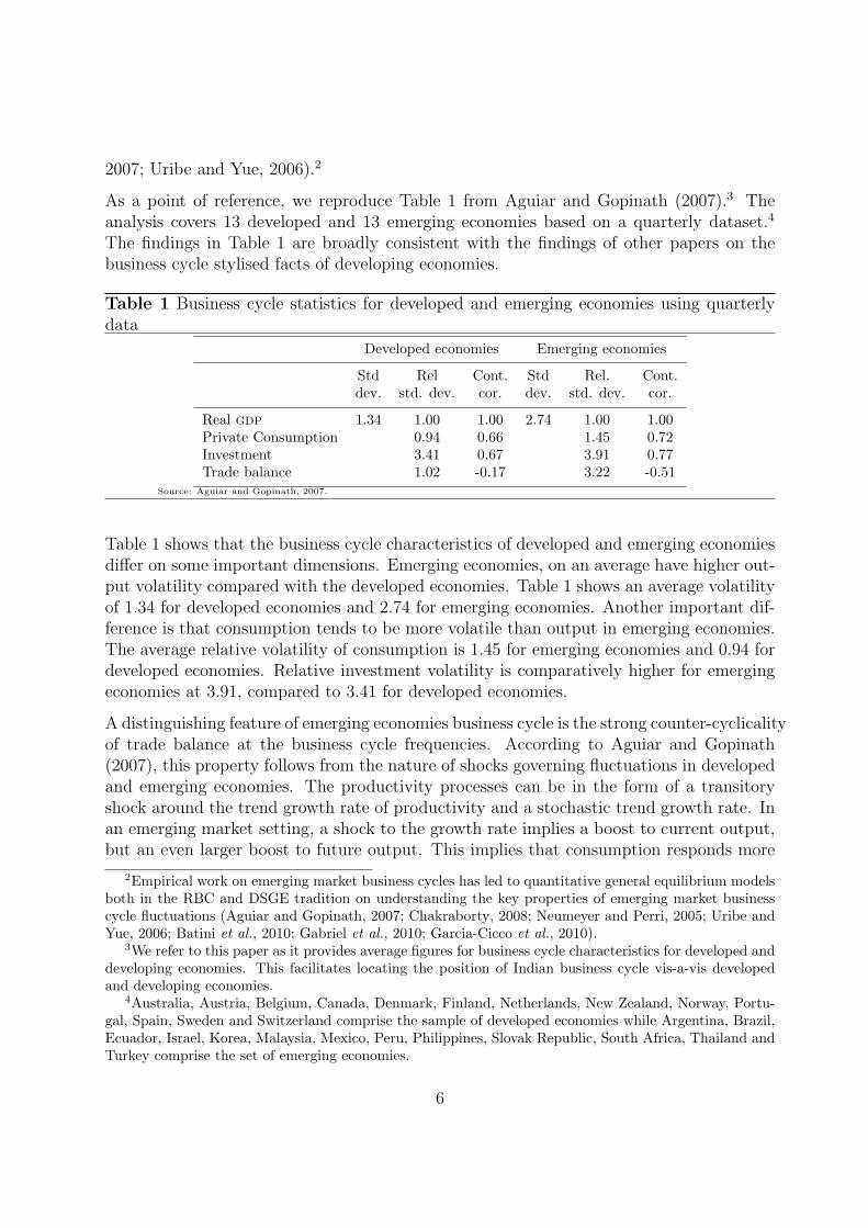
As a point of reference, we reproduce Table 1 from Aguiar and Gopinath (2007).3 Theanalysis covers 13 developed and 13 emerging economies based on a quarterly dataset.4
The findings in Table 1 are broadly consistent with the findings of other papers on thebusiness cycle stylised facts of developing economies.
Table 1 Business cycle statistics for developed and emerging economies using quarterlydata
Developed economies Emerging economies
Std Rel Cont. Std Rel. Cont.dev. std. dev. cor. dev. std. dev. cor.
Real gdp 1.34 1.00 1.00 2.74 1.00 1.00Private Consumption 0.94 0.66 1.45 0.72Investment 3.41 0.67 3.91 0.77Trade balance 1.02 -0.17 3.22 -0.51
Source: Aguiar and Gopinath, 2007.
Table 1 shows that the business cycle characteristics of developed and emerging economiesdiffer on some important dimensions. Emerging economies, on an average have higher out-put volatility compared with the developed economies. Table 1 shows an average volatilityof 1.34 for developed economies and 2.74 for emerging economies. Another important dif-ference is that consumption tends to be more volatile than output in emerging economies.The average relative volatility of consumption is 1.45 for emerging economies and 0.94 fordeveloped economies. Relative investment volatility is comparatively higher for emergingeconomies at 3.91, compared to 3.41 for developed economies.
A distinguishing feature of emerging economies business cycle is the strong counter-cyclicalityof trade balance at the business cycle frequencies. According to Aguiar and Gopinath(2007), this property follows from the nature of shocks governing fluctuations in developedand emerging economies. The productivity processes can be in the form of a transitoryshock around the trend growth rate of productivity and a stochastic trend growth rate. Inan emerging market setting, a shock to the growth rate implies a boost to current output,but an even larger boost to future output. This implies that consumption responds more
2Empirical work on emerging market business cycles has led to quantitative general equilibrium modelsboth in the RBC and DSGE tradition on understanding the key properties of emerging market businesscycle fluctuations (Aguiar and Gopinath, 2007; Chakraborty, 2008; Neumeyer and Perri, 2005; Uribe andYue, 2006; Batini et al., 2010; Gabriel et al., 2010; Garcia-Cicco et al., 2010).
3We refer to this paper as it provides average figures for business cycle characteristics for developed anddeveloping economies. This facilitates locating the position of Indian business cycle vis-a-vis developedand developing economies.
4Australia, Austria, Belgium, Canada, Denmark, Finland, Netherlands, New Zealand, Norway, Portu-gal, Spain, Sweden and Switzerland comprise the sample of developed economies while Argentina, Brazil,Ecuador, Israel, Korea, Malaysia, Mexico, Peru, Philippines, Slovak Republic, South Africa, Thailand andTurkey comprise the set of emerging economies.
6
than income, reducing savings and generating a current account deficit. If growth shocksdominate transitory income shocks, the economy resembles a typical emerging market withits volatile consumption process and counter-cyclical current account. Conversely, a de-veloped economy characterised by relatively stable growth process will be dominated bystandard, transitory productivity shocks. Such a shock will generate an incentive to savethat will offset any increase in investment, resulting in limited cyclicality of the currentaccount. However, counter-cyclical net exports is also reported for developed economiesby Stock and Watson (1999); Rand and Tarp (2002).
Aguiar and Gopinath (2007) use a standard RBC model to explain the business cycleproperties of emerging markets. Because emerging market economies are characterizedby frequent changes in economic policy, they assume that shocks to trend growth are theprimary source of fluctuations. This implies that the random walk component of the Solowresidual is relatively larger. However, Calderon and Fuentes (2006) suggest that becausethe sources of shocks in Aguiar and Gopinath (2007) remain a black box, it is not clearwhether these are being driven by changes in economic reforms, or other market frictions.Indeed, Chari et al. (2007) show that a variety of frictions can be represented in reducedform as Solow residuals. Garcia-Cicco et al. (2010) show that when estimated over a longsample, the RBC model driven by permanent and transitory shocks - a la Aguiar andGopinath (2007) - does a poor job in explaining observed business cycles in Argentinaand Mexico, along a number of dimensions. These findings of Garcia-Cicco et al. (2010)suggest that the RBC model driven by productivity shocks does not provide an adequateexplanation of business cycles in emerging economies.
Other papers in the literature, such as Neumeyer and Perri (2005) emphasize the interac-tion between foreign interest rate shocks and domestic financial frictions that drive businesscycle fluctuations in emerging market economies. Firms in their model demand workingcapital to finance their wage bill making labour demand sensitive to interest rate fluctua-tions. An increase in the emerging market country’s interest rate leads to a rise in labourcosts. Since labour supply is insensitive to interest rate shocks, a lower demand for labourleads to lower levels of employment and output in equilibrium. Uribe and Yue (2006) findthat both country interest rates drive output fluctuations in emerging market economiesas well as the other way around. Kose et al. (2003) analyse the importance of domesticand external factors as causing cycles. Calvo (1998) argues that the idea of sudden stopsare an important factor of large cycles in emerging markets.
A discussion of the sources of aggregate business cycle fluctuations assumes greater rel-evance for a country like India that has undergone significant transformation since theearly nineties. With high growth, there has been a sharp increase in India’s integrationon both trade and financial flows, possibly leading to one source of volatility.5 Rameyand Ramey (1995) however find, that there is a negative correlation between volatility andgrowth. This would suggest that whether India’s output is more volatile (compared to
5Jayaram et al. (2009) show that the integration with the global economy has also resulted in greaterbusiness cycle synchronisation with advanced economies and with the US.
7
OECD economies), because it is growing faster, would seem unlikely, unless growth hasincreased volatility and volatility itself reduces growth subsequently. We therefore thinka plausible story of the changing pattern of the Indian business cycle is to link it withthe policy regime. In particular, prior to 1991, positive productivity shocks could notbe accommodated and generated inflationary pressures and a worsening of the exchangerate. After the 1991 reforms, the same shocks were permitted to generate growth, makinginvestment and imports go up, with foreign investment flowing in and the exchange rateappreciating. As in Aguiar and Gopinath (2007), consumption volatility remained highmostly because of permanent productivity shocks, i.e., consumption volatility was drivenby shocks to income that are larger or more persistent than they should be. However, thefocus of this paper is in documenting the changing nature of the Indian business cycle inthe pre and post reform period.6
3 India in Transition
As mentioned earlier, a careful analysis of business cycle stylised facts assume greaterrelevance for an economy like India that is subject to significant transformation over thelast two decades. In this section, we present some of the key elements of transformation inthe Indian economy from 1950 - 2009.
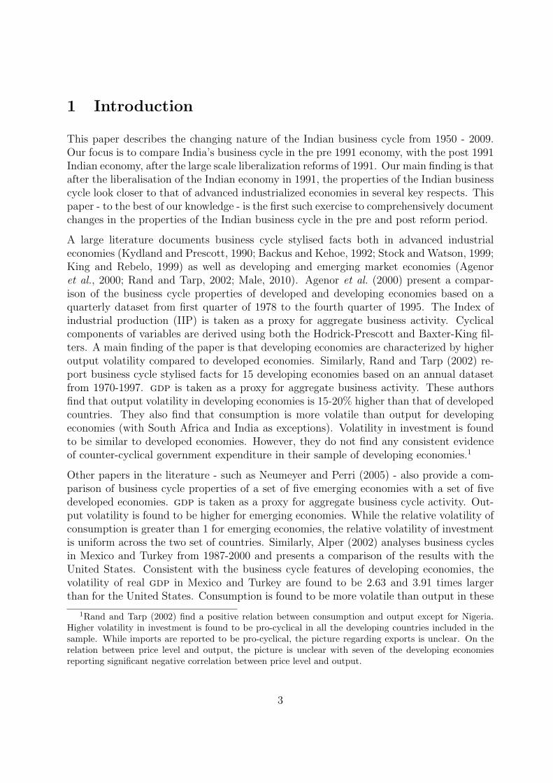
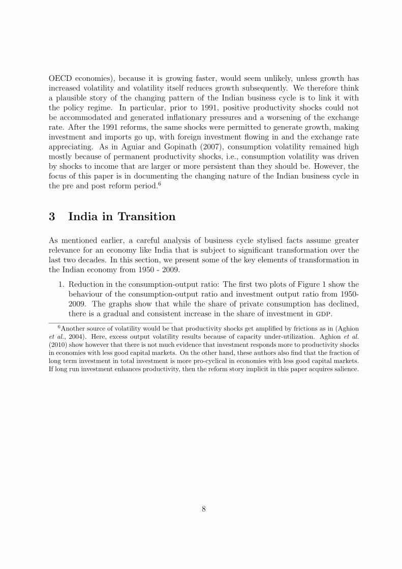
1. Reduction in the consumption-output ratio: The first two plots of Figure 1 show thebehaviour of the consumption-output ratio and investment output ratio from 1950-2009. The graphs show that while the share of private consumption has declined,there is a gradual and consistent increase in the share of investment in gdp.
6Another source of volatility would be that productivity shocks get amplified by frictions as in (Aghionet al., 2004). Here, excess output volatility results because of capacity under-utilization. Aghion et al.(2010) show however that there is not much evidence that investment responds more to productivity shocksin economies with less good capital markets. On the other hand, these authors also find that the fraction oflong term investment in total investment is more pro-cyclical in economies with less good capital markets.If long run investment enhances productivity, then the reform story implicit in this paper acquires salience.
8
Figure 1 The story of India’s transition
Sha
re o
f priv
ate
cons
umpt
ion
(Per
cen
t to
GD
P)
1950 1960 1970 1980 1990 2000 2010
6575
8595
Sha
re o
f inv
estm
ent (
Per
cen
t to
GD
P)
1950 1960 1970 1980 1990 2000 2010
1520
2530
35
Sha
re o
f agr
icul
ture
(P
er c
ent t
o G
DP
)
1950 1960 1970 1980 1990 2000 2010
2030
4050
Pub
lic s
ecto
r in
vest
men
t (P
er c
ent t
o to
tal)
1950 1960 1970 1980 1990 2000 2010
2535
4555
Priv
ate
corp
orat
e G
CF
(P
er c
ent t
o G
DP
)
1950 1960 1970 1980 1990 2000 2010
05
1015
Gro
ss fl
ows
(Per
cen
t to
GD
P)
1950 1960 1970 1980 1990 2000 2010
020
4060
capital accountcurrent account
In addition, since the mid 1990s, the Indian economy has undergone a significanttransformation in many aspects. From a purely monsoon driven economy, fluctu-ations in the economy are now driven primarily by fluctuations in inventory andinvestment. The share of investment in gdp has increased from 13% in 1950-51 to35% in 2009-10. The increase has been particularly prominent since 2004-05.
2. Declining share of agriculture: In the India of old, monsoon performance used to
9
define a good or bad time. Adverse agricultural performance used to throw gdpgrowth off trend (Shah, 2008; Patnaik and Sharma, 2002). In the India of presenttimes, monsoon shocks matter less. This is evident in the declining share of agricul-ture in Indian gdp. The third graph in Figure 1 shows a consistently declining shareof agriculture since 1950s. Table 2 shows the changing composition of Indian gdp,the decline in the share of agriculture has been matched with a rise in the share ofservices.
Table 2 Changing composition of gdp
Agriculture Industry Services
1951 53.15 16.5 30.21992 28.8 27.4 442009 14.6 28.4 57
3. Shift away from state domination: An important dimension of India’s transition isthe shift away from state domination towards a market economy. This is visible inthe fourth graph of Figure 1. The graph shows that the share of public investment intotal investment surged in the 1960s and 1970s. Since then it has been consistentlydeclining.
4. Emergence of a conventional business cycle: The policy set up in India of old timeswas characterised by controls on capacity creation and barriers to trade. In sucha scenario, conventional business cycles characterised by an interplay of inventoriesand investment did not exist. One prominent source of investment was governmentinvestment in the form of plan expenditure, which did not show any cyclical fluc-tuations. In the present environment with eased controls on capacity creation anddismantling of trade barriers, private sector investment as a share of gdp has showna significant rise.
The fifth graph in Figure 1 shows the time series of private corporate gross capitalformation expressed as a percent to gdp. In recent years we can see the emergenceof the behaviour found in the conventional business cycle. In the investment boomof the mid-1990s, private corporate gcf rose from 5% of gdp in 1990-91 to 11% ofgdp in 1995-96. This then fell dramatically in the business cycle downturn to 5.39%in 2001-02, and has since recovered to 17.6% in 2007-08. The recent recession hasled to its fall to 13.5% in 2009-10.
5. Increased integration with the rest of the world: The India of old was sheltered fromexternal competition through high import duties and other barriers to trade. Thecapital account was also subject to strict regulations on inflows and outflows. Sincethe adoption of liberalisation policy, the restrictions on current and capital accounthave been eased. This has resulted in India moving away from an autarky situation.
An effective way of measuring the openness is to sum the earnings and payments
10
on the current and capital account and express the sum as a percent to gdp. Thelast graph in Figure 1 shows the time series of current and capital account flowsexpressed as a percent to gdp. In the pre-reform period the flows on current andcapital account were around 20% of GDP. The conducive policy environment hasresulted in both current and capital account flows to gdp ratio rising to around 60%each in 2009.
4 The Dataset
We now undertake a formal analysis of Indian business cycle stylised facts. In India, quar-terly data for output and key macroeconomic variables is available only from June 1999.To understand the changing nature of Indian business cycles, we examine annual data.We then check the validity of our results with quarterly data. This is consistent with theliterature on stylised facts (King and Rebelo, 1999; Stock and Watson, 1999; Male, 2010),that relies on quarterly data to study business cycle properties of macroeconomic variables.Following (King and Rebelo, 1999) we choose private consumption and investment as keyvariables. In addition, we analyze exports, imports, net exports, consumer prices (Con-sumer Price Index-Industrial Worker (cpi-iw))7, government expenditure and the nominalexchange rate. Data on hours worked, real wage rate and total factor productivity is notavailable for India. We use gdp as a measure of aggregate activity in the economy.
For the annual analysis, we have a sample period covering 1950-2009. To study the tran-sition of the economy, the data is analyzed in two periods: the pre-liberalisation periodfrom 1950-1991 and the post liberalisation period from 1992 to 2009. The primary datasource is the National Accounts Statistics of the Ministry of Statistics and ProgrammeImplementation. The data for consumer prices is taken from the Labour Bureau, Min-istry of Labour and Employment. The data for government expenditure is taken fromthe budget documents of the Government of India. gdp, private consumption, gross fixedcapital formation, exports and imports are expressed at constant prices with base 2004.Government expenditure is expressed in real terms by deflating it with the gdp deflator.Following (Agenor et al., 2000) and (Neumeyer and Perri, 2005) net exports is divided byreal gdp to control for scale effects. We source the data from the Business Beacon databaseproduced by the Centre for Monitoring Indian Economy (CMIE), who source it from theprimary data sources mentioned above. All variables and their sources are described indetail in the Appendix.
For their analysis of investment, King and Rebelo (1999) use only the fixed investmentcomponent of gross domestic private investment. The other components of gross domesticprivate investment are residential and non-residential investment. The volatility of grossdomestic private investment in the US is higher than the component of fixed investment
7In most countries the headline inflation number is consumer prices, in India it is wholesale prices. Wefollow the literature on stylised facts in using consumer prices.
11

as residential investment is highly volatile. We take gross fixed capital formation as aproxy for investment since unlike the US, we do not have data on the categories of grossinvestment.
The variables analyzed are log transformed. The cyclical components of these variablesare obtained from the Hodrick-Prescott filter, as is standard in the literature (King andRebelo, 1999; Agenor et al., 2000; Neumeyer and Perri, 2005). The cyclical components arethen used to derive the business cycle properties of the variables in terms of their volatilityand co-movement. For the sensitivity analysis, we test the robustness of our results byusing the band-pass filter of Baxter-King (Agenor et al., 2000). As a further check, we alsouse quarterly data to verify the validity of our results.
5 Statistical Methodology
The business cycles examined in the literature are typically known as growth cycles, ex-tending from the work of (Lucas, 1977) where the business cycle component of a variableis defined as its deviation from trend.8 We follow this standard methodology in derivingthe stylised facts for Indian business cycles.
For annual data analysis, the log transformed series is passed through a filter to extract thecyclical (stationary) and trend (non-stationary) component. In case of quarterly data, thevariables are adjusted for seasonal fluctuations using the x-12-arima seasonal adjustmentprogram.9 Once adjusted for seasonality, the series are transformed to log terms and thenfiltered to extract the cyclical and trend component.
A large literature exists on the choice of the de-trending procedure to extract the busi-ness cycle component of the relevant time series (Canova, 1998; Burnside, 1998; Bjornland,2000). Canova (1998) argues that the application of different de-trending procedures ex-tract different types of information from the data. This results in business cycle propertiesdiffering widely across de-trending methods. However, commenting on (Canova, 1998),Burnside (1998) shows through spectral analysis, that the business cycle properties of vari-ables are robust to the choice of the filtering methods if the definition of business cyclefluctuations are uniform across all the de-trending methods.
In choosing the technique to derive the cyclical component, the literature on stylised factsmainly relies on either the Hodrick-Prescott filter (King and Rebelo, 1999; Male, 2010) orthe band-pass filter proposed by Baxter and King (Stock and Watson, 1999). We use the
8Business cycles dating goes back to the early work by (Burns and Mitchell, 1946). The classicalapproach propounded by (Burns and Mitchell, 1946) defines business cycles as sequences of expansionsand contractions in the levels of either total output or employment. In 1990, (Kydland and Prescott, 1990)established the first set of stylised facts for business cycles in other developed economies, based on theirresearch of US business cycle.
9We have set set up a website, www.mayin.org/cycle.in/ which has seasonally adjusted data for keyIndian monthly and quarterly time-series. This data is updated every Monday.
12
Hodrick-Prescott filter (Hodrick and Prescott, 1997) to de-trend the series and then checkthe robustness of our results with the Baxter-King filter (Baxter and King, 1999).
In essence, the Hodrick-Prescott method involves defining a cyclical output yct as current
output yt less a measure of trend output ygt with trend output being a weighted average of
past, current and future observations:
yct = yt + yg
t = yt −J∑
J=−j
ajyt−j
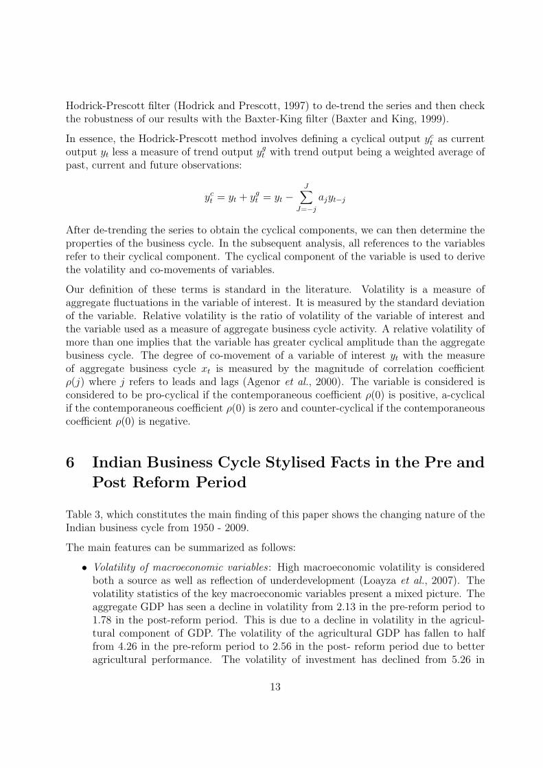
After de-trending the series to obtain the cyclical components, we can then determine theproperties of the business cycle. In the subsequent analysis, all references to the variablesrefer to their cyclical component. The cyclical component of the variable is used to derivethe volatility and co-movements of variables.
Our definition of these terms is standard in the literature. Volatility is a measure ofaggregate fluctuations in the variable of interest. It is measured by the standard deviationof the variable. Relative volatility is the ratio of volatility of the variable of interest andthe variable used as a measure of aggregate business cycle activity. A relative volatility ofmore than one implies that the variable has greater cyclical amplitude than the aggregatebusiness cycle. The degree of co-movement of a variable of interest yt with the measureof aggregate business cycle xt is measured by the magnitude of correlation coefficientρ(j) where j refers to leads and lags (Agenor et al., 2000). The variable is considered isconsidered to be pro-cyclical if the contemporaneous coefficient ρ(0) is positive, a-cyclicalif the contemporaneous coefficient ρ(0) is zero and counter-cyclical if the contemporaneouscoefficient ρ(0) is negative.
6 Indian Business Cycle Stylised Facts in the Pre and
Post Reform Period
Table 3, which constitutes the main finding of this paper shows the changing nature of theIndian business cycle from 1950 - 2009.
The main features can be summarized as follows:
• Volatility of macroeconomic variables : High macroeconomic volatility is consideredboth a source as well as reflection of underdevelopment (Loayza et al., 2007). Thevolatility statistics of the key macroeconomic variables present a mixed picture. Theaggregate GDP has seen a decline in volatility from 2.13 in the pre-reform period to1.78 in the post-reform period. This is due to a decline in volatility in the agricul-tural component of GDP. The volatility of the agricultural GDP has fallen to halffrom 4.26 in the pre-reform period to 2.56 in the post- reform period due to betteragricultural performance. The volatility of investment has declined from 5.26 in
13
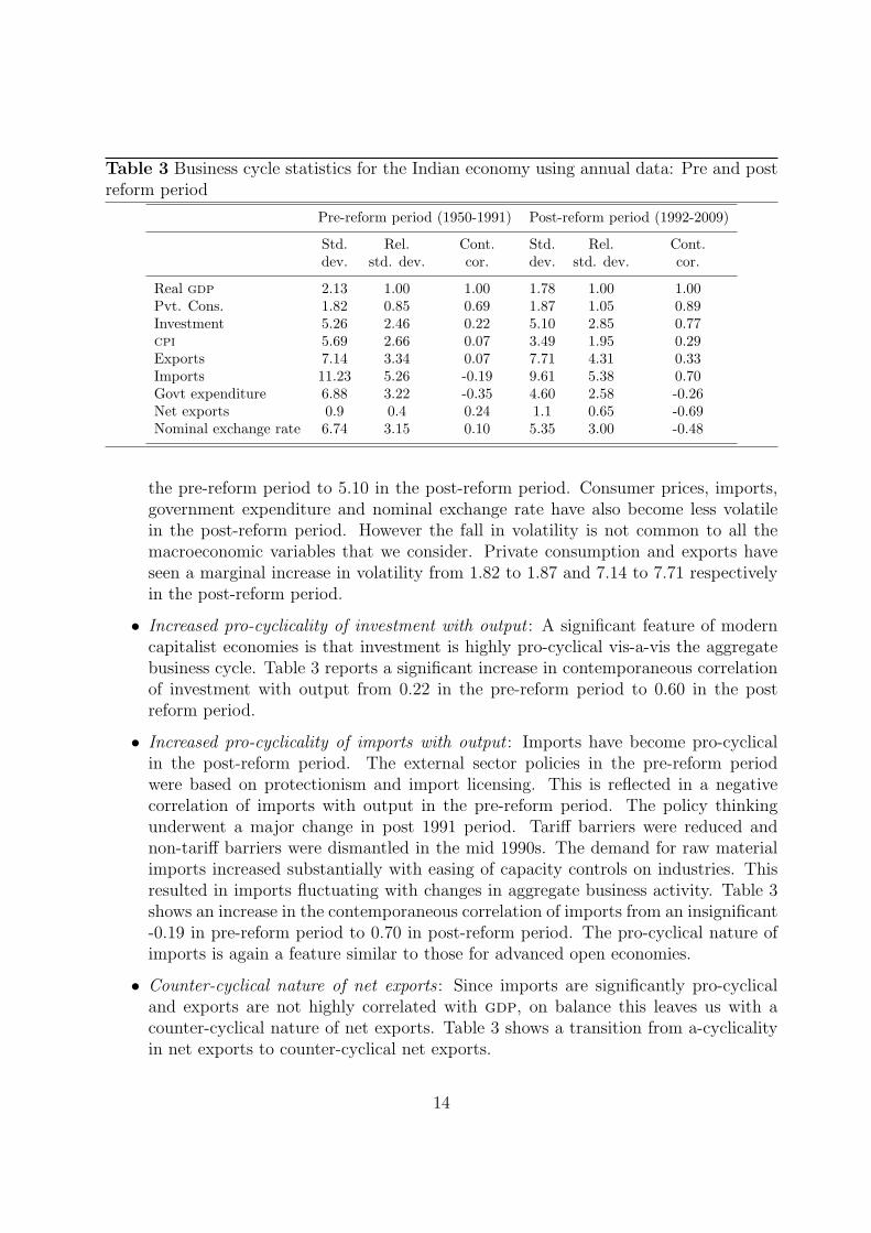
Table 3 Business cycle statistics for the Indian economy using annual data: Pre and postreform period
Pre-reform period (1950-1991) Post-reform period (1992-2009)
Std. Rel. Cont. Std. Rel. Cont.dev. std. dev. cor. dev. std. dev. cor.
Real gdp 2.13 1.00 1.00 1.78 1.00 1.00Pvt. Cons. 1.82 0.85 0.69 1.87 1.05 0.89Investment 5.26 2.46 0.22 5.10 2.85 0.77cpi 5.69 2.66 0.07 3.49 1.95 0.29Exports 7.14 3.34 0.07 7.71 4.31 0.33Imports 11.23 5.26 -0.19 9.61 5.38 0.70Govt expenditure 6.88 3.22 -0.35 4.60 2.58 -0.26Net exports 0.9 0.4 0.24 1.1 0.65 -0.69Nominal exchange rate 6.74 3.15 0.10 5.35 3.00 -0.48
the pre-reform period to 5.10 in the post-reform period. Consumer prices, imports,government expenditure and nominal exchange rate have also become less volatilein the post-reform period. However the fall in volatility is not common to all themacroeconomic variables that we consider. Private consumption and exports haveseen a marginal increase in volatility from 1.82 to 1.87 and 7.14 to 7.71 respectivelyin the post-reform period.
• Increased pro-cyclicality of investment with output : A significant feature of moderncapitalist economies is that investment is highly pro-cyclical vis-a-vis the aggregatebusiness cycle. Table 3 reports a significant increase in contemporaneous correlationof investment with output from 0.22 in the pre-reform period to 0.60 in the postreform period.
• Increased pro-cyclicality of imports with output : Imports have become pro-cyclicalin the post-reform period. The external sector policies in the pre-reform periodwere based on protectionism and import licensing. This is reflected in a negativecorrelation of imports with output in the pre-reform period. The policy thinkingunderwent a major change in post 1991 period. Tariff barriers were reduced andnon-tariff barriers were dismantled in the mid 1990s. The demand for raw materialimports increased substantially with easing of capacity controls on industries. Thisresulted in imports fluctuating with changes in aggregate business activity. Table 3shows an increase in the contemporaneous correlation of imports from an insignificant-0.19 in pre-reform period to 0.70 in post-reform period. The pro-cyclical nature ofimports is again a feature similar to those for advanced open economies.
• Counter-cyclical nature of net exports : Since imports are significantly pro-cyclicaland exports are not highly correlated with gdp, on balance this leaves us with acounter-cyclical nature of net exports. Table 3 shows a transition from a-cyclicalityin net exports to counter-cyclical net exports.
14

• Counter-cyclicality of nominal exchange rate: The nominal exchange rate has turnedcounter-cyclical in the post-reform period. From an a-cyclical relation in the pre-reform period, the post-reform period shows that the exchange rate goes up in badtimes and moves down in good times. This is indicative of the presence of a flexibleexchange rate regime in the post-91 period.
Hence, in several key respects, the features of the Indian business cycle have undergonea transformation and have converged to those of advanced economies. Investment andimports are found to be strongly correlated with output in the post-reform period. Netexports and nominal exchange rate are found to be strongly counter-cyclical in the post-reform period.
Finally, following (Ambler et al., 2004), we investigate whether our correlation results aremere statistical noise or are robust to procedures for testing the statistically significantdifference in correlation.10
Table 4 shows the difference in correlation and the associated p-value. The application ofthe test shows that the difference in correlation between the pre and post-reform periodis statistically significant for investment, imports, net exports and the nominal exchangerate. These are the variables that drive the transition in the economy from the pre topost reform period. As an example, these results imply that the difference in the cyclicalrelation between, say, investment and output, is statistically significant between the preand post reform period.
10The procedure for testing the statistically significant difference in correlation involves the followingsteps:
• Let r1 be the correlation between the two variables for the first group with n1 subjects.
• let r2 be the correlation for the second group with n2 subjects.
• To test H0 of equal correlations we convert r1 and r2 via Fisher’s variance stabilizing transformationz = 1/2 ∗ ln[(1 + r)/(1− r)] and then calculate the difference:zf = (z1 − z2)/sqrt(1/(n1 − 3) + 1/(n2 − 3))
• The difference is approximately standard normal distribution.
• If the absolute value of the difference is greater than 1.96 (assuming 95% confidence interval) thenwe can reject the null of equal correlations.
15
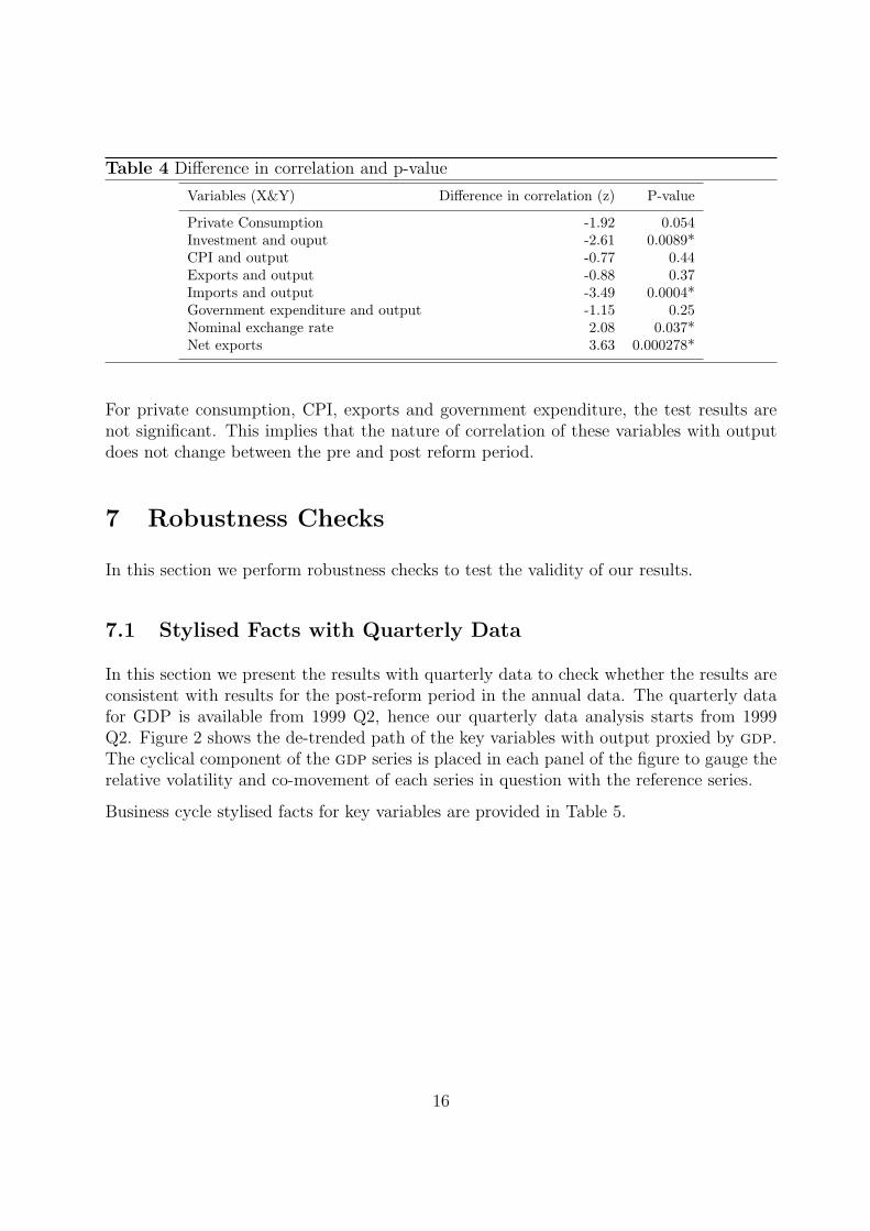
Table 4 Difference in correlation and p-value
Variables (X&Y) Difference in correlation (z) P-value
Private Consumption -1.92 0.054Investment and ouput -2.61 0.0089*CPI and output -0.77 0.44Exports and output -0.88 0.37Imports and output -3.49 0.0004*Government expenditure and output -1.15 0.25Nominal exchange rate 2.08 0.037*Net exports 3.63 0.000278*
For private consumption, CPI, exports and government expenditure, the test results arenot significant. This implies that the nature of correlation of these variables with outputdoes not change between the pre and post reform period.
7 Robustness Checks
In this section we perform robustness checks to test the validity of our results.
7.1 Stylised Facts with Quarterly Data
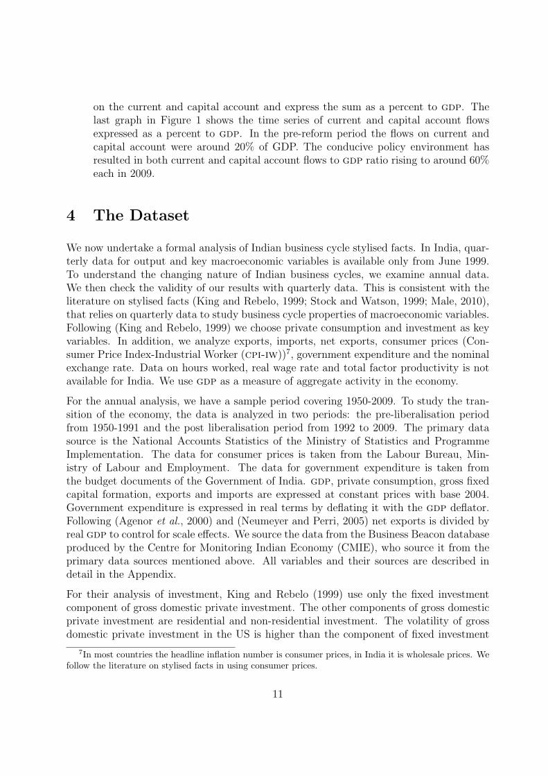
In this section we present the results with quarterly data to check whether the results areconsistent with results for the post-reform period in the annual data. The quarterly datafor GDP is available from 1999 Q2, hence our quarterly data analysis starts from 1999Q2. Figure 2 shows the de-trended path of the key variables with output proxied by gdp.The cyclical component of the gdp series is placed in each panel of the figure to gauge therelative volatility and co-movement of each series in question with the reference series.
Business cycle stylised facts for key variables are provided in Table 5.
16
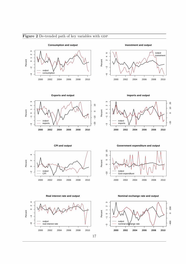
Figure 2 De-trended path of key variables with gdp
Consumption and output
Per
cent
2000 2002 2004 2006 2008 2010
−4
−2
01
23
outputconsumption
Investment and output
Per
cent
2000 2002 2004 2006 2008 2010
−6
−2
24
6 outputinvestment
Exports and output
Per
cent
2000 2002 2004 2006 2008 2010
−3
−1
01
23
2000 2002 2004 2006 2008 2010
−20
−10
010
outputexports
Imports and output
Per
cent
2000 2002 2004 2006 2008 2010
−3
−1
01
23
2000 2002 2004 2006 2008 2010
−20
010
20
outputimports
CPI and output
Per
cent
2000 2002 2004 2006 2008 2010
−2
02
4
outputCPI
Government expenditure and output
Per
cent
2000 2002 2004 2006 2008 2010
−10
05
1015
outputGovt expenditure
Real interest rate and output
Per
cent
2000 2002 2004 2006 2008 2010
−8
−4
02
4
outputreal interest rate
Nominal exchange rate and output
Per
cent
2000 2002 2004 2006 2008 2010
−3
−1
01
23
2000 2002 2004 2006 2008 2010
−40
00
200
outputnominal exchange rate
17
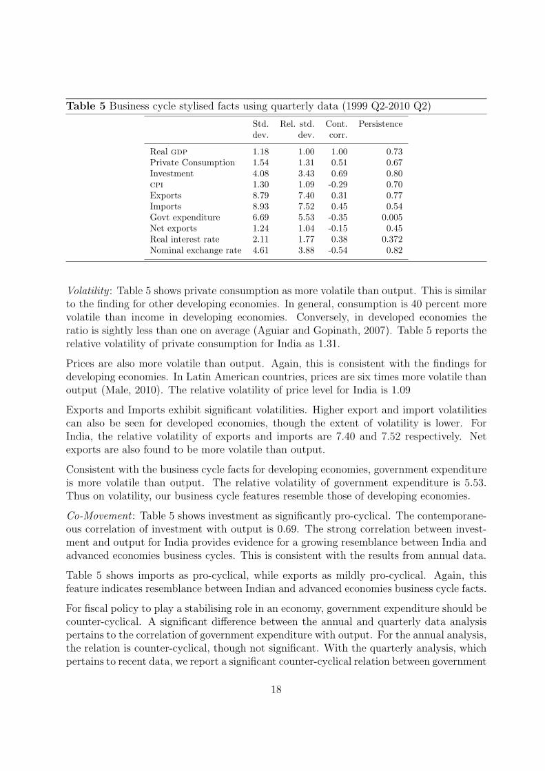
Table 5 Business cycle stylised facts using quarterly data (1999 Q2-2010 Q2)
Std. Rel. std. Cont. Persistencedev. dev. corr.
Real gdp 1.18 1.00 1.00 0.73Private Consumption 1.54 1.31 0.51 0.67Investment 4.08 3.43 0.69 0.80cpi 1.30 1.09 -0.29 0.70Exports 8.79 7.40 0.31 0.77Imports 8.93 7.52 0.45 0.54Govt expenditure 6.69 5.53 -0.35 0.005Net exports 1.24 1.04 -0.15 0.45Real interest rate 2.11 1.77 0.38 0.372Nominal exchange rate 4.61 3.88 -0.54 0.82
Volatility : Table 5 shows private consumption as more volatile than output. This is similarto the finding for other developing economies. In general, consumption is 40 percent morevolatile than income in developing economies. Conversely, in developed economies theratio is sightly less than one on average (Aguiar and Gopinath, 2007). Table 5 reports therelative volatility of private consumption for India as 1.31.
Prices are also more volatile than output. Again, this is consistent with the findings fordeveloping economies. In Latin American countries, prices are six times more volatile thanoutput (Male, 2010). The relative volatility of price level for India is 1.09
Exports and Imports exhibit significant volatilities. Higher export and import volatilitiescan also be seen for developed economies, though the extent of volatility is lower. ForIndia, the relative volatility of exports and imports are 7.40 and 7.52 respectively. Netexports are also found to be more volatile than output.
Consistent with the business cycle facts for developing economies, government expenditureis more volatile than output. The relative volatility of government expenditure is 5.53.Thus on volatility, our business cycle features resemble those of developing economies.
Co-Movement : Table 5 shows investment as significantly pro-cyclical. The contemporane-ous correlation of investment with output is 0.69. The strong correlation between invest-ment and output for India provides evidence for a growing resemblance between India andadvanced economies business cycles. This is consistent with the results from annual data.
Table 5 shows imports as pro-cyclical, while exports as mildly pro-cyclical. Again, thisfeature indicates resemblance between Indian and advanced economies business cycle facts.
For fiscal policy to play a stabilising role in an economy, government expenditure should becounter-cyclical. A significant difference between the annual and quarterly data analysispertains to the correlation of government expenditure with output. For the annual analysis,the relation is counter-cyclical, though not significant. With the quarterly analysis, whichpertains to recent data, we report a significant counter-cyclical relation between government
18
expenditure and output. The correlation coefficient is -0.35. Crucially, this is similar tothe findings for developed economies.
Also consistent with the results of the annual post-reform period, nominal exchange rateis found to be counter-cyclical.
Persistence11 A central issue in business cycle research is the nature of persistence inoutput fluctuations. Table 5 shows persistent output fluctuations for the Indian businesscycle. The magnitude of persistence is however lower compared to those of developedeconomies. Male (2010) finds the average persistence for developed economies to be 0.84and for developing economies to be 0.59. The persistence of output for India is higher thanthe developing economies average figure. The persistence is even higher at 0.84 if non-agricultural gdp is taken as the aggregate measure of business cycle activity. Price levelsare also significantly persistent. Significant price persistence justifies the use of theoreticalmodels with staggered prices and wages for the modeling of developing and emerging mar-ket business cycles. Other variables in Table 5 are also found to be significantly persistent(with the exception of Government expenditure and real interest rate).
In summary, the results of the quarterly data analysis broadly confirm the findings of thepost-reform period using annual data. The findings support that the Indian economy isin a transition phase. While on volatility, the business cycle features resemble those ofdeveloping economies, the correlation results show growing similarity with the advancedeconomies business cycle.
7.2 An Alternative Detrending Method
As another sensitivity measure, we check the robustness of our annual results to the choiceof the de-trending technique. Following (Stock and Watson, 1999; Agenor et al., 2000)we use the Baxter-King to derive the business cycle properties of our macroeconomicvariables. Baxter-King filter belong to the category of band-pass filters that extract datacorresponding to the chosen frequency components. We are interested in extracting thebusiness cycle components. In line with the NBER definition, the business cycle periodicityis defined as those ranging between 8 to 32 quarters.
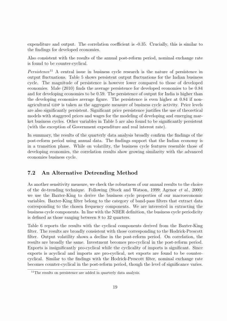
Table 6 reports the results with the cyclical components derived from the Baxter-Kingfilter. The results are broadly consistent with those corresponding to the Hodrick-Prescottfilter. Output volatility shows a decline in the post-reform period. On correlation, theresults are broadly the same. Investment becomes pro-cyclical in the post-reform period.Exports is insignificantly pro-cyclical while the cyclicality of imports is significant. Sinceexports is acyclical and imports are pro-cyclical, net exports are found to be counter-cyclical. Similar to the findings with the Hodrick-Prescott filter, nominal exchange ratebecomes counter-cyclical in the post-reform period, though the level of significance varies.
11The results on persistence are added in quarterly data analysis.
19
There are some notable differences in the results related to volatility. This arises due todifferences in the properties of the two filters. While the Baxter-King filter belongs tothe category of band-pass filters that remove slow moving components and high frequencynoise, the Hodrick-Prescott filter is an approximation to a high-pass filter that removes thetrend but passes high frequency components in the cyclical part. The Baxter-King filter,however tends to underestimate the cyclical component. (Rand and Tarp, 2002)12. As anexample, in contrast to the findings of the Hodrick-Prescott filter, the absolute volatilityof private consumption declines in the post-reform period, when the Baxter-King filter isused to de-trend the variables. The statistical testing procedure shows that the differencein correlations is close to the cut-off value of 1.96, even though it is not as strong as withthe Hodrick-Prescott filter.
Table 6 Business cycle statistics for the Indian economy using annual data: Pre and postreform period (with Baxter-King filter)
Pre-reform period (1950-1991) Post-reform period (1992-2009)
Std. Rel. Cont. Std. Rel. Cont.dev. std. dev. cor. dev. std. dev. cor.
Real gdp 1.94 1.00 1.00 0.95 1.00 1.00Pvt. Cons. 1.59 0.81 0.86 1.05 1.10 0.84Investment 3.49 1.79 0.22 3.12 3.26 0.60cpi 4.29 2.20 0.28 1.51 1.58 0.28Exports 5.99 3.07 -0.03 6.08 6.35 0.36Imports 8.76 4.49 -0.06 6.15 6.42 0.47Govt expenditure 6.39 3.10 -0.17 3.73 3.90 -0.44Net exports 0.68 0.34 0.08 0.81 0.84 -0.26Nominal exchange rate 4.34 2.23 0.05 2.17 2.27 -0.17
7.3 Redefining the Sample Period
Finally, we check the robustness of our results to a change in the sample period. Tomaintain uniformity in sample size we redefine the pre-reform period as starting from1971.
12For a detailed comparison of the filtering procedure of Hodrick-Prescott and Baxter-King, refer to(Baxter and King, 1999)
20
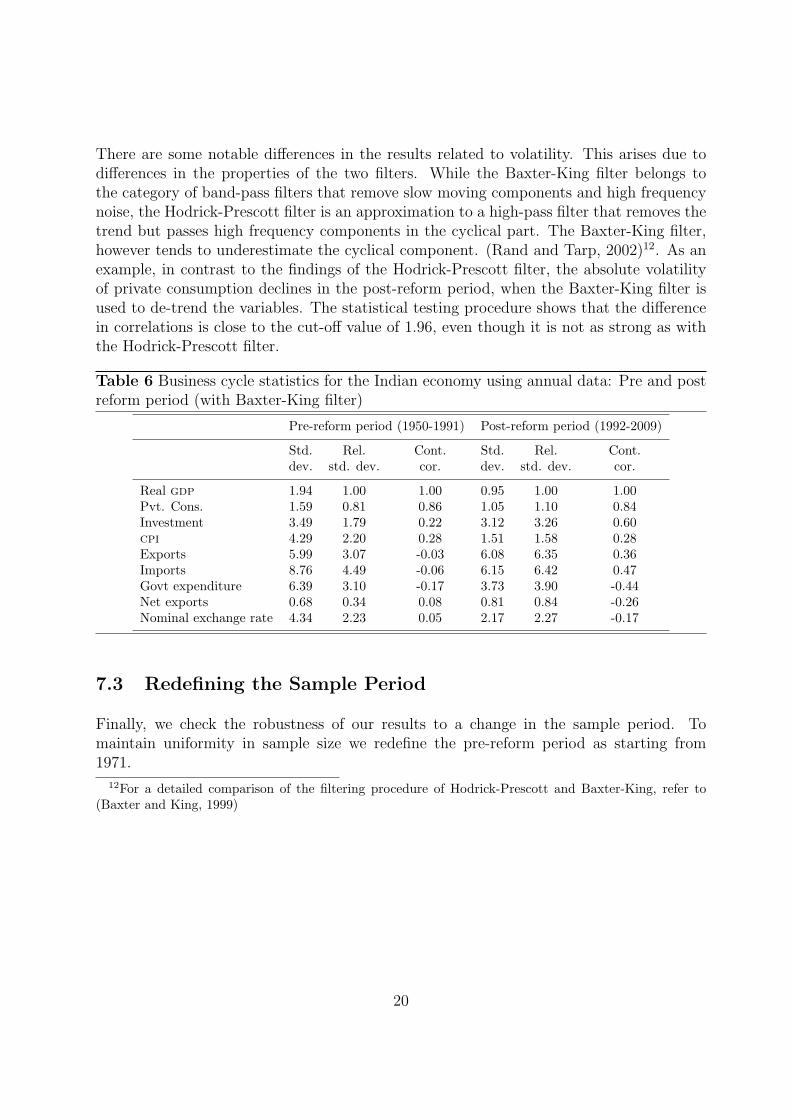
Table 7 Business cycle statistics for the Indian economy using annual data: Pre (1971-1991) and post reform period
Pre-reform period (1971-1991) Post-reform period (1992-2009)
Std. Rel. Cont. Std. Rel. Cont.dev. std. dev. cor. dev. std. dev. cor.
Real gdp 2.24 1.00 1.00 1.78 1.00 1.00Pvt. Cons. 1.94 0.86 0.69 1.87 1.05 0.89Investment 3.55 1.57 0.50 5.10 2.85 0.77cpi 5.96 2.64 -0.16 3.49 1.95 0.29Exports 6.00 2.66 0.10 7.71 4.31 0.33Imports 8.71 3.87 -0.10 9.61 5.38 0.70Govt expenditure 5.62 2.62 0.50 4.60 2.58 -0.26Net exports 0.8 0.3 0.12 1.1 0.65 -0.69Nominal exchange rate 5.54 2.46 0.40 5.35 3.00 -0.48
Table 7 reports business cycle facts when the pre-reform period is defined as starting from1971. The broad stylised facts remain the same. On correlation, our results remain thesame as reported in Table 3. Investment and imports become highly pro-cyclical, whilenet exports and nominal exchange rate turn counter-cyclical in the post-reform period.On volatility, we get a mixed picture. While aggregate gdp is highly volatile at 2.24 inthe pre-reform period, it falls to 1.78 in the post-reform period. Other variables, with theexception of investment, exports, imports and net exports also show a fall in volatility fromthe pre to post reform period.
8 Conclusion
Documenting business cycle stylised facts forms the foundation of quantitative generalequilibrium models either in the RBC or DSGE tradition. Such a study assumes greaterrelevance in the context of an economy like India which has undergone significant trans-formation since 1991. The industrial sector has been freed from capacity controls, importduties have been reduced and a reasonably conducive environment towards the global econ-omy has evolved over the last few years. The novel aspect of this paper is to present acomprehensive set of stylized facts governing an economy in transition. We locate factsabout Indian business cycles in the context of other industrial economies, as well as otheremerging and developing countries.
Our main findings are as follows:
• Output volatility, as measured by the percentage standard deviation of the filteredcyclical component of gdp is considerably reduced in the post-reform period.
21
• Consistent with the business cycle facts for developed economies, investment becomeshighly pro-cyclical in the post-reform period.
• Imports become highly pro-cyclical in the post-reform period.
• Net exports and nominal exchange rate become counter-cyclical in the post-reformperiod.
• The quarterly data analysis that focuses only on recent data shows government ex-penditure to be counter-cyclical. This feature is indicative of the growing resemblancebetween the Indian and the advanced economies business cycle.
This kind of study holds relevance not just for India, but for any economy that undergoestransition. An important finding is that for DSGE models to effectively incorporate thefeatures of an economy in transition, recent data should be taken.
Future work can use the findings of this paper to assess the extent to which DSGE models,starting with the simplest RBC model through to New-Keynesian models with labour mar-kets and financial frictions introduced in stages, can explain business cycle fluctuations inIndia. Both closed and open economy models can be examined. Comparisons with a rep-resentative developed economy, say the US, can then be made. Proceeding in this way, onewill be able to assess the relative importance of various frictions in driving aggregate fluc-tuations in India. Another avenue for future work relates to (Lucas, 1987), which pointedout that the welfare gains from eliminating business cycle fluctuations in the standardRBC model are small, and dwarfed by the gains from increased growth. While addingNew Keynesian frictions significantly increases the gains from stabilization policy, theystill remain small compared to the welfare gains from increased growth. However, thereis relatively little work introducing long-run growth into DSGE models, and exploring therelationship between volatility and endogenous growth. This takes particular importancefor India which has moved to a higher growth path in recent years, with the attendantdecline in macroeconomic volatility, as documented in this paper.
22
References
Agenor P, McDermott C, Prasad E (2000). “Macroeconomic fluctuations in developing countries:Some stylised facts.” The World Bank Economic Review.
Aghion P, Angeletos G, Banerjee A, Manova K (2010). “Volatility and growth: Credit constraintsand the composition of investment.” Journal of Monetary Economics, 57(3), 246–265. ISSN0304-3932.
Aghion P, Bacchetta P, Banerjee A (2004). “Financial development and the instability of openeconomies.” Journal of Monetary Economics, 51, 1077–1106.
Aguiar M, Gopinath G (2007). “Emerging market business cycles: The cycle is the trend.”Journal of Political Economy, 115(1).
Alper C (2002). “Business cycles, excess volatility, and capital flows: Evidence from Mexico andTurkey.” Emerging Markets Finance & Trade, pp. 25–58. ISSN 1540-496X.
Ambler S, Cardia E, Zimmermann C (2004). “International business cycles? What are the facts?”Journal of Monetary Economics.
Apergis N (1996). “The cyclical behaviour of prices: Evidence from seven developing countries.”The Developing Economies.
Backus D, Kehoe P (1992). “International evidence on the historical properties of business cycles.”The American Economic Review, 82(4), 864–888. ISSN 0002-8282.
Batini N, Gabriel V, Levine P, Pearlman J (2010). “A floating versus managed exchange rateregime in a DSGE model of India.” Department of Economics, Surrey University, DiscussionPapers.
Baxter M, King R (1999). “Measuring business cycles: approximate band-pass filters for economictime series.” Review of Economics and Statistics, 81(4), 575–593. ISSN 0034-6535.
Bjornland H (2000). “Detrending methods and stylized facts of business cycles in Norway- aninternational comparison.” Empirical Economics.
Boshoff W (December, 2010). “Band-pass filters and business cycle analysis: High- frequencyand medium-term deviation cycles in South Africa and what they measure .” UniverseteitStellenbosch University, Working Paper, 200.
Burns A, Mitchell W (1946). “Measuring business cycles.” NBER Books.
Burnside C (1998). “Detrending and business cycle facts: A comment.” Journal of MonetaryEconomics.
Calderon C, Fuentes R (2006). “Complementarities between institutions and openness in economicdevelopment: Evidence for a panel of countries.” Cuadernos de economıa, 43, 49–80. ISSN0717-6821.
Calderon C, Fuentes R (2010). “Characterising the business cycles of emerging economies.” PolicyResearch Working Paper, The World Bank.
23
Calvo G (1998). “Capital flows and capital-market crises: the simple economics of sudden stops.”Journal of Applied Economics, 1(1), 35–54.
Canova F (1998). “Detrending and business cycle facts.” Journal of Monetary Economics.
Chadha B, Prasad E (1994). “Are prices countercyclical?: Evidence from the G-7.” Journal ofMonetary Economics, pp. 239–254.
Chakraborty S (2008). “Indian economic growth.” UNU-WIDER Research Paper No. 2008/67.
Chari V, Kehoe P, McGrattan E (2007). “Business cycle accounting.” Econometrica, 75(3),781–836. ISSN 1468-0262.
Den Reijer A (2002). “International business cycle indicators, measurement and forecasting.” DeNederlandsche Bank Research Memorandum.
Dua P, Banerji A (2001). “An indicator approach to business and growth rate cycles: The caseof India.” Indian Economic Review, 36, 55–78.
Gabriel V, Levine P, Pearlman J, Yang B (2010). “An estimated DSGE model of the Indianeconomy.” Department of Economics, Surrey University, Discussion Papers.
Garcia-Cicco J, Pancrazi R, Uribe M (2010). “Real business cycles in emerging countries?” TheAmerican Economic Review, pp. 2510–2531.
Hodrick R, Prescott E (1997). “Postwar US business cycles: An empirical investigation.” Journalof Money, Credit & Banking, 29(1).
Iacobucci A, Noullez A (2005). “A frequency selective filter for short-length time series.” Com-putational economics, 25(1), 75–102. ISSN 0927-7099.
Jayaram S, Patnaik I, Shah A (2009). “Examining the decoupling hypothesis for India.” Economicand Political Weekly, XLIV(44), 109–116.
Kaldor N (1957). “A model of economic growth.” The Economic Journal, 67(268), 591–624.ISSN 0013-0133.
King R, Rebelo S (1999). “Resuscitating real business cycles.” Handbook of macroeconomics, 1,927–1007.
Kose M, Otrok C, Whiteman C (2003). “International business cycles: World, region, andcountry-specific factors.” American Economic Review, 93(4), 1216–1239. ISSN 0002-8282.
Kydland F, Prescott E (1990). “Business cycles: Real facts and a monetary myth.” Real businesscycles: a reader, p. 383.
Loayza N, Ranciere R, Serven L, Ventura J (2007). “Macroeconomic volatility and welfare indeveloping countries: An introduction.” The World Bank Economic Review, 21(3), 343. ISSN0258-6770.
Lucas R (1987). Models of business cycles. Basil Blackwell New York. ISBN 0631147918.
Lucas RJ (1977). “Understanding business cycles.” In “Carnegie-Rochester Conference Series onPublic Policy,” .
24
Male R (2010). “Developing country business cycle: Revisiting the stylised facts.” Queen Mary,University of London, Working Paper No. 664.
Neumeyer P, Perri F (2005). “Business cycles in emerging economies: The role of interest rates.”Journal of Monetary Economics.
Patnaik I, Sharma R (2002). “Business cycles in the Indian economy.” MARGIN-NEW DELHI-,35, 71–80. ISSN 0025-2921.
Ramey G, Ramey VA (1995). “Cross-country evidence on the link between volatility and growth.”The American Economic Review, 85(5), 1138–1151.
Rand J, Tarp F (2002). “Business cycles in developing countries: Are they different?” WorldDevelopment, 30(12), 2071–2088. ISSN 0305-750X.
Rebelo S (2005). “Business cycles.” Annals of Economics and Finance, 6, 229–250.
Shah A (2008). “New issues in macroeconomic policy.” Business Standard India, pp. 26–54.
Shah A, Patnaik I (2010). “Stabilising the Indian business cycle.” India on growth turnpike:Essays in honour of Vijay L. Kelkar, pp. 136–154.
Stock J, Watson M (1999). “Business cycle fluctuations in US macroeconomic time series.”Handbook of Macroeconomics, 1, 3–64. ISSN 1574-0048.
Uribe M, Yue V (2006). “Country spreads and emerging markets: Who drives whom?” Journalof International Economics, pp. 6–36.
25
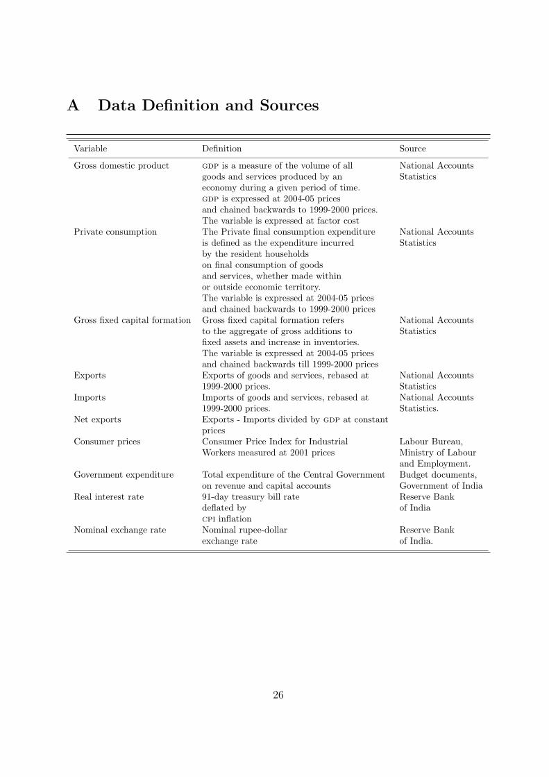
A Data Definition and Sources
Variable Definition Source
Gross domestic product gdp is a measure of the volume of all National Accountsgoods and services produced by an Statisticseconomy during a given period of time.gdp is expressed at 2004-05 pricesand chained backwards to 1999-2000 prices.The variable is expressed at factor cost
Private consumption The Private final consumption expenditure National Accountsis defined as the expenditure incurred Statisticsby the resident householdson final consumption of goodsand services, whether made withinor outside economic territory.The variable is expressed at 2004-05 pricesand chained backwards to 1999-2000 prices
Gross fixed capital formation Gross fixed capital formation refers National Accountsto the aggregate of gross additions to Statisticsfixed assets and increase in inventories.The variable is expressed at 2004-05 pricesand chained backwards till 1999-2000 prices
Exports Exports of goods and services, rebased at National Accounts1999-2000 prices. Statistics
Imports Imports of goods and services, rebased at National Accounts1999-2000 prices. Statistics.
Net exports Exports - Imports divided by gdp at constantprices
Consumer prices Consumer Price Index for Industrial Labour Bureau,Workers measured at 2001 prices Ministry of Labour
and Employment.Government expenditure Total expenditure of the Central Government Budget documents,
on revenue and capital accounts Government of IndiaReal interest rate 91-day treasury bill rate Reserve Bank
deflated by of Indiacpi inflation
Nominal exchange rate Nominal rupee-dollar Reserve Bankexchange rate of India.
26