Embed Size (px)
Citation preview
NASA-CR-194838
Determination of the Stability and Control Derivatives of
the NASA F/A-18 HARV Using Flight Data
Contractor Reportfor
NASA Grant # NCC 2-759
NASA Technical Contact
Albion H. Bowers
NASA Dryden Flight Research Facility
Authors
Principal Investigator: Marcello R. Napolitano
Graduate Student: Joelle M. Spagnuolo
May 15, 1993 -December 15, 1993
(NASA-CR-19483_) OETERMINATION OF
T_E STABILITY AND CONTROL
DERIVATIVES OF THE NASA F/A-IB HARV
USING FLIGHT OATA Contractor
Report, 15 May - 15 Dec. 1993
(West Virginia Univ.) 123 p
N94-24804
Unclas
G3/08 0202113
https://ntrs.nasa.gov/search.jsp?R=19940020331 2018-06-26T21:04:19+00:00Z
Determination of the Stability and Control Derivatives ofthe NASA F/A-18 HARV Using Flight Data
Contractor Reportfor
NASA Grant # NCC 2-759
NASA Technical ContactAlbion H. Bowers
NASA Dryden Flight Research Facility
Authors
Principal Investigator: Marcello R. Napolitano
Graduate Student: JoeUe M. Spagnuolo
December 1993
ABSTRACT
ti
This report documents the research conducted for the NASA-Ames Cooperative
Agreement No. NCC 2-759 with West Virginia University. The NASA technical officer for
this grant is Albion H. Bowers, an aerospace engineer at NASA
A complete set of the stability and control derivatives for varying angles of attack
from 10" to 60" were estimated from flight data of the NASA F/A-18 HARV. The data
were analyzed with the use of the pEst software which implements the output-error method
of parameter estimation. Discussions of the aircraft equations of motion, parameter
estimation process, design of flight test maneuvers, and formulation of the mathematical
model are presented. The added effects of the thrust vectoring and single surface excitation
systems are also addressed. The results of the longitudinal and lateral directional derivative
estimates at varying angles of attack are presented and compared to results from previous
analyses. The results indicate a significant improvement due to the independent co0trol
surface deflections induced by the single surface excitation system, and at the same time, a
need for additional flight data especially at higher angles of attack.
ACKNOWLEI_MENTS
aoa
Ul
The authors would like to express their sincere gratitude to Mr. Albion Bowers, the
NASA technical monitor, Mr. Brent Cobleigh, Dr. Kenneth nift and the other researchers
at NASA Dryden Flight Research Facility for their much appreciated advice and assistance.

TABLE OF CONTENTS
TITLE PAGE •
ABSTRACT
ACKNOWLEDGEMENTS
TABLE OF CONTENTS
LIST OF TABLES AND FIGURES
NOMENCLATURE
Page
i
ii
*l.
111
iv
vi
X
iv
CHAFrER 1: INTRODUCTION
1.1 Literature Review
CHAPTER 2: AIRCRAFT STABILITY AND CONTROL
2.1: Aircraft Stability and Control Definition
2.2: Aerodynamic Force and Moment Representation
CHAFrER 3: PARAMETER ESTIMATION
3.1: Purpose
3.2: Techniques
3.3: The Maximum Likelihood Method
CHAPTER 4: AIRCRAFT EQUATIONS OF MOTION
4.1: Newtonian Mechanics
4.2: Applied Forces
4.3: Applied Moments
1
3
8
8
9
11
11
11
13
21
21
23
24
4.4: Euler Angles
4.5: Velocity Components (Polar Form)
4.6: Six-Degree-of-Freedom Equations of Motion
4.7: Observation Equations
CHAPTER 5: HIGH ALPHA RESEARCH
5.1: Purpose of High Alpha Technology Program
52: High Alpha Research Vehicle (HARV) Description
5.3: lnstnmlentation and Airdata Systems
CHAPTER 6: FLIGHT TEST MANEUVERS
6.1: Design Considerations
6.2: Maneuvers Developed for the HARV
CHAPTER 7: HARV AERODYNAMIC MODEL
7.1: Equation Modification
72: Sign Convention
CHAPTER 8: RESULTS AND CONCLUSIONS
8.1: Lateral Directional Derivatives
8.2: Longitudinal Directional Derivatives
8.3: Conclusions
26
29
31
32
37
37
39
41
46
46
48
56
56
59
62
63
68
71
V
REFERENCES 104

TABLES
Table 5.1:
FIGURES
Figure 3.1:
Figure 3.2:
Figure 3.3:
Figure 4.1:
Figure 4.2:
Figure 5.1:
Figure 5.2:
Figure 6.1:
Figure 6.2:
Figure 6.3:
Figure 6.4:
Figure 6.5:
Figure 7.1:
Figure 8.1:
Figure 8.2:
LIST OF TABLES AND FIGURES
Physical Characteristics of the F/A-18 HARV
Block Diagram of the Parameter Estimation Process
Geometric Meaning of the Modified Newton-Raphson Method
A Qualitative Trend of J with the Nttmber of Iterations, K
Body Axis System
Representation of ELder Angles
Three-view Drawing of the F-18 HARV
F-18 HARV Engine Thrust Vectoring Vane Configuration
Flight Test Maneuver Input Shapes
(a) Frequency Sweep (b) 3211 (c) Pulse-Type (Doublet)
Control Surface Deflection Time Histories without OBES
Correlation between the Rudder & Aileron Deflections without OBES
Control Surface Deflection Time Histories with OBES
Correlation between the Rudder & Aileron Deflections with OBES
Thrust Vectoring Vane Positions
Computed and Measured Response Time Histories for ct = 10° in the
Lateral Direction (a) Sideslip Angle (b) Rolling Moment
(c) Yawing Moment (d) Roll Angle (e) Lateral Acceleration
Computed and Measured Response Time Histories for a = 25 ° in the
Lateral Direction (a) Sideslip Angle (b) Rolling Moment
(c) Yawing Moment (d) Roll Angle (e) Lateral Acceleration
vi
PAGE
43
18
19
2O
35
36
44
45
51
52
53
54
55
61"
73
74
Figure 8.3: Computed and Measured Response T'nne Histories for a = 30 ° in the
Lateral Direction (a) Sideslip Angle (b) Rolling Moment(c) Yawing Moment (d) Roll Angle (e) Lateral Acceleration
vii
75
Figure 8.4: Computed and Measured Response T'tme Histories for a = 40 ° in the
Lateral Direction (a) Sideslip Angle (b) Rolling Moment(c) Yawing Moment (d) Roll Angle (e) Lateral Acceleration
76
Figure 8.5: Computed and Measured Response Time Histories for ct - 50 ° in the
Lateral Direction (a) Sideslip Angle (b) Rolling Moment(c) Yawing Moment (d) Roll Angle (e) Lateral Acceleration
77
Figure 8.6: Computed and Measured Response Tune Histories for a = 60 ° in the
Lateral Direction (a) Sideslip Angle Co) Rolling Moment(c) Yawing Moment (d) Roll Angle (e) Lateral Acceleration
78
Figure 8.7: Aerodynamic Bias Derivatives (Lateral-Directional)(a) Lateral Force (b) Rolling Moment (c) Yawing Moment
79
Figure 8.8: Sideslip Derivatives (Lateral-Directional)
(a) Lateral Force Co) Roiling Moment (c) Yawing Moment8O
Figure 8.9: Roll Rate Derivatives (Lateral-Directional)
(a) Lateral Force (b) Rolling Moment (c) Yawing Moment81
Figure 8.10: Yaw Rate Derivatives (Lateral-Directional)
(a) Lateral Force (b) Roiling Moment (c) Yawing Moment82
Figure 8.11: Aileron Derivatives (Lateral-Directional)
(a) Lateral Force (b) Rolling Moment (c) Yawing Moment
83
Figure 8.12: Rudder Derivatives (Lateral-Directional)
(a) Lateral Force (b) RoiLing Moment (c) Yawing Moment
Figure 8.13: Differential Horizontal Tail Derivatives (Lateral-Directional)(a) Lateral Force (13) Roiling Moment (c) Yawing Moment
84
85
Figure 8.14: Pitch Vane Derivatives (Lateral-Directional)
(a) Lateral Force (b) Rolling Moment (c) Yawing Moment86
Figure 8.15: Yaw Vane Derivatives (Lateral-Directional)
(a) Lateral Force (b) Rolling Moment (c) Yawing Moment
87
Figure 8.16: Calculated Thrust Moment Arm at Varying Angles of Attack 88
Figure 8.17:
Figure 8.18:
Figure 8.19:
Figure 8.20:
Figure 8.21:
Figure 8.22:
Figure 8.23:
Figure 8.24:
Figure 8.25:
Figure 8.26:
Figure 8.27:
Figure 8.28:
Figure 8.29:
Computed and Measured Response Time Histories for a = 10O m
the Longitudinal Direction (a) Angle of Attack (b) Pitching Moment(c) Pitch Angle (d) Normal Acceleration (e) Axial Acceleration
Computed and Measured Response Time Histories for at = 25 ° m
the Longitudinal Direction (a) Angle of Attack (b) Pitching Moment(c) Pitch Angle (d) Normal Acceleration (e) Axial Acceleration
Computed and Measured Response Time Histories for a = 30 ° m
the Longitudinal Direction (a) Angle of Attack (b) Pitching Moment(c) Pitch Angle (d) Normal Acceleration (e) Axial Acceleration
Computed and Measured Response Time Histories for a = 40 ° m
the Longitudinal Direction (a) Angle of Attack Ca) Pitching Moment(c) Pitch Angle (d) Normal Acceleration (e) Axial Acceleration
Computed and Measured Response Time Histories for a = 50 ° m
the Longitudinal Direction (a) Angle of Attack Ca) Pitching Moment(c) Pitch Angle (d) Normal Acceleration (e) Axial Acceleration
Computed and Measured Response Time Histories for a = 60 ° m
the Longitudinal Direction (a) Angle of Attack Ca) Pitching Moment(c) Pitch Angle (d) Normal Acceleration (e) Axial Acceleration
Aerodynamic Bias Derivatives (Longitudinal-Directional)
(a) Normal Force Ca) Pitching Moment (c) Axial Force
Angle of attack Derivatives 0.ongltudinal-Directional)(a) Normal Force (b) Pitching Moment (c) Axial Force
Pitch Rate Derivatives (Longitudinal-Directional)(a) Normal Force Ca) Pitching Moment (c) Axial Force
Trailing Edge Flap Derivatives (Longitudinal-Directional)
(a) Normal Force (b) Pitching Moment (c) Axial Force
Leading Edge Flap Derivatives (Longitudinal-Directional)(a) Normal Force (b) Pitching Moment (c) Axial Force
Symmetric Aileron Derivatives (Longitudinal-Directional)(a) Normal Force (b) Pitching Moment (c) Axial Force
Elevator Derivatives (Longitudinal-Directional)(a) Normal Force (b) Pitching Moment (c) Axial Force
vln
89
9O
91
92
93
94
95
96
97
98
99
100
101
Figure 8.30: Pitch Vane Derivatives (Longitudinal-Directional)(a) Normal Force Co) Pitching Moment (c) Axial Force
Figure 8.31: Yaw Vane Derivatives (Longitudinal-Directional)(a) Normal Force Co) Pitching Moment (c) Axial Force
ix
102
103
NOMENCIATURE
X
_aats2t Um_
a_
a_
%
a_
b
C
CA
C_
C._
CAeE
C^_L_
CASI-_
c^_,
CA6rV
CAeW
CD
C_
Normal Acceleration
Longitudinal Acceleration
Lateral Acceleration
Vertical Acceleration
Reference Span
Reference Chord
Axial Force Coefficient
Axial Force Aerodynamic Bias
Axial Force due to a
Axial Force due to 6 E
Axial Force due to 6x._
Axial Force due to 6n_
Axial Force due to 6sA
Axial Force due to q
Axial Force due to 6rv
Axial Force due tO 6yv
Drag Coefficient
Rolling Moment Coefficient
g
g
g
g
morft
morft
per deg
per deg
per deg
per deg
per deg
per rad
per deg
per deg
Ci6DHT
CI6R
C!6rv
CL
Cm
C_
Cm_
Cm6E
Cm6LEF
C,.sr_
Cm_A
C_q
Cm6rv
C_tv
Co
C_o
Rolling Moment Aerodynamic Bias
Rolling Moment clue to/3
Rolling Moment due to p
Rolling Moment due to r
Rolling Moment due to 6^
Rolling Moment due to 6D_
Rolling Moment due to 6 R
Rolling Moment due to 6rv
Rolling Moment due to 6_
Lift Coefficient
Pitching Moment Coefficient
Pitching Moment Aerodynamic Bias
Pitching Moment due to a
Pitching Moment due to 6E
Pitching Moment due to 6_
Pitching Moment due to
Pitching Moment due to 6sA
Pitching Moment due to q
Pitching Moment due to 6rv
Pitching Moment due to 6_
Yawing Moment Coefficient
Yawing Moment Aerodynamic Bias
per deg
per rad
per rad
per deg
per deg
per deg
per deg
per deg
per deg
per deg
per deg
per deg
per deg
per rad
per deg
per deg
xi
Call
%
Cn6DHT
CnSR
Cn6PV
Ca vv
CN
C_
C_
CN6E
CN6_
CN6"rEF
CN_SA
CN6_,
CN6yV
Cx
Yawing Moment due to
Yawing Moment due tO p
Yawing Moment due tO r
Yawing Moment due to 6A
Yawing Moment due to 6Din-
Yawing Moment due to 6 R
Yawing Moment due to 6pv
Yawing Moment due to 6w
Normal Force Coefficient
Normal Force Aerodynamic Bias
Normal Force due to a
Normal Force due to 6F.
Normal Force due to 6ta_
Normal Force due to 6TFJ,
Normal Force due to 6SA
Normal Force due to q
Normal Force due to 6pv
Normal Force due to 6w
Longitudinal Force Coefficient
Lateral Force Coefficient
Lateral Force Aerodynamic Bias
Lateral Force due to
per deg
per rad
per rad
per deg
per deg
per deg
per deg
per deg
per deg
per deg
per deg
per deg
per deg
per rad
per deg
per deg
per deg

%
Cyr
Cy6DHT
C_R
Cy6Fv
C¥6yv
DHT
F
g
GG
H
h
J
I_Kp
LEF
m
Lateral Force due to p
Lateral Force due to r
Lateral Force due to 6^
Lateral Force due to 6Dtrr
Lateral Force due to 6 R
Lateral Force due to 6rv
Lateral Force due to 6¥v
Vertical Force Coefficient
Differential Horizontal Tail
External Applied Force
Components of External Force
Gravitational Acceleration
Measurement Noise Covariance
Altitude
Angular Momentum Vector
Moments of Inertia
Engine Moment of Inertia
Cross Products of Inertia
Cost Function
Upwash and Sidewash Factors
Leading Edge Flap
Mass
per rad
per rad
per deg
per deg
per deg
per deg
per deg
N or lb
N or lb
m/sec 2 or ft/sec 2
kg-m 2 or slug-ft 2
kg-m 2 or slug-ft 2
kg-m 2 or slug-ft 2
kg or slug
Xlll
M
Mx, My,Mz
n
N
P
P
q
r
S
SA
t
T
TEF
U
V
W
l
External Applied Moment
Components of External Moment
Measurement Noise
Number of Time History Points
Number of Response Va_.-iab]es
Engine Speed
Roll Rate
Probability
Pitch Rate
Dynamic Pressure
Yaw Rate
Reference area
Symmetric Aileron
Time Variable
Thrust
Trailing Edge Flap
Velocity Components
Input
Velocity
Response Weighting Matrix
System State
Sensor Position x-axis
N-m or ft-lb
N-m or ft-lb
rad/sec
rad/sec or deg/see
rad/sec or deg/sec
N/m=or lb/
rad/sec or deg/sec
m 2 or
N or lb
m/sec or ft/sec
m/sec or ft/sec
morft
xiv
Yo,Yp,YwYq,Y-
Y
z
Z
ZwZlt,zax, Zay,Zaa
GREEK
A
6A
6DHT
6F_
6t._F
6SA
6,,r_
6pv
6 R
6vv
rl
0
Sensor Position y-axis
Modeled Response
Measured Response
Computed Response
Sensor Position z-axis
Angle of Attack
Angle of Sideslip
Sample Interval
Aileron Deflection
Differential Horiz. Taft Def.
Elevator Deflection
Leading Edge Flaps Def.
Symmetric Ailerons Deflection
Trailing Edge Flaps Def.
Pitch Vane Deflection
Rudder Deflection
Yaw Vane Deflection
Measurement Noise
Pitch Attitude
Unknown Parameter Vector
morft
morft
rad or deg
rad or deg
sec
rad or deg
rad or deg
rad or deg
rad or deg
rad or deg
rad or deg
rad or deg
rad or deg
rad or deg
rad or deg
xv
¢
t
V
{9
Roll A_mde
Gradient
Angular Velocity
tad or deg
rad or deg
rad/sec or deg/sec
xvi
SUBSCRIPTS
a
b
B
E
K
m
wmd
Z
SUPERSCRIPTS
T
ABBREVIATIONS
aoa
c.g.
HARV
MMLE
pEst
Actual System
Bias
Ax s
Earth Axis
Iteration Number
Modeled System
Wind Axis
Observation
Transpose
Angle of Attack
Center of Gravity
High Alpha Research Vehicle
Modified Maximum Likelihood Estimation
Parameter Estimation

xvii
PID Parameter Identification

CHAPTER 1
INTRODUCTION
The National Aeronautics and SpaceAdministration is currently involved in a High
Alpha Technology Program which has the following objectives:
1. To provide flight validated prediction methods including experimental and
computational methods that accurately simulate high angle of attack
aerodynamics, flight dynamics, and flying qualities.
2. To improve aircraft agility at high angles of attack.
In undertaking this type of research, the airplane dynamics in the high alpha regimes
must be understood. For this reason, part of the overall program for each test aircraft
includes a parameter estimation analysis in which a complete set of stability and control
parameters is extracted from flight data. Although a thorough basis of the vehicle
aerodynamics is generated by analytic computations and wind tunnel tests performed during
the design process, the true aerodynamic characteristics of the aircraft cannot be verified
until flight test data has been analyzed. Primarily, the verification of the aircraft
aerodynamics is accomplished by comparing the stability and control derivatives extracted
from both wind tunnel tests and flight data. This comparison allows for validation of the
prediction methods applied to the wind tunnel data and complete understanding of the
vehicle aerodynamics. In addition, the results of the parameter estimation analysis are
significant, for they not only compose an extensive data base of the vehicle aerodynamic
qualities but are also used to update the stability and control data in flight simulators. This
is performed in order to ensurethat the responsesin the simulators are comparable to those
experienced in flight
The use of flight data to estimate the stability and control derivatives of aircraft has
been implemented for many years. In the past, most flight testing was limited to conditions
in which linear equations of motion would appropriately describe the dynamic modeL
Several computer programs were developed and used for this type of analysis. For these
cases, the parameter estimation program MMLE3 developed at Ames-Dryden in the early
197ffs was widely used. MMLE was used for several parameter estimation analyses of many
aircraft including the space shuttle throughout the 197ffs and early 1980's. However, more
recent research such as the high alpha research, is exploring flight regimes in which
nonlinearities occur and need to be included in the dynamic model. Hence, the data
analysis for these types of investigations is often performed with the more recently
developed pEst estimation program. This software was also developed at NASA Dryden,
and it is capable of supporting nonlinearities in the dynamic equations of motion.
The purpose of this report is to document the estimates of the stability and control
parameters of one of the test airplanes involved in the high alpha program The airplane
under investigation is the NASA F/A-18 High Alpha Research Vehicle which has been
equipped with a thrust vectoring system and an On Board Excitation System which induces
independent control surface motions. The thrust vectoring system consists of axisymmetric
nozzles and six post exit vanes that allow vectoring capability in both pitch and yaw. It is
explained how the six vane deflections are combined to produce a single deflection value
for either a pitch or yaw maneuver.
2
This document includes discussions of the aircraft equatiom of motion, parameter
estimation process, design of the flight test maneuvers, and the formulation of the
mathematical model. In addition, the results of the longitudinal and lateral derivative
estimates at varying angles of attack are presented and compared to results from previous
analyses.
1.1 LITERATURE REVIEW
This section presents a summary of some previous parameter estimation analyses.
The various methods used and conclusions for each analysis are discussed.
In 1986 Richard Maine and Kenneth Iliff t examined the practical application of
parameter estimation methodology to the problem of est/matlns aircraft stability and control
derivatives from flight test data. In-depth discussions of all aspects of the parameter
estimation process beginning with reasons why this type of analysis is performed were
provided. Derivadom of the aircraft equations of motion and methods in which the
equations are modified to be used in the estimation process were also presented. The
output error estimation technique was chosen as the focus for detailed examination. Topics
such as the design of flight test maneuvers, flight safety considerations, pilot involvement,
data acquisition and instrumentation systems were all extensively reviewed. The evaluation
of the parameter estimation results were considered, and several suggestions to improve
results were given.
A study of estimating the parameters of highly unstable aircraft was conducted by
3
Maine and Murray 2 in 1986. This investigation involved data from the higi_ unstable X-29
aircraft. It was concluded that problems exist in applying the output error method to such
highly unstable aircraft. From the analysis, it was found that the more appropriate
maximum likelihood estimator was the filter error method.
A parameter estimation analysis for the AD-1 Oblique Wing Research Airplane was
conducted by Alex Sire and Robert Cu@ in 1984. In this investigation, the MMLE3
program was used to produce a complete set of both longitudinal and lateral-<lirectional
derivatives. The flight determined derivatives were compared to the predictions obtained
from wind tunnel data. The results for the primary longitudinal derivatives were somewhat
consistent. However, it was concluded that the discrepancies in the remaining derivatives
were due to the poor quality of the time response data. This was due to the fact that the
airplane was designed to be a low cost aircraft which implied that the instrumentation
system was not of the best quality. Also, it was determined that the longitudinal response
was heavily damped and significant aerolastic and nonlinear effects were present but not
considered in the model used in MMLE3.
PeUicano, K_,'umenacker and Vanhoy 4provided a technical overview of the procedures
and analyses tools used to conduct a successful expansion of the flight envelope for the X-29
aircraft. The design of the flight test maneuvers used for the aerodynamic analysis and
flight envelope clearance were discussed, and three different methods were used to update
the aerodynamic database and extrapolate the results. These methods were:
1. A parameter identification program
2. An off-line closed loop simulation
4
3. A total aerodynamiccoefficient matching method.
Specifically. the parameter estimation program pest was utilized during the first
expansion flights. The program was used primarily for analysis of yaw-roll doublets, lateral
stick raps, and rudder pedal raps in order to obtain lateral-directional derivatives. However,
it was concluded that the use of pest in the longitudinal axis was impaired by the high static
instability and the three-surface pitch control.
In 1989, Vladislav Klein, Kevin Breneman and Thomas Ratvasky 5 presented
preliminary results of the aerodynamic parameters estimated from flight data of an advanced
fighter aircraft. In this analysis, a summary of the aerodynamic parameters of the NASA
F-18A High Alpha Research Vehicle and an assessment of the accuracy of the
instrumentation system and parameter estimates were discussed. The parameters were
estimated from transient maneuvers at different angles of attack varying from 8 to 54
degrees. A stepwise regression with the ordinary least squares technique was applied for
the data analysis. Some of the conclusions suggested that insufficient excitation of the
transient maneuvers resulted in large scatter of the estimated parameters. The resulting low
accuracy of the parameters indicated that it was not poss_le to comment on their agreement
with wind tunnel measurement and previous flight data.
A parameter identification study of the X-31 was performed in 1991 by Rohlf,
Plaetschke, and Weib. 6 Selected results from both simulated and flight test data obtained
by using a maximum likelihood method for parameter estimation in nonlinear systems were
presented. In this investigation, the researchers had to implement a stabilization procedure
to the Maximum Likelihood output error parameter estimation algorithm since the X-31A
5
aircraft is partially aerodynamicallyunstable. This was done in order to avoid divergence
in the numerical integration. Essentially, the estimates from the fl/ght test data compared
well with the predicted values. However, the uncertainty of the values was due to the fact
that flight test data was not particularly suited for aerodynamic parameter estimation.
Parameter estimation results of the F-18 stability and control derivatives were
discussed in a NASA internal memo written by K. IlifF in December of 1990. The
parameter estimation program pEst was used to obtain the derivative estimates for the
lateral-direction. It was explained how the estimation of stability and control derivatives
at high angles of attack is always difficult due to the uncertainty of the aerodynamic
mathematical model and the occurrences of uncommanded responses during the dynamic
maneuvers. In general, the agreement between the flight determined derivatives and the
predictions from the wind tunnel data was good considering an of the difficulties in
obtaining derivative estimates from both the flight and wind tunnel data. It was concluded
that many of the differences encountered in the estimates were due to the lack of
independent control surface deflections.
In addition, Klein s estimated a complete set of stability and control derivatives for
a low-wing, single engine, general aviation airplane using the equation error method and the
maximum likelihood method. The mathematical model of the airplane was based on the
equations of motion with linear aerodynamics. Klein utilized two standard-deviation
confidence intervals obtained from repeated measurements as bounds for the comparison
of the parameters determined by both methods. From the analysis, it was determined that
the estimated parameters of both methods agreed within the two standard-deviation
6

confidence intervals for the parameter. Both estimation methods provided identical values
for most of the longitudinal parameters; however, a significant difference in the derivative
of the vertical force coefficient with respect to the angle of attack was found. The results
showed that the maximum likelihood estimates agreed better with the computed parameters
from steady flight data than with those from the equation error method. For the lateral
directional derivatives, the mean values from both estimation methods agreed in general
7
CHAPTER 2
AIRCRAFt STABILITY AND CONTROL
2.1: AIRCRAFT STABILITY AND CONTROL DEFINITION
The subject of aircraft stability and control involves controlling the attitude and flight
path of an aircraft. The desired position of the aircraft is affected by either internally or
externally generated disturbances. For instance, an internal disturbance could be the result
of pilot interaction or an automatic flight control system. Some examples of these types of
disturbances are changes in the airplane configuration, changes in center of gravity locations,
or Changes in the control surface deflections. All of these changes have an effect on the
aerodynamic forces and moments on the vehicle.
External disturbances are caused by things such as turbulence, wind gusts, etc.
Several factors are involved in maintaining total control of an aircraft, and many complex
control systems are integrated to produce the desired result. However, in a parameter
estimation process, the main concern lies with the response of the aircraft to certain control
surface deflections. It is irrelevant how the surfaces are moved or what caused them to do
so. The goal is to use the simplest model possible and estimate only the aerodynamic forces
and moments.
8
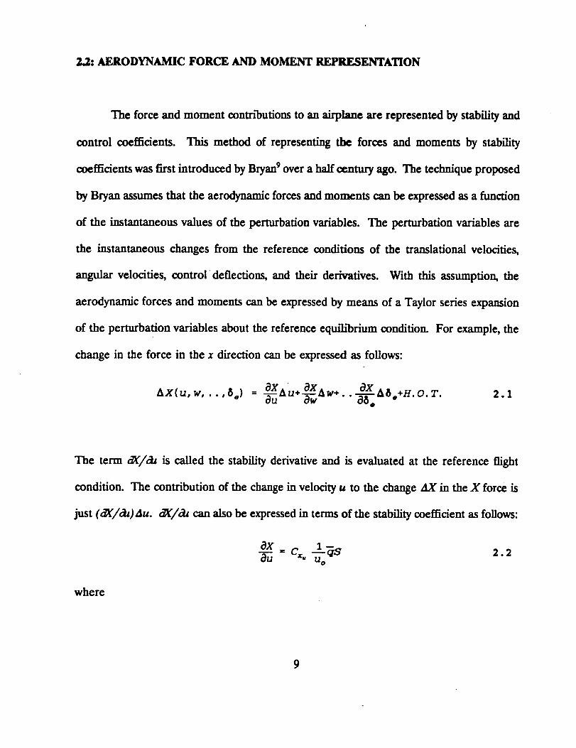
2..2: AERODYNAMIC FORCE AND MOMENT REPRESENTATION
The force and moment contributions to an airplane are represented by stability and
control coefficients. This method of representing the forces and moments by stability
coefficients was first introduced by Bryan 9 over a half century ago. The technique proposed
by Bryan assumes that the aerodynamic forces and moments can be expressed as a function
of the instantaneous values of the perturbation variables. The perturbation variables are
the instantaneous changes from the reference conditions of the translational velocities,
angular velocities, controldeflections, and their derivatives. With this assumption, the
aerodynamic forces and moments can be expressed by means of a Taylor series expansion
of the perturbation variables about the reference equilibrium condition. For example, the
change in the force in the x direction can be expressed as follows:
Ax{u,w, 8.) = aXAu+ aXAw+ ax•"" au aw . .-_-z-.ASo+H. O.T. 2. Ioo .
The term a_/_ is called the stability derivative and is evaluated at the reference flight
condition. The contribution of the change in velocity u to the change AX in the X force is
just (c_/(:t,)Au. c2_/& can also be expressed in terms of the stability coefficient as follows:
OX- c,, "I--F ws0
2.2
where
9
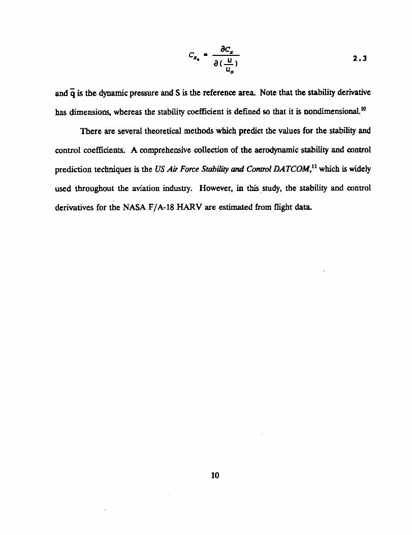
ac_Ox, = 2.3
a(u)U o
and q is the dynamic pressure and S is the reference area. Note that the stability derivative
has dimensions, whereas the stability coefficient is defined so that it is nondimensional, t°
There are several theoretical methods which predict the values for the stability and
control coefficients. A comprehensive collection of the aerodynamic stability and control
prediction techniques is the US Air Force Stability and Control DATCOM, n which is widely
used throughout the aviation industry. However, in this study, the stability and control
derivatives for the NASA F/A-18 HARV are estimated from flight data.
10

CHAPTER 3
PARAMETER ESTIMATION
3.1: PURPOSE
Estimation of aircraft stability and control derivatives has several practical uses such
as validating wind-tunnel or analytical predictions. A thorough basis of the veh/cle
aerodynamics is generated by these means such as the wind tunnel tests and analytical
predictions, but some error may be involved. For instance, the results from the wind-tunnel
tests are not expected to be truly accurate because it is practically imposs_le to simulate
the exact flight conditions and Reynolds number. Also, differences in the vehicle
configuration may be present. Therefore, it is beneficial to compare the results from both
the wind tunnel tests and flight data in order to validate the prediction methods of the
aircraft aerodynamics.
Another use of the derivative estimates is to update the current flight simulators.
The simulators require a complete database of the vehicle's stability and control
characteristics to appropriately represent the aircraft in flight.
3.2: TECHNIQUES
The number of parameter estimation computer programs has greatly increased since
the first application performed with high-speed digital computers in 1968. However, the
11
MMLE3 (Modified Maximum Likelihood Estimation, Version 3) TM developed at NASA
Ames Dryden has been accepted as an industry standard for aircraft parameter estimation.
MMI.E3 has two characteristics that somewhat limit its use in recent research:
1. It is designed for use solely in a batch processing environment.
2. The equations of motion defining the dynamic model used in the program
are linear.
These characteristics do not pose serious limitations for many parameter estimation
problems; however, recent flight test experience at NASA Dryden Flight Research Facility
has indicated that the MMLE3 program does not have the capabilities of handling the more
modern parameter estimation problems. For instance, the newly developed test aircraft are
being subjected to more extreme flight conditions where nonlinearities arise in the dynamic
behavior of the aircraft. Such behavior cannot be appropriately modeled using the simple
linear dynamic equations of motion. In addition, the new aircraft configurations are
becoming more unique. This increases the complexity of the problem, in that it requires the
analyst to interact more with the code. In response to these problems, another parameter
estimation program, pest, was designed by the researchers at NASA Dryden.
The pEst program is designed to be fully interactive; however, it can be run in a
batch mode, and it supports full nonlinear capability in the dynamic equations of motion. _
The form of the dynamic equations of motion for the aircraft system is assumed to be
known. The unknowns are the values of the coefficients in these equations. The output of
a parameter estimation process will therefore be an estimate of these unknown coefficients.
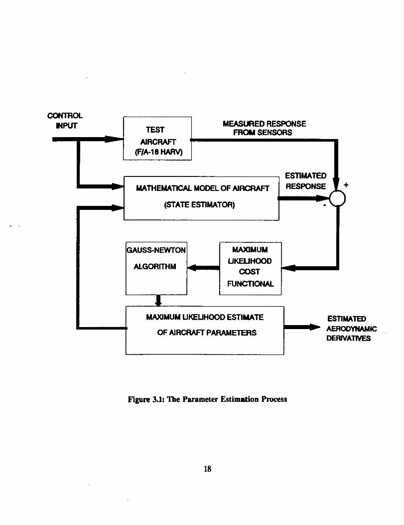
Particularly, the aircraft system is flown and the dynamic responses following a given
12
maneuverare recorded,alongwith the input maneuver. The sameinput maneuveris g/ven
to an "a priori" model of the system. In the caseof the Modified Maximum L/kelihood
Method, the l/kelihood cost function is maxim/zed through the application of a particular
method. This method is known as the Modified Newton-Raphson Method which provides
new estimates of the unknown coefficients on the basis of the response error which is the
difference between the actual and computed responses. The updated mathematical model
(with the updated values of the unknown coeffidents) is used to prov/de a new computed
response, and therefore a new response error. The updating of the mathematical model
continues iteratively until the response error satisties some user-defined convergence
criterion. Figure 3.1 illustrates the Maximum Likelihood Estimation Concept. More
analytical details are g/ven in the next section.
3.3: THE MAXIMUM LIKELIHOOD METHOD
forin:
The actual aircraft dynamic system can be described in the general state variable
,_,(t) = f, [x,(t), u(t), _] 3.i
z(t I) =g. [x4(t_), u(t,), _] + 11_ i=l,...n c 3.2
for given known initial conditions. The input vector, u, is assumed to be known as a
function of time. The response vector, z from the on-board sensors, is measured at discrete
time points, t_. The variable r_ is the measurement noise and is assumed to be a sequence
13
of independent Gaussian vectors with zero mean and known covariance matrix.
objective is to estimate the unknown parameters in the vector [.
Similarly, a mathematical model for the aircraft system is given by
k.(t) -f. [x.(t), u(t), [(t)] 3.3
"['he
y(Cz) -g= [xB(tz), u(ti), _(tl)] i=l,...nt 3.4
A
for given initial conditions and initial estimates of the unknown parameters _, that is [(0).
As previously stated, independent initial estimates _(0) of the unknown coefficients
are available from wind-tunnel analysis or theoretical methods. It is definitely desirable to
use this "a priori" information so that all available information is used to help the
convergence in the estimation process. When this feature is used, the Maximum Likelihood
Method is known as the Modified Maximum L/kelihood Method.
At this point, consider the following definitions:
P(z/_) is the probability of having the response, z, for given values of the unknown vector
_. P(_) is the probability that the unknown vector _ is a vector of "a priori" values of the
unknown coefficients _(0) (values of the aerodynamic and control stability derivatives from
wind tunnel and/or theoretical methods). Note that these two events are assumed to be
independent.
Now assume that the errors (measurement noise vector and "a priori" values error
vector) have a normal distribution. Therefore;
14
P(z/_)-
IIt
-J (_ (,c,-,)-,(,,))_(,<,_) -y(**)) ]1 oIQ e 3.5
-! [<_-E(o)) "_ (_-! (o>) ]2p(_) = i e
3 6-_ 1 _
2x 2 (._2)
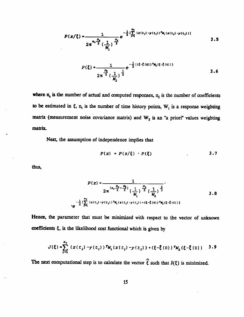
where n, is the number of actual and computed responses, ne is the number of coefficients
to be estimated in _, nt is the number of time history points, W, is a response weight_g
matrix (measurement noise covariance matrix) and W2 is an "a priori"values weighting
matrix.
Next, the assumption of independence implies that
P(z) = P(z/_) • P(_) , 3.7
thus,
.e
P(z) - I .nt 1
t,,, "--'+$] I _- _I ) ..-+2,, + + (_) (w+
_1 [_ (z (%) -y(c_) ) rw_(z(c,) -y(c,) ) +(4:-_(o)) _z_(_-_ (o)) )/--1
3.8
Hence, the parameter that must be minimiTed with respect to the vector of unknown
coefficients _, is the likelihood cost functional which is given by
rt_
J(_) =_-I (Z(tl) -Y(tl) )rW1(z(ti) -Y(tl))+({-_ (o))TW2({-[ (0)) . 3.9
*%
The next computational step is to calculate the vector _ such that J(_) is minimized.
15
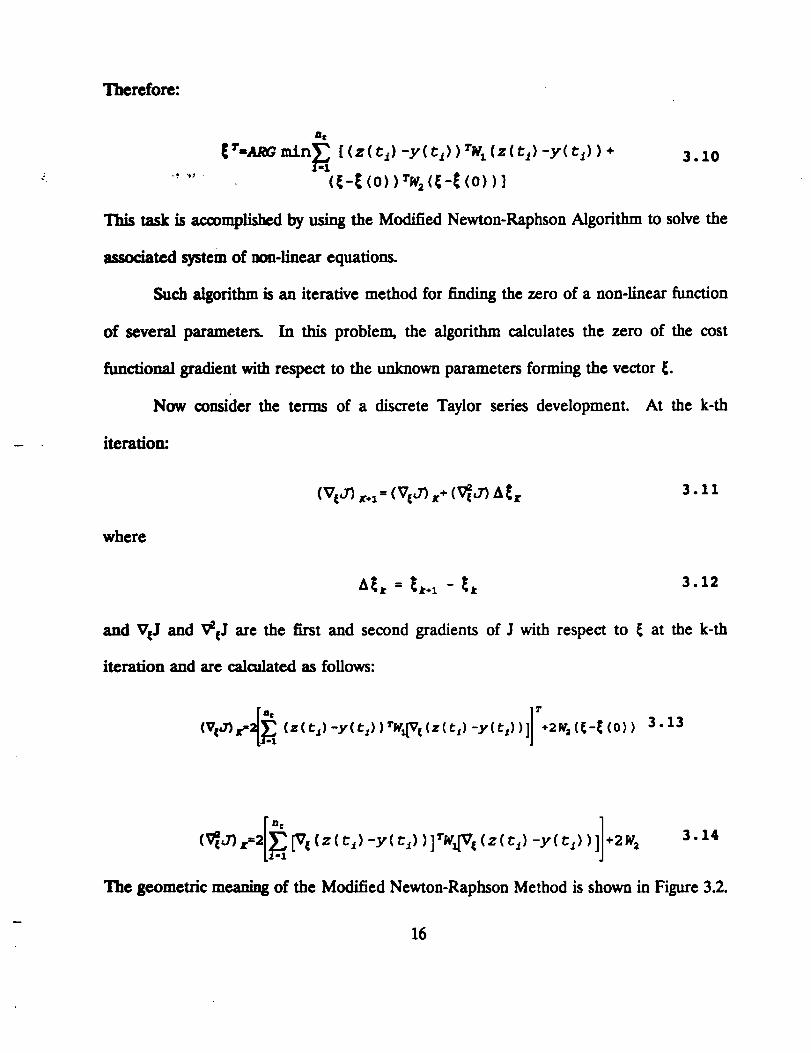
Therefore:
min__. [(z(t i)-y(t i))TWx (z(t i)-y(ci) )+ 3.10
This task is accomplished by using the Modified Newton-Raphson Algorithm to solve the
associated system of non-linear equations.
Such algorithm is an iterative method for finding the zero of a non-linear function
of several parameters. In this problem, the algorithm calculates the zero of the cost
functional gradient with respect to the unknown parameters forming the vector _.
Now consider the terms of a discrete Taylor series development. At the k-th
iteration:
where
3.11
/1_t : _t-1 - _t 3.12
and VeJ and V_eJ are the first and second gradients of J with respect to _ at the k-th
iteration and are calculated as follows:
(VgJ)if (E(tl)-y(tl))_'Wx[V{(z(tl)-y(tt))] +2w,((-_(o)) 3.13
(1_J)z=2 _7{(z(ti) -Y(ti) )]Tw_V((z(ti ) -Y(ti) )] +2W2 3.14
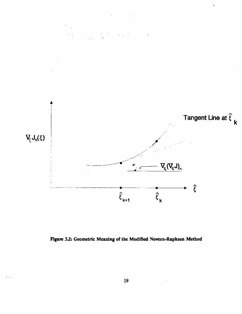
The geometric meaning of the Modified Newton-Raphson Method isshown inFigure3.2.
16
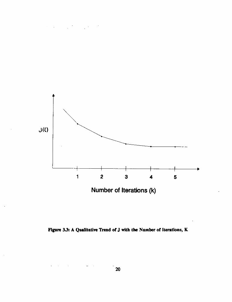
Note that the iterative process converges when _,c.s = { implying that A = 0. A
qualitative trend of J with the number of iterations 0c) is shown in Figure 3.3. Usually a
limited number of iterations (5-I0) are required to obtain convergence. More analytical
details on the Maximum Likelihood Method are given in References [i] and [12].
17
CONTROL
INPUT
v
v
v
TEST
NRCRAFT
(FIA-18 HARV)
MEASURED RESPONSEFROM SENSORS
MATHEMATICAL MODEL OF AI_
(STATE ESTIMATOR)
ESTIMATED
RESPONSE
GAUSS-NEWTON
ALGORITHM
1
MAXIMUM
UKEUHOOD
COST
FUNCTIONAL
MAXIMUM UKEUHOOD ESTIMATE
OF AIRCRAFT PARAMETERS
ESTIMATED
AEROOYNAMIC
DERIVATNIES
Figure 3.1: The Parameter Estimation Process
18
Tangent Une at
A
A
¢k+I (k
k
Figure 3.2: Geometric Meaning of the Modified Newton-Raphson Method
19
J(_)
I I I I I
1 2 3 4 5
Number of Iterations (k)
figure 3.3: A Qualitative Trend of J with the Number of Iterations, K
"- - 20
CHAPTER 4
_IRCRAZr EQUATIONS OF MOTION
This chapter consists of the derivation of the aircraft equations of motion which serve
as a basis for any aircraft stability and control analysis.
4.1: NEWTONIAN MECHANICS
The basic equations for linear and angular momentum in a nonrotating inertial axis system
fixed relative to the air will be the beginning of the derivation:
I_ - d (m_9 4.1dt
= _ (7i) 4.2dt
where ._ is the external applied force, V is the velocity vector, M is the external applied
moment, and h is the angular momentum vector. Both the external applied moment and
the angular momentum vector are about the center of gravity. Since most of the quantifies
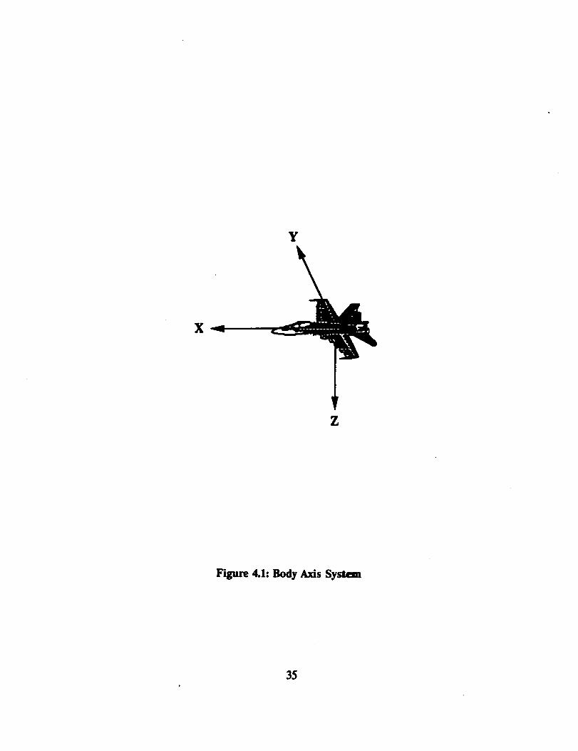
of interest are referenced to the aircraft geometric body axis, the above equations must be
transformed to this coordinate system which is fixed to and rotates with the aircraft. The
rotating aircraft body axis system is shown in Figure 4.1. The transformation of the above
equationsgive
21
- _(_) ÷Ex (]5) 4.4
where the angular momentum _) is given by:
-i. -zy, z, j
where _ is the angular velocity vector, and the a/a operator symbolizes the vector of partial
derivatives of the vector components. The components of the angular velocity (_) in the
body-axis system are roll rate (p), pitch rate (q), and yaw rate (r), and the components of
the velocity vector (V) are u, v, and w. Substituting the components of V, _, and h into
equation 4.3 and 4.4 gives scalar forms of the equations for the external applied forces and
moments (F_, Fy, F_, M_ M r and M,.)
Fx = m(_ + qw - rv) 4.6
Fy = m(_, + ru - pw) 4.7
F,,= m(_, + pv - qu) 4.8
+ (r 2 _ q2)Iy, -pqI n + rpIw4.9
My = -l_Ixy + ¢Iy - fI_ * rp(I x - I,)
÷ (p2 _ r2)In _ qIIxy + pqIy s4.10
22
H, = -_z** - _z_ + _z, + pq(z). - z,)+ (q2 _ p2).r.,- rpz r, + _z....
4.11
4.2: APPHI_.D FORCES
Now consider the sources of the external forces and moments beginning with the
three components of the applied forces: the aerodynamic, gravity, and thrust components./
The aerodynamic forces in terms of the nondimensional force coefficients (Cx, C¢, and Cz)
in the X, Y, and Z axes are
Fr._ ° = -_5C r 4.13
Fz..., ' = "_5C z 4.14
where _ is the dynamic pressure and S is the reference area.
Gravity is considered to exert a force mg along the earth Z axis. However, the
components given here are referenced to the body axis. Therefore, a transformation of axes
is necessary. This transformation is performed with the use of the Euler angles (8,_,_)
which will be discussed later in this chapter. The gravitational force components are as
fonows:
Fx_,. = -rag sinO 4.15
Fr,.."= mg sin_ cos0 4.16
23
_'_ Fs,.. =mg cos#cose 4.17 -_
The third force component is the engine thrust T which is assumed to only act alon 8
the body X axis:
Fx,,,_ = T 4.18
Thus, combining all components the total applied forces can be written as
F = Fj,ro + F_, v + F_,= 4.19
and
Fz = qSC z - mgsin8 + T 4.20
Fr = [;SCy + mgsin_ cos8 4.21
F, = _SC z ÷ mg cos4,cose 4.22
4.3: APPLIED MOMENTS
Only two components of the applied moment are examined, the aerodynamic and
gyroscopic moment. The aerodynamic components are
24

Mxu,_ = qSbCl 4 •23
Mr._° = _scc. 4.24
Mz,_o ffi "qSbC. 4.2 5
where b and c are the reference span and chord, and C1, Cm, C a are the nondimensional
coefficients of rolling moment, pitching moment, and yawing moment.
"l%e other component of the applied moment is the component caused by the
gyroscopic effects of the rotating machinery in the engine. Assuming that the engine is
oriented along the X axis, the gyroscopic effects contribute to moments along the Y and Z
axes:
MZ_o = rNIze 4.2 6
Mzm,,° = -qNI., 4 •27
where N is the engine speed in radians per second, and I= is the moment of inertia of the
rotating mass.
The total applied moment can be written as
and
M = Macro + M_r o 4.28
25
Nz. _rSbCI 4.29
Mr = _ScC m + rNix ° 4.30
M z : qSbC n - qNIzm 4.31
4.4: EULER ANGLES
In the equations for the external forces, it was noted that the forces are functions of
the ELder angles. Therefore, it is necessary to define the angles and present their respective
equations.
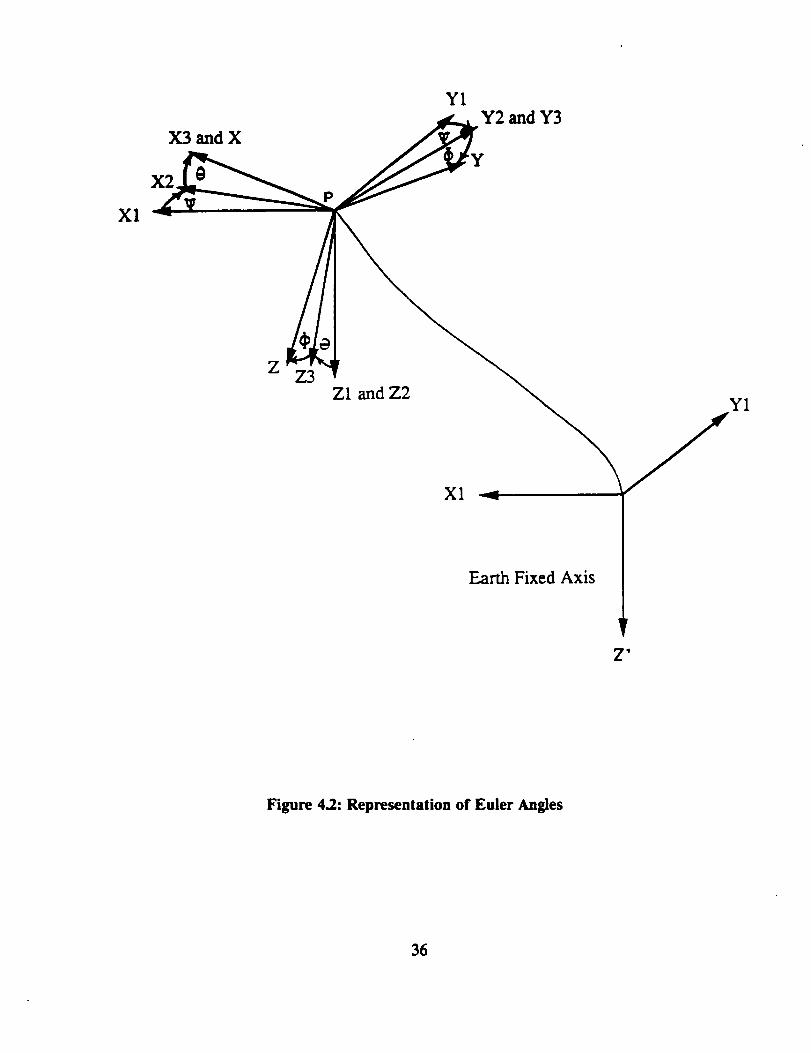
To describe the orientation of the airplane relative to the earth, it is necessary to
descn'be the orientation of the body-fixed coordinate system XYZ relative to the earth-fixed
coordinate system X'Y'Z'. To accomplish this, consider system X'Y'Z' translated parallel
to itself until its origin coincides with the center of mass P of the airplane. See Figure 4.2,
where this translated system X'Y'Z' has been renamed X,Y,Z_.
It is conventional to describe the relative orientation of XYZ to X,Y1Z1 by means
of three consecutive rotations. Emphasis is placed on "consecutive" because the order of
which these rotations are carried out is important because rotations cannot be considered
as vectors.
The followingrotations are applied:
1. Coordinate system X1Y,Z_ is rotated about the Z,-axis over an angle 11,,positive
26
asindicated in Figure 4.2. This yields coordinate systemX2Y.7_,2. The angle _ is referred
to as the heading (or yaw) angle.
2. Coordinate system X2Y2Z, 2 is rotated about the Y2-axis over an angle 0, positive
as indicated in Figure 4.2. This yields coordinate system X3Y3Z 3. The angle 0 is referred
to as the attitude (or pitch) angle.
3. Coordinate system X3Y3Z 3 is rotated about the X3-axis over an angle 0, positive
as indicated in Figure 4.2. This yields coordinate system XYZ. The angle 0 is referred to
as the bank (or roll) angle, u
With these transformation angles it is now possible to describe the way in which the
flight path of an airplane with respect to the earth-fixed system can be determined from the
knowledge of the body-fixed velocity components u, v, and w. These components are
f_nctions of the wind relative velocity, V, the angle of attack, a, and angle of sideslip,
which can be found from
v--Ju + ÷ 4.32
= tan -lw 4.33u
= sin -*v 4.34V
Substituting and inverting the above equations gives
27
u = Vcos_ cos_ 4.35
v = V sin_ 4.36
w = V sina cos_ 4.37
As a result, the expression for obtaining the flight path of an aircraft is
lw!l [! 0 0 ]IcosO 0-s_nSl[c!s . sin. !IIUwilv8 = cos_ sin_ 0 1 -s n_ cost vx 4.38
-sin_ cos_J sin8 0 cosSJ 0
This equation is found by means of orthogonal transformations and can be reversed
to give the earth-fixed components in terms of the body-fixed components by multiplying the
rotation matrices and taking the inverse.
It is now important to find a relationship between the time derivatives of the euler
angles and the rotational velocity components. Assuming a fiat, nonrotating earth, the total
angular velocity can be expressed as the sum of the time derivatives of the ELder angles
(t,0,O) components. Transforming all of the components into the body-axis coordinate
system with the use of equation 4.38 and equating the sum to the body-axis components of
the angular velocity gives
with the inverse being
cos_ sin_cos8
-sin_ cos_cos8
= p ÷ q tan8 sin_ + r tan% cos_
4.39
4.40
28

I
e - q cos# - r sin_ 4.41
= r cos$ sec% + q sinS secO 4.42
4.5: VELOCITY COMPONENTS (POLAR FORM)
Since it is pothole to measure flow angles that are closely related to angle of attack,
a and sideslip angle,/3, it is more convenient to have the velocity equations in terms of a,
_, and V rather than the spherical components u, v, and w. 1
In order to derive the a, /3, and V equations, equations 4.32-4.34 must first be
differentiated as follows:
= !(uO + vg+ w_)V
4.43
_, _ u_,- w_ 4.44/./2 + W 2
= (u 2 + w 2)_,- _- vu_ 4.45v2_(u 2 + w 2)
Substituting for &,_;, and _ from equations 4.6-4.8 and for u, v, and w from equations 4.35-
4.37 gives
29
I_ = F---ZCOSaCOS_ + F---rsin_ + F---Ssin_cos_m m m
4.46
1 (F,cos= - Fxsin_) + q - tan_ (pcos_ + rsin_)& = mVcos_
4.47
:_ = c°s_F + psin= - rcos= - _ (Fzsin= + Fzcos_)mV • mV
4.48
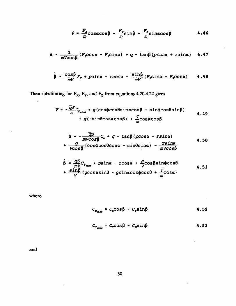
Then substituting for F x, F v, and Fz from equations 420-4.22 gives
D
= -_mmSC_ + g(cos_cosesinacos_ + sin_cosSsin_)
÷ g(-sin0cosacos_) + Tcosacos_m
4.49
÷
a = - _S tan_(pcosa rsina)mVcos_CL ÷ q - +
(cos_cosScos= + sinSsin_) Tsinavcos_ mvcos_
4.50
6 = _Cr,_ +psina - rcosa + _vCOS_sin_cos@
+ _ (gcos_sin8 -gsin_cos_cos8 + --Tcosa)V m
4.51
where
C_,_ -- Cocos _ - Crsin _ 4.52
Cn_._ = Cycos_ + C_sin_ 4.53
and
30
CL • -C, cos=+ C_ina 4.54
Cn = -Czcosa - Czsing
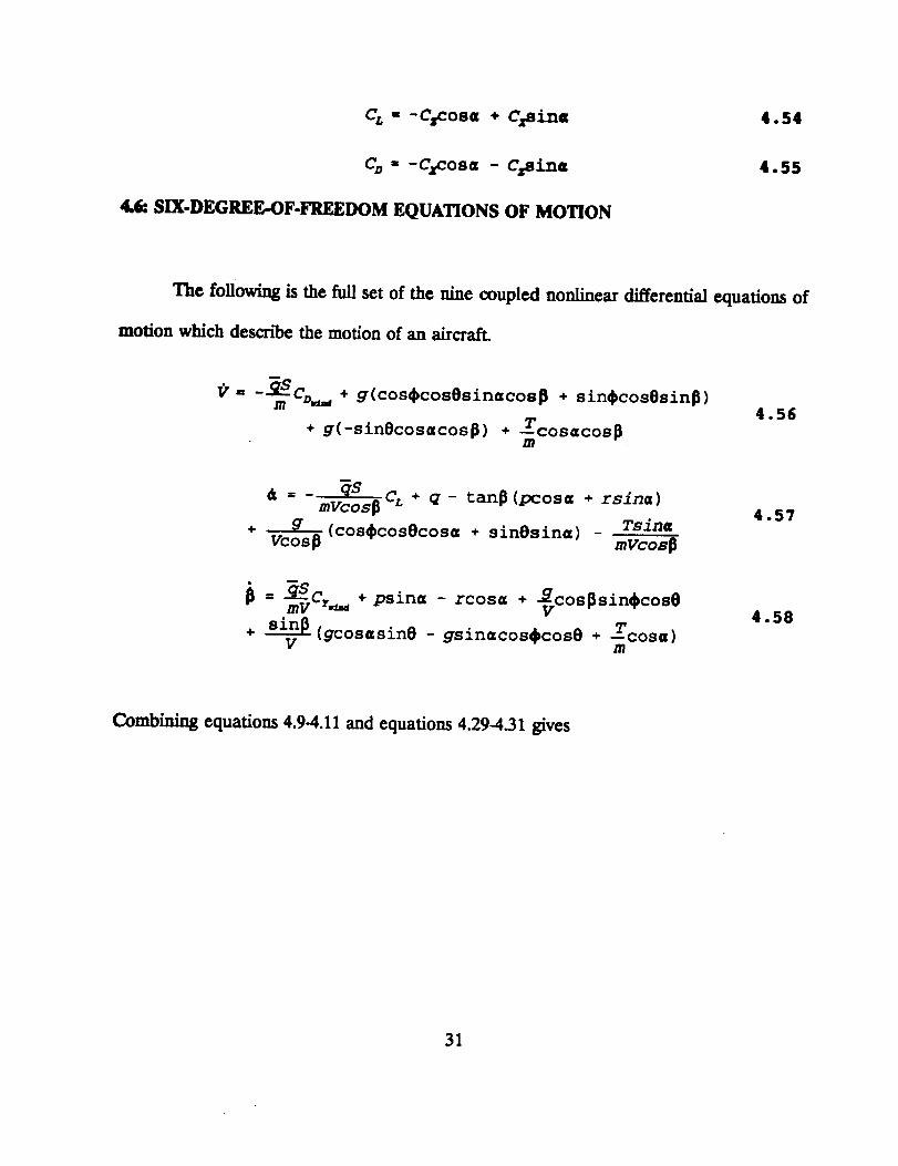
41_ SIX-DEGREF.,-OF-FREEDOM EQUATIONS OF MOTION
4.55
The following is the full set of the nine coupled nonLinear differential equations of
motion which descn'be the motion of an aircraft.
m
= --mmSC=_._ + g(cos_cosOsinacos_ + sin_cosSsin_)
+ g(-sin0cosacos_) + --Tcos_cos_m
4.56
÷
= _ ta r 13mvcosp cL + q - (pcos_
g (cos_cosScos= + sinSsina)vcos_
+ rsina)
Tsina
mVcos_
_Cr.._ + psin_ - rcos= + _cos_sin_cose
+ _ (gcos=sin8 - gsin=cos_cosO + --Tcos_)V m
4.57
4.58
Combining equations 4.9-4.11 and equations 4.29-4.31 gives
31
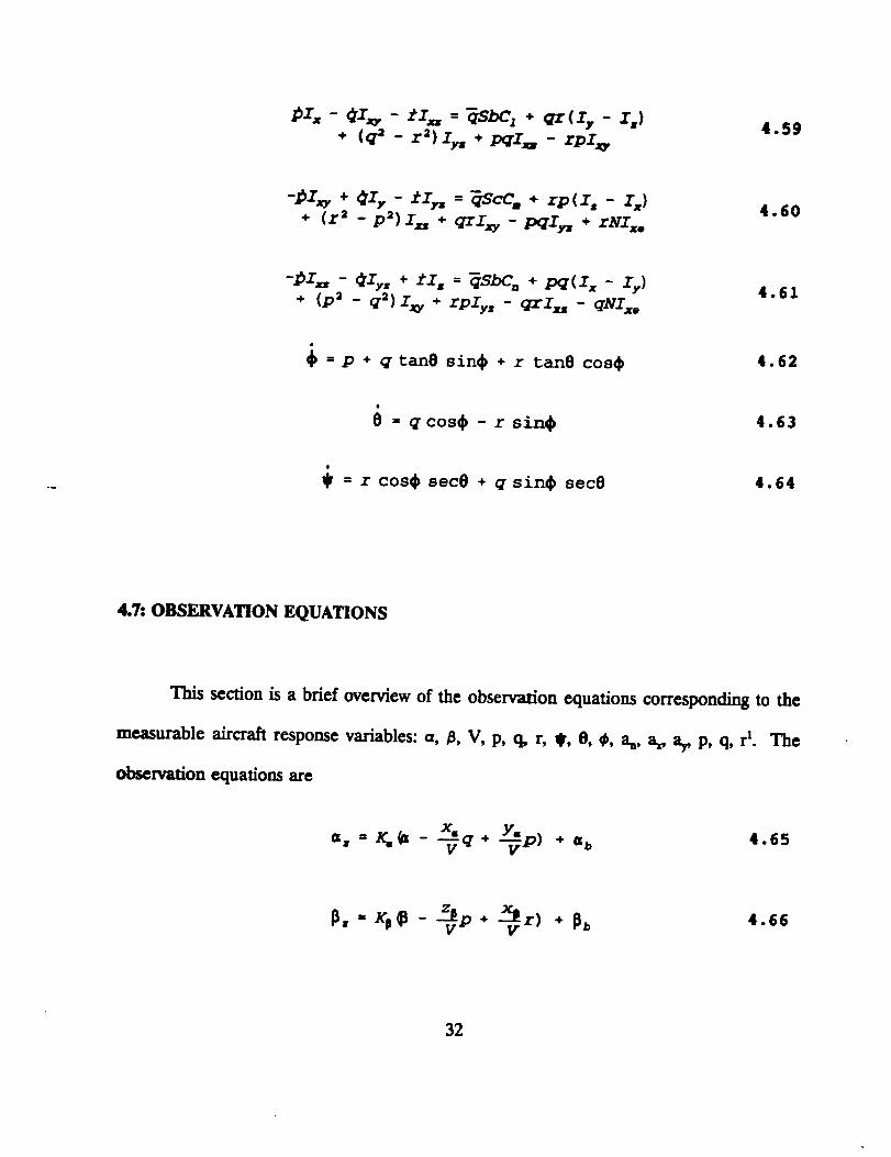
_z. - Cz_ - ±_= = _Sbq ÷ _(z, - z,)÷ _ - r_)z. ÷ pqs= - rp_
4.5g
-_z_ ÷ ely - ±z. --_scc. ÷ rp _z, - s._
+ (r 2 _ p2)iz * + qrIw -pqIy. + rNIxo4.60
÷ (p2 _ q2)sw ÷ rpsy,- _r__ - q_s..4.61
= p + q tan8 sins + r tan8 cos$ 4.62
= q cos_ - r sin_ 4.63
= r cos_ sec8 + q sin_ sec8 4.64
4.7: OBSERVATION EQUATIONS
This section is a brief overview of the observation equations corresponding to the
measurable aircraft response variables: a, _, V, p, q, r, ii,, O, _, a_, a= ar p, q, r_. The
observation equations are
-_q + p) + ab 4.65
_" = KP_--_vP +--_vr) + _b 4.66
32
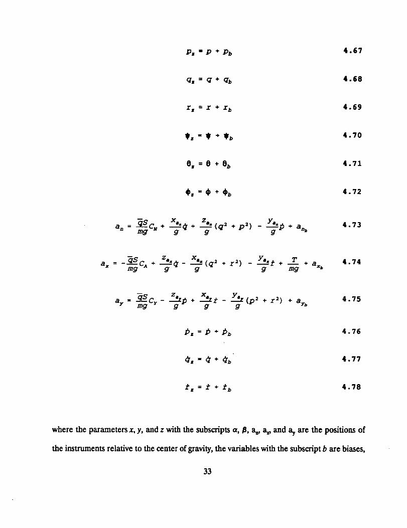
P, = P + Pb 4.67
q, = q+ qb 4.68
r, = r + r b 4.69
$, = _' + Sb 4.70
8, = 8 + 8b 4.71
#, = 4) +_ 4.72
ao : 9 c. ÷ + z,. y...mg _ (q2 + p2) _ ..._.p + a=b4.73
ax _ _S c,_ z,. xa,, (q2 r2) Ya,,t T= + -- __ + -- + -- ÷
mg -_ -- g g mg axb4.74
ay = qS c, - -_-Zl}+ .__Z_P- YJy (L)2 + r a)mg g g g + aYb
4.75
¢, = ¢+ Cb" 4.77
_z = f + /'b 4.78
where the parameters x, y, and z with the subscripts a, iS, a_, a_ and ay are the positions of
the instruments relative to the center of gravity, the variables with the subscript b are biases,
33

and K_ and I_ are upwash factors for the angle of attack and sideslip.
The above equations are for arbiumy instrument positions. It should be noted that
for a rigid aircraft, the sensed flow angles and linear accelerations vary with sensor positions,
but the sensed angular accelerations, rates, and attitudes do not vary with sensor positions.
34
Y
X
Z
Figure 4.1: Body Axis System
35
X1
X3 and X
X2
Y1Y2 and Y3
Y
ZZ3
Z1 and Z2
X1 ---"
Y1
Earth Fixed Axis
'I
Figure 4.2: Representation of Euler Angles
36
CHAPTER 5
HIGH ALPHA RESEARCH
5.1: PURPOSE OF THE NASA HIGH ALPHA TECHNOLOGY PROGRAM - (HATP)
The history of air combat has indicated the need of having fighter airplanes with safe,
predictable, and usable high-angle-of-attack capabilities. The demand for this increase in
agility has been due to the advancements in today's highly lethal point and shoot air-to-air
missiles. In a modern combat situation, the ability to rapidly obtain the first shot at the
enemy in an engagement may determine the difference between a kill or a failure.
It has been shown through training and combat experience that a fighter's safety and
maneuverability are related to its high angle-of-attack characteristics (also known as stall).
Pilots who seek to have maximum turning performance and agility wiLl push the aircraft to
its maximum controllable angles of attack in order to obtain more lift, make tighter turns,
or point at their enemy in the shortest amount of time. Airplanes that have good stability
and control characteristics in this separated flow regime will typically outperform those with
deficiencies. _ Thus, the need for an improvement of the performances for a modern
military aircraft motivated a research effort in the high alpha technology area.
In the past, high alpha capability was not a design goal: high alpha conditions were
regarded as being extremely hazardous and to be avoided. However, as the United States
advanced fighter aircraft such as the F-14 and F-15 evolved, their stall characteristics
improved. The high alpha design methods were poor, but the experimental prediction
37
methods suchaswind tunnel tests performed during the airplane development provided a
sufficient database of the staU/spin characteristics.
On the other hand, more recent fighters such as the F-16 and F-18 were designed to
accommodate the goal of achieving high-sustained performance and good stall
characteristics. The new designs were based on aerodynamic principles that included vortex
lift and automatically scheduled wing flaps. Unforumately, prediction methods of the
aircraft aerodynamics at high alpha for these aircraft were not as valid as those for the
previous aircraft. In fact, many discrepancies evolved in the region of maximum lift and
beyond (35 - 60 degrees alpha). 16,17These problems have been thoroughly investigated, but
not quite understood. Therefore, it was obvious that further research was needed to
produce a better understanding of the experimental methods for high alpha aerodynamics.
NASA's first major effort in high alpha technology started in the mid 1970's. It was
a joint effort with the Navy to develop and validate in flight a high alpha control system for
the F-14. The outcome of the program was a set of control laws that significantly improved
the high alpha maneuverability and spin resistance of the F-14. TM The success of this
program and the shortcomings of the available prediction methods and technology of today's
fighter aircraft prompted NASA to formulate the High Alpha Technology Program (HATP).
The HATP began in the mid 1980's with objectives to provide flight-validated
prediction/analysis methodology including experimental and computational methods that
accurately simulate high-angle-of-attack aerodynamics, flight dynamics, and flying qualities,
and to improve agility at high angles of attack and expand the usable high alpha envelope. _
Currently, many programs are dedicated to high alpha research. For instance, the
38

DARPA Enhanced Fighter Maneuverability Program is using two X-31 aircraft to
demonstrate the tactical utility of post stall maneuverability with pilots in the loop. Also,
the USAF/NASA/DARPA X-29 Program has shown impressive controllability in the stall
regime with its forward swept wing and canard configuration. In addition, the USAF F-15
STOL (Short Takeoff and landing) and Maneuver Technology Demonstrator (S/MTD) is
currently using a thrust-vectoring/reversal nozzle highly integrated with the flight control
system to show performance gains in takeoff and landing from short runways. Another
essential element in the HATP is the High Alpha Research Vehicle (HARV) which is the
testbed aircraft for this investigation.
5.2: HIGH ALPHA RESEARCH VEHICLE (HARV) DESCRIF_ON
The F-18 HARV (Figure 5.1) is a full-scale developmem two engine, single seat,
fighter/attack airplane built for the U.S. Navy by the McDonnell Douglas Corp. It is
powered by two modified General Electric F404-GE-400 afterburning turbofan engines each
rated at approximately 16000 lbs. static sea level thrust. The HARV features a midwing
configuration with a wing-root leading edge extension. It is highly instrumemed for research
purposes; the wingtip launching rails and missiles were replaced with specially designed
camera pods and airdata sensors. In addition, a pilot-actuated spin chute is onboard in case
an uncontrolled spin is entered.
surfaces. These include the
trailing-edge flaps.
It is equipped with five pairs of aerodynamic control
ailerons, rudders, stabilators, leading-edge flaps, and
The twin vertical stabilizers with trailing edge rudders are canted
39
outboard at approximately 20 ° from the vertical. All _fac_ except the rudders are capable
of moving symmetrically and differentially. A summary of the physical characteristics of the
HARV is shown in Table 5.1.
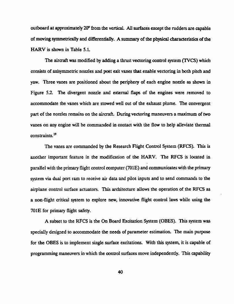
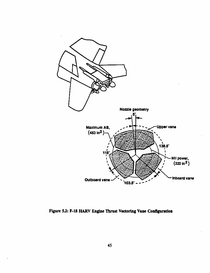
The aircraft was modified by adding a thrust vectoring control system (TVCS) which
consists of axisymmetric nozzles and post exit vanes that enable vectoring in both pitch and
yaw. Three vanes are positioned about the periphery of each engine nozzle as shown in
Figure 5.2. The divergent nozzle and external flaps of the engines were removed to
accommodate the vanes which are stowed well out of the exhaust plume. The convergent
part of the nozzles remains on the aircraft. During vectoring maneuvers a maximum of two
vanes on any engine will be commanded in contact with the flow to help alleviate thermal
constraints. 19
The vanes are commanded by the Research Flight Control System (RFCS). This is
another important feature in the modification of the HARV. The RFCS is located in
parallel with the primary flight control computer (701E) and commtmicates with the primary
system via dual port ram to receive air data and pilot inputs and to send commands to the
airplane control surface actuators. This architecture allows the operation of the RFCS as
a non-flight critical system to explore new, innovative flight control laws while using the
701E for primary flight safety.
A subset to the RFCS is the On Board Excitation System (OBES). This system was
specially designed to accommodate the needs of parameter estimation. The main purpose
for the OBES is to implement single surface excitations. With this system, it is capable of
programming maneuvers in which the control surfaces move independently. This capability
40
is of extreme importance to this investigation and is believed to improve the parameter
estimation at higher angles of attack.
5.3: INSTRUMENTATION AND AIRDATA SYSTEMS
Standard aircraft are equipped with instruments that measure control surface
positions, linear acceleratiom, angular rates etc. as well as certain airdata parameters such
as angle of attack, angle of sideslip, pressures etc. However, the F-18 aircraft production
airdata system was not designed to perform well at high angles of attack. Therefore, new
sensors and analysis techniques had to be implemented to the HARV's insta-umentation and
airdata systems in order to obtain the necessary accuracy in the measurements at high angle
of attack flight.
As stated previously, the wingtip missile rails were removed and replaced with special
camera pods also used to mount wingtip airdata booms. These booms served as the base
for the NACA angle of attack and angle of sideslip flow direction vanes and the specially
designed swivel probe that is capable of self-aligning itself with the local flow. The presence
of the booms and the aircraft corrupt the static pressure measurements consequently
affecting Mach number. This is commonly referred to as static pressure position error and
must be determined for all flight conditions. In addition, a correction is also needed for the
measurements of angle of attack and angle of sideslip. This is required to take into account
the upwash induced by the aircraft. The procedure for these corrections are complex and
are thoroughly explained in Reference [20].
41

Other researchmeasurementsobtained on the HARV included: three-axis angular
velocities from a body-axis rate gyro package, pitch, roll, and yaw attitudes from a gimbaUed
attitude gyro, and linear accelerations from a set of body-axis accelerometers. The accuracy
of these sensors was established from the flight data noise band. Root mean square noise
was 0.025 g for the linear accelerometers, 0.2 deg/sec for the three rate gyros, and 0.25
degrees for the three attitudes.
All data were digitally encoded on board the aircraft using pulse code modulation
and telemetered to the ground while being displayed in real time and recorded for postflight
analysis. The angular rates, attitudes, and accelerations were recorded at 200 samples/sec,
and the pressures were recorded at 50 samples/sec. 2°
42
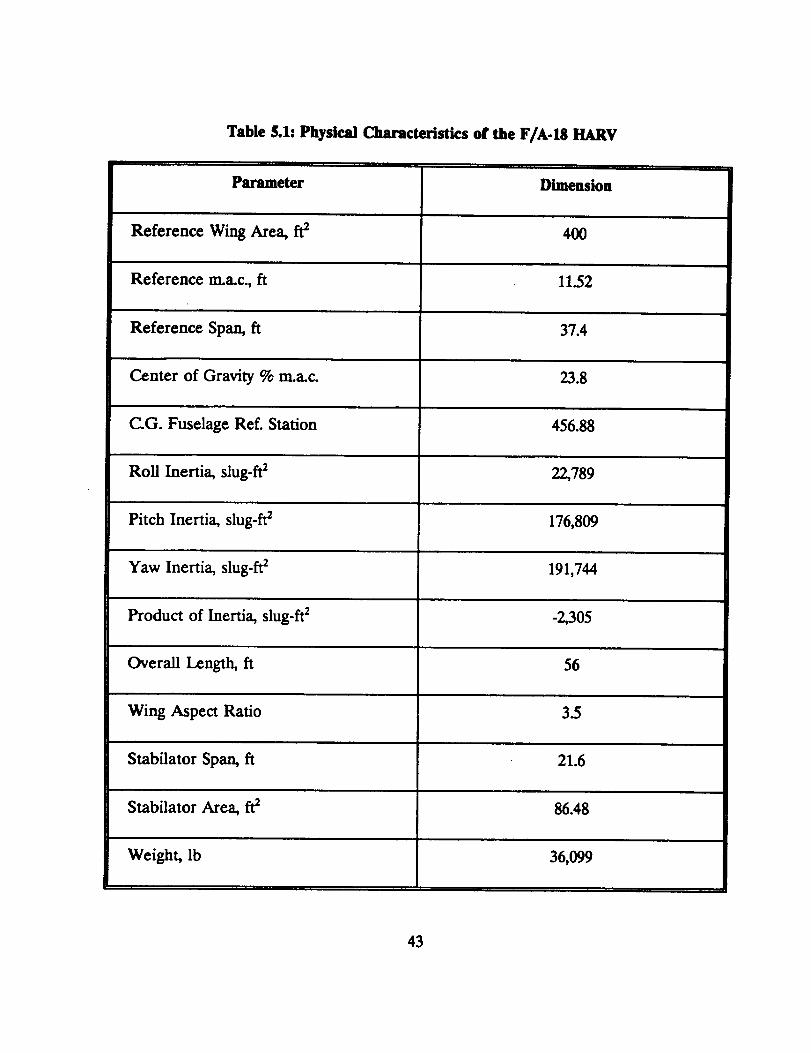
Table $.1: Physical Characteristics of the F/A-18 HARV
Parameter
Reference Wing Area, ft2
Reference m_a.c., ft
Reference Span, ft
Center of Gravity % m.a.c.
C.G. Fuselage Ref. Station
Roll Inertia, slug-_
Pitch Inertia, slug-ffl
Yaw Inertia, slug-ft 2
Product of Inertia, slug-ft 2
Overall Length, ft
Wing Aspect Ratio
Stabilator Span, ft
Stabilator Area, fta
Weight, lb
Dimension
4OO
11.52
37.4
23.8
456.88
22,789
176,809
191,744
-2,305
56
3.5
21.6
86.48
36,099
43

Figure 5.1: _view DTawing of the F-18 HARV
44
• geometry
Maximum AB, ,. ,._.,f Upper vane
',____-.,, _ow..
_ _ . _.__ _.=r" _--Inboam vaneL],L'tDOam vane -_ ,,. ., ,,
103.5" - - --
Figure 5.2:F-18 HARV Engine Thrust Vectoring Vane ConiiguraUon
45

_6
FLIGHT TEST MANEUVERS
6.1: DESIGN CONSIDERATIONS
The flight test maneuvers are a key factor in the parameter estimation process. The
quality of the estimates is directly related to the quality of the maneuvers; therefore, special
consideration must be taken in the design of the inputs that make up the flight test
maneuvers. The maneuver design is dependent on the aircraft dynamic characteristics and
available control surfaces. In the past, most aircraft were limited to three or four control
surfaces, but modern aircraft, especially those that fall into the fighter category, are
sometimes equipped with eight or more control surfaces. In these cases, it is first necessary
to determine which control surface deflection would induce the most desirable response.
It is also important to account for the constraints that may affect the design, such as limits
on the control surface position and actuator rates.
To estimate the derivatives, it is necessary to have independent inputs on every
control surface used in the maneuver. This is very important because if two surfaces are
directly proportional to each other it is practically imposs_le to determine their individual
effectiveness. For example, some airplanes have the aileron and rudder interconnected.
If the pilot of an airplane with this setup commands the airplane to roll by moving the stick
laterally, the rudder and aileron both move simultaneously. The data from this maneuver
would not be useful in the parameter estimation problem because the rudder deflection
46

actually destroys the aileron effectiveness information. Even though both surfaces move,
neither the rudder nor the aileron derivatives could be determined because the motions are
dependent. It would be possible however to estimate a combined effectiveness of both
surfaces, but the amount that each surface contributes to the effect would be unknown.
The main goal in the design of the inputs for the flight test maneuvers is to properly
excite the modes of the aircraft that are of interest. The selection of the control surfaces
and the shape of the inputs are two important issues to be considered. A control surface
that not only generates a good response but also makes the system mode controllable is
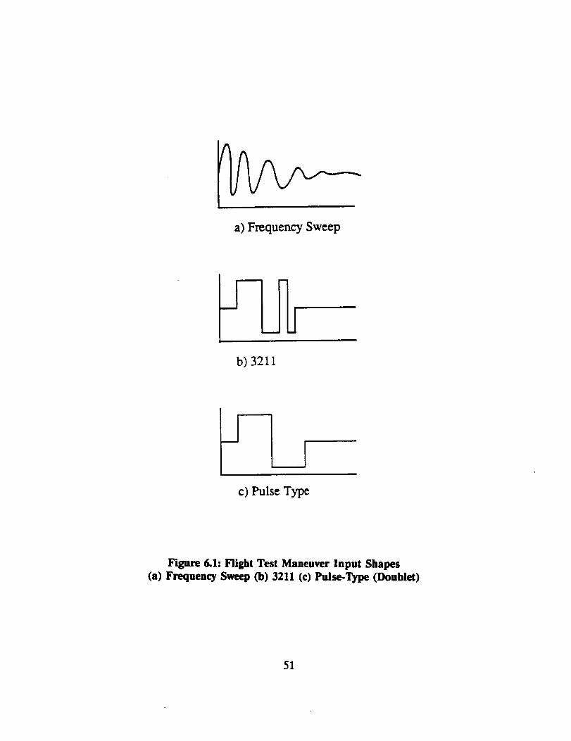
desired. The shape of the input is based on the fact that the system modes are best excited
by frequencies near the system natural frequencies. This implies that the inputs should be
in shapes that cover the range of the system natural frequencies. A good example of this
type of input signal shape is a frequency sweep. Other signal shapes such as the 3211 input
of Koehler and Wilhelm 2' are also based on the frequency concepts. The 3211 input is a
series of four steps that alternate in sign. The first step is three time units long, the second
is two, and the last two are each one time unit long. The length of the time unit is varied
accordingly in order to center the frequency band of the input around the system natural
frequencies.' Another type of input shape is that of the pulse-type. This type of input
is simple, more easily performed by the pilot, and widely used in recent PID work. As for
the size of the pulse and the selection of singlets or doublets, it is necessary to consider the
constraints of the control surface positions and actuator rates. Figure 6.1 shows various
input shapes.
The design of the maneuvers for the longitudinal cases is based usually on the
47
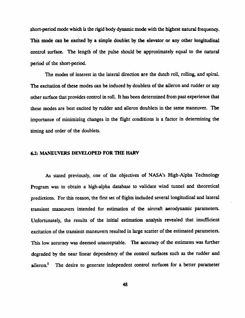
short-period mode which is the rigid body dynamic mode with the highest natural frequency.
This mode can be excited by a simple doublet by the elevator or any other longitudinal
control surface. The length of the pulse should be approximately equal to the natural
period of the short-period.
The modes of interest in the lateral direction are the dutch roll, rolling, and spiral.
The excitation of these modes can be induced by doublets of the aileron and rudder or any
other surface that provides control in rolL It has been determined from past experience that
these modes are best excited by rudder and aileron doublets in the same maneuver. The
importance of minimizing changes in the flight conditions is a factor in determining the
timing and order of the doublets.
6.2: MANEUVERS DEVELOPED FOR THE HARV
As stated previously, one of the objectives of NASA's High-Alpha Technology
Program was to obtain a high-alpha database to validate wind tunnel and theoretical
predictions. For this reason, the first set of flights included several longitudinal and lateral
transient maneuvers intended for estimation of the aircraft aerodynamic parameters.
Unfortunately, the results of the initial estimation analysis revealed that insufficient
excitation of the transient maneuvers resulted in large scatter of the estimated parameters.
This low accuracy was deemed unacceptable. The accuracy of the estimates was further
degraded by the near linear dependency of the control surfaces such as the rudder and
aileron s The desire to generate independent conuol surfaces for a better parameter
48

estimation process was the basis for the design of an additional control system for the
HARV. This system has been named OBES (On Board Excitation System) and is
essentially a single surface excitation system. It has the capability of exciting the control
surfaces one at a time, thus alleviating the problem of dependency. OBES was implemented
after the thrust vectoring control system and Research Flight Control System were installed,
and it was very successful in reducing the correlation of the control surface deflections. The
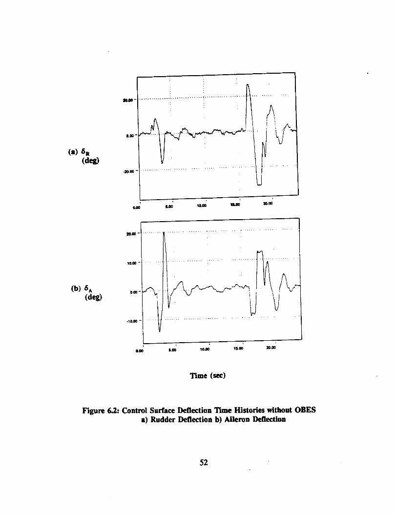
improvements that OBES introduced are shown in Figures 6.2- 6.5. Figure 6.2a and 6.2b
show time histories of aileron and rudder deflections without the OBES activated, and it is
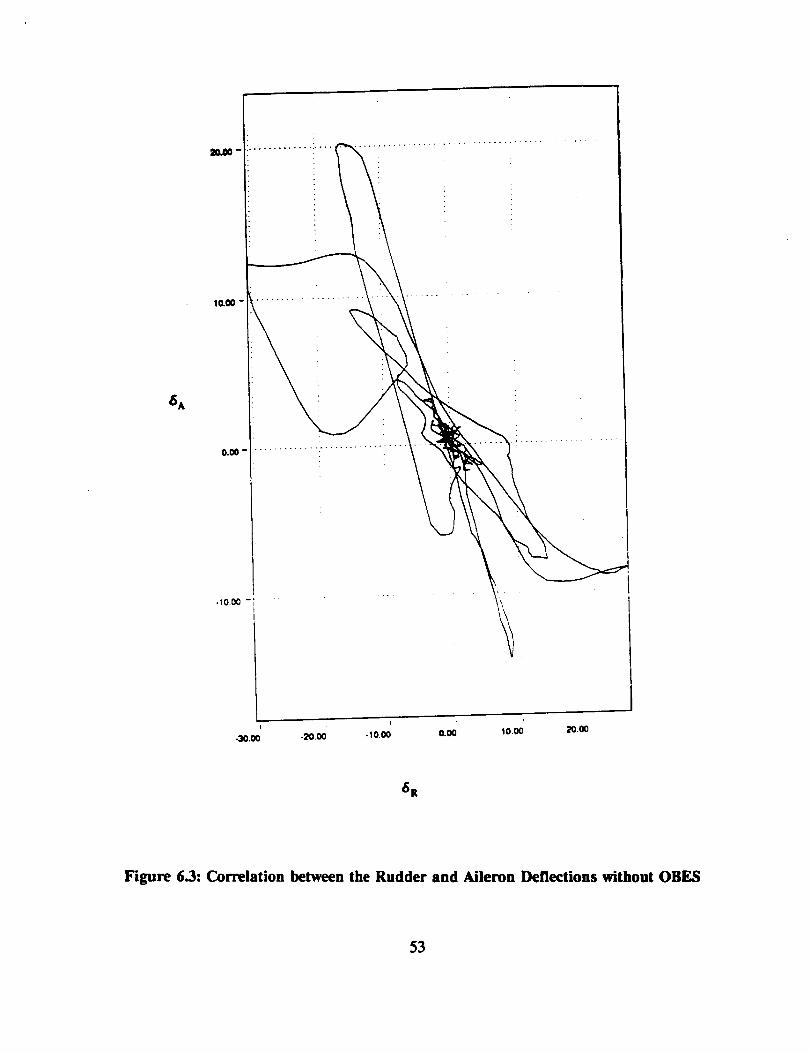
obvious that the two surfaces are correlated. This is also shown in Figure 6.3 where the two
deflections are plotted against each other and clearly indicate a somewhat linear
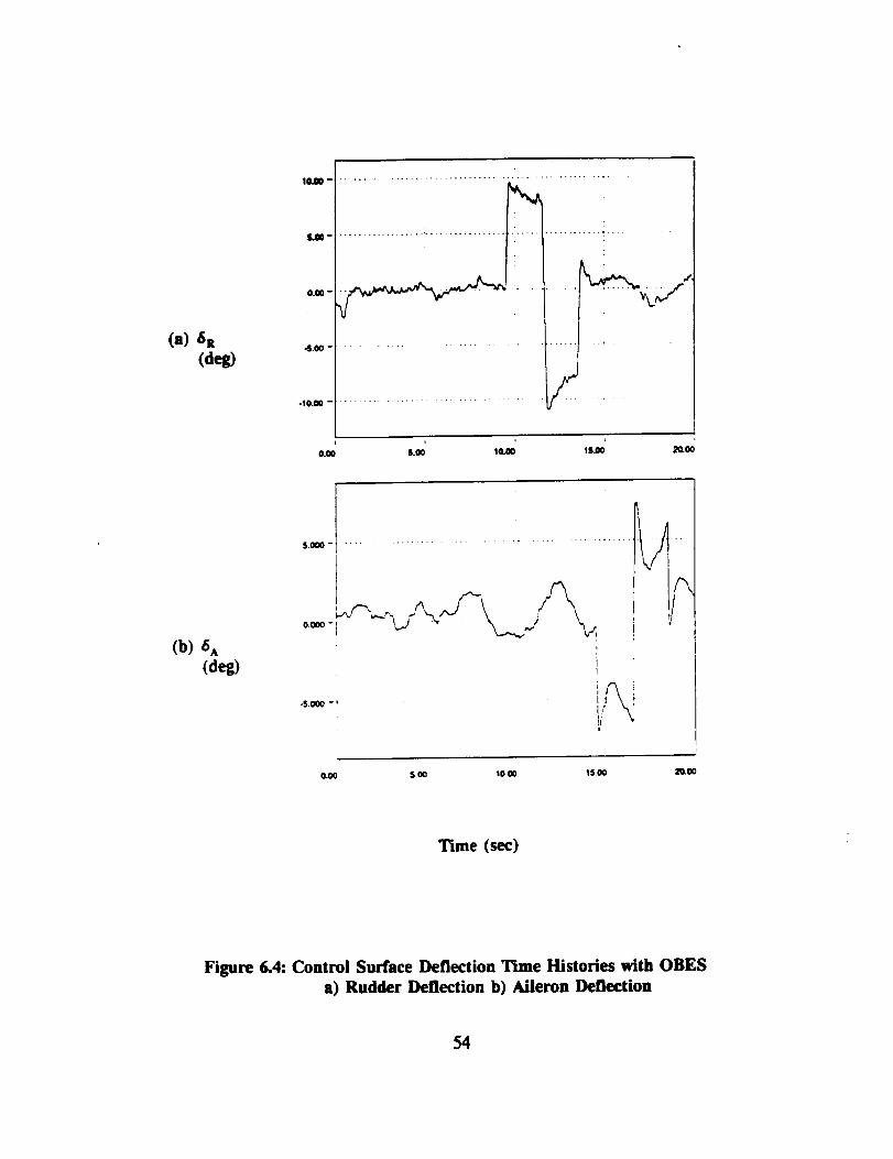
relationship. However, with the OBES activated, it can be seen in Figures 6.4a and 6.4b
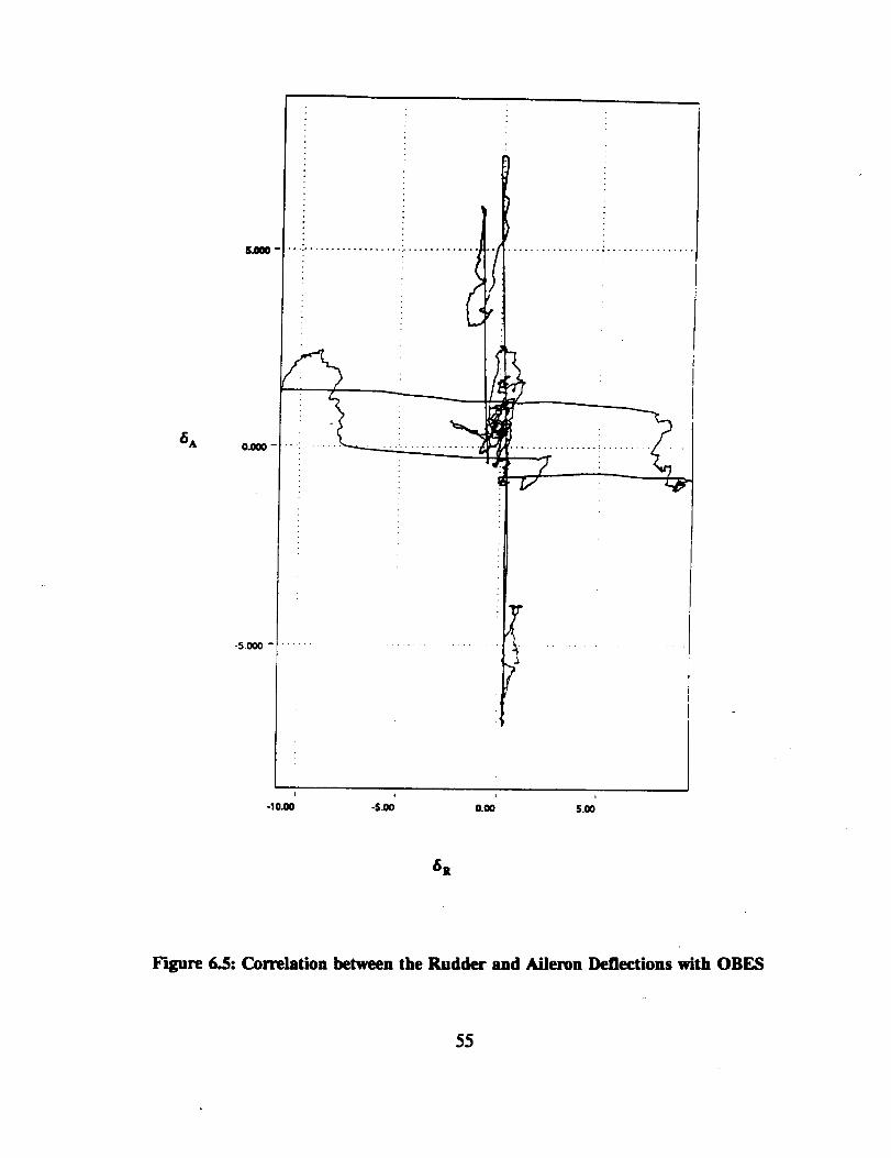
that the simultaneous movements of the surfaces is adequately reduced. The main effect
of the OBES activation can be seen in Figure 6.5 which shows the ailerons and the rudder
deflections plotted against each other, revealing a much lower correlation.
The size and shape of the inputs programmed into the OBES system software were
developed by a trial and error approach in the fixed base simulator at NASA Dryden Flight
Research Facility. Different combinations of control surface doublets were tested until the
best response was generated. The amplitudes of the doublets were also varied to determine
the optimal excitation of the aircraft modes. After several trials, the best maneuvers for
each direction were as follows:
49
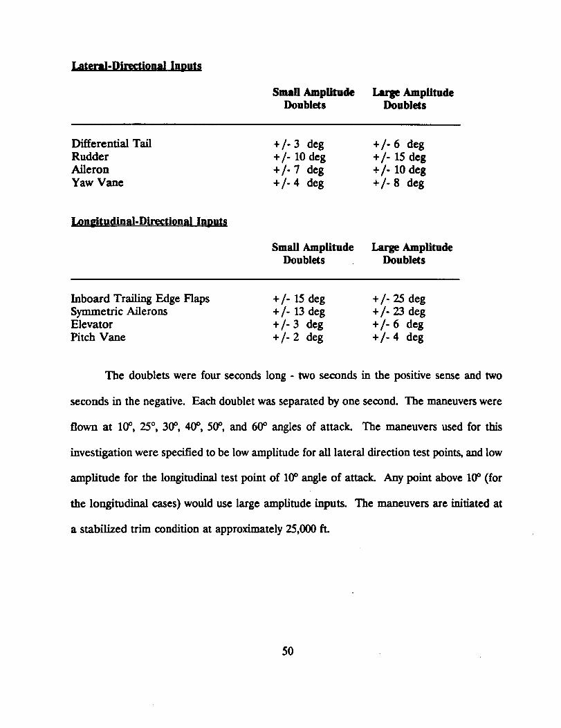
Lateral-Directional Inouts
Small AmplitudeDoublets
Large AmplitudeDoublets
Differential TailRudderAileronYaw Vane
+/-3 deg+I- 10 deg
+I- 7 deg
+I- 4 deg
+I- 6 deg+/- 15 deg
+/- lOdeg
+/- 8 deg
Lon_tudinal-Directional Inputs
Small AmplitudeDoublets
Large AmplitudeDoublets
Inboard Tra/ling Edge FlapsSymmetric AileronsElevatorPitch Vane
+ I- 15 deg + I- 25 deg+ I- 13 deg + I- 23 deg
+ I- 3 deg + I- 6 deg
+/-2 deg +/-4 deg
The doublets were four seconds long - two seconds in the positive sense and twO
seconds in the negative. Each doublet was separated by one second. The maneuvers were
flown at 10° , 25 °, 30°, 40 °, 50 °, and 60 ° angles of attack. The maneuvers used for this
investigation were specified to be low amplitude for all lateral direction test points, and low
amplitude for the longitudinal test point of 10° angle of attack. Any point above 10° (for
the longitudinal cases) would use large amplitude inputs. The maneuvers are in/dated at
a stabilized trim condition at approximately 25,000 ft.
5O
a) Frequency Sweep
b) 3211
c) Pulse Type
Figure 6.1: Flight Test Maneuver Input Shapes
(a) Frequency Sweep Co) 3211 (c) Pulse-Type (Doublet)
51
(a) 6_
(del0
0,00 "
.20.00 -
0_0
• "''!
i....t
i
S.O0 1000 lS.O0 _0.00
(b) 6 A
(deg)
20.00"
10.00 -
0.00-
-lO.O0 -
0.00 S.W lOJ)O IS.O0 20.W
Time (see)
Figure 6.2: Control Surface Deflection Time Histories without OBESa) Rudder Deflection b) Aileron Deflection
52
6 A
0.00 ..................
-30.00 -20.00-10.00 0.00 10.00 20.00
6 R
Figure 6.3: Correlation between the Rudder and Aileron Deflections without OBES
53
(a) 6x(deg)
(b) 6 A
(deg)
|0J J0 .....................................................
v_
..$OO
I • t.+..........................................t it.
++-_,,-'u]\_ _,J _tiI
+ _Q._ r
os._ -! ! ;
O.OG S.OQ 1000 1S.00 20.00
Time (sec)
Figure 6.4: Control Surface Deflection Time Histories with OBESa) Rudder Deflection b) Aileron Deflection
54
6 A
U_0-
..-. .................. ........................... i ................
-SO00 -
7
-10.00
I
-S._ 0._ S._
6 R
Figure 6..5: Correlation between the Rudder and Aileron Deflections with OBES
55
CHAPTER 7
HARV AERODYNAMIC MODEL
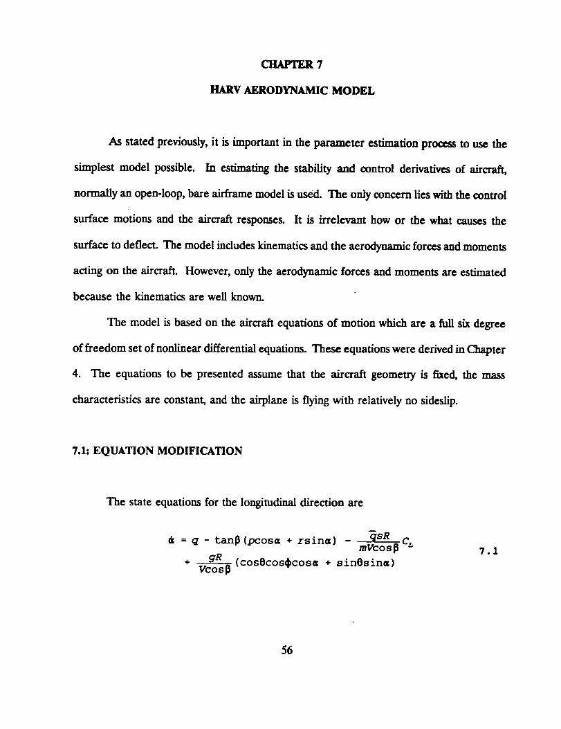
As stated previously, it is important in the parameter estimation process to use the
simplest model possible. In estimating the stability and control derivatives of aircraft,
normally an open-loop, bare air_ame model is used. The only concern lies with the control
surface motions and the aircraft responses. It is irrelevant how or the what causes the
surface to deflect. The model includes kinematics and the aerodynamic forces and moments
acting on the aircraft. However, only the aerodynamic forces and moments are estimated
because the kinematics are well known.
The model is based on the aircraft equations of motion which are a full six degree
of freedom set of nonlinear differential equations. These equations were derived in Chapter
4. The equations to be presented assume that the aircraft geometry is fixed, the mass
characteristics axe constant, and the airplane is flying with relatively no sideslip.
7.1: EQUATION MODIFICATION
The state equations for the longitudinal direction are
= q - tan_ (pcosa ÷ zsin_) - qsamvcos q
+ gR (COSSCOS_COS_ + sinSsin_)Vcos_
7.1
56
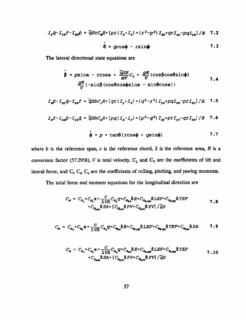
lyC-zy/-z_ = _scc,x+[pr(x,-r,)+(r2-p")x=+qrz.-pqx,]/a 7.2
= _os, - _sin@ _.
The lateral directional state e,quadons are
= psin= - zoos= + _C + gR (cos_cosOsin_)mV _ V 7.4
gR (-sin_ (cosScos_sin_ - sinecos_) )V
I_6-IxT¢-Ixrt = qSbCia+ [qr (Iy-I,) + (q2-r2) Iy,+pqXx,-prIxT] /R 7.5
I/-IxzI5-Iy,¢ = qSbC=R+ [pq(Ix-Iy) + (pa_q2) i +prIy _qrIx.] /R 7.6
= p + tanO(rcos_ + qsin_) 7.7
where b is the reference span, c is the reference chord, S is the reference area, R is a
conversion factor (57.2958), V is total velocity, CL and Cy are the coefficients of lift and
lateral force, and C, Cm C, are the coefficients of rolling, pitching, and yawing moments.
The total force and moment equations for the longitudinal direction are
+_ C.q+C_SE+C_nEF÷C.._ TEFc. = C_o+C.a 2vR 7.8
7.9
7.10
57
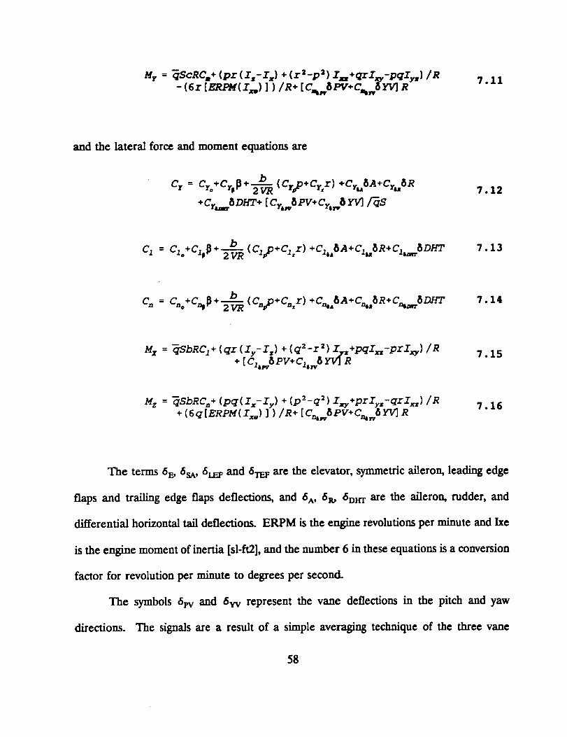
Mr = _ScaC.+ (pr (X,-I_)+(x'-p2)Z=+_X_-_Zy,) Ix-(6r [m_w(x_.) ])Ix+ [c_.8Pv+c_,) YV]a
7.11
and the lateral force and moment equations are
C +_ _+ bc,= ,oLr,p _ (c,2+c,,r)+c,sz+cr..sa
+ b (c_2+c_r)+c_bA+C_a+C,. 8DHTC_= C_o+C_,p2---_
7.12
7.13
7.14
M x = qSbRCz+ (qr (Iy-I,) + (q2-r2 - /R)z_.+;qz=;r1_.) 7.15+ [c1,_ PV+C1._ YvI R
Mz = -qSbRC.+ (pq(Ix-Iy) + (pZ_q2) i.y+prIyz_qrix,)/R 7.16
+ (6q[ERPM(Ix,) ] )/R+ [C%,v6PV+C_6YVI R
The terms 6 E, 6sA, 6L_ and 6T_ are the elevator, symmetric aileron, leading edge
flaps and trailing edge flaps deflections, and 6^, 6_ 6DHT are the aileron, rudder, and
differential horizontal tail deflections. ERPM is the engine revolutions per minute and he
is the engine moment of inertia [sl-ft2], and the number 6 in these equations is a conversion
factor for revolution per minute to degrees per second.
The symbols 6rv and 6w represent the vane deflections in the pitch and yaw
directions. The signals are a result of a simple averaging technique of the three vane
58
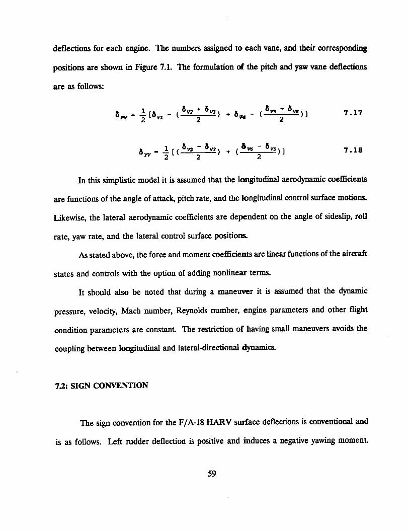
deflections for each engine. The numbers assigned to each vane, and their corresponding
positions are shown in Figure 7.1. The formulation of the pitch and yaw vane deflections
are as follows:
b_,=-_[b_- ( 2 2 )]7.17
b_= _[( _- ) +( 27.18
In this simplistic model it is assumed that the longitudinal aerodynamic coefficients
axe functions of the angle of attack, pitch rate, and the longitudinal control surface motions.
Likewise, the lateral aerodynamic coefficients axe dependent on the angle of sideslip, roll
rate, yaw rate, and the lateral control surface positions.
As stated above, the force and moment coefficients are linear functions of the aircraft
states and controls with the option of adding nonlinear terms.
It should also be noted that during a maneuver it is assumed that the dynamic
pressure, velocity, Mach number, Reynolds number, engine parameters and other flight
condition parameters are constant. The restriction of having small maneuvers avoids the
coupling between longitudinal and lateral-directional dynamics.
7.2: SIGN CONVENTION
The sign convention for the F/A-t8 HARV surface deflections is conventional and
is as follows. Left rudder deflection is positive and induces a negative yawing moment.
59

Aileron deflection is found from subtractingthe right aileron deflection from the left aileron
deflection. This implies that a positive 6A is left aileron down which induces a positive
rolling moment. Finally, the elevator deflection is positive down which gives a negative
pitching moment.
6O

Figure 7.1: Thrust Vectoring Vain Positions
61
CHAPTER $
RF_._ULTS AND CONCLUSIONS
The flight tests for this investigation were condu_.xi on September 29, 1992 at NASA
Dryden Flight Research Facility in California. The On Board Excitation System (OBES)
maneuvers were performed once at 10°, 25 °, 30 °, 40 °, 50 °, 60 ° angles of attack in both the
lateral and longitudinal directions. The relevant data was recorded and analyzed at NASA
Dryden using the pest code.
It should be noted that the results presented do not represent any information of the
thrust vectoring (yaw vane and pitch vane) doublets. The analysis was restricted to
incorporate only the three of the four doublets of the OBES flight test maneuvers discussed
in Chapter 5. This was done in accordance with International Traffic in Arms Regulations.
Recently, the restrictions on the technical diffusion of these data have been lifted.
The results of the derivative values axe presented in graphic and numeric forms. The
pest code integrates the equations of motion to generate estimates of the derivative values
and to produce a time history of the computed variables. All computed variables are first
assigned constant default values for the entire time history. These default values for the
F/A-18 HARV were chosen from wind tunnel analysis of McDonnell Douglas' clean
aerodynamic model of the F/A-18. The program then integrates the equations of motion
using current program status, replacing the default values with the computed values as the
integration proceeds. The integration continues until the difference between the measured
and computed responses is minimized.
62
The results frompEst usingthe measured flight data are compared with results from
a previous parameter estimation analysis of the F/A-18 and values obtained from wind
tunnel tests performed by McDonnell Douglas. This previous PID analysis was performed
by Dr. K. l]iff at NASA Dryden. 7 It should be noted that the estimates that he obtained and
those obtained from McDonnell Douglas' wind tunnel tests were for the F/A-18 before it
had the capability of independently moving the control surfaces with the OBES system. An
additional comparison was made with values from apEst analysis of data that was obtained
from the F/A-18 flight simulator at NASA Dryden. A pEst analysis was performed with
simulator data because only one maneuver was actually flown at each test point and
additional PID maneuvers were not scheduled for several months. It was necessary to obtain
extra data at the same flight conditions in order to make a more diverse comparison.
However, not much emphasis is placed on the results from the simulator data because
several effects are not included in the simulator model
8.1: LATERAL DIRECTIONAL DERIVATIVES
The time histories of the computed and measured responses of sideslip (/3), roll rate
(p), yaw rate (r), roll angle (0), and lateral acceleration (ay) for the 10, 25, 30, 40, 50, 60
degree angle of attack (aoa) test points for the lateral direction are shown in Figures 8.1 -
8.6. From these figures it can be seen that for the lower angles of attack (ie. 10° and 25°),
the computed responses closely match the measured responses. However; as the aoa
increases, the computed response curves seem to deviate slightly from the measured time
63
histories. This type of deviation implies that the estimated derivative values do not
accurately describe the airplane's characteristics. Basically, the more the computed response
resembles or fits the measured response, the more the estimated coefficients are accurate.
This accuracy of the parameters is also indicated by Cramer-Rao bounds. The Cramer-Rao
equality defines the minimum achievable variance for the estimation error of any unbiased
estimate."
The effects of the aerodynamic biases,/3, P, r, 0, 6A, 6it , 6DHT, 61,V, and 6yv on the
sideforce, rolling moment and yawing moment are shown in Figures 8.7 - 8.15. The square
symbols are the coefficient Values computed by pEst using the flight data, the circles are
values obtained from Dr. K. Biffs analysis for the F/A-18. The triangles represent the
results obtained frompEst of the data recorded from the F/A-18 flight simulator, and the
x's are the coefficient values from McDonnell Douglas' wind tunnel tests. Notice that the
results from niff are only for aoa's of 10° - 40 °, and that some of the values from the wind
tunnel tests are not available. The vertical bars on the estimated derivative values
symbolize the Cramer Rao bounds. To accentuate the bounds on the plotted results, they
were multiplied by a scale factor of 5.
Figure 8.8 includes plots of the effect of sideslip (Cyp, Clp, and C,,). Cyp is the
change in side-force coefficient due to a sideslip angle, and it is generally negative. All four
values at each aoa compare reasonably with exception to the flight determined data at 30 °
and 40 °. The scatter of these data points could be due to the unsteady behavior of the
vortical flow fields associated with the forebody and wings, coupled with the rolling degree
of freedom of the aircraft. This dynamic phenomenon that plagues many slender-wing
64
aircraft is called wing rock and is basically a single-degree-of-freedom,limit cyde, roll
oscillation. Previous wing rock investigations for the HARV have indicated a rising trend
of motion between 30 ° and 40O angles of attack. 23
The Cm_term indicates the change in rolling moment coefficient due to a sideslip
angle and is also known as the airplane dihedral effect. All values in Figure 8.8b are
negative, as expected, and similar in magnitude. The estimates from flight data compare
well with the other values except for the 40 ° aoa. This scatter may be attributed to the
noise level of the lateral acceleration signal at the 40 ° aoa as shown in Figure 8.4e. The
sideslip and sideforce terms are directly related to the lateral acceleration. Hence, if the
signal is not clear the estimates may not be valid.
Co_ is the change in yawing moment coefficient due to a sideslip angle. This term
is primarily responsible for the aircraft directional dynamic stability, and it is expected to
be positive. Figure 8.8c shows a close comparison among the values at 10" - 40° aoas. The
Cramer Rao bounds are small thus implying a good accuracy.
The contributions of the roiling moment, p, to sideforce, rolling moment, and yawing
moment are shown in Figure 8.9. The C__p and Cop shown in figures 8.9a and 8.9c are two
less important derivatives. As it can be seen the data points are somewhat scattered with
large Cramer Rao bounds, thus indicating that the accuracy is poor. The arrows on the
graphs symbolize data points that were off the vertical scale. The appropriate values and
Cramer Rao bounds for these points are located in the legend to the right of the graph.
The C_ graph in Figure 8.9b shows favorable agreement among each of the values
for the lower aoas; however, after 30° aoa the scatter tends to increase. The sign of the
65
values is positive as expected.
Figure 8.10 contains the yawing moment effects. The more important of these three
derivatives is the derivative Cm_ The C_ terms are very similar in magnitude with exception
to the 30 ° and 40 ° aoa, and the Cyr graph shows considerable distribution of the flight data
values. The Cramer Rao bounds are quite large, therefore the estimates are considered to
be a poor representation of the yawing moment's effect on the sideforce. In a similar
manner to the values of C_ the C_ values decrease in accuracy in the higher aoa range.
The effects of the aileron control surface deflections are represented in Figure 8.11.
The plot of Cv6A shows a change in sign of the values as the aoa changes. There is no
visible trend of the flight data values.
determine the tendency of the results.
More data points at each aoa are needed to
However, the C_ estimates depict a good
representation of the aileron effect on the rolling moment. The small Cramer Rao bounds
on both the simulator and flight data results suggest that the values are valid. The values
decrease in almost a linear fashion from approximately 0.(_26 to 0.000015 as the aoa
increases. The positive sign of the values is expected because a positive aileron deflection
(which is one half of a positive left aileron minus a negative right aileron) generates a
positive rolling moment. The large uncertainty of the results from Iliff's analysis could be
due to the insufficient excitation of the rolling mode.
F/A-18 was not yet equipped with the OBES system.
Recall that in his investigation, the
He concluded that the differences in
the derivatives the he obtained was due to the lack of independent control surface
deflections. 7 The results for this particular derivative show that the single surface excitations
from OBES definitely improve the estimation.
66

The values for Co6^ from the flight data, simulator data and Iliff's analysis notably
agree throughout the aoa range. The generally negative sense of this derivative implies that
a positive aileron deflection induces an adverse yawing situation.
The rudder effects are shown in Figure 8.12. The more important of the three 6R
coefficients are C_eR and CoeR. Figure 8.12a indicates that the largest uncertainty of the
estimates for Cyex lies within the aoa range of 300 - 40 °. The estimates for C_e R are
expected to be positive. The tendency of the CneR esa_mtes obtained from the flight data
first decreases slightly in magnitude to 40 ° aoa then increases at the higher angles.
The differential horizontal tail contributions are shown in Figure 8.13. The
derivatives were only estimated up to a 50° angle of attack because past 50° the differential
horizontal tail is ineffective due to flow detachment. This control surface acts in a ._imilar
manner to the ailerons because it produces a positive rolling moment when deflected
positively. However, the same positive deflection is expected to yield a proverse yawing
situation unlike the ailerons which induce adverse ,,-aw when deflected positively. This
proverse yaw is due to the increase in the amount of drag on the right side of the tail
section.
The thrust vector derivatives are shown in Figures 8.14 and 8.15. It should be noted
again that the thrust vector control surfaces were not used to independently excite the
aircraft's motion. Therefore, the results presented here are not the best representation of
the thrust vectoring effects. Even though the pitch vane is almost negligible in the lateral
sense, the corresponding derivatives were also estimated. This was done in order to get a
better perspective of the way in which the thrust vector controls were modeled. As it is
67
evident, each of the coefficientsare large in magnitude and vary throughout the aoa range.
The validity of the estimates for C_syv and C,tsyv was examined by comparing the
calculated moment arm of the deflected thrust force to the real moment arm defined from
the aircraft dimensions. The calculated thrust moment arm was found by dividing the
yawing moment derivative C,syv by the sideforce derivative C_a,v. These values were
calculated from the estimates at each angle of attack and are shown in Figure 8.16. The
real thrust moment arm was found as the distance between the aircraft center of gravity and
the point were the exhaust plume was deflected. This value was determined to be -20.1 feet.
The negative sign indicates that the distance is aft of the center of gravity. As seen in
Figure 8.16, the calculated moment arm is never -20.1 feet. This suggests that the estimates
are not accurately describing these characteristics.
It is not possible however, to imply that the modeling of the thrust vector terms is
completely wrong. The insuffident amount of data does not allow a complete comparison
of results. Additional data is needed at the same conditions in order to verify the modelling
techniques.
8.2: LONGITUDINAL DIRECTIONAL DERIVATIVES
Even though the lateral derivative estimates were more of a concern, a preliminary
set of longitudinal derivatives was estimated to generate a complete set of values for each
direction.
The computed response time histories are compared to the measured responses for
68

the longitudinal direction at 10°, 25 °, 30 °, 40°, 50°, 60° angles of attack in Figures 8.17 - 8.22.
Essentially, the fits of the computed and measured times histories are good. However, the
pEst program had difficulty matching the measured respo_es of the axial acceleration, ax
because of the noise level in the ax measurements. Therefore, the accuracy of the axial
force coefficient estimates is degraded.
The amount of noise of the normal acceleration and the angle of attack signals also
decreases as the airplane is subjected to the more dynamic conditions at the higher angles
of attack. At the higher angles of attack, the airplane undergoes an ample amount of
changes. For instance, the amount of structural vibration increases, the aerodynamics turn
nonlinear, wing rock occurs, and many others. All of these events may affect the shape or
amount of noise on the signals.
The offsets in the fits of the computed and measured responses could also be the
results of time shifts in the data. For instance, in Figure 8.19c it can be seen that the
computed response begins to estimate a change in the pitch angle before the actual
measured response changes. This type of situation suggests that a lead in the data transfer
is present because pEst begins to compute the response as soon as it detects movement of
the control surfaces. The computed response starts to indicate a change in the aircraft
motion before the measured response shows a change, it is possible that the data for the
control surface deflection was not transferred at the exact time that the surface moved.
However, in order to determine if in this case the offsets are due to time shifts in the data
transfer, additional maneuvers axe needed. The additional maneuvers would allow a better
comparison of responses.
69
The longitudinal derivative estimates are shown in Figures 8.23 - 8.31. Essentially,
the small Cramer Rao bounds on the more important of the derivatives such as C_o Cm,
Cm, C,,_ C,_SA, Cm6E imply that the estimates are a valid representation of the
longitudinal stability and control characteristics. Notice that the uncertainty of the estimates
at the 10° aoa is larger than other data points. This could be due to the fact that the low
amplitude doublets used at the 10° aoa did not sufficiently excite the aircraft modes. It is
expected that the large amplitude maneuvers would improve that results.
Again, the large amount of scatter of the thrust vector terms is possibly due to the
fact that the vanes were not used to independently induce the motion of the aircraft.
Inclusion of the thrust vectoring (pitch vane and yaw vane) doublets would possibly raise the
accuracy of these estimates.
Note that the axial force coefficients estimated from the simulator data are expected
to be invalid. This is because the effect of charting angle of attack on the thrust is not
modelled in the simulator.
7O
8.3: CONCLUSIONS
In the previous chapters, the procedure for estimating the aircraft stability and
control derivatives was presented. It was shown how the aircraft equations of motion were
developed and incorporated in the maximum likelihood method to generate estimates for
the derivatives.
For this investigation, a particular application of parameter estimation was applied
to the NASA F/A-18 High Alpha Research Vehicle. Discussions of the vehicle and why it
is being used to study the characteristics in the high angle of attack regime are included.
The design of the flight test maneuvers and mathematical modelling of the airplane are also
addressed.
The results of the analysis provide a reasonable base for further research in this area.
From the results it can be concluded that the single surface excitation system (OBES)
greatly improved the derivative estimates. This is due to the fact that the system effectively
reduced the correlation among the deflection of different control surfaces.
In addition, this investigation includes results of the first attempt to model the thrust
vectoring effects. Unfortunately, the flight data which included the thrust vectoring doublets
could not be used for this analysis due to the International Traffic in Arms Regulations.
Therefore, the results presented for the thrust vector derivatives can be deemed as only
initial predictions of the thrust vectoring characteristics. Additional research is required to
determine an accurate method of modelling these effects.
The estimates at the higher angles of attack suggest that problems do exist in this
71
region. For example, the uncertainty of the estimates in the 30 ° - 60 ° angle of attack is
possibly due to occurrences of wing rock, turbulence and separated flow conditions.
However, it is difficult to determine the exact problem with only one estimate at each flight
condition. Essentially, additional data is needed to verify the modelling techniques and
gather a complete understanding of the airplane characteristics at these high angle of attack
conditions.
72
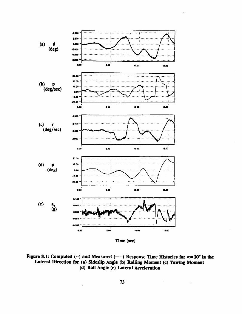
(b) p(deg/sec)
(c) r
(deg/ .c)
_m
It.am o
I._ u u
10.00"
Lm °
-IO.m ""
, , ,
4..000 ....................... " ...........................................
t i 4
0.00 J,O0 I0.00 ISJO
(d) 0
(deg)
_O.oo
10.00
0.o0
.tO.O0
.20.00
i
000 LO0
r
10.00 1S.W
0.1W
O_
4.0S0
i i ¢
'I_e (sec)
Figure 8.1: Computed (-) and Measured (_) Response Time Histories for a=10 ° is the
Lateral Direction for (a) Sideslip Angle (b) Rolling Moment (c) Yawing Moment
(d) Roll Angle (e) Lateral Acceleration
73
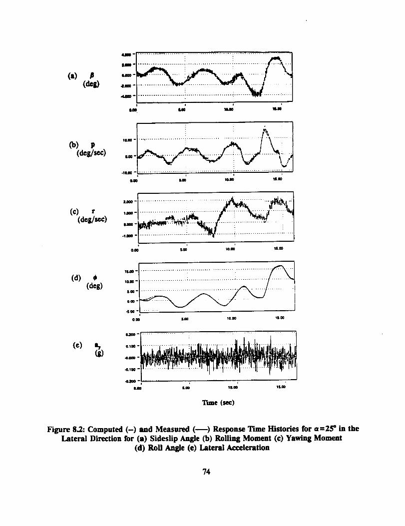
10.00-
(b) p
(_s/_) _=-
-tO.m -
0.00 LeO IO.O0 tS.O0
(c) r ,m -(de_sec)
0._0-
-1.000 "
0.00
1_00 °
(d) @ ,uo -(dog)
$,O0-
OO0"
-SO0-
(c) _,(g)
Lm [email protected] llLO0
...................... i ...................... !................. -.
iiiiiiiiiiiiiiiiiiiiiii/iiiiiiiiiiiiiiii.....iiii ...........,
ILW lo.oo tS.O00.00
0_00 ................................. .
0.1W *
•0.000 °
-8.100 --
.0280-
I,.18
i i
LO0 10.00 1S.00
Tune (see)
Figure 8.2: Computed (-) and Measured (--) Response Time Histories for a=2S* in the
Lateral Direction for (a) Sideslip Angle (b) Rolling Moment (c) Yawing Moment
(d) Roll Angle (e) Lateral Acceleration
74
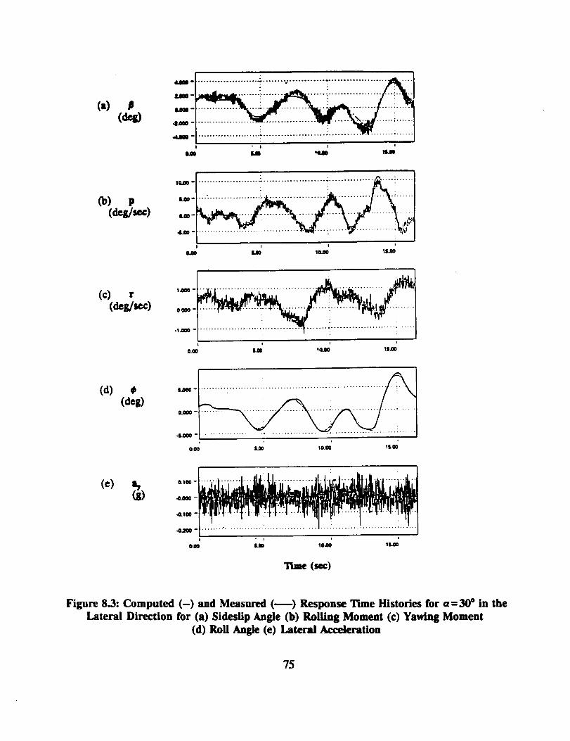
(c) r(des/_)
•"___i.............:::!::::_......:::i:iiiiiiii:::::::....::1J
10.110"
LO0"
O.O0-
•ILO0 -
..................... _ ..................... .:............... ,,-,..... ! ......
I I I
_ IOAO tliJlO
i
1.11nO .........
ol.llaO ....
¢ I |
O.O0 _ ' 0.,00 IS.O0
(d)
0.0_
•S.O00 ......................................
i
0.0o _ Io.00 15.00
0.100
4._ao
,.o.loo
O.gO
" n I i
SAO IOAO 1SAO
(see)
Figure 8.3: Computed (-) and Measured (--) Response Time Histories for a = 30 ° in the
Lateral Direction for (a) Sideslip Angle (b) Rolling Moment (e) Yawing Moment
(d) Roll Angle (e) Lateral Acceleration
75

(a) (d_IO
l.lm o
ll.llm o
41A00 *
ass 141A0 U
0o)(deg/sec) 0.000 °
som ........... "_............................. - ..................... _"i
, * s0A0 ILM 10.00 %S.00
2_0 ....................... -....................................... !--.
1.000 .................... _................ """
0.000 "
$ , i
0.00 IA0 10.00 1100
(d)
(e)
1o+o....................... _....................... _.................
OW- J ........... ' ..............................
4.00 "
i + , ,
_) -, ....i- ...... _.................................+....41"4.100 -
I • i i iiL00 !0.41 lS_O0
"l_e Oec)
F'_ure 8.4: Computed (-) and Measured (--) Response Tune Histories for 0=40" in the
Lateral Direction for (a) Sideslip Angle (b) RoUing Moment (c) Yawing Moment
(d) RoU Angle (e) Lateral Acceleration
76
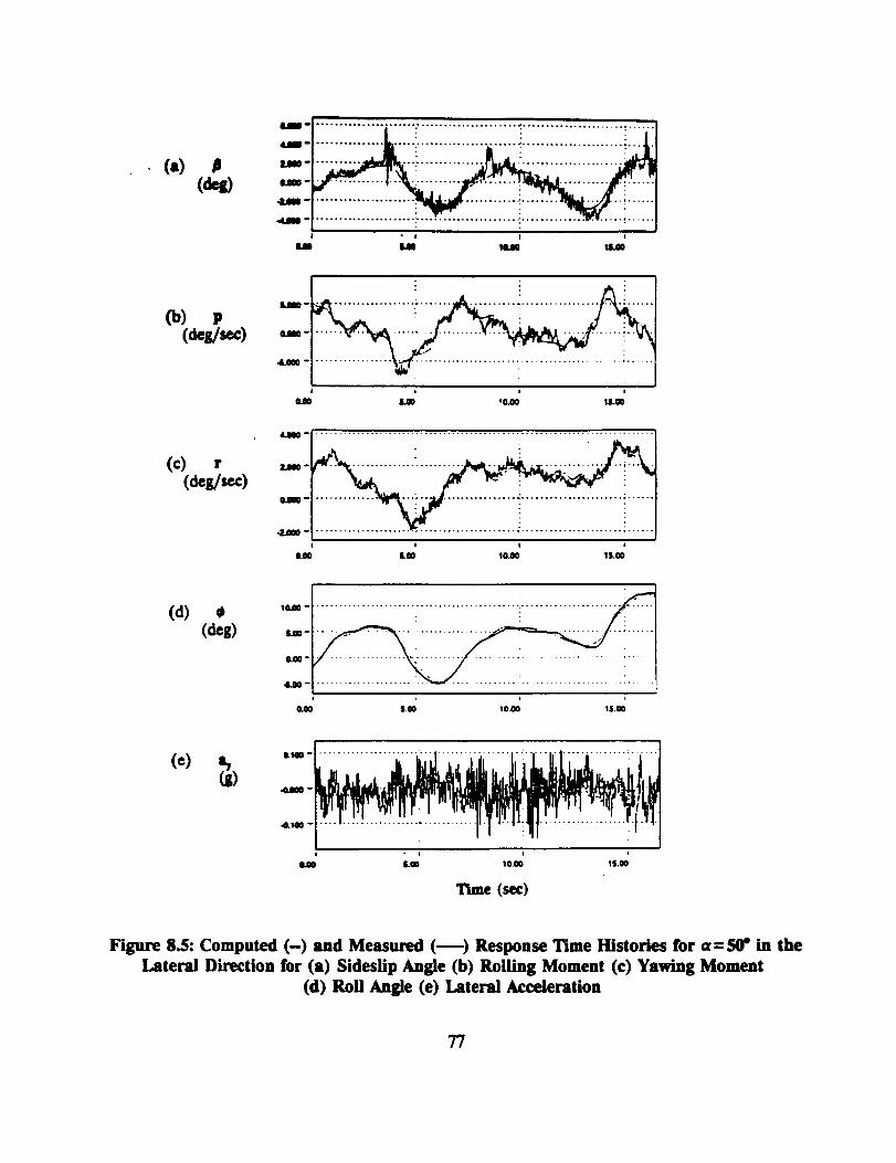
(*) (d_)
@.ms
4Am
um
.4.rag °
am
l
!
ass 10_0' U
(¢) r(deS/_)
(d)(des)
@_lO-
.&ram-
I I
* 0.00 11.00
i !
! I 0
15.00 10._ IS.00
(c)_)
aLlOO
4kilo
.0.1a
0.80
- I , i
&.Oo lo.0o IS.O0
11me (sec)
Figure 8.5: Computed (-) ud Measured (--) Response Time Histories for a= SO"in theLateral Direction for (a) Sideslip Angle (b) Rolling Moment (c) Yawing Moment
(d) Roll Angle (e) Lateral Acceleration
77

4_00 °
I.OW o
O..MO -
+l
iiiiiiiiiiiiiiiiiiiiiiiii!iiiiii iiiiiiiiiiiiiiiiiiiiiii
J,.O00 _
O.mO o
-i._00
0.00i i , g
4Ao LO0 8.00 IO.eO
(c) r(des/see)
2.O0O
1.11_
CLOaO
O.O0
..........._?_ .....+.............+.,<+._.............++_l I I I
2.1_ 4.00 l.O0 8.00 10.00
!_0
lOgO
I.OO
i.O0
4.00-
0.00 2.00 a.o0 LW 800 IO.O0
0.010 ............. _...................................... i ........... : .....
_+I--_W_'+O+O00............ "
0.00 , ! i 001 i• 2.OO _ LW L 'lO.m
(see)
Figure 8.6: Computed (-) and Measured (--) Response Time Histories for a = 60 ° in theLateral Direction for (a) Sideslip Angle (b) Rolling Moment (e) Yawing Moment
(d) Roll Angle (e) Lateral Acceleration
78
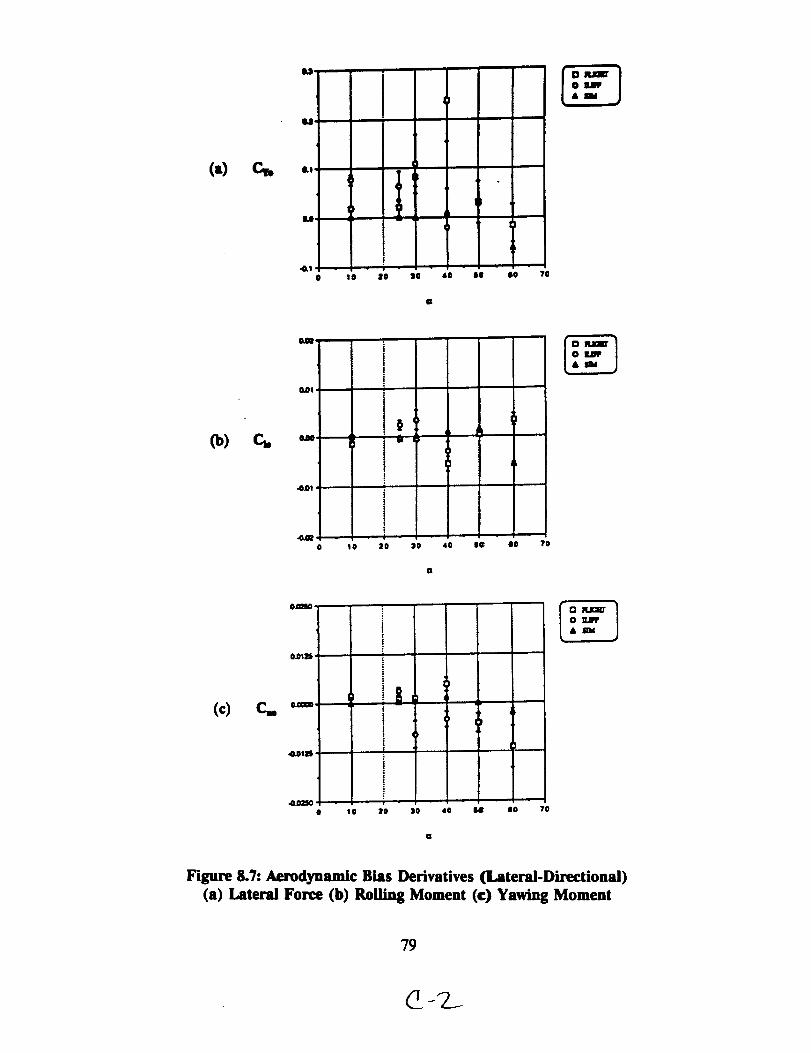
U
U
(I) C_. ,,
U
-0.10 10 8O SO 4O
4Z
$8 40 70
nns
0.01
-4.01
i'Jtiii!|
I0 20 20 4O
I1
J8 80 70
OJ_50
0.012S
(c) ¢..
4,01_S
Iii
iili
t!!i
ti
10 20 20 40 i_ 80 70
O_
Figure 8.7: Aerodynamic Bias Derivatives (Lateral-Directional)
(a) Lateral Force (b) Rolling Moment (c) Yawing Moment
79
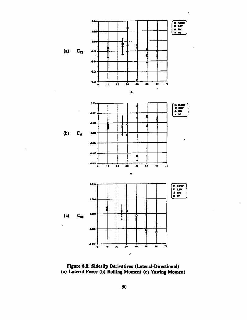
(a)
W
i!ii
10 8O SO 14) l0 ?0
(b)
-0A01 '
•.0Am,
.4_W'
.Gin6,
iI
i"
i!iiiiI
10 Z0 S0 10 7O
0.010
(c) _ o.=o
,,0.010
i!
!
| ,,.I] ,,
i
i]i
10 Z_ 30 40 $8 10 ?0
Figure 8.8: Sideslip Derivatives (Lateral-Directional)(a) Lateral Force (b) Rolling Moment (¢) Yawing Moment
80
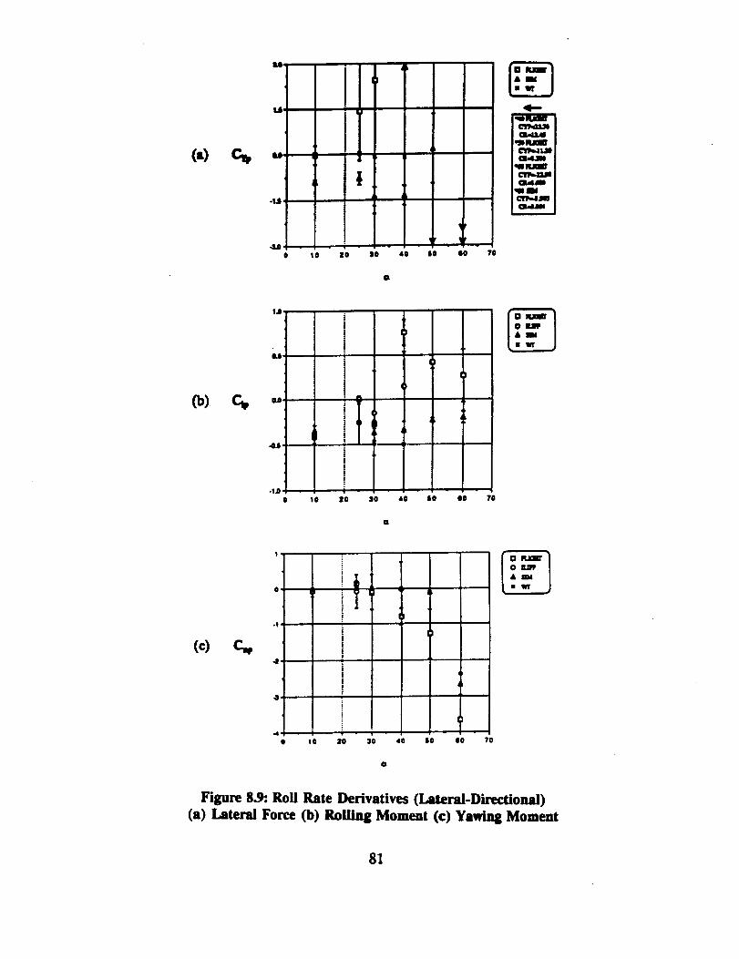
(_ c,,
U_
IUF
i!o Io 8o 4O IO IlO 70
41--.
¢0) c,,
1JJ!Ii
u
]ILO
!I
J!i
i• lh ! -
0 10 20 )0 SO O0 70
Olu_rou, P
(c) c,,,
I
!i0
.I i
ii
41 !i
!@
4 -- -
• I0 _ 30
0
40 SO |0 70
[n_l
l_ J
Figure 8.9: Roll Rate Derivatives (Lateral-Directional)
(a) Lateral Force (b) Rolling Moment (c) Yawing Moment
81
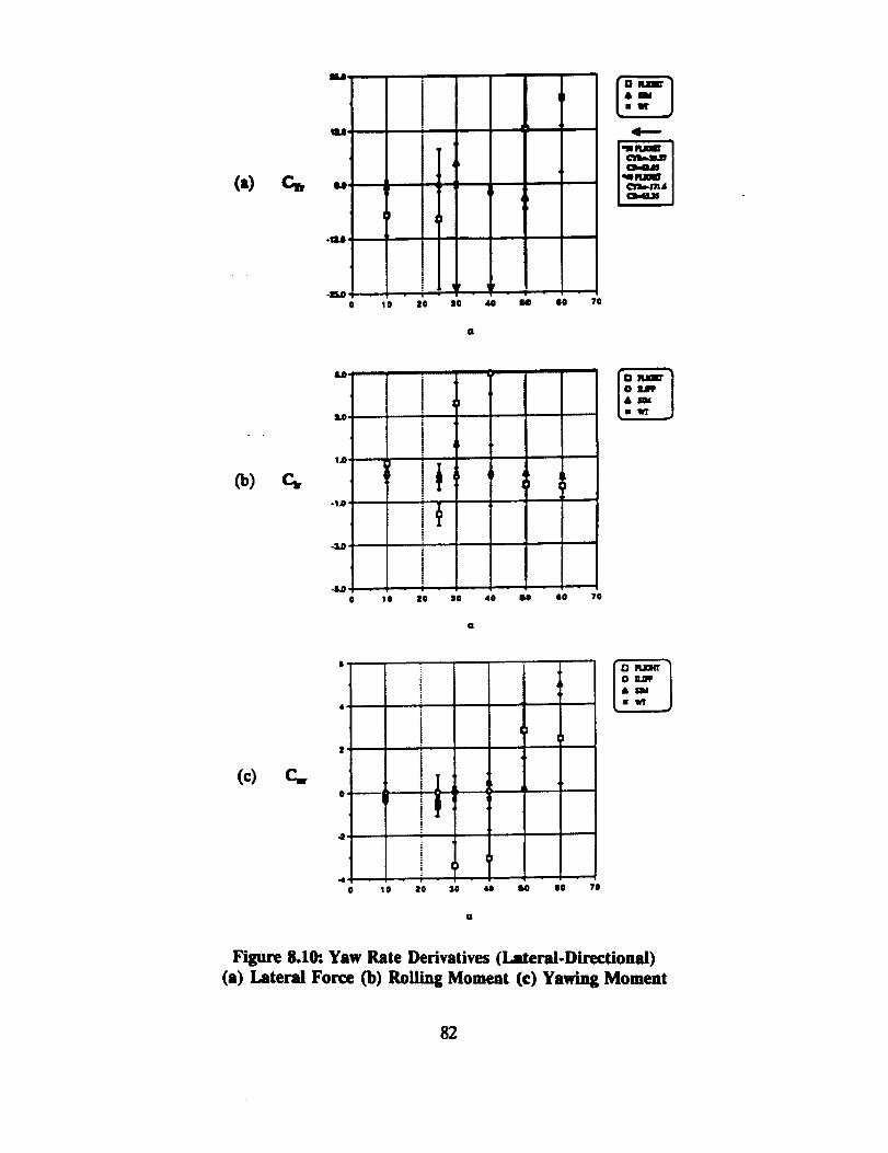
ILl,
IU.
(a) C_r U.
(_)
U-
u
I.o
.I.o
-Lo
I
!
t
- I -10 I0 SO 40 _ O0 70
(c) C,,r
-4
i
!i
i!i
I,L
ii
sO0 10 $0 40 &O 00 ?0
O
Figure 8.10:. Yaw Rate Derivatives (Lateral.Directional)
(a) Lateral Force (b) Rolling Moment (c) Yawing Moment
82
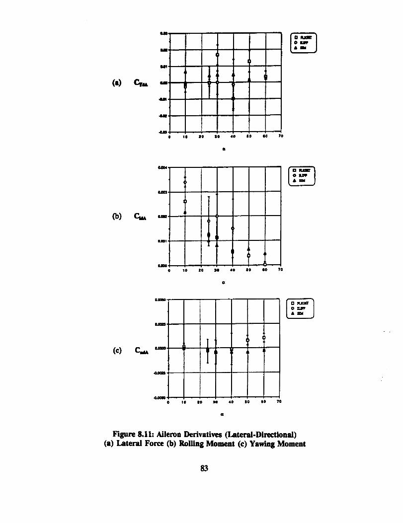
(a) c,,,
aim
Ul
Ut
U
4141
0
A_
i
ii
10 ZO SO I0 110 ?O
po) c._ -,-
ClLO0!
o.ono
o
i
tiiliIt!l
tO 20 JO 410 7O
(c) _ o,o.
ilIit
i
t
T
ii
_ , 1
I 0 dtO 310,,o.omo
o lo so 41o ?o
o+
Figure 8.11: Aileron Derivatives (Lateral-Directional)
(a) Lateral Force (5) Rolling Moment (c) Yawing Moment
83
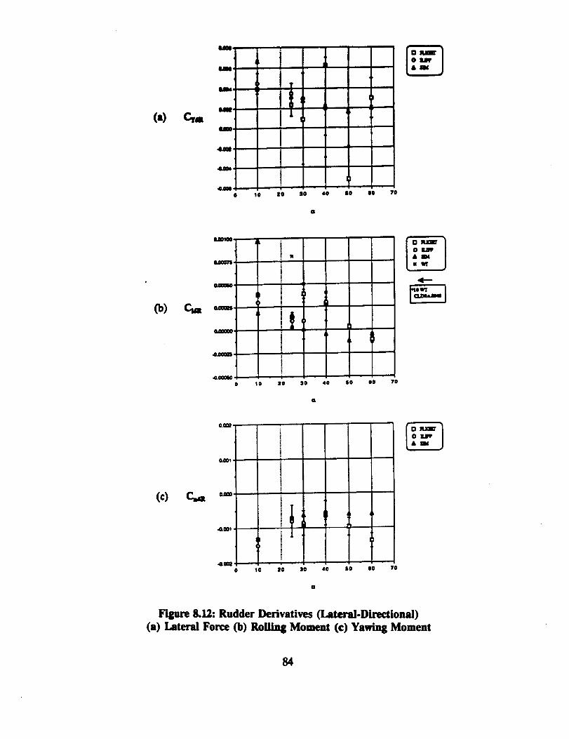
(a) Cya
MMImm
m _
asss _
4km8'
.@AnS0 10 30 S0 4O
O
JO 30 70
(b) C,,I
0.0O10O
0.000711
0.00010
m
m
4.00MS
0 I0
i!i!i
IO $0 40 SO O0 70
o
41--"
onn_
0,001
(c) C.,,
4ml -
!
i|
i1!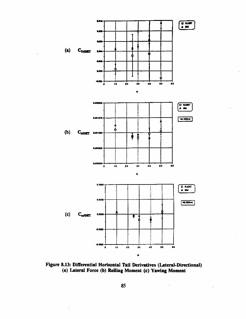
(.)
18W
I'
I'
J
10
t
IIO _0 40 $0 80
_)
o._cesm
o.clolI
I
I
o
I
ii
io.
!!i
1!t
i
1 -10
!
iii
i
_0 30 40 SO
G
SO
(c)
0 rmw.,
OI
4).1
.O_lO
i
- , - , - • - II0 20 30 "tO SO IO
Figure 8.13: Differential Horizontal Tail Derivatives (Lateral-Directional)
(a) Lateral Force (b) Rolling Moment (c) Yawing Moment
85
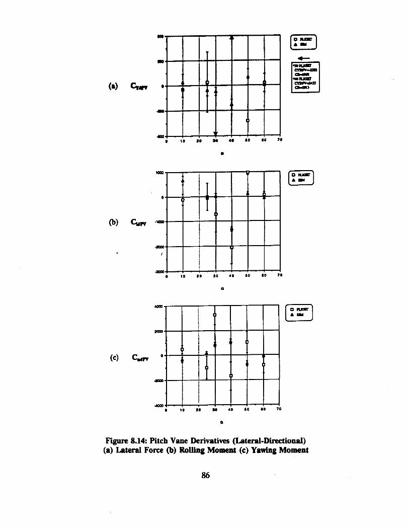
mo
SlO
(a) C,,r, .
410
.48O0
l!
+ .
I 0 I0 N SO O0 70
41---
m
o
(b) C_ .m
I
4000
|
l
!;
i
J+ | -
10 10 30 10 00 70
(c) _ o
dceo
0 SO 80 70
+3i
!
I! •|
t|i
!$
+|
- , |
10 10 N 40
Figure 8.14: Pitch Vane Derivatives (Lateral.Directional)
(a) lateral Force (1)) RoUing Moment (¢) Yswing Moment
86

m
llln
('). _,,ir, .
4110
.7OO0
ii
- I
I0 _0 SO
Cl
4O
t!
$0 I0
'4"--"
7O
IDO0
I000
Co) _ o
.I000
iI
i!
ii!!
iii
J
'Ii
i
10 20 _0 4O
0
+ •|0 I10 70
41-'--
(c) c,,,r,,
I00o
4OOO
i
- I - • . + , . I,
IO I0 20 ,40 I0 II0 70
Figure 8.15: Yaw Vane Derivatives (Lateral.Directional)
(a) Lateral Force (b) Rolling Moment (c) Yawing Moment
87

5O
25
[.->.
o[.._u'_Z -25
¢¢imu
p,
-5o
J_
E!
I:] IE!A dt
_VTOMI_NT ARM = -20.1• I " , • 1 • - I •
0 10 20 30 40 50 60
"30 SIMM-AR.M-118.5
"60 SIMM-ARM-1630
70
F'q_re 8.16: Calculated Thrust Moment Arm at Varying Angles of Attack
88
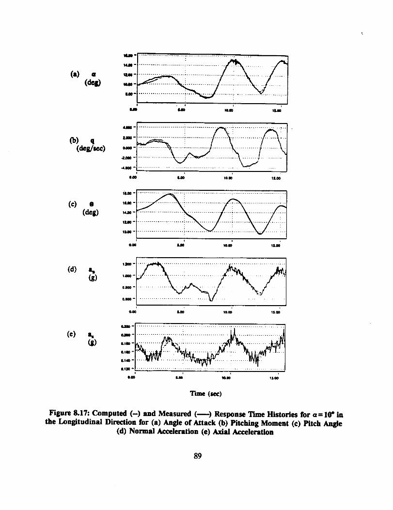
(a) a
U o
I4A0"
U
U
ILM
I
. I 4 ,U ULI0
(c) •(deg)
_I_ I
3_ll-
&m0-
.._00 o
0410¢
UO IO.W IS.OO
fiLm-
11410-
t4A0-
I_LII0 -
1OA0-
I I ,
(d) a.
0.I00 -
0.IO0 -
O_ IkO0 10.00 IS.00
• *_ "I ..............................................................t i i ,
OAO t4o _IO 19&.W
Tune (sec)
Figure 8.17: Computed (-) and Measured (--) Response Tune Histories for a= I0" inthe Longitudinal Direction for (a) Angle of Attack (b) Pitching Moment (c) Pitch Angle
(d) Normal Acceleration (e) Axial Acceleration
89
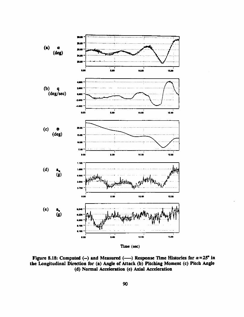
(.) Cl
(c_l)
I i i ,
III lnSS I_
_o
41 °
i
i
I_W ILW
(c) "-,..._i iiiii!iiiiiiiiiiiiiiiiiii_ii................................... !-o
$I .......................................................
(d) a,(g)
I.!m "
II-
OI-
__,-._:..........i_,__,,_./I.............__, .........................0_0 I.O0 IO.m laO0
I-
ILIIO -
&110 -
I._ $_ 10 _ 1L nn
(sec)
Figure 8.18: Computed (-) and Measured (_) Response Time Histories for a=2S ° inthe Longitudinal Direction for (a) Angle of Attack Co) Pitching Moment (c) Pitch Angle
(d) Normal AccelerItion (e) Axial Acceleration
9O
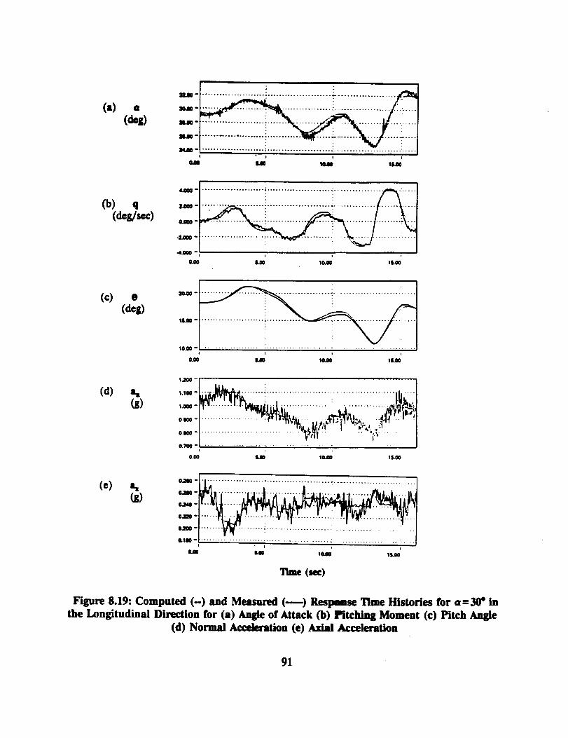
(*) a
(deg)
U
u
u
I I o i
0,40 lls IOiO
(b) q(des/s_)
(c) •(des)
(d) a m
(s)
_-
.aLm-i i i
ooo IJO IO.ll II.O0
10.00-
11+110-
10.00 -
0.00
1200-
I
i i i
i.40 I0.00 IS.O0
l.lm .........
0.1_ °
0.00 91+00 10.00 I $.0C,
(e) a,0,,II0 -
IHM0-
0.,120-
O.UlO ............................................ .. .................... -....i l l
0.00 iLgO 10.80 IS.O0
l_e (.ec)
Figure 8.19: Computed (-) and Measured (--) Reslmmse Time Histories for a=30" inthe Longitudinal Direction for (a) Angle of Attack (b) Pitching Moment (c) Pitch Angle
(d) Normal Acceleration (e) Axial Acceleration
91
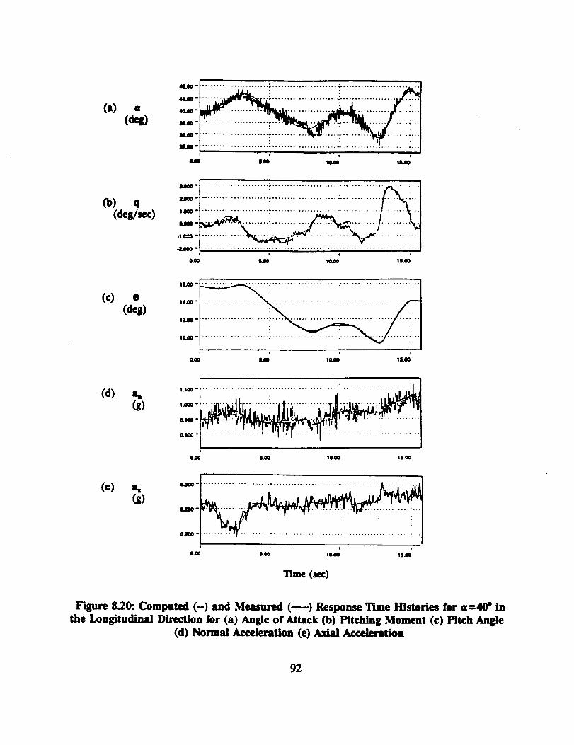
(a)41J10 *
40.80-
ILO0"
I.M"
111_8 ................................................ -- ..................... ;...
J , em ifJI _ U
Co) q(deS/r,e_)
--'iiiiiiiiiiiiiiiiiiiiiiiiiiiiiiiiiiiiiiiiiiiiii iiiiiiiiiiiii..... iiill
o , !
(c) •(des)
IILO0
14_0
13.00
I0.00
CLO0 LO0 10.00 SS.O0
1.100(d) _,(S) 1=
O.IKffi
O.lffiO
o.oo S.oo sO.Oo 'tS oO
(e) a, "-_"
, | ,
$.0o I0_o IS.00
Time (sec)
F'_,ure 8.20:. Computed (-) and Measured (--) Response Time Histories for a=40" inthe Longitudinal Direction for (a) Angle of Attack Co) Pitching Moment (c) Pitch Angle
(d) Normal AcceleraUon (e) Axial Acceleration
92
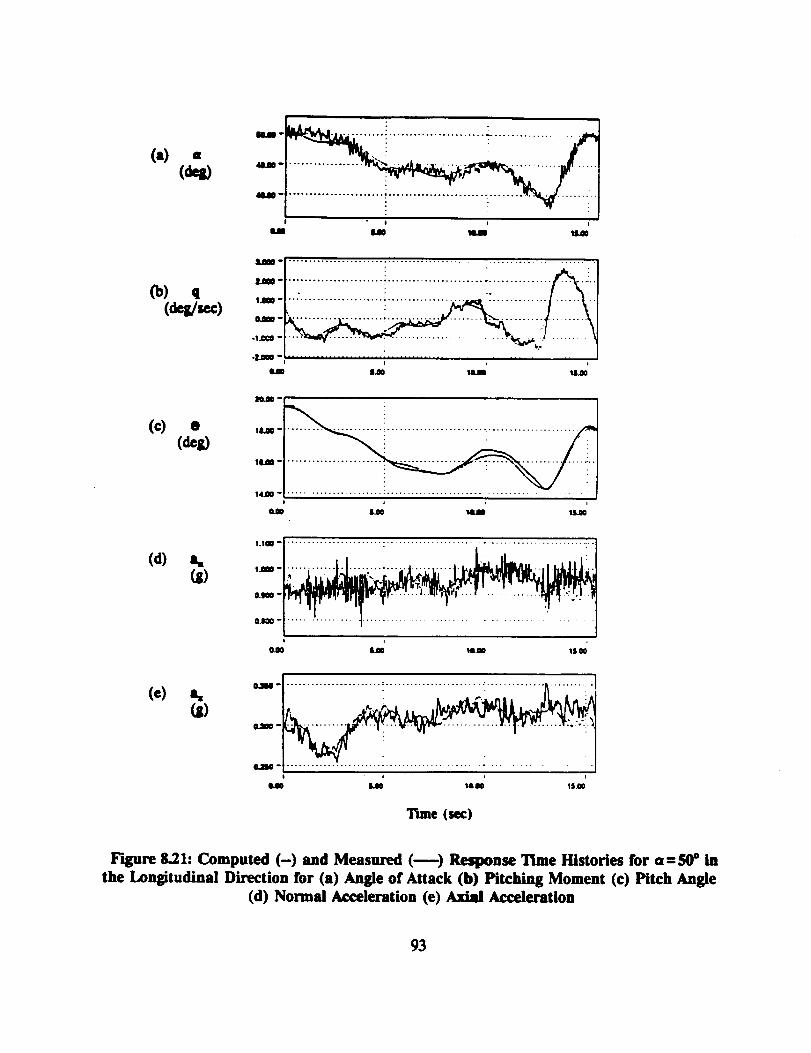
(.) -{dq)
(c) •(des)
_0.10 I
4&m
ass U tlL00
........................ i.......................-............... • --:-'
|.00 I TM lJ.O0
M-
ILL00 -Ill,d0 -
i
Q.00 S.00 M 1S.II0
(d) an(z)
(e)(_)
1.100 °
5.0mr o
0.900-
0.8_ o
........ :.., ..... .._.._...... _....... ,:....
0Jl0 s II0 1lira0 ISO0
O580
O.,.5O0
O,,d_"
li_ Silo 18 .m IS_O
Tune (sec)
Figure 8.21: Computed (-) and Measured (--) Response Time Histories for a=50 ° inthe Longitudinal Direction for (a) Angle of Attack (b) Pitching Moment (c) Pitch Angle
(d) Nomal Acceleration (e) Axial Acceleration
93
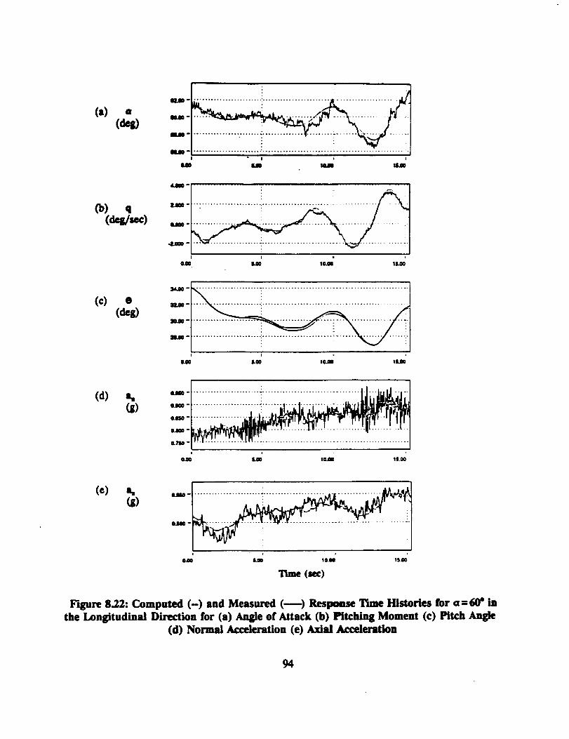
T
U
U
U
m
(c)_dl.O0 --
U o
aOAO o
m.W o
i
0.00 iLO0 10A8 tS._
_L_l_O i" ....................... . .........................................O.JO0
IL?SO
i ,0._ IL_ IO.OI IS00
(e) _,
|OAO ILO0 I0._ IS00
l_me (sec)
Figure 8.22: Computed (-) and Measured (m) Respmlse Time Histories for a:60" inthe Longitudinal Direction for (a) Angle of Attack (b) Pitching Moment (c) Pitch Angle
(d) Normal Acceleration (e) Axial Acceleration
94
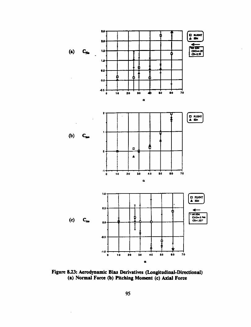
(_ c,,.
U
:L0
. !
1,0
0,S
0
•O.S - t -o 10 Z0 :1o
o
SO Io ?0
(b) c.
li
1 !
J
Id,,
° Tii4
-1 - i -0 10 20
12
A
40 SO S0 70
(c) c,.
1.0,
0,S
Oh
-O5 !
,,]'
J )
- , - | -
lo 20 3O 40o so So ?o
,4--'e 60SD4 i
CAO-.3.N6 I
C::lt-lJD7 ]
Q
Figure 8.23: Aerodynamic Bias Derivatives (Longitudinal-Directional)
(a) Normal Force (b) Pitching Momeat (c) Axial Force
95
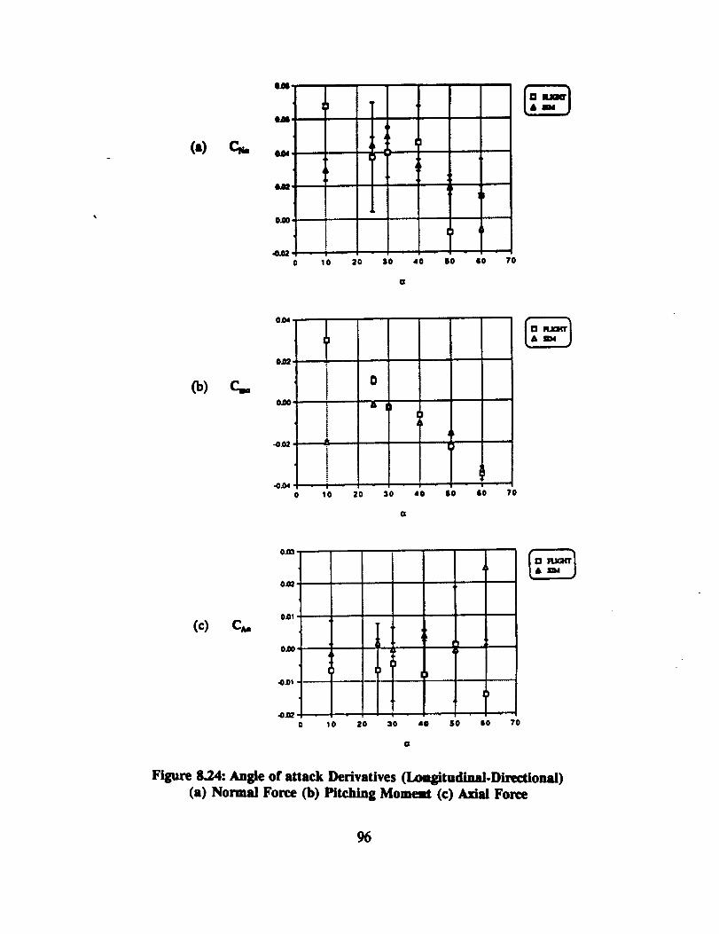
(a) c,,.
OAS,
IkOdl_
O.IR _
0.00
i•0.02 - t -
o lO 20
T
So 4o 60 60 70
o
Co) c..
O.04
0.00
-0_02
-0.04
t!iii!I
lO 2O
0
a
- • - _ |
30 4O SO 6O 7O
(¢) C,.
O.W
O.02
o.o_
o_o
,o.ol
.on_10 20 30 40 SO $0 70
O
Figure 8.24: Angle of attack Derivatives (Lomgitudinal-Directional)(a) Normal Force (b) Pitching Momemt (c) Axial Force
96
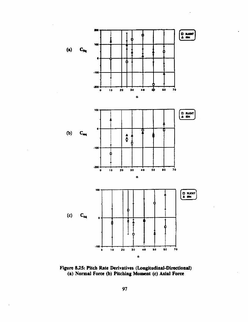
(_ c_
am
14o
e
.lOO
ii
.aoo - Z -o 10 20 So
CL
4O IO ?0
(_) c.,
lOO
i
,o !
Lt!
-Ioo
II
-200 i0 I0 20
& 4
30 40 SO SO 70
G
(c) CAq
lOO ¸
(
.looo !o 20 30
T40
O
i!i
II
J
so $o 7o
Figure 825: Pitch Rate Derivatives (Longitudinal.Directional)
(a) Normal Force (b) Pitchiag Moment (c) Axial Force
97

(a) W, •
IJ
0.001
it!
-0.01 - _ -
o lO 2o 30 40 SO SO ?0
(b)
(c)
0.003
0.002
0.001
0.000
-0.001
it
!ii
| -
lO 20
(
J
A
So 40 SO 8O 70
O.(X_ o
0.00,* •
C.u'z_ oms.
0.002.
OCO!
OCCO10 20 30 40 SO 60 70
(1
Figure 8.26: Trailing Edge Flap Derivatives (Longitudinal-Directional)(a) Normal Force (b) Pitching Moment (c) Axial Force
98

US
4
am
.401,
|
0 20
o
SO
0so,
0.01'
•0.01 '
.02)2,
0
|
|)
1 2O
O
$0
(c) C,_._
oJo_
0_01 '
1o 20 3o
a
Figure 8.27: Leading Edge Flap Derivatives (Longitudinal-Directional)(a) Normal Force (b) Pitching Moment (c) Axial Force
99
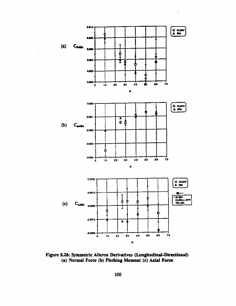
(a)
O.010
Clcau ,m_
O0O4
0.000
T
I. | *
1o 2o
I!
4O IO 70
(b)
0.000,
-0.001,
•0._02,
-0.003
.0.004
i
iI
i
!?t|i!i
A
0
o 1o 20 30 40 SO SO 70
G
(c) C,,s,
0_01S
0.0000
-o.ools
.o_oo
[
A
- I - , - ! - , "
Io 20 30 40 SO
i •
1I
i
!
÷so 70
Figure 8.28: Symmetric Aileron Derivatives (Longitudinal-Directional)
(a) Normal Force (b) Pitching Momeat (c) Axial Force
100
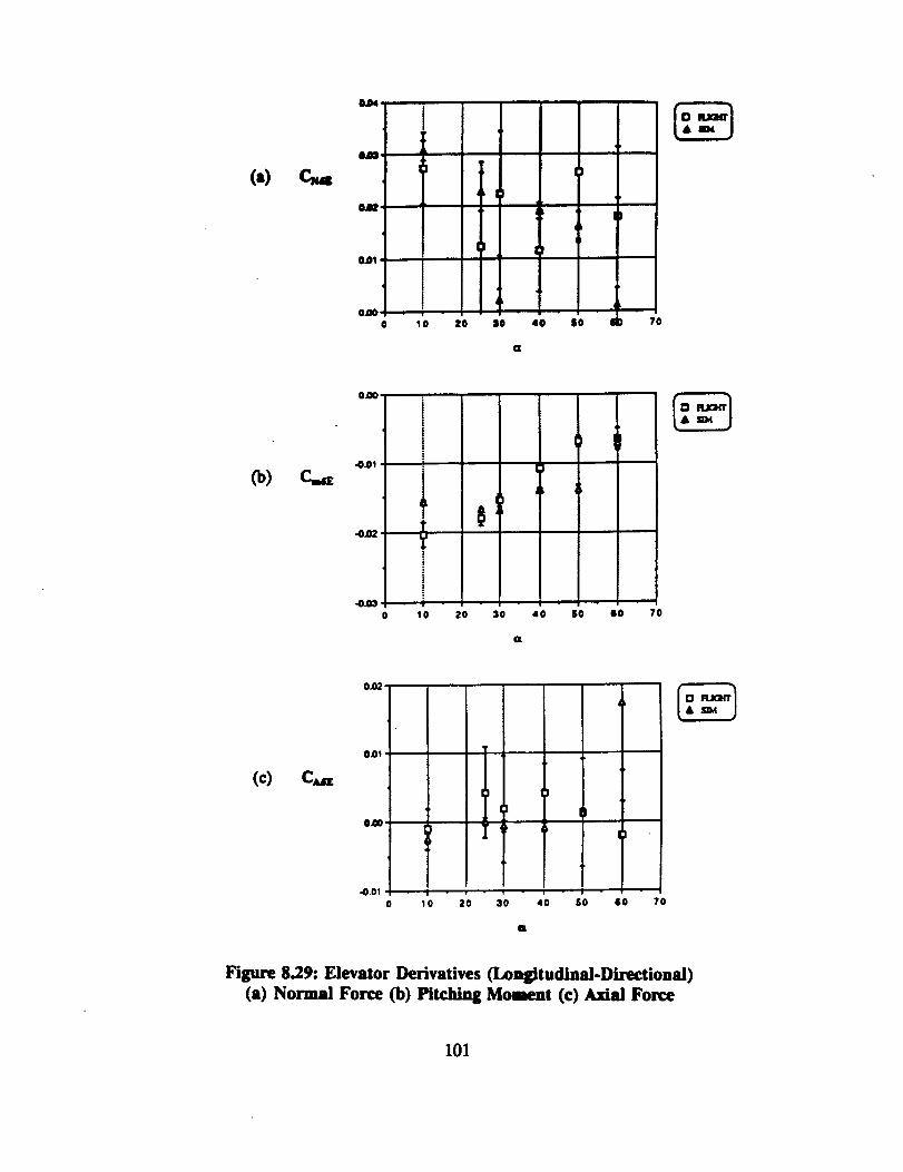
(.) c_
U4
ILm
OJIt'
0.01_
to.oo - ; -
o lO 20 40 SO ?0
Co)
0.00.
-0.01
-O.O2
-O.O3
J
!i
1!
I
i
J0 10 20 3O 40 SO IO 7O
0
(c) C,_
O.02
0.0_
0_0
.0.01
,r
)|
) b
10 20 30 40 SO 60 70
a
Figure 8.29: Elevator Derivatives (Lomgitudinal-Directional)
(a) Normal Force (b) Pitching Moment (¢) Axial Force
101

3oeo
lOOO
,I0
tS
• 1000 - _ -
0 10 30 SO SO 80 70
Co)
2OOO
IOO0
0
-1000
!
!
Jfi
+lo 2o
d5
- | -
SO 4O SO so 7o
(c) C,,,.v
SO0,
0
-SO0
• i+
.10_0, . I - ; - - I -0 10 20 30 40 so ?0
%
!i!
i
i
!
!
++
60
"lO_CADI_1334
Figure 8,30:, Pitch Vane Derivatives (Longitudinal.Directional)
(a) Normal Force Co) Pitching Moment (c) Axial Force
102

(..) c,,,,.,
moo
1ooo,
o
.1oooo 2o 40 SO IO 70
(b)
Sooo To !
r.too+ !
f•10000 - ; -
0 10 20
II
30 40 SO Io 70
O
ca.._ I
(c) C,,_r
1cco
soo:
o
-ioo
.lOOO . , -o _o SO 7o20 30 40 SO
rl
Figure 8.31: Yaw Vane Derivatives (Longitudinal-Directional)(a) Normal Force (b) Pitching Moment (c) Axial Force
103
REFERENCES
1. Maine, Richard E.; and lliff, Kenneth W.: Application of Parameter Estimation to Aircraft
Stability and Control - The Output-Error Approach. NASA RP-1168, 1986.
2. Maine, Richard E.; and Murray, James E.: Application of Parameter Estimation to Highly
Unstable Aircraft. NASA TM-88266, 1986.
3. Sire, Alex G.; and Curry, Robert E.: Flight-Detemffned Aerodynamic Derivatives of the
AD-1 Oblique-W'mg Research Airplane. NASA TP-2222, 1984.
4. PeUicano, Paul; Krumenacker, Joseph; and Vanhoy, David: X-29 High Angle-of-Attack
Flight Test Procedures, Results, and Lessons Learned.
5. Klein, Vladislav; Breneman, Kevin P.; and Ratvasky, Thomas P.: Aerodynamic Parameters
o]'an Advanced Fighter Aircraft Estimated from Flight Data; Preliminary Remits. NASA
TM-101631, 1989.
6. RohlL D.; Plaetschke, E; and Weiss, S.: X-31_A Model Evaluation and Validao'on via System
Identification. AIAA Atmospheric Flight Mechanics Conference, New Orleans, LA,
August 12-14, 1991, Paper No. 91-2875.
7. Iliff, Kenneth W.: Updated Stability and Control Derivatives for F-18. Memo 1990.
8. Klein, Vladislav: Determination of Stability and Control Parameters of a Light Airplane from
Flight Data Using Two Estimation Methods. NASA TP-1306, 1979.
9. Bryan, G.H.: Stability in Aviation, Macmillan, London, England, 1911.
10. Nelson, Robert C.: Flight Stability and Automatic Control, McGraw-Hill Book Co., New
York, 1989.
104
11. USAF Stability and Control DATCOM, Flight Control Division, Air Force Flight
Dynamics Laboratory, Wright-Patterson Air Force Base, OH.
12. Maine, Richard E.; and Iliff, Kenneth W.: User's Manual for MMLE3, A Gowtrd
FORTRAN PhTgram for Madmwn Likelihotrl Parameter F.Jffmation. NASA TP-1563,
1980.
13. Murray, James E.; and Maine, Richard E.: pEst Version 21 User's Manual. NASA TM-
88280, 1987.
14. Roskam, Jan: A/rp/ane Flight Dynamics and Automatic Flight Controls, Part I, Roskam
Aviation and Engineering Corp., Ottawa, Kansas, 1979.
15. Gilbert, William P.; and Gatlin, Donald H.: Rev/ew of the NASA High-Alpha Technology
Program.
16. Hammett. L. N., Jr.: An Investigation of the F-16 High Angle-of-Attack Pitching Moment
Discrepancy. Technical Report AFWAL-TR-81-3107.
17. Erickson, Gary E.: Water Tunnel Flow Visualization and Wind-Tunnel Data Anal)sis
of the F/A-18. NASA CR 165859, May 1982.
18. Dornheim, Michael A.: NASA Control Laws Boost F-14 High Angle-of Attack
Performance. Aviation Week and Space Technology, Page 71, October 14, 1985.
19. Bowers, Albion H.; Noffz, Gregory; Grafton, Sue B.; Mason, Mary L; and Peron, Lee
R.: Multiaxis Thrust Vectoring Using Axisymmetric Nozzles and Poste_it Vanes on an
F/A-18 Configuration Vehicle. NASA TM 101741, 1991.
20. Moes, Timothy R.; and Whitmore, Stephen A.: A Preliminary Look at Techniques Used
to Obtain Airdata from Flight at High Angles of Attack. NASA TM 101729, 1990.
105
21. Koehler, R.; and Wilhelm, K.: Auslegung von Eingangssignalen fur die
Kennwertermittlung. IB 154-77/40, DFVI_ Institut fur Flugmechanik, Braunschweig,
Federal Republic of Germany, 1977.
22. Maine R.E.; and Iliff, ICW.: Identification of Dynamic Systems - Theory and Formulation.
NASA RP-1138, 1985.
23. Williams, David; Quast, Thomas; and Nelson, Robert C.: Comparison of Flight and Sub-
scale Model Wing Rock Characte_tics of an F-18 A/rcrafl. Final Report for NASA
Grant NCA2-513, 1993.
106