Embed Size (px)
Citation preview
PhD Thesis
Harmonic Analysis onTriple Spaces
Thomas Hjortgaard DanielsenDepartment of Mathematical SciencesUniversity of CopenhagenDenmark
PhD School of Science – Faculty of Science – University of Copenhagen
Thomas Hjortgaard DanielsenDepartment of Mathematical SciencesUniversity of CopenhagenUniversitetsparken 5DK-2100 København ØDenmark
[email protected]://www.math.ku.dk/~thd/
PhD thesis submitted to the PhD School of Science, Faculty of Science, Univer-sity of Copenhagen, Denmark in May 2013.
Academic advisor: Henrik SchlichtkrullUniversity of Copenhagen, Denmark
Assessment committee: Jean-Louis ClercUniversité de Lorraine, France
Mogens Flensted-Jensen (chair)University of Copenhagen, Denmark
Bent ØrstedAarhus University, Denmark
Day of defense: June 19, 2013
c© Thomas Hjortgaard Danielsen, 2013 – except for the paperDecomposition Theorems for Triple Spaces.
ISBN 978-87-7078-991-2
AbstractIn this thesis we study examples of triple spaces, both their structure theory,
their invariant differential operators as well as analysis on them. The first majorresults provide us with some examples of triple spaces which are strongly spher-ical, i.e. satisfy some conditions reminiscent of properties of symmetric spaces.The algebras of invariant differential operators for these spaces are studied andthe conclusion is that most of them are non-commutative. Finally, we restrictour attention to a single triple space, giving a specific polar decomposition andcorresponding integration formula, and studying the relations between open or-bits of parabolic subgroups, multiplicities and distribution vectors.
ResuméFokus for denne afhandling er tripelrum, det være sig deres strukturteori, deresinvariante differentialoperatorer, såvel som analyse på dem. Det første hove-dresultat giver os en række eksempler på triplerum, som er stærkt sfæriske,dvs. opfylder nogle betingelser, der tilsvarer nogle egenskaber ved symmetriskerum. Algebraen af invariante differentialoperatorer for disse rum studeres, og detvises, at de fleste af dem er ikke-kommutative. Til sidst fokuserer vi udelukkendepå et enkelt tripelrum, hvor vi giver en specifik polardekomposition og tilhørendeintegrationsformel, og studerer sammenhængen mellem åbne baner af parabolskeundergrupper, multipliciteter og distributionsvektorer.

CONTENTS
Preface 1
1 Preliminaries 31.1 Topological Vector Spaces . . . . . . . . . . . . . . . . . . . . . . 31.2 Basic Representation Theory . . . . . . . . . . . . . . . . . . . . 61.3 K-Finite Vectors . . . . . . . . . . . . . . . . . . . . . . . . . . . 91.4 Invariant Differential Operators . . . . . . . . . . . . . . . . . . . 131.5 Direct Integrals . . . . . . . . . . . . . . . . . . . . . . . . . . . . 181.6 Fourier Transforms . . . . . . . . . . . . . . . . . . . . . . . . . . 231.7 More on Smooth Vectors . . . . . . . . . . . . . . . . . . . . . . . 281.8 Discrete Series Representations . . . . . . . . . . . . . . . . . . . 331.9 Some Representation Theory of SL(2,R) . . . . . . . . . . . . . . 381.10 Generalities on Symmetric Spaces . . . . . . . . . . . . . . . . . . 44
2 Triple Spaces 512.1 Examples and Elementary Properties . . . . . . . . . . . . . . . . 512.2 Uniqueness in the Polar Decomposition . . . . . . . . . . . . . . 602.3 Plancherel Decomposition . . . . . . . . . . . . . . . . . . . . . . 642.4 Invariant Differential Operators . . . . . . . . . . . . . . . . . . . 70
5
3 A Special Case 773.1 Invariant Differential Operators . . . . . . . . . . . . . . . . . . . 773.2 Action on Matrix Coefficients . . . . . . . . . . . . . . . . . . . . 823.3 Finite-Dimensional Spherical Representations . . . . . . . . . . . 853.4 The Polar Decomposition . . . . . . . . . . . . . . . . . . . . . . 883.5 Failure of Convexity . . . . . . . . . . . . . . . . . . . . . . . . . 953.6 Plancherel Decomposition . . . . . . . . . . . . . . . . . . . . . . 983.7 Orbits of Parabolic Subgroups . . . . . . . . . . . . . . . . . . . . 1053.8 H-Invariant Distribution Vectors . . . . . . . . . . . . . . . . . . 1103.9 The Most Continuous Part . . . . . . . . . . . . . . . . . . . . . 118
Bibliography 124
Index 128
Paper - Decomposition theorems for triple spaces 130
PREFACE
The harmonic analysis on semisimple/reductive symmetric spaces is well under-stood thanks to the effort of Helgason, Flensted-Jensen, Oshima, Matsuki, vanden Ban, Schlichtkrull, Delorme and others which again rests on the work ofHarish-Chandra. However, the requirement on symmetric spaces - the existenceof an involution - seems unnatural, of more like a technical rather than a geo-metric requirement on the space. Two properties seem to be of great importancefor symmetric spaces, namely sphericality and polarity - properties of a moregeometric nature than the existence of an involution. Thus, the overall idea isto generalize the Plancherel formula from symmetric spaces to spaces which areonly spherical and polar. This, however, seems to be an overwhelming task andby no means the scope of this thesis. Here we will focus on certain examples ofspherical and polar spaces, to see which phenomena we can expect or not expectto occur in general.The thesis is divided into three chapters as follows: The first chapter contains
background material on more or less advanced topics from representation theoryand harmonic analysis. The results obtained during the studies are described inthe following 2 chapters. In Chapter 2, we study triple spaces in as much gener-ality as we can (the number of spherical and polar triple spaces turns out to bequite limited). The main result here is a polar decomposition for certain triplespaces, a result obtained jointly with Schlichtkrull and Krötz. The resulting pa-per [10] is attached as an appendix. Finally, in Chapter 3, we study a particularexample of a triple space. Here we are able to determine the Plancherel measure
(up to absolute continuity) and describe a relation between the multiplicitiesof the different representations and the number of open orbits of the parabolicsubgroup from which this representation is induced. Also the algebra of invari-ant differential operators is determined.
AcknowledgementsI am indebted to many people who have helped, aided or otherwise supportedme during the past 4 years of ph.d.-studies. Where to begin?First, I would like to thank Mogens Flensted-Jensen and Bernhard Krötz
for fruitful discussions. I would also like to convey my thanks to “Rejselegatfor matematikere” for giving me the wonderful opportunity of traveling oneyear abroad. In this connection I would like thank heartily Prof. Karl-HermannNeeb from the University of Erlangen, and Prof. Sigurdur Helgason from MITfor hosting me at my stays at their respective institutes!A special thank goes to my (now former) fellow ph.d.-students, Adam, Hannes,
Henrik, and Tim for many joyous moments. We had so much fun!And finally, I wish to express my deep gratitude to Henrik Schlichtkrull, my
supervisor, for his aid, his patience, and his inspiration!
Copenhagen, June 2013. Thomas Hjortgaard Danielsen.
CHAPTER 1
PRELIMINARIES
In this first chapter we recall different notions and concepts from representationtheory and harmonic analysis that will be used throughout this thesis. I makeno claims to novelty in this chapter.Most results are stated without proofs (indeed, some of the theorems men-
tioned are so profound, that in-depth proofs would make up a thesis of its own)but references to relevant literature are given. In a few cases, where I was unableto find a proper reference, I have added my own proofs (most notably the proofof Proposition 1.36 and of the lemmas preceding it), and in a few cases I haveadded a proof from the literature, if I thought it to be an illustrative applicationof a previously stated theorem (e.g. the proof of Lemma 1.42).
1.1 Topological Vector SpacesDefinition 1.1. A topological vector space V is a vector space over a field Kequipped with a topology such that addition V × V −→ V and scalar multipli-cation K× V −→ V are continuous maps.
Obviously, the definition implies that the translation map v 7−→ v+a for somefixed vector a is a homeomorphism. Thus, the topology of V is determined solelyby the system of neighborhoods of 0, and a linear map between two topologicalvector spaces is continuous if and only if it is continuous at 0.
3
4 Chapter 1 – Preliminaries
A topological vector space is called locally convex if there exists a neighbor-hood basis of 0 consisting of convex sets. An obvious example is a normed space,where the system (Br(0)) of balls of radius r > 0 is a convex neighborhood ba-sis. More generally if P is a system of seminorms on a vector space V , such thatfor each seminorm p ∈ P, there exists another seminorm q ∈ P and a constantc > 0, such that
∀v ∈ V : p(v) ≤ cq(v), (1.1)
then the system (Bpr (0))p∈P,r>0 of balls is a neighborhood basis of 0 and bytranslation defines a locally convex topology on V . The converse also holds:if V is a locally convex topological vector space, then there exists a family ofseminorms satisfying (1.1), which generates the topology on V (cf. Proposition7.6 of [30]).In other words: a locally convex topology on a vector space means a topology
generated by seminorms.If there a exists a countable family (pn)n∈N of seminorms generating the
topology (equivalently, if there exists a countable neighborhood basis of 0), wecan define a metric, by
d(v, w) :=∑
n∈N
1
2npn(v − w)
1 + pn(v − w)
and this metric, which is obviously translation invariant, defines the topologyon the vector space. The space is called a Fréchet space if it is complete asa metric space. One example of a Fréchet space is the Schwartz space S(Rn) .The classical Schwartz space allows several generalizations to Schwartz spaceson a group G. Here we outline the definition of a Schwartz space as given in [5]in Section 2.5: First, pick an inner product on TeG and extend this to a left-invariant Riemannian metric on G. The metric gives rise to a distance functiond(g1, g2) (note that a change in the inner product in TeG just amounts to ascaling, and thus the resulting distance functions will just differ by a factor).Define the scale function : s(g) := exp(d(g, e)). Then we define the Schwartzspace (or rather the L1-Schwartz space)
S(G) := f ∈ C∞(G) | ∀D ∈ U(gC)∀n ∈ N : s(g)nDf(g) ∈ L1(G). (1.2)
The Schwartz space becomes a Fréchet space by equipping it with the topologygenerated by the seminorms ‖f‖n,D := ‖s(g)nDf(g)‖L1 for n ∈ N and D ∈U(g). We return to this space later.
1.1 Topological Vector Spaces 5
For a given topological vector space we denote by V ∗ the algebraic dual ofV , i.e. the vector space of linear maps V −→ K. By V ′ we denote the contin-uous dual , i.e. the subspace of V ∗ consisting of continuous linear functionals.The continuous dual can be equipped with several different vector space topolo-gies. The weak topology, is the topology given by the seminorms (pv)v∈V wherepv(ϕ) := |ϕ(v)|. This is the weakest vector space topology on V ′ for whichit holds that the dual of V ′ equals V (as a vector space) in the sense thatthe canonical map V −→ (V ′)′ is surjective. The strongest topology on V ′ forwhich it holds that (V ′)′ = V is called the Mackey topology . A third importanttopology is the strong topology which is the topology of uniform convergence onbounded subsets. In general, the strong topology is stronger than the Mackeytopology, i.e. the dual of V ′ is larger than V . In the case where the strong topol-ogy and the Mackey topology coincide, i.e. when (V ′)′ = V , we say that V isa semi-reflexive space . If the identity holds as topological vector spaces when(V ′)′ is given the strong dual topology, then we say that V is reflexive .A matter which is even more delicate than giving the dual space a topology,
is that of topologizing a tensor product of two topological vector spaces. Giventwo locally convex topological vector spaces V and W we denote by V ⊗W thealgebraic tensor product of V andW , i.e. the space of finite linear combinationsof elements of the form v⊗w. There are two “extreme” topologies on the tensorproduct: The first is the projective topology or π-topology we understand thestrongest vector space topology on V ⊗W making the canonical bilinear mapV×W −→ V⊗W continuous. V⊗W equipped with this topology will be denotedV ⊗πW and the completion of this space by V ⊗πW . By [30] Proposition 43.4 theprojective tensor product satisfies the following topological universal property:any continuous bilinear form ψ : V × W −→ X to some topological vectorspace X extends uniquely to a continuous linear map ψ : V ⊗π W −→ X. Theprojective topology on V ⊗W is the unique topology with this property.If ϕ1 ∈ V ′ and ϕ2 ∈W ′ (the continuous linear duals), then ϕ1 ⊗ ϕ2 given by
(ϕ1 ⊗ ϕ2)(v, w) := ϕ1(v)ϕ2(w)
is a linear functional on V ⊗W , and by the universal property this functional isindeed continuous if the tensor product is equipped with the projective topology,i.e. ϕ1 ⊗ ϕ2 ∈ (V ⊗π W )′.By construction, the projective topology is in some sense the strongest topol-
ogy we could meaningfully put on a tensor product. At the other end of thescale we find the injective topology or ε-topology which is the weakest vectorspace topology on V ⊗W such that linear functionals of the form ϕ1 ⊗ ϕ2 are
6 Chapter 1 – Preliminaries
continuous. These were already found to be continuous in the projective topol-ogy, hence the injective topology is weaker than the projective topology. ByV ⊗εW and V ⊗εW we denote the tensor product equipped with the ε-topologyresp. the completion of this. The identity map on the algebraic tensor productinduces an injection V ⊗πW −→ V ⊗εW .A locally convex topological space V is called nuclear if for any locally convex
vector spaceW this injection is a homeomorphism. In other words V is nuclear ifand only if the injective and projective topology coincide. Examples of nuclearspaces are D(M), S(Rn), S(G), C∞(M) (for M a manifold) as well as theirsubspaces and their strong duals (cf. [30] p. 530 as well as Proposition 50.1 andProposition 50.6). Taking the strong continuous dual of a tensor product whereat least one of the spaces is nuclear is very easy (cf. loc. cit. Proposition 50.7):
(V ⊗W )′ = V ′⊗W ′. (1.3)
Here V ′ and W ′ are both equipped with the strong dual topology.If V and W happen to be Hilbert spaces, we have a natural Hilbert space
topology on V ⊗W , namely that given by the inner product
〈v1 ⊗ w2, v2 ⊗ w2〉 := 〈v1, v2〉〈w1, w2〉.
We denote the completion of the tensor product of two Hilbert spaces simplyby V ⊗W underlining that this choice of topology is the canonical one. How-ever, in general, this topology is neither equal to the projective nor the injectivetopology, it is somewhere in between. In fact, a Hilbert space (or even a normedspace) is nuclear if and only if it is finite-dimensional. In particular the topo-logical universal property fails to hold in general.
1.2 Basic Representation TheoryDefinition 1.2 (Representation). A continuous representation or just arepresentation of a Lie group G on a topological vector space Vπ is a group ho-momorphism π : G −→ Aut(Vπ) (where Aut(Vπ) is the group of linear bijectionsVπ
∼−−→ Vπ) such that the map (g, v) 7−→ π(g)v is continuous G × Vπ −→ Vπ.We will often refer to the space Vπ as a G-module.
The definition obviously implies that π(g) is a linear homeomorphism of Vπto itself.
Definition 1.3. A representation is called irreducible if the only closed invari-ant subspaces are the trivial ones.
1.2 Basic Representation Theory 7
A vector v ∈ Vπ is called smooth , if the map g 7−→ π(g)v is a smooth mapg 7−→ π(g)v. By V∞π we denote the space of smooth vectors. The space canbe embedded into C∞(G,Vπ) (the vector v representing the map g 7−→ π(g)vwhich was smooth by definition). The latter space is given the topology ofuniform convergence of functions and its derivatives over compact subsets ofG, and V∞π is given the subspace topology. It is not hard to see that V∞π is aG-invariant subspace of Vπ (albeit not a closed one) and that π restricts to acontinuous representation of G on V∞π .If Vπ = Hπ is a Hilbert space, π is called unitary if π(g) is a unitary map
for each g. For a Lie group G we denote by G the set of equivalence classes ofirreducible unitary representations. We will reserve the notation Hπ for infinite-dimensional Hilbert spaces. For a finite-dimensional representation we will useVπ.Given two groups G1 and G2, and two unitary representations π1 and π2 of
G1 and G2 respectively we form the so-called outer product π1×π2 of G1×G2
on Hπ1⊗Hπ2
given by
(π1 × π2)(g1, g2)v1 ⊗ v2 := (π1(g1)v1)⊗ (π2(g2)v2)
(this is sometimes also denoted π1 π2 but we will not use this notation here).If G1 = G2, the restriction to the diagonal is called the tensor product anddenoted π1 ⊗ π2
1:
(π1 ⊗ π2)(g)v1 ⊗ v2 := (π1(g)v1)⊗ (π2(g)v2).
Note that the canonical unitary map Hπ1⊗Hπ2
∼−−→ Hπ2⊗Hπ1 intertwines π1⊗π2 and π2 ⊗ π1 which are thus unitarily equivalent, unlike π1 × π2 and π2 × π1
which are usually not necessarily equivalent.In the unitary case, the topology on H∞π is a Fréchet topology and it is
generated by the seminorms
‖x‖U := ‖Ux‖H
for U ∈ U(gC), the universal enveloping algebra of gC. By a theorem of Gaarding,H∞π is dense in Hπ.In what follows, our focus will be almost exclusively on unitary represen-
tations. The main source of non-unitary representations will be restrictions of1Generally in the literature π1 ⊗ π2 is used both for the tensor product and the outer
product construction. However, at certain places in this thesis we need to distinguish them,and therefore I found it prudent to have two different notations for them.

8 Chapter 1 – Preliminaries
unitary representations to the space of smooth vectors or extensions to distri-bution vectors : If (π,Hπ) is a unitary representation, then by H−∞π we denotethe continuous linear dual of H
∞π , i.e. the space of continuous conjugate linear
functionals H∞π −→ C. The elements in this space are called distribution vec-tors. The space is equipped with the strong dual topology and is turned into aG-representation space by the dual representation of H∞π , i.e.
(π(g)η)(v) := η(π(g−1)v).
Since H∞π ⊆ Hπ we get by dualizing (using the fact that the dual of Hπ is Hπ):
Hπ ⊆ H−∞π , and hence we obtain the following string of (topological) inclusions
H∞π ⊆ Hπ ⊆ H−∞π .
This explains the conjugation in the definition of distribution vectors.For the remainder of this section we assume G to be a semisimple Lie group
with finite center and with maximally compact subgroup K. We turn now to thedefinition of some very important representations, namely the so-called principalseries representations . Let P = MAN be the Langlands decomposition of aparabolic subgroup (not necessarily a minimal one), let ξ be an irreducibleunitary representation of M on some Hilbert space Hξ and let λ ∈ a∗C. Then wedefine a representation (ξ, λ) of P on Hξ by 2
(ξ, λ)(man) := aλ+ρξ(m)
and we induce from this a representation πP,ξ,λ ofG. To be more specific this rep-resentation is constructed as follows: Consider the space of continuous functionsf : G −→ Hξ with the following equivariance f(xman) = a−(λ+ρ)ξ(m)−1f(x).Equip it with the norm
‖f‖ :=
∫
K
|f(k)|2dk,
which is indeed a norm on the given space, since a function in there is determinedcompletely by its behavior on K (because of the decomposition G = KMANand the equivariance above). Let HP,ξ,λ denote the norm closure and define thecontinuous representation πP,ξ,λ on this space by
(πP,ξ,λ(g)f)(x) := f(g−1x).
2Here ρ = 12
∑α∈Σ+(g,a)(dim gα)α is half the sum of the positive roots for the root system
Σ(g, a).
1.3 K-Finite Vectors 9
The representation is unitary if λ is imaginary.Not all of the principal series representations are irreducible, and they are
not all inequivalent. It is a delicate issue, and here we only focus on the casewhere P = MAN is a minimal parabolic and λ imaginary. Bruhat showed thatthe dimension of the space of self-intertwiners of the representation πP,ξ,λ isbounded by |Wξ,λ| 3 where
Wξ,λ = w ∈W (G,A) | wξ = ξ, wλ = λandW (G,A) = NK(a)/ZK(a) is the Weyl group. Since the Weyl group is gener-ated by root reflections of simple roots, it follows that there exists a non-trivialw mapping λ to itself, if and only if there exists a root α such that 〈λ, α〉 = 0. Inparticular, πP,1,λ (these are the so-called spherical principal series representa-tions ) is reducible if and only if there exists a root α such that 〈λ, α〉 = 0. Theset of such λ’s is clearly a set of measure 0 in ßa. Moreover two representationsπP,ξ1,λ1
and πP,ξ2,λ2are equivalent if and only if there exists a w ∈ W (G,A)
such that ξ2 = wξ1 and λ2 = wλ1. The construction of an actual intertwineris very involved as it is first constructed for λ in a certain subset of a∗C (whichdoes not necessarily contain ia) and then meromorphically extended.We shall return to the principal series representations in a later section, when
we discuss the representation theory of SL(2,R).
1.3 K-Finite VectorsWe retain the notation from the previous section and let G be a semisimple Liegroup with finite center, and let K be its maximally compact subgroup. Let π bea representation of G on some Hilbert space Hπ. For δ ∈ K we denote by Hπ[δ]the space of K-finite vectors of δ type, i.e. vectors v for which the K-modulespanπ(K)v is equivalent to δ⊕n for some finite n. If π|K is unitary we can, byPeter-Weyl, decompose π|K into K-types
Hπ∼=⊕
δ∈K
V ⊕nδδ (1.4)
where nδ ∈ N0 ∪ ∞. Under this isomorphism Hπ,δ is simply V ⊕nδδ .
Definition 1.4 (Admissible representation). A representation π on a Hilbertspace Hπ for which π|K is unitary and which allows a decomposition (1.4) withnδ <∞ for all δ ∈ K, is called an admissible representation.
3See Theorem 7.2 of [21].
10 Chapter 1 – Preliminaries
This notion was introduced by Harish-Chandra. Admissible representationsconstitute a particularly well-behaved class of representations, where a lot ofinformation can be extracted from its corresponding infinitesimal Lie algebrarepresentation (or rather of its corresponding (g,K)-module - a notion to bedefined shortly). Harish-Chandra showed that all irreducible unitary represen-tations of G are indeed admissible ([21] Theorem 8.1). However, irreduciblenon-unitary representations need not be admissible, as was proved by Soergel[29].Let
Hπ,K :=⊕
δ∈K
Hπ[δ]
denote the space of K-finite vectors (note that the direct sum here is algebraic!).From (1.4) it follows that Hπ,K is dense in Hπ. Moreover ([21] Proposition 8.5):
Theorem 1.5 (Harish-Chandra). For π an admissible representation, anyK-finite vector is smooth, i.e. Hπ,K ⊆ H∞π .
Since π(k)π(X)v = π(Ad(k)X)π(k)v it follows easily that Hπ,K is invariantunder π(g). Obviously, it is also invariant under the K-action. Motivated by thiswe therefore define
Definition 1.6. A (g,K)-module is a vector space V (no topology involved)on which we have a representation of the Lie algebra g and a representation ofthe group K satisfying the following requirements
1) k ·X · v = Ad(k)X · k · v.
2) For each v ∈ V , spanK ·v is finite-dimensional and the K-action on thisspace is continuous.
3) For X ∈ k we have ddt
∣∣t=0
exp(tX) · v = X · v.
Note that 3) makes sense due to 2). For a unitary representation π which is notnecessarily admissible, the space of K-finite vectors is in general not a (g,K)-module, as it may not admit an action of g. On the other hand it is also clearthat H∞π is in general not a (g,K)-module since requirement 2 is not necessarilysatisfied for an arbitrary smooth vector. However, the space Hπ,K ∩H∞π is infact a (g,K)-module and we call this the (g,K)-module associated with π. If πhappens to be admissible, then Hπ,K ∩H∞π = Hπ,K is the associated (g,K)-module.
1.3 K-Finite Vectors 11
Theorem 1.7 (Harish-Chandra). If π is any representation on Hπ, thenHπ,K ∩ H∞π is dense in H∞π . In particular, if π is admissible, then Hπ,K isdense in H∞π .
For a proof see for instance [34], Theorem 4.4.2.1 on p. 261.If V and W are two (g,K)-modules, Homg,K(V,W ) is the set of linear maps
V −→ W which intertwine both the g-action and the K-action and V and Ware said to be equivalent as (g,K)-modules if there exists an invertible elementin Homg,K(V,W ). A (g,K)-module V is called irreducible if the only subspacesinvariant under both the g-action and the K-action are 0 and V . By a versionof Schur’s Lemma : if V and W are irreducible, then Homg,K(V,W ) ∼= C if themodules are equivalent, and Homg,K(V,W ) = 0 if they are non-equivalent.Just as we have dual representations, we also have dual (g,K)-modules . For a
module V , this is defined as V := (V ∗)K , as the K-finite vectors in the algebraicdual of V .
Lemma 1.8. Let (π,Hπ) be an admissible G-module. The dual of the (g,K)-module Hπ,K is the module associated with the dual representation of π onH′π = Hπ, in other words, the restriction map
(Hπ)K = (H′π)K −→ Hπ,K
is a linear isomorphism.
Proof. Since Hπ,K is dense in Hπ, it is clear that the restriction map is injec-tive.We decompose Hπ into irreducible K-modules:
Hπ =⊕
δ∈K
V ⊕nδδ
and since π is admissible, each nδ is finite. Thus
Hπ,K∼=⊕
δ∈K
V ⊕nδδ .
This implies thatH∗π,K =
∏
δ∈K
(V ⊕nδδ )∗.
H∗π,K is a K-module and the map that restricts an element in H∗π,K to V ⊕nδδ is aK-intertwiner (the dual map of an intertwiner is an intertwiner, and restriction
12 Chapter 1 – Preliminaries
is the dual map of inclusion map, which is an intertwiner). It means that anelement ξ ∈ (H∗π,K)K when restricted to V ⊕nδδ is non-zero only for finitely manyδ’s. Hence
(H∗π,K)K ∼=⊕
δ∈K
(V ⊕nδδ )∗.
On the other hand, we have
H′π =⊕
δ∈K
(V ⊕nδδ )∗
and hence(H′π)K =
⊕
δ∈K
(H⊕nδδ )∗
which equals (H∗π,K)K . This proves the lemma.
A unitary representation of G is said to be infinitesimally irreducible if itsassociated (g,K)-module is irreducible, and two unitary representations are saidto be infinitesimally equivalent if there associated (g,K)-modules are equiva-lent. It is a deep result by Harish-Chandra that a unitary representation of Gis irreducible if and only if it is infinitesimally irreducible and that two irre-ducible unitary representations are unitarily equivalent if and only if they areinfinitesimally equivalent. For more on (g,K)-modules see [32] Ch. 3.A (g,K)-module V is called admissible if Homg,K(Vδ, V ) is finite-dimensional
for all δ ∈ K 4. Obviously, the (g,K)-module associated with an admissiblerepresentation is admissible.
Definition 1.9 (Harish-Chandra module). An admissible (g,K)-module Vis called a Harish-Chandra module 5 if it is finitely generated, i.e. if there existsa finite set v1, . . . , vn ⊆ V such that
V =
n⊕
j=1
U(gC)vj .
We see that an irreducible (g,K)-module is finitely generated, since it is gen-erated by any non-zero vector. Thus if π is an irreducible admissible representa-tion, its associated (g,K)-module is a Harish-Chandra module. The requirement
4In [5] this is called weak admissibility.5In [5] a Harish-Chandra module is also called an admissible module.
1.4 Invariant Differential Operators 13
of being finitely generated might seem a bit awkward. The reason is that we wantthis category to contain also the (associated (g,K)-modules of) non-irreducibleprincipal series representations.One of the fundamental results in the theory of Harish-Chandra modules is
the celebrated Casselman Subrepresentation Theorem
Theorem 1.10 (Casselman). Any Harish-Chandra module can be embeddedinto the (g,K)-module associated to a principal series representation.
So not only does the category of Harish-Chandra modules contain all theprincipal series representations - these and their submodules are the only Harish-Chandra modules.
1.4 Invariant Differential Operators
Invariant differential operators play a very important role in all of harmonicanalysis. It is visible already in the Fourier theory on R: here the invariantdifferential operators are the constant coefficient ones, and we expand functionsin integrals involving exponential maps which are exactly the eigenfunctions ofthe constant coefficient differential operators.We begin with some basic definitions. Let ϕ : M −→M be a diffeomorphism
of a manifold. Then we define an automorphism of C∞(M) by ϕ 7−→ fϕ :=f ϕ−1. Similarly, we define an automorphism on the set of differential operatorson M by
Dϕf := (Dfϕ−1
)ϕ = (D(f ϕ)) ϕ−1.
We say that D is invariant under the mapping ϕ, if Dϕ = D, i.e. if D(f ϕ) =(Df) ϕ.On a Lie group we have some standard diffeomorphisms: `g : G −→ G, given
by h 7−→ gh as well as rg mapping h 7−→ hg−1. For a subgroup H the left actiondescends to diffeomorphisms of the quotient `g : G/H −→ G/H.
Definition 1.11 (Invariant Differential Operator). A differential operatoron a Lie group G is called G-invariant or just invariant if it is invariant under allleft translations `g. The space of all such differential operators is denoted D(G).More generally, a differential operator on a homogenous space G/H is calledinvariant if it is invariant under all left translations `g of G/H. The space ofsuch operators is denoted D(G/H).
14 Chapter 1 – Preliminaries
It is not hard to check that (D1D2)ϕ = Dϕ1D
ϕ2 and hence the spaces D(G) and
D(G/H) are actually algebras. Note also the inclusion g ⊆ D(G), since elementsof g are (by definition) first order invariant differential operators 6.We would like some kind of characterization of the algebra D(G) or D(G/H)
in terms of the Lie algebras g and h. The algebra D(G) is easy to handle. Recallthe universal enveloping algebra U(gC) which as a vector space can be identifiedwith the symmetric algebra S(gC) consisting of complex polynomials
∑ai1...inX
i11 · · ·Xin
n
for some basis X1, . . . , Xn for g. Since compositions of differential operators areagain invariant, the extension of the map X 7−→ X given in the footnote above,to U(gC) (which consists of compositions of elements of gC subject to the Lie-algebra relations) should embed U(gC) into D(G). They even turn out to beequal:
Theorem 1.12. The map λ : U(gC) −→ D(G) given by
(λ(P )f)(g) = P (∂1, . . . , ∂n)f(g exp(t1X1 + · · ·+ tnXn))|t=0 , f ∈ C∞(G)
is an algebra homomorphism.
By Z(G) we denote the center of D(G) ∼= U(gC). The center turns out tohave an interesting interpretation. First note, that since Ad(g) : g −→ g is aLie algebra homomorphism, it extends uniquely to an algebra homomorphismAd(g) : U(gC) −→ U(gC). By I(gC) we denote the subset of elements which areinvariant under all Ad(g), i.e. satisfy Ad(g)x = x for all g. These are called theAd-invariant polynomials.For the differential operators we define
Ad(g)D := Drg .
This is again an algebra homomorphism. The motivation for this definition isthat Ad(g) in some sense is a conjugation with g and since D is left-invariant
6However, we may also view g as the tangent space TeG. The connection is that we canview a tangent vector X as the vector field or differential operator given by
Xf(g) :=d
dt
∣∣∣∣t=0
f(g exp(tX)).
1.4 Invariant Differential Operators 15
only the right translation is left. Furthermore, a simple calculation reveals thatfor X ∈ g:
(Ad(g)X) = Xrg
which shows that λ(Ad(g)x) = Ad(g)λ(x) for x ∈ U(gC).
Corollary 1.13. Let G be a connected Lie group. The isomorphism λ mapsI(gC) bijectively onto Z(G), in other words the center Z(G) consists of invariantdifferential operators which are Ad(g)-invariant i.e. invariant both from the rightand from the left.
For the proof one needs to note that D commutes with X if and only if D isright exp(tX)-invariant. Since any element in G is a finite product of the formexpX1 · · · expXn the equality of Z(G) and the set of Ad-invariants follows.One prominent element which is always in Z(G) (when G is semisimple) is
the Casimir element. It is defined as follows: Let X1, . . . , Xn be some basisfor g, and let X1, . . . , Xn be the dual basis w.r.t. the Killing form B (which isnon-degenerate as G is semisimple). The Casimir element is defined as follows:
ω :=
n∑
i,j=1
B(Xi, Xj)XiXj .
The center of the universal enveloping algebra can be used to define whatis knows as an infinitesimal character. First we recall the Schur lemma, whichsays that the only bounded operators commuting with an irreducible unitaryrepresentation are scalar operators 7 Dixmier proved an infinitesimal version ofthis: Let gC be a complex Lie algebra and U(gC) its universal enveloping algebraand Z(gC) the center of U(gC) (not to be confused with the center of gC whichwe denote ZgC). In the following a unital U(gC)-module is a U(gC)-module where1 ∈ U(gC) (the enveloping algebra, by definition, always contains a unit) actsas the identity.
Theorem 1.14 (Dixmier). Let ρ be an irreducible unital left U(gC) module.Then the only U(gC)-linear maps commuting with ρ are scalar operators.
Now, let π be an irreducible admissible representation of a connected reductiveLie group G. This induces a representation π∗ of the Lie algebra g on the (dense)space of K-finite vectors. We can complexify this representation and extend to
7In fact, by definition quasisimple representations are representations satisfying that theonly bounded operators commuting with then are scalars. In that sense, Schur’s lemma assertsthat irreducible unitary representations are quasisimple.
16 Chapter 1 – Preliminaries
an algebra representation, also denoted π∗, of the universal enveloping algebraU(gC) on V K . Dixmier’s Theorem implies that π∗(X) is just a scalar multipleof the identity map idV K when X ∈ Z(g). By the homomorphism property ofπ∗ this implies the existence of a homomorphism χπ : Z(gC) −→ C such that
π∗(X) = χπ(X) idV K
for all X ∈ Z(gC). Here χπ is called the infinitesimal character of π. Thus weare interested in classifying the characters on the algebra Z(gC). This was oneof the first of Harish-Chandra’s great achievements.The strategy is to identify Z(gC) with a more manageable algebra whose
characters are easier to classify. This identification is via the Harish-Chandrahomomorphism which we now define. We fix a Cartan subalgebra hC ⊆ gCand let Σ+ = Σ+(gC, hC) denote the set of positive roots w.r.t. hC and somechoice of positivity. In this case we know that (gC)α is 1-dimensional so picka basis Eα for each of the root spaces as well as a basis H1, . . . ,Hk for theCartan subalgebra. Inside U(gC) we consider the two subspaces U(hC) (whichis obviously a commutative subalgebra) and
P :=⊕
α∈∆+
U(gC)Eα. (1.5)
Then one can show that U(hC)∩P = 0 and that Z(gC) ⊆ U(hC)⊕P. Whatdoes this mean? It means the following: By the Poincaré-Birkhoff-Witt-theorema basis for U(gC) is given by elements of the form
Eq1−α1· · ·Eql−αlH
m11 · · ·Hmk
k Ep1α1· · ·Eplαl ,
and if this belongs to the center, then p1 = · · · = pl = 0 implies q1 = · · · = ql =0. In other words, assume v to be a highest weight vector in a U(gC)-module ofhighest weight λ, then a basis element of the form (1.5) would act on v eitherby 0 (if there exists pj 6= 0) or by the scalar
λ(H1)m1 · · ·λ(Hk)mk
(if p1 = · · · = pl = 0 in which case also q1 = · · · = ql = 0).Since hC and C are both abelian, λ extends via the universal property to an
algebra homomorphism λ : U(hC) −→ C. Thus letting γ′Σ+ : Z(gC) −→ U(hC)denote the projection onto the first component we see that
X · v = λ(γ′Σ+(X))v (1.6)
1.4 Invariant Differential Operators 17
for all X ∈ Z(gC).Remembering that ρ = 1
2
∑α∈Σ+ α (for the root system Σ(gC, hC) all the
roots automatically have multiplicity 1) we define a map σΣ+ : hC −→ U(hC)by
σ∆+(H) := H − ρ(H)1,
we more or less translate by ρ. Again by the universal property, this map extendsto a map σΣ+ : U(hC) −→ U(hC).
Definition 1.15 (Harish-Chandra homomorphism). The Harish-Chandrahomomorphism is the homomorphism γ : Z(gC) −→ U(hC) defined by
γ := σΣ+ γ′Σ+ . (1.7)
Then, bearing (1.6) in mind, it should come as no surprise that in the highestweight U(gC)-module of highest weight λ considered before, we have
X · v = (λ− ρ)(γ(X))v. (1.8)
Even though σΣ+ and γ′Σ+ depend on the choice of positivity, the Harish-Chandra homomorphism does not. Finally, recall that the Weyl group acts onhC (it acts by the adjoint action of certain equivalence classes of elements in K)and this action extends to an algebra action on U(hC). Let U(hC)W denote thesubalgebra of elements fixed by the Weyl group action.
Theorem 1.16. The Harish-Chandra homomorphism is an algebra isomor-phism
γ : Z(gC)∼−−→ U(hC)W . (1.9)
As, mentioned, any Λ ∈ hC extends to an algebra homomorphism Λ : U(hC) −→C. Composing with the Harish-Chandra homomorphism gives us
χΛ := Λ γ : Z(gC) −→ C.
Not all of these maps are different, since γ(X) ∈ U(hC)W we see
χw·Λ(X) = (w · Λ)(γ(X)) = Λ(Ad(w−1)γ(X)) = Λ(γ(X)) = χΛ(X)
and hence χw·Λ = χΛ. Actually the converse statement also holds: if χΛ = χΛ′
then Λ′ = w · Λ for some w in the Weyl group. Thus 8:8This is Proposition 8.20 and 8.21 in [21]. The last claim, that a closed Weyl chamber is a
fundamental domain for hC/W is Lemma 10.3.B in [20].
18 Chapter 1 – Preliminaries
Theorem 1.17. Every homomorphism χ : Z(gC) −→ C is of the form χΛ forsome Λ ∈ h′C, i.e. the set of all characters on Z(gC) is in 1-1 correspondencewith (h∗C)W which in turn is in 1-1 correspondence with a closed Weyl chamber.
We end this section with some general remarks on the algebra D(G/H). Letπ : G −→ G/H denote the natural projection. This gives us a map C∞(G/H) −→C∞(G), by
f 7−→ f := f π.It is not hard to check that the image of this map inside C∞(G) is C∞(G)Hwhich are the functions which are right H-invariant, i.e. satisfy f(gh) = f(g)for all h ∈ H. We use this map to identify the spaces C∞(G/H) and C∞(G)H .In the following, we let DH(G) denote the subset of D(G) consisting of dif-
ferential operators which in addition to the left invariance are also right H-invariant, i.e. satisfy Drh = D for h ∈ H (another way to phrase this is thatit should be left G-invariant and AdG(H)-invariant). Our first task is to re-late DH(G) to D(G/H). Unfortunately, it is too much to hope for that the twospaces can be identified as in the case of smooth functions. If D ∈ DH(G) andf ∈ C∞(G/H), it is not hard to check that Df ∈ C∞(G) is actually rightH-invariant, thus it is of the form F for some unique F ∈ C∞(G/H). Let µ(D)denote the operator mapping f to F , i.e. satisfying
(µ(D)f)∼ = Df.
It is not hard to see that µ(D) is linear and decreases support, and hence is adifferential operator on G/H. Checking that it is left invariant is also straight-forward. Thus we get a map µ : DH(G) −→ D(G/H)
Theorem 1.18. The map µ : DH(G) −→ D(G/H) is a surjective algebra ho-momorphism whose kernel equals DH(G) ∩ D(G)h. Thus it induces an algebraisomorphism
DH(G)/(DH(G) ∩ D(G)h)∼−−→ D(G/H). (1.10)
A much more explicit isomorphism can be given, in the case where G/H =G/K is a Riemannian symmetric space of non-compact type, but we will not gointo that here. We will eventually return to the explicit calculation of two suchalgebras in the final chapter.
1.5 Direct IntegralsFor compact groups we know (Peter-Weyl) that a unitary representation alwaysdecomposes in a direct sum of irreducible representations. For representations of
1.5 Direct Integrals 19
a non-compact group, however, it is no longer the case, that any representationdecomposes discretely, as it may have “continuous” components also. Hence weneed a framework which allows us to deal with non-discrete decompositions ofrepresentations. This framework is provided by the direct integral construction.Throughout this section, G will denote an arbitrary Lie group.Let (X,µ) be a measure space and assume we have a family of separable K-
Hilbert spaces Hx parametrized by X. A measurable family of Hilbert spaces isa family of Hilbert spaces together with a countable set (ei)
∞i=1 of vector fields
satisfying that the linear span of ei(x)∞i=1 is dense in Hx and satisfying thatx 7−→ 〈ei(x), ej(x)〉Hx is a measurable function. From this definition it follows(cf. Proposition (7.27) in [15]) that there exists disjoint measurable subsetsXn ⊆ X, for n ∈ N ∪ ∞ such that X =
⋃∞i=1 and such that
∀x ∈ Xn : Hx∼= Kn
where K∞ stands for the Hilbert space `2(N,K). A section of a measurablefamily of Hilbert spaces is a map
s : X −→∐
x∈XHx
such that s(x) ∈ Hx and such that x 7−→ 〈s(x), ei(x)〉Hx is a measurable functionfor all i. Note that ei is a section. We identify two sections if they agree almosteverywhere.
Definition 1.19 (Direct integral). For a measurable family (Hx) of Hilbertspaces, we define the direct integral
∫ ⊕
X
Hxdµ(x)
to be the set of equivalence classes of measurable sections satisfying∫
X
‖s(x)‖2Hxdµ(x) <∞.
Endowed with the inner product
〈s1, s2〉 :=
∫
X
〈s1(x), s2(x)〉Hxdµ(x)
this becomes a Hilbert space.
20 Chapter 1 – Preliminaries
There are two things to note in this connection: 1) the direct integral dependson the choice of (ei) (the sections used to define measurability). However, fora different choice of (ei) the corresponding direct integral Hilbert space will,in a canonical way, be isomorphic to the first one. 2) if ν is another measureon X such that µ and ν are mutually absolutely continuous, then the maps 7−→ s
√dµ/dν is a unitary map
∫ ⊕X
Hxdµ(x)∼−−→
∫ ⊕X
Hxdν(x) (here dµ/dν isthe Radon-Nikodym derivative of µ w.r.t. ν).We have two obvious examples of direct integrals: 1) a Hilbert (i.e. completed)
direct sum⊕
i∈IHi where the measure space is some discrete countable set Iwith the counting measure, and 2) the space L2(X,K, µ) where the measurespace is (X,µ) and Hx = K.
Proposition 1.20. For the direct integral construction the following hold
1) If Hx,y is a doubly indexed measurable family of Hilbert spaces over X×Y ,with X carrying the measure µ and Y carrying the measure ν, then
∫ ⊕
X×YHx,yd(µ⊗ ν)(x, y) ∼=
∫ ⊕
X
∫ ⊕
Y
Hx,ydν(y)dµ(x)
∼=∫ ⊕
Y
∫ ⊕
X
Hx,ydµ(x)dν(y).
2) If Hx and Hy are Hilbert spaces indexed over X and Y , then
(∫ ⊕
X
Hxdµ(x))⊗(∫ ⊕
Y
Hydν(y))∼=∫ ⊕
X×YHx ⊗Hyd(µ⊗ ν)(x, y).
The first claim is a simple consequence of the Tonelli Theorem. For the secondclaim, simply consider two orthonormal bases and check that the natural mapmaps one orthonormal basis to the other.An operator A on H =
∫ ⊕X
Hxdµ(x) is called decomposable if there exists afamily of operators Ax on Hx such that for all s ∈ H and almost all x ∈ X:
(As)(x) = Ax(s(x)).
Should this be the case, we write A =∫ ⊕XAxdµ(x) and call A the direct integral
of the family of operators (Ax).This carries over to representations where a direct integral decomposition is
a decomposition of each of the operators π(g) in a “compatible way”:
1.5 Direct Integrals 21
Definition 1.21. A unitary representation (π,Hπ) of a topological group ona direct integral Hilbert space Hπ =
∫ ⊕X
Hxdµ(x) is called a direct integralrepresentation and is written
π =
∫ ⊕
X
πxdµ(x)
if there exist representations πx of G on Hx so that each operator π(g) is de-composable with (π(g))x = πx(g).
Stated differently, if s is a section of the direct integral over X, then π =∫ ⊕Xπxdµ(x) simply means that
(π(g)s)(x) = πx(g)(s(x))
for almost all x.For representations we see as a consequence of Proposition 1.20 above, that
if (πx) and (πy) are families of representations of G1 resp. G2, then(∫ ⊕
X
πxdµ(x))×(∫ ⊕
Y
πydν(y))
=
∫ ⊕
X×Y(πx × πy)d(µ⊗ ν)(x, y)
as representations of G1 × G2. In particular, if G1 = G2, we get by restrictingto the diagonal in G×G, that
(∫ ⊕
X
πxdµ(x))⊗(∫ ⊕
Y
πydν(y))
=
∫ ⊕
X×Y(πx ⊗ πy)d(µ⊗ ν)(x, y)
as representations of G.The following can be seen as a generalization of the Peter-Weyl theorem to
non-compact groups (cf. Theorem 14.10.5 in [33] - the unitary dual of G isdenoted by E(G), see p. 311).
Theorem 1.22. For any unitary representation π of a locally compact group Gof type I 9 there exists a Radon measure on G (depending on π) and a measurable
9A topological group G is said to be of type I, if any unitary representation π for whichthe space of self-intertwiners is just CI, decomposes into a direct sum of irreducibles. Theterminology comes from operator algebra theory: ifAπ denotes the closure in the weak operatortopology of the sub-algebra of B(Hπ) generated by π(g) for g ∈ G, then the requirement thatthere are no self-intertwiners of π except the trivial ones, translates into the fact that thevon Neumann algebra Aπ has trivial center, i.e. is a so-called factor , and the condition ofreducibility translates into all Aπ being factors of so-called type I. Examples of type I groupsare compact groups, abelian groups, as well as semisimple and nilpotent groups (cf. [15]Theorem (7.8)). The result for semisimple groups is due to Harish-Chandra cf. [17], Theorem7.
22 Chapter 1 – Preliminaries
function m : G −→ N0 ∪ ∞ such that
Hπ =
∫ ⊕
G
H⊕m(λ)λ dµ(λ) and π =
∫ ⊕
G
π⊕m(λ)λ dµ(λ).
The measure µ is unique up to multiplication with an a.e.-bounded measurablefunction with a.e.-bounded inverse.
The number m(λ) is the multiplicity of the irreducible representation πλ inthe decomposition of π.In the case of G being a Lie group of type I, this decomposition gives rise to
corresponding decompositions of H∞π and H−∞π .
Theorem 1.23. Let π =∫ ⊕Xπxdµ(x) be a direct integral representation. Then
the following hold :
1) If v ∈ H∞π and v = (vλ) as an element in∫ ⊕X
Hλdµ(λ), then vλ ∈ H∞λ fora.e. λ ∈ X and π(X0)v = (πλ(X0)vλ) for X0 ∈ g. Conversely, if v = (vλ)and vλ ∈ H∞λ for a.e. λ ∈ X, and if (πλ(X0)vλ) ∈ Hπ for X0 ∈ g, thenv ∈ H∞π .
2) If η ∈ H−∞π , then for a.e. λ ∈ X there exists ηλ ∈ H−∞λ , so
η(v) =
∫
X
ηλ(vλ)dµ(λ)
for all v = (vλ) ∈ H∞π . The integral is absolutely convergent and the ηλare a.e. unique. Conversely, if ηλ ∈ H−∞λ is a collection of distributionvectors, such that λ 7−→ ηλ(vλ) is integrable for all v ∈ H∞π , then
v 7−→∫
X
ηλ(vλ)dµ(λ)
defines an element of H−∞π .
For a proof of the second claim and for a reference to a proof of the first,consult [26], Theorem C and Corollary C.I.With this theorem at hand we can justify a notation like
H∞π =
∫ ⊕
X
H∞λ dµ(λ) and H−∞π =
∫ ⊕
X
H−∞λ dµ(λ)
even though it is not a direct integral of Hilbert spaces.A distribution vector η is called cyclic if v ∈ H∞π and η(π(g)v) = 0 for all g
implies that v = 0. In particular, a cyclic distribution vector is non-zero.
1.6 Fourier Transforms 23
Corollary 1.24. If η = (ηλ) ∈ H−∞π =∫ ⊕G
H−∞λ dµ(λ) is a cyclic distributionvector, then ηλ is cyclic for almost all λ.
This is Theorem (II.5) of [26].
1.6 Fourier Transforms
In the previous section we recorded a theorem guaranteeing the existence of a de-composition of any unitary representation into a direct integral of irreducibles.In harmonic analysis on a group, one is usually interested in one particularrepresentation (or rather 3 related representations) namely the regular repre-sentations: the left-regular representation L, the right-regular representation Rand the outer product of these two - the bi-regular representation T . The first2 are representations of G on L2(G) given by
Lg0f(g) := f(g−10 g) and Rg0f(g) := f(gg0)
and the bi-regular representation is a representation of G × G on L2(G) givenby
T(g1,g2)f(g) = f(g−11 gg2)
The left- and right-regular representations are the dual of the actions ` and r ofG on itself defined in Section 1.4.For a homogenous space G/H, we only have a left-regular representation -
a representation of G on L2(G/H). The goal is the decomposition of that intoirreducibles. Note that if we view a group G as the homogenous space (G×G)/G(this is an example of a symmetric space, more on this later), then the regularrepresentation of this space is the same as the bi-regular representation of G.A Fourier transform is a specific unitary intertwiner between the left-regular
representation and its direct integral decomposition. In the following we onlydeal with Fourier transforms on groups. Fourier transforms on homogenousspaces (to the extend that they can even be defined) are much more complicated,one reason being that higher multiplicities may occur.For the Abelian group Rn we know all the irreducible unitary representations,
they are maps Rn −→ C of the form x 7−→ eiξ·x where ξ runs through Rn. Theclassical Fourier transformed of an L1-function, defined as
f(ξ) =
∫
Rnf(x)e−iξ·xdx
24 Chapter 1 – Preliminaries
can thus be viewed as a function on Rn where we integrate f against the irre-ducible unitary representation of Rn corresponding to ξ. This is the idea thatwe generalize to a general group:
Definition 1.25 (Fourier transform). Let G be a topological group and Gits unitary dual. For f ∈ L1(G) we define the Fourier transformed f of f to bethe operator-valued function on G given by
f(π) =
∫
G
f(g)π(g−1)dg ∈ U(Hπ). (1.11)
The map f 7−→ f is denoted F.
First we note, some basic properties of the Fourier transform:
Proposition 1.26. For the Fourier transform the following hold :
1) The map F is linear, in the sense that for each π ∈ G:
(af1 + bf2)∧(π) = af1(π) + bf2(π).
2) (f1 ∗ f2)(π) = f2(π)f1(π).
3) If f∗(g) = f(g−1), then (f∗)(π) = f(π)∗.
4) When Lg and Rg are the left and right regular representations respectively,then
(Lgf)(π) = f(π)π(g−1) and (Rgf)(π) = π(g)f(π).
One of the high points of Fourier theory, is the existence of a measure on Gw.r.t. which one can define an inverse Fourier transform. Before we can state theinversion formula, we briefly recall the definition of Hilbert-Schmidt and traceclass operators. Let H be a Hilbert space and consider the algebraic tensorproduct H ⊗ H. This tensor product is identifiable with the space F (H) offinite-rank operators H −→ H. We can equip this space with (at least) 3 norms,1) the operator norm, ‖ · ‖, 2) the so-called trace norm : ‖A‖1 :=
∑sk(|A|)
where sk(|A|) are the eigenvalues of the operator |A| := (A∗A)12 , and 3) with
the so-called Hilbert-Schmidt norm
‖A‖2 := Tr(A∗A)
1.6 Fourier Transforms 25
(note that the trace and the sum of eigenvalues are well-defined, as the operatorshave finite rank). The Hilbert-Schmidt norm comes from the inner product on(A | B) = Tr(A∗B) on F (H). Thus the completion of F (H) = H ⊗H in thisnorm equals the Hilbert tensor product H⊗H.The three norms are related as follows
‖A‖ ≤ ‖A‖2 ≤ ‖A‖1.The completion of F (H) in the operator norm is nothing but the space ofcompact operators K(H), the completion in the trace norm, S1(H) is the spaceof so-called trace class operators and the completion S2(H) = H⊗H in theHilbert-Schmidt norm consists of the so-called Hilbert-Schmidt operators . Fromthe relations among the norms we have the following inclusions of spaces
S1(H) ⊆ S2(H) ⊆ K(H).
The trace class operators are characterized by the fact that for any orthonormalbasis (en) for H, the series ∑
i
〈Aei, ei〉
is absolutely convergent, and inspired by the finite-dimensional case, we definethe trace TrA of A to be the above sum (which can be shown to be indepen-dent of the choice of orthonormal basis). From the definition of Hilbert-Schmidtoperators we see that S2(H)S2(H) ⊆ S1(H), i.e. that a product of two Hilbert-Schmidt operators has a trace.Theorem 1.22 guaranteed, for each representation, the existence of a certain
equivalence class of measures, such that the representation decomposes in adirect integral w.r.t. this measure. For the bi-regular representation of G×G wecan be more specific. The following general version of the Plancherel theoremsays that the measure is supported on the diagonal of (G×G)∧ = G× G, thatthe multiplicity is at most 1, and that the Fourier transform is an intertwiner
Theorem 1.27 (Plancherel). 10 Let G be a second countable, unimodulartopological group of type I with a fixed Haar measure dg. There exists a uniquemeasure µ on G such that π 7−→ Hπ⊗Hπ is a measurable field of Hilbert spacesand such that F as defined in (1.11) maps L1(G)∩L2(G) into
∫ ⊕G
Hπ⊗Hπdµ(π)and extends to a unitary map
F : L2(G)∼−−→
∫ ⊕
G
Hπ⊗Hπdµ(π)
10Cf. [15] Theorem (7.44).
26 Chapter 1 – Preliminaries
which intertwines the bi-regular representation T and∫ ⊕Gπ × π∗dµ(π).
For this measure it holds for f1, f2 ∈ L1(G) ∩ L2(G) that∫
G
f1(g)f2(g)dg =
∫
G
Tr(f1(π)f2(π)∗
)dµ(π) (1.12)
and in particular
‖f‖2L2(G) =
∫
G
‖f(π)‖22dµ(π). (1.13)
For f ∈ L2(G)∗L2(G) (i.e. f being a linear combination of convolution products)we have the inversion formula
f(g) =
∫
G
Tr(f(π)π(g)∗
)dµ(π). (1.14)
Note that the first part of the theorem states that f(π) is a Hilbert-Schmidtoperator for almost all π, and hence the trace in the Plancherel formula (1.12) iswell-defined. Similarly, for f ∈ L2(G)∗L2(G), f(π) will be a linear combinationof products of the form f1(π)f2(π) which are all trace class operators (for almostall π) and hence the trace in the inversion formula (1.14) well-defined.
Definition 1.28 (Plancherel measure). The measure on G whose existenceis guaranteed in the theorem above is called the Plancherel measure of G. Thesupport Gr := suppµ of the Plancherel measure is called the reduced dual ofG.
Summing it all up briefly, relative to the Plancherel measure we have thefollowing unitary equivalences (2 and 3 following from restriction to the firstresp. second factor)
T ∼∫ ⊕
G
(π × π∗)dµ(π),
L ∼∫ ⊕
G
(π ⊗ I)dµ(π),
R ∼∫ ⊕
G
(I⊗ π∗)dµ(π).
where the Fourier transform acts as the unitary intertwiner. The first equivalenceis a decomposition into irreducibles, the two last are not.
1.6 Fourier Transforms 27
The explicit determination of the Plancherel measure is one of the really dif-ficult tasks in harmonic analysis. In the 60s and 70s Harish-Chandra succeededin determining the reduced dual and the Plancherel measure for general non-compact semisimple Lie groups. However, the full dual G is still unknown forall but a few of these groups.The Plancherel formula (1.13) actually follows from the inversion formula at
e ∈ G for f ∈ C∞c (G):
f(e) =
∫
G
Tr(f(π)
)dµ(π)
simply replace f by f∗ ∗f where f∗(g) := f(g−1) and perform a limit argumentto go from C∞c (G) to L2(G). Hence Fourier decomposition smooth compactlysupported functions at the identity element is sometimes called a Plancherelformula .For Abelian and compact groups, we can write down explicitly the unitary
dual and the Plancherel measure. For an Abelian group A, we know that thedual A is again a topological group. The Plancherel measure turns out to benothing but the Haar measure (properly normalized) and the direct integral∫ ⊕A
Hπ ⊗Hπdµ(π) is ∫ ⊕
A
C dµ(π) = L2(A, µ).
Thus the Fourier transform is a unitary map L2(A)∼−−→ L2(A).
To determine the Plancherel measure for a compact group K, we observe thefollowing identity
Tr(f(δ)π(k)
)= f ∗ χδ(k)
for δ ∈ K and χδ(k) := Tr(δ(k)). Hence the Peter-Weyl decomposition of f ∈L2(K) can be written as
f(k) =∑
δ∈K
d(δ) Tr(f(δ)π(k)
)
where d(δ) is the dimension of Vδ. This is a Fourier inversion formula for compactgroups. Thus, Fourier theory of a compact group reduces to Peter-Weyl theory,and that the Plancherel measure on K is nothing but
µ(E) =∑
δ∈E
d(δ),
i.e. the counting measure weighted by the function d.
28 Chapter 1 – Preliminaries
More generally, instead of considering decompositions of L2(G) for a givengroup G, we can consider decomposing L2(G/H) for a homogenous space G/H.The space has a natural left G-action g0(gH) := (g0g)H which induces a left-regular representation of G on L2(G/H) by
L(g0)f(gH) = f(g−10 gH).
As an example: If we view a groupG′ as the homogenous spaceG′ = (G′×G′)/G′(where G′ is embedded in G′ ×G′ as the diagonal), we see that the left-regularrepresentation of G′ × G′ on G′ (viewed as a homogenous space) equals thebi-regular representation. We refer to this example as the group case . Anotherexample is a G/K where G is a semisimple group and K is a maximally compactsubgroup. Both are examples of symmetric spaces. The latter is referred to asa Riemannian symmetric space of non-compact type . We return to symmetricspaces later in this chapter.Unlike the decomposition of a group, it is no longer to be expected, that
L2(G/H) will have a multiplicity free decomposition. In principle, an irreducibleunitary representation could occur with infinite multiplicity. This makes it verydifficult to write down a general Fourier transform for homogenous spaces.
1.7 More on Smooth VectorsAfter the previous two quite general sections, we return, to the setting of Gbeing a semisimple Lie group with finite center, and K its maximally compactsubgroup. We denote by g = k⊕ p the Cartan decomposition of the Lie algebraof G.
Definition 1.29 (Moderate Growth). A representation π of a group G withscale function s on a locally convex topological vector space V is said to be ofmoderate growth if for each seminorm p on V there exists a seminorm q on Vand an integer N > 0 such that
∀g ∈ G∀v ∈ V : p(π(g)v) ≤ s(g)Nq(v).
On p. 272 of [9] it is shown that any continuous representation of a groupon a Banach space, as well as its submodule of smooth vectors are always ofmoderate growth.
Definition 1.30 (Smooth Representation). A continuous representation ona topological vector space V is called smooth if all vectors are smooth, i.e. ifV = V∞.
1.7 More on Smooth Vectors 29
A unitary representation π on Hπ restricts to a continuous representation onthe Fréchet space H∞π , and the smooth vectors of this representation turn outto be the same space, i.e.
(H∞π )∞ = H∞π ,
so H∞π is a smooth G-representation. More contraintuitively, also H−∞π is asmooth G-representation, i.e. (H−∞π )∞ 11.So smooth distribution vectors aren’t necessarily vectors. But K-finite distri-
bution vectors are:
Proposition 1.31. If π is admissible, then (H−∞π )K = Hπ,K .
Proof. Since Hπ ⊆ H−∞π the inclusion “⊇” is obvious. On the other hand, wehave
(H−∞π )K ⊆ ((Hπ,K)∗)K = (Hπ,K)∼ = Hπ,K
where the last identity follows from Lemma 1.8.
Another way of transforming distribution vectors into actual vectors is toapply π(f) for f ∈ C∞c (G) where
π(f)η :=
∫
G
f(g)π(g)ηdg
which is to be understood as an integral in H−∞π . If π is the left-regular repre-sentation, then π(f)η is actually nothing but a convolution with f . One of themost important applications of a convolution in analysis is to turn “nasty” func-tions into nice ones. This is indeed also the case for this generalized convolutionπ(f):
Proposition 1.32. If π is unitary and f ∈ C∞c (G) and η ∈ H−∞π , then π(f)η ∈H∞π . If η is in H−∞,Hπ , then the conclusion holds with a function f ∈ C∞(G/H).
Proof. A priori we only know that π(f)η is inH−∞π , i.e. there exists a U ∈ U(g)such that |η(v)| ≤ C‖v‖U for all v ∈ H∞π . The first goal is to show that η iscontinuous w.r.t. the Hilbert space norm, i.e. that we can pick U = 1.First we note that
π(g0)π(f)v = π(Lg0f)v
11See [5], Remark 2.12.
30 Chapter 1 – Preliminaries
when v is a smooth vector. From that we get
π(X)π(f)v =d
dt
∣∣∣∣t=0
π(exp tX)π(f)v =d
dt
∣∣∣∣t=0
π(Lexp tXf)v
=d
dt
∣∣∣∣t=0
∫
G
(Lexp(tX)f)(g)π(g)vdg
=
∫
G
( d
dt
∣∣∣∣t=0
Lexp(tX)f)
(g)π(g)vdg
=
∫
G
(Xf)(g)π(g)vdg = π(Xf)v
when X ∈ g. Consequently, π(U)π(f)v = π(Uf)v for U ∈ U(gC).A quick calculation shows that for v ∈ H∞π we have
(π(f)η)(v) = η(π(f)v)
where f(g) := f(g−1). Then:
(π(f)η)(v) = |η(π(f)v)| ≤ C‖π(f)v‖U= C‖π(U)π(f)v‖ = C‖π(Uf)v‖≤ C ′‖v‖
where continuity of π(Uf) follows from the fact that Uf is compactly supported.Thus π(f)η ∈ Hπ.Now we need to show that it is actually a smooth element in Hπ. By the
same calculations as above, one shows that the X-derivative of π(f)η exists andequals π(Xf)η which is an element ofHπ. Since f is smooth, we can differentiatearbitrarily often, hence π(f)η is smooth.If η ∈ H−∞,Hπ and f ∈ C∞c (G/H) it makes sense to define
π(f)η :=
∫
G/H
f(x)π(x)ηdx
as an integral in H−∞,Hπ . We can find a function F ∈ C∞c (G) such that
f(gH) =
∫
H
F (gh)dh
hence π(f)η = π(F )η which is then actually in H∞π by the first part of theproof.
1.7 More on Smooth Vectors 31
If v = η in the proposition above is actually in Hπ, then π(f)v (and linearcombinations of such) is called a Gaarding vector and the space of all Gaardingvectors is denoted C∞c (G)∗Hπ (the star is there to indicate convolution). This isa subspace of the smooth vectors, and Gaarding proved that this space is dense.A famous theorem by Dixmier and Malliavin sharpens this result, as theyproved that S(G) ∗ H∞π (where S(G) denotes the space of Schwartz functionsdefined in (1.2)) actually equals the space of smooth vectors. Casselman andWallach were able to push this even further for admissible representations
Theorem 1.33 (Casselman-Wallach). For any admissible representation πon a Hilbert space it holds that
H∞π = S(G) ∗Hπ,K .
The result can be found in [9], Théorème 3.1.2. It is crucial that the G-module H∞π is of (at most) moderate growth, otherwise it would grow too fastto be balanced by the rapidly decreasing functions in S(G) and the convolutionwouldn’t make any sense.We will be using this result shortly when we prove that the operation of taking
smooth vectors behaves nicely under tensor products. However, this involves theintricacies of topological tensor products of Fréchet spaces. To cope with thesedifficulties, the following result (which can be found in [5]) is extremely useful12.
Theorem 1.34. If (π,Hπ) is a representation such that its associated (g,K)-module is a Harish-Chandra module, then the space of smooth vectors H∞π withthe standard Fréchet topology, is a nuclear space. In particular H∞π is nuclearfor π ∈ G.
Intuitively the theorem follows from the Casselman-Wallach theorem sinceS(G) is nuclear and Hπ,K is finitely generated.In order to study tensor products of smooth vectors, it is fruitful to first ex-
amine how theK-finite vectors behave under tensor products of representations:Consider the outer product representation π1 × π2 of G1 ×G2. The maximallycompact subgroup is K1×K2 and the K-finite vectors of type δ1×δ2 ∈ K1×K2
are given by(Hπ1×π2
)[δ1 × δ2] = Hπ1[δ1]⊗Hπ2
[δ2]. (1.15)12The result was known to Harish-Chandra in the case where the representation was irre-
ducible unitary. The theorem here generalizes the statement to encompass e.g. non-irreducibleor non-unitary principal series representations.
32 Chapter 1 – Preliminaries
The inclusion “⊇” follows trivially and the inclusion “⊆” follows from the factthat any v ⊗w ∈ (Hπ1×π2
)δ1×δ2 is in the image of (π1 × π2)(χδ1χδ2) (note thatχδ1×δ2(k1, k2) = χδ1(k1)χδ2(k2)), i.e.
v ⊗ w = (π1 × π2)(χδ1×δ2)v′ ⊗ w′
=
∫
K1×K2
(χδ1(k1)π1(k1)v′)⊗ (χδ2(k2)π2(k2)w′) dk1dk2
=(∫
K1
χδ1(k1)π1(k1)v′ dk1
)⊗(∫
K2
χδ2(k2)π2(k2)w′dk2
)
which is clearly in Hπ1[δ1]⊗Hπ2
[δ2].Consequently, by taking a direct sum over K1 ×K2-types, we arrive at
Lemma 1.35. For any two representations π1 and π2 of G1 and G2, it holdsthat
(Hπ1×π2)K1×K2
= Hπ1,K1⊗Hπ2,K2
(1.16)
where the tensor product to the right is the algebraic tensor product.
The next step, is then to ask if this holds also on the level of smooth vectors,and indeed, this is the case:
Proposition 1.36. Let π1 and π2 be admissible representations of G1 and G2
respectively and assume that either H∞π1or H∞π2
is nuclear, then it holds thatH∞π1×π2
= H∞π1⊗H∞π2
as Fréchet spaces.
Proof. Consider the map
H∞π1×H∞π2
−→ H∞π1×π2, (v, w) 7−→ v ⊗ w. (1.17)
This map is continuous, for if (vn, wn)→ (0, 0), then ‖vn‖U1→ 0 and ‖wn‖U2
→0 for all U1 ∈ U(g1) and U2 ∈ U(g2). From this we get
‖vn ⊗ wn‖U1⊗U2= ‖π1(U1)vn ⊗ π2(U2)wn‖= ‖π1(U1)vn‖‖π2(U2)wn‖ = ‖vn‖U1
‖wn‖U2→ 0
and hence that the map (1.17) is continuous. By the universal property of theprojective topology (recall, the projective and injective topologies on the tensorproduct are identical) the map extends to a continuous injection
H∞π1⊗H∞π2
−→ H∞π1×π2.
1.8 Discrete Series Representations 33
But by the Casselman-Wallach Theorem combined with the lemma above, weget
H∞π1×π2= S(G1 ×G2) ∗Hπ1×π2,K1×K2
= (S(G1)⊗S(G2)) ∗ (Hπ1,K1 ⊗Hπ2,K2)
=⊕
(δ1,δ2)∈K1×K2
(S(G1)⊗S(G2)) ∗ (Hπ1[δ1]⊗Hπ2
[δ2])
and as (S(G1)⊗S(G2)) ∗ (Hπ1,δ1 ⊗Hπ2,δ2) = (S(G1) ∗Hπ1,δ1)⊗(S(G2) ∗Hπ2,δ2),we conclude that H∞π1×π2
= H∞π1⊗H∞π2
as vector spaces, i.e. that the map (1.17)is bijective. By the Banach isomorphism theorem for Fréchet spaces, the map isa homeomorphism.
1.8 Discrete Series RepresentationsDefinition 1.37 (Matrix coefficient). If π is a representation of G on Hπ
and v, w ∈ Hπ, the continuous function on G by
g 7−→ 〈v, π(g)w〉 =: Mv,w (1.18)
is called a matrix coefficient of π.
Matrix coefficients play a very important role in the Peter-Weyl theory ofcompact groups, as they provide a concrete realization of an irreducible subrep-resentation in L2(K).For non-compact groups, the situation is more complicated, as matrix coeffi-
cients need not be square integrable over G. For instance, the matrix coefficientsfor the principal series representations defined earlier are never square integrable.The ones for which the matrix coefficients are indeed square integrable, have aspecial name
Definition 1.38 (Discrete series representations). If π ∈ G is such thatall matrix coefficients are square integrable functions on G, then π is called adiscrete series representation
For the record, we list some equivalent conditions
Proposition 1.39. For a representation π ∈ G, the following are equivalent
1) π is a discrete series representation.
34 Chapter 1 – Preliminaries
2) There exists a matrix coefficient which is square integrable.
3) The space HomG(Hπ, L2(G)) is non-trivial.
4) The singleton set π ⊆ G has strictly positive Plancherel measure.
Matrix coefficients are important, since they give an explicit realization of adiscrete series representation inside L2(G). More precisely, from the abstractPlancherel theorem, we know that L2(G) decomposes as
L2(G) ∼=(⊕
π∈Gd
Hπ⊗Hπ
)⊕∫ ⊕
Gc
Hπ⊗Hπdµ(π)
and the embedding of Hπ⊗Hπ into L2(G) for π a discrete series representation,is by the mapping v ⊗ w 7−→ Mv,w (thanks to the conjugation on the secondfactor, this is indeed a linear map).The question of which semisimple Lie groups (with finite center) admit dis-
crete series representations, was completely solved by Harish-Chandra in the60’s. We give here a brief description of the result as well as the classification ofdiscrete series representations which he was also able to obtain.
Theorem 1.40 (Harish-Chandra). A semisimple Lie group G admits discreteseries representations if and only if the rank of G equals the rank of its maximallycompact subgroup K 13.
The classical real simple groups: First SL(n,R), this has rank n− 1, whereasthe maximal compact subgroup SO(n) has rank bn2 c and these are identicalif and only if n = 2, thus among the special linear groups only SL(2,R) has adiscrete series. Second SU(p, q) whose maximally compact subgroup is S(U(p)×U(q)) and both of these have rank p+q−1 and thus these groups always have adiscrete series. For SO(p, g) which has rank bp+q2 c we have a maximal compactsubgroup S(O(p)×O(q)) which has rank bp2c+ b q2c and these are equal if andonly if pq is even. Finally, Sp(n,R) has the maximal compact subgroup U(n)and both have rank n, and thus the real symplectic groups always have discreteseries.
13Recall that the rank of a semisimple Lie group is the dimension of a Cartan subgroup.For a compact semisimple group, any maximal torus is automatically a Cartan subgroup, andhence the rank just equals the dimension of a maximal torus. In other words, the condition forthe existence of discrete series representations is that a maximal torus in K is also a Cartansubgroup of G.
1.8 Discrete Series Representations 35
The theorem also accounts for a phenomenon observed by Gelfand and oth-ers in the 40s, that complex semisimple Lie groups never admit discrete seriesrepresentations. This is for the following reason: If G is a complex semisimpleLie group, then it has a compact real form K, i.e. a compact subgroup whosecomplexification is all of G. The Cartan decomposition of g is k⊕ ik. If t ⊆ k isa maximal torus, then t⊕ it is a Cartan subalgebra in g and hence
rankG
rankK= 2.
This excludes the possibility of having rankK = rankG. This also implies thatgroups like SL(n,C), SO(n,C) and Sp(n,C) have no discrete series representa-tions.Now for the classification result: Recall that g has the Cartan decomposition
g = k ⊕ s and assume rankG = rankK. Then a Cartan subalgebra hC ⊆ kCis also a Cartan subalgebra of gC, consequently we can consider the two rootsystems
ΣG := Σ(gC, hC) and ΣK := Σ(kC, hC).
Since the Cartan subalgebra hC is contained in kC it is seen that the roots in ΣGare preserved under the Cartan involution, i.e. θ(α) = α, thus the root spacesare θ-invariant and thus lie either inside kC or inside sC. A root α ∈ ΣG is calledcompact resp. non-compact if (gC)α ⊆ kC resp. (gC)α ⊆ sC. It is easy to seethat ΣK is precisely the set of compact roots. Let WG and WK denote the Weylgroups of the two root systems. If we have picked a notion of positivity on ΣG,it induces a positivity on ΣK by Σ+
K = ΣK ∩Σ+G. With respect to these choices
of positivity let ρG and ρK denote half the sum of the positive roots of ΣG resp.ΣK . The following theorem and its proof can be found in [21] (Theorem 9.20).
Theorem 1.41 (Classification of the Discrete Series). Under the assump-tion that G is semisimple with finite center and that rankG = rankK and h isthe common Cartan subalgebra, let λ ∈ (ih)′ be a ΣG-regular element (meaningthat 〈λ, α〉 6= 0 for all α ∈ ΣG) such that λ + ρG is an analytically integralelement. Then there exists a discrete series representation πλ with the followingproperties:
1) πλ has infinitesimal character χλ.
2) πλ|K contains with multiplicity 1 the K-type with highest weight Λ =λ+ ρG − 2ρK .
36 Chapter 1 – Preliminaries
3) If Λ′ is a highest weight for a K-type appearing as a summand in πλ|K ,then Λ′ is of the form Λ′ = Λ +
∑α∈Σ+(λ) nαα for nα ∈ Z≥0 where Σ+(λ)
consists of all the roots α satisfying 〈λ, α〉 > 0.
Two such representations πλ and πλ′ are equivalent if and only if λ′ = w · λ forw ∈WK , and each discrete series representation is of the form πλ for some λ.
This result is due to Harish-Chandra in 1966, and the parameter λ is calledthe Harish-Chandra parameter . If we would rather parametrize it by its high-est/lowest weight, we can parametrize it by λ + ρG − 2ρK which is called theBlattner parameter . The problem of finding a global realization of the discreteseries wasn’t solved until much later by Schmid and others. We return to thediscrete series representations in the concrete case G = SL(2,R) in the nextsection.
Now, let’s generalize to a homogenous space G/H. Here we can still talk about adiscrete series representation, namely a representation π ∈ G for which it holdsthat HomG(Hπ, L
2(G/H)) 6= 0. But here we can’t form matrix coefficients as wedid above, simply because g 7−→ 〈v, π(g)w〉 need not descend to a function onG/H. It would do so, if w was fixed by the H-action, but such H-fixed vectorsneed not always exist. Instead we consider for η ∈ H
−∞π (recall that H−∞π is the
continuous dual of Hπ, hence H−∞π consists of continuous linear functionals on
H∞π ), and v ∈ H∞π the generalized matrix coefficient
Mη,v(g) := η(π(g−1)v).
For this function to be right H-invariant we need η to be an H-invariant distri-bution vector, and the space of these is denoted H
−∞,Hπ . The set of irreducible
unitary representations of G which have non-trivial H-invariant distributionvectors is denoted GH . This is a much weaker requirement on a representationthan having an H-fixed vector (see also Section 3.3).The following lemma and its proof has been taken from [18] p. 136:
Lemma 1.42. The support of the Plancherel measure of G/H is contained inGH , in other words, almost all of the representations occurring in the Planchereldecomposition of L2(G/H) have a non-trivial H-invariant distribution vector.In particular all discrete series representations for G/H have non-trivial H-invariant distribution vectors.
Proof. By δ0 we denote the Dirac distribution in eH. By a Sobolev-embeddingargument, we have a continuous injection L2(G/H)∞ ⊆ C∞(G/H) and hence
1.8 Discrete Series Representations 37
point-evaluations on L2(G/H)∞ are continuous. Clearly, δ0 is a cyclic distribu-tion vector and by Theorem 1.23 we can decompose δ0:
δ0 =
∫ ⊕
G
δπ0 dµ(π)
where µ is the Plancherel measure for the left-regular representation on G/Hand where δπ0 is cyclic for almost all π. But since δ0 is H-invariant, we get
∫ ⊕
G
δπ0 dµ(π) = δ0 = L(h)δ0 =
∫ ⊕
G
π(h)δπ0 dµ(π)
and thus by uniqueness of the decomposition, it follows that π(h)δπ0 = δπ0 foralmost all π. Thus, except for π in a set of measure 0, δπ0 is cyclic (in particu-lar non-zero) and H-invariant. Hence the support of the Plancherel measure iscontained in GH .
By (H−∞π )Hds we denote the space of H-fixed distribution vectors η for which
the matrix coefficients Mη,v are in L2(G/H) for all v ∈ H∞π . For a fixed η, themap H∞π 3 v 7−→ Mη,v extends to a linear map Hπ −→ L2(G/H), and this isin fact (can easily be checked) a G-intertwiner. In other words
(H−∞π )Hds
∼= HomG(Hπ, L2(G/H))
and therefore (H−∞π )Hds is nontrivial if and only if π is a discrete series repre-
sentation. The map (embedding) Hπ −→ L2(G/H) is a realization of Hπ insideL2(G/H), and the multiplicity ofHπ inside L2(G/H) equals dim(H
−∞π )Hds which
is always finite.We consider in the following two special cases: the group case and the Rie-
mannian case. If we view a group G′ as a homogenous space by identifyingit with (G′ × G′)/G′, a matrix coefficient of some representation π × π∗ (weknow by the abstract Plancherel theory, that any representation appearing inthe decomposition is of this form) of G′ ×G′ is
[g1, g2] 7−→ η(π × π∗(g−11 , g−1
2 )v1 ⊗ v2)
where η is a linear form on H∞π×π∗ = H∞π ⊗H∞π∗ . A natural guess for such a formwould be the (restriction of the) inner product on Hπ:
v ⊗ w 7−→ 〈v, w〉.
38 Chapter 1 – Preliminaries
This is obviously linear and it is continuous for the following reason: The innerproduct is continuous as a bilinear map Hπ×Hπ −→ C, and so is its restrictionto H∞π ×H
∞π since the topology here is stronger. But these spaces are nuclear,
hence a continuous bilinear map extends to a continuous linear map on thetensor product, by the universal property (any tensor product topology equalsthe projective topology). η is invariant under the diagonal action since
η(π × π∗(g−1, g−1)v ⊗ w) = 〈π(g−1)v, π(g−1)w〉 = 〈v, w〉 = η(v ⊗ w)
by unitarity of π. Upon identifying G′ ∼= (G′ ×G′)/G′ by g ∼ [g, e], we see thatthe matrix coefficient as a function on G′ is given by
g 7−→ η(π × π∗(g−1, e)v ⊗ w) = 〈π(g−1)v, w〉 = 〈v, π(g)w〉
which is precisely the expression for the matrix coefficient Mv,w from (1.18).Now we consider the Riemannian case where H = K is compact. But then
we haveH−∞,Kπ ⊆ (H
−∞π )K = Hπ,K .
Thus in this case η is just the inner product with some K-finite vector, and thusthe matrix coefficient is again of the form (1.18).
1.9 Some Representation Theory of SL(2,R)In this section we describe, in more concrete terms, the representation theoryof SL(2,R), notably we give concrete realizations of the principal and discreteseries representations.We begin by the discrete series representations, which we know exist from
the discussion in the previous section. Here K = SO(2) which is abelian ofdimension 1, i.e. its rank is 1 which equals the rang of SL(2,R). Thus in thecomplexification sl(2,C) we can take as common Cartan subalgebra so(2,C),i.e.
hC =(z 0
0 −z
) ∣∣∣ z ∈ C.
Just to fix notation, the functional λ ∈ h′C given by
λ
(i 00 −i
)= a
will just be denoted a.
1.9 Some Representation Theory of SL(2,R) 39
The root system ΣK , in this case, is empty, whereas ΣG consists of two roots±α where α = 2 and with root spaces
(gC)α = C(
0 10 0
)and (gC)−α = C
(0 01 0
).
It is an easy calculation to see that the algebraically integral elements of h′C areexactly the functionals n ∈ Z and that this is also equal to the space of analyt-ically integral elements (recall, analytically integral elements are only definedrelative to the system (kC, hC)). Finally, we see that ρK = 0 and that ρG = ±1 -the sign depending on the choice of positivity (recall, that the positivity is deter-mined by the element λ, in this case, if λ = ±n for n > 0, then ρG = ±1). Thusthe set of discrete series representations of SL(2,R) is thus parametrized byZ \ 0. However, in the following, instead of parametrizing the representationsaccording to the Harish-Chandra parameter λ, we will rather parametrize themby their highest or lowest weight, i.e. by their Blattner parameter. The Blattnerparameter corresponding to the Harish-Chandra parameter ±n (for n > 0) is±(n + 1), thus we have discrete series representations T±n for n = 2, 3, 4, . . ..The two classes Tn and T−n for n ≥ 2 are called the holomorphic discrete seriesand anti-holomorphic discrete series respectively.Now, we will describe a concrete model for these representations. Let C+
denote the set of complex numbers with strictly positive imaginary part (i.e.the upper half plane). The Hilbert space for Tn is
Hn :=f : C+ −→ C holomorphic
∣∣∣∫
C+
|f(x+ iy)|2yn−2dxdy <∞
and the action is
Tn
(a bc d
)f(z) := (−bz + d)−nf
( az − c−bz + d
).
The space Hilbert space H−n for T−n is
H−n :=f : C+ −→ C anti-holomorphic
∣∣∣∫
C+
|f(x+ iy)|2yn−2dxdy <∞
and the action of T−n is given by
T−n
(a bc d
)f(z) := (−bz + d)−nf
( az − c−bz + d
).
40 Chapter 1 – Preliminaries
It is easy to see from these definitions that T ∗n = T−n. Remembering that anti-holomorphic functions are exactly of the form f for f holomorphic, we have
T−n(g)f = Tn(g)f. (1.19)
Furthermore, we can realize H−n as the dual of Hn in that we let f ∈ H−n acton h ∈ Hn by
f(h) = 〈h, f〉. (1.20)
The Hilbert spaces Hn are the so-called weighted Bergman spaces over C+,in particular they are reproducing kernel Hilbert spaces:
Lemma 1.43. The spaces H±n are reproducing kernel Hilbert spaces, i.e. pointevaluations are continuous.
Proof. We show it only for Hn, from this the similar property for H−n followseasily. Fix z0 = x0 + iy0 ∈ C+ and an R > 0 such that the closed ball BR(z0)is contained in C+. Then for any 0 ≤ r ≤ R we have by the Cauchy formula
f(z0) =1
2π
∫ 2π
0
f(z0 + reiθ)dθ
and from this
f(z0) =1
πR2
∫ R
0
2πrf(z0)dr =1
πR2
∫ R
0
r
∫ 2π
0
f(z0 + reiθ)dθdr
=1
πR2
∫
BR(z0)
f(z)dz.
If z = x+ iy ∈ BR(z0) we have 0 < y0 −R ≤ y ≤ y0 +R and hence
|f(z0)| ≤ 1
πR2
∫
BR(z0)
|f(z)|dz
≤ 1
πR2
1
(y0 −R)(n−2)/2
∫ ∫
BR(z0)
|f(x+ iy)|y(n−2)/2dxdy.
From this we get by Cauchy-Schwartz
|f(z0)| ≤ 1
πR2
1
(y0 −R)(n−2)/2
(∫ ∫
BR(z0)
|f(x+ iy)|2yn−2dxdy) 1
2√πR
=1√πR
1
(y0 −R)(n−2)/2‖f‖
which shows that evaluation at z0 is continuous.
1.9 Some Representation Theory of SL(2,R) 41
In particular this simplifies the process of calculating the derived Lie algebrarepresentation: For some X ∈ sl(2,R) and f ∈ H∞n the derived Tn(X)f isagain an element in H∞n ⊆ Hn in particular a holomorphic function on C+. Bycontinuity of point evaluations
(Tn(X)f)(z0) = evz0( d
dt
∣∣∣∣t=0
Tn(exp tX)f)
=d
dt
∣∣∣∣t=0
[Tn(exp tX)f(z0)]
we reduce from differentiation in a Hilbert space to differentiation of scalar-valued functions.For the basis
H0 :=
(1 00 −1
), X0 :=
(0 10 0
), Y0 :=
(0 01 0
)
the following formulas are trivially checked:
Tn(H0)f(z) = nf(z) + 2zf ′(z)
Tn(X0)f(z) = nzf(z) + z2f ′(z)
Tn(Y0)f(z) = −f ′(z).
This sl2 triple has one disadvantage, however, namely that none of its elementslies in the compact Lie subalgebra k. Therefore we will also have to consider thefollowing triple
T :=
(0 1−1 0
), X+ :=
1
2
(1 ii −1
), X− :=
1
2
(1 −i−i −1
)(1.21)
which satisfies
[T,X+] = 2iX+, [T,X−] = −2iX−, [X+, X−] = iT
i.e. (iT,X+, X−) is an sl2-triple. Note that we now have complex matrices! Aswe are using these as building blocks for invariant differential operators whichare elements in the enveloping algebra of the complexification of g, this is noproblem.For later use we record the following transformation formulas
H0 = X+ +X−, X0 = 12T − i
2X+ + i2X−, Y0 = − 1
2T − i2X+ + i
2X−.
In particular we get
ω = − 12T
2 +X+X− +X−X+.
42 Chapter 1 – Preliminaries
Extending Tn by complexification to a representation of sl(2,C) we get by useof the above formulas
Tn(T )f(z) = nzf(z) + (z − i)(z + i)f ′(z)
Tn(X+)f(z) = in2 (z − i)f(z) + i
2 (z − i)2f ′(z)
Tn(X−)f(z) = − in2 (z + i)f(z)− i2 (z + i)2f ′(z).
Complexifying T−n we get by (1.19)
T−n(X)f = Tn(X)f. (1.22)
The discrete series representations have a particularly nice weight structure.Namely, consider the representation Tn and define for k ≥ 0
ψkn(z) :=(z − i)k
(z + i)k+n.
It can be checked that ψkn ∈ Hn. Defining kθ :=
(cos θ sin θ− sin θ cos θ
)= exp(θT ) we
calculate that
Tn(kθ)ψkn = ei(n+2k)θψkn and Tn(T )ψkn = i(n+ 2k)ψkn.
Similarly, we define ψ−k−n := ψkn ∈ H−n (i.e. the complex conjugate) and from(1.19) we get
T−n(kθ)ψ−k−n = e−i(n+2k)θψ−k−n and T−n(T )ψ−k−n = −i(n+ 2k)ψ−k−n
We phrase this by saying that ψkn is a K-weight vector for Tn with weight n+2kand that ψ−k−n is a K-weight vector for T−n with weight −n− 2k. In particularwe see that Tn has a lowest weight, namely n and that T−n has a highest weight,namely −n.From the formulas above for Tn(X+) and Tn(X−) as well as the identity
ψkn−1 − 2iψkn = ψk+1n−1 we get
Tn(X+)ψkn = −(k + n)ψk+1n and Tn(X−)ψkn = kψk−1
n .
In particular we see that Tn(X+) raises theK-weight by 2i whereas Tn(X−) low-ers the weight by 2i which was to be expected, given the commutation relationsabove. Also we see Tn(X−)ψ0
n = 0.
1.9 Some Representation Theory of SL(2,R) 43
For the anti-holomorphic discrete series we get by (1.22)
T−n(X+)ψ−k−n = kψ−k+1−n and T−n(X−)ψ−k−n = −(k + n)ψ−k−1
−n .
So much for the discrete series representation. We end this section by de-scribing a concrete model for the principal series representations. In SL(2,R)we have, up to conjugation, only 1 proper parabolic subgroup, namely the sub-group of upper triangular matrices
P ′ =(a b
0 a−1
) ∣∣∣ a 6= 0, b ∈ R.
The Langlands decomposition is as follows:
M = ±(
1 00 1
)
A =(
a 00 a−1
) ∣∣∣ a > 0
N =(1 b
0 1
) ∣∣∣ b ∈ R
Hence M ∼= Z2 in the sense that an irreducible unitary representation of Mis either the trivial one, mapping everything to the identity, or the definingrepresentation. We also note that A is 1-dimensional. Hence principal seriesrepresentations are parametrized by the parameters ξ = ±1 and λ ∈ C. Aconcrete model for the representation πξ,λ is provided by the Hilbert space
Hξ,λ∼= L2(R, (1 + x2)Reλdx)
with the following SL(2,R)-action:
π+,λ
(a bc d
)f(x) = | − bx+ d|−1−λf(
ax− c−bx+ d
)
π−,λ
(a bc d
)f(x) =
sign(−bx+ d)
| − bx+ d|−1−λ f(ax− c−bx+ d
).
The representations are unitary if and only if λ is purely imaginary. Moreover,they are all irreducible, unless (ξ, λ) = ((−1)n+1, n) for some n ∈ Z, and if λ isimaginary, it holds that πξ,λ is equivalent to πξ,−λ (this follows from the generaltheory of principal series, since wξ = ξ for w being one of the two elements inW (G,A)).
44 Chapter 1 – Preliminaries
It is conspicuous that the principal series are reducible for the same n’s forwhich we have discrete series representations 14. As a matter of fact, the discreteseries representation Tn actually sits inside π(−1)n+1,n (thus making explicit theCasselman subrepresentation theorem in this case). More precisely, for n ≥ 2and ξ = (−1)n+1 the following sequences of (g,K)-modules are exact
0 −→ (Hn ⊕H−n)K −→ (Hξ,n)K −→ Fn −→ 0
0 −→ Fn −→ (Hξ,−n)K −→ (Hn ⊕H−n)K −→ 0
where Fn is the unique irreducible representation of SL(2,R) of dimension n. By[33] Theorem 11.6.7 (all the (g,K)-modules here are Harish-Chandra modules)these (g,K)-maps lift to continuous G-homomorphisms and hence we get exactsequences
0 −→ H∞n ⊕H∞−n −→ H∞ξ,n −→ Fn −→ 0 (1.24)
0 −→ Fn −→ H∞ξ,−n −→ H∞n ⊕H∞−n −→ 0 (1.25)
1.10 Generalities on Symmetric SpacesIn the following 2 chapters we set out to study triple spaces. The overall phi-losophy is to mimic, as closely as possibly, the theory for symmetric spaces. Inthis section we give an ultra-short introduction to the topic.
Definition 1.44 (Symmetric space). Let σ be an involution on a Lie groupG. A symmetric space is a homogenous spaceG/H whereH is an open subgroupof the fixed-point set Gσ.
In this section we will focus solely on semisimple symmetric spaces, i.e. sym-metric spaces where G is semisimple. The structure theory of symmetric spacesis due largely to Rossmann (see [28]) whereas the analysis and representationtheory was developed by Flensted-Jensen, Oshima, van den Ban, Schlichtkrulland Delorme.Let G be a semisimple group with finite center and with Cartan involution θ.
The induced involution on the Lie algebra is also denoted θ. Let σ be a second14There actually also exist certain representations of SL(2,R) for n = ±1 - these are called
Mock discrete series representations or limit discrete series representations, however we willnot treat them here.
1.10 Generalities on Symmetric Spaces 45
involution and let G/H be a symmetric space w.r.t. this. We can always assumeσ and θ to commute, so this we will do henceforth. The Cartan involution givesa decomposition g = k⊕s and σ likewise gives a decomposition g = h⊕q (we usethe non-standard notation s for the negative eigenspace of the Cartan involutionto avoid confusion with parabolic subalgebras). As σ and θ commute, it followsthat k and s are σ-invariant and likewise that h and q are θ-invariant and thuswe get a decomposition
g = (k ∩ h)⊕ (k ∩ q)⊕ (s ∩ h)⊕ (s ∩ q).
Putting g+ := (k∩h)⊕(s∩q) and g− := (k∩q)⊕(s∩h) it is clear that g = g+⊕g−is the decomposition of g induced from the involution θ σ = σ θ. Moreoverthe decomposition g+ = (k ∩ h)⊕ (s ∩ q) is the Cartan decomposition of g+.An abelian subalgebra a ⊆ g is said to be split in g, if g decomposes into a
direct sum of root spaces of a. It turns out that an abelian subalgebra of g issplit if and only if it is in s. In particular a is θ-invariant. We will consider splitalgebras which are also σ-invariant, hence we let aq ⊆ s ∩ q be a maximallyabelian subspace. The dimension of aq is called the split rank of the symmetricspace. aq is clearly split in both g and in g+ so we have two root systemsΣ(g, aq) and Σ(g+, aq) and two corresponding Weyl groups W := W (g, aq) andWK∩H := W (g+, aq). As in the Riemannian case we have W = NK(aq)/ZK(aq)and WK∩H is the image of NK∩H(aq) in W , hence the notation. We denote byW ⊆ NK(aq) a set of representatives for the quotient W/WK∩H .One should carefully distinguish the two root systems, since they are both
relevant in different situations. Let a+q0 denote a choice of open positive Weyl
chamber in aq w.r.t. the big root system Σ(g, aq), i.e. a connected component of
aq \⋃
α∈Σ(g,aq)
kerα.
These Weyl chambers are of course smaller than the Weyl chambers for thesmaller root system Σ(g+, aq), and in fact
⋃
v∈W
Ad(v)a+q0
is a closed Weyl chamber w.r.t. Σ(g+, aq). Let a+q denote the corresponding
open Weyl chamber. For the polar decomposition, it is actually the bigger Weylchambers that we need. Let
aregq := aq \
⋃
α∈Σ(g+,aq)
kerα
46 Chapter 1 – Preliminaries
then a+q is a connected component of areg
q . This component determines a posi-tive system Σ+(g+, aq) (all the roots that are positive on a+
q ). Put Aq := exp aq,Aregq := exp areg
q and A+q := exp a+
q . The following result (the polar decomposi-tion) is due to Flensted-Jensen ([13]):
Theorem 1.45. Each element g ∈ G has a decomposition g = kah, for k ∈ K,a ∈ Aq and h ∈ H, i.e. G = KAqH and if g ∈ KaH, then a is uniquelydetermined modulo WK∩H . The map Φ : K/ZK∩H(aq)×A+
q −→ G/H, given by
(kZK∩H , a) 7−→ kaH
is surjective, and it maps K/ZK∩H(aq) × A+q diffeomorphically onto an open
dense subset of G/H.
The spaceG/H has a unique (up to a scalar) invariant measure µ. We can pushit forward along Φ−1 from the theorem above to a measure on K/ZK∩H(aq)×A+q which is absolutely continuous w.r.t. the canonical invariant measures on
K/ZK∩H(aq) and A+q , the first one which has been normalized so that
∫Kf(k) =
∫K/ZK∩H(aq)
(∫ZK∩H(aq)
f(kz)dz)d(kZ). In particular, for ZK∩H(aq)-invariant
functions on K, integration over K/ZK∩H(aq) is the same as integration overK. Thus we get Φ−1
∗ µ = J(k, a)dadk where J(k, a) is the determinant of theJacobian of the diffeomorphism. This Jacobian has been explicitly computedby Flensted-Jensen ([14]). To state the expression, we need to introduce somenotation (and here we actually need the root system Σ(g, aq)). Let Σ+(g, aq)denote a fixed choice of positive system which contains Σ+(g+, aq). Put forα ∈ Σ(g, aq)
gα := X ∈ g | ∀H ∈ aq : [H,X] = α(H)X.Since aq is θ σ-invariant, it follows that also gα is θ σ-invariant, and if we putg±α := gα ∩g±, we have a decomposition gα = g+
α ⊕g−α . Let m±α := dim g±α , then
J(k, a) =∏
α∈Σ+
(aα − a−α)m+α (aα + a−α)m
−α ,
(note, in particular, that the map is independent of k). Thus we get the inte-gration formula
Corollary 1.46. If dx is a choice of invariant measure on G/H and if dk isthe normalized Haar measure on K, there exists a unique Haar measure da onAq such that for any f ∈ L1(G/H):
∫
G/H
f(x)dx =
∫
K
∫
A+q
f(kaH)J(a)dadk.
1.10 Generalities on Symmetric Spaces 47
Example 1.47 (The Group Case). Let G′ be a semisimple group and putG := G′×G′. Let H = G′ viewed as the diagonal in G′×G′. H is the fixed-pointgroup of the involution σ on G given by σ(g1, g2) = (g2, g1), hence G/H ∼= G′ isa symmetric space. This particular space was studied by Harish-Chandra whodeveloped the full Plancherel theory for it in the 50s, 60s and early 70s. Thenotion of a triple space, which will be introduced in the next chapter, is a naturalgeneralization of the group case symmetric space.On the Lie algebra level, we have g = g′ ⊕ g′ and if g′ = k′ ⊕ s′ is the
Cartan decomposition of g′, then (k′ ⊕ k′) ⊕ (s′ ⊕ s′) =: k ⊕ s is the Cartandecomposition of g. The induced involution σ gives rise to a decompositiong = h⊕q where h = (X,X) |X ∈ g′ and q = (X,−X) |X ∈ g′. In particularwe see that s ∩ q = (X,−X) | X ∈ s. If a′ ⊆ s′ is maximally abelian, thenaq := (X,−X) | X ∈ a is maximally abelian in s ∩ q (and it extends to themaximally abelian subspace a⊕ a in s). There is a 1-1 correspondence betweenthe two root systems Σ(g′, a′) and Σ(g, aq), namely α′ ∈ Σ(g′, a′) is mapped to(α′, α′) ∈ Σ(g, aq) and similarly there is a bijection W (g′, a′)
∼−−→ W (g, aq) bymapping w′ 7−→ (w′, w′). In this way the well-known structure theory for g′ iscarried over to g.
Example 1.48 (Hyperbolic Spaces). Consider Rp+q (for p, q ≥ 1) equippedwith the pseudo inner product
〈x, y〉 := x1y1 + · · ·+ xpyp − xp+1yp+1 − · · · − xp+qyp+qand let Xp,q := x ∈ Rp+q | 〈x, x〉 = 1 if p ≥ 2. If p = 1 the set x ∈Rp+q | 〈x, x〉 = 1 has two connected components, one with x1 > 0 and one withx1 < 0, and we define X1,q to be the connected component with x1 > 0. Notethat the group SOe(p, q) acts transitively on Xp,q and that the stabilizer of thepoint e1 = (1, 0, . . . , 0) is SOe(p − 1, q) (viewed as sitting in the lower rightcorner of SOe(p, q)). Hence Xp,q = SOe(p, q)/SOe(p − 1, q) as a homogenousspace. Put I := Diag(1,−1, . . . ,−1) and σ(g) := IgI. This is an involution onSOe(p, q) and it is clear that SOe(p− 1, q) equals the fixed-point set of it. ThusXp,q is a symmetric space.The hyperbolic spaces turn out to be split rank 1 spaces, for instance one could
take as aq the span of Y := Ep+q,1 + E1,p+q (the matrix with 1 in the upperright and lower left entry and zeros elsewhere). Defining α ∈ a∗q by α(Y ) = 1,we get that Σ(g, aq) = ±α. In particular W (g, aq) = ±1. Moreover it holdsthat the other root space Σ(g+, aq) is trivial when q = 1 and equal to Σ(g, aq)when q > 1. In particularWK∩H is trivial in the first case and equal toW (g, aq)in the second.
48 Chapter 1 – Preliminaries
We now briefly discuss parabolic subgroups. Consider the root system Σ(g, aq)and pick a positive system Σ+(g, aq) or, equivalently, a positive Weyl chambera+q . We let ∆ ⊆ Σ+(g, aq) be a set of simple roots. For a subset F ⊆ ∆, we
define ΓF := Σ+(g, aq) ∪ (Σ(g, aq) ∩ spanF ). Put
pF := Zg(aq)⊕⊕
α∈ΓF
gα.
This is a parabolic subalgebra of g, meaning that the normalizer of pF in gequals pF itself. Moreover, pF is σθ-invariant. Put PF := NG(pF ), then PF isa σθ-invariant parabolic subgroup of G, and the map F 7−→ PF is a bijectionbetween the set of subsets of ∆ and the set of all σθ-invariant subgroup ofG containing exp aq. If F = ∅, then PF is a minimal σθ-invariant parabolicsubgroup.We get a Langlands decomposition of the parabolic subalgebra p = pF =
m1P ⊕ nP where
m1P = Zg(aq)⊕⊕
α∈ΓF∩(−ΓF )
gα
nP =⊕
α∈ΓF \(−ΓF )
gα
Since m1P is reductive, we can split it as m1P = Z(m1P )⊕[m1P ,m1P ], and hencewe can split m1P = mP ⊕ aP where
mP = (m1P ∩ k)⊕ ([m1P ,m1P ] ∩ s)
aP = Z(m1P ) ∩ s
and this gives us the Langlands decomposition
p = mP ⊕ aP ⊕ nP
which gives rise to a Langlands decomposition P = MPAPNP on the grouplevel.Inside the Weyl group W (g, aq) we have a subgroup WP (depending on P )
which is the subgroup generated by reflections in the roots in ΓF∩(−ΓF ). DenotebyWP a set of representatives for the double quotientWP \W (g, aq)/WK∩H(g, aq).A parabolic subgroup P acts on G/H in a natural way from the left. As
proved by Matsuki and Rossmann, the set of orbits in G/H of this action is
1.10 Generalities on Symmetric Spaces 49
finite, and the map w 7−→ PwH gives a bijection between WP and the set ofopen orbits.From these parabolic subgroup we can induce principal series representations,
in the same manner as we did above, with some slight modifications. Given aparabolic subgroup P (corresponding to the subset F ⊆ ∆), we define
ρP :=∑
α∈ΓF∩(−ΓF )
(dim gα)α.
Then from ξ ∈ MP and λ ∈ ia∗q , we can define a principal series representationπP,ξ,λ, in the following way: let C(P, ξ, λ) be the space of continuous functionsf : G −→ Hξ which satisfy f(mang) = aλ+ρP ξ(m)f(g). This space is equippedwith the inner product
〈f1, f2〉 :=
∫
K
f1(k)f2(k)dk
and the completion of C(P, ξ, λ) w.r.t. this inner product is denoted HP,ξ,λ.This is the representation space for the unitary G-representation
πP,ξ,λ(g0)f(g) = f(g−10 g)
which is induced from the P -representation (ξ, λ)(man) := ξ(m)aλ+ρP .We are interested in the H-invariant distribution vectors for these representa-
tions. These can be viewed as H−∞ξ -valued distributions on G/H satisfying theequivariance Lmanη = aλ+ρP ξ(m)η. The equivariance implies that this distribu-tion is actually a smooth function on the open P -orbits in G/H 15. In particularit makes sense to talk about η(w) for w ∈WP (which parametrise the open or-bits), and it turns out that η(w) ∈ H−∞ξ is actually fixed by (ξ, λ)|P∩wHw−1
which again implies that η(w) ∈ H−∞,MP∩wHw−1
ξ and that λ|aP∩h = 0. Sinceonly representation with non-trivial H-fixed distribution vectors can occur inthe Plancherel decomposition, we infer from the above that these can only beinduced from ξ ∈ ⋃w∈WP M
MP∩wHw−1
P and λ ∈ ia∗Pq. So already this puts somerestrictions on ξ and λ. But it turns out we have to shrink the possible ξ’s evenfurther: we only need the ξ’s which are discrete series representations. Moreformally put
V (P, ξ, w) := (H−∞ξ )MP∩wHw−1
ds
15For some more details on this see also Section 3.8.
50 Chapter 1 – Preliminaries
(which is 0, if ξ is not a discrete series representation) and
V (P, ξ) :=⊕
w∈WP
V (P, ξ, w).
This is a finite-dimensional space (a non-trivial fact)!
Theorem 1.49. The evaluation map η 7−→ (η(w))w∈WP is linear H−∞,HP,ξ,λ −→
V (P, ξ) which is injective for almost all λ ∈ a∗PqC.
The last claim follows by an application of Bruhat theory.We can invert this map (at least for almost all λ) as follows: Assume that
λ ∈ a∗PqC satisfies that Reλ+ ρP is strictly P -dominant, meaning that 〈Reλ+ρP , α〉 > 0 for all α ∈ ΓF ∩ (−ΓF ), then for η ∈ V (P, ξ) we define a functionj(P, ξ, λ, η) on G/H by
j(P, ξ, λ, η)(manwH) := aλ+ρP ξ(m)ηw
on the open orbit given by w ∈WP , and zero outside the union of open orbits.This function turns out to be locally integrable, in particular a distribution,and hence j(P, ξ, λ, η) ∈ H
−∞,HP,ξ,λ . The map η 7−→ j(P, ξ, λ, η) is obviously a
right inverse of the evaluation map above (for the λ’s where the above mapwas injective). There is one major problem, however, and that is that elementsin iaq are not strictly P -dominant. The way to circumvent this problem is tomeromorphically extend λ 7−→ j(P, ξ, λ, η) to all of a∗PqC: The first, one hasto realise is that one can identify H
−∞,HP,ξ,λ with the dual of C∞(K, ξ) which is
the space of smooth functions f : K −→ H∞ξ satisfying f(mk) = ξ(m)f(k) fork ∈ K and m ∈ K ∩MP . Thus we may view λ 7−→ j(P, ξ, λ, η) as a map froma cone in a∗PqC into the λ-independent space C∞(K, ξ)′. It is to this map, weperform a meromorphic extension:
Theorem 1.50. The map λ 7−→ j(P, ξ, λ, η) extends to a meromorphic mapa∗PqC −→ C∞(K, ξ)′. If λ is not a pole of this map, then j(P, ξ, λ, η) mapsV (P, ξ) injectively to H
−∞,HP,ξ,λ and for λ outside the complement of a countable
union of complex hypersurfaces in a∗PqC, the map j(P, ξ, λ) : V (P, ξ) −→ H−∞,HP,ξ,λ
is a bijection, the inverse being the evaluation map from above.
CHAPTER 2
TRIPLE SPACES
2.1 Examples and Elementary PropertiesWe now embark on our study of so-called triple spaces which are a straightfor-ward generalizations of the group case for symmetric spaces:
Definition 2.1 (Triple Space). A triple space is a homogenous space G/Hwhere G = G′×G′×G′ for some Lie group G′ and where H = G′ = (g, g, g) ∈G | g ∈ G′ is the diagonal.
In the following we will only consider triple spaces for G′ semisimple.A triple space G/H is a reductive homogenous space , meaning that h has
a vector space complement q which is h-invariant in the sense that it satisfies[h, q] ⊆ q. Unlike in the symmetric space case, where one picks the −1 eigenspaceof the involution σ, the is no canonical way of picking a complementary subspacein this case. One example is q := (X1, X2, X3) ∈ g′⊕g′⊕g′ |X1 +X2 +X3 = 0.This is the complement to h which is orthogonal to h w.r.t. the Killing form, andin this sense we may call this choice of complement “canonical”. More generally,if (λ1, λ2, λ3) ∈ R3 satisfies that λ1 + λ2 + λ3 6= 0, then
qλ := (X1, X2, X3) ∈ g′ ⊕ g′ ⊕ g′ | λ1X1 + λ2X2 + λ3X3 = 0is an h-invariant complement to h. In fact any h-invariant complement is of thisform:
51
52 Chapter 2 – Triple Spaces
Proposition 2.2. Let G′ be simple, then qλ as defined above is an h-invariantcomplement to g′ and any h-invariant complement is of this form.
Proof. We have already seen that qλ is an h-invariant complement. Assumeq to be an h-invariant complement, and let projh : g −→ h be the projectiononto h along q. Note that both g′ and h are g′-modules in obvious ways (theyare even equivalent) and as g′ is simple, they are irreducible. The two mapsg′ −→ h given by X 7−→ projh(X, 0, 0) and X 7−→ (X,X,X) respectively, areg′-homomorphisms. By Schur’s lemma there must exist a constant λ1 ∈ R suchthat
projh(X, 0, 0) = λ1(X,X,X).
Similarly there exist constants λ2 and λ3 such that
projh(0, X, 0) = λ2(X,X,X),
projh(0, 0, X) = λ3(X,X,X).
This means that
projh(X1, X2, X3) =
(λ1X1 + λ2X2 + λ3X3, λ1X1 + λ2X2 + λ3X3, λ1X1 + λ2X2 + λ3X3)
and henceq = ker projh = qλ.
This proves the proposition.
However, one big difference to the symmetric case is that we can no longerfind an h-invariant h-complement containing a maximally abelian subalgebra a:If G′ has rank 1 (and that is our sole concern in the following), a maximallyabelian subalgebra of g is of the form a = R(X1, 0, 0)⊕R(0, X2, 0)⊕R(0, 0, X3)for Xi ∈ g′. It is quite clear that there exists no λ for which a is contained inqλ.
For the proof of the Plancherel formula for symmetric spaces, it seems crucialthat symmetric pairs exhibit the following 2 features: (1) the polar decompo-sition and (2) the existence of open orbits in G/H of the action of a minimalparabolic subgroup P . This motivates the following definition which was intro-duced in [24] (here we restrict to semisimple groups):
2.1 Examples and Elementary Properties 53
Definition 2.3 (Strongly spherical pair). Let G be a semisimple Lie group,and let H be a closed subgroup. Let a ⊆ s be a maximally abelian subalgebra ofthe negative Cartan eigenspace of G. The pair (G,H) is called strongly sphericalif there exist minimal parabolic subgroups P1, . . . , Pn all containing exp a suchthat the following are satisfied
1) PiH is open for all i = 1, . . . , n.
2) G =⋃ni=1KA
+i H.
In 2) A+i is the open Weyl chamber corresponding to the set of positive roots
determined by the parabolic subgroup Pi.
In [24] it is showed that a symmetric pair is in particular also strongly spher-ical.In the following we show that the triple spaces for G′ = SL(2, R) or G′ =
SOe(n, 1) are strongly spherical. The first will be our prime example, and theentire next chapter is devoted to this space alone.
Theorem 2.4. The triple space with G′ = SL(2,R) is strongly spherical.
Proof. To see that this is spherical, it suffices to find a minimal parabolicsubgroup of the triple product whose Lie algebra p satisfies p + sl(2,R) =sl(2,R) ⊕ sl(2,R) ⊕ sl(2,R) (the copy of sl(2,R) on the left hand side is tobe viewed as the diagonal). Since p is just a sum of minimal parabolic subalge-bras in the three copies of sl(2,R), it is 6-dimensional, and thus, for dimensionreasons, it suffices to show that p∩ sl(2,R) = 0 (again viewed as the diagonalin the triple product) is 0. This is equivalent to showing that p1∩p2∩p3 = 0.But actually, we prove a little more than that. We prove that if pi = ai⊕ni are
parabolic subalgebras 1, where ai∩aj = 0 when i 6= j, then p1×p2×p3+h = g.
W.l.o.g. we may assume that a1 = R(
1 00 −1
). Let θ2, θ3 ∈ [0, 2π[ be so that
Ad(kθi)a1 = ai where kθ =
(cos θ − sin θsin θ cos θ
)∈ SO(2) is the standard rotation
by the angle θ. It then follows that pi = Ad(kθi)p1. By assumption on the ai’s,we have sin θi 6= 0. A calculation shows that a general element of pi has theform(a cos2 θi − b cos θi sin θi − a sin2 θi 2a cos θi sin θi + b cos2 θi
2a cos θi sin θi − b sin2 θi a sin2 θi − a cos2 θi + b cos θi sin θi
)
1Note that SL(2,R) is a so-called split group , meaning that the m-part of a minimalparabolic is always 0.
54 Chapter 2 – Triple Spaces
and from this (putting b = 2a cos θisin θi
) we read off that
p1 ∩ pi = R(
1 −2 cot θi0 −1
)
and since cot is injective and θ2 6= θ3 we get
p1 ∩ p2 ∩ p3 = (p1 ∩ p2) ∩ (p1 ∩ p3) = 0.Now we want to show that the space is also of polar type. This is a bit moredifficult. Here we sketch the idea of the proof. For the details consult [10] (whichis added as an appendix to this thesis). Let Ai := exp ai for i = 1, 2, 3 be abeliansubgroups of SL(2,R) such that the span of a1, a2 and a3 in s is two-dimensional(this condition on the ai’s is weaker than above for the sphericality). For theabelian subgroup A = A1 ×A2 ×A3, the existence of the KAH-decompositionor equivalently the HAK-decomposition is proved using a geometric argument:Mod’ing out K to the right, we should prove that G/K = HA·o, in other words,given a triple of elements (z1, z2, z3) ∈ G/K = G′/K ′ × G′/K ′ × G′/K ′ thereshould exist an element g ∈ H = G′ and (a1, a2, a3) ∈ A such that zi = gai · o.First we consider the similar situation in R2, so we have 3 lines `1, `2 and `3passing through 0, and we have 3 distinct points x1, x2 and x3 and we wantan isometry that brings xi to lie on line `i. First, we may assume that x1 = 0and that x2 ∈ `2, this is by two-point homogeneity of R2. Now we slide thetriangle given by x1, x2 and x3 by isometries in such a way that x1 stays on line`1 and x2 stays on `2, until x2 reaches −x2. But then x3 will have changed to−x3 and it will have done so following a continuous curve. Thus at some point,x3 will have passed the line `3. The argument in SL(2,R)/SO(2) is completelyanalogous, with straight lines through 0 replaced by geodesic curves througheK, and using that SL(2,R)/SO(2) is 2-point homogenous (since it is of rank1).So now we have showed that if ai ∩ aj = 0 (thus automatically spanning a
two-dimensional subspace of s), then we have aKAH-decomposition and for anyminimal parabolic subgroup Pi containing Ai = exp ai, we have (P1×P2×P3)Hopen. If we split up
A = A1 ×A2 ×A3 =⋃
w∈W (G,A)
w−1A+w
where A+ is some fixed Weyl chamber in A+, then we get
G = KAH =⋃
w∈W (G,A)
KA+wH.
2.1 Examples and Elementary Properties 55
W (G,A) = W ′×W ′×W ′ where W ′ ∼= Z2 is the Weyl group of SL(2,R). If weput WK∩H = ±(1, 1, 1), then we see KA+wH = KA+H if w ∈ WK∩H , thuswe get
G =⋃
w∈W (G,A)/WK∩H
KA+wH.
Since all the parabolic subgroups w−1Pw contain a = a1 × a2 × a3 it followsfrom the first part of the proof that w−1PwH is open, and hence the definition2.3 is satisfied.
Note, however, that the geometric argument fails in higher dimension than 2:In R3 we could have the three points (1, 0, 0), (0, 0, 0) and (−1, 0, 0) and as lineswe could have the 3 coordinate axes. It is quite obvious that it is impossibleto move isometrically the 3 points to the three lines. That seems to put therestriction on the ai’s that they should span a space of dimension 2. That is whatwe will assume in the example below. It can be shown by a direct calculationin the case G′ = SOe(3, 1) that the KAH-decomposition fails, if the ai’s spana 3-dimensional space!
Theorem 2.5. For G′ = SOe(n, 1) the pair (G′ × G′ × G′, G′) is stronglyspherical.
Proof. First we note that SOe(2, 1) is locally isomorphic to SL(2,R), hencethis case is already captured by the example above. So we need only considerSOe(n, 1) for n ≥ 3. We can use induction to reduce to the case n = 2.The proof follows the same line of reasoning as in the SL(2,R) case. Let
K ′ = SO(n) sitting in the upper left corner of SOe(n, 1) and Z ′ := G′/K ′.Putting o := en+1 ∈ Rn+1, then the map gK ′ 7−→ g · o sends Z ′ bijectively toz ∈ Rn+1 | z2
1 + ...+ z2n − z2
n+1 = −1. This is our model of Z ′.From the Cartan decomposition we have s′ ∼= Rn where the column X ∈ Rn
can be embedded into so(n, 1) as the symmetric matrix(
0 XXT 0
).
Now, put G := G′ × G′ × G′ and H := Diag(G′) and K := K ′ × K ′ × K ′.Pick nonzero X1, X2, X3 ∈ s′ which span a 2-dimensional subspace in s. LetAi := exp(RXi) and A := A1×A2×A3. The claim is that we can use this A forthe KAH-decomposition. Or rather for the equivalent HAK-decomposition.Following the idea from the SL(2,R)-case, an equivalent statement of the
HAK-decomposition is that for all triples (z1, z2, z3) ∈ Z ′ × Z ′ × Z ′, there
56 Chapter 2 – Triple Spaces
exists g ∈ G′ and ai ∈ Ai such that g · zi = ai · o. Note that K ′ acts likeSO(n) on Z ′ ∼= s′ ∼= Rn, and hence with an element of K ′ we can rotate the 2-dimensional subspace spanned by X1, X2, X3 so that it is embedded in s′ ∼= Rnas (0, · · · , 0, ∗, ∗).As mentioned, our strategy is to reduce to n = 2, so put G′ = SOe(2, 1) which
embeds into SO(n, 1) as (In−2 0
0 G′
)
Note that G′ contains A1, A2 and A3. Put G = G′ × G′ × G′. By the HAK-decomposition of G it suffices to show that G = HGK. In other words we needto show that for all triples (z1, z2, z3) ∈ Z ′ × Z ′ × Z ′ there exists g ∈ G′ suchthat g · z1, g · z2, g · z3 are all in G′ · o, i.e. viewed as vectors in Rn+1 they have0 in the first n− 2 coordinates.Since G′ acts transitively on Z ′ we can pick g1 so that g1 · z1 = o. Since K ′
is transitive on the unit ball in Rn, we can pick k2 ∈ K ′ in such a way thatk2g1 · z2 is of the form (0, . . . , 0, ∗) (note that k2 stabilizes o = g1 · z1). Finallywe can pick k3 ∈ SO(n− 1) (sitting in SO(n) in the upper left corner) so thatk3k2g1 · z3 is of the form (0, . . . , 0, ∗, ∗) (note that k3 stabilizes both g1 · z1 andk2g1 · z2). Put g = k3k2g1 and we are done proving that it is polar.Now to prove that it is also spherical: we use induction, and since and since
SOe(2, 1) is locally isomorphic to SL(2,R) (in particular they have the sameLie algebras), we already know it to be true in this case. Thus we considerSOe(n, 1) for n ≥ 3 (where SOe(m, 1) for m < n sits in the lower right cornerof SOe(n, 1)). To ease notation let
gn := so(n, 1)⊕ so(n, 1)⊕ so(n, 1)
and let hn be the diagonal in that.Let a1, a2 and a3 be 1-dimensional subalgebras of s′ which together span a
2-dimensional subspace. W.l.o.g. we may assume that ai = RHi where
Hi :=
(0 qiqi 0
). (2.1)
andqi :=
(0qi
).
for q1, q2 and q3 some unit vectors in Rn−1 which span a subspace of dimension2. Let pi = mi ⊕ ai ⊕ ni be the corresponding parabolic subalgebra. Our goal is
2.1 Examples and Elementary Properties 57
it to show thatgn = (p1 × p2 × p3) + hn
Our induction assumption is that this holds for n − 1 and hence it suffices toshow that
gn = (p1 × p2 × p3) + hn + gn−1
since p1 × p2 × p3 ⊆ gn−1. From the Bruhat decomposition we know that gn =(p1×p2×p3)⊕ (n1×n2×n3) so it suffices to show that n1×n2×n3 ⊆ (p1×p2×p3)+hn+gn−1. Actually it is enough to verify that n1 ⊆ p1+p2∩p3+so(n−1, 1)(and similarly for n2 and n3) for that being the case, an X ∈ n1 can be writtenas X = A+B + C, and then
(X, 0, 0) = (A,−B,−B) + (B,B,B) + (C, 0, 0)
where (A,−B,−B) ∈ p1 × p2 × p3, (B,B,B) ∈ hn and (C, 0, 0) ∈ gn−1.Now to prove that n1 ⊆ p1 + p2 ∩ p3 + so(n − 1, 1) actually holds. First
we note that m + n = X ∈ so(n, 1) | X(q1
)= 0 (to ease the notation we
leave out the subscript i for the moment, since it holds for any unit vectorq ∈ Rn). First we check that the dimensions agree. To that end, consider the
map so(n, 1) −→ Rn+1 given by X 7−→ X
(q1
). Since q has norm 1, we can find
A ∈ SO(n) such that Aq = (0, . . . , 0, 1)T , so if we put A :=
(A 00 1
)then
A
(q1
)=
0...11
=: v0.
It is easy to check that so(n, 1)v0 = w ∈ Rn+1 | wn = wn+1 and hence ofdimension n. Thus we get
so(n, 1)
(q1
)= A(so(n, 1)v0)
in other words, the image of the map so(n, 1) −→ Rn+1 has dimension n. Thusthe kernel has dimension 1
2n(n−1) which is exactly equal to dimm+dim n (usethe NMAN -decomposition along with the fact that dimA = 1). Hence we only
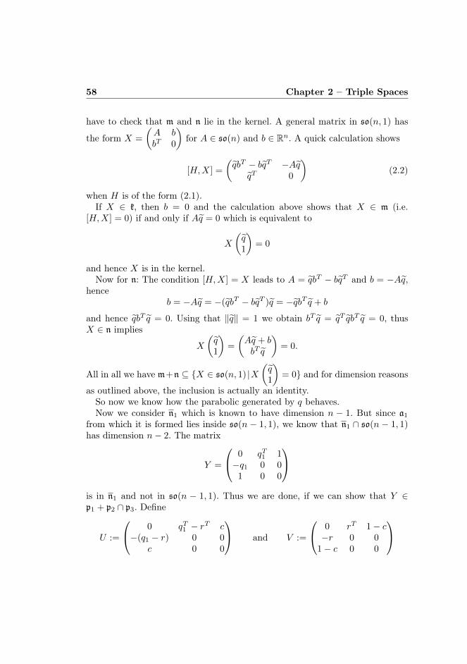
58 Chapter 2 – Triple Spaces
have to check that m and n lie in the kernel. A general matrix in so(n, 1) has
the form X =
(A bbT 0
)for A ∈ so(n) and b ∈ Rn. A quick calculation shows
[H,X] =
(qbT − bqT −Aq
qT 0
)(2.2)
when H is of the form (2.1).If X ∈ k, then b = 0 and the calculation above shows that X ∈ m (i.e.
[H,X] = 0) if and only if Aq = 0 which is equivalent to
X
(q1
)= 0
and hence X is in the kernel.Now for n: The condition [H,X] = X leads to A = qbT − bqT and b = −Aq,
henceb = −Aq = −(qbT − bqT )q = −qbT q + b
and hence qbT q = 0. Using that ‖q‖ = 1 we obtain bT q = qT qbT q = 0, thusX ∈ n implies
X
(q1
)=
(Aq + bbT q
)= 0.
All in all we have m+n ⊆ X ∈ so(n, 1) |X(q1
)= 0 and for dimension reasons
as outlined above, the inclusion is actually an identity.So now we know how the parabolic generated by q behaves.Now we consider n1 which is known to have dimension n − 1. But since a1
from which it is formed lies inside so(n − 1, 1), we know that n1 ∩ so(n − 1, 1)has dimension n− 2. The matrix
Y =
0 qT1 1−q1 0 0
1 0 0
is in n1 and not in so(n − 1, 1). Thus we are done, if we can show that Y ∈p1 + p2 ∩ p3. Define
U :=
0 qT1 − rT c−(q1 − r) 0 0
c 0 0
and V :=
0 rT 1− c−r 0 0
1− c 0 0
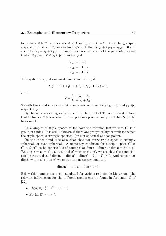
2.1 Examples and Elementary Properties 59
for some r ∈ Rn−1 and some c ∈ R. Clearly, Y = U + V . Since the qi’s spana space of dimension 2, we can find λi’s such that λ1q1 + λ2q2 + λ3q3 = 0 andsuch that λ1 + λ2 + λ3 6= 0. Using the characterization of the parabolic, we seethat U ∈ p1 and V ∈ p2 ∩ p3 if and only if
r · q1 = 1 + c
r · q2 = −1 + c
r · q3 = −1 + c
This system of equations must have a solution r, if
λ1(1 + c) + λ2(−1 + c) + λ3(−1 + c) = 0,
i.e. ifc =
λ1 − λ2 − λ3
λ1 + λ2 + λ3.
So with this c and r, we can split Y into two components lying in p1 and p2∩p3
respectively.By the same reasoning as in the end of the proof of Theorem 2.4 it follows
that Definition 2.3 is satisfied (in the previous proof we only used that SL(2,R)has rang 1).
All examples of triple spaces so far have the common feature that G′ is agroup of rank 1. It is still unknown if there are groups of higher rank for whichthe triple space is strongly spherical (or just spherical and/or polar).On the other hand it is also clear that not every triple space is strongly
spherical, or even spherical. A necessary condition for a triple space G′ ×G′ × G′/G′ to be spherical is of course that dim p + dim h ≥ dim g = 3 dim g′.Writing h = g′ = k′ ⊕ a′ ⊕ n′ and p′ = m′ ⊕ a′ ⊕ n′, we see that the conditioncan be restated as 3 dimm′ + dim a′ + dim n′ − 2 dim k′ ≥ 0. And using thatdim k′ = dim n′ + dimm′ we obtain the necessary condition
dimm′ + dim a′ − dim n′ ≥ 0.
Below this number has been calculated for various real simple Lie groups (therelevant information for the different groups can be found in Appendix C of[22]):
• SL(n,R): 12 (−n2 + 3n− 2)
• Sp(2n,R): n− n2.
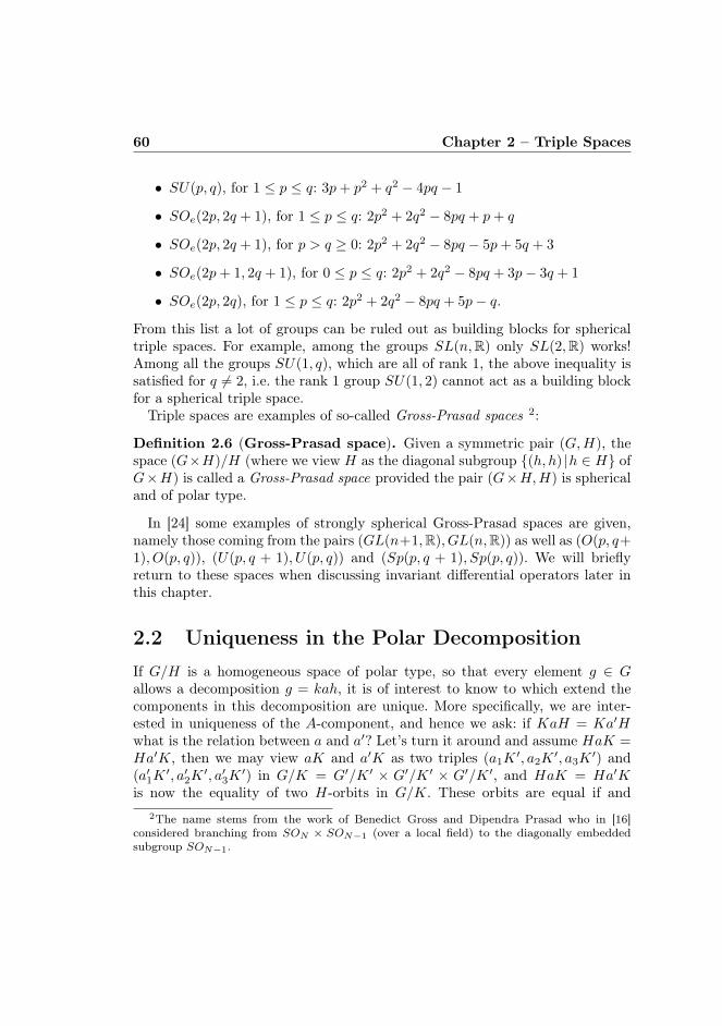
60 Chapter 2 – Triple Spaces
• SU(p, q), for 1 ≤ p ≤ q: 3p+ p2 + q2 − 4pq − 1
• SOe(2p, 2q + 1), for 1 ≤ p ≤ q: 2p2 + 2q2 − 8pq + p+ q
• SOe(2p, 2q + 1), for p > q ≥ 0: 2p2 + 2q2 − 8pq − 5p+ 5q + 3
• SOe(2p+ 1, 2q + 1), for 0 ≤ p ≤ q: 2p2 + 2q2 − 8pq + 3p− 3q + 1
• SOe(2p, 2q), for 1 ≤ p ≤ q: 2p2 + 2q2 − 8pq + 5p− q.From this list a lot of groups can be ruled out as building blocks for sphericaltriple spaces. For example, among the groups SL(n,R) only SL(2,R) works!Among all the groups SU(1, q), which are all of rank 1, the above inequality issatisfied for q 6= 2, i.e. the rank 1 group SU(1, 2) cannot act as a building blockfor a spherical triple space.Triple spaces are examples of so-called Gross-Prasad spaces 2:
Definition 2.6 (Gross-Prasad space). Given a symmetric pair (G,H), thespace (G×H)/H (where we view H as the diagonal subgroup (h, h) |h ∈ H ofG×H) is called a Gross-Prasad space provided the pair (G×H,H) is sphericaland of polar type.
In [24] some examples of strongly spherical Gross-Prasad spaces are given,namely those coming from the pairs (GL(n+1,R), GL(n,R)) as well as (O(p, q+1), O(p, q)), (U(p, q + 1), U(p, q)) and (Sp(p, q + 1), Sp(p, q)). We will brieflyreturn to these spaces when discussing invariant differential operators later inthis chapter.
2.2 Uniqueness in the Polar DecompositionIf G/H is a homogeneous space of polar type, so that every element g ∈ Gallows a decomposition g = kah, it is of interest to know to which extend thecomponents in this decomposition are unique. More specifically, we are inter-ested in uniqueness of the A-component, and hence we ask: if KaH = Ka′Hwhat is the relation between a and a′? Let’s turn it around and assume HaK =Ha′K, then we may view aK and a′K as two triples (a1K
′, a2K′, a3K
′) and(a′1K
′, a′2K′, a′3K
′) in G/K = G′/K ′ × G′/K ′ × G′/K ′, and HaK = Ha′Kis now the equality of two H-orbits in G/K. These orbits are equal if and
2The name stems from the work of Benedict Gross and Dipendra Prasad who in [16]considered branching from SON × SON−1 (over a local field) to the diagonally embeddedsubgroup SON−1.
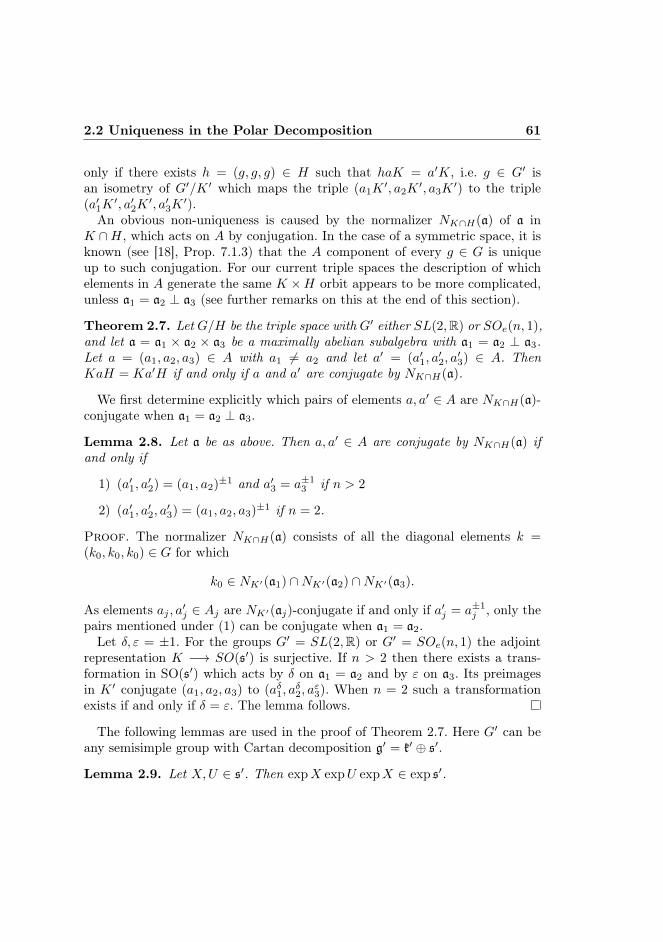
2.2 Uniqueness in the Polar Decomposition 61
only if there exists h = (g, g, g) ∈ H such that haK = a′K, i.e. g ∈ G′ isan isometry of G′/K ′ which maps the triple (a1K
′, a2K′, a3K
′) to the triple(a′1K
′, a′2K′, a′3K
′).An obvious non-uniqueness is caused by the normalizer NK∩H(a) of a in
K ∩H, which acts on A by conjugation. In the case of a symmetric space, it isknown (see [18], Prop. 7.1.3) that the A component of every g ∈ G is uniqueup to such conjugation. For our current triple spaces the description of whichelements in A generate the same K ×H orbit appears to be more complicated,unless a1 = a2 ⊥ a3 (see further remarks on this at the end of this section).
Theorem 2.7. Let G/H be the triple space with G′ either SL(2,R) or SOe(n, 1),and let a = a1 × a2 × a3 be a maximally abelian subalgebra with a1 = a2 ⊥ a3.Let a = (a1, a2, a3) ∈ A with a1 6= a2 and let a′ = (a′1, a
′2, a′3) ∈ A. Then
KaH = Ka′H if and only if a and a′ are conjugate by NK∩H(a).
We first determine explicitly which pairs of elements a, a′ ∈ A are NK∩H(a)-conjugate when a1 = a2 ⊥ a3.
Lemma 2.8. Let a be as above. Then a, a′ ∈ A are conjugate by NK∩H(a) ifand only if
1) (a′1, a′2) = (a1, a2)±1 and a′3 = a±1
3 if n > 2
2) (a′1, a′2, a′3) = (a1, a2, a3)±1 if n = 2.
Proof. The normalizer NK∩H(a) consists of all the diagonal elements k =(k0, k0, k0) ∈ G for which
k0 ∈ NK′(a1) ∩NK′(a2) ∩NK′(a3).
As elements aj , a′j ∈ Aj are NK′(aj)-conjugate if and only if a′j = a±1j , only the
pairs mentioned under (1) can be conjugate when a1 = a2.Let δ, ε = ±1. For the groups G′ = SL(2,R) or G′ = SOe(n, 1) the adjoint
representation K −→ SO(s′) is surjective. If n > 2 then there exists a trans-formation in SO(s′) which acts by δ on a1 = a2 and by ε on a3. Its preimagesin K ′ conjugate (a1, a2, a3) to (aδ1, a
δ2, a
ε3). When n = 2 such a transformation
exists if and only if δ = ε. The lemma follows.
The following lemmas are used in the proof of Theorem 2.7. Here G′ can beany semisimple group with Cartan decomposition g′ = k′ ⊕ s′.
Lemma 2.9. Let X,U ∈ s′. Then expX expU expX ∈ exp s′.
62 Chapter 2 – Triple Spaces
Proof. Let θ denote the Cartan involution and note that the productexp(tX) exp(tU) exp(tX) belongs to S := g ∈ G′ | θ(g) = g−1 for all t ∈ [0, 1].It is easily seen that k expY ∈ S implies k2 = e for k ∈ K0 and Y ∈ s′, andsince e is isolated in the set of elements of order 2 it follows that exp s′ is theidentity component of S. Hence expX expU expX ∈ exp s′.
Lemma 2.10. Let a′ ⊂ s′ be a one-dimensional subspace and let A′ = exp a′.
1) If g ∈ exp s′ and ga0 ∈ a′0K ′ for some a0, a′0 ∈ A′, then g = a′0a
−10 .
2) If g ∈ G′ and ga1, ga2 ∈ A′K ′ for some a1, a2 ∈ A′ with a1 6= a2 theng ∈ NK′(a′)A′.
Proof. (1) It follows from ga0 ∈ a′0K′ that a0ga0 ∈ a0a
′0K′. Since a0ga0 ∈
exp s′ by Lemma 2.9, it follows from uniqueness of the Cartan decompositionthat a0ga0 = a0a
′0 and thus g = a′0a
−10 .
(2) Put z0 = eK ′, then A′.z0 is a geodesic in G′/K ′. Since g maps two distinctpoints on A′.z0 into A′.z0, it maps the entire geodesic onto itself, and hence sodoes g−1. In particular g−1.z0 ∈ A′K ′, that is, g = k0a0 for some k0 ∈ K ′,a0 ∈ A′. It follows for all a ∈ A′ that
k0ak−10 = ga−1
0 ak−10 ∈ gA′K ′ = A′K ′.
As k0ak−10 ∈ exp s′, uniqueness of the Cartan decomposition implies k0ak
−10 ∈
A′, i.e. k0 ∈ NK′(a′).
Lemma 2.11. Let a1, a3 ⊂ s′ be one-dimensional subspaces with a1 ⊥ a3 andlet A1 = exp a1, A3 = exp a3. If g ∈ NK′(a1)A1 and ga3 ∈ a′3K
′ for somea3, a
′3 ∈ A3, not both equal to e, then g ∈ NK′(a1) ∩NK′(a3).
Proof. We may assume a′3 6= e, as otherwise we interchange it with a3 andreplace g by g−1. We consider the geodesic triangle in G′/K ′ formed by thegeodesics
L1 := A1.z0, L2 := A3.z0, L3 := gA3.z0.
The vertices are
D3 := z0, D2 := g.z0, D1 := ga3.z0 = a′3.z0.
As L1 and L2 intersect orthogonally, angle D3 is right. The isometry g maps L1
to itself and L2 to L3. Hence L1 and L3 also intersect orthogonally and angleD2 is right. As the sectional curvature of G′/K ′ is non-positive, it is impossible
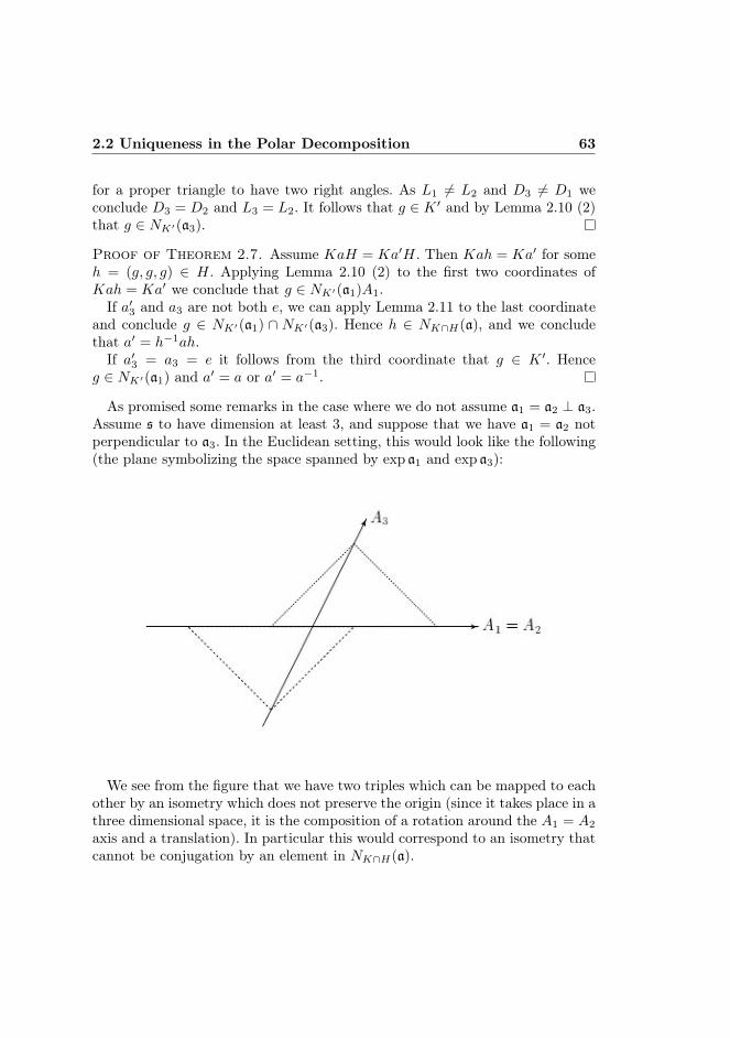
2.2 Uniqueness in the Polar Decomposition 63
for a proper triangle to have two right angles. As L1 6= L2 and D3 6= D1 weconclude D3 = D2 and L3 = L2. It follows that g ∈ K ′ and by Lemma 2.10 (2)that g ∈ NK′(a3).
Proof of Theorem 2.7. Assume KaH = Ka′H. Then Kah = Ka′ for someh = (g, g, g) ∈ H. Applying Lemma 2.10 (2) to the first two coordinates ofKah = Ka′ we conclude that g ∈ NK′(a1)A1.If a′3 and a3 are not both e, we can apply Lemma 2.11 to the last coordinate
and conclude g ∈ NK′(a1) ∩ NK′(a3). Hence h ∈ NK∩H(a), and we concludethat a′ = h−1ah.If a′3 = a3 = e it follows from the third coordinate that g ∈ K ′. Hence
g ∈ NK′(a1) and a′ = a or a′ = a−1.
As promised some remarks in the case where we do not assume a1 = a2 ⊥ a3.Assume s to have dimension at least 3, and suppose that we have a1 = a2 notperpendicular to a3. In the Euclidean setting, this would look like the following(the plane symbolizing the space spanned by exp a1 and exp a3):
We see from the figure that we have two triples which can be mapped to eachother by an isometry which does not preserve the origin (since it takes place in athree dimensional space, it is the composition of a rotation around the A1 = A2
axis and a translation). In particular this would correspond to an isometry thatcannot be conjugation by an element in NK∩H(a).
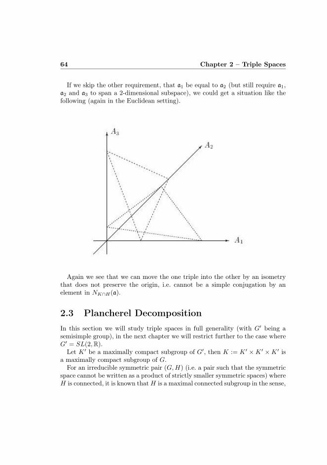
64 Chapter 2 – Triple Spaces
If we skip the other requirement, that a1 be equal to a2 (but still require a1,a2 and a3 to span a 2-dimensional subspace), we could get a situation like thefollowing (again in the Euclidean setting).
Again we see that we can move the one triple into the other by an isometrythat does not preserve the origin, i.e. cannot be a simple conjugation by anelement in NK∩H(a).
2.3 Plancherel DecompositionIn this section we will study triple spaces in full generality (with G′ being asemisimple group), in the next chapter we will restrict further to the case whereG′ = SL(2,R).Let K ′ be a maximally compact subgroup of G′, then K := K ′ ×K ′ ×K ′ is
a maximally compact subgroup of G.For an irreducible symmetric pair (G,H) (i.e. a pair such that the symmetric
space cannot be written as a product of strictly smaller symmetric spaces) whereH is connected, it is known thatH is a maximal connected subgroup in the sense,
2.3 Plancherel Decomposition 65
that if H0 is another connected subgroup such that H ⊆ H0 ⊆ G, then H0 iseither H or G. In the triple case, this is no longer true, albeit almost
Proposition 2.12. Let H0 be a connected subgroup satisfying H ⊆ H0 ⊆ G,then H0 is either H, G or one of the following 3 groups
H1 := (x, g, g) | x, g ∈ G′H2 := (g, x, g) | x, g ∈ G′H3 := (g, g, x) | x, g ∈ G′.
Proof. Consider for i = 1, 2, 3 the projection pi : G′ × G′ × G′ −→ G′ × G′which leaves out the i’th component. The image pi(H0) is a connected subgroupof G′ × G′ containing the diagonal. Since (G′ × G′, G′) is a symmetric pair,there are only two possibilities, pi(H0) equals the diagonal or everything. Thatbasically leaves us four different cases to check.First case: If pi(H0) equals the diagonal for all i, then H0 = H.Second case: If pi(H0) equals G′ ×G′ and the two others equal the diagonal:
this can’t occur.Third case: If pi(H0) equals the diagonal for some i and the two others equal
G′ ×G′, then H0 = Hi.Fourth case: If pi(H0) = G′ ×G′ for all i, then H0 = G.
In certain situations it can be useful to have a concrete model for the triplespace, just as in the group case, where the group itself is a model for the spaceG′ ×G′/G′. The map
[g1, g2, g3] 7−→ (g1g−13 , g2g
−13 )
is easily seen to be a well-defined diffeomorphism ϕ : G/H∼−−→ G′ × G′ with
inverse(g1, g2) 7−→ [g1, g2, e].
Note, however, that this concrete model is rather non-canonical: we singled outthe third component. Of course, this component is nothing special, we couldjust as well have picked the first or the second. In the following we will usethis model mostly for calculations, and to the extend possible we will try toformulate results without reference to the model.G/H has a natural G-action ρg = ρ(g1,g2,g3) given by componentwise left mul-
tiplication. Under the diffeomorphism ϕ above this is turned into the followingG-action on G′ ×G′:
(g1, g2, g3) · (g′1, g′2) = (g1g′1(g3)−1, g2g
′2(g3)−1)
66 Chapter 2 – Triple Spaces
which we also denote ρ. We can write it a little more compactly,
ϕ ρ(g1,g2,g3) = `(g1,g2) r(g3,g3) ϕ. (2.3)
where `(g1,g2) and r(g3,g3) are the left and right actions of G′ ×G′ on itself (cf.Section 1.4).
Proposition 2.13. Let G′ be a semisimple group. Then the triple space G/Hhas a G-invariant measure (unique up to a scalar), and under the diffeomor-phism ϕ above, this measure coincides (up to scalar multiplication) with theHaar measure on G′ ×G′. In particular we have the following isomorphisms ofG-spaces
L2(G/H) ∼= L2(G′ ×G′) ∼= L2(G′)⊗L2(G′) (2.4)
where the first isomorphism is f 7−→ f ϕ−1.
Proof. Since G and H are both semisimple, they are unimodular, hence aninvariant measure on G/H exists.Let µ denote the Haar measure on G′ ×G′, then (ϕ−1)∗(µ) by (2.3) satisfies
ρ(g1,g2,g3)∗(ϕ−1)∗(µ) = (ϕ−1)∗ `(g1,g2)∗ r(g3,g3)∗(µ) = (ϕ−1)∗(µ)
by left and right invariance of µ. Thus (ϕ−1)∗(µ) is G-invariant and thereforemust equal the G-invariant measure on G/H (up to a nonzero scalar).The last claim of the proposition now easily follows.
Our goal in the following is to develop a Plancherel decomposition for triplespaces. First we consider a compact example, to see what we can expect.
Example 2.14. Let’s consider the space compact triple space
SU(2)× SU(2)× SU(2)/SU(2).
The Plancherel formula for a compact homogenous space K/M tells us that
L2(K/M) =⊕
π∈KM
Hom(Vπ, VMπ ).
In this case where K = SU(2) × SU(2) × SU(2), the dual K consists of allrepresentations of the form π1 × π2 × π3 on V1 ⊗ V2 ⊗ V3. To find the M -fixedvectors we make the following general observation: assume G1 ⊆ G2 are two
2.3 Plancherel Decomposition 67
arbitrary Lie groups and that we have representations πi of Gi on Vi. Then wecan form a representation π of G1 ×G2 on Hom(V1, V2) by
π(g1, g2)(T ) := π2(g2) T π1(g1)−1.
Viewing G1 as the diagonal in G1 × G2, the invariant vectors in Hom(V1, V2)are simply HomG1
(V1, V2), i.e. the set of intertwining operators between π1 andπ2|G2
. MoreoverHom(V1, V2) ∼= V ∗1 ⊗ V2
as G1 ×G2-spaces and thus
(V ∗1 ⊗ V2)G1 ∼= HomG1(V1, V2).
We can apply this to the following situation: assume we have a group G and3 finite-dimensional G-representations V1, V2 and V3. Put G2 := G × G andlet G1 = G be sitting in G2 as the diagonal. Consider now the triple productV1⊗V2⊗V3 under the action of G×G×G, and write it as V1⊗ (V2⊗V3) underthe action of G × (G × G). Viewing G as the diagonal in G × G we are in thesituation as before and we get
(V1 ⊗ V2 ⊗ V3)G ∼= HomG(V ∗1 , V2 ⊗ V3).
Note, that the representation V2 ⊗ V3 on the right is the restriction to thediagonal, i.e. it is to be considered a representation of G and not of G × G(in which case it would have been irreducible and the HomG space would havebeen either 0 or 1-dimensional)!Obviously, there is nothing special about V1, even though we have singled it
out here. We have a natural isomorphism V1 ⊗ V2 ⊗ V3∼−−→ V2 ⊗ (V1 ⊗ V3) and
hence a natural isomorphism HomG(V ∗1 , V2⊗V3)∼−−→ HomG(V ∗2 , V1⊗V3) which
are of course also isomorphic to HomG(V ∗3 , V1 ⊗ V2).Now we return to SU(2). Given a representation V1 ⊗ V2 ⊗ V3, in order to
find the space (V1⊗V2⊗V3)SU(2) (the dimension of which ultimately equals themultiplicity of π1×π2×π3 in the Plancherel decomposition of L2(K/M)) we haveto decompose π1 ⊗ π2 according to Clebsch-Gordan and find the multiplicity ofπ∗3 in this decomposition.Recall that the irreducible representations of SU(2) are ρn for n ∈ Z≥0 of
dimension n+ 1 and that ρn ⊗ ρm decomposes according to
ρn ⊗ ρm = ρ|n−m| ⊕ ρ|n−m|+2 ⊕ · · · ⊕ ρn+m−2 ⊕ ρn+m. (2.5)
68 Chapter 2 – Triple Spaces
Moreover, all these representations are self-dual. From the discussion above weinfer that ρn × ρm × ρk occurs in the Plancherel decomposition if and only ifk ∈ |n−m|, |n−m|+ 2, . . . , n+m, and they do so with multiplicity 1.A concrete example: does the representation ρ5× ρ7× ρ1 occur in the decom-
position? Well, according to our recipe, we form the tensor product ρ7⊗ ρ1 anddecompose according to Clebsch-Gordan:
ρ5 ⊗ ρ1 = ρ4 ⊕ ρ6.
We see that ρ1 does not occur in this, and hence that ρ5×ρ1×ρ1 does not occurin the Plancherel decomposition. Then what about, say ρ5× ρ7× ρ12. Again wedecompose
ρ7 ⊗ ρ12∼= ρ5 ⊕ ρ7 ⊕ · · · ρ17 ⊕ ρ19
and see that ρ5 does occur, and hence ρ5× ρ7× ρ12 is present in the Planchereldecomposition.
This is the idea we want to generalize to non-compact triple spaces.Recall from the section on Fourier transforms that L2(G′) can be decomposed
as
L2(G′) ∼=∫ ⊕
G′Hπ⊗Hπdµ(π)
and that the bi-regular representation TG′ of G′ ×G′ on L2(G′) is decomposedas
TG′ ∼∫ ⊕
G′(π × π∗)dµ(π).
Replacing G′ by G′×G′ we have a bi-regular representation TG′×G′ of G′×G′×G′ ×G′ on L2(G′ ×G′) which is given by
TG′×G′(g1, g2, g3, g4)f(g, g′) = LG′×G′(g1, g2) RG′×G′(g3, g4)f(g, g′)
= f(g−11 gg3, g
−12 g′g4)
The action of G′ ×G′ ×G′ on G/H gives a representation ρ of G′ ×G′ ×G′ onL2(G/H). Under the isomorphism L2(G/H) ∼= L2(G′ ×G′) this representationis simply (cf. (2.3))
ρ(g1, g2, g3)f(g, g′) = f(g−11 gg3, g
−12 g′g3).
I.e. if we inject G′ ×G′ ×G′ into G′ ×G′ ×G′ ×G′ by
(g1, g2, g3) 7−→ (g1, g2, g3, g3),
2.3 Plancherel Decomposition 69
ρ is simply the restriction of TG′×G′ to G′ × G′ × G′. Decomposing TG′×G′ weget
TG′×G′ ∼∫ ⊕
G′×G′(π1 × π2)× (π1 × π2)∗dµ(π1)dµ(π2).
Restricting to G′ ×G′ ×G′ (which comes down to restricting (π1 × π2)∗ to thediagonal of G′ ×G′) and replacing πi by π∗i (this is allowed, since π is in G′ ifand only if π∗ is) we get
ρ ∼∫ ⊕
G′×G′(π∗1 × π∗2)× (π1 ⊗ π2)dµ(π1)dµ(π2). (2.6)
Decomposing the tensor product π1 ⊗ π2 =∫G′π⊕mπ33 dνπ1,π2
(π3) (cf. Theorem1.22) we arrive at
Theorem 2.15. The decomposition of ρ into irreducibles is
ρ ∼∫ ⊕
G′×G′π∗1 × π∗2 ×
(∫ ⊕
G′π⊕mπ33 dνπ1,π2
(π3))dµ(π1)dµ(π2)
∼∫ ⊕
G′×G′×G′(π∗1 × π∗2 × π3)⊕mπ3 dνπ1,π2
(π3)dµ(π2)dµ(π1) (2.7)
where µ is the Plancherel measure on G′.
This is the general version of the observation from the compact case above.In effect, the result states that the triple product π∗1 × π∗2 × π3 “occurs” in thedecomposition of ρ if and only if π3 “occurs” in the decomposition of the tensorproduct π1 ⊗ π2, and with the same multiplicity.Just as for groups, we can talk about discrete series representations for a
homogenous space:
Definition 2.16 (Discrete Series). A representation (π,Hπ) ∈ GH is calleda discrete series representation for G/H if HomG(Hπ, L
2(G/H)) 6= 0.
It is clear from the theorem above, that π1 × π2 × π3 is a discrete seriesrepresentation for the triple space G/H, if and only if π1 and π2 are discreteseries representations with π∗3 sitting discretely in π1 ⊗ π2, and it is clear thatthe multiplicity of π1× π2× π3 in L2(G/H) equals that of π3 in π∗1 ⊗ π∗2 . If thismultiplicity is finite we can write down an explicit isomorphism
Φ : HomG′(H3,H1⊗H2)∼−−→ HomG(H∗1⊗H∗2⊗H3, L
2(G/H))
70 Chapter 2 – Triple Spaces
given by
Φ(S)(ϕ1⊗ϕ2⊗v3)[g1, g2, g3] :=(π∗1(g−1
1 )ϕ1 ⊗ π∗2(g−12 )ϕ2
)S(π3(g−1
3 )v3). (2.8)
2.4 Invariant Differential Operators
In this section we investigate the algebra of invariant differential operatorsD(G/H) first for a general triple space. More specifically, our first concern willbe, to determine, for which of the strongly spherical spaces listed previously inthis chapter, the algebra of invariant differential operators is commutative. Itturns out to be the case for only a few of them.
Definition 2.17. Let G be a Lie group and let K be a compact subgroup. Thepair (G,K) is called a Gelfand pair if for any irreducible unitary representationπ of G, it holds that the multiplicity of the trivial representation of K in π|K isat most 1.
In the older literature, the terminology will often be used that K is a sphericalsubgroup of G.As the following proposition states there are other (equivalent) ways of defin-
ing Gelfand pairs. We took the above one as the defining property since it is theone which is best suited for our needs.
Proposition 2.18. For a pair (G,K) of a Lie group and a compact subgroupK, the following are equivalent
1) (G,K) is a Gelfand pair.
2) The algebra D(G/K) of left G-invariant differential operators on G/K iscommutative.
3) The convolution algebra L1(K\G/K) is commutative.
The equivalence between 1) and 2) is proved in Proposition 6.3.1 in [12] andthe equivalence between 2) and 3) is stated in Theorem 4 in [11].Well known examples are non-compact Riemannian symmetric pairs (G,K)
where G is a reductive Lie group and K is a maximally compact subgroup. Be-cause of the duality between compact and non-compact Riemannian symmetricspaces, also compact Riemannian symmetric pairs (U,K) are Gelfand pairs.
2.4 Invariant Differential Operators 71
Definition 2.19. A pair (G,K) of a Lie group G and a compact subgroup Kis called a strong Gelfand pair provided that (G ×K,∆K) (where ∆K meansthe K-diagonal in G×K) is a Gelfand pair.
Proposition 2.20. A pair (G,K) where G is connected and K is connectedand compact, is a strong Gelfand pair if and only if for any π ∈ G and anyδ ∈ K, the multiplicity of δ in π|K is at most 1.
Proof. If π ∈ G and δ ∈ K, we note the identities 3
H∆Kπ×δ = (Hπ⊗Hδ)
∆K = HomK(δ∗, π|K)
where δ∗ is the dual of δ. This leads to the following string of identities ofdimensions:
dim HomK(1, (π × δ)|∆K) = dim HomK(π × δ|∆K , 1) = dimH∆Kπ×δ
= dim HomK(δ∗, π|K).
Since any irreducible unitary representation of G × K is of the form π × δ, itfollows that (G×K,∆K) is a Gelfand pair, if and only if the multiplicity of δ∗in π|K is at most 1.
From the proposition it is clear that any strong Gelfand pair is in particulara Gelfand pair, hence justifying the name. Note that if (G,K) and (G′,K ′) arestrong Gelfand pairs, then so is (G × G′,K × K ′), simply because, if π|K =⊕
δ∈K δ⊕mδ and π′|K′ =
⊕τ∈K′ τ
⊕mτ for irreducible representations π and π′of G and G′ respectively, then mδ,mτ ≤ 1 and hence
(π × π′)|K×K′ =⊕
(δ,τ)∈K×K′
(δ × τ)⊕mδmτ
wheremδmτ ≤ 1. Thus irreducible representations of G×G′ decompose withoutmultiplicity when restricted to K ×K ′.In the case where G itself is compact, the strong Gelfand pairs have been
classified by Krämer in [23] (he uses the terminology that K is a multiplicityfree subgroup in G). The first two results of his paper relevant to us are thefollowing (Proposition 2 slightly reformulated and Corollary 2 in loc.cit.):
3We use the notation that π× δ is the representation of G×K on Hπ⊗Hδ (the completedHilbert tensor product) given by (π × δ)(g, k)v ⊗ w = π(g)v ⊗ δ(k)w.
72 Chapter 2 – Triple Spaces
Lemma 2.21. Let (G,K) and (G′,K ′) be pairs where G and G′ are compactand connected, and where K and K ′ are closed and connected subgroups andassume we have a local isomorphism G −→ G′ which maps K to K ′, then(G,K) is a strong Gelfand pair if and only if (G′,K ′) is a strong Gelfand pair.
Lemma 2.22. Let G be a compact connected and simple Lie group and K aclosed subgroup and K0 the identity component, then (G,K) is a strong Gelfandpair if and only if (G,K0) is a strong Gelfand pair.
The following is the main theorem of Krämer’s paper. Note that point 4) is aconsequence of the preceding two lemmas.
Theorem 2.23 (Krämer). Let G be a compact connected Lie group and K aclosed subgroup whose identity component we denote K0.
1) If G is simple, then (G,K) is a strong Gelfand pair if and only if up tocovering, either
• the pair is of the form (SU(n), U(n− 1)) for n ≥ 2, or
• G = SO(n) and K0 = SO(n− 1) for n ≥ 3, n 6= 4, or
• G = SO(8) and K0 = Spin(7), or
• trivially G = K.
2) If G is semisimple, then (G,K) is a strong Gelfand pair if and only ifthere exist strong Gelfand pairs (G1,K1), . . . , (Gn,Kn) with Gi simple andKi connected, and there exists a number m, such that we have a localisomorphism G
∼−−→ G1×· · ·×Gn×SO(4)×m which maps K0 to K1×· · ·×Kn×SO(3)×m where SO(3) sits inside SO(4) (which is locally isomorphicto SO(3)× SO(3)) as the diagonal.
3) If G = Gs × T where Gs is semisimple and T is a torus, then (G,K) isa strong Gelfand pair if and only if (Gs, p(K)) is a strong Gelfand pair(where p : G −→ Gs is the projection).
4) If q : G −→ G is a connected covering of G, then (G,K) is a strongGelfand pair, if and only if (G, q−1(K)) is a strong Gelfand pair.
This theorem enables us to determine for each pair (G,K) (where G is com-pact and connected, and K is a closed subgroup) if it is a strong Gelfand pairor not: As G is compact, its Lie algebra is automatically reductive, hence is of
2.4 Invariant Differential Operators 73
the form g = gs ⊕ Zg, i.e. is a direct sum of a semisimple part gs = [g, g] andthe center. Let Gs be the analytic subgroup of G corresponding to gs, then wehave a covering map π : Gs×T −→ G by (g, z) 7−→ gz. Thus (G,K) is a strongGelfand pair if and only if (Gs, q(π
−1(K))) is a strong Gelfand pair.
Corollary 2.24. The only strong Gelfand pair of the form (G0 ×G0, G0) withG0 compact, connected and simple is (SO(3) × SO(3), SO(3)). Consequently,(SO(n)×SO(n), SO(n)) is a strong Gelfand pair, if and only if n = 3 or n = 4.
Proof. (SO(3) × SO(3), SO(3)) is a strong Gelfand pair as it is locally iso-morphic to the Gelfand pair (SO(4), SO(3)). Also (SO(4)× SO(4), SO(4)) is astrong Gelfand since it is locally isomorphic to the product of the strong Gelfandpair (SO(3)× SO(3), SO(3)) with itself. The only if statement of this corollaryfollows from Krämer’s list of semisimple strong Gelfand pairs above.
Recall that given a real Lie algebra g, we denote by U(gC) the universalenveloping algebra of the complexification of g and we identify this with thealgebra D(G) of left-invariant differential operators on G. If H is a closed sub-group of G we can extend the adjoint action of H on g to an algebra action ofH on U(gC) by
Ad(h)X1 · · ·Xn := (Ad(h)X1) · · · (Ad(h)Xn).
Let U(gC)k denote the set of elements of U(g) of degree at most k. By the PBW-Theorem this is a finite-dimensional space, and it is clear, that it is preservedby Ad(h). Thus Ad is a finite-dimensional representation of H on U(gC)k. Thisof course has a derived representation of h:
Ad∗(X)(X1 · · ·Xn) =d
dt
∣∣∣∣t=0
Ad(exp(tX))(X1 · · ·Xn)
=d
dt
∣∣∣∣t=0
(Ad(exp(tX))X1) · · · (Ad(exp(tX))Xn)
=
n∑
j=1
X1 · · ·( d
dt
∣∣∣∣t=0
Ad(exp(tX))Xj
)· · ·Xn
=
n∑
j=1
X1 · · · [X,Xj ] · · ·Xn.
74 Chapter 2 – Triple Spaces
We extend this representation to U(gC) =⋃U(gC)k and denote it ad:
ad(X)(X1 · · ·Xn) =
n∑
j=1
X1 · · · (ad(X)Xj) · · ·Xn
= X(X1 · · ·Xn)− (X1 · · ·Xn)X
where the last equality follows from a simple computation involving commuta-tors. The first expression tells us that ad(X) is a derivation of U(gC) and thesecond, that we can view ad(X) as a commutator, just as in the Lie algebrasituation. Since U(gC) is a complex algebra, we can without problems extendad to a representation of hC.By U(gC)H we denote the subset of elements of U(gC) which are invariant
under Ad(h) for all h ∈ H, and by U(gC)h the set of elements which are mappedto 0 by ad(X) for all X ∈ h, i.e.
U(gC)h =⋂
X∈h
ker ad(X).
U(gC)hC is defined similarly.
Lemma 2.25. If H is a connected subgroup of G, it follows that U(gC)H =U(gC)h = U(gC)hC .
Proof. The last identity is obvious and holds whether H is connected or not.For the first identity, the inclusion “⊆” follows easily by the above, since ad
is the derived representation of Ad. For the reverse inclusion “⊇” we need theconnectivity assumption, for then any h ∈ H can be written as a finite producth = expX1 · · · expXn for Xj ∈ h so we may assume w.l.o.g. that h = expX1. IfX ∈ U(gC)h, then
Ad(expX1)X = exp(ad(X1))X = (I + (adX1) + 12 (adX1)2 + · · · )X = X,
i.e. X ∈ U(gC)H .
Lemma 2.26. If G and G′ are Lie groups with closed connected subgroups Hand H ′ respectively, for which there is a Lie algebra isomorphism ϕ : gC
∼−−→ g′Cbetween the complexifications of the Lie algebras of G and G′ and such thatϕ(hC) = ϕ(h′C), then D(G/H) and D(G′/H ′) are isomorphic as algebras.
2.4 Invariant Differential Operators 75
Proof. For any homogenous space, we have an algebra isomorphism
D(G/H)∼−−→ U(gC)H/(U(gC)H ∩ U(gC)h) (2.9)
and by the lemma above the latter equals U(gC)hC/(U(gC)hC ∩ U(gC)hC).The Lie algebra isomorphism ϕ induces an algebra isomorphism ϕ : U(gC)
∼−−→U(g′C), and it requires but a small calculation to verify that ϕ(U(gC)hC) =
U(g′C)h′C and ϕ(U(gC)hC) = U(g′C)h′C. Thus ϕ induces an algebra isomorphism
U(gC)hC/(U(gC)hC ∩ U(gC)hC)∼−−→ U(g′C)h
′C/(U(g′C)h
′C ∩ U(g′C)h′C)
which, by the remarks at the beginning of the proof, is the desired algebraisomorphism D(G/H)
∼−−→ D(G′/H ′).
Let us apply this to triple spaces. If G′ is a compact Lie group, it followsfrom the above discussion of Gelfand pairs that (G′ ×G′ ×G′, G′) (where G′ isviewed as the diagonal) is a Gelfand pair if and only if (G′ ×G′, G′) is a strongGelfand pair.Any linear semisimple Lie group G′ has a complexification G′C which in turn
has a compact real form G′, in other words, for any linear semisimple Lie groupG′, there is a compact Lie group G′ such that the complexification of the twoLie algebras are isomorphic. We call G′ the compact form of G′. By the abovelemma, commutativity of D(G/H) follows if and only if (G′× G′, G′) is a strongGelfand pair. Thus we get
Theorem 2.27. Let G/H be a triple space as above with G′ connected andsemisimple. The algebra D(G/H) is commutative if and only if the compactform of G′ is locally isomorphic to SO(3) or SO(4). In particular, among thegroups G′ = SOe(n, 1), only SOe(2, 1) and SOe(3, 1) have corresponding triplespaces with commuting invariant differential operators.
Our second application will be to Gross-Prasad spaces. These have been stud-ied in [24] where it was found that Gross-Prasad spaces from the pairs
• (GL(n+ 1,F), GL(n,F)) for F = R,C,
• (O(p, q + 1), O(p, q)) for p+ q ≥ 2,
• (U(p, q + 1), U(p, q)) for p+ q ≥ 2,
• (Sp(p, q + 1), Sp(p, q)) for p+ q ≥ 2
76 Chapter 2 – Triple Spaces
are spherical and polar.
Theorem 2.28. For all the Gross-Prasad spaces in the list above except (Sp(p, q+1)×Sp(p, q))/Sp(p, q), it holds that the algebra of invariant differential operatorsis commutative.
Proof. Again it follows from Lemma 2.26 that if (G′, H ′) is a compact form of(G,H), then D(G ×H/H) ∼= D(G′ ×H ′/H ′). And it follows from Proposition2.18 that D(G′ × H ′/H ′) is commutative if and only if (G′, H ′) is a strongGelfand pair.The pair (GL(n + 1,R), GL(n,R)) has the compact form (U(n + 1), U(n)).
The map q : SU(n+1)×U(1) −→ U(n+1) given by (A, z) 7−→ zA is a coveringmap (since it is a group homomorphism whose corresponding Lie algebra mapis an isomorphism). If we view U(n) as sitting in U(n + 1) in the lower rightcorner, then
q−1(U(n)) =
(
(z−1 00 z−1A′
), z)∣∣∣A′ ∈ U(n) zn+1 = detA′
.
The projection of this set onto SU(n+ 1) is therefore
p(q−1(U(n))) =(
z−1 00 z−1A′
) ∣∣∣A′ ∈ U(n) zn+1 = detA′
which is just the standard embedding of U(n) into SU(n + 1). Since (SU(n +1), U(n)) is a strong Gelfand pair, it follows (by Krämer’s theorem and Lemma2.22) that (U(n+1), U(n)) is a strong Gelfand pair. Hence the algebra of differ-ential operators for the Gross-Prasad space of the pair (GL(n+1,R), GL(n,R))is commutative.Similarly, the pair (U(p, q+1), U(p, q)) has compact form (U(p+q+1), U(p+
q)), and this is a strong Gelfand pair by the same arguments as above.The pair (O(p, q+1), O(p, q)) has compact form (O(p+q+1), O(p+q)) which
is locally isomorphic to the strong Gelfand pair (SO(p+ q + 1), SO(p+ q)).Finally (Sp(p, q + 1), Sp(p, q)) has compact form (Sp(p + q + 1), Sp(p + q))
which is not a strong Gelfand pair.
CHAPTER 3
A SPECIAL CASE
3.1 Invariant Differential Operators
We continue our description of the algebra D(G/H) from the previous chapter,now only for the triple space with G′ = SL(2,R). We prove that this is anabelian algebra in 3 generators.In this section we will work a lot with U(g1C⊕ g2C), and the following lemma
will make this space slightly easier to handle.
Lemma 3.1. We have an algebra isomorphism
D(G1 ×G2) = U(g1C ⊕ g2C)∼−−→ U(g1C)⊗ U(g2C) = D(G1)⊗ D(G2)
which maps
(X1, 0) · · · (Xn, 0)(0, Y1) · · · (0, Ym) 7−→ (X1 · · ·Xn)⊗ (Y1 · · ·Ym)
Proof. Consider the map g1 ⊕ g2 −→ U(g1C) ⊗ U(g2C) given by (X,Y ) 7−→X⊗1+1⊗Y . It is easily checked that this map is linear and satisfies the bracketrelation. Thus it factorizes as an algebra homomorphism through U(g1C⊕ g2C).This is the desired map. It is easily seen to map a PBW-basis to a PBW-basis,and thus it is an algebra isomorphism.
77
78 Chapter 3 – A Special Case
We use the model G/H ∼= G′ × G′. The G-action on G′ × G′ is simply thatthe two first copies act on each of the arguments from the left and the thirdcopy acts diagonally from the right. Thus we immediately see that we have thefollowing string of inclusions
Z(G′ ×G′) ⊆ D(G/H) ⊆ D(G′ ×G′) (3.1)
where Z(G′×G′) is the algebra of bi-invariant differential operators on G′×G′,which happens to be equal to the center of D(G′ × G′) ∼= U(g′C ⊕ g′C). In ourpresent example, all inclusions will be strictConsider the standard basis for sl(2,R)
H0 :=
(1 00 −1
), X0 :=
(0 10 0
), Y0 :=
(0 01 0
)
(we add subscripts 0 to avoid confusion between H0 as a matrix and H as asubgroup), which satisfies the usual commutation relations
[X0, Y0] = H0, [H0, X0] = 2X0, [H0, Y0] = −2Y0.
Consider the inclusions (3.1). Z(G′×G′) ⊆ D(G/H) and Z(G′×G′) ∼= Z(G′)⊗Z(G′) (it is a standard fact from algebra, that the center of a tensor productof algebras is the tensor product of the centers), and in this specific case ofG′ = SL(2,R), the center Z(G′) is generated by the Casimir element , whichrelative the the basis for sl(2,R) above takes the following form: ω = 1
2H20 +
X0Y0+Y0X0 = 12H
20 +H0+2X0Y0. Consequently, we have at least two generators
for the algebra D(G/H), namely ω⊗1 and 1⊗ω. Furthermore, it can be checkedthat the element
Ω := 12H0 ⊗H0 +X0 ⊗ Y0 + Y0 ⊗X0
is actually an element of D(G/H) ∼= U(g′C ⊕ g′C)H without being an element ofthe center Z(G′ × G′) (it doesn’t commute with H0 ⊗ 1 for instance). In fact,ω⊗1 and 1⊗ω and Ω constitute a basis for U(g′C⊕g′C)H2 . Thus we have a thirdgenerator and in particular the first inclusion in (3.1) is strict. Also the otherinclusion is strict: X0⊗Y 2
0 for example, is an element in D(G′×G′) = U(g′C⊕g′C)which is not in U(g′C⊕g′C)H = U(g′C⊕g′C)h (it is not ad(H0)-invariant - in orderto be so, the sum of the powers of X0 should equal the sum of the powers ofY0).That leaves us the following question: are there any more generators for
D(G/H) other than ω ⊗ 1, 1 ⊗ ω and Ω? The answer turns out to be no, as
3.1 Invariant Differential Operators 79
we now explain. First, note that so(4) ∼= su(2)⊕ su(2) and hence by complexi-fication sl(2,C)⊕ sl(2,C) ∼= so(4,C). Thus U(sl(2,C)⊕ sl(2,C)) ∼= U(so(4,C)).Furthermore sl(2,C) ∼= su(2)C ∼= so(3,C). Thus we have
D(G/H) = U(g′C ⊕ g′C)hC = U(so(4,C))so(3).
This particular algebra has been studied in [4] and the statement is that itis generated by Z(SO(4)) and by Z(SO(3)) (the centers of U(so(4,C)) andU(so(3,C)) respectively). SO(4) has rank 2 and SO(3) has rang 1 and hence intotal there are 3 generators for D(G/H). Wrapping up:
Theorem 3.2. D(G/H) is a commutative algebra in 3 generators. Viewed asa subalgebra of D(G′ × G′) ∼= D(G′) ⊗ D(G′), the generators are ω ⊗ 1, 1 ⊗ ωand Ω.
One drawback of this viewpoint is that it depends on the specific realizationof G/H as G′ ×G′, which is non-canonical since we singled out the third com-ponent. A slightly different and more invariant viewpoint is the following. Forany homogenous space G/H we have an algebra homomorphism
p : DH(G) −→ D(G/H)
given by (p(D)f)p = D(f p) where p : G −→ G/H is the projection and whereDH(G) is the algebra of differential operators which are left G-invariant andright H-invariant (this algebra is isomorphic to U(gC)H). In particular we canrestrict p to Z(G) ⊆ DH(G) and study how the generators of Z(G) are mappedto D(G/H). Both algebras are abelian in 3 generators, so if we can show thatit maps generators to generators, it follows that it is an algebra isomorphism.The identification of D(G/H) with Z(G′ ×G′ ×G′) is more canonical than theidentification with U(g′C ⊕ g′C)h.To formalize this, let ϕ : G/H
∼−−→ G′ × G′ be the G-equivariant diffeomor-phism [g1, g2, g3] 7−→ (g1g
−13 , g2g
−13 ). The induced map on algebras of differential
operators ϕ : D(G/H) −→ DG′(G′ ×G′) given by
(ϕ(D)f)(g1, g2) = D(f ϕ)(ϕ−1(g1, g2))
is a realization of the identification D(G/H) ∼= DG′(G′ ×G′). Composing p andϕ we obtain the map ϕ p : Z(G′×G′×G′) −→ DG′(G′×G′) which is given by
(ϕ p)(D)f(ϕ(g0H)) = D(f ϕ p)(g0). (3.2)
80 Chapter 3 – A Special Case
Note how the right-hand side makes sense, for any D ∈ D(G), whereas the left-hand side only makes sense as an invariant differential operator on functions onG/H if D ∈ DH(G).We want to calculate the action of this map on the three generators ω⊗1⊗1,
1 ⊗ ω ⊗ 1 and 1 ⊗ 1 ⊗ ω of Z(G′ × G′ × G′) ∼= Z(G′) ⊗ Z(G′) ⊗ Z(G′). It isnot hard to see that ω ⊗ 1 ⊗ 1 and 1 ⊗ ω ⊗ 1 are mapped to ω ⊗ 1 and 1 ⊗ ωrespectively. So the only problem is calculating (ϕ p)(1⊗ 1⊗ ω). We calculatethe right hand side of (3.2) term by term. First 1⊗ 1⊗H2
0 :
(1⊗ 1⊗H20 )(f ϕ p)(g1, g2, e)
=∂2
∂t∂s
∣∣∣∣(0,0)
(f ϕ p)(g1, g2, exp((s+ t)H0))
=∂2
∂t∂s
∣∣∣∣(0,0)
f(g1 exp(−(s+ t)H0), g2 exp(−(s+ t)H0)).
For a function h of the form (s, t) 7−→ f(s+ t, s+ t) we get from the chain rule
∂2h
∂t∂s(0, 0) =
∂2f
∂x21
(0, 0) +∂2f
∂x22
(0, 0) + 2∂2f
∂x1∂x2(0, 0).
Applied to the expression above we get
(1⊗ 1⊗H20 )(f ϕ p)(g1, g2, e) = (H2
0 ⊗ 1 + 1⊗H20 + 2H0 ⊗H0)f(g1, g2)
in other words (ϕ p)(1⊗ 1⊗H20 ) = H2
0 ⊗ 1 + 1⊗H20 + 2H0 ⊗H0.
Then what about (ϕ p)(1⊗ 1⊗X0Y0)?
(1⊗ 1⊗X0Y0)(f ϕ p)(g1, g2, e)
=∂2
∂t∂s
∣∣∣∣(0,0)
(f ϕ p)(g1, g2, exp(tX0) exp(sY0))
=∂2
∂s∂t
∣∣∣∣(0,0)
f(g1 exp(−sY0) exp(−tX0), g2 exp(−sY0) exp(−tX0)).
The t-derivative must be (−X0⊗ 1− 1⊗X0)f(g1 exp(−sY0), g2 exp(−sY0)) andthe s-derivative of this must be
(−Y0 ⊗ 1− 1⊗ Y0)(−X0 ⊗ 1− 1⊗X0)f(g1, g2)
in other words
(ϕ p)(1⊗ 1⊗X0Y0) = Y0X0 ⊗ 1 + Y0 ⊗X0 +X0 ⊗ Y0 + 1⊗ Y0X0
3.1 Invariant Differential Operators 81
and similarly
(ϕ p)(1⊗ 1⊗ Y0X0) = X0Y0 ⊗ 1 +X0 ⊗ Y0 + Y0 ⊗X0 + 1⊗X0Y0.
From these formulas we conclude that
(ϕ p)(1⊗ 1⊗ ω) = ω ⊗ 1 + 1⊗ ω + 2Ω (3.3)
and this in combination with 1⊗ω and ω⊗ 1 is a complete set of generators forDG′(G′ ×G′). Since ϕ is already an algebra homomorphism we conclude
Theorem 3.3. The map p : Z(G′ × G′ × G′) −→ D(G/H) is an algebra iso-morphism.
In the previous chapter, we noted that there were only two triple spaces(known so far) which have commuting algebras of invariant differential opera-tors, namely triple spaces with G′ = SL(2,R) and G′ = SOe(3, 1).For the second space, we have
D(G/H) = U(so(4,C)⊕ so(4,C))so(4)
and as so(4) ∼= so(3)⊕ so(3), we can write this as
U(so(3,C)⊕4)so(3)⊕so(3)
where (X,Y ) ∈ so(3)⊕ so(3) =: h sits inside so(4,C)⊕ so(4,C) ∼= so(3,C)⊕4 as(X,Y,X, Y ). We can also embed so(3)⊕so(3) in so(4,C)⊕so(4,C) ∼= so(3,C)⊕4
as (X,Y ) 7−→ (X,X, Y, Y ), i.e. a componentwise embedding of so(3) into so(4)(as the diagonal). We call this subalgebra h′. It is clear that the Lie algebraautomorphism so(3,C)⊕4 −→ so(3,C)⊕4 which flips the second and third com-ponent, maps h to h′ and thus gives an isomorphism
D(G/H) ∼= U(so(4,C)⊕ so(4,C))h′.
By (1.15) (in the special case where δ1 and δ2 are both the trivial representa-tion) we get that the space ofK1×K2-invariant vectors in a tensor product is thetensor product of the spaces of K1 and K2-invariant vectors for the individualrepresentations. We can apply this to the above setting with K1 = K2 = SO(3)acting on the finite-dimensional spac U(so(4,C))N (the set of elements of degreeat most N). Then we get
U(so(4,C)⊕ so(4,C))h′
2N = [U(so(4,C))N ⊗ U(so(4,C))N ]SO(3)×SO(3)
∼= U(so(4,C))SO(3)N ⊗ U(so(4,C))
SO(3)N .
82 Chapter 3 – A Special Case
As this holds for all N , we conclude
U(so(4,C)⊕ so(4,C))h′ ∼= U(so(4,C))SO(3) ⊗ U(so(4,C))SO(3)
and hence:
Theorem 3.4. For the triple space (G′ ×G′ ×G′)/G′ with G′ = SOe(3, 1), itholds that
D(G′ ×G′ ×G′)/G′) ∼= D(SL(2,R)×3/SL(2,R))⊗2
hence the algebra of invariant differential operators is a commutative algebra in6 generators.
This shows, however, that the identification D(G/H) ∼= Z(G) which was truefor the SL(2,R)-triple space, is not true in general, since Z(SOe(3, 1)×3) is anabelian algebra in only 3 generators.
3.2 Action on Matrix CoefficientsNow we return to the triple space G/H with G′ = SL(2,R). Next goal is to seehow invariant differential operators act on irreducible matrix coefficients and toshow that they are eigenfunctions for the invariant differential operators. Thisis analogous to the result for reductive symmetric spaces, where it was shownby van den Ban in [2], Theorem 1.5.
Theorem 3.5. For any D ∈ D(G/H) and any π ∈ GH , thenDMη,v = Mπ(D)η,v = χπ(D)Mη,v (3.4)
holds for all v ∈ H∞π and η ∈ H−∞,Hπ where χπ is the infinitesimal character ofπ.
Proof. The entire proof is based on the fact, that we can identify D(G/H)with Z(G) as shown in the previous section. For any such D we know thatπ(D) : H∞π −→ H∞π is just multiplication by χπ(D), the infinitesimal characterevaluated in D. By duality, π(X) acts by the same scalar on H−∞,Hπ . Thisexplains the last identity in (3.4). To verify the first, we view Mη,v as a rightH-invariant function on G and compute for X ∈ g:
(XMη,v)(g) =d
dt
∣∣∣∣t=0
η(π(exp(−tX)g−1)v) = (Xη)(π(g−1)v) = MXη,v(g).
This shows the identity.
3.2 Action on Matrix Coefficients 83
In general, if hC is a Cartan subalgebra of gC, we recall the Harish-Chandraisomorphism (1.9)
γ : Z(G)∼−−→ U(hC)W
from Z(G) onto Weyl-invariant polynomials over h∗C. For any λ ∈ h∗C we get acharacter of Z(G) by composing it with the Harish-Chandra isomorphism
χλ(D) := λ(γ(D))
and all characters of Z(G) are of this form (cf. Theorem 1.17).Getting back to SL(2,R): the holomorphic discrete series representation Tm
has Harish-Chandra parameter m+ 1 (the m is the Blattner parameter, i.e. thelowest K-weight for the representation) and the anti-holomorphic discrete seriesrepresentation T−n has Harish-Chandra parameter −n− 1. Thus
χTm(D) = γ(D)(m± 1)1.
As the infinitesimal character satisfies
χπ1×π2(D1 ⊗D2) = χπ1
(D1) + χπ2(D2)
we get in general
χTn×Tm×Tk(D1 ⊗D2 ⊗D3) = γ(D1)(n± 1) + γ(D2)(m± 1) + γ(D3)(k ± 1).
In the following example we verify the above considerations by a direct com-putation.
Example 3.6. Let us confirm these deductions by a concrete hands-on examplewhere we consider the representation T−n×T−m×Tn+m which is a discrete seriesrepresentation for G/H, since Tn+m sits as a direct summand in T ∗−n ⊗ T ∗−m =Tn⊗Tm. From [27] we know that HomG′(Tn+m, Tn⊗Tm) is 1-dimensional. Fromthe proof in [27] of the decomposition of Tn⊗Tm we know that both Tn+m andTn⊗Tm have unique (up to a scalar) K-weight vectors of weight n+m, namelyψ0n+m and ψ0
n ⊗ ψ0m respectively. Thus any S ∈ HomG′(Hn+m,Hn⊗Hm) must
map ψ0n+m to a multiple of ψ0
n ⊗ ψ0m. We scale S such that it actually maps
ψ0n+m to ψ0
n ⊗ ψ0m.
Under the isomorphism (2.8)
Φ : HomG′(Hn+m,Hn⊗Hm)∼−−→ HomG(H−n⊗H−m⊗Hn+m, L
2(G/H)),
1Here the ± should be interpreted so that it is + when m > 0 and − when m < 0.
84 Chapter 3 – A Special Case
Φ(S) maps ψ0−n ⊗ ψ0
−m ⊗ ψ0n+m to the following function in L2(G/H):
Φ(S)(ψ0−n ⊗ ψ0
−m ⊗ ψ0n+m)[g1, g2, g3]
=(T−n(g−1
1 )ψ0−n ⊗ T−m(g−1
2 )ψ0−m)S(Tn+m(g−1
3 )ψ0n+m).
By the identification G/H ∼= G′ ×G′, (g1, g2) ∼ [g1, g2, e] it suffices to look at
f(g1, g2) := Φ(S)(ψ0−n ⊗ ψ0
−m ⊗ ψ0n+m)(g1, g2)
=[T−n(g−1
1 )ψ0−n ⊗ T−m(g−1
2 )ψ0−m]S(ψ0
n+m)
= [T−n(g−11 )ψ0
−n ⊗ T−m(g−12 )ψ0
−m](ψ0n ⊗ ψ0
m)
= (T−n(g−11 )ψ0
−n)(ψ0n) · (T−m(g−1
2 )ψ0−m)(ψ0
m).
We know that ψ0−n = ψ0
n, and
T−n(g−11 )ψ0
n = Tn(g−11 )ψ0
n,
and we know how this acts on the vector ψ0n, namely by
Tn(g−11 )ψ0
n(ψ0n) = 〈Tn(g−1
1 )ψ0n, ψ
0n〉.
Thus we end up with the function
f(g1, g2) = 〈Tn(g−11 )ψ0
n, ψ0n〉〈Tm(g−1
2 )ψ0m, ψ
0m〉.
Now, let us see how a differential operator of the form X⊗1 acts on this function
(X ⊗ 1)f(g1, g2) =d
dt
∣∣∣∣t=0
〈Tn(exp(−tX)g−11 )ψ0
n, ψ0n〉〈Tm(g−1
2 )ψ0m, ψ
0m〉
= 〈−Tn(X)Tn(g−11 )ψ0
n, ψ0n〉〈Tm(g−1
2 )ψ0m, ψ
0m〉
= 〈Tn(g−11 )ψ0
n, Tn(X)ψ0n〉〈Tm(g−1
2 )ψ0m, ψ
0m〉.
Thus the X-action is moved to the other side of the bracket. Acting with Ω =12T ⊗ T +X+ ⊗X− +X− ⊗X+ (written in the basis (1.21)) we get
(Ωf)(g1, g2) = − 12 〈Tn(g−1
1 )ψ0n, Tn(T )ψ0
n〉〈Tm(g−12 )ψ0
m, Tm(T )ψ0m〉
+ 〈Tn(g−11 )ψ0
n, Tn(X+)ψ0n〉〈Tm(g−1
2 )ψ0m, Tm(X−)ψ0
m〉+ 〈Tn(g−1
1 )ψ0n, Tn(X−)ψ0
n〉〈Tm(g−12 )ψ0
m, Tm(X+)ψ0m〉
3.3 Finite-Dimensional Spherical Representations 85
and since the two last terms are 0 and Tn(T )ψ0n = inψ0
n we get
Ωf = 12nmf.
This constant is in agreement with the general considerations above: from (3.3)we can identify Ω with
1
2(1⊗ 1⊗ ω − ω ⊗ 1⊗ 1− 1⊗ ω ⊗ 1).
In [21] p. 220 the action of the Harish-Chandra isomorphism on the Casimirelement of SL(2,R) is calculated to be
γ(ω) = 12h
2 − 12
and thus we get
χT−n×T−m×Tn+m(Ω) = 1
2 (γ(ω)(n+m+ 1)− γ(ω)(−n− 1)− γ(ω)(−m− 1))
= 12
(( 1
2 (n+m+ 1)2 − 12 )− ( 1
2 (n+ 1)2 − 12 )− ( 1
2 (m+ 1)2 − 12 ))
= 12nm.
3.3 Finite-Dimensional Spherical RepresentationsSometimes it can be beneficial to be able to embed a homogenous space G/Hinto a finite-dimensional vector space, giving a concrete model of the space. Thisis possible if the group G admits a so-called strongly H-spherical representation:
Definition 3.7. Let G be a Lie group and H a subgroup. A representation(π,Hπ) of G is called H-spherical if there exists a non-trivial vector v ∈ Hπ
such that π(h)v = v for all h ∈ H. The space of such vectors is denoted HHπ .
The representation is called strongly H-spherical if there exists v ∈ HHπ for
which the fixed-point group g ∈ G | π(g)v = v equals H.
Clearly, if π is a finite-dimensional strongly H-spherical representation of G,and v a vector with fixed-point group H, then clearly the map g 7−→ π(g)vdescends to an embedding G/H −→ Vπ, providing us with a model of G/H inVπ.In this section we determine the finite-dimensional irreducible H-spherical
representations of G. The set of these we denote by GfdH (even though they are
not unitary). But first, let’s recall the corresponding for results for Riemanniansymmetric spaces (Helgason).
86 Chapter 3 – A Special Case
By Weyl’s unitary trick, all finite-dimensional irreducible representations ofa semisimple group G (for which the complexification exists and is simply con-nected) are in 1-1 correspondence with irreducible finite-dimensional complexgC-modules, which are again classified by their highest weights. To be more pre-cise, let hC be a Cartan subalgebra of gC and let Σ(gC, hC) be the correspondingroot system. An element λ ∈ h∗C is called dominant , if
〈λ, α〉 ≥ 0
for all α ∈ Σ+(gC, hC), and λ is called algebraically integral if
2〈λ, α〉〈α, α〉 ∈ Z
for all α ∈ Σ(gC, hC). However, by Proposition 4.15 in [21] it suffices to show thiscondition for the simple roots only. Irreducible finite-dimensional gC-modulesare - through their highest weights - in bijective correspondence with dominantintegral elements. Helgason sought out the ones, corresponding to K-sphericalrepresentations of G (cf. [22], Thm. 8.49):
Theorem 3.8 (Helgason). Let G be as above, and g = k ⊕ s the Cartandecomposition and h = t⊕a a maximally non-compact Cartan subalgebra (a ⊆ sis maximally abelian and t ⊆ Zk(a) is maximally abelian). The K-sphericalrepresentations of G are the πλ’s for which the highest weight λ ∈ hC of thecorresponding gC-module satisfies
1) λ|t = 0,
2) 〈λ|a,β〉〈β,β〉 ∈ Z for all restricted roots β ∈ Σ(g, a).
The conditions can be paraphrased as follows: λ is a functional on a for which12λ is an integral element for the root system Σ(g, a).For any root system Σ, with a given set of simple roots α1, . . . , αn we can
define fundamental weights ω1, . . . , ωn by the requirement
2〈ωi, αj〉〈αj , αj〉
= δij .
These are clearly integral elements and actually the Z-span of them equals theset of integral elements. If the fundamental weights are defined relative to the
3.3 Finite-Dimensional Spherical Representations 87
root system Σ(g, a) from Helgason’s theorem, it is clear that the K-sphericalrepresentations are parametrized by the lattice
ΛK := Z(2ω1) + · · ·+ Z(2ωn).
In the special case of sl(2,R), (since it is split), a := R(
1 00 −1
)is a maxi-
mally non-compact Cartan subalgebra. The roots can be identified with ±2 (in
the sense, that they are the functionals on a mapping(
1 00 −1
)to ±2). From
that it is clear that the fundamental weight is 1, and hence that the dominantintegral weights are just Z≥0 and for each such k we have a highest weight rep-resentation πk of dimension k + 1. π0 is the trivial one and π1 is the definingrepresentation. Note that these representations are self-dual: π∗ = π. The finite-dimensional irreducible representations of the triple product group SL(2,R)×3
are parametrized by triples (n,m, k) with n,m, k ∈ Z≥0.
Theorem 3.9. The set GfdH is in 1-1 correspondence with the lattice ΛH :=
N0µ1 + N0µ2 + N0µ3 where µ1 = (1, 1, 0), µ2 = (1, 0, 1) and µ3 = (0, 1, 1).
Proof. From the discussion in Example 2.14 we know exactly which finite-dimensional irreducible representations have non-trivial H-fixed vectors, namelyπn × πm × πk where |n−m| ≤ k ≤ n+m and where k has the same parity asn+m.A general element in ΛH is of the form (λ1, λ2, λ3) = (x+ y, x+ z, y + z) for
positive integers x, y and z, and it is quite easy to see that this triple satisfiesthe double inequality above. Moreover λ1 + λ2 − λ3 = 2x, i.e. λ3 has the sameparity as λ1 + λ2. This shows that any element in ΛH is the highest weight ofan H-spherical finite-dimensional irreducible representation.On the other hand given a triple (λ1, λ2, λ3) satisfying |λ1−λ2| ≤ λ3 ≤ λ1+λ2,
then
x :=1
2(λ1 + λ2 − λ3), y :=
1
2(λ1 − λ2 + λ3), z :=
1
2(−λ1, λ2, λ3)
are actually integers and (λ1, λ2, λ3) = x(1, 1, 0) + y(1, 0, 1) + z(0, 1, 1), i.e.(λ1, λ2, λ3) ∈ ΛH .
Combining this theorem with the theorem of Helgason we get the highestweights corresponding to representations having both H- and K-fixed vectors:
88 Chapter 3 – A Special Case
Corollary 3.10. The finite-dimensional irreducible representations having bothK-invariant vectors and H-invariant vectors are parametrized by the weightlattice
ΛK,H := N0ν1 + N0ν2 + N0ν3,
where ν1 = 2µ1 = (2, 2, 0), ν2 = 2µ2 = (2, 0, 2) and ν3 = 2µ3 = (0, 2, 2).
Note however, that none of the H-spherical irreducible representations arestrongly H-spherical: the condition that k should have the same parity as n +m excludes the possibility that they are all odd. Assume n to be even, then(πn × πm × πk)(−1, 1, 1) is the identity, and hence any H-fixed vector is alsofixed under (−1, 1, 1) which is not in H.
Example 3.11. Here is an example of a (necessarily non-irreducible) stronglyH-spherical representation: π := (π1×π∗1×π0)⊕(π0×π1×π∗1) acting on (Vπ1
⊗V ∗π1⊗C)⊕ (C⊗Vπ1
⊗V ∗π1). Under the isomorphism Vπ1
⊗V ∗π1∼= HomC(Vπ1
, Vπ1)
the representation (π1×π∗1)(g1, g2) corresponds to the representation π′(g1, g2)T =π1(g2) T π1(g−1
1 ). The group elements fixing the identity in HomC(Vπ1 , Vπ1)are exactly (g, g). Now let v be the element in Vπ1 ⊗ V ∗π1
corresponding to theidentity map. Then (v ⊗ 1, 1 ⊗ v) is an element in the representation space ofπ, and we note that (π1 × π∗1 × π0)(g1, g2, g3) fixes v ⊗ 1 if and only if g1 = g2.Similarly, (π0 × π1 × π∗1)(g1, g2, g3) fixes 1 ⊗ v if and only if g2 = g3. All in allπ(g1, g2, g3) fixes (v ⊗ 1, 1 ⊗ v) if and only if g1 = g2 = g3. In other words, thefixed point group of that element is exactly equal to H.
3.4 The Polar DecompositionIn the theory of symmetric spaces root systems are used to define regular el-ements. However, in our case, we don’t have a root system at hand. Well, ofcourse we do have Σ(g, a), but the problem with this root system is, that it hasnothing to do with the subgroup H (unlike in the symmetric case, where oneconsiders the root systems Σ(g, aq) or Σ(g+, aq) which depend on σ). There-fore we begin this section by giving an alternative characterization of regularelements in the Riemannian symmetric case and use this as motivation for thedefinition of regular elements in our case. We then set out to determine the setof such elements.But first, we consider the Riemannian symmetric case: The set of regular
elements of a is defined as
areg := a \⋃
α∈Σ(g,a)
kerα.
3.4 The Polar Decomposition 89
Recall that m equals Zk(a) by definition.
Proposition 3.12. An element H ∈ a is regular if and only if (Ad(expH)k) ∩k = m which on the other hand is equivalent to Ad(expH)k + a + k = g.
Proof. Let a := expH. We note first, that m always sits in (Ad(a)k) ∩ k sinceAd(a)X = X for X ∈ m. But of course, the intersection Ad(a)k ∩ k may bebigger (for instance if a = e). However, for dimension reason, the only casein which Ad(expH)k + a + k can fill up g, is when this intersection is minimal:from the Iwasawa decomposition and root space decomposition, we easily obtaindim k = dim n + dimm, therefore the dimension of (Ad(a)k) + a + k is at most
2 dim k + dim a− dimm = dim g.
which is only attained in the case of minimal intersection. This verifies the lastequivalence.Assume now that α(H) = 0 for some root α and let Xα 6= 0 be a root vector.
Then obviously Xα + θXα ∈ k and Ad(a)Xα = Xα and Ad(a)(θXα) = θXα
(since θXα = X−α - a root vector for the root −α). Thus Xα+θXα ∈ Ad(a)k aswell. Clearly this is not in m. In other words if H is not regular, the intersectionis non-minimal.For the converse implication, we note that
k = m + X + θX |X ∈ nfor dimension reasons (the formula for dim k above). Now we assume (Ad(a)k)∩kto contain an element X which is not in m. Since it is in particular in k we canassume it of the form X0 +
∑α∈Σ+(g,a)(Xα + θXα) with X0 ∈ m and Xα an
element of gα for which at least one Xα is non-zero. Note that θXα ∈ g−α. Then
Ad(a)X = X0 +∑
α∈Σ+(g,a)
(exp(ad(H))Xα + exp(ad(H))θXα)
= X0 + (eα(H)Xα + e−α(H)θXα)
and since this is also in k, we must have
0 =∑
α∈Σ+(g,a)
[(eα(H)Xα + e−α(H)θXα)− θ(eα(H)Xα + e−α(H)θXα)]
=∑
α∈Σ+(g,a)
2 sinh(α(H))Xα −∑
α∈Σ+(g,a)
2 sinh(α(H))θXα
and since the root spaces gα are linearly independent, we get α(H) = 0 for allα where Xα 6= 0. Hence H is not regular. This proves the first equivalence.
90 Chapter 3 – A Special Case
In the semisimple symmetric case, a similar result holds. Recall from Section1.10 that we defined areg
q to be the complement in aq of the union of kernelsof roots in the smaller root system Σ(g+, aq). Then the following holds (cf. [31]Lemma 1.5):
Proposition 3.13. If a ∈ Aregq , then there is a decomposition
g = Ad(a)k + aq + h.
Now, let as usual K be a threefold product of K ′ = SO(2). From our studyof polar decompositions in the Sections 2.1 and 2.2, we know that we need A =A1×A2×A3 to be such that two of the groups are equal and orthogonal to theother, in order to obtain a polar decomposition with minimal non-uniqueness.The condition is fulfilled for A = A1 ×A2 ×A1 where
A1 =(
et 00 e−t
) ∣∣∣ t ∈ R
= exp(R(
1 00 −1
))
A2 =(cosh t sinh t
sinh t cosh t
) ∣∣∣ t ∈ R
= exp(R(
0 11 0
))= SOe(1, 1)
and A = A2 × A1 × A2. The propositions above and the fact that m = 0motivates the following definition
Definition 3.14. An element a ∈ A is called regular if Ad(a)k ∩ (a ⊕ h) isnon-trivial. An element in A which is not regular is called singular.
The main result in this subsection is the determination of the regular elementsas well as a “regular” polar decomposition of G and an explicit formula for theHaar measure, when pulled back along the decomposition. Some notation: lett = (t1, t2, t3) and define
at :=((cosh t1 sinh t1
sinh t1 cosh t1
),
(et2 00 e−t2
),
(cosh t3 sinh t3sinh t3 cosh t3
))
which is a typical element in A (in fact t 7−→ at is the exponential map a ∼=R3 ∼−−→ A).
Proposition 3.15. The element at is regular, precisely when t1 6= t3. Equiva-lently, at is singular precisely when t1 = t3.
Note that the set of singular elements is a hypersurface in A.
3.4 The Polar Decomposition 91
Proof. at being of the form above, and Xθ ∈ k of the form
Xθ =(( 0 −θ1
θ1 0
),
(0 −θ2
θ2 0
),
(0 −θ3
θ3 0
))
we calculate
Ad(at)Xθ =(θ1
(sinh(2t1) − cosh(2t1)cosh(2t1) − sinh(2t1)
), θ2
(0 −e2t2
e−2t2 0
),
θ3
(sinh(2t3) − cosh(2t3)cosh(2t3) − sinh(2t3)
)). (3.5)
A general element of a⊕ h is of the form
(( a b+ αc+ α −a
),
(a+ β bc −a− β
),
(a b+ γ
c+ γ −a
))(3.6)
for some a, b, c, α, β, γ ∈ R. The question that we ask is: for which t is it possibleto bring Ad(at)Xθ on the form (3.6) (by choosing θ properly)? By comparingthe diagonal elements in the first and the third matrix we get the equation
θ1 sinh(2t1) = θ3 sinh(2t3).
The difference between the antidiagonal elements in all three matrices shouldalso be the same, i.e.
θ1 cosh(2t1) = θ2 cosh(2t2) = θ3 cosh(2t3).
All in all we get the following system of equations
θ1 sinh(2t1)− θ3 sinh(2t3) = 0
θ1 cosh(2t1)− θ3 cosh(2t3) = 0
θ1 cosh(2t1)− θ2 cosh(2t2) = 0
in the variables θi (the ti’s are fixed). The determinant of this equation systemis (use a hyperbolic addition formula) cosh(2t2) sinh(2(t3 − t1)). Thus if thisdeterminant is non-zero, i.e. if t1 6= t3, then we have only the trivial solutionθ1 = θ2 = θ3 = 0 and the overlap Ad(at)k ∩ (a⊕ h) is trivial.
92 Chapter 3 – A Special Case
If t1 = t3, we get a non-trivial solution θ2 = 1 and θ1 = θ3 = cosh(2t2)cosh(2t1) , it is
easy to see that Ad(at)Xθ is in a⊕ h with
a = β = cosh(2t2) tanh(2t1)
b = −e2t2
c = e−2t2
α = γ1 = − cosh(2t2) + e2t2
This proves the proposition.
By areg we denote the set of regular elements in a, and similarly by Areg :=exp(areg) = (a1, a2, a3) | a1 6= a3 the set of regular elements in A. Denote byG+ the set KAregH inside G and let X+ be the image of G+ in G/H.It is clear from the proposition that Areg consists of two connected com-
ponents. These will serve as our “Weyl chambers”. We now fix the chamberA+ := at | t1 > t3.Theorem 3.16. It holds that G+ = (g1, g2, g3) ∈ G|g1g
−13 /∈ K ′. Hence G+ is
open and dense in G and X+ is open and dense in G/H. Put M := ±(e, e, e).Then the map
Φ : K/M ×A+ ∼−−→ X+
given by (kM, a) 7−→ kaH is a diffeomorphism.
Proof. From Theorem 2.4 we know that the pair (G,H) is polar, i.e. we haveG = KAH. Hence for each triple (g1, g2, g3) we can find k1, k2, k3 and a1, a2,a3 as well as h = (g0, g0, g0) such that
g1 = k1a1g0
g2 = k2a2g0
g3 = k3a3g0
from which we see that g1g−13 = k1a1a
−13 k−1
3 . Obviously this is in K ′ if and onlyif a1 = a3 (the “if” statement is trivial and the “only if” statement follows fromuniqueness of the A-part in the K ′AK ′-decomposition).Next we check that Φ is injective. For this we need the fact, that (SL(2,R), A2)
is a symmetric pair (the symmetric space SL(2,R)/SOe(1, 1) is locally isomor-phic to the hyperbolic space SOe(2, 1)/SOe(1, 1)). Hence we have a decompo-sition
G′ = K ′A1A2. (3.7)
3.4 The Polar Decomposition 93
As WK∩H = e (cf. Example 1.48: SL(2,R)/SOe(1, 1) is locally isomorphic toSOe(2, 1)/SOe(1, 1) - in particular anything that has to do with root spaces andWeyl groups is the same for these two spaces) and ZK′∩A2(A1) = e (even K ′∩A2 = e) the K ′A1A2-decomposition of any element in G′ is actually unique(the irregular elements are in the set K ′A1, i.e. a2 = e, and decompositions inK ′A1 are unique, since K ′ ∩A1 = e).In the first of the equations above we eliminate g0, insert it in the following
two and multiply the first equation by k1 to obtain
k2a2a−11 = g2g
−11 k1
k3a3a−11 k−1
1 = g3g−11 .
In the second equation (note, that a1, a3 ∈ A2) we now fix k1, k3 and a :=a3a−11 according to the K ′A2K
′-decomposition of SL(2,R). k1 is unique up tomultiplication by an element in M ′ = ±e (cf. Theorem 7.39 in [22]), and ais unique up to inverse. In the first equation we fix k2, a2 ∈ A1 and a1 ∈ A2
according to the decomposition (3.7). As noted above, these choices are unique.Now we can either pick a3 = aa1 or a3 = a−1a1 and since a 6= e, we see thatwe can pick a3 in a unique way such that (a1, a2, a3) ∈ A+. We also see, thatif we change k1 to −k1 we have also to change k2 to −k2 and k3 to −k3. Inother words k = (k1, k2, k3) is unique up to M (which happens to be equal toZK∩H(A)).To check that Φ, which is already smooth and bijective, is a diffeomorphism,
it suffices to calculate the determinant of the differential
dΦ(kM,at) : T(kM,at)(K/M ×A) −→ TkatHG/H.
We identify the tangent space T(kM,at)(K/M ×A+) = TkMK/M × TatA+ withk⊕ a via the identification of X ∈ k and Y ∈ a with
d
ds
∣∣∣∣s=0
k exp(sX)M resp.d
ds
∣∣∣∣s=0
at exp(sY ).
and if we identify G/H with G′ ×G′, we may identify TgHG/H with g′ ⊕ g′.To calculate the determinant, we first fix orthonormal bases for k⊕a and g′⊕g′,
determine the matrix of the differential w.r.t. this basis and then calculate thedeterminant. Now put
X :=
(0 −11 0
), Y :=
(1 00 −1
), Z :=
(0 11 0
).
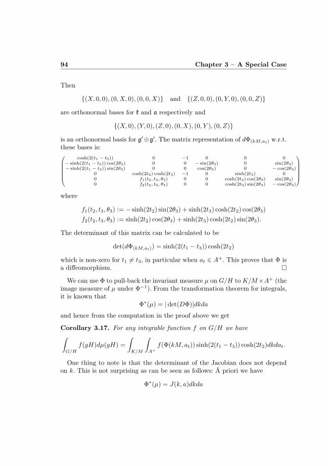
94 Chapter 3 – A Special Case
Then
(X, 0, 0), (0, X, 0), (0, 0, X) and (Z, 0, 0), (0, Y, 0), (0, 0, Z)
are orthonormal bases for k and a respectively and
(X, 0), (Y, 0), (Z, 0), (0, X), (0, Y ), (0, Z)
is an orthonormal basis for g′⊕g′. The matrix representation of dΦ(kM,at) w.r.t.these bases is:
cosh(2(t1 − t3)) 0 −1 0 0 0− sinh(2(t1 − t3)) cos(2θ3) 0 0 − sin(2θ3) 0 sin(2θ3)− sinh(2(t1 − t3)) sin(2θ3) 0 0 cos(2θ3) 0 − cos(2θ3)
0 cosh(2t2) cosh(2t3) −1 0 sinh(2t3) 00 f1(t2, t3, θ3) 0 0 cosh(2t3) cos(2θ3) sin(2θ3)0 f2(t2, t3, θ3) 0 0 cosh(2t3) sin(2θ3) − cos(2θ3)
where
f1(t2, t3, θ3) := − sinh(2t2) sin(2θ3) + sinh(2t3) cosh(2t2) cos(2θ3)
f2(t2, t3, θ3) := sinh(2t2) cos(2θ3) + sinh(2t3) cosh(2t2) sin(2θ3).
The determinant of this matrix can be calculated to be
det(dΦ(kM,at)) = sinh(2(t1 − t3)) cosh(2t2)
which is non-zero for t1 6= t3, in particular when at ∈ A+. This proves that Φ isa diffeomorphism.
We can use Φ to pull-back the invariant measure µ on G/H toK/M×A+ (theimage measure of µ under Φ−1). From the transformation theorem for integrals,it is known that
Φ∗(µ) = |det(DΦ)|dkdaand hence from the computation in the proof above we get
Corollary 3.17. For any integrable function f on G/H we have∫
G/H
f(gH)dµ(gH) =
∫
K/M
∫
A+
f(Φ(kM, at)) sinh(2(t1 − t3)) cosh(2t2)dkdat.
One thing to note is that the determinant of the Jacobian does not dependon k. This is not surprising as can be seen as follows: Á priori we have
Φ∗(µ) = J(k, a)dkda
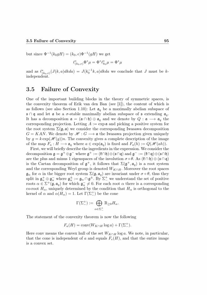
3.5 Failure of Convexity 95
but since Φ−1(k0gH) = (k0, e)Φ−1(gH) we get
`∗(k0,e)Φ∗µ = Φ∗`∗k0µ = Φ∗µ
and as `∗(k0,e)(J(k, a)dkda) = J(k−10 k, a)dkda we conclude that J must be k-
independent.
3.5 Failure of ConvexityOne of the important building blocks in the theory of symmetric spaces, isthe convexity theorem of Erik van den Ban (see [1]), the content of which isas follows (see also Section 1.10): Let aq be a maximally abelian subspace ofs ∩ q and let a be a σ-stable maximally abelian subspace of s extending aq.It has a decomposition a = (a ∩ h) ⊕ aq and we denote by Q : a −→ aq thecorresponding projection. Letting A := exp a and picking a positive system forthe root system Σ(g, a) we consider the corresponding Iwasawa decompositionG = KAN . We denote by H : G −→ a the Iwasawa projection given uniquelyby g = k exp(H (g))n. The convexity gives a complete description of the imageof the map Fa : H −→ aq where a ∈ exp(aq) is fixed and Fa(h) := Q(H (ah)).First, we will briefly describe the ingredients in the expression. We consider the
decomposition g = g+⊕g− where g+ := (k∩h)⊕(s∩q) and g− := (k∩q)⊕(s∩h)are the plus and minus 1 eigenspaces of the involution σ θ. As (k∩ h)⊕ (s∩ q)is the Cartan decomposition of g+, it follows that Σ(g+, aq) is a root systemand the corresponding Weyl group is denoted WK∩H . Moreover the root spacesgα for α in the bigger root system Σ(g, aq) are invariant under σ θ, thus theysplit in g+
α ⊕ g−α where g±α := gα ∩ g±. By Σ+− we understand the set of positive
roots α ∈ Σ+(g, aq) for which g−α 6= 0. For each root α there is a correspondingco-root Hα, uniquely determined by the condition that Hα is orthogonal to thekernel of α and α(Hα) = 1. Let Γ(Σ+
−) be the cone
Γ(Σ+−) :=
⊕
α∈Σ+−
R≥0Hα.
The statement of the convexity theorem is now the following
Fa(H) = conv(WK∩H log a) + Γ(Σ+−).
Here conv means the convex hull of the set WK∩H log a. We note, in particular,that the cone is independent of a and equals Fe(H), and that the entire imageis a convex set.
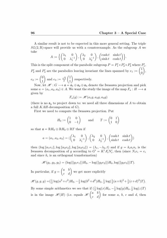
96 Chapter 3 – A Special Case
A similar result is not to be expected in this more general setting. The tripleSL(2,R)-space will provide us with a counterexample. As the subgroup A wetake
A :=(λ1 0
0 λ−11
),
(λ2 00 λ−1
2
),
(cosh t sinh tsinh t cosh t
).
This is the split component of the parabolic subgroup P = P ′1×P ′2×P ′3 where P ′1,
P ′2 and P ′3 are the parabolics leaving invariant the lines spanned by e1 :=
(10
),
e2 :=
(01
)and e3 :=
√2
2
(11
)respectively.
Now, let H : G −→ a = a1⊕ a2⊕ a3 denote the Iwasawa projection and picksome a = (a1, a2, a3) ∈ A. We want the study the image of the map Fa : H −→ agiven by
Fa(g) := H (a1g, a2g, a3g)
(there is no aq to project down to: we need all three dimensions of A to obtaina full KAH-decomposition of G).First we need to compute the Iwasawa projection. Put
H0 :=
(1 00 −1
)and T :=
(0 11 0
)
so that a = RH0 ⊕ RH0 ⊕ RT then if
a = (a1, a2, a3) = (
(λ1 00 λ−1
1
),
(λ2 00 λ−1
2
),
(cosh t sinh tsinh t cosh t
))
then (log ‖a1e1‖, log ‖a2e2‖, log ‖a3e3‖) = (λ1,−λ2, t) and if g = kiaini is theIwasawa decomposition of g according to G′ = K ′A′iN
′i , then (since Niei = ei
and since ki is an orthogonal transformation)
H (g1, g2, g3) = (log(‖g1e1‖)H0,− log(‖g2e2‖)H0, log(‖g3e3‖)T ).
In particular, if g =
(a bc d
)we get more explicitly
H (g, g, g) =(
12 log(a2 +c2)H0,− 1
2 log(b2 +d2)H0,12 log( 1
2 (a+b)2 + 12 (c+d)2)T
).
By some simple arithmetics we see that if ( 12 log(x)H0,− 1
2 log(y)H0,12 log(z)T )
is in the image H (H) (i.e. equals H
(a bc d
)for some a, b, c and d, then
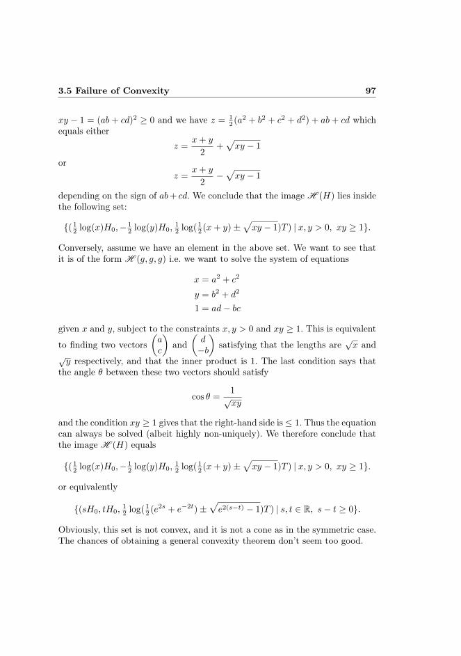
3.5 Failure of Convexity 97
xy − 1 = (ab+ cd)2 ≥ 0 and we have z = 12 (a2 + b2 + c2 + d2) + ab+ cd which
equals either
z =x+ y
2+√xy − 1
orz =
x+ y
2−√xy − 1
depending on the sign of ab+ cd. We conclude that the image H (H) lies insidethe following set:
( 12 log(x)H0,− 1
2 log(y)H0,12 log( 1
2 (x+ y)±√xy − 1)T ) | x, y > 0, xy ≥ 1.
Conversely, assume we have an element in the above set. We want to see thatit is of the form H (g, g, g) i.e. we want to solve the system of equations
x = a2 + c2
y = b2 + d2
1 = ad− bc
given x and y, subject to the constraints x, y > 0 and xy ≥ 1. This is equivalent
to finding two vectors(ac
)and
(d−b
)satisfying that the lengths are
√x and
√y respectively, and that the inner product is 1. The last condition says that
the angle θ between these two vectors should satisfy
cos θ =1√xy
and the condition xy ≥ 1 gives that the right-hand side is ≤ 1. Thus the equationcan always be solved (albeit highly non-uniquely). We therefore conclude thatthe image H (H) equals
( 12 log(x)H0,− 1
2 log(y)H0,12 log( 1
2 (x+ y)±√xy − 1)T ) | x, y > 0, xy ≥ 1.
or equivalently
(sH0, tH0,12 log( 1
2 (e2s + e−2t)±√e2(s−t) − 1)T ) | s, t ∈ R, s− t ≥ 0.
Obviously, this set is not convex, and it is not a cone as in the symmetric case.The chances of obtaining a general convexity theorem don’t seem too good.
98 Chapter 3 – A Special Case
3.6 Plancherel DecompositionThe first point here is to describe what happens when we take the outer productof two principal series representations. We consider a semisimple group G withmaximally compact subgroup K and a parabolic subgroup P = MAN (notnecessarily minimal). If ξ ∈ M and λ ∈ a∗C, we denote by (πξ,λ,Hξ,λ) thecorresponding principal series representation of G on Hξ,λ. If G′ is anotherreductive group and P ′ = M ′A′N ′ a parabolic subgroup, then P × P ′ is aparabolic subgroup of G×G′ with Langlands decomposition
P × P ′ = (M ×M ′)(A×A′)(N ×N ′).
The claim is thatπξ,λ × πξ′,λ′ = πξ×ξ′,(λ,λ′) (3.8)
as representations of G×G′.Let’s set up some machinery to prove this
Definition 3.18 (Hilbert Bundle). A Hilbert bundle over a connected topo-logical space X is a topological space HX along with a continuous map p :HX −→ X so that
1) Each fiber p−1(x) has a vector space structure.
2) The subspace topology from E on the fiber can be generated by an innerproduct.
3) There exists an open cover (Ui) of X and a Hilbert space H and a home-omorphism
p−1(Ui)∼−−→ Ui ×H
whose restriction to a fiber is a unitary map p−1(x)∼−−→ H.
Assume now that the space X comes equipped with a Radon measure. Wewill focus on the space of L2-sections L2(X,HX) of a Hilbert bundle and inorder to analyze this, the following result will be useful 2.
Theorem 3.19 (Kuiper). Any infinite-dimensional Hilbert bundle over a com-pact base space is trivial, i.e. isomorphic to a product bundle X ×H for somefixed Hilbert space, H.
2The usual statement of Kuiper’s Theorem is that the set of homotopy classes of maps[X,GL(H)] where X is compact, H is an infinite-dimensional Hilbert space and GL(H) isthe space of invertible bounded isomorphisms of H equipped with the norm topology, is asingleton. That the following statement follows from this is remarked in [6] p. 63.
3.6 Plancherel Decomposition 99
In particular L2-sections of such a vector bundle are justH-valued L2-functionon X, i.e.
L2(X,HX) = L2(X,H) = L2(X)⊗H. (3.9)
In the case of a finite-dimensional Hilbert bundle , the situation is of coursemore complicated, since it is by no means true that any vector bundle overa compact space is trivial (just consider the Möbius bundle over the circle).However, in this case (3.9) is still true, as we now show.
Lemma 3.20. Let p : E −→ X be a topological vector bundle over a compacttopological space X. There exists a measurable bundle isomorphism Φ : E −→X × Cn (i.e. a measurable map with measurable inverse) whose restrictions tothe fibers are unitary maps.
Proof. We assume the vector bundle to be complex. The real case is similar.Pick a finite family of local, continuous trivializations
Φi : p−1(Ui)∼−−→ Ui × Cn, i = 1, . . . , N
about which we may assume that they are fiberwise unitary (if they are not,simply perform a Gram-Schmidt orthonormalization). Define
V1 := U1, V2 := U2 \ U1, . . . Vk := Uk \ (U1 ∪ · · · ∪ Uk−1), . . .
V1, . . . , VN , is a division ofX into disjoint measurable sets. Consequently, p−1(Vi)is a measurable subset of E. We can restrict Φi to p−1(Vi) to obtain a measur-able map Φi : p−1(Vi) −→ Vi × Cn with measurable inverse. Thus we defineΦ : E −→ X × Cn by
Φ(e) :=
Φ1(e), e ∈ p−1(V1)...
ΦN (e), e ∈ p−1(VN )
.
This is a measurable map with inverse
Φ−1(x, v) =
Φ−11 (x, v), x ∈ V1
...Φ−1N (x, v), x ∈ VN
which is also measurable. They are clearly both bundle maps. This proves thelemma.
100 Chapter 3 – A Special Case
Lemma 3.21. If E is an n-dimensional complex vector bundle over the compactbase manifold X then the measurable bundle isomorphism from above gives riseto a unitary isomorphism Φ : L2(X,E)
∼−−→ L2(X,Cn) ∼= L2(X) ⊗ Cn, morespecifically, the map is given by
(Φf)(x) := p2 Φ(f(x)) almost everywhere
where p2 : X ×Cn −→ Cn is the projection on the second factor. The inverse isgiven by
Φ−1(x) = Φ−1(x, f(x)) almost everywhere.
These are easily checked to be inverses of each other. Unitarity of Φ followsfrom fiberwise unitarity of Φ.Now given two Hilbert bundles (finite or infinite-dimensional), we form the
outer tensor product HX HY over the base space X ×Y where the fiber over(x, y) is Hx⊗Hy
3. We now consider the L2-space of such a tensor product
Proposition 3.22. If HX and HY are two Hilbert bundles over compact basespaces, then the map L2(X,HX)⊗L2(Y,HY ) −→ L2(X × Y,HX HY ) whichsends s1 ⊗ s2 to the section (x, y) 7−→ s1(x)⊗ s2(y) is a unitary isomorphism.
Proof. It is easy to check that the map is actually unitary. In particular it isinjective and has closed image. Thus we only need to check that the image isdense.Assume that en and fm are orthonormal bases for L2(X,HX) and L2(Y,HY )
respectively. The claim is that the sections
(x, y) 7−→ en(x)⊗ fm(y)
form an orthonormal basis for L2(X × Y,HX HY ).Trivialize the bundles by Φ : HX −→ X ×H and Φ′ : HY −→ Y ×H′ (in the
infinite-dimensional case, this can be done continuously by Kuiper’s Theorem, inthe finite-dimensional case, this can be done measurably by the lemma above).If (vi) and (wj) are orthonormal bases of H and H′ respectively, we can formglobal L2-sections by
ϕi(x) := Φ−1(x, vi) and ψj(y) := Φ′−1(y, wj).
Obviously (ϕi(x)) and (ψj(y)) are orthonormal bases of the fibers Hx and Hy.For this it is important that the base spaces are compact.
3This is opposed to the usual tensor product of two bundles over X, which is the pullbackof the outer tensor product from X ×X to X along the diagonal embedding map.
3.6 Plancherel Decomposition 101
Now assume that g ∈ L2(X × Y,HX HY ) satisfies 〈en ⊗ fm, g〉 = 0, i.e.∫
X
∫
Y
〈en(x)⊗ fm(y), g(x, y)〉 dydx = 0
for all n and m. We can expand g(x, y) ∈ Hx⊗Hy in ϕi(x)⊗ ψj(y) to obtain
g(x, y) =∑
i,j
aij(x, y)ϕi(x)⊗ ψj(y)
for some coefficients aij(x, y) which are L2-functions. Hence the equation be-comes
0 =
∫
X
∫
Y
⟨en(x)⊗ fm(y),
∑
ij
aij(x, y)ϕi(x)⊗ ψj(y)⟩dxdy
=
∫
X
〈en(x), ϕi(x)〉(∫
Y
⟨fm(y),
∑
ij
aij(x, y)ψj(y)⟩dy)dx.
Since functions of the form x 7−→ 〈en(x), ϕi(x)〉 span L2(X), it follows that thefunction
x 7−→∫
Y
⟨fm(y),
∑
ij
aij(x, y)ψj(y)⟩dy
is zero as an L2-function. Since (fm) is an orthonormal basis of L2(Y,HY ), itmeans that for almost all x, the section
y 7−→∑
ij
aij(x, y)ψj(y)
is zero as an L2-section. Thus it follows that aij are all zero as L2-functions,and hence that g = 0 in L2(X × Y,HX HY ).
In the case of trivial line bundles, we recover the well-known fact that L2(X×Y ) ∼= L2(X)⊗L2(Y ).We can formulate the inducing construction in this setting. Let P = MAN
be some parabolic subgroup (not necessarily minimal). Then the flag varietyG/P = K/(M ∩K) is compact and
P −→ G −→ G/P
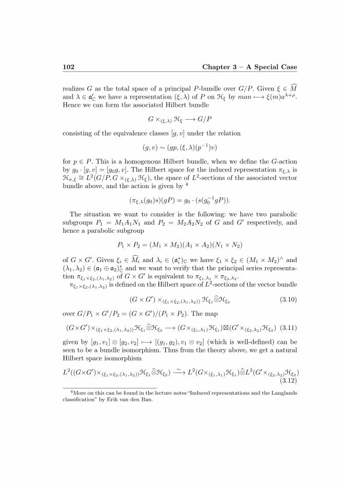
102 Chapter 3 – A Special Case
realizes G as the total space of a principal P -bundle over G/P . Given ξ ∈ Mand λ ∈ a′C we have a representation (ξ, λ) of P on Hξ by man 7−→ ξ(m)aλ+ρ.Hence we can form the associated Hilbert bundle
G×(ξ,λ) Hξ −→ G/P
consisting of the equivalence classes [g, v] under the relation
(g, v) ∼ (gp, (ξ, λ)(p−1)v)
for p ∈ P . This is a homogenous Hilbert bundle, when we define the G-actionby g0 · [g, v] = [g0g, v]. The Hilbert space for the induced representation πξ,λ isHπ,ξ
∼= L2(G/P,G×(ξ,λ) Hξ), the space of L2-sections of the associated vectorbundle above, and the action is given by 4
(πξ,λ(g0)s)(gP ) = g0 · (s(g−10 gP )).
The situation we want to consider is the following: we have two parabolicsubgroups P1 = M1A1N1 and P2 = M2A2N2 of G and G′ respectively, andhence a parabolic subgroup
P1 × P2 = (M1 ×M2)(A1 ×A2)(N1 ×N2)
of G × G′. Given ξi ∈ Mi and λi ∈ (a∗i )C we have ξ1 × ξ2 ∈ (M1 ×M2)∧ and(λ1, λ2) ∈ (a1 ⊕ a2)∗C and we want to verify that the principal series representa-tion πξ1×ξ2,(λ1,λ2) of G×G′ is equivalent to πξ1,λ1
× πξ2,λ2.
πξ1×ξ2,(λ1,λ2) is defined on the Hilbert space of L2-sections of the vector bundle
(G×G′)×(ξ1×ξ2,(λ1,λ2)) Hξ1⊗Hξ2 (3.10)
over G/P1 ×G′/P2 = (G×G′)/(P1 × P2). The map
(G×G′)×(ξ1×ξ2,(λ1,λ2))Hξ1⊗Hξ2 −→ (G×(ξ1,λ1)Hξ1)(G′×(ξ2,λ2)Hξ2) (3.11)
given by [g1, v1] ⊗ [g2, v2] 7−→ [(g1, g2), v1 ⊗ v2] (which is well-defined) can beseen to be a bundle isomorphism. Thus from the theory above, we get a naturalHilbert space isomorphism
L2((G×G′)×(ξ1×ξ2,(λ1,λ2))Hξ1⊗Hξ2)∼−−→ L2(G×(ξ1,λ1)Hξ1)⊗L2(G′×(ξ2,λ2)Hξ2)
(3.12)4More on this can be found in the lecture notes “Induced representations and the Langlands
classification” by Erik van den Ban.
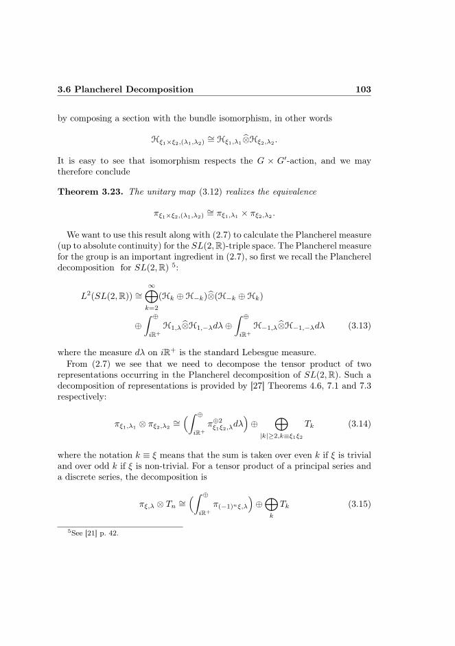
3.6 Plancherel Decomposition 103
by composing a section with the bundle isomorphism, in other words
Hξ1×ξ2,(λ1,λ2)∼= Hξ1,λ1
⊗Hξ2,λ2.
It is easy to see that isomorphism respects the G × G′-action, and we maytherefore conclude
Theorem 3.23. The unitary map (3.12) realizes the equivalence
πξ1×ξ2,(λ1,λ2)∼= πξ1,λ1
× πξ2,λ2.
We want to use this result along with (2.7) to calculate the Plancherel measure(up to absolute continuity) for the SL(2,R)-triple space. The Plancherel measurefor the group is an important ingredient in (2.7), so first we recall the Planchereldecomposition for SL(2,R) 5:
L2(SL(2,R)) ∼=∞⊕
k=2
(Hk ⊕H−k)⊗(H−k ⊕Hk)
⊕∫ ⊕
iR+
H1,λ⊗H1,−λdλ⊕∫ ⊕
iR+
H−1,λ⊗H−1,−λdλ (3.13)
where the measure dλ on iR+ is the standard Lebesgue measure.From (2.7) we see that we need to decompose the tensor product of two
representations occurring in the Plancherel decomposition of SL(2,R). Such adecomposition of representations is provided by [27] Theorems 4.6, 7.1 and 7.3respectively:
πξ1,λ1 ⊗ πξ2,λ2∼=(∫ ⊕
iR+
π⊕2ξ1ξ2,λ
dλ)⊕
⊕
|k|≥2,k≡ξ1ξ2
Tk (3.14)
where the notation k ≡ ξ means that the sum is taken over even k if ξ is trivialand over odd k if ξ is non-trivial. For a tensor product of a principal series anda discrete series, the decomposition is
πξ,λ ⊗ Tn ∼=(∫ ⊕
iR+
π(−1)nξ,λ
)⊕⊕
k
Tk (3.15)
5See [21] p. 42.
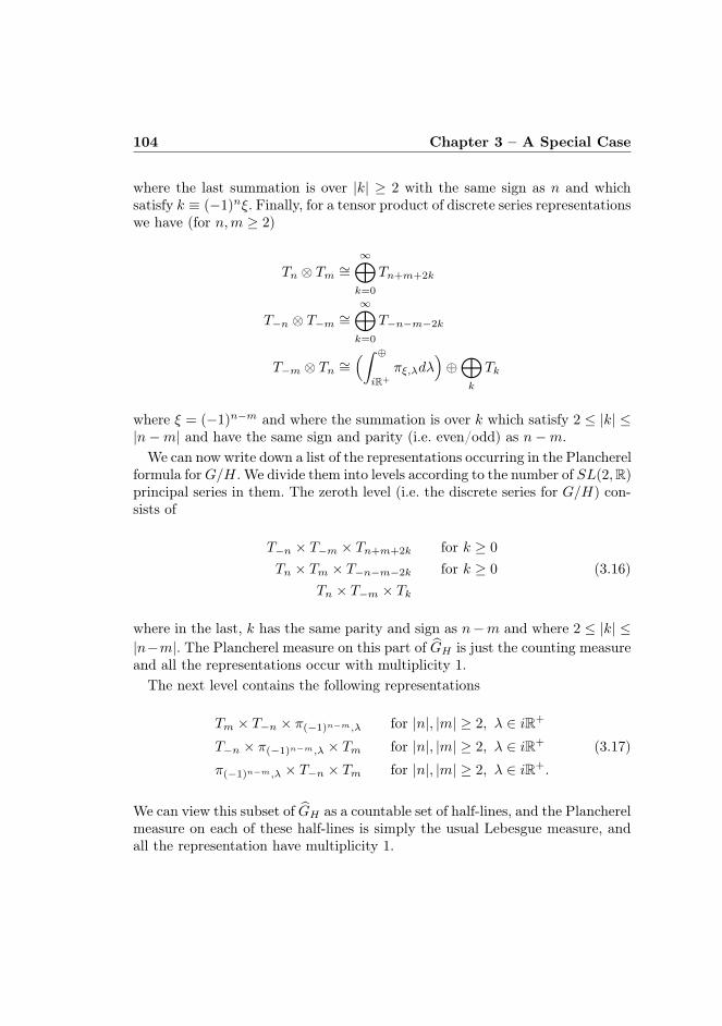
104 Chapter 3 – A Special Case
where the last summation is over |k| ≥ 2 with the same sign as n and whichsatisfy k ≡ (−1)nξ. Finally, for a tensor product of discrete series representationswe have (for n,m ≥ 2)
Tn ⊗ Tm ∼=∞⊕
k=0
Tn+m+2k
T−n ⊗ T−m ∼=∞⊕
k=0
T−n−m−2k
T−m ⊗ Tn ∼=(∫ ⊕
iR+
πξ,λdλ)⊕⊕
k
Tk
where ξ = (−1)n−m and where the summation is over k which satisfy 2 ≤ |k| ≤|n−m| and have the same sign and parity (i.e. even/odd) as n−m.We can now write down a list of the representations occurring in the Plancherel
formula forG/H. We divide them into levels according to the number of SL(2,R)principal series in them. The zeroth level (i.e. the discrete series for G/H) con-sists of
T−n × T−m × Tn+m+2k for k ≥ 0
Tn × Tm × T−n−m−2k for k ≥ 0 (3.16)Tn × T−m × Tk
where in the last, k has the same parity and sign as n−m and where 2 ≤ |k| ≤|n−m|. The Plancherel measure on this part of GH is just the counting measureand all the representations occur with multiplicity 1.The next level contains the following representations
Tm × T−n × π(−1)n−m,λ for |n|, |m| ≥ 2, λ ∈ iR+
T−n × π(−1)n−m,λ × Tm for |n|, |m| ≥ 2, λ ∈ iR+ (3.17)
π(−1)n−m,λ × T−n × Tm for |n|, |m| ≥ 2, λ ∈ iR+.
We can view this subset of GH as a countable set of half-lines, and the Plancherelmeasure on each of these half-lines is simply the usual Lebesgue measure, andall the representation have multiplicity 1.
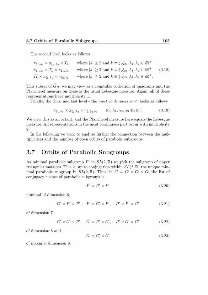
3.7 Orbits of Parabolic Subgroups 105
The second level looks as follows
πξ1,λ1 × πξ2,λ2 × Tk where |k| ≥ 2 and k ≡ ξ1ξ2, λ1, λ2 ∈ iR+
πξ1,λ1× Tk × πξ2,λ2
where |k| ≥ 2 and k ≡ ξ1ξ2, λ1, λ2 ∈ iR+ (3.18)
Tk × πξ1,λ1× πξ2,λ2
where |k| ≥ 2 and k ≡ ξ1ξ2, λ1, λ2 ∈ iR+.
This subset of GH , we may view as a countable collection of quadrants and thePlancherel measure on these is the usual Lebesgue measure. Again, all of theserepresentations have multiplicity 1.Finally, the third and last level - the most continuous part looks as follows
πξ1,λ1× πξ2,λ2
× πξ1ξ2,λ3for λ1, λ2, λ3 ∈ iR+. (3.19)
We view this as an octant, and the Plancherel measure here equals the Lebesguemeasure. All representations in the most continuous part occur with multiplicity2.In the following we want to analyze further the connection between the mul-
tiplicities and the number of open orbits of parabolic subgroups.
3.7 Orbits of Parabolic SubgroupsAs minimal parabolic subgroup P ′ in SL(2,R) we pick the subgroup of uppertriangular matrices. This is, up to conjugation within SL(2,R) the unique min-imal parabolic subgroup in SL(2,R). Thus, in G = G′ × G′ × G′ the list ofconjugacy classes of parabolic subgroups is
P ′ × P ′ × P ′ (3.20)
minimal of dimension 6,
G′ × P ′ × P ′, P ′ ×G′ × P ′, P ′ × P ′ ×G′ (3.21)
of dimension 7
G′ ×G′ × P ′, G′ × P ′ ×G′, P ′ ×G′ ×G′ (3.22)
of dimension 8 andG′ ×G′ ×G′ (3.23)
of maximal dimension 9.
106 Chapter 3 – A Special Case
By Theorem 3.23 the representations (3.16) are trivially induced from theparabolic (3.23), the representations (3.17) are induced from (3.22), the rep-resentations (3.18) are induced from (3.21) and the representations (3.19) areinduced from (3.22).The parabolic subgroups act on G/H. We want to analyze the orbit structure
of this action. Since (G,H) is a spherical pair, we know at least that it admitsopen orbits. For the further analysis we introduce the functions c : SL(2,R) −→R and d : SL(2,R) −→ R
(a bc d
)7−→ c resp.
(a bc d
)7−→ d
andB := g ∈ SL(2,R) | c(g) 6= 0.
The Bruhat-decomposition of SL(2,R) states that SL(2,R) is the disjoint union
of P andB = NMAN = MANwMAN where w =
(0 −11 0
)is a representative
of the non-trivial Weyl group element in SL(2,R).In the following theorem we make use of our “non-canonical” model G/H ∼=
G′×G′. However, later in the case of P minimal, we shall give a more invariantcharacterization 6.
Theorem 3.24. Consider a parabolic P acting on G/H ∼= G′ ×G′. If P is ofthe form (3.23) or (3.22) there is exactly one orbit, namely G/H itself.If P is of the form (3.21), then there are two orbits, one open, namely G′×B
and one of lower dimension, namely G′ × P ′.If P is of the form (3.20) there are two open orbits, namely
O1 := (g1, g2) ∈ G′ ×G′ | c(g1), c(g2) 6= 0, d(g1)c(g1) <
d(g2)c(g2)
O2 := (g1, g2) ∈ G′ ×G′ | c(g1), c(g2) 6= 0, d(g1)c(g1) >
d(g2)c(g2)
3 orbits of dimension 5, namely
O3 := B × P ′O4 := P ′ ×BO5 := (g1, g2) ∈ B ×B | g1g
−12 ∈ P ′
6A similar result as the following has been obtained in [25] Proposition 1.2. The result thereis for minimal P but for more general groups than just G′ = SL(2,R). Instead of consideringP -orbits in G/H they consider H-orbits in G/P but that of course amounts to the same thing.
3.7 Orbits of Parabolic Subgroups 107
and one orbit of dimension 4, namely O6 := P ′ × P ′. Furthermore
∂O1 = ∂O2 = O3 ∪ O4 ∪ O5 ∪ O6
∂O3 = ∂O4 = ∂O5 = O6.
Proof. If P = G′ ×G′ ×G′, it is clear that the only orbit is G/H.Now consider the parabolic P ′ × G′ × G′. This action is transitive on G/H,
since the point [g1, g2, g3] can be reached from [e, e, e] via (e, g−11 g2, g
−11 g3) ∈
P ′ ×G′ ×G′. Similar of course with the other parabolics in (3.22).For the parabolic G′ × P ′ × P ′ acting on G′ ×G′, the claim is that we have
2 orbits, namely G′ × P ′ and G′ × B. These orbits contain the points (e, e)and (e, w). We can reach any point (g, p) in G′ × P ′ from (e, e) by acting with(g, p, e). Similarly, we can reach any point (g1, g2) ∈ G′ ×B from (e, w): simplyby picking p1 and p2 in P ′ such that p1wp
−12 = g2 and g0 ∈ G′ such that
g0p−12 = g1. Then (g0, p1, p2) · (e, w) = (g1, g2). Similarly for the parabolics
P ′ ×G′ × P ′ and P ′ × P ′ ×G′.Now we come to the minimal parabolic P = P ′×P ′×P ′. Note that G′×G′ =
(P ′ × P ′) ∪ (B × P ′) ∪ (P ′ ×B) ∪ (B ×B) by the Bruhat decomposition of G′.Note also that B×B = O1∪O2∪O5, since we can reformulate the condition onO5 to d(g1)
c(g1) = d(g2)c(g2) . Therefore the sets O1, . . . ,O6 fill up all of G′ × G′. Hence
we just have to prove that they are actually orbits, i.e. that the action of P istransitive on them. This is clear in the case of the orbit P ′ × P ′.Now consider O3 = B × P ′. It is easily checked to be invariant under P . It
contains (w, e). Given (g, p) ∈ B × P ′, we can find p1 and p3 in P ′ such thatg = p1wp
−13 . Put p2 := pp3, then (g, p) = (p1, p2, p3) · (w, e). Hence B×P ′ is an
orbit. Similarly with P ′ ×B.Next we consider O5. This set contains (w,w). Again it is easy to see that it
is P -invariant. For transitivity: let (g1, g2) ∈ O5 be given, and find p1 and p3 inP ′ such that g1 = p1wp
−13 and put p2 := (g2g
−11 )p1, then (p1, p2, p3) · (w,w) =
(g1, g2).
Finally, we come to the orbit O1. The set contains the point (w,
(0 −11 1
)).
Let (g1, g2) be some arbitrary element in O1, thend(g1)c(g1) <
d(g2)c(g2) . We define
t :=
√d(g2)
c(g2)− d(g1)
c(g1)and x := − d(g1)
c(g1)tand p0 :=
(t x0 t−1
)
108 Chapter 3 – A Special Case
and from that we get
d(g1p0)
c(g1p0)= t−2
(xt+
d(g1)
c(g1)
)= 0 and
d(g2p0)
c(g2p0)= t−2
(xt+
d(g2)
c(g2)
)= 1.
In other words, by acting with (e, e, p−10 ) ∈ P we can bring (g1, g2) on the
following form
g1p0 =
(a1 b1c1 0
)and g2p0 =
(a2 b2c2 c2
)
with c1, c2 6= 0. Now we see that(c1 −a1
0 c−11
)g1p0 =
(0 −11 0
)and
(c2 −a2
0 c−12
)g2p0 =
(0 −11 1
)
and this means that we can bring any element in O1 to (w,
(0 −11 1
)) by acting
with an element in P . Hence the P -action is transitive on O1. The same proofwith obvious modifications, works for O2.
If [x0] is a point in a P -orbit O in G/H, then the stabilizer for the P -actionat that point is easily seen to be P ∩ x0Hx
−10 . Consequently, we have a diffeo-
morphismP/P ∩ x0Hx
−10
∼−−→ O (3.24)
by mapping [p] 7−→ p ·x0. In the case of a symmetric space, if P is a θσ-invariantparabolic subgroup we get a Langlands-like decomposition of this quotient aswell:
Lemma 3.25. Let (G,H) be a symmetric pair and P ⊆ G a σθ-invariantparabolic subgroup. Then for each w ∈ WP we have a diffeomorphism
(MP /MP ∩ wHw−1)×APq ×NP ∼−−→ P/P ∩ wHw−1 (3.25)
by mapping([m], a, n) 7−→ [man].
Proof. Assume first that w = e. The map is well-defined, for if [m] = [m′],i.e. m′m−1 ∈ H, then m′an(man)−1 = m′m−1 ∈ H, i.e. [man] = [m′an].It is surjective by the Langlands decomposition and it is injective for the fol-lowing reason: if ([m], a, n) is mapped to [e], then man ∈ H, meaning that
3.7 Orbits of Parabolic Subgroups 109
manσ(n)−1σ(a)−1σ(m)−1 = e. Using the fact that σ(a) = a−1 and the normal-ization properties of MP and AP we get
manσ(n)−1σ(a)−1σ(m)−1 = mσ(m)−1a2n′
for some n′ ∈ NP . By uniqueness of the Langlands decomposition we getmσ(m)−1 = e and a2 = e, which implies m ∈ MP ∩ H and a = e. Fromthis it follows that n ∈ NP ∩H = e and hence the map is injective.We can reduce P/P ∩ wHw−1, to the above case, since (G,wHw−1) is a
symmetric pair under the involution σw := Cw σCw−17 of G, and P is a σwθ-
invariant parabolic. Equivalently, wPw−1 is a σθ-invariant parabolic. This is forthe following reason: The Lie algebra of the parabolic P splits in a Langlandsdecomposition mP ⊕aP ⊕nP . Consider aP which by definition is contained in s.We can extend it to a maximally abelian subspace a in s containing aq. We canchoose w in such a way that Ad(w) preserves both a∩ q = aq and a∩ h := ah
8.First, we consider aP which splits into aPh
⊕ aPq. The fact that σ preserves
ah and aq translates into the fact that Ad(w)|aP commutes with σ. Since Ad(w)also commutes with θ (as w is chosen in K), it commutes with σθ. Thus, asaP is σθ-invariant, so is Ad(w)aP . In particular it also follows that Ad(w)aPq
isσθ-invariant. From this it easily follows that mP ⊕aP which is the centralizer ofaPq
in g is σθ-invariant. So we are only left with nP . A trivial calculation showsthat if
nP =⊕
α∈Γ
gα
thenAd(w)nP =
⊕
α∈Γ
gw·α.
Again, θ commutes with Ad(w), and a quick calculation reveals that [H,σ Ad(w)Xα] = −(w · α)(H)(σ Ad(w)Xα), i.e. that sigma maps gw·α to g−w·α.This is equal to the action of θ, and hence nP is σθ-invariant.
In the symmetric space case, this is important since it allows us to effectivelyreduce to MP /(MP ∩ wHw−1) and combined with the fact that MP /(MP ∩wHw−1) is again a symmetric pair, an induction argument can be applied.Inspired by this, we might anticipate a relation like the following
P/P ∩ x0Hx−10 = MP /MP ∩ x0Hx
−10 ×AP /AP ∩ x0Hx
−10 ×NP /NP ∩ x0Hx
−10
7Cw is conjugation with w.8This is Lemma 1.1 in [3].
110 Chapter 3 – A Special Case
to hold in our setting. The following example, however, shows that this cannotbe the case in general. Take as P the parabolic G′ × G′ × P ′. Then P ∩ H =(p, p, p) | p ∈ P ′ has dimension 2, and hence P/P ∩H has dimension 6. Butas MP = G′×G′×M ′ and MP ∩H = ±(1, 1, 1) then MP /MP ∩H alone hasdimension 6. As AP = 1×1×A′, NP = 1×1×N ′ and AP ∩H = NP ∩H = e,then AP /AP ∩H and NP /NP ∩H both have dimension 1, and we see that theabove identity cannot be satisfied.Moreover, it is no longer true, that (MP ,MP ∩ x0Hx
−10 ) is a spherical pair:
With the same parabolic as above: a minimal parabolic P0 inMP = G′×G′×M ′has dimension 4, but asMP ∩H has dimension 0, it is impossible for P0×(MP ∩H) to have an open orbit in MP (which should be 6-dimensional).
3.8 H-Invariant Distribution VectorsFirst a useful lemma
Lemma 3.26. Let G be a Lie group and H a closed subgroup such that G/H hasan invariant measure. Let η be a distribution on G/H satisfying Lgη = f(g)ηfor some f ∈ C∞(G). Then f is a homomorphism f : G −→ R \ 0, constant1 on H, and η equals the smooth function g 7−→ cf(g)−1 for some constant c.
Proof. First we assume that H = e and that η is left invariant, i.e. Lgη = ηfor all g ∈ G. We calculate (for ϕ a test function)
Xη(ϕ) = −η(Xϕ) = −η(
limt→0
Lexp(−tX)ϕ− ϕt
)
= − limt→0
η(Lexp(−tX)ϕ− ϕ
t
)= − lim
t→0
(Lexp(tX)η − ηt
(ϕ))
= 0.
From this formula it follows immediately that a left invariant η satisfies Xη = 0.Consequently it is also in the kernel of every invariant differential operator on G.Pick an inner product on TeG and extend it to a G-invariant Riemannian metricon G. Then the Laplace-Beltrami operator constructed through this metric, isG-invariant and elliptic. As η is in the kernel of it, η must be a smooth function,and a constant one even.For non-trivial H: Assume η ∈ D ′(G/H)G. We lift η to a distribution η] on
G by defining η](ϕ) := η(ϕ]) where
ϕ](gH) :=
∫
H
ϕ(gh)dh
3.8 H-Invariant Distribution Vectors 111
for ϕ ∈ C∞c (G). It is easy to see that η] is a G-invariant distribution on G.By the first part of the proof, it is a constant. This means that its action onfunctions is just the integral times a constant. For a function ϕ ∈ C∞c (G/H) wecan (by [19] Lemma I.1.10) assume it to be of the form ϕ = ψ] for ψ ∈ C∞c (G)and hence we get (assuming that the measures on G, H and G/H are properlynormalized)
η(ϕ) = η(ψ]) = c
∫
G
ψ(g)dg = c
∫
G/H
(∫
H
ψ(gh)dh)d(gH)
= c
∫
G/H
ψ](gH)d(gH).
This shows that η is constant.In the more general case, it is easy to see (by multiplicativity of g 7−→ Lg)
that f is a homomorphism f : G −→ R∗ (ifη happens to be the zero distribution,we can pick f to be constant 1). In particular f is everywhere non-zero. Nowconsider the distribution fη. It is easily checked that Lg(fη) = (Lgf)(Lgη) =f(g−1)ff(g)η = fη, i.e. is left-invariant, hence constant cf. the first part of theproof. Consequently η = cf−1.
Now, consider a principal series representation πP,ξ,λ occurring in the Planchereldecomposition of G/H. Then H
−∞,HP,ξ,λ 6= 0 and any such η ∈ H
−∞,HP,ξ,λ 6= 0 can be
viewed as a H−∞ξ -valued distribution on G/H satisfying left P -equivariance, inthe sense that
Lmanη = aλ+ρξ(m)η.
From the lemma above, it follows that η restricts to a smooth function on theopen P -orbits in G/H (since an open P -orbit is of the form P/P ∩ x0Hx
−10
- it has an invariant measure, since it is an open subset of G/H). Recall thediffeomorphism (3.24). On an orbit O containing x0, η satisfies η(p ·x0) = η(x0),and by the equivariance of η:
(ξ, λ)(p)η(x0) = η(x0)
in other words, η(x0) ∈ H−∞ξ should be invariant under the representation (ξ, λ).
In particular η(x0) ∈ H−∞,MP∩x0Hx
−10
ξ and aλ+ρ = 1 for all a ∈ AP ∩ x0Hx−10 .
For symmetric spaces it holds in general that H−∞,Hπ is finite-dimensionalwhen π ∈ G (cf. [2] Lemma 3.3) and if π = πP,ξ,λ is a principal series represen-tation for a generic λ (meaning for λ ∈ a∗qC outside a countable union of certain
112 Chapter 3 – A Special Case
hyperplanes), then a distribution vector η ∈ H−∞,HP,ξ,λ is actually completely de-
termined by its valued on the open P -orbits in G/H (this is Corollary 5.3 in [3]when P is minimal parabolic, in the non-minimal case this is due to Brylinskiand Delorme in [7]).In our case, we can prove a similar result, namely that for generic λ, the
H-fixed distribution vectors are determined by their values on the open orbits.Our main tool in the following will be a theorem of Bruhat which we firstdescribe in full generality (following the delineation in [3] Appendix A which isfor distributions with values in a finite-dimensional vector space - the infinite-dimensional version is treated in [8] Appendix A2). Later we restrict to thesituation we need.Consider a manifold M on which a group G acts smoothly. Assume further-
more that we have a finite-dimensional representation τ of G on a vector spaceV . By D ′(M,V ) we denote the space of V -valued distributions on M , i.e. thespace of continuous linear maps D(M) −→ V , and we denote by D ′(M, τ) thesubspace of D ′(M,V ) of distributions η which satisfy Lgη = τ(g−1)η (here Lgηis the dual of the left action on smooth functions on M , just as in the lemmaabove in the case ofM being G itself). For a G-orbit O inM , we let D ′k(M,O, τ)denote the space of distributions η ∈ D ′(M, τ) of distribution order at most kwhich satisfy
O ∩ supp η open in supp η.
In order to exclude the trivial case, where O ∩ supp η is open in supp η becauseit is empty, we define
D ′k(O, τ) := D ′k(M,O, τ)/η ∈ D ′k(M,O, τ) | supp η ∩ O = ∅.The Bruhat theorem is exactly the tool we need to determine this dimension. Inorder to state the theorem, we need some more notation. Fix a point x0 in theorbit O and let Gx0 denote the stabilizer at this point. Gx0 acts in a natural wayon Tx0M , and it maps the subspace Tx0O to itself. In other words, we have arepresentation of Gx0
on the quotient Tx0M/Tx0
O. By taking the derivative, weobtain a representation of the Lie algebra gx0
on the quotient Tx0M/Tx0
O. Fora given H ∈ gx0
we denote by γ1(H), . . . , γm(H) (where m is the codimensionof O in M) the eigenvalues of the corresponding endomorphism of Tx0M/Tx0O.
Theorem 3.27 (Bruhat). If there exists H ∈ gx0, such that for all eigenvalues
µ of τ(H) and for all ν ∈ Nm0 with |ν| := ν1 + · · ·+ νm ≤ k, it holds thatm∑
i=1
(νi + 1)γi(H) + µ 6= 0, (3.26)
3.8 H-Invariant Distribution Vectors 113
then D ′k(O, π) = 0.
Now, let’s apply it to our setting. The quotient G/H will play the role as themanifold M , on which the minimal parabolic P = P ′×P ′×P ′ is acting. As wehave seen in the previous section, there are 6 orbits for this action. Consider nowthe unitary principal series π = πP,ξ,λ = πξ1,λ1
× πξ2,λ2× πξ3,λ3
(i.e. λj ∈ iR).Taking τ to be the character (ξ, λ) of P , we see that H−∞,Hπ is exactly equal tothe space D ′(G/H, τ). Since H−∞ξ = Hξ = C, these are C-valued distributions.For simplicity of the exposition we shall assume in the following that ξ is the
trivial character of M . The effect of a different ξ just an overall sign change,that will not affect the analysis.The strategy is now to apply the Bruhat theorem to the non-open orbits one
by one. First the orbit O3. This orbit contains the point x0 := [w, e, e] and thestabilizer at that point is
Px0= P ∩ x0Hx
−10 =
(a−1 00 a
),
(a 00 a−1
),
(a 00 a−1
) ∣∣∣ a ∈ R∗.
For notational convenience we denote an element as above by pa := (p′−1a , p′a, p
′a).
Then the representation (1, λ) restricted to Px0is just
(1, λ)(pa) = |a|−λ1−1|a|λ2+1|a|λ3+1 = |a|−λ1+λ2+λ3 .
If we put
X0 :=((−1 0
0 1
),
(1 00 −1
),
(1 00 −1
))
then the Lie algebra of the stabilizer is px0= RX0. For the corresponding Lie
algebra representation, we see
(1, λ)(X0) = −λ1 + λ2 + λ3 + 1,
and this obviously has the eigenvalue −λ1 + λ2 + λ3 + 1.On the other hand we have the action of the stabilizer on the quotient
Tx0(G/H)/Tx0
O3. For these calculations we use the model G/H = G′ × G′.The point x0 = [w, e, e] is identified with (w, e) and we see
Tx0(G/H) ∼= TwG′ × TeG′ = ((Lw)∗TeG
′)× TeG′,
and the action of pa on this quotient is
pa ·((Lw)∗X1, X2) = (p′−1a wX1p
′−1a ,Ad(p′a)X2) = ((Lw)∗Ad(p′a)X1,Ad(p′a)X2).
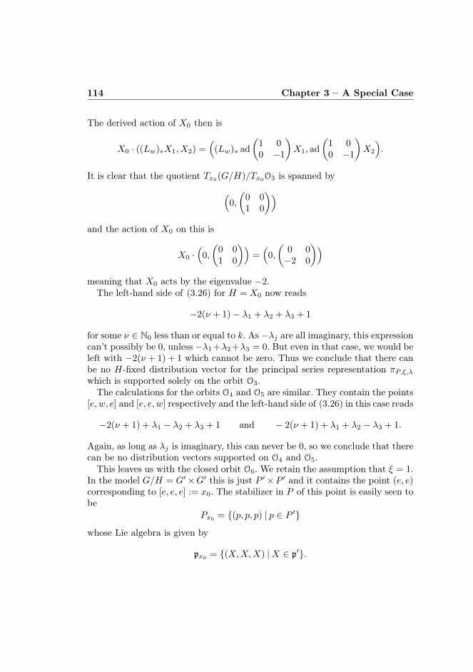
114 Chapter 3 – A Special Case
The derived action of X0 then is
X0 · ((Lw)∗X1, X2) =(
(Lw)∗ ad
(1 00 −1
)X1, ad
(1 00 −1
)X2
).
It is clear that the quotient Tx0(G/H)/Tx0O3 is spanned by
(0,
(0 01 0
))
and the action of X0 on this is
X0 ·(
0,
(0 01 0
))=(
0,
(0 0−2 0
))
meaning that X0 acts by the eigenvalue −2.The left-hand side of (3.26) for H = X0 now reads
−2(ν + 1)− λ1 + λ2 + λ3 + 1
for some ν ∈ N0 less than or equal to k. As −λj are all imaginary, this expressioncan’t possibly be 0, unless −λ1 +λ2 +λ3 = 0. But even in that case, we would beleft with −2(ν + 1) + 1 which cannot be zero. Thus we conclude that there canbe no H-fixed distribution vector for the principal series representation πP,ξ,λwhich is supported solely on the orbit O3.The calculations for the orbits O4 and O5 are similar. They contain the points
[e, w, e] and [e, e, w] respectively and the left-hand side of (3.26) in this case reads
−2(ν + 1) + λ1 − λ2 + λ3 + 1 and − 2(ν + 1) + λ1 + λ2 − λ3 + 1.
Again, as long as λj is imaginary, this can never be 0, so we conclude that therecan be no distribution vectors supported on O4 and O5.This leaves us with the closed orbit O6. We retain the assumption that ξ = 1.
In the model G/H = G′×G′ this is just P ′×P ′ and it contains the point (e, e)corresponding to [e, e, e] := x0. The stabilizer in P of this point is easily seen tobe
Px0= (p, p, p) | p ∈ P ′
whose Lie algebra is given by
px0 = (X,X,X) |X ∈ p′.
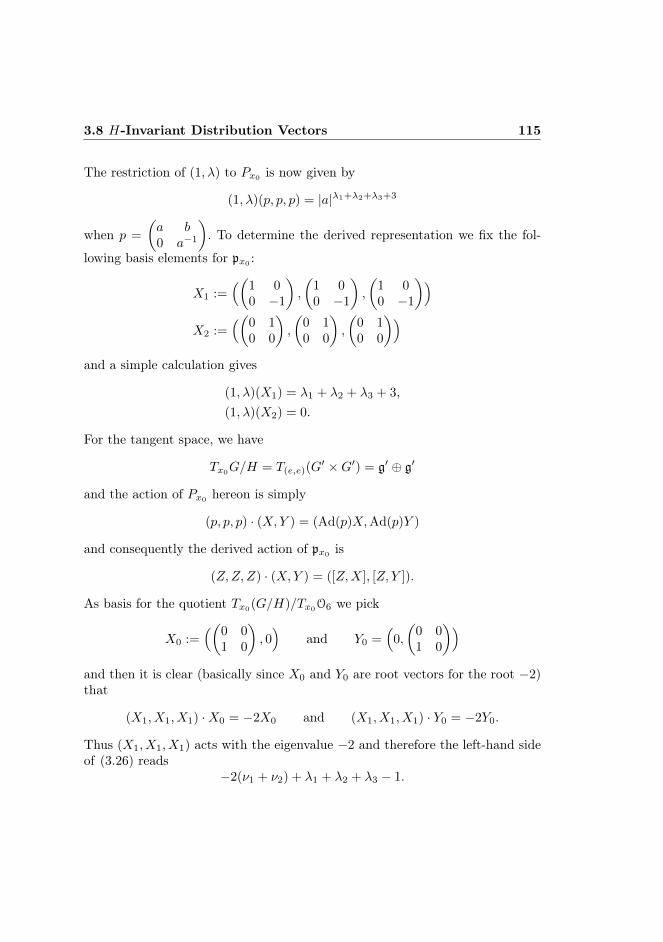
3.8 H-Invariant Distribution Vectors 115
The restriction of (1, λ) to Px0is now given by
(1, λ)(p, p, p) = |a|λ1+λ2+λ3+3
when p =
(a b0 a−1
). To determine the derived representation we fix the fol-
lowing basis elements for px0:
X1 :=((
1 00 −1
),
(1 00 −1
),
(1 00 −1
))
X2 :=((
0 10 0
),
(0 10 0
),
(0 10 0
))
and a simple calculation gives
(1, λ)(X1) = λ1 + λ2 + λ3 + 3,
(1, λ)(X2) = 0.
For the tangent space, we have
Tx0G/H = T(e,e)(G
′ ×G′) = g′ ⊕ g′
and the action of Px0hereon is simply
(p, p, p) · (X,Y ) = (Ad(p)X,Ad(p)Y )
and consequently the derived action of px0is
(Z,Z,Z) · (X,Y ) = ([Z,X], [Z, Y ]).
As basis for the quotient Tx0(G/H)/Tx0
O6 we pick
X0 :=((
0 01 0
), 0)
and Y0 =(
0,
(0 01 0
))
and then it is clear (basically since X0 and Y0 are root vectors for the root −2)that
(X1, X1, X1) ·X0 = −2X0 and (X1, X1, X1) · Y0 = −2Y0.
Thus (X1, X1, X1) acts with the eigenvalue −2 and therefore the left-hand sideof (3.26) reads
−2(ν1 + ν2) + λ1 + λ2 + λ3 − 1.
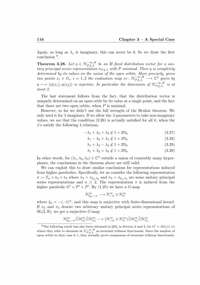
116 Chapter 3 – A Special Case
Again, as long as λj is imaginary, this can never be 0. So we draw the firstconclusion 9.
Theorem 3.28. Let η ∈ H−∞,HP,ξ,λ be an H-fixed distribution vector for a uni-
tary principal series representation πP,ξ,λ with P minimal. Then η is completelydetermined by its values on the union of the open orbits. More precisely, giventwo points xi ∈ Oi, i = 1, 2 the evaluation map ev : H−∞,HP,ξ,λ −→ C2 given byη 7−→ (η(x1), η(x2)) is injective. In particular the dimension of H−∞,HP,ξ,λ is atmost 2.
The last statement follows from the fact, that the distribution vector isuniquely determined on an open orbit by its value at a single point, and the factthat there are two open orbits, when P is minimal.However, so far we didn’t use the full strength of the Bruhat theorem. We
only used it for λ imaginary. If we allow the λ-parameters to take non-imaginaryvalues, we see that the condition (3.26) is actually satisfied for all k, when theλ’s satisfy the following 4 relations.
−λ1 + λ2 + λ3 /∈ 1 + 2N0 (3.27)λ1 − λ2 + λ3 /∈ 1 + 2N0 (3.28)λ1 + λ2 − λ3 /∈ 1 + 2N0 (3.29)λ1 + λ2 + λ3 /∈ 1 + 2N0 (3.30)
In other words, for (λ1, λ2, λ3) ∈ C3 outside a union of countably many hyper-planes, the conclusions in the theorem above are still valid.We can exploit this to draw similar conclusions for representations induced
from higher parabolics. Specifically, let us consider the following representationπ := Tn× π2× π3 where π2 = πξ2,λ2
and π3 = πξ3,λ3are some unitary principal
series representations and n ≥ 2. The representation π is induced from thehigher parabolic G′ × P ′ × P ′. By (1.25) we have a G-map
H∞ξ0,−n −→ H∞−n ⊕H∞n
where ξ0 = −(−1)n, and this map is surjective with finite-dimensional kernel.If π2 and π3 denote two arbitrary unitary principal series representations ofSL(2,R), we get a surjective G-map
H∞ξ0,−n⊗H∞π2⊗H∞π3
−→ (H∞−n ⊕H∞n )⊗H∞π2⊗H∞π3
9The following result has also been obtained in [25], in Section 2 and 3, for G′ = SOe(1, n)
where they refer to elements in H−∞,HP,ξ,λ as invariant trilinear functionals. Since the number of
open orbits in their case is 1, they actually prove uniqueness of invariant trilinear functionals.
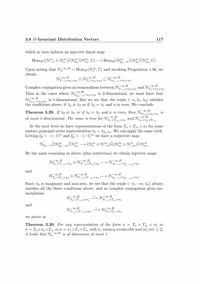
3.8 H-Invariant Distribution Vectors 117
which in turn induces an injective linear map
HomH((H∞−n ⊕H∞n )⊗H∞π2⊗H∞π3
,C) −→ HomH(H∞ξ0,−n⊗H∞π2⊗H∞π3
,C).
Upon noting that H−∞,Hπ = HomH(H∞π ,C) and invoking Proposition 1.36, weobtain
H−∞,HT−n×π2×π3
⊕H−∞,HTn×π2×π3
⊆ H−∞,Hπξ,−n×π2×π3
.
Complex conjugation gives an isomorphism betweenH−∞,HT−n×π2×π3
andH−∞,HTn×π2×π3
.Thus in the cases where H
−∞,Hπξ0,−n×π2×π3
is 2-dimensional, we must have thatH−∞,HT±n×π2×π3
is 1-dimensional. But we see that the triple (−n, λ1, λ2) satisfiesthe conditions above, if λ2 6= λ3 or if λ2 = λ3 and n is even. We conclude
Theorem 3.29. If λ2 6= λ3 or if λ2 = λ3 and n is even, then H−∞,HT±n×π2×π3
isat most 1-dimensional. The same is true for H
−∞,Hπ1×T±n×π3
and H−∞,Hπ1×π2×T±n
At the next level we have representations of the form Tn × Tm × π3 for someunitary principal series representation π3 = πξ3,λ3 . We can apply the same trick.Letting ξ0 = −(−1)n and ξ′0 = −(−1)m we have a surjective map
Hξ0,−n⊗H∞ξ′0,−m⊗H∞π3−→ (H∞n ⊕H∞−n)⊗(H∞m ⊕H∞−m)⊗H∞π3
.
By the same reasoning as above (plus restriction) we obtain injective maps
H−∞,HTn×T−m×π3
⊕H−∞,HT−n×Tm×π3
−→ H−∞,Hπξ,−n×πξ′,−m×π3
andH−∞,HTn×Tm×π3
⊕H−∞,HT−n×T−m×π3
−→ H−∞,Hπξ,−n×πξ′,−m×π3
.
Since λ3 is imaginary and non-zero, we see that the triple (−n,−m,λ3) alwayssatisfies all the three conditions above, and as complex conjugation gives iso-morphisms
H−∞,HTn×T−m×π3
∼−−→ H−∞,HT−n×Tm×π3
andH−∞,HT−n×T−m×π3
∼−−→ H−∞,HTn×Tm×π3
we arrive at
Theorem 3.30. For any representation of the form π = Tn × Tm × π3 orπ = Tn×π2×Tm or π = π1×Tn×Tm with πi unitary irreducible and |n|, |m| ≥ 2,it holds that H−∞,Hπ is of dimension at most 1.
118 Chapter 3 – A Special Case
We can summarize this by saying, that outside the discrete series, the set ofirreducible unitary representations π for which it does not hold that the dimen-sion of H−∞,Hπ equals the number of open orbits in G/H of the correspondingparabolic, is a set of Plancherel measure 0.Unfortunately, the method does not apply to the discrete series. Then we
would have to consider triples (n,m, k) of integers and here there are lot ofexamples where the conditions above are not satisfied.
3.9 The Most Continuous PartIn this section, we study the H-fixed distribution vectors of the unitary principalseries representations induced from a minimal parabolic. Here we are able toshow that the space of H-fixed distribution vectors is actually equal to 2.However, before we can do that we need to put up some machinery. We begin
by giving a more invariant characterization of the orbits under the minimalparabolic subgroup (without referring to the model G/H ∼= G′ ×G′). First wedefine the following functions on G/H:
ψ1([g1, g2, g3]) := c(g2g−13 )
ψ2([g1, g2, g3]) := c(g1g−13 )
ψ3([g1, g2, g3]) := c(g1g−12 ).
Then we see that we can characterize the minimal P -orbits along the followinglines
O1 : ε1ψ1, ε2ψ2, ε3ψ3 > 0, when ε1ε2ε3 = 1
O2 : ε1ψ1, ε2ψ2, ε3ψ3 > 0, when ε1ε2ε3 = −1
O3 : ψ1 = 0, ψ2 6= 0, ψ3 6= 0
O4 : ψ1 6= 0, ψ2 = 0, ψ3 6= 0
O5 : ψ1 6= 0, ψ2 6= 0, ψ3 = 0
O6 : ψ1 = ψ2 = ψ3 = 0.
In the following we concentrate on the two open orbits O1 and O2. Defin-
ing γ1 :=
(0 −11 1
)and γ2 :=
(1 0−1 1
), then (w, γi) lies in Oi (where w =
(0 −11 0
)). It is easy to see that the stabilizer of the P -action at (w, γi) is
3.9 The Most Continuous Part 119
±(1, 1, 1) i.e. equals M ∩H. Hence we have a diffeomorphism
M/(M ∩H)×A×N ∼−−→ Oi
([m], a, n) 7−→ man · (w, γi). (3.31)
From this it is clear, that if η ∈ H−∞,HP,ξ,λ , then η(w, λi) ∈ HM∩H
ξ , meaning thatwe only need to consider ξ ∈ MM∩H , which are ξ = (ξ1, ξ2, ξ3) (viewed as anelement in Z2 × Z2 × Z2) which satisfy ξ1ξ2ξ3 = 1.Composing the inverse of the above diffeomorphism with the projection onto
the M -part resp. the A-part gives us maps
m : Oi −→M/(M ∩H)
a : Oi −→ A ∼= R3+
and the individual components of the map a are denoted ai, i = 1, 2, 3. Note thatthese maps depend on the choice of base points. We now set out to compute thesemaps. The first thing to note is that the maps ψi are left N = N ′ × N ′ × N ′-invariant, simply because an upper triangular matrix leaves the c-componentunchanged. Therefore, since MA normalizes N we see
ψi(man · x) = ψi(n′ma · x) = ψi(ma · x).
Thus we may neglect N . An element of M ′A′ is a diagonal matrix of the formDiag(ma, (ma)−1) where a ∈ ]0,∞[ and m = ±1. Thus we consider a point inO1 of the form
x := (
(m1a1 0
0 (m1a1)−1
),
(m2a2 0
0 (m2a2)−1
),
(m3a3 0
0 (m3a3)−1
))·[w, γ1, e]
(3.32)with a1, a2, a3 > 0 and m1,m2,m3 = ±1. A simple calculation gives
ψ1(x) = (m2a2m3a3)−1, ψ2(x) = (m1a1m3a3)−1, ψ3(x) = (m1a1m2a2)−1
(note that ψ1(x)ψ2(x)−1ψ3(x)−1 and the two other expressions are automati-cally positive). Solving this system of equations gives us the following formulasfor the a-components
a1(x) =√ψ1(x)ψ2(x)−1ψ3(x)−1 , a2(x) =
√ψ1(x)−1ψ2(x)ψ3(x)−1
a3(x) =√ψ1(x)−1ψ2(x)−1ψ3(x).
120 Chapter 3 – A Special Case
According to the remarks above, these formulas hold for any point in O1 andnot just for those of the form (3.32).On O2 relative to the point (w, γ2) = [w, γ2, e] we have similar formulas
a1(x) =√−ψ1(x)ψ2(x)−1ψ3(x)−1 , a2(x) =
√−ψ1(x)−1ψ2(x)ψ3(x)−1
a3(x) =√−ψ1(x)−1ψ2(x)−1ψ3(x).
As in the symmetric case we want to examine the connection between the openorbits and the principal series representations. In the previous section we showedthat the space H
−∞,HP,ξ,λ was at most 2-dimensional. We devote the rest of this
section to prove the result promised at the beginning, namely that the dimensionof this space is equal to 2. We do it concretely by writing down an explicit inverseto the evaluation map ev : H−∞,HP,ξ,λ −→ C2: Given η = (η1, η2) ∈ C2, ξ ∈ MM∩H
as well as λ = (λ1, λ2, λ3) ∈ a∗C × a∗C × a∗C we can construct an H-invariantdistribution vector as the function
j(P, ξ, λ, η)(x) :=
ξ(m(x))a1(x)λ1+1a2(x)λ2+1a3(x)λ3+1ηi if x ∈ O1 ∪ O2
0 if x /∈ O1 ∪ O2
.
Here λi ∈ a∗C is identified with an element in C.
Lemma 3.31. The function j(P, ξ, λ, η) : G/H −→ C as defined above is acontinuous function on G/H if λ satisfies
Re(λ1 − λ2 − λ3 − 1) > 0,
Re(−λ1 + λ2 − λ3 − 1) > 0,
Re(−λ1 − λ2 + λ3 − 1) > 0.
(3.33)
This is an open set in a∗C∼= C3 and consists of the λ’s where Reλ lies in the
translated cone
Γ := R−
110
+ R−
101
+ R−
011
−
111
.
Proof. Substituting in the definition of j(P, ξ, λ, η) the formulas for aj plusdefining
σ1 := 12 (λ1 − λ2 − λ3 − 1)
σ2 := 12 (−λ1 + λ2 − λ3 − 1)
σ3 := 12 (−λ1 − λ2 + λ3 − 1)
3.9 The Most Continuous Part 121
we get on Oi (for i = 1, 2):
j(P, ξ, λ, η)(x) = ξ(m(x))|ψ1(x)|σ1 |ψ2(x)|σ2 |ψ3(x)|σ3ηi.
We want this expression to go to 0, when we converge to the boundary. Recallthat the boundary of O1∪O2 is O3∪O4∪O5∪O6, and from the characterizationof these orbits earlier in this section we see that converging to a point on theboundary implies the functions ψ1, ψ2 and ψ3 converge to some finite numbers10, at least one of which is zero. When the λ’s satisfy the conditions in thelemma, then also the expression above converges to zero. The continuity nowfollows.
The problem with the above lemma, is that it only guarantees continuity ofj(P, ξ, λ, η) in a sector in a∗C which does not contain the imaginary “axis” ia∗. Inthe theory for symmetric spaces, this problem is dealt with by a meromorphicextension of λ 7−→ j(P, ξ, λ, η) to all of a∗C.However, in our case we can do with less. A function need not be continuous
in order to be a distribution, if suffices that it be locally integrable. This isactually the case for j(P, ξ, λ, η) for λ on the imaginary axis
Theorem 3.32. The function j(P, ξ, λ, η) on G/H is locally integrable whenλ ∈ ia∗, in particular j(P, ξ, λ, η) ∈ H
−∞,HP,ξ,λ for λ ∈ ia∗.
Proof. Since j(P, ξ, λ, η) is smooth on O1 ∪ O2, it is locally integrable aroundany of these points. So we only have to show local integrability around pointson the boundary of O1 ∪ O2. First, from the expression of j(P, ξ, λ, η) from theproof above with λ imaginary, we see that
|j(P, ξ, λ, η)(x)| = |ψ1(x)|− 12 |ψ2(x)|− 1
2 |ψ3(x)|− 12 |ηi|
on Oi, i.e. λ-independent. First we assume x ∈ O3, then ψ2(x), ψ3(x) 6= 0, sowe can chose a neighborhood around x where these are non-zero. The problemis with ψ1(x) = 0. To analyze |ψ1|−
12 around this point we use again our model
G/H ∼= G′ ×G′. Thus
|ψ1(g1, g2)|− 12 = |c(g1)|− 1
2
where c(g1) is the lower left entry of the matrix g1. Writing g1 = kna = kan′
according to the K ′N ′A′ and K ′A′N ′ decomposition respectively, and letting10As opposed to the a-functions which can diverge to ∞.
122 Chapter 3 – A Special Case
U1 and U2 be open neighborhoods around g1 and g2 respectively (U2 of totalmeasure 1) we get (assuming for simplicity of calculations that |ηi| = 1)
∫
G′×G′1U1×U2
|ψ1(g1, g2)|− 12 dg1dg2 =
∫
K′×N ′×A′1U1|c(kna)|− 1
2 dadndk
and since |c(kna)|− 12 = |c(kan′)|− 1
2 = |c(ka)|− 12 we get
∫
G′×G′1U1×U2
|ψ1(g1, g2)|− 12 dg1dg2 =
∫
K′×N ′×A′1U1|c(ka)|− 1
2 dadndk.
Putting a = at = Diag(et, e−t) and k =
(cos θ − sin θsin θ cos θ
)the expression equals
∫
N
∫ 2π
0
∫
R1V | sin θ|−
12 e−
12 tdtdθdn
where V is the preimage in N ′ × [0, 2π[×R of U1 under the natural map N ′ ×[0, 2π[×R −→ SL(2,R). As | sin θ| ≥ 1
2 |θ| for sufficiently small θ, we have| sin θ|− 1
2 ≤√
2|θ|− 12 and since
∫ ε
−ε|θ|− 1
2 dθ = 4√ε <∞
we see that the integral above converges provided U1 is chosen small enough.Thus j(P, ξ, λ, η) is integrable around any point x ∈ O3. The argument runssimilarly for x ∈ O4 or x ∈ O5.Therefore only the case of a point in O6 remains. So we have to investigate
the function
|j(P, ξ, λ, η)(x)| = |ψ1(x)|−12 |ψ2(x)|−
12 |ψ3(x)|−
12 |ηi| (3.34)
around a point where ψ1(x) = ψ2(x) = ψ3(x) = 0. We may assume that |ηi| = 1,and employing our model G/H = G′ ×G′ we consider the function
(g1, g2) 7−→ |c(g2)|− 12 |c(g1)|−
12 |c(g1g
−12 )|− 1
2 .
We write gi = ainiki (for i = 1, 2) and since the c-function is both left and rightN -invariant, we get
|c(a2n2k2)|− 12 |c(a1n1k1)|− 1
2 |c(a1n1k1k−12 n−1
2 a−12 )|− 1
2
= |c(a2k2)|− 12 |c(a1k1)|− 1
2 |c(a1k1k−12 a−1
2 |−12
3.9 The Most Continuous Part 123
and if ai =
(eti 00 e−ti
)and ki =
(cos θi − sin θisin θi cos θi
), then
k1k−12 =
(cos(θ1 − θ2) − sin(θ1 − θ2)sin(θ1 − θ2) cos(θ1 − θ2)
)
so that c(k1k−12 ) = sin(θ1 − θ2) and the expression above becomes
| sin θ1|−12 | sin θ2|−
12 | sin(θ1 − θ2)|− 1
2 et1+t2 . (3.35)
We need to analyze this around (θ1, θ2) = (0, 0). The exponential factor is locallybounded, so that we need not worry about. As above, when |θi| is sufficientlysmall, we may assume | sin θi|−
12 ≤√
2|θi|−12 . Thus we can estimate (again in a
proper neighborhood of (0, 0)) the expression (3.35) to be bounded by
|θ1|−12 |θ2|−
12 |θ1 − θ2|−
12
(times some constant which we leave out). We want to integrate this expressionover a ball of sufficiently small radius ε in the θ1θ2-plane, and switch to polarcoordinates (r, ϕ):
∫∫
Bε(0)
|θ1|−12 |θ2|−
12 |θ1 − θ2|−
12 dθ1dθ2 (3.36)
=
∫ ε
0
r−12 dr
∫ π
−π| cosϕ sinϕ(cosϕ− sinϕ)|− 1
2 dϕ.
The first integral is convergent, so no worry here. For the second integral, we have7 problematic points where the integrand diverges to infinity: 0, π and 2π (wheresinϕ = 0), π2 and 3π
2 where cosϕ = 0 and finally π4 and 5π
4 where cosϕ−sinϕ =
0. Around 0 we can estimate as we did above, namely | sinϕ|− 12 ≤
√2|ϕ|− 1
2
and |ϕ|− 12 is integrable around 0. Thus 0 is no problem. Similar arguments
work for the points π, 2π, π2 and 3π
2 . Around π4 we can estimate as follows:
| cosϕ− sinϕ| ≥ 12 |ϕ− π
4 | and consequently | cosϕ− sinϕ|− 12 ≤ |ϕ− π
4 |−12 and
the right-hand side is integrable around π4 . This means that the integral (3.36)
converges and that (3.34) is locally integrable around points in O6.
Corollary 3.33. When λ ∈ ia∗, then the map C2 3 η 7−→ j(P, ξ, λ, η) ∈ H−∞,HP,ξ,λ
is an inverse to the evaluation map ev. In particular H−∞,HP,ξ,λ is 2-dimensional.

BIBLIOGRAPHY
[1] Erik P. van den Ban, A convexity theorem for semisimple symmetric spaces,Pacific Journal of Mathematics 124 (1986), 21–55.
[2] , Invariant differential operators on a semisimple symmetric spaceand finite multiplicities in a Plancherel formula, Ark. Math. 25 (1987),175–187.
[3] , The principal series for a reductive symmetric space, I. H-fixeddistribution vectors, Annales scientifiques de l’É.N.S. 24.3 (1988), 359–412.
[4] Abdel-Ilah Benabdallah, Générateurs de l’algébre U(G)K avec G = SO(m)ou SO0(1,m− 1) et K = SO(m− 1), Bull. Soc. Math. France 111 (1983),303–326.
[5] Joseph Bernstein and Bernhard Krötz, Smooth Fréchet globalizations ofHarish-Chandra modules, To appear in Israel Journal of Mathematics.
[6] Bernhelm Booss, Topologie und Analysis: Eine Einführung in die Atiyah-Singer Indexformel, Hochschultext, Springer-Verlag, 1977.
[7] J.-L. Brylinski and P. Delorme, Vecteurs distributions H-invariants pourles séries principales généralisées d’espaces symétriques réductifs et pro-longement méromorphe d’intégrales d’Eisenstein, Invent. Math. 109 (1992),619–664.
125
126 BIBLIOGRAPHY
[8] J. Carmona and P. Delorme, Base méromorphe de vecteurs distributionsH-invariants pour les séries principales généralisées d’espace symétriquesréductifs: équation fonctionelle, J. Funct. Anal. 122 (1994), 152–221.
[9] Fokko du Cloux, Sur les représentations différentiables des groupes de Liealgébriques, Annales scientifiques de l’É.N.S. 24.3 (1991), 257–318.
[10] Thomas Danielsen, Bernhard Krötz, and Henrik Schlichtkrull, Decomposi-tion theorems for triple spaces, Arxiv: 1301.0489.
[11] Gerrit van Dijk, On generalized Gelfand pairs, Proc. Japan Acad. 60(A)(1984), 30–34.
[12] , Introduction to Harmonic Analysis and Generalized Gelfand Pairs,de Gruyter Studies in Mathematics, vol. 36, Walter de Gruyter, 2009.
[13] Mogens Flensted-Jensen, Spherical functions of a real semisimple Lie group.A method of reduction to the complex case, J. Funct. Anal. 30 (1978), 152–221.
[14] , Discrete series for semisimple symmetric spaces, Ann. of Math.111 (1980), 253–311.
[15] Gerald B. Folland, A Course in Abstract Harmonic Analysis, Studies inAdvanced Mathematics, CRC Press, 1995.
[16] Benedict Gross and Dipendra Prasad, On the decomposition of a repre-sentation of SOn when restricted to SOn−1, Canad. J. Math 44 (1992),974–1002.
[17] Harish-Chandra, Representations of a semisimple Lie group on a Banachspace I, Trans. Amer. Math. Soc. 75 (1953), 185–243.
[18] Gerrit Heckman and Henrik Schlichtkrull, Harmonic Analysis and SpecialFunctions on Symmetric Spaces, Perspectives in Mathematics, vol. 16, Aca-demic Press, 1994.
[19] Sigurdur Helgason, Groups and Geometric Analysis, Mathematical Surveysand Monographs, vol. 83, American Mathematical Society, 2002.
[20] James E. Humphreys, Introduction to Lie Algebras and Representation The-ory, Graduate Texts in Mathematics, vol. 9, Springer, 1973.
BIBLIOGRAPHY 127
[21] Anthony W. Knapp, Representation Theory of Semisimple Groups, Prince-ton Landmarks in Mathematics, Princeton University Press, 2001.
[22] , Lie Groups Beyond an Introduction, 2nd ed., Progress in Mathe-matics, vol. 140, Birkhäuser, 2005.
[23] Manfred Krämer, Multiplicity free subgroups of compact connected Liegroups, Archiv der Mathematik 27 (1976), 28–36.
[24] Bernhard Krötz, Eitan Sayag, and Henrik Schlichtkrull, Decay of ma-trix coefficients on reductive homogenous spaces of spherical type, Arxiv:1211.2943.
[25] Bent Orsted and Jean-Louis Clerc, Conformally invariant trilinear formson the sphere, Annales de l’Institute Fourier 61.5 (2011), 1807–1838.
[26] Richard Penney, Abstract Plancherel theorems and a Frobenius reciprocitytheorem, Journal of Functional Analysis 18 (1975), 177–190.
[27] Joe Repka, Tensor products of unitary representations of SL(2,R), Amer-ican Journal of Mathematics 100 (1978), 747–774.
[28] W. Rossmann, The structure of semisimple symmetric spaces, Can. J.Math. 31 (1979), 157–180.
[29] Wolfgang Soergel, An irreducible not admissible Banach representation ofSL(2,R), Proceedings of the AMS 104 (1988), 1322–1324.
[30] François Treves, Topological Vector Spaces, Distributions and Kernels, Pureand Applied Mathematics, vol. 25, Academic Press, 1967.
[31] Nolan R. Wallach, Asymptotic expansions of generalized matrix entriesof representations of real reductive groups, Lecture Notes in Mathematics1024 (1983), 287–369.
[32] , Real Reductive Groups I, Pure and Applied Mathematics, vol. 132,Academic Press, 1988.
[33] , Real Reductive Groups II, Pure and Applied Mathematics, vol.132, Academic Press, 1992.
[34] Garth Warner, Harmonic Analysis on Semi-Simple Lie Groups I,Grundlehren der mathematischen Wissenschaften, vol. 188, Springer-Verlag, 1972.
INDEX
algebraic dual, 5algebraically integral element, 86
bi-regular representation, 23Blattner parameter, 36
Casimir element, 15, 78Clebsch-Gordan decomposition, 67continuous dual, 5
decomposable operator, 20direct integral, 19, 20direct integral representation, 21discrete series, 33
classification, 35discrete series representation, 69distribution vector, 8Dixmier’s Theorem, 15dominant element, 86dual representation, 8
factor, 21Fourier transform, 24Fréchet space, 4
fundamental weight, 86
Gaarding vector, 31generalized matrix coefficient, 36(g,K)-module, 10, 11
admissible, 12dual, 11
G-module, 6Gross-Prasad space, 60group case, 28, 47
Harish-Chandra homomorphism, 16, 17Harish-Chandra module, 12Harish-Chandra parameter, 36Hilbert-Schmidt norm, 24Hilbert-Schmidt operator, 25
infinitesimal character, 16infinitesimal irreducibility, 12injective topology, 5invariant differential operator, 13, 70inversion formula, 26
Langlands decomposition, 43
128
INDEX 129
left-regular representation, 23, 28
Mackey topology, 5matrix coefficient, 33
generalized, 36measurable family of Hilbert spaces, 19most continuous part, 105multiplicity, 22
nuclear space, 6
outer product, 7
parabolic subgroup, 8Plancherel decomposition
for SL(2,R), 103Plancherel formula, 27Plancherel measure, 26Plancherel theorem, 25polar decomposition, 60principal series, 8
spherical, 9projective topology, 5
quasisimple representation, 15
reduced dual, 26reductive homogenous space, 51reflexive space, 5representation, 6
admissible, 9continuous, 6dual, 8irreducible, 6moderate growth, 28outer product, 7principal series, 8quasisimple, 15smooth, 28spherical, 85
strongly spherical, 85tensor product, 7unitary, 7
Riemannian symmetric space, 28right-regular representation, 23root
compact, 35non-compact, 35
scale function, 4Schur’s lemma, 11Schwartz space, 4section, 19semi-reflexive space, 5smooth vector, 7split group, 53strongly spherical pair, 53symmetric space, 44
tensor product, 7algebraic, 5topology, 5
TheoremBruhat, 112Casselman subrepresentation, 13Casselman-Wallach, 31Dixmier-Malliavin, 31Helgason, 86
topological vector space, 3locally convex, 4
trace, 25trace class operator, 25trace norm, 24triple space, 51
for G′ = SL(2,R), 53for G′ = SOe(n, 1), 55for G′ = SU(2), 66not spherical, 59
DECOMPOSITION THEOREMS FOR TRIPLE SPACES
THOMAS DANIELSEN1, BERNHARD KROTZ2 ANDHENRIK SCHLICHTKRULL1
Abstract. A triple space is a homogeneous space G/H whereG = G0 × G0 × G0 is a threefold product group and H ≃ G0
the diagonal subgroup of G. This paper concerns the geometryof the triple spaces with G0 = SL(2,R), SL(2,C) or SOe(n, 1) forn ≥ 2. We determine the abelian subgroups A ⊂ G for whichthere is a polar decomposition G = KAH, and we determine forwhich minimal parabolic subgroups P ⊂ G, the orbit PH is openin G/H.
Date: December 20, 2012.2000 Mathematics Subject Classification. 22F30, 22E46.Key words and phrases. triple space, polar decomposition, spherical.1Department of Mathematical Sciences, University of Copenhagen, Denmark.2Department of Mathematics, University of Paderborn, Germany.
1
2
1. Introduction
Let G0 be a real reductive group and let G = G0 × G0 × G0 andH = diag(G0). The corresponding homogeneous space G/H is called atriple space. Triple spaces are examples of non-symmetric homogeneousspaces, as there is no involution of G with fixed point group H. It isinteresting in the non-symmetric setting to explore properties, whichplay an important role for the harmonic analysis of symmetric spaces.In this paper we examine the geometric structure of some triple spacesfrom this point of view.One important structural result for symmetric spaces is the polar de-
composition G = KAH. Here K ⊂ G is a maximal compact subgroup,and A ⊂ G is abelian. Polar decomposition for a Riemannian symmet-ric space G/K is due to Cartan, and it was generalized to reductivesymmetric spaces in the form G = KAH by Flensted-Jensen [2].For triple spaces in general, the sum of the dimensions of K, A and
H can be strictly smaller than the dimension of G, which obviouslyprevents G = KAH. Here we are interested in the triple spaces with
(1.1) G0 = SL(2,R), SL(2,C), SOe(n, 1) (n = 2, 3, . . . )
for which there is no obstruction by dimensions. In Theorem 3.2 weshow that indeed these spaces admit a polar decomposition as above,and we determine precisely for which maximal split abelian subgroupsA the decomposition is valid. For the simplest choice of group A we de-scribe the indeterminateness of the A-component for a given element inG, and we identify the invariant measure on G/H in these coordinates.Another important structural result for a Riemannian symmetric
space G/K is the fact (closely related to Iwasawa decomposition) thatminimal parabolic subgroups P act transitively. For non-Riemanniansymmetric spaces there is no transitive action of P , but it is an im-portant result, due to Wolf [7], that P has an orbit on G/H whichis open. In Proposition 6.1 we verify that this is the case also for thespaces in (1.1), and we determine precisely for which minimal parabolicsubgroups P the orbit through the origin is open.By combining these results we conclude in Corollary 6.4 that there
exist maximal split abelian subgroups A for which G = KAH and forwhich PH is open for all minimal parabolic subgroups P with P ⊃ A,a property which plays an important role in [5].An interesting observation (which surprised us) is that in some cases
there are also maximal split abelian subgroups A for which PH is openfor all minimal parabolic subgroups P with P ⊂ A, but for which thepolar decomposition fails (see Remark 6.5).
DECOMPOSITION THEOREMS 3
The fact that the triple space of SL(2,C) admits open P -orbits fol-lows from [4] p. 152. A homogeneous space of algebraic groups over Cwith an open Borel orbit is said to be spherical, cf [1], and the spaceswe consider may be seen as prototypes of spherical spaces over R.In a final section we introduce an infinitesimal version of the polar
decomposition, and show that in the current setting it is valid if andonly if the global polar decomposition G = KAH is valid.The harmonic analysis on SL(2,R) is an essential example for un-
derstanding the harmonic analysis on general reductive groups. Weexpect the triple spaces considered here to serve similarly for the har-monic analysis on non-symmetric homogeneous spaces, which is yet tobe developed.
2. Notation
Let g0 = k0 ⊕ s0 be a Cartan decomposition of the Lie algebra g0 ofG0, and put
k = k0 × k0 × k0, s = s0 × s0 × s0,
then g = k ⊕ s is also a Cartan decomposition. The maximal abeliansubspaces of s have the form
(2.1) a = a1 × a2 × a3
with three maximal abelian subspaces a1, a2, a3 in s0.If for each j we let Aj = exp aj and choose a positive system for
the roots of aj, then with G0 = K0AjNj for j = 1, 2, 3 we obtain theIwasawa decomposition G = KAN where
K = K0 ×K0 ×K0, A = A1 × A2 × A3, N = N1 ×N2 ×N3.
Likewise we obtain the minimal parabolic subgroup
P = P1 × P2 × P3 = MAN
where M = M1 × M2 × M3 and each Pj = MjAjNj is a minimalparabolic subgroup of G0.
3. Polar decomposition
Let G/H be a homogeneous space of a reductive group G, and letg = k ⊕ s be a Cartan decomposition of the Lie algebra of G. Adecomposition of G of the form
(3.1) G = KAH,
with A = exp a, for an abelian subspace a ⊂ s, is said to be a polardecomposition. If such a decomposition exists, then the homogeneousspace G/H is said to be of polar type (see [5]).
4 DANIELSEN, KROTZ, SCHLICHTKRULL
The fact that symmetric spaces are of polar type implies in particularthat every double space G/H = (G0 × G0)/ diag(G0) with G0 a realreductive group admits a polar decomposition. Here we can take
a = a0 × a0
for a maximal abelian subspace a0 ⊂ s0 (in fact, it would suffice totake already the antidiagonal of a0×a0). Then A has the form A1×A2
with A1 = A2. In contrast, triple spaces do not admit G = KAH forA = A1 × A2 × A3 if A1 = A2 = A3:
Lemma 3.1. Let G/H be the triple space of a non-compact semisimpleLie group G0. Let a0 ⊂ s0 be maximal abelian and let A = A0×A0×A0.Then KAH is a proper subset of G.
Proof. Let a0 ∈ A0 be a regular element. We claim that a triple(g1, g2, g3) = (g1, a0, e) belongs to KAH only if g1 ∈ K0A0. Assumegi = kiaig for i = 1, 2, 3 with ki ∈ K0, Ai ∈ A0 and g ∈ G0. From
a0 = g2g−13 = k2a2a
−13 k−1
3
we deduce that k2 = k3, and from the regularity of a0 we then deducethat k3 belongs to the normalizer NK0(a0) (see [3], Thm. 7.39). Then
g1 = g1g−13 = k1a1a
−13 k−1
3 ∈ K0A0.
The lemma follows immediately. It was observed in [5] that the triple spaces for the groups considered
in (1.1) are of polar type. In the following theorem we determine, forthese groups, all the maximal abelian subspaces a of g for which (3.1)holds.
Theorem 3.2. Let G0 be one of groups (1.1) and a ⊂ s as in (2.1).Then G = KAH if and only if a1 + a2 + a3 has dimension two in g0.In particular, G/H is of polar type.
We shall approach G = KAH by a geometric argument. Let Z0 =G0/K0 be the Riemannian symmetric space associated with G0, andlet z0 = eK0 ∈ Z0 denote its origin. Recall that (up to covering) G0
is the identity component of the group of isometries of Z0. Then it iseasily seen that G = KAH is equivalent to the following:
Property 3.3. For every triple (z1, z2, z3) of points zj ∈ Z0 there exista triple (y1, y2, y3) of points yj ∈ Z0 with yj ∈ Ajz0 for each j, and anisometry g ∈ G0 such that gzj = yj for j = 1, 2, 3.
In order to illustrate the idea of proof, let us first state and prove aEuclidean analogue.
DECOMPOSITION THEOREMS 5
Proposition 3.4. Let ℓ1, ℓ2, ℓ3 ⊂ Rn be lines through the origin O.The following statements are equivalent
(1) dim(ℓ1 + ℓ2 + ℓ3) = 2(2) For every triple of points z1, z2, z3 ∈ Rn there exists a rigid
motion g of Rn with g(zj) ∈ ℓj for each j = 1, 2, 3.
Proof. (1)⇒(2). Since the group of rigid motions is transitive on the 2-planes in Rn, we may assume that z1, z2 and z3 belong to the subspacespanned by the lines. This reduces the proof to the case n = 2.We shall assume the zj are distinct as otherwise the result is easily
seen. Furthermore, as at most two of the lines are identical, let usassume that ℓ1 6= ℓ2. Let d denote the distance between z1 and z2, andconsider the set X of pairs (X1, X2) of points X1 ∈ ℓ1 and X2 ∈ ℓ2 withdistance d from each other. Let D1 be a point on ℓ1 with distance d tothe origin, then (D1, O) and (−D1, O) belong to X, and it follows fromthe geometry that we can connect these points by a continuous curves 7→ (X1(s), X2(s)) in X, say with s ∈ [−1, 1]. For example, we canarrange that first X1(s) moves from −D1 to O along ℓ1, while at thesame time X2(s) moves along ℓ2 at distance d from X1(s). Then X2(s)moves from O to a point D2 ∈ ℓ2 at distance d from O. After that,X1(s) moves from O to D1, while X2(s) moves back from D2 to O.When s passes through the interval [−1, 1], the line segment from
X1(s) to X2(s) slides with its endpoints on the two lines. We defineX3(s) such that the three points form a triangle congruent to the oneformed by z1, z2 and z3. In other words, for each s ∈ [−1, 1] thereexists a unique rigid motion gs of Rn for which gs(z1) = X1(s) andgs(z2) = X2(s). We let X3(s) = gs(z3). See the following figure.
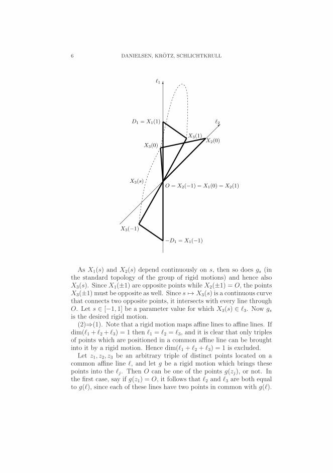
6 DANIELSEN, KROTZ, SCHLICHTKRULL
ℓ1
ℓ2
−D1 = X1(−1)
O = X2(−1) = X1(0) = X2(1)
X3(−1)
X2(0)X3(0)
X3(s)
D1 = X1(1)
X3(1)
As X1(s) and X2(s) depend continuously on s, then so does gs (inthe standard topology of the group of rigid motions) and hence alsoX3(s). Since X1(±1) are opposite points while X2(±1) = O, the pointsX3(±1) must be opposite as well. Since s 7→ X3(s) is a continuous curvethat connects two opposite points, it intersects with every line throughO. Let s ∈ [−1, 1] be a parameter value for which X3(s) ∈ ℓ3. Now gsis the desired rigid motion.(2)⇒(1). Note that a rigid motion maps affine lines to affine lines. If
dim(ℓ1 + ℓ2 + ℓ3) = 1 then ℓ1 = ℓ2 = ℓ3, and it is clear that only triplesof points which are positioned in a common affine line can be broughtinto it by a rigid motion. Hence dim(ℓ1 + ℓ2 + ℓ3) = 1 is excluded.Let z1, z2, z3 be an arbitrary triple of distinct points located on a
common affine line ℓ, and let g be a rigid motion which brings thesepoints into the ℓj. Then O can be one of the points g(zj), or not. Inthe first case, say if g(z1) = O, it follows that ℓ2 and ℓ3 are both equalto g(ℓ), since each of these lines have two points in common with g(ℓ).
DECOMPOSITION THEOREMS 7
Hence dim(ℓ1 + ℓ2 + ℓ3) ≤ 2. In the second case, the line g(ℓ) togetherwith O spans a 2-dimensional subspace of Rn, which contains all thelines ℓj. Hence again dim(ℓ1 + ℓ2 + ℓ3) ≤ 2.
We proceed with the proof of Theorem 3.2.
Proof. Note that SL(2,R) and SL(2,C) are locally isomorphic to SOe(2, 1)and SOe(3, 1), respectively. The centers of SL(2,R) and SL(2,C) be-long to K, and hence G = KAH will hold for the triple spaces ofthese groups if and only if it holds for the triple spaces of their adjointgroups. Thus it suffices to consider G0 = SO(n, 1) with n ≥ 2.The elements in so(n, 1) have the form
(3.2) X =
(A bbt 0
)
where A ∈ so(n) and b ∈ Rn, and s0 consists of the elements withA = 0.Assume first that a1+a2+a3 is 2-dimensional. By transitivity of the
action of K0 = SO(n) on the 2-dimensional subspaces of Rn we mayassume that a1+a2+a3 consists of the matrices X as above with A = 0and b non-zero only in the last two coordinates. Hence a1 + a2 + a3 iscontained in the so(2, 1)-subalgebra in the lower right corner of so(n, 1).It follows that exp(a1 + a2 + a3).z0 is a 2-dimensional totally geodesicsubmanifold of Z0.Let z1, z2, z3 ∈ Z0 be given. Every triple of points in Z0 belongs to
a 2-dimensional totally geodesic submanifold Z ′0 of Z0. For example,
in the model of Z0 as a one-sheeted hyperboliod in Rn+1, we can ob-tain Z ′
0 as the intersection of Z0 with a 3-dimensional subspace of Rn+1
containing the three points. Since G0 is transitive on geodesic subman-ifolds, we may assume that z1, z2, z3 are contained in the submanifoldgenerated by a1+a2+a3. We have thus essentially reduced to the casen = 2, and shall assume n = 2 from now on.We proceed exactly as in the Euclidean case and produce a pair of
points X1(s) and X2(s) on the geodesic lines exp(a1).z0 and exp(a2).z0,respectively. The two points are chosen so that they have the samenon-Euclidean distance from each other as z1 and z2, and they de-pend continuously on s ∈ [−1, 1]. Moreover, X1(−1) and X1(1) aresymmetric with respect to z0, while X2(−1) = X2(1) = z0. As Z0
is two-point homogeneous, there exists for each s ∈ [−1, 1] a uniqueisometry gs ∈ G0 such that gs(zj) = Xj(s) for j = 1, 2. As before, avalue of s, where the continuous curve s 7→ gs(z3) intersects exp(a3),produces the desired isometry gs of Property 3.3. Hence G = KAH.
8 DANIELSEN, KROTZ, SCHLICHTKRULL
We return to the case n ≥ 2 and assume conversely that G = KAH.It follows from Lemma 3.1 that dim(a1 + a2 + a3) > 1. We want toexclude dim(a1 + a2 + a3) = 3. Again we follow the Euclidean proofand select an arbitrary triple of distinct points z1, z2, z3 on a singlegeodesic γ in Z0. Then there is g ∈ G0 such that gzj = yj for someyj ∈ exp(aj).z0, for j = 1, 2, 3. If one of the yj’s, say y1, is z0, thenexp(a2).z0 = exp(a3).z0 = g(γ) and hence a2 = a3. Otherwise, thegeodesic g(γ) is contained, together with O, in a 2-dimensional totallygeodesic submanifold of Z0. This submanifold necessarily contains thegeodesic exp(aj).z0 for each j. Hence dim(a1 + a2 + a3) ≤ 2.
4. Uniqueness
If G/H is a homogeneous space of polar type, so that every elementg ∈ G allows a decomposition g = kah, it is of interest to know towhich extend the components in this decomposition are unique. Anobvious non-uniqueness is caused by the normalizer NK∩H(a) of a inK ∩ H, which acts on A by conjugation. In the case of a symmetricspace, it is known (see [6], Prop. 7.1.3) that the A component of everyg ∈ G is unique up to such conjugation. For our current triple spacesthe description of which elements in A generate the same K ×H orbitappears to be more complicated, unless a1 = a2 ⊥ a3.
Theorem 4.1. Let G/H be the triple space with G0 as in (1.1), andlet a be as in (2.1) with a1 = a2 ⊥ a3. Let a = (a1, a2, a3) ∈ A witha1 6= a2 and let a′ = (a′1, a
′2, a
′3) ∈ A. Then KaH = Ka′H if and only
if a and a′ are conjugate by NK∩H(a).
We first determine explicitly which pairs of elements a, a′ ∈ A areNK∩H(a)-conjugate when a1 = a2 ⊥ a3.
Lemma 4.2. Let a be as above. Then a, a′ ∈ A are conjugate byNK∩H(a) if and only if
(1) (a′1, a′2) = (a1, a2)
±1 and a′3 = a±13 if n > 2
(2) (a′1, a′2, a
′3) = (a1, a2, a3)
±1 if n = 2.
Proof. The normalizer NK∩H(a) consists of all the diagonal elementsk = (k0, k0, k0) ∈ G for which
k0 ∈ NK0(a1) ∩NK0(a2) ∩NK0(a3).
As elements aj, a′j ∈ Aj are NK0(aj)-conjugate if and only if a′j = a±1
j ,only the pairs mentioned under (1) can be conjugate when a1 = a2.Let δ, ǫ = ±1. For the groups in (1.1) the adjoint representation is
surjective K0 → SO(s0). If n > 2 then there exists a transformation inSO(s0) which acts by δ on a1 = a2 and by ǫ on a3. Its preimages in K0
DECOMPOSITION THEOREMS 9
conjugate (a1, a2, a3) to (aδ1, aδ2, a
ǫ3). When n = 2 such a transformation
exists if and only if δ = ǫ. The lemma follows. The following lemmas are used in the proof of Theorem 4.1. Here G0
can be any real reductive group with Cartan decomposition g0 = k0+s0.
Lemma 4.3. Let X,U ∈ s0. Then expX expU expX ∈ exp s0.
Proof. Let θ denote the Cartan involution and note that the productexp(tX) exp(tU) exp(tX) belongs to S = g ∈ G0 | θ(g) = g−1 forall t ∈ [0, 1]. It is easily seen that k expY ∈ S implies k2 = e fork ∈ K0 and Y ∈ s0, and since e is isolated in the set of elements oforder 2 it follows that exp s0 is the identity component of S. HenceexpX expU expX ∈ exp s0. Lemma 4.4. Let a0 ⊂ s0 be a one-dimensional subspace and let A0 =exp a0.
(1) If g ∈ exp s0 and ga0 ∈ a′0K0 for some a0, a′0 ∈ A0, then g =
a′0a−10 .
(2) If g ∈ G0 and ga1, ga2 ∈ A0K0 for some a1, a2 ∈ A0 witha1 6= a2 then g ∈ NK0(a0)A0.
Proof. (1) It follows from ga0 ∈ a′0K0 that a0ga0 ∈ a0a′0K0. Since
a0ga0 ∈ exp s0 by Lemma 4.3, it follows from uniqueness of the Cartandecomposition that a0ga0 = a0a
′0 and thus g = a′0a
−10 .
(2) Put z0 = eK0, then A0.z0 is a geodesic in G0/K0. Since g mapstwo distinct points on A0.z0 into A0.z0, it maps the entire geodesiconto itself, and hence so does g−1. In particular g−1.z0 ∈ A0K0, thatis, g = k0a0 for some k0 ∈ K0, a0 ∈ A0. It follows for all a ∈ A0 that
k0ak−10 = ga−1
0 ak−10 ∈ gA0K0 = A0K0.
As k0ak−10 ∈ exp s0, uniqueness of the Cartan decomposition implies
k0ak−10 ∈ A0, i.e. k0 ∈ NK0(a0).
Lemma 4.5. Let a1, a3 ⊂ s0 be one-dimensional subspaces with a1 ⊥ a3and let A1 = exp a1, A3 = exp a3. If g ∈ NK0(a1)A1 and ga3 ∈ a′3K0
for some a3, a′3 ∈ A3, not both equal to e, then g ∈ NK0(a1) ∩NK0(a3).
Proof. We may assume a′3 6= e, as otherwise we interchange it witha3 and replace g by g−1. We consider the geodesic triangle in G0/K0
formed by the geodesics
L1 := A1.z0, L2 := A3.z0, L3 := gA3.z0.
The vertices are
D3 := z0, D2 := g.z0, D1 := ga3.z0 = a′3.z0.
10 DANIELSEN, KROTZ, SCHLICHTKRULL
As L1 and L2 intersect orthogonally, angle D3 is right. The isometryg maps L1 to itself and L2 to L3. Hence L1 and L3 also intersectorthogonally and angleD2 is right. As the sectional curvature of G0/K0
is ≤ 0, it is impossible for a proper triangle to have two right angles.As L1 6= L2 and D3 6= D1 we conclude D3 = D2 and L3 = L2. Itfollows that g ∈ K0 and by Lemma 4.4 (2) that g ∈ NK0(a3).
Proof of Theorem 4.1. Assume KaH = Ka′H. Then Kah = Ka′ forsome h = (g, g, g) ∈ H. Applying Lemma 4.4 (2) to the first twocoordinates of Kah = Ka′ we conclude that g ∈ NK0(a1)A1.If a′3 and a3 are not both e, we can apply Lemma 4.5 to the last
coordinate and conclude g ∈ NK0(a1) ∩NK0(a3). Hence h ∈ NK∩H(a),and we conclude that a′ = h−1ah.If a′3 = a3 = e it follows from the third coordinate that g ∈ K0.
Hence g ∈ NK0(a1) and a′ = a or a′ = a−1.
Remark 4.6. When dim s0 = 2 the assumption in Theorem 4.1 andLemmas 4.2, 4.5, that a1 = a2 ⊥ a3, can be relaxed to a1 = a2 6=a3 with unchanged conclusions. This follows from the fact that ina two dimensional space the only proper orthogonal transformationswhich normalize a one-dimensional subspace are ±I. Hence NK0(a1) =NK0(a3) in this case.
5. A formula for the invariant measure
In a situation where there is uniqueness (up to some well-describedisomorphism), it is of interest to explicitly determine the invariant mea-sure with respect to the KAH-coordinates.For any triple space G/H of a unimodular Lie group G0 we note that
the map
(5.1) G0 ×G0 → G/H, (g1, g2) 7→ (g1, g2, e)H
is a G0 × G0-equivariant diffeomorphism. Accordingly the invariantmeasure on G/H identifies with the Haar measure on G0 ×G0.For G0 = SOe(n, 1) we define X ∈ so(n, 1) by (3.2) with A = 0
and b = en, and Y ∈ so(n, 1) similarly with A = 0 and b = e1. Leta1 = a2 = RX and a3 = RY , then a3 ⊥ a1. Let
at = exp(tX) ∈ A1 = A2, bs = exp(sY ) ∈ A3.
Lemma 5.1. Let G/H be the triple space of G0 = SOe(n, 1) and leta1 = a2 and a3 be as above. Consider the polar coordinates
(5.2) K × R3 ∋ (k, t1, t2, s) 7→ (k1at1 , k2at2 , k3bs)H
DECOMPOSITION THEOREMS 11
on G/H. The invariant measure dz of G/H can be normalized so thatin these coordinates
(5.3) dz = J(t1, t2, s) dk dt1 dt2 ds
where dk is Haar measure, dt1, dt2, ds Lebesgue measure, and where
J(t1, t2, s) = | sinhn−1(t1 − t2) sinhn−2(s) cosh(s)|.
Proof. On G0×G0 we use the formula (see [6], Thm. 8.1.1) for integra-tion in KAH coordinates for the symmetric space G0×G0/ diag(G0) =G0. The map
(K0 ×K0)× A0 ×G0 → G0 ×G0
defined by
(k, at, g) 7→ (k1at/2g, k2a−t/2g)
is a parametrization (up to the sign of t), and the Haar measure onG0 ×G0 writes as
(5.4) | sinhn−1(t)| dk1 dk2 dt dg .
Further we decompose the diagonal copy of G0 by means of theHAK coordinates for the symmetric space G0/(SO(n−1)×A1), whereSO(n − 1) is located in the upper left corner of G0. Note that thesubgroup A3 serves as the ‘A’ in this decomposition. In the coordinates
K0 × A3 × SO(n− 1)× A1 → G0, (k3, bs,m, au) 7→ aumbsk3
we obtain (again using [6], Thm. 8.1.1),
(5.5) dg = | sinhn−2(s) cosh(s)| dk3 dbs dmdu .
Combining (5.4) and (5.5), we have the coordinates
(k1au+t/2mbsk3, k2au−t/2mbsk3)
on G0 ×G0, with Jacobian | sinhn−1(t) sinhn−2(s) cosh(s)|. As the sub-group SO(n − 1) centralizes A1, the integration over m is swallowedby the integrations over k1 and k2. Changing coordinates u, t tot1 = u+ t/2 and t2 = u− t/2 we find t = t1 − t2.Finally we apply (5.1) so that the above coordinates correspond to
(k1, k2, k3)(at1 , at2 , b−s) diag(G0)
This proves (5.3).
12 DANIELSEN, KROTZ, SCHLICHTKRULL
6. Spherical decomposition
A decomposition of g of the form
(6.1) g = p+ h
with p a minimal parabolic subalgebra is said to be a spherical decom-position. If such a decomposition exists, then the homogeneous spaceG/H is said to be of spherical type (see [5]).Note that with g0 = so(n, 1) we have (see (6.4) and (6.5))
dim p+ dim h− dim g = 12(n2 − 5n+ 6) ≥ 0.
In particular spherical decompositions will be direct sums if n = 2, 3.It was observed in [5] that the triple spaces for the groups considered
in (1.1) are of spherical type. In the following we determine for each nall the minimal parabolic subalgebras p for which (6.1) holds.
Proposition 6.1. Let G0 be one of the groups (1.1) and let p = p1 ×p2 × p3 a minimal parabolic subalgebra. Then g = p + h holds if andonly if p1, p2 and p3 are distinct.In particular, the triple space G/H is of spherical type for all groups
G0 in (1.1).
We prepare by the following lemma.
Lemma 6.2. Let U1, U2, U3 ⊂ V be subspaces of a vector space V . Put
U := U1 × U2 × U3 ⊂ X := V × V × V,
and Y := diag(V ) ⊂ X. Then X = U + Y if and only if
(6.2) V = U1 + (U2 ∩ U3) = U2 + (U3 ∩ U1) = U3 + (U1 ∩ U2).
Proof. Assume first that X = U + Y and let v ∈ V be given. Writing
(v, 0, 0) = (u1, u2, u3) + diag(w)
we see that w = −u2 = −u3 ∈ U2 ∩ U3, and hence v = u1 + w ∈U1 + (U2 ∩ U3). The other two statements in (6.2) follow similarly.Conversely, we assume (6.2) and let x = (x1, x2, x3) ∈ X be given.
We decompose x1, x2 and x3 according to the three decompositions in(6.2), that is,
x1 = u1 + t1, u1 ∈ U1, t1 ∈ U2 ∩ U3
x2 = u2 + t2, u2 ∈ U2, t2 ∈ U3 ∩ U1
x3 = u3 + t3, u3 ∈ U3, t3 ∈ U1 ∩ U2.
Then
x = (u1 − t2 − t3, u2 − t1 − t3, u3 − t1 − t2) + diag(t1 + t2 + t3)
is a decomposition of the desired form U + Y .
DECOMPOSITION THEOREMS 13
Remark 6.3. In fact, it is easily seen that any two of the decomposi-tions of V in (6.2) together imply the third.
Proof of Proposition 6.1. It suffices to consider G0 = SO0(n, 1) becauseof the local isomorphisms.If for example p1 = p2 then p1 + (p2 ∩ p3) = p1. Hence p1 + (p2 ∩ p3)
is proper in g0 and it follows from Lemma 6.2 that g = p + h fails tohold. This implies one direction of the first statement.For the other direction it follows from Lemma 6.2 that it suffices to
prove
g0 = p1 + (p2 ∩ p3)
for all triples of distinct parabolics in so(n, 1). We shall do this byproving
(6.3) dim g0 = dim p1 + dim(p2 ∩ p3)− dim(p1 ∩ p2 ∩ p3).
We find
(6.4) dim g0 = dim so(n, 1) = 12(n2 + n),
and claim that
dim p1 =12(n2 − n+ 2)(6.5)
dim(p1 ∩ p2) =12(n2 − 3n+ 4)(6.6)
dim(p1 ∩ p2 ∩ p3) =12(n2 − 5n+ 6).(6.7)
The equations (6.4)-(6.7) imply (6.3).The parabolic subalgebras p of so(n, 1) are the normalizers of the
isotropic lines in Rn+1, that is, the one-dimensional subspaces of theform Lq = R(q, 1) where q ∈ Rn with ‖q‖ = 1.Recall that all elements in so(n, 1) have the form (3.2) with A ∈ so(n)
and b ∈ Rn. It follows that X ∈ p if and only if
(6.8) Aq + b = (b · q)q.Let us prove (6.5). Let q1 be the unit vector such that p1 is the
stabilizer of Lq1 , and extend q1 to a basis q1, . . . , qn for Rn. For b ∈ Rn
we let x1 = (b · q1)q1 − b and we observe that x1 · q1 = 0. According to(6.8) the matrix X of (3.2) belongs to p1 if and only if Aq1 = x1. Inorder to satisfy that we can define an n× n matrix A by
(6.9) Aqi · qj :=
x1 · qj for i = 1
−x1 · qi for j = 1
aij for i, j > 1
14 DANIELSEN, KROTZ, SCHLICHTKRULL
with arbitrary antisymmetric entries in the last line. Then A ∈ so(n)and Aq1 = x1. The degree of freedom for each b is
dim so(n− 1) = 12(n− 1)(n− 2),
and hence dim p1 = n+ 12(n− 1)(n− 2) = 1
2(n2 − n+ 2) as asserted.
Next we prove (6.6). Let q1, q2 be the unit vectors such that pi is thestabilizer of Lqi . By assumption q1 6= q2. For the element X of (3.2) tobe in p1 ∩ p2 we need that (6.8) is satisfied in both cases, that is,
(6.10) Aqi = xi, (i = 1, 2).
where xi = (b · qi)qi − b. Now
x2 · q1 + x1 · q2 = (q1 · q2 − 1)(b · (q1 + q2)).
Note that q1 · q2 < 1 since q1 6= q2. As A ∈ so(n) we conclude that
b · (q1 + q2) = 0
since otherwise (6.10) would lead to contradiction.Conversely, let b ∈ Rn be such that b · (q1 + q2) = 0 and define x1, x2
by xi = (b · qi)qi − b. Then xi · qj = −xj · qi for all pairs i, j ≤ 1, 2. Weextend q1, q2 to a basis and define an n× n matrix A by
(6.11) Aqi · qj =
xi · qj for i = 1, 2
−xj · qi for j = 1, 2
aij for i, j > 2
with arbitrary antisymmetric entries in the last line. Then A ∈ so(n)and (6.10) holds. The degree of freedom for each b is
dim so(n− 2) = 12(n− 2)(n− 3)
and hence dim(p1 ∩ p2) = n− 1 + 12(n− 2)(n− 3) = 1
2(n2 − 3n+ 4) as
asserted.Finally, to prove (6.7) assume that X in (3.2) belongs to p1∩p2∩p3.
As above, it follows that
b · (q1 + q2) = b · (q1 + q3) = b · (q2 + q3) = 0
which implies that b · qi = 0 for i = 1, 2, 3. If this is satisfied by b, thecondition (6.8) simplifies to
(6.12) Aqi = −b, i = 1, 2, 3.
We first assume that q1, q2, q3 are linearly independent and extend toa basis as before. Given b ∈ Rn such that b · qi = 0 for i = 1, 2, 3 we
DECOMPOSITION THEOREMS 15
define A by
(6.13) Aqi · qj =
−b · qj for i = 1, 2, 3
b · qi for j = 1, 2, 3
aij for i, j > 3
with arbitrary antisymmetric entries in the last line. The degree offreedom for each b is
dim so(n− 3) = 12(n− 3)(n− 4)
and hence dim(p1 ∩ p2 ∩ p3) = n− 3+ 12(n− 3)(n− 4) = 1
2(n2− 5n+6)
as asserted.Next we assume linear dependence of q1, q2, q3. This implies a further
obstruction to b. In fact, let λ1q1 + λ2q2 + λ3q3 = 0 be a non-trivialrelation, then it follows from (6.12) that (λ1 + λ2 + λ3)b = 0. Sinceq1, q2, q3 are assumed to be distinct unit vectors the sum of the λ’scannot be zero, and we conclude that b = 0. Thus in this case the onlyfreedom comes from the choice of A. That can be chosen arbitrarilyfrom the annihilator in so(n) of the space spanned by the three q’s. Weobtain dim(p1 ∩ p2 ∩ p3) = dim so(n − 2) = 1
2(n2 − 5n + 6) as before.
This concludes the proof of (6.7).In particular, if a1, a2 and a3 are all different, then g = p + h for
every parabolic subalgebra p above a = a1 × a2 × a3. Hence G/H is ofspherical type.
Corollary 6.4. There exists a maximal abelian subspace a ⊂ s forwhich both
(i) the polar decomposition (3.1) is valid, and(ii) the spherical decomposition (6.1) is valid for all minimal para-
bolic subalgebras containing a.
Proof. Let aj ⊂ s0 for j = 1, 2, 3 be mutually different and with atwo-dimensional sum. It follows from Theorem 3.2 and Proposition 6.1that a = a1 × a2 × a3 satisfies (i) and (ii).
Remark 6.5. The properties of a reductive homogeneous space G/Hthat it is of polar type, respectively of spherical type, appear to beclosely related. However, the relation is not as strong as one mighthope, because the conditions on a are different in Theorem 3.2 andProposition 6.1. In particular, there exist maximal abelian subspacesa ⊂ g which fulfill (ii) but not (i), namely the ’most generic’ ones, forwhich dim(a1 + a2 + a3) = 3.
16 DANIELSEN, KROTZ, SCHLICHTKRULL
7. Infinitesimal polar decomposition
Here we consider an infinitesimal version of the polar decompositionG = KAH. Let G/H be a homogeneous space of a reductive group G,and let g = k+ s be a Cartan decomposition.
Definition 7.1. A decomposition of the form
(7.1) s = Ad(K ∩H)a+ s ∩ h
with an abelian subspace a ⊂ s is called a polar decomposition.If there exists such a decomposition of s then we say that G/H is
infinitesimally polar.
Here
Ad(K ∩H)a = Ad(k)X | k ∈ K ∩H,X ∈ a.Note that this need not be a vector subspace of s.If G/H is a symmetric space, then we can choose the Cartan decom-
position so that k and s are stable under the involution σ that deter-mines G/H. If g = h+ q denotes the decomposition of g in +1 and −1eigenspaces for σ, then s = s∩q+s∩h. If furthermore aq is a maximalabelian subspace of s ∩ q, then it is known that s ∩ q = Ad(K ∩H)aqand hence (7.1) follows.The following lemma suggests that there is a close connection be-
tween polar decomposability and infinitesimally polar decomposability.
Lemma 7.2. Let G0 be one of groups (1.1) and let a = a1 × a2 × a3.Then the infinitesimal polar decomposition (7.1) holds if and only ifdim(a1 + a2 + a3) = 2.
Proof. For the triple spaces, the polar decomposition (7.1) interprets tothe statement that for every triple of points Z1, Z2, Z3 ∈ s0 there existk ∈ K0, T ∈ s0 and Xj ∈ aj (j = 1, 2, 3) such that Zj = Ad(k)Xj +T . As the maps X 7→ Ad(k)X + T with k ∈ K0 and T ∈ s0 areexactly the rigid motions of s0, this lemma is precisely the content ofProposition 3.4.
Combining the lemma with Theorem 3.2 we see that for our triplespaces the infinitesimal polar decomposition holds with a given a ifand only if the global polar decomposition G = KAH holds for thecorresponding A = exp a.
References
[1] M. Brion, Classification des espaces homogenes spheriques, Compositio Math.63 (1987), 189–208.
DECOMPOSITION THEOREMS 17
[2] M. Flensted-Jensen, Spherical functions on rank one symmetric spaces andgeneralizations. Proc. Sympos. Pure Math., Vol. XXVI, pp. 339–342. Amer.Math. Soc., Providence, R.I., 1973.
[3] A. W. Knapp, Lie groups beyond an introduction. Birkhauser, 2002.[4] M. Kramer, Spharische Untergruppen in kompakten zusammenhangenden
Gruppen, Compositio Math. 38 (1979), 129–153.[5] B. Krotz, H. Schlichtkrull and E. Sayag, Decay of matrix coefficients on reduc-
tive homogeneous spaces of spherical type, submitted.[6] H. Schlichtkrull, Hyperfunctions and harmonic analysis on symmetric spaces,
Birkhauser 1984.[7] Wolf, Joseph A. Finiteness of orbit structure for real flag manifolds. Geome-
triae Dedicata 3 (1974), 377–384.
E-mail address : [email protected] address : [email protected] address : [email protected]


![Stratified fibre bundles - arXiv · topology, product topology, and compact-open topology in function spaces. As application we study in [4] algebraic constructions on stratified](https://img.pdfslide.us/doc/110x75/5edc0be3ad6a402d66668b4f/stratiied-ibre-bundles-arxiv-topology-product-topology-and-compact-open.jpg)